Download A Short Guide To Approximation Preserving Reductions

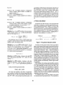
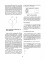
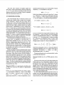
A Short Guide to ApproximationPreserving Reductions
Pierluigi CrescenzP
Dipartimento di Scienze dell’informazione
Universita di Roma “La Sapienza”
Via Salaria 113, 00198 Roma, Italy
E-mail: piluc @ dsi.uniroma1.it
Abstract
cheap personal computers to extremely expensive workstations. This should lead you to change your original question: ‘Which computer should I buy?’ to the more intimate
question: “What am I going to do with the computer?’.
Clearly, one possible consequence of this change of focus
is the decision of not buying a computer at all. But let us
assume that, after all, you really need one. After carefully
analyzing your needs, you finally decide to buy the RTM
9000 personal computer.
Eventually, you will get it, unpack it, and put it on the
table just in front you. The next question will then be “How
do I use it?’. The answer to this question may depend on
the computer itself the so-called user-friendly computers
should allow you to learn to use them without any further
help while most of the others will force you to read dozens
and dozens of pages on quite cryptic user manuals. Certainly, after a while you will learn how to use the RTM
9000 even though you will also realize that in the meanwhile much better machines have been produced. This will
likely lead you to the ultimate question “Should I buy a new
computer?’.
Comparing the complexity of different combinatorial optimization problems has been an extremely active research
area during the last 23 years. This has led to the definition of several approximation preserving reducibilities and
to the development of powelful reduction techniques. We
first review the main approximation preserving reducibilities that have appeared in the literature and suggest which
one of them should be used. Successively, we give some
hints on how to prove new non-approximability results by
emphasizing the most interesting techniques among the new
ones that have been developed in the last few years.
1. Introduction
What is it that makes algorithms for different problems behave in the same way? Is
there some stronger kind of reducibility than
the simple polynomial reducibility that will explain these results, or are they due to some
structural similarity between the problems as
we define them?
A quite similar situation can arise when you decide to
prove that a given optimization problem A is not approximable. As stated in [2], “the first step in proving an inapproximability result for a given problem is to check whether
it is already known to be inapproximable. For instance, the
problem might be listed in [14].” If you are lucky, you will
find the answer to your question with, basically, no effort
(but, unfortunately, with no publication either . . .). Otherwise, you can either try to prove that approximating problem A is NP-hard or try to compare problem A with any
of the optimization problems for which inapproximability
results are already known.
After examining the literature, you will immediately realize that a fundamental tool in order to follow the second alternative is the notion of approximation preserving
reducibility which should allow you to compare the complexity of approximating A to that of some other optimiza-
David S. Johnson [26]
. . . ce sont rarement les reponses qui apportent la verite, mais I’enchainement des questions.
Daniel Pennac [38]
Suppose that you have decided to buy a new computer.
The first thing you will probably realize is the incredibly high number of possibilities you have, ranging from
*Starting from November 1, 1997, the author’s new affiliation will be:
Dipartimento di Sistemi ed Informatica, Universith di Firenze, Via Cesare
Lombroso 6/17,50134 Firenze, Italy (e-mail: [email protected]).
1093-0159/97 $10.000 1997 IEEE
262
tion problem. Different from proving NP-completeness (in
which case the only reducibility to be used is the many-toone polynomial-time reducibility), you will also discover
that many approximation preserving reducibilities can be
used, ranging from very strict kinds of reducibilities to extremely general ones.
The first goal of this paper is to briefly review the main
reducibilities that have been defined in the last 20 years
organizing them into a taxonomy (a similar overview of
approximation preserving reducibilities that have been defined in the 80s is contained in [ll]). After examining
the differences between these reducibilities, we will suggest you concentrate your attention on three of them, the Lreducibility,the AP-reducibility and the PTAS-reducibility.
The choice between these three reducibilities will then depend mainly on the following question: “What am l going
to do with the reducibility?’. Most of the time, the answer
will be: “To prove a non-approximability result” in which
case the L-reducibility will likely suffice. Sometimes, instead, the answer will be: “To prove a completeness result”
in which case you should seriously consider the possibility
of switching either to the AP-reducibility or to the PTASreducibility.
Once you have decided which reducibility you are going
to use, the next question will be: “How do 1develop an approximation preserving reduction?’. This is a much harder
question and, unfortunately, thcrc is no user-manual (not
even a cryptic one) that can explain the secrets of proving
these kinds of results.
The second goal of this paper is to give some guidelines
that, we hope, can be usefully followed in order to obtain
the desired result. To this aim, we will describe two of
the most interesting techniques that have been developed in
the last few years in order to obtain non-approximability results: expansion and randomization. We believe that these
techniques are general enough to deserve a special treatment. Paraphrasing [20], this will not be a classification
of all non-approximability results. Our main intent will be
to illustrate two ways of thinking about approximation preserving reduction proofs that were not explicitly present in
previously known N P-completeness proofs.
Clearly, it may be still possible that your attempts to
prove the non-approximability of A fail: do not forget that
it is possible that A is very well approximable (or even solvable in polynomial-time). In the meanwhile, more powerful approximation preserving reducibilities could have
been defined by somebody else and you could ask yourself “Should 1 use this new reducibility?’. Even more.
You could ask yourself “Should 1 define a new approximation preserving reducibility?’. Indeed, this has been the
approach followed by several authors (including this guide’s
one) in the last ten years: this is the reason why so many reducibilities are now available “on the market”!
Organization of the guide The paper is organized as follows. In Section 2, we give the basic definitions regarding optimization problems and approximation algorithms.
In Section 3, we give the general definition scheme of an
approximation preserving reducibility, and a taxonomy of
existing reducibilities is presented. At the end of the section, we recommend three of these reducibilities and try to
suggest when they should be used. Finally, in Section 4 we
outline our approximation preserving reduction guide emphasizing the role of expander graphs and of randomization
as new techniques useful to obtain reductions.
2. Basic definitions
We assume the reader to be familiar with the basic concepts of computational complexity theory as presented in
one of the available text books (see, for example, [8, 10,20,
351).
We now give some standard definitions in the field of
optimization and approximationtheory. For a more detailed
exposition of this theory we refer the readcr to [5, 241. A
preliminary version of some chapters of [4] is also available
on request to one of the authors.
Definition 1 An NP optimizationproblem .-is
Ia fourtuple
( I ,sol, m, type) such that
1.
I is the set of the instances of -4and it is recognizable
in polynomial time.
2. Given an instance x of I , sol( T ) denotes the set of feasible solutions of s. These solutions are short, that is,
a polynomial p exists such that, f o r any y E S O ~ ( T ) ,
lyl 2 ~ ( 1 x 1 ) . Moreovel; f o r any T and f o r any y
with IyI 5 ,u(l<rI),it is decidable in polynomial time
whether y E sol(x).
3. Given an instance
t
and a feasible solution y of x,
m(x , y) denotes the positive integer measure of y
(of-
ten also called the value of y). Thefunction m is computable in polynomial time and is also called the ob-
jective function.
4. type
E {max, iniii}.
The goal of an NP optimization problem with respect to an
instance T is to find an optimum solution, that is, a feasible
solution y such that
m(x, y) = type{m(z, y’) . y’
E sol(r)}.
In the following opt will denote the function mapping an
instance T to the measure of an optimum solution. The class
NPO is the set of all NP optimization problems.
In the following we will mainly refer to satisfiabilityoptimization problems. In particular, we will make use of the
following optimizationproblems.
263
very difficult. Parallelizing the development of the theory of
NP-completeness, we can then look for the “hardest” problems in the above classes, that is, problems which cannot
have stronger approximation properties unless P = NP. In
complexity theory, saying that a problem is the hardest one
in a class is equivalent to saying that it is complete for that
class with respect to a suitable reducibility. The goal of the
next section is to identify the right notion of such reducibility.
MAXSAT
INSTANCE:Set ,Ti of variables, collection p of disjunctive
clauses of literals, where a literal is a variable or a
negated variable in -Y.
SOLUTION:A truth assignment for S.
MEASURE:Number of clauses satisfied by the truth assignment.
MAX SAT
3. Which reducibility?
INSTANCE:Set S of variables, collection p of disjunctive
clauses of at most k literals, where a literal is a variable
or a negated variable in X ( k is a constant, k 2 2).
SOLUTION:A truth assignment for .‘i.
MEASURE:Number of clauses satisfied by the truth assignment.
It should be clear that the many-to-one polynomial-time
reducibility is inadequate to study the approximabilityproperties of optimization problems. Indeed, if we want to map
an optimization problem A into an optimization problem B
then we need not only a polynomial-time computable function f mapping instances of A into instances of B but also a
polynomial-time computable function g mapping back solutions of B into solutions of A (see Fig. l).
Definition 2 Let A be an NPO problem. Given an instance
x and a feasible solution y of x, we define the performance
ratio of y with respect to x as
The performance ratio is always a number greater than
or equal to 1 and is as close to 1 as the value of the feasible
solution is close to the optimum value.
Figure 1. The general reduction scheme
Definition 3 Let il be an NPO problem and let T be an
algorithm that, for any instance x of A, returns a feasible
solution T (x) in polynomial time. Given a rational r > 1,
we say that T is an r-approximation algorithm for A ifthe
pelformance ratio of thefeasible solution T (x)with respect
to x verifies the following inequality:
R ( x ,T ( x ) )_<
Consistent with the general scheme shown in the above
figure, several approximation preserving reducibilities have
been defined in the literature differing for the way they preserve the performance ratios and/or for the additional information used by functions f and g. Before proceeding to
describe these different reducibilities, we note that the metric reducibility defined in [30]does not really fit into this
framework. Indeed, this reducibility allows one to compute
function opt, by using an algorithm to compute Opt, without preserving any level of approximability but the best one
(that is, performance ratio equal to 1). It is thus not surprising that the class of complete problems introduced in [30]
includes problems with drastically different approximability properties.
More adequate for studying approximability properties
of optimization problems is the ratio preserving reducibility
[37]. This reducibility has been used to show that a variety of NP-hard problems can be inteneduced via reductions
that preserve the quality of the approximation. However,
this reducibility is “non-constructive”, that is, it does not
include the function g in order to compute an approximate
solution. That is why we do not include the ratio preserving
reducibility within our taxonomy.
For different reasons we do not include in our review
the structure preserving reducibility [ 6 ] .This reducibilty is
I’.
Definition 4 An NPOproblem A belongs to the class APX
i f an r-approximation algorithm T for A exists, for some
rational r > 1.
Definition5 An NPO problem A belongs to the class
PTAS i f an algorithm T exists such that, f o r any $xed rational I’ > 1, T ( . ,r) is an r-approximation algorithm for
A.
Clearly, the following inclusions hold
PTAS
APX
NPO.
The major open problem in the theory of approximation complexity is whether the inclusions among these three
classes are strict. It is easy to see that this is the case if and
only if P # NP, so that solving this problem seems to be
264
based on a very detailed examination of the combinatorial
structures both of the problems being reduced and of the reductions. In our opinion the conditions under which structure preserving interreducible optimization problems have
similar approximability properties are too restrictive to still
be of general interest. Nevertheless, it is worth pointing out
that by means of the structure preserving reducibility, as far
as we know, the first completeness result for optimization
problems has been obtained: indeed, in [7] it is implicitly
shown that a weighted version of the maximum satisfiability problem is NPO-complete with respect to the structure
preserving reducibility.
In the following, we say that a pair ( f ,g) of polynomialtime computable functions (as in Fig. 1) is a reduction from
-4 to B. Moreover, we denote by E ( t, y) the absolute error
ofy withrespecttor,thatis,E(r,y)
= lopt(s)-m(t,y)I.
Finally, we say that a reducibility 5 preserves membership
in a class C if A 5 B and B E C imply A E C and that a reducibility is approximation preserving if it preserves membership in either APX, PTAS, or both.
is a c(r)-approximation algorithm for -4. A similar proof
holds for the P-reducibility.
0
Clearly, every strict reduction is also an A-reduction and
a P-reduction (it suffices to set c equal to the identity function). Observe also that a P-reduction is an A-reduction if
and only if the inverse of function c is a computable function from Q n (1,(x>)
to Q n (1,XI).
3.2. Continuous reducibility [41]
A reduction ( f ,g) is said to be a continuous reduction if
a positive constant (1 exists such that, for any x E IAand
foranyy E S O l B ( f ( a ' ) ) ,
R A ( X , g ( s ? y ) )I . R B ( f ( X ) , Y ) .
Clearly, a continuous reduction is also an A-reduction
(it suffices to define c ( r ) = ay). Thus, the continuous reducibility preserves membership in APX.
33. Lreducibility [36]
3.1. Strict, A-, and P-reducibility [34,16]
A reduction (.f,g) is said to be an L-reduction if two positive constants Q and /? exist such that:
A reduction ( f , g) is said to be a strict reduction if, for
any z E I A and for any y E S O ~ B ( ~ ( X ) ) , the following
holds:
RA(z,g(X,Y)) 5 RB(f(Z),Y).
A reduction ( f , g ) is said to be an A-reduction if a computable function e : Q n (1,CQ) -+ Q n (1,o
x
)exists such
that,foranyr E IA,foranyy E s o l B ( f ( z ) ) , a n d f o r a n y
r > 1, the following holds:
R B ( f ( X 1 ,Y)
5r
3 RA4(x,g(z,
Y))
5 4.1.
Proposition 7 If a minimization (respectively, maximization) problem A reduces to an NPO problem B via an
L-reduction ( f ,g.cy, d ) , then il reduces to B via the Preduction ( f , g ?c) where c ( r ) = 1 + ( r - l)/(cyd) (respectively, c(r) = 1 ( r + l)/(oOr)).
A reduction ( f ,g) is said to be a P-reduction if a computable function c : Q n (1,ocl) -+ Q n (1,a)
exists such
that, for any x E I A , for any y E s o l ~ ( f ( x )and
) , for any
r > 1,the following holds:
R B ( f ( z )y)
,
The L-reducibility preserves membership in PTAS. Indeed, this is a consequence of the following result.
+
PROOF: Assume that A is a minimization problem. Observe that if ( f ,g, a,P ) is an L-reduction from A to B, then,
foranya E
andforanyy E ~ ~ l g ( f ( z ) ) ,
5 c ( r ) * R A ( z , g ( z , y)) 5 7'.
Observe that, in [34], an A-reduction (respectively, Preduction) is called a bounded (respectively, continuous) reduction.
Proposition 6 ([34]) The A-reducibility (respectively, Preducibility) preserves membership in APX (respectively,
PTAS).
It is also easy to see that
PROOF:Let TB be an r-approximation algorithm for B and
let ( f ,g, e ) be an A-reduction from A to B. Then
Thus, we have that
265
By defining
47') =
1
+ ( r - l)/(a,d),it follows that
and log-APX, that is, the class of problems approximable
within a logarithmic factor (for a formal definition of these
two classes see [29]). It is also worth observing that within
the class APX the E-reducibility is just a generalization of
the L-reducibility [ 151.
R B ( f ( X ) , y ) 5 e(.) implies R A ( x , g ( x > y ) )5 r.
A similar proof holds in the case .4 is a maximization
problem.
0
From the proof of the above proposition, it also follows
that if a minimization problem -4 is L-reducible to an NPO
problem B then -4 is A-reducible to B. In other words,
L-reductions from minimization problems to optimization
problems preserve membership in APX. However, there is
strong evidence that, in general, this is not true whenever
the starting problem is a maximization one [15]. The intuitive reason of this fact is that, when Q and 3 are sufficiently
large, the function e in the above proposition is not invertible.
3.6. PTAS-reducibility [18]
The PTAS-reducibility is the first example of reducibility that allows the functions .f and y to depend on the performance ratio. This implies that different constraints have
to be put on the computation time of .f and g .
A reduction ( f , g ) is said to be a PTAS-reduction if a
computablefunctione : Q n ( l > m t
) Q n ( 1 , ~exists
)
such that:
3.4. S-reducibility [13]
1. For any s E 1, and for any 7'
computable in time t f ( I z I T ) .
> 1, f ( x , r )
E / B is
~
A reduction (f,g ) is said to be an S-reductioni f
E E I A , for any 7' > 1, and for any y E
soI,(f(x>r)),g ( x , y , r ) E s o I ~ ( xiscomputablein
)
2. For any
1. For any s E l a . optB(f(s)) = opt4(x).
2. For any x E
.(A
timef,(lxI, l y l , r ) .
and for any y E sol^ ( f ( z ) ) ,
3. For any fixed 70, bothtf
by a polynomial.
4. For any x E
Clearly, every S-reduction is also a strict reduction, a
continuous reduction and an L-reduction.
/A,
r ) andt,(.. ., r ) are bounded
(.?
for any r
>
1, and for any y E
S O l B ( f ( Z L ' ,T I ) ,
3.5. E-reducibility [29]
Observe that according to this definition, functions like
21/('-1)nh or nl/('-') are admissible bounds on the computation time of f and g , while this is not true for functions
like 2".
It is easy to see that the PTAS-reducibility preserves
membership in PTAS (this is the motivation for imposing
the bounds on the computation time o f f and 9).
The PTAS-reducibility is a generalization of the Preducibility. Indeed, the only difference between the PTASreducibility and the P-reducibility is the fact that f and g
may depend on r: this generalization is necessary to prove
completeness results. Indeed, by making use of the PTASreducibility it is possible to prove the APX-completeness of
MAX SAT and thus of other important optimization problems [18,29]. On the other hand, it is possible to prove that
the APX-completeness of MAX SATwith respect to either
the P-reducibility or the L-reducibility would imply that
p S A T - pSAT[logn]
where PsAT(respectively, PSAT[log1
denotes the class of languages decidable in polynomial time
asking a polynomial (respectively, logarithmic) number of
queries to an oracle for the satisfiabilityproblem. This latter
event seems to be unlikely and, in any case, the relationship
between these two classes is a well-known open question in
complexity theory [23].
A reduction (,f,g ) is said to be an E-reduction if a polynomial p and a positive constant d exist such that:
1. Foranyr E I.4,0PtB(.f(x))
2. For any c E
/A
5 P(lzl)optA(s).
and for any y E
sol^ (f(x)),
Clearly, every E-reduction is also an A-reduction and a
P-reduction. Indeed, it suffices to define e( r ) = 1+p( T - 1)
in the case of the A-reducibility and e(.) = 1 + ( r - l ) / D
in the case of the P-reducibility. The E-reducibility is thus
the first significant example of a reducibility that preserves
membership both in APX and in PTAS.
Observe that, for any function T , an E-reduction maps
r(n)-approximate solutions (that is, solutions y of an instance z whose performance ratio R ( z ,y) is bounded by
T (1
2I)) into ( l + a ( r ( n ') - 1))-approximatesolutionswhere
h is a constant depending only on the reduction. Hence,
the E-reducibility not only preserves membership in APX
and in PTAS but also membership in poly-APX, that is, the
class of problems approximable within a polynomial factor,
266
Additional
parameters
Constraints
to be satisfied
Membership
preserved
all
function c
APX
function c
PTAS
constant a
APX
constants a , 3
PTAS
APX if typeA = min
all
polynomial p
constant d
all
ratio r
PTAS
constant (I
Table 1. Summary of the nine reducibilities
3.7. AP-reducibility [15]
on the computation time o f f and g : for any fixed n, both
t f ( n ,.) and t , ( n n , .) are non-increasing functions.
A PTAS-reduction ( f , g , e ) is said to be an AP-reduction
if a constant (I exists such that e(.) = 1 (1' - l ) , ' ~ .In
other words, the fourth condition of the PTAS-reducibility
is changed into
+
3.8. The taxonomy
In Fig. 2 and in Table 1 we summarize all the approximation preserving reducibilities that we have reviewed. Both
in the figure and in the table we have denoted by IC(respectively, (strict, < A , IP,
IL,
Ss, SE, <PTAS, and
1 4 p ) the continuous (respectively, strict, A-, P-, L-, S-, E-,
PTAS-, AP-) reducibility.
We do not claim that this taxonomy covers all the approximation preserving reducibilities that have appeared in
the literature. However, we are very confident that the reducibilities we missed are restrictions of one of those included in the taxonomy.
Observe that the fact that the taxonomy does not con-
Since the AP-reducibility is a restriction of the PTASreducibility, it preserves membership in PTAS. Moreover,
from the fact that function c is invertible it follows that it
also preserves membership in APX. On the other hand, it
is clear that the AP-reducibility is a generalization of the Ereducibility. In order to maintain the nice property of this
latter reducibility of preserving membership in poly-APX
and log-APX, we impose the following further restriction
267
one’s goal, then the L-reduction must be turned into either
an AP-reduction or a PTAS-reduction.
verge into one reducibility is due to the fact that we did not
require that the inverse of function c in the definitions of
the two reducibilities is computable. If we do so, then any
A-reduction turns out to be a PTAS-reduction, while the
opposite not necessarily holds. Since, as far as we know,
no approximation preserving reduction that has appeared in
the literature makes use of a non-invertible function e, we
recommend the PTAS-reducibilityas the first effective candidate to be used. This choice allows one to rephrase all
approximation preserving reduction results that have been
obtained within class APX in terms of PTAS-reducibility.
I L
FAP
I E
classes
I
inapproximability I completeness 1
poly-APX
log-APX
FAP
<PTAS
Table 2. The three candidates
I:A
IPTA4S
<P
I
As we will see in the next section, sometimes it is useful
to switch from the L-reducibility to one of the other two
reducibilitiesjust because a more powerful reducibility may
allow one to obtain simpler reductions. Simple reductions,
in turn, can be easily explained, checked, and interpreted.
1
I C
\ ‘ /
4. How to reduce?
Lmct
Once the reducibility to be used has been decided (that
is, the L-reducibility, the AP-reducibility, or the PTASreducibility), a harder task still awaits the reader, that is,
the task of effectively reducing to the target problem A another problem B for which non-approximability results are
already known.
5s
Figure 2. The taxonomy of approximation preserving reducibiIities
4.1. Using NP-hardness proofs
In order to deal with classes larger than APX (such
as log-APX, poly-APX, and NPO), the AP-reducibility
seems, instead, to be more adequate since, as we have already observed, this reducibility preserves membership in
all the above classes. In other words, when dealing with
problems in one of these classes we recommend the APreducibility as the second effective candidate to be used.
Finally, a distinction has to be made depending on the
type of results one wants to obtain. In spite of the fact
that the L-reducibility cannot be used to obtain completeness results in classes such as APX, log-APX, and polyAPX [ 151, as a matter of fact it seems to be the most widely
used when the goal is not a completeness result but a nonapproximability result. This is mainly due to its simple and
natural definition: somehow, such a simple definition already suggests what to do and how to obtain it. It is for this
reason that we recommend the L-reducibility as the third
effective candidate to be used.
In Table 2 we summarize the above discussion showing for each class and for each type of result the most effective candidate to be used. This table also suggests to
first try to use the L-reducibility in order to obtain a nonapproximability result. Successively, if completeness is
To this aim, the first thing one should do is to check the
NP-hardness proof of -4 (if any exists). It can likely happen that this proof is already an approximation preserving
reduction: if the starting problem of the NP-hardness proof
has the desired non-approximabilityproperties, then you are
done. As an example of this “technique”, let us prove that
M A X 3 s A T is L-reducible to MAX 2 S A T by using the 20year old NP-hardness proof of MAX 2 s A T .
Theorem 8 ([21]) M A X 3 s A T L-reduces to MAX 2sAT.
PROOF:Given an instance p of MAX SAT with 7n clauses,
let a? V b, V c1 be the ith clause, for i = 1 , .. . , m, where
each a , , h, ,and e , represents either a variable or its negation
(note that without loss of generality, we may assume that
each clause contains exactly three literals). To this clause,
we associate the following ten new clauses with at most two
literals per clause:
1. a,
2. b;
3 . ci
268
4. d,
are the non-approximability results for the MAXIMUM
3DIMENSIONAL
MATCHING[27] and for the MINIMUM
GRAPHCOLORING
[32]. Intuitively, these modifications
try to restrict the solutions of the target problem to a subset of “good” solutions: whenever a solution which is not
in this subset is computed, it can be transformed into a
good solution in polynomial time and without any loss in
the measure.
The first application of this technique made use of expander graphs in order to prove that MAX 3sAT is Lreducible to MAX 3SAT(B), that is, MAX3sAT restricted
to instances in which each variable appears at most B times
[36]. In the following, however, we will describe the technique as presented in [2].
Recall that the standard NP-hardness proof is based on
the following idea. If a variable y occurs h times, then create h new variables y?, substitute the ith occurrence of y
with U,, and add the following h - 1 constraints: y1 z y:!,
y3, . . . , y h - 1 E Y h (observe that each constraint
y2
y,
yJ may be expressed by the two clauses y, V ~ y . and
?
-yz
V Y,~). Graphically, the new clauses can be represented
as a simple path of h nodes as shown in Fig. 3 in the case of
h = 5. In the figure, each edge ( y, , yJ ) corresponds to the
two clauses y, V ~ y . and
? ly, V yJ.
5. T U , v 4,
8.
a, V
-d,
9. 6, V d t
10.
c1 V
-d,
where d, is a new variable. Let .f(c)= 9’be the resulting
instance of MAX2sAT.
Observe that, for any truth assignment satisfying the ith
clause, a truth setting for d, exists causing precisely seven
of the above ten clauses to be satisfied: indeed, if only one
(respectively,two) among a,, b, ,and e, is (respectively, are)
true, then we set d, to false (respectively, true), otherwise d,
may be either true or false. Moreover, for any truth assignment for which a ? ,b,, and e, are false, no truth setting of d,
can cause more than six of the ten clauses to be satisfied.
This implies that
opt($’) = G m + opt(9) 5 13opt(p)
where the last inequality is due to the fact that opt(g) 2
n1/2 (see [26]). Finally, for any truth assignment T’ to the
variables of p’,its restriction g ( p ,T ’ ) = 7 to the variables
of p is such that
ys
Y3
t
Y1
Y1
Y?
= yz
Figure 3. The equivalence path
It follows that f and q. are an L-reduction from MAX SAT
0
to MAX2sAT with Q = 13 and ,b = 1.
This reduction is not approximation preserving since
deleting just one edge of the graph may allow to assign inconsistent truth-values to the h copies of y and to satisfy
an arbitrarily large number of the clauses corresponding to
the original ones (for example, consider the case in which
the original formula contains h / 2 copies of the clause containing only y and h / 2 copies of the clause containing only
-y). The problem is that a simple path admits “almost balanced” partitions of its nodes whose correspondingnumber
of cut-edges is small. The solution to this problem consists
of “enforcing” the bonds that link the copies of the same
variable. A possible such enforcement could consist of substituting the path of Fig. 3 with a complete graph (see Fig.
4).
Observe that this new graph corresponds to the following
set of equivalence constraints:
Even if the following statement has not been “empirically” checked, we claim that a large fraction of the NPhardness proofs that have appeared in the literature tum out
to be approximation preserving. The basic idea behind this
claim is that the NP-completeness proofs normally use the
fact that, after all, most NP-complete problems originate
from optimization problems.
4.2. Expander graphs
Even if the original NP-hardness proof is not approximation preserving, it can still be useful. Indeed, in
several cases this proof can be transformed into an approximation preserving reduction by means of some “expanding” modifications. Typical examples of this fact
269
one of their variations).
Y4
Definition 9 A d-regular graph C: = ( I -, E) is an expander
&for any S C I., the number of edges between S and I - S
is at least iiiiii (ISI.
I T - SI).
~
~
Y1
Theorem 10 ([31]) A polynomial-time algorithm T and a
Jined integer S exist such that, for any 7) > ?;, T (I ? ) pro-
= Ys
duces a 14-regular expander E,, with II nodes.
To be precise, the algorithm of the above theorem produces a graph with n (1 U ( 1))nodes. However, this does
not affect the proof of the following result.
Figure 4. The equivalence complete graph
+
Theorem 11 ([36,2]) MAX 3sAT is L-reducibZe to MAX
3sAT(29).
In this case, any proper subset T of the nodes of the
graph yields a number of cut-edges equal to /TI( h - /TI)
which is always greater than or equal to IT/.
If a truthassignment does not assign the same value to all copies
of y, then these copies are divided into two sets according to the value they have received. Let T be the smaller
of these two sets and consider the corresponding set of vertices of the complete graph. At least IT/ edges leave this
set and each of them corresponds to an unsatisfied equivalence constraint (that is, an unsatisfied clause). Hence, by
changing the truth-values of these 12-1 copies, we gain at
least I T
I clauses “belonging” to the equivalence complete
graph. On the other hand, at most I
T1 of the clauses corresponding to the original ones can now be unsatisfied. This
implies that we do not loose anything if we impose that any
truth-assignment assigns the same value to all the copies of
one variable.
This approach, however, has two disadvantages. First,
the number of occurrences of a variable is no more bounded
by a constant smaller than h (actually, we have 2h - 1
occurrences of each copy). Second, the measure of a solution for the new instance is no more bounded by a linear function of the measure of the corresponding solution
for the original instance. Indeed, if a truth-assignment
satisfies k clauses in the original formula, then the corresponding truth-assignment for the new formula satisfies
k + C:=,( h , - 1) h , clauses where n denotes the number
of variables and h , denotes the number of occurrences of
the ith variable. This implies that this reduction would not
be an L-reduction.
Actually, what we need is a graph which is an expanded
version of the path of Fig. 3 (or, equivalently, a sparsified
version of the complete graph of Fig. 4) with maximum
degree bounded by a constant (this property is satisfied by
the path) and such that any “almost balanced” partition of
its nodes yields a large number of cut-edges (this property
is satisfied by the complete graph). Such graphs exist and
are well-known: they are the expander graphs (or at least
270
Let 9 be an instance of MAX3sAT with 7n clauses.
For each variable y, let h , be the number of occurrences of
y (without loss of generality, we may assume that Ity 2 12’
where A’ is the fixed integer of Theorem 10).
Let ElLybe a 14-regular expander. For each node U of
Eh y , we create one new variable y, and, for each edge
( U . l s ) of E h y , we create two new clauses y
, V l y v and
l y u V yt . Finally, we substitute the ith occurrence of y in the
original clauses with ytLwhere U is the ith node of Eh y. This
concludes the definition of function f . Observe that each
variable occurs at most 29 times (28 times in the clauses
corresponding to edges of the expander and one time in the
original clause): that is, p’ = f ( p) is indeed an instance of
MAX3SAT(%).
From the above discussion, it follows that we can now
restrict ourselves to truth-assignments for the variables of 9’
that assign the same value to all copies of the same variable.
Given such an assignment T’, we define a truth-assignment
T = g(p. T ’ ) for the variables of p by assigning to y the
value of its copies.
We then have that
PROOF:
opt(/) = 14
h,
+ opt(,-) 5 850pt((p)
Y
where the last inequality is due to the fact that each clause
contains at most three literals and to the fact that opt (p) 2
m/2 [26].
Moreover, we have that, for any truth-assignment T’ to
the variables of p’, the corresponding truth-assignment T to
the variables of p satisfies the following equality:
opt(p) - m(9, T ) = opt((p’) - m(p’, T ’ ) .
That is,
g) is an L-reduction with a = 85 and p = 1
0
from MAX3sAT to MAX3SAT(29).
(f?
Observe that reducing MAX3SAT(29)to MAX SAT(^)
is an easier task indeed, in this case it is sufficient to use
graphs similar to that of Fig. 3.
After [36], other variations of expander graphs have
been used to obtain approximation preserving reductions
[ 1, 12, 171. In some cases, this technique has also led to the
definition and the proof of existence of types of expanders
that were not previously known 1171.
putable in polynomial time), and a be the number of clauses
satisfied by 73. It is immediate to verify that
opt(9) 5 ’La
+
??1/
.
(1)
Indeed, any assignment cannot satisfy more than 2a clauses
in p3 (otherwise ~3 would not be 2-approximate) and more
then 1 ~ 1 1 clauses in 31. We now define a random assignment
TR over the variables of p with the following distribution:
4.3. Randomized perturbing
The second technique that we describe is based on the
following rule of thumb (widely accepted in the computer
science community): whenever you do not know what to
do, flip a coin. In a few words, this technique makes use of
randomization to “perturb” a feasible solution of the target
problem in order to obtain a feasible solution of the original
problem (that is, randomization is used to compute function 9). For this reason, we call this technique randomized
perturbing. Before describing the technique more precisely,
we recall that randomization has been used for developing
approximation algorithms [40] and has also been used to
compute the function f of an approximation preserving reduction [171. As far as we know, the randomized perturbing
technique is the first example of application of the probabilistic method to the computation of function y.
We will describe the technique by referring to MAXSAT
and MAX 3sAT. In particular, we will show how a 2approximation algorithm for MAX SAT can be used to
develop a 3-approximation algorithm for MAX SAT. This
may seem somehow useless since a 2-approximation algorithm for MAXSATis known since 1974 [26]. However,
we have chosen this example because it is simple enough to
be described in one page but, at the same time, sufficiently
explicative of the approach.
Recall that standard reduction techniques based on local
replacement [20] fail to approximation preserving reduce
MAX SAT to MAX 3sAT due to the possible presence of
large clauses. Large clauses, however, are easy to satisfy using a simple randomized algorithm (that, in turn, performs
poorly on small clauses) [26]. We then combine (in a probabilistic sense) a solution based on standard reductions and
one given by the randomized algorithm, and this mixed solution will be good for any combination of small and large
clauses. The idea of probabilistically combining different
solutions has been already used in the design of approximation algorithms (e.g. [22]).
0
If a variable L occurs in 43, then
Pr[rR(r) = T ~ ( X )=
]
3
.
4
-
If a variable x occurs in p but not in 133, then
P T [ T R ( s ) =true]
1
=2
Let us now estimate the average number of clauses of y that
are satisfied by TR.Since any literal is true with probability
at least 1/4, the probability that a clause in p1 is not satisfied
is at most (3/4)‘. On the other hand, if a clause is satisfied
by ~ 3 then
,
there is a probability at least 3/4 that it is still
satisfied by TR. We can thus infer a lower bound on the
average number of clause of p that are satisfied by TR:
where the last inequality is due to (1). Using the method of
conditional probabilities [33], we can find in linear time an
assignment T such that m(p, T) _> E[m(p,
TR)]. That is,
0
the performance ratio of T is at most 3.
The previous theorem can be easily generalized in order
to obtain the following result.
Theorem 13 ([19]) MAXSATis PTAS-reducib2e to MAX
3 sAT.
We point out that in the proof of the above theorem, the
authors make use of an “intermediate” problem in order to
go from MAXSAT to MAX3SAT. This problem is not fixed
but depends on the approximation factor that we want to
preserve. This is not in contradiction with the definition of
PTAS-reduction. Indeed, the only known proof of the analogue of the above result with respect to the L-reducibilityis
based on the PCP theorem [3] and thus makes use of much
more complicated techniques [29].
It is also worth observing that the previous result is an
example of the fact that approximation preserving reductions are not only a method of proving non-approximability
results, but they are very useful for finding positive results
Theorem 12 ([19]) If a 2-approximation algorithm exists
for MAX3sAT, then MAXSAT admits a 3-approximation
algorithm.
PROOF:Let 43 be an instance of MAX SATwith m clauses,
mg be the number of clauses of 9 with 3 or less literals,
and p3 be instance p restricted to these 7n3 clauses. Define nil = n2 - m3 and p/ = ‘p - 43. Let 5-3 be a 2approximate solution for p3 (which, by hypothesis, is com-
271
as well (even if one has to be a bit careful when using the
L-reducibility for this). Indeed, in [19] it is shown that the
reduction from MAXSATto MAX3 s A T can be used to obtain a more efficient approximation scheme for the “planar”
version of MAXSAT [25,28].
We want to conclude by recalling that, whenever no
problem has been found that is reducible to the target
problem -4, there is still another possibility: the nonapproximability result for -4 may be derived directly from
the PCP theorem (or from one of its variations [9]) by making use, for instance, of the gadget method introduced in [9]
(this method has the advantage that the gadgets can be constructed automatically [43]). This alternative may be summarized in the following statement (which is a slight modification of a motto that has been used in the 80s): real men
reduce from PCP!
5. Conclusions
Stojil, Stojil, tu m’avais pourtant jure que
tu etais immortel!
MOI:
LUI: C’est vrai, mais je ne t’ai jamais jure que
j’etais infaillible.
Daniel Pennac [39]
Acknowledgments Before writing this paper, I have benefited from conversations with Christos Papadimitriou and
Luca Trevisan. I would like to express my gratitude to
Viggo Kann, Alessandro Panconesi, Riccardo Silvestri, and
Luca Trevisan for pointing out many corrections which have
improved the quality of the manuscript. Finally, I am grateful to Larry Winter for providing numerous helpful suggestions that have enforced a consistency of grammatical style
that appears to be foreign to my natural way of writing.
The first goal of this paper has been to guide the reader
through the wide range of definitions of approximation preserving reducibilities that can be used for proving nonapproximability results. At the end of this guided tour,
we have recommended three reducibilities as the most effective candidates to be used: the L-reducibility, the APreducibility, and the PTAS-reducibility. While the first one
was seen to be natural, simple, and, in most cases, sufficient, the other two reducibilities were seen to be more powerful, which makes it possible to prove more results or to
simplify reductions that would otherwise be overly complicated. Nevertheless, we do not think that the last word about
approximation preserving reducibilities has been said: it is
still possible that new reducibilities have their role to play.
Even if we do not encourage the reader to define new reducibilities when it is not necessary, we think that reconsidering this possibility is an ultimate alternativewhen all other
attempts seem to fail. Coming back to our initial analogy
with the process of buying a computer, after all, defining
new reducibilities is much less expensive than producing
new computers!
The second goal has been to suggest some guidelines to
be followed when trying to develop an approximation preserving reduction. To this aim, we have emphasized two
techniques that we believe will play an ever-increasing important role in this field: the use of expander graphs and the
use of randomization. Both techniques are well-known in
the theoretical computer science community and have been
used mainly to design new algorithms: only recently they
have been used in the field of approximation preserving reductions. This also suggests that other consolidated techniques in other fields (mainly, those related to algorithm
engineering) may play an important role in order to obtain
new or better non-approximability results. Support for this
claim comes from recent applications of error-correcting
codes [42] and of linear programming [43]. In our opinion,
indeed, this is one of the main novelties of approximation
preserving reductions with respect to NP-hardness proofs.
References
[ 11 E. Amaldi and V. Kann. The complexity and approximabil-
ity of finding maximum feasible subsystems of linear relations. Theoretical Computer Science, 147:181-210,1995.
[2] S. Arora and C. Lund. Hardness of approximations, chapter
10 of [24]. PWS, 1997.
[3] S. Arora, C. Lund, R. Motwani, M. Sudan, and M. Szegedy.
Proof verification and hardness of approximation problems.
In Proceedings of the 33rd Symposium on Foundations of
Computer Science, pages 14-23. IEEE, 1992.
[4] G. Ausiello, P. Crescenzi, G. Gambosi, V. Kann, A. Marchetti Spaccamela, and M. Protasi. Approximate solution of
NP-hard optimization problems. Springer Verlag, 1997.
[5] G. Ausiello, P. Crescenzi, and M. Protasi. Approximate solution of NF’ optimization problems. Theoretical Computer
Science, 15O:l-55,1995.
[6] G. Ausiello, A. D’Atri, and M. Protasi. Structure preserving
reductions among convex optimizationproblems. Journal of
Computer and System Sciences, 21:136-153,1980.
[7] G. Ausiello, A. D’Atri, and M. Protasi. Lattice theoretic
ordering properties for NP-complete optimization problems.
Annales Societatis Mathematicae Polonae, 4:83-94, 198 1.
[8] J. Balcizar, J. Diaz, and J. Gabm6. Structural complexity I.
Springer-Verlag, 1988.
[9] M. Bellare, 0.Goldreich,and M. Sudan. Free bits, PCPs and
non-approximability - towards tight results. In Proceedings
of the 36th Symposiumon Foundations of Computer Science,
pages422-431. EEE, 1995.
[lo] D. Bovet and P. Crescenzi. Introduction to the Theory of
Complexity. Prentice Hall, 1993.
272
D.Bruschi, D. Joseph, and P. Young. A structural overview
of NP optimization problems. Algorithms Review, 2:1-26,
1991.
A. Clementi and L. Trevisan. Improved non-approximability
results for vertex cover problems with density constraints.
In Proc. 2nd Conferenceon Computingand Combinatorics,
number 1090 in Lecture Notes in Computer Science, pages
333-342. Springer Verlag, 1996.
P. Crescenzi, C. Fiorini, and R. Silvesh-i. A note on the approximation of the MAX CLIQUE problem. Information
Processing Letters, 4O:l-5, 1991.
P. Crescenzi and V. Kann. A compendium of NP optimization problems. TechnicalReport SI/RR - 95/01, Dipartimento di Scienze dell’hformazione, University of Rome, 1995.
The list is updated continuously. The latest version is available as http://www.nada.kth.se/theory/problemlist.html.
P. Crescenzi, V. Kann, R. Silvestri, and L. Trevisan. Structure in approximation classes. In Proc. 1st Conference
on Computing and Combinatorics, number 959 in Lecture
Notes in Computer Science, pages 539-548. Springer Verlag, 1995.
P. Crescenzi and A. Panconesi. Completeness in approximation classes. Information and Computation, 93:241-262,
1991.
P. Crescenzi, K. Silvestri, and L. Trevisan. To weight or
not to weight: Where is the question? In Proc. 6th Israeli
Symposiumon Theory of Computing Systems, pages 68-77.
WEE, 1996.
P. Crescenzi and L. Trevisan. On approximationschemepreserving reducibility and its applications. In Proc. 14th Conference on Foundations of Software Technology and Theoretical Computer Science, number 880 in Lecture Notes in
Computer Science, pages 330-341. Springer Verlag, 1994.
P. Crescenzi and L. Trevisan. MAXNP-completenessmade
easy. Technical Report SVRR - 97/01, DSI, University of
Rome, 1997.
M. Garey and D. Johnson. Computers and Intractability: a
Guide to the Theory of NP-Completeness. Freeman, 1979.
M. Garey, D. Johnson, and L. Stockmeyer. Some simplified NP-complete graph problems. Theoretical Computer
Science, 1:237-267,1976.
M. Goemans and D.Williamson. New 3/4-approximation
algorithms for the maximum satisfiability problem. SIAM
Journal on Discrete Mathematics, 7:656-666, 1994.
L. Hemaspaandra. Complexity theory column 5: the notready-for-prime-time conjectures. SIGACT News, 1994.
D. Hochbaum, editor. Approximation algorithms for NPhardproblems. PWS, 1997.
[25] H. B. Hunt Ill, M. V. Marathe, V. Radhakrishnan, S. S.
Ravi, D. J. Rosenkrantz, and R. E. Steams. Approximation
schemes using L-reductions. In Proc. 14th Conference on
Foundations of Sofrware Technologyand Theoretical Computer Science, number 880 in Lecture Notes in Computer
Science, pages 342-353. Springer Verlag, 1994.
[26] D. Johnson. Approximation algorithms for combinatorial problems. Joumal of Computer and System Sciences,
9~256-278,1974.
[27] V. Kann. Maximum bounded 3-dimensional matching
is MAX SNP-complete. Information Processing Letters,
37~27-35,1991.
[28] S. Khanna and R. Motwani. Towards a syntactic characterization of PTAS. In Proceedings of the 28th Symposium on
Theory of Computing. ACM, 1996.
[29] S. Khanna, R. Motwani, M. Sudan, and U. Vazirani. On
syntactic versus computational views of approximability. In
Proceedings of the 35th Symposiumon Foundationsof Computer Science, pages 819-830. IEEE, 1994.
[30] M. Krentel. The complexity of optimizationproblems. Journal of Computer and System Sciences, 36:490-509,1988.
[31] A. Lubotzky, R. Phillips, and P. Sarnak. Ramanujan graphs.
Combinatorica, 8:261-277,1988.
[32] C . Lund and M. Yannakakis.On the hardness of approximating minimization problems. Joumal of ACM, 41:960-981,
1994.
[33] R. Motwani and P. Raghavan. Randomized algorithms.
Cambridge University Press, 1995.
[34] P. Orponen and H. Mannila. On approximation preserving
reductions: Complete problems and robust measures. Technical Report C-1987-28, Department of Computer Science,
University of Helsinki, 1987.
[35] C. Papadmitriou. Computational Complexity. AddisonWesley, 1993.
[36] C . Papadimitriouand M. Yannakakis. Optimization, approximation, and complexity classes. Joumal of Computer and
System Sciences, 43:425-440,1991.
[37] A. Paz and S . Moran. Non deterministic polynomial optimization problems and their approximations. Theoretical
Computer Science, 15:251-277, 1981.
[38] D. Pennac. La fke carabine. Gallimard, 1987.
[39] D.Pennac. Monsieur MalaussPne. Gallhard, 1996.
[40] P. Raghavan. Randomized approximation algorithms in
combinatorial optimization. In Proc. 14th Conference on
Foundations of SoftwQre Technologyand Theoretical Computer Science, number 880 in Lecture Notes in Computer
Science, pages 300-317. Springer Verlag, 1994.
[41] H. Simon. Continous reductions among combinatorial optimization problems. Acta Informatica, 26:771-785,1989.
[42] L. Trevisan. When Hamming meets Euclid: the approximability of geometric TSP and MST. In Proceedings of the
29th Symposiumon Theory of Computing. ACM, 1997.
[43] L. Trevisan, G. Sorkin, M. Sudan, and D. Williamson. Gadgets, approximation, and linear programming. In Proceedings of the 37th Symposium on Foundations of Computer
Science, pages 617-626. IEEE,1996.
273