Download Further development of a pulse magnetizer - IEA

Industrial Electrical Engineering and Automation
CODEN:LUTEDX/(TEIE-5286)/1-111/(2011)
Further development of a
pulse magnetizer
Jon Axelsson
Per Söderberg
Division of Industrial Electrical Engineering and Automation
Faculty of Engineering, Lund University
Abstract
A machine for magnetizing permanent magnets is under development at LTH. The idea of the
machine is to affect only small pieces of a magnet at the time to obtain magnets with an arbitrary flux
density, of course with respect to the magnetic material. The final machine is supposed to work in a
closed loop fashion. Every part of the magnet is magnetized, measured and magnetized again with a
flux density based on the desired flux density and the measured magnetizing result until the final
result is satisfactory. This thesis covers the development of a new control system for the machine
including a new current controller for the coils providing the flux. It also includes performance tests
of the magnetizing head and a parameter study of the magnetization result as a function of current
magnitude, shape and pulse time.
Preface
This thesis has been made at LTH for the division of Industrial Electrical Engineering and
Automation (IEA) in cooperation with Industrial Production (IPROD) and is the final part of our
education. We want to thank both IEA and IPROD for their help, and special thanks to:
Mats Alaküla, our supervisor, for his dedication, inspiration and imaginativeness which has led the
project to interesting conclusions.
Getachew Darge, at LTH, for his knowledge and experience, all his hints and his almost inexhaustible
supply of “good to have” stuff which altogether has saved us a lot of time and made this project
possible.
Kenneth Frogner, at IPROD, for his knowledge and hints about the machine as well as his knowledge
about everything from magnets to electronics.
Andreas Jönsson and Christoffer Örndal, former DLAB, for introduction and support in labVIEW
programming.
Svante Bouvin, at IPROD, for his knowledge and experience in mechanical workshops.
Contents
1 Introduction ....................................................................................................................................... 1
1.1
Background .............................................................................................................................. 1
1.2
Objectives ................................................................................................................................ 2
1.3
Scope ........................................................................................................................................ 2
2 Theory ............................................................................................................................................... 3
2.1
Current control with inductive loads ....................................................................................... 3
2.2
The choice of control system ................................................................................................... 3
3 Hardware ........................................................................................................................................... 5
3.1
Existing hardware .................................................................................................................... 5
3.1.1
Enclosure .......................................................................................................................... 5
3.1.2
Magnetizing head ............................................................................................................. 7
3.1.3
Magnet holder .................................................................................................................. 7
3.1.4
Power electronics ............................................................................................................. 7
3.1.5
Inrush current limiter ....................................................................................................... 8
3.1.6
Hall sensors ...................................................................................................................... 8
3.2
Developed hardware ................................................................................................................ 9
3.2.1
The usage of a CompactRIO .......................................................................................... 10
About the CompactRIO ................................................................................................. 10
Input and output modules .............................................................................................. 10
Interface ..........................................................................................................................11
3.2.2
Current control ................................................................................................................11
Overview ........................................................................................................................11
Current measuring ......................................................................................................... 13
Comparison electronics ................................................................................................. 13
Variable inductance ....................................................................................................... 13
Calibrating electronics ................................................................................................... 14
Voltage measuring ......................................................................................................... 16
3.2.3
Level converter to the IGBT's ........................................................................................ 16
3.2.4
Power supplies ............................................................................................................... 17
3.2.5
Hall sensors .................................................................................................................... 18
3.2.6
Cooling of the flux providing coils ................................................................................ 19
3.2.7
Safety ............................................................................................................................. 19
Control panel ................................................................................................................. 19
Shake to wake ................................................................................................................ 22
Diagnostics .................................................................................................................... 23
Fast stop ......................................................................................................................... 23
3.2.8
The philosophy of the construction ................................................................................ 24
EMC .............................................................................................................................. 24
Choice of components ................................................................................................... 24
4 Software .......................................................................................................................................... 25
4.1
Distribution of tasks ............................................................................................................... 25
4.2
Communication between the different parts .......................................................................... 26
4.2.1
Variables ......................................................................................................................... 26
4.2.2
FIFO-queues................................................................................................................... 26
4.2.3
Interrupts ........................................................................................................................ 26
4.3
The structure of the program on the embedded computer ..................................................... 27
4.3.1
User interface ................................................................................................................. 27
4.3.2
Operating system............................................................................................................ 35
Structure ........................................................................................................................ 35
Implementing a state machine ....................................................................................... 36
How the operating system is used ................................................................................. 36
Current pulse generation ............................................................................................... 37
Hall sensor sampling ..................................................................................................... 38
Serial communication with the servo ............................................................................ 38
Positioning the servo motor ........................................................................................... 39
Positions calibration ...................................................................................................... 41
Pulse state machine ....................................................................................................... 42
Reset state machine ....................................................................................................... 43
Scan state machine ........................................................................................................ 44
Magnet diagnostics ........................................................................................................ 45
Scan magnet band and data save ................................................................................... 46
Performance measurements ........................................................................................... 46
Pause and resume sequence ........................................................................................... 49
Safety in software .......................................................................................................... 49
4.4
The FPGA program ................................................................................................................ 50
4.4.1
Overall structure ............................................................................................................. 50
4.4.2
Current control logic ...................................................................................................... 50
4.4.3
Generation of tolerance bands........................................................................................ 52
4.4.4
Comparator calibration .................................................................................................. 53
4.4.5
Current pulse generation ................................................................................................ 54
4.4.6
Error watcher.................................................................................................................. 55
4.4.7
Data sampling ................................................................................................................ 56
4.4.8
Safety in software........................................................................................................... 57
4.4.9
Switch pattern analyzer .................................................................................................. 58
4.5
MATLAB programs ............................................................................................................... 58
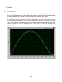
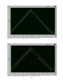
5 Results ............................................................................................................................................. 60
5.1
Current control ....................................................................................................................... 60
5.2
Magnetizing performance ...................................................................................................... 69
5.2.1
Reset results ................................................................................................................... 69
5.2.2
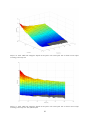
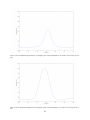
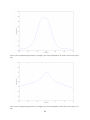
Surfaces .......................................................................................................................... 70
5.3
Time ....................................................................................................................................... 86
6 Discussion and conclusions ............................................................................................................. 87
6.1
Current control ....................................................................................................................... 87
6.1.1
The work of the controller ............................................................................................. 87
6.1.2
Suggestions of improvements ........................................................................................ 87
6.2
Magnetizing results ................................................................................................................ 88
6.2.1
Reset ............................................................................................................................... 88
6.2.2
Discussion about the surfaces ........................................................................................ 88
References ............................................................................................................................................ 89
Attachments ......................................................................................................................................... 91
Hardware ......................................................................................................................................... 91
Connection lists .......................................................................................................................... 91
Interconnections.......................................................................................................................... 93
MATLAB code ................................................................................................................................ 95
1 Introduction
1.1 Background
In a large range of electromechanical applications a magnetic force is used in the conversion
between electrical power and mechanical power in either direction. Many of these devices involve
permanent magnets and in these devices there is often a strong correlation between the
performance of the used permanent magnets and the performance of the final device. For that
reason it is desirable with permanent magnets whose properties are within tight tolerances.
Different materials have different magnetic properties. [1] What is common for those material that
are used for permanent magnets are the ability to remember a magnetic flux, this is called
remanence. The properties of the remanence differ between different materials in several ways.
Generally, the most important parameter is how large flux the magnet is able to store.
Magnets are magnetized by affecting the magnetic entities of the magnet called magnetic domains.
This is achieved by exposing the magnet to an magnetic field, usually provided by an
electromagnet. Since different materials have different properties it is not unreasonable to assume
that they should be magnetized in different ways. If the desired remanent flux is large the flux
applied by the electromagnet must also be large. Nevertheless, there is profit in exposing a magnet
for a flux that is much larger than the possible amount of remanent flux.
The maximum applied flux is not the only important parameter. The way the flux is applied is also
important. If the magnet is able to carry an electric current, eddy currents will occur if the flux is
applied to fast. These will act like a magnetic shield which inhibits the magnetization since they
will provide a flux that is opposite to the magnetizing flux.
As mentioned, this magnetic property differs between different magnet materials. Even the
properties inside a piece of magnet differ from spot to spot. This makes it difficult to manufacture
magnets of a consistent quality since it seems like it is desirable to treat every spot of it
individually. To get around this problem LTH has produced a prototype with the aim to
individually magnetize small spots of permanent magnets. The magnet that is to be magnetized is
placed in an air gap where the flux is concentrated to a small slit. This is done dynamically with
lenses made of copper where the eddy currents generated in the lenses is forcing the flux through
the slit. The flux is provided by two copper coils in which it is driven a pulse shaped current.
The equipment before this thesis was not working satisfactory and was in need for improvements.
The achieved magnetization was not as precise as wanted and the reason for this is not directly
specified. A possible reason is that the ripple of the current driven through the flux providing coils
was to large, hence a new current controller is to be implemented. To gain better control of the
machine a new modern control system has been purchased. The new control system is meant to
replace the old one and allow development of a more advanced control system with better
performance, but still be easy to use.
1
1.2 Objectives
 Replace the current controller to a control system based on NI CompactRIO and introduce a
method of modulation that minimizes the ripple of the current.
 Improve the usage of sensors for measuring the accomplished magnetization. The measuring
width should be the same as the magnetizing width.
 Further improvement for automatic, iterative magnetization of discrete magnets.
 Initial study of the possibility to industrialize the process in terms of the cycle time and the
quality of the final magnets.
1.3 Scope
The target of this thesis is to meet all the objectives of the project plan. Since the conditions for
some of the parts of the project was unknown the objectives was adjusted during the project.
The current controller is built as planned, but a lot of safety devices are added to minimize the risk
for damage on hardware as well as humans and hence minimize the number of delays in the work.
No advanced measuring head is developed. Instead hall sensors placed next to the magnet band
are used.
Instead of studying the possibilities of automatic iterative magnetization the performance and
properties of the magnetizer is studied. Only small spots were magnetized and the peak
magnetization and pulse width is studied as functions of magnitude, time and shape of the current.
Due to this delimitation the possibilities to industrialize the process is not studied
2
2 Theory
2.1 Current control with inductive loads
There are two main types of current controllers, the sampled current controller and the direct
current controller. [2] This book is the basis for our view of how these two controllers work, but to
make this text more readable, here is a short summary. It is assumed that the reader is familiar
with switching electronics and the voltage/current characteristics of inductive loads.
The sampled current controller uses a triangular wave modulator to create a switch pattern which
result in a mean output voltage that corresponds to the desired voltage reference. The current
through the load is sampled in the middle of the current rise or the current fall to obtain a mean
value of the current without using any averaging. The sampled current and the current reference
are feed to a regulator which creates the voltage reference to the modulator. It is possible to
calculate the ideal regulator parameters analytically from the inductance and the resistance of the
load and the time between the samples. These parameters are called dead beat parameters and
provide a new voltage reference that will eliminate all the error in the current. This controller has
many advantages, for instance that the switching frequency can be chosen to a known value.
The direct current controller, or the tolerance band current controller is much more simple. In its
most simple form it compares the actual current with two references which forms the tolerance
band. If the current is below the lower band, the voltage is turned on. If the current is above the
upper band, the voltage is turned off. This creates a self-oscillating controller which is very
simple, but also stable. When using a four quadrant converter there are more choices than only on
and off, the voltage can be reversed to. This means that there are three different current slopes to
choose between, hence a little refinement is needed. The solution is to add two more bands outside
the earlier two bands to find out if the chosen action was sufficient. For example: the current
crosses the upper inner band and the controller changes the output voltage to zero, but this is not
enough to make the current fall. Hence the current will cross the outer upper band, and a more
suitable output voltage could be applied. This controller has its strength in its simplicity and
insensitivity for outer variations.
2.2 The choice of control system
It is desirable to use currents the order of 300 A and it is known that at least parts of the magnetic
circuit is saturating at the flux densities that these currents will result in. This means the
inductance will vary to and hence the sampled current controller is not the wisest choice. Instead,
the choice is a direct current controller, or a tolerance band controller as it is going to be called in
this text.
Today, there are mainly two different ways when designing a tolerance band current controller.
The old way is to use analog electronics for the comparisons and digital circuits to choose action.
The new way is to sample the current extremely fast and practically implement the same thing in
software. The new way requires an extremely fast (hundreds of kHz) AD converter and calculating
performance that can handle the amount of data. But in return it is more flexible.
Our choice is to make a hybrid of these to variants. The bands are going to be generated digitally
3
and hence the controller will be as flexible as the digital version. But the comparisons are going to
be made with analog electronics, and hence there will be no need for an extreme AD converter.
4
3 Hardware
3.1 Existing hardware
As you may have noticed this thesis is not about building a magnetizing machine from scratch.
Most of the hardware for the prototype was already built, but in need for some improvements. But
to give the reader of this report a fair picture of the conditions for our work here is a description of
the hardware that we recycled for our work. This chapter will only cover a description of the
hardware, not necessarily an explanation about why it is built as it is.
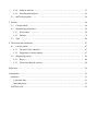
3.1.1 Enclosure
Image 1: Pulse magnetizer machine
In the image above the pulse magnetizer machine is seen. It is built in and on top of a metal box.
The inside is split into two different volumes where the big one is inside the feet of the cabinet. On
top of this part the magnet holder and the magnetizing head is placed. In front of the top of this
part is a pult shaped enclosure. This part is electrically shielded from the rest of the machine and
represents the smaller volume. On top of it the control panel is placed.
5
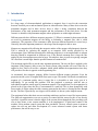
Image 2: The big volume inside the feet of the pulse magnetizer machine
In the big volume all high voltage devices such as power electronics, etc. is placed. This is seen in
the image above and gives the opportunity to connect the power electronics to the magnetizing
head with short cables. In the smaller volume the control system is placed, as far as possible
protected against electromagnetic interference. Nevertheless, since the mains instrumentation and
the power supplies for the cRIO and the peripheral electronics are placed here to it occurs mains
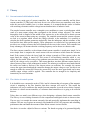
voltage. A close up image of the inside of the smaller volume is seen below.
Image 3: The smaller volume with cRIO, metal box containing developed electronics and two power supplies
6
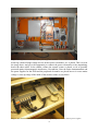
3.1.2 Magnetizing head
Image 4: The magnetizing head of the pulse magnetizer machine
The magnetizing head is seen in the image above and consists of an adjustable yoke with an air
gap containing the magnet that is supposed to be magnetized. Next to the magnet the yoke ends up
with two flux collection lenses that are concentrating the flux to a defined area. This area is shaped
as an upended rectangle with the height of the magnet and the width equal to the desired resolution
of the magnetization. Next to these lenses there are two coils providing the flux when an
appropriate current is driven through them. These coils are coupled in series.
3.1.3 Magnet holder
The magnet holder is a prototype made for evaluation of the rest of the machine. It is simply two
pieces of magnet band glued to the cutting surface of a piece of plastic pipe. The plastic pipe is in
turn attached to a rotatable base consisting of an aluminum plate and a servo motor. This means
that you can choose which part of the magnet band that is to be exposed to the concentrated flux of
the magnetizing head by sending a position reference to the servo.
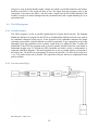
3.1.4 Power electronics
The old power electronics was used as well, however a new controller was a part of the thesis. The
power electronics has been used almost as it was except for some smaller changes and repairs. It is
7
built like a module with IGBT's with suitable drivers, DC link capacitors, rectifier and inductors
for the rectifier mounted on a metal plate. The IGBT’s and the rectifier are further more mounted
on a water cooling block, however this is not connected since the losses does not seem to cause
any significant temperature rise.
It is supplied directly from rectified 400 volts three phase mains. There is no transformer isolating
this power supply from the mains, hence it is completely isolated from the rest of the construction.
This means that there is a lot of power available to the rectifier, since there is no stray inductance
of resistance as in regular power supply with a transformer. To make it possible for the rectifier to
survive a sudden drop of the DC voltage there are two inductors of 0,3 mH between the rectifier
and the DC link capacitors with the aim to smooth current peaks.
Between the rectifier and the inrush current limiter there is a mains filter with the aim to prevent
the machine from disturbing other equipment.
3.1.5 Inrush current limiter
When energizing the DC link the voltage across the DC link capacitors are usually zero. This
means that the current through them will huge if the rated voltage of the machine is applied at
once. To prevent this inrush current from breaking the mains fuses or even the rectifier the
machine is equipped with an inrush current limiter consisting of two contactors, one time relay
and three power resistors of 100 ohms. The function is very simple, the first contactor connects the
mains voltages to the rectifier via the power resistors. The voltage drop over the resistors enables
the DC link capacitors to be charged at a more suitable current. After approximately four seconds
the time relay closes the second contactor which short circuits the resistors, however, during these
four seconds the DC link voltage has been able to rise to approximately 500 volts. The first
contactor and the time relay is activated by an external input for 230 volts.
3.1.6 Hall sensors
During the early test of the performance of the machine it was provided with a hall sensor
mounted next to the outside of the magnet band. Unfortunately this sensor was damaged during
our tests.
8
3.2 Developed hardware
Image 5: The inside of the metal box containing the developed electronics
The developed hardware can be seen in image 2, 3, 4 and 5. On the far right in image 2 electronics
for calibration can be seen, it is the card to the right of the indicator for the DC link voltage. Image
3 show the smaller volume of the enclosure with the cRIO, a metal box containing developed
hardware and two power supplies. On the left side of image 4 a card for the hall sensors can be
seen. Most of the developed hardware is nevertheless in the metal box and a close-up of it can be
seen in image 5. The large circuit board is for the current controller. On the top right is a circuit
board with level converters for the power electronics. On the small prototype board is signal
conditioning and the large prototype board beneath it is more electronics involved in calibration.
Since it is very tight on tight with space in the box there is another prototype board under the large
prototype board the can be seen in the image. This board is involved in something called Shake to
wake and is explain in Shake to wake in 3.2.7.
9
3.2.1 The usage of a CompactRIO
About the CompactRIO
We did not develop the CompactRIO system, but to give the reader a fair overview of the control
system, here is a short description of the cRIO.
The cRIO consists of three parts, an embedded computer, a field programmable gate array (FPGA)
and a number of input and output modules (I/O modules). The embedded computer that is used is
a NI cRIO-9022 and the used FPGA is a NI-9114. All together they form the cRIO into a compact
industrial controller and measurement system. It is up to the programmer which part of the code
that is to be executed in the embedded computer and which part that is to be executed in the FPGA
and the code look similar, but it is executed in very different ways. The code executed in the
embedded computer executes task by task since it is a single core processor, nevertheless it is
executed in a real-time operating system. The code that is downloaded into the FPGA is
practically built into hardware. This sets clear limitations in the complexity and the size of the
code. The big advantage is that everything that runs into the FPGA is executed simultaneously,
hence it is very powerful in controlling applications if it is used properly. The FPGA is connected
to both the I/O modules and the embedded computer. Hence controlling tasks can be handled by
the I/O modules and the FPGA only with extremely short response time, while heavier less time
critical calculations is delegated by the FPGA to the embedded computer. The embedded computer
is equipped with two Ethernet ports. These are used for communication with the host PC that is
used for programming and interfacing it for example. Furthermore it is equipped with one RS232
port for miscellaneous use and an USB port to connect an extra storage volume. [3]
The RS232 port is in our case used for communication with the servo used for positioning of the
permanent magnet.
Input and output modules
The cRIO is very flexible in the way that you can choose I/O modules that suits you task. In this
project five modules are used where two of them are the same. The used modules are:
NI 9205 that is an analog input module with 32 channel and 16 bits resolution. [4] The sampling
rate is 250 kS/s distributed over all used inputs. It is also provided with a digital output. In our
case it is used for non time critical data sampling as hall sensor data and diagnostics of the
machine.
NI 9215 that is an analog input module with four inputs and 16 bits resolution. [5] The sampling
rate is 250 kS/s, however this module is capable of sampling all inputs simultaneously at a sample
rate of 100 kS/s.
NI 9263 that is an analog output module with four output and 16 bits resolution. [6] The sample
rate is 333 kS/s if one channel is used and 105 kS/s if all four is used.
NI 9401 that is a TTL I/O module with 8 channels. [7] The channels can be configured as in or
outputs in groups of four and the performance varies with the number of channels used. Two of
these modules are used.
10
Interface
The interface to the user consists of two parts, the front panel on the host PC and the control panel
located on the machine. During normal operation the user only uses the front panel for
programming and monitoring of the machine. The control panel is there for both practical and
safety reasons. It makes it possible to shut parts of the machine down during troubleshooting for
example, and if something in the control system hangs up the user can safely stop the machine
from it.
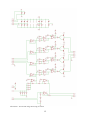
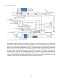
3.2.2 Current control
Overview
The current that is driven through the flux providing coils is regulated to a shape and magnitude
decided by the user to allow maximum flexibility. To ensure good control of the current ripple a
tolerance band controller is used. As mentioned earlier a hybrid between the analog and the digital
tolerance band controller is used. The desired tolerance bands, in other words the current shape
and magnitude, are generated digitally. But the comparisons, ie what determines if the current is
within tolerance or not is done analogy which gives almost immediate response. To make this
possible the generated bands DA converted with an analog output module and feed to the
peripheral electronics. The comparison signals is feed back to the FPGA where the choice of new
signals to the IGBT drivers is made.
There are totally four tolerance bands, two inner and two outer. The purpose of the inner bands is
to know if the current is within tolerance or not. The purpose of the outer bands is to know if the
chosen control action was sufficient or not.
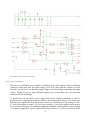
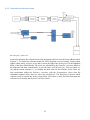
The schematic of the peripheral electronics is found below and will be explained the following
paragraphs.
11
Illustration 1: Current and voltage measuring electronics
12
Current measuring
The current transducer is delivered by LEM. It is a LA 306-S/SP1 and it is capable of
measuring
properly configured. [8] The conversion ratio is 1:5000 and the measuring
resistance is selected to 25 ohms. Since the output from the power electronics only passes through
the transducer once this gives a total conversion ratio of
. This signal is inverted and
amplified four times by the IC1D which implies that the conversion ratio will be
. This
signal is used in the comparison with the tolerance bands and for monitoring after being inverted
another time by IC1A.
One of the channels of the NI 9215 are used to sample this signal. Notice that this signal is
sampled for monitoring purposes only. It is used when the current controller is to be tuned.
Comparison electronics
As mentioned, the decision if the current is within tolerance or not is made with analog
electronics. There are four identical couplings based on IC2, IC3 and IC4. The left most
operational amplifier buffers the output signal from the analog output module. The right most IC is
a comparator that is provided with a hysteresis band to minimize the risk flickering. The hysteresis
band corresponds to
of the total output voltage swing of the comparator which is equal
to
.The consequences of this hysteresis is taken care of which will be explained later.
Since this comparator circuit only does the comparison around zero volts the measured current is
subtracted from the tolerance band level and feed to the comparator. This is done by the
operational amplifiers in the middle. When the current is approaching the the tolerance band level
the output of this operational amplifier will approach zero which, if it continues will result in a
comparator output change. The comparator output signal is buffered and converted in TTL level
signals with the transistor couplings to the right of them.
Variable inductance
The power electronic converter and its control system are designed to handle in the order of
hundreds of amperes with small amounts of current ripple but still acceptable rise times. This
means that if the current reference is in the order of ten amperes instead, the ripple will probably
be unacceptable. To come around this problem an extra inductor is connected in series with the
flux providing coils when the current peak value is 20 A or less. The coupling is very simple and is
shown below.
13
Illustration 2: Variable inductance electronics
In high current mode a contactor makes the current flow through the flux providing coils only. In
low current mode this contactor is opened and another contactor is closed which makes the current
flow through an extra inductance of
. To improve the signal to noise ratio in the current
measurement 9 extra turns around the current transducer is added in the same way when choosing
low current mode, this result in a new conversion ratio of
. Of course, this is taken care
of in software.
It should be mentioned that during the development of the current controller, it was unknown that
there was a need for good current quality at this low currents. Hence these parts of the hardware
are implemented in a more temporary way.
Calibrating electronics
The current controller is partly an analog construction with all that it implies, and as mentioned the
comparators have a small hysteresis that must be taken care of. The amplifiers and the current
transducer are assumed to behave linearly but with an uncertainty in amplification and offset. All
of the comparators have a certain position when the current is within tolerance and the other
position tells the control system when it is not. This means that the comparator hysteresis can be
treated as an offset as well.
14
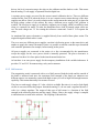
To be able to compensate for both offset and amplification uncertainties a test current is needed.
This is in principle achieved with voltage source and a resistor.
Illustration 3: Calibrating electronics
The supply voltage is 5 V and the resulting resistance is around 1 ohm which gives a resulting
current on 5 A. The current runs through the current transducer 20 times which makes the control
system think that the actual current is 100 A. All switches are actually relays which can be
maneuvered from the cRIO, and to minimize the risk for disturbances there are opto-couplers
between the cRIO and the relay driver.
The upper most relay closes the coil which thus are disconnected during normal operation. The
two other relays make it possible to make the control system experience both 100 A and -100 A.
The current through the coil is measured as a voltage with the 0.1 ohm shunt by the cRIO with one
of the channels on the NI 9205 module during the calibration.
The execution of the calibration will be described in the software chapter of this report.
15
Voltage measuring
The DC link voltage is measured only for monitoring. To ensure galvanic isolation between the
DC link and the control system a voltage transducer from LEM is used. It is a LV 25-P/SP2 and it
is approved for measuring up to
[9] Actually it is a current to current converter with
galvanic insulation and a conversion ratio of 2500:1000. The resistors that are used
are
for the primary side, and
for the secondary side.
This gives a total conversion ratio of
The used operational amplifier is a LF347. [10] The used operational amplifier is a LM339. [11]
One of the channels of the NI 9215 is used to sample this signal. As mentioned, this signal is
sampled for monitoring purposes only. It is used when the current controller is to be tuned.
As an extra monitor, and a remained there is a voltmeter next to the power electronics in the feet
of the cabinet.
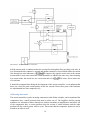
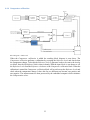
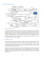
3.2.3 Level converter to the IGBT's
The IGBT driver is configurable to handle both 5 V and 15 V signal levels on the input, however
the manufacturer recommends the use of 15 V level when the signal cable is as long as for the
construction. [12] The output on the NI 9401 is a 5 V TTL output, hence a level converter is
needed. The level converter card does not only convert the signal levels. It inverts the signal to the
lower IGBT in the bridge and has the ability to put zero volts on all outputs which is used to reset
errors reported by the driver. The complete circuit is in Illustration 4 below.
There are four inputs and one output to the cRIO. The upper most input is the enable input. If it is
enabled the control signals will reach the drivers. If it disables, all outputs will be zero which as
mentioned resets the driver. The first inverter buffers and inverts the signal. The transistor
coupling makes the conversion from 5 V to 15 V and inverts one more time. This signal is used to
the output AND gates.
The next two inputs are for the bridge controlling signals. The level conversion is made in the
same way as for the enable signal. The capacitor in the transistor coupling shortens the fall time of
the converted signal since the base current will be greater at the transition. The capacitance is
experimentally determined to make the fall time as close the rise time as possible. It is feed to an
inverter to buffer and make the signal to the lower IGBT and then inverted again to make the
signal to the upper IGBT.
The last input is only buffered with to inverters to use for other purposes.
The level converter listens to the error output of the drivers. Since it is negated it is inverted and
then converted into a 5 V signal by two resistors and feed to a input on one of the NI 9401
modules. The inverter is driving a transistor to with the purpose of providing the card with an
extra error indicating signal output with the capability to driving a led or a relay for example.
The used logical gates were 74HCU04 [13], TC4049 [14] and HEF4081 [15].
16
Illustration 4: Level converter electronics
3.2.4 Power supplies
There are several different power supplies for different parts of the machine. There are different
reasons for using more than one power supply. First of all, many different voltages are used.
Secondly, it is not wise to use the same supply voltage to feed for example both analog and digital
circuits. Thirdly, if you use many different supplies you can start them up in an order that
minimizes the risk for damage.
To provide power to the cRIO a power supply delivered by National instruments is used. To
provide power to all peripheral electronics related to the current control and power electronics two
different power supplies are used. The first one, delivered by VERO power is providing +15 and 15 volts to the analog electronics. [16] It is also providing +5 volts to the digital circuits used in
the level conversion stage, the calibration equipment controller and the shake to wake. Another
+15 voltage is supplied by a power supply delivered by XP power. [17] This is used for the IGBT
17
drivers, the level conversion stage, the relays to the calibrator and the shake to wake. This means
that the analog 15 volt supply is separated from the digital one.
A separate power supply was used for the current control calibration device. There are different
reasons for this, first of all, when the device is in use it requires more current that any of the other
supplies can deliver. Since it is used in relation to the current sensor the main part of it is placed in
the high voltage volume of the cabinet. By using a different power supply EMC problem is
avoided. The used power supply is an ordinary computer power supply which is modified to start
when it is connected to mains. To make the installation more clean all unused output cables are
cut. The used voltages are 5 V for creating the reference current and -5 and 12 V for operate the
relays.
As mentioned the power electronics is supplied directly from rectified three phase mains. The
original design described earlier is used.
The servo uses two different power supplies, one that is delivering power to the motor drive and
another to supply the control electronics. Hence it is possible to start the controller up to download
safe controller parameters for example, before turning on the power.
All power supplies are connected to the mains via a fuse recommended by the manufacturer
except the supply for the servo power which is internally protected. The power electronics is
connected via three 16A fuses placed in the inrush current limiter box.
At last there is an extra power supply for the temporary installation of the variable inductance. It
provides 5 V and 24 V for maneuvering a relay and a contactor.
3.2.5 Hall sensors
The magnetizing result is measured with a set of hall sensors. Both the inside and the outside of
the band is measured and since the maximum field strength of the band was unknown two
different sensors was mounted to ensure both high accuracy as well as high field strength measure
capability. This means that totally four sensors are used.
They have a rated supply voltage of 5 volts, which is available. But since it is used to feed digital
circuits it was not used for this purpose. Instead the analog 15 volt was used a regulated down to 5
volts via a voltage regulator. The output of this type of hall sensor is a function of the field
strength in the measuring direction and the supply voltage. Hence, the supply voltage is sampled
to and taken into account in the software. The coupling is shown below.
Illustration 5: Hall sensor voltage regulator electronics
18
3.2.6 Cooling of the flux providing coils
When using current greater than 100 A and shooting many and longer pulses the flux providing
coils get hot. And in order to not take any risks with the coil insulation these has to able to cool
down after more intense periods, for example a reset. To make the cool down time shorter a fan is
placed close to the yoke and the air flow is guided through it to cool the coils as effectively as
possible. The fan is activated when the inductance is set to high current mode. This leaves the
opportunity to leave the fan on during a cool of pause, as well as turning it off during a hall
measurement.
3.2.7 Safety
The DC link capacitors of the power electronics are able to store a lot of energy. If something goes
wrong in the control system it can result in quite dangerous situations where hardware as
expensive IGBTs or as well humans can take damage. Hence a little extra effort was paid when the
control panel of the magnetizer was made.
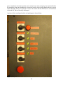
Control panel
To begin with, there are four groups of power supplies, each group has its own circuit breaker. The
first switch turns on the power supply to the cRIO and the power supply to the servo controller.
This makes it possible to set parameters, etc. to both the cRIO and the servo before powering up
anything else.
The second switch turns on the power supplies to the peripheral electronics, i.e., the +/- 15 volts to
the analog electronics and the +5 and +15 volts to the digital electronics, including the drivers for
the IGBT's. This makes it possible to make the calibration of the analog electronics or
troubleshoot in a safe way if needed. It is also used to the power supply for the variable
inductance and as a main switch for the cooling fan to the flux providing coils.
The third switch turns on the power supply to the servo. Finally the fourth switch turns on the DC
link voltage by applying 230 volts to the enable input on the inrush current limiter.
The order the different switches are listed in above is the order they are supposed to be started in
to. For safety they are coupled in a way which means that a higher order switch becomes
ineffective if not all of the lower order switches are set to on. The switches for the servo power
and the DC link are furthermore only functioning when the machine is in Operational mode. The
condition for Operational is that none of the two emergency switches has been tripped. One of
them is located on the control panel and the other one is represented by the Shake to wake, which
will be explained later in this chapter. Every power supply, except for the DC link is equipped with
a pilot lamp that indicates if it is supplied with mains, i.e. it will light up if the power to the supply
is on and the fuse is intact.
As mentioned the machine should be started in a certain order. The same applies when shutting it
down. To make sure that the controller software is not shut down while the DC link is charged the
stop execution button on front panel is disabled while the DC link voltage is above 20 volts.
The instrumentation also includes an emergency stop. The emergency stop does not turn of the
19
power completely since this is not the wisest action in case of an emergency! As mentioned before
the emergency stops only disables the Operational mode, which in turn disables the servo power
and the DC link, if they are turned on of course. This means that the IGBT drivers will remain on
so that the DC link can be safely discharged.
A picture of the control panel and the wiring diagram is shown below.
Image 6: Control panel
20
Il
lustration 6: Control panel
21
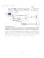
Shake to wake
The second, earlier mention emergency stop called shake to wake has the same effect as the first
emergency stop. But instead of a button it is a relay connected to a circuit board connected to the
cRIO. The main function is to detect if the FPGA freezes, and if it is happening it trips the
emergency stop. This is done by a VI that continuously generates square wave via one of the
digital outputs. This square wave is filtered by a low pass filter to obtain a signal around 2.5 volts
which is compared with 2 and 3 volts. If the comparisons show that the signal is between 2 and 3
volts it will close the relay. Of course, this leaves the opportunity to trip the emergency stop from
the software as well. This is used by diagnostics, the activate button and the emergency stop on
the front panel. The activate button turns on the shake to wake if the control system is in ready
mode. This occurs if the diagnostics part of the program does not find any faults.
The coupling is shown below and the used circuits were HEF4030 [18] and LF347 [10].
Illustration 7: Shake to wake electronics
22
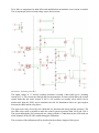
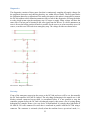
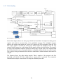
Diagnostics
The diagnostics consists of three parts. One that is continuously sampling all supply voltages for
the peripheral electronics and checking that they are within allowed limits. The next part checks
the calibration data after a calibration of the analog electronics, this makes it impossible to turn on
the DC link without valid calibration parameters since a fault in the diagnostics will stop the shake
to wake which in turn trips the emergency stop. Of course a supply failure voltage will have the
same effect. The last part is listening to the error signal from the drivers. If a driver announces an
error it freezes the bridge position to make it possible for the user to see what caused the error. Of
course, even this error will result in an emergency stop. The voltage dividers are shown below.
Illustration 8: Diagnostics electronics
Fast stop
If one of the emergency stops trips the power to the DC link and servo will be cut, but normally
the DC link capacitors will still be charged. The only thing discharging in the normal case is the
bleeder resistors connected across them. As mentioned before it is not possible to stop the
controller program before the DC link is discharged properly, this means a lot of waiting during
debugging for example. Hence a fast stop device is implemented. It is simply three light bulbs of
60 watts at 230 volts connected in series that is connected in parallel with the DC link using a
contactor. The contactor is activated (closed) when the machine leaves operational mode, i.e.,
23
when one of the emergency buttons trips. This means that a fast stop will occur if the machine
halts on some kind of fault to.
3.2.8 The philosophy of the construction
EMC
During the design phase of the machine EMC problems was avoided as far as possible. To begin
with the control system and its peripheral electronics are placed in a separate volume electrically
shielded from the power electronics. Furthermore the peripheral electronics is placed in a
screening box of aluminum. All cables related to the control system are shielded as well and the
shields are only connected to the screening box containing the peripheral electronics to avoid
ground loops. For the same reason is the screening box the only connection between the earth of
the control system and protective earth. More specific solutions will be described under the
heading for each part.
Choice of components
The attentive reader or maybe the next person who are going to develop the machine further will
probable find the choice of components a little strange in some parts of the construction. Therefore
we want to point out that we used parts that we found in stock at IEA to minimize the number of
orders and delays. The parts are selected to not compromise the function or the result, but as said
some of the choices may seem a little illogical.
24
4 Software
The basis of our understanding how to use the program language LabVIEW and the cRIO is the
course manuals [19] and [20].
4.1 Distribution of tasks
The tasks of the software in this project ranges from a user friendly measurement system with
settings, graphs and the possibility to save measurements to a file down to the current controller
with response times that are less than one µs. To accomplish this the cRIO system has been used
since it can provide both ends on this scale and of course everything in between. To understand
how to distribute tasks between the FPGA and the embedded computer in the cRIO system a little
more information about the cooperation between the embedded computer, FPGA and the I/O
modules, than given in 3.2.1 is needed.
The I/O modules communicate with the FPGA which in turn communicates with the embedded
computer. If the embedded computer wants to communicate with the I/O modules, this is done
through a program on the FPGA. The embedded computer runs a real-time operating system
(RTOS) made by National Instruments. This makes the cRIO to a stable controller with features
found in a normal operating system for a PC. This includes a file structure, ethernet connections,
ftp server capabilities and hardware resource monitoring.
The sequential nature of executing a program for a CPU leads to latency between input and output
which can be a limitation when implementing controllers with the embedded computer.
Furthermore, an increased workload can decrease the performance. In that essence the FPGA has
an advantage since the program is literally implemented in hardware which makes the execution
parallel of its nature. Thereby an increased workload of the FPGA will not decrease the
performance. It is also possible to make FPGA programs with very low latency. The limitations of
the FPGA is its size and thereby the size of the program that can be implemented on it. Other
disadvantages is that compared to the embedded computer the compile time for the FPGA is many
times longer and the programs are thereby harder to debug. This makes the development time for
the FPGA programs longer. To not reach the hardware recourse limit of the FPGA and have a to
long development time it is essential to not use the FPGA unnecessarily.
The programs for the embedded computer and the FPGA are developed in National Instruments
development environment LabVIEW. Except for hardware restrictions the programs for the
embedded computer and the FPGA is the same and the development tool takes care of the
integration in the real-time operating system on the embedded computer and with the FPGA. The
programmer programs a task for the embedded computer, the FPGA or a combination of both.
This choice can later be changed and the code can be reused as long as it meets the hardware
restrictions of the intended target. Sometimes the choice between the embedded computer and the
FPGA is easy and sometimes it is harder.
The FPGA is the link between the embedded computer and the I/O-modules and a custom FPGA
program has been developed to provide communication between them. A custom FPGA program
provides maximum control of the digital inputs and outputs and the sampling rates of the A/D- and
D/A-converters. In the FPGA it is possible to make the signal processing fast and achieve control
loops running faster than one µs when using the digital I/O signals. Tasks with a close relation to
25
the I/O modules, like fast control loops is also directed to the FPGA. Tasks that involve input from
the user or presenting data to the user is not that time critical and is thereby natural to implement
in the embedded computer. Tasks involving signal processing before presentation to the user could
be implemented on the embedded computer or the FPGA. Where it is implemented depends on
demands on speed, amount of data, complexity of the algorithm and the integration with the rest of
the program. It is also possible to split it and do some processing in the FPGA and the rest in the
embedded computer.
4.2 Communication between the different parts
Everywhere in the programs, both in the embedded computer and the FPGA there is a need to send
and receive information from other parts of the program. As expected there is more than one way
to do this and the ones used in this project will be explained here.
4.2.1 Variables
Sometimes a control or an indicator on the front panel is needed in more than one place in the
program. This is achieved with a so called local variable to the control or indicator. Local
variables can only be used in the same VI and in this project they are only used in the embedded
computer. Related to the local variable is the global variable. Instead of being located on the front
panel of the program it is placed on the front panel of a separate VI. This makes the global
variable accessible from more than one VI. If more than one global variable is needed, more
variables can be added to the separate VI with the first global variable. The structure of the FPGA
program makes global variables very useful to create variables that are used within the FPGA. In
the program for the embedded computer global variables are only used for communication
between loops that run in parallel.
4.2.2 FIFO-queues
FIFO-Queues (First In First Out Queues) are essential in both the program for the embedded
computer and the transfer of large amounts of data from the FPGA program to the program in the
embedded computer or vice versa. A queue is a data structure that allows data to be produced and
consumed at different times but still not lose the order of the data. A FIFO-queue dequeues the
data in the same order as they are enqueued.
4.2.3 Interrupts
The program in the FPGA can generate an interrupt to the CPU in the embedded computer. An
interrupt is meant to interrupt the normal execution of the program in the embedded computer and
run a special part of the code called the interrupt routine. The interrupt routine is then supposed to
take care of the reason for the generation of the interrupt. It is possible to generate up 32 different
interrupts.
26
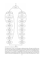
4.3 The structure of the program on the embedded computer
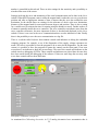
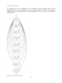
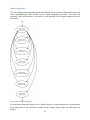
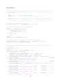
4.3.1 User interface
Front panel 1: Whole system
The front panel seen above is the whole user interface. Since it is a tab-based interface not
everything can be shown at the same time. The idea with the tab-based interface is to save space
on the front panel and make it user friendly but at the same time advanced and powerful by only
showing the necessary controls, graphs, etc. to the user. The interface utilizes the space of two
screens and can be divided into three parts. Some controls are always good to keep within reach
and these are placed in the upper part of the left screen, the rest of the left screen contains the main
tab interface. The right screen contains a tab interface controlling which graph to show and these
tabs correspond to tabs in the main tab interface. These three areas will be described separately in
the following text.
It is natural to start describing the controls that always are within reach. This part of the user
interface contains a system for activating and deactivating the machine. It contains an emergency
stop button which disables the servo power and the DC-link, if they are turned on. This is done by
turning the shake to wake signal off. Next to the emergency stop button is a button named Stop
execution, when pressed it will stop the execution of the RT- and FPGA-program if the DC-link
voltage is below 20 V. The machine goes into the operational mode and a boolean indicator called
Operational on the front panel turns green when the Activate button is pressed. However, there are
some conditions for the Activate button to turn the machine into the operational state. These
conditions are; no error from the IGBT drivers may occur, the supply voltages has to be within
limits and the compensation values for the comparators has to be okay. This is indicated by a
boolean indicator that is located above the Activate button. When the conditions are not met the
indicator is red and contains the text Check diagnostics and when the conditions are met the
indicator is green and contains the text Ready.
When a scanning sequence of the magnet band or a magnetization sequence of the magnet band is
started a timer starts. The timer is used to show the time in minutes and seconds since the
sequence was started and is located in the upper part of the interface. In the same area there are
buttons to pause the execution of a sequence and resume it later. These buttons are called Pause
sequence and Resume sequence. When the servo can not go to the desired position it will also
pause the sequence in the same way as the pause button does, the sequence can then be resumed
27
using the resume button when the user has solved the problem.
The upper part of the user interface also contains a dial and an indicator of the DC-link voltage
and a dial and indicator of the rotor position in degrees. Finally there is two boolean indicators,
one that show when there is serial communication with the servo controller and the other shows
when the RT uses the FIFOs for sampled current and voltage data.
Underneath this is the main tab interface with four different tabs, diagnostics, calibration of
comparators, current control and magnetization. Three of these tabs have in turn a tab interface
into them, these tab interfaces is referred to as sub-tabs.
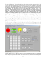
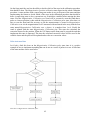
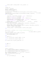
Front panel 2: Diagnostics
The Diagnostics tab seen above presents information and controls that are useful when the user
wants to see if the system reports anything that is wrong. There are three sub-tabs in the
diagnostics tab to limit the information presented to the specific interest; hardware, servo or
software.
The Hardware tab shows information about the supply voltages in the control electronics. These
voltages are continuously controlled to be within the tolerance limits. The nominal values and
tolerance for the supply voltages are set in this sub-tab. Since resistors are dividing the voltages
before they are read by the A/D-converter this sub-tab contains controls for these scale factors.
Here is also information about eventual comparator- and driver-errors. Finally here are settings for
sampling of the hall sensors. The hall sensors are continuously sampled just like the supply
voltages. But when they are used for taking a reading of a specific position of the magnet the A/Ddigital converter goes to a special mode that takes an average on a number of samples. This
28
number is controlled in this sub-tab. There are also settings for the sensitivity and a possibility to
trim the offset error of the sensor.
Settings involving the servo and monitoring of the serial communication can be done in the Servo
sub-tab. When the RT-program wants to rotate the magnet band it orders the servo to go to the new
position and after an appropriate amount of time it ensures that the servo has reached the new
destination. In the sub-tab there are settings for the tolerance of check at the new destination,
diameter of the magnet band for conversion between degrees and position. There is also a setting
for a variable used to estimate the time for rotation using the distance to travel. Further on there is
a button to manually enable the servo controller. The servo controller can indicate errors from the
servo controller electronics, the most important of these is decoded and displayed on the Servo
sub-tab. If there is an error in the servo communication there are also indicators of that. Finally
there is the possibility to save the servo communication to a log file.
There is a sub-tab called Software that contains controls and indicators to debug the embedded
computer program. For example, to see if the diagnostics of the supply voltages consumes too
much CPU time it is possible to force the program to do or not to do the diagnostics. For the same
reason it is possible to force the program to ignore the controls on the front panel. If an error
occurs there is an indicator to show the error message. The rest of the controls and indicator on the
sub-tab involves debugging of FIFOs. These controls and indicators are placed there because they
have been useful during the debugging of the software. If there are more bugs the user may want
to use these controls and see these indicators.
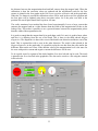
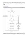
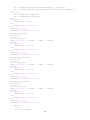
Front panel 3: Calibration of comparators
As mentioned in Calibrating electronics in 3.2.2 analog electronics have uncertainties that is
29
measured and taken care of in software. To perform this calibration the sub-tab Calibration of
comparators that is seen above is used. It is easy to perform a calibration, it is just to press the
Calibrate button. After the calibration is done the scale factors that was calculated from the
measurements is presented to the user in indicators in the sub-tab. The K-factor for each channel is
the calculated gain for each channel. It should be compared to the conversion ratio 0.02 V/A that
was calculated in Current measuring in 3.2.2. The M-factor is an calculated offset and for the
comparator channels it will compensate for hysteresis in the comparator and offsets in amplifiers.
The fact that they compensate for the hysteresis means that they should not be zero but sill rather
small. Comparing the M-factor between the channels there should be two groups, channel 0 and 1
and channel 2 and 3. If user thinks that all of the values shown in the indicators are okay they
could be downloaded and used in the FPGA with the Use button. Finally there is a control called
Voltage scale factor and it is ideally the inverse of the conversion ratio calculated in Voltage
measuring in 3.2.2. Since it is a control it is hence possible to compensate if the real conversion
ratio differs from ideal one.
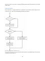
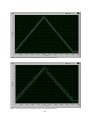
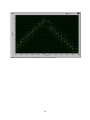
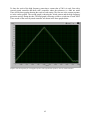
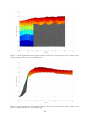
Front panel 4: Current control
The next tab in the main-tab interface is the seen above, namely the Current control tab. It is
important that the performance of the current controller is as good as it can be and this tab is used
to test and trim the performance. To do a test of the controller a set of controller parameters and
settings for a test pulse is entered. Then the RUN button is pressed and the current controller
parameters are loaded and the system changes the current reference to create the test pulse. The
current controller follows the reference according to the controller parameters and the resulting
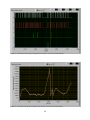
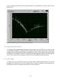
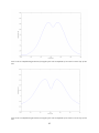
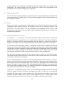
current can be seen in a graph in the main-tab interface. For further evaluation of the performance
of the current controller there are four other graphs available in the Current control analysis tab in
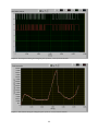
the graph-tabs for. The first graph shows the switch time (the inverse of the switching frequency)
30
for each switching event. The second graph shows the resulting switching pattern of switch 1 and
2 it also tells if and when the high switching frequency protection was engaged. The third graph
shows the DC-link voltage during the pulse. The fourth graph shows a numerical calculation on
the inductance based on the sampled current and voltage. The calculation of the inductance is only
valid during the time while there is an active vector applied and no switching occurs. In the
settings for the pulse generator the pulse type, amplitude and pulse time can be configured. The
pulse time is either entered directly or calculated from the values of the slope and amplitude
controls. It should be noted that this calculation is only valid for the triangle pulse type. In the
settings for the controller parameters there is a control for size of the tolerance band, this value is
used for the inner bands. The value of the outer bands is given as a percentage of the inner bands.
When small currents are generated inductance is added in series with the flux providing coils for
better performance. This means that there are two identical sets of controls for the controller
parameters. In fact there is a third set of controls since the inductance changes when the inductor
starts to saturate. Depending on the peak current the system uses one of these three settings for the
current controller. Finally it is possible to plot the reference, inner and outer bands in the same
graph as the resulting current.
Last but not least is the Magnetization-tab in the main interface. It is used for magnetization and
measurements of the resulting magnetization. There is a sub-tab system in the Magnetization-tab
to separate different magnetization related activities.
Front panel 5: Magnetization, Free run tab
The first sub tab is Free run and is seen above. It gives the opportunity to rather freely program an
array with pairs of positions and currents. The values in the array can then be used to magnetize
31
the magnet band, scan the band or to plot a result of a scan in the Free run scan tab in the graphtab interface. The positions to magnetize, scan or plot can be made arbitrary in the array. To make
that possible in this tab all references are made to the array indexes and not the position values. To
manually enter many values in the array is time consuming so there is two toolboxes to do that.
The first creates equally spaced position values and the second fills them with current values. The
servo motor can run in two different control modes, speed control and position control. Normally
the position control is used because it is the position that is interesting to control. The speed
control is used to make the servo and thereby also the magnet band spin at a constant speed. This
could be used to check mechanical variations and other testing. To change between the two control
modes the servo needs to be disabled before the change and enabled after by the Enable servo
button.
Front panel 6: Magnetization, Position calibration
The next sub-tab is seen above and it is used for the next step in the creation of a working
magnetization system and that is to calibrate the positions of the hall sensors. When the servo is at
0º, the position 0 mm is defined as the middle of the magnetization head. When this position of the
magnet band is scanned the servo motor will not be at 0º, for example it could be at 180º in the
case that the hall sensors is at the opposite of the magnetization head. This offset needs to be
calibrated using this sub-tab. The method for this calibration is to have a band with a constant
magnetization level and then magnetize one position in the band. This position can then be found
by scanning the band and find the position of the peak value of the magnetization level. This subtab gives the opportunity to do a reset of the band (which will be explained later), a pulse at a
specific position in the band and of course scan the band and find the peaks. For each sensor the
estimated distance and a search width is specified, this is to make sure that only a healthy part of
the magnet band is used in the analysis of the peak value. The value for the Estimated distance is
32
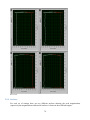
the distance between the magnetization head and hall sensors along the magnet band. When the
calibration is done the correction values are updated and the uncalibrated result for the four
sensors is plotted in the four graphs in the Hall sensor position calibration tab in the graph-tabs.
When the Use button is pressed the calibration values will be used in the rest of the program and
the four plots will be updated using these correction values. So if the pulse was done at the
position 100 mm all plots should show a peak at 100 mm.
The earlier mentioned reset method has been found experimentally. It uses a large current that
saturates the magnet band on a wider distance than the width of the magnetization slit due to the
leakage flow. This makes it possible to use a greater distance between the magnetization pulses
than the width of the magnetization slit.
It is good to control that the magnet band is in good shape, and if it is not it is good to know where
and how it is differing from the rest of the band. This is done in the third sub-tab Magnet
diagnostics. The diagnostics is done with a reset of the band in one direction and then a scan of the
band. This is repeated but with a reset in the other direction. The result is then plotted in the
Magnet diagnostics in the graph-tabs. It is possible to plot the raw data from the scans and/or the
difference between the two scans. If the absolute value of the magnetization level is the same for
the reset with positive current and negative current the difference will be zero.
To do a quick scan of a segment of the whole band the Scan band sub-tab can be used. The result
is plotted in the Scan band tab in the graph-tabs. The data can be saved to a file using the controls
in this sub-tab.
Front panel 7: Magnetization, Surfaces
33
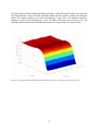
The last sub-tab in the interface is called Surface and is seen above. It is used for testing the
performance of the magnetization device. These tests always start with a band that is evenly
magnetized, this is done with the same reset method that was mentioned earlier. The simplest test
imaginable to then perform is to shoot a pulse and scan the affected stretch of the magnet. An
analysis of the result can then tell how much it was magnetized and how long section of the
magnet that was affected. The result will depend on a number of things and this sub-tab is used to
investigate them. Things that have been tested are to vary the current, pulse type, number of pulses
and the slope. Again, it should be noted that the calculation for the slope is only valid for the
triangle pulse type. The tests in this sub-tab are designed to vary two of these parameters the
current and the number of pulses or the current and the slope. This will result in a number of test
configurations. To cover these configurations the test starts at a point on the magnet band. The
servo then moves the magnet band so that a new test point comes up and a second test is
performed. It is important that these test points do not interfere with each other. This procedure is
done over and over again until all the test points have been used. Now it is time to scan the whole
magnet band for the analysis. This procedure can then be started over again to cover more test
points. Of course the magnet band needs a reset before each round with set of test pulses.
The test points are specified in the Surface sub-tab and it is possible to specify up to 32 points.
These points should be points on the magnet band where the band is healthy. It is also important
that the different points behave in a similar way to the same test conditions since this contributes
to the uncertainty of the measurement. To check the condition of the magnet band the Magnet
diagnostics sub-tab is recommended to use. To perform a test it is also important to state the
number of positions to be used and the width that should be used to examine the result. The
scanned result is saved into a file for further analysis and that requires a file name. The file name
contains information about the test conditions and the word entered in the User string. The pulse
type is determined by the setting in the Current control sub-tab but since it is a part of the file
name it also needs to be put in a string in the Surface sub-tab. To ensure that the magnet band has
been reseted properly a test is done to ensure that the magnetization level is within a certain
tolerance entered as a reset setting. Since the magnetization head and in particular the coils get hot
when running large currents there is a fan to cool off the magnetization head. This fan could
potentially disturb the measurements. Therefore there is a timer that starts after the reset and
pauses the testing until the timer runs out. This time is also entered as a reset setting. Next of is the
settings for the current.
Since the goal of these measurements is to investigate what happens at different currents there
needs to be a way to get different currents. The way it is done is by three controls. The first is the
starting current, Io. A typical value for the starting current is zero. The current is then increased in
steps with amount of Delta I, this is then repeated the number of times entered in Ires. These three
settings will result in a maximum current that is displayed in the indicator Imax. The current is one
of two parameters to vary. The second is the number of pulses or the slope. In the sub-tab there is
another tab interface with two tabs where each contains settings for the number of pulses or the
slope. Both of these sets of settings are similar to the settings for the current with a start value,
delta and the number of times to increase. Beyond that the Pulse tab has a setting for the pulse
time and the Slope [kA/s] tab has a setting for the number of pulses to do at every position. Finally
there is button to start the testing called Start surface measurement. Here it is also good to know
the total number of test positions and the number of rounds that is needed to do.
34
4.3.2 Operating system
Structure
When making a program for the embedded computer it is important to have some sort of plan
from the beginning. Especially if the program will have as many features as this program have.
From the beginning we knew roughly what type features the structure of the program would need.
There is a need to run different parts of the program in parallel and that is easy to do with parallel
loops in LabVIEW. Related to parallel features is that the user wants to be able to give the
machines various commands in arbitrary order. Some of them might even need to run in the
background after they have started. In addition, many of the tasks need to share variables. To
implement that kind of program with a state machines and parallel loops would probably be hard.
It would also grow in size and complexity considerably fast. This would have a negative impact on
other features of the structure of the program, namely that it needs to be easy to develop the
program and add more tasks with ease.
The solution used to satisfy the needs was to develop a structure that could be seen as a very
simple form of operating system. The first building block of the operating system is a FIFO-queue
called the task queue. It contains elements that refer to a task to do, so when there is a new task to
do the corresponding element is enqueued in the task queue. The second part of the operating
system is a while loop that starts to dequeue one element from the task queue. That element is then
used to execute a piece of code that implements that task. Each task is implemented in a case is a
case structure and the case structure would then contains one case for each task. The case structure
is the third and last part of the operating system. These three building blocks are shown in
LabVIEW code below.
LabVIEW code 1: The three main parts of the operating system in the embedded computer
35
Implementing a state machine
This simple operating system can be used to implement a state-machine. Imagine a simple statemachine with two states that enqueues each other like in the one below.
State machine 1: Example of state machine
To implement the state machine the case structure in the operating system would contain two
tasks, one for each state. The program in each task would simply enqueue the other task. When
this state machine is started it would continue forever. Imagine that two of these state machines are
implemented and that they are independent of each other. Now this operating system starts to be
useful since it is easy to see that this could be expanded to more than two state machines. It is also
possible to see that this could be used to implement more advanced state machines. In fact each
state in a state machine could be rather advanced in itself. When the programmer understands the
structure of the operating system well it is a very powerful tool. It will be easy to develop a state
machine and change it during the development, without the need to be concerned about the other
state machines in the operating system. This operating system has one drawback nevertheless.
When a task executes, it executes and it will only stop when it is finished and hands the control to
the operating system. This implies that a task can not make a busy wait because that will stop all
other tasks to execute. A busy wait is seldom a good idea anyhow. More important is that the
execution time of a task can get so long that it will interfere with other tasks. The programmer
thereby needs to ensure that a task does not take too long time. Of course it is possible to create a
loop next to the operating system loop to deal with time critical tasks. These will then use the
RTOS on the embedded computer take care of the parallelism of the loops. Luckily it is possible to
enqueue elements to a queue in one loop and dequeue the elements in another parallel loop in
LabVIEW.
How the operating system is used
The operating system structure described above was considered to be a good starting point for the
program for the embedded computer and has been that throughout the project. The heart of the
program developed is a state machine looking much like the state machine with two states above
but it is expanded to four states. There are four tasks that implement these four states and these
tasks are Idle, Check front panel, Diagnostics and Background activities. The Idle task enqueues
the other tasks and itself as well. This will work since they are enqueued in a FIFO-queue. It can
also stop the program by dequeueing all elements if a stop condition is met. The last purpose of
the Idle task is to keep the cycle time of the state machine constant. When the Idle task is finished
next up is the Check front panel task. The name describes it very well since its job is to read the
front panel controls and start the corresponding state machine if a control implies that. It does this
for all controls on the front panel that could imply that a state machine should be started. Next up
is the Diagnostics which gathers information from the FPGA program and presents this in the
Diagnostics tab in the main-tab interface. It also checks so that the monitored power supply
36
voltages are okay and reports this to the FPGA program. Finally Background activities have
various tasks to do, hence the little more generic name. It implements three timers where two of
them were mentioned in 4.3.1, namely the elapsed timer and the cool of timer. The third timer
involves the servo motor and more specifically the time it takes for the servo to move to a new
position. It also now and then asks the servo controller if there are any errors and checks if the
servo controller has sent any new messages.
Another interesting thing is how the state machine described above is started. It is started by a task
called Init which enqueues the Idle task. The Init task also initiates some variables and the
communication with the servo. The Idle state in turn is enqueued before the while loop that is a
part of the operating system.
In program like this the number of variables used within the program to store values and send
values between tasks get fairly large. To cope with this a cluster containing the variables is used.
The cluster is coupled to a shift register on the operating system while loop. This means that the
values stored in the cluster from one task can be read by the next task. If all tasks pass on all the
variables except the one that they change a value that is stored can be read by any task that later
executes.
The FPGA program can generate three different interrupts. To deal with this a while loop parallel
to the one of the operating system is used. When an interrupt occurs it will simply enqueue a task
to the task queue of the operating system that handles the interrupt. The FPGA program generates
interrupts when the calibration for the comparators is done, when a magnetization pulse is done
and when a sampling of the hall sensors with averaging is done.
Current pulse generation
To shoot a current pulse the pulse needs to be generated in software first. The method used in this
project is to generate the pulse in the software of the embedded computer and then load the data
points to FPGA. The FPGA then consumes the data points at a constant rate and uses the value as
the present current reference. During a period of time this will create a current pulse. To send the
generated data from the embedded computer to the FPGA a FIFO-queue called Current to play is
used. Using a FIFO-queue is a good idea since that is are made to send large amounts of data from
the embedded computer to the FPGA or vice versa. The task Current: Generate generates the
current reference described above and writes the data to the Current to play FIFO. To get the
desired current the current controller in the FPGA needs the correct tolerance bands. The Current:
Generate task therefore also sends the correct values for the tolerance bands to the FPGA. When
the data is loaded the only thing remaining to do is to start the playback of the data. This is done
by the Current: Run task.
After a current has been played the user may want to see how the resulting current was. Therefore
the FPGA program samples the real current at the same rate that current reference is played. These
samples are written to a FIFO-queue called Analog samples. The DC-link voltage is also sampled
during the current pulse. It would be neat to put these samples in another FIFO-queue. However it
is only possible to have three FIFO-queues and the third is needed for another thing. The solution
is put both the current sample and the voltage sample in the same FIFO-queue. The samples are
taken at the same time, thus there will be equally many of them and they will be interleaved in the
FIFO-queue. The software in the embedded computer needs to take care of this and to make the
data useful in needs to separate it into two vectors.
37
The third FIFO-queue is called Digital samples and it transfers data about the switching instances
of the power electronics to the embedded computer. When a switching instance occurs an element
is written to the FIFO-queue. This elements contains information about which switch was
activated, the boolean value after the switch and on which clock cycle it occurred. The embedded
computer can then reconstruct the entire switching pattern from the data in the FIFO-queue.
When a current pulse has been played and the FIFOs Analog samples and Digital samples is filled
with data the FPGA program generates an interrupt. This means that the program can continue
with the next step. That could be analyzing the data or continue with a magnetization procedure.
Therefore the System: Read FIFOs task that is enqueued by the interrupt enqueues other tasks so
that they can continue.
Hall sensor sampling
To make the measurement of the hall sensors more accurate averaging is applied. As described in
3.2.5 the supply voltage for the hall sensor is needed to calculate the magnetic flux. The FPGA
program sums up a number of samples from a sensor and does the same for the supply voltage.
This is then repeated for the other three hall sensors. The task named Hall: Start sampling makes
the FPGA program start this measurement. When the measurement is done the FPGA program
sends an interrupt to the embedded computer. The embedded computer then enqueues a task called
Hall: Read sample. This task reads the values from the FPGA program and divides them with the
number of samples that were taken. It then calculates the magnetic flux. Since this procedure is
started by the Hall: Start sampling there is always a task that is interested of the result. Of course
this is tasks that are scanning the band. To let these continue on their work the task Hall: Read
sample enqueues the one that initiated the sampling.
Serial communication with the servo
For the serial communication there are two while loops parallel to the one of the operating system.
One of them is used to send data and the other is used to receive data. To write and read from the
serial port the standard VIs in LabVIEW to do that is used.
To communicate with the controller for the servo motor a special protocol is used. It is described
in depth in [21]. It is a protocol where the computer is the master and the servo controller is the
slave. The master is always the initiator of communication. This means that to get information
from the servo controller to the embedded computer the embedded computer needs to ask for it
first. When a message is sent to the servo controller it will always answer. If a value was requested
that value will be sent back. If a value or command was sent to the servo controller it will respond
with a message that tells if it was okay or not. The request used continuously in this project is
requests for errors and a request for the current position of the servo motor. The commands sent to
the servo controller are enable, disable, clear errors, change to position control, change to speed
control and go to new position. Also two commands that sends a value to the servo controller is
used, these values are new position and speed set points. The Init task also uses some commands
not mentioned above for the initialization of the communication with the servo controller.
A FIFO-queue called send queue contains commands to send. This is a good solution since it is
tasks in the operating system that know when to send a command and it is the while loop parallel
to the operating system that sends the message containing the command. It will also be easy to
38
send commands from a task since it is just to enqueue the command to the queue. The rest of the
job is handled by the parallel while loop for sending data with the serial port. To have a FIFOqueue for communication between tasks in the operating system and the parallel while loop that
reads the serial port is also a good idea. But in this case it is called receive queue and received
messages is enqueued in the while loop and dequeued in the operating system. When a message is
available in the receive queue a task called Decode is started. If the decoding finds that requested
data was received it starts a task that can use it. If the message got corrupted on the way it will be
enqueue again to the send queue. To be able to know what the message was there is a third queue
called sent queue. This contains the messages that has been sent and they are enqueued in the
parallel while loop that sends commands. In the normal case the message is not corrupted but the
element in the sent queue needs to be dequeued and thrown away.
Positioning the servo motor
The servo motor is used to rotate the magnet band and thus changing the position that is
magnetized. To move the servo to a desired position a command is sent to the servo controller. It
will take some time for the servo to rotate and then the position of the servo motor is checked.
This is done to detect if the servo motor can not position itself correctly. There could be different
reasons for this. It could be mechanical problems, power supply failure or random errors. To
implement this a two state in the operating system has been added, Servo: Display rotor position
and Servo: Change position. The first is enqueued when a message about the position of the servo
motor is received. The message is converted from the position format used by the servo controller
into position in degrees and mm. It also enqueues the Servo: Change position if it was the one that
requested the position. The Servo: Change position is enqueued when a task wants to change the
position. The tasks that request the change in position must provide the new position in the
variable New position in mm in the variable cluster. Servo: Change position ensures that the servo
motor will be at the desired position by looking at the present position and the desired position
order the servo controller the move according to the difference in position. This means that Servo:
Change position will be enqueued more than once to ensure that the servo motor will be at the
desired position. If it does not make it on the first try it tries again until it decides that it is not
possible to reach the goal and alerts the user. A flowchart for the logic of this task is presented
below.
39
Flowchart 1: Servo: Change position
There is very often something to do when the servo motor has reached the desired position. Either
a current pulse or sampling of the hall sensor should be done at the new position. Therefore a task
called Servo: Schedule at new position is enqueued when the servo motor has reached the desired
position. This task checks what there is to do and enqueues Current: Run to do a current pulse or
Hall: Start sampling to take samples of the hall sensors. These tasks will in turn start a chain
reaction that will enqueue the task that requested the new position.
40
Positions calibration
As described in 4.3.1 the calibration of the position of the hall sensors relative to the
magnetization head is an important step to get a working machine. Another state machine is
implemented in the operating system to do this calibration. As seen below it is a state machine
with nine states.
State machine 2: Position calibration
41
On the front panel the user has the ability to decide which of the steps in the calibration procedure
that should be done. The Magnetization: position calibration state supervises the whole calibration
procedure. A state machine with a supervising state makes it easy to skip one of the states and thus
implementing the feature to decide which of the steps in the calibration procedure that should be
done. A supervising state is also a convenient way to initialize variables before entering the other
states. First the Magnetization: Calibration reset band will be executed to reset the band then a
pulse at a known position is shot with the Magnetization: Calibration pulse state. After that it is
time to scan the band and first an array to put the measurements is created in Magnetization:
Calibration scan init the magnetization level is measured with and stored in the array with the four
states named Magnetization: Calibration scan x, where x is a number from 1 to 4. Finally the
result is plotted with the state Magnetization: Calibration plot. This state also calculates the
correction factors for the position. When the USE button on the front panel is pressed the task that
implements this state is enqueued. This time the calculated correction values will be saved in the
variable cluster and the plots will be updated and use the new correction values.
Pulse state machine
Let’s look a little bit closer on the Magnetization: Calibration pulse state since it is a perfect
example of how to implement something that can do one or a series of pulses in a row. A flowchart
of the state machine can be seen below.
Flowchart 2: Magnetization: Calibration pulse
42
The variable # mark pulses is in the variable cluster and is initiated to zero in the Magnetization:
position calibration state. The state machine utilizes the fact that both Current: Run and Servo:
Change position will start a chain reaction that will enqueue task that implements this state
machine.
Reset state machine
A flowchart of the state Magnetization: Calibration reset band can be seen in the flowchart below.
Flowchart 3: Magnetization: Calibration reset band
It looks similar to the previous flowchart and that is not a coincidence. The method to utilize the
chain reaction is also used here which leads to similar logic. This state also shoots pulses but in
43
this case it is done on over and over again on different positions until it has iterated over the whole
magnet band.
Scan state machine
Once again there is a good example how to implement a state machine with the Magnetization:
Calibration scan 1 state. The corresponding flowchart is seen below.
Flowchart 4: Magnetization: Calibration scan 1
Once again the winning concept to utilize the chain reaction is used and the logic of the state has
similarities with the other two.
44
Magnet diagnostics
The same thinking when implementing the state machine for the position calibration has been used
when implementing the state machine for the magnet diagnostics procedure. This makes the
structures of the state machines very similar. A state machine for the magnet diagnostics can be
seen below.
State machine 3: Magnet diagnostics
It has the supervising state Magnetization: Magnet diagnostics that determines the execution order
of the other states. It also initializes variables in the variable cluster before the other states are
entered.
45
Scan magnet band and data save
This is a rather simple state machine as seen below.
State machine 4: Left: Scan band. Right: Scan band save
It has no supervising state but that is because it does not need to be more advanced than it is. The
state Magnetization: Init scan band initializes an array to save the measurement data into. The
next state is Magnetization: Scan band. It utilizes the fact that Servo: Change position will start a
chain reaction that will enqueue the task that implements this state machine again. Finally the
result is presented in a plot in the Magnetization: Scan band plot state. As seen in the state
machine the there is a separate state for saving the data to a file.
Performance measurements
As described in 4.3.1 there is a test procedure that tests the performance of the machine. The test
conditions are different combinations of current and pulses/slopes and the program in the
embedded computer performs the tests and saves the resulting magnetization. The state machine
that implements this is rather large but has a simple structure, it could be seen in the state machine
below.
46
State machine 5: Performance measurements
The Magnetization: Surface init state initiates variables and creates a file name for the file to store
data in. It also creates an array with positions to use from the controls on the front panel and saves
it to a file with the created file name. The Magnetization: Surface pulse reset and Magnetization:
Surface pulse reset scan states are implemented in the same way as the reset and scan states
described above except that the reset starts a timer so the flux providing coils can cool down. An
analysis of the achieved magnetization level with the reset is done in the Magnetization: Surface
47
pulse reset scan analysis and decision where to go next is made based on the result. When the
reset is adequate it is stored in the file.
The flowchart for the Magnetization: Surface pulse pulse is seen below.
Flowchart 5: Magnetization: Surface pulse pulse
48
It is a more advanced state machine than previous once but it uses the same concept. The called
Magnetization: Surface pulse first pulse will produce the first pulse then jump to the
Magnetization: Surface pulse pulse. It is almost the same but with some minor differences since it
is producing the first pulse. When the tasks that implements these flowchart executes the machine
will start at the start current and the starting number of pulses at the first test position. Then it will
increase the number of pulses with delta number of pulses and shoot the resulting number of
pulses at the next position to use. The number of pulses is increased until they reach the limit of
the testing interval. Then the current is increased by delta current and the number of pulses starts
over again at the starting number of pulses. The task will continue to do this until there is no more
positions to use for tests or there is no more tests to do. The Magnetization: Surface slope pulse
works in the same way but the number of pulses is fixed and instead the slope.
After that once again a scan of the magnet band is performed and the result is then saved. If the
machine is finished it alerts the user about that else it continues in the loop and runs more test
pulses. To be able to perform the analysis of the results in MATLAB the test conditions needs to
be known. This is achieved with the file name. The format of the file name and an example can be
seen in table 1 and table 2 below. For the tests with number of pulses “number of pulses” is used
instead of “slope” in the file name. The Pulse time is irrelevant for the test with slope but a value
is used anyway to be consistent with the file name.
Table 1: File name format
1
2
3
4
Date
Io [A] Delta i [A]
6
7
# pulses 0 Delta
# pulses
5
Max
# pulses
Pulse
[mm]
1
101
30.0
8
9
10
with Waveform Pulse time User
[ms]
string
11
.xls
Table 2: File name example
11-08-02 0.0
5.0
5
Triangle
0.005
Final
test
.xls
Pause and resume sequence
On the front panel there are buttons to pause and resume the execution of a sequence. Too
implement that the Servo: Change position checks if this should be done. If so it enqueues a task
called System: Clear new tasks to schedule. This task stores variables that determines the program
flow of the sequence and sets them to do nothing. The same task can be enqueued again to restore
these variables.
Safety in software
There are a number of safety precautions in software. Both the embedded computer and the FPGA
are responsible for the safety. The utmost responsibility lies on the FPGA since it is considered to
be most stable and besides has the fastest response time. The shake to wake signal is generated in
the FPGA so it is also logical to put it in the FPGA for that reason. The program in the embedded
computer however can unload the FPGA program from the FPGA. Therefore the program in the
embedded computer prevents itself from do that until the DC link voltage has dropped below 20 V.
This is done in the System: Idle task. There is also a task called System: Activate which sends a
signal from the embedded computer to the FPGA that it is okay to turn on the shake to wake
signal. The rest of the safety precautions for the embedded computer are in the System:
49
Diagnostics task. It checks that the supply voltages are within a user defined tolerance and sends a
boolean to the FPGA if the result was okay or not. The signal from the emergency stop on the
front panel is also sent to the FPGA. The task reads a signal from the FPGA that indicates if the
machine is ready to be started (changed into the operational state) and a signal indicating if it is in
operational state.
4.4 The FPGA program
4.4.1 Overall structure
The FPGA program is as far as possible implemented in a logical block structure. The thoughts
behind the making of a program for the FPGA are fundamentally different from the ones used in
the embedded computer in this project. In the program for the embedded computer the simple
operating system makes it obvious that the execution is sequential. To get a program to work in the
operating system the parallelism of the software would need to be adapted to that. To utilize the
parallelism of the FPGA the program needs to be truly parallel and this makes the code harder to
understand straight away. To describe the FPGA program and make it easier to understand it is
explained with block diagrams. The block diagrams are as far as possible made to correspond to
the actual code. The blocks are representing VIs and are all placed in a VI called Pulse magnetizer
1.0.vi. This makes them run in parallel. The signal lines between blocks are implemented with
global variables.
4.4.2 Current control logic
Block diagram 1: FPGA code
50
The logic of the current controller is seen in the block diagram above. The block Digital input in
the upper left corner provides the four signals from the comparison electronics to the logic of the
current controller that is implemented in the FPGA. The logic of the controller is implemented
with the three subsequent blocks, Comparator interpreter, Vector type selector and Use both zero
vectors. The Comparator interpreter interprets the signals from the comparators and creates two
new signals, I/D and Zm. I/D tell the controller if it is supposed to increase the current or decrease
the current. It is not always certain if a passive voltage vector (zero output voltage) increases or
decreases the current, and since it is desirable to use passive voltage vector every second switch
the controller needs to be informed about what the passive vector achieves. This is done with the
signal Zm.
This application is a special case since it is known if the pulse is positive or negative before it
occurs. Therefor there is an ideal value for the signals I/D and Zm to start at and they can be forced
to change by setting the C I/D or C Zm input high.
These two signals, I/D and Zm, is sent to the Vector type selector which only translate them into
Inc, Zero and Dec. Inc corresponds to an active vector with a positive output voltage, Dec
corresponds to an active vector with a negative output voltage and Zero corresponds to passive
vector, i.e. zero output voltage.
These signals are used by Use both zero-vectors. It translates them into signals to the bridge where
Inc will be translated into S1 TB = true and S2 TB = false, Dec will be translated into S1 TB =
false and S2 TB = true and Zero will be translated into either S1 TB = false and S2 TB = false or
S1 TB = true and S2 TB = true depending which of them that were used the last time. When
passive vectors are used it changes the used passive vector every second time.
Since it is a tolerance band controller it can introduce undesirable high switching frequencies
when it is not properly tuned. Therefor there is a high switching frequency protection
implemented, the HF-protection as seen in the upper right corner of block diagram 1 in the
attachments. There are two identical blocks for this purpose, one for each leg in the bridge. The
only thing that differs is the S1 and the S2 in the names.
The desired leg position comes from Use both zero vectors and if it is okay to switch it is directly
forwarded to S1. The protection uses a timer that starts counting when a switching occur to
prevent that the same transistor is turned on again, in a certain time. This means for example that
the transistor could be turned on, and immediately off again, but then the transistor can not be
turned on again before the timer has counted to the desired limit that defines the highest switch
frequency. The same thing applies for next turn off. The minimum time between switches is sent
to the block in ticks to the Min ticks input. The output signals from the two HF-protection blocks
are sent to the Digital out block.
51
4.4.3 Generation of tolerance bands
Block diagram 2: FPGA code
In the block diagram above blocks involved in the analog reference levels has been added to Block
diagram 1. To control the tolerance bands the FPGA program uses four analog voltage output
signals called Analog reference levels and is seen to the right of the Analog out. It is the rightmost
block of the blue colored blocks. The levels are calculated by the Reference calculator which is
the leftmost of the blue colored blocks. It uses the Outer band distance [A], Tolerance band size
[A] and the current reference, I*, to calculate the ideal value for the reference levels. These are
then recalculated within the Reference calculator with the Compensation values from the
embedded computer before they are sent to the Multiplexers. The Multiplexers chooses which
reference levels to send to the Analog output block. So far there is only one block that generates
reference levels, namely the Reference calculator block.
52
4.4.4 Comparator calibration
Block diagram 3: FPGA code
When the Comparator calibration is added the resulting block diagram is seen above. The
Comparator calibration performs a calibration by sweeping the Reference levels and check when
the comparators change. To do this the Reference levels it generates needs to be sent to the Analog
out block, here the Multiplexers block comes in handy. With the input Mode it can choose to use
the Reference levels from the Reference calculator or the Comparator calibration block. When the
calibration is started the Comparator calibration block will as said sweep the Reference levels and
check when the comparators change. It does this for two different test currents, one positive and
one negative. The measurements are then processed by the embedded computer which calculates
the Compensation values.
53
4.4.5 Current pulse generation
Block diagram 4: FPGA code
To generate a current pulse the Sequence player is added to the block diagram and the resulting
block diagram is seen above. The current reference, I*, is changed by the Sequence player to
generate a current pulse. It gets the data points for the current pulse from a FIFO-queue called
Current to play which the embedded computer puts the data points into. When the Start playback
signal is activated the Sequence player starts to consume the data points at a constant rate and uses
the value as the present current reference, I*. During a period of time this will create a current
pulse. The Sequence player is also responsible for changing the values of the I/D and the Zm
signals with the C I/D and C Zm signals before it starts to generate the current pulse.
54
4.4.6 Error watcher
Block diagram 5: FPGA code
In the block diagram above the Error watcher block has been added. It ensures that the IGBT
drivers is only enabled when it is needed it is also responsible for shutting down the IGBT driver
if an errors occurs. It the driver itself that detects an error the Error watcher gets to know this by
the signal Driver error. If driver causes the error the S1 and S2 signals are saved to help the error
search afterwards.
55
4.4.7 Data sampling
Block diagram 6: FPGA code
In the block diagram above the Analog input block has been added. It samples the analog power
supplies and sends the measured data to the embedded computer. The embedded computer
analyzes the samples and returns the Voltages OK signal to the FPGA program. When the Take
hall sample signal is activated the Analog input block changes the sampling tactics and only
samples the hall sensors for a while along with the supply voltage to the hall sensors. The samples
are sent to the embedded computer which uses them to take a mean value of the magnetization
level. When the hall sensors are sampled the driver is disabled with the Disable drivers hall signal.
This is only a safety precaution because the driver should not be enabled when the hall sensors is
sampled.
The Sequence player also takes analog samples. That is samples of the current in the flux
providing coils and the DC link voltage when a current pulse is generated. The comparator
calibration also samples current when it is doing the calibration procedure.
56
4.4.8 Safety in software
Block diagram 7: FPGA code
In the block diagram above the Safety features, Shake to wake and Comparator error blocks has
been added. These two first is responsible for turning on the DC link voltage when the Activate
signal is activated and everything is okay. The Comparator values OK signal should indicate that
they are okay, the software controlled Emergency stop should not be activated and there should not
be any Driver error. The Shake to wake block will provide a 1 kHz signal to the Shake to wake
electronics when the Operational signal is true. The Comparator error block is also added in
block diagram 5. It looks at the comparator signals to detect if there is any illegal combination and
stores it if one found. An illegal combination could be that the comparators indicates that the
current is both higher and lower than the reference at the same time. This is a tool that could come
in handy to detect if there is problem with noise in the analog electronics.
57
4.4.9 Switch pattern analyzer
Block diagram 8: FPGA code
In the block diagram above the Switch pattern analyzer block is added. This is the final block in
the FPGA code and is used to analyze the switch pattern of the IGBTs but also the desired
switching instances. This block stores which variable that where changed, to which value it was
changed and on which clock cycle it changed into the FIFO-queue called Digital samples. This
allows the embedded computer to analyze the data and reconstruct the switching pattern both of
the IGBT and the desired values from the current controller logic. This means that is also can
detect when the HF protection was engaged.
4.5 MATLAB programs
The purpose of the programs in MATLAB is to compile the results into information that could be
analyzed by the user. The result is presented as a surface with the test conditions on the x- and yaxis and the analyzed parameter on the z-axis. The analyzed parameters are the maximum
resulting magnetization and width of the magnetized segment. The width is from 50% on the
positive edge to 50% of the negative edge.
The first m-script downloads files from the cRIO to the working directory of the computer it is
running on. It does this by presenting a list of the files in the folder Surface results in the cRIO.
When the script runs the user can then choose a file to download and when done the script can be
stopped. The script is called cRIO_result_files_getter.m and can be found in the attachment
MATLAB code.
58
The next m-script loads a file from the working directory into a matrix in the MATLAB
workspace. It also interprets the file name that has the format presented in table 1 in the
attachments, and saves the values from segment 2 to 7 and 10 into variables. The user interface for
this script is used in the same way as for the previous script. The script is called
MATLAB_file_loader.m and can be found in the attachment MATLAB code.
The analysis is done with the third m-script. First of all the user needs to enter what type of test
that is analyzed, if it is a performance test with different currents and number of pulses or with
different currents and slopes. The user can also specify which of the sensor to use. First the script
extracts the used positions from the data. Then it starts to divide the rest of the loaded array into
smaller arrays that each one contains the data from one scanning round of the band. In this process
the reset data is denoised. The number of test positions that has been used in every one of the
scanning rounds is also extracted and saved in variables. Note that there are two scans for each test
round, one from the reset scan and one from the pulse or slope scan. The scanned rounds are then
iterated through and analyzed by a MATLAB function that has been created, it is called
PeakNDeltFinderOneRound. The results from PeakNDeltFinderOneRound are added up to a
resulting matrix. After this the script takes the data corresponding to the chosen sensor from the
matrix and plots three different plots. The first is a surface plot with the test conditions on the xand y-axis and the maximum resulting magnetization on the z-axis. The second surface plot has
the maximum resulting magnetization relative to the magnetization for the reset at the z-axis. The
third surface plot has the width of the magnetized segment on the z-axis. The script is called
Data_divider.m and can be found in the attachment MATLAB code.
The function PeakNDeltFinderOneRound mentioned earlier uses the reset data and result data
from one round along with conditions of the tests. It goes through every tested position and
analyzes the data with a MATLAB function called PeakNDeltaFinder for every sensor. When it is
finished it returns the result. It also returns matrix with the invalid results that is used to make the
grayed area in the surface plots. The code for PeakNDeltFinderOneRound can be found in the
attachment MATLAB code.
The PeakNDeltaFinder function takes two vectors, one containing data with a peak in and one
containing the data from the reset scan. It then finds the peak value in the data and calculates the
width of the peak. It also returns the peak value the data relative to the reset. The code for
PeakNDeltaFinder can be found in the attachment MATLAB code.
If the user wants to study the pulse that analyzed to get the data point in a surface there is a mscript that does that. When an interesting data point has been found the x and y values is entered in
the script. The script finds the round containing that pulse and plots it. It also tells which of the
pulse that is the interesting in the command window in MATLAB. The script is called
peakCurrentPlotter.m and can be found in the attachment MATLAB code.
59
5 Results
5.1 Current control
One of the objectives in this thesis was to develop a current controller for the flux providing coils.
In order to facilitate the tuning of the controller the current is sampled by the cRIO and plotted on
the front panel during the test shots. The same plot tool is used to show these results.
Several different currents were tested to show the performance. The results will begin with tests at
the rated current for the machine, 315 A and then gradually decrease to 5 A. The tests at the rated
current will be shown for both a half sinusoidal pulse and a triangular pulse while the rest of the
currents only will be shown for triangular pulses. These results are shown in following eight
graphs.
Graph 1: Current response for a sinusoidal reference with a peak value of 315 A
60
Graph 2: Current response for a triangular reference with a peak value of 315 A
Graph 3: Current response for a triangular reference with a peak value of 200 A
61
Graph 4: Current response for a triangular reference with a peak value of 100 A
Graph 5: Current response for a triangular reference with a peak value of 50 A
62
Graph 6: Current response for a triangular reference with a peak value of 20 A
Graph 7: Current response for a triangular reference with a peak value of 10 A
63
Graph 8: Current response for a triangular reference with a peak value of 5 A
64
To show the work of the high frequency protection a current shot of 300 A is used, first with a
correctly tuned controller and then with a controller where the tolerances is a little too small.
There will be three graphs showing the result of each setting. The first one is the current response,
as in the earlier graphs. The second graph is showing the switch pattern and the high frequency
protection activity during the shot. The third graph is showing switch to switch time of each IGBT.
These results of the correctly tuned controller are shown in the three graphs below.
Graph 9: Current response for a triangular reference with a peak value of 300 A, correctly tuned controller
65
Graph 10: Switch pattern during the triangular pulse of 300 A, correctly tuned controller
Graph 11: Switch times during the triangular pulse of 300 A, correctly tuned controller
66
These next three graphs shows the behavior of controller where the tolerances are a little too tight.
The interference of the high frequency protection are shown by the two lower lines in the switch
pattern graph.
Graph 12: Current response for a triangular reference with a peak value of 300 A, incorrectly tuned controller
67
Graph 13: Switch pattern during the triangular pulse of 300 A, incorrectly tuned controller
Graph 14: Switch times during the triangular pulse of 300 A, incorrectly tuned controller
68
At last a graph showing the DC link voltage during a 300 A triangular current shot is shown in the
graph below.
Graph 15: DC link voltage during the triangular pulse of 300 A
5.2 Magnetizing performance
As mentioned, the magnetizing performance of the machine was tested. These tests were focused
on the ability to magnetize small spots of the magnet band. The studied parameters were the peak
magnetization and the spread around the magnetization peak, called magnetization width. These
parameters were studied as a function of different current magnitudes, shapes and different pulse
times. There will also be some graphs on some of the accomplished magnetizing pulses.
5.2.1 Reset results
To make these tests possible the band was restored to fairly uniform magnetization every time all
positions of the band were used. The method of this restoration, called reset in the program was
found by trial and error, and the result is shown in reset result below.
69
Reset result
5.2.2 Surfaces
For each set of settings there are two different surfaces showing the peak magnetization
respectively the magnetization width and all surfaces is shown in three different angles
70
To begin with two measurements with identical settings, except for the pulse shape was made. The
first measurement is done with half sinusoidal pulses and the second is made with triangular
pulses. The current is starting a 0 A and is increasing by 5 up to 150 A. The number of pulses is
starting at 1 pulse and is increasing by 5 up to 101 pulses. The pulse time is fixed to 5 ms. The
resulting surfaces for the half sinusoidal current pulses are shown in the six surfaces below.
Surface 1: Peak magnetization with half sinusoidal shaped current pulses and with pulse time fixed to 5 ms
71
Surface 2: Peak magnetization with half sinusoidal shaped current pulses and with pulse time fixed to 5 ms. Seen
from the front
72
Surface 3: Peak magnetization with half sinusoidal shaped current pulses and with pulse time fixed to 5 ms. Seen
from the right
Surface 4: Pulse width with half sinusoidal shaped current pulses and with pulse time fixed to 5 ms
73
Surface 5: Pulse width with half sinusoidal shaped current pulses and with pulse time fixed to 5 ms. Seen from the front
74
Surface 6: Pulse width with half sinusoidal shaped current pulses and with pulse time fixed to 5 ms. Seen from the right
75
The resulting surfaces for the triangular current pulses are shown in the six surfaces below.
Surface 7: Peak magnetization with triangular shaped current pulses and with pulse time fixed to 5 ms
Surface 8: Peak magnetization with triangular shaped current pulses and with pulse time fixed to 5 ms. Seen from
the front
76
Surface 9: Peak magnetization with triangular shaped current pulses and with pulse time fixed to 5 ms. Seen from
the right
Surface 10: Pulse width with triangular shaped current pulses and with pulse time fixed to 5 ms
77
Surface 11: Pulse width with triangular shaped current pulses and with pulse time fixed to 5 ms. Seen from the front
Surface 12: Pulse width with triangular shaped current pulses and with pulse time fixed to 5 ms. Seen from the right
78
The last measurement was made in a different way. Triangular pulses with the same current
magnitudes were used. But this time the pulse time was altered in correlation to the current
magnitude to obtain a constant slope of the triangular shape. Hence the axis earlier used for
number of pulses was used for current slope instead, and only one current pulse was shot. The
current slope was varied from
to
in steps of
. The resulting surfaces
six surface in presented below. A piece of each of these surfaces is grayed to show were the
requested current slope could not be maintained due to the request of current magnitude.
Surface 13: Peak magnetization with triangular shaped current pulses with varied pulse time to obtain current
slopes according to the slope axis
79
Surface 14: Peak magnetization with triangular shaped current pulses with varied pulse time to obtain current
slopes according to the slope axis. Seen from the front
Surface 15: Peak magnetization with triangular shaped current pulses with varied pulse time to obtain current
slopes according to the slope axis. Seen from the right
80
Surface 16: Pulse width with triangular shaped current pulses with varied pulse time to obtain current slopes
according to the slope axis
Surface 17: Pulse width with triangular shaped current pulses with varied pulse time to obtain current slopes
according to the slope axis. Seen from the front
81
Surface 18: Pulse width with triangular shaped current pulses with varied pulse time to obtain current slopes according
to the slope axis. Seen from the right
To facilitate an attempt to explain the shapes of these surfaces here are six pictures on carefully
selected magnetizing pulses.
82
Pulse 1: The accomplished magnetization of triangular pulse with an amplitude of 20 A and a current slope of 16,5
kA/s
Pulse 2: The accomplished magnetization of triangular pulse with an amplitude of 55 A and a current slope of 101,5
kA/s
83
Pulse 3: The accomplished magnetization of triangular pulse with an amplitude of 85 A and a current slope of 96,5
kA/s
Pulse 4: The accomplished magnetization of triangular pulse with an amplitude of 150 A and a current slope of 1,5
kA/s
84
Pulse 5: The accomplished magnetization of triangular pulse with an amplitude of 150 A and a current slope of 96,5
kA/s
Pulse 6: The accomplished magnetization of triangular pulse with an amplitude of 250 A and a current slope of 100
kA/s
85
5.3 Time usage
The time to perform a magnetization pulse is less than 1 s, the exception is when the pulse time is
close to or more than 1 s. That includes calculating the current reference, shooting the pulse and
transferring the data to the embedded computer. When the current controller is tuned the
embedded computer makes an analysis of the resulting current and plots it. The analysis is also
done within this second for pulses with a pulse time less than a tens of ms. In cases with a longer
pulse time the calculation time for the analysis makes it take longer time.
The time to position the servo depends on the distance to travel. It basically consists of two parts,
the time it takes to communicate with the servo and the time it takes for the servo to rotate. The
time of the communication differs from time to time depending on if the data is intact at arrival or
not. To turn rotate the magnet band 180º (which is the worst case) it takes barely 6 s. To scan the
whole magnet band with the highest resolution that the equipment allows it takes barely 30 min to
perform the scan. The highest resolution that the equipment allows is 0.25 mm and with that
resolution there is more than 2000 points on the magnet band to scan. This means that is takes less
than 1 s to move the magnet band 0.25 mm and to take a measurement with the hall sensors.
86
6 Discussion and conclusions
6.1 Current control
6.1.1 The work of the controller
As one can see the controller is keeping the current within tolerances when it is possible. At graph
1 the current is falling behind in the beginning of the half period. This is because the voltage is not
high enough in comparison with the inductance to obtain a sufficient current slope, the controller
could not possibly do more.
For the triangular pulse of the same magnitude in graph 2 is the current slope on the way up no
problem. In Graphs 3 – 5 one can clearly see that on the way down zero output voltage is not
enough to make the current fall in the desired way. The current crosses the outer upper band and
the controller changes negative output voltage to make the current fall faster. Furthermore, the
ripple on the current becomes more and more significantly due to the decreasing magnitude of the
references. Where the current slope is steep one can see that the current actually is crossing the
reference. This is due to the delay in the power electronics.
In graph 6 one can see that the ripple performance is improved. This is due to the variable
inductance which has increased the inductance.
In graph 9 is a triangular current shot of 300 A, and in graph 10 is the corresponding switch
pattern. On the switch pattern one can see that both output combinations resulting in zero output
voltage is used to distribute the switching load. On graph 11 the corresponding time between each
switch with each IGBT is shown. Around 1 –2,5 ms at the time axis the times between the
switches are close to 10 µs which corresponds to 10 kHz which in turn is the threshold for the high
frequency protection.
Graph 12 – 14 shows to the same thing as graph 9 – 11, but with an incorrectly tuned controller,
the tolerances are too tight. This means that the switching frequency will be too high which trips
the high frequency protection. The green and the blue line show where the high frequency
protection is engaged. A cursor is showing one of the interventions and cursors are found at the
corresponding time in the other graphs. At the time where the high frequency is active the switch
time is down to 10 µs which as mentioned is the threshold of it. It is also clear that to tight
tolerances result in more current ripple than necessary.
6.1.2 Suggestions of improvements
The overall current performance could be improved a little more if the tolerance bands where
shaped progressively to always utilize the highest possible switching frequency. However, it
would not improve the maximum ripple level of a given current pulse with a correctly tuned
controller.
A more sophisticated solution of the variable inductance with a bigger variety of inductances
could be implemented, but faster power electronics would probably be a better solution.
87
Another approach is to control the actual flux instead. This could be done by for example a time
integration of the voltage applied on the flux proving coils, which will be proportional to the
provided flux if the resistive voltage drop is subtracted.
6.2 Magnetizing results
First of all, when reasoning about these measurements, the reader should keep in mind that the
used magnet material is bonded ferrite. This means that no significant eddy current should occur
in the magnetic material.
6.2.1 Reset
There is not much to say about the reseting results. It was obtained by trial and error to find
something to make further tests from. The method is as one can see working well and it is in
practical use very time effective. The big variations at the beginnings and the ends of each
measurements corresponds to the ends of the magnet band and the small variations corresponds to
mechanical unevennesses.
6.2.2 Discussion about the surfaces
The Surfaces 1 – 12, especially 2 and 8 tells us that the number of pulses does not affect the
magnetizing result in any significant way. Another obvious conclusion is that the resulting flux
density is correlated with the current magnitude until the magnet is saturated. By trying to
magnetize the magnet more, the resulting flux density is decreasing, which invites to discussion.
As one can see the magnetizing width is consequently which could be explained by that the
leakage flux will increase with the total flux. Another interesting trend is that triangular shaped
current pulses results in both higher resulting flux and narrower magnetizing pulses, only benefits
in other words! Likely it depends on that the flux collecting lenses is doing a better work when
flux derivative and hence the eddy currents in them are kept at a more constant level.
The foregoing reasoning is supported by for example surface 16 where one can see that steeper
current slope results in narrower pulses. In the same way the maximum achievable flux in surface
14 increases with steeper current slopes.
A set of magnetizing pulses are shown in attachment Magnetizing results as Pulses 1-6. Pulse 1
shows the result of a relatively small current pulse while pulse 2 shows the result of a bigger pulse,
but still in the linear area of magnetization. Pulse 3 shows the beginning of the saturation of the
magnet. The pulses 5 and 6 show a rather interesting phenomenon which in a way explains the
look on the surfaces at higher currents. The widening of the pulse is continuing while flux density
is decreasing at the location where it should be peaking.
A proposal to an explanation of why is that it is due to unexpected eddy currents in the air gap
where the magnet is located. This theory is supported by surface 13 where one can see that the
extremely flat slopes which of course results in less eddy current does not suffer from the same
peak flux reduction at high currents. This is further supported by pulse 4 which is done with a
small current slope and a big current. Of course it will result in an extreme pulse width to.
88
References
[1]
Joseph J. Stupak Jr. “Methods magnetizing permanent magnets” Oersted Technology
corporation. pp. 1 - 8, October 2000.
[2]
Mats Alaküla and Per Karlsson, “Power Electronics – Devices, Converters, Control and
Applications”, Lund University, Department of Industrial Electrical Engineering and
Automation, pp. 33 – 106.
[3]
National Instruments Corporation, “Operating instructions and specifications
ComapctRIO NI cRIO-9022”, pp. 5 - 17.
[4]
National Instruments Corp., “Operating instructions and specifications – NI 9205”, pp. 1 –
25.
[5]
National Instruments Corp., “Operating instructions and specifications – NI 9215”, pp. 1 –
21.
[6]
National Instruments Corp., “Operating instructions and specifications – NI 9263”, pp. 1 –
15.
[7]
National Instruments Corp., “Operating instructions and specifications – NI 9401”, pp. 1 –
14.
[8]
LEM, Datasheet for: “Current Transducer LA 306-S/SP1”, pp. 1 - 3, July 2007.
[9]
LEM, Datasheet for: “Voltage transducer LV 25-P/PS2”, pp. 1 - 2, Mars 2006.
[10]
National Semiconductor, Datasheet for: “LF347”, pp. 1 – 2, August 2000.
[11]
National Semiconductor, Datasheet for: “LM339”, pp. 1 - 4, March 2004.
[12]
Semikron, Datasheet for: “SKHI 23/17 (R)”, pp. 1-10, June 2006.
[13]
Philips Semiconductor, Datasheet for: “74HCU04” pp. 3 – 5, September 1993.
[14]
Toshiba, Datasheet for: “TC4049”, pp. 1 – 3, February 1998.
[15]
Philips Semiconductor, Datasheet for: “HEF4081”, pp. 2 - 3, January 1995.
[16]
VERO POWER, Datasheet for: “EPLAX PK-serie, PK60”, pp. 10- 11.
[17]
XP POWER, Datasheet for: “VCS Series – VCS50US15”, pp. 1 - 2, May 2011.
[18]
Philips Semiconductor, Datasheet for: “HEF4030”, pp. 2 – 3, January 1995.
[19]
National Instruments Corporation, “LabVIEW Core 1 Course Manual”, pp. 1-1 – 9-24,
August 2010.
[20]
National Instruments Corporation, “CompactRIO and LabVIEW
Fundamentals - Course Manual”, pp. 1-1 – 9-49, September 2008.
89
–
Development
[21]
Cooper PowerTools, “User Manual – DIS-2 48/10 IC”, Metronix Messgeräte und
Elektronik GmbH, pp. 13 – 138, 2006
90
Attachments
Hardware
Connection lists
cRIO
NI 9205
AI0
AI1
AI2
AI3
AI4
AI5
AI6
AI7
AI8
AI9
AI10
AI11
AI12
AI13
AI14
AI15
AI16
AI17
AI18
AI19
AI20
AI21
AI22
AI23
AI24
AI25
AI26
AI27
AI28
AI29
AI30
AI31
COM
DO0
AISENSE
Diagnostics X1-1
Diagnostics X3-1
Diagnostics X3-2
Diagnostics X3-3
Diagnostics X3-4
NC
NC
NC
Diagnostics X1-2
NC
NC
NC
NC
NC
NC
NC
Hall sensor supply, X2-1
Hall sensor 1
Hall sensor 2
Hall sensor 3
Hall sensor 4
NC
NC
NC
NC
NC
NC
NC
NC
NC
NC
NC
Screening box ground, variable inductance electronics
Variable inductance electronics
Diagnostics circuit, X5-1
91
PFI0
NC
NI 9215
AI0 +
AI0 AI1 +
AI1 AI2 +
AI2 AI3 +
AI3 NC
COM
Current and voltage measuring electronics, X3-1
Current and voltage measuring electronics, X3-2
Current and voltage measuring electronics, X3-3
Current and voltage measuring electronics, X3-2
Current and voltage measuring electronics, X3-2
Current and voltage measuring electronics, X3-2
Current and voltage measuring electronics, X3-2
Current and voltage measuring electronics, X3-2
NC
Screening box ground
NI 9263
AO0
COM
AO1
COM
AO2
COM
AO3
COM
NC
COM
Current and voltage measuring electronics, X4-2
Current and voltage measuring electronics, X4-5
Current and voltage measuring electronics, X4-1
Current and voltage measuring electronics, X4-5
Current and voltage measuring electronics, X4-3
Current and voltage measuring electronics, X4-5
Current and voltage measuring electronics, X4-4
Current and voltage measuring electronics, X4-5
NC
Screening box ground
NI 9401 (1)
COM
NC
COM
COM
NC
COM
COM
NC
COM
COM
NC
COM
COM
DIO0
NC
DIO1
DIO2
Current and voltage measuring electronics, X1-5
NC
Current and voltage measuring electronics, X1-5
Current and voltage measuring electronics, X1-5
NC
Current and voltage measuring electronics, X1-5
Calibrating electronics, X1-1
NC
Calibrating electronics, X1-1
NC
NC
NC
NC
Current and voltage measuring electronics, X1-4
NC
Current and voltage measuring electronics, X1-3
Current and voltage measuring electronics, X1-1
92
NC
DIO3
DIO4
NC
DIO5
DIO6
NC
DIO7
NC
Current and voltage measuring electronics, X1-2
Calibrating electronics, X1-3
NC
Calibrating electronics, X1-4
NC
NC
NC
NI 9401 (2)
COM
NC
COM
COM
NC
COM
COM
NC
COM
COM
NC
COM
COM
DIO0
NC
DIO1
DIO2
NC
DIO3
DIO4
NC
DIO5
DIO6
NC
DIO7
Level converter electronics, X4-2
NC
Level converter electronics, X4-2
Level converter electronics, X4-2
NC
Level converter electronics, X3-6
Level converter electronics, X3-6
NC
Level converter electronics, X3-6
Level converter electronics, X3-6
NC
Level converter electronics, X3-6
NC
Level converter electronics, X4-2
NC
Level converter electronics, X4-2
Level converter electronics, X4-2
NC
Level converter electronics, X3-1
Level converter electronics, X3-5
NC
Level converter electronics, X3-4
Level converter electronics, X3-3
NC
Level converter electronics, X3-2
Interconnections
Level converter electronics, X6-2 – Shake to wake electronics, X1-1
Level converter electronics, X1-1 – IGBT driver, supply voltage
Level converter electronics, X1-2 – IGBT driver, ground
Level converter electronics, X1-3 – IGBT driver, S1 lower
Level converter electronics, X1-4 – IGBT driver, S1 upper
Level converter electronics, X1-5 – IGBT driver, S2 lower
Level converter electronics, X1-6 – IGBT driver, S2 upper
IGBT driver, error out – Level converter electronics, X1-7
93
Calibration electronics, X3-1 – Diagnostics electronics, X1-1
Calibration electronics, X3-2 – Diagnostics electronics, X1-2
Analog supply voltage (+15) – Diagnostics electronics, X4-1
Analog supply voltage (-15) – Diagnostics electronics, X4-2
Digital supply voltage (+5) – Diagnostics electronics, X4-3
Digital supply voltage (+15) – Diagnostics electronics, X4-4
Shake to wake electronics, X2-1 – Control panel, Shake to wake electronics
Shake to wake electronics, X2-2 – Control panel, Shake to wake electronics
94
MATLAB code
cRIO_result_files_getter.m
cRIO = ftp('130.235.80.52')
cd(cRIO, 'Surface results');
fileslist = dir(cRIO);
for n = 1:length(fileslist)
disp( strcat([num2str(n) ': ' fileslist(n).name]) )
end
file = 1;
while file > 0
file = input('Select file, enter 0 to close:');
if(file > 0)
%
fileformat = fileslist(file).name;
disp(mget(cRIO, fileslist(file).name))
end
end
close(cRIO)
clear cRIO
clear fileslist
clear n
clear file
95
MATLAB_file_loader.m
fileslist2 = ls;
ps = size(fileslist2);
n=1;
while n <= ps(1)
if strfind(fileslist2(n,:), '.xls')
disp( strcat([num2str(n) ': ' fileslist2(n,:)]) )
n = n+1;
else
fileslist2(n,:) = [];
ps(1) = ps(1)-1;
end
end
file = 1;
while file > 0
file = input('Select file, enter 0 to close:');
if(file > 0)
filesformat = strread(fileslist2(file,:), '%s');
current0 = str2double(filesformat(2));
delta_current = str2double(filesformat(3));
number_of_pulses = str2double(filesformat(4));
delta_number_of_pulses = str2double(filesformat(5));
max_number_of_pulses = str2double(filesformat(6));
pulse_width = str2double(filesformat(7));
time = 1000*str2double(filesformat(9));
workname = cell2mat(filesformat(10));
workname = workname(1:(length(workname)-4));
workname = genvarname(workname);
plotname = strcat([cell2mat(filesformat(8)) ' ' num2str(time) 'ms '
workname]);
eval([workname '=load(fileslist2(file,:));']);
end
end
clear
clear
clear
clear
clear
clear
fileslist2
ps
n
filesformat
file
time
96
Data_divider.m
% ----------------------------------------------------------------------- %
% These variables should be changed by the user to fit the measurment that
% is analyzed
slope = 1;
sensor = 1;
% 0 - curent and pulse
% Which sensor to look at, 1, 2, 3 or 4
figure_start = 1; % Figure number to start at when generatong the 4 plots
% ----------------------------------------------------------------------- %
% create the variable used positions
eval(['usedpositions = ' workname '(1:32,1:2);']);
% Clear unused positions from usedpositions
n = 1;
while n <= length(usedpositions)
if usedpositions(n,1) == 0
usedpositions(n,:) = [];
else
n = n+1;
end
end
usedpositions = usedpositions(:,2);
% create a vairiable containing the scanning resoulution
eval(['scaningres = ' workname '(34,1) - ' workname '(33,1);']);
nbr_of_index = round(180*pi/scaningres);
% divides the loaded datafile inso smaller parts that contain one scan of
% the band
divide_index = 33;
n = 0;
eval(['datalength = length(' workname ');']);
while divide_index < datalength
n = n + 1;
resetname = genvarname([workname '_reset_' num2str(n)]);
dataname = genvarname([workname '_data_' num2str(n)]);
datanumbername = genvarname([workname '_datanumber_' num2str(n)]);
eval([resetname
'
=
'
workname
'(divide_index:divide_index+nbr_of_index,:);']);
divide_index = divide_index + nbr_of_index + 1;
eval([dataname
'
=
'
workname
'(divide_index:divide_index+nbr_of_index,:);']);
eval([datanumbername ' = ' workname '(divide_index+nbr_of_index+1,2);']);
eval([resetname
'(:,2)
=
''sqtwolog'',''s'',''one'',4,''sym4'');']);
eval([resetname
'(:,3)
=
''sqtwolog'',''s'',''one'',4,''sym4'');']);
eval([resetname
'(:,4)
=
''sqtwolog'',''s'',''one'',4,''sym4'');']);
eval([resetname
'(:,5)
=
''sqtwolog'',''s'',''one'',4,''sym4'');']);
97
wden('
resetname
'(:,2),
wden('
resetname
'(:,3),
wden('
resetname
'(:,4),
wden('
resetname
'(:,5),
divide_index = divide_index + nbr_of_index + 2;
end
rounds = n;
current = current0;
pulses = number_of_pulses;
result = zeros(0,14);
invalid_result = NaN(0,14);
invalid_current = ceil((20.001-current0)/delta_current)*delta_current;
invalid_pulse
=
ceil((300number_of_pulses)/delta_number_of_pulses)*delta_number_of_pulses;
for n = 1:rounds
resetname = genvarname([workname '_reset_' num2str(n)]);
eval(['reset_data = ' resetname ';']);
dataname = genvarname([workname '_data_' num2str(n)]);
eval(['pulse_data = ' dataname ';']);
datanumbername = genvarname([workname '_datanumber_' num2str(n)]);
eval(['iterations = ' datanumbername ';']);
[result_part,
invalid_result_part,
current,
pulses]
=
PeakNDeltaFinderOneRound( ...
reset_data, pulse_data, usedpositions, iterations, scaningres, ...
pulse_width, current, delta_current, ...
pulses, delta_number_of_pulses, number_of_pulses, max_number_of_pulses, ...
invalid_current, invalid_pulse);
result = [result; result_part];
invalid_result = [invalid_result; invalid_result_part];
end
max_current = current; % this is used in peakCurrentPlotter.m
nbr_of_pulse_types
=
number_of_pulses+1)/delta_number_of_pulses);
if nbr_of_pulse_types == Inf
nbr_of_pulse_types = 1;
end
if slope == 1
x = result(1:nbr_of_pulse_types, 2)./10;
else
x = result(1:nbr_of_pulse_types, 2);
end
y = result(1:nbr_of_pulse_types:end, 1);
ceil((max_number_of_pulses-
if y(1) < 2
cut = 1
else
cut = 0
end
sensor = sensor*3;
z1 = vec2mat([result(:,sensor)], length(x));
z1i = vec2mat([invalid_result(:,sensor)], length(x));
z2 = vec2mat([result(:,sensor+1)], length(x));
z2i = vec2mat([invalid_result(:,sensor+1)], length(x));
tmp = result(:,sensor+2);
tmpi = invalid_result(:,sensor+2);
if cut >= 1
y3 = y(2:length(y));
98
z3 = vec2mat([tmp(length(x)+1:length(result))], length(x));
z3i = vec2mat([tmpi(length(x)+1:length(invalid_result))], length(x));
else
y3 = y;
z3 = vec2mat(tmp, length(x));
z3i = vec2mat(tmpi, length(x));
end
if slope == 1
xlabel('Slope [kA/s]')
else
xlabel('Number of pulses')
end
ylabel('Current [A]')
zlabel('Maximum magnetization [G]')
figure(figure_start)
surf(x,y,z1)
hold on
h = surf(x,y,z1i);
set(h, 'FaceColor', [0.3804
0.3804
hold off
if slope == 1
xlabel('Slope [kA/s]')
else
xlabel('Number of pulses')
end
ylabel('Current [A]')
zlabel('Maximum magnetization [G]')
0.3804])
figure(figure_start+1)
surf(x,y,z2)
hold on
h = surf(x,y,z2i);
set(h, 'FaceColor', [0.3804
0.3804
hold off
if slope == 1
xlabel('Slope [kA/s]')
else
xlabel('Number of pulses')
end
ylabel('Current [A]')
zlabel('Maximum magnetization [G]')
0.3804])
figure(figure_start+2)
surf(x,y3,z3)
hold on
h = surf(x,y3,z3i);
set(h, 'FaceColor', [0.3804
0.3804
hold off
if slope == 1
xlabel('Slope [kA/s]')
else
xlabel('Number of pulses')
end
ylabel('Current [A]')
zlabel('Maximum magnetization [G]')
0.3804])
if slope == 1
% Slope
mx = x(1):15:x(end);
99
my = (y(1):2.5:y(end))';
else
% Pulse
mx = x(1):2:x(end);
my = (y(1):2:y(end))';
end
[mxi,myi] = meshgrid(mx, my);
zi = interp2(x,y,z1,mx,my,'linear');
figure(figure_start+3)
surf(mx,my',zi)
if slope == 1
xlabel('Slope [kA/s]')
else
xlabel('Number of pulses')
end
ylabel('Current [A]')
zlabel('Maximum magnetization [G]')
clear
clear
clear
clear
clear
clear
n
nbr_of_index
divide_index
resetname
dataname
datanumbername
100
PeakNDeltFinderOneRound.m
function
[result,
invalid_result,
current_out,
pulses_out]
=
PeakNDeltaFinderOneRound( ...
reset_data, pulse_data, usedpositions, iterations, scaningres, ...
pulse_width, current, delta_current, ...
pulses, delta_number_of_pulses, number_of_pulses, max_number_of_pulses, ...
invalid_current, invalid_pulse)
result = zeros(iterations, 14);
invalid_result = NaN(iterations, 14);
half_width = floor((pulse_width/scaningres)/2);
for n = 1:iterations
index = usedpositions(n)/scaningres;
result(n,:) = [current pulses result(n,3:14)];
pd = pulse_data(index-half_width:index+half_width, 2);
rd = reset_data(index-half_width:index+half_width, 2);
if current > 1
[PeakValue,
RelPeakValue,
FirstIndex,
SecondIndex,
PeakNDeltaFinder(pd, rd);
else
mid = floor(pulse_data(length(pd/2)));
PeakValue = pd(mid);
RelPeakValue = pd(mid) - rd(mid);
DeltaX = 0;
end
DeltaX]
=
result(n,:) = [result(n,1:2) PeakValue RelPeakValue DeltaX*scaningres
result(n,6:14)];
if current <= invalid_current
if pulses >= invalid_pulse
invalid_result(n,:) = [invalid_result(n,1:2) PeakValue RelPeakValue
DeltaX*scaningres invalid_result(n,6:14)];
end
end
pd = pulse_data(index-half_width:index+half_width, 3);
rd = reset_data(index-half_width:index+half_width, 3);
if current > 1
[PeakValue,
RelPeakValue,
FirstIndex,
SecondIndex,
DeltaX]
=
PeakNDeltaFinder(pd, rd);
else
mid = floor(pulse_data(length(pd/2)));
PeakValue = pd(mid);
RelPeakValue = pd(mid) - rd(mid);
DeltaX = 0;
end
result(n,:) = [result(n,1:5) PeakValue RelPeakValue DeltaX*scaningres
result(n,9:14)];
if current <= invalid_current
if pulses >= invalid_pulse
invalid_result(n,:) = [invalid_result(n,1:5) PeakValue RelPeakValue
DeltaX*scaningres invalid_result(n,9:14)];
end
end
101
pd = pulse_data(index-half_width:index+half_width, 4);
rd = reset_data(index-half_width:index+half_width, 4);
if current > 1
[PeakValue,
RelPeakValue,
FirstIndex,
SecondIndex,
DeltaX]
=
PeakNDeltaFinder(pd, rd);
else
mid = floor(pulse_data(length(pd/2)));
PeakValue = pd(mid);
RelPeakValue = pd(mid) - rd(mid);
DeltaX = 0;
end
result(n,:) = [result(n,1:8) PeakValue RelPeakValue DeltaX*scaningres
result(n,12:14)];
if current <= invalid_current
if pulses >= invalid_pulse
invalid_result(n,:) = [invalid_result(n,1:8) PeakValue RelPeakValue
DeltaX*scaningres invalid_result(n,12:14)];
end
end
pd = pulse_data(index-half_width:index+half_width, 5);
rd = reset_data(index-half_width:index+half_width, 5);
if current > 1
[PeakValue,
RelPeakValue,
FirstIndex,
SecondIndex,
DeltaX]
=
PeakNDeltaFinder(pd, rd);
else
mid = floor(pulse_data(length(pd/2)));
PeakValue = pd(mid);
RelPeakValue = pd(mid) - rd(mid);
DeltaX = 0;
end
result(n,:) = [result(n,1:11) PeakValue RelPeakValue DeltaX*scaningres];
if current <= invalid_current
if pulses >= invalid_pulse
invalid_result(n,:)
=
[invalid_result(n,1:11)
PeakValue
RelPeakValue DeltaX*scaningres];
end
end
pulses = pulses + delta_number_of_pulses;
if pulses > max_number_of_pulses
pulses = number_of_pulses;
current = current + delta_current;
end
end
current_out = current;
pulses_out = pulses;
102
PeakNDeltaFinder.m
%%%%%%%%%%%%%%%%%%%%%%%%%%%%%%%%%%%%%%%%%%%%%%%%%%%%%%%%%%%%%%%%%%%%%%%%%%
%
%
% Pulse magnetizer
%
% 2001-08-17
%
%
%
%%%%%%%%%%%%%%%%%%%%%%%%%%%%%%%%%%%%%%%%%%%%%%%%%%%%%%%%%%%%%%%%%%%%%%%%%%
function [PeakValue, RelPeakValue, FirstIndex, SecondIndex, DeltaX] = ...
PeakNDeltaFinder(PeakData, ResetData)
NbrOfElements = length(PeakData);
NormData = PeakData - ResetData;
ResetMean = mean(ResetData);
if(ResetMean < 0)
[PeakValue, I] = max(PeakData);
else
[PeakValue, I] = min(PeakData);
end
if(ResetMean < 0)
[RelPeakValue, I] = max(NormData);
else
[RelPeakValue, I] = min(NormData);
end
FirstHalf = NormData(1:I);
[Moonshine, FirstIndex] = min(abs(FirstHalf - ((PeakValue-ResetMean)/2)*...
ones(length(FirstHalf), 1)));
SecondHalf = NormData((I+1):NbrOfElements);
[Moonshine, SecondIndex] = min(abs(SecondHalf - ((PeakValue-ResetMean)/2)*...
ones(length(SecondHalf), 1)));
SecondIndex = SecondIndex + length(FirstHalf);
DeltaX = SecondIndex - FirstIndex;
end
103
peakCurrentPlotter.m
current = current0;
pulses = number_of_pulses;
% ----------------------------------------------------------------------- %
current_goal = 150; % Y in a surface plot
pulse_goal = 965; % X in a surface plot
% ----------------------------------------------------------------------- %
test_point_nbr = 1;
round_nbr = 1;
while current < current_goal
if pulses >= max_number_of_pulses
pulses = number_of_pulses;
current = current + delta_current;
else
pulses = pulses + delta_number_of_pulses;
end
test_point_nbr = test_point_nbr + 1;
datanumbername = genvarname([workname '_datanumber_' num2str(round_nbr)]);
eval(['temp = ' datanumbername ';']);
if test_point_nbr > temp
test_point_nbr = 1;
round_nbr = round_nbr + 1;
end
if current > max_current
disp('This was bad 1 !')
break
end
end
datanumbername = genvarname([workname '_datanumber_' num2str(round_nbr)]);
eval(['temp = ' datanumbername ';']);
while pulses < pulse_goal
pulses = pulses + delta_number_of_pulses;
test_point_nbr = test_point_nbr + 1;
if test_point_nbr > temp
test_point_nbr = 1;
round_nbr = round_nbr + 1;
datanumbername
=
genvarname([workname
'_datanumber_'
num2str(round_nbr)]);
eval(['temp = ' datanumbername ';']);
end
end
dataname = genvarname([workname '_data_' num2str(round_nbr)])
eval(['temp_data = ' dataname ';']);
if pulses > max_number_of_pulses
disp('This was bad 2 !')
else
interresting_pulse = test_point_nbr
end
104
figure(figure_start+4)
plot(temp_data(:,1), temp_data(:,1+sensor/3))
xlabel('Position [mm]')
ylabel('Magnetization [G]')
center = 220;
axis([center-15 center+15 -300 500])
105