1
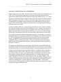
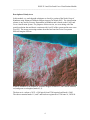
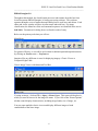
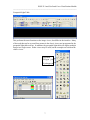
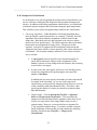
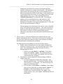
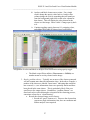
LLU – ESSE21
Land Use/Land Cover Classification Module
Honduras Land Use/Land Cover Case Study
ESSE 21 Land Use/Land Cover Classification Module
________________________________________________________________________
Table of Contents
Overview of Land Use/Land Cover Classification
3
Description of Study Area
4
Land Use/Land Cover Classes
5
Overview of ERDAS Imagine Tools and Menus
6
Classification Process Summary
8
Image Preparation
8
Classification Algorithms
9
Supervised Classification
Training Sites Creation
Training site Evaluation
Band Selection
Apply Decision Rule
Evaluation
Recode and Smooth
Accuracy Assessment
Unsupervised Classification
Clustering Algorithms
Cluster Analysis
Resolving Problem Classes
Recode and Smooth
Accuracy Assessment
9
10
11
20
21
21
22
23
25
25
26
27
28
28
Questions
29
Example Exercises
29
References
30
2
ESSE 21 Land Use/Land Cover Classification Module
________________________________________________________________________
Overview of Land Use/Land Cover Classification
Digital image data are frequently the basis to derive land use/land cover information over
large areas. Classification of image data is the process where individual pixels that
represent the radiance detected at the sensor are assigned to thematic classes. As a result
the image is transformed from continuous values, generally measured as digital numbers
(DN) or brightness values (BV) to discrete values that represent the classes of interest.
Traditionally the algorithms employed for this process differentiate and assign pixels
based on the values recorded at that pixel for each of the wavelength regions (bands) in
which the sensor records data.
A universal land use/land cover classification system does not exist. Instead, a number
have been developed to reflect the needs of different user(s). Typically, the systems are
hierarchically arranged with the ability to consolidate lower level classes into the next
highest level and with a consistent detail for all classes at a given level in the hierarchy.
In selecting a classification system for use with remotely sensed data, the classes must
have a surface expression in the electromagnetic spectrum. For example, a crop such as
pineapples reflects electromagnetic radiation, but an automatic teller machine (ATM) on
the side of a building cannot easily be detected, especially from most down-looking
sensors. In addition, the resolution characteristics of the imagery selected must be
compatible with the classification system. That is, the imagery must have the spatial
detail, spectral discrimination and sensitivity, and temporal characteristics required for
the classes of interest.
For purposes of applying the system for image classification, we must differentiate the
information classes represented by the land use/land cover classification system from the
spectral classes that we can obtain from the imagery. Often an information class will have
a range of spectral responses that represent the inherent variability within a class that is
intended to capture like activities. This may be due to composition of covers that are
necessary to express the class, e.g., residential class would include materials for roads,
lawns/gardens, rooftops and other building materials. Or, multiple land covers may
individually satisfy the criteria for a given land use class, e.g., crops of barley, corn,
lettuce, sugar beets, etc are all in the class “field crop”, but would have different spectral
responses. The diurnal and seasonal aspect also contributes to spectral variability due to
variation in planting dates, vegetation phenology, and illumination. Thus multiple
spectral classes, called signatures or training sites, that capture the variability are required
to represent a single information class.
3
ESSE 21 Land Use/Land Cover Classification Module
________________________________________________________________________
Description of Study Area
In this module, we work through techniques to classify a portion of the North Coast of
Honduras using Enhanced Thematic Mapper imagery for March 2003. The classification
scheme is one used by Forestry Department in Honduras and is based on the FAO Land
Cover classification system. For purposes of this exercise, we are working with 30m
spatial resolution data and that is consistent with Level II of the system and in some cases
Level III. The image processing routines described are based on Leica Geosystems
ERDAS Imagine software.
Northern Honduras from Enhanced Thematic Mapper on March 6, 2003 in near-infrared,
red, and green wavelengths (bands 4,3,2).
The data set is a subset of 1633 x 1280 pixels from ETM acquired on March 6, 2003.
The subset contains bands 1-5, and 7 and has been registered to UTM zone 16, WGS 84.
4
ESSE 21 Land Use/Land Cover Classification Module
________________________________________________________________________
Land Use/Land Cover Classes
Evaluacion Nacional Forestal de Honduras
Level I
Level II
Level III
Forest
Lowland Broadleaf
Coniferous
Mixed Forest
Mangrove
Nonforest
Other natural areas w/ woody cover
Shrubs
Pasture w/ trees
Savanna w/ trees
Other lands w/out trees – except agri-forest
Natural pasture
Savanna
Wetlands
Bare soil
Agri-forest
Annual crop
Permanent crop
Animal husbandry
Human settlement
At level IV and lower forest classes are grouped further by age class, then cover.
From Carla Ramírez Zea y Julio Salgado, eds. Manual para levantamiento de campo
para la Evaluación Nacional Forestal Honduras 2005.
5
ESSE 21 Land Use/Land Cover Classification Module
________________________________________________________________________
ERDAS Imagine 9.0
Throughout this module, the classification processes and routines described are from
LeicaGeosystems ERDAS Imagine 9.0 image processing software. This software
operates through a series of menus that open dialog boxes, tools bars, and editors. Each
editor and viewer window will have its own menus and tools bars. For image
classification, the Menu bar clicks and command sequences are identified in the text in
bold italics. Parameters for dialog boxes are listed in order of entry.
Below are the primary tools that you will use:
Main Menu:
For greater efficiency, it is useful to set location for default input and output directories
by clicking on Session menu -> Preferences.
Imagine offers two different viewers for displaying imagery: Classic Viewer or
Geospatial Light Table:
Classic Image Viewer with Menu and Tool Bar:
Viewing an image: click on File -> Open -> Raster Layer. This opens a dialog box in
which you enter or browse for the image file name. If you click on the “Raster Options”
tab that control display characteristics, including image bands, size of image, etc.
You may open multiple classic viewers and display different images or band
combinations of the same image.
6
ESSE 21 Land Use/Land Cover Classification Module
________________________________________________________________________
Geospatial Light Table:
This performs the same functions as the image viewer, but differs in the interface. Many
of the tools that can be accessed from menus in the classic viewer are incorporated in the
geospatial light table tool bar. In addition, the geospatial light table will display multiple
images in a single screen. Either viewer may be used, but the examples are based on the
classic viewer.
Squashed
Polygon
Eyedropper
Signature Editor
AOI Tool Palette
7
ESSE 21 Land Use/Land Cover Classification Module
________________________________________________________________________
Classification Process
Classification is a multi-step undertaking and is summarized in following
outline/flowchart:
I.
II.
Image preparation
Algorithm Selection
A. Supervised
1. Develop Training Sites/Image Signatures
2. Evaluate training data
3. Band Selection
4. Apply Decision Rule
5. Evaluate classification
6. Recode
7. Assessment
B. Unsupervised
1. Clustering algorithm and parameters
2. Cluster analysis
3. Resolve problem classes and clean-up
4. Recode
5. Assessment
I. Image preparation
Image data must be in a form that can be used for classification. A number of processes
may be involved and are lumped under the term preprocessing. The exact tasks will
depend on the application. Typically this may include:
1. Image import – ingest imagery from its transfer format e.g., TIFF to
format used by the software, e.g., Imagine *.img file.
2. Image registration/rectification – usually performed to geometrically
register to a coordinate system and to remove geometric distortions if
present.
3. Image subset – limit the processing to the area of interest.
4. Radiometric correction – may be required if sensor anomalies are
present or if atmospheric contamination is severe. Removal of
atmospheric effects can be difficult and time-consuming and generally
will not improve classification results unless the effects are nonuniform across the scene and/or extreme – e.g., visible haze.
5. Data transform – discrimination among classes may be enhanced by
creating new spectral bands based on some combination of the image
data. A variety of transforms can be used for this purpose including
bands derived from a principle components analysis (PCA), indices
used for vegetation, moisture, or geologic properties, and linear
transforms such as the tasseled cap transform.
6. Layer stack – combining bands of the original image with transformed
data to create a new image.
8
ESSE 21 Land Use/Land Cover Classification Module
________________________________________________________________________
II. Classification Algorithms
The traditional spectral based classification is approached by using one of two methods:
supervised or unsupervised. Both require input from a knowledgeable user, but vary
when that input occurs in the process. In a supervised classification, the user identifies
spectral signatures that are representative of the classes of interest. A decision rule is
then implemented that will assign each pixel in the image to a class based on how closely
it matches the spectral characteristics of the input spectral signatures (also called training
sites). In contrast, an unsupervised classification allows the computer to cluster/partition
the image into spectrally homogeneous clusters. The user then assigns a class name to
those clusters. The following outlines the steps to perform first a supervised
classification, then an unsupervised using Imagine image processing software.
Successful classification requires knowledge of the area of interest and the spectral
reflectance characteristics of the land use/land cover classes. Before undertaking the
classification you should familiarize yourself with the area and the imagery. Information
and images of the north coastal region of Honduras with a virtual tour can be found
starting at http://resweb.llu.edu/rford/ESSE21/LUCCModule/ (see Introduction).
Compare this information with the image data and the land use classes used for the
Honduras data set so that you recognize the land use/land cover categories of interest in
the imagery and understand how that response varies with wavelength. In addition to
visual examination of the imagery and ancillary (non-image data), you can further
explore the data by:
a. Examining band histograms and statistics
b. Determine correlation of bands using scatterplots
c. Calculate correlation for pairs of wavelength bands
II. A. Supervised Classification
1. Select training sites/image signatures – the quality of a supervised
classification depends on the quality of the training sites. Particular care
should be taken as outlined below to create, evaluate, and edit training sites.
a. Characteristics – training sites are spectral signatures and the terms
are used interchangeably. An individual training site must be
i. Contiguous group of pixels that is representative of a class;
ii. Homogeneous as possible. When examining the histogram for
the training site, it should be unimodal and have a relatively
narrow range of values (low standard deviation); and
iii. Be comprised of n+1 number of pixels, where n is the number
of bands in the image.
As a group the training sites must
iv. Capture all of the variability within an information class.
While an individual training site should be homogeneous with
little variance, multiple training sites will be required so that all
9
ESSE 21 Land Use/Land Cover Classification Module
________________________________________________________________________
of the possible variation present in a given information class is
captured. A single information (land use) class will be
represented by multiple training sites/signatures (land cover).
b. Creating training sites.
i. Manual Delineation (Manual Digitizing) – On Imagine Main
(top) menu click Classifier -> Signature Editor. Be sure to
name the file and save it occasionally. Outline training sites –
groups of homogeneous pixels that represent a given class – by
a. clicking on the Viewer menu bar AOI -> Tools -> then
in tool palette window on “Squashed” Polygon tool.
b. Select your area within the image for the signature. Left
click to add vertices, double-click to finish. Use the
viewer magnification and reduction tools to enlarge or
reduce image as needed and ensure that the pixels
within the training site are homogenous.
c. Add the outlined area to your signature editor using
plus-arrow icon
Edit -> Add.
or under signature editor menu
As you add your signatures, you should enter a meaningful
signature name. It is also helpful to assign a color that
corresponds to the information class of this signature (rightclick on color box next to signature name and select color).
You will need to be able to identify the training sites as you
evaluate them prior to classification and recoding following
classification.
Continue adding signatures until you have examples of all
possible variations for each information class. For example
forests in mountainous regions will vary considerably in
their spectral response because slope and aspect affect
illumination and will change spectral properties of the
forest. In addition, you may need to add training sites for
anomalies such as clouds or cloud shadows to prevent these
areas being classified as one of the legitimate land cover
categories.
ii. Region Growing - Automatically generates a training site from
a representative “seed” pixel
a. From viewer menu click on AOI -> seed properties. In
the region-growing properties dialog, select the 9-pixel
neighborhood, 1000 pixel area, 3 pixel search distance,
Euclidean distance to mean center of 8.
10
ESSE 21 Land Use/Land Cover Classification Module
________________________________________________________________________
b. Select region growing tool from AOI palette
(eyedropper
) and click on a representative pixel
for your signature. After the Add the signature
generated to signature editor. After you add a signature
using the region growing tool, look at the pixel count.
Eliminate any signatures within pixel counts of less
than number of input bands plus 1.
Using both seed pixel and manual methods, generate
enough signatures to adequately represent all classes and
their variability.
Manual digitizing of African oil palm training sites (in
yellow)
2. Evaluation –you should review your training sites to ensure that (1) each is
homogeneous, (2) that all classes in the image data have been captured, and
the (3) training sites are spectrally separable. Various tools in the software
will allow you to make those assessments. After your evaluation, you may
11
ESSE 21 Land Use/Land Cover Classification Module
________________________________________________________________________
wish to delete, perhaps merge very small training sites, or add more
signatures. In evaluating separability between training sites remember the
distinction between information classes and spectral classes. That is, a single
information class will be represented by multiple spectral classes that may not
(probably will not) have good spectral separability. However, you should
strive for good spectral separability among training sites/signatures that
represent different information classes.
The tools in Imagine will also allow you to select those bands that are most
suited to your classification. Typically not all bands are used because of the
high degree of redundancy in image bands e.g., visible bands tend to be highly
correlated. Use of feature space plots and transformed divergence analysis
will provide insight into how many and which bands are best.
a. Modality and Variation Evaluation using Histogram tool for a Single
Band - In signature editor tools, click on histogram icon -> in dialog
click buttons for all selected signatures and all bands, click on plot
button to view histograms.
To view statistics, using the signature menu bar click on view ->
statistics. Use the histogram and statistics to determine if your
signatures are homogeneous and normally distributed. Discard any
multimodal training sites or data that does not approximate a normal
distribution. Multiple modes indicate that more than one spectral class
was captured. The training signatures should be approximately
normally distributed to satisfy assumptions of parametric decision
rules used to assign pixels from the image to an output class.
By highlighting multiple signatures in the signature editor and clicking
on the histogram icon you can display multiple signatures. This
provides an indication for a given band of whether there is overlap
among signatures. As noted above you will probably have overlap if
the spectral signatures are in the same information class, but should
NOT if they represent different information classes. Determine
whether some of your signatures should be discarded.
The plot on the following pages illustrates several issues:
i. Most of the signatures are unimodal except for the one of the water
signatures (near-shore water) that is variable and lacks a mode.
ii. In bands 5 and 6, the growing pineapple category shows a range of
spectral response rather than a clustering around the mean. A wider
response (more variability) in one or more bands may aid in
discrimination, but also may be source of confusions between training
sites.
12
ESSE 21 Land Use/Land Cover Classification Module
________________________________________________________________________
iii. Discrimination for the three cover types, bare soil, growing crop, and
water is better in bands 4 – 6 than bands 1 – 3 where there is overlap
among all of the categories.
iv. The four water signatures exhibit overlap, but since this allows you to
capture the variability within the information class the overlap will not
a problem. However, the overlap of near-shore water signature with
vegetation and bare soil is a problem. This coupled with its variability
and lack of mode makes it an unsuitable training site.
b. Separability and Band Correlation based on Feature space
(scatterplots) for Pairs of Bands - In signature editor, click on feature > create, feature space layers. Use the subset as the input file, check
output to viewers, and use default output root name. Click OK. For
each band pair, a feature space (scatterplot) window will be opened
that displays the spectral values for the two bands – also called a 2-D
histogram. The frequency of occurrence in the image of a pair of
values is indicated by the color. That is, pairs of values that occur
least frequently are in magenta, while those that occur most frequently
are in yellow to red.
13
ESSE 21 Land Use/Land Cover Classification Module
________________________________________________________________________
To plot signature ellipses in the feature space viewers, highlight one or
more signatures in cell array of the signature editor (click in column
under Class#). In the signature editor menu click Feature -> Objects.
In the dialog box, enter the number of a feature space viewer, check
plot ellipses, 2 standard deviations, labels.
The center of the ellipse is the mean value of the signature for the two
bands displayed and the size of the ellipse (outer boundary) represents
the variation of the signature. You are looking for signature ellipses
that (1) have relatively narrow boundaries; (2) do not overlap between
information classes; and (3) cover different regions of the feature
space. Perform this analysis for each pair of input bands.
Bands 4 and 6
Bands 2 and 5
In the above two feature space plots, most of the ellipses do not overlap
and exhibit a small degree of variance. One exception is the large blue
ellipses for one of the water training sites. This has a large variance,
overlaps with multiple non-water signatures, and should be eliminated.
Feature space is also useful to determine if two bands are highly
correlated, that is information in the bands are redundant If so, use of both
bands will probably add little to discrimination of classes of interest.
14
ESSE 21 Land Use/Land Cover Classification Module
________________________________________________________________________
Bands 1 and 2
Bands 5 and 6
In the above plots the two band pairs shown are highly correlated,
particularly bands 1 and 2 and will be more limited for feature
discrimination. Compare this to the spread in scatterplots for band pairs 4
and 6 and pairs 2 and 5.
c. Quantitative Separability/Confusion determined by Contingency
matrix computed for All Bands - In signature editor cell array select
(highlight) all signatures. Then in signature editor menu click
evaluate -> contingency. Use parallepiped as the non-parametric rule,
parametric rule for overlap and unclassified and minimum distance as
parametric rule, check on pixel percentages and click ok. Print report
and save to text file.
The purpose of the contingency matrix is to classify the training site
pixels and assess how many are assigned to the correct class. Ideally
the output class for the pixels will be the same as the input training
class. The matrix is useful to determine if two or more training input
classes will be confused. Again, if the two training classes represent
variability within the same information class, confusion is not a
problem.
In this example, most of the training site pixels were correctly
assigned. Some confusion was found between lowland and upland
forests.
15
ESSE 21 Land Use/Land Cover Classification Module
________________________________________________________________________
16
ESSE 21 Land Use/Land Cover Classification Module
________________________________________________________________________
d. Quantitative Separability and Band Selection from Transformed
Divergence calculation using All Bands - In signature editor menu
click evaluate ->separability. Use options for transformed divergence,
ASCII output, and summary report. Start with 3 bands per
combination, but you may want to consider more (4, 5 or 6 band
combinations). The tools will evaluate separability between each pair
of signatures for a given number and image bands. The best average
or minimum transformed divergence calculated can be used to
determine how many and which bands to use for classification.
The report is in 3 sections. The header material lists the image file
used, distance measure, image bands, and number of bands considered.
In the next section, the training sites/signatures are listed. In the third
section, the divergence between each pair of signatures for a given set
of bands is listed. The signature pairs are listed first, then below is the
divergence value. Values greater than 1900 indicate good
separability, while values less than 1700 have poor separability. In the
summary report, rather than list all possible band combinations, the
information is given only for those bands that produce the best average
separability and the best minimum separability.
In the following example, the separability of all of the signatures
except signatures 10 (lowland rainforest) and 17 (upland rainforest)
was high. This is consistent with the results for the contingency
matrix in which these two classes showed some confusion.
Both the minimum and average separability results indicate that bands
1 and 6 would provide good discrimination. The results differed with
respect to the third band, either band 4 in near-infrared or band 5 in
mid-infrared. These bands provide somewhat different information
with respect to vegetation and moisture and selection should be based
on goals of the classification.
17
ESSE 21 Land Use/Land Cover Classification Module
________________________________________________________________________
e. Completeness of signature set using Image alarm with All Bands -To
highlight all pixels in the image that are estimated to belong to a class
use the image alarm. The image alarm performs a quick “preclassification” of the image data. Before using the alarm, select
distinguishable colors for your signatures (see color column) if you
have not already done so. Highlight some or all of your signatures for
the evaluation. From signature editor menu click view,-> image alarm
18
ESSE 21 Land Use/Land Cover Classification Module
________________________________________________________________________
-> edit parallelpiped limits -> set – either max/min or 2 standard
deviations. Check box to indicate overlap and leave white as color to
highlight signature overlap
The colors displayed over the image data (bands 4,3,2) are those assigned to the
training data. If no colors are displayed over the original data, then the pixels do
not fall within boundaries determined by the training data and additional training
sites may need to be defined.
The image alarm shows that some of small holdings and pasture areas within the
lowland plain have not been well characterized by the training sites and additional
sites are needed. The image alarm also indicates that the offshore water needs
additional signatures. Also remember, that the software will assign each pixel in
the image to a class, whether or not you have designated an appropriate class. For
example, because clouds are visible in the image, the classifier will place them in
the spectral class to which there is the best match. To avoid confusing clouds
with other classes such as urban (concrete), or agriculture (bare soil), or dirt roads
19
ESSE 21 Land Use/Land Cover Classification Module
________________________________________________________________________
it is best to create training sites for the clouds. Thus, you may have training sites
that are not of interest in your classification scheme, but are required to deal with
the actual phenomena present in the imagery.
The image alarm also indicates where potential confusion among
classes may occur. The sprinkling of white is an indication of
overlapping signatures, for example between upland and lowland
forests.
f. Edit signatures – based on your analysis, delete, merge, or add training
sites as needed. In addition, determine which and how many bands
should be used for your classification.
Each of the various tools used to examine and evaluate the training
data provides different insights. Visually you are able to assess the
homogeneity and distribution of the training sites using histograms,
statistics, and the ellipses. You can also use the
histograms and ellipses to examine overlap vs. separability of
signatures in individual bands and band pairs with these tools.
Quantitative information on the separability of pairs of signatures is
provided by the transformed divergence analysis. The confusion
matrix also provides quantitative data by showing which signatures are
likely to be confused. Finally, the image alarm generates a quick “preclassification”. This is also a visual tool that gives an overview of
where the classes will be assigned in the image and whether additional
classes are required.
SAVE your edited signatures to a file with a *.sig extension (from
signature editor menu File -> Save or Save As.
3. Select Bands
The feature space plots and transformed divergence tools are useful to
choose which and how many bands should be used for the
classification. Redundancy and correlation between two bands are
easily assessed visually using feature space plots. The transformed
divergence analysis is more effective as a quantitative measure of the
separability using different number of bands and band combinations.
a. Select bands - Open your training signature file in the signature editor
if not already open. Select the bands for the classification by clicking
on signature editor menu Edit -> Layer Selection. Highlight the bands
that you wish to use (use shift key to highlight multiple bands).
b. SAVE your signature file.
20
ESSE 21 Land Use/Land Cover Classification Module
________________________________________________________________________
4. Apply decision rule
a. Select decision rule - From the signature editor menu, click Classify ->
Supervised. Enter a name for your output file and check box and
enter a name for an output distance file. The software provides choices
for the rules that will be used to assign image pixels to one of the
spectral classes represented by the training sites.
Generally non-parametric rules are faster, but less robust than
parametric rules. These partition the feature space into regions and
assign pixels if they fall within one of the defined region. A nonparametric rule can be used where little ambiguity exists for assigning
a pixel to a class, while the more rigorous, but slower, parametric rule
is better used to resolve similar spectral responses that employs
statistics. The parametric rules use statistics of the training sites as the
basis for assigning pixels to a class. The three primary decision rules
in ERDAS Imagine are (1) minimum distance; (2) Mahalanobis; and
(3) maximum likelihood. As indicated, the first two assign based on
training sites that are the shortest distance in spectral (feature) space
from the pixel. Maximum likelihood assigns pixels based on
probability that the pixel belongs to a class. Maximum likelihood is
the most robust of the three, but does require that the training
signatures are normally distributed and is also slower than other
algorithms.
For the parametric rule use parallelpiped and maximum likelihood
decision rule for parametric rule. Accept the defaults of parametric
rule for overlap and unclassified rule.
5. Evaluate results
a. display your output file using the pseudo-color option under raster
options (from viewer menu bar click File -> Open -> Raster Layer ->
in “Select Layer To Add” dialog enter file name -> click Raster
Options tab -> from pull-down menu for display select pseudo color > OK . The colors in the output classified image correspond to those
assigned when you created the training sites.
b. In a separate viewer display the output distance file. The output
distance file is a grey scale image that measures how closely the
spectral characteristics of an individual pixel match the class to which
the pixel was assigned. If the match is “close” or good, then the
distance is “small” and will appear dark in the image. If the match is
poor or “far”, then the distance between that pixel and its class is
longer. These pixels will be much brighter. The brighter the output
pixel, the higher the likelihood that it has been assigned to an incorrect
class.
21
ESSE 21 Land Use/Land Cover Classification Module
________________________________________________________________________
A technique called thresholding can be used to interactively isolate the
pixels in the image that have a long distance, i.e. have a higher
likelihood of misclassification. The process of thresholding uses a chisquare distribution of the distance measurements and isolates pixels in
the tail of the histogram. The user can interactively determine where
the distance threshold should be set. Once a threshold based on
distance is set, all pixels that exceed that threshold are set to zero. The
user can then reassign them to a correct category based on some other
criteria. ERDAS Imagine threshold tools are under the classifier
menu -> threshold.
6. Recode and Smoothing
a. In this step, you will group together all of the spectral signature classes
that you created to characterize each of the information classes. This
is the process of assigning a new class – the information class – to the
spectral classes generated from the classification. Each of the
information classes must have a unique numeric value (code) assigned
to it.
In the main menu click on Interpreter -> GIS Analysis -> Recode.
Enter the name of your classified image and assign a new name for the
output. Click on “Setup Recode” Button. This opens up a Thematic
Recode window. Click on a row in the value column, enter the value
of the information class in the box at the bottom labeled “New Value”
then click button to “Change Selected Rows”.
22
ESSE 21 Land Use/Land Cover Classification Module
________________________________________________________________________
Continue the process of highlighting each of the spectral classes listed,
entering the new value in the box, and clicking “Change Selected
Rows” until all of the spectral classes have been recoded. Do NOT
attempt to enter the new value in the column labeled “New Value” as
it will not be saved. When all values have been reassigned, click OK > OK.
b. Smoothing – the process of classification may result in isolated pixels
and an overall speckled appearance. To reassign these stray pixels, a
smoothing operation can be employed. Click on Interpreter -> GIS
Analysis -> Neighborhood Functions. Enter file names for the
classified and recoded image as input and assign a new output name.
Use Majority from the pull-down menu for the Function Definition.
This will apply a moving window filter that will assign the value that
occurs most often within the window to the center pixel within the
window. The default window size is 3x3, but can be adjusted
depending on your image and data.
7. Accuracy Assessment
Land use/land cover data are used for a variety of purposes and
consequently some understanding is needed as to how accurately it
represents reality. A comparison of a random sample of the classified
data with ground reference data is the generally the basis of accuracy
assessments.
a. Sample – the sample must be of adequate size for amount of variation
present in the imagery and desired level of confidence. Frequently,
this requires very large samples. As a rule of thumb, Jensen (2005)
cites studies that suggest 50 samples per class are adequate.
The sampling design is also important. Random sampling is often
recommended to achieve a representative sample. However, this may
under-sample classes with few members. In this case, some form of
stratified sampling may be required.
The sample should not include pixels used for training sites. Instead a
different set of pixels should be generated for accuracy assessment.
b. Error matrix
An error matrix is similar to the contingency matrix described in
evaluation of training sites. The matrix provides a cross-comparison
of pixels taken from the classified image with corresponding ground
reference data. One dimension of the matrix is the ground reference
data, the other dimension are the corresponding classified pixels.
23
ESSE 21 Land Use/Land Cover Classification Module
________________________________________________________________________
i. Overall accuracy – percent of number of correctly classified
pixels to total pixels in sample
ii. Errors of omission/commission – Accuracy by class
Within classes, the accuracy may vary substantially from the
average or overall accuracy. Two analyses using the error
matrix can provide additional insight.
Errors of omission determine the total number of reference
pixels within a class that were classified corrected. The
reference pixels that were not assigned to the correct class are
“omitted”.
Errors of commission determine the number of pixels that were
correctly assigned in the classified image output class. Pixels
that were included in a class that should not have been are
errors of commission.
iii. Kappa analysis – The K-hat statistic generated by Kappa
analysis is used to determine whether the classification results
are different/better than results that could be achieved by
chance.
iv. Perform an accuracy assessment.
a. Generate Sample from Image - On main menu click
Classifier -> Accuracy Assessment -> File -> Open the
file for your final recoded classification. In Accuracy
Assessment dialog menu click View -> Select Viewer
and click in the viewer where you have displayed your
final recoded classification. Select edit, create/add
random points and continue until you have the number
of points needed. This will create a random distribution
of points in your classified image.
b. Collect/Enter Ground Reference Points – In Accuracy
Assessment dialog click on Edit -> Show Class Values.
Reference values may be obtained from some other
image (e.g., high spatial resolution aerial photography)
or GIS data layer (e.g., a prior land use classification).
Once reference values have been entered, the color of
the points should change from white to yellow.
c. Generate an accuracy report. Options include an error
matrix, accuracy totals, and kappa statistics. Be aware
that the matrix can be quite lengthy. To create report
from dialog click Report -> Options -> Accuracy
Report.
24
ESSE 21 Land Use/Land Cover Classification Module
________________________________________________________________________
II. B. Unsupervised Classification
As an alternative to a user designating the training sites for classification, you
can use software to find/group the image data into spectrally homogeneous
clusters. In addition to the image preparation outlined above, you should also
evaluate the spectral response and correlation among the input image bands.
This will allow you to select the optimal image bands for the classification.
1. Clustering Algorithms – While hundreds of clustering algorithms have
been developed, certain characteristics are common. Generally all of the
algorithms start with an arbitrary assignment of initial clusters in the
image data. Individual pixels are then assigned to the cluster to whose
mean is closest in spectral space. The cluster means are then recalculated
based on the new assignment of image pixels. The process is then
repeated: each pixel is compared to the recalculated cluster mean and
assigned to the cluster which is closest spectrally, then cluster statistics are
recalculated. This iteration continues until one of two criteria set by the
user is reached:
a. A convergence criterion specifies some maximum number of
pixels that are allowed to change cluster assignment. If that
number of pixels or fewer change between iterations, the clustering
is said to have converged;
b. In some cases, this convergence will never occur and the process
needs to be stopped based on performing the user-specified
number of iterations.
In addition the user must specify the number of classes that should
be created in the clustering. As you saw in the supervised
classification, you must specify enough spectral classes to cover all
of the variability within an information class. Therefore, when
specifying the number of classes you should overestimate rather
than underestimate.
c. Cluster image – click on main menu Classifier -> Signature
Editor or Unsupervised Classification. You can initiate the
unsupervised classification from the signature editor menu if you
wish to use some subset of the image bands, but not create a
separate image. However, you must also have a signature file
(*.sig) associated with the image. If you have created a separate
image with bands of interest then you may initiate the clustering
from the classifier menu (Classifier -> Unsupervised
Classification).
25
ESSE 21 Land Use/Land Cover Classification Module
________________________________________________________________________
Imagine uses the ISODATA (Iterative Self-Organizing Data
Analysis Technique) for unsupervised clustering. The algorithm is
robust and has the advantage that the clusters generated are not
biased to any particular location in the image. In the Unsupervised
Classification dialog enter names for your output cluster layer and
output signature file (*.sig). Under clustering options, the
“initialize from statistics” box should be ON. The minimum
number of classes should be based on your experience with
training data sets, but probably at least 50-60. Set maximum
iterations to 20 and leave convergence threshold at 0.95. Click OK
once all relevant information is filled in.
Note that unsupervised clustering can be used to create a classified
image AND generate spectral signatures. This can be an effective
means to create and/or training sites for supervised classification.
The software is effective at discriminating subtle spectral
differences, especially for classes that may be difficult for the user
to define.
2. Cluster Analysis – After the image has been clustered, the user must
identify and label the clusters. If the clusters will be used as training data
for supervised classification then the analysis and evaluation of training
data described above should also be performed.
The following tools and techniques can be used to label clusters:
a. Display clustered image in one view and original (unclassified)
imagery in a separate viewer. The clustered image will be a greyscale. You can automatically assign colors that can aid in
distinguishing the classes:
i. Click on view menu Raster -> Atttributes. In Attribute
dialog click on Edit -> Colors. The default options are
effective as a first cut (IHS Slice Method, Slice by Value,
with Maximal Hue Variation).
b. Alternatively, you may display the clustered image OVER the
original image data.
i. In Viewer display three bands of the image data. Then
open the clustered image. Use the Raster Options tab and
UNCLICK box to clear display. The clustered image now
appears over the image data.
ii. In View Menu, click on Raster -> Attributes. In the dialog,
select all rows, right click on column labeled “Opacity” ->
Formula. In the formula dialog enter “0” (zero) in
Formula: box at bottom of dialog, click Apply. After
setting opacity to zero, your original 3-band image data will
again appear.
26
ESSE 21 Land Use/Land Cover Classification Module
________________________________________________________________________
iii. Analyze and label clusters one at a time. For a single
cluster change the opacity value back to 1 and in color
column change the color to something that will stand out
from the background (right click on the color column for
that cluster). This will display the color chosen for the
cluster over the image. Enter a label. Change opacity back
to 0.
iv. Continue toggling opacity between 0/1, assigning colors,
and adding labels until all clusters have been labeled.
Assignment of colors and labels to unsupervised classification using opacity toggle
c. The blend-swipe-flicker utilities (Viewer menu -> Utilities) are
another means to overlay clusters on the image.
3. Resolve problem classes – Typically one or more of the clusters generated
will still contain more than one information class. In the above example, a
number of the classes are labeled “forest/water” indicating that confusion
has occurred, i.e., two information classes are spectrally similar and have
been placed in the same cluster. This is particularly likely if the user
specifies too few output classes. Nonetheless, “problem clusters” are
usual and can be resolved through a re-iteration of the clustering process,
sometimes referred to as “cluster busting”.
a. Recode the clustered image to two classes:
i. Recode all “good” clusters as 0. These are the clusters that
represent a single information class, have no confusion and
further analysis is not required.
27
ESSE 21 Land Use/Land Cover Classification Module
________________________________________________________________________
ii. Label all “bad” clusters as 1. These are the clusters that
represent more than one information class and thus are
“confused”. These are the clusters that you will further
analyze.
b. Using the recoded image, mask the original image data that you
used for the unsupervised clustering. Click on main menu
Interpreter -> Utilities -> Mask. The input file is the original
image data, the mask file is the recoded image, and assign a name
to the output file.
c. Perform unsupervised clustering on the masked image. The
number of clusters is dependent on how much confusion there was
after the first clustering.
d. Analyze and label clusters. Repeat process if necessary.
e. Combine the masked new clusters with the “good” classes from the
first clustering. You can combine the two layers by
i. Creating a mask that is the inverse of your original mask
and applying it to the first clustering output. Your “good”
classes will have their assigned value, while “bad” classes
are all set to zero. Add this masked clustered image to the
results you obtained in step d. (Main menu -> Interpreter > Utilities -> Operators. Choose subtraction (-) from pulldown menu, assign new file name for output). OR
ii. Create a model using Modeler tool. The inputs will be your
mask, original clustered image, and your re-clustered
image. Use a conditional function statement to select the
original clustered image if mask equals 0, or the reclustered file if mask equals 1.
4. Recode and Smoothing
a. As in the supervised classified, you must now group all of the
spectral clusters into the information classes. Again you should
use a unique numeric value (code) for each information class and
these values should be the same values that you used for the
supervised classification. (In main menu click on Interpreter ->
GIS Analysis -> Recode).
b. To remove speckle due to isolated pixel and create more
contiguous classes, run a majority filter over the recoded, classified
image (In main menu click Interpreter -> GIS Analysis ->
Neighborhood Functions).
5. Accuracy Assessment – see description under supervised classification.
28
ESSE 21 Land Use/Land Cover Classification Module
________________________________________________________________________
Questions:
1. How separable were your signatures based on each of the measures that you used for
evaluation?
2. Which signatures/training sites gave you the most difficulty? Why?
3. Did you need to add signatures to capture all of the variability within the scene?
4. Which bands did you select for the classification?
5. How did results compare between supervised and unsupervised approaches? Which
classes were more successfully classified under each approach?
Other Examples of Classification Exercises:
http://www.cas.sc.edu/geog/rslab/751/e10.html - John Jensen Image Classification
Exercise
http://www.cas.sc.edu/geog/rslab/Rscc/fmod7.html - Remote Sensing Core Curriculum
http://www.nr.usu.edu/Geography-Department/rsgis/Remsen1/ex5/ex5.html - Utah State
University, Exercises 5-8
29
ESSE 21 Land Use/Land Cover Classification Module
________________________________________________________________________
References:
Jensen, John R. 2005. Introductory Digital Image Processing. New York: PrenticeHall.
DiGregorio, Antonio and Louisa J.M. Jansen. 1998. Land Cover Classification System
(LCCS): Classification Concepts and User Manual. Rome: Food and Agriculture
Association of the United Nations.
Carla Ramírez Zea y Julio Salgado, eds. Manual para levantamiento de campo para la
Evaluación Nacional Forestal Honduras 2005. Financiado por la Organización de
Naciones Unidas para la Agricultura y la alimentación a través del Proyecto de Apoyo a
la evaluación e inventario de bosques y árboles, TCP/HON/3001 (A)
30