Download SUPERCAB V14 English

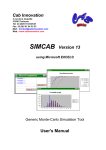
Cab Innovation
3 rue de la Coquille
31500 Toulouse
Tel. 33 (0)5 61 54 68 08
Fax. 33 (0)5 61 54 33 32
Mail : [email protected]
Web : www.cabinnovation.com
SUPERCAB
Version 14
using Microsoft EXCEL®
Reliability / availability & markovian processing
User's Manual
FOREWORD
The software SUPERCAB BASIC version 4 includes some of the SUPERCAB version 14
features. It is not the subject of a specific user manual
The copyright law and international conventions protect the SUPERCAB software and its
User’s Manual. Their reproduction or distribution, either wholly or partly, through any means
whatsoever, is strictly prohibited. Any person who does not comply with such provisions is
committing an offence of forgery and is liable to prosecution and can be sentenced under the
provisions prescribed by the law.
The Programming Protection Agency (A.P.P.) references SUPERCAB at the I.D.D.N. (Inter
Deposit Digital Number) index, with the following reference:
IDDN.FR.001.070017.00.R.P.2000.000.20600
CONTENTS :
1 The SUPERCAB Software
1.1 General Presentation
1.2 Installing SUPERCAB on Hard Disk
1.3 Starting SUPERCAB
2
Teachware
2.1
2.2
2.3
2.4
2.5
Basic concepts
Rate of transition
Markovian process
Treatment of the Markov matrices
Advantages, limitations and palliative solutions
2.5.1 Automatic generation of models
2.5.2 Regrouping of equivalent states
2.5.3 Coupling between Markovian treatments and Faults-Trees
2.5.4 Method of the fictitious states
2.5.5 Treatment by phases
2.6 Formulas of redundancy
2.7 Optimization of system architectures
3
Assessing System Architecture
3.1 Entering an Architecture
3.2 Calculating Reliability / Availability
3.3 Generating Block Diagram Automatically
4 Markovian Processing
4.1 Reminder on Markov Matrixes
4.2 Entering an Markov Matrix
4.3 Processing Markov Matrixes
4.4 Fictitious States' Method
4.5 Evolutionary System
4.6 Principle of Insertion
4.7 Logical Analyzer
4.8 Personalized Functions
4.9 Approximation of One Law
4.10 A Few Examples of Markovian Modelling
3
5 Redundancy Formulas
5.1
5.2
5.3
5.4
5.5
5.6
5.7
Active Redundancy
Passive Redundancy
Redundancy With Reconfiguration Duration
Redundancy of Repairable Elements
Redundancy Repairable With Reconfiguration Duration
Global Redundancy
Active and passive redundancy with stock of spares
Licence agreement
4
1
The SUPERCAB Software
1.1 General Presentation
SUPERCAB makes available to users, whether they are reliability experts or unspecialised
designers, efficient reliability and availability assessment tools :
. An architecture assessment program allowing to compute the reliability and availability of systems
from features of their components, draw evolution curves, and draw Block-Diagram automatically.
. A program for processing Markov matrixes, capable of assuming uncontinuous transition rates
using the fictitious-state method. In addition to the availability in transient and steady state, this
program computes MTTF, MUT, MDT and MTBF.
. A program for assessing evolutionary systems whose state or behaviour is modified at determined
times. Such program enables to model limited lifetime elements, maintenance being periodical or
limited to working hours and any other type of determinist evolution.
. A logic analyzer enabling to build automatically the Markov matrix of a complex system from
logic expressions featuring its operation.
. An approximation function allowing to obtain a Markovian model (or various laws of
probabilities) typical of whatsoever transition law. Such a model may be used for representing the
behaviour of an element undergoing a wear (curve of bath-type fault rate), or to replace a
subassembly in a complex model so as to avoid a combinatory explosion.
. Reliability/availability calculation functions for elements in redundancy M among N, assuming
reconfiguration or repair times, and a program for creating personalized Markovian functions
allowing to achieve its own library of various-redundancy calculation function.
1.2 Installing SUPERCAB on Hard Disk
Please comply with instructions shown in CD-ROM.
1.3 To Start SUPERCAB
In EXCEL, open SUPERCAB.XLA file.
Software's functionalities are then accessible using menu "Dependability", spreadsheet
functionalities remaining always available.
5
Banner on Excel versions after 2007
Menu on Excel versions prior to 2007
A help and a teachware are proposed in the menu.
6
2
Teachware
The teachware presents Markovian process by means of various boards and demonstrations.
2.1 Basic concepts
2.2 Rate of transition
7
2.3 Markovian process
8
2.4 Treatment of the Markov matrices
9
2.5 Advantages, limitations and palliative solutions
2.5.1 Automatic generation of models
10
2.5.2 Regrouping of equivalent states
11
2.5.3 Coupling between Markovian treatments and FaultsTrees
12
2.5.4 Method of the fictitious states
13
2.5.5 Treatment by phases
2.6 Formulas of redundancy
14
2.7 Optimization of system architectures
15
16
3
Architecture Assessment
SUPERCAB calculates the reliability and availability of one architecture, from the features of its
components preliminarily entered in one table, and draws the block-diagram automatically:
Architectures may consist of classical redundancies of type M among N active or passive, with
possible reconfiguration or repair times, or more complex redundancies defined by user expressing
their operating mode by logical expressions or using specific modelling.
Used with a posterior version of Excel to version 4, SUPERCAB allows to enter several tables in
the same sheet, corresponding for example each one to a subsystem, and to obtain the blockdiagram in the form of drawing or image. The various tables can be treated individually or
collectively.
The operation of the system from that of subsystems, as well as the operation of the latter from that
of the blocks which compose them, can be defined by logical expressions.
17
3.1 Entering an Architecture
Menu command "Entering architecture" allows getting the following dialog box which helps obtain
a blank table, as that shown below, the last two columns of which are optional (used if system is
unavailable during certain reconfigurations or if it contains repairable elements).
UNITS
$
MTTF
ON
(hour)
Nb
Kind of
redundancy
MTTF
OFF
(hour)
Operation Switching
rate
delay
r (%)
(hour)
MTTR
(hour)
Total :
Elements may be featured by their MTTF (in hour) or their fault rate (in hour-1 or fit = hour-1*109). Table and documents made may be requested in the English or French language and one
example of architecture preliminarily entered may be displayed for illustration purposes.
Then, the user enters features of system elements either directly in table, or by using the utilities bar
"Blocks" the use of which is specified below.
The architecture entry table is filled in as follows :
1 - The name of the element is entered in the first column.
2 - The MTTF or the fault rate of element in active condition is entered in second column.
3 - The number of series elements or sets is entered in the third column.
18
4 - The type of redundancy to be entered in the fourth column may be "Active m/n", "Passive m/n",
"Series", "Logic" (defined by an expression featuring the system availability) or "Complex". This
last type does not lead to any processing but allows the user to complete manually the generated
calculation tables and Block-Diagrams.
An active or passive redundancy 1/2 is assumed by default if m/n is omitted.
A probability value can be taken by default by entering it in this column.
5 - A MTTF OFF equal to MTTF On * 10, or a fault rate OFF equal to the fault rate On / 10, is
assumed by default if the latter is omitted in the fifth column.
6 - A 100 % operation rate is assumed by default if the latter is omitted in the sixth column.
7 - A reconfiguration time (in hour) may be entered in the seventh column. Parameter k of an Erlang
law used for featuring this time may be related with it in parenthesis (see MARKOV program).
8 - MTTR may be entered in the same way in the eighth column.
The following utilities bar "Blocks" facilitates such entry. It is displayed or disappears using menu
command "Utilities bar".
Meaning of buttons is as follows :
Adding a series block
Initiating this button allows to display the following dialog box enabling to insert a series block in
the table (or many identical ones) just above the line selected.
Unit 9
11000 hr
r=10%
Série
*2
19
Adding redundancy blocks
Initiating this button allows to display the following dialog box enabling to insert a redundancy
block in the table (or many identical ones) just above the line selected.
Unit 7
Unit8
5820 hr / 10000 off
2856 hr
r=60%
Mttr=2000h tr=800h
*2
*4
Passive 7/8
*2
The considered redundancy may concern a unique block or a chain of various blocks as in example
above (2 * Unit 7 + 4 * Unit 8, the whole in redundancy 7/8).
The type of redundancy of the complete chain is then informed in the entry table at next line
according to those of relevant Units.
Adding a logic set
Initiating this button allows to display the following dialog box enabling to insert a logic set in the
table (or many identical ones) just above the line selected.
Unit 2
Unit 3
1500 hr / 20000 off
1300 hr
Unit 4
15300 hr
Mttr=1500h
Unit 5
2560 hr
Bloc (*2)
Unit 5 off if Unit 2 and Unit 3 ok
20
The condition of proper operation of the set is defined by a logical expression between its various
constituents. So, in this example, the expression "a*(b+c)+d" means :
"Unit 2 OK AND (Unit 3 OK OR Unit 4 OK) OR Unit d OK".
For each block of logic set, a similar expression may be used to define the possible conditions of
setting to OFF condition (cold redundancy). So, in this example, Unit 5 (d) is in OFF condition as
long as condition "a*b" is verified, that is "Unit 2 OK AND Unit 3 OK".
Adding a complex set
Initiating this button allows to display the following dialog box enabling to insert a complex set in
the table (or many identical ones) just above the line selected.
This last type of set does not lead to any specific processing but allows the user to complete
manually the generated Block-Diagrams and calculation tables, by using specific modelling. This
dialog box is used as previous ones.
Result of the table
The activation of this button allows to display the following dialog box making it possible to insert
in the table a logical expression defining the operation of the system from that of the blocks which
make it up (by defect the blocks are in series). Each block of the table is then identified by a small
letter (automatically inserted) and the expression is built by simple selection in a drop-down list of
the logical operators (+: OR, *: AND, ~: NOT), the symbols of bracket and the various blocks. The
logical expression is recopied in the table with the activation of button OK.
UNITS
a - Unit 1
Unit 2 (a)
Unit 3 (b)
Unit 4 (c)
Unit 5 (d)
b
c - Unit 6
Unit 7
Unit 8
d
e - Unit 9
$
MTTF
Nb
Kind of
MTTF
ON
redundancy
OFF
(hour)
(hour)
833333,33 5
Active
1250000
5000000
2000000
1000000
133333,33
2
a*(b+c)+d d off : a*b
1055966,2
Passive
455996,35 2
1333333
27777778 4
2 Passive 7/8
11363636
Serie
TOTAL
a+~a*(b*c+d*e)
21
Structure on the N+1
The activation of this button allows to display the following dialog box making it possible to insert
on the sheet a logical expression defining the operation of the system, in nominal or degraded
modes, from that the different ones subsystems which make it up (each one being defined by its own
table).
UNITS
Unit 1
Unit 2
$
UNITS
Unit 3
Unit 4
Unit 5
$
UNITS
Unit 6
Unit 7
$
MTTF
Nb
Kind of
ON
redundancy
(hour)
833333,33 5
Active
1055966,2
Passive
A - TOTAL
MTTF
Nb
Kind of
ON
redundancy
(hour)
11363636
Serie
455996,35 2
27777778 4
2
Passive 7/8
B - TOTAL
MTTF
Nb
Kind of
ON
redundancy
(hour)
11363636
Serie
833333,33 3
Active
C - TOTAL
ARCHITECTURE ON THE N+1 LEVEL
Logical
condition:
A+B*C
$$
Each subsystem is then identified by a capital letter (automatically inserted) and the expression is
built again by simple selection in a drop-down list. The logical expression is recopied in an
additional table corresponding to the system (N+1 level) with the activation of button OK.
Drawing of the logic structure
The activation of this button makes it possible to draw a logic structure, in the shape of a block
diagram, starting from its expression defined in the selected cell (the symbol ~ corresponds to the
negation of the element concerned).
a
a+~a*(b*c+d*e)
~a
b
c
d
e
22
Block Diagram
The activation of this button has the same effect as the command "Block Diagram" of the menu.
Notes :
- Lines may be inserted or deleted in the table provided the character "$" is maintained at the bottom
of the latter (menu "Edit insert" or "Edit cancel").
- Blank lines may be especially used for separating elements or blocks in the table but they should
not be inserted within a same block.
3.2 Calculating Reliability / Availability
Menu command "Processing" allows to calculate the reliability and the availability of the
architecture preliminarily entered.
The user chooses in a dialog box the time unit to be considered (hour, day or year), and quotes the
value of time t for which it desires a processing.
He may possibly request the calculation of the equivalent lambda or the equivalent MTTF for this
time value (failure rate or MTTF of an element with same reliability at t than considered
architecture).
If he wishes to get a reliability/availability graph, he should enter various time values in discrete
form, or define a calculation increment, a starting value (tmin) and a final value (tmax).
The program also helps calculate the asymptotic availability of repairable systems (with infinite t)
together with the MTTF, MTBF, MUT and MDT parameters of the different subassemblies.
Acting on the OK button commands the processing. Then, the program adds at table of calculation
columns in which redundancy formulas (showed in paragraph 3.4) or probability formulas (below
defined) are entered with their various arguments.
If architecture consists of logic sets, relevant Markovian models are automatically generated in
specific sheets (see logic analysis program).
Notes :
The number of characters per cell being limited, an error will be indicated if the size of a block's
redundancy formula exceeds spreadsheet capacity. So, the user will have to gather manually the
features of some block elements to reduce the formula size.
23
Rates entered by the program in the line defining the type of block redundancy (second and fifth
column) correspond to rates at active and passive condition of relevant chains.
For evaluation of architecture, the tool uses formulas of redundancy and Markovian treatments
whose limitations are specified in the corresponding chapters.
For the treatment of the logical expressions of level higher than that of the block (table and N+1
level), it uses the following formula of probability (in the shape of macro function of the
spreadsheet):
=PROBA("A+~A*B*C", Probability of A, Probability of B, Probability of C )
The first argument is the logical expression between quotation marks and the following corresponds
to the value of the various probabilities in the alphabetical order.
By defect, the results displayed at bottom of columns correspond to products of intermediate results
shown in relevant columns.
3.3 Generating Block-Diagram Automatically
The program automatically generates the Block-Diagram as soon as the user initiates the menu
command "Block-Diagram". Such function may be achieved prior or after the reliability /
availability calculation.
The Block-Diagram may be in-line plotted or cut depending on printing format (Portrait or
Landscape) and be subject to a reduction or enlargement rate.
Used with a posterior version of Excel to version 4, the tool allows obtaining the block-diagram in
the form of image. Of variable size according to enlarging or reduction ratio's, the Block Diagram is
then drawn in-line and appears on the right of the corresponding table.
24
4 Markov Matrix
4.1 Reminder on Markov Matrixes
Markovian processes are used in reliability/availability analyses for modelling the behaviour of
various systems. The example below illustrates the way followed.
λ/µ
System conditions :
λ/µ
2∗λ
1
2
λ
3
1 : No fault
λ : fault rate
2 : Element loss
µ : repair rate
3 : System loss
µ
2∗µ
Markov graph
The analyst identifies different system conditions, then defines transition rates between conditions.
Certain equivalent conditions may be regrouped as the loss of one or another element in this
example.
System may also be represented directly in the form of matrix :
1
λ/µ
λ/µ
2
3
No fault : 1
- 2∗λ 0
Loss of one element : 2
µ
-
λ
0 2∗µ -
System loss : 3
Markov matrix
Coefficients λij of matrix correspond to transition rates of conditions i in line towards conditions j
in column :
1
1 2
2
j
n
-
i
n
λ ij
-
-
Such matrix representation is more synthetic than the graph and limits risks of errors (forgotten
transition).
Transition rate λii located on the main diagonal are not generally informed ( λ ii = −
n
∑t
ij
),
j=1; j≠ i
together with the zero-value rates.
More complex examples of modelling are given in chapter 4.10 of this manual and are quoted for
demonstration in online help (menu "Help").
25
4.2 Entering an Markov Matrix
Menu command "matrix entry" helps obtaining on a calculation sheet, from the selected cell (top
left corner), the following format of a blank matrix with dimension n.
MAT :
1
2
3
4
5
1
-
INIT :
1
0
0
0
0
STATE :
1
1
1
1
0
2
3
4
5
-
Then, the user enters matrix's transition rates (in hour -1) likely to be expressed either in the discrete
form, or in the form of formulas incorporating variable names (terms of main diagonal are
automatically computed during the processing and empty cells are replaced by 0).
He enters vector INIT, corresponding to probabilities to be in different states at T = 0, and defines a
combination of states to be assessed by entering 1 or 0 in corresponding cells of vector STATE.
The following utilities bar "Matrixes" allows to facilitate the entry. It is displayed or disappears
using menu command "Utilities bar".
Meaning of buttons is as follows :
Defining names
Initiating this button allows to display the following dialog box which helps define variable names
in selected sheet.
26
Such names may refer to discrete values or to contents of sheet cells.
The box especially enables to give a name to contents of cell selected and possibly recopy such
name on sheet, at the left hand side of such cell.
Using names in a formula
Initiating this button allows to display the following dialog box which helps use names of
predefined variables in a formula to enter in selected sheet.
Selecting one name in the list generates its immediate copy in formula.
Selected cell may be incremented in any direction so as to successively enter the different rates of
matrix.
Displaying formulas
Initiating this button allows to display immediately all formulas entered in sheet instead of the value of their result
(replacement of "=" by " =" or inversely).
Displaying / deleting square pattern
Initiating this button allows to display or delete sheet square pattern.
27
4.3 Processing Markov Matrixes
SUPERCAB processes Markov matrixes in transient and steady state and calculates the MTTF,
MUT, MDT and MTBF parameters :
PROBABILITY
MAT :
1
1
2
3
4 1,2E-2
2
8,0E-6
5,0E-4
3
4
6,0E-4
1,05
1
3,2E-4
-
0,95
0,9
-
Proba (∞
∞)
0,85
0,8
INIT :
STATE :
0,8
0,2
0
0
1
1
0
0
0
1000
2000
3000
4000
5000
hours
MTTF
MDT
MUT
t=0
MTBF
MTTF : Mean Time To Failure
MUT : Mean Up Time
MDT : Mean Down Time
MTBF : Mean Time Between Failure
(MTBF = MUT + MDT)
Calculating the probability to be in the various states or a combination of states, at time T, is
performed by using menu command "Processing".
Initiating the latter generates the display of a dialog box in which the user enters the value of T,
together with a number of intermediate values if he wishes to get the evolution curve between 0 and
T.
In addition to Markovian calculation (resolution of the equation of Chapman-Kolmogorov), the
treatment can be also carried out in transient state by Monte-Carlo simulation. The user then defined
a number of steps corresponding to the number of simulations to carry out between 0 and T.
Pressing button OK commands the processing (see example 1).
If vector STATE is not defined, the program calculates the probability to be in state 1 and displays
all probabilities from P1 to Pn if a calculation for intermediate values was requested.
28
If various matrixes were entered on the same sheet, the user may choose one of them by selecting
the relevant cell "MAT :" prior to command the processing.
The probability calculation may also be directly carried out in any cell of calculation sheet by
entering the MARKOV function as follows :
"=MARKOV(MAT;INIT;STATE;T)"
This function meets the formalism of spreadsheet macro-functions, a " ; " separating each
arguments, and matrix arguments being defined by references of top left hand side and lower right
hand side cells of relevant matrixes separated by " : ".
If argument T is not defined, MARKOV function calculates in steady state (at T infinite).
It calculates MTTF, MUT, MDT or MTBF if user enters "MTTF", "MUT", "MDT" or "MTBF"
respectively as an argument T, instead of a numerical value.
MARKOV function may be used in matrix form. To do so, select a range of cells and press "block
capital" and "CTRL" keys by entering the function.
Used in matrix form, MARKOV function helps displaying time T, probability Pr to be in the
combination of states defined by vector STATE, or probabilities P1 to Pn if vector STATE is not
defined. It gives such results for intermediate time values between 0 and T if range of selected cells
includes various lines.
Following examples specify the formalism adopted for such function when used in matrix form.
a ) Vector STATE is defined :
0
T/(Nblines -1)
T
2 columns or more
1 column
Time
0
100
200
300
Pr
0,9
0,82142808
0,78539121
0,76749154
Pr
0,9
0,82142808
0,78539121
0,76749154
b ) Vector STATE is not defined :
0
T/(Nblines -1)
T
1 column
2 columns
P1
0,8
0,75790422
0,74332265
0,73803747
P1
0,8
0,75790422
0,74332265
0,73803747
29
P2
0,1
0,13709395
0,15914719
0,17235284
n columns
0
T/(Nblines -1)
T
P1
0,8
0,75790422
0,74332265
0,73803747
P2
0,1
0,13709395
0,15914719
0,17235284
0,1
0,06352386
0,04206856
0,02945406
Pn
0
0,04147797
0,0554616
0,06015563
n columns + 1 or more
0
T/(Nblines -1)
T
Time
0
100
200
300
P1
0,8
0,75790422
0,74332265
0,73803747
P2
0,1
0,13709395
0,15914719
0,17235284
0,1
0,06352386
0,04206856
0,02945406
Pn
0
0,04147797
0,0554616
0,06015563
The treatment by Monte-Carlo simulation is carried out in a similar way by means of function
MARK_SIM defined below:
"=MARK_SIM(MAT;INIT;STATES;T,N)"
With the exception of additional argument N, corresponding to the number of steps of simulation,
the formalism of this macro-function is identical to that of the Markov function. Its employment
with SIMCAB tool makes it possible to introduce various laws of probability into a Markovian
model.
Notes :
- Algorithm of MARKOV function is based on calculation of matrix exponential. It allows to
process Markov matrixes of dimension lower than 254 (80 for thr Excel versions before 2007) with
a 10-15 resolution.
Accuracy of results is guaranteed at 10-13 for any value of T lower than the lowest mean transition
duration of system (opposite to maximum transition rate).
Beyond such value, the guaranteed accuracy deteriorates proportionally (10-9 for a value of T equal
to 10000 times the minimum transition duration), and processing duration increases linearly.
- Error value #N/A is returned if sum of probabilities of vector INIT is not equal to 1 or in case of
typing error (confusion between dot (.) and decimal point (,) especially in numbers).
- In steady state, the error value #DIV/0! is returned if Markov matrix consists of various absorbing
conditions (zero-rate line) or absorbing loops between conditions.
- During a MTTF calculation, the error value #DIV/0! is returned if Markov matrix consists of an
absorbing condition (or loop) among the combination of conditions retained.
30
Example 1 :
MAT :
1
2
3
4
1,00E-02
INIT :
STATE :
1
-
2
8,00E-06
5,00E-03
3
3,00E-04
-
0,8
0,1
0,1
0
1
0
1
0
Probability : 0,75250553
à t (hr) :
500
4
8,50E-04
3,00E-07
-
0,95
0,9
T (hr)
0
100
200
300
400
500
PR
0,9
0,82142808
0,78539121
0,76749154
0,75793647
0,75250553
infinite
0,05858807
MTTF (hr) :
MUT (hr) :
MDT (hr) :
MTBF (hr) :
952,399732
206,160984
3312,6611
3518,82208
PR = P1 + P3
MAT :
1
2
3
4
1
-
1,00E-02
INIT :
0,8
0,85
0,8
0,75
0,7
0,65
0
2
8,00E-06
5,00E-03
3
3,00E-04
-
0,1
0,1
100
200
300
400
500
4
8,50E-04
3,00E-07
0
STATE :
Probability : 0,73481079
à t (hr) :
500
(P1)
T (hr)
0
100
200
300
400
500
P1
0,8
0,75790422
0,74332265
0,73803747
0,73589341
0,73481079
P2
0,1
0,13709395
0,15914719
0,17235284
0,18035253
0,18528851
P3
0,1
0,06352386
0,04206856
0,02945406
0,02204306
0,01769473
P4
0
0,04147797
0,0554616
0,06015563
0,061711
0,06220596
infinite
0,00211764
0,94123024
0,05647043
0,00018169
31
Example 2 :
Redondancy 1 among 2
No failure :
Loss of unit 1 :
Loss of unit 2 :
System loss :
Unit1
Lbd1 / Mu1
Unit2
Lbd2 / Mu2
Availabity
2000 hours:
1
Mu1
Mu2
0
2
Lbd1
0
Mu2
3
Lbd2
0
Mu1
1
2
3
MAT :
1
0,00001 0,0005
2 0,02083
3 0,01389
4
0,01389 0,02083
Lbd1 = 1E-05 hr -1
Lbd2 = 0,0005 hr -1
Mu1 = 0,0208 hr -1 (MTTR : 48 hours)
Mu2 = 0,0139 hr -1 (MTTR : 72 hours)
at T =
1
2
3
4
0,9999833
32
4
0
Lbd2
Lbd1
4
0,0005
0,00001
-
INIT :
1
0
0
0
STATE :
1
1
1
0
P (2000hr) : 0,96479 0,00046 0,03473 1,70E-05
4.4 Fictitious State Method
Only the homogeneous Markovian processes, in which transition rates are constant, may be
processed with a matrix calculation (resolution of Chapman-Kolmogorov equation
dP/dt = P*M).
Now, if a constant fault rate may have a physical meaning, especially for certain electronic
components, it differs for a repair rate.
However, the fictitious state method helps compensate for such limitation. It consists in
replacing in a Markovian model any transition between two states by a set of constant-rate
transitions between fictitious states.
1
2
1
2
Any type of transition may be modelled in this way, and the sequence of transitions between
fictitious states may be limited to Cox model shown below :
λa
1
2
λb
λc
1
2
λ1
State
1
λ2
-
λ3
λ4
λa
λ1
λb
-
Relevant
Markov matrix :
λc
-
State
2
λ2
λ3
λ4
-
If transition rates of direct chain are identical (λa, λb, λc... = λ), model is said generalized
Erlang.
If, moreover, the sequence of transitions is limited to direct chain, the resulting law is a simple
Erlang law with parameter k, corresponding to the convolution of exponential laws k.
λ
1
2
λ
λ
1
2
Adding up k-1 fictitious states
Close to a log-normal law, the latter is often used for modelling repair rates.
33
The features of a simple Erlang law are as follows :
Simple Erlang law
(m = 8 / k = 4)
36
33
30
27
24
0
21
(k −1)!
0,02
18
t e
0,04
15
−λt
0,06
12
Density : f(x)= λ
k k −1
m
k
=
λ
k
9
Standard deviation : σ =
0,08
6
λ
0,1
3
k
0
Mean value :
Density of probability
0,12
Tim e (hr)
The fictitious state method is implemented on SUPERCAB using different programs we are
about to describe below.
Simple Erlang Law
To enable that a transition in a Markovian model follows a simple Erlang law, the user enters
directly in matrix mean value m (in hours) of distribution and parameter value k as follows :
E(m;k)
d
a
e
b
c
-
0
a
-
λ
-
λ
λ
-
λ
d
e
The program will automatically generate the k-1 relevant fictitious states before processing the
matrix (see example 3).
Generating Markovian Models
SUPERCAB helps generating Markovian models typical of any transition laws.
So, it is possible to process correctly fault rates relating to mechanical elements (bath-shaped
curve), or overcome the combinatory explosion encountered in the study of certain systems by
replacing subassembly models by simplified models limited to a few conditions. Such
functionality is described in chapter 4.9.
34
b
c
c
c
c
c
-
Modelling Entirely A System
In order to facilitate the implementation of the fictitious state method, SUPERCAB helps user
achieve the Markov matrix of a complete system from various matrixes, which model its transitions.
It generates automatically this matrix from a user-defined simplified matrix in which the complex
transition rates are replaced by references to defined Markov matrixes :
1
2
3
4
1
e
h
M1 :
2
M1
f
i
3
a
c
j
4
b
d
g
-
Automatic
generation of
overall matrix
112 113
121
123
131 132
-
1 1 bis 2
1 112 113
1 bis 121
123
2 131 132
3 e
0
f
4 h
0
i
3
a
a
c
j
4
b
b
d
g
-
The simplified matrix may contain up to 10 different references (M1 to M10), and relevant
matrixes, preliminarily entered on calculation sheet, are entered as an additional argument of
"Markov" function as follows :
"=MARKOV(MAT;INIT;STATE;T;M1;M2;...;M10)"
This functionality enables to achieve automatically the Markov matrix of a complex system from
the matrixes of its constituents.
Such matrices may possibly be linked each other and represent an arborescence. (see examples 4
and 5).
Notes Relating To Using Fictitious States :
- If a transition rate tij is replaced by a Markov matrix, transition from state j to state i is also
defined by the latter and relevant cell may remain empty.
- Transition rates placed on the same line as a matrix with transition Mi or as a "simple Erlang" type
transition, remain operational for the whole fictitious states generated.
- Using various transition matrixes or "simple Erlang" type transitions on a same line should be
proscribed as it results in conflicts between transitions.
- The Markov program is currently limited to the processing of a 80-states matrix including the
possibly generated fictitious states.
- The error value #DIV/0 is returned if mean transition duration m is zero in the expression E(m;k).
- Menu command "Used Matrix " helps displaying, following processing, the matrix generated by
program including all fictitious states.
35
Example 3 :
Simple repairable redundancy
Lbd
Mttr
No fault
Loss of one element : 2
Sysem loss : 3
INIT :
2000 hours
0,999885
STATE :
Program Generated Matrix :
Mat :
Init :
State :
-0,00002 0,00002
0
0
0
0
0
-0,08334 0,083333
0
0
0,00001
0
0
-0,08334 0,083333
0
0,00001
0
0
0
-0,08334 0,083333 0,00001
0,083333
0
0
0
-0,08334 0,00001
0
0
0
0
0
0
0,8
0,2
0
0
0
0
1
1
1
1
1
0
36
2
2*Lbd
0
3
0
Lbd
-
1
2
3
MAT :
1
0,00002
2 E(48;4)
0,00001
3
-
Lbd = 0,00001 hr -1
Mttr =
48 hours
k=
4 --> typical deviation : 24 hours
Availability at T=
1
Mttr
0
0,8
0,2
0
1
1
0
Example 4 :
Arborescence
A
D
4
5
0
E(8;1)
E(8;1)
-
0
0
0
M4
-
0
0
0
0
1
0
1
-
2
9E-07
-
3
M3
0
-
INIT :
1
0
STATE :
1
0
MAT :
No fault : 1
Loss of D : 2
Loss of : 3
Reconfigured on E : 4
Sytem loss : 5
C
B
tr = 8 hr
E
Availability at
T= 4000 hours :
0,999984971
1
2
M1 (A) :
No loss : 1
9E-06
Repairable deterioration : 2 E(48;1)
Definitive loss of A : 3
3
4E-06
8E-06
-
1
2
M2 (B) :
No fault : 1
8E-06
Repairable deterioration : 2 E(24;1)
Definitive loss of B : 3
3
3E-06
6E-06
-
M3 (C) :
No fault : 1
Loss of A : 2
Loss of C : 4
1
-
2
M1
-
1
2
M4 (E) :
No fault : 1
9E-06
Repairable deterioration : 2 E(36;1)
Non-repairble deterioration : 3
Definitive loss of E : 4
37
3
0
M2
3
4E-06
8E-06
-
4
1E-06
5E-06
6E-06
-
Example 5 :
Elements undergoing wear
passively redundant
M1
M1:
Initial status : 1*
2*
3*
4*
5*
Final status : 6*
Reliability at T=
2000 hours:
MAT :
No fault : 1
Loss of active element : 2
System loss : 3
1
-
2
M1
-
3
0
M1
-
INIT :
1
0
0
STATE :
1
1
0
3*
4*
5*
6*
0,0002
0,00005
0,00015
0,00045
0,00135
-
1*
-
2*
0,001
-
400000
300000
200000
100000
0
1000
2000
hours
Reliability of element and
redundancy
1
0,9
0,8
0,7
0,6
0
0,001
-
0,001
-
0,952194
Equivalent
elementary fault rate (fits)
0
0,001
-
1000
2000
hours
38
T
(hr)
0
200
400
600
800
1000
1200
1400
1600
1800
2000
2200
Elem,
rel,
1
0,96338
0,93194
0,90353
0,87635
0,84897
0,82035
0,78983
0,75712
0,72217
0,68521
0,6466
equiv,
rate
186539
165912
154781
152713
158719
171472
189533
211530
236250
262686
290037
red,
rel,
1
0,99929
0,99745
0,99476
0,99134
0,98719
0,98226
0,97642
0,96955
0,96151
0,95219
0,9415
4.5 Evolutionary System
SUPERCAB allows to process Markovian systems the state or the behaviour of which is modified at
determined times.
Such developments may correspond to changes in transition rate values or to forcing of states, as
shown by examples below :
Maintenance limited to working hours
1
Availability
0,95
0,9
0,85
0,8
0,75
0
1
2
3
4
5
6
7
8
days
Repair rates are zero out of working hours.
Failure rates are modified during the journey (high or low speed sections).
Performing a preventive maintenance action
préventive
1
Av 0,8
aila
bili 0,6
ty
0,4
with
without
0,2
0
0
2000
4000
6000
8000
10000
hours
System condition is periodically modified by a preventive maintenance action.
39
Menu command "Evolutionary System " helps processing systems submitted to such determinist
developments.
After stating the different numbers of Markov matrixes and forcings required for describing system
development, the user defines the latter numbers on a program-formatted calculation sheet (see
example 6).
The user specifies the beginning and duration of validity phase of each matrix, which can possibly
be periodic.
If validity phases of different matrixes are superimposed, the program warns about it and only
considers the phase of matrix with superscript.
Similarly, user specifies the occurrence time of each forcing as well as any possible periodicity.
If forcing sequences take place simultaneously, the latter will be successively performed in their
numbering order.
Probabilities (P1 to Pn) following a forcing of states, may be defined either by numerical values, or
by expressions comprising such probabilities just prior to forcing (sum is to be equal to 1) :
P1 : P1+alpha*P2 +P3
P2 : (1-alpha)*P2
P3 : 0
P4 : (unchanged if empty box)
n
(sum of probabilities after forcing is equal to
∑ Pi prior to forcing).
i =1
Finally the user defines vectors INIT and STATE, duration of mission considered (Tmax) and the
calculation sequence. The latter should be lower than half the duration of matrix validity phases and
lower than forcing periods.
Processing will be performed by initiating menu command "Processing".
Notes :
- In addition to the graph of results and relevant numeric values entered in two columns of sheet,
detail of calculations is given in the form of one table (in depth configuration for each calculation
sequence and in width configuration if events occur between two successive sequences).
- Sum of probabilities of vector INIT should be equal to 1.
- In the event where the processing is requested for a time value corresponding to one forcing,
obtaining the calculation result before or after the latter is possible.
40
Example 6 :
EVOLUTIONARY SYSTEM
Tmax :
800
Step :
4
Tinit
0
Period
24
Tinit
8
Period
24
Tinit
120
Period
168
Tinit
120
Period
336
(hours)
Duration
8
Duration
16
Duration
48
INIT :
1
0
0
STATE :
1
1
0
MAT1 :
1
2
3
1
-
2
0,005
-
3
0,1
MAT2 :
1
2
3
1
-
MAT3 :
1
2
3
1
-
Forcing1
P1
p1+p2
2
0,005
-
2
0,005
-
P2
0
0,01
3
0,01
3
0,01
-
P3
Availability
1,05
1
0,95
0,9
0,85
0,8
0,75
96
12
0
14
4
16
8
19
2
21
6
24
0
26
4
28
8
31
2
33
6
36
0
38
4
40
8
43
2
45
6
48
0
50
4
52
8
55
2
57
6
60
0
62
4
64
8
67
2
69
6
72
0
74
4
76
8
79
2
72
48
0
24
0,7
hours
System only maintained on working hours
being subject to a specific periodic-maintenance action
(every 2 weeks on the weekend)
41
4.6 Principle of Insertion
Menu command "Matrix entry" helps obtain the matrix of a system of n elements (n ≤ 6), each with
two possible states (proper operation or failure), in applying the principle called "Insertion" which is
described below.
System elements are designated by characters (from a to f).
Table is updated automatically as soon as user enters elements' fault or repair rates.
Such rates may generate fictitious states if necessary.
LAMBDA
Lbda
a
Lbdb
b
Lbdc
c
MU
Mua
Mub
Muc
STATES
C B A
C B nA
C nB A
C nB nA
nC B A
nC B nA
nC nB A
nC nB nA
MAT : 1
1
2 Mua
3 Mub
4
5 Muc
6
7
8
INIT :
STATE :
42
2
3
4
Lbda Lbdb
Lbdb
Lbda
Mub Mua
-
5
Lbdc
Muc
Muc
7
8
Lbdc
Lbdc
Mua
Mub
Muc
6
Lbdc
Lbda Lbdb
Lbdb
Lbda
Mub Mua
-
4.7 Logic Analyzer
SUPERCAB generates automatically Markov matrix of a system, from logic expressions featuring
its behaviour, and possibly optimizes the dimension of the latter :
a) With No Optimization :
a
MAT
c b a
c b na
c nb a
c nb na
nc b a
nc b na
nc nb a
nc nb na
b
c
Cold
Available states : (a × b) + c
Dependence relation : a × b ⇒ λc* (λ
λoff)
:
1
2
3
4
5
6
7
8
STATE :
1
µa
µb
µc
1
2
λa
µb
µc
1
3
λb
µa
µc
1
4
λb
λa
-
µc
1
5
λc*
µa
µb
1
6
λc
λa
-
7
λc
λb
8
λc
µb
µa
λb
λa
-
0
0
0
:
States in which system is available are defined by a logic expression using operators OR (+),
AND (×), NOT (n).
Any possible dependence relations, linking certain transition rate values to system conditions
(conditional maintenance, cold redundancy...), may be similarly expressed.
Dimension of matrix generated being 2n, the number of elements is limited to 6 (26 < 80).
b) With Optimization :
If system elements are not all considered as individually repairable, equivalent states may be
regrouped by program for optimizing matrix dimension :
a
b
c b a
nc b a
c nb na
nc nb na
c
Cold
MAT :
1
2
3
4
1
-
STATUSES:
1
2
3
4
λc* λa+λb
λa+λb
λc
1
1
0
So as to identify the regrouped states, to each of them is given the name of group state comprising
most of failing elements :
c nb na = c b na + c nb a + c nb na
nc nb na = nc b na + nc nb a + nc nb na
Repair rates relating to blocks may be subsequently introduced in reduced matrix (example : repair
rates of set ab).
The number of elements is limited to 26 (a to z) and that of regrouped states to 80.
The operator NOT (n) cannot be used in logic expressions when optimization is requested.
43
Menu command "Logic analyzer" helps obtaining entry formats (see example 7) in which system
elements are designated by characters (a to f).
User defines the combination of states being sought, i.e. the one in which system is available, by
entering a logic expression between the states of different elements as follows :
n(a*b+n(c+e*nf))
Then, he enters the time, transition rate values (in hr-1), and any possible dependence relations from
logic expressions identical to previous one.
Many dependence relations may affect a same rate and user may insert if necessary additional lines
in the table.
In case of superimposing states between different logic expressions, the lowest suffix rate is
considered.
Markov matrix is generated then processed by the program as soon as user initiates menu command
"Processing".
Notes : Example 7 processed with optimization leads to a matrix of dimension 12 instead of 64.
Such dimension may still be reduced to 8, as shown below, if logic expressions defining dependence
relations are modified for considering the latter only when concerned elements are operational.
A
Cold
C
D
E
B
Cold
Logic
expressions :
Avail :
c*d*e+a*e+c*b
c:
λc
MAT : 1
e d c b a:1 e d c b na : 2
e d c nb a : 3
e nd c b a : 4
e d c nb na : 5
e nd nc nb a : 6
ne nd c b na : 7
ne nd nc nb na : 8
d:
λd
STATE : 1
e:
λe
a:
b:
λa
λa*
c*d*(a*e)
λb
λb*
e*(d+a)*(c*b)
44
2
3
4
5
6
7
8
λa* λb* λd
λc
λe
λb*
λd+λe
λc
λa* λc+λd
λe
λb*+λc λa+λe
λc+λd+λe
λa+λe
λb+λc
1
1
1
1
1
1
0
Example 7 :
Available states :
A
Cold
C
D
E
B
Cold
Loss of C or D -> use of A
Loss of E or (D and A) -> use of B
Probability = 0,9999768
à t (hr) = 5000
Lbda : 7,00E-07
7E-08
Lbda*2
Logic expressions
c*d*e+a*e+c*b
c*d
Mua : 9,00E-06
Mua*1
Mua*2
Lbdb : 8,00E-07
8E-08
Lbdb*2
Mub : 7,00E-06
Mub*1
Mub*2
Lbdc : 4,50E-07
Lbdc*1
Lbdc*2
Muc : 8,00E-06
Muc*1
Muc*2
Lbdd : 7,50E-07
Lbdd*1
Lbdd*2
Mud : 6,00E-06
Mud*1
Mud*2
Lbde : 9,00E-07
Lbde*1
Lbde*2
Mue : 9,50E-06
Mue*1
Mue*2
45
e*(d+a)
4.8 Personalized Functions
Menu command "Personalized Functions" helps creating and using personalized Markovian
functions with the same formalism as redundancy functions m among n shown in previous chapters.
Such functions are stored in files of directory "PERSO" the opening and closing command of which
is directly accessible by pressing button "Loading".
Button "Creation" allows to create such function, either in an already existing file, or in a new file.
The user defines in a dialog box the names of function and each of its arguments (maximum 10), the
dimension of Markov matrix, then the value and position in the latter of the different transition rates
(see example 9).
To do so, he enters relations made from different arguments and may use the $ as variable of 1 to n
(n being the matrix dimension).
If different relations define rates in a same position of matrix, only the last relation is considered.
The user may command additional dialog boxes, if necessary, to enter all transition rates.
When matrix is completely defined, initiating the button OK displays a new dialog box used for
defining the combination of states being sought (states at 1).
Then, initiating the button OK commands the creation of the personalized function then its storage
in the predefined file.
Notes :
- To validate a personalized function, the user may use it on a numerical example and display the
relevant Markov matrix using menu command "Matrix used".
- In EXCEL5, personalized function files are displayed in reduced-size windows.
46
Example 9 :
Crating a personalized function
Redundancy m among n repairable with final absorbing state
Markov Matrix:
No fault : 1
1 element loss : 2
2 element loss : 3
...
loss N-M-1 elements : N-M
Loss N-M elements : N-M+1
System loss : N-M+2
STATE :
Formula :
1
µ
1
2
Mλ + (N-M) λ*
µ
3
...
N-M
N-M+1
N-M+2
µ
Mλ + λ*
0
Mλ
-
1
1
0
Mλ + (N-M-1)λ*
-
1
1
"= REPAIRABLE _REDUNDANCY_WITH_ABSORBING_STATE (M;N;lbdON;lbdOFF;Mu;T)"
Procedure :
47
4.9 Approximation of One Law
Menu command "Approximation of one law " helps making a model from a reliability curve,
probability density, fault rates or a time sample.
The user chooses one type of model among the exponential, normal, lognormal, Weibull,
generalized Erlang or any Markovian laws. He specifies in the last two cases, the dimension of
relevant Markov matrix (≤10) and, in the last case, the number of parameters to be considered
(≤10).
He also specifies the nature of data considered, the number of curve points or the size of relevant
sample, then presses button OK.
Then the program offers a format in which the user enters his data, defines, if necessary, a Markov
matrix by using 10 maximum parameters (a to j), and possibly initializes model's parameters.
Then, he initializes menu command "Processing" and defines the number of calculation sequences
to be performed.
Then, parameter optimization of model is performed using the method of least error squares in the
case of a reliability curve, probability density or fault rate or is based on the method of maximum
likelihood in the case of a time sample.
The user may reinitiate the calculation using command "Processing", as many times as desired, after
being informed of the evolution of the residual error or likelihood (see example 8).
Notes :
- Normal and lognormal laws can only be used for modelling probability density curves or time
samples (due to the absence, for such laws, of an analytical expression of reliability and fault rate).
- In the case of the approximation of a curve by a Markovian model, the processing is slightly
quicker if time values start from 0 and follow an arithmetic progression.
- In the case of any Markovian model, seeking an optimum may prove to be very hard as error
shows generally many local minima.
48
Example 8 :
Time
0
10
20
30
40
50
Reliability
1
0,9
0,85
0,81
0,78
0,72
Markovian model (generalized Erlang)
1
2
3
1
d
2
d
3
4
5
a0 :
b0 :
c0 :
d0 :
Error :
0,009447231
0,001432604
0,000354237
0,019258912
0,031726406
a:
b:
c:
d:
Error :
4
5
a
b
c
d
-
d
-
0,009187634
0,001253136
0,000309561
0,019306467
0,027472586
1,05
1
0,95
0,9
0,85
0,8
0,75
0,7
Reliability
Initial
Final
0
0
10
20
30
40
50
Matrix :
1
-
10
20
Reliability
1
0,9
0,85
0,81
0,78
0,72
30
Initial
1
0,916639127
0,851477823
0,799183676
0,755466131
0,717064578
40
50
Final
1
0,918959937
0,855651882
0,80483682
0,76228833
0,724791482
2
3
4
5
0,000309561
0,000309561
0,009187634
0,000309561 0,001253136
0,000309561
-
Approximation of a reliability curve using a generalized Erlang law
49
4.10 A Few Examples of Markovian Modelling
Example 10 :
Cold redundancy initiated by a switch
1
e
2
λ1
µ1
λ2
µ2
e : efficient when initiated
OK on 1 : 1
OK on 2 : 2
Loss 1 : 3
Loss 2 : 4
Unavailable : 5
1
-
µ2
2
µ1
3
e×λ1
λ1*
µ2
4
λ2*
e×λ2
µ1
5
(1-e)×λ1
(1-e)×λ2
λ2
λ1
-
λ1* / λ2* : fault rate in off condition of elements 1 / 2
50
Example 11 :
Cross-strapping with common resources
Example 8 :
a = a'
b = b'
c = c' (ressources)
c
a
b
a'
Cold
b'
Cold
Lambda(a in hot condition) = a
Lambda(a in cold condition) = a* = a/10
Lambda(b in hot condition) = b
Lambda(b in cold condition) = b* = b/10
Lambda(c in hot condition) = c
Lambda(c in cold condition) = c* = c/10
c'
Cold
Simultaneous activation of the minimum elements
No fault : 1
Loss of a or a' : 2
loss of b or b' : 3
Loss of a and b' or a' and b : 4
Loss of all redundancies : 5
System loss : 6
a = 9,8E-08
b = 7,8E-08
c = 6,2E-08
Reliab(t=10000) =
1
0
0
0
0
0
2
a+a*
0
0
0
0
3
b+b*
0
0
0
0
4
0
b
a
0
0
5
c+c*
b*+c*
a*+c*
0
0
6
0
a+c
b+c
a+b+2c
a+b+c
0
1
2
3
4
5
6
1
0
0
0
0
0
INIT :
1
0
0
0
0
0
STATE :
1
1
1
1
1
0
hr -1
hr -1
hr -1
0,9999977
51
2
3
4
5
1,1E-07 8,6E-08
0
6,8E-08
0
0
7,8E-08 1,4E-08 1,6E-07
0
9,8E-08 1,6E-08 1,4E-07
0
0
0
3E-07
0
0
0
2,4E-07
0
0
0
0
0
Example 12 :
Commands of redundancy mechanisms 3 among 4
E1
M1
E2
M2
E3
M1 = M2 = M3 = M'1 = M'2 = M'3 = M
(mechanisms)
M3
E1 = E2 = E3 = E4 = E
(control electronics)
M1'
Cold
M2'
Cold
M3'
Cold
Lambda(E in hot condition) = E
Lambda(E in cold condition) = E* = E/10
Lambda(M in hot condition) = M
Lambda(M in cold condition) = M* = M/10
Switch
E4
Cold
1
0
0
0
0
2
3*M*
0
0
0
3
4
0
3*(E+M)+E*
2*M* 2*(E+M)+E*
E+M+M*+E*
0
0
0
1
2
3
4
5
1
0
0
0
0
2
2E-07
0
0
0
3
4
5
0
5,6465E-06
0
1E-07 3,8085E-06 1,838E-06
2,0218E-06 3,676E-06
0
5,514E-06
0
0
-
INIT :
1
0
0
0
0
STATE :
1
1
1
1
0
No fault : 1
Loss of 1 passive elements M' : 2
Loss of 2 passive elements M' : 3
Loss of all redundancies : 4
System loss : 5
E = 1,325E-06 hr -1
M = 5,13E-07 hr -1
Reliab (t=4000hr) = 0,999752
52
5
0
E+M
2*(E+M)
3*(E+M)
-
Example 13 :
Redundancy Calculators
Example 10 :
Calculator
OSR
Eff
Calculator
Cold
OSR : Supervision and Reconfiguration Component
(watchdog...)
Eff : Supervision Efficiency (rate)
Lambda(Calculator in hot condition) = Lbd
Lambda(Calculator in cold condition) = Lbdf
Lambda(OSR) = r
1
0
0
3
eff*Lbd+r+Lbdf
0
3
(1-eff)*Lbd
Lbd
-
1
2
3
1
0
0
3
0,0000029
0
3
0,00000025
0,0000025
-
INIT :
1
0
0
STATE :
1
1
0
No fault : 1
Loss of a channel : 3
System loss : 3
Lbd = 2,5E-06 hr -1
Lbdf = 2,5E-07 hr -1
r = 4E-07 hr -1
eff =
90%
Reliab (t=8000hr) = 0,997796
53
Example 14 :
Redunded Communication System
Example 11:
L
E
R
X* : Cold redundancy equipment
Lambda E (Transmitter) = E
Lambda R (Receiver) = R
Lambda L (Linking) = L
Lambda OFF = Lambda* = Lambda/10
Reconfiguration on E* L* R* in case of loss of L
L*
L*
E*
L*
R*
MAT : 1
No fault : 1 Loss 1 linking : 2
Loss 2 linkings : 3
Loss 1 transmitter (or linkings) : 4
Loss 1 receiver (or linkings) : 5
All redundancy loss : 6
System loss : 7
E = 2,40E-7
R = 1,10E-7
C = 8,00E-8
Reliability (t=10 years) :
0,9997083
2
L+3L*
-
3
0
L+2L*
-
4
5
6
7
E+E*
R+R*
0
0
E+E*+L* R+R*+L*
0
0
0
0
E+E*+R+R*+L+L*
0
0
R+R*+L+L*
E
E+E*+L+L*
R
E+L+R
-
MAT : 1
2
3
4
5
1 - 1,04E-7 0,00E+0 2,64E-7 1,21E-7
2
9,60E-8 2,72E-7 1,29E-7
3
0,00E+0 0,00E+0
4
0,00E+0
5
6
7
6
0,00E+0
0,00E+0
4,73E-7
2,09E-7
3,52E-7
-
7
0,00E+0
0,00E+0
0,00E+0
2,40E-7
1,10E-7
4,30E-7
-
INIT : 1
0
0
0
0
0
0
STATE : 1
1
1
1
1
1
0
54
5
Redundancy Formulas
SUPERCAB offers a number of macro-functions to calculate the reliability or the availability of a
set of elements in redundancy m among n.
Such functions may be directly selected in the list of functions proposed by spreadsheet by
following menu "Selection" then "Insert a function ".
5.1 Active Redundancy
n elements are simultaneously active but only m elements are necessary to ensure mission.
Reliability is obtained by the following formula by replacing arguments in the indicated order :
"= ACTIVE_REDONDANCY(M;N;lambda;T)"
1
lambda : fault rate of element in hourT : mission duration in hour
"= ACTIVE_REDONDANCY (5;7;0,00001;5000)" = 0,9965
Note : Reliability of such redundancy may be expressed as follows :
N−M
R=
∑C
− λt i − λt N − i
i
) (e
)
N (1 − e
i =0
5.2 Passive Redundancy
Only m elements required for ensuring the mission are simultaneously active.
The reliability is obtained by following formula :
"= PASSIVE_REDUNDANCY(M;N;lambda_on;lambda_off;T)"
lambda_on : fault rate of element in active condition
lambda_off : fault rate of element in passive condition
Note : Reliability of such redundancy may be expressed as follows :

R=e
− Mλt 
N−M
∑
1 +

i =1

(1 − e

− λ*t i i −1
)
i!
λ 
∏ ( j + M λ * ) 
j =0

55
with λ* = lambda_off
5.3 Redundancy with Reconfiguration Duration
In case of failure of an active element, the mission is stopped for all reconfiguration duration.
Availability is obtained by the following formula :
"= REDONDANCY_WITH_DURATION(M;N;lambda_on;lambda_off;T;Treconf;k)"
Treconf : average reconfiguration duration in hour
k : parameter of an Erlang law
(random variable of mean value Treconf and with typical deviation Treconf/k)
k = 1 by default (exponential law)
Notes : Such function is processed by performing the following Markov matrix with dimension
2*(N-M)+2.
Therefore it is limited at values of M and N defined by relation N-M ≤ 39 (if k = 1).
1
No fault : 1 Reconfiguration : 2
2
Mλ
-
1 element loss : 3
Reconfiguration : 4
2-element loss : 5
...
Reconfiguration : 2(N-M)
N-M element loss : 2(N-M)+1
System loss : 2(N-M)+2
λ: lambda ON
3
4
(N-M) λ*
tr
(M-1) λ +
(N-M) λ*
-
Mλ
-
5
...
2(N-M)+2
tr
-
(M-1) λ + λ*
Mλ
-
(N-M-1) λ*
tr
-
λ* : lambda Off
2(N-M)+1
tr : 1/Treconf if k=1
5.4 Redundancy of Repairable Elements
Availability is obtained by following formula :
"= REPAIRABLE_REDUNDANCY(M;N;lambda_on;lambda_off;T;MDT;k)"
MDT : mean repair time in hour
Notes : Such function considers only one single repair officer and is processed by performing
following Markov matrix with dimension N-M+2 .
It is therefore limited to values of M and N defined by relation N-M ≤ 78 (if k = 1).
56
No fault : 1
1 element loss : 2
2-element loss : 3
...
N-M element loss : N-M+1
System loss : N-M+2
1
µ
2
Mλ + (N-M) λ*
µ
3
...
N-M+1
N-M+2
Mλ + (N-M-1)λ*
µ
Mλ
-
µ : 1/MDT if k=1
5.5 Repairable Redundancy with Reconfiguration Duration
In case of failure of an active element, the mission is stopped for all reconfiguration duration.
Elements are repairable.
Availability is obtained by the following formula :
"=M_AMONG_N_REDUNDANCY(M;N;Lambda_on;Lambda_off;T;Treconf;kr;MDT;km)"
Treconf : reconfiguration meantime in hour
kr : parameter of the relevant Erlang law
MDT : mean repair time in hour
km : parameter of relevant Erlang law
Notes : Such function is processed by performing the following Markov matrix.
It is limited to values of M and N defined by relation N-M ≤ 39 (if kr and km = 1).
1
No fault : 1 Reconfiguration : 2 µ
1 element loss : 3 µ
Reconfiguration : 4
2-element loss : 5
...
Reconfiguration : 2(N-M)
N-M element loss : 2(N-M)+1
System loss : 2(N-M)+2
2
Mλ
-
3
4
(N-M) λ*
Tr
(M-1) λ +
(N-M) λ*
µ
µ
Mλ
-
5
...
2(N-M)+2
tr
µ
(M-1) λ + λ*
Mλ
-
(N-M-1) λ*
tr
-
57
2(N-M)+1
5.6 Global Redundancy
This more generic model can take into account ON and OFF failure rates (λ and λOFF), probability
of failure before using up (γ), average reconfiguration duration in which the mission is stopped
(MDT_s) and average non-operational duration due to failure (MDT_l).
Both durations can be modelled by exponential (rates µi) or Erlang law (with k fictitious states).
Several politics of maintenance can be considered with 1 or n repair officers or with duration of
reparation independent of the number of units in failure.
GLOBAL_REDONDANCY (M; N; λ;λ
λOFF; γ; T; MDT_l; kl; Type_l; MDT_s; ks; Type_s; Re; Na; Nb)
This parametrical function assesses the availability (at t or ∝) or the reliability, considering the loss
of system as an absorbing state.
In case of the mission is not stopped during reconfiguration duration, the markovian matrix with
dimension N-M+2 as shown in the following figure is used.
1
2
3
4
-
Mλ(1-γ) + (N-M) λ*
Mλγ (1-γ)
Mλγ2 (1-γ)
MλγN-M-1 (1-γ)
Mλγ N-M
Loss of 1 unit : 2 µl1
-
Mλ(1-γ) + (N-M-1)λ*
Mλγ (1-γ)
MλγN-M-2 (1-γ)
Mλγ N-M-1
Loss of 2 unit : 3 µl’
µl2
-
Mλ(1-γ) + (N-M-2)λ*
MλγN-M-3 (1-γ)
Mλγ N-M-2
-
N-M-4
Mλγ N-M-3
No failure : 1
Loss of 3 unit : 4 µl’
µl3
...
N-M+1
Mλγ
(1-γ)
N-M+2
...
Loss of N-M unit : N-M+1 µl’
System loss: N-M+2 µl’’
-
Mλ
µlN-M+1
-
M among N redundancy (system available during reconfigurations)
In case of the mission is stopped during reconfiguration duration, the markovian matrix shown in
the following figure, with dimension 2(N-M)+2, is used.
1
No failure : 1
-
Reconfiguration : 2 µ2
2
3
4
5
6
2(N-M)+2
Mλ (N-M) λ*
tr(1-γ)
trγ +(M-1) λ +(N-M) λ*
-
Mλ
(N-M-1) λ*
Reconfiguration : 4
µ2
-
tr(1-γ)
trγ +(M-1) λ +(N-M-1) λ*
Loss of 2 unit : 5
µ1
-
Mλ
Loss of 1 unit : 3 µ1
..
.
-
Reconfiguration : 6
-
...
trγ +(M-1) λ + λ*
Reconfiguration : 2(N-M)
Loss of N-M unit : 2(N-M)+1
Mλ
System loss : 2(N-M)+2
-
M among N redundancy (system unavailable during reconfigurations)
58
Type_l = 1 : 1 repair officer (µli = µl , µl’ = µl’’ = 0)
Type_l = 2 : n repair officers (µli = i * µl , µl’ = µl’’ = 0)
Type_l = 3: duration of reparation independent of the number of units in failure
(µli = 0, µl’ = µ l, µl’’ = µl if R = False)
Type_s = true: repairing starts at the beginning of reconfiguration duration
Re = true (Reliability) ⇒ µlN-M+1 and µl’’ = 0.
The parameter Na allows to assess the probability of the state of row Na (in case of the mission is
stopped during reconfiguration or not)
The Nb parameter allows per example to calculate the reliability or the availability of a set of units
in redundancy M among N with a stock S of spares as shown in the following figure.
M : Number of units necessary for the mission
T=0
Global number of units : N
MDT (MDT_s)
S : Stock of spares
TAT (MDT_l)
Factory
M among N with a stock S of spares
The system is available during the Nb = N-M-S first reconfiguration duration but unavailable during
the following ones.
Example 15 of the following page uses this formula of redundancy within the framework of an
optimization of batches of spare. The coupling of software SUPERCAB and GENCAB indeed
makes it possible to automate this type of treatment of minimizing, for example, the total cost of a
system having to respect a certain objective of availability.
59
5.6 Active and passive redundancy with stock of spares
One second generic formula of redundancy is proposed to treat the active or passive
redundancies of type M among N with spares stock of S dimension.
This one allows evaluating the reliability or the availability of such a redundancy by
considering the duration of reconfiguration (Treconf), the duration of repair per standard
exchange (MDT) and the Turn around Time (TAT), corresponding to the duration of spare
replacement.
Redondancy(M;N;λ
λON;λ
λOFF;T;Treconf;MDT;Nb_operators;S;TAT;Nb_repairers;Acti
ve/passive; Reliability/Availability)
λ, 1/λ
λOFF
T, Treconf, MDT, TAT, 1/λ
•
Same unit of time
λOFF
•
0 per defect
Nb_operators
•
•
1 : 1 operator carries out the standard exchanges (in series)
2 : N operators carry out the standard exchanges (in parallel)
Nb_ repairers
•
•
1 : 1 repairer carries out repairs (in series)
2 : N repairers carry out repairs (in parallel)
Active/passive
•
•
1 : Active
2 : Passive
Reliability/Availability
•
•
•
1 : Final loss of the system so less M active elements
2 ou 3 : Temporary unavailability so less M active elements
3 : Final loss of the system so less M active elements and absence of spare
The Markovian models used by this formula are provided in the following pages.
60
Example 15 :
UNITS
MTTF
ON
(hour)
Az/el Engine
100000
Coders
100000
Butted
1000000
ACU
40000
Piloting Calculator
31150
LNA chanel PCG or PCD
100000
Down converterchanel PCG or PCD 60000
Up converter
100000
HPA
20000
PM -TC Modulator
8000
PM/PSK-TC Modulator
50000
SEBB Calculator
16013
DRR70 Receiver
33300
Time link 1
35000
Router
50000
Electric box
50000
$
Nb
2
2
4
1
1
2
2
1
1
1
1
1
1
1
1
1
Kind of
Stock
redundancy
Serie
Serie
Serie
Serie
Passive 1/2
Serie
Serie
Serie
Serie
Serie
Serie
Passive 1/2
Serie
Serie
Serie
Serie
1
2
1
1
0
1
1
1
1
2
1
1
1
1
1
1
Unit
Cost
(Euros)
4500
1500
500
6500
4000
3500
2500
2000
5000
3500
3500
7000
8000
4500
1500
1000
MDT
(hour)
TAT
(hour)
28
2400
28
2400
28
2400
26
1368
25
1368
27
3120
26
2256
26
2376
27
1368
26
1200
26
1200
27
1368
26
1200
26
1248
26
1080
26
432
GLOBAL STATION :
Availability > Objective:
Operational
availability
Cost
(Euros)
0,9972
0,9993
0,9998
0,9981
0,9980
0,9957
0,9937
0,9991
0,9940
0,9932
0,9989
0,9991
0,9979
0,9979
0,9990
0,9994
0,9609
13500
6000
2500
13000
8000
10500
7500
4000
10000
10500
7000
21000
16000
9000
3000
2000
143500
0,96
Optimization of a stock of spares by using GENCAB tool
Criterion of cost with respect of a constraint of availability
61
Active redundancy
OK
Loss 1 unit
Loss 2 units
Loss N-M-1 units
Loss N-M units
Indisponible
Loss 1 unit
Loss 2 units
Loss N-M-1 units
Loss N-M units
Indisponible
Loss 1 unit
Loss N-M-1 units
Loss N-M units
Loss Système
1
-
1
2
3
-
2
3
-
N-M
N-M+2
N-M+3
S∗λOFF
1/MDT
N-M+4
N-M+5
S∗λOFF
1/MDT (4)
S∗λOFF
-
(N-M+2)*2-1 (N-M+2)*2
(N-M+2)*3
(N-M+2)*4
-
(N-M+2)*(S+1)-1
-
N-M
N-M+2
(Μ+1)∗λON
Μ∗λΟΝ (2)
-
N-M+3 1/TAT
S∗λOFF
1/MDT (4)
-
1/TAT
N-M+4
Ν∗λON
-
1/TAT
N-M+5
-
S∗λOFF
1/MDT (4)
Μ∗λON (1)
S∗λOFF
(S-1)∗λOFF
1/MDT
(S-1)∗λOFF
1/MDT (4)
(Ν−1)∗λON
-
1/TAT
(N-M+2)*2-2
1/TAT
(N-M+2)*2-1
1/TAT
(N-M+2)*2
(Μ+1)∗λON
Μ∗λΟΝ (2)
-
1/TAT (5)
(N-M+2)*3
Μ∗λON (1)
-
1/TAT (5)
(N-M+2)*4
-
Ν∗λON
-
(N-M+2)*(S+1)-2
(N-M+2)*(S+1)-1
(N-M+2)*(S+1)
M:
N:
S:
(N-M+2)*(S+1) :
(N-M+2)*(S+1)
-
N-M+1
-1 spare
-1 spare
-1 spare
-1 spare
-1 spare
-1 spare
-2 spares
-2 spares
-S spares
-S spares
N-M+1
Ν∗λON
(Ν−1)∗λON
-
2
4
2
12
(1) Reliability/Availability = 1 : Final Loss of the system so less M units active
(2) Reliability/Availability = 2 or 3 : Temporary unavailability so less M units active
(3) Reliability/Availability = 2 : Unavailability of MDT+TAT/i duration if i repairers
Reliability/Availability = 1 ou 3 : Absorbing state
(4) i/MDT I operators, with I lower or equal to the number of spares available
(5) j/TAT if j repairers
(Μ+1)∗λON
1/(TAT+MDT) (3)
Active M/N
S
Redondancy(M;N;λ
λON;λ
λOFF;T;Treconf;MDT;Nb_operators;S;TAT;Nb_repairers;Active/passive;Reliability/Availability)
Factory
MDT
TAT
Μ∗λON
-
Passive Redundancy - Treconf = 0
OK
Loss 1 unit
Loss 2 units
Loss N-M-1 units
Loss N-M units
Indisponible
Loss 1 unit
Loss 2 units
Loss N-M-1 units
Loss N-M units
Indisponible
Loss 1 unit
Loss N-M-1 units
Loss N-M units
Loss Système
1
-
1
2
3
-
2
3
-
N-M
N-M+2
N-M+3
S∗λOFF
1/MDT
N-M+4
N-M+5
S∗λOFF
1/MDT (4)
S∗λOFF
- (N-M+2)*2-2
(N-M+2)*2-1
(N-M+2)*2
S∗λOFF
1/MDT (4)
S∗λOFF
(N-M+2)*3
-
N-M
N-M+2
Μ∗λON+λOFF
Μ∗λΟΝ (2)
-
N-M+3 1/TAT
S∗λOFF
1/MDT (4)
-
1/TAT
N-M+4
1/TAT
N-M+5
-
(N-M+2)*(S+1)-1
(N-M+2)*(S+1)
Μ∗λON (1)
Μ∗λON+(N-M)*λOFF
Μ∗λON+(N-M-1)*λOFF
-
(S-1)∗λOFF
1/MDT
(S-1)∗λOFF
1/MDT (4)
-
-
1/TAT
(N-M+2)*2-2
1/TAT
(N-M+2)*2-1
1/TAT
(N-M+2)*2
Μ∗λON+λOFF
Μ∗λΟΝ (2)
-
1/TAT (5)
(N-M+2)*3
Μ∗λON (1)
-
1/TAT (5)
(N-M+2)*4
Μ∗λON+(N-M)*λOFF
-
-
-
(N-M+2)*(S+1)-2
(N-M+2)*(S+1)-1
(N-M+2)*(S+1)
M:
N:
S:
(N-M+2)*(S+1) :
(N-M+2)*4
-
N-M+1
-1 spare
-1 spare
-1 spare
-1 spare
-1 spare
-1 spare
-2 spares
-2 spares
-S spares
-S spares
N-M+1
Μ∗λON+(N-M)*λOFF
Μ∗λON+(N-M-1)*λOFF
-
2
4
2
12
(1) Reliability/Availability = 1 : Final Loss of the system so less M units active
(2) Reliability/Availability = 2 or 3 : Temporary unavailability so less M units active
(3) Reliability/Availability = 2 : Unavailability of TAT/(S+1) duration if S repairers
Reliability/Availability = 1 ou 3 : Absorbing state
(4) i/MDT I operators, with I lower or equal to the number of spares available
(5) j/TAT if j repairers
Passive M/N
Treconf = 0
S
MDT
Redondancy(M;N;λ
λON;λ
λOFF;T;Treconf;MDT;Nb_operators;S;TAT;Nb_repairers;Active/passive;Reliability/Availability)
Factory
63
TAT
Μ∗λON+λOFF
1/TAT (3)
Μ∗λON
-
Passive redundancy - Treconf <> 0
1
OK
1
Reconfiguration
Loss 1 unit
Reconfiguration
Loss 2 units
Reconfiguration
Loss N-M-1 units
Reconfiguration
Loss N-M units
Indisponible
2
3
2
3
4
Μ∗λON (Ν−Μ)∗λOFF
1/Treconf
-
4
-
5
Μ∗λON+(N-M-1)*λOFF
Μ∗λON
-
2*(N-M)
2*(N-M)+1
2*(N-M)+2
2*(N-M)+3 2*(N-M)+4
2*(N-M)+5
2*(N-M)+6
S∗λOFF
1/MDT
S∗λOFF
S∗λOFF
1/MDT (4)
-
-
- 1/Treconf Μ∗λON+λOFF
Μ∗λON
λOFF
1/Treconf Μ∗λΟΝ (2)
Μ∗λΟΝ (2)
-
2*(N-M)-1
2*(N-M)
2*(N-M)+1
2*(N-M)+2
2*(N-M)+3 1/TAT
Μ∗λON
-
1/TAT
2*(N-M)+4
1/TAT
2*(N-M)+5
(Ν−Μ)∗λOFF
1/Treconf
-
1/TAT
2*(N-M)+6
-1 spare
-
2*(N-M)-1
(Ν−Μ−1)∗λOFF
1/Treconf
-
2*(N-M)-2
-1 spare
-
S∗λOFF
5
-1 spare
Reconfiguration
Loss 1 unit
Reconfiguration
Loss 2 units
Reconfiguration
Loss N-M-1 units
Reconfiguration
Loss N-M units
Indisponible
-
Μ∗λON+(N-M-1)*λOFF
Μ∗λON
-
1/TAT
2*(N-M)+7
(2*(N-M)+2)*2-4
-1 spare
1/TAT
(2*(N-M)+2)*2-3
1/TAT
(2*(N-M)+2)*2-2
-1 spare
-1 spare
-2 spares
Reconfiguration
Loss 1 unit
-2 spares
Reconfiguration
Loss N-M-1 units
-S spares
Reconfiguration
Loss N-M units
-S spares
Loss Système
1/TAT
(2*(N-M)+2)*2-1
1/TAT
(2*(N-M)+2)*2
1/TAT (5)
(2*(N-M)+2)*2+1
1/TAT (5)
(2*(N-M)+2)*2+2
1/TAT (5)
(2*(N-M)+2)*2+3
(2*(N-M)+2)*(S+1)-4
(2*(N-M)+2)*(S+1)-3
(2*(N-M)+2)*(S+1)-2
(2*(N-M)+2)*(S+1)-1
(2*(N-M)+2)*(S+1)
M:
N:
S:
(2*(N-M)+2)*(S+1) :
2
4
2
18
(1) Reliability/Availability = 1 : Final Loss of the system so less M units active
(2) Reliability/Availability = 2 or 3 : Temporary unavailability so less M units active
(3) Reliability/Availability = 2 : Unavailability of TAT/(S+1) duration if S repairers
Reliability/Availability = 1 ou 3 : Absorbing state
(4) i/MDT I operators, with I lower or equal to the number of spares available
(5) j/TAT if j repairers
Passive M/N
Treconf
S
λON;λ
λOFF;T;Treconf;MDT;Nb_operators;S;TAT;Nb_repairers;Active/passive;Reliability/Availability)
Redondancy(M;N;λ
Factory
64
MDT
TAT
2*(N-M)+7
-
(2*(N-M)+2)*2-3
(2*(N-M)+2)*2-2
(2*(N-M)+2)*2-1
(2*(N-M)+2)*2
(2*(N-M)+2)*2+1
(2*(N-M)+2)*2+2
(2*(N-M)+2)*2+3 -
(2*(N-M)+2)*(S+1)-3
(2*(N-M)+2)*(S+1)-2 (2*(N-M)+2)*(S+1)-1
(2*(N-M)+2)*(S+1)
S∗λOFF
S∗λOFF
Μ∗λON (1)
Μ∗λON (1)
S∗λOFF
1/MDT (4)
S∗λOFF
1/MDT (4)
(S-1)∗λOFF
(S-1)∗λOFF
(Ν−Μ−1)∗λOFF
1/Treconf
-
1/MDT
(S-1)∗λOFF
1/MDT (4)
-
1/Treconf
-
Μ∗λON+λOFF
Μ∗λON
-
λOFF
1/Treconf
-
Μ∗λΟΝ (2)
Μ∗λΟΝ (2)
-
Μ∗λON (1)
Μ∗λON (1)
-
Μ∗λON
-
(Ν−Μ)∗λOFF
1/Treconf
-
65
1/Treconf
-
Μ∗λON+λOFF
Μ∗λON
-
λOFF
1/Treconf
1/TAT(3)
Μ∗λON
Μ∗λON
-
OPERATING LICENCE AGREEMENT
OF SUPERCAB SOFTWARE PACKAGE
ARTICLE 1 : SUBJECT
The purpose of this Agreement is to define the conditions in which the CAB INNOVATION Company grants the customer
with a non-transferable, non-exclusive and personal right to use the software package referred to as "SUPERCAB" and
whose features are specified in user's manual.
ARTICLE 2 : SCOPE OF THE OPERATING RIGHT
The customer may use the software package on one single computer and on a second one provided that the second computer
does not operate at the same time as the first one. The customer can only have one software package copy maintained in a
safe place as a backup copy.
If this license is regarding a performance on site, the customer may install the package software on a server, while
scrupulously complying with purchase conditions stated on specific conditions especially defining the maximum number of
users authorized to use the software package from their terminal and the maximum number of users authorized to use it
simultaneously. The customer is therefore authorized to perform a number of software package documentation copies equal
to the maximum number of users allowed to use it..
CAB INNOVATION will be in a position to perform inspections, either itself or through a specialized entity purposefully
authorized by CAB INNOVATION, at customer premises to verify if customer has met its requirements : number of software
package copies used, location of such copies, etc... Parties will agree as regards the practical modalities of performance of
such inspections so as to disturb minimally customer's activity.
ARTICLE 3 : DELIVERY, INSTALLATION AND RECEPTION
The software package and attached supplies will be delivered to the customer on mail reception date. The customer installs,
at its own costs, the software package using relevant manual delivered by CAB INNOVATION.
The customer performs the inventory and shall inform CAB INNOVATION, within three working days of the delivery, of
any apparent nonconformity with respect to the order. The customer is liable for any loss or any damage caused to supplies as
from the delivery.
ARTICLE 4 : TESTING AND GUARANTEE
Guarantee is effective as from the mail delivery date set forth in Article 3 and has a three-month validity.
During the guarantee validity, if the customer experiences a software package operation trouble, he should inform CAB
INNOVATION about it, so as to receive any helpful explanations with the purpose of remedying such trouble. If the trouble
is continuing, the customer will return the C.D. ROM to CAB INNOVATION, at CAB INNOVATION's Head Office, at his
own expense and with registered mail with acknowledgement of receipt, by specifying exactly the troubles encountered.
Within the three months of reception of consignment set forth in preceding paragraph, CAB INNOVATION will deliver, at
its own expense, a new product version to the customer. This new version will be benefiting of the same guarantee as
benefited the first version.
The customer looses the benefit of the guarantee if he does not comply with the instructions manual recommendations, if he
performs modifications of configuration set forth in Article 2 above without obtaining a prior written consent from CAB
INNOVATION, or if he performs modifications, additions, corrections, etc... on software package, even with the support
from a specialized service company, without obtaining a prior written consent from CAB INNOVATION.
ARTICLE 5 : PROPERTY RIGHT
CAB INNOVATION declares to be holding all the rights provided for by the intellectual property code for SUPERCAB
package software and its documentation.
As this operating-right granting generates no property-right transfer, the customer abstains from :
- any SUPERCAB software package reproduction, whether it is wholly or partly carried out, whatever the form assumed,
excepting the number of copies authorized in Article 2 ;
- any SUPERCAB software package transcription in any other language than that provided for in this Agreement (see
Appendix), any adaptation to use it in other equipment or with other basic software packages de base than those provided for
in this Agreement.
To ensure this property protection, the customer undertakes especially to
- maintain clearly visible any property and copyright specifications that CAB INNOVATION would have affixed on
programs, supporting material and documentation ;
- assume with respect to his staff and any external person any helpful information and prevention step.
ARTICLE 6 : USING SOURCES
Any SUPERCAB software package modification, transcription and, as a general rule, any operation requiring the use of
sources and their documentation are exclusively reserved for CAB INNOVATION.
The customer holds the right to get the information required for the software package interoperability with other softwares he
is using, under the conditions provided for in the intellectual property code.
In each case, an amendment of these provisions will set out the price, time limits and general terms of performance thereof.
ARTICLE 7 : LIABILITY
The customer is liable for :
- choosing SUPERCAB software package, its adequacy with his requirements, precautions to be assumed and back-up files
to be made for his operation, his staff qualification, as he received from CAB INNOVATION recommendations and
information required upon its operating conditions and limits of its performances set forth in user's manual;
- the use made for results he obtains.
CAB INNOVATION is liable for the software package conformity with his documentation. The customer shall prove any
possible non-conformity.
CAB INNOVATION does not assume any whatsoever guarantee, whether explicit or implicit, relating to the software
package, manuals, attached documentation or any supporting item or material provided and, especially, any guarantee for
marketing of any products relating to software package or for using software package for a determined use, any guarantee for
absence of forgery, etc...
Under no circumstances CAB INNOVATION could be held responsible for any whatsoever damage, especially loss in
performance, data loss or any other financial loss resulting from the use or impossibility to use the SUPERCAB software
package, even if CAB INNOVATION was told about the possibility of such damage.
In the event where CAB INNOVATION liability is retained, it is expressly agreed upon that the total amount of
compensation to be paid by CAB INNOVATION, all cases taken together, could not in any way exceed the initial-royalty
price reduced by 25 % per period of twelve months elapsed as from the mailing delivery date.
ARTICLE 8 : DURATION
This Agreement is entered into for an undetermined period of time as of the date set forth in Article 3.
ARTICLE 9 : TERMINATION
Each party may terminate this Agreement, by registered mail with acknowledgement of receipt forwarded to the other party,
for any breach by such party of its obligations, despite a notice remaining unresponsive for 15 days, and this occurring with
no prejudice to damages it could claim and provided that the last paragraph of Article 7 above, be enforced.
At end of this Agreement or in case of termination for whatsoever reason, the customer will have to stop using SUPERCAB
software package, pay all sums remaining due on date of termination and return all elements composing the software package
(computer programs, documentation, etc ... ) without maintaining any copy of it.
ARTICLE 10 : ROYALTY
As a payment for the operating-right concession, the customer pays CAB INNOVATION an initial royalty the amount of
which is determined in specific conditions.
ARTICLE 11 : PROHIBITED TRANFER
The customer refrains from transferring the software package operating right granted personally to him by these provisions.
The customer also abstains from making documentation and supporting material (CD ROM), even free of charge, available to
a person not expressly set forth in second paragraph of Article 2.
ARTICLE 12 : ADDITIONAL SERVICES
Any additional services will be subject to an amendment of these provisions, possibly through an exchange of letters, so as to
specify the contents, modalities of achievement and the price.
ARTICLE 13 : CORRECTIVE AND PREVENTIVE MAINTENANCE
67
The corrective and preventive maintenance may be subject, upon customer's request, to a separate Agreement attached to
these provisions.
ARTICLE 14 : ENTIRETY OF THE AGREEMENT
The user's manual defining the SUPERCAB software package features is appended to these provisions.
The provisions of this Agreement and his Appendix express the entirety of the Agreement entered into between the parties.
They are prevailing among any proposition, exchange of letters preceding its signing up, together with any other provision
stated in documents exchanged between the parties and relating to the Agreement's subject matter.
If any whatsoever clause of this Agreement is null and void with respect to a rule of Law or a Law in force, it will considered
as not being written though not involving the Agreement's nullity.
ARTICLE 15 : ADVERTISING
CAB INNOVATION could mention the customer in its business references as a SUPERCAB software package user.
ARTICLE 16 : CONFIDENTIALITY
Each party undertakes not to disclose any kind of documents or information about the other party that it would have been
informed of on the Agreement's performance and undertakes to have such obligation fulfilled by the persons it is liable for
ARTICLE 17 : AGREEMENT'S LANGUAGE
This Agreement is entered into and drawn up in the French language.
In the event where it is translated into one or more foreign languages, only the French text will be deemed authentic in case
of any dispute between the parties.
ARTICLE 18 : APPLICABLE LAW - DISPUTES
The French Law governs this Agreement.
In the event of any disagreement over the interpretation and performance of any whatsoever provision of this Agreement, and
if parties fail to reach an agreement under an arbitration procedure, only Toulouse’s Courts will be competent to settle the
dispute, despite the plurality of defendants or the appeal for guarantee.
68