Download PDF

Performance Analysis of Embedded Software Using
Implicit Path Enumeration
Yau-Tsun Steven Li
Sharad Malik
Department of Electrical Engineering,
Princeton University,
NJ 08544, USA.
Abstract — Embedded computer systems are characterized
by the presence of a processor running application specific software. A large number of these systems must satisfy real-time constraints. This paper examines the problem of determining the
bound on the running time of a given program on a given processor. An important aspect of this problem is determining the extreme case program paths. The state of the art solution here relies on an explicit enumeration of program paths. This runs out of
steam rather quickly since the number of feasible program paths
is typically exponential in the size of the program. We present a
solution for this problem, which considers all paths implicitly by
using integer linear programming. This solution is implemented
in the program cinderella 1 which currently targets a popular
embedded processor — the Intel i960. The preliminary results of
using this tool are presented here.
I
I NTRODUCTION
A Motivation
Embedded computer systems are characterized by the presence
of a processor running application specific dedicated software.
Recent years have seen a large growth of such systems. This
paper examines the problem of determining the extreme (best
and worst) case bounds on the running time of a given program
on a given processor. It has several applications in the design of
embedded systems. In hard-real time systems the response time
of the system must be strictly bounded to ensure that it meets
its deadlines. These bounds are also required by schedulers in
real-time operating systems. Finally, the selection of the partition between hardware and software, as well as the selection of
the hardware components is strongly driven by the timing analysis of software.
B Problem Statement
A more precise statement of the problem addressed in this paper
is as follows. We need to bound (lower and upper) the running
1 In recognition of her hard real-time constraint — she had to be back home
at the stroke of midnight!
time of a given program on a given processor assuming uninterrupted execution. The term “program” here refers to any sequence of code, and does not have to include a logical beginning and an end. The term “processor” here includes the complete processor and the memory system.
The running time of a program may vary according to different input data and initial machine state. Suppose that, of
all the possible running times, Tmin and Tmax are the minimum
and maximum of these times respectively. We define the actual bound of the program as the time interval [Tmin ; Tmax ]. Our
objective is to find out a correct estimate of this without introducing undue pessimism. Thus, the estimated time interval
[tmin ; tmax ], defined as the estimated bound, must enclose the actual bound. This is illustrated in Fig. 1.
There are two components to the prediction of extreme case
performance:
1. program path analysis, which determines what sequence
of instructions will execute in the extreme case, and
2. micro-architectural modeling, which models the host
processor system and computes how much time it will take
for the system to execute that sequence.
Both these aspects need to be studied well in order to provide
a solution to this problem. In our research we have attempted
to isolate these aspects as far as possible in an attempt to clearly
understand each problem. The focus of this paper is on program
path analysis.
II
P REVIOUS W ORK
A static analysis of the code is needed to see what the possible extreme case paths through the code are. It is well accepted that this problem is undecidable in general and equivalent to the halting problem. Kligerman and Stoyenko [1] as well
as Puschner and Koza [2] have suggested restrictions on programs that make this problem decidable. These are: absence
pessimism Actual bound pessimism
t min
Tmin
Tmax
Estimated bound
t max
time
Fig. 1: Estimated bound [tmin ; tmax ] and Actual bound [Tmin ; Tmax ]
of dynamic data structures, such as pointers and dynamic arrays; the absence of recursion; and bounded loops. These restrictions may be imposed either through specific language constructs, or programmer annotations on conventional programs.
While specific language constructs, such as those provided in
Real-Time Euclid [1], are useful in as much as they provide
checks for the programs, they come with the usual high costs
associated with a new programming language. Mok and his coworkers [3], Puschner and Koza [2], and Park and Shaw [4],
adopt the latter approach. They all use annotations to existing
programs to fix the bounds on loops. We believe that this approach is more practical, since it involves only minimal additional programming tools.
The timing analysis can be done at either the programming
language level, or the assembly language level. Mok and his
co-workers [3] use the high-level program description to provide functional information about the program through annotations which are then passed on to the assembly language program. We believe that this is the correct approach, the highlevel language program is the right place to provide useful
annotations, since that is what the programmer directly sees.
However, the final analysis must be performed on the assembly
language program so as to capture all the effects of the compiler
optimizations and the micro-architectural implementation.
The functionality of the program determines the actual paths
taken during its execution. Any information regarding this
helps in deciding which program paths are feasible and which
are not. While some of this information can be automatically
inferred from the program, it is widely felt that this is a difficult
task in general. In contrast, it is relatively easier for the programmer to provide such information since he/she is familiar
with what the program is supposed to do 2 . Initial efforts [2, 3]
to include this information were restricted to providing annotations about loop bounds and the maximum execution counts of
a given statement within a given scope. This information, albeit useful, is very limited. It does not capture any information
about the functional interactions between different parts of the
program. Subsequent work by Park and Shaw [4] in this area
attempts to overcome this limitation. They recognize that the
set of statically feasible program paths and other path information can be expressed by regular expressions. The intersection
of these regular expressions represents all the feasible paths,
which can then be examined explicitly to determine the best and
the worst case paths. Although the regular expression is powerful in describing all possible paths, it has several drawbacks.
First, as the authors admit, these are not amenable for specification by programmers. The IDL language interface provided
to the programmer is an exercise in compromise, giving up full
generality for ease of use and analysis. Even so, the complexity
of intersecting regular expressions and the need to examine explicitly a potentially exponential number of paths is still very
prohibitive. In many cases, this results in the use of approximate solutions.
The main contribution of this paper is to provide a method
that does not explicitly enumerate program paths, but rather implicitly considers them in its solution. This is accomplished
2 There is an analog of this in the domain of digital circuits. There, designer
annotations were commonly used to mark paths in the digital circuit that were
never exercised [5]. These paths were then eliminated from consideration in
the timing analysis of the circuit.
by converting the problem of determining the bounds to one
of solving a set of integer linear programming (ILP) problems.
While each ILP problem can in the worst case take exponential time, in practice exponential blowup never occurred in our
experiments. In fact, we observed that in practice, the actual
computation done by the ILP solver is solving a single linear
program. The reasons for this will be briefly examined in Section III, and practical data supporting this will be presented in
Section VI.
III
ILP FORMULATION
A Objective Function
Our objective is to determine the extreme case running times
and not necessarily actually identify the extreme case paths.
This observation led to the following formulation of the problem. For the rest of this section, the focus will be the worst case
timing, the best case can be obtained analogously. Let xi be the
number of times the basic block Bi is executed when the program takes the maximum time to complete. A basic block of
code is a maximal sequence of instructions for which the only
entry point is the first instruction and the only exit point is the
last instruction. Let ci be the running time (or cost) of this basic
block in the worst case. For now let us assume that ci is constant
over all possible times this basic block is executed. This issue
will be examined in more detail in Section IV. Thus, if there
are N basic blocks in the program, the worst case timing for the
program is given by the maximum value of the expression:
N
∑ ci xi
i=1
:
(1)
Clearly, xi ’s cannot be any value. They are constrained by the
program structure and the program functionality, which deals
with what the program is computing and depends on the data
variables. What we need to do is to maximize (1) while taking into account the restrictions imposed by the program structure and functionality. Since (1) is a linear expression, if we can
state these restrictions in the form of linear constraints, it will
enable us to use ILP to determine the maximum value of the
expression. In the following subsections we will demonstrate
how this can be done.
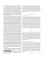
B Program Structural Constraints
The structural constraints are extracted automatically from the
program’s control flow graph (CFG) [6]. This is illustrated in
Fig. 2, which contains an if-then-else statement and its
CFG. In the CFG, we label the edges and the basic blocks by
variables di ’s and xi ’s respectively. These variables represent
the number of times that the control is passing through those
edges and basic blocks when the code is executed. The constraints can be deduced from the CFG as follows: At each node,
the execution count of the basic block is equal to both the sum
of the control flow going into it, and the sum of the control flow
going out from it. Thus, from the graph, we have the following
constraints:
x1
=
d1 = d2 + d3
(2)
d1
d2
if (p)
q = 1;
else
q = 2;
r = q;
d3
B2 q = 1; x2
void store(int i)
{
...
}
d5
B4 r = q; x4
B1 i = 10;
store(i);
x2
B2 n = 2*i;
store(n);
(ii) CFG
d2
CFG of
store()
d3
f2
(i) Code
d6
(i) Code
x1
f1
B3 q = 2; x3
d4
d1
i = 10;
store(i);
n = 2*i;
store(n);
B1 if (p) x1
(ii) CFG
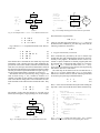
Fig. 4: An example showing how function calls are represented.
Fig. 2: An example of the if-then-else statement and its CFG.
this information is represented by:
=
x2
x3
x4
=
=
d2 = d4
d3 = d5
d4 + d5 = d6
(3)
(4)
(5)
Fig. 3 shows a while-loop statement and its CFG. The constraints are:
x1
x2
x3
x4
=
=
=
=
d1 = d2
d2 + d4 = d3 + d5
d3 = d4
d5 = d6
(6)
(7)
(8)
(9)
Note that the above constraints do not contain any loop count
information. This is because the loop count information depends on the values of the variables, which are not tracked in the
CFG. However, the loops can be detected and marked. After all
the structural constraints have been constructed, the user will be
asked to provide the loop bound information as part of specifying the program functionality constraints (see Section C).
The function calls are represented by using f -edges in the
CFG as shown in Fig. 4. An f -variable is similar to a dvariable, except that its edge contains a pointer pointing to the
CFG of the function being called. The construction of structural constraints in the caller function remains the same. They
are:
x1
x2
=
=
d1 = f 1
f1 = f2
(10)
(11)
The number of times that the function is executed can be
tracked by knowing the f -edges pointing to it. In our example,
d1
B1 q = p; x1
/* p >= 0 */
q = p;
while(q<10)
q++;
r = q;
d2
d4
B2 while(q<10) x2
d3
d5
B3 q++; x3
B4 r = q; x4
d6
(i) Code
(ii) CFG
Fig. 3: An example of the while-loop statement and its CFG.
d2 = f 1 + f 2
(12)
where d2 is the first edge of the function store()’s CFG. For
the main function, which has d1 as its first edge in the CFG, the
following constraint is constructed.
d1 = 1
(13)
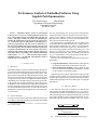
C Program Functionality Constraints
These constraints are provided by the user to denote loop
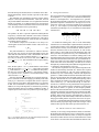
bounds and other path information that depend on the functionality of the program. We illustrate the use of these constraints to capture conditions on feasible program paths with
the example (Fig. 5) taken from Park’s thesis [4]. The function check data() checks the values of the data[] array.
If any of them is less than zero, the function will stop checking
and return 0, otherwise it will return 1.
The while-loop in the function will be executed between 1
and DATASIZE times. Suppose that DATASIZE is previously
defined as a constant value 10, then the following constraints
are used to specify this loop bound information.
1x1
x2
x2
10x1
(14)
(15)
Here, x1 is the count for the basic block just before entering the
loop and x2 is the count for the first basic block inside the loop.
1:
2:
3:
4:
5:
6:
7:
8:
9:
10:
11:
12:
13:
14:
15:
16:
check_data()
{ int i, morecheck, wrongone;
x1
morecheck = 1; i = 0; wrongone = -1;
while (morecheck) {
if (data[i] < 0) {
wrongone = i; morecheck = 0;
}
else
if (++i >= DATASIZE)
morecheck = 0;
}
x2
x3
x4
x5
x6
x7
x8
if (wrongone >= 0)
return 0;
else
return 1;
x9
}
Fig. 5: check data example from Park’s thesis. The xi variables
denote the execution counts of their corresponding basic blocks.
Since all the loops are marked, these two variables can be determined automatically. All the user has to provide are the values
1 and 10.
The minimum user information required to perform timing
analysis is the loop bound information. After that, the user
can provide addition information so as to tighten the estimated
bound. For example, we see that inside the loop, line 6 and line
10 are mutually exclusive and either of them is executed at most
once. This information can be represented by:
(x3 = 0
& x5 = 1) j (x3 = 1 & x5 = 0)
(16)
The symbols ‘&’ and ‘j’ represent conjunction and disjunction
respectively. Note that this constraint is not a linear constraint
by itself, but a disjunction of linear constraint sets. This can be
viewed as a set of constraint sets, where at least one constraint
set member must be satisfied.
As an another example, line 6 and line 13 are always executed together for the same number of times. This can be represented by:
(17)
x3 = x8
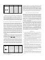
The path information is not limited to within a function.
The user may also specify the path relationship between the
caller and the callee function. This is illustrated in the example shown in Fig. 6. We see that the function clear data()
will only be executed if the return value from the function
check data() is 0. This information can be represented by
the constraint:
x12 = x8 : f1
(18)
Here, the dot symbol ‘:’ in x8 : f1 means that the count of basic
block B8 in function check data() when called at location
f1 . If the function check data() is called from other places,
the value of x8 will not affect that of x12 . For purpose of analysis, a separate set of xi variables is used for this instance of the
call to function check data().
Since the functionality constraints are serving the same purpose as constructs in the IDL language provided by Park in his
work [4], it is instructive to compare their relative expressive
powers. We have been able to demonstrate that every construct
in IDL can be translated to a disjunctive form constraint. In
addition, we can provide disjunctive constraints for practically
useful annotations that are beyond the capabilities of IDL. A
complete proof of this claim is beyond the scope of this paper.
x7
x8
x9
x10 , f1
x11
x12 , f2
check_data()
{ ...
if (wrongone >= 0)
return 0;
else
return 1;
}
task()
{ ...
status = check_data();
if (!status)
clear_data();
...
}
Fig. 6: An example showing how the path relationship between the
caller and the callee function can be specified.
D Solving the Constraints
The program structural constraint set is a set of constraints that
are conjunctive, i.e., they must all be satisfied simultaneously.
Because of the disjunction ‘j’ and conjunction ‘&’ operators,
the program functionality constraints may, in general, be a disjunction of conjunctive constraint sets. Giving us a set of constraint sets, at least one of which is satisfied for any assignment
to the xi ’s. For example, by intersecting all the functionality
constraints ((14) through (17)), we will obtain two functionality
constraint sets:
First set
x1 ? x2 0
10x1 ? x2 0
x3 = 0
x3 ? x8 = 0
x5 = 1
Second set
x1 ? x2 0
10x1 ? x2 0
x3 = 1
x3 ? x8 = 0
x5 = 0
To estimate the running time, each set of the functionality
constraint sets is combined (the conjunction taken) with the set
of structural constraints. This combined constraint set is passed
to the ILP solver with (1) to be maximized. The ILP solver returns the maximum value of the expression, as well as basic
block counts (xi values) that result in this maximum value. The
above procedure is repeated for every set of functionality constraint sets. The maximum over all these running times is the
maximum running time of the program. Note that a single value
of the basic block counts for the worst case is provided in the solution even if there are a large number of solutions all of which
result in the same worst case timing. The ILP solver in effect
has implicitly considered all paths (different assignments to the
xi variables) in determining the worst case.
The total time required to solve the problem depends on the
number of functionality constraint sets, and the time required
to solve each constraint set. The size of the constraint sets is
doubled every time a functionality constraint with disjunction
operator ‘j’ is added. While no theoretical bounds on this can be
derived, our observations have been that in practice this is not a
problem. We found the size to be small at the beginning, and as
more constraints are added, some of the constraint sets will become a null set (e.g. xi 1 intersected with xi = 0). These trivial null sets, if detected, will be pruned before being passed to
ILP solver. The second issue is the complexity of solving each
ILP problem, which is, in general, an NP-complete problem.
We were able to demonstrate that if we restrict our functionality
constraints to those that correspond to the constructs in the IDL
language, then the ILP problem is equivalent to a network flow
problem, which can be solved in polynomial time. However,
the full generality of the functionality constraints can result in it
being a general ILP problem. In practice, this was never experienced, i.e., in the branch and bound solution to the ILP, the first
call to the linear program package resulted in an integer valued
solution. More specific data will be provided in Section VI.
IV
M ICRO - ARCHITECTURAL M ODELING
Currently we are using a simple hardware model to determine
the bound of the running time (cost) of a basic block. For each
assembly instruction in the basic block, we analyze its adjacent
instructions within the basic block, and determine the bound
on its effective execution time from the hardware manual. The
bound of the complete basic block is obtained by summing
up all the bounds of the instructions. This model can handle
pipelining reasonable well. However, it is very simplistic in
its approach to modeling cache memory. Since the costs must
be constants, for best case running time, we assume the execution always has cache-hits, whereas, for worst case running
time, we assume that the execution will always result in cachemisses. Although this still gives a valid estimated bound on the
program’s execution time, it is clearly a conservative approximation and needs to be tightened. In particular, it may happen
that the first iteration of a loop results in cache misses, while the
subsequent iterations will result in cache-hits. Assuming that
all iterations result in all cache misses can be very pessimistic.
This pessimism can easily be avoided in the path analysis stage
by considering the first iteration of the loop as a separate basic
block, distinct from the other iterations, with its own xi and ci
variables. We are currently working on the modeling of cache
memory. Several other researchers are also looking into this
problem [7].
V
I MPLEMENTATION
We have developed a tool called cinderella that incorporates the ideas presented in this paper for timing analysis. It
contains approximately 8,000 lines of C++ code. Currently,
cinderella is implemented to estimate the running time of
programs running on an Intel i960KB processor. The processor is a 32 bit RISC processor that is being used in many embedded systems (e.g. in laser printers). It contains a 4-stage
pipelined execution unit, a floating point unit and a 512-byte
direct-mapped instruction cache [8].
Cinderella first reads the executable code for the program. It then constructs the CFG and derives the program structural constraints. Next, it reads the source files and outputs the
annotated source files, where all the xi and fi variables are labelled alongside with the source code (Fig. 5). Then, for all
loops in the program it asks the user to provide the loop bounds.
This is all the information that is mandatory to provide the timing bounds, and an initial estimate of these bounds can be obtained at this point. To tighten the estimated bound, the user
can provide additional functionality constraints and re-estimate
the bounds again. After each estimation, cinderella outputs the estimated bound (in units of clock cycles), the basic
blocks’ costs and their counts.
VI
E XPERIMENTAL R ESULTS
Our solution is not guaranteed to give the exact bounds, and in
general some pessimism will be introduced in the estimation.
There are two sources for the pessimism in (1): the pessimism
in ci ’s and the pessimism in xi ’s. The former pessimism results
from the inaccuracies of the micro-architectural modeling. It
can be reduced by improving the modeling. The latter is due
to insufficient path information, so that some infeasible paths
are considered to be feasible. This can hopefully be reduced
by providing more functionality constraints.
Since our current work focuses on the path analysis problem,
we would like to evaluate the efficacy of our methodology in
determining the worst and best case paths. Experiment 1 described below is directed towards evaluating the pessimism in
path analysis. In addition to this, we also conducted Experiment 2, with the goal of measuring the inadequacies in our current micro-architectural modeling.
A Experiment 1: Evaluating the Path Analysis Accuracy
Since there are no established benchmarks for this purpose, we
collected a set of example programs from a variety of sources
for this task. Some of them are from academic sources: from
Park’s thesis [4] on timing analysis of software and also from
Gupta’s thesis [9] on the hardware-software co-design of embedded systems. Others are from standard DSP applications,
as well as software benchmarks used for evaluating optimizing
compilers. These routines, their sizes and the number of constraint sets being passed to the ILP solver are shown in Table I.
Of the eight constraint sets of function dhry, five of them are
detected as null sets and eliminated. For each routine, we obtain the estimated bound by using cinderella and calculate
the calculated bound, which is obtained by the following steps:
1. Insert a counter into each basic block of the routine.
2. Identify the initial data set that corresponds to the longest
(shortest) running time of the routine.
3. Run the routine with that data set and record the values of
all the counters.
4. Multiply each counter value with the slowest (fastest)
running time for that basic block as provided by
cinderella.
5. Add up all these products. This is the upper (lower) bound
of the calculated bound.
Note that in order to find the actual upper (lower) bound on
the execution time, we would have to run the routine for all
possible inputs. This is clearly not feasible. Thus, we have replaced this step by actually trying to identify the best (worst)
case data set by a careful study of the program. Clearly if
we could rely on this identification of the best and the worst
case, we do not need to do the analysis at all. However, as we
have no other mechanism to evaluate the result, we have to use
this method. We do know however, that if the analysis result
agrees with our selection of the data set, then it will be the worst
case data set and also our analysis is completely accurate. As
the results of Experiment 1 show (Table II), the analysis provides results that are either in agreement with the selection of
the data set, or very close to it. The pessimism in the evaluation measures the relative difference between the calculated
bound [Cl ; Cu ] and the estimated bound [El ; Eu ]. It is defined as
C ?E
E ?C
[ lC l ; uC u ].
u
l
Function
check data
fft
piksrt
des
line
circle
jpeg fdct islow
jpeg idct islow
recon
fullsearch
whetstone
dhry
matgen
Description
Example from Park’s thesis
Fast Fourier Transform
Insertion Sort
Data Encryption Standard
Line drawing routine in Gupta’s thesis
Circle drawing routine in Gupta’s thesis
JPEG forward discrete cosine transform
JPEG inverse discrete cosine transform
MPEG2 decoder reconstruction routine
MPEG2 encoder frame search routine
Whetstone benchmark
Dhrystone benchmark
Matrix routine in Linpack benchmark
Lines
17
56
15
185
143
88
150
246
137
204
245
480
50
TABLE I: S ET OF B ENCHMARK E XAMPLES
Sets
2
1
1
2
1
1
1
1
1
1
2
8 3
1
)
Function
check data
fft
piksrt
des
line
circle
jpeg fdct islow
jpeg idct islow
recon
fullsearch
whetstone
dhry
matgen
Estimated Bound
[32, 1,039]
[0.97e6, 3.35e6]
[146, 4,333]
[42,302, 604,169]
[336, 8,485]
[502, 16,652]
[4,583, 16,291]
[1,541, 20,665]
[1,824, 9,319]
[43,082, 244,305]
[4.54e6, 13.7e6]
[0.22e6, 1.26e6]
[5,507, 13,933]
Calculated Bound
[32, 1,039]
[0.98e6, 3.31e6]
[146, 4,333]
[43,254, 592,559]
[336, 8,485]
[502, 16,301]
[4,583, 16,291]
[1,541, 20,665]
[1,824, 9,319]
[43,085, 244,025]
[4.54e6, 13.7e6]
[0.22e6, 1.26e6]
[5,507, 13,933]
Pessimism
[0.00, 0.00]
[0.01, 0.01]
[0.00, 0.00]
[0.02, 0.02]
[0.00, 0.00]
[0.00, 0.02]
[0.00, 0.00]
[0.00, 0.00]
[0.00, 0.00]
[0.00, 0.00]
[0.00, 0.00]
[0.00, 0.00]
[0.00, 0.00]
TABLE II: P ESSIMISM IN PATH ANALYSIS.
From these results, we see that when given enough information, the path analysis can be very accurate. The CPU times
taken for each ILP problem were insignificant, less than 2 seconds on an SGI Indigo Workstation. This is largely due to the
fact that the branch-and-boundILP solver finds that the solution
of the very first linear program call it makes is integer valued.
B Experiment 2: Comparison with Actual Running Times
In this experiment, we measured the actual running time of the
program and compared it with the estimated bound. Each program is compiled and then run on an Intel QT960 board [10],
which is a development board containing a 20MHz i960KB
processor, memory and some other peripherals. To measure the
worst case running time, we initialize the routine with its worst
case data set and then run it in a loop several hundred times
and measure the elapsed time. The cache memory is flushed
before each function call. Since this value includes the time to
do the loop iterations and cache flushing, we run an empty loop
and measure its execution time again. The difference between
these two values is the actual running time of the routine. The
best case running time is obtained analogously, but without the
cache flush.
Table III shows the results of this experiment. The estimated
bound is the same as in Experiment 1. The measured values
described above are shown in the measured bound column. The
pessimism is defined as [ MlM?El ; EuM?uMu ] where [Ml ; Mu ] denotes
l
the measured bound.
We observe that while the estimated bound does enclose the
measured bound, the pessimism in the estimation is rather high.
This is mainly due to the fact that a simple hardware model
is used. In particular, the pessimism is bigger when there are
many small basic blocks in the function. This is because all
the cost analysis is currently being done within the basic block.
Function
check data
fft
piksrt
des
line
circle
jpeg fdct islow
jpeg idct islow
recon
fullsearch
whetstone
dhry
matgen
Estimated Bound
[32, 1,039]
[0.97e6, 3.35e6]
[146, 4,333]
[42,302, 604,169]
[336, 8,485]
[502, 16,652]
[4,583, 16,291]
[1,541, 20,665]
[1,824, 9,319]
[43,082, 244,305]
[4.54e6, 13.71e6]
[218,013, 1,264,430]
[5,507, 13,933]
Measured Bound
[38, 441]
[1.93e6, 2.05e6]
[338, 1,786]
[109,329, 242,295]
[963, 4,845]
[641, 14,506]
[7,809, 10,062]
[2,913, 13,591]
[4,566, 4,614]
[62,463, 62,468]
[6.83e6, 6.83e6]
[551,460, 551,840]
[9,260, 9,280]
Pessimism
[0.16, 1.36]
[0.50, 0.63]
[0.57, 1.43]
[0.61, 1.49]
[0.65, 0.75]
[0.22, 0.15]
[0.41, 0.62]
[0.47, 0.52]
[0.60, 1.02]
[0.31, 2.91]
[0.34, 1.01]
[0.60, 1.29]
[0.41, 0.50]
TABLE III: D ISCREPANCY BETWEEN THE ESTIMATED BOUND
AND THE MEASURED BOUND .
For blocks with only a few assembly instructions, the cache
and pipeline behavior is not being modeled very accurately because they depend a lot on the surrounding instructions. Consequently, the costs of these blocks are loose and these contribute
to the discrepancy between the estimated and the measured
bounds. A more sophisticated micro-architectural modeling
will certainly improve the accuracy of the estimated bound.
VII
C ONCLUSIONS
AND
F UTURE W ORK
In this paper, we have presented an efficient method to estimate
the bounds of the running time of a program on a given processor. The method uses integer linear programming techniques
to perform the path analysis without explicit path enumeration.
It can accept a wide range of information on the functionality
of the program in the form of sets of linear constraints. A tool
called cinderella has been developed to perform this timing analysis. Experimental results on a set of examples show
the efficacy of this approach.
The future work includes improving the hardware model to
take into account the effects of cache memory and other features of modern processors that tend to make the timing relatively non-deterministic. We would also like to explore the
possibility of using symbolic analysis techniques to automatically derive some of the functionality constraints. Finally, we
are working on porting cinderella to handle programs running on other hardware platforms. In collaboration with AT&T,
we have completed a port for the AT&T DSP3210 processor.
This is intended for use in the VCOS operating system to bound
the running times of processes for use in scheduling.
R EFERENCES
[1] Eugene Kligerman and Alexander D. Stoyenko, “Real-time Euclid: A
language for reliable real-time systems”, IEEE Transactions on Software
Engineering, vol. SE-12, no. 9, pp. 941–949, September 1986.
[2] P. Puschner and Ch. Koza, “Calculating the maximum execution time of
real-time programs”, The Journal of Real-Time Systems, vol. 1, no. 2, pp.
160–176, September 1989.
[3] Aloysius K. Mok, Prasanna Amerasinghe, Moyer Chen, and Kamtron
Tantisirivat, “Evaluating tight execution time bounds of programs by annotations”, in Proceedings of the 6th IEEE Workshop on Real-Time Operating Systems and Software, May 1989, pp. 74–80.
[4] Chang Yun Park, Predicting Deterministic Execution Times of Real-Time
Programs, PhD thesis, University of Washington, Seattle 98195, August
1992.
[5] R. B. Hitchcock, “Timing Verification and the Timing Analysis Program”, in Proceedings of the 19th Design Automation Conference, June
1982, pp. 594–604.
[6] Alfred V. Aho, Ravi Sethi, and Jeffery D. Ullman, Compilers Principles,
Techniques, and Tools, Addison-Wesley, 1986, ISBN 0-201-10194-7.
[7] Byung-Do Rhee, Sang Lyul Min, Sung-Soo Lim, Heonshik Shin,
Chong Sang Kim, and Chang Yun Park, “Issues of advanced architectural
features in the design of a timing tool”, in Proceedings of the 11th IEEE
Workshop on Real-Time Operating Systems and Software. May 1994, pp.
59–62, IEEE Computer Soc. Press, ISBN 0-8186-5710-3.
[8] Intel Corporation, i960KA/KB Microprocessor Programmers’s Reference
Manual, 1991, ISBN 1-55512-137-3.
[9] Rajesh Kumar Gupta, Co-Synthesis of Hardware and Software for Digital
Embedded Systems, PhD thesis, Stanford University, December 1993.
[10] Intel Corporation, QT960 User Manual, 1990, Order Number 270875001.