Download Measurement-Based Timing Analysis *

Measurement-Based Timing Analysis ⋆
Ingomar Wenzel, Raimund Kirner, Bernhard Rieder, and Peter Puschner
Institut für Technische Informatik,
Technische Universität Wien, Vienna, Austria
Abstract. In this paper we present a measurement-based worst-case execution
time (WCET) analysis method. Exhaustive end-to-end execution-time measurements are computationally intractable in most cases. Therefore, we propose to
measure execution times of subparts of the application code and then compose
these times into a safe WCET bound.
This raises a number of challenges to be solved. First, there is the question of how
to define and subsequently calculate adequate subparts. Second, a huge amount
of test data is required enforcing the execution of selected paths to perform the
desired runtime measurements.
The presented method provides solutions to both problems. In a number of experiments we show the usefulness of the theoretical concepts and the practical
feasibility by using current state-of-the-art industrial case studies from project
partners.
1 Introduction
In the last years the number of electronic control systems has increased rapidly. In order
to stay competitive, more and more functionality is integrated into a growing number
of powerful and complex computer hardware. Due to these advances in control systems
engineering, new challenges for analyzing the timing behavior of real-time computer
systems arise.
Resulting from the temporal constraints for the correct operation of such a real-time
system, predictability in the temporal domain is a stringent imperative to be satisfied.
Therefore, it is necessary to determine the timing behavior of the tasks running on a realtime computer system. Worst-case execution time (WCET) analysis is the research field
investigating methods to assess the worst-case timing behavior of real-time tasks [1].
A central part in WCET analysis is to model the timing behavior of the target platform. However, manual hardware modelling is time-consuming and error prone, especially for new types of highly complex processor hardware. In order to avoid this effort
and to address the portability problem in an elegant manner, a hybrid WCET analysis
approach has been developed. Execution-time measurements on the instrumented application executable substitute the hardware timing model and are combined with elements
from static static timing analysis.
There are also other approaches of measurement-based timing analysis. For example, Petters et al. [2] modifies the program code to enforce the execution of selected
paths. The drawback of this approach is that the measured program and the final program cannot be the same. Bernat et al. [3] and Ernst et al. [4] calculate a WCET estimate
⋆
This work has been supported by the FIT-IT research project “Model-based Development of
Distributed Embedded Control Systems (MoDECS)”.
from the measured execution times of decomposed program entities. While the last two
approaches like our technique also partition the program for the measurements, they do
not address the challenging problem of systematic generation of input data for the measurements. Heuristic methods for input-data generation have been developed [5] which
alone are not adequate to ensure a concrete coverage for the timing measurements.
2 Basic Concepts
In this section, basic concepts for modeling a system by measurement-based timing
analysis are introduced. These include modeling the program representation, the semantics, and the physical hardware.
2.1 Static Program Representation
A control flow graph (CFG) is used to model the control flow of a program. A CFG
G = hN, E, s, ti consists of a set of nodes N representing basic blocks, a set of edges
E : N × N representing the control flow, a unique entry node s, and a unique end node
t. A basic block contains a sequence of instructions that is entered at the beginning and
the only exit is at the end, i.e., only the last instruction may be a control-flow changing
instruction. The current support for function calls is done by function inlining.
2.2 Execution Path Representation
We introduce paths in order to describe execution scenarios (Def. 1).
Definition 1. Path / Execution Path / Sub-Path
Given a CFG G = hN, E, s, ti, a path π from node a ∈ N to node b ∈ N is a sequence
of nodes π = (n0 , n1 , ..., nn ) (representing basic blocks) such that n0 = a, nn = b,
and ∀ 0 ≤ i < n : hni , ni+1 i ∈ E . The length of such a path π is n + 1.
An execution path is defined as a path starting from s and ending in t. Π denotes the
set of all execution paths of the CFG G, i.e., all paths that can be taken through the
program represented by the CFG.
A sub-path is a subsequence of an execution path.
If programs are analyzed the set of feasible paths, i.e., the set of paths that can be
actually executed is of special interest (because exclusively the execution times of these
paths can influence the timing behavior).
Our approach, based on model-checking, allows to check the feasibility of a path
(see Def. 2). To ensure the termination of the analysis, the model checker is stopped if
it cannot perform the analysis of a path within a certain amount of time. However, in
this case the feasibility of the respective paths has to be checked manually.
Definition 2. Feasibility of paths
Given that the set of execution paths of a program P is modeled by its CFG G, we call a
path π ∈ G feasible, iff there exist input data for program P enforcing that the controlflow follows π. Conversely, paths that are not feasible are called infeasible. Defining Π
as the paths of the CFG and Π f as the set of feasible paths, it holds that Π f ⊆ Π.
3 The Principle of Measurement-Based Timing Analysis
The measurement-based timing analysis (MBTA) method is a hybrid WCET analysis
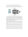
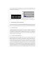
technique, i.e., it combines static program analysis with a dynamic part, the executiontime measurements. As shown in Figure 1, the following steps are performed [6]:
C-Source
Analyzer
tool
Analysis phase
Execution time
measurement
framework
Measurement phase
Calculation
tool
Calculation phase
+
WCET
bound
Fig. 1. The three phases of measurement-based timing analysis
1. Analysis Phase: First the source code is parsed and static analyzes extract path
information. Then, the program is partitioned into segments, which are defined in Section 4. The segment size is customizable to keep the number of different paths for
the later measurement phase tractable. To assess the execution time that a task spends
within each of the identified program segments, adequate test data are needed to guide
the program’s execution into all the paths of a segment. These test data are generated automatically. Besides applying random test-data vectors and heuristics, bounded model
checking for test-data generation is introduced.
As described in Section 4, when using model checking, we generate for each program
segment and instrumented instance of the source-code.
In contrast to methods that work on object-code level, the C-code analysis ensures a
high level of portability because ANSI C is a well established programming language
in control systems engineering. Additionally, C is also used as output format of code
generation tools like Real-Time Workshop (Mathworks Inc.) or TargetLink (dSpace
GmbH).
2. Measurement Phase: The generated test data force program execution onto the
required paths within the program segments. The measured execution times are captured by code instrumentations that are automatically generated and placed at program
segment boundaries. The instrumented programs are executed and timed on the target
platform.
3. Calculation Phase: The obtained execution times and path information are combined to calculate a final WCET bound. This calculation uses techniques from static
WCET analysis. It utilizes the path information acquired in the static analysis phase.
(see 1.)
In case of complex hardware where the instruction timing depends on the execution history, MBTA can still provide safe WCET bounds when using explicit state enforcement
at the beginning of each segment to eliminate state variations. For example, the pipeline
could be flushed or the cache content could be invalidated or pre-loaded.
The contributions of this measurement-based worst-case execution time analysis
(MBTA) method are:
Avoidance of explicit hardware modelling. In contrast to pure static WCET analysis
methods [1], this approach does not require to build a sophisticated execution-time
model for each instruction type. In fact, the actual timing behavior of instructions
within their context is obtained from execution-time measurements on the concrete
hardware.
Automated test-data generation using model checking. This allows us to completely
generate all required and feasible test data. In the first experiments we used symbolic model checking. Later, bounded model checking turned out to be superior
wrt. model size and computation times.
Parametrizable complexity reduction. The control-flow graph partitioning algorithm
allows a parameterizable complexity reduction of the analysis process (i.e., the
number of required execution-time measurements and the size of the test data set
can be chosen according to the available computing resources). On the reverse side,
the accuracy of the analysis decreases by reducing the number of tests. This allows
for an adaptation to user demands and available resources.
Modular tool architecture. The tool structure is completely modular. It is possible to
improve the components for each step independently (e.g., the test-data generation
mechanism, WCET bound calculation step).
Scalability of the analysis process. Execution-time measurements and test-data generation (that consume together around 98% of the total analysis time) can be executed highly parallel if multiple target machines respectively host computers are
available.
In our implementation, the interface data passed between the three phases (i.e., extracted path information, the test data, and the obtained execution times) are stored in
XML files.
4 Parameterizable Program Partitioning for MBTA
In the following sections, the main concepts of the measurement-based timing analysis
approach [7] are described in detail. The proposed method is a hybrid approach that
combines elements of static analysis with the dynamic execution of software.
After preparing the previously described CFG, the partitioning algorithm is invoked
to split the CFG into smaller entities, so-called program segments (Definition 3). This
segmentation is necessary, because when instead trying to use end-to-end measurements the number of paths in Π (the set of paths of the function subject to analysis) is
in general intractable. Our segmentation is similar to that described by Ernst et al. [4].
However, we do not differ between segments of single or multiple paths, instead we
use a path bound to limit segment size. In a second step, the paths within the program segments are explicitly enumerated in a data structure called dtree (coming from
decision-tree).
Definition 3. Program Segmentation (PSG)
A program segment (PS ) is a tuple PS = hs, t, Πi where s is the start node and t is
the respective end node. Π refers to the set of associated paths πi ∈ Π. Further, each
path of a segment has its origin in s and its end in t:
∀π = (n1 , ..., nn ) ∈ Π : n1 = s ∧ nn = t
The intermediate nodes of a path of a segment may not be equal to its start or end node:
∀π = (n1 , n2 , ..., nn−1 , nn )∈Π ∀2≤i≤n−1 : ni 6= s ∧ ni 6= t
The set of all program segments PS of a program is denoted as PSG.
Each program segment spawns a finite set of paths Πj . For each of these paths
we are interested in the set of feasible paths and the respective input data (test data)
that force the execution of the code onto this path. This set is constructed by using a
hierarchy of test-data generation methods. When decomposing a program into program
segments, two important issues arise:
First, each program segment has to be instrumented for obtaining the execution
times of its feasible paths. Each instrumentation introduces some overhead. Therefore,
these instrumentations are not desired and their number should be minimized.
Second, the computational effort of generating input data increases with larger program segments sizes, especially when using model checking.
If no constraints are given, there are many different program segmentations possible.
For instance, one extreme segmentation would be that for each CFG edge one program
segment is generated, i.e., PSG = {PS i | PS i = hno , np , {(no , np )}i ∧ (no , np )∈E}.
The other end of the spectrum would be to put all nodes into one program segment, i.e.,
PSG = {PS } with PS = hs, t, Πi and Π having a complete enumeration of all paths
within a function (and its called functions).
A “good” program segmentation PSG is a program segmentation that balances the
number of program segments and the average number of paths per program segment.
These two “goals” are not independent. When the number of program segments is decreased, typically1 the sum of paths increases and vice versa. A segmentation resulting
in fewer program segments causes (i) less instrumentation effort and related overheads
at runtime and (ii) higher computational resource needs during analysis because more
paths have to be evaluated. In contrast, a segmentation into more program segments
results in (i) higher instrumentation effort and (ii) faster path evaluation. This is because the larger a segment is, the more paths are inside a segment, but the less different
segment boundaries have to be instrumented.
In practice, a reasonable combination of the number of paths per segment and the
number of program segments has to be selected. The major limitation turned out to
be the computational resources required to generate the input data for the paths (see
Section 5).
4.1 Path-Bounded Partitioning Algorithm
The partitioning algorithm automatically partitions a CFG into program segments. As
there is a functional relationship between the number of program segments and the
overall number of sub-paths to be measured, we choose one factor and derive the other
one. One possibility is to provide a target value for the maximum number of paths for
each PS j (denoted as path bound PB ), i.e., ideally |Πj | ≈ PB .
1
The term “typically” is used because there are some exceptions at the boundaries. Examples
for this are presented in Section 4.2.
The detailed description of the partitioning algorithm is given in [6]. Basically, the
partitioning algorithm investigates the number of paths between dominated nodes and
in case it is higher than PB a recursive decomposition is performed. Due to the short
runtime of the partitioning algorithm (even for large code samples), it is possible to
experiment with various values for PB and calculate the resulting number of paths
within reasonable time (< 1s).
4.2 Example of Path-Bounded Program Partitioning
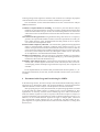
To demonstrate the operation of the MBTA framework, the C code example given in
Figure 2(a) is used. The corresponding CFG is given in Figure 2(b).
0
2
4
3
5
7
11
17
12
1
2
3
4
5
6
7
8
9
10
11
12
13
14
15
16
17
18
19
20
21
22
23
24
25
26
int x;
int main nice partitioning (
int y , int i , int a , int b)
{
i f ( x == 1 ) {
x ++; / / BB 2
} else {
x−−; / / BB 4
}
/ / BB 3
i f ( b == 1 ) {
/ / BB 5
i f ( a == 1 ) {
/ / BB 7
i f ( x == 3 ) {
x ++; / / BB 9
} else {
/ / BB 11
i f ( x == 2 ) {
x ++; / / BB 12
} else {
/ / BB 14
i f ( x == 4 ) {
x ++; / / BB 15
}
27
28
29
30
31
32
33
34
35
36
37
38
39
40
41
42
43
44
45
46
47
48
49
50
14
}
}
} else {
x ++; / / BB 17
}
x ++; / / BB 8
}
/ / BB 6
i f ( b == 2 ) {
/ / BB 18
i f ( a == 1 ) {
x ++; / / BB 20
} else {
x−−; / / BB 22
}
x ++; / / BB 21
}
/ / BB 19
i f ( y == 1 ) {
x ++; / / BB 23
} else {
x−−; / / BB 25
}
9
15
8
6
18
20
22
21
19
23
25
}
(a) Sample Code
1
(b) CFG
Fig. 2. Example code and the corresponding CFG
Assuming a path bound PB = 5, the partitioning algorithm constructs a segmentation with 6 program segments, i.e., PSG = {PS 0 , PS 1 , PS 2 , PS 3 , PS 4 , PS 5 } with
PS 0 = (0, 3, {(0, 2, 3), (0, 4, 3)}),
PS 1 = (3, 5, {(3, 5)}),
PS 2 = (3, 6, {(5, 7, 9, 8, 6), (5, 7, 11, 12, 8, 6), (5, 7, 11, 14, 8, 6),
(5, 7, 11, 14, 15, 8, 6), (5, 17, 8, 6)}),
PS 3 = (3, 6, {(3, 6)}),
PS 4 = (6, 19,{(6, 18, 20, 21, 19), (6, 18, 22, 21, 19), (6, 19)}),
PS 5 = (19, 1,{(19, 23, 1), (19, 25, 1)}).
The partitioning results for PB being 5, 10, 20, and 100, respectively are summarized in Figure 3(a). Figure 3(b) shows the dependency of the number of segments
P
(|PSG|) and the number of sub-paths ( |Πj |) for each of these segmentations. This
example illustrates that in general fewer program segments cause a higher overall number of paths to be considered.
80
PB=100
Path Bound
1
5
10
20
100
|PSG|
30
6
3
2
1
#Paths ( ™ |ʌj| )
30
14
14
18
72
#Paths ( ™ |ʌj| )
70
60
50
40
PB=1
30
PB=20
PB=10
20
10
PB=5
0
0
10
20
30
Program segments ( |PSG| )
(b) Dependency between |PSG | and
P
|Πj |
P
Fig. 3. Dependency between number of segments (|PSG|) and number of sub-paths ( |Πj |)
(a) Partitioning Results
5 Automated Test-Data Generation
For each path that has been previously determined in the program segmentation step, we
are interested in whether it is a feasible path. Feasible paths may contribute to the timing
behavior of the application and thus have to be subject to execution-time measurements.
5.1 Problem Statement
P
As described previously the set of paths
|Πj | has to be executed to perform the
execution-time measurements. Therefore, it is necessary to acquire for each path πi ∈
Πj a suitable set of input-variable assignments such that the respective assignments
at the function start causes exactly the control flow that follows πi . In contrast, for
infeasible paths their infeasibility has to be proven to know that they cannot contribute
to the timing behavior of the program.
5.2 Test-Data Generation Hierarchy
When applying the method it turned out that the test-data generation process is the
bottleneck of the analysis. Especially, model checking is very resource intensive. To
improve performance we decided to use a combination of different methods for generating the input data. We start by using fast techniques and gradually use more formal
and resource-consuming methods to cover the paths for which the cheaper methods did
not found appropriate input data. Figure 4 shows the hierarchy of methods we apply.
On the basic level test-data reuse is applied. This means that we reuse all existing test
data for that application from previous runs. On the second level, pure random search
is performed, i.e., all input variables are bound to random numbers. Third, heuristics
like genetic algorithms can be used. Finally, all data that could not be found using the
generation methods of level 1 to 3, are calculated by model checking. Especially, the
infeasibility of paths can be proven only by model checking (at level 4). The actual
Level 4: Model checking
Level 3: Heuristics
Level 2: Random search
0000
1111
111111
000000
0000
1111
0000
1111
000000
111111
0000
1111
000000
111111
00000000
11111111
11111111
00000000
00000000
11111111
00000000
11111111
Fig. 4. Test-data generation hierarchy
Level 1: Test-data reuse
computational effort spent on each of the levels is application dependent. If an application has many infeasible paths, model checking is required to show that each of these
paths is really infeasible.
The key advantages of this hierarchical test-data generation approach are (i) that
many test data are generated by fast strategies, only left over cases have to resort to
expensive model checking; (ii) the correlation of test data and the covered path is known
even when applying heuristics since we monitor the covered paths before doing the
measurements; (iii) and complementary, model checking is used in the final phase of
test data generation. This allows generating input data for a desired path whenever such
a path is feasible or otherwise to prove that the path is infeasible.
5.3 Test-Data Generation using Model Checking
The basic idea of performing test-data generation by model checking (level 4) is that
the CFG (and the instructions in the nodes) are transformed into a model that can be
analyzed by a model checker. For each πi ∈ Πj to be analyzed a new model model (πi )
is generated. This model is passed to a model checker check (model (πi )) that yields a
suitable variable binding in case a counter example can be found by the model checker.
Otherwise, the function check returns that the path is infeasible.
When generating a model model (πi ), an assertion is added stating that the particular
path πi cannot be executed within that model. Program code that does not influence the
reachability of that path πi is cut away (slicing) to reduce the size of the model. Then
the model checker tries to prove this formally. Whenever the proof fails, the model
checker provides a counter example that represents the exact input data that enforce an
execution of the desired path πi . However, if the assertion holds, the path is infeasible
and therefore no input data do exist.
The current implementation does not support the analysis of loops. However, we
work on loop unrolling to support loops.
Symbolic Model Checking vs. Bounded Model Checking We implemented model
checking backends for symbolic model checking and bounded model checking [8]. The
model checker SAL [9] is used for symbolic model checking [9] and the model checkers
SAL-BMC [9] and CBMC [10] are used for bounded model checking. In experiments,
it turned out that bounded model checking supports (i) bigger applications in terms of
lines of code and (ii) supports longer program segments (i.e., longer paths). Therefore,
our MBTA uses the bounded model checker CBMC by default.
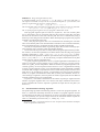
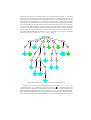
5.4 Example Application for Test-Data Generation
In this section we show the result of applying bounded model checking to find a specific path in the sample program of Figure 2. The paths for program segmentation PSG
described in Section 4.2 are represented as dtree data structure (Figure 5). This data
structure is a tree which root node has the name of the CFG (name of subroutine). All
immediate successor nodes denote a program segment. In the parentheses the starting
basic-block node is denoted, e.g., PS 0 starts at basic block 0. Then, the succeeding
nodes denote the intermediary basic blocks. The end nodes provide additional information corresponding to the path starting from the start node and leading to this end node,
i.e., every end node represents one path within a program segment. This information
consists of the data-set number and the model number. The data-set number identifies
the input data to reach this path. When using model checking to generate the test data,
the model number identifies the model model (πi ) for path πi . For instance, the model
number of model(π3 ) for path π3 = (5, 7, 9, 8, 6) equals 3.
main_nice_partitioning
PS0(0)
2
3
ds=1
mc=1
PS1(3)
PS2(5)
4
5
ds=2
mc=2
7
3
ds=0
9
11
8
PS3(3)
6
ds=0
17
8
14
6
ds=7
mc=7
8
8
15
6
ds=4
mc=4
6
ds=6
mc=6
PS5(19)
19
ds=0
18
20
12
6
ds=3
mc=3
PS4(6)
22
21
21
19
ds=8
mc=8
19
ds=9
mc=9
23
1
ds=10
mc=10
25
1
ds=0
8
6
ds=5
mc=5
Fig. 5. Representation of dtree data structure for test-data generation
In Figure 6 the code of the automatically generated model for π3 = (5, 7, 9, 8, 6)
is depicted. In the main function the program counter mc pc is initialized. Next, the
function subject to analysis is called with its respective parameters. Within the function,
first all instructions preceding the PS are conserved, i.e., basic blocks BB0, BB2, BB4,
BB3. Starting with BB5, the PS entry node, cut off actions take place. These cut-off actions mean that the functional code of BB17 has been removed. Instead of this removed
code additional exits have to be added. This avoids that other basic blocks modify the
calculations and change the execution path.
Whenever code of basic blocks residing on the actual investigated path is executed,
the program counter mc pc of the model is increased. Thus, this increase is performed
for basic blocks BB5, BB7, BB9, BB8 and BB6.
Finally, after returning to main the assertion assert(mc pc != 5) ensures
that mc pc 6= 5, i.e., path π3 = (5, 7, 9, 8, 6) cannot be executed.
In a standard program execution, this assertion would be raised whenever – depending on the currently assigned variable values – path π3 is executed. However, when
passed to a C model checker, the model checker tries to formally prove whether this
assertion always holds. If not, the model checker provides a counter example containing variable bindings that violate the assertion. In this case, we get the data binding
{x ← 4, y ← 0, i ← 0, a ← 1, b ← 1}. If the model checker affirms that the assertion
holds, then we know that the path is infeasible. In case the model checker runs out of
resources, the path has to be checked manually.
}
} else {
mc pc = −1; /∗ BB 17 ∗/
return 0 ;
}
mc pc ++; /∗ BB 8 ∗/
x ++;
i n t mc pc ;
i nt x , local y , l o c a l i , l o cal a , l o c al b
int main nice partitioning ( int y , int i , int a , int b)
{
i f ( x == 1 ) {
x ++; / / BB 2
} else {
x−−; / / BB 4
}
/ / BB 3
i f ( b == 1 ) {
/∗ mc p c i n c r e m e n t ∗/
mc pc ++; /∗ BB 5 ∗/
i f ( a == 1 ) {
mc pc ++; /∗ BB 7 ∗/
/∗ mc p c i n c r e m e n t ∗/
i f ( x == 3 ) {
mc pc ++; /∗ BB 9 ∗/
/∗ mc p c i n c r e m e n t ∗/
x ++;
} else {
/∗ mc c u t o f f ∗/
mc pc = −1; /∗ BB 11 ∗/
return 0 ;
/∗ mc c u t o f f ∗/
}
mc pc ++; /∗ BB 6 ∗/
return 0 ;
/∗ mc c u t o f f ∗/
/∗ mc c u t o f f ∗/
/∗ mc p c i n c r e m e n t ∗/
/∗ mc p c i n c r e m e n t ∗/
/∗ mc c u t o f f ∗/
}
i n t main ( )
{
mc pc = 0 ;
/∗ mc p c r e s e t ∗/
m ai n n i c e p a rt i t i o n i n g ( local y , l o c a l i , l o cal a , l o ca l b ) ;
a s s e r t ( mc pc ! = 5 ) ;
/∗ mc a s s e r t i o n ∗/
}
Fig. 6. Automatically generated code for model(π3 ) with π3 = (5, 7, 9, 8, 6)
5.5 Complexity Reduction
S
When evaluating the paths Πj | Πj ∈ PSG that have to be analyzed with model
checking, it is essential to apply a number of complexity reductions on the models.
For each path πi the complexity reduction is performed in several steps:
1. All paths after a PS are cut off because they do not influence the control flow
leading to a PS or inside a PS .
2. Paths preceding the PS are kept without modifications. This has practical reasons.
Originally, it was intended to remove the preceding code. However, it turned out
that this is not necessary immediately because the model checker can solve the
problem within a reasonable amount of time. The advantage why this code remains
unchanged is that more infeasible paths – namely from the global function view –
can be determined. Thus, only feasible paths contribute to the timing information
of the program segment.
3. Due to the goal of model checking (namely to check whether there exists a specific path), the model checker can perform optimizations on its own, e.g., program
slicing [11] by removing unused variables (i.e., variables that do not influence the
actual execution paths).
6 The Execution-Time Model of MBTA
The role of the execution time model is to provide the information to map execution
times to instruction sequences. The use of the execution time model in MBTA is in
principal the same as in static WCET analysis [1]. However, the main difference is that
in MBTA the timing information is obtained by measurements instead of deriving it
from the user manual and other sources as done in static WCET analysis.
The execution time measurements of MBTA in general require to instrument the
code with additional instructions to signal program locations and/or store measurement
results. Since the instrumentations change the analyzed object code, there are some
requirements on the code instrumentations:
1. The impact of the instrumentation code on the execution time and code size should
be small.
2. If the instrumented code used for MBTA is not the same as the final application
code under operation, the code instrumentations should allow to determine an estimate on the change of the WCET of suitable precision between the instrumented
code and the final application code. Fulfilling this requirement may be challenging in practice, e.g, when requiring precise safe upper bounds on complex target
hardware.
6.1 Enforcing Predictable Hardware States
Besides the above quality criteria of code instrumentations, there is also a substantial
potential of using code instrumentations: on complex hardware where the instruction
timing depends on the execution history it is challenging to determine a precise WCET
bound. Code instrumentations can be used to enforce an a-priori known state at the
beginning of a program segment, thus avoiding the need for considering the execution
history when determining the execution time within a program segment. For example,
code instrumentations could be used to explicitly load/lock the cache, to synchronize
the pipeline, etc.
6.2 Execution-Time Composition
After performing the execution-time measurements we know that each path π ∈ Πj
is assigned its measured execution time t(π). Now, the next step is to compose these
measured execution times into a WCET estimate. In general, three different approaches
are possible, which are explained in [1]. Using tree-based methods, the WCET is calculated based on the syntactic constructs. In path-based methods, a longest path search is
performed. The Implicit path enumeration technique (IPET) models the program flow
by (linear) flow constraints. After applying this calculation step, we get a final WCET
estimate that is the overall result of the MBTA.
In order to illustrate this flexibility of choosing the calculation method, a path-based
calculation method (longest path search) and IPET (using integer linear programming
- ILP) have been implemented in our MBTA framework. It has been shown that it is
possible to incorporate flow facts into the ILP model without restricting generality [6].
7 Experiments
We have implemented the described MBTA as a prototype. The host system of the
framework has been installed on two systems, on Linux and also on Microsoft Windows
XP with Cygwin. The quantitative results described in this section have been obtained
using a PC system with an Intel Pentium 4 CPU at 2.8 Ghz and 2.5GB RAM running
on a Debian 4.0 Linux system.
As target system we used a Motorola HCS12 evaluation board (MC9S12DP256).
The board is clocked at 16Mhz, has 256kB flash memory, 4kB EEPROM, and 12kB
RAM. It is equipped with two serial communication interfaces (SCI), three serial port
interfaces (SPI), two controller area network (CAN) modules, eight 16bit timers, 16
A/D converters.
As a measurement device our frameworks can either use one of the counters of the
HCS12 board or an external timer. The experiments reported here have been performed
using a custom-built external counter device that is clocked at 200MHz. This device is
connected via USB to the host system and by two I/O pins to the target hardware [6].
Application Name
TestNicePartitioning
ActuatorMotorControl
ADCConv
ActuatorSysCtrl
Source
Teaching example
Industry
Industry
Industry
LOC
#BB #Execution Paths
30
72
1150
171
1.90E+11
321
31
144
274
54
97
46
Fig. 7. Summary of the used case studies
In order to study relevant program code, we investigated the code structure of applications delivered by industrial partners (Magna Steyr Fahrzeugtechnik, AVL List). It
was decided to support code structures representing a class of highly important applications (safety-critical embedded real-time system). Figure 7 summarizes the benchmark programs used in the experiments (LOC = lines of code, #BB = number of basic
blocks, #ExecutionPaths = number of execution paths) of the active application.
The first benchmark has been written by hand as a test program in order to evaluate
the MBTA framework. The second one has been developed using Matlab/Simulink in
order to walk through all stages of a modern software development process. The last
three benchmarks representing industrial applications from our industrial project partners have been the key drivers for the development of the MBTA framework.
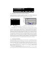
7.1 Experiment with Model Checking for Automated Test-Data Generation
The goal of this experiment is to compare the performance of different model checkers
for automatically generating test data. Figure 8 shows the analysis time of the different
model checkers that have been introduced in Section 5.3. Please note that these figures
do not state anything about the general quality of a model checker, as even in case of
test-data generation, the model-checker performance is of high sensitivity. Thus, the
following interpretation is only valid for the concrete case study (model).
The main result gained from our experiment is that the CBMC model checker is
well-suited for these types of problems. It boosts test data calculation by factors 10-20
over using symbolic model checking. Some applications cannot be analyzed using SAL
at all.
#Paths MC
TestNicePartitioning
ActuatorMotorControl
ADCConv
ActuatorSysCtrl
1
CBMC
11.2
1202.2
65.2
32.7
63
280
136
96
Time Analysis [s]
SAL
SAL BMC
109.6
259.3
N.A.1
N.A.1
7202.5
2325.5
507.4
491.3
Model size is too big, memory error of the model checker (core dump)
Fig. 8. Comparison of required model-checking time to generate test data
7.2 Experiments with Automated Complexity Reduction
In this experiment we repeated the complexity reduction of the didactic sample code
summarized in Figure 3 with the industrial case study ActuatorMotorControl.
The results are given in Figure 9 using a logarithmic scale for the X-axis.
1600
|PSG|
171
88
38
21
14
13
11
8
7
5
#Paths ( ™ |ʌj| )
171
117
84
83
92
106
130
242
336
1455
(a) Partitioning results
PB=1000
1400
#Paths ( ™ |ʌj| )
Path bound
1
2
4
6
10
15
20
50
100
1000
1200
1000
800
600
PB=100
400
PB=1
PB=10
200
0
1
10
100
1000
Program segments ( |PSG| )
(b) Dependency between |PSG| and
P
|Πj |
Fig. 9. Program segmentation results for ActuatorMotorControl
Enumerating all 1.9 ∗ 1011 different execution paths (see Figure 7) of the case study
ActuatorMotorControl is practically intractable. Thus, partitioning into program
segments is necessary. With a path bound P B = 1 each basic block of the program resides in a separate segment and with an unlimited path bound the whole program is
placed in one segment. The partitioning results in FigureP9 show that there is a certain
path bound for which the resulting number of sub-paths |Πj | is minimal. When further increasing the path bound the number of program segments still decreases (which
is profitable as it increases the precision of the measurements because the segments
get larger). However, at the same time the number of sub-paths strongly increases,
which increases the overall computational effort needed for test-data generation and
execution-time measurements. Thus, the right path bound to be chosen depends on how
much computational resources are available and how much precision is required.
7.3 Experiments with MBTA
Applying the MBTA on the case studies presented in Figure 7 using different values for
the path bound leads to the results in Figure 10. “#Paths Random” gives the number of paths
that have been already found by using random generation of test data and “#Paths MC”
gives the remaining number of paths that had to be generated using model checking.
“Coverage (#Paths)” represents the number of feasible paths. Note that if for a path bound
PB=1 it implies that “#Paths Random” + “#Paths MC” 6= “Coverage (#Paths)” it follows that the
program contains unreachable code. Column “WCET Bound” shows the WCET estimate
obtained with the MBTA framework.
“Time (Analysis) [s]” shows the time spent within the analysis phase. “Time (ETM) [s]” shows
the time spent within the execution-time measurement phase, which includes also the
165
68
89
130
31
9
14
12
54
36
25
30
14
14
15
26
Time Analysis / Path MC [s]
Overall Time [s]
Time (ETM) [s]
Time (Analysis) [s]
WCET Bound
Coverage (#Paths)
#Paths MC
165
6
63
29
57 279
82 1373
31
0
8
9
8
66
12 132
54
0
36
0
18
79
6
24
4
10
3
11
2
16
1
71
N.A.
468 1289 1757 78.00
3445
841 116
957 29.00
3323 7732
62 7794 27.71
3298 41353
49 41402 30.12
872
24 192
216 N.A.
870
31
22
53 3.44
872
220
17
237 3.33
872
483
11
494 3.66
173
26 318
344 N.A.
173
10
85
95 N.A.
131
191
10
201 2.42
151
34 175
209 1.42
151
15
39
54 1.50
151
16
21
37 1.45
150
22
16
38 1.38
129
106
12
118 1.49
#Paths / Program Segment
TestNicePartitioning
171
14
7
5
31
3
2
1
54
14
1
30
6
3
2
1
Time ETM / Covered Path [s]
ActuatorSysCtrl
#Paths Random
ADCConv
1 171
10
92
100 336
1000 1455
1
31
10
17
100
74
1000 144
1
54
10
36
100
97
1
30
5
14
10
14
20
18
100
72
#Program Segments
ActuatorMotorControl
#Paths ( ™ |ʌj| )
Path Bound
compile and load time. “Overall Time [s]” is the sum of “Time (Analysis) [s]” and “Time (ETM)
[s]”. “Time Analysis / Path MC [s]” gives the average time required for using model checking
(CBMC) to generate a single test vector for a sub-path. This number is quite significant,
because the time required for test-data generation using model checking contributes
most of the runtime of the analysis phase (except for very low path bounds). It has a
rather small variation over different sub-paths of the same model. “Time (ETM) / Covered Path
[s]” gives the average runtime needed to measure a single sub-path. “#Paths / Program Segment”
shows the average number of feasible paths per program segment.
7.8
1.7
0.7
0.4
6.2
2.4
1.2
0.9
5.9
2.4
0.4
5.8
2.8
1.5
1.1
0.5
1.0
6.6
48.0
291.0
1.0
5.7
37.0
144.0
1.0
2.6
97.0
1.0
2.3
4.7
9.0
72.0
Fig. 10. Summarized experiments of case studies
The experimental results illustrate the tradeoff between precision and required analysis time. For the case study TestNicePartitioning the gained bound contains
some pessimism due to the lack of flow facts that characterize path dependencies across
program segment boundaries. However, it has been shown that it is possible to include
additional flow information in the analysis in order to tighten the bound by increasing the program-segment size. For ActuatorSysCtrl the situation is similar. With
increasing program-segment size (i.e., by choosing a higher path bound) the existing
pessimism can be stepwise eliminated. Such variations do not exist for ADCConv. Here
all obtained results are almost identical. ActuatorMotorControl indicates similar
results. Whenever the path bound is increased, the WCET bound is tightened a little bit
yielding a WCET bound of 3298 cycles (for a program segmentation having path bound
1000). However, the cost for this increase in precision is an analysis time of about 11.5
hours. The missing WCET bound (N.A.) for path bound PB=1 is caused by a limitation
in the current tool implementation and is not a conceptional problem.
8 Conclusion
In this paper we presented the design and implementation results of MBTA, a fully
automated WCET analysis process that does not require any user intervention. The
input program is partitioned into segments, allowing the user to select a path bound for
the size of the segments. Depending on this parameter, the analysis time ranges from
a few seconds up to multiple hours. The bigger the chosen program-segment size, the
more implicit flow information and hardware effects are incorporated into the timing
model. Also, in this case the number of required instrumentations is low.
As a separate model (to be solved by the model checker) is used for each required
path, this stage of the test-data generating process can be easily parallelized. The MBTA
is easily retargetable to new target hardware due to its operation on a restricted set of
ANSI-C code.
The MBTA allows to derive safe WCET estimates even on complex hardware. To
achieve this, additional instrumentations are necessary to enforce predictable hardware
states. The experimentation with such instrumentations and the analysis of program
loops is considered future work.
References
1. Kirner, R., Puschner, P.: Classification of WCET analysis techniques. In: Proc. 8th IEEE
International Symposium on Object-oriented Real-time distributed Computing, Seattle, WA
(2005) 190–199
2. Petters, S.M.: Bounding the execution of real-time tasks on modern processors. In: Proc. 7th
IEEE International Conference on Real-Time Computing Systems and Applications, Cheju
Island, South Korea (2000) 12–14
3. Bernat, G., Colin, A., Petters, S.M.: WCET analysis of probabilistic hard real-time systems.
In: Proc. 23rd Real-Time Systems Symposium, Austin, Texas, USA (2002) 279–288
4. Ernst, R., Ye, W.: Embedded program timing analysis based on path clustering and architecture classification. In: Proc. International Conference on Computer-Aided Design (ICCAD
’97), San Jose, USA (1997)
5. Puschner, P., Nossal, R.: Testing the results of static worst-case execution-time analysis. In:
Proceedings of the 19th IEEE Real-Time Systems Symposium (RTSS 1998), IEEEP (1998)
134–143
6. Wenzel, I.: Measurement-Based Timing Analysis of Superscalar Processors. PhD thesis,
Technische Universität Wien, Institut für Technische Informatik, Treitlstr. 3/3/182-1, 1040
Vienna, Austria (2006)
7. Wenzel, I., Kirner, R., Rieder, B., Puschner, P.: Measurement-based worst-case execution
time analysis. In: Third IEEE Workshop on Software Technologies for Future Embedded
and Ubiquitous Systems (SEUS). (2005) 7–10
8. Biere, A., Cimatti, A., Clarke, E., Zhu, Y.: Symbolic model checking without BDDs. Lecture
Notes in Computer Science 1579 (1999) 193–207
9. Moura, L.D., Owre, S., Ruess, H., Rushby, J., Shankar, N., Sorea, M., Tiwari, A.: SAL 2.
CAV 2004 (2004)
10. Clarke, E., Kroening, D., Lerda, F.: A tool for checking ANSI-C programs. In: Tools and
Algorithms for the Construction and Analysis of Systems (TACAS 2004). Volume LNCS
2988., Springer (2004) 168–176
11. Tip, F.: A survey of program slicing techniques. Journal of Programming Languages 3
(1995) 121–189