Download Control of a Model Sized Hovercraft

TIIC UNIVCRSITY or
NEW SOUTH WALES
TU e
5 YDNEY' AUS T RA llA
Control of a Model Sized Hovercraft
R.M.W. Sanders
DeT nr. 2003-27
Research report
Coach:
prof. V. Solo
University of New South Wales
School of Electrical Engineering & Telecommunications
Systems & Control Research Group
Supervisor: prof.dr.ir.M.Sleinbuch
University of Technology Eindhoven
Depal1ment of Mechanical Engineering
Control Systems Technology
Eindhoven. March 2003
I
~
THE UNIVERSITY OF
NEW SOUTH WALES
SYDNEY· AUSTRALIA
Foreword
I would like to thank the school of Electrical Engineering & Telecommunications for giving us the
opportunity to do our internship at the University of New South Wales. Especially Prof Victor Solo,
head of Systems and Control Research group for his supports and valuable advises. I would like to
thank also Chris Lu for his helps and discussions in the laboratory and also Dr. R Eaton and Dr.
Clements for invaluable advises during our project. Besides the school of EE&T I would also thank
the school of Mechanical Engineering for making it possible to do experiments at the the test rig of the
department Mechatronics and especially Dr. J Katupitiya and Mr.C J Sanderson.
After all I look back at a great and valuble time at the University in Sydney and in Australia. It was a
great experience, but the time to stay was to short.
This report contains the work that I have done with Bart Consten during the period of 9th September to
7th December for the hovercraft project at the Systems and Control Research laboratory at the UNSW.
1
I
~
THE UNIVERSITY OF
NEW SOUTH WALES
SYDNEY· AUSTRALIA
Summary
The development of the hovercraft started with Sir Christopher Cockerell. He developed for the ftrst
time a 'vessel' that could float over land or water. Cockerell used an air cushion underneath the vessel
and this cushion reduced the friction between the surface of the water and hulls so much because of an
air-lubricated layer. The hovercraft in this project is a two channel AM remote controlled model
hovercraft from HOVERCRAFTmodels.com T"; type electro cruiser. Research purposes in future are
making use of vision and control. But before this is possible has to be made a connection with the
computer. The purposes for this project are creating an open loop PC controlled hovercraft and
deriving a dynamical model for the hovercraft.
A few adjustments are made to the hardware and software to come to a PC controlled hovercraft. The
remote control transmitter is ftrst of all transformed to a PC compatible transmitter. Normal remote
control is still possible. Therefore are attached two switches on top of the transmitter to switch
between normal remote control mode and PC control mode. Remote control mode is active if both
switches are pointing to the antenna of the transmitter and PC control model is active when the
switches are pointing to the outside. Sending signals out of a PC requires a data acquisition board. The
data acquisition board that is used during the project is from AXIOM Technology Co. Ltd, type
AX541lH. A real-time environment is desired in control technology and in this project is used Realtime linux. Real-time Linux is a small real-time operating system and is used to get the Linux system
under control to meet real-time computing needs. On the conceining computer is therefore installed
linux kerneI2.2.18 and rt-linux kernel 3.0.
Control software is designed using an older version of a SISO program of Ray Eaton. The new
program makes it possible to send two signals out at one time. Controlling of the hovercraft open loop
works with four buttons in the designed Graphical User Interface. Two buttons Left and Right are for
controlling the rudder and Up and Down are for controlling the lift motor. Current software and
hardware make it possible to control the hovercraft open loop.
Deriving a dynamical model of the hovercraft is done with the Newton-Euler method. A 3 degrees of
freedom model is formulated after making a few assumptions. In the model is the moment of inertia
about the z-axis an unknown parameter and an experiment at the school of mechanical engineering is
done to fmd out the value of the moment of inertia. A mathematical method is done to check the
obtained value of the experiment. The mathematical value is less reliable, but nevertheless are both
values lying within 10% of each other. From this result can be concluded that the empirical value is
reliable.
Validation of the dynamical model is done as good as possible, because validation experiments require
some free space with no obstacles. Validation experiments are done to get an indication of the
characteristics of motion. Comparing the experiment results with the results from the simulation gives
a reasonable idea about the correctness of the model. The hovercraft model is acceptable for future
use. A point of improvement in the hovercraft model is the non-uniform mass dependency effects. It is
not necessary to improve the model if a better mass distribution can be created in the new hovercraft.
Two things have to be done to implement vision and control in the future. First, a driver for the XIO
Video USB adapter has to be designed and after that can be started with vision and designing a
controller. Control purposes can be for example following a straight line or going to a marker on a
wall.
2
I
~
THE UNIVERSITY OF
NEW SOUTH WALES
SYDNEY' AUSTRALIA
Summary (Dutch)
De ontwikkeling van de hovercraft is begonnen met Sir Christopher Cockerell. Hij ontwikkelde voor
het eerst een 'vaartuig', dat kon zweven over land of water. Cockerell maakte gebruik van een
luchtkussen onder het vaartuig. Dit luchtkussen zorgt voor een aanzienlijke vermindering van wrijving
tussen het wateroppervlak en de scheepsromp middels een gecreeerde luchtlaag. De hovercraft in dit
project is een twee kanaals AM radio grafisch bestuurbare model hovercraft van
HOVERCRAFTmodels.com T~ type electro cruiser. Toekomstige onderzoeksdoeleinden zijn het
toepassen van vision en control, maar voordat dat mogelijk is, zal eerst een aansluiting met te PC
gemaakt moeten worden. De doeien van dit project zijn het open loop bestuurbaar maken van de
hovercraft en het ontwerpen van een dynamisch model.
Om te komen tot een PC gestuurde hovercraft zijn een aantal aanpassingen gedaan zowel aan de
hardware als software. Allereerst is de twee kanaals zender aangepast zodat of PC control of radio
grafisch control mogelijk is. Hiervoor zijn twee schakelaars boven op de zender bevestigd. Indien de
schakelaars beide naar de antenne van de zender wijzen is de radio grafisch control mode actief. PC
control mode is ingeschakeld als beide schakelaars naar buiten wijzen. Om signalen te kunnen
versturen naar de zender van de hovercraft is een data acquisitie bord ingebouwd in de computer. Het
bord is van AXIOM Technology Co. Ltd., type AX5411H. In de regeltechniek is een real-time
omgeving gewenst en in dit project is Real-time linux het besturingsprogramma dat ervoor zorgt dat
de normale linux kernel real time wordt. Op de betreffende PC zijn daarom allereerst Linux 2.2.18 en
Rt-linux 3.0 geinstalleerd.
De control software is vervolgens ontworpen aan de hand van een ouder SISO programma van Ray
Eaton. Het nieuwe programma maakt het mogelijk om twee signalen uit te sturen. De besturing zelf
gaat door op de gewenste knoppen te drukken in de ontworpen Graphical User Interface. Twee
knoppen Left en Right zijn ter besturing van het roer en de knoppen Up en Down zijn voor het
aansturen van de lift motor. De huidige software en hardware maken het mogelijk om de hovercraft
open loop te besturen.
Het afleiden van een dynamisch model is gedaan met behulp van Newton-Euler. Na enkele
vereenvoudigingen doorgevoerd te hebben is een model met 3 graden van vrijheid opgesteld. In het
model was de massatraagheid van de hovercraft om de z-as een onbekende parameter. Om deze
parameter te achterhalen is allereerst op empirische wijze bij de faculteit van werktuigbouwkunde een
waarde bepaald en vervolgens met een analytische methode een controle check uitgevoerd. De
analytische uitkomst is echter minder betrouwbaar vanwege meerdere afschattingen, maar
desalniettemin liggen beide waarden niet meer dan 10% uit elkaar. De experimenteel bepaalde waarde
voor de massatraagheid kan als betrouwbaar verondersteld worden.
Validatie van het model is zo goed als mogelijk gedaan in verband met de beperkte test mimte. Uit de
validatie experimenten kan toch emg inzicht verkregen worden in de bewegingskarakteristieken van
de hovercraft. En door deze karakteristieken te vergelijken met de simulatie kan geconcludeerd
worden dat het model voldoet. Echter de niet-uniforme massa verdeling binnen de hovercraft zorgt bij
lage lift krachten voor meer wrijving aan de voorkant. Dit verschijnsel is nog met meegenomen in de
modeHering en kan in de toekomst verbeterd worden. Het verschijnsel hoeft met meegenomen te
worden als het nieuwe ontwerp van de hovercraft een betere massa verdeling heeft. Om vision en
control in de toekomst te gaan implementeren zuHen nog twee belangrijke zaken moeten gebeuren.
Allereerst zal er een driver geschreven moeten worden die de Video USB adapter ondersteund van
XIO en vervolgens kan begonnen worden met vision en een ontwerp van een regelaar die ervoor zal
moeten zorgen dat de hovercraft bijvoorbeeld een rechte lijn gaat volgen.
3
I
THE UNIVERSITY OF
NEW SOUTH WALES
SYDNEY' AVSTRA lIA
Table of Contents
Foreword .....•.•.•••............••••••.......•....••••.............•••.•..........••••.•.••.•..•...•••••••.....•.•.•.•.•.•.•.....•.•.•..... 1
Summary................................................................•.
8 • • • • • • • • • • • • • • 00000 • • 000 • • • 00e.0008 • • • • • • • • • • • • • • • • • • • • • • • • • • • • • •
2
Summary (Dutch).••.•...........••••.•...........••••••...........•.•••.............••••..........•.•.•.•...•.....•••.•......•••••.... 3
Table of Contents •.•...........••..•••...•.....••..•••...•.........•••••......•.......••••.........••.•....•.•.•...•••.••..•....•...... 4
Introduction.................................................................•...............................•............................. 6
1
Background......•••••.............•••.••..•...•.•.•.•••.......•.....•.•..•...........••••.•.........•••••.•...•....••.•......•••.• 7
1.1 Hovercraft principle...........•.................................................................•.•.........•.•........... 7
1.2 Skirt design ..........•...................................................................•.................•...........•........ 8
2
Set up project equipment ...........•.......................•...........................................•.•................. 9
2.1 Hardware .........................................•.....................•................................•....................•.• 9
2.2 Software..................•...............•.............•...................................•............•.•..•.................... 9
3
Hovercraft conu/fol •......••••••.••...•.•••••••••••••••••.••.•••••••••.•••.•.•.••••..•....•..••.•••.......•.•••..........•••.. 10
3.1 Control configuration .....•.................•...............................................•..•....................... 10
3.2 Open loop PC control............................................•................................•..................... 11
3.3 Control program ....................................•.................................•..............•..................... 12
4
Model••......•..•..•.•...•.....•...•••.........•...••........•......••.•.............•.•..........•.••••.........•.•••..•..•..•...... 15
4.1 Dynamical model ..............•...............•...........................................................•............... 15
4.2 Moment of inertia...............••...............•...............................•....•..........•........................ 20
4.3 Simulation results ...................•..................................................................................... 25
5
Recommendations & conclusions
B ibliograpI'ly •"••"." e!''' ••••••• '"
I!I '" e5 5e5 0 00 0 0 00 00 0 0 0 00 5 0 000 0 0 00 00 0 0 " " 0 0 00 II 00 000 00 0 " " " " . " • • • • • • • • • • • • • • • • • • • • • • • • • • • • • • • • • • • • • • • • • • • • • • e . e . e .
28
29
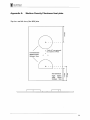
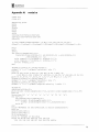
Appendix A:
Medium Density Fibreboard test plate
30
AppendixB:
rtmodule. c ......•.•.......•...•••.•............•.•••.•..........•.•••.......•.•.•••........•..•••..........••••. 31
Appendix C:
cloop.h•...........•.••••••........••.••.•...........•.••............•.•••••.....•..•..•••.•..•..•.••.•..•.......•• 34
AppendixD:
cloop.c •••••...•.......•••••••.......•.•••••......•....••••.•..........•..••.•.•.•.....•.••.•••..•..•.••••.......•. 37
AppendixE:
thread code. c...•....••.•...•...•...•..•••...........••.••......•.•....••••.•........••••••.•....•.•••........ 44
AppendixF:
hovercraft. c•...........••••.....•......•.••••.••.......•.•••...•.•.•.....•••••..........•••••.....•..•••....... 48
Appendix G:
hovercraft.h......................................................•.•.....••••...•..••••••••••••.••••••••••.•••. 55
AppendixH:
CDSM. c.•..•.•...•.......••••.........•...••.••.•.........••.••............•••.......•.....•••..•......•........• 56
Appendix/:
CDSM.h .•.•.....•.•.•••••........••••••.•••....•...••••.•••.......•....••.•........•••••••••.....••••.•.......•. 57
4
I
~
THE UNIVERSITY OF
NEW SOUTH WALES
SYDNEY-AUSTRALIA
AppendixJ:
mbu$h
AppendixK:
makefile•.........•.....•..••.•••.•...........•..............•..••••••..•...................•...•••.•...•...•....• 62
AppendixL:
Linux kernel 2.2.18 installation..................................................•.•............... 63
58
AppendixM: RT-Linux 3. 0 installation..............................•.............................•.•...•........... 68
AppendixN:
modeLm
72
Appendix 0:
modelsim.m
74
AppendixP:
shipplot.m
76
AppendixQ:
Armature resistance test....................................................................•........... 77
AppendixR:
Fitting files.................................................. ................................................... 78
5
I
~
THE UNIVERSITY OF
NEW SOUTH WALES
SYDNEY-AUSTRALIA
Introduction
Over the centuries there have been made many efforts to reduce the element of friction between
moving parts. Shipbuilders have always known that 'drag' results from the skin friction of water
acting on hulls. Early attempts at forcing air through tiny jets either under the hull or all around it
failed simply because the engine needed to produce too much air and the propulsion engines put the
cost way above any advantage in speed. Many other ideas where tried during the early 20 th century
until they came together in the genius of one man - Sir Christopher Cockerell. Although Cockerell's
fIrst tests were carried out on dry land the main aim was to prove that drag or friction between boats
and water could be substantially reduced if the 'craft' floated on an air cushion. And so the
'hovercraft' came in to behig. t~owadays there are several types of hovercrafts, but a definition of a
hovercraft can still be given:
A hovercraft is a self-propelled vehicle, dynamically supported on a self-generated cushion of air
contained in a flexible skirt such that it is totally amphibious and has some ability to travel over less
than perfect surfaces. Propulsion is not derived from contact with the water or the ground.
The hovercraft that is used in this project is a lightweight 2-channel model hovercraft from
HOVERCRAFTmodels. com T~ type Electro Cruiser. Aims for this hovercraft project are developing a
dynamical model of the hovercraft and making a connection between hovercraft and PC for PC
control.
The document is organized as follows: the fIrst chapter gives an introduction about the working
pr..nciples of the hovercraft. Chapter 2 covers the hardware and software issues in this project. Chapter
3 describes the steps that lead to a 2-channel open loop PC controlled hovercraft. In chapter 4 is
derived a dynamical model of the hovercraft. The last chapter gives recommendations for future
research and summarizes the project.
6
I
~
THE UNIVERSITY OF
NEW SOUTH WALES
SYDNEY-AUSTRALIA
1 Background
A hovercraft or also called an air cushion vehicle is a vehicle that can drive on both land and water.
This vehicle differs from other vehicles in that way, it needs no surface contact for traction. Obstacles
such as gullies and waves can be taken very easily like it is a flat surface. The reason for this is a
generated air cushion between the hovercraft itself and the ground surface. The model hovercraft that
is used in this project is a remote controlled model hovercraft with two manually controlled input
channels. In this chapter will be explained the working principle ofthe hovercraft.
1.1 Hovercraft principle
In fact there are different types of hovercraft, one of them is an amphibious hovercraft. The model
hovercraft is also supposed to be an amphibious hovercraft, this means it can operate over land and
over water.
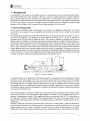
In the hovercraft are placed two propellers both driven by an electric motor and one of them is used to
provide lift by keeping a low-pressure air cavity under the craft full of air. As the air pressure is
increased the air lifts the craft by filling the cavity. The cavity or chamber in which the air is kept is
called a 'plenum' chamber. At the point when the air pressure equals the weight of the hovercraft over
the chambers surface area the hovercraft lifts and the air starts to escape through two holes made in the
bottom plate. The escaped air creates an air-lubricated layer between the hovercraft and the ground
surface. This will lead to a frictionless motion of the hovercraft, taken into account that the minimum
contact between skirt and the ground surface during the motion is negligible. The amount of the total
weight that a hovercraft can raise is equal to the pressure in the plenum chamber multiplied by the area
of the hovercraft. In basic hovercrafts does the air escape around the edge of the skirt, but the main
principle is the same. This plenum chamber principle is visualized in fig 1.1.
I
I
rn~=~~===:::J~~1
J)
I
f,--/") ~'--+
__
LL_ _-.l::4I1"l'{"---'
~~
I
J ) ~'--+
Air-lubricated layer
'~'~<~'~""'~""'~~""'~'~"'<x~"'~<i,,'<'<'<'<
figure 1.1: plenum chamber
A constant feed of air is needed to lift the hovercraft and to compensate for the air being lost through
the holes in the bottom plate. The flow must also be greater than the amount of air that escapes
through the holes in the bottom plate. The rate of the air loss is not constant, because there is no way
of ensuring that any air escapes evenly all around the hovercraft. To maintain also the lift, the engine
and propeller have to be sufficiently powerful enough to provide a high airflow rate into the chamber.
A cylinder is placed around the lift propeller to improve the efficiency, because it reduces the pressure
loss around the propeller tube.
The second propeller is driven by another motor and is placed on the back end of the hovercraft. This
motor can only deliver a constant speed to the propeller in contrast to the lift propeller and is used to
generate a displacement forward. The propeller can deliver a maximum force of 1,8 N, when there is
no wind and the battery is fully charged. This model hovercraft can reach a maximum speed of 3 m/s
when full lift is generated and if the rudder is in default position so that the hovercraft only moves in a
straight line.
Without a rudder de hovercraft is unmanoeuvrable. Therefore a vertical rudder is placed on the back of
the hovercraft behind the back thrust propeller. Conventional hovercrafts normally have a very high
rudder position over the center of gravity. Its action not only creates turning moments but also a
drifting force and rolling moment, which leads to an outward-banked turn. The position of the rudder
7
I
~
THE UNIVERSITY OF
NEW SOUTH WALES
SYDNEY-AUSTRALIA
on the model hovercraft is not extremely high, but these effects have to be hold in the back of the head
when studying the motion characteristics of the hovercraft.
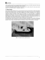
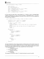
A camera is also placed on the hovercraft. This camera will be used in future for vision and control
aspects. The model hovercraft is visualized in figure 1.2.
1.2 Skirt design
The invention of the flexible skirt was a big step forward in the hovercraft history. Before the flexible
skirt had been thought necessary, powerful lift engines were needed to create only a few millimeters
lift under the hull hard structure. The main idea behind the air cushion introduction was to create air
lubrication between the ground surface and the hovercraft, in a way that leads to a significant
reduction of the lift power. The use of an inflated bag around the hovercraft resulted in an efficient air
distribution and a reduction of the lift power. Other advantages of the flexible skirt development are a
better stability and a better obstacle clearance. The function of skirts for a hovercraft has proved to be
as important to the air cushion vehicles as that of rubber tyres for an automobile.
The material type and the structure of the skirt are playing an important role in the skirt design step.
The material for a skirt bag should have high tearing and tension strength, but with as few as possible
abrasion. The skirt bag is normally divided in several parts to improve the absorption of obstacles.
figure 1.2: Electro Cruiser, model hovercraft
8
I
~
THE UNIVERSITY OF
NEW SOUTH WALES
SYDNEY-AUSTRALIA
2 Set up project equipment
In this chapter will be discussed the set up of hardware and software equipment during the hovercraft
project.
2.1 Hardware
One goal is to connect the hovercraft to the computer and control it open loop. A computer is not
being able to send signals out without using correct software and a data acquisition board. The
software will come up in section 2.2, but the data acquisition board that is used during the project is
from AXIOM Technology Co. Ltd, type AX5411H. Tnis DA&C board has 24 digital I/O channels, i 6
analog inputs with a 12-bit resolution and a maXitllUm sample rate of 60 KHz. Further has the board 2
analog outputs with a l2-bit resolution and output ranges are available between 0 to 5V or 0 to 10 V.
At this time only the two analog outputs are in use. Software cannot communicate with the DAC board
if the base address isn't defmed. On the DAC board is set the correct base address with a DIP switch.
The DIP switch address for this board in hexadecimal notation is OX320. In switch notation this
means: off off on on off on. Also the D/A range is specified on the DAC board with a jumper. The
range for signals going out lies between 0 and +5 Volt. More details about the AX5411H DA&C
board can be found in the reference manual available at the research laboratory of Systems and control
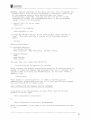
research or on the internet link http://www.axiomtek.comIDownloadlManual/AX5411H.pdf.
Future research purposes will be vision and control in combination with the hovercraft. The cameras
for vision and control are from XlO model Xcam2 (http://www.xlO.com). One camera on the
hovercraft for vision and control is not enough, because it is very difficult to get the orientation and
position out of one camera image. Therefore a second camera needs to be suspended, to overlook the
whole area. XlO has delivered the hardware for multi camera use. With this hardware it is possible to
change from one camera to another one. Both cameras are wireless color cameras with a CMOS
sensor and a frame rate of30 frames per second. Images are 510 x 492 pixels with a resolution of 1/3".
The range of view is 60° and minimum illumination of 3 lux (£1.9). XlO uses also a VAllA USB
adapter to convert video signals into USB, but at the moment there is no support for this USB adapter
under linux. People in Europe are developing a driver under linux, which is supporting most camera
types including the XIO camera, but there are no working drivers yet. The development of the driver is
slower than expected and the perspectives for the near future are not positive. This will result in
writing an own driver for the XIO VAllA USB adapter. This adapter is using a Video-USB chip of
Sunplus Technology Co, Ltd type SPCA506AI. The user manual of the sunplus chip can be found on
the following internet link
http://www.sunplus.com.tw/products/pdflmedia/spca/datasheet/ca506al vI O.pdf .
2.2 Software
There are two operating systems, Windows and Linux, available on the computer in the laboratory.
The problem with Windows and Linux is that they are designed to optimise average performance and
try to give every process a fair share of computing time. This is great for general purpose computing,
but for real-time programming are precise timing and predictable performance more important than
average performance. For example, if a camera fills a buffer every millisecond, a momentary delay in
the process reading that buffer can cause data loss. For Windows and Linux are both methods to create
a real-time environment, but the source code for software in Windows is generally not available, so
further development is limited. Therefore Linux is chosen instead of Windows as operating system
during this project. Real-time Linux is a small real-time operating system and is used to get the Linux
system under control to meet real-time computing needs. The basic idea is to run Linux under the
control of a real-time kernel. When there is real-time work to be done, the real-time operating system
runs its task. When there is no real-time work to be done, the real-time kernel schedules Linux to run.
So Linux is the lowest priority task of the RT-Kernel. At the computer belonging to the hovercraft are
installed a Linux kernel version 2.2.18 and a RT kernel version 3.b. Both installation instructions are
added in the appendices respectively Land M.
9
I
~
THE UNIVERSITY OF
NEW SOUTH WALES
SYDNEY' AUSTRALIA
3 Hovercraft control
In this chapter are presented the hardware configuration of the hovercraft and the hardware changes to
the radio control transmitter to create a PC compatible transmitter. The last section of this chapter
gives an explanation of the used control software.
3.1 Control configuration
The hovercraft is a vehicle with 6 degrees of freedom and there are only two input channels that can
be used to control the hovercraft. This means the hovercraft is an under-actuated vehicle, because
there are less control actuators than degrees of freedom. Let us first consider the control configuration
options. The model hovercraft has besides the air rudder also two propeilers, one for the lift and one
for the drive forward. Due to the limitation of only two output channels, two control configurations
can be presented.
The first configuration operates with the lift propeller on a constant maximum lift and the back thrust
propeller is variable. So the control channels in this configuration are the back thrust motor and the air
rudder. It is hard to keep the hovercraft on the same position during operation in this configuration.
This is a balancing problem and balancing the hovercraft is difficult, because not only the flexible
structure of the hovercraft also the replacement of the battery pack after recharging leads to small
change in the weight distribution. Manoeuvring in a small area makes it difficult to work with this
configuration.
The second configuration keeps the back thrust on a constant speed and makes it possible to vary the
lift propeller speed. The rudder is now one output channel and the lift motor is one. Using a variable
lift creates friction if the lift force is lowered. With creating friction, the hovercraft is not really a
hovercraft any more, but it is easier to control it in the current test environment. Configuration two is
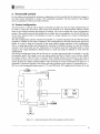
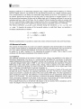
chosen because of a better manoeuvrability of the hovercraft in the test environment. In figure 3.1 is
presented a connection diagram of the motors and radio equipment with respect to configuration two.
BPI is a 6-cell rechargeable battery pack of 7,2V and 2200 mAh. BPI supplies the lift motor Mo 2 and
Sw2
Qnc.rnr
Transmission
Sr
CH2
CH 1
Receiver
CH2
CH 1
®
Transmitter
fuse
Speed
Controller
figure 3.1: connection diagram ofthe radio equipment and the motors
10
I
~
THE UNIVERSITY OF
NEW SOUTH WALES
SYDNEY- AUSTRALIA
the electronic speed controller, that is also secured with a fuse. Switch Sw 1 is used to tum the receiver
and speed controller on or off. The other rechargeable battery pack (BP2) of 7,2 V and 1500 mAh
supplies the back thrust motor Mo 1. Between Mo 1 and the back thrust propeller is also placed a
transmission, with a gearbox ratio of 1:3. The delivered drive forward is to low without using a
transmission. Switch Sw 2 is used to turn the back thrust motor on or off. To complete the whole
circuit, a receiver is needed for receiving the input channels from the radio control transmitter and
subsequently sending it to the speedcontroller and the rudder servo, Sr. Motors Mo 1 and Mo 2 are
electro motors of the type Graupner speed 400. The system has a receiving range of 350 yards.
3.2 Open loop PC control
The hovercraft is a remote controlled vehicle, which has to be converted to a PC controlled vehicle.
Therefore, the transmitter is converted to a control station that can be used as a normal manual remote
controller and it can be used for PC control. Manual remote control has to be fully uncoupled if PC
control is used and also in the other way round. Two double pole double throw (dpdt, on-off-on)
switches are used to establish an uncoupling of one control mechanism when the other is used. The
place where the disconnection takes place is at the joysticks of the transmitter. These joysticks are
variable resistors, which can be replaced by a computer output voltage during PC control. Each
variable resistor has a certain range in which the hovercraft is responding. The voltage range, initial
value and the resolution of each channel are tested and given in table 3.1. It is also verified that the
variable resistor is linear.
D/A Channel
number
0
1
lower boundary
[Volts]
2,45
2,10
initial value
[Volts]
2,80
2,56
upper boundary
[Volts]
2,80
3,03
table 3.1: channel specification
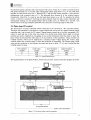
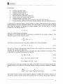
The implementation of the dpdt switches, Switch CH2 and CHI, and the connection diagram of the PC
I.•.· .· . ·.{.·.· · .·.·.·.·._·. ·. ·.·. ···..··,·.·.1. ·.·. PC with integrated
'. ..
DAC board
_,.
I
2,1 - 3,03 Volts
2,45 - 2,8 Volts
r~
r~
+ -
12 Volt, 8 AA batteries
Radio control Transmitter
figure 3.2: Converted radio control transmitter
11
I
~
THE UNIVERSITY OF
NEW SOUTH WALES
SYDNEY' AUSTRALIA
compatible transmitter is visualised in figure 3.2.
In figure 3.2 are used a few names referring to channels. To make it clear, Switch CH2 and Switch
CHi are related to the channels on the transmitter. CH2 and CHI on the transmitter refer to
respectively the lift motor output and rudder servo output. D/A CH 0 and D/A CH 1 are used on the
data acquisition connection tenninal and in the control software on the computer. Here CHO and CHI
are referred to respectively the lift motor and rudder servo.
Both dpdt switches are placed on top of the remote controller and each has three possible positions.
Nonnal remote control mode is active when both switches are pointed to the transmitter antenna and
PC control mode is active when both switches are pointing to the outside. The middle position can be
seen as an off position. Be aware of the fact, that the transmitter is sensitive for disturbances and if the
transmitter is unplugged of the data acquisition connection tenninal during PC control mode, this will
lead to another configuration and the hovercraft starts moving. So fIrst tum off the receiver switch Sw
i on the hovercraft before disconnecting.
3.3 Control program
Hovercraft is the name of the designed control program based on Rtcon to do real time control of the
hovercraft in RTLinux. Rtcon uses real time threads to do data acquisition, calculating controller
outputs and sending signals out sequentially. Rtcon is written by Ray Eaton and is based on SISO
control and therefore it can send only one signal out at a certain time. To control the hovercraft, two
output signals have to be implemented namely one for the air rudder servo and one for the lift motor.
Control purposes for this project are controlling the hovercraft open loop by clicking buttons in a
created Graphical User Interface. The main structure of Rtcon is left unchanged as much as possible to
make future implementation of a feedback controller easier.
3.3.1 Program structure
Hovercraft is using three separated real time threads as mentioned above. The three threads are
executed in succession starting with the sampling thread (AID). When the sampling has taken place, it
tenninates and starts the control thread. When the control thread is finished it tenninates and starts the
D/A conversion thread. When the third thread is fmished, it stops and awakes the sample thread again.
The cycle will start from the beginning again. All the treads are placed in a coded control module
controCmod.o. The source code of the control module can be found in rtmodule.c, appendix B.
Rtmodule.c starts with making the treads and can also unload the threads when the control module is
removed. After the making of the threads will be started with sampling.
Real time threads in RT-Linux can communicate with each other through the use of global memory.
This is because they exist in the same kernel space. A nonnal Linux task, for example the user
interface, exists in its own space, separated with other tasks by a protected memory barrier. To
communicate with a Linux task, global memory is not sufficient. RT-Linux provides a mechanism
known as shared memory to communicate between real-time threads and Linux tasks. This mechanism
is provided by mbuffmodule, see appendix J. This means, if a user changes a value in the Graphical
User Interface (user space), the controller thread in the kernel space will use this new value in the next
calculations. The main part of the shared memory structure is the shared structure cloop. This structure
contains controller parameters and state variables to share between the user space and the kernel space.
The cloop (appendix D) structure and its functions are defmed in the header file cloop.h, appendix C.
The functions for sampling, sample(cloop), controlling, control(cloop) and digital to analog
conversion, dtoa(cloop) are placed in a separated file called threadJode.c, appendix E. To ease
programming, a common interface for sharing an array of long data type (CDSM) in user and kernel
space is provided in cdsm.c and cdsm.h, respectively appendix Hand 1.
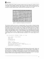
A Graphical User Interface (Gill), see fig 3.3, is created in the file hovercraft.c using the GTK toolkit,
see appendix F. The Gill contains eight buttons four buttons in the middle called Left, Right, Up and
Down are used to control the hovercraft. By clicking on the hovercraft control buttons the output
voltages change and the hovercraft will move. The change of the output voltages can also be seen on
the right side of the hovercraft control buttons. At the bottom of the Gill is a start and stop button to
start and stop control. Stop resets the output values, so the rudder and the lift motor are going to their
initial position. Clicking on the Quit button means leaving the hovercraft program without resetting
12
I
~
THE UNIVERSITY OF
NEW SOUTH WALES
SYDNEY-AUSTRALIA
the output channels and with the Log button can data be stored in an output file. Clicking on the log
button again will stop logging. The name of the log file is hcraft and it contains columns with time, r,
y, uO and u1. The time and data of the output channels u1 and u2 are at the moment the only
parameters of interest. Reference signal r and input (ofDAC board) signal y are not used.
figure 3.3: Graphical User Inteiface for hovercraft control
The buttons are created in hovercraft.c as mentioned earlier. If the user clicks on a button the output
changes and the new value has to be sent to the shared memory because the real time threads in the
kernel space need to know what the user wants. A hovercraft control button function as for example
the left_button function works as follows. After clicking on the LEFT button, the new value is
obtained by subtracting 0,01 of the old value. The new value has to be checked if the value is lying
within a certain range defmed in table 3.1, before sending it to setpt] in the shared memory structure.
Therefore a saturation function in cloop.c is used. The boundary values for both channels are specified
in function lookup_sat in cloop.c. Function left_button is illustrated below. The resolution of both
output channels is 0,01 Volt. For the rudder this means a resolution of 1,29°, within a range of -60° to
60°.
void left_button ( GtkWidget *widget, int *arg)
float setptl = cloop->setptl;
char s[14];
float a,b;
a=lookup_sat(l);
b=lookup sat(2);
setptl -= 0.01;
setptl = sat(setptl,a,b);
sprintf(s,"LEFT-RIGHT : %3.2f",setptl);
gtk_label_set_text((GtkLabel *) (cguLlabel[4]), s);
cloop->setptl = setptl;
printf("ul = %3.2f\n",setptl);
Real time threads can now use the latest data from the shared memory when they need it. Sample- and
control thread are only there to make implementation of it in the future easier. At the moment it is
open loop control, so the digital to analog conversion is the only real time thread that has actually a
task. Function dtoa is responsible for sending signals out, because it calls on the function io_dacout,
which is standing in cloop.c. But dtoa scales first with the function scaleJioi a float to a 12bit integer,
taking into account a lower and upper boundary. Function dtoa is added below.
13
THE UNIVERSITY OF
NEW SOUTH WALES
SYDNEY' AUSTRALIA
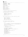
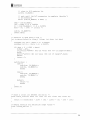
void dtoa(volatile cloop_t *cloop)
{
float utO,ut1;
int uintO,uint1,stat;
utO = (get(cloop,O)) .uO;
uintO = scale_ftoi(utO, 0.0, 5.0, 0, 4096);
stat = io_dacout(cloop, 0, uintO);
ut1 = (get(cloop,O)) .u1;
uint1 = scale_ftoi(ut1, 0.0, 5.0, 0, 4096);
stat = io_dacout(cloop, 1, uint1);
fo_dacout sends the scaled value to output channel 0 or 1. Function io_dacout is presented below.
Channel 0 is represented in io_dacout by case 0 and channel 1 is represented by case 1. 10_BASE+4
and 10_BASE+5 represent the addresses in I/O space for D/A CHO. For D/A CHI the addresses are
10 BASE+6 and 10 BASE+7.
int io dacout(volatile cloop_t *cloop, int chan, int data)
{
unsigned int low = (data « 4) & OxOOfO;
unsigned int hi = (data » 4) & OxOOff;
if( data < 0 II 4095 < data) {
#ifdef
RTL
rtl_printf("ax5411: dac out value (%d) out of range\n",data);
#else
piintf("ax5411: dac out value (%d) out of range\n",data);
#endif
return -1;
}
switch (chan) {
case 0:
outb(low, IO_BASE+4);
outb(hi, IO_BASE+5);
break;
case 1:
outb(low, IO_BASE+6);
outb(hi, IO_BASE+7);
break;
default:
return -1;
break;
}
return 0;
The steps described above from clicking the buttons to sending signals out will continue as long as the
user doesn't press the stop button. Starting Hovercraft is not only running hovercraft, but fIrst has to
be inserted the control module in RTLinux. To insert the control module and starting the hovercraft
program go through the following steps while running RTLinux with root privileges.
• Go to the directory
> !home!hovercraft!hover
• Insert the control module
> insmod control mod. 0
• Start Hovercraft
> .!hovercraft
The Graphical User Interface in fIgure 3.3 is launched and open loop control is possible.
14
I
THE UNIVERSITY OF
NEW SOUTH WALES
4
Model
~
SYDNEY· AUSTRALIA
In this chapter will be started with deriving a dynamical model for the hovercraft. Subsequently are
detennined the model parameters such as moment of inertia and at the end will be given the simulation
results with validation of the dynamical model.
4.1 Dynamical model
Analyzing the motion of hovercrafts is possible in 6 degrees of freedom (DOF) using the equations of
motion of the hovercraft. But before deriving the equations of motion it is convenient to define the
coordinate frames and the 6 DOF as indicated in figure 4.1 and table 4.1.
(surge)
v (sway)
Yo
Zo
Earth-iIxed
y~X
Z
Figure 4.1: BodY-fIXed and earth-fixed reference frames
DOF
1
2
3
4
5
6
motions in x-direction (surge)
motions iny-direction (sway)
motions in z-direction (heave)
rotation about the x-axis (roll)
rotation about the y-axis (pitch)
rotation about the z-axis (yaw)
Forces and
moments
X
Y
Z
K
M
N
Linear and
angular velocity
u
v
w
p
Positions and
Euler angles
x
y
z
¢
q
()
r
If/
table 4.1: 6 DOF coordinates specifications
Two coordinate frames are chosen, the moving coordinate frame X o Yo Zo, which is a body-fixed frame
on the hovercraft and an earth-fixed frame xyz. The motion of the hovercraft will be described
relative to the earth-fixed frame.
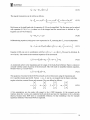
The rigid body equations of motion are derived using Euler's first and second axioms, respectively:
(4.1)
(4.2)
15
I
~
THE UNIVERSITY OF
NEW SOUTH WALES
SYDNEY' AUSTRALIA
Here the index c indicates that it is referred to the body's centre of gravity..fc and me are the forces and
moments acting on the body, OJ is the angular velocity and Ie is the inertia tensor about the centre of
gravity of the body. A few assumptions are made when deriving the equations of motion. It will be
assumed that the mass of the body is constant in time and the vehicle is rigid. When the hovercraft is
assumed rigid this means there are no forces acting between individual elements of mass. Another
assumption is made with respect to the earth-fixed frame, this is assumed to be inertial. The following
formula is needed to derive the equations of motion for an origin in a body fixed rotating coordinate
system.
c = C+OJXC
(4.3)
Here c is the time derivative of a vector c in the earth-fixed frame and c is the tLllle derivative in the
body fixed reference frame XoY020. This formula describes a relation between a time derivative of an
arbitrary vector c in XYZ and XoY020. It can be verified that the angular acceleration OJ is equal in the
body-fixed and earth-fixed reference frame using equation (4.3).
v
~-~x
z
Earth-fixed
reference frame
figure 4.2: Earth-{zxedJrameXYZ and body-fixedJrameXoYoZo
Deriving the equations of motion is divided in two parts. A trans1ation- and rotation part described by
respectively equation (4.1) and (4.2).
4.1.1 Translation dynamics
Starting with the translation part it can be seen from figure 4.2 that,
(4.4)
The velocity ofthe centre of gravity is obtained by differentiating equation (4.4).
(4.5)
Using equation (4.3) and assuming that va = fa and r
g
= 0 it follows that,
(4.6)
1:..1.en,
(4.7)
16
I·
~
THE UNIVERSITY OF
NEW SOUTH WALES
SYDNEY· AUSTRALIA
The acceleration of the centre of gravity can be found by differentiating the velocity vector this leads
to:
(4.8)
which yields
(4.9)
Substituting equation (4.9) into (4.1) leads to,
(4.10)
The vector r g is a null vector when the origin of the body-fixed frame coincides with the centre of
gravity of the hovercraft. With the body-fixed frame XoY020 chosen in the centre of gravity equation
(4.10) can be rewritten as,
m(~ +
e
OJ X ve )
= Ie
(4.11)
4.4.2 Rotation dynamics
Rotational equations of motion can be obtained by using equation (4.2). The angular momentum about
the origin of the body-fixed frame is defined as:
(4.12)
Differentiating equation (4.12) with respect to time leads to,
(4.13)
v
Moment vector mo
The following relation for the velocity of a volume element can be found in figure 4.2.
(4.l4a ,b)
Substituting expression (4.14b) into equation (4.13) and making use of property that v x v = 0 leads to
a new expression for the derivative of the angular momentum.
(4.15)
or similarly,
Equation (4.16) can be rewritten using the derivative of the vector r g •
rg
Using the expression Yg =
OJ x
1 i rpA dV
=-J
m v
differentiating leads to
,
7
mr•g
=
J'vrPAalV
(4 .17a, b')
rg and equation (4. 17b) leads to a new equation for ho'
17
I
~
THE UNIVERSITY OF
NEW SOUTH WALES
SYDNEY-AUSTRALIA
(4.18)
The angular momentum can be written as follows,
(4.19)
v
v
1"
2nd
Both terms on the right hand side of expression (4.19) can be simplified. The first term can be reduced
with equation (4.17a) if x v 0 is taken out of the integral and the second term is defined as IoOJ.
Equation can now be written as,
(4.20)
Differentiating equation (4.20) gives a new expression for ho assuming that lois time independent.
(4.21)
Equation (2.82) can now in combination with (OJ x rg)x Vo = -vo x (OJ x rg ) be used to eliminate
ho
out of (4.21). This results in the rotational equations of the hovercraft.
(4.22)
As mentioned earlier in the translation part the origin of the body-fixed reference frame is chosen to
coincide with the centre of gravity of the hovercraft. This will result in simplified rotation equations,
because vector r g is a null vector.
(4.23)
The equations of motion for the 6 DOF hovercraft can be written down using the translation part
(4.11) and the rotation part (4.23). Vectors v, OJ, Ie and me are respectively the linear velocities,
angular velocities, external forces and moments. They are defmed as follows,
V~l:l m~ln f'~ln m'~l~]
(4.24)
A few assumptions are also made with respect to the 6 DOF dynamics. At the moment are the
rotations about the x and y-axis neglected (roll and pitch) and also the translation in the z-direction
(heave), because these DOF have no considerable influence. In ship modelling it has for example
significant influence when these DOF are neglected.
18
I
~
THE UNIVERSITY OF
NEW SOUTH WALES
SYDNEY' AUSTRALIA
.
1X
u=vr+-
m
.
1Y
v=-ur+-
(4.25)
m
The forces.x; Y and moment N are defmed using figure 4.3. The back thrust propeller causes an
r
u
v
figure 4.3: defining externalforces and moments
external force in surge direction of 1,8 N if the rudder stands in its initial position O. This value for the
back thrust force is measured statically with a modem version of a steelyard. It was possible to
measure the pulling power of the hovercraft and because there is no friction the pulling force is equal
to the back thrust force. A force in sway direction and a moment about the yaw axis result from
another rudder position 6. If the rudder stands in a position except 0 than liz Fx works purely in surge
direction and the other liz Fx can be spit up into a surge part, sway part and a moment about the yaw
axis. X; Y and N are defmed as,
X =,Yz . F x (l + cos(5))
Y = ,Yz. F x sin(5)
N
(4.26)
=,Yz. F x • a· sin(5)
Here a is the distance in negative surge direction between centre of gravity and the point where the
rudder is attached to the hovercraft. The value for a is 0,4 m.
In reality the model hovercraft has two main types of friction. The first type of friction is dependent of
the lift force. At maximum lift force is no contact with the ground surface and also no friction. If the
lift force is lowered to 0 the friction will increase and stop the hovercraft because the coulomb friction
is to big for the back thrust force to get over it. Implementation of this friction is done with an arctan
function multiplied with a lift force dependency. The lift force F z is unknown but is chosen equal to
the normal force of the hovercraft mg= 2lN. This means the lift force is variable between ON and 21
N. The other friction is dependent of the velocity as a result of air friction and can be seen as a
damping term. Implementation of these two frictions results in a dynamic model of the hovercraft with
3 DOF.
u = vr + ~ (- d ·u + ,Yz. F
l
v = -ur + ~ (-
d2
•V
x
(l + cos(5))- III
+ ,Yz . Fx sin(5)- f12
~ (mg - ~ )arctan(SOOO .u))
~ (mg - Fz )arctan(SOOO. v))
(4.27)
r = _1 (- d 3 • r + ,Yz. Fx • a .sin(5)- 113 2(mg - ~ )arctan(SOOO. r)1
Iz
Jr
)
19
I
~
THE UNIVERSITY OF
NEW SOUTH WALES
SYDNEY· AUSTRALIA
Damping coefficient d] is determined empirical using a digital camera and the equation of it above.
With the digital camera it was possible to film the passing hovercraft at a constant maximum speed.
The covered distance in one frame was measurable using markers on the floor. The equation of it can
be reduced, because the hovercraft was moving purely in surge direction at constant speed (it = 0),
the hovercraft had maximum lift force and the rudder angle was 0. Damping coefficient d] can now be
calculated and has a value of 0,6 Ns/m. For d2 is taken 0,8 Ns/m, because the surface in contact with
the air in sway direction is bigger than in surge direction, this is an assumption. Damping coefficient
d3 is also unknown and for this coefficient is therefore chosen a reasonable value of 0,1 Nms/rad.
The friction coefficients Ill' Ilz and 113 are estimated during the simulation; f.1J = 0,1 ,J-l2 = 0,01 and
J-l3 = 0,004. To describe the motion of the hovercraft relative to earth-fixed frame, we introduce a
coordinate transformation as follows.
Zl = x· cos(V/)+ y' sin(V/)
Zz
=
-x· sin(V/) + y . cos(V/)
(4.28)
Z3 = V/
With this transformation it is possible to analyse the motion of the hovercraft in the earth-fixed frame.
4.2 Moment of inertia
The moment of inertia about the z-axis is an unknown paral'neter in the derived model. It is essential
for future control ambitions to calculate the moment of inertia of the hovercraft. This can be done in
two ways, namely empirical and analytical. In the next two sections will be discussed both ways.
In section 4.2 is used J instead of I z for indicating the moment of inertia. This is done to avoid
confusion with the Laplace transformed of the armature current I
4.2.1 Empirical
The empirical calculation of the moment of inertia is done, using a test installation at the school of
Mechanical Engineering. The line-up is a vertical placed controllable DC servomotor of which the
angular displacement and indirectly the angular velocity can be measured. On the output shaft is fixed
a specially designed timber plate of MDF to carry the hovercraft during the experiment. Fixing the
MDF plate on the output shaft is possible using a flange, which is already on the shaft. When the
Hovercraft is placed on the plate, its centre of gravity lies automatically on the output shaft of the
motor. A drawing of the MDF plate is enclosed in appendix A.
The moment of inertia of the hovercraft can be calculated, if the moment of inertia of the motor and
the plate are known. Therefore, two separated experiments are done. The first one is done without
using the hovercraft to calculate the inertia of the motor and the MDF plate. The other experiment is
done including the hovercraft. The difference in inertia between the two experiments should be the
inertia of the hovercraft. For each experiment is measured the angular displacement and the time,
while a step input is generated to the motor. In the next part of this section will be gone through the
calculation steps that result in a value for the moment of inertia of the hovercraft.
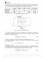
First a transfer function has to be derived with respect to the test system, before calculations can be
made. The diagram of the test system is presented in figure 4.4
figure 4.4: Diagram test system
20
I,
~
THE UNIVERSITY OF
NEW SOUTH WALES
SYDNEY-AUSTRALIA
In this system,
Ra
La
ia
ea
eb
w
T
J
b
armature resistance, [Ohm]
= armature inductance, [Henry]
= armature current, [Ampere]
= applied armature voltage, [Volt]
= back electromotive force (back emf), [Volt]
= angular velocity of the motor shaft, [Rad/sec]
= torque developed by the motor, [Nm]
= moment of inertia of the motor and load referred to the motor shaft, [kg. m 2]
= viscous damping coefficient of the motor and load referred to the motor shaft,[Nm/rad/sec]
=
A rotating circuit called the armature, through which the current i a flows passes through a magnetic
field developed by stationary permanent magnets. This results fmally in a torque that turns the output
shaft. Since the armature is rotating in a constant magnetic field, the back emf eb is directly
proportional to the angular velocity w.
(4.29)
,where K b is called the back emf constant.
The speed of an armature-controlled dc servomotor is controlled by the armature voltage ea. The
differential equation for the armature circuit is
(4.30)
The armature current produces the torque that is applied to the inertia and damping.
(4.31)
Where K t is a constant of proportional, called the motor torque constant. In a consistent set of units,
the value of K t is equal to the value of K b •
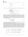
Assuming that all initial conditions are zero, and taking the Laplace transforms of equations (4.29),
(4.30), and (4.31), the following equations are obtained:
(4.32)
(4.33)
(4.34)
Considering Ea(s} as the input and Q(s) as the output, it is possible to derive the transfer function from
equations (4.32), (4.33), and (4.34). The transfer function for the dc servomotor considered is obtained
as
n(s) _
E a(s)
Kt
2
L aJs + {Lab + RaJ)s + Rab + KtK b
(4.35)
This transfer function contains several unknown parameters including the moment of inertia J. To
calculate the moment of inertia, all the other parameters have to be known. The armature inductance
21
I
~
THE UNIVERSITY OF
NEW SOUTH WALES
SYDNEY' AUSTRALIA
La is a motor constant and has a value of 0,62 mHo La in the armature circuit is small and therefore La
is not determined empirical but taken from the specification data of the motor. The other parameters
R a , b, K t and K b are determined empirical, because they have significant values in the transfer function
comparing with the inductance.
Determining the armature resistance R a can be done easily by supplying a small voltage to the
armature circuit. When the motor is not moving with the small input voltage because of friction, the
back emf will be zero. The armature resistance is 1,779 n and is calculated with Ohm's law, because
the voltage and the current are measured, see appendix Q.
The back emf/torque constant and the viscous damping of the motor with the supporting plate are
measured during one and the same test experiment. For this test, a constant voltage is supplied that
results in a constant speed of the motor. During the test are measured the angular velocity, the
armature current and the armature voltage. Using equation (4.30) and neglecting the inductance part, it
results in a value for the back emf. The back emf constant can subsequently be calculated by making
use of equation (4.29) and the values for the angular velocity and the back emf. The value for the back
emf constant K b or torque constant K t is 0,1066 Vslrad respectively Nm/A.
The only remaining unknown parameter except for the moment of inertia is the viscous damping
coefficient. Making use of equation (4.31), it is possible to calculate the damping coefficient because
the angular acceleration is zero and the other parameters are known. It follows that b is 0,000114
Nms/rad.
The following strategy is used to calculate the moment of inertia J. A transfer function of the test
installation is available, thus an analytical step response can also be derived. Measuring a step
response of the real system and subsequently fitting the analytical step response on it will give a value
for J. Writing with the step response in the frequency domain leads to
(4.36)
where Cstep is the step amplitude.
The step response of the system in the frequency domain is not useful to fit with, therefore an inverse
Laplace transformation is needed to transform the step response to the time domain. Calculating the
zeros of the denominator called the roots is required to transform from frequency to time domain.
Using the roots, the step response can be rewritten in the following form
(4.37a)
with
(4.37b)
PI =0
P2,3 =
-(RaJ +Lab)±~(RaJ+ LabY -4LaJ(R ab+Kt K b )
2L J
(4.37c)
a
Taking the inverse Laplace transformation of equation (4.37a) and using (4.37b) and (4.37c), we
obtained the following step response in the time domain for the angular velocity OJ.
(4.38)
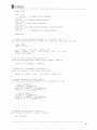
Measuring a step response on the real system is the next step. A step with amplitude of 24 Volt is
supplied to the motor and the angular velocity is measured. This data has to be fitted with the
analytical step response function. An optimisation routine called Fminsearch in Matlab is used to
22
I
~
THE UNIVERSITY OF
NEW SOUTH WALES
SYDNEY-AUSTRALIA
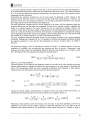
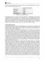
minimize the squared error between the two step responses. See appendix R for Fit_J.m and
Determine_J.m. The results are presented in figure 4.5. It can be seen that the gearbox has some
~~_._--
200
~
/~
'I
Ji
150
/
Lo
/
~ Jj}/
i
hi \
Ii
50
Ii
o
t-
.1
I
-
step response 'With hovercraft
fitted response funlion with hovercraft
step response \6.~thout hovercraft
fitted response function without hovercraft
-500:---:-0.0:0-,------..-'0.1~~O,
15~-;:":0.2C--:O:-:::.2'C--:O:'::-.3----':0-=.35----':0":-"----::-0..::-5------:0'0.5
timers!
figure 4.5:Moment ofinertia fitting results
backlash in the beginning of the acceleration. The motor is turned a little bit through the backlash
before each experiment to avoid the backlash as much as possible. The resulting J for the motor
including the MDF plate has a value of 0,000295 kg.m2 • All the steps from calculating the system
parameters have to be redone to obtain the moment of inertia with the hovercraft on it. This leads to a
moment of inertia of 0,000552 kg.m2 . Fitting results including the hovercraft are also presented in
figure 4.5.
Now the difference between the two tests is known and represents the hovercraft inertia. One point has
to be taken into account before using the moment of inertia. This moment of inertia is referred to the
output shaft of the motor, but in reality there is also a gearbox between the motor output shaft and the
actually output shaft. A gearbox ratio of 19,2:1 leads to an increase of the moment of inertia with
19,22 • The moment of inertia about the z-axis of the hovercraft is
Jhovercrajt
= (0,000552 - 0,000295)*19,2 2 = 0,0948 kg.m 2
fu table 4.2 are summarised the results of the tests with and without the hovercraft. All the data is
considered before the gearbox.
Variable/constant parameter
Step response voltage, Cstev
Armature resistance, Ra
Armature current, i a
Back emf, eb
Viscous damping coefficient b
Back emf/ torque constant, K b/ K t
Moment of inertia before gearbox
Test without the hovercraft
23,895
1,779
0,235
23,477
0,000114
0,1066
0,000295
Test with the hovercraft
23,650
1,779
0,618
22,551
0,000308
0,1061
0,000552
table 4.2: test results
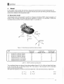
4.2.2 Analytical
Besides the empirical calculation, an analytical calculation of the moment of inertia is done to verify
the empirical results. The hovercraft with a total mass of 2,1 kg can roughly be divided in five main
parts, with a certain weight and dimension. Namely a battery pack, wireless camera, lift motor, back
thrust motor and a main plate. Geometry's for the main parts are chosen basic, like cylinders and
beams. Moments of inertia can be calculated for every part with respect to there own centre of gravity.
After this, the inertias need to be shifted to the centre of gravity referring to the hovercraft to obtain a
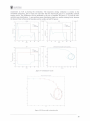
moment of inertia for the hovercraft. fu figure 4.6 is shown a top view of hovercraft with the
placement of the main parts.
23
I
~
THE UNIVERSITY OF
NEW SOUTH WALES
SYDNEY' AUSTRALIA
The explanation of the letters and the dimensions and masses of each part are specified in table 4.3.
Notice that the Lift motor B coincides with the centre of gravity of the hovercraft and therefore Lzb is
zero. E is the back thrust motor and is supposed to be a cylinder lying on its side.
Battery pack, A
Lift motor, B
Main plate, C
Camera, D
Back thrust motor, E
mass [kg]
0,625
0,1
0,955
0,285
0,135
length [m]
0,13
width [m]
0,05
radius [m]
-
shift length [m]
Lza=O,13
-
-
0,015
-
0,76
0,39
-
-
-
0,035
0,015
L zc=0,08
L zd=O,ll
L ze=0,20
0,07
table 4.3: specification hovercraft parts
Centre ofgravify
hovercraft
A
BCD
I
I
~
k
E
:0cp
Lza
figure 4.6: schematically representation hovercraft
To calculate the total hovercraft inertia, all the separated inertias of battery pack, lift motor, main
plate, camera and back thrust motor have to be summarised. The moment of inertia for a beam
geometry can be calculated as follows
(4.39)
where mfzi is the shift term to the centre of gravity of the hovercraft and i can be A or C.
For a cylinder, the moment of inertia can be obtained with formula (4.40) including the same shift
term as in formula (4.39)
(4.40)
where i can be B, D or E.
The back thrust motor is also a cylinder, but the moment of inertia has to be determined about another
axis. Equation (4.40) cannot be used to calculate the moment of inertia of a cylinder on its side. The
next formula can be used to calculate the moment of inertia of the back thrust motor.
(z
. E2) +mZ2zE
J E =m
- engthE2+3·radzus
12
(4.41)
24
I
~
THE UNIVERSITY OF
NEW SOUTH WALES
SYDNEY' AUSTRALIA
In table 4.4 is calculated the hovercraft inertia about the z-axis by summarising the moments of inertia
values of the separated hovercraft parts A to E.
Battery pack, A
Lift motor, B
Main plate, C
Camera, D
Back thrust motor, E
Hovercraft inertia
moment of inertia [kg.m2]
0,0116
1,125 e-5
0,0642
0,0036
0,0055
0,0849
table 4.4: inertia calculation analytical
The analytical value for the moment of inertia is 0,0849 kg.m2 • Comparing this value with the
obtained empirical value, it is only 10% lower. Taking into account, that the analytical value is a rough
calculation, it is only more acceptable to use the empirical value as a modelling parameter for the
moment of inertia. The analytical value will only get nearer to the empirical value if the calculation is
more exact, because there are a few other components on the hovercraft that are not taken into
account. These components, such as rudder servo and speed controller, cause a non-uniform
distribution in the main plate that leads to an increase of the analytical moment of inertia.
4.3 Simulation results
Simulation of the hovercraft model is done using Matlab 6.1. The used ill-files for sh'1lulation of the
hovercraft model are added in appendix N, 0 and P. Modelsim.m contains the model information and
mode1.m contains solving and plotting orders. Shipplot is only used to plot hovercraft shapes on a
trajectory in the earth-fixed reference frame.
The simulation results of one simulation are presented below. This simulation starts with maximum
lift force and a rudder angle of 0°. After 5 seconds the rudder turns to -10° and stays there till the end
of the simulation t=60s. These values are maintained during 45 seconds and from that time the lift
force is lowered half for 10 seconds. At t=50s the lift force is lowered to 0 till the end of the simulation
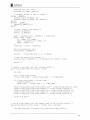
t=60s. The results are presented in figure 4.7 and 4.8. In figure 4.7 can be seen the velocities in surge,
sway, yaw and the movement of the hovercraft in earth coordinates. The plots of the velocities contain
also the input variables FI (lift force) and Rudder (rudder angle). Figure 4.8 gives an indication of the
orientation of the hovercraft on the trajectory and also is indicated the intervals of input change. The
red interval starts at t=5s and ends at t=40s. At t=40s is started lowering the lift force, this is where the
color black starts. Keep in mind that the vertical axis in figure 4.8 and 4.7 (movement of the hovercraft
in earth coordinates) normally is directed in the opposite direction. The hovercraft is still turning in
negative direction about the z-axis.
Balancing the hovercraft with small masses of lead is done, before starting validation of the simulation
results. The hovercraft is not stable at all if no balancing masses are used. Placing masses on the body
of the hovercraft is done by trial and error. Validation of the simulation is also not easy, because
validation experiments in real with the hovercraft require some free space with no obstacles. A few
validation experiments are done to get an indication of the characteristics of motion. One of them is a
maximum velocity experiment in surge direction. As mentioned earlier this is done using a digital
camera and some additional software. With the software and markers on the surface it is possible to
determine the covered distance between two frames. By means of the distance and the frame rate can
be obtained an indication of the maximum speed of the hovercraft in surge direction. This speed is
estimated on 3,0 mls and turned out to be a good validation value for the simulation. The second
validation experiment is done in a bigger room at the school of electrical engineering. This room was
actually still to small, but with the lift motor on half power and a rudder angle of 10° it was possible to
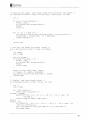
see some characteristics of the hovercraft in motion. Releasing the hovercraft with the settings above
resulted in figure 4.9. This figure can be used for a rough validation of some characteristics of motion
and nothing more than that, because the camera is not standing still and it is also standing under an
angle. It can be seen that the hovercraft is always directed to the inside of the turning circle during the
25
1
litI UNIVIMSIHOl
"fIV <;O\J!H WAII~
"u~"
.Al "OA! 'A
experiment as well as during the simulation. The trajectory during validation is similar to the
simulation trajectory: first a large tum and after that the hovercraft goes to a reasonable constant
turning circle. The difference can be attributed to the LIse of another lift force (Y:! F/) and the non·
uniform mass distribution. A non-uniform mass distribution leads to a smaller turning circle, because
the heavier front of hovercraft touches just the surface at halflifl power.
,•
,
••••
"
"
-
..... OC~)
",do., oollio
,,
,
o
."
I
\
o
0
-,
Ilutlo.lol
-"
I'
• I'
•
"
'----
0
•
-
~
,,
"'
0
,-
"
-
_
~
"""Mo'
.n~,.
"'
'----
•
~
II • J
•
ro
0
I
"
•.1
E
0
"' ,
~
ro
~
0
0
t[
Mo<IfTltf\l 011"0 ~"""<t,,! '" .. ~n <""'d,o....
of-
•
."
-
-'----
1l"~·"I·1
."
'----
•
00
..lo<:lJ
,.ddo, 0"9"
~
1\
"
". .locnr
\,
"
R"o"'lol
-~
.,
,•
(\
:J
O'
•
."
"0 ,
• • " "
~(mJ
.
" "
E
figure 4. 7:Simullllioll results
,
1
,
--~ 1
,
,.,:
"
1
•
figure 4.8: HOI'ercraft oriellfllliol1 plot
26
With these validation results it can be $3.id that the hovercraft model is acceptable for future usc. A
point of improvement in the hovercraft model is the non-uniform mass dependency effects. Nonunifornl mass distribution effects become more dominant when the lift force is lowered. It is not
necessary to improve the model if a better mass distribution can be created in the new hovercraft.
figure 4.9: ValidtltiOll expe,.imclIl
27
I
~
5
THE UNIVERSITY OF
NEW SOUTH WALES
SYDNEY' AUSTRALIA
Recommendations & conclusions
Control engineers are always looking for new challenges and this under actuated model hovercraft is a
challenge for control engineers, but before control techniques can be implemented the hovercraft has
to be made controllable by PC. Achieving a connection between hovercraft and PC is one aim of this
traineeship. Open loop control by PC is made possible and the control program for it makes it already
easier to implement a controller in future. Vision and control will be used in future to control the
hovercraft. Therefore are used wireless XIO cameras, one camera is placed already on the hovercraft
and another camera has to be suspended to overlook the room. The camera on the hovercraft can be
used for determining the orientation and the suspended camera can be used' for determining the
position of the hovercraft. Besides a stabilizing controller has to be designed a driver, that supports the
XIO VAllA video usb adapter, to complete the control scheme presented in figure 5.1. Conceivable
aims with vision and control can be following a straight line on the ground or going to a marker on a
wall.
+
Vision & Control
L-
Transmitter
----1
I Video
USB to
Hovercraft
Camera
1-..------
f----'
Figure 5.1: Control Scheme
The second aim of this project was deriving a dynamical model for the hovercraft. A 3 DOF
dynamical model is derived with Newton-Euler and is simulated in Matlab. In this model was the
moment of inertia about the z-axis an unknown parameter. A few additional experiments at the school
of Mechanical Engineering are done with success to determine a value for the moment of inertia.
Simulation results in Matlab with the 3 DOF model are validated as good as possible, because space to
do validation experiments in real is a problem. The model is answering the expectations, but can be
improved on one point. In the model hovercraft is a non-uniform mass distribution that leads to an
unwanted behaviour if the lift force is lowered. The hovercraft touches namely the ground in front,
because of the heavy two battery packs. A more uniform mass distribution gives a better behaviour of
the hovercraft in motion. For the damping coefficients d2 and d3 and the friction coefficients
Jll ,Jl2 and Jl3 are chosen reasonable values, but for future aspects are maybe more exact values
required.
A few improvements can be made with respect to the current hovercraft design. These improvements
can be taken into account for building the new hovercraft in the near future. Materials for constructing
a hovercraft need to be as light and rigid as possible, these properties improve also the balancing
problem. It is very difficult to balance the hovercraft, for example the battery pack can never be placed
back on exact the same place after recharging. This will lead to a shift of mass inside the hovercraft.
The battery pack is 30% of the total mass of the hovercraft, so this is substantial. All components need
to be attached at one and the same place each time. Another problem is that the battery pack causes a
non-uniform mass distribution. Two solutions are possible for this problem. The first one solves the
problem by moving one 6-cell battery pack to the back of the hovercraft. Using 2-takt fuel engines is
the second option it reduces the weight also.
Current hovercraft had initially not a good place for the wireless camera, but between the lift motor
and the back thrust motor is created a plateau for the camera. Another optional place is on the back
wing, but it is not rigid enough in this design to carry the camera. It is better to place the camera on the
back wing if it is possible Lll the new design, because a better mass distribution will be created.
28
I
~
THE UNIVERSITY OF
NEW SOUTH WALES
SYDNEY-AUSTRALIA
Bibliography
Nise, Nonnan S., Control Systems Engineering, Second edition. MP: Addison-Wesley, 1995
Ogata, K., Modern Control Engineering. Englewood Cliffs, NJ: Prentice-Hall, 1970
Franklin, G.F., Powell, J.D., Emami-Naeini, A., Feedback Control ofDynamic Systems, Third edition.
MA: Addison-Wesley, 1994.
Fossen, Thor 1., Guidance and Control ofOcean Vehicles. Chichester, England: John Wiley & Sons,
1994.
Yun, L., Bliault, A., Theory and design ofAir Cushion Craft. London: Arnold, 2000.
29
I
~
THE UNIVERSITY OF
NEW SOUTH WALES
SYDNEY-AUSTRALIA
Appendix A:
Medium Density Fibreboard test plate
Top view and side view ofthe MDF plate
IT
I
/
Circle dimensions
clia.nreter: 125mm
thickness: 16mm
o :3 holes of? :mm equispaced
Oll. a diam.eter of 54:mm
+
o
0
@- -
-
'-----------'-
-
-
-
Plate dimensions
length:
width:
500mm
300mm
thickness: 9mm
::
::
!!
30
I
~
THE UNIVERSITY OF
NEW SOUTH WALES
SYDNEY' AUSTRALIA
Appendix B:
#include
#include
#include
#include
#include
rtmodule.c
<rtl.h>
<pthread.h>
"mbuff.h"
"cloop.h"
"cdsm.h"
void *sample_code(void *arg);
void *control_code(void *arg);
void *dtoa code(void *arg);
pthread_t sample_thread;
pthread_t control thread;
pthread_t dtoa_thread;
volatile cloop_t *cloop;
/* module initialisation */
int init_module(void)
{
int module status=O;
float a,b;
/* initialise shared memory */
cloop = (volatile cloop_t*) mbuff alloc("control loop", sizeof (cloop_t) );
if (cloop == NULL) {
rtl_printf("Shared Memory Allocation Problem: Returning\n");
return -1;
CDSM init();
if
(1)
{
cloop init(cloop);
cloop->simulation
0;
}
a=lookup_sat(S);
b=lookup_sat(3);
io_dacout(cloop,0,a/S*409S);
io dacout(cloop,1,b/S*409S);
module_status = pthread_create(&sample thread,NULL,sample code,O);
if (module status != 0) {
rtl_printf("Thread initialisation failed: sample status
%d\n",module status);
return module status;
module status = pthread_create(&control thread,NULL,control code,O);
if (module_status != 0) {
rtl_printf("Thread initialisation failed: control status
%d\n",module status);
return module status;
module status
pthread_create(&dtoa thread,NULL,dtoa_code,O);
31
I
~
THE UNIVERSITY OF
NEW SOUTH WALES
SYDNEY' AUSTRALIA
if (module status != 0) {
rtl_printf("Thread initialisation failed: dtoa status
%d\n",module status);
return module status;
}
return 0;
1* module destroy *1
void cleanup_module (void)
{
pthread_delete_np(sample_thread);
pthread_delete_np(control_thread) ;
pthread_delete_np(dtoa_thread);
rnbuff_free("control_loop", (void *)cloop);
CDSM_done();
1* sampling thread code *1
void *sample_code(void *arg)
{
struct sched_param p;
hrtime t now;
long interval;
now
=
gethrtime();
p.sched_priority = 1;
pthread_setschedparam(pthread_self(),SCHED FIFO,&p);
pthread_setfp_np(pthread_self(),l);
interval = (long) (cloop->dt * 1000000000.0);
pthread_make_periodic_np(pthread_self(),now,interval);
while (1) {
pthread_wait np();
if (cloop->cstate) sample(cloop);
Ilrtl printf("debug message: %d \t %d\n",cloop->cstate,
cloop->calibrate_count);
pthread_wakeup_np(control_thread);
return 0;
1* controller thread code *1
void *control code(void *arg)
{
struct sched_param p;
p.sched_priority = 1;
pthread_setschedparam(pthread_self(),SCHED FIFO,&p);
pthread_setfp_np(pthread_self(),l);
while(l) {
pthread_suspend_np(pthread_self());
II run 'control' if not in stop mode
if (cloop->cstate) control(cloop);
32
I
~
THE UNIVERSITY OF
NEW SOUTH WALES
SYDNEY· AUSTRALIA
//rtl_printf("debug message: control thread\n");
pthread_wakeup_np(dtoa_thread);
return 0;
/* dtoa thread code */
void *dtoa_code(void *arg)
{
struct sched_param p;
p.sched_priority = 1;
pthread_setschedparam(pthread_self(),SCHED FIFO,&p);
pthread_setfp_np(pthread_self(),l);
while (1) {
pthread_suspend np(pthread self());
if (cloop->cstate) dtoa(cloop);
//rtl_printf("debug message: dtoa thread\n IJ ) ;
return 0;
}
33
I·
~
THE UNIVERSITY OF
NEW SOUTH WALES
SYDNEY-AUSTRALIA
Appendix C:
#define
#define
#define
#define
cloop.h
MAX DATA 1000
DEF INTERVAL 0.1
CAL PERIOD 3
10 BASE Ox320
typedef float
II
Maximum data points
(fp) (float *, float,
float);
1* Signal structure *1
typedef struct sig {
float y;
float uO;
float ul;
float r;
float time;
1* Control Loop Structure *1
typedef struct {
sig_t cloop_sig[MAX_DATAJ;
int time_index, last;
int num data;
int sig_Iow, sig_hi;
float dt;
float param[20J;
int num_params;
float x [20J;
float setptO, setptl;
float ramp_increment;
int rampcount;
int input;
int adc_chan;
int inchannel;
int dac_chan;
int filter;
int initialised;
int simulation;
int cmode;
int cstate;
int idle_tag;
int datalog;
int datastart;
int dataend;
cloop t;
II
II
II
II
II
II
II
II
II
II
II
II
control loop signals
array index and oldest data
number of valid data
signal limits
sampling interval
control gains, O-P, 1-1, 2-D, 3-N,
4-low, 5-hi
number of control gains
state variables
step value and ramp increment for
setpoint
counter for ramp input
O-step, l-ramp
AID channel
II DIA channel
II low pass filter coefficient
II O-uninitialised, l-initialised
II O-process, l-simulation
II O-Manual, l-PID, 2-0THER, 3-0THER
II O-stop, l-start
II
II
II
O-not data logging, l-data logging
time to start data logging
time to end data logging
1* signal initialisation function *1
void sig_init(volatile sig_t *signal);
1* copy signal *1
void sig_copy(volatile sig_t *source, volatile sig_t *dest);
1* Functions for the cloop structure *1
34
I
~
THE UNIVERSITY OF
NEW SOUTH WALES
SYDNEY' AUSTRALIA
/* Initialise the cloop structure */
void cloop_init(volatile cloop_t *cloop);
/* Function to clear the cloop */
void cloop_clear(volatile cloop_t *cloop);
/* Function to reset signal nodes */
void cloop_reset(volatile cloop_t *cloop);
/* Function to sample/scale and store data */
void sample(volatile cloop t *cloop);
/* Calculate the control */
void control (volatile cloop t *cloop);
/* D/A function - send control to D/A */
void dtoa(volatile cloop_t *cloop);
/* Set the controller gains */
void set_params(volatile cloop t *cloop, float *params, int num_params);
/* Function to sample from the A/D */
int io adcin(volatile cloop t *cloop, int channel);
/* Function to send data to D/A */
int io_dacout(volatile cloop t *cloop, int chan, int data);
/* Scale a 12 bit int between low and hi */
float scale itof(int data, int ilow, int ihi, float low, float hi);
/* Asking function for saturation range values */
float lookup_sat (int i);
/* Scale a float between low and hi to a 12bit int */
int scale_ftoi(float data, float low, float hi, int ilow, int ihi);
/* Filter data using a coeeficient of a */
float filter_data(float ydata, float udata, float a);
/* Function to store data in 'fname' */
int store log(volatile cloop_t *cloop, char *fname);
/* Setup counters on ax5411 card */
void set_io_counters(unsigned int nl, unsigned int n2);
/* Setup the 10 (ax5411) card */
int setup_io(volatile cloop_t *cloop);
/* Insert a new node in the circular buffer */
void insert_new(volatile cloop_t *cloop);
/* Write a signal into the newest node of the buffer */
void store data(volatile cloop t *cloop, sig_t new_sig);
/* Read of the last 'num' signal nodes from the buffer */
int read_data (volatile cloop_t *cloop, sig t *data store, int num);
/* Pull of the signal with delay 'delay' */
sig_t get (volatile cloop_t *cloop, int delay);
35
I
~
THE UNIVERSITY OF
NEW SOUTH WALES
SYDNEY· AUSTRALIA
/* Display signal nodes */
void display(volatile cloop t *cloop, int num);
/* Function to calculate manual control */
float manual (volatile cloop_t *cloop);
/* Function to calculate pid control */
float pid(volatile cloop_t *cloop);
/* state equation 1 for pid control */
float pidfl(float *params, float x, float
u);
/* state equation 4 for pid control */
float pidf4(float *params, float x, float u);
/* Function to implement saturation */
float sat(float x, float xlo, float xhi);
/* 3rd Runga-Kutta integration */
float rk3(volatile cloop_t *cloop, fp f,
float x, float u, float dt);
36
I
~
THE UNIVERSITY OF
NEW SOUTH WALES
SYDNEY· AUSTRALIA
Appendix D:
cloop.c
#ifdef
KERNEL
#ifdef
RTL
#include <rtl_printf.h>
#endif /*
RTL
*/
#else
#include <stdio.h>
#endif /*
KERNEL
*/
#include <sys/io.h>
#include <linux/ioport.h>
#include "cloop.h"
/* Functions to operate on the cloop structure */
/* signal initialisation function */
void sig_init(volatile sig_t *signal)
{
signal->y = 0.0;
signal->uO = lookup sat(5);
signal->u1 = lookup sat(3);
signal->r = 0.0;
signal->time = 0.0;
void sig_copy(volatile sig_t *source, volatile sig t *dest)
{
dest->y
source->y;
dest->uO = source->uO;
dest->u1 = source->u1;
dest->r = source->r;
dest->time = source->time;
/* initialisation function (default) */
void cloop init(volatile cloop_t *cloop)
{
int i;
for (i=O ; i<MAX_DATA; i++) sig init(&(cloop->cloop sig[i]));
cloop->time_index = 0; cloop->last = 0; cloop->num_data = 0;
cloop->dt = DEF_INTERVAL;
cloop->sig_low = -5; cloop->sig_hi
for (i=O;
i < 20 ; iH) {
cloop->x[i] = 0.0;
cloop->param[i] = 0.0;
5;
}
cloop->setptO = lookup_sat(5);
cloop->setpt1 = lookup_sat(3);
cloop->ramp increment = 0.0; cloop->rampcount
cloop->input = 0;
cloop->filter = 0.5;
cloop->adc_chan = cloop->dac chan
0;
cloop->inchannel = 0;
cloop->cmode = 0;
cloop->cstate = 0;
cloop->initialised = 1;
cloop->simulation = 0;
cloop->datalog = 0;
0;
37
I
~
THE UNIVERSITY OF
NEW SOUTH WALES
SYDNEY· AUSTRALIA
cloop->datastart = 0;
cloop->dataend = -1;
setup_io(cloop);
1* reset cloop signal values *1
void cloop reset(volatile cloop_t *cloop)
{
int i;
for (i=O
i<MAX DATA
i++) sig_init (& (cloop->cloop_sig[i] ));
1* clear cloop signal values *1
void cloop_clear(volatile cloop_t *cloop)
{
cloop_reset(cloop);
cloop->time_index = 0; cloop->last = 0; cloop->num_data = 0;
cloop->datalog = 0; cloop->datastart = 0; cloop->dataend = -1;
cloop->rampcount = 0;
1* Set the controller gains *1
void set_params(volatile cloop_t *cloop, float *params, int num_params)
{
int i;
for (i=O; i < num_params ; i++) cloop->param[i]
cloop->num_params
num_params;
1* 3rd order Runge-Kutte integration *1
float rk3(volatile cloop_t *cloop, fp f,
params[i] ;
float x, float u, float dt)
{
int j;
float sl, s2, s3,
float params[20];
XX;
for (j = 0; j < 20; j++) params[j]
cloop->param[j];
sl
f(params,x,u);
xx
X + dt * sl;
s2
f(params,xx,u);
xx
x + dt * (sl + s2) I 4.0;
s3
f(params,xx,u);
xx
x + (sl + 4.0 * s3 + s2) * dt I 6.0;
return xx;
1* Function to sample AID *1
int io adcin(volatile cloop_t *cloop, int channel)
{
int low = 0, hi = 0, temp = 0, i;
int data = 0, chan;
& OxOOOF;
chan
(channel)
chan
chan + (chan «
4);
II Select our channel by writing our value to the MUX
II ==> we start and finish on the same channel
for
(i=O; i<200; i++) outb(chan, IO_BASE+2);
38
I
~
THE UNIVERSITY OF
NEW SOUTH WALES
SYDNEY-AUSTRALIA
II clear to AID register 1st
outb(O, 10_BASE);
II wait until the AID conversion is complete (shouldn't
II be necessary
while
(inb(IO_BASE+8) & Ox80)
{}
temp = inb(IO_BASE);
low = (temp » 4) & OxOOOF;
hi = (inb(IO_BASE+l) « 4) & OxOFFO;
data = (hi I low); 1* 12 bits *1
outb(O, 10 BASE+9);
return data;
1* Function to send data to D/A *1
int io_dacout(volatile cloop_t *cloop, int chan, int data)
{
unsigned int low = (data « 4) & OxOOfO;
unsigned int hi = (data » 4) & OxOOff;
if( data < 0 I I 4095 < data) {
#ifdef
RTL
rtl_printf(n ax 5411: dac out value (%d) out of range\n",data);
#else
printf(" ax 5411: dac out value (%d) out of range\n",data);
#endif
return -1;
switch (chan)
case 0:
outb(low, IO_BASE+4);
outb(hi, IO_BASE+5);
break;
case 1:
outb(low, IO_BASE+6);
outb(hi, IO_BASE+7);
break;
default:
return -1;
break;
}
return 0;
1* Scale a 12 bit int between low and hi *1
float scale itof(int data, int ilow, int ihi, float low, float hi)
{
return (( ((float)data - ilow) I
(ihi - ilow)) * (hi - low) + low);
1* Asking function for saturation range values
float lookup_sat(int i)
*1
{
39
THE UNIVERSITY OF
NEW SOUTH WALES
SYDNEY' AUSTRALIA
float a=O;
if(i == 1)
a=2.10;
II lowest value channell
if (i == 2)
a=3.03;
II highest value channell
if(i == 3)
a=2.56;
II init value channell
if (i == 4)
a=2.45;
II lowest value channelO (max throttle)
if (i == 5)
a=2.80;
II highest/init value channelO
return a;
1* Scale a float between low and hi to a 12bit int *1
int scale ftoi(float data, float low, float hi, int ilow, int ihi)
{
float temp;
float iI, ih;
il = (float) ilow; ih = (float) ihi;
temp = ((data - low) I (hi - low)) * (ih - ill + il;
return (int)temp;
1* Filter data using coefficient a *1
float filter_data(float ydata, float udata, float a)
{
return ((l-a)*udata + a*ydata);
1* Function to implement saturation *1
float sat (float x, float xlo, float xhi)
{
return (x < xlo)
? xlo :
((x> xhi) ? xhi
x);
1* Setup counter on ax5411 card *1
void set io counters (unsigned int n1, unsigned int n2)
{
1* load counter 2 *1
outb(Oxb4, 10_BASE+15);
outb((n2 & OxOOff), 10_BASE+14);
outb((n2 » 8), 10_BASE+14);
1* load counter 1 *1
outb(Ox74, 10_BASE+15);
outb( (n1 & OxOOff), 10_BASE+13);
outb((n1 » 8), 10_BASE+13);
1* Setup the 10 (ax5411) card *1
int setup_io(volatile cloop_t *cloop)
{
int ad chan;
40
I
~
THE UNIVERSITY OF
NEW SOUTH WALES
SYDNEY"AUSTRALIA
unsigned int n1=0, n2=0;
unsigned int temp, temp1=1;
1* request access to the i/o region *1
#ifdef
KERNEL
release_region (10_BASE, 16);
request region(IO_BASE, 16, "AX5411");
#endif
#ifndef
KERNEL
ioperm(IO_BASE,16,1);
#endif
1* reset control and status
outb(O, IO_BASE+9);
outb(O, IO_BASE+8);
*1
temp = (unsigned int) (1000000.0 * cloop->dt);
while (temp> temp1) {
n1 = temp; n2 = temp1;
temp = (unsigned int) (temp I 5);
temp1 = temp1 * 5;
};
cloop->dt = n1*n2 I 1000000.0;
set_io_counters(n1, n2);
outb(OxOOD3, ··IO_BASE+9);
ad_chan =
(cloop->adc_chan «
4)
& OxOOFO;
1* set mux control for channel *1
outb(ad_chan, IO_BASE+2); II conversion for channel O-chan
return 0;
1* Insert a new node into the circular buffer
void insert_new(volatile cloop_t *cloop)
*1
{
int old;
old = cloop->time index;
cloop->time_index = (cloop->time_index + 1) % MAX DATA;
if (cloop->time_index == cloop->last) {
cloop->num_data--;
cloop->last = (cloop->last + 1) % MAX_DATA;
}
cloop->cloop_sig[c1oop->time_index] .time = c1oop->cloop sig[old] .time;
cloop->cloop_sig[cloop->time_index].y = cloop->cloop_sig[old] .y;
c1oop->cloop_sig[cloop->time_index] .uO = cloop->cloop_sig[old] .uO;
cloop->cloop_sig[cloop->time_index] .u1 = cloop->cloop_sig[old] .u1;
cloop->cloop sig[cloop->time index] .r
cloop->cloop_sig[old] .r;
cloop->num_data++;
1* Write a new signal into the newest node of the circular buffer
void store_data(volatile cloop t *cloop, sig_t new_sig)
*1
{
sig_copy(&new_sig, &(cloop->cloop_sig[cloop->time_index]));
41
I
~
THE UNIVERSITY OF
NEW SOUTH WALES
SYDNEY-AUSTRALIA
/* Read off the oldest 'num' signal nodes from the end of the buffer */
int read_data (volatile cloop t *cloop, sig_t *data store, int num)
{
int i;
if (num > cloop->num_data)
#ifdef
RTL
rtl_printf("Not enough data\n");
#endif
return 0;
for (i = 0; i < num; i++) {
sig_copy(&(cloop->cloop_sig[cloop->last]), &(data store[i]));
cloop->last = (cloop->last + 1) % MAX_DATA;
cloop->num_data--;
return num;
/* Pull off the signal with delay 'delay' */
sig_t get (volatile cloop t *cloop, int delay)
{
int index;
sig_t temp;
sig_init (&t.emp);
if (cloop->num_data == 0)
#ifdef
RTL
rtl_printf("Not enough data\n");
#endif
return temp;
index = cloop->time_index - delay;
if (index < 0) index += MAX_DATA;
sig_copy(&(cloop->cloop_sig[index]), &temp);
return temp;
/* Display 'num' past signal values */
void display(volatile cloop_t *cloop, int num)
{
int i;
sig_t temp;
for (i=O;i<num;i++) {
temp = get(cloop,num-i-1);
#ifndef
KERNEL
printf("y : %d \t y1 : %d \t u : %d \t r
%d \t time
%d
\n",temp.y,
temp.uO,temp.u1,temp.r,temp.time);
#endif
#ifdef
RTL
rtl_printf ("y : %d \ t y1 : %d \ t u : %d \ t r : %d \t time
\n", (int) (100*temp.y),
(int) (100*temp.uO), (int) (100*temp.u1), (int) (100*temp. r) ,
(int)temp.time);
%d
42
I,
~
THE UNIVERSITY OF
NEW SOUTH WALES
SYDNEY' AUSTRALIA
#endif
}
/* function to log data to a file 'fname' */
int store log (volatile cloop_t *cloop, char *fname)
{
#ifndef
KERNEL
int i, start, end;
FILE *fd_open;
int fd write;
sig_t temp;
float uO,u1,y,r;
float time;
float oldu,oldy;
start = cloop->datastart;
if (cloop->dataend < cloop->datastart) end
else end = cloop->dataend;
cloop->num_data-1;
fd_open = fopen(fname, " W+");
if (fd_open == NULL) {
printf("Error opening file \n");
return -1;
for ( i=start ; i<=end ; i++)
temp = get(cloop,end-i);
time = temp. time; uO = temp.uO; y = temp.y; u1 = temp.u1
;r = temp.r;
fprintf(fd_open, "%4.2f \t %4.3f \t %4.3f\t %4.3f\t
%4.3f\n",time,r,y,uO,u1);
fclose(fd_open);
#endif
return 0;
}
43
I,
~
THE UNIVERSITY OF
NEW SOUTH WALES
SYDNEY' AUSTRALIA
Appendix E:
thread code.c
#include <rtl_printf.h>
#include "cloop.h"
#include "cdsm.h"
/* Function to sample/scale and store data */
/* Called directly from 'sample' thread */
void sample (volatile cloop_t *cloop)
{
int data=Oi
float sdata, fdata=O.O, fdata1=0.0;
static float yold, y101d;
float setpt=O.O;
sig_t new_signal;
/* get copy of old data */
new_signal = get(cloop,O);
/* create space for new data */
insert_new(cloop);
if (cloop->simulation) {
fdata = 0.95*new_signal.y + 0.05*new signal.uO;
//fdata = yold + 0.35*fdata;
else {
data
io adcin(cloop,O);
sdata
scale_itof(data, 0, 4096, -10.0, 10.0);
fdata = filter_data (yold, sdata, cloop->filter);
data = io_adcin(cloop,l);
sdata = scale_itof(data, 0, 4096, -10.0, 10.0);
fdata1 = filter data(y101d, sdata, cloop->filter);
// update old values
yold = fdata; y101d = fdata1;
/* update setpoint */
switch (cloop->input) {
case 0: setpt
cloop->setptO;
break;
case 1: setpt
new_signal.r + cloop->ramp_increment;
if (setpt >= 1.0) {
setpt = -1.0;
cloop->rampcount++;
}
if (cloop->rampcount
break;
default: break;
5) setpt
0;
}
44
I-
THE UNIVERSITY OF
NEW SOUTH WALES
~
SYDNEY-AUSTRAliA
1* update new signal *1
new_signal.y = fdata;
new_signal.r = setpt;
new_signal.time += cloop->dt;
1* store in CDSM *1
CDSM_set(O, (long) (lOO*fdata));
CDSM_set(l, (long) (lOO*setpt));
1* store the value in y buffer *1
store_data (cloop, new_signal);
1* Calculate the control *1
1* Called directly from 'control' thread *1
void control (volatile cloop_t *cloop)
{
float contO = 0.0, contI = 0.0;
float a,b,c,d;
II define some temporary static variables to use for memory
Iistatic float x[lO];
II
II
II
II
II
Declare a 'signal' node. Each node has setpoint (r), output (y),
input (u), and time (time) elements. To retrieve a node, you use
the 'get' function. That is, 'get (cloop, delay) , where delay is
the signal delay in discrete-time. Example: to retrieve the control
data from 2 samples back use 'get(cloop,2) .u'
II
II
II
II
we are in run mode
control mode: 0 - manual control
control mode: 1 - PID control
can simply add in another case statement and define another control
scheme
II the control action is returned to the variable 'cont'
switch (cloop->cmode) {
case 0: contO
cloop->setptO;
contI
cloop->setptl;
break;
case 1: contO
pid(cloop);
break;
default: break;
#ifdef
RTL
rtl_printf("mode
#endif
%d %d\n", cloop->cmode, (int) (100*contO) ) ;
1* apply signal limits */
a=lookup_sat(l);
b=lookup_sat(2);
c=lookup_sat(4);
d=lookup_sat(5);
contO
sat(contO, c,d);
contI = sat(contl, a,b);
curr_signal
get(cloop,O);
45
I
~
THE UNIVERSITY OF
NEW SOUTH WALES
SYDNEY' AUSTRALIA
curr_signal.uO
curr signal.u1
CDSM_set(2,
CDSM_set(3,
contO;
cont1;
(long) (100*contO));
(long) (100*contl));
store_data (cloop, curr_signal);
/* Function to send to dtoa */
/* Called directly by 'dtoa' thread */
void dtoa(volatile cloop_t *cloop)
{
float utO,ut1;
int uintO,uint1,stat;
utO = (get(cloop,O)) .uO;
uintO = scale_ftoi(utO, 0.0, 5.0, 0, 4096);
stat = io_dacout(cloop, 0, uintO);
ut1 = (get(cloop,O)) .u1;
uint1 = scale_ftoi(ut1, 0.0, 5.0, 0, 4096);
stat = io dacout(cloop, 1, uint1);
/* Function to calculate pid control */
float pid(volatile cloop_t *cloop)
{
float kp, ti, td, N;
sig_t curr_signal;
N = cloop->param[3];
kp
cloop->param[O];
ti = cloop->param[l];
td = cloop->param[2];
curr signal = get(cloop,O);
if (td> 0.0) {
cloop->x[4]
cloop->dt);
cloop->x[3]
rk3(cloop, pidf4, cloop->x[4], curr_signal.y,
curr_signal.y + N * (curr_signal.y - cloop->x[4]);
}
else {
cloop->x[3]
curr_signal.y;
}
cloop->x[2] = kp * (curr_signal.r - cloop->x[3]);
if (ti >= 20) cloop->x[l] = 0;
else {
cloop->x[l] = rk3(cloop, pidf1, cloop->x[l], cloop->x[2],
cloop->dt);
return (cloop->x[l] + cloop->x[2]);
/* state equation 1 for pid control */
float pidf1(float *params, float x, float u)
46
I
~
THE UNIVERSITY OF
NEW SOUTH WALES
SYDNEY"AUSTRALIA
float
t~mp,
ti;
ti = params[l];
temp
((sat(x+u,params[4],params[5]) - x)
/ til;
return temp;
/* state equation 2 for pid control */
float pidf4(float *params, float x, float u)
{
float td, N;
td = params[2]; N = params[3];
return (10 * (u - x) );
}
47
I
~
THE UNIVERSITY OF
NEW SOUTH WALES
SYDNEY' AUSTRALIA
Appendix F:
#include
#include
#include
#include
#include
#include
#include
#include
hovercraft.c
<stdio.h>
<unistd.h>
<gtk/gtk.h>
<gtk/gtkhscale.h>
<gtk/gtkvscale.h>
"cloop.h"
"hovercraft.h"
"mbuff.h"
/* shared memory variable */
volatile cloop_t *cloop;
volatile unsigned char *cch;
volatile int *flag;
/* gui object */
guiobj cgui;
/* This callback quits the program */
gint delete event ( GtkWidget *widget, GdkEvent
*event, gpointer
data)
{
gtk_main_quit ();
return (FALSE) ;
/* function to initialise gui */
int gui_init(void)
{
/* initialise gtk */
gtk_init (0,0);
/* init shared memory */
cloop = (volatile cloop_t*) mbuff_alloc("control_loop",sizeof(cloop t));
if (cloop == NULL) {
printf("Shared Memory Allocation Failed!\n");
return -1;
}
cch = (volatile unsigned char *) mbuff alloc("char",sizeof(char));
flag = (volatile int *) mbuff_alloc("flag",sizeof(int));
*flag = 0;
/* test to see if cloop is initialised */
if (! (cloop->initialised)) {
printf("Control Loop Not Initialised \n");
return -1;
}
cloop->cstate = 0;
cloop->cmode = 0;
return 0;
/* callback for start button */
void start function ( GtkWidget *widget, int *arg)
{
/* start the control loop */
cloop->cstate = 1;
48
I
~
THE UNIVERSITY OF
NEW SOUTH WALES
SYDNEY-AUSTRALIA
/* callback for stop button */
void stop_function ( GtkWidget *widget, GtkLabel *label)
{
float a,b;
char sO [14J, sl [14J;
a=lookup_sat(S);
b=lookup_sat(3);
/* stop the control loop */
cloop->cstate = 0;
io_dacout(cloop,0,a/S*4095) ;
io_dacout(cloop,1,b/S*4095);
cloop->setptO=a;
cloop->setpt1=b;
sprintf(sO,"UP-DOWN: %3.2f",a);
gtk_label_set_text ((GtkLabel *) (cguLlabel [3J), sO);
sprintf(sl,"LEFT-RIGHT : %3.2f",b);
gtk_label set_text ( (GtkLabel *) (cguLlabel [4 J ), sl);
store_log(cloop,"hcraft");
cloop_clear(cloop);
gtk_label_set_text(label, "Logging OFF");
/* callback for up button */
void up_button( GtkWidget *widget, int *arg)
{
float setptO = cloop->setptO;
char s [14 J ;
float a,b;
a=lookup_sat(4);
b=lookup_sat(S);
setptO -= 0.01;
setptO = sat(setptO,a,b);
sprintf(s,"UP-DOWN: %3.2f",setptO);
gtk_label_set_text((GtkLabel *) (cguLlabel[3J), s);
cloop->setptO = setptO;
printf("uO = %3.2f\n",setptO);
/* callback for down button */
void down_button ( GtkWidget *widget, int *arg)
{
float setptO = cloop->setptO;
char s [14J ;
float a,b;
a=lookup_sat(4);
b=lookup_sat(S);
setptO += 0.01;
setptO = sat(setptO,a,b);
sprintf(s,"UP-DOWN: %3.2f",setptO);
gtk_label_set_text((GtkLabel *) (cgui.label[3J), s);
cloop->setptO = setptO;
printf("uO = %3.2f\n",setptO);
49
I
~
THE UNIVERSITY OF
NEW SOUTH WALES
SYDNEY-AUSTRALIA
/* callback for left button */
void left_button ( GtkWidget *widget, int *arg)
{
float setpt1 = cloop->setpt1;
char s[14];
float a,b;
a=lookup_sat(l);
b=lookup_sat(2);
setpt1 -= 0.01;
setpt1 = sat(setpt1,a,b);
sprintf(s,"LEFT-RIGHT : %3.2f",setpt1);
gtk_label set_text((GtkLabel *)(cgui.label[4]), s);
cloop->setpt1 = setpt1;
printf("u1 = %3.2f\n",setpt1);
/* callback for right button */
void right_button ( GtkWidget *widget, int *arg)
{
float setpt1 = cloop->setpt1;
char s[14];
float a,b;
a=lookup_sat(l);
b=lookup_sat(2);
setpt1 += 0.01;
setpt1 = sat(setpt1,a,b);
sprintf(s, "LEFT-RIGHT: %3.2f",setpt1);
gtk_label_set_text((GtkLabel *) (cgui.label[4]), s);
cloop->setpt1 = setpt1;
printf("u1 = %3.2f\n",setpt1);
/* callback for data log button */
void data_log_function( GtkWidget *widget, GtkLabel *label)
{
/* start datalog flag */
if (cloop->datalog) {
cloop->datalog
0;
cloop->dataend
cloop->time_index;
}
else {
cloop->datalog
1;
cloop->datastart
cloop->time index;
if (cloop->datalog) gtk_label_set_text(label, "Logging ON");
else gtk_label set_text(label, "Logging OFF");
/* callback for quit button */
void quit function ( GtkWidget *widget, int *arg)
50
I
~
THE UNIVERSITY OF
NEW SOUTH WALES
SYDN EY· AUSTRALIA
float a,b;
a=lookup_sat(S);
b=lookup_sat(3);
/* stop the control loop */
cloop->cstate = 0;
io_dacout(cloop,0,a/S*409S);
io_dacout(cloop,1,b/S*409S);
gtk_idle_remove( cloop->idle_tag );
store_log(cloop,"hcraft");
cloop_clear(cloop);
gtk_main_quit ();
/* idle function */
int hover idle(GtkLabel *label)
{
/* sig_t curr;
char sO [ 4 J , s 1 [ 4 J ;
GtkLabel *labelO, *label1;
if (*flag)
labelO
(GtkLabel * ) (cgui.label [3J) ;
label1
(GtkLabel * ) (cgui.label[4J) ;
curr = get(cloop,O);
'i' ) curr.uO += 0.1 ;
i f (*cch
'm' ) curr.uO 0.1;
i f (*cch
'j , ) curr.u1 i f (*cch
0.1 ;
i f (*cch
'1' ) curr.u1 += 0.1;
curr.uO = sat(curr.uO,O.O,S.O);
curr.u1 = sat(curr.u1,0.0,S.0);
sprintf(sO,"%3.2f",curr.uO);
gtk_label_set_text(labelO, sO);
sprintf(sl,"%3.2f",curr.u1);
gtk_label set text(label1, sl);
printf("Char = %c \t %f\t %f\n",*cch,curr.uO,curr.u1);
store_data (cloop, curr);
*flag = 0;
}*/
return TRUE;
/* gui for lab */
void gui lab( GtkWidget *window)
/* remove initial window */
/* Create the new window */
cgui.window[OJ = gtk_window_new (GTK WINDOW TOPLEVEL);
gtk_widget_set_usize (cgui.window[OJ,SOO,300);
gtk_widget set_uposition (cgui.window[OJ, 0, 0);
/* Set the window title */
gtk_window_set_title (GTK_WINDOW (cgui.window[OJ), "HOVERCRAFT");
51
I
~
THE UNIVERSITY OF
NEW SOUTH WALES
SYDNEY-AUSTRALIA
/* Set a handler for delete_event that immediately exits GTK. */
gtk_signal_connect (GTK_OBJECT (cgui.window[O] ), "delete_event",
GTK_SIGNAL_FUNC (delete_event), NULL);
/* Sets the border width of the window. */
gtk_container_set_border_width (GTK_CONTAINER (cgui.window[O]), 20);
/* Create a 5xl table */
cgui.table[O] = gtk_table_new (6, 7, TRUE);
gtk_table_set_row_spacings (GTK_TABLE (cgui.table[O]), 0);
gtk_table_set col spacings (GTK_TABLE (cgui.table[O]), 25);
/* Put the table in the main window */
gtk_container_add (GTK_CONTAINER (cgui.window[O]), cgui.table[O]);
/* create controller label */
cgui.label[O] = gtk_label_new(nHOVERCRAFT CONTROL");
gtk_label_set_justify(GTK_LABEL(cgui.label[O]),GTK_JUSTIFY_LEFT);
gtk_table_attach_defaults (GTK_TABLE(cgui.table[O]),
cgui.label[O], 1, 5, 0, 1); gtk_widget_show (cgui.label[O]);
/* include seperator */
cgui.separator = gtk_hseparator new ();
gtk_table_attach_defaults (GTK_TABLE(cgui.table[O]),
cgui.separator, 0, 6, 1, 2); gtk_widget show(cgui.separator);
/* put in buttons at bottom - up button */
cgui.button = gtk_button_new_with_label ("UP");
gtk_signal connect(GTK_OBJECT (cgui.button), "clicked",
GTK_SIGNAL_FUNC (up_button), NULL);
gtk_table attach_defaults (GTK_TABLE(cgui.table[O]),
cgui.button, 2, 3, 2, 3); gtk_widget_show (cgui.button);
/* put in buttons at bottom - down button */
cgui.button = gtk_button_new_with_label ("DOWN");
gtk_signal connect(GTK_OBJECT (cgui.button), "clicked",
GTK_SIGNAL_FUNC (down_button), NULL);
gtk_table attach_defaults (GTK_TABLE(cgui.table[O]),
cgui.button, 2, 3, 4, 5); gtk_widget show (cgui.button);
/* put in buttons at bottom - left button */
cgui.button = gtk_button_new_with_label ("LEFT");
gtk_signal connect(GTK_OBJECT (cgui.button), "clicked",
GTK_SIGNAL_FUNC (left_button), NULL);
gtk_table attach_defaults (GTK_TABLE(cgui.table[O]),
cgui.button, 1, 2, 3, 4); gtk_widget_show (cgui.button);
/* put in buttons at bottom - right button */
cgui.button = gtk_button_new_with_label ("RIGHT");
gtk_signal connect(GTK_OBJECT (cgui.button), "clicked",
GTK_SIGNAL_FUNC (right_button), NULL);
gtk_table_attach_defaults (GTK_TABLE(cgui.table[O]),
cgui.button, 3, 4, 3, 4); gtk_widget show (cgui.button);
/* create up-down label */
cgui.label[3] = gtk_label_new("UP_DOWN : 2.80");
gtk_label_set justify(GTK_LABEL(cgui.label[3]),GTK_JUSTIFY_LEFT);
52
I
~
THE UNIVERSITY OF
NEW SOUTH WALES
SYDNEY"AUSTRAlIA
gtk_table attach_defaults (GTK_TABLE(cgui.table[O]),
cgui.label[3], 4, 6, 2, 3); gtk_widget show (cgui.label[3]);
/* create left-right label */
cgui.label[4] = gtk_label_new("LEFT-RIGHT : 2.56");
gtk_label set_justify (GTK_LABEL (cgui.label [4] ),GTK_JUSTIFY_LEFT);
gtk_table_attach_defaults (GTK_TABLE(cgui.table[O]),
cgui.label[4], 4, 6, 4, 5); gtk_widget_show (cgui.label[4]);
/* include seperator */
cgui.separator = gtk_hseparator new ();
gtk_table_attach_defaults (GTK_TABLE(cgui.table[O]),
cgui.separator, 0, 6, 5, 6); gtk_widget show(cgui.separator);
/* put in buttons at bottom - start button */
cgui.button = gtk_button_new_with_label ("Start");
gtk_signal connect(GTK_OBJECT (cgui.button), "clicked",
GTK_SIGNAL_FUNC (start_function), NULL);
gtk_table_attach_defaults (GTK_TABLE(cgui.table[O]),
cgui.button, 0, 1, 6, 7); gtk_widget show (cgui.button);
/* create logging status label */
cgui.label[5] = gtk_label_new("Logging OFF");
gtk_label_set_justify(GTK_LABEL(cgui.label[5]),GTK_JUSTIFY LEFT);
gtk_table_attach_defaults (GTK_TABLE(cgui.table[O]),
cgui.label[5], 4, 6, 6, 7); gtk_widget show (cgui.label[5]);
/* put in buttons at bottom - stop button */
cgui.button = gtk_button new with label ("Stop");
gtk_signal connect (GTK_OBJECT (cgui.button), "clicked",
GTK_SIGNAL_FUNC (stop_function), GTK_LABEL(cgui.label[5]));
gtk_table attach_defaults (GTK_TABLE(cgui.table[O]),
cgui.button, 1, 2, 6, 7); gtk_widget show (cgui.button);
/* put in buttons at bottom - log button */
cgui.button = gtk_button_new_with_label ("Log");
gtk_signal_connect(GTK_OBJECT(cgui.button), "clicked",
GTK_SIGNAL_FUNC(data_log_function), GTK_LABEL(cgui.label[5]));
gtk_table attach_defaults (GTK_TABLE(cgui.table[O]),
cgui.button, 3, 4, 6, 7); gtk_widget show (cgui.button);
/* put in buttons at bottom - quit button */
cgui.button = gtk_button_new_with_label ("Quit");
gtk_signal connect (GTK_OBJECT (cgui.button), "clicked",
GTK_SIGNAL_FUNC (delete_event), NULL);
gtk_table_attach_defaults (GTK_TABLE(cgui.table[O]),
cgui.button, 2, 3, 6, 7); gtk_widget show (cgui.button);
/* show window and table*/
gtk_widget show(cgui.table[O]);
gtk_widget show(cgui.window[O]);
gtk_main() ;
/* main gui function - run from main */
void gui_main(guiobj *gui)
53
I
~
THE UNIVERSITY OF
NEW SOUTH WALES
SYDNEY-AUSTRALIA
gui lab(gui->window[O]);
/* main gtk function */
/*gtkyain();*/
int main ( int
argc, char *argv[]
{
float a,b;
/* initialisation */
if (gui_init() == -1) {
printf("Initialisation Problem - EXITING \n");
return -1;
/* reset card */
a=lookup_sat(S);
b=lookup_sat(3);
ioperm(IO_BASE,16,1);
io_dacout(cloop,0,a/5*4095) ;
io dacout(cloop,1,b/S*409S);
/* Create main gui */
gui_main (&cgui) ;
io_dacout(cloop,0,a/S*409S);
io_dacout(cloop,1,b/5*4095);
/* free shared memory */
mbuff_free("control_loop", (void *)cloop);
return 0;
}
/* gui end */
54
I
THE UNIVERSITY OF
NEW SOUTH WALES
~
SYDNEY' AUSTRALIA
Appendix G:
hovercraft.h
II type definition of the gui
typedef struct gtk_gui
{
GtkWidget
GtkWidget
GtkWidget
GtkWidget
*window[3];
*table[2];
*label[6];
*button;
GtkWidget *radio[8];
GSList *group[3];
GtkObject *adjust[lO];
GtkWidget *separator;
GtkWidget *spin[4];
GtkWidget *textbox;
GtkWidget *hbox;
GtkWidget *vscrollbar;
guiobj;
55
I
~
THE UNIVERSITY OF
NEW SOUTH WALES
SYDNEY-AUSTRALIA
Appendix H:
CDSM.c
/*
File name: cdsm.c
Data Sharing
interface
*/
#include "cdsm.h"
#ifdef
KERNEL
#include <mbuff.h>
#include <linux/malloc.h>
#endif
inline void CDSM_init(void)
CDSM data
(volatile long*)mbuff_alloc(CDSM_DATA_Sr,
CDSM_NUMBER_OF_CHANNEL*sizeof(long));
inline void CDSM_done(void) {
mbuff_free(CDSM_DATA_Sr, (void*)CDSM_data);
inline void CDSM_set(int chan, long data)
*(CDSM data+chan)
=
data;
inline long CDSM_get(int chan)
return *(CDSM_data+chan);
56
I,
~
THE UNIVERSITY OF
NEW SOUTH WALES
SYDNEY-AUSTRALIA
Appendix I:
CDSM.h
1*
CDSM - Common Data Sharing Mechanism
written by: Linh Vu
(C) 2002
*1
#ifndef
#define
CDSM H
CDSM H
II maximum of 16 channel, can change to any number
#define CDSM NUMBER OF CHANNEL 128
II data in string id
#define CDSM DATA SI
II
II
II
II
II
"CDSM DATA SI"
mechanism:
common data sharing mechanism (CDSM)
data will be shared among modules
by read/write to an array of long type elements (also pointer)
volatile long *CDSM_data;
inline
inline
inline
inline
void
void
void
long
CDSM init(void);
CDSM_done(void);
CDSM_set(int chan, long data);
CDSM_get(int chan);
#endif
57
I·
~
THE UNIVERSITY OF
NEW SOUTH WALES
SYDNEY' AUSTRALIA
Appendix J:
mbuff.h
#ifndef
MBUFF H
MBUFF H
#define
#ifdef
cplusplus
extern "C" {
#endif
#define RTL SHM MISC MINOR 254
/* max length
#define MBUFF/* max number
#define MBUFF
of the name of the shared memory area */
NAME - LEN 32
of attached mmaps per one area */
MAX MMAPS 16
#ifdef SHM DEMO
#define MBUFF DEV NAME ". /mbuff"
#else
#define MBUFF DEV NAME "/dev/mbuff"
#endif
#ifdef
#include
#include
#else
#include
#include
#include
#include
#include
#include
#include
#include
#endif
KERNEL
<linux/types.h>
<linux/fs.h>
<stdio.h>
<unistd.h>
<fcntl. h>
<string.h>
<sys/ioctl.h>
<sys/mman.h>
<sys/types.h>
<sys/stat.h>
#define MBUFF VERSION "0.7.2"
/*
All ioctl()s are called with name filled in with the appropriate
name for the mbuff to be referenced.
Calls to any ioctl() makes
that mbuff "active", i.e., read(), write(), and mmap() use that
mbuff.
I didn't do this yet.
ioctl()s:
ALLOCATE:
Call with size=O to just find out if the area exists; no
mbuff will be allocated. Otherwise, allocate an mbuff with
that size.
DEALLOCATE:
Decrease reference count for an mbuff.
issues:
- using this method, it is *really* easy to get dangling
mbuffs, i.e., mbuffs that nobody owns. When you close
/dev/mbuff, it would be a good idea to decrease the ref
count of the active mbuff.
*/
58
I
~
THE UNIVERSITY OF
NEW SOUTH WALES
SYDNEY-AUSTRALIA
#define
#define
#define
#define
#define
IOCTL
IOCTL IOCTLIOCTLIOCTL
MBUFF
MBUFFMBUFFMBUFFMBUFF
INFO 0
ALLOCATE 1
DEALLOCATE 2
SELECT 3
LAST IOCTL MBUFF SELECT
struct mbuff_request_struct{
unsigned int flags;
char name[MBUFF NAME_LEN+1];
size t
size;
unsigned int reserved[4];
};
#ifndef
KERNEL
/* you can use mbuff alloc several times, the buffer
will be deallocated when mbuff free was called the same number of times
AND area is not mmaped anywhere anymore
AND it is not used in the kernel as well */
/* if you have a need to mmap the area at the specific address, use
* mbuff alloc at */
inline void * mbuff alloc_at(const char *name, int size, void * addr)
int fd;
struct mbuff_request_struct req={O, "default", 0, {O}};
void * mbuf;
if (name) strncpy(req.name,name,sizeof(req.name));
req.name[sizeof(req.name)-l]='\O';
req.size = size;
if(( fd = open (MBUFF_DEV_NAME,O_RDWR) ) < 0 ) {
perror("open failed");
return NULL;
}
size=ioctl (fd, IOCTL_MBUFF ALLOCATE,&req);
if(size<req.size)
return NULL;
/* the type of first mmap's argument depends on libc version? This really
* drives me crazy. Man mmap says "void * start" */
mbuf=mmap(addr, size,PROT_WRITEIPROT_READ,MAP_SHAREDIMAP_FILE,fd, 0);
if( mbuf == (void *) -1)
mbuf=NULL;
close (fd) ;
return mbuf;
inline void * mbuff_alloc(const char *name, int size)
return mbuff_alloc_at(name, size, NULL);
inline void mbuff_free(const char *name, void * mbuf)
int fd;
struct mbuff_request struct req={O,"default",O, {O}};
int size;
if (name) strncpy(req.name,name,sizeof(req.name));
req.name[sizeof(req.name)-l]='\O';
if(( fd = open (MBUFF_DEV_NAME, O_RDWR) ) < 0 ) {
59
I
~
THE UNIVERSITY OF
NEW SOUTH WALES
SYDNEY-AUSTRALIA
~error("open
failed");
return;
}
size=ioctl(fd,IOCTL_MBUFF DEALLOCATE,&req);
if(size> 0) munmap( mbuf, size);
close (fd) ;
/* in general, it could return size, but typical "free" is void */
return;
/* mbuff_attach and mbuff_detach do not change usage counters area allocated using mbuff_attach will be deallocated on program
exit/kill
if nobody else uses it - mbuff_detach is not needed the only lock keeping area allocated is mmap */
inline void * mbuff attach_at (const char *name, int size, void * addr)
int fd;
struct mbuff request struct req={O, "default", 0, {O}};
void * mbuf;
if (name) strncpy(req.name, name, sizeof(req.name));
req.name[sizeof(req.name)-1]='\0';
req.size = size;
if(( fd = open(MBUFF_DEV_NAME, O_RDWR) ) < 0 ) {
perror("open failed");
return NULL;
}
ioctl(fd,IOCTL_MBUFF_ALLOCATE,&req);
mbuf=mmap(addr, size, PROT_WRITEIPROT READ, MAP SHAREDIMAP FILE, fd,
/* area will be deallocated on the last munmap, not now */
ioctl(fd, IOCTL_MBUFF_DEALLOCATE, &req);
if( mbuf == (void *) -1)
mbuf=NULL;
close (fd) ;
return mbuf;
0);
inline void * mbuff_attach(const char *name, int size)
return mbuff_attach_at(name, size, NULL);
inline void mbuff_detach(const char *name, void * mbuf)
int fd;
struct mbuff_request struct req={O,"default",O,{O}};
int size;
if (name) strncpy(req.name,name,sizeof(req.name));
req.name[sizeof(req.name)-1]='\0';
if(( fd = open (MBUFF_DEV_NAME, O_RDWR) ) < 0 ) {
perror("open failed");
return;
}
size=ioctl(fd,IOCTL MBUFF_SELECT,&req);
if(size> 0) munmap( mbuf, size);
close (fd) ;
/* in general, it could return size, but typical "free" is void */
return;
}
#else
60
I
~
THE UNIVERSITY OF
NEW SOUTH WALES
SYDNEY' AUSTRALIA
struct mbuff{
struct mbuff *next;
struct mbuff *prev;
char name[MBUFF_NAME_LEN+l];
struct Vffi_area_struct * (Vffi_area[MBUFF_MAX MMAPS]);
struct file *file;
unsigned char *buf;
unsigned long size;
int count;
/* number of allocations from user space */
int kcount; /* number of allocations from kernel space */
int open_cnt; /* #times opened */
int open_mode;
};
extern struct mbuff * mbuff_list lookup_name(const char *name,int
priority) ;
extern struct mbuff * mbuff_list lookup_buf(void *buf);
extern int shm_allocate(const char *name,unsigned int size, void **shm);
extern int shm_deallocate(void * shm);
static inline void * mbuff_alloc(const char *name, int size)
void *tmp=NULL;
if( shm_allocate(name, size, &tmp) > 0 )
return tmp;
else
return NULL;
}
static inline void mbuff free(const char *name, void * mbuf)
/* it would be no problem to deallocate using only name */
shm_deallocate(mbuf);
}
/* in kernel space implementing "nonlocking" attach and detach
would be very unsafe (deallocation from user space possible at any time)
*/
#define mbuff_attach(name,size) mbuff_alloc(name,size)
#define mbuff detach (name,mbuf) mbuff_free(name,mbuf)
extern char mbuff_default_name[];
extern int mbuff_ioctl(struct inode *inode, struct file *file, unsigned int
cmd,
unsigned long arg);
#ifdef LINUX V22
extern int mbuff_mmap(struct file *file, struct Vffi_area struct *vma);
#else
extern int mbuff_mmap(struct inode *inode, struct file *file,
struct Vffi_area_struct *Vffia);
#endif
extern int mbuff_open_with_name( struct inode *inode, struct file *file,
const char * name);
#endif
#ifdef
cplusplus
}
#endif
#endif
61
I
~
THE UNIVERSITY OF
NEW SOUTH WALES
SYDNEY"AUSTRALIA
Appendix K:
makefile
all: hovercraft control mod.o
include rtl.mk
control mod.o: cloop.o thread_code.o rtmodule.o cdsm.o
ld -r -0 control mod.o rtmodule.o cloop.o thread code.o cdsm.o
cloop_nrt.o: cloop.c
gee -c -02 -0 cloop nrt.o cloop.c
hovercraft: hovercraft.c cloop_nrt.o
gcc -02 -c -0 hovercraft.o hovercraft.c 'gtk-config --cflags'
gcc -0 hovercraft hovercraft.o cloop_nrt.o 'gtk-config --libs'
clean:
TIll
-f *.0 hovercraft
62
I
THE UNIVERSITY OF
NEW SOUTH WALES
~
SYDNEY' AUSTRALIA
Appendix L:
Linux kernel 2.2.18 installation
Linux kernel release 2.2.xx
These are the release notes for Linux version 2.2. Read them carefully,
as they tell you what this is all about, explain how to install the
kernel, and what to do if something goes wrong.
However, please make sure you don't ask questions which are already
answered
See DOCUMENTATION below.
in various files in the Documentation directory.
WHAT IS LINUX?
Linux is a Unix clone written from scratch by Linus Torvalds with
assistance from a loosely-knit team of hackers across the Net.
It aims towards POSIX compliance.
It has all the features you would expect in a modern fully-fledged
Unix, including true multitasking, virtual memory, shared libraries,
demand loading, shared copy-on-write executables, proper memory
management and TCP/IP networking.
It is distributed under the GNU General Public License - see the
accompanying COPYING file for more details.
ON WHAT HARDWARE DOES IT RUN?
Linux was first developed for 386/486-based PCs. These days it also
runs on ARMs, DEC Alphas, SUN Spares, M68000 machines (like Atari and
Amiga) , MIPS and PowerPC, and others.
DOCUMENTATION:
There is a lot of documentation available both in electronic form on
the Internet and in books, both Linux-specific and pertaining to
general UNIX questions.
I'd recommend looking into the documentation
subdirectories on any Linux FTP site for the LOP (Linux Documentation
Project) books. This README is not meant to be documentation on the
system: there are much better sources available.
- There are various README files in the Documentation/ subdirectory:
these typically contain kernel-specific installation notes for some
drivers for example. See ./Documentation/OO-INDEX for a list of what
is contained in each file.
Please read the Changes file, as it
contains information about the problems, which may result by upgrading
your kernel.
INSTALLING the kernel:
- If you install the full sources, do a
cd /usr/src
gzip -cd linux-2.2.XX.tar.gz I tar xfv to get it all put in place. Replace "XX" with the version number of the
latest kernel.
- You can also upgrade between 2.2.xx releases by patching.
Patches are
distributed in the traditional gzip and the new bzip2 format.
To
63
I
THE UNIVERSITY OF
NEW SOUTH WALES
~
SYDNEY-AUSTRALIA
install by patching, get all the newer patch files and do
cd /usr/src
gzip -cd patchXX.gz I patch -pO
or
cd /usr/src
bzip2 -dc patchXX.bz2 I patch -pO
(repeat xx for all versions bigger than the version of your current
source tree,
in order ) and you should be ok.
You may want to remove
the backup files (xxx- or xxx.orig), and make sure that there are no
failed patches (xxx# or xxx.rej). If there are, either you or me has
made a mistake.
Alternatively, the script patch-kernel can be used to automate this
process.
It determines the current kernel version and applies any
patches found.
cd /usr/src
linux/scripts/patch-kernel
The default directory for the kernel source is /usr/src/linux, but
can be specified as the first argument.
Patches are applied from
the current directory, but an alternative directory can be specified
as the second argument.
- Make sure you have no stale
.0
files and dependencies lying around:
cd /usr/src/linux
make mrproper
You should now have the sources correctly installed.
SOFTWARE REQUIREMENTS
Compiling and running the 2.2.xx kernels requires up-to-date
versions of various software packages.
Consult
./Documentation/Changes for the minimum version numbers required
and how to get updates for these packages.
Beware that using
excessively old versions of these packages can cause indirect
errors that are very difficult to track down, so don't assume that
you can just update packages when obvious problems arise during
build or operation.
CONFIGURING the kernel:
- Do a "make config" to configure the basic kernel.
"make config" needs
bash to work: it will search for bash in $BASH, /bin/bash and /bin/sh
(in that order), so one of those must be correct for it to work.
Do not skip this step even if you are only upgrading one minor
version.
New configuration options are added in each release, and
odd problems will turn up if the configuration files are not set up
as expected.
If you want to carry your existing configuration to a
new version with minimal work, use "make oldconfig", which will
only ask you for the answers to new questions.
- Alternate configuration commands are:
"make menuconfig" Text based color menus, radiolists & dialogs.
"make xconfig"
X windows based configuration tool.
64
I
THE UNIVERSITY OF
NEW SOUTH WALES
~
SYDNEY' AUSTRALIA
"make oldconfig"
Default all questions based on the contents of
your existing ./.config file.
NOTES on "make config":
- having unnecessary drivers will make the kernel bigger, and can
under some circumstances lead to problems: probing for a
nonexistent controller card may confuse your other controllers
- compiling the kernel with "Processor type" set higher than 386
will result in a kernel that does NOT work on a 386. The
kernel will detect this on bootup, and give up.
- A kernel with math-emulation compiled in will still use the
coprocessor if one is present: the math emulation will just
never get used in that case. The kernel will be slightly larger,
but will work on different machines regardless of whether they
have a math coprocessor or not.
the "kernel hacking" configuration details usually result in a
bigger or slower kernel (or both), and can even make the kernel
less stable by configuring some routines to actively try to
break bad code to find kernel problems (kmalloc()). Thus you
should probably answer 'n' to the questions for
"development", "experimental", or "debugging" features.
- Check the top Makefile for further site-dependent configuration
(default SVGA mode etc) .
- Finally, do a "make dep" to set up all the dependencies correctly.
COMPILING the kernel:
- Make sure you have gcc-2.7.2 or newer available.
It seems older gcc
versions can have problems compiling newer versions of Linux.
This
is mainly because the older compilers can only generate "a.out"-format
executables. As of Linux 2.1.0, the kernel must be compiled as an
"ELF" binary.
If you upgrade your compiler, remember to get the new
binutils package too (for as/ld/nm and company) .
Please note that you can still run a.out user programs with this
kernel.
- Do a "make zImage" to create a compressed kernel image.
If you want
to make a boot disk (without root filesystem or LILO), insert a floppy
in your A: drive, and do a "make zdisk".
It is also possible to do
"make zlila" if you have lilo installed to suit the kernel makefiles,
but you may want to check your particular lilo setup first.
- If your kernel is too large for "make zImage", use "make bzImage"
instead.
- If you configured any of the parts of the kernel as 'modules', you
will have to do "make modules" followed by "make modules_install".
Read Documentation/modules.txt for more information.
For example,
an explanation of how to use the modules is included there.
Keep a backup kernel handy in case something goes wrong.
This is
especially true for the development releases, since each new release
contains new code which has not been debugged. Make sure you keep a
backup of the modules corresponding to that kernel, as well.
If you
are installing a new kernel with the same version number as your
working kernel, make a backup of your modules directory before you
do a "make modules install".
65
THE UNIVERSITY OF
NEW SOUTH WALES
SYDNEY- AUSTRA LlA
- In order to boot your new kernel, you'll need to copy the kernel
image (found in /usr/src/linux/arch/i386/boot/zlmage after compilation)
to the place where your regular bootable kernel is found.
For some, this is on a floppy disk, in which case you can "cp
/usr/src/linux/arch/i386/boot/zlmage /dev/fdO" to make a boot able
floppy.
Please note that you can not boot a kernel by
directly dumping it to a 720k double-density 3.5" floppy.
In this
case, it is highly recommended that you install LILO on your
double-density boot floppy or switch to high-density floppies.
If you boot Linux from the hard drive, chances are you use LILO which
uses the kernel image as specified in the file /etc/lilo.conf.
~ne
kernel image file is usually /vmlinuz, or /zImage, or /etc/zlmage.
To use the new kernel, save a copy of the old image and copy the new
image over the old one. Then, you MUST RERUN LILO to update the
loading map!! If you don't, you won't be able to boot the new kernel
image.
Reinstalling LILO is usually a matter of running /sbin/lilo.
You may wish to edit /etc/lilo.conf to specify an entry for your
old kernel image (say, /vmlinux.old) in case the new one does not
work.
See the LILO docs for more information.
After reinstalling LILO, you should be all set.
reboot, and enjoy!
Shutdown the system,
If you ever need to change the default root device, video mode,
ramdisk size, etc.
in the kernel image, use the 'rdev' program (or
alternatively the LILO boot options when appropriate)
No need to
recompile the kernel to change these parameters.
- Reboot with the new kernel and enjoy.
IF SOMETHING GOES WRONG:
- If you have problems that seem to be due to kernel bugs, please check
the file MAINTAINERS to see if there is a particular person associated
with the part of the kernel that you are having trouble with. If there
isn't anyone listed there, then the second best thing is to mail
them to me ([email protected]), and possibly to any other
relevant mailing-list or to the newsgroup.
The mailing-lists are
useful especially for SCSI and networking problems, as I can't test
either of those personally anyway.
- In all bug-reports, *please* tell what kernel you are talking about,
how to duplicate the problem, and what your setup is (use your common
sense).
If the problem is new, tell me so, and if the problem is
old, please try to tell me when you first noticed it.
- If the bug results in a message like
unable to handle kernel paging request at address C0000010
Oops: 0002
EIP:
0010:XXXXXXXX
edx: xxxxxxxx
eax: xxxxxxxx
ebx: xxxxxxxx
ecx: xxxxxxxx
esi: xxxxxxxx
edi: xxxxxxxx
ebp: xxxxxxxx
ds: xxxx es: xxxx fs: xxxx gs: xxxx
Pid: xx, process nr: xx
xx xx xx xx xx xx xx xx xx xx
66
I
~
THE UNIVERSITY OF
NEW SOUTH WALES
SYDNEY-AUSTRALIA
or similar kernel debugging information on your screen or in your
system log, please duplicate it *exactly*. The dump may look
incomprehensible to you, but it does contain information that may
help debugging the problem. The text above the dump is also
important: it tells something about why the kernel dumped code (in
the above example it's due to a bad kernel pointer). More information
on making sense of the dump is in Documentation/oops-tracing.txt
- You can use the "ksymoops" program to make sense of the dump.
Find
the C++ sources under the scripts/ directory to avoid having to do
the dump lookup by hand:
In debugging dumps like the above, it helps enormously lr you can
look up what the EIP value means.
The hex value as such doesn't help
me or anybody else very much: it will depend on your particular
kernel setup. What you should do is take the hex value from the EIP
line (ignore the "0010:"), and look it up in the kernel namelist to
see which kernel function contains the offending address.
To find out the kernel function name, you'll need to find the system
binary associated with the kernel that exhibited the symptom.
This is
the file 'linux/vmlinux'.
To extract the namelist and match it against
the EIP from the kernel crash, do:
nm vmlinux
sort I less
This will give you a list of kernel addresses sorted in ascending
order, from which it is simple to find the function that contains the
offending address. Note that the address given by the kernel
debugging messages will not necessarily match exactly with the
function addresses (in fact, that is very unlikely), so you can't
just 'grep' the list: the list will, however, give you the starting
point of each kernel function, so by looking for the function that
has a starting address lower than the one you are searching for but
is followed by a function with a higher address you will find the one
you want.
In fact, it may be a good idea to include a bit of
"context" in your problem report, giving a few lines around the
interesting one.
If you for some reason cannot do the above (you have a pre-compiled
kernel image or similar), telling me as much about your setup as
possible will help.
- Alternately, you can use gdb on a running kernel. (read-only; i.e. you
cannot change values or set break points.) To do this, first compile the
kernel with -g; edit arch/i386/Makefile appropriately, then do a "make
clean". You'll also need to enable CONFIG_PROC_FS (via "make config").
After you've rebooted with the new kernel, do "gdb vmlinux /proc/kcore".
You can now use all the usual gdb commands. The command to look up the
point where your system crashed is "1 *OxXXXXXXXX". (Replace the XXXes
with the EIP value.)
gdb'ing a non-running kernel currently fails because gdb (wrongly)
disregards the starting offset for which the kernel is compiled.
67
I
~
THE UNIVERSITY OF
NEW SOUTH WALES
SYDNEY' AUSTRALIA
Appendix M:
RT-Linux 3.0 installation
RTLINUX INSTALLATION INSTRUCTIONS
FSM Labs, Inc.
http://www.fsmlabs.com
DOWNLOADING THE APPROPRIATE LINUX KERNEL:
In order to compile the RTLinux kernel, you first need to download the
kernel for which RTLinux was built.
To do so; note that there are two
patches in the top-level directories:
kernel_patch-2.2, and
kernel_patch-2.4
Where:
kernel_patch-2.2 is for 2.2.18 (x86 only):
http://ftp.kernel.org/pub/linux/kernel/v2.2/linux-2.2.18.tar.gz
kernel_patch-2.4 is for 2.4.0-test1 (x86, PowerPC, Alpha):
http://ftp.kernel.org/pub/linux/kernel/v2.4/linux-2.4.O-test1.tar.gz
Choose which of the two Linux kernels you would like to run, and
download it from the appropriate website, as described above.
PREPARING FOR INSTALLATION:
Make sure you have gcc 2.7.2.3 or egcs-1.1.2 or egcs-2.91 installed.
You can verify that with
gcc -v
On Debian, it is enough to install the "gcc272" package. On RedHat systems,
one needs to install the "kgcc" RPM.
You may be able to use other compiler versions, but this is not
recommended.
RTLINUX INSTALLATION:
If you have downloaded the RTLinux distribution with a prepatched
kernel, skip steps 1 and 2. Quick check: if your kernel contains file
arch/i386/kernel/rtlinux.c, you do not need to patch the kernel.
1. put a fresh copy of the Linux kernel in the /usr/src/linux
directory:
cd /usr/src
tar xzf linux-2.2.18.tar.gz
cd linux
1.b. If you haven't done so already, put a fresh copy of the RTLinux
kernel in the /usr/src/rtlinux directory:
68
I
~
THE UNIVERSITY OF
NEW SOUTH WALES
SYDNEY"AUSTRALIA
cd /usr/src
tar xzf rtlinux.tar.gz
I.e. Create a symbolic link from within the rtlinux directory to the
linux directory:
cd /usr/src/rtlinux
In -sf /usr/src/linux ./linux
2. Patch the kernel with the RTLinux patch:
cd /usr/src/linux
patch -pI < /usr/src/rtlinux/kernel_patch-2.2
OR, if you're using a 2.4.xx kernel:
patch -pI < /usr/src/rtlinux/kernel_patch-2.4
3. Now, configure the Linux kernel:
cd /usr/src/linux
make config
or
make menuconfig
or
make xconfig
Note: Enabling APM support is not recommended. APM BIOS calls may
have unpredictable effect on real-time performance.
Note: On Alpha, you need to enable RTLinux Support (CONFIG_RTLINUX). On
i386
and PPC, this is done automatically.
Note: Please make sure to specify the correct CPU type for the target
machine.
4. After you are finished configuring the Linux kernel, type:
make dep
Note. Steps 5 through 7 are x86-specific.
5. Compile the Linux kernel and modules:
make bzImage
make modules
5.b Install the Linux modules:
make modules install
cp arch/i386/boot/bzImage /boot/rtzImage
6. Configure LILa.
To do so, edit /etc/lilo.conf to contain the
following piece (you only need to do this once):
image=/boot/rtzImage
label=rtlinux
read-only
root=/dev/hdal
69
I
~
THE UNIVERSITY OF
NEW SOUTH WALES
SYDNEY"AUSTRALIA
WARNING: replace Idev/hdal in the above with your root filesystem. The
easiest way to find out which filesystem it should be, take a look
at the existing entry in your letc/lilo.conf for "root=".
Alternatively, type "df", and look for the line for "I" in the
"mounted on" column. The corresponding entry in the "Filesystem"
column is your root filesystem.
7. Install LILO. To do so, type:
Isbin/lilo
7.b. Restart the computer:
Isbin/shutdown -r now
7.c Load the RTLinux kernel: At the LILO: prompt, press "Shift" or
"Tab". This will give you a listing of the available kernels.
Enter:
rtlinux
RTLinux should boot.
8. Configure RTLinux:
cd lusrlsrc/rtlinux
make config OR
make menuconfig
OR make xconfig
9. Compile RTLinux:
make
make devices
make install
The last step will create the directory:
lusr/rtlinux-xx (xx denotes the version)
which contains the default installation directory for RTLinux which is
needed to create and compile user programs (that is, it contains the
include files, utilities, and documentation). It will also create a
symbolic link:
lusr/rtlinux
which points to lusr/rtlinux-xx.
In order to maintain future
compatibility, please make sure that all of your own RTLinux programs
use lusr/rtlinux as its default path.
POST INSTALLATION AND RUNNING RTLINUX PROGRAMS:
To be able to run any programs, you must first load the rtlinux
modules. To do so, type:
lusr/rtlinux/bin/rtlinux start
Or
lusr/rtlinux/bin/rtlinux start <programname>
where <programname> is the name of the rtlinux program/module you want
to run.
70
THE UNIVERSITY OF
NEW SOUTH WALES
$YDN EY' AUSTRALIA
You can also try running the examples. To do so, simply go to the
appropriate directory under /usr/rtlinux/examples and type:
make test
For example:
cd /usr/rtlinux/examples/sound
make test
SPECIAL
t~OTES:
If you change any Linux kernel options, please don't forget to do:
cd /usr/src/rtlinux
make clean
make
make install
DOCUMENTATION AND SOURCES OF HELP:
The docs/html/GettingStarted document contains a brief introduction to
RTLinux. Additional documents in docs/html also provide information
about other aspects to RTLinux such as web installation, CD
installation, FAQ, and RTiC-Lab.
In case of problems, please consult the FAQ first, available in the
docs/ directory.
If all of the above fails, you can obtain help -- free of charge -from your peers via the [email protected] mailing list for which you can
un/subscribe to via http://www.rtlinux.org/mailing_lists.html.
FSM Labs further provides commercial support, development, and
training.
Please contact FSM Labs at
[email protected] for
additional information or visit their website at
http://www.fsmlabs.com.
71
I
~
THE UNIVERSITY OF
NEW SOUTH WALES
SYDNEY"AUSTRALIA
Appendix N:
model.m
clear all
close all
%Starting point
xO=O;
yO=O;
fiO=O;
uO=O;
vO=O;
rO=O;
z10=cos(fiO)*xO+sin(fiO)*yO;
z20=-sin(fiO)*xO+cos(fiO)*yO;
z30=fiO;
[t, sol] =ode45 ( 'modelsim7ehv' , [0,60] , [z10, z20, z30, uO, vO, rO] ) ;
zl=sol(:,1);z2=sol(:,2);z3=sol(:,3);u=sol(:,4);v=sol(:,5);w=sol(:,6);
x=[] ;
y=[] ;
fi= [] ;
for hihi=1:1ength(sol(:,1))
trans=inv( [cos (z3 (hihi, 1)) sin(z3 (hihi, 1)) ;-sin(z3 (hihi, 1))
cos (z3 (hihi, 1)) ]);
x=[x trans(l,:)*[zl(hihi,l) z2(hihi,1)]'];
y= [y trans (2, :) * [zl (hihi, 1) z2 (hihi, 1)] '] ;
fi=[fi z3(hihi,1)];
end
figure(l),plot(t,u),title('surge');
xlabel('t [ s ] '),ylabel('velocity [ m/s ] ')
hold on
plot( [0 40], [2.25 2.25], 'k', [40 40], [2.25 1.125], 'k'
,[4050],[1.125 1.125],'k',[50 50],[1.125 0],'k',[50 60],[0 O],'k')
plot([O 5],[0 0],'r',[5 5],[0 1.5],'r',[5 60],[1.5 1.5],'r')
figure(2),plot(t,v),title('sway');
xlabel('t [ s ] '),ylabel('velocity [ m/s ] ')
figure(3),plot(t,w),title('yaw');
xlabel('t [ s ] '),ylabel('angular velocity [ rad/s ] ')
figure(4)
okj=find(t<5*5&t>0);
plot ([x (okj) x (okj (length (okj) ) +1)] , [y (okj) Y (okj (length (okj) ) +1) ] , 'b')
hold on
kleurtj es= [ 'r' 'r' 'r' 'r' 'r' 'r' 'r' 'k' 'k' 'k' 'k']
for ay=1:11
okj=find(t«ay+1)*5&t>ay*5);
plot([x(okj) x(okj (length(okj) )+1)],
[y(okj) y(okj (length(okj) )+l)],kleurtjes(ay))
hold on
end
title('Movement of the hovercraft in earth coordinates');
hold on
x2=x(find(t>=45));
y2=y(find(t>=45));
[i, j] =size (sol) ;
111=0.3; %length of the ship
n=[30 34 82 99 105 109 112 114 116 119
124 131 138 150 190 227 245 259 578 4601];
72
I
~
THE UNIVERSITY OF
NEW SOUTH WALES
SYDNEY-AUSTRALIA
colortjes=['b' 'b' 'r' 'r' 'r' 'r' 'r' 'r'
'r' ' r ' 'r' 'r' 'r ' 'r' 'r' 'k' 'k' 'k' 'k' 'k'J;
for nij=l:l:length(n)
shipplot(x(l,n(nij)),y(l,n(nij) ),fi(l,n(nij)),lll,colortjes(nij));
end
xlabel ( I X [ m J'), ylabel ( 'Y [ m J ' )
figure(5),subplot(2,42,1:16);
plot(t,u),hold on,title1'surge');
xlabel ('t [ s J'), ylabel ('velocity [ m/s J'),
plot([O 40],[2.25 2.25],'k',[40 40],[2.25 1.125],'k',[40 50],
[1.125 1.125],'k',[50 50],[1.125 0],'k',[50 60],[0 O],'k')
plot([O 5],[0 0],' r ',[5 5],[0 1.5],'r',[5 60],[1.5 1.5],'r')
subplot(2,42,18) ,title('Fl ' ) ,subplot(2,42,20) ,title('Rudder');
subplot(2,42,23:38)plot(t,v),hold on,
title(' sway ') ;xlabel('t [ s J '),ylabel('velocity [ m/s J '),
plot([O 40],[2.25 2.25],'k',[40 40],[2.25 1.125],'k',[40 50],
[1.125 1.125],'k',[50 50],[1.125 0],'k',[50 60],[0 O],'k ' )
plot([O 5],[0 0],'r',[5 5],[0 1.5],'r',[5 60],[1.5 1.5],'r')
subplot(2,42,40),title('Fl ' ),subplot(2,42,42),title('Rudder');
subplot(2,42,43:58),plot(t,w),hold on,title('yaw'),
plot([O 40], [2.i5 2.25],'k',[40 40],[2.25 1.125],'k',[40 50],
[1.125 1.125],'k',[50 50],[1.125 0],'k',[50 60],[0 O],'k ' )
plot([O 5],[0 0],'r',[5 5],[0 1.5],'r',[5 60],[1.5 1.5],'r')
xlabel('t [ s J '),ylabel('angular velocity [ rad/s J '),
subplot(2,42,60),title('Fl'),subplot(2,42,62),title('Rudder');
subplot(2,42,65:84)
okj=find(t<5*5&t>0);
plot([x(okj) x(okj (length(okj))+l)J, [y(okj) y(okj (length(okj))+l)J, 'b ' )
hold on
for ay=1:11
okj=find(t«ay+1)*5&t>ay*5);
plot([x(okj) x(okj (length(okj) )+l)J,
[y(okj) y(okj (length(okj) )+l)J,kleurtjes(ay))
hold on
end
title('Movement of the hovercraft in earth coordinates');
hold on
[i,jJ=size(sol) ;
xlabel('X [ m J '),ylabel('Y
m ] ')
set(4,'Position',[0 50 530-30 530-50J)
set (5, 'Position', [500 50 530-30 530-50])
73
I
THE UNIVERSITY OF
NEW SOUTH WALES
~
SYDNEY-AUSTRALIA
Appendix 0:
modelsim.m
function [xdotJ=modelsim4(t,x)
% Defining parameters
m=2.1;
dll=0.6;
d22=0.8;
d33=.1;
a=O.4;
rT=1n,
':::l
mu1=0.1;
mu2=0.01;
mu3=0.004;
Jz=0.0948;
~~,
T1=5;
Fx=[1.8 1.8 1.8 1.8 1.8 1.8 1.8 1.8 1.8 1.8 1.8J;% back thrust force
ang=[O -10 -10 -10 -10 -10 -10 -10 -10 -10 -10J;% rudder angle
FI=[21 21 21 21 21 21 21 21 10 10 OJ;% lift force
%Simulation intervals
if t<=T1
Fxx=Fx(l);
%in Newton
d=ang (1) /360*2*pi;
% in rad
FII=FI (1) ;
elseif t>T1&t<=2*T1
Fxx=Fx(2);
d=ang(2)/360*2*pi;
FII=FI (2) ;
elseif t>2*T1&t<=3*T1
Fxx=Fx (3) ;
d=ang(3)/360*2*pi;
FII=FI(3) ;
elseif t>3*T1&t<=4*T1
Fxx=Fx(4);
d=ang(4)/360*2*pi;
FlI=Fl (4) ;
elseif t>4*T1&t<=5*T1
Fxx=Fx(5);
d=ang(5)/360*2*pi;
FII=FI (5) ;
elseif t>5*T1&t<=6*T1
Fxx=Fx (6) ;
d=ang(6)/360*2*pi;
FlI=FI (6) ;
elseif t>6*T1&t<=7*T1
Fxx=Fx(7);
d=ang(7)/360*2*pi;
FlI=FI (7) ;
elseif t>7*T1&t<=8*T1
Fxx=Fx(8);
d=ang(8)/360*2*pi;
FII=FI (8) ;
elseif t>8*T1&t<=9*T1
Fxx=Fx (9) ;
d=ang(9)/360*2*pi;
FlI=FI (9) ;
74
I
~
THE UNIVERSITY OF
NEW SOUTH WALES
SYDNEY- AUSTRALIA
elseif t>9*T1&t<=10*T1
Fxx= Fx (1 0) ;
d=ang(10)/360*2*pi;
Fll=Fl (10) ;
else
Fxx=Fx (11) ;
d=ang(11)/360*2*pi;
Fll=F1 (11)
end
xdot=[x(4)+x(2)*x(6)
x(5)-x(1)*x(6)
x (6)
x(5)*x(6)-d11/m*x(4)+1/m*2/4*Fxx*(1+cos(d) )
-mu1/m*(m*g-Fll)*atan(5000*x(4) )*2/pi
-x(4)*x(6)-d22/rn*x(5)+1/rn*2/4*Fxx*sin(d)
-mu2/m*(m*g-Fll)*atan(5000*x(5))*2/pi
-d33/Jz*x(6)+1/Jz*2/4*a*Fxx*sin(d)
-mu3/Jz*(m*g-Fll)*atan(5000*x(6))*2/piJ;
75
I
~
THE UNIVERSITY OF
NEW SOUTH WALES
SYDNEY"AUSTRALIA
Appendix P:
shipplot.m
function y=shipplot(x,y,fi,length,kleur)
% y=shipplot(x,y,fi,length,kleur)
% give the coordinates, angle, length of the ship and color of the ship
lll=length; %length of the ship
1111=111;
Ax=x-cos (fi)*lll;Ay=y-sin(fi) *111;
Ax2=x-cos(fi)*1.4*111;Ay2=y-sin(fi)*1.4*111;
Ax3=x-cos(fi)*0.8*111;Ay3=y-sin(fi)*0.8*111;
Bx~x+cos(fi)*lll;By=y+sin(fi)*lll;
Ox=Ax-sin(fi) *0.5*1111;
Dy=Ay+cos(fi)*0.5*1111;
Ex=Ax+sin(fi) *0.5*1111;
Ey=Ay-cos(fi) *0.5*1111;
Cx=Bx-sin(fi)*0.5*1111-0.5*1111*tan(40/360*2*pi)*cos(fi);
Cy=By+cos(fi)*0.5*1111-0.5*1111*tan(40/360*2*pi)*sin(fi);
Fx=Bx+sin(fi)*0.5*1111-0.5*1111*tan(40/360*2*pi)*cos(fi);
Fy=By-cos(fi)*O.5*1111-0.5*1111*tan(40/360*2*pi)*sin(fi);
plot([Ax3 Ax2], [Ay3 Ay2],kleur, [Dx Ex], [Dy Ey],kleur,
[Ex Fx], [Ey Fy],kleur, [Fx Bx], [Fy By],kleur,
[Bx Cx], [By Cy], kleur, [Cx Dx], [Cy Dy], kleur)
76
I
~
THE UNIVERSITY OF
NEW SOUTH WALES
SYDNEY' AUSTRALIA
Appendix Q:
Armature resistance test
Armature Resistance Test on Maxon Motor
Voltage
(V)
0,333
0,368
0,403
0,477
0,474
1,327
1,470
1,466
1,310
1,510
Current
Resistance
(A)
(Q)
0,1833
0,2216
~,~3751
0,2444
0,2506
0,6790
0,8200
0,8694
0,7580
0,9350
1,814
1,661
1, 697
1,952
1,891
1,954
1,793
1,686
1,728
1,615
1
!Average Measured armature Resistance (n)
77
I
~
THE UNIVERSITY OF
NEW SOUTH WALES
SYDNEY' AUSTRALIA
Appendix R:
Fitting files
Determine J.m
clear all
load data
t
om
a=23.9;
kt=0.1065;
kv=kt;
b=O. 000114;
la=0.62/l000;
ra=1.779;
% time vector
% measured angular velocity
%
%
%
%
step input amplitude
torque constant
back emf constant
damping constant
% inductance
% resistance
options=optimset ('ToIFun', [le-18], 'Tolx', [le-18]);
J=fminsearch('Fit J',0.OOl,options,t2,om2)
yfit=[] ;
pI=(ra*J+la*b)/2/la/J-sqrt( (ra*J+la*b)A2-4*la*J*(ra*b+kt*kv) )/2/la/J;
p2=(ra*J+la*b)/2/la/J+sqrt( (ra*J+la*b)A2-4*la*J*(ra*b+kt*kv) )/2/la/J;
for i=l:length(t)
t2=t(i);
yfit=[yfit; kt/J/la*a/pl/p2*(1+p2/(pl-p2)*exp(-pl*t2)-pl/(pl-p2)*exp(p2*t2))] ;
end
hold on
plot(t,om,t,yfit, 'r')
Fit J.m
function sse=Fit J(params,input,output)
t2=input;
J=params;
a=23.5;
kt=0.1065;
kv=kt;
b=O.000308;
la=0.62/I000;
ra=1.779;
pI=(ra*J+la*b)/2/la/J-sqrt( (ra*J+la*b) A2-4*la*J* (ra*b+kt*kv) )/2/la/J;
p2=(ra*J+la*b)/2/la/J+sqrt( (ra*J+la*b) A2-4*la*J* (ra*b+kt*kv) )/2/la/J;
fitted_curve=[];
for i=1:length(t2)
t=t2(i);
fitted_curve=[fitted_curve; kt/J/la*a/pl/p2* (1+p2/(pI-p2) *exp(-pI*t)
-pI/(pI-p2)*exp(-p2*t))];
end
error_v=fitted_curve-output;
sse=sum(error_v. A2) ;
78