Download MLPowSim manual - University of Bristol

A Guide to Sample Size Calculations for Random
Effect Models via Simulation and the MLPowSim
Software Package
William J Browne, Mousa Golalizadeh Lahi*
& Richard MA Parker
School of Clinical Veterinary Sciences,
University of Bristol
*Tarbiat Modares University, Iran
This draft – March 2009
A Guide to Sample Size Calculations for Random Effect Models via
Simulation and the MLPowSim Software Package
© 2009 William J. Browne, Mousa Golalizadeh and Richard M.A. Parker
No part of this document may be reproduced or transmitted in any form or by any
means, electronic or mechanical, including photocopying, for any purpose other than
the owner’s personal use, without prior written permission of one of the copyright
holders.
ISBN: 0-903024-96-9
Contents
1
Introduction..........................................................................................................1
1.1
Scope of document.........................................................................................1
1.2
Sample size / Power Calculations ..................................................................2
1.2.1
What is a sample size calculation?.........................................................2
1.2.2
What is a hypothesis test? ......................................................................2
1.2.3
How would such hypotheses be tested?.................................................2
1.2.4
What is Power? ......................................................................................4
1.2.5
Why is Power important?.......................................................................5
1.2.6
What Power should we aim for?............................................................5
1.2.7
What are effect sizes? ............................................................................6
1.2.8
How are power/sample size calculations done more generally? ...........6
1.3
Introduction to MLPowSim ...........................................................................6
1.3.1
A note on retrospective and prospective power calculations.................7
1.3.2
Running MLPowSim for a simple example...........................................7
1.4
Introduction to MLwiN and MLPowSim ......................................................9
1.4.1
Zero/One method .................................................................................11
1.4.2
Standard error method..........................................................................12
1.4.3
Graphing the Power curves..................................................................12
1.5
Introduction to R and MLPowSim...............................................................14
1.5.1
Executing the R code ...........................................................................14
1.5.2
Graphing Power curves in R ................................................................17
2
Continuous Response Models ...........................................................................19
2.1
Standard Sample size formulae for continuous responses...........................19
2.1.1
Single mean – one sample t-test...........................................................20
2.1.2
Comparison of two means – two-sample t-test....................................20
2.1.3
Simple linear regression.......................................................................21
2.1.4
General linear model............................................................................21
2.1.5
Casting all models in the same framework ..........................................22
2.2
Equivalent results from MLPowSim ...........................................................22
2.2.1
Testing for differences between two groups........................................23
2.2.2
Testing for a significant continuous predictor .....................................28
2.2.3
Fitting a multiple regression model. ....................................................29
2.2.4
A note on sample sizes for multiple hypotheses, and using sample size
calculations as ‘rough guides’..............................................................................33
2.2.5
Using RIGLS .......................................................................................33
2.2.6
Using MCMC estimation.....................................................................34
2.2.7
Using R ................................................................................................36
2.3
Variance Components and Random Intercept Models ................................38
2.3.1
The Design Effect formula...................................................................38
2.3.2
PINT.....................................................................................................41
2.3.3
Multilevel two sample t-test example ..................................................41
2.3.4
Higher level predictor variables...........................................................48
2.3.5
A model with 3 predictors....................................................................52
2.3.6
The effect of balance............................................................................55
2.3.6.1 Pupil non-response...........................................................................56
2.3.6.2 Structured sampling .........................................................................59
2.4
Random slopes/ Random coefficient models...............................................61
2.5
Three-level random effect models ...............................................................68
2.5.1
Balanced 3-level models – The ILEA dataset......................................68
2.5.2
Non-response at the first level in a 3-level design...............................71
2.5.3
Non-response at the second level in a 3-level design ..........................72
2.5.4
Individually chosen sample sizes at level 1 .........................................73
2.6
Cross-classified Models ...............................................................................74
2.6.1
Balanced cross-classified models. .......................................................75
2.6.2
Non-response of single observations. ..................................................77
2.6.3
Dropout of whole groups .....................................................................80
2.6.4
Unbalanced designs – sampling from a pupil lookup table. ................81
2.6.5
Unbalanced designs – sampling from lookup tables for each
primary/secondary school. ...................................................................................83
2.6.6
Using MCMC in MLwiN for cross-classified models.........................86
3
Binary Response models....................................................................................89
3.1
Simple binary response models – comparing data with a fixed proportion. 89
3.2
Comparing two proportions. ........................................................................90
3.3
Logistic regression models ..........................................................................91
3.3.1
A single proportion in the logistic regression framework ...................92
3.3.2
Comparing two proportions in the logistic regression framework ......94
3.4
Multilevel logistic regression models ..........................................................96
3.5
Multilevel logistic regression models in R ................................................100
4
Count Data........................................................................................................101
4.1
Modelling rates ..........................................................................................102
4.2
Comparison of two rates ............................................................................102
4.3
Poisson log-linear regressions....................................................................103
4.1.1
Using R ..............................................................................................106
4.4
Random effect Poisson regressions ...........................................................107
4.5
Further thoughts on Poisson data...............................................................111
5
Code Details, Extensions and Further work..................................................112
5.1
An example using MLwiN.........................................................................113
5.1.1
The simu.txt macro.............................................................................115
5.1.2
The simu2.txt macro...........................................................................116
5.1.3
The setup.txt macro............................................................................116
5.1.4
The analyse.txt macro ........................................................................119
5.1.5
The graph.txt macro...........................................................................121
5.2
Modifying the example in MLwiN to include a multiple category predictor
……………………………………………………………………………122
5.2.1
Initial macros .....................................................................................123
5.2.2
Creating a multiple category predictor ..............................................124
5.2.3
Linking gender to school gender........................................................125
5.2.4
Performing a deviance test.................................................................126
5.3
An example using R...................................................................................128
5.3.1
The R code produced by MLPowSim: powersimu.r .........................128
5.3.1.1 “Required packages”......................................................................130
5.3.1.2 “Initial Inputs” ...............................................................................130
5.3.1.3 “Inputs for model fitting”...............................................................131
5.3.1.4 “Initial inputs for power in two approaches”.................................131
5.3.1.5 “To set up X matrix”......................................................................132
5.3.1.6 “Inputs for model fitting”...............................................................132
5.3.1.7 “Fitting the model using lmer function” ........................................132
5.3.1.8 “To obtain the power of parameter(s)” ..........................................132
5.3.1.9 “Powers and their CIs”...................................................................133
5.3.1.10
“Export output in a file”.............................................................133
5.3.2
The output file produced by R: powerout.txt .....................................133
5.3.3
Plotting the output..............................................................................134
5.4
Modifying the example in R to include a multiple category predictor ......136
5.4.1
Initial changes ....................................................................................136
5.4.2
Creating a multiple category predictor ..............................................136
5.4.3
Linking gender to school gender........................................................137
5.4.4
Performing the deviance test..............................................................138
5.5
The Wang and Gelfand (2002) method .....................................................140
1 Introduction
1.1 Scope of document
This manual has been written to support the development of the software package
MLPowSim which has been written by the authors as part of the work in ESRC grant
R000231190 entitled ‘Sample Size, Identifiability and MCMC Efficiency in Complex
Random Effect Models.’
The software package MLPowSim creates R command scripts and MLwiN macro
files which, when executed in those respective packages, employ their simulation
facilities and random effect estimation engines to perform sample size calculations for
user-defined random effect models. MLPowSim has a number of features novel to
this software: for example, it can create scripts to perform sample size calculations for
models which have more than two levels of nesting, for models with crossed random
effects, for unbalanced data, and for non-normal responses.
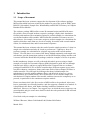
This manual has been written to take the reader from the simple question of ‘what is a
sample size calculation and why do I need to perform one?’ right up to ‘how do I
perform a sample size calculation for a logistic regression with crossed random
effects?’ We will aim to cover some of the theory behind commonly-used sample size
calculations, provide instructions on how to use the MLPowSim package and the code
it creates in both the R and MLwiN packages, and also examples of its use in practice.
In this introductory chapter we will go through this whole process using a simple
example of a single-level normal response model designed to guide the user through
both the basic theory, and how to apply MLPowSim’s output in the two software
packages R and MLwiN. We will then consider three different response types in the
next three chapters: continuous, binary and count. Each of these chapters will have a
similar structure. We will begin by looking at the theory behind sample size
calculations for models without random effects, and then look at how we can use
MLPowSim to give similar results. We will next move on to consider sample size
calculations for simple random effect models, and then increase the complexity as we
proceed, in particular for the continuous response models.
Please note that as this is the first version of MLPowSim to be produced, it does not
have a particularly user-friendly interface, and also supports a limited set of models. It
is hoped that in the future, with further funding, both these limitations can be
addressed. However, in Chapter 5 we suggest ways in which the more expert user can
extend models and give some more details on how the code produced for MLwiN and
R actually works.
Good luck with your sample size calculating!
William J Browne, Mousa Golalizadeh Lahi, Richard MA Parker
March 2009
1
1.2 Sample size / Power Calculations
1.2.1
What is a sample size calculation?
As the name suggests, in simplest terms a sample size calculation is a calculation
whose result is an estimate of the size of sample that is required to test a hypothesis.
Here we need to quantify more clearly what we mean by ‘required’ and for this we
need to describe some basic statistical hypothesis-testing terminology.
1.2.2
What is a hypothesis test?
When an applied researcher (possibly a social scientist) decides to do research in a
particular area, they usually have some research question/interest in mind. For
example, a researcher in education may be primarily interested in what factors
influence students’ attainment at the end of schooling. This general research question
may be broken down into several more specific hypotheses: for example, ‘boys
perform worse than average when we consider total attainment at age 16,’ or a similar
hypothesis that ‘girls perform better than boys.’
1.2.3
How would such hypotheses be tested?
For the first hypothesis we would need to collect a measure of total attainment at age
16 for a random sample of boys, and we would also need a notional overall average
score for pupils. Then we would compare the boys’ sample mean with this overall
average to give a difference between the two and use the sample size and variability
in the boys’ scores to assess whether the difference is more than might be expected by
chance. Clearly, an observed difference based on a sample average derived from just
two boys might simply be due to the chosen boys (i.e. we may have got a very
different average had we sampled two different boys) whereas the same observed
difference based on a sample average of 2,000 boys would be much clearer evidence
of a real difference. Similarly, if we observe a sample mean that is 10 points below
the overall average, and the boys’ scores are not very variable (for example, only one
boy scores above the overall average), then we would have more evidence of a
significant difference than if the boys’ scores exhibit large variability and a third of
their scores are in fact above the overall average.
For the second hypothesis (‘girls perform better than boys’) we could first collect a
measure of total attainment at age 16 for a random sample of both boys and girls, and
compare the sample means of the genders. Then, by using their sample sizes and
variabilities, we could assess whether any difference in mean is more than might be
expected by chance.
For the purposes of brevity we will focus on the first hypothesis in more detail and
then simply explain additional features for the second hypothesis. Therefore our initial
hypothesis of interest is ‘boys perform worse than average’; this is known as the
alternative hypothesis (H1), which we will compare with the null hypothesis (H0, so2
called because it nullifies the research question we are hoping to prove) which in this
case would be ‘boys perform no different from the average’. Let us assume that we
have transformed the data so that the overall average is in fact 0.
We then wish to test the hypotheses
H0: µB=0 versus H1: µB<0
where µB is the underlying mean score for the whole population of boys (the
population mean).
We now need a rule/criterion for deciding between these two hypotheses. In this case,
a natural rule would be to consider the value of the sample mean x and then reject the
null hypothesis if x ≤ c where c is some chosen constant. If x > c then we cannot
reject H0 as we do not have enough evidence to say that boys definitely perform
worse than average. We now need to find a way to choose the threshold c at which
our decision will change. The choice of c is a balance between making two types of
error. The larger we make c the more often we will reject the null hypothesis both if it
is false but also if it is true. Conversely the smaller we make c the more often we fail
to reject the null hypothesis both if it is true but also if it false.
The error of rejecting a null hypothesis when it is true is known as a Type I error, and
the probability of making a Type I error is generally known as the significance level,
or size, of the test and denoted α. The error of failing to reject a null hypothesis when
it is false is known as a Type II error, and the probability of making a Type II error is
denoted β. The quantity 1- β, which represents the probability of rejecting the null
hypothesis when it is false, is known as the power of a test.
Clearly, we only have one quantity, c, which we can adjust for a particular sample,
and so we cannot control the values of both α and β. Generally we choose a value of c
that enables us to get a particular value for α, and this is done as follows. If we can
assume a particular distributional form for the sample mean (or a function of it) under
H0 then we can use properties of the distribution to find the probability of rejecting H0
for various values of c. In our example, we will assume the attainment score for each
individual boy (xi) comes from an underlying Normal distribution with mean µB and
unknown variance σ2B. If we knew the variance then we could assume that the sample
mean also came from a Normal distribution with mean µB and variance σ2B/n where n
is our sample size. From this we could also see that
x − µB
follows a standard normal distribution from which we can conclude that if
σB / n
 x − µB
c − µB 
we wish P( x ≤ c ) = α then P ( x ≤ c) = P 
≤
 =α
 σ B / n σ B / n 
c − µB
= Z α where Zα is the α-th quantile of the Normal distribution.
implies
σB / n
Rearranging gives c = µ B + Zα σ B / n .
3
In the usual case when σ2B is unknown we substitute the sample variance s2B but as
this is an estimate for σ2B we now also need to take its distribution into account. This
results in using a tn-1 distribution in place of a Normal distribution and we have
c = µ B + t n −1, α s B / n as our formula for the threshold. Note that as the sample size n
increases, the t distribution approaches the Normal distribution, and so often we will
simply use the Normal distribution quantiles as an approximation to the t distribution
quantiles.
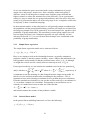
1.2.4
What is Power?
As previously defined, power is the probability of rejecting the null hypothesis when
it is false. In the case of our example, we have a null hypothesis H0: µB=0; this is
known as a simple hypothesis since there is only one possible value for µB if the
hypothesis is true. The alternative hypothesis H1: µB<0 has an infinite number of
possible values and is known as a composite hypothesis. The power of the test will
therefore depend on the true value of µB. Clearly the further µB is from 0, the greater
the likelihood that a chosen sample will result in rejecting H0, and so the power is
consequently a function of µB.
We can evaluate the power of the test for a particular value of µB: for example, if we
believe that the true value of µB=-1 then we could estimate the power of the test given
this value. This would give us how often we would reject the null hypothesis if the
specific alternative µB=-1 was actually true. We have Power = P ( x ≤ c | µB=-1)
where c is calculated under the null hypothesis, i.e.:
(t n −1, α / 2 s B / n ) + 1
c +1
Power = t n−−11 (
)
) = t n−−11 (
sB / n
sB / n
So, for example, if n = 100 and sB=1 and α=0.05(2-sided)1 we have t99, 0.05/2 = -1.98
approximately and
Power = t 99−1 ((-0.198 + 1) / 0.1) = t 99−1 (8.02) = huge! (approximately 1).
So here 100 boys is more than ample to give a large power.
However, if we instead believed the true value of µB was only -0.10 then we would
have
Power = t 99−1 ((-0.198 + 0.10) / 0.1) = t 99−1 (-0.98) = 0.165.
1
NB Whilst many of the alternative hypotheses we use as examples in this manual will be directional
(e.g. H1: µB<0 rather than H1: µB≠0), we generally use 2-sided tests of significance, rather than 1-sided.
This is simply because, in practice, many investigators are likely to adopt 2-sided tests, even if a priori
they formulate directional alternative hypotheses. Of course, there may be circumstances in which
investigators decide to employ 1-sided tests instead: for example, if it simply isn’t scientifically
feasible for the alternative hypothesis to be in a direction (e.g. H1: µB>0) other than that proposed a
priori (in this case H1: µB<0), or, if it were, if that outcome were of no interest to the research
community.
4
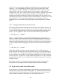
Here the power is rather low and we would need to have a larger sample size to give
sufficient power. If we want to find a sample size that gives a power of 0.8, we would
need to solve for n; this is harder in the case of the t distribution compared to the
Normal, since the distribution function of t changes with n. However, as n gets large
the t distribution gets closer and closer to a Normal distribution; if we then assume a
Normal distribution in this case, we have the slightly simpler formulation:
Power = Φ (
c + 0 .1
sB / n
) = Φ(
( Z α / 2 s B / n ) + 0.1
sB / n
)
where Φ=Z-1 is the inverse of the standard normal CDF. In the case where sB=1 and
Zα/2 = -1.96 we have:
 (−1.96 / n ) + 0.1
Power = Φ 
 which means for a Power of at least 0.8 we have
1/ n


 (−1.96 / n ) + 0.1
(−1.96 / n ) + 0.1
Φ
≥ 0.842
 ≥ 0.8 →
1/ n
1/ n


Solving for n we get n ≥ (10 × (0.842 + 1.96)) 2 = 785.1 thus we would need a sample
size of at least 786. Here 0.842 is the value in the tail of the Normal distribution
associated with a Power of 0.8 (above which 20% of the distribution lies).
1.2.5
Why is Power important?
When we set out to answer a research question we are hoping both that the null
hypothesis is false and that we will be able to reject it based on our data. If, given our
believed true estimate, we have a hypothesis test with low power, then this means that
even if our alternative hypothesis is true, we will often not be able to reject the null
hypothesis. In other words, we can spend money collecting data in an effort to
disprove a null hypothesis, and fail to do so.
On closer inspection the power formula is a function of the size of the data sample
that we have collected. This means that we can increase our power by collecting a
larger sample size. Hence a power calculation is often turned on its head and
described as a sample size calculation. Here we set a desired power which we fix, and
then we solve for n the sample size instead.
1.2.6
What Power should we aim for?
In the literature the desired power is often set at 0.8 (or 0.9): i.e. in 80% (or 90%) of
cases we will (subject to the accuracy of our true estimates) reject the null hypothesis.
Of course, in big studies there will be many hypotheses and many parameters that we
might like to test, and there is a unique power calculation for each hypothesis. Sample
size calculations should be considered as rough guides only, as there is always
uncertainty in the true estimates, and there are often practical limitations to consider
as well, such as maximum feasible sample sizes and the costs involved.
5
1.2.7
What are effect sizes?
In sample size calculations the term effect size is often used to refer to the magnitude
of the difference in value expected for the parameter being tested, between the
alternative and null hypotheses. For example, in the above calculations we initially
believed that the true value of µB=-1 which, as the null hypothesis would correspond
to µB=0, would give an effect size of 1 (note: it is common practice to assume an
effect size is positive). We will use the term effect size both in the next section, and
when we later use the formula to give theoretical results for comparison. However, in
the simulation-based approach, we often use the signed equivalent of the effect size
and so we drop this term and use the terms parameter estimate or fixed effect estimate.
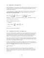
1.2.8
How are power/sample size calculations done more generally?
Basically, for many power/sample size calculations there are four related quantities:
size of the test, power of the test, effect size, and standard error of the effect size
(which is a function of the sample size). The following formula links these four
quantities when a normal distributional assumption for the variable associated with
the effect size holds, and can be used approximately in other situations:
γ
SE (γ )
≈ z1−α / 2 + z1− β
Here α is the size of the test, 1-β is the power of the test, γ is the effect size, and we
assume that the Null hypothesis is that the underlying variable has value 0 (another
way to think of this is that the effect size represents the increase in the parameter
value).
Note that the difficulty here is in determining the standard error formula (SE(γ)). For
specific sample sizes/designs; this can be done using theory employed by the package
PINT (e.g. see Section 2.3.2). In MLPowSim we adopt a different approach which is
more general, in that it can be implemented for virtually any parameter, in any model;
however, it can be computationally very expensive!
1.3 Introduction to MLPowSim
For standard cases and single-level models we can analytically do an exact (or
approximate) calculation for the power, and we will discuss some of the formulae for
such cases in later sections. As a motivation for a different simulation-based
approach, let us consider what a power calculation actually means. In some sense, the
power can be thought of as how often we will reject a null hypothesis given data that
comes from a specific alternative. In reality we will collect one set of data and we will
either be able to reject the null hypothesis, or not. However power, as a concept
coming from frequentist statistics, has a frequentist feel to it in that if we were to
repeat our data-collecting many times we could get a long term average of how often
we can reject the null hypothesis: this would correspond to our power.
6
In reality, we do not go out on the street collecting data many times, but instead use
the computer to do the hard work for us, via simulation. If we were able to generate
data that comes from the specific alternative hypothesis (many times), then we could
count the percentage of rejected null hypotheses, and this should estimate the required
power. The more sets of data (simulations) we use, the more accurate the estimate will
be. This approach is particularly attractive as it replicates the procedure that we will
perform on the actual data we collect, and so it will take account of the estimation
method we use and the test we perform.
This book will go through many examples of using MLPowSim (along with MLwiN
and R) for different scenarios, but here we will replicate the simple analysis that we
described earlier, in which we compared boys’ attainment to average attainment; this
boils down to a Z or t test.
1.3.1
A note on retrospective and prospective power calculations
At this point we need to briefly discuss retrospective power calculations. The term
refers to power calculations based on the currently collected data to show how much
power it specifically has. These calculations are very much frowned upon, and really
give little more information than can be obtained from P-values. In the remainder of
the manual we will generally use existing datasets to derive estimates of effect sizes,
predictor means, variabilities, and so on. Here, the idea is NOT to perform
retrospective power calculations, but to use these datasets to obtain (population)
estimates for what we might expect in a later sample size collection exercise. Using
large existing datasets has the advantage that the parameter estimates are realistic, and
this exercise likely mirrors what one might do in reality (although one might round
the estimates somewhat, compared to the following example, in which we have used
precise estimates from the models fitted to the existing datasets).
1.3.2
Running MLPowSim for a simple example
MLPowSim itself is an executable text-based package written in C which should be
used in conjunction with either the MLwiN package or the R package. It can be
thought of as a ‘program-generating’ program, as it creates macros or functions to be
run using those respective packages.
In the case of our example, the research question is whether boys do worse than
average in terms of attainment at age 16. For those of you familiar with the MLwiN
package and its User’s Guide (Rasbash et al, 2004), the tutorial example dataset is our
motivation here. In the case of that dataset, exam data were collected on 4,059 pupils
at age 16, and the total exam score at age 16 was transformed into a normalised
response (having mean 0 and variance 1). If we consider only the boys’ subset of the
data, and this normalised response, we have a mean of -0.140 and a variance of 1.051.
Clearly, given the 1,623 boys in this subset, we have a significant negative effect for
this specific dataset. Let us now assume that this set of pupils represents our
population of boys, and we wish to see how much power different sample sizes
produce.
7
We could consider sub-sampling from the data (see Mok (1995) and Afshartous
(1995) for this approach with multilevel examples) if this genuinely is our population,
but here let us assume that all we believe is that the mean of the underlying population
of boys is -0.140 and the variance is 1.051.
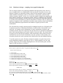
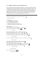
Now we will fire up the MLPowSim executable and answer the questions it asks. In
the case of our example, appropriate questions and responses in MLPowSim are given
below:
Welcome to MLPowSim
Please input 0 to generate R code or 1 to generate MLwiN macros: 1
Please choose model type
1. 1-level model
2. 2-level balanced data nested model
3. 2-level unbalanced data nested model
4. 3-level balanced data nested model
5. 3-level unbalanced data nested model
6. 3-classification balanced cross-classified model
7. 3-classification unbalanced cross-classified model
Model type : 1
Please input the random number seed: 1
Please input the significant level for testing the parameters: 0.025
Please input number of simulations per setting: 1000
Model setup
Please input response type [0 - Normal, 1- Bernouilli, 2- Poisson] : 0
Please enter estimation method [0 - RIGLS, 1 - IGLS, 2 - MCMC] : 1
Do you want to include the fixed intercept in your model (1=YES 0=NO )? 1
Do you want to include any explanatory variables in your model (1=YES 0=NO)? 0
Sample size set up
Please input the smallest sample size : 20
Please input the largest sample size : 600
Please input the step size: 20
Parameter estimates
Please input estimate of beta_0: -0.140
Please input estimate of sigma^2_e: 1.051
Files to perform power analysis for the 1 level model with the following sample criterion have been
created
Sample size starts at 20 and finishes at 600 with the step size 20
1000 simulations for each sample size combination will be performed
Press any key to continue…
8
If we analyse these inputs in order, we begin by stating that we are going to use
MLwiN for a 1-level (single-level) model. We then input a random number seed2, and
state that we are going to use a significance level (size of test) of 0.025. Note that
MLPowSim asks for the significance level for a 1-sided test; hence, when we are
considering a 2-sided test, we divide our significance level by 2 (i.e. 0.05 / 2 = 0.025).
For a 1-sided test, we would therefore input a significance level of 0.05. We then state
that we will use 1000 simulated datasets for each sample size, from which we will
calculate our power estimates.
We are next asked what response type and estimation methods we will use. For our
example we have a normal response, and we will use the IGLS estimation method.
Note that as this method gives maximum likelihood (ML) estimates, it is preferred to
RIGLS for testing the significance of estimates, since hypothesis-testing is based on
ML theory.
We then need to set up the model structure; in our case this is simply an intercept
(common mean) with no predictor variables. Next, we are asked to give limits to the
sample sizes to be simulated, and a step size. So, for our example we will start with
samples of size 20 and move up in increments of 20 through 40,60,… etc., up to 600.
We then give an effect size estimate for the intercept (beta_0) and an estimate for the
underlying variance (sigma^2_e). When we have filled in all these questions, the
program will exit having generated several macro files to be used by MLwiN.
1.4 Introduction to MLwiN and MLPowSim
The MLPowSim program will create several macro files which we will now use in the
MLwiN software package. The files generated for a 1-level model are simu.txt,
setup.txt, analyse.txt and graphs.txt. In this introductory section we will simply give
instructions on how to run the macros and view the power estimates. In later sections
we will give further details on what the macro commands are actually doing.
The first step to running the macros is to start up MLwiN. As the macro files call each
other (i.e. refer to each other whilst they are running), after starting up MLwiN we
need to let it know in which directory these files are stored. We can do this by
changing the current directory, as follows:
Select Directories from the Options menu.
In the current directory box change this to the directory containing the macros.
Click on the Done button.
We next need to find the macro file called simu.txt, as follows:
2
Note that different random number seeds will result in the generation of different random numbers,
and so sensitivity to a particular seed can be tested (e.g. one can test how robust particular estimates are
to different sets of ‘random’ numbers). However, using the same seed should always give the same
results (since it always generates the same ‘random’ numbers), and so if the user adopts the same seed
as used in this manual, then they should derive exactly the same estimates (see e.g. Browne, 2003,
p.59).
9
Select Open Macro from the File menu.
Find and select the file simu.txt in the filename box.
Click on the Open button.
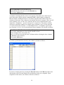
A window containing the file simu.txt now appears. Note that some of the lines of
code in the macro begin with the command NAME, which renames columns in
MLwiN. Before starting the macro it is useful to open the data window and select
columns of interest to view so that we can monitor the macro’s progress. Here we will
select columns c210, c211 & c231; from the code we can see that the macro will
name these ‘Samplesize’, ‘zpow0’ and ‘spow0’, respectively. These three columns
will hence contain the sample size, and the power estimate (‘pow’) for the intercept
(‘0’) derived from the zero/one (‘z’) and standard error (‘s’) methods, respectively
(see Sections 1.4.1 & 1.4.2 for a discussion of these methods). We do this as follows:
Select View or Edit Data from the Data Manipulation menu.
Click on the view button to select which columns to show.
Select columns C210, C211 and C231.
Note you will need to hold down the Ctrl button when selecting the later columns
to add them to the selection.
Click on the OK button
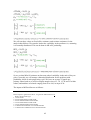
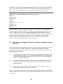
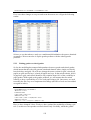
If you have performed this correctly, the window will look as follows:
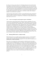
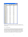
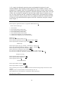
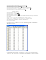
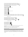
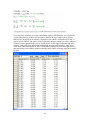
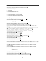
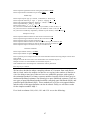
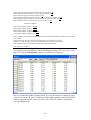
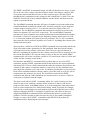
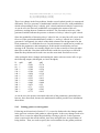
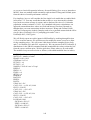
If you now run the macro by pressing the Execute button on the Macro window, the
data window will fill in the sample size calculations as they are computed. Upon
completion of the macro, the window will look as follows:
10
So here we see estimates of power of around 0.1 for just 20 boys, and above 0.9 for
600 boys. Next, we give more details on the two methods used to estimate power with
the IGLS method.
1.4.1
Zero/One method
The first method used is perhaps the most straightforward, but can take a long time to
get accurate estimates. For each simulation we get an estimate of each parameter of
interest (in our case just an intercept) and the corresponding standard error. We can
then calculate a (Gaussian) confidence interval for the parameter. If this confidence
interval does not contain 0 we can reject the null hypothesis and give this simulation a
score of 1. However, if the confidence interval does contain 0, we cannot reject the
null hypothesis and so the simulation scores 0. To work out power across the
11
corresponding set of simulations we simply take the average score (i.e. # of 1s / total
number of simulations).
1.4.2
Standard error method
A disadvantage of the first method is that to get an accurate estimate of power we
need a lot of simulations. An alternative method (suggested by Joop Hox, 2007) is to
simply look at the standard error for each simulation. If we take the average of these
estimated standard errors over the set of simulations, together with the ‘true’ effect
size γ, and the significance level α, we can use the earlier given formula:
γ
SE (γ )
≈ z1−α / 2 + z1− β
and solve for the power (1-β). This method works really well for the normal response
models that we first consider in this guide, but will not work so well for the other
response types that we investigate later.
If we look closely at the two columns on the right, we see that the differences between
consecutive values produced using the zero/one method (i.e. those in the column
headed ‘zpow0’) are quite variable and can be negative, whilst the values estimated
using the standard error method (‘spow0’) demonstrate a much smoother pattern. If
we are interested in establishing a power of 0.8 then both methods suggest a sample
size of 420 will be fine. We can also plot these power curves in MLwiN, and indeed
MLPowSim outputs another macro, graphs.txt, specifically for this purpose.
1.4.3
Graphing the Power curves
To plot the power curves, we need to find the graphing macro file called graphs.txt, as
follows:
Select Open Macro from the File menu.
Select the file graphs.txt in the filename box.
Click on the Open button.
On the graph macro window click on the Execute button.
This has set up graphs in the background that can be viewed as follows:
Select Customised graph(s) from the Graphs menu.
Click on the Apply button on the Customised graph(s) window.
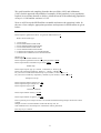
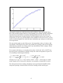
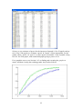
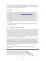
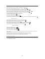
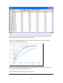
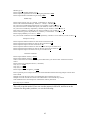
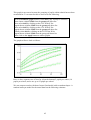
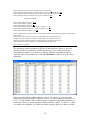
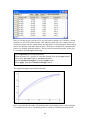
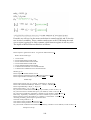
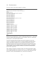
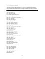
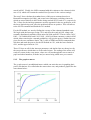
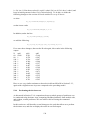
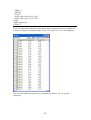
The following graph will appear:
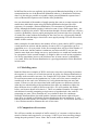
12
This graph contains two solid lines along with confidence intervals (dashed lines).
Here, the smoother brighter blue line is the standard error method, and has confidence
interval lines around it that are actually indistinguishable from the line itself. The
darker blue line plots the results from the zero/one method, and we can see that, in
comparison, it is not very smooth and has wide confidence intervals; however, it does
seem to track the brighter line, and with more simulations per setting we would expect
closer agreement.
We can use this graph to read off the power for intermediate values of n that we did
not simulate. Note that the curves here are produced by joining up the selected points,
rather than any smooth curve fitting, and so any intermediate value is simply a linear
interpolation of the two nearest points.
If we return to the theory, we can plug in the values -0.140 and 1.051 (1.02522) into
the earlier power calculation to estimate exactly the n that corresponds to a power of
0.8 (assuming a normal approximation):
 (−1.96 *1.0252 / n ) + 0.14 
(−1.96 / n ) + 0.14
Φ
≥ 0.842
 ≥ 0.8 →
1.0252 / n
1.0252 / n


Solving for n we get n ≥ (7.142 × 1.0252 × (0.842 + 1.96)) 2 = 420.9 thus we would
need a sample size of at least 421; therefore, our estimate of around 420 is correct.
We will next look at how similar calculations can be performed with MLPowSim
using the R package, instead of MLwiN, before looking at other model types.
13
1.5 Introduction to R and MLPowSim
As explained earlier, MLPowSim can create output files for use in one of two
statistical packages. Having earlier introduced the basics of generating and executing
output files for power analyses in MLwiN, here we do the same for the R package.
Once the user has first requested that R code, rather than MLwiN macros, be
generated in MLPowSim (by pressing 0 when indicated), most of the subsequent
questions and user inputs are the same as for MLwiN, and so we shan’t cover all these
in detail again. However, there are some differences when specifying the model
setup, which reflect differences in the methods and terminologies of the estimation
algorithms used by the two packages. Therefore, we shall consider these in a little
more detail.
The R package is generally slower than MLwiN when simulating and fitting
multilevel models. In R, we focus on the lme and nlme functions, and for single-level
models the glm function. Employing the same example we studied earlier, the model
setup questions, along with the user entries when selecting R, look like this:
__________________________________________________________________
Model setup
Please input response type [0 - Normal, 1- Bernouilli, 2- Poisson] : 0
Do you want to include the fixed intercept in your model (1=YES 0=NO )? 1
Predictor(s) input
Do you want to include any explanatory variables in your model (1=YES 0=NO)? 0
R does not provide a choice of estimation methods for single-level models, although it
does for multilevel models; therefore in the model setup dialogue presented above,
there are no questions about estimation methods (unlike the situation we encountered
earlier, for MLwiN). This is because the function glm is used to fit single-level
models in the R package. In this function there is only one method implemented,
iteratively reweighted least squares (IWLS).
1.5.1
Executing the R code
Before we introduce the procedure for executing the R code generated by
MLPowSim, please note that this manual is written with reference to R version 2.5.1,
on a Windows machine. It is possible that there may be some minor differences when
executing the R code on other platforms such as Linux, or indeed with other versions
of the software.
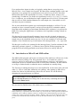
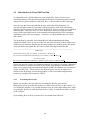
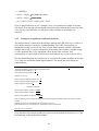
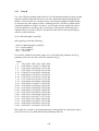
Upon starting R we will be presented by a screen that looks like this:
14
In contrast to the output for MLwiN, MLPowSim generates a single file
(powersimu.r) for the R package. This file has the extension r which is the default for
R command files. If this file is saved in the same directory as the R package itself,
then by entering the following command, R will read the commands contained in the
file:
source(“powersimu.r”)
If it is not saved in that directory, then one can either give the full path to the output
file as an argument (i.e. enter the full path between the brackets in the above
command), or change the working directory in R to the one in which the file is saved,
as follows:
Select Change dir … from the File menu.
In the window which appears, do one of the following:
either write the complete pathname to the output file,
or select Browse and identify the directory containing the output file.
Click on the OK button.
Another simple option is to drag and drop the entire file (i.e. powersimu.r) into the R
console window.
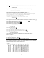
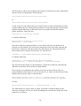
During the simulation, the R console provides updates, every 10th iteration, of the
number of iterations remaining for the current sample size combination being
simulated. The start of the simulation for each different sample size combination is
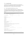
also indicated. In the case of our example, part of this output is copied below:
15
__________________________________________________________________
> source("powersimu.r")
The programme was executed at Tue Aug 05 10:13:35 2008
-------------------------------------------------------------------Start of simulation for sample sizes of 20 units
Iteration remain= 990
Iteration remain= 980
Iteration remain= 970
Iteration remain= 960
Iteration remain= 950
Iteration remain= 940
Iteration remain= 930
Iteration remain= 920
Iteration remain= 910
Iteration remain= 900
Iteration remain= 890
Iteration remain= 880
Iteration remain= 870
Iteration remain= 860
Iteration remain= 850
Iteration remain= 840
Iteration remain= 830
Iteration remain= 820
Iteration remain= 810
Iteration remain= 800
Iteration remain= 790
Iteration remain= 780
………….
………….
………….
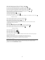
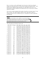
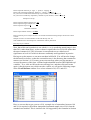
The first line of the above screen indicates the date and time powersimu.r was
executed in R. There is also another date at the top of the file itself (not shown here)
indicating the time MLPowSim produced the R code. When the cursor appears in
front of the command line again (i.e. in front of sign >), the power calculations are
complete, and the power estimates and their confidence intervals (if the user has
answered YES, in MLPowSim, to the question of whether or not they wish to have
confidence intervals), for the various sample size combinations chosen by the user,
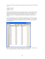
will automatically be saved as powerout.txt. Since it is a text file, the results can, of
course, be viewed using a variety of means; here, though, we view them by typing the
name of the data frame saved by the commands we have just executed in the R
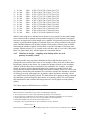
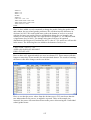
console:
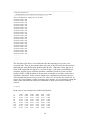
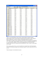
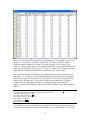
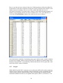
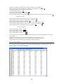
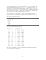
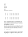
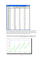
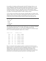
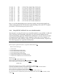
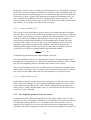
output
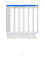
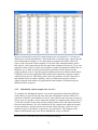
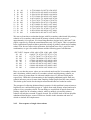
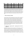
In the case of our example, the results look like this:
n
20
40
60
80
100
120
140
160
zLb0
0.073
0.129
0.148
0.214
0.258
0.298
0.351
0.381
zpb0
0.091
0.151
0.171
0.241
0.286
0.327
0.381
0.411
zUb0
0.109
0.173
0.194
0.268
0.314
0.356
0.411
0.441
sLb0
0.089
0.136
0.183
0.229
0.277
0.321
0.365
0.407
spb0
0.09
0.137
0.184
0.23
0.279
0.323
0.367
0.409
16
sUb0
0.091
0.138
0.186
0.232
0.281
0.325
0.369
0.412
180
200
220
240
260
280
300
320
340
360
380
400
420
440
460
480
500
520
540
560
580
600
0.41
0.457
0.479
0.552
0.56
0.601
0.627
0.664
0.679
0.727
0.731
0.755
0.761
0.793
0.804
0.823
0.823
0.864
0.859
0.87
0.906
0.911
0.441
0.488
0.51
0.583
0.59
0.631
0.656
0.693
0.707
0.754
0.758
0.781
0.786
0.817
0.827
0.845
0.845
0.884
0.879
0.889
0.923
0.927
0.472
0.519
0.541
0.614
0.62
0.661
0.685
0.722
0.735
0.781
0.785
0.807
0.811
0.841
0.85
0.867
0.867
0.904
0.899
0.908
0.94
0.943
0.447
0.486
0.522
0.559
0.594
0.627
0.655
0.684
0.71
0.734
0.757
0.777
0.797
0.816
0.833
0.848
0.863
0.875
0.886
0.898
0.907
0.917
0.45
0.489
0.524
0.562
0.596
0.629
0.657
0.686
0.712
0.736
0.759
0.778
0.799
0.818
0.834
0.849
0.865
0.876
0.887
0.899
0.908
0.918
0.452
0.491
0.527
0.564
0.599
0.631
0.659
0.688
0.714
0.738
0.761
0.78
0.8
0.819
0.836
0.85
0.866
0.877
0.889
0.9
0.909
0.918
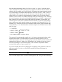
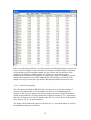
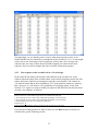
The first column in this output file contains the sample size. In multilevel models,
depending on the model type chosen by the user, we might have one, two or three
columns representing the various sample size combinations at each level. The rest of
the columns are either the estimated power or the lower/upper bounds, calculated
using the methods described earlier (i.e. in Sections 1.4.1 and 1.4.2).
The column headings on the first row denote the specific method, statistic and
parameter. This nomenclature uses the prefixes z and s for the zero/one and standard
error methods of calculating power, respectively. Furthermore, the characters L and U
indicate the lower (L) and upper (U) bounds of the confidence intervals, whilst the
character p stands for the power estimate. Finally, in keeping with common notation
for estimated parameters (i.e. β0, β1 etc.), the characters b0, b1, etc., finish the column
headings.
The results indicate a sample size of between 420 and 440 should be sufficient to
achieve a power of 0.8; this is very similar to our earlier finding using MLwiN, and
indeed our theory-based calculations (Section 1.4).
1.5.2
Graphing Power curves in R
R has many facilities for producing plots of data, and users can load a variety of
libraries and expand these possibilities further.
When fitting a multilevel (mixed effect) model in R we have a grouped data structure,
and a number of specific commands have been written to visualise such data (see, for
example, Venables and Ripley, 2002, Pinheiro and Bates, 2000). For instance, the
trellis graphing facility in the lattice package is useful for plotting grouped data, and
many other complex multivariate data as well. Among the many plotting commands
and functions in the trellis device, the command xyplot ( ), combined with others such
17
as lines ( ), via the function panel, are useful tools. For example, one can employ code
such as the following:
library(lattice)
output<-read.table("powerout.txt",header =T,sep = " ", dec = ".")
method<-rep(c("Zero/one method","Standard error method"),each=length(n1range),times=betasize)
sample<-rep(n1range,times=2*betasize)
parameter<-rep(c("b0"),each=2*length(n1range))
power<-c(output$zpb0,output$spb0)
Lpower<-c(output$zLb0,output$sLb0)
Upower<-c(output$zUb0,output$sUb0)
dataset<-data.frame(method,sample,parameter,Lpower,power,Upower)
xyplot(power~sample | method*parameter ,data=dataset,xlab="Sample size of first level",
scales=list(x=list(at=seq(0,600,100)),y=list(at=seq(0,1,.1))),
as.table=T,subscripts=T,
panel=function(x,y,subscripts)
{
panel.grid(h=-1,v=-1)
panel.xyplot(x,y,type="l")
panel.lines(dataset$sample[subscripts],dataset$Lpower[subscripts],lty=2,col=2)
panel.lines(dataset$sample[subscripts],dataset$Upower[subscripts],lty=2,col=2)
})
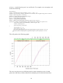
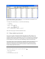
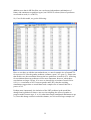
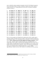
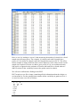
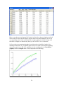
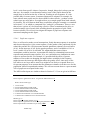
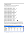
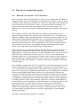
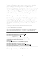
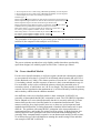
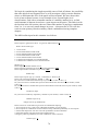
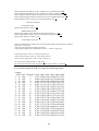
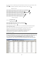
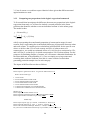
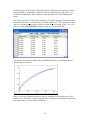
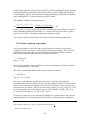
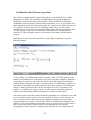
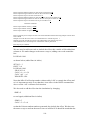
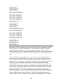
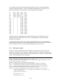
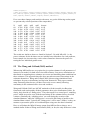
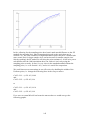
This will produce the following graphs:
The curves are shown in two different panels to make comparison easier. In both
panels, the solid lines (in blue) indicate the estimated powers while the broken lines
18
(in red) are the confidence bounds. It can be seen that the bound interval of the
estimated power in the zero/one method is wider than that in standard error method.
If one wanted to read off the predicted power for a predefined sample size (or vice
versa), one could make the grids in the panels thinner, via the available parameters in
the panel function. However, it’s likely that visual interpolation with the coarse grid
above will give approximately the same result.
For further guidance on plotting power estimates in R, please see Section 5.3.3.
2 Continuous Response Models
In this section we describe sample size calculations for continuous (normallydistributed) response models in general. For these models there exists further exact
formulae that can be used for other single-level models, and also an existing piece of
software (PinT) that gives sample size formulae for balanced 2-level nested models.
In Section 2.1 we will review some of the single-level model formulae while
comparing results in Section 2.2 with the simulation approach. In Section 2.3 we look
at 2-level nested variance components models and describe the design effect formula,
the PinT software package, and the simulation-based approach we adopt in
MLPowSim. Finally, in Sections 2.4 to 2.6 we discuss extending our calculations to
other 2-level nested models, 3-level models and cross-classified models.
2.1 Standard Sample size formulae for continuous responses
In the introductory chapter we described how one approximate formula can link
power, significance level, effect size and sample size (through the standard error of
the effect size). This formula is as follows:
γ
SE (γ )
≈ z1−α / 2 + z1− β
The approximation here is in terms of assuming an underlying normal distribution for
γ when in reality this is only asymptotically correct: i.e. we should really use a t
distribution; however, this will not matter much as long as the sample size is
reasonable. When we are sure about the size and power we require, we can simplify
this further by plugging these values in and having a simple relationship linking the
effect size and its standard error, as described in Chapter 20 of Gelman and Hill
(2007). They consider as we do in general two-sided tests with a significance level of
0.05 and a power of 0.8 which results in γ= (1.96+0.84)SE(γ) = 2.8SE(γ).3
3
Note that if we were considering a one-sided test with the same significance level and power, this
would result in γ= (1.645+0.842)SE(γ) = 2.487SE(γ).
19
2.1.1
Single mean – one sample t-test
In the introduction we showed that to test whether a sample mean is greater than 0 we
needed to perform a one sample t-test which could be approximated by a Z test for
suitably large sample sizes.
To repeat the theory, we plugged in the values -0.140 and 1.051 (1.02522) into the
power calculation to estimate exactly the n that corresponds to a power of 0.8
(assuming a normal approximation):
 (−1.96 *1.0252 / n ) + 0.14 
(−2.01 / n ) + 0.14
Φ
≥ 0.842
 ≥ 0.8 →
1.0252 / n
1.0252 / n


Solving for n we get n ≥ (7.142 × 1.0252 × (0.842 + 1.96)) 2 = 420.9 thus we would
need a sample size of at least 421.
With our simplified formula we have:
γ = 2.802SE (γ )
→ 0.140 = 2.802 ×
1.0252
n
→ n=
2.87
= 20. 5
0.14
→ n = 421
which is exactly the same calculation.
2.1.2
Comparison of two means – two-sample t-test
If we have a binary predictor variable then we have a predictor that essentially splits
our dataset in two. We might then be interested in whether these two groups have
significantly different means, or equivalently in a linear modelling framework (see
Section 2.1.5), whether the predictor has a significant effect on the response.
The common approach for testing the hypothesis that two independent samples have
differing means is the two-sample t-test which can be approximated for large sample
sizes by the Z test using the standard formula.
Letting y1i be the ith observation in the first sample, and y2j be the jth observation in
the second sample, then the test statistic that will play the role of γ is the difference in
sample means y1 − y 2 , which has associated (pooled) standard error
σ 12 / n1 + σ 22 / n2 .
Here we can see that to perform a power calculation we need to estimate the
difference between the means, the variances of the two groups and the sizes of the
samples in the two groups. We can then work out the power for any combination of
sample sizes.
20
So we can calculate the power associated with various combinations of group 1
sample sizes, and group 2 sample sizes. If the variability within each group is
different, it may be advantageous to sample more from the group which has the
highest variance to reduce the standard error of the difference. In an experimental
setting it is easy to sample the two groups independently, and if the effect of the two
groups is of great interest and/or one of the two groups is rare, it might be useful to do
so explicitly (a form of stratified sampling).
In observational studies, on the other hand, we will generally sample at random from
the population, and the group identifier/binary predictor will simply be recorded. Here
the two group sample sizes will be replaced by an overall sample size, together with a
probability of group membership. The uncertainty in actual group sample sizes will
have an impact on power, but a simulation approach can cope with this. As later
discussed in Section 2.1.5, we can calculate desired sample sizes conditional on the
probability of group membership.
2.1.3 Simple linear regression
The simple linear regression model can be written as follows:
yi = β 0 + β1 xi + ei , ei ~ N (0,σ 2 )
Here we are aiming to look at the relationship between a (typically continuous)
predictor variable x, and the response variable y, where i indexes the individuals. Our
null hypothesis will generally be that the predictor has no effect, i.e. β1=0, although
we might also wish to test for a strictly non-zero intercept as well, i.e. β0=0.
From regression theory we can calculate the standard errors for the two quantities β0
(∑i xi ) 2
1 x2
2
+
respectively. It
and β1 which are σ
and σ / S xx where S xx = ∑ xi −
n S xx
n
i
is important to note the meaning of σ has changed from the simple mean model. In
this case it is the residual variation after accounting for the predictor x. This is
important to note when choosing an estimate for σ to perform the power calculation.
From the standard error formulae we can see that we also need to give an estimate for
S xx to perform a sample size calculation. This quantity is not an intuitive one to
estimate, so it makes more sense to make use of the fact that
S xx = ∑ ( xi − x ) 2 = (n − 1) var( xi )
i
and instead estimate the variance of the predictor variable.
2.1.4
General linear model
In the general linear modelling framework, we have the following:
yi = X iT β + ei , ei ~ N (0,σ 2 )
21
Here Xi is a vector of predictor variables for individual i that are associated with
response yi. The corresponding coefficient vector β represents the effects of the
various predictor variables. Usually our null hypotheses will be based on specific
elements of the vector β, and whether they are zero. For this we will require the
standard errors for β. The variance matrix associated with the β predictors has formula
σ2 (XTX)-1 from which we can pick out the standard errors for specific βi. The
standard error formula will then be a function of the sample size, the variance of the
particular predictor, and the covariances between the predictors. Therefore, as we will
see in Section 2.2, if we specify that our predictors are multivariate normallydistributed, then we will need to specify both their means and also their covariance
matrix.
2.1.5
Casting all models in the same framework
For normal response models which do not involve higher-level random structure, the
linear modelling framework covers most cases. There is one minor exception which
we have already looked at briefly: namely the two population different means (two
sample t / Z test) hypothesis. Here we can write out the linear regression model
yi = β 0 + β1 xi + ei , ei ~ N (0,σ 2 )
where xi is a binary indicator that an observation belongs to group 2. Clearly this
model is a member of the linear model family and testing the hypothesis that β1=0 is
equivalent to the hypothesis that the two group means differ. However, this model
makes the implicit assumption that the two group variances are equal, and equal to σ2.
To allow a model with differing group variances we would need the more general
model:
yi = β 0 + β1 xi + ei , ei ~ N (0,σ i2 )
which allows different variances for each observation. We would then need to
implicitly set the variances for each observation in group 1 to be equal and similarly
set the variances for each observation in group 2 to be equal. Such a model is fitted
easily in packages such as MLwiN, with which a simulation study can be conducted
to work out power. For this first version of MLPowSim, however, we have assumed
that single-level models fit in the standard linear modelling framework with constant
residual variation.
We will now introduce a selected range of the possible single-level models that
MLPowSim can fit, using the tutorial example introduced in the last chapter.
2.2 Equivalent results from MLPowSim
In this section we will begin each example by describing the research question, and
then show how to set up the model in MLPowSim. We will then look at the answers
produced in MLwiN, and compare them with theoretical results. Note that similar
results would be attained via R, but these are not included for brevity.
22
2.2.1
Testing for differences between two groups
The tutorial dataset contains a gender predictor for each pupil. In the introduction we
looked at the hypothesis that boys did worse than an average value. Perhaps a more
sensible hypothesis would be that girls do better than boys. We will here consider the
hypothesis within a regression framework, and consider the model:
yi = β 0 + β1 xi + ei , ei ~ N (0,σ 2 )
where xi takes value 1 for a girl, and 0 for a boy. Our null hypothesis is that β1=0, with
an alternative hypothesis β1>0. To fit this model we need estimates for β0, β1 and σ2,
along with some information about the predictor.
We will take estimates from the full tutorial dataset, and so we have
β0=-0.140, β1=0.234 and σ2=0.985.
In the population we have 60% girls and 40% boys and so we will consider two
possible ways of including information about the predictor:
(i)
(ii)
assume xi is Bernouilli-distributed, with underlying probability 0.6;
assume a normal approximation, and so xi ~N(0.6,0.24).
We will describe each of these, in turn, below. We will fire up the MLPowSim
executable and answer the questions it asks. Using our tutorial example, here we
present questions and responses corresponding to (i):
Welcome to MLPowSim
Please input 0 to generate R code or 1 to generate MLwiN macros: 1
Please choose model type
1. 1-level model
2. 2-level balanced data nested model
3. 2-level unbalanced data nested model
4. 3-level balanced data nested model
5. 3-level unbalanced data nested model
6. 3-classification balanced cross-classified model
7. 3-classification unbalanced cross-classified model
Model type : 1
Please input the random number seed: 1
Please input the significant level for testing the parameters: 0.025
Please input number of simulations per setting: 1000
Model setup
Please input response type [0 - Normal, 1- Bernouilli, 2- Poisson] : 0
Please enter estimation method [0 - RIGLS, 1 - IGLS, 2 - MCMC] : 1
Do you want to include the fixed intercept in your model (1=YES 0=NO )? 1
Do you want to include any explanatory variables in your model (1=YES 0=NO)? 1
How many explanatory variables do you want to include in your model? 1
Please choose a type for the predictor x1 (1=Binary 2=Continuous 3=all MVN): 1
23
Please input probability of a 1 for x1 : 0.6
Sample size set up
Please input the smallest sample size : 50
Please input the largest sample size : 1500
Please input the step size: 50
Parameter estimates
Please input estimate of beta_0: -0.140
Please input estimate of beta_1: 0.234
Please input estimate of sigma^2_e: 0.985
Files to perform power analysis for the 1 level model with the following sample criterion have been
created
Sample size starts at 50 and finishes at 1500 with the step size 50
1000 simulations for each sample size combination will be performed
Press any key to continue…
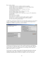
We will now run the code in MLwiN as we did in the introductory example (see
Section 1.4 for information on starting up MLwiN and changing directories).
Again, before starting the macro, it is useful to open the View/Edit Data window to
view its progress (Section 1.4 details how to do this). In this case, it is useful to select
columns c210, c211, c212, c231 and c232 to view, since, as the coding in the macro
indicates, it will place the sample sizes in the first of these columns, and the estimated
powers for the two predictors, using two different methods detailed earlier (Sections
1.4.1 & 1.4.2), in the last four of these columns.
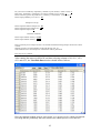
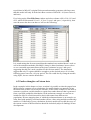
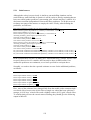
If we now run the macro by pressing the Execute button on the Macro window the
data window will fill in the sample size calculations as they are computed. Upon
completion of the macro, the window will look as follows:
24
So here we see estimates of power for the intercept of around 0.1 for 50 pupils, and up
to 0.92 for 1500 pupils (see columns ‘zpow0’ & ‘spow0’). More importantly, for the
gender effect (‘zpow1’ & ‘spow1’) we have power of around 0.13 for 50 pupils, rising
to 0.991 for 1500 pupils, with around 600 pupils giving a power of 0.8.
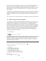
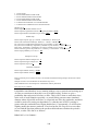
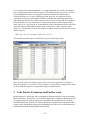
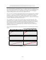
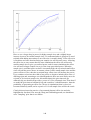
If we graph the curves (see Section 1.4.3 on finding and executing the graphs.txt
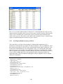
macro, and then viewing the resulting graph), they look as follows:
25
This graph contains two lines, along with confidence intervals, for each parameter,
with the intercept in blue and the gender effect in green. The smoother brighter lines
correspond to the standard error method and have confidence interval lines around
them that are actually indistinguishable from the lines themselves. The darker lines
are the zero/one method results and we can see they are not very smooth and have
wide confidence intervals; however, as we mentioned in Section 1.4.3, they do seem
to track the brighter lines and with more simulations per setting we would expect
more agreement.
We next consider option (ii), and look at the effect of assuming an approximate
normal distribution for gender: i.e. in the simulated dataset that generated 0 and 1
values for boys and girls, we will have a continuous predictor with mean and variance
equal to the mean and variance of the binary predictor considered in option (i),
remembering the mean of a Bernouilli(p) distributed variable is p and the variance is
p(1-p). In our case we have p = 0.6.
To do this, we have to make some minor changes to the questions in MLPowSim
regarding types of predictor. Rather than repeat all the code from the example relating
to (i), we only show the relevant changes below:
Please choose a type for the predictor x1 (1=Binary 2=Continuous 3=all MVN): 2
Assuming normality, please input its parameters here:
The mean of the predictor x1: 0.6
The variance of the predictor x1: 0.24
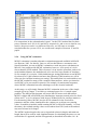
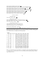
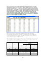
Running this model results in the following table of output:
26
There is very little difference between the results produced using the normal
approximation, and the results produced using the binary predictor, which suggests
that we might like to consider using the normal approximation at all times,
particularly as it makes it easy to include correlations between predictors (see Section
2.2.3). One word of caution, though: in this case we have an underlying probability of
0.6, and reasonable sample sizes; the normal approximation works best in these
situations but may not be so good when the probability is more extreme or the sample
size is small.
From a theory point of view, we can consider the 2-sample Z-test with fixed sample
size ratio of 60% girls and 40% boys and equal variance (0.985), and an effect size of
0.234.
Then the sample size calculation becomes:
27
γ = 2.802SE (γ )
→ 0.234 = 2.802 × σ 2 / 0.4n + σ 2 / 0.6n
→ 0.234 = 2.802 × 0.985 / 0.24n
→ n = (2.802 / 0.234) 2 × 0.985 / 0.24 = 588.5
So if we had fixed ratios in our 2-sample Z-test, we would need a sample of at least
589 pupils. Even though our simulation is based on observational data, where the ratio
6:4 is just the expected ratio, we still get a similar estimate of the sample size
required.
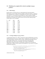
2.2.2
Testing for a significant continuous predictor
The main predictor of interest in the tutorial example in the MLwiN User’s Guide is a
prior ability measure: namely the London Reading Test (LRT; this predictor is
standardised using Z-scores in the User’s Guide, and is named ‘standlrt’) which the
students take at age 11 prior to taking their main exams (the response variable) at age
16. This predictor has a very significant effect on the exam response, and
consequently we expect that we will need a small sample size to gain a power of 0.8.
We can run MLPowSim in a similar way as we did for the gender predictor in Section
2.2.1 when we assumed a normal approximation. The inputs that will change are
outlined below:
Please choose a type for the predictor x1 (1=Binary 2=Continuous 3=all MVN): 2
Assuming normality, please input its parameters here:
The mean of the predictor x1: 0
The variance of the predictor x1: 1
Sample size set up
Please input the smallest sample size : 5
Please input the largest sample size : 50
Please input the step size: 5
Parameter estimates
Please input estimate of beta_0: -0.001
Please input estimate of beta_1: 0.595
Please input estimate of sigma^2_e: 0.648
Files to perform power analysis for the 1 level model with the following sample criterion have been
created
Sample size starts at 5 and finishes at 50 with the step size 5
1000 simulations for each sample size combination will be performed
Press any key to continue…
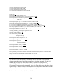
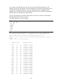
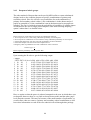
If we run these new macros in MLwiN as previously described (in Section 1.4) we get
the following values in the Data window:
28
So, looking at columns ‘zpow1’ and ‘spow1’ we see that with even around 15 to 20
pupils, we have a power greater than 0.8.
To compare this with the theory, we can look at the following:
γ = 2.802SE (γ )
→ 0.595 = 2.802 × σ 2 / S xx
→ 0.595 = 2.802 × 0.648 /(n − 1)
→ n − 1 = (2.802 / 0.595) 2 × 0.648 → n = 14.37
and so this clearly agrees with the simulation results.
2.2.3
Fitting a multiple regression model.
We can next consider a model that includes both gender and LRT predictors. We
already have sample size estimates for the relationship between each of these two
predictors and the response independently, but now we are looking at the relationships
conditional on the other predictor. For this model we will get three estimated powers
for each sample size: one for each of the relationships, and one for the intercept.
We will once again use the actual estimates obtained from fitting the model to the full
tutorial dataset for our effect estimates, our variability, and so on. Note that the
estimates are reduced due to the correlation between the two predictors. We will
firstly assume independence between the two predictor variables; the MLPowSim
session will then proceed as follows:
Welcome to MLPowSim
Please input 0 to generate R code or 1 to generate MLwiN macros: 1
Please choose model type
1. 1-level model
2. 2-level balanced data nested model
29
3. 2-level unbalanced data nested model
4. 3-level balanced data nested model
5. 3-level unbalanced data nested model
6. 3-classification balanced cross-classified model
7. 3-classification unbalanced cross-classified model
Model type : 1
Please input the random number seed: 1
Please input the significant level for testing the parameters: 0.025
Please input number of simulations per setting: 1000
Model setup
Please input response type [0 - Normal, 1- Bernouilli, 2- Poisson] : 0
Please enter estimation method [0 - RIGLS, 1 - IGLS, 2 - MCMC] : 1
Do you want to include the fixed intercept in your model (1=YES 0=NO )? 1
Do you want to include any explanatory variables in your model (1=YES 0=NO)? 1
How many explanatory variables do you want to include in your model? 2
Please choose a type for the predictor x1 (1=Binary 2=Continuous 3=all MVN): 1
Please input probability of a 1 for x1 : 0.6
Please choose a type for the predictor x2 (1=Binary 2=Continuous): 2
Assuming normality, please input its parameters here:
The mean of the predictor x2: 0
The variance of the predictor x2: 1
Sample size set up
Please input the smallest sample size : 50
Please input the largest sample size : 1500
Please input the step size: 50
Parameter estimates
Please input estimate of beta_0: -0.103
Please input estimate of beta_1: 0.170
Please input estimate of beta_2: 0.591
Please input estimate of sigma^2_e: 0.642
Files to perform power analysis for the 1 level model with the following sample criterion have been
created
Sample size starts at 50 and finishes at 1500 with the step size 50
1000 simulations for each sample size combination will be performed
Press any key to continue…
We will now run the macros in the usual way and we will need to look at seven
columns to get the power for all three parameters using both methods. For the 0/1
method, the power for the fixed effects starts in column c211 and proceeds
sequentially, whilst for the standard error method the power for the fixed effects starts
in column c231 and proceeds sequentially. As a side issue, this means that there is an
implicit limit of 20 fixed effects in MLPowSim when using MLwiN, as otherwise the
columns will start being reused for more than one purpose!
The Data window for this model looks as follows:
30
Here we see that the LRT predictor has associated power (see columns ‘zpow2’ and
‘spow2’) of essentially 1 at sample sizes of only 100 pupils, whilst the gender
predictor requires samples of around 750 to gain a power of 0.8 (‘zpow1’ and
‘spow1’). This is higher than the 600 required when LRT was not considered, but this
will be in part due to the reduced effect size of 0.170 versus 0.234, which more than
outweighs the reduction in unexplained variability (0.642 versus 0.985).
We could also consider including the correlation between our two predictors in our
simulation; i.e. at present we are assuming independence between prior attainment
and gender, whereas in reality there is a small positive correlation, with girls doing
better in the LRT than boys. To do this we need to approximate the 0/1 gender
predictor with a continuous predictor for simulation purposes and assume a
multivariate normal distribution. This involves minor changes to the above macro as
follows:
Please choose a type for the predictor x1 (1=Binary 2=Continuous 3=all MVN): 3
Assuming multivariate normality, please input its parameters here:
The mean of the predictor x1: 0.6
The mean of the predictor x2: 0
The variance matrix of the predictors
The element [1,1]: 0.24
The element [2,1]: 0.026
The element [2,2]: 1
Note that here we have worked out the correlation between the two predictors based
on the full tutorial dataset and then converted this to a covariance value of 0.026. In
31
addition, note that in MLPowSim, one can choose independent combinations of
binary and continuous as predictor types, but if MVN is selected, then all predictors
are treated as such (i.e. as MVN).
So, if we fit this model, we get the following:
Here we see that, as with the uncorrelated case, we need a sample size of around 750
for a power of 0.8 for the gender predictor (columns ‘zpow1’ & ‘spow1’). Please note
that in this case, the correlation between the two predictors is small (0.053). Allowing
for correlations between predictors will be more important, however, when those
correlations are larger. In fact, if we were to increase the covariance from 0.026 to
0.26 (i.e. a correlation of 0.53 between gender and LRT), then the resulting
simulations suggest that we would then need a sample size of around 1000 for a
power of 0.8.
Perhaps more importantly, the inclusion of the LRT predictor in the model has
changed our hypothesis so that we are now investigating the effect of gender on
progress made between ages 11 to 16, rather than simply unadjusted attainment at age
16; since this change results in reduced estimates, we now need a larger sample size.
32
2.2.4
A note on sample sizes for multiple hypotheses, and using sample size
calculations as ‘rough guides’
This example illustrates several important factors when constructing sample size
calculations. Firstly, each hypothesis will have a unique sample size calculation. So,
even though we found that a very small sample is required to show the significant
relationship between the response and LRT, the same data are to be used to show a
significant relationship between the response and gender, and so our chosen sample
size will need to satisfy all our hypotheses. Secondly, in this section we have used
existing data – in fact the true tutorial dataset – to estimate parameter values, and so
we have been able to establish, for example, that there is a reduction in the effect of
gender when we include LRT in the model. This illustrates that when conducting our
power calculation, it is important to replicate exactly what we expect to happen in our
data collection. However, this is easier said than done. This is why sample size
calculations can be thought of as a rough guide: in practice, it might be best to treat
them with some caution and scale them up to cover factors such as over-optimism in
effect sizes, missing variables, and so on. In addition, if we were to switch to a onesided test, then this would decrease our sample sizes, whereas if we were to choose a
power of 0.9, then this would increase our sample sizes.
2.2.5 Using RIGLS
Up to this point we have focussed solely on the IGLS method in the MLwiN package.
This is because when fitting models in MLwiN, most people use IGLS. This is
because it gives maximum likelihood (ML) estimates and therefore allows likelihood
ratio tests to be used when comparing models. In terms of single-level normal models,
we do have a bit of a dilemma, since, typically, general purpose statistical software
packages output unbiased standard errors for coefficients. These coefficients are
equivalent to restricted maximum likelihood (REML) estimates, as used in the RIGLS
estimation method. This difference amounts to changing the divisor in the formula for
estimating the residual variance from n in the ML estimate, to n-p in the REML
estimate, where p is the number of fitted parameters. This will only have a big impact
when n is sufficiently small, and in these cases the fact that we are assuming a normal
distribution, rather than a t distribution, is also a problem.
In Section 2.2.2 we encountered an example where this would make a difference;
there we looked at sample sizes for estimating the effect of LRT (the London Reading
Test score indicator). We can repeat this analysis using RIGLS estimation simply by
changing our selection, when prompted in MLPowSim, of the estimation method
from a 1 to a 0. If we do this, and run the resulting macros in MLwiN, we get the
following:
33
For comparison, in the column headed ‘spow1’ for the IGLS method the first three
power estimates are 0.369, 0.619 and 0.810, respectively, and so we see that for very
small n, the power can be very different. However, we still come to a similar
conclusion that for a power of 0.8, we would need a sample of between 15 and 20
pupils.
2.2.6
Using MCMC estimation
MCMC estimation is another alternative estimation approach available in MLwiN
(see Browne, 2003, for details). Later we will see that when we encounter crossclassified models, we turn to MCMC estimation to work out power calculations in
MLwiN. One problem with MCMC estimation, however, is its speed, as it is far
slower than the IGLS method. This is because it is an iterative procedure, and so for
each simulated dataset, the method needs to be run for a large number of iterations.
So for example if we require 1,000 simulations per setting and choose to run MCMC
for a burn-in of 1,000 iterations and store the following 5,000 iterations we will in
effect run for 6 million iterations per setting! This means that it is not desirable to use
the MCMC method for many of the examples illustrated here, unless you intend to
use MCMC to fit your model in practice (for example, for non-normal responses,
where MCMC estimation has some advantages over the classical methods).
At this stage, we will simply illustrate MCMC estimation in the case of the simple
example given in Chapter 1, in which we estimated power for a 1-sample mean
problem. The MLPowSim program will create MLwiN macro code that utilises
MCMC with the MLwiN default prior distributions: improper normal priors for fixed
effects and Г-1(ε,ε) for variances (with inverse Wishart priors for variance matrices).
For the starting values, MCMC uses the IGLS estimates for the fixed effect
parameters and the values simulated for the variances to avoid any zero starting
values. In multilevel models (unlike running MCMC in MLwiN normally, i.e. from
the menu), the residual starting values are not taken from IGLS, and so the method
may need to burn in for longer.
The MCMC method requires the user to input both a burn-in length, and main run
length, that will be used for each simulated dataset. In calculating the power we can
use both the 0/1 approach, and the SE approach (as described in Sections 1.4.1 &
34
1.4.2), simply by taking the posterior means and standard deviations for each
simulated dataset. Here, though, another approach is also available, namely a nonparametric 0/1 method, where for each parameter the chain of stored values is sorted,
and the value of the appropriate quantile is calculated from this sorted chain. The sign
of this value can then be evaluated to decide if the credible interval contains zero or
not. So, when selecting MCMC estimation in MLPowSim, and running the resulting
macros in MLwiN, power estimates from three different methods are produced. Here
we show the relevant MLPowSim inputs for MCMC estimation, using the example
from Chapter 1:
Welcome to MLPowSim
Please input 0 to generate R code or 1 to generate MLwiN macros: 1
Please choose model type
1. 1-level model
2. 2-level balanced data nested model
3. 2-level unbalanced data nested model
4. 3-level balanced data nested model
5. 3-level unbalanced data nested model
6. 3-classification balanced cross-classified model
7. 3-classification unbalanced cross-classified model
Model type : 1
Please input the random number seed: 1
Please input the significant level for testing the parameters: 0.025
Please input number of simulations per setting: 1000
Model setup
Please input response type [0 - Normal, 1- Bernouilli, 2- Poisson] : 0
Please enter estimation method [0 - RIGLS, 1 - IGLS, 2 - MCMC] : 2
Please input burnin length for each simulation: 1000
Please input main run length for each simulation : 5001
Do you want to include the fixed intercept in your model (1=YES 0=NO )? 1
Do you want to include any explanatory variables in your model (1=YES 0=NO)? 0
Sample size set up
Please input the smallest sample size : 20
Please input the largest sample size : 500
Please input the step size: 20
Parameter estimates
Please input estimate of beta_0: -0.140
Please input estimate of sigma^2_e: 1.051
Files to perform power analysis for the 1 level model with the following sample criterion have been
created
Sample size starts at 20 and finishes at 500 with the step size 20
1000 simulations for each sample size combination will be performed
Press any key to continue…
35
Here we see that we have selected a burn-in of 1000 iterations to allow the chains for
each model to settle down, and then a main run of 5001 iterations from which we will
obtain our power estimates. Note we use 5001, rather than 5000, for ease of
calculation of quantiles. The macros take a while to run in MLwiN (approximately 43
minutes on my machine) and if one selects columns c210, c211, c231 and c421 to
view in the View/Edit Data window, the results can be seen as follows:
Note that the three methods of estimating power give similar results, and the estimates
for power are broadly similar to those using IGLS. In addition, for small sample sizes,
the power from MCMC is systematically smaller than that for IGLS; again, this is due
to the bias of ML variance estimates.
2.2.7 Using R
Whilst RIGLS and MCMC estimation are not offered in MLPowSim when producing
output for R (as opposed to producing output for MLwiN), power calculations for the
various models we have discussed above can be performed in R, using the default
estimation method of iteratively reweighted least squares (IWLS; see Section 1.5 for
36
notes on both this, and on running the outputted code in R). For illustrative purposes,
here we present the results of a power calculation conducted in R for the model we
studied in Section 2.2.1 (testing differences between the two genders, treating the
predictor as binary):4:
n
50
100
150
200
250
300
350
400
450
500
550
600
650
700
750
800
850
900
950
1000
1050
1100
1150
1200
1250
1300
1350
1400
1450
1500
zLb0
0.085
0.121
0.168
0.208
0.262
0.308
0.35
0.418
0.448
0.485
0.513
0.542
0.565
0.616
0.648
0.655
0.677
0.732
0.777
0.807
0.783
0.833
0.853
0.843
0.869
0.885
0.889
0.886
0.893
0.905
zpb0
0.107
0.146
0.196
0.238
0.294
0.342
0.384
0.453
0.483
0.52
0.548
0.577
0.6
0.65
0.681
0.688
0.709
0.762
0.805
0.833
0.811
0.858
0.876
0.867
0.891
0.906
0.909
0.907
0.913
0.924
zUb0
0.129
0.171
0.224
0.268
0.326
0.376
0.418
0.488
0.518
0.555
0.583
0.612
0.635
0.684
0.714
0.721
0.741
0.792
0.833
0.859
0.839
0.883
0.899
0.891
0.913
0.927
0.929
0.928
0.933
0.943
sLb0
0.09
0.141
0.192
0.239
0.289
0.335
0.382
0.428
0.47
0.51
0.549
0.588
0.622
0.653
0.683
0.711
0.737
0.761
0.782
0.803
0.822
0.84
0.856
0.87
0.883
0.894
0.904
0.915
0.923
0.932
spb0
0.091
0.142
0.193
0.241
0.291
0.337
0.384
0.43
0.473
0.513
0.551
0.59
0.624
0.655
0.685
0.713
0.739
0.763
0.784
0.805
0.824
0.841
0.857
0.871
0.884
0.895
0.905
0.916
0.924
0.933
sUb0
0.092
0.144
0.195
0.243
0.293
0.34
0.387
0.432
0.475
0.515
0.553
0.593
0.626
0.657
0.687
0.715
0.741
0.765
0.785
0.806
0.825
0.843
0.858
0.872
0.885
0.896
0.906
0.917
0.925
0.934
zLb1
0.106
0.172
0.253
0.335
0.413
0.497
0.574
0.615
0.665
0.723
0.747
0.763
0.793
0.87
0.85
0.862
0.905
0.919
0.945
0.939
0.935
0.957
0.975
0.974
0.971
0.993
0.98
0.984
0.978
0.986
zpb1
0.13
0.2
0.285
0.369
0.448
0.532
0.609
0.649
0.698
0.754
0.777
0.792
0.82
0.892
0.874
0.885
0.924
0.936
0.959
0.954
0.95
0.969
0.984
0.983
0.981
0.997
0.988
0.991
0.986
0.992
zUb1
0.154
0.228
0.317
0.403
0.483
0.567
0.644
0.683
0.731
0.785
0.807
0.821
0.847
0.914
0.898
0.908
0.943
0.953
0.973
0.969
0.965
0.981
0.993
0.992
0.991
1
0.996
0.998
0.994
0.998
sLb1
0.123
0.207
0.291
0.368
0.443
0.512
0.576
0.634
0.685
0.73
0.77
0.806
0.836
0.862
0.884
0.903
0.92
0.933
0.944
0.954
0.962
0.969
0.975
0.979
0.983
0.986
0.988
0.991
0.992
0.994
spb1
0.124
0.209
0.293
0.371
0.446
0.514
0.578
0.636
0.687
0.732
0.771
0.808
0.838
0.863
0.885
0.904
0.921
0.934
0.945
0.954
0.963
0.969
0.975
0.979
0.983
0.986
0.989
0.991
0.992
0.994
sUb1
0.126
0.211
0.295
0.373
0.448
0.516
0.581
0.638
0.69
0.734
0.773
0.809
0.839
0.864
0.886
0.905
0.921
0.935
0.945
0.955
0.963
0.97
0.975
0.98
0.983
0.986
0.989
0.991
0.993
0.994
Here we see the sample size indicated in the column on the far left, with the power
estimates (together with upper and lower bounds) of the intercept and the predictor in
the remaining columns, for each method of power calculation. As discussed in Section
1.5.1, ‘z’ and ‘s’ denote the zero/one and standard error methods, respectively, whilst
‘p’, ‘L’ and ‘U’ denote the power estimate, and the lower and upper bounds,
respectively, whilst ‘b0’ and ‘b1’ denote the intercept (β0) and predictor (β1). The
results indicate that sampling around 600 pupils should provide a power of 0.8 for the
gender predictor (columns ‘zpb1’ and ‘spb1’). These findings are very similar to the
results we found earlier when using MLwiN (Section 2.2.1), although performing the
above power calculation in R is computationally more expensive (taking
approximately 9 minutes (for R) versus a minute or so (for MLwiN) on my machine).
4
Note that to aid the reader, we have widened the spaces between columns relating to different
predictors/methods, and have formatted the power estimates in bold.
37
2.3 Variance Components and Random Intercept Models
We now turn our attention to multilevel data, as this is one of the chief motivations in
writing MLPowSim. This is because apart from simple cases, such as those described
in Sections 2.3.1 and 2.3.2, when we move to multilevel modelling, standard sample
size formulae do not exist. In Section 2.3.1 we will discuss a specific formula – the
design effect formula – that can be used for scaling up sample sizes in variance
components models to account for clustering; we will compare results from that
formula with MLPowSim. In Section 2.3.2 we will discuss the PINT modelling
software that can be used to fit (balanced) two-level nested models, and will again
compare results between PINT and MLPowSim.
Before we begin, however, please note that in this section we are considering random
intercepts models – i.e. models that can be written as follows:
y ij = X ijT β + u j + eij , u j ~ N (0, σ u2 ), eij ~ N (0, σ e2 )
where j indexes clusters (schools, in our example) and i indexes units within clusters
(pupils, in our example). We also assume that the uj and the eij are independent, and
we have J clusters with the jth cluster containing nj units.
2.3.1
The Design Effect formula
In the case of a model where we test just a mean against some known constant (as
described in the introductory chapter), but with clustering in the data (i.e. a variance
components model) and balance in the clusters (i.e. nj=nC for all j), there is a simple
scaling formula that can be used.
The design effect formula requires an estimate of ρ, the intra-class correlation. This is
a measure of how much correlation exists within clusters. If we initially work out a
required sample size without accounting for clustering, then to subsequently account
for clustering we need to multiply by the Design effect = 1 + (nC-1)ρ where nC is the
cluster size.
To see this in practice, we will return to the introductory example in which we
estimated sample sizes to show that boys do significantly worse at age 16 than
average, with a power of 0.8. The tutorial dataset consists of 65 schools with 4059
pupils in total, leaving an average cluster sample size of 62, but 60% of these pupils
are, on average, girls and so we will now consider a (balanced) analysis where we
take samples of between 10 and 60 boys from each school and we visit between 10
and 50 schools. When we look at the model fitted to all the boys in the tutorial dataset
(accounting for clustering) we get an estimate of -0.177. The estimates of the level 1
and level 2 variances are 0.916 and 0.151, respectively.
If we assume a total variance of 0.916+0.151 = 1.067, we can then repeat our
calculations from Section 2.1.1 to give:
38
γ = 2.802SE (γ )
→ 0.177 = 2.802 ×
1.067
2.89
→ n=
= 16.352
0.177
n
→ n = 267.4
which, due to the increased parameter estimate, is smaller than in Chapter 1. With the
design effect formula we can now work out total sample sizes required for clusters of
sizes 10 to 60. Note that ρ has the formula:
ρ=
σ u2
0.151
=
= 0.142 in our example.
2
2
σ u + σ e 1.067
Cluster size
10
20
30
40
50
60
Design formula
2.278
3.698
5.118
6.538
7.958
9.378
Total sample size
610
989
1369
1749
2128
2508
Number of clusters
61
50
46
44
43
42
We will now show how to fit this model using MLPowSim to confirm that it gives
similar sample sizes. Below, we show how to set up this model (to generate output for
MLwiN):
Welcome to MLPowSim
Please input 0 to generate R code or 1 to generate MLwiN macros: 1
Please choose model type
1. 1-level model
2. 2-level balanced data nested model
3. 2-level unbalanced data nested model
4. 3-level balanced data nested model
5. 3-level unbalanced data nested model
6. 3-classification balanced cross-classified model
7. 3-classification unbalanced cross-classified model
Model type : 2
Please input the random number seed: 1
Please input the significant level for testing the parameters: 0.025
Please input number of simulations per setting: 1000
Model setup
Please input response type [0 - Normal, 1- Bernouilli, 2- Poisson] : 0
Please enter estimation method [0 - RIGLS, 1 - IGLS, 2 - MCMC] : 1
Do you want to include the fixed intercept in your model (1=YES 0=NO )? 1
Do you want to have a random intercept in your model (1=YES 0=NO )? 1
Do you want to include any explanatory variables in your model (1=YES 0=NO)? 0
Sample size set up
39
Please input the smallest number of units for the second level: 10
Please input the largest number of units for the second level: 50
Please input the step size for the second level: 10
Please input the smallest number of units for the first level per second level: 10
Please input the largest number of units for the first level per second level: 60
Please input the step size for the first level per second level: 10
Parameter estimates
Please input estimate of beta_0: -0.177
Please input estimate of sigma^2_u: 0.151
Please input estimate of sigma^2_e: 0.916
Files to perform power analysis for the 2 level nested model with the following sample criterion have
been created
Sample size in the first level starts at 10 and finishes at 60 with the step size 10
Sample size in the second level starts at 10 and finishes at 50 with the step size 10
1000 simulations for each sample size combination will be performed
Press any key to continue…
If we run the macros in MLwiN, we can view the following results via the View or
edit data menu option:
Looking at the power estimates we see that with 40 schools (see the column headed
‘N-level 2’), only a cluster size of 60 produces a power around 0.8, but for 50 schools
40
we have all bar cluster size 10 producing a power above 0.8; this corresponds to the
design effect table where the required number of schools for the various cluster sizes
is between 40 and 50 for cluster sizes greater than 10.
2.3.2 PINT
The PINT program (Bosker, Snijders and Guldemond, 2003) calculates Power IN
Two-level designs and is available at http://stat.gamma.rug.nl/snijders/. PINT takes
user input detailing the proposed design, including effect sizes and anticipated
variabilities, and for a range of sample sizes, both for the clusters and within clusters,
it gives standard error estimates for the fixed effect parameters in the model. The
mathematics that it uses to construct its approximation to the standard errors can be
found in Snijders and Bosker (1993). It is very fast for the models it fits, as it is
simply deriving matrix formulae, but it has some limitations: for example, it only
deals with normal response models with equal-sized (balanced) clusters and only one
set of clusters.
We will compare the results we get from MLPowSim to PINT in the remaining
examples in this section.
2.3.3
Multilevel two sample t-test example
We earlier studied power calculations pertaining to the hypothesis that girls did better
than boys, and we saw in Section 2.2.1 how to test this hypothesis with independent
samples of girls and boys. We now look at what happens when the girls and boys are
clustered together in schools. We will again use the tutorial dataset example to get
hold of our parameter estimates. For this model, the tutorial example gives estimates
of the intercept and female effects of -0.161 and 0.262, respectively (note in the onelevel case, these were -0.140 and 0.234), and the split of the variability is 0.161 at
school level with 0.839 left as residual variability.
We will consider two methods of describing the variability in the predictor variable of
gender. Firstly, as in Section 2.2.1, we will assume a normal approximation to the
Binomial with probability of 0.6 of being a girl, with a mean of 0.6 and a variance of
0.24. Secondly, we will take account of clustering by assuming the variability is split
into 0.12 between schools, with 0.12 left as residual variability. In reality, the tutorial
dataset has some single sex schools which can explain this clustering, and which we
will examine in Section 2.3.4.
Below, we give details of the MLPowSim inputs which have changed from
previously:
Model setup
Please input response type [0 - Normal, 1- Bernouilli, 2- Poisson] : 0
Please enter estimation method [0 - RIGLS, 1 - IGLS, 2 - MCMC] : 1
Do you want to include the fixed intercept in your model (1=YES 0=NO )? 1
Do you want to have a random intercept in your model (1=YES 0=NO )? 1
Do you want to include any explanatory variables in your model (1=YES 0=NO)? 1
41
How many explanatory variables do you want to include in your model? 1
Please choose a type for the predictor x1 (1=Binary 2=Continuous 3=all MVN): 2
Assuming normality, please input its parameters here:
The mean of the predictor x1: 0.6
The variance of the predictor x1 at level 1: 0.24
The variance of the predictor x1 at level 2: 0
Do you want the coefficient associated with explanatory variable x1 to be random (1=YES 0=NO) ? 0
Sample size set up
Please input the smallest number of units for the second level: 10
Please input the largest number of units for the second level: 50
Please input the step size for the second level: 10
Please input the smallest number of units for the first level per second level: 10
Please input the largest number of units for the first level per second level: 60
Please input the step size for the first level per second level: 10
Parameter estimates
Please input estimate of beta_0: -0.161
Please input estimate of beta_1: 0.262
Please input estimate of sigma^2_u: 0.161
Please input estimate of sigma^2_e: 0.839
Files to perform power analysis for the 2 level nested model with the following sample criterion have
been created
Sample size in the first level starts at 10 and finishes at 60 with the step size 10
Sample size in the second level starts at 10 and finishes at 50 with the step size 10
1000 simulations for each sample size combination will be performed
Press any key to continue…
If we run the macros in MLwiN, and look at the following six columns in the View
Data window, we see the following:
42
Here the interesting thing is that if we look at ‘zpow1’ or ‘spow1’, then the power
values obtained for equal-sized designs (for example 10 schools with 60 students, 20
schools with 30 students and 30 schools with 20 students) are approximately equal at
0.92 (note numbers of students and schools are stored as ‘N-level 1’ and ‘N-level 2’,
respectively). This is not the case for the intercepts, where the power goes up from
around 0.24 for 10 schools with 60 students, to around 0.4 for 30 schools with 20
students. This is because in a random intercept model, the clustering is only affecting
the overall response and not the relationship with predictor variables. It appears here
that a sample size somewhere between 400 and 500, regardless of clustering, will
result in a power of 0.8; this is smaller than in Section 2.2.1, but this will be mainly
due to the increase in the gender estimate we are using (0.262 instead of 0.234). To
illustrate, if we consider the one-level calculation with the new gender estimate and
total variability, we see that indeed the estimated sample size would be between 400
and 500, since
γ = 2.802SE (γ )
→ 0.262 = 2.802 × σ 2 / 0.4n + σ 2 / 0.6n
→ 0.262 = 2.802 × 1 / 0.24n
→ n = (2.802 / 0.262) 2 × 1 / 0.24 = 476.6
This method of calculating the sample size is, of course, not appropriate here, and it
transpires that when we fix the number of schools to 50 then a power of 0.8 is
achieved somewhere between 8 and 9 pupils per school, which is smaller than the 477
obtained here. However, what we are illustrating is the fact that it is not necessarily
true that accounting for a clustered design, as in a variance components model,
automatically requires a larger sample size.
If we now consider the effect of changing the variability of the predictor so that it is
split between the 2 levels, we will need to rerun MLPowSim and change the
following lines:
The variance of the predictor x1 at level 1: 0.12
The variance of the predictor x1 at level 2: 0.12
The rest of the inputs will be as before. Running this in MLwiN gives the following:
43
Here we see (by looking at ‘zpow1’) that increasing the number of schools for a fixed
sample size increases power. For example, 10 schools each with 20 pupils has a
power of 0.34, whilst 20 schools each with 10 pupils has a power of 0.36. The effect
in this example is rather small but what is more impressive is the effect on the overall
sample size required. We now see that to get a power of 0.8, we would need nearly
800 pupils, as opposed to the estimate of between 400 and 500 we found when we
didn’t account for the variability between the gender ratios in schools.
We will now confirm these findings with PINT.
PINT requires a text file as input, containing all the information about the design we
are interested in. For the example that contains all the variability in gender at level 1
we need to create a text file as follows:
1 1 0
10 -10 60
10 50
0.839
0.161
0.24
0.0
0.6
44
Here we have, in order:
1 for the number of level 1 predictors (in this case gender);
1 for the number of level 1 predictors that are not also random effects;
0 for the number of level 2 predictors;
10 for the smallest number of level 1 units per level 2 unit;
-10 for the step size at level 1;
60 for the largest number of level 1 units per level 2 unit;
10 for the smallest number of level 2 units;
50 for the largest number of level 2 units (note a step size of 2 is chosen here
automatically);
0.839 for the level 1 variance;
0.161 for the level 2 variance;
0.24 for the level 1 variance associated with the predictor (gender);
0 for the level 2 variance associated with the predictor (gender);
0.6 for the mean of the gender predictor.
As PINT only calculates the standard errors, the fixed effect estimates are not required
as inputs. Loading up PINT (version 2.11) we are first asked for the input file in a
dialogue box, and then are greeted by a screen as follows:
Clicking on the OK button will result in many windows appearing, each asking the
user to confirm (or change) the inputs. If you click on OK at each prompt, PINT will
run and store the output in a file named gender.out (assuming you have named the
input text file gender.txt, as we have).
The file gender.out contains a large amount of background information on the input
settings before giving a table of standard error estimates. We show this for every
combination with the number of clusters as a multiple of 10 to save some space:
45
The following table contains the standard errors (s.e.):
Fixed:
s.e. of regr. coeff.s of level-1 variables with a fixed
effect only.
Const:
s.e. of the intercept.
Sample sizes
N*n
100
200
300
400
500
200
400
600
800
1000
300
600
900
1200
1500
400
800
1200
1600
2000
500
1000
1500
2000
2500
600
1200
1800
2400
3000
N
10
20
30
40
50
10
20
30
40
50
10
20
30
40
50
10
20
30
40
50
10
20
30
40
50
10
20
30
40
50
Standard errors
n
10
10
10
10
10
20
20
20
20
20
30
30
30
30
30
40
40
40
40
40
50
50
50
50
50
60
60
60
60
60
Fixed
0.18697
0.13221
0.10795
0.09349
0.08362
0.13221
0.09349
0.07633
0.06610
0.05913
0.10795
0.07633
0.06232
0.05397
0.04828
0.09349
0.06610
0.05397
0.04674
0.04181
0.08362
0.05913
0.04828
0.04181
0.03739
0.07633
0.05397
0.04407
0.03817
0.03414
Const
0.19255
0.13615
0.11117
0.09627
0.08611
0.16306
0.11530
0.09414
0.08153
0.07292
0.15196
0.10745
0.08773
0.07598
0.06796
0.14610
0.10330
0.08435
0.07305
0.06534
0.14246
0.10073
0.08225
0.07123
0.06371
0.13999
0.09898
0.08082
0.06999
0.06260
We can now use these output standard errors to convert into an equivalent power. We
have to do this by hand as this is not done explicitly by the PINT software.
We earlier had the formula
γ
SE (γ )
= Z 1−α / 2 + Z 1− β
→ Z 1− β =
γ
− Z 1−α / 2
SE (γ )
for our example we have
0.262
− 1.96
SE (γ )
and so for each of the standard errors given in the 4th column of the above outcome
we can use the above formula and look up the power in the normal tables. For a power
of 0.8 we find we require a standard error of 0.0935, or less, in this example. Looking
at the PINT column we see that this value would occur at around 400 pupils in total,
Z 1− β =
46
as we observed in MLPowSim. We can also see in the PINT output that, for all
designs with exactly 400 pupils, the same standard error and hence the same power is
obtained for the gender predictor. This was suggested earlier, and MLPowSim
appears to give this result (with some Monte Carlo error), but the PINT approximate
standard errors are identical for each scenario.
We can also look at the second scenario where we have the variance of the gender
predictor split between the two levels.
The PINT input file is now as follows:
1 1 0
10 -10 60
10 50
0.839
0.161
0.12
0.12
0.6
If we run this input file in PINT, we can again look at the output standard errors:
The following table contains the standard errors (s.e.):
Fixed:
s.e. of regr. coeff.s of level-1 variables with a fixed
effect only.
Const:
s.e. of the intercept.
Sample sizes
N*n
100
200
300
400
500
200
400
600
800
1000
300
600
900
1200
1500
400
800
1200
1600
2000
500
1000
1500
2000
2500
600
N
10
20
30
40
50
10
20
30
40
50
10
20
30
40
50
10
20
30
40
50
10
20
30
40
50
10
Standard errors
n
10
10
10
10
10
20
20
20
20
20
30
30
30
30
30
40
40
40
40
40
50
50
50
50
50
60
Fixed
0.22820
0.16136
0.13175
0.11410
0.10205
0.17021
0.12035
0.09827
0.08510
0.07612
0.14248
0.10075
0.08226
0.07124
0.06372
0.12519
0.08852
0.07228
0.06260
0.05599
0.11304
0.07993
0.06526
0.05652
0.05055
0.10388
Const
0.20794
0.14703
0.12005
0.10397
0.09299
0.17528
0.12394
0.10120
0.08764
0.07839
0.16188
0.11447
0.09346
0.08094
0.07239
0.15440
0.10918
0.08914
0.07720
0.06905
0.14959
0.10578
0.08637
0.07480
0.06690
0.14623
47
1200
1800
2400
3000
20
30
40
50
60
60
60
60
0.07345
0.05997
0.05194
0.04646
0.10340
0.08443
0.07311
0.06540
Here we see that – as with MLPowSim – the standard errors, and hence power
associated with the sample sizes, does depend on the design, and for equivalent total
numbers of pupils the greater the number of schools the smaller the standard error and
the larger the power. Looking for a standard error of 0.0935 or smaller we see that this
occurs when we have 40 pupils in 20 schools, 20 pupils in 40 schools, and so on, as
we found with MLPowSim.
We will occasionally compare our results from MLPowSim with those from PINT in
later examples, but as this is a book about MLPowSim our coverage of PINT will be
brief. If the reader requires more information regarding PINT, there is a user’s guide
available from http://stat.gamma.rug.nl/snijders/ which provides further details.
2.3.4
Higher level predictor variables
Continuing with our topic of the effect of gender on exam score, we saw in the last
example that differential sex ratios between schools had an impact on our sample size
calculation. In fact we saw an ICC for gender of 0.5: i.e. 50% of the variability
between “pupil’s gender” is due to schools. This is partly due to the large numbers of
single sex schools in the tutorial dataset. In the MLwiN User’s Manual they study
another hypothesis concerning the effect of single sex school attendance, as it appears
that such pupils do better, in general, than pupils in a mixed school.
Here we will test a version of this hypothesis to demonstrate how to use MLPowSim
with predictors at the cluster (school) level. In the tutorial dataset there is a categorical
variable school gender which takes 3 values: mixed schools, boys’ schools and girls’
schools. As the current version of MLPowSim only deals with continuous and binary
variables, and in fact the effects of boys’ schools and girls’ schools are similar in
magnitude, we will create a version of this predictor that purely differentiates between
mixed and single-sex schools. Note that in Chapter 5, we will revisit this as an
example of how to modify the macros produced by MLPowSim to deal with
categorical predictors at higher levels.
We fitted a model with this predictor to the tutorial dataset and the result was
estimates of -0.101 for the intercept (mixed schools) and 0.193 for the single-sex
schools predictor. The model had estimates of 0.159 and 0.848 for level 2 and residual
(level 1) variances, respectively. Of the 65 schools in the dataset, we have 30 single
sex schools, but to express the variable as a level 2 predictor we (currently) have to
convert this to a continuous variable with mean 30/65 = 0.462, and variance
(0.462)*(1-0.462) = 0.249.
We will use these numbers to set up an MLPowSim scenario. For illustration, we will
assume a constant 40 pupils per school, and then vary the number of schools.
After choosing a balanced 2-level model, and the usual numbers of simulations, and
the usual random seed and significance level, we enter the following inputs when
prompted:
48
Model setup
Please input response type [0 - Normal, 1- Bernouilli, 2- Poisson] : 0
Please enter estimation method [0 - RIGLS, 1 - IGLS, 2 - MCMC] : 1
Do you want to include the fixed intercept in your model (1=YES 0=NO )? 1
Do you want to have a random intercept in your model (1=YES 0=NO )? 1
Do you want to include any explanatory variables in your model (1=YES 0=NO)? 1
How many explanatory variables do you want to include in your model? 1
Please choose a type for the predictor x1 (1=Binary 2=Continuous 3=all MVN): 2
Assuming normality, please input its parameters here:
The mean of the predictor x1: 0.462
The variance of the predictor x1 at level 1: 0
The variance of the predictor x1 at level 2: 0.249
Do you want the coefficient associated with explanatory variable x1 to be random (1=YES 0=NO) ? 0
Sample size set up
Please input the smallest number of units for the second level: 10
Please input the largest number of units for the second level: 200
Please input the step size for the second level: 10
Please input the smallest number of units for the first level per second level: 40
Please input the largest number of units for the first level per second level: 40
Please input the step size for the first level per second level: 10
Parameter estimates
Please input estimate of beta_0: -0.101
Please input estimate of beta_1: 0.193
Please input estimate of sigma^2_u: 0.159
Please input estimate of sigma^2_e: 0.848
Files to perform power analysis for the 2 level nested model with the following sample criterion have
been created
Sample size in the first level starts at 10 and finishes at 200 with the step size 10
Sample size in the second level starts at 40 and finishes at 40 with the step size 10
1000 simulations for each sample size combination will be performed
Press any key to continue…
If we run the macro code produced in MLwiN, we will get the following output in the
View/Edit Data window:
49
Here we see that we need around 160 schools of size 40 to detect a single sex school
effect which is more schools than are present in the real tutorial dataset! This is not
very surprising, since in the real dataset the average pupils per school is larger, and
the effect of single sex schools only has a p-value of 0.033 on a 1-sided test.
So far, we have not mentioned graphs in our discussion of multilevel models. As
described in Section 1.4.3, to plot the power curves we need to execute the graphing
macro file graphs.txt in MLwiN, and then view the resulting plot via Customised
graph(s) from the Graphs menu. This will produce the following:
50
Note, by default the graphs.txt macro plots separate curves for each parameter, and
estimation method, against column c210 (‘N-level 2’: the number of schools). This
means that if we vary the number of pupils and the number of schools we will get a
messy graph, but in this case, as we have fixed the number of pupils as 40 per school,
this is not the case. Once again, we observe that the brighter curves, plotting results
from the SE method, are much smoother than the 0/1 method.
We can compare our results with PINT. On this occasion, since the parameter
estimate is 0.193, we are looking for a standard error of 0.0689 for a power of 0.8.
We will use the following input file:
0 0 1
40 -10 40
10 150
0.848
0.159
0.249
0.462
which results in the following output file:
Sample sizes
N*n
400
800
1200
1600
2000
2400
2800
3200
3600
4000
4400
4800
5200
5600
6000
6400
6800
7200
7600
8000
N
10
20
30
40
50
60
70
80
90
100
110
120
130
140
150
160
170
180
190
200
Standard errors
n
40
40
40
40
40
40
40
40
40
40
40
40
40
40
40
40
40
40
40
40
Const
0.18294
0.12936
0.10562
0.09147
0.08181
0.07468
0.06914
0.06468
0.06098
0.05785
0.05516
0.05281
0.05074
0.04889
0.04723
0.04573
0.04437
0.04312
0.04197
0.04091
Group
0.26902
0.19022
0.15532
0.13451
0.12031
0.10983
0.10168
0.09511
0.08967
0.08507
0.08111
0.07766
0.07461
0.07190
0.06946
0.06725
0.06525
0.06341
0.06172
0.06015
Here we see that around 160 schools results in the required reduction in standard
error, as we found with MLPowSim.
51
2.3.5
A model with 3 predictors
So far we have looked at predictors in isolation, but as we saw in Section 2.2 for
single level models, if we are interested in testing many hypotheses we might need to
consider a model with many predictor variables. For the final model considered in this
section we will look at three predictor variables: gender, school gender, and the
London Reading Test (LRT) score. We have discussed the first two in this section
already, and encountered the LRT when considering single level models (e.g. Section
2.2.2). Our hypotheses here will concern the effect of gender and school gender when
accounting for intake ability, and conversely the effect of intake ability when
accounting for gender and school gender.
If we fit a variance components model to the tutorial dataset with these three predictor
variables, we will get the following:
Here we see for the real data that there are significant effects for all three predictor
variables. As we discovered earlier for one-level models, the relationship of the
response with LRT is particularly strong, and we need very small sample sizes to find
a significant effect. In order to get accurate sample size estimates we require
information about the variability (at both levels) and correlation between the
predictors. To estimate these from the real data we could look at school means of the
three predictors, and their variability and correlations. We could also look at fitting a
multilevel multivariate model for the two predictors, gender and LRT, to get the
within covariance matrix. In the inputs that follow, we will take estimates obtained
from such an approach. Note that this will result in an assumed multivariate normal
distribution for the predictors, which is an approximation for the binary variables. In
Chapter 5 we discuss what may be a better approach of dealing with the school gender
and gender predictors.
After choosing a balanced 2-level model, and the usual numbers of simulations, and
the usual random seed and significance level, we enter the following inputs when
prompted:
Model setup
Please input response type [0 - Normal, 1- Bernouilli, 2- Poisson] : 0
Please enter estimation method [0 - RIGLS, 1 - IGLS, 2 - MCMC] : 1
Do you want to include the fixed intercept in your model (1=YES 0=NO )? 1
52
Do you want to have a random intercept in your model (1=YES 0=NO )? 1
Do you want to include any explanatory variables in your model (1=YES 0=NO)? 1
How many explanatory variables do you want to include in your model? 3
Please choose a type for the predictor x1 (1=Binary 2=Continuous 3=all MVN): 3
Assuming multivariate normality, please input its parameters here:
The mean of the predictor x1: 0.6
The mean of the predictor x2: 0.462
The mean of the predictor x3: 0
The variance matrix of the predictors at level 1
The element [1,1] : 0.120
The element [2,1] : 0
The element [2,2] : 0
The element [3,1] : 0.020
The element [3,2] : 0
The element [3,3] : 0.902
The variance matrix of the predictors at level 2
The element [1,1] : 0.125
The element [2,1] : 0.045
The element [2,2] : 0.249
The element [3,1] : 0.013
The element [3,2] : -0.006
The element [3,3] : 0.116
Do you want the coefficient associated with explanatory variable x1 to be random (1=YES 0=NO) ? 0
Do you want the coefficient associated with explanatory variable x2 to be random (1=YES 0=NO) ? 0
Do you want the coefficient associated with explanatory variable x3 to be random (1=YES 0=NO) ? 0
Sample size set up
Please input the smallest number of units for the second level: 10
Please input the largest number of units for the second level: 150
Please input the step size for the second level: 10
Please input the smallest number of units for the first level per second level: 40
Please input the largest number of units for the first level per second level: 40
Please input the step size for the first level per second level: 10
Parameter estimates
Please input estimate of beta_0: -0.167
Please input estimate of beta_1: 0.166
Please input estimate of beta_2: 0.165
Please input estimate of beta_3: 0.560
Please input estimate of sigma^2_u: 0.081
Please input estimate of sigma^2_e: 0.562
Files to perform power analysis for the 2 level nested model with the following sample criterion have
been created
Sample size in the first level starts at 10 and finishes at 150 with the step size 10
Sample size in the second level starts at 40 and finishes at 40 with the step size 10
1000 simulations for each sample size combination will be performed
Press any key to continue…
This will create the macros needed to perform this simulation exercise in MLwiN. To
run these macros takes a little longer than the earlier examples (around 7.5 minutes).
If we run the macros and look at the View/Edit Data window with the following five
columns chosen (i.e. only the number of schools and the powers from the SE method),
we have:
53
So here we see that to gain a power of 0.8 we need less than 10 schools for the LRT
predictor (‘spow3’), around 30 for the gender predictor (‘spow1’), and between 110
and 120 for the school gender predictor (‘spow2’).
Again we can plot the power curves associated with the three predictors and the
intercept, with the following results:
Here we see the intercept in dark blue, the gender effect in green, the school gender
effect in cyan and the LRT predictor in red.
The PINT input code for this model is as follows:
2
2
1
54
40 -10 40
10 150
0.562
0.081
0.120
0.020 0.902
0.249
0.045 0.125
-0.006 0.013 0.116
0.6 0.0
0.462
which results in the following output:
Sample sizes
N*n
400
800
1200
1600
2000
2400
2800
3200
3600
4000
4400
4800
5200
5600
6000
N
10
20
30
40
50
60
70
80
90
100
110
120
130
140
150
Standard errors
n
40
40
40
40
40
40
40
40
40
40
40
40
40
40
40
Fixed
0.10136
0.07168
0.05852
0.05068
0.04533
0.04138
0.03831
0.03584
0.03379
0.03205
0.03056
0.02926
0.02811
0.02709
0.02617
Fixed
0.03917
0.02770
0.02262
0.01959
0.01752
0.01599
0.01481
0.01385
0.01306
0.01239
0.01181
0.01131
0.01086
0.01047
0.01011
Const
0.14280
0.10097
0.08244
0.07140
0.06386
0.05830
0.05397
0.05049
0.04760
0.04516
0.04306
0.04122
0.03960
0.03816
0.03687
Group
0.19624
0.13876
0.11330
0.09812
0.08776
0.08012
0.07417
0.06938
0.06541
0.06206
0.05917
0.05665
0.05443
0.05245
0.05067
Here the 4th column corresponds to gender, the 5th to LRT and the last to school
gender. As we have different parameter estimates for each variable, for powers of 0.8
we require standard errors of 0.059, 0.200 and 0.059, respectively. Looking at the
columns we see that these occur at around 30 schools for gender, with less than 10
schools for LRT and between 110 and 120 schools for school gender which agrees
exactly with the results from MLPowSim!
Once you have figured out how to specify your model in PINT, and how to perform
the post output translation from parameter estimates and standard errors to powers, it
is clear that PINT is quicker than the simulation approach, but it is restricted to 2-level
balanced models and to normal responses, neither of which restrictions exist with
MLPowSim. We will briefly consider one of these restrictions in the next section.
2.3.6
The effect of balance
One of the features that PINT, in particular, relies on when constructing sample size
calculations is that the nested design is balanced. Here we mean that we have the
same number of level 1 units within each level 2 unit. This would seem a sensible
strategy to adopt when collecting data, as there isn’t usually a reason to pick more
55
level 1 units from specific clusters. In practice, though, things don’t always pan out
that way: for example, in an education setting, some of the pupils chosen in the
sample may be absent on the day of the test, resulting in non-responses. It’s also
possible that, for some reason, a structured approach is adopted: for example, for
some schools more pupils may be chosen than for other schools – perhaps certain
school types are rarer and so we might wish to over-sample pupils from such schools,
for instance. We will illustrate both these possibilities using the example we examined
in Section 2.3.3, in which we compared boys’ and girls’ performance. There we saw
that to have a power of 0.8 of detecting a positive effect on attainment for girls, we
needed a sample size of nearly 800, assuming that the proportion of girls varied
between schools. We will now investigate the impact of pupil non-response and
structured sampling on this figure.
2.3.6.1 Pupil non-response
Here we will need to make several assumptions, firstly that non-response is at random
and does not depend on (i) the exam response (ii) the gender of the pupils and (iii) the
school they attend. We will also assume that the parameter estimates we used earlier
(0.161 for the intercept, 0.262 for the gender predictor, and of variabilities 0.161 at
level 2, and 0.839 at level 1) still hold. We might think that some of these
assumptions could be incorrect, in particular the lack of a relationship between nonresponse and potential exam response. If so, we could adjust our simulation in some
respect to account for this. For example, it’s possible that the effect of greater
numbers of low achievers dropping out might reduce variability in the response,
might increase the intercept, and might reduce the gender effect, since more of the
low achievers are boys and so more boys might be less likely to respond. However,
for present purposes let us assume that the parameter estimates cited above are for the
population who did respond and continue. We will now assume that we expect around
20% of pupils not to respond in the study.
The MLPowSim inputs are similar to those in Section 2.3.3, but are given in full here:
Welcome to MLPowSim
Please input 0 to generate R code or 1 to generate MLwiN macros: 1
Please choose model type
1. 1-level model
2. 2-level balanced data nested model
3. 2-level unbalanced data nested model
4. 3-level balanced data nested model
5. 3-level unbalanced data nested model
6. 3-classification balanced cross-classified model
7. 3-classification unbalanced cross-classified model
Model type : 3
Please input the random number seed: 1
Please input the significance level for testing the parameters: 0.025
Please input number of simulations per setting: 1000
Model setup
56
Please input response type [0 - Normal, 1- Bernouilli, 2- Poisson] : 0
Please enter estimation method [0 - RIGLS, 1 - IGLS, 2 - MCMC] : 1
Do you want to include the fixed intercept in your model (1=YES 0=NO )? 1
Do you want to have a random intercept in your model (1=YES 0=NO )? 1
Do you want to include any explanatory variables in your model (1=YES 0=NO)? 1
How many explanatory variables do you want to include in your model? 1
Please choose a type for the predictor x1 (1=Binary 2=Continuous 3=all MVN): 2
Assuming normality, please input its parameters here:
The mean of the predictor x1: 0.6
The variance of the predictor x1 at level 1: 0.12
The variance of the predictor x1 at level 2: 0.12
Do you want the coefficient associated with explanatory variable x1 to be random (1=YES 0=NO) ? 0
Sample size set up
Please input the smallest number of units for the second level: 10
Please input the largest number of units for the second level: 50
Please input the step size for the second level: 10
Please choose one of the following scenarios for unbalance:
1: Binomial with the fixed trial and probability of non-response for first level nested in second
2: Fixed sample with your preference
Scenario type: 1
Please enter your probability of non-response: 0.2
Please input the smallest number of units for the first level per second level: 10
Please input the largest number of units for the first level per second level: 60
Please input the step size for the first level per second level: 10
Parameter estimates
Please input estimate of beta_0: -0.161
Please input estimate of beta_1: 0.262
Please input estimate of sigma^2_u: 0.161
Please input estimate of sigma^2_e: 0.839
Files to perform power analysis for the 2 level unbalanced nested model with the following sample
criterion have been created
Sample size in the first level starts at 10 and finishes at 60 with the step size 10
Sample size in the second level starts at 10 and finishes at 50 with the step size 10
1000 simulations for each sample size combination will be performed
Press any key to continue…
We can now run this scenario in MLwiN and look at the power estimates that it
produces in the View/Edit Data window:
57
Here we see that compared to the power estimates in Section 2.3.3, the values are
reduced, as might be expected given the smaller actual sample size compared to the
designed sample size. As we have a non-response probability of 0.2, we could
consider the effect of looking at a sampling scheme with step sizes of 8 pupils per
school as opposed to 10: i.e. 8, 16, 24, 32, 40 and 48 in a balanced model. If we do
this by rerunning MLPowSim and MLwiN, we will get the following table of powers:
58
Here we see that the results are very close to those from the non-response scenario. Of
course, for this example we have chosen a non-response probability that corresponds
in expectation to a whole number sample size per cluster, and it would have been
quicker to use PINT to establish sample sizes. However, if the non-response
probability had resulted in an average of 8.3 pupils per cluster, for instance, it would
not have been possible to use PINT, although we could still have used PINT with
sample sizes 8 per cluster and 9 per cluster, and then interpolated between the two.
2.3.6.2 Structured sampling
The other option available in MLPowSim is for the user to specify the number of
clusters of each particular size. This might occur due to over-sampling specific
clusters, or the user may simply wish to get estimates of power for specific datasets
which are not balanced. We will consider the example in Section 2.3.6.1, and assume
that 80% of clusters are of size 30, but the other 20% are of size 60. We will consider
cases with 10, 20, 30, 40 and 50 schools.
The inputs will be almost the same as in Section 2.3.6.1, apart from where we specify
the unbalanced structure, as follows:
59
Please choose one of the following scenarios for unbalance:
1: Binomial with the fixed trial and probability of non-response for first level nested in second
2: Fixed sample with your preference
Scenario type : 2
Please choose how many distinct cluster sizes you want for second level units: 2
Unbalanced set up inside the second level with 10 level 2 units
How many (from 1 to 10) groups do you want to be in the class 1? 8
For class 1, please input the number of level 1 units: 30
How many (from 2 to 2) groups do you want to be in the class 2? 2
For class 2, please input the number of level 1 units: 60
Unbalanced set up inside the second level with 20 level 2 units
How many (from 1 to 20) groups do you want to be in the class 1? 16
For class 1, please input the number of level 1 units: 30
How many (from 4 to 4) groups do you want to be in the class 2? 4
For class 2, please input the number of level 1 units: 60
Unbalanced set up inside the second level with 30 level 2 units
How many (from 1 to 30) groups do you want to be in the class 1? 24
For class 1, please input the number of level 1 units: 30
How many (from 6 to 6) groups do you want to be in the class 2? 6
For class 2, please input the number of level 1 units: 60
Unbalanced set up inside the second level with 40 level 2 units
How many (from 1 to 40) groups do you want to be in the class 1? 32
For class 1, please input the number of level 1 units: 30
How many (from 8 to 8) groups do you want to be in the class 2? 8
For class 2, please input the number of level 1 units: 60
Unbalanced set up inside the second level with 50 level 2 units
How many (from 1 to 50) groups do you want to be in the class 1? 40
For class 1, please input the number of level 1 units: 30
How many (from 10 to 10) groups do you want to be in the class 2? 10
For class 2, please input the number of level 1 units: 60
The rest of the inputs are as before. As you can see, the procedure for inputting the
model structure is relatively laborious, and we would not anticipate that this form of
unbalanced design will be heavily-used in MLPowSim; however, the inputs only take
a minute or two to type in, which is quicker than the macros take to run, so it is only a
small overhead.
Running the resulting macros in MLwiN gives the following power estimates:
If we compare the powers produced here with those produced for the balanced design
in Section 2.3.3, we can see that they lie somewhere between the powers for balanced
60
designs with 30 pupils per school and those with 40 pupils per school, as we might
expect given our design has on average 36 pupils per school.
2.4 Random slopes/ Random coefficient models
Random intercept models are a special case of two-level model where the only
relationship that is assumed different at the cluster level is the average effect or
intercept in the model. The effect of predictors is assumed constant across clusters in
a random intercept model. If we wish to allow for a different effect for a predictor in
each cluster then we will fit a random slopes model, or random coefficients model.
Note that the term ‘slope’ is generally reserved for continuous predictors where the
coefficient associated with the predictor can be thought of as the slope of a predicted
regression line. If such a regression were plotted for binary predictors, it would
essentially join up the predictions for the two states of the predictor, and so ‘random
coefficient model’ is a better term, meaning the effect of the binary predictor is
different for different groups.
We could go through lots of examples of random coefficient models in this section,
but we will limit ourselves to just one for brevity.
The tutorial dataset presents us with some problems when trying to find examples of
random slopes models that follow on from our earlier investigations. Firstly, the
gender predictor exhibits no significant between-school variability: i.e. the effect of
gender doesn’t vary across schools. This is possibly because many of the schools are
single sex, and so can give no information on the effect of gender within them – in
fact, the concept doesn’t make sense in such schools. Secondly, the school gender
predictor is a school-level predictor, and so cannot be treated as random at the schoollevel, and finally the LRT predictor is such a strong predictor that we will only need
very small sample sizes regardless of any random slope.
We will therefore turn to a different example, again from an educational setting. Later
on, we will investigate this example further when we look at cross-classified models.
The example is used in the MLwiN User’s Guide (Rasbash et al, 2004) to illustrate
cross-classified modelling, and consists of exam scores for 3,435 secondary school
pupils in Fife, Scotland. The response used is an attainment score for students at age
16, with the students nested within both primary school, and secondary school. For
the purposes of our example, we will consider the primary school nesting which
results in 3,435 pupils nested within 148 primary schools. We will again consider a
gender predictor (sex), which in this case is also significant for the dataset, but also
exhibits variability in effect between primary schools: i.e. the size of the effect of
gender on attainment varies across schools.
The model fitted in MLwiN can be seen below:
61
We will use these values as fixed effect estimates, and variance estimates, for the
analysis that follows. We can also look at the variability in the predictor sex, assuming
it is normally distributed. This can be done in MLwiN, producing:
So we see that MLwiN estimates no between-school variability in the ratio of boys to
girls. Given this, we will assume a binomial distribution for the predictor with
probability 0.494 of each pupil being a girl. We have on average 23 pupils per
primary school, and so we will investigate sample sizes of 5, 10, 15, 20 and 25 within
school, and numbers of schools ranging from 20 to 160, in steps of 20.
The inputs to MLPowSim are as follows:
Welcome to MLPowSim
Please input 0 to generate R code or 1 to generate MLwiN macros: 1
Please choose model type
1. 1-level model
2. 2-level balanced data nested model
3. 2-level unbalanced data nested model
4. 3-level balanced data nested model
5. 3-level unbalanced data nested model
6. 3-classification balanced cross-classified model
7. 3-classification unbalanced cross-classified model
62
Model type : 2
Please input the random number seed: 1
Please input the significance level for testing the parameters: 0.025
Please input number of simulations per setting: 1000
Model setup
Please input response type [0 - Normal, 1- Bernouilli, 2- Poisson] : 0
Please enter estimation method [0 - RIGLS, 1 - IGLS, 2 - MCMC] : 1
Do you want to include the fixed intercept in your model (1=YES 0=NO )? 1
Do you want to have a random intercept in your model (1=YES 0=NO )? 1
Do you want to include any explanatory variables in your model (1=YES 0=NO)? 1
How many explanatory variables do you want to include in your model? 1
Please choose a type for the predictor x1 (1=Binary 2=Continuous 3=all MVN): 1
Please input probability of a 1 for x1 : 0.494
Do you want the coefficient associated with explanatory variable x1 to be random (1=YES 0=NO) ? 1
Sample size set up
Please input the smallest number of units for the second level: 20
Please input the largest number of units for the second level: 100
Please input the step size for the second level: 20
Please input the smallest number of units for the first level per second level: 5
Please input the largest number of units for the first level per second level: 25
Please input the step size for the first level per second level: 5
Parameter estimates
Please input estimate of beta_0: 5.370
Please input estimate of beta_1: 0.495
There is more than one random effect in your model and so you need to enter variance/covariance
matrix.
Please input lower triangular entries ( 3 elements):
entry (1,1) is : 1.064
entry (2,1) is : 0.109
entry (2,2) is : 0.180
Please input estimate of sigma^2_e: 8.098
Files to perform power analysis for the 2 level nested model with the following sample criterion have
been created
Sample size in the first level starts at 5 and finishes at 25 with the step size 5
Sample size in the second level starts at 20 and finishes at 100 with the step size 20
1000 simulations for each sample size combination will be performed
Press any key to continue…
This will set up the model. If we now run the macros in MLwiN, and focus on the
columns for the gender predictor, we see the following:
63
We see here that a power of greater than 0.8 is achieved by 25 pupils in 60 schools, 20
pupils in 80 schools, and 15 pupils in 100 schools. The power for 10 pupils in 100
schools is greater than that for 25 pupils in 40 schools, and so for the same total pupil
number it is better to have more clusters with less pupils per cluster.
To plot the curves, we can execute the macro file graphs.txt (see Section 1.4.3); this
produces the following graphs (via Customised graph(s) from the Graphs menu):
64
This graph is not correct because the grouping of pupils within schools has not been
accounted for. To account for this we need to do the following:
In the Customised graph window select ds#1 (may already be selected)
Now choose column C209 from the group pull down list.
Next select ds#2 by clicking on the c212 in the Y list
Again choose column C209 from the group pull down list
Next select ds#3 by clicking on the c231 in the Y list
Again choose column C209 from the group pull down list
Finally select ds#4 by clicking on the c232 in the Y list
Again choose column C209 from the group pull down list
Now click on the Apply button to redraw graphs.
The graphs will now look as follows:
Here we have separate sets of lines for (from the bottom) 5 pupils per school, 10
pupils per school, and so on, up to 25 pupils per school.
We can compare results with those from a fitted model with no random slopes. A
random intercepts model for the actual data has the following estimates:
65
If we use these estimates to set up a simulation study in MLPowSim, we will get the
results shown below in MLwiN. We can see that the designs with a power greater
than 0.8 are 20 pupils in 60 schools, 15 pupils in 80 schools, and between 10 and 15
pupils in 100 schools. The power of the equivalent designs appears to reduce when we
account for the random slopes, as we might expect. It also appears that having more
schools, each with fewer pupils but maintaining the total pupil number, tends to be
associated with reduced power. This is somewhat contrary to what one might expect,
and may be due to the binary predictor having more chance of being constant in small
clusters.
66
It is possible to fit random coefficient models in the PINT package. However, as a
result of making the mathematics behind the approximate standard errors easier to
calculate, PINT has some restrictions. In particular, all predictors treated as random
coefficients must have mean zero. This makes sense for some predictors, where
centering is probably a sensible modelling option, however for categorical predictors,
e.g. gender, a centered gender indicator is rather a strange concept!
As we only have one predictor, then centering it will only change our estimate of the
intercept, which we are not interested in, and which PINT does not require. It will also
change the between-intercept variance and covariance at level 2, but we can reevaluate these on the real data and then run PINT with the following input code:
1 0 0
5 -5 25
20 100
8.098
1.215
0.198 0.180
0.249964
The fixed effect estimate for gender is 0.495, which means we would like a standard
error smaller than 0.495/2.802 = 0.177. PINT gives standard errors for all
combinations of pupils and schools, with a step size for both of 5, so from the output
file we can extract the appropriate sample sizes, as follows:
Sample sizes
N*n
1050
1125
1200
1275
1100
1200
1300
1400
1125
1250
1375
1500
N
70
75
80
85
55
60
65
70
45
50
55
60
Standard errors
n
15
15
15
15
20
20
20
20
25
25
25
25
Const
0.15833
0.15296
0.14811
0.14369
0.17162
0.16431
0.15787
0.15212
0.18493
0.17544
0.16727
0.16015
Random
0.18283
0.17663
0.17102
0.16591
0.18090
0.17320
0.16640
0.16035
0.18110
0.17181
0.16381
0.15684
Here we see that for only 15 pupils per school we would need 75 schools, for 20
pupils per school we would need 60, and for 25 pupils per school we would need 50,
which roughly corresponds to the results in MLPowSim, although any minor
differences may be due to the approximation used in PINT, or to Monte Carlo
standard errors in MLPowSim, or even the fact that in MLPowSim we assumed that
the predictor was binomially-distributed rather than a normal approximation.
67
2.5 Three-level random effect models
2.5.1
Balanced 3-level models – The ILEA dataset
Here we continue with an education theme, and use as our example the ILEA dataset
dating from 1985-1987, and consisting of exam results at 16 for three years of London
secondary school children (see Nuttall et al., 1989). The subsample of the data that we
have used to derive the effect sizes is large: 15,632 pupils from 304 cohorts in 139
schools (note some schools did not participate in all 3 years of the study). We
therefore have a three-level structure with pupils nested within cohorts, nested within
schools.
The response of interest is the total exam score based on grades achieved in all
subjects summed together. This response takes values from 1 to 70. We look at two
predictor variables: gender, and the proportion of pupils in the cohort eligible for free
school meals (FSM). Both these predictors are very significant with this large sample
size, but we are interested in whether (i) a smaller sampling scheme would have
resulted in sufficient power, or more importantly (ii) if we were to attempt a similar
data collection exercise today, using smaller samples (assuming broadly similar
effects exist), what sample sizes would result in similar power?
Here we will use the estimates produced by this large dataset as a guide for what we
might expect in our data collection exercise. The fixed effect estimates from the
whole data are 21.535 for the intercept, 2.839 for the gender effect, and -6.039 for the
FSM effect. We will therefore use the values 21.5, 3 and -6 in our simulations as
estimated effect sizes: i.e. girls tend to do 3 grades better in total over their collection
of exams than boys, while the difference between a school with no pupils eligible to
FSM, and one with all FSM pupils, is 6 grades in total across each pupil’s collection
of exam results.
The variability is estimated as 12.174, 2.5 and 142.635, for between schools, between
cohorts within schools, and residual variability, respectively. We will therefore use
12, 2.5 and 140 here. The gender predictor has mean 0.523 and variances 0.138, 0.001
and 0.116, respectively: so slightly more girls than boys, with slightly more variability
between schools than within schools. However, we will assume for our study an
average 50/50 split, and equal variance between schools and within cohorts (residual
variability) i.e. variances of 0.125, 0, and 0.125, respectively. There doesn’t appear to
be a significant relationship between %FSM and gender, and the average proportion
of FSM per cohort is 0.423, with variability split as 0.017 between schools and 0.09
between cohorts. So, for the purposes of our illustration, we will use the values 0.4 for
the mean and 0.02, 0.01 and 0 for the variances, respectively, for %FSM and
independence between the 2 predictors. In terms of sample size we will assume a
similar 3-year study design, and so we will have 3 cohorts per school, and we will
vary the numbers of schools (between 10 and 40), and pupils per cohort sampled
(between 10 and 50).
The inputs for MLPowSim will then be as follows:
68
Welcome to MLPowSim
Please input 0 to generate R code or 1 to generate MLwiN macros: 1
Please choose model type
1. 1-level model
2. 2-level balanced data nested model
3. 2-level unbalanced data nested model
4. 3-level balanced data nested model
5. 3-level unbalanced data nested model
6. 3-classification balanced cross-classified model
7. 3-classification unbalanced cross-classified model
Model type : 4
Please input the random number seed: 1
Please input the significance level for testing the parameters: 0.025
Please input number of simulations per setting: 1000
Model setup
Please input response type [0 - Normal, 1- Bernouilli, 2- Poisson] : 0
Please enter estimation method [0 - RIGLS, 1 - IGLS, 2 - MCMC] : 1
Do you want to include the fixed intercept in your model (1=YES 0=NO )? 1
Do you want to have a random intercept associated with the second level in your model (1=YES
0=NO )? 1
Do you want to have a random intercept associated with the third level in your model (1=YES 0=NO
)? 1
Do you want to include any explanatory variables in your model (1=YES 0=NO)? 1
How many explanatory variables do you want to include in your model? 2
Please choose a type for the predictor x1 (1=Binary 2=Continuous 3=all MVN): 2
Assuming normality, please input its parameters here:
The mean of the predictor x1: 0.5
The variance of the predictor x1 at level 1: 0.125
The variance of the predictor x1 at level 2: 0
The variance of the predictor x1 at level 3: 0.125
Please choose a type for the predictor x2 (1=Binary 2=Continuous ): 2
Assuming normality, please input its parameters here:
The mean of the predictor x2: 0.4
The variance of the predictor x1 at level 1: 0
The variance of the predictor x1 at level 2: 0.01
The variance of the predictor x1 at level 3: 0.02
Do you want the coefficient associated with explanatory variable x1 to be random at level two (1=YES
0=NO) ? 0
Do you want the coefficient associated with explanatory variable x2 to be random at level two (1=YES
0=NO) ? 0
Do you want the coefficient associated with explanatory variable x1 to be random at level three
(1=YES 0=NO) ? 0
Do you want the coefficient associated with explanatory variable x2 to be random at level three
(1=YES 0=NO) ? 0
Sample size set up
Please input the smallest number of units for the third level: 10
Please input the largest number of units for the third level: 40
Please input the step size for the third level: 10
Please input the smallest number of units for the second level per third level: 3
Please input the largest number of units for the second level per third level: 3
69
Please input the step size for the second level per third level: 1
Please input the smallest number of units for the first level per second level: 10
Please input the largest number of units for the first level per second level: 50
Please input the step size for the first level per second level: 10
Parameter estimates
Please input estimate of beta_0: 21.5
Please input estimate of beta_1: 3
Please input estimate of beta_2: -6
Please input estimate of the level 3 variance (sigma^2_v): 12
Please input estimate of the level 2 variance (sigma^2_u): 2.5
Please input estimate of sigma^2_e: 140
Files to perform power analysis for the 3 level nested model with the following sample criterion have
been created
Sample size in the first level starts at 10 and finishes at 50 with the step size 10
Sample size in the second level starts at 3 and finishes at 3 with the step size 1
Sample size in the third level starts at 10 and finishes at 30 with the step size 10
1000 simulations for each sample size combination will be performed
Press any key to continue…
We can run the macros produced in MLwiN in the usual way. Since we are only
interested in the two predictors, and not the intercept, if we select the columns
containing the sample size at each level, and the columns containing the power
estimates for the two predictors (via the View/Edit Data window), we will see the
following:
Here we see that for the gender predictor (‘zpow1’ & ‘spow1’) we do not need a
particularly big design, with 10 schools (‘N-level 3’) with 3 cohorts of 30 pupils (‘Nlevel 1’), or 20 schools with 3 cohorts between 10 and 20 both producing powers of
around 0.8. However, for the proportion FSM predictor (‘zpow2’ & ‘spow2’), which
is a cohort-level predictor, we clearly need more schools, and we see that even with
70
30 schools with 50 pupils per cohort we do not reach a power of 0.8, whilst for 40
schools 50 pupils per cohort suffices to produce a power greater than 0.8.
MLPowSim is flexible enough to allow the numbers of units at all three levels to vary,
and we have simply fixed the number of cohorts here to 3 as this represents our study
design. As with 2-level modelling, MLPowSim can also allow any of the predictor
variables to be treated random at higher levels for 3-level models as well, but we do
not give examples of this here. We will, however, consider the options that exist for
unbalanced 3-level models, and we turn to these in the following few sections.
2.5.2
Non-response at the first level in a 3-level design
We will consider here a scenario where individual pupils do not respond at random
from our sample – for example, perhaps we constructed a sampling frame of students
earlier in their schooling, and some students then moved school and so were not
included in the final sample. We will use exactly the same inputs for parameter
estimates as in Section 2.5.1, but will assume a non-response probability of 0.2, and
will additionally consider 60 pupils per school to account, in part, for this nonresponse.
To investigate a non-balanced 3-level design we need to select option:
5 (‘3-level unbalanced data nested model’)
when prompted in MLPowSim, and then all our inputs are as for the balanced case
until we reach the section on Sample size set up, where we enter the following:
Sample size set up
Please input the smallest number of units for the third level: 10
Please input the largest number of units for the third level: 40
Please input the step size for the third level: 10
Unbalanced set up
Please choose one of the following scenarios for unbalanced sampling:
1: Non-response of level 1 units using a Binomial probability of non-response
2: Non-response of level 2 units using a Binomial probability of non-response
3: Fixed sample size in first level with your preference
Scenario type : 1
Please input the probability of non-response for the first level units: 0.2
Please input the smallest number of units for the second level per third level: 3
Please input the largest number of units for the second level per third level: 3
Please input the step size for the second level per third level: 1
Please input the smallest number of units for the first level per second level: 10
Please input the largest number of units for the first level per second level: 60
Please input the step size for the first level per second level: 10
The remaining inputs are as in Section 2.5.1. If we run the macros produced in
MLwiN, we get the following in the View/Edit Data window:
71
Unsurprisingly, we see that the power is lower when non-response occurs, as we
found with the two-level models we considered earlier (Section 2.3.6.1). As one might
expect, the power for designs with 50 pupils per school, and a 20% average nonresponse rate, are close to those observed with 40 pupils per school and no nonresponse. Next we will investigate the effect of whole cohort non-response.
2.5.3
Non-response at the second level in a 3-level design
In the actual ILEA dataset, the design is not balanced at the second level: some
schools joined the study in the second cohort, some schools dropped out after the first
cohort, and some schools even managed to miss the second cohort. 304 cohorts for
139 schools means that in the actual dataset 27% of the possible cohorts are missing.
Here, however, we will stick to a 0.2 probability of a missing cohort, in line with
Section 2.5.2. Again, we need to modify our inputs in MLPowSim, but this time there
are only a few changes, as follows:
Unbalanced set up
Please choose one of the following scenarios for unbalanced sampling:
1: Non-response of level 1 units using a Binomial probability of non-response
2: Non-response of level 2 units using a Binomial probability of non-response
3: Fixed sample size in first level with your preference
Scenario type : 2
Please input the probability of non-response for the second level units: 0.2
If we run the resulting macros in MLwiN and view the Data window as before we
will this time get the following results:
72
We have assumed an average 20% non-response rate as in Section 2.5.2 except at a
different level of the data structure. This means that we should expect, on average, the
same total number of pupils, so it is interesting to compare the relative effects on
power of the two forms of non-response. If we look at the columns headed ‘spow1’
and ‘spow2’, and compare them with the equivalent columns in Section 2.5.2, we can
gauge the effect on power for the two predictors: gender and proportion FSM. We see
that there is very little to choose between the two forms of non-response for the
gender predictor (a level 1 predictor which exhibits no between-cohort within-school
variability), but for the proportion FSM predictor the cohort non-response scenario
results in worse power. This makes sense, since this predictor is at the cohort-level
and exhibits between-cohort variability, and so a cohort non-response scenario
reduces both the total number of pupils and the total number of cohorts having an
additional effect on power.
2.5.4
Individually chosen sample sizes at level 1
To complete our unbalanced options, we have the possibility of allowing differentsized clusters, as specified by the user. Here the assumption is that for each level 3
unit there will be the same number of level 2 units with the same structure in terms of
cluster sizes: for instance, for the education example we might assume cluster sizes of
30, 40 and 50 pupils for the three cohorts within a school, but each school must then
have the same structure. We will consider the ILEA example once again but assume,
as discussed above, that the cluster sizes of each cohort increase, and so we have 3
cohorts of sizes 30, 40 and 50, respectively, for each school. The changes to the
inputs to MLPowSim only occur for the unbalanced set up, as follows:
Unbalanced set up
Please choose one of the following scenarios for unbalanced sampling:
73
1: Non-response of level 1 units using a Binomial probability of non-response
2: Non-response of level 2 units using a Binomial probability of non-response
3: Fixed sample size in first level with your preference
Scenario type : 3
Please input the smallest number of units for the second level per third level: 3
Please input the largest number of units for the second level per third level: 3
Please input the step size for the second level per third level: 1
Please choose how many distinct classes you want the second level to have: 3
Unbalanced set up inside the second level with 3 level 2 units
How many (from 1 to 3) level 2 units do you want to be in the class 1 ? 1
For class 1, please input the number of level 1 units: 30
How many (from 1 to 2) level 2 units do you want to be in the class 2 ? 1
For class 2, please input the number of level 1 units: 40
For class 3, please input the number of level 1 units: 50
The remainder of the inputs are as previously given. Once the macros have been run
in MLwiN, the outputs for this analysis are as follows:
The power estimates produced are only slightly smaller than those produced by
equivalent designs, but with 40 pupils in each of the 3 cohorts per school.
2.6 Cross-classified Models
For the cross-classified models we will once again consider the educational example
we encountered in Section 2.4, from Fife in Scotland (taken from the MLwiN User’s
Guide (Rasbash et al, 2004)). The dataset consists of records for 3,435 children from
19 secondary schools, and the response of interest is their exam attainment at age 16.
For each child, we have also recorded the primary school they attended prior to
secondary school, of which there are 148 in our sample. The data structure is therefore
crossed, and we hypothesise that attainment at 16 will be affected by both the primary
and secondary schools that the children attended.
One difficulty with cross-classified models is their estimation. In MLwiN it is
generally recommended that MCMC estimation be used. The IGLS/RIGLS algorithm
can be adapted to fit cross-classified models but this is currently achieved via some
macros that cast the cross-classified model as a constrained nested model. These
macros work fine for a single model, however we have not yet incorporated such
methods into MLPowSim, as fitting thousands of models in this framework is more
difficult. The problem with using MCMC estimation is the increased burden of
computational time, and in this case using R will be quicker. In R the function lmer
does not appear to have problems with cross-classified models although they are
generally more computationally-expensive to run than nested models. In this section,
we will therefore provide information on running the models using R first and then
one example of MCMC in MLwiN.
74
As with nested data, ideally we might like to collect balanced cross-classified data. In
this section we will firstly consider balanced data, before moving on to potentially
more realistic unbalanced data scenarios.
2.6.1
Balanced cross-classified models.
As further background to our example, the response we are interested in is an
attainment score from 1 to 10 that represents the pupils’ score on a school leaving
exam. For simplicity, we assume this score is continuous and normally-distributed as
fitted in the User’s Guide (although in reality an ordered categorical model might be
more appropriate).
We will then fit a simple variance components model that assumes that the exam
score for a particular pupil includes an overall population mean, an effect for the
primary school they attended, an effect for the secondary school they attended, and a
residual for that particular pupil. The average score in the actual data is 5.5, and so we
form a null hypothesis (for illustration) that the average score is 5 versus an
alternative that the average is higher than 5. For simplicity, we subtract 5 from all
scores – as a result, we now have a null hypothesis that the average score is 0 – and
we input an effect size (for the intercept) of 0.5. We give similar variances to those
which appeared in the actual data, and use values of 0.4 for secondary school, 1.2 for
primary school, and 8 for residual variability.
As we are assuming balanced data we will try to mimic a little the actual data
collected. Given there were 148 primary schools and 19 secondary schools making
potentially nearly 3,000 combinations this would be a little over 1 pupil per
combination. We however see that in reality the data is fairly sparse with only 303 of
the pairings of primary and secondary school actually occurring, with on average 11
pupils per combination. We will compromise by having 3 pupils per combination and
trying between 20 and 100 primary schools (first cross-classified factor) and 10 and
30 secondary schools (second cross-classified factor). Here we give instructions for
fitting this model in R, since this is quicker than the MCMC methods in MLwiN. The
inputs for MLPowSim are as follows:
Welcome to MLPowSim
Please input 0 to generate R code or 1 to generate MLwiN macros: 0
Please choose model type
1. 1-level model
2. 2-level balanced data nested model
3. 2-level unbalanced data nested model
4. 3-level balanced data nested model
5. 3-level unbalanced data nested model
6. 3-classification balanced cross-classified model
7. 3-classification unbalanced cross-classified model
Model type : 6
Please input the random number seed: 1
Please input the significance level for testing the parameters: 0.025
75
Please input number of simulations per setting: 1000
Model setup
Please input response type [0 - Normal, 1- Bernouilli, 2- Poisson] : 0
Please enter estimation method [0 - REML, 1 - ML] : 1
Do you want to include the fixed intercept in your model (1=YES 0=NO )? 1
Do you want to have a random intercept associated with the first XC factor in your model (1=YES
0=NO )? 1
Do you want to have a random intercept associated with the second XC factor in your model (1=YES
0=NO )? 1
Predictor(s) input
Do you want to include any explanatory variables in your model (1=YES 0=NO)? 0
Sample size set up (balance)
Please input the smallest number of units for the first cross-classified factor: 20
Please input the largest number of units for the first cross-classified factor: 100
Please input the step size for the first cross-classified factor: 20
Please input the smallest number of units for the second cross-classified factor: 10
Please input the largest number of units for the second cross-classified factor: 30
Please input the step size for the second cross-classified factor: 10
Please input the smallest number of replications per XC cell : 3
Please input the largest number of replications per XC cell : 3
Please input the step size for the number of replications : 1
Parameter estimates
Fixed effects input
Please input estimate of beta_0: 0.5
Random effects input
Please input estimate of the variance of first factor (sigma^2_u): 1.2
Please input estimate of the variance of second factor (sigma^2_v): 0.4
Please input estimate of sigma^2_e: 8
Final sample size check
The first XC factor: start=20 end=100 step size=20
The second XC factor: start=10 end=30 step size=10
The first level (replication): start=3 end=3 step size=1
Do you want to continue (YES=1 , NO=0)? 1
Do you want to have the CI for the power in your output (YES=1 , NO=0)? 1
After running MLPowSim we need to start up R and read in and run the file
powersimu.r (see Section 1.5) which contains all the inputs for running the
simulations. The simulations will take close to an hour to run in R, and at the end we
get the following results if we ask to see the stored data frame output by typing output
at the command prompt:
> output
#XC2 #XC1 #repeat zLb0 zpb0 zUb0 sLb0 spb0 sUb0
1 10 20
3 0.328 0.358 0.388 0.330 0.335 0.340
2 10 40
3 0.419 0.450 0.481 0.459 0.466 0.473
3 10 60
3 0.520 0.551 0.582 0.533 0.541 0.548
76
4
5
6
7
8
9
10
11
12
13
14
15
10 80
10 100
20 20
20 40
20 60
20 80
20 100
30 20
30 40
30 60
30 80
30 100
3
3
3
3
3
3
3
3
3
3
3
3
0.574 0.604 0.634 0.578 0.586 0.595
0.582 0.612 0.642 0.605 0.614 0.624
0.388 0.419 0.450 0.409 0.414 0.420
0.537 0.568 0.599 0.592 0.597 0.602
0.663 0.692 0.721 0.690 0.695 0.700
0.716 0.743 0.770 0.749 0.754 0.759
0.780 0.805 0.830 0.793 0.798 0.803
0.457 0.488 0.519 0.451 0.457 0.463
0.633 0.662 0.691 0.655 0.660 0.665
0.739 0.765 0.791 0.768 0.772 0.776
0.803 0.826 0.849 0.834 0.837 0.841
0.840 0.861 0.882 0.872 0.875 0.879
We can see from these results that designs with 20 secondary schools and 100 primary
schools or 30 secondary schools and 80 primary schools result in a power of
approximately 0.8 or greater. It is interesting that these designs have 6,000 and 7,200
pupils, respectively, whilst the actual dataset has only 3,435 pupils. This is in part due
to the replication of pupils within a particular pairing of primary school and secondary
school. If in fact we remove this replication, and instead have only 1 pupil for each
combination, we get a far smaller dataset and the following power calculations:
#XC2 #XC1 #repeat zLb0 zpb0 zUb0 sLb0 spb0 sUb0
20 80
1
0.683 0.711 0.739 0.707 0.713 0.719
20 100
1
0.717 0.744 0.771 0.756 0.761 0.767
20 120
1
0.754 0.780 0.806 0.792 0.797 0.803
20 140
1
0.786 0.810 0.834 0.813 0.818 0.824
30 80
1
0.784 0.808 0.832 0.804 0.808 0.812
30 100
1
0.830 0.852 0.874 0.853 0.857 0.860
30 120
1
0.860 0.880 0.900 0.878 0.882 0.885
30 140
1
0.884 0.902 0.920 0.905 0.908 0.911
Here we see that the power values are not reduced much and for 20 secondary schools
and 140 primary schools, and for 30 secondary schools and 80 primary schools, we
have a power of greater than 0.8 with total sample sizes of 2,800 and 2,400 pupils,
respectively. What this is demonstrating is that sampling additional pupils from new
schools increases power far more than sampling further pupils from the same schools.
This backs up the results for the simpler nested models that we looked at earlier.
The prospect of collecting balanced data in practice for this problem is non-existent as
logistically we could not take groups of 3 pupils from each primary school and send a
group to every secondary school. For one thing we would need 60 pupils from each
primary school for 20 secondary schools, which is unlikely given many primary
schools will only have around 30 pupils in total. We will now look at various possible
unbalanced data designs, some of which are feasible in this situation and some of
which we include for completeness.
2.6.2
Non-response of single observations.
77
We begin by considering the simplest possible cause of lack of balance, the possibility
that some pupils do not respond. Here we will investigate a fairly extreme situation
where we anticipate that 50% of the pupils will not respond. We have chosen this
level of non-response because, in our example of two crossed higher level
classifications, each with a reasonable amount of variability attached to it, we find
small amounts of dropout do not have a great impact on the power. This links in with
the fact that in the last section when we reduced the number of pupils per combination
from 3 to 1, we saw only small changes in power. A dropout rate of 50% will also
result in some primary school/secondary school combinations having complete
dropout.
The MLPowSim input for this situation is as follows:
Welcome to MLPowSim
Please input 0 to generate R code or 1 to generate MLwiN macros: 0
Please choose model type
1. 1-level model
2. 2-level balanced data nested model
3. 2-level unbalanced data nested model
4. 3-level balanced data nested model
5. 3-level unbalanced data nested model
6. 3-classification balanced cross-classified model
7. 3-classification unbalanced cross-classified model
Model type : 7
Please input the random number seed: 1
Please input the significance level for testing the parameters: 0.025
Please input number of simulations per setting: 1000
Model setup
Please input response type [0 - Normal, 1- Bernouilli, 2- Poisson] : 0
Please enter estimation method [0 - REML, 1 - ML] : 1
Do you want to include the fixed intercept in your model (1=YES 0=NO )? 1
Do you want to have a random intercept associated with the first XC factor in your model (1=YES
0=NO )? 1
Do you want to have a random intercept associated with the second XC factor in your model (1=YES
0=NO )? 1
Predictor(s) input
Do you want to include any explanatory variables in your model (1=YES 0=NO)? 0
Random slope set up
Sample size set up (unbalanced)
Please choose one of the following scenarios for unbalanced sampling:
1: Non-response of level 1 units using a Binomial probability of non-response
2: Non-response of combinations of crossed factors using a Binomial probability of non-response
3: Fixed sized samples for each XC1 unit with probabilities for XC2 identifiers
4: Fixed total sample with each observation sampled from a
contingency table of probabilities for each combination of XC1 and XC2
Scenario type : 1
78
Please input the probability of non-response : 0.5
Please input the smallest number of units for the first cross-classified factor: 20
Please input the largest number of units for the first cross-classified factor: 100
Please input the step size for the first cross-classified factor: 20
Please input the smallest number of units for the second cross-classified factor: 10
Please input the largest number of units for the second cross-classified factor: 30
Please input the step size for the second cross-classified factor: 10
Please input the smallest number of replications per XC cell : 3
Please input the largest number of replications per XC cell : 3
Please input the step size for the number of replications : 1
Parameter estimates
Fixed effects input
Please input estimate of beta_0: 0.5
Random effects input
Please input estimate of the variance of first factor (sigma^2_u): 1.2
Please input estimate of the variance of second factor (sigma^2_v): 0.4
Please input estimate of sigma^2_e: 8
Final sample size check
The first XC factor: start=20 end=100 step size=20
The second XC factor: start=10 end=30 step size=10
The first level (replication): start=3 end=3 step size=1
Do you want to continue (YES=1 , NO=0)? 1
Do you want to have the CI for the power in your output (YES=1 , NO=0)? 1
Having answered all the questions we next run the R package, and after waiting again
for around an hour we will get the following output:
>output
#XC2 #XC1 #1-level zLb0 zpb0 zUb0 sLb0 spb0 sUb0
1 10 20
3
0.308 0.337 0.366 0.307 0.312 0.318
2 10 40
3
0.422 0.453 0.484 0.428 0.435 0.443
3 10 60
3
0.466 0.497 0.528 0.503 0.511 0.519
4 10 80
3
0.507 0.538 0.569 0.547 0.555 0.564
5 10 100
3
0.542 0.573 0.604 0.591 0.600 0.610
6 20 20
3
0.375 0.405 0.435 0.386 0.391 0.397
7 20 40
3
0.518 0.549 0.580 0.566 0.571 0.576
8 20 60
3
0.637 0.666 0.695 0.668 0.673 0.678
9 20 80
3
0.713 0.740 0.767 0.728 0.734 0.739
10 20 100
3
0.728 0.755 0.782 0.774 0.780 0.785
11 30 20
3
0.415 0.446 0.477 0.430 0.437 0.443
12 30 40
3
0.611 0.641 0.671 0.639 0.644 0.649
13 30 60
3
0.711 0.738 0.765 0.751 0.755 0.760
14 30 80
3
0.792 0.816 0.840 0.817 0.820 0.824
15 30 100
3
0.840 0.861 0.882 0.863 0.866 0.869
Here we see that the power has reduced, in comparison to the data without dropout, as
we might expect; we now need at least 30 secondary schools and 80 primary schools
to get a power of 0.8.
79
2.6.3
Dropout of whole groups
The other method of dropout that can be used in MLPowSim to create unbalanced
designs involves the complete dropout of specific combinations of primary and
secondary school. Here we will have two possibilities for each combination of
primary and secondary school: either (i) the combination is in the dataset and so 3
pupils are sampled or (ii) the combination is not in the dataset and so no pupils are
sampled. The user is required to input the probability of possibility (ii) and the inputs
are identical to the case of single person dropout, aside from selecting sampling
option 2 rather than 1 as detailed below:
Sample size set up (unbalanced)
Please choose one of the following scenarios for unbalanced sampling:
1: Non-response of level 1 units using a Binomial probability of non-response
2: Non-response of combinations of crossed factors using a Binomial probability of non-response
3: Fixed sized samples for each XC1 unit with probabilities for XC2 identifiers
4: Fixed total sample with each observation sampled from a
contingency table of probabilities for each combination of XC1 and XC2
Scenario type : 2
Please input the probability of non-response : 0.5
Upon running the R code we get the following output:
> output
#XC2 #XC1 #1-level
1 10 20
3
2 10 40
3
3 10 60
3
4 10 80
3
5 10 100
3
6 20 20
3
7 20 40
3
8 20 60
3
9 20 80
3
10 20 100
3
11 30 20
3
12 30 40
3
13 30 60
3
14 30 80
3
15 30 100
3
zLb0 zpb0 zUb0 sLb0 spb0 sUb0
0.297 0.326 0.355 0.300 0.305 0.311
0.412 0.443 0.474 0.425 0.432 0.439
0.467 0.498 0.529 0.494 0.502 0.510
0.512 0.543 0.574 0.546 0.555 0.564
0.539 0.570 0.601 0.584 0.593 0.603
0.368 0.398 0.428 0.388 0.394 0.399
0.537 0.568 0.599 0.561 0.567 0.573
0.631 0.660 0.689 0.663 0.668 0.673
0.697 0.725 0.753 0.730 0.735 0.741
0.748 0.774 0.800 0.774 0.779 0.785
0.403 0.434 0.465 0.429 0.434 0.440
0.608 0.638 0.668 0.633 0.638 0.644
0.719 0.746 0.773 0.745 0.750 0.754
0.808 0.831 0.854 0.819 0.823 0.827
0.817 0.840 0.863 0.859 0.862 0.866
Here we again see that the power is reduced compared to the case in which there were
no dropouts, however there is very little to choose between this and the other (pupil
level) dropout scenario. This may be because of the small number of replications, or
even because when we remove a primary and secondary school combination we still
have other information on each of the two schools involved through other pairings.
80
2.6.4
Unbalanced designs – sampling from a pupil lookup table.
The two dropout options for producing unbalanced designs make sense when it is
easy to sample from every combination of the two factors. In reality, however, the
majority of pupils in a particular primary school will all attend the same secondary
school, and the real design is close to a nested one, with primary schools nested
within secondary schools. In fact, if we count the number of pupils not attending the
most popular secondary for a particular primary school, we find that only 288 pupils
do not fit a nested structure. In order to more closely mimic the actual data structure
we could use the actual data as a guide for the pattern of schools. Here we tally up the
numbers of pupils in each combination of primary and secondary school and simulate
data with probabilities proportional to the numbers of pupils present for each
combination.
We will look first at simply choosing pupils at random from the set of all pupils (this
is option 4 in the list of (unbalanced) scenarios in MLPowSim). Essentially we are
using the 3,435 pupils to give probabilities of each combination of primary and
secondary school, and so if no pupils in the real data went to a particular combination,
then in the simulated datasets no pupils would be observed either. The school labels
are purely used to describe the structure of the data and the school effects from the
actual data are not used. In the simulations, only the variances of the primary and
secondary schools are used to generate new school effects for the simulated schools.
To run this option we need a file that contains the numbers of pupils observed for
each combination, and this is provided as ‘fife.txt’ which contains a row for each
primary school. We will consider sampling between 200 and 4,000 pupils, and the
inputs for MLPowSim are as follows:
Welcome to MLPowSim
Please input 0 to generate R code or 1 to generate MLwiN macros: 0
Please choose model type
1. 1-level model
2. 2-level balanced data nested model
3. 2-level unbalanced data nested model
4. 3-level balanced data nested model
5. 3-level unbalanced data nested model
6. 3-classification balanced cross-classified model
7. 3-classification unbalanced cross-classified model
Model type : 7
Please input the random number seed: 1
Please input the significance level for testing the parameters: 0.025
Please input number of simulations per setting: 1000
Model setup
Please input response type [0 - Normal, 1- Bernouilli, 2- Poisson] : 0
Please enter estimation method [0 - REML, 1 - ML] : 1
Do you want to include the fixed intercept in your model (1=YES 0=NO )? 1
Do you want to have a random intercept associated with the first XC factor in your model (1=YES
0=NO )? 1
81
Do you want to have a random intercept associated with the second XC factor in your model (1=YES
0=NO )? 1
Predictor(s) input
Do you want to include any explanatory variables in your model (1=YES 0=NO)? 0
Sample size set up (unbalanced)
Please choose one of the following scenarios for unbalanced sampling:
1: Non-response of level 1 units using a Binomial probability of non-response
2: Non-response of combinations of crossed factors using a Binomial probability of non-response
3: Fixed sized samples for each XC1 unit with probabilities for XC2 identifiers
4: Fixed total sample with each observation sampled from a
contingency table of probabilities for each combination of XC1 and XC2
Scenario type : 4
Please input the filename (text file) including sample sizes of cells for XC1 crossed with XC2 : fife.txt
Please input the unit numbers of XC1 (numbers of row in fife.txt file): 148
Please input the unit numbers of XC2 (numbers of column in fife.txt file): 19
Please input the smallest number of total units: 200
Please input the largest number of total units: 4000
Please input the step size for the total units: 200
Parameter estimates
Fixed effects input
Please input estimate of beta_0: 0.5
Random effects input
Please input estimate of the variance of first factor (sigma^2_u): 1.2
Please input estimate of the variance of second factor (sigma^2_v): 0.4
Please input estimate of sigma^2_e: 8
Final sample size check
The first and second XC samples are row and column numbers in fife.txt file as follows:
Row=148 column=19
The first level (replication) sample is fixed as 1.
Total sample range for XCs combination: start=200 end=4000 step size=200
Do you want to continue (YES=1 , NO=0)? 1
Do you want to have the CI for the power in your output (YES=1 , NO=0)? 1
If we run the file produced in R (which again will take an hour or so), we will get the
following estimates stored in the data frame output:
> output
#XC2 #XC1 #Tsample zLb0 zpb0 zUb0 sLb0 spb0 sUb0
1 19 148
200 0.388 0.419 0.450 0.429 0.435 0.442
2 19 148
400 0.575 0.605 0.635 0.573 0.581 0.589
3 19 148
600 0.605 0.635 0.665 0.650 0.658 0.666
4 19 148
800 0.646 0.675 0.704 0.691 0.699 0.708
5 19 148
1000 0.689 0.717 0.745 0.708 0.716 0.725
6 19 148
1200 0.693 0.721 0.749 0.731 0.740 0.748
7 19 148
1400 0.725 0.752 0.779 0.747 0.755 0.762
8 19 148
1600 0.728 0.755 0.782 0.757 0.764 0.772
82
9
10
11
12
13
14
15
16
17
18
19
20
19
19
19
19
19
19
19
19
19
19
19
19
148
148
148
148
148
148
148
148
148
148
148
148
1800
2000
2200
2400
2600
2800
3000
3200
3400
3600
3800
4000
0.728 0.755 0.782 0.760 0.768 0.775
0.722 0.749 0.776 0.763 0.771 0.779
0.725 0.752 0.779 0.777 0.785 0.792
0.745 0.771 0.797 0.780 0.788 0.795
0.744 0.770 0.796 0.779 0.786 0.793
0.742 0.768 0.794 0.782 0.789 0.796
0.746 0.772 0.798 0.783 0.790 0.798
0.752 0.778 0.804 0.788 0.795 0.803
0.748 0.774 0.800 0.790 0.797 0.804
0.740 0.766 0.792 0.798 0.805 0.812
0.760 0.785 0.810 0.796 0.803 0.810
0.768 0.793 0.818 0.800 0.807 0.814
What is interesting here is that the power increases very quickly for the small sample
sizes but then tends to plateau having reached roughly 0.8 after around 3,000 pupils.
Increases in sample sizes when sample size is smaller will generally increase both the
number of pupils and the numbers of schools. However, having reached 3,000 pupils,
most simulated datasets will include virtually all the primary schools, and so further
increasing the number of pupils will not have as much of an impact. Note that some
primary schools only have 1 or 2 pupils in the real data, and so even with 3,000 pupils
there is a good chance they will not appear in a simulated dataset.
2.6.5 Unbalanced designs – sampling from lookup tables for each
primary/secondary school.
The final possible way to generate unbalanced data in MLPowSim (option 3) is
perhaps the most realistic in the case of our example. Often, when one collects data,
the design is based on one factor, for example the primary schools or the secondary
schools, with the other factor recorded but not controlled. For example, we might
decide we wish to collect educational data from pupils in secondary school, and
having decided to take a balanced sample from each secondary school, we also record
the primary school that each attended. We could also consider the alternative situation
of setting up a study while pupils are in primary school and hence selecting a fixed
size sample from each primary school. We then follow these pupils as they go through
the education system noting also their choice of secondary school. We will consider
this situation first and consider following between 2 and 20 pupils in each primary
school.
The (later) inputs to MLPowSim are as follows:
Sample size set up (unbalanced)
Please choose one of the following scenarios for unbalanced sampling:
1: Non-response of level 1 units using a Binomial probability of non-response
2: Non-response of combinations of crossed factors using a Binomial probability of non-response
3: Fixed sized samples for each XC1 unit with probabilities for XC2 identifiers
4: Fixed total sample with each observation sampled from a
contingency table of probabilities for each combination of XC1 and XC2
Scenario type : 3
Please input the filename (text file) including sample sizes of cells for XC1 crossed with XC2 : fife.txt
83
Please input the unit numbers of XC1 (numbers of row in fife.txt file): 148
Please input the unit numbers of XC2 (numbers of column in fife.txt file): 19
Please input the smallest number of units per first cross-classified factor unit: 2
Please input the largest number of units per first cross-classified factor unit: 20
Please input the step size per first cross-classified factor unit: 1
Parameter estimates
Fixed effects input
Please input estimate of beta_0: 0.5
Random effects input
Please input estimate of the variance of first factor (sigma^2_u): 1.2
Please input estimate of the variance of second factor (sigma^2_v): 0.4
Please input estimate of sigma^2_e: 8
Final sample size check
The first and second XC samples are row and column numbers in fife.txt file as follows:
Row=148 column=19
The first level (replication) sample is fixed as 1.
Total sample range for XCs combination: start=2 end=20 step size=1
The first XC factor: start=10 end=50 step size=10
The second XC factor: start=10 end=30 step size=10
The first level (replication): start=5 end=5 step size=1
Do you want to continue (YES=1 , NO=0)? 1
Do you want to have the CI for the power in your output (YES=1 , NO=0)? 1
If we run the output file in R we will get the following output:
>output
#XC2 #XC1 #Tninrow zLb0 zpb0 zUb0 sLb0 spb0 sUb0
1 19 148
2
0.527 0.558 0.589 0.558 0.567 0.575
2 19 148
3
0.600 0.630 0.660 0.637 0.646 0.654
3 19 148
4
0.636 0.665 0.694 0.683 0.692 0.700
4 19 148
5
0.683 0.711 0.739 0.716 0.724 0.733
5 19 148
6
0.683 0.711 0.739 0.730 0.739 0.747
6 19 148
7
0.728 0.755 0.782 0.745 0.754 0.763
7 19 148
8
0.738 0.764 0.790 0.756 0.764 0.772
8 19 148
9
0.724 0.751 0.778 0.764 0.772 0.780
9 19 148
10
0.726 0.753 0.780 0.773 0.781 0.789
10 19 148
11
0.736 0.762 0.788 0.775 0.783 0.791
11 19 148
12
0.730 0.757 0.784 0.780 0.788 0.796
12 19 148
13
0.762 0.787 0.812 0.786 0.793 0.801
13 19 148
14
0.724 0.751 0.778 0.792 0.800 0.807
14 19 148
15
0.747 0.773 0.799 0.792 0.800 0.808
15 19 148
16
0.768 0.793 0.818 0.804 0.811 0.818
16 19 148
17
0.755 0.781 0.807 0.797 0.804 0.812
17 19 148
18
0.753 0.779 0.805 0.799 0.807 0.814
18 19 148
19
0.758 0.784 0.810 0.803 0.810 0.818
19 19 148
20
0.766 0.791 0.816 0.803 0.811 0.818
84
Here we see that, even for small sample sizes, the power is quite big, and again
plateaus out at the desired level of 0.8 by about 14 pupils per primary school – 2,072
pupils in total. Sampling further pupils has very little impact on the power. It is
interesting here that the standard error method tends to give a larger power estimate
than the 0/1 method.
We can also consider sampling fixed numbers of pupils per secondary school. To do
this we require a file with secondary schools as rows, and primary schools as
columns, and such a file is available as fife2.txt. The inputs are as above apart from
the following:
Please input the filename (text file) including sample sizes of cells for XC1 crossed with XC2 :
fife2.txt
Please input the unit numbers of XC1 (numbers of row in fife.txt file): 19
Please input the unit numbers of XC2 (numbers of column in fife.txt file): 148
Please input the smallest number of units per first cross-classified factor unit: 5
Please input the largest number of units per first cross-classified factor unit: 200
Please input the step size per first cross-classified factor unit: 5
This will produce the following output in R:
#XC2 #XC1 #Tninrow
1 148 19
5
2 148 19
10
3 148 19
15
4 148 19
20
5 148 19
25
6 148 19
30
7 148 19
35
8 148 19
40
9 148 19
45
10 148 19
50
11 148 19
55
12 148 19
60
13 148 19
65
14 148 19
70
15 148 19
75
16 148 19
80
17 148 19
85
18 148 19
90
19 148 19
95
20 148 19
100
21 148 19
105
22 148 19
110
23 148 19
115
24 148 19
120
25 148 19
125
26 148 19
130
27 148 19
135
28 148 19
140
29 148 19
145
zLb0 zpb0 zUb0 sLb0 spb0 sUb0
0.281 0.310 0.339 0.287 0.291 0.295
0.403 0.434 0.465 0.429 0.435 0.442
0.502 0.533 0.564 0.518 0.525 0.532
0.546 0.577 0.608 0.584 0.591 0.599
0.586 0.616 0.646 0.620 0.628 0.636
0.619 0.649 0.679 0.650 0.658 0.666
0.647 0.676 0.705 0.678 0.686 0.694
0.654 0.683 0.712 0.693 0.701 0.709
0.673 0.701 0.729 0.698 0.706 0.714
0.659 0.688 0.717 0.716 0.723 0.731
0.692 0.720 0.748 0.724 0.732 0.739
0.702 0.730 0.758 0.727 0.735 0.743
0.697 0.725 0.753 0.729 0.737 0.745
0.692 0.720 0.748 0.739 0.747 0.755
0.706 0.733 0.760 0.745 0.753 0.761
0.716 0.743 0.770 0.749 0.757 0.765
0.721 0.748 0.775 0.754 0.761 0.769
0.719 0.746 0.773 0.756 0.763 0.771
0.729 0.756 0.783 0.763 0.770 0.778
0.732 0.759 0.786 0.759 0.767 0.775
0.722 0.749 0.776 0.769 0.776 0.783
0.725 0.752 0.779 0.773 0.781 0.788
0.730 0.757 0.784 0.773 0.780 0.788
0.756 0.782 0.808 0.773 0.781 0.788
0.724 0.751 0.778 0.777 0.784 0.791
0.749 0.775 0.801 0.788 0.795 0.802
0.749 0.775 0.801 0.781 0.788 0.796
0.757 0.783 0.809 0.787 0.794 0.801
0.730 0.757 0.784 0.782 0.789 0.796
85
30
31
32
33
34
35
36
37
38
39
40
148
148
148
148
148
148
148
148
148
148
148
19
19
19
19
19
19
19
19
19
19
19
150
155
160
165
170
175
180
185
190
195
200
0.752 0.778 0.804 0.788 0.795 0.802
0.772 0.797 0.822 0.787 0.794 0.801
0.748 0.774 0.800 0.791 0.798 0.805
0.762 0.787 0.812 0.790 0.798 0.805
0.786 0.810 0.834 0.789 0.796 0.803
0.768 0.793 0.818 0.787 0.794 0.801
0.755 0.781 0.807 0.799 0.806 0.813
0.754 0.780 0.806 0.792 0.799 0.806
0.766 0.791 0.816 0.788 0.794 0.801
0.753 0.779 0.805 0.798 0.805 0.812
0.767 0.792 0.817 0.802 0.809 0.816
Here we see that although the power increases quickly with increasing pupils per
school, it then plateaus off. We therefore need something of the order of 170 pupils
per school (3,230 in total) to get a power of 0.8.
2.6.6
Using MCMC in MLwiN for cross-classified models.
The alternative to using R for the cross-classified models is to use MCMC in MLwiN.
This is far more time-consuming, and so here we just repeat the balanced crossclassified modelling approach. With MCMC estimation we need to decide on a burnin length and main run length for each simulation. In the case of our example, we
have chosen the (rather arbitrary) values of 5,000 and 10,000 iterations, respectively.
The following inputs are required in MLPowSim:
Welcome to MLPowSim
Please input 0 to generate R code or 1 to generate MLwiN macros: 1
Please choose model type
1. 1-level model
2. 2-level balanced data nested model
3. 2-level unbalanced data nested model
4. 3-level balanced data nested model
5. 3-level unbalanced data nested model
6. 3-classification balanced cross-classified model
7. 3-classification unbalanced cross-classified model
Model type : 6
Please input the random number seed: 1
Please input the significance level for testing the parameters: 0.025
Please input number of simulations per setting: 1000
Model setup
Please input response type [0 - Normal, 1- Bernouilli, 2- Poisson] : 0
Currently only MCMC estimation is available in MLPowSim for cross-classified models
Please input burnin length for each simulation : 5000
Please input main run length for each simulation : 10000
Do you want to include the fixed intercept in your model (1=YES 0=NO )? 1
Do you want to have a random intercept associated with the first XC factor in your model (1=YES
0=NO )? 1
86
Do you want to have a random intercept associated with the second XC factor in your model (1=YES
0=NO )? 1
Do you want to include any explanatory variables in your model (1=YES 0=NO)? 0
Sample size set up
Please input the smallest number of units for the first cross-classified factor: 20
Please input the largest number of units for the first cross-classified factor: 100
Please input the step size for the first cross-classified factor: 20
Please input the smallest number of units for the second cross-classified factor: 10
Please input the largest number of units for the second cross-classified factor: 30
Please input the step size for the second cross-classified factor: 10
Please input the smallest number of replications per XC cell : 3
Please input the largest number of replications per XC cell : 3
Please input the step size for the number of replications : 1
Parameter estimates
Fixed effects input
Please input estimate of beta_0: 0.5
Random effects input
Please input estimate of the variance of the first classification: 1.2
Please input estimate of the variance of the second classification: 0.4
Please input estimate of sigma^2_e: 8
Files to perform power analysis for the 3 level cross-classified model with the following sample
criterion have been created
Power analysis for the model with the following sample criterion starts now. Please wait ...
Sample size in the first factor starts at 20 and finishes at 100 with the step size 20
Sample size in the second factor starts at 10 and finishes at 30 with the step size 10
Number of replications per cell starts at 3 and finishes at 3 with the step size 1
1000 simulations for each sample size combination will be performed
Press any key to continue…
Having run MLPowSim we next need to run the macros produced in MLwiN. For this
we will need to select the macro simu.txt and view the columns c208, c209, c210
c211, c231 and c421 in the View/Edit Data window (see Section 1.4). The
simulations here took 36 hours on my machine and produced the following output:
87
Here we see that we need to sample at least 80 primary schools and 30 secondary
schools to gain a power of 0.8. We can see that the stability of the power estimates
using MCMC with a burn-in of 5000 and a main run of 10,000 is not as good as that
observed using R. For example all 3 power estimation methods suggest that a design
with 80 primary schools and 20 secondary schools has more power than one with 100
primary schools and 20 secondary schools! This suggests that maybe 5,000 and
10,000 iterations are still not enough, and we need even more. Given that the above
run took 36 hours this starts becoming infeasible, but for the purposes of comparison,
below we present the results from 100,001 iterations:
Here we see the power estimates are considerably more stable, increasing
monotonically with sample size (Note that we actually ran the above analysis in
several bits and pieced them together and so the power values you see will not be
exactly identical to if you run them yourself)
The table below compares the power estimates we earlier derived via R (see Section
2.6.1) with those we have just obtained above (all the power estimates listed in the
table are those derived from the standard error method):
N-XC Fact1
20
20
20
40
40
40
60
60
N-XC Fact2
10
20
30
10
20
30
10
20
Estimation method (with stats
package)
N-level 1 MCMC (MLwiN)
ML (R)
3
0.288
0.335
3
0.361
0.414
3
0.395
0.457
3
0.387
0.466
3
0.556
0.597
3
0.616
0.660
3
0.447
0.541
3
0.649
0.695
88
60
80
80
80
100
100
100
30
10
20
30
10
20
30
3
3
3
3
3
3
3
0.750
0.475
0.719
0.819
0.502
0.736
0.867
0.772
0.586
0.754
0.837
0.614
0.798
0.875
It’s apparent that, especially for smaller sample sizes, the power estimates from the
MCMC method (run for 100,001 iterations) are smaller than those generated by R
(using maximum likelihood estimation), but the estimates derived from each method
become more similar as sample size increases. It has been shown (Browne and
Draper, 2006) that ML estimation (via the IGLS) algorithm gives under-estimates for
higher level variances in multilevel models when the number of higher level units is
small. This underestimation will result in larger power estimates when the number of
higher level units is small which may in part explain the differences in the above
table.
3 Binary Response models
In the last chapter we dealt with models where the response variable is assumed to be
continuous and to follow a normal distribution. In other situations we might have
binary response data: for example, in educational research the response might be
whether or not a student passes an exam, in health many studies have success of a
treatment or mortality as a response variable, and so on. As with continuous
responses, binary responses can also exhibit dependence through clustering: for
example, more students will pass the exam in a good school than in a poorer school,
and so the results of different pupils from the same school are likely to be more
correlated than the results of pupils chosen at random. In this chapter, we begin by
looking at the common methods of devising power calculations for simple binary
response models before linking models together in a unified framework, and also
adding-in multilevel structure.
3.1 Simple binary response models – comparing data with a fixed
proportion.
In this chapter our dataset of interest involves the use of contraceptives by women in
Bangladesh: an example dataset used in the MLwiN User’s Guide (Rasbash et al,
2004). We will therefore have a binary response which represents whether or not a
woman uses any form of contraceptive. The simplest possible model is then a single
proportion model, where we disregard possible predictor variables and simply assume
there is an underlying proportion of women who use contraceptives: i.e. for each
woman there is a probability π of using contraceptives. We may then want to compare
this unknown proportion against some fixed value, for example we might like to know
89
how many women we would need to sample to be able to state that the proportion of
women using contraceptives is greater or less than ½ .
The approach that is commonly used for getting approximate sample sizes in this
simple scenario is to make a normal assumption to the Binomial distribution, and then
test the hypothesis as we would with the simple single means model described earlier.
The normal approximation to the Binomial assumes that a sample proportion p is
normally-distributed with mean π and variance π(1- π)/n, which is approximated by
p(1-p)/n where n here represents the chosen sample size. This approximation is best
when the underlying π is close to 0.5 and the sample size is large.
So let us suppose that we believe the proportion of women that use contraceptives is
0.4, and we wish to estimate how many women we need to sample to have a power of
0.8 of saying that the proportion is less than 0.5. The formula for calculating the
sample size is as follows (assuming a two-sided test):
2
 Φ −1 (0.8) π (1 − π ) + Φ −1 (0.975) π 0 (1 − π 0 ) 
 0.842 0.4(1 − 0.4) + 1.96 0.5(1 − 0.5) 
n≥
 =

π −π0
0.4 − 0.5




Here as we see π0 is the probability under the null hypothesis (0.5) whilst π is the
believed value (0.4). Solving for n we get n ≥ 193.9 thus we would need a sample
size of at least 194.
As we see a little later, this model can be cast into a standard modelling formulation –
namely that of generalized linear models. When we considered continuous responses
then the simple means model was a special case of the general linear modelling
framework, but in the binary response case the simple proportion model is not quite a
special case as it involves a different normal approximation as will become clear in
Section 3.3.
3.2 Comparing two proportions.
The other commonly-considered simple model is used when we wish to establish
whether the proportion of positive responses are different for two populations. For
example, in our dataset we have a descriptive indicator of the area where the women
live (either urban or rural). We might then like to see whether women use
contraceptives more in urban or rural areas. Our null hypothesis in this case is that
women are equally likely to use contraceptives in both areas, whereas we might
hypothesise the alternative that women in urban areas are more likely to use
contraceptives. Here we will use normal approximations again, so that under the null
hypothesis we assume all women come from an approximate Normal distribution with
some mean π and variance π(1- π)/n. Under the alternative hypothesis, the women
come from different populations and have approximate Normal distributions with
means πU and πR with corresponding variances πU(1- πU)/nu and πR(1- πR)/nR where
n= nu + nR.
Now we choose nu and nR as part of our sampling strategy, and our options are to
sample the same number of each, or to assume some fixed ratio for the two categories
90
2
based on the perceived population sizes. If the same sample size is assumed to be the
same for each group, then the following formula holds:
 0.842 π u (1 − π u ) + π R (1 − π R ) + 1.96 2π 0 (1 − π 0 ) 

nu = n R = 


−
π
π
u
R


2
If we assume that πU=0.5 and πR=0.35 then π0 = (0.5+0.35)/2 = 0.425. Solving, we
find we need 170 women in each group and 340 women in total for a power of 0.8. In
the Bangladesh dataset the ratio of urban to rural dwellers is 30%:70%; hence, to get a
similar power, we will need 130 urban women and 302 rural dwellers, making 432 in
total, which shows that a balanced number in each group is preferred as it reduces the
overall sample size.
3.3 Logistic regression models
The two models described above – in which we compared an observed proportion to a
fixed proportion, and also compared the proportions in two populations – are widely
used in many applied areas, especially medical research. It is, however, difficult to
extend this modelling framework to account for further categorical predictors and/or
continuous predictors. Instead, we turn to generalized linear models and in particular
logistic regression models. Here, we transform the underlying probability to a
measure that can take values on the whole real line via a link function, and then fit a
model to this transformed measure. As probabilities lie between 0 and 1 we need a
function that maps values in the range [0,1] to values in the range (-∞,∞). The
function has to be monotonic: i.e. with each probability mapping onto a different
value; by convention, we expect 0 to map onto -∞ and 1 onto ∞. This suggests that
inverse cumulative distribution functions (CDFs) are ideal candidates, and the most
commonly-used function is the inverse CDF of the logistic distribution, resulting in a
model known as a logistic regression. Please note that the inverse (standard) normal
CDF is also commonly-used, resulting in probit regression.
We can write a logistic regression model as follows:
y i ~ Bernouilli(π i )
 π 
log i  = X i β
1− π i 
Here the logit function of πi is modelled by predictors Xi and corresponding
coefficients β. The reason this function is modelled rather than simply πi is that the
product Xiβ (which is known as the linear predictor) can take any value, and so
modelling πi directly can result in predicted probabilities less than 0 and greater than
1!
Models similar to those we explored above, namely the single proportion and the
comparison of two proportions, can be fitted in this framework by careful selection of
predictor variables, as we discuss next.
91
3.3.1 A single proportion in the logistic regression framework
The simplest logistic regression model is created by including just an intercept in the
linear predictor. This model basically fits a single proportion to a set of data and the
coefficient β can be back-transformed to this underlying proportion π as follows:
π=
eβ
.
1+ eβ
The estimate of π obtained via this transformation will be the same as the estimate
obtained in the single proportion model: i.e. the number of successes out of the
number of trials. The difference when fitting a logistic regression model is that the
parameter β is estimated along with its standard error, and so we have the option of
using a different normal approximation by assuming β is normally-distributed rather
than π. In reality, neither of these quantities is truly normally-distributed, but making
the assumption for β, rather than π, links in with further logistic regression models
and leads to the use of Wald tests for testing significance.
We will now investigate how we can use MLPowSim to determine power for various
sample sizes for this model, using the Bangladeshi dataset. As discussed earlier, we
are trying to establish a sample size to detect that the actual usage of contraceptives is
less than 50%, based on our belief that the actual usage is 40%. For a logistic
regression model, the proportion 40% corresponds to a value of -0.4055 for β. We are
fortunate that 50% corresponds to 0, and so we only need to test whether β is less than
0, which is the standard test in MLPowSim. Note: if you wanted to check whether the
proportion is different from another value, you would need to modify the macros
produced by MLPowSim to test whether the corresponding transformed value for β is
in the intervals or not.
Here are the inputs required in MLPowSim to fit this model using MLwiN:
Welcome to MLPowSim
Please input 0 to generate R code or 1 to generate MLwiN macros: 1
Please choose model type
1. 1-level model
2. 2-level balanced data nested model
3. 2-level unbalanced data nested model
4. 3-level balanced data nested model
5. 3-level unbalanced data nested model
6. 3-classification balanced cross-classified model
7. 3-classification unbalanced cross-classified model
Model type : 1
Please input the random number seed: 1
Please input the significant level for testing the parameters: 0.025
Please input number of simulations per setting: 1000
Model setup
Please input response type [0 - Normal, 1- Bernouilli, 2- Poisson] : 1
92
Please input link function [0 – logit, 1 – probit, 2- cloglog] : 0
Please enter estimation method [0 - RIGLS, 1 - IGLS, 2 - MCMC] : 1
Do you want to include the fixed intercept in your model (1=YES 0=NO )? 1
Do you want to include any explanatory variables in your model (1=YES 0=NO)? 0
Sample size set up
Please input the smallest sample size : 30
Please input the largest sample size : 300
Please input the step size: 30
Parameter estimates
Please input estimate of beta_0: -0.4055
Files to perform power analysis for the 1 level model with the following sample criterion have been
created
Sample size starts at 30 and finishes at 300 with the step size 30
1000 simulations for each sample size combination will be performed
Press any key to continue…
Note, that whilst our hypothesis is one-sided (i.e. we’re predicting actual usage is less
than 50%, rather than more), we have chosen a significance level of 0.025 rather than
the more common 0.05. This is because it corresponds to a two-sided test of
significance at level 0.05 which is the more commonly used hypothesis in practice.
Having set up the macros we can now run them in MLwiN. You will need to change
the directories as before, so that the current directory is the directory that contains the
macros (see Section 1.4). You may get an error message when you first attempt to
execute the macros of the form “column length mismatch between DENOM and expl.
variables.” If so, click on OK on the error message box, and then click on Execute
again. After the macros run, which can take a while, we will get the following output
in the View/Edit Data window if we select columns c210, c211 and c231.
Here we can see that to get a power of 0.8, a sample size of somewhere between 180
and 210 is required, with a linear interpolated estimated sample size of 201 from the
standard error method. This is similar to the 194 suggested by the formulae in Section
93
3.1, but of course we would not expect identical values given that different normal
approximations are used.
3.3.2
Comparing two proportions in the logistic regression framework
To fit a model that investigates the difference between two proportions in the logistic
regression framework, we will need to include a second predictor in the linear
predictor that identifies whether or not an individual woman is in the urban group.
The model is then
y i ~ Bernouilli (π i )
 π
log i
1− π i

 = β 0 + β1Urbani

with β0 representing the transformed proportion of contraception usage for rural
women, and β1 representing the (transformed) difference in proportion between urban
and rural women. To conduct power calculations in MLPowSim for the specific case
where we believe that 35% of rural women, and 50% of urban women, use
contraceptives, we would use estimated effects of -0.619 for β0 to correspond to 35%,
and 0.619 for β1, so that β0+β1=0 which corresponds to 50% of urban women. For the
purposes of simulating samples of women, we will assume a binomial distribution for
the urban indicator, with probability 0.3; if we are simply surveying women and
recording their residence indicator, then this is a more realistic scenario than
generating particular sample sizes in each category.
The inputs in MLPowSim are then as follows:
Welcome to MLPowSim
Please input 0 to generate R code or 1 to generate MLwiN macros: 1
Please choose model type
1. 1-level model
2. 2-level balanced data nested model
3. 2-level unbalanced data nested model
4. 3-level balanced data nested model
5. 3-level unbalanced data nested model
6. 3-classification balanced cross-classified model
7. 3-classification unbalanced cross-classified model
Model type : 1
Please input the random number seed: 1
Please input the significant level for testing the parameters: 0.025
Please input number of simulations per setting: 1000
Model setup
Please input response type [0 - Normal, 1- Bernouilli, 2- Poisson] : 1
Please input link function [0 – logit, 1 – probit, 2- cloglog] : 0
Please enter estimation method [0 - RIGLS, 1 - IGLS, 2 - MCMC] : 1
Do you want to include the fixed intercept in your model (1=YES 0=NO )? 1
94
Do you want to include any explanatory variables in your model (1=YES 0=NO)? 1
How many explanatory variables do you want to include in your model? 1
Please choose a type for the predictor x1 (1=Binary 2=Continuous 3=all MVN): 1
Please input probability of a 1 for x1 : 0.3
Sample size set up
Please input the smallest sample size : 50
Please input the largest sample size : 500
Please input the step size: 25
Parameter estimates
Please input estimate of beta_0: -0.619
Please input estimate of beta_1: 0.619
Files to perform power analysis for the 1 level model with the following sample criterion have been
created
Sample size starts at 50 and finishes at 500 with the step size 25
1000 simulations for each sample size combination will be performed
Press any key to continue…
After running the macros in MLwiN, and then selecting columns c210, c211, c212,
c231 and c232, the View/Edit Data window should look as follows:
Here the columns headed ‘zpow0’ and ‘spow0’ give powers for β0, which corresponds
to testing that the probability that rural women use contraceptives is less than 0.5;
95
with around 125 women, this power reaches 0.8. The more interesting parameter is β1,
and we see that we need a sample of between 400 to 425 women to establish a
difference between the probabilities of using contraceptives with a power of 0.8; this
approximates the 432 that was calculated in Section 3.2 using the different normal
approximation.
As with the normal response models in Section 2, we can perform power calculations
for further categorical predictors and continuous predictors as well, but for brevity we
do not give examples here, other than noting the inputs in MLPowSim will be very
similar.
We will now move on to describe multilevel extensions of the binary response model.
3.4 Multilevel logistic regression models
If we return to our example dataset of Bangladeshi contraceptive use, we have now
established how many women we need to survey to test two simple hypotheses with a
certain power. The modelling so far has assumed that we can randomly sample
women from the population; in practice, however, we are more likely to take samples
from specific places, in which case we will have a structure of women nested within
districts. It is likely that women from the same district will have similar probabilities
of using contraceptives, and so we will not end up with an independent random
sample. We can take this into account by fitting a random effect for district in our
logistic regression model, as follows:
y ij ~ Bernouilli (π ij )
 π ij 
 = β 0 + u j , u j ~ N (0, σ u2 )
log
1− π 
ij 

Here j indexes district, i indexes women within each district, β0 is the overall average
(transformed) proportion, and uj represents district effects. From the real data we will
again assume that our believed proportion is 0.4 which corresponds to a value of
-0.4055 for β0, and we will assume a variance of 0.25 for the clusters. The inputs in
MLPowSim are then as follows:
Welcome to MLPowSim
Please input 0 to generate R code or 1 to generate MLwiN macros: 1
Please choose model type
1. 1-level model
2. 2-level balanced data nested model
3. 2-level unbalanced data nested model
4. 3-level balanced data nested model
5. 3-level unbalanced data nested model
6. 3-classification balanced cross-classified model
7. 3-classification unbalanced cross-classified model
Model type : 2
Please input the random number seed: 1
96
Please input the significant level for testing the parameters: 0.025
Please input number of simulations per setting: 1000
Model setup
Please input response type [0 - Normal, 1- Bernouilli, 2- Poisson] : 1
Please input link function [0 – logit, 1 – probit, 2- cloglog] : 0
Please enter estimation method [0 - RIGLS, 1 - IGLS, 2 - MCMC] : 1
Please input Method [0 – MQL, 1 - PQL]: 0
Please input order [1 – 1st, 2 – 2nd]: 1
Do you want to include the fixed intercept in your model (1=YES 0=NO )? 1
Do you want to have a random intercept in your model (1=YES 0=NO )? 1
Do you want to include any explanatory variables in your model (1=YES 0=NO)? 0
Sample size set up
Please input the smallest number of units for the second level: 10
Please input the largest number of units for the second level: 50
Please input the step size for the second level: 5
Please input the smallest number of units for the first level per second level: 10
Please input the largest number of units for the first level per second level: 10
Please input the step size for the first level per second level: 1
Parameter estimates
Please input estimate of beta_0: -0.4055
Please input estimate of sigma^2_u: 0.25
Files to perform power analysis for the 2 level nested model with the following sample criterion have
been created
Sample size in the first level starts at 10 and finishes at 10 with the step size 1
Sample size starts at 10 and finishes at 50 with the step size 5
1000 simulations for each sample size combination will be performed
Press any key to continue…
We have here decided to adopt a sampling scheme of 10 women from each district
that is visited, and so the sample size that we are varying is the number of districts to
visit. One thing to note here is that we have two additional questions with regard to
the estimation method. For binary response multilevel models, MLwiN does not give
maximum likelihood estimates, but instead gives quasi-likelihood estimates. There are
two types of quasi-likelihood method available: marginal quasi-likelihood (MQL) and
penalized quasi-likelihood (PQL). These methods use a Taylor series approximation
and the order of this approximation can also be altered. Firstly we will show results
for the simplest method: MQL 1.
If we look at columns c209, c210, c211 and c231 we see the following:
97
Here we see that to get a power of 0.8, we will need to sample 30-35 districts, which
translates to 300-350 women in total. This compares with only 201 women when we
assume no district effects, which shows the importance of accounting for clustering in
power calculations. One other thing to note is that the two methods of calculating the
power give slightly different answers. This is better illustrated by graphs, which can
be viewed by performing the following:
Select Open Macro from the File menu.
Select the macro file ‘graphs.txt’ from the list and click on the Open button.
Click on the Execute button on the macro window.
Select Customised Graph(s) from the Graphs menu
Select Apply from the Customised Graph window.
The graphs that appear should look like this:
Here we see that the smoother SE method tends to give higher power values than the
0/1 method. In this case it is probably better to use the 0/1 method, because the SE
98
method only works well if the estimation method is unbiased, and it has been shown
previously that 1st order MQL estimation tends to underestimate fixed effects (e.g.
Goldstein and Rasbash, 1996), and hence their standard errors, thus inflating the
power.
We will now look at 2nd order PQL estimation. To do this we again run MLPowSim,
but this time answer 1, when prompted, for PQL and 2 for 2nd order estimation. Once
more, we run the resulting macros in MLwiN and look at columns C209, c210, c211
and c231 in the View/Edit Data window, where we see the following:
We can also look at the graphs for this estimation method by repeating the boxed
instructions given above:
Here we see better agreement between the two methods of calculating power. This
makes sense, since PQL is less biased than MQL, and the bias will only be noticeable
in designs with very large cluster variability.
99
3.5 Multilevel logistic regression models in R
Power calculations for all the models outlined above can also be conducted using R,
with generally little change in MLPowSim user input. For illustrative purposes, here
we will outline power calculations for a multilevel logistic regression model in R.
Compared to MLwiN, R has a different selection of possible estimation methods for
binary response models. We will choose PQL in keeping with the example above,
although it is also possible to use Laplace approximation methods, and Adaptive
Gaussian Quadrature. The inputs in MLPowSim are as follows:
Welcome to MLPowSim
Please input 0 to generate R code or 1 to generate MLwiN macros: 0
Please choose model type
1. 1-level model
2. 2-level balanced data nested model
3. 2-level unbalanced data nested model
4. 3-level balanced data nested model
5. 3-level unbalanced data nested model
6. 3-classification balanced cross-classified model
7. 3-classification unbalanced cross-classified model
Model type : 2
Please input the random number seed: 1
Please input the significant level for testing the parameters: 0.025
Please input number of simulations per setting: 1000
Model setup
Please input response type [0 - Normal, 1- Bernouilli, 2- Poisson] : 1
Please input link function [0 – logit, 1 – probit, 2- cloglog] : 0
Please input approximation method [0 - PQL, 1 - Laplace, 2 - AGQ] : 0
Do you want to include the fixed intercept in your model (1=YES 0=NO )? 1
Do you want to have a random intercept in your model (1=YES 0=NO )? 1
Predictor(s) Input
Do you want to include any explanatory variables in your model (1=YES 0=NO)? 0
Sample size set up
Please input the smallest number of units for the second level: 10
Please input the largest number of units for the second level: 50
Please input the step size for the second level: 5
Please input the smallest number of units for the first level per second level: 10
Please input the largest number of units for the first level per second level: 10
Please input the step size for the first level per second level: 1
Parameter estimates
Fixed Effects Input
Please input estimate of beta_0: -0.4055
Random Effects Input
100
Please input estimate of sigma^2_u: 0.25
Final sample size check
The second level: start=10 end=50 step size=5
The first level: start=10 end=10 step size=1
Do you want to continue (YES=1 , NO=0)? 1
Do you want to have the CI for the power in your output (YES=1 , NO=0)? 1
Having responded to all the questions in MLPowSim, we now need to fire up the R
package and run the macro file powersimu.r (see Section 1.5 for details on how to do
this). Please note that R will take considerably longer than MLwiN to run this model,
but will give you progress updates by letting you know each time 10 iterations are
complete. Upon finishing all iterations, R will finish running the code, and the results
will be stored in a file called powerout.txt. We can view the results by typing the
name of the data frame (output) saved by the commands we have just executed in the
R console:
> output
N
n
10
10
15
10
20
10
25
10
30
10
35
10
40
10
45
10
50
10
zLb0
0.319
0.422
0.573
0.673
0.75
0.803
0.835
0.891
0.926
zpb0
0.349
0.453
0.603
0.701
0.776
0.826
0.857
0.909
0.941
zUb0
0.379
0.484
0.633
0.729
0.802
0.849
0.879
0.927
0.956
sLb0
0.342
0.491
0.601
0.701
0.769
0.832
0.875
0.914
0.942
spb0
0.35
0.499
0.61
0.709
0.777
0.838
0.88
0.918
0.945
sUb0
0.358
0.508
0.62
0.718
0.784
0.844
0.885
0.922
0.948
Here we see that R gives powers of 0.826 and 0.838 for 35 districts, which compares
favourably with powers of 0.831 and 0.844 from MLwiN.
MLPowSim can fit all the data structures covered in Chapter 2 using binary responses
as well as normally distributed responses. For the sake of brevity we will not,
however, give examples of unbalanced data structures, three level models and crossclassified models. Instead we move onto count data.
4 Count Data
We have now considered modelling both continuous and binary responses and
calculating power calculations for such models. Clustered binary responses can also
be considered as counts. If we assume we have collected pass/fail exam responses for
children within a classroom, we would generally model the data as binary to allow the
inclusion of predictor variables for the individual children, for example gender or
birth date, to see if they influence whether the child passes. If, however, we have no
pupil-level predictors, then we could model the proportion that pass using a (general)
Binomial distribution with parameters ni (the number of pupils in classroom i (that is
known)) and pi (the probability of passing for classroom i which we will model using
classroom and school level predictors).
101
In MLPowSim we do not explicitly deal with general Binomial modelling as it is less
common than the use of the Bernouilli (Binomial when n=1) distribution for binary
data. It is also always possible to expand a single general Binomial response into a
series of Bernouilli responses each with the same probability.
One can also think of the number of pupils passing the exam as a count response and
model these individual counts using a different distribution designed for such
responses, for example a Poisson distribution. We encounter two problems here:
firstly, although the number passing is indeed a count, it has a finite upper limit – the
number of pupils in the school. This means that through a Poisson model we will have
a positive probability of more pupils passing than are present in the class. Secondly, if
we model the counts without accounting for the class-size we will generally find the
unsurprising result that larger classes have more pupils passing! We will discuss this
further in later sections.
Other examples of count data are the number of heavy good vehicles (HGVs) passing
a road junction in an hour and the number of cancer cases of a particular type in a
population over a 10 year period. In the first example there will be a finite number of
HGVs in the area, but the number is unknown, and also each HGV can pass the
junction more than once during our survey period and so we would not consider this
as a proportion. In the second example, we might be able to work out the population
size for the population, however the incidence rate of most cancers is (thankfully)
very small, and so the Poisson distribution is a good approximation for the Binomial
in such cases.
4.1 Modelling rates
Both the illustrative examples of HGVs and cancer cases have one thing in common:
the response is a count over a fixed time period. In reality, the Poisson distribution is
generally used to model event rates: for example HGVs per hour. If the time periods
for each measurement (or the population size, in the case of the cancer example we
considered) are the same size, then there isn’t a big distinction between rates and
counts. If, however, the sizes associated with each response are different (which is
often the case when dealing with populations) then there are methods to adjust for
these different sizes via what is known as an offset. We will consider this further
below, and in more detail in Section 4.4. There are standard formulae for sample size
calculations for models comparing a single rate to a hypothesized value, and for
comparing two rates. These formulae are very similar to those for continuous
Normally-distributed data, but with both the variances and means replaced by the
rates. Here we should recall that the Poisson distribution has one parameter, λ, and
both the mean and variance of a Poisson (λ) distribution are λ. We will now describe a
1-level Poisson model to illustrate the case of two rates.
4.2 Comparison of two rates
We will here consider an example of traffic control. Let’s assume we believe that a
stretch of minor road experiences, on average, 10 HGVs per hour travelling along it
during the peak period of 7am to 10am. Due to road works to another road, local
102
people believe that this will increase to 15 HGVs per hour during this period, and they
want to petition the authorities to put safety measures in place whilst the roadworks
are taking place. They want to know how many periods they would need to watch the
road, counting HGVs, to show an increase in HGV traffic.
The standard formula for the sample size is
( Z β + Z α / 2 ) 2 (λ a + λ b )
(0.842 + 1.96) 2 (15 + 10)
= 7.85
(λ a − λ b ) 2
(15 − 10) 2
where λb and λa are the expected rates before and after the road works start, and so 8
hours of watching both before and after (i.e. 16 hours in total) will suffice to gain a
power of at least 0.8 of detecting a significant increase in traffic.
n≥
=
We will now show how this model can fit into a Poisson modelling framework.
4.3 Poisson log-linear regressions
For Poisson models we need to relate a rate (that has to be positive) to predictor
variables in such a way that we do not predict rates that are negative. We do this by
modelling the log of the rate as a linear function of predictor variables in what is
known as a log-linear model and can be described as follows:
y i ~ Poisson(λi )
log(λi ) = X i β
Here the exponentials of the β coefficients represent multiplicative effects to the rate
as we would predict λi as exp(Xiβ).
We can fit a model with different rates for two groups as follows:
y i ~ Poisson(λi )
log(λi ) = β 0 + β 1 Afteri
Here Afteri is an indicator variable that takes value 1 if the hour was after the
roadworks started and 0 if the hour was before the roadworks started. We now need to
link the effect sizes β to the expected rates for the two periods. For the period before
the road works we expect 10 HGVs per hour and so exp(β0)=10 so β0=loge(10)=2.303.
For the period after the road works we expect 15 HGVs and so exp(β0+ β1)=15, β0+
β1=loge(15)=2.708 and so β1=2.708-2.303 = 0.405.
To test for no increase we are interested in whether β1 is greater than 0. We will now
run MLPowSim to create the macros for MLwiN to perform the power calculation.
Welcome to MLPowSim
Please input 0 to generate R code or 1 to generate MLwiN macros: 1
Please choose model type
103
1. 1-level model
2. 2-level balanced data nested model
3. 2-level unbalanced data nested model
4. 3-level balanced data nested model
5. 3-level unbalanced data nested model
6. 3-classification balanced cross-classified model
7. 3-classification unbalanced cross-classified model
Model type : 1
Please input the random number seed: 1
Please input the significant level for testing the parameters: 0.025
Please input number of simulations per setting: 1000
Model setup
Please input response type [0 - Normal, 1- Bernouilli, 2- Poisson] : 2
Please enter estimation method [0 - RIGLS, 1 - IGLS, 2 - MCMC] : 1
Do you want to include the fixed intercept in your model (1=YES 0=NO )? 1
Do you want to include any explanatory variables in your model (1=YES 0=NO)? 1
How many explanatory variables do you want to include in your model? 1
Please choose a type for the predictor x1 (1=Binary 2=Continuous 3=all MVN): 1
Please input probability of a 1 for x1 : 0.5
Sample size set up
Please input the smallest sample size : 4
Please input the largest sample size : 40
Please input the step size: 2
Parameter estimates
Please input estimate of beta_0: 2.303
Please input estimate of beta_1: 0.405
Files to perform power analysis for the 1 level model with the following sample criterion have been
created
Sample size starts at 2 and finishes at 40 with the step size 2
1000 simulations for each sample size combination will be performed
Press any key to continue…
It should be noted that here we are starting with two survey periods and working up to
40. Due to restrictions in how this is set up in MLPowSim, we have to give a
probability that each period is before or after. This is NOT what we want here since,
in the case of small samples especially, we would likely generate some simulated
datasets where all periods are before, or all periods are after, the roadworks, and these
would be useless for testing our hypothesis (i.e. that the rate of HGVs passing is
greater after the roadworks have begun, than before). Consequently, we will need to
slightly modify the macros produced. If we load up the file setup.txt in a text editor
we can find the line that produces the predictor that indicates whether the period is
before, or after. This line is as follows:
BRAN b23 c11 0.500000 1
104
We can remove this line and place the following three lines before the line LOOP b40
1 b41
CALC b24 = b23/2
CODE 2 1 b24 c11
CALC c11 = c11 – 1
Note that these lines firstly work out the number of pairs of survey periods, and then
generate a predictor that labels the pairs and place this in c11. The CODE line uses
the labels 1 and 2, and so to use the labels 0 and 1 to indicate before and after, we
subtract 1 from c11. It is important after making these changes to ensure you save
setup.txt.
If we now run the macro simu.txt in MLwiN, changing directory as usual, and open
the View/Edit Data window to view columns c210, c212 and c232, to see the sample
size and power estimates for the difference parameter β1 from the two methods, we
get the following:
Here we see that a power of 0.8 is reached when we have roughly 16 observations, i.e.
8 in each group which agrees with the formulae given previously.
105
4.1.1 Using R
For 1-level Poisson models (and in fact for 1-level Binomial models) it turns out that
using R is quicker than MLwiN as we can call a function designed specifically for
fitting a 1-level model. If we initially select 0 for R when prompted in MLPowSim,
we can enter the same inputs as above, although for R we will not be asked which
estimation method we require. As above, we will again need to modify the code to
create the balanced x predictor, and we do this by removing the following line in
outputted file powersimu.r (NB we can inactivate this line of code by preceding it
with ##, as shown below):
x[,2]<-rbinom(length,1,xprob[2])
and replacing it with the following:
##x[,2]<-rbinom(length,1,xprob[2])
zer <- rep(0,length/2)
one <- rep(1,length/2)
x[,2] <- c(zer,one)
If we run R, and then look at the output, we see the following estimates for the β1
parameter (note here we don’t show the estimates for β0):
> output
n
zLb1 zpb1 zUb1 sLb1 spb1 sUb1
1 4 0.258 0.286 0.314 0.277 0.280 0.282
2 6 0.383 0.414 0.445 0.394 0.397 0.399
3 8 0.470 0.501 0.532 0.500 0.503 0.506
4 10 0.548 0.579 0.610 0.595 0.598 0.601
5 12 0.664 0.693 0.722 0.672 0.674 0.676
6 14 0.729 0.756 0.783 0.739 0.741 0.744
7 16 0.771 0.796 0.821 0.795 0.797 0.799
8 18 0.824 0.846 0.868 0.841 0.842 0.844
9 20 0.876 0.895 0.914 0.877 0.878 0.879
10 22 0.910 0.926 0.942 0.905 0.906 0.907
11 24 0.919 0.934 0.949 0.928 0.929 0.929
12 26 0.926 0.941 0.956 0.945 0.946 0.947
13 28 0.962 0.972 0.982 0.958 0.959 0.959
14 30 0.968 0.977 0.986 0.969 0.969 0.970
15 32 0.963 0.973 0.983 0.977 0.977 0.978
16 34 0.975 0.983 0.991 0.983 0.983 0.983
17 36 0.989 0.994 0.999 0.987 0.987 0.988
18 38 0.986 0.992 0.998 0.991 0.991 0.991
19 40 0.994 0.997 1.000 0.993 0.993 0.993
Here again we see that we need approximately 8 observations in each group to get a
power of 0.8 as we saw both theoretically and using MLwiN.
106
4.4 Random effect Poisson regressions
We will here consider another example that appears in the MLwiN User’s Guide
(Rasbash et al, 2004). The melanoma mortality dataset (Langford, Bentham &
McDonald, 1998) contains data on the number of male deaths due to malignant
melanoma in various regions of the European community over a 10 year period. The
dataset has three levels, with individual counts for counties nested within regions of 9
EC countries. For the purpose of our modelling example here, we will simply
consider the two levels of counties nested within regions, and will consider the effect
of UVB exposure on the rates of melanoma. UVB exposure is measured as the
amount of UVB reaching the surface of the earth in each county, and this data is
centred.
Running the two-level model in MLwiN (1st order MQL estimation) we get the
following output:
So we actually see (perhaps surprisingly) a negative effect of UVB exposure on the
number of melanoma cases. Note that we are purely using this example to illustrate a
certain type of model, but any reader interested in why this happens in this dataset
should read the Langford et al. paper; our interest here is in performing a sample size
calculation to determine how many counties in how many regions we would need to
sample to find a significant effect. In the real dataset there are 354 counties in 78
regions, i.e. roughly 5 per region, so here we will consider varying the number of
regions while maintaining a balanced design of 5 counties in each region.
One thing to note in the above model is that the population size of counties varies, and
so we are using an offset term to convert the number of cases to a rate response. In
fact, as cancers are rare, rather than use the (logged) population size as an offset,
expected numbers of cases are used instead. These are calculated by taking the total
number of cases and working out how many cases we would expect in each county if
there was an equal risk for each person (in fact, information on sex and age
demographics in each region are usually used to calculate more accurate expected
107
counts). Therefore, in order to replicate the model for the sample size calculation, we
will need to modify the standard macro generated by MLPowSim to include an offset
term.
If we plot a histogram of the 354 expected counts, we get the following:
Basically, a fairly skewed distribution; taking logs of the data we get:
This is slightly longer-tailed than a normal distribution (compare the histogram with
the curve in the figure above), however the normal is nevertheless a reasonable
approximation. For each observation we will therefore generate a normally distributed
offset from a Normal (2.9,1) distribution.
Firstly, however, we need to run MLPowSim to generate the macro code without the
offset. To get information on the (centred) variable uvbi we first fit a 2-level model to
see where the variance in this predictor lies:
108
From this we will use 0 as the mean (as the data is centred) and 0.4 and 22.4 as the
two levels of variability. These variances make sense as the UVB hitting the earth
over a region is going to be fairly constant, while between regions it can vary a lot.
The inputs to MLPowSim are therefore as follows:
Welcome to MLPowSim
Please input 0 to generate R code or 1 to generate MLwiN macros: 1
Please choose model type
1. 1-level model
2. 2-level balanced data nested model
3. 2-level unbalanced data nested model
4. 3-level balanced data nested model
5. 3-level unbalanced data nested model
6. 3-classification balanced cross-classified model
7. 3-classification unbalanced cross-classified model
Model type : 2
Please input the random number seed: 1
Please input the significant level for testing the parameters: 0.025
Please input number of simulations per setting: 1000
Model setup
Please input response type [0 - Normal, 1- Bernouilli, 2- Poisson] : 2
Please enter estimation method [0 - RIGLS, 1 - IGLS, 2 - MCMC] : 1
Please input Method [0 - MQL, 1 - PQL] : 0
Please input order [1 - 1st, 2 - 2nd] : 1
Do you want to include the fixed intercept in your model (1=YES 0=NO )? 1
Do you want to have a random intercept in your model (1=YES 0=NO )? 1
Do you want to include any explanatory variables in your model (1=YES 0=NO)? 1
How many explanatory variables do you want to include in your model? 1
Please choose a type for the predictor x1 (1=Binary 2=Continuous 3=all MVN): 2
Assuming normality, please input its parameters here:
The mean of the predictor x1: 0
The variance of the predictor x1 at level 1: 0.4
The variance of the predictor x1 at level 2: 22.4
Do you want the coefficient associated with explanatory variable x1 to be random (1=YES 0=NO) ? 0
Sample size set up
109
Please input the smallest number of units for the second level: 20
Please input the largest number of units for the second level: 80
Please input the step size for the second level: 5
Please input the smallest number of units for the first level per second level: 5
Please input the largest number of units for the first level per second level: 5
Please input the step size for the first level per second level: 1
Parameter estimates
Please input estimate of beta_0: -0.05
Please input estimate of beta_1: -0.04
Please input estimate of sigma^2_u: 0.2
Files to perform power analysis for the 2 level nested model with the following sample criterion have
been created
Sample size in the first level starts at 5 and finishes at 5 with the step size 1
Sample size in the second level starts at 20 and finishes at 80 with the step size 5
1000 simulations for each sample size combination will be performed
Press any key to continue…
We now need to add some code to include the offset; this variable will be added into
column c6. We make changes to the macro setup.txt, adding extra code around the
line
LOOP b40 1 b41
as shown below (added lines in italics)
SET b13 = 3
DOFF 1 c6
LOOP b40 1 b41
NRAN b23 c8
CALC c6 = c8+2.9
CALC ‘offs’ = c6
NRAN b22 c590
Note that MLwiN will assign another column called ‘offs’ to contain the offsets and
so it is important not only to say that there is an offset via the DOFF command but
also to set the ‘offs’ column at each iteration.
We also need to add the offset into the simulations by changing
SIMU c5
to read (again, additional line in italics)
SIMU c5
CALC c5= c5+c6
so that the Poisson random numbers generated also include the offset. We then save
the macro setup.txt and run the macro simu.txt in MLwiN. It should be noted that due
110
to problems in MLwiN’s original Poisson random number generator with large rates
that this model will only fit in the later Beta versions of MLwiN 1.10 (beta version 9,
and later).
If we bring up the View/Edit Data window and select columns c209, c210, c212 and
c232, which will be named N-level 1, N-level 2, zpow1 and spow1, respectively, then
once the macro has been run then we will see the following:
It is worth noting that for non-normal data the standard-error method doesn’t work so
well with estimation methods (like MQL1) that give biased estimates, however here
we see reasonable agreement between the power estimates in zpow1 and spow1,
suggesting that this isn’t such a problem for this Poisson model. The simulations
suggest that only 35 regions should be enough to get the desired power of 0.8 when
following cancer rates for a 10-year period. The user could also try fitting the models
using PQL2, but we omit the details here.
4.5 Further thoughts on Poisson data
In the examples in this chapter we have seen that it is possible to alter the output from
MLPowSim to construct power calculations for models that do not naturally fit into
the framework of those covered by the software. In the traffic example we saw how to
construct a predictor variable that has a regular form rather than one that is generated
from a specified probability distribution. In the melanoma example we saw how to
include an offset in a Poisson model to deal with counts from different size
populations. Disease mapping data, of which the melanoma dataset is an example, are
often fitted with spatially-correlated random effects, either using multiple membership
models or CAR models. Power calculations for these models are beyond the scope of
the current version of MLPowSim but should be included (subject to funding) in later
developments.
111
If we return to the melanoma dataset, it’s worth noting that we can alter the sample
size by changing more than just one aspect of the study design. Up to now, we have
been looking at the effect of varying the number of counties for which data is
collected (based on a 10-year collection period), however we could also look at
varying the collection period length. We have seen that the modelling contains an
offset that contains the (log of the) expected cases in a 10-year period. If we assume
the probability of a case is uniform over that period, then we would expect half as
many cases in a 5-year period. If we translate this into a distribution for the log of the
expected counts we find that a Normal with a mean of 2.2, and a variance (once
again) of 1, fits the bill. To fit such a model we simply need to modify one line in the
macro setup.txt :
CALC c6 = c8+2.9 becomes CALC c6 = c8+2.2
We can then rerun the macros in MLwiN to get the following results:
Here we now require 45 regions to get a power of 0.8 (as opposed to 35 when we
study the regions over 10 years). So we see that we can reduce the length of the study
by increasing the number of regions and still get a similar power.
5 Code Details, Extensions and Further work
In this chapter we will firstly use an example to illustrate what the code generated by
MLPowSim does, line by line. We will then employ this example to demonstrate how
we might change the code to find power calculations for models that do not fit the
standard framework. Finally, we will briefly discuss a further Bayesian method that
creates power calculations using prior distributions for effect sizes, rather than point
estimates (described in Wang and Gelfand, 2002).
112
5.1 An example using MLwiN
In this section, we will return to the tutorial example considered in Chapter 2. There
we considered a variance components model with three predictors, but here we will
ignore the London Reading Test (LRT) predictor, which needed a very small sample
size due to its high correlation with the outcome. Instead, we will just focus on two
gender-related predictors: pupil gender and school gender. The observed effects in the
real dataset are different from those in the three predictor model since – when we do
not include an intake measure – they represent effects of gender and school gender on
raw attainment, rather than progress. Here we will use the actual estimates we
obtained in the tutorial example, and we will give all the inputs for the model, so that
we can see where the numbers come from when we look at the macros in detail.
Welcome to MLPowSim
Please input 0 to generate R code or 1 to generate MLwiN macros: 1
Please choose model type
1. 1-level model
2. 2-level balanced data nested model
3. 2-level unbalanced data nested model
4. 3-level balanced data nested model
5. 3-level unbalanced data nested model
6. 3-classification balanced cross-classified model
7. 3-classification unbalanced cross-classified model
Model type : 2
Please input the random number seed: 1
Please input the significant level for testing the parameters: 0.025
Please input number of simulations per setting: 1000
Model setup
Please input response type [0 - Normal, 1- Bernouilli, 2- Poisson] : 0
Please enter estimation method [0 - RIGLS, 1 - IGLS, 2 - MCMC] : 1
Do you want to include the fixed intercept in your model (1=YES 0=NO )? 1
Do you want to have a random intercept in your model (1=YES 0=NO )? 1
Do you want to include any explanatory variables in your model (1=YES 0=NO)? 1
How many explanatory variables do you want to include in your model? 2
Please choose a type for the predictor x1 (1=Binary 2=Continuous 3=all MVN): 3
Assuming multivariate normality, please input its parameters here:
The mean of the predictor x1: 0.6
The mean of the predictor x2: 0.462
The variance matrix of the predictors at level 1
The element [1,1] : 0.120
The element [2,1] : 0
The element [2,2] : 0
The variance matrix of the predictors at level 2
The element [1,1] : 0.125
The element [2,1] : 0.045
The element [2,2] : 0.249
Do you want the coefficient associated with explanatory variable x1 to be random (1=YES 0=NO) ? 0
Do you want the coefficient associated with explanatory variable x2 to be random (1=YES 0=NO) ? 0
Sample size set up
113
Please input the smallest number of units for the second level: 20
Please input the largest number of units for the second level: 300
Please input the step size for the second level: 20
Please input the smallest number of units for the first level per second level: 40
Please input the largest number of units for the first level per second level: 40
Please input the step size for the first level per second level: 10
Parameter estimates
Please input estimate of beta_0: -0.226
Please input estimate of beta_1: 0.257
Please input estimate of beta_2: 0.146
Please input estimate of sigma^2_u: 0.156
Please input estimate of sigma^2_e: 0.839
Files to perform power analysis for the 2 level nested model with the following sample criterion have
been created
Sample size in the first level starts at 20 and finishes at 300 with the step size 20
Sample size in the second level starts at 40 and finishes at 40 with the step size 10
1000 simulations for each sample size combination will be performed
Press any key to continue…
If we run the macros in MLwiN, and then highlight columns c210, c212, c213, c232
and c233 in the View/Edit Data window, we will see the following:
Here we see that the gender predictor needs very few (less than 20) schools to gain a
power of 0.8 (zpow1 & spow1), whilst the school gender predictor needs at least 260
schools to gain this power (zpow2 & spow2). We will now examine, in detail, the
corresponding macros:
114
5.1.1 The simu.txt macro
The simu.txt macro code for this example is as follows:
NOTE MLwiN macro code generated by MLPowSim
NOTE This is outer code to be run directly in MLwiN
NOTE You will also need simu2.txt, setup.txt and analyse.txt
SEED 1
ERASE C594-C598
NOTE setup the values of beta, sigma2u, sigma2e etc.
JOIN C598 -0.226000 C598
JOIN C598 0.257000 C598
JOIN C598 0.146000 C598
JOIN C596 0.156000 C596
JOIN C596 0.839000 C596
NOTE put MVN variances for predictors in model
JOIN c594 0.120000 c594
JOIN c594 0.000000 c594
JOIN c594 0.000000 c594
JOIN c595 0.125000 c595
JOIN c595 0.045000 c595
JOIN c595 0.249000 c595
NAME c209 "N-level 1"
NAME c210 "N-level 2"
NAME c211 "zpow0" c231 "spow0"
NAME c251 "zlow0" c291 "slow0"
NAME c271 "zupp0" c311 "supp0"
NAME c212 "zpow1" c232 "spow1"
NAME c252 "zlow1" c292 "slow1"
NAME c272 "zupp1" c312 "supp1"
NAME c213 "zpow2" c233 "spow2"
NAME c253 "zlow2" c293 "slow2"
NAME c273 "zupp2" c313 "supp2"
CALC b41 = 1000
LOOP b22 20 300 20
OBEY simu2.txt
ENDL
MLwiN uses two storage devices: columns, which begin with the letter ‘c’ (but which
can also be named), and which contain a vector of numbers, and boxes, which begin
with the letter ‘b’, and contain single numbers.
The NOTE command in MLwiN allows us to provide comments, for our own
reference as is done at the top of this file. The macro begins by setting the random
number seed (SEED command) to the value inputted in MLPowSim. Then the
columns c594-c598 are erased in case other macros have been run previously. The
fixed effect estimates for the simulation are then stacked in column C598 using the
JOIN command, as are the variance estimates in C596. Next the (lower diagonal)
variance matrices for the two predictor variables are stacked in c594 and c595 for
levels 1 and 2, respectively.
Then a number of columns are named to aid the viewer when inspecting the output.
These contain the sample size at each level (N-level 1 or 2), and the power estimates
(pow), together with upper (upp) and lower (low) intervals, for the intercept (0) and
predictors (1 and 2) (for both standard error (s) and zero/one method (z)).
115
The number of simulations to be executed per setting (1000) is then stored in box b41.
A loop is then run over the numbers of level 2 units, which at each pass through the
loop are stored in box b22. Here the command LOOP b22 20 300 20 means looping
starts from value 20 and steps through the loop in multiples of 20 until we reach 300.
The OBEY command within the loop then calls another macro (simu2.txt) which will
be run each time through the LOOP. Note that one feature of the MLwiN macro
language is that only one LOOP can be present in each macro hence the need for
additional macro files that are called via the OBEY command. We next look at the
macro simu2.txt.
5.1.2 The simu2.txt macro
The simu.txt macro sets up looping through the desired numbers of highest level (in
this case level 2) units. For one-level models, this macro will call straight through to
the setup macro, whilst for three-level models there will be both a simu2 and a simu3
macro. In our case, the simu2 macro allows looping through the numbers of level 1
units to be considered within the level 2 units, and the code, in simu2, looks like this:
NOTE MLwiN macro code generated by MLPowSim
NOTE This code simply covers second level of looping!
LOOP b21 40 40 10
OBEY setup.txt
ENDL
Here b21 will store the number of level 1 units per level 2 unit, and since here we
only consider 40, we have a loop running from 40 to 40 which will simply set b21 to
40 and be performed once. The file then calls the setup macro which does most of the
work.
5.1.3 The setup.txt macro
As the name suggests, the setup macro sets up the data structures for the simulations,
and runs the models. The code is as follows:
NOTE MLwiN macro code generated by MLPowSim
NOTE b21 - number of level per level 2, b22 - number of level 2
CALC b23 = b21*b22
ERASE c1011 c1012
GENErate 1 b23 c1
CODE b22 b21 1 c2
PUT b23 1 c4
PUT b23 1 c5
NAME c1 'l1id' c2 'l2id' c4 'cons' c5 'resp'
RESP c5
IDEN 2 c2
IDEN 1 c1
EXPL 1 c4
SETV 1 c4
SETV 2 c4
PUT b23 1 c11
116
ADDT c11
PUT b23 1 c12
ADDT c12
ERROR 0
BATCH 1
PREF 0
POST 0
LOOP b40 1 b41
MRAN b22 c595 c601-c602
REPE b21 c601 c621
REPE b21 c602 c622
MRAN b23 c594 c11-c12
CALC c11 = 0.600000 + c11 +c621
CALC c12 = 0.462000 + c12 +c622
PICK 1 c598 b51
EDIT 1 c1098 b51
PICK 2 c598 b51
EDIT 2 c1098 b51
PICK 3 c598 b51
EDIT 3 c1098 b51
PICK 1 c596 b51
EDIT 1 c1096 b51
PICK 2 c596 b51
EDIT 2 c1096 b51
SIMU c5
METH 1
START
JOIN c1098 c1096 c1011 c1011
JOIN c1099 c1097 c1012 c1012
ENDL
OBEY analyse.txt
PAUSE 1
As can be seen, there is slightly more to this macro. The first CALC command puts
the total number of pupils into box b23. The ERASE command empties some
columns that will be used later. The command GENE 1 b23 c1 creates a column that
contains the sequence of numbers from 1 to b23, representing the level 1 identifiers.
Next, the CODE command will create a column of b21 repeats of the numbers
between 1 and b22: i.e. will create a column of level 2 identifiers. The two PUT
commands then create constant columns, one for the intercept and one for the
response, which will later be replaced with a simulated response.
The NAME command labels the columns created, and the RESP command tells
MLwiN that the response variable is stored in column c5. The IDEN commands give
the columns that contain the level 2 and level 1 identifiers. The EXPL command sets
the intercept as a predictor variable, and the two SETV commands then include
residuals at level 1, and random intercepts at level 2, respectively.
The combinations of PUT and ADDT commands create columns for the two
predictors (gender and school gender) which, before simulating, are simply given
constant values, and adds these predictors into the model. The command ERROR 0
tells MLwiN to continue running the macro regardless of error messages, and the
BATCH 1 command tells MLwiN that we are running in batch mode: i.e. from a
macro.
117
The PREF 0 and POST 0 commands simply tell MLwiN that there are no pre or post
files to be run, since we have a normal response model. Note that pre and post files
are separate macros that MLwiN uses for other response types. We then LOOP
through the b41 simulations for this setting (in this example b41 is 1000). The code
inside the LOOP will create a simulated dataset, run the model, and then store the
output as described below.
The first MRAN command generates b22 pairs of random (zero mean) multivariate
normal-distributed variables in columns c601 and c602, using the (lower diagonal)
variance matrix stored in c595: i.e. it creates the school-level parts of the two
predictors. The two REPEat commands then match these school-level parts to the
dataset in columns C621 and C622, respectively. The second MRAN command
generates b23 pairs of random (zero mean) multivariate normal-distributed variables
in columns c11 and c12, using the (lower diagonal) variance matrix stored in c594:
i.e. it creates the student-level parts of the two predictors. The 2 CALC commands
then create the whole predictor variables in c11 and c12, by adding their means to the
student and school parts.
There are then a whole list of PICK and EDIT commands; these basically transfer the
fixed effect and variance parameters for the simulation from their stored columns
(c596 and c598) to the columns c1096 and c1098. These are special columns in
MLwiN, containing the estimates for the variances and fixed effects (respectively) for
the current fitted model. We copy the values in here so that we can run the SIMU
command; this will create a response variable in C5 based on the values in c1096 and
c1098, and the currently-set-up model.
We then have the METH 1 command which confirms that we are to use IGLS
estimation, and the START command which fits the model to the current simulated
data using IGLS. The two JOIN commands then take the estimates (fixed effects and
variances) and variance of estimate matrices, respectively, for this simulation and
place them into columns c1011 and c1012. It would be possible here to only store the
fixed effects estimates and their variance matrix, since that is all we will use, but for
completeness the variances are stored. The LOOP then ends with the ENDL
command, and after the 1000 simulations are run the analyse.txt macro is called to
create power estimates from the output.
The macro ends with a PAUSE 1 command which, for a split second, gives back
control to the screen, and hence updates all the windows so that we can observe
progress of the macro in the Data window. It is worth noting that if the macros have
come up with a numerical error while model-fitting, which is possible for example
when we have small sample sizes and random slopes models, then this error will be
displayed when the PAUSE 1 command is reached; here, the effect of the errorsuppressing ERROR 0 command will be nullified at this point. If you have this
problem, it will be sensible to either increase the size of your smaller simulation
designs, or remove the PAUSE 1 command so that MLwiN will perform all
simulations before displaying the error message.
118
5.1.4 The analyse.txt macro
The analyse.txt macro takes the output from one set of simulations and calculates
power estimates and confidence intervals for these estimates. The code is as follows:
NOTE MLwiN macro code generated by MLPowSim
CODE 5 1 b41 c30
CODE 9 1 b41 c31
SPLIT c1011 c30 c51-c55
SPLIT c1012 c31 c101-c109
NOTE calculate IGLS interval coverage
NED 0.975000 b42
JOIN c209 b21 c209
JOIN c210 b22 c210
CALC c101 = c101*(c101>0) - c101*(c101<0)
CALC c101 = sqrt(c101)
CALC c200= c51 + b42*c101
CALC c201= c200<0
AVER c201 b202 b203 b204
JOIN c211 b203 c211
CALC b204 = (b203)*(1-b203)/b41
CALC b205 = b203-b42*sqrt(b204)
JOIN c251 b205 c251
CALC b205 = b203+b42*sqrt(b204)
JOIN c271 b205 c271
CALC c103 = c103*(c103>0) - c103*(c103<0)
CALC c103 = sqrt(c103)
CALC c200= c52 - b42*c103
CALC c201= c200>0
AVER c201 b202 b203 b204
JOIN c212 b203 c212
CALC b204 = (b203)*(1-b203)/b41
CALC b205 = b203-b42*sqrt(b204)
JOIN c252 b205 c252
CALC b205 = b203+b42*sqrt(b204)
JOIN c272 b205 c272
CALC c106 = c106*(c106>0) - c106*(c106<0)
CALC c106 = sqrt(c106)
CALC c200= c53 - b42*c106
CALC c201= c200>0
AVER c201 b202 b203 b204
JOIN c213 b203 c213
CALC b204 = (b203)*(1-b203)/b41
CALC b205 = b203-b42*sqrt(b204)
JOIN c253 b205 c253
CALC b205 = b203+b42*sqrt(b204)
JOIN c273 b205 c273
NOTE calculate IGLS SE method
AVER c101 b202 b203 b204 b205
CALC b206= b203+b42*b205
CALC b207= b203-b42*b205
CALC b203=(-0.226000)/b203
CALC b203 = b203+b42
CALC b206=(-0.226000)/b206
CALC b206 = b206+b42
CALC b207=(-0.226000)/b207
CALC b207 = b207+b42
NPRO b203 b204
JOIN c231 b204 c231
119
NPRO b206 b204
JOIN c291 b204 c291
NPRO b207 b204
JOIN c311 b204 c311
AVER c103 b202 b203 b204 b205
CALC b206= b203+b42*b205
CALC b207= b203-b42*b205
CALC b203=0.257000/b203
CALC b203 = (-1)*b203+b42
CALC b206=0.257000/b206
CALC b206 = (-1)*b206+b42
CALC b207=0.257000/b207
CALC b207 = (-1)*b207+b42
NPRO b203 b204
JOIN c232 b204 c232
NPRO b206 b204
JOIN c292 b204 c292
NPRO b207 b204
JOIN c312 b204 c312
AVER c106 b202 b203 b204 b205
CALC b206= b203+b42*b205
CALC b207= b203-b42*b205
CALC b203=0.146000/b203
CALC b203 = (-1)*b203+b42
CALC b206=0.146000/b206
CALC b206 = (-1)*b206+b42
CALC b207=0.146000/b207
CALC b207 = (-1)*b207+b42
NPRO b203 b204
JOIN c233 b204 c233
NPRO b206 b204
JOIN c293 b204 c293
NPRO b207 b204
JOIN c313 b204 c313
Here there is a lot of repetition, since there are three fixed effect parameters to deal
with. The first two CODE commands are to create indicator columns, so that the
individual parameter estimates (in c1011) and their variances (in c1012) can be
extracted. The two SPLIT commands perform this extraction, and put the estimates in
columns beginning with c51, and their variance matrices in columns beginning with
c101.
Next, the NED command finds the correct value from the normal distribution to
represent the desired significance level; since we have set the significance level at
0.025, this is set at 0.975 (1-0.025). The following two JOIN commands store the
numbers of level 1 and 2 units in c209 and c210, respectively for output purposes. We
then have 4 CALC commands, followed by an AVER command and a JOIN
command. The first CALC ensures the variances of the estimates are positive, the
second CALC converts the variances to standard errors, whilst the third CALC then
creates upper limits for the confidence intervals (as the predicted effect is negative)
and stores them in c200. We then evaluate how many of these upper limits are
themselves negative (i.e. we evaluate whether the confidence interval contains 0 or
not): if an upper limit doesn’t contain 0 then a value of 1 is stored in c201, whereas if
it does contain 0 then a value of 0 is stored. The AVER command calculates the
average of the 0/1 values, which is the 0/1 method of estimating power; this is then
120
stored in b203. Finally, the JOIN command adds this estimate to the column (in this
case c211) which will contain the stacked list of powers for the various settings.
The next 5 lines calculate the standard error of this power estimate based on a
Bernouilli assumption (in b204), and create lower and upper confidence intervals
which are stored initially in b205 before being stacked in c251 and c271, respectively.
The 11 lines for the intercept parameter are then repeated for the two predictors, with
the lower limits being used, since the predicted effects are positive. This will take us
to the NOTE command and finish the O/1 method.
For the SE method, we start by finding the average of the estimated standard errors.
We begin with the intercepts, using C101, and store the result in b203, along with
normally-distributed confidence limits stored in b206 and b207. The two lines CALC
b203 = (-0.226000)/b203 and CALC b203 = b203+b42 then construct a value in b203
which, when converted to a normal probability, will give the power. Similar lines are
given for the two confidence limits. The 3 pairs of NPRO and JOIN commands then
calculate and stack the powers for the SE method in c231, with the lower limits in
c291, and the upper limits in c311.
These 15 lines are all for the intercept parameter, and similar lines are then given for
the two predictors, which takes us to the end of macro. The ending of the macro will
result in a return to the setup macro, where we will run through the next scenario of
pupil and school numbers, with the analyse macro being called once per scenario.
5.1.5 The graph.txt macro
The graphs macro is an additional macro which can assist the user in graphing their
power calculations. It is called after the macros have run, and produces graphs like the
ones shown below:
121
Basically, for each predictor and each method, three lines are drawn giving the mean
power curve and confidence intervals. The macro is rather repetitive and so here we
give just the code that produces the lines for the 0/1 method, and the intercept:
NOTE MLwiN macro code generated by MLPowSim
NOTE can be run after finishing execution to give graphs
GIND 1 1
GYCO c211
GXCO c210
GTYP 1
GCLR 1
CALC c251 = c211 - c251
GYER 1 c251
GYER 2 c251
GETY 1
The commands, in sequence, give the display and line number in GIND, and the
columns to plot in GYCO and CXCO; GTYP 1 gives a line graph, and GCLR 1 gives
colour 1 (dark blue). The CALC command constructs the difference between the
mean and the upper limit to use as errors. Note that for the SE method, we do not have
symmetric errors, and so there will be two CALC commands. The two GYER
commands then state that the upper and lower errors are in C251. The GETY
command sets error plotting to lines, as opposed to bars.
5.2 Modifying the example in MLwiN to include a multiple category
predictor
Again, using the education-based example we employed in the preceding section, here
we will look at how we might alter the code produced by MLPowSim to better
represent the predictors in the model. Our modifications will need to take account of
the following three factors:
(i)
in reality, the school gender takes 3 values, representing mixed schools, girls’
schools and boys’ schools. We would typically fit this as a pair of indicator
vectors that signify whether a school is a girls’ school or not, and whether a
school is a boys’ school or not;
(ii)
the gender predictor is strongly related to the school gender predictor, and if
the school is single sex, then the gender predictor is determined for all the
school’s pupils;
(iii)
the school gender predictor would normally be tested using a deviance test
rather than separate Z tests for each category.
We will show how to modify the code to cater for each of these features, building up
from the initial macros that can be generated by MLPowSim, which is where we start
our discussion.
122
5.2.1
Initial macros
Although the code given previously is similar to our modelling situation, and we
could in theory start from that, in practice it will be easier to start by assuming that we
have two school gender predictors, representing girls’ schools and boys’ schools. It is
also better to assume independence between the three predictors. To do this we need
to change two parts of the macros we employed earlier. Firstly, when defining the
predictors, we will have:
How many explanatory variables do you want to include in your model? 3
Please choose a type for the predictor x1 (1=Binary 2=Continuous 3=all MVN): 1
Please input probability of a 1 for x1 : 0.6
Please choose a type for the predictor x2 (1=Binary 2=Continuous): 2
Assuming normality, please input its parameters here:
The mean of the predictor x2: 0.15
The variance of the predictor x2 at level 1: 0
The variance of the predictor x2 at level 2: 0.13
Please choose a type for the predictor x3 (1=Binary 2=Continuous): 2
Assuming normality, please input its parameters here:
The mean of the predictor x3: 0.30
The variance of the predictor x1 at level 1: 0
The variance of the predictor x1 at level 2: 0.21
Do you want the coefficient associated with explanatory variable x1 to be random (1=YES 0=NO) ? 0
Do you want the coefficient associated with explanatory variable x2 to be random (1=YES 0=NO) ? 0
Do you want the coefficient associated with explanatory variable x3 to be random (1=YES 0=NO) ? 0
In the real data there are twice as many girls’ schools than boys’ schools, and we want
to specify these as level 2 variables; this can only be done in MLPowSim if we
assume the predictors are continuous, as we have specified in our input above.
Secondly, we need to alter the expected estimates to cater for the additional predictor,
as follows:
Parameter estimates
Please input estimate of beta_0: -0.228
Please input estimate of beta_1: 0.262
Please input estimate of beta_2: 0.191
Please input estimate of beta_3: 0.123
Please input estimate of sigma^2_u: 0.155
Please input estimate of sigma^2_e: 0.839
Here, most of the estimates have changed little from the model with a common singlesex school effect, however the 0.146 effect of single sex school has been split into a
stronger (0.191) boys’ school effect, and a slightly weaker (0.123) girls’ school effect.
To confirm that you have the correct macros running, they should give the following
output in MLwiN:
123
Here, we see results similar to those in Section 5.1, indicating that we need very few
schools to detect a gender effect (spow1) but far more schools to detect school gender
effects. We see that the girls’ school effect (spow3) has less power than the boys’
school effect (spow2); this is due, in the main, to the estimate for boys’ schools being
bigger in magnitude than the estimate for girls’ schools.
5.2.2
Creating a multiple category predictor
The results above are based on assuming two independent continuous level 2
predictors to represent the two single sex school categories. This is problematic, since
the continuous predictors will have more information than the binary predictors, and
so the power calculations may be overoptimistic. Here, we will alter the code in the
macro setup.txt to convert these two continuous predictors to a multinomial variable
that corresponds to two dummy variables. Below is the start of the inner loop code in
setup.txt where added lines have been included in italics, and removed lines are
superseded with a NOTE command (although in reality it might be easier to simply
delete the commands):
LOOP b40 1 b41
BRAN b23 c11 0.600000 1
URAN b22 c589
CALC c590 = c589< 0.15
NOTE NRAN b22 c590
NOTE CALC c590 = c590*0.360555
NOTE REPE b21 c590 c591
NOTE NRAN b23 c12
NOTE CALC c12 = 0.150000 + c12*0.000000 + c591
REPE b21 c590 c12
NOTE NRAN b22 c590
NOTE CALC c590 = c590*0.458258
CALC c590 = (c589 > 0.15)&(c589 < 0.45)
NOTE REPE b21 c590 c591
NOTE NRAN b23 c13
REPE b21 c590 c13
124
NOTE CALC c13 = 0.300000 + c13*0.000000 + c591
If we save these changes to setup.txt and rerun the macros we will get the following
results:
So here we see that when we truly use a multinomial distribution, the powers obtained
are smaller. We next need to tie up the gender predictor with the school gender
predictor.
5.2.3
Linking gender to school gender
So far, the modelling has assumed independence between gender and school gender,
which means that the code will generate simulated datasets where single sex schools
have both boys and girls. We will now change the macro so that for girls’ schools all
pupils are girls and for boys’ schools all pupils are boys. In the mixed schools, 48.8%
of pupils are girls, and school identifier only explains about 10% of the variability in
pupil gender. With regard to the gender predictor, we will assume that for mixed
schools we have a probability of 0.5 for each pupil being a girl. Once more, we need
to modify the file setup.txt to implement this change (the lines of code we have added
are again in italics):
LOOP b40 1 b41
NOTE BRAN b23 c11 0.600000 1
BRAN b23 c11 0.5 1
URAN b22 c589
CALC c590 = c589< 0.15
REPE b21 c590 c12
CALC c590 = (c589 > 0.15)&(c589 < 0.45)
REPE b21 c590 c13
CALC c11 = c13 + c11*((c12==0)&(c13==0))
Here we have changed 2 lines. Firstly we have updated the probability of being a girl
to 0.5, as this now corresponds to mixed schools only. Secondly, whilst the gender
125
response is created as before, in the last line its value is only taken if both c12 and c13
are 0: i.e. only for mixed schools. Otherwise, all pupils have gender 1 for girls’
schools, and gender 0 for boys’ schools. If we again run the macros with these
changes, we will get the following results:
Here we see that the power for the gender predictor reduces when we use this better
simulation of the predictors. Again, this makes sense, since for the single sex schools
you will not be able to separate both the gender effect and the school gender effect,
and so for the gender predictor you are relying on the mixed effect schools. The
school gender power is also slightly reduced for the same reasons.
5.2.4
Performing a deviance test
Generally one would test the inclusion of a group of predictors as a group using a
single test. For example, we would often use a deviance test in which we record the
difference in deviance (-2*loglike) between models fitted both with, and without, the
terms to be tested. To do this here, we will use the LIKE command to store the
deviance for each model. We will need to change both the setup.txt macro and the
analyse.txt macro.
With regard to the setup.txt macro, we need to change one line at the top as follows:
ERASE c1011 c1012 c1013
(i.e. the addition of c1013 to the existing line), together with the following changes to the
bottom of setup.txt macro:
SIMU c5
METH 1
EXPL 0 c12
EXPL 0 c13
START
126
LIKE b52
EXPL 1 c12
EXPL 1 c13
START
LIKE b53
CALC b53 = b52 - b53
JOIN c1098 c1096 c1011 c1011
JOIN c1099 c1097 c1012 c1012
JOIN c1013 b53 c1013
ENDL
Here we have added several commands to change the model, fitting the model with,
and without, the two school gender predictors. We will then store the difference in
deviance in c1013. We need to add some code to the bottom of analyse.txt to deal
with the deviance test results. Here we will hardwire things for our example, and
assume we are interested in the 0.025 significance level again (i.e. a 2-sided test with
a significance level of 0.05). The change in deviance follows a chi-squared
distribution with 2 degrees of freedom; the 0.975 value is 7.38, and so we will use this
in the macro. The following lines are added to the bottom of analyse.txt:
CALC c1014 = c1013 > 7.38
AVER c1014 b202 b203 b204 b205
JOIN c235 b203 c235
Here we have a 0/1 approach which we store in column c235. These macros will take
longer to run as they fit two models for each simulated dataset. The results of running
the macros after these changes can be seen below:
Here we see that the power values from the deviance test (c235) start lower than the
two independent Z test powers, as might be expected. Then, as the sample size
increases, the power sits somewhere between the power when testing the 2 individual
school gender terms.
127
5.3 An example using R
As discussed elsewhere in this document, MLPowSim can create either MLwiN
macros, or R code, as specified by the user. Above, we discussed editing the outputted
MLwiN macros to accommodate models which cannot be specified in the
MLPowSim interface; here, we will do the same for the R code produced
5.3.1
The R code produced by MLPowSim: powersimu.r
We will again consider the example studied in Section 5.1. In MLPowSim, if we
request output for R rather than MLwiN, and then enter the same inputs as in Section
5.1 (requesting ML estimation, and asking for the confidence intervals to be included
in the output), the code (saved in a file called powersimu.r) produced will be as
follows:
###
A programme to obtain the power of parameters in 2 level
#
balanced model with Normal response
#
generated on 17/12/08
###~~~~~~~~~~~~~~~~~
Required packages ~~~~~~~~~~~~~~~~~~~~~###
library(MASS)
library(lme4)
###~~~~~~~~~~~~~~~~~~~
Initial inputs
~~~~~~~~~~~~~~~~~~~~###
set.seed(1)
siglevel<-0.025
z1score<-abs(qnorm(siglevel))
simus<-1000
n1low<-40
n1high<-40
n1step<-10
n2low<-20
n2high<-300
n2step<-20
npred<-2
randsize<-1
beta<-c(-0.226000,0.257000,0.146000)
betasize<-length(beta)
effectbeta<-abs(beta)
sgnbeta<-sign(beta)
randcolumn<-0
meanpred<-c(0,0.600000,0.462000)
varpred<-matrix(c(0.120000,0.000000,0.000000,0.000000),npred,npred)
varpred2<-matrix(c(0.125000,0.045000,0.045000,0.249000),npred,npred)
sigma2u<-matrix(c(0.156000),randsize,randsize)
sigmae<-sqrt(0.839000)
n1range<-seq(n1low,n1high,n1step)
n2range<-seq(n2low,n2high,n2step)
n1size<-length(n1range)
n2size<-length(n2range)
totalsize<-n1size*n2size
finaloutput<-matrix(0,totalsize,6*betasize)
rowcount<-1
##----------------Inputs for model fitting
-----------------##
fixname<-c("x0","x1","x2")
fixform<-"1+x1+x2"
randform<-"(1|l2id)"
expression<-paste(c(fixform,randform),collapse="+")
modelformula<-formula(paste("y ~",expression))
data<-vector("list",2+length(fixname))
names(data)<-c("l2id","y",fixname)
#####--------- Initial input for power in two approaches ----------------#####
powaprox<-vector("list",betasize)
128
names(powaprox)<-c("b0","b1","b2")
powsde<-powaprox
cat("
cat("
The programme was executed at", date(),"\n")
--------------------------------------------------------------------\n")
for(n2 in seq(n2low,n2high,n2step)){
for(n1 in seq(n1low,n1high,n1step)){
length=n1*n2
x<-matrix(1,length,betasize)
z<-matrix(1,length,randsize)
l2id<-rep(c(1:n2),each=n1)
sdepower<-matrix(0,betasize,simus)
powaprox[1:betasize]<-rep(0,betasize)
powsde<-powaprox
cat(" Start of simulation for sample sizes of ",n1," micro and ",n2,"macro units\n")
for(iter in 1:simus){
if(iter/10==floor(iter/10)){
cat(" Iteration remain=",simusiter,"\n")
}
#######------------
To set up X matrix
--------------########
micpred<-mvrnorm(length,meanpred[-1],varpred)
macpred<-mvrnorm(n2,rep(0,npred),varpred2)
x[,(2:dim(x)[2])]<-micpred+macpred[l2id,]
#####-----------------------------------------------------------------------#####
e<-rnorm(length,0,sigmae)
u<-mvrnorm(n2,rep(0,randsize),sigma2u)
fixpart<-x%*%beta
randpart<-rowSums(z*u[l2id,])
y<-fixpart+randpart+e
##------------------Inputs for model fitting
---------------##
data$l2id<-as.factor(l2id)
data$y<-y
data$x0<-x[,1]
data$x1<-x[,2]
data$x2<-x[,3]
###~~~~~~~~~~
Fitting the model using lmer funtion
~~~~~~~~~~###
(fitmodel <- lmer(modelformula,data,method="ML"))
######~~~~~~~~~~
To obtain the power of parameter(s) ~~~~~~~~~~######
estbeta<-fixef(fitmodel)
sdebeta<-sqrt(diag(vcov(fitmodel)))
for(l in 1:betasize)
{
cibeta<-estbeta[l]-sgnbeta[l]*z1score*sdebeta[l]
if(beta[l]*cibeta>0)
powaprox[[l]]<-powaprox[[l]]+1
sdepower[l,iter]<-as.numeric(sdebeta[l])
}
##------------------------------------------------------------------------##
} ## iteration end here
###---------
Powers and their CIs
---------###
for(l in 1:betasize){
meanaprox<-powaprox[[l]]<-unlist(powaprox[[l]]/simus)
Laprox<-meanaprox-z1score*sqrt(meanaprox*(1-meanaprox)/simus)
Uaprox<-meanaprox+z1score*sqrt(meanaprox*(1-meanaprox)/simus)
meansde<-mean(sdepower[l,])
varsde<-var(sdepower[l,])
USDE<-meansde-z1score*sqrt(varsde/simus)
LSDE<-meansde+z1score*sqrt(varsde/simus)
powLSDE<- pnorm(effectbeta[l]/LSDE-z1score)
powUSDE<- pnorm(effectbeta[l]/USDE-z1score)
powsde[[l]]<-pnorm(effectbeta[l]/meansde-z1score)
###---------
Restrict the CIs within 0 and 1
if(Laprox<0) Laprox<-0
129
---------##
if(Uaprox>1) Uaprox<-1
if(powLSDE<0) powLSDE<-0
if(powUSDE>1) powUSDE<-1
finaloutput[rowcount,(6*l-5):(6*l-3)]<-c(Laprox,meanaprox,Uaprox)
finaloutput[rowcount,(6*l-2):(6*l)]<-c(powLSDE,powsde[[l]],powUSDE)
}
###~~~~~~~~~~
Set out the results in a data frame
~~~~~~~~~~###
rowcount<-rowcount+1
cat("--------------------------------------------------------------------\n")
} ## end of the loop over the first level
} ## end of the loop over the second level
###---------
Export output in a file
---------###
finaloutput<-as.data.frame(round(finaloutput,3))
output<-data.frame(cbind(rep(n2range,each=n1size),rep(n1range,n2size),finaloutput))
names(output)<c("N","n","zLb0","zpb0","zUb0","sLb0","spb0","sUb0","zLb1","zpb1","zUb1","sLb1","spb1"
,"sUb1","zLb2","zpb2","zUb2","sLb2","spb2","sUb2")
write.table(output,"powerout.txt",sep="\t
",quote=F,eol="\n",dec=".",col.names=T,row.names=F,qmethod="double")
As can be seen, the code is organised into various sections, and we will now look at
each of these in turn.
5.3.1.1 “Required packages”
The first line(s) of code in powersimu.r (not including comments, which in the R
language are denoted by a # sign) specify the packages that are required for the
subsequent code to execute correctly: in this case MASS and lme4 (note that it is not
necessary to load the package lme4 to fit one-level models, since the command glm is
used for model fitting, and this is already available in the package MASS).
5.3.1.2
“Initial Inputs”
The next section of code includes some of the variables and objects which will be
used as inputs in later commands and functions. The first line (set.seed) declares the
random seed, i.e. the value for the random number generator. The significance level
is specified in the second line (siglevel); in this example, it is set to 0.025 (for a 2sided test with a significance level of 0.05). The third line (z1score) represents the
absolute value of the quantile of the standard Normal distribution evaluated at the
specified significance level. Next the number of simulations to be conducted, for
each sample size combination, is declared (simus).
Lines 5 to 10 specify the minimum sample size (low), maximum sample size (high),
and intervening step size (step) for each level (n1 and n2). Line 11 (npred) specifies
the number of fixed predictors (not including the intercept), whilst the following line
(randsize) specifies the number of unique elements in the variance matrix at level 2.
Next, the fixed coefficients are stored in the vector variable beta, with the next three
lines indicating the length (betasize), effect size (effectbeta) and sign (sgnbeta) of this
vector. The last of these variables is required in order to obtain the confidence
130
intervals for the power estimates calculated using the zero/one method (e.g. see
Section 1.4.1).
The variable randcolumn is only important for random slopes models, and so here is
set to zero. The next three lines (meanpred, varpred & varpred2) store the mean and
variances of the predictors (at the first and second levels). The following two lines
(sigma2u & sigmae) define the variances of the residuals at the second and first
levels, respectively.
The range of sample units at each level, along with their length (i.e. how many
different sizes of sample units there are at each level), are then specified in the next
few lines (n1range, n2range, n1size & n2size). From these sample ranges, the total
number of sample size combinations is determined, and this is saved as the variable
totalsize.
Next, the variable finaloutput defines a matrix structure, with the columns
representing the power estimates, together with corresponding confidence intervals,
generated from each of the two different methods (i.e. zero/one and standard error),
with a separate row for each sample unit combination. The final line in this section of
code, rowcount, acts as a counter.
5.3.1.3 “Inputs for model fitting”
The next section of code creates a structure for the grouped data which will be used as
an argument when fitting the model using the function lmer; the grouped data
structure consists of a formula and a data set (a data frame object). The predictors are
specified by the variable fixname, and the model formula is then created by combining
the form of the fixed and random parts (fixform, randform, expression). If further
explanation is required, we recommend that the reader consults the relevant available
documentation discussing model formulae in mixed effect models in R (e.g. Pinheiro
and Bates (2000)).
Finally, we build a data structure (modelformula & data) and assign relevant names
(names), so that at the end of this section we have a grouped data structure consisting
of the formula for the hierarchical structure, together with the names of the variables
in the data. Note that in each simulation, the dataset changes, whilst the formula and
names of the variables remains fixed.
5.3.1.4 “Initial inputs for power in two approaches”
The next section of code creates two vector lists corresponding to the zero/one and
standard error method, and gives their corresponding column names the same names
as the fixed parameters in the model. In our current example, the parameters are b0,
b1 and b2.
The command cat, which can be combined with other arguments (e.g. date), prints the
material between the subsequent quotation marks; therefore, the next two commands
print the time and date the code is run in R, above a long dashed line.
131
We then start to loop (for) over the sample size units in the second and first levels,
respectively. Note that the inner loop is over the lowest level. The total number of
observations depends on the sample size combination, and this is calculated in the
following lines (length).
The design matrices for the fixed (x) and random (z) effects, respectively, are then
initialised. In order to identify the structure of the grouped data, we create a vector for
the second level (l2id), and use this as a grouping factor when fitting the model.
Next, matrices are initialised to store the power estimates (sdepower, powaprox &
powsde). Then, just before the simulation starts, a message is printed (cat) declaring
the current sample size combination being simulated. Using the if command, together
with cat, the number of remaining iterations is then printed after every tenth iteration.
5.3.1.5 “To set up X matrix”
The components of the design matrix are a mixture of random variables at different
levels, and so in the next section of code we combine the random vectors generated
for the first and second levels to create the predictors (micpred, macpred & x). If
appropriate, we would derive the design matrix of the random effects in the next few
sections; however, since we have only a random intercept in this example, with a
design matrix consisting of a vector of ones, no such commands are included.
We are now at the stage of creating the residuals at both levels, and deriving the
response vector; therefore, we generate the random vector corresponding to the level
one residual in the next line (e), and then simulate the level two residuals (u). Matrix
manipulations are then used to build the fixed part (fixpart) and random part
(randpart), which correspond to Xβ and ZU in mathematical formulae; these are then
added to the level one residual to create the response vector, y.
5.3.1.6 “Inputs for model fitting”
We now save the generated objects (l2id, y & x) in the data frame before fitting the
model, allocating each element of the data frame to a corresponding object.
5.3.1.7 “Fitting the model using lmer function”
Immediately after storing all the required objects in our data frame, we can fit the
model (fitmodel) for the i-th iteration of the current simulation run. The model is fitted
using the lmer function, along with any required arguments. In this example,
maximum likelihood estimation, ML, is used to fit the model. However, by changing
the method argument, other estimation methods, such as REML (the default method
when calling the lmer function), can be implemented instead.
5.3.1.8 “To obtain the power of parameter(s)”
132
In the next section of code we obtain our estimated powers by extracting the estimated
fixed effects (estbeta) and their standard errors (sdebeta), before closing the loop. For
the zero/one method of calculating power, we construct an upper/lower bound for the
fixed effects (cibeta), whilst for the standard error method of calculating power, we
just accumulate the standard errors of the estimated fixed effects (sdepower). The
entire procedure is then set in a loop over the fixed effects in the model, and once this
loop finishes, we are ready to go ahead to the next stage.
5.3.1.9 “Powers and their CIs”
The section of code which follows derives the power estimates and their confidence
intervals. Here, for the zero/one method, the estimated power (meanaprox) is taken as
the average of the 0s and 1s (powaprox) obtained for each simulation. Then, as this is
a binary variable, the confidence interval (Laprox (lower) & Uaprox (upper)) is
derived using a Normal approximation. For the standard error method, the mean
(meansde) and variance (varsde) of the vector of the standard errors for the fixed
parameters is first derived, and then the confidence interval about the mean is
obtained (USDE, LSDE). Finally, the mean (powsde) and its confidence interval
(powLSDE, powUSDE) are plugged into the approximated formula
γ
≈ z1−α + z1− β
SE (γ )
to obtain the approximated power and confidence intervals.
Since the confidence intervals are approximate, the lower and upper bounds may be
less than zero or greater than one, respectively, and therefore the next section of code
(the four lines beginning with if) constrains such values to zero and one.
The relevant information is then saved in the correct row and correct columns of the
matrix object finaloutput. The row counter (rowcount) then increases by one, and the
two loops over the sample units in the first and second level, respectively, end.
5.3.1.10 “Export output in a file”
In this final section of code the matrix object finaloutput is first converted to a data
frame. Then, after adding two extra columns detailing the sample size units at each
level (in the line beginning output), each column is identified with an appropriate
name (names). Finally, the data frame output is saved into the text file powerout.txt
via the write.table command.
5.3.2 The output file produced by R: powerout.txt
As mentioned earlier, MLPowSim produces R code output which it saves in a file
called powersimu.r, an example of which we reviewed above. Once this code has run
to completion in R (see Section 1.5.1 for details on how to execute the code), an
output text file called powerout.txt is saved; this presents the estimated power and
confidence intervals (if requested) for both the zero/one and standard error method. If
133
we run the R code we have been discussing in this section, we get the following
results (for details of how to view the estimates outputted by R, see Section 1.5.1;
please note that here we only show a selected portion of the output):
N
20
40
60
80
100
120
140
160
180
200
220
240
260
280
300
zpb1
0.818
0.981
0.999
1
1
1
1
1
1
1
1
1
1
1
1
spb1
0.827
0.983
0.999
1
1
1
1
1
1
1
1
1
1
1
1
zpb2
0.142
0.2
0.288
0.333
0.431
0.475
0.531
0.606
0.625
0.692
0.717
0.735
0.771
0.822
0.852
spb2
0.117
0.192
0.267
0.341
0.406
0.475
0.529
0.589
0.64
0.687
0.726
0.764
0.794
0.824
0.848
A quick look at the estimated powers indicates that they are similar to those we
obtained earlier in MLwiN (see Section 5.1), especially those derived from the
standard error method.
As mentioned earlier, the R code produced by MLPowSim does not automatically
produce plots of the power curves, and this task is left to the user. However, below we
give an example of how one can go about plotting power curves in R.
5.3.3 Plotting the output
Unlike the output for MLwiN, MLPowSim does not generate R code to generate
graphs (i.e. this task is left to the user). Whilst it’s possible to plot the outputs using
some simple graphics tools available in the MASS library, we provide an example here
of how to do so using the lattice package:
library(lattice)
output<-read.table("powerout.txt",header =T,sep = " ", dec = ".")
method<-rep(c("Zero/one method","Standard error method"),each=length(n2range),times=betasize)
sample<-rep(n2range,times=2*betasize)
parameter<-rep(c("b0","b1","b2"),each=2*length(n2range))
power<-c(output$zpb0,output$spb0,output$zpb1,output$spb1,output$zpb2,output$spb2)
Lpower<-c(output$zLb0,output$sLb0,output$zLb1,output$sLb1,output$zLb2,output$sLb2)
Upower<-c(output$zUb0,output$sUb0,output$zUb1,output$sUb1,output$zUb2,output$sUb2)
dataset<-data.frame(method,sample,parameter,Lpower,power,Upower)
xyplot(power~sample | method*parameter ,data=dataset,xlab="Sample size of second level",
scales=list(x=list(tick.number=12,at=sample),y=list(tick.number=12,at=seq(0,1,.1))),
as.table=T,subscripts=T,
panel=function(x,y,subscripts)
{
panel.grid(h=15,v=15)
panel.xyplot(x,y,type="l")
134
panel.lines(dataset$sample[subscripts],dataset$Lpower[subscripts],lty=2,col=2)
panel.lines(dataset$sample[subscripts],dataset$Upower[subscripts],lty=2,col=2)
})
We’ll go through these commands line by line, and then look at the resulting power
curves. The first line loads the lattice package, which we will use for plotting the data.
Then we load the file powerout.txt, and store this as a table (output), keeping the
column headings and the space between the columns and rows.
Next, we create a data frame indicating the method used to obtain the power estimates
(method; i.e. zero/one or standard error), the sample size combinations (sample), the
parameters in the model (parameter), and the power estimates (power) with their
corresponding lower and upper confidence intervals (Lpower, Upower). These objects
are then combined to form the data frame dataset.
The command xyplot is then used to plot the output stored in the data frame. This
command involves a number of arguments, including a formula which describes the
form of the plot, together with arguments specifying the axis labels and tick markers.
The panel function is then used to specify how each panel will be plotted; for
example, the panel.lines command draws the confidence intervals as dashed lines
around the estimated powers.
After copying and pasting these lines into the R console, the following graph should
appear.
20
60
80 100 120 140 160 180 200 220 240 260 280 300
b0
Zero/one method
b1
Standard error method
b1
Zero/one method
power
1.0
0.9
0.8
0.7
0.6
0.5
0.4
0.3
0.2
0.1
40
b0
Standard error method
b2
Standard error method
b2
Zero/one method
1.0
0.9
0.8
0.7
0.6
0.5
0.4
0.3
0.2
0.1
20
40
60
80 100 120 140 160 180 200 220 240 260 280 300
Sample size of second level
135
1.0
0.9
0.8
0.7
0.6
0.5
0.4
0.3
0.2
0.1
5.4 Modifying the example in R to include a multiple category
predictor
5.4.1
Initial changes
In this section we will look at how we might change the R code generated by
MLPowSim. We will consider the same example we studied in Section 5.2, when we
were adjusting macros in MLwiN. The input data is the same as that which appeared
in Section 5.2.1, except that R, instead of MLwiN, is chosen, together with ML
estimation, and also we start the sample size for the second level at 60, instead of 20.
Running the generated R code in the R console will lead to the following output
(which, again, we have abridged):
N
60
80
100
120
140
160
180
200
220
240
260
280
300
5.4.2
spb1
1
1
1
1
1
1
1
1
1
1
1
1
1
spb2
0.243
0.312
0.378
0.434
0.49
0.546
0.596
0.64
0.681
0.722
0.753
0.786
0.809
spb3
0.178
0.224
0.271
0.312
0.354
0.395
0.436
0.474
0.512
0.549
0.58
0.612
0.641
Creating a multiple category predictor
As mentioned in Section 5.2.2, there is currently no option in MLPowSim to specify a
multinomial density when one is asked to choose a distribution for the predictor(s). In
our example dataset it would be useful to assume a multinomial distribution for the
school gender predictor. Here, we will look at how the R code produced by
MLPowSim can be altered to accommodate such a model, by changing the
independent continuous predictors to multinomial variables. Here, we change the
design matrix as follows; in the section of code entitled To set up X matrix, we replace
the following eight lines:
micpred<-rnorm(length,meanpred[3],sqrt(varpred[3]))
macpred<-rnorm(n2,0,sqrt(varpred2[3]))
macpred<-rep(macpred,each=n1)
x[,3]<-micpred+macpred
micpred<-rnorm(length,meanpred[4],sqrt(varpred[4]))
macpred<-rnorm(n2,0,sqrt(varpred2[4]))
macpred<-rep(macpred,each=n1)
x[,4]<-micpred+macpred
with these three lines:
136
macpred<-rmultinom(n2,1,c(0.15,0.30,0.55))
x[,3]<-macpred[1,][l2id]
x[,4]<-macpred[2,][l2id]
There is no change in the first predictor, but the second (school gender) is constructed
differently. First, we generate n2 multinomial variables of size one, with probabilities
which corresponding to boys’ schools, girls’ schools and mixed schools, respectively.
As can be seen, the first two probabilities correspond to the means of the two
predictors, treating them as continuous variables. The first and second rows of the
generated variable indicate the presence or absence of a boys’ school or girls’ school.
Since the probability of choosing a boys’ school is low, we may have all zeroes in the
first row of the generated multinomial variable: i.e. no boys’ schools in n2 schools
generated. Consequently, the whole of the third column of the design matrix for the
fixed parameters, X, would then be zero. In such instances it would not be possible to
estimate the parameters, and attempting to fit this model would lead to an error
message in R. Therefore we start the sample size for the second level from 60 rather
than 20 to avoid this. Note that in MLwiN this would also occur however MLwiN
identifies the problem and in such cases sets the associated fixed effect to zero.
After storing the above changes and running the entire code once more in R, we get
the following output (which again, we have abridged):
N
60
80
100
120
140
160
180
200
220
240
260
280
300
spb1
1
1
1
1
1
1
1
1
1
1
1
1
1
spb2
0.226
0.284
0.344
0.398
0.454
0.507
0.552
0.594
0.642
0.676
0.71
0.742
0.772
spb3
0.174
0.214
0.256
0.297
0.339
0.377
0.413
0.448
0.488
0.52
0.553
0.583
0.612
As can be seen, the powers associated with each of the parameters, particularly the
last two, have decreased, because the multinomial variable provides less information
about them.
5.4.3
Linking gender to school gender
Following our discussion in Section 5.2.3, we need to further alter the changes made
in the previous section to link gender to school gender. In fact, two changes need to be
made. First, we need to adjust the probability of being a girl to 0.5; this represents
what is expected in the mixed schools, since boys and girls have an equal chance of
being chosen. Then, we need to specify the correct number for the gender predictor:
137
i.e. fix it to 1 if the chosen school is a girls’ school, fix it to 0 if it is boys’ school, and
keep its initial generated value if it is a mixed school. To do this, we make the
following changes to the section of R code entitled To set up X matrix:
we alter:
x[,2]<-rbinom(length,1,xprob[2])
so that it now reads:
x[,2]<-rbinom(length,1,0.5)
In addition, under the line:
x[,4]<-macpred[2,][l2id]
we add the following:
x[,2]<-x[,4]+x[,2]*(x[,3]==0&x[,4]==0)
If we store these changes, then run the R code again, this results in the following
output:
N
60
80
100
120
140
160
180
200
220
240
260
280
300
spb1
0.999
1
1
1
1
1
1
1
1
1
1
1
1
spb2
0.221
0.278
0.336
0.389
0.445
0.497
0.541
0.583
0.63
0.665
0.699
0.731
0.761
spb3
0.169
0.207
0.247
0.286
0.327
0.363
0.399
0.433
0.471
0.503
0.535
0.565
0.593
Here we see very similar estimates to those derived from MLwiN in Section 5.2.3,
again with a slight decrease in power compared to the preceding model.
5.4.4
Performing the deviance test
As discussed in Section 5.2.4, comparisons between whole groups of predictors can
be conducted using deviance tests, comparing likelihood statistics from models with,
and without, certain predictors. We can achieve this in R using the command
deviance.
In this section we will describe several changes to the code that allow us to perform
the deviance test, and also to display the result in our final output.
138
We first need to add an extra column to the output to contain the deviance information
and can do this by changing the following line:
finaloutput<-matrix(0,totalsize,6*betasize)
to:
finaloutput<-matrix(0,totalsize,6*betasize+1)
To the section of code entitled Inputs for model fitting we add a formula that specifies
a model without the two school gender predictors; we will subsequently fit this model,
and then find the difference in deviance between it and the fitted model with the
gender predictors. Under the line:
names(data)<-c("l2id","y",fixname)
we add the following:
modelformula1<-formula(y~1+x1+(1|l2id))
devtestsim <- rep(0,simus)
Note the second line simply initialises a vector which will store the difference in
deviance for each dataset. We next need to change the code in the inner loop that fits
the model, so that it now fits the model with, and without, the school gender terms,
and we then need to compare the deviance. So, after the line:
(fitmodel <- lmer(modelformula,data,method="ML"))
we add the following:
(fitmodel1 <- lmer(modelformula1,data,method="ML"))
devtestsim[iter] <- deviance(fitmodel1) - deviance(fitmodel)
The first line fits the model we specified above, whilst the second line calculates the
difference in deviance between the two fitted models.
The next step is to summarise the variable devtestsim in terms of how often it is
greater than the critical value of 7.38 (see Section 5.2.4), and we do this when piecing
together the finaloutput object. After the lines:
finaloutput[rowcount,(6*l-5):(6*l-3)]<-c(Laprox,meanaprox,Uaprox)
finaloutput[rowcount,(6*l-2):(6*l)]<-c(powLSDE,powsde[[l]],powUSDE)
we add:
finaloutput[rowcount,6*l+1] <- mean(devtestsim > 7.38)
The final change we need to make is simply to include a column heading for the
deviance test output, and we can do this by adding the relevant name at the end of the
names line, as follows:
139
names(output)<c("N","n","zLb0","zpb0","zUb0","sLb0","spb0","sUb0","zLb1","zpb1","zU
b1","sLb1","spb1","sUb1","zLb2","zpb2","zUb2","sLb2","spb2","sUb2","z
Lb3","zpb3","zUb3","sLb3","spb3","sUb3","devtest")
If we save these changes, and run this code anew, we get the following results (again
we present only selected portions of the output here):
N
60
80
100
120
140
160
180
200
220
240
260
280
300
zpb2
0.229
0.296
0.332
0.394
0.477
0.496
0.524
0.602
0.649
0.65
0.713
0.713
0.756
spb2
0.221
0.278
0.336
0.389
0.445
0.497
0.541
0.583
0.63
0.665
0.699
0.731
0.761
zpb3
0.191
0.211
0.265
0.264
0.35
0.359
0.38
0.416
0.476
0.495
0.539
0.561
0.602
spb3
0.169
0.207
0.247
0.286
0.327
0.363
0.399
0.433
0.471
0.503
0.535
0.565
0.593
devtest
0.158
0.197
0.237
0.283
0.38
0.394
0.453
0.505
0.557
0.571
0.648
0.669
0.707
The results are similar to those we found in Section 5.2.4 (with MLwiN): i.e. the
power estimates for the deviance test are initially lower than those for each predictor,
but as sample size increases they reach values somewhere between the power for
testing the two individual gender terms.
5.5 The Wang and Gelfand (2002) method
When using MLPowSim we are required to give point estimates for all parameters of
interest in our model, for both effect sizes and variances. Our power calculations are
then based on assuming these estimates are correct and simulating data conditional on
these estimates. This approach therefore does not take account of uncertainty in the
estimates themselves. Wang and Gelfand (2002) discuss using simulation-based
techniques for power calculations in a Bayesian framework. Their paper contains
many interesting ideas but we will here focus only on one: namely allowing
uncertainty in the estimated effect sizes and variances.
Wang and Gelfand (2002) use MCMC methods to fit their models in a Bayesian
framework, and consequently all their parameters have prior distributions which, for
clarity, they describe as ‘fitting priors’. They then argue for a second set of ‘sampling
priors’ which are used to cope with the uncertainty in the estimated effect sizes and
variances. Basically the ‘sampling priors’ are used during the creation of the
simulated datasets, while the ‘fitting priors’ are used in the fitting of models to the
simulated data created. Typically the ‘fitting priors’ will be more ‘diffuse’ as they are
meant to represent the priors we would anticipate using once the data is obtained.
Here we will adapt the MLwiN macro output from MLPowSim so that we use a
method similar to that of Wang and Gelfand (2002); in fact, the only difference is that
140
we revert to classical frequentist inference for model fitting (if we were to instead use
MCMC, then our method would essentially replicate that of Wang and Gelfand, apart
from the choice of model performance criteria).
For simplicity, here we will consider the first single level model that we studied back
in Section 1.3.2. You may recall that in that section we were interested in whether
boys fared worse than average in exams, and we had an effect size of -0.140 and a
population variance estimate of 1.051. As is standard with power calculations, our
approach assumed that these values are fixed and known, but what if instead we
thought there was some uncertainty in these measures? Wang and Gelfand (2002)
often use Uniform priors in their examples, and so let us instead assume that the effect
size (β0) has a Uniform[-0.18,-0.1] sampling prior and σ2e has a
Uniform[0.8051,1.2051] prior.
We will firstly repeat our earlier inputs in MLPowSim by working through Section
1.3.2 to create the macros. We will then need to modify the macro setup.txt to allow
for the sampling priors. We will create 1000 draws from the sampling priors for β0
and σ2e in columns c501 and c502, respectively. We can generate from a Uniform[0,1]
distribution via the URAN command, and then manipulate the values so that they are
from the correct uniform prior. We then pick these values when we fit each model.
The modified setup.txt macro looks as follows (with added/modified lines in italics):
NOTE MLwiN macro code generated by MLPowSim
NOTE b23 - number of units
ERASE c1011 c1012
GENErate 1 b23 c1
PUT b23 1 c4
PUT b23 1 c5
NAME c1 'l1id' c4 'cons' c5 'resp'
RESP c5
IDEN 1 c1
EXPL 1 c4
SETV 1 c4
ERROR 0
BATCH 1
PREF 0
POST 0
URAN b41 c501
CALC c501 = (c501-0.5)*0.08
PICK 1 c598 b51
CALC c501 = c501+b51
URAN b41 c502
CALC c502 = (c502-0.5)*0.4
PICK 1 c596 b51
CALC c502 = c502+b51
LOOP b40 1 b41
PICK b40 c501 b51
EDIT 1 c1098 b51
PICK b40 c502 b51
EDIT 1 c1096 b51
141
SIMU c5
METH 1
START
JOIN c1098 c1096 c1011 c1011
JOIN c1099 c1097 c1012 c1012
ENDL
OBEY analyse.txt
PAUSE 1
If we save this macro and then run the macro simu.txt in the usual way (as detailed in
Section 1.4), then by viewing columns C210, C211 and C231 we see the following:
We can also run the macro graphs.txt (as detailed in Section 1.4.3) to get the
following:
142
In fact, allowing for the sampling priors here hasn’t made much difference to the SE
method (the smoother line) when comparing this graph to the equivalent one in
Section 1.4.3, but it has resulted in a slight reduction in power for the 0/1 method (the
more erratic line) for larger sample sizes, and an increase for smaller sample sizes.
Strictly speaking, the SE method is still using the point estimate of -0.140 in its power
calculations after the 1000 simulations have run, and so it isn’t truly using the
sampling prior correctly. In fact, it’s very close to the standard method without the
sampling prior (i.e. as in Section 1.4.3), and so it is useful for comparison.
We could increase our uncertainty in our effect sizes by doubling the widths of the
Uniform priors, i.e. change the following lines in the setup.txt macro:
CALC c501 = (c501-0.5)*0.08
and
CALC c502 = (c502-0.5)*0.4
to
CALC c501 = (c501-0.5)*0.16
and
CALC c502 = (c502-0.5)*0.8
If we were to restart MLwiN and rerun the macros then we would now get the
following graphs:
143
Here we see a larger drop in power for higher sample sizes and a slightly larger
increase in power for smaller sample sizes. To understand what is going on we need
to think what adding uncertainty to our effect size is actually doing. If our effect size
is fixed then we know that increasing our sample size will increase power. Allowing
the effect size to vary means that for some simulations the effect size will need a
smaller sample size to give a prescribed power, and for some simulations the effect
size will need a larger sample size to give the same prescribed power. When the
sample size is such that power to detect is normally high, the occasional small effect
sizes will pull the power down; in contrast, when we have small sample sizes and the
power to detect is low, then the occasional large effect sizes will increase the power.
If we continue to increase the width of our priors we begin to include effect sizes of
differing signs and, assuming a one-sided hypothesis, these are more likely not to be
rejected as we increase sample size; this means that as the prior intervals get
arbitrarily big we should end up with a power of 0.5 for all sample sizes. Note that if
we make the prior interval arbitrarily big and consider a 2-sided alternative, then the
probability of generating an effect size (for use in simulations) that is close to 0
becomes arbitrarily small, and so a power of 1 for all sample sizes will be the result.
Clearly this motivates the practice of an assumed (known) effect size and also
highlights the fact that if one uses the Wang and Gelfand approach, one should not
use a ‘sampling’ prior that is too diffuse.
144
REFERENCES
Afshartous, D. (1995). Determination of sample size for multilevel model design. In:
V.S. Williams, L.V. Jones and I. Olkin (Eds.), Perspectives on statistics for
educational research: Proceedings of the National Institute of Statistical Sciences
(NISS) (Tech. Rep. No. 35).
Bosker R.J., Snijders T.A.B, and Guldemond, H. (2003). PINT (Power IN Two-level
designs) User Manual.
Browne, W.J. (2003). MCMC Estimation in MLwiN. London: Institute of Education.
Browne, W.J. and Draper, D. (2006). A comparison of Bayesian and likelihood-based
methods for fitting multilevel models. Bayesian Analysis 1: 473-550
Gelman, A. and Hill, J. (2007) Data Analysis Using Regression and Multilevel /
Hierarchical Models. Cambridge University Press: Cambridge.
Goldstein, H. and J. Rasbash. (1996). Improved approximations for multilevel models
with binary responses. Journal of the Royal Statistical Society (Series A) 159: 505513.
Langford, I.H., Bentham, G. and McDonald, A. (1998). Multilevel modelling of
geographically aggregated health data: a case study on malignant melanoma mortality
and UV exposure in the European community. Statistics in Medicine 17: 41-58.
Mok, M. (1995) Sample Size Requirements for 2-Level Designs in Educational
Research Multilevel Modelling Newsletter 7 (2): 11-15
Nuttall DL, Goldstein H, Prosser R & Rasbash J. (1989). Differential School
Effectiveness. International Journal of Educational Research, 13: 769-776.
Pinheiro, J.C. and Bates, D.M. (2000). Mixed-Effects Models in S and S-PLUS. New
York, NY: Springer-Verlag.
Rasbash, J., Steele, F., Browne, W.J. and Prosser, B. (2004). A User’s Guide to
MLwiN. London: Institute of Education.
Snijders T.A.B, and Bosker R.J. (1993) Standard Errors And Sample Sizes For 2Level Research. Journal Of Educational Statistics 18 (3): 237-259.
Wang, F. and Gelfand, A.E. (2002). A simulation-based approach to Bayesian sample
size determination for performance under a given model and for separating models.
Statistical Science, 17(2), 193-208.
145