Download Manual supplement for MLwiN Version 2.26

Manual supplement for MLwiN
Version 2.26
Jon Rasbash
Chris Charlton
Kelvyn Jones
Rebecca Pillinger
September 2012
Manual supplement for MLwiN Version 2.26
©
Copyright
2012 Jon Rasbash, Chris Charlton, Kelvyn Jones and Rebecca
Pillinger. All rights reserved.
No part of this document may be reproduced or transmitted in any form or by any
means, electronic or mechanical, including photocopying, for any purpose other
than the owner’s personal use, without the prior written permission of one of the
copyright holders.
ISBN: 978-0-903024-98-3
Printed in the United Kingdom
First Printing September 2008.
Updated for University of Bristol, October 2009.
Updated for University of Bristol, September 2012.
ii
New Features
New features for version 2.1 include:
1. Improved model specification functionality
2. A new Customised predictions window for constructing and
graphing model predictions
3. Basic surface plotting with rotation
4. Creation and export of model comparison tables
5. A new method for estimating autocorrelated errors in continuous
time
6. Saving and retrieving of Minitab, Stata, SPSS and SAS data files
7. Saving and retrieving of MLwiN worksheets in a compressed
(zipped) format
8. New data manipulation commands
Acknowledgements
Thanks to Mike Kelly for converting this document from Word to LATEX.
iii
1
Improved model specification functionality
When variables and interactions were created in previous versions, recoding
main effects (centring, changing reference categories) did not result in automatic recoding of the same variables wherever they appeared in interactions.
Interactions and main effects had to be removed, main effects recoded and
then main effects and interactions re-entered. This can be a time consuming and error prone process. In the latest version, polynomials are created
by specifying an optional order. If the polynomial order, reference category
(for a categorical variable) or the type of centring used for a main effect are
changed then all interactions involving that variable are updated.
1.1
Recoding: reference categories, centring, and polynomials
For example, the model below, which uses the tutorial dataset used in chapters 1-6 of the MLwiN User’s Guide, contains main effects for the continuous
variable standlrt and the categorical variable schgend (consisting of dummy
variables mixedsch, boysch, and girlsch) and the interaction of standlrt
and schgend.
In previous versions, to change the reference category for schgend from
mixedsch to boysch required:
ˆ
Click on term standlrt.boysch
ˆ
In the window that appears, click the delete Term button
ˆ
When asked if the term is to be deleted, select Yes
ˆ
Click on term schgend
ˆ
In the window that appears, click the delete Term button
ˆ
When asked if the term is to be deleted, select Yes
1
ˆ
Click on the Add Term button
ˆ
Select schgend in the variable drop-down list
ˆ
Select boysch in the drop-down list labelled reference category
ˆ
Click the Done button
ˆ
Click on the Add Term button
ˆ
Select 1 from the drop-down list labelled order
ˆ
Select standlrt in the first variable drop-down list
ˆ
Select schgend in the second variable drop-down list
ˆ
Select boysch in the drop-down list labelled reference category
ˆ
Click the Done button
In version 2.1 the same operation is achieved by:
ˆ
Click on the term boysch (or any term that involves schgend categories)
ˆ
In the window that appears click the Modify Term button
ˆ
Select boysch in the drop-down list labelled ref cat
ˆ
Click the Done button
Which produces:
The new form of the Specify term window for a continuous term can be
seen if you:
ˆ
Click on the term standlrt
ˆ
In the window that appears click the Modify Term button
This produces the Specify term window:
2
If polynomial is ticked then a drop-down list appears for the degree of the
polynomial. Continuous variables can be uncentred, centred around means
of groups defined by codes contained in a specified column, centred around
the grand mean (i.e. the overall mean) or centred around value. Thus,
ˆ
Click on the polynomial check box
ˆ
A drop-down list labelled poly degree will appear; select 3
ˆ
Click the Done button in the Specify term window
produces:
Note that changing standlrt to be a cubic polynomial also updates the
interaction of standlrt and schgend to be cubic with respect to standlrt.
If you want a cubic main effect for standlrt but interaction terms with
schgend to be linear with respect to standlrt then click on any of the
interaction terms and set the degree of polynomial for standlrt to be 1.
3
1.2
1.2.1
Orthogonal Polynomials
Orthogonal Polynomials
Orthogonal polynomials are useful when fitting variables measured on an
ordinal scale as predictors in models. An example would be Age with categories 21–30, 31–40, 41–50 and on. Instead of fitting the ordinal variable
as a constant and a contrasted set of dummies (with one left out), we fit
it as an orthogonal polynomial of degree at most one less than the number
of categories. We thus have at most the same number of variables making
up the orthogonal polynomial as we would have dummies if we fitted the
ordinal variable using that specification. Unlike the dummies, the variables
comprising the terms of the orthogonal polynomial are not (0,1) variables.
They contain values between −1 and 1. For each term, there is a different
value for each category of the ordinal variable. These values depend only
on the number of categories the ordinal variable has. The values for ordinal
variables with 3, 4 and 6 categories are shown below. The values give the
terms of the polynomial certain properties when the data are balanced:
ˆ
They are orthogonal. In mathematical terms this means that if you pick
any two terms of the polynomial, and for each category multiply the
value for that category for the first term by the value for that category
for the second term, then add these products together, the result will be
0: for example, picking the two terms of the polynomial for a 3 category
variable, −0.707 × 0.408 + 0 × −0.816 + 0.707 × 0.408 = 0. In statistical
terms, this means that each pair of terms is uncorrelated, which turns
out to be useful in modelling as we will see later: in particular estimates
associated with these orthogonal variables are likely to be numerically
stable.
ˆ
They each have the same mean and variance. The mean is always 0
but the variance depends on the number of categories in the ordinal
variable. Again this will turn out to be useful in modelling
ˆ
Each term is a function of the appropriate power of some value. In
other words, the linear term is always a linear function of some value,
the quadratic term is a quadratic function of some value, the cubic
term is a cubic function of some value and so on. Consequently, when
an intercept and the full set of terms are included in the model, they
can completely capture the effects of all the categories of the ordinal
variable on the response, no matter what those effects are. Another
consequence of this property is that in many cases we can achieve a
more parsimonious model by using a subset of the terms, as we will
see. The linear term captures the linear effect across categories of the
ordinal variable, the quadratic term captures the quadratic effect, and
so on. We cannot of course achieve this if we use an intercept plus a set
4
of contrasted dummies: to leave a dummy out means conflating that
category with the reference category.
Note that the current implementation in MLwiN assumes that the categories
of the ordinal variable are equally spaced.
Below are three examples of coding when 3, 4 and 6 categories of an ordered
variable are included (it is presumed that the model contains a constant).
Categorical Variables Codings for 3 categories
3 groups
1
2
3
Parameter coding
Linear Quadratic
-.707
.408
.000
-.816
.707
.408
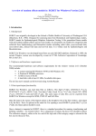
Categorical Variables Codings for 4 categories
4 groups
1
2
3
4
Parameter coding
Linear Quadratic Cubic
-.671
.500
-.224
-.224
-.500
.671
.224
-.500
-.671
.671
.500
.224
Categorical Variables Codings for 6 categories
6 groups
1
2
3
4
5
6
Linear
-.598
-.359
-.120
.120
.359
.598
Parameter coding
Quadratic Cubic 4th order
.546
-.373 .189
-.109
.522
-.567
-.436
.298
.378
-.436
-.298 .378
-.109
-.522 -.567
.546
.373
.189
5th order
-.063
.315
-.630
.630
-.315
.063
As an example we will work with the tutorial dataset and turn standlrt
into 4 ordered categories: this requires 3 cut points; we use the nested means
procedure explained in Section 2.1.4 to get our values. Note that we are
making standlrt into an ordinal variable purely to show the operation of
the orthogonal polynomial feature; if we were really performing some analysis
5
using a continuous variable like standlrt this would not be a recommended
procedure. The nested means when rounded are −0.81, 0.00, and 0.76 and
we use these values to recode the data into 4 groups via the recode → by
range option from the Data manipulation menu:
ˆ
In the Names window, change the name of c11 to be LRTgrps
ˆ
Click on Toggle categorical to change it from a continuous to an ordinal variable (note that the orthogonal polynomial facility can only
be accessed when the variable has been predefined as categorical)
For purposes of comparison we begin with the 4 groups included in the model
in the usual way for categorical variables i.e. as a constant and three contrasted dummies. We will then go on to see whether we can fit a more
parsimonious model using orthogonal polynomials.
Start by setting up the model as follows:
ˆ
Click on Add Term
ˆ
From the variable drop-down list select LRTgrps
6
ˆ
From the ref cat drop-down list select LRTgrps 1
ˆ
Click Done
We now fit a model with LRTgrps entered as an orthogonal polynomial
instead of as three dummies. We start by including all three terms of the
orthogonal polynomial. First, though, we need to change the tolerance used
by MLwiN. The tolerance is set by default to a value which is most appropriate for the most commonly used kinds of estimation. However, using this
value of the tolerance when working with orthogonal polynomials can lead to
the wrong values being calculated for the terms of the polynomial, which in
turn leads to incorrect estimates for the coefficients. This is particularly true
when the categorical variable has a larger number of categories. To change
the tolerance,
ˆ
From the Data Manipulation window, select Command interface
ˆ
In the Command interface window, type CTOL 10
The tolerance is now set to a value of 1010 . This should be sufficient in most
cases. The default tolerance that MLwiN normally uses is 106 and the tolerance can be set back to this value by typing CTOL 6 in the Command
interface window. This should be done after working with orthogonal polynomials as using a tolerance of 1010 can cause problems in other areas.
We can now proceed to set up the model
ˆ
Click on any of the three LRTgrps dummies
ˆ
Click on the Delete Term button
ˆ
Click Yes
ˆ
Click on the Add Term button
7
ˆ
Select LRTgrps from the variable drop-down list
ˆ
Tick the orthogonal polynomial box
ˆ
From the orthog poly degree drop-down list select 3 (note that the
greatest degree that the software will allow you to specify is always
one less than the number of categories)
ˆ
Click Done
Three new variables containing the appropriate values are automatically generated as appropriately named columns in the worksheet and added to the
model:
At this point the model is equivalent to our first model with LRTgrps entered as dummies: it has the same deviance and the estimates for the random
part are identical, although the coefficients are different because the terms
of the polynomial are measured on a different scale to the dummies and the
intercept now has a different value because it is the average value of the response when all three terms of the polynomial are 0, not the average value
of the response for the reference category of LRTgrps. We can see in the
graph below that these two models give us the same results.
The important difference is that the four group model is not readily reducible
whereas the orthogonal polynomial one is. The three terms all have the same
mean and variance so their coefficients are directly comparable and so it is
clear from the estimates that the linear effect is markedly bigger than the
quadratic and cubic, thereby suggesting that the model be simplified to have
8
just a linear trend across all four ordered categories. We fit a model using
just a linear effect:
ˆ
Click on any of the terms of the orthogonal polynomial
ˆ
Click Modify Term
ˆ
Select 1 from the orthog poly degree drop-down list
ˆ
Click Done
The graph shows that the linear trend model well captures the underlying
trend in a parsimonious way. We have thus succeeded in simplifying our
model without losing much information.
1.2.2
Using orthogonal polynomials with repeated measures data
Orthogonal polynomials are especially useful with repeated measures data
and fitting a more parsimonious model is not the only reason to use them.
Hedeker and Gibbons (2006)(3) give the following reasons to use orthogonal
polynomials in their discussion of growth curves for longitudinal data where
the predictor representing time is not a continuous variable but 1, 2, 3 etc
representing the first, second and third occasion on which the person has
been measured:
ˆ
for balanced data, and compound symmetry structure (that is a variance components model), estimates of polynomial fixed effects (e.g.
9
constant and linear) do not change when higher-order polynomial terms
(e.g. quadratic and cubic) are added to the model
ˆ
using the original scale, it gets increasingly difficult to estimate higherdegree non-orthogonal polynomial terms
ˆ
using orthogonal polynomials avoids high correlation between estimates
(which can cause estimation problems)
ˆ
using orthogonal polynomials provides comparison of the ‘importance’
of different polynomials, as the new terms are put on the same standardized (unit) scale. This holds exactly when the number of observations at each timepoint are equal, and approximately so when they are
unequal.
ˆ
the intercept (and intercept-related parameters) represents the grand
mean of the response, that is, the model intercept represents the mean
of the response at the midpoint of time.
Another reason for using them is the orthogonality property: since each pair
of terms in the polynomial are orthogonal, i.e. uncorrelated, the coefficients
of the terms do not change according to which other terms are included.
This means that if we decide that the linear and quadratic effects are the
most important based on the model using all terms and go on to fit a model
including just the linear and quadratic terms, we will not find for example
that now the higher order terms have been removed, the quadratic effect is
no longer important.
As an example of using orthogonal polynomials with repeated measures data,
we will use the reading1 dataset which forms the basis for analysis in Chapter 13 of the User’s Guide. We begin with the variance components model
of page 184 (you will need to follow the instructions on pages 197 to 200 and
202 to get the data in the correct form to set this model up and create a
constant column):
We are going to pretend that we do not know the age at which the reading
score was evaluated but only know that the reading was taken on 1st, 2nd,
10
3rd etc occasion. We can fit a linear trend by putting ‘occasion’ into the
fixed part of the model:
ˆ
In the Names window, highlight occasion and click Toggle categorical
ˆ
Add occasion to the model
The estimate 3.235 gives the mean Reading score at occasion 0 (that is the
occasion before the first measurement!) and the mean reading score improves
by 1.19 for each subsequent occasion. We can now fit a similar model but
replacing occasion by the linear orthogonal variable.
ˆ
Click on occasion
ˆ
Click Delete Term
ˆ
In the Names window, highlight occasion and click Toggle Categorical
ˆ
In the Equations window, click Add Term
ˆ
From the variable drop-down list select occasion
ˆ
Tick the orthogonal polynomial box
ˆ
From the orthog poly degree drop-down list select 1
ˆ
Click Done
11
The deviance and the random part are the same (as is the Wald test for the
growth term), but now the estimate of the intercept gives the grand mean
at the mid-point of the occasions and the slope gives the improvement in
reading with a unit change in the linear orthogonal polynomial. We now
add the quadratic orthogonal polynomial into the model using the Modify
Term option and should find that the linear term does not change (in fact it
does a bit due to imbalance in the data). It is clear that the quadratic term
is of much less ‘importance’ than the linear term.
Using the Predictions and Customised graphs windows we can see the
quadratic growth curve which is characterized by a strong linear trend, with
some slight curvature. We can now add in all the other polynomials (there
is then a term for each occasion) and it is clear that there are ‘diminishing
returns’ as each additional order is included
12
but all terms have some effect: with even the 5th order term having a p value
of 0.002
As in the example using the tutorial dataset, this model which fits an intercept and 5 growth terms is equivalent to fitting a separate parameter for each
occasion; the graph below makes this clear. However we can readily leave
out one or more terms of the orthogonal polynomial to achieve a more parsimonious model; the same is not true of the intercept and dummy variables
specification.
(Note that the way the response has been constructed will have a great effect
on these results; see page 178 of the User’s Guide)
The tolerance should now be set back to the default value before working
further in MLwiN
13
ˆ
1.3
In the Command interface window, type CTOL 6
Commands
The ADDT command has been extended to allow specification of polynomial
terms:
ADDT C <mode N> C <mode N>
Create a main effect or interaction term from a series of one or more variables.
Each variable can be categorical or continuous. Categorical variables can
have a reference category specified, by setting the corresponding mode value
to the number of the reference category. If no reference category is specified,
then the lowest category number is taken as the reference category. If −1 is
given as the reference category then no reference category is assumed and a
full set of dummies are produced. Variables of appropriate names and data
patterns are created and added as explanatory variables. If N > 10000,
then N − 10000 is taken to be the polynomial degree that is required for the
corresponding variable. If the corresponding variable is categorical then an
orthogonal polynomial of degree N − 10000 is fitted.
Examples:
ADDT 'standlrt' 10003 'schgend'
adds an interaction between a cubic in standlrt and 2 dummies for schgend
with reference category mixedsch.
ADDT 'standlrt' 'schgend' 10002
adds an interaction term between ‘standlrt’ and an orthogonal polynomial of
degree 2 for schgend.
The SWAP command edits a main effect and updates all affected interactions
SWAP main effect C with C mode N
14
Mode N has the same meaning as in the ADDT command.
Examples:
SWAP 'standlrt' 'standlrt' 10003
removes standlrt as a main effect and all interactions involving standlrt
from the model and replaces them with a cubic polynomial in standlrt;
note all interactions involving standlrt are also replaced.
Note that the SWAP command will not do anything if the variable you ask
to swap is only present in an interaction term.
The CENT command controls centring for continuous explanatory variables
CENT
CENT
CENT
CENT
mode
mode
mode
mode
0:
1:
2:
3:
uncentred
around grand mean
around means of groups defined by codes in C
around value N
Examples:
CENT 2 'school'
ADDT 'standlrt'
adds the variable standlrt to the model centered around the group mean of
standlrt, where groups are defined by the codes in the column ‘school’
CENT 0
ADDT ‘standlrt'
adds standlrt to the model with no centring.
The default for CENT is no centring: if ADDT is used without CENT having
been previously used, then the term is added with no centring. The kind of
centring set up by use of the CENT command remains in place until the
CENT command is used again to change it: it is not necessary to use the
CENT command before every ADDT if the same kind of centring is required
in each case.
15
2
2.1
Out of Sample predictions
Continuous responses
The current Predictions window generates a predicted value of the response
for each level 1 unit in the dataset, using their values of the explanatory
variables. Thus, predictions are only generated for the combinations of values
of the explanatory variables occurring in the dataset. Often, however, we
want to generate predictions for a specific set of explanatory variable values
to best explore a multidimensional model predictions space.
We have added a Customised Predictions window, with an associated
plot window, to aid this task by allowing predictions to be generated for any
desired combinations of explanatory variable values, whether or not these
combinations occur in the dataset. Given the model on the tutorial data
where avslrt is the school mean for standlrt, we can use the old Predictions window to explore this relationship
16
This window applies the specified prediction function to every point in the
dataset and produces a predicted value for each point. If we plot these
predictions, grouped by school, we get
This plot has one line for each school; the line for the jth school is given
by the prediction equation (β̂0 + β̂2 avslrtj ) + (β̂1 + β̂3 avslrtj )standlrtij .
However, it might be more revealing to plot lines for a small number of
different values of avslrt, say {-0.5, 0, 0.5}
The Customised predictions window will now do this and other such
prediction tasks automatically for us.
ˆ
Select Customised Predictions from the Model menu.
The following screen appears:
17
Main effects are listed in the setup pane. We can click on them and specify
a set of values we want to make a prediction dataset for.
ˆ
Highlight standlrt
ˆ
Click Change Range
We see:
18
Currently the value is set to the mean of standlrt. We can specify a set
of values for the predictor variables for which we want to make predictions.
We can do this for continuous variables as a set of Values, as a Range, as
Percentiles, or Nested Means Here we use a range, postponing discussion
of the other options until later.
Note that, whether we specify values as a set of values, as a range, as percentiles, or as nested means, we are setting values for the original predictor
variable. If for example we have centred the variable using one of the options in the Specify Term window, or via the CENT and ADDT commands,
then we specify values for the uncentred variable, not for the centred variable.
The same applies for other transformations such as polynomials, as long as
the transformation was carried out as part of entering the variable into the
model, via the Specify Term window or the ADDT command. MLwiN will
display the name of the original, untransformed variable in the Customised
predictions and will apply the necessary transformation to produce transformed values to use in calculating the prediction. This behaviour makes
it easier for the user to specify a range of values and also enables plotting
predictions against the original rather than the transformed variable.
2.1.1
Setting values as a range
The output column is set by default to the next free column (c13 in this case)
ˆ
Click the Range tab and specify Upper Bound: 3, Lower: −3,
Increment: 1
ˆ
Click the Done button to close the Values to include window
ˆ
Using the same procedure, set the range for avslrt to be Upper
Bound: 0.5, Lower: −0.5, Increment: 0.5
ˆ
Click Fill Grid and Predict
ˆ
Select the Predictions tab
The Fill Grid button creates a mini dataset with all combinations of the
explanatory variable values you have specified. The Predict button takes
the estimates for the parameters of the current model and applies them to
the mini dataset to create predicted values with confidence intervals.
19
The columns in this prediction grid have all been created as columns in the
worksheet. The columns at the left (cons.pred, standlrt.pred, avslrt.pred)
contain the values of the explanatory variables that we specified and requested predictions for; mean.pred contains the predicted value of the response for each combination of explanatory variable values, and mean.low.pred
and mean.high.pred contain the lower and upper bounds respectively of the
confidence intervals for the predictions.
We can plot these results :
ˆ
Click Plot Grid
This screen has been designed to help construct plots from a multidimensional
grid. Here we want
X: standlrt.pred
Y: mean.pred
Grouped by avslrt.pred
that is,
20
ˆ
Click Apply
The settings for this plot are held in Display 1 of Customised graphs.
We can look at the differences (and the confidence intervals of the differences)
from any reference group. For example if we wanted to look at the above
plot as differences from avslrt.pred = −0.5, then we would
ˆ
Select the Customised predictions window
ˆ
Tick the Differences checkbox (click the Setup tab first if necessary)
ˆ
In the from variable drop-down list select avslrt
ˆ
In the box labelled Reference value type −0.5
ˆ
Click Predict
The graph will update automatically to look like this:
21
If we want to put confidence intervals around these differences then, in the
Customised prediction plot window:
ˆ
Tick the 95% confidence interval check box
Options appear allowing the confidence intervals to be drawn as bars or lines,
with lines as the default.
ˆ
Click Apply
ˆ
Click the OK button on the warning message which may appear
to produce:
We now discuss the other possibilities for specifying the values of the explanatory variables for which you want predictions.
22
2.1.2
Specification using the Values tab
ˆ
Return to the Customised Predictions window
ˆ
Highlight standlrt and click the Change Range button
ˆ
Click the Values tab
ˆ
In the top pane type −2 and click the Add button
ˆ
Add the values 0 and 3 in the same way
ˆ
Click Done
Clicking Fill Grid and Predict in the Customised Predictions window
will now produce predictions as before but this time taking {−2, 0, 3} as the
set of values for standlrt instead of {−3, −2, −1, 0, 1, 2, 3}. Notice that
using the Values tab automatically cleared the values previously specified
using the Range tab.
Note also that the software will automatically check whether the values you
specify are within the range of the variable and an error message will appear
if you try to specify a value outside of this range.
2.1.3
Specification using the Percentiles tab
ˆ
Highlight standlrt and click the Change Range button
ˆ
Click the Percentiles tab
ˆ
In the top pane type 10 and click the Add button
ˆ
Add the percentiles 50 and 90 in the same way
ˆ
Click Done
The set of values for standlrt that will be used if Fill Grid and Predict
are pressed is now (to 2 d.p.) {−1.28, 0.04, 1.28}. These are the 10th, the
50th and the 90th percentile of standlrt respectively. Again, notice that the
previously specified values have been automatically removed.
Percentiles are a useful way of specifying values when we would like, for
example, a prediction for those with a ‘low’ value of standlrt, those with a
‘mid’ value of standlrt, and those with a ‘high’ value of standlrt because
they provide a convenient way of deciding what counts as ‘low’, ‘mid’ and
‘high’, although there is still some subjectivity involved: in this case we
could equally well have decided to use, for example, the 25th, 50th and 75th
percentiles, which would give less extreme values for ‘low’ and ‘high’.
23
We need not necessarily use three percentiles; we can specify as many as we
like, though generally a small number of percentiles will be quite sufficient
for what we want here.
2.1.4
Specification using the Nested Means tab
Nested means are another way of dividing a numerical variable into groups;
again they provide a convenient means of choosing, for example, a ‘low’, a
‘mid’ and a ‘high’ value (if you use 4 groups). Simply put, a set of nested
means which divides the values into 4 groups is doing the same thing as
quartiles (i.e. the 25th, 50th and 75th percentiles) but using the mean instead
of the median. For quartiles, the 2nd quartile (or 50th percentile) is the
median of the variable. The 1st quartile (or 25th percentile) is the median of
the values between the minimum and the 2nd quartile, and the 3rd quartile
(or 75th percentile) is the median of the values between the 2nd quartile and
the maximum. In the same way, to get four groups using nested means we
first calculate the mean of the variable and call this MidMean, then calculate
the mean of the values between the minimum and MidMean and call this
LowMean, and calculate the mean of the values between MidMean and the
maximum and call this HighMean; LowMean, MidMean and HighMean are
then the divisions between our four groups.
More generally, a frequency distribution is balanced about its mean, and this
forms an obvious point of division to give two groups; each of these classes
may be subdivided at its own mean; and so on, giving 2, 4, 8, 16, . . . , classes.
Evans (1977)(1) claims this approach has desirable ‘adaptive’ properties
“Since means minimize second moments (sums of squared deviations), they
are the balancing points of the part of the scale which they subdivide, with
respect to both magnitude and frequency. Class intervals thus defined are
narrow in the modal parts of a frequency distribution and broad in the tails.
Extreme values are not allowed to dominate, but they do influence the positions of means of various orders so that the less closely spaced the values in a
given magnitude range, the broader the classes. For a rectangular frequency
distribution, nested means approximate the equal-interval or percentile solutions; for a normal one, they approximate a standard deviation basis; and for
a J-shaped, a geometric progression. Hence nested means provide the most
robust, generally applicable, replicable yet inflexible class interval system.”
To specify values using the Nested Means tab,
ˆ
Highlight standlrt and click the Change Range button
ˆ
Click the Nested Means tab
ˆ
To get 4 groups, specify 1 level of nesting
24
ˆ
Click Done
The three values that will be used for standlrt in predictions are now the cut
points of the four groups: the overall mean, the mean of values between the
minimum and the overall mean, and the mean of values between the overall
mean and the maximum.
We could also have obtained 7 values (the cut points of 8 groups) by specifying 2 levels of nesting, or 15 values (the cut points of 16 groups) by specifying
3 levels of nesting, and so on.
2.1.5
Specifying values for categorical variables
Let’s set up a model with categorical predictors. This can be done in the
Equations window or via commands in the Command Interface window. First
let us recode the variable girl:
ˆ
In the Names window, select girl and click the Edit name button
ˆ
Change the name of girl to ‘gender’
ˆ
Click the Toggle Categorical button
ˆ
Click the View button in the categories section
ˆ
Change the names of the categories from gender 0 to ‘boy’ and from
gender 1 to ‘girl’
ˆ
Click OK to close the Set category names window
We will use as our predictors gender and vrband, which is a categorised
prior ability measure on pupils (vb1 = high, vb2 = mid, vb3 = low). Type
the commands in the left hand column of the table below in the Command
interface window
Command
CLEAR
IDEN 1 'student' 2 'school'
RESP 'normexam'
EXPL 1 'cons' 'gender'
'vrband'
ADDT 'gender' 'vrband'
SETV 2 'cons'
SETV 1 'cons'
STAR 1
Explanation
clear the current model
declare multilevel structure
declare response variable
specify explanatory variables
add interaction term
specify random intercept at level 2
specify constant variance at level 1
estimate model updating GUI
25
Note that the command STAR 1 has the same effect as pressing the Start
button at the top left of the screen. This will produce the following results
in the Equations window
ˆ
Open the Customised predictions window
A message appears at the top of the window:
“Prediction is out of date, specification disabled until it is cleared”
This is because the current prediction grid refers to a previous model. Indeed
looking at the list of explanatory variables in the Customised predictions
window, you will see the variables standlrt and avslrt listed. When the
main effects in a model are altered the prediction grid is flagged as being out
of date. To proceed with a prediction for the new model we must clear the
current prediction grid specification
ˆ
Press the Clear button in the Customised predictions window
This will clear any columns or graphs referred to by the prediction grid and
set the prediction grid to refer to the current model. You will now see that
the list of explanatory variables in the Customised predictions window is
up to date. In the Customised predictions window:
ˆ
Highlight gender
ˆ
Click Change Range
ˆ
Select Category
ˆ
Select boy and girl in the Values to include list
ˆ
Click Done
ˆ
Highlight vrband in the Customised predictions window
ˆ
Click Change Range
ˆ
Click Category
26
ˆ
Select vb1, vb2 and vb3
ˆ
Click Done
ˆ
Click the Fill Grid and Predict buttons in the Customised predictions window
ˆ
Select the Predictions tab in the Customised predictions window
This shows us the predicted values and confidence intervals for the 6 combinations of gender and vrband
Note that, because simulation is used to calculate these values, these numbers
may be slightly different every time.
Plotting this out using the Customised prediction plot window filled in
as follows:
gives this:
27
This shows girls doing uniformly better than boys across all 3 levels of vrband. Recall that vrband is a categorised prior ability measure on pupils
(vb1 = high, vb2 = mid, vb3 = low). The default choice for displaying data
against a categorical x variable is to plot the data as bars. We can change
this or other characteristics of the plots produced by the Customised prediction plot window by editing the Customised graph window for the
appropriate graph display. For example, suppose we wanted to draw the
above relationship using line + point instead of bars. Then
ˆ
Select Customised Graph(s) from the Graphs menu
ˆ
Select line + point from the drop-down list labelled plot type
ˆ
Click Apply
This produces:
Both these graphs show girls outperforming boys at all three levels of vrband. Looking at the graphs (and noting in which cases the error bars
overlap) it might appear that this gender difference is significant for vb3
28
children, but not for children in vb2 and vb1. However, care is needed
here. The graphs are showing 95% confidence intervals around the predicted
means for each of the 6 groups. If we are interested in making inferences
about how the gender difference changes as a function of vrband, we must
request confidence intervals for these differences:
ˆ
Select the Customised predictions window
ˆ
Tick the Differences checkbox
ˆ
In the from variable drop-down list select gender
ˆ
In the Reference value drop-down list select boy
ˆ
Click Predict
The graph will update
which shows that the 95% confidence intervals for the gender differences do
not overlap zero for vb1, vb2 or vb3, and thus there is a significant gender
difference for each of the three categories of vrband.
2.1.6
Commands for building customised predictions for Normal
response models
PGDE : clears the current prediction grid — it should be used before constructing a new prediction grid
PGRI constructs a prediction grid:
PGRI {Continuous C contmode = N, contmode values N..N}
{categorical C catmode N, catmode N..N} Outputcols C..C
29
contmode N
=
=
=
=
0
1
2
3
list of values: N..N
range: upper bound N, lower N, increment N
centiles: N..N
nested means: level of nesting N
catmode N
= 1 category numbers N . . . N
= 2 all categories
Example:
PGRId 'cons' 0 1 'standlrt' 1 3 -3 1 'schgend' 2 C22 C23
C24
PREG calculates predictions for the prediction grid currently set up.
For Normal response models:
PREG confidence interval N mean C lower C upper C, differences N
(differences for column C, differences from category N), multivariate N
(respcol C), coverages {level N coverage range N low C up C} . . .
Examples:
(1)
PREG 95 mean c100 lower c101 upper c102, difference 0,
multivariate 0
Given PGRID established as above, predicted mean +/- 95 percentile output
to c100 c101 c102, no differences selected
(2)
PREG 95 mean c100 lower c101 upper c102, difference 0,
multivariate 1 'normexam'
Given PGRID established for a multivariate response model, performs same
task as example (1) above; predictions are for the response ‘normexam’.
30
(Note that we describe later how to make predictions for multivariate models
using the customised predictions window).
(3)
PREG 95 mean c100 lower c101 upper c102, difference 1
'schgend' 1, multivariate 1 'normexam'
As (2) above but predictions are differenced from schgend category 1
(4)
PREG 95 mean c100 lower c101 upper c102, difference 1
'schgend' 1, multivariate 1 'normexam' 2 99 c103 c104
As (3) above but also calculate 99% coverage for predictions based on level
2 variance; lower and upper coverage values to c103 and c104
2.1.7
Commands for plotting customised predictions
The PLTPrediction command is used for displaying predictions and performs
the same task as the Customised prediction plot window; though it can
also be used more generally to plot data other than predictions since it just
plots one column against another, with confidence intervals if supplied, with
the options to plot the data by groups and to split the plot into two separate
graphs (horizontally or vertically), with data plotted on one graph or the
other according to values of a supplied variable:
PLTPrediction in graph display N, dataset (X,Y),
0 (do nothing) or grouped by values in C,
0 (do nothing) or split into separate graphs across rows of a trellis according to values in C,
0 (do nothing) or split into separate graphs across columns of a trellis
according to values in C,
{confidence intervals: lower in C, upper in C, plot style 10=bar, 11=line}
Note that if you do not already have the graph display window open then
you will need to go to the Customised graph window and click Apply
after entering the command.
Examples:
(1)
31
PLPT 2 c1 c2 0 0 0 c3 c4 11
Sets up graph display 2: x = c1 y = c2, lower and upper confidence intervals
are in c3 and c4, plot confidence intervals as lines
(2)
PLPT 2 c1 c2 ‘social class' 0 0
Sets up graph display 2: x = c1 y = c2, one line for each social class, don’t
display confidence intervals
(3)
PLPT 2 c1 c2 'social class.pred' 'gender.pred' 0 c3 c4 11
Sets up graph display 2: x = c1 y = c2, one line for each social class, repeat
plot in a 2 x 1 graph trellis for gender = 0 in first pane and gender = 1
in second pane (i.e. split into two plots arranged vertically, with the upper
plot including data points for which gender = 0 and the lower plot including
data points for which gender = 1), lower and upper confidence intervals are
in c3 and c4, plot confidence intervals as lines
2.2
2.2.1
Binomial models
Predicting mean and median
To give ourselves a binary response variable so we can demonstrate prediction
for binomial models, let’s create a dichotomised variable from the Normalised
response in the tutorial dataset. Responses with a value of greater than or
equal to 1.5 we will set to 1 otherwise we will set the dichotomised variable
to 0. To do this, type in the Command interface window
calc c11 = 'normexam' >= 1.5
name c11 'pass'
Now set up the following multilevel binomial model and estimate the model
with the non-linear options set to 2nd order PQL estimation :
32
The Customised predictions window now looks like this:
The Customised predictions window for binomial response models looks
similar to that for Normal response models. However there are a few changes.
You can choose whether predictions should be made on the logit or probability scales and also you can ask for these predictions to be for the mean or
median value of the prediction distribution.
What does prediction distribution mean? This data is based on 65 schools.
The level 2 variance of 1.596 on the logit scale is the between school variance,
33
in the population from which our schools are sampled, of the school means
(on the logit scale). Suppose we now ask the question of what the mean
and median pass rates are on the probabilty scale, for pupils attending three
schools (of identical size) with values of u0j = {−2, 0, 2}. This is a school
from either end and the middle of the distribution of schools. We obtain
pk , the pass rate on the probability scale, for each school k by taking the
antilogit of the model equation −3.18 + u0k (putting in the appropriate value
for u0k )
pk = {antilogit(−3.18 − 2), antilogit(−3.18), antilogit(−3.18 + 2)}
= {0.006, 0.040, 0.234}
mean(pk ) = 0.093
median(pk ) = 0.040
The thing to note is that if we take the antilogit of the mean of our three
logit values, that is antilogit(−3.18) = 0.040, this is equal to the median of
our three probabilities but not the mean of the three probabilities (0.0918).
This is because in this case before we take antilogits the mean of our three
values equals the median, and the median of the antilogits of a set of values
is always equal to the antilogit of the median of the set of values. The mean
of the antilogits of a set of values on the other hand will in general not be
equal to the antilogit of the mean of the set of values.
This comes about because of the non-linearity of the logit transformation as
we can see from the graph below, which graphs logit(p) and places our three
schools as the points marked by triangles on the line.
When we fit a multilevel model and take the antilogit of a fixed part predictor
(i.e. a sum of fixed part coefficients multiplied by particular values of their
associated explanatory variables), this gives us the median (not the mean)
probability for the prediction case consisting of those values of the explanatory variables. Again, this is because before we take antilogits, median =
34
mean (since we are dealing with a normal distribution), and antilogit(median)
= median(antilogits). From the above multilevel model we get a prediction
of −3.18 on the logit scale which corresponds to a median probability of
passing of 0.040. We may however want to know what the mean probability
is of passing, not taking account of only three schools, but allowing for the
whole distribution of schools. The mean cannot be directly calculated from
the model in the same way that the median can; but we can estimate it using
simulation. We know that the distribution of all schools on the logit scale is
N(−3.183, 1.5960.5 ). Thus the following will give us an estimate of the mean
pass rate
1. Simulate the value on the logit scale for a large number of schools, say
1000, from the distribution N(−3.183, 1.5960.5 ). That is:
Zj = N(−3.183, 1.5960.5 ),
j = 1, . . . , 1000
2. Calculate the predicted probability for each of our 1000 schools and
calculate their mean. That is, antilogit(Zj ).
We can do this in MLwiN using the following commands (click the Output
button on the Command interface window before typing them in order to
properly see the output at the end)
Command
seed 8
nran 1000 c100
calc
c100=c100*1.596^0.5-3.183
calc c101=alog(c100)
aver c101
Explanation
set random number seed (so we can
replicate our results)
pick 1000 values from N(0,1)
transform to N(−3.183, 1.5960.5 )
generate 1000 probabilities
calculate their mean
This produces an estimate of the mean pass rate as 0.072. In this example
our prediction case is very simple, it is simply the unconditional mean pass
rate (i.e. the mean pass rate taking no explanatory variables into account);
if we calculate that directly (by taking the mean of the variable pass) we get
a value of 0.070, so we can see our estimate is very good. In more complex
conditional predictions, for example the mean pass rate for girls with intake
scores of 1 in girls’ schools, we may have very few (or in fact no) individuals
exactly fitting our prediction case and a reasonable empirical estimate of the
mean for that prediction group is not available. However, the model based
estimate is available.
All the predictions and confidence intervals calculated with the out of sample predictions window are derived by simulation, in a similar fashion to the
35
example we just typed in the commands for. The detailed simulation algorithms for a range of model types are given in Appendix 1 of this document.
These median and mean predictions are often referred to as cluster specific
and population average predictions respectively. Instead of typing in the
above commands, we can obtain these simply using the Customised predictions window:
ˆ
Select Probabilities
ˆ
Check boxes to request predicted Medians and Means
ˆ
Click Fill Grid
ˆ
Click Predict
ˆ
Select the Predictions tab
We see that the median (‘median.pred’) and mean (‘mean.pred’) predictions
are as expected. Note that these results are from simulation algorithms where
we have drawn a particular number of simulated values.
If you click on the Setup panel in the Customised predictions window
you will see
#
#
#
#
predicted cases: 1
draws from cov(Beta) 2000
nested draws from cov(u) 1000
simulations 2000000
The number of predicted cases is 1 because we are predicting for the unconditional mean only. When we typed in commands to estimate the mean
probability and generated 1000 draws from N(−3.183, 1.5960.5 ), we always
used the same value for β̂0 of -3.183. In fact, s.e.(β̂0 ) = 0.189 and the full
simulation procedure as implemented by the Customised predictions window
is as follows
1. Simulate K= 2000 values of
β0k ∼ N(−3.183, 0.1890.5 ), k = 1 : K
2. For each value of β0k simulate j = 1000 values of
β0kj ∼ N(β0k , 0.1890.5 ), j = 1 : J
36
3. Then let pkj = antilogit(β0kj ) and for each value of k calculate pk =
J
P
1
pkj
J
j=1
4. Finally we calculate the mean probability as p =
1
K
K
P
pk
k=1
This actually involves K × J = 2000000 simulation draws and the results in
this case are identical to the simplified procedure where we typed in commands and assumed a fixed value for β̂0 .
2.2.2
Predictions for more complex Binomial response models
Let’s fit a model where the probability of passing is a function of pupil
intake score (standlrt), peer group ability (avslrt) and an interaction of
pupil intake score and peer group ability. Note the interaction effect between
avslrt and standlrt is not significant; we leave it in the model for the purposes
of demonstrating the graphing of interactions, particularly for log odds ratios
in the next section.
In the Customised predictions window, set
ˆ
standlrt = range {3, −3, 0.25} (note we will use this notation from
now on for convenience; it means ‘define the values of standlrt using
the Range tab; set Upper Bound = 3, Lower = −3, Increment =
0.25’)
ˆ
avslrt = values {0.5, −0.5}
ˆ
Select Median predictions
ˆ
Select predictions for Probabilities
37
ˆ
Click Fill grid
ˆ
Click Predict
ˆ
Click Plot grid
In the Customised prediction plot window
ˆ
Select Y: median.pred
ˆ
Select X: standlrt.pred
ˆ
Select Grouped by: avslrt.pred
ˆ
Click Apply
Which produces:
The graph shows how the probability of passing increases as pupil intake
ability increases, with the increase being stronger for those in high ability
peer groups. We now explore the differences between low and high ability
peer groups as functions of standlrt and assess if and where those differences
are significant. In the Customised predictions window
ˆ
Select Differences; from variable: avslrt Reference value: −0.5
ˆ
Press the Predict button
In the Customised prediction plots window
ˆ
Select 95% confidence interval:
ˆ
Click Apply
38
We can see that after standlrt scores become greater than around −0.5, the
probability of passing for those in the high ability group becomes significantly
different from the low ability group.
2.2.3
Log Odds ratios
Return to the Customised predictions window
ˆ
Select logit
ˆ
Click Predict
The variable standlrt.pred contains the requested values range {−3, 3,
0.25}. The graph plots
odds passing|avslrt.pred = 0.5, standlrt.predi
log
,
odds passing|avslrt.pred = −0.5, standlrt.predi
standlrt.predi = {−3, −2.75, . . . , 3}
that is, the log odds ratio of passing for high versus low peer groups as a
function of pupil intake score. We may want to view the graph as odds
ratios, rather than log odds ratios. Looking at the Names window we see
that the log odds ratio and its upper and lower bounds are in the columns
named median.pred, median.low.pred and median.high.pred, that is
c18-c20. To create a graph of odds ratios type the command
39
expo 'median.pred' 'median.low.pred' 'median.high.pred'
'median.pred' 'median.low.pred' 'median.high.pred'
A message will appear asking if you want to clear the prediction grid; click
”No”.
2.2.4
Customised prediction commands for discrete response models
PREG confidence interval N,
predict mean values N (mean values output set C lower C upper C),
predict median values N (median C lower C upper C)
prediction scale N,
differences N (diffcol C, diff reference C)
multivariate N (respcol C)
coverages {level N coverage range N low C up C} ..
This is an extension of the PREG command for Normal responses. The
differences are
predict mean values N=
0: no mean value output set to follow
1: mean value output set required
(mean value output set: mean to C, lower confidence interval for mean
to C, upper confidence interval for mean to C)
predict median values N =
0: no median value output set to follow
1: median value output set required
(median value output set: median to C, lower confidence intervals for
median, upper confidence intervals for median)
40
Prediction scale N =
0: for raw response scale
2: for link function attached to model
Note raw response scale is probability (binomial, multinomial models) or
counts (negative binomial, Poisson models)
Examples
(1)
PREG 95 0 1 c100 c101 c102 0 0 0
If we have a binary response model set up, then the above command evaluates
the current PGRID, calculating median (i.e. cluster specific) predictions on
the probability scale, and writes the predicted medians and their lower and
upper 95% confidence intervals to c100, c101, c102
(2)
PREG 95 0 1 c100 c101 c102 1 'schgend' 1 0 0
As (1) above but predictions are differenced from schgend category 1
2.3
2.3.1
Multinomial models
Unordered Multinomial Models
We will take the contraception dataset used in Chapter 10 of the User’s
Guide:
ˆ
Open bang.ws
ˆ
Select the variable use4 in the Names window
ˆ
Click the View button in the categories section
Set the 4 categories to be :
41
Let’s use the Command interface window to set up a multinomial model,
where the log odds of using different types of contraception compared with
no contraception are allowed to vary as a function of age.
Command
MNOM 0 'use4' c13 c14 4
NAME c13 'resp' c14
'resp cat'
IDEN 1 'resp cat' 2 'woman'
3 'district'
ADDT 'cons'
ADDT 'age'
SETV 3 'cons.ster'
'cons.mod' 'cons.trad'
DOFFs 1 'cons'
LINEarise 1 2
Explanation
the reference category is 4- none
specify level IDs
add 3 intercepts — one for each log
odds ratio
add 3 age coefficients — one for each
log odds ratio
specify random intercepts across districts
specify denominator
select PQL order 2
Running this model gives:
42
In the Customised predictions window :
ˆ
Set age to range {19, −14, 1}
ˆ
Select Probabilities
ˆ
Select Medians
ˆ
Click the Fill grid, Predict and Plot Grid buttons
In the Customised prediction plot window
ˆ
Select Y: median.pred, X: age.pred, Grouped by: use4.pred
ˆ
Click Apply
which produces
43
or with error lines
Let’s elaborate the model adding number of children (lc) and an lc*age
interaction:
ADDT 'lc'
ADDT 'lc' 'age'
Running this model produces:
44
Let’s now set up a prediction to explore the interactions between age (old and
young mothers), number of children and the probabilities of using different
methods of contraception. In the Customised predictions window make
the following specifications:
ˆ
use4: all categories
ˆ
age: Values (10, −10) (note you will have to remove the mean value
of −0.3278697)
ˆ
lc: select all categories
ˆ
Select Probabilities
ˆ
Select Medians
ˆ
Click the Fill grid, Predict and Plot Grid buttons
and then set plot up as follows
ˆ
Select Y: median.pred, X: lc.pred,
ˆ
Select Grouped by: use4.pred
ˆ
Select Trellis X: age.pred
ˆ
Select 95% confidence intervals
ˆ
Select Error bars
45
ˆ
Click Apply
This produces:
This graph shows that across ages (top graph panel = young, bottom graph
panel = old) and parities (that is, number of children) the most prevelent
contraceptive behaviour is to use no contraception at all. However, some
interesting trends can be observed — for example, the probability of using
no contaception is highest for women with no children. For both young and
old women once they have had one child the probability of using some form of
active contraception increases. For young women the pattern is more striking
and the preferred method of active contraception for young women is modern
contraception. Active contraceptive use is strongest for young women with
3 or more children.
We may wish to explore whether differences from a particular reference group
are statistically significant. For example, we may wish to choose women with
no children as a reference group and evaluate:
p(usage = ster|lc = lc1, age = −10) − p(usage = ster|lc = lc0, age = −10)
..
.
p(usage = ster|lc = lc3, age = −10) − p(usage = ster|lc = lc0, age = −10)
That is, see how the difference from women with no children changes as a
function of age, usage type and number of children. In the Customised
predictions window:
46
ˆ
Select Differences; from variable: lc; Reference value: lc0
ˆ
Click the Predict button
The graph display will update to:
Remember each bar represents the difference of a probability of usage for a
specified method, age and number of children from the same method and
age with number of children = 0. So all the bars corresponding to number
of children = 0 disappear since we are subtracting a probability of usage for
a particular combination of explanatory values from itself.
Let’s look at the 4 bars for the 4 usage types at number of kids = 1, age
= −10. That is, young women with one child. This is the leftmost cluster of
bars in the top graph panel which corresponds to prediction cases 5-8 in the
Predictions tab of the Customised predictions window.
47
We see from row 8 of the above table (under median.pred) that
p(method = none|lc = lc1, age = −10)
−p(method = none|lc = lc0, age = −10) = −0.162
That is, the probability that young women with one child used no contraception is 0.162 less than young women with no children. Once young women
have had a child they are more likely to use some active form of contraception. We can see which form of contraception these young women switch
to by looking at rows 5–7 of the prediction table. We thus discover that
0.162 = 0.034(ster) + 0.097(mod) + 0.033(trad). Note that there is a tiny
discrepancy in this equality due to rounding error.
We can carry out the same prediction on the logit scale and get log odds
ratios. In the Customised predictions window
ˆ
Select logit
ˆ
Click Predict
Now the leftmost mid grey (blue on your screen) bar in the upper graph
panel represents the log odds ratio
p(usage = ster|age = −10, lc = lc1)/p(usage = none|age = −10, lc = lc1)
log
p(usage = ster|age = −10, lc = lc0)/p(usage = none|age = −10, lc = lc0)
We get a log odds ratio (as opposed to a logit) because in our prediction we
asked for logits to be differenced from lc = lc0.
48
2.3.2
Ordered Multinomial
We will take the A-level dataset used in Chapter 11 of the User’s Guide:
ˆ
Retrieve alevchem.ws
Let’s set up a basic model using the following commands:
Command
MNOM 1 'a-point'c10 c11 6
NAME c10 'resp'c11
'respcat'
IDEN 1 'respcat' 2 'pupil'
3 'estab'
ADDT 'CONS'
RPAT 1 1 1 1 1
ADDT 'cons'
SETV 3 'cons.12345'
FPAR 0 'cons.12345'
DOFFs 1 'cons'
LINEarise 1 2
Explanation
note the reference category is 6, <= A
specify level IDs
add a different intercept for each response category
specify that future added terms have
same coefficient for each multinomial
category
add a common intercept for categories
1–5
allow common intercept to vary across
establishments
remove common intercept from fixed
part of the model so it is no longer
overparameterized
specify denominator
select PQL order 2
49
In the Customised predictions window:
ˆ
Set a-point to all categories apart from the reference category A
ˆ
Select Probabilities
ˆ
Select Medians
ˆ
Click the Fill grid and Predict buttons
ˆ
Select the Predictions tab
This prediction gives the cumulative probabilities of passing across the grade
categories
The Differences from functionality, in the Customised predictions window, is not currently implemented for ordered multinomial models.
50
2.4
Poisson models
We will work with the skin cancer dataset used in Chapter 12 of the User’s
Guide.
ˆ
Open the worksheet mmmec.ws
Let’s model malignant melanoma county level death rates as a function of
UVBI exposure, allowing for between region and country variation:
Command
resp 'obs'
iden 1 'county' 2 'region'
3 'nation'
expl 1 'cons' 'uvbi'
rdist 1 1
lfun 3
doffs 1 'exp'
loge 'exp' 'exp'
setv 2 'cons'
setv 3 'cons'
linea 1 2
Explanation
set response to be Poisson
specify log link function
offsets in 'exp'
In the Customised predictions window
ˆ
Set uvbi to range {13,−8, 1}
ˆ
Select Medians and Means
51
ˆ
Click the Fill Grid and Predict buttons
ˆ
Using the Customised graphs window from the Graphs menu,
plot the median and the mean predictions (median.pred and
mean.pred) against UBVI exposure (uvbi.pred)
We see that the mean is uniformly higher than the median. This is due
to the shape of the link function. This difference that we see emphasises
the need to consider the shape of the distribution when reporting results
or making inferences: for example, just as we saw for binomial models, the
mean probability cannot be obtained by taking the exponential of the mean
XB ; and confidence intervals must be found before, not after, transforming
to probabilities via the exponential. This also explains why we won’t expect
the predicted value of, for example, the unconditional mean to exactly match
our observed value.
2.5
Multivariate models
The Customised predictions window can deal with only one response at
a time when a multivariate model is set up. To demonstrate this, let’s create
a binary variable from the exam scores in the tutorial data. We then fit a
multilevel bivariate response model with the original continuous score as the
first response and the dichotomised variable as the second response. Open
the tutorial worksheet and type the following commands
calc c11 = c3 > 1.5
name c11 'pass'
mvar 1 c3 c11
52
expl 1 'cons' 'standlrt'
iden 2 'student' 3 'school'
setv 3 'cons.normexam' 'cons.pass'
setv 2 'cons.normexam'
linea 1 2
rdist 2 0
doffs 2 'cons'
In the Customised prediction window notice in the top right hand corner
the name of the response we are working with, normexam. This means
that any prediction we specify will be applied to the continuous response
normexam only.
ˆ
Set standlrt to range {3,−3, 1}
ˆ
Click Fill Grid, Predict and Plot Grid
ˆ
Set X: standlrt.pred, Y: mean.pred
ˆ
Click Apply
Now let’s make a prediction for the binomial response. In the Customised
predictions window
53
ˆ
Change normexam to pass in the drop-down list on the top right
of the window
ˆ
Click Predict and Plot Grid
ˆ
Set Y: median.pred and Click Apply
54
3
3D Graphics
We have implemented some preliminary 3D graphics in the software. These
are currently implemented as 3 commands:
SURF 3d graph number N, X, Y, Z
SCATt 3d graph number N, X, Y, Z, [group column]
SHOW 3d graph number N
Let’s start by constructing a surface with the Customised predictions window
and then plotting it.
Return to the model
In the Customised Predictions window
ˆ
Set the range for standlrt to be Upper Bound: 3, Lower: −3, Increment: 1
ˆ
Set the range for avslrt to be Upper Bound: 0.5, Lower: −0.5,
Increment: 0.1
ˆ
Click Fill Grid and Predict
Set up the plot using
55
which produces:
To plot this as a surface, in the Command interface window type
surf 1 'standlrt.pred' 'avslrt.pred' 'mean.pred'
show 1
which produces (after rotating the view using the horizontal slider to 80.0 —
see top left of window for current view angle):
56
Right clicking on the graph and selecting
<Plotting Method><Surface with Contouring> produces
The SURF plot requires a rectangular data grid of X, Y values with a Z value
in each cell of the grid. So to plot the function z = 2x3 + 3y for x = {1, 2, 3},
y = {4, 5, 6, 7} we need to first construct
x
1
1
1
1
..
.
y
4
5
6
7
..
.
3
3
3
3
4
5
6
7
then create z from these two columns. This can be done by typing the
following commands into the Command interface window (close the 3d
57
graph display window first)
gene 1 3 1 c100
gene 4 7 1 c101
ucom c100 c101 c102 c103
name c102 'x' c103 'y' c104 'z'
calc 'z'=2*'x'^3+3*'y'
surf 1 'x' 'y' 'z'
show 1
which produces (after right clicking on the graph and selecting <Plotting
Method><Wire Frame>):
Going back to the model we have just fitted:
the intercept and slopes are distributed
u0j
0.074
∼ N (0, Ωu ) ,
Ωu =
θ=
u1j
0.011 0.011
58
The probability density function for this bivariate Normal model where the
means of the two variables are 0 is
p(θ) =
1
1
|Ωu |−1/2 exp(− (θT Ω−1
u θ)
(2π)
2
To calculate and plot this bivariate distribution, close the graph then type:
Command
erase 'z'
join 0.074 0.011 0.011 c100
calc c101 = sym(c100)
gene -0.8 0.8 0.05 c102
gene -0.4 0.4 0.05 c103
ucom c102 c103 c104 c105
name c104 'u0' c105 'u1'
c107 'z'
count 'u1' b1
join 'u0' 'u1' c106
matr c106 b1 2
calc 'z' = 1/(2*3.1416)
* det(c101)^(-0.5) *
expo(-0.5*diag(c106
*.inv(c101) *.(∼c106)))
surf 1 'u0' 'u1' 'z'
show 1
Explanation
create Ωu
fill in (1,2) value of Ωu (omitted in notation because Ωu a symmetric matrix)
generate values for u0j
generate values for u1j
create all combinations of (u0j, u1j )
turn this grid into a b1 by 2 matrix
Apply the Normal PDF to all values
of of (u0j, u1j ) in c106
Selecting <plotting method><surface with contouring> on the graph that
appears produces
The SCATter command can produce 3D scatters. For example,
59
ˆ
Close the 3d graph window
ˆ
In the Command interface window type:
SCAT 1 'avslrt' 'normexam' 'standlrt'
Show 1
We can group the plot by vrband:
ˆ
Close the 3D graph window
ˆ
In the Command interface window type:
SCAT 1 'avslrt' 'normexam' 'standlrt' 'vrband'
show 1
60
4
Model Comparison Tables
MLwiN now has a mechanism for storing the results of a series of models and
displaying them in a single table. This has two main uses. Firstly, it is useful
when conducting an analysis as it enables the user to easily see the results of
a series of models. Secondly, often when writing papers, results from a series
of models are presented in a single table; constructing these tables manually
can be a time consuming and error prone process. To a large extent MLwiN
now automates this process.
Let’s set up a variance components model on the tutorial dataset
ˆ
Open the tutorial worksheet
ˆ
In the Equations window click on y
ˆ
In the y variable window select:
y:
Normexam
N levels: 2
level 2(j): school
level 1(i): student
ˆ
Click done
ˆ
Click on β0 x0
ˆ
Select cons from the drop-down list in the X variable window
ˆ
Tick j(school), i(student)
ˆ
Click Done
Running the model gives:
We can add this model to the stored sequence of models under the name
‘Model 1’ by clicking on the Store button at the bottom of the Equations
window and typing a name for the model in the window which appears, in
this case Model 1. We can view the sequence of stored models (so far only
one model) by selecting Compare stored models from the Model menu.
This produces:
61
Clicking the Copy button will paste a tab-delimited text file into the clipboard.
ˆ
Click the Copy button
In Microsoft Word:
ˆ
Paste the text into a document
ˆ
Highlight the pasted text in Microsoft Word
ˆ
Select the <Table><Insert><Table. . . > menu item
This produces:
62
We can see a list of all models currently stored by selecting Manage stored
models from the Model menu (shown here after storing several more models).
This allows us to select just some of the models to view in a results table,
rather than having to display all of them as we would if we selected Compare
stored models; to delete any or all stored models; or to rename any stored
model. Note that there is no way to bring any of the stored models up again
in the Equations window - if you wish to be able to easily return to working
with a certain model after moving on to another one, you should save the
worksheet (probably under a different name), and then you can return to
that model by returning to that saved worksheet.
The tick-box labelled Include extended MCMC information controls
how much information is displayed for models estimated using MCMC. Regardless of whether this box is ticked or not, when the model is stored, as
well as all the same information that is stored for models estimated using
(R)IGLS, the median of the chain for each parameter, upper and lower ends
of the 95% credible interval, and effective sample size are also stored. This
information is only displayed in the Results Table if the Include extended
MCMC information box is ticked.
Note that neither the Results Table nor the list of stored models will not
refresh automatically when a new model is stored. You will need to close
them and once again select Compare stored models or Manage stored
models from the Model menu for the new model to be included.
Storing and retrieving of model results can also be done using commands.
The formats of the model table commands are
MSTO <S> : store model results as S
for example, entering the command
63
MSTOre 'modela'
appends the current model to the table of models and names the model
‘modela’
MPRI : print stored model results to Output window
MCOM <S> . . . <S> : compare the listed models; compare all if no parameters
for example, entering the command
MCOM 'Model 1' 'modela' 'Model 4'
would create a model table comparing Model 1, modela and Model 4
MERA <S> : erase stored model results for listed models
for example:
MERA 'modela'
erases modela
MWIPe : erase all stored models
Let’s create a macro to run a sequence of models and store each one in a
model comparison table
Command
clear
mwipe
resp 'normexam'
iden 1 'student' 2 'school'
addt 'cons'
setv 2
setv 1
expa 3
estm 2
maxi 1000
batc 1
star 1
Explanation
clear any current model
clear model comparison table
set response
set level IDs
intercept
set variance components
expand terms in Equations window
show estimates in Equations window
set maximum iterations to 1000
do not pause in between iterations
run the variance components model
64
msto
addt
next
msto
'Model 1'
'standlrt'
1
'Model 2'
setv 2
next 1
msto 'Model 3'
store the results
add a slope to the model
run the new model
store the fixed slope variance components model
add a random slope
run the random slopes model
store the random slopes model
Note the START and NEXT commands when called from a macro with
parameter 1 will cause the Equations window to be updated after each
modelling iteration. Sometimes this can result in the software spending too
much time updating the screen and not enough time doing sums. In this
case you may prefer to use the START and NEXT commands with no
added parameter, in which case screens are not updated during macro file
execution. You can however place a PAUSE 1 command at any point in a
macro script which will cause all displayed windows to update themselves.
ˆ
From the File menu select New Macro
ˆ
Type or paste the above command sequence into the macro window
ˆ
Make sure the Equations window is open and visible
ˆ
Click the Execute button at the bottom of the macro window
You should now see the sequence of requested models being executed in the
Equations window. To view the model comparison table, type
mcomp
in the Command interface window or select Compare stored models
from the Model menu. This produces:
65
Suppose we decided to recode a variable, e.g., turning standlrt into a binary
variable. We can recode the variable and reanalyse and the model comparison
table will get reformed.
ˆ
In the Command interface window, type
calc 'standlrt' = 'standlrt' > 0
ˆ
Rerun the analysis macro file
ˆ
In the Command interface window, type
mcomp
which then produces the updated results table:
66
67
5
A new method for estimating autocorrelated errors in continuous time
Previous versions of MLwiN implemented in a set of macro files the algorithms in Goldstein et al. (1994) to estimate models with autocorrelated
errors at level 1. The macros were rather unstable and we removed them in
version 2.02 of MLwiN. We introduce here a simpler method of estimating
these models.
A common use of these models is where we have repeated measures data and
the measurement occasions are close together in time.
Time
The above graph shows a linear time trend fitted to repeated measurements
on one individual. We can see that the residuals around the graph are not
independent. Residuals close together in time show positive correlations; this
correlation decreases as the time distance between measurements increases.
In a multilevel analysis we will have many such lines, one for each individual
in the dataset. In the multilevel case too, the residuals around each person’s
line may show a pattern of non-independence which is a violation of our model
assumptions and could potentially lead to incorrect estimates of parameters.
The covariance between two measurements taken at occasions i1 and i2 on
individual j cannot be assumed to be 0. That is
cov(ei1 j , ei2 j ) 6= 0
We expect this covariance to decrease as the time interval between the measurements increases. Let tij denote the time of the ith measurement on the
jth individual. A natural model for the covariance is
cov(ei1 j , ei2 j ) = α
|ti1 j
1
− ti2 j |
The autocorrelation is then
cor(ei1 j , ei2 j ) =
α |ti
1j
1
−ti2 j |
σe2
(1)
We will use the Oxford boys dataset to illustrate how to fit multilevel time
series models with autocorrelated errors modelled as (1). The Oxford boys
68
dataset contains height measurements on 26 boys each measured on nine
occasions between the ages of 11 and 13.
First we set up a repeated measures model on the oxboys data with no
autocorrelation structure. The data is in the worksheet oxboys.ws. The
following model should already be set up in the Equations window:
To add the term (1) to the model we first construct
δ(i1 ,i2 )j = |ti1 j − ti2 j |
In this dataset we have 26 individuals each with 9 measurements so δ is a
list of 26 symmetric matrices of dimension 9x9. That is


t1,1 − t1,1
t2,1 − t1,1

0




..
..
.
..


.
.
t9,1 − t1,1 t9,1 − t2,1 · · ·
t9,1 − t9,1
..
.


t1,26 − t1,26
t2,26 − t1,26

0




..
..
.
.


.
.
.
t9,26 − t1,26 t9,26 − t2,26 · · · t9,26 − t9,26
The SUBS command can set up such difference matrices (see ‘command
SUBS’ in MLwiN Help for details on how to use this command). In the
Command interface window type
69
subs c1 -1 c2 c2 c10
In this format the command calculates the required 26 symmetric matrices
and stacks them in c10. These matrices can be viewed with the MVIEw
command:
MVIE 'ID' c10
which produces, after clicking the Output button in the Command interface
window:
..
.
Now we form
1
|ti1 j ti2 j |
Command
chan 0 c10 -1 c10
calc c11=1/c10
chan -1 c11 0 c11
Explanation
avoid zero divide
set diagonal back to 0
C10 now contains the required structure to be added to the covariance matrix
automatically specified by the multilevel model
cov(ei1 j , ei2 j ) = α
|ti1 j
1
− ti2 j |
where |ti j1ti j | are known and stored in c11, and α is to be estimated. The
1
2
command
70
SETDesign 2 C11
adds the design matrix held in C11 to the model at level 2. It may seem odd
that this design matrix is applied at level 2 even though we are modelling
autocorrelation between level 1 errors. This is because MLwiN thinks of any
design matrices modelling non-independence between level 1 units as a higher
level phenomenon.
At the moment the Equations window does not show the matrices specified
via SETD and their associated parameter estimates. We have to revert to
the Command interface to see them. In the Command interface window
type
Command
batc 1
maxi 50
star
fixed
random
like
Explanation
don’t pause in between iterations
set maximum no. of iterations to 50
run model
print out fixed parameters
print out random parameters
print out log likelihood
which updates the text Output window:
The estimate of α is 0.01625. The range of ti1 j − ti2 j is from 0.16 to 2 years.
So we can generate the autocorrelation function by
71
Command
gene 0.16 2 0.01 c100
calc c101 =
0.01625*(1/c100)
calc c101 = c101/0.275
Explanation
generate ti1 j − ti2 j
1
calculate α |ti j −t
i j|
1
2
Then plotting c101 against c100 gives:
The drop in the likelihood from adding the autocorrelation parameter to this
model is only 2. So in this case the extra term is not required.
72
6
Saving and retrieving of Minitab, Stata and
SPSS work files
MLwiN now provides the following additional data file types on the Save /
Open worksheet dialogue boxes:
Stata (*.dta files, versions 5 - 12)
SPSS (*.sav files, up to version 14)
Minitab (*.mtw, versions 12 and 13)
SAS transport (*.xpt)
Data, missing data values, variable names and category names are transferred.
Commands:
Command
RSTAta filename
SSTAta filename
RSPSs filename
SSPSs filename
RMTW filename
SMTW filename
RSAS filename
SSAS filename
Function
-open a Stata file
-save as a Stata file
-open an SPSS file
-save as an SPSS file
-open a Minitab file
-save as a Minitab file
-open a SAS transport file
-save as a SAS transport file
73
7
Zipped MLwiN worksheets
MLwiN can now save and open zipped versions of MLwiN worksheets (*.wsz).
This format can reduce disc space usage by between 95% and 99%. Saving
as a zipped version is the default option when selecting Save from the File
menu; there are also commands which will save and open zipped versions of
worksheets.
Commands:
Command
Function
ZRETr filename -open a zipped worksheet
ZSAVe filename -save worksheet in zipped form
74
8
8.1
Other new features
Window tabs
There is now a series of tabs shown at the bottom of MLwiN, with one for
each window open. Clicking on these provides an easy way to bring up the
required window.
When there are too many windows open for all the tabs to be able to be
shown at once, a pair of arrow buttons are shown which allow the user to
scroll through the tabs:
8.2
The Names window
The new Names window has some extra features for ease of usage. The new
Names window looks like this:
8.2.1
Column buttons
The Name button under Column allows the name of the highlighted column to be changed.
You can now add descriptions for each variable in the worksheet by selecting
a column in the Names window and pressing the Description button.
See section 8.2.3 for documentation of the Toggle Categorical button.
75
8.2.2
Data buttons
You can now highlight variables in the Names window and view the corresponding data directly by pressing the View button under Data. For
example (using the tutorial dataset),
ˆ
Highlight columns 8–10 (avslrt, schav, vrband) in the Names
window (use ctrl + click to select multiple columns)
ˆ
Click View under Data
This produces:
The Copy and Paste buttons under Data can be used to copy and paste
variables from column to column in the worksheet, from one MLwiN worksheet to another, or to/from other applications such as Excel spreadsheets.
To copy, highlight a column or columns (which need not be consecutive) and
click Copy under Data. The column name is also copied and placed into the
first row of the relevant column (the data the column contains being shifted
down to row 2 onwards). To paste, first the destination columns must be
highlighted. You can highlight the required number of columns, which need
not be consecutive; in this case any data already present in these columns
will be overwritten. Alternatively, you can highlight just one column; in this
case the first column of data will be pasted into this column, whether it contains data or not, and the remaining columns will be pasted into the next
free columns in the worksheet after this one. After highlighting, click Paste
under Data. See section 8.2.3 for more details on copying and pasting categorical variables. If the first row of the pasted data contains a non-numerical
string, this will be used as the column name; otherwise the column keeps the
name it already has. This means that if copying and pasting from column
to column within a worksheet, you will get an error message when you paste
warning you that a column with the name you are trying to assign to the
column you are pasting into already exists ”duplicate name(PAST)”. Simply
click ok, and the column will retain the name it had before you pasted into
it. You can then change this name if you wish to something else (that is not
already used as a name by another column in the worksheet).
The Delete button will erase all the data in the highlighted column(s) and
76
rename them as c<column number>.
8.2.3
Categorical variables
There is now a column in the Names window that indicates whether a variable is categorical or not. The Toggle Categorical button will toggle the
categorical status of a variable. When converting a non-categorical variable
to categorical using this button, category names are automatically generated. These will be of the form <variable name> <category number>, e.g.
ethnicity 1. The category labels can be viewed and edited using the View
under Categories, as we will see shortly. (Note that from v2.10 to v2.17,
this function was performed by the Categories button).
Beware unexpected behaviour for categorical variables. When the underlying
data in a column defined as categorical changes MLwiN does not update the
list of category names associated with that column. To illustrate this:
ˆ
Select the schav variable in the Names window
ˆ
Click the View button in the categories section
This shows schav is a 3 category variable
ˆ
Click the OK button
Let’s now overwrite the data in this column with a set of uniform random
numbers:
ˆ
In the Command interface window type:
uran 4059 'schav'
ˆ
Now click the Data button in the Names window
This shows the following odd mixture of numbers and category names for
column 9
77
What has happened is that the category information for column 9 has persisted and where any numbers in column 9, rounded to the nearest integer,
correspond to a category number the name for that category is displayed.
You can verify this by deselecting the Show value labels tick box in the
Data window.
Whenever the underlying data for a categorical variable changes in such a
way that the categories present in the data change, you need to update the
category information. Changes to the underlying data could happen through
a recoding (such as we just carried out), or when selecting or omitting certain cases, for example omitting all cases belonging to a certain category.
Updating the category information would mean toggling the categorical status variable off if the variable has become continuous. If instead the variable
remains categorical, you can Toggle categorical off, Toggle categorical
on and then, if non-default category names are required, use View under
Categories to re-enter the category names.
A shortcut when some of the categories remain the same is the Regenerate
button. This retains category names for numbers which are still present
in that variable, discards the category names for any numbers which are no
longer present in the variable, and adds automatically generated category
names for any numbers which did not already have category names assigned
but are now present in the variable. These automatically generated names (if
any) can then if desired be edited as described above using the View button
under Categories. Take care when using the Regenerate button after
recoding the underlying numerical values to be sure that any retained category names apply to the appropriate category numbers (since the numbers
the names should apply to may change when you recode).
The Regenerate button may also be useful after importing data to MLwiN
from other programs such as SPSS or Stata which allow several different
categories of MISSING. On importing, MLwiN will recode all these values
to its MISSING value but the labels remain assigned to their original codes,
causing extra unwanted dummies or equations to appear when entering the
variable into a model as an explanatory or response variable. Highlighting
each variable in turn and pressing the Regenerate button will remove the
78
unneeded category labels.
Category labels can be copied from a variable by highlighting this variable
and pressing Copy under Categories. These can then be pasted onto another column by highlighting that column and pressing Paste under Categories. The column pasted to need not already be categorical; if it is not
then it will become categorical when the categories are pasted into it. (Note
that there is no undo button for this paste operation). Category labels can
also be pasted into a program such as Word Pad, Excel, or Word, edited here
if desired, then copied from these programs and pasted back into MLwiN.
Copying a categorical variable (not just its labels) to another column in the
same worksheet or to a different worksheet and preserving its category labels is a two step task. First the data must be copied, by highlighting the
variable, pressing Copy under Data, highlighting the destination column,
and pressing Paste under Data. This will copy the numerical values of the
variable, but the variable will not be declared as categorical, and if Toggle
Categorical is pressed it will not have the original category labels but instead automatically generated ones. To preserve the labels, the second step
is, after pasting, to highlight the original variable again, press Copy under
Categories, highlight the new variable, and press Paste under Categories.
8.2.4
New commands
We document here new commands in v2.1* and v2.2* which carry out the
same functions as the buttons in the Names window.
DESC C ’description’
assigns a description to a column
e.g.
DESC c10 'This variable was collected from...'
COPY Mode N C..C
N = 0/1 exclude/include column headings
copies listed variables into the clipboard with tab delimited format
PASTe C..C
79
pastes clipboard data into listed columns. If there are fewer columns provided
in the command than columns of data on the clipboard then writing of data
continues from the last column number supplied (note that in this case, the
data is not only pasted into free columns: the writing of data continues into
consecutive columns whether or not they already contain data).
CCAT C
copies the category labels from the specified column
PCAT C
pastes the category labels on the clipboard to the specified column
RCAT C
regenerates the category labels for the specified column
8.3
8.3.1
New data manipulation windows and commands
Combining categorical columns
The COMBine command combines 2 or more columns containing categorical
data. The categories of the output column will consist of a category for each
possible different combination of the input codes with the names of these
categories formed from the concatenation of the input category names. For
example, given we have variables schav (1 = low, 2 = mid, 3 = high) and
vrband (1 = vb1, 2 = vb2, 3 = vb3)
ˆ
If you carried out the demonstration in 8.1.2 showing how category
names persist after changing the data in the schav column, then
close the worksheet without saving and re-open it so you will have
the correct data for schav
ˆ
In the Command interface window type:
comb 'schav' 'vrband' c11
ˆ
Select C11 in the Names window
ˆ
Click the View button in the categories section of the Names window
This will produce:
80
8.3.2
Finding unique codes
The UNIQue command will find each different value that occurs in the input
column and place it just once in the output column (regardless of how many
times it appears in the input column). For example, typing the command
UNIQue 'normexam' c12
and then looking at the Names window shows that c12 contains 71 unique
values in the range (−3.66, 3.66). This will have come about because our
“continuous” variable Normexam was originally formed by applying a normal
score transformation to a discrete scale with data on 71 points.
8.3.3
Creating numeric grids
It is sometimes useful to create a set of output columns containing all combinations of values occurring in a set of input columns. The UCOM command
does this. For example,
join 1 2 3 c100
join 4 5 6 c101
UCOM c100 c101 c102 c103
would create
81
8.3.4
Recoding variables with short sequences of codes
The existing Recode window is convenient for discretising continuous variables according to a set of ranges. When we have variables with a small
number of values an interface which lists each unique value and allows a new
value to be specified is more helpful for recoding or merging short sequences
of codes. Both these options are now available on the Recode sub-menu of
the Data Manipulation menu.
Note that when you recode a categorical variable the category code information is not updated. So if you recode a variable so as to collapse 4 categories
into 3, the variable will still be considered to have 4 categories (though one
will have zero observations); or if you recode all observations in category 3
to have the value 10 and you do not already have a category with code 10,
then category 3 will still have code 3 (and will have no observations) and
observations with code 10 will not be considered to belong to any category.
In order to update the category information after recoding you will need to
highlight the variate in the Names window and press Toggle Categorical
twice. This switches the variable to continuous and back to categorical, and
when it is switched back to categorical the category names are re-created
(if you have specific names you want to give the categories you will need to
re-enter these by clicking on Categories).
8.3.5
Unvectorising data
For repeated measures analyis MLwiN requires the data to be structured one
row per occasion, and for multivariate response modelling MLwiN automatically structures the data with one row per response variable. Sometimes it
useful to take MLwiN data with one row per multivariate response or one
row per occasion and unvectorise it, that is, turn it back so that it has one
row per individual. This can be done with the UNVEctorise command:
82
UNVEctorise N stacked variables, stacked variable indicators in C, repeated individual codes in C, stacked data values in C, unique individual
codes to C, unstacked data to C..C
Which is a bit of a mouthful. An example will help. Given the stacked data
Individual ID
C1
1
1
1
2
2
Indicator
C2
1
2
3
1
3
Value
C3
11
12
14
16
18
UNVEct 3 c2 c1 c3 c4 c5 c6 c7
will produce
C4 C5 C6
1
11 12
2
16 MISSING
C7
14
18
The Unsplit Records menu item on the Data Manipulation menu provides a window to help specify the UNVEct command. It also makes it
possible to unstack several variables at once, which cannot be done with
the UNVEct command (to unstack multiple variables you have to use the
command repeatedly). To demonstrate how to use the window:
ˆ
Open the reading1.ws worksheet
ˆ
Split the data as shown on pages 179–182 of the MLwiN User’s Guide.
ˆ
Delete columns c1–c13
ˆ
Choose Unsplit Records from the Data Manipulation menu
ˆ
Set up the Unsplit records window as follows:
83
ˆ
Click Unstack
ˆ
Select No when the box appears asking if you want to save the
worksheet.
ˆ
Ignore the warning message that appears.
c1–c13 will now contain the data as it was when you opened the worksheet.
8.4
8.4.1
Macro Programming
Executing models from macros
You can run models from macros using the STARt and NEXT commands.
By default the Equations window is not updated. Let’s set up and run
a couple of basic binary response models on the Bangladeshi fertility data
from a macro. Open the worksheet bang.ws, then type or copy and paste the
sequence of commands in the left column of the table below into an MLwiN
macro
84
Command
mwipe
wset 15 1
resp 'use'
rdist 1 0
lfun 0
linea 1 2
doffs 1 'cons'
iden 1 'woman' 2 'district'
addt 'cons'
setv 2 'cons'
maxi 50
batc 1
star
msto 'model 1'
addt 'age'
next
msto 'model 2'
mcomp
Explanation
clear model comparison table
show the Equations window
declare response
set distribution for first (and only) response to be binomial
set link function to logit
set linearisation to 2nd order PQL
set denominator to column of 1's
declare level ids
add intercept
declare random intercepts
set maximum iteration = 50
don't pause in between iterations
run model
add age
If you execute this macro, the screen will not be updated until macro execution has been completed. You will then see the final model in the Equations
window and both models in the model comparison table (click the Estimates button on the Equations window to see the results). (Note that the
estimates in the Equations window always appear in blue when you run models from a macro, rather than in green, but this does not mean they have not
converged).
You may want to see the results after each model has been completed. In
which case we place a PAUSe 1 command after the first STARt command
in the macro. Even finer grained updating of the Equations (and other
85
windows) is possible when running models from a macro. If you use the
commands STARt and NEXT commands with the optional parameter 1,
then windows are updated after each model estimation iteration.
It is sometimes useful to control the Equations window display from a macro.
The following commands are useful for this
NOTAtion N: 0; 1 = Simple; General
EXPAnd N: 0; 1; 2; 3 = Show βs only; show βs and uj s; show βs, uj s and
Ωu ; show βs, uj s, Ωu and priors (if MCMC)
NMVA N: 0; 1 = display observed variables as symbols; display observed
variables as names
INDExing N: 0; 1 = multiple subscript; single subscript
ESTMates N: 0; 1; 2 = symbols all black; symbols + convergence indication (blue, green); numbers + convergence indication
Other useful commands for specifying discrete response models in macros:
RDISTribution for response N, distribution type M
N is in range 1 to Number of responses, M = 0 binomial, 1 Poisson, 2
negative binomial, 3 Normal, 4 multinomial, 5 ordered multinomial
LFUN N: 0, 1, 2 = logit, probit, cloglog, log
If response distribution is Normal LFUN setting is ignored and identity
link is used.
LINEarise N M: N is 0, 1 = MQL, PQL; M is 1, 2 = order 1, order 2
Taylor expansion
86
DOFFs for response N is in C: set denominator or offset column to C
N is in range 1 to Number of responses. If the response variable has a
binomial or multinomial distribution the column is taken to contain denominators. If the response variable has a Poisson or Negative Binomial
distribution, the column is taken to be the natural log of the required
offset value.
8.4.2
Other New Commands
The following commands have been added / extended, which may be useful
when programming in macros.
SJOIn S ‘text’ B N. . . S : string concatenation. For example:
sjoin 'There are' s1
set b1 7
sjoin s1 ' ' b1 ' deadly sins' s2
say s2
produces (in the Output window): There are 7 deadly sins
NMSTr C S : create a string consisting of the name of a column
for example:
NAME c1 'hello'
NMSTR c1 s1
SAY s1
The following commands have been updated to work with string variables:
All worksheet save and retrieve commands
PREf
POSTf
DESCription
SAY
WMSG
LOGOn
87
MSTOre
MPRInt
MDELete
For example,
SAVE c:\test.ws
is equivalent to
SJOIN 'c:\test.ws' s1
SAVE s1
8.5
Invoking MLwiN from a command line (or other
packages)
MLwiN can be invoked from a command line with a number of potentially
useful switches. Probably the main purpose of this is if MLwiN is to be called
from an external scripting engine.
mlwin <switches> <worksheet name>
Switches:
/help show list of switch options
/run an mlwin macro file
/load an mlwin macro into mlwin’s macro file editor
/sheetsize worksheet size in k cells
/levels number of levels to allow in analysis
/columns number of worksheet columns
/min start MLwiN minimized
/nogui hide MLwiN graphical interface
/reset reset MLwiN settings to defaults
/nowarn suppress warning messages
88
A
Algorithm used for producing predicted
means and intervals
Simulation techniques, for predicting means, intervals and coverage (from
higher level variances), are used for all models even when there is an analytical solution (eg for Normal response models and cluster specific predictions
from discrete repsonse models). This is not always computationally most
efficient, but allows the same code for all model types.
A.1
Normal response models
yij = (Xβ)ij + Zij uTj + eij
uj ∼ N(0, Ωu )
eij ∼ N(0, σe2 )
Suppose the user wants to make predictions for a user specified set of values
of explanatory variables. We have x(c) , the set of user specified explanatory
variable values for the cth prediction case and z (c) , the set of user defined
explanatory variables with random coefficients at level 2 (note that the code
generalises to any number of hierarchical levels).
For case c we pick
Bk ∼ N(β̂, cov(β̂)),
k = 1, . . . , K
and form
ŷck = xc Bk
Thus for case c we have K predictions from which we derive required statistics
eg mean, upper and lower confidence intervals eg
ŷc =
K
1 X
ŷck
K k=1
If coverage intervals, from higher level variances, are required we pick M
values of u from N(0, Ω̂u ). We then construct
ŷcm = xc β̂ + Zc uTm
from which we can derive coverage statistics for case c
89
A.1.1
Predictions and confidence intervals for differences
We often want predictions and confidence intervals not for means but for
differences. For example given a model:
yij = β0 x0 + β1 x1ij + β2 x2ij + β3 x1ij x2ij + uj + eij
uj ∼ N(0, σu2 )
eij ∼ N(0, σe2 )
we may want the difference curve with confidence intervals for x2ij = a
and x2ij = b, i.e. the curve giving the difference in yij for two different
values of x2ij , a and b, across a range of values of x1ij . In the Normal
case this can be derived analytically: the difference curve is given by the
formula β2 x2dij + β3 x1ij x2dij , where x2dij = a − b; however the software uses
simulation. For example if the user asks for the difference curve for x2ij =
0 and x2ij = 1 for x1ij = {−3, 0, 3}, by asking for predictions for values
{x1ij = {−3, 0, 3}; x2ij = {0, 1}} and setting differences from x2ij = 0, the
software follows this procedure:
1. Simulate Bk ∼ N(β̂, cov(β̂)),
k=1:K
2. For each k, calculate xc Bk for each combination xc of values of the
other explanatory variables (in this case, just x1ij ), for both x2ij = 0
(call this ŷ0ck ) and x2ij = 1 (call this ŷ1ck ). So in this example, for each
k calculate
c x1ij
y0ck
ˆ
y1ck
ˆ
1 −3 βk0 − 3βk1 βk0 − eβk1 + βk2 − 3βk3
2
0
βk0
βk0 + βk2
3
3
βk0 + 3βk1 βk0 + 3βk1 + βk2 + 3βk3
3. Now for each c calculate
dck = ŷ0ck − ŷ1ck
and then
dc =
K
1 X
dck
K k=1
is the difference for prediction case c, so the set {dc } is the set of values
requested by the user. The software uses the same simulation process to
calculate confidence intervals for differences, finding for each c the range of
values between which dck lies for 95% of the Bk .
If coverage intervals are required, then in step 1 the software simulates M
values of u from N(0, Ω̂u ). In step 2 the software calculates xc β̂ + Zc uTm for
90
each c, for x2ij = a (call this ŷacm ) and x2ij = b (call this ŷbcm ), and then the
difference between these, dˆcm = ŷacm − ŷbcm .
dˆc =
1
M
A.2
M
P
dˆcm now gives the required coverage intervals.
m=1
Binomial models
As an example let’s take a 2 level binomial model
yij ∼ Binomial(nij , πij )
f (πij ) = (Xβ)ij + Zij uTj
uj ∼ N(0, Ωu )
Now we can get predictions on the raw (probabilities) or transformed (logit)
scales and predictions can be for the median or mean
A.2.1
Median (Cluster specific)
As with Normal models we form
Bk ∼ N(β̂, cov(β̂)),
k=1:K
Now for each k and each c, the median (cluster specific) predicted probability
is
p̂ck = antilogit(xc Bk )
and the median predicted probability from the cluster specific predictions is
p̂c = median(p̂ck ) across k
Again percentiles are derived from the set p̂ck .
Predictions and confidence intervals on the logit scale we derive from
ŷck = xc Bk
Required summary statistics for differences are calculated from the following:
(y)
dˆck = xc Bk − (xcr Bk )
(p)
dˆck = antilogit (xc Bk ) − antilogit (xcr Bk )
For coverage intervals from higher level variances, we pick M values of u
from N(0, Ωu ). We then construct
p̂cm = antilogit(xc β̂ + zc uTm )
91
and required coverage intervals can be calculated from the p̂cm chain and
likewise for logit predictions. Coverage intervals for differences:
T
T
dˆ(y)
cm = xc β̂ + zc um − (xcr β̂ + zcr um )
T
T
dˆ(p)
c,m = antilogit(xc β̂ + zc um ) − antilogit(xcr β̂ + zcr um )
A.2.2
Mean (Population average)
We pick M values of u from N(0, Ωu ); these M values are applied to each
combination of xc and Bk . So now
1 X
p̂ck =
antilogit(xc Bk + zc uTm )
M m
p̂ck
1 X
p̂c =
K k
Again upper and lower intervals can be calculated from the p̂c chain. On the
population average logit scale we work with:
ŷck = logit (p̂ck )
and
ŷc =
1 X
ŷck
K k
Coverage intervals from level 2 variance do not apply in population average
models
Differences on the probability scale are given by
1X
(p)
(p̂ck − p̂cr k )
dˆck =
k k
and on the logit scale are given by
1 X
(y)
dˆck =
(logit (pck ) − logit (pcr k ))
K k
A.3
Unordered Multinomial
With A categories and the Ath category as the base
p(s)
c
(s)
(A)
f (p(s)
c ) = log(pc /pc )

exp((xc β)(s) )

A−1

P
 1+ exp((xc β)(a) )
a=1
= f 0 (β, s, c) =
A
P

(a)


1−
pc
a=1
92
a 6= A
otherwise
where s and a both index the categories of the multinomial response
Bk ∼ N(β̂, cov(β̂)),
k=1:K
Now
(s)
p̂ck = f 0 (B(k) , s, c)
and the median predicted probability from the cluster specific predictions is
p̂(s)
c =
1 X (s)
p̂
K k ck
The simulation method gives us confidence intervals for all categories including the reference category A.
For cluster specific logits:
(s)
ŷck
=
0
(xc βk )(s)
and
ŷc(s) =
s=A
otherwise
1 X (s)
ŷ
K k ck
Required summary statistics for differences are calculated from the following
chains:
0
s=A
(y)(s)
ˆ
dck =
(s)
(s)
(xc Bk ) − (xrc Bk )
otherwise
(p)(s)
dˆck = f 0 (B(k) , s, c) − f 0 (B(k) , s, cr )
For coverage intervals from higher level variances, we pick M values of u from
N(0, Ω2 ). We then construct
0
p̂(s)
cm = f (β, s, c, m) =

A−1
P (a)


1
−
pc



a=1





s=A
exp((xc β)(s) +(zc uTm )(s) )
otherwise
1+
exp((xc β)(a) +(zc uTm )(a) )
A−1
P
a=1
(s)
and required coverage intervals can be calculated from the p̂cm chain and
likewise for logit predictions. Coverage intervals for differences:
(
0
s=A
dˆ(y)(s)
=
(s)
T
(s)
(s)
T
(s)
cm
(xc β̂) + (zc um )
− (xrc β̂) + (zrc um )
otherwise
dˆ(p)(s)
= f 0 (β̂, s, c, m) − f 0(β̂, s, c, m)
cm
93
A.3.1
Population average
We pick M values of u from N(0, Ωu ), these M values are applied to each
combination of c and k. So now
1 X 0
(s)
f (βk , s, c, m)
p̂ck =
M m
p̂(s)
c =
1 X (s)
p̂
K k ck
Again upper and lower intervals can be calculated from the p̂c chain. On the
population average logit scale we work with:
(s)
(s)
(A)
ŷck = log p̂ck /p̂ck
and
ŷc(s) =
1 X
ŷck
K k
Coverage intervals from level 2 variance do not apply in population average
models
Differences on the probability scale are given by
1 X (s)
(s)
(p)(s)
ˆ
p̂ck − p̂cr k
dck =
K k
and on the logit scale are given by
1 X (s) (A) (y)(s)
(s)
(A)
dˆck =
log p̂ck /p̂ck − log p̂cr k /p̂cr k
K k
A.4
Ordered Multinomial
(s)
oc is the cumulative probability for category s in an ordered set of categories
o(s)
c
=
s
X
p(a)
c
s=1:A−1
a=1
(s)
f (o(s)
c ) = logit(oc )
p(s)
c
0
= f (β, s, c) =
1
a=A
antilogit(xc β) otherwise
Since we are working with predictions now on the logit scale, we can proceed
with customised predictions as described for the binary, logistic case (as in
section A.2)
94
References
[1] Evans, I S (1977) The Selection of class intervals Transactions of the
Institute of British Geographers, New Series, Vol. 2(1), pp. 98-124
[2] Goldstein, H., Rasbash, J., Healy, M. (1994) Multilevel time series models with applications to repeated measures data Statistics in Medicine
Vol 13 Issue 16 pp 1643-1655
[3] Hedeker, D. and Gibbons, R.D. (2006) Chapter 5: Mixed-effects polynomial regression models for continuous outcomes, Longitudinal Data
Analysis, Wiley, New York
[4] Scripter, M W (1970) Nested-means map classes for statistical maps,
Annals of the Association of American Geographers, Vol. 60 (2), pp
385-393.
95