1
Derivative Design: Computation and
Optimization of the Black-Scholes
Equation Solution with a
Crank-Nicolson Scheme and
SQP-Methods
Diplomarbeit
zur Erlangung des Grades eines Diplom-Mathematikers
der Gottfried Wilhelm Leibniz Universität Hannover
vorgelegt von
Hans-Jörg von Mettenheim
geboren am 24. Juli 1981 in Hannover
Erstgutachter: Prof. Dr. Michael H. Breitner
Zweitgutachter: Prof. Dr. Gerhard Starke
Hannover, 27. August 2008
Executive Summary
The content, summarized for rushing practitioners in 100 words:
I present the WARRANT-PRO-2 software for designing customer tailored derivatives to support risk management. The software optimizes an option’s ∆ to be
constant. This significantly improves hedging for both buyer and issuer. The issuer can set up a hedge and forget scheme and stays ∆-neutral until expiry. You
can adjust the payout profile at time to maturity and at the upper and lower cash
settlements of the two-barrier option. I develop an example of a combined option
on oil and the EUR-USD exchange rate. The result is an option which fixes the price
of oil in Euro, with constant ∆.
2
Acknowledgements
I thank my supervisor Prof. Dr. Michael H. Breitner who encouraged me in many
ways to write this thesis. His ideas appear throughout the work and it was always
interesting to discuss new topics with him. I also thank Prof. Dr. Gerhard Starke
for accepting to write a report about this thesis. Without the sympathy of my
colleagues I wouldn’t have been able to accomplish this work.
I dedicate this work to my family. My family’s continuous support is essential
for me. Thank you!
3
Contents
Executive Summary
2
Acknowledgements
3
Abstract
6
List of Figures
7
Nomenclature
12
1 Introduction
13
1.1 How to Read Me. . . . . . . . . . . . . . . . . . . . . . . . . . . . . . . . . . . . 17
1.2 Black-Scholes Model . . . . . . . . . . . . . . . . . . . . . . . . . . . . . . . . 18
1.3 The Greek Letters . . . . . . . . . . . . . . . . . . . . . . . . . . . . . . . . . 20
1.4 ∆ Hedging . . . . . . . . . . . . . . . . . . . . . . . . . . . . . . . . . . . . . . 21
1.5 WARRANT-PRO-2 . . . . . . . . . . . . . . . . . . . . . . . . . . . . . . . . . 23
1.6 Literature Review
. . . . . . . . . . . . . . . . . . . . . . . . . . . . . . . . . 23
2 Crank-Nicolson Scheme and Black-Scholes Partial Differential Equation
26
2.1 Motivation . . . . . . . . . . . . . . . . . . . . . . . . . . . . . . . . . . . . . . 26
2.2 Workflow and Setup . . . . . . . . . . . . . . . . . . . . . . . . . . . . . . . . 27
2.3 Finite Differences . . . . . . . . . . . . . . . . . . . . . . . . . . . . . . . . . 28
2.4 Explicit Finite Difference Scheme . . . . . . . . . . . . . . . . . . . . . . . . 31
2.5 Implicit Finite Difference Scheme . . . . . . . . . . . . . . . . . . . . . . . . 33
2.6 Crank-Nicolson Scheme . . . . . . . . . . . . . . . . . . . . . . . . . . . . . . 35
2.7 LU -decomposition for Crank-Nicolson Linear System . . . . . . . . . . . 38
2.8 Summary . . . . . . . . . . . . . . . . . . . . . . . . . . . . . . . . . . . . . . . 42
3 The WARRANT-PRO-2 1.0 Software for Customized Options
43
3.1 Development . . . . . . . . . . . . . . . . . . . . . . . . . . . . . . . . . . . . 43
4
3.2 WARRANT-PRO-2 User Manual . . . . . . . . . . . . . . . . . . . . . . . . . 45
3.3 Optimization with SQP methods . . . . . . . . . . . . . . . . . . . . . . . . 53
3.4 Automatic Differentiation . . . . . . . . . . . . . . . . . . . . . . . . . . . . 57
3.5 Summary . . . . . . . . . . . . . . . . . . . . . . . . . . . . . . . . . . . . . . . 60
4 Examples
61
4.1 The Situation . . . . . . . . . . . . . . . . . . . . . . . . . . . . . . . . . . . . 61
4.2 Determining the Parameters . . . . . . . . . . . . . . . . . . . . . . . . . . . 63
4.3 An Optimized Option on Oil . . . . . . . . . . . . . . . . . . . . . . . . . . . 67
4.4 An Optimized Option on the EUR-USD Exchange Rate . . . . . . . . . . . 73
4.5 A Combined Option . . . . . . . . . . . . . . . . . . . . . . . . . . . . . . . . 79
4.6 Derivative Hedging: Considerations for the Option Issuer . . . . . . . . 86
4.7 Summary . . . . . . . . . . . . . . . . . . . . . . . . . . . . . . . . . . . . . . . 90
5 Conclusions and Outlook
91
Bibliography
96
Glossary
108
Index
110
5
Abstract
Derivatives are financial instruments which allow market participants to reduce
risk. This is called hedging. Alternatively traders use derivatives for speculation.
The rate of change of the derivative’s value with the underlying is called ∆. It is
an important measure when hedging with derivatives on the buy side. On the side
of the issuer ∆ is equally important when the issuer wants to hedge his exposure.
Often a scheme called ∆ hedging is used. However, ∆ is not constant. This means
that the portfolio has to be rebalanced frequently to maintain the hedge. This is
costly and time consuming.
I present the software WARRANT-PRO-2 which optimizes derivatives for a constant ∆. Additionally the user has the possibility to set boundary conditions. The
type of derivative under consideration is a two-barrier option. It expires when
the upper or lower barrier is hit. Optimization occurs by numerically solving the
Black-Scholes partial differential equation with the finite difference Crank-Nicolson
scheme. Boundary conditions are optimized within the specified constraints with
the optimizer NPSOL. NPSOL implements a sequential quadratic programming algorithm. The gradient of the objective function is computed with the same accuracy
as the objective function as automatic differentiation is used.
A complex example shows how the software works. Two options are optimized:
An option on one barrel of oil in USD, then an option on the EUR-USD exchange
rate. Both are combined to give an option which fixes the price of one barrel of oil
in Euro. This allows, e. g., an energy producer in Euroland to hedge against rising
oil prices and a weakening Euro.
I conclude that the software is not only well-suited for option optimization but
also for the computation of options with specific payout profiles. These occur
often in the over the counter market. Computation of these options is often done
manually. With the software this tedious task is automated.
6
1 Introduction
In my diploma thesis I address the question: Can optimally designed derivatives
help to improve risk management for buyer and issuer? Although this question
might sound as if using buzz words from the business world, like optimally, improve, risk management, and so on, it requires a significant amount of mathematics
to answer it adequately. Whether you are mathematically interested or a financial
practitioner, I hope, that you will find some interesting ideas on the following pages.
Should you have any questions or comments: I am glad to hear from you. If you are
in a hurry to get started, I urge you to just read the following section How to read
me. . . It should give you a good idea where you will find the relevant material for
you. If you are even more in a hurry just look at figure 1.1 on the following page.
As the thesis deals with derivative design I will define the term derivative first.
The meaning of the expression derivative used in the financial world is notably
different from the significance of a mathematical derivative. For the purpose of
this thesis a derivative is also a financial instrument. This instrument is somehow
derived from an underlying. The underlying may be an equity, like, e. g., IBM shares.
It may be an exchange rate, like the EUR-USD exchange rate. It may also be the
price of a commodity, e. g., the price of oil or the price of copper, etc. A derivative
is correlated with the underlying in the following sense. If the underlying moves
in a certain direction, by a certain amount, there is a formula which describes
the change in value of the derivative. Often, derivatives are used to amplify the
movement of the underlying, so-called leveraging. E. g., a one percent change in
the underlying results in a 10 percent change in the derivative. Derivatives need
not follow the direction of the underlying’s movement. It is common for certain
types of derivatives to follow an inverse movement. I. e., they appreciate when the
underlying depreciates and vice-versa.
Derivatives serve two main purposes: hedging and speculation. A hedger might,
e. g., buy a derivative to protect his cash-flow in a foreign currency. Imagine an
automobile producer based in Euroland who sells cars to the USA. He will receive
13
Chapter 1 The Black-Scholes model . . . but ∆ is not constant.
∂C
∂t
2
+ 12 σ 2 S 2 ∂∂SC2 + r S ∂C
− rC = 0
∂S
20
10
5
1
30
0.8
25
20
0.6
15
0.4
10
0.2
5
0
0
80
0
80
85
90
95
100
105
Price of underlying
110
115
∆
Time to maturity
Premium
15
85
90
120
95
100 105 110
Price of underlying
115
120
Chapter 2 The idea — Design optimized derivatives. Use
Crank-Nicolson, SQP/NPSOL and Automatic differentiation
CN,+
p
−β
C
Ck,j−1 = k+1,j−1 dkk k+1,j−1
and get the WARRANT-PRO-2 software in Chapter 3:
Chapter 4 Examples — We look at two optimized options:
on a barrel of oil and the EUR-USD exchange rate
and combine them:
160
100 EUR in USD
40
150
30
20
140
10
0
130
-10
Profitability of hedge
50
0.201
0.005
0.2
∆
0.199
Change
0.198
0.197
120
-20
100
110
120
130
USD per barrel
140
150
5
0
-0.005
4
3
2
1 110
120
130
140
USD per barrel
Time to maturity
5
4
3
2
1
Time to maturity
0
Chapter 5 This leads to the following conclusions:
• Algorithm delivers fast and accurate results.
• Constant ∆ improves hedging significantly, reduces risk.
• Inclusion of assets with yield broadens application domain.
• Easy to use thanks to user-friendly graphical interface.
Figure 1.1: Steps towards derivative design.
14
100
110
120
130
140
USD per barrel
150
the proceeds of the sales in Dollars in, say, two months. He can buy a derivative
today to protect himself from a depreciating Dollar. It is also common for portfolio
managers to hedge part of their investment. If a portfolio manager holds, e. g., a
significant amount of IBM shares he could hedge this position. If he thinks that
IBM faces rough times in the following six months he would buy a derivative to
equilibrate the adverse movement. Speculation, on the other hand, arises when
derivatives are bought for the purpose of amplifying the underlying’s movement,
without actually holding the underlying in the portfolio. Used this way derivatives
offer the possibility to profit from very small changes in the underlying’s value
without the need to invest huge amounts of money to buy the underlying.
The generic term derivative actually comprehends three distinct types of financial instruments:
• forwards or futures
• swaps
• options or warrants.
In the thesis I concentrate on the third category and analyze the creation of
customer tailored options. But for comparative purposes it is of importance to
also briefly describe the other two types.
Forwards or futures are contracts in which both counterparties agree on the exchange of a specified amount of the underlying on a specified date. A forward or
future is therefore opposed to a spot deal which settles today or on the next trading day. In such a contract the counterparties assume a long and a short position.
The party with the long position is obliged to buy the underlying at the specified
date for the agreed price. The short position has to sell the equivalent quantity.
The nature of the contract requires no upfront payment. If both counterparties
are trustworthy the contract as is suffices. Normally however it is usage to post
a collateral for mutual guarantee or a margin. Forwards are traded OTC (Over the
Counter) while futures are traded on an exchange. The price of the forward or
futures varies accordingly with the expectation of the market participants for the
price of the underlying at the time of expiry. An actual exchange of goods is rarely
done in a future position as the future is closed out before expiry. A cash settlement is the usual way to go; and in case of, e. g., exchange rates, the only possibility.
However, the possibility of a settlement by delivery of the good and payment still
15
4.45
Euribor in Percent
4.40
4.35
4.30
4.25
4.20
4.15
4.10
Feb/08 Mar/08 Apr/08 May/08 Jun/08
Time
Jul/08
Aug/08
Figure 1.2: The Euribor (Euro Interbank Offered Rate) is the rate at which banks will
lend to others or accept deposits from others under normal conditions.
In the past Euribor has fluctuated considerably and during the so-called
credit crisis of 2007/08 banks mostly not agreed to lend to each other
although Euribor was relatively high. (Source [41])
exists. There is the anecdotal story that one unlucky future trader forgot to close
out his cattle future on 40000 pounds of cattle, see [59], p. 22. The short side was
held by a farmer who insisted on delivering his cattle. Now, the trader was stuck
for several days with a herd of cattle until he could sell it again at an auction.
Swaps engage two counterparties on the exchange of cash-flows from comparable instruments. An interest rate swap, e. g., is a contract in which the cash-flows
from two different interest rates investments are exchanged. Usually a fixed and
a variable rate is used. With a swap an investment in, e. g., Euribor can be transformed into a fixed income investment. In this case a swap is used for hedging, see
figure 1.2.
Options and warrants are the topic which I will discuss more amply in my thesis.
Options are derivative instruments which indeed confer an option to the buyer: the
right but not the obligation to buy the underlying equity at the specified strike price.
This is known as a call option. The put option confers the reverse right: the buyer
of the put option has the possibility to sell the underlying equity at the strike price.
16
Therefore a call option carries value at expiry, if the equity market price is greater
than the strike price. It allows the option buyer to acquire equities for less than
they are actually worth today. Conversely the put option carries value if the equity
market price is lower than the strike price. It offers the possibility to sell the equity
for more than it is worth. This, again, generates a profit. Options are generally
issued by financial institutions, like the well-known Société Générale, Citigroup,
Deutsche Bank or Goldman Sachs and several other banks or investment banks.
Warrants on the contrary are issued by firms covering their own shares. Warrants
are mostly traded OTC. Also they are not well standardized like options which are
traded on specific option exchanges with clearly defined rules. Yet, the difference
between options and warrants is marginal for the purpose of optimization. In the
following I will use the term option to designate options and warrants.
The focus of the thesis is on optimized two-barrier options. These options differ
from the classically known options by the fact that they will expire when one of
the two barriers is hit. The appropriate premium is then payed out. The presented
software WARRANT-PRO-2 1.0 optimizes the option Greek ∆, see section 1.3. The
optimized option can then be hedged easily by the issuer.
1.1 How to Read Me. . .
The thesis consists of five chapters. The three main chapters in the middle all
feature a short summary at the end. If you are in a hurry, concentrate on the
summary. It is not merely a condensed restatement of the chapters. The summary
shifts the focus from mathematical or technical to more practitioner oriented. If
you want to start optimizing options right away, have a look at the WARRANT-PRO2 user manual in section 3.2. I encourage you to use the glossary and the index
at the end of the thesis. Most of the literature is on the accompanying disc. You
will find what you are looking for ordered by author(s) and year. One exception:
cited books are not included, but otherwise all papers and documentation. The
WARRANT-PRO-2 software including source code is also available. If you have any
additional question or comments I’m very glad to here from you.
The outline of the thesis is as follows, see also figure 1.1: In the introductory
chapter I present the Black-Scholes model for option valuation. I introduce the
nomenclature used throughout the thesis and show the advantages of hedging with
a constant ∆. As an option practitioner you might want to jump straight to the
17
next chapter introducing the mathematical “meat” of the thesis: Here the CrankNicolson scheme is derived in detail. I also show how to solve the resultant linear
system. The next chapter deals with the WARRANT-PRO-2 software. It is mixed in
the sense that it is first technical, presenting development and user manual, and
then mathematical again, presenting some additional special aspects of the software. This includes the optimizer NPSOL and sequential quadratic programming
methods. Finally, the next chapter features a complex example with two combined
options on oil and the EUR-USD exchange rate. The conclusions and outlook give
some additional ideas and visions.
I allow myself two remarks on my style of writing. The first thing is obvious: At
times, I use the first person. This is to make the whole text more lively and more
interesting to read for you. It emphasizes that I’m really a person and not simply
the author. Conversely, I normally won’t call you the reader. I will mostly refrain
from using the passive voice. Indeed, even after prolonged investigation, I couldn’t
find any rule stating that scientific writing has to be boring and incomprehensible.
The contrary seems to be the case, see [39]. My second remark concerns footnotes.
I won’t use footnotes in my thesis1 . Some people seemingly measure the quality of
scientific writing by the number of footnotes used in the text. I’m not one of them.
My opinion is the following. Either something is important. Then why not put it in
the text? — Or something is not so important after all, justifying only a footnote.
Then why not leave it out altogether? I frequently find that footnotes draw your
attention from the main text.
I hope that you will enjoy the text.
1.2 Black-Scholes Model
The Black-Scholes model is very well described in various books. See [59] for a
detailed introduction. I only present what is needed in the context of this thesis,
leaving out proofs. The Black-Scholes model is one of several possible alternatives
to value an option. Other valuation techniques include binomial trees or Monte
Carlo simulations. See the literature overview in section 1.6 for more information.
The Black-Scholes model uses essentially no-arbitrage arguments to arrive at the
1
This being the only exception. Did you notice how your attention was driven away from the
main text, wandering over to this footnote?
18
5 Conclusions and Outlook
This thesis addresses the question: Can optimally designed derivatives help to improve risk management for buyer and issuer? To answer this question I first present
the Black-Scholes partial differential equation. Then I solve the equation numerically with a Crank-Nicolson scheme including yield. The following chapter deals
with the SQP method used and among others the technique of automatic differentiation. Finally, in chapter 4 the question is answered. Two ∆ optimized option
on oil and the EUR-USD exchange rate are combined. The combined option provides a very good hedge for both buyer and issuer. The buyer in Euroland has the
advantage that a predefined maximal price for one barrel of oil in Euro is fixed in
advance. The issuer can hedge his exposure with respect to ∆ using a hedge and forget scheme. Due to the constant nature of ∆ he limits the risk to other factors like
volatility, time decay and interest rate changes. However, these risks are normally
left unhedged.
For the optimization I use the WARRANT-PRO-2 1.0 software. Ongoing development of this software is also part of the thesis. I build upon the work of several
authors before me. Most of the important issues risen in [34, 69] are now resolved.
These include:
• The input of the optimization region is now possible using values of the underlying. I. e. the values are units of the price of the underlying and time.
Until now, input had to use grid points of the Crank-Nicolson discretization.
The actual version is more intuitive.
• Users can freely choose where parameters are saved. This reduces significantly the risk of inadvertently overwriting parameters. Conversely, loading
parameters is possible via files. Meaningful names can now be chosen.
• The software runs on Windows and Linux without necessitating Matlab, neither for development nor at runtime. The GUI is realized with the open source
91
toolkit wxWidget which features native widgets on every platform. This enhances the professional appearance of the software. The wxWidget toolkit is
in active development since 1992. Community support is available as well
as professional consultancy and support. GUIs can also be created by using
Rapid Application Development tools. Here, the developer can choose from a
wide range of alternatives from free and open source to very complete commercial tools with extensive support. The software now uses the Gnuplot
engine with wxWidget terminal for three dimensional plotting. This terminal
is equivalent to the Matlab version and is even more customizable.
• Usage of platform specific directives is reduced to a minimum. Paths are
always created using platform neutral mechanisms. The only platform dependency left is the creation of processes as Windows doesn’t implement fork.
However, at run time an appropriate platform check is performed to use the
correct starting mechanism.
• The software is now compiled against actual multithreaded libraries. Although
it doesn’t use multithreading itself this is an important step because it can
now be compiled with up-to-date tools on Windows. Not to say that old versions of Visual Studio were bad but they are simply not available anymore.
On Linux, of course, such problems simply don’t come up ;-)
• Deployment is automatic. This allows for continuous integration. One single
script fetches the necessary files, produces an archive and creates a setup
file. This is realized with the comprehensive make alternative for the Ruby
scripting language rake.
• Installation is automatic, at least on Windows. No more downloads of a Matlab
Component Runtime, creation of bizarre directories, editing of batch files.
Simply execute the setup. On Linux there are several alternatives. The *.deb
file should provide you with a painless setup. But even, if you choose to
install by hand the dependencies are easily achievable and well documented,
see section 3.2.
• Assets with continuous yields are finally valued correctly. Currently, the user
can choose between assets with a continuous yield and foreign currencies.
This makes the software more interesting also for the financial practitioner.
The corresponding text labels change automatically.
92
• User guidance is enhanced via the new tab design. A main tab allows for easy
input of the most important parameters. Optimization runs can be started at
every moment with the run button. No more annoying modal dialogs which
pop up when you least expect them.
• The input of the boundary conditions is simplified significantly. Instead of
text fields which had to be traversed cumbersomely a grid input is provided.
The old line input menu is replaced by a context menu and not only allows
the setting of single values but also of a complete set of boundary conditions.
• Tooltips help users to understand what a specific input field does. Although
the user manual is comprehensive, I think that a quick in-place help significantly adds to the user experience.
There are also some aspects which could still be improved or simply developed
further. These include:
• An interface to data providers. It is now cumbersome to perform volatility calculations and to fetch the risk-free interest rate. Although these parameters
should still be changeable by the user it helps especially novice users when
they don’t have to perform volatility calculations with another tool. This interface would also allow to compare the optimized option prices to those of
options traded in the market.
• Add additional modes for more types of underlyings. Especially discrete dividend payments should be realizable. External data, see above, could also be
used to determine a realistic yield.
• A combination mode. The example in section 4.5 shows that two combined
options work very well together for buyer and issuer. The involved computations were however cumbersome, although not difficult. A feature that provides users with ready to use results would be useful. However, as these combined options depend on three parameters, i. e. two underlyings and time,
additional effort has to go into the visualization. For this it might be necessary to enhance the current plotting engine. I consider this doable, though, as
the wxt-terminal source code for Gnuplot is very readable.
• Output of a concrete hedging strategy for buyer and issuer. Not every user
will immediately be able to interpret the results of the optimization. For these
93
users it would be helpful, if ready-to-use strategies for hedging were given by
the software. With external data, the software could even give concrete advice
which financial instruments should be bought. It is not desirable or possible
to buy every type of underlying directly. This is the case for all commodities,
like oil or gold. Here, the hedger has to use, e. g., appropriate futures.
• For first-time users it is not immediately obvious how to realize the equivalent to a call, a put or more exotic options. A wizard could help to set the
parameters heuristically to adequate values.
• Switch to another automatic differentiation tool. I outline alternatives in section 3.4.
• Research how WARRANT-PRO-2 behaves for grid sizes in the order of 104
square or even more. Does this improve the accuracy of the solution significantly? Or are small grid sizes already sufficient for the practitioner as
indicated from the examples?
• Could computations occur in parallel? Computing times are presently in the
order of seconds for a single run of the optimizer. This is perhaps no limiting
factor. But practitioners may require to optimize portfolios of several thousand options in real-time or near real-time. Could the software handle these
portfolios in an automated way?
If you are a financial practitioner the following key advantages of the WARRANTPRO-2 approach might interest you:
• Hedging the option is possible without rebalancing when ∆ is constant. It
is therefore much easier to synthesize the option by holding the underlying.
Also, transaction costs are reduced.
• The issuer does not have to assign traders to constantly monitor markets
and options. This tedious and boring job becomes obsolete and the financial
institution can put traders to work in other more interesting domains.
• The software uses a file-based interface to the optimizing kernel. It can be
integrated directly into the issuer’s risk management system. The software
isn’t a pure GUI tool.
94
• The process of option creation no longer relies on semi-manual calculations.
The risk of costly miscalculations is reduced.
• As options are optimized automatically, the issuer rapidly becomes cost competitive in the domain of customized options. Share in this very lucrative
business can be enlarged.
• Buyer and issuer can use fast results to improve there overall reactivity.
• Buyer and issuer can check if market offers are fair. Overpriced options are
identified and singled out. Conversely, relatively cheap options can be used
for, e. g., arbitrage or simply for hedging.
• Even for very special cases and requirements concerning the payout profile a
premium is calculated. This is the advantage of using a numerical tool.
For financial institutions a range of new product ideas emerges:
• Automated pricing of over the counter options without human intervention
would allow increased liquidity and competitiveness for buyer and issuer.
• On special market conditions, options could be dynamically created based on
the heuristics of what market participants expect.
• In cooperation with the insurance business, options on exotic underlyings
could be created, like, e. g., weather options.
I think that given the list of already integrated improvements and future realizable options the question asked at the beginning is answered positively: Optimally
designed derivatives help financial practitioners considerably to reduce risk. The
reason is twofold: One reason is that the combination of a Crank-Nicolson scheme
and the optimizer NPSOL proves to be well-suited for the task. Results are obtained
within seconds of computing time and are accurate as the examples show. A second reason is that the optimizer is easily put to work via the GUI. In fact, usage of
the optimizer is summarized in a few sentences: Decide on the type of underlying,
with or without yield. Enter the barriers for the lower and upper cash settlement
and time to maturity. Set volatility and interest rate appropriately. Decide on a target ∆ to optimize for. Set an optimizing region. Optionally, boundary conditions
are useable, too.
I hope that you gained some insight or new ideas from reading my thesis. Happy
optimizing!
95