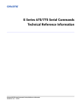
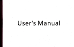
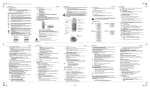
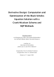
1
Markit iBoxx Bond Index Calculus March 2014 Index Calculus Table of Contents 1. 2. Introduction .......................................................................................................................................................... 4 Index Calculation ................................................................................................................................................. 4 2.1. Price and Total Return Indices ....................................................................................................................... 4 2.1.1. Price Index Calculation ........................................................................................................................... 4 2.1.2. Total Return Index Components ............................................................................................................. 4 2.1.3. Total Return Index Calculations .............................................................................................................. 5 2.1.4. Daily and Month-to-Date Returns ........................................................................................................... 6 2.2. Gross Price and Income Indices ..................................................................................................................... 6 2.2.1. Gross Price Indices ................................................................................................................................. 6 2.2.2. Income Indices ........................................................................................................................................ 6 2.3. Rebalancing cost factor for liquid indices ....................................................................................................... 7 2.4. Hedged and Unhedged Index Calculation ...................................................................................................... 7 2.5. Bond Capping ................................................................................................................................................. 8 3. Bond Analytics ................................................................................................................................................... 10 3.1. Accrued Interest ............................................................................................................................................ 10 3.1.1. ACT/n (ACT/360, ACT/364, ACT/365) .................................................................................................. 10 3.1.2. ACT/ACT ............................................................................................................................................... 11 3.1.3. 30/360 ................................................................................................................................................... 11 3.1.4. 30E/360 ................................................................................................................................................. 12 3.1.5. BUS/252 ................................................................................................................................................ 13 3.2. Bond Returns ................................................................................................................................................ 13 3.3. Bond Analytics .............................................................................................................................................. 13 3.3.1. Yield-to-worst Calculation ..................................................................................................................... 13 3.3.2. Average Expected Remaining Life ....................................................................................................... 14 3.3.3. (Average Redemption) Yield ................................................................................................................. 15 3.3.4. Duration ................................................................................................................................................ 15 3.3.5. Modified Duration .................................................................................................................................. 15 3.3.6. Convexity .............................................................................................................................................. 16 3.4. Bond Spread Analytics ................................................................................................................................. 16 3.4.1. Benchmark Spread ............................................................................................................................... 16 3.4.2. Spread to Benchmark Curve ................................................................................................................ 17 3.4.3. Spread to LIBOR Curve ........................................................................................................................ 18 3.4.4. Z-Spread ............................................................................................................................................... 19 3.4.5. Option Adjusted Spread ........................................................................................................................ 20 3.4.6. Asset Swap Spread .............................................................................................................................. 21 4. Index Analytics ................................................................................................................................................... 23 4.1. Weightings for index analytics ...................................................................................................................... 23 4.1.1. Nominal value weighting ....................................................................................................................... 23 4.1.2. Base market value weighting ................................................................................................................ 23 4.1.3. Market value weighting ......................................................................................................................... 23 4.1.4. Duration-adjusted market value weighting ........................................................................................... 24 4.2. Index Analytics .............................................................................................................................................. 24 4.2.1. Average Yield ........................................................................................................................................ 24 4.2.2. Index Benchmark Spread ..................................................................................................................... 25 4.2.3. Average Duration .................................................................................................................................. 25 4.2.4. Average Modified Duration ................................................................................................................... 25 4.2.5. Average Convexity ................................................................................................................................ 26 4.2.6. Average Coupon ................................................................................................................................... 27 4.2.7. Average Time to Maturity ...................................................................................................................... 27 4.2.8. Index Spread to Benchmark Curve ....................................................................................................... 27 4.2.9. Index Spread to LIBOR Curve .............................................................................................................. 27 4.2.10. Index Z-Spread ..................................................................................................................................... 28 4.2.11. Index OAS ............................................................................................................................................. 28 4.2.12. Index Asset Swap Spread .................................................................................................................... 28 5. Inflation Linked Index Calculations .................................................................................................................. 29 5.1. Calculating nominal data .............................................................................................................................. 29 5.2. Index Ratio .................................................................................................................................................... 29 Copyright © 2014, Markit Group Limited. All rights reserved. www.markit.com 2 Index Calculus 5.3. Index Calculation .......................................................................................................................................... 30 5.4. Bond and Index Analytics ............................................................................................................................. 30 6. Appendix ............................................................................................................................................................. 31 6.1. Cash and Turnover Reinvestment Cost ....................................................................................................... 31 6.2. Calculation of the hedged index returns in terms of market values and cash .............................................. 34 7. Annotations ........................................................................................................................................................ 36 8. Further Information ............................................................................................................................................ 43 Copyright © 2014, Markit Group Limited. All rights reserved. www.markit.com 3 Index Calculus 1. Introduction All Markit iBoxx indices follow a standard set of rules and calculation procedures. This document outlines the calculation principles for all Markit iBoxx indices and the standard bond and index level analytics published for Markit iBoxx. The annotations used in the formulae are attached in the Annotations section. 2. Index Calculation 2.1. Price and Total Return Indices 2.1.1.Price Index Calculation All iBoxx indices are basket indices that express relative changes in value compared to the beginning of the respective period. The composition and weightings of the index are adjusted at the beginning of each period. Accordingly, adjustments to index-tracking portfolios are only needed at the end of each period. Benchmark price index n PI t PI t s P i ,t i 1 n Fi ,t s Ni ,t s Fi ,Cap t s P i 1 Fi ,t s Ni ,t s Fi ,Cap t s i ,t s Price index calculation for liquid indices For liquid indices that maintain cash at month-ends in between quarterly rebalancing, the price index includes the rebalancing cash: n PI t PI t s P i 1 n i ,t P i 1 Fi ,t s N i ,t s Fi ,Cap t s CASH t s i ,t s Fi ,t s N i ,t s Fi ,Cap t s CASH t s The indices are based on consolidated bid quotes. Bonds not currently in the iBoxx universe enter the indices at the next rebalancing and are included in the index calculation at the beginning of the next period using the closing ask prices from the last trading day of the previous period. 2.1.2.Total Return Index Components Nominal Value The nominal value of the index is the sum of the individual bond nominal values and is calculated as follows: n NVt Fi ,t s N i ,t s Fi ,Cap t s i 1 Market Value The market value of a single bond at time t is calculated as follows: MVi ,t Pi ,t Ai ,t XDi ,t s CPi ,t FAi ,t Fi ,t N i ,t s Fi ,Cap t s Cap The capping factor, Fi ,t s will be normally be 1, unless in cases where capping is applied. The market value of the index is the sum of the market values of all bonds at time t and is calculated as follows: n MVt MVi ,t i 1 Copyright © 2014, Markit Group Limited. All rights reserved. www.markit.com 4 Index Calculus Base Market Value The base market value is the market value of the bond calculated at the rebalancing date (t-s); it also does not take cash payments into account. The base market value of a single bond at time t is calculated as follows: BMVi ,t s Pi ,t s Ai ,t s FAi ,t s Fi ,t s N i ,t s Fi ,Cap t s The base market value of the index is the sum of the base market values of all bonds and is calculated as follows: n BMVt s BMVi ,t s i 1 2.1.3.Total Return Index Calculations Cash Payment The cash payment for a single bond at time t is the sum of all coupon and scheduled redemption payments since the last index rebalancing plus the redemption value if the bond has already been fully redeemed: s CVi ,t CVi ,Coupons CVi ,Redemption t t CVi ,Coupons t G t s j t Redemptions i ,t CV i, j XDi , j 1 Fi , j 1 FAt ,i , j N i ,t s Fi ,Cap t s R t s j t i, j RPi , j FAt ,i , j N i ,t s Fi ,Cap t s Generally, it is assumed that there is only one coupon payment and one redemption payment per calculation period. The XD factor only applies for the first coupon payment in the given period. In situations where this is not the case, special cash payments are dealt with as follows: n n CVi ,t s j t XDi ,t s Gi ,t1 FAt ,i ,t1 Fi ,t11 Gi , j Fi , j 1 FAt ,i , j Ri , j RPi , j FAt ,i , j N i ,t s Fi ,Cap t s t1 j t t s j t The different adjustment factors ( Fi ,t , Fi ,t s ) are used for sinking funds, amortizing bonds, pay-in-kind bonds and unscheduled full redemptions. For other bond types, F always equals 1. The cash payment of all bonds in an index is calculated as follows: n CVt CVi ,t i 1 Benchmark total return Index The calculation for the local currency total return index is below. The total return index can be expressed in terms of market values and cash: TRt TRt s MVt CVt MVt s Total return index calculation for liquid indices The main difference between the various liquid index methods is the frequency of the cash investment in the money market. There are two main varieties of liquid indices with cash: Copyright © 2014, Markit Group Limited. All rights reserved. www.markit.com 5 Index Calculus (i) Liquid indices with quarterly or semi-annual rebalancing and monthly cash accrual For non-rebalancing months, the cash is invested into the money market until the following month-end. CASH t CVt CASH t -s 1 YLIBID t s days MM (t s, t ) (ii) 1m Liquid indices with cash accrual until the end of the month In addition to the investment of cash from month-end to month-end according to the version (i) above, some indices also invest coupon and redemption payments until the end of the month at the money market rate of the payment date: CASH t CVt CVt 1 CV t 1 t s i i CVi 1 1 YLIBID i days MM (i, t ) CASH t -s 1 YLIBID t s days MM (t s, t ) 1m 1m The cash is added to the standard formula for the indices: TRt TRt s MVt CASH t MVt s CASH t s 2.1.4.Daily and Month-to-Date Returns Daily index returns are calculated for all Markit iBoxx benchmark indices according to the following formula: Rt 1,t TRt 1 TRt 1 Month-to-date index returns are calculated as follows: Rt s ,t TRt 1 TRt s 2.2. Gross Price and Income Indices 2.2.1.Gross Price Indices The gross price index represents the portion of the total return that is due to movements of the dirty price of the constituent bonds. Benchmark Gross Price Indices The benchmark gross price index is calculated as follows: GI t GI t s MVt MVt s Liquid Gross Price Indices The liquid gross price index is calculated as follows: GI t GI t s MVt 1 XRt CASH t CVt XRt CASH t s MVt s CASH t s 2.2.2.Income Indices The income indices measure the portion of the index return that is due to actual cash payments. Interest payments are represented in the coupon income index, redemptions in the redemption income index and the total of these in the income index. Copyright © 2014, Markit Group Limited. All rights reserved. www.markit.com 6 Index Calculus Income indices are set to 0 at the beginning of each calendar year. Benchmark Income Indices The benchmark coupon income index is calculated as follows: ICt ICt s GI t s CVi ,Coupons t MVt s The benchmark redemption income index is calculated as follows: IRt IRt s GIt s s CVi ,Redemption t MVt s The benchmark income index is calculated as follows: IN t IN t s GIt s s CVi ,Coupons CVi ,Redemption t t MVt s Or simplified: IN t ICt IRt Liquid Income Indices The liquid coupon income index is calculated as follows: CVt Coupons XRt CASH t CASH t s CVt ICt ICt s GI t s MVt s CASH t s The liquid redemption income index is calculated as follows: CVt Redemptions IRt IRt s GI t s MVt s CASH t s The liquid income index is calculated as follows: IN t IN t s GI t s CVt XRt CASH t CASH t s CVt MVt s CASH t s 2.3. Rebalancing cost factor for liquid indices At the end of each month, after the rebalancing, the index level of most liquid indices is adjusted to account for the cost occurred in rebalancing the index. For most of the index adjustments between two rebalancing dates, the adjustment cost should be zero and no adjustment will be necessary. There are two approaches to capture the cost. The cost is either fixed (e.g. 2bps) or takes into account the actual transaction costs: ∑ ∑ ∑ ∑ Hence, at each rebalancing the index level is adjusted as follows: ( ) ( ) ( ) For a detailed explanation of the formula, please refer to the Appendix. 2.4. Hedged and Unhedged Index Calculation Copyright © 2014, Markit Group Limited. All rights reserved. www.markit.com 7 Index Calculus Currency hedging is applied to the index constituents on each monthly rebalancing. At the rebalancing day the position is fully hedged, using one month forwards. During the month, the index will be partially hedged, with the bond market value fluctuations (since rebalancing) remaining unhedged. The below formulae apply for both Total Return and Price Return indices. Unhedged Index Return IXR IXR U t U t s TRtLCY FX tLCY / CCY LCY / CCY TRt s FX tLCY s Unhedged Multicurrency Index Return IXRiLCY FX tLCY / CCY ,t wi LCY / CCY IXRiLCY i 1 ,t s FX t s n IXR IXR U t U t s Hedged Index Return IXR IXR H t H t s / CCY IXRtLCY FX tLCY / CCY FX tLCY FX tLCY / CCY s ,t LCY LCY / CCY / CCY FX tLCY s IXRt s FX t s Generally, the hedged index is calculated by multiplying the month-to-date hedge return with the hedged index level from the last rebalancing: IXRtH IXRtHs 1 rt H Hedged Multicurrency Index Return LCY / CCY n IXRiLCY FX tLCY / CCY FX tLCY / CCY FX t s ,t ,t IXRtH IXRtHs wi LCY LCY / CCY / CCY FX tLCY i 1 s IXRi ,t s FX t s For additional information, please reference chapter 6.2, Calculation of the hedged index returns in terms of market values and cash. 2.5. Bond Capping Weight limits (caps) can be applied in order to prevent a single bond or groups of bonds from dominating an index. A group of bonds can be represented by a country or a market sector. At the regular rebalancing dates the index composition and weighting is reviewed and weight caps are applied if necessary. For market value weighted indices, the weight of a bond is derived from its market value in relation to the overall index market value. In the following the term class refers to either a single bond or groups of bonds. In general, two basic procedures are applied: Pro Rata Capping If one or more classes account for more than the defined maximum weight their weight is reduced to the cap limit by reducing the amount outstanding of all the bonds in the class. The excess weight is distributed pro rata to the remaining classes. Should another class exceed the cap limit afterwards, its weight is reduced and redistributed accordingly. Step-wise weight reduction If one or more classes account for more than the defined maximum weight their weight is reduced by reducing the weight of the smallest bond. If – as a consequence - this bond is removed from the index portfolio the process is continued with the next smallest bond. Copyright © 2014, Markit Group Limited. All rights reserved. www.markit.com 8 Index Calculus The iBoxx index guides provide detailed information on which applicable capping method is used for those indices which are subject to weight restrictions. Copyright © 2014, Markit Group Limited. All rights reserved. www.markit.com 9 Index Calculus 3. Bond Analytics The following section defines how bond analytics are calculated for the securities within the index. With the exception of section 3.2 Bond Returns, all analytics for securities traded flat-of-accrued are assumed to be zero. 3.1. Accrued Interest The following day count conventions are taken into account when calculating the iBoxx Indices: ACT/360 ACT/364 ACT/365 ACT/ACT 30/360 30E/360 BUS/252 The following conventions are necessary for bonds that pay a coupon at/around month-end: Non-EOM: Bonds with this convention pay on the same calendar day each month, i.e. 30 June and 30 December No Leap Year: Bonds that do not pay interest on 29 February Other bonds that pay at month-end always pay on the last calendar day on the month, i.e. 30 June and 31 December In addition, some bonds may pay interest on the first or last business day of the month. If such a bond is identified, the relevant coupon/interest payment schedule is used to calculate accrued interest and coupon payments for this bond. Coupon Date Formulae for Different Day Count Conventions: The table below summarises the different formulae used for calculating accrued interest under different scenarios. The table includes the section reference where the formulae are defined. Day Count Normal Coupon Normal First Coupon Long First Coupon Short First Coupon ACT/n Section 3.1.1 Section 3.1.1 ACT/ACT 30/360 30E/360 Section 3.1.2 Section 3.1.4 Section 3.1.5 Section 3.1.2 Section 3.1.4 Section 3.1.5 BUS/252 Section 3.1.6 Section 3.1.6 Same formula as Normal Coupon Section 3.1.2 Section 3.1.4 Same formula as Normal Coupon N/A Same formula as Normal Coupon Section 3.1.2 Section 3.1.4 Same formula as Normal Coupon N/A 3.1.1.ACT/n (ACT/360, ACT/364, ACT/365) The accrued interest calculation is based on ISMA standards. In addition to the normal coupon dates, the calculation also takes into account odd first coupons, coupon changes during a period and ex-dividend details. The calculation is the same regardless of whether the basis is 360, 364 or 365 days. Accrued interest for the 2 Ai ,t nd and subsequent coupon periods: days ACT Dat Ci ,prev , t n C FAt ,i , j Accrued interest for the first coupon period: Ai ,t days ACT FSD, t C FAt ,i , j n Coupon changes: Copyright © 2014, Markit Group Limited. All rights reserved. www.markit.com 10 Index Calculus The following formula shows how to calculate the accrued interest when a coupon change occurs during a period: days ACT DatCa , Cb , t days ACT DatCi , DatCa , Cb Ai ,t Ca Cb FAt ,i ,t n n For the coupon payment in the period of the coupon change, the following formula applies: Ci 1 days ACT ( Dat(Ci ), Dat(Ca , Cb )) days ACT ( Dat(Ca , Cb ), Dat(Ci 1 )) Ca Cb n n 3.1.2.ACT/ACT The accrued interest calculation is based on ISMA standards. In addition to the normal coupon dates, the calculation also takes into account odd first coupons, coupon changes during a period, and ex-dividend details. Accrued interest for the 2 Ai ,t nd and subsequent coupon periods: days ACT ( Dat(Ci 1 ), t ) C FAt ,i ,t days ACT ( Dat(Ci 1 ), Dat(Ci )) Accrued interest for the first coupon period: Ai ,t days ACT ( FSD, t ) C FAt ,i ,t days ACT ( FSD, Dat (C1 )) Long first coupon: The coupon payment is divided into a short and a normal coupon period. If the settlement date lies between the first settlement date and the following fictitious coupon date, accrued interest is calculated as follows: Ai ,t days ACT ( FSD, t ) C FAt ,i ,t days ACT ( Dat(CF 1 ), Dat(CF )) Otherwise the accrued interest is calculated as follows: days ACT ( FSD, Dat(CF )) days ACT ( Dat(CF ), t ) C FAt ,i ,t Ai ,t days ACT ( Dat(CF 1 ), Dat(CF )) days ACT ( Dat(CF ), Dat(C1 )) Short first coupon: Ai ,t days ACT ( FSD, t ) C FAt ,i ,t days ACT ( Dat(CF 1 ), Dat(C1 )) Coupon changes: The following formula shows how to calculate accrued interest when a coupon change occurs during a period: days ACT ( Dat(Ci ), Dat(Ca , Cb )) days ACT ( Dat(Ca , Cb ), t ) Ai ,t Ca Cb FAt ,i ,t days ACT ( Dat(Ci ), Dat(Ci 1 )) days ACT ( Dat(Ci ), Dat(Ci 1 )) For the coupon payment in the period of the coupon change, the following formula applies: Ci 1 days ACT ( Dat(Ci ), Dat(Ca , Cb )) days ACT ( Dat(Ci 1 ), Dat(Ca , Cb )) Ca Cb days ACT ( Dat(Ci ), Dat(Ci 1 )) days ACT ( Dat(Ci ), Dat(Ci 1 )) 3.1.3. 30/360 The accrued interest calculation is based on ISDA standards. For two given dates d1/m1/y1 and d2/m2/y2: 1) If d1=31, then set d1=30 Copyright © 2014, Markit Group Limited. All rights reserved. www.markit.com 11 Index Calculus 2) If d2=31 and d1=30, then set d2 = 30 Afterwards, the days between the two dates are calculated as follows: days360(d1 / m1 / y1, d 2 / m2 / y 2) ( y 2 y1) 360 (m2 m1) 30 (d 2 d1) Accrued interest for the first coupon period: Ai ,t days30 ( FSD, t ) C FAt ,i ,t 360 nd Accrued interest for the 2 and subsequent coupon periods: The days between the settlement date and the last coupon date are calculated as follows: Ai ,t days30 ( Dat(Ci 1 ), t ) C FAt ,i ,t 360 Accrued interest for irregular first coupon dates: days30 ( FSD, Dat(C F )) days30 ( Dat (C F ), t ) Ai ,t C FAt ,i ,t 360 Coupon changes: The following formula shows how to calculate the accrued interest when a coupon change during a period occurs. days30 ( Dat(Ca , Cb ), t ) days30 ( Dat (Ci ), Dat (Ca , Cb )) Ai ,t Ca Cb FAt ,i ,t 360 360 For the coupon payment in the period of the coupon change, the following formula applies: Ci 1 days30 ( Dat(Ci ), Dat(Ca , Cb )) days30 ( Dat(Ca , Cb ), Dat(Ci 1 )) Ca Cb 360 360 3.1.4. 30E/360 The accrued interest calculation is based on ISMA standards. st If one of the dates t or Dat(Ci-1) is dated on the 31 , it is set to 30. The days between the settlement date and the last coupon date are calculated as follows: days30E ( Dat(Ci1 , t ) ( y 2 y1) 360 (m2 m1) 30 (d 2 d1) Normal coupon date: Ai ,t days30E ( Dat(Ci 1 ), t ) C FAt ,i ,t 360 First coupon date: Ai ,t days30E ( FSD, t ) C FAt ,i ,t 360 Coupon changes: The following formula shows how to calculate the accrued interest when a coupon change occurs during a period. days30E ( Dat(Ca , Cb ), t ) days30E ( Dat (Ci ), Dat (Ca , Cb )) Ai ,t Ca Cb FAt ,i ,t 360 360 Copyright © 2014, Markit Group Limited. All rights reserved. www.markit.com 12 Index Calculus For the coupon payment in the period of the coupon change, the following formula applies: Ci 1 days30E ( Dat(Ci ), Dat(Ca , Cb )) days30E ( Dat(Ca , Cb ), Dat(Ci 1 )) Ca Cb 360 360 3.1.5.BUS/252 The calculation follows the convention for bonds that accrue interest only on business days. The distance between two calendar days is expressed as the number of days that are not public holidays and that do not fall on a Saturday or Sunday. The convention is mainly used for Brazilian bonds. A standard year is supposed to contain 252 business days, regardless of the actual number of business days. The accrued interest for standard bonds is calculated as: C annual 1m bdays ( Dat(Ci 1 ), t ) 1 100 FAt ,i ,t Ai ,t 1 i bdays Dat(Ci 1 ), Dat(Ci ) 100 For bonds, the coupon of which is paid at maturity: bdays( FSD,t ) Ciannual 252 Ai ,t 1 1 100 FAt ,i ,t 100 3.2. Bond Returns Daily and month-to-date bond returns are calculated for all bonds. The formulae below are valid for daily and month-to-date calculations (the daily returns read (t-1) instead of (t-s)). Daily local bond return: LCRiD,t MVi ,t CVi ,t CVi ,t 1 MVi ,t 1 1 Month-to-date local bond return: LCRiM,t MVi ,t CVi ,t MVi ,t s 1 3.3. Bond Analytics 3.3.1.Yield-to-worst Calculation For callable and putable bonds, a yield-to-worst calculation is necessary to determine when a bond is likely to be redeemed. For European options, the yield-to-worst calculation is performed at each exercise date. For American options, the yield-to-worst calculation is performed at the first future iBoxx yield-to-worst calculation date and any ensuing iBoxx yield-to-worst calculation date. iBoxx yield-to-worst calculation dates are: Coupon and/or redemption payment date inside an exercise period Start and end of an exercise period Date on which the exercise price changes Copyright © 2014, Markit Group Limited. All rights reserved. www.markit.com 13 Index Calculus The final redemption date The first future iBoxx yield-to-worst calculation date is: The next iBoxx yield-to-worst calculation date on or after the current settlement date plus any notice period if the latter exists, or the next iBoxx yield-to-worst calculation date after the current settlement date. The yield of the bond is calculated according to the general yield formula for each relevant call/put date and the final maturity date. The following procedure determines when the bond is most likely to be redeemed: 1) The call date with the lowest yield to call is determined 2) The put date with the highest yield to put is determined 3) The determined yield to call, yield to put and the yield to maturity are compared: If the yield to call is lower than the yield to maturity, then the bond is assumed to be called If the yield to put is higher than the yield to maturity, then the bond is assumed to be put 4) The expected redemption path is: Bond is assumed to be called No Yes No Yes Bond is assumed to be put No No Yes Yes Expected redemption date Maturity date Call date with lowest yield to call Put date with highest yield to put Earlier of the call and put date The expected redemption date is used in the calculation of the expected remaining life and in the other bond analytics calculations. 3.3.2.Average Expected Remaining Life The calculation depends on the bond type and takes into account the day count convention of the bond. Bullet bonds without options: For plain vanilla bonds, the expected remaining life of the bond is its time-to-maturity, calculated as the number of days between the rebalancing and its maturity. Bullet bonds with options: For callable/putable bonds, a yield-to-worst calculation determines when the bond is expected to redeem. This date is the expected redemption date. The expected remaining life is calculated as the number of days between the rebalancing and the expected redemption date. Hybrid capital: For hybrid capital bonds with call dates, i.e. perpetual bonds or other callable dated hybrid capital bonds, the first call date is always assumed to be the expected redemption date. The expected remaining life is calculated as the number of days between the rebalancing and the expected redemption date. For non-callable fixed-to-floater bonds, the expected remaining life is calculated as the number of days between the rebalancing and the conversion date, i.e. the date on which the bond turns into a floating rate note. Amortizing bonds without options: For sinking funds and amortizing bonds, the average life is used as a measure for the expected remaining life of the bonds. The average life is calculated as the sum of the distances to each future redemption cash flow weighted by the percentage redeemed at the respective date. The redemption payments are not discounted: Copyright © 2014, Markit Group Limited. All rights reserved. www.markit.com 14 Index Calculus R L R j t LFi ,t a i ,t , j i, j j t i, j Amortizing bonds with options: For callable/putable bonds, the yield-to-worst calculation determines the expected redemption path of the bond. All outstanding redemption payments are assumed to be made on the worst date determined by the yield to worst calculation. The average life is then calculated as per the formula above. Fully redeemed bonds: The expected remaining life for fully redeemed bonds is 0. 3.3.3.(Average Redemption) Yield The yield of a bond at time t is calculated as follows: P i ,t Ai ,t Fi ,t CFi , j 1 yi ,t n Li , j j 1 For bonds during an ex-dividend period, the future cash-flows for the yield calculation exclude the current coupon payment. The Newton iteration method is used to solve the equation for yi ,t . Fi ,t is a redemption factor that is relevant for sinking funds, amortizing bonds and unscheduled full redemptions. For other bond types, F always equals 1. The yield is set to 0 if Fi ,t is 0. The true yield is calculated as follows: Yi t,t Yi ,t m The periodic yield can be transformed into the annual yield: Yi a,t 1 Yi ,t 1 m The semi-annualized yield is calculated as follows: Yi ,st 2 1 Yi a,t 1 3.3.4.Duration The duration of a bond at time t is calculated as follows: n Di ,t CF j 1 Lt , j 1 yi ,t Li ,t , j i, j CF 1 y n j 1 Li ,t , j i, j P i ,t 1 Ai ,t Fi ,t m CFi , j Li ,t , j 1 yi ,t n Li ,t , j j 1 i ,t 3.3.5.Modified Duration The modified duration of a bond at time t is calculated as follows: MDi ,t Di ,t 1 1 Yi ,t In the same way, the annual modified duration can be expressed as: Copyright © 2014, Markit Group Limited. All rights reserved. www.markit.com 15 Index Calculus MDUia,t Di ,t 1 1 Yi ,at The semi-annualized modified duration is calculated as follows: MDUiS,t Di ,t 1 Yi ,st 1 2 3.3.6.Convexity The convexity of a bond at time t is calculated as follows: CX i ,t P i ,t n 1 Ai ,t Fi ,t m The convexity is set to 0 if Li ,t , j Li ,t , j 1 CFi , j 1 Yi ,2t 2 Li ,t , j 2 j 1 Fi ,t is 0. Using the annualized yield, the annualized convexity of a bond can be calculated as: CX ia,t CX i ,t 1 yai,t MD 1 1 1 y 1m2 i ,t ai,t 2 1 1 m m Similarly, using the semi-annualized yield, the semi-annualized convexity of a bond can be calculated as: CX S i ,t y CX i ,t 1 2i ,t 2 2 2 1 m 2 1 y m MDi ,t 1 2i ,t 2 2 2 2 m 3.4. Bond Spread Analytics 3.4.1.Benchmark Spread The benchmark spread can be defined as a premium above the yield on a default-free bond necessary to compensate for additional risk associated with holding the bond. Markit calculates the benchmark spread as the difference between the yield of the bond and the benchmark bond. Selection criteria for a benchmark bond are: – Government bond is selected as an approximation of a „default-free bond‟ – The difference between maturities of a bond and the benchmark bond is the smallest in comparison to other alternatives Copyright © 2014, Markit Group Limited. All rights reserved. www.markit.com 16 Index Calculus 6.0% 5.0% Benchm ark Spread 4.0% 3.0% 2.0% 1.0% 0.0% 0.5 2.5 4.5 6.5 8.5 10.5 12.5 14.5 16.5 18.5 20.5 22.5 24.5 26.5 28.5 30.5 148.0661645 148.0661645 Benchm ark Yield Curve 57.44261768 57.44261768 Annual Benchmark Spread The annual benchmark spread of a bond 0 0 Bond Yield i at time t is: 0 BMS i,ta a a Yi ,t YBM (i ),t Note that for benchmark bonds BMS i,ta 0 Semi-annual Benchmark Spread The semi-annual benchmark spread of a bond i at time t is: 0 BMS iS,t s s Yi ,t YBM (i ),t Note that for benchmark bonds BMS i ,t 0 S 3.4.2.Spread to Benchmark Curve Spread to benchmark curve can be defined as a premium above the yield on a default-free bond necessary to compensate for additional risk associated with holding the bond. The default-free yield to maturity is found by a linear interpolation of two benchmark bonds with maturities being just above and just below the time to maturity of a bond. Selection criteria for benchmark bonds are: – Government bonds are selected as an approximation of a „default-free bond‟ – The difference between maturities of a bond and the benchmark bonds is the smallest in absolute terms in comparison to other alternatives Copyright © 2014, Markit Group Limited. All rights reserved. www.markit.com 17 Index Calculus Annual Spread to Benchmark Curve The annual spread to benchmark of a bond i at time t is: 0 SBC i,ta a a Yi ,t YInBM i ,t Note that for benchmark bonds SBC i,ta 0 Semi-annual Spread to Benchmark Curve The semi-annual benchmark spread of bond i at time t is: 0 SBC i,ts s s Yi ,t YInBM i ,t Note that for benchmark bonds SBC i,ts 0 3.4.3.Spread to LIBOR Curve Spread to Libor curve can be defined as a premium above the yield on Markit SWAP curve, constructed from Libor rates and ICAP swap rates, necessary to compensate for additional risk associated with holding the bond. 5.0% 4.0% Spread to Libor Curve 3.0% 2.0% 1.0% 0.0% 1.5 2.0 2.5 3.0 3.5 4.0 4.5 5.0 5.5 Bond Yiled Copyright © 2014, Markit Group Limited. All rights reserved. www.markit.com 6.0 6.5 7.0 7.5 8.0 8.5 9.0 9.5 ICAP Curve 18 Index Calculus Annual Spread to LIBOR Curve The spread to benchmark of a bond i at time t is: 0 SLC i,ta a a Yi ,t YSWAPt Semi-annual Spread to LIBOR Curve The spread to benchmark of a bond i at time t is: 0 SLC i,ts s s Yi ,t YSWAPt 3.4.4.Z-Spread The Z-spread is a measure of the spread the investor would realize over the entire benchmark zero coupon curve if the bond is held to maturity. The Z-spread is calculated as the spread that will make the present value of the cash flows of respective bond equal to the market dirty price, when discounted at the benchmark spot rate plus the spread. The spread is found iteratively using the Newton method. In general, constant spread si , j over the spot curve zt (L) for a bond at time t on an annual basis is calculated iteratively by using the Newton method: Pi ,t Ai ,t CFi , j 1 zt Li , j si , j n Li , j j 1 Benchmark Zero Coupon Curve Benchmark zero curve ( ) also known as spot rate curve is calculated form dirty prices of defined benchmark bonds. The following equation is solved using the Nelder-Mead-Simplex Method: n min Pk ,t Ak ,t CFi ,kj 1 zt Lki , j k 1 j 1 ! m Lki , j 2 In the figure below the estimated zero curve is compared to annual yields of the benchmark bonds: Copyright © 2014, Markit Group Limited. All rights reserved. www.markit.com 19 Index Calculus Z-Spread Over LIBOR Curve The Z-spread over Libor Curve is a measure of the spread that the investor would realize over the entire ICAP curve, constructed from Libor rates and ICAP swap rates, if the bond is held to maturity. The Z-spread is calculated as the spread that will make the present value of the cash flows of respective bond equal to the market dirty price, when discounted at the ICAP rate plus the spread. The spread is found iteratively using the Newton method. In general, Z-spread si , j over Markit SWAP curve zt (L) for a bond at time t on an annual basis is calculated iteratively using the Newton method: Pi ,t Ai ,t CFi , j 1 zt Li , j si , j n Li , j j 1 3.4.5.Option Adjusted Spread Similar to Z-spread, OAS is the spread over the benchmark zero coupon curve realized if the bond is held until maturity. The major difference is the interest rate volatility assumption used in OAS. Due to the fact that interest rate changes can affect the cash flows of the security with embedded option the following relationship cab be highlighted: Z-spread = OAS + Option cost Constructing Binomial Interest Rate Tree Two components are required to determine the interest rate tree: – Benchmark Zero Coupon Curve – Empirical Volatility Empirical volatility is annualized daily standard deviation of percentage change in daily yields from their mean. The number of observations equals to the number of trading days in one year period minus 5% of observations from each tail of the distribution of percentage change in daily yields. The daily standard deviation is annualized by multiplying it by the square root of 252 trading days in a year. Copyright © 2014, Markit Group Limited. All rights reserved. www.markit.com 20 Index Calculus OAS Calculation The OAS is calculated as the spread that will make the present value of the cash flows of the respective bond equal to the market dirty price when discounted at the benchmark spot rate plus the OAS spread. Given spot rates and empirical volatility the interest rate tree is derived using the iterative search method. After the binomial interest rate tree is derived, the theoretical price of the bond is found by conventional backward induction of future cash flows. The OAS is found iteratively by using the Newton method, such that adding the spread to every node of the interest rate tree would make the present value of the cash-flows equal to the market dirty price of the bond. 3.4.6.Asset Swap Spread Markit SWAP curve, constructed from Libor rates and ICAP swap rates, is central to the process of asset swap spreads calculation. As soon as the curve is defined the present value of fixed and floating payoffs is calculated, and the asset swap spread is determined. The curve is interpolated to account for fixed and floating payoffs dates. Asset Swap Spread Calculation To evaluate asset swap spread one needs to distinguish between fixed and floating payments. Given the frequency of fixed rate payments, the floating rate payment frequency is determined as follows: 1 Fixed rate paid yearly = Floating rate paid semiannually 2 Fixed rate paid semiannually = Floating rate paid quarterly 3 Fixed rate paid quarterly = Floating rate paid monthly 4 else: Fixed frequency = Floating frequency Fixed Rate Payments DFnFixed 1 SWAPn 1L Fixed /360 n Copyright © 2014, Markit Group Limited. All rights reserved. www.markit.com Floating Rate Payments DFnFloating 1 SWAPn 1L Floating n / 360 21 Index Calculus Floating Rate Payments Fixed Rate Payments T PVFixed Ct DFtFixed PrincipalT DFtFixed t 1 T Lt DFtFloating 360 t 1 PVFloating Given the present value of fixed and floating rate payments, the asset swap spread is calculated as follows: ASW PVFixed DP PVFloating Copyright © 2014, Markit Group Limited. All rights reserved. www.markit.com 22 Index Calculus 4. Index Analytics 4.1. Weightings for index analytics There are four different weighting concepts for index analytics, depending on the specific analytical value being calculated. 4.1.1.Nominal value weighting For an index of bonds, the nominal weight is the share of each bond‟s notional in the aggregate notional of the index: wiN,t Fi ,t N i ,t s Fi ,Cap t s n F i ,t i 1 N i ,t s Fi ,Cap t s CASH t s For an index of indices, the nominal weight is equal to the (fixed) weight of the sub-index in the overall index as of the last rebalancing: wiN,t wiFix ,t s 4.1.2.Base market value weighting For an index of bonds, the base market value weight is the share of each bond‟s base market value in the aggregate base market value of the index: wiBMV ,t MVi ,t s n MV i ,t s i 1 For an index of indices, the base market value weight is equal to the (fixed) weight of the sub-index in the overall index as of the last rebalancing: wiN,t wiFix ,t s 4.1.3.Market value weighting For an index of bonds, the market value weight is the share of each bonds market value in the aggregate market value of the index: MVi ,t wiMV ,t n MV i 1 i ,t For an index of indices, the market value weight is equal to the current weight of the sub-index in the overall index as of the last rebalancing: wiMV ,t 1 r w 1 r w Fix i ,t s i ,t s ,t n i 1 i ,t s ,t Fix i ,t s The bond market value weighting adjusted for cash is not applicable for indices of indices. For indices of bonds, it is calculated as: wiMVC ,t MVi ,t MV n i 1 i ,t CVi ,t Copyright © 2014, Markit Group Limited. All rights reserved. www.markit.com 23 Index Calculus 4.1.4.Duration-adjusted market value weighting For an index of bonds, the duration-adjusted market value weight is the adjusted share of each bonds market value in the aggregate adjusted market value of the index: wiD,t Di ,t MVi ,t n D i 1 i ,t MVi ,t For an index of indices, the market value weight is equal to the current weight of the sub-index in the overall index as of the last rebalancing: wiD,t DU i ,t 1 ri ,t s ,t wiFix ,t s DU 1 r n i 1 i ,t i ,t s ,t w Fix i ,t s 4.2. Index Analytics As noted above in section 3.1 Bond Analytics, the analytics for securities that are traded flat-of-accrued are assumed to be zero and are not accounted for in the overall index analytics. 4.2.1.Average Yield The average annual yield is calculated by weighting the yield of each bond with the corresponding market capitalization and duration of the respective bond. n a D Yi ,t wi ,t Index of bonds i 1 RYt n RY w D Index of indices i ,t i ,t i 1 The average semi-annualized yield is calculated as follows: n s D Yi ,t wi ,t Index of bonds i 1 RYS t n RYS w D Index of indices i ,t i ,t i 1 The average portfolio yield is calculated by adjusting the portfolio for the cash portion: MVt RYt MV CV Index of bonds t t RYPt n RYP w D Index of indices i ,t i ,t i 1 The average semi-annualized portfolio yield is calculated as follows: MVt RYS t MV CV Index of bonds t t RYPS t n RYPS w D Index of indices i ,t i ,t i 1 Copyright © 2014, Markit Group Limited. All rights reserved. www.markit.com 24 Index Calculus 4.2.2.Index Benchmark Spread The index benchmark spread is calculated for all indices. The annualized index benchmark spread at time t is: n a D BMS i ,t wi ,t Index of bonds i 1 BMS ta n BMS a w D Index of indices i ,t i ,t i 1 The semi-annualized index benchmark spread at time t is: n s D BMS i ,t wi ,t Index of bonds i 1 BMS ts n BMS s w D Index of indices i ,t i ,t i 1 4.2.3.Average Duration The average duration is weighted by the market capitalization of the respective bonds. n MV Di ,t wi ,t Index of bonds i 1 DU t n DU w MV Index of indices i ,t i ,t i 1 The average portfolio duration is calculated as follows: n MVC Di ,t wi ,t Index of bonds i 1 DPU t n DPU wMV Index of indices i ,t i ,t i 1 4.2.4.Average Modified Duration The calculation method for average modified duration is similar to that previously described for average duration, except that duration is replaced by modified duration. Annual Modified Duration: n a MV MDi ,t wi ,t Index of bonds i1 MDUta n MDU a wMV Index of indices i ,t i ,t i 1 The average semi-annualized modified duration is calculated as follows: Copyright © 2014, Markit Group Limited. All rights reserved. www.markit.com 25 Index Calculus n s MV MDi ,t wi ,t Index of bonds i1 MDUts n MDU s wMV Index of indices i ,t i ,t i 1 The average modified portfolio duration is calculated as follows: n a MVC MDi ,t wi ,t Index of bonds i 1 MDPU ta n MDPU a wMV Index of indices i ,t i ,t i 1 The average semi-annualized modified portfolio duration is calculated as follows: n s MVC MDi ,t wi ,t Index of bonds i 1 MDPU ts n MDPU s wMV Index of indices i ,t i ,t i 1 4.2.5.Average Convexity The calculation method for average convexity is similar to that previously described for average duration and average modified duration, except that duration/modified duration is replaced by convexity. n a MV CX i ,t wi ,t Index of bonds i1 CXU ta n CXU a wMV Index of indices i ,t i ,t i 1 The average semi-annualized convexity is calculated as follows: n s MV CX i ,t wi ,t Index of bonds i1 CXU ts n CXU s wMV Index of indices i ,t i ,t i 1 The average portfolio convexity is calculated as follows: n a MVC CX i ,t wi ,t Index of bonds i 1 CXPU ta n CXPU a wMV Index of indices i ,t i ,t i 1 The average semi-annualized portfolio convexity is calculated as follows: Copyright © 2014, Markit Group Limited. All rights reserved. www.markit.com 26 Index Calculus n s MVC CX i ,t wi ,t Index of bonds i 1 CXPU ts n CXPU s wMV Index of indices i ,t i ,t i 1 4.2.6.Average Coupon The average coupon is nominal weighted. For bonds with a multi coupon schedule, the current coupon is included. n N Ci ,t wi ,t Index of bonds i1 COt n CO w N Index of indices i ,t i ,t i 1 4.2.7.Average Time to Maturity The calculation method for average time to maturity is similar to the previously described calculation. A weighting is carried out in accordance with the amount outstanding. n N LFi ,t wi ,t Index of bonds i1 LFU t n LFU w N Index of indices i ,t i ,t i 1 4.2.8.Index Spread to Benchmark Curve Annual Index Spread to Benchmark Curve The annual index spread to benchmark curve is calculated as follows: n a D SBC i ,t wi ,t Index of bonds i 1 SBC ta n SBC a w D Index of indices i ,t i ,t i 1 Semi-annual Index Spread to Benchmark Curve The semi-annual index benchmark spread is calculated as follows: n s D SBC i ,t wi ,t Index of bonds i 1 SBC ts n SBC s w D Index of indices i ,t i ,t i 1 4.2.9.Index Spread to LIBOR Curve The index spread to Libor curve is calculated as follows: Copyright © 2014, Markit Group Limited. All rights reserved. www.markit.com 27 Index Calculus n D SLCi ,t wi ,t Index of bonds i 1 SLCt n SLC w D Index of indices i ,t i ,t i 1 4.2.10. Index Z-Spread The index Z-spread is calculated as follows: n D Z Spread i ,t wi ,t Index of bonds i 1 Z Spread t n Z Spread w D Index of indices i ,t i ,t i 1 The same formula applies for the index Z-spread over LIBOR 4.2.11. Index OAS n D OAS i ,t wi ,t Index of bonds i 1 OAS t n OAS w D Index of indices i ,t i ,t i 1 4.2.12. Index Asset Swap Spread n D ASWi ,t wi ,t Index of bonds i 1 ASWt n ASW w D Index of indices i ,t i ,t i 1 Copyright © 2014, Markit Group Limited. All rights reserved. www.markit.com 28 Index Calculus 5. Inflation Linked Index Calculations The calculation of the inflation-linked indices follows the calculation principles for the standard bond indices. Each inflation-linked index is calculated in two versions, one version without adjusting for inflation (“real”) and one version including the past and projected future inflation adjustments (“nominal”).In this chapter, real values (without inflation R adjustments) are denoted with the superscript R and nominal values with the superscript N (e.g. P for real price and N P for nominal price). The standard calculus formulae apply to the corresponding real and nominal index and analytics calculations. For the index calculation in real terms, all prices, accrued interest and projected future cash flows used need to be without inflation adjustments and for the nominal calculations all data needs to include the inflation adjustment. 5.1. Calculating nominal data Nominal prices, accrued interest as well as coupon and redemption payments are calculated by multiplying the real values with the applicable index ratio: Pi ,Nt Pi ,Rt IRi ,t AiN,t AiR,t IRi ,t CiN,t ,t ^ CiR,t ^ IRi ,t ,t ^ The current market capitalization of a bond is affected by the real face amount issued, the real price of the bond, and by any adjustments due to past inflation. Similarly, the inflation-adjusted amount outstanding is equal to the product of the index ratio multiplied by the unadjusted amount outstanding: N iN,t N i ,t IRi ,t 5.2. Index Ratio The index ratio captures the inflation adjustment due on a specific calculation date or a future cash flow date. The current index ratio IRi ,t captures the inflation-adjustment due on the calculation date. The index ratio is derived from the corresponding country-specific inflation index (CPI). There are two main versions of the index ratio. For most countries, the index ratio is calculated by dividing the current CPI level by the CPI level from the base date, which may be the interest accrual date of the bond or a fixed date: IRi ,t CPI t . The base date is bond specific and therefore the index ratio is bond specific as well. CPI i ,t 0 The index ratio is rounded to a country-specific number of decimal places. Since the CPI is only released monthly or quarterly, and is only available in arrears, the CPI level CPI t applicable to a certain calculation date refers to CPI data n months prior to the calculation date, and may be interpolated between two neighboring CPI levels. The specific procedure varies from country to country. For Chile, Colombia, Costa Rica, Mexico, Uruguay use a real monetary unit (RMU) that serves as the index ratio. The real monetary unit is derived from the CPI changes but is the same for all bonds: IRi ,t RMU t . The index ratio is not bond specific but applies equally to all issued inflation-linked debt from this country. For future cash flows IRi ,t ,t ^ will be estimated to capture the additional inflation-adjustment expected to occur between the calculation date t and the cash flow date t^. The index ratio for future cash flows is estimated from the index ratio calculated from the most recently released CPI data by adding the projected future inflation to it: IRi ,t ,t ^ IRi ,t ,t 1 t t ^ t Copyright © 2014, Markit Group Limited. All rights reserved. www.markit.com 29 Index Calculus Please note that the estimated index ratio for a future cash flow may change from day to day if new CPI data is released. The assumed inflation t is usually estimated from the most recent CPI data and is the current one year inflation rate: t CPI t 1 CPI t ( y 1) A small number of countries use either a fixed inflation assumption or forecasted values which will be used instead of the above formula. The inflation is assumed to remain constant throughout the life of the bond. 5.3. Index Calculation The standard calculus formulae apply. 5.4. Bond and Index Analytics The standard calculus formulae apply. Copyright © 2014, Markit Group Limited. All rights reserved. www.markit.com 30 Index Calculus 6. Appendix 6.1. Cash and Turnover Reinvestment Cost At the end of each month, the proceeds from coupons received and from the sale of dropped or reduced-weight bonds need to be reinvested in the indices. At the same time, new bonds will enter the indices. These can be of two different types: 1. new bonds entering the index family for the first time or 2. bonds migrating from one index to another (e.g. due to rating changes). A portfolio manager tracking a liquid index may attempt to replicate the index by reinvesting the proceeds from bonds sold at the bid price or coupon payments received into the index, i.e. into bonds that need to be purchased at the ask price. In the case of bonds already in the index, the portfolio manager will purchase additional notional of the bond on the ask side but the same bond is valued in the index at the bid, or in the case of a mid-price index the mid, thus resulting in a tracking cost. The following rules can be established for an index-tracking portfolio: 1. Buying and selling only takes place on the rebalancing date, cash is reinvested and no cash is added to or taken from the portfolio. 2. During the bond substitution at the end of a month, the complete proceeds of a bond are invested in a new bond. 3. If no buying and selling takes place, the index and the portfolio are marked to market using the same price as the index (either bid or mid – depending on the index methodology) and no cost is incurred. 4. For the iBoxx indices that use bid prices, the following re-balancing scenario applies: All bonds in the index are valued at their bid prices, except new bonds that enter at their ask price. Therefore, selling or buying a new bond does not incur any cost. If a trader must purchase additional notional of an existing bond he will incur costs in the form of the bond‟s bid-ask spread. 5. For the iBoxx indices that use mid prices, the following re-balancing scenario applies: All bonds in the index are valued at their mid prices. Therefore, selling bonds does incur a midbid spread and purchasing bonds incurs a mid-ask spread. Liquid Index Cost Factor Rebalancing Scenario of Markit iBoxx Liquid Indices Bonds that drop out of the index (1) Bonds that remain in the index (2) Bonds that enter the index (3) Bonds in the four different regions may be characterized as follows: Region 1: Bonds that leave the liquid indices at the rebalancing; Region 2: Bonds that remain in the liquid indices; Region 3: Bonds that newly enter a liquid index at the rebalancing The time before the rebalancing is denoted with (-). The time after the rebalancing is denoted with (+). The market value of the portfolio before the rebalancing (without ex-dividend periods) is given as the sum of the market value of all bonds plus cash: Copyright © 2014, Markit Group Limited. All rights reserved. www.markit.com 31 Index Calculus n M Pi I Ai f i 1 Cash is treated as a bond with a price of 100 and accrued interest of 0. Since no cash is added or taken from the portfolio at the rebalancing, the assumption of no further cash addition leads us to the following equation: M M P That is the market value of the portfolio before the rebalancing equals the market value after rebalancing using transaction prices. Cost means the relative difference between market value of the portfolio using transaction prices to the portfolio valued with index prices: M I M P 1 cost The investor has to rebalance his index-tracking portfolio by adjusting the weights of each bond in his portfolio to the new weights of the bond in the index. Any bonds that need to be sold will be sold at the bid price, while bonds purchased are bought at the offer price. If the pricing of a bond in the index deviates from the prices that the investor has to use, he will incur cost. The following table gives a summary by region. Region 1 2 3 Region 1 2 3 * ** Summary by type (bid/ask indices) Portfolio Index Description Price price** Bond drops out Bid Bid (2 ) Bond does not need to be purchased Bid Bid + (2 ) Bond has to be purchased* Ask Bid New bond to a liquid index Ask Ask New Portion 0 + f + f + f Old Portion f f f 0 Summary by type (mid indices) Portfolio Index Description Price price** Bond drops out Bid Mid (2 ) Bond does not need to be purchased Mid Mid + (2 ) Bond has to be purchased* Ask Mid New bond to a liquid index Ask Mid New Portion 0 + f + f + f Old Portion f f f 0 + + 2 : Region of all bonds with a weight increase in the portfolio: f > f For the change in amount outstanding during the rebalancing Cost No No Yes No Cost Yes No Yes Yes - The amount invested per bond after the rebalancing can be stated as: f i M I Similarly, Oi MV f i can be calculated using the amount outstanding of the bond, and index and portfolio market value before the rebalancing. The weighting per bond before and after rebalancing can be described as follows: Before: wi P i I Ai f i M Copyright © 2014, Markit Group Limited. All rights reserved. www.markit.com 32 Index Calculus i w After: P I i Ai f i M I f i and f i leads to: The same applies to cash. Solving for fi Before: fi After: wi M Pi I Ai wi M I I Pi Ai It will be assumed that a bond increases its weight in the portfolio if its weight increased in the index: wi wi f i f i The market value using index prices can be expressed using the new amount: n M I Pi I Ai fi i 1 And using transaction prices: n M P Pi I Ai fi Pi P Ai fi fi i 1 Please note that the index price and the transaction price of cash are equal to 100. Combining the formulas above: P n i 1 I i n Ai fi Pi I Ai fi Pi P Ai fi fi i 1 Or simplified: n 0 Pi P Ai fi fi i 1 f i and f i can be replaced in the previous formula: n w M I wi M 0 Pi P Ai i I I P A P A i 1 i i i i Solving for M I gives: Pi P Ai wi I i 1 Pi Ai MI n P M Pi Ai wi I i 1 Pi Ai n Since M = M P , it leads to Copyright © 2014, Markit Group Limited. All rights reserved. www.markit.com 33 Index Calculus Pi P Ai wi I i 1 Pi Ai cost 1 n P Pi Ai wi I i 1 Pi Ai n We can now separate the cash from the bonds: Pi P Ai wi I i 1 Pi Ai cost 1 n P P Ai wcash iI wi i 1 Pi Ai n wcash The solution is independent of the individual portfolio. In addition, bid and offer prices, amount outstanding before and after the rebalancing, as well as the index market value before and after the rebalancing are known at the time of the rebalancing, so the cost (percentage) can be calculated using data known at the time of the rebalancing. 6.2. Calculation of the hedged index returns in terms of market values and cash The local currency index market value is the sum of the market values of all the components (MV) plus any cash that has been paid since the last rebalancing. IVt MVt Casht The rebalancing index base market value is the sum of all components in the index at the rebalancing (BMV). IVt s BMVt s Hedged indices are calculated by hedging the value of the index from one rebalancing to the next. Hedging therefore occurs once a month at the rebalancing. During the month, the index value consists of a hedged portion and an unhedged portion. The unhedged part of the index is caused by the performance of the bonds: IVt Hedge BMVt s s / CCY IVt HedgedPortion BMVt s FX tLCY s ,t IVtUnhedgedRe sidual MVt Casht BMVt s FX tLCY / CCY The hedge performance can therefore be written as: 1 r IV H t t IVtUnhedgedRe sidual / CCY IVt Hedge FX tLCY s s HedgedPortion Rewriting using local currency market values and cash: 1 r H t / CCY MVt Casht BMVt s FX tLCY / CCY BMVt s FX tLCY s ,t / CCY BMVt s FX tLCY s Rearranging: 1 r H t / CCY MVt Casht FX tLCY / CCY BMVt s FX tLCY FX tLCY / CCY s ,t / CCY BMVt s FX tLCY s Copyright © 2014, Markit Group Limited. All rights reserved. www.markit.com 34 Index Calculus The first part of the return is the unhedged performance of the index, and the second part is the hedge effect: 1 r t H LCY / CCY FX tLCY / CCY MVt Casht FX tLCY / CCY FX t s ,t / CCY BMVt s FX tLCY s Copyright © 2014, Markit Group Limited. All rights reserved. www.markit.com / CCY FX tLCY s 35 Index Calculus 7. Annotations = Change in amount outstanding of bond j at time i j,i Ai Ai ,t = Accrued interest for bond i Ai ,t s = Accrued interest of bond i at the last rebalancing = Accrued interest of bond i at time t N i ,t = Nominal accrued interest for bond i at date t R i ,t A = Real accrued interest for bond i at date t ASWi ,t = Asset swap spread of a bond i at time t bdays BMS ta = Business Days BMS tS = Semi-annualized index benchmark spread at time t BMS i,ta = Annualized benchmark spread of bond i at time t A BMS S i ,t = Annualized index benchmark spread at time t = Semi-annualized benchmark spread of bond i at time t BMVt s = Base market value of the index at the rebalancing BMVi ,t s = Base market value of bond i at the rebalancing C Ca Cb = Annual Coupon = Next coupon before the coupon change Ci = (Next) coupon payment C i ,t = Current coupon of bond i at time t Ci 1 = Coupon payment in the period of the coupon change Ciannual = Annual coupon of bond i = Next coupon after the coupon change C N i ,t ,t ^ = Nominal coupon payment for bond i payable at t^ as of the calculation date C R i ,t ^ = Real coupon payment for bond i payable at t^ Ct = Coupon payment CASH t CASH t -1 CASH t-s = Cash at time t CFi , j = Cash flow of bond i in the jth period CFi ,t = Cash-flow of bond i at date t quoted to a notional of 100 CFi ,kj = Cash flow of a bond COt = Average coupon at date t COi ,t cost CPi,t = Average coupon for bond i at time t = Cash at the previous trading day = Cash at the end of the last month = Cost factor = Value of the next coupon payment of bond i during an ex-dividend period (because the next coupon is separated from the bond during the ex-dividend period). Outside the ex-dividend period, the value is 0 CPi,t s = Value of the next coupon payment of bond i (at the last rebalancing) during an ex-dividend period (because the next coupon is separated from the bond during the ex-dividend period). Outside the ex-dividend period, the value is 0 Copyright © 2014, Markit Group Limited. All rights reserved. www.markit.com 36 Index Calculus CPI t CPI i ,t 0 = CPI level on the calculation date = CPI level on the base date of bond i CPI t ( y 1) = CPI level one year prior to the calculation date CVt = Cash payment of all bonds at time t CVi ,t = Cash payment of bond i at time t CVt Coupons = Coupon payments of all bonds i at time t CVt Redemptions = Redemption payments of all bonds at time t Coupons i ,t = Coupon payment of bond i at time t Redemptions i ,t = Redemption payment of bond i at time t a i ,t = Annual convexity of bond i at time t CV CV CX CX i ,t CX = Convexity of bond i at time t S i ,t = Semi-annualized convexity of bond i at time t CXPU s t = Average semi-annualized portfolio convexity at time t CXPU S i ,t = Average semi-annualized portfolio convexity for bond i at time t CXPU ta = Average annual portfolio convexity at time t CXPU ia,t = Average annual portfolio convexity for bond i at time t CXU ts = Average semi-annualized convexity at time t CXU iS,t = Average semi-annualized convexity for bond i at time t CXU ta = Average annual convexity at time t CXU a i ,t Di ,t = Average annual convexity for bond i at time t = Duration of bond i at time t d1, d 2 = Day of date ½ Dat(Ca , Cb ) = Date of coupon change = Date of i-th coupon payment Dat(Ci ) = Date of the (next) coupon payment Dat(Ci 1 ) Dat(CF ) = Fictitious coupon date one exact coupon period before the first coupon payment date Dat(CF 1 ) = Fictitious coupon date one exact coupon period prior to Dat(CF ) days (date1, date 2) = Function to calculate the number of days between two dates for the ACT/ACT day count convention days ACT days MM (t s, t ) DP DPU t = Day count fraction using the actual number of days in the period DPU i ,t = Average portfolio duration for bond i at time t DU t DU i ,t = Average duration at time t fi = Amount invested for bond i = Day count fraction between dates t-s and t according to the prevailing money market day count = Dirty Price = Average portfolio duration at time t = Average duration for bond i at time t Copyright © 2014, Markit Group Limited. All rights reserved. www.markit.com 37 Index Calculus fi fi = Amount invested per bond after the rebalancing = Amount invested per bond before the rebalancing Fi ,t = The product of the redemption adjustment and the pay-in-kind adjustment factors for bond i at date t Fi , j 1 = The product of the redemption adjustment and the pay-in-kind adjustment factors for sinking funds, amortizing and pay-in-kind bonds of fully redeemed bond i at date j-1, i.e. one day before j Fi ,t s = The product of the redemption adjustment and the pay-in-kind adjustment factors for bond i at the last rebalancing Fi Cap = Capping factor for bond i Fi ,Cap t s = Capping factor for bond i at the last rebalancing FAi ,t = Flat of accrued flag of bond i and date t (0 if the bond is trading flat of accrued, 1 otherwise) FAi ,t s = Flat of accrued flag of bond i at the last rebalancing (0 if the bond is trading flat of accrued, 1 otherwise) FAt ,i ,t = Flat of accrued flag of bond i and date t that is valid on date t (0 if the bond is trading flat of accrued, 1 otherwise) = First settlement date FSD FX tLCY / CCY = Spot exchange rate at t (rebalancing) / CCY FX tLCY s = Spot exchange rate at t-s (last rebalancing) / CCY FX tLCY s ,t = Forward exchange rate at t-s for the period t-s, t Gi , j = Coupon payment received from bond i between the day of the payment and month-end. If none the value is set to 0. = Value of any coupon payment received from bond i at time t. If none the value is 0. Gi ,t Gi ,t1 = Value of any coupon payment received from bond i at the first payment date. If none the value GIt is 0. = Gross price index at date t GIt s ICt ICt s IN t IN t s IRt IRt s IRi ,t = Gross price index at the last rebalancing before t IRi ,t ,t = Index ratio based on the most recently published CPI level on the calculation date applicable to = Coupon income index at date t = Coupon income index at the last rebalancing before t = Income index at date t = Income index at the last rebalancing before t = Redemption income index at date t = Redemption income index at the last rebalancing before t = Index ratio applicable to bond i on the calculation date t+ IRi ,t ,t ^ = Index ratio applicable to the cash flow at t* for bond i estimated as of the calculation date t IVt = Index market value at time t Hedge t s IV IVt HedgedPortion = Hedged index market value at the rebalancing = Hedged portion of the index market value at time t IVtUnhedgedRe sidual = Unhedged portion of the index market value at time t Copyright © 2014, Markit Group Limited. All rights reserved. www.markit.com 38 Index Calculus IXRtLCY = Local currency index return level at time t LCY t s IXR = Local currency index return level at the last rebalancing, can apply to both total return and price return IXRtH = Hedged index returns at time t, can apply to both total return and price return U t IXR = Unhedged index returns at time t, can apply to both total return and price return a i ,t , j L = Time in years for bond i between date t and the jth cash flow Li ,t , j = Time in coupon periods for bond i between date t and the jth cash flow Lt , j = Time difference in coupon periods between t and j Lt = Number of days between floating rate payments D i ,t = Daily local index return for bond i at time t M i ,t LCR = Daily local index return for bond i at time t LFi ,t = Expected remaining life of bond i at time t; average life for amortizing bonds and sinking funds LFU t = Average expected remaining life at time t LFU i ,t m m1, m2 = Average expected remaining life for bond i at time t LCR = Number of coupon payments per year = Month of date ½ M = Market value of portfolio before rebalancing MDi ,t = Modified duration of bond i at time t MDU a t = Average annualized modified duration at time t MDU a i ,t = Average annualized modified duration for bond i at time t MDU s t = Average semi-annualized modified duration at time t MDUiS,t = Average semi-annualized modified duration for bond i at time t MDPU ta = Average annualized modified portfolio duration at time t MDPU ia,t = Average annualized modified portfolio duration for bond i at time t MDPU ts = Average semi-annualized modified portfolio duration at time t MDPU M I M P MV i,t S i ,t = Average semi-annualized modified portfolio duration for bond i at time t = Market value of portfolio after rebalancing based upon index prices = Market value of portfolio after rebalancing based upon transaction prices = Market value of bond i at date t MVt = Market value of all bonds in the index at time t MVi ,t s = Base market value of bond i at the last rebalancing MVt s = Base market value of the index at the last rebalancing MVi P = Market value of bond i referring to transaction prices MVi n N i ,t I = Market value of bond i referring to index price N i ,t s = Number of bonds (number of future cash flows in the index) = Adjusted amount issued of bond i at date t = Notional of bond i at the last rebalancing = (a) Notional amount outstanding of bond i at the last rebalancing Copyright © 2014, Markit Group Limited. All rights reserved. www.markit.com 39 Index Calculus = (b) Fictitious nominal of bond i (substitutes) = (c) Zero (0) for dropped bonds = Inflation-adjusted notional for bond i on the calculation date N iN,t NVt t = Nominal value at date t OASi ,t = is the OAS of a bond i at time t Pi ,t = Clean price of bond i at time t Pi I = Index price of bond i Pi ,Nt = Nominal clean price for bond i on the calculation date Pi P = Portfolio price of bond i = Assumed annual inflation on the calculation date R i ,t P = Real clean price for bond i on the calculation date Pi ,t s = Closing price of bond i on the last trading day of the previous month PI t = Price index level at time t PI t s PVFixed PVFloating = Closing price index level on the last calendar day of the previous month Ri ,t = Redeemed portion of the issue (in % of par) of bond i at date t Ri , j = Redeemed portion of the issue (in % of par) of bond i in the jth period Ri = Index return for bond i Rt 1,t = Daily index return Rt s ,t = Month-to-date index return ri ,t s ,t = Total return of sub-index i from the last rebalancing (t-s) to t H = Present value of fixed payments = Present value of floating payments rt RMU t RPi ,t = Hedged return at time t RPi , j = Redemption price of a redeemed portion of bond i in the jth period RYPS t RYPt RYS t = Average semi-annual portfolio yield at time t RYS i ,t = Average semi-annual yield for bond i at time t RYt = Average annual yield at time t s SBC = Redemption price of a redeemed portion of bond i at date t = Average annual portfolio yield at time t = Average semi-annual yield at time t = Time since last rebalancing a i ,t SBC is,t SD SLC i,ta SLC = Value of the real monetary unit on the calculation date s i,t SWAPn = Annual spread to benchmark curve of bond i at time t = Semi-annual spread to benchmark curve of bond i at time t = Settlement date = Annual spread to LIBOR curve of bond i at time t = Annual spread to LIBOR curve of bond i at time t = Markit SWAP curve rate at the next coupon payment day Copyright © 2014, Markit Group Limited. All rights reserved. www.markit.com 40 Index Calculus t t* t^ t t0 t ( y 1) t1 t2 ti TRt = = = = = = Time of calculation Date of the coupon payment t* in the same month as the settlement date t, but before or at t Date of a cash flow Calculation date for which most recently published CPI is valid Base date of an inflation linked bond One year prior to the calculation date = Next coupon payment after the settlement date t = Next-but-one coupon payment after the settlement date t = Date ti (the date of the i-th cash flow) = Total return index level at time t Final t = Total Return index level after cost adjustment Ideal t TR = Total Return index level before cost adjustment TRiLCY ,t = Local currency total return index level for bond i at time t TRtLCY = Local currency total return index level at time t TRtLCY s TRt s ts wi = Local currency total return index level at the last rebalancing TR wi cash = Total Return index level after rebalancing / adjustment from the end of last month = Date of last rebalancing = Weight of bond i = Weight of bond i before rebalancing w = Weight of cash in the index prior to the rebalancing wi = Weight of bond i after rebalancing wcash = Weight of cash in the index after the rebalancing D i ,t = Duration weight of bond i at time t N i ,t = Nominal weight of bond i at time t Fix i ,t s = Fixed weight of bond i at the last rebalancing BMV i ,t w = Base market value weight of bond i at time t wiMV ,t = Market value weight of bond i at time t wiMVC ,t = Market value weighting adjusted for cash of bond i at time t XDi ,t = Variable indicating whether bond i entered the index at the last rebalancing (t-s) during its ex- w w w dividend period XDi,t-s = 0, if the bond enters the index at the ex-dividend period (to ensure that the next coupon payment is excluded from the total return calculation) = 1, if (a) coupon payments are not ex-dividend, (b) has not entered the index during an exdividend period, or (c) entered the index during a previous ex-dividend period XDi , j 1 = The ex-dividend factor of bond i at date j-1, i.e. one day before j. = 0, if the bond enters the index at the ex-dividend period (to ensure that the next coupon payment is excluded from the total return calculation) = 1, if (a) coupon payments are not ex-dividend, (b) has not entered the index during an exdividend period, or (c) entered the index during a previous ex-dividend period XRt = Rebalancing flag. It is linked to whether an index rebalancing occurs on the day. It is 1 on calculation days where the index re-balances and zero elsewhere. XR applies to full rebalancings as well as partial rebalancings (e.g. month-ends between quarters for liquid indices). Yi ,t = Yield of bond i at time t Copyright © 2014, Markit Group Limited. All rights reserved. www.markit.com 41 Index Calculus y1, y 2 Yi ,at = Year of date 1/2 = Annualized yield of bond i at time t s i ,t = Semi-annualized yield of a bond at time a BM(i),t = Annual benchmark yield of bond i at time t s BM(i),t = Semi-annual benchmark yield of bond i at time t a InBM i ,t = Annualized yield of the interpolated benchmark of bond i at time t s InBM i ,t Y = Semi-annualized yield of the interpolated benchmark of bond i at time t a YSWA Pt = Annualized value of Markit SWAP curve at time t Y Y Y Y s SWAPt Y y 2 i ,t = Semi-annualized value of Markit SWAP curve at time t = Semi-annual yield of bond i at time t 1m YLIBID t s zt (L) Z Spreadi ,t = 1-month interest rate for cash at the last rebalancing = the function constructed by natural splines with defined knots = is the Z-spread of a bond i at time t Copyright © 2014, Markit Group Limited. All rights reserved. www.markit.com 42 Index Calculus 8. Further Information For contractual or content issues please refer to: Markit Indices Limited Walther-von-Cronberg-Platz 6 60594 Frankfurt am Main Germany Tel Fax +49 (0) 69 299 868 100 +49 (0) 69 299 868 149 E-mail: Internet: [email protected] indices.markit.com For technical issues and client support please contact [email protected] or Asia Pacific Europe USA Japan: +81 3 6402 0127 General: +800 6275 4800 +1 877 762 7548 Singapore: +65 6922 4200 Frankfurt: +49 69 299 868 100 UK: +44 20 7260 2111 Licences and Data iBoxx is a registered trademark of Markit Indices Limited. Markit Indices Limited owns all iBoxx data, database rights, indices and all intellectual property rights therein. A licence is required from Markit Indices Limited to create and/or distribute any product that uses, is based upon or refers to any iBoxx index or iBoxx data. Ownership Markit Indices Limited is a wholly-owned subsidiary of Markit Group. www.markit.com. Other index products Markit Indices Limited owns, manages, compiles and publishes the iTraxx credit derivative indices and the iBoxxFX Trade Weighted Indices. Copyright © 2014, Markit Group Limited. All rights reserved. www.markit.com 43