1
The DADiSP™ Worksheet
Data Analysis and Display Software
Function Reference Manual
July, 2003
Copyright © 2003 DSP Development Corporation
ii
The DADiSP Licensing Agreement
It is important to read and understand the DADiSP Licensee Agreement prior to opening
the disk envelope. By opening this envelope, you indicate your acceptance of the
following terms and conditions:
• The Licensee has non-exclusive rights for use of the supplied software.
• The supplied programs may not be copied except as described by the Installation
Procedure listed in Chapter 1 of the DADiSP Worksheet Manual.
• The Licensee may not disclose or resell any part of the program or documentation
to unlicensed parties.
Disclaimer of Warranties and Liability
The information contained in this document is believed to be reliable and accurate.
However, DSP Development Corporation assumes no responsibility whatsoever for
errors, omissions, or inaccuracies. DSP DEVELOPMENT CORPORATION
DISCLAIMS ANY AND ALL WARRANTIES, EXPRESSED OR IMPLIED,
INCLUDING THE WARRANTY OF MERCHANTABILITY AND FITNESS FOR A
PARTICULAR PURPOSE, WITH RESPECT TO THE INFORMATION CONTAINED
IN THIS MANUAL AND THE SOFTWARE DESCRIBED THEREIN.
The buyer or user assumes all risks as to the quality and performance of this product.
DSP development shall not be liable for any damages, including special or consequential
damages arising out of the use of such information and software even if DSP
Development Corporation has been notified in advance of the possibility of such damage.
About This Manual
This manual contains detailed descriptions of each command and function available at the
Worksheet level. Once you have read The DADiSP Worksheet User Manual and are
familiar with the DADiSP environment, you should rely on this manual for most of your
day-to-day work.
The listing of Worksheet functions, which appears starting on the next page, is organized
by the type of operation that each function or command performs. The main body of the
manual consists of an alphabetical listing of function definitions.
iii
iv
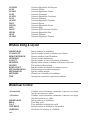
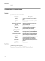
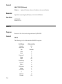
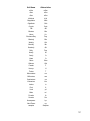
DADiSP Worksheet Function Categories
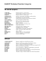
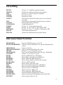
3D and 4D Graphics
CONTOUR
CONTOURSET
DENSITY
GETPALETTE
HATCHCOLOR
IGRID
MAPPALETTE
MOUSEROTATE
PLOT3D
ROTATE3D
SETPALETTE
SETPLOTMETHOD
SETSHADING
SETXPAL
SGRID
SHADEWITH
SPIN
WATERFALL
WFSET
XYZ
Display matrix as a contour plot
Specify display attributes of contour plot
Display matrix as a density plot
Return a series of the color indices used in palette
Set the color of 3D cross-hatching
Grid XYZ data using the inverse distance method
Set color palette for density plot
Rotate a 3-D plot with the mouse
Plot table in true 3-D perspective
Rotate a 3-D plot
Define ordered list of shading colors
Set plotting method
Select the range of shading colors
Set RGB value for color index
Grid XYZ data using spline interpolation
Shade 3-D objects with another object
Spin a 3D plot
Display table as a 3-D waterfall plot
Change attributes of waterfall plot
Create a 3D XYZ plot
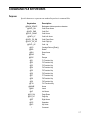
ActiveX
CREATEOBJECT
GETOBJECT
MSWORD
MSWORD2
RELEASE
WS2HTML
XLCLEAR
XLGET
XLINIT
XLPUT
Return a handle to an ActiveX server object
Return a handle to a running ActiveX server object
Write a string to MS Word using ActiveX
Insert a metafile of a Worksheet into MS Word using ActiveX
Release an ActiveX server object
Convert Worksheet to HTML using MS Word and ActiveX
Clear ActiveX connection to Excel
Return a range of values from Excel via ActiveX Automation
Start an ActiveX connection to Excel
Transfer a range of values to Excel via ActiveX Automation
v
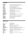
Annotation
COMMENT
DFLOOD
DLNABS
DPTABS
LABEL
LEGCUR
LEGEND
LINEANN
LINECOPY
LINECUR
LINEDEL
LINEDRAW
LINEMOVE
NFORMAT
SETCOMMENT
SFORMAT
TEXT
TEXTANN
TEXTCUR
TEXTDEL
TEXTEDIT
TEXTMOVE
Set comment for the first series in a window
Change the color of the area containing specified points
Draw a line at specified coordinates
Draw a point at specified coordinates
Label the window with text
Insert a legend for all the series in a window
Set the attributes and location for a standard legend
Annotate graph with lines at specified coordinates
Copy line annotation
Freehand line drawing cursor in window
Delete line annotation
Draw a polyline between specified coordinates.
Move line annotation
Format a list of numbers
Set the comment for any window, overlays and overplots
Format a list of strings
Draw a left-justified block of text at a given point
Annotate graph with text at specified coordinates
Freehand text annotation cursor in window
Delete text annotation
Edit text annotation
Move text annotation
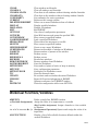
Binary Series
&& || !
< <= > >= == !=
AND &&
DELETE
EQUAL
FLIPFLOP
GREATER
GREATEREQUAL
ISNAN
LESSER
LESSEREQUAL
NOT !
NOTEQUAL
OR ||
REPLACE
XOR
vi
Logical Operators
Conditional operators
Logical AND
Eliminate points based on condition
Determine if two expressions are equal
Combine binary series inputs
Determine if one expression is greater than another
Determine if one expression is greater than or equal to another
Return 1 for each element that is a NA value
Determine if one expression is less than another
Determine if one expression is less than or equal to another
Logical NOT
Determine if two expressions are not equal
Logical OR
Replace values in a series based on a logical condition
Logical XOR
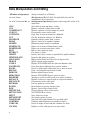
Colors
COLORBAR
COOL
COPPER
DFLOOD
GETCOLORMAP
GETCRANGE
GETGCOLOR
GETGRIDCOLOR
GETPALETTE
GETRBG
GRAY
GRIDCOLOR
HATCHCOLOR
HOT
MAPPALETTE
RAINBOW
RESETMAP
SAVECMAP
SERCOLOR
SETCOLOR
SETCOLORMAP
SETCRANGE
SETGCOLOR
SETPALETTE
SETPMAP
SETSHADING
SETXPAL
SHOWCMAP
STRCOLOR
WINCOLOR
Display the current colormap
Generate a colormap of shades of blue
Generate a copper colormap
Change the color of the area containing specified points
Return the colormap for density and shaded plots
Get color shading range
Get global color parameter
Get color of the grids
Return a series of the color indices used in palette
Return the separate RGB components of an image
Generate a black & white colormap
Set grid color
Set the color of 3D cross-hatching
Generate a colormap of black, red, yellow, white
Sets color palette for density plot
Generate a colormap of the visible color spectrum
Reset the colormaps of all Windows containing an image
Save and automatically restores the Worksheet colormap
Specify series color only
Set series color
Set the colormap for density and shaded plots
Set color shading to a specific range
Set global color parameter
Define ordered list of shading colors
Convert palette color to colormap values
Select the range of shading colors
Set RGB value for color index
Display the current colormap as a density plot
Return the Color Name for specified Color Index
Specify background window and series color
Complex Conversions
ANGLE
CARTESIAN
CONJUGATE
IMAGINARY
MAGNITUDE
MAKECARTESIAN
Extract Angular portion
Convert to Cartesian
Generate Complex Conjugate
Calculate real component of imaginary series
Return magnitude component of series
Combine two input expressions into complex Cartesian
(Real/Imaginary) form
vii
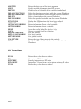
MAKEPOLAR
PHASE
POLAR
REAL
Combine two input expressions into complex Polar
(Magnitude/Phase) form
Calculate the phase angle of a Complex expression
Convert to Polar
Extract Real part
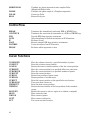
Control Flow
BREAK
CONTINUE
FOR
GOTO
IF
LOOP
WAITKEY
WHILE
Terminate the immediately enclosing FOR or WHILE loop
Terminate the execution of statements in a FOR or WHILE loop
Provide FOR-loop iterative statements
Allow branching to labeled statements in SPL functions
Evaluate if true
Execute simple FOR-Loop iterative statements
Pause execution of an SPL function
Evaluate while expression is true
Cursor Functions
COLNMOVE
COLNPUT
COLPOS
CURMOVE
CURNMOVE
CURNPUT
CURPOS
CURPOS2
CURPUT
CURSORON
ITEMNPUT
ITEMPOS
MAGNIFY
MOVE
NMOVE
NPUT
PUT
viii
Move the column cursor by a specified number of points
Reset the column cursor position
Return the item or column number of the last cursor position
Move the cursor position by a specified offset in x-axis units
Move the cursor position by a specified number of points
Reset the cursor position
Return last position of point cursor
Return position of second cursor
Reset the cursor position at the specified x-axis location
Turn cross hair cursors on
Reset the item cursor position
Return the item number of the last position of the crosshair
cursor
Enable the cursor to select a region in a window to magnify
Move cursor by time
Move cursor n points
Move cursor to nth point
Put cursor on time in series
Curve Fitting
EXPFIT
INTERP2
LFIT
LINREG
LINREG2
LSINFIT
PFIT
POLYFIT
POLYGRAPH
POWFIT
SINFIT
SINTREND
SPLINE
SPLINE2
Fit y(x) = A * exp(B*x) using linearization
Perform two-dimensional linear interpolation
Fit a line to a series using the end points
Fit a line to series
Regress two series
Least Squares method for fitting sine curves of known
frequency
Least Squares Polynomial fitting with error statistics
Return polynomial coefficients
Graph polynomial fit
Fit y(x) = A * x^B using linearization
Fit y(x) = A + B * sin(C*x + D) using the FFT
Fit y(x) = A + B*x + C * sin(D*x + E) using the FFT
Cubic spline interpretation
Perform two-dimensional cubic spline fitting
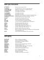
Data Input/Output Functions
EXPORTFILE
EXPORTWORKSHEET
IMPORTFILE
IMPORTWORKSHEET
INPORT
MULTIREADB
OUTPORT
READA
READB
READBMP
READMAT
READTABLE
READTB
RUN
SHELL
WRITEA
WRITEB
WRITEBMP
WRITEHED
WRITETABLE
WRITETB
Export a DADiSP series to a data file
Save the current Worksheet to an external Worksheet file
(.dwk)
Import a data file
Load an external Worksheet file (.dwk)
Retrieve 1, 2, or 4 bytes from a port
Read a multi-channel Binary data file into a Worksheet
Output 1, 2, or 4 bytes to a port
Read an ASCII file into a Worksheet
Read a Binary data file into a Worksheet
Read a Microsoft .BMP bitmap file
Read a binary Matlab .mat file with colormap
Read an ASCII table file
Read a binary table from a file
Run an external program from a Worksheet
Exit to operating system from a Worksheet
Write a series to an ASCII file
Write a series to a Binary file
Write a Microsoft .BMP bitmap file
Automated Import Header File Creation
Write a table from the Worksheet into an ASCII file
Write a binary table to a file
ix
Data Manipulation and Editing
: (Window Assignment)
Assign a formula to a Window
(Bit Operators) Bit left shift, bit right shift, bit and, bit
complement, bit or operators
+= -= /= *= >>= <<= &= |= (Assignment Operators) Operate and assign the value of an
expression
CLIP
Set outlier to min and max y values
COL
Extract a column of data from a table
COLEXTRACT
Extract a portion of each column of a table
CONCAT
Concatenate series (end to end)
COPYDATA
Copy data in current window to clipboard
CUT
Cut the displayed contents of a Window
DECIMATE
Linearly remove points from a series
DELAY
Delay a series by n number of points
DELETE
Eliminate points based on condition
DELETECOL
Delete one or more columns from a table
DELETEROW
Delete one or more rows from a table
EDIT
Edit y values point by point
EXTRACT
Cut pieces of series
INSERT
Insert values into a series as specified by explicit indices
INTERPOLATE
Linearly add points to a series
ISNAVALUE
Binary series based on NA values in input series
MERGE
Splice several series together
NAFILL
Replace NAVALUES with the previous known value
PASTEDATA
Paste data from clipboard into current window
RAVEL
Create a multi-series table from one or more sources
REGION
Copy a rectangular region from a table
REMOVE
Remove points from a series
REMOVENA
Remove NAVALUES from a series or array
REORDER
Arrange a series or table based on a series of indices
REPLACE
Replace values in a series based on a logical condition
REPLICATE
Concatenate series with itself
REVERSE
Put last point in a series first
ROUND
Round input to nearest integer value
ROW
Extract a row of data from a table
SETDELTAX
Change delta-x values of the series
SETNAVALUE
Set NAVALUE in a series
SETPT
Set a point in a series
SETXOFFSET
Set starting point of series
TRANSPOSE
Swap the rows and columns of a specified table
UNMERGE
Unmerge (demultiplexes) an interlaced series
UNRAVEL
Create a single vector from the columns of a table
VALFILL
Replace a value with previous or next value
>> << & ~ bitor
x
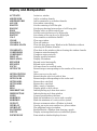
Data Type Conversion
BYTESWAP
CASTBYTE
CASTCOMPLEX
CASTINTEGER
CASTREAL
CASTSERIES
CASTSTRING
CASTVARIANT
CASTVARIANTARRAY
DOUBLE
FLOAT
INT
JULSTR
JULYMD
LONG
SBYTE
SINT
STRJUL
UBYTE
UINT
ULONG
XYDT
Reverse bytes of input series
Cast the values of a series to a new data type
Explicitly casts input as a complex number
Cast input as an integer
Cast input as a real value
Cast input as a series
Cast input as a string
Explicitly casts the input to a variant of a specified type
Explicitly converts a series to an array of variants
Specify double-precision data-file type
Specify floating point data-file type
Calculate integer value of expression
Convert date string to Julian date integer
Convert a series of yymmdd values to Julian dates
Specify long integer data-file type
Specify signed byte data-file type
Specify signed integer data-file type
Convert Julian date integer to date string
Specify unsigned byte data-file type
Specify unsigned integer data-file type
Macro. Provides an argument for functions specifying unsigned
long integer data type
Create an XY plot from Date, Time and Y series
Debugging
DBCLEAR
DBCONT
DBDOWN
DBQUIT
DBSTACK
DBSTATUS
DBSTEP
DBSTEPI
DBSTEPO
DBSTOP
DBUP
DEBUG
LOCALS
Clear a debugger breakpoint
Start or continues the debugger
Move down the debugger callstack
Quit the debugger
Show the status of the debugger callstack
Display debugger status
Step the debugger to the next executable line
Step into the next SPL routine
Step out of the current SPL routine
Set a debugger breakpoint
Move up the debugger callstack
Debugger summary
Display current SPL local variable
xi
Display and Manipulation
ACTIVATE
ADDWFORM
ADDWKSFORM
ASCALE
BARCTR
BARGAP
BARS
BARSTYLE
BARTOP
CALC
CLEAR
CLEARALL
CLEARALLDATA
CLEARDATA
COMPRESSH
COMPRESSV
DISPLAY
DISPLAYALL
EXPANDH
EXPANDV
FOCUS
GETFOCUS
GETPLOTSTYLE
GETPLOTTYPE
GETSCALES
GETXLABEL
GETYLABEL
HIDE
HILO
INHSERSTYLE
INHWINSTYLE
LINES
MARKMAX
MARKMIN
ONPLOT
OVERLAY
OVERPLOT
PLOTMODE
POINTS
POPWINDOW
xii
Activate a window
Add to a window formula
Add a command to a worksheet formula
Set window autoscaling
Set the centering of a 2D bar plot
Set the gap drawing between bars of a 2D step plot
Display series as thick vertical bars
Set the vertical reference of a 2D bar plot
Set coloring of the top face of a 3D bar plot
Set automatic recalculation On/Off
Clear any window
Clear all windows
Clear the data from every Window in the Worksheet without
removing the Window formulae
Clear data in the window without clearing the window formula
Compress series horizontally
Compress series vertically
Display specified windows
Display all windows
Expand series horizontally
Expand series vertically
Set input focus for overlaid series
Return integer corresponding to the number of the curve in
focus
Allow you to set a plot style
Return the plot type for a table of data
Return integer corresponding to the scales used
Return the x-axis label
Return the y-axis label
Hide a range of windows
Display graph as hi-lo values
Inherit plotting style from data series
Inherit plotting style from window
Connect graph points with lines
Mark the maximum of a series with a symbol
Mark the minimum of a series with a symbol
Execute statements when a Window is plotted
Overlay one series onto another in a given window
Plot additional series in window
Enable/Disable a Window from drawing a graph
Display un-interpolated series as individual points
Zoom window whether displayed or not
PROTECT
REDRAW
REFRESH
SCREENOPT
SERCOLOR
SETCOLHEADER
SETCOLOR
SETDATE
SETGCOLOR
SETHATCH
SETLINE
SETLINEWIDTH
SETPLOTMETHOD
SETPLOTSTYLE
SETPLOTTYPE
SETTIME
SETVPORT
SETWFORM
SETWINCURSORINFO
SETWLAB
SETWLIKE
SPANX, SPANY
STACK
STEPCTR
STEPS
STICKS
SYNC
TABLEVIEW
TILE
TOOLBAR
UNACTIVATE
UNITS
UNOVERLAY
UNOVERPLOT
UNPOPWINDOW
UNZOOM
UPDATE
WINCOLOR
WINLOCK
WINNAME
ZOOM
Protect window from propagation
Redraw all windows
Reevaluate worksheet
Select Worksheet elements to be visible or hidden in display
Specify series color only
Set the text of a column header in a Window
Set series color
Set series date acquired
Set global color parameter
Turn 3D cross-hatching On or Off
Set line style
Set thickness of line in graph
Specify method to use when drawing plots
Specify plot style
Specify plot type
Set series time acquired
Set the viewport of the current window to the input window
Set formula for a window
Set the level of information displayed in the Window formula
line
Set the label of a Window
Copy attributes of one window to another
Restrict the scale display to a subrange of the Window
Create a vertical stacked bar chart from a series
Set the vertical reference of a 2D bar plot
Display the series as step line graph
Display the series as thin vertical bars
Set sync mode that controls scaling and scrolling
Display as a table
Arrange the screen into equal size windows
Edit the properties of a DADiSP toolbar
Inactivate the window
Display unit selections
Remove one or more overlayed series
Remove one or more overplotted series
Unzoom a window
Compress window size
Update each formula in worksheet window
Specify background window and series color
Lock the window formula
Specify a name for the window number
Expand window size
xiii
Dynamic Data Exchange (DDE)
DDEADVISE
DDEEXECUTE
DDEGETDATA
DDEGETLINK
DDEINITIATE
DDELINK
DDEPOKE
DDEREQUEST
DDESTATUS
DDETERMINATE
DDEUNADVISE
DDEUNLINK
Retrieve an item from a DDE conversation whenever the item
changes
Execute a command in another application
Retrieve a series item from a DDE conversation
Retrieve a DDE link name from the Clipboard
Begins a DDE Conversation
Retrieve an item from a DDE conversation whenever the item
changes
Send data to a DDE conversation in string form
Retrieve a string item from a DDE conversation
Report the error status of the last DDE operation
Terminate a DDE Conversation
End a previous DDEADVISE operation
End a previous DDELINK operation
File Manipulation
ANYFORMAT
FCLOSE
FCLOSEALL
FFLUSH
FGETS
FOPEN
FPRINTF
FPUTS
FREADA
FREADB
FSEEK
FSTAT
FTELL
FWRITEA
FWRITEB
PRINTF
SFORMAT
SPRINTF
SSCANF
xiv
Produce a formatted output string
Close a file
Close all open files
Flush a buffer to the file
Get a string from an open file
Open a file
Perform formatted output to a file
Put a string in an open file
Read ASCII data from an open file
Read binary data from an open file
Advance file pointer to specified byte in open file
Return selected information about a file
Return the byte of file pointer in open file
Write ASCII data to an open file
Write binary data to an open file
Perform formatted output to the screen
Format a list of strings
Produce an output string in the format of the C/C++ language
printf function
Convert an input string by applying a C/C++ style format
control string
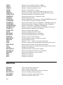
Fourier Transform and Related Functions
ACORR
ACOV
AUTOCOR
AVGFILT
BESTPOW2
BILINEAR
BITQUANT
BITSCALE
CCEPS
CLOGMAG
CONV
CONV2D
COVM
CPHASE
CROSSCOR
DCT
DECONV
DEMEAN
DEMODFM
DFT
EFFBIT
ENDFLIP
FACORR
FACOV
FACTORS
FCONV
FDECONV
FFT
FFTP
FFTSHIFT
FILTEQ
FIRSAMP
FREQSAMP
FXCORR
FXCOV
FZINTERP
HAMMING
HANNING
HILB
ICCEPS
IDCT
Auto-correlation using the convolution method
Auto-covariance using the convolution method
Auto-correlation, time domain
Filter a series using the average of the N neighboring points
Find the power of 2 greater than or equal to the input value
Bilinear transformation with optional frequency pre-warping
Quantize an input series to 2^bits levels
Convert raw AD counts to scales engineering values
Calculate the complex cepstrum
Evaluate the log magnitude of Cascade form coefficients
Convolution
Two-dimensional convolution
Calculate the covariance matrix of an array
Evaluate the phase response of Cascade form filter coefficients
Cross-correlation, time domain
Calculate the Discrete Cosine Transform
Perform deconvolution of two series in the time domain
Remove the mean (or DC value) from a series
Demodulate an FM waveform using the Hilbert Transform
Digital Fourier Transform, Real/Imaginary
Calculate the number of effective bits possible at a given
frequency for a quantizing device
Pad the ends of a series with endpoint reflections
Auto-correlation using the FFT method
Auto-covariance using the FFT method
Return the prime factors of a scalar
Convolution using the FFT method
Perform deconvolution of two series in the time domain
Fast Fourier Transform, Real/Imaginary
Fast Fourier Transform, Magnitude/Phase
Shift a 1D or 2D FFT so the 0 frequency is the midpoint
Evaluate a Linear Constant Coefficient Difference Equation
Design an arbitrary FIR filter using frequency sampling
Design a FIR filter from a given magnitude response using the
frequency sampling method
Cross correlation using the FFT method
Cross covariance using the FFT method
Interpolate a series by a factor using FFT zero insertion
Hamming window
Hanning window
Calculate a simple Hilbert transform of a real series
Calculate the inverse complex cepstrum
Calculate the Inverse Discrete Cosine Transform
xv
IDFT
IFFT
IFFTP
IMPULSE
KAISER
LINSCALE
LOG2
NEXTPOW2
NONLIN2D
OASFILT
PADFILT
POLY
PSD
QUANTIZE
RCEPS
RESCALE
SHP
SINC
SLP
SOBEL
SONOGRAM
SPECGRAM
SPECTRUM
STARMS
TF2SS
WINFUNC
XCORR
XCOV
ZEROFLIP
ZFREQ
ZINTERP
ZPFCOEF
Inverse DFT, Real/Imaginary
Inverse FFT, Real/Imaginary
Inverse FFT, Magnitude/Phase
Generate discrete unit impulse series
Kaiser window
Linearly rescales an input series
Calculate Log base 2 of the input
Determine the exponent for the next power of 2
Perform nonlinear 2d filtering with filter kernel
Filter data using the overlap and save method
FIR filtering with optional endpoint padding
Calculate coefficients of the characteristic polynomial
Power spectral density, Magnitude2
Quantize an input series to N levels
Calculate the real cepstrum
Linearly rescales an input series
Emulate a single pole analog high pass filter
Calculate sin(x)/(x)
Emulate a single pole analog low pass filter
Perform nonlinear 2D Sobel edge detection
Calculate the 2D Spectrogram as a B&W image
Calculate the 2D Spectrogram as an image
Magnitude of a normalized FFT
Calculate the short time averaged RMS series
Calculate the state-space representation
Multiplie a series with a spectral window
Cross correlation using the convolution method
Cross covariance using direct convolution
Pad the ends of a series with endpoint reflections about 0.0
Evaluate the frequency response of a Z transform
Sinx/sin interpolation of periodic band limited waveforms
Design a digital filter from a set of analog zeros and poles
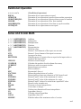
Generated Series
.. (Range Specifier)
{ } Array Construction
: (Window Assignment)
EYE
FXYVALS
GEXP
GHAMMING
GHANNING
xvi
Generate a series consisting of a range of numbers
Create a series or multiple column array
Assign a formula to a Window
Generate an identity matrix
Generate 2D XY values
Generate Exponential series
Generate Hamming window
Generate Hanning window
GIMPULSE
GKAISER
GLINE
GLN
GLOG
GLOG10
GNORMAL
GNUMBER
GRANDOM
GRTSQR
GSERIES
GSQRT
GSQRWAVE
GTRIWAVE
JN
LINE
LINSPACE
LOGSPACE
MESHGRID
ONES
PEAKS
RAND
RANDN
SEEDRAND
YN
ZEROS
Generate an impulse with an optional spacing and delay
Generate Kaiser window
Generate line
Generate logarithmic (base e) series
Generate logarithmic (base e) series
Generate logarithmic (base 10) series
Generate normal series
Generate a series consisting of a range of numbers
Generate random series
Generate a squarewave with a specified rise time
Generate series from points
Generate square root series
Generate square wave
Generate triangle wave
Bessel function
Generate a line
Create a series of n equally spaced values from lo to hi inclusive
Create a series of n log spaced values from 10lo to 10hi inclusive
Create 2D XY values from X and Y input series
Generate an array of all ones
Generate a Gaussian function of two variables, z = f(x, y)
Generate a uniformly distributed random array
Generate a normally distributed random array
Set seed for random number generation
Integer Bessel function
Generate an array of all zeros
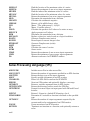
Image Processing
BRIGHTEN
DCT2
FFT2
FFTP2
HISTEQ
IDCT2
IFFT2
IFFTP2
IMAGE24
IMINTERP
INTERP2
RGB2MONO
RGBIMAGE
SPLINE2
Brighten or darkens an image
Calculate the 2D Discrete Cosine Transform
Calculate the 2D FFT of an array
Calculate the 2D FFT of an array in polar (mag-phase) form
Perform histogram equalization of an image
Calculate the 2D Inverse Discrete Cosine Transform
Calculate the 2D IFFT of an array
Calculate the 2D IFFT in polar (magnitude - phase) form
Convert an image with a colormap to a 24 bit color image
Interpolate an image
Perform two-dimensional linear interpolation
Convert an RGB image to 8 bit monochrome
Create a 24 bit image from red, green and blue components
Perform two-dimensional cubic spline fitting
xvii
Datasets, Worksheets, and Labbooks
COPYDATASET
COPYSERIES
DELETEDATASET
DELETELABBOOK
DELETESERIES
DELETEWORKSHEET
LOADDATASET
LOADSERIES
LOADWORKSHEET
NEWWORKSHEET
OPENLABBOOK
SAVESERIES
SAVEWORKSHEET
Copy a Series from a Dataset
Copy a Series from a Dataset
Delete an entire Dataset of the current Worksheet
Delete an entire Labbook
Delete one or more Series from a Dataset
Delete one or more Worksheets from a Labbook
Load entire Dataset into Worksheet
Load a specified Series
Load a specified Worksheet
Create a new, empty Worksheet
Open an entire Labbook
Save data as a DADiSP Series
Save the Worksheet
Logical Operators
&& || !
AND &&
FLIPFLOP
NOT !
OR ||
XOR
Logical Operators
Logical AND
Combine binary series inputs
Logical NOT
Logical OR
Logical XOR
Macro and Command File Functions
#DEFAULT
#DEFINE
#INCLUDE
#UNDEFALL
#UNDEFINE
; (Semicolon)
| (Vertbar)
ALLMACROS
CALL
COMFILESTATUS
xviii
Restore default macros
Define a macro
Include macro files in other macro files
Undefine all macros
Undefine a macro
Combine several functions, commands, or macros on a single
line for execution as a whole.
Combine several functions, commands, or macros on a single
line for execution as a whole.
Display all macros
Call a command file n times
Return the execution status of a command file
COMMAND FILE FUNC…
COMMAND FILE KEYS…
COMMANDS
DEFMACRO
DSPMACREAD
DSPMACVIEW
EVAL
EVALTOSTR
FUNCS
GETMACRO
ISMACRO
JUMP
LOAD
MACREAD
MACROS
MACWRITE
MESSAGELOG
NOP
OFF
ON
SETMACDEPTH
VIEWFILE
Execute a command file function
Represent non-standard keystrokes
Display list of commands available at worksheet level
Define macro string or scalar constant
Read macro definitions from file in the MACROS subdirectory
View an ASCII text file from the MACROS subdirectory
Evaluate string expression
Evaluate to a string
Display list of available functions
Return information about a macro
Determine whether a macro is defined
Jump to a label in a macro
Load a command file
Read an external file of macro definitions
List current macros defined in worksheet
Write current macro list to an external file
Write status line messages to text file
Perform no operation
Macro returning integer 0
Macro returning integer 1
Set maximum depth for nesting macros
Display contents of ASCII file
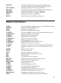
Matrix Math
{ } Array Construction
*^ (Matrix Multiply)
^^ (Matrix Power)
\^ (Matrix Solve)
/^ (Matrix Right Div)
' (Matrix Transpose)
~^ (Matrix Conj Trans)
BALANCE
CHOLESKY
COLNOS
COND
DET
DIAGONAL
EIG
EIGVAL
EIGVEC
EXPM
FLIPLR
Create a series or multiple column array
Multiply two matrices
Raise a matrix to a scalar power or a scalar to a matrix power
Divide one matrix by another
Performs matrix right division
Swap the rows and columns of a specified table
Complex conjugate of the matrix transpose
Balance a matrix
Compute the Cholesky factorization of a square matrix
Return an array of COL numbers
Estimate the condition number of a matrix
Calculate matrix determinant
Get the main diagonal of a matrix
Compute the Eigenvalues and Eigenvectors of a square matrix
Get Eigenvalues of a matrix
Get Eigenvectors of a matrix
Calculate the exponential of a matrix
Reverse the elements of each row of an array
xix
FLIPUD
HESS
INTERPOSE
INNERPROD
INVERSE
KRON
LLU
LOTRI
LOTRIX
LU
MAGIC
MDIV
MMULT
NBEIGVAL
NBEIGVEC
NORM
NULL
NUMCOLS
NUMROWS
ORTH
OUTERPROD
PARTPROD
PINV
QR
RANK
REPMAT
ROWNOS
SCHUR
SIZE
SVD
TRACE
TRANSPOSE
TRIL
TRIU
ULU
UPTRI
UPTRIX
USCHUR
xx
Reverse the elements of each column of an array
Find the Hessenberg form of a matrix
Apply REDUCE associatively
Matrix Inner Product
Invert a matrix
Return the Kronecker tensor product of two arrays
Lower triangular matrix in LU decomposition
Return the lower triangle of a matrix including the main
diagonal
Return the lower triangle of a matrix excluding the main
diagonal
LU decomposition
Create an NxN magic square
Matrix Division
Matrix Multiplication
Get Eigenvalues without balancing step
Get Eigenvectors without balancing step
Calculate the norm of a series or array
Compute an orthogonal basis for the Null space of an array
Return the number of columns in a Window or DADiSP
expression
Return the number of rows in a Window or DADiSP expression
Compute an orthonormal basis of an array using SVD
Outer Product of two vectors
Partial Product of two vectors
Calculate the pseudo inverse of a matrix using SVD
QR decomposition
Estimate the number of independent rows or columns of an
array
Replicate an array down and across
Return an array of row numbers
Generate the SCHUR form of a matrix
Return a 2 point series containing the dimensions of an array
Generate Singular Value Decomposition of a matrix
Calculate the trace of an array, the sum of the diagonal
elements
Transpose a matrix
Return the lower triangle of a matrix
Return the upper triangle of a matrix
Upper triangular matrix in LU decomposition
Return the upper triangle of a matrix including the main
diagonal
Return the upper triangle of a matrix excluding the main
diagonal
Compute the SCHUR form of an input matrix
Menu Functions
ECHO
GETSTRING
HELP
HELPFILE
INPUT
MENUCLEAR
MENUFILE
MENULIST
MENUPRINT
MESSAGE
MESSAGELOG
PICKFILE
PICKLIST
PICKUNITS
VIEWFILE
Print text at the bottom of the screen
Prompt for textual input via input panel with OK and Cancel
buttons
Accesse the on-line help file, dspfun.hlp
Accesse on-line help files
Allow the user to input values to functions
Clear menus from the screen
Generate a pop-up menu at the worksheet level
Display a specified menu from the screen
Send menu text to file
Display a message box with an OK button and/or a Cancel
button
Write status line messages to text file
Use a native GUI dialog box to select a file
Display a list and returns the item selected by the user
Select units from a pop-up list
Display ASCII text file
Numerical Formatting
SETDEGREE
SETFORMAT
SETPRECISION
SETRADIAN
Change mode of trigonometric functions to degrees
Set display type for numerical values
Set number of significant digits after the decimal point to
display
Change mode of trigonometric functions to radians
Operating System Interface
DOS, UNIX, VMS
GETENV
GOTOURL
PATHCHAR
PUTENV
RUN
SHELL
VIEWFILE
Temporarily exit DADiSP to operating system
Get the value of an environment parameter
Start Web browser and opens the specified URL
Macro for path character in DOS, UNIX, or VMS
Set the value of an environment parameter
Run an external program from a worksheet
Exit to operating system from shell
Display contents of ASCII file
xxi
Output
INFOPLOT
INFOPLOTALL
INFOPRINT
INFOPRINTALL
INFOPS
INFOPSALL
PLOT
PLOTALL
PLOTWS
PREVIEWALL
PREVIEWINFO
PREVIEWWIN
PREVIEWWS
PRINT
PRINTALL
PRINTOPT
PRINTWS
PRNSCREEN
PS
PSALL
PSWS
SCREENOPT
Plot window and series information box
Plot all windows, each with its series information box
Print window and series information box
Print all windows, each with its series information box
Create PostScript plot of window and series information box
Create PostScript plot of all windows, each with info box
Plot a window
Plot all windows
Plot Worksheet as displayed
Preview a PRINTALL of the current Window
Preview an INFOPRINT of the current Window
Preview a PRINT of the current Window
Preview a PRINTWS of the current Window
Print a window
Print all windows
Select Worksheet elements to be visible or hidden in a display
Print Worksheet as displayed
Print a snapshot of the screen
Create PostScript file of current window
Create PostScript file of all windows
Create PostScript file of the Worksheet as displayed
Select Worksheet elements to be visible or hidden in display
Peak Analysis
COLIDX
COLMAXIDX
COLMINIDX
FINDMAX
FINDMIN
FINDVAL
FMAX
FMIN
FPEAK
FPEAKN
FPEAKP
FVALL
FVALLN
xxii
Return the indices for each column of the input table
Return a row of indices for the maximums of each column of the
input table
Return a row of indices for the minimums of each column of the
input table
Return X and Y value of the maximum of a series
Return X and Y value of the minimum of a series
Return X and Y values of a series from a specified Y value
Find and go to maximum of series
Find and go to minimum of series
Find first peak
Find next peak
Find previous peak
Find first valley
Find next valley
FVALLP
GETPEAK
GETPT
GETVALLEY
LEVELCROSS
MAX
MAXIDX
MAXLOC
MAXVAL
MIN
MINIDX
MINLOC
MINVAL
REALMAX
REALMIN
VMAX
VMIN
Find previous valley
Find peaks of series
Display value of nth point
Find valleys of series
Determine where series crosses level
Find maximum of series
Find the index of the maximum value of a series
Find the location of the maximum value of a series
Return the maximum of one or two input arguments
Find minimum of series
Find the index of the minimum value of a series
Find the location of the minimum value of a series
Return the minimum of on or two input arguments
Return the largest positive real number
Return the smallest positive real number
Return the maximum of one or more input arguments
Return the minimum of one or more input arguments
Plot Attributes
CLEARXLABEL
CLEARYLABEL
GETPLOTSTYLE
GETPLOTTYPE
GRIDCOLOR
GRIDDASH
GRIDDOT
GRIDH
GRIDHV
GRIDOFF
GRIDSOL
GRIDV
INHSERSTYLE
INHWINSTYLE
PLOTMODE
SCALES
SCALES
SCALESOFF
SCALESON
SCROLLD
SCROLLL
SCROLLR
Reset x-axis label
Reset y-axis label
Allow you to set a plot style
Return the plot type for a table of data
Set grid color
Turn grid to dashed
Turn grid to dotted
Set grid orientation horizontal
Set grid orientation horizontal and/or vertically
Turn grid off
Turn grid to solid
Set grid orientation vertical
Inherit plotting style from data series
Inherit plotting style from window
Enable/Disable a Window from drawing a graph
Set types of scales
Set types of scales
Turn scales off
Turn scales on
Scroll display down
Scroll display left
Scroll display right
xxiii
SCROLLU
SETAORIX
SETAORIY
SETAROTX
SETAROTY
SETAVDEFX
SETAVDEFY
SETHUNITS
SETLINE
SETLINEWIDTH
SETPLOTMETHOD
SETPLOTSTYLE
SETPLOTTYPE
SETSYMBOL
SETTORIX
SETTORIY
SETTROTX
SETTROTY
SETTVDEFX
SETTVDEFY
SETVUNITS
SETWLIKE
SETX
SETXLABEL
SETYLABEL
SETXLOG
SETXOFFSET
SETXTIC
SETXY
SETY
SETYLOG
SETYTIC
SETZ
SETZTIC
STAGGERX
STAGGERY
SYNC
WFSET
WHICHSCALES
XSUBTIC
YSUBTIC
xxiv
Scroll display up
Set the axis label orientation
Set the axis label orientation
Set the axis label rotation
Set the axis label rotation
Set the default rotation for x-axis labels
Set the default rotation for y-axis labels
Set horizontal units
Set line style
Set thickness of line in graph
Specify method to use when drawing plots
Specify plot style
Specify plot type
Specify symbol to mark data points
Set the x-tic label orientation
Set the y-tic label orientation
Set the x-tic label rotation
Set the y-tic label rotation
Set the default rotation for x-tic labels
Set the default rotation for y-tic labels
Set vertical units
Copy attributes of one window to another
Specify x-axis coordinate range
Set the x-axis label
Set the y-axis label
Turn on/off log scales for x-axis of current window
Set starting point of series
Set tic interval on x-axis
Specify y-axis coordinate range
Specify y-axis coordinate range
Turn on/off log scales for y-axis of current window
Set tic interval on y-axis
Specify the z-axis coordinate range of a Window
Set the tic spacing on the z-axis
Turn staggered scales on or off
Turn staggered scales on or off
Set sync mode that controls scaling and scrolling
Set attributes of a waterfall plot
Return scale which matches the described property parameter
Set subtic labeling for log X axis
Set subtic labeling for log Y axis
Query Functions
BUILTINS
CHILDREN
CLOCK
COLNOS
DELTAX
DIRPATH
FINITE
GETCOMMENT
GETCONF
GETDATE
GETGCOLOR
GETGRIDCOLOR
GETHOME
GETHUNITS
GETLABEL
GETLABNAME
GETLABPATH
GETPALETTE
GETSYMBOL
GETTIME
GETVUNITS
GETWCOLOR
GETWCOUNT
GETWFORMULA
GETWINCURSORINFO
List all built-in functions available in DADiSP
Return number of children for the window
Return the current execution clock in seconds
Return an array of COL numbers
Display delta-x value (1/sample rate)
Return the directory component of a path string
Return 1 for each element that is not infinite (inf) or NA (nan)
Get comment string for first series in a window
Get value of configuration parameter
Get system date
Get global color parameter
Get color of the grids
Get the path to DADiSP's home directory
Get horizontal units
Get the label of the specified window
Get the name of current Labbook
Get the path to the current Labbook
Return a series of the color indices used in palette
Return the type of symbol used for the specified series.
Get the system time
Get vertical units
Get the color of a window
Get the number of series in a window
Get the formula for a window in string form
Return the setting for the level of information displayed in a
Window formula line
GETWMARGIN
Get percentage of margin for window
GETWNUM
Get the number of the current window
GETWORKSHEETNAME Get the name of the current Worksheet
GETWSIZE
Get the window dimensions
GETXL
Get leftmost x-coordinate
GETXR
Get rightmost x-coordinate
GETXTIC
Get x-axis tic interval
GETYB
Get bottom y-coordinate
GETYT
Get top y-coordinate
GETYTIC
Get y-axis tic interval
GETZB
Return the bottom z coordinate of a Window
GETZT
Return the top z coordinate of a Window
GETZTIC
Return the z-axis tic interval of a Window
IDX
Return the indices of a series or array
ISCOMPLX
Return 1 if input parameter is complex
ISEMPTY
Return 1 if the input series is empty.
ISFUNC
Return 1 if input is a loaded SPL function, else 0
xxv
ISINF
ISNAN
ISREAL
ISSTR
ISUNIT
ITEMCOL
ITEMCOUNT
ITEMTYPE
LENGTH
NUMCOLS
NUMITEMS
NUMROWS
NUMVWINS
NUMWINDOWS
OBJECTLIST
PARENTS
PICKUNITS
RATE
REALMAX
REALMIN
ROWNOS
SERCOUNT
SERSIZE
SIGN
SIZE
STRCOLOR
TOC
UNITS
WINSTATUS
WRITECNF
XOFFSET
XTIC
YTIC
ZTIC
Return 1 for each element that is infinite
Return 1 for each element that is a NA value
Return 1 if input parameter is real
Return 1 if the input is a string
Return 1 if string is a recognized engineering unit, else 0
Return the column number where the specified item starts
Return the number of columns in an item
Return the item type of a composite series
Return length of series
Return the number of columns in a Window/DADiSP expression
Count number of items in window or matrix
Return the number of rows in a Window or DADiSP expression
Return the number of displayed Windows in the Worksheet
Return total number of windows in Worksheet
Return a string of available Labbooks, Worksheets, Datasets
Return number of parents of the window
Select units from a pop-up list
Display sampling rate of the series
Return the largest positive real number
Return the smallest positive real number
Return an array of row numbers
Count number of series in window or matrix
Return length of series
Return +1, 0 or –1 based on the sign of the input
Return a 2 point series containing the dimensions of an array
Return the Color Name for specified Color Index
Return the number of seconds since the internal timer started
Display unit selections
Return the status of the current window
Write the configuration table to an ASCII file
Return the x offset of a series or table
Return x-tic interval
Return y-tic interval
Return z-tic interval
Real Time
RTREAD
RTSPIN
RTTINIT
RTTPAUSE
RTTTERM
RTWRITE
xxvi
Read real time data from a file
Spin a 3D plot in Real Time
Place a real time task in the queue for execution
Pause a real time task in the queue
Remove a real time task from the queue
Read real time data from a file
Relational Operators
< <= > >= == !=
EQUAL
GREATER
GREATEREQUAL
LESSER
LESSEREQUAL
NOTEQUAL
(Conditional operators)
Determine if two expressions are equal
Determine if one expression is greater than another expression
Determine if one expression is greater than or equal to another
Determine if one expression is less than another
Determine if one expression is less than or equal to another
Determine if two expressions are not equal
Series and Scalar Math
+ - * / ^ (ARITHMETIC)
+ - * / ^ (ARITHMETIC)
+ - * / ^ (ARITHMETIC)
+ - * / ^ (ARITHMETIC)
+ - * / ^ (ARITHMETIC)
ABS
ALL
ANY
AVGS
BESTPOW2
CEILING
COLPROD
CURRENT
DEG
E
EXP
FACTORS
FIND
FINDMAX
FINDMIN
FINDVAL
FIX
FLOOR
INT
INTERP2
LN
LOG
LOG10
MAXIDX
Addition
Subtraction
Multiplication
Division
Exponentiation
Absolute value
Return 1 if all elements of the input are non-zero
Return 1 if any element of the input is non-zero
Average of n series
Find the power of 2 greater than or equal to the input value or
length of the input series
Round to closest integer
Calculate the product of each column of an array
Reference series in current window
Return degrees per radian
Euler's number e
Exponential, (base e)
Return the prime factors of a scalar
Return indices of non-zero elements or NA if none found
Return X and Y value of the maximum of a series
Return X and Y value of the minimum of a series
Return X and Y values of a series from a specified Y value
Round a value towards zero
Truncate to closest integer below
Cast scalar as integer
Perform two-dimensional linear interpolation
Logarithm, (base e)
Calculate natural logarithm
Logarithm, (base 10)
Find the index of the maximum value of a series
xxvii
MAXLOC
MAXVAL
MINIDX
MINLOC
MINVAL
MOD
NEGATE
NIBBLE
PHI
PI
PROD
REDUCE
REM
REPLACE
ROOTS
ROUND
RTHROOT
SQRT
SUM
SUMS
VMAX
VMIN
W0
Find the location of the maximum value of a series
Return the maximum of one or two input arguments
Find the index of the minimum value of a series
Find the location of the minimum value of a series
Return the minimum of on or two input arguments
Determine the remainder from a division.
Calculate the arithmetic negative
Extract a 4 bit nibble from a value
Macro. "The golden mean" (-1+(5))/2
Macro. Provides value of
Calculate the product of all values of a series or array
Apply operator to all values
Determine the remainder from a division.
Replace values in a series based on a logical condition
Generate Complex roots (series)
Round input to nearest integer value
Generate Complex root (scalar)
Square root
Calculate the sum of a series
Sum n series
Return the maximum of one or more input arguments
Return the minimum of one or more input arguments
Alternate reference for CURRENT window
Series Processing Language (SPL)
#INCLUDE
ARGCOUNT
ARGTYPE
ARGV
CLEAROPL
ERROR
GETARGV
GETSPLPATH
GETSTRING
ISFUNC
ISVARIABLE
OUTARGC
PAUSE
RETURN
xxviii
Include macro files in other macro files
Return the number of arguments specified in an SPL function
Return the data type of the input argument
Specify variable arguments in an SPL routine
Delete all .OPL files located on the SPLPATH
Abort an SPL routine and optionally displays a message
Return a variable argument from an SPL routine
Return the directory path to search for SPL files
Prompt for textual input via input panel with OK and Cancel
buttons
Return 1 if input is a loaded SPL function, else 0
Determine if a variable or function is defined as the specified
type
Return the number of output arguments expected by the
current multi-value assignment of an SPL function
Pause execution of an SPL function
Terminate an iteration or a function, and optionally returns a
value
SERIES.H
SPLCOMPILE
SPLLOAD
SPLREAD
SPLWRITE
VIEW
WHICH
Contain definitions of global data types, variables, and
miscellaneous macros, for including in SPL function files.
Compile an SPL function file into an OPL file
Compile and reads an external SPL file into the Worksheet
Read an external SPL file into the Worksheet
Write SPL functions to an external ASCII file
Display the contents of an SPL file
Return the path to an SPL file or filename
Statistics and Calculus
A2STD
AMPDIST
AREA
BETAI
CNF2STD
COLLENGTH
COLMAX
COLMEAN
COLMEDIAN
COLMIN
COLREDUCE
COLSTDEV
COLSUM
CONFX
CTREE
DERIV
DYDX
EPS
ERF
ERFC
ERFCINV
ERFINV
ERRORBAR
GAMM
GAMMA
GAMMLN
GAMMP
GAMMQ
GRADIENT
HISTOGRAM
IGRID
Convert an alpha confidence level to a standard deviation range
Calculate Amplitude Distribution
Calculate area under curve
Return the incomplete beta function
Convert a confidence level (%) to a standard deviation range
Number of samples in each column
Maximum value in each column
Mean value for each column
Median value for each column
Minimum value for each column
Apply REDUCE function to each column
Standard deviation of each column
Produce a row of the sums of each column of the input table
Calculate confidence level for a given density function and x
value
Creates a binary fractal
Calculate derivative
Perform a derivative on XY data
Return the minimum positive real value
Error function
Complementary error function
Return the inverse incomplete error function
Return the inverse error function
Add error bars to graph
Gamma Function
Numeric constant: 0.577216
Natural log of the Gamma function
Incomplete Gamma function
Complementary incomplete Gamma function
Calculate the 2D derivative of an array
Calculate the frequency of values in a series
Grid XYZ data using the inverse distance method
xxix
INDEX
INF
INTEG
INVDISTANCE
INVPROBN
IVSNORMPB
LDERIV
LENGTH
LINREG
LINREG2
MAX
MEAN
MEDIAN
MOVAVG
MOVAVG2
MOVMAX
MOVMIN
MOVRMS
MOVSTD
PARTSUM
PDFNORM
PEARSON
POLYROOT
PROBN
RDERIV
RMS
ROWREDUCE
SERSIZE
SGRID
SPLINE2
STATS
STDERR
STDEV
SVD
SVDDIV
TRAPZ
TREND
XCONF
xxx
Normalize series to percentage terms
Return the numeric representation of positive infinity
Calculate the integral of a series or series expression.
Interpolate XYZ data to arbitrary XY coordinates using the
inverse distance method
Return z value of the probability of X <= z for a normal
distribution
Return z value for input probability based on normal pdf
Calculate derivative from the left
Return length of series
Determine linear regression
Linear regression of two or more series
Calculate max
Calculate mean
Calculate median
Moving Average
Moving average with end point padding
Perform n-point moving maximum calculations
Perform n-point moving minimum calculations
Calculate the "moving" RMS of a series
Calculate the "moving" standard deviation of a series
Calculate Partial sum
Return the probability density function for a normal
distribution
Calculate Pearson's Linear Correlation Coefficient
Find the roots of a polynomial using the companion matrix
Calculate the probability of X <= z for a normal distribution
Calculate derivative from right
Root Mean Square
Apply REDUCE function to each row of a matrix
Return length of series
Grid XYZ data using spline interpolation
Perform two-dimensional cubic spline fitting
Display statistics, STDEV and ERROR
Calculate the standard error of a series or table
Calculate Standard Deviation
Generate Singular Value Decomposition of a matrix
Solve for x in A *^ x = b using singular value decomposition
Integration using the trapezoidal rule
Fit a line to a series
Calculate x value for a given density function and confidence
level
String Manipulation
ANYFORMAT
CHARSTR
CHARSTRS
DIRPATH
FPRINTF
GETSTRING
ISNUMBER
NFORMAT
NUMSTR
NUMSTRS
PATHCHAR
PRINTF
SFORMAT
SPRINTF
SSCANF
STRCAT
STRCHAR, STRCHARS
STRCMP
STRESCAPE
STREXTRACT
STRFILE
STRFIND
STRFTIME
STRGET
STRLEN
STRLIST
STRNUM
STRREVERSE
STRTOD
STRWIN
TODSTR
TODMSECSTR
TOLOWER
TOUPPER
Format a list of strings or scalars
Find the ASCII code for the specified character
Find the ASCII codes for the specified string
Return the directory component of a path string
Perform formatted output to a file
Prompt for textual input via input panel with OK and Cancel
buttons
Test whether input string is a number
Format a list of numbers
Convert a string into a scalar
Convert a string that contains a list of scalars into a series
Return the separator character used in the file path names by
the operating system
Perform formatted output to the screen
Format a list of strings
Produce an output string in the format of the C/C++ language
printf function
Converts an input string by applying a C/C++ style format
control string
Concatenate two or more strings
Convert numbers to 8 bit ASCII characters
Compare two strings
Convert escape characters in a string
Extract a part of a string
Turn an ASCII text file into a string
Find a position within a string
Convert a time value to a string
Return the nth substring
Return the length of a string
Convert a list of several strings into one string
Convert a number into a string
Reverse order of characters in a string
Return the time form of integer in seconds
Return the window number as a string
Return the number of seconds from a time string
Return the seconds to millisecond precision from a time string
Convert string to lowercase
Convert string to uppercase
xxxi
Table Manipulation
COL
COLEXTRACT
COLLENGTH
COLMAX
COLMEAN
COLMEDIAN
COLMIN
COLREDUCE
COLSTDEV
COLSUM
DELETECOL
DELETEROW
FLIPLR
FLIPUD
GETSERIES
GRADE
ISNAVALUE
LOOKUP
NAN
NAVALUE
NUMCOLS
NUMEL
NUMITEMS
NUMROWS
RAVEL
REGION
REORDER
REPMAT
RESHAPE
ROW
ROWREDUCE
SERCOUNT
SETCOLHEADER
SETMATRIX
SORT
TABLE
TABLES
TABLEVIEW
UNMERGE
UNRAVEL
xxxii
Extract a column of a table
Extract a portion of each column of a table
Number of samples in each column
Maximum value in each column
Mean value for each column
Median value for each column
Minimum value for each column
Apply REDUCE function to each column
Standard deviation of each column
Produce a row of the sums of each column of the input table
Delete one or more columns from a table
Delete one or more rows from a table
Reverse the elements of each row of an array
Reverse the elements of each column of an array
Return the nth column of table corresponding to nth overplot
Rank table values
Binary series based on NA values in input series
Pick selected points by table
The value used to represent NAs in numeric data
Null data value
Return the number of columns in a Window or DADiSP
expression
Return the total number of array elements
Count number of items in window or matrix
Return the number of rows in a Window or DADiSP expression
Create a table from a single vector
Extract a rectangular region of a table
Reorder based on rank values
Replicate an array down and across
Create a table with different length columns
Extract a row of a table
Apply REDUCE function to each row of a matrix
Determine number of series in a window
Set the text of a column header in a Window
Turn table mode on/off
Sort a table
Display point values of one series
Display point values of n series
Display as a table
Unmerge (demultiplexes) an interlaced series
Create a single vector from multiple columns
Trigonometric Functions:
ACOS
ACOSH
ACOT
ACOTH
ACSC
ACSCH
ASEC
ASECH
ASIN
ASINH
ATAN
ATANH
COS
COSH
COT
COTH
CSC
CSCH
DEG
SEC
SECH
SIN
SINC
SINH
TAN
TANH
ArcCosine
Hyperbolic ArcCosine
ArcCotangent
Hyperbolic ArcCotangent
ArcCosecant
Hyperbolic ArcCosecant
ArcSecant
Hyperbolic ArcSecant
ArcSine
Hyperbolic ArcSine
ArcTangent
Hyperbolic ArcTangent
Cosine
Hyperbolic Cosine
Cotangent
Hyperbolic Cotangent
Cosecant
Hyperbolic Cosecant
Degrees per radian (360/2*pi)
Secant
Hyperbolic Secant
Sine
Sin(x)/x
Hyperbolic Sine
Tangent
Hyperbolic Tangent
Trigonometric Series Generation:
GACOS
GACOSH
GACOT
GACOTH
GACSC
GACSCH
GASEC
GASECH
GASIN
GASINH
GATAN
Generate ArcCosine
Generate Hyperbolic ArcCosine
Generate ArcCotangent
Generate Hyperbolic ArcCotangent
Generate ArcCosecant
Generate Hyperbolic ArcCosecant
Generate ArcSecant
Generate Hyperbolic ArcSecant
Generate ArcSine
Generate Hyperbolic ArcSine
Generate Arctangent
xxxiii
GATANH
GCOS
GCOSH
GCOT
GCOTH
GCSC
GCSCH
GSEC
GSECH
GSIN
GSINC
GSINH
GTAN
GTANH
Generate Hyperbolic ArcTangent
Generate Cosine
Generate Hyperbolic Cosine
Generate Cotangent
Generate Hyperbolic Cotangent
Generate Cosecant
Generate Hyperbolic Cosecant
Generate Secant
Generate Hyperbolic Secant
Generate Sine
Generate SINC function (sin(x)/x)
Generate Hyperbolic Sine
Generate Tangent
Generate Hyperbolic Tangent
Window Sizing & Layout
ADDWINDOW
COLLAYOUT
REMOVEWINDOW
GETWSIZE
LAYOUT
MOVEWIN
NEATEN
ROWLAYOUT
SETALLWMARGIN
SETWMARGIN
SETWSIZE
TILE
Insert windows in worksheet
Specify number of rows of windows per column
Remove windows from Worksheet
Get the window dimensions
Specify number of rows and columns of windows
Specify which corners of windows will move and resize
Tile windows after resizing
Specify number of columns of windows per row
Set percentage of window for margin
Specify window margin
Change size of windows in worksheet
Arrange the screen into equal-sized windows
Worksheet Control
; (Semicolon)
| (Vertbar)
ADDWINDOW
BEEP
CALC
CHILDREN
CHKFILES
xxxiv
Combine several functions, commands, or macros on a single
line for execution as a whole.
Combine several functions, commands, or macros on a single
line for execution as a whole.
Insert windows in worksheet
Turn Beep on/of
Turn worksheet calculations on/off
Return number of children for the window
Check the file integrity of a Labbook
CLEAR
CLEARALL
CLEARALLDATA
CLEARDATA
CONFORMITY
CURRENT
DELETEWORKSHEET
DISPLAY
DISPLAYALL
EXIT
GETCONF
GOTOURL
GOTOWINDOW
LOADWORKSHEET
MESSAGELOG
MOVETO
NEWWORKSHEET
NUMWINDOWS
PARENTS
REDRAW
REDRAWALL
REFRESH
REMOVEWINDOW
SAVEWORKSHEET
SETBUFSIZE
SETCONF
SETWSCURSOR
TIC
UPDATE
VERSION
W0
WRITECNF
Clear window and formula
Clear all windows and formulas
Clear data in all windows without clearing window formulas
Clear data in the window without clearing window formula
Set conformity for series operations
Reference the current window
Delete one or more Worksheets from a Labbook
Display specified windows
Display all windows
Exit DADiSP
Get value of configuration parameter
Start Web browser and opens the specified URL
Move cursor to specified window
Load a specified Worksheet
Write status line messages to text file
Move cursor to specified window
Create a new, empty Worksheet
Return total number of windows in Worksheet
Return number of parents of the window
Redraw screen
Redraw screen
Recalculate windows
Remove windows from Worksheet
Save the Worksheet
Set number of points of series to keep in memory
Set a configuration parameter
Set display for Worksheet cursor
Start the internal timer
Re-evaluate and recalculate the entire Worksheet
Report full version information of DADiSP
Alternate reference for CURRENT window
Write the configuration table to an ASCII file
Worksheet Functions/Variables
#DEFFUN
Define a single line DADiSP function
= (Variable Assignment) Assign the value of an expression to a variable
:=
(Hot Variable Assignment) Assign a formula to a hot variable
or Window
+= -= /= *= >>= <<= &= |= (Assignment Operators) Operate and assign the value of an
expression
ALLFUNCTIONS
Display a list of all available functions defined within the
current Worksheet
xxxv
ARGTYPE
ARGV
DEFVAR
DELALLFUNCTIONS
DELALLVARIABLES
DELFUN
DELVARIABLE
FUNCTIONS
GETARGV
GETLOCALVARIABLE
GETVARIABLE
HELP
LOCAL
SETHOTVARIABLE
SETLOCALVARIABLE
SETVARIABLE
VALUETYPE
VARS
Return the data type of the input argument
Specify variable arguments in an SPL routine
Set the value of a variable if the variable is undefined
Delete the functions associated with the current Worksheet
Delete all the variables associated with current Worksheet
Delete a function from the current Worksheet
Delete the specified variable from the current Worksheet
Display the SPL functions that have been defined
Return a variable argument from an SPL routine
Return information about a local variable
Return information about a variable
Access the on-line help file, dspfun.hlp
Declare a variable local to a function
Set a hot variable
Set a local variable
Set a global variable
Return the type of data stored in the variable
List all the SPL variables that have been defined in the current
Worksheet
XY Functions
XVALS
XY
XYINTERP
XYLOOKUP
YVALS
xxxvi
Return the x values from a window
Generate an XY plot in a window
Linearly interpolate an XY series
Interpolate Y values from a series given arbitrary X values
Return the y values from a window
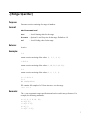
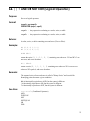
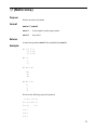
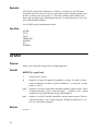
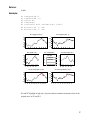
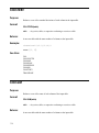
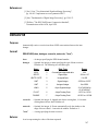
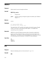
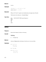
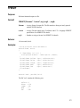
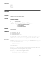
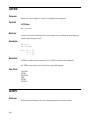
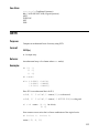
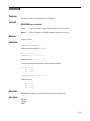
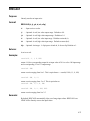
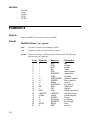
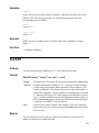
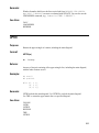
..(Range Specifier)
Purpose:
Generates a series consisting of a range of numbers.
Format:
start..increment..end
start
- A real. Starting value for the range.
increment - Optional. A real. Step size for the range. Defaults to 1.0.
end
- A real. Ending value for the range.
Returns:
A series.
Example:
1..5
returns a series consisting of the values {1, 2, 3, 4, 5}.
1..0.8..5
returns a series consisting of the values {1,1.8,2.6,3.4,4.2,5}.
5..1
returns a series consisting of the values {5, 4, 3, 2, 1}.
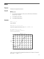
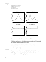
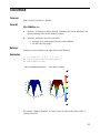
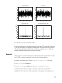
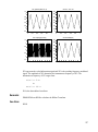
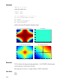
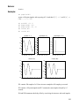
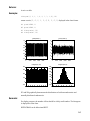
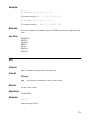
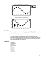
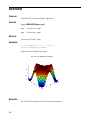
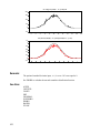
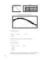
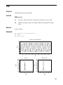
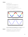
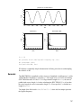
t = -2..0.01..2
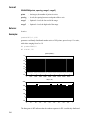
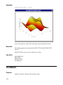
f = 3
W1: sin(2*pi*f*t)
W1 contains 401 samples of a 3 Hertz sinewave over the range
–2 <= t <= 2
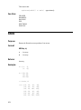
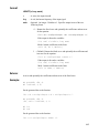
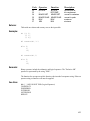
Remarks:
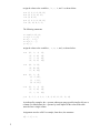
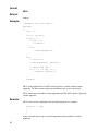
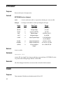
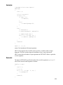
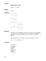
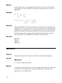
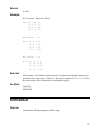
The .. acts as a numeric range specification and can be used in array references. For
example, the following statements:
a
b
c
d
f
=
=
=
=
=
{2, 4, 6, 8, 10, 12};
a[2..6];
a[2..2..6];
a[..];
a[6..-1..2];
1
assign the values to the variables a, b, c, d, and f as shown below:
a
b
c
d
f
==
==
==
==
==
{2, 4, 6, 8, 10, 12}
{4, 6, 8, 10, 12}
{4, 8, 12}
{2, 4, 6, 8, 10, 12}
{12, 10, 8, 6, 4}
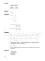
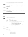
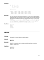
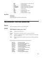
The following statements:
u
v
w
x
y
=
=
=
=
=
ravel(1..16, 4);
u[1..3, 2..4];
u[.., 1..3];
u[1..3, ..];
u[..];
assign the values to the variables u, v, w, x, and y as shown below:
u ==
{{1,
{2,
{3,
{4,
5, 9,
6, 10,
7, 11,
8, 12,
v ==
{{5, 9, 13},
{6, 10, 14},
{7, 11, 15}}
w ==
{{1, 5, 9},
{2, 6, 10},
{3, 7, 11},
{4, 8, 12}}
x ==
{{1,
{2,
{3,
y ==
{1, 2, 3, 4, 5, 6, 7, 8, 9, 10, 11, 12, 13, 14}
5, 9,
6, 10,
7, 11,
13},
14},
15},
16}}
13},
14},
15}}
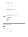
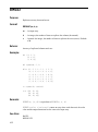
As indicated by examples, the .. operator without any range specifies implies all rows or
columns. For tabular data, the .. operator by itself implies all the values of the table
unraveled into a single column.
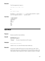
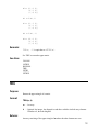
Assignments are also valid. For example, from above, the statement:
u[1..3, 1] = -1;
2
assigns the values to variable u as:
u == {{-1,
{-1,
{-1,
{ 4,
5,
6,
7,
8,
9,
10,
11,
12,
13},
14},
15},
16}}
Assigning elements to the empty series, {}, removes values. For example:
u[2, ..] = {}
removes the 2nd row and returns the array:
{{-1, 5, 9, 13},
{-1, 7, 11, 15},
{ 4, 8, 12, 16}}
The range specifier can be implemented as:
gline(int((end-start)/inc)+1,1,inc,start)
See Also:
{} Array Construction
GLINE
GNUMBER
LINSPACE
LOGSPACE
RAVEL
UNRAVEL
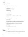
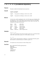
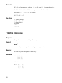
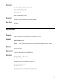
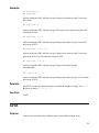
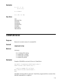
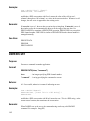
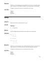
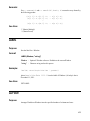
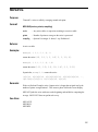
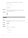
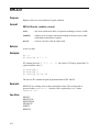
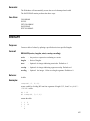
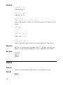
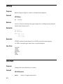
{} Array Construction
Purpose:
Creates a series or multiple column array.
Format:
{a, b, c}
{{a, b}, {c, d}}
a, b, c, d
- Any number of expressions resulting in an integer, real, complex, series,
or string.
3
Returns:
A series or array.
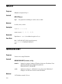
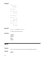
Example:
a = {1, 2, 3}
produces a single column, 3 element series
a = {0, a, 0}
returns the series {0, 1, 2, 3, 0}.
b = {{1, 2}, {3, 4}, {5, 6}}
creates the 3x2 array
{{1, 2}
{3, 4}
{5, 6}}
c = {"a ", "string"}
creates the series {97, 32, 115, 116, 114, 105, 110, 103}
d = {1, 2i, 3}
creates the complex series {1+0i, 0+2i, 3+0i}
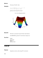
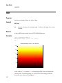
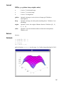
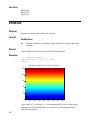
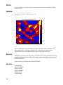
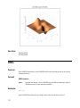
W1: gnorm(1000,1)
W2: {max(w1)};tablev
displays the maximum of W1 as a number in W2. W2 contains a single point series
displayed as a table.
Assigning elements to the empty series, {}, removes values. For example:
a = ravel(1..9, 3);
a[.., 2] = {};
removes the 2nd column and returns the array:
{{1, 7},
{2, 8},
{3, 9}}
Remarks:
4
The {} operator acts as a powerful CONCAT function by combining any number of any
kind of data types to produce a single or multi-column array.
See Also:
.. (Range Specifier)
CONCAT
GLINE
GNUMBER
GSERIES
RAVEL
UNRAVEL
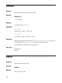
#DEFAULT
Purpose:
Reinitializes all DADiSP macros found in system.mac and dadisp.mac files.
Format:
#DEFAULT
Remarks:
Useful after #UNDEFALL is used.
See Also:
#DEFINE
#UNDEFALL
#UNDEFINE
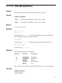
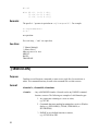
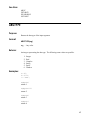
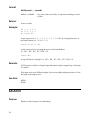
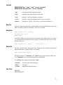
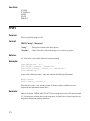
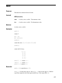
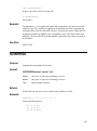
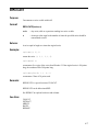
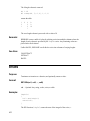
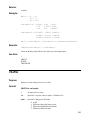
#DEFFUN
Purpose:
Defines a single line DADiSP function.
Format:
#DEFFUN name(arg1, arg2, ..., argn) statement
name
- A string up to 15 characters long, naming the function.
argn
- Optional. Any argument being passed to the function.
statement
- The body of the function. An equation or expression incorporating the
function arguments.
5
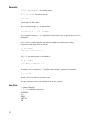
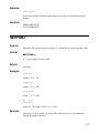
Example:
#deffun normal(s) s/max(s)
defines a function which normalizes a series by its maximum value.
W1: {1,2,3,4,5}
normal(W1)
returns the series {0.2, 0.4, 0.6, 0.8, 1.0}.
#deffun minmax max-min
defines a function minmax equal to the range of the data.
Remarks:
SPL function names are not case sensitive.
If a function does not accept arguments, the argument list is omitted. Multi-line functions
must be specified in separate ASCII files.
You can use #DEFFUN to redefine existing functions. Functions are defined and saved
with the Worksheet.
Use SPLWRITE to write functions to a file.
See Also:
ALLFUNCTIONS
DELALLFUNCTIONS
DELFUN
FUNCTIONS
SPLREAD
SPLWRITE
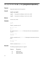
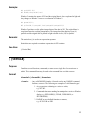
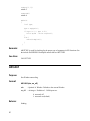
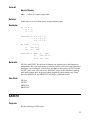
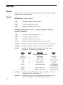
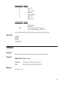
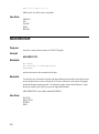
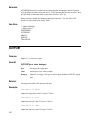
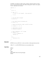
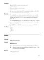
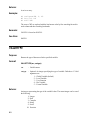
#DEFINE
Purpose:
Defines a DADiSP macro.
Format:
6
#DEFINE name(arg1, arg2, ..., argn) formula
name
- A string up to 15 characters long naming the macro.
argn
- Optional. Any argument being passed to the formula.
formula
- An equation or macro expansion incorporating those arguments and
evaluating to a real, string, series, or table.
Example:
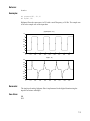
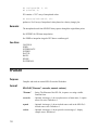
#define autocor(s) conv(s, reverse(s))/(2*sersize(s))
defines a macro which performs an auto-correlation of a series.
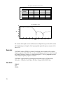
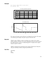
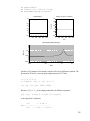
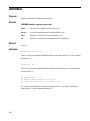
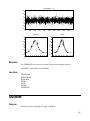
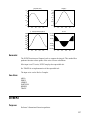
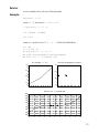
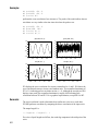
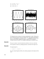
W1: gsin(128, 1/128, 4.0)
autocor(W1)
calculates the auto-correlation of the sine wave.
Remarks:
You can use #DEFINE to redefine existing macros.
Macros are defined and saved with the Worksheet. Use MACWRITE to write macros to a
file.
See Also:
#DEFAULT
#UNDEFALL
#UNDEFINE
MACREAD
MACWRITE
#INCLUDE
Purpose:
Format:
Includes macro files in other macro files, and SPL files in other SPL files.
#INCLUDE filename
filename
- A string identifying the filename including the path to the file.
Example:
In the dadisp.mac file:
#include macros\cursor.mac
#include macros\matrix.mac
reads the macros in the cursor.mac and matrix.mac files automatically at startup.
If the macro file myfile.mac resides in the same directory as the DADiSP executable,
the following statement in the dadisp.mac file reads the macros in myfile.mac
automatically upon startup:
#include {gethome + "myfile.mac"}
To load SPL files automatically upon startup, include them in the dadisp.spl file:
7
#include myfuncs.spl
Remarks:
Macros are defined and saved with Worksheets. Use MACWRITE to write macros to a
file.
See Also:
#DEFAULT
#DEFINE
#UNDEFALL
#UNDEFINE
MACREAD
MACWRITE
#UNDEFALL
Purpose:
Deletes the entire list of macros associated with the current Worksheet.
Format:
#UNDEFALL
Remarks:
If you use #UNDEFALL, the DADiSP menus will not work until you use #DEFAULT to
re-initialize the default macros.
See Also:
#DEFAULT
#DEFINE
#UNDEFINE
#UNDEFINE
Purpose:
Format:
Deletes a macro from the current Worksheet.
#UNDEFINE macro_name
macro_name
8
- Name of macro to delete.
Example:
#UNDEFINE autocor
deletes the macro autocor.
See Also:
#DEFAULT
#DEFINE
#UNDEFALL
= (Variable Assignment)
Purpose:
Assigns the value of an expression to a variable.
Format:
variable = <expr>
variable
- A variable.
<expr>
- Any expression evaluating to a scalar, series, table or string.
Returns:
Nothing, the result of the expression is assigned to the variable.
Example:
a = 5
b = 10
a * b
returns 50.
c = {1, 2, 3}
a * c
returns the series {5, 10, 15}.
Assigning elements to the empty series, {}, removes data points. For example:
a = {1, 2, 3, 4, 5}
a[3] = {}
returns the series {1, 2, 4, 5}.
9
Remarks:
Multiple return assignments are support. For example, the expression:
(u, w, v) = svd(a)
assigns the variables u, w, and v.
The = operator can assign a series to a Window, however, the Window formula remains
unchanged. For example:
W1: 1..100
W2: integ(w1)
W1 = gnorm(100,1)
The original ramp data in W1 is replaced with random data. The formula of W1 is
unchanged, but W2 automatically recalculates because the series in W1 changed. This
behavior is very useful with cyclical Worksheets. For example:
W1: W2
W2: W1 - delay(W1,10)
If your Calculation Settings has Cyclical Window Formulae enabled, the mutually
dependent Windows will recalculate as many times as specified by the Iteration Count.
However, since W1 is initially empty, there is no data to evaluate. To start the iteration,
simply assign a series to W1.
W1 = 1..10
The := operator assigns both a formula and series to a Window. For example:
W1 := gnorm(100,1)
sets the data and the formula of W1.
The = operator performs a standard variable assignment. Standard variables do not
propagate changes. For example:
a = 5
b = a * a
a = 10
The variable b retains the original value 25.
Use the := operator to create “hot variables”. Hot variables propagate changes. For
example:
a:= 5
b:= a * a
a:= 10
10
The := operator creates hot variables a and b. Variable b now automatically updates
whenever a changes, thus b has the value 100.
See == to compare two expressions.
See Also:
:= (Hot Variable Assignment)
: (Window Assignment)
== (Conditional Operators)
Assignment Operators
SETHOTVARIABLE
SETVARIABLE
:= (Hot Variable Assignment)
Purpose:
Assigns a formula to a hot variable or Window.
Format:
variable := <formula>
variable
- A hot variable or Window.
<formula> - Any formula evaluating to a scalar, series, table or string.
Returns:
Nothing, the formula is assigned to the hot variable.
Example:
a:= 5
b:= a * a
b
returns 25.
a:= 10
b
returns 100.
W1:= gnorm(1000,1)
W2:= integ(W1)
assigns the formulae to W1 and W2.
11
Remarks:
See the = operator to perform a standard variable assignment. Standard variables do not
propagate changes.
Use () to group multiple statements for a hot variable assignment in an SPL routine. For
example:
setw1()
{
W1 := (integ(gnorm(1000,1));label("Test Data"));
}
The setw1() routine assigns the formula:
integ(gnorm(1000,1));label("Test Data")
to Window 1 just as if the formula was entered from the command line.
The : and := operators are interchangeable for Window assignments.
See == to compare two expressions.
See Also:
= (Variable Assignment)
: (Window Assignment)
== (Conditional Operators)
Assignment Operators
SETHOTVARIABLE
SETVARIABLE
SETWFORM
: (Window Assignment)
Purpose:
Assigns a formula to a Window.
Format:
Window : <formula>
Window
- A Window.
<formula> - Any formula evaluating to a scalar, series, table or string.
Returns:
Nothing, the formula is assigned to the Window.
12
Example:
W1 : gnorm(1000,1)
W2 : integ(W1)
assigns the Window formulae to W1 and W2.
Remarks:
Use () to group multiple statements for a Window assignment in an SPL routine. For
example:
setw1()
{
W1 : (integ(gnorm(1000,1));label("Test Data"));
}
The setw1() routine assigns the formula:
integ(gnorm(1000,1));label("Test Data")
to Window 1 just as if the formula was entered from the command line.
The : and := operators are interchangeable for Window assignments.
See Also:
:= (Hot Variable Assignment)
= (Variable Assignment)
== (Conditional Operators)
SETHOTVARIABLE
SETVARIABLE
SETWFORM
+ - * / ^ % \ (Arithmetic Operators)
Purpose:
Add/subtract/multiply/divide/exponentiate two expressions.
Format:
<expr1> op <expr2>
<expr1> - Any expression evaluating to a scalar, series, or table.
<expr2> - Any expression evaluating to a scalar, series, or table.
13
Returns:
If one or both of the expressions is a series, then a series results. The following is a list of
type conversion rules:
Integer
Integer
Integer
Real
Real
Complex
+
+
+
+
+
+
Integer
Real
Series
Complex
Series
Real Series
yields an Integer
yields a Real
yields a Series
yields a Complex
yields a Series
yields a Complex Series
Example:
128 + 13.29
displays the real result 141.29.
W1: {1,2,0,4,5)
4 * (W1)
multiplies each element of the series by a factor of four and produces the new series {4,
8, 0, 16, 20}.
-3 ^ 1.8
displays the complex result 5.844884 - 4.246557i.
12 % 5 returns 2, the remainder when 12 is divided by 5.
The right divide operator \ performs division such that
a \ b == b / (1/a).
For example 10 \ 5 == 5 / (1/10) == 0.5
Remarks:
A division by zero produces a default value of 0. This default value can be specified with
the DEFAULT_MATH_VALUE configuration parameter.
The ^ operator can return a complex result if the first expression is negative and the
second expression has a non-zero fractional part.
See *^ (Matrix Multiply) to perform matrix multiplication.
See ^^ (Matrix Power) to raise a matrix to a power.
See \^ (Matrix Solve) for solve a system of equations.
See /^ (Matrix Right Division) to perform matrix right division.
See ' (Matrix Transpose) to transpose a matrix.
14
&& || ! AND OR NOT XOR (Logical Operators)
Purpose:
Serves as logical operators.
Format:
<expr1> op <expr2>
OPERATOR (expr1, expr2)
<expr1> - Any expression evaluating to a scalar, series, or table.
<expr2> - Any expression evaluating to a scalar, series, or table.
Returns:
A scalar, series, or table containing ones and zeros (True or False).
Example:
W1: {0, 4, 9, 1, 2, 5}
W2: {1, 4, 0, 9, 3, 6}
W1 && (W2>3)
returns the series {0, 1, 0, 1, 0, 1} containing ones wherever W1 and W2>3 are
non-zero, and zeros elsewhere.
W1 || (W2==4)
returns a series {0, 1, 1, 1, 1, 1} containing ones wherever W1 is non-zero or
wherever W2 equals 4, and zeros elsewhere.
Remarks:
The returned series of ones and zeros is called a "Binary Series" and is useful for
identifying points that meet a given condition.
&& is functionally equivalent to AND, but the syntax is different.
|| is functionally equivalent to OR, but the syntax is different.
! is functionally equivalent to NOT, but the syntax is different.
See Also:
< <= > >= == != (Conditional Operators)
AND
FLIPFLOP
NOT
NOTEQUAL
OR
XOR
15
< <= > >= == != (Conditional Operators)
Purpose:
Determines conditional relationships between expressions.
Format:
<expr1> op <expr2>
<expr1> - Any expression evaluating to a scalar, series, or table.
<expr2> - Any expression evaluating to a scalar, series, or table.
Returns:
A scalar, series, or table (containing the value 1 or 0) of the same type as the higher of the
two expressions. 1: True; 0: False. Integer is the lowest type, Real is next, and Complex
is the highest type. If one or both of the expressions is a series, then a series results. The
following is a list of type conversion rules:
Integer
Integer
Integer
Real
Real
Complex
>
>
>
>
>
>
Real
Series
Integer
Complex
Series
Real Series
yields a Real
yields a Series
yields an Integer
yields a Complex
yields a Series
yields a Complex Series
Example:
max(W1) <= 10.0
returns a 1 if the maximum value of W1 is less than or equal to 10.0, or 0 if the maximum
value of W1 is not less than or equal to 10.0. If W1 contains a series, then
W1 > 10.0
returns a series the same length as W1 containing a 1 for each observation that is greater
than 10 and 0 for each observation that is less than or equal to 10.0.
Remarks:
The returned series of ones and zeros is called a "Binary Series".
See Also:
&& || ! AND OR NOT XOR (Logical Operators)
GREATER
GREATEREQUAL
LESSER
LESSEREQUAL
NOTEQUAL
16
>> << & ~ bitor (Bit Operators)
Purpose:
Bit left shift, bit right shift, bit and, bit complement, bit or operators.
Format:
<expr1> op <expr2>
<expr1> - Any expression evaluating to a scalar, series, or table.
<expr2> - Any expression evaluating to a scalar, series, or table.
Returns:
A scalar, series, or table.
Example:
W1: {1, 2, 3, 4}
W2: W1 >> 1
returns the series {0, 1, 1, 2}. The bits of each value in the series are shifted one
place to the right resulting in an integer divide by 2.
W3: W1 & 0x01
returns the series {1, 0, 1, 0} indicating the values that have the lowest bit set.
W4: bitor(W1, 0x01)
returns the series {1, 3, 3, 5}.
Remarks:
The following bit operators are supported:
Operator
>>
<<
&
~
Function
Description
BITRSHIFT
BITLSHIFT
BITAND
BITCOMP
BITOR
bit shift right
bit shift left
bit and
bit complement
bit or
The | symbol is not currently used as the BITOR operator since | is the pipe operator.
See Also:
Assignment Operators
Conditional Operators
Logical Operators
17
+= -= /= *= >>= <<= &= |= %= (Assignment Operators)
Purpose:
Operate and assign the value of an expression.
Format:
<expr1> op= <expr2>
<expr1> - Any expression evaluating to a scalar, series, or table.
<expr2> - Any expression evaluating to a scalar, series, or table.
Returns:
A scalar, series, or table.
Example:
j = 10;
j += 2;
Variable j contains the value 12.
W1: {1, 2, 3, 4}
W1 += 2
W1 contains the series {3, 4, 5, 6}. Each value of the series is incremented by the
value 2.0.
a = {1, 2, 3, 4}
a &= 0x01
Variable a contains the series {1, 0, 1, 0} indicating the values that have the lowest
bit set.
b = {1, 2, 3, 4}
b |= 0x01
Variable b contains the series {1, 3, 3, 5}.
Remarks:
The following assignment operators are supported:
Operator
+=
-=
*=
18
Description
add then assign
subtract then assign
multiply then assign
Operator
Description
divide then assign
modulo then assign
bit right shift then assign
bit left shift then assign
bit and then assign
bit or then assign
/=
%=
>>=
<<=
&=
|=
If e1 and e2 are expressions, then
e1 op= e2
is equivalent to
e1 = (e1) op (e2)
except that e1 is computed only once. Notice the parenthesis.
x *= y + 1
is equivalent to
x = x * (y + 1)
not
x = x * y + 1
Assignment operators are not only fast and concise, they correspond better to the way
people think. We say “add 2 to j” or “increment j by 2,” not “take j, add 2, then put the
result back into j.” Thus, j += 2.
See Also:
:= (Hot Variable Assignment)
= (Variable Assignment)
Bit Operators
Logical Operators
*^ (Matrix Multiply)
Purpose:
Multiplies two matrices.
19
Format:
matrix1 *^ matrix2
matrix1
- A matrix.
matrix2
- A matrix.
Returns:
A matrix.
Example:
W1: {{1, 3, 4},
{5, 7, 9},
{8, 9, 12}}
W2: {{1, 3, 2},
{2, 4, 5},
{1, 2, 0}}
W1 *^ W2 == {{11, 23, 17},
{28, 61, 45}}
{38, 84, 61}}
W2 *^ W1 == {{32, 42, 55},
{62, 79, 104},
{11, 17, 22}}
Remarks:
The number of columns in matrix1 must be equal to the number of rows in matrix2. The
number of rows in the output matrix is equal to the number of rows in matrix1, and the
number of columns in the output matrix is equal to the number of columns in matrix2.
Matrix multiplication is not commutative, the order of the arguments is important.
a *^ b is equivalent to mmult(a, b).
If any argument is a scalar, *^ defaults to standard element by element multiplication
(equivalent to the * operator). For example:
4 *^ 5 == 20
See the ^^Matrix_Power operator to raise a matrix to a scalar power or raise a scalar to a
matrix power.
See Also:
\^ (Matrix Solve)
^^ (Matrix Power)
INNERPROD
INTERPOSE
20
See Also:
INVERSE
MDIV
MMULT
OUTERPROD
REDUCE
TRANSPOSE
^^ (Matrix Power)
Purpose:
Raises a matrix to a scalar power or a scalar to a matrix power.
Format:
arg1 ^^ arg2
arg1
- A non-singular, square matrix or a scalar. The base.
arg2
- A square matrix or scalar if arg1 is a matrix. The exponent.
Returns:
A matrix.
Example:
a = {{1, 2, 3},
{4, 5, 6},
{7, 8, 0}}
b = a^^3
b == {{279, 360, 306},
{684, 873, 684},
{738, 900, 441}}
c = a^^1.5
c == {{ 7.245 - 2.116i, 9.115 - 1.718i, 6.304 + 2.891i},
{17.096 - 2.596i, 21.508 - 2.608i, 14.875 + 4.099i},
{15.465 + 6.185i, 19.456 + 5.746i, 13.457 - 9.250i}}
d = 1.5^^a
d == {{24.009, 29.166, 20.401},
{54.739, 69.769, 47.985},
{49.996, 62.783, 43.550}}
21
Remarks:
A^^0 == eye(size(A)) the identity matrix.
A^^-1 == inv(A) the matrix inverse.
A^^1 == A
Given matrix A and scalar p:
For p a positive integer, A^^p is equivalent to:
A *^ A^* A *^ A ... *^ A
(p times.)
For p a negative integer, A^^p is equivalent to the positive case except the inverse of A is
multiplied.
For p a real or complex number, the function computes the matrix power using
eigenvectors and eigenvalues as follows:
(v, d) = eig(A)
A^^p == (v *^ (d ^ p)) /^ v
For p^^A, the matrix power is calculated as:
(v, d) = eig(A)
(v *^ diag(p ^ diag(d))) /^ v
If neither p nor A are matrices, ^^ defaults to the standard ^ operator. For example:
4 ^^ 3 == 64
If both p and A are matrices, an error occurs.
See the ^ operator to raise each element of an array to a power.
See Also:
*^ (Matrix Multiply)
+ - * / ^ % (Arithmetic Operators)
INVERSE
LU
MDIV
MMULT
QR
22
\^ (Matrix Solve)
Purpose:
Divides one matrix by another.
Format:
matrix1 \^ matrix2
matrix1
- A non-singular, usually square matrix.
matrix2
- Any matrix.
Returns:
A matrix that produces matrix2 when multiplied by matrix1.
Example:
W1: {{1, 4, 7},
{2, 5, 8},
{3, 6, 0}}
W2: {1,
2,
3}
W3: W1 *^ W2
{30,
36,
15}
W4: W1 \^ W3
{1,
2,
3}
W4 solves the following system of equations:
x + 4y + 7z = 30
2x + 5y + 8z = 36
3x + 6y
= 15
x == 1
y == 2
z == 3
23
Now consider:
A = {{1,
{2,
{3,
{1,
4,
5,
6,
2,
7},
8},
0},
1}}
x = {30,
36,
15,
2}
b = A \^ x
b == {-1.8,
3.2,
2.8}
y = A *^ b
y == {30.0,
34.8,
13.0,
7.4}
norm(x-y) == 5.6921
This example solves the following over-determined system of equations using least
squares:
x + 4y + 7z = 30
2x + 5y + 8z = 36
3x + 6y
x + 2y +
= 15
z =
2
The solution y minimizes the mean squared error.
Remarks:
If A, b, and x are matrices, such that A *^ x = b, then A \^ b returns the matrix x.
A \^ b is equivalent to mdiv(A, b).
For A \^ b, where A is square, the system is solved using LU decomposition. This is
usually numerically more stable than directly calculating the inverse matrix, i.e.
x = inv(A) *^ b.
24
If matrix A is not square, the system is considered a least squares problem and is solved
by QR decomposition. The resulting matrix is the best solution in the least squares sense.
For scalars, a \^ b == a \ b
== a \ (1/b). For example:
10 \^ 2 == 10 \ 2 == 0.2
See Also:
*^ (Matrix Multiply)
/^ (Matrix Right Division)
INVERSE
LU
MDIV
MMULT
QR
/^ (Matrix Right Division)
Purpose:
Performs matrix right division.
Format:
matrix1 /^ matrix2
matrix1
- Any matrix.
matrix2
- A non-singular, usually square matrix.
Returns:
A matrix that numerically approximates matrix1 *^ inv(maxtrix2) .
Example:
A = {{0, 1, 2},
{1, 0, 1},
{2, 2, 1}}
x = {{3, 5, 4},
{1, 9, 2},
{3, 2, 1}}
B = A *^ x
B /^ A == {{3, 5, 4},
{1, 9, 2},
{3, 2, 1}}
25
Remarks:
If A, B, and x are matrices, such that A *^ x = B, then B /^ A returns the matrix x.
B /^ A calculates (A’ \^ B’)’ as an approximation to B *^ inv(A).
For scalars B /^ A == B / A. For example:
10 /^ 2 = 10 / 2 == 5
See Also:
*^ (Matrix Multiply)
^^ (Matrix Power)
\^ (Matrix Solve)
INVERSE
MDIV
MMULT
' (Matrix Transpose)
Purpose:
Swaps the rows and columns of a specified array.
Format:
array'
array - Any array or expression evaluating to an array or series.
Returns:
A NxM array where the input is an MxN array.
Example:
W1: {{1, 2, 3},
{1, 2, 3},
{1, 2, 3}}
W2: W1'
W2 == {{1, 1, 1},
{2, 2, 2},
{3, 3, 3}}
26
Remarks:
The postfix ' operator is equivalent to TRANSPOSE . For example:
a = transpose(b)
a = b'
are equivalent.
See the postfix ~^ operator to perfom a complex conjugate transpose.
See Also:
*^ (Matrix Multiply)
\^ (Matrix Solve)
~^ (Matrix Conjugate Transpose)
Macros in matrix.mac
MMULT
RAVEL
TRANSPOSE
~^ (Matrix Conjugate Transpose)
Purpose:
Complex conjugate of the matrix transpose.
Format:
array~^
array - Any array or expression evaluating to an array or series.
Returns:
An NxM array where the input is an MxN array.
Example:
W1: {{i, 2, 3},
{1, 2i, 3},
{1, 2, 3i}}
W2: W1~^
W2 == {{0 – 1i, 1 + 0i, 1 + 0i},
{2 + 0i, 0 – 2i, 2 + 0i},
{3 + 0i, 3 + 0i, 0 – 3i}}
27
W3 : W1’
W3 == {{0 + 1i, 1 + 0i, 1 + 0i},
{2 + 0i, 0 + 2i, 2 + 0i},
{3 + 0i, 3 + 0i, 0 + 3i}}
Remarks:
The postfix A~^ operator is equivalent to conj(transpose(A)) . For example:
b = conj(transpose(A))
b = A~^
are equivalent.
For a real array, ~^ and ‘ are equivalent.
See Also:
*^ (Matrix Multiply)
\^ (Matrix Solve)
Macros in matrix.mac
MMULT
RAVEL
TRANSPOSE
; (SEMICOLON)
Purpose:
Format:
Combines several functions, commands, or macros on a single line for execution as a
whole. This command form may be used at the command line or within a macro.
<formula1> ; <formula2>;<formulan>
<formula>
- Any valid DADiSP formula. A formula can be any DADiSP command,
function, or macro. The following are examples of valid formula types:
1. Any expression evaluating to a series or scalar,
e.g. W1*W1.
2. Commands that return nothing but manipulate a series or Window
display, e.g. EXPANDH(2), FPEAK, CURSORON, or
PLOTMODE(0).
3. DADiSP or user-defined functions or macros,
e.g. AUTOCOR or PSD.
28
Example:
W1: gsin(100,.01)
W2: W1*W1;overplot(W1,lred)
Window 2 contains the square of W1 and the original data is also overplotted in light red.
Any changes to Window 1 cause a re-evaluation of Window 2.
W1: gnorm(10,1);
W2: spline(W1,3);overp(W1,lred);setsym(4);setsym(14,2)
Window 2 performs a cubic spline interpolation of the data in W1. The original data is
overplotted onto the resulting interpolation. The interpolated data displays cross (4)
symbols and the original data is plotted in light red with circles (14) as symbols.
Remarks:
The semicolon (;) is used as an expression separator.
Semicolons are required to terminate expressions in SPL routines.
See Also:
| (Vertical Bar)
| (VERTBAR)
Purpose:
Format:
Combines several functions, commands, or macros on a single line for execution as a
whole. This command form may be used at the command line or within a macro.
<formula1> | <formula2> | <formulan>
<formula>
- Any valid DADiSP formula. A formula can be any DADiSP command,
function, or macro. The following are examples of valid formula types:
1. Any expression evaluating to a series or scalar,
e.g. W1*W1.
2. Commands that return nothing but manipulate a series or Window
display, e.g. EXPANDH(2), FPEAK, CURSORON, or
PLOTMODE(0).
3. DADiSP or user-defined functions or macros,
e.g. AUTOCOR or PSD.
29
Example:
gsin(100,0.01,2.0)|expandv|scrolll|cursoron
generates a 2 Hz sine wave (100 points), expands it vertically, scrolls it left, and finally
places a cursor on the series.
Remarks:
The | (vertical bar) is an alternate syntax for combining multiple commands.
The ; (semicolon) is now the preferred and recommended syntax. The | is supported only
for backwards compatibility with legacy systems.
See Also:
; (Semicolon)
A2STD
Purpose:
Converts an alpha confidence level to a standard deviation range.
Format:
A2STD(alpha)
alpha - A real or series. The confidence level(s). Defaults to, 0.01, a 99% confidence
level.
Returns:
A real or series. The standard deviation range for the given confidence level(s).
Example:
a2std(0.01)
returns 2.5758 the standard deviation range for a confidence level of 99%.
W1: {0.01, 0.02, 0.03, 0.04, 0.05}
W2: a2std(W1)
W2 == {2.5758, 2.3263, 2.1701, 2.0537, 1.9600}
the standard deviation ranges for confidence levels 99%, 98%, 97%, 96%, and 95%.
Remarks:
A2STD uses the built-in INVPROBN function to lookup a Z value for a given
probability.
30
See Also:
INVPROBN
CNF2STD
PDFNORM
PROBN
ABS
Purpose:
Produces the absolute value of any expression.
Format:
ABS(expr)
expr - Any expression evaluating to a scalar, series, or table.
Returns:
A scalar, series, or table.
Example:
abs(-3)
returns 3.
abs(-3 + 2i)
returns 3.605551 + 0.000000i, a complex scalar.
mag(-3 + 2i)
returns 3.605551, a real scalar.
abs(mean(W7))
returns a scalar which is the absolute value of the mean of the series in Window 7.
To rectify a sine wave, type:
abs(gsin(100,0.1,1))
This new sine wave contains only positive values in the y domain.
31
Remarks:
ABS always returns a complex result (where the imaginary part is always 0) for a
complex input. Use MAG to return a purely real result.
See Also:
IMAGINARY
MAGNITUDE
PHASE
REAL
ACORR
Purpose:
Calculates the auto-correlation using the convolution method.
Format:
ACORR(s, norm)
s
- An input series.
norm - Optional. An integer, the normalization method. Valid inputs are:
0: None (Default)
1: Unity (-1 to 1)
2: Biased
3: Unbiased
Returns:
A series.
Example:
W1: gsin(1000, .001, 4)
W3: acorr(W1)
performs the auto-correlation of a sinewave. The peaks of the result indicate the
waveform is very similar to itself at the time intervals where the peaks occur, i.e. the
waveform is periodic.
W1:
W2:
W3:
W4:
gsin(1000, .001, 4)
gnorm(1000, .001)
acorr(W1, 1)
acorr(W2, 1)
W3 displays the auto-correlation of a sinewave normalized to -1 and 1. W4 shows the
normalized auto-correlation of random noise.
32
The normalized maximum of both results is 1.0 at time t == 0, indicating the expected
perfect correlation at time t == 0 (true for all series).
The waveform of W4 displays only one distinct peak at t == 0, indicating that W2 is not
correlated with itself and is non-periodic.
Both waveforms display a triangular envelope due to the assumption that the input series
is zero before the first sample and after the last sample.
Remarks:
The auto-correlation is used to determine how similar a series is to itself or if a series is
periodic. ACORR performs correlation by computing the direct convolution of the input
series.
The output length L is:
L = 2 * length(s) + 1
The zeroth lag component is the mid point of the series.
The BIASED normalization divides the result by M, the length of the input series.
The UNBIASED normalization divides the result by
M - abs(M - i - 1) + 1
where i is the index of the result.
See FACORR for the frequency domain implementation.
See Also:
ACOV
CONV
FACORR
FACOV
FCONV
FXCORR
XCORR
ACOV
Purpose:
Calculates the auto-covariance using the convolution method.
33
Format:
ACOV(s, norm)
s
- An input series.
norm - Optional. An integer, the normalization method. Valid inputs are:
0: None (Default)
1: Unity (-1 to 1)
2: Biased
3: Unbiased
Returns:
A series.
Example:
W1: gsin(1000, .001, 4)
W3: acov(W1)
performs the auto-covariance of a sinewave. The peaks of the result indicate the
waveform is very similar to itself at the time intervals where the peaks occur, i.e. the
waveform is periodic.
W1:
W2:
W3:
W4:
gsin(1000, .001, 4)
gnorm(1000, .001)
acov(W1, 1)
acov(W2, 1)
W3 displays the auto-covariance of a sinewave normalized to -1 and 1. W4 shows the
normalized auto-covariance of random noise.
The normalized maximum of both results is 1.0 at time t == 0, indicating the expected
perfect covariance at time t == 0 (true for all series).
The waveform of W4 displays only one distinct peak at t == 0, indicating that W2 is not
correlated with itself and is non-periodic.
Both waveforms display a triangular envelope due to the assumption that the input series
is zero before the first sample and after the last sample.
Remarks:
The auto-covariance is used to determine how similar a series is to itself or if a series is
periodic. ACOV performs covariance by computing the direct convolution of the input
series.
The output length L is:
L = 2 * length(s) + 1
34
The zeroth lag component is the mid point of the series.
The BIASED normalization divides the result by M, the length of the input series.
The UNBIASED normalization divides the result by
M - abs(M - i - 1) + 1
where i is the index of the result.
See FACOV for the frequency domain implementation.
See Also:
ACORR
CONV
FACORR
FACOV
FCONV
FXCORR
FXCOV
XCORR
ACTIVATE
Purpose:
Format:
Activates the specified Window.
ACTIVATE(Window)
Window - Optional. Window reference. Defaults to the current Window.
Remarks:
Equivalent to pressing [Enter] (carriage return) in the Window.
See Also:
UNACTIVATE
WINSTATUS
35
ADDWFORM
Purpose:
Adds to the formula in the Window without causing a complete re-evaluation.
Format:
ADDWFORM(Window, "formula")
Window
- Optional. Window reference. Defaults to current Window.
"formula" - Any valid DADiSP formula in quotes. A formula can be any DADiSP
command, function, or macro. The following are examples of valid
formula types:
1. Any expression evaluating to a series or scalar,
e.g. W1*W1.
2. Commands that return nothing but manipulate a series or Window
display, e.g. EXPANDH(2), FPEAK, CURSORON, or
PLOTMODE(0).
3. DADiSP or user-defined functions or macros,
e.g. AUTOCOR or PSD.
Example:
W1: gnorm(1000,1)
W2: W1*W1
addwform(W2,"overplot(W1,lred)")
This example adds the overplot and sets the Window's formula to
W1*W1;overplot(W1, lred) without re-evaluating the formula W1*W1.
Remarks:
This function is useful when editing the formula line would cause an unwanted or lengthy
recalculation. ADDWFORM can be abbreviated ADDWF.
See Also:
:= (Hot Variable Assignment)
ADDWFORM
GETWFORMULA
SETWFORM
36
ADDWINDOW
Purpose:
Adds the indicated number of Windows to the Worksheet after the current Window.
Format:
ADDWINDOW(win, n)
win - Optional. Window Reference. The Window after which new windows are added.
Defaults to the current Window.
n
- An integer representing the number of Windows to be added to the Worksheet.
Returns:
The total number of Windows in the Worksheet.
Example:
addwindow(3)
adds three Windows after the current Window. If Window 6 is current, three Windows
will be added after Window 6.
addwindow(W2, 4)
adds four Windows after Window 2.
Remarks:
The current Window is indicated by the position of the cursor. ADDWINDOW can be
abbreviated ADDWIN.
See Also:
REMOVEWINDOW
ADDWKSFORM
Purpose:
Format:
Adds a command to the Worksheet formula.
ADDWKSFORM("command")
"command" - A command to annotate the Worksheet background.
37
Example:
addwksform("text(0,0.1,4,'Results of Analysis')");redrawall
puts the annotation "Results of Analysis" onto the Worksheet at (0, 0.1).
W1: grand(100,0.01)
addwksform("Label('Random Series')");
puts a label on W1 using the text Random Series.
Remarks:
Worksheet formulas cannot be set like Window formulas. The primary use for
ADDWKSFORM is for annotations to the Worksheet background that do not belong to
specific Windows. Once a command is added to the Worksheet formula, the only way to
delete it is to start a new Worksheet. A new Worksheet starts with no Worksheet
formula.
See Also:
ADDWFORM
REDRAWALL
SETWSIZE
TEXT
ALL
Purpose:
Returns 1 if all elements of the input are non-zero.
Format:
ALL(val)
val - A series, scalar or string input.
Returns:
The scalar 1.0 or 0.0 or a row array if the input is an array with more than 1 row and
column.
Examples:
all(3)
returns 1.0
all({0.0, 1.0})
returns 0.0
38
all(ones(3,1))
returns 1.0
all(ones(3,3))
returns the 1x3 array {{1.0, 1.0, 1.0}}
Remarks:
The input is cast to a series if it is a scalar or a string.
See Also:
ANY
FIND
ONES
ZEROS
ALLFUNCTIONS
Purpose:
Displays a list of all available functions defined within the current Worksheet. Lists
function names, arguments, and definitions, and allows functions to be created, edited,
and deleted.
Format:
ALLFUNCTIONS
Remarks:
Displays all functions including those beginning with the underscore character (_). When
a list of available functions is generated using the FUNCTIONS command, functions
whose names begin with the underscore character are not included.
See Also:
FUNCTIONS
SPLREAD
SPLWRITE
ALLMACROS
Purpose:
Displays a list of all available macros defined within the current Worksheet. Lists macro
names, arguments, and definitions, and allows macros to be created and edited.
39
Format:
ALLMACROS
Remarks:
Displays all macros including those beginning with the underscore character (_). When a
list of available macros is generated using the MACROS function, macros beginning with
the underscore character are not included.
See Also:
MACREAD
MACROS
MACWRITE
AMPDIST
Purpose:
Format:
Returns:
Finds the amplitude distribution of a specific series.
AMPDIST(series, delta-y)
series
- Any series, table, or expression evaluating to a series or table.
delta-y
- The y increment or "bucket size." The smaller the delta-y value, the greater
the number of amplitude ranges that will be defined and hence, the greater
the number of points in the resulting series.
A series or table.
Example:
W1: {1.0, 1.5, 2.0, 2.5, 3.0}
W2: ampdist(W1, 0.7)
returns a series containing the points {2.0, 1.0, 2.0} indicating there are:
• 2 point values between 1.0 and 1.7
• 1 point value between 1.7 and 2.4
• 2 point values between 2.4 and 3.1
See Also:
HISTOGRAM
40
AND
Purpose:
Performs a logical AND of two expressions.
Format:
AND(expr1, expr2)
expr1 - Any expression evaluating to a scalar, series, or table.
expr2 - Any expression evaluating to a scalar, series, or table.
Returns:
A scalar, series, or table.
Example:
and(W1, W2)
returns a series or table with zeros at points where either W1 or W2 contain a zero, and
ones where both W1 and W2 have non-zero values.
and({0, 1, 5, 9},1)
returns a series {0,1,1,1}. This is equivalent to: {0, 1, 5, 9} && 1
Remarks:
AND can also be performed using the infix operator &&. The function AND(W1, W2) is
identical to the expression (W1 && W2).
See Also:
< <= > >= == != (Conditional Operators)
&& || ! AND OR NOT XOR (Logical Operators)
FLIPFLOP
NOT
OR
XOR
ANGLE
Purpose:
Calculates the phase component of a Complex expression.
41
Format:
ANGLE(expr)
expr - Any expression evaluating to a scalar, series, or table.
Returns:
Series, scalar, or table.
Example:
angle(-1.0)
returns the scalar 3.14159625, or π.
angle(5+5i)
yields 0.78539816 or π/4
angle(W2)
returns a new series which corresponds to the angle component of the polar or Cartesian
series in Window 2.
Remarks:
ANGLE returns a value from 0 to 2π.
PHASE returns a value from -π to π.
See Also:
CARTESIAN
IMAGINARY
MAGNITUDE
PHASE
POLAR
REAL
ANY
Purpose:
Returns 1 if any element of the input is non-zero.
42
Format:
ANY(val)
val - A series, scalar or string input.
Returns:
The scalar 1.0 or 0.0 or a row array if the input is an array with more than 1 row and
column.
Examples:
any(3)
returns 1.0
any({0.0, 1.0})
returns 1.0
any(zeros(3,1))
returns 0.0
any(zeros(3,3))
returns the 1x3 array {{0.0, 0.0, 0.0}}
Remarks:
The input is cast to a series if it is a scalar or a string.
See Also:
ALL
FIND
ONES
ZEROS
ANYFORMAT
Purpose:
Produces an output string in the format of the C/C++-language printf function.
43
Format:
ANYFORMAT("control", val1, val2, val3)
"control" - Format control string. Conforms to C/C++ language printf specifications.
Control strings may contain ordinary characters, escape sequences, and
format specifications. Ordinary characters are copied to the output string.
Escape sequences are introduced by a backslash (\). Format specifications
in the control string are matched to the values and are introduced by a
percent sign (%). The form is as follows:
% [flags] [width] [.precision] type
Flags:
-
Meaning
Left justify.
+
Explicit sign (+ or -) before number.
blank
Insert blank before positive number.
#
With type o: prefixes '0'.
With type x: prefixes '0X'.
With type X: prefixes '0X'.
Width:
Optional. Minimum number of characters in output.
Precision:
Optional. Maximum number of characters printed for
all or part of the output field, or minimum number of
digits printed for integer values.
Integers:
Minimum number of digits in output, padded left
with zeros if necessary.
Types e, E, f:
Number of digits after decimal point, last digit
rounded.
Types g, G:
Maximum number of significant digits.
String:
Number of characters copied from string to output.
Type:
Required character that determines whether the
associated argument is interpreted as a character,
string, or a number.
Type Characters
Output Format
d, I
Signed decimal integer.
u, o
Unsigned decimal integer.
x,X
Unsigned hex integer using "abcdef" or "ABCDEF"
f
Signed value having the form
[-]dddd.dddd, where dddd is one or more decimal
digits.
44
Type Characters
Output Format
e
Signed value having the form [-]d.dddd e
[sign]ddd, where d is a single decimal digit, dddd is
one or more decimal digits, ddd is exactly three
decimal digits, and sign is + or -.
valn
E
Identical to the e format, except that E, rather than e,
introduces the exponent.
g
Signed value printed in f or e format, whichever is
more compact or the given value and precision. The e
format is used only when the exponent of the value is
less than -4 or greater than or equal to the precision
argument. Trailing zeros are truncated, and the
decimal point appears only if one or more digits
follow it.
G
Identical to the g format, except that G, rather than g,
introduces the exponent
c
Single character.
s
String. Characters printed up to the first null
character or until the precision value is reached.
- Scalar or string value that matches control string.
String or scalar values in the specified format.
Returns:
A string.
Example:
anyformat( "Max: %f (%s %s)", max, getdate, gettime)
returns a string such as "Max: 32.7 (05/19/94 12:00.37)"
Remarks:
ANYFORMAT is a constrained version of SPRINTF. The SPRINTF function allows
more flexibility in the control string.
See Also:
NFORMAT
SFORMAT
SPRINTF
45
AREA
Purpose:
Calculates the area of a series, or portion of a series, using Simpson's Rule.
Format:
AREA(series, start, length)
series
- Optional. Any series or expression evaluating to a series. Defaults to the
current Window.
start
- Optional. An integer. Index of the point defined as the start of the series
section to be used. Defaults to 1.
length - Optional. An integer. The length of the series portion to be used; only valid
when start has been specified. Defaults to the length from the start value to the
end of the series.
Returns:
A scalar.
Example:
area(gsin(100,0.01))
returns the area 0.00042. The area of a sine wave over one period should cancel out to
zero, but by virtue of a low digital sampling rate, which in this example is 100 points per
second, our curve is a rough approximation of a true sine. If we generate a single period
sine wave at a rate of 1000 Hz, gsin(1000,0.001), DADiSP calculates the area of that
curve as 0.0.
Remarks:
The AREA function returns a number, INTEG returns a series.
DADiSP will calculate AREA correctly even if the defined start or length require points
beyond the end of the series.
Remember: The area below the origin on the y-axis is negative area. If you want to
include area below y=0 as positive area, take the absolute value of the series first, e.g.
area(abs(W1)).
See Also:
46
ABS
INTEG
ARGCOUNT
Purpose:
Returns the number of arguments specified in an SPL function.
Format:
ARGCOUNT
Returns:
A real.
Example:
myfun(a, b, c, d)
{
return(argcount);
}
myfun(1) returns: 1
myfun(1, 1, 10) returns: 3
Remarks:
Arguments to SPL functions are optional. ARGCOUNT is a simple method for checking
if an argument was specified.
ARGCOUNT can be abbreviated ARGC.
ARGC returns the total number of input arguments. See ARGV to specify variables
arguments in an SPL routine.
See OUTARGC for a count of output arguments.
See Also:
ARGV
GETARGV
ISVARIABLE
OUTARGC
ARGV
Purpose:
Specifies variable arguments in an SPL routine.
47
Format:
ARGV
Returns:
Nothing.
Example:
/* maximum of one or more inputs */
vmax(argv)
{
local i, s;
/* 0 or 1 arg case */
if (argc < 2) {
if (argc < 1) {
s = maxval();
}
else {
s = maxval(getargv(1));
}
}
else {
/* initialize */
s = maxval(getargv(1), getargv(2));
/* compare input args */
for (i = 3; i <= argc; i++) {
s = maxval(s, getargv(i));
}
}
returns(s)
}
ARGV in the argument list of an SPL routine specifies a variable number of input
arguments. The above routine returns the maximum of two or more expressions.
ARGC returns the total number of input arguments and GETARGV obtains a particular
variable argument.
Remarks:
ARGV can be used in combination with specified arguments. For example:
func1(a, b, c, argv)
{
}
creates a function that accepts 3 specified arguments and any number of variable
arguments.
48
See Also:
ARGC
GETARGV
ISVARIABLE
OUTARGC
ARGTYPE
Purpose:
Returns the data type of the input argument.
Format:
ARGTYPE(arg)
arg - Any value.
Returns:
An integer representing the data type. The following return values are possible:
1:
2:
3:
4:
5:
6:
Integer
Real
Complex
String
Series
Window
Examples:
a = 10;
b = 12.5i;
c = "text";
argtype(a)
returns 1.
argtype(a*1.1)
returns 2.
argtype(b)
returns 3.
argtype(c)
returns 4.
49
argtype({1, 2})
returns 5.
argtype(W1)
returns 6.
myfun(x)
{
local type;
type = argtype(x);
if (type != 5 || type != 6) {
error("myfun - series required");
}
else {
return(integ(x*x));
}
}
Remarks:
ARGTYPE is useful in checking for the proper type of arguments in SPL functions. See
the include file SERIES.H for helpful macros that use ARGTYPE.
See Also:
VALUETYPE
ASCALE
Purpose:
Format:
Sets Window autoscaling.
ASCALE(win, on_off)
win
- Optional. A Window. Defaults to the current Window.
on_off - An integer. Defaults to 1. Valid inputs are:
0: autoscale off
1: autoscale on (default)
Returns:
50
Nothing.
Example:
W1: gsin(1000,1/1000,4);ascale(0)
turns off autoscaling in W1.
ascale(W1, 1)
turns on autoscaling for W1.
Remarks:
ASCALE is useful for data in real time Windows.
See Also:
RTTINIT
AUTOCOR
Purpose:
Format:
Macro. Performs a time domain auto-correlation of a series.
AUTOCOR(series)
series
- Any series, multi-series table, or expression resulting in a series or table.
Returns:
A series or table.
Expansion:
CONV(S, REVERSE(S))/2*SERSIZE(S)
Example:
W1: gsin(128, 1/128, 4.0)
W2: autocor(W1)
calculates the auto-correlation of a sine wave.
W1: grand(128, 1/128)
W2: autocor(W1)
calculates the auto-correlation of the random series.
51
Remarks:
AUTOCOR is often used to indicate how "similar" a waveform is to itself. The autocorrelation of the above sine wave shows several distinct peaks, indicating that the series
at time t is similar to the series at time t+T. The auto-correlation of the random series
shows only one distinct peak, indicating that the series is correlated at time=0 (as are all
series) and dissimilar elsewhere.
Use ACORR to specify normalization factors.
See Also:
ACORR
ACOV
CONV
CROSSCOR
FACORR
FFT
PEARSON
AVGFILT
Purpose:
Filters a series using the average of the N neighboring points.
Format:
AVGFILT(s, n, gval, lval)
s
- An input series or array.
n
- Optional. An integer, the number of neighbors to average. For point i, average
points i-n through i+n exclusive of point i. Defaults to 1, i.e. for point i, average
points i-1 and i+1.
gval - Optional. A real, the "greater than" threshold at which to replace a point. Point i
is replaced if: point[i] > gval * current average[i].
Defaults to 1.0, i.e. replace
each point if it is greater than the average of the neighbors.
lval
Returns:
52
- Optional. A real, the "less than" threshold at which to replace a point. Point i is
replaced if: point[i] < lval * current average[i]. Defaults to unspecified, i.e. do
not use a "lesser than" threshold.
A series.
Example:
W1: gnorm(100,.01)
W2: avgfilt(W1)
replaces each point of W1 with the average of the previous and next point if it exceeds
the average.
W3: avgfilt(W1, 2)
replaces each point of W1 with the average of the two previous and two next points if it
exceeds the average.
W3: avgfilt(W1, 1, 1.2)
replaces each point of W1 with the average of the previous and next point if it exceeds
the average by 20%.
W4: avgfilt(W1, 1, 1.2, 1.3)
replaces each point of W1 with the average of the previous and next point if it exceeds
the average by 20% or is less than the average by 30%.
W5: avgfilt(W1, 1, 0, 0)
replaces each point of W1 with the average of the previous and next point
unconditionally.
W6: -avgfilt(-W1, 1, 1.2)
replaces each point of W1 with the average of the previous and next point if it is less than
the average by 20%.
Remarks:
AVGFILT uses the convolution function to calculate the neighbor averages. For n == 1,
the kernel is simply: {1, 0, 1} / 2
See Also:
CONV
AVGS
Purpose:
Creates a new series that is the arithmetic mean of any number of input series.
53
Format:
AVGS(series1, ..., seriesN )
series1, ..., seriesN
Returns:
- Any series, multi-series table, or expression resulting in a series
or table.
A series or table.
Example:
W1: {3, 5, 7, 9, 3}
W2: {9, 8, 4, 2, 1}
W3: avgs(W1, W2)
creates a new series {6.0, 6.5, 5.5, 5.5, 2.0} in W3 by averaging the series in
the listed Windows (i.e. (W1+W2)/2.0).
avgs(W1, W2, W6, W7, W9)
creates a new series by averaging the series in the listed Windows
(i.e. (W1 + W2 + W6 + W7 + W9) / 5.0).
avgs(W3..W8)
averages Windows 3 through 8, i.e. (W3 + W4 + W5 + W6 + W7 + W8) / 6.0.
Remarks:
AVGS operates on Real or Complex input and returns Complex output if any of the input
is Complex.
If the input series are of different lengths, all series are padded with point values of 0.0 to
the length of the longest series.
See Also:
MEAN
SUMS
BALANCE
Purpose:
Balances a table to improve its conditioning.
54
Format:
BALANCE(table)
table
- A Real or Complex square table.
Returns:
A table whose row and column norms are approximately equal.
Example:
W1: {{1, 8, 3},
{3, 5, 2},
{1, 3, 4}}
balance(W1) == {{1.0, 4.0, 1.5},
{6.0, 5.0, 2.0},
{2.0, 3.0, 4.0}}
W2: {{0+8i,
0, 1+i},
{0,
1001, 0+3i},
{90,
0+i, 200}}
balance(W2) == {{0+8i, 0,
8+8i},
{0,
1001, 0+1.5i},
{11.25, 0+2i 200}}
Remarks:
EIGVAL and EIGVEC first perform a balancing step where the rows and columns are
transformed to have root mean squares as close as possible while leaving the Eigenvalues
and Eigenvectors unchanged. In most cases, this improves the accuracy of EIGVAL and
EIGVEC, but in some cases it does not. BALANCE can be used to check that relatively
small table elements have not become unduly magnified by the balancing step. If they
have, then NBEIGVAL and NBEIGVEC are likely to yield better results.
See Also:
EIGVAL
EIGVEC
NBEIGVAL
NBEIGVEC
BARCTR
Purpose:
Sets the centering of a 2D bar plot.
55
Format:
BARCTR(win, on_off)
win
- Optional. A Window. Defaults to the current Window.
on_off - An integer. Valid inputs are:
0: bars begin on values
1: bars centered on values (default)
Returns:
If on_off not specified returns 1 if bar centering is on, else 0.
Example:
W1: gnorm(10, 1);bars;barctr(1)
W2: W1;bars;barctr(0)
The bars in W1 are centered around the data values (the default) while the bars in W2
begin at the data values (the default).
Remarks:
BARCTR only effects 2D bar charts.
BARCTR is a Window property. All bar plots plotted in the Window will be drawn in the
current BARCTR mode.
See Also:
BARS
BARGAP
BARSTYLE
STEPCTR
STEPS
BARGAP
Purpose:
Format:
Sets the gap drawing between bars of a 2D step plot.
BARGAP(win, on_off)
win
- Optional. A Window. Defaults to the current Window.
on_off - An integer. Valid inputs are:
0: do not draw gaps
1: draw gaps (default)
56
Returns:
If on_off not specified returns 1 if bar gaps are on, else 0.
Example:
W1: gnorm(10, 1);bars;bargap(1)
W2: W1;bars;bargap(0)
The bars in W1 are drawn with gaps between each bar (the default), while the bars in W2
abut each other with no gaps.
Remarks:
BARGAP only effects 2D bar charts.
BARGAP is a Window property. All bar plots plotted in the Window will be drawn in the
current BARGAP mode.
See Also:
BARCTR
BARS
BARSTYLE
STEPS
BARS
Purpose:
Displays the data points of a Window as thick vertical bars.
Format:
BARS
Example:
grand(100, 0.1); bars
generates a 100-point series of random numbers and displays them as thick vertical bars.
Remarks:
Without a Window reference, BARS is equivalent to the fourth mode of the [F7] key or
Graph Styles toolbar button and SETPLOTSTYLE(3).
See Also:
BARCTR
BARGAP
BARSTYLE
LINES
POINTS
57
See Also:
SETPLOTSTYLE
STEPS
STICKS
TABLEVIEW
BARSTYLE
Purpose:
Sets the vertical reference of a 2D bar plot.
Format:
BARSTYLE(win, on_off)
win
- Optional. A Window. Defaults to the current Window.
on_off
- An integer. Valid inputs are:
0: reference bars to 0.0 (default)
1: bar bottoms start at the Window bottom
Returns:
If on_off not specified returns 1 if bars drawn to the Window bottom, else 0.
Example:
W1: gnorm(10, 1);bars;barstyle(1)
W2: W1;bars;barstyle(0)
The bars in W1 are drawn from a vertical reference of 0.0 (the default), while the bars in
W2 begin at the bottom of the Window.
Remarks:
BARSTYLE only effects 2D bar charts.
BARSTYLE is a Window property. All bar plots plotted in the Window will be drawn in
the current BARSTYLE mode.
See Also:
BARCTR
BARGAP
BARS
BARTOP
58
BARTOP
Purpose:
Sets coloring of the top face of a 3D bar plot.
Format:
BARTOP(win, on_off)
win
- Optional. A Window. Defaults to the current Window.
on_off
- An integer. Valid inputs are:
0: do not color bar tops (default)
1: color bar tops
Returns:
If on_off not specified returns 1 if top coloring is on, else 0.
Example:
W1: xyz(gsin(10,.1),gcos(10,.1),1..10);bars;bartop(1)
The tops of the resulting 3D bar plot are colored with the current axes color (default
black).
Remarks:
Coloring the tops of the bar plot can help clarify the orientation if the plot is rotated.
BARTOP is a Window property. All 3D bar plots plotted in the Window will be drawn in
the current BARTOP mode.
See Also:
BARCTR
BARGAP
BARS
BARSTYLE
ROTATE3D
SPIN
XYZ
BEEP
Purpose:
Turn automatic error beeper ON or OFF.
59
Format:
BEEP(mode)
mode - An integer. 1: ON, 0: OFF. Defaults to 1.
Example:
beep(1)
turns error beeper on.
BESTPOW2
Purpose:
Finds the power of 2 greater than or equal to the input value or length of the input series.
Format:
BESTPOW2(s)
s - An input series or real number.
Returns:
A real number.
Example:
bestpow2(30)
returns 32.
bestpow2(64)
returns 64.
W1: 1..200
bestpow2(W1)
returns 256.
Remarks:
If the input is a series or table, the return value is the next power of 2 greater than or
equal to the length of the series.
See Also:
FFT
LOG2
NEXTPOW2
60
BETAI
Purpose:
Calculates the incomplete beta function.
Format:
BETAI(x, a, b)
x
- Any expression evaluating to a scalar, series, or table where each element is
between 0 and 1 inclusive.
a
- A real number greater than 0.
b
- A real number greather than 0.
Example:
betai(.3, .4, .5)
returns 0.440684.
betai({0.0, 0.5, 1.0}, 0.1, 0.2)
returns the incomplete beta function values {0.0, 0.67057, 1.0}.
W1: betai(0..0.01..1, 8, 10)
setxlabel("x");setylabel("Ix(8,10)");
scales(2);griddot;gridhv
betai(0..0.01..1, 8, 10)
1.2
1
Ix(8,10)
0.8
0.6
0.4
0.2
0
-0.2
0
0.1
0.2
0.3
0.4
0.5
x
0.6
0.7
0.8
0.9
1
returns a series consisting of the incomplete beta function for 101 values of x between 0
and 1, with a == 8 and b == 10.
61
Remarks:
betai(x, a, b) == Ix(a, b) == 1 – I1-x(b, a)
See Also:
GAMM
JN
YN
BILINEAR
Purpose:
Performs a bilinear transformation with optional frequency prewarping.
Format:
(Zd,Pd,Kd) = BILINEAR(Z,P,K,Fs,Fp)
Z
- A series containing the zeros of the transfer function.
P
- A series containing the poles of the transfer function.
K
- A real. The gain constant.
Fs
- A real. The sampling frequency in Hertz.
Fp
- Optional. A real, the frequency in Hertz specifying at which point the frequency
responses before and after mapping match exactly. Each of the three forms of
BILINEAR accepts this optional additional input argument.
(Ad,Bd,Cd,Dd) = BILINEAR(A,B,C,D,Fs,Fp)
A,B,C,D - Matrices containing the state-space representation of the filter to be
transformed.
(b, a) = BILINEAR(NUM,DEN,Fs,Fp)
NUM - Series containing the numerator transfer function coefficients in descending
powers of s.
DEN
62
- Series containing the denominator transfer function coefficients in descending
powers of s.
Returns:
In the first case, two series and a constant. Zd is the vector of zeros, Pd is the series of
poles, and Kd is the gain constant.
In the second case, Ad, Bd, Cd and Dd are the state-space representations of the ztransform discrete equivalent filter.
In the third case, b and a are series containing numerator and denominator transfer
function coefficients.
Example:
(Zd,Pd,Kd) = bilinear(Z,P,K,Fs)
creates the series of zeros, the series of poles, and the gain constant for the z-transform
discrete equivalent of the filter defined by Z, P and K.
(b,a) = bilinear(NUM,DEN,Fs)
creates the series containing the numerator and denominator transfer function coefficients
for the discrete equivalent of the filter defined by the difference equation coefficients a
and b. The resulting coefficients are in linear difference form such that:
y[n] = a[1]*y[n-1] + a[2]*y[n-2] + ... + a[N]*y[n-N] +
b[1]*x[n]
+ b[2]*x[n-1] + ... + b[M]*x[n-M]
(A,B,C,D) = tf2ss(NUM,DEN)
(Ad,Bd,Cd,Dd) = bilinear(A,B,C,D,Fs)
creates the four matrices for the z-transform discrete equivalent of the filter defined by A,
B, C and D, the same one defined by NUM and DEN.
Remarks:
Make sure that Z and P are series if your inputs are in (Z,P,K,Fs) form. Similarly,
make sure that NUM and DEN are series if your inputs are in (NUM,DEN,Fs) form.
See Also:
ADSGN
CDSGN
FILTEQ
ZFREQ
63
BITQUANT
Purpose:
Quantizes an input series to 2^bits levels.
Format:
BITQUANT(s, bits, xl, xh)
s
- An input series or scalar.
bits - Optional. An integer, the number of quantization bits. Defaults to 8 (i.e. 256
levels)
xl
- Optional. A real, the low value input range. Defaults to min(s).
xh
- Optional. A real, the high value input range. Defaults to max(s).
Returns:
A series or real
Examples:
bitquant(1..100, 3);stem
quantizes the series to 2^3 == 8 levels and returns a 100 point series with quantized
values of: 0, 1, 2, 3, 4, 5, 6, 7
bitquant(1..100, 3, -100, 100);stem
The input full scale input range is to +-100. The resulting output now shows only 4
distinct levels since the actual input series only ranges from 1 to 100, about half the full
scale input range.
Remarks:
BITQUANT always outputs integer values. See QUANTIZE to quantize a series to an
arbitrary number of levels.
See Also:
64
BITSCALE
LINSCALE
QUANTIZE
BITSCALE
Purpose:
Converts raw AD counts to scaled engineering values.
Format:
BITSCALE(xi, numbits, yl, yh)
xi
- An input series or scalar.
numbits
- An integer. The number of AD converter bits.
yl
- A real. The low value output range.
yh
- A real. The high value output range.
Returns:
A series or real.
Example:
bitscale(4096, 16, -2.5, 2.5)
returns 0.312543, the corresponding output for input 4096 of a 16 bit converter with an
output range of +-2.5
bitscale(-128..127, 8, 0.0, 10.0)
returns a series ranging from 0.0 to 10.0
Remarks:
BITSCALE assumes offset binary input data, i.e the input data ranges from
-(2^numbits)/2 to (2^numbits)/2 - 1. BITSCALE does not automatically clip out of range
values.
See Also:
LINSCALE
BREAK
Purpose:
Terminates the immediately enclosing FOR or WHILE loop.
Format:
BREAK
65
Example:
ValChk(s)
{
local ns, ival;
ns = s;
ival = max(deriv(ns));
while(ival < 10) {
ns = deriv(ns);
ival = max(ns);
if (ival < 0) break;
}
return(ival);
}
In the SPL function, ValChk, if ival, the max of the derivative of the input series, s, is
less than zero, then the break statement will break out of the while loop, and return the
value.
Remarks:
BREAK is for use in SPL files.
See Also:
CONTINUE
FOR
IF
LOOP
RETURN
SPL: DADiSP's Series Processing Language
WHILE
BRIGHTEN
Purpose:
Format:
Brightens or darkens an image.
BRIGHTEN(beta, cmap)
beta
- Optional. A real, -1 <= beta <= 1. Default 0.5.
cmap - Optional. A colormap. Defaults to current colormap.
66
Returns:
A colormap or alters the current colormap.
Example:
W1: rainbow();showcmap()
brighten(.5)
brightens the rainbow colormap.
brighten(-.5)
restores the brightened colormap to the original colors.
Remarks:
For beta > 0, the color map is brightened. If beta < 0, the colormap is darkened.
See Also:
GETCOLORMAP
SHOWCMAP
SETCOLORMAP
BUILTINS
Purpose:
Format:
Lists all the built-in functions available in DADiSP.
BUILTINS
Returns:
A list box of all Worksheet functions.
Remarks:
BUILTINS displays a GUI list of function names sorted alphabetically.
BUILTINS does not display the arguments or function descriptions. If an item is
selected, the help page of that item is opened.
BUILTINS and FUNCS are identical functions.
See Also:
COMMANDS
FUNCS
FUNCTIONS
MACROS
67
BYTESWAP
Purpose:
Reverses the bytes of an input series.
Format:
BYTESWAP(series, datatype)
series
- A series, multi-series table, or expression evaluating to a series or table.
datatype
- An integer code number or name specifying the data type.
Name
Code
Data Type
Range
SBYTE
1
Signed Byte
-128 to +127
UBYTE
2
Unsigned Byte
0 to 255
BYTE
2
(same as UBYTE)
0 to 255
SINT
3
Signed Integer
-32768 to +32767
UINT
4
Unsigned Integer
0 to 65536
LONG
5
4-byte Signed Integer
-2,147,483,648 to
+2,147,483,647
FLOAT
6
4-byte Floating Point
-10^37 to +10^38
DOUBLE
7
8-byte Floating Point
-10^-307 to +10^-308
ULONG
8
4-byte Unsigned
Integer
0 to 4,294,967,295
Returns:
A series or table.
Example:
byteswap(W1, SINT)
converts W1 into signed 2 byte integers and then reverses the bytes. BYTESWAP can be
very useful when reading foreign data files via READB.
Remarks:
All of the datatypes listed above are macros that are described in this manual.
CALC
Purpose:
Turns automatic Worksheet recalculation mode ON or OFF.
68
Format:
CALC(mode)
mode - Optional. An integer.
0:
1:
2:
3:
OFF
ON (default), immediately update changed Windows
Step through cyclical calculations
ON, but do immediately evaluate changed Windows
Example:
calc(1)
specifies automatic Window recalculation.
calc(0)
disables automatic recalculation.
Remarks:
If the calculation mode is OFF, or disabled, you can enter Window formulae without
immediately calculating new series results. Once you type CALC(0), enter new formulae
in the desired Windows and then type CALC(1) to reset the Worksheet to automatic
mode. DADiSP will automatically update each Window as needed.
CALC(2) steps through cyclical calculations that are mutually dependent. A progress
message is displayed in the status area. Press the space bar to step to the next iteration.
CALC(3) turns on auto-calculation, but does not immediately evaluate changed
Windows. The Windows will re-evaluate after a formula has been entered.
See Also:
PLOTMODE
PROTECT
REFRESH
UPDATE
CALL
Purpose:
Calls a command file n times.
69
Format:
CALL("comfile", n)
"comfile" - The name of the command file in quotes.
n
- Optional. An integer specifying the number of times to call the command
file. Defaults to 1.
Example:
call("MYFILE.DSP", 2)
executes MYFILE.DSP two times from within the current Worksheet.
Remarks:
CALL is useful for creating loops in a command file. Within a command file, use
@CALL and @LOAD to CALL or LOAD other "sub" command files so that control is
returned to the originating command file after the execution of the "sub" command file.
See Also:
LOAD
CARTESIAN
Purpose:
Converts an expression to Real/Imaginary form in Cartesian coordinates.
Format:
CARTESIAN(expr)
expr - Any scalar or series in integer, Real/Complex, or polar coordinate form.
Returns:
Complex scalar, series, or table.
Example:
cartesian(gsin(20,.05,1.0))
creates a 1 Hz sine wave of 20 points spaced 0.05 seconds apart. The value of each point
in the sine wave is a Complex number in Real/Imaginary form where the imaginary part
is zero.
cartesian(-1)
returns the Complex scalar -1.0 + 0i.
70
Remarks:
CARTESIAN returns a Complex value regardless of the input value. For series,
CARTESIAN always returns a Complex series.
See Also:
IMAGINARY
PHASE
POLAR
REAL
CASTBYTE
Purpose:
Casts the values of a series to a new data type.
Format:
CASTBYTE(series, datatype, swapflag)
series
- Any series, multi-series table, or expression resulting in a series or table.
datatype
- An integer code number or name specifying the data type.
Name
Code
Data Type
Range
SBYTE
1
Signed Byte
-128 to +127
UBYTE
2
Unsigned Byte
0 to 255
BYTE
2
(same as UBYTE)
0 to 255
SINT
3
Signed Integer
-32768 to +32767
UINT
4
Unsigned Integer
0 to 65536
LONG
5
4-byte Signed Integer
-2,147,483,648 to
+2,147,483,647
FLOAT
6
4-byte Floating Point
-10^37 to +10^38
DOUBLE
7
8-byte Floating Point
-10^-307 to +10^-308
ULONG
8
4-byte Unsigned
Integer
0 to 4,294,967,295
swapflag
- Integer. 0 - No swap. 1 - Swap byte order. Defaults to 0.
Returns:
A series or table.
71
Example:
castbyte(W1, UBYTE)
converts the values into unsigned bytes ranging from 0 to 255.
Remarks:
All of the data types listed above are macros that are described in this manual.
See Also:
BYTESWAP
CASTCOMPLEX
Purpose:
Explicitly casts the input to a complex scalar.
Format:
CASTCOMPLEX(expr)
expr - A scalar, series, table or expression returning a scalar, series, or table.
Returns:
A complex number. If the imaginary part of the complex value is zero, only the real part
is returned
Example:
W1: gline(10,1,.5,.2) + i*gline(10,1,.5,8)
castcomplex(W1)
returns the value 0.2 + 8i.
Remarks:
CASTCOMPLEX is helpful when writing SPL functions that require a specific type of
input, and you don’t know whether the variable being passed into the function will be of
that type.
If you pass CASTCOMPLEX a series, it will only operate on the first point of the series.
If you pass CASTCOMPLEX a table, it will only operate on the first point in the first
column of the table.
See Also:
CASTINTEGER
CASTREAL
CASTSERIES
CASTSTRING
72
CASTINTEGER
Purpose:
Explicitly casts the input to an integer.
Format:
CASTINTEGER(expr)
expr - A scalar, series, table or expression returning a scalar, series, or table.
Returns:
An integer.
Example:
castinteger(1.9)
returns the integer 1.
castinteger(2.2)
returns the integer 2.
castinteger(3.7 + 8i)
returns the integer 3.
Remarks:
CASTINTEGER truncates real values to integers. CASTINTEGER is helpful when
writing SPL functions that require an explicit integer input and the type of the variable
passed into the function may not be an integer.
If you pass CASTINTEGER a series, it will only operate on the first point of the series.
Use INT, FLOOR, CEIL or ROUND to convert an entire series or table.
If you pass CASTINTEGER a table, it will only operate on the first point in the first
column of the table.
CASTINTEGER can abbreviated CASTINT.
See Also:
CASTCOMPLEX
CASTREAL
CASTSERIES
CASTSTRING
INT
73
CASTREAL
Purpose:
Explicitly casts the input to a real value.
Format:
CASTREAL(expr)
expr - A scalar, series, table or expression returning a scalar, series, or table.
Returns:
A real value.
Example:
castreal(1)
returns the value 1.0.
castreal(0.2 + 8i)
returns the value 0.2.
Remarks:
CASTREAL is helpful when writing SPL functions that require an explicit real input and
the type of the variable passed into the function may not be real.
If the input to CASTREAL is a series, it will only operate on the first point of the series.
If the input to CASTREAL a table, it will only operate on the first point in the first
column of the table.
See Also:
CASTCOMPLEX
CASTINTEGER
CASTSERIES
CASTSTRING
CASTSERIES
Purpose:
Explicitly casts the input to a series.
74
Format:
CASTSERIES(expr)
expr - A scalar, series, table, string or expression returning a scalar, series, table, or
string.
Returns:
A series.
Example:
castseries(8)
returns a one point series with the value 8. This is equivalent to: {8}
castseries(8 + 23i)
returns a series with one complex value: 8 + 23i. This is equivalent to:
{8 + 23i}
castseries("string")
Equivalent to {"string"} and returns a series with the ASCII codes for the characters
in the string "string": {115,116,114,105,110,103}
castseries("DADiSP")
returns a series with the ASCII codes for the characters in the string "DADiSP":
{68,65,68,105,83,80}
Remarks:
CASTSERIES is helpful when writing SPL functions that require an explicit series input
and the type of the variable passed into the function may not be a series.
The {} also cast the input into a series.
When used with table input, CASTSERIES operates on the first column of the table and
returns it as the series.
When used with string input, CASTSERIES functions like CHARSTRS.
See Also:
{} Array Construction
CASTCOMPLEX
CASTINTEGER
CASTREAL
CASTSTRING
CHARSTRS
GSERIES
75
CASTSTRING
Purpose:
Explicitly casts the input to a string.
Format:
CASTSTRING(expr)
expr - A scalar, series, table, string or expression returning a scalar, series, table, or
string.
Returns:
A string.
Example:
caststring(8)
returns the string: 8
caststring(2+3i) + " hello"
returns the string: 2.0000 + 3.0000i hello
W1: gsin(100,.01)
caststring(max(W1))
returns the string: 1
W1: {68, 65, 68, 105, 83, 80}
caststring(W1)
returns the string: DADiSP
Remarks:
CASTSTRING is helpful when writing SPL functions that require an explicit string input
and the type of the variable passed into the function may not be a string.
When used with integer input, CASTSTRING functions like STRCHARS.
When used with table input, CASTSTRING operates on the first column of the table.
See Also:
CASTCOMPLEX
CASTINTEGER
CASTREAL
CASTSERIES
SPRINTF
STRCHAR, STRCHARS
STRNUM
76
CASTVARIANT
Purpose:
Explicitly casts the input to a Variant of a specified type for Automation.
Format:
CASTVARIANT(expr, vtype)
expr
- A scalar, series, table, string or expression returning a scalar, series, table, or
string.
vtype
- Optional. An integer specifying the Variant type. If not specified, defaults to
the original type of the input. Valid conversions are as follows:
vtype
Description
VARTYPE
1
2
3
4
5
6
7
8
10
11
12
13
16
17
18
19
20
21
22
23
24
28
30
31
nothing
2 byte integer
4 byte integer
4 byte float
8 byte double
currency
date
binary string
error
boolean
variant
unknown
char
unsigned char
unsigned short
unsigned int
8 byte integer
8 byte unsigned
machine int
unsigned machine int
void
C-style array
null-terminated string
wide null-terminated string
VT_EMPTY
VT_I2
VT_I4
VT_R4
VT_R8
VT_CY
VT_DATE
VT_BSTR
VT_ERROR
VT_BOOL
VT_VARIANT
VT_UNKNOWN
VT_I1
VT_UI1
VT_UI2
VT_UI4
VT_I8
VT_UI8
VT_INT
VT_UINT
VT_VOID
VT_CARRAY
VT_LPSTR
VT_LPWSTR
Returns:
The input value. The input is marked so that it is converted to the specified type when
used with ActiveX Automation.
77
Example:
xl = createobject("Excel.Application");
xl.workbooks.add();
xl.range("A1").value = "1.11.58";
xl.range("B1").value = castvariant("1.11.58", 7);
xl.visible = 1;
Starts Excel and creates a new workbook. The string “1.11.58” is placed in cell A1 and
the same string is converted into date form and placed in cell B1. A1 contains a string and
B1 contains the time value 1:11:58 AM.
a = {1,1.5,2,2.5,3};
xl.range("C1:C5").value = castvariant(a, 2);
The cells C1 through C5 contain the values 1, 1, 2, 2, 3 since the series in variable a was
converted to an array of 2 byte integers.
Remarks:
CASTVARIANT is helpful with ActiveX Automation when an object of an explicit type
is to be transferred. The data is converted only when transferred.
Normally, a series is transferred as an array of doubles. As shown in the second example,
CASTVARIANT can convert the series to an array of almost any type supported by
Automation.
Use CASTVARIANTARRAY to convert a series to an array of variants.
See Also:
CREATEOBJECT
CASTVARIANTARRAY
CASTVARIANTARRAY
Purpose:
Format:
Explicitly converts a series to an array of variants for Automation.
CASTVARIANTARRAY(series)
series
- A series or table.
Returns:
The series. The series is marked so that it is converted to an array of variants when used
with ActiveX Automation.
78
Example:
a = 1..5;
xl = createobject("Excel.Application");
xl.workbooks.add();
xl.range("A1:A5").value = a;
xl.range("B1:B5").value = castvariantarray(a);
xl.visible = 1;
Starts Excel and creates a new workbook. The series in variable a is transferred to cells
A1 through A5. The same series is converted to an array of variants and placed in cells
B1 through B5. Because Excel internally converts both arrays in the same manner, the
results are identical.
Remarks:
CASTVARIANTARRAY is helpful with ActiveX Automation when a series must be
transferred as an array of variants instead of the normal array of doubles.
Use CASTVARIANT to convert a series to an array of almost any type supported by
Automation.
See Also:
CREATEOBJECT
CASTVARIANT
CCEPS
Purpose:
Format:
Returns:
Calculates the complex cepstrum.
CCEPS(s, n)
(c, d) = CCEPS(s)
s
- An input series or array.
n
- Optional. An integer, the number of samples to use. If n > length(s), the series is
zero padded. Defaults to length(s).
A real series or array.
(c, d) = CCEPS(s)
returns the cepstrum in c and the lag used to unwrap the phase in d.
79
Example:
W1:
W2:
W3:
W4:
gtri(100, 1, 1/100)^3
W1+delay(W1, 60)/2
cceps(W2)
cceps(W2, 512)
W1: gtri(100, 1, 1/100)^3
W2: W1+delay(W1, 60)/2
1.2
1.2
1
1
0.8
0.8
0.6
0.6
0.4
0.4
0.2
0.2
0
0
-0.2
-0.2
0 10 20 30 40 50 60 70 80 90
0
20
40
W3: cceps(W2)
1
0.5
0.5
0
0
-0.5
-0.5
-1
-1
-1.5
-1.5
-2
-2
-2.5
-2.5
20
40
60
80 100 120 140
80 100 120 140
W4: cceps(W2, 512)
1
0
60
0
100
200
300
400
500
W2 adds a synthesized echo at 60 seconds to the data of W1.
W3 displays a small peak at t == 60 indicating the presence of the echo. W4 performs the
same calculation with the data padded to 512 samples.
W1: {1, -4.0996, 8.4057, -10.1765, 7.7801, -3.5142, 0.7939}
W2: cceps(W1, 1024)
returns the example listed in [2].
Remarks:
80
The complex cepstrum of a series is essentially ifft(log(fft(s))). However, the
complex log calculation requires the evaluation of the continuous phase component.
CCEPS unwraps the phase using Shafer's Algorithm. A line is subtracted from the
unwrapped phase to remove the integer lag component.
(c, d) = cceps(s)
returns both the cepstrum and the lag used to unwrap the phase such that:
icceps(c, d)
ideally returns s if mean(s) > 0.
CCEPS was tested successfully against the output from [2].
References:
[1] Oppenheim & Shafer
Discrete-Time Signal Processing
Prentice Hall, 1989
pp 788-792
[2] IEEE Press
Programs for Digital Signal Processing
IEEE Press, 1979
Section 7
See Also:
ICCEPS
RCEPS
CEILING
Purpose:
Finds the smallest integer greater than or equal to the input value.
Format:
CEILING(expr)
expr - Any expression evaluating to a scalar, series, or table.
Returns:
A scalar, series, or table.
Example:
ceiling(2.4)
returns 3, whereas round(2.4) returns 2.
ceiling(-2.4 + 7.2i)
returns -2.0 + 8.0i.
81
ceiling(W2)
creates a new series by applying CEILING to each series element of Window 2. The
integer value returned by CEILING is converted to a floating point value.
Remarks:
CEILING can be abbreviated CEIL. Use ROUND to round the value up.
See Also:
FIX
FLOOR
INT
ROUND
CHARSTR
Purpose:
Finds the ASCII code for the specified character.
Format:
CHARSTR("char")
"char"
- Any ASCII character enclosed in quotes.
Returns:
An integer.
Example:
charstr("X")
returns the number 88.
See Also:
CHARSTRS
STRCHAR, STRCHARS
CHARSTRS
Purpose:
Finds the ASCII codes for the specified string.
82
Format:
CHARSTRS("string")
"string" - An ASCII text string enclosed in quotes.
Returns:
A series.
Example:
charstrs("XYZ")
returns the series {88, 89, 90}.
See Also:
CHARSTR
STRCHAR, STRCHARS
CHILDREN
Purpose:
Returns the number of Windows that depend on a specified Window, i.e. the number of
its children.
Format:
CHILDREN(Window)
Window - Optional. Window reference. Defaults to the current Window.
Returns:
An integer.
Example:
For the following Worksheet:
W1: {2, 4, 5}
W2: grand(length(W1), .1)
W3: xyplot(W1, W2)
children(W1)
returns a 2 at the bottom of the screen. This indicates that W1 has two dependent
Windows.
See Also:
PARENTS
83
CHKFILES
Purpose:
Checks the file integrity of a Labbook.
Format:
CHKFILES(mode)
mode - Optional. An integer. 1: delete orphaned files. 0: do not delete. Defaults to 1.
Returns:
Nothing. Renames unreferenced Labbook files with the extension .ORF, and optionally
deletes them.
Example:
chkfiles
Examines each Worksheet, Dataset and Channel file in the current Labbook and
automatically deletes any unreferenced files.
Remarks:
CHKFILES checks if any Labbook files are no longer referenced by Labbook objects.
For example, temporary files will not be deleted if the machine improperly shuts down
while a Labbook is open. These temporary files will be unreferenced in the next DADiSP
session and CHKFILES can be used to automatically remove and recover the file space.
See Also:
EVAL
RUN
CHOLESKY
Purpose:
Computes the Cholesky factorization of a square matrix.
Format:
84
CHOLESKY(a, eflag)
(C, p) = CHOLESKY(a)
a
- An expression evaluating to a real or complex matrix.
eflag
- Optional. An integer flag. 0: report errors, 1: suppress errors. Defaults to 0.
Returns:
An upper triangular matrix, the Cholesky factor of the input matrix.
(C, p) = cholesky(a)
returns both the Cholesky factor C and p, the number of Nulls if the input is not positive
definite, or 0 if the input is positive definite. If p is non-zero, a is not positive definite and
C is not fully computed.
Example:
a = {{3, 2, 3},
{2, 4, 2},
{3, 2, 4}}
C = cholesky(a)
C == {{1.73205, 1.1547,
1.73205},
{0,
1.63299, -2.71948e-016},
{0,
0,
1}}
Matrix a is positive definite and C represents the Cholesky factor.
conj(C’) *^ C == {{3, 2, 3},
{2, 4, 2},
{3, 2, 4}}
eig(a) == {8.36468, 0.434583, 2.20074}
Because matrix a is positive definite, the eigenvalues of a are all positive.
v = {1, 10, -20}
conj(v’) *^ a *^ v == {1123}
also demonstrating that a is positive definite.
b = {{3, 2, 3},
{2, 4, 2},
{3, 2, 1}}
(C, p) = chol(b)
p == 1 indicating b is not positive definite and C was not fully computed.
eig(b) == {7.44241, -1.21371, 1.7713}
Because matrix b is not positive definite, the eigenvalues of b are not all positive.
conj(v’) *^ b *^ v == {-77}
also demonstrating that b is not positive definite.
85
Remarks:
Matrix a is positive definite if conj(v’) *^ a *^ v > 0 for any vector v with the
same number of rows as the number of columns of a.
The eigenvalues of a positive definite matrix are all positive.
For a positive definite matrix a, the Cholesky factor C is an upper triangular matrix such
that:
conj(C’) * C == a
If the input matrix is not positive definite, an error results unless eflag is 1. However,
for (C, p) = cholesky(a), no error message is printed regardless of the eflag
argument. Testing for p > 0 is one method of determining if the input is positive definite
without returning an error.
CHOLESKY can be abbreviated CHOL.
See Also:
*^ (Matrix Multiply)
DIAGONAL
EIG
LU
SVD
QR
CLEAR
Purpose:
Clears the Window contents and formula.
Format:
CLEAR(W1 .. WN)
W1 .. WN - Optional. A range or list of Windows. Defaults to the current Window.
Example:
clear
clears the current Window.
clear(W1, W5, W9)
clears Windows 1, 5, and 9.
86
clear(W3..W8)
clears Windows 3 through 8.
clear W1
clears Window 1 using the shorter command form. Only one Window at a time can be
cleared using this syntax.
Remarks:
A cleared Window propagates throughout the entire Worksheet. If W2 depends on W1
and W1 is cleared, DADiSP will clear the data in W2 and display the symbol ** NA **
(not available) in the center of W2. The Window formula in W2 is not cleared. To
prevent losing important Windows, use PROTECT.
CLEAR can also delete variables. For example:
a = 10
clear a
deletes variable a.
See Also:
CLEARALL
CLEARDATA
CLEAROPL
PROTECT
WINLOCK
CLEARALL
Purpose:
Clears all Window contents and formulas from every Window in the Worksheet. Be
careful using this function!
Format:
CLEARALL
Example:
clearall
removes all series and formulas from every Worksheet Window.
87
Remarks:
Consider saving your Worksheet before using CLEARALL.
CLEARALL does not effect functions or variables.
See CLEARALLDATA to remove the data from all Windows while preserving the
Window formulae.
See Also:
CLEAR
CLEARALLDATA
CLEARDATA
CLEARALLDATA
Purpose:
Format:
Clears the data from every Window in the Worksheet without removing the Window
formulae.
CLEARALLDATA
Example:
clearalldata
clears the data only from each Window in the Worksheet without removing the Window
formulae.
Save this Worksheet as a compact template. When loaded, use UPDATE to recalculate
the Worksheet.
Remarks:
CLEARALLDATA is useful for creating compact Worksheet templates by preserving the
formulae but not saving the Window data.
See Also:
CLEAR
CLEARALL
CLEARDATA
UPDATE
88
CLEARDATA
Purpose:
Clears the data from one or more Windows without removing Window formulae.
Format:
CLEARDATA(W1 .. WN)
W1 .. WN - Optional. A range or list of Windows. Defaults to the current Window.
Example:
cleardata(W1)
clears the data from Window 1 without removing its Window formula.
cleardata(W1..)
clears the data from all Windows in the Worksheet without removing the Window
formulas. Save this Worksheet as a compact template. When loaded, use UPDATE to
recalculate the Worksheet.
cleardata; integ(W1)
removes the data from the current Window (thus freeing any memory used by the data)
and then calculates the integral of W1.
Remarks:
CLEARDATA is useful for creating Worksheet templates by preserving the formulae,
but not saving the data of the cleared Windows.
CLEARDATA can be helpful during large calculations. DADiSP normally does not
remove old data from a Window until a new calculation has completed. Using
CLEARDATA, the old data is removed immediately, and more memory is available to
perform calculations.
See Also:
CLEAR
CLEARALL
CLEARALLDATA
UPDATE
89
CLEAROPL
Purpose:
Deletes all .OPL files located on the SPLPATH.
Format:
CLEAROPL(memflag)
memflag
- Optional. An integer. 1: clear SPL functions from memory, 0: do not clear
functions from memory. Defaults to 0.
Example:
clearopl
deletes all .OPL files normally found on SPLPATH.
clearopl(1)
same as above accept all SPL functions are also cleared from memory.
Remarks:
CLEAROPL is useful for resetting the compiled state of SPL routines.
CLEAROPL only removes files with extension .OPL. SPL files and any other files are
not removed.
See Also:
CLEAR
DELALLFUNCTIONS
GETSPLPATH
CLEARXLABEL, CLEARYLABEL
Purpose:
Clears the x-axis or y-axis label, and resets the display to the horizontal (x-axis) or
vertical (y-axis) units.
Format:
CLEARXLABEL(Window)
CLEARYLABEL(Window)
Window - Optional. Window reference. Defaults to the current Window.
90
Example:
clearxlabel
clears the definition of the x-axis label on the current window, and displays the horizontal
units.
Remarks:
Once the x-axis or y-axis label is cleared, the units label will reappear as usual.
Horizontal and Vertical units have a 15 character maximum length restriction.
SETXLABEL and SETYLABEL allow the user to set an axis label which can be more
than 15 characters long and which is independent of units, so that the automatic
translation of units can continue to operate.
See Also:
GETXLABEL, GETYLABEL
SETHUNITS
SETVUNITS
SETXLABEL, SETYLABEL
CLIP
Purpose:
Format:
Returns:
Modifies the points in a series or table according to specified maximum and minimum y
values.
CLIP(series, maxthresh, minthresh)
series
- Any series, table, or expression resulting in a series or table.
maxthresh
- Optional. Real number, or expression resolving to a Real number. Sets
the upper y limit. Defaults to the maximum of the series.
minthresh
- Optional. Real number, or expression resolving to a Real number. Sets
the lower y limit. Defaults to the minimum of the series.
A series or table.
Example:
W1: gsin(100,0.01)
clip(W1, 0.5, -0.5)
modifies the series in Window 1 so that all points equal to or above the maxthresh value
are set to 0.5, and all points equal to or below the minthresh value are set to –0.5.
91
W2: {1, 2, 3, 4, 5, 4, 3, 2, 1}
clip(W2, 4)
modifies the series in Window 2 so that all points equal to or above the maxthresh value
are set to 4. The resulting series is {1, 2, 3, 4, 4, 4, 3, 2, 1}.
clip(W3, 4.5, -3.0)
modifies the series in Window 3 so that all points equal to or above the maxthresh value
are set to 4.5, and all points equal to or below the minthresh value are set to -3.0.
clip(W4, max(W4), -2.0)
effectively sets only a minthresh (of -2.0) because the maxthresh is the highest peak of
the series in W4.
W5 - clip(W5,1.0,-1.0)
performs an "inverse" CLIP by modifying those points between the thresholds from the
original series in W5.
Remarks:
For complex series, CLIP operates on the REAL or MAGNITUDE part only.
If only one threshold argument is given, DADiSP assumes it is the maxthresh. If no
threshold arguments are given, DADiSP will use the MAX and MIN values of the series
as default arguments and CLIP will return an exact copy of the current series.
CLIP does not eliminate any points from a series, although it can be used to modify the
value of points in a series.
See Also:
< <= > >= == != (Conditional Operators)
DECIMATE
DELETE
MAX
MIN
REMOVE
CLOCK
Purpose:
Format:
92
Returns the current execution clock in seconds.
CLOCK
Returns:
A real indicating the total number of seconds since invocation.
Example:
a=clock();fft(w1);b=clock();
sprintf("FFT execution time %g seconds", b-a);
prints the approximate time required to calculate and display the FFT of W1.
See Also:
GETTIME
TIC
TOC
CLOGMAG
Purpose:
Format:
Returns:
Evaluates the log magnitude squared of Cascade form filter coefficients.
CLOGMAG(c, N, r)
(m, p) = CLOGMAG(c, N, r)
c
- A series. The filter coefficients in cascade format.
N
- Optional. An integer, the number of output samples. Defaults to 2048.
r
- Optional. A real, the sample rate of the data. Defaults to rate of filter.
A real series. The log magnitude squared frequency response of the filter.
(m, p) = CLOGMAG(c, N, r)
returns both the log magnitude squared, m, and the phase response, p.
Example:
W1: elliptic(1,1000.0,200.0,3.0,40.0,250.0)
W2: clogmag(W1, 1024)
93
W1: elliptic(1,1000.0,200.0,3.0,40.0,250.0)
1:No Units
1:
0.068231
2:
1.000000
3:
1.339368
4:
1.000000
5:
-1.168010
6:
0.553014
W2: clogmag(W1, 1024)
20
0
dB
-20
-40
-60
-80
-100
0
50
100
150
200
250
Hertz
300
350
400
450
W1 contains the bi-quad cascade coefficients of an elliptical low pass filter. W2 contains
1024 uniformly spaced samples of the log magnitude squared frequency response of the
filter in W1.
Remarks:
CLOGMAG employs ZFREQ to evaluate N uniformly spaced samples of the complex
frequency response of the filter. The cascade coefficients are converted to direct form and
the complex frequency response is evaluated using the FFT. The log magnitude squared
of the complex frequency response is returned.
CLOGMAG is appropriate for calculating the magnitude response of Butterworth,
Chebyshev1, Chebyshev2 and Elliptic IIR filters designed by DADiSP/Filters.
See Also:
CPHASE
FFT
ZFREQ
94
CNF2STD
Purpose:
Converts a confidence level (%) to a standard deviation range.
Format:
CNF2STD(alpha)
alpha - A real or series. The confidence level(s) in %. Defaults to, 99, a 99%
confidence level.
Returns:
A real or series. The standard deviation range for the given confidence level(s).
Example:
cnf2std(99)
returns 2.5758, the standard deviation range for a confidence level of 99%.
W1: {99, 98, 97, 96, 95}
W2: cnf2std(w1)
W2 == {2.5758, 2.3263, 2.1701, 2.0537, 1.9600}
the standard deviation ranges for confidence levels 99%, 98%, 97%, 96%, and 95%.
Remarks:
CNF2STD uses the built-in INVPROBN function to lookup a Z value for a given
probability.
See Also:
A2STD
INVPROBN
PDFNORM
PROBN
COL
Purpose:
Extracts a column of data from a table.
95
Format:
COL(table, column)
table
- Any table or expression evaluating to a table.
column - An integer. Column number to extract.
Returns:
A series.
Example:
W1: {{1,
{2,
{3,
4,
5,
6,
6},
7},
8}}
col(W1, 2)
returns {4, 5, 6}
Remarks:
The COL function may be used with any graph style, not only the table view, to extract a
particular series of data from a multi-series set. To extract more than a single column at a
time, use the REGION function.
See Also:
NUMCOLS
REGION
ROW
SERCOUNT
COLEXTRACT
Purpose:
Format:
Extracts a portion of each column of a table.
COLEXTRACT(table, start, length, offset)
table
- Any table or expression resulting in a table.
start
- A series. A list of integer starting points.
length - A series. A list of integers specifying the number of points to be extracted
from each column. –1 implies extract to the end of the column
offset
96
- Optional. A series. A list of real values specifying the x-offset of the resulting
columns. Defaults to the x-value of the starting points.
Returns:
A table.
Example:
W1:
W2:
W3:
W4:
W5:
W6:
W7:
integ(gnorm(100,1))
integ(gnorm(200, .1))
ravel(W1, W2)
colmaxidx(W3)’
colextract(W3, W4-10, ones(numcols(W3), 1)*20+1)
W1;overp(col(w5, 1), lred)
W2;overp(col(W5, 2), lred)
W1: integ(gnorm(100,1))
W2: integ(gnorm(200, .1))
1
0.5
0
6
2
-2
-0.5
-1
-1.5
-6
-10
0
0 10 20 30 40 50 60 70 80 90
W3: ravel(W1, W2)
2
4
6
8 10 12 14 16 18
W4: colmaxidx(W3)'
6
W5: colextract(W3, W4-1
7
1:No Units
2
1:
75.000000
5
-2
2:
139.000000
3
-6
3:
1
-10
-1
0
20
40
60
80
64
W6: W1;overp(col(w5, 1), lred)
68
72
76
80
W7: W2;overp(col(W5, 2), lred)
1
0.5
0
-0.5
6
2
-2
-6
-1
-1.5
-10
0 10 20 30 40 50 60 70 80 90
0
2
4
6
8 10 12 14 16 18
W6 and W7 highlight in light red a 20 point window around the maximum values of the
original series in W1 and W2.
97
a = {{1,
{4,
{7,
{3,
2,
5,
8,
4,
3},
6},
9},
5}}
b = colextract(a, {1, 2, 3}, {3, 2, -1})
b == {{1, 5, 9},
{4, 8, 5},
{7}}
Here COLEXTRACT implies the following:
Starting at the first point, extract 3 points from column 1.
Starting at the second point, extract 2 points from column 2.
Starting at the third point, extract to the end of column 3.
Remarks:
If start is negative, zeros are prepended to the result. If the number of points to extract
is greater than the series or table length, the result is padded with zeros.
See Also:
CONCAT
CUT
EXTRACT
RAVEL
COLIDX
Purpose:
Format:
Returns the indices for each column of the input table.
COLIDX(table, unravel)
table
- Any series or expression resulting in a table.
unravel - Optional. An integer indicating if “unraveled” (i.e. sequential) indices should
be returned.
0: Normal indices (default)
1: Unraveled indices
Returns:
An array or series.
98
Example:
W1: gnorm(5, 1)
W2: colidx(W1)
W2 == {1, 2, 3, 4, 5}
W1: {{1, 2, 3},
{2, 1, 3},
{3, 2, 1}}
W2: colidx(w1)
W2 == {{1, 1, 1},
{2, 2, 2},
{3, 3, 3}}
a = colidx(W1, 1)
b = W1[a]
a == {{1, 4, 7},
{2, 5, 8},
{3, 6, 9}}
b == W1
Remarks:
COLIDX(table, 1) returns the indices in sequential, unraveled order. This form is useful
in array reference expressions.
Use XVALS to return the X axis values.
See Also:
COLLENGTH
IDX
XVALS
COLLAYOUT
Purpose:
Arranges Worksheet Windows into the indicated number of rows per column.
Format:
COLLAYOUT(row1, row2, row3, ..., rowN)
rowN - Number of rows for column N.
99
Example:
collayout(1, 3, 2)
creates three columns of Windows, where the first column has 1 row, the second column
has three rows and the last column has two rows.
See Also:
LAYOUT
ROWLAYOUT
SETALLWMARGIN
COLLENGTH
Purpose:
Produces a row of the lengths of each column of the input table.
Format:
COLLENGTH(table, unravel)
table
- Any series or expression resulting in a table.
unravel - Optional. An integer indicating if “unraveled” (i.e. sequential) lengths should
be returned.
0: Normal indices (default)
1: Unraveled indices
Returns:
A one-row table with the same number of columns as the input table.
Example:
a = ravel({1, 2, 6, 4, 5}, {1, 3})
b = collength(a)
a == {{1, 1},
{2, 3},
6,
4,
5}
b == {{5, 2}}
c = collength(a, 1)
d = a[c]
c == {{5, 7}}
d == {{5, 3}}
100
Remarks:
COLLENGTH(table, 1) returns the lengths in sequential, unraveled order equivalent to a
running total of the column lengths. This form is useful in array reference expressions.
See Also:
COL
COLMAX
COLMEAN
COLMEDIAN
COLMIN
COLSTDEV
LENGTH
SIZE
TRANSPOSE
COLMAX
Purpose:
Produces a row of the maximum values of each column of the input table.
Format:
COLMAX(table)
table
- Any series, table, or expression evaluating to a series or table.
Returns:
A one-row table with the same number of columns as the input table.
Example:
colmax(ravel({2, 4, 6}, {8, 10, 12}))
returns {{6, 12}}
Remarks:
Use COLMAXIDX to find the indices for each column of an array.
See Also:
COL
COLLENGTH
COLMAXIDX
COLMEAN
COLMEDIAN
COLMIN
COLSTDEV
TRANSPOSE
101
COLMAXIDX
Purpose:
Returns a row of indices for the maximums of each column of the input table.
Format:
COLMAXIDX(table, unravel)
table
- Any series or expression resulting in a table.
unravel - Optional. An integer indicating if “unraveled” (i.e. sequential) indices should
be returned.
0: Normal indices (default)
1: Unraveled indices
Returns:
A row series.
Example:
W1: {{1, 2, 3},
{2, 1, 3},
{3, 2, 1}}
W2: colmaxidx(w1)
W2 == {3, 1, 1}
a = colmaxidx(W1, 1)
b = colmax(W1)
c = W1[a]
a == {{3, 4, 7}}
b == c == {{3, 2, 3}}
Remarks:
COLMAXIDX finds the index of the maximum value for each column in an array. If
more than one maximum exists per column, the first index found is returned.
COLMAXIDX(table, 1) returns the indices in sequential, unraveled order. This form is
useful in array reference expressions.
Use MAXIDX to find the index of the overall maximum.
102
See Also:
COLLENGTH
COLMAX
COLMIN
COLMINIDX
FIND
FMAX
FMIN
MAX
MAXIDX
MAXLOC
MAXVAL
MIN
MINLOC
COLMEAN
Purpose:
Produces a row of the means of each column of the input table.
Format:
COLMEAN(table)
table
- Any series, table, or expression evaluating to a series or table.
Returns:
A one-row table with the same number of columns as the input table.
Example:
colmean(ravel({2, 4, 6}, {8, 10, 12}))
returns {{4, 10}}
See Also:
COL
COLLENGTH
COLMAX
COLMEAN
COLMEDIAN
COLMIN
COLSTDEV
TRANSPOSE
103
COLMEDIAN
Purpose:
Produces a row of the medians of each column of the input table.
Format:
COLMEDIAN(table)
table
- Any series, table, or expression evaluating to a series or table.
Returns:
A one-row table with the same number of columns as the input table.
Example:
colmedian(ravel({1,2,3},{2,3,4}))
returns {{2, 3}}
See Also:
COL
COLLENGTH
COLMAX
COLMEAN
COLMIN
COLSTDEV
TRANSPOSE
COLMIN
Purpose:
Format:
Produces a row of the minimum values of each column of the input table.
COLMIN(table)
table
- Any series, table, or expression evaluating to a series or table.
Returns:
A one-row table with the same number of columns as the input table.
Example:
colmin(ravel({1,2,3},{2,3,4}))
returns {{1, 2}}
104
Remarks:
Use COLMINIDX to find the indices of each column of an array.
See Also:
COL
COLLENGTH
COLMAX
COLMEAN
COLMEDIAN
COLMINIDX
COLSTDEV
COLSUM
TRANSPOSE
COLMINIDX
Purpose:
Returns a row of indices for the minimums of each column of the input table.
Format:
COLMINIDX(table, unravel)
table
- Any series or expression resulting in a table.
unravel
- Optional. An integer indicating if “unraveled” (i.e. sequential) indices
should be returned.
0: Normal indices (default)
1: Unraveled indices
Returns:
A row series.
Example:
W1: {{1, 2, 3},
{2, 1, 3},
{3, 2, 1}}
W2: colminidx(w1)
W2 == {1, 2, 3}
a = colminidx(W1, 1)
b = colmin(W1)
c = W1[a]
a == {{1, 5, 9}}
b == c == {{1, 1, 1}}
105
Remarks:
COLMINIDX finds the index of the minimum value for each column in an array. If more
than one minimum exists per column, the first index found is returned.
COLMINIDX(table, 1) returns the indices in sequential, unraveled order. This form is
useful in array reference expressions.
Use MINIDX to find the index of the overall minimum.
See Also:
COLLENGTH
COLMAX
COLMAXIDX
COLMIN
FIND
FMAX
FMIN
MAXLOC
MAXVAL
MIN
MINIDX
MINLOC
COLNMOVE
Purpose:
Moves the column cursor position by a specified number of columns from the current
cursor location.
Format:
COLNMOVE(Window, delta, item, cursor)
Window - Optional. Window reference. Defaults to the current Window.
delta
- An integer. The number of columns to move the cursor.
item
- Optional. A positive integer. The index to the item in the Window. Defaults
to 1.
cursor
- Optional. A positive integer. The index to a column cursor in the item.
Defaults to 1.
Remarks:
If the sum of delta and the cursor is less than one, then the cursor will be set to one. If the
sum of delta and cursor is greater than the number of columns in the item, then the cursor
will be set to the number of columns in the item.
106
See Also:
COLNPUT
COLPOS
CURMOVE
CURNMOVE
CURNPUT
CURPOS
CURPUT
CURSORON
COLNOS
Purpose:
Returns an array of column numbers.
Format:
COLNOS(m)
m - An array.
Returns:
An array of size(m).
Example:
W1: ones(3)
W2: colnos(W1)
W2 == {{1, 2, 3},
{1, 2, 3},
{1, 2, 3}}
W1: zeros(3, 2)
W2: colnos(W1)
W2 == {{1, 2},
{1, 2},
{1, 2}}
Remarks:
COLNOS is used by several of the matrix dissection routines to select specific regions of
an array.
107
See Also:
LOTRI
LOTRIX
ROWNOS
UPTRI
UPTRIX
COLNPUT
Purpose:
Format:
Resets the column cursor position.
COLNPUT(Window, index, item, cursor)
Window - Optional. Window reference. Defaults to the current Window.
index
- An integer. The number of the column in the item.
item
- Optional. A positive integer. The index to the item in the Window. Defaults
to 1.
cursor
- Optional. A positive integer. The index to a column cursor in the item.
Defaults to 1.
Remarks:
If the index is less than one, then the cursor will be set to one. If the index is greater than
the number of columns in the item, then the cursor will be set to the number of columns
in the item.
See Also:
COLNMOVE
COLPOS
CURMOVE
CURNMOVE
CURNPUT
CURPOS
CURPUT
CURSORON
108
COLORBAR
Purpose:
Adds a vertical color bar to a Window.
Format:
COLORBAR(w, fs)
w - Optional. A Window to obtain colormap. Defaults to the current Window or the
system colormap if the current Window is empty.
fs - Optional. An Integer, the color scale mode.
0: autoscale, scale color range to Window values (default)
1: use full scale color range
Returns:
Overlays a vertical colorbar to the right of the current Window.
Examples:
(x, y) = fxyvals(-1, 1, 0.1, -1, 1, 0.1)
W1: cos(x*y);setplotstyle(0);setplottype(4)
W2: 2*W1;rainbow;colorbar
cos(x*y);setplotstyle(0);setplotty
2*W1;rainbow;colorbar
2.2
2
1
2
0.9
1.8
0.8
1.6
0.7
1.4
0.6
1.2
1
0.5
0
-1 -1
1.8
1.6
1.4
1
0.5
0
-1 -1
1.2
1
W2 contains a shaded 3D surface. A vertical color bar scaled to the values of W2 is
overlayed onto W2.
109
setcrange(0, 2)
W3: W1;colorbar(1)
W4: W1;colorbar(0)
The color range is now scaled to Z values from 0.0 to 2.0. The colorbar added in W3
shows the full color range while the colorbar of W4 is scaled to the values of W4.
Remarks:
The colorbar is an overlay. Use the FOCUS command to directly manipulate the colorbar
and UNOVERPLOT to remove the colorbar.
See Also:
FOCUS
OVERLAY
SETCOLORMAP
SETCRANGE
SETSHADING
SHOWCMAP
UNOVERPLOT
COLPOS
Purpose:
Returns the item or column number of the last position of the crosshair cursor in a
Window.
Format:
COLPOS(Window, item, cursor_num)
Window
- Optional. Window reference. Defaults to the current Window.
item
- Optional. An integer specifying the item number (i.e. series) in the
window. Defaults to 1.
cursor_num - Optional. An integer specifying the cursor number. 1: First Cursor, 2:
Second Cursor. Defaults to 1.
Returns:
The item or column number in the specified Window where the cursor was most recently
placed. If the cursor was never activated in the given Window, the column number
returned is 0.
110
Example:
region(W1,1,length(W1),colpos(W1,1,1),
numcols(W1)-colpos(W1,1,1))
extracts a rectangular region from the table in Window 1, starting from the item where
the first cursor was last placed.
colpos(W1, 1, 2)
returns the item number of the second cursor location for the first item in W1.
Remarks:
Changes in cursor position do not propagate through the Worksheet. If you want to
update a Window dependent on a new cursor position, use the Line Editor ([F3] key) to
re-enter the line so that the cursor position is re-evaluated.
A series or an XY plot are considered an item.
DADiSP "remembers" the last position of the cursors; when a cursor is placed on the
series, it is drawn at the most recent location (which may mean that the Window is
redrawn to display that x or y range). To disable this feature, use
setconf("CURSOR1_MEMORY","0") and setconf("CURSOR2_MEMORY","0").
To disable DADiSP from remembering the column number of the last cursor location,
use setconf("ITEM_MEMORY","0").
See Also:
COLNMOVE
CURMOVE
CURNMOVE
CURPOS
CURPUT
CURSORON
dadisp.cnf (configuration file)
NUMITEMS
COLPROD
Purpose:
Format:
Calculates the product of each column of an array.
COLPROD(x)
x - An input array.
111
Returns:
A series.
Example:
a = {{1, 2, 3},
{4, 5, 6},
{7, 8, 9}}
b = colprod(a)
b == {{28}, {80}, {162}}
See Also:
PROD
SUM
COLREDUCE
Purpose:
Applies the REDUCE function to each column of a table.
Format:
COLREDUCE(table, "op", opcode)
table
- Any table or expression evaluating to a table.
"op"
- Optional. A string, the binary operator in quotes.
opcode - Optional. An integer, the binary operator function code.
Returns:
A one-row table with the same number of columns as the input table.
Example:
colreduce(ravel({1,2,3},{2,3,4}), "*")
returns {{6, 24}}
colreduce(ravel({1,2,3},{2,3,4}), 3)
returns {{6, 24}}
Remarks:
112
Binary operators include the arithmetic and logical operators. The "Exclusive OR"
operator is represented by the string "XOR".
The function also accepts an explicit function code instead of an operator string. Either an
operator string or function code must be supplied.
The following function codes are supported:
Code Operator
Function
Description
1
2
3
4
5
6
7
8
9
10
11
12
13
14
15
16
17
18
19
20
21
22
23
24
25
26
27
ADD
SUB
MULT
DIV
ADD
GREATER
LESS
GREATEREQ
LESSEQ
EQUAL
NOTEQUAL
AND
OR
XOR
FLIPFLOP
ATAN2
BITAND
BITLSHIFT
BITRSHIFT
BITOR
MOD
BITXOR
BITCOMP
MAKECART
MAKEPOLAR
MAX
MIN
add
subtract
multiply
divide
raise to power
greater than
less than
greater or equal to
less or equal to
equal to
not equal to
logical and
logical or
logical exclusive or
dual pad flip flop
inverse tangent
bit and
bit shift left
bit shift right
bit or
modulo
bit exclusive or
bit complement
convert to cartesian
convert to polar
maximum
minimum
+
*
/
^
>
<
>=
<=
==
!=
&&
||
XOR
FLIPFLOP
ATAN2
&
<<
>>
|
%
BITXOR
~
MAKECART
MAKEPOLAR
MAX
MIN
See Also:
+ - * / ^ (Arithmetic Operators)
&& || ! AND OR NOT XOR (Logical Operators)
INNERPROD
INTERPOSE
OUTERPROD
REDUCE
ROWREDUCE
TRANSPOSE
113
COLSTDEV
Purpose:
Produces a row of the standard deviations of each column in the input table.
Format:
COLSTDEV(table)
table
- Any series, table, or expression evaluating to a series or table.
Returns:
A one-row table with the same number of columns as the input table.
Example:
colstdev(ravel({1,2,3},{2,3,4}))
returns {{1, 1}}
See Also:
COL
COLLENGTH
COLMAX
COLMEAN
COLMEDIAN
COLMIN
COLSTDEV
TRANSPOSE
COLSUM
Purpose:
Produces a row of the sums of each column of the input table.
Format:
COLSUM(table)
table
- Any series, table, or expression evaluating to a series or table.
Returns:
A one-row table with the same number of columns as the input table.
114
Example:
a = {{2, 4, 6},
{8, 10, 12}}
b = colsum(a)
b == {{10, 14, 18}}
See Also:
COL
COLLENGTH
COLMAX
COLMEAN
COLMEDIAN
COLMIN
COLSTDEV
TRANSPOSE
COMFILESTATUS
Purpose:
Returns the execution status of a command file.
Format:
Returns:
COMFILESTATUS
An integer.
0: no command file running
1: command file is running
3: command file suspended
5: command file paused
Example:
Example of DADiSP as an ActiveX Server in Visual Basic:
Set DADiSP = CreateObject("DADiSP.Application")
DADiSP.Execute("Load('comfile.dsp')")
’’’ wait for command file to finish
While DADiSP.Execute("ComfileStatus")
Wend
The While statement effective pauses the Visual Basic program until the execution of the
DADiSP command file is completed
115
See Also:
LOAD
COMMAND FILE FUNCTIONS
Purpose:
Special functions used in command files.
Function
Description
@BEEP
Causes your computer to emit an audible
beep.
@CALL
Executes another command file a specified
number of times.
@HIGHLIGHT_MESSAGE
@LOAD
Displays a line message in reverse video.
Loads a command file.
@MESSAGE
Displays a message in normal video.
@PAUSE
Forces a timed pause in command file
execution unless a key is pressed.
@PRINT_SCREEN
Sends a screen dump to the default printer.
@SUSPEND
Allows user input in a running command file.
Last key pressed is passed to DADiSP.
@SUSPEND_NOPASS
Allows user input in a running command file.
Last key pressed is not passed to DADiSP.
@UNPOP
@WAIT
Clears a specified pop-up box from the screen.
Forces a timed pause in command file
execution regardless of any keystrokes.
@WAITKEY
Halts command file processing until a key is
pressed.
@RETURN
Returns control.
See Also:
COMMAND FILE KEYSTROKES
Discussion of Command Files in DADiSP Worksheet Manual.
116
COMMAND FILE KEYSTROKES
Purpose:
Special characters to represent non-standard keystrokes in command files.
Keystrokes
@BACK_SPACE
@CNTL_DN
@CNTL_END
@CNTL_HOME
Description
Backspace deletes previous character
Cntrl-Down Arrow
Cntrl-End
Cntrl-Home
@CNTL_LF
Cntrl-Left Arrow
@CNTL_PG_DN
Cntrl-Page Down
@CNTL_PG_UP
Cntrl-Page Up
@CNTL_UP
@CR
Cntrl- Up
Carriage Return ([Enter])
@DEL
Delete
@DN
Down Arrow
@END
End
@ESC
Escape
@F1
F1 Function Key
@F2
F2 Function Key
@F3
F3 Function Key
@F4
F4 Function Key
@F5
F5 Function Key
@F6
F6 Function Key
@F7
F7 Function Key
@F8
F8 Function Key
@F9
F9 Function Key
@F10
F10 Function Key
@HOME
Home
@INS
Insert
@LF
Left Arrow
@PG_DN
Page Down
@PG_UP
Page Up
@RT
Right Arrow
@SP
Spacebar
@UP
Up Arrow
!
Comment
117
See Also:
COMMAND FILE FUNCTIONS
Discussion of Command Files in DADiSP Worksheet Manual
COMMANDS
Purpose:
Returns a list of commands available from the Worksheet level. These include all the
commands for creating and managing Macro and Function definitions.
Format:
COMMANDS
Returns:
A list of commands available from the Worksheet level.
See Also:
FUNCS
FUNCTIONS
MACROS
COMMENT
Purpose:
Sets the comment for the first series in a Window.
Format:
COMMENT(Window, "string")
Window - Optional. Window reference. Defaults to the current Window.
string
- Any string of characters enclosed in quotes.
Example:
comment(W4, "Data as of " + getdate)
places a string similar to Data as of 1-11-2003 into the current comment field.
Press [F2] to see the new comment field.
118
Remarks:
The comment field is displayed in the information box. It can be accessed by pressing
[F2] or by clicking on the "I" icon.
Each Dataset has one comment. All series within a Dataset have the same comment.
Changing the comment does not automatically save the new comment with the Dataset.
You must save the series to save the comment.
Use GETCOMMENT to return the comment of a series.
See Also:
GETCOMMENT
SETCOMMENT
COMPRESSH
Purpose:
Compresses a series horizontally in the current Window.
Format:
COMPRESSH(factor)
factor
Remarks:
- Optional. A ratio of the current series horizontal dimension to the desired
dimension. Defaults to 3/2, which makes the series appear 2/3 of its original
size.
To return the Window to its original display, use:
a) the reciprocal ratio of the argument you chose before,
b) the EXPANDH with the same argument, or
c) [CTRL]-[HOME] when the window is active.
The default argument accomplishes the same result as hitting [CTRL] - [←] when the
current Window is active.
See Also:
COMPRESSV
EXPANDV
EXPANDH
119
COMPRESSV
Purpose:
Compresses a series vertically in the current Window.
Format:
COMPRESSV(factor)
factor
- Optional. A ratio of the current series vertical dimension to the desired
dimension. Defaults to 3/2, which makes the series appear 2/3 of its original
size.
Remarks:
To return the Window to its original display, use:
a) the reciprocal ratio of the argument you chose before,
b) the EXPANDV with the same argument, or
c) [CTRL]-[HOME] when window is active.
The default argument accomplishes the same result as pressing [CRTL]-[DNARROW]
when the current Window is active.
See Also:
COMPRESSH
EXPANDV
EXPANDH
CONCAT
Purpose:
Concatenates any number of series or tables.
Format:
CONCAT(series1, series2, ..., seriesN)
series1, ..., seriesN
Returns:
120
- Any number of series referenced by a Window number or
expressions evaluating to series.
A table or series whose length is the end-to-end sum of the input lengths.
Example:
W1: {1, 2, 3}
W2: concat(W1, rev(W1))
W2 contains the series {1, 2, 3, 3, 2, 1}
concat(W1,W2,W6, gcos(100,0.1))
creates a new series by appending the series in Window 1, Window 2 and Window 6, and
a generated cosine wave end-to-end.
concat(W3..W8)
concatenates the series in Windows 3 through 8.
Remarks:
CONCAT concatenates tables on a column-by-column basis.
CONCAT operates on any number of series.
CONCAT operates on both Real and Complex series and returns a
complex series if any of the input series are Complex.
See the {} operator to combine scalars and/or series.
See Also:
.. (Range Specifier)
{} Array Construction
EXTRACT
INSERT
MERGE
RAVEL
REPLICATE
COND
Purpose:
Estimates the condition number of a matrix.
Format:
COND(a)
a
- An input array. Defaults to the current series.
121
Returns:
A real, the estimated condition number.
Example:
W1: {{1, 2, 3},
{4, 5, 6},
{7, 8, 9}}
W2: {{1, 2, 3},
{4, 5, 6},
{7, 8, 0}}
cond(W1) == 8.579581E+016
cond(W2) == 35.105870
Remarks:
COND uses SVD to compute the singular values of a matrix. The result is the ratio of the
maximum and minimum singular values.
The condition number is infinite for a singular matrix, thus a large condition number
indicates an ill conditioned matrix.
See Also:
NORM
RANK
SVD
CONFORMITY
Purpose:
Defines how DADiSP deals with series with the same delta x but different x offsets.
Format:
CONFORMITY(mode)
mode - Optional. An integer. Defaults to 0. Valid arguments are:
0 - The series are aligned by point values, with zeros padded on the end of
the shorter series.
1 - The union mode. The series are aligned by x values, and the x values
that are in only one series are padded with NAVALUE. The resulting
series has all the x values that are in either of the input series.
2 - The intersection mode. The x values are aligned, and the resulting
series has only those x values that are in both the input series.
122
Example:
W1:
W2:
W3:
W4:
W5:
1..5
2..4
conformity(0);W1+W2
conformity(1);W1+W2
conformity(2);W1+W2
results are as follows:
W3 == {3, 5, 7, 4, 5}
W4 == {NA, 4, 6, 8, NA}
W5 == {4, 6, 8}
Remarks:
If the delta x values in the input series are different, conformity has no effect; the delta x
of the output series is forced to 1, and the points are aligned by point values.
CONFX
Purpose:
Format:
Returns confidence level for a given density function and X value.
CONFX(pdens, x)
pdens
- A series. The probability density function or histogram series.
x
- A real, the X value.
Returns:
A real.
Example:
W1: gnorm(10000,1) + 10
W2: histogram(W1, 1000)
confx(W2, 10)
returns 0.496275, a confidence level of approximately 50%.
Remarks:
The input density function or histogram is normalized between 0 and 1.
CONFX returns NA if the X value is out of range.
123
See Also:
FIND
GNORMAL
GRANDOM
INTEG
INVPROBN
PDFNORM
PROBN
XCONF
CONJUGATE
Purpose:
Calculates the Complex conjugate.
Format:
CONJUGATE(expr)
expr - Any expression evaluating to a scalar, series, or table.
Returns:
A series, scalar, or table.
Example:
conjugate(3+4i)
results in 3 - 4i.
conjugate(polar(1 + i))
returns mag = 1.41421; angle = -0.7854, -45, which describes a Complex number in polar
coordinates where the magnitude is 1.41421 and the angle is -0.7854 radians, or -45
degrees.
Remarks:
The output is Complex regardless of input.
CONJUGATE can be abbreviated CONJ.
See Also:
IMAGINARY
REAL
124
CONTINUE
Purpose:
Terminates the execution of any remaining statements in the body of a FOR or WHILE
loop. Control is transferred to the end of the body and the next loop test expression is
evaluated.
Format:
CONTINUE
Example:
CountIt(n)
{
local a, j;
a = 0;
for(j = 1; j < n; j++) {
if(a > 10) continue;
a += j;
}
return(a);
}
In the SPL function CountIt, if a is greater than 10, then nothing more will be added to it.
The CONTINUE statement will break out of the FOR loop, and, after j == n, will
return the value.
Remarks:
CONTINUE is for use in SPL files.
See Also:
BREAK
FOR
IF
LOOP
RETURN
SPL: DADiSP's Series Processing Language
WHILE
CONTOUR
Purpose:
Displays table data as a contour plot.
125
Format:
CONTOUR(table, levels, incolor, labeling, factor)
table
- Any multi-series table or expression resulting in a table.
levels
- Optional. An Integer. The number of contour levels to draw. Defaults to 10.
incolor
- Optional. An integer. Designates whether plot will be in color or not. 0:
OFF, or no color. 1: ON, or color. Defaults to 0.
labeling
- Optional. 4 or 8 Real numbers representing end points of labeling axes.
Label points are interpreted as a list of (x, y) pairs, either as x1, y1, x2, y2;
or x1,y1, x2, y2, x3, y3, x4, y4. If four label points are entered, labels are
drawn on an axis from (x1, y1) to (x2, y2). If eight label points are entered,
labels are drawn on two axes: one axis from (x1, y1) to (x2, y2), and the
second axis from (x3, y3) to (x4, y4). Defaults to no labels.
factor
- Optional integer specifying the contour label factor. The factor specifies
that every nth intersecting contour will be labeled. Defaults to 1.
Example:
W1: spline2(rand(20), 4)
W2: contour(W1, 6, 0, 0.0, 0.0, 20.0, 20.0, 5)
contour(W1, 6, 0, 0.0, 0.0, 20.0, 20.0, 5)
0.497
0.497
0.701
0.497
0.497
0.497
0.293
shows contents of W1 as a 6 level contour, with labels drawn wherever the contour lines
cross an Imaginary line with endpoints of (0.0, 0.0) and (20.0, 20.0) (i.e., a diagonal line).
The background of the plot is not filled and every 5th intersecting contour is labeled.
W3: contour(W1, 6, 1, 0.0, 0.0, 20.0, 20.0, 5)
Same as above, except the background of the contour is filled based on the magnitude of
the data and the current color map.
126
Remarks:
Up to two axes (eight real numbers specifying a total of four coordinates) can be
specified for labeling.
CONTOUR can be obtained by pressing [F7] or executing SETPLOTTYPE(2).
See Also:
DENSITY
MAPPALETTE
SETPALETTE
SETPLOTTYPE
SETSHADING
SHADEWITH
TABLEVIEW
WATERFALL
CONTOURSET
Purpose:
Specifies how a contour plot is to be displayed.
Format:
CONTOURSET(levels, incolor, labeling, interval)
levels
- Optional. An integer. The number of contour levels. Defaults to 10.
incolor
- Optional. An integer. 0: OFF, or no color. 1: ON, or color. Defaults to 0.
labeling
- Optional. 4 or 8 real numbers representing end points of labeling axes.
Label points are interpreted as a list of (x, y) pairs, either as x1, y1, x2, y2;
or x1,y1, x2, y2, x3, y3, x4, y4. If four label points are entered, labels are
drawn on an axis from (x1, y1) to (x2, y2). If eight label points are entered,
labels are drawn on two axes: one axis from (x1, y1) to (x2, y2), and the
second axis from (x3, y3) to (x4, y4). Defaults to no labels.
interval
- Optional. An integer. Specifies the labeling interval. Defaults to 1, label
each crossing.
Example:
W1: contour(spline2(rand(10), 5));cool
contourset(10, 1, 0.0, 0.0, 9.0, 9.0)
shows the contour plot as a 10-level contour, with labels drawn wherever the contour
lines cross an imaginary line with endpoints of (0, 0) and (9, 9) (i.e., a diagonal that spans
from the lower left to the upper right of the plot). The background of the plot is filled
according to the magnitude of the data, with colors as defined by the COOL colormap.
127
W2: contour(spline2(rand(10), 5));cool
contourset(10, 1, 0.0, 0.0, 9.0, 9.0, 2)
same as above, except every other diagonal crossing is labeled.
See Also:
CONTOUR
CONV
Purpose:
Convolves two series or series expressions.
Format:
CONV(series1, series2, start, length, interval)
series1
- Any series, multi-series table, or expression resulting in a series or table.
series2
- Any series, multi-series table, or expression resulting in a series or table.
start
- Optional integer. Starting point. Defaults to the first point of the series.
length
- Optional integer. Number of points to process. Defaults to the
length(series1) + length(series2) - start.
interval
- Optional integer. Convolution interval. Defaults to 1.
Returns:
A series or table.
Example:
conv({3, 1, 1}, {2, 1})
yelds the series {6, 5, 3, 1} producing the coefficients of the following polynomial
multiplication:
(3*x^2 + x + 1) * (2*x + 1) = (6*x^3 + 5*x^2 + 3*x + 1)
conv(W1, reverse(W1))
yields the auto-correlation of the series in W1.
W1:
W2:
W3:
W4:
128
gnorm(1000,1)
rev(w1)
conv(W1, W2)
conv(W1, W2, 900, 200)
W1: gnorm(1000,1)
W2: rev(w1)
4
4
3
3
2
2
1
1
0
0
-1
-1
-2
-2
-3
-3
-4
-4
0
200
400
600
800
-900
W3: conv(W1, W2)
1200
1000
1000
800
800
600
600
400
400
200
200
0
0
-200
-400
0
400
-500
-300
-100
W4: conv(W1, W2, 900, 200)
1200
-800
-700
800
-200
-100
-60
-20
20
60
W3 contains the raw auto-correlation of W1.
W4 starts calculating the convolution when the first point in W2 reaches the 900th point
of W1 (the Start point), and continues calculating until 200 points have been processed.
The resulting series length is 200. In this example, the resulting series is a 200 point
window around the mid point of the full auto-correlation.
Remarks:
CONV computes convolution directly in the time domain and is optimized for real data.
Use FCONV to perform convolution via the Fourier Transform method.
By default, the resulting series contains length(s1)+length(s2)-1 data points.
If start <= 0, start defaults to 1.
If length <= 0, length defaults to length(s1)+length(s2)-start
As demonstrated by the first example, convolution is equivalent to polynomial
multiplication where the terms of the polynomials are arranged in descending powers.
129
See Also:
AUTOCOR
CONV2D
CROSSCOR
DECONV
FCONV
FDECONV
FFT
References:
Oppenheim and Schafer.
Digital Signal Processing
Prentice Hall, 1975
Digital Signal Processing Committee
Programs for Digital Signal Processing
I.E.E.E. Press, 1979
CONV2D
Purpose:
Convolves two matrices.
Format:
CONV2D(matrix1, matrix2, row1, col1, row2, col2)
matrix1
- A matrix or expression resulting in a matrix.
matrix2
- A matrix or expression resulting in a matrix.
row1
- Optional. The start row in matrix1. Defaults to 1.
col1
- Optional. The start column in matrix1. Defaults to 1.
row2
- Optional. The end row in matrix1. Defaults to the number of image table
rows.
col2
- Optional. The end column in matrix1. Defaults to the number of image table
columns.
Returns:
A convolved table.
Example:
W1: {{4, 8, 2},
{1, 1, 3},
{3, 2, 2}}
130
W2 contains a filter kernel table:
W2: {{1, 3}
{3, 2}}
conv2d(W1, W2) ==
{{ 4,
{13,
{ 6,
{ 9,
20,
36,
16,
12,
26, 6},
28, 13},
19, 12},
10, 4}}
conv2d(W1, W2, 2, 2, 4, 4) ==
{{36, 28, 13, 0},
{16, 19, 12, 0},
{12, 10, 4, 0},
{ 0, 0, 0, 0}}
Remarks:
This is a two-dimensional linear convolution.
See Also:
CONV
References:
Oppenheim and Schafer.
Digital Signal Processing
Prentice Hall, 1975
Digital Signal Processing Committee
Programs for Digital Signal Processing
I.E.E.E. Press, 1979
COOL
Purpose:
Generates a colormap of shades of blue.
Format:
COOL(len)
len - Optional. An integer, the colormap length. Defaults to the length of the current
colormap.
131
Returns:
A table of RGB triples suitable for the SETCOLORMAP function.
Example:
clen = length(getcolormap());
density(ravel(rep(0..(clen-1), 32), clen)');
cool;
density(ravel(rep(0..(clen-1), 32), clen)');cool
250
200
150
100
50
0
0
1000
2000
3000
4000
5000
6000
7000
8000
creates a table of 32 x N (where N == colormap length) RBG values and displays the
resulting colors. The resulting image is a vertical plot of colors ranging from aqua
(lowest) to violet (highest).
Remarks:
cool by itself sets the colormap and shading.
a = cool or setcolormap(cool) returns the RGB values. In this case, use
SETSHADING to make the new colormap take effect on an existing density or 2D plot.
See Also:
132
COPPER
GRAY
HOT
RAINBOW
SETCOLORMAP
SETSHADING
SHOWCMAP
COPPER
Purpose:
Generates a brownish colormap.
Format:
COPPER(len)
len - Optional. An integer, the colormap length. Defaults to the length of the current
colormap.
Returns:
A table of RGB triples suitable for the SETCOLORMAP function.
Example:
clen = length(getcolormap());
density(ravel(rep(0..(clen-1), 32), clen)');
copper;
density(ravel(rep(0..(clen-1), 32), clen)');copper
250
200
150
100
50
0
0
1000
2000
3000
4000
5000
6000
7000
8000
creates a table of 32 x N (where N == colormap length) RBG values and displays the
resulting colors. The resulting image is a vertical plot of colors ranging from brown
(lowest) to white (highest).
133
Remarks:
copper by itself sets the colormap and shading.
a = copper or setcolormap(copper) returns the RGB values. In this case, use
SETSHADING to make the new colormap take effect on an existing density or 2D plot.
See Also:
COOL
GRAY
HOT
RAINBOW
SETCOLORMAP
SETSHADING
SHOWCMAP
COPYDATA
Purpose:
Format:
Copies the data from a DADiSP Window into the Microsoft WindowsTM clipboard.
COPYDATA(Window)
COPYDATA(series)
COPYDATA("text")
Window - Optional Window reference. Defaults to the current Window if series or
text not specified.
series
- Optional series.
"text"
- Optional string.
Example:
copydata(W4)
copies the series in W4 into the clipboard as ASCII and also copies the plot of the series
as a bitmap and metafile.
copydata(integ(gnorm(100,1)))
copies the generated series to the clipboard as ASCII data.
134
copydata("clipboard text")
copies the string “clipboard text”.
Remarks:
This function can only be used in the MS-WindowsTM Version of DADiSP.
If a Window is copied, the series of the Window is copied as ASCII data and the plot of
the series is copied as a bitmap and a Enhanced Metafile.
See Also:
PASTEDATA
COPYDATASET
Purpose:
Copies a Series from a Dataset.
Format:
COPYDATASET("srcdname", "desdname", verbose, overwrite)
"srcdname"
- A string. The source Dataset to copy from. The name can also contain a
path and Labbook specifier.
"desdname" - Optional, a string. The destination Dataset to copy to. Defaults to the
same Dataset name in srcdname.
verbose
- Optional, an integer. Verbose flag, 1: display error messages and
warnings, 0: do not display messages. Defaults to 1.
overwrite
- Optional, an integer. Overwrite flag, 1: overwrite existing destination
Dataset if it already exists, 0: do not overwrite. Defaults to 0.
Returns:
An integer, 1 if the source Dataset is successfully copied to the destination Dataset, else
0.
Example:
copydataset("\Dir1\Book1\RUN1.1","\Dir2\Book2\Job.2", 0)
copies the Dataset RUN1.1 in the Book1 Labbook located in the Dir1 sub-directory to
the Dataset Job.2 in the Book2 Labbook located in the Dir2 sub-directory. The copy is
performed silently.
135
copydataset("Demo4\RUN1.1")
copies the Dataset RUN1.1 from the Demo4 Labbook to the Dataset RUN1.1 in current
Labbook.
Remarks:
The specified Dataset names are case-sensitive.
The Dataset name must also contain the Version number.
The name string can contain directory and Labbook specifiers separated by the \ path
delimiter.
See Also:
COPYSERIES
DELETEDATASET
DELETEWORKSHEET
LOADDATASET
LOADSERIES
SAVESERIES
COPYSERIES
Purpose:
Copies a Series from a Dataset.
Format:
COPYSERIES("srcname", "desname", verbose)
"srcname"
- A string. The source Series to copy from. The name can also contain a
path and Labbook specifier.
"desname"
- Optional, a string. The destination Series to copy to. Defaults to the
same Series name in srcname.
verbose
- Optional, an integer. Verbose flag, 1: display error messages and
warnings, 0: do not display messages. Defaults to 1.
Returns:
An integer, 1 if the source Series is successfully copied to the destination Series, else 0.
136
Example:
copyseries("Demo4\RUN1.1.ANALOG1")
copies the Series RUN1.1.ANALOG1 from the Demo4 Labbook to the Series
RUN1.1.ANALOG1 in current Labbook.
copyseries("\Dir1\Book1\RUN1.1.ANALOG1","\Dir2\Book2\Job.2.Data", 0)
copies the Series RUN1.1.ANALOG1 in the Book1 Labbook located in the Dir1 subdirectory to the Series Job.2.Data in the Book2 Labbook located in the Dir2 subdirectory. The copy is performed silently.
Remarks:
The specified Series names are case-sensitive.
The Series name must also contain the Dataset and Version number.
The name string can contain directory and Labbook specifiers separated by the \ path
delimiter.
See Also:
COPYDATASET
DELETEDATASET
DELETEWORKSHEET
LOADDATASET
LOADSERIES
SAVESERIES
COVM
Purpose:
Calculates the covariance matrix of an array.
Format:
COVM(m)
m - An array.
Returns:
An array.
137
Example:
a = {{1.00, 3.00, 2.20},
{1.10, 4.00, 2.40},
{1.20, 5.00, 2.60}}
b = covm(a)
b == {{0.01, 0.10, 0.02},
{0.10, 1.00, 0.20},
{0.02, 0.20, 0.04}}
c = diag(sqrt(b))
d = colstdev(a)'
c == d
Remarks:
The mean is removed from each column before the covariance is computed. The
standard deviations of each column can be calculated by:
diag(sqrt(covm(m)))
See Also:
*^
COLSTDEV
CPHASE
Purpose:
Format:
Evaluates the phase response of Cascade form filter coefficients.
CPHASE(c, N, r)
c
- A series. The filter coefficients in cascade format.
N
- Optional. An integer, the number of output samples. Defaults to 2048.
r
- Optional. A real, the sample rate of the data. Defaults to rate of filter.
Returns:
A real series. The phase response of the filter in radians.
138
Example:
W1: elliptic(1,1000.0,200.0,3.0,40.0,250.0)
W2: cphase(W1, 1024)
W1: elliptic(1,1000.0,200.0,3.0,40.0,250.0)
1:No Units
1:
0.068231
2:
1.000000
3:
1.339368
4:
1.000000
5:
-1.168010
6:
0.553014
Radians
W2: cphase(W1, 1024)
4
3
2
1
0
-1
-2
-3
-4
0
50
100
150
200
250
Hertz
300
350
400
450
W1 contains the bi-quad cascade coefficients of an elliptical low pass filter. W2 contains
1024 uniformly spaced samples of the phase response of the filter in W1.
Remarks:
CPHASE employs ZFREQ to evaluate N uniformly spaced samples of the complex
frequency response of the filter. The cascade coefficients are converted to direct form and
the complex frequency response is evaluated using the FFT. The phase of the complex
frequency response is returned.
CPHASE is appropriate for calculating the phase response of Butterworth, Chebyshev1,
Chebyshev2 and Elliptic IIR filters designed by DADiSP/Filters.
See Also:
CLOGMAG
FFT
ZFREQ
139
CREATEOBJECT
Purpose:
Returns a handle to an ActiveX server object.
Format:
CREATEOBJECT("objname")
objname
- A string, the name of the ActiveX object.
Returns:
A handle to the object or –1 if an error occurs.
Example:
Word = createobject("word.application");
Word.visible = 1;
creates MS word as an ActiveX server and makes Word visible.
Remarks:
CREATEOBJECT starts an ActiveX object as a server. Once connected, any methods or
properties supported by the object can be invoked, set or queried. Use GETOBJECT to
connect to a server that is already running.
See the .\SPL\ACTIVEX directory for more examples of ActiveX routines.
See Also:
CASTVARIANT
CASTVARIANTARRAY
GETOBJECT
RELEASE
CROSSCOR
Purpose:
Macro. Performs a time domain cross-correlation of a series.
Format:
CROSSCOR(series1, series2)
series1 - Any series, multi-series table, or expression resulting in a series or table.
series2 - Any series, multi-series table, or expression resulting in a series or table.
140
Returns:
A table or series.
Expansion:
CONV(S1,REVERSE(S2)/(SERSIZE(S1)+SERSIZE(S2))
Example:
W1: gsin(128, 1/128, 4.0)
W2: gsin(128, 1/128, 4.0)
W3: crosscor(W1, W2)
performs a cross-correlation of two sine waves.
W1: grand(128, 1/128)
W2: gsin(128, 1/128, 4.0)
W3: crosscor(W1, W2)
performs the cross-correlation of a sine wave with a random series.
Remarks:
CROSSCOR calculates the cross-correlation directly in the time domain via convolution
without normalization. Use XCORR for a time domain version that supports
normalization and FXCORR for a frequency domain implementation.
The cross-correlation function is often used to indicate how "similar" one waveform is to
another. The cross-correlation of the above sine waves returns a waveform with several
distinct peaks, indicating that the two series are very similar at each point in time where
the peaks occur. The cross-correlation of the random series with the sine wave results in
a waveform with some peaks, but the amplitude of the waveform is considerably reduced
(try OVERPLOT), indicating that the two input series are very dissimilar.
See Also:
AUTOCOR
CONV
FFT
FXCORR
PEARSON
XCORR
CTREE
Purpose:
Creates a binary fractal.
141
Format:
CTREE(stages, cangle, cindex)
stages
- Optional. An integer, the depth of fractal recursion. Defaults to 6.
cangle - Optional. A real, the angle increment per radians. Defaults to 4.
cindex - Optional. An integer, the starting color index. Defaults to 15, white.
Returns:
Multiple overplotted XY series.
Example:
ctree
displays a depth 6 binary C-Tree.
W1: ctree
ctree(12)
displays a depth 12 binary C-Tree.
Remarks:
CTREE draws a binary fractal called the Pythagorean Tree created by A. E. Bosman.
The fractal is produced by starting with a square of width W. Two smaller squares of
width W * sqrt(2)/2 are connected to one side of the first square to form a 45-45-90
triangle. The process is repeated with each of the smaller squares over and over again.
Because each new stage creates twice as many squares as the preceding stage, the
Pythagorean Tree is considered a binary fractal.
The SPL code is based on an algorithm by Hans Lauwerier.
142
See Also:
OVERPLOT
XY
References:
Hans Lauwerier
Fractals: Endlessly Repeated Geometrical Figures.
Princeton University Press, 1991
p111-112
CURMOVE
Purpose:
Moves the cursor position by an offset in x-axis units from the current cursor location.
Format:
CURMOVE(Window, deltax, item, cursor)
Window - Optional. Window reference. Defaults to the current Window.
deltax
- A scalar. The offset in x-axis units to move the cursor.
item
- Optional. A positive integer. The index to the item in the Window. Defaults
to 1.
cursor
- Optional. A positive integer. The index to a cursor location in the item.
Defaults to 1.
Remarks:
If the sum of delta index implied by the specified deltax and the cursor location is less
than one, then the cursor will be set to one. If the sum of delta index implied by the
specified deltax and cursor location is greater than the number of points in the item, then
the cursor will be set to the number of points in the item.
See Also:
COLNMOVE
COLNPUT
COLPOS
CURNMOVE
CURNPUT
CURPOS
CURPUT
CURSORON
143
CURNMOVE
Purpose:
Moves the cursor position by a specified number of points from the current cursor
location.
Format:
CURNMOVE(Window, delta, item, cursor)
Window - Optional. Window reference. Defaults to the current Window.
delta
- An integer. The number of points to move the cursor.
item
- Optional. A positive integer. The index to the item in the Window. Defaults
to 1.
cursor
- Optional. A positive integer. The index to a cursor location in the item.
Defaults to 1.
Remarks:
If the sum of delta and the cursor location is less than one, then the cursor will be set to
one. If the sum of delta and cursor location is greater than the number of points in the
item, then the cursor will be set to the number of points in the item.
See Also:
COLNMOVE
COLNPUT
COLPOS
CURMOVE
CURNPUT
CURPOS
CURPUT
CURSORON
CURNPUT
Purpose:
Resets the cursor position.
144
Format:
CURNPUT(Window, index, item, cursor)
Window - Optional. Window reference. Defaults to the current Window.
index
- An integer. The index in the item.
item
- Optional. A positive integer. The index to the item in the Window. Defaults
to 1.
cursor
- Optional. A positive integer. The index to a column cursor in the item.
Defaults to 1.
Remarks:
If the index is less than one, then the cursor will be set to one. If the index is greater than
the number of points in the item, then the cursor will be set to the number of points in the
item.
See Also:
COLNMOVE
COLNPUT
COLPOS
CURMOVE
CURNMOVE
CURPOS
CURPUT
CURSORON
CURPOS
Purpose:
Returns the last position of the crosshair cursor in a Window.
Format:
CURPOS(Window, item, cursor_num)
Window
- Optional. Window reference. Defaults to the current Window.
item
- Optional. An integer specifying the item number (i.e. series) in the
Window. Defaults to 1.
cursor_num
- Optional. An integer specifying the cursor number.
1: First Cursor (default)
2: Second Cursor
145
Returns:
The point or index number in the specified series or item where the cursor was most
recently placed. If the cursor was never activated in the given Window, the point number
returned is 0.
Example:
extract(W1,curpos(W1),10)
extracts 10 points from the series in Window 1, starting from wherever the cursor was
last placed.
curpos(W1, 1,2)
returns the index number of the second cursor location for the first series in Window 1.
Remarks:
CURPOS allows you to simply move the cursor to an interesting part of a series without
referencing a specific point number.
Changes in cursor position do not propagate through the Worksheet. If you want to
update a Window dependent on a new cursor position, use the Line Editor ([F3] key) to
re-enter the line so that the cursor position is re-evaluated.
The x-axis value at the cursor location is: (CURPOS-1)*deltax + xoffset
A series or an XY plot are considered an item.
DADiSP "remembers" the last position of the cursors; when a cursor is placed on the
series, it is drawn at the most recent location (which may mean that the window is
redrawn to display that x or y range). To disable this feature, use
setconf("CURSOR1_MEMORY","0") and
setconf("CURSOR2_MEMORY","0").
In an XY plot, the crosshair cursor follows the data points, but the mouse pointer icon is
not "linked" to the crosshair cursor.
See Also:
COLNMOVE
COLPOS
CURMOVE
CURNMOVE
CURPUT
CURSORON
dadisp.cnf (configuration file)
NUMITEMS
146
CURPOS2
Purpose:
Returns the position of the second crosshair cursor in the designated Window.
Format:
CURPOS2(Window)
Window - Optional. Window reference. Defaults to the current Window.
Returns:
The point number in the series where the second cursor was most recently placed. If the
second cursor was never activated in the given Window, the position returned is 0.
Example:
CURPOS2 can be used to specify an index in a Window expression.
extract(W1,curpos2(W1),10)
extracts 10 points from the series in Window 1, starting from wherever the second cursor
was last placed.
Remarks:
CURPOS2 allows you to simply move the second cursor to a desired part of a series
without referencing a specific point number.
Changes in second cursor position do not propagate through the Worksheet. If you want
to update a Window dependent on a new second cursor position, use the Line Editor ([F3]
key) to re-enter the line so that the second cursor position is re-evaluated.
Note: CURPOS also allows you to reference the second cursor in a Window.
See Also:
CURPOS
CURSORON
CURPUT
Purpose:
Resets the cursor position at a specified x-axis location.
147
Format:
CURPUT(Window, xvalue, item, cursor)
Window - Optional. Window reference. Defaults to the current Window.
xvalue
- A real number. The x-value for desired cursor location.
item
- Optional. A positive integer. The index to the item in the Window. Defaults
to 1.
cursor
- Optional. A positive integer. The index to a column cursor in the item.
Defaults to 1.
Remarks:
If the index implied by the xvalue is less than one, then the cursor will be set to one. If
the index implied by the xvalue is greater than the number of points in the item, then the
cursor will be set to the number of points in the item.
See Also:
COLNMOVE
COLNPUT
COLPOS
CURMOVE
CURNMOVE
CURNPUT
CURPOS
CURSORON
CURRENT
Purpose:
Reference series in the current Window. It is used only to overwrite the current series
with a modified version of that series.
Format:
CURRENT
Returns:
A scalar, series, or table.
Example:
If Window 3, the current Window, contained a 200-point series generated by a test
instrument, but only the first 128 points were useful, you could type:
extract(current,1,128)
to replace the original series with an extracted portion of it.
148
grand(1000,1);curr - mean(curr)
creates a uniformly random noise series with amplitude between –0.5 to 0.5 by removing
the DC offset of original random series.
Remarks:
CURR is an abbreviation for CURRENT.
CURRENT allows you to process a series continuously in one Window without taking up
Worksheet space. The disadvantage of using CURRENT is the previous series in the
Window is usually overwritten.
A series can be saved from a Worksheet to a Dataset with the [F9] key, the menus, or the
SAVESERIES function.
Use W0 to refer to the current Window.
See Also:
W0
CURSORON
Purpose:
Places a set of crosshairs, or cursor, on the current series and returns point values at the
bottom of the screen (same as using the [F9] key in an activated Window).
Format:
CURSORON(stick)
stick - An optional integer, 1: cursor “sticks” at the initial value, 0: cursor moves with
the mouse. Defaults to 0.
Returns:
Changes to cursor mode: arrow keys are active and current point value is displayed at
bottom of screen.
Example:
W1:gsin(128, 1/128, 4)
cursoron
activates the crosshair cursor. The cursor will immediately track mouse movements.
W1:gsin(128, 1/128, 4)
cursoron(1)
Same as above except the cursor does not track the mouse until the mouse has been left
clicked.
149
Remarks:
The cursor is a set of crosshairs placed on the series. When the cursor mode is on, the
command line is disabled.
If stick is set to 1, the cursor initially ignores mouse movements. Left clicking the mouse
causes the cursor to respond to mouse movements when the window is active.
See Also:
CURPOS
CURPOS2
CUT
Purpose:
Cuts the displayed contents of a Window.
Format:
CUT(win)
win
- Optional. A window reference. Defaults to the current Window.
Returns:
A series or array.
Example:
W1: gnorm(1000,.01);setx(.2, .5)
W2: cut(W1)
W2 contains the data actually displayed in W1.
Remarks:
Cut works properly on arrays and images.
See Also:
150
EXTRACT
REGION
SETVPORT
DBCLEAR
Purpose:
Clears a debugger breakpoint
Format:
DBCLEAR function
DBCLEAR lineno
DBCLEAR("function")
DBCLEAR(lineno)
Returns:
function
- Name of the SPL routine.
lineno
- Optional. An integer, the line number.
Nothing.
Example:
dbstop myfunc
dbcont
myfunc(10)
dbclear myfunc
dbcont
sets a breakpoint in the SPL routine named myfunc and starts debugging. The myfunc
routine is then called and the debugger stops at the first executable line.
dbclear then clears the breakpoint.
Remarks:
Use DBCONT to start the debugging process. Use DBSTEP or DBCONT to resume
execution after a breakpoint has been reached. Use DBQUIT to exit debugging.
Any DADiSP command or function can be executed once a breakpoint has been reached.
Both the command form,
dbclear function
and functional form
dbclear("function")
are supported.
151
See Also:
DBCONT
DBDOWN
DBQUIT
DBSTACK
DBSTATUS
DBSTEP
DBUP
LOCALS
VARS
DBCONT
Purpose:
Starts or continues the debugger.
Format:
DBCONT
Returns:
Nothing.
Example:
dbstop myfunc
dbcont
myfunc(10)
dbstop 7
dbcont
sets a breakpoint in the SPL routine named myfunc and starts debugging. The myfunc
routine is then called and a new breakpoint is set at line 7. DBCONT continues the
debugger until line 7 is reached or the routine exits.
Remarks:
Use DBCONT to start the debugging process. Use DBSTEP or DBCONT to resume
execution after a breakpoint has been reached. Use DBQUIT to exit debugging.
Any DADiSP command or function can be executed once a breakpoint has been reached.
See Also:
DBCLEAR
DBDOWN
DBQUIT
DBSTACK
152
See Also:
DBSTATUS
DBSTEP
DBSTOP
DBUP
LOCALS
VARS
DBDOWN
Purpose:
Move down the debugger callstack.
Format:
DBDOWN
Returns:
Nothing.
Example:
Assume the following two SPL routines:
mycall(x)
{
local y;
y = x + x;
y = myfunc(y);
return(y);
}
myfunc(x)
{
local y;
y = x*x;
return(y);
}
153
Now consider the following debugger session:
dbstop myfunc
dbcont
mycall(10)
dbstack
locals
dbup
locals
dbdown
locals
A breakpoint is set in the routine myfunc and the function mycall is executed. Since
mycall calls myfunc, the debugger stops in myfunc. DBSTACK shows the debugger
stepped through mycall at line 6 and myfunc at line 5.
At this point, the LOCALS command shows that the local variable x is set to 20, the
value set by the calling mycall function.
The DBUP command moves up the call stack to the mycall function. Now the LOCALS
command shows x has the value 10, the value specified when mycall was executed.
Finally, the DBDOWN command returns to the MYFUNC routine.
Remarks:
Use DBCONT to start the debugging process. Use DBSTEP or DBCONT to resume
execution after a breakpoint has been reached. Use DBSTATUS for information on the
current breakpoint. Use DBQUIT to exit debugging.
Any DADiSP command or function can be executed once a breakpoint has been reached.
See Also:
DBCLEAR
DBCONT
DBQUIT
DBSTACK
DBSTATUS
DBSTEP
DBSTEPI
DBSTEPO
DBSTOP
DBUP
LOCALS
VARS
154
DBQUIT
Purpose:
Quits the debugger.
Format:
DBQUIT
Returns:
Nothing.
Example:
dbstop myfunc
dbcont
myfunc(10)
dbstep
locals
dbquit
sets a breakpoint in the SPL routine named myfunc and starts debugging. The myfunc
routine is then called and the debugger stops at the first executable line in myfunc.
DBSTEP steps to the next line and LOCALS displays the local variables of myfunc.
Finally, DBQUIT exits the debugger.
Remarks:
Use DBCONT to start the debugging process. Use DBSTEP or DBCONT to resume
execution after a breakpoint has been reached. Use DBQUIT to exit debugging.
Any DADiSP command or function can be executed once a breakpoint has been reached.
See Also:
DBCLEAR
DBCONT
DBDOWN
DBSTACK
DBSTATUS
DBSTEP
DBSTEPI
DBSTEPO
DBSTOP
DBUP
LOCALS
VARS
155
DBSTACK
Purpose:
Displays the status of the debugger callstack.
Format:
DBSTACK
Returns:
The status of the debugger callstack.
Example:
Assume the following two SPL routines:
mycall(x)
{
local y;
y = x + x;
y = myfunc(y);
return(y);
}
myfunc(x)
{
local y;
y = x*x;
return(y);
}
Now consider the following debugger session:
dbstop myfunc
dbcont
mycall(10)
dbstack
locals
dbup
locals
A breakpoint is set in the routine myfunc and the function mycall is executed. Since
mycall calls myfunc, the debugger stops in myfunc. DBSTACK shows the debugger
stepped through mycall at line 6 and myfunc at line 5.
At this point, the LOCALS command shows that the local variable x is set to 20, the
value set by the calling mycall function.
156
The DBUP command moves up the call stack to the mycall function. Now the LOCALS
command shows x has the value 10, the value specified when mycall was executed.
Remarks:
Use DBCONT to start the debugging process. Use DBSTEP or DBCONT to resume
execution after a breakpoint has been reached. Use DBSTATUS for information on the
current breakpoint. Use DBQUIT to exit debugging.
Any DADiSP command or function can be executed once a breakpoint has been reached.
See Also:
DBCLEAR
DBDOWN
DBCONT
DBQUIT
DBSTATUS
DBSTEP
DBSTEPI
DBSTEPO
DBSTOP
DBUP
LOCALS
VARS
DBSTATUS
Purpose:
Displays the status of the debugger.
Format:
DBSTATUS
Returns:
The status of the debugger.
Example:
Consider the following SPL routine:
myfunc(x)
{
local y;
y = x*x;
return(y);
}
157
Now consider the following debugger session:
dbstop myfunc
dbcont
myfunc(10)
dbstatus
dbstep
dbstatus
sets a breakpoint in the SPL routine named myfunc and starts debugging. The myfunc
routine is then called. The DBSTATUS command indicates the debugger stopped at line
5.
Next, DBSTEP executes the next line and DBSTATUS indicates the debugger is at line
6.
Remarks:
Use DBCONT to start the debugging process. Use DBSTATUS or DBCONT to resume
execution after a breakpoint has been reached. Use DBQUIT to exit debugging.
Any DADiSP command or function can be executed once a breakpoint has been reached.
See Also:
DBCLEAR
DBCONT
DBDOWN
DBQUIT
DBSTACK
DBSTEP
DBSTEPI
DBSTEPO
DBSTOP
DBUP
LOCALS
VARS
DBSTEP
Purpose:
Steps the debugger to the next line.
Format:
158
DBSTEP
Returns:
Nothing.
Example:
dbstop myfunc
dbcont
myfunc(10)
dbstep
sets a breakpoint in the SPL routine named myfunc and starts debugging. The myfunc
routine is then called and DBSTEP steps the debugger to the next line.
Remarks:
Use DBCONT to start the debugging process. Use DBSTEP or DBCONT to resume
execution after a breakpoint has been reached. Use DBQUIT to exit debugging.
Use DBSTEPI to step into the SPL routine at the current line number. Use DBSTEPO to
step out of the current function.
Any DADiSP command or function can be executed once a breakpoint has been reached.
See Also:
DBCLEAR
DBCONT
DBDOWN
DBQUIT
DBSTACK
DBSTATUS
DBSTEPI
DBSTEPO
DBSTOP
DBUP
LOCALS
VARS
DBSTEPI
Purpose:
Steps into the next SPL routine
Format:
DBSTEPI
159
Returns:
Nothing.
Example:
Assume the following two SPL routines:
mycall(x)
{
local y;
y = x + x;
y = myfunc(y);
return(y);
}
myfunc(x)
{
local y;
y = x*x;
return(y);
}
Now consider the following debugger session:
dbstop mycall
dbcont
mycall(10)
dbstep
dbstepi
dbstack
A breakpoint is set in the routine mycall and the function is executed. The debugger stops
at line 5.
DBSTEP steps the debugger to line 6 and DBSTEPI steps into the myfunc routine.
DBSTACK indicates the debugger stepped through mycall at line 6 and myfunc at line 5.
Remarks:
Use DBCONT to start the debugging process. Use DBSTEP or DBCONT to resume
execution after a breakpoint has been reached. Use DBSTATUS for information on the
current breakpoint. Use DBQUIT to exit debugging.
Any DADiSP command or function can be executed once a breakpoint has been reached.
If there is no SPL routine at the current line, DBSTEPI acts like DBSTEP.
160
See Also:
DBCLEAR
DBCONT
DBDOWN
DBQUIT
DBSTACK
DBSTATUS
DBSTEP
DBSTEPO
DBSTOP
DBUP
LOCALS
VARS
DBSTEPO
Purpose:
Steps out of the current SPL routine.
Format:
DBSTEPO
Returns:
Nothing.
Example:
Assume the following two SPL routines:
mycall(x)
{
local y;
y = x + x;
y = myfunc(y);
return(y);
}
myfunc(x)
{
local y;
y = x*x;
return(y);
}
161
Now consider the following debugger session:
dbstop myfunc
dbcont
mycall(10)
dbstepo
A breakpoint is set in the routine mycall and the function is executed. The debugger stops
at line 5.
DBSTEPO steps to the last executable line myfunc.
Remarks:
Use DBCONT to start the debugging process. Use DBSTEP or DBCONT to resume
execution after a breakpoint has been reached. Use DBSTATUS for information on the
current breakpoint. Use DBQUIT to exit debugging.
Any DADiSP command or function can be executed once a breakpoint has been reached.
See Also:
DBCLEAR
DBCONT
DBDOWN
DBQUIT
DBSTACK
DBSTATUS
DBSTEP
DBSTEPI
DBSTOP
DBUP
LOCALS
VARS
DBSTOP
Purpose:
Sets a debugger breakpoint.
Format:
162
DBSTOP function
DBSTOP lineno
DBSTOP("function")
DBSTOP(lineno)
Returns:
function
- Name of the SPL routine.
lineno
- Optional. An integer, the line number. Defaults to the first executable line
of the function.
Nothing.
Example:
dbstop myfunc
dbcont
myfunc(10)
dbstop 7
dbcont
sets a breakpoint in the SPL routine named myfunc and starts debugging. The myfunc
routine is then called and a new breakpoint is established at line 7.
Remarks:
Use DBCONT to start the debugging process. Use DBSTEP or DBCONT to resume
execution after a breakpoint has been reached. Use DBQUIT to exit debugging.
Any DADiSP command or function can be executed once a breakpoint has been reached.
Both the command form,
dbstop function
and functional form
dbstop("function")
are supported.
See Also:
DBCLEAR
DBCONT
DBDOWN
DBQUIT
DBSTACK
DBSTATUS
DBSTEP
DBUP
LOCALS
VARS
163
DBUP
Purpose:
Moves up the debugger callstack.
Format:
DBUP
Returns:
Nothing.
Example:
Assume the following two SPL routines:
mycall(x)
{
local y;
y = x + x;
y = myfunc(y);
return(y);
}
myfunc(x)
{
local y;
y = x*x;
return(y);
}
Now consider the following debugger session:
dbstop myfunc
dbcont
mycall(10)
dbstack
locals
dbup
locals
A breakpoint is set in the routine myfunc and the function mycall is executed. Since
mycall calls myfunc, the debugger stops in myfunc. DBSTACK shows the debugger
stepped through mycall at line 6 and myfunc at line 5.
At this point, the LOCALS command shows that the local variable x is set to 20, the
value set by the calling mycall function.
164
The DBUP command moves up the call stack to the mycall function. Now the LOCALS
command shows x has the value 10, the value specified when mycall was executed.
Remarks:
Use DBCONT to start the debugging process. Use DBSTEP or DBCONT to resume
execution after a breakpoint has been reached. Use DBSTATUS for information on the
current breakpoint. Use DBQUIT to exit debugging.
Any DADiSP command or function can be executed once a breakpoint has been reached.
See Also:
DBCLEAR
DBCONT
DBDOWN
DBQUIT
DBSTACK
DBSTATUS
DBSTEP
DBSTOP
LOCALS
VARS
DCT
Purpose:
Calculates the Discrete Cosine Transform.
Format:
DCT(series, n)
series
- An input series or array.
n
- Optional. An integer, the transform length. Defaults to length(s).
Returns:
A series or array.
Example:
dct(gcos(100, 1/100, 20))
returns a series with a peak at 20 Hz.
dct(gcos(100, 1/100, 20), 1024)
Same as above, but the input is zero padded to length 1024 before the DCT is calculated.
165
Remarks:
The transform is applied to each column if the input is an array. The DCT is often used
in image processing applications to perform image compression.
See Also:
DCT2
IDCT
IDCT2
FFT
DCT2
Purpose:
Calculates the 2D Discrete Cosine Transform.
Format:
DCT2(series, nr, nc)
series - An input array or an expression resulting in a table.
nr
- Optional. An integer, the transform row size. Defaults to row length of input
array.
nc
- Optional. An integer, the transform column size. Defaults to column length of
input array.
Returns:
An array.
Example:
W1: ravel(gcos(100, 1/100, 3), 10)
W2: dct2(W1)
W3: idct2(W2)
returns the original array (within roundoff error).
Remarks:
DCT2 is often used in conjunction with IDCT2 to perform image compression.
See Also:
DCT
FFT
FFT2
IDCT
IDCT2
166
References:
[1] Jae S. Lim, "Two-dimensional Signal and Image Processing",
pp. 148-162. Implements an even-symmetrical DCT.
[2] Jain, "Fundamentals of Digital Image Processing", pp. 150-153.
[3] Wallace, "The JPEG Still Picture Compression Standard",
Communications of the ACM, April 1991.
DDEADVISE
Purpose:
Automatically retrieves a series item from a DDE conversation whenever the item
changes.
Format:
DDEADVISE(chan, datatype, overwrite, autoscale, "item")
chan
- An integer specifying the DDE channel number.
datatype
- Optional. An integer or name specifying the type of data to retrieve.
Defaults to 0. The following are valid data types:
Name
Code
Data Type
Range
ASCII
0
Comma/Space delimited data
N/A
SBYTE
1
Signed Byte
-128 to +127
UBYTE / BYTE
2
Unsigned Byte
0 to 255
SINT
3
Signed Integer
-32768 to +32767
UINT
4
Unsigned Integer
0 to 65536
LONG
5
4-byte Signed Integer
-2,147,483,648 to
+2,147,483,647
FLOAT
6
4-byte Floating Point
-10^37 to +10^38
DOUBLE
7
8-byte Floating Point
-10^307 to +10^308
overwrite
- Optional. An integer. 0: Append new data to existing data, 1: Overwrite
existing data with new data. Defaults to 0.
autoscale
- Optional. An integer, 0: Do not automatically scale the window to the
range of the new data, 1: Autoscale the window. Defaults to 1.
"item"
- A string specifying the item to retrieve.
Returns:
A series representing the value of the item requested.
167
Example:
chan = ddeinit("Excel", "Sheet1")
ddeadvise(chan, "R1C1:R100C1")
establishes a DDE conversation with Excel, returns the value of the cells in row 1,
column 1 through row 100 column 1 as a series in the current window. Whenever a cell
changes, the new series is appended to the existing series.
Remarks:
If overwrite is set to 1, the new data overwrites the existing data. If autoscale is set to 0,
the window scales do not automatically adjust to fit the range of the new data. Use
DDEUNADVISE to terminate a DDEADVISE operation. DDEADVISE uses an explicit
DDE channel number. DDELINK is similar to DDEADVISE but the channel number is
managed internally.
See Also:
DDEGETDATA
DDELINK
DDEUNADVISE
DDEEXECUTE
Purpose:
Executes a command in another application.
Format:
DDEEXECUTE(chan, "command")
chan
- An integer specifying DDE channel number.
"command" - A string specifying the command to execute.
Returns:
A 1 if successful; otherwise it returns 0 indicating an error.
Example:
chan = ddeinit("winword")
ddeexecute(chan, '[Insert "This is a DDE string"]')
ddeterm(chan)
establishes a DDE conversation with Word, inserts the text - This is a DDE string - at the
current cursor location, then terminates the conversation.
Remarks:
When DADiSP acts as the server, the command string can be any valid DADiSP
command. For example: Integ(W1)
168
See Also:
DDELINK
DDEPOKE
DDEREQUEST
DDESTATUS
DDEGETDATA
Purpose:
Retrieves a series item from a DDE conversation.
Format:
DDEGETDATA(chan, datatype, "item")
chan
- An integer specifying DDE channel number.
datatype
- Optional. An integer or name specifying the type of data to retrieve.
Defaults to 0. The following are valid data types:
Name
"item"
Code
Data Type
Range
ASCII
0
Comma/Space delimited data
N/A
SBYTE
1
Signed Byte
-128 to +127
UBYTE / BYTE
2
Unsigned Byte
0 to 255
SINT
3
Signed Integer
-32768 to +32767
UINT
4
Unsigned Integer
0 to 65536
LONG
5
4-byte Signed Integer
-2,147,483,648 to
+2,147,483,647
FLOAT
6
4-byte Floating Point
-10^37 to +10^38
DOUBLE
7
8-byte Floating Point
-10^307 to +10^308
- A string specifying the item to retrieve.
Returns:
A series representing the value of the requested item.
Example:
chan = ddeinit("Excel", "Sheet1")
ddegetdata(chan, "R1C1:R100C1")
ddeterm(CHAN)
establishes a DDE conversation with Excel, returns the value of the cells in row 1,
column 1 through row 100 column 1 as a series in the current window and then
terminates the conversation.
169
Remarks:
DDEGETDATA always returns a series. Use DDEREQUEST to obtain a string.
See Also:
DDEADVISE
DDELINK
DDEREQUEST
DDESTATUS
DDEGETLINK
Purpose:
Retrieves a DDE link name from the Clipboard.
Format:
DDEGETLINK
Returns:
A string in the form app|topic!item representing the DDE link.
Example:
Select W1, and from the Edit pull-down menu select Copy from Window.
ddegetlink
returns the string DADiSP|Commands!W1, the link name of W1.
Remarks:
DDEGETLINK and DDELINK can be used to manually establish a DDE link that was
copied to the Clipboard. The Paste Link menu item essentially performs the following:
ddelink(ddegetlink)
See Also:
DDELINK
DDEINITIATE
Purpose:
Begins a DDE Conversation.
170
Format:
DDEINITIATE("app", "topic", "item", "server", autostart)
DDEINITIATE("app|topic!item", "server", autostart)
"app"
- A string specifying the application name.
"topic"
- Optional. A string specifying the topic name.
"item"
- Optional. A string specifying the item name.
"server"
- Optional. A string specifying the name of server executable.
autostart
- Optional. An integer. 1: Start server, 0: Don't start. Defaults to 0.
Returns:
A positive integer representing the channel number for subsequent DDE operations. If the
DDE conversation cannot be established, a value of 0 is returned.
Example:
chan = ddeinit("Excel", "Sheet1")
dderequest(chan, "R1C1")
ddeterm(chan)
establishes a DDE conversation with Excel, returns the value of the cell in row 1, column
1 as a string and then terminates the conversation. To automatically start Excel if it is not
already running, try:
chan = ddeinit("Excel, "Sheet1", "", "C:\excel\excel", 1)
Remarks:
The "app", optional "topic" and optional "item" strings can also be placed in one string of
the following format: "app|topic!item". For example:
chan = ddeinit("Excel|Sheet1")
DADiSP supports the "Commands" and "System" topics when acting as a DDE server.
The "Commands" topic is for normal interaction with DADiSP.
The "System" topic supports the following "items":
"SysItems" - All items under the System topic.
"Topics"
- All topics.
"Formats" - Supported Clipboard formats.
See Also:
DDELINK
DDETERMINATE
171
DDELINK
Purpose:
Retrieves a series item from a DDE conversation whenever the item changes. The DDE
channel number is managed internally.
Format:
DDELINK("app", "topic", "item")
"app"
- A string specifying the application name.
"topic"
- A string specifying the topic name.
"item"
- A string specifying the item to retrieve.
DDELINK("app|topic!item", "server", autostart, startmode, datatype,
overwrite, autoscale)
172
"app"
- A string specifying the application name.
"topic"
- A string specifying the topic name.
"item"
- A string specifying the item to retrieve.
"server"
- Optional. A string specifying the name of server executable.
autostart
- Optional. An integer, 1: Start server, 0: Don't start server. Defaults to 0.
startmode
- Optional. An integer, 1: Normal, 2: Icon, 3: Full size. Defaults to 1.
datatype
- Optional. An integer or name specifying the type of data to retrieve.
Defaults to 0. The following are valid data types:
Name
Code
Data Type
Range
ASCII
0
Comma/Space delimited data
N/A
SBYTE
1
Signed Byte
-128 to +127
UBYTE / BYTE
2
Unsigned Byte
0 to 255
SINT
3
Signed Integer
-32768 to +32767
UINT
4
Unsigned Integer
0 to 65536
LONG
5
4-byte Signed Integer
-2,147,483,648 to
+2,147,483,647
FLOAT
6
4-byte Floating Point
-10^37 to +10^38
DOUBLE
7
8-byte Floating Point
-10^307 to +10^308
overwrite
- Optional. An integer. 0: Append new data to existing data, 1: Overwrite
existing data with new data. Defaults to 0.
autoscale
- Optional. An integer, 0: Do not automatically scale the Window to the
range of the new data, 1: Autoscale the Window. Defaults to 1.
Returns:
A series representing the value of the item requested.
Example:
ddelink("Excel", "Sheet1", "R1C1:R100C1")
establishes a DDE conversation with Excel, returns the value of the cells in row 1,
column 1 through row 100 column 1 as a series in the current window. Whenever a cell
changes, the new series is appended to the existing series.
Remarks:
Use DDEUNLINK to terminate a DDELINK operation. The "app", optional "topic"
and optional "item" strings can also be placed in one string of the following format:
"app|topic!item". For example:
ddelink("Excel|Sheet1!R1C1:R100C1")
DDELINK combines DDEINIT and DDEADVISE into one function. See DDEINIT and
DDEADVISE for a discussion of the optional arguments.
See Also:
DDEADVISE
DDEGETDATA
DDEINITIATE
DDEUNLINK
DDEPOKE
Purpose:
Sends data to a DDE conversation in string form.
Format:
DDEPOKE(chan, "item", data)
chan
- An integer specifying the DDE channel number.
"item" - A string specifying the item of the data destination.
data
- A string, number or series representing the data to send.
Returns:
A 1 if successful; otherwise it returns 0 indicating an error.
173
Example:
chan = ddeinit("Excel", "Sheet1")
ddepoke(chan, "R1C1", 12.7)
ddeterm(chan)
establishes a DDE conversation with Excel, sends the value 12.7 as a string to the cell in
row 1, column 1 and then terminates the conversation.
ddepoke(chan, "R1C1:R100C1", W1*10)
sends the entire series of W1*10 as a CR-LF delimited string to the cells in row 1 column
1 through row 100 column 1.
Remarks:
DDEPOKE always converts the data into an appropriate string format.
See Also:
DDELINK
DDEREQUEST
DDEREQUEST
Purpose:
Retrieves a string item from a DDE conversation.
Format:
DDEREQUEST(chan, "item")
chan
- An integer specifying the DDE channel number.
"item" - A string specifying the item to retrieve.
Returns:
A string representing the value of the item requested.
Example:
chan = ddeinit("Excel", "Sheet1")
dderequest(chan, "R1C1")
ddeterm(chan)
establishes a DDE conversation with Excel, returns the value of the cell in row 1, column
1 as a string and then terminates the conversation.
Remarks:
DDEREQUEST always returns a string. Use DDEGETDATA to obtain a series.
174
See Also:
DDEGETDATA
DDELINK
DDEPOKE
DDESTATUS
Purpose:
Reports the error status of the last DDE operation.
Format:
DDESTATUS
Returns:
A string indicating the status of the last DDE operation.
Example:
chan = ddeinit("DummyAPP", "DummyTopic")
ddestatus
returns: DDE STATUS: DMLERR_NO_CONV_ESTABLISHED
indicating the conversation could not be established.
Remarks:
The following DDE errors are reported:
DMLERR_ADVACKTIMEOUT - A request for a synchronous advise operation has
timed out.
DMLERR_BUSY - The responding application is busy.
DMLERR_DATAACKTIMEOUT - A request for a synchronous data operation has
timed-out.
DMLERR_DLL_NOT_INITIALIZED - A DDE function was called before
DDEINITIATE.
DMLERR_DLL_USAGE - An application that is not a DDE server has attempted
server operations.
DMLERR_EXECACKTIMEOUT - A request for a synchronous execute operation has
timed out.
DMLERR_INVALIDPARAMETER - A parameter failed to be validated by the
DDEML.
DMLERR_LOW_MEMORY - An application has created a prolonged race condition
where the server application outruns the client, causing large amounts of data to be
consumed.
175
DMLERR_MEMORY_ERROR - A memory allocation failed.
DMLERR_NOTPROCESSED - An operation failed.
DMLERR_NO_CONV_ESTABLISHED - A client's attempt to establish a
conversation has failed.
DMLERR_POKEACKTIMEOUT - A request for a synchronous poke transaction has
failed.
DMLERR_POSTMSG_FAILED - An internal call to the PostMessage function has
failed.
DMLERR_REENTRANCY - An application instance with a synchronous operation
already in progress attempted to initiate another synchronous operation.
DMLERR_SERVER_DIED - A server-side operation was attempted on a conversation
that was terminated by the client, or the server terminated before completing an
operation.
DMLERR_SYS_ERROR - An internal error has occurred in the DDEML.
DMLERR_UNADVACKTIMEOUT - A request to end an advise operation has timed
out.
DMLERR_UNFOUND_QUEUE_ID - An invalid identifier was passed to a DDEML
function.
OK - No error.
See Also:
DDEINITIATE
DDETERMINATE
Purpose:
Terminates a DDE Conversation.
Format:
DDETERMINATE(chan1, chan2, chan3, ..., chanN)
chanN - An integer list of DDE channel numbers.
Returns:
Channel number of the last terminated conversation.
176
Example:
chan = ddeinit("Excel", "Sheet1")
dderequest(chan, "R1C1")
ddeterm(chan)
establishes a DDE conversation with Excel, returns the value of the cell in row 1, column
1 as a string and then terminates the conversation.
ddeterm(1, 3, 2)
terminates the conversations with channel numbers 1, 3 and 2.
Remarks:
All DDE conversations that were initiated by DADiSP are automatically terminated upon
exit from DADiSP.
See Also:
DDEINITIATE
DDEUNADVISE
Purpose:
Ends a previous DDEADVISE operation.
Format:
DDEUNADVISE(chan, "item")
chan
- An integer specifying the DDE channel number.
"item" - A string specifying the item.
Returns:
A 1 if successful; otherwise it returns 0 indicating an error.
Example:
chan = ddeinit("Excel", "Sheet1")
ddeadvise(chan, "R1C1:R100C1")
perform other operations ...
ddeunadvise(chan, "R1C1:R100C1")
establishes a DDE conversation with Excel, returns the value of the cells in row 1,
column 1 through row 100 column 1 as a series in the current window. Whenever a cell
changes, the new series is appended to the existing series. Lastly, the link is terminated.
177
Remarks:
DDEUNADVISE only terminates the advise operation, the DDE channel is still valid for
other DDE operations.
See Also:
DDEADVISE
DDELINK
DDEUNLINK
Purpose:
Ends a previous DDELINK operation.
Format:
DDEUNLINK("app", "topic", "item")
DDEUNLINK("app|topic!item")
"app"
- A string specifying the application name.
"topic" - A string specifying the topic name.
"item"
- A string specifying the item to retrieve.
Returns:
A 1 if successful; otherwise it returns 0 indicating an error.
Example:
ddelink("Excel", "Sheet1", "R1C1:R100C1")
perform other operations ...
ddeunlink("Excel", "Sheet1", "R1C1:R100C1")
establishes a DDE conversation with Excel, returns the value of the cells in row 1,
column 1 through row 100 column 1 as a series in the current window. Whenever a cell
changes, the new series is appended to the existing series. Lastly, the link is terminated.
Remarks:
The "app", optional "topic" and optional "item" strings can also be placed in one string of
the following format: "app|topic!item". For example:
DDEUNLINK("Excel|Sheet1!R1C1:R100C1")
See Also:
178
DDEADVISE
DDEGETDATA
DDELINK
DEBUG
Purpose:
Debugger summary.
Format:
DEBUG
Returns:
Nothing, displays this help page.
Example:
Assume the following two SPL routines:
mycall(x)
{
local y;
y = x + x;
y = myfunc(y);
return(y);
}
myfunc(x)
{
local y;
y = x*x;
return(y);
}
Now consider the following debugger session:
dbstop myfunc
dbcont
mycall(10)
dbstatus
dbstack
locals
dbup
locals
A breakpoint is set in the routine myfunc and the function mycall is executed. Since
mycall calls myfunc, the debugger stops in myfunc. DBSTATUS shows the debugger has
stop at line 5 in myfunc. DBSTACK shows the debugger stepped through mycall at line 6
and myfunc at line 5.
At this point, the LOCALS command shows that the myfunc local variable x is 20, the
value set by the calling mycall routine.
179
The DBUP command moves up the call stack to the mycall function. Now the LOCALS
command shows x has the value 10, the value specified when mycall was executed at the
command line.
Remarks:
Use DBCONT to start the debugging process. DBSTOP sets a breakpoint. Use DBSTEP
or DBCONT to resume execution after a breakpoint has been reached. Use DBSTATUS
for information on the current breakpoint and DBSTACK for information on the current
call stack. Use DBQUIT to exit debugging.
Use DBSTEPI to step into an SPL routine and DBSTEPO to step out of the current SPL
routine.
DBCLEAR clears a breakpoint.
Any DADiSP command or function can be executed once a breakpoint has been reached.
See Also:
DBCLEAR
DBCONT
DBDOWN
DBQUIT
DBSTACK
DBSTATUS
DBSTEP
DBSTOP
DBUP
LOCALS
VARS
DECIMATE
Purpose:
Linearly decimates (reduces) the sampling rate and the number of points in a series by a
factor n.
Format:
180
DECIMATE(series, n, start)
series
- Any series, multi-series table, or expression resulting in a series or table.
n
- An integer factor by which to decimate the series.
start
- Optional. An integer specifying where to start the decimation.
Returns:
A series.
Example:
W1: 1..5
W2: decimate(W1, 3)
reduces the series in Window 1 by a factor of 3 by keeping every third point. The
resulting series contains the values {1, 4}.
decimate(W3,4,10)
decimates the series from Window 3 by a factor of 4, starting from the 10th point of the
series, and places the result in the current Window.
Decimate is useful for extracting individual series from an interlaced source series:
W1:
W2:
W3:
W4:
W5:
W6:
W7:
gsin(100,.01)
gtri(100,.01)
gnorm(100,.01)
merge(W1, W2, W3)
decimate(w4, 3, 1)
decimate(W4, 3, 2)
decimate(W4, 3, 3)
W5, W6 and W7 contain the original interlaced series of W1, W2 and W3.
Remarks:
The decimation factor automatically adjusts the sampling rate (1/deltax) of the resulting
series.
See Also:
DELETE
EXTRACT
INSERT
INTERPOLATE
MERGE
RAVEL
REMOVE
DECONV
Purpose:
Performs deconvolution of two series in the time domain.
181
Format:
DECONV(b, a)
(q, r) = DECONV(b, a)
a
- An input series or expression evaluating in a series.
b
- An input series or expression evaluating in a series.
Returns:
A series such that b = conv(a, q) + r.
Example:
a = {1, 2, 3};
x = {1, 0, -1, 2};
b = conv(a, x);
(q, r) = deconv(b, a);
b == {1, 2, 2, 0, 1, 6}
q == {1, 0, -1, 2}
r == {0, 0, 0, 0, 0, 0}
(q, r) = deconv({1, 5, 1, 2}, a)
q == {1, 3}
r = {0, 0, -8, -7}
conv(q, a) + r == {1, 5, 1, 2}
Remarks:
If a and b represent polynomial coefficients, q will contain the quotient of the polynomial
and r the lowest order remainder polynomial.
DECONV implements deconvolution by using FILTEQ to find the impulse response of
the system:
B(z) / A(z)
Where B(z) is the Z transform of b and A(z) is the Z transform of a.
See FDECONV for the frequency domain implementation.
See Also:
CONV
FCONV
FDECONV
FILTEQ
182
DEFMACRO
Purpose:
Creates or defines a DADiSP Macro.
Format:
DEFMACRO("name", expr, quotes)
"name" - Name of the macro, with optional arguments in quotes.
expr
- Macro body. A quoted string or any expression evaluating to a scalar.
quotes
- Optional. Integer value indicating quote characters to be used. Valid
arguments are:
1 - The macro body is evaluated and used as is the macro definition
will be silent, i.e. it won't display (default).
2 - Put single quotes around the macro body and cause the macro
definition to be silent.
3 - Put double quotes around the macro body and cause the macro
definition to be silent.
Example:
W1: 0..9
defmacro("m1", mean(W1))
creates a macro M1 containing the value of the mean of Window 1: 4.5.
This construction is identical to:
#define m1 mean(W1)
To create a macro with arguments, the argument list must be included in the macro name,
as in:
defmacro("mymac(a,b,c,d)","a*(b+max(c))+d")
W1: 0..9
W2: {1, 4, 7}
W3: mymac(2, 4, W1, W2)
W3 contains the series {27, 30, 33}.
defmacro("d1", getdate, 3)
returns the string "6-21-2003" if today's date is June 21, 2003.
183
Remarks:
DEFMACRO provides a method to create and store constants derived in a Worksheet.
Macros are fully expanded before the statements are evaluated.
If you redefine a macro and use it within the same statement, you must EVAL the macro
before using it. For example: defmacro("x", 2); eval('x') + W1. Quotes
determine how the macro is defined and interpreted, and what is returned after it is
evaluated.
DEFMACRO or #DEFINE is extremely useful for short, algorithmic abbreviations or
constants. Use SPL to create more sophisticated functions or procedures.
See Also:
#DEFINE
MACROS
DEFVAR
Purpose:
Sets the value of a variable if the variable is undefined.
Format:
DEFVAR(vname, val)
vname
- A string. The name of the variable.
value
- The value to assign if the variable is undefined.
Returns:
Nothing. Defines and sets the variable if it is undefined.
Example:
defvar("myvar", 10)
If myvar is undefined, myvar is set to 10.0
Remarks:
DEFVAR is used by several panels and SPL routines to create variables that behave
similar to C/C++ static variables.
See Also:
184
SETVARIABLE
DEG
Purpose:
Macro. Returns degrees per radian (360/2*pi).
Format:
DEG
Returns:
A scalar.
Expansion:
57.29577951308232087680
Example:
pi/4*deg
yields 45, the value of π/4 in degrees.
See Also:
E
GAMMA
LN
PHI
PI
SETDEGREE
DELALLFUNCTIONS
Purpose:
Deletes all the functions associated with the current Worksheet.
Format:
DELALLFUNCTIONS
Remarks:
Use CLEAROPL to delete the associated .OPL files.
See Also:
#DEFFUN
DELFUN
185
DELALLVARIABLES
Purpose:
Deletes the entire list of variables associated with the current Worksheet.
Format:
DELALLVARIABLES
Remarks:
Use SPLLOAD to restore variables in SPL files.
DELALLVARIABLES can be abbreviated DELALLVAR.
See Also:
DELALLFUNCTIONS
DELFUN
DELVARIABLE
GETVARIABLE
SETVARIABLE
SPLLOAD
SPLREAD
DELAY
Purpose:
Offsets a series by n number of points along the x-axis.
Format:
DELAY(series, n)
series
- Any series, table, or expression resulting in a series or table.
n
- An integer number of points to offset series.
Returns:
A series or table.
Example:
W1: 1..3
W2: delay(w1, 2)
offsets W1 by two points by prepending two zeros to the beginning of the series. The
resulting series contains the values {0, 0, 1, 2, 3}.
186
W1 - delay(W1, 1)
returns a series containing the difference in y-values between each point and the previous
point.
Remarks:
DELAY effectively moves a series n points to the right by setting the first n points of the
new series to zero. The remaining point values of the new series are set according to the
following relation:
newseries[x] = oldseries[x-n]
In other words the nth point of the delayed series is equal to the first point of the original
one. The delay amount can only be specified as an integer number of points. For
example:
delay(W1,floor(4.2/deltax(W3)))
DELAY is useful for creating finite impulse response (FIR) filters.
See EXTRACT to prepend a series with zeros and preserve the original origin.
See Also:
EXTRACT
DELETE
Purpose:
Deletes points from the input series if the corresponding point in the binary control series
is non-zero.
Format:
DELETE(series, condition)
series
- Any series, multi-series table, or expression resulting in a series or table.
condition - Binary control series, table, or expression resulting in a series or table to
determine which points to delete.
Returns:
A series or table.
Example:
W1: 1..5
W2: delete(W1, {1, 0, 1})
deletes the first and third point from W1 resulting in {2, 4, 5}.
187
W3: delete(W1, W1 > 2.0)
deletes all the points from W1 that are larger than 2.0.
See Also:
DELETECOL
DELETEROW
DECIMATE
INSERT
REMOVE
REPLACE
DELETECOL
Purpose:
Deletes one or more columns from a table.
Format:
DELETECOL(series, columns)
series
- A series, table, or expression resulting in a series or table.
columns
- A series of integers specifying the columns to remove.
Returns:
A series or table.
Example:
W1: ravel(1..16, 4)
W2: deletecol(W1, {2})
W2 contains the table: {{1, 9, 13},
{2, 10, 14},
{3, 11, 15},
{4, 12, 16}}.
W3: deletecol(W1, {1, 4, 2})
W3 contains the single column series {9, 10, 11, 12}.
Remarks:
The columns to removed specified by the columns series can be in any order.
Values can also be deleted by assigning the empty series. For example:
188
a = ravel(1..16, 4);
a[.., 3] = {}
a == {{1,
{2,
{3,
{4,
5,
6,
7,
8,
13},
14},
15},
16}}
See DELETEROW to delete rows.
See Also:
DECIMATE
DELETE
DELETEROW
EXTRACT
MERGE
RAVEL
REMOVE
DELETEDATASET
Purpose:
Deletes an entire Dataset of the current Worksheet.
Format:
DELETEDATASET("dsname1", "dsname2", ..., "dsnameN", confirm)
"dsetnameN" - Name of Dataset(s) to delete in quotes.
confirm
Returns:
- Optional. Confirmation flag, 1: confirm deletion 0: do not confirm.
Defaults to 1.
An integer, 1 if successful else <=0.
Example:
deletedataset("RUN1.1")
deletes all the series in Dataset RUN1.1. If a version number is not specified, it is
defaulted to version 1.
deletedataset("RUN1.1", "RUN1.2”, 1)
deletes both RUN1.1 and RUN1.2 with confirmation.
189
Remarks:
The specified Dataset names are case-sensitive.
See Also:
COPYDATASET
DELETELABBOOK
DELETESERIES
DELETEWORKSHEET
IMPORTFILE
LOADDATASET
LOADSERIES
SAVESERIES
DELETELABBOOK
Purpose:
Format:
Returns:
Deletes an entire Labbook.
DELETELABBOOK("labname", confirm)
"labname"
- A string, the name of the Labbook to delete in quotes or a string
variable.
confirm
- Optional. Confirmation flag, 1: confirm deletion, 0: do not confirm.
Defaults to 1.
An integer, 1 if successful else <= 0.
Example:
deletelabbook("MyBook")
deletes the Labbook MyBook with confirmation.
deletelabbook("\OldBooks\Book1", 0)
deletes the Labbook Book1 in the \OldBooks directory without confirmation.
Remarks:
The Labbook name can contain a path.
The currently opened Labbook cannot be deleted. First open a different Labbook, then
delete the desired Labbook.
190
See Also:
DELETEDATASET
DELETEWORKSHEET
LOADDATASET
LOADSERIES
OPENLABBOOK
SAVESERIES
DELETEROW
Purpose:
Deletes one or more rows from a table.
Format:
DELETEROW(series, rows)
series
- A series, table or expression resulting in a series or table.
rows
- A series of integers specifying the rows to remove.
Returns:
A series or table.
Example:
W1: ravel(1..16, 4)
W2: deleterow(W1, {2})
W2 contains the table: {{1, 5, 9, 13},
{3, 7, 11, 15},
{4, 8, 12, 16}}.
W3: deleterow(W1, {1, 4, 2})
W3 contains the single row series {{3, 7, 11, 15}}.
Remarks:
The rows to removed specified by the rows series can be in any order.
Values can also be deleted by assigning the empty series. For example:
a = ravel(1..16, 4);
a[2, ..] = {}
a == {{1, 5, 9, 13},
{3, 7, 11, 15},
{4, 8, 12, 16}}.
See DELETECOL to delete columns.
191
See Also:
DECIMATE
DELETE
DELETECOL
EXTRACT
MERGE
RAVEL
REMOVE
DELETESERIES
Purpose:
Deletes one or more Series from a Dataset.
Format:
DELETESERIES("sname1", "sname2", ..., "snameN", confirm)
"sname"
- Name of Series to delete in quotes.
confirm
- Optional. Confirmation flag, 1: confirm deletion 0: do not confirm.
Defaults to 1.
Returns:
An integer, 1 if successful else <=0.
Example:
deleteseries("RUN1.1.ANALOG1")
deletes the series RUN1.1. ANALOG1.
deleteseries("RUN1.1,ANALOG1","RUN1.1,ANALOG2", 1)
deletes both RUN1.1.ANALOG1 and RUN1.1.ANALOG2 with confirmation.
Remarks:
The specified Series names are case-sensitive.
See Also:
COPYSERIES
DELETEDATASET
DELETELABBOOK
DELETEWORKSHEET
IMPORTFILE
LOADDATASET
LOADSERIES
SAVESERIES
192
DELETEWORKSHEET
Purpose:
Deletes one or more Worksheets from a Labbook.
Format:
DELETEWORKSHEET("wsname1", "wsname2", ..., "wsnameN", confirm)
"wsname" - Name of Worksheet(s) to delete in quotes.
confirm
- Optional. Confirmation flag, 1: confirm deletion 0: do not confirm.
Defaults to 1.
Returns:
An integer, 1 if successful else <=0.
Example:
deleteworksheet("Demo5")
deletes the Worksheet Demo5.
deleteworksheet("Demo5", "Demo6", 1)
deletes both Demo5 and Demo6 Worksheets with confirmation.
Remarks:
The specified Worksheet names are case-sensitive.
See Also:
DELETEDATASET
DELETESERIES
LOADDATASET
LOADSERIES
LOADWORKSHEET
SAVEWORKSHEET
DELFUN
Purpose:
Deletes a function from the current Worksheet.
193
Format:
DELFUN(function_name)
function_name - The name of the function to delete.
Example:
delfun(test)
deletes the function test from the current Worksheet.
Remarks:
The CLEAR function also deletes a function:
clear test
See Also:
#DEFFUN
CLEAR
CLEAROPL
DELALLFUNCTIONS
FUNCTIONS
SPLREAD
SPLWRITE
DELTAX
Purpose:
Returns the delta x increment of a series or table, i.e. the inverse of the sampling rate.
Format:
DELTAX(series)
series
- Optional. Any series, table, or expression evaluating to a series or table.
Defaults to the current Window.
Returns:
A scalar.
Example:
deltax(gsin(20,.05))
returns 0.05, the inverse of the sampling rate.
194
Remarks:
When referencing a table, DELTAX returns the delta x increment of the first column in
the table.
See Also:
RATE
SETDELTAX
DELVARIABLE
Purpose:
Deletes the specified variable associated with the current Worksheet.
Format:
DELVARIABLE(variable_name)
variable_name
- The name of the variable to delete.
Example:
delvariable(B)
deletes the variable B from the current Worksheet.
Remarks:
Use SPLREAD to restore variables in SPL files.
DELVARIABLE can be abbreviated DELVAR.
The CLEAR function can also delete a variable:
clear b
See Also:
CLEAR
DELALLFUNCTIONS
DELALLVARIABLES
DELFUN
GETVARIABLE
SETVARIABLE
SPLREAD
195
DEMEAN
Purpose:
Removes the mean (or DC value) from a series.
Format:
DEMEAN(series)
series
- A series, table, or expression evaluating to a series or table.
Returns:
A series or a table.
Example:
demean(gsin(100,0.01)+23)
returns the sinewave minus the mean, or gsin(100,0.01).
Remarks:
DEMEAN removes the mean (or DC value) of your data. This is useful when looking at
the spectrum of your data.
See Also:
MEAN
SPECTRUM
DEMODFM
Purpose:
Demodulates an FM waveform using the Hilbert Transform.
Format:
DEMODFM(series)
series
- A series, table, or expression evaluating to a series or table.
Returns:
A series or array.
Example:
W1:
W2:
W3:
W4:
196
gtriwave(1000,.001, 4)
W1 * 100 + 20
cos(integ(2*pi*W2))
demodfm(W3)
W1: gtriwave(1000,.001, 4)
W2: W1 * 100 + 20
1.2
140
1
120
0.8
100
0.6
80
0.4
60
0.2
40
0
20
-0.2
0
0
0.2
0.4
0.6
0.8
1
0
0.2
W3: cos(integ(2*pi*W2))
0.4
0.6
0.8
1
0.8
1
W4: demodfm(W3)
1.5
140
1
120
100
0.5
80
0
60
-0.5
40
-1
20
-1.5
0
0
0.2
0.4
0.6
0.8
1
0
0.2
0.4
0.6
W2 represents the scaled information signal and W3 is the resulting frequency modulated
signal. The amplitude of W2 determines the instantaneous frequency of W3. The
instantaneous frequency of W3 ranges from:
min(w3) == 20 Hz
to
max(w3) == 120 Hz
W4 is the demodulated waveform.
Remarks:
DEMODFM uses HILB to calculate the Hilbert Transform.
See Also:
HILB
197
DENSITY
Purpose:
Displays table data as a density plot.
Format:
DENSITY(table)
table
- Any multi-series matrix or expression resulting in a table.
Example:
density(ravel(grand(100,1),10))
fills the current Window with a colored ten by ten checkerboard. Each square of the
checkerboard is filled according to the magnitude of the data, with colors as defined by
the current shading scheme.
Remarks:
DENSITY can be obtained by pressing the [F7] key, the Graph Styles toolbar button, or
executing setplottype(3).
See Also:
CONTOUR
MAPPALETTE
SETPALETTE
SETPLOTSTYLE
SETPLOTTYPE
SETSHADING
SHADEWITH
TABLEVIEW
WATERFALL
DERIV
Purpose:
Calculates the derivative.
Format:
DERIV(series)
series
198
- Any series, multi-series table, or expression resulting in a series or table.
Returns:
A series or table.
Example:
W1: {1, 3, 2, 7}
W2: deriv(w1)
W2 contains the derivative with values {2, 0.5, 2, 5} representing the slope of W1
at each point.
Remarks:
DADiSP calculates the derivative by taking points n, n-1, and n+1, finding the quadratic
curve to fit those three points, and using the slope of the curve at point n as the derivative
of point n.
See Also:
GRADIENT
INTEG
LDERIV
RDERIV
DET
Purpose:
Computes the determinant of a square matrix.
Format:
DET(matrix)
matrix
- Optional. A real or complex square table or expression resulting in a real or
complex square table. Defaults to the current Window.
Returns:
A real.
Example:
W1: {{1, 3, 4},
{5, 6, 7},
{8, 9, 12}}
det(W1)
returns -15.
199
a = {{1, 2, 3},
{4, 5, 6},
{7, 8, 9}}
det(a) returns 0, indicating the INVERSE of matrix a does not exist.
Remarks:
A determinant of 0 indicates the matrix is singular to machine precision and the matrix
inverse cannot be found.
See Also:
*^
INVERSE
MMULT
PINV
TRANSPOSE
DFLOOD
Purpose:
Changes the color of the colored area containing the specified point.
Format:
DFLOOD(x, y, color)
x
- X coordinate of point in colored area.
y
- Y coordinate of point in colored area.
color - Any pre-defined macro name or integer for a color supported by DADiSP. For
a list of supported colors, use the macros function.
Remarks:
DFLOOD is usually used for changing the internal color of a polygon. The flood
algorithm looks at the old color of the indicated point and continues to change the color
of surrounding points until it meets a point which has a different color from the initial old
color.
This function is available only on PCs.
See Also:
DLNABS
DPTABS
200
DFT
Purpose:
Directly calculates the discrete Fourier Transform of any table or series expression in
Real/Imaginary form.
Format:
DFT(series)
series
- Any series, multi-series table, or expression resulting in a series or table.
Returns:
A series or table.
Example:
W1: gsin(256, 1/256, 1.0)
W2: dft(W1)
W3: fft(W1)
The DFT and FFT functions produce the same results. The FFT will compute the answer
much faster than the DFT since the number of points (256) is a power of 2.
Remarks:
The DFT returns the same result as an FFT. Although the DFT is a more straightforward
method than the FFT for calculating the Discrete Fourier Transform, it is also a much
slower algorithm.
See Also:
FFT
IDFT
SPECTRUM
References:
Oppenheim and Schafer.
Digital Signal Processing
Prentice Hall, 1975
Digital Signal Processing Committee
Programs for Digital Signal Processing
I.E.E.E. Press, 1979
201
DIAGONAL
Purpose:
Computes a matrix diagonal.
Format:
DIAGONAL(series, n)
series
- Any series, multi-series table, or expression resulting in a series or table.
n
- Optional. Defaults to 0. Integer specifying diagonal number. Valid arguments
are:
0 - Main diagonal (default)
> 0 - Above main diagonal
< 0 - Below main diagonal
Returns:
A series or table.
Example:
W1: {1, 2, 3}
W2: diagonal(W1)
returns: {{1, 0, 0},
{0, 2, 0},
{0, 0, 3}}
W3: diag(W2)
returns: {1, 2, 3}
W4: diag(W2, 1)
returns: {0, 0}
Remarks:
diagonal(series) returns a square matrix where the diagonal of the resulting matrix
has the same values as the input series.
diagonal(matrix, n) returns a single column series where the values are the
diagonal of the input matrix. n specifies the optional diagonal number.
DIAGONAL can be abbreviated DIAG.
See Also:
EIGVAL
EIGVEC
MMULT
202
DIRPATH
Purpose:
Returns the directory component of a path string.
Format:
DIRPATH(path)
path -
Optional. A string, a full path string containing a directory component.
Returns:
A string, the directory name.
Example:
dirpath("\dsp\system.mac")
returns the directory component "\dsp\"
Remarks:
DIRPATH is used internally to retrieve the last directory in file dialog boxes - see
system.mac.
If the path string does not contain a directory component, the current LABBOOK path is
returned.
See Also:
EVAL
STRFIND
STRREV
SYSTEM.MAC
DISPLAY
Purpose:
Displays a specified set of Windows in a Worksheet.
Format:
DISPLAY(W1, ..., Wn)
W1, ..., Wn - List of Windows to display.
203
Example:
If a Worksheet contains 12 Windows,
display(W1..W4, W7, W11)
displays only Windows 1, 2, 3, 4, 7, and 11.
Remarks:
Be aware that if anything other than two dots separates a defined range of Windows to
display (e.g. W1....W4), DADiSP does not perform the command.
Hidden Windows still automatically recalculate if they are effected by the calculation.
To redisplay all of the Windows, use DISPLAYALL.
See Also:
DISPLAYALL
HIDE
DISPLAYALL
Purpose:
Displays all the Windows in a Worksheet.
Format:
DISPLAYALL
Example:
displayall
redisplays all Windows.
See Also:
DISPLAY
HIDE
DLNABS
Purpose:
Draws a line from the current cursor position to the specified point.
204
Format:
DLNABS(x, y, color, style)
x
- X coordinate of point. Defaults to 1.
y
- Y coordinate of point. Defaults to 1.
color - An integer. Color parameter. Defaults to the color of the primary series.
style
- An integer. Style parameter. Defaults to 1. Valid arguments are:
0
1
2
3
- No visible line
- Solid (default)
- Dashed
- Dotted
Example:
gsin(100,0.01);dlnabs(0.2,-1,lblue);dlnabs(0.3,1,lblue);dlnabs(0.25,0,lblue)
draws a triangle connecting the three (x, y) pairs.
Remarks:
The coordinates are in "absolute" or "world" coordinates, those of the data displayed in
the Window. The style parameter controls how the line is drawn.
The function also relocates the cursor to the endpoint of the line.
Unlike LINECUR, this formula has no effect if executed when the Window is activated.
It must be part of the Window formula to have an effect.
See Also:
DPTABS
LINEANN
LINECUR
DOS, UNIX, VMS
Purpose:
Macro. Leaves DADiSP temporarily, via the DADiSP shell, and enters the operating
system at the current working directory.
Format:
DOS, UNIX, VMS(pause, save)
pause
- Optional. An integer. 1 forces DADiSP to pause before returning to the last
Worksheet screen. This pause is useful if a error occurs while DADiSP
attempts to enter the operation system, e.g. insufficient memory.
205
save
- Optional. An integer. 0 causes DADiSP to save the last screen image to disk
rather than store it in memory. Saving the screen to disk frees up a
considerable amount of memory for external programs, especially if you are
running in color mode.
Expansion:
SHELL
Remarks:
DOS, UNIX and VMS are pre-defined Macros equivalent to running the Pipeline
command "SHELL" as noted in the Macro Expansion above. To return to DADiSP from
the operating system, type:
exit
If you have trouble escaping to the operating system from a Worksheet on an MS-DOS
machine, try typing:
DOS(0)
See Also:
RUN
SHELL
DOUBLE
Purpose:
Format:
Macro. Provides an argument for functions specifying double-precision data type.
DOUBLE
Expansion:
7
Example:
writeb("MYFILE", DOUBLE)
writes the series in the current Window to a file named MYFILE as 64-bit IEEE standard
double-precision floating point values. The above example is equivalent to
writeb("MYFILE",7).
Remarks:
DOUBLE is not a stand-alone Worksheet function. It can only act as an argument for
functions, such as READB, WRITEB, and other functions with data type arguments.
206
When writing a file using DOUBLE as the file type be sure to read the file back into the
Worksheet using the same binary format.
See Also:
FLOAT
LONG
READB
SBYTE
SINT
UBYTE
UINT
ULONG
WRITEB
DPTABS
Purpose:
Format:
Draws a point in the current Window at the indicated coordinates.
DPTABS(x, y, color, style)
x
- X coordinate of point. Defaults to 1.
y
- Y coordinate of point. Defaults to 1.
color - An integer. Color parameter. Defaults to color of primary series.
style
- An integer. Style parameter. 1: show the point; 0: do not show the point.
Defaults to 1.
Remarks:
The coordinates are in "absolute" or "world" coordinates, those of the data displayed in
the Window. A style parameter of 0 is useful for anchoring a line drawing for DPTABS.
The function also relocates the cursor to the endpoint of the line.
Unlike LINECUR, this formula has no effect if executed when the Window is activated.
It must be part of the Window formula to have an effect.
See Also:
DLNABS
LINEANN
LINECUR
207
DSPMACREAD
Purpose:
Reads an external file of macro definitions from the macros sub-directory.
Format:
DSPMACREAD("filename")
"filename"
Remarks:
- The name of the external macro text file located in the macros subdirectory in quotes.
DADiSP includes several helpful macro files located in the macros sub-directory. To
load any of the DSP-supplied macro files, use the DSPMACREAD function.
See Also:
DSPMACVIEW
MACREAD
MACROS
MACWRITE
DSPMACVIEW
Purpose:
Displays the contents of a macro file in the macros sub-directory.
Format:
DSPMACVIEW("filename")
"filename"
- The name of the external macro text file located in the macros subdirectory in quotes. Function form.
DSPMACVIEW filename
filename
- The name of the external macro text file located in the macros subdirectory without quotes. Command form.
See Also:
DSPMACREAD
MACREAD
MACROS
See Also:
208
MACWRITE
VIEW
DYDX
Purpose:
Format:
Calculates the derivative of XY data.
DYDX(ysig, xsig)
ysig
-
An input XY series.
xsig
-
Optional. A series. The explicit xvalues.
Returns:
An XY series.
Example:
W1: xy(gexp(100,.01), gline(100,.01,1,0))
W2: dydx(W1);
W2 contains the first derivative of the XY data in W1.
Remarks:
DYDX is similar to DADiSP's built-in RDERIV function and DYDX defaults to
RDERIV for non XY series input.
See Also:
DERIV
LDERIV
RDERIV
E
Purpose:
Macro. Computes Euler's number e (LN(e) = 1).
Format:
E
Returns:
209
A scalar.
Expansion:
2.7182818284590452353602874
Example:
e^3
returns 20.08553692.
See Also:
DEG
GAMMA
LN
PHI
PI
SETDEGREE
ECHO
Purpose:
Prints text on the status line.
Format:
ECHO(val)
val - A string, scalar, or any expression evaluating to a string or scalar.
Returns:
A string.
Example:
echo("hi")
prints 'hi' on the status line.
W1: 10..20
echo(strcat("MIN W1: ", strnum(min(W1))))
prints MIN W1: 10.0 on the status line.
printf("Min val: %2.2f, Max Val: %2.2f", min, max)
prints 'Min val: x, Max val: y, where x and y evaluate to the minimum and maximum
values of the current Window. Note that echo is not needed here since printf returns a
string.
210
Remarks:
The ECHO function is useful for debugging and testing SPL functions. Local variables
can be verified via the status line. The WAITKEY can be used to suspend the execution
of the SPL routine in order to verify results.
See Also:
MESSAGE
PRINTF
SPRINTF
EDIT
Purpose:
Permits point-by-point editing of the y-axis values of a series or table.
Format:
EDIT(series)
series
- Optional. Any series, table, or expression evaluating to a series or table.
Defaults to the current Window.
Example:
edit(W2)
returns a table of points (the index, x-values, and y-values of W2) and puts a cursor on
the first point. The arrow and Page keys will move the cursor through the list of values.
To change a value, move the cursor to that point, type the new y-value at the command
line, and press [Enter].
To delete a value, press the [Del] key.
To return the old value before pressing [Enter], press [Esc].
To leave the EDIT function, press [Esc]. This will plot the new series in the current
Window.
Remarks:
The EDIT function replaces the Window formula with: "EDIT".
See Also:
EXTRACT
PROTECT
TABLE
TABLEVIEW
211
EFFBIT
Purpose:
Calculate the number of effective bits possible at a given frequency for a quantizing
device.
Format:
EFFBIT(s, freq, fs)
s
- A series, the input Sinusoid.
freq - A real, the known frequency of the input sinusoid.
fs
- Optional. A real, the full scale input amplitude of the device being tested.
Defaults to abs(max(s) - min(s)).
Returns:
A scalar constant.
Example:
W1: gsin(1000,1/1000,4)
W2: quantize(W1, 8)
effbit(w2, 4)
returns 2.81, indicating the number of effective bits at a frequency of 4 Hertz is slightly
less than 3, the ideal number of bits for 8 levels of quantization.
Remarks:
This routine uses the LSINFIT spl to match a sine wave to the input data. The input is
assumed to be a sinusoid.
The number of effective bits is calculated as:
-log2(rms(input data - fitted sin wave) * sqrt(12) / Fs)
See Also:
BITQUANT
LSINFIT
QUANTIZE
References:
IEEE Std 1057-1994
212
EIG
Purpose:
Computes Eigenvalues and Eigenvectors of a square matrix.
Format:
EIG(a)
(vec, val) = EIG(a)
a - An expression resolving to a Real or Complex square matrix.
Returns:
A single column real or complex series that contains the eigenvalues.
(vec, val) = EIG(a)
returns both the eigenvector array and the eigenvalues as the diagonal of an array
Example:
a = {{1, 3, 4},
{5, 6, 7},
{8, 9, 12}}
val = eig(a)
val == {19.964160,
-1.473921,
0.509760}
a = {{1, 3, 4},
{5, 6, 7},
{8, 9, 12}}
(x, lambda) = eig(a)
x == {{ -0.253874, -0.896277, 0.046508},
{ -0.504564, 0.270278, -0.801862},
{ -0.825205, 0.351621, 0.595697}}
lambda == {{ 19.964160, 0.000000,
{ 0.000000, -1.473921,
{ 0.000000, 0.000000,
0.000000},
0.000000},
0.509760}}
213
a *^ x == x *^ lambda ==
{{ -5.068385, 1.321041, 0.023708},
{-10.073188, -0.398369, -0.408757},
{-16.474527, -0.518261, 0.303662}}
Remarks:
For (x, lambda) = eig(a), the nth entry of the diagonal of the eigenvalue array
lambda corresponds to the eigenvector in column n of x.
See Also:
*^ (Matrix Multiply)
BALANCE
CHOLESKY
DIAGONAL
EIGVAL
EIGVEC
MMULT
NBEIGVAL
NBEIGVEC
EIGVAL
Purpose:
Computes Eigenvalues of a square matrix.
Format:
EIGVAL(matrix)
matrix
- An expression resolving to a Real or Complex square matrix.
Returns:
A series with as many rows as the input table. Each entry in the series is an Eigenvalue.
The Eigenvalue in row n of EIGVAL corresponds to the Eigenvector in column n of
EIGVEC.
Example:
x = {{1, 3, 4},
{5, 6, 7},
{8, 9, 12}}
eigval(x) == {19.964160, -1.473921, 0.509760}
Remarks:
x *^ eigvec(x) == eigvec(x) *^ diag(eigval(x)))
214
See Also:
BALANCE
DIAGONAL
EIG
EIGVEC
MMULT
NBEIGVAL
NBEIGVEC
EIGVEC
Purpose:
Computes the Eigenvectors of a square matrix.
Format:
EIGVEC(matrix)
matrix
- Real or Complex matrix.
Returns:
A square table of the same dimensions as the input matrix. Each column of the output
table is an Eigenvector. The Eigenvector in column n of EIGVEC corresponds to the
Eigenvalue in row n of EIGVAL.
Example:
x = {{1, 3, 4},
{5, 6, 7},
{8, 9, 12}}
eigvec(x) == {{-0.25387, -0.89628, 0.04651},
{-0.50456, 0.27028, -0.80186},
{-0.82521, 0.35162, 0.59570}}
Remarks:
x *^ eigvec(x) == eigvec(x) *^ diag(eigval(x))
See Also:
BALANCE
EIG
EIGVAL
MMULT
NBEIGVAL
NBEIGVEC
215
ENDFLIP
Purpose:
Pads the ends of a series with endpoint reflections.
Format:
ENDFLIP(s, padlen)
s
- An input series.
padlen
- Optional. An integer, the length of segment with which to pad. Defaults to
length(s) / 10.
Returns:
A series.
Example:
W1: integ(gnorm(1000,1/1000))
W2: endflip(W1, 200); overp(W1, lred)
The simulated data in W1 is padded at the beginning and end with segments of length
200 that are reflections of the beginning and end segments. The original data is
overplotted to provide a comparison.
Remarks:
ENDFLIP is useful in FIR filtering operations where the input data is padded at the
beginning and end to diminish the ramp up and ramp down transients implicit in the
filtering process. The transients occur because the input data is assumed to be zero prior
to the start and after the end of the data. See PADFILT for more information.
See Also:
FIR
PADFILT
ZEROFLIP
EPS
Purpose:
Returns the minimum positive real value such that 1.0 + eps != 1.0.
Format:
216
EPS
Returns:
A real such that 1.0 + eps != 1.0.
Example:
1.0 + eps == 1.0
returns 0.0
1.0 + eps/2 == 1.0
returns 1.0
Consider the following one line statement:
j=0; eps1=1; while(eps1+1>1, eps1/=2; j++); eps1*=2;
After the calculation:
j == 53
eps1 == eps == 2.2204E-016
Remarks:
The configuration parameter DEFAULT_MATH_VALUE determines the result of
expressions such as 1/0.
EPS is often used as a tolerance value for matrix calculations.
See Also:
INF
REALMAX
REALMIN
SVDDIV
EQUAL
Purpose:
Determines if two expressions are equal.
Format:
EQUAL(expr1, expr2)
expr1 - Any expression evaluating to a scalar, series, or table.
expr2 - Any expression evaluating to a scalar, series, or table.
217
Returns:
A scalar, series, or table containing a 1 when the condition is true and 0 when the
condition is false.
Example:
equal(W1, W2)
returns a series containing a 1 for every observation where W1 is equal to W2, or a 0 if
they are not.
equal({1, 5, 3, 2}, max({1, 5}))
returns a series {0, 1, 0, 0}.
This is equivalent to:
{1, 5, 3, 2} ==
Remarks:
max({1, 5})
The == is the operator equivalent of EQUAL.
See Also:
< <= > >= == != (Conditional Operators)
&& || ! AND OR NOT XOR (Logical Operators)
ERF
Purpose:
Computes the error function.
Format:
ERF(series)
series - Any expression evaluating to a scalar, series, or table.
Returns:
A scalar, series, or table.
Example:
erf(1)
returns 0.84270079.
218
erf(W1)
returns a series or table where each point is the error function of the corresponding point
in Window 1.
erfinv(erf(.2))
returns 0.2 indicating that ERF and ERFINV are inverse functions.
Remarks:
The error function is defined as:
erf(x) = 2/sqrt(π)* integral from 0 to x of exp(-t^2) dt.
See Also:
ERFC
ERFINV
PROBN
ERFC
Purpose:
Computes the complementary error function.
Format:
ERFC(expr)
expr - Any expression evaluating to a scalar, series, or table.
Returns:
A scalar, series, or table.
Example:
erfc(1)
returns 0.15729921.
erfc(W1)
returns a series or table where each point in the complementary error function of the
corresponding point in Window 1.
erfcinv(erfc(.2))
returns 0.2 indicating that ERFC and ERFCINV are inverse functions.
219
Remarks:
The complementary error function is defined as:
erfc(x) = 1 - erf(x)
erfc(x) = 2/sqrt(π)* integral from x to infinity of exp(-t^2) dt.
See Also:
ERF
ERFCINV
ERFCINV
Purpose:
Returns the inverse incomplete error function.
Format:
ERFCINV(y)
y -
A real or series.
Returns:
A real or series, the inverse incomplete error function x where y = erfc(x) for 0 <= y
<= 2 and –inf <= x <= inf.
Example:
erfcinv(.2)
returns 0.90619381, the inverse incomplete error function of 0.2.
erfc(erfcinv(.2))
returns 0.2, indicating that ERFC and ERFCINV are inverse functions.
Remarks:
ERFCINV uses the built-in INVPROBN function to find the Z value for a given
probability value of a normal distribution.
erfc(erfcinv(x)) == x
erfcinv(x) == -invprobn(x/2) / sqrt(2)
220
See Also:
ERF
ERFC
ERFINV
INVPROBN
PROBN
ERFINV
Purpose:
Format:
Returns the inverse error function.
ERFINV(y)
y -
A real or series.
Returns:
A real or series, the inverse error function x where y = erf(x) for -1 <= y <= 1 and –
inf <= x <= inf.
Example:
erfinv(.2)
returns 0.17914345, the inverse error function of 0.2.
erf(erfinv(.2))
returns 0.2, indicating that ERF and ERFINV are inverse functions.
Remarks:
ERFINV uses the built-in INVPROBN function to find the Z value for a given
probability value of a normal distribution.
erf(erfinv(x)) == x
erfinv(x) == invprobn((x+1)/2) / sqrt(2)
See Also:
ERF
ERFC
ERFCINV
INVPROBN
PROBN
221
ERROR
Purpose:
Aborts an SPL routine and optionally displays a message.
Format:
ERROR(message, guiflag)
message
-
An optional string. Error message to display.
guiflag
-
Optional. An integer. Defaults to 0. Valid inputs are:
0: Display error message in lower message area. (default)
1: Display message using a pop-up GUI box.
Returns:
Nothing.
Example:
invnum(x)
{
if (x == 0) {
error("invnum - input must be non-zero");
}
else return(1/x);
}
invnum(0)
aborts and displays the message:
invnum - input must be non-zero
sqrt(invnum(0))
aborts and displays the message:
invnum - input must be non-zero
Remarks:
ERROR aborts further SPL processing. As shown in the second example, nested
functions or SPL routines also terminate as a result of ERROR.
See Also:
ECHO
FPRINTF
PRINTF
SPRINTF
WAITKEY
222
ERRORBAR
Purpose:
Displays four or five series of data as errorbars.
Format:
ERRORBAR(bartop, sticktop, stickbottom, barbottom, midpoint, tees)
bartop
- Any series, or rectangular table of four or more columns.
sticktop
- Any series, or expression evaluating to a series.
stickbottom - Any series, or expression evaluating to a series.
barbottom
- Any series, or expression evaluating to a series.
midpoint
- Optional. Any series, or expression evaluating to a series.
tees
- Optional. An Integer. 1: ON, 0: OFF. Defaults to OFF.
Example:
W1: {1, 2, 3, 4, 5, 4, 3, 2, 1, 0}
W2: errorbar(1.1*W1, 1.2*W1, 0.8*W1, 0.9*W1, 1)
W1 is a series of 10 observations therefore this example plots ten errorbars, with "tees",
background filled.
Remarks:
The ordering of the data series is important. The observations in STICKTOP should all
be greater than the corresponding observations in STICKBOTTOM, and so on.
The MIDPOINT series determines how the bars will be filled. Each observation of
MIDPOINT should range between the corresponding observations in BARTOP and
BARBOTTOM. The region of the bar from BARTOP to MIDPOINT is color filled. The
region from MIDPOINT to BARBOTTOM is background filled. If MIDPOINT is
missing or equal to BARTOP the bar is completely filled. If MIDPOINT is equal to
BARBOTTOM, the bar is completely empty.
All data series must have the same length.
EVAL
Purpose:
Evaluates its input argument.
223
Format:
EVAL("string")
"string" - Any string, series, table, number, or macro enclosed in quotes.
Returns:
A string, series, table, or number.
Example:
mvwin(n)
{
eval(sprintf("moveto(W%d)", n))
}
creates an SPL routine that moves to a Window given a Window number.
mvwin(2)
moves to Window 2.
MVWIN builds the string "moveto(W2)" and uses EVAL to evaluate the string. This
has the same effect as typing moveto(w2) directly at the command line.
Remarks:
Multiple statements separated by semicolons are treated as a single unit in DADiSP. That
is, they are evaluated as a group, and all macros on the line are expanded before the
statements are evaluated.
EVAL accepts a string as its input argument and evaluates the argument.
See Also:
#DEFINE
| (Vertical Bar)
DEFMACRO
EVALTOSTR
IF
MACROS
ONPLOT
WHILE
EVALTOSTR
Purpose:
Evaluates its input argument and places the result in a string.
224
Format:
EVALTOSTR("string")
"string" - Any string, series, table, number, or macro enclosed in quotes.
Returns:
A string.
Example:
#define mx evaltostr("max(W1)")
message(mx)
pops up a message with the maximum value of W1.
Remarks:
Same as EVAL, but the result is placed in a string. Useful for numeric results that must
be reported in text form.
See Also:
EVAL
EXIT, EXITOS
Purpose:
Terminates the DADiSP session and returns to the operating system.
Format:
EXIT(confirm)
confirm
Remarks:
- Optional. An integer to confirm exit. 1: CONFIRM; 0: DO NOT
CONFIRM. Defaults to 1.
Use exit(0) to exit DADiSP without prompting.
EXP
Purpose:
Raises the constant e (=2.71828...) to the specified power.
225
Format:
EXP(expr)
expr - Any expression evaluating to a scalar, series, or table.
Returns:
A scalar, series, or table.
Example:
exp(W2)
creates a new series from the contents of Window 2 and places the result in the current
Window. The value of each point in the new series will be e raised to the value of the
corresponding point in Window 2.
exp(1)
returns the scalar 2.71828182.
See Also:
LN
LOG
EXPANDH
Purpose:
Expands a series horizontally in the current Window.
Format:
EXPANDH(factor)
factor
- Optional. A ratio of the current series horizontal dimension to the desired
dimension. Defaults to 2/3, which makes the series appear 3/2 of its original
size.
Remarks:
To return the Window to its original display, use the reciprocal ratio of your original
argument, COMPRESSH with the same argument, or press [CTRL]-[HOME].
The default argument accomplishes the same result as pressing [CTRL]-[→] when the
current Window is active.
See Also:
226
COMPRESSH
COMPRESSV
EXPANDV
EXPANDV
Purpose:
Expands a series vertically in the current Window.
Format:
EXPANDV(factor)
factor
- Optional. A ratio of the current series vertical dimension to the desired
dimension. Defaults to 2/3, which makes the series appear 3/2 of its original
size.
Remarks:
To return the Window to its original display, use the reciprocal ratio of your original
argument, COMPRESSV with the same argument, or press [CTRL]-[HOME].
The default argument accomplishes the same result as hitting [CTRL]-[PGUP] when the
current Window is active.
See Also:
COMPRESSH
COMPRESSV
EXPANDH
EXPFIT
Purpose:
Fits y(x) = A * exp(B*x) using linearization.
Format:
EXPFIT(s)
s - Input series or array.
Returns:
A series.
Example:
W1: 10 * exp((1..100) * -0.5)
W2: expfit(w1);overplot(w1, lred)
overplots the original data with the calculated exponential fit.
227
(fit, coef) = expfit(w1)
fit is the same series as in W2
coef == {10.0, -0.5}
Remarks:
EXPFIT fits an exponential curve of the form y = A*e^(b*x). The fit is accomplished
by fitting a line to the following equation:
ln(y) = ln(A) + b*x
Note that y must be positive.
The fitted exponential curve (fit, coef) = expfit(s) returns both the fit and the
coefficients as a series.
The fitted exponential curve (fit, A, b) = expfit(s) returns the fit as a
series and the coefficients as separate scalars.
See Also:
POLYFIT
POWFIT
TREND
EXPM
Purpose:
Format:
Calculates the exponential of a matrix.
EXPM(matrix)
matrix
- Real or Complex square table.
Returns:
A matrix.
Example:
W1: ravel({1,2,3,4},2);Tableview
W2: expm(W1)
produces the following matrix in W2:
{{51.968956, 112.104847},
{74.736565, 164.073803}}
228
Remarks:
The Padé approximation algorithm is used to calculate the matrix exponential.
See Also:
EXP
INNERPROD
References:
Matrix Computations
Gene H. Golub and Charles F. Van Loan
The Johns Hopkins University Press,London, 1989
Second Edition, pp. 555-558
EXPORTFILE
Purpose:
Format:
Exports a DADiSP series to a data file from the command line.
EXPORTFILE("seriesname", "filename", filetype, exporttype, overwrite)
"seriesname"
- A quoted string or string result indicating the series name to export.
"filename"
- Optional. A quoted string or string result indicating the export file
name. Defaults to "export.dat".
filetype
- Optional. An integer filetype code. Defaults to 0. Valid arguments
are:
Name
Code
Data Type
Range
ASCII
0
Comma/Space delimited data
N/A
SBYTE
1
Signed Byte
-128 to +127
UBYTE
2
Unsigned Byte
0 to 255
BYTE
2
(same as UBYTE)
0 to 255
SINT
3
Signed Integer
-32768 to +32767
UINT
4
Unsigned Integer
0 to 65536
LONG
5
4-byte Signed Integer
-2,147,483,648 to
+2,147,483,647
FLOAT
6
4-byte Floating Point
-10^37 to +10^38
DOUBLE
7
8-byte Floating Point
-10^307 to +10^308
ULONG
8
4-byte Unsigned Integer
0 to 4,294,967,295
229
exporttype
- Optional. An integer. Defaults to 1. Valid arguments are:
1 - Header and Data (default)
2 - Header Only
3 - Data Only
overwrite
Returns:
- Optional. An integer. 0: prompt user before overwriting; 1: overwrite
existing output file. Defaults to 0.
A 1 if export is successful; otherwise it returns a 0.
Example:
exportfile("RUN1.1.ANALOG1")
exports the series RUN1.1.ANALOG1 in ASCII format to the file export.dat.
exportfile("RUN1.1.ANALOG1", "myfile.bin", 7)
exports the series RUN1.1.ANALOG1 in binary DOUBLE format to the file
myfile.bin.
Remarks:
EXPORTFILE is simply a non-GUI version of the built in export facility.
See Also:
IMPORTFILE
READA
READB
WRITEA
WRITEB
EXPORTWORKSHEET
Purpose:
Saves the current Worksheet to an external Worksheet File (DWK).
Format:
EXPORTWORKSHEET("wname")
"wname" - The name of the Worksheet to save in quotes.
Returns:
A 1 if saved correctly, otherwise 0.
230
Example:
exportworksheet("\My Worksheets\Run1.dwk")
saves the current Worksheet under the name Run1.dwk in the \My Worksheet subdirectory..
Remarks:
This Worksheet can be retrieved using the IMPORTWORKSHEET command.
The wname argument is case-sensitive.
If no extension is provided, the .dwk extension is automatically appended,
See Also:
IMPORTWORKSHEET
NEWWORKSHEET
SAVESERIES
EXTRACT
Purpose:
Format:
Extracts a portion of a series or table.
EXTRACT(series, start, length, offset)
series
- Any series, table, or expression resulting in a series or table.
start
- An integer value for the starting point.
length - An integer value for the number of points to be extracted. –1 implies extract to
the end of the series
offset
- Optional. A real value specifying the x-offset of the resulting series. Default is
the x-value of the starting point.
Returns:
A series or table.
Example:
extract(W1,1,512)
extracts the first 512-point subset series from Window 1. This is equivalent to
W1[1..512].
231
W2: {1, 2, 3, 4, 5, 6, 7, 8, 9, 10}
extract(W2, 4, 3)
results is the series {4, 5, 6}. The deltax remains the same while the xoffset is equal
to 3, the x-value of the 4th point.
extract(W5, 1, 2 * length(W5))
copies the series from Window 5 to the current Window and pads it with enough zeros to
equal two times the original series length.
extract(W5, 10, -1)
extracts from Window 5 points 10 through the end of the series.
extract(W5, 10, -1, 0.0)
Same as above, except the XOFFSET of the result is set to 0.0.
Remarks:
If Start is negative, zeros are prepended to the result. If the number of points to extract is
greater than the series or table length, the result is padded with zeros.
See COLEXTRACT to extract a column specific number of points from each column of
an array.
See Also:
COLEXTRACT
CONCAT
CUT
DECIMATE
LENGTH
RAVEL
REGION
REMOVE
REVERSE
EYE
Purpose:
232
Generates an identity matrix.
Format:
EYE(nunrows, numcols)
numrows
- An integer. The number of output rows.
numcols
- Optional. An integer, the number of output columns. Defaults to
numrows.
Returns:
The NxN or NxM identity matrix.
Example:
eye(3)
creates the 3x3 matrix:
{{1, 0, 0},
{0, 1, 0},
{0, 0, 1}}
eye(3,2)
creates the 3x2 matrix:
{{1, 0},
{0, 1},
{0, 0}}
Remarks:
EYE uses DIAG to create the identity matrix.
See Also:
DIAGONAL
ONES
ZEROS
FACORR
Purpose:
Calculates the auto-correlation using the FFT method.
233
Format:
FACORR(series, norm)
series - A series, table or expression resulting in a series or table.
norm - Optional. An integer, the normalization method. Valid inputs are:
0: None (Default)
1: Unity (-1 to 1)
2: Biased
3: Unbiased
Returns:
A series.
Example:
W1: gsin(1000, .001, 4)
W3: acorr(w1)
performs the auto-correlation of a sinewave. The peaks of the result indicate the
waveform is very similar to itself at the time intervals where the peaks occur, i.e. the
waveform is periodic.
W1:
W2:
W3:
W4:
gsin(1000, .001, 4)
gnorm(1000, .001)
facorr(W1, 1)
facorr(W2, 1)
W3 displays the auto-correlation of a sinewave normalized to -1 and 1. W4 shows the
normalized auto-correlation of random noise.
The normalized maximum of both results 1.0 at time t == 0, indicating the expected
perfect correlation at time t == 0 (true for all series).
The waveform of W4 displays only one distinct peak at t == 0, indicating that W2 is not
correlated with itself and is non-periodic.
Both waveforms display a triangular envelope due to the assumption that the input series
is zero before the first sample and after the last sample.
Remarks:
The auto-correlation is used to determine how similar a series is to itself or if a series is
periodic. FACORR performs correlation by computing the FFT of the input series.
The output length L is:
L = 2 * length(s) + 1
The zeroth lag component is the mid point of the series.
The BIASED normalization divides the result by M, the length of the input series.
234
The UNBIASED normalization divides the result by
M - abs(M - i - 1) + 1
where i is the index of the result.
See ACORR for the time domain implementation.
See Also:
ACORR
CONV
FACOV
FCONV
FXCORR
FACOV
Purpose:
Calculates the auto-covariance using the FFT method.
Format:
FACOV(series, norm)
series - A series, table, or expression resulting in a series or table.
norm - Optional. An integer, the normalization method. Valid inputs are:
0: None (Default)
1: Unity (-1 to 1)
2: Biased
3: Unbiased
Returns:
A series.
Example:
W1: gsin(1000, .001, 4)
W3: acov(W1)
performs the auto-covariance of a sinewave. The peaks of the result indicate the
waveform is very similar to itself at the time intervals where the peaks occur, i.e. the
waveform is periodic.
W1:
W2:
W3:
W4:
gsin(1000, .001, 4)
gnorm(1000, .001)
facov(W1, 1)
facov(W2, 1)
235
W3 displays the auto-covariance of a sinewave normalized to -1 and 1. W4 shows the
normalized auto-covariance of random noise.
The normalized maximum of both results 1.0 at time t == 0, indicating the expected
perfect covariance at time t == 0 (true for all series).
The waveform of W4 displays only one distinct peak at t == 0, indicating that W2 is not
correlated with itself and is non-periodic.
Both waveforms display a triangular envelope due to the assumption that the input series
is zero before the first sample and after the last sample.
Remarks:
The auto-covariance is used to determine how similar a series is to itself or if a series is
periodic. FACOV performs covariance by computing the FFT of the input series.
The output length L is:
L = 2 * length(s) + 1
The zeroth lag component is the mid point of the series.
The BIASED normalization divides the result by M, the length of the input series.
The UNBIASED normalization divides the result by
M - abs(M - i - 1) + 1
where i is the index of the result.
See ACOV for the time domain implementation.
See Also:
ACORR
ACOV
CONV
FACORR
FCONV
FXCORR
FACTORS
Purpose:
Returns the prime factors of a scalar.
236
Format:
FACTORS(int)
int
- An integer or an expression which returns an integer.
Returns:
A series.
Example:
factors(357)
returns the series: {3, 7, 17}.
factors(1975)
returns the series: {5, 5, 79}.
factors(19)
returns the series: {19}. 19 is a prime number, so there is only one point in the resulting
series.
Remarks:
FACTORS is particularly useful in determining whether a series length is prime. The
FFT algorithm runs slowest on series with prime lengths.
See Also:
FFT
LENGTH
FCLOSE
Purpose:
Closes a file that was opened using FOPEN.
Format:
FCLOSE("filename")
"filename"
- The name of the file to close in quotes.
Returns:
A 1 if the close was successful; otherwise it returns 0.
237
Example:
fclose("myfile")
closes myfile (an open file) and displays a 1 at the bottom of the screen if the close is
completed successfully.
Remarks:
For all files which were opened with FOPEN, it is highly recommended to perform an
FCLOSE or FCLOSEALL prior to exiting DADiSP.
See Also:
FCLOSEALL
FOPEN
FCLOSEALL
Purpose:
Closes all files that were opened using FOPEN.
Format:
FCLOSEALL
Returns:
A 1 if all files were closed successfully.
See Also:
FCLOSE
FOPEN
FCONV
Purpose:
Performs convolution using the FFT method.
Format:
FCONV(s1, s2)
s1 - A series, table, or expression resulting in a series or table.
s2 - A series, table, or expression resulting in a series or table.
238
Returns:
A series.
Example:
W1:
W2:
W3:
W4:
gsin(1000, .001, 2)
gsin(1000, .001, 4, 4)
conv(W1, W2)
fconv(W1, W2)
performs the convolution of two sinewaves. W3 performs direct convolution in the time
domain and W4 performs the same convolution using the FFT method.
Remarks:
FCONV performs convolution by computing the FFTs of the input series. This method is
faster than CONV for large series.
See CONV for the time domain implementation.
See Also:
ACORR
CONV
DECONV
FACORR
FILTEQ
FDECONV
FXCORR
XCORR
FDECONV
Purpose:
Format:
Performs deconvolution of two series in the frequency domain.
FDECONV(b, a)
(q, r) = FDECONV(b, a)
a
- A series or expression resulting in a series.
b
- A series or expression resulting in a series.
Returns:
A series such that b = conv(a, q) + r.
239
Example:
a = {0, 3, 2, 3};
x = {1, 2, 1};
b = conv(a, x);
(q, r) = fdeconv(b, a);
b == {0, 3, 8, 10, 8, 3}
q == {1, 2, 1}
r == {0, 0, 0, 0, 0, 0}
a = gnorm(1000, .001)
x = gsin(1000, .001, 3)
b = conv(x, a)
q = fdeconv(b, a)
q
recovers the 3 Hertz sinewave.
Remarks:
FDECONV is appropriate for recovering a series from a convolution process. FDECONV
uses the FFT to compute the deconvolution with:
real(ifft(fft(b) / fft(a)))
If the denominator series a contains a zero, the FFT quotient value is replaced by
DEFAULT_MATH_VALUE.
See DECONV for a time domain implementation that also calculates
the polynomial quotient.
See Also:
CONV
DECONV
FCONV
FFT
FFLUSH
Purpose:
240
Clears the buffer of input from or output to the specified file.
Format:
FFLUSH("filename")
"filename"
- The name of the file in quotes.
Returns:
A 1 if successful; otherwise it returns nothing.
Remarks:
If the file was open for output, the remaining contents of the buffer are written to the file.
Used with FOPEN and FCLOSE.
See Also:
FCLOSE
FOPEN
FFT
Purpose:
Calculates the Fast Fourier transform of a series or series expression in Cartesian
(Real/Imaginary) form.
Format:
FFT(series, len)
series
- Any series, multi-series table, or expression resulting in a series or table.
len
- Optional. An integer. FFT length. Defaults to the length of the input series. If
len > length(series), the series is padded with zeros.
Returns:
A complex series or table in Cartesian form.
Example:
W1: fft({1, 2, 3})
returns the complex series {6, -1.5 + 0.8660i, -1.5 - 0.8660i}
W1:
W2:
W3:
W4:
gsin(1021,0.01,1.0)
gsin(1024,0.01,1.0)
fft(w1)
fft(w2)
241
W2: gsin(1024,0.01,1.0)
1.5
1
1
0.5
0.5
No Units
No Units
W1: gsin(1021,0.01,1.0)
1.5
0
-0.5
-1
0
-0.5
-1
-1.5
-1.5
0 1
2 3 4 5 6 7 8
Sec
9 10
0 1 2
7 8 9 10
W4: fft(w2)
400
400
300
300
200
No Units
No Units
W3: fft(w1)
3 4 5 6
Sec
100
0
200
100
0
-100
-100
-200
0
20
40
60
Hertz
80
0
20
40
60
Hertz
80
compare the speeds of the two FFTs. The 1024 (a power of 2 ) point FFT should be
considerably faster.
W5: fft(w1, 1024)
calculates a 1024 point FFT of W1 by appending 3 (1024 – 1021) zeros before
performing the FFT computation.
W6: fft(w1, bestpow2(w1))
calculates a 1024 point FFT of W1 where 1024 is the smallest power of two size based on
the length of W1..
Remarks:
The FFT result is complex and DADiSP plots the Real component of the resultant series.
DADiSP uses a mixed radix FFT, however series with lengths equal to a power of 2 will
be processed faster than series with lengths that are not equal to a power of 2.
Use LENGTH or SIZE to find out if a series is a power of 2 points long.
If the series length is a power of two and the series is purely real, further speed
optimizations based on symmetry are employed.
242
Use FFTP to get magnitude/phase output and SPECTRUM to get a normalized
magnitude plot.
See Also:
BESTPOW2
DFT
FFT2
FFTSHIFT
IFFT
IMAGINARY
MAGNITUDE
PHASE
PSD
REAL
SPECGRAM
SPECTRUM
References:
Oppenheim and Schafer.
Digital Signal Processing
Prentice Hall, 1975
Digital Signal Processing Committee
Programs for Digital Signal Processing
I.E.E.E. Press, 1979
FFT2
Purpose:
Calculates the two-dimensional (2D) FFT of an array.
Format:
FFT2(array, rlen, clen)
array - A multi-column series or expression resulting in a multi-column series.
Returns:
rlen
- Optional. An integer. The FFT row size. Defaults to numrows(a).
clen
- Optional. An integer. The FFT column size. Defaults to numcols(a).
A complex array.
243
Example:
fft2({{1, 2}, {3, 4}})
returns the complex array:
{{10+0i, -2+0i},
{-4+0i, 0+0i}}
(x, y) = fxyvals(-2, 2, .1, -2, 2, .1);
W1: cos(x*y);setplottype(3);rainbow
W2: fft2(W1)
W3: fftshift(log10(mag(W2)))
W4: fftshift(phase(W2))
produces interesting 2D magnitude and phase images.
W1: cos(x*y);setplottype(3);rainbow
W2: fft2(W1)
10
2
8
1
6
0
4
-1
2
-2
0
-2
-1.5
-1
-0.5
0
0.5
1
1.5
2
0
1
W3: fftshift(log10(mag(W2)))
4
2
2
0
0
-2
-2
-4
-4
-3
-2
-1
0
1
2
3
4
3
4
5
6
7
8
9
W4: fftshift(phase(W2))
4
-4
2
5
-4
-3
-2
-1
0
1
2
3
4
5
Remarks:
FFT2 is often used in image processing applications. Use FFTSHIFT to flip the output
so the 0 frequency is in the center of the plot.
If the input data is a series (i.e. a single column), a 1D FFT is performed.
See Also:
FFT
IFFT2
244
FFTP
Purpose:
Calculates the Fast Fourier transform of a series in polar (Magnitude/Phase) form.
Format:
FFTP(series, len)
series
- Any series, multi-series table, or expression resulting in a series or table.
len
- Optional. An integer. FFT length. Defaults to the length of the input series. If
len > length(series), the series is padded with zeros.
Returns:
A complex series or table in Polar form.
Example:
W1: gsin(1000, 0.001, 50)
W2: fft(w1, 1024)
W3: fftp(w1, 1024)
Although W2 and W3 are identical in terms of the complex result, W2 contains the FFT
result in Cartesian form (a + b*i) while W3 represents the result in polar form
(M*exp(i*theta)). For plotting purposes, W2 displays the real part of the FFT and
W3 displays the magnitude part.
Remarks:
The FFTP result is complex polar and DADiSP plots the magnitude of the resultant
series. DADiSP uses a mixed radix FFT.
FFTP uses the same algorithm as the FFT but is slightly slower because it calculates
magnitude/phase.
Use SPECTRUM to get a normalized magnitude plot.
See Also:
DFT
FFT2
FFT
IFFTP
PSD
SPECTRUM
References:
Oppenheim and Schafer.
Digital Signal Processing
Prentice Hall, 1975
245
References:
Digital Signal Processing Committee
Programs for Digital Signal Processing
I.E.E.E. Press, 1979
FFTP2
Purpose:
Calculates the 2D FFT of an array in polar (magnitude-phase) form.
Format:
FFTP2(array, rlen, clen)
array - A multi-column series or expression resulting in a multi-column series.
rlen
- Optional. An integer. The FFT row size. Defaults to numrows(a).
clen
- Optional. An integer. The FFT column size. Defaults to numcols(a).
Returns:
A complex array.
Example:
fftp2({{1, 2}, {3, 4}})
returns the complex polar array:
{{10*exp(i*0), 2*exp(i*PI)},
{ 4*exp(i*PI), 0*exp(i*0)}}
(x,
W1:
W2:
W3:
W4:
y) = fxyvals(-2, 2, .1, -2, 2, .1);
cos(x*y);setplottype(3);rainbow
fftp2(W1)
fftshift(log10(mag(W2)))
fftshift(phase(W2))
Produces interesting 2D magnitude and phase images.
246
W1: cos(x*y);setplottype(3);rainbow
W2: fftp2(W1)
10
2
8
1
6
0
4
-1
2
-2
0
-2
-1.5
-1
-0.5
0
0.5
1
1.5
2
0
1
W3: fftshift(log10(mag(W2)))
4
2
2
0
0
-2
-2
-4
-4
Remarks:
-3
-2
-1
0
1
2
3
4
3
4
5
6
7
8
9
W4: fftshift(phase(W2))
4
-4
2
5
-4
-3
-2
-1
0
1
2
3
4
5
FFTP2 is often used in image processing applications.
Use FFTSHIFT to flip the output so the 0 frequency is in the center of the plot.
If the input data is a series (i.e. a single column), a 1D FFT is performed.
See Also:
FFT
FFT2
FFTP
IFFT2
IFFTP2
FFTSHIFT
Purpose:
Shifts a 1D or 2D FFT so the 0 frequency is the midpoint.
247
Format:
FFTSHIFT(series)
series
- A series, array or an expression resulting in a series or array.
Returns:
A series or array.
Example:
W1: {1, 2, 3, 2, 1}
W2: fft(W1)
W3: fftshift(W2)
The zero frequency (i.e. DC) value of W2 is the first point. The zero frequency of W3 is
the 3rd point and appears in the middle of the resulting graph.
W1: gcos(100,.01,10)
W2: fftp(w1, 8*1024)
W3: fftshift(w2)
W1: gcos(100,.01,10)
1.5
No Units
1
0.5
0
-0.5
-1
-1.5
0
0.1
0.2
0.3
0.4
0.5
Sec
0.6
0.7
60
50
50
40
40
30
20
30
20
10
10
0
0
-10
-10
0
20
40
60
Hertz
80
100
-50
The frequency peaks in W3 appear at +- 10 Hertz.
248
0.9
W3: fftshift(W2)
60
No Units
No Units
W2: fftp(W1, 8*1024)
0.8
-30
-10
10
Hertz
30
50
Remarks:
FFTSHIFT also works on 2D FFT array.
See Also:
FFT
FFT2
FGETS
Purpose:
Format:
Returns the next line from the specified input file.
FGETS("filename")
"filename"
- The name of the input file in quotes.
Returns:
A string.
Example:
If the file myheader.hdr contains the following:
ASCII data file
Interval 20
.
.
.
then the commands:
fopen("myheader.hdr", 'r+')
fgets("myheader.hdr")
fclose("myheader.hdr")
display "ASCII data file" at the bottom of the screen before closing the file.
fopen("myheader.hdr", 'r+')
str1 = fgets("myheader.hdr")
str2 = fgets("myheader.hdr")
fclose("myheader.hdr")
sets the variable str1 to "ASCII data file" and str2 to "Interval 20".
249
Remarks:
FGETS must be used with FOPEN and FCLOSE. The file name must be in quotes or
otherwise in string form. When the file is first opened, FGETS returns the first line.
Subsequent calls to FGETS return the line following the line previously returned.
See Also:
FCLOSE
FCLOSEALL
FOPEN
FPUTS
FILTEQ
Purpose:
Evaluates a Linear Constant Coefficient Difference Equation.
Format:
FILTEQ(b, a, x, yi)
b - A series, x[n] coefficients.
a - A series, y[n] coefficients.
x - A series, the input.
yi - Optional. A series, the initial conditions.
Returns:
A series.
Example:
x = {1, 0, 0, 0, 0}
y = filteq({1, -0.5}, {0.8, -0.2, -0.5}, x)
y == {1.0, 0.3, 0.04, -0.528, -0.5804}
y is the output produced by the difference equation:
y[n] = x[n] - 0.5*x[n-1] + 0.8*y[n-1] - 0.2*y[n-2] - 0.5*y[n-3]
250
W1: gimpulse(1024,1)
W2: filteq({1,-0.5}, {0.8,-0.2,-0.5},W1)
W3: spectrum(W2);setxlog(1);setylog(1)
gimpulse(1024,1)
filteq({1,-0.5}, {0.8,-0.2,-0.5},W1)
1.2
1.2
1
0.8
No Units
0.8
0.6
0.4
0.2
0.4
0
-0.4
0
-0.2
-0.8
0
200
400
600
800 1000
0
200
400 600
Sec
800 1000
No Units
spectrum(W2);setxlog(1);setylog(1)
0.01
0.001
0.0001
0.001
0.01
0.1
0.4
Hertz
calculates 1024 samples of the impulse response of the above difference equation. The
Spectrum in W3 shows a resonate peak at approximately 0.127 Hertz.
x = {1, 0, 0, 0, 0}
y = filteq({1, -0.5}, {1, -0.2, -0.5}, x)
y == {1.0, -0.3, 0.44, -0.062, 0.2076}
Because a[1] == 1, y is the output produced by the difference equation:
y[n] = x[n] - 0.5*x[n-1] + 0.2*y[n-1] + 0.5*y[n-2]
or the equivalent Z transform:
Y(z)
1 - 0.5*z^-1
H(z) = ---- = -----------------------X(z)
1 - 0.2*z^-1 - 0.5*z^-2
251
Remarks:
FILTEQ evaluates a linear constant coefficient difference equation of the following form:
y[n] = a[1]*y[n-1] + a[2]*y[n-2] + ... + a[N]*y[n-N] +
b[1]*x[n]
+ b[2]*x[n-1] + ... + b[M]*x[n-M-1]
for n >=1
The initial conditions, y[O], y[-1], ... y[-L] are specified by the optional series
yi. If not specified, yi is assumed to be 0.
If a[1]==1, the coefficients are assumed to be in standard Z transform form:
Y(z)
b[1] + b[2]*z^-1 + ... + b[M]*z^-(M-1)
H(z) = ---- = -------------------------------------X(z)
1
+ a[2]*z^-1 + ... + a[N]*z^-(N-1)
See Also:
FIR
IIR
ZFREQ
FIND
Purpose:
Returns indices of non-zero elements or NA if none found.
Format:
FIND(s)
(row, col) = FIND(s)
(row, col, val) = FIND(s)
s - A series, array or expression resulting in a series or array.
Returns:
A series or array.
(row, col) = FIND(s) returns the row and column indices of the non-zero elements.
(row, col, val) = FIND(s) returns the row and column indices and the non-zero elements
of s.
252
Example:
a
b
c
d
=
=
=
=
{1, 0, 5};
find(a);
find(a > 1);
a[b];
returns the following:
b == {1, 3}
c == {3}
d == {1, 5}
a = {{1, 2, 3}, {4, 5, 2}, {2, 8, 9}}
b = find(a == 2);
c = a[b];
b and c return:
b == {3, 4, 8}
c == {2, 2, 2}
The following statement:
(r, c) = find(a == 2)
returns:
r == {3, 1, 2}
c == {1, 2, 3}
(r, c, v) = find((a>=5)*a)
r == {2, 3, 3}
c == {2, 2, 3}
v == {5, 8, 9}
Remarks:
As indicated by the second example, FIND returns the indices of the non-zero elements
of the array as a single "unraveled" series. These indices can be used to address arrays.
See Also:
DELETE
FINDMAX
FINDMIN
FINDVAL
RAVEL
REMOVE
UNRAVEL
253
FIND PEAKS AND VALLEYS
Purpose:
Sets the crosshair cursor to the first, previous, or next Peak or Valley from a specified
threshold.
Format:
FUNCTION(Window, threshold, width)
Window
- Optional. Window reference. Defaults to the current Window.
threshold
- A real number above/below which the peak/valley will be found.
width
- Optional. An integer minimum width. Defaults to 1.
FPEAK
FPEAKN
FPEAKP
FVALL
FVALLN
FVALLP
Sets the crosshair cursor to the first peak above the threshold.
Sets the crosshair cursor to the next peak above the threshold.
Sets the crosshair cursor to the previous peak above the
threshold.
Sets the crosshair cursor to the first valley below the
threshold.
Sets the crosshair cursor to the next valley below the
threshold.
Sets the crosshair cursor to the previous valley below the
threshold.
Remarks:
FVALL must be executed before FVALLN. FVALLN must be executed before using
FVALLP. FPEAK must be executed before using FPEAKN. FPEAKN must be executed
before using FPEAKP.
The threshold argument is optional for FPEAKN, FPEAKP, FVALLN, and FVALLP. If
no threshold argument is specified for these functions, the last threshold value is used by
default.
These functions set the cursor position but do not display point values nor do they
provide an active cursor. Use CURSORON to activate the cursor.
See Also:
CURPOS
CURSORON
FMAX
FMIN
GETPEAK
GETVALLEY
MAX
MIN
254
FINDMAX
Purpose:
Returns the X and Y value of the maximum of a series.
Format:
FINDMAX(s)
(x, y, z) = FINDMAX(s)
s - A series or expression resulting in a series.
Returns:
An XY series or separate scalars:
b = findmax(s)
returns an XY or XYZ series.
(x, y) = findmax(s)
returns the X and Y values as separate scalars.
(x, y, z) = findmax(s)
returns the X, Y and Z values as separate scalars.
Example:
a = {1, 12, 0, 5};
b = findmax(a);
(x, y) = findmax(a, 0);
b == xy({1}, {12})
x == 1.0
y == 12.0
W1: gnorm(100,.1):overp(findmax(curr),lred);setsym(CIRCLE,2)
marks the MAX of W1 with a red circle.
Remarks:
FINDMAX returns an XY series with the same units as the input series. If the series is
XYZ or a LIST (i.e. Z surface, density or contour), FINDMAX returns an XYZ series.
(x, y) = findmax(s) returns the first occurrence of the maximum in s.
255
See Also:
FIND
FINDMIN
FINDVAL
MARKMAX
MARKMIN
MAXVAL
MINVAL
FINDMIN
Purpose:
Returns the X and Y value of the minimum of a series.
Format:
FINDMIN(s)
(x, y, z) = FINDMIN(s)
s - A series or expression resulting in a series.
Returns:
An XY series or separate scalars:
b = findmin(s)
returns an XY or XYZ series.
(x, y) = findmin(s)
returns the X and Y values as separate scalars.
(x, y, z) = findmin(s)
returns the X, Y and Z values as separate scalars.
Example:
a = {1, 12, 0, 5};
b = findmin(a);
(x, y) = findmin(a, 0);
b == xy({1}, {12})
x == 1.0
y == 12.0
W1: gnorm(100,.1):overp(findmin(curr),lred);setsym(CIRCLE,2)
marks the MIN of W1 with a red circle.
256
Remarks:
FINDMIN returns an XY series with the same units as the input series. If the series is
XYZ or a LIST (i.e. Z surface, density or contour), FINDMIN returns an XYZ series.
(x, y) = findmin(s) returns the first occurrence of the maximum in s.
See Also:
FIND
FINDMAX
FINDVAL
MARKMAX
MARKMIN
MAXVAL
MINVAL
FINDVAL
Purpose:
Returns the X and Y values of a series from a specified Y value.
Format:
Returns:
FINDVAL(s, val)
s
- A series, array or expression resulting in a series or array.
val
- A real or series. The values to search.
An XY series or separate scalars:
b = findval(s, val)
returns an XY series.
(x, y) = findval(s, val)
returns the X and Y values as separate scalars.
Example:
a = {1, 12, 0, 5};
b = findval(a, 0);
(x, y) = findval(a, 0);
257
b == xy({2}, {0})
x == 2.0
y == 0.0
W1: gnorm(100,.1);overp(findval(curr,max),lred);setsym(CIRCLE,2)
marks the MAX of W1 with a red circle.
Remarks:
FINDVAL returns an XY series with the same units as the input series. Multiple x values
can be returned if val occurs multiple times in the series.
(x, y) = findval(s, val) returns the first occurrence of val in s.
See Also:
FIND
FINDMAX
FINDMIN
FINITE
Purpose:
Returns 1 for each element that is not infinite (inf).
Format:
FINITE(series)
series
Returns:
- A series, array or expression evaluating to a series or array.
A series where each element is 1 where the input series is not inf and 0 where the input
series is inf.
Example:
a = {1, 2, inf, 3};
b = 5;
c = {};
returns {1, 1, 0, 1}
returns {1}
finite(c) returns {}
finite(a)
finite(b)
258
Remarks:
FINITE always returns a series.
FINITE returns an empty series if the input is an empty series.
See Also:
INF
ISEMPTY
ISINF
ISNAN
FIRSAMP
Purpose:
Designs an arbitrary FIR filter using frequency sampling.
Format:
FIRSAMP(f, m)
f
- An XY series specifying the desired frequencies (in Hertz) and magnitudes of the
filter or an explicit series specifying the frequencies only.
m - Optional. A series, the explicit desired magnitudes.
Returns:
A series.
Example:
W1:
W2:
W3:
W4:
W5:
{0, 1, 10, 20, 30}
{1, 1, 2, 0, 0}
xy(W1, W2)
firsamp(W3)
mag(fft(W4, bestpow2(length(W4))))
259
W1: {0, 1, 10, 20, 30}
W2: {1, 1, 2, 0, 0}
W3: xy(W1, W2)
2.5
2.5
2
2
1.5
1.5
15
1
1
10
0.5
0.5
0
0
35
30
25
20
5
0
-5
-0.5
0
1
2
3
-0.5
0
4
1
2
3
W4: firsamp(W3)
4
0
6
12
18
24
30
W5: mag(fft(W4, bestpow2(length(W4))))
1
2.5
0.8
2
0.6
1.5
0.4
1
0.2
0.5
0
0
-0.2
-0.4
-0.5
-0.4
-0.2
0
0.2
0.4
0
10
20
30
40
50
60
W4 contains a 61 point linear phase FIR filter. The filter has unity gain from at 0 and 1
Hz and a gain of 2 at 10 Hz. W5 shows the magnitude response of the filter.
firsamp(W1, W2)
same as above except the frequencies and magnitudes are specified explicitly.
Remarks:
FIRSAMP sorts the input frequencies in ascending order. If a frequency of 0 Hz is not
specified, a 0 Hz term equal to the magnitude of the frequency nearest 0 is added to the
list.
FIRSAMP produces non-causal filters with linear phase.
See Also:
FFT
FFTSHIFT
XYINTERP
260
FIX
Purpose:
Rounds a value towards zero.
Format:
FIX(val)
val - A real, series or expression evaluating to a real or series.
Returns:
A real or series.
Example:
fix(3.8)
returns 3.
fix(-3.8)
returns -3.
fix({1.2, -1.2})
returns the series {1, -1}.
See Also:
CEILING
FLOOR
FLIPFLOP
Purpose:
Combines two binary series into a "flipflop" output, where each output point is a function
of two input points and the last output point.
Format:
FLIPFLOP(onseries, offseries)
onseries
- A binary series that flips the output to "on."
offseries
- A binary series that flips the output to "off."
261
Returns:
A series.
Example:
flipflop({1, 1, 1, 0}, {0, 0, 1, 0})
returns a series {1, 1, 0, 0}.
Remarks:
When an "off" and "on" signal occur simultaneously, the output state will switch.
This function is also known as a "dual pad flipflop."
See Also:
&& || ! AND OR NOT XOR (Logical Operators)
AND
NOT
OR
XOR
FLIPLR
Purpose:
Reverses the elements of each row of an array.
Format:
FLIPLR(a)
a
- An input array.
Returns:
An array of size(a) where the elements of each row are in reversed order.
Example:
W1: {{1, 2, 3},
{4, 5, 6},
{7, 8, 9}}
W2: fliplr(W1)
W2 == {{3, 2, 1},
{6, 5, 4},
{9, 8, 7}}
262
Remarks:
FLIPLR reverses the elements of each row which has the effect of reversing the column
order of the array. Use REVERSE or FLIPUD to reverse the elements of each column.
The input is converted to a series if it is not already a series or array.
See Also:
FLIPUD
RAVEL
REVERSE
FLIPUD
Purpose:
Reverses the elements of each column of an array.
Format:
FLIPUD(a)
a
- An input array.
Returns:
An array of size(a) where the elements of each column are in reversed order.
Example:
W1: {{1, 2, 3},
{4, 5, 6},
{7, 8, 9}}
W2: flipud(W1)
W2 == {{7, 8, 9},
{4, 5, 6},
{1, 2, 3}}
Remarks:
FLIPUD reverses the elements of each column which has the effect of reversing the row
order of the array. Use FLIPLR to reverse the order of the elements in each row.
The input is converted to a series if it is not already a series or array.
See Also:
FLIPLR
RAVEL
REVERSE
263
FLOAT
Purpose:
Macro. Provides an argument for functions specifying single-precision data type.
Format:
FLOAT
Expansion:
6
Example:
writeb("MYFILE",FLOAT)
writes the series in the current Window to the file named MYFILE as 32-bit IEEE
standard single-precision floating point values. The above example is equivalent to
writeb("MYFILE",6).
Remarks:
FLOAT is not a stand-alone Worksheet function. It can only act as an argument for
functions, such as READB, WRITEB, and other functions with data type arguments.
See Also:
DOUBLE
LONG
READB
SBYTE
SINT
UBYTE
UINT
ULONG
WRITEB
FLOOR
Purpose:
Finds the greatest integer less than or equal to the input value.
Format:
FLOOR(expr)
expr - Any scalar, series, multi-series table or expression evaluating to a scalar, series,
or table.
264
Returns:
A scalar, series, or table.
Example:
floor(-3.4)
returns the scalar value -4.
floor(2.2 + 7.8i)
yields a value of 2.0 + 7.0i.
floor(W2)
creates a new series in the current Window by applying FLOOR to each element of W2.
The integer value returned by FLOOR is converted to a floating point value.
See Also:
CEILING
FIX
INT
FMAX
Purpose:
Places the cursor on the maximum value of the series.
Format:
FMAX(Window)
Window - Optional. Window reference. Defaults to the current Window.
Example:
W1: gsin(100, 0.01)
fmax
places the cursor on the 26th point of that sine wave where y=1.0. To display the
crosshair cursor, type cursoron.
Remarks:
If there is more than one peak of the same height, FMAX will find the first one. FMAX
sets the cursor position to the maximum point of the series but does not display point
values nor does it provide an active cursor. Use CURSORON to activate the cursor.
265
See Also:
CURPOS
CURSORON
FMIN
FIND PEAKS AND VALLEYS
MAX
MIN
FMIN
Purpose:
Places the cursor on the minimum value of the series.
Format:
FMIN(Window)
Window - Optional. Window reference. Defaults to the current Window.
Example:
W1: gsin(100, 0.01)
fmin
places the cursor on the 76th point (where the y-value is -1.0). To display the crosshair
cursor, type cursoron.
Remarks:
If there is more than one valley of the same depth, FMIN will find the first one. FMIN
sets the cursor position to the minimum point of the series but does not display point
values nor does it provide an active cursor. Use CURSORON to activate the cursor.
See Also:
CURPOS
CURSORON
FMAX
FIND PEAKS AND VALLEYS
MAX
MIN
266
FOCUS
Purpose:
Sets the input focus for Windows with overlayed series by specifying which series are to
respond to the scrolling and scaling commands.
Format:
FOCUS(Window, sernum)
Window - Optional. Window reference. Defaults to the current Window.
sernum
- Optional. An integer designating the series. Defaults to the first series in the
current Window. Series are counted starting at 1.
Example:
W1: gnorm(1000,1)
W2: integ(w1)
W3: w1*w2;overlay(W1, lred);overlay(w2, lgreen)
focus(w3, 2)
In this example, W3 has 2 overlayed series, the second one responds to the scrolling and
scaling commands.
Remarks:
The SYNC function can be used to "share" scrolling and scaling attributes. The SCALES
function can be used to explicitly set types of scales used for the series.
See Also:
GETFOCUS
OVERLAY
SCALES
SYNC
FOPEN
Purpose:
Opens a file in a specified mode.
267
Format:
FOPEN("filename", mode)
"filename" - The name of the file to open in quotes.
mode
- The file mode in quotes. Valid arguments are:
"r"
- Open the file for read access; if the file does not exist, FOPEN
fails.
"w" - Open the file for write access; if the file exists, its contents are
overwritten; if the file does not exist, it is created.
"a" - Open the file for appending; if the file does not exist, it is
created.
"r+" - Open the file for read and write access; if the file does not
exist, FOPEN fails.
"w+" - Open the file for read and write access; if the file exists, its
contents are overwritten; if the file does not exist, it is created.
"a+" - Open the file for read and append access; if the file does not
exist, it is created.
"rb" - Open the file for binary read access; if the file does not exist,
FOPEN fails.
"wb" - Open the file for binary write access; if the file exists, its
contents are overwritten; if the file does not exist, it is created.
Returns:
A 1 if the open is successful; otherwise 0.
Example:
fopen("header.hdr", "w+")
opens the file header.hdr for read and write access, and displays a 1 at the bottom of
the screen if the open is successful.
fopen("myfile.dat", "rb")
opens the file myfile.dat for binary read access, and displays a 1 at the
bottom of the screen if the open is successful.
Remarks:
It is recommended to use an FCLOSE or FCLOSEALL with any files opened with
FOPEN before exiting DADiSP.
The "rb" and "wb" modes are required under Windows to prevent the FREADB and
FWRITEB functions from translating a [CR] into a [CR]-[LF] when reading or writing a
binary file (i.e., these modes prevent a 10 from being translated into a 10 and a 13).
268
See Also:
FCLOSE
FCLOSEALL
FOR
Purpose:
Performs FOR-Loop iterative statements.
Format:
FOR(expr1, expr2, expr3, statements)
FOR (expr1; expr2; expr3) { statements; }
expr1
- An expression initializing the counter variable.
expr2
- A conditional expression used to test the counter variable before each
iteration. If non-zero, statement is evaluated.
expr3
- An expression evaluated after each iteration of statement.
statements
- Any valid DADiSP statements separated by semicolons. The statements
to execute after each iteration.
Example:
for(j=1; j<=10; j++) echo(j);
sets j equal to 1 and increments j by 1 until j equals 10 while echoing j to the status
line.
The SPL function, WinSines:
WinSines()
{
local i, N;
N = numwin;
for(i = 1; i <= N; i++){
eval(sprintf("W%d := gsin(100,.01, %d)", i, i));
}
}
increments local variable, i, and fills each Window in the Worksheet with a sinewave of
the same frequency as the Window number. Note since i is declared as a local, it does
not conflict with the built-in constant i == sqrt(-1).
269
Remarks:
The FOR function uses the same ; and , syntax as C/C++.
The expression:
for (expr1; expr2; expr3) statement;
is equivalent to:
expr1;
while (expr2) {
statement;
expr3;
}
See LOOP for a faster, but less flexible iteration construct.
For best performance, try to avoid loops altogether by exploiting the vectorized nature of
SPL. For example:
y = {};
t = 0..0.01..1
for (n = 1; n <= 101; n++) {
y[n] = sin(2*pi*10*t[n]);
}
can be performed much faster, more intuitively and concisely with:
t = 0..0.01..1;
y = sin(2*pi*10*t);
or even faster with:
y = gsin(101, .01, 10);
See Also:
270
SPL: DADiSP's Series Processing Language
BREAK
CONTINUE
LOOP
RETURN
WHILE
FPRINTF
Purpose:
Performs formatted output to a file.
Format:
FPRINTF("filename", "control", arg1, arg2, ..., argN)
filename - A string. Name of output file. The file must have been previously opened
with the FOPEN function.
control
- A string. Format control string. Conforms to the C/C++ language SPRINTF
specification. See SPRINTF for details.
argN
- Number or string to format. See SPRINTF for details.
Returns:
1 if successful, else 0.
Example:
/* write out useful series attributes */
writeval(fname, series)
{
if (fopen(fname, "w") != 1) {
error(sprintf("writeval - cannot open %s", fname));
}
fprintf(fname,"Xoffset : %g\n", xoffset(series));
fprintf(fname,"Deltax : %g\n", deltax(series));
fprintf(fname,"Length : %d\n", length(series));
fprintf(fname,"Mean
: %g\n", mean(series));
fprintf(fname,"Sum
: %g\n", sum(series));
fclose(fname);
}
writeval("test", gsin(100,.01)+1)
The file "test" contains the following text:
Xoffset
Deltax
Length
Mean
Sum
:
:
:
:
:
0
0.01
100
1
100
271
See Also:
FCLOSE
FCLOSEALL
FOPEN
FPUTS
SPRINTF
FPUTS
Purpose:
Format:
Writes a specified string to a file.
FPUTS("string", "filename")
"string"
- String to be written to the file in quotes.
"filename"
- Name of the file to which the string is to be written, in quotes.
Returns:
A 1 if the write is successful; otherwise it returns nothing.
Example:
fopen("myheader.hdr", "w+")
fputs("DATASET Pressure\n", "myheader.hdr")
fputs("SERIES Pressure_1, Pressure_2\n", "myheader.hdr")
fclose("myheader.hdr")
creates a file called myheader.hdr that contains the following information:
DATASET Pressure
SERIES Pressure_1, Pressure_2
If the file myheader.hdr already existed, its former contents would be lost and
replaced by the information shown above.
Remarks:
Must be used with FOPEN and FCLOSE. The last string written to the file must end with
'\n'. The string may contain other escape sequences, as listed below. Escape sequences are
designed to output non-printing characters.
272
Escape Sequence Meaning
\n
\t
\v
\b
\r
\f
\a
\'
New Line
Tab
Vertical Tab
Backspace
Carriage Return
Form Feed
Bell
Single Quote
Escape Sequence Meaning
\"
\\
\ddd
Double Quote
Backslash
d is an octal digit ASCII character
with corresponding octal ASCII code.
A back slash followed by any other character simply writes the character.
See Also:
FCLOSE
FGETS
FOPEN
STRESCAPE
FREADA
Purpose:
Format:
Reads an ASCII data file and loads it directly into the current Window.
FREADA("filename", chan)
"filename"
- The name of the file to read, in quotes.
chan
- Optional. Channel number. Defaults to 0.
Returns:
A scalar or series.
273
Example:
If the file sonar.dat contained the following data:
1
2
3
4
5
6
7
8
9
fopen("sonar.dat", "r+")
freada("sonar.dat", 2)
reads the third channel, and returns the following series: {3,6,9}.
Remarks:
File must be opened with FOPEN before using FREADA. FREADA is like READA once
FOPEN is used to open the file.
FREADA assumes multiple channels are interlaced.
See Also:
FCLOSE
FOPEN
FREADB
READA
FREADB
Purpose:
Reads a binary data file and returns the values as a series.
Format:
274
FREADB("filename", filetype, length, byteswap)
"filename"
- The name of the file in which to read in quotes.
filetype
- The binary format type of the data file described by either its name or
integer code. Valid arguments are:
Name
Code
Data Type
SBYTE
1
Signed Byte
-128 to +127
UBYTE
2
Unsigned Byte
0 to 255
BYTE
2
(same as UBYTE)
0 to 255
Range
SINT
3
Signed Integer
-32768 to +32767
UINT
4
Unsigned Integer
0 to 65536
LONG
5
4-byte Signed Integer
-2,147,483,648 to
+2,147,483,647
FLOAT
6
4-byte Floating Point
-10^37 to +10^38
DOUBLE
7
8-byte Floating Point
-10^307 to +10^308
ULONG
8
Unsigned Long Integer
0 to 4,294,967,295
length
- Optional. An integer. The number of data points to read. If length is set
to -1, the entire file is read. Defaults to -1.
byteswap
- Optional. An integer. Swap the order of the bytes read.
1: swap
0: do not swap (default).
Returns:
A series.
Example:
writeb("mix.dat", float, 1, {1.5, 2.5, 3.5})
writeb("mix.dat", sint, 2, {10, -20})
fopen("mix.bin", "r")
a = freadb("mix.bin", float, 3);
b = freadb("mix.bin", sint, 2)
fclose("mix.dat")
a == {1.5, 2.5, 3.5}
b == {10, -20}
The WRITEB function creates a file that contains 3 float values and then appends 2
signed integer values. FREADB reads the values into the series variables.
fopen("mix.bin", "r")
fseek("mix.bin", 8, 0)
c = castreal(freadb("mix.bin", float, 1));
fclose("mix.dat")
c == 3.5
The FSEEK positions the file at the third float value by skipping the first 8 bytes.
FREADB reads the float value as a one point series. The CASTREAL function converts
the series into a real scalar.
275
fopen("speech.dat", "r")
dbser = freadb("speech.dat", DOUBLE, -1)
fcloseall
returns a series that contains all the data in speech.dat read as doubles.
Remarks:
File must be opened with FOPEN before using FREADB.
FREADB is like READB once FOPEN is used to open the file.
FREADB always returns a series. To return a scalar, use GETPT or the CAST functions.
For example, to read a single integer from a file:
fopen("test.dat", "r")
iser = freadb("test.dat", SINT, 1)
ival = castint(iser)
See Also:
CASTBYTE
CASTINT
CASTREAL
FCLOSE
FCLOSEALL
FOPEN
FREADA
FWRITEB
READB
WRITEB
FREQSAMP
Purpose:
Designs a FIR filter from a given magnitude response using the frequency sampling
method.
Format:
276
FREQSAMP(f, m, full)
f
-
An XY series specifying the desired frequencies (in Hertz) and magnitudes of
the filter OR an explicit series specifying the frequencies only.
m
-
Optional. A series, the explicit desired magnitudes.
full
-
Optional. An integer specifying if f and m represent the entire magnitude
response. 1: full response, 0: response from 0Hz to the Nyquist frequency.
Defaults to 0.
Returns:
A series, the impulse response of the filter.
Example:
W1:
W2:
W3:
W4:
W5:
{0, 1, 10, 20, 30}
{1, 1, 2, 0, 0}
xy(W1, W2)
freqsamp(W3)
mag(fft(W4, bestpow2(length(W4))))
W1: {0, 1, 10, 20, 30}
W2: {1, 1, 2, 0, 0}
35
30
W3: xy(W1, W2)
2.5
2.5
2
2
1.5
1.5
1
1
0.5
0.5
0
0
25
20
15
10
5
0
-5
-0.5
0
1
2
3
4
-0.5
0
1
2
3
W4: freqsamp(W3)
4
0
6
12 18
24 30
W5: mag(fft(W4, bestpow2(length(W4))
1
2.5
0.8
2
0.6
1.5
0.4
1
0.2
0.5
0
0
-0.2
-0.4
-0.5
-0.4
-0.2
0
0.2
0.4
0
10
20
30
40
50
60
W4 contains a 61 point linear phase FIR filter. The filter has unity gain from at 0 and 1
Hz and a gain of 2 at 10 Hz. W5 shows the magnitude response of the filter.
freqsamp(W1, W2)
Same as above, except the frequencies and magnitudes are specified explicitly.
W1: {1, 1, 2, 1, 0, 0}
W2: freqsamp(W1);
W3: mag(fft(W2));overp(W1, lred)
An arbitrary magnitude response is created in W1 and the magnitude response of the
resulting frequency sampling filter is compared in W3.
277
W1:
W2:
W3:
W4:
hamming(gsinc(100, .1, 2*pi, -5*2*pi));setxoffset(-5.0)
mag(fft(W1))
freqsamp(W2, 1)
W1-W3
W1 creates a simple 1 Hz low pass filter with a gain of 5.0. The impulse response using
the frequency sampling method is compared to the original impulse response in W4. The
entire magnitude response is used to design the filter.
Remarks:
The FIR filter is designed by performing the IFFT of the given magnitude response after
adding a linear phase component. The resulting FIR filter has linear phase.
FREQSAMP sorts the input frequencies in ascending order. If a frequency of 0 Hz is not
specified, a 0 Hz term equal to the magnitude of the frequency nearest 0 is added to the
list.
See Also:
IFFT
DADiSP Filters Module
XYINTERP
FSEEK
Purpose:
Moves the file pointer to the location indicated by the specified origin and modified by
the specified offset.
Format:
FSEEK("filename", offset, mode)
"filename"
- The name of the file in which to move the pointer in quotes.
offset
- An integer. Position to seek in bytes relative to the mode.
mode
- An integer. The position from which the offset is calculated. Valid
arguments are:
0 - Seek relative to the beginning of the file.
1 - Seek relative to the current file position.
2 - Seek relative to the end of the file.
Returns:
A 1 if the pointer move is successful; otherwise it returns nothing.
278
Example:
If the file myheader.hdr contains the following:
DATASET Pressure
SERIES PTop, PBottom
then the commands:
fopen("myheader.hdr", "r+")
fseek("myheader.hdr", 18, 0)
fgets("myheader.hdr")
displays the string SERIES PTop, PBottom on the status line.
fseek(filename, 0, 2)
moves the pointer to the end of the file.
Remarks:
File must be opened with FOPEN before using FSEEK. FSEEK changes the read/write
position of the file specified by filename.
FTELL can be used to determine the byte position of the file pointer.
See Also:
FCLOSE
FOPEN
FREADB
FTELL
FSTAT
Purpose:
Returns selected information about a file.
Format:
FSTAT("filename", infofield)
"filename"
- A string. Name of the file in quotes.
infofield
- Optional. An integer specifying the file information to return. Defaults
to 8.
279
Valid infofield arguments are:
1
2
3
4
5
6
7
8
9
10
11
12
st_dev:
st_ino:
st_mode:
st_nlink:
st_uid:
st_gid:
st_rdev:
st_size:
st_atime:
st_mtime:
st_ctime:
st_btime:
Disk drive on which the file resides.
Inode number
File mode.
Number of hard links.
User id.
Group id.
Device type.
Total file size.
Last accessed time.
Last modified time.
Last status change time.
Last archived time.
Returns:
An integer as specified by the infofield or -1 if the file does not exist.
Example:
fstat("myfile")
returns the size of myfile or -1 if it does not exist.
fstat("myfile", 10)
returns the last time (as an integer) myfile was modified or -1 if it does not exist.
Remarks:
FSTAT is a direct implementation of the stat function found in most versions of UNIX,
Windows and DOS. See STRFTIME to convert the file time into a string.
See Also:
STRFTIME
FTELL
Purpose:
Returns the current byte location of the file pointer, as measured from the beginning of
the file.
Format:
FTELL("filename")
"filename"
280
- The name of the file in which to locate the pointer, in quotes.
Returns:
The byte position of the file pointer or nothing if the operation is unsuccessful.
Example:
ftell("myheader.hdr")
displays the location of the file pointer at the bottom of the screen.
Remarks:
A file must be opened with FOPEN before using FTELL.
See Also:
FCLOSE
FOPEN
FSEEK
FUNCS
Purpose:
Lists all the built-in functions available in DADiSP.
Format:
FUNCS
Returns:
A list box containing all the built-in functions.
Remarks:
FUNCS displays GUI list of built-in function names sorted alphabetically. FUNCS does
not display the arguments or function descriptions. If an item is selected, the help page of
that item is opened.
FUNCS and BUILTINS are identical functions.
See Also:
BUILTINS
COMMANDS
FUNCTIONS
MACROS
281
FUNCTIONS
Purpose:
Displays the list of all SPL functions that have been defined in the current Worksheet.
Lists function definitions and their arguments, and allows functions to be created and
edited.
Format:
FUNCTIONS
See Also:
DELALLFUNCTIONS
DELFUN
SPL: DADiSP's Series Processing Language
SPLREAD
SPLWRITE
FWRITEA
Purpose:
Writes a series as an ASCII file directly from the Worksheet without a file header.
Format:
FWRITEA("filename", col)
"filename"
- The name of the file to write, in quotes.
col
- Optional. Column number. Defaults to 1.
Returns:
Nothing.
Example:
fwritea("myoutput.dat")
writes the contents of the current Window to an ASCII file named myoutput.dat.
This file contains no header.
Remarks:
File must be opened with FOPEN before using FWRITEA. FWRITEA operates like
WRITEA once FOPEN is used to open the file.
282
See Also:
FCLOSE
FOPEN
FWRITEB
WRITEA
FWRITEB
Purpose:
Writes a series to a binary file.
Format:
FWRITEB("filename", filetype, byteswap, series)
"filename"
- The name of the file to write in quotes.
filetype
- The binary format type of the data file described by either its name or
integer code. Valid arguments are
Name
Code
Data Type
Range
SBYTE
1
Signed Byte
-128 to +127
UBYTE
2
Unsigned Byte
0 to 255
BYTE
2
(same as UBYTE)
0 to 255
SINT
3
Signed Integer
-32768 to +32767
UINT
4
Unsigned Integer
0 to 65536
LONG
5
4-byte Signed Integer
-2,147,483,648 to
+2,147,483,647
FLOAT
6
4-byte Floating Point
-10^37 to +10^38
DOUBLE
7
8-byte Floating Point
-10^307 to +10^308
ULONG
8
Unsigned Long Integer
0 to 4,294,967,295
byteswap
- Optional. An integer. Swap the order of the bytes to write.
1: swap
0: do not swap (default).
series
Returns:
- Optional. A series, the values to write. Defaults to the current Window.
Nothing.
283
Example:
fopen("test.bin", "w")
fwriteb("test.bin", sint, {1..5})
fclose("test.bin")
a = readb("test.bin", sint)
a == {1, 2, 3, 4, 5}
FWRITEB writes 5 signed integer values to the file. READB returns the values as a
series in variable a.
Remarks:
File must be opened with FOPEN before using FWRITEB. FWRITEB operates like
WRITEB once FOPEN is used to open the file.
See Also:
FCLOSE
FOPEN
FWRITEB
FWRITEA
WRITEB
FXCORR
Purpose:
Calculates the cross correlation using the FFT method.
Format:
FXCORR(series1, series2, norm)
series1 - A series, array or expression resulting in a series or array.
series2 - A series, array or expression resulting in a series or array.
norm
- Optional. An integer, the normalization method. Valid inputs are:
0: None (Default)
1: Unity (-1 to 1)
2: Biased
3: Unbiased
Returns:
A series.
284
Example:
W1: gsin(1000, .001, 4)
W2: gsin(1000, .001, 4)
W3: fxcorr(W1, W2)
performs the cross correlation of two sinewaves. The peaks of the result indicate the two
waveforms are very similar at the time intervals where the peaks occur.
W1:
W2:
W3:
W4:
gsin(1000, .001, 4)
gnorm(1000, .001)
fxcorr(W1, W1, 1)
fxcorr(W1, W2, 1)
W3 displays the cross correlation of a sinewave normalized to -1 and 1. W4 shows the
cross correlation between a sinewave and random noise. The normalized maximum of
W3 is 1.0, indicating perfect correlation at time t == 0. Although the waveform of W4
displays some peaks, the normalized maximum is roughly 0.04, indicating little
correlation between W1 and W2. For a graphical representation, overplot W4 in W3.
Remarks:
The cross-correlation is used to determine how similar two series are to each other.
FXCORR performs correlation by computing the FFT's of the input series.
The output length L is:
L = length(s1) + length(s2) - 1
For series of equal lengths and offsets, the zeroth lag component is the mid point of the
series.
The BIASED normalization divides the result by M, the maximum length of the input
series.
The UNBIASED normalization divides the result by
M - abs(M - i - 1) + 1
where i is the index of the result.
See XCORR for the time domain implementation.
See Also:
ACORR
CONV
FACORR
FCONV
XCORR
285
FXCOV
Purpose:
Calculates the covariance using the FFT method.
Format:
FXCOV(series1, series2, norm)
series1 - A series, array or expression resulting in a series or array.
series2 - A series, array or expression resulting in a series or array.
norm
- Optional. An integer, the normalization method. Valid inputs are:
0: None (Default)
1: Unity (-1 to 1)
2: Biased
3: Unbiased
Returns:
A series.
Example:
W1: gsin(1000, .001, 4)
W2: gsin(1000, .001, 4)
W3: fxcov(W1, W2)
Performs the cross covariance of two sinewaves. The peaks of the result indicate the two
waveforms are very similar at the time intervals where the peaks occur.
W1:
W2:
W3:
W4:
gsin(1000, .001, 4)
gnorm(1000, .001)
fxcov(W1, W1, 1)
fxcov(W1, W2, 1)
W3 displays the cross covariance of a sinewave normalized to -1 and 1. W4 shows the
cross covariance between a sinewave and random noise. The normalized maximum of
W3 is 1.0, indicating perfect covariance at time t == 0. Although the waveform of W4
displays some peaks, the normalized maximum is roughly 0.04, indicating little
covariance between W1 and W2. For a graphical representation, overplot W4 in W3.
Remarks:
The cross-covariance is used to determine how similar two series are to each other.
FXCOV performs covariance by computing the FFT's of the input series.
286
The output length L is:
L = length(s1) + length(s2) - 1
For series of equal lengths and offsets, the zeroth lag component is the mid point of the
series.
The BIASED normalization divides the result by M, the maximum length of the input
series.
The UNBIASED normalization divides the result by
M - abs(M - i - 1) + 1
where i is the index of the result.
See XCOV for the time domain implementation.
See Also:
ACORR
CONV
FACORR
FCONV
XCORR
XCOV
FXYVALS
Purpose:
Creates 2D XY values.
Format:
(x, y) = FXYVALS(xl, xu, xinc, yl, yu, yinc)
xl
- A real. The lower x value.
xu
- A real. The upper x value.
xinc
- A real. The x increment.
yl
- A real. The lower y value.
yu
- A real. The upper y value.
yinc
- A real. The y increment.
287
Returns:
Two arrays of X and Y values.
Example:
(x, y) = fxyvals(-2, 2, .2, -2, 2, .2);
cos(x*y);setplottype(4);rainbow
generates an interesting 2D cosine plot.
W1: cos(x*y);setplottype(4);rainbow
1
0.5
0
-0.5
2
2
1
0
0
-1
-2
-2
Remarks:
FXYVALS is used by the Generate 2D data creation function.
See MESHGRID to generate XY values from two input series.
See Also:
GLINE
MESHGRID
RAVEL
SETPLOTTYPE
FZINTERP
Purpose:
Interpolates a series by a factor using FFT zero insertion.
288
Format:
FZINTERP(s, n)
s - An input series or array.
n - A real, the interpolation factor, N > 1.0. Defaults to 2.0.
Returns:
A series or array.
Example:
W1: gsin(64, 1/64, 3)
W2: fzinterp(W1, 4)
W1 contains 64 samples of a 3 Hz sine wave sampled at 64 Hz.
W2 produces a 253 point interpolated 3 Hz sine wave with a sample rate of 64 * 4 = 256
Hz.
W3: fzinterp(W1, 3.5)
produces a 221 point interpolated 3 Hz sinewave with a sample rate of 64 * 3.5 = 224 Hz.
Remarks:
FZINTERP is identical to ZINTERP except that the interpolation factor (i.e. the multiple
of the original sampling rate) is specified instead of the new rate. Although the
interpolation factor N is NOT required to be an integer, for an output length L, the
relation:
N = L / length(s)
must hold, so the actual interpolation factor might differ from N. See ZINTERP for
algorithm details.
See Also:
FSINTERP
INTERPOLATE
POLYFIT
SPLINE
ZINTERP
GAMM
Purpose:
Executes the gamma function; a generalization of factorial for the domain of real
numbers.
289
Format:
GAMM(expr)
expr - Any expression evaluating to a scalar, series, or table.
Returns:
A scalar, series, or table.
Example:
gamm({1,2,3,4})
returns series {1, 1, 2, 6}.
The gamma of n is the factorial of (n-1).
Remarks:
In practice, it is often advisable to use the natural log version of GAMM, GAMMLN,
because GAMM will exceed the maximum floating point representation for arguments
greater than about 171.62.
See Also:
GAMMA
GAMMLN
GAMMA
Purpose:
Macro. Returns the scalar GAMMA constant.
Format:
GAMMA
Expansion:
0.57721566490153286061
Remarks:
Use GAMM to compute the gamma function.
See Also:
DEG
E
GAMM
LN
PHI
PI
SETDEGREE
290
GAMMLN
Purpose:
Computes the natural log of the gamma function. GAMMLN is often used in place of
GAMM when the value of GAMM becomes very large.
Format:
GAMMLN(expr)
expr - Any expression evaluating to a scalar, series, or table.
Returns:
A scalar, series, or table.
Example:
gammln({1,2,3})
returns a series {-3.4136E-011,-7.8188E-011,6.9315E-001}, the natural log of
GAMM.
Remarks:
In practice, it is often advisable to recast equations to use GAMMLN instead of GAMM,
as the GAMM value of arguments greater than 171.62 exceeds the maximum floating
point representation.
See Also:
GAMM
GAMMA
GAMMP
Purpose:
Format:
Computes the incomplete gamma function.
GAMMP(expr, value)
expr
- Any expression evaluating to a scalar, series, or table.
value - A scalar.
Returns:
A scalar, series, or table.
291
Remarks:
GAMMP(a, x) = 1 - GAMMQ(a, x).
See Also:
GAMMA
GAMMQ
GAMMQ
Purpose:
Format:
Computes the complementary incomplete gamma function.
GAMMQ(expr, value)
expr
- Any expression evaluating to a scalar, series, or table.
value - A scalar.
Returns:
A scalar, series, or table.
Remarks:
GAMMQ(a, x) = 1 - GAMMP(a, x).
See Also:
GAMMA
GAMMP
GETARGV
Purpose:
Returns a variable argument from an SPL routine.
Format:
GETARGV(n)
n - An integer specifying the index of the variable argument.
Returns:
The value of the variable input argument.
292
Example:
/* maximum of one or more inputs */
vmax(argv)
{
local i, s;
/* 0 or 1 arg case */
if (argc < 2) {
if (argc < 1) {
s = maxval();
}
else {
s = maxval(getargv(1));
}
}
else {
/* initialize */
s = maxval(getargv(1), getargv(2));
/* compare input args */
for (i = 3; i <= argc; i++) {
s = maxval(s, getargv(i));
}
}
returns(s)
}
vmax(2, 3, 1, 5, 4)
returns 5, the maximum of the input arguments.
ARGV in the argument list of an SPL routine specifies a variable number of input
arguments. The above routine returns the maximum of two or more expressions.
ARGC returns the total number of input arguments and GETARGV obtains a particular
variable argument.
Remarks:
The input for GETARGV specifies the index of the variable argument so getargv(2)
refers to the second variable argument. Consider:
fact2(a, b, argv)
{
local f, i;
f = a * b;
for (i = 1; i <= argc – 2; i++) {
f *= getargv(i);
}
return(f);
}
293
fact2(2, 3, 4, 5, 6, 7) == 5040
FACT2 is an SPL routine that accepts 2 specified arguments and any number of variable
arguments. The result is the product of all the arguments. The expression getargv(i)
returns the ith variable argument.
See Also:
ARGC
ARGV
ISVARIABLE
OUTARGC
GETCOLORMAP
Purpose:
Returns the colormap for density and shaded plots.
Format:
GETCOLORMAP(win)
win
- Optional. Window reference. Defaults to the system colormap.
Returns:
An Nx3 array of reals ranging from 0.0 to 1.0. N is the number of values for each Red,
Green, and Blue component.
Example:
all
zip
= (0..255)/255
= zeros(255, 1);
map = ravel(all, zip, all);
setcolormap(map);showcmap();
creates and displays a black to magenta colormap.
cmap = getcolormap;
cmap == map
Remarks:
294
returns all ones.
The colormap is an array of N rows by 3 columns where 1 <= N <= 255. Each individual
RGB (red, green, blue) value is a real number ranging from 0 to 1.0.
See Also:
COOL
COPPER
GRAY
HOT
RAINBOW
SETCOLORMAP
SHOWCMAP
GETCOMMENT
Purpose:
Returns the comment string for any series in a Window, including overplots and overlays.
Format:
GETCOMMENT(series, item, column)
series
-
Optional. A series. Defaults to the series in the current Window.
item
-
Optional. Item number. Defaults to 1.
column -
Optional. Column number within the specified item. Defaults to 1.
Returns:
A string.
Example:
getcomment(W3)
returns the comment of the first series in W3 from the information box.
Remarks:
The comment field for the primary series is displayed in the information box, and can be
viewed by pressing [F2] or clicking on the 'I' icon.
The comment is displayed as the column header when in table view.
See Also:
COMMENT
SETCOMMENT
295
GETCONF
Purpose:
Returns the value of the specified configuration parameter.
Format:
GETCONF("param")
"param" - Configuration parameter to return.
Returns:
A string.
Example:
getconf("beep")
returns "1" if the beeper is ON, "0" if the beeper is OFF.
Remarks:
GETCONF always returns a string. If the configuration parameter does not exist, a zero
length string is returned.
See Also:
dadisp.cnf (configuration file)
SETCONF
GETCRANGE
Purpose:
Gets color shading range.
Format:
296
GETCRANGE(valflag)
(loval, hival, set) = GETCRANGE()
valflag
- Optional. A real, which value to return. 0: get loval, 1: get hival. If not
specified, returns 1 if color range set else 0.
loval
- A real. Lowest shade value.
hival
- A real. Highest shade value.
set
- A real. Returns 1 if color range set else 0.
Returns:
A real as determined by valflag.
(loval, hival, set) = getcrange()
returns color range and setting flag.
Example:
(x, y) = fxyvals(-1, 1, 0.1, -1, 1, 0.1)
W1: cos(x*y);setplotstyle(0);setplottype(4)
setcrange(0.5, 2);
W2: W1;rainbow
(lo, hi) = getcrange()
lo == 0.5
hi == 2.0
W2 contains a shaded 3D surfaces. The color range is scaled to Z values from 0.5 to 2.0.
The surface in W2 shows the portion of the color map that corresponds to the Z values of
W2. GETCRANGE returns the color range specified by SETCRANGE.
Remarks:
See SETCRANGE to specify a constrained color range.
See Also:
COLORBAR
COOL
GETCOLORMAP
HOT
RAINBOW
SETCOLORMAP
SETCRANGE
SETSHADING
GETDATE
Purpose:
Returns the system date or the creation date of a series.
Format:
GETDATE(series)
series
- Optional. Any valid series. If no series is specified, the system date is
returned.
297
Returns:
A string containing the series date or the current date, in mm-dd-yy format.
Example:
getdate
returns the system date.
getdate(W1)
returns the date of the series in Window 1.
See Also:
GETTIME
SETDATE
SETTIME
GETENV
Purpose:
Returns the setting of a specified environment parameter.
Format:
GETENV("envstr")
"envstr" - An environment string in quotes.
Returns:
A string.
Example:
getenv("PATH")
returns the definition of PATH, the current search path string.
Remarks:
The environment string, envstr, must contain a text string that is identical to a defined
operating system environment variable.
See Also:
PUTENV
298
GETFOCUS
Purpose:
Returns an integer corresponding to number of the curve in focus in the specified
Window.
Format:
GETFOCUS(Window)
Window - Optional. Window reference. Defaults to the current Window.
Returns:
An integer.
Example:
W1:gsin(100,.01);overlay(grand(10,5),LRED);focus(2)
getfocus(W1)
returns the value 2; the light red series of random noise is in focus.
Remarks:
GETFOCUS is useful when maneuvering in Windows with many overlayed series.
See Also:
FOCUS
OVERLAY
SCALES
GETGCOLOR
Purpose:
Returns the global DADiSP color as listed in the file dspcolor.
Format:
GETGCOLOR(color_param)
color_param
Returns:
- Optional. An integer. Corresponds to the color-related parameters in
the file dspcolor.
An integer.
299
Example:
getgcolor(17)
returns the number corresponding to the color of the 17th parameter (Window color) in
the file dspcolor.
strcolor(getgcolor(17))
returns the color as a string.
See Also:
dspcolor file
SETGCOLOR
STRCOLOR
GETGRIDCOLOR
Purpose:
Returns the current color of the grid.
Format:
GETGRIDCOLOR(Window)
Window - Optional. Window reference. Defaults to the current Window.
Returns:
An integer.
Example:
gridcolor(W2, BLACK)
getgridcolor(W2)
returns a 0, indicating the grid color of Window 2 is black.
See Also:
dspcolor file
GRIDCOLOR
SETCOLOR
SETGCOLOR
STRCOLOR
300
GETHOME
Purpose:
Returns the drive and directory from which DADiSP is being run.
Format:
GETHOME
Returns:
A string.
Example:
viewfile(gethome + "dadisp.cnf")
shows the configuration file in the home directory.
See Also:
GETLABNAME
GETLABPATH
GETWORKSHEETNAME
GETHUNITS
Purpose:
Returns the horizontal units of the primary series in a Window.
Format:
GETHUNITS(Window)
Window - Optional. Window reference. Defaults to the current Window.
Returns:
A string.
Example:
gethunits(W3)
returns the horizontal units of Window 3.
message(sprintf("The units of Window %d are %s per %s", getwnum,
getvunits, gethunits))
displays a message box with the text - The units of Window 1 are Volts per Second.
301
Remarks:
Especially useful in custom menu and report panels.
When using GETHUNITS without the Window argument, GETHUNITS
returns the horizontal units of the series in focus.
See Also:
FOCUS
GETVUNITS
SETHUNITS
SETVUNITS
UNITS
GETLABEL
Purpose:
Format:
Returns the label of the specified Window.
GETLABEL(Window)
Window - Optional. Window reference. Defaults to the current Window.
Returns:
A string.
Example:
getlabel(W3)
returns the label of the series in Window 3.
Remarks:
If a label has not been set for the Window, GETLABEL returns the Window formula.
See Also:
LABEL
GETLABNAME
Purpose:
Returns the current Labbook name.
302
Format:
GETLABNAME
Returns:
A string.
Example:
strcat(getlabpath, getlabname)
returns the full path name of the current Labbook.
See Also:
GETHOME
GETLABPATH
GETWORKSHEETNAME
GETLABPATH
Purpose:
Format:
Returns the directory of the current Labbook.
GETLABPATH
Returns:
A string.
Example:
strcat("My directory is: ", getlabpath)
returns the statement - My directory is: C:\DSP\ - or the directory of your Labbook.
See Also:
GETHOME
GETLABNAME
GETWORKSHEETNAME
GETLOCALVARIABLE
Purpose:
Returns information about a local variable.
303
Format:
GETLOCALVARIABLE(variable_name, element)
variable_name
- The name of the variable.
element
- Optional. The element within the variable, if it is a series. Defaults
to the entire series.
Example:
setlocalvariable(A, {25, 41, 33});
curr * getlocalvariable(A)
multiplies the series in the current window (curr) by the local variable A.
Remarks:
SETLOCALVARIABLE and GETLOCALVARIABLE are very useful for storing and
retrieving intermediate results when working from the command line in the Worksheet.
For example, if you had to calculate some value and wanted to use it later in the window
formula, you could set it as a local variable with SETLOCALVARIABLE, then retrieve
it later with GETLOCALVARIABLE. Local variables are deleted after the function in
which they are used terminates.
GETLOCALVARIABLE and SETLOCALVARIABLE can be abbreviated GETLOCAL
and SETLOCAL
See Also:
DELALLVARIABLES
DELVARIABLE
SETVARIABLE
VARS
GETMACRO
Purpose:
Returns information about the make-up of a macro.
Format:
304
GETMACRO("macro_name", form)
"macro_name"
- The name of the macro in quotes.
form
- Optional. An integer representing the form in which the macro is
displayed. Defaults to 0.
Valid form arguments are:
0 - body
1 - name
2 - arguments
3 - name + arguments
4 - name + body + arguments
Returns:
A string.
Example:
getmacro("AUTOCOR", 0)
returns the string CONV(s, REVERSE(s))/(2*SERSIZE(s))) which is the body of the
macro.
getmacro("AUTOCOR", 2)
returns the string (s), the macro arguments.
See Also:
DEFMACRO
MACREAD
MACROS
MACWRITE
GETOBJECT
Purpose:
Format:
Returns a handle to a running ActiveX server object.
GETOBJECT("objname")
objname
- A string, the name of the ActiveX object.
Returns:
A handle to the running object or –1 if an error occurs.
Example:
Word = getobject("word.application");
Word.visible = 1;
connects to the running MS word as an ActiveX server and makes Word visible.
305
Remarks:
GETOBJECT connects to a running ActiveX object as a server. Once connected, any
methods or properties supported by the object can be invoked, set or queried. Use
CREATEOBJECT to connect to a server that is not already running.
See Also:
CREATEOBJECT
GETPALETTE
Purpose:
Returns a series that contains the color palette entries.
Format:
GETPALETTE(Window)
Window - Optional. Window reference. Defaults to the current Window.
Returns:
A series of color indices.
Example:
If the palette in Window 2 is set to (blue, red, green),
getpalette(W2)
returns the series {1, 4, 2}, where 1, 4, and 2 are the color indices of blue, red, green.
To set the palette of W3 to the same as that of W2, use the following command in W3:
mappalette(getpalette(W2))
Remarks:
Because GETPALETTE returns a series, you should call this function from a Window
other than the one specified as the function argument.
See Also:
MAPPALETTE
SETPALETTE
306
GETPEAK
Purpose:
Finds the peaks of a series or table.
Format:
GETPEAK(series, threshold, width, size, padmode, fillval)
series
- Any series, multi-series table, or expression resulting in a series or table.
threshold
- Optional. Specifies the minimum value above which peaks will be
accepted. Defaults to the minimum of the series.
width
- Optional. An integer that specifies the minimum number of points that
comprise a peak. Defaults to 1.
size
- Optional. Specifies the minimum acceptable peak to valley height of a
peak. Defaults to 0.0.
padmode
- Optional. Determines whether the values between the peaks in the
resulting series will be padded. 0: do not pad, 1: pad, 2: linear
interpolation. Defaults to 1.
fillval
- Optional. The padding value to use when padmode is on. Defaults to 0.0.
Returns:
A series or table.
Example:
getpeak(W1)
finds all the peaks of Window 1.
W2: gsin(128, 1/128, 4)
getpeak(W2)
finds the four peaks associated with the peak of each sine wave.
getpeak(W1, min(W1), 1, 0.0, 1, 0.0)
does the same thing. Note that because the default fillval is 0.0, it is possible that peaks
and valleys of height 0.0 will be indistinguishable from the fillval. If this is a problem, set
the fillval to be the minimum of the input series for GETPEAK and the maximum value
of the input series for GETVALLEY .
Remarks:
If padmode is set to 0 (do not pad), GETPEAK returns an XY series where the x values
are set to the location of the peaks, and the Y values are set to the amplitude of the peaks.
307
If padmode is set to 1, non-peak values are set to 0.0. If padmode is set to 2, GETPEAK
performs envelope detection by linearly interpolating between detected peaks.
The default values for the optional arguments suffice for most applications.
See Also:
GETVALLEY
GETPLOTSTYLE
Purpose:
Format:
Allows you to set a plot style.
GETPLOTSTYLE(Window, n)
Window - Optional. Window or series reference. Defaults to the current Window.
n
- Optional. An integer. Index of series. Defaults to 1.
Returns:
An integer. The possible return values are as follows:.
0 - Lines
1 - Points
2 - Sticks
3 - Bars
4 - Table View
5 - Hilo
6 - Reserved
7 - Stack
8 - Percent Stack
9 - Steps
10 - Stem
Example:
W1: 1..5;bars
getplotstyle(W1)
returns 3, indicating a bar plot.
a = gnorm(100,1)
setplotstyle(a, 9)
getplotstyle(a)
returns 9, a step plot.
308
Remarks:
See SETPLOTSTYLE to set the plotting style of a series or Window.
See Also:
BARS
GETPLOTSTYLE
HILO
LINES
POINTS
SETPLOTSTYLE
SETPLOTTYPE
SETSYMBOL
STACK
STEPS
STICKS
TABLEVIEW
GETPLOTTYPE
Purpose:
Returns the plot type for a table of data.
Format:
GETPLOTTYPE(Window, n)
Window - Optional. Window or series reference. Defaults to the current Window.
n
- Optional. An integer. Index of series. Defaults to 1.
Returns:
An integer. The possible return values are as follows:.
0 - Series graphs
1 - Waterfall plot
2 - Contour map
3 - Density (image) plot
4 - Z Surface (plot3d)
5 - Image (density) plot
6 - Chart (multiple line plots)
Example:
W1: contour(spline2(rand(10), 5))
getplottype(W1)
returns 2, a contour map.
309
a = spline2(rand(12), 4);setplottype(a, 5)
getplottype(a)
returns 5, an image plot
Remarks:
Use SETPLOTTYPE, the menus, the Graphical Styles toolbar button, or the [F7] key to
see different styles of a particular plot type. For example, a waterfall plot could be
viewed as a surface, line, or point plot; a 3-D bar graph; or a table of values.
See Also:
CONTOUR
DENSITY
GETPLOTSTYLE
PLOT3D
SETPLOTSTYLE
SETPLOTTYPE
TABLEVIEW
WATERFALL
GETPT
Purpose:
Displays the value of the nth point of a Series in any Window.
Format:
GETPT(series, index)
series
- Optional. Any series or expression resulting in a series. Defaults to the current
Window.
index
- An integer referencing the point index.
Returns:
A scalar.
Example:
getpt(gsin(20,.05),5)
displays the value .951056 because the sine function has a y value of 1 at 1/4th of a
period.
Remarks:
An index n refers to the nth point in the series. GETPT works on Real and Complex
series.
310
Remarks:
You can also use the following syntax to retrieve a value from a series or table:
W3[n]
returns the nth point from Window 3.
W4[r,c]
returns the element in the table in W4 at row r and column c.
See Also:
CURSORON
FIND PEAKS AND VALLEYS
FMAX
FMIN
GETRGB
Purpose:
Returns the separate RGB components of an image.
Format:
(r, g, b) = GETRGB(image)
image
- An array, the input image.
r
- An array, the output red values.
g
- An array, the output green values.
b
- An array, the output blue values.
Returns:
Up to three arrays.
Example:
W1: readbmp("mandrill.bmp")
(r, g, b) = getrgb(w1);
g *= 1.2;
W2: rgbimage(r, g, b);
W2 has a new RGB image formed by increasing the green component of W1 by 20%.
Remarks:
Each RGB value ranges from 0.0 to 1.0.
311
See Also:
IMAGE24
RGBIMAGE
READBMP
GETSCALES
Purpose:
Returns an integer corresponding to the scales used by the current focus of the specified
Window.
Format:
GETSCALES(Window)
Window - Optional. Window reference. Defaults to current Window.
Returns:
An integer.
Example:
W1: gsin(100,.01);scales(16)
getscales(W1)
returns the value 16; scales(16)yields x-axis on top with labels.
Remarks:
GETSCALES applies to the current focus of the specified Window.
See Also:
FOCUS
OVERLAY
SCALES
GETSERIES
Purpose:
Returns the nth column of a table which is equivalent to the nth series of an overplotted
Window.
312
Format:
Returns:
GETSERIES(table, n)
table
- Any table or expression resulting in a table.
n
- An integer. Column number.
A series.
Example:
W1: ravel(gline(100, 1, 1, 1), 10)
W2: getseries(W1, 3)
returns a series in Window 2 consisting of the numbers 21 through 30, which is the third
column of Window 1.
getseries(W1, 4)
returns the fourth column or third overplot(i.e., the fourth series) in Window 1.
Remarks:
Works on Real and Complex series.
See Also:
COL
OVERLAY
OVERPLOT
ROW
GETSPLPATH
Purpose:
Returns the directory path to search for SPL files.
Format:
GETSPLPATH
Returns:
A string.
Example:
message(getsplpath)
displays the current SPL search directory list.
313
Remarks:
The SPL search path can be set using the SPLPATH configuration parameter. The default
path includes the directory that contains the DADiSP executable, the current Labbook
directory and any sub-directories contained within the SPL sub-directory.
See Also:
GETHOME
GETLABNAME
GETLABPATH
GETWORKSHEETNAME
GETSTRING
Purpose:
Prompts for textual input via input panel with OK and Cancel buttons.
Format:
GETSTRING(label, message, default)
label
- A string used to label the top of the input panel.
message
- A string used as a message within the input panel.
default
- A string placed as a default in the input panel.
Returns:
User input string.
Example:
getstring("Label","Column Header","Column 1")
pops up the input panel and prompts for a string. The default value, column 1, is
displayed in the input panel. The value entered in the panel is displayed on the status
line.
mylabel = Getstring("Label","Column Header","Col 1");
setcomment(mylabel)
pops up the input panel and prompts for a string. The text entered into the panel is stored
in the variable mylabel, then is set to the comment for the series.
Remarks:
GETSTRING is useful in SPL functions and Command Files for requesting user input.
314
See Also:
INPUT
MESSAGE
GETSYMBOL
Purpose:
Returns the type of symbol used for the specified series.
Format:
Returns:
GETSYMBOL(Window, ser_num)
Window
- Optional. Window reference. Defaults to the current Window.
ser_num
- Optional. Series number. Defaults to the series in focus.
An integer specifying the symbol from the list below:
Description
Macro Equivalent
Integer
Value
No symbol
DOTS
0
Box
SQUARE
1
Triangle
TRIANGLE
2
Upside Down Triangle
INV_TRIANGLE
3
+
CROSS
4
x
XCROSS
5
Empty Up-Arrow
CLR_UP_ARROW
6
Empty Down-Arrow
CLR_DN_ARROW
7
Filled Up-Arrow
UP_ARROW
8
Filled Down-Arrow
DN_ARROW
9
Empty Diamond
CLR_DIAMOND
10
Empty Square
CLR_SQUARE
11
Empty Triangle
CLR_TRIANGLE
12
Empty Upside Down Triangle
CLR_INV_TRI
13
Circle
CIRCLE
14
Empty Circle
CLR_CIRCLE
15
315
Example:
W1: gcos(100,.01)
W2: gsin(100,.01)
W3: W1;setsymbol(2);overlay(W2,red);setsymbol(4,2,1,10)
getsymbol(W3)
returns the value 2.
focus(2);getsymbol(W3)
returns the value 4.
See Also:
SETPLOTSTYLE
SETSYMBOL
GETTIME
Purpose:
Returns the system time or the time associated with a Window series.
Format:
GETTIME(series, usefmt)
series
- Optional. Any series. If no series is specified, the system time is returned.
usefmt - Optional. An integer. Use time format flag.
0: use standard format (default)
1: use time axes millisecond precision
Returns:
A string containing the time in the format hh:mm:ss.msec.
Example:
gettime
returns the system time.
gettime(W3)
returns the time in the series header in Window 3.
316
gettime(W3, 1)
displays the time using the millisecond precision as specified in the Tools-OptionsSystem Preferences-Date/Time configuration dialog.
Remarks:
The millisecond precision can also be specified with the TIME_PRECISION
configuration parameter.
See Also:
CLOCK
GETDATE
SETDATE
SETTIME
GETVALLEY
Purpose:
Finds the valleys of a series or table.
Format:
GETVALLEY(series, threshold, width, size, padmode, fillval)
series
- Any series, multi-series table, or expression resulting in a series or table.
threshold
- Optional. Specifies the maximum value below which valleys will be
accepted. Defaults to the maximum of the series.
width
- Optional. An integer that specifies the minimum number of points that
comprise a valley. Defaults to 1.
size
- Optional. Specifies the minimum acceptable peak to valley height of a
valley. Defaults to 0.0.
padmode
- Optional. Determines whether the values between the valleys in the
resulting series will be padded. 0: do not pad, 1: pad, 2: linear
interpolation. Defaults to 1.
fillval
- Optional. The padding value to use when padmode is on. Defaults to 0.0.
Returns:
A series or table
Example:
getvalley(W1)
finds all the valleys of Window 1.
317
W2: gsin(128, 1/128, 4)
getvalley(W2)
finds the four valleys associated with the valley of each sine wave.
getvalley(W1, max(W1), 1, 0.0, 1, 0.0)
does the same thing. Note that because the default fillval is 0.0, it is possible that peaks
and valleys of height 0.0 will be indistinguishable from the fillval. If this is a problem, set
the fillval to be the minimum of the input series for GETPEAK and the maximum value
of the input series for GETVALLEY.
For example, to uniquely find all the valleys of a series:
getvalley(W1, max(W1), 1, 0.0, 1, max(W1))
Remarks:
The default values for the optional arguments suffice for most applications.
See Also:
GETPEAK
GETVARIABLE
Purpose:
Returns the value of a global variable.
Format:
GETVARIABLE(variable_name, element)
variable_name
- The name of the variable.
element
- Optional. The element within the variable, if it is a series. Defaults
to the entire series.
Example:
A = 25
B = {25, 41, 33}
getvariable(A)
returns 25.
getvariable(B)
returns the series {25, 41, 33}.
318
getvariable(B, 2)
returns the value 41 to the status line.
B[2]
also returns 41.
Remarks:
All variables in an SPL routine are considered local. GETVARIABLE and
SETVARIABLE allow SPL routines to explicitly manipulate global variables.
See Also:
DELALLVARIABLES
DELVARIABLE
SETHOTVARIABLE
SETVARIABLE
VARS
GETVUNITS
Purpose:
Format:
Returns the vertical units of the primary series in a Window.
GETVUNITS(Window)
Window - Optional. Window reference. Defaults to the current Window.
Returns:
A string.
Example:
message(sprintf("The units of Window %d are %s per %s", getwnum,
getvunits, gethunits))
displays a message box with the text - The units of Window 1 are Volts per Second.
Remarks:
Especially useful in custom menu and report panels.
When using GETVUNITS without the Window argument, GETVUNITS returns the
vertical units of the series in focus.
319
See Also:
FOCUS
GETHUNITS
SETHUNITS
SETVUNITS
UNITS
GETWCOLOR
Purpose:
Format:
Returns the color of a Window or its data series.
GETWCOLOR(Window, sernum)
Window
- Optional. Window reference. Defaults to the current Window.
sernum
- Optional. An integer designating the series number. Defaults to 0 (no
series).
Returns:
An integer representing a color.
Example:
getwcolor
returns the number corresponding to the inner Window color.
getwcolor(W4, 2)
returns the number corresponding to the color of the second series in Window 4.
strcolor(getwcolor(W4, 2))
returns the color name.
See Also:
SETGCOLOR
STRCOLOR
WINCOLOR
320
GETWCOUNT
Purpose:
Returns the number of series in a Window.
Format:
GETWCOUNT(Window)
Window - Optional. Window reference. Defaults to the current Window.
Returns:
An integer.
Example:
getwcount(W1)
returns the number of series in Window 1.
Remarks:
If a Window contains a table, the number of series is equal to the number of columns.
See Also:
SERCOUNT
GETWFORMULA
Purpose:
Returns the formula of a Window in string form.
Format:
GETWFORMULA(Window)
Window - Optional. Window reference. Defaults to the current Window.
Returns:
A string.
Example:
W1: gnorm(1000,1)
W2: W1*deriv(W1)
321
getwformula(W2)
returns the string W1*deriv(W1).
Remarks:
GETWFORMULA may be abbreviated GETWFORM.
See Also:
ADDWFORM
SETWFORM
GETWINCURSORINFO
Purpose:
Returns the setting for the level of information displayed in a Window formula line.
Format:
GETWINCURSORINFO(Window)
Window - Optional. Window reference. Defaults to the current Window.
Returns:
An integer that represents the level of information displayed in the window formula line,
where:
0
1
2
3
See Also:
-
Shows Worksheet Cursor Info Setting
Shows Window Label
Shows Nothing
Shows Window Formula
SETWINCURSORINFO
SETWSCURSOR
GETWMARGIN
Purpose:
Returns the margin setting for the specified Window.
322
Format:
GETWMARGIN(Window, margin)
Window - Optional. Window reference. Defaults to the current Window.
margin
- Optional. Window margin to return. Defaults to 1. Valid argument are:
1
2
3
4
-
Left
Right
Top
Bottom
Returns:
A real number.
Example:
getwmargin(W2, 4)
returns the current bottom margin setting for Window 2.
See Also:
SETALLWMARGIN
SETWMARGIN
GETWNUM
Purpose:
Returns the current Window number.
Format:
GETWNUM
Returns:
An integer.
Example:
If you are working in Window 2,
getwnum - 1
returns 1.
eval(sprintf("deriv(W%d)", getwnum-1))
performs a derivative of Window 1.
Remarks:
GETWNUM is useful in SPL routines and command files where the current Window
number may not be obvious.
323
See Also:
NUMWINDOWS
STRWIN
WINNAME
GETWORKSHEETNAME
Purpose:
Returns the current Worksheet name.
Format:
GETWORKSHEETNAME
Returns:
A string.
See Also:
GETHOME
GETLABNAME
GETLABPATH
GETWSIZE
Purpose:
Returns a string containing the size of a specified Window.
Format:
GETWSIZE(Window)
Window - Optional. Window reference. Defaults to the current Window.
Example:
If W1 is 1/2 the size of the Worksheet,
getwsize(W1)
returns the following string:
setwsize(0, 0, 1, 0.5)
324
Remarks:
See Also:
The string returned contains the SETWSIZE command which you can use to set the
Window to the current size. The size is specified in terms of a normal coordinate system
where 0.0, 0.0 represents the upper left corner of the Worksheet and 1.0, 1.0 represents
the lower right corner of the Worksheet.
MOVEWIN
SETWSIZE
GETXL
Purpose:
Returns the leftmost x coordinate in a Window.
Format:
GETXL(Window)
Window - Optional. Window reference. Defaults to the current Window.
Returns:
A real number.
Example:
setx(2*getxl, 2*getxr)
doubles the x-range.
See Also:
GETXR
GETYB
GETYT
SETX
SETXY
SETY
GETXLABEL, GETYLABEL
Purpose:
Returns the x-axis or y-axis label.
325
Format:
GETXLABEL(Window)
GETYLABEL(Window)
Window - Optional. Window reference. Defaults to the current Window.
Returns:
A string.
Example:
getxlabel(W3)
returns the x-axis label of Window 3.
Remarks:
If no label has been set, GETXLABEL returns the horizontal (x-axis) units and
GETYLABEL returns the vertical (y-axis) units. This is especially useful in custom
menu and report panels. In both interactive and printed output, an axis label, if set, will
cover whichever units label has been defined for the axis. If the user has set an axis label,
then units will not appear.
See Also:
CLEARXLABEL, CLEARYLABEL
GETHUNITS
GETVUNITS
SETHUNITS
SETVUNITS
SETXLABEL, SETYLABEL
GETXR
Purpose:
Format:
Returns the rightmost x coordinate in a Window.
GETXR(Window)
Window - Optional. Window reference. Defaults to the current Window.
Returns:
A real number.
326
Example:
setx(getxl(W2), getxr(W2))
sets the current Window's x-axis range to be the same as that of
Window 2.
See Also:
GETXL
GETYB
GETYT
SETX
SETXY
SETY
GETXTIC
Purpose:
Format:
Returns the x-axis tic interval of a Window.
GETXTIC(Window)
Window - Optional. Window reference. Defaults to the current Window.
Returns:
A real number.
Example:
setxtic(getxtic(W2) * 2)
sets the current x-axis tic interval to be twice the length of the XTIC interval in W2.
See Also:
GETYTIC
SETXTIC
SETYTIC
XTIC
YTIC
327
GETYB
Purpose:
Returns the bottom y coordinate of a Window.
Format:
GETYB(Window)
Window - Optional. Window reference. Defaults to the current Window.
Returns:
A real number.
Example:
sety(getyb(W2), getyt(W2))
sets the current Window's y-axis range to be the same as that of
Window 2.
See Also:
GETXL
GETXR
GETYT
SETX
SETXY
SETY
GETYT
Purpose:
Returns the top y coordinate of a Window.
Format:
GETYT(Window)
Window - Optional. Window reference. Defaults to the current Window.
Returns:
A real number.
328
Example:
sety(2*getyb, 2*getyt)
doubles the y-range.
See Also:
GETXL
GETXR
GETYB
SETX
SETXY
SETY
GETYTIC
Purpose:
Format:
Returns the y-axis tic interval of a Window.
GETYTIC(Window)
Window - Optional. Window reference. Defaults to the current Window.
Returns:
A real number.
Example:
setytic(2*getytic(W2))
sets the current Window's ytic interval to be two times that of Window 2.
See Also:
SETXTIC
SETYTIC
XTIC
YTIC
GETZB
Purpose:
Returns the bottom z coordinate of a Window.
329
Format:
GETZB(Window)
Window - Optional. Window reference. Defaults to the current Window.
Returns:
A real number.
Example:
setz(getzb(W2), getzt(W2))
sets the current Window's z-axis range to be the same as that of
Window 2.
See Also:
GETZT
SETZ
SETZTIC
GETZT
Purpose:
Returns the top z coordinate of a Window.
Format:
GETZT(Window)
Window - Optional. Window reference. Defaults to the current Window.
Returns:
A real number.
Example:
setz(2*getzb, 2*getzt)
doubles the z-range.
See Also:
GETZB
SETZ
SETZTIC
330
GETZTIC
Purpose:
Returns the z-axis tic interval of a Window.
Format:
GETZTIC(Window)
Window - Optional. Window reference. Defaults to the current Window.
Returns:
A real number.
Example:
setztic(2*getztic(W2))
sets the current Window's ztic interval to be two times that of Window 2.
See Also:
SETXTIC
SETYTIC
SETZTIC
XTIC
YTIC
GEXP
Purpose:
Generates an exponential curve in accordance with the specified parameters.
Format:
GEXP(points, spacing, factor, offset)
points
- Number of points in the waveform.
spacing
- Spacing between each point on the x-axis.
factor
- Optional. A multiplicative factor to expand or contract the waveform along
the x-axis. Defaults to 1.
offset
- Optional. An operand to adjust the x position of the waveform, specified in
radians. Defaults to 0.
331
Returns:
A series.
Example:
gexp(100, 0.1, 2, 5)
creates an exponential curve shifted 5 x-units along the x-axis and compressed by a factor
of 2. The first half of this series is equivalent to taking every second point from a
gexp(100, 0.1) series.
See Also:
LOG
GHAMMING
Purpose:
Format:
Generates a Hamming Window.
GHAMMING(points, spacing, alpha)
points
- Number of points to generate.
spacing
- Spacing between points.
alpha
- Optional. Scaling parameter. Defaults to 0.54.
Returns:
A series.
Example:
ghamming(100,.01)
generates a 100-point Hamming Window using the following formula:
w[n] = α – (1 – α) (1 – cos(2πn spacing / (N-1)))
where α is the default value 0.54, n is the nth point, the spacing is 0.01, and N is 100, the
number of points.
ghamming(100,.01,.5)
creates a similar Window as above, except that alpha is now 0.5 and the formula used is:
w[n] = ½ (1 – cos(2πn spacing / (N-1)))
A Hamming Window with alpha=0.5 is identical to a Hanning Window.
332
Remarks:
Use the HAMMING macro command to automatically create and multiply a Hamming
Window with a series. For example: HAMMING(W1) will multiply Window 1 with a
Hamming Window calculated to the same length and spacing as the series in W1.
Hamming, Hanning and Kaiser Windows are useful in creating FIR filters and in
preprocessing series for FFT calculations.
See Also:
FFT
GHANNING
GKAISER
PSD
SPECTRUM
References:
Oppenheim and Schafer.
Digital Signal Processing
Prentice Hall, 1975
Digital Signal Processing Committee
Programs for Digital Signal Processing
I.E.E.E. Press, 1979
GHANNING
Purpose:
Generates a Hanning Window.
Format:
GHANNING(points, spacing, alpha)
points
- Number of points to generate.
spacing
- Spacing between points.
alpha
- Optional. Scaling parameter. Defaults to 0.5.
Returns:
A series.
Example:
ghanning(100,.01)
creates a 100-point Hanning Window with points spaced with an interval of 0.01 by the
following formula:
333
w[n] = ½ (1 – cos(2πn spacing / (N-1)))
where n is the index and N is the number of points to generate.
Remarks:
Use the HANNING macro command to automatically create and multiply a Hanning
Window with a series. For example:
hanning(W2)
multiplies Window 2 with a Hanning Window calculated to the same length and spacing
as the series in W2.
Hamming, Hanning and Kaiser Windows are useful in creating FIR filters and in
preprocessing series for FFT calculations.
See Also:
FFT
GHAMMING
GKAISER
PSD
SPECTRUM
References:
Oppenheim and Schafer.
Digital Signal Processing
Prentice Hall, 1975
Digital Signal Processing Committee
Programs for Digital Signal Processing
I.E.E.E. Press, 1979
GIMPULSE
Purpose:
Generates an impulse with an optional spacing and delay.
Format:
334
GIMPULSE(points, spacing, offset)
points
- An integer, the number of points to generate.
spacing
- Optional. A real, the spacing between points. Defaults to 1.0.
offset
- Optional. A real, the location of the impulse. Defaults to 0.0.
Returns:
A series.
Example:
W1: gimpulse(100)
creates a 100-point impulse with a spacing of 1.0 such that W1[1] == 1 and W1[n] ==
0 for 1 < n <= 100
W1:
W2:
W3:
W4:
W5:
gsin(200, .01, 1)
gimpulse(200, .01)
gimpulse(200, .01, .5)
conv(W1, W2)
conv(W1, W3)
gsin(200, .01, 1)
gimpulse(200, .01)
gimpulse(200, .01, .5)
1.5
1.2
1.2
1
1
1
0.8
0.8
0.6
0.6
0.4
0.4
0.2
0.2
0
0
0.5
0
-0.5
-1
-0.2
-1.5
0
-0.2
0
0.4 0.8 1.2 1.6
0.4 0.8 1.2 1.6
0
conv(W1, W2)
0.4 0.8 1.2 1.6
conv(W1, W3)
1.5
1.5
1
1
0.5
0.5
0
0
-0.5
-0.5
-1
-1
-1.5
-1.5
0
0.5
1
1.5
2
2.5
3
3.5
0
0.5
1
1.5
2
2.5
3
3.5
W1 contains 200 samples of a 1 Hertz sinewave sampled at 100 samples per second.
W2 contains a 200 point impulse and W3 contains the same impulse delayed by 0.5
seconds.
W4 and W5 demonstrate the delay effect by convolving the sinewave with each impulse.
335
Remarks:
Unlike IMPULSE, GIMPULSE generates an impulse with a given Delta X and delay.
If specified, 0.0 <= offset < length * deltax.
See Also:
EXTRACT
IMPULSE
ONES
GKAISER
Purpose:
Generates a Kaiser Window.
Format:
GKAISER(points, spacing, beta)
points
- Number of points to generate.
spacing
- Spacing between points.
beta
- Optional. Scaling factor. Defaults to 7.865.
Returns:
A series.
Example:
gkaiser(100,.01)
generates a 100-point Kaiser Window using the following formula:
Ιo * (β * (((N-1)/2)^2 – (n-1 –((N-1)/2))^2)^0.5)
Io * β * ((N-1)/2)
where i is the modified zeroth order Bessel function. Default beta is 7.865 and N is the
number of points to generate.
gkaiser(100,.01,8.0)
generates the same Window as above except that beta equals 8.0.
336
Remarks:
Use the KAISER macro command to automatically create and
multiply a Kaiser Window with a series. For example:
kaiser(W3)
multiplies Window 3 with a Kaiser Window calculated to the same length and spacing as
the series in W3.
Hamming, Hanning and Kaiser Windows are useful in creating FIR filters and in
preprocessing series for FFT calculations.
See Also:
FFT
GHAMMING
GHANNING
PSD
SPECTRUM
References:
Oppenheim and Schafer.
Digital Signal Processing
Prentice Hall, 1975
Digital Signal Processing Committee
Programs for Digital Signal Processing
I.E.E.E. Press, 1979
GLINE
Purpose:
Generates a line in accordance with the specified parameters.
Format:
GLINE(points, spacing, slope, y-intercept)
points
- An integer. Number of points in the series.
spacing
- Spacing between each point on the x-axis.
slope
- The slope of the desired line.
y-intercept
- The point of intersection with the y-axis.
Returns:
A series.
337
Example:
gline(100, 0.1, 4, 2)
creates a line in the current Window. The line will be comprised of 100 points spaced 0.1
x-units apart. The equation of the line will be
y = 4x + 2.
See Also:
.. (Range Specifier)
LINE
GNUMBER
GLN , GLOG
Purpose:
Generates a natural logarithmic curve (base e) in accordance with the specified
parameters.
Format:
Returns:
GLN(points, spacing, factor, offset)
GLOG(points, spacing, factor, offset)
points
- An integer. Number of points in the waveform.
spacing
- Spacing between each point on the x-axis.
factor
- Optional. An operand to compress or expand the waveform along the xaxis. Defaults to 1.
offset
- Optional. An operand to adjust the x-axis position of the waveform,
specified in radians. Defaults to 1.
A series.
Example:
gln(100,0.1,2,5)
creates a logarithmic series of 100 points spaced 0.1 x-units apart. This waveform will
also be shifted by five x-units (the offset value) on the x-axis, and compressed by a factor
of two.
glog(100,0.1,2,5)
same as above.
338
Remarks:
The formula used to generate each point (i) in the waveform is as follows:
log(i*spacing*factor + offset)
GLN and GLOG are identical.
See Also:
GLOG10
GLOG10
Purpose:
Generates a logarithmic curve (base 10) in accordance with the specified parameters.
Format:
GLOG10(points, spacing, factor, offset)
points
- An integer. Number of points in the waveform.
spacing
- Spacing between each point on the x-axis.
factor
- Optional. An operand to compress or expand the waveform along the xaxis. Defaults to 1.
offset
- Optional. An operand to adjust the x-axis position of the waveform,
specified in radians. Defaults to 1.
Returns:
A series.
Example:
glog10(100,0.1,2,5)
creates a logarithmic series of 100 points spaced 0.1 x-units apart. This waveform will
also be shifted by five x-units (the offset value) on the x-axis, and compressed by a factor
of two.
Remarks:
The formula used to generate each point (i) in the waveform is as follows:
log10(i*spacing*factor + offset)
See Also:
GLN,GLOG
339
GNORMAL
Purpose:
Generates a normally distributed random series.
Format:
GNORMAL(points, spacing, mean, std)
points
- An integer, the number of points in the series.
spacing
- A real, the spacing between each point of the x-axis.
mean
- Optional. A real, the series mean. Defaults to 0.0.
std
- Optional. A real, the series standard deviation. Defaults to 1.
Returns:
A series.
Example:
gnormal(100, .01, 2.0, 3.0)
creates a 100 point, normally distributed random series with a mean of 2.0 and a standard
deviation of 3.0.
gnormal(100, .01)
creates a 100 point, normally distributed random series with mean near 0.0 and standard
deviation near 1.0.
W1: gnormal(2000,1, -1, 3)
W2: hist(W1, 100);rescale(curr, 0, 1);lines
W3: pdfnorm(-14..0.01..14, -1, 3);overp(W2, lred)
W3 compares the distribution of a generated normal series to the analytic distribution
with a mean of –1 and a standard deviation of 3.
340
gnormal(2000,1, -1, 3)
15
10
5
0
-5
-10
-15
0
200
400
600
800
1000
1200
1400
Histogram
1800
Pdfnorm
1.2
1.2
1
1
0.8
0.8
0.6
0.6
0.4
0.4
0.2
0.2
0
0
-0.2
-0.2
-10
Remarks:
1600
-6
-2
2
6
10
-14
-10
-6
-2
2
6
10
14
See SEEDRAND to set a new seed value for the pseudo-random sequence.
GNORMAL can be abbreviated GNORM.
See Also:
GRANDOM
HISTOGRAM
PDFNORM
PROBN
RAND
RANDN
SEEDRAND
GNUMBER
Purpose:
Generates a series consisting of a range of numbers.
341
Format:
GNUMBER(start, end, increment)
start
- A real. Starting value for the range.
end
- A real. Ending value for the range.
increment
- Optional. A real. Step size for the range. Defaults to 1.0.
Returns:
A series.
Example:
gnumber(1, 5)
returns a series {1, 2, 3, 4, 5}
gnumber(1, 5, .8)
returns a series {1, 1.8, 2.6, 3.4, 4.2, 5}. This is equivalent to 1..0.8..5.
Remarks:
gnumber(start, end, inc) can be implemented as:
gline(int((end-start)/inc)+1, 1, inc, start)
See Also:
.. (Range Specifier)
GLINE
GOTO
Purpose:
Allows branching to labeled statements in SPL functions.
Format:
GOTO identifier:
identifier
342
- A string which is used as the target of a GOTO.
Example:
In an SPL file, use the GOTO to jump to statements labeled by the identifier:
TestVal(a)
{
if (a>=1000) {
goto BadValue;
}
return(1);
BadValue:
return(99)
}
The SPL function, TestVal, returns a 1 if the value is less than 1000, and returns 99 if the
value is greater than or equal to 1000.
See Also:
BREAK
IF
SPL: DADiSP's Series Processing Language
WHILE
GOTOURL
Purpose:
Format:
Starts Web browser and opens the specified URL.
GOTOURL("url")
url -
URL string in quotes.
Example:
gotourl("www.dadisp.com")
Opens the Web browser and loads the www.dadisp.com homepage.
Remarks:
GOTOURL uses the current running browser if available, else it starts the browser as
specified by the system.
See Also:
RUN
343
GOTOWINDOW
Purpose:
Moves the Worksheet cursor to the specified Window.
Format:
GOTOWINDOW(Window)
Window - Optional. Window reference. Defaults to current Window.
Example:
gotowindow(W3)
moves the Worksheet cursor to Window 3.
Remarks:
Unlike MOVETO , GOTOWINDOW can move to hidden Windows.
See Also:
MOVETO
POPWINDOW
GRADE
Purpose:
Ranks the indices of a series in ascending or descending order.
Format:
GRADE(series, order)
series
- Any series, table, or expression evaluating to a series or table.
order
- An integer. 0: descending order; 1: ascending order. Defaults to 0.
Returns:
Series that contains the indices (i.e. sample numbers) of the sorted input series.
Example:
W1: {6, 2, 4, 1, 8}
W2: grade(W1)
returns a the series {5, 1, 3, 2, 4}, the indices of W1 in descending order.
344
See Also:
LOOKUP
REORDER
SORT
GRADIENT
Purpose:
Calculates the 2D derivative of an array.
Format:
GRADIENT(array)
array - A multi-column series.
Returns:
An array.
Example:
(x, y) = fxyvals(-2, 2, .1, -2, 2, .1);
z = cos(x*y);
g = gradient(z);
calculates the surface derivative of cos(x*y).
W1: plot3d(g)
W2: plot3d(z);shadewith(W1);
shades the original surface with its gradient.
Remarks:
If the input is a series, the derivative is returned.
See Also:
DERIV
GRANDOM
Purpose:
Generates a random series based on a uniform or flat distribution. The optional range
arguments let you determine the output range.
345
Format:
GRANDOM(points, spacing, range1, range2)
points
- An integer, the number of points in series.
spacing
- A real, the spacing between each point of the x-axis.
range1
- Optional. A real, the low end of the range.
range2
- Optional. A real, the high end of the range.
Returns:
A series.
Example:
grandom(100,0.1,1,10)
generates a uniformly distributed random series of 100 points, spaced every 0.1 x-units,
with values ranging from 1 to 10.
W1: grandom(50000,1)
W2: hist(W1, 30)
grandom(50000,1)
1.2
1
0.8
0.6
0.4
0.2
0
-0.2
0
5000
10000
15000
20000
25000
30000
35000
40000
0.6
0.7
0.8
45000
hist(W1, 30)
2000
1500
1000
500
0
-500
0
0.1
0.2
0.3
0.4
0.5
0.9
1
The histogram in W2 indicates that the random sequence in W1 is uniformly distributed.
346
Remarks:
If no range is given, default is [0,1]. If only one range is given, range is [0,range]
or [range,0], depending on whether range is positive or negative.
See SEEDRAND to set a new seed value for the pseudo-random sequence.
GRANDOM can be abbreviated GRAND.
See Also:
GNORMAL
HISTOGRAM
RAND
RANDN
SEEDRAND
GRAY
Purpose:
Format:
Generates a black & white colormap.
GRAY(len)
len - Optional. An integer, the colormap length. Defaults to the length of the current
colormap.
Returns:
A table of RGB triples suitable for the SETCOLORMAP function.
Example:
clen = length(getcolormap());
density(ravel(rep(0..(clen-1), 32), clen)');
gray;
creates a table of 32 x N (where N == colormap length) RBG values and displays the
resulting colors. The resulting image is a vertical plot of colors ranging from black
(lowest) to white (highest).
347
density(ravel(rep(0..(clen-1), 32), clen)');gray
250
200
150
100
50
0
0
Remarks:
1000
2000
3000
4000
5000
6000
7000
8000
gray by itself sets the colormap and shading.
a = gray or setcolormap(gray) returns the RGB values. In this case, use
SETSHADING to make the new colormap take effect on an existing density or 2D plot.
See Also:
COOL
HOT
RAINBOW
SETCOLORMAP
SETSHADING
SHOWCMAP
GREATER
Purpose:
Determines the greater of two expressions.
Format:
GREATER(expr1, expr2)
expr1 - Any expression evaluating to a scalar, series, or table.
expr2 - Any expression evaluating to a scalar, series, or table.
348
Returns:
A scalar, series, or table (containing the value 1 or 0) of the same type as the higher of the
two expressions. 1: TRUE, 0: FALSE. Integer is the lowest type, Real is next, and
Complex is the highest type. If one or both of the expressions is a series, then a series
results. The following is a list of type conversion rules:
Integer
Integer
Integer
Real
Real
Complex
String
> Real
> Series
> Integer
> Complex
> Series
> Real Series
> String
yields a Real
yields a Series
yields an Integer
yields a Complex
yields a Series
yields a Complex Series
yields a string
Example:
greater(max(W1), 20)
returns a 1 if the maximum value of W1 is greater than 20.0, or 0 if the maximum value
of W1 is less than or equal to 20.0.
greater({3, 5, 1, 10}, 8)
returns a series {0, 0, 0, 1}.
Remarks:
greater(a, b) is equivalent to a > b.
String comparisons use STRCMP
See Also:
< <= > >= == != (Conditional Operators)
&& || ! AND OR NOT XOR (Logical Operators)
GREATEREQUAL
LESSER
GREATEREQUAL
Purpose:
Format:
Determines if one expression is greater than or equal to another expression.
GREATEREQUAL(expr1, expr2)
expr1 - Any expression evaluating to a scalar, series, or table.
expr2 - Any expression evaluating to a scalar, series, or table.
349
Returns:
A scalar, series, or table (containing the value 1 or 0) of the same type as the higher of the
two expressions. 1: TRUE; 0: FALSE. Integer is the lowest type, Real is next, and
Complex is the highest type. If one or both of the expressions is a series, then a series
results. The following is a list of type conversion rules:
Integer
Integer
Integer
Real
Real
Complex
String
>= Real
>= Series
>= Integer
>= Complex
>= Series
>= Real Series
>= String
yields a Real
yields a Series
yields an Integer
yields a Complex
yields a Series
yields a Complex Series
yields a string
Example:
greaterequal(max(W1), 20.0)
returns a 1 if the maximum value of W1 is greater than or equal to 20.0, or 0 if the
maximum value of W1 is not greater than or equal to 20.0.
greaterequal({7, 5, 3, 4}, min({6, 5}))
returns a series {1, 1, 0, 0}.
Remarks:
greaterequal(a, b) is equivalent to a >= b.
String comparisons use STRCMP
See Also:
< <= > >= == != (Conditional Operators)
&& || ! AND OR NOT XOR (Logical Operators)
GREATER
LESSER
GRIDCOLOR
Purpose:
Sets the color of the grid lines in the current Window.
Format:
GRIDCOLOR(color)
color - An integer. Any pre-defined macro name or integer for a color supported by
DADiSP.
350
Example:
gridcolor(RED)
sets the grid color to red.
Remarks:
For a list of supported colors, use the MACROS function.
See Also:
GRIDDASH
GRIDDOT
GRIDH
GRIDHV
GRIDOFF
GRIDSOL
GRIDV
GRIDDASH
Purpose:
Places a dashed grid over the series in the current Window. This is equivalent to using the
[F6] toggle key.
Format:
GRIDDASH
Returns:
A dashed grid in the Window display.
Example:
griddash
sets dashed grids. Typing GRIDHV will display horizontal and vertical, dashed grids.
Remarks:
To turn grids on, press the [F6] key or specify horizontal grids, vertical grids, or both by
using GRIDH , GRIDV , or GRIDHV respectively via the menus or command line.
See Also:
GRIDDOT
GRIDH
GRIDHV
GRIDOFF
GRIDSOL
GRIDV
351
GRIDDOT
Purpose:
Places a dotted grid over the series in the current Window. This is equivalent to using the
[F6] toggle key.
Format:
Returns:
GRIDDOT
A dotted grid in the Window display.
Remarks:
To turn grids on, press the [F6] key or specify horizontal grids, vertical grids, or both by
using GRIDH , GRIDV , or GRIDHV respectively via the menus or command line.
See Also:
GRIDDASH
GRIDH
GRIDHV
GRIDOFF
GRIDSOL
GRIDV
GRIDH
Purpose:
Sets grid orientation horizontal.
Format:
GRIDH
Example:
gridsol;gridh
displays horizontal, solid grids when a series is displayed.
Remarks:
GRIDH does not automatically set the grids to be visible. GRIDH must be used in
conjunction with GRIDSOL, GRIDDASH, GRIDDOT, the menus, or the [F6] toggle
key.
352
See Also:
GRIDDASH
GRIDDOT
GRIDHV
GRIDOFF
GRIDSOL
GRIDV
GRIDHV
Purpose:
Sets grid orientation horizontal and vertical.
Format:
GRIDHV
Example:
griddash;gridhv
displays horizontal and vertical, dashed grids when a series is displayed.
Remarks:
GRIDHV does not automatically set the grids to be visible. GRIDHV must be used in
conjunction with GRIDSOL, GRIDDASH, GRIDDOT, the menus, or the [F6] toggle
key.
See Also:
GRIDDASH
GRIDDOT
GRIDH
GRIDOFF
GRIDSOL
GRIDV
GRIDOFF
Purpose:
Turns off grids over the series in the current Window. This is equivalent to using the [F6]
key toggle.
Format:
GRIDOFF
353
Example:
griddash;gridh
displays horizontal, dashed grids when a series is displayed.
Use gridoff to turn the grids off.
See Also:
GRIDDASH
GRIDDOT
GRIDH
GRIDHV
GRIDSOL
GRIDV
GRIDSOL
Purpose:
Places a solid grid over the series in the current Window. This is equivalent to using the
[F6] key toggle.
Format:
GRIDSOL
Returns:
A solid grid in the Window display.
Example:
gridsol
displays solid grids.
gridv
displays vertical, solid grids.
Remarks:
To turn grids on, press the [F6] key or specify horizontal grids, vertical grids, or both by
using GRIDH , GRIDV , or GRIDHV respectively via the menus or command line.
See Also:
GRIDDASH
GRIDDOT
GRIDH
GRIDHV
GRIDOFF
GRIDV
354
GRIDV
Purpose:
Sets grid orientation vertical.
Format:
GRIDV
Example:
griddot;gridv
displays vertical, dotted grids when a series is displayed.
Remarks:
GRIDV does not automatically set the grids to be visible. GRIDV must be used in
conjunction with GRIDSOL, GRIDDASH, GRIDDOT, the menus, or the [F6] toggle
key.
See Also:
GRIDDASH
GRIDDOT
GRIDH
GRIDHV
GRIDOFF
GRIDSOL
GRTSQR
Purpose:
Generates a square wave with a specified rise time.
Format:
GRTSQR(len, dx, f, p, rt)
len - An integer, the number of samples.
dx - A real, the sample interval.
f
- A real, the squarewave frequency, in Hertz.
p
- Optional. A real, the phase in radians. Defaults to 0.0.
rt
- Optional. A real, the rise time, in seconds. Defaults to 0.1
Returns:
A series.
355
Example:
grtsqr(100, .01, 3, 0, .04)
generates 100 points of a 3 Hz squarewave with a rise time of 0.04 seconds.
grtsqr(100, .01, 3, 0, .04)
1.2
1
0.8
0.6
0.4
0.2
0
-0.2
0
0.1
0.2
0.3
0.4
0.5
0.6
0.7
0.8
0.9
Remarks:
Filters an ideal squarewave with a single pole lowpass analog filter to produce a
squarewave with a specified rise time. The rise time is defined as the time required for a
step to go from 10% to 90% of final value. The desired rise time, τ, specifies the low
pass cutoff frequency of the filter as follows:
Fc = 2.2 / 2πτ
The squarewave is normalized with an amplitude of 0.0 to 1.0 Volts.
The single pole analog lowpass filter is implemented in the digital domain using the
impulse invariance technique.
See Also:
IIR
SLP
356
GSERIES
Purpose:
Generates a Real series from the specific values.
Format:
GSERIES(val1, val2, ..., valn)
valn - A real or complex integer or scalar.
Returns:
A series.
Example:
gseries(0, 0, 0, 1, 1, 1)
generates a 3-point square wave delayed by 3 points.
gser(1, 1+2i, 3)
returns: {1+0i, 1+2i, 3+0i} i.e. a complex series.
gser(1, 2, 3)
returns: {1, 2, 3} i.e. a real series.
Remarks:
Delta x is fixed at 1.0. Use SETDELTAX to change the spacing on the x-axis. The values
specified are Real by default.
GSERIES can be abbreviated GSER.
The { } can also be used to construct a series or array.
See Also:
.. (Range Specifier)
{} (Array Construction)
GNUMBER
GSQRT
Purpose:
Generates a square root waveform based on a positive range of numbers in accordance
with the specified parameters.
357
Format:
GSQRT(points, spacing, factor, offset)
points
- An integer. Number of points in the waveform.
spacing
- Spacing between each point on the x-axis.
factor
- Optional. An operand to compress or expand the waveform along the xaxis. Defaults to a factor of 1.
offset
- Optional. An operand to adjust the x-axis position of the waveform,
specified in radians. Defaults to 0.
Returns:
A series.
Example:
gsqrt(100,0.1,2,5)
creates a square root curve of 100 points spaced 0.1 x-units apart. This waveform will
also be shifted by five x-units (the offset value) on the x-axis, and compressed by a factor
of two.
Remarks:
The formula used to generate each point (i) in the waveform is as follows:
(i*spacing*factor + offset)^1/2
GSQRWAVE
Purpose:
Generates a square wave in accordance with the specified parameters.
Format:
358
GSQRWAVE(points, spacing, frequency, phase)
points
- An integer. Number of points in the waveform.
spacing
- Spacing between each point on the x-axis.
frequency
- Optional. An operand, expressed in cycles per second, to adjust the
frequency of the waveform. Defaults to 1.
phase
- Optional. An operand to adjust the phase of the waveform, specified in
radians. Defaults to 0.
Returns:
A series.
Example:
gsqrwave(100,0.1,2,5)
creates a square wave of 100 points spaced 0.1 x-units apart. This waveform will also be
shifted by five x-units (the offset value) on the x-axis. The values of this wave will be
either at 1.0 or at zero.
Remarks:
The square wave is generated by calculating:
S = sin(i*spacing*frequency*2π + phase)
and returns a step function with a line at 1 when S is negative, and at 0 when S is
positive.
See GRTSQR to generate a square wave with a specified rise time.
See Also:
GTRIWAVE
GTRIWAVE
Purpose:
Generates a triangular wave in accordance with the specified parameters.
Format:
Returns:
GTRIWAVE(points, spacing, frequency, phase)
points
- An integer. Number of points in the waveform.
spacing
- Spacing between each point on the x-axis.
frequency
- Optional. An operand, expressed in cycles per second, to adjust the
frequency of the waveform. Defaults to 1.
phase
- Optional. An operand to adjust the phase of the waveform, specified in
radians. Defaults to 0.
A series.
359
Example:
gtriwave(100,0.1,2,5)
creates a triangular wave of 100 points spaced 0.1 x-units apart. This waveform will also
be shifted by five x-units (the offset value) on the x-axis. The values of this will vary
between 1.0 and zero.
Remarks:
The triangular wave is generated by calculating:
S = sin 2*(i*spacing*frequency*2π + phase)
and returns a line rising from 0 to 1 where S is positive, and a line falling from 1 to 0
where S is negative.
See Also:
GRTSQR
HAMMING
Purpose:
Multiplies a series with a Hamming window.
Format:
HAMMING(s, ampflag)
s
- A series or array.
ampflag
- Optional. An integer. Defaults to 0. Valid inputs are:
0: do not correct amplitude (default)
1: correct amplitude
2: correct RMS amplitude
Returns:
A series or array.
Example:
W1: gsin(1000, .001, 45)
W2: spectrum(hamming(W1))
W3: spectrum(hamming(W1, 1))
The MAX of W2 == 0.539 and the MAX of W3 == 1.0. The amplitude of the spectrum in
W3 has been corrected to take into account amplitude effects of the Hamming window.
360
Remarks:
HAMMING was implemented as a macro in versions prior to DADiSP 2000. You may
need to remove the macro definition with:
undefmacro("hamming")
from old Worksheets.
If ampflag == 1, the correction factor is the mean of the spectral window. This assures
that the spectrum of a sinusoid of amplitude A has a peak of A.
If ampflag == 2, the correction is applied as follows:
w = hamming(s) * rms(s) / rms(hamming(s))
This assures that:
sqrt(area(psd(w))) == rms(s)
approximately
See Also:
GHAMMING
HANNING
KAISER
PSD
SPECTRUM
WINFUNC
HANNING
Purpose:
Multiplies a series with a Hanning window.
Format:
HANNING(s, ampflag)
s
- A series or array.
ampflag
- Optional. An integer. Defaults to 0. Valid inputs are:
0: do not correct amplitude (default)
1: correct amplitude
2: correct RMS amplitude
Returns:
A series or array.
361
Example:
W1: gsin(1000, .001, 45)
W2: spectrum(hanning(W1))
W3: spectrum(hanning(W1, 1))
The MAX of W2 == 0.4995 and the MAX of W3 == 1.0. The amplitude of the spectrum
in W3 has been corrected to take into account amplitude effects of the Hanning window.
Remarks:
HANNING was implemented as a macro in versions prior to DADiSP 2000. You may
need to remove the macro definition with:
undefmacro("hanning")
from old Worksheets.
If ampflag == 1, the correction factor is the mean of the spectral window. This assures
that the spectrum of a sinusoid of amplitude A has a peak of A.
If ampflag == 2, the correction is applied as follows:
w = hanning(s) * rms(s) / rms(hanning(s))
This assures that:
sqrt(area(psd(w))) == rms(s)
See Also:
GHANNING
HAMMING
KAISER
PSD
SPECTRUM
WINFUNC
HATCHCOLOR
Purpose:
Sets the color of 3D cross-hatching.
362
approximately
Format:
HATCHCOLOR(win, color)
win
- Optional. A window reference. Defaults to the current Window.
color - An integer. The color index.
Returns:
Nothing.
Example:
(x, y) = fxyvals(-2, 2, 0.1, -2, 2, 0.1);
cos(x*y);setplottype(4);hot();hatchcolor(LBLUE);
creates a shaded 3D plot of cos(x*y) with light blue cross-hatching.
Remarks:
HATCHCOLOR is distinct from the background GRIDCOLOR of a 3D plot.
See Also:
GRIDCOLOR
PLOT3D
SETPLOTTYPE
HELP
Purpose:
Accesses the on-line help file, dspfun.hlp.
Format:
HELP("helptopic")
HELP helptopic
helptopic
- The help topic.
Example:
help("movavg")
loads the help file dspfun.hlp (the DADiSP Function Reference Manual), and
displays the topic page for the MOVAVG function.
The shorter command form is also available:
help movavg
363
Remarks:
Functional form: help("helptopic")
Command form: help helptopic
The functional form is useful in SPL functions and menus. The command form is easier
to enter when used interactively.
See Also:
HELPFILE
VIEW
VIEWFILE
WHICH
HELPFILE
Purpose:
Accesses on-line help files.
Format:
HELPFILE("topic", "filename")
"topic"
- The help topic in quotes.
"filename"
- Optional. The name of the help file in quotes. Defaults to
dspfun.hlp.
Example:
helpfile("movavg","dspfun.hlp")
loads the help file dspfun.hlp (the DADiSP Function Reference Manual), and
displays the topic page for the MOVAVG function.
helpfile("Menus with Custom Help files","dspum.hlp")
loads the help file dspum.hlp (the DADiSP Worksheet Manual), and displays the topic
page for "Menus with Custom Help Files".
To use HELPFILE in a custom dialog box or menu, use the following syntax (note the
tilde character):
@h ~helpfile(topic, filename)
For example:
@h ~helpfile("SPL Hot variables","dspum.hlp")
364
Remarks:
If the specified topic does not exist in the help file, the help system will display a topic
"search" listbox with alphabetized entries; the closest entry to the specified topic will be
highlighted.
The specified filename can include the entire path to the help file.
See Also:
HELP
HESS
Purpose:
Computes the Hessenberg form of a table.
Format:
HESS(matrix)
matrix
Returns:
- A Real or Complex square matrix.
A matrix.
Example:
x =
{{1, 3, 4},
{5, 6, 7},
{8, 9, 12}}
hess(x) = {{ 1.0,
-4.982, -0.424},
{-9.434, 17.506,
1.809},
{ 0.0,
-0.19101, 0.49438}}
Remarks:
If a matrix is an upper Hessenberg, then elements in the matrix below the first
subdiagonal are all zero.
See Also:
LU
MMULT
QR
SCHUR
SVD
TRANSPOSE
365
HIDE
Purpose:
Hides a range of Windows.
Format:
HIDE(Window)
Window - Optional. Window reference. Defaults to current Window.
Example:
If your Worksheet contained 10 Windows,
hide(W2, W4, W7..W9)
would hide Windows 2, 4, 7, 8, and 9, and display the remaining Windows.
Remarks:
HIDE will retain the custom Worksheet layout. Hidden Windows still automatically
recalculate. To redisplay all of the Windows, use DISPLAYALL.
See Also:
DISPLAYALL
DISPLAY
HILB
Purpose:
Calculates a simple Hilbert transform of a real series.
Format:
HILB(s)
s - The input series (real).
Returns:
366
A complex series or array.
Example:
W1:
W2:
W3:
W4:
gnorm(1000, 0.1)
hilb(W1)
real(W2)
imag(W2)
The real part of HILB is the same as the input series. The imaginary part of HILB is the
Hilbert Transform.
Remarks:
HILB uses the FFT and IFFT to calculate the Hilbert transform.
See Also:
DEMODFM
HILO
Purpose:
Displays the data points of a series as horizontal dashes.
Format:
HILO
See Also:
BARS
ERRORBAR
POINTS
STEPS
STICKS
HISTEQ
Purpose:
Performs histogram equalization of an image.
Format:
HISTEQ(array, intflag)
array - An input image.
intflag - Optional. An integer. Cast result to integer values. 1: Yes, 0: No, Defaults to 0.
367
Returns:
An array.
Example:
W1: density(ravel(gsin(400, 1/400, 4), 20))
W2: histeq(W1)
returns an equalized image.
W1: density(ravel(readb("baboon.dat", ubyte), 128))
W2: histeq(W1)
equalizes the black & white mandrill image.
W1: Baboon
W2: histeq(W1)
Remarks:
HISTEQ expects an image of integer values.
See Also:
AMPDIST
HISTOGRAM
PARTSUM
HISTOGRAM
Purpose:
Macro. Creates a histogram of the input series.
Format:
368
HISTOGRAM(series, nbins)
series
- Any series, table, or expression evaluating to a series or table.
nbins
- An integer number of bins.
Returns:
A series or table.
Example:
histogram({3, 5, 1, 7, 4, 5, 7, 3, 1, 9}, 10)
returns a series {2, 0, 2, 1, 2, 0, 0, 2, 0, 1} displayed in bar chart format.
W1: grand(10000, 1)
W2: gnorm(10000, 1)
W3: histogram(w1, 30)
W4: histogram(w2, 30)
grand(10000, 1)
gnorm(10000, 1)
1.2
6
1
4
0.8
2
0.6
0
0.4
-2
0.2
-4
0
-0.2
-6
0
2000
4000
6000
8000
0
2000
histogram(w1, 30)
4000
6000
8000
histogram(w2, 30)
400
1200
1000
300
800
200
600
100
400
200
0
0
-100
-200
0
0.2
0.4
0.6
0.8
1
-4
-3
-2
-1
0
1
2
3
W3 and W4 graphically demonstrate the distributions of uniform random noise and
normally distributed random noise.
Remarks:
For display purposes, the number of bins should be a fairly small number. The histogram
is displayed as a bar chart.
HISTOGRAM can be abbreviated HIST.
369
See Also:
AMPDIST
HOT
Purpose:
Generates a colormap of black, red, yellow, white.
Format:
HOT(len)
len - Optional. An integer, the colormap length. Defaults to the length of the current
colormap.
Returns:
A table of RGB triples suitable for the SETCOLORMAP function.
Example:
clen = length(getcolormap());
density(ravel(rep(0..(clen-1), 32), clen)');
hot;
density(ravel(rep(0..(clen-1), 32), clen)');hot
250
200
150
100
50
0
0
1000
2000
3000
4000
5000
6000
7000
8000
creates a table of 32 x N (where N == colormap length) RBG values and displays the
resulting colors. The resulting image is a vertical plot of colors ranging from black
(lowest) to red to yellow to white (highest).
370
Remarks:
hot by itself sets the colormap and shading.
a = hot or setcolormap(hot) returns the RGB values. In this case, use
SETSHADING to make the new colormap take effect on an existing density or 2D plot.
See Also:
COOL
COPPER
GRAY
RAINBOW
SETCOLORMAP
SETSHADING
SHOWCMAP
ICCEPS
Purpose:
Calculates the inverse complex cepstrum.
Format:
ICCEPS(s, d)
s - An input series or array.
d - Optional. An integer, the lag value for phase correction. Defaults to 0.
Returns:
A real series or array.
Example:
W1:
W2:
W3:
W4:
W5:
gtri(100, 1, 1/100)^3
W1-delay(W1, 60)/2
W1+W2
cceps(W3)
icceps(W4)
A synthesized echo at 60 seconds is added to the data of W1. The cepstrum is calculated
in W4 and the inverse cepstrum in W5. The inverse cepstrum is identical to the original
data except for a period shift of 50 samples.
W6: (c, d) = cceps(W3);c
W7: icceps(W6, d)
Same as W5 except the 50 sample period shift is now corrected.
371
Remarks:
The complex cepstrum of a series is essentially ifft(log(fft(s)). Because the log is
used, some information is lost and ICCEPS cannot always reconstruct the original data.
For more information, see CCEPS .
See Also:
CCEPS
RCEPS
IDCT
Purpose:
Calculates the Inverse Discrete Cosine Transform.
Format:
IDCT(s, n)
s - An input series or array.
n - Optional. An integer, the transform length. Defaults to length(s).
Returns:
A series or array.
Example:
idct(dct(gcos(100, 1/100, 20)))
returns a 20 Hz cosine wave.
Remarks:
The transform is applied to each column if the input is an array. The IDCT is often used
in conjunction with DCT to perform image compression.
See Also:
DCT
DCT2
IDCT2
IFFT
372
IDCT2
Purpose:
Calculates the 2D Inverse Discrete Cosine Transform.
Format:
IDCT2(s, nr, nc)
s
- An input array.
nr
- Optional. An integer, the number of rows. Defaults to row length of input array.
nc
- Optional. An integer, the number of columns. Defaults to column length of input
array.
Returns:
An array.
Example:
W1: ravel(gcos(100, 1/100, 3), 10))
W2: dct2(W1)
W3: idct2(W2)
returns the original array (within roundoff error).
Remarks:
IDCT2 is often used in conjunction with DCT2 to perform image compression.
See Also:
DCT
DCT2
IDCT
IFFT
References:
[1] Jae S. Lim, "Two-dimensional Signal and Image Processing",
pp. 148-162. Implements an even-symmetrical DCT.
[2] Jain, "Fundamentals of Digital Image Processing", pp. 150-153.
[3] Wallace, "The JPEG Still Picture Compression Standard",
Communications of the ACM, April 1991.
373
IDFT
Purpose:
Calculates the inverse Discrete Fourier Transform of any series or series expression in
Real/Imaginary form.
Format:
IDFT(series)
series
- Any series, multi-series table, or expression resulting in a series or table.
Returns:
A series or table.
Example:
Try setting up a three Window Worksheet:
W1: gsin(128, 0.01, 1.0)
W2: ifft(W1)
W3: idft(W1)
Windows 2 and 3 will produce the same results, however the IDFT will be considerably
slower.
Remarks:
The IDFT returns the same result as an IFFT. Although the IDFT is a more
straightforward method than the IFFT is for calculating the Discrete Fourier Transform, it
is also a much slower algorithm.
See Also:
DFT
IFFT
References:
Oppenheim and Schafer.
Digital Signal Processing
Prentice Hall, 1975
Digital Signal Processing Committee
Programs for Digital Signal Processing
I.E.E.E. Press, 1979
374
IDX
Purpose:
Returns the indices of a series or array.
Format:
IDX(table, unravel)
table
- Any series or array.
unravel - Optional. An integer indicating if “unraveled” (i.e. sequential) indices should
be returned.
0: Normal indices
1: Unraveled indices (default)
Returns:
An array or series.
Example:
W1: gnorm(5, 1)
W2: idx(W1)
W2 == {1, 2, 3, 4, 5}
W1: {{1, 2, 3},
{2, 1, 3},
{3, 2, 1}}
W2: idx(w1)
W2 == {{1, 4, 7},
{2, 5, 8},
{3, 6, 9}}
a = idx(W1, 0)
a == {{1, 1, 1},
{2, 2, 2},
{3, 3, 3}}
Remarks:
By default, IDX(a) returns the indices in sequential, unraveled order. This form is useful
in array reference expressions.
idx(a, 0) == colidx(a)
Use XVALS to return the X axis values.
375
See Also:
COLIDX
COLLENGTH
XVALS
IF
Purpose:
Evaluates a conditional expression. If the conditional expression is TRUE (non-zero), the
true-exp is evaluated, if the conditional expression is FALSE (zero), the optional falseexp is evaluated. True-exp and false-exp can be any DADiSP expression.
Format:
IF(cond, true-exp, false-exp)
cond
- Any expression resolving to a number.
true-exp
- Expression to evaluate if condition is TRUE (non-zero).
false-exp
- Optional. Expression to evaluate if condition is FALSE (zero).
Alternative SPL compound syntax:
if (expr) statements
if (expr) statements1 else statements2
expr
- Any valid expression resolving to a number.
statement
- One or more valid expressions separated by semicolons.
Returns:
The result of evaluating the true-exp or false-exp.
Example:
if(max(W1)>max(W2),gsin(100,.01,1.0),grand(200,1.0))
Functional form. If the maximum value of W1 is greater than the maximum value of W2,
then generate a sine wave in the current Window. If not, generate a random series in the
current Window.
if (length(W1) > 25) deriv(W1);
SPL form. If the length of the series in W1 is greater then 25, calculate the derivative and
return it to the current Window.
376
Remarks:
The compound IF-ELSE statement applies to SPL files.
Versions of DADiSP prior to 3.0 required quotes around true-exp and false-exp. For the
sake of backward compatibility, DADiSP accepts the true and false expressions with or
without quotes. However, if possible, do not include quotes around these expressions as
future versions of DADiSP may not support this syntax.
See Also:
SPL: DADiSP's Series Processing Language
WHILE
IFFT
Purpose:
Calculates the Inverse Fast Fourier Transform of a series or series expression with the
result in Cartesian (Real/Imaginary) form.
Format:
IFFT(series)
series
- Any series, multi-series table, or expression resulting in a series or table.
Returns:
A complex series or table in Cartesian form.
Example:
W1: 1..5
W2: fft(w1)
W3: real(ifft(W2))
W3 contains the series {1, 2, 3, 4, 5}.
Remarks:
DADiSP uses a mixed radix IFFT. Series with lengths that are a power of 2 will be
processed faster than other series. Use the LENGTH function to find out if a series is a
power of 2 points long.
Use IFFTP to get magnitude/phase output.
IFFT returns a complex result. Use REAL to obtain the real part.
See Also:
FFT
FFTP
IDFT
377
See Also:
LENGTH
REAL
References:
Oppenheim and Schafer.
Digital Signal Processing
Prentice Hall, 1975
Digital Signal Processing Committee
Programs for Digital Signal Processing
I.E.E.E. Press, 1979
IFFT2
Purpose:
Format:
Calculates the 2D IFFT of an array.
IFFT2(array)
array - A multi-column series.
Returns:
A complex array.
Example:
ifft2(fft2({{1, 2}, {3, 4}}))
returns the complex array
{{1+0i, 2+0i},
{3+0i, 4+0i}}
Remarks:
Since IFFT2 returns a complex result, the result can be converted into real form using the
REAL function.
If the input data is a series (i.e. a single column), a 1D IFFT is performed.
See Also:
FFT2
IFFT
378
IFFTP
Purpose:
Calculates the Inverse Fast Fourier Transform of a series with the result in polar
(magnitude/phase) form.
Format:
IFFTP(series)
series
- Any series, multi-series table, or expression resulting in a series or table.
Returns:
A complex series or table in Polar form.
Example:
W1: gsin(128,0.01,1, 4)
W2: ifftp(W1)
displays the inverse Fourier Transform in magnitude and phase form.
W1: gsin(100,0.001,50, 0)
W2: fftp(W1)
W3: ifftp(W2)
returns a rectified waveform because the magnitude in W2 is always positive.
W4: ifft(W2)
returns a sine wave that looks like W1 because DADiSP first converts W2 to cartesian
coordinates then takes the IFFT.
Remarks:
Uses the same algorithm as the IFFT but is slower because it calculates magnitude/phase.
See Also:
FFT
FFTP
IFFT
References:
Oppenheim and Schafer.
Digital Signal Processing
Prentice Hall, 1975
Digital Signal Processing Committee
Programs for Digital Signal Processing
I.E.E.E. Press, 1979
379
IFFTP2
Purpose:
Calculates the 2D IFFT in polar (magnitude - phase) form.
Format:
IFFTP2(array, rlen, clen)
array - A multi-column series.
rlen
- Optional. An integer. The IFFT row size. Defaults to numrows(a).
clen
- Optional. An integer. The IFFT column size. Defaults to numcols(a).
Returns:
A complex array.
Example:
ifftp2(fft2({{1, 2}, {3, 4}}))
returns the complex polar array:
{{1*exp(i*0), 2*exp(i*0)},
{3*exp(i*0), 4*exp(i*0)}}
Remarks:
Since IFFTP2 returns a complex result, the result can be converted into real form using
the REAL function.
If the input data is a series (i.e. a single column), a 1D IFFT is performed.
See Also:
FFT2
FFTP
FFTP2
IFFT2
IFFTP
IGRID
Purpose:
Grids irregular XYZ data to a uniform grid using the inverse distance method.
380
Format:
IGRID(x, y, z, gridsize, interp, weights, radius)
x
- A series. X or horizontal range.
y
- A series. Y or vertical range.
z
- A series. Z or height data.
gridsize - Optional. An integer or series, the size of output grid. Defaults to
sqrt(length(x)).
interp
- Optional. An integer, the cubic spline smoothing factor. Defaults to 1 (no
smoothing).
weights - Optional. A series, the weights of distance function. Defaults to {0, 0,
1, 1, 1}.
radius
- Optional. A real, the maximum radius to include in the interpolation.
Defaults to all.
Returns:
An array.
Example:
x =
y =
z =
xyz
grand(100, 1)*2 - 1;
grand(100, 1)*2 - 1;
cos(x*y);
= igrid(x, y, z);
grids the function cos(x*y) over the range -1 to 1 with an interpolated grid of 11x11.
381
xyz2 = igrid(x, y, z, 20)
Same as above but the interpolated grid is 20x20.
xyz2 = igrid(x[..], y[..], z[..], {20, 30}, 3)
Same as above but the interpolated grid is 20x30 and the surface is further interpolated by
a factor of 3 using cubic spline interpolation.
IGRID also accepts a single XYZ series as input:
xyzser = xyz(x, y, z)
xyz3 = igrid(xyzser)
Same as first example.
xyz3 = igrid(xyzser, 20)
Same as second example.
xyz3 = igrid(xyzser, {20, 30}, 3)
Same as third example.
xyz4 = igrid(xyzser, {20, 30}, 3, {0, 1})
Same as above except the classical inverse squared distance weighting function is used
instead of the default.
Remarks:
IGRID uses INVDISTANCE, the inverse distance method of griding irregularly spaced
data.
If GRIDSIZE is a series, the first element specifies the output number of columns and the
second element specifies the output number of rows.
The optional WEIGHTS series specifies the weighting of the radius terms:
{r^-1, r^-2, r^-3, r^-4, ...}.
The default of {0, 0, 1, 1, 1} specifies a linear combination of r^-3 + r^-4 +
r^-5 terms and {0, 1} specifies the classical inverse squared distance weighting
function. See INVDISTANCE for algorithmic details.
See Also:
INTERP2
INVDISTANCE
SPLINE2
382
IMAGE24
Purpose:
Converts an image with a colormap to a 24 bit color image.
Format:
IMAGE24(inwin)
inwin
- Optional. A Window containing the source image. Defaults to the current
Window.
Returns:
An array, a 24 bit color image.
Example:
W1: density(spline2(ravel(gnorm(100,1),10), 8));rainbow()
W2: image24(W1)
W1 contains an image of a random surface shaded with the colors of the spectrum
ranging from red to blue. W2 converts the image into a 24 bit color image.
Remarks:
Unlike standard images, a 24 bit image does not reference a separate colormap. Instead,
each pixel of the image is comprised of a composite 24 bit RED, GREEN, BLUE value
packed into a long integer (4 bytes). Use
(r, g, b) = getrgb(image)
to retrieve the separate red, green and blue values from a composite 24 bit image.
image = rgbimage(r, g, b)
To construct a 24 bit composite image from separate RGB values.
Because 24 bit color images do not require a colormap (the colors are implicit), the image
can be saved and restored automatically with the correct colors.
See Also:
DENSITY
GETCOLORMAP
GETRGB
IMINTERP
RGBIMAGE
SPLINE2
INTERP2
383
IMAGINARY
Purpose:
Returns the Imaginary component of a complex expression.
Format:
IMAGINARY(expr)
expr - Any expression evaluating to a scalar, series, or table.
Returns:
A scalar, series, or table.
Example:
imaginary(1)
returns the result 0.0.
imag(3.0 + 4.0i)
returns 4.0.
imag(gsin(20,0.05))
returns a series with twenty zeros because a generated sine wave contains no Imaginary
component.
Remarks:
The series or scalar returned is always Real.
IMAGINARY can be abbreviated IMAG.
See Also:
ANGLE
MAGNITUDE
PHASE
REAL
IMINTERP
Purpose:
Interpolates an image.
384
Format:
IMINTERP(image, factor, method)
image
- An array. The input image.
factor
- Optional. An integer, the interpolation factor. Defaults to 2.
method
- Optional. An integer, the interpolation method. Defaults to 0. Valid inputs
are: 0:linear (Default), 1:cubic spline
Returns:
An array.
Example:
W1: readbmp("\windows\circles.bmp")
W2: iminterp(W1, 4, 0)
W3: iminterp(W1, 4, 1)
W2 produces a linearly interpolated image and W3 contains a cubic spline interpolated
image. The both images are interpolated by a factor of 4.
Remarks:
If the image is an RGBIMAGE (i.e. a 24 bit image), IMINTERP automatically
interpolates each R, G, B component.
See Also:
GETRGB
INTERP2
READBMP
SPLINE2
IMPORTFILE
Purpose:
Imports a data file from the command line.
Format:
IMPORTFILE("filename", "headerfile", autoload, overwrite, onewin)
"filename"
- A string. Import file name in quotes.
"headerfile"
- Optional. A string. Import header file name in quotes.
autoload
- Optional. An integer. Defaults to 0.
0: do not load into Window
1: automatically load into Window (Defaults 0).
385
overwrite
- Optional. An integer. Overwrite flag if loading. 1: overwrite any
existing series in a Window, 0: do not overwrite. Defaults to 0.
onewin
- Optional. An integer. 1: load all the series in the specified file into the
current window. 0: do not load into one window. If onewin = 1, the
overwrite argument has no effect; the data in the current window is
overwritten.
Example:
importfile("data.dat")
imports the file, data.dat, into the current Labbook. If the data file does not contain a
DADiSP header, the standard importing defaults are used.
importfile("data2.dat","data2.hed",1)
imports the file, data.dat, using the header file, data2.hed, into the current
Labbook, and automatically loads the Dataset into the current Window.
Remarks:
IMPORTFILE is simply a non-GUI version of the built in import facility.
See Also:
EXPORTFILE
LOADDATASET
IMPORTWORKSHEET
Purpose:
Loads an external Worksheet file (DWK).
Format:
IMPORTWORKSHEET("wname")
"wname" - The name of the Worksheet to load, in quotes.
Returns:
A 1 if the specified Worksheet is loaded successfully; 0 otherwise. If the Worksheet does
not exist, DADiSP returns a 0.
Example:
importworksheet("\My Worksheets\Run1.dwk")
loads a the worksheet \My Worksheet\Run1.dwk , overwriting the current Worksheet.
386
Remarks:
The specified Worksheet name is case sensitive.
See Also:
EXPORTWORKSHEET
SAVEWORKSHEET
IMPULSE
Purpose:
Format:
Macro. Generates a discrete unit impulse series.
IMPULSE(start, length)
start
- An integer. Point location of the impulse.
length - An integer. Total length of the series.
Returns:
A series.
Expansion:
EXTRACT(GSERIES(1), 2 - START, LENGTH)
Example:
impulse(10,20)
creates a series of 20 points where the 10th point of the series has a value of 1.0 and the
other points are zero.
Remarks:
Impulse creates an impulse with a sample rate of 1.0. See GIMPULSE to create an
impulse with a specified sample rate.
See Also:
EXTRACT
GIMPULSE
GSERIES
ONES
387
INDEX
Purpose:
Vertically rescales the series to percentiles of the first point.
Format:
INDEX(series)
series
- Any series, table, or expression resulting in a series or table.
Returns:
A series or table.
Example:
index({3, 4, 3, 5})
creates a new series with values {100, 133, 100, 166}. The original shape of the
data is maintained by preserving the relative change between each value.
See Also:
PARTSUM
INF
Purpose:
Returns the numeric representation of positive infinity.
Format:
INF
Returns:
A real representing positive infinity.
Example:
exp(1000)
returns inf
1/inf
returns 0.0
388
Remarks:
The configuration parameter DEFAULT_MATH_VALUE determines the result of
expressions such as 1/0. DEFAULT_MATH_VALUE defaults to 0.0, but can be set to
inf.
Overflow operations return INF as a result.
See Also:
EPS
REALMAX
REALMIN
INHSERSTYLE
Purpose:
Causes the Window to inherit/not inherit its plotting style(s) from its data series.
Format:
INHSERSTYLE(Window, n, sernum)
Window - Optional. Window reference. Defaults to the current Window.
n
- Optional. An integer. 0: OFF, 1: ON. Defaults to 1.
sernum
- Optional. Index specifying a data series. Defaults to 1, the primary series.
Example:
a =
b =
W1:
W1:
gnorm(10,1);setplotstyle(a, 10)
gnorm(10,1);setplotstyle(b, 3)
a
b
The series variable a has the stem plotting style set and variable b is set to a bar plot. By
default, a window displays a series in plotting style of the series, so Window 1 plots
variable a as a stem plot and variable b as a bar plot.
inhserstyle(w1, 0)
W1: a
W1: b
Window 1 no longer inherits the series plotting style, so each series is plotted in the
Window’s plotting style, in this case a line plot.
389
Remarks:
Explicitly setting the Windows plotting style with LINES, POINTS, BARS
inhserstyle.
See Also:
INHWINSTYLE
SETPLOTSTYLE
INHWINSTYLE
Purpose:
Causes series to inherit/not inherit its plotting style from the Window.
Format:
INHWINSTYLE(Window, n, sernum)
Window - Optional. Window reference. Defaults to the current Window.
n
- Optional. An integer. 0: OFF, 1: ON. Defaults to 1.
sernum
- Optional. Index (origin 1) specifying which data series to set. Defaults to 1,
the primary series.
Remarks:
In general, use INHSERSTYLE to control window style inheritance.
Explicitly setting the Windows plotting style with LINES, POINTS, BARS
inhwinstyle.
See Also:
INHSERSTYLE
SETPLOTSTYLE
INNERPROD
Purpose:
Computes the table inner (or "dot") product.
390
Format:
INNERPROD(table1, table2,"op1", "op2")
table1 - A rectangular table.
table2 - A table with as many rows as table1 has columns.
"op1" - The first binary operator in quotes.
"op2" - The second binary operator in quotes.
Returns:
Each entry of the output table is computed from a row of table1 and a column of table2.
For an entry in the ith row and the jth column in the output table, the value is equivalent
to:
reduce(transpose(row(table1, i)) op2 col(table2, j), op1)
The number of columns in table1 must be equal to the number of rows in table2. The
number of rows in the output table is equal to the number of rows in table1, and the
number of columns in the output table is equal to the number of columns in table2.
Example:
a = {{0, 1, 2},
{3, 4, 5}},
b = {{4, 0},
{3, 2},
{0, 1}}
innerprod(a, b, '+', '*')
returns a table with the values:
{ 3, 4},
{24, 13}}
innerprod(a, b, '+', '-')
returns a table with the values:
{ 4, 0},
{-5, -9}}
If W1 and W2 contain conforming matrices, this expression results in their "table
product." That is:
innerprod(W1, W2, "+", "*")
is equivalent to W1 *^ W2.
391
Remarks:
Binary operators include the arithmetic and logical operators. The "Exclusive OR"
operator is represented by the string "XOR".
See Also:
*^ (Matrix Multiply)
\^ (Matrix Solve)
INTERPOSE
MMULT
OUTERPROD
REDUCE
TRANSPOSE
INPORT
Purpose:
Format:
Retrieve 1, 2, or 4 bytes from a port.
INPORT(port, datatype)
port
- An integer, the output port
datatype
- Optional. An integer. The type of data to input. Defaults to SBYTE,
signed byte.
Returns:
An integer, the value read from the port.
Example:
inport(0x11, sbyte)
inputs a single byte from port 17 (0x11).
inport(0x11, sint)
inputs two bytes from port 17 (0x11).
inport(0x11, long)
inputs four bytes from port 17 (0x11).
Remarks:
The datatype parameter may be SBYTE, UBYTE, SINT, UINT, ULONG, LONG,
FLOAT or DOUBLE.
392
See Also:
CASTBYTE
DOUBLE
FLOAT
LONG
OUTPORT
SBYTE
SINT
UBYTE
UINT
ULONG
INPUT
Purpose:
Allows the user to input values to functions.
Format:
INPUT(type, "prompt", "help_msg", "default_val", low_lim, high_lim)
type
- Optional. Data type to enter. Defaults to 1. Valid arguments are:
1
2
3
4
5
Returns:
-
Real (default)
Integer
String (in quotes)
Series
Series Expression or Window
"prompt"
- Optional. String which is written at the beginning of the text entry
line in quotes. The string is followed by a colon. Defaults to "Input:".
"help_msg"
- Optional. String which is written at the bottom of the screen in
quotes. Defaults to "Enter Number.".
"default_val"
- Optional. String which is written on the text enter line as a default
input value in quotes. Defaults to nothing.
low_lim
- Optional. Low limit on the enter value, or the smallest number of
characters to enter if type = 3. Defaults to no low limit.
high_lim
- Optional. High limit on the enter value, or the largest number of
characters to enter if type = 3. Defaults to no high limit.
The string, scalar, series, expression, or Window reference entered by the user.
393
Example:
gsin(input(2, "Number of Points", "Enter Value Between 10 and 1000",
"100", 10, 1000),1)
prompts the user to input the number of points used to generate the sine wave. The string
"Number of Points" displays at the beginning of the text entry line followed by a colon.
The string "Enter Value Between 10 and 1000" appears at the bottom of the screen. '100'
is written in the text enter line above as a default value. The user can erase this value and
enter any value between 10 and 1000, or press [Enter] to accept the default value. When
[Enter] is pressed, a sine wave of the specified length is generated in the current Window.
strcat("MY STRING:", input(3,"Your String"))
prompts the user with the words Your String: to enter characters on the text entry line.
INPUT adds quotes around the user's input string before passing it to DADiSP. This
command prints MY STRING: input_string at the bottom of the screen where
input_string is the characters typed in on the input line.
See Also:
GETSTRING
INSERT
Purpose:
Inserts values into a series as specified by explicit indices.
Format:
INSERT(series, values, idxseries, insertflag)
series
- A series, the series to insert into.
values
- A series, the values to insert.
idxseries
- A series of integers. Specifies the indices of where to insert the new
values.
insertflag
- Optional. An integer specifying how to insert the new values, 0: insert
before index, 1: insert after index. Defaults to 0.
Returns:
A series or table.
394
Example:
W1: 1..5
W2: insert(W1, {10, 11, 12}, {1, 3, 5})
W2 contains the series {10, 1, 2, 11, 3, 4, 12, 5}.
W3: insert(W1, {10, 11, 12}, {1, 3, 5}, 1)
W3 contains the series {1, 10, 2, 3, 11, 4, 5, 12}.
Remarks:
If an index is larger than the number of points, INSERT pads the intervening values with
zeros.
See Also:
DECIMATE
DELETE
EXTRACT
MERGE
RAVEL
REMOVE
REPLACE
INT
Purpose:
Format:
Macro. Calculates the integer value of an expression.
INT(expr)
expr - Any expression evaluating to a scalar, series or table.
Returns:
A scalar, series or table.
Expansion:
FLOOR(ARG)
Example:
int(5.73)
returns the integer value 5.
395
int(W1)
returns a new series by applying INT to each value of the W1 series. The data values of
this new series will range between -32768 and +32767.
Remarks:
INT does not round to the nearest integer. If you want to round to the nearest integer,
use: round(expr)
See Also:
CEILING
FLOOR
ROUND
INTEG
Purpose:
Format:
Calculates the integral of a series or series expression.
INTEG(series)
series
- Any series, multi-series table, or expression resulting in a series or table.
Returns:
A series or table.
Example:
W1:
W2:
W3:
W4:
gsin(1000,.001)
integ(w1)
(1 - cos(2*pi*xvals(w1)))/(2*pi)
w2 - w3
W2 contains the integral of the 1 Hertz sinewave in W1 over one period. The value of
each point in W2 is the definite integral of W1 up to the corresponding point in W1. W4
displays the difference between the calculated integration and the analytical result in W3.
396
gsin(1000,.001)
integ(w1)
0.35
0.3
0.25
0.2
0.15
0.1
0.05
0
-0.05
1.5
1
0.5
0
-0.5
-1
-1.5
0
0.2
0.4
0.6
0.8
1
0
0.2
(1 - cos(2*pi*xvals(w1)))/(2*pi)
0.4
0.6
0.8
1
0.8
1
w2 - w3
0.35
0.3
0.25
0.2
0.15
0.1
0.05
0
-0.05
1.5e-006
1e-006
5e-007
0
-5e-007
-1e-006
-1.5e-006
0
0.2
0.4
0.6
0.8
1
0
0.2
0.4
0.6
Remarks:
The INTEG function uses Simpson's rule to compute the integral. This method fits a
quadratic function to three points of the series for area calculations.
If the input is an XY series, INTEG employs the trapezoidal rule.
See TRAPZ for an implementation of the trapezoidal rule
The input series can be Real or Complex.
See Also:
AREA
DERIV
LDERIV
PARTSUM
RDERIV
TRAPZ
INTERP2
Purpose:
Performs 2 dimensional linear interpolation.
397
Format:
INTERP2(array, numrows, numcols)
array
-
An input array to interpolate.
numrows
-
An integer, the row interpolation factor.
numcols
-
Optional. An integer, the column interpolation factor. Defaults to
numrows.
Returns:
An array.
Example:
W1: ravel(gnorm(100, 1), 10);
W2: interp2(W1, 4);
W2 contains a 37x37 array of linearly interpolated values.
W1: density(interp2(rand(10), 10));
produces a 91x91 array of linearly interpolated values plotted as a density (image) plot.
Remarks:
The interpolated result from INTERP2 always passes through the original data points.
See SPLINE2 for 2D cubic spline interpolation.
See IGRID to interpolate irregular XYZ data to a uniform grid.
See Also:
CONTOUR
IGRID
INTERPOLATE
PLOT3D
RAVEL
SPLINE
SPLINE2
WATERFALL
INTERPOLATE
Purpose:
Linearly interpolates n points between existing points in a series and increases the
sampling rate by a factor of n.
398
Format:
Returns:
INTERPOLATE(series, n)
series
- Any series, multi-series table, or expression resulting in a series or table.
n
- An integer point number used to interpolate the series.
A series or table.
Example:
W1: {1, 2, 3}
W2: interpolate(W1, 2)
W2 contains the series {1, 1.5, 2, 2.5, 3}
interp(W1, 5)
enlarges the series in Window 1 by a factor of 5 and places the result in the current
Window. This new series is created by inserting five points between each point of W1 by
linear interpolation.
interp(extract(W2,10,length(W2)-10),4)
enlarges the series from Window 2 by a factor of 4, starting from the 10th point of the
series, and places the result in the current Window.
Remarks:
The interpolation factor automatically adjusts the sampling rate (1/deltax) of the resulting
series.
INTERPOLATE can be abbreviated INTERP.
See SPLINE for cubic spline interpolation.
See XYINTERP to linearly interpolate XY data (a series with arbitrary X values) into an
interval series (constant deltax).
See Also:
DECIMATE
INTERP2
POLYFIT
SPLINE
XYINTERP
399
INTERPOSE
Purpose:
Inserts an operator between every observation in a series, then evaluates associatively,
producing a vector of successive intermediate results.
Format:
INTERPOSE(series, "op", opcode)
series
- Any series, multi-series table, or expression resulting in a series or table.
"op"
- Optional. A string, the binary operator in quotes.
opcode - Optional. An integer, the binary operator function code.
Returns:
A series or table.
Example:
interpose({2,3,4}, "*")
produces the series {2, 6, 24} by expanding to the expression (((2)*3)*4), and
evaluating associatively, producing one value for each pair of parentheses.
interpose({2,3,4}, 3)
returns the series {2, 6, 24}
Remarks:
Operators include the arithmetic and logical operators. The "Exclusive OR" operator is
represented by the string "XOR".
The function also accepts an explicit function code instead of an operator string. Either an
operator string or function code must be supplied.
The following function codes are supported:
Code
1
2
3
4
5
6
7
8
9
400
Operator
+
*
/
^
>
<
>=
<=
Function
Description
ADD
SUB
MULT
DIV
ADD
GREATER
LESS
GREATEREQ
LESSEQ
add
subtract
multiply
divide
raise to power
greater than
less than
greater or equal to
less or equal to
Code
10
11
12
13
14
15
16
17
18
19
20
21
22
23
24
25
26
27
Operator
==
!=
&&
||
XOR
FLIPFLOP
ATAN2
&
<<
>>
|
%
BITXOR
~
MAKECART
MAKEPOLAR
MAX
MIN
Function
Description
EQUAL
NOTEQUAL
AND
OR
XOR
FLIPFLOP
ATAN2
BITAND
BITLSHIFT
BITRSHIFT
BITOR
MOD
BITXOR
BITCOMP
MAKECART
MAKEPOLAR
MAX
MIN
equal to
not equal to
logical and
logical or
logical exclusive or
dual pad flip flop
inverse tangent
bit and
bit shift left
bit shift right
bit or
modulo
bit exclusive or
bit complement
convert to cartesian
convert to polar
maximum
minimum
See Also:
INNERPROD
OUTERPROD
REDUCE
INVDISTANCE
Purpose:
Interpolates XYZ data to arbitrary XY coordinates using the inverse distance method.
Format:
INVDISTANCE(xy, z, ri, weights, radius)
xy
- A 2 column series. X (horizontal) and Y (vertical) input values.
z
- A single column series, the Z input height at coordinates X,Y.
ri
- A 2 column series, the desired output XY coordinates.
weights - Optional. Any series, or expression evaluating to a series containing the
weights of distance function. Defaults to {0, 0, 1, 1, 1}.
radius
- Optional. A real number representing the maximum radius to include in the
interpolation. Defaults to all.
401
Returns:
A series, the interpolated Z heights for the specified output coordinates.
Example:
xi = grand(100, 1)*2 - 1;
yi = grand(100, 1)*2 - 1;
zi = cos(xi*yi);
(x, y) = fxyvals(-1, 1, 0.1, -1, 1, 0.1);
xo = x[..];
yo = y[..];
z1 = invdistance(ravel(xi,yi),zi,ravel(xo,yo));
z2 = invdistance(ravel(xi,yi),zi,ravel(xo,yo),{0, 1});
W1: xyz(xi, yi, zi);points;setsym(14)
W2: xyz(xo[..], yo[..], z1);points;setsym(14)
W3: xyz(xo[..], yo[..], z2);points;setsym(14)
This example demonstrates the interpolation of random samples of the function
cos(x*y) over the XY range of –1 to 1. xi, yi and zi contain the original XYZ
samples. xo and yo specify the desired output interpolation locations. z1 contains the
interpolated Z values using the default weighting scheme and z2 contains the interpolated
result using the classical inverse distance weighting function. W1, W2 and W3 display
the results as XYZ plots.
Remarks:
INVDISTANCE grids XYZ data over any arbitrary XY coordinates. However, a uniform
grid is most useful for interpolating XYZ points to a surface. See IGRID to directly
convert XYZ data to a surface by interpolating to a uniform grid.
The inverse distance method of gridding irregularly spaced XYZ data computes the new
Z value at the specified output coordinates by computing the ratio of the known Z values
to their distances from the desired output coordinate.
Zo = F(Xo, Yo) =
Σ(Wi*Zi)
where the weighting function Wi = Ri^-p /
ΣR^-p
and R = sqrt((X-Xi)^2 + (Y-Yi)^2)) the radius or distances from the
interpolated value to the known input Z locations.
The new Z value is computed as a weighted sum of the distances from the desired
location to the known locations. The weighting function varies from a value of 1.0 if the
desired output point is located exactly at an input coordinate to a value approaching 0.0
as the distance from the desired output coordinate increases. Thus, the Z output values are
most strongly influenced by samples located closest to the value being interpolated.
402
The classical technique, known as Shepard’s method, uses a single distance term with a
typical value of p = 2, thus directly computing the inverse squared distance as the
weighting function. By default, DADiSP uses a linear combination of r^-3 + r^-4 +
r^-5 terms for better results. The optional WEIGHTS series specifies the weighting of
the radius (distance) terms:
{r^-1, r^-2, r^-3, r^-4, ...}.
and default of {0, 0, 1, 1, 1} specifies a linear combination of r^-3 + r^-4 +
r^-5 terms and {0, 1} specifies the classical direct inverse squared distance weighting
function.
See Also:
IGRID
INTERP2
SPLINE2
INVERSE
Purpose:
Format:
Computes the inverse of a table.
INVERSE(matrix)
matrix
- Real or Complex square table.
Returns:
A matrix.
Example:
a = {{1, 3, 4},
{5, 6, 7},
{8, 9, 12}}
b = inverse(a)
b == {{-0.6,
0.0,
0.2},
{ 0.26667, 1.3333, 0.8667},
{ 0.2,
-1.0,
0.6}}
a *^ b == {{1, 0, 0},
{0, 1, 0},
{0, 0, 1}}
to within machine precision.
403
Remarks:
The inverse, b, of matrix a produces a result such that:
a *^ b == I, the identity matrix.
When matrix is badly scaled or nearly singular, the inverse cannot be obtained.
When det(matrix)== 0, the matrix is singular and the inverse cannot be calculated
reliably.
See PINV to compute the pseudo-inverse.
See SVD for an alternate computation of the matrix inverse.
INVERSE can be abbreviated INV.
See Also:
*^ (Matrix Multiply)
\^
DET
MDIV
MMULT
PINV
SVD
TRANSPOSE
INVPROBN
Purpose:
Returns z value of the probability of X <= z for a normal distribution.
Format:
INVPROBN(p, mean, std)
p
- A real or series. The probability value.
mean
- Optional. A real. The mean of the distribution. Defaults to 0.0.
std
- Optional. A real. The standard deviation of the distribution. Defaults to 1.0.
Returns:
A real or series, the z value of the inverse normal cumulative distribution function with
the given mean and standard deviation.
For the input probability p, returns the z value where P(X <= z) = p.
404
Example:
invprobn(.5)
returns 0.0, the z value where 50% of the values are less than or equal to for a normal
distribution with a mean of 0.0 and a standard deviation of 1.0.
In probabilistic terms, given the normal distribution N(0, 1), (i.e. mean of 0, variance of
1):
P(X <= 0.0) = 0.5
invprob(.2, 10, 2)
returns 8.31675753, the z value where 20 percent of the values are less than or equal to
for a normal distribution with a mean of 10.0 and a standard deviation of 2.0.
In probabilistic terms, given the normal distribution N(10, 4), (i.e. mean of 10, variance
of 4):
P(X <= 8.31675753) = 0.2
probn(invprobn(.35))
returns 0.35 indicating that PROBN and INVPROBN are inverse functions.
invprobn(0.01..0.01..0.99)
displays the inverse normal cumulative distribution function over the range 0.01 to 0.99.
Remarks:
INVPROBN uses a minimax approximation by rational functions and the result has a
relative error less than 1.15e-9. A last refinement by Halley's rational method is applied
to achieve full machine precision. The algorithm was originally developed by Peter J.
Acklam.
INVPROBN is much faster and more accurate than IVSNORMPB.
For 0.5 <= z < 1.0, invprobn(z) == ivsnormpb(z – 0.5) approximately.
See PROBN to return p for a given z such that P(X <= z) = p. INVPROBN is the inverse
of PROBN.
See PDFNORM to generate the normal density function.
405
See Also:
A2STD
CNF2STD
CONFX
ERF
ERFINV
IVSNORMPB
PDFNORM
PROBN
XCONF
ISCOMPLX
Purpose:
Returns 1 if input parameter is complex.
Format:
ISCOMPLX(val)
val
- A series, scalar or string input.
Returns:
The scalar 1 if the input is complex or a complex series, else 0.
Example:
iscomplx(3i)
returns 1.
iscomplx("string")
returns 0.
iscomplx(fft({1, 2, 3, 4}))
returns 1.
Remarks:
See Also:
406
If the input series is empty, iscomplx returns 0.
ISREAL
ISSTR
ISEMPTY
Purpose:
Returns 1 if the input series is empty.
Format:
ISEMPTY(ser)
ser
- Optional. A series, defaults to the current Window.
Returns:
An integer, 1 if the input series is empty (i.e. length == 0), else 0.
Example:
a = {1};
b = {};
c = a * b;
returns 0
returns 1
isempty(c) returns 1
isempty(a)
isempty(b)
Remarks:
An empty series has a length of 0.
The syntax a = {} creates an empty series.
ISEMPTY returns 1 if the input is not a series.
See Also:
FINITE
INF
ISINF
ISNAN
ISFUNC
Purpose:
Returns 1 if input is a loaded SPL function, else 0.
407
Format:
ISFUNC("funcname")
funcname
- A string specifying the SPL function.
Returns:
An integer 1 or 0.
Example:
zeros(1, 1);
isfunc("zeros");
returns 1 since DADiSP automatically loaded ZEROS.SPL.
See Also:
GETSPL
ISINF
Purpose:
Returns 1 for each element that is infinite (inf).
Format:
ISINF(ser)
ser
Returns:
- A series.
A series where each element is 1 where the input series has an INF value and 0 where the
input series is not INF.
Example:
a = {1, 2, inf, 3};
b = 5;
c = {};
returns {0, 0, 1, 0}
returns {0}
isinf(c) returns {}
isinf(a)
isinf(b)
Remarks:
ISINF always returns a series.
ISINF returns an empty series if the input is an empty series.
408
See Also:
FINITE
INF
ISEMPTY
ISNAN
ISMACRO
Purpose:
Determines whether a macro is defined.
Format:
ISMACRO("name")
"name"
- The name of the macro in quotes.
Returns:
A 1 if the macro exists as specified, else returns a 0.
Example:
#define square(S) S*S
ismacro("square") returns the value 1.
See Also:
ISVARIABLE
ISNAN
Purpose:
Returns 1 for each element that is a NA value.
Format:
ISNAN(ser)
ser
- A series.
Returns:
A series where each element is 1 where the input series is an NA value and 0 where the
input series is not an NA value.
409
Example:
a = {1, 2, nan, 3};
b = 5;
c = {};
returns {0, 0, 1, 0}
returns {0}
isnan(c) returns {}
isnan(a)
isnan(b)
Remarks:
ISNAN always returns a series.
ISNAN returns an empty series if the input is an empty series.
Use NAN or NAVALUE to create an NA value.
See Also:
FINITE
INF
ISEMPTY
ISINF
NAN
ISNAVALUE
Purpose:
Returns data of the same type as its input, with ones wherever the input is NA, zeros
elsewhere.
Format:
ISNAVALUE(series)
series
- Any series, multi-series table, or expression resulting in a series or table.
Returns:
A series or table.
Example:
W1: {3, 6, 9, 12, navalue, 15, 18}
isnavalue(w1)
returns the series {0, 0, 0, 0, 1, 0, 0}.
isnavalue(W1) * 100
generates a series with a 100 where there is an NAVALUE and 0 otherwise.
410
See Also:
NAVALUE
READTABLE
SETNAVALUE
ISNUMBER
Purpose:
Tests whether the input is a number.
Format:
ISNUMBER(expr)
expr
Returns:
- Any expression.
An integer, 1 or 0.
Example:
If a macro, GAIN, were defined as:
#define gain mean(W1)
isnumber(gain)
returns 1 since gain expands to mean(W1) which evaluates to a scalar.
If the macro, GAIN, were defined as:
#define gain 'mean(W1)'
isnumber(gain)
returns 0 since the macro gain is defined as the string: 'mean(W1)'.
a = 12
b = "12"
isnumber(a)
returns 1.
isnumber(b)
returns 0.
See Also:
NUMSTR
411
ISREAL
Purpose:
Returns 1 if input parameter is real.
Format:
ISREAL(val)
val
- A series, scalar or string input.
Returns:
The scalar 1 if the input is real or a real series, else 0.
Example:
isreal(3i)
returns 0.
isreal("string")
returns 0.
isreal(mag(fft({1, 2, 3, 4})))
returns 1.
Remarks:
See Also:
If the input series is empty, isreal returns 0.
ISCOMPLX
ISSTR
ISSTR
Purpose:
Returns 1 if the input is a string.
Format:
ISSTR(a)
a
412
- Any input.
Returns:
An integer, 1, if the input is a string, else 0.
Example:
a = {1};
b = {};
c = “yes”;
returns 0
returns 0
isstr(c) returns 1
isstr(a)
isstr(b)
Remarks:
ISSTR always returns an integer.
See Also:
ISCOMPLX
ISREAL
ISUNIT
Purpose:
Returns 1 if string is a recognized engineering unit, else 0.
Format:
ISUNIT(str)
str
Returns:
- A string.
An integer, 1 if str is a unit, else 0.
Example:
a = isunit("Volts")
b = isunit("xxx")
a == 1
b == 0
Remarks:
The recognizable unit list can change if units were defined with the SETHUNITS,
SETVUNITS or SETZUNITS function.
413
See Also:
SETHUNITS
SETVUNITS
SETZUNITS
ISVARIABLE
Purpose:
Determines whether a variable or function is defined as the specified type.
Format:
ISVARIABLE("name", vartype)
"name"
- The name of the variable or function in quotes.
vartype
- Optional. An integer. The type of argument. Defaults to 1. Valid arguments
are:
1
2
3
4
5
-
Global Variable (default)
Local Variable
User Function
Hot Variable
Formal Variable
Returns:
A 1 if the function or variable exists as specified, else returns a 0.
Example:
a = grand(100, 0.01)
b := max(a)
isvariable(a,1) returns the value 1.
isvariable(b,1) returns the value 1.
isvariable(b,4) returns the value 1.
isvariable(b,2) returns the value 0.
Remarks:
Note that all hot variables are global variables.
414
The following macros are defined in system.mac:
isglobal(v)
isvariable(v,1)
islocal(v)
isvariable(v,2)
isspl(v)
isvariable(v,3)
ishotvar(v)
isvariable(v,4)
isformal(v)
isvariable(v,5)
ISVARIABLE and ARGC are useful in detecting optional arguments to an SPL function.
ISVARIABLE can be abbreviated ISVAR.
See Also:
ARGCOUNT
ISMACRO
VALUETYPE
ITEMCOL
Purpose:
Returns the column number where the specified item starts relative to the starting column
in the window.
Format:
ITEMCOL(Window, item)
Window - Optional. Window reference. Defaults to the current Window.
item
- Optional. A positive integer. The index to the item in the Window. Defaults
to 1.
Remarks:
If the specified item is greater than the number of items in the window, ITEMCOL
returns 0.
See Also:
COL
ITEMCOUNT
ITEMNPUT
ITEMPOS
NUMITEMS
SERCOUNT
415
ITEMCOUNT
Purpose:
Returns the number of columns in an item.
Format:
ITEMCOUNT(Window, item)
Window - Optional. Window reference. Defaults to the current Window.
item
- Optional. A positive integer. The index to the item in the Window. Defaults
to 1.
Example:
W1: gsin(100, .01)
W2: gcos(100, .01)
W3: xy(W1, W2)
itemcount(W3, 1)
returns the value 2. There are two columns in an XY plot.
W4:errorbar(W1+3*stdev(W1), W1+stdev(W1), W1-stdev(W1), W1-3*stdev(W1), 1)
itemcount(W4,1)
returns the value 4.
Remarks:
If the specified item number is larger than the number of items in the window,
ITEMCOUNT returns 0.
See Also:
COL
ITEMCOL
ITEMNPUT
ITEMPOS
NUMITEMS
SERCOUNT
416
ITEMNPUT
Purpose:
Resets the item cursor position.
Format:
ITEMNPUT(Window, item)
Window - Optional. Window reference. Defaults to the current Window.
item
- Optional. A positive integer. The index to the item in the Window. Defaults
to 1.
Remarks:
If the index is less than one, then the cursor will be set to one. If the index is greater than
the number of columns in the item, then the cursor will be set to the number of columns
in the item.
See Also:
COLNPUT
COLPOS
CURNPUT
CURPOS
CURPUT
CURSORON
ITEMCOL
ITEMCOUNT
ITEMPOS
ITEMPOS
Purpose:
Format:
Returns the item number of the last position of the crosshair cursor in a window.
ITEMPOS(Window, cursor_num)
Window
- Optional. Window reference. Defaults to the current Window.
cursor_num
- Optional. An integer specifying the cursor number. 1: First Cursor, 2:
Second Cursor. Defaults to 1.
417
Returns:
The item number in the specified window where the cursor was most recently placed. If
the cursor was never activated in the specified window, the item number returned is 1.
Remarks:
Changes in cursor position do not propagate through the Worksheet. If you want to
update a window dependent on a new cursor position, use the Line Editor ([F3] key) to
re-enter the line so that the cursor position is re-evaluated.
A series or an XY plot is considered an item.
DADiSP "remembers" the last position of the cursors; when a cursor is placed on the
series, it is drawn at the most recent location (which may mean that the window is
redrawn to display that x or y range). To disable this feature, use
setconf("item_memory", "0").
See Also:
COLNPUT
COLPOS
CURNPUT
CURPOS
CURPUT
CURSORON
ITEMCOL
ITEMCOUNT
ITEMNPUT
ITEMTYPE
Purpose:
Returns the item type of a composite series.
Format:
ITEMTYPE(ser)
ser - Optional. A series or expression evaluating to a series. Defaults to the series in
the current Window.
418
Returns:
An integer. The following itemtypes are defined:
0: Series
1: XY series
2: List
3: Error Bar
4: Reserved
5: Reserved
6: Symbol Plot
7: XY Symbol Plot
8: XYZ Plot
Example:
a = gsin(100, .01, 4);
b = gcos(100, .01, 4);
c = a * b;
W1: a
W2: xy(a, b)
W3; xyz(a, b, c)
returns 0.
itemtype(W2) returns 1.
itemtype(W3) returns 8.
itemtype(W1)
Remarks:
By combining one or more series, new data items can be represented. The most common
items are simple series and multiple series or lists.
See Also:
SETPLOTSTYLE
SETPLOTTYPE
IVSNORMPB
Purpose:
Returns the corresponding z value for the input, a probability value, based on the normal
probability distribution function. See the preferred INVPROBN function.
Format:
IVSNORMPB(prob)
prob - Probability value, a number between 0 and 1.0.
419
Example:
ivsnormpb(0.1)
returns 0.2533, the z value for a probability of 0.10.
Remarks:
The preferred INVPROBN function employs a faster and more accurate algorithm of
calculating the inverse normal cumulative distribution function.
For 0.5 <= z < 1.0, invprobn(z) == ivsnormpb(z – 0.5) approximately.
See Also:
A2STD
CNF2STD
INVPROBN
PDFNORM
PROBN
JN
Purpose:
Performs the Bessel function on an entire input series or a single scalar input.
Format:
JN(expr, order)
expr
- Any expression evaluating to a scalar, series, or table.
order
- Integer order.
Returns:
Scalar, series, or table.
Example:
jn(3.0, 1)
returns the scalar 0.3390.
See Also:
YN
420
JULSTR
Purpose:
Converts a date string into a Julian date integer.
Format:
JULSTR("date")
"date" - Date in dd/mm/yy format, in quotes.
Returns:
An integer.
Example:
julstr("1/11/58")
returns 2436215.
See Also:
JULYMD
STRJUL
JULYMD
Purpose:
Converts a series of YYMMDD values to Julian dates.
Format:
JULYMD(dtser, format)
dtser
- A series of date/time values.
format
- Optional. An integer. Valid inputs are: 0:YYMMDD (default)
1:YYYYMMDD
Returns:
A series or array of Julian integers.
Example:
W1: {980101, 980102, 980103, 980112}
W2: julymd(W1);
W3: xy(W2, {1, 2, 3, 4})
421
W2 contains the series {2450815, 2450816, 2450817, 2450826}. Each value is
the Julian representation of the original date/time values of W1. In this case, W1 is
specified in YYMMDD format.
W1: {19980101, 19980102, 19980103, 19980112}
W2: julymd(W1);
W3: xy(W2, {1, 2, 3, 4})
Same as the first example, but the date/time format is YYYYMMDD.
Remarks:
JULYMD attempts to recognize the YYYYMMDD and YYMMDD date/time formats
and returns a 0 for any date/time values that cannot be converted.
See Also:
JULSTR
JUMP
Purpose:
Format:
Performs logical branching in macros, i.e. jumping to a particular point in the macro.
JUMP(cond, "label")
cond
- Logical condition that must be true if the jump is to occur.
"label" - Label to jump to if condition is true in quotes or string form.
Example:
fft(W1); jump(mean(phase(curr)), "NEG"); echo("Positive"); jump(1, "END");
NEG: echo("Negative");END: label("Mean Phase")
is equivalent to:
fft(W1); if(mean(phase(curr)), echo("Negative"),
echo("Positive"));label(“Mean Phase”)
Remarks:
In the JUMP statement, the label is in string form; at the branch point in the macro, the
label is not quoted and followed by a colon.
GOTO is preferred in SPL routines.
422
See Also:
GOTO
IF
WHILE
KAISER
Purpose:
Multiplies a series with a Kaiser window.
Format:
KAISER(s, ampflag)
s
ampflag
- A series or array.
- Optional. An integer. Defaults to 0. Valid inputs are:
0: do not correct amplitude (default)
1: correct amplitude
2: correct RMS amplitude
Returns:
A series or array.
Example:
W1: gsin(1000, .001, 45)
W2: spectrum(kaiser(W1))
W3: spectrum(kaiser(W1, 1))
The MAX of W2 == 0.4389 and the MAX of W3 == 1.0. The amplitude of the spectrum
in W3 has been corrected to take into account amplitude effects of the Kaiser window.
Remarks:
KAISER was implemented as a macro in versions prior to DADiSP 2000. You may need
to remove the macro definition with:
undefmacro("kaiser")
from old Worksheets.
If ampflag == 1, the correction factor is the mean of the spectral window. This assures
that the spectrum of a sinusoid of amplitude A has a peak of A.
If ampflag == 2, the correction is applied as follows:
w = kaiser(s) * rms(s) / rms(kaiser(s))
423
This assures that:
sqrt(area(psd(w))) == rms(s)
approximately
See Also:
GKAISER
HAMMING
HANNING
PSD
SPECTRUM
WINFUNC
KRON
Purpose:
Returns the Kronecker tensor product of two arrays.
Format:
KRON(a, b)
a
- An array.
b
- An array.
Returns:
An array.
Example:
a = {{ 1, 2},
{-1, -2}}
b = {{10, 20},
{30, 40},
{50, 60}}
c = kron(a, b)
c == {{ 10, 20,
20,
40},
{ 30, 40,
60,
80},
{ 50, 60, 100, 120},
{-10, -20, -20, -40},
{-30, -40, -60, -80},
{-50, -60, -100, -120}}
424
Remarks:
For m = numrows(a) and n = numcols(b), kron(a, b) returns the array formed by
the following product:
{{a[1, 1] * b, a[1, 2] * b, ... a[1, n] * b},
{a[2, 1] * b, a[2, 2] * b, ... a[2, n] * b},
...
{a[m, 1] * b, a[m, 2] * b, ... a[m, n] * b}}
See Also:
*^ (Matrix Multiply)
^^ (Matrix Power)
LABEL
Purpose:
Sets the label for a Window.
Format:
LABEL(Window, "string")
Window - Optional. Window reference. Defaults to the current Window.
"string" - Character string enclosed in quotes.
Example:
label(W4, strcat("Acquisition Date ", getdate))
places Acquisition Date 11-11-11 into the label of Window 4, if today's date is
November 11, 2011.
See Also:
GETLABEL
LAYOUT
Purpose:
Arranges Worksheet Windows into the specified number of columns and rows.
425
Format:
LAYOUT(cols, rows)
cols
- An integer. Number of Windows oriented horizontally in new layout.
rows
- An integer. Number of Windows oriented vertically in new layout.
Example:
layout(1, 4)
rearranges the Windows into 1 column by 4 rows.
Remarks:
layout(-1, -1)
restores automatic layout.
See Also:
COLLAYOUT
ROWLAYOUT
SETALLWMARGIN
LDERIV
Purpose:
Calculates the derivative of a series or series expression using a left-to-right slope
algorithm.
Format:
LDERIV(series)
series
- Any series, multi-series table, or expression resulting in a series or table.
Returns:
A series or table.
Example:
lderiv(W1)
creates a new series from the contents of Window 1 and places the result in the current
Window. The value of each point in the new series will be the slope of the series in
Window 1 at that point.
426
Remarks:
The formula used to compute derivatives with the LDERIV function for each point i is as
follows:
lderiv[i] = (series[i] – series[i-1]) / deltax(series)
The derivative of the first point is computed using the method of RDERIV .
See Also:
INTEG
DERIV
RDERIV
LEGCUR
Purpose:
Inserts a legend for all the series in the Window.
Format:
LEGCUR(target, fg_color, bg_color, font, box, margin_flag, focus)
target
- An integer. Defines the manner in which the text should scroll with
the series. Valid arguments are:
0 - PAPER. Moves with the series.
1 - GLASS. Remains in place as the series is scrolled.
2 - GLASS_WMARGIN. Glass-style plotting over the entirety
of the Window.
3 - GLASS_WPMARGIN. Glass-style plotting over the
Window's entire vertical dimensions, but only over the
horizontal dimensions of the plotting area.
fg_color
- Optional. Integer representing the text color. Defaults to the series’
color, or -1.
bg_color
- Optional. Integer representing the background color. Defaults to the
Window’s color, or -1.
427
font
- Optional. Integer specifying a font type. Defaults to 0. Valid
arguments are:
0
1
2
3
4
5
6
7
8
9
10
11
-
NORM_FONT
SMALL_FONT
STATLINE_FONT
POPBOX_FONT
WINLABEL_FONT
TOOLBAR_FONT
LISTBOX_FONT
MENU_FONT
USER1_FONT
USER2_FONT
USER3_FONT
PANEL_FONT
box
- Optional. Integer. 0: OFF; 1: ON. Draws a box around the legend
text. Defaults to 1.
margin_flag
- Optional. Integer. Margin to be adjusted. Defaults to -1. Valid
arguments are:
-1
0
1
2
3
focus
-
No Margin Adjustment.
Top Margin.
Right Margin.
Bottom Margin.
Left Margin.
- Optional. Integer. In a Window with overlays, the desired series.
Returns:
A legend associated with the various series in the Window.
Example:
legcur(1, 12, -1, 0, 0, -1, 1)
returns a legend in the current Window that does not scroll with the Worksheet, has light
red text against a background the same color as the window, with small font, with the
default margin style, and that has as focus the first series overlayed into the window.
Remarks:
If the Window in which you have inserted a legend with LEGCUR evaluates often, you
might want to try using LEGEND instead. Because LEGCUR is a plot-time function,
every time the Window is reevaluated, LEGCUR inserts a new cursor in the Window.
Until you set the cursor’s position, the Window is frozen at that point.
LEGCUR derives the text it uses in the legend from the comments associated with each
series in the window. You can manipulate comments using the SETCOMMENT,
GETCOMMENT, and COMMENT functions.
428
The colors available to you for the text and background colors are pre-defined in
palette.mac. Refer to this file for numbers associated with your desired color
selections.
You can perform the standard editing functions on a legend with the TEXTMOVE,
TEXTEDIT, and TEXTDEL functions. These functions are easily accessed from the
Drawing pull-down.
See Also:
COMMENT
GETCOMMENT
LEGEND
SETCOMMENT
LEGEND
Purpose:
Sets the attributes and location for a standard legend.
Format:
LEGEND(win, x, y, target, fg_clr, bg_clr, font, box_flg, margin_flg, focus, "s1", ...,
"sn")
win
- Optional. Target Window. Defaults to the current Window
x,y
- Real numbers that designate the upper left anchor coordinate pair for
annotation text.
target
- Optional. An integer specifying the relationship of the text to the
Window. Defaults to 0. Valid arguments are:
0 - PAPER. Text on the "graph paper" in the Window; within the
coordinate system of the data.
1 - GLASS. Text within the plotting area of the Window.
2 - GLASS_WMARGIN. Text within the area of the entire
Window.
3 - GLASS_WPMARGIN. Text within the vertical dimensions of
a Window, and within the horizontal dimensions of the plotting
area.
fg_clr
- Optional. An integer specifying color of series in the Window. Defaults
to –1, the color of the primary series.
bg_clr
- Optional. An integer specifying the background color of the annotated
text. Defaults to –1, the Window background color.
429
font
- Optional. An integer specifying a font type. Defaults to 0. Valid
arguments are:
0
1
2
3
4
5
6
7
8
9
10
11
-
NORM_FONT
SMALL_FONT
STATLINE_FONT
POPBOX_FONT
WINLABEL_FONT
TOOLBAR_FONT
LISTBOX_FONT
MENU_FONT
USER1_FONT
USER2_FONT
USER3_FONT
PANEL_FONT
box_flg
- Optional. 1: ON; 0: OFF. Draws a box around the legend text. Defaults
to 1.
margin_flg
- Optional. An integer specifying margin to be adjusted. Defaults to -1.
Valid arguments are:
-1
0
1
2
3
focus
-
No Margin Adjustment.
Top Margin.
Right Margin.
Bottom Margin.
Left Margin.
- Optional. An integer specifying focus for PAPER annotations. Defaults
to 1.
"s1", ..., "sn"- Optional. The text that will be printed at coordinates x and y above.
Annotation lines are in top to bottom order. If not specified, the text
defaults to the series comment.
Example:
W1: gsin(100,.01);setsym(SQUARE,1,10,1);comment("Sine")
W2: gcos(100,.01);setsymb(9,1,10,5);comment("Cosine")
legend(W2,.1,.8,1)
puts a legend in the bottom left corner of W2.
legend(w1,.8,.2,2,-1,-1,1,1,1,"Sinewave")
places a legend in the upper right margin of W1.
430
gsin(100,.01);setsym(SQUARE,1,10,1);comment("Sine")
1.5
Sinewave
1
0.5
0
-0.5
-1
-1.5
0
0.1
0.2
0.3
0.4
0.5
0.6
0.7
0.8
0.9
gcos(100,.01);setsymb(9,1,10,5);comment("Cosine")
1.5
1
0.5
0
-0.5
Cosine
-1
-1.5
0
Remarks:
0.1
0.2
0.3
0.4
0.5
0.6
0.7
0.8
0.9
The standard legend uses the comment field, retrieved via GETCOMMENT, to describe
each item. Revising the comments via SETCOMMENT or COMMENT, followed by a
PON will revise the standard legend.
All GLASS coordinates are normalized to the specified rectangular regions in the
Window or Worksheet, where the upper left corner is (0.0, 0.0) and the lower right corner
is (1.0, 1.0). GLASS annotations "stick" to the Window like the viewfinder in a camera,
while PAPER annotations scroll with the data.
See Also:
COMMENT
GETCOMMENT
LEGCUR
SETCOMMENT
TEXT
TEXTANN
TEXTCUR
TEXTDEL
TEXTEDIT
TEXTMOVE
431
LENGTH
Purpose:
Macro. Returns the length of a series.
Format:
LENGTH(series)
series
Returns:
- Optional. Any series, or expression resulting in a series. Defaults to the
current Window.
An integer.
Expansion:
SERSIZE
Example:
length({4,5,6})
returns 3, the length of the generated series.
Remarks:
The LENGTH Macro is a renaming of the SERSIZE Worksheet function. COLLENGTH
should be used with tables.
LENGTH of an empty Window or variable returns 0.
See Also:
COLLENGTH
NUMEL
SERSIZE
SIZE
LESSER
Purpose:
Determines the lesser of two scalars.
Format:
LESSER(expr1, expr2)
expr1 - Any expression evaluating to a scalar, series, or table.
expr2 - Any expression evaluating to a scalar, series, or table.
432
Returns:
A scalar, series, or table (containing the value 1 or 0) of the same type as the higher of the
two expressions. 1: TRUE, 0: FALSE. Integer is the lowest type, Real is next, and
Complex is the highest type. If one or both of the expressions is a series, then a series
results. The following is a list of type conversion rules:
Integer
Integer
Integer
Real
Real
Complex
String
<= Real
<= Series
<= Integer
<= Complex
<= Series
<= Real Series
<= String
yields a Real
yields a Series
yields an Integer
yields a Complex
yields a Series
yields a Complex Series
yields a String
Example:
lesser(4, max({2, 4, 6}))
returns a value of 1.
lesser(4, {2, 4, 6})
returns the series {0, 0, 1}.
Remarks:
LESSER(a, b) is equivalent to a < b.
String comparisons use STRCMP
See Also:
&& || ! AND OR NOT XOR (Logical Operators)
< <= > >= == != (Conditional Operators)
GREATER
LESSEREQUAL
LESSEREQUAL
Purpose:
Determines if one expression is less than or equal to another expression.
Format:
LESSEREQUAL(expr1, expr2)
expr1 - Any expression evaluating to a scalar, series, or table.
expr2 - Any expression evaluating to a scalar, series, or table.
433
Returns:
A scalar, series, or table (containing the value 1 or 0) of the same type as the higher of the
two expressions. 1: TRUE, 0: FALSE. Integer is the lowest type, Real is next, and
Complex is the highest type. If one or both of the expressions is a series, then a series
results. The following is a list of type conversion rules:
Integer
Integer
Integer
Real
Real
Complex
String
<= Real
<= Series
<= Integer
<= Complex
<= Series
<= Real Series
<= String
yields a Real
yields a Series
yields an Integer
yields a Complex
yields a Series
yields a Complex Series
yields a String
Example:
lesserequal(max(W1), 30)
returns a 1 if the maximum value of W1 is less than or equal to 30.0, or 0 if the maximum
value of W1 is not less than or equal to 30.0.
lesserequal({1, 3, 4}, {0, 5, 2})
returns a series {0, 1, 0}.
Remarks:
LESSEREQUAL(a, b) is equivalent to a <= b.
String comparisons use STRCMP
See Also:
&& || ! AND OR NOT XOR (Logical Operators)
< <= > >= == != (Conditional Operators)
GREATER
LESSER
LEVELCROSS
Purpose:
Creates a series with 1.0 (TRUE) where the input series crosses the level and 0.0
(FALSE) elsewhere.
434
Format:
LEVELCROSS(series, level, edgedetect, edgeout)
series
- Any series, multi-series table, or expression evaluating to a series or
table.
level
- Scalar. Level crossing threshold.
edgedetect
- Optional. An integer for crossing definition. Defaults to 0. Valid
arguments are:
0 - Detect both rising and falling edges (default).
1 - Detect rising edges only.
2 - Detect falling edges only.
edgeout
- Optional. An integer. Output value alignment. Defaults to 0. The output
value will be placed to the left or right of the actual crossing point as
specified below:
0
1
2
3
4
-
Left if input edge rising, right if falling (default).
Right on rising, left on falling.
Right whether rising or falling.
Left whether rising or falling.
Linearly interpolate the X crossing value if necessary.
Returns:
A binary series.
Example:
levelcross(gsin(100, .01, 4), 0.0)
returns a binary series with values of 1 wherever the sine wave crosses a threshold of 0.0
(whether rising or falling), and 0 elsewhere.
Remarks:
Because LEVELCROSS returns a regularly spaced series (i.e. an interval series), the
actual crossing point may occur between two data points. The optional EDGEOUT
parameter determines where the detected edge output will be placed.
LEVELCROSS returns the exact crossing point if EDGEOUT is set to 4. In this case,
LEVELCROSS returns an XY series, where X is the crossing location and Y is 1.0. For
example:
W1: gsin(100, .01)
W2: xvals(levelcross(W1, 0.2, 0, 4))
returns the series {0.032058, 0.467942}, the interpolated X locations of where W1
== 0.2.
435
When EDGEOUT != 4, LEVELCROSS returns a zero if there is a value in the series
identically equal to the crossing threshold. To identify this point as a crossing point use:
levelcross(series,level,edgedetect) || (series == level)
See Also:
&& || ! AND OR NOT XOR (Logical Operators)
< <= > >= == != (Conditional Operators)
LFIT
Purpose:
Fits a line to a series using the end points.
Format:
LFIT(s)
s - A series, the input data.
Returns:
A series.
Example:
W1: integ(gnorm(1000,1))
W2: lfit(W1);overplot(W1, lred)
W2 contains a linear fit of the data that exactly passes through the first and last point of
W1. The resulting line is plotted with the original data.
W3: xy(W1, deriv(W1))
W4: lfit(W3);overplot(W3, lred)
W4 contains the end point linear fit to the XY data in W3.
Remarks:
The first and last points of the resulting line will always match the first and last points of
the input series.
See Also:
POLYFIT
TREND
436
LINE
Purpose:
Generates a line in accordance with the specified parameters.
Format:
LINE(series, slope, offset)
series
- Any series or expression evaluating to a series.
slope
- A scalar. The slope of the generated line.
offset
- A scalar. The offset of generated line.
Example:
line({1, 2, 3}, 2, 3)
generates the series {5, 7, 9} with a sample spacing of 1.
gline(3, 1, 2, 5)
Remarks:
returns an identical series.
Equivalent to series * slope + offset (y = mx + b).
See Also:
.. (Range Specifier)
GLINE
LINSCALE
RESCALE
LINEANN
Purpose:
Draws a polyline between specified coordinates. Use the newer LINEDRAW function
instead.
Format:
LINEANN(color, style, target, match, focus, width, x1, y1, ..., xn, yn)
color
- Optional. An integer or macro color name (e.g. RED) specifying
line color. Defaults to color of primary series.
437
style
- Optional. An integer specifying line style. Defaults to solid. Valid
arguments are:
1 - Solid
2 - Dashed
3 - Dotted
target
- Optional. An integer specifying the relationship of the line to the
Window. Defaults to 0. Valid arguments are:
0 - PAPER. Text on the "graph paper" in the Window; within
the coordinate system of the data.
1 - GLASS. Text within the plotting area of Window.
2 - GLASS_WMARGIN. Text within the area of the entire
Window.
3 - GLASS_WPMARGIN. Text within the vertical
dimensions of a Window, and within the horizontal
dimensions of the plotting area.
4 - GLASS_WSMARGIN. Text within the entire Worksheet
area.
match
- Optional. An integer that sets the line color to match the color of the
selected overplot. Defaults to 1 (primary series).
focus
- Optional. An integer specifying 1-based focus offset for PAPER
annotations.
width
- Optional. An integer specifying the line width in pixels. Defaults to
1.
x1, y1... xn, yn
- Real number coordinates representing endpoints of line segments.
Example:
gtri(100,.01,2);lineann(purple,2,1,-1,0.09,0.04,0.9,0.5)
creates a purple dashed (2) line in "glass mode" (1). The color of the line is purple, and is
unrelated to any overplots ( -1); the line spans from coordinates (0.09, 0.04) to (0.9, 0.5).
The following lines accomplish the same result:
gtri(100,0.01,2);
addwform("lineann(purple,2,1,-1,0.09,0.04,0.9,0.5)");
pon;
Remarks:
In general, the newer LINEDRAW function replaces LINEANN.
To use LINEANN from the command line, you must enclose a call to LINEANN( ) in a
string passed to ADDWFORM() manually, or append it to the current Window formula.
438
This adds the command to the Window formula. You must then call PON to see the
effect. Because it is a plottime function, LINEANN() is reevaluated on every redraw.
To use the default value for any integer parameter (from target to focus), use -1 as the
argument to LINEANN.
All polylines created with a single call to LINEANN (or LINECUR) are displayed in the
same color. Specify the color explicitly for a polyline by using the "color" argument or by
supplying an overplot index number.
The overplot index match lets you associate a polyline annotation with a specific
overplot, by guaranteeing that the polyline color will be the same as the overplot color.
When setting an index match, use 1 to refer to the color of your primary series; use 2 to
refer to the color of your first overplot; 3 for your second overplot, etc..
The rules for determining the drawing color used for LINEANN (or LINECUR) follow.
If a color is supplied as the first argument, that color will be used to draw all polylines. If
-1 is specified as the first argument, DADiSP checks the overplot index match, the fourth
argument. If an overplot index is specified, DADiSP draws all polylines using the color
that corresponds to the index. If the color argument is -1 and the overplot index is -1 (or
omitted), DADiSP draws the polylines using the color of the primary series.
See Also:
ADDWFORM
LINECOPY
LINECUR
LINEDEL
LINEDRAW
LINEMOVE
LINECOPY
Purpose:
Copies a polyline created with LINECUR or LINEANN.
Format:
LINECOPY
Remarks:
LINECOPY places handles at each polyline point in the Window and allows you to copy
the line by holding down the left mouse button and dragging the line anywhere within the
Window.
You can copy any of the polylines multiple times during a single LINECOPY session.
Press the right mouse button (or [ESC]) to indicate that you are finished copying lines.
439
See Also:
LINEANN
LINECUR
LINEDEL
LINEDRAW
LINEMOVE
LINECUR
Purpose:
Brings up a freehand line drawing cursor in a Window.
Format:
LINECUR(color, style, target, i, focus)
color
- Optional. An integer specifying the color of the series in the Window.
Defaults to color of primary series.
style
- Optional. Integer specifying line style of series in the Window. Defaults to
solid line. Valid arguments are:
1 - Solid
2 - Dashed
3 - Dotted
target
- Optional. An integer specifying the relationship of the line to the Window.
Defaults to 0. Valid arguments are:
0 - PAPER. Text on the "graph paper" in the Window; within the
coordinate system of the data.
1 - GLASS. Text within the plotting area of Window.
2 - GLASS_WMARGIN. Text within the area of the entire
Window.
3 - GLASS_WPMARGIN. Text within the vertical dimensions of a
Window, and within the horizontal dimensions of the plotting area.
4 - GLASS_WSMARGIN. Text within the entire Worksheet area.
440
i
- Optional. An integer that sets the line color to match the color of the selected
overplot. Defaults to 1 (primary series).
focus
- Optional. An integer specifying 1-based focus offset for PAPER annotations.
Example:
linecur(-1, 3, 0, 2)
brings up a dotted crosshair cursor with the color of the second series (i.e. the first
overplot).
Remarks:
LINECUR brings up a crosshair cursor in the middle of the Window. To move the cursor
use the mouse, the arrow keys, or use the CTRL arrow key combinations for higher
speed. Pressing the mouse button, ".", or [Enter] will anchor the first line segment. After
moving to a new spot, pressing [Enter] or clicking the mouse button again will draw the
line from the anchor to the current position and then reset the anchor. Successive moves
and carriage returns will leave a trail of connected line segments.
The "." key (or the middle mouse button on some platforms) can be used at any time to
drop the anchor without drawing a line from the prior position.
All polylines created with a single call to LINECUR (or LINEANN) are displayed in the
same color. You may specify the color explicitly for a polyline by using the "color"
argument or by supplying an overplot index number (i).
Using an overplot index lets you associate a polyline annotation with a specific overplot,
by guaranteeing that the polyline color will be the same as the overplot color. When
setting an index (i), use 1 to refer to the color of your primary series; use 2 to refer to the
color of your first overplot; 3 for your second overplot, etc..
The rules for determining the drawing color used for LINECUR (or LINEANN) follow.
If a color is supplied as the first argument, that color will be used to draw all polylines. If
-1 is specified as the first argument, DADiSP checks the overplot index (i), the fourth
argument. If an overplot index is specified, DADiSP draws all polylines using the color
that corresponds to the index. If the color argument is -1 and the overplot index is -1 (or
omitted), DADiSP draws the polylines using the color of the primary series.
See Also:
LINEANN
LINECOPY
LINEDEL
LINEDRAW
LINEMOVE
LINEDEL
Purpose:
Deletes polylines created with LINEANN or LINECUR.
441
Format:
LINEDEL
Remarks:
LINEDEL puts handles at each polyline point. You can delete any line either by crossing
it with the mouse cursor while holding down the left mouse button or by placing the
mouse cursor anywhere on the line and then clicking the left mouse button.
See Also:
LINEANN
LINECOPY
LINECUR
LINEDRAW
LINEMOVE
LINEDRAW
Purpose:
Draws a polyline between specified coordinates.
Format:
LINEDRAW(color, style, target, match, focus, width, x1, y1, ..., xn, yn)
color
- Optional. An integer or macro color name (e.g. RED) specifying
line color. Defaults to color of primary series.
style
- Optional. An integer specifying line style. Defaults to solid. Valid
arguments are:
1 - Solid
2 - Dashed
3 - Dotted
target
- Optional. An integer specifying the relationship of the line to the
Window. Defaults to 0. Valid arguments are:
0 - PAPER. Text on the "graph paper" in the Window; within
the coordinate system of the data.
1 - GLASS. Text within the plotting area of Window.
2 - GLASS_WMARGIN. Text within the area of the entire
Window.
3 - GLASS_WPMARGIN. Text within the vertical
dimensions of a Window, and within the horizontal
dimensions of the plotting area.
4 - GLASS_WSMARGIN. Text within the entire Worksheet
area.
442
match
- Optional. An integer that sets the line color to match the color of the
selected overplot. Defaults to 1 (primary series). –1 implies use
color parameter.
focus
- Optional. An integer specifying 1-based focus offset for PAPER
annotations.
width
- Optional. An integer specifying the line width in pixels. Defaults to
1.
x1, y1... xn, yn
- Real number coordinates representing endpoints of line segments.
Example:
gtri(100,.01,2);linedraw(purple,2,1,-1,0.09,0.04,0.9,0.5)
creates a purple dashed (2) line in "glass mode" (1). The color of the line is purple, and is
unrelated to any overplots (match == -1); the line spans from coordinates (0.09, 0.04) to
(0.9, 0.5).
The following lines accomplish the same result:
gtri(100,0.01,2);
linedraw(purple,2,1,-1,0.09,0.04,0.9,0.5);
Remarks:
In general, LINEDRAW replaces the older LINEANN functions.
LINEDRAW can be used directly from the command line or as part of an SPL routine to
draw lines in a Window that contains data. The result is identical to adding lines via the
Line Toolbar and the lines can subsequently be manipulated with the mouse.
To use the default value for any integer parameter (from target to width), use -1 as the
argument to LINEANN.
All polylines created with a single call to LINEDRAW (or LINECUR) are displayed in
the same color. Specify the color explicitly for a polyline by using the "color" argument
or by supplying an overplot index number.
The overplot index match lets you associate a polyline annotation with a specific
overplot, by guaranteeing that the polyline color will be the same as the overplot color.
When setting an index match, use 1 to refer to the color of your primary series; use 2 to
refer to the color of your first overplot; 3 for your second overplot, etc..
The rules for determining the drawing color used for LINEDRAW (or LINECUR)
follow. If a color is supplied as the first argument, that color will be used to draw all
polylines. If -1 is specified as the first argument, DADiSP checks the overplot index
match, the fourth argument. If an overplot index is specified, DADiSP draws all
polylines using the color that corresponds to the index. If the color argument is -1 and the
overplot index is -1 (or omitted), DADiSP draws the polylines using the color of the
primary series.
443
See Also:
LINECOPY
LINECUR
LINEDEL
LINEMOVE
TEXT
LINEMOVE
Purpose:
Format:
Remarks:
Moves a polyline created with LINECUR or LINEANN.
LINEMOVE
LINEMOVE draws handles at each polyline vertex. To move a multi-line group, move
the mouse cursor to the polyline you wish to move. Press and hold the left mouse button,
and drag the polyline to a new location.
Release the mouse button when you have positioned the polyline. You may move
polylines repeatedly while in the LINEMOVE mode. When you have finished moving
polylines, press the right mouse button or [ESC].
See Also:
LINEANN
LINECOPY
LINECUR
LINEDEL
LINEDRAW
LINES
Purpose:
Sets the graph style of the current Window to connect the graph's points with lines.
Format:
444
LINES
Example:
{3, 5, 10}; lines
generates a series {3, 5, 10} and connects the data points using lines.
Remarks:
LINES accomplishes the same result as the first mode of the [F7] key and
SETPLOTSTYLE(0). The line mode is only a graphical representation. It does not affect
the actual data point values.
See Also:
BARS
POINTS
SETPLOTSTYLE
STEPS
STICKS
TABLEVIEW
LINREG
Purpose:
Determines the best linear fit to a series.
Format:
LINREG(series, info)
series
- Any series, multi-series table, or expression resulting in a series or table.
info
- Optional. An integer. 0: OFF, the line is plotted immediately. 1: ON, the line's
slope, y-intercept, and standard error are displayed in an “info” window, and
after the OK button is pressed, the line is plotted. Defaults to 0.
Returns:
The slope (m), the y-intercept (b), and the standard error in an “info” window and, after
the OK button is pressed, plots the line.
Example:
linreg(gline(100, .01, 1.0, 1.0)^3, 1)
displays the slope and y-intercept of the line and after the OK button is pressed, plots the
line that best fits the data.
Remarks:
After the slope and intercept are displayed, you must press th eOK button to see the
display of the generated line.
445
This function can be used in DADiSP expressions or as a calculator function.
See PFIT to fit a polynomial with error statistics.
See Also:
LINREG2
PFIT
POLYFIT
POLYGRAPH
LINREG2
Purpose:
Performs a linear regression of one series vs. another. The y values of each series are
used to make an x-y plot. The line generated is the best fit to this x-y data.
Format:
LINREG2(series1, series2, info)
series1
- First series, or expression resulting in a series.
series2
- Second series, or expression resulting in a series.
info
- Optional. An integer. 0: OFF, the line is plotted immediately. 1: ON, the
line's slope, y-intercept, and standard error are displayed in an “info”
window, and after the OK button is pressed, the line is plotted. Defaults to 0.
Example:
W1: gsin(25, .01)
W2: linreg2(3*W1 - 1, W1, 1)
displays y = 3.000x + -1.000, Standard error = 0.0, and after the OK button
is pressed, plots the line that best fits the data.
linreg2(3*W1 – 1, W1)
plots the line that best fits the data, immediately.
Remarks:
Argument order affects line generated.
The length of the shorter series determines number of points to be used and the length of
the generated line.
See PFIT to fit a polynomial with error statistics.
446
See Also:
LINREG
PFIT
POLYFIT
POLYGRAPH
LINSCALE
Purpose:
Linearly rescales an input series.
Format:
LINSCALE(xi, xl, xh, yl, yh, clipflag)
xi
- An input series or scalar.
xl
- A real. The low value input range.
xh
- A real. The high value input range.
yl
- A real. The low value output range.
yh
- A real. The high value output range.
clipflag
- Optional. An integer. Defaults to 1. Valid inputs are:
1: clip input to xl and xh (default)
0: do not clip
Returns:
A series or real.
Example:
linscale(10, 0, 100, -1, 1)
returns -0.8, the corresponding output for an input value of 10.0 on a 0 to 100 input range
and a corresponding -1.0 to 1.0 output range.
linscale(0..100, 0.0, 100, -5, 5)
returns a series ranging from -5 to 5.
Remarks:
By default, LINSCALE automatically clips out of range input values.
See Also:
BITSCALE
RESCALE
QUANTIZE
447
LINSPACE
Purpose:
Create a series of n equally spaced values from lo to hi inclusive.
Format:
LINSPACE(lo, hi, n)
lo - Optional. A real, the start range. Defaults to 0.0.
hi - Optional. A real, the end range. Defaults to 1.0.
n - Optional. An integer, the number of samples. Defaults to 100.
Returns:
A series of n equally spaced values.
Example:
linspace(1, 5, 5)
returns {1, 2, 3, 4, 5}
W1: cos(linspace(-pi, pi, 1000))
W2: gcos(1000, 2*pi/(999), 1/(2*pi), -pi);setxoffset(-pi)
W1 == W2
Remarks:
See Also:
within the machine precision
The DELTAX values of the resulting series is (hi-lo)/(n-1) and the XOFFSET is set
to lo.
.. (Range Specifier)
GLINE
LOGSPACE
LLU
Purpose:
Computes a permutation of a lower triangular table in LU decomposition.
Format:
LLU(matrix)
matrix
448
- A Real or Complex square matrix.
Returns:
A matrix.
Example:
x =
{{1, 2, 3},
{4, 5, 6},
{7, 8, 10}}
llu(x) = {{0.143, 1.000, 0.000},
{0.571, 0.500, 1.000},
{1.000, 0.000, 0.000}}
Remarks:
The LU decomposition of a matrix, A:
A = llu(A) *^ ulu(A)
also:
A = lu(A, 0, 1) *^ lu(A, 1, 1))
LLU(matrix) is a permutation of a lower triangular matrix that has ones on the diagonal.
To get the non-permuted version of the lower triangular matrix, use:
lu(matrix, 0, 0)
See Also:
LU
MMULT
ULU
LN
Purpose:
Calculates the natural logarithm of the specified expression.
Format:
LN(expr)
expr - Any expression evaluating to a scalar, series, or table.
Returns:
A scalar, series, or table.
449
Example:
ln(W2)
creates a new series from the contents of Window 2 and places the result in the current
Window. The value of each point in the new series will be the natural logarithm (base e)
of the corresponding point in Window 2.
ln(1)
returns 0, the natural log of 1.
Remarks:
LN and LOG are identical.
See LOG10 for log base 10.
See Also:
E
LOG
LOG10
LOAD
Purpose:
Format:
Loads and executes a command file directly from a Worksheet.
LOAD("filename")
"filename"
- Name of the command file to load in quotes.
Example:
load("mycfile.dsp")
loads and executes the command file MYCFILE.DSP.
Remarks:
The specified command file will be loaded into the current Worksheet. Be sure your
command file is meant to run in an open Worksheet. Within a command file, use
@CALL and @LOAD to CALL or LOAD other "sub" command files, in order to have
control returned to the originating command file after the execution of the "sub"
command file.
To create a conditional split in the original command file, use CALL or LOAD as they do
not return to the command file in progress.
450
For example, in the originating command file, include a statement such as:
if(length(W1)>600, load("x.dsp")). Then, if the series length is greater than
600, x.dsp is executed without returning to the original command file and the original
command file can be written so as to deal only with cases where length(W1)<=600.
See Also:
CALL
RUN
LOADDATASET
Purpose:
Loads an entire Dataset into a Worksheet from a starting Window.
Format:
LOADDATASET(Window, "dsetname", overwrite, onewin, usecolor)
Window
- Optional. Starting Window. Defaults to the current Window.
"dsetname" - Name of Dataset to load in quotes.
overwrite
- Optional. Overwrite flag, 1: overwrite any existing series in a Window.
0: do not overwrite. Defaults to 0.
onewin
- Optional. Flag to load the entire Dataset into the current Window or to
load each series into consecutive Windows.
0 - Loads each series into consecutive Windows beginning at the
Starting Window. If there are not enough Windows, verifies to
add the required amount of Windows up to the maximum
(Default).
1 - Loads all the series into the specified or default Windows. The
result is a multi-column Window. The overwrite flag is
ignored.
2 - Loads each series into consecutive Windows beginning at the
Starting Window. If there are not enough Windows,
automatically adds the required amount of Windows (up to the
maximum) without verification.
3 - Loads each series into consecutive Windows beginning at the
Starting Window. If there are not enough Windows, prompts
the user to specify the number of Windows to add.
usecolor
- Optional. Color flag, 1: load series with different colors. 0: load series
using the default color. Defaults to 0.
451
Example:
loaddataset("RUN1.1")
loads all the series in Dataset RUN1.1 into the Windows starting from the current
Window. If a version number is not specified, it is defaulted to version 1.
loaddataset(W4, "RUN1.1")
loads the data into the specified Window, W4.
Remarks:
The specified Dataset name is case sensitive.
If a specified Window already contains a series, LOADDATASET by default prompts
the user for overwrite permission. LOADDATASET also accepts an optional overwrite
flag to automatically overwrite existing series in a Window without prompting.
See Also:
DELETEDATASET
IMPORTFILE
LOADSERIES
OPENLABBOOK
SAVESERIES
LOADSERIES
Purpose:
Loads Series1...SeriesN from a Dataset into a list of Windows.
Format:
LOADSERIES(W1, ..., Wn, "ser1", ..., "serN", overwrite)
W1, ..., Wn
- Optional. List of Windows to load series into.
"ser1", ..., "serN"
- List of series to load in quotes.
overwrite
- Optional. Overwrite flag, 1: overwrite any existing series in a
Window, 0: do not overwrite. Defaults to 0.
Example:
loadseries("MYSERIES.1.SERIES")
loads the series MYSERIES.1.SERIES into the current Window.
loadseries(W1, W4, W5, "D.1.S1", "D.1.S2", "D.1.S3")
loads D.1.S1, D.1.S2, and D.1.S3 into W1, W4, and W5 respectively.
452
loadseries(W1..W4,"D.1.S1","D.1.S2","D.1.S3","D.1.S4",1)
loads the series in W1 through W4 and automatically overwrites the previous series in the
Windows if they exist.
Remarks:
The specified series name is case sensitive.
If a specified Window already contains a series, LOADSERIES by default prompts the
user for overwrite permission. LOADSERIES also accepts an optional overwrite flag to
automatically overwrite existing series in a Window without prompting.
See Also:
DELETESERIES
LOADDATASET
OPENLABBOOK
SAVESERIES
LOADWORKSHEET
Purpose:
Format:
Loads a specified Worksheet.
LOADWORKSHEET("wname")
"wname" - The name of the Worksheet to load, in quotes.
Returns:
A 1 if the specified Worksheet is loaded successfully; 0 otherwise. If the Worksheet does
not exist, DADiSP returns a 0.
Example:
loadworksheet("run1")
loads a previously saved Worksheet, overwriting the current Worksheet.
Remarks:
The specified Worksheet name is case sensitive.
See Also:
DELETEWORKSHEET
IMPORTWORKSHEET
SAVEWORKSHEET
453
LOCAL
Purpose:
Declares a variable local to a function.
Format:
LOCAL var1,var2, ..., varn
varn - A variable name.
Example:
myfun(x)
{
local j, fft;
for (j = fft = 0, j < x, j++) {
fft += j;
}
return(fft);
}
SPL recognizes j and fft as local variables. The symbol fft is treated as a local
variable, not the FFT function.
Remarks:
The LOCAL declaration eliminates conflicts between local variables and functions or
macros.
See Also:
SETLOCALVARIABLE
LOCALS
Purpose:
Format:
Displays current SPL local variables.
LOCALS
Returns:
Displays local variables at the current call depth.
454
Example:
Assume the following two SPL routines:
mycall(x)
{
local y;
y = x + x;
y = myfunc(y);
return(y);
}
myfunc(x)
{
local y;
y = x*x;
return(y);
}
Now consider the following debugger session:
dbstop myfunc
dbcont
mycall(10)
dbstack
locals
dbup
locals
A breakpoint is set the routine myfunc and the function mycall is executed. Since mycall
calls myfunc, the debugger stops in myfunc. DBSTACK shows the debugger stepped
through mycall at line 6 and myfunc at line 5.
At this point, the LOCALS command shows that the local variable x is set to 20, the
value set by the calling mycall function.
The DBUP command moves up the call stack to the mycall function. Now the LOCALS
command shows x has the value 10, the value specified when mycall was executed.
Remarks:
Use DBCONT to start the debugging process. Use DBSTEP or DBCONT to resume
execution after a breakpoint has been reached. Use DBSTATUS for information on the
current breakpoint. Use DBQUIT to exit debugging.
Any DADiSP command or function can be executed once a breakpoint has been reached.
455
See Also:
DBCLEAR
DBCONT
DBDOWN
DBQUIT
DBSTACK
DBSTATUS
DBSTEP
DBSTEPI
DBSTEPO
DBSTOP
DBUP
LOCALS
VARS
LOG
Purpose:
Calculates the natural logarithm of the specified expression.
Format:
LOG(expr)
expr - Any expression evaluating to a scalar, series, or table.
Returns:
A scalar, series, or table.
Example:
log(W1)
creates a new series from the contents of Window 1 and places the result in the current
Window. The value of each point in the new series will be the natural logarithm (base e)
of the corresponding point in Window 1.
log(1)
returns 0, the natural log of 1.
Remarks:
LOG and LN are identical. See LOG10 for log base 10.
See Also:
E
LOG
LOG10
LN
456
LOG10
Purpose:
Calculates the common (base 10) logarithm of the specified expression.
Format:
LOG10(expr)
expr - Any expression evaluating to a scalar, series, or table.
Returns:
A scalar, series, or table.
Example:
log10(W3)
creates a new series from the contents of Window 1 and places the result in the current
Window. The value of each point in the new series will be the base 10 logarithm of the
corresponding point in Window 3.
log(10)
See Also:
returns 1, the common log of 10.
E
LN
LOG
LOG2
Purpose:
Returns Log base 2 of the input.
Format:
LOG2(expr)
expr - Any expression evaluating to a scalar, series, or table.
Returns:
A real, series or table.
457
Example:
log2(1024)
returns 10.
log2({2, 4, 8, 16})
returns the series {1, 2, 3, 4}.
Remarks:
LOG2 is useful for manipulating the lengths of FFT calculations.
See Also:
FFT
LOG
LOG10
LOGSPACE
Purpose:
Creates a series of n log spaced values from 10^lo to 10^hi inclusive.
Format:
LOGSPACE(lo, hi, n)
lo - Optional. A real, the start range. Defaults to 0.0.
hi - Optional. A real, the end range. Defaults to 3.
n - Optional. An integer, the number of samples. Defaults to 100.
Returns:
A series of n logarithmically spaced values.
Example:
logspace(1, 5, 5)
returns {10, 100, 1000, 10000, 100000}
logspace(0, 5, 5)
returns {1, 17.783, 316.228, 5623.413, 100000}
458
Remarks:
The DELTAX values of the resulting series is (10^hi - 10^lo)/(n-1) and the
XOFFSET is set to 10^lo.
See Also:
.. (Range Specifier)
GLINE
LINSPACE
LONG
Purpose:
Macro. Provides an argument for functions specifying long integer data type.
Format:
LONG
Expansion:
5
Example:
writeb("MYFILE", long)
writes the series in the current Window to a file named MYFILE as 32-bit signed integer
point values ranging from -2147483648 to +2147483647. The above example is
equivalent to writeb("MYFILE", 5).
Remarks:
LONG is not a stand-alone Worksheet function. It can only act as an argument for
functions, such as READB and WRITEB, and other functions with data type arguments.
See Also:
DOUBLE
FLOAT
READB
WRITEB
SBYTE
SINT
UBYTE
UINT
ULONG
459
LOOKUP
Purpose:
Selects data points from one series according to a "table" of point numbers contained in a
second series. The point values isolated by this method are then plotted in the current
Window.
Format:
LOOKUP(series1 , series2 , factor, offset)
series1
- A series or table, containing point numbers to be selected from series 2.
Points in this series must be integers because they refer to point numbers and
not y-values.
series2
- Any series, table, or expression evaluating to a series or table.
factor
- Optional. A multiplicative factor for series 1, the "table" of point numbers.
Defaults to 1.
offset
- Optional. An offset added to the table after multiplying by the factor
argument. Defaults to 0.
Returns:
A series or table.
Example:
W1: gline(10, 0.1, 2, 1)
W2: {1, 2, 4, 5}
W3: lookup(W2, W1)
return the series {1, 1.2, 1.6, 1.8}. This is equivalent to using the array index
syntax W1[W2].
lookup(W2, W1, 2, 1)
yields the series {1.4, 1.8, 2.6, 0.0}. The final 0.0 occurs because the fourth value
in the lookup table is 5 which, when multiplied by 2 and added to 1, yields 11. There is
no 11th point in the target series, so the default y value is 0.
Remarks:
Use factor and offset arguments to adjust the x-axis units.
See Also:
GRADE
REORDER
SORT
460
LOOP
Purpose:
Executes simple FOR-Loop iterative statements.
Format:
LOOP(var = array, statements)
LOOP (var = array) { statements; }
var
- A variable used as the iteration index.
array
- A series or array. If array is a single column series, var is assigned the
next row element of array after every iteration. If array is a multicolumn array, var is assigned the next column of array after each
iteration.
statement
- Any valid DADiSP commands or expressions separated by semicolons.
The statements to execute after each iteration.
Example:
loop(j = 1..10, echo(j))
sets j equal to 1 and increments j by 1 until j equals 10 while echoing j to the status
line.
The SPL function, WinSines:
WinSines()
{
local i, N;
N = numwin;
loop(i = 1..N) {
eval(sprintf("W%d := gsin(100,.01, %d)", i, i));
}
}
increments local variable, i, and fills each Window in the Worksheet with a sinewave of
the same frequency as the Window number. Note since i is declared as a local, it does
not conflict with the built-in constant i == sqrt(-1).
461
Remarks:
The expression:
loop (j=M..N) {
statement1;
statement2;
}
is equivalent to:
loop(j = M..N, statement1;statement2)
and equivalent to:
for(j=M; j <=N; j++) {
statement1;
statement2;
}
Because LOOP is a simpler and less flexible iteration construct than FOR , LOOP
generally runs faster than FOR. LOOP is preferred for simple iterations where the
iteration index is not modified.
As mentioned, unlike for, the iteration index cannot be modified. However, the BREAK
and CONTINUE statements can alter the iteration behavior.
See FOR or WHILE for more flexible iteration constructs.
For best performance, try to avoid loops altogether by exploiting the vectorized nature of
SPL. For example:
y = {};
t = 0..0.01..1
loop (n = 1..101) {
y[n] = sin(2*pi*10*t[n]);
}
can be performed much faster, more intuitively and concisely with:
t = 0..0.01..1;
y = sin(2*pi*10*t);
or even faster with:
y = gsin(101, .01, 10);
462
See Also:
SPL: DADiSP's Series Processing Language
BREAK
CONTINUE
FOR
WHILE
LOTRI
Purpose:
Format:
Returns the lower triangle of a matrix, including the main diagonal.
LOTRI(m)
m - An array.
Returns:
An array of size(m) consisting of the lower triangle of m, including the main diagonal,
with the other elements set to 0.
Example:
W1: ones(3)
W2: lotri(W1)
W2 == {{1, 0, 0},
{1, 1, 0},
{1, 1, 1}}
Remarks:
LOTRI includes the main diagonal. Use LOTRIX to exclude the main diagonal.
See TRIL to return the lower matrix below a specified diagonal.
See Also:
COLNOS
LOTRIX
ROWNOS
TRIL
UPTRI
UPTRIX
463
LOTRIX
Purpose:
Returns the lower triangle of a matrix, excluding the main diagonal.
Format:
LOTRIX(m)
m - An array.
Returns:
An array of size(m) consisting of the lower triangle of m, excluding the main diagonal,
with the other elements set to 0.
Example:
W1: ones(3)
W2: lotrix(W1)
W2 == {{0, 0, 0},
{1, 0, 0},
{1, 1, 0}}
Remarks:
LOTRIX excludes the main diagonal. Use LOTRI to include the main diagonal.
See TRIL to return the lower matrix below a specified diagonal.
See Also:
COLNOS
LOTRI
ROWNOS
TRIL
UPTRI
UPTRIX
LSINFIT
Purpose:
Performs known frequency sine curve fitting using the least squares method.
464
Format:
LSINFIT(s, freq, mode)
s
- A series, the input sinusoid.
freq
- A real, the known frequency of the input signal.
mode
- Optional. An integer. Defaults to 1. Specifies output in one of the two
following forms:
0 - Returns the fitted curve and optionally the coefficients and rms error
for the equation:
f(t) = A1 * cos(2*pi*freq*t) + B1 * sin(2*pi*freq*t) + C
If the output is directed to variables:
(fit, coef) = lsinfit(s, freq, mode)
Mode 0 returns coefficients in the form:
coef = {A1, B1, C, RmsError}
1 - (Default). Returns the fitted curve and optionally the coefficients and
rms error for the equation:
f(t) = A * cos(2*pi*freq*t + theta) + C
If the output is directed to variables:
(fit, coef) = lsinfit(s, freq, mode)
Mode 1 returns coefficients in the form:
coef = {A, theta, C, RmsError}
Returns:
A series and optionally the coefficients and rms error of the fitted curve.
Example:
W1: gsin(1000, .001, 4)
W2: lsinfit(w1, 4, 0)
fits the generated data to the function:
f(t) = A1 * cos(2*pi*freq*t) + B1 * sin(2*pi*freq*t) + C.
W1: gsin(1000, .001, 4)
(fit, coef) = lsinfit(w1, 4, 1)
W2: fit
W3: coef
fits the generated data to the function:
f(t) = A * cos(2*pi*freq*t + theta) + C.
465
W2 will contain the fitted curve and W3 will contain the coefficients in the form:
coef = {A, theta, C, rmserror}
Remarks:
The known frequency approach to sine curve fitting is commonly used in effective bits
calculation. The output of the function is totally dependant on knowing the frequency of
the input series.
See Also:
EFFBIT
SINFIT
References:
IEEE Std 1057-1994 Annex A "Derivation of three parameter (known frequency) sine
wave curve fit algorithm"
LU
Purpose:
Computes an LU decomposition matrix.
Format:
LU(matrix, type, permute)
matrix
- A Real or Complex square matrix.
type
- Optional. An integer specifying the type of matrix. Defaults to 1. Valid
arguments are:
0 - Lower LU decomposition matrix.
1 - Upper LU decomposition matrix (default).
2 - Complete LU decomposition matrix.
permute
- Optional. An integer specifying whether or not to permute. 0: No
permutation, 1: permute. Defaults to 1.
Returns:
A matrix.
Example:
A = {{1, 2, 3},
{4, 5, 6},
{7, 8, 10}}
lu(A, 0, 0) = {{1.000, 0.000, 0.000},
{0.143, 1.000, 0.000},
{0.571, 0.500, 1.000}}
466
Remarks:
The LU decomposition of a matrix, A:
A == lu(A, 0, 1) *^ lu(A, 1, 1))
or:
A == llu(A) *^ ulu(A)
For matrices A, b, and x, where A *^ x = b, and A is square, the built in \^ operator
uses LU decomposition such that A \^ b produces matrix x.
See Also:
*^ (Matrix Multiply)
\^ (Matrix Solve)
CHOLESKY
LLU
MMULT
QR
SVD
ULU
MACREAD
Purpose:
Format:
Reads an external file of macro definitions.
MACREAD("filename")
"filename"
- The name of external macro text file in quotes.
Example:
macread("macros\cursor.mac")
reads the cursor.mac macro file from the macros subdirectory.
Remarks:
A macro file is a simple ASCII text file you can create with any text editor. The file
should contain only one macro definition per line. This macro definition is similar to the
form required by #define except that the "#define" string itself is optional. For Example:
467
NORMALIZE(S) (S-MIN(S))/(MAX(S)-MIN(S))
#define SQUARE(S) S*S
CONSTANT 12.85
are all acceptable macro definitions. If a macro was previously defined, the new
definition loaded from the macro file will supersede the old one. The macro file name
may be any legal "filename" (e.g., 8 alphanumeric characters followed by an optional 3
character alphanumeric extension under DOS).
By default, DADiSP reads a macro file named dadisp.mac when the Worksheet
option is first selected. By placing your custom macros in dadisp.mac, you can insure
that these macros are always available during your DADiSP session.
MACREAD can also be invoked in command form:
macread macros\cursor.mac
See Also:
ALLMACROS
DSPMACREAD
MACROS
MACWRITE
MACROS
Purpose:
Displays the list of Macros defined within the current Worksheet. Lists Macro definitions
and their arguments, and also allows macros to be created and edited.
Format:
MACROS
Remarks:
To create a new macro, click on the New button. Enter the macro name, argument list,
and body. Click on the OK button to define the macro. To edit a macro, select the macro
and click on the Edit button. The macro name, argument list, and body can be edited.
To delete a macro, select the macro and click on the Delete button. DADiSP will prompt
you before deleting the macro. To find a macro, click on the Find button and enter the
macro name. DADiSP will place the cursor on the macro or the closest match.
468
See Also:
ALLMACROS
COMMANDS
FUNCS
MACREAD
MACWRITE
MACWRITE
Purpose:
Format:
Writes the current macro list to an external file.
MACWRITE("filename", start, end, all)
"filename" - Name of external macro text file in quotes.
start
- Optional. An integer. The macro number, appearing in the current macro
table, to begin writing from. Defaults to -1.
end
- Optional. An integer. The macro number, appearing in the current macro
table, to end writing. Defaults to 1 (all macros).
all
- Optional. Specifies what types of macros to include. Valid arguments are:
0 - Write only 'normal' macros.
1 - Include hidden macros.
> 1 - Write only hidden macros.
Example:
macwrite("THREE.MAC")
would write the following lines to the file named THREE.MAC:
NORMALIZE(S) (S-MIN(S))/(MAX(S)-MIN(S))
SQUARE(S) S*S
CONSTANT 12.85
if these were the only macros currently defined. To write a subset of the macro list, use
the start and end parameters:
macwrite("MYMAC", 4, 15)
writes macros 4 through 15 to the file named MYMAC.
469
macwrite("ALLMACS", 1, -1, 1)
writes all macros including those which begin with an underscore(_) to the file named
ALLMACS.
Remarks:
MACWRITE writes the current macro list (one macro per line as displayed by the
MACROS command) to the specified file as ASCII text.
The macro file name may be any legal "filename" (e.g., 8 alphanumeric characters
followed by an optional 3 character alphanumeric extension under DOS).
The MACROS command displays the macro number in the status area.
See Also:
#DEFINE
MACROS
MACREAD
MAGIC
Purpose:
Creates an NxN magic square.
Format:
MAGIC(n)
n
Returns:
- An integer. The number of output rows and columns.
A square matrix.
Example:
a = magic(3)
a == {{8, 1, 6},
{3, 5, 7},
{4, 9, 2}}
colsum(a)
== {{15, 15, 15}}
colsum(a’)
== {{15, 15, 15}}
sum(diag(a)) == 15
470
Remarks:
A magic square is a square matrix where the sum of each row equals the sum of each
column and also equals the sum of the main diagonal.
MAGIC(2) does not produce a true magic square since a 2x2 magic square does not exist.
For n <= 0, MAGIC returns the empty matrix.
See Also:
COLSUM
DIAGONAL
MAGNIFY
Purpose:
Enables the cursor to select a region in a window to magnify.
Format:
MAGNIFY(mode)
(x1, y1, x2, y2) = MAGNIFY(mode)
mode - Optional, An integer, the operation mode:
0: resize window region and return coordinates of dragged rectangle
(default)
1: do not resize, return x, y coordinates immediately after mouse click
2: do not resize, return coordinates of dragged rectangle
Returns:
(x1, y1, x2, y2) = magnify
returns the new magnified coordinates after scaling the plot.
(x, y) = magnify(1)
returns the x, y, coordinates after the mouse click without modifying the plot.
(x1, y1, x2, y2) = magnify(2)
returns the coordinates of the dragged rectangle without modifying the plot.
Remarks:
MAGNIFY with no arguments performs the same function as the magnifier button in the
toolbar.
471
Use (x, y) = magnify(1) to return the coordinates of a free roaming cursor after a
mouse click.
If the magnify operation is canceled, the returned coordinates are undefined.
See Also:
SETXY
ZOOM
MAGNITUDE
Purpose:
Returns the magnitude component of an expression that is in Polar (magnitude/angle),
Cartesian (Real/Imaginary) or other form.
Format:
MAGNITUDE(expr)
expr - Any scalar, series, table or expression evaluating to a scalar, series, or table.
Returns:
A scalar, series, or table.
Example:
magnitude(-3)
returns 3.
mag(3.0 + 4.0i)
yields 5, the hypotenuse length of a 3-4-5 triangle.
mag(W1)
returns a new series corresponding to the magnitude component of the original series,
whether Polar or Cartesian form.
Remarks:
MAGNITUDE always returns real, positive values.
MAGNITUDE can be abbreviated MAG.
472
See Also:
ABS
ANGLE
IMAGINARY
PHASE
REAL
MAKECARTESIAN
Purpose:
Format:
Combines two input expressions into complex Cartesian (Real/Imaginary) form.
MAKECARTESIAN(expr1, expr2)
expr1 - Any expression evaluating to a scalar, series, or table.
expr2 - Any expression evaluating to a scalar, series, or table.
Returns:
Complex scalar, series, or table in Real/Imaginary form.
Example:
makecartesian(1, 2)
returns the scalar 1 + 2i.
makecartesian(1..5, 2)
returns the complex series {1+2i, 2+2i, 3+2i, 4+2i, 5+2i}.
makecartesian(W1, W2)
is equivalent to W1 + W2*i for W1 and W2 real series.
Remarks:
Returns a Complex value regardless of the input value. If at least one of the input
arguments is a series, MAKECARTESIAN returns a Complex series.
makecartesian(a, b) is equivalent to a + b*i.
For complex inputs, makecartesian(a, b) is equivalent to:
real(a) + real(b)*i.
473
See Also:
CARTESIAN
IMAGINARY
MAKEPOLAR
PHASE
POLAR
REAL
MAKEPOLAR
Purpose:
Combines two input expressions into complex Polar (Magnitude/Phase) form.
Format:
MAKEPOLAR(expr1, expr2)
expr1 - Any expression evaluating to a scalar, series, or table.
expr2 - Any expression evaluating to a scalar, series, or table.
Returns:
Complex scalar, series, or table in Magnitude/Phase form.
Example:
makepolar(1, 2)
returns the scalar 1, 2a == -0.416147 +0.909297i.
makepolar(1..5, 2)
returns the complex series {1 2a, 2 2a, 3 2a, 4 2a, 5 2a}.
makepolar(W1, W2)
is equivalent to W1 * exp(i*W2) for W1 and W2 real series.
Remarks:
Returns a Complex value regardless of the input value. If at least one of the input
arguments is a series, MAKEPOLAR returns a Complex series.
makepolar(a, b) is equivalent to a * exp(i*b).
For complex inputs, makepolar(a, b) is equivalent to real(a) *
exp(i*real(b)).
474
See Also:
CARTESIAN
IMAGINARY
MAKECARTESIAN
PHASE
POLAR
REAL
MAPPALETTE
Purpose:
Sets the color palette for shading in the current Window.
Format:
MAPPALETTE(series)
series
- Any series specifying the color indices.
Example:
mappalette({3, 12, 4, 0})
sets the current Window's palette to: cyan, lred, red, and black.
Remarks:
To assign specific RGB values for a color number, refer to the palette.mac file.
MAPPALETTE is identical to SETPALETTE in function. However, because
MAPPALETTE accepts a series as the color indices, it can be more useful when creating
larger or complicated color palettes.
See Also:
GETPALETTE
SETPALETTE
MARKMAX
Purpose:
Marks the maximum of a series with a symbol.
475
Format:
MARKMAX(s, color, symbol)
s
- Optional. A series, defaults to the current Window.
color
- Optional. An integer, the color for the maximum marker. Defaults to RED.
symbol
- Optional. An integer, the symbol for the maximum marker. Defaults to
DN_ARROW.
Returns:
Nothing. Overplots the series with a symbol.
Example:
W1: gnorm(1000,.01);markmax;
creates 1000 samples of uniformly distributed random noise and marks the maximum
with a light green up arrow.
W1: gnorm(1000,.01);markmax(BLUE, CIRCLE)
Same as above except the maximum is marked with a blue circle.
W1: randn(100,100);setplotstyle(2);markmax
creates a 100x100 image and marks the maximum.
Remarks:
If the series is XYZ or a LIST (i.e. Z surface, density or contour), MARKMAX overplots
an XYZ series.
See Also:
FIND
FINDMAX
FINDMIN
FINDVAL
MARKMIN
MAXVAL
MINVAL
MARKMIN
Purpose:
Marks the minimum of a series with a symbol.
476
Format:
MARKMIN(s, color, symbol)
s
- Optional. A series, defaults to the current Window.
color
- Optional. An integer, the color for the minimum marker. Defaults to
LGREEN.
symbol
- Optional. An integer, the symbol for the minimum marker. Defaults to
UP_ARROW.
Returns:
Nothing. Overplots the series with a symbol.
Example:
W1: gnorm(1000,.01);markmin;
creates 1000 samples of uniformly distributed random noise an marks the minimum with
a light green up arrow.
W1: gnorm(1000,.01);markmin(BLUE, CIRCLE)
Same as above except the minimum is marked with a blue circle.
W1: randn(100,100);setplotstyle(2);markmin
creates a 100x100 image and marks the minimum.
Remarks:
If the series is XYZ or a LIST (i.e. Z surface, density or contour), MARKMIN overplots
an XYZ series.
See Also:
FIND
FINDMAX
FINDMIN
FINDVAL
MARKMAX
MAXVAL
MINVAL
MAX
Purpose:
Finds the maximum of a series or two expressions.
477
Format:
MAX(series)
(val, idx) = MAX(series)
MAX(expr1, expr2)
series
- Any series or expression resulting in a series. Defaults to the current Window.
expr1
- Any integer, real or series expression.
expr2
- Any integer, real or series expression.
Returns:
A scalar. MAX(expr1, expr2) can return a series.
(val, idx) = MAX(series) returns both the maximum value and the index of the
maximum.
Example:
W1: gsin(100,.01)
max(W1)
returns 1.0
(v, idx) = max(W1)
v == 1.0
idx == 26
max(10, 20)
returns 20.
max({2, 3, 4}, 3)
returns the series {3, 3, 4}.
max({1, 2, 3}, {0, 4, 2})
returns the series {1, 4, 3}.
Remarks:
COLMAX can be used to find the maximums of array columns.
See VMAX to compare more than two expressions.
See MAXLOC to obtain the location of the maximum.
See Also:
478
COLMAX
COLMAXIDX
COLMINIDX
FIND
FMAX
FMIN
See Also:
MAXIDX
MAXLOC
MAXVAL
MIN
MINIDX
MAXIDX
Purpose:
Format:
Finds the index of the maximum value of a series.
MAXIDX(series)
series
- Any series or expression resulting in a series.
Returns:
An integer.
Example:
W2: gsin(100,.01)
maxidx(W2)
returns 26, the index of the location of the maximum.
W2[maxidx(w2)] == max(W2) == 1.0
verifies that maxidx returns the index of the maximum.
(x, y) = fxyvals(-2, 2, .1, -2, 2, .1);
z = sin(x*y)
mi = maxidx(z)
mi == 296
z[mi] == max(z) == 0.999942
Remarks:
For tabular or XYZ data, MAXIDX returns the index in “unraveled” form such that
z[maxidx(z)] == max(z).
See MAXLOC to obtain the location of the maximum.
See COLMAXIDX to find the indices of the maximums for each column of a table.
479
See Also:
COLMAX
COLMAXIDX
COLMINIDX
FIND
FMAX
FMIN
MAX
MAXLOC
MAXVAL
MIN
MINIDX
MAXLOC
Purpose:
Format:
Finds the location of the maximum value of a series.
(x, y, z) = MAXLOC(series)
series
- Any series or expression resulting in a series.
Returns:
One or more scalars.
Example:
W2: gsin(100,.01)
maxloc(W2)
returns 0.25, the x location of the maximum.
(mx, my) = maxloc(w2)
mx == 0.25
my == max(W2) == 1.0
mx returns the x location of the maximum while my returns the y location of the
maximum.
Remarks:
See MAXIDX to obtain the index of the maximum.
480
See Also:
COLMAX
FIND
FMAX
FMIN
MAX
MAXIDX
MAXVAL
MIN
MINLOC
MAXVAL
Purpose:
Returns the maximum of one or two input arguments.
Format:
MAXVAL(val1, val2)
val1 - A series or numeric argument.
val2 - A series or numeric argument.
Returns:
A real or series.
Example:
maxval(10, 20)
returns 20.
maxval({1, 2, 3}, {0, 4, 2})
returns the series {1, 4, 3}.
W1:{{1, 2, 3}, {4, 5, 6}, {7, 8, 9}}
W2: maxval(W1)
W2 == {7, 8, 9}, the maximums of each column of W1.
Remarks:
MAXVAL with no input arguments uses the current Window.
481
The built-in MAX function is equivalent to MAXVAL.
See VMAX to compare more than two values.
See Also:
COLMAX
MAX
MIN
MINVAL
VMAX
MDIV
Purpose:
Divides one matrix by another.
Format:
MDIV(matrix1, matrix2)
matrix1 - A non-singular square matrix.
matrix2 - Any matrix.
Returns:
A matrix.
Example:
W1: {{1, 4, 7},
{2, 5, 8},
{3, 6, 0}}
W2: {1,
2,
3}
W3: W1 *^ W2
{30,
36,
15}
482
W4: mdiv(W1, W3)
{1,
2,
3}
W5: inv(W1)
{{-1.78, 1.56, -0.11},
{ 0.89, -0.78, 0.22},
{-0.11, 0.22, -0.11}}
W6: W5 *^ W3
{1,
2,
3}
Remarks:
If a, b, and x are matrices, and a *^ x = b, then mdiv(a, b) returns the matrix x.
mdiv(a, b) is equivalent to a /^ b.
MDIV uses LU decomposition to solve for matrix x and is usually more numerically
stable than directly calculating the inverse matrix, i.e.
x = inv(a) *^ b.
See Also:
*^ (Matrix Multiply)
\^ (Matrix Solve)
INVERSE
LU
MMULT
MEAN
Purpose:
Calculates the mean value of a series.
483
Format:
MEAN(series, first, points)
series
- Optional. Any series or expression resulting in a series. Defaults to the current
Window.
first
- Optional. An integer. The first point to include in the calculation of the mean.
Defaults to 1.
points - Optional. An integer. The number of points to take for the mean calculation.
Defaults to the number of points from first to the end of the series.
Returns:
A real.
Example:
mean(gsin(200,0.01))
returns -5.592748E-016.
mean(gsin(200,0.01),1,50)
returns 0.636410.
Remarks:
MEAN works with Real or Complex series. COLMEAN can be used to determine the
means of each column of an array.
See Also:
AVGS
COLMEAN
STATS
STDEV
SUM
SUMS
MEDIAN
Purpose:
Finds the median value of a series.
Format:
MEDIAN(series)
series
484
- Optional. Any series or expression resulting in a series. Defaults to the current
Window.
Returns:
A scalar.
Example:
median({2,8,4,32,16})
returns 4, because there are two observations greater than four and two lower.
median({2,8,4,32})
returns 6.0, the average of the two middle values.
Remarks:
MEDIAN must sort its input, which can be slow for large amounts of data.
COLMEDIAN should be used with tables.
See Also:
COLMEDIAN
MEAN
STDEV
MENUCLEAR
Purpose:
Format:
Clears menus from the screen.
MENUCLEAR(num)
num - Optional. The number of menus to clear. If num is positive, a corresponding
number of menus are cleared from the screen. If num is negative, all but that
number of menus are cleared. The default clears all menus.
Example:
menuclear()
clears all menus from the screen.
menuclear(-2)
clears all but 2 menus from the screen.
See Also:
INPUT
MENULIST
MENUFILE
485
See Also:
MENUPRINT
VIEWFILE
MENUFILE
Purpose:
Reads a text menu file and returns the menu on the screen in accordance with the
specified parameters.
Format:
MENUFILE(x, y, text_color, bg_color, "filename")
x
- Optional. The x-coordinate in text columns. Defaults to -1 (centered).
y
- Optional. The y-coordinate in text columns. Defaults to -1 (centered).
text_color
- Optional. The color of menu text. Defaults to white.
bg_color
- Optional. The background color of menu. Defaults to red.
"filename" - Filename of the menu file in quotes.
Example:
menufile(0,0,WHITE,LBLUE, "MENU1.MEN")
reads the menu file MENU1.MEN and returns a white on light-blue menu in the upper-left
corner of the Worksheet.
menufile(-1, -1, "MSG.MEN")
reads the menufile MSG.MEN and displays a white on red menu in the center of the
Worksheet.
Remarks:
The upper left-hand corner of the screen is the origin, with coordinates of x=0, y=0. The
screen has dimensions of 80 columns by 24 rows. The bottom right-hand corner of the
screen has coordinates x=80, y=24. To center the menu, set x and y to -1.
See Also:
ECHO
INPUT
MENUCLEAR
MENULIST
MENUPRINT
VIEWFILE
486
MENULIST
Purpose:
Generates a pop-up menu at the Worksheet level of DADiSP in accordance with the
specified parameters.
Format:
MENULIST(x, y, text_color, bg_color, "option_1", "option_n")
x
- Optional. The x-coordinate in text columns. Defaults to -1 (centered).
y
- Optional. The y-coordinate in text rows. Defaults to -1 (centered).
text_color
- Optional. The color of menu text. Defaults to white.
bg_color
- Optional. The background color of menu. Defaults to red.
"option_1" - Menu selection option 1 in quotes.
"option_n" - Menu selection option n in quotes.
Example:
menulist(0,0,WHITE,LBLUE," min~min(W1)"," max~max(W1)")
pops up a white on light-blue menu in the upper-left corner of the screen. There are two
selections in the menu. Selecting MIN prints the minimum value of Window 1 at the
bottom of the screen. Pressing the down arrow key moves the menu cursor to the
selection MAX, and pressing [Enter] prints the maximum value of Window 1 at the
bottom of the screen.
menulist(2, " min~printf('Min of W1 = %g', min(W1))")
pops up a menu centered on the x-axis and 2 rows down in the default colors (white text,
red background), with one selection (MIN). Pressing [Enter] causes the line after the
tilde (~) to be executed. This line writes MIN of W1 = n at the bottom of the screen
where n is evaluated to the value of the minimum of W1. Pressing [Esc] clears any menu.
Remarks:
The upper left-hand corner of the screen is the origin, with coordinates of x=0, y=0. The
screen has dimensions of 80 columns by 24 rows. The bottom right-hand corner of the
screen has coordinates x=80, y=24. To center the menu, set x and y to -1.
See Also:
ECHO
INPUT
MENUCLEAR
MENUFILE
MENUPRINT
OBJECTLIST
VIEWFILE
487
MENUPRINT
Purpose:
Reads a menu file and prints the menu to a file rather than the screen.
Format:
MENUPRINT(x, y, "filename")
x
- Optional. The x-coordinate in text columns. Defaults to -1 (centered).
y
- Optional. The y-coordinate in text columns. Defaults to -1 (centered).
"filename" - Filename of the menu file in quotes.
Example:
menuprint("MENU1.MEN")
reads the menu file MENU1.MEN and writes the result to a file.
Remarks:
By default, the output file will be named menu1.prn. The user is given an opportunity
to override the default name before the file is written.
See Also:
ECHO
INPUT
MENUCLEAR
MENUFILE
MENULIST
VIEWFILE
MERGE
Purpose:
Creates a new series or table by splicing input series or tables.
Format:
MERGE(ser1, ser2, ..., serN , n, pad)
ser1, ..., serN - Any series, table, or expression resulting in a series or table.
488
n
- Optional. An integer, number of times to merge the series. Defaults to 1.
pad
- Optional. An integer, the "pad" flag. 0: do not pad unequally sized series
with zeros, 1: pad unequally sized with zeros. Defaults to 1.
Returns:
A new series where the first point is point 1 of series 1, the second point is point 1 of
series 2, the third point is point 1 of series 3, etc..
Example:
merge({1,2,3},{1,2,3})
returns the merged series {1,1,2,2,3,3}
merge({1,2,3},{1,2,3},2)
merges the input series twice to yield {1,1,1,2,2,2,3,3,3}
merge(W1,W2,W6,gcos(100,0.1),0)
creates a new series by splicing the series in Window 1, Window 2, Window 6, and a
generated cosine wave in the method described above but will not pad unequal sized
series with zeros.
To merge series in Window 3 through Window 8, where W3's series is 100 points long
and the rest have 75 points each:
merge(W3..W8)
will merge the series in Windows 3 through 8 and pad the series in W4 to W8 with zeros
to the length of 100 points.
Remarks:
MERGE operates on any number of input series. Input series can be Real or Complex;
MERGE returns a Complex series if any of the input series are Complex.
If the merged series have different lengths, DADiSP will pad series with zeros to the
length of the longest series. Setting the optional “pad” argument to 0 suspends the
padding function.
See Also:
CONCAT
DECIMATE
INSERT
REMOVE
REPLICATE
UNMERGE
489
MESHGRID
Purpose:
Creates 2D XY values from X and Y input series.
Format:
(x, y) = MESHGRID(xser, yser)
xser - A series, the x range.
yser - A series, the y range.
Returns:
Two arrays of X and Y values.
Example:
(x, y) = meshgrid(-2..0.2..2, -2..0.2..2);
cos(x*y);setplottype(4);rainbow
generates an interesting 2D cosine plot.
W1: cos(x*y);setplottype(4);rainbow
1
0.5
0
-0.5
2
2
1
0
0
-1
-2
Remarks:
490
-2
See FXYVALS to generate XY value from scalar parameters.
See Also:
FXYVALS
GLINE
RAVEL
SETPLOTTYPE
MESSAGE
Purpose:
Displays a message box with an OK, Cancel, Yes and/or No buttons.
Format:
MESSAGE("label", "message", type)
"label"
- Optional string to label the top of the message box.
"message" - A string for the message within the box.
type
- An optional integer. Specifies icon and buttons within the box. Defaults
to 3. Valid arguments are:
12345678910-
A question mark icon, OK and Cancel buttons.
An exclamation point icon, OK and Cancel buttons.
An "I" (information) icon, and OK button.
A stop sign icon, and OK button.
A question mark icon, Yes and No buttons (default Yes).
An exclamation point icon, Yes and No buttons.
A question mark icon, Yes, No, and Cancel buttons.
An exclamation point icon and OK button.
A question mark icon, Yes and No buttons (default No).
A question mark icon, Yes, Yes to All, No and Cancel buttons
(default Yes)
Returns:
For types 1 and 2 :
For types 3, 4 and 8 :
For types 5, 6 and 9 :
For type 7 :
For type 10 :
1=OK, -1=Cancel.
1=OK
1=Yes, 0=No.
1=Yes, 0=No, -1=Cancel
1=Yes, 2=Yes to All, 0=No, -1=Cancel
Example:
message("Test Message")
pops up a message box with an “I” sign.
491
message(sprintf(“Max: %g Min:%g”, max, min))
pops up a message box that displays the maximum and minimum of the current window.
To make multiple lines, use the STRESCAPE function:
message(strescape(sprintf("Max:%g\n Min:%g", max, min)))
same as above except the maximum and minimum are reported on two lines.
message("Warning", "Value out of Range", 4)
pops up a warning message with a stop sign and a single OK button.
Remarks:
MESSAGE is useful in SPL files and Command files when automating processes.
See Also:
ECHO
PRINTF
SPRINTF
STRESCAPE
MESSAGELOG
Purpose:
Format:
Writes status line messages to text file.
MESSAGELOG("filename", mode)
"filename" - Optional. A string, the name of the logfile in quotes into which messages
are to be written. Defaults to message.log.
mode
- Optional. An integer. Valid arguments are:
-1
0
1
2
492
-
Write all messages (default)
Write no messages
Write only informational messages
Write only errors
Example:
messagelog(2)
user actions...
messagelog(0)
viewfile("message.txt")
creates the logfile message.txt, then closes and displays the file.
Remarks:
The logfile is automatically closed when DADiSP exits.
Message logging can also be set in dadisp.cnf via the following parameters:
MESSAGE_LOGNAME filename
MESSAGE_LOGGING -1:ALL 0:off (default) 1:info 2:errors
Turning on message logging via dadisp.cnf allows all startup messages to be placed
in the logfile.
See Also:
dadisp.cnf (configuration file)
VIEWFILE
MIN
Purpose:
Determines the minimum value of a series or two expressions.
Format:
MIN(series)
(val, idx) = MIN(series)
MIN(expr1, expr2)
series
- Any series or expression resulting in a series. Defaults to the current Window.
expr1
- Any integer, real or series expression.
expr2
- Any integer, real or series expression.
493
Returns:
A scalar. MIN(expr1, expr2) can return a series.
(val, idx) = MIN(series) returns both the minimum value and the index of the minimum.
Example:
W1: gsin(100, 0.01)
min(W1)
returns –1.0
(v, idx) = min(W1)
v == -1.0
idx == 76
min(10, 20)
returns 10.
min({2, 3, 4}, 3)
returns the series {2, 3, 3}.
min({1, 2, 3}, {0, 4, 2})
returns the series {0, 2, 2}.
Remarks:
COLMIN can be used to determine the minimums of array columns.
See VMIN to compare more than two expressions.
See MINLOC to obtain the location of the minimum.
See Also:
COLMIN
FIND
FMAX
FMIN
MAX
MINIDX
MINLOC
VMAX
VMIN
MINIDX
Purpose:
Finds the index of the minimum value of a series.
494
Format:
MINIDX(series)
series
- Any series or expression resulting in a series.
Returns:
An integer.
Example:
W2: gsin(100,0.01)
minidx(W2)
returns 76, the index of the location of the minimum.
W2[minidx(W2)] == min(W2) == 1.0
verifies that minidx returns the index of the minimum.
(x, y) = fxyvals(-2, 2, .1, -2, 2, .1);
z = sin(x*y)
mi = minidx(z)
mi == 320
z[mi] == min(z) == -0.999942
Remarks:
For tabular or XYZ data, MINIDX returns the index in “unraveled” form such that
z[minidx(z)] == min(z).
See MINLOC to obtain the location of the minimum.
See COLMINIDX to find the indices of the minimums for each column in a table.
See Also:
COLMAX
COLMINIDX
FIND
FMAX
FMIN
MAXLOC
MAXVAL
MIN
MINLOC
495
MINLOC
Purpose:
Finds the location of the minimum value of a series.
Format:
(x, y, z) = MINLOC(series)
series
- Any series or expression resulting in a series.
Returns:
One or more scalars.
Example:
W2: gsin(100,0.01)
minloc(W2)
returns 0.75, the x location of the minimum.
(mx, my) = minloc(w2)
mx == 0.75
my == min(W2) == 0.0
my returns the x location of the minimum while my returns the y location of the minimum.
Remarks:
See MINIDX to obtain the index of the minimum.
See Also:
COLMAX
FIND
FMAX
FMIN
MAXIDX
MAXVAL
MIN
MINIDX
MINVAL
Purpose:
Returns the minimum of one or two input arguments.
496
Format:
Returns:
MINVAL(val1, val2)
val1
- A series or numeric argument.
val2
- A series or numeric argument.
A real or series.
Example:
minval(10, 20)
returns 10.
minval({1, 2, 3}, {0, 4, 2})
returns the series {0, 2, 2}.
W1:{{1, 2, 3}, {4, 5, 6}, {7, 8, 9}}
W2: minval(W1)
W2 == {1, 2, 3}, the minimums of each column of W1.
Remarks:
MINVAL with no input arguments uses the current Window.
The built-in MIN function is equivalent to MINVAL.
See VMIN to compare more than two values.
See Also:
COLMIN
MAX
MAXVAL
MIN
VMIN
MMULT
Purpose:
Multiplies two matrices.
497
Format:
MMULT(matrix1, matrix2)
matrixn
- Any matrix.
Returns:
A matrix.
Example:
W1: {{1, 3, 4},
{5, 7, 9},
{8, 9, 12}}
W2: {{1, 3, 2},
{2, 4, 5},
{1, 2, 0}}
mmult(W1,W2) == {{11, 23, 17},
{28, 61, 45}}
{38, 84, 61}}
mmult(W2,W1) == {{32, 42, 55},
{62, 79, 104},
{11, 17, 22}}
Remarks:
The number of columns in matrix1 must be equal to the number of rows in matrix2.
The number of rows in the output matrix is equal to the number of rows in matrix1, and
the number of columns in the output matrix is equal to the number of columns in
matrix2.
Matrix multiplication is not commutative, the order of the arguments is important.
mmult(a, b) is equivalent to a *^ b.
See Also:
*^
\^ (Matrix Solve)
INNERPROD
INTERPOSE
INVERSE
MDIV
OUTERPROD
REDUCE
TRANSPOSE
498
MOD
Purpose:
Determine the remainder from a division.
Format:
MOD(num,den)
num
- A scalar, series, or table. The numerator value.
den
- A scalar, series, or table. The denominator value.
Returns:
A scalar, series, or table.
Example:
mod(5,3)
returns 2.
W1: 1..10
W2: ravel(W1,5)
mod(W1,5)
returns the series: {1,2,3,4,0,1,2,3,4,0}
mod(W2,5)
returns the 5x2 array:
{{1,
{2,
{3,
{4,
{0,
1},
2},
3},
4},
0})
returns –2.7
returns 0.3
mod(12.3, 0) returns 12.3
mod(12.3, -3)
rem(12.3, -3)
Remarks:
mod(a, b) is equivalent to a % b
mod(a, b) has the same sign as b and rem(a, b) has the same sign as a. Both are
equal if the inputs have the same sign, but differ by b if the signs differ, i.e.:
499
mod(-a, b) == rem(-a, b) + b
MOD works for scalars, series, and tables.
See Also:
CEILING
FIX
FLOOR
REM
ROUND
MOUSEROTATE
Purpose:
Format:
Activates a mouse-driven rotation of a PLOT3D graph.
MOUSEROTATE
Example:
W1: rand(5)
W2: spline2(W1, 5);setplottype(4);hot
mouserotate
activates the mouse-driven rotation of the plot.
Remarks:
To select the axis of rotation, keep the left mouse button pressed while moving the mouse
across the desired axis. Once selected, the XYZ axes will rotate as the mouse is dragged
and the left button remains pressed. To redraw the graph, release the left button. To quit
the mouse rotation, press [Esc] or press the right mouse button.
MOUSEROTATE can be abbreviated MOUSEROT.
See Also:
PLOT3D
ROTATE3D
RTSPIN
SPIN
500
MOVAVG
Purpose:
"Smooths" a series or table by averaging around each point.
Format:
MOVAVG(series, points, rampflag)
series
- Any series, table, or expression resulting in a series or table.
points
- Number of points to average as the series is processed.
rampflag
- Optional. An integer. 0: down; 1: up. Defaults to 1.
Returns:
A series or table.
Example:
movavg({4, 3, 2, 1, 2, 3, 4}, 3)
returns the series {4.0, 3.5, 3, 2, 1.67, 2, 3, 3.5, 4}.
movavg({4, 3, 2, 1, 2, 3, 4}, 3, 0)
returns the series {1.33, 2.33, 3.0, 2.0, 1.67, 2, 3, 2.33}
In particular, movavg(S, 3) returns the series:
{(S[1])/1, (S[1]+S[2])/2, (S[1]+S[2]+S[3])/3, (S[2]+S[3]+S[4])/3, ...,
(S[n-2]+S[n-1]+S[n])/3, (S[n-1]+S[n])/2, (S[n])/1}
Remarks:
Works on Real and Complex series. Output series is longer than original one by the
number of points averaged minus 1. This causes a phase shift in the screen display.
MOVAVG pads the series with zeros at the beginning and end before computing the
average. MOVAVG2 does not pad in such a way.
See Also:
MOVAVG2
MOVMAX
MOVMIN
501
MOVAVG2
Purpose:
Performs a moving average with end point padding.
Format:
MOVAVG2(s, n)
s - An input series.
n - An integer. The number of points to average as the series is processed.
Returns:
A series.
Example:
W1: 1..10
W2: movavg(W1, 3)
W3: movavg2(W1, 3)
W2 contains the series: {1.0,1.5,2.0,3.0,4.0,5.0,6.0,7.0,8.0,9.0,9.5,10.0}
and W3 contains the series: {1.333,2.0,3.0,4.0,5.0,6.0,7.0,8.0,9.0,9.667}
The standard moving average ramps the average up and down at the end points, whereas
MOVAVG2 pads the endpoints.
Remarks:
MOVAVG2 is an adjusted moving average. The standard MOVAVG function performs
a "stepped up" average at the start of the series and a "stepped down" average at the end.
MOVAVG2 pads the end points with the initial and final values before calculating the
moving average.
See Also:
MOVAVG
MOVE
Purpose:
Moves the cursor by an offset x-axis units from the current cursor position.
502
Format:
MOVE(offset)
offset - Distance to move in x-axis coordinates (must be positive or negative, integer or
real number)
Example:
W1: gsin(100,.01)
move(5.0)
moves the cursor 5.0 x-axis units, so in this case the cursor moves 50 points.
Remarks:
This function moves the cursor by x-axis units whereas NMOVE moves cursor by
number of datapoints.
See Also:
CURPOS
CURSORON
NMOVE
NPUT
PUT
MOVETO
Purpose:
Moves the Worksheet cursor to a specific Window.
Format:
MOVETO(Window)
Window - Window reference.
Example:
moveto(W3)
moves the input cursor to Window 3.
Remarks:
MOVETO is particularly useful in command files. This function will only work at the
initial Worksheet level, i.e. not if a Window is active. You cannot MOVETO a Window
that is not displayed.
503
See Also:
The discussion of Command Files in the User Manual
GOTOWIN
SETWFORM
MOVEWIN
Purpose:
Moves or sizes a Window within a Worksheet using keyboard or mouse input.
Format:
MOVEWIN(Window, corner)
Window - Any Window in a Worksheet to move or size.
corner
- The side or corner of the Window to resize or move. Defaults to 1. Valid
arguments are:
1
2
3
4
5
7
8
9
10
-
All corners, i.e. move Window (default).
Lower right.
Lower left.
Upper right.
Upper left.
Bottom side.
Left side.
Right side.
Top side.
Example:
movewin(W2, 10)
resizes W2 by allowing the top side of that Window to slide up or down.
See Also:
NEATEN
MOVMAX
Purpose:
504
Performs n-point moving maximum calculations.
Format:
MOVMAX(series, points)
series
- Any series, table, or expression resulting in a series or table.
points - An integer. The number of points on which to compute the maximum.
Returns:
A series or table.
Example:
W1: {2,3,1,5,2,4,5,7,2}
W2: movmax(W1,4)
returns the series: {2,3,3,5,5,5,5,7,7}.
In this example where there is a 4-point sliding window in which the maximum is
calculated, the first 3 points in the returned series are the maxima from a 1, 2, and 3 point
window respectively.
decimate(movmax(W1,10), 10)
calculates the 10 point moving maximum of non-overlapping blocks.
Remarks:
The first N-1 points returned for MOVMAX over an N-point window are the max values
in consecutively larger windows of size 1, 2, 3, ... , N-1.
See Also:
MOVAVG
MOVMIN
MOVMIN
Purpose:
Performs n-point moving minimum calculations.
Format:
MOVMIN(series, points)
series
- Any series, table, or expression resulting in a series or table.
points - An integer. The number of points on which to compute the minimum.
505
Returns:
A series or table.
Example:
W1: {2,3,1,5,2,4,5,7,2}
W2: movmin(W1,4)
returns the series: {2,2,1,1,1,1,2,2,2}.
In this example where there is a 4-point sliding window in which the minimum is
calculated, the first 3 points in the returned series are the minima from a 2, and 3 point
window respectively.
decimate(movmin(W1,10), 10)
calculates the 10 point moving minimum of non-overlapping blocks.
Remarks:
The first N-1 points returned for MOVMIN over an N-point window are the min values
in consecutively larger windows of size 1, 2, 3, ... , N-1.
See Also:
MOVAVG
MOVMAX
MOVRMS
Purpose:
Calculates the moving RMS of a series.
Format:
MOVRMS(series, n, rampflag)
series
- An input series.
n
- An integer. The block size.
rampflag
- Optional. An integer. Valid inputs are: 0:down 1:up. Defaults to 1.
Returns:
A series or table.
506
Example:
W1: {1, 2, 4, 7}
W2: movrms(W1, 3)
returns the series {1, 1.581, 2.646, 4.796, 5.701, 7}
W3: movrms(W1, length(W1))
W3[length(w1)] == rms(w1) == 4.183
Remarks:
For speed, this routine uses the built-in function MOVAVG.
See Also:
MOVAVG
RMS
MOVSTD
Purpose:
Calculates the moving standard deviation of a series.
Format:
MOVSTD(series, n, rampflag)
series
- An input series.
n
- An integer. The block size.
rampflag
- Optional. An integer. Valid inputs are: 0:down 1:up. Defaults to 1.
Returns:
A series or table.
Example:
W1: {1, 2, 4, 7}
W2: movstd(W1, 3)
returns the series {0, 0.612, 1.528, 2.517, 1.837, 0}
W3: movstd(W1, length(W1))
W3[length(w1)] == stdev(w1) == 2.645751
Remarks:
For speed, this routine uses the built-in function MOVAVG .
507
See Also:
MOVAVG
STDEV
MSWORD
Purpose:
Writes a string to MS Word using ActiveX
Format:
MSWORD(str)
str - Optional. A string.
Returns:
Nothing. Starts MS Word and inserts the string.
Example:
msword("This is some text.")
DADiSP starts MS Word and inserts the string
This is some text.
into the new document.
Remarks:
MSWORD is a simple example of how to invoke an external application (MS Word) as
an ActiveX server using SPL.
SPL uses an ActiveX syntax similar to C/C++ and Visual Basic.
Here are the pertinent SPL statements:
word = CreateObject("Word.Application");
doc = word.Documents;
range = doc.Add().Range();
range.InsertAfter(str);
word.Visible = 1;
See Also:
508
CREATEOBJECT
GETPROPERTY
SETPROPERTY
//
//
//
//
//
start Word
get Doc object
get Range object
insert string
show on screen
MSWORD2
Purpose:
Inserts a metafile of a Worksheet into MS Word using ActiveX.
Format:
MSWORD2
Returns:
Nothing. It creates and inserts a Worksheet into MS Word.
Example:
msword2
creates a new example Worksheet in DADiSP, then starts MS Word and inserts the
metafile of the Worksheet into the current Word document.
Remarks:
MSWORD2 is a simple example of how to invoke an external application (MS Word) as
an ActiveX server using SPL. SPL uses an ActiveX syntax similar to C++ and Visual
Basic.
Here are the pertinent SPL statements:
copyworksheet(); // copy DADiSP Worksheet into the clipboard
word = createobject("Word.Application");
doc = word.Documents;
range = doc.Add().Range();
word.Visible = 1;
//
//
//
//
start Word
get Doc object
get Range object
show on screen
See MSWORD for an example of copying text into.
See Also:
CREATEOBJECT
GETPROPERTY
MSWORD
SETPROPERTY
MULTIREADB
Purpose:
Reads an interlaced multi-channeled binary file and places it in a series of Windows.
509
Format:
MULTIREADB("filename", "vunits", "hunits", filetype, numseries, start,
offset, byteswap,Windows, deltax, slope, yoffset, islope, iyoffset)
"filename"
- Name of the input binary file in quotes. If no path is given,
MULTIREADB looks for the file in the current working directory.
"vunits"
- Optional. String containing vertical units.
"hunits"
- Optional. String containing horizontal units.
filetype
- Binary data type.
numseries
- An integer. Number of series.
start
- Optional. An integer. First series to be read as data. Defaults to all series.
offset
- Optional. An integer. The number of bytes to skip. Defaults to 0.
byteswap
- Optional. An integer. Swap the order of the bytes read.
1: swap
0: do not swap (default)
Windows
- Optional. List of destination Windows. Defaults to current Window.
deltax
- Optional. A real number specifying spacing between points.
slope
- Optional. A real number specifying the y multiplier. Defaults to 1.
yoffset
- Optional. A real number specifying y offset. Defaults to 0.
islope
- Optional. An integer specifying y multiplier to apply to raw data.
Defaults to 1.
iyoffset
- Optional. Integer specifying y offset to apply to raw data. Defaults to 0.
Example:
W1:
W2:
W3:
W4:
gsin(100,.01,1)
gsqr(100,.01,2)
gtri(100,.01,3)
merge(W1,W2,W3)
writeb("merged.dat",double,W4)
multireadb("merged.dat",double,3)
W4 merges a sine, square and triangle wave. The interlaced series is written to the file
merged.dat. The three original series are demultiplexed into W5, W6 and W7.
(s1, s2, s3) = multireadb("merged.dat",double,3)
same as above except the series are loaded into the variables s1, s2, and s3.
510
Remarks:
The file name must be in quotes or otherwise specified as a string. Specify the binary data
as in READB. The number of series in the file is specified in num_series. Use this only if
the data in the file is interlaced. MULTIREADB puts each series in a Window, starting
with the current Window.
The slope, islope, yoffset, and iyoffset parameters provide methods for scaling
the data. If all scaling parameters are specified, the scaling occurs as follows:
Yout = slope*(islope*Yin+iyoffset)+ yoffset,
where islope * Yin is an integer multiplication; + iyoffset is an integer addition; and
slope and yoffset are floating point multiplications and additions.
See Also:
FREADB
FWRITEB
MERGE
READB
WRITEB
NAFILL
Purpose:
Replaces NA values based on other known data points.
Format:
NAFILL(series, method)
series
- A series, multi-series table, or expression evaluating to a series or table.
method
- An integer. Method used to "fill" NA values. Valid arguments are:
0
1
2
3
4
-
No fill, retain NA values.
Fill forward using the last known value.
Fill forward, then backward.
Fill backward using the next known value.
Fill backward, then forward.
Returns:
A series or table.
Example:
nafill(curr, 1)
replaces each NA value with the preceding known value.
511
W1: {2, 5, 7, 9, navalue, 13, 15}
nafill(W1, 3)
replaces each NA value with the preceding known value. The new series is {2, 5, 7,
9, 13, 13, 15}.
Remarks:
READTABLE will read the strings NA or NULL as NAVALUES.
See Also:
ISNAN
ISNAVALUE
NAN
NAVALUE
SETNAVALUE
NAN
Purpose:
The value used to represent NAs in numeric data.
Format:
NAN
Returns:
A real, the NA marker.
Example:
{1, 2, nan, 3, 4}
generates a series with the third element as an NA value.
Remarks:
READTABLE will read the strings NA, NAN or NULL as NAVALUES.
NAVALUEs are skipped when plotted. The graph of {1, 2, nan, 3, 4} displays a
gap between the 2nd and 4th data points.
NAN is equivalent to NAVALUE.
See Also:
ISNAN
ISNAVALUE
NAFILL
NAVALUE
READTABLE
SETNAVALUE
512
NAVALUE
Purpose:
The value used to represent NAs in numeric data.
Format:
NAVALUE
Returns:
A real number.
Example:
{1, 2, navalue, 3, 4}
generates a series with the third element as an NA.
Remarks:
READTABLE will read the strings NA, NAN or NULL as NAVALUES.
NAVALUEs are skipped when plotted. The graph of {1,2,navalue,3,4} displays a
gap between the 2nd and 4th data points.
NAVALUE is equivalent to NAN.
See Also:
ISNAVALUE
NAFILL
NAN
READTABLE
SETNAVALUE
NBEIGVAL
Purpose:
Computes the Eigenvalues of a square table without a preliminary balancing step.
Format:
NBEIGVAL(matrix)
matrix
- A Real or Complex square table.
513
Returns:
A series with as many rows as the input table. Each entry in the series is an Eigenvalue.
The Eigenvalue in row n of NBEIGVAL corresponds to the Eigenvector in column n of
NBEIGVEC .
Example:
W1: {{8i, 0,
1+i},
{0, 1001, 3i},
{90, i,
200}}
nbeigval(W1) == {{ -0.43153 + 7.5348i},
{ 200.44
+ 0.46525i},
{1001.0
- 0.0i}}
Remarks:
EIGVAL and EIGVEC first perform a balancing step in which the rows and columns are
transformed to have root mean squares as close as possible while leaving the Eigenvalues
and Eigenvectors unchanged. In most cases, this improves the accuracy of EIGVAL and
EIGVEC, but in some cases it does not. BALANCE can be used to check that relatively
small table elements have not become unduly magnified by the balancing step. If they
have, then NBEIGVAL and NBEIGVEC are likely to yield better results.
See Also:
BALANCE
EIGVAL
EIGVEC
NBEIGVEC
NBEIGVEC
Purpose:
Computes the Eigenvectors of a square table without a preliminary balancing step.
Format:
NBEIGVEC(x)
x - A Real or Complex square table.
Returns:
514
A square table of the same dimensions as the input table. Each column of the output table
is an Eigenvector. The Eigenvector in column n of NBEIGVEC corresponds to the
Eigenvalue in row n of NBEIGVAL .
Example:
W1: {{8i, 0,
1+i},
{0, 1001, 0+3i},
{90, 0+i, 200}}
nbeigvec(W1) ==
{{-0.911 + 0.048i, -0.006 – 0.005i, 0.000 – 0.000i},
{ 0.000 – 0.001i, 0.000 + 0.004i, -1.000 – 0.005i},
{ 0.409 – 0.006i, -1.090 + 0.096i, 0.000 – 0.001i}}
Remarks:
EIGVAL and EIGVEC first perform a balancing step in which the rows and columns are
transformed to have root mean squares as close as possible while leaving the Eigenvalues
and Eigenvectors unchanged. In most cases, this improves the accuracy of EIGVAL and
EIGVEC, but in some cases it does not. BALANCE can be used to check that relatively
small table elements have not become unduly magnified by the balancing step. If they
have, then NBEIGVAL and NBEIGVEC are likely to yield better results.
See Also:
BALANCE
EIGVAL
EIGVEC
NBEIGVAL
NEATEN
Purpose:
Arranges the Worksheet Windows in a uniform manner.
Format:
NEATEN
Remarks:
NEATEN is particularly useful to straighten out the Window layout after resizing
Windows with the mouse.
See Also:
MOVEWIN
SETWSIZE
515
NEGATE
Purpose:
Multiplies an expression by -1.
Format:
NEGATE(expr)
expr - Any expression evaluating to a scalar, series, or table.
Returns:
A scalar, series, or table.
Example:
negate({1, 2, 3, 4, 0})
returns a series {-1, -2, -3, -4, 0}.
Remarks:
See Also:
Equivalent to (-expr), the arithmetic negative of expr.
&& || ! AND OR NOT XOR (Logical Operators)
< <= > >= == != (Conditional Operators)
NOT
NEWWORKSHEET
Purpose:
Creates a new, empty Worksheet
Format:
NEWWORKSHEET(numwin, verify)
numwin
- Optional. An integer. Number of Windows for the new Worksheet. If not
specified, defaults to the configuration parameter:
NUM_DEFAULT_WINDOWS.
verify
- Optional. An integer. 1: (default) ask to save the current Worksheet if
changed, 0: do not ask or save the current Worksheet.
Returns:
1 if Worksheet created, 0 if error.
516
Example:
newworksheet(2)
creates a two Window Worksheet and prompts to save the current Worksheet if it has
changed.
See Also:
REMOVEWINDOW
SAVEWORKSHEET
NEXTPOW2
Purpose:
Determines the exponent for the next power of 2 greater than or equal to the input value.
Format:
NEXTPOW2(s)
s - A real value or a series or table.
Returns:
An integer.
Example:
nextpow2(55)
returns 6. 2^6 == 64.
nextpow2(64)
returns 6. 2^6 == 64.
nextpow2(100)
returns 7. 2^7 == 128.
W1: 1..1024
nextpow2(w1)
returns 10. The length is 1024; 2^10 == 1024.
Remarks:
If the input is a series or table, the return value is the next power of 2 greater than or
equal to the length of the series.
517
See Also:
BESTPOW2
FFT
LOG2
NFORMAT
Purpose:
Formats a list of scalars.
Format:
NFORMAT("control", arg1, arg2, ..., argn)
"control" - Format control string containing only scalar number field specifiers.
Conforms to C/C++ language printf specifications. Control strings may
contain ordinary characters, escape sequences, and format specifications.
The ordinary characters are copied to the output string in order of their
appearance. Escape sequences are introduced by a backslash (\). Format
specifications in the control string are introduced by a percent sign (%),
and are matched to the specified arguments in order. If there are more
arguments than there are format specifications, the extra arguments are
ignored.
argn
- A scalar value that matches control string.
Format Specification Fields:
% [flags] [width] [.precision] type
Flags are optional character(s) that control justification of output and
printing of signs, blanks, decimal points, and octal and hexadecimal
prefixes. More than one flag can appear in a format specification.
518
Flag
-
Meaning
Left justify.
+
Explicit sign (+ or -) before number.
0
If width is prefixed with 0, zeros are added until the minimum
width is reached. If 0 and - appear, the 0 is ignored. If 0 is
specified with an integer format (i,u,o,d), the 0 is ignored.
blank
Insert blank before positive number.
#
When used with the o format, the # prefixes any nonzero
output value with 0. When used with the e,E, or f format, the
# forces the output value to contain a decimal point in all
cases. When used with the g or G format, the # forces the
output value to contain a decimal point in all cases and
prevents the truncation of trailing zeros.
Width is an optional number that specifies the minimum number of
characters output.
Precision is an optional number that specifies the maximum number of
characters printed for all or part of the output field, or minimum number of
digits printed for integer values.
Types
d, I, u, o
Behavior
Precision specifies the minimum number of digits to be
printed. If number of digits in the argument is less than
precision, the output value is padded on the left with
zeros. The value is not truncated when the number of
digits exceeds precision.
e, E
Precision specifies the number of digits to be printed after
the decimal point. The last printed digit is rounded.
f
Precision specifies the number of digits to be printed after
the decimal point. If a decimal point appears, at least one
digit appears before it. The value is rounded to the
appropriate number of digits.
g, G
Precision specifies the maximum number of significant
digits printed. If specified as 0, is treated as 1.
Type is a required character that determines whether the associated
argument is interpreted as a character, string, or a number.
Type Characters
d, I
Output Format
Signed decimal integer.
u, o
Unsigned decimal integer.
f
Signed value having the form [-]dddd.dddd, where
dddd is one or more decimal digits.
e
Signed value having the form [-]d.dddd e[sign]ddd,
where d is a single decimal digit, dddd is one or more
decimal digits, ddd is exactly three decimal digits,
and sign is + or -.
E
Identical to the e format, except that E, rather than e,
introduces the exponent.
519
g
Signed value printed in f or e format, whichever is
more compact or the given value and precision. The e
format is used only when the exponent of the value is
less than -4 or greater than or equal to the precision
argument. Trailing zeros are truncated, and the
decimal point appears only if one or more digits
follow it.
G
Identical to the g format, except that G, rather than g,
introduces the exponent.
Returns:
A string.
Example:
nformat("Max: %4.2F Min: %4.2F", max, min)
returns a string like "Max: 47.20 Min: 22.03"
Remarks:
NFORMAT is a variation of the SPRINTF function that is constrained to scalars. See any
standard C/C++ language reference for further information.
See Also:
SFORMAT
SPRINTF
NIBBLE
Purpose:
Extracts a 4 bit nibble from a value.
Format:
NIBBLE(val, num, bitpos)
val
- An input series or number.
num
- Optional. An integer, the nibble to retrieve. Defaults to 1 (the first four bits).
bitpos - Optional. An integer. Bit position. bitpos: 1 then num refers to starting LSB
BIT position, else num refers to 4 bit nibble boundary. Defaults to 0.
Returns:
A series or number.
520
Example:
nibble(7+16)
returns 7, the value of the first 4 bits.
nibble(7+16, 2)
returns 1, the value of the second 4 bits.
nibble(7+16, 2, 1)
returns 11, the value of the 4 bits starting at the 2nd bit, where the 2nd bit is the least
significant bit - i.e. the value of bits 2 through 6.
Remarks:
Nibble also operates on series.
See Also:
>> << & ~ bitor (Bit Operators)
NMOVE
Purpose:
Moves the cursor by the stated number of points from the current position.
Format:
NMOVE(points)
points - An integer. Number of points to move the cursor.
Example:
W1: gsin(100,.01)
nmove(-5)
moves the cursor backwards 5 points , so in this case the cursor moves backward 0.5 xunits.
Remarks:
This function moves by number of data points whereas MOVE moves by x-axis units.
See Also:
CURSORON
CURPOS
MOVE
NPUT
PUT
521
NONLIN2D
Purpose:
Peforms nonlinear 2D filtering with a kernel of size KSIZE on a square image matrix.
Format:
NONLIN2D(table, type, ksize)
table
- Any image table or expression evaluating to a table.
type
- An integer. The filter type. Valid arguments are:
0 - Median Filter
1 - Minimum Filter
2 - Maximum Filter
ksize
Returns:
- Optional. An integer. Kernel size, must be odd. Defaults to 3.
A table.
Example:
W1: readb("baboon.dat", UBYTE)
W2: ravel(W1, 128); setmatrix(1); setplottype(3)
W3: nonlin2d(W2, 0, 3); setmatrix(1); setplottype(3)
filters the baboon image with a 3x3 median filter kernel.
See Also:
CONV2D
SOBEL
NOP
Purpose:
Format:
522
Performs "No operation".
NOP
Remarks:
A no-operation function. The name of this function includes a leading space, and it
cannot be entered into a Window or macro, or evaluated from a string. NOP is used
internally as a function placeholder.
NORM
Purpose:
Calculates the norm of a series or array.
Format:
NORM(m, mode)
m
-
An input series or array. Defaults to the current Window.
mode
-
Optional. Type of norm calculation. Defaults to 2, the largest singular value.
Valid inputs can be any positive integer or:
1:
2:
inf:
-inf:
"fro":
1-norm. The maximum of the column sum.
Largest singular value.
Maximum of the row sum.
Minimum of the row sum.
Froenius norm.
Returns:
A real representing the norm value.
Example:
a = {{1, 2, 3},
{4, 5, 6},
{7, 8, 9}}
norm(a)
norm(a,
norm(a,
norm(a,
norm(a,
norm(a,
1)
2)
inf)
-inf)
"fro")
returns
returns
returns
returns
returns
returns
16.848103
18
16.848103
24
6
16.881943
Remarks:
The mode parameter specifies the following norm calculations:
523
Mode
Series Input
Array Input
1
2
N
inf
-inf
"fro"
sum(mag(m))
max(svd(m))
sum(mag(m)^N)/(1/N)
max(mag(m))
min(mag(m))
undefined
max(colsum(mag(m)))
max(svd(m))
undefined
max(colsum(mag(m)')')
min(colsum(mag(m)')')
sqrt(sum(diag(m'*^m)))
See Also:
COND
RANK
SVD
NOT
Purpose:
Performs a logical NOT.
Format:
NOT(expr)
expr - Any expression evaluating to a table, series, or scalar.
Returns:
A scalar, series, or table.
Example:
not(W1)
returns a table or series with ones where W1 contains zeros, and zeros where W1 contains
non zero values.
not({1, 2, 0})
returns {0, 0, 1}.
Remarks:
524
The NOT function can also be performed using the ! character. The expression not(W1)
is identical in effect to !W1. However, NOT is particularly useful for macro, SPL,
command files, and menu creation, as the "!" character also indicates a single line
comment.
See Also:
< <= > >= == != (Conditional Operators)
&& || ! AND OR NOT XOR (Logical Operators)
AND
FLIPFLOP
NEGATE
NOTEQUAL
OR
XOR
NOTEQUAL
Purpose:
Determines if two expressions are not equal.
Format:
NOTEQUAL(expr1, expr2)
expr1 - Any expression evaluating to a scalar, series, or table.
expr2 - Any expression evaluating to a scalar, series, or table.
Returns:
A scalar, series, or table (containing the value 1 or 0) of the same type as the higher of the
two expressions. Integer is the lowest type, Real is next, and Complex is the highest type.
If one or both of the expressions is a series, then a series results. The following is a list of
type conversion rules:
Integer
Integer
Integer
Real
Real
Complex
String
!= Real
!= Series
!= Integer
!= Complex
!= Series
!= Real Series
!= String
yields a Real
yields a Series
yields an Integer
yields a Complex
yields a Series
yields a Complex Series
yields a String
Example:
notequal(max(W1), 10.0)
returns a 1 if the maximum value of W1 does not equal 10.0, or 0 if the maximum value
of W1 equals 10.0.
notequal({1, 5, 6}, {1, 2, 4})
returns the series {0, 1, 1}.
525
Remarks:
notequal(a, b) is equivalent to a != b.
NOTEQUAL uses STRCMP for string arguments.
See Also:
< <= > >= == != (Conditional Operators)
&& || ! AND OR NOT XOR (Logical Operators)
NOT
NPUT
Purpose:
Places the cursor on the nth point of the series in the current or active Window.
Format:
NPUT(point)
point - An integer. Point to where cursor will be moved.
Example:
W1: gsin(100, 0.1)
nput(20)
puts the cursor on the twentieth point of the series. In this case the 20th point is x = 1.9
sec and y = -0.587785.
Remarks:
The first point of the series corresponds to point = 1 and not 0. NPUT does not display
point values; use CURSORON or the [F9] key to activate the cursor.
See Also:
CURPOS
CURSORON
MOVE
NMOVE
PUT
526
NULL
Purpose:
Computes an orthogonal basis for the Null space of an array.
Format:
NULL(a)
a - An input array.
Returns:
An orthogonal array of n columns where n is the Null space size.
Example:
a = {{1, 2, 3},
{4, 5, 6},
{7, 8, 9}}
b = null(a)
b
b' *^ b
a *^ b
returns {-0.408248, 0.816497, -0.408248}
returns {1}
returns {1.332268E-015, 8.881784E-016, 0.0}
Remarks:
NULL uses SVD to compute the orthogonal basis. The number of output columns is the
dimension of the Null space. The number of output rows is the number of input columns.
If b = null(a) exists, the output columns of b are orthogonal and have a norm of 1
such that:
conj(b') *^ b == eye(numcols(b)), the identity matrix.
See Also:
NORM
ORTH
RANK
SVD
NUMCOLS
Purpose:
Returns the number of columns in a Window or DADiSP expression.
527
Format:
NUMCOLS(series)
series
Returns:
- Optional. Window reference or DADiSP expression evaluating to a series or
multi-series table. Defaults to the current Window.
An integer.
Example:
numcols(rand(10, 3))
returns 3, the number of columns created by RAND.
See Also:
COL
GETWCOUNT
LENGTH
NUMITEMS
NUMROWS
SERCOUNT
SIZE
NUMEL
Purpose:
Returns the total number of array elements.
Format:
NUMEL(a)
a - Optional. An array, defaults to the current Window.
Returns:
An integer, the total number of array elements.
Example:
a = rand(20, 3);
numel(a) == 60
b = {{1..10, 2, 1..2}}
numel(b) == 13
528
Remarks:
For a series, numel(s) == length(s).
See Also:
LENGTH
SIZE
NUMITEMS
Purpose:
Format:
Returns the total number of data items in a Window.
NUMITEMS(Window)
Window - Optional. Window reference. Defaults to current Window.
Returns:
An integer.
Example:
W1: gnorm(1000,1)
W2: integ(w1);overp(w1)
numitems(W2)
returns 2.
W3: xy(w1, w2)
returns 1.
returns 2.
numitems(W3)
numcols(w2)
Remarks:
See NUMCOLS to count all columns.
See Also:
ITEMCOUNT
NUMCOLS
SIZE
529
NUMROWS
Purpose:
Returns the number of rows in a Window or DADiSP expression.
Format:
NUMROWS(series)
series
- Optional. Window reference or DADiSP expression evaluating to a series or
multi-series table. Defaults to the current Window.
Returns:
An integer.
Example:
numrows(rand(10, 3))
returns 10, the number of rows created by RAND .
See Also:
LENGTH
NUMCOLS
SERSIZE
SIZE
NUMSTR
Purpose:
Converts a string into a scalar.
Format:
NUMSTR("string")
"string" - Character string to be converted into a scalar, in quotes.
Returns:
A scalar.
Example:
numstr(strfind("XINC", "YOR:12.3 XINC:1.0 YREF:120.0"))
returns: 1.0
530
Remarks:
NUMSTR is a simple string to numeric converter. See SPRINTF for more conversion
options.
See Also:
STREXTRACT
STRFIND
STRGET
STRNUM
NUMSTRS
Purpose:
Converts a string that contains a list of scalars into a series.
Format:
NUMSTRS("string")
"string" - Character string containing scalars, in quotes.
Returns:
A series.
Example:
numstrs("1 2 3")
returns the series {1, 2, 3}.
See Also:
NUMSTR
NUMVWINS
Purpose:
Returns the number of displayed Windows in the Worksheet.
Format:
NUMVWINS
Returns:
An integer, number of visible Windows.
531
Example:
newworksheet(6, 0)
display(W1..W4)
numvwins
creates a 6 Window Worksheet, displays W1 through W4. NUMVWINS returns 4.
See Also:
NUMWINDOWS
WINSTATUS
NUMWINDOWS
Purpose:
Returns the total number of Windows in the Worksheet.
Format:
NUMWINDOWS
Example:
addwin(10 - numwindows)
adds the necessary amount of Windows to equal 10. If Windows are hidden, it may not be
obvious how many are in the Worksheet.
See Also:
GETWNUM
OASFILT
Purpose:
Filters data using the overlap and save method.
Format:
532
OASFILT(s, f, blocksize)
s
-
An input data series.
f
-
A series. The filter impulse response.
blocksize
-
Optional. An integer, the size of processing block. Defaults to the best
power of two for the filter length.
Returns:
A series.
Example:
W1: gnorm(1000, .01)
W2: gsin(100, .01, 3)
W3: oasfilt(W1, W2)
Block filters the noise in W1 with the sin filter in W2. The blocksize defaults to 128.
Remarks:
OASFILT uses the overlap and save method of block filtering by computing the FFT of
blocks of the input data.
See Also:
CONV
FFT
OBJECTLIST
Purpose:
Returns a string of the available Labbooks, Worksheets, Datasets, or Series in a specified
Dataset.
Format:
OBJECTLIST(type, for_menus, sorted, "name")
type
- Optional. An integer specifying the object type.
Defaults to 0. Valid arguments are:
0
1
2
3
4
5
6
-
Do Nothing (default)
Labbooks
Worksheets
Datasets
Series
Units
Files
for_menus - Optional. An integer specifying whether the objects in the list can be
selected. 1: On, 0: Off. Defaults to 0.
sorted
- Optional. An integer specifying whether to sort the objects alphabetically.
1: On. 0: Off. Defaults to 0.
"name"
- Optional. A string representing the name of the Dataset from which to
generate a list of series. Only applicable when type is 4.
533
Example:
picklist("Open", "Dataset:"," " , 1, objectlist(3,0,1))
returns a dialog box with a sorted list of all available Datasets in the current Labbook.
When the user selects one and clicks OK, the name of the Dataset is returned by the
PICKLIST function.
menulist(objectlist(2,1,1))
returns a menu of available Worksheets. The objects can be selected from the menu, and
are listed in alphabetical order.
menulist("Windows Dir", objectlist(6, 1, 1, "\windows"))
returns a menu of the files located in the \windows directory sorted in alphabetical
order.
See Also:
MENULIST
PICKLIST
OFF
Purpose:
Macro. Specifies the value 0.
Format:
OFF
Returns:
The integer 0.
Example:
setdegree(off)
is the same as setdegree(0) which toggles the trigonometric functions from degree to
radian mode.
Remarks:
The OFF Macro is simply a more descriptive method of specifying the value 0.
See Also:
ON
534
ON
Purpose:
Macro. Specifies the value 1.
Format:
ON
Returns:
The integer 1.
Example:
setdegree(on)
is the same as setdegree(1) which toggles the trigonometric functions from radian to
degree mode.
Remarks:
The ON Macro is simply a more descriptive method of specifying the value 1.
See Also:
OFF
ONES
Purpose:
Creates an array of all ones.
Format:
ONES(numrows, numcols)
numrows - An integer. The number of output rows.
numcols
Returns:
- Optional. An integer, the number of output columns. Defaults to
numrows.
A series or array.
Example:
ones(3, 1)
returns the series {1, 1, 1}
535
ones(3)
returns the 3x3 array
{{1, 1, 1},
{1, 1, 1},
{1, 1, 1}}
Remarks:
ones(size(A)) returns a array of all ones with same dimension as A.
See Also:
GLINE
RAVEL
SIZE
ZEROS
ONPLOT
Purpose:
Format:
Executes statements when a Window is plotted.
ONPLOT(statements)
statements - Any valid SPL expressions separated by semicolons.
Returns:
Nothing, executes the statement list whenever the Window is plotted.
Example:
W1: gnorm(100,.01);onplot(setwlike(W1,W2,1,1))
W2: gnorm(100,.01)
When W1 is scrolled or sized, W2 also scrolls or sizes. W2 is graphically linked to W1.
However, in this case, changing W2 causes W1 to update since W1 explicitly depends on
W2 (from the ONPLOT expression).
W1: gnorm(100,.01);onplot(eval('setwlike(W1,W2,1,1)'))
W2: gnorm(100,.01)
Same as above, except EVAL removes the explicit dependency of W1 on W2. W2
automatically scrolls or sizes when W1 scrolls or sizes, but W1 does not update when
W2 changes.
536
W1: gnorm(100,.01);onplot(eval('setwlike(W1,W2,1,1)'))
W2: gnorm(100,.01);onplot(eval('setwlike(W2,W1,1,1)'))
W1 scrolls or sizes when W2 scrolls or sizes and W2 scrolls or sizes when
W1 scrolls or sizes. EVAL removes the circular dependencies of W1 and W2.
Remarks:
Any valid statements can be used. Multiple statements are delimited by the ;
(semicolon).
See Also:
EVAL
PLOTMODE
SETWLIKE
OPENLABBOOK
Purpose:
Opens a Labbook.
Format:
Returns:
OPENLABBOOK("labname", "wrkname", confirm, create)
"labname"
-
A string, the name of the Labbook to open in quotes or a string
variable.
"wrkname"
-
Optional. A string. The name of the Worksheet to load in quotes or a
string variable. Defaults to a new Worksheet.
confirm
-
Optional. An integer. Confirmation flag, 1: confirm new open, 0: do
not confirm. Defaults to 1.
create
-
Optional. An integer. Creation flag, 1: create Labbook if it does not
exist, 0: do not create. Defaults to 0.
An integer, 1 if successful else <= 0.
Example:
openlabbook("MyBook")
opens the Labbook MyBook with confirmation and loads a new Worksheet.
openlabbook("\NewBooks\MyBook","Work1", 0)
opens the Labbook MyBook in the directory \NewBooks and loads the Worksheet
Work1 without confirmation.
537
openlabbook("\NewBooks\MyBook2", 0, 1)
creates the Labbook MyBook2 in the directory \NewBooks if it does not exist. The
Labbook is opened with a new Worksheet without confirmation.
Remarks:
The Labbook name can contain a path.
See Also:
DELETEDATASET
DELETELABBOOK
DELETEWORKSHEET
IMPORTFILE
LOADDATASET
LOADSERIES
SAVESERIES
OR
Purpose:
Performs a logical OR of two expressions.
Format:
OR(expr1, expr2)
expr1 - Any expression evaluating to a scalar, series, or table.
expr2 - Any expression evaluating to a scalar, series, or table.
Returns:
A scalar, series, or table.
Example:
or(W1, W2)
returns a series or table with zeros at points where both W1 and W2 contain a zero, and
ones where either W1 and W2 have nonzero values.
or({0, 2, 5, 1}, 0)
returns a series {0, 1, 1, 1}
Remarks:
538
OR can also be performed using the infix operator ||. The function or(W1, W2) is
identical to the expression W1 || W2.
See Also:
< <= > >= == != (Conditional Operators)
&& || ! AND OR NOT XOR (Logical Operators)
AND
FLIPFLOP
NOT
XOR
ORTH
Purpose:
Computes an orthonormal basis of an array using SVD.
Format:
ORTH(a)
a - An input array.
Returns:
An orthonormal array of n columns where n == rank(a).
Example:
W1: {{1, 3},
{2, 2},
{3, -1}}
W2: orth(W1)
W2 == {{-0.666667, -0.447214},
{-0.666667, 0.000000},
{-0.333333, 0.894427}}
Since W2 is an orthonormal basis for W1,
col(w2, 1)' *^ col(w2, 1) returns {1}, i.e. orthonormal
col(w2, 1)' *^ col(w2, 2) returns {-1.665335E-016}, i.e orthogonal
w2' *^ w2
returns {{1, 0}, i.e. identity
{0, 1}}
Now construct a new series that is a linear combination of the original series:
W3: 2*col(w1, 1) - 5*col(w1, 2)
returns {-13, -6, 11}.
539
W3 can also be expressed as a linear combination of W2, the orthonormal basis:
a1 = w3' *^ col(w2, 1)
a2 = w3' *^ col(w2, 2)
W4: a1 * col(w2, 1) + a2 * col(w2, 1)
a1 == {9.0}
a2 == {15.652476}
W4 == {-13, -6, 11}
Remarks:
ORTH uses SVD to compute the orthonormal basis. The number of output columns is
limited to the RANK of the input array.
See Also:
NORM
NULL
RANK
SVD
OUTARGC
Purpose:
Returns the number of output arguments expected by the current multi-value assignment
of an SPL function.
Format:
OUTARGC
Returns:
An integer.
Example:
Consider myfunction defined as follows:
myfunction(x)
{
if (outargc > 1) {
return(x, x*x);
}
else {
return(x);
}
}
540
(a,b) = myfunction(10)
assigns a the value 10 and b the value 100
a = myfunction(10)
only assigns a.
Remarks:
The parentheses ( )'s are required for multi-value assignments. If a function returns N
values but only N-P variables are supplied on the left hand side of the assignment, the
remaining return values are discarded. Likewise, if a function returns N values and N+P
assignment variables are supplied, only N assignments occur. This allows multi-value
functions to be more efficient by testing whether a particular return value even needs to
be calculated.
See Also:
ARGCOUNT
OUTERPROD
Purpose:
Computes the outerproduct of two series.
Format:
Returns:
OUTERPROD(series1, series2, "op")
series1
- Any series or expression evaluating to a series.
series2
- Any series or expression evaluating to a series.
"op"
- Binary operator in quotes.
A table with as many rows as series1 and as many columns as series2.
Example:
outerprod({2, 3, 4}, {1, 2, 3, 4}, "^")
returns the following array:
{{2, 4, 8, 16},
{3, 9, 27, 81},
{4, 16, 64, 256}}
541
Remarks:
OUTERPROD results in a table built by interposing the outerproduct operator between
every possible pair from series1 and series2. If Qj represents the Jth entry in series2, then
the Jth column of the output table is equivalent to series1 "OP1" Qj.
Binary operators include the arithmetic and logical operators. The "Exclusive OR"
operator is represented by the string "XOR".
See Also:
*^ (Matrix Multiply)
\^ (Matrix Solve)
INNERPROD
INTERPOSE
MMULT
REDUCE
TRANSPOSE
OUTPORT
Purpose:
Output 1, 2, or 4 bytes to a port.
Format:
OUTPORT(port, value, datatype)
port
- An integer, the output port
value
- An integer or real, value to output
datatype - Optional. An integer. The type of data to input. Defaults to SBYTE, signed
byte.
Returns:
An integer, the actual value written to the port.
Example:
outport(0x11, 32, SBYTE)
outputs the single byte value 32 to port 17 (0x11).
outport(0x11, 32, SINT)
outputs the two byte value 32 to port 17 (0x11).
outport(0x11, 32, LONG)
outputs the four byte value 32 to port 17 (0x11).
542
Remarks:
The datatype parameter may be SBYTE, UBYTE, SINT, UINT, LONG, FLOAT or
DOUBLE.
See Also:
CASTBYTE
DOUBLE
FLOAT
INPORT
LONG
SBYTE
SINT
UBYTE
UINT
OVERLAY
Purpose:
Overlays a series onto another in a specified Window.
Format:
OVERLAY(series, Window, color, sync_type)
series
- Any series or expression resulting in a series.
Window
- Optional. Window in which series is to be overlayed. Defaults to the
current Window.
color
- Optional integer. Color of overlayed series.
sync_type
- Optional integer. Sync mode. Defaults to 0 (no sync).
Integer
Expand
Expand &
Scroll
0
1
X
2
Y
3
X&Y
4
X
5
Y
6
X&Y
543
Example:
W1: gnorm(1000,1)
W2: integ(w1);overlay(W1, lred)
overlays the series in W1 onto the series in Window 2. The two series can be scrolled and
scaled independently, preserving their own frames of reference.
Remarks:
Each overlay in a Window has its own set of scales.
In order for an overlay to be updated automatically when the Window is updated, it must
be part of the Window formula.
Use UNOVERLAY to remove an overlayed series and axes.
See Also:
FOCUS
SCALES
SYNC
OVERPLOT
UNOVERLAY
UNOVERPLOT
OVERPLOT
Purpose:
Overplots a series in the current or active Window.
Format:
OVERPLOT(series, color)
series
- Any series expression evaluating to a series.
color
- Optional. Color of overplotted series.
Example:
W1: gsin(100, .01)
W2: w1*w1;overplot(w1, lred)
plots W1 on top of the series in W2. The overplotted series will be displayed in light red
and plotted using the coordinates of W2.
unoverplot
544
removes all overplots and overlays in the current Window.
Remarks:
All overplots in the Window are linked to the same set of scales and move together
during scrolls, magnification, expansion and compression. When the cursor is on, you
may switch the cursor between overplotted series and the original by using the up and
down arrow keys.
In order for an overplot to be updated automatically when the current Window is updated,
it must be part of the Window formula.
See OVERLAY to plot multiple series with independent scales.
See Also:
OVERLAY
UNOVERLAY
UNOVERPLOT
PADFILT
Purpose:
FIR filtering with optional endpoint padding.
Format:
PADFILT(s, h, pad)
s
- An input series.
h
- A series. The FIR filter coefficients (i.e. impulse response).
pad
- Optional. An integer to specify start and end point padding method. 0:none,
1:flip about end points, 2: flip about 0.0. Defaults to 0, no padding.
padlen
- Optional. An integer, the length of segment with which to pad. Defaults to
length(h) / 2.
Returns:
A series.
Example:
W1:
W2:
W3:
W4:
integ(gnorm(1000,.001))*10+1
klpass(1000.0, 50.0, 60.0, 70.0)
padfilt(W1, W2, 0);
padfilt(W1, W2, 1); overp(W3, lred); overp(W1, lgreen)
W1 consists of simulated data with a low frequency trend. W2 contains an FIR lowpass
filter with a cutoff frequency of 50 Hertz. The data is filtered by straight convolution
in W3.
545
Before filtering, the beginning and end points of the data are padded by flipping the end
segments in time and amplitude in W4. The overplot of the original and convolution data
provides a comparison of the effects of the padding on the ramp-up and ramp-down
transient implicit in the filtering process. Straight convolution assumes the data is zero
prior to the start and after the end of the data.
W5: padfilt(W1, W2, 2)
Same as W4, except the start and end points are padded by flipping the start and end
point segments about 0.0.
Remarks:
PADFILT uses time domain convolution to perform the filtering.
PADFILT automatically sets the XOFFSET of the resulting data to the correct value. For
non-causal filters of even length, the XOFFSET of the output may be larger (i.e. more
positive) than the XOFFSET of the input data.
See Also:
CONV
ENDFLIP
FILTEQ
FIR
ZEROFLIP
PARENTS
Purpose:
Returns the number of Windows the specified Window depends on, i.e., the number of its
parents.
Format:
PARENTS(Window)
Window - Optional. Window reference. Defaults to the current Window.
Returns:
An integer.
546
Example:
For the following Worksheet:
W1: gsin(1000,.1)
W2: grand(length(W1), .1)
W3: spectrum(W1 + W2)
parents(W3)
displays a message indicating that W3 has two parent Windows, W1 and W2.
See Also:
CHILDREN
PARTPROD
Purpose:
Calculates the partial (cumulative) product of a series.
Format:
PARTPROD(series)
series
Returns:
- Any series, multi-series table, or expression resulting in a series or table.
A series or table.
Example:
partprod({2, 4, 7})
returns the series: {2, 14, 119}.
Remarks:
The partial product, y, of a series, x, is equal to the following:
y[1] = x[1];
for (i = 2; i <= length(x); i++)
y[i] = (x[i] + 1) * (y[i-1] + 1) – 1;
See Also:
REDUCE
547
PARTSUM
Purpose:
Calculates the cumulative sum of a series.
Format:
PARTSUM(series)
series
- Any series, multi-series table, or expression resulting in a series or table.
Returns:
A series or table.
Example:
partsum({20, 15, 30, 10, 25})
returns a new series containing the cumulative sums {20,35,65,75,100}.
Remarks:
The nth value of the output series is equal to the sum of the first n points of the input
series. PARTSUM calculates the cumulative sum of a series. PARTSUM differs from
integration in that the deltax information is not incorporated into the calculation.
See Also:
INTEG
SUM
PASTEDATA
Purpose:
Copies the data from the MS Windows clipboard into a DADiSP Window.
Format:
PASTEDATA(Window, format)
Window - Optional. Window reference. Defaults to the current Window.
format
- Optional. An integer specifying the format of data to paste. Defaults 0,
ASCII table, or 2, Bitmap, depending on what is stored in the clipboard.
0:
1:
2:
3:
548
ASCII table
Excel Table
Bitmap
String
Example:
pastedata(W2)
copies the data from the clipboard into W2.
a = pastedata(3)
copies the string from the Clipboard to variable a.
Remarks:
This function can only be used with the MS Windows version of DADiSP.
See Also:
COPYDATA
PATHCHAR
Purpose:
Returns the separator character used in the file path names by the operating system. On
DOS machines, this character is '\'; in UNIX, it is '/'; in VMS, it is '.'.
Format:
PATHCHAR
Returns:
A string.
Example:
#define DSPMACREAD(S)
macread(strcat("DSP", pathchar, "macros", S))
defines the macro DSPMACREAD to read in macro file, S, from the "macros"
subdirectory of DSP.
Remarks:
PATHCHAR is helpful when you are setting up subdirectories for your menus and
macros.
549
PAUSE
Purpose:
Pauses execution of an SPL function.
Format:
PAUSE(seconds, mode, break_on_key)
seconds
- A real. Number of seconds to pause.
mode
- Optional. An integer. Background processing mode. 0: do not
process background events, 1: process events. Defaults to 0.
break_on_key
- Optional. An Integer. 0: do not break when a key is pressed, 1: break
when a key is pressed. Defaults to 0.
Returns:
Nothing.
Example:
echo("Paused ...");pause(10);echo("Done")
The "Paused ..." message is displayed on the status bar. All processing is suspended for
10 seconds, then the "Done" message is displayed on the status bar.
echo("Paused ...");pause(10, 1);echo("Done")
Same as above accept background processing is enabled (e.g. the clock continues to tick).
Remarks:
break_on_key requires mode to be set to 1.
When used in conjunction with ECHO or PRINTF, PAUSE is helpful for checking
intermediate values of variables during execution.
See Also:
ECHO
PRINTF
SPRINTF
WAITKEY
550
PDFNORM
Purpose:
Returns the probability density function for a normal distribution.
Format:
PDFNORM(z, mean, std)
z
- A real or series. The z value.
mean
- Optional. A real, the mean of the distribution. Defaults to 0.0.
std
- Optional. A real, the standard deviation of the distribution. Defaults to 1.0.
Returns:
A real or series, the value of the normal distribution function for the given mean and
standard deviation.
Example:
pdfnorm(0)
returns 1, the value of the normal distribution with a mean of 0.0 and a standard deviation
of 1.0.
pdfnorm(-8..0.01..8)
displays the normal distribution with a mean of 0.0 and a standard deviation
of 1.0 over the range -8 to 8.
pdfnorm(-8..0.01..8, 0, 2.0)
Same as above except the standard deviation of the distribution is set to 2.0.
W1: hist(gnorm(10000, 1, 10, 3), 200);lines
W2: pdfnorm(xvals(W1), 10, 3);overp(rescale(W1, 0, 1), lred)
compares the calculated normal distribution of random values with mean 10 and standard
deviation 3 in W1 with the analytic distribution in W2;
551
W1: hist(gnorm(10000, 1, 10, 3), 200);lines
200
150
100
50
0
-50
0
2
4
6
8
10
12
14
16
18
20
W2: pdfnorm(xvals(W1), 10, 3);overp(rescale(W1, 0, 1), lred)
1.2
1
0.8
0.6
0.4
0.2
0
-0.2
0
Remarks:
2
4
6
8
10
12
14
16
18
The optional standard deviation input, std, is set to 1 if it was equal to 0.
See PROBN to calculate the normal cumulative distribution function.
See Also:
A2STD
CNF2STD
CONFX
ERF
GNORMAL
INVPROBN
PROBN
RANDN
XCONF
552
20
22
PEAKS
Purpose:
Generates a Gaussian function of two variables, z = f(x, y).
Format:
PEAKS(n)
PEAKS(x, y)
n
- Optional. An integer. n x n output array size.
x
- Optional. A real, the X value.
y
- Optional. A real, the Y value.
Returns:
peaks(n)
returns an array.
peaks(x, y)
returns a scalar.
Example:
W1: peaks()
W2: peaks(20)
W1 contains the default 49 x 49 surface.
W2 contains a 20 x 20 surface.
z
W2: peaks(20)
8
6
4
2
0
-2
-4
-6
3
3
1
y
1
-1
-1
-3
x
-3
553
peaks(1, 1)
returns 2.433789, the value of Z at X = 1.0, Y = 1.0
Remarks:
Peaks generates a Z surface of scaled and translated Gaussians.
The function of X and Y is :
z = 3*(1-x)^2*exp(-(x^2) - (y+1)^2)
- 10*(x/5 – x^3 – y^5)*exp(-(x^2)-(y^2))
- 1/3*exp(-((x+1)^2) – y^2)
where the default X and Y range is -3..(1/8)..3
See Also:
FXYVALS
PEARSON
Purpose:
Calculates Pearson's Linear Correlation Coefficient.
Format:
PEARSON(x, y)
x - An input series.
y - An input series.
Returns:
A number, the correlation coefficient.
Example:
W1: gsin(100, .01, 4)
W2: gsin(100, .01, 4, pi/3)
pearson(W1, W2)
returns: 0.5
pearson(W1, W1)
returns: 1.0
pearson(W1, W1/2)
pearson(W1, -W1)
554
returns: 1.0
returns: -1.0
Remarks:
Pearson returns the degree of linear correlation between the two input series. The result
ranges from -1 to 1.
Pearson assumes X and Y have the same number of points.
See Also:
AUTOCOR
CROSSCOR
PFIT
TREND
PFIT
Purpose:
Performs Least Squares Polynomial fitting with error statistics.
Format:
PFIT(series, order, mode, form)
(coef, R2, Se, res) = PFIT(series, order, mode, form)
series
- The input series.
order
- An integer, the polynomial order.
mode
- Optional. An integer. Defaults to 1. Valid options are 0: no statistics, 1:
return R^2 and Se (Standard Error of Estimate).
form
- Optional. An integer, form of the polynomial coefficients, 0: ascending
powers, 1: decreasing powers. Defaults to 0.
Returns:
A series or table.
(coef, R2, Se, res) = pfit(series, order, mode, form)
returns the polynomial coefficients, residual squared, standard error and residual in
separate variables.
Example:
W1: gsin(100, 0.01, 0.8)
W2: pfit(W1, 2)
W3: polygraph(col(W2,1),xvals(W1));overplot(W1,lred)
555
W2: pfit(W1, 2)
W1: gsin(100, 0.01, 0.8)
1.5
1:Coeff
0.5
-0.5
1:
0.349702
2:
2.744303
3:
-4.769116
2:R^2
3:Se
0.896020
0.232544
4:
-1.5
0
0.2
0.4
0.6
0.8
W3: polygraph(col(W2,1),xvals(W1));overplot(W1,lred)
1.5
1
0.5
0
-0.5
-1
-1.5
-2
0
0.1
0.2
0.3
0.4
0.5
0.6
0.7
0.8
0.9
W2 contains the table:
Coeff
0.349702
2.744303
-4.769116
R2
0.896020
Se
0.232544
W3 contains the fitted result with an overplot of the original data.
W4: pfit(W1, 4)
W4 contains the table:
Coeff
-0.044900
6.293248
-6.989869
-12.180623
12.057509
R2
0.999201
Se
0.020604
The increase in R2 and the corresponding decrease in Se indicates the 4th order fit
performs better in the least squares sense than the previous 2nd order fit.
556
Remarks:
pfit(series, N) performs a least squares fit of a series to
y = a[1] + a[2]*x + a[3]*x^2 + ... + a[N+1]*x^N
where y is the input series and N is the order of the fit.
PFIT returns the coefficients, a[k], of the above power series.
If form is 1 then:
y = a[1]*x^N + a[2]*x^(N-1) + ... + a[N}*x + a[N+1]
R2, sometimes called the Coefficient of Determination, is an indication of how the fit
accounts for the variability of the data. R2 can be thought of as
variability of model
-------------------variability of data
An R2 of 1 indicates the model accounts for ALL the variability of the data. An R2 of 0
indicates no data variability is accounted for by the model.
The Standard Error of Estimate, Se, can be thought of as a normalized standard deviation
of the residuals, or prediction errors.
Residuals = Y - Yestimate
Se = sqrt(sum(Residuals^2)/(length(Y) - order - 1))
As the model fits the data better, Se approaches 0.
See Also:
POLYFIT
POLYROOT
STDEV
PHASE
Purpose:
Macro. Calculates the phase angle of a Complex expression.
557
Format:
PHASE(expr)
expr - Any expression resolving to a scalar, series, or table.
Returns:
A scalar, series, or table.
Expansion:
ATAN(IMAG(ARG)/REAL(ARG))
Example:
phase(1 + i)
returns 0.78539816, or is π/4.
Remarks:
PHASE returns a value from -π to π.
ANGLE returns a value from 0 to 2π.
See Also:
ANGLE
CARTESIAN
IMAGINARY
MAGNITUDE
POLAR
REAL
PHI
Purpose:
Macro. Returns the "golden mean".
Format:
PHI
Expansion:
1.61803398874989484820
Remarks:
You can derive this constant by solving the following set of equations:
if a/b == b/(a + b)
and a == 1
then b == PHI
558
Remarks:
PHI is the positive root of the polynomial x^2 – x – 1.
PHI is particularly useful if you happen to be an ancient Greek.
See Also:
DEG
E
GAMMA
LN
PI
POLYROOT
SETDEGREE
PI
Purpose:
Format:
Expansion:
Macro. Provides the value of π.
PI
3.1415926535897932384626
Example:
cos(pi)
returns -1.0.
exp(pi * i)
yields: MAG = 1.0, Angle = 3.14, 180.00.
See Also:
DEG
E
GAMMA
LN
PHI
SETDEGREE
559
PICKFILE
Purpose:
Uses a native GUI system dialog box for selecting a file.
Format:
PICKFILE("default_dir", "title_bar", "filename_filter", mode)
"default_dir"
- Optional. The directory where the file to be selected is located, in
quotes. Defaults to DADiSP’s working directory.
"title_bar"
- Optional. Character string to be placed on the title bar, in quotes.
Defaults to "File Name".
"filename_filter"
- Optional. Displays only files that obey the given wildcard.
Defaults to ‘*’.
mode
- Optional. An integer. 0: All files in listbox are shown in normal
font (enabled); 1: All files in listbox are shown "grayed out".
–1: pick directory only. Defaults to 0.
Returns:
A string representing the selected path and filename or directory.
Example:
Under Windows:
pickfile("c:\dsp2000\macros", "Pick a Macro File", strescape("Macro
Files(*.mac)\0\*.mac\0\All Files(*.*)\0\*.*\0"))
Under Unix:
pickfile("/home4/dadispapps/macros", "Pick a Macro File", "*.mac")
brings up a dialog box that has "Pick a Macro" on the title bar, prompts you for "Macro
File Name", and only list files given in the given directory that end in the .mac
extension.
See Also:
MESSAGE
PICKLIST
560
PICKLIST
Purpose:
Displays a list and returns the item selected by the user, using the native GUI.
Format:
PICKLIST("titlebar", "prompt", "defaultvalue", pickonly, multi, "list1", ...,
"listN")
"titlebar"
- Character string to be placed on the titlebar, in quotes.
"prompt"
- Character string used to prompt, in quotes.
"defaultvalue"
- String representing the default value, in quotes.
pickonly
- An integer. 1: specifies whether the user can only pick from the
provided list. 0: specifies the user can type a new value.
multi
- An integer. 1: return multiple values as a comma separated
string. 0: return a single value (default).
"list1", ..., "listN"
- List of items to select, in quotes.
Returns:
The item selected as a string.
Example:
picklist("Open", "Select:", " " , 1, "A", "B", "C")
creates a picklist with three options, “A”, “B” and “C”, and only one value may be
returned.
picklist("Open", "Select:", "B" , 1, 1, "A", "B", "C")
Same as above, except multiple values can be returned as a comma separated string and
the default value is set to B.
Remarks:
The list can be provided by other functions such as STRFILE and STRLIST. The
appearance of the PICKLIST is system dependent.
See Also:
MESSAGE
OBJECTLIST
PICKFILE
PICKUNITS
561
PICKUNITS
Purpose:
Selects units from a pop-up list.
Format:
PICKUNITS(mode)
mode - Optional. An integer. Format of the units string. Defaults to 0. Valid inputs are:
0: Long Name (Default)
1: Abbreviation
2: Both Long Name and Abbreviation
Returns:
The selected units as a string or a string of length 0 if no units were selected.
Example:
pickunits
returns the selected units
strlen(pickunits)
returns > 0 if a units was selected, else 0.
See Also:
PICKLIST
PINV
Purpose:
Calculates the pseudo inverse of a matrix using SVD.
Format:
PINV(a, tol)
a
- An input array.
tol - Optional Real. Singular value tolerance. Defaults to: (max of rows or cols) *
max(singular values) * eps
Returns:
An array, P, the pseudo inverse of the input matrix a, such that a *^ P ^* a == a.
562
Example:
a = {{1, 4, 7},
{2, 5, 8},
{3, 6, 9}}
P = pinv(a)
P == {{-0.638889, -0.055556, 0.527778},
{-0.166667, 0.000000, 0.166667},
{ 0.305556, 0.055556, -0.194444}}
a *^ P *^ a == {{1, 4, 7},
{2, 5, 8},
{3, 6, 9}}
P *^ a *^ P == {{-0.638889, -0.055556, 0.527778},
{-0.166667, 0.000000, 0.166667},
{ 0.305556, 0.055556, -0.194444}}
Remarks:
PINV use SVD to compute the pseudo inverse. The pseudo inverse P, of a matrix m has
the same size as transpose(m) such that:
m *^ P *^ m == m
P *^ m *^ P == P
See Also:
*^
INVERSE
NORM
RANK
SVD
PLOT3D
Purpose:
Creates a true perspective plot of multi-column data with XYZ axes.
Format:
PLOT3D(table)
table
- Any table or expression evaluating to a table.
563
Example:
plot3d(spline2(rand(5), 6));hot
creates a true perspective plot of the cubic spline interpolated random surface.
Remarks:
The resulting graph can be rotated with the ROTATE3D and MOUSEROTATE
functions.
SETPLOTTYPE can also converts a table into a 3D plot,
See Also:
MOUSEROTATE
ROTATE3D
SETPLOTTYPE
WATERFALL
PLOTMODE
Purpose:
Enables or Disables a Window from drawing a graph.
564
Format:
PLOTMODE(Window, mode, plotnow)
Window - Optional. Window Reference. Defaults to the current Window.
mode
- An integer. The plotting mode:
0: Plotting disabled
1: Plotting enabled (default).
plotnow
- An integer. Force immediate replot if mode is 1:
0: Plot when ready
1: Plot immediately (default)
Returns:
An integer, 1 if plotting is enabled, else 0.
Example:
The PLOTMODE function can be very useful in a vertical bar construction if you do not
want DADiSP to plot the intermediate steps in the command string. For example, if
Window 1 contained a test series :
W2: plotmode(0)|W1*W1|setdeltax(.01)|expandh(2)|plotmode(1)
displays only the squared and expanded waveform.
However, PLOTMODE is generally not required. For example, the above expression can
be written as:
W2: W1*W1;setdeltax(.01);expandh(2)
DADiSP automatically suppresses intermediate plots between each semicolon delimited
expression until the entire statement has been evaluated. Separating multiple statements
by semicolons is preferred.
Remarks:
POFF (a macro) is equivalent to plotmode(0) and disables plotting.
PON (a macro) is equivalent to plotmode(1) and enables plotting and forces an
immediate re-plot.
See Also:
| (Vertical Bar)
CALC
ONPLOT
PROTECT
565
POINTS
Purpose:
Displays the data points of a series or table rather than connecting the points with a
continuous curve.
Format:
POINTS
Example:
gsin(100, 0.01); points
generates a sine wave and displays the data points of the series as points.
Remarks:
POINTS is equivalent to the second mode of the [F7] key and SETPLOTSTYLE(1).
See Also:
BARS
LINES
SETPLOTSTYLE
STEPS
STICKS
TABLEVIEW
POLAR
Purpose:
Converts the input value to magnitude/phase form.
Format:
POLAR(expr)
expr - Any expression evaluating to a scalar, series, or table.
Returns:
Complex scalar, series, or table.
Example:
polar(gsin(20,.05,1))
creates a 1 Hz sine wave consisting of 20 points spaced every 0.05 radians apart. The
value of each point in the sine wave is a Complex number in magnitude/phase form.
566
Example:
polar(-1)
produces a Complex scalar where the magnitude = 1.0 and the phase = π radians.
Remarks:
Returns a Complex value regardless of the input value.
See Also:
CARTESIAN
POLY
Purpose:
Calculates coefficients of the characteristic polynomial.
Format:
POLY(x)
x - A matrix. Coefficients from highest degree to lowest.
Returns:
A series.
Example:
poly(1..3)
returns the series {1, -6, 11, -6}
See Also:
POLYFIT
POLYFIT
Purpose:
Performs a Least Squares Polynomial fit.
567
Format:
POLYFIT(yseries, xseries, order, overwrite, form, "specfile")
yseries
- Any series, multi-series table, or expression evaluating to a series or table.
xseries
- Optional. A series, the explicit X values. Defaults to the X values of the Y
series.
order
- An integer, the order of the polynomial fit.
overwrite - Optional. An integer, the overwrite flag for existing "specfile". 0: prompt
to overwrite file; 1: does not prompt to overwrite file; -1: does not write a
file. Defaults to 0.
form
- Optional. An integer, form of the polynomial coefficients, 0: ascending
powers, 1: decreasing powers. Defaults to 0..
"specfile" - Optional. A string, the name of summary statistics file to create in quotes.
Defaults to polyN.fit.
Returns:
A series of coefficients.
Example:
W1: gline(100,.01,1.0,1.0)^2
W2: polyfit(W1, 3)
returns a 4 point series with values {1.0, 2.0, 1.0, 5.89E-14} as the resulting 3rd
order coefficients, a[1], a[2], a[3], a[4].
W3: polygraph(W2, xvals(W1))
graphs the fit. POLYFIT also works with XY data. For example:
W1:
W2:
W3:
W4:
xy(gexp(100, 0.01), gsin(100, 0.01))
polyfit(W1, 5)
polyfit(W1, xvals(W1), 5)
polygraph(W2, xvals(W1), 1)
W2 and W3 produce the same coefficients. The last parameter of 1 in the POLYGRAPH
function creates an explicit XY graph.
Remarks:
polyfit(series, N) performs a least squares fit of a series to
y = a[1] + a[2]*x + a[3]*x^2 + ... + a[N+1]*x^N
where y is the input series and N is the order of the fit.
POLYFIT returns the coefficients, a[k], of the above power series.
568
If form is 1 then:
y = a[1]*x^N + a[2]*x^(N-1) + ... + a[N}*x + a[N+1]
For a tabular view of the coefficients, use the TABLEVIEW function in the Window
containing the results of the POLYFIT operation.
See PFIT to fit a polynomial with error statistics.
See Also:
INTERPOLATE
LFIT
LINREG
LINREG2
PFIT
POLYGRAPH
POLYROOT
SPLINE
TREND
XYINTERP
POLYGRAPH
Purpose:
Graphs polynomial coefficients, such as those generated by POLYFIT, using the x values
in the second series.
Format:
POLYGRAPH(coef, xdata, xy, form)
coef
- Any series, or expression resulting in a series containing polynomial
coefficients.
xdata - Any series, or expression resulting in a series containing x values.
xy
- Optional. An integer, the series output form. 1: output XY series (X data
irregularly spaced); 0: output interval series (regularly spaced X data). Defaults
to 0.
form
- Optional. An integer, form of the polynomial coefficients, 0: ascending
powers, 1: decreasing powers. Defaults to 0..
Returns:
A series.
569
Example:
W1: gline(100,.01,1.0,1.0)^3
W2: polyfit(W1, 3)
returns a 4 point series with values {1,3,3,1} as the resulting 3rd order coefficients
W3: polygraph(W2, xvals(w1))
graphs the fit.
Remarks:
If y[j] is the j-th point in the series generated by POLYGRAPH using the coefficients
of an Nth order POLYFIT, then:
y[j] =
a[1] + a[2]*x[j] + ... + a[N+1]*x[j]^N
where a[k] is the k-th point in the coefficient series, and x[j] is the j-th point in the xvalue series.
If form is 1, then:
y[j] =
a[1]*x[j]^N + ... + a[N]*x[j] + a[N+1]
The x offset is set to the first point of the x series, and the x interval is set to the
difference of the first two points in the x series.
See Also:
LINREG
LINREG2
PFIT
POLYFIT
POLYROOT
TREND
POLYROOT
Purpose:
Format:
570
Finds the roots of a polynomial using the companion matrix.
POLYROOT(coef, form)
coef
- Any series, or expression resulting in a series containing polynomial
coefficients.
form
- Optional. An integer, form of the polynomial coefficients, 0: ascending powers,
1: decreasing powers. Defaults to 0.
Returns:
A real or complex series, the roots of the polynomial.
Example:
polyroot({0, -2, 1})
returns {2, 0}, the roots of 0 - 2*x + x^2.
r = polyroot({1, -1, -1}, 1)
r == {1.618034, -0.618034}
r[1] == phi
returns 1, i.e. positive root of x^2 - x - 1 is PHI, the Golden Mean.
a := rand
x = -10..0.01..10
W1: polyroot({a, 1, -1, -1}, 1)
W2: xy(W1, zeros(length(W1),1));points;setsym(14)
W3: a*x^3 + x^2 - x - 1;overp(W2, lred)
W1: polyroot({a, 1, -1, -1}, 1)
W2: xy(W1, zeros(length(W1),1));points;s
1.5
1.5
1
1
0.5
0.5
0
0
-0.5
-0.5
-1
-1
-1.5
-2
-1.5
0
0.4
0.8
1.2
1.6
2
-1.6 -1.2 -0.8 -0.4
0
0.4
0.8
W3: a*x^3 + x^2 - x - 1;overp(W2, lred)
1000
800
600
400
200
0
-200
-400
-600
-800
-10
-8
-6
-4
-2
0
2
4
6
8
10
571
W3 displays a cubic of the form a*x^3 + x^2 - x - 1 over the range
-10 <= x <= 10. The roots of the cubic are overplotted in red and displayed as solid
circles.
Executing the statement a := rand creates a new polynomial that is automatically
updated in W3.
Remarks:
POLYROOT calculates the roots of a polynomial by finding the eigenvalues of the
companion matrix for the corresponding characteristic polynomial.
polyroot(a) or polyroot(a, 0) finds the roots of:
a[1] + a[2]*x + a[3]*x^2 + ... + a[N]*x^(N-1)
this is the same form as POLYFIT and POLYGRAPH, where the polynomial coefficients
are ordered from lowest power to highest power.
polyroot(a, 1) finds the roots of:
a[1]*x^(N-1) + a[2]*x^(N-2) + ... + a[N-1]*x + a[N]
where the coefficients are ordered from highest power to lowest power.
See Also:
PFIT
POLY
POLYFIT
POLYGRAPH
POPWINDOW
Purpose:
Zooms the specified Window.
Format:
POPWINDOW(Window)
Window - Optional. Window reference. Defaults to the current Window.
Example:
popwindow(W3)
zooms Window 3.
572
Remarks:
Unlike ZOOM, POPWINDOW can zoom hidden Windows. POPWINDOW also works
whether the specified Window is activated or not.
See Also:
MOVETO
UNPOPWINDOW
UNZOOM
WINSTATUS
ZOOM
POWFIT
Purpose:
Fits y(x) = A * x^B using linearization.
Format:
POWFIT(s)
s - Input series or array.
Returns:
A series.
Example:
W1: 10 * (1..100)^0.5
W2: powfit(w1);overp(w1, lred)
overplots the original data with the calculated power fit.
(fit, coef) = powfit(w1)
fit is the same series as in W2
coef == {10.0, 0.5}.
Remarks:
POWFIT fits a power curve of the form y = A*x^b. The fit is accomplished by fitting a
line to the following equation:
ln(y) = ln(A) + b*ln(x)
Note that both x and y must be positive.
573
The fitted power curve (fit, coef) = powfit(s) returns both the fit and the
coefficients as a series.
The fitted power curve (fit, A, B) = powfit(s) returns the fit as a series and the
coefficients as separate scalars.
See Also:
EXPFIT
POLYFIT
TREND
PRINTF
Purpose:
Performs formatted output to the screen.
Format:
PRINTF("control", arg1, arg2, ..., argn)
"control" - Format control string. Conforms to C/C++ language printf specifications.
Control strings may contain ordinary characters, escape sequences, and
format specifications. The ordinary characters are copied to the output
string in order of their appearance. Escape sequences are introduced by a
backslash (\). Format specifications in the control string are introduced by
a percent sign (%), and are matched to the specified arguments in order. If
there are more arguments than there are format specifications, the extra
arguments are ignored.
argn
- Scalar or string value that matches control string.
Format Specification Fields:
% [flags] [width] [.precision] type
Flags are optional character(s) that control justification of output and
printing of signs, blanks, decimal points, and octal and hexadecimal
prefixes. More than one flag can appear in a format specification.
574
Flag
-
Meaning
Left justify.
+
Explicit sign (+ or -) before number.
0
If width is prefixed with 0, zeros are added until the minimum
width is reached. If 0 and - appear, the 0 is ignored. If 0 is
specified with an integer format (i,u,x,X,o,d), the 0 is ignored.
blank
Insert blank before positive number.
#
When used with the o,x,or X format, the # prefixes any
nonzero output value with 0, 0x, or 0X. When used with the
e,E, of f format, the # forces the output value to contain a
decimal point in all cases. When used with the g or G format,
the # forces the output value to contain a decimal point in all
cases and prevents the truncation of trailing zeros.
Width is an optional number that specifies the minimum number of characters
output.
Precision is an optional number that specifies the maximum number of
characters printed for all or part of the output field, or minimum number of
digits printed for integer values.
Types
d, I, u, o, x, X
Behavior
Precision specifies the minimum number of digits to be
printed. If number of digits in the argument is less than
precision, the output value is padded on the left with zeros.
The value is not truncated when the number of digits exceeds
precision.
e, E
Precision specifies the number of digits to be printed after the
decimal point. The last printed digit is rounded.
f
Precision specifies the number of digits to be printed after the
decimal point. If a decimal point appears, at least one digit
appears before it. The value is rounded to the appropriate
number of digits.
g, G
Precision specifies the maximum number of significant digits
printed. If specified as 0, is treated as 1.
s
Precision specifies the maximum number of characters to be
printed.
Type is a required character that determines whether the associated argument is
interpreted as a character, string, or a number.
Type Characters
d, I
Output Format
Signed decimal integer.
u, o
Unsigned decimal integer.
x,X
Unsigned hex integer using "abcdef" or "ABCDEF"
f
Signed value having the form [-]dddd.dddd, where dddd is
one or more decimal digits.
e
Signed value having the form [-]d.dddd e [sign]ddd, where d
is a single decimal digit, dddd is one or more decimal digits,
ddd is exactly three decimal digits, and sign is + or -.
E
Identical to the e format, except that E, rather than e,
introduces the exponent.
575
g
Signed value printed in f or e format, whichever is more
compact or the given value and precision. The e format is
used only when the exponent of the value is less than -4 or
greater than or equal to the precision argument. Trailing
zeros are truncated, and the decimal point appears only if
one or more digits follow it.
G
Identical to the g format, except that G, rather than g,
introduces the exponent.
c
Single character.
s
String. Characters printed up to the first null character or
until the precision value is reached.
Returns:
A string.
Example:
printf("Today is %s, at %s. The temperature is %3.2f
degrees.",getdate,gettime,75.636)
returns a string like:
Today is 02-02-2002, at 14:48:20.30.
printf("Mean:%8.2f
The temperature is 75.64 degrees.
Stdev:%8.2f Max:%8.2f",mean,stdev,max)
returns a string like:
Mean:
Remarks:
0.52
Stdev:
0.28
Max:
0.98
printf(arg1,arg2,args)
is the equivalent of
echo(sprintf(arg1,arg2,arg3)).
PRINTF produces an output string in the format of the C/C++ language printf function.
For more detailed information, see a C/C++ language function reference.
See Also:
ECHO
FPUTS
MESSAGE
SPRINTF
STRCAT
TEXT
576
PRINTING AND PLOTTING FUNCTIONS
Purpose:
Sends the image of a Window, all Windows, a Window with an information box, or the
entire Worksheet as displayed to the default printer, plotter, or PostScript file.
Format:
FUNCTION(arguments: see list below)
The following printing and plotting functions are supported by DADiSP:
INFOPLOT (Window, "title")
INFOPLOTALL("title")
INFOPRINT(Window, "title")
INFOPRINTALL("title")
INFOPS(Window, "title")
INFOPSALL("title")
PLOT(Window, "title", "hpfile", colormode)
PLOTALL("hpfile", colormode)
PLOTWS("hpfile", colormode)
PRINT(Window, "title", colormode)
PRINTALL("title", colormode)
PRINTWS(colormode)
PRNSCREEN
PS ("title", "psfile", colormode)
PSALL("title", "psfile", colormode)
PSWS(colormode)
Window
- Optional. Window reference. Defaults to the current Window.
"title"
- Optional. The string to be printed in the Window formula bar.
colormode
- Optional. An integer. 0: Black & White; 1: Color.
Defaults to 0.
"hpfile"
- Optional. The HPGL output filename or printer port, in quotes. Defaults
to "hpgl.out".
"psfile"
- Optional. The PostScript output filename or printer port, in quotes.
Defaults to "post.eps".
See Also:
PRINTOPT
PRINT PREVIEW FUNCTIONS
SCREENOPT
577
PRINTOPT
Purpose:
Selects Worksheet elements to be visible on or hidden from printouts.
Format:
PRINTOPT(legends, titles, wbar, wborder, wmargin)
legends
- Optional. An integer value; 1: ON, 0: OFF, -1: Keep current setting.
Legends are text annotations in the Windows. Defaults to -1.
titles
- Optional. An integer value; 1: ON, 0: OFF, -1: Keep current setting. Titles
are text annotations on the Worksheet. Defaults to -1.
wbar
- Optional. An integer value; 1: ON, 0: OFF, -1: Keep current setting. Wbar
specifies the text for the Window number, Window formula and/or
Window label. Defaults to -1.
wborder
- Optional. An integer value; 1: ON, 0: OFF, -1: Keep current setting.
Wborder specifies the outer border outline of each Window. Defaults to -1.
wmargin
- Optional. An integer value; 1: ON, 0: OFF, -1: Keep current setting.
Wmargin specifies the border outline on the inner Window (separating the
inner Window from the Window plotting margin). Defaults to -1.
Example:
printopt(1,1,0,0,0)
leaves legends and titles in the printouts of the Worksheet, and disables the printing of
Window bars, borders, and margins.
printopt(-1,-1,1)
leaves all the settings as they currently are, and enables the printing of the Window bars.
Remarks:
PRINTOPT and SCREENOPT are particularly useful in formatting the Worksheet
display for presentations, demonstrations, printouts, and custom applications. All
parameters are optional integer arguments, defaulting to current values. Use -1 to leave a
parameter unchanged.
Changes made to print options are stored as configuration parameters in the
dadisp.ses file, and will be the default settings in the next session.
See Also:
LAYOUT
PRINTING AND PLOTTING FUNCTIONS
PRINT PREVIEW FUNCTIONS
SCREENOPT
578
PRINT PREVIEW FUNCTIONS
Purpose:
Expands a Window, all Windows, a Window with an information box, or the Worksheet
as currently displayed to full screen for print preview.
Format:
FUNCTION(arguments: see list below)
The following printing and plotting functions are supported by DADiSP:
PREVIEW(Window, "title")
PREVIEWALL
PREVIEWINFO(Window, "title")
PREVIEWWS
Window - Optional. Window reference. Defaults to the current Window.
"title"
- Optional. The string to be printed on the Window formula line in quotes.
Example:
preview(W7,"FFT OF ACOUSTIC.2")
expands Window 7 to full screen print preview with the title "FFT OF ACOUSTIC.2".
previewall
consecutively expands each Window in the Worksheet to full screen for print preview.
After each Window is previewed, hit any key to advance to the next Window for
previewing, and finally back to the Worksheet.
previewinfo(W3, "Spectacular Results!")
expands Window 3 and its Information Box for print preview.
previewws
print previews the current Worksheet as displayed for a one-page printout.
Remarks:
PREVIEW, PREVIEWALL, and PREVIEWINFO use the current Printing Options set
with PRINTOPT.
Hit any key to exit the print preview mode.
PREVIEWWS uses the current screen options set with SCREENOPT.
See Also:
PRINTING AND PLOTTING FUNCTIONS
PRINTOPT
SCREENOPT
579
PROBN
Purpose:
Returns the probability of X <= z for a normal distribution.
Format:
PROBN(z, mean, std)
z
- A real or series. The z value.
mean
- Optional. A real, the mean of the distribution. Defaults to 0.0.
std
- Optional. A real, the standard deviation of the distribution. Defaults to 1.0.
Returns:
A real or series, the probability that a value is less than or equal to the input z value for a
normal distribution with the given mean and standard deviation.
For the input value z, returns the probability p where P(X <= z) = p.
Example:
probn(0)
returns 0.5, the probability that a value is less than or equal to 0.0 for a normal
distribution with a mean of 0.0 and a standard deviation of 1.0.
In probabilistic terms, given the normal distribution N(0, 1), (i.e. mean of 0, variance of
1):
P(X <= 0.0) = 0.5
probn(2, 1, 2) - probn(0, 1, 2)
returns 0.382925, the probability that a value is less than or equal to 2 and greater than or
equal to 0.0 for a normal distribution with a mean of 1.0 and a standard deviation of 2.0
In probabilistic terms, given the normal distribution N(1, 4), (i.e. mean of 1, variance of
4):
P(0.0 <= X <= 2.0) = 0.382925
1 – probn(.5)
returns 0.30853754, the probability that a value is greater than 0.5 for a normal
distribution with a mean of 0.0 and a standard deviation of 1.0
probn(invprobn(.3))
returns 0.3, indicating that PROBN and INVPROBN are inverse functions.
580
probn(-3..0.01..3)
displays the normal cumulative distribution function from –3 to 3.
Remarks:
PROBN uses the built-in ERF function to evaluate the area under the normal distribution
curve. Note that probn(z) returns the area from negative infinity to z.
See INVPROBN to calculate the inverse normal cumulative distribution function.
PROBN and INVPROBN are inverse functions.
See PDFNORM to generate the normal density function.
See Also:
A2STD
CNF2STD
CONFX
ERF
INVPROBN
PDFNORM
XCONF
PROD
Purpose:
Format:
Calculates the product of all values of a series or array.
PROD(x)
x - An input series or array. Defaults to the current Window.
Returns:
A scalar.
Example:
prod({5, 9, 2, 0.5})
returns 45.
a = {{1, 2, 3},
{4, 5, 6},
{7, 8, 9}}
prod(a)
returns 362880.
581
See Also:
COLPROD
SUM
PROTECT
Purpose:
Protects a Window from the effects of series propagation by isolating it from any
dependence on other Windows.
Format:
PROTECT(Window , "name")
Window - Optional. Window reference. Defaults to the current Window.
"name"
- The new title replacing the Window formula in quotes.
Example:
W3: W1 + W2
protect(W3,"Ultimate Sum")
replaces the formula in Window 3 with the name "Ultimate Sum", and if W1 or W2 are
altered, W3 will not be affected.
Remarks:
To avoid confusion, protect a Window with a genuinely new name, rather than re-using
the Window formula, e.g. protect(W3, "W1+W2"). This would make W3 look like a
normal Window. Instead, use protect(W3, "PROTECTED W1+W2")
However, sometimes it is useful to protect the Window using the original formula. In this
case, the Window does not automatically update, so the results are preserved until the
formula is manually re-evaluated with the F2 or F3 key.
See Also:
CALC
UPDATE
WINLOCK
582
PSD
Purpose:
Calculates the power spectral density.
Format:
PSD(ser, len)
ser - Any series, multi-series table, or expression resulting in a series or table.
len - Optional. An integer. Input series length. Defaults to the length of the input
series.
Returns:
A series or table.
Example:
W1: gsin(100,1.0,0.2)*5;setvunits("V")
W2: psd(W1)
W3: psd(W1, 1024)
gsin(100,1.0,0.2)*5;setvunits("V")
6
4
Volts
2
0
-2
-4
-6
0
10
20
30
40
50
Sec
60
70
1400
1200
1000
800
600
400
200
0
-200
800
600
400
200
0
-200
0
0.1
0.2
0.3
Hertz
90
psd(W1, 1024)
1400
1200
1000
V^2/Hz
V^2/Hz
psd(W1)
80
0.4
0.5
0
0.1
0.2
0.3
Hertz
0.4
0.5
583
max(W2) occurs at 0.2 Hz. with amplitude 1.0*100*(5^2)/2 = 1250.
mean(W1*W1)
==
sum(W1*W1)
==
sum(W2) == 1250
area(W2)
==
area(W3)
==
12.50
1250
8.33
12.50
The true PSD for the series is continuous. Because the PSD function returns samples of
the continuous power spectral density, we must use more samples for the area to
approximate the mean squared power as demonstrated by W3.
Remarks:
PSD (Power Spectral Density) is now a built-in function rather than a macro. The PSD is
normalized so the area of the PSD is ideally equal to the mean of the input series squared,
i.e.:
area(PSD(s)) == mean(s*s)
ideally
The PSD is calculated by the FFT and has the following form:
psd(s) = 2*deltax(s)*(mag(fft(s))^2/length(s))
with a total of length(s)/2 frequency values from 0 to Fs/2 Hz., where Fs is the
sampling rate of the data (i.e. rate(s)). The first value (DC component) and the last
value (at Fs/2, the Nyquist frequency) are not scaled by 2 to preserve Parseval’s theorem.
For Fs equal to 1.0, by Parseval’s theorem, the sum of the PSD terms equals the sum of
the series squared, i.e.:
sum(psd(s)) == sum(s*s)
A sinewave of amplitude A, frequency F, sample rate T, and length L, yields a PSD with
an amplitude of T*L*A^2/2 at frequency F. If the input series is in Volts, the resulting
PSD has units of V^2/Hz.
If len is larger than the length of ser, the series is zero padded to length len before
calculating the PSD. If len is less than the series length, the series is truncated to length
len. If not specified, len defaults to the length of ser.
The PSD function calculates faster than the macro version.
Note: Worksheets previous to Version 3.01D have the PSD stored as a macro. To
override the macro definition, delete the macro or use #undef PSD, or use the full name
of the new PSD function: PSDSPECTRUM.
584
See Also:
DFT
FFT
SPECTRUM
References:
Oppenheim & Shafer
Digital Signal Processing
Prentice Hall, 1975
pp. 548-556
Oppenheim & Shafer
Discrete-Time Signal Processing
Prentice Hall, 1989
pp. 730-742
Programs for Digital Signal Processing
IEEE Press, 1979
Section 2.1-1 - 2.1-10
S. Lawrence Marple, Jr.
Digital Spectral Analysis with Applications
Prentice Hall, 1987
pp. 152-158
PUT
Purpose:
Places the cursor at a specified value on the x-axis.
Format:
PUT(x-units)
x-units
- The value of the desired cursor location.
Example:
W1: gsin(100, .1)
put(5.0)
puts the cursor on the point at 5.0 x-units. In this case, the cursor is located on the 51st
point in the series.
585
See Also:
CURPOS
CURSORON
MOVE
NMOVE
NPUT
PUTENV
Purpose:
Format:
Sets an operating system environment variable.
PUTENV("string")
"string" - Full environment variable string to set in quotes.
Example:
putenv("PATH=C:\;C:\DOS;C:\DSP")
sets the path to C:\; C:\DOS; C:\DSP.
See Also:
GETENV
QR
Purpose:
Calculates the QR decomposition of a matrix.
Format:
QR(matrix, otype)
(q, r) = QR(matrix)
matrix
-
A square or rectangular matrix.
otype
-
Optional. An integer specifying the type of matrix to return. Defaults to 11.
Valid arguments are:
01: R, the Upper triangular matrix.
10: Q, the Orthogonal matrix.
11: Combined upper and orthogonal matrix (default).
586
Returns:
A matrix.
(q, r) = qr(matrix) returns the q and r components in separate variables.
Example:
W1: {{1, 4, 7},
{2, 5, 8},
{3, 6, 9}}
W2: qr(W1, 01)
{{-3.74, -8.55, -13.36},
{ 0.00, 1.96,
3.93},
{ 0.00, 0.00,
0.00}}
W3: qr(W1, 10)
{{-0.27, 0.87, 0.41},
{-0.53, 0.22, -0.82},
{-0.80, -0.44, 0.41}}
W4: W3 *^ W2
{{1, 4, 7},
{2, 5, 8},
{3, 6, 9}}
Another example:
a = {{1, 4, 7},
{2, 5, 8},
{3, 6, 9}}
(q, r) = qr(a)
q == {{-0.267261, 0.872872, 0.408248},
{-0.534522, 0.218218, -0.816497},
{-0.801784, -0.436436, 0.408248}}
r == {{-3.741657, -8.552360, -13.363062},
{ 0.000000, 1.963961,
3.927922},
{ 0.000000, 0.000000,
0.000000}}
b = q *^ r
b == {{1, 4, 7},
{2, 5, 8},
{3, 6, 9}}
587
Remarks:
The input matrix is decomposed into an orthogonal matrix Q and an upper triangle matrix
R such that M = Q *^ R.
For an over determined or under determined system of equations of the form A *^ x =
b, The \^ operator automatically uses QR decomposition such that:
A \^ b
returns the best solution for x in the least squares sense.
See Also:
*^ (Matrix Multiply)
\^ (Matrix Solve)
CHOLESKY
HESS
LLU
MMULT
SVD
QUANTIZE
Purpose:
Quantizes an input series to N levels.
Format:
QUANTIZE(s, levels, xl, xh yl, yh)
s
- An input series or scalar.
levels
- Optional. An integer, the number of quantization levels. Defaults to 256.
xl
- Optional. A real, the low value input range. Defaults to min(s).
xh
- Optional. A real, the high value input range. Defaults to max(s).
yl
- Optional. A real, the low value output range. Defaults to xl.
yh
- Optional. A real, the high value output range. Defaults to xh.
Returns:
A series or real.
Example:
quantize(1..100, 10)
returns a 100 points series with quantize values of 1,12,23,34,45,56,67,78,89,100
588
Example:
W1: gcos(100, .01, 2)
W2: quantize(W1, 2^4)
The cosine is quantized to 16 levels ranging from -1 to 1.
W3: quantize(W1, 2^4, min(W1), max(W1), 0, 2^4 - 1)
The cosine is quantized to 16 levels ranging from 0 to 15.
W1: gcos(100, .01, 2);setlinewidth(2);shadewith(W2);rainbow
W2: quantize(W1, 10);plotmode(W1, 1)
gcos(100, .01, 2);setlinewidth(2);shadewith(W2);rainbow
1.5
1
0.5
0
-0.5
-1
-1.5
0
0.1
0.2
0.3
0.4
0.5
0.6
0.7
0.8
0.9
0.8
0.9
quantize(W1, 10);plotmode(W1, 1)
1.5
1
0.5
0
-0.5
-1
-1.5
0
0.1
0.2
0.3
0.4
0.5
0.6
0.7
The cosine is quantized to 10 levels ranging from -1 to 1. W1 is shaded to show the 10
distinct levels. The linewidth is thickened to highlight the color shading.
Remarks:
QUANTIZE quantizes a series to any number of quantization levels.
Use BITQUANT to specifically quantize a series to 2^n levels.
589
See Also:
BITQUANT
BITSCALE
LINSCALE
RAINBOW
Purpose:
Generates a colormap of the visible color spectrum.
Format:
RAINBOW(len)
len - Optional. An integer, the colormap length. Defaults to the length of the current
colormap.
Returns:
A table of RGB triples suitable for the SETCOLORMAP function.
Example:
clen = length(getcolormap());
density(ravel(rep(0..(clen-1), 32), clen)');
rainbow;
density(ravel(rep(0..(clen-1), 32), clen)');rainbow
250
200
150
100
50
0
0
1000
2000
3000
4000
5000
6000
7000
8000
creates a table of 32 x N (where N == colormap length) RBG values and displays the
resulting colors. The resulting image is a vertical plot of colors ranging from blue
(lowest) to red (highest).
590
Remarks:
rainbow by itself sets the colormap and shading.
a = rainbow or setcolormap(rainbow) returns the RGB values. In this case, use
SETSHADING to make the new colormap take effect on an existing density or 2D plot.
See Also:
COOL
HOT
SETCOLORMAP
SETSHADING
SHOWCMAP
RAND
Purpose:
Generates a uniformly distributed random array with values between 0.0 and 1.0.
Format:
Returns:
RAND(numrows, numcols)
numrows
- An integer. The number of output rows.
numcols
- Optional. An integer, the number of output columns. Defaults to
numrows.
A scalar, series or array.
Example:
rand(20, 5)
generates a 20 row by 5 column array of uniformly distributed random numbers with
values between 0.0 and 1.0.
rand(20)
generates a 20 x 20 random array.
rand
returns a single random real value between 0.0 and 1.0.
591
Remarks:
RAND uses GRAND to generate the random values. The SEEDRAND function
determines the initial seed of the random number generator.
RAND with no input arguments returns a scalar.
See Also:
GNORMAL
GRANDOM
RANDN
SEEDRAND
RANDN
Purpose:
Generates a normally distributed random array.
Format:
RANDN(numrows, numcols, mean, std)
numrows - An integer. The number of output rows.
numcols - Optional. An integer, the number of output columns. Defaults to numrows.
mean
- Optional. A real, the mean of the distribution. Defaults to 0.0.
std
- Optional. A real, the standard deviation of the distribution. Defaults to 1.0.
Returns:
A scalar, series or array.
Example:
randn(20, 5)
generates a 20 row by 5 column array of normally distributed random numbers with
values between 0.0 and 1.0 and a mean of 0 and standard deviation of 1.
randn(20, 5, 10, 3)
same as above except the mean is 10.0 and the standard deviation is 3.0.
randn
returns a single random real value chosen from a set of normally distributed random
values with a mean of 0 and a standard deviation of 1.0.
592
Remarks:
RANDN uses GNORM to generate the random values. The SEEDRAND function
determines the initial seed of the random number generator.
RANDN with no input arguments returns a scalar.
See Also:
GNORMAL
GRANDOM
RAND
SEEDRAND
RANK
Purpose:
Estimates the number of independent rows or columns of an array.
Format:
RANK(m, tol)
m - An input array. Defaults to the current series.
tol - Optional Real. Singular value tolerance. Defaults to: (max of rows or cols) *
max(singular values) * eps
Returns:
An integer, the estimated rank.
Example:
W1: rand(3)
W2: ravel(W1, W1)
W3: rand(6)
rank(w1) returns 3.
rank(w2) returns 6.
rank(w3) returns 3.
Remarks:
RANK use SVD to compute the singular values of an array.
See Also:
COND
NORM
SVD
593
RATE
Purpose:
Returns the sampling rate of a series.
Format:
RATE(series)
series
- Optional. Any series or expression evaluating to a series. Defaults to the
current Window.
Returns:
A scalar.
Example:
W1: grand(100, 0.001, 3, 6)
rate
returns 1000.0.
Remarks:
RATE is the inverse of DELTAX.
See Also:
DELTAX
SETDELTAX
RAVEL
Purpose:
Creates a multi-series table from one or more sources.
Format:
594
RAVEL(series, length, start, overlap)
RAVEL (series1, series2, ..., seriesN)
series
- Any series or multi-series table, or expression evaluating to a series or table.
length
- An integer length of ravel segments.
start
- Optional. An integer. The point in the series at which to begin splitting and
copying.
overlap
- Optional. An integer representing the segment overlap. Defaults to 0.
Returns:
A multi-column table.
Example:
W1: ravel(1..9, 3)
returns the 3x3 table: {{1, 4, 7},
{2, 5, 8},
{3, 6, 9}}
ravel(W1, 100, 1, 10)
ravels the series in W1 into multiple 100 point long segments where each segment
overlaps the previous segment by 10 points. The overlap parameter must be less than the
segment length.
a
b
c
d
=
=
=
=
{1, 2, 3}
{1, 0, 1}
{9, 8, 7}
ravel(a, b, c)
creates a new array d where the columns of d are the series a, b and c.
d == {{1, 1, 9},
{2, 0, 8},
{3, 1, 7}}
ravel(W1, W4..W6)
creates a multi-series table of Windows 1, 4, 5 and 6.
Remarks:
RAVEL is useful when performing iterative operation or the same operation on multiple
series. RAVEL returns a multi-series table which DADiSP operates on in a columnoriented fashion.
See RESHAPE to divide a series into columns of varying lengths.
See UNRAVEL to convert a table into a single column series.
See Also:
.. (Range Specifier)
{} Array Construction
CONCAT
DECIMATE
EXTRACT
FLIPLR
INSERT
REMOVE
595
See Also:
REPLICATE
RESHAPE
SPECGRAM
UNRAVEL
WATERFALL
RCEPS
Purpose:
Format:
Calculates the real cepstrum.
RCEPS(s, n)
s
- An input series or array.
n
- Optional. An integer, the number of samples to use. If n > length(s), the series is
zero padded. Defaults to length(s).
Returns:
A real series or array.
Example:
W1:
W2:
W3:
W4:
gtri(100, 1, 1/100)^3
W1-delay(W1, 60)/2
rceps(W1)
rceps(W1, 512)
W2 adds a synthesized echo at 60 seconds to the data of W1.
W3 displays a small peak at t == 60 indicating the presence of the echo. W4 performs the
same calculation with the data padded to 512 samples.
Remarks:
The complex cepstrum of a series is essentially ifft(log(fft(s))). However, the
complex log calculation requires the evaluation of the continuous phase component.
RCEPS ignores the phase component and calculates:
real(ifft(log(mag(fft(s)))))
See Also:
CCEPS
ICCEPS
596
RDERIV
Purpose:
Calculates the derivative using a right-to-left algorithm.
Format:
RDERIV(series)
series
- Any series, multi-series table, or expression resulting in a series or table.
Returns:
A series or table.
Example:
rderiv(W3)
creates a new series from the contents of Window 3 and places the result in the current
Window. The value of each point in the new series will be the slope of the series in
Window 3 at that point.
Remarks:
The formula used to compute derivatives with the RDERIV function for each point (i) is
as follows:
rderiv[i] = (series[i+1] – series[i]) / deltax(series)
The derivative of the last point is computed using the method of LDERIV.
See Also:
INTEG
LDERIV
DERIV
READA
Purpose:
Reads an ASCII data file from disk and returns a series.
597
Format:
Returns:
READA("filename", col_num, num_points, offset)
"filename"
- The name of input file in quotes. If no path is given, READA looks for
the file in the current, working directory.
col_num
- Optional. An integer. The column of data to accept. Column number
index begins at zero. Defaults to 0.
num_points
- Optional. An integer. The number of points to accept. Defaults to all
the points in the column (-1).
offset
- Optional. An integer. The first point of data to accept. Defaults to 1.
A series.
Example:
reada("STRAIN.TS")
reads the ASCII file STRAIN.TS, without a header, from disk into the current Window.
Remarks:
READA ignores any header information in the data file. To retain header info, use the
Import Utilities.
You can write any series back to disk with WRITEA or WRITEB.
To bring multiple columns of a multi-column data file into the Worksheet, use the Import
Utilities or the READTABLE function.
READA ignores any NA values in a file. READTABLE will read NA values in a file.
See Also:
EXPORTFILE
IMPORTFILE
READB
READTABLE
WRITEA
WRITEB
WRITETABLE
READB
Purpose:
Reads a BINARY data file from disk and returns a series.
598
Format:
READB("filename", filetype, numpts, offset, byteswap)
"filename"
- The name of the input file in quotes. If no path is given, READB looks
for the file in the current working directory.
filetype
- The binary format type of the data file described by either its name or
integer code. Valid arguments are
Name
Code
Data Type
Range
SBYTE
1
Signed Byte
-128 to +127
UBYTE
2
Unsigned Byte
0 to 255
BYTE
2
(same as UBYTE)
0 to 255
SINT
3
Signed Integer
-32768 to +32767
UINT
4
Unsigned Integer
0 to 65536
LONG
5
4-byte Signed Integer
-2,147,483,648 to
+2,147,483,647
FLOAT
6
4-byte Floating Point
-10^37 to +10^38
DOUBLE
7
8-byte Floating Point
-10^-307 to +10^-308
ULONG
8
4-byte Unsigned
Integer
0 to 4,294,967,295
numpts
- Optional. An integer. The number of points to read. Defaults to all
points (-1).
offset
- Optional. An integer. The number of bytes to skip. Defaults to 0.
byteswap
- Optional. An integer. Swap the order of the bytes read.
1: swap
0: do not swap (default).
Returns:
A series.
Example:
writeb("test.bin", SINT, {1, 2, 3, 4})
W1: readb("test.bin", SINT)
returns the series {1, 2, 3, 4}.
readb("myfile", FLOAT, 1024, 18)
reads 1024 floating point numbers starting at the 19th byte in the file.
a = readb("myfile", FLOAT, -1, 18)
reads all floating point numbers in the file starting at the 19th byte and assigns the series
to variable a.
599
Remarks:
READB ignores any header information in the data file. To retain header info, use the
Import Utilities.
You can write any series to disk with WRITEA or WRITEB.
See Also:
EXPORTFILE
FREADB
FWRITEB
IMPORTFILE
MULTIREADB
READA
READTABLE
WRITEA
WRITEB
WRITETABLE
READBMP
Purpose:
Reads a Microsoft .BMP bitmap file.
Format:
READBMP(filename)
filename
- A string. The name of a .BMP file.
Returns:
An array.
Example:
readbmp("mandrill.bmp")
reads and displays the bitmap file "mandrill.bmp".
(image, cmap) = readbmp("mandrill.bmp")
reads the bitmap file into the variable image and copies the colormap into the variable
cmap.
Remarks:
READBMP currently supports only uncompressed .BMP files. If the image is a 24 or 32
bit bitmap, it is automatically read as an RGBIMAGE (i.e. 24 bits).
600
READBMP.SPL is based on LOADBMP.M (Copyright 1993) written by:
Ralph Sucher
Dept. of Communications Engineering
Technical University of Vienna
Gusshausstrasse 25/389
A-1040 Vienna
AUSTRIA
See Also:
GETRGB
IMAGE24
RGBIMAGE
WRITEBMP
READMAT
Purpose:
Reads a Matlab .mat file.
Format:
READMAT("fname")
fname - A string. A file name in quotes.
Returns:
A series or array.
Example:
readmat("mymat.mat")
reads the matrix file "mymat.mat" and creates global array variables with the same
names as each of the stored matrices.
Remarks:
If the matrix is an image, the image is displayed using the saved colormap, if any.
See Also:
FREADB
READA
READB
READTABLE
601
READTABLE
Purpose:
Reads an ASCII file with multiple columns of data from disk and returns a series or table.
Format:
READTABLE("filename", startrow, startcol, collist, numrows,del)
Returns:
"filename"
- Name of ASCII file to read as a multi-column table in quotes. If no path
is given, READTABLE looks for the file in the current working
directory.
startrow
- Optional. An integer. Number of first ASCII line of data to accept.
Defaults to 1.
startcol
- Optional. An integer. Number of first column of data to accept. Defaults
to 1.
collist
- Optional. List of integers indicating which columns of data to accept.
Defaults to all columns (-1).
numrows
- Optional. An integer. The number of rows to accept. Defaults to all rows
(-1).
del
- Optional. A string. Column delimiters. Defaults to space.
A series, or table.
Example:
readtable("mytable.dat",1,1,12,17)
returns a table with two columns of data, as found in columns 12 and 17 of
mytable.dat.
a = readtable("table.dat",1,1,-1,10)
assigns the first 10 rows of the file table.dat to variable a.
readtable("data.tab",5,1,2,3,-1,10)
returns the first 10 rows starting at row 5, and only accepting columns 2 and 3.
Remarks:
READTABLE translates the NA or NULL (without quotes) in a file to NA in a DADiSP
table. However, "na" and "null" are translated into 0's. The collist argument precedes the
numrows argument for backward compatibility, therefore one must specify a -1 to
indicate the end of the collist.
READTABLE can be abbreviated READT.
602
See Also:
EXPORTFILE
IMPORTFILE
READA
WRITEA
WRITETABLE
READTB
Purpose:
Format:
Reads a binary table.
READTB("filename")
filename
- A string. A filename, in quotes.
Returns:
A series or array.
Example:
writetb("bin.dat", SINT, {{1, 2, 3}, {4, 5, 6}});
mydata = readtb("bin.dat");
writes the 2x3 array
{{1, 2, 3},
{4, 5, 6}}
to the file bin.dat as signed integers and reads the array into the variable mydata.
Remarks:
READTB does not currently handle DELTAX, XOFFSET or Units.
See Also:
READA
READB
WRITEA
WRITEB
WRITETB
603
REAL
Purpose:
Returns the Real component of a Complex expression.
Format:
REAL(expr)
expr - Any expression evaluating to a scalar, series, or table.
Returns:
A scalar, series, or table.
Example:
real(42.1)
returns 42.1.
real(3.2 +4.7i)
returns 3.2.
real(W8)
returns a new series, in the current Window, which is the Real part of W8.
See Also:
ANGLE
IMAGINARY
MAGNITUDE
PHASE
REALMAX
Purpose:
Format:
Returns the largest positive real number.
REALMAX
Returns:
A real, the largest positive value less than inf.
604
Example:
realmax + realmax
returns inf.
realmax > inf
returns 0.0
Remarks:
Any operation resulting in a value greater than REALMAX is an overflow and will return
INF.
See Also:
EPS
INF
REALMIN
REALMIN
Purpose:
Returns the smallest positive real number.
Format:
REALMIN
Returns:
A real, the smallest positive value.
Example:
realmin < eps
returns 1.0.
Remarks:
Any operation resulting in a value less than REALMIN is an underflow.
See Also:
EPS
INF
REALMAX
605
REDRAW
Purpose:
Redraws all the Windows in a Worksheet.
Format:
REDRAW
Remarks:
Does not redraw toolbar or Worksheet margins.
See Also:
REDRAWALL
REDRAWALL
Purpose:
Redraws the entire DADiSP screen.
Format:
REDRAWALL(mode)
mode - Optional. An integer. Specifies actions for redraw. Defaults to 0. Valid
arguments are:
0
1
2
3
4
-
Redraw entire screen (default).
Re-initialize graphics and redraw.
Re-initialize fonts, re-initialize graphics, and redraw.
Re-initialize Windows, re-initialize graphics, and redraw.
Re-initialize system colors, re-initialize graphics, and redraw.
Remarks:
REDRAWALL is useful for restoring a disrupted DADiSP screen.
See Also:
REDRAW
606
REDUCE
Purpose:
Inserts an operator between every observation of a series, evaluating it to an expression
and reducing it to a scalar.
Format:
REDUCE(series, "op", opcode)
series
- Any series, table, or expression resulting in a series or table.
"op"
- Optional. A string, the binary operator in quotes.
opcode - Optional. An integer, the binary operator function code. The following
function codes are supported:
Code
Operator
Function
Description
1
2
3
4
5
6
7
8
9
10
11
12
13
14
15
16
17
18
19
20
21
22
23
24
25
26
27
+
*
/
^
>
<
>=
<=
==
!=
&&
||
XOR
FLIPFLOP
ATAN2
&
<<
>>
|
%
BITXOR
~
MAKECART
MAKEPOLAR
MAX
MIN
ADD
SUB
MULT
DIV
ADD
GREATER
LESS
GREATEREQ
LESSEQ
EQUAL
NOTEQUAL
AND
OR
XOR
FLIPFLOP
ATAN2
BITAND
BITLSHIFT
BITRSHIFT
BITOR
MOD
BITXOR
BITCOMP
MAKECART
MAKEPOLAR
MAX
MIN
add
subtract
multiply
divide
raise to power
greater than
less than
greater or equal to
less or equal to
equal to
not equal to
logical and
logical or
logical exclusive or
dual pad flip flop
inverse tangent
bit and
bit shift left
bit shift right
bit or
modulo
bit exclusive or
bit complement
convert to cartesian
convert to polar
maximum
minimum
607
Returns:
A scalar.
Example:
reduce({2, 4, 6}, "*")
expands to the expression 2*4*6, which evaluates to the scalar result 48.
reduce({2, 4, 6}, "+")
expands to the expression 2+4+6 which evaluates to the scalar result 12.
reduce({2, 4, 6}, 1)
returns 12.
Remarks:
Binary operators include the arithmetic and logical operators. The "Exclusive OR"
operator is represented by the string "XOR".
The function also accepts an explicit function code instead of an operator string. Either an
operator string or function code must be supplied.
See Also:
&& || ! AND OR NOT XOR (Logical Operators)
COLREDUCE
INTERPOSE
INNERPROD
OUTERPROD
ROWREDUCE
REFRESH
Purpose:
Causes the entire Worksheet to be re-calculated.
Format:
REFRESH
Remarks:
Refresh re-calculates each Window in the correct dependency order.
Window formula which have the form DATASET.VER.SERIES (e.g.
RUN1.1.ANALOG1) are not re-evaluated with REFRESH. If you want these Windows
to re-evaluated with REFRESH, change the Window formula to load the series with the
LOADSERIES command, e.g., LOADSERIES("RUN1.1.ANALOG1").
608
See Also:
UPDATE
REGION
Purpose:
Copies a rectangular region from a table.
Format:
REGION(table, row, rowlen, col, collen, nopad)
table
- Any table, or expression resulting in a table.
row
- An integer. Number of first row of data to copy.
rowlen
- An integer. Number of rows to copy. If nopad = 0, the rows are padded with
zeros as needed.
col
- An integer. Number of first column of data to copy.
collen
- An integer. Number of columns to copy. If nopad =0, the columns are
padded with zeros as needed.
nopad
- Optional. An integer, the zero padding flag. 0: pad with zeros; 1: do not pad
with zeros. Defaults to 0.
Returns:
A table.
Example:
W1: {{ 2, 4, 6, 8},
{ 8, 10, 12, 14},
{14, 16, 18, 20}}
region(W1, 3, 1, 2, 2)
returns the table: {{16, 18}}
See Also:
MACROS in matrix.mac
READTABLE
609
RELEASE
Purpose:
Releases an ActiveX server object.
Format:
RELEASE(object)
object - A handle to an ActiveX object.
Returns:
An integer, 1 if successful else 0.
Example:
word = CreateObject(“word.application”);
word.visible = 1;
Release(word);
Starts an instance of Word as an ActiveX server, makes it visible,
then releases the word object.
Remarks:
Release is not required on object handles that fall out of scope. For example:
wtest()
{
local word;
word = createobject(“word.application”);
word.visible = 1;
}
RELEASE is not required in the above SPL routine because the local variable word falls
out of scope when the routine terminates. However, RELEASE is useful for explicitly
terminating ActiveX connections.
See Also:
CREATEOBJECT
GETOBJECT
610
REM
Purpose:
Determine the remainder from a division.
Format:
REM(num,den)
num
- A scalar, series, or table. The numerator value.
den
- A scalar, series, or table. The denominator value.
Returns:
A scalar, series, or table.
Example:
rem(5,3)
returns 2.
W1: 1..10
W2: ravel(W1,5)
rem(W1,5)
returns the series: {1,2,3,4,0,1,2,3,4,0}
rem(W2,5)
returns the 5x2 array:
{{1,
{2,
{3,
{4,
{0,
1},
2},
3},
4},
0})
returns 0.3
returns –0.3
mod(-12.3, 3) returns –2.7
rem(12.3, 3)
rem(-12.3, 3)
Remarks:
rem(a, b) has the same sign as a and mod(a, b) has the same sign as b. Both are
equal if the inputs have the same sign, but differ by b if the signs differ, i.e.:
rem(-a, b) == mod(-a, b) - b
REM works for scalars, series, and tables.
611
See Also:
CEILING
FIX
FLOOR
MOD
ROUND
REMOVE
Purpose:
Format:
Removes points from a series on a periodic basis or by explicit indices.
REMOVE(series, interval, start, blocksize)
REMOVE(series, idxseries)
series
- Optional. Any series, table, or expression resulting in a series or table.
Defaults to the current Window.
interval
- An integer specifying the remove interval.
start
- Optional. An integer starting point. Defaults to 1.
blocksize
- Optional. An integer, the number of points to remove at every interval.
Defaults to 1.
idxseries
- Optional. Any series, table, or expression resulting in a series or table.
Specifies the indices of the points to remove.
Returns:
A series or table.
Example:
remove(W1,64,4)
removes every 64th point, starting at the 4th point.
remove(W1,64,4,8)
removes a block of eight points, every 64 points, starting at the 4th point.
W1: 10..1
W2: remove(w1, {1..5, 8})
W2 contains the series {5, 4, 2, 1}.
612
Remarks:
remove(series, idxseries) explicitly defines the indices of the points to be
removed.
See Also:
DECIMATE
DELETE
DELETECOL
DELETEROW
EXTRACT
INSERT
MERGE
RAVEL
REPLACE
REMOVENA
Purpose:
Removes the NAVALUEs from a series or array.
Format:
REMOVENA(s)
s - An input series or array.
Returns:
A series or array with all of the NAVALUEs removed.
Examples:
W1: {5, navalue, navalue, 1}
W2: removena(W1)
W2 == {5.0, 1.0}
See Also:
DELETE
FIND
ISNAVALUE
NAFILL
NAVALUE
613
REMOVEWINDOW
Purpose:
Removes the indicated number of Windows from the Worksheet starting with the current
Window.
Format:
REMOVEWINDOW(win, n)
win
- An optional Window, the Window from which to begin removing. Defaults to
the current Window.
n
- An integer representing the number of Windows to remove from the Worksheet.
Example:
removewindow(3)
removes three Windows starting with the current Window. If Window 6 is current, then
Windows 6 through 8 are removed from the Worksheet.
removewindow(W2, 3)
removes three Windows starting with Window 2.
removewindow(-1)
removes all the Windows in a Worksheet.
Remarks:
The current Window is indicated by the position of the Window cursor.
REMOVEWINDOW can be abbreviated REMOVEWIN.
See Also:
ADDWINDOW
NEWWORKSHEET
614
REORDER
Purpose:
Arranges a series or table based on a list of indices.
Format:
REORDER(series, indices)
series
- Any series, table, or expression resulting in a series or table.
indices
- Series of indices (i.e. sample numbers) on which to reorder.
Returns:
A series or table.
Example:
reorder(W1, grade(W1))
returns a the same result as sort(W1).
W1: {2, 5, 9, 1, 3}
reorder(W1, {3, 1, 2, 4, 5})
returns the series {9, 2, 5, 1, 3}.
To reorder a table based upon the values in the first column:
W1: {{2, 5, 3},
{1, 1, 1},
{4, -1, 0}}
reorder(W1, grade(col(W1, 1), 1))
returns the array:
{{1, 1, 1},
{2, 5, 3},
{4, -1, 0}}
Remarks:
REORDER is similar to LOOKUP but much faster on larger series.
See Also:
GRADE
LOOKUP
SORT
615
REPLACE
Purpose:
Replaces values in a series based on a logical condition.
Format:
REPLACE(series, condition, newval)
series
- Any series, multi-series table, or expression resulting in a series or table.
condition
- A binary series or logical expression resulting in a binary series or table
to determine which points to replace.
newval
- A real or series, the value to replace with.
Returns:
A series or table.
Example:
W1: 1..5
W2: replace(W1, W1 > 3, -1)
W2 contains the series {1, 2, 3, -1, -1}. Any value of W1 that is greater than 3 is
replaced with the value -1.
W1: gnorm(1000,1)
W2: gnorm(1000,1)
W3: replace(W1, W2 > W1, W2)
The series in W3 contains the point by point maximum of W1 and W2.
Remarks:
REPLACE uses a binary series to detect and replace values. The existing value is
preserved where condition == 0 and the value is replaced by newval where
condition != 0.
See Also:
DELETE
DELETECOL
DELETEROW
DECIMATE
INSERT
REMOVE
616
REPLICATE
Purpose:
Concatenates a series or table with itself.
Format:
REPLICATE(series, n)
series
- Any series, table or expression resulting in a series or table.
n
- An integer value equal to the number of times the specified series should be
concatenated to itself.
Returns:
A series equal in length to n times the original series.
Example:
replicate{{1, 2}, 3)
returns the series {1, 2, 1, 2, 1, 2}.
replicate(W2, 5)
concatenates five copies of the series from Window 2. If the original series is 100 points
long, the resultant will be 500 points long.
replicate(gline(10, 1, 1, 1), 5)
concatenates 5 lines of 10 points each.
Remarks:
REPLICATE is a special version of CONCAT.
REPLICATE can be abbreviated REP.
See REPMAT to replicate both rows and columns.
See Also:
CONCAT
EXTRACT
MERGE
RAVEL
REPMAT
617
REPMAT
Purpose:
Replicates an array down and across.
Format:
REPMAT(m, d, a)
m - An input array.
d
- An integer, the number of times to replicate the columns (downward).
a
- Optional. An integer, the number of times to replicate the rows (across). Defaults
to d.
Returns:
An array of replicated columns and rows.
Example:
W1: {{1, 2, 3},
{4, 5, 6},
{7, 8, 9}}
W2: repmat(W1, 2, 3)
W2 == {{1,
{4,
{7,
{1,
{4,
{7,
2,
5,
8,
2,
5,
8,
3,
6,
9,
3,
6,
9,
1,
4,
7,
1,
4,
7,
2,
5,
8,
2,
5,
8,
3,
6,
9,
3,
6,
9,
1,
4,
7,
1,
4,
7,
2,
5,
8,
2,
5,
8,
3},
6},
9},
3},
6},
9}}
a = repmat(10, size(W1))
a == {{10, 10, 10},
{10, 10, 10},
{10, 10, 10}}
Remarks:
REPMAT(m, {a, d}) is equivalent to REPMAT(m, a, d).
REPMAT(scalar, size(array)) returns an array where each element is the scalar
value and the output dimensions are the same as the input array.
See Also:
RAVEL
REPLICATE
618
RESCALE
Purpose:
Linearly rescales an input series.
Format:
RESCALE(xi, yl, yh, xl, xh, clip)
xi
- Input series or scalar.
yl
- Optional. A real, low value output range. Defaults to 0.0.
yh
- Optional. A real. high value output range. Defaults to 1.0.
xl
- Optional. A real, low value input range. Defaults to minval(xi).
xh
- Optional. A real, high value input range. Defaults to maxval(xi).
clip - Optional. An integer. 1: clip input to xl and xh, 0: do not clip. Defaults to 1.
Returns:
A series or real.
Example:
rescale(10, -1, 1, 0, 100)
returns -0.8, the corresponding output for an input value of 10.0 on a 0 to 100 input range
and a corresponding -1.0 to 1.0 output range.
rescale(0..100)
returns a series ranging from 0 to 1. This is equivalent to: rescale(0..100, 0, 1, 0, 100)
rescale(0..100, -5, 5)
returns a series ranging from -5 to 5. This is equivalent to:
rescale(0..100, -5, 5, 0, 100)
rescale(0..100, -5, 5, -200, 200)
returns a series ranging from 0 to 2.5
Remarks:
By default, RESCALE automatically clips out of range input values. RESCALE uses
LINSCALE to linearly convert the input values.
619
SEE Also:
BITSCALE
LINSCALE
QUANTIZE
RESETMAP
Purpose:
Sets color shading to a specific range.
Format:
RESETMAP(cmap, lo, hi)
cmap
- Optional. An array specifying an RGB colormap. Defaults to the current
colormap
lo
- Optional. A real, the low value of the color range.
hi
- Optional. A real, the high value of the color range.
Returns:
Nothing. Re-colors all image windows.
Example:
rgbmap = {{1, 0, 0},
{0, 1, 0},
{0, 0, 1}}
resetmap(rgbmap)
defines a colormap that consists of only three colors, pure red, pure green and pure blue.
All windows containing an image are updated with this colormap.
Remarks:
To create a Worksheet that automatically restores the RGB colormap upon loading, try
the following:
1. Save the colormap to a variable:
cmap = getcolormap()
2. Define the macro $INITWKS that is automatically run when the Worksheet is loaded:
#define $initwks resetmap(cmap)
3. Save the Worksheet.
620
Remarks:
The Worksheet will automatically restore the saved colormap when loaded.
The SAVECMAP routine performs the above steps.
See Also:
COLORBAR
FOCUS
GETCOLORMAP
SAVECMAP
SETCOLORMAP
RESHAPE
Purpose:
Creates a table of values by splitting a specified series into specified lengths.
Format:
RESHAPE(series, lengths, start, overlap, zeroflag)
series
- Any series or expression evaluating to a series.
lengths
- Series of lengths.
start
- Optional. An integer indicating start index. Defaults to 1.
overlap
- Optional. An integer indicating segment overlap. Defaults to 0.
zeroflag
- Optional. An integer. Allow zero length segments. Defaults to 0.
Returns:
A table.
Example:
reshape(W1, {2, 12, 8})
creates a table by dividing W1 into four segments of length 2, 12, 8 and length(W1)(2+12+8) values.
W1: 1..10
W2: reshape(W1, {3, 0, 4})
returns the table:
1
2
3
5
6
7
8
9
10
621
The 0 length column is removed.
W1: 1..10
W2: reshape(W1, {3, 0, 4}, 1, 0, 1)
returns the table:
1
2
3
0
4
5
6
7
8
9
10
The zero length column is preserved with a value of 0.
Remarks:
RESHAPE creates a table of values by splitting series into multiple columns where the
length of each column is specified by the lengths series. Any remaining values are
placed in the final column.
Unlike RAVEL, RESHAPE can divide the series into columns of varying lengths.
See Also:
COLEXTRACT
EXTRACT
RAVEL
RETURN
Purpose:
Terminates an iteration or a function, and optionally returns a value.
Format:
RETURN(val1, val2, ..., valN)
val - Optional. Any string, scalar, series, or table.
Example:
IntgVal(s)
{
ival = max(integ(s));
return(ival);
}
The SPL function, IntgVal, returns the max of the integral of the series, s.
622
AVGHIST is an example of an SPL routine to calculate a histogram where the X values
are the average of the points within a bin: Either the histogram as a whole or the separate
X and Y components can be returned.
avghist(s, n)
{
local h, a;
if (argc < 2) {
if (argc < 1) error("avghist – input required");
n = 10;
}
// first get normal histogram
h = hist(s, n);
// sort original data in ascending order
a = sort(s, -1);
// reshape such that each column is actual bin values
a = reshape(a, h, 1, 0, 1);
// compute mean of each bin
a = transpose(colmean(a));
// return components or full XY graph
if (outargc > 1) {
// (x, y) = avghist(s, n)
return(a, h);
}
else {
return(xy(a, h));
}
}
Remarks:
RETURN is for use in SPL files. It can be used with or without optional return values.
Unlike C/C++, the SPL RETURN function can return multiple values.
See Also:
BREAK
FOR
IF
LOOP
SPL: DADiSP's Series Processing Language
WHILE
623
REVERSE
Purpose:
Plots the data points of a given series or table in reverse order.
Format:
REVERSE(series)
series
- Any series, multi-series table or expression resulting in a series or table.
Returns:
A series or table.
Example:
reverse({1, 2, 3})
returns a series {3, 2, 1}.
Taking the reverse of a 10-point line with equation y = 2x + 1,
reverse(gline(10,0.1,2,1))
creates a 10-point series (line) with equation y = -2x + 1.
conv(W2,rev(W2))/2*length(W2)
creates a new series, in the current Window, which is the auto-correlation of the series in
Window 2. This formula will show the periodicity of the series.
Remarks:
Operates on Real and Complex series or tables.
REVERSE can be abbreviated REV.
See Also:
AUTOCOR
CONCAT
EXTRACT
FLIPLR
FLIPUD
624
RGB2MONO
Purpose:
Converts an RGB image to an 8 bit monochrome image.
Format:
RGB2MONO(inwin)
inwin
- A series or Window. The source image.
Returns:
An array, an 8 bit monochrome image.
Example:
W1: density(spline2(ravel(gnorm(100,1),10),8));rainbow
W2: image24(W1)
W3: rgb2mono(W2)
W1 contains an image of a random surface shaded with the colors of the spectrum
ranging from red to blue. W2 converts the image into a 24 bit color image.
W3 contains the monochrome image displayed in the current colormap. The monochrome
image contains values ranging from 0 to 255.
Remarks:
RGB2MONO converts the 24 bit image into 8 bit integer values ranging from 0 to 255.
The resulting image is displayed using the current colormap.
For each RGB pixel, the converted pixel is determined as follows:
mono = 0.56*r + 0.33*g + 0.11*b
where r, g, b are the red, green and blue components of the original RGB image.
See Also:
DENSITY
GETCOLORMAP
GETRGB
IMAGE24
IMINTERP
INTERP2
RGBIMAGE
SPLINE2
625
RGBIMAGE
Purpose:
Creates a 24 bit image from red, green and blue components.
Format:
RGBIMAGE(r, g, b)
r
- An array of red values.
g
- An array of green values.
b
- An array of blue values.
Returns:
An array, a 24 bit color image.
Example:
W1: density(spline2(ravel(gnorm(100,1),10), 8));rainbow()
(r, g, b) = getrgb(W1)
W2: rgbimage(r, g*1.1, b);
W1 contains an image of a random surface shaded with the colors of the spectrum
ranging from red to blue. W2 converts the image into a 24 bit color image with the green
intensities increased by 10%.
Remarks:
Unlike standard images, a 24 bit image does not reference a separate colormap. Instead,
each pixel of the image is comprised of a composite 24 bit RED, GREEN, BLUE value
packed into a long integer (4 bytes). Use
(r, g, b) = getrgb(image)
to retrieve the separate red, green and blue values from a composite 24 bit image.
image = rgbimage(r, g, b)
to construct a 24 bit composite image from separate RGB values.
Because 24 bit color images do not require a colormap (the colors are implicit), the image
can be saved and restored automatically with the correct colors.
RGBIMAGE is a built-in function.
626
See Also:
DENSITY
GETCOLORMAP
GETRGB
IMAGE24
IMINTERP
INTERP2
SPLINE2
RMS
Purpose:
Macro. Calculates the root mean square of a series or scalar expression.
Format:
RMS(series)
series
- Any scalar, series, or expression resulting in a scalar or series.
Returns:
A scalar.
Expansion:
SQRT(MEAN(ARG*ARG))
Example:
W1: gsin(100,.01)
rms(W1)
returns 0.707107.
See Also:
MEAN
MOVRMS
SQRT
ROOTS
Purpose:
Generates a series containing the n-Complex roots of unity.
627
Format:
ROOTS(n)
n - An integer. Number of roots to generate.
Returns:
Series or table with n points.
Example:
roots(3)
returns the complex series {1 + 0i, -0.5 + 0.8660i, -0.5 - 0.8660i}
Remarks:
ROOTS is used internally, but you are welcome to find a use for it.
See POLYROOT to find the roots of a polynomial.
See Also:
POLYROOT
RTHROOT
ROTATE3D
Purpose:
Rotates a 3D graph in the current Window.
Format:
ROTATE3D(xa, ya, za)
xa, ya, za
- Angles for X, Y and Z rotation.
Example:
W1: xyz(gsin(200,.01,5),gcos(200,.01,5),1..200)
creates a 200 point spiral.
rotate3d(60, 45, 15)
rotates the spiral 60 degrees in the X direction, 45 degrees in the Y direction, and 15
degrees in the Z direction.
rtspin
spins the spiral. Use rtspin(0) to halt spinning.
628
Remarks:
The PLOT3D or SETPLOTTYPE function must be performed on the table before
ROTATE3D is used.
ROTATE3D sets the rotation matrix of a 3d surface by performing rotations first around
the x-axis, then the y-axis, and finally the z-axis from an initial front view which is
perpendicular to the xy plane (x is horizontal, y is vertical, and z is depth (invisible)).
SETRADIAN and SETDEGREE determine whether rotation is in radians or degrees.
Defaults to degrees.
See Also:
MOUSEROTATE
PLOT3D
RTSPIN
SPIN
ROUND
Purpose:
Rounds input to nearest integer value.
Format:
ROUND(expr)
expr - Any expression evaluating to a scalar, series or table.
Returns:
A scalar, series or table.
Example:
round(5.73)
returns the integer value 6.
round(W1)
returns a new series by applying ROUND to each value of the W1 series.
Remarks:
Use INT to truncate to the smallest integer.
See Also:
CEILING
FLOOR
INT
629
ROW
Purpose:
Produces a table of the n-th point of each column from a given table.
Format:
ROW(table, rownum)
table
- A table or expression resulting in a table.
rownum
- An integer. Row number.
Returns:
A row.
Example:
row(W1,3)
returns a row containing the elements in the third row of the table in Window 1.
transpose(row(W1, 3))
converts the row into a column of data.
Remarks:
See Also:
To perform series operations on a single row of data, first use the TRANSPOSE function
to convert the row into a column, or series. To select more than one row of data, use the
REGION function.
COL
REGION
TRANSPOSE
ROWLAYOUT
Purpose:
Arranges Worksheet Windows into the indicated number of columns per row.
Format:
ROWLAYOUT(col1, col2, col3, ..., coln)
coln - An integer. Number of columns for row n.
630
Example:
rowlayout(1, 3, 2)
creates three rows of Windows, where the first row has 1 column, the second row has
three columns and the last row has two columns.
See Also:
COLLAYOUT
LAYOUT
SETALLWMARGIN
ROWNOS
Purpose:
Format:
Returns an array of row numbers.
ROWNOS(m)
m - An array.
Returns:
An array of size(m).
Example:
W1: ones(3)
W2: rownos(W1)
W2 == {{1, 1, 1},
{2, 2, 2},
{3, 3, 3}}
W1: zeros(3, 2)
W2: rownos(W1)
W2 == {{1, 1},
{2, 2},
{3, 3}}
Remarks:
ROWNOS is used by several of the matrix dissection routines to select specific regions of
an array.
631
See Also:
COLNOS
LOTRI
LOTRIX
UPTRI
UPTRIX
ROWREDUCE
Purpose:
Format:
Applies the REDUCE function to each row of a table.
ROWREDUCE(table, "op", opcode)
table
- Any table or expression evaluating to a table.
"op"
- Optional. A string, the binary operator in quotes.
opcode - Optional. An integer, the binary operator function code. The following
function codes are supported:
632
Code
Operator
Function
Description
1
2
3
4
5
6
7
8
9
10
11
12
13
14
15
16
17
18
19
20
21
+
*
/
^
>
<
>=
<=
==
!=
&&
||
XOR
FLIPFLOP
ATAN2
&
<<
>>
BITOR
%
ADD
SUB
MULT
DIV
ADD
GREATER
LESS
GREATEREQ
LESSEQ
EQUAL
NOTEQUAL
AND
OR
XOR
FLIPFLOP
ATAN2
BITAND
BITLSHIFT
BITRSHIFT
BITOR
MOD
add
subtract
multiply
divide
raise to power
greater than
less than
greater or equal to
less or equal to
equal to
not equal to
logical and
logical or
logical exclusive or
dual pad flip flop
inverse tangent
bit and
bit shift left
bit shift right
bit or
modulo
Code
Operator
Function
Description
22
23
24
25
26
27
BITXOR
~
MAKECART
MAKEPOLAR
MAX
MIN
BITXOR
BITCOMP
MAKECART
MAKEPOLAR
MAX
MIN
bit exclusive or
bit complement
convert to cartesian
convert to polar
maximum
minimum
Returns:
Table with one column and as many rows as the input table.
Example:
W1: {{1, 2},
{2, 3},
{3, 4}}
W2: rowreduce(W1, "*")
W2 == {2,
6,
12}
W3: rowreduce(W1, 3)
W3 == {2,
6,
12}
Remarks:
Binary operators include the arithmetic and logical operators. The "Exclusive OR"
operator is represented by the string "XOR".
The function also accepts an explicit function code instead of an operator string. Either an
operator string or function code must be supplied.
See Also:
&& || ! AND OR NOT XOR (Logical Operators)
COLREDUCE
INNERPROD
INTERPOSE
OUTERPROD
REDUCE
633
RTHROOT
Purpose:
Returns the principal Complex rth root of unity.
Format:
RTHROOT(r)
r - Real number.
Returns:
A Complex scalar, e^ (2π i / r).
Example:
rthroot(2.0)
returns mag = 1; angle = 3.14159, 180.
rthroot(6.9)
returns mag = 1; angle = 0.91061, 52.17391.
Remarks:
Returns Complex number in polar form. Use cartesian(rthroot(r)) to see the root
in Cartesian form. Use rthroot(r)^n to see the other rth roots of unity.
See POLYROOT to find the roots of a polynomial.
See Also:
POLYROOT
ROOTS
RTREAD
Purpose:
Format:
Reads real time data from a file.
RTREAD
Returns:
Places new series in W1.
634
Example:
Start first DADiSP to simulate a real time data source:
rttinit("rtwrite")
Start second DADiSP to read real time data:
rttinit("rtread")
The series generated by the first DADiSP is read synchronously by the second DADiSP.
The real time data appears in W1 of the second DADiSP.
Remarks:
The first DADiSP writes a binary series to the file named RTDATA.DAT. An ASCII
value of 1.0 is also written to the text file GATE.TXT to indicate new data is available.
New data is not written to RTDATA.DAT until an ASCII value of 0.0 is detected in
GATE.TXT.
The second DADiSP polls GATE.TXT. If the value is 1.0, the file RTDATA.DAT is read
and the result is placed in W1. A value of 0.0 is then written to GATE.TXT to indicate
that the new data was read.
Both the RTREAD and RTWRITE are performed in the background via RTTINIT.
See Also:
ASCALE
RTTINIT
RTTTERM
RTWRITE
RTSPIN
Purpose:
Spins a 3D plot in Real Time.
Format:
RTSPIN(win, inc)
win - Optional. Window that contains a 3D plot. Defaults to the current Window.
inc
- Optional. An integer. Spin increment in degrees. Defaults to 3 degrees. A value
of 0 terminates the current rtspin.
Returns:
Nothing, spins the 3D plot.
635
Example:
W1: XYZ(gsin(100,.01,4),gcos(100,.01,4),0..0.01..0.99)
scalesoff
rtspin
spins the spiral 3 degrees in each direction. Because the spin routine is automatically
executed in the background, DADiSP is still responsive to user input while the plot spins.
W1: XYZ(gsin(100,.01,4),gcos(100,.01,4),0..0.01..0.99)
scalesoff
rtspin(w1, 8)
same as above except the spin increment is 8 degrees.
Remarks:
Use rtspin(0) to terminate the real time spin.
RTSPIN automatically adds itself to the real time task list using RTTINIT. Currently,
only one RTSPIN function is active per real time session.
See Also:
ROTATE3D
RTTINIT
RTTTERM
SPIN
XYZ
RTTINIT
Purpose:
Places a real time task in the queue for execution.
Format:
RTTINIT("rttaskname")
rttaskname - A string. The name of the real time task.
Returns:
An integer task number for use in subsequent RTT functions.
Example:
Start first DADiSP to simulate a real time data source:
rttinit("rtwrite")
636
Start second DADiSP to read real time data:
rtnum = rttinit("rtread")
The series generated by the first DADiSP is read synchronously by the second DADiSP.
The real time data appears in W1 of the second DADiSP.
Terminate the reading task:
rttterm(rtnum)
Remarks:
The first DADiSP writes a binary series to the file named RTDATA.DAT. An ASCII
value of 1.0 is also written to the text file GATE.TXT to indicate new data is available.
New data is not written to RTDATA.DAT until an ASCII value of 0.0 is detected in
GATE.TXT.
The second DADiSP polls GATE.TXT. If the value is 1.0, the file RTDATA.DAT is read
and the result is placed in W1. A value of 0.0 is then written to GATE.TXT to indicate
that the new data was read.
Both the RTREAD and RTWRITE are performed in the background via RTTINIT.
See Also:
ASCALE
RTREAD
RTTPAUSE
RTTTERM
RTWRITE
RTTPAUSE
Purpose:
Pauses a real time task in the queue.
Format:
RTTPAUSE(tasknum, mode)
tasknum - An integer. The task number returned by RTTINIT.
mode
- Optional. An integer. Valid inputs are: 1: pause, 0: continue. Defaults to 1.
Returns:
An integer, 1 if paused, else 0.
637
Example:
Start first DADiSP to simulate a real time data source:
rttinit("rtwrite")
Start second DADiSP to read real time data:
rtnum = rttinit("rtread")
The series generated by the first DADiSP is read synchronously by the second DADiSP.
The real time data appears in W1 of the second DADiSP.
Pause the RT reading task:
rttpause(rtnum)
The task is suspended and no new data is read.
Continue the RT reading task:
rttpause(rtnum, 1)
See Also:
ASCALE
RTREAD
RTTINIT
RTTTERM
RTWRITE
RTTTERM
Purpose:
Removes a real time task from the queue.
Format:
RTTTERM(rttasknum)
rttasknum
638
- An integer. The task number as returned from a previous RTTINIT
function. A value of -1 terminates all RT tasks.
Returns:
An integer indicating the number of terminated tasks.
Example:
Start first DADiSP to simulate a real time data source:
rttinit("rtwrite")
Start second DADiSP to read real time data:
rtnum = rttinit("rtread")
The series generated by the first DADiSP is read synchronously by the second DADiSP.
The real time data appears in W1 of the second DADiSP.
Terminate the RT reading task:
rttterm(rtnum)
The task is discontinued and no new data is read.
See Also:
ASCALE
RTTINIT
RTREAD
RTWRITE
RTWRITE
Purpose:
Reads real time data from a file.
Format:
RTWRITE(len, freq)
len - Optional. An integer, the number of samples. Defaults to 1000.
f
Returns:
- Optional. A real, the frequency. Defaults to 8 Hz.
Places new series in W1.
639
Example:
Start first DADiSP to simulate a real time data source:
rttinit("rtwrite")
Start second DADiSP to read real time data:
rttinit("rtread")
The series generated by the first DADiSP is read synchronously by the second DADiSP.
The real time data appears in W1 of the second DADiSP.
rttinit("rtwrite(300, 2)")
Same as above, but the series contains 300 points with a frequency of 2 Hz.
Remarks:
The first DADiSP writes a binary series to the file named RTDATA.DAT. An ASCII
value of 1.0 is also written to the text file GATE.TXT to indicate new data is available.
New data is not written to RTDATA.DAT until an ASCII value of 0.0 is detected in
GATE.TXT.
The second DADiSP polls GATE.TXT. If the value is 1.0, the file RTDATA.DAT is read
and the result is placed in W1. A value of 0.0 is then written to GATE.TXT to indicate
that the new data was read.
Both the RTREAD and RWRITE are performed in the background via RTTINIT.
See Also:
RTREAD
RTTINIT
RTTTERM
RUN
Purpose:
Runs an external program from an open Worksheet.
640
Format:
RUN("filename", wait, showmode)
"filename"
- A string, the filename of the program to run.
wait
- Optional. A negative integer.
–1: runs the specified program without displaying it and waits
until the program has terminated before returning to DADiSP.
Useful for programs without a user interface.
–4: runs the program using showmode if specified and waits until
the program has terminated before returning to DADiSP.
If wait is not specified, DADiSP does not wait and continues
to run concurrently with the executed program.
showmode
- Optional. A positive integer specifying the display mode of the
application to run. 0: hidden, 1: normal, 2: minimized, 3: maximized,
defaults to 1. Has no effect if wait is –1.
Example:
run("MYPROG")
runs the program "MYPROG" without waiting.
run("dir > tmpfile", -1);viewfile("tmpfile")
runs the dir system command without display and waits until the task has completed,
then returns control to DADiSP. The result of the listing is displayed after the command
has completed.
run("notepad", 3)
runs Notepad maximized and does not wait until Notepad is finished.
run("notepad", -4, 3)
runs Notepad maximized and waits for Notepad to finish before returning to DADiSP.
Remarks:
RUN can call executable programs written in any language. The only limitation is the
amount of system memory available for the external program.
An error message is displayed if the program cannot be executed.
641
See Also:
dadisp.cnf (configuration file)
DOS, VMS or UNIX macro
SETCONF
SHELL
SAVECMAP
Purpose:
Saves and automatically restores the Worksheet colormap.
Format:
SAVECMAP
Returns:
Nothing. The colormap is saved to a global variable and automatically restored when the
Worksheet is loaded.
Example:
W1: spline2(rand(10), 4);setplottype(3)
rainbow
savecmap
creates a density plot in W1 by interpolating a grid of 10x10 random values. The image is
shaded with the RAINBOW colormap and the colormap is saved with the Worksheet.
When the Worksheet is reloaded, the RAINBOW colormap is automatically restored.
Remarks:
SAVECMAP uses RESETMAP to restore the colormap.
If set, the color range as specified by SETCRANGE is also restored.
See Also:
GETCOLORMAP
RESETMAP
SETCOLORMAP
SETCRANGE
642
SAVESERIES
Purpose:
Saves a series or list of series to a list of series names.
Format:
SAVESERIES(W1, ..., Wn, "ser1", ..., "serN", overwrite)
W1, ..., Wn
- Optional. A list of Windows with series to save. Defaults to the
current Window.
"ser1", ..., "serN"
- List of series names to save in quotes. Must have the format:
dataset.version.series.
overwrite
- Optional. An integer overwrite flag. 1: overwrite existing saved
series; 0: Do not overwrite. Defaults to 0.
Example:
saveseries("MYSERIES.1.SERIES")
saves the series in the current Window to MYSERIES.1.SERIES.
saveseries(W1, W4, W5, "D.1.S1","D.1.S2","D.1.S3")
saves the series in W1, W4, W5 to D.1.S1, D.1.S2 and D.1.S3 respectively.
saveseries(W1..W4, "D.1.S1", "D.1.S2", "D.1.S3", "D.1.S4", 1)
saves the series in W1 through W4 and automatically overwrites the previous series if
they exist.
Remarks:
If a specified series name already exists, SAVESERIES by default prompts the user for
overwrite permission. SAVESERIES also accepts an optional overwrite flag to
automatically overwrite existing Datasets without prompting.
The Dataset and Series names are case-sensitive.
Use COPYSERIES to copy individual series from different Labbooks.
See Also:
COPYSERIES
LOADDATASET
LOADSERIES
643
SAVEWORKSHEET
Purpose:
Saves the current Worksheet in the current Labbook.
Format:
SAVEWORKSHEET("wname")
"wname" - The name of the Worksheet to save in quotes.
Returns:
A 1 if saved correctly, otherwise 0.
Example:
saveworksheet("run1")
saves the current Worksheet under the name "run1".
Remarks:
This Worksheet can be retrieved using the LOADWORKSHEET command. The wname
argument is case-sensitive.
See Also:
EXPORTWORKSHEET
NEWWORKSHEET
SAVESERIES
SBYTE
Purpose:
Macro. Provides an argument for functions specifying signed byte data type.
Format:
SBYTE
Expansion:
1
Example:
writeb("MYFILE",SBYTE)
writes the series in the current Window to a file named MYFILE as 8-bit signed byte
point values ranging from -128 to +127. The above example is equivalent to
writeb("MYFILE",1).
644
Remarks:
SBYTE is not a stand-alone Worksheet function. It can only act as an argument for
functions, such as READB, WRITEB and other functions with data type arguments.
See Also:
DOUBLE
FLOAT
LONG
READB
SINT
UBYTE
UINT
ULONG
WRITEB
SCALES
Purpose:
Sets the type of scales.
Format:
SCALES(Window, scale_type)
Window
- Optional. Window reference. Defaults to the current Window.
scale_type
- Integer specifying type of scales. Valid arguments are:
0 1 2 3 4 5 6 7 8 9 10 11 12 13 14 15 16 -
No scales
X bottom Y left
X bottom Y left with labels
X bottom Y right with labels
X bottom Y right
X top Y right
X top Y left
X top Y left with labels
X top Y right with labels
Y left
Y right
X bottom
X top
Y left with labels
Y right with labels
X bottom with labels
X top with labels
645
Example:
scales(W3,6)
places the X axis scales along the top and the Y along the left hand side of Window 3.
See Also:
FOCUS
OVERLAY
SCALESOFF
SCALESON
SYNC
SCALESOFF
Purpose:
Removes x-y scales from the current Window.
Format:
SCALESOFF
Remarks:
This function is equivalent to SCALES(0).
See Also:
SCALES
SCALESON
SCALESON
Purpose:
Displays x-y scales in the current Window.
Format:
SCALESON
Remarks:
This function has the same effect as pressing the [F5] key or scales toolbar button.
See Also:
SCALES
SCALESOFF
646
SCHUR
Purpose:
Computes the Schur form of a table.
Format:
SCHUR(matrix)
(u, s) = SCHUR(matrix)
matrix
- An expression resolving to a Real or Complex square table.
Returns:
A matrix.
(u, s) = schur(matrix) returns the Unit Schur and Schur components in separate
variables.
Example:
x = {{1, 3, 4},
{5, 6, 7},
{8, 9, 12}}
schur(x) == {{19.964, 4.353,
2.2431},
{ 0.0, -1.4739, -0.1399},
{ 0.0,
0.0,
0.50976}}
uschur(x) == {{-0.25387,
{-0.50456,
{-0.82521,
Remarks:
-0.96612, -0.046551},
0.17334, -0.84579},
0.19124, 0.53147}}
For matrix A, SCHUR and USCHUR produce matrixes such that:
A == (uschur(A)*^ schur(A)) *^ transpose(uschur(A))
If the matrix is Real, SCHUR returns the Real Schur form which has the Real
Eigenvalues on the diagonal and the Complex Eigenvalues in 2-by-2 blocks on the
diagonal.
If the matrix is Complex, SCHUR returns the Complex Schur form which is upper
triangular with the Eigenvalues of the table on the diagonal.
See Also:
MMULT
TRANSPOSE
USCHUR
647
SCREENOPT
Purpose:
Selects Worksheet elements to be visible on or hidden from the screen display.
Format:
SCREENOPT(legends, titles, wbar, wborder, wmargin)
legends
- Optional. An integer value; 1: ON, 0: OFF, -1: Keep current setting.
Legends are text annotations in the Windows. Defaults to -1.
titles
- Optional. An integer value; 1: ON, 0: OFF, -1: Keep current setting. Titles
are text annotations on the Worksheet. Defaults to -1.
wbar
- Optional. An integer value; 1: ON, 0: OFF, -1: Keep current setting. Wbar
specifies the text for the Window number, Window formula and/or
Window label. Defaults to -1.
wborder
- Optional. An integer value; 1: ON, 0: OFF, -1: Keep current setting.
Wborder specifies the outer border outline of each Window. Defaults to -1.
wmargin
- Optional. An integer value; 1: ON, 0: OFF, -1: Keep current setting.
Wmargin specifies the border outline on the inner Window (separating the
inner Window from the Window plotting margin). Defaults to -1.
Example:
screenopt(1,1,0,0,0)
leaves legends and titles in the Worksheet display, and disables the display of Window
bars, borders, and margins.
screenopt(-1,-1,1)
leaves all the settings as they currently are, and enables the display of the Window bars.
Remarks:
SCREENOPT and PRINTOPT are particularly useful in formatting the Worksheet
display for presentations, demonstrations, printouts, and custom applications.
All parameters are optional integer arguments, defaulting to current values. Use -1 to
leave a parameter unchanged.
Changes made to screen options are stored as configuration parameters in the
dadisp.ses file, and will be the default settings in the next session.
648
See Also:
LAYOUT
PRINTING AND PLOTTING FUNCTIONS
PRINTOPT
PRINT PREVIEW FUNCTIONS
SCROLLD
Purpose:
Scrolls the current Window down over the series.
Format:
SCROLLD(amount)
amount
Remarks:
- Optional. A real, the number of y-axis units to scroll the Window down.
Defaults to 1/3 of the Window height.
With the default argument, SCROLLD has the same effect as the [↓] key in an active
Window.
See Also:
SCROLLL
SCROLLR
SCROLLU
SCROLLL
Purpose:
Scrolls the current Window left over the series.
Format:
SCROLLL(amount)
amount
Remarks:
- Optional. A real, the number of x-axis units to scroll the Window left.
Defaults to 1/3 of the Window width.
With the default argument, SCROLLL has the same effect as the [→] key in an active
Window.
649
See Also:
SCROLLD
SCROLLR
SCROLLU
SCROLLR
Purpose:
Scrolls the current Window right over the series.
Format:
SCROLLR(amount)
amount
Remarks:
See Also:
- Optional. A real, the number of x-axis units to scroll Window right.
Defaults to 1/3 of Window width.
With the default argument, SCROLLR has the same effect as the [←] key in an active
Window.
SCROLLD
SCROLLL
SCROLLU
SCROLLU
Purpose:
Scrolls the current Window up over the series.
Format:
SCROLLU(amount)
amount
Remarks:
650
- Optional. A real, the number of y-axis units to scroll the Window up.
Defaults to 1/3 of the Window height.
With the default argument, SCROLLU has the same effect as the [↑] key in an active
Window.
See Also:
SCROLLD
SCROLLL
SCROLLR
SEEDRAND
Purpose:
Sets the seed value for the random number generator.
Format:
SEEDRAND(value)
value - Optional. An integer used as the seed value.
Returns:
A string message indicating seed value has been set.
Example:
seedrand(4242)
Remarks:
DADiSP sets a seed value of 1 every time it is started up. Every random number in
DADiSP is calculated in a deterministic way (using a standard formula) from the
previous random number, except for the first random number which is calculated from
the seed. (In calculating the next random number, DADiSP does not refer to the clock or
anything other than the previous random number or the seed.) The random numbers
generated cannot be distinguished from actual random numbers by statistical methods.
However, because the formula is deterministic, such random numbers are sometimes
called pseudo-random numbers.
Since DADiSP uses a seed of 1 every time it starts up, all the random numbers are
duplicated in every DADiSP session. You can vary this pattern by setting a seed of your
choosing. When the seed is reset with this function, all random numbers are henceforth
calculated from the new seed.
seedrand without an input argument sets the seed to a value determined by the current
date and time.
SEEDRAND can be abbreviated SEED.
See Also:
GNORMAL
GRANDOM
651
SERCOLOR
Purpose:
Modifies the series color in a Window without changing the Window color.
Format:
SERCOLOR(color)
color - Any pre-defined macro name or integer for a color supported by DADiSP.
Example:
sercolor(green)
sets the current Window's series color to green.
Remarks:
For a list of colors use the MACROS function.
See Also:
SETCOLOR
SETGCOLOR
WINCOLOR
SERCOUNT
Purpose:
Format:
Returns the number of series or columns in a Window or DADiSP expression.
SERCOUNT(series)
series
- Optional. Window reference or DADiSP expression evaluating to a series or
multi-series table. Defaults to the current Window.
Returns:
An integer.
Example:
sercount(ravel(grand(100,.01),10))
returns 10, the number of series (columns) created by RAVEL .
652
See Also:
GETWCOUNT
NUMCOLS
NUMITEMS
SIZE
SERIES.H
Purpose:
Contains definitions of global data types, variables, and miscellaneous macros, for
including in SPL function files.
Format:
Example:
#include SERIES.H
The following are examples of definitions within SERIES.H:
/* type of variables */
#define UNSPECIFIED_VARIABLE 0
#define GLOBAL_VARIABLE
1
/* temporary unspecified type */
/* global */
/* argument and variable value types */
#define INTEGER_VALUE
1
#define REAL_VALUE
2
#define COMPLEX_VALUE
3
/* variable type tests */
#define IS_INTEGER(v)
(argtype(v)==INTEGER_VALUE)
#define IS_REAL(v)
(argtype(v)==REAL_VALUE)
#define IS_COMPLEX(v)
(argtype(v)==COMPLEX_VALUE)
/* series item types */
#define ITEM_TYPE_SERIES
#define ITEM_TYPE_XY
#define ITEM_TYPE_LIST
Remarks:
(0)
(1)
(2)
There are many more definitions within SERIES.H. It is a system file, shipped with each
version of DADiSP.
See Also:
#DEFINE
#INCLUDE
653
SERSIZE
Purpose:
Determines the length of a series as the number of data points.
Format:
SERSIZE(series)
series
- Optional. Any series or expression resulting in a series. Defaults to the current
Window.
Returns:
An integer.
Example:
W1: {3, 5, 7}
sersize
returns 3.
W2: {3 + 4i, 7 + 4i, 2 + i}
sersize(W2)
returns 3.
Remarks:
Series length is usually available in the information box available by pressing [F2]. It is
listed under "Num Samples."
SERSIZE is the same as the LENGTH macro.
See Also:
EXTRACT
LENGTH
SIZE
SETALLWMARGIN
Purpose:
Sets the plotting margin for each Window of a Worksheet.
654
Format:
SETALLWMARGIN(margin, size)
margin - Window margin. Valid arguments are:
1
2
3
4
size
-
Left (default)
Right
Top
Bottom
- An integer. Size of the margin (0 < = size <= 100). Defaults to -1 (auto
margin sizing).
Example:
setallwmargin(1, 20)
sets the left plotting margin of each Window to 20% of the plotting area. The left axes of
all the Windows of the Worksheet will line up.
setallwmargin(1, -1)
sets the left side plotting margin to the default.
Remarks:
Size is specified in terms of percent of the plotting area of a Window, where 0 means no
margin and 100 means full margin (i.e. no plotting area). If size is set to -1, then the
margin is sized automatically.
SETALLWMARGIN can be used to ensure that the axes of all the Windows are aligned.
It is possible to set a margin so small that no scales appear or to set it so large that no plot
appears. setallwmargin(-1, -1) restores the plotting margins to the default.
See Also:
GETWMARGIN
LAYOUT
SETWMARGIN
SETAORIX, SETAORIY
Purpose:
Sets the orientation of the axis labels.
655
Format:
SETAORIX(Window, orient)
SETAORIY(Window, orient)
Window - Optional. Window reference. Defaults to the current Window.
orient
- An integer value; 1: Horizontal, 2: Vertical. Defaults to 1.
Example:
W1: gsin(100,.01);setvunits("Volts")
W2: gcos(100,.01);setvunits("Amps")
W3: w1;staggery(0);staggerx(0);Scales(2);
sety(-4,1.5);spany(-1,1);overlay(w2,red);
focus(2);staggery(0);staggerx(0);scales(13);
sety(-1.5,4);spany(-1,1);focus(1);setaoriy(1);
focus(2);setaoriy(2)
Window 3 contains the 2 overlayed curves with flush scales and different axis label
orientations. The axis labels for the sine wave are horizontal, while those for the cosine
wave are vertical.
Remarks:
SETAORIX and SETAORIY apply to the scales associated with the current focus of the
specified Window. By setting the orientation, the label will be drawn horizontally or
vertically, i.e. succeeding characters in a label string will be drawn below or above
(vertical) or to the right or left (horizontal) of preceding characters. If the axis label is
vertically oriented, then its rotation is defined to be the vertical label default rotation for
its label type and axis.
See Also:
FOCUS
OVERLAY
SCALES
SETAROTX, SETAROTY
SETAVDEFX, SETAVDEFY
SETTORIX, SETTORIY
SETTROTX, SETTROTY
SETTVDEFX, SETTVDEFY
SETXTIC
SETYTIC
SETAROTX, SETAROTY
Purpose:
Sets the rotation for axis labels on x- and y-axis.
656
Format:
SETAROTX(Window, rotation)
SETAROTY(Window, rotation)
Window
- Optional. Window reference. Defaults to the current Window.
rotation
- An integer. Valid arguments are:
0
1
2
3
4
-
No Rotation.
90 degree rotation of entire string.
180 degree rotation (i.e. upside down).
270 degree rotation (i.e. 90 degrees clockwise).
Horizontal characters laid out in vertical sequence. Horizontal
leftmost letter becomes vertical topmost letter.
Example:
W1: gsin(100,.01,4);scales(3);settrotx(0);setarotx(0);
Rotation")
W2: gsin(100,.01,4);scales(3);settrotx(1);setarotx(1);
Rotation")
W3: gsin(100,.01,4);scales(3);settrotx(2);setarotx(3);
Rotation")
W4: gsin(100,.01,4);scales(3);settrotx(3);setarotx(4);
Rotation")
label("No
label("90 deg
label("270 deg
label("Character
Shows the x-axis tic labels and axis labels in various modes of rotation.
Remarks:
The combination of orientation (SETAORIX, SETAORIY) and vertical default rotation
(SETAVDEFX, SETAVDEFY) covers most cases desired by users. Setting rotation
explicitly via SETAROTX, SETAROTY rotation functions is meant for users who want
to fine-tune a plot presentation for printing.
It is recommended that you use the SETTORI-, SETAORI-, SETTVDEF-, and
SETAVDEF- functions. SETAROTX and SETAROTY apply to the scales associated
with the current focus of the specified Window.
If scales change via execution of the SCALES command, function key (F5) or toolbar
button, then any rotations set explicitly by rotation functions will be replaced by the
rotation values inferred from orientation and vertical default rotation.
See Also:
FOCUS
OVERLAY
SCALES
SETAORIX, SETAORIY
SETAVDEFX, SETAVDEFY
SETTORIX, SETTORIY
SETTROTX, SETTROTY
SETTVDEFX, SETTVDEFY
657
SETAVDEFX, SETAVDEFY
Purpose:
Sets the default rotation for labels on x- and y-axis.
Format:
SETAVDEFX(Window, rotation)
SETAVDEFY(Window, rotation)
Window - Optional. Window reference. Defaults to the current Window.
rotation
- An integer. Valid arguments are:
0 - 90 degree rotation of entire string, all sides.
1 - 270 degree rotation of entire string (i.e. 90 degrees CW), all sides.
2 - Horizontal characters laid out in vertical sequence, all sides.
Horizontal leftmost letter becomes vertical topmost letter.
3 - 90 degree rotation of entire string for left and bottom sides 270
degree rotation of entire string for right and top sides.
4 - 270 degree rotation of entire string for left and bottom sides 90
degree rotation of entire string for right and top sides.
Example:
W1: grand(100,.5,1);scales(2);setaoriy(2);setavdefy(4)
Click on the scales button in the toolbar (or F5), and see how the y-axis labels change
their rotation as the scales move from the left side to the right side of the window.
Remarks:
SETAVDEFX and SETAVDEFY set the vertical default rotation for axis labels. The
default settings are 90 degree rotation for x-axis labels, 90 degree rotation for y-axis
labels on left and bottom sides, 270 degree rotation for y-axis labels on right and top
sides.
See Also:
658
FOCUS
OVERLAY
SCALES
SETAORIX, SETAORIY
SETAROTX, SETAROTY
SETTORIX, SETTORIY
SETTROTX, SETTROTY
SETTVDEFX, SETTVDEFY
SETBUFSIZE
Purpose:
Sets the number of points in a series that DADiSP will keep in main memory before
using the disk for further storage.
Format:
SETBUFSIZE(size)
size - An integer. Number of points per series to buffer.
Returns:
An integer, the previous buffer size.
Examples:
orgsize = setbufsize(1024*1024);
a = integ(gnorm(1024*1024, 1));
setbufsize(orgsize);
The previous buffer size is stored in orgsize and the buffer size is temporarily set to
1MB. A 1MB series is generated and saved to variable a and the original buffer size is
restored.
Remarks:
Defaults to 32768 points. There is a trade-off between buffer size and the number of
series a Worksheet can process. If you are working with long data series, raising this
parameter will improve throughput, but may cause an out-of-memory condition for
Worksheets with very large numbers of long series.
Increasing the buffer size generally increases speed of calculation for long series at the
expense of available memory. Reducing the buffer size decreases calculation speed, but
enables a greater number of long series to be processed.
If a series is larger than the buffer size, only one buffer of data is kept in memory at a
time. However, each column of a multi-column series or table has a buffer assigned to it.
If a series is smaller than the buffer size, the series buffer is automatically reduced to the
actual series length.
Use setbufsize() (no arguments ) to return the current buffer size.
See Also:
GETCONF
SETCONF
659
SETCOLHEADER
Purpose:
Sets the text of a column header in a Window.
Format:
SETCOLHEADER(Window, text, colnum)
Window - Optional. Window reference. Defaults to the current Window.
text
- A string, the column header text.
colnum
- An integer, the number of the column to set.
Example:
setcolheader(“My Data”, 2)
sets the column header of the 2nd column in the current Window to “My Data”.
Remarks:
The column header can also be set by left clicking the header when the Window is
displayed in TABLEVIEW.
See Also:
SERCOLOR
WINCOLOR
SETCOLOR
Purpose:
Sets the color of a series in a Window.
Format:
SETCOLOR(Window, color, item, index)
Window - Optional. Window reference. Defaults to the current Window.
660
color
- Any pre-defined macro name or integer for a color supported by DADiSP.
item
- Optional. Item to set. Defaults to 1, the primary series.
index
- Optional. Series to set. Defaults to 1, the first series.
Example:
W1: gnorm(100,1)
W2: w1*w1;overplot(w1)
W3: ravel(W1, w2)
setcolor(W3, lred, 2)
setcolor(W3, lred, 1, 2)
sets the second series in W2 and W3 to light red.
W2 contains two items, the original series and the overplotted series. The statement
setcolor(W2, lred, 2) sets the color of the second item, the overplot.
W3 contains one item that is comprised of two columns of data. The statement
setcolor(W3, lred, 1, 2) sets the color of the second series in the first item. I.e.
column 2.
setcolor(W2, lgreen)
setcolor(W3, lgreen)
The first or primary series of W2 is set to light green. Because W3 is comprised of one
multi-column item, all the series of W3 are set to light green.
Remarks:
The range of colors available is machine-dependent. The color names shown in the
example are actually pre-defined macros representing some of the colors available on any
color machine.
For a list of colors, use the MACROS function.
See Also:
SERCOLOR
WINCOLOR
SETCOLORMAP
Purpose:
Sets the colormap for density and shaded plots.
Format:
SETCOLORMAP(map)
map - An array of RGB triples.
661
Returns:
Nothing.
Example:
all
zip
= (0..255)/255
= zeros(255, 1);
map1 = ravel(all, all, all);
map2 = ravel(all, zip, all);
map3 = ravel(all, all, zip);
setcolormap(map1);showcmap();
creates and displays a black to white colormap.
setcolormap(map2);showcmap();
creates and displays a black to magenta colormap.
setcolormap(map2);showcmap();
creates and displays a black to yellow colormap.
Remarks:
The colormap must be an array of N rows by 3 columns where 1 <= N <= 255. Each
individual RGB (red, green, blue) value is a real number ranging from 0 to 1.0.
See Also:
COOL
COPPER
GETCOLORMAP
GETCRANGE
GRAY
HOT
RAINBOW
SETCRANGE
SETPALETTE
SETPMAP
SHOWCMAP
SETCOMMENT
Purpose:
Sets the comment for any series in a Window, including overlays and overplots.
662
Format:
SETCOMMENT(series, "string", item, column)
series
- Optional. A series. Defaults to the series in the current Window.
"string" - Comment for series in quotes.
item
- Optional. An integer, the item number. Defaults to 1.
column
- Optional. An integer, the column number within the specified item. Defaults
to 1.
Example:
W1: grand(100,.01)
W2: gnorm(100,.01)
W3: W1;overplot(w2, red);tablev
setcomment("Normal", 2, 1);pon
sets the text at the top of the second column to "Normal".
Remarks:
The comment is displayed as the column header when in TABLEVIEW.
See Also:
COMMENT
GETCOMMENT
SETCONF
Purpose:
Sets the configuration parameters named in a specified string to a specified value during
the current session of DADiSP.
Format:
SETCONF("param", "value")
"param" - Configuration parameter to set in quotes.
"value"
- New configuration setting for the parameter in quotes.
Returns:
The value to which the specified parameter was set.
Example:
setconf("beep", "0")
turns the beeper off.
663
Remarks:
"value" is always a string even if the parameter appears numeric.
Although SETCONF overrides settings contained in the dadisp.cnf configuration
file, it does not alter dadisp.cnf in any way.
See Also:
dadisp.cnf (configuration file)
GETCONF
SETCRANGE
Purpose:
Sets color shading to a specific range.
Format:
SETCRANGE(loval, hival)
loval
- A real, the lowest shade value.
hival
- A real, the highest shade value.
Returns:
Nothing.
Example:
(x, y) = fxyvals(-1, 1, 0.1, -1, 1, 0.1)
W1: cos(x*y);setplotstyle(0);setplottype(4)
setcrange(0.5, 2);
W2: W1;rainbow
W3: 2*W1;rainbow
W1: cos(x*y);setplotstyle(0
W2: W1;rainbow
W3: 2*W1;rainbow
W2 and W3 contain a shaded 3D surfaces. The color range is scaled to Z values from 0.5
to 2.0. The surface in W2 shows the portion of the color map that corresponds to the Z
values of W2. Since the Z values of W3 are different from W2, a different set of colors is
displayed.
664
Remarks:
By default, a surface is shaded such that all the colors of a color map are used.
SETCRANGE sets a restricted range of colors to be mapped such that the same Z values
of different surfaces are mapped to the same color.
Use setcrange() (no arguments) to remove the color range.
See GETCRANGE to return the color range.
See Also:
COLORBAR
COOL
GETCOLORMAP
GETCRANGE
HOT
RAINBOW
SETCOLORMAP
SETSHADING
SETDATE
Purpose:
Sets the date for a series.
Format:
SETDATE(Window, "date")
Window - Optional. Window reference. Defaults to the current Window.
"date"
- String representing new date in quotes. Must be in the form "MM-DD-YY"
or "MM-DD-YYYY".
Example:
setdate(W3, "6-12-2003")
sets the date of the series in W3. To verify the change, press [F2] to display the
information box.
Remarks:
To save the change, save the series after its date has been changed.
See Also:
GETDATE
GETTIME
SAVESERIES
SETTIME
665
SETDEGREE
Purpose:
A global system operation changing the mode of DADiSP trigonometric functions to
degrees.
Format:
SETDEGREE
Example:
setdegree
sin(90)
returns 1.
setradian
sin(90)
returns 0.89399666.
Remarks:
By default, trigonometric calculations are in radians.
See Also:
OFF
ON
SETRADIAN
SETDELTAX
Purpose:
Format:
Modifies the spacing between points on the horizontal axis.
SETDELTAX(series, newdeltax)
series
- Optional. Any series, table, or expression evaluating to a series or table.
Defaults to the current Window.
newdeltax
- A real, the new deltax.
Example:
setdeltax(0.2)
sets the current DELTAX to 0.2 (a sampling rate of 5 per second if the units are seconds).
666
Remarks:
When referencing a table, SETDELTAX changes the deltax of each column of data to the
newdeltax. For example,
ravel({1, 3, 5}, grandom(3, 0.1)); setdeltax(0.5)
sets the current deltax of the generated series in column 1 as well as the generated
random series in column 2 to 0.5.
See Also:
DELTAX
RATE
SETFORMAT
Purpose:
Sets the display type for numerical values, including table listings and scales.
Format:
SETFORMAT(mode)
mode - An integer. Format mode. Valid arguments are:
Mode
Resulting Format
-1
Auto Format (default)
0
Regular Floating Notation
1
Exponential Notation with Uppercase 'E’
2
Picks Most Concise of Mode 0 or 1
3
Exponential Notation with Lowercase 'E'
4
Picks Most Concise of Mode 0 or 3
5
User Specified Format String
6
Hex Format
Example:
setformat(0)
sets the display type to regular floating notation.
Remarks:
Use in conjunction with SETPRECISION to control the appearance of numerical values.
This function affects the display of numerical values everywhere in the Worksheet, not
just the current Window.
667
See Also:
SETPRECISION
SETGCOLOR
Purpose:
Dynamically sets a global DADiSP color parameter.
Format:
SETGCOLOR(color_param, color)
color_param
- An integer. Corresponds to the color-related parameters in the file
dspcolor.
color
- Any pre-defined macro name or integer for a color supported by
DADiSP.
Example:
setgcolor(17, red)
sets the 17th parameter (Window color) in dspcolor to RED. To see the change, use
REDRAWALL .
Remarks:
To see the entire list of color parameters, view dspcolor. To list the colors supported
by DADiSP, use the MACROS function.
See Also:
GETGCOLOR
REDRAWALL
SETHATCH
Purpose:
Turns 3D cross-hatching On or Off.
Format:
668
SETHATCH(win, mode)
win
- Optional. A Window, defaults to the current Window.
mode
- An integer. Valid inputs are: 0:OFF, 1:ON
Returns:
Nothing.
Example:
(x, y) = fxyvals(-2, 2, 0.1, -2, 2, 0.1);
cos(x*y);setplottype(4);hot();sethatch(0);
creates a shaded 3D plot of cos(x*y) without cross-hatching.
(x, y) = fxyvals(-2, 2, 0.1, -2, 2, 0.1);
W1: cos(x*y);setplottype(4);hot();sethatch(0);
W2: deriv(w1)
moveto(w1);shadewith(w2);pon;
creates a shaded 3D plot of cos(x*y) without cross-hatching using the derivative of the
surface as the lighting model.
Remarks:
sethatch(0) is useful for high density 3D plots.
See Also:
PLOT3D
SETPLOTTYPE
SETHOTVARIABLE
Purpose:
Format:
Sets a hot variable.
SETHOTVARIABLE(name, value)
name - A string. The name of the variable.
value - Any string, scalar, series, table, or expression resulting in a string, scalar,
series, or table.
Example:
sethotvariable(RateOfChange, deriv(w1))
sets the hot variable, Rate_Of_Change, to the derivative of Window 1. Whenever
Window 1 changes, the hot variable, Rate_Of_Change, will be updated.
669
Remarks:
Hot Variables are linked such that if the dependent value changes, then the value for the
hot variable changes.
Hot variables can also be assigned with the syntax:
RateOfChange := deriv(W1)
A Window formula can also be assigned with the := syntax.
W1 := gnorm(1000,1)
This form is useful in SPL routines that must set explicit Window formulae.
SETHOTVARIABLE can be abbreviated SETHOTVAR.
See Also:
:= (Hot Variable Assignment)
: (Window Assignment)
DELALLVARIABLES
DELVARIABLE
GETVARIABLE
SETVARIABLE
SETLOCALVARIABLE
SPLREAD
VARS
SETHUNITS
Purpose:
Sets horizontal units for the series in the current Window.
Format:
SETHUNITS(Window, "name")
Window - Optional. Window reference. Defaults to the current Window.
"name"
- String identifying the unit in quotes.
Example:
sethunits("Hz")
sets the horizontal units of the series in the current Window to Hz, or Hertz.
670
Remarks:
See UNITS for a list of units recognized by DADiSP.
DADiSP attempts to reduce subsequent horizontal unit calculations in terms of known
units. If the unit string is not a known (such as LIGHTYEARS), the string will be
assigned to the horizontal unit but further unit reduction will not be performed, however
unit expansion (e.g. LIGHTYEARS^2) will still occur.
See Also:
GETHUNITS
GETVUNITS
SETVUNITS
SETXLABEL
SETYLABEL
UNITS
SETLINE
Purpose:
Sets the line style of the series curve.
Format:
SETLINE(linetype, sernum)
linetype
- An integer value indicating line type. Valid arguments are:
1 - Solid
2 - Dashed
3 - Dotted
sernum
- Optional. An integer, the index of the series to set. Defaults to 1.
Example:
setline(1, 2)
sets the line type of series 2 to solid lines.
See Also:
SETLINEWIDTH
SETPLOTSTYLE
671
SETLINEWIDTH
Purpose:
Sets the line thickness for line plots.
Format:
SETLINEWIDTH(width, index)
width
- An integer. Line width. Defaults to 0.
index
- Optional. An integer. Index of series to set. Defaults to the primary series.
Example:
setlinewidth(3)
accentuates the plot by setting the line thickness to 3 lines.
See Also:
SETLINE
SETPLOTSTYLE
SETLOCALVARIABLE
Purpose:
Format:
Sets a local variable.
SETLOCALVARIABLE(name, value)
name - A string. The name of the variable.
value - Any string scalar, series, table, or expression resulting in a string, scalar, series,
or table.
Example:
setlocalvariable(Gain, Min(Curr))
sets the local variable, Gain, to the minimum value of the current Window.
Remarks:
672
SETLOCALVARIABLE and GETLOCALVARIABLE are very useful for storing and
retrieving intermediate results when working from the command line in the Worksheet.
For example, if you had to calculate some value and wanted to use it later in the Window
formula, you could set it as a local variable with SETLOCALVARIABLE, then retrieve
it later with GETLOCALVARIABLE.
Remarks:
Local variables are deleted after the function in which they are used terminates.
SETLOCALVARIABLE can be abbreviated SETLOCALVAR.
See Also:
= (Variable Assignment)
DELALLVARIABLES
DELVARIABLE
GETLOCALVARIABLE
GETVARIABLE
LOCAL
SETHOTVARIABLE
SETVARIABLE
SPLREAD
VARS
SETMACDEPTH
Purpose:
Sets the maximum macro depth (i.e., the number of macros that can be nested inside each
other).
Format:
SETMACDEPTH(level)
level
- An integer. Number of levels. A setting of 0 disables all macros.
See Also:
MACROS
SETMATRIX
Purpose:
Forces column-oriented operations on a table.
Format:
SETMATRIX(onoff)
onoff - Optional. An integer. 1: ON. 0: OFF. Defaults to 1.
673
Example:
setmatrix(1)
forces column oriented operations for each column of the table.
Remarks:
If the matrix attribute is off, serial functions of the Window are performed only on the
first column. If the matrix attribute is on, serial functions of the Window are performed
on each column in the Window, with the columns of the resultant Window being the
result of applying the serial function to each column of the source Window.
The following functions default to setmatrix(ON): RAVEL, READTABLE,
OUTERPROD.
The following functions default to setmatrix(OFF): OVERPLOT, OVERLAY,XY,
ERRORBAR.
See Also:
RAVEL
READTABLE
OVERPLOT
OVERLAY
SETNAVALUE
Purpose:
Replaces the NA values in a Window with user-defined input.
Format:
SETNAVALUE(series, value)
series
- Optional. Any series, multi-series table, or expression resulting in a series or
table. Defaults to the current Window.
value
- A scalar value that replaces all NAs in the specified Window.
Returns:
A series or table.
Example:
W1: {3.5, 5.0, 6.7, navalue, 4.0, 8.0}.
setnavalue(W1, 0)
sets all NA values in W1 to 0.0 resulting in the series {3.5, 5.0, 6.7, 0.0, 4.0,
8.0}.
674
Example:
setnavalue(curr, 100)
sets all NA values in the current Window to 100.
See Also:
ISNAVALUE
NAVALUE
READTABLE
SETPALETTE
Purpose:
Sets an ordered list of colors to use in shading.
Format:
SETPALETTE(color)
color - Series color. Any pre-defined macro name or integer for a color supported by
DADiSP.
Example:
W1: plot3d(spline2(rand(10), 4))
setshading
setpalette(yellow, lgreen, lblue, lpurple, lred, white)
sets a palette of six colors for use by plots which employ shading. In a surface plot, for
example, points falling within the first sixth of the range of the data are colored
YELLOW, those in the next sixth are LGREEN, and so on.
Remarks:
The range of colors available is machine dependent. The color names shown in the
example are actually pre-defined macros representing some of the colors available on any
color machine.
Each Window can have its own palette of colors. See the discussion on color in the User
Manual and the palette.mac file for a list of default colors for your machine.
See SETPMAP to set the palette colors of a DENSITY plot. Because SETPMAP sets a
colormap, it is usually preferred over SETPALETTE.
675
See Also:
GETPALETTE
MAPPALETTE
SETCOLORMAP
SETPMAP
SETSHADING
SHADEWITH
SETPLOTMETHOD
Purpose:
Determines which method to use when drawing plots.
Format:
SETPLOTMETHOD(method)
method
- An integer. 0: Horizon Method; 1: Painter's Method.
Remarks:
Waterfall and related (surface, mesh) plots have two methods to be drawn. These are
called the Painter's method (1) and Horizon method (0).
By default (-1), DADiSP will dynamically decide which to use. In general, DADiSP uses
the Painter's method except when sending output to a pen plotter.
By default, surfaces are drawn with cross hatches at each observation. The lines are
drawn using the grid color and then filled using the data series color.
See Also:
PLOT
PLOTALL
WATERFALL
SETPLOTSTYLE
Purpose:
676
Allows you to set a plot style.
Format:
SETPLOTSTYLE(Window, n)
Window - Optional. Window reference. Defaults to the current Window.
n
- An integer. Valid arguments are:
0 - Lines
1 - Points
2 - Sticks
3 - Bars
4 - Table View
5 - Hilo
6 - Reserved
7 - Stack
8 - Percent Stack
9 - Steps
10 - Stem
Example:
setplotstyle(W3, 2)
sets the graph style in Window 3 to sticks.
a = gnorm(100,1);setplotstyle(a, 9)
sets the style of a to steps. If a is placed in an empty window, it will automatically be
displayed as a step plot.
Remarks:
If the plot style of a Window has not been set, the series will be displayed in the style of
the series. If the window style has been set, the series will be displayed in the style of the
Window. For example:
W1:
a =
W1:
W2:
1..100;bars
gnorm(100,1);setplotstyle(a, 10)
a
a
The plotting style of W1 is set to bars and all series placed in W1 will be displayed as
bars. The variable a plots as bars in W1 even though the style was set to stem. However,
because the plot style of W2 was not previously set, the series is displayed as a stem plot.
Use CLEAR to remove the Window plotting style.
clear(w1)
W1: a
The series is now displayed as a stem plot.
See INHSERSTYLE and INHWINSTYLE to control plot style inheritance.
677
See Also:
BARS
GETPLOTSTYLE
GETPLOTTYPE
HILO
INHSERSTYLE
INHWINSTYLE
LINES
POINTS
SETPLOTTYPE
SETSYMBOL
STACK
STEPS
STICKS
TABLEVIEW
SETPLOTTYPE
Purpose:
Sets the plot type for a table of data.
Format:
SETPLOTTYPE(Window, n)
Window - Optional. Window reference. Defaults to the current Window.
n
- An integer. Valid arguments are:
0
1
2
3
4
5
6
-
Series graphs
Waterfall plot
Contour map
Density (image) plot
Z Surface (plot3d)
Image (density) plot
Chart (multiple line plots)
Example:
setplottype(W3, 2)
sets the graph in Window 3 to be a contour map.
W1: spline2(rand(10), 5);setplottype(4)
creates and displays a spline interpolated Z surface.
678
Remarks:
Use SETPLOTTYPE, the menus, the Graphical Styles toolbar button, or the [F7] key to
see different styles of a particular plot type. For example, a waterfall plot could be
viewed as a surface, line, or point plot; a 3-D bar graph; or a table of values.
If the plot type of a Window has not been set, the series will be displayed in the type of
the series. If the Window type has been set, the series will be displayed in the type of the
Window. For example:
W1:
a =
W1:
W2:
spline2(rand(10), 3);setplottype(5)
spline2(rand(10), 3);setplottype(a, 2)
a
a
The plot type of W1 is set to image and all (multiple column) series placed in W1 will be
displayed as an image. The variable a plots as an image in W1 even though the plot type
was set to contour. However, because the plot type of W2 was not previously set, the
series plots as a contour map.
Use CLEAR to remove the Window plot type.
clear(w1)
W1: a
The series is now displayed as a contour map.
See Also:
CONTOUR
DENSITY
GETPLOTSTYLE
GETPLOTTYPE
PLOT3D
SETPLOTSTYLE
TABLEVIEW
WATERFALL
SETPMAP
Purpose:
Converts palette colors to colormap values.
Format:
SETPMAP(c1, c2, c3, ..., cN)
cN
- List of integers, the palette colors.
679
Returns:
A Nx3 colormap or if no return value is requested, shades the current Window with the
specified colors.
Example:
W1: density(spline2(rand(10), 5))
setpmap(blue, lblue, red, lred, yellow)
colorbar
W1: density(spline2(rand(10), 5))
1.1
8
1
0.9
0.8
6
0.7
0.6
0.5
4
0.4
0.3
0.2
2
0.1
0
-0.1
0
0
1
2
3
4
5
6
7
8
9
10
creates a 46x46 density plot and shades the image with colors of blue, light blue, red,
light red and yellow. The image is divided into 5 equal slices and shaded with the
specified colors. The COLORBAR function adds a color legend to the plot.
Remarks:
SETPMAP accepts the same color values as SETPALETTE , however SETPMAP creates
an RGB colormap that can be used to shade images, surface and 2D plots and is preferred
over SETPALETTE.
Palette colors are specified in the file PALETTE.MAC.
See Also:
COLORBAR
GETCOLORMAP
GETCRANGE
SETCOLORMAP
SETPALETTE
SETSHADING
680
SETPRECISION
Purpose:
Sets the number of significant digits after the decimal place to display for numerical
values including tabular listings and scales.
Format:
SETPRECISION(prec)
prec - An integer number of digits of precision after the decimal point.
Example:
setprecision(3)
sets the number of digits after the decimal place to 3.
setprecision(-1)
resets the display precision to the internal default.
Remarks:
SETPRECISION affects only the display of a value. It does not affect the internal
precision used for calculations.
Use setprecision (with no arguments) to display the current precision.
Because the tabular view of data automatically conforms to the specified precision, this
function can be extremely useful for formatting a table Window.
SETPRECISON affects all numerical displays in each Window of a Worksheet, including
Window annotation.
To observe the change in precision, the Window must be redrawn.
SETPRECISION can be abbreviated SETPREC.
See Also:
SETFORMAT
SETPT
Purpose:
Modifies the value of a single point in a Window.
681
Format:
SETPT(Window, value, index)
Window - Optional. Window reference. Defaults to the current Window.
value
- A real, the value used to replace the current value.
index
- An integer specifying the point index.
Example:
a = {1, 2, 3}
a = setpt(a, 10, 3)
sets the third point in the series a to 10. This is equivalent to a[3] = 10
Remarks:
An index n refers to the nth point in the series, therefore the new value is assigned to the
nth point in the series.
You may also use the following syntax to set values in a series:
Wn[index] = value
For example: W3[2] = 10.
SETPT is useful when using expressions containing CURR. For example,
W1: 1..8;setpt(curr, 0, 2)
creates the series {1, 0, 3, 4, 5, 6, 7, 8}
See Also:
CURRENT
GETPT
SETRADIAN
Purpose:
A global system operation changing the mode of DADiSP trigonometric functions to
radians (default mode).
Format:
682
SETRADIAN
Example:
setradian
sin(pi/2) yields 1.
If setdegree is invoked, then sin(pi/2) yields .02741213.
Remarks:
This function has no effect unless SETDEGREE has been invoked.
See Also:
OFF
ON
SETDEGREE
SETSHADING
Purpose:
Sets the range of colors used in shading on systems which support dynamic color
assignment.
Format:
SETSHADING("color1", "color2", ..., "colorN")
"color" - A string representing a color in quotes.
Example:
W1: spline2(rand(10), 5);setplottype(4)
setshading("lred", "yellow", "lgreen")
creates a 3D surface and shades the surface with smoothly graded palette of colors
ranging from light red, to yellow through light green. The number of shades created
depends on machine resources available.
Remarks:
SETSHADING sets the shading scheme for the entire Worksheet, but each Window can
use either the smooth shades or its private palette of discrete colors (see SETPALETTE).
For any given Window, the discrete colors are in effect by default until SETSHADING is
used in that Window.
See Also:
SETPALETTE
SHADEWITH
683
SETSYMBOL
Purpose:
Places a specified symbol on the chosen data points of a series.
Format:
SETSYMBOL(Window, symbol, ser_num, interval, offset)
Window - Optional. Window reference. Defaults to the current Window.
symbol
- Optional. An integer. Defaults to 0. Valid arguments are:
Description
Macro Equivalent
Integer
Value
No symbol
DOTS
0
Box
SQUARE
1
Triangle
TRIANGLE
2
Upside Down Triangle
INV_TRIANGLE
3
+
CROSS
4
X
XCROSS
5
Empty Up-Arrow
CLR_UP_ARROW
6
Empty Down-Arrow
CLR_DN_ARROW
7
Filled Up-Arrow
UP_ARROW
8
Filled Down-Arrow
DN_ARROW
9
Empty Diamond
CLR_DIAMOND
10
Empty Square
CLR_SQUARE
11
Empty Triangle
CLR_TRIANGLE
12
Empty Upside Down
Triangle
CLR_INV_TRI
13
Filled Circle
CIRCLE
14
Empty Circle
CLR_CIRCLE
15
Numeric Values
16
ser_num - Optional. Series number. Defaults to the primary series.
interval
- Optional. Data point interval for symbol. Defaults to 1.
offset
- Optional. Start point for symbol. Defaults to 1.
Example:
setsymbol(1, 2)
sets a box as the symbol that surrounds every data point of the second series in the
current Window.
684
Example:
setsymbol(W2, 1, 2)
does the same for the second series in W2.
setsymbol(W2, 3, 4, 5, 6)
sets an upside down triangle every fifth point starting at the sixth point for the fourth
series in W2.
Remarks:
Numeric values can be added to the symbols by adding 1000 to the symbol type. For
example: setsymbol(1014)
create a symbol plot with circles and numeric values.
The size of the symbol can be set with the SYMBOL_SIZE configuration parameter.
SETSYMBOL can be abbreviated SETSYM.
See Also:
OVERLAY
OVERPLOT
SETPLOTSTYLE
SETTIME
Purpose:
Sets the time for a series.
Format:
SETTIME(Window, "time")
Window - Optional. Window reference. Defaults to the current Window.
"time"
- String representing new time. Use hh:mm:ss format.
Example:
settime(W3, "14:00")
sets the time of the series in W3. To verify the change, press [F2] to display the
information box.
Remarks:
To save the change, save the series with the updated time.
685
See Also:
GETDATE
GETTIME
SAVESERIES
SETDATE
SETTORIX, SETTORIY
Purpose:
Sets the orientation of the labels associated with the tic marks on axes.
Format:
SETTORIX(Window, orient)
SETTORIY(Window, orient)
Window - Optional. Window reference. Defaults to the current Window.
orient
- An integer value; 1: Horizontal, 2: Vertical. Defaults to 1.
Example:
W1: gsin(100,.01);setvunits("Volts")
W2: gcos(100,.01);setvunits("Amps")
W3: w1;staggery(0);staggerx(0);Scales(2);
sety(-4,1.5);spany(-1,1);overlay(w2,red);
focus(2);staggery(0);staggerx(0);scales(13);
sety(-1.5,4);spany(-1,1);focus(1);settoriy(1);
focus(2);settoriy(2)
Window 3 contains the 2 overlayed curves with flush scales and different tic label
orientations. The tic labels for the sine wave are horizontal, while those for the cosine
wave are vertical.
Remarks:
SETTORIX and SETTORIY apply to the scales associated with the current focus of the
specified window. By setting the orientation, the label will be drawn horizontally or
vertically, i.e. succeeding characters in a label string will be drawn below or above
(vertical) or to the right or left (horizontal) of preceding characters. If the tic label is
vertically oriented, then its rotation is defined to be the vertical label default rotation for
its label type and axis.
See Also:
686
FOCUS
OVERLAY
SCALES
SETAORIX, SETAORIY
See Also:
SETAROTX, SETAROTY
SETAVDEFX, SETAVDEFY
SETTROTX, SETTROTY
SETTVDEFX, SETTVDEFY
SETXTIC
SETYTIC
SETTROTX, SETTROTY
Purpose:
Sets the rotation for tic labels on x- and y-axis.
Format:
SETTROTX(Window, rotation)
SETTROTY(Window, rotation)
Window - Optional. Window reference. Defaults to the current Window.
rotation
- An integer. Valid arguments are:
0
1
2
3
4
-
No Rotation.
90 degree rotation of entire string.
180 degree rotation (i.e. upside down).
270 degree rotation (i.e. 90 degrees clockwise).
Horizontal characters laid out in vertical sequence. Horizontal
leftmost letter becomes vertical topmost letter.
Example:
W1: gsin(100,.01,4);scales(3);settrotx(0);
label("No Rotation")
W2: gsin(100,.01,4);scales(3);settrotx(1);
label("90 deg Rotation")
W3: gsin(100,.01,4);scales(3);settrotx(3);
label("270 deg Rotation")
W4: gsin(100,.01,4);scales(3);settrotx(4);
label("Character Rotation")
Show the x-axis tic labels in various modes of rotation.
Remarks:
The combination of orientation (SETTORIX, SETTORIY) and vertical default rotation
(SETTVDEFX, SETTVDEFY) covers most cases desired by users. Setting rotation
explicitly via SETTROTX, SETTROTY rotation functions is meant for users who want
to fine-tune a plot presentation for printing.
687
It is recommended that you use the SETTORI-, SETAORI-, SETTVDEF-, and
SETAVDEF- functions. SETTROTX and SETTROTY apply to the scales associated
with the current focus of the specified window.
If scales change via execution of the SCALES command, function key (F5) or toolbar
button, then any rotations set explicitly by rotation functions will be replaced by the
rotation values inferred from orientation and vertical default rotation.
See Also:
FOCUS
OVERLAY
SCALES
SETAORIX, SETAORIY
SETAROTX, SETAROTY
SETAVDEFX, SETAVDEFY
SETTORIX, SETTORIY
SETTVDEFX, SETTVDEFY
SETXTIC
SETYTIC
SETTVDEFX, SETTVDEFY
Purpose:
Format:
Sets the default rotation for tic labels on x- and y-axis.
SETTVDEFX(Window, rotation)
SETTVDEFY(Window, rotation)
Window - Optional. Window reference. Defaults to the current Window.
rotation
- An integer. Valid arguments are:
0 - 90 degree rotation of entire string, all sides.
1 - 270 degree rotation of entire string (i.e. 90 degrees CW), all
sides.
2 - Horizontal characters laid out in vertical sequence, all sides.
Horizontal leftmost letter becomes vertical topmost letter.
3 - 90 degree rotation of entire string for left and bottom sides 270
degree rotation of entire string for right and top sides.
4 - 270 degree rotation of entire string for left and bottom sides 90
degree rotation of entire string for right and top sides.
688
Example:
W1: grand(100,.5,1);scales(2);settoriy(2);settvdefy(3)
Now, click on the scales button in the toolbar (or F5), and see how the y-axis tic labels
change their rotation as the scales move from the left side to the right side of the window.
Remarks:
SETTVDEFX and SETTVDEFY set the vertical default rotation for tic labels. The
default settings are 90 degree rotation for x-axis tic labels, 90 degree rotation for y-axis
tics on left and bottom sides, 270 degree rotation for y-axis tics on right and top sides.
See Also:
FOCUS
OVERLAY
SCALES
SETAORIX, SETAORIY
SETAROTX, SETAROTY
SETAVDEFX, SETAVDEFY
SETTORIX, SETTORIY
SETTROTX, SETTROTY
SETVARIABLE
Purpose:
Sets a global variable.
Format:
SETVARIABLE(name, value)
name - A string. The name of the variable.
value - Any scalar, series, table, or expression resulting in a scalar, series, or table.
Example:
setvariable(DcOffset, mean(curr))
sets the variable, DcOffset to the value which is the mean of the current Window.
Remarks:
Variables set with SETVARIABLE are global to the session. Use VARS to view
variables in the worksheet.
SETVARIABLE can be abbreviated SETVAR.
Variables can also be assigned with the = operator:
DcOffset = mean(curr)
689
See Also:
=
DEFVAR
DELALLVARIABLES
DELVARIABLE
GETVARIABLE
SETLOCALVARIABLE
SETHOTVARIABLE
SPLREAD
VARS
SETVPORT
Purpose:
Sets the viewport of the current Window to the input Window.
Format:
SETVPORT(srcwin, deswin)
srcwin - A Window. The template Window.
deswin - Optional. A Window, the Window to modify. Defaults to the current Window.
Returns:
Nothing.
Examples:
W1: gnorm(1000,.01);setx(.2, .5)
W2: W1*W1;setvport(w1);
The squared data in W2 is displayed with the same X and Y range as W1.
setvport(w1, w2)
Same as above, but the destination window, W2, is explicit.
W3: gnorm(100,1);onplot(eval("setvport(w3, w4)"))
W4: gsin(100,1,.02)
The viewport of W4 is linked to the viewport of W3. W4 will scroll, expand or compress
whenever W3 scrolls, expands or compresses (ONPLOT). The ONPLOT function uses
EVAL to prevent W3 from referring to itself.
690
Remarks:
SETVPORT also works properly on arrays and images and is useful when visually
comparing data.
See Also:
CUT
EVAL
ONPLOT
SETVUNITS
Purpose:
Sets the vertical units for the first series in the current Window.
Format:
SETVUNITS(Window, "name")
Window - Optional. Window reference. Defaults to the current Window.
"name"
- String identifying the units in quotes.
Example:
setvunits("Volts")
sets vertical units of the series in the current Window to Volts.
Remarks:
See UNITS for a list of units recognized by DADiSP.
DADiSP attempts to reduce subsequent vertical unit calculations in terms of the above
units. If the unit string is not one internally defined by DADiSP (such as Grams), the
string is still assigned to the vertical unit string, but further unit reduction is not
performed, however unit expansion (e.g. Grams^2) will still occur.
See Also:
GETHUNITS
GETVUNITS
SETHUNITS
SETXLABEL
SETYLABEL
UNITS
691
SETWFORM
Purpose:
Sets the formula for a Window.
Format:
SETWFORM(Window, "formula")
Window
- Optional. Window reference. Defaults to the current Window.
"formula" - Any valid DADiSP formula in quotes. A formula can be any DADiSP
command, function, or macro.
Example:
setwform("reverse(W1)")
calculates the expression reverse(W1) in the current Window and stores the formula in
the current Window.
setwform(W2, "reverse(W1)")
explicitly sets the formula for W2.
SETWFORM is useful in SPL routines and custom menus executed by the MENUFILE
function.
Remarks:
The := operator can also set a window formula. For example:
W2 := reverse(w1)
Is equivalent to : setwform(W2, "reverse(W1)")
See Also:
:= (Hot Variable Assignment)
: (Window Assignment)
ADDWFORM
GETWFORMULA
MENUFILE
SETWINCURSORINFO
Purpose:
Sets the level of information displayed in a Window formula line.
692
Format:
SETWINCURSORINFO(Window, level)
Window - Optional. Window reference. Can be a list of Windows. Defaults to the
current Window.
level
- Optional. Integer specifying the display level. Defaults to 0. Valid
arguments are:
0
1
2
3
-
Show Worksheet Cursor Info Setting (default).
Show Window Label.
Show Nothing.
Show Window Formula.
Example:
setwincursorinfo(W4,1)
sets W4 to display only the Window label in the formula line.
See Also:
GETWINCURSORINFO
SETWSCURSOR
SETWLAB
Purpose:
Sets the label of a Window.
Format:
Returns:
SETWLAB(win, label)
win
- Optional. A Window, defaults to the current Window.
label
- A string.
1 if label was changed, else 0.
Example:
setwlab("This is my label")
sets the label of the current Window to: This is my label
Remarks:
SETWLAB, SETHLAB and SETVLAB are used by the menu system.
693
See Also:
LABEL
SETXLABEL, SETYLABEL
SETWLIKE
Purpose:
Copies the attributes of one Window to another.
Format:
SETWLIKE(srcwin, deswin1, deswin2, ... deswinN, coords, level)
srcwin
- Source Window.
deswin
- Optional. Zero or more Destination Windows. Defaults to the current
Window.
coords
- Optional. An integer indicating coordinate setting; 0: do not alter
coordinates of destination windows, 1: set coordinates of destination
windows to source window. Defaults to 0.
level
- Optional. An integer indicating level of similarity; 0: Copy only static
attributes (like color). 1: Copy computed attributes (like tic interval) as well.
Defaults to 0.
Example:
setwlike(W3)
sets the color and other static Window attributes of the current Window to the values in
W3.
setwlike(W3, W1, W2, W5, 1, 1)
sets the coordinates, colors, plot styles and other static attributes of W1, W2 and W5 to
be the same as W3.
See Also:
694
SETCOLOR
SETXY
SETWMARGIN
Purpose:
Sets the plotting margin for a given Window of a Worksheet.
Format:
SETWMARGIN(Window, margin, size)
Window - Optional. Window reference. Defaults to the current Window.
margin
- Optional. An integer. Defaults to 1. Valid arguments are:
1
2
3
4
size
-
Left
Right
Top
Bottom
- A scalar. Size is specified in terms of percent of the plotting margin of a
Window. It ranges from 0.0 (no margin) to 100.0 (full margin or no plotting
area). If size is negative, then the margin is sized automatically.
Example:
setwmargin(W3, 2, 10.0)
sets the right side plotting margin of each Window to 10% of the plotting area.
See Also:
SETALLWMARGIN
SETWSCURSOR
Purpose:
Sets the type of Window information shown at the Worksheet Formula line.
Format:
SETWSCURSOR(level)
level - Optional. Integer specifying the display level. Defaults to 0. Valid arguments are:
0 - Show Window formula (default).
1 - Show Window label.
2 - Show nothing.
695
Example:
setwscursor(1)
sets the display at the command line to the Window label.
Remarks:
SETWSCURSOR is helpful in command files and when generating screen dumps, as
long Window formulae at the command line can be distracting.
See Also:
GETWINCURSORINFO
SETWINCURSORINFO
SETWSIZE
Purpose:
Sets the size of a Window.
Format:
SETWSIZE(Window, xl, yt, width, height, drawmode)
Window
- Optional. Window reference. Defaults to the current Window.
xl
- A real, the left location.
yt
- A real, the top location.
width
- A real, the new Window width.
height
- A real, the new Window height.
drawmode - Optional. An integer, the redraw option. Defaults to 0. Valid arguments:
0 - Redraw Worksheet (default).
1 - Do not Redraw.
2 - Clear display of all Windows.
Example:
setwsize(W1, 0, 0, .5, .5)
resizes W1 to be 1/4 the size of the worksheet.
If xl = yt = height = width = -1.0, the Window is autosized. For example:
setwsize(W1.., -1, -1, -1, -1)
resets all the Windows to autosize mode.
DISPLAYALL and adding Windows also reset the Windows to autosized.
696
Remarks:
The size is specified in terms of a normal coordinate system where 0.0, 0.0 is the upper
left corner of the Worksheet and 1.0, 1.0 is the lower right corner.
See Also:
COLLAYOUT
GETWSIZE
LAYOUT
MOVEWIN
ROWLAYOUT
SETX
Purpose:
Specifies the x-axis coordinate range of a Window.
Format:
SETX(Window, xleft, xright)
Window - Optional. Window reference. Defaults to the current Window.
xleft
- A real. Left-hand Window boundary.
xright
- A real. Right-hand Window boundary.
Example:
setx(-10.0,11.0)
sets the left-hand side of the Window to -10.0 and the right-hand side to 11.0.
setx(0.0,100*deltax)
configures the Window to display the first 100 points of the current series.
Remarks:
SETX will expand or compress the current units scale. To refresh the Window and
redraw appropriate scales, toggle the [F5] key or Scales toolbar button.
See Also:
GETXL
GETXR
GETYT
GETYB
SETXY
SETY
697
SETXLABEL, SETYLABEL
Purpose:
Sets the x-axis or y-axis label independently of Units.
Format:
SETXLABEL(Window, "label")
SETYLABEL(Window, "label")
Window - Optional. Window reference. Defaults to the current Window.
"label"
- A string, the axis label in quotes.
Example:
setxlabel("Variability, % Total")
sets the x-axis label in the current Window to display: Variability, % Total.
Remarks:
Horizontal and Vertical units have a 15 character maximum length restriction.
SETXLABEL and SETYLABEL allow the user to set an axis label which can be more
than 15 characters long and which is independent of units, so that the automatic
translation of units can continue to operate.
In both interactive and printed output, an axis label, if set, will cover whichever units
label has been defined for the axis. If the user has set an axis label, then units will not
appear.
Axis labels apply to the current focus, so to apply axis label functions to an overlay, use
FOCUS to set the current focus to the desired overlay before calling any axis label
functions.
See Also:
CLEARXLABEL, CLEARYLABEL
GETXLABEL, GETYLABEL
SETHUNITS
SETVUNITS
SETXLOG
Purpose:
Turns the log scales on/off for the x-axis of the current Window.
698
Format:
SETXLOG(mode, subtic)
mode - Optional. An integer.
1 - On, set log axis.
0 - Off, set linear axis (default).
subtic - Optional. An integer.
1 - label sub-tics.
0 - do not label sub-tics (default).
Example:
setxlog(1)
turns on x-axis log scaling.
setxlog(1, 1)
turns on x-axis log scaling with labeled sub-tics.
setxlog(0)
turns off x-axis log scaling.
See Also:
SETYLOG
XSUBTIC
SETXOFFSET
Purpose:
Specifies the x-offset of a series.
Format:
SETXOFFSET(series, xoffset)
series
- Optional. Any series or table. Defaults to the current Window.
xoffset
- A real, the desired starting X value of the series.
Example:
setxoffset(W1, -10.0)
sets the offset of the series in W1 to -10.0. If you do not specify a Window, DADiSP uses
the current Window.
699
To set the offset of W1 to the offset of W2:
setxoffset(W1, xoffset(W2))
Functions such as AUTOCOR, CROSSCOR and AMPDIST display the correct X axis
values.
EXTRACT also sets the offset. For example, to extract 128 points at index 100 and set a
zero x offset, use:
extract(W1, 100, 128, 0.0);
Remarks:
The Import Utilities recognize the optional header keyword X_OFFSET, so you can
specify the offset when importing data files.
See Also:
DELAY
SETDELTAX
SETX
SETXPAL
Purpose:
Sets the color index to correspond to the indicated palette color.
Format:
SETXPAL(cindex, cpal)
cindex
- An integer, the color index.
cpal
- An integer, the palette color.
Returns:
A series or table.
Remarks:
The color index is the internal color number that other functions use to refer to a color.
For example, wincolor(BLUE) is equivalent to wincolor(1) because BLUE is a macro
that expands to the number 1; and 1 is the color index that initially is set to get a color
from the device that the developers regard as a pleasing shade of blue. On a PC, default
color indices are in the range 0-15; on workstations, the default color indices are in the
range 0-31.
700
Remarks:
The palette color is the color number that the graphics library uses to get the color from
the display device. The palette color is a long integer constructed from three shorter
integers that range from 0 to 63, each controlling the levels of red, blue, and green: the
long integer is red + 256*green + 65536*blue.
SETXTIC
Purpose:
Sets the tic spacing on the x-axis.
Format:
SETXTIC(Window, xtic)
Window - Optional. Window reference. Defaults to the current Window.
xtic
- A real, the desired X tic interval.
Example:
setxtic(.01)
sets the x tic interval on the current Window to 0.01.
setxtic
sets the tic intervals of the current Window to the default values.
The GETXTIC and GETYTIC functions return the current tic intervals.
setxtic((W2), getxtic(W1))
sets the tic interval of W2 to the interval of W1.
Remarks:
If you do not specify an interval, or if you specify a negative interval, the tic intervals are
scaled automatically.
See Also:
GETXTIC
GETYTIC
SETYTIC
SETX
SETXY
XTIC
YTIC
701
SETXY
Purpose:
Specifies the overall coordinate range of a Window.
Format:
SETXY(Window, xleft, xright, ybottom, ytop)
Window - Optional. Window reference. Defaults to the current Window.
xleft
- A real. Left-hand Window boundary.
xright
- A real. Right-hand Window boundary.
ybottom - A real. Bottom Window boundary.
ytop
- A real. Top Window boundary.
Example:
setxy(0.0,100.0,-1.0,1.0)
sets the x-axis from 0.0 to 100.0 and the y-axis boundaries from -1.0 to 1.0.
If Window 1 contained a 1024-point series, then
setxy(0.0,100*deltax,0.0,max(W1))
would display the first 100 points of the current series falling between the values of 0.0
and the maximum y value of the entire series.
Remarks:
SETXY will expand or compress the current units scale. To refresh the Window and
redraw appropriate scales, toggle the F5 key or Scales toolbar button.
See Also:
GETXL
GETXR
GETYB
GETYT
SETWLIKE
SETX
SETY
702
SETY
Purpose:
Specifies the y-axis coordinate range of a Window.
Format:
SETY(Window, ybottom, ytop)
Window - Optional. Window reference. Defaults to the current Window.
ybottom - A real. Bottom Window boundary.
ytop
- A real. Top Window boundary.
Example:
sety(-1.0,1.0)
sets the bottom of the Window to -1.0 and the top to 1.0.
sety(min(W1), max(W1))
sets the y-axis range from the minimum value of the series to the maximum value of the
series.
Remarks:
SETY will expand or compress the current units scale. To refresh the Window and
redraw appropriate scales, toggle the [F5] key or Scales toolbar button.
See Also:
GETXL
GETXR
GETYB
GETYT
SETX
SETXY
SETYLOG
Purpose:
Turns log scales On/Off for the y-axis of the current Window.
703
Format:
SETYLOG(mode, subtic)
mode - Optional. An integer.
1 - On, set log axis.
0 - Off, set linear axis (default).
subtic - Optional. An integer.
1 - label sub-tics.
0 - do not label sub-tics (default).
Example:
setylog(1)
turns on y-axis log scaling.
setylog(1, 1)
turns on y-axis log scaling with labeled sub-tics.
setylog(0)
turns off y-axis log scaling.
See Also:
SETXLOG
YSUBTIC
SETYTIC
Purpose:
Sets the tic spacing on the y-axis.
Format:
SETYTIC(Window, ytic)
Window - Optional. Window reference. Defaults to the current Window.
ytic
- A real, the desired Y tic interval.
Example:
setytic(.01)
sets the y tic interval on the current Window to 0.01.
704
Example:
setytic(-1)
sets the ytic interval of the current Window to the default values.
The GETXTIC and GETYTIC functions return the current tic intervals.
setytic(W3, 0.5*getytic)
shrinks the y-tic interval of W3 by a factor of 2.
Remarks:
If you do not specify an interval, or if you specify a negative interval, the tic intervals are
scaled automatically.
See Also:
GETXTIC
GETYTIC
SETXTIC
SETXY
SETY
XTIC
YTIC
SETZ
Purpose:
Specifies the z-axis coordinate range of a Window.
Format:
SETZ(Window, zbottom, ztop)
Window - Optional. Window reference. Defaults to the current Window.
zbottom - A real. Bottom 3D axis boundary.
ztop
- A real. Top 3D axis boundary.
Example:
W1: xyz(grand(10,1), grand(10, 1), grand(10, 1))
setz(-3.0, 3.0)
creates a 3D series and sets the Z axis range from –3.0 to 3.0.
705
setz(min(W1), max(W1))
sets the z-axis range from the minimum value of the series to the maximum value of the
series.
Remarks:
Use SETZTIC to set the tic spacing.
See Also:
GETZB
GETZT
SETZTIC
SETZTIC
Purpose:
Sets the tic spacing on the z-axis.
Format:
SETZTIC(Window, ytic)
Window - Optional. Window reference. Defaults to the current Window.
ztic
- A real, the desired Z tic interval.
Example:
setztic(.01)
sets the z tic interval on the current Window to 0.01.
setztic
sets the ytic interval of the current Window to the default values.
The GETZTIC function returns the current tic interval.
setztic(W3, 0.5*getztic)
shrinks the z-tic interval of W3 by a factor of 2.
Remarks:
If you do not specify an interval, or if you specify a negative interval, the tic intervals are
scaled automatically.
706
See Also:
GETXTIC
GETYTIC
GETZTIC
SETXTIC
SETXY
SETY
XTIC
YTIC
ZTIC
SFORMAT
Purpose:
Formats a list of strings.
Format:
SFORMAT("control", arg1, arg2,..., argn)
"control" - Format control string containing only string field specifiers. Conforms to
C/C++ language printf specifications. Control strings may contain ordinary
characters, escape sequences, and format specifications. The ordinary
characters are copied to the output string in order of their appearance.
Escape sequences are introduced by a backslash (\). Format specifications
in the control string are introduced by a percent sign (%), and are matched
to the specified arguments in order. If there are more arguments than there
are format specifications, the extra arguments are ignored.
argn
- A string value that matches control string.
Format Specification Fields:
% [flags] [width] [.precision] type
Flags are optional character(s) that control justification of output.
Flag
-
Meaning
Left justify.
Width is an optional number that specifies the minimum number of
characters output.
Precision specifies the maximum number of characters to be printed.
Type is a required character that specifies that the associated argument is
interpreted as string.
707
Type Characters
s
Output Format
String. Characters printed up to the first null
character or until the precision value is reached.
Returns:
A string.
Example:
sformat("Comment: %s", getcomment)
returns a string like "Comment: IBM"
Remarks:
SFORMAT is a variation of the SPRINTF function that is constrained to strings only. See
any standard C/C++ language reference for further information.
See Also:
NFORMAT
SPRINTF
STRCAT
SGRID
Purpose:
Grids XYZ data using spline interpolation.
Format:
SGRID(x, y, z, xi, yi)
x
- A series. X or horizontal range.
y
- A series. Y or vertical range.
z
- A series. Z or height data.
xi
- Optional. A series, the output X range.
yi
- Optional. A series, the output Y range.
Returns:
An array.
708
Example:
(x, y) = fxyvals(-10, 10, 2, -10, 10, 2)
z = cos(x*y)
xyz = sgrid(x[..], y[..], z[..], -10..0.5..10, -10..0.5..10)
grids the function cos(x*y) over the range -10 to 10 interpolated with an increment of 0.5.
Remarks:
SGRID first interpolates in the direction with the most variability. The output X and Y
ranges (xi, yi) are determined from the data if not specified.
See Also:
IGRID
SPLINE
SHADEWITH
Purpose:
Adds a fourth "shading" dimension to various three dimensional plots of table data.
Format:
SHADEWITH(srcwin, targwin)
srcwin
- Any Window that contains a table. The shading data.
targwin
- Optional. The target Window. Defaults to the current Window.
Example:
shadewidth(W2)
If the current Window contains a rectangular table of data shown as a meshed waterfall
plot, and W2 contains the columnwise derivative of that data, the data in W2,
representing the rate-of-change of W1, will be mapped onto the surface of W1 using the
shading scheme currently in effect.
W1: spline2(rand(10),8);setplottype(4);sethatch(0);hot
W2: deriv(w1)
Now set the current Window to W1 and use shadewith(W2);pon
The surface in W1 is shaded with its derivative, producing the effect of a light source
illuminating the surface from the left.
W1: peaks(50);copper;sethatch(0)
W2: deriv(w1)
shadewith(W2, W1);pon
709
See Also:
SETPALETTE
SETSHADING
SHELL
Purpose:
Exits DADiSP temporarily via the DADiSP shell to the operating system at the current
working directory.
Format:
SHELL(pause)
pause
- Optional. An integer. 1 forces DADiSP to pause before returning to the last
Worksheet screen. 0 does not pause (default).
Example:
shell(1)
pauses DADiSP and enters the operating system at the current directory level.
710
Remarks:
To return to DADiSP from the operating system, type:
Exit
Setting pause to 1 is useful if an error occurs while DADiSP attempts to enter the
operating system.
See Also:
DOS, UNIX or VMS macros
RUN
SHOWCMAP
Purpose:
Displays the current colormap as a density plot.
Format:
SHOWCMAP(s, len)
s
- Optional. A series to scale colormap.
len - Optional. An integer, the colormap length. Defaults to the length of the current
colormap.
Returns:
A table of values graded from 0 to 255 displayed as an image. If a series is specified, the
Y values of the colormap is scaled to the series.
Example:
setcolormap(rainbow);
showcmap
sets the colormap to colors ranging from blue to red and displays the colors as a density
plot. (See below.)
711
W1: showcmap
250
200
Index
150
100
50
0
0
5
10
15
20
25
30
Range
W1: spline2(ravel(gnorm(100, 1), 10), 3)
W2: showcmap(w1)
Shows the colormap in W2 scaled to the Z values of W1.
Remarks:
Use SETSHADING to make a new colormap take effect on an existing density plot.
See Also:
GETCOLORMAP
SAVECMAP
SETCOLORMAP
SETCRANGE
SETSHADING
SHP
Purpose:
Emulates a single pole analog high pass filter.
Format:
712
SHP(s, fc)
s
- An input series.
fc
- The cutoff frequency in Hertz.
Returns:
A series.
Example:
W1: gsqrwave(100, .01, 4)
W2: shp(W1, 10)
Highpass filters the squarewave in W1 with a cutoff frequency of 10 Hz. The sample rate
is set to the sample rate of the input data.
gsqrwave(100, .01, 4)
1.2
1
0.8
0.6
0.4
0.2
0
-0.2
0
0.1
0.2
0.3
0.4
0.5
0.6
0.7
0.8
0.6
0.7
0.8
0.9
shp(W1, 10)
0.8
0.6
0.4
0.2
0
-0.2
-0.4
-0.6
-0.8
0
Remarks:
0.1
0.2
0.3
0.4
0.5
0.9
The single pole analog highpass filter is implemented in the digital domain using the
impulse invariance technique.
See Also:
IIR
SLP
713
SIGN
Purpose:
Returns +1, 0 or -1 based on the sign of the input.
Format:
SIGN(x)
x - An input real, complex or series.
Returns:
A real, complex or series.
Example:
sign({10, 0, -10})
returns {1, 0, -1}
Remarks:
If the input is complex, SIGN returns x / mag(x). For example:
sign(3 + 4i)
returns 0.6 + 0.8i
See Also:
ABS
MAGNITUDE
SINFIT
Purpose:
Fits y(x) = A + B * sin(C*x + D) using the FFT.
Format:
SINFIT(s)
(fit, coef) = SINFIT(s)
s - The input series or array.
Returns:
A series, the fitted sin curve.
714
(fit, coef) = sinfit(s)
returns both the fit and the coefficients as a series.
Example:
W1: 5 + 3 * gsin(100, .01, 4, pi) + gnorm(100, .01)
W2: sinfit(w1);overp(W1, lred)
overplots the original data with the calculated sin fit.
W1: 5 + 3 * gsin(100, .01, 4, pi) + gnorm(100, .01)
12
10
8
6
4
2
0
0
0.1
0.2
0.3
0.4
0.5
0.6
0.7
0.8
0.9
0.7
0.8
0.9
W2: sinfit(W1);overp(W1, lred)
12
10
8
6
4
2
0
0
0.1
0.2
0.3
0.4
0.5
0.6
(fit, coef) = sinfit(W1)
fit is the same series as in W2
coef == {5.0000, 3.0931, 25.1327, 3.1270}
Note: since C == coef[3] == 2*pi*F, in this case,
F == 25.1327 / (2*pi) = 4.0
Remarks:
SINFIT uses the FFT to find the dominant frequency present in the series. The phase
term, D == coef[4], is in radians.
715
See Also:
FFT
LSINFIT
SINTREND
TREND
SINT
Purpose:
Macro. Provides an argument for functions specifying signed integer data type.
Format:
SINT
Expansion:
3
Example:
writeb("MYFILE",SINT)
writes the series in the current Window to a file named MYFILE as 16-bit signed integer
point values ranging from -32768 to +32767. The above example is equivalent to
writeb("MYFILE",3).
Remarks:
SINT is not a stand-alone Worksheet function. It can only act as an argument for
functions, such as READB, WRITEB and other functions with data type arguments.
See Also:
DOUBLE
FLOAT
LONG
READB
SBYTE
UBYTE
UINT
ULONG
WRITEB
716
SINTREND
Purpose:
Fits y(x) = A + B*x + C * sin(D*x + E) using the FFT.
Format:
SINTREND(s)
(fit, coef) = SINTREND(s)
s - The input series or array.
Returns:
A series, the fitted sin curve.
(fit, coef) = sintrend(s)
returns both the fit and the coefficients as a series.
Example:
W1: 5 + 3 * gsin(100, .01, 10) + gline(100, .01, 20, 0)
W2: sintrend(W1);overp(W1, lred)
overplots the original data with the calculated sin fit.
(fit, coef) = sintrend(W1)
fit is the same series as in W2
coef == {5.2742, 19.4460, 2.9830, 62.8319, -0.0019}
Note: since D == coef[4] == 2*pi*F, in this case,
F == 62.8319 / (2*pi) = 10.0
Remarks:
SINTREND first calculates and removes the linear trend in the data, fits a sine, then adds
in the calculated linear trend. SINTREND uses SINFIT to find the dominant frequency
present in the series.
See Also:
FFT
LSINFIT
SINFIT
TREND
717
SIZE
Purpose:
Returns a 2 point series containing the dimensions of an array.
Format:
SIZE(s, n)
(nrows, ncols) = SIZE(s)
s - A series or array.
n - Optional. An integer, the dimension to return. Valid inputs: 1: return numrows, 2:
return numcols. If n is unspecified, size returns the 2 point series {numrows,
numcols}.
Returns:
A series of 2 values, the number of rows and the number of columns.
(nrows, ncols) = size(s)
returns the number of rows and columns in separate variables.
Example:
a = 1..10;
s = size(a);
s == {10, 1}.
b = ravel(a, a};
size(b);
displays the string 10x2 since the result from SIZE was not assigned.
SIZE also supports multiple return values:
(nr, nc) = size(b)
nr == 10
nc == 2
W1: rand(10, 3)
size
displays 10x3 in the status area.
718
Remarks:
SIZE returns the series {1, 1} for scalar inputs.
SIZE with no arguments displays the size of the current Window in the status area.
If the output from SIZE is not assigned, the size of the input is displayed as a string. To
return the size as a series and place it in the current Window, use:
{size(x)}
See Also:
LENGTH
NUMEL
SLP
Purpose:
Emulates a single pole analog low pass filter.
Format:
SLP(s, fc)
s
- An input series.
fc
- The cutoff frequency in Hertz.
Returns:
A series.
Example:
W1: gsqrwave(100, .01, 4)
W2: slp(W1, 10)
Lowpass filters the squarewave in W1 with a cutoff frequency of 10 Hz. The sample rate
is set to the sample rate of the input data.
719
gsqrwave(100, .01, 4)
1.2
1
0.8
0.6
0.4
0.2
0
-0.2
0
0.1
0.2
0.3
0.4
0.5
0.6
0.7
0.8
0.9
0.6
0.7
0.8
0.9
slp(W1, 10)
1.2
1
0.8
0.6
0.4
0.2
0
-0.2
0
0.1
0.2
0.3
0.4
0.5
Remarks:
The single pole analog lowpass filter is implemented in the digital domain using the
impulse invariance technique.
See Also:
IIR
SHP
SOBEL
Purpose:
Performs a nonlinear 2D Sobel edge detection.
Format:
SOBEL(table, thresh, overlay)
table
- Any image table or expression evaluating to a table.
thresh
- Optional. A real, the threshold for edge detection. Defaults to mean of image.
overlay - Optional. An integer, overlay pixel flag. 0: do not overlay, 1: overlay pixels.
Defaults to 0.
720
Returns:
A table.
Example:
If 15 represents White, and 0 Black,
W1: {{ 5,
{ 1,
{11,
{ 6,
2,
4,
8,
6,
9, 1},
3, 5},
7, 10},
1, 2}}
W2: sobel(W1, 5, 1)
W2 == {{0,
{0,
{0,
{0,
0,
4,
8,
0,
0,
3,
7,
0,
0},
0},
0},
0}}
W3: sobel(W1, 3, 0)
W3 == {{0, 0, 0, 0},
{0, 15, 15, 0},
{0, 15, 0, 0},
{0, 0, 0, 0}}
Remarks:
If the absolute value difference between pixels is less than the threshold, a black pixel is
produced in the output image. Otherwise a white pixel is produced. If overlay is 1, then
the actual image value is substituted for resulting black pixels.
See Also:
CONV2D
NONLIN2D
SONOGRAM
Purpose:
Calculates the 2D Spectrogram as a B&W image.
721
Format:
SONOGRAM(series, len, lap, swin)
series
- An input series.
len
- An integer. The FFT length.
lap
- Optional. An integer, the overlap length. Defaults to len / 2.
swin
- Optional. An integer, the windowing function. Valid arguments include:
0:Hamming (default)
1:Hanning
2:Rectangle (none)
3:Kaiser
Returns:
A table of Amplitude values in Frequency vs Time format.
Example:
sonogram(W1, 128)
divides W1 into columns of 128 points that overlap by 64 points. Each segment is
multiplied by a Hamming window. The Spectrum (i.e. magnitude of the FFT) of each
column is calculated and the result is displayed as a Black on White image.
Remarks:
See the related SPECGRAM function for more details.
See Also:
FFT
RAVEL
SPECGRAM
SPECTRUM
SORT
Purpose:
Format:
722
Rearranges the y values of a series in ascending or descending numerical order.
SORT(series, order)
series
- Any series, table, or expression evaluating to a series or table.
order
- Optional. An integer. 0: descending, 1: ascending order. Defaults to 0.
Returns:
A sorted series or table.
Example:
W1: {2, 1, 4, 5, 3, 6}
W2: sort(W1, 0)
returns the series {6, 5, 4, 3, 2, 1}
W3: sort(W1, 1)
returns the series {1, 2, 3, 4, 5, 6}
Remarks:
SORT returns a table with each column sorted in ascending/descending order. To sort a
table based on a column, see REORDER .
See Also:
GRADE
LOOKUP
REORDER
SPANX, SPANY
Purpose:
Format:
Restricts the scale display to a subrange of the plotting Window.
SPANX(Window, min, max)
SPANY(Window, min, max)
Window - Optional. Window reference. Defaults to the current Window.
min
- A real, the minimum x or y value for displayed range.
max
- A real, the maximum x or y value for displayed range.
Example:
W1: gsin(100,.01);setvunits("Volts")
W2: gcos(100,.01);setvunits("Amps")
W3: w1;staggery(0);staggerx(0);Scales(2);sety(-4,1.5);
spany(-1,1);overlay(w2,red);focus(2);staggery(0);
staggerx(0);scales(13);sety(-1.5,4);spany(-1,1)
Window 3 contains the 2 curves overlayed with flush scales with a defined y-axis span
which is a portion of the entire plot range.
723
Remarks:
SPANX and SPANY require scales to be flush with the plotting area, that is,
STAGGERX(0) and/or STAGGERY(0) must be used first. SPANX and SPANY apply
to the scales associated with the current focus of the specified Window.
The commands restrict a scale on the x or y axis to the intersection of the range given by
the min and max endpoints, and the range covered by the plotting area of the specified
Window.
Use SETXY to set the range (full span) covered by the plotting area. Use the mouse to
drag the curve with its scales in the plotting area, or the toolbar buttons to
expand/contract the x- and y-axis span.
See Also:
FOCUS
OVERLAY
SCALES
SETXY
STAGGERX, STAGGERY
SPECGRAM
Purpose:
Calculates the 2D Spectrogram as an image.
Format:
SPECGRAM(series, len, lap, fftlen, swin)
series
- An input series.
len
- An integer. The segment length. Defaults to 512.
lap
- Optional. An integer, the overlap length. Defaults to len / 2.
fftlen
- Optional. An integer, the length of the FFT. Defaults to len.
swin
- Optional. An integer, the windowing function. Valid arguments include:
0: Hamming (default)
1: Hanning
2: Rectangle (none)
3: Kaiser
Returns:
A table of Amplitude values in Frequency vs Time format.
724
Example:
W1: {gsin(300,.01,20),gsin(300,.01,40),gsin(300,.01,30)}
W2: spectrum(W1)
W3: specgram(W1,128);rainbow
W1 consists of three concatenated sinusoids of 20, 40 and 30 Hertz.
W2 shows the frequency spectrum with peaks at 20, 40, and 30 Hertz.
W3 divides W1 into columns of 128 points that overlap by 64 points. The Spectrum (i.e.
magnitude of the FFT) of each column is calculated and the result is displayed as an
image with the rainbow colormap.
{gsin(300,.01,20),gsin(300,.01,40),gsin(300,.01,30)}
No Units
1.5
0.5
-0.5
-1.5
0
1
2
3
4
5
6
7
8
Sec
No Units
spectrum(W1)
0.3
0.1
-0.1
0
5
10
15
20
25
30
35
40
45
50
Hertz
specgram(W1,128);rainbow
specgram(W1,128,120,1024)
40
Hertz
Hertz
40
20
0
20
0
0
1
2
3
4
5
6
7
Sec
8
9
0
1
2
3
4
5
6
7
8
9
Sec
The image in W3 shows how the frequency of the series in W1 changes over time, clearly
showing the distinct 20, 40 and 30 Hertz components and the times when the components
occurred.
W4: specgram(W1,128,120,1024)
Same as above, but a longer segment overlap is used and the FFT size is zero padded to
1024 points producing a finer resolution image.
725
Remarks:
The SPECTRUM function displays the frequency content of the data where the
SPECGRAM functions displays the frequencies and the times at which those frequencies
occurs.
For example, when applied to music, the spectrum (or FFT) only indicates the notes and
the amplitudes of the notes of a given song. The specgram is more like a musical score,
displaying the notes, the amplitudes of the notes and the times at which those notes were
played.
See Also:
FFT
RAVEL
SONOGRAM
SPECTRUM
SPECTRUM
Purpose:
Returns the normalized magnitude of the FFT.
Format:
SPECTRUM(series, len)
series
- Any series multi-series table, or expression resulting in a series or table.
len
- Optional. An integer. Input series length. Defaults to the length of the input
series.
Returns:
A real series or table.
Example:
W1: gsin(100, 0.01, 4)*5;setvunits("V")
W2: spectrum(W1)
Max(W2) occurs at 4 Hz. with an amplitude of 5. The length of W2 is 51 points.
W3: spectrum(W1, 2048)
Same as above except a 2048 point FFT is used to calculate the Spectrum, resulting in a
1025 point series.
726
gsin(100, 0.01, 4)*5;setvunits("V")
6
4
Volts
2
0
-2
-4
-6
0
0.1
0.2
0.3
0.4
0.5
Sec
0.6
6
5
5
4
4
3
3
2
1
0.8
0.9
spectrum(W1, 2048)
6
Volts
Volts
spectrum(W1)
0.7
2
1
0
0
-1
-1
0 5 10 15 20 25 30 35 40 45 50
Hertz
0 5 10 15 20 25 30 35 40 45 50
Hertz
fn := 1.0
W1: gsin(100,.01,fn);label(sprintf("Frequency: %g", fn))
W2: spectrum(W1, 1024)
fn:=1;while(fn<=100, fn++)
W2 displays a remarkably simple demonstration of aliasing errors due to undersampling
the sinewave in W1.
Remarks:
The SPECTRUM is normalized so that a sinewave of amplitude A and frequency F yields
a SPECTRUM of amplitude A at frequency F. If the input series is in Volts, the resulting
SPECTRUM has units of Volts. If len is larger than the length of series, the series is
padded with zeros to length len before calculating the SPECTRUM. If len is less than
the series length, the series is truncated to length len. If not specified, len defaults to a
length of series.
The length of the final result is int(fftlen/2) + 1 where the last sample represents
the Nyquist frequency.
727
The SPECTRUM is calculated by the FFT and has the following form:
spectrum(s) = 2*mag(fft(s))/length(s)
with frequency values from 0 to Fs/2 Hz., where Fs is the sampling rate of the data (i.e.
rate(s)). The first value (DC component) and the last value (at Fs/2, the Nyquist
frequency) are not scaled by 2 to preserve Parseval's theorem.
See PSD to compute the Power Spectral Density.
See SPECGRAM to compute a joint time-frequency distribution.
Beginning with Version 3.01D, SPECTRUM is implemented as a built-in function rather
than a macro.
See Also:
DFT
FFT
PSD
SPECGRAM
SPIN
Purpose:
Spins a 3D plot.
Format:
SPIN(xdegree, ydegree, zdegree, num)
xdegree
- Optional. A real, the X rotation increment. Defaults to 3 degrees.
ydegree
- Optional. A real, the Y rotation increment. Defaults to 3 degrees.
zdegree
- Optional. A real, the Z rotation increment. Defaults to 3 degrees.
num
- Optional. A real, the number of times to rotate. Defaults to 300.
Returns:
Nothing.
Example:
W1: xyz(gsin(100,.01,4),gcos(100,.01,4),0..0.01..0.99)
scalesoff
spin
spins the spiral 3 degrees in each direction 300 times.
728
spin(2, 2, 3, 200)
spins the spiral 2 degrees in the X and Y directions, 3 degrees in the Z direction, 200
times.
Remarks:
The default spin angle is 3 degrees and the default total number of times to spin is 300.
See RTSPIN to spin the plot in background mode.
See Also:
RTSPIN
ROTATE3D
XYZ
SPLCOMPILE
Purpose:
Compiles an SPL function file into an OPL file.
Format:
SPLCOMPILE("filename", overwrite, expand, load, verbose)
"filename"
- String. The filename of the SPL file, in quotes. Function form.
overwrite
- Optional. An integer. 0: do not replace macro of same name, 1: replace
macro if it exists. Defaults to 1.
expand
- Optional. An integer. 0: do not include source code in the OPL file, 1:
include source code. Defaults to 0.
load
- Optional. An integer. 0: do not load function into memory, 1: load
function into memory. Defaults to 0.
verbose
- Optional. An integer. 0: do not provide error messages, 1: display
compile errors. Defaults to 1.
SPLCOMPILE filename
filename
- The filename of the SPL file, without quotes. Command form.
Example:
splcompile("myfuncs.spl")
compiles myfuncs.spl, and creates the file, myfuncs.opl. The OPL file does not
include the source code and is not loaded into memory.
729
splcompile myfuncs.spl
same as above. The command form is easier to type when using the command line.
Remarks:
SPLCOMPILE only creates OPL files. By default, it does not read the functions into the
Worksheet. Any errors found during compile are written to the ASCII text file,
filename.err.
The command form does not accept optional arguments.
See Also:
FUNCTIONS
SPLLOAD
SPLREAD
SPLWRITE
SPLINE
Purpose:
Performs cubic spline interpolation.
Format:
Returns:
SPLINE(series, n)
series
- Any series, multi-series table, or expression resulting in a series or table.
n
- An integer. Interpolation factor.
Interpolated time domain series.
Example:
W1: {6, 5, 8, 11, 6}
W2: spline(W1, 10)
W3: W2;overplot(W1, RED);setsymbol(SQUARE, 2)
compare the spline fit with the original data (red curve with square symbols). The cubic
spline interpolation is smoother.
SPLINE is also useful for XY plots. For example:
W1:
W2:
W3:
W4:
730
{1, 5, 8, 10, 15}
{2, 6, 4, 8, 10}
xy(W1, W2)
xy(xyinterp(W1, 10), spline(W2, 10))
Remarks:
SPLINE effectively fits a third order polynomial between adjacent samples and uses the
polynomial equation to calculate the interpolated values.
See Also:
INTERPOLATE
INTERP2
POLYFIT
SGRID
SPLINE2
XYINTERP
SPLINE2
Purpose:
Performs two-dimensional cubic spline fitting.
Format:
SPLINE2(array, numrows, numcols)
array
- An input array to interpolate.
numrows
- An integer, the row interpolation factor.
numcols
- Optional. An integer, the column interpolation factor. Defaults to
numrows.
Returns:
An array.
Example:
W1: ravel(gnorm(100, 1), 10)
W2: spline2(W1, 4)
80
80
60
60
40
40
20
20
0
0
0
2
4
6
8
0
1
2
3
4
5
6
7
8
9
731
W1: ravel(gnorm(100, 1), 10);
W2: spline2(W1, 4);
W2 contains a 37x37 array of interpolated values.
W1: density(spline2(rand(10), 10));
produces a 91x91 array of interpolated values plotted as a density (image) plot.
Remarks:
The interpolated result from SPLINE2 always passes through the original data points.
See INTERP2 for 2D linear interpolation.
See IGRID to interpolate irregular XYZ data to a uniform grid.
See Also:
CONTOUR
IGRID
INTERPOLATE
INTERP2
PLOT3D
RAVEL
SPLINE
WATERFALL
SPLLOAD
Purpose:
Compiles and reads an external SPL file into the Worksheet.
Format:
732
SPLLOAD("filename", overwrite, expand, verbose)
"filename"
- String. The filename of the SPL file, in quotes or a string variable.
Function form.
overwrite
- Optional. An integer. 0: do not replace macro of same name, 1: replace
macro if it exists. Defaults to 1.
expand
- Optional. An integer. 0: do not include source code in the OPL file, 1:
include source code. Defaults to 1.
verbose
- Optional. An integer. 0: do not provide error messages, 1: display
compile errors. Defaults to 1.
SPLLOAD filename
filename
- The name of the external SPL file without quotes. Command form.
Example:
splload("splfiles\testdata.spl")
compiles and reads the testdata.spl file from the splfiles subdirectory. The
OPL file contains the source code and a macro by the same name is replaced if it exists.
splload splfiles\testdata.spl
Same as above but expressed in the easier to type command form.
Remarks:
An SPL file is a simple ASCII text file you can create with any text editor. The file
contains SPL functions which you can use in a Worksheet. Any errors detected during
the compile and read are written to an ASCII file, filename.err. To automatically
read in function files at start up time, include the filenames in the dadisp.spl file.
If you specify a filename with an SPL extension, DADiSP will compile and load the SPL
file.
If you specify a filename with an OPL extension, DADiSP will read the compiled OPL
file.
If you do not specify an extension for the filename, DADiSP will look first for
filename.OPL (a compiled version) and try to load it into the Worksheet. If there is
no OPL file, DADiSP will look for filename.SPL, and compile and read the
functions into the Worksheet. The compiled functions will be placed in
filename.OPL.
If both OPL and SPL files exist for the specified filename, DADiSP will check the dates
on the files; if the SPL file is more recent than the OPL file, it will recompile the SPL file
(creating a new OPL file), and then load it into the Worksheet.
The command form does not accept optional arguments.
See Also:
#INCLUDE
FUNCTIONS
SPLCOMPILE
SPLREAD
SPLWRITE
733
SPLREAD
Purpose:
Reads an external SPL file into the Worksheet.
Format:
SPLREAD("filename", overwrite)
"filename"
- The name of the external SPL file in quotes or a string variable.
Function form.
overwrite
- Optional. An integer. 0: do not replace macro of same name, 1: replace
macro if it exists. Defaults to 1.
SPLREAD filename
filename
- The name of the external SPL file without quotes. Command form.
Example:
splread("splfiles\testdata.spl")
reads the testdata.spl file from the splfiles subdirectory.
splread splfiles\testdata.spl
Same as above but expressed in the easier to type command form.
Remarks:
An SPL file is a simple ASCII text file you can create with any text editor. The file
contains SPL functions which you can use in a Worksheet. Any errors detected during
the read are written to an ASCII file, filename.err.
To automatically read in function files at start up time, include the filenames in the
dadisp.spl file.
SPLREAD does not generate or read OPL files, see SPLLOAD.
The command form does not accept optional arguments.
See Also:
#INCLUDE
FUNCTIONS
SPLCOMPILE
SPLLOAD
SPLWRITE
734
SPLWRITE
Purpose:
Writes SPL functions to an external ASCII file.
Format:
SPLWRITE("filename", start, end, all)
"filename"
- The name of the external file in quotes or a string variable.
start
- Optional. An integer. The function number, appearing in the function
table, to begin writing. Defaults to 1.
end
- Optional. An integer. The function number, appearing in the function
table, to end writing. Defaults to -1 (all functions).
all
- Optional. An integer. Specifies what types of functions to include. Valid
arguments are:
0 - Write only 'normal' functions (default).
1 - Write 'normal' and hidden functions.
2 - Write only hidden functions.
Example:
splwrite("testdata.spl", 1, 25)
writes functions 1 through 25, as defined by the list of functions generated by the
FUNCTIONS command, to the ASCII file, testdata.spl.
Remarks:
An SPL file is a simple ASCII text file you can create with any text editor. The file
contains SPL functions that can be used just like any BUILTINS function.
See Also:
#INCLUDE
BUILTINS
FUNCTIONS
SPLCOMPILE
SPLLOAD
SPLREAD
SPRINTF
Purpose:
Produces an output string in the format of the C/C++ language printf function.
735
Format:
SPRINTF("control", arg1, arg2, ..., argN)
"control" - Format control string. Conforms to C/C++ language printf specifications.
Control strings may contain ordinary characters, escape sequences, and
format specifications. The ordinary characters are copied to the output
string in order of their appearance. Escape sequences are introduced by a
backslash (\). Format specifications in the control string are introduced by
a percent sign (%), and are matched to the specified arguments in order. If
there are more arguments than there are format specifications, the extra
arguments are ignored.
argN
- Scalar or string value that matches control string.
Format Specification Fields:
% [flags] [width] [.precision] type
Flags are optional character(s) that control justification of output and
printing of signs, blanks, decimal points, and octal and hexadecimal
prefixes. More than one flag can appear in a format specification.
Flag
-
Meaning
Left justify.
+
Explicit sign (+ or -) before number.
0
If width is prefixed with 0, zeros are added until the minimum
width is reached. If 0 and - appear, the 0 is ignored. If 0 is
specified with an integer format (i,u,x,X,o,d), the 0 is ignored.
blank
Insert blank before positive number.
#
When used with the o,x,or X format, the # prefixes any
nonzero output value with 0, 0x, or 0X. When used with the
e,E, of f format, the # forces the output value to contain a
decimal point in all cases. When used with the g or G format,
the # forces the output value to contain a decimal point in all
cases and prevents the truncation of trailing zeros.
Width is an optional number that specifies the minimum number of
characters output.
Precision is an optional number that specifies the maximum number of
characters printed for all or part of the output field, or minimum number of
digits printed for integer values.
Types
d, I, u, o, x, X
736
Behavior
Precision specifies the minimum number of digits to be
printed. If number of digits in the argument is less than
precision, the output value is padded on the left with
zeros. The value is not truncated when the number of
digits exceeds precision.
e, E
Precision specifies the number of digits to be printed
after the decimal point. The last printed digit is
rounded.
f
Precision specifies the number of digits to be printed
after the decimal point. If a decimal point appears, at
least one digit appears before it. The value is rounded
to the appropriate number of digits.
g, G
Precision specifies the maximum number of significant
digits printed. If specified as 0, is treated as 1.
s
Precision specifies the maximum number of characters
to be printed.
Type is a required character that determines whether the associated
argument is interpreted as a character, string, or a number.
Type Characters
d, I
Output Format
Signed decimal integer.
u, o
Unsigned decimal integer.
x,X
Unsigned hex integer using "abcdef" or "ABCDEF"
f
Signed value having the form
[-]dddd.dddd, where dddd is one or more decimal
digits.
Returns:
e
Signed value having the form [-]d.dddd e[sign]ddd,
where d is a single decimal digit, dddd is one or more
decimal digits, ddd is exactly three decimal digits,
and sign is + or -.
E
Identical to the e format, except that E, rather than e,
introduces the exponent.
g
Signed value printed in f or e format, whichever is
more compact or the given value and precision. The e
format is used only when the exponent of the value is
less than -4 or greater than or equal to the precision
argument. Trailing zeros are truncated, and the
decimal point appears only if one or more digits
follow it.
G
Identical to the g format, except that G, rather than g,
introduces the exponent.
c
Single character.
s
String. Characters printed up to the first null
character or until the precision value is reached.
A string.
737
Example:
sprintf("Today is %s, at %s. The temperature is %3.2f
degrees.",getdate,gettime,75.636)
returns a string like:
Today is 6-21-2003, at 14:48:20.30.
sprintf("Mean:%8.2f
Stdev:%8.2f
The temperature is 75.64 degrees.
Max:%8.2f",mean,stdev,max)
returns a string like:
Mean:
0.52
Stdev:
0.28
Max:
0.98
sprintf("Hex Value %x", 10)
returns:
Remarks:
Hex value: a
SPRINTF produces an output string in the format of the C/C++ language printf and
sprintf functions. For more detailed information, see a C/C++ language function
reference.
See Also:
ECHO
FPUTS
MESSAGE
PRINTF
STRCAT
TEXT
SQRT
Purpose:
Format:
Calculates the square root.
SQRT(expr)
expr - A real, series, multi-series table, or expression evaluating to a real, series, or
multi-series table.
Returns:
A real, series, or table.
738
Example:
sqrt(W1)
creates a new series from the contents of Window 1 and places the result in the current
Window. The value of each point in the new series will be the square root of the
corresponding point in Window 1.
sqrt(-1)
returns 0 + 1i
sqrt(-1 + 0i)
yields 0 + 1i.
Remarks:
SQRT can return a complex series or real if the input value is complex or real and
negative.
See Also:
^ (Arithmetic Operators)
SSCANF
Purpose:
Converts an input string by applying a C/C++ style format control string.
Format:
SSCANF(“string”, "control", var1, var2, ..., varN)
"string"
- The input string. The string to be converted by applying the control string,
"control" - Format control string. Conforms to C/C++ language printf specifications.
Control strings may contain ordinary characters, escape sequences, and
format specifications. The ordinary characters are copied to the output in
order of their appearance. Escape sequences are introduced by a backslash
(\). Format specifications in the control string are introduced by a percent
sign (%), and are matched to the specified arguments in order. If there are
more arguments than there are format specifications, the extra arguments
are ignored. See SPRINTF for further details.
varN
- Optional. One or more variables. Each variable is set to the result of the
string conversion. If no variables are specified, sscanf returns the result of
the conversion.
Returns:
The result of the conversion (a string or scalar) if no variables are specified else the
number of variables successfully processed.
739
Example:
sscanf("123”, “%d”)
returns the integer 123:
sscanf("123”, “%g”)
returns the real 123.0
a = b = c = 0;
sscanf("10 Units 0xff", "%d %s %x", a, b, c);
returns 3 indicating that 3 variables were successfully converted. The variables are set as
follows:
a == 10
b == “Units”
c == 255
a = 0;
sscanf("123”, “%g”, a);
returns 1 and a == 123:
a = 0;
sscanf("alpha”, “%g”, a);
returns 0 indicating the string could not be converted using the “%g” format control.
Remarks:
SSCANF uses a control string in the format of the C/C++ language sscanf and sprintf
functions. For more detailed information, see a C/C++ language function reference.
See Also:
NUMSTR
PRINTF
SPRINTF
STACK
Purpose:
Creates a vertical stacked bar from the values of a series or multi-series table.
Format:
740
STACK
Example:
{10, 25, 33, 11, 5, 20};stack
creates a vertical stacked bar of the six values and labels the right side of the bar.
Remarks:
STACK operates on the current Window. It does not accept arguments. If the current
Window contains a table, STACK displays as many vertical bars as number of columns
in the table.
The color of each segment in the vertical stacked bar is dependent upon the Window
color. The COLOR_INDEX of the Window color is the "starting index"; the color for
each segment is incremented from the starting index by 1. That is, if the Window color is
set to 1 (BLUE), the colors of the vertical stacked bar in the above example are:
STRCOLOR (2), STRCOLOR(3), STRCOLOR(4), ..., STRCOLOR(7).
See Also:
HISTOGRAM
SETPLOTSTYLE
STAGGERX, STAGGERY
Purpose:
Staggers the x- or y-axis scale display, and locates the scale in a region which is farther
away from the plotting area than the regions taken by any preceding scales on the same
side of the specified window.
Format:
STAGGERX(Window, onoff)
STAGGERY(Window, onoff)
Window - Optional. Window reference. Defaults to the current Window.
onoff
- An integer value; 1: ON, 0: OFF. Defaults to 1.
Example:
W1:
W2:
W3:
gsin(100,.01);setvunits("Volts")
gcos(100,.01);setvunits("Amps")
w1;Scales(2);overlay(w2,red);focus(2);scales(2);label("Staggered
Scales")
Window 3 contains the 2 curves overlayed with staggered scales.
Remarks:
STAGGERX and STAGGERY apply to the scales associated with the current focus of
the specified Window. Staggered scales are only applicable in OVERLAY plots.
741
Precede-succeed order is defined by the order in which overlays are created in the
Windows. Overlays created earlier have precedence. If onoff is OFF, then DADiSP
will turn off staggering, and the current focus scale will stay flush with the plotting area.
See Also:
FOCUS
OVERLAY
SCALES
SETXY
SPANX, SPANY
STARMS
Purpose:
Calculates the short time averaged RMS series.
Format:
STARMS(s, intv)
s
- An input series.
intv
- Optional. An integer, the duration of each RMS segment. Defaults to 1.0 second.
Returns:
A series, the short time averaged RMS series.
Example:
W1: gsin(1000, .01, 1)
W2: starms(W1)
W2 consists of a 10 point series where each point has a value of 0.707107, the RMS
value of each 1 second segment of W1.
W4: starms(W1, 0.1)
W4 consists of a 10 point series where the values now vary since the RMS value of W1
varies over a 0.1 second interval.
Remarks:
The number of segments used to calculate the RMS value is
segsize = int(interval / deltax(s))
where s is the input series.
The segments are non-overlapping.
742
See Also:
COLMEAN
RMS
STATS
Purpose:
Calculates and displays the arithmetic mean and the standard deviation.
Format:
STATS(series, first, number)
series
- Optional. An expression resulting in a series. Defaults to the current
Window.
first
- Optional. An integer. The first series point to include in the calculation of
statistics. Defaults to the first point.
number
- Optional. An integer. The number of points to take for the calculation.
Defaults to the number of points from first to the end of the series.
Returns:
A string.
Example:
stats(gsin(100,0.1),10,50)
returns Mean = 9.50+E-016
Standard Deviation = 0.7143.
Remarks:
Cannot be used in DADiSP expressions. Strictly a calculator function. Use MEAN and
STDEV in expressions.
See Also:
MEAN
STDERR
STDEV
STDERR
Purpose:
Calculates the standard error of a series or table.
743
Format:
STDERR(series)
series
- An input series or table.
Returns:
A series or table.
Example:
W1: gsin(100, .01, 0.8)
stderr(W1)
returns 0.071384.
Remarks:
The standard error of series s is equal to:
stdev(s)/sqrt(length(s))
If the input is a table, STDERR calculates the standard error of each column.
See Also:
STATS
STDEV
STDEV
Purpose:
Calculates the standard deviation of a series.
Format:
STDEV(series, first, number)
series
- Optional. Any series or expression resulting in a series. Defaults to the
current Window.
first
- Optional. An integer. The first point to include in the calculation of standard
deviation. Defaults to 1.
number
- Optional. An integer. The number of points to take for the standard
deviation calculation. Defaults to all points from first to the end of the
series.
Returns:
A real.
744
Example:
stdev(gsin(100,0.01), 5, 20)
returns the standard deviation value 0.2403611.
stdev(W3, 5, 10)
returns the standard deviation of 10 points of the series in Window 3 starting with the 5th
point.
Remarks:
STATS provides both STDEV and MEAN.
COLSTDEV can be used to determine the standard deviations of each column in a table.
See Also:
COLSTDEV
MEAN
MOVSTD
STATS
STDERR
STEPCTR
Purpose:
Sets the centering reference of a 2D step plot.
Format:
STEPCTR(win, on_off)
win
- Optional. A Window, defaults to the current Window.
on_off
- An integer. Valid inputs are:
0: steps begin on values (default)
1: center steps on values.
Returns:
If on_off not specified returns 1 if step centering is on, else 0.
Example:
W1: gnorm(10, 1);steps;stepctr(1);setsym(14)
W2: W1;steps;stepctr(0);setsym(14)
The steps in W1 are centered around the data value W2 begin at the data value (the
default).
745
Remarks:
STEPCTR only effects 2D step charts.
STEPCTR is a Window property. All step plots plotted in the Window will be drawn in
the current STEPCTR mode.
See Also:
BARCTR
BARS
STEPS
STEPS
Purpose:
Displays a series as a step plot.
Format:
STEPS
Example:
grand(10, 0.1);steps
generates a 10-point series of random numbers and displays the data points as a step plot.
Remarks:
A step plot produces a staircase-like effect where each point is connected to the
subsequent data point by a horizontal and vertical line (rather than by the shortest straight
line as with a line plot).
See Also:
BARS
LINES
POINTS
STEPCTR
STICKS
STICKS
Purpose:
Displays the data points of the series as very thin vertical bars.
746
Format:
STICKS
Example:
grand(10, 1);sticks
generates a 10-point series of random numbers and displays the data points as vertical
sticks.
Remarks:
STICKS is equivalent to the third mode of the [F7] key or Graph Style toolbar button and
SETPLOTSTYLE.
See Also:
BARS
LINES
POINTS
SETPLOTSTYLE
TABLEVIEW
STRCAT
Purpose:
Concatenates two or more strings.
Format:
STRCAT("str1", ..., "strN")
"str1", ..., "strN"
- Two or more strings or string variables.
Returns:
A string.
Example:
strcat("DADiSP", " is pronounced ", "Day-Disp")
results in the string: "DADiSP is pronounced Day-Disp."
W1: 1..0.5..6.5
strcat("The max of Window 1 is ", strnum(max(W1)))
displays : The max value of Window 1 is 6.5 on the status line.
message(strcat("The max of Window 1 is ", strnum(max(W1))))
displays a pop-up message.
747
Remarks:
The + operator also combines strings. For example:
”String 1” + ” String 2”
is equivalent to:
strcat(”String1”, ” String2”)
and yields:
String1 String2
See Also:
SPRINTF
STRCHAR, STRCHARS
STREXTRACT
STRFIND
STRNUM
STRCHAR, STRCHARS
Purpose:
Converts numerical input into 8-bit ASCII characters.
Format:
STRCHAR(expr)
STRCHARS(expr)
expr - Any real, series, or expression resulting in a real or series.
Returns:
A character or string.
Example:
strchar(88)
displays the character X.
strchars({88, 89, 90})
displays the string XYZ.
748
See Also:
CHARSTR
CHARSTRS
STRCAT
STRCMP
Purpose:
Compares two strings.
Format:
STRCMP("string1","string2", caseflag)
"string1" - A string or expression returning a string.
"string2" - A string or expression returning a string.
caseflag
- Optional. An integer, the case sensitivity flag. 0: case not significant, 1:
case is significant. Defaults to 0.
Returns:
An integer. Returns a negative number if string1 is less than string2 , 0 if they are the
same, and a positive number if string1 is greater than string2.
Example:
strcmp("test", "test1")
performs a case independent comparison and returns -1 (a negative number) signifying
the first string is less than the second.
strcmp("Hello","hello")
performs a case independent comparison and returns 0 indicating that the two strings are
the same.
strcmp("Hello", "hello", 1)
performs a case dependent comparison and returns -1 (a negative number) signifying the
first string is less than the second.
Remarks:
Non-alphabetic characters are assigned lexicographic positions based on their ASCII
codes.
749
When a non-zero number is returned, the exact number that is returned is the difference
in ASCII codes between the characters in the first position that are different.
Leading and trailing blanks are significant. Case is not significant if the optional case
sensitivity flag is unspecified or 0. If the case sensitivity flag is nonzero, a case-sensitive
comparison is performed.
The == operator performs a case dependent comparison that returns either 1 or 0. For
example:
"Hello" == "hello"
returns 0.
See Also:
STREXTRACT
STRFIND
STRGET
STRCOLOR
Purpose:
Returns the name of the color corresponding to the input argument.
Format:
STRCOLOR(color)
color - Any pre-defined macro name or integer for a color supported by DADiSP.
Returns:
A string.
Example:
strcolor(1)
returns the string BLUE.
strcolor(getwcolor(W1))
returns the color of Window 1 as a string.
See Also:
GETWCOLOR
WINCOLOR
750
STRESCAPE
Purpose:
Converts special "escape" characters in a string.
Format:
STRESCAPE("string")
"string" - A text string in quotes.
Returns:
A string.
Example:
fopen("TEST.TXT","w+")
fputs(strcat("This will display", strescape("\n"), "two lines.",
strescape("\n")), "TEST.TXT")
fclose("TEST.TXT")
viewfile("TEST.TXT")
The \n is evaluated as a carriage return when the string is written to a file.
Remarks:
The following escape sequences are recognized:
\n
\t
\b
\r
\f
\\
\’
\ddd
Newline
Horizontal tab
Backspace
Carriage return
Form feed
Backslash
Single quote
Bit pattern
See Also:
CHARSTR
CHARSTRS
SPRINTF
STRCAT
751
STREXTRACT
Purpose:
Extracts part of a string.
Format:
STREXTRACT("string", start, length)
"string" - String to extract from in quotes.
start
- An integer value for the starting character.
length
- An integer value for the number of characters to extract.
Returns:
A string.
Example:
strextract("One and a two and a three", 11, 3)
returns: two.
See Also:
STRCAT
STRCMP
STRFIND
STRGET
STRFILE
Purpose:
Reads and converts a plain text file into a string with embedded newlines.
Format:
STRFILE("filename", reverse, no_interpret)
"filename"
- Name of file with path that you wish to convert into a string, enclosed in
quotes.
reverse
- Optional. An integer. The reverse parameter can reverse a file so that it
reads from end to beginning rather than from beginning to end. 0: OFF,
1: ON. Defaults to 0.
no_interpret - Optional. An integer. Specifies whether or not expressions in braces
should be interpreted. 0: OFF, 1: ON. Defaults to 0.
752
Returns:
A string.
Example:
strfile("symbols.txt", 1, 1)
returns the contents of the file symbols.txt as a single string with embedded
newlines, and the lines of the file in reverse order. Expressions in braces are not
interpreted.
Remarks:
Useful with annotation functions such as TEXT for placing the contents of text files in
Windows. For example:
{0, 1, 2};text(1, 1, strfile("ascii.txt"))
See Also:
STRLIST
TEXT
STRFIND
Purpose:
Returns a portion of a string that is located in another string.
Format:
STRFIND("string1", "string2")
"string1" - String to search for in quotes.
"string2" - String to search in quotes.
Returns:
A string.
Example:
strfind("XINC", "YOR:12.3 XINC:1.0 YREF:120.0")
returns the string: XINC:1.0 YREF:120.0.
Load the series RUN1.ANALOG1 into Window 1. (Press [F8], choose RUN1, then
choose ANALOG1). Typing:
strfind("AN", getwformula(W1))
returns: ANALOG1.
753
See Also:
STRCAT
STRCMP
STREXTRACT
STRGET
STRFTIME
Purpose:
Converts a time value to a string.
Format:
STRFTIME("format", timeval)
"format" - Optional. A string. Defaults to "%c". Valid arguments are:
%a - Locale's abbreviated weekday name.
%A - Locale's full weekday name.
%b - Locale's abbreviated month name.
%B - Locale's full month name.
%c - Locale's appropriate date and time representation.
%d - Day of month as a decimal number (01-31).
%D - Date in the format mm/dd/yy.
%h - Locale's abbreviated month name.
%H - Hour (24 hour clock) as a decimal number (00-23).
%I
- Hour (12 hour clock) as a decimal number (00-12).
%j
- Day of the year as a decimal number (001-366).
%m - Month as a decimal number (01-12).
%M - Minute as a decimal number (00-59).
%n - Newline character.
%p - Locale's equivalent of either AM or PM.
%r
- 12 hour clock time (01-12) using AM/PM notation in the
format HH:MM:SS (AM/PM).
%S - Seconds as a decimal number (00-59).
%t
- Tab character.
%T - 24 hour clock time in the format HH:MM:SS.
%U - Week number of the year as a decimal number
(00-52) where Sunday is the first day of the week.
754
%w - Weekday as a decimal number (0-6) where 0 is Sunday.
%W - Week number of the year as decimal number
(00-52) where Monday is the first day of the week.
%x - Locale's appropriate date representation.
%X - Locale's appropriate time representation.
%y - Year without century as a decimal number (00-99).
%Y - Year with century as a decimal number.
%Z - Timezone name or no characters if no timezone.
%% - The % character.
timeval
- Optional. An integer. Time value as returned by the STAT
function. Defaults to the current time.
Returns:
Time value formatted as a string.
Example:
strftime
returns the current time in the following form:
Fri Oct 12 21:00:18 2001
strftime("%D", fstat("myfile", 10))
returns the modified time of myfile in the following form:
10/12/01
See Also:
FSTAT
STRGET
Purpose:
Returns the nth substring of a string.
Format:
STRGET(num, "string", "delimit")
num
- An integer. The number of the substring to return.
"string"
- String to search in quotes.
"delimit" - Optional. A string specifying the characters used to separate substrings in
quotes. Defaults to a space delimiter character.
755
Returns:
A string.
Example:
strget(2, "YOR:12.3 XINC:1.0 YREF:120.0")
returns: XINC:1.0 because that is the second substring.
By default substring is delimited by spaces. You may optionally specify your own
delimiter characters.
strget(2, "YOR:12.3 XINC:1.0 YREF:120.0",":")
returns: 12.3 XINC because the : is the separator character.
See Also:
STRCAT
STRCMP
STREXTRACT
STRFIND
STRJUL
Purpose:
Converts a Julian date integer into a date string.
Format:
STRJUL(julian)
julian
- An integer. Julian date.
Returns:
A string.
Example:
strjul(2436215)
returns 1/11/58.
See Also:
JULSTR
756
STRLEN
Purpose:
Returns the length of a specified string.
Format:
STRLEN("string")
"string" - A string or expression returning a string in quotes.
Returns:
An integer.
Example:
strlen("I did it my way")
returns 15.
W1: 1..124
strlen(strcat("The maximum is ", strnum(max(W1))))
returns 20.
Remarks:
All characters including whitespaces are counted.
See Also:
STRCAT
STRNUM
STRLIST
Purpose:
Converts a list of several strings into one long string with embedded newline characters.
Format:
STRLIST("str1", ...,"strN")
"str1", ..., "strN"
Returns:
- Two or more strings or string variables.
A string.
757
Example:
strlist("One", "Two")
returns the string One Two with embedded newlines.
W1: 1..100
message(strlist(sprintf(“Mean of W%d”, getwnum), strnum(mean)))
Displays a message box with the text:
Mean of W1
50.5
Remarks:
STRLIST is useful in custom dialog boxes that include pull down combo boxes or list
boxes.
See Also:
MESSAGE
SPRINTF
STRFILE
STRNUM
Purpose:
Converts a number into a string.
Format:
STRNUM(num)
num - Real to convert into a string.
Returns:
A string.
Example:
strcat("The number ", strnum(11), "is prime")
returns: The number 11 is prime.
W1: 1..100
strcat("The mean value is ", strnum(mean(W1)))
results in: The mean value is 50.5.
758
strcat("The max to min difference is ", strnum(max(W1) - min(W1)))
displays: The max to min difference is 99.0.
Remarks:
See SPRINTF for a numeric conversion function offering more formatting options.
See Also:
NUMSTR
SPRINTF
STRCAT
STRREVERSE
Purpose:
Reverses the order of characters in a string.
Format:
STRREVERSE("string")
"string" - Any valid string of characters in quotes.
Returns:
A string.
Example:
strreverse("abcdefg")
returns: gfedcba.
Remarks:
STRREVERSE can be abbreviated STRREV.
See Also:
STRCMP
STRFIND
STRGET
STRLEN
759
STRTOD
Purpose:
Returns the time form of any integer number of seconds.
Format:
STRTOD(seconds)
seconds
- An integer. The number of seconds from which to calculate the time.
Returns:
A string in hh:mm:ss format.
Example:
strtod(3660)
returns 1:01:00.
See Also:
STRJUL
STRWIN
Purpose:
Converts a Window argument into a string.
Format:
STRWIN(Window)
Window - Optional. Window reference. Defaults to the current Window.
Returns:
A string.
Example:
strwin(W9)
produces the string: W9.
strcat(strwin(W5), "is correct")
returns the string: W5 is correct.
760
Remarks:
STRWIN can be useful when creating custom menus and input panels.
See Also:
GETWNUM
WINNAME
SUM
Purpose:
Format:
Calculates the sum of a series.
SUM(series)
series
- A series.
Returns:
A real or complex scalar.
Example:
sum(1..10)
returns : 55
sum((1..10) + i * (1..10))
returns 55 + 55i
Remarks:
NA values in a series are skipped over by SUM.
See Also:
MEAN
PARTSUM
SUMS
SUMS
Purpose:
Creates a series that is the arithmetic sum of the input series.
761
Format:
SUMS(series1 , ..., seriesN)
series1, ..., seriesN
- Any series, table, or expression resulting in a series or table.
Returns:
A series or table.
Example:
sums(W1, W2, W6, W9)
creates a new series by adding the series in Window 1, Window 2, Window 6, and
Window 9. The result is placed in the current Window.
sums(W3..W8)
sums Windows 3 through 8 and places the result in the current Window.
Remarks:
SUMS operates on both Real and Complex series - returns a Complex series if any of the
input series are Complex.
Shorter series are padded with 0.0 to the length of the longest series.
See Also:
AVGS
MEAN
SUM
SVD
Purpose:
Calculates the singular value decomposition of an array.
Format:
SVD(a, mode)
(u, w, v) = SVD(a)
a
- The input array.
mode - Optional, An integer, the type of output matrix:
00
01
10
11
762
-
W, Singular values as a column (default).
V, Right singular value matrix.
U, Left singular value matrix.
Combined U W V matrix.
Returns:
SVD(a) returns a series containing the singular values of a.
(u, w, v) = SVD(a) returns u, w and v as three separate matrices.
Example:
W1: {{1, 2, 3},
{4, 5, 6},
{7, 8, 9}}
W2: svd(w1)
W2 == {1.6848E+001,
1.0684E+000,
1.9637E-016}
W2 contains the singular values of W1 as a single column series. The singular values are
ranked from largest to smallest.
(u, w, v) = svd(w1)
u == {{-0.2148, 0.8872, 0.4082},
{-0.5206, 0.2496,-0.8165},
{-0.8263,-0.3879, 0.4082}}
w == {{1.6848E+001, 0.0000E+000, 0.0000E+000},
{0.0000E+000, 1.0684E+000, 0.0000E+000},
{0.0000E+000, 0.0000E+000, 1.9637E-016}}
v == {{-0.4797,-0.7767,-0.4082},
{-0.5724,-0.0757, 0.8165},
{-0.6651, 0.6253,-0.4082}}
u *^ w *^ v' == {{1, 2, 3},
{4, 5, 6},
{7, 8, 9}}
Remarks:
The input matrix A is decomposed into a left singular value matrix U, a diagonal matrix W,
and a right singular matrix V such that:
A = U *^ W *^ conj(V')
The inverse of the matrix can be calculated as:
V *^ diag(1/diag(W)) *^ conj(U')
763
See Also:
References:
*^
\^ (Matrix Solve)
COND
DIAGONAL
HESS
INVERSE
LU
NORM
NULL
ORTH
PINV
QR
RANK
SVDDIV
TRANSPOSE
[1] Press, Flannery, Teukolsky, Vetterling
Numerical Recipes in C
Cambridge Press, 1988
pp. 407-552
Note: For reference only, the algorithm used by DADiSP is more accurate than the
algorithm presented in [1].
SVDDIV
Purpose:
Solves for x in A *^ x = b using singular value decomposition.
Format:
SVDDIV(A, b, tol)
A
- An input array.
b
- An input array.
tol
- Optional. A real, the threshold at which to zero out singular values. If not
specified, all singular values are used.
Returns:
A series or array
764
Example:
W1:
W2:
W3:
W4:
gnorm(100,.01)
5*W1 + 3*sin(W1) - 2*W1^3
ravel(W1, sin(W1), W1^3)
svddiv(W3, W2)
W4 == {5, 3, -2}, the coefficients of W2.
Remarks:
SVDDIV solves the set of simultaneous equations as specified by A and b. Given the
matrix equation:
A *^ x = b
SVDDIV calculates:
x = V *^ (1/W) *^ (transpose(U) *^ B)
where
A = U *^ W *^ transpose(V)
as calculated by SVD. By specifying TOL, singular values less than TOL are eliminated
and SVDDIV essentially calculates a least squares fit. A typical value for TOL is EPS.
See [1] for further details.
See Also:
*^ (Matrix Multiply)
\^
EPS
MMULT
QR
SVD
References:
[1] Press, Flannery, Teukolsky, Vetterling
Numerical Recipes in C
Cambridge Press, 1988
pp. 407-552
SYNC
Purpose:
Sets the "sync" mode that controls scaling and scrolling of series and Window axes.
765
Format:
SYNC(Window, sync_type)
Window
- Optional. Window reference. Defaults to the current Window.
sync_type
- Integer. Valid arguments are:
Integer
Expansion &
Compression
Expansion,
Compression &
Scrolling
0
1
X
2
Y
3
X&Y
4
X
5
Y
6
X&Y
Example:
Assuming the current Window has an overlay in it,
sync(4)
tells DADiSP to expand or compress the X axis in sync while keeping the scrolling
independent.
Remarks:
SYNC is meaningful only for Windows with overlays.
See Also:
FOCUS
OVERLAY
SCALES
TABLE
Purpose:
Lists the x and y values of a series. This allows you to scroll through point values.
Format:
TABLE(series)
series
766
- Optional. Any series, table or expression resulting in a series or table. Defaults
to the current Window.
Example:
table(W4)
returns a table of point values for the series in Window 4.
Remarks:
The maximum number of columns displayed is 6.
To change point values in any series use the EDIT or TABLEVIEW functions.
When the table is displayed, press the [F2] key to write the table to an external file.
See TABLEVIEW to set a Window to tabular display.
See TABLES to display multi-column tables.
See Also:
EDIT
TABLES
TABLEVIEW
TABLES
Purpose:
Lists the values of n number of series. This allows you to scroll through point values and
compare them.
Format:
TABLES(series1 , ..., seriesN)
series1, ..., seriesN
- Optional. Any series, table or expression resulting in a series or
table. Defaults to the current Window.
Example:
tables(W2, gsin(100,0.1))
returns a table of point values for the series in Window 2 and a 100-point sine wave.
W1: integ(gnorm(100,1))
W2: polyfit(W1, 10)
W3: polygraph(W2, xvals(W1))
tables(W1, W3, W1-W3)
displays the original data, the 10th order polynomial fit and the difference between the
data and the fit in tabular form.
767
Remarks:
To change point values in any series use the EDIT or TABLEVIEW functions.
When the table is displayed, press the F2 key to write the table to an external file.
TABLES accepts up to 6 series for the display.
See TABLEVIEW to set a Window to tabular display.
See Also:
EDIT
TABLE
TABLEVIEW
TABLEVIEW
Purpose:
Displays the first few data points of the Window in an ASCII-table format. This display
allows you to scroll through the point values.
Format:
TABLEVIEW(Window)
Window - Optional. Window reference. Defaults to the current Window.
Example:
tableview(W3)
places Window 3 in a tabular mode. Each series is in a separate column; if there is more
than one series in a Window (i.e. overplots or overlays), each series appears as a separate
column.
Remarks:
Without a Window reference, tableview is equivalent to setplotstyle(4).
To change point values, press [F9] in an active Window to display a cursor. Select the
point values to edit using the arrow keys. Type the new value and press [Enter] to
overwrite the old value.
See Also:
EDIT
SETPLOTSTYLE
SETPLOTTYPE
TABLE
TABLES
768
TEXT
Purpose:
Draws a left-justified block of text at a given point.
Format:
TEXT(win, x, y, target, fg_clr, bg_clr, font, box_flg, legend_flg, stretch_flg,
margin_flg, focus, "s1", ..., "sN")
win
- Optional. Target Window. Defaults to the current Window.
x, y
- Real numbers that designate the upper left anchor coordinate pair for
annotation text.
target
- Optional. An integer specifying the relationship of the text to the
Window. Defaults to 0. Valid arguments are:
0 - PAPER. Text on the "graph paper" in the Window; within the
coordinate system of the data.
1 - GLASS. Text within the plotting area of Window.
2 - GLASS_WMARGIN. Text within the area of the entire
Window.
3 - GLASS_WPMARGIN. Text within the vertical dimensions of
a Window, and within the horizontal dimensions of the plotting
area.
4 - GLASS_WSMARGIN. Text within the entire Worksheet area.
fg_clr
- Optional. An integer specifying color of series in the Window. Defaults
to –1, the color of the primary series.
bg_clr
- Optional. An integer specifying the background color of the annotated
text. Defaults to –1, the Window background color.
font
- Optional. An integer specifying font. Defaults to 0. Valid arguments are:
0
1
2
3
4
5
6
7
8
9
10
11
-
NORM_FONT
SMALL_FONT
STATLINE_FONT
POPBOX_FONT
WINLABEL_FONT
TOOLBAR_FONT
LISTBOX_FONT
MENU_FONT
USER1_FONT
USER2_FONT
USER3_FONT
PANEL_FONT
769
box_flg
- Optional. An integer specifying presence or absence of solid line box
surrounding the text (with margin if legend_flg is ON, otherwise, no
margin). 1: ON; 0: OFF. Defaults to 1.
legend_flg
- Optional. An integer specifying whether legend symbols are present or
absent. 1: ON; 0: OFF. Defaults to 0.
stretch_flg
- Optional. An integer specifying whether to stretch the annotation to fit
the rectangular region where the text block resides. 1: ON; 0: OFF.
Defaults to 0.
margin_flg
- Optional. An integer specifying margin to be adjusted. Defaults to -1.
Valid arguments are:
-1
0
1
2
3
focus
-
No Margin Adjustment.
Top Margin.
Right Margin.
Bottom Margin.
Left Margin.
- Optional. An integer specifying focus for PAPER annotations. Defaults
to 1, the primary focus.
"s1",..,"sN" - At least one string is required. Additional strings are optional. This is the
text that will be printed at the specified x and y coordinates. Annotation
lines are in top to bottom order.
Example:
grand(100,1)*10;text(6.0, 3.0, 0, -1, YELLOW, 1, 1, 0, "Temp over Time")
In this example, TEXT prints the text, Temp over Time at axis coordinates (6.0, 3.0)
of the Window. The 0 as the target indicates that the text will scroll with the data
(PAPER). The -1, Yellow instruct DADiSP to use the color of the primary series and
yellow for the background. The text will be drawn using the small font (1), and it will be
surrounded by a box.
W1: gsin(100,.01);setsymb(SQUARE,1,10,1)
W2: W1;overlay(gcos(100,.01),RED);setsymb(9,2,10,5)
text(0.5,0.2,1,"Sampled Data")
places text that remains fixed as the data scrolls (GLASS) in the current Window.
text(W2,.1,.8,2,-1,-1,1,1,1,0,3,'Sine','Cosine')
puts a legend in the left window margin of W2.
Remarks:
In general, TEXT replaces the older TEXTANN function.
770
All GLASS coordinates are normalized to the specified rectangular regions in the
Window or Worksheet, where the upper left corner is (0.0, 0.0) and the lower right corner
is (1.0, 1.0). GLASS annotations "stick" to the Window like the viewfinder in a camera,
while PAPER annotations scroll with the data.
TEXT can be used directly from the command line or as part of an SPL routine to
annotate a Window that contains data. The result is identical to adding text via the Text
Toolbar and the text can subsequently be manipulated with the mouse.
To use the default value for any integer parameter (from target to focus), use -1 as the
argument to TEXT.
If the box_flg is ON, then its background will be filled with the background color, and
its edges will be drawn as solid lines in the foreground color.
If legend_flg is ON, then the x,y parameters refer to the lower left corner of the first
symbol in the legend block, not to the lower left corner of the first line in the text block.
Each next line in the legend refers to the next overplot for color, line style, and symbols.
Also, the interline spacing in legends is greater than in the no-legend-symbol case.
See Also:
LEGEND
LINEDRAW
TEXTANN
TEXTCUR
TEXTDEL
TEXTEDIT
TEXTMOVE
TEXTANN
Purpose:
Draws a left-justified block of text at a given point. Use the newer TEXT function
instead.
Format:
TEXTANN(x, y, target, fg_clr, bg_clr, font, box_flg, legend_flg, stretch_flg,
margin_flg, focus, "s1", ..., "sN")
x, y
- Real numbers that designate the upper left anchor coordinate pair for
annotation text.
target
- Optional. An integer specifying the relationship of the text to the
Window. Defaults to 0. Valid arguments are:
771
0 - PAPER. Text on the "graph paper" in the Window; within the
coordinate system of the data.
1 - GLASS. Text within the plotting area of Window.
2 - GLASS_WMARGIN. Text within the area of the entire
Window.
3 - GLASS_WPMARGIN. Text within the vertical dimensions of
a Window, and within the horizontal dimensions of the plotting
area.
4 - GLASS_WSMARGIN. Text within the entire Worksheet area.
fg_clr
- Optional. An integer specifying color of series in the Window. Defaults
to color of primary series.
bg_clr
- Optional. An integer specifying the background color of the annotated
text. Defaults to Window background color.
font
- Optional. An integer specifying font. Defaults to 0. Valid arguments are:
0
1
2
3
4
5
6
7
8
9
10
11
-
box_flg
- Optional. An integer specifying presence or absence of solid line box
surrounding the text (with margin if legend_flg is ON, otherwise, no
margin). 1: ON; 0: OFF. Defaults to 1.
legend_flg
- Optional. An integer specifying whether legend symbols are present or
absent. 1: ON; 0: OFF. Defaults to 0.
stretch_flg
- Optional. An integer specifying whether to stretch the annotation to fit
the rectangular region where the text block resides. 1: ON; 0: OFF.
Defaults to 0.
margin_flg
- Optional. An integer specifying margin to be adjusted. Defaults to -1.
Valid arguments are:
-1
0
1
2
3
772
NORM_FONT
SMALL_FONT
STATLINE_FONT
POPBOX_FONT
WINLABEL_FONT
TOOLBAR_FONT
LISTBOX_FONT
MENU_FONT
USER1_FONT
USER2_FONT
USER3_FONT
PANEL_FONT
-
No Margin Adjustment.
Top Margin.
Right Margin.
Bottom Margin.
Left Margin.
focus
- Optional. An integer specifying focus for PAPER annotations. Defaults
to 1.
"s1",..,"sN" - At least one string is required. Additional strings are optional. This is the
text that will be printed at the specified x and y coordinates. Annotation
lines are in top to bottom order.
Example:
grand(100,1)*10;textann(6.0, 3.0, 0, -1, 5, 1, 1, 0, "Temp over Time")
In this example, TEXTANN prints the text, Temp over Time at axis coordinates (6.0,
3.0) of the Window. The 0 as the target indicates that the text will scroll with the data
(PAPER). The -1, 5 instruct DADiSP to use the color of the primary series and color 5
for the background. The text will be drawn using the small font (1), and it will be
surrounded by a box.
W1: gsin(100,.01);setsymb(SQUARE,1,10,1)
W2: W1;overlay(gcos(100,.01),RED);setsymb(9,2,10,5)
addwf("textann(.1,.8,2,-1,-1,1,1,1,0,3,'Sine','Cosine')");pon
puts a legend in the left window margin.
Remarks:
In general, the newer TEXT function replaces TEXTANN.
All GLASS coordinates are normalized to the specified rectangular regions in the
Worksheet, where the upper left corner is (0.0, 0.0) and the lower right corner is (1.0,
1.0). GLASS annotations "stick" to the Window like the viewfinder in a camera, while
PAPER annotations scroll with the data.
To use TEXTANN from the command line, you must enclose a call to TEXTANN in a
string passed to ADDWF manually, or append it to the current Window formula. This
adds the command to the Window formula. You must then call PON to see the effect.
Because it is a plottime function, TEXTANN is re-evaluated on every PON redraw.
The newer TEXT function eliminates the need for ADDWF.
To use the default value for any integer parameter (from target to focus), use -1 as the
argument to TEXTANN.
If the box_flg is ON, then its background will be filled with the background color, and
its edges will be drawn as solid lines in the foreground color.
If legend_flg is ON, then the x,y parameters refer to the lower left corner of the first
symbol in the legend block, not to the lower left corner of the first line in the text block.
Each next line in the legend refers to the next overplot for color, line style, and symbols.
Also, the interline spacing in legends is greater than in the no-legend-symbol case.
773
See Also:
ADDWFORM
TEXTCUR
TEXTDEL
TEXTEDIT
TEXTMOVE
TEXTCUR
Purpose:
Brings up a free-roaming crosshair cursor in the middle of the Window.
Format:
TEXCUR(target, fg_clr, bg_clr, font, box_flg, legend_flg,
stretch_flg, margin_flg, focus)
target
- Optional. An integer specifying the relationship of the text to the Window.
Defaults to 0. Valid arguments are:
0 - PAPER. Text on the "graph paper" in the Window; within the
coordinate system of the data.
1 - GLASS. Text within the plotting area of Window.
2 - GLASS_WMARGIN. Text within the area of the entire
Window.
3 - GLASS_WPMARGIN. Text within the vertical dimensions of a
Window, and within the horizontal dimensions of the plotting area.
4 - GLASS_WSMARGIN. Text within the entire Worksheet area.
fg_clr
- Optional. An integer specifying color of series in the Window. Defaults to
color of primary series.
bg_clr
- Optional. An integer specifying the background color of the annotated
text. Defaults to Window background color.
font
- Optional. An integer specifying font. Defaults to 0. Valid arguments are:
0
1
2
3
4
5
6
7
8
9
10
11
774
-
NORM_FONT
SMALL_FONT
STATLINE_FONT
POPBOX_FONT
WINLABEL_FONT
TOOLBAR_FONT
LISTBOX_FONT
MENU_FONT
USER1_FONT
USER2_FONT
USER3_FONT
PANEL_FONT
box_flg
- Optional. An integer specifying presence or absence of solid line box
surrounding the text (with margin if legend_flg is ON, otherwise, no
margin). 1: ON; 0: OFF. Defaults to 1.
legend_flg - Optional. An integer specifying whether legend symbols are present or
absent. 1: ON; 0: OFF. Defaults to 0.
stretch_flg - Optional. An integer specifying whether to stretch the annotation to fit the
rectangular region where the text block resides. 1:ON; 0:OFF. Defaults to
0.
margin_flg - Optional. An integer specifying margin to be adjusted. Defaults to -1.
Valid arguments are:
-1 - No Margin Adjustment.
0 - Top Margin.
1 - Right Margin.
2 - Bottom Margin.
3 - Left Margin.
focus
- Optional. An integer specifying focus for PAPER annotations. Defaults to
1.
Example:
textcur
brings up a free-roaming crosshair cursor in the middle of the Window. To move the
cursor, use the mouse, the arrow keys or the [CTRL] arrow keys. Pressing the left mouse
button, the [RETURN] key, or typing in text causes the "Input:" prompt to appear. You
may then enter lines of text at the command line. Each newly entered text line
immediately follows the most recently completed text line on the screen as the next row
of the text block.
Pressing [RETURN] ends editing of the current line. At this point, you can position the
cursor anywhere else in the Window and continue to input blocks of text. Or you can
press the right mouse button (or [ESC]) to complete your text editing.
Pressing the right mouse button, pressing [ESC], or moving the crosshair cursor
completes the previous text block.
Remarks:
To evaluate functions or macros and have their scalar or string return value(s) displayed
as a text annotation, surround the function name by curly braces. For example, {max}
evaluates "max" and displays the maximum value of the current series in the text
annotation.
To erase single lines of text (while in the input mode) use [CTRL]-[X]; use TEXTDEL to
erase blocks of text.
TEXTCUR does not work in an empty Window.
Use SETPRECISION to control display of numeric values returned from DADiSP
functions that you have embedded in text.
775
See Also:
LEGCUR
TEXT
TEXTDEL
TEXTEDIT
TEXTMOVE
TEXTDEL
Purpose:
Format:
Remarks:
Deletes a block of text created with TEXT or TEXTCUR.
TEXTDEL
TEXTDEL surrounds each text block in a Window with four "handles", one at each
corner. Position the mouse cursor over your text block and press the left mouse button.
The text block then disappears.
You may delete multiple blocks of text with TEXTDEL. Press the right mouse button (or
[ESC]) when you are finished deleting text blocks.
All visible text blocks in the current window and worksheet margin will be marked by
handles for possible deletion. To make titles and legends visible, call SCREENOPT(1,1)
before using TEXTDEL.
See Also:
TEXT
TEXTCUR
TEXTEDIT
TEXTMOVE
TEXTEDIT
Purpose:
Format:
776
Edits text annotation created by TEXT or TEXTCUR.
TEXTEDIT
Remarks:
You can edit any text block by moving the mouse cursor over any line in the block and
pressing the left mouse button. After a line has been selected, it is surrounded by line
handles, one at each corner and the chosen line of text is placed in its unevaluated form,
(with curly braces around DADiSP expressions to be evaluated), in the command line
buffer. You may edit the line in the line buffer and indicate that you are done by pressing
the left mouse button, RETURN or the up or down arrow keys.
You can leave the line you are editing and move to the line above or below by pressing
the up (or down) arrow keys. When you do, the line handles also move up and down and
the current line appears in the command buffer.
Pressing the right mouse button (or the [ESC] key) aborts the line that you are editing. At
this point you may place the mouse cursor on a new line of text and resume inputting
text. When you've completed your text block editing, pressing the right mouse button (or
[ESC]) a second time indicates that you're done.
TEXTEDIT allows you to edit single lines of text. It does not, however, allow you to
erase single lines of text. Use TEXTDEL to delete text blocks.
Cursoring through lines of text to edit causes the surrounding box to be partially erased.
The box can be redrawn with the PON command. All visible text blocks in the current
Window and Worksheet margin are marked by handles for possible editing. To make
titles and legends visible, call SCREENOPT(1, 1) before using TEXTEDIT.
See Also:
TEXT
TEXTCUR
TEXTDEL
TEXTMOVE
TEXTMOVE
Purpose:
Moves a block of text created with TEXT or TEXTCUR.
Format:
TEXTMOVE
Remarks:
TEXTMOVE surrounds each text block in a Window with four "handles", one at each
corner. You may choose a text block by moving the mouse cursor from within a text
block while pressing the left mouse button. When you begin moving your text, all
handles disappear and a rubberband box replaces the handles around the chosen text
block. Releasing the mouse button completes the move.
777
You may move multiple blocks of texts during a single TEXTMOVE session.
To leave TEXTMOVE, press the right mouse key (or [ESC]).
See Also:
TEXT
TEXTCUR
TEXTDEL
TEXTEDIT
TF2SS
Purpose:
Calculates the state-space representation:
x = Ax + Bu
y = Cx + Du
of the system:
NUM(s)
H(s) = -------DEN(s)
from a single input.
Format:
(A,B,C,D) = Tf2ss(Num,Den)
Num
- A Matrix. Must contain the numerator coefficients with as many rows as there
are outputs, y.
Den
- A series. Must contain the coefficients of the denominator in descending
powers of s.
Returns:
The A,B,C,D matrices of the state space transformation in controller canonical form.
Example:
(A,B,C,D) = tf2ss(Num,Den)
creates the A,B,C,D matrices of the state space transformation in controller canonical
form.
Remarks:
This calculation also works for discrete systems.
778
To avoid confusion when using this function with discrete systems, always use a
numerator polynomial that has been padded with zeros to make it the same length as the
denominator.
See Also:
BILINEAR
TIC
Purpose:
Starts the internal timer.
Format:
TIC
Returns:
Nothing, the timer is restarted.
Example:
tic;fft(w1);b=toc;
sprintf("FFT execution time %g seconds", b);
prints the approximate time required to calculate and display the FFT of W1.
W1: gnorm(1024*32, 1)
W2: tic;fft(w1);label(strnum(toc))
W2 is labeled with the approximate time to calculate the FFT of W1.
See Also:
CLOCK
GETTIME
TOC
TILE
Purpose:
Arranges the screen into equal-sized windows.
779
Format:
TILE(mode)
mode - Optional. An integer. Defaults to 0.
0:
1:
2:
3:
Auto tile (default)
Tile vertically
Tile horizontally
Tile equal size.
Example:
newworksheet(7)
tile(0)
tile(1)
tile(2)
tile(3)
creates a 7 Window worksheet. Each of the tile modes are applied to the Window layout.
See Also:
COLLAYOUT
NEATEN
ROWLAYOUT
TOC
Purpose:
Returns the number of seconds since the internal timer started.
Format:
TOC
Returns:
A real, the number of seconds since the last TIC command.
Example:
tic;fft(w1);b=toc;
sprintf("FFT execution time %g seconds", b);
prints the approximate time required to calculate and display the FFT of W1.
W1: gnorm(1024*32, 1)
W2: tic;fft(w1);label(strnum(toc))
W2 is labeled with the approximate time to calculate the FFT of W1.
780
See Also:
CLOCK
GETTIME
TIC
TODMSECSTR
Purpose:
Returns the number of seconds to millisecond precision from a time string.
Format:
TODMSECSTR(timestr)
timestr
Returns:
- A string. The time in hh:mm:ss.iii format.
A real, the total number of seconds represented by the time string. The fractional part
represents milliseconds.
Example:
todmsecstr("12:00:00.101")
returns 43200.101.
Remarks:
A value of 0 seconds represents midnight. Since the total number of seconds in a day is
86400, todmsecstr("12:00:00.000") is 43200.0 or noon.
Use STRTODMSEC to convert seconds into a time string with milliseconds.
See Also:
STRJUL
STRTOD
STRTODMSEC
TODSTR
TODSTR
Purpose:
Returns the number of seconds from a time string.
781
Format:
TODSTR(timestr)
timestr
- A string. The time in hh:mm:ss format.
Returns:
An integer, the total number of seconds represented by the time string.
Example:
todstr("12:00:00")
returns 43200.
Remarks:
A value of 0 seconds represents midnight. Since the total number of seconds in a day is
86400, todstr("12:00:00") is 43200 or noon.
Use TODMSECSTR to handle milliseconds.
Use STRTOD to convert seconds into a time string.
See Also:
STRJUL
STRTOD
STRTODMSEC
TODMECSTR
TOLOWER
Purpose:
Converts a string to lower case.
Format:
TOLOWER("string")
"string" - Any string expression.
Returns:
A string.
Example:
tolower("MYFILE.DAT")
returns: myfile.dat.
See Also:
TOUPPER
782
TOOLBAR
Purpose:
Edits the properties of a DADiSP toolbar.
Format:
TOOLBAR( which_toolbar, which_button, method, fg, bg, action_key,
"label", "command" , "message")
which_toolbar - An integer. Valid arguments are:
1 - Main Worksheet toolbar.
2 - Activated Window toolbar.
3 - Data cursor toolbar.
which_button - An integer. The location, counted from left, starting from 1. Set to -1
to place a button as the last button on the toolbar.
method
- An integer. This is the method for rendering the buttons on the screen.
Valid arguments are:
1 - BIT MAPPED. Button is rendered using either its preinstalled bitmap or the "label".
2 - DRAWN. Button is rendered using its pre-installed drawn
figure.
4 - WRITTEN. Button is a string, supplied by "label."
8 - NONE. The button is removed from the screen.
fg, bg
- Optional. An integer. Foreground and background colors. Color
mapping varies, depending on "method."
action_key
- Optional. An integer. Returns a single character code to the
application. Keys are integer key codes, based on ASCII. Non-ASCII
keys are private to the application. Action_keys are used internally in
the application and are mentioned here for completeness, but
"command" strings (below) are the preferred method of customization.
"label"
- A string to label the button under the "WRITTEN" rendering. For
BIT_MAPPED, this is the path to a loadable bitmap file.
"command"
- A string. This is the action taken when the button is pressed. Valid
strings include any commands that can be executed in the current state
of the application.
"message"
- Optional. A string. This help message is displayed on the status line
when the mouse is held over the button. Defaults to the button label.
783
Example:
Add a button called "Stats", to the main worksheet toolbar, which pops up the "Summary
Statistics" menu:
toolbar(1, 8, 4, RED, " Stats", '_MF("statsum.men")')
Likewise, you can convert the "style" button to a menu of choices:
toolbar(1,5,2, " ", '_MF("gviews.men")')
Remarks:
"Command," if present, overrides ‘action_key’. An empty command string (" ") will
allow the ‘action_key,’ if any, to take precedence.
BIT MAPPED rendering may not be available on all platforms.
It is possible to install buttons that are inappropriate to the state of the worksheet (e.g., a
button to fetch new data, which would be fine on the main Worksheet toolbar, would be
inappropriate to the data cursor toolbar).
If your functions contains quotes, use double quotes, then surround the entire string with
single quotes.
To make a toolbar button permanent, add the toolbar function to the splmain() routine
in the file dadisp.spl. For example, in dadisp.spl:
splmain()
{
toolbar(1, 8, 4, RED, " Stats", '_MF("statsum.men")')
}
The button now appears on the toolbar for every DADiSP session.
TOUPPER
Purpose:
Converts a string to upper case.
Format:
TOUPPER("string")
"string" - Any string expression.
Returns:
784
A string.
Example:
toupper("Myfile.dat")
returns MYFILE.DAT.
See Also:
TOLOWER
TRACE
Purpose:
Calculates the trace of an array, the sum of the diagonal elements.
Format:
TRACE(a)
a - An input array. Defaults to the current series.
Returns:
A real, the diagonal sum.
Example:
W1: {{1, 2, 3},
{4, 5, 6},
{7, 8, 9}}
trace(w1) returns 15.
Remarks:
TRACE defaults to the current series if no input is supplied.
See Also:
DIAG
SUM
TRANSPOSE
Purpose:
Swaps the rows and columns of a specified table.
785
Format:
TRANSPOSE(table)
table
- Any table or expression evaluating to a table.
Returns:
A table.
Example:
W1: {{1, 2, 3},
{1, 2, 3},
{1, 2, 3}}
W2: transpose(W1)
W2 == {{1, 1, 1},
{2, 2, 2},
{3, 3, 3}}
Remarks:
The postfix ' operator is equivalent to transpose. For example:
a = transpose(b)
a = b’
are equivalent.
See Also:
*^ (Matrix Multiply)
\^ (Matrix Solve)
Macros in matrix.mac
MMULT
RAVEL
TRAPZ
Purpose:
Integrates using the trapezoidal rule.
Format:
TRAPZ(series)
series
Returns:
A series.
786
- An input series.
Example:
W1: {0, 2, 4, 6, 8, 10}
W2: integ(W1)
W3: trapz(W1)
W2 == {0.0, 1.3, 4.0, 9.3, 16.0, 25.3}
W3 == {0.0, 1.0, 4.0, 9.0, 16.0, 25.0}
W2 contains the integrated series using Simpson's rule.
W3 contains the integrated series using the Trapezoidal rule.
Remarks:
For series S, the trapezoidal rule calculates the running sum of:
deltax * (S[i+1] + S[i]) / 2.
See Also:
INTEG
TREND
Purpose:
Format:
Fits a line to a series.
TREND(series)
series
- An input series.
Returns:
A series.
Example:
W1: integ(gnorm(1000,1))
W2: trend(W1);overp(W1, lred)
W2 contains the least squares best linear fit of the data. The resulting line is plotted with
the original data.
W3: xy(W1, deriv(W1))
W4: trend(W3);overp(W3, lred)
W4 contains the best linear fit to the XY data in W3.
787
Remarks:
(fit, coeff) = trend(s) returns both the resulting fit and the linear coefficients
{a0, a1} of the equation:
y = a0 + a1 * x
See Also:
INTERPOLATE
LFIT
PFIT
POLYFIT
POLYGRAPH
TRIGONOMETRIC FUNCTIONS
Purpose:
Format:
Calculates the trigonometric functions of a Window.
FUNCTION(expr)
expr - Any expression evaluating to a series, table, integer, real or complex number.
DADiSP assumes operation is in radians unless you have invoked the
SETDEGREE function. Real input values must be in the range -1 to +1 inclusive
for the arc (inverse) functions. The following trigonometric functions are
supported by DADiSP:
ACOS
ACOSH
ACOT
ACOTH
ACSC
ACSCH
ASEC
ASECH
ASIN
ASINH
ATAN
ATANH
COS
COSH
COT
COTH
CSC
CSCH
788
Calculates ArcCosine
Calculates Hyperbolic ArcCosine
Calculates ArcCotangent
Calculates Hyperbolic ArcCotangent
Calculates ArcCosecant
Calculates Hyperbolic ArcCosecant
Calculates ArcSecant
Calculates Hyperbolic ArcSecant
Calculates ArcSine
Calculates Hyperbolic ArcSine
Calculates ArcTangent
Calculates Hyperbolic ArcTangent
Calculates Cosine
Calculates Hyperbolic Cosine
Calculates Cotangent
Calculates Hyperbolic Cotangent
Calculates Cosecant
Calculates Hyperbolic Cosecant
DEG
SEC
SECH
SETDEGREE
SETRADIAN
SIN
SINC
SINH
TAN
TANH
Calculates Degrees per radian (360/2*pi)
Calculates Secant
Calculates Hyperbolic Secant
Calculates Trig functions using degrees
Calculates Trig functions using radians
Calculates Sine
Calculates Sin(x)/x
Calculates Hyperbolic Sine
Calculates Tangent
Calculates Hyperbolic Tangent
See Also:
SETDEGREE
SETRADIAN
TRIGONOMETRIC FUNCTION GENERATORS
TRIGONOMETRIC FUNCTION GENERATORS
Purpose:
Generates trigonometric functions in a specified Window.
Format:
FUNCTION(points, spacing, factor, offset)
points
- Number of points in the curve.
spacing
- Spacing between each point on the x-axis measured in seconds.
factor
- Optional. A multiplicative factor to expand or contract the waveform along
the x-axis. Defaults to 1.
offset
- Optional. Operand used to adjust the position of the waveform, specified in
radians.
DADiSP supports the following trigonometric function generators:
GACOS
GACOSH
GACOT
GACOTH
GACSC
GACSCH
GASEC
GASECH
GASIN
GASINH
Generate ArcCosine
Generate Hyperbolic ArcCosine
Generate ArcCotangent
Generate Hyperbolic ArcCotangent
Generate ArcCosecant
Generate Hyperbolic ArcCosecant
Generate ArcSecant
Generate Hyperbolic ArcSecant
Generate ArcSine
Generate Hyperbolic ArcSine
789
GATAN
GATANH
GCOS
GCOSH
GCOT
GCOTH
GCSC
GCSCH
GSEC
GSECH
GSIN
GSINC
GSINH
GTAN
GTANH
Generate Arctangent
Generate Hyperbolic ArcTangent
Generate Cosine
Generate Hyperbolic Cosine
Generate Cotangent
Generate Hyperbolic Cotangent
Generate Cosecant
Generate Hyperbolic Cosecant
Generate Secant
Generate Hyperbolic Secant
Generate Sine
Generate SINC function (sin(x)/x)
Generate Hyperbolic Sine
Generate Tangent
Generate Hyperbolic Tangent
See Also:
SETDEGREE
SETRADIAN
TRIGONOMETRIC FUNCTIONS
TRIL
Purpose:
Returns the lower triangle of a matrix.
Format:
TRIL(m, d)
m - An array.
d
Returns:
- Optional. An integer, the diagonal on and below which to include array elements.
Defaults to 0, the main diagonal.
An array consisting of the lower triangle of m where the other elements are zero.
Example:
W1: {{1, 2, 3},
{4, 5, 6},
{7, 8, 9}}
W2: tril(W1)
790
W2 == {{1, 0, 0},
{4, 5, 0},
{7, 8, 9}}
W3: tril(W1, 1)
W3 == {{1, 2, 0},
{4, 5, 6},
{7, 8, 9}}
W4: tril(W1, -1)
W4 == {{0, 0, 0},
{4, 0, 0},
{7, 8, 0}}
Remarks:
TRIL(m, -1) is equivalent to LOTRIX(m).
See TRIU to return the upper matrix.
See Also:
COLNOS
LOTRIX
ROWNOS
TRIU
UPTRI
UPTRIX
TRIU
Purpose:
Returns the upper triangle of a matrix.
Format:
TRIU(m, d)
m - An array.
d
- Optional. An integer, the diagonal on and above which to include array elements.
Defaults to 0, the main diagonal.
Returns:
An array consisting of the upper triangle of m where the other elements are zero.
791
Example:
W1: {{1, 2, 3},
{4, 5, 6},
{7, 8, 9}}
W2: triu(W1)
W2 == {{1, 2, 3},
{0, 5, 6},
{0, 0, 9}}
W3: triu(W1, 1)
W3 == {{0, 2, 3},
{0, 0, 6},
{0, 0, 0}}
W4: triu(W1, -1)
W4 == {{1, 2, 3},
{4, 5, 6},
{0, 8, 9}}
Remarks:
TRIU(m, 1) is equivalent to UPTRIX(m).
See TRIL to return the lower matrix.
See Also:
COLNOS
LOTRIX
ROWNOS
TRIL
UPTRI
UPTRIX
UBYTE
Purpose:
Macro. Provides an argument for functions specifying unsigned byte data type.
Format:
792
UBYTE
Expansion:
2
Example:
writeb("MYFILE",UBYTE)
writes the series in the current Window to a file named MYFILE as 8-bit unsigned byte
point values ranging from 0 to +255. The above example is equivalent to
writeb("MYFILE",2).
Remarks:
UBYTE is not a stand-alone Worksheet function. It can only act as an argument for
functions, such as READB, WRITEB, and other functions with data type arguments.
See Also:
DOUBLE
FLOAT
LONG
READB
SBYTE
SINT
UINT
ULONG
WRITEB
UINT
Purpose:
Macro. Provides an argument for functions specifying unsigned integer data type.
Format:
Expansion:
UINT
4
Example:
writeb("MYFILE",UINT)
writes the series in the current Window to a file named MYFILE as 16-bit unsigned
integer point values ranging from 0 to +65535. The above example is equivalent to
writeb("MYFILE",4).
Remarks:
UINT is not a stand-alone Worksheet function. It can only act as an argument for
functions, such as READB, WRITEB, and other functions with data type arguments.
793
See Also:
DOUBLE
FLOAT
LONG
READB
SBYTE
SINT
UBYTE
ULONG
WRITEB
ULONG
Purpose:
Macro. Provides an argument for functions specifying unsigned long integer data type.
Format:
ULONG
Expansion:
8
Example:
writeb("MYFILE", ulong)
writes the series in the current Window to a file named MYFILE as 32-bit signed integer
point values ranging from 0 to +4294967295. The above example is equivalent to
writeb("MYFILE", 8).
Remarks:
ULONG is not a stand-alone Worksheet function. It can only act as an argument for
functions, such as READB and WRITEB, and other functions with data type arguments.
See Also:
DOUBLE
FLOAT
LONG
READB
WRITEB
SBYTE
SINT
UBYTE
UINT
794
ULU
Purpose:
Computes an upper triangular table in LU decomposition.
Format:
ULU(matrix)
matrix
- A Real or Complex square matrix.
Returns:
A matrix.
Example:
x = {{1, 2, 3},
{4, 5, 6},
{7, 8, 10}}
ulu(x) =
{7.0, 8.0,
10.0},
{0.0, 0.85714, 1.5714},
{0.0, 0.0,
-0.5}}
Remarks:
For the LU decomposition of a matrix, A:
A =
llu(A) *^ ulu(A)
also:
A = lu(A, 0, 1) *^ lu(A, 1, 1)
See Also:
LLU
LU
MMULT
UNACTIVATE
Purpose:
Deactivates the specified Window.
795
Format:
UNACTIVATE(Window)
Window - Optional. Window reference. Defaults to the current Window.
Remarks:
Equivalent to pressing the [ESC] key in an activated Window.
See Also:
ACTIVATE
WINSTATUS
UNITS
Purpose:
Returns the list of axis unit strings understood by DADiSP.
Format:
UNITS
The following is a list of the units that DADiSP recognizes:
796
Unit Name
Abbreviation
No units
NU
Real Time
s
Sec
Seconds
Volts
V
Amps
A
Degrees C
'C
Watts
W
Hertz
Hz
Raw Binary
bit
Percent
%
Meters
m
Kilograms
kg
Joules
J
Coulombs
C
G
G
Newtons
N
Pascals
Pa
Unit Name
Abbreviation
mSec
mSec
uSec
uSec
nSec
nSec
kiloHertz
kHz
MegaHertz
MHz
GigaHertz
GHz
Counts
Cnts
DB
dB
Minutes
Min
Hours
Hr
Business Day
Day
Minutely
Min
Weekly
Wk
Monthly
Mo
Quarterly
Qrt
Daily
Day
Hourly
Hr
Yearly
Yr
Years
Yr
Ohms
Ohm
Webers
Wb
Farads
F
Henrys
H
Teslas
T
Micrometers
um
Millimeters
mm
Centimeters
cm
Kilometers
Km
Inches
in
Feet
ft
Yard
yd
Miles
mi
Pounds
lb
Smoots
Sm
Horsepower
hp
Nerd Power
np
samples
Samples
797
Returns:
A table of the engineering units in DADiSP.
Remarks:
DADiSP attempts to perform appropriate scaling and reduction given the axes' horizontal
and vertical units string. For example, if a series is imported with horizontal units "SEC"
and you change the units to "MSEC", DADiSP automatically scales the X-axis by a factor
of 1000.
Of course, Nerd Power is defined as:
Np = Sm * lb / Sec
Where Smoots (Sm) is a unit of distance.
See Also:
SCALESON
SCALESOFF
SETHUNITS
SETVUNITS
UNMERGE
Purpose:
Unmerges (demultiplexes) an interlaced series.
Format:
UNMERGE(s, n)
s
- An interlaced (merged) series or array.
n
- An integer. The number of interlaced series. Defaults to 2.
Returns:
A series or array.
Example:
W1: merge(gsin(100,.01),gnorm(100,.01),gsqr(100,.01,4))
W2: unmerge(W1, 3)
W1 contains one column of three interlaced series.
W2 contains three columns where:
col(w2, 1) == gsin(100, .01)
col(w2, 2) == gnorm(100, .01)
col(w2, 3) == gsqr(100, .01, 4)
798
Remarks:
UNMERGE demultiplexes an interlaced series. Each of the interlaced components must
be of the same length.
See Also:
DECIMATE
MERGE
RAVEL
UNRAVEL
UNOVERLAY
Purpose:
Removes one or more overlayed series.
Format:
UNOVERLAY(Window, ser_num)
Window
- Optional. Window reference. Defaults to current Window.
ser_num
- Optional. An integer. Specifies one or more series to remove.
Example:
unoverlay(W7)
removes all overlayed series and leaves the original waveform in Window 7.
unoverlay(3, 5)
removes the third and fifth overlayed series from the current Window.
Remarks:
Series are numbered increasingly in the order in which they were added. The first
overlayed series is number 1, etc..
UNOVERLAY does not remove overplotted series.
Unlike UNOVERPLOT, UNOVERLAY removes overlayed axes.
See Also:
OVERLAY
OVERPLOT
UNOVERPLOT
799
UNOVERPLOT
Purpose:
Removes one or more overplotted or overlayed series.
Format:
UNOVERPLOT(Window, sernum)
Window
- Optional. Window reference. Defaults to current Window.
sernum
- Optional. An integer. Specifies one or more series to remove.
Example:
unoverplot(W7)
removes all overplotted and overlayed series and leaves the original waveform in
Window 7.
unoverplot(3, 5)
removes the third and fifth overplotted series from the current Window.
Remarks:
Series are numbered increasingly in the order in which they were added. The first
overplotted or overlayed series is number 1, etc..
See UNOVERLAY to remove the axes of an overlayed plot.
See Also:
OVERLAY
OVERPLOT
UNOVERLAY
UNPOPWINDOW
Purpose:
Unzooms the specified Window.
Format:
UNPOPWINDOW(Window)
Window - Optional. Window reference. Defaults to the current Window.
800
Example:
unpopwindow(W3)
returns W3 to its normal size.
Remarks:
Use UNPOPWINDOW to unzoom hidden Windows that have been zoomed by using the
POPWIN function.
See Also:
POPWINDOW
UNZOOM
ZOOM
UNRAVEL
Purpose:
Format:
Create a single vector from the columns of a table.
UNRAVEL(table)
table
- A table or expression evaluating to a table.
Returns:
A series.
Example:
W1: rand(10, 3)
W2: unravel(w1)
W1 contains a 10x3 table of random values. W2 contains a single 30 point series that is
constructed by appending the rows of W1.
If W1 contains a 3 by 3 table, this expression returns a series with 9 observations; the
elements of column 1 of W1, followed by the elements of column 2 of W1, followed by
the elements of the last column of W1.
Remarks:
The A[..] syntax is equivalent to unravel(A). For example:
a = rand(10)
b = unravel(a)
c = a[..]
b == c
801
See Also:
CONCAT
MERGE
RAVEL
UNMERGE
UNZOOM
Purpose:
Returns a zoomed Window to its normal size.
Format:
UNZOOM
Example:
unzoom
returns an enlarged Window back to its normal size.
See Also:
POPWINDOW
UNPOPWINDOW
ZOOM
UPDATE
Purpose:
Format:
Updates each formula in a Worksheet.
UPDATE
Returns:
The entire Worksheet is re-evaluated just as if each formula were to be re-typed.
Example:
update
DADiSP sequences through each Window in the Worksheet and re-evaluates all
formulas. Unlike REFRESH, each formula is re-evaluated just as if it were manually reentered into the Window. UPDATE is useful for updating Worksheets from prior
versions of DADiSP to the latest version. This is particularly true if the old Worksheet
contains functions that have been revised in the latest DADiSP release.
802
Remarks:
Window formulas which have the direct series load form DATASET.VER.SERIES
(e.g., RUN1.1.ANALOG1) are now re-evaluated with UPDATE. You can also use the
LOADSERIES command, (e.g., loadseries("RUN1.1.ANALOG1").
See Also:
CALC
LOADSERIES
REFRESH
UPTRI
Purpose:
Returns the upper triangle of a matrix, including the main diagonal.
Format:
UPTRI(m)
m - An array.
Returns:
An array of size(m) consisting of the upper triangle of m, including the main diagonal,
with the other elements set to 0.
Example:
W1: ones(3)
W2: uptri(W1)
W2 == {{1, 1, 1},
{0, 1, 1},
{0, 0, 1}}
Remarks:
UPTRI includes the main diagonal. Use UPTRIX to exclude the main diagonal.
Use TRIU to return the upper matrix above a specified diagonal.
See Also:
COLNOS
LOTRI
LOTRIX
ROWNOS
TRIU
UPTRIX
803
UPTRIX
Purpose:
Returns the upper triangle of a matrix, excluding the main diagonal
Format:
UPTRIX(m)
m - An array.
Returns:
An array of size(m) consisting of the upper triangle of m, excluding the main diagonal,
with the other elements set to 0.
Example:
W1: ones(3)
W2: uptrix(W1)
W2 == {{0, 1, 1},
{0, 0, 1},
{0, 0, 0}}
Remarks:
UPTRIX excludes the main diagonal. Use UPTRI to include the main diagonal.
Use TRIU to return the upper matrix above a specified diagonal.
See Also:
COLNOS
LOTRI
LOTRIX
ROWNOS
TRIU
UPTRI
USCHUR
Purpose:
Computes the Unitary Schur form of a matrix.
Format:
USCHUR(matrix)
matrix
804
- A Real or Complex square matrix.
Returns:
A matrix.
Example:
matrix =
{{1, 3, 4},
{5, 6, 7},
{8, 9, 12}}
schur(matrix) ==
{{19.964, 4.353, -2.2431},
{ 0.0,
-1.4739, 0.1399},
{ 0.0,
0.0,
0.50976}}
uschur(matrix) == {{0.25387, 0.96612, 0.046551},
{0.50456, -0.17334, -0.84579},
{0.82521, -0.19124, 0.53147}}
matrix = (uschur(matrix) *^ schur(matrix)) *^ transpose(uschur(matrix))
Remarks:
transpose(uschur(matrix)) *^ uschur(matrix)
returns an identity matrix which is the same size as the input matrix.
See Also:
*^
MMULT
SCHUR
TRANSPOSE
VALFILL
Purpose:
Replaces a value with previous or next value.
Format:
VALFILL(s, val, mode)
s
- An input series or array.
val
- Optional. A real, the value to replace. Defaults to 0.0.
mode - Optional. A integer, the fill mode:
0:
1:
2:
3:
no fill
fill forward using last known value
fill forward then backward (default)
fill backward then forward
805
Returns:
A series or array.
Example:
W1: ravel(gnorm(100, 1), 10)
W2: (W1 > 0.4) * W1
W3: valfill(W2)
The zeros of W2 are replaced with the last known value by first searching forward in
each column and then searching backwards.
Remarks:
VALFILL is based on NAFILL.
See Also:
NAFILL
VALUETYPE
Purpose:
Returns the type of data stored in the specified variable.
Format:
VALUETYPE(var, vartype)
var
- Variable name.
vartype
- Optional. An integer specifying the type of variable. Defaults to 1. Valid
arguments are:
1
2
3
4
5
-
Global Variable (default)
Local Variable
User Function
Hot Variable
Formal Variable
Returns:
An integer representing the type of the variable's data. The return integer can be one of
the following:
1:
2:
3:
4:
5:
10:
806
Integer
Real
Complex
String
Series
Function
Example:
a = 10; b = 20.0; c = integ(w1)
valuetype(a)
returns 1
valuetype(b)
returns 2
valuetype(c)
returns 5
See Also:
ISVARIABLE
ISMACRO
VARS
Purpose:
Displays the list of all SPL variables which have been defined in the current Worksheet.
Lists variables, and allows variables to be created and edited.
Format:
VARS
See Also:
DELALLVARIABLES
FUNCTIONS
GETVARIABLE
SETVARIABLE
SPL: DADiSP's Series Processing Language
SPLREAD
SPLWRITE
VERSION
Purpose:
Reports full version information of the active DADiSP.
Format:
VERSION
Returns:
VERSION returns a string containing the: (1) product name, (2) version number, (3)
product type, (4) target OS system, and (5) build date.
807
Remarks:
Have this information ready when speaking to DSP's Technical Support staff.
VIEW
Purpose:
Display the contents of an SPL file.
Format:
VIEW("splfile")
VIEW splfile
"splfile" - Name of the SPL file to display.
Example:
view("trapz")
displays the SPL file trapz.spl.
view trapz
Same as above accept VIEW is specified in command form.
Remarks:
VIEW is a quick way of inspecting the source code of an SPL file. DADiSP
automatically searches all of the directories returned by the GETSPLPATH function to
locate the SPL file.
VIEW can also display other files when an extension is provided, e.g.
view dadisp.cnf
See Also:
GETSPLPATH
VIEWFILE
WHICH
VIEWFILE
Purpose:
Returns the contents of an ASCII file on the screen.
808
Format:
VIEWFILE(x, y, "filename", start, end, tabs, lineno)
x
- Optional. The x coordinate in text columns.
y
- Optional. The y coordinate in text rows.
"filename" - Name of file to display in quotes.
start
- Optional. An integer. Starting line in file. Defaults to 1, the first line.
end
- Optional. An integer. Last line to display. Defaults to –1, last line in file.
tabs
- Optional. An integer. Expand tabs. Defaults to 0, tabs not expanded.
lineno
- Optional. An integer. Display line numbers. Defaults to 0, do not show
line numbers.
Example:
viewfile("dadisp.cnf")
displays the DADiSP configuration file.
Remarks:
The upper left-hand corner of the screen is the origin, with coordinates of x=0, y=0. The
screen has dimensions of 80 columns by 24 rows. The bottom right-hand corner of the
screen has coordinates x= 80, y=24. To center the menu, set x and y to -1.
See Also:
DSPMACVIEW
MENUFILE
VIEW
WHICH
VMAX
Purpose:
Format:
Returns the maximum of one or more input arguments.
VMAX(val1, val2, ..., valN)
val1, val2, …, valN
- One or more series or numeric arguments.
Returns:
A real or series.
809
Example:
vmax(10, 15, 20)
returns 20.
vmax({1, 2, 3}, {0, 4, 2}, {0, 3, 8})
returns the series {1, 4, 8}.
W1:{{1, 2, 3}, {4, 5, 6}, {7, 8, 9}}
W2: vmax(w1)
returns {7, 8, 9} the maximums of each column of W1.
Remarks:
VMAX with no input arguments uses the current Window. VMAX is an SPL routine that
accepts a variable number of input arguments.
See Also:
ARGV
MAX
MAXVAL
MIN
MINVAL
VMIN
VMIN
Purpose:
Returns the minimum of one or more input arguments
Format:
VMIN(val1, val2, ..., valN)
val1, val2, …, valN
Returns:
A real or series.
Example:
vmin(10, 15, 20)
returns 10.
810
- One or more series or numeric arguments.
vmin({1, 2, 3}, {0, 4, 2}, {0, 3, 8})
returns the series {0, 2, 2}.
W1:{{1, 2, 3}, {4, 5, 6}, {7, 8, 9}}
W2: vmin(w1)
returns {1, 2, 3} the minimums of each column of W1.
Remarks:
VMIN with no input arguments uses the current Window. VMIN is an SPL routine that
accepts a variable number of input arguments.
See Also:
ARGV
MAX
MAXVAL
MIN
MINVAL
VMAX
W0
Purpose:
References the current Window.
Format:
W0
Returns:
A Window.
Example:
setx(W0, 1.0, 2.0)
sets the x-range of the current Window.
Remarks:
W0 can only be used with functions that affect Window attributes.
See Also:
CURRENT
811
WAITKEY
Purpose:
Pauses execution of an SPL function until a key is pressed.
Format:
WAITKEY
Example:
Assume the following function definition, power, is loaded.
/* raise x to the n-th power for n > 0 */
power(x, n)
{
for (p = 1, n > 0, --n) {
echo(p);
waitkey;
p = p * x;
}
return(p);
}
Then, type the following at the command line:
power(2,8)
The value 1 is returned, and the power function pauses until any key is pressed. Pressing
the spacebar after each new value is displayed steps through the loop, and displays the
following series of intermediate values for the variable, p: 1, 2, 4, 8, 16, 32, 64, 128, 256.
2 raised to the 8th power (i.e. 2^8) equals 256.
Remarks:
The WAITKEY function is useful for debugging and testing custom SPL functions.
The WAITKEY function is similar to the command file keyword @WAITKEY.
See Also:
@PAUSE in Command File Functions
DEBUG
PAUSE
812
WATERFALL
Purpose:
Display several series in waterfall format.
Format:
WATERFALL(series1, ..., seriesN)
series1, ..., seriesN - Any series, multi-series table, or expression resulting in a series
or table.
Example:
waterfall(W1, W2)
places the series from Window 1 and 2 into the current Window and creates a Waterfall
plot.
Remarks:
Use WFSET to change the plot attributes once this plot has been created.
WATERFALL can be obtained by using the [F7] key, the Graph Styles toolbar button, or
SETPLOTTYPE(1).
See Also:
CONTOUR
DECIMATE
DENSITY
RAVEL
SETPLOTTYPE
SPLINE2
TABLEVIEW
WFSET
WFSET
Purpose:
Sets the attributes of a Waterfall plot.
813
Format:
Returns:
WFSET(hide, hatch_style, hatch_int, h_exp, v_exp)
hide
- Optional. An integer. 0: No line hiding, 1 = Line hiding. Defaults to 1.
hatch_style
- Optional. An integer. 0: No cross hatch, 1: On X-axis tics, 2: On every
point, 3: User defined interval. Defaults to 2.
hatch_int
- Optional. A real number. Meaningful only when hatch_style is User
defined.
h_exp
- Fraction (0) used to shift traces horizontally.
v_exp
- Fraction (0) used to shift traces vertically.
Nothing. Effects are seen when Window is next plotted.
Example:
ravel(grand(100,1),10);setplottype(1);wfset(-1,-1,-1, 0.01)
reduces the horizontal shift to 1 percent.
ravel(grand(100,1),10);setplottype(1);wfset(0,0,0,0,1)
removes the horizontal shift and line hiding, so the surface becomes 2 dimensional, with
each column vertically shifted up the screen.
wfset(-1, 4)
turns off the grids in a waterfall plot.
Remarks:
The expansion factors are expressed as a fraction which is multiplied by the range of the
data and added in to the starting point of the trace. Defaults are 0.03 and 0.03, which shift
each trace up by three percent and over by three percent.
Typically, a Waterfall plot is created and WFSET is then used to change its plot
attributes.
See Also:
814
WATERFALL
WHICH
Purpose:
Returns the path to an SPL file or filename.
Format:
WHICH("splfile")
WHICH splfile
"splfile"
- Name of the SPL file to display.
Returns:
A string. The full path to the file or the string Built-in Function or the string
Global Macro.
Example:
which("trapz")
returns: DSPHOME\spl\math\trapz.spl where DSPHOME is installation
directory.
which trapz
Same as above accept WHICH is specified in command form.
which fft
returns: Built-in Function since the FFT routine is built-in.
Remarks:
WHICH is a quick way of locating an SPL file. DADiSP automatically searches all of the
directories returned by the GETSPLPATH function to locate the SPL file.
WHICH can also locate other files when an extension is provided, e.g.
which dadisp.cnf
See Also:
GETSPLPATH
HELP
VIEW
VIEWFILE
815
WHICHSCALES
Purpose:
Returns integer corresponding to the scale which matches described property parameters.
Format:
WHICHSCALES(yvis, ymax, yaxis, xvis, xmax, xaxis)
yvis
- An integer specifying if y-axis scales should be visible.
1: visible; 0: not visible.
ymax - An integer specifying if y-axis scales should be on right.
1: on right; 0: not on right.
yaxis - An integer specifying if y-axis labels should be visible.
1: visible; 0: not visible.
xvis
- An integer specifying if x-axis scales should be visible.
1: visible; 0: not visible.
xmax - An integer specifying if x-axis scales should be on top.
1: on top; 0: not on top.
xaxis - An integer specifying if x-axis labels should be visible.
1: visible; 0: not visible.
Returns:
An integer that can be used as the argument to the SCALES function to produce the
scales with desired properties.
Example:
whichscales(1,0,1,1,0,1)
returns the value: 2. If you executed the command SCALES(2), you would get the x-axis
displayed on the bottom and the y-axis displayed on the left with labels on both the x-axis
and y-axis.
whichscales(1,1,1,0,0,0)
returns the value 14; y-axis on right with labels displayed.
whichscales(0,0,0,1,1,1)
returns the value 16; x-axis on bottom with labels displayed.
See Also:
816
SCALES
WHILE
Purpose:
Evaluates an expression while the condition is non-zero.
Format:
WHILE(expr, statements)
WHILE (expr) { statements; }
expr
- Any valid DADiSP expression that evaluates to a scalar.
statement
- Any valid DADiSP statements separated by semicolons to evaluate while
expr is non-zero.
Returns:
Result of statements.
Example:
while(max(CURR) < 10.0, deriv(CURR))
differentiates the current Window until the maximum value is greater than 10.0
while(max(CURR) < 25, curr * 2)
multiplies the current window by 2 until the resulting value is greater than 25.
f := 1.0
W1: gsin(100,.01,f);label(sprintf("Frequency: %g", f))
W2: spectrum(W1, 1024)
f:=1;while(f<=100, f++)
W2 displays a remarkably simple demonstration of aliasing errors due to undersampling
the sinewave in W1.
Remarks:
Versions of DADiSP prior to 3.0 required quotes around do_exp. For the sake of
backward compatibility, DADiSP allows do_exp to be quoted or not quoted. However,
whenever possible, do not quote do_exp as future versions of DADiSP may not support
this syntax.
See LOOP for a faster but less flexible iteration construct.
817
Remarks:
For best performance, try to avoid loops altogether by exploiting the vectorized nature of
SPL. For example:
y = {};
t = 0..0.01..1
n = 1;
while(n <= 101) {
y[n] = sin(2*pi*10*t[n]);
}
can be performed much faster, more intuitively and concisely with:
t = 0..0.01..1;
y = sin(2*pi*10*t);
or even faster with:
y = gsin(101, .01, 10);
See Also:
BREAK
CONTINUE
FOR
IF
LOOP
RETURN
WINCOLOR
Purpose:
Modifies the background Window color.
Format:
818
WINCOLOR(Window, win_color , ser_color )
Window
- Optional. Window reference. Defaults to the current Window.
win_color
- Background Window color. Any pre-defined macro name or integer for a
color supported by DADiSP.
ser_color
- Optional. Series color. Any pre-defined macro name or integer for a color
supported by DADiSP.
Example:
wincolor(green, blue)
sets the current Window's series color to blue and background Window color to green.
wincolor(lred)
changes the Window color to light red without altering the series color.
Remarks:
For a list of supported colors use the MACROS function.
See Also:
GETWCOLOR
SERCOLOR
SETCOLOR
WINFUNC
Purpose:
Multiplies a series with a spectral window.
Format:
WINFUNC(func, s, ampflag)
func
- An integer. The windowing function. Valid inputs are:
0:
1:
2:
3:
Hamming
Hanning
Rectangular
Kaiser
s
- A series or array.
ampflag
- Optional. An integer.
0: do not correct amplitude (default)
1: correct amplitude
2: correct RMS amplitude
Returns:
A series or array.
819
Example:
W1: gsin(1000, .001, 45)
W2: spectrum(winfunc(0, W1))
W3: spectrum(winfunc(0, W1, 1))
The MAX of W2 == 0.539 and the MAX of W3 == 1.0. The amplitude of the spectrum in
W3 has been corrected to take into account amplitude effects of the Hamming window.
Remarks:
WINFUNC is the core routine for the Hamming, Hanning and Kaiser SPL functions.
If fixamp == 1, the correction factor is the mean of the spectral window. This assures
that the spectrum of a sinusoid of amplitude A has a peak of A.
If fixamp == 2, the correction is applied as follows:
w = winfun(s) * rms(s) / rms(winfun(s))
where winfun is Hamming, Hanning or Kaiser. This assures that:
sqrt(area(psd(w))) == rms(s)
See Also:
approximately
HAMMING
HANNING
KAISER
WINLOCK
Purpose:
Locks a Window so it's formula cannot be cleared or edited.
Format:
WINLOCK(Window, mode)
Window - Optional. Window reference. Defaults to the current Window.
mode
- Optional. Mode, 1: ON, 0: OFF. Defaults to 0.
Example:
winlock(W3, 1)
locks the formula of Window 3.
820
Remarks:
Locked Windows cannot be removed. If no mode is specified, WINLOCK reports the
lock status of the Window. Locked Windows can be useful when creating analysis
template worksheets.
Unlike PROTECT, WINLOCK allows the Window to be updated.
See Also:
CLEAR
CLEARDATA
PROTECT
WINNAME
Purpose:
Creates a Window name that can be used as an alternative to the Window number.
Format:
WINNAME(Window, "name")
Window - Optional. Window reference. Defaults to the current Window.
"name"
- Window name in quotes.
Example:
winname(W1, "Pressure")
fft(Pressure) is now equivalent to fft(W1).
Remarks:
If new data is put into the Window, the Window name remains the same. To reset the
Window name in the above example, type
winname(W1, "W1").
When resetting the Window name, be sure to specify both the Window and "name"
arguments.
See Also:
DEFMACRO
GETWNUM
STRWIN
821
WINSTATUS
Purpose:
Returns status of current Window.
Format:
WINSTATUS(attrib)
attrib - Optional. Integer value indicating the window attribute to query. Defaults to 0.
Valid arguments are:
0
1
2
3
-
Window number (default)
Active status
Zoomed status
Hidden status
Returns:
For attribute 0, WINSTATUS returns the current window number.
For attributes 1-3, WINSTATUS returns 0 or 1.
Example:
In a four window worksheet with window 2 current and zoomed
winstatus(2)
returns a 1 indicating the current window, W2, is zoomed.
Remarks:
WINSTATUS returns a real number.
WINSTATUS is useful when writing code that interacts with a worksheet especially
when there is no prior knowledge of the status of the worksheet.
See Also:
GETWNUM
STRWIN
ZOOM
WRITEA
Purpose:
Writes a series as an ASCII file directly to disk from the Worksheet, without a file header
(as created by the EXPORT routine).
822
Format:
WRITEA("filename", series, overwrite)
"filename"
- Name for output file in quotes. If no path is given, WRITEA puts the file
in the current working directory.
series
- Optional. Any series or expression resulting in a series. Defaults to the
current Window.
overwrite
- Optional. 0: prompt before overwriting file. 1: overwrite file if it exists
without prompting. 2: append data to the specified file. Defaults to 0.
Example:
writea("SINETEST",gsin(20,0.1))
puts the generated sine wave into an ASCII (text) file named SINETEST without a
header.
Remarks:
WRITEA is one way to export a series to a file, although it does not export a header with
series information like the Export Utilities.
See Also:
EXPORTFILE
IMPORTFILE
READA
READB
READTABLE
WRITEB
WRITETABLE
WRITEB
Purpose:
Writes a series to disk directly from the Worksheet, in binary format, without a file
header (as created by the EXPORT routine).
Format:
WRITEB("filename", filetype, overwrite, byteswap, series)
"filename"
- Name of output file in quotes. If no path is given, WRITEB puts file in
the current working directory.
filetype
- The binary format type of the data file to store described by either its
name or integer code. Valid arguments are:
823
Filetype
Code
Data Type
Range
SBYTE
1
Signed Byte
-128 to +127
UBYTE
2
Unsigned Byte
0 to 255
BYTE
2
(same as UBYTE)
0 to 255
SINT
3
Signed Integer
-32768 to +32767
UINT
4
Unsigned Integer
0 to 65536
LONG
5
4-byte Signed Integer
-2,147,483,648 to +2,147,483,647
FLOAT
6
4-byte Floating Point
-10^37 to +10^38
DOUBLE
7
8-byte Floating Point
-10^-307 to +10^-308
ULONG
8
4-byte Unsigned
Integer
0 to 4,294,967,295
overwrite
- Optional. An integer overwrite flag.
0: verify before overwriting (default)
1: overwrite file if it exists without verification
2: append data to file
byteswap
- Optional. An integer. Swap the order of the bytes read.
1: swap
0: do not swap (default)
series
- Optional. Any series or expression evaluating to a series. Defaults to the
current Window.
Example:
writeb("test.bin", SINT, {1, 2, 3, 4})
W1: readb("test.bin", SINT)
returns the series {1, 2, 3, 4}.
writeb("TEST.DAT", SBYTE, 2, W4)
appends the contents of Window 4 to a binary file named TEST.DAT in a signed-byte
format. If using READB to bring the file back into a Worksheet, be sure to use the same
binary format, i.e. in this case, SBYTE.
Remarks:
This is another way to export a file, although it does not export a header with series
information like the EXPORT Utilities. To minimize disk utilization, the "filetype"
should be chosen to fit the magnitude and precision of the data.
You can read the data that you have saved this way with READB.
824
See Also:
EXPORTFILE
FREADB
FWRITEB
IMPORTFILE
WRITEA
WRITETABLE
READA
READB
WRITEBMP
Purpose:
Writes a Microsoft .BMP bitmap file.
Format:
WRITEBMP(filename, image, colormap)
filename
- A string. The destination .BMP file.
image
- Optional. An image array. Defaults to the current Window.
colormap
- Optional. A 3xN colormap. Defaults to the current colormap.
Returns:
1 if successful.
Example:
(x, y) = fxyvals(-1, 1, 0.05, -1, 1, 0.05);
W1: density(cos(x*y))
writebmp("cos2d.bmp", W1)
writes the image displayed in W1 as a bitmap file.
Remarks
WRITEBMP currently supports only uncompressed .BMP files with at most 256 colors.
The image is automatically scaled to 8 bits per pixel.
WRITEBMP.SPL is based on SAVEBMP.M (Copyright 1993) written by:
Ralph Sucher
Dept. of Communications Engineering
Technical University of Vienna
Gusshausstrasse 25/389
A-1040 Vienna
AUSTRIA
825
See Also:
READBMP
WRITECNF
Purpose:
Writes the configuration table to an ASCII file.
Format:
WRITECNF(fname)
fname - Optional. A string, the filename. Defaults to "config.txt".
Returns:
1 if successful.
Example:
writecnf
viewfile config.txt
writes the current configuration table to "config.txt" and displays the table in a pop-up
box.
See Also:
FCLOSE
FOPEN
FPUTS
WRITEHED
Purpose:
Creates a header file based upon user input.
Format:
WRITE_HEADER(fname)
fname - A string. The path and filename for the desired header file.
Returns:
An ASCII header file.
826
Remarks:
WRITEHED.SPL contains a number of functions to support the automatic import header
file creation capabilities.
DOSINGLE and DOMULTI are the main calling functions to create a header file for
Single and Multi-channel data files.
Note: these functions only create a header file. This file must be loaded in the Import
Utilities dialog box, or specified in a call to the IMPORTFILE function. The header file
is an ASCII text file which can be edited in any text editor.
WRITE_HEADER relies on global variables to output the header information to the
specified header file. These variables are set in the menus called by DOSINGLE and
DOMULTI.
WRITE_HEADER is not intended for stand-alone use.
See Also:
DOMULTI
DOSINGLE
WRITETABLE
Purpose:
Writes a multi-series table in ASCII format directly from the Worksheet to disk.
Format:
WRITETABLE("filename", series, overwrite,row,col,collist,del,prec)
"filename"
- Name for output file in quotes. If no path is given, WRITETABLE puts
the file in your current, working directory.
series
- Optional. Any series or multi-series table. Defaults to the series in the
current Window.
overwrite
- Optional. 0: prompt before overwriting file. 1: overwrite file if it exists
without prompting. 2: append data to the specified file. Defaults to 0.
row
- Optional. An integer. The starting row. Defaults to 1.
col
- Optional. An integer. The starting column. Defaults to 1.
collist
- Optional. Integer(s). The column list. Defaults to –1, all columns.
del
- Optional. A string. Column delimiters. Defaults to space.
prec
- Optional An integer. Digit precision. Defaults to –1, automatic.
827
Example:
writetable("table.dat",ravel(gsin(100, 0.1, 10), 10))
puts the generated sine wave into an ASCII (text) file named table.dat without a
header.
writetable("table.dat",ravel(gline(15, 1, 1, 0), 5), ",")
produces the following comma separated file:
0.000000,5.000000,10.000000
1.000000,6.000000,11.000000
2.000000,7.000000,12.000000
3.000000,8.000000,13.000000
4.000000,9.000000,14.000000
Remarks:
WRITETABLE exports a table to an ASCII file. It does not export a header with series
information.
WRITETABLE can be abbreviated WRITET.
See Also:
EXPORTFILE
IMPORTFILE
READA
READB
READTABLE
WRITEA
WRITEB
WRITETB
Purpose:
Writes a binary table.
Format:
WRITETB("filename", type, data)
filename - A string. A filename, in quotes.
type
828
- An integer. The file data type. Valid inputs are:
Type
Code
Data Type
Range
SBYTE
1
Signed Byte
-128 to +127
UBYTE
2
Unsigned Byte
0 to 255
BYTE
2
(same as UBYTE)
0 to 255
SINT
3
Signed Integer
-32768 to +32767
UINT
4
Unsigned Integer
0 to 65536
LONG
5
4-byte Signed Integer
-2,147,483,648 to
+2,147,483,647
FLOAT
6
4-byte Floating Point
-10^37 to +10^38
DOUBLE
7
8-byte Floating Point
-10^-307 to +10^-308
ULONG
8
4-byte Unsigned
Integer
0 to 4,294,967,295
data
- A series or array.
Returns:
Nothing.
Example:
writetb("bin.dat", SINT, {{1, 2, 3}, {4, 5, 6}});
mydata = readtb("bin.dat");
writes the 2x3 array
{{1, 2, 3},
{4, 5, 6}}
to the file bin.dat as signed integers and reads the array into the variable mydata.
Remarks:
WRITETB does not currently handle DELTAX, XOFFSET or Units.
See Also:
READA
READB
READTB
WRITEA
WRITEB
829
WS2HTML
Purpose:
Converts the current Worksheet to HTML using MS Word and ActiveX.
Format:
WS2HTML(fname)
fname
- Optional. A string containing the filename in quotes. Defaults to
"dadisp.htm".
Returns:
An HTML file suitable for the Web
Example:
ws2html
converts the current Worksheet to the HTML file named "dadisp.htm". The conversion is
accomplished using the SaveAs ActiveX method of Microsoft Word. The resulting
HTML file can be displayed with any Web Browser.
Remarks:
WS2HTM requires MS Word.
See Also:
CREATEOBJECT
MSWORD
MSWORD2
XCONF
Purpose:
Returns x value for a given density function and confidence level.
Format:
XCONF(pdens, c, interp)
pdens
- A series. The probability density function or histogram series.
c
- A real. The confidence level or percentile (0.0 <= c <= 1.0).
interp - Optional. An integer, the interpolation flag. Linearly interpolate x value. 0:No,
1:Yes. Defaults to 1.
830
Returns:
A real.
Example:
W1: gnorm(10000,1) + 10
W2: histogram(W1, 1000)
xconf(W2, 0.5)
returns 10.022808, the approximate mean of the original series.
Remarks:
The input density function or histogram is automatically normalized between 0 and 1.
XCONF returns NA if the confidence level is out of range.
Unless specified, XCONF automatically performs linear interpolation to find the best X
value for a given confidence level if an exact match is not found.
See Also:
CONFX
FIND
GNORMAL
GRANDOM
INTEG
XCORR
Purpose:
Format:
Calculates the cross correlation using the convolution method.
XCORR(s1, s2, norm)
s1
- An input series.
s2
- An input series.
norm - Optional. An integer, the normalization method. Valid inputs are:
0: None (Default)
1: Unity (-1 to 1)
2: Biased
3: Unbiased
Returns:
A series.
831
Example:
W1: gsin(1000, .001, 4)
W2: gsin(1000, .001, 4)
W3: xcorr(W1, W2)
performs the cross correlation of two sinewaves. The peaks of the result indicate the two
waveforms are very similar at the time intervals where the peaks occur.
W1:
W2:
W3:
W4:
gsin(1000, .001, 4)
gnorm(1000, .001)
xcorr(W1, W1, 1)
xcorr(W1, W2, 1)
gsin(1000, .001, 4)
gnorm(1000, .001)
3
2
1
0
-1
-2
-3
-4
1.5
1
0.5
0
-0.5
-1
-1.5
0
0.2
0.4
0.6
0.8
1
0
0.2
xcorr(W1, W1, 1)
0.4
0.6
0.8
1
xcorr(W1, W2, 1)
0.06
0.04
0.02
0
-0.02
-0.04
-0.06
-0.08
1.5
1
0.5
0
-0.5
-1
-0.8
-0.4
0
0.4
0.8
-0.8
-0.4
0
0.4
0.8
W3 displays the cross correlation of a sinewave normalized to -1 and 1. W4 shows the
cross correlation between a sinewave and random noise. The normalized maximum of
W3 is 1.0, indicating perfect correlation at time t == 0. Although the waveform of W4
displays some peaks, the normalized maximum is roughly 0.04 indicating little
correlation between W1 and W2. For a graphical representation, overplot W4 in W3.
Remarks:
The cross-correlation is used to determine how similar two series are to each other.
XCORR performs correlation by computing the direct convolution of the input series.
The output length L is:
L = length(s1) + length(s2) - 1
For series of equal lengths and offsets, the zeroth lag component is the mid point of the
series.
832
The BIASED normalization divides the result by M, the maximum length of the input
series.
The UNBIASED normalization divides the result by
M - abs(M - i - 1) + 1
where i is the index of the result.
See FXCORR for the frequency domain implementation.
See Also:
ACORR
CONV
FACORR
FCONV
FXCORR
XCOV
Purpose:
Calculates the cross covariance using direct convolution.
Format:
XCOV(s1, s2, norm)
s1
- An input series.
s2
- An input series.
norm - Optional. An integer, the normalization method. Valid inputs are:
0: None (Default)
1: Unity (-1 to 1)
2: Biased
3: Unbiased
Returns:
A series.
Example:
W1: gsin(1000, .001, 4)
W2: gsin(1000, .001, 4)
W3: xcov(W1, W2)
performs the cross covariance of two sinewaves. The peaks of the result indicate the two
waveforms are very similar at the time intervals where the peaks occur.
833
W1:
W2:
W3:
W4:
gsin(1000, .001, 4)
gnorm(1000, .001)
xcov(W1, W1, 1)
xcov(W1, W2, 1)
W1: gsin(1000, .001, 4)
W2: gnorm(1000, .001)
1.5
4
3
1
2
0.5
1
0
0
-1
-0.5
-2
-1
-3
-1.5
-4
0
0.2
0.4
0.6
0.8
1
0
0.2
W3: xcov(W1, W1, 1)
0.4
0.6
0.8
1
W4: xcov(W1, W2, 1)
1.5
0.06
1
0.04
0.02
0.5
0
0
-0.02
-0.5
-0.04
-1
-0.06
-0.8
-0.4
0
0.4
0.8
-0.8
-0.4
0
0.4
0.8
W3 displays the cross covariance of a sinewave normalized to -1 and 1. W4 shows the
cross covariance between a sinewave and random noise. The normalized maximum of
W3 is 1.0, indicating perfect covariance at time t == 0. Although the waveform of W4
displays some peaks, the normalized maximum is roughly 0.04 indicating little
covariance between W1 and W2. For a graphical representation, overplot W4 in W3.
Remarks:
The cross-covariance is used to determine how similar two series are to each other.
XCOV performs covariance by computing the direct convolution of the input series.
Remarks:
The output length L is:
L = length(s1) + length(s2) - 1
For series of equal lengths and offsets, the zeroth lag component is the mid point of the
series.
834
The BIASED normalization divides the result by M, the maximum length of the input
series.
The UNBIASED normalization divides the result by
M - abs(M - i - 1) + 1
where i is the index of the result.
See FXCOV for the frequency domain implementation.
See Also:
ACORR
CONV
FACORR
FCONV
FXCOV
XCORR
XLCLEAR
Purpose:
Format:
Clears ActiveX connection to Excel established by XLGET or XLPUT.
XLCLEAR
Returns:
A 1 if a connection existed, else 0.
Example:
W1: rand(10, 3)
xlput("A1:C10", W1)
W2: xlget("A1:C10")
xlclear
W1 == W2 is all ones, that is W1 and W2 are equivalent. The data is retrieved from the
current Sheet of the current Workbook. The Excel connection is terminated.
Remarks:
If Excel is visible, XLCLEAR does not terminate Excel, though the variables used by
DADiSP are still cleared.
See Also:
XLINIT
XLGET
XLPUT
835
XLGET
Purpose:
Returns a range of values from Excel via ActiveX Automation.
Format:
XLGET("rangestr", "bookname", sheet)
rangestr
- A string in quotes. Excel input range. Defaults to "A1", the first cell.
bookname - Optional. A string in quotes or a string variable, the Excel Workbook
name. Defaults to "" (empty) indicating use current Workbook
sheet
- Optional. An integer or string, the Excel Sheet number, or sheet name.
Defaults to 1, the first sheet if bookname is specified, else the current
sheet.
Returns:
A series, string or scalar if a single value is requested.
Example:
W1: rand(10, 3)
xlput("A1:C10", W1)
W2: xlget("A1:C10")
W1 == W2 is all ones, that is W1 and W2 are equivalent. The data is retrieved from the
current Sheet of the current Workbook.
W1: rand(10, 3);
xlput("A1:C10", W1, "Book2", 2)
W2: xlget("A1:C10", "Book2", 2);
W1 == W2 is all ones, that is W1 and W2 are equivalent. The data is retrieved from the
second Sheet of Workbook Book2.
Remarks:
If Excel is already running, XLGET attempts to connect to the running instance of Excel,
otherwise XLGET connects to a new instance of Excel.
Numeric data is transferred as double precision values.
See Also:
836
XLCLEAR
XLINIT
XLPUT
XLINIT
Purpose:
Starts an ActiveX connection to Excel for XLGET or XLPUT.
Format:
XLINIT("filename")
"filename" - Optional. A string in quotes or a string variable. The name of an XLS file
to open. Defaults to the current running Excel Worksheet.
Returns:
A 1 if a connection is established, else 0.
Example:
xlinit()
W1: rand(10, 3)
xlput("A1:C10", W1)
W2: xlget("A1:C10")
xlclear
W1 == W2 is all ones, that is W1 and W2 are equivalent. A new instance of Excel is
started and the data is retrieved from the current Sheet of the current Workbook. The
Excel connection is then terminated.
xlinit("C:\my documents\dsp.xls")
W1: xlget("A1:C10")
W1 contains the data from cells A1 through C10 from the XLS file "C:\my
documents\dsp.xls".
Remarks:
XLINIT closes any previous connection established by XLGET, XLPUT or a previous
call to XLINIT and starts a new instance of Excel.
Use XLGET or XLPUT without XLINIT to connect to a running instance of Excel.
XLCLEAR closes the connection.
See Also:
XLCLEAR
XLGET
XLPUT
837
XLPUT
Purpose:
Transfers a range of values to Excel via ActiveX Automation.
Format:
XLPUT("rangestr", value, "bookname", sheet)
rangestr
- A string. Excel input range. Defaults to "A1", the first cell.
value
- A series, string or scalar to transfer.
bookname
- Optional. A string, the Excel Workbook name. Defaults to "" (empty)
indicating use current Workbook.
sheet
- Optional. An integer or string, the Excel Sheet number, or sheet name.
Defaults to 1, the first sheet if bookname is specified, else the current
sheet.
Returns:
A 1 if successful, else an error.
Example:
W1: rand(10, 3)
xlput("A1:C10", W1)
W2: xlget("A1:C10")
W1 == W2 is all ones, that is W1 and W2 are equivalent. The data is transferred to the
current Sheet of the current Workbook.
W1: rand(10, 3)
xlput("A1:C10", W1, "Book2", 2)
W2: xlget("A1:C10", "Book2", 2)
W1 == W2 is all ones, that is W1 and W2 are equivalent. The data is transferred to the
second Sheet of Workbook Book2.
Remarks:
If Excel is already running, XLPUT attempts to connect to the running instance of Excel,
otherwise XLPUT connects to a new instance of Excel.
Numeric data is transferred as double precision values.
See Also:
XLCLEAR
XLGET
XLINIT
838
XOFFSET
Purpose:
Returns the x offset of a series or table.
Format:
XOFFSET(series)
series
- Optional. Any series, table, or expression evaluating to a series or table.
Defaults to the current Window.
Returns:
A real.
Example:
xoffset(gsin(20,.05))
returns 0.0, the offset of the series.
W1: gsin(20, .05)
W2: extract(w1, -10, -1)
xoffset(w2)
returns –0.55, the offset produced by extracting the data prior to the first sample.
Remarks:
When referencing a table, XOFFSET returns the x offset of the first column in the table.
See Also:
RATE
SETDELTAX
SETXOFFSET
XOR
Purpose:
Performs the logical XOR (exclusive OR) of two expressions.
Format:
XOR(exp1, exp2)
exp1 - Any expression evaluating to a real, series, or table.
exp2 - Any expression evaluating to a real, series, or table.
839
Returns:
A real, series, or table.
Example:
xor(W1, W2)
returns a series or table with zeros at points where both W1 and W2 are zero and nonzero, and ones at points where either W1 or W2 is zero, but not both.
xor({0, 1, 5, 7}, 1)
returns a series {1, 0, 0, 0}.
W1: {1, 2, 3, 4, 5}
W2: {0, 2, 0, -3, 1}
W3: xor(W1, W2)
Window 3 contains the series {1, 0, 1, 0, 0}.
See Also:
< <= > >= == != (Conditional Operators)
&& || ! AND OR NOT XOR (Logical Operators)
AND
FLIPFLOP
NOT
OR
XSUBTIC
Purpose:
Format:
Sets subtic labeling for log X axis.
XSUBTIC(win, on_off)
win
- Optional. A Window, defaults to the current Window.
on_off - An integer. Valid inputs are: 0:OFF, 1:label subtics. Default to 0.
Returns:
Nothing.
840
Example:
W1: gnorm(200, 1);setxlog(1);xsubtic(0)
W2: W1;setxlog(1);xsubtic(1)
Only the decades of the log plot in W1 are labeled (the default), where each subtic of W2
is labeled if there is enough room.
Remarks:
Some subtics may not be labeled if there is not enough room between tics.
See Also:
SETXLOG
SETYLOG
YSUBTIC
XTIC
Purpose:
Format:
Returns the x-axis tic interval of a Window.
XTIC(Window)
Window - Optional. Window reference. Defaults to the current Window.
Example:
setxtic(2 * xtic(W2))
sets the current Windows x-tic interval to two times that of Window 2.
See Also:
GETXTIC
GETYTIC
SETXTIC
SETYTIC
YTIC
XVALS
Purpose:
Returns the X values from a series.
841
Format:
XVALS(series)
series
- Any series, table, or expression evaluating to a series or table.
Returns:
A new series or table containing the x values of the series.
Example:
W1: grand(5, 2)
xvals(W1)
returns the series {0.0, 2.0, 4.0, 6.0, 8.0}.
xvals(W1)
returns a series that consists of the x values of W1.
Remarks:
Use IDX to return the indices of a series or array.
See Also:
IDX
XY
YVALS
XY
Purpose:
Creates an XY plot in a Window.
Format:
Returns:
842
XY(xseries, yseries)
xseries
- Series to be used as X values.
yseries
- Series to be used as Y values.
An XY series.
Example:
W1: gcos(100, .01, 10) + 3
W2: xy(W1,gsin(100,.01,10))
creates an XY graph in the current Window where the X values are identical to the Y
values of W1 and the Y values of the XY plot are obtained from the specified GSIN
function.
xy(log10(xvals(W1)+.0001),log10(W1))
returns a log-log plot of W1.
Remarks:
Use XYINTERP to convert an XY series into an interval series for processing by
standard series operations.
See Also:
XYINTERP
XVALS
XYZ
YVALS
XYDT
Purpose:
Creates an XY plot from Date, Time and Y series.
Format:
XYDT(date, time, y)
date - A series of date values.
time - A series of time values.
y
- A series of y values.
Returns:
An XY series.
Examples:
W1:
W2:
W3:
W4:
{julstr("1-1-99"), julstr("1-10-99"), julstr("4-2-99")}
{todstr("12:00"), todstr("14:00"), todstr("9:35")}
{1, 2, .5};setvunits("V")
xydt(w1, w2, w3)
843
The series in W4 consists of the values:
1-01-99
1-10-99
4-02-99
12:00,
14:00,
09:35,
1.0
2.0
0.5
Remarks:
To configure the x-axis to display both date and time values, use
SETCONF("dt_scales_format", "1").
See Also:
JULSTR
TODSTR
JULYMD
XY
XYINTERP
Purpose:
Format:
Linearly interpolates an XY series to a standard interval series that can be numerically
processed by DADiSP.
XYINTERP(xyseries, interval)
xyseries
- An XY series or expression resulting in an XY series.
interval
- Optional. A real number. Defaults to the smallest x increment.
Alternative format:
XYINTERP (xseries, yseries, interval)
xseries
- The series to be used as x-values.
yseries
- The series to be used as y-values.
interval
- Optional. A real number. Defaults to the smallest x increment.
Returns:
An interval series, i.e. a series of equally spaced values.
Example:
W1: xy({1, 3, 4, 8}, {1, 2, 3, 2});setsym(square)
W2: xyinterp(w1);setsym(circle)
linearly interpolates the XY series in W1 using the smallest x interval. In this case, the x
interval is 1 and the resulting series in W2 contains 8 evenly spaced y values.
844
XYINTERP accepts an interpolation interval, so
xyinterp(W1, .2)
interpolates W1 with an increment of 0.2 resulting in 35 equally spaced values.
XYINTERP also accepts x-series and y-series arguments as shown here:
xyinterp(W1, W2, 0.1)
uses the series in W1 as the x-values, and the series in W2 as the y-values and linearly
interpolates them with an increment of 0.1.
Once an XY series has been interpolated, you can operate on it with any DADiSP
function. For example,
fft(xyinterp(W1)).
Remarks:
The X values of the XY series should be monotonic (i.e. either steadily rising or falling).
Non-monotonic values are ignored.
See Also:
INTERPOLATE
POLYFIT
SPLINE
XY
XVALS
YVALS
XYLOOKUP
Purpose:
Format:
Interpolates Y values from a series given arbitrary X values.
XYLOOKUP(series, xi, method, range)
series
- A series. The input series to interpolate from.
xi
- A series. The desired output X values.
method
- Optional. A string, the interpolation method.
“none”: return nearest neighbor (no interpolation)
“linear”: use linear, straight line interpolation (default)
“spline”: use cubic spline interpolation
845
range
- Optional. An integer, the out of range method.
0: interpolate out of range values (default)
1: clip out of range values to end points
2: set out of range values to NA
Alternative format:
XYLOOKUP(xseries, yseries, xi, method, range)
xseries
- A series. The input X series to interpolate from.
yseries
- A series. The input Y series to interpolate from.
xi
- A series. The desired output X values.
method
- Optional. A string, the interpolation method.
“none”: return nearest neighbor (no interpolation)
“linear”: use linear, straight line interpolation (default)
“spline”: use cubic spline interpolation
range
- Optional. An integer, the out of range method.
0: interpolate out of range values (default)
1: clip out of range values to end points
2: set out of range values to NA
Returns:
An XY series where the Y values are the interpolated output result.
Example:
W1: {1, 2, 3, 2}
W2: xylookup(w1, {0.2, 1.5, 2.4})
W3: W1;overp(w2,lred);setsym(14,2);setplotstyle(1,2)
W1 contains the source series.
W2 linearly interpolates W1 at X = {0.2, 1.5, 2.4} to produce an XY series with Y
values of {1.2, 2.5, 2.6}.
W3 displays the original series with the interpolated values overplotted as red circles.
W4: xylookup(w1, {0.2, 1.5, 2.4}, "spline", 1)
Same as above except cubic spline interpolation is performed and out of range values are
clipped to the first or last point of W1.
W5: xylookup(xvals(w1), yvals(w1), -1..0.2..4, "spline")
interpolates W1 over the range -1 to 4 using cubic splines. Explicit X and Y input series
are specified.
846
Remarks:
If the desired X values lie outside the X range of the input series, the resulting output
values depend on the RANGE parameter.
If RANGE is 0 or unspecified, out of range output values are computed by applying the
interpolation method on the first two or last two points of the input series and
extrapolating to the new X value.
If RANGE is 1, out of range output values are set to the first or last point of the input
series.
If RANGE is 2, out of range output values are set to NA.
If METHOD is "none", out of range values are always clipped to the end point values
(same as RANGE == 1).
If xi is a real, the result is a real. In the example above, to return the interpolated Y value
at X = 1.5:
yi = xylookup(W1, 1.5)
See Also:
INTERPOLATE
SPLINE
XYINTERP
XY
XYZ
Purpose:
Creates a 3D XYZ plot.
Format:
Returns:
XYZ(xsig, ysig, zsig)
xsig
- A series. The X values.
ysig
- A series. The Y values.
zsig
- A series. The Z values.
An XYZ series.
847
Example:
xyz(gsin(100, .01, 4), gcos(100, .01, 4), 0..0.01..0.99)
creates an XYZ spiral.
W1: xyz(gsin(100, .01, 4), gcos(100, .01, 4), 0..0.01..0.99)
1
0.8
0.6
0.4
0.2
1
1
0.5
0
0
-0.5
-1
-1
spin
spins the XYZ plot.
rtspin
spins the XYZ plot in the background, Use rtspin(0) to cancel the spin.
Remarks:
Use ROTATE3D to rotate an XYZ plot. The configuration parameters X_ROTATE3D,
Y_ROTATE3D and Z_ROTATE3D set the default rotation angles in degrees for an XYZ
plot. The default values are X:20, Y:-15, Z:35 degrees.
See Also:
MOUSEROTATE
ROTATE3D
RTSPIN
SPIN
XY
848
YN
Purpose:
Returns an integer Bessel function.
Format:
YN(expr, order)
expr
- Any expression evaluating to a real, series, or table.
order - Optional. An integer specifying order.
Returns:
A real, series, or table.
Example:
yn(3.0,1)
returns 0.3246.
Remarks:
YN will perform the Bessel function on an entire input series or a single scalar input.
See Also:
JN
YSUBTIC
Purpose:
Sets subtic labeling for log Y axis.
Format:
YSUBTIC(win, on_off)
win
- Optional. A Window, defaults to the current Window.
on_off - An integer. 0:Off, 1:label subtics. Defaults to 0.
Returns:
Nothing.
849
Example:
W1: abs(gnorm(200, 1));setylog(1);ysubtic(0)
W2: W1;setylog(1);ysubtic(1)
Only the decades of the log plot in W1 are labeled (the default), where each subtic of W2
is labeled if there is enough room.
Remarks:
Some subtics may not be labeled if there is not enough room between tics.
See Also:
SETXLOG
SETYLOG
XSUBTIC
YTIC
Purpose:
Returns the y-axis tic interval of a Window.
Format:
YTIC(Window)
Window - Optional. Window reference. Defaults to the current Window.
Example:
setytic(.5 * ytic)
shrinks the y-tic interval by a factor of 2.
See Also:
GETXTIC
GETYTIC
XTIC
YVALS
Purpose:
850
Returns the Y values from a Window.
Format:
YVALS(series)
series
- Any series, table, or expression evaluating to a series or table.
Returns:
A new series or table containing the y values of the series.
Example:
yvals(W1)
returns a series that consists of the Y values of W1.
See Also:
XVALS
ZEROFLIP
Purpose:
Format:
Pads the ends of a series with endpoint reflections about 0.0.
ZEROFLIP(s, padlen)
s
- An input series.
padlen
- Optional. An integer, the length of segment with which to pad. Defaults to
length(s) / 10.
Returns:
A series.
Example:
W1: integ(gnorm(1000,1/1000))
W2: zeroflip(W1, 200); overp(W1, lred)
The simulated data in W1 is padded at the beginning and end with segments of length
200 that are reflections of the beginning and end segments about 0. The original data is
overplotted to provide a comparison.
Remarks:
ZEROFLIP is useful in FIR filtering operations where the input data is padded at the
beginning and end to diminish the ramp up and ramp down transients implicit in the
filtering process. The transients occur because the input data is assumed to be zero prior
to the start and after the end of the data. See PADFILT for more information.
851
See Also:
ENDFLIP
FIR
PADFILT
ZEROS
Purpose:
Creates an array of all zeros.
Format:
ZEROS(numrows, numcols)
numrows - An integer. The number of output rows.
numcols - Optional. An integer, the number of output columns. Defaults to numrows.
Returns:
A series or array.
Example:
zeros(3, 1)
returns the series {0, 0, 0}.
zeros(3)
returns the 3x3 array
{{0, 0, 0},
{0, 0, 0},
{0, 0, 0}}
Remarks:
zeros(size(A)) returns a array of all zeros with the same dimension as A.
See Also:
GLINE
ONES
RAVEL
SIZE
852
ZFREQ
Purpose:
Evaluates the frequency response of a Z transform.
Format:
ZFREQ(b, a, N, rate, whole)
b
- A series. The numerator (i.e. zero) coefficients.
a
- A series. The denominator (i.e. pole) coefficients. If the first coefficient is not
1.0, the coefficients are assumed to be in difference equation form
N
- Optional. An integer, the number of output samples, defaults to 2048.
rate
- Optional. A real, the sample rate of data. Defaults to 1.0.
whole - Optional. An integer. Defaults to 0. Valid inputs are:
0: evaluate the transform only over the upper half of the unit circle
1: evaluate the transform over the entire unit circle
Returns:
A complex series.
Example:
W1: zfreq( {1}, {1, -0.5, 0.6} )
setxlog(w1, 1);setylog(w1, 1);
gridsol;gridhv;scales(2)
zfreq( {1}, {1, -0.5, 0.6} )
10
No Units
1
0.1
0.01
0.001
0.01
0.1
0.3
Hertz
853
W1 contains 2048 uniformly spaced samples of the frequency response of the Z
transform:
1
H(z) = ----------------------1 - 0.5*z^-1 + 0.6*z^-2
The frequency samples range from 0 to 0.5 Hz.
W2: zfreq( {1}, {0.5, -0.6} )
Since the leading pole coefficient is not 1.0, the coefficients are assumed to be in
difference equation form, i.e. the coefficients represent the system:
y[n] = 1.0*x[n] + 0.5*y[n-1] - 0.6*y[n-2]
The Z transform of this difference equation is identical to the previous example, so
ZFREQ yields the same result.
W1: zfreq( {1}, {1, -0.5, 0.6}, 1024, 1.0, 1 )
Same as the first example, except the 1024 samples of the frequency response are
evaluated over the entire unit circle, i.e. the frequency samples range from 0.0 to 1.0 Hz.
Remarks:
ZFREQ uses the FFT method to evaluate N uniformly spaced samples over the unit circle
of a Z transform in direct form:
Y(z)
b[1] + b[2]*z^-1 + ... + b[M]*z^-(M-1)
H(z) = ---- = -------------------------------------X(z)
1
+ a[2]*z^-1 + ... + a[N]*z^-(N-1)
where:
z=e
M
N
jω
unit circle (frequency response)
number of numerator terms
number of denominator terms
If the leading term of the denominator is not 1.0 (a[1] != 1), the coefficients are
assumed to be in difference equation form:
y[n] = a[1]*y[n-1] + a[2]*y[n-2] + ... + a[N]*y[n-N] +
b[1]*x[n]
+ b[2]*x[n-1] + ... + b[M]*x[n-M-1]
for n >= 1
ZFREQ returns a complex series. Use MAG or PHASE to obtain the magnitude and/or
phase components separately.
854
See Also:
FFT
FILTEQ
FIR
IIR
MAGNITUDE
PHASE
ZINTERP
Purpose:
Interpolates a series to a new sample rate by FFT zero insertion.
Format:
Returns:
ZINTERP(s, r)
s
- An input series or array.
r
- A real. The new sample rate of the interpolated series, R > Rate(s). Defaults to
2*Rate(s).
A series or array.
Example:
W1: gsin(64, 1/64, 3)
W2: zinterp(W1, 4*rate(W1))
W1 contains 64 samples of a 3 Hz sine wave sampled at 64 Hz.
W2 produces a 3 Hz sine wave with an interpolated sample rate of 64 * 4 = 256 Hz. The
length is 253 samples.
W3: zinterp(W1, 100)
produces a 99 point interpolated 3 Hz sine wave with a sample rate of 100 Hz.
Remarks:
ZINTERP effectively resamples the input series to the higher rate R using ideal sinx/sin
interpolation. The interpolation is calculated by the following remarkably simple and
efficient method:
1. The FFT is calculated.
855
2. N zeros are inserted into the FFT starting at the Nyquist frequency,
Fn = .5 * rate(s).
N is determined such that:
L / R = length(s) / rate (s)
where L is the length of the output series. Since:
L = length(s) + N
we have:
N = ((R * length(s)) / rate(s)) - length(s)
3. The inserted series is IFFTed to produce the interpolated time domain series.
The zero insertion step is equivalent to convolving the input series with a symmetric
"continuous" periodic sinx/sin window of the same length as the output series and then
sampling this "continuous" waveform at the new rate. This is the precise definition of
ideal sinx/sin interpolation for a periodic time series. If the input series is band limited,
that is, if the series can be thought of as having been obtained by sampling a continuous
time signal at rate Fs and
X(f) = 0 for f > .5 * Fs
where X(f) is the Fourier Transform of the continuous time signal, then the
interpolation will be exact (within numerical roundoff errors).
Although the output rate R is NOT required to be an integer multiple of the input sample
rate, the relation:
R / rate(s) = L / length(s)
must hold, so the actual output rate might differ from R.
Sinx/sin interpolation can be thought of as periodic sinx/x interpolation, i.e. for periodic
waveforms, sinx/x interpolation is identical to sinx/sin interpolation. The sinx/sin
function acts as a periodic version of the sinc (sinx/x) function.
For non-periodic waveforms, sinx/sin interpolation produces the same result as sinx/x
interpolation to within a few percent.
ZINTERP also works on arrays.
See Also:
FZINTERP
FSINTERP
INTERPOLATE
POLYFIT
SPLINE
856
ZOOM
Purpose:
Enlarges the current Window to fill screen.
Format:
ZOOM
Example:
Activate a Window with a series by pressing the [Enter] key. Type:
zoom
to enlarge the Window display.
Remarks:
You must activate the Window before enlarging it using ZOOM.
See Also:
ACTIVATE
POPWINDOW
UNPOPWINDOW
UNZOOM
WINSTATUS
ZPFCOEF
Purpose:
Designs a digital filter from a set of analog (s domain) zeros and poles.
Format:
ZPFCOEF(z, p, K, Fs, Fp)
z
- A series consisting of the zeros of the analog filter transfer function in Hertz.
p
- A series consisting of the poles of the analog filter transfer function in Hertz.
K
- Optional. A real, the filter gain. Defaults to 1.0.
Fs - Optional. A real, the sample rate of the digital filter. Defaults to 1.0.
Fp - Optional. An integer, the warping frequency. The magnitude to the digital filter at
Fp matches the magnitude of the analog filter, defaults to Fs.
857
Returns:
A series. The coefficients of the digital filter in cascade form.
Example:
f := 0..1..10000
w := 2*pi*f
s := i*w
W1: 5 * (s+40*2*pi)*(s+30*2*pi) / ((s+20*2*pi)*(s+300*2*pi))
W2: 20 * log10(mag(W1));setxlog(1)
W3: zpfcoef({-40, -30}, {-20, -300}, 5, 10000, 200)
W4: clogmag(W3, 4096);setxlog(1)
W5: integ(gnorm(1000, 1/10000))
W6: cascade(W5, W3)
5 * (s+40*2*pi)*(s+30*2*pi) / ((s+20*2*pi)*(s+3
6
20 * log10(mag(W1));setxlog(1)
14
10
6
2
-2
4
2
0
0
2000
4000
6000
8000
1
10
zpfcoef({-40, -30}, {-20, -300}, 5, 10000, 200)
6
100
1000
clogmag(W3, 4096);setxlog(1)
14
10
6
2
-2
2
-2
-6
-10
0
0.00015
0.0003
0.00045
2
10
integ(gnorm(1000, 1/10000))
100
1000 3000
cascade(W5, W3)
0.006
0.004
0.002
0
-0.002
-0.004
0.004
0.002
0
-0.002
0
0.02
0.04
0.06
0.08
0
0.02
0.04
0.06
0.08
W1 contains the original S domain transfer function. The magnitude of the transfer
function is displayed in W2.
W3 contains the resulting digital filter coefficients in 2nd order cascade form. The sample
rate of the digital filter is 10000 Hz and the response is set to match the analog filter at
200 Hz. The entire frequency response of the digital filter is displayed in W4.
W5 contains synthesized data and W5 filters the data with the resulting digital filter in
W3.
858
Remarks:
The digital filter conversion is performed using the bilinear transform. The cascade
format is used for speed and accuracy in the digital filtering process.
The number of poles must equal or exceed the number of zeros.
See Also:
BILINEAR
CASCADE
DADISP FILTERS MODULE
ZTIC
Purpose:
Returns the z-axis tic interval of a Window.
Format:
ZTIC(Window)
Window - Optional. Window reference. Defaults to the current Window.
Example:
setztic(.5 * ztic)
shrinks the z-tic interval by a factor of 2.
See Also:
GETXTIC
GETYTIC
GETZTIC
859