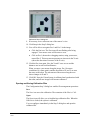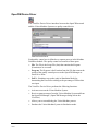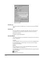
Download 100299-d ViewFlex-v28 full 02-01

9LHZ)OH[
Y151;
8VHU#0DQXDO
100299 Rev. D (January 2002)
 2002 Intelitek Inc.
Catalog #100299 Rev. D
January 2002
Every effort has been made to make this book as complete and accurate as possible. However, no
warranty of suitability, purpose or fitness is made or implied. Intelitek is not liable or responsible
to any person or entity for loss or damage in connection with or stemming from the use of the
software, hardware and/or the information contained in this publication.
Intelitek bears no responsibility for errors that may appear in this publication and retains the right
to make changes to the software, hardware and manual without prior notice.
The printed ViewFlex User Manual that is supplied with the ViewFlex system contains an
abridged version of the Matrox Inspector software manual.
The complete Matrox Inspector User Guide can be viewed and printed from the PDF file named
InsptrUG included on the ViewFlex software CD.
INTELITEK INC.
444 East Industrial Park Drive
Manchester NH 03109-537
Tel: (603) 625-8600
Fax: (603) 625-2137
www.intelitek.com
ViewFlex v.2.8
0201
3
User Manual
ViewFlex v.2.8
0201
4
User Manual
Contents
4###9LHZ)OH[#,QVWDOODWLRQ 11111111111111111111111111111111111111111111111111111111111111111111111111 :
Unpacking the Equipment................................................................................................... 7
Installing the ViewFlex System .......................................................................................... 7
Assembling the Camera Stand ...................................................................................... 7
Software Initialization ................................................................................................. 11
Activating ViewFlex ................................................................................................... 12
5###6RIWZDUH#2SHUDWLRQ 111111111111111111111111111111111111111111111111111111111111111111111111111 46
ViewFlex Toolbar ....................................................................................................... 13
Image Processing Tool ................................................................................................ 13
Camera (Camera 1 / Camera 2 / ServeCam) ............................................................... 14
Video Source – Camera Configuration ....................................................................... 16
Camera Connection (Client Camera only) .................................................................. 20
ACL Terminal for ViewFlex....................................................................................... 20
Abort All ..................................................................................................................... 24
Go To Position ............................................................................................................ 25
Calibration................................................................................................................... 27
OpenCIM Device Driver............................................................................................. 30
6###9LHZ)OH[#IRU#6&25%$6( 1111111111111111111111111111111111111111111111111111111111111111111 67
ViewFlex for SCORBASE Toolbar ............................................................................ 34
Results Table ............................................................................................................... 34
Vision Commands in SCORBASE ............................................................................. 36
Calibration................................................................................................................... 39
ViewFlex v.2.8
0201
5
User Manual
ViewFlex v.2.8
0201
6
User Manual
4
9LHZ)OH[#,QVWDOODWLRQ
Unpacking the Equipment
Before installing the equipment, check for signs of shipping damage. If
any damage is evident, contact your freight carrier, and begin appropriate
claims procedures. Make sure you have received all the items listed on the
packing list. If anything is missing, contact your supplier.
Installing the ViewFlex System
Install the ViewFlex system in the following order:
•
Assemble the camera stand and attach the camera to it.
•
Connect software protection key.
•
Install the ViewFlex software. The ViewFlex installation is supplied
on one CD ROM.
Do not plug the camera into the USB port of the computer until after the
software installation.
Assembling the Camera Stand
To assemble the camera stand, do the following:
1. Put one of the upright posts (hollow aluminum pole) into the base.
Make sure it goes all the way in.
2. Lock the post into place by tightening the knob on the base. Make sure
the post does not move.
Option: if you want to place the base on the floor connect the two
upright posts together.
‹
Insert the posts together.
‹
Twist and lock the posts.
‹
Insert the post assembly into the base.
‹
Lock the assembly into place as described above.
3. Open the knob on the arm unit.
4. Slide the arm unit onto the post.
ViewFlex v.2.8
0201
7
User Manual
5. Tighten the knob.
6. Attach the camera rod to the arm unit.
7. Tighten the knob.
8. Slide the camera mount out of the Intel camera.
9. Attach the camera to the camera rod with the tripod connector on the
bottom of the camera.
Camera
mount
Tripod
connector
Camera connections
10. Place the completed assembly in a safe convenient location near the
computer.
Arm Unit
Upright Post
Base
Camera attached to stand
Do not plug the camera into the USB port of the computer until after the
software installation.
ViewFlex v.2.8
0201
8
User Manual
Software Protection Key
1. Without the software protection key, the software is programmed to
run on a 30-day trial basis.
2. Plug the software protection key into the printer port of your computer.
3. If you also want to connect a printer to your computer, plug the printer
cable into the connector on the software key.
Software protection key
Installing the ViewFlex Software
1. Place the ViewFlex CD-ROM in the drive.
2. The installation procedure should begin to run automatically. If it does
not, select Start|Run, and select Install.exe from the CD-ROM.
ViewFlex Setup dialog box
You must first install the Image Processing Tool module. Only then
can you install the ViewFlex software.
3. Click on Image Processing Tool.
The Matrox Inspector setup will begin to run.
4. Follow the directions on your screen.
ViewFlex v.2.8
0201
9
User Manual
5. Select No, I will restart my computer later, when prompted at the
end of the installation process.
Setup complete
You only need to restart the computer after you have completed all
three installations.
6. Click Finish.
7. From the ViewFlex setup click ViewFlex. A dialog box will appear
prompting you to select one of three options:
„
ViewFlex (ER-5, ER-9, ER-14, SV3 and Open CIM)
„
ViewFlex for SCORBASE for ER-4pc
„
ViewFlex for SCORBASE for ER-4u
8. Follow the directions on the screen.
9. Select No, I will restart my computer later, when prompted at the
end of the installation process.
10. Click Finish.
11. From the ViewFlex setup dialog box, select Image Quest.
The Image Quest installation will begin.
12. Follow the directions on the screen.
13. Restart the computer after you have completed the Image Quest
installation.
14. Make sure the camera’s shutter is open.
ViewFlex v.2.8
0201
10
User Manual
Digital PC camera
15. Connect the camera to a USB port if you are installing ViewFlex on
the PC.
Note: If you are installing ViewFlex for SCORBASE you will need to
install the ViewFlex ServeCam on another computer with USB
connection that is also connected to a network.
16. A driver message will appear. Click OK.
Software Initialization
The ViewFlex.ini file initializes the ViewFlex software.
ViewFlex Properties
The ViewFlex.ini file includes the following:
The directory in which the script files are located (only for the ViewFlex
Device Driver).
[Device Driver Definitions]
ScriptPath= \Vision Script
You can choose the controller type – A, B, PC, USB.
ViewFlex v.2.8
0201
11
User Manual
[Controller Setting]
Controller=A
(Note: You can choose: ER4, ER4u, ER5, ER9, ER14, SV)
RobotType=ER14
Activating ViewFlex
To start the ViewFlex software, double-click the ViewFlex
icon on the desktop.
OR
From the Start menu, select Programs | ViewFlex | ViewFlex.
Activating ViewFlex for SCORBASE for ER-4pc
To start ViewFlex for SCORBASE, do the following:
1. Activate ServeCam.
2. Double-click the SCORBASE icon.
Or, double-click the ViewFlex for SCORBASE icon.
ViewFlex for SCORBASE Program Group
ViewFlex v.2.8
0201
12
User Manual
5
6RIWZDUH#2SHUDWLRQ
ViewFlex Toolbar
The ViewFlex Toolbar contains icons that are shortcuts for selecting
certain commands and functions:
ViewFlex Toolbar
•
Image Processing Tool
•
Camera 1
•
Camera 2
•
ACL Terminal (for ViewFlex)
•
Abort All
•
Go Position
•
Calibration
•
OpenCIM Device Driver
•
About
•
Exit
Image Processing Tool
Open the image processing tool (Matrox Inspector).
(Refer to the Matrox Inspector Instruction Manual for more information.)
ViewFlex v.2.8
0201
13
User Manual
Matrox Inspector
Camera (Camera 1 / Camera 2 / ServeCam)
When two cameras are used, a Select Video Device dialog box will
prompt you. The camera icon opens the Camera (capture) window or the
Client Camera window.
Client (remote) camera operation is available only in ViewFlex for
SCORBASE for ER 4pc.
As soon as Client Camera is activated, it connects to the server, and
displays the computer IP address where the ServeCam is located as soon
as it detects it.
Camera window
ViewFlex v.2.8
0201
Client Camera window
14
User Manual
Snap
Grabs (captures) a picture and displays it in a frame.
OR
Inserts an updated picture from the ServeCam.
Options
Opens a dialog box use for video settings and configuration.
Connection (available only in Client Camera)
Enables connection of remote cameras on a network.
Exit
Closes the Camera window.
Camera Options
Camera Options
Always On Top:
Checking this box prevents the Camera window from being hidden by
other windows.
Snap Into Current Frame
The captured image will be put into the current frame in the Image
Processing Tool. The part of the image that will be inserted into the frame
depends on the current frame size. If left unchecked, a new frame will be
created each time an image is captured (every Snap).
Image Format
Opens the Video Format dialog box.
Video Format dialog box
ViewFlex v.2.8
0201
15
User Manual
Configuration
Opens the Video Source dialog box.
Video Source dialog box
Video Source – Camera Configuration
Main
Video Input
Choose the video source for the applications that use video. Your options
for video source include the Intel PC Camera Pro or you can attach an
external video device like a VCR or camcorder.
When you select an external video source, some options are not available.
Optimize for maximum frame rate
Ensures that the frame rate never drops below 15 frames per second (in
dim light the video may appear dark).
Optimize for low light conditions
Ensures that the video is properly exposed in low light conditions like
when indoors, but may appear washed out in bright light conditions. The
frame rate for this option is between 8 and 15 frames per second. This
option is not available when the video source is an external video device.
Optimize for best image quality
Ensures that each frame of the video is high quality, but it does reduce the
frame rate so that the frame rate never exceeds 15 frames per second.
ViewFlex v.2.8
0201
16
User Manual
Exposure
Choose Automatic Exposure control to have the camera automatically
adjust the image according to the brightness slider setting.
•
Use the Light Sensitivity slider to control how long the image must be
too dark or too light before the camera adjusts. Move the slider all the
way to the left for the camera to adjust immediately. Move the slider
all the way to the right for the camera to adjust after 10 continuous
seconds of poor exposure.
•
Use the Brightness slider to set how bright the automatic exposure
should make the scene.
Choose Manual Exposure control to adjust the exposure settings
yourself.
•
Use the Gain slider to make the scene dimmer or brighter.
•
Use the Exposure Time slider to set the length of time light will hit
the sensor for each image.
Click Restore Defaults to set the sliders to the factory settings for this tab.
Color
This tab lets you control the colors in the video. Using the sliders, you can
instantly see the effect each is having on the video picture as you move the
slider. Adjust the sliders until you are satisfied with the picture.
Saturation
Drag the slider to the right to increase the intensity of the colors, drag the
slider to the left to decrease the intensity. Moving the slider all the way to
the left changes the colors to black and white.
Hue
Drag the slider to the left to increase the blue in the video, drag the slider
to the right to increase the green.
Red, Green, Blue
Drag the red, green and blue sliders left and right to decrease and increase
the tones of the colors in the video. This option is not available when the
video source is an external video device.
Click Restore Defaults to set the sliders to the factory settings for this tab.
Image
White Balance
White balance is not available when the video source is an external video
device.
ViewFlex v.2.8
0201
17
User Manual
Automatic White Balance.
Automatically makes the whitest color in the video whiter and adjusts the
other colors proportionately. Move the slider to the left to make the video
appear cooler (adds blue), move the slider to the right to make the video
appear warmer (adds red).
Any changes made take a few seconds to happen.
Manual White Balance
When switching from automatic to manual, the settings from the
automatic white balance control are initially matched until you change
them. Move the slider to the left to make the video appear cooler (adds
blue), move the slider to the right to make the video appear warmer (adds
red).
Manually adjusting the white balance may be useful when using a laptop
computer in differing lighting conditions, for instance going from room
lighting to sunlight, or when automatic adjusting is unsatisfactory.
Image Effects
Click Mirror Image to reverse the image in the video window.
Click Flip Image to have the image flip from top to bottom. This could be
used when the camera is upside down, for instance when mounted
underneath a cabinet.
Image Sharpness
Drag the slider left to soften the image, drag the slider right to sharpen the
image.
Advanced
USB Bandwidth
When you have multiple USB devices in use at the same time, and the
camera is using too much of the USB bus, use this control to specify how
much of the bus to allocate for the camera.
Drag the slider to the left to decrease the amount of the bus used by the
camera, drag the slider to the right to increase the amount of the bus used
by the camera.
Changes made here won't take effect until video is stopped and restarted.
CPU Usage
When using the camera on a computer with a processor running at
233MHz or less, the minimize CPU Usage checkbox is enabled by default.
On computers with faster processors, only use this control when the
computer becomes sluggish while using the camera.
Click Restore Defaults for All Camera Settings to restore all of the tab
settings to their factory settings.
ViewFlex v.2.8
0201
18
User Manual
Pan/Tilt/Zoom
Controls the location of the image in the field of view.
Pan box
Pan/Tilt/Zoom tab
Pan
Moves across the image horizontally. This option does not work when the
camera is zoomed all the way out or when the capture size is 640 x 480.
Tilt
Moves across the image vertically. This option does not work when the
camera is zoomed all the way out or when the capture size is 640 x 480.
Zoom In
Zooms in on the portion of the image currently visible in the video
window. The size of the rectangle shows the amount that the camera is
zoomed.
Zoom Out
Zooms out on the portion of the image currently visible in the video
window. The size of the rectangle shows the amount that the camera is
zoomed.
Shortcuts
Right-clicking the mouse inside the pan area opens a menu with the
following:
ViewFlex v.2.8
0201
•
MaxZoom In: the camera zooms all the way in
•
MaxZoom Out: the camera zooms all the way out
•
Center View: places the image in the center of the field of view.
•
Always on top: prevents the Camera window from being hidden by
other windows.
19
User Manual
Camera Connection (Client Camera only)
Connect to
If there is more than one ServeCam on the network, then you can make a
connection to the specific ServeCam that you want by entering the IP
address of that ServeCam’s computer.
The default IP address is the one that initially appears in the box, which
was automatically detected.
Clicking OK will connect to the ServeCam at the IP address shown.
ACL Terminal for ViewFlex
ACL, Advanced Control Language, is an advanced, multi-tasking robotic
programming language.
The ACL Terminal for ViewFlex is the software interface that provides
access to the controller from a PC, and provides functions needed to
configure, program and operate the robot system.
ACL Terminal for ViewFlex
Save
Saves a listing of all user programs, variables and positions in one file.
The files are in ACL format (.acl).
Download
Downloads data from a user-backup file in the host computer to the
controller. (Does not erase or modify existing programs.)
Abort All
Immediately aborts all running programs and stops movement of axes.
On-Line/Off-Line
Opens/closes the communications port.
ViewFlex v.2.8
0201
20
User Manual
ON-CON
Enables servo control for all axes, a specified group of axes, or a single
axis.
OFF-COFF
Disables servo control for all axes, a specified group of axes, or a single
axis.
Home
Drives all robot axes to their home position.
Port Properties
Opens a dialog box that allows you to configure the RS232 serial
communication port in the PC that communicates with the robot
controller:
ACL Terminal CommPort Properties
ACL ViewFlex String Commands
The ViewFlex String Commands are written as:
3ULQW#2#3ULQWOQ#´(9LHZ)OH[#VWULQJ#FRPPDQGV#(µ
ViewFlex helps you make applications that combine vision and robot
guiding that will use the ACL language for controlling and executing
robot tasks.
ViewFlex Variable
Vision functions are written in Visual Basic (VB) script. The vision script
will operate the vision task. To synchronize the vision and robot tasks,
there is the Global Variable (VF). After executing the Vision Function or
subroutine, the VF value will be 1 (VF=1).
61$3
ViewFlex v.2.8
0201
21
User Manual
Format:
%SNAP%
Description:
Will capture an image from the camera and put it into
the Image Processing Tool.
581
Format:
(581#SURJ(
Description:
Where: prog is the name of a function or subroutine in
the script. The function returns the ACL command back
to the controller.
Examples:
35,17/1#(581#SURJ(
This executes the function or subroutine in the open VB
script file. If you execute the function, the results will be
sent to the controller.
The script must be loaded before it can be executed from
the ACL.
6(7326
Format:
(6(7326#3RVLWLRQ/#7DEOH#LQGH[/#7DEOH#QDPH/#=+PP,(
Description:
Where:
Position is a defined robot position.
Table index is a position of the object in a measurement
table that was found in the image after searching. The
reserve word ALL means that if a Position is the name of
a vector all the positions in the table will be set.
Table name is the name of the measurement table. If
omitted, it means Current table.
Z is the value of the Cartesian coordinate Z in
millimeters.
Examples:
PRINTLN “%SETPOS pos,1, , 60%”
Position pos receives the coordinate value of position 1
in the Current measurement Table, while the coordinate
value of Z is 60 mm.
PRINTLN “%SETPOS pv[4],3,table1 , 80%”
Position pv[4] receives the coordinate value of position 3
in the measurement table named table1, while the
coordinate value of Z is 80 mm.
PRINTLN “%SETPOS pv,ALL,table2 , 80%”
ViewFlex v.2.8
0201
22
User Manual
Vector pv receives the coordinate values of ALL
positions in the measurement table named table2, while
the coordinate value of Z is 80 mm.
Project:
The following example project shows how the ACL
program is used with the Vision System, in order to
automate the robot and the Vision System. The example
is made from two programs:
•
ACL: for the robot task
•
Visual Basic Script: for the vision task.
GOPOS.ACL
(Note: N should be a Global Variable.)
•
The code initiates the global variable VF before
sending comments to the Vision System, so that it
can cause the ACL program to wait until the vision
command is finished. This happens when VF is 1.
•
The program tells the Vision System to Snap, then
executes the GetPos function in the script. The results
of the GetPos function is a string that is an ACL
command. If the search results are 3, for example,
then set N to 3 (“set n=3”).
•
SETPOS takes the position of the object from the
measurement table that was found after the search,
and converts it to positions that can be sent.
•
ALL takes every position from the Measurement
Table and sets them into positions in the vector.
•
At the end of GoPos, the program moves the robot to
the position in the vector.
PROGRAM GOPOS
*********************
SET VF = 0
PRINTLN "%SNAP%"
WAIT VF = 1
SET VF = 0
PRINTLN "%RUN GETPOS%"
WAIT VF = 1
SET VF = 0
PRINTLN "%SETPOS POS,ALL,,60%"
WAIT VF = 1
FOR I = 1 TO N
MOVED POS[I]
ENDFOR
END
GETPOS.BAS
ViewFlex v.2.8
0201
23
User Manual
•
In order for the Run command to work, the script
must be loaded.
•
The model for the object whose script will be
searched should also be loaded.
•
When the script will be executed, a measurement
table with the positions will be created. The script
will also send a command that initiates a sign of the
number of objects that were found.
Function GETPOS()As String
I_IMAGE1$ = Insptr.ImgGetCur
Insptr.ImgSetCurrent I_IMAGE1$, R_Def$,
ALL_BANDS
Insptr.ImgConvertType(TO_8U)
Insptr.MeasNew()
M_X_MOD$=Insptr.PatGetCur
Insptr.PatSetCur M_X_MOD$
x=Insptr.PatFind
Insptr.ImgClose
Num=Insptr.MeasGetLastID
GETPOS="SET N=" + CStr(num)
End Function
Abort All
Format:
>&WUO@#.#$
Description:
Immediately aborts all running programs and stops
movement of axes.
>&WUO@#.#$#is the fastest software method for stopping
program execution and halting movement of all axes. It
can be used at any moment, even while entering another
command, in order to instantly halt programs and axes.
This command is entered from keyboard, but does not
require [Enter] for execution.
ViewFlex v.2.8
0201
24
User Manual
Go To Position
Go to Position dialog box
Movement
Move/MoveL (Move Linear).
Table
Can be the Current table, or any other named measurement table.
Position
The index of a position in the measurement table.
Z-axis (mm)
The Cartesian coordinates in millimeters.
Fixed Angle
Enabling this option causes only the X and Y axes to be. This option can
be used with circular objects when the gripper rotation is not important.
Example of Using Go To Position
1. System must be calibrated, so that real-world measurements
correspond with the Vision System’s world of pixels.
2. Open Camera 1.
3. Click the Image Processing Tool icon.
4. In this example, put a cube down within the camera’s field of vision,
so that its edge is parallel to the edge of Camera 1 dialog box’s border.
In order for both the robot gripper and the cube to be set to zero
degrees, the cube must be defined as parallel to the X-axis of the
camera’s world. Subsequently, the robot arm’s rotation will now be
relative to this point.
5. In Camera 1, click Snap.
6. Click the ROI (Region of Interest) icon, and outline the perimeter of
the cube that was set.
7. Click the Pattern Matching icon.
ViewFlex v.2.8
0201
25
User Manual
Pattern Matching Model dialog box
„
From the Dimension tab, you will see the cube that was outlined
using the ROI icon.
„
From the Search tab, click All.
„
From the Angle tab, check Enable Search With Rotate. Then enter
180 for Delta Negative, and 180 for Delta Positive (this enables a
full 360-degree search).
„
Click Search. This will build a Measurement Table containing all
the positions of the object relative to Pos 1.
Measurement Table
ViewFlex v.2.8
0201
26
User Manual
Searched Images
8. In this example, choose the Current table (which will be the opened
table), and Position 1 (Pos 1). Click OK.
The robot will move according to the Go To Position and find the
cube.
Calibration
Synchronizing the Vision System and the Robot
To calibrate real-world measurements with the Vision System’s world of
pixels, it is necessary to perform the following steps:
1. Make sure that there is communication between the controller and the
robot.
Click the ACL Terminal icon. Click the On-Line/Off-Line icon if
necessary.
2. Execute the HOME routine.
3. Open Camera 1.
Check camera to make sure that the picture is adjusted, clear, and free
of distortions.
4. Click the Calibration icon. This automatically establishes a connection
between controller and robot.
5. Move robot arm into desired position within the camera’s field of
vision.
6. Using a pen or marker, mark a position on a piece of paper (or on the
coordinate grid) close to the robot and strong enough to be seen in the
ViewFlex v.2.8
0201
27
User Manual
camera picture. This position should be aligned with the TCP (tool
center position – the exact center of the robot gripper). This first
position is called Pos 1.
Calibration Step 1 dialog box
Click Record Position 1. (If using Controller-B, be sure it is in Auto
Mode.)
If trying to record a position produces a beep sound the reason may be
that the Teach Pendant has not been changed from Teach Mode to
Auto Mode. (In the ACL Terminal, type Auto, then click Enter.)
7. Only along the X-axis, move the robot to a position on the X-axis that
would be greater (+X) than Pos 1. Take a writing instrument and mark
the position. This second position is called Pos 2.
Click Record Position 2. (If using Controller-B, be sure it is in Auto
Mode.)
8. Now you will see in the Combo box the distance between the two
positions (Setting Distance) on the X-axis. To achieve the most
accurate measurement, take a ruler and measure the distance between
Pos 1 and Pos 2 by hand.
ViewFlex v.2.8
0201
„
Change the distance if necessary according to the hand
measurement.
„
Click Set Distance.
„
Click Next Step. This will take you to the Step 2 dialog box.
28
User Manual
Calibration Step 2 dialog box
9. If necessary, move robot arm out of the camera’s view.
10. Click Snap in the Step 2 dialog box.
11. You will be able to recognize Pos 1 and Pos 2 in the image.
„
Click the Pen icon. The Pen icon will start flashing after being
engaged. Your mouse arrow will become a cross.
„
Click on Pos 1, then make a dragging motion, using your mouse,
toward Pos 2. This movement represents an increase in the X-axis.
(shows the direction of increase of the X-axis).
12. Click the Pen icon again. Now the X and Y-axes are set and the
distances are in real-world millimeters.
When you move your mouse along the image, Pos 1 becomes
coordinate 0,0 (center-point), and the directions of X and Y are now
the same as the robot. The movement of the mouse along the axes
shows changes in X and Y.
13. Click OK. Now the Vision System is calibrated and synchronized with
the robot, and all new images will become calibrated.
Opening and Saving Calibration Files
The Configuration Step 2 dialog box enables file management operations.
Save
The Save icon saves the calibration. The extension of the files is .CAL.
Open
The Open icon will allow you to load backup calibration files. When the
OK icon is clicked, the system is calibrated.
You can configure immediately in the Step 2 dialog box and open the
calibrated file.
ViewFlex v.2.8
0201
29
User Manual
OpenCIM Device Driver
The ViewFlex Device Driver interfaces between the OpenCIM network
and the Vision Machine System as a quality control device.
ViewFlex Device Driver
Each quality control test is defined as a separate process in the Machine
Definition module. The quality control test consists of three parts:
•
File: The File is the Script File (.bas) that contains the Program
(Function) to be executed.
•
Program: The Program is the Function from the File that returns the
results of the quality control process to the OpenCIM Manager as
Pass/Fail or Error.
•
Fail %: Simulates test results (only in Simulation Mode) by
determining the Pass/Fail according to the percentage of failure that
was input.
The ViewFlex Device Driver performs the following functions:
ViewFlex v.2.8
0201
•
Activates a test on the Vision Machine System.
•
Receives status messages from the Vision Machine System and from
the OpenCIM Manager. (OpenCIM Messages dialog title in the
ViewFlex.)
•
Allows you to test and debug the Vision Machine process.
•
Emulates the Vision Machine System in Simulation mode.
30
User Manual
ViewFlex Properties
ViewFlex.exe
After the ViewFlex is installed, copy ViewFlex.exe to the OpenCIM\Bin
folder.
ViewFlex.ini
Be sure to update the script-path to the folder where the scripts files are.
An example of where the directory that the script files are located in:
>'HYLFH#'ULYHU#'HILQLWLRQV@
6FULSW3DWK #&=?RSHQFLP65?OLE?9LHZ)OH[
Operation Modes
The Operation Mode lets you to define the control mode ViewFlex Device
Driver is running in:
On-Line
On-Line mode the ViewFlex Device Driver waits for the commands from
the OpenCIM Manager, and then Snap, Load Script, Execute Program
Script, and Send Results.
Manual
Manual Mode allows you to test the OpenCIM Manager and manually
simulate conditions of Fail and Pass.
The following are activated only in Manual Mode, after a request from the
OpenCIM Manager:
Send Pass
Sends pass to the Manager.
ViewFlex v.2.8
0201
31
User Manual
Send Fail
Sends fail to the Manager.
Simulation
Simulation Mode allows you to simulate test results by determining the
Pass/Fail according to the percentage of failure that was input to the
OpenCIM Manager.
Debug
The Debug Mode allows you to debug every step of the script. This is
made for testing the script before it will be run online.
The following are activated only in Debug mode:
Open File lets you load the script.
Run Script icon executes the script that has been chosen.
Step-By-Step icon lets you to execute each command line of the script
individually.
Example of Script for Pass/Fail Test
The following script is an example for testing Pass/Fail Models. A Model
refers to the pattern for which you are searching, and the image for which
it is extracted.
The following program will try to find the “x” object by using the x-model
(x.mod). If found, Fail is sent (QCR=“Fail”). If not found, then it will try
to find the “v” object. If found, Pass is sent (QCR=“Pass”). If neither is
found, Error is sent (QCR=“Error”).
For more information on the commands, refer to Inspector’s online help.
)XQFWLRQ#4&5+,#$V#6WULQJ
#'LP#[#$V#,QWHJHU
,B,0$*(4'# #,QVSWU1,PJ*HW&XU
#,QVSWU1,PJ6HW&XUUHQW#,B,0$*(4'/#5B'HI'/#$//B%$1'6
#*#;1PRG#LV#D#0RGHO#6HDUFK#RI#REMHFW#IRU#)DLO#VLJQ
#0B;B02''# #,QVSWU13DW/RDG+%&=?2SHQ&,065?0,&5286$?:66?;1PRG%,
#,QVSWU13DW6HW&XU#0B;B02''
#,QVSWU1,PJ&RQYHUW7\SH+72B;8,
#,QVSWU10HDV1HZ+,
#[ ,QVSWU13DW)LQG
#,I#[ 4#7KHQ
#4&5 %)DLO%
ViewFlex v.2.8
0201
32
User Manual
#(OVH
#*#91PRG#LV#D#0RGHO#6HDUFK#RI#REMHFW#IRU#3DVV#VLJQ
#0B<B02''# #,QVSWU13DW/RDG+%&=?2SHQ&,065?0,&5286$?:66?91PRG%,
#,QVSWU13DW6HW&XU#0B<B02''
#[ ,QVSWU13DW)LQG
#,I#[ 4#7KHQ
#4&5 %3DVV%
#(OVH
#4&5 %(UURU%
#(QG#,I
#(QG#,I
#,QVSWU13DW&ORVH
#,QVSWU1,PJ&ORVH
#,QVSWU10HDV&ORVH
#,QVSWU1&ORVH$OO
(QG#)XQFWLRQ
ViewFlex v.2.8
0201
33
User Manual
6
9LHZ)OH[#IRU#6&25%$6(
ViewFlex for SCORBASE Toolbar
The ViewFlex Toolbar contains icons that are shortcuts for selecting
certain commands and functions:
ViewFlex Toolbar
•
Image Processing Tool; see details in Chapter 2
•
Camera (Client Camera: for ER-4pc only); see details in Chapter 2
•
Results Table
•
Calibration
•
About
•
Exit
Results Table
The Results Table window is divided into two sections: one section is a
tree representing the ViewFlex folders, and the second section is a table
with the coordinates of the object in the robot world – including blob
features.
ViewFlex v.2.8
0201
34
User Manual
Results Table
Every time a new file is saved in one of the ViewFlex for SCORBASE
folders, the tree is updated.
•
Selecting one of the Pattern Models executes Find Object with the
model on the current image.
•
Selecting one of the Blob Settings executes Find Blobs with the
Blobset on the current image
•
Selecting one of the Scripts executes the first function/ subroutine in
the Script.
File
Save Results to file so that they can be opened with Excel.
Load results from file into the Results Table.
Pattern Option
Foreground: Defines whether black pixels or white pixels are to act as the
foreground (or blob) pixels.
With Blob Features: Adds the blob feature to the robot coordinate in the
table. This applies only to Find Object.
View
Always on top: Checking this box prevents this window from being
hidden by other windows.
ViewFlex v.2.8
0201
35
User Manual
Vision Commands in SCORBASE
All SCORBASE programming commands are available from the
Command List and are easily compiled into a robot program.
The list shows the two-letter hot-key combinations that allow you to enter
commands from the keyboard.
Many commands open dialog boxes for completing the command line
parameters.
Left: Command list with the Vision Command (ER 4pc).
Right: Vision Command Group (ER 4u).
SN Snap
Captures an image.
FO Find Object
Finds object according to the Pattern Model Name that has been saved in
the Pattern folder. Returns Number of Object.
Enter the name of the model in the Model Name field.
ViewFlex v.2.8
0201
36
User Manual
(Note: The name must be the same as it is in the Result Table.)
The SCORBASE variable must be entered into the Number of Object
field. The results (Number of Object) will be assigned to the variable.
All of the robot’s coordinates and blob features will be put into the Results
Table
FB Find Blobs
Finds blobs according to the blob analysis name that has been save in the
Blobs folder. Returns Number of Blobs.
Enter the name of the model in the Blobs Name field. (The name must be
the same as it is in the Result Table.)
The SCORBASE variable must be entered into the Number of Blobs field.
The results (Number of Blobs) will be assigned to the variable.
All of the robot’s coordinates and blob features that were defined by the
user will be put into the Results Table.
SP Set Position
Sets coordinate value from the Results Table into the SCORBASE
Position Number.
In the Position field, insert SCORBASE Position Number.
In the Row field insert the Position Number (Row) in the Results Table.
In the Z (mm) field insert the Z-coordinate, by default the value in the Zcoordinate will be the same as the value of the calibrated position.
Z can be a variable or constant.
ViewFlex v.2.8
0201
37
User Manual
EF External Function
Executes the function or subroutine that the user writes in the Matrox
script.
The results of the function will be assigned to the variable.
In the Script Name field, insert the name of the script in the script folder.
In the Function field insert the function or subroutine name that is in the
script.
In the Parameter field insert the parameter that can be the SCORBASE
variable or constant. (Note: Available for ViewFlex for SCORBASE for
ER-4u only.)
In the Return field, insert SCORBASE variable that will get the function
return.
GV Get Value
Receive a value from any cell in the Results Table.
In the Variable Name field, insert the SCORBASE Variable. The cell
value will be assigned in the variable.
In the Row field insert the cell row in the Results Table.
In the Column field insert the column name in the Results Table. The
Column can be a number or the exact column name.
ViewFlex v.2.8
0201
38
User Manual
CT Change Table
Change value in any cell of the Results Table.
In the Row field insert the cell row in the Results Table.
In the Column field insert the column name in the Results Table. The
Column can be a number or the exact column name.
In the Value field insert the SCORBASE variable, or constant that you
want the cell to have.
Calibration
Synchronizing the Vision System and the Robot
To calibrate real-world measurements with the vision system’s system of
pixels, it is necessary to perform the following steps:
1. Execute the HOME routine.
2. Open Client Camera.
Check camera to make sure that the picture is adjusted, clear and free
of distortions.
3. Click the Calibration icon.
4. Move robot arm into desired position within the camera’s field of
vision.
5. Using a pen or marker, mark a position on a piece of paper (or on the
coordinate grid) close to the robot and strong enough to be seen in the
camera picture. This position should be aligned with the TCP (tool
center position – the exact center of the robot gripper). This first
position is called Pos 1.
6. Click Record Position 1.
ViewFlex v.2.8
0201
39
User Manual
Calibration Step 1 dialog box
7. Only along the X-axis, move the robot to a position on the X-axis that
would be greater (+X) than Pos 1. Take a writing instrument and mark
the position. This second position is called Pos 2.
Click Record Position 2.
8. Now you will see in the Combo box the distance between the two
positions (Setting Distance) on the X-axis. To achieve the most
accurate measurement, take a ruler and measure the distance between
Pos 1 and Pos 2 by hand.
„
Change the distance if necessary according to the hand
measurement.
„
Click Set Distance.
„
Click Next Step. This opens the Step 2 dialog box.
Calibration Step 2 dialog box
9. If necessary, move robot arm out of the camera’s view.
10. Click Snap in the Step 2 dialog box.
ViewFlex v.2.8
0201
40
User Manual
11. You will be able to recognize Pos 1 and Pos 2 in the image.
„
Click the Pen icon. The Pen icon will start flashing after being
engaged. Your mouse arrow will become a cross.
„
Click on Pos 1, then make a dragging motion, using your mouse,
toward Pos 2. This movement represents an increase in the X-axis.
(shows the direction of increase of the X-axis).
12. Click the Pen icon again. Now the X and Y-axes are set and the
distances are in real-world millimeters.
When you move your mouse along the image, Pos 1 becomes
coordinate 0,0 (center-point), and the directions of X and Y are now
the same as the robot. The movement of the mouse along the axes
shows changes in X and Y.
13. Click OK. Now the Vision System is calibrated and synchronized with
the robot, and all new images will become calibrated.
Opening and Saving Calibration Files
The Configuration Step 2 dialog box enables file management operations.
Save
Saves the calibration. The file name extension is CAL.
Open
Allows you to load backup calibration files. When the OK icon is clicked,
the system is calibrated.
You can configure immediately in the Step 2 tab and open the calibrated
file.
Example of Creating a Pattern Model
1. System must be calibrated, so that real-world measurements
correspond with the vision system’s set of pixels.
2. Open Client Camera.
3. Click the Image Processing Tool icon to open Matrox Inspector.
4. For this example, set a cube down within the camera’s field of vision,
so that its edge is parallel to the edge of the Client Camera window.
In order for both the robot gripper and the cube to be set to zero
degrees, the cube must be defined as parallel to the X-axis of the
camera’s world. Subsequently, the robot arm’s rotation will be relative
to this point.
5. In Client Camera, click Snap.
6. Click the ROI (Region of Interest) icon, and outline the perimeter of
the cube that was set.
ViewFlex v.2.8
0201
41
User Manual
7. Click the Pattern Matching icon.
Pattern Matching Model dialog box
„
From the Dimension tab, you will see the cube that was outlined
using the ROI icon.
„
From the Search tab, click All.
„
From the Angle tab, check Enable Search With Rotate. Then enter
180 for Delta Negative, and 180 for Delta Positive (this enables a
full 360-degree search).
„
Click Search. This will build a Measurement Table containing all
the positions of the object relative to Pos 1.
Measurement Table
ViewFlex v.2.8
0201
42
User Manual
Searched Images
8. Save the Pattern Matching Model in the Pattern Folder, located in the
ViewFlex for SCORBASE root folder.
9. Open the Results Table and expand the Pattern Models in the folder
tree. Check that the name you gave is listed in the tree.
10. Use this name when you Find Object.
ViewFlex v.2.8
0201
43
User Manual
Matrox Inspector
version 3.0
User Guide
Manual no. 10478-301-0300
August 13, 1999
Matrox® is a registered trademark of Matrox Electronic Systems Ltd.
Microsoft®, MS-DOS®, Windows®, and Windows NT® are registered
trademarks of Microsoft Corporation.
Intel®, Pentium®, and Pentium II® are registered trademarks of Intel
Corporation.
Texas Instruments is a trademark of Texas Instruments Incorporated.
RAMDAC™ is a trademark of Booktree.
All other nationally and internationally recognized trademarks and
tradenames are hereby acknowledged.
© Copyright Matrox Electronic Systems Ltd., 1999. All rights reserved.
Disclaimer: Matrox Electronic Systems Ltd. reserves the right to make
changes in specifications at any time and without notice. The
information provided by this document is believed to be accurate and
reliable. However, no responsibility is assumed by Matrox Electronic
Systems Ltd. for its use; nor for any infringements of patents or other rights
of third parties resulting from its use. No license is granted under any
patents or patent rights of Matrox Electronic Systems Ltd.
PRINTED IN CANADA
Contents
Chapter 1: Getting started . . . . . . . . . . . . . . . . . . . . . . . 21
Welcome to Inspector . . . . . . . . . . . . . . . . . . .22
What you need to run Inspector . . . . . . . . . . .26
Installation . . . . . . . . . . . . . . . . . . . . . . . . . . .26
System Allocation . . . . . . . . . . . . . . . . . . . . . .29
Inspector documentation conventions . . . . . . .30
Menu conventions . . . . . . . . . . . . . . . . . . .30
Dialog box conventions . . . . . . . . . . . . . . . .30
Multiple tabs . . . . . . . . . . . . . . . . . . . . . . .31
Chapter 2: A few tutorials . . . . . . . . . . . . . . . . . . . . . . . . 33
Image processing . . . . . . . . . . . . . . . . . . . . . .34
Inspector and image processing . . . . . . . . . . .35
Typical application steps . . . . . . . . . . . . . . . . .36
A few examples . . . . . . . . . . . . . . . . . . . . . . . .37
Example 1: Analyzing a blister package . . . . . .38
Example 2: Scaling-calibration and
pattern matching . . . . . . . . . . . . . . . . . . . . . .50
Example 3: Working with many images and
non-standard image file types . . . . . . . . . . . . .62
Example 4: Grabbing an image . . . . . . . . . . . .73
Chapter 3: Dealing with images . . . . . . . . . . . . . . . . . . . 77
Images in general . . . . . . . . . . . . . . . . . . . . . .78
Loading an image . . . . . . . . . . . . . . . . . . . . . .79
Grayscale or single-band images . . . . . . . . . . .80
Signed images . . . . . . . . . . . . . . . . . . . . . .80
Processing a grayscale image . . . . . . . . . . . 81
Non 8-bit images . . . . . . . . . . . . . . . . . . . . 81
Packed binary images . . . . . . . . . . . . . . . . 81
Displaying grayscale images. . . . . . . . . . . . 81
Displaying single-band images
with a palette. . . . . . . . . . . . . . . . . . . . . . . 83
Color images . . . . . . . . . . . . . . . . . . . . . . . . . 85
Multiple views . . . . . . . . . . . . . . . . . . . . . . 85
Color spaces . . . . . . . . . . . . . . . . . . . . . . . 86
Representing color images . . . . . . . . . . . . . 86
Operating on regions of interest
in your image . . . . . . . . . . . . . . . . . . . . . . . . . 87
Defining ROIs . . . . . . . . . . . . . . . . . . . . . . 87
ROI properties . . . . . . . . . . . . . . . . . . . . . . 88
Choosing a source and a destination . . . . . . . 89
Selecting a different source
and destination . . . . . . . . . . . . . . . . . . . . . 89
Processing color images . . . . . . . . . . . . . . . . . 90
Duplicating images. . . . . . . . . . . . . . . . . . . . . 91
Performing a color or data type conversion . . . 91
Other image and sequence file types. . . . . . . . 93
Raw format . . . . . . . . . . . . . . . . . . . . . . . . 93
DICOM medical format . . . . . . . . . . . . . . . 94
Collection files . . . . . . . . . . . . . . . . . . . . . . . . 95
Zooming. . . . . . . . . . . . . . . . . . . . . . . . . . . . . 97
Frame size . . . . . . . . . . . . . . . . . . . . . . . . . 98
Accessing context menus in zoom mode. . . 98
Special scrolling mode . . . . . . . . . . . . . . . . 98
View as text . . . . . . . . . . . . . . . . . . . . . . . . . . 98
View 3D surfaces . . . . . . . . . . . . . . . . . . . . . .99
Using palettes with an
8-bit display resolution . . . . . . . . . . . . . . . . .100
Chapter 4: Improving image quality . . . . . . . . . . . . . .103
Image quality . . . . . . . . . . . . . . . . . . . . . . . .104
Techniques to improve images. . . . . . . . . . . .105
Adjusting the intensity distribution . . . . . . . .106
Window leveling . . . . . . . . . . . . . . . . . . . .106
Adjusting the brightness and
contrast linearly . . . . . . . . . . . . . . . . . . . .107
Histogram equalization mapping . . . . . . . .108
Applying low-pass spatial filters . . . . . . . . . .109
Opening and closing . . . . . . . . . . . . . . . . . . .110
Basic geometrical transforms . . . . . . . . . . . .112
Scaling . . . . . . . . . . . . . . . . . . . . . . . . . . .112
Rotating images . . . . . . . . . . . . . . . . . . . .112
Translating and changing the symmetry . .113
Interpolation modes . . . . . . . . . . . . . . . . .114
Chapter 5: Image transformations . . . . . . . . . . . . . . . . 115
Operating on your images . . . . . . . . . . . . . . .116
Thresholding images . . . . . . . . . . . . . . . . . . .116
Accentuating edges . . . . . . . . . . . . . . . . . . . .118
Edge enhancers . . . . . . . . . . . . . . . . . . . .119
Edge detection . . . . . . . . . . . . . . . . . . . . .119
Arithmetic with images . . . . . . . . . . . . . . . . .121
Erosion and dilation . . . . . . . . . . . . . . . . . . .122
Other morphological operations. . . . . . . . . . .123
Chapter 6: Advanced image processing . . . . . . . . . . 125
Advanced image processing . . . . . . . . . . . . . 126
Creating custom filters . . . . . . . . . . . . . . . . . 126
Creating custom structuring elements . . . . . 127
Fast Fourier transformations . . . . . . . . . . . . 130
FFT defined . . . . . . . . . . . . . . . . . . . . . . . 130
Inspector and FFTs . . . . . . . . . . . . . . . . . 131
An example . . . . . . . . . . . . . . . . . . . . . . . 131
Filtering in the frequency domain . . . . . . 133
Operations supported on
FFT -type images . . . . . . . . . . . . . . . . . . . 135
Polar-to-rectangular and
rectangular-to-polar transform. . . . . . . . . . . 136
Watershed transformations . . . . . . . . . . . . . 138
Chapter 7: Analyzing images . . . . . . . . . . . . . . . . . . . . 139
Analyzing images with Inspector. . . . . . . . . . 140
Result log window . . . . . . . . . . . . . . . . . . . . 141
Displaying results . . . . . . . . . . . . . . . . . . . . 141
The measurement table . . . . . . . . . . . . . . . . 142
Calibration . . . . . . . . . . . . . . . . . . . . . . . . . . 143
Exporting results . . . . . . . . . . . . . . . . . . . . . 144
Exporting results . . . . . . . . . . . . . . . . . . . 144
Exporting graphics . . . . . . . . . . . . . . . . . 144
Keeping analysis statistics . . . . . . . . . . . . . . 145
Pixel conventions . . . . . . . . . . . . . . . . . . . . . 146
Chapter 8: Histograms, profiles, and measurements 147
Performing a histogram . . . . . . . . . . . . . . . . .148
Histogram window . . . . . . . . . . . . . . . . . .148
Examining pixel values using profiles . . . . . .149
Profiles of line and other
graphic objects . . . . . . . . . . . . . . . . . . . . .149
Outline thickness . . . . . . . . . . . . . . . . . . .150
X and Y profiles of a region . . . . . . . . . . . .150
Profile window . . . . . . . . . . . . . . . . . . . . .151
Adjusting profiles . . . . . . . . . . . . . . . . . . .151
Features of histogram/profile
graph windows . . . . . . . . . . . . . . . . . . . . . . .152
Taking measurements using
graphic objects . . . . . . . . . . . . . . . . . . . . . . .154
Finding average intensities
using graphic objects . . . . . . . . . . . . . . . .154
Taking measurements between
result objects . . . . . . . . . . . . . . . . . . . . . . . .155
Chapter 9: Pattern matching . . . . . . . . . . . . . . . . . . . .157
Pattern matching . . . . . . . . . . . . . . . . . . . . .158
Steps to performing a search. . . . . . . . . . . . .159
Defining a search model . . . . . . . . . . . . . . . .160
Saving a model . . . . . . . . . . . . . . . . . . . . .160
Fine-tuning the model . . . . . . . . . . . . . . . . . .161
Masking a model. . . . . . . . . . . . . . . . . . . .161
Redefining a model’s hot spot . . . . . . . . . .162
Setting a model’s search constraints . . . . . . 163
Number of matches . . . . . . . . . . . . . . . . . 163
Search region . . . . . . . . . . . . . . . . . . . . . 163
The acceptance level . . . . . . . . . . . . . . . . 164
Setting the certainty level. . . . . . . . . . . . . 164
The positional accuracy . . . . . . . . . . . . . . 166
The search speed . . . . . . . . . . . . . . . . . . . 166
Preprocessing the search model . . . . . . . . . . 167
Rotation . . . . . . . . . . . . . . . . . . . . . . . . . . . . 168
Rotated model search . . . . . . . . . . . . . . . 169
Circular overscan model search . . . . . . . . 169
Searching for a model within
a range of angles . . . . . . . . . . . . . . . . . . . 170
Quickly finding the orientation
of an image or model . . . . . . . . . . . . . . . . . . 171
Speeding up the search . . . . . . . . . . . . . . . . 173
Choose the appropriate model . . . . . . . . . 173
Adjust the search speed constraint . . . . . 173
Effectively choose the search
region and search angle . . . . . . . . . . . . . . 173
The pattern matching algorithm
(for advanced users) . . . . . . . . . . . . . . . . . . . 174
Normalized Correlation . . . . . . . . . . . . . . 174
Hierarchical Search . . . . . . . . . . . . . . . . . 176
Search Heuristics . . . . . . . . . . . . . . . . . . 177
Sub-pixel accuracy . . . . . . . . . . . . . . . . . 178
Chapter 10: Analyzing blobs . . . . . . . . . . . . . . . . . . . . .181
Blob analysis . . . . . . . . . . . . . . . . . . . . . . . .182
Performing blob analysis . . . . . . . . . . . . . . . .183
Blob analysis applications . . . . . . . . . . . .183
Performing the same blob analysis on
different images . . . . . . . . . . . . . . . . . . . . . .185
Selecting blob features . . . . . . . . . . . . . . . . .186
Area and perimeter . . . . . . . . . . . . . . . . . .186
Dimensions . . . . . . . . . . . . . . . . . . . . . . .187
Determining the shape . . . . . . . . . . . . . . .189
Segmenting an image . . . . . . . . . . . . . . . . . .193
From a source image . . . . . . . . . . . . . . . .193
Importing a segmentation mask . . . . . . . .193
Specifying your segmentation preferences . . .194
Counting and calculating selected
blob features . . . . . . . . . . . . . . . . . . . . . . . . .196
Saving and loading blob settings . . . . . . . . . .197
Filtering blobs based on features . . . . . . . . . .198
Defining a filter . . . . . . . . . . . . . . . . . . . . .198
Classifying blobs . . . . . . . . . . . . . . . . . . . . . .200
Bins method . . . . . . . . . . . . . . . . . . . . . . .201
Filters method . . . . . . . . . . . . . . . . . . . . .201
Training set method . . . . . . . . . . . . . . . . .201
Statistics and tolerances . . . . . . . . . . . . . . . .203
Chapter 11: Finding and measuring
edges and stripes . . . . . . . . . . . . . . . . . . . 205
Finding and measuring edges and stripes. . . 206
Steps to finding and obtaining
measurements of markers . . . . . . . . . . . . . . 207
Markers: edges and stripes. . . . . . . . . . . . . . 208
The search box. . . . . . . . . . . . . . . . . . . . . . . 209
Searching within a range of angles . . . . . . . . 211
Search algorithm . . . . . . . . . . . . . . . . . . . . . 212
Markers: fundamental characteristics . . . . . 213
Polarity . . . . . . . . . . . . . . . . . . . . . . . . . . 213
Position . . . . . . . . . . . . . . . . . . . . . . . . . . 213
Contrast . . . . . . . . . . . . . . . . . . . . . . . . . 214
Markers: advanced characteristics . . . . . . . . 215
Width . . . . . . . . . . . . . . . . . . . . . . . . . . . 215
Edge strength . . . . . . . . . . . . . . . . . . . . . 216
Weight factors . . . . . . . . . . . . . . . . . . . . . 218
Inside edges. . . . . . . . . . . . . . . . . . . . . . . 219
Multiple marker characteristics . . . . . . . . . . 220
Measurement results . . . . . . . . . . . . . . . . . . 221
Measurement statistics . . . . . . . . . . . . . . . . 222
Chapter 12: Defining ROIs and annotating images. . 223
Using ROIs and graphic annotations . . . . . . 224
Annotation and ROI drawing tools . . . . . . . . 225
Annotation drawing tools . . . . . . . . . . . . . 226
ROI drawing tools . . . . . . . . . . . . . . . . . . 227
Specifying your drawing preferences . . . . . . .228
Drawing destination . . . . . . . . . . . . . . . . .228
Analyzing graphic objects: Profiles . . . . . .229
Analyzing graphic objects:
Measuring objects. . . . . . . . . . . . . . . . . . .229
Multiple mode. . . . . . . . . . . . . . . . . . . . . .229
Selecting a drawing color . . . . . . . . . . . . .230
Outline properties. . . . . . . . . . . . . . . . . . .231
Converting graphic objects . . . . . . . . . . . .231
Chapter 13: Grabbing images and
specifying camera settings . . . . . . . . . .233
Cameras and input devices . . . . . . . . . . . . . .234
Specifying your camera settings . . . . . . . . . .234
Grabbing. . . . . . . . . . . . . . . . . . . . . . . . . . . .235
Grab mode . . . . . . . . . . . . . . . . . . . . . . . .235
Setting digitizer controls . . . . . . . . . . . . . .236
More advanced options - LUTs and
grabbing with triggers . . . . . . . . . . . . . . . .237
Grabbing more than 8 bits . . . . . . . . . . . . . .238
Configuring the synchronization
and signal channels . . . . . . . . . . . . . . . . . . .238
Using multiple digitizers . . . . . . . . . . . . . . . .239
Chapter 14: Creating and
manipulating sequences . . . . . . . . . . . . .241
Sequences. . . . . . . . . . . . . . . . . . . . . . . . . . .242
Loading sequences and
the sequence window . . . . . . . . . . . . . . . . . .243
Sequence properties . . . . . . . . . . . . . . . . .243
Opening compressed sequences . . . . . . . . 244
Playing back sequences . . . . . . . . . . . . . . . . 245
Grabbing sequences . . . . . . . . . . . . . . . . . . . 246
Grabbing memory type sequences . . . . . . 247
Grabbing disk type sequences . . . . . . . . . 248
Creating sequences . . . . . . . . . . . . . . . . . . . 249
Deleting frames in a sequence . . . . . . . . . . . 250
Saving and compressing sequences . . . . . . . 250
Processing the frames of a sequence. . . . . . . 251
Sequences and scripts . . . . . . . . . . . . . . . 252
Chapter 15: Calibration . . . . . . . . . . . . . . . . . . . . . . . . . 253
Calibration . . . . . . . . . . . . . . . . . . . . . . . . . . 254
Types of distortions . . . . . . . . . . . . . . . . . 254
Calibrating in Inspector . . . . . . . . . . . . . . . . 255
Calibrating your imaging setup . . . . . . . . . . 256
Non-unity aspect ratio . . . . . . . . . . . . . . . 256
Uniform rotation and scaling . . . . . . . . . . 256
Perspective and other spatial distortions . 257
Relative coordinate system . . . . . . . . . . . . . . 260
Saving . . . . . . . . . . . . . . . . . . . . . . . . . . . . . 262
Displayed world units. . . . . . . . . . . . . . . . . . 262
Returned results . . . . . . . . . . . . . . . . . . . 262
Processing calibrated images . . . . . . . . . . 263
Part I:
Inspector
...Processing your images
Chapter 1: Getting started
This chapter presents the features of the Matrox Inspector
application. It also describes what you need to run Matrox
Inspector, and the installation procedure.
22
Chapter 1: Getting started
Welcome to Inspector
Inspector is a hardware-independent application designed to
let you work interactively with images for image capture,
storage, and processing applications. Inspector is a 32-bit
Windows-based package, giving you the full potential and ease
of use of a graphical interface. It is capable of running on any
system that runs Windows 95/98 or Windows NT 4.0.
Acquiring images
With Inspector, you can load grayscale and color images from
disk in a variety of file formats, or grab them from a wide range
of supported input devices. They can then be saved to a file,
exported to other applications, printed, or copied to the
clipboard.
With Inspector, you can also load or grab sequences, and then
play them back. Sequences are a set of sequential frames that
can be grabbed from a camera or loaded from AVI, TIFF, or
DICOM files. You can process a frame of a sequence as you
would any Inspector image.
In order to grab with Inspector, you must have an installed
Matrox frame grabber. Images can be grabbed one at a time or
grabbed continuously, using any camera supported by your
frame grabber.
Image processing
capabilities
Inspector includes a variety of point-to-point, statistical,
spatial filtering, Fourier transform, and morphological
operations. You can use these operations, for example, to
smooth, accentuate, or qualify images.
Inspector supports geometric operations including interpolated
resizing, rotation, and distortion correction, as well as
polar-to-rectangular unwrapping.
Processing can be restricted to a rectangular or
non-rectangular region of interest (ROI). Processing can also
be restricted to a selected component of a color image.
Welcome to Inspector
23
Image calibration
Image calibration allows measurements and analysis to be
carried out in real-world coordinates. Various calibration
mappings can compensate for non-uniform aspect ratios,
rotation, perspective foreshortening, and other more complex
distortions.
Pattern matching
capabilities
Inspector’s pattern matching capabilities allow you to find a
pattern (referred to as a model) in an image, with sub-pixel
accuracy. Pattern matching can help solve machine vision
problems, such as alignment and inspection of objects. You can
create a model manually or have Inspector automatically select
a unique one (called an automodel) from an image. In addition,
you can have Inspector search for all occurrences of the model,
or the specified number of occurrences.
In some cases, the orientation of the model and/or the target
image can play a factor in the search operation. Inspector
includes a number of options to deal with such cases, each
optimized for different image and background conditions. For
example, you can find the orientation of a target image or you
can search for occurrences of a model at any angle, in the target
image.
Blob analysis
capabilities
Inspector’s blob analysis capabilities allow you to identify and
measure connected regions of pixels (commonly known as blobs
or objects) within a grayscale image. You can calculate upto
forty selected features of these blobs, such as their area, center
of gravity, perimeter, and Feret diameter. You can also
automatically discard blobs that are not of interest, and classify
the remaining blobs according to the values of the features.
The classification capabilities let you automatically classify
blobs based on simple criteria, such as ranges (bins) of one
value, or based on more sophisticated criteria such as
combination of features (filter) or selection from viewing
(training set).
Measuring
capabilities
Inspector’s measuring capabilities allow you to quickly take
position, distance, angle, and area measurements within an
image. You can also have Inspector locate and measure image
characteristics (markers), such as edges and stripes (pairs of
edges), in an image, based on differences in pixel intensities.
24
Chapter 1: Getting started
Edges and stripes are located with sub-pixel accuracy. You can
also take measurements between positional results obtained
from different image analysis operations.
Annotation
capabilities
With Inspector, you can annotate your images with text, lines,
filled shapes, or outlined shapes, in any specified color. These
can also be used as ROIs. Annotation can be added directly into
your images, or into an overlay buffer.
Exporting results
Inspector-generated data can be exported directly to any
application that suports OLE automation. Exporting to
Microsoft Excel or Word requires no scripting. If you want to
export to an application other than Excel or Word, you can
create a custom export script module modeled on the ones
provided in Inspector for Microsoft Excel or Word.
Scripting
capabilities
You can automate your applications by recording actions in a
script. You can easily modify the script with the help of
Expression Builder. The resulting script can be executed as
many times as required with Inspector’s Script interpreter. For
easy recall, scripts can be associated with shortcut keys or
buttons on the script bar or added as menu items. In addition,
if your script has logical problems, you can use Inspector’s
debugging capabilities to determine where the problems occur.
Inspector offers two scripting languages: Basic and C-Script.
The version of Basic used by Inspector is compatible with
Microsoft Visual Basic for Applications. C-Script is a scripting
language similar to C.
Both languages allow you to extend the functionality of your
application by making script calls from Inspector to functions
in external DLLs.
Using Basic, you can also use Inspector either as a client or a
server of another Windows’ based application that supports
OLE (object linking and embedding) Automation. Basic can
also be used to develop semi-autonomous scripts that support
user intervention.
Welcome to Inspector
Collection files
25
With Inspector, you can create collection files. Collections are
visual directories that contain thumbnails of images. They are
useful for visually tracking and managing your image and
sequence files.
You can drag and drop images and sequences into a collection
from Explorer or the Find File dialog box (under Windows
95/98 or Windows NT 4.0). You can also drag and drop an open
Inspector image/sequence into a collection. From a collection,
you can open one or more images into the Inspector workspace.
Manual overview
This manual is divided into two parts. Part I describes how to
load, grab, process, and analyze images. Part II describes how
to automate your application and how to use Inspector as an
automation client or server. The appendices describe aspects of
Inspector not covered in previous chapters.
❖ This manual assumes you are familiar with basic Windows
operations; if necessary, review your Windows
documentation.
Note that all procedures, except for the ones in Chapter 2: A few
Tutorials, are only available in the on-line help included with
Inspector.
On-line help
You can obtain context-sensitive help by pressing F1 or by using
the context-sensitive button on the Inspector toolbar.
Image Quest
Included with Inspector is Image Quest, a multimedia
introduction to image processing that is divided into two parts:
theory and problem solving. It includes text, images, video, as
well as real-life applications implemented with Inspector.
26
Chapter 1: Getting started
What you need to run Inspector
In addition to your Inspector CD, you will require a hardware
key (a two-sided, 25-pin connector) to run your Inspector
software once the 30-day evaluation period has expired. To use
Inspector, you require the following:
■
An 80486 processor or higher.
■
Windows 95/98 or Windows NT 4.0. We recommend that you
have at least 32 Mbytes of memory if you are running
Inspector with a VGA card; 64 Mbytes if you are using a
digitizer board.
■
A Windows display adapter and compatible monitor.
■
A Windows-supported mouse or another pointing device.
In addition to the above, you need a Matrox frame grabber in
order to grab images.
Installation
You install Inspector by running the Inspector Setup utility (see
below). Note that Inspector has been developed using the
Matrox Imaging Library (MIL) and requires some of its driver
and DLL components. If you have already installed MIL-Lite
or if you have installed the full MIL development package,
Inspector’s setup will only re-install those drivers and DLLs
that are out-of-date.
❖ If you have an installed Matrox frame grabber, you are
presented with the System Allocation list box when you
first load Inspector. This list box allows you to choose the
system you want to use to run Inspector. It is primarily useful
if you have two or more frame grabbers. The System
Allocation list box is discussed later in this chapter.
Installing Inspector
If you abort the Setup utility prematurely (Cancel), some files
might not be copied or modified. In this case, you should re-run
the Setup utility to ensure that everything is installed.
Installation
27
To install Inspector:
1. Attach the hardware key to the parallel port of your PC (if
another device such as a printer is attached to the parallel
port, disconnect it, attach the hardware key, and then attach
the printer connector to the other end of the hardware key).
If a MIL hardware key is attached, connect them together.
2. Insert the Inspector CD into a CD drive. The Setup utility
should run automatically. If the Setup utility does not run
automatically, click on the Start button, select Run, and
then type at the prompt, using the appropriate drive letter:
F>UGVWR
If Inspector is run without the hardware key, a temporary
license is assigned to your system, allowing use of Inspector for
30 days. Each time you run Inspector, a dialog box appears
indicating the number of days until the temporary license
expires. Once this time period has elapsed, Inspector will not
run unless a hardware key is attached.
❖ Note that Inspector’s 30-day evaluation license can only be
installed once. Any attempt to tamper with the PC’s calender,
before the date of expiry, will disable Inspector. In that event,
Inspector can only be re-used once a hardware key is
obtained.
After installation
Once Inspector is installed, a group titled Matrox
Inspector 3.0, containing the icons for the Inspector
application, is created. Note that one of the icons is for the
readme.chm file. This is an on-line help file containing
important information about troubleshooting and features
specific to imaging boards. Be sure to read it.
The following are also created after installation:
■
An entry for Inspector in the Windows registry. This contains
information used by Inspector during start-up.
■
Directories containing image, sequence, C-Script, Basic
script, utility, and sample automation project files.
28
Chapter 1: Getting started
Note that, if you add a frame grabber after installing Inspector,
you should uninstall MIL from the Control Panel, otherwise
the drivers will not be installed. Then, re-run the Inspector
Setup utility. This will ensure that the necessary files are added.
Uninstall under
Windows 95/98 or
NT 4.0
You can uninstall Inspector as follows:
3. Select Settings from the Start menu.
4. Select Control Panel from the presented sub-menu.
5. Select Add/Remove Programs from the Control Panel
menu. The Add/Remove Programs Properties dialog
box appears, with the Install/Uninstall tab active.
6. Select Matrox Inspector 3.0 from the presented list box.
7. Click on Add/Remove.
❖ To completely remove Inspector from your system, you should
also uninstall Matrox Imaging Library Products, if
present.
System Allocation
29
System Allocation
If you have an installed Matrox frame grabber, you are
presented with the System Allocation list box when you run
Inspector. This list box contains all the systems that Inspector
detects on your computer. If your computer only has one board,
you can check the Don’t ask me again option, and the next
time you open Inspector, it will open using that board. The
system choice you make is saved in the registry.
If you are always going to use the same system to run Inspector,
you can disable the System Allocation list box for future
sessions, in which case the system specified in the registry is
used to run Inspector. To disable the System Allocation list
box, use the Options Preferences command (in the General
tab).
30
Chapter 1: Getting started
Inspector documentation conventions
This section describes some conventions used in this manual.
Menu conventions
This manual refers to operations, accessible through the menus,
as commands, and refers to them by their menu and sub-menu
names. For example, selecting Geometry from the Tools menu
and then selecting Scale from the presented sub-menu is
referred to as the Tools Geometry Scale command.
Dialog box conventions
In general, when a command is called, a dialog box appears.
Dialog boxes allow you to specify how you want the command
performed. To use a dialog box, you might have to enter values
in edit fields, select items from list boxes, specify options, or
click on buttons and selectors.
Calibration dialog box
Apply to options
Units drop-down list box
Square pixels checkbox
Pixels edit field
Angle button
An ordinary list box differs from a drop-down list box in that
the list is immediately visible. To view the contents of a
drop-down list box, click on the arrow next to the box.
Inspector documentation conventions
31
Multiple tabs
Most of Inspector’s dialog boxes are actually multiple dialog
boxes, that is, different dialog boxes overlaid one on top of the
other. The main dialog box is referred to as a dialog box, while
its internal dialog boxes (or property pages) are referred to as
tabs. The tab name appears at the top of the tab.
32
Chapter 1: Getting started
Chapter 2: A few tutorials
This chapter introduces you to image processing and
provides a tutorial on Inspector’s processing operations.
34
Chapter 2: A few tutorials
Image processing
Pictures, or images, are important sources of information for
interpretation and analysis. These might be images of a
building undergoing renovations, a planet’s surface
transmitted from a spacecraft, plant cells magnified with a
microscope, or electronic circuitry. Human analysis of these
images or objects has inherent difficulties: the visual inspection
process is time-consuming and is subject to inconsistent
interpretations and assessments. Computers, on the other
hand, are ideal for performing some of these tasks.
For computers to process images, the images must be
numerically represented. This process is known as image
digitization. The digitization process divides an image into a
two-dimensional grid of small units called pixels (picture
elements). Each pixel has a value that corresponds to the
intensity or color at that location in the image. Each pixel in
the image is identified by its position in the grid and is
referenced by its row and column number.
Once images are represented digitally, computers can reliably
automate the extraction of useful information using digital
image processing. Digital image processing performs various
types of image enhancements, distortion corrections, and
measurements.
Inspector and image processing
35
Inspector and image processing
Inspector provides a comprehensive set of image processing
operations. There are two main types of processing operations:
Image enhancement
and transformation
■
Those that enhance or transform an image.
■
Those that analyze an image (that is, generate a numeric or
graphic report that relates specific image information).
Inspector’s image enhancement and transformation operations
allow you to improve the quality of your image and/or transform
your image. These include:
■
Point-to-point operations. These operations include
brightness and contrast adjustment, constant thresholding,
arithmetic, and image mapping operations. Point-to-point
operations compute each pixel result as a function of the pixel
value at a corresponding location in either one or two images.
■
Spatial filtering operations. These operations are also
known as convolution. They include operations that can
enhance and smooth images, accentuate image edges, and
remove ‘ noise’ from an image. Most of these operations
compute results based on an underlying neighborhood
process: the weighted sum of a pixel value and its neighbors’
values. You can use one of Inspector’s pre-defined filters or
create your own filter(s).
■
Morphological operations. These operations include
erosion, dilation, opening, and closing of images. These
operations compute new values according to geometric
relationships and matches to known patterns (structuring
elements) in the source image. If necessary, you can create
your own structuring element for one of Inspector’s
morphological operations.
■
Geometric operations: These operations include scaling,
rotating, translating and flipping of images, as well as
polar-to-rectangular and distortion correction.
36
Chapter 2: A few tutorials
Image analysis
Inspector’s image analysis operations summarize a frame of
pixels into a set of values which relate specific image
information. These include:
■
Basic statistical operations. These operations extract
statistical information from a specified region of an image,
such as its distribution of pixel values or its profile.
■
Pattern matching operations. These operations allow you
to determine how similar certain areas of the image are to a
pattern.
■
Blob analysis operations. These operations allow you to
identify and measure aggregated regions of pixels within an
image (commonly known as blobs).
■
Measurement operations. These operations allow you to
locate edges or pairs of edges (known as stripes) and measure
their features. In addition, they allow you to take a variety
of measurements between their positional results, and get
quick on-the-spot measurements, such as length, area, and
angle.
For most image analysis operations, you can maintain statistics
in Inspector.
Typical application steps
Although there are many applications for which Inspector can
be used, most involve the same basic steps:
1. Load an image from disk or grab one from an input device.
2. To optimize the image(s), use Inspector’s enhancement and
transformation operations. You might need to use some of
Inspector’s analysis operations to determine your
optimization strategy.
3. To generate the required image information, use Inspector’s
analysis operations.
4. Save and/or export numeric results. Inspector can export
results to most popular spreadsheet and database
packages. Calculated data can then be compared with
existing data or used in statistical computations.
A few examples
37
A few examples
To get you started, the remainder of this chapter will serve as
a tutorial. As such, we provide four examples that will
familiarize both novices and advanced users with Inspector’s
operations. The four examples have been chosen to introduce
you to processing operations, as well as reveal shortcuts,
suggest hints and alternative methods for efficient use of
Inspector’s imaging software. Each example is presented as a
sequence of operations, and lists the steps to complete the
relevant task at hand.
The first and second examples serve as a warm up. They allow
you to perform some general commands (for example, load an
image file from disk), as well as enhance and analyze an image.
Since blob (object) analysis and pattern matching (recognition)
are the most common uses of Inspector’s image processing
capabilities, the first and second example focus on blob analysis
and pattern matching, respectively. The second example has
been chosen to introduce you to Inspector’s calibration and edge
(stripe) finding capabilities.
The third and fourth examples focus on dealing with many
images and grabbing (digitizing) an image from an input device
(camera), respectively. These examples build on techniques
presented in the first two examples and allow you to take full
advantage of useful commands and/or operations such as
window leveling and locking targets.
38
Chapter 2: A few tutorials
Example 1: Analyzing a blister package
In the first example, you will analyze an image of a blister
package that could be found along a pharmaceutical inspection
line. For the initial assessment, you will perform a basic
histogram operation, which gives you a intensity distribution
graph of the entire image. Then, you will focus on a selected
area in an image to determine an enhancement and analysis
strategy suited to the image. You will perform "thick"
horizontal and vertical line profiles, each of which provides a
graph of the pixel values along a small horizontal and vertical
line segment, respectively, to assess the lighting condition in
the selected region. Then, you will perform a histogram of this
same selected region since, like most images, this one contains
some noise. Then, to enhance the image and remove some of
the noise, you will perform a smoothing (spatial filtering)
operation.
For image analysis, you will segment the pills from the
background. Since the image has been smoothed, you will
ensure that the edges of the pills are distinct enough for the
segmentation. To do this, you will make use of both "thick" line
profiles. Then, after segmentation, you will perform a pill (blob)
count to confirm the presence of the specified number of pills.
At the same time, you will extract some basic feature
information that will allow you to determine which pill is
missing if one is missing.
Loading an image file
into Inspector’s
workspace
1. Load the blispac4.jpg image of the blister package filled
with pills from the \IMAGES folder. Use the File Open
command or drag the image from Windows Explorer into
Inspector.
In general, to open more than one image file at a time from
the same folder using the File Open command or Windows
Explorer, click on the first image file, then do one the
following:
❐
If the files are in consecutive order, hold down the Shift
key and click on the last item of the group of files to be
included.
Example 1: Analyzing a blister package
❐
If the files are not in consecutive order, hold down the Ctrl
key while clicking on each file to be included in the group.
❖
Performing a histogram
on the whole image
Note that when an image file is of a type that does not
correspond to one of those presented in the Files of type
drop-down list box, use the Open As drop-down list box
to specify the file’s data type.
Perform a histogram operation on this color image. To do so,
click on the Histogram button; alternatively, use the Image
Statistics Histogram command. The histogram graph
displays the three color bands present in the image (default
ROI).
❖
Converting a color
image to grayscale
39
Note, that the histogram for the entire image is basically
smooth, despite the fact that there is some random noise
in the image.
To simplify the statistical analysis of the image, we will convert
the image to an 8-bit, unsigned grayscale image. After
conversion, the statistical graphs generated will show only one
band, instead of three.
Working with a grayscale image is useful since you will need
one to perform blob analysis later on. Inspector can only
perform blob analysis on 8-bit, one band images, however, if
you do not perform this conversion operation manually,
Inspector will perform it automatically (if necessary) for any
blob analysis operation.
40
Chapter 2: A few tutorials
To convert the image from color to grayscale, use the Image
Convert command. Alternatively, right-click on the image to
generate the image’s context menu, and then select Convert.
Then, choose 8-bit Unsigned from the sub-menu.
Image processinginitial approach
The best approach to analyze the noise that is present in the
image is to analyze a small region that should have a uniform
dark pixel intensity. You will use the statistical tools available
in Inspector to do so.
Performing a line profile
to check lighting
conditions
To determine whether or not the lighting condition is uniform
in the small region, you will create a thick line profile in the
horizontal and vertical direction, respectively. Performing a
line profile across what should be a uniform area will determine
if the lighting condition is uniform in that direction. A "thick"
line profile will be generated, so that an average of the pixel
values along the width of the line segment will be obtained.
1. To set the thickness of the line profile, click on the line above
the Options section of the Drawing Tools toolbar. The
Drawing Tool Properties dialog box appears.
2. Ensure the Outline tab is selected. Set the line’s pixel
width in the Width edit field to 4. You can use the
incremental push button arrows, or type in this value
directly.
3. Now, click on the Line Profile tool, or use the Image
Statistics Line Profile command. Alternatively, you can
enable the Profile option and then use the line tool in the
Drawing Tools toolbar.
4. Create a short horizontal line in a uniform dark region of
the image by clicking at the start position and dragging
across to the final position.
Example 1: Analyzing a blister package
41
5. Create a short vertical line in a similar fashion. Draw the
lines intersecting as illustrated.
6. Position these two graphs generated in a tile fashion, so
that they are both easily visible on screen. Ensure there is
enough work space to view the two line profiles and the
image.
The line shows a relatively constant variation along its entire
length (minimum and maximum pixel intensity show little
variation, respectively, from the average value). Therefore, the
background lighting is evenly distributed in the horizontal and
vertical direction in this small region. Analyzing the noise in
this small region will provide valid pixel intensity results (as
opposed to values due to lighting artifacts).
42
Chapter 2: A few tutorials
Performing a histogram
to analyze noise
To analyze the noise in the region, you will take its histogram.
A histogram on the background pixels will determine how the
pixel values deviate from the expected value.
1. Draw a small ROI enclosing the lines used for the profiles.
To do this, enable the ROI drawing tool. Click on the ROI
drawing tool button in the tool button bar. Alternatively,
choose the rectangular ROI tool from the Drawing Tools
toolbar.
2. Click on the Histogram button; alternatively, use the
Image Statistics Histogram command. The histogram
graph displays the grayscale pixel values present in the
defined ROI.
From the shape of the histogram of this small uniform area,
it is apparent that there is random noise in the image.
Example 1: Analyzing a blister package
Using a line profile to
check for sharp edges
43
To remove the noise in the image, a smoothing operation
(spatial filter) will be performed. However, applying a spatial
filter might cause the edges between the background and the
pill objects to lose their sharpness. An easy way to keep track
of edge sharpness after a processing operation is to monitor
changes in the edge width and edge angle of the line profiles
taken across the pills in both directions. To take these profiles,
you will deselect the small ROI, and reactivate the original
lines. Then, extend these lines across the pills in the horizontal
and vertical direction, respectively.
1. Click on the original horizontal line profile.
2. Create a horizontal line stretching across a row of pills in
the image by dragging the line’s handles across to the final
position. Extend the line as illustrated.
3. Reposition the vertical line profile by enabling and then
dragging the line. Then, resize it by moving the vertical
line’s handles so as to extend it across a column of pills.
Both line profile graphs are updated with new line profile
data.
44
Chapter 2: A few tutorials
4. Position the graphs in Inspector’s workspace in a tiled
fashion, so that they are all easily visible on screen. Ensure
that the image is also visible. You can change the height
and width of the histogram window.
Removing random
noise from an image
using a filter
Although the noise in the image leads to variation in pixel
intensity, the distribution is relatively random; therefore, the
noise in the image can be removed using a smoothing filter. You
will determine the number of times to apply the filter based on
the histogram of the flat area, since a narrow histogram curve
will indicate that there is a more uniform area.
1. Click on the Filters tool button, or use the Image
Processing Filters command. Alternatively, right-click on
the image to obtain the image’s context menu and select
Processing. The Processing Operations dialog box is
presented.
2. Ensure that the Filters tab is displayed. Select
Smooth5x5 from the list box.
Example 1: Analyzing a blister package
45
3. Make sure the destination (D) Selector bar at the bottom
of the Processing Operations dialog box is set to
R_BLISPAC4_JPG (not New 3-Band RGB).
4. Click on Apply two times to perform the smoothing
operation twice. Note how the graphs changes each time.
❖
From the change in the histogram of the small region,
you can see that the background noise is reduced and the
region has a more uniform value.
Look at the pixel intensity values. The pill pixel values are quite
distinct from the background pixel values. Moreover, the edge
width and edge angle (between the foreground and background)
is well-maintained. Therefore, the edges should be sharp
enough so that a single threshold value can be chosen that will
properly segment your foreground objects from the background.
46
Chapter 2: A few tutorials
Undoing a processing
operation
After an enhancement or transformation operation has
modified an ROI, such as the smoothing operation just
performed, the operation can be undone by clicking on the
Undo button or using Inspector’s Edit Undo command.
❖
Note, you can specify the number of operations that can
be undone in the General tab of the Options
Preferences command. Note also that an operation that
places results in a new window cannot be undone.
To reverse the undo, click on the Redo button or use the Edit
Redo command
Blob analysis
Now, perform a blob analysis operation on the grayscale image,
so that you can determine if there are the correct number of
pills in the blister package. The first step will be segmentation,
that is, providing a pixel intensity threshold value such that
pill objects (blobs) are white (foreground object) and the
background is black. Then, you will count these blobs, as well
as obtain some statistical information about each blob.
1. Click the Blob Analysis button; use the Analysis Blob
New command; or alternatively, select New Blob from the
image’s context menu. A blob settings (Blobset) dialog box
appears.
2. Select the Segmentation tab to identify your objects. A
segmentation mask is presented.
3. Use the Threshold slider to verify that the background
lighting is evenly distributed throughout the entire
segmentation mask image. To do this, drag the slider from
70 to 130.
Example 1: Analyzing a blister package
47
4. Threshold the segmentation mask using a value that is
between the maximum background value and the minimum
foreground value returned from the previous line profile.
For this example, set the Threshold value to 115. You can
type the setting directly into the edit field or use the slider.
5. Magnify the previewed segmentation mask to view small
artifacts. To do this, select the Zoom button and click on
the center of the segmentation mask. To increase the
magnification, continue to left click on the center of the
segmentation mask. Zoom in 2 more times.
❖
To zoom out by standard increments, right-click the
mouse.
Now, deselect the zoom tool (magnifying glass icon) by
clicking on the Zoom button again.
6. Since there are small artifacts after segmentation, which
will affect the pill count, have Inspector ignore these by
choosing a minimum area for the blob analysis search. To
do this, select the Settings tab and type the value 100 in
the Min. area (minimum area) edit field, located in the
Remove Blobs section. This will remove any small artifact
from the blob count that has an area less than 100 pixels 2.
48
Chapter 2: A few tutorials
7. Select the Features tab of the Blobset dialog box.
8. Choose the Centroid features from the Quick Select list
box. Then, click on the Select button. Alternatively,
double-click on this feature. All centroid features are added
for calculation and are listed in the Selected list box.
❖
Note that a label is always associated to each blob and
an area is always calculated.
9. Select Count to count the blobs in the image and calculate
the specified features (minimum area and features related
to centroid). A blue line outlining each blob that has an area
above the specified minimum is displayed along with the
blob’s label number.
Example 1: Analyzing a blister package
49
In addition, an AllResults table is displayed which shows
the blob count, and lists all blobs meeting specifications,
including their calculated blob features.
Inspector should count the correct number of pills
(blobs)- 12. However, if an artifact with an area greater
than 100 pixels2 is present in your image, take note of its
area. Then, you can return to the Settings tab and increase
the minimum area to a value above that for the remaining
artifact(s). Then, click the Count button again. An updated
blob count will appear in the AllResults table.
If pills are missing, you could use the coordinates of each
pill’s centroid to determine the pockets which are empty.
Demos...
To familiarize yourself with other blob analysis tools in
Inspector, run the MissingBlobDemo.bas and
MoneyToClassify.scr scripts included with your software
package. To do so, use the File Open command or Windows
Explorer to open the script files. The MissingBlobDemo.bas
Basic script is in the \Basic Files folder, while the
MoneyToClassify.scr C-Script script is in the \Files folder.
The MissingBlobDemo.bas script determines if a pill has been
placed in each pocket. It uses an alternative approach to the
one we just presented; it calculates and searches for the pill at
each position. Then, the Inspector script returns a flag each
time a blob is not present at the expected position.
50
Chapter 2: A few tutorials
The MoneyToClassify.scr is an Inspector script that sorts coins
in an image, counts the different denominations, and then
returns the values into a text file.
Example 2: Scaling-calibration and pattern
matching
This second example focuses on processing an image of three
pins on a computer chip. The image has a square pixel aspect
ratio (each pixel represents the same real distance both in
width and in height), but the chip in the image does not have
the same size as in the real world since the camera positioning
has resulted in a magnified image. You will calibrate your
imaging setup in Inspector so that the image’s pixels are scaled
to real-world dimensions. With these scaled dimensions,
measurement results will be returned in real-world units.
Subsequently, you will perform a pattern matching and
measurement operation to determine if the correct number of
pin-legs are present in the image, and if they are structurally
intact. To determine if the correct number of pin-legs are
present in the image, a pattern (model) is used as the basis for
finding similar patterns in the image. Then, the location of the
first model will be used as the relative origin for finding the
pin-legs seen as stripes (pairs of edges) in the image. Inspector’s
measurement capabilities will determine the structural
integrity of the pin-legs.
Although in this example you find stripes in the image
manually, the approach taken is amenable to using Inspector’s
automating (scripting) capabilities.
1. Load the image, threepins.tif, from the \IMAGES folder. To
do so, use the File Open command, or drag the file from
Windows Explorer into Inspector.
2. To magnify the region between the central and right-most
pin, first, zoom in 2 times on the image using the Zoom tool
button.
3. Then, once the appropriate magnification is obtained,
deselect the Zoom tool.
Example 2: Scaling-calibration and pattern matching
Calibration: pixel-world
scaling
51
Now, calibrate the pixel-to-world scaling of your imaging setup
using the threepins.tif image.
1. Select the Options Calibration New command. The
Calibration dialog box is presented, which is used to create
a calibration object.
2. Make sure the Square Pixels option is selected from this
Calibration dialog box.
❖
Note, for this example, the pixels are square, but in
Inspector, you can also create a calibration object that
corrects an image with a distorted aspect ratio.
3. Assign a specified number of pixels to a specified number
of real world units. To do so, click on the calibration line
which flashes blue when selected.
4. Using the mouse, draw a line extending from the first edge
of the first pin to the first edge of the second pin in the
image. The length of this line should be 95 pixels. The
length will be displayed at the bottom of the image in the
status bar. Adjust this line if necessary and click the
calibration line button a second time when finished.
5. Inspector places the line’s pixel length in the Pixels edit
field.
6. The distance from the first edge of the first pin to the first
edge of the second pin is 2.5 millimeters (mm). So, type 2.5
in the World edit field.
7. Select millimeters (mm) from the Units drop-down list box.
52
Chapter 2: A few tutorials
8. Apply the calibration object to the current image by
ensuring that the Apply to option is set to the threepins.tif
image. Then, click OK.
Note that although the image remains the same after
calibration, you will now obtain measurements and positional
results from the scale-calibrated image in real world units. To
test this, move the cursor over the image and note the reported
coordinated in the image’s status bar.
It is important to mention that most dialog boxes (for example,
measurement and pattern matching) take positional and
measurement data in uncalibrated (pixel) units, while all tables
present results in calibrated units. Interactively, you can
determine the uncalibrated equivalents by setting the status
bar to show uncalibrated coordinates. Scripting functions
which access results can access results in calibrated or
uncalibrated units.
Pattern matching
Now, you will perform a pattern matching operation on the
calibrated threepins.tif source image. You will first define a
rectangular region to be used as the search model (search
pattern). Then, you will search the whole image for occurrences
of matches to your model to ensure that the three pins are
present. In addition, the position of the first occurrence of the
pattern will be used to set up the subsequent stripe finding
operation.
Example 2: Scaling-calibration and pattern matching
53
1. Use the ROI tool button, or select the ROI rectangle tool
from the Drawing Tools toolbar, to draw a region around
the pin’s waist. The ROI’s origin should begin at coordinate
location (1.40,4.40) and its width (w) and height (h) should
be roughly 1.50 and 0.85, respectively, as illustrated below.
2. Click on the Pattern Matching button. Alternatively, use
the Analysis Pattern New Model command.
3. The Model dialog box appears with the Dimensions tab
selected, and the search model displayed in the upper-left
corner.
54
Chapter 2: A few tutorials
❖
Note, for some images, it is advisable to mask the
undesired areas using the colored eyedropper tool to
minimize interference from background pixels and
increase the accuracy of your search.
4. Now, select the Search tab from the Model dialog box.
Since we are expecting a maximum of three pins in the
image, type 3 in the Only first edit field.
5. To ensure that search results are drawn with a bounding
box (graphic object) in the image’s overlay, right-click on the
Model dialog box. The Model Properties dialog box is
presented. Select the Draw graphic object in image
option under the General tab.
6. Click the Search button to search for the three occurrences
of the model in the image.
Example 2: Scaling-calibration and pattern matching
55
7. A measurement table is displayed listing the calibrated
positions of all models found in the image in the X1 and Y1
columns, and the match score (%) obtained for each
occurrence, in the Info columns.
Do not close this table since this positional data will be used
shortly.
❖
A few points to
consider...
By default, you will also obtain an on-screen log for all
pattern matching operations. To disable this option,
right-click on the measurement table and choose
Properties from the table’s context menu. A
Measurement Table Properties dialog box is
presented. Choose the Results tab, and then disable the
Log results option.
It is important to note that for this example, you perform a
pattern matching operation in a source image with a square
pixel aspect ratio (1:1). Accordingly, it is not necessary to
physically correct the image when performing the pattern
matching operation. However, as a general rule, you must
physically correct an image if its distortions can significantly
impact your particular processing operation.
For example, significant perspective distortion can affect the
success of a processing operation like pattern matching.
56
Chapter 2: A few tutorials
Even if your imaging setup causes your images to have a
non-unity aspect ratio, and you want to find a model that can
appear within an angular range, you will have to correct your
image before performing the search. In these cases, after
calibrating your image, use the Image Advanced Geometry
Correct command to correct your image using its associated
calibration object. Note that after correction, results are still
returned in real-world units.
Search using an
occurrence of a
pattern as the relative
origin
Next, you will search for and measure three pin-legs in the
image. In this case, you will use coordinates of the first pin waist
(Pattern 1 match), determined from the pattern matching
operation, as the relative origin for setting up a search area
(search box).
When automating this application using scripting, it is
important to note that Inspector’s scripting functions take
values only in uncalibrated units, although they can return
results in either calibrated or uncalibrated units. It is
important to remember most dialog boxes and tables do not
take and return values in an identical fashion.
Changing status bar
display settings from
calibrated units to
uncalibrated units
Interactively, get uncalibrated positional data in the status bar.
To do so, right-click on the image and choose Properties from
the image’s context menu. The Image Properties dialog box
appears. Select the Display tab, and then set the Status Bar
Format option so that Show Calibrated is not selected.
Finding stripes and
angles in an image
Now, we will use Inspector to check for the structural integrity
of the three pin-legs on the chip in our image, because after
much wear and tear, the pin-legs might be bent. Since the pins
themselves constitute a pair of edges (a stripe), an easy way to
determine if their legs are bent is to search for three edge-pairs
(stripes) in the image, and then analyze the angle
measurements calculated by Inspector.
Example 2: Scaling-calibration and pattern matching
57
1. To accomplish the stripe search, click the Edge and Stripe
button; alternatively, use the Analysis Measurement
Edge and Stripe command. The Edge and Stripe dialog
box is presented.
2. Click on the Stripe option (not Edges).
3. Select the Multiple search option to search for multiple
instances of the stripe.
4. Type 3 in the Number edit field, since there are three pins
in the image.
❖
A 0 in the number or spacing edit field means that
Inspector will search for any number of stripes or stripes
that are separated by any amount of space, respectively.
These settings will result in slower processing since the
search algorithm will need to determine these values
automatically. The search algorithm is much more
efficient and more robust if the expected number of
stripes and their spacing (in pixels) are specified as
opposed to being left as 0 (unspecified).
❖
The default auto-polarity setting is suited for this
example.
5. Set the initial search box orientation to Vertical, since the
pin-legs will be in a vertical orientation.
6. Click on the Draw the Search Box button within the
Edge and Stripe dialog box. This search box button flashes
blue.
58
Chapter 2: A few tutorials
Defining a search area
7. Now, draw a rectangular search box that encloses the upper
portion of the three pin-legs. The search box should be
placed just below the pin’s waist. To accomplish this, the
box should have a negative horizontal offset of 50 pixels,
and a negative vertical offset of 30 pixels from Pattern 1’s
X and Y coordinates, respectively. The height of the box
should be 20 pixels. A suitable search box with dimensions
290 pixels (width) x 20 pixels (height) is illustrated below.
8. Adjust your search box area if necessary, and then click the
flashing search box button a second time when finished.
9. Now, click on the Graph>> button to see the edge values
for every edge profile value in the search box region.
Example 2: Scaling-calibration and pattern matching
59
On the graph, six peaks are presented. Each pair of adjacent
peaks represents two distinct edges; one positive and one
negative. An edge value greater than +/- 10 is necessary for
accurate edge/stripe finding results.
10. Click the Find button. The centers of the three stripes
found by Inspector will appear as pink crosses.
11. A Quick View-Multiple Find Summary dialog box
appears. A synopsis of the stripe search results including
the number and mean angle of the 3 stripes found are
displayed in this dialog box. Other data is also generated in
calibrated units.
Look at the mean angle and standard deviation generated
from the stripe search. If the standard deviation is within
the expected range, you can be reasonably assured that the
stripes found are valid. Otherwise, choose Close and
redefine the stripe find operation.
60
Chapter 2: A few tutorials
12. Select Transfer to transfer positional and angle results to
a measurement table. In addition, edge and stripe centers
are now shown in yellow.
13. To determine whether or not there are bent pins, look at the
angle values determined for each stripe in the second Info
column (column 6) of the measurement table. From the
measurement data generated for the left-most pin, rows one
(Stripe Pos. 1), this pin is clearly bent. That is, its stripe
Example 2: Scaling-calibration and pattern matching
61
angle (in addition to its two edge angles) is not close enough
to 90 degrees as compared to the other two stripes (Stripe
Pos. 2 and Stripe Pos. 3).
If you obtain lines that go off at undesired angles after the stripe
finding operation, try one or both of the following:
Demos...
❐
Narrow the search box region.
❐
Look at the stripe area that you have selected. Ensure that
in this area the pin-legs have no artifacts or large dark
areas. Otherwise, reposition the search box to avoid these
areas.
To see more examples of calibration operations in Inspector, run
the Calibration and Image Correction demos. For an example
of a stripe finding and pattern matching operation, respectively,
run the Broken Gear and Track Object demo, respectively. To
run any of these demo:
1. Use the File Open command or Explorer to open the demo
launcher BasicDemo.bas that can be found in the
\BasicFiles folder. Alternatively, use the Options
Utilities Basic Demo command.
2. Choose the Wait for user response option to run the demo.
3. Select the demo, and then click the OK button.
62
Chapter 2: A few tutorials
The Calibration (Calibration.bas) demo is a Inspector script
that has been written to physically correct a radially distorted
image. It first determines the correction needed by calibrating
the imaging setup using a grid image and then applying the
correction to the destination image.
Similarly, the Image Correction demo (CalibGrid.bas) is an
Inspector script that has been written to physically correct an
image with a distorted perspective by first calibrating the
imaging setup using a grid.
The Broken Gear demo (BrokenGear.bas) is an Inspector script
that incorporates a multiple stripe find operation to detect the
broken teeth of a gear.
The Track Object demo (TrackingDemo.bas) is a script that uses
a pattern matching operation to track a moving object in a
sequence file. This demo will also serve as a good introduction
to the next example topic.
Example 3: Working with many images and
non-standard image file types
In this example, you will open a collection of sample images,
and work with a sequence of diagnostic medical images. This
sequence is an angiogram which isolates a major blood vessel
and its primary branches during the course of a few cardiac
cycles.
You will play all the frames in this sequence of angiogram
images, and then do a histogram to obtain a dynamic
representation of the pixel values in a defined region in the
sequence.
In addition, you will remap the pixel values in some of the
sequence’s grayscale images to confer greater distinction
(contrast) between the blood vessels and the gray background.
To do this, you will take advantage of Inspector’s live preview
and locked preview capabilities. These will help you choose the
Example 3: Working with many images and non-standard image file types
63
most appropriate remapping. After this, you will create your
own short sequence with images that you will enhance, and
then apply the selected remapping.
Finally, you will use the magic wand ROI tool to distinguish a
specific region of the vasculature in order to show changes in
vessel positioning during the circulatory cycle.
Loading a collection of
images
1. Load the collection of image and sequence files, Sample.col,
from the \IMAGES folder. To do this, use the File Open
command or drag the collection file from the Windows
Explorer folder into Inspector.
2. Double-click on the sample.dcm sequence file which
appears as a single thumbnail image in the collection. The
sample.dcm sequence is loaded; the 57 thumbnail frames
which make up the sequence are also displayed.
3. Use the scroll bar to scroll through the 57 thumbnail frames
which make up the sequence.
4. Now, click the Play button to view the sequential series of
frames.
5. Using the ROI tool button or the rectangular ROI tool from
the Drawing Tools toolbar, draw a small rectangle around
the blood vessel in the first sequence frame as illustrated
below. This is an area where the vessel is ruptured and
dynamic changes in blood flow are easy to see.
64
Chapter 2: A few tutorials
6. Click the Histogram button to get a graphical
representation of the pixel intensity distribution for this
particular ROI.
7. Click the Play button to view the automatic and dynamic
histogram update, for the region selected, as the blood flow
through the ruptured vessel undergoes dynamic changes.
Window leveling
Now, you will determine the appropriate window leveling
setting to use to remap the range of pixel intensities in the
source region (or entire image) to a new range that yields
greater contrast. Inspector automatically sets the input range
using the minimum and maximum pixel values in the source
ROI. Values below / above the values in the input range are
mapped to the lowest / highest value, respectively, of the output
range. By stretching the range of pixel values, window leveling
allows you to make use of all available intensities.
Example 3: Working with many images and non-standard image file types
65
1. To select the appropriate window leveling settings for the
entire vascular bed (not just a small ROI), expand the small
ROI so that it encompasses the entire vasculature for all
frames in the sequence. To do this, select the ROI
(R_SAMPLE_DCM_0) and drag one of its handles to make
a rectangle of the required size.
2. Now click on the Window Leveling button to remap the
range of pixel values in the larger ROI. Alternatively, use
the Image Processing Mapping Window Leveling
command.
As a third alternative, right-click on the active sequence
and choose Processing from the context menu. The
Processing Operations dialog box appears. Select the
Mapping tab of the Processing Operations dialog box.
The (WL) Window Leveling button will be selected by
default.
Live preview and
locking the live preview
Determining the output pixel value range that produces the
best contrast in your image might be difficult. However,
Inspector allows you to obtain a live preview of any mapping
modifications and maintain this live preview over all the
required frames in a sequence.
66
Chapter 2: A few tutorials
1. Ensure that the Output Range is set for the full pixel value
range, from 0 to 255.
2. Adjust the pixel intensity Input Range to between 50 and
175 using the slider or type these values directly into the
edit fields. A live preview is obtained.
3. Now, click the Lock Live Preview button to lock the
on-screen display in preview mode. Alternatively, use the
Options Lock Preview command. The locked live preview
allows you to preview the remapped pixel range in the
source region during playback, without making permanent
changes to the pixel range.
4. Close the dynamic histogram graph to allow for a faster
playback rate.
5. Click on the Repeat button and Play the sequence again.
Example 3: Working with many images and non-standard image file types
67
6. Now, adjust the Input Range to between 75 and 160
during the playback while the preview is maintained. This
pixel range should provide an optimal contrast level.
7. Click on the Stop button after a few iterations.
8. Now, unlock the Live Preview by clicking on the lock
button again. The unlocked icon reappears.
Adjusting the playback
range in a sequence
By viewing a limited range of frames in the angiogram
sequence, it is possible to determine that the point of maximal
dynamic flow from the ruptured vessel occurs in frames 6-10,
and an instance of maximal displacement for the main vessel
occurs in frame 28.
1. Adjust the range of frames in the sequence for playback to
1 and 30 by right-clicking on the dual slider and dragging.
A small, yellow rectangular text box is displayed showing
the frame numbers to be included in the sequence.
Alternatively, you can select the range of frames for viewing
by right-clicking on the image and then choosing
Properties from the sequence’s context menu.
2. In the Properties dialog box, select the Sequence Info
tab. In the Playback Range section, type 1 and 30 in the
In and Out edit fields, respectively.
3. Click on Repeat and Play to play this limited sequence.
Creating a memory
sequence
Now, you will create a sequence made up of this limited range
of frames. Since you cannot modify the frames of a sequence
that is saved to disk (known as a disk sequence), you must
68
Chapter 2: A few tutorials
create a memory sequence. A memory sequence can be changed
because each frame is allocated its own memory. Then, you can
apply the window leveling to this range of frames in the
sequence, to obtain a better contrast between all blood vessels
and the background.
1. Use the File New command.
2. Select Sequence from the New Inspector Document list
box.
❖
Note, do not select SequenceAVI or SequenceTIF because
these create disk sequences, that is, each frame added to
either of these sequences is saved immediately to disk.
Therefore, the frames of these sequences cannot be
modified, only rearranged.
3. Reactivate the sample.dcm file.
4. Click on the thumbnail of frame 1.
5. Hold down the Shift key, and then click on frame 30.
6. Using the mouse, drag and drop these frames into the new
sequence that you recently created. Check for the small (+)
sign on the mouse cursor when you drag to the new memory
sequence window.
❖
Note, because sample.dcm is a disk sequence, the frames
are copied, not moved to the open memory sequence. In
the case of a memory sequence, you must hold down the
Ctrl key when dragging frames to another sequence;
otherwise, frames will be moved instead of copying.
7. Now, click on the Window Leveling button or use the
Image Processing Mapping Window Leveling
command to return to the Mapping tab of the Processing
Operations dialog box.
8. Again, ensure that the Output Range is set for a full pixel
range, from 0 to 255 and adjust the Input Range to
between 75 and 160.
9. Now, click on the Apply button to set this new pixel range
to frame 1. This pixel range will provide optimal contrast
to distinguish the vessel from the background.
Example 3: Working with many images and non-standard image file types
❖
69
It is worth noting that once a processing operation is
applied, the preview becomes unlocked automatically.
10. Click on the thumbnail of frame 12, and Apply the pixel
re-mapping operation.
11. Apply this mapping operation to thumbnail frames 21 and
28 as well.
❖
Using the magic wand
tool to define and fill a
region of interest
Note that you can apply the mapping to a specified range
of frames in your sequence using scripting. To do this,
you have to loop through each frame
(SeqSetCurrentFrame()).
The positional changes of a vessel can be important during each
cycle. To verify this for this example, you will define an ROI
that traces the outline of a portion of the vessel in frame 1, and
then you will fill this region with a distinguishing color. Next,
you will playback the sequence, and note the frames wherein
the vessel re-establishes its initial position, and where it shows
maximal displacement from its initial position. Finally, you will
use Inspector’s measurement capabilities to determine the
resultant displacement for this positional change.
1. To set the reference frame, click on the first thumbnail
frame.
2. Enable Inspector’s measurement capabilities, by clicking
on the Measure option under the Drawing Options
section of the Drawing Tools toolbar.
3. Generate an ROI outlining the main vessel using the Magic
Wand ROI tool. This creates an ROI from connected regions
with the same pixel value range. To do this, click on the
Magic Wand button from the Drawing Tools toolbar.
❖
Note that the magic wand ROI tool also works on image
previews, for example, of a watershed operation.
4. Click on the main vessel in the image (with the magic wand
cursor).
5. Move the cursor over the red ROI outline which appears. A
dashed-square box appears near the mouse cursor (arrow).
70
Chapter 2: A few tutorials
6. Right-click on the ROI outline, and then select Magic
Wand Properties from the presented context menu.
Alternatively, right-click on the Magic Wand ROI button
in the Drawing Tools toolbar and select Properties from
the list box presented to obtain the Drawing Tools
Properties dialog box.
7. Adjust the wand properties to redefine which pixel values
are included in the ROI. Set the value to 21 using the slider
or type it directly into the edit field.
8. A modified red ROI outlining the vessel is generated.
Example 3: Working with many images and non-standard image file types
❖
71
If you have not clicked directly on the vessel, the defined
ROI will not isolate the vessel. In this case, delete the
ROI selected using the Edit Delete command or use the
Delete key on your keyboard.
9. In addition, a Quick View-Measured Objects
Properties dialog box appears.
Take note of the centroid coordinates (X,Y) for the defined
ROI.
10. To verify that the vessel re-establishes its initial position in
frame 1, play back the sequence.
Adding a fill color to an
ROI
Now, add a dark fill colour to distinguish this defined region of
the vasculature.
1. To fill in the selected ROI, click the Arithmetic operation
button. Alternatively, right-click on the image and select
Processing from the image’s context menu.
2. Select Fill with value from list box presented in the
Artithmetic tab.
72
Chapter 2: A few tutorials
1. Type 1 in the Color Picker edit field, then click on Apply
to fill the ROI with this color.
2. Playback all the frames, with this ROI overlayed on the
sequence, to see the positional changes of the main vessel.
3. Click on the Pause button when the main vessel shows
maximal displacement. In the sequence, this fame should
correspond to frame 28.
4. Repeat the steps previously described to define an ROI that
encompasses the curvature of the entire vessel in frame 28.
Example 4: Grabbing an image
73
5. Take note of the centroid position (X,Y) for this defined ROI.
6. The resultant vector, between the initial vessel position and
maximal displacement, can be determined by calculating
the difference in the centroid coordinates of these two
defined ROIs.
Collection demo...
To familiarize yourself with creating a collection in Inspector,
run the MakeCollection.bas script provided in your software
package. To do so, use the File Open command or Explorer to
open the script file found in the \BasicFiles folder.
The MakeCollection.bas demonstration is a script which
creates a sequence containing a variety of image files, of various
file types, and displays each file as a single thumbnail image.
Example 4: Grabbing an image
In this example, you will grab two images using a camera and
an installed frame grabber (digitizer). Then, you will perform
a standard arithmetic operation to determine the pixel
difference between these two grabbed images. As a final
exercise, you will remap this small range of pixel values to the
full pixel-value range for an 8-bit image (0 to 255) so that the
difference in values is visible.
1. When a frame grabber is installed and a camera is attached,
the Continuous (Grab) tool button will be available.
2. Click on the Continuous tool button to grab the required
image. Alternatively, use the File Grab Continuous
command. A live window is opened.
3. Use the Digitizer Control dialog box to make any
necessary adjustments to your image. The changes are
displayed immediately.
74
Chapter 2: A few tutorials
4. Make sure the Continuous drop-down list box is set to
Normal as illustrated below.
5. Freeze the grab on the required frame by clicking on the
Halt Grab tool button; alternatively, use the File Grab
Halt Grab command.
6. Use the File Save command to save the first image,
grabbed with the Normal setting, as normal.jpg.
7. Click on the Continuous tool button again to restore the
live window.
8. Now, select the Averaged setting from the Continuous
tool button’s drop-down list box. This provides the average
of 8 consecutive frames.
9. Again, freeze the grab by clicking the Halt Grab button or
using the File Grab Halt Grab command.
10. Use File Save command to save this second image, grabbed
with the Averaged setting, as averaged.jpg.
Performing arithmetic
operations on images
In this part of the example, you will perform an arithmetic
operation which provides the pixel difference between the
normal and frame-averaged image.
1. Click the Arithmetic operation button. Alternatively,
right-click on the image and select Processing from the
image’s context menu.
2. Select Absolute of Difference from the list box presented
in the Arithmetic tab.
Locking and unlocking
targets
Now, you will lock the images into their required roles (source
and destination) by clicking on the required source or
destination image, respectively.
Example 4: Grabbing an image
75
1. Select the first grabbed image (normal.jpg) and lock it as
Source 1. To do this, right-click on the normal grabbed
image, and then select Lock Source 1 from the image’s
context menu.
❖
Note, by default, the target Selector bar at the bottom
of the Processing Operations dialog box lists the last
region activated as Source 1 (S1).
2. Select your second grabbed image (averaged.jpg) and lock
it as Source 2. To do this, select the file (AVERGAED_JPG)
from the Source 2 (S2) drop-down list box of the Selector
bar, which appears at the bottom of the Processing
Operations dialog box. The list box presented lists all
images that can be designated as S2.
Alternatively, you can lock the grabbed frame-averaged
image by right-clicking on the image, and then selecting
Lock Source 2 from the image’s context menu.
3. Lock the destination image (D) as a new 8-bit, unsigned
image. To do this, choose use the Selector bar at the bottom
of the Processing Operations dialog box.
4. Now, click on the Apply button to implement this
arithmetic operation.
❖
Note, to remove the locks on all targets without
performing the operation, that is, to return to the default
source and destination images, select Unlock All
Targets from the image’s context menu.
5. Select the Mapping tab and click on the Window
Leveling operation button to remap the pixel value range
to a full range.
76
Chapter 2: A few tutorials
Chapter 3: Dealing with
images
This chapter describes the types of images Inspector
supports, dealing with grayscale (single-band) and color
images, image conversion, image duplication, and band
extraction. It also discusses how to use ROIs, special file
types, how to use collection files, and special display
effects, such as zooming, view as text, view 3D, and using
palettes.
78
Chapter 3: Dealing with images
Images in general
Inspector supports the loading, saving, and creation of
grayscale and color images, as well as the grabbing, displaying
(directly or indirectly), and processing of these image types.
Once you have loaded, grabbed, or created an image, it can be
zoomed, converted into another data type, or associated with a
display palette. You can perform operations on an entire image,
individual color components of an image, or on a localized
region of interest. Several images can be grouped into
collections to facilitate maintaining images.
Inspector supports images with the following data types and
pixel depths:
■
1-bit (packed binary) images.
■
8-bit, 16-bit, and 32-bit signed or unsigned images.
■
8-bit 3-band RGB and HSL images.
■
32-bit floating point images.
Inspector supports loading images from single-image files (for
example TIFF, BMP, and JPEG), sequence files (for example,
AVI and TIFF), and raw and DICOM images. For a list of
supported file types, see Appendix B.
Note that 4-bit images can be loaded, but they are converted to
8-bit. In addition, HSL images can be loaded or saved but color
space information is not retained. See Color images.
With Inspector, you can create a color or grayscale.
(single-band) image and fill it with a specified value. See the
on-line procedure, To create a new grayscale or color image.
Loading an image
79
Loading an image
An image can be loaded in one of several ways, most of which
are standard Windows methods of opening files.
■
The File Open command.
■
The Recent Files and Recent Scripts list in the File menu.
■
A collection file (discussed later in this chapter).
■
Explorer. Select the required image(s), and then drag them
into the Inspector workspace.
All methods, except for the Recent Files and Recent Scripts
methods, allow you to open several images at once. You can
change the maximum number of most-recently used files
shown, as well as choose whether to display the complete path
of each file or just the names, using the Options Preferences
command (in the General tab).
You can view information about an image before loading it,
using the Info button of the File Open command. In addition,
you can obtain information about the image, such as file type
and size, after it is loaded, by using the View Properties
command.
Inspector will open files according to its extension, as long as
the extension is listed in the Files of type drop down list. If
your image has an unfamiliar extension, 7 you should specify
how the image should be loaded by selecting the appropriate
item in the Open As field of the File Open command. For
example, you can specify to open an image as a raw image using
this field.
If Inspector cannot determine the file type, the image will be
opened as a raw image. See the section, Raw format.
80
Chapter 3: Dealing with images
Grayscale or single-band images
A single-band image is an image whose data has two
dimensions, X and Y. These images are usually monochrome,
or grayscale; grayscale images are essentially a subset of
single-band images.
Single-band images, however, are not exclusively grayscale;
they can contain color information. For example, unlike
single-band images, color images have three dimensions: X, Y,
and a color band dimension. Therefore a color image, which has
three bands can be represented as three single-band images.
See Color images, Displaying single-band images with a palette,
and Creating and using one-band color images.
Grayscale or single-band images include packed binary images,
8-, 16-, and 32-bit signed and unsigned images, as well as 32-bit
floating-point images.
The value ranges for the corresponding types of grayscale
images are shown below.
■
■
■
■
■
■
■
■
packed binary:
8-bit unsigned:
8-bit signed:
16-bit unsigned:
16-bit signed:
32-bit unsigned:
32-bit signed:
32-bit float:
0 to 1
0 to 255
-128 to 127
0 to 64 Kbyte-1
-32 Kbyte to 32 Kbyte-1
0 to 4 Gbyte-1
-2 Gbyte to 2 Gbyte-1
1.17 x 10-38 to 3.40 x 1038
Signed images
If you are performing operations that result in negative values,
you should use a signed image type as a destination. Otherwise,
negative values will wrap around to the higher end of the value
range.
Grayscale or single-band images
81
Processing a grayscale image
All processing and analysis operations can be performed on
grayscale images. However, the pattern matching operations
can only be performed on 8-bit unsigned grayscale images.
Inspector will automatically convert the image to the
appropriate type if required.
Non 8-bit images
Inspector uses deep buffers to store large image types, such as
16- and 32-bits (including 32-bit float). Such images are useful
for storing intermediate processing results, since they can
contain a wide range of values. You can also use 16-bit images
to store data grabbed from 10- or 12-bit deep (camera) sources.
❖ Note that all non 8-bit single-band images can only be saved
as .mim files.
If you want to view a histogram of a deep image that has only
a small range of values, you can select the View Zoom
Interactive command to draw the histogram with the small
subset of the dynamic range of values in your image. See
Performing a histogram of Chapter 8: Histograms, profiles and
measurements.
Packed binary images
Inspector also supports packed binary images. Generally,
processing operations are optimized for packed binary images,
especially morphological operations. With all processing
operations, you can specify if you want the results in a packed
binary format.
❖ Packed binary images can only be saved in .mim format.
Displaying grayscale images
Regardless of your display resolution, image depths other than
8-bit unsigned or 3-band 8-bit color will require remapping to
the display. Inspector displays these images by mapping them
to a separate display buffer. When creating a new image with
a type and depth other than 8-bit unsigned, you will be
presented with a dialog box, where you can select a mapping
method:
82
Chapter 3: Dealing with images
■
Autoscale: The autoscale display method linearly maps the
values in the image so that the minimum and maximum
values in the display buffer are set to 0 and 255, respectively.
Autoscale is the default remapping mode.
Note that, if the image contains a single value (that is, if the
image was created and filled with a single value), this value
is mapped to 0, 127, or 255, depending in which third of the
total data range (in the image) this single value falls.
■
Bitshift: The bitshift display method bitshifts the image
data so that the 8 most-significant valid bits of data are
displayed. For this method, you should specify the number of
bits that actually have significant data. For example, if you
are grabbing into a 16-bit buffer with a 10-bit camera, use
the bitshift display method, and set the significant bits to 10.
This method should be used when you know how many bits
of the image contain valid image data, for example, when
storing a 10-bit image data in a 16-bit image. This ensures
that as much of the available dynamic range of the 8-bit
display buffer is used. This is particularly useful when most,
but not all of your image values, lie within a small range.
When selecting the bitshift method, you can also specify the
number of bits that contain valid image data.
■
Logarithmic: The logarithmic display method is a
logarithmic remapping of values which emphasizes the lower
values in the data range. This is particularly useful when
your image is a 32-bit floating point image.
■
None: When loading or creating an image, you can also select
not to display the actual image data (the image window
displays a "cross hatch" instead of image data). This method
is useful if the image is to be used for processing only. Note
that non-displayable images do not support graphic
annotations, ROIs, and line profiles.
Note that even if a display buffer is used to display the image,
the displayed image’s status bar shows the actual value of the
pixel under the cursor. If the image is associated with a palette,
the mapped RGB component values (or gray values if using a
grayscale palette) will also be displayed in the image’s status
bar.
Grayscale or single-band images
83
You can change the display method at any time using the View
Properties command.
Displaying single-band images with a palette
Inspector displays any single-band image with a display
palette, in order to best represent the ideal colors of the image.
Palettes map an image’s pixel values to required display values;
the image's data is not directly affected. Palettes can adjust the
color and even improve the image for visualization purposes;
this is sometimes called pseudo-coloring. By default, the palette
associated with an image is linear gray.
You can view a 1-band image, a component of a color image, or
a pane in 3D view in another color scheme by associating it with
an Inspector palette. Although palettes are not available for
color images viewed in composite mode, when a color image is
viewed in component mode, each component can be associated
with a different palette.
You can change an image’s display palette using the Palette
Editor, which is only available from the image’s context menu.
The final quality of the colors displayed depends on the number
of colors available in your Windows display resolution. If it has
256 colors, the settings of the Options Preferences command
(in the General tab) will affect what is shown on the screen.
❖ Imaging boards with a display section which use digital
keying, do not have a palette for displaying 8-bit unsigned
images; therefore you cannot use the Palette Editor
command or display a quantized image with its palette (see
Creating and using one-band color images).
❖ The status bar will display both the pixel value and the RGB
palette entry for that value whenever a non-default palette
is chosen.
84
Chapter 3: Dealing with images
Creating user-defined palettes
Inspector has several predefined palettes, which can be used
as-is, or can be used as a base upon which to create a
user-defined palette. Any of a palette’s 256 entries can be
changed to create a user-defined palette. Single entries can be
changed by selecting the entry and changing its values. If you
want to change a range of colors, you can add nodes to the
palette. A palette node is a point in the palette that interrupts
the original color range. Adding one node simply changes the
color of the entry, but when two or more nodes are added, the
palette editor linearly interpolates the RGB values of entries
between those that have been added as nodes, creating a
user-defined palette. Adding nodes is a very efficient way of
creating ramps and ranges of color.
To keep any user-defined palette, you must save it from the
Palette Editor as a .pal file. The predefined palettes cannot
be changed. Palettes can only be saved with the image in
formats that support palettes, such as .tif or .bmp, but not .mim.
Images opened from such files will use the palette from the file
instead of the default grayscale palette.
See the on-line help: Description of Inspector palettes, and
Creating a user-defined palette.
Creating and using one-band color images
You can convert a 3-band image into a 1-band image with a color
palette by using the Image Convert command and selecting
8-bit Unsigned Quantized (this command is discussed later in
this chapter). A 3-band 8-bit color image has 16.7 million
possible colors. A quantized image has these 16.7 million
possible colors reduced to 256 colors in a single band. When
converting a 3-band image to a single-band color image, the
Octree algorithm is used to reduce the number of color values.
(Octree is one of three algorithms Inspector uses to optimize
palettes in an 8-bit display resolution. See the section, Using
palettes with an 8-bit display resolution.)
Color images
85
If you need to process a quantized image, you should first
convert it to RGB to produce meaningful results. If your system
cannot display quantized images, you can use the system bar
and drag the image to the VGA system.
Color images
Color images include 8-bit 3-band images, such as RGB and
HSL true color images.
Multiple views
Inspector provides a very flexible 3-band color image display.
See the View menu. Color images can be displayed in:
■
One window as a composite image, using the View View
Composite command.
■
Three separate windows, where each window displays one of
the image’s color components, using the View View
Components (MDI) command.
■
One window divided into three panes, where each pane
displays one of the image’s color components, using the View
View Components (3) command.
■
One window divided into four panes, where one pane displays
the composite image and the remaining panes display each
of the individual color components of the image, using the
View View Components (4) command.
Even though the latter two view modes are part of the same
window, each pane, once selected, can be resized and have its
contents zoomed and scrolled independently. Select a pane by
clicking on it; the active pane is identified in the image's title
bar. Note that the palette of the active pane is favored when
displaying the image with its own palette.
If a window or pane displays a single component, you can
change its display palette, using the Palette Editor. This
command is discussed later in this chapter.
86
Chapter 3: Dealing with images
Color spaces
The color space of a color image refers to the way color in that
image is represented. Common color spaces are RGB and HSL.
RGB color space
In the RGB color space, color is represented as a combination
of red, green, and blue components. This color space is generally
used for display hardware, since it best matches the three
colored phosphors of display monitors. It is also the color space
of many cameras and input devices.
HSL color space
In the HSL color space, color is represented as a combination
of hue, saturation, and luminance components. The hue
component can be thought of as the actual color information.
The 360 degrees of the ideal color wheel are mapped onto 256
values, starting with red at 0° and going through yellow, green,
cyan, blue, and magenta. Saturation can be thought of as the
measure of color purity or concentration. Luminance
corresponds to the brightness of the colors, and is what a
grayscale version of the image looks like.
The HSL color space is similar to the human way of describing
colors. Each color has its own hue value (such as red, orange,
or green). Once the hue value is chosen, changes to the
saturation or the luminance alter only the color quality, not the
basic color.
Representing color images
RGB and HSL true color images are represented using three
8-bit bands of data, where each band of data represents a color
component of the image's color space.
RGB and HSL true color images
When you save true color (3-band) images, information about
the color space (RGB or HSL) is not saved. Therefore, when
Inspector loads any 3-band image, it assumes that it is an RGB
color image. If you know that an image is an HSL color image,
you should indicate this using the View Properties (in the
Image tab) command.
Operating on regions of interest in your image
87
Operating on regions of interest in your
image
ROIs are defined regions of images. They are often rectangular,
but they can have any shape. You might want to perform more
localized processing on an ROI.
An image can contain several ROIs; when created, each is
assigned a name beginning with R_. The default ROI is the
entire image, and is named R_imagename_DEF. Unless you
lock targets, only one ROI can be selected at any one time when
performing operations. Even when the entire image is the ROI,
make sure the required ROI is selected when performing
operations; when selected, the ROI’s name will appear in the
selector bar.
Defining ROIs
To define ROIs based on areas of several different shapes, or on
the gray or color values in an image. Use the ROI tools on the
Drawing Tools toolbar. Certain types of ROIs can be resized
and moved using the Image ROI Properties command. See
“Using ROIs and graphic annotations” in Chapter 12: Defining
ROIs and annotating images, for more information about
drawing tools.
See the on-line help for the ROI tools commands.
You can use a user-defined ROI to process or analyze only a
portion of an image (which reduces processing time), as well as
to copy a specified portion of an image to the clipboard, or for
export. A user-defined ROI can also be set as a destination for
processing, and as a source or mask of blob analysis, and as a
source for pattern matching model definition. Note the
following processing restrictions of ROIs:
■
Some operations, such as blob segmentation, use the
bounding box of a non-rectangular ROI as the processing
region. Pattern matching operations, for example, will also
use the bounding box of a non-rectangular ROI for selecting
the model pattern.
88
Chapter 3: Dealing with images
■
General processing operations, except the Geometry
Rotation command and Image Convert command. 8-bit
Quantized operations, are performed on the active ROI
instead of the entire image.
■
Profiles access all pixels under the outline of the graphic
object, regardless of whether it is in the ROI.
ROI properties
ROI properties are available by calling the Image ROI
Properties command, or from the image’s context menu. The
properties window displays the ROI’s width and height in
pixels, and the pixel coordinates of the ROI’s origin (the top
left-hand corner of the bounding box). For rectangular or
elliptical ROIs, you can change these fields directly from the
properties window; for other ROIs you will have to move or
resize their graphic objects manually.
Choosing a source and a destination
89
Choosing a source and a destination
The ROI on which you apply an operation is called the source
region. The default source region is the active ROI in the active
window. The source region will hereafter be referred to as the
source.
For operations that result in an image, results are placed into
a destination region. The default destination region is set using
the Options Preferences command (in the Image tab). The
destination region can be either:
■
The active ROI.
■
A new image.
A new image destination inherits the same type as the source
(if there are two sources of different types, the new image
destination inherits the greater depth type of the two). A new
image destination also inherits the display options of the
source, if applicable. The size of the new destination region is
determined by the operation. The destination region will
hereafter be referred to as the destination.
Note that the names of an operation’s source and destination
regions appear on the Selector (at the bottom of the
Processing Operations or Geometry Operations dialog
box). To view the Selector, make sure that the View Selector
command is enabled.
Selecting a different source and destination
For an operation, you can specify a source and/or destination
other than the default one, by locking the required image/ROI
into the required role. Locking is accomplished by using the
Targets Lock Source1command. For operations that require
two sources (such as some arithmetic operations), you must lock
the second source by using the Targets Lock Source2
command. A destination can also be set using the Lock
Destination commands.
An alternative way to lock an image/ROI as a second source is
to select it from the S2 list box on the Selector.
90
Chapter 3: Dealing with images
Note that locked images appear in blue on the Selector. In
addition, a blue icon appears in a locked image’s context menu.
By default, locks are removed after the operation is performed.
To keep images locked for more than one operation, use the
Targets Keep Targets command. Targets remain locked until
you call the command again or quit Inspector.
To remove locks without performing the operation, that is, to
return to the default source and destinations, use the Targets
Unlock All Targets command.
If you did not use the Keep Targets command for your
operation and you want to use those targets again, use the
Targets Restore Targets command. If there were no
previously locked images, Restore Targets is disabled.
❖ Note that all these commands are also available from the
image’s/ROI’s context menu.
Processing color images
Unless otherwise specified, processing operations are
performed on all the color components of an image. In some
instances, however, it is only necessary to process one of the
image components. If you want to process the component in
place without creating a new image, view the image in
component mode, activate the required component, and then
lock the component as a source using the Targets Lock
Source1 command. If you want a new image upon which to
perform an operation, extract a band using the Image Extract
Band command.
❖ When using the geometry operations, you cannot operate on
a single component of an image. If you need to perform such
an operation on a component of the image, you will first have
to extract a band.
Duplicating images
91
Duplicating images
Duplicating images is more powerful than simply copying
images. The Duplicate command allows you to optionally
duplicate the data objects associated with the image. The data
objects that can be duplicated are:
■
ROI objects
■
Graphic objects
■
Blob objects
■
Measurement objects (note that once duplicated,
measurement objects become "moveable" and are no longer
associated with measurement table entries).
This command also copies the selection state of those data
objects being duplicated. If the image or object is associated
with a palette, or has been calibrated, the duplication command
respects those associations.
Performing a color or data type conversion
With Inspector, you can convert an image between color and
grayscale, convert a color image to a different color space, or
convert a grayscale image to another grayscale type, by using
the Image Convert command. The resulting image is always
placed in a new image. Note that you can use an existing image
as the destination by using a script function.
When processing images, you often need to perform such color
conversions, because:
■
All operations under the Analysis menu can only be
performed on 8- or 16-bit unsigned grayscale images. (If your
source is not 8- or 16-bit unsigned, an 8-bit unsigned image
will be created automatically when using a command under
the Analysis menu.)
■
A specific color space might be better suited to a particular
application, and converting to that color space minimizes the
amount of processing. For example, you might want to
determine how many basic colors are represented in an image
92
Chapter 3: Dealing with images
that contains several colored objects, some of which are in a
shadow. If the image is an RGB color image, all three
components must be examined before classifying a color. If,
however, the same image is represented in HSL, only the hue
component need be analyzed to determine a color. Portions of
an object lying inside and outside of a shadow have the same
hue, although their luminance and possibly their saturation
values are different.
Note that if you perform an arithmetic copy operation using
different types for the source and the destination, the data is
simply copied, without being scaled or converted, to the
destination.
❖ When converting to a smaller buffer depth, Inspector
attempts to scale the data down as best as possible.
For a summary of how conversions are performed, see the
on-line help, Grayscale source image, Source RGB image,
Source 1 specified band of an RGB image, Source HSL image,
Source 1 specified band of an HSL image, Source Binary image.
Other image and sequence file types
93
Other image and sequence file types
In addition to standard image and sequence formats, Inspector
supports the reading of specialized image and sequence
formats: raw and DICOM medical formats.
Raw format
The raw format is the most basic way of storing data; data is
simply stored as an array of data values. Raw data can be either
a single frame or a sequence. A raw image will typically consist
of an optional frame header, the image data, and an optional
frame footer. If the data is a sequence, there might be an
optional file header for the entire sequence (as well as headers
for each frame).
❖ 8-, 16-, and 32-bit grayscale, and 3-band 8-bit (24-bit) color
data values are supported. Note that if raw data is color, the
data is internally stored in a packed format. When
determining the frame size for a 3-band color image, the
number of bytes/pixel is 3.
When opening a raw image (as specified in the Open as field
in the File Open command), or any image whose type Inspector
cannot detect, the Raw Image Information dialog box opens.
You can specify whether there are frame headers in the data,
whether the data is unsigned or not, and if the image data has
its bytes swapped by checking the appropriate check boxes.
You must specify the size of the image frame. Inspector guesses
the image’s dimensions based on the file’s size (displayed at the
bottom of the Raw Image Information window) and the pixel
depth, which is selected from the radio buttons. The size of a
given frame of raw data is defined in bytes, and the width times
the height is the number of pixels in the image:
Frame size = # bytes/pixel * width * height
If the settings which appear for your image are inappropriate,
start at the Pixel depth radio buttons, and the image’s height
and width are automatically recalculated. If you open the image
with inappropriate settings, you will not be able to work with
the image.
94
Chapter 3: Dealing with images
If the raw data is a sequence, the Number of frames field will
show the number of frames in the sequence, which is calculated
based on the specified size of the frames.
DICOM medical format
DICOM is an industry standard format for representing and
transmitting medical images, and was developed as a method
of communication between a medical instrument and the
computer. Typical types of DICOM images are:
■
Ultrasound type images. These are usually low resolution
grayscale images, with 256 intensities. Typically, these
images are in sequences, which render more information to
the user.
■
Cardiac-based images. These are usually of medium
resolution, containing up to 10-bits deep. Typically these
images are in sequences, which render more information to
the user.
■
CT scans, magnetic resonance imaging (MRI), and
X-ray-type images. These are usually high resolution,
containing up to 12-bits.
DICOM image and sequence files have no standard extension.
Inspector recognizes files of type DCM. For other DICOMs, you
must specify Dicom medical in the Open as field in the File
Open command. There are several types of DICOM formats,
and Inspector can read most types.
Many DICOM images have several types of information
associated with them, such as Patient Relationship, Patient
Identification, Image type, and Study Identification. If you
require more information about your DICOM images, use the
View Dicom Information command. In addition, you can choose
whether or not to display this information in the image’s
overlay by using the View Dicom Overlay command.
See the on-line help for the explanations of these two dialog
boxes.
Collection files
95
Collection files
You can easily track and manage your images and sequences
using collection files. Collection files are visual directories that
contain image files, and there is no limit to the number of
images in the collection, provided there is sufficient memory or
disk space. Each collection keeps a thumbnail or file list
representation of the images or sequences in the collection, as
well as their file name and disk location (path). In addition,
each collection keeps track of image types and sizes, allowing
images of different types and sizes in one collection.
Using a collection, you can quickly identify the image/sequence
file to work with from its thumbnail representation or from
other information about that file, for example its type and size.
You can also use a collection to group related images that have
to be analyzed for a specific application. For example, a
collection could contain images of parts on an assembly line,
taken with a variety of lighting conditions. With these images,
the collection could also contain images of the same parts
showing expected defects. This collection could then be used to
validate other images with an Inspector script.
Use the File New command to create new collections. Once you
create the collection window, you insert image files into it using
the Collection Insert command, or by dragging and dropping
files from Explorer. Images that are open in the Inspector
desktop can also be dragged and dropped into the collection. If
you close your collection without saving, Inspector will prompt
you.
Inspector will open files according to its extension, as long as
the extension is listed in the Files of type drop down list. If
Inspector does not recognize the file type, the image is inserted
as an 8-bit grayscale raw image. See Raw format earlier in this
chapter. See the on-line help for the procedure, To create a new
collection.
Several collections can be opened (using the File Open
command) and then maintained at the same time; however, the
number of collections that can be opened at any one time
depends on the amount of free memory in your system.
96
Chapter 3: Dealing with images
Image representations in a collection can be organized by
dragging them from one position to another or by using the
available sort commands. In addition, they can be dragged or
copied between collections. See the on-line procedure,
Organizing image representations.
From the collection window, you can also manage image files
on disk. You can open images (by dragging them from the
collection window onto the Inspector workspace), or delete
images. Once an image is viewed in its full size, you can
manipulate it as you would any other Inspector image. You can
also change the current path of image files in your collection by
using the Collection Modify Paths command. This is
particularly useful when you are loading images from network
drives.
The collection can be associated with a description, presumably
the image theme of the collection. You can also associate a
description with each image representation within a collection
to distinguish the various images. When copying an image
representation, its associated description, if any, is also copied.
You can then change the description of the new image
representation without affecting the description of the original
image representation. See the on-line procedure, Identifying
and maintaining collections.
Zooming
97
Zooming
With Inspector, you can zoom in or out of an image up to
64 times. When working with a very small or very large image,
if you perform a processing operation on the zoomed image, the
zoom factor is maintained in the resulting image.
❖ Under Windows 95, any zoom factor that would make the
vertical or horizontal dimension of the selected image greater
than 32767K is not available. Under Windows 95 or
Windows NT, any zoom factor that would make the selected
image smaller than 1 pixel by 1 pixel is not available.
Use the View Zoom In and View Zoom Out commands to
select the zoom factor directly. Zoom factors are presented as
the proportion of the expected size to the original size (not to
the current size). For example, a zoom factor of 8 zooms the
original image by 8. Zooming occurs from the center of the
image.
Use the Zoom In/Out button when you want to zoom on a
specific section directly or are unsure of the required zoom
factor. When the Zoom In/Out button is clicked, the cursor
changes to a magnifying glass shape and you enter zoom mode.
Once you are in zoom mode, you can zoom in or out on any area
of the image by clicking on the area with the left or right mouse
button, respectively. Each click zooms the image by an
additional factor of 2 in both the horizontal and vertical
directions, and the selected area is centered when possible.
When you place your cursor over an image in zoom mode, the
magnifying glass displays a plus sign (+) if the image is zoomed
in or a minus sign (-) if the image is zoomed out.
If you want to view an image at its original size, hold the Ctrl
key and click the left mouse button to "shrink" to the original
size, or click the right mouse button to "grow" to the original
size.
To return to normal viewing mode, press on Esc or click on the
Zoom button again.
98
Chapter 3: Dealing with images
Frame size
When zooming in, the image’s frame is normally expanded as
the image is zoomed, up to a maximum size. If you do not want
the image’s frame to expand as you are zooming in on the image,
select the View Properties Display tab and deselect the
Frame Expands option from the tab.
Accessing context menus in zoom mode
Note that, in zoom mode, pressing the right mouse button will
normally zoom the image out, if possible. To access the image’s
context menu in zoom mode, hold the Shift key and click the
right mouse button.
Special scrolling mode
In addition to using the scroll bars to view different parts of an
image, you can press the Shift key while dragging the cursor
over the image. This mode allows you to move the entire image
diagonally, rather than scrolling in one direction at a time.
View as text
With Inspector, you can display the pixel values of the current
image as a series of hexidecimal numbers in an adjoining pane
using the View View as text command. This feature is useful
if you need to determine the numeric value for a given color at
any point in the image; you can also precisely determine the
position of a given pixel using the results of this command. For
example, if you see a black strip along one of your image’s
borders, this might indicate that the selected .dcf ’s blanking
width is not appropriate for your camera. Using the View View
as text command, you can determine the number of pixels by
which the blanking is off.
Note that when viewing a color image, the red component is
represented by the most-significant bits.
The pixel coordinates are shown in the image’s status bar when
dragging the mouse over the text pane.
View 3D surfaces
99
View 3D surfaces
You can display the image as a 3-dimensional surface, using the
View View 3D command. This command maps the color
intensities of the image to the "Z" or depth dimension in the 3D
view. Therefore, the lightest colors in the image will be the
highest in the 3D view, and the darkest colors will be the lowest.
The surface can be drawn as a smooth shaded (Gouraud
shaded) surface of triangular patches or four-sided polygons, or
as a set of points or as a wire frame grid. You can control how
the 3D image is drawn using the View 3D settings command.
Display quality of 3D view in 256-color display resolution is
poor due to the use of dithering; therefore, a true color display
is recommended when using the View View 3D command.
The 3D image is drawn with triangular patches or 4-sided
polygons, the size of which is determined by the sampling value.
The sampling value is the number of pixels represented by a
given triangle edge. A low sampling value will have lots of
triangles, and follows the variations of the image more closely,
but will be slower to draw and manipulate.
The 3D image can be zoomed or rotated about each of its 3 axes.
See the on-line help for the View 3D and 3D Settings
commands.
100
Chapter 3: Dealing with images
Using palettes with an 8-bit display
resolution
When using a high or true color display resolution, color images
are always displayed in true color. However, with an 8-bit
display driver, there are only 256 colors (out of 16.7 M) available
to the display at any given moment. When using an 8-bit
display resolution, the Windows display palette determines the
set of values currently loaded into your display hardware; the
contents of the hardware palette can be seen using the View
Palette Viewer command. The Windows palette manager
determines how the 256 colors are shared among the Windows
desktop and the open windows. The palette manager can share
these colors by using one of the following methods found under
the Options Preferences - Display Tab command.
❖ Note the Options Preferences Display tab is not available
under a true color display resolution
■
Common palette - In most applications, the current image
asks to have its ideal palette loaded into the Windows display
palette. The Windows palette manager responds by loading
a certain number of the requested colors and approximating
the others to colors it considers similar. This process is time
consuming and must be done whenever a particular image is
selected. To save processing time, Inspector maintains a
Common palette which, when used, tells the palette
manager to use the same palette (the Common palette) for
all images. The palette manager tries to match the images’
colors as closely as possible with those available in the
palette. The Common palette contains several shades of
red, green, blue, yellow for color images, and several shades
of gray for single-band grayscale, and therefore provides
adequate display colors for most images, and should suit most
of your application needs. This option provides the fastest
image repainting.
Using palettes with an 8-bit display resolution
101
■
Own palette - Sometimes the Common palette is
unsuitable, for example when the image’s ideal palette has
few color in common with the common palette, or when
grabbing directly into the VGA (for example, with Matrox
Meteor-II). You can use the Own palette option in such a
case, which tells the palette manager to use the currently
selected image's palette for display purposes, and displays
this image with the best quality possible. The palette
manager then tries to provide the closest color match possible
for the background images (images in windows other than
the active window), if background repainting has not been
disabled. However, with the Own palette option, the
background images may not display properly, but their
appearance can be improved by redrawing them using a
matching scheme that finds the closest colors in the hardware
palette for each of the image’s requested colors. Since
repainting of the background images takes time, you can
choose not to repaint them if their display quality is not
important.
■
Don’t care about Background Quality - When the Own
Palette option is enabled, the palette manager ignores the
palette requirement for the image’s background. Essentially,
this option, when selected, disables the background image
remapping.
102
Chapter 3: Dealing with images
Palette optimization
The Palette Optimization command is only available in an
8-bit display resolution when the Own palette option has been
selected from the Options Preferences command, and when the
current image is a 3-band color image. This command remaps
the pixel values to 256 discrete values. In effect, the Palette
Optimization command improves the appearance of the
image on the display. Note however, that the command requires
a fair amount of computation, therefore it is not performed
automatically whenever the content of a 3-band image is
processed. The Palette Optimization command is most useful
if your image has a large range of colors that do not exist in the
common palette, or if you want a high-quality grayscale image.
Inspector uses three industry-standard algorithms to optimize
the palette, Median cut, Popularity, and Octree. You can
select one of these algorithms from the Options Preferences
command. When you use the Edit Palette Optimization
command, the palette will use the algorithm specified by the
Options Preferences - Display tab command. For a more
complete explanation on these algorithms, see Computer
Graphics Principles and Practice second edition, Foley et al.
The Options Preferences command has an option, At
creation, to optimize the palette upon creation or loading of
an image. This option is only available when the Own palette
option is selected; it is unchecked by default, and the common
palette is used to display the image. Enabling this option
essentially informs Inspector to find the best palette for the
image when it is created or loaded by using the selected
algorithm. Since palette optimization requires extensive
computations, it is not always efficient to use the At creation
option.
Chapter 4: Improving image
quality
This chapter describes how to improve the quality of your
images by increasing contrast, removing noise, and
compensating for aspect ratio distortions.
104
Chapter 4: Improving image quality
Image quality
Prior to extracting information from an image, many
applications require that you obtain the best possible digital
representation of that image. Several factors affect the quality
of an image. These include:
■
Poor contrast. Often, the contrast (brightness attributes)
in an image is poor. This usually means that the full dynamic
range of pixel values (0 to 255) is not being used.
■
Random noise. There are two main types of random noise:
❐
Gaussian noise. When this type of noise is present, the
exact value of any given pixel is different for each grabbed
image; this type of noise adds to or subtracts from the
actual pixel value.
❐
Salt-and-pepper noise (also known as impulse or shot
noise). This type of noise introduces pixels of arbitrary
values that are generally noticeable because they are
completely unrelated to the neighboring pixels.
Random noise can be caused, for example, by the camera or
digitizer because, in general, electronic devices tend to
generate noise. If the images were broadcast, the distance
between the sending and receiving devices also magnifies the
random noise problem because of interference.
■
Systematic noise. Unlike random noise, this type of noise
can be predicted, appearing as a group of pixels that should
not be part of the actual image. Systematic noise can be
caused, for example, by the camera or digitizer, or by uneven
lighting. If the image was magnified, microscopic dust
particles, on either the object or a camera lens, can appear to
be part of the image.
■
Distortions. Distortions appear as geometric transforms of
the actual image. These can be caused, for example, by the
position of the camera relative to the object (if it is not
perpendicular), the curvature in the optical lenses, or a
non-unity aspect ratio of an acquisition device.
Techniques to improve images
105
Techniques to improve images
If interference problems cannot be removed at the source,
preprocessing might be required to improve the image as much
as possible, without affecting the information that you are
seeking. There are several techniques that you can use to
improve your image:
■
Adjust the intensity distribution of your image by performing
a window leveling or a histogram equalization operation, or
by changing the image contrast and brightness.
■
Reduce Gaussian random noise and systematic noise with
small scale variations by applying a low-pass spatial filter to
your image. This technique replaces each pixel with a
weighted sum of its neighborhood. Alternatively, to reduce
Gaussian noise you can perform a frame averaging type grab.
■
Remove salt-and-pepper noise by applying a median filter to
your image. This technique replaces each pixel with the
median pixel value of its neighborhood.
■
Perform a morphological opening operation to remove small
particles and break isthmuses between objects in your image.
■
Perform a morphological closing operation to remove small
holes in objects in your image.
■
Remove systematic noise by determining the pattern(s)
(frequencies) of the noise and filtering out these patterns.
This can be done using an FFT transform.
■
Reduce object shape distortions by making sure that the type
of camera you allocate digitizes the image with square pixels
(that is, a 1:1 aspect ratio). If this is not possible or does not
correct the problem, you can resize or calibrate the image.
106
Chapter 4: Improving image quality
Adjusting the intensity distribution
From the histogram of an image, you obtain a concise
representation of the pixel count versus the brightness in the
image, commonly known as the intensity distribution. The
width of the occupied portion shows the dynamic range. The
distribution of the intensities within this range shows the
image contrast.
Low contrast appears as a clump of pixels in one area of the
image histogram; medium contrast appears as a good spread
from black to white; high contrast appears as a bi-modal
histogram in which peaks exist at the outer brightness regions.
When an image has low contrast, there might be objects that
are not easily distinguished because of their similarity in
intensities.
Inspector supports three methods of adjusting or mapping the
intensity distribution:
■
Window leveling.
■
Adjusting the brightness and contrast linearly.
■
Histogram equalization mapping.
Window leveling
Window leveling takes a range of pixel values in the source
image and maps these values to a different range in the
destination image. In essence, the input range is linearly
"stretched" or "contracted" to the output range.
By stretching the range of values actually present in an image
to the full range available, window leveling allows you to use
all available intensities in the image. Window leveling also
allows you to examine a range of interest in more detail. For
example, if your image produces a bi-modal histogram, you
might want to stretch both ranges to examine them in detail.
To perform a window leveling operation, use the Image
Processing Mapping Brightness/Contrast/Window
leveling/Histogram equalization command.
Adjusting the intensity distribution
107
Adjusting the brightness and contrast linearly
Using the Image Processing Mapping
Brightness/Contrast/Window leveling/Histogram
equalization command, you can adjust the brightness and
contrast in your image. The brightness and contrast slide and
stretch the intensity distribution, respectively, of an image
relative to the center of the intensity range. The following
diagram shows how changes to the brightness and contrast
affect the image intensity mapping.
255
new pixel values
new pixel values
255
192
+ contrast
- contrast
128
64
192
+ brightness
128
- brightness
64
0
0
64
128
192
original pixel values
255
64
128
192
255
original pixel values
Note that a 100% increase in contrast moves all values above
the middle intensity to the maximum intensity, and all those
below the middle intensity to zero. A 100% decrease reduces an
image to a single value (the middle value of the destination
image’s full dynamic range).
108
Chapter 4: Improving image quality
Histogram equalization mapping
Histogram equalization operations change the intensity
distribution (histogram) of your image. With Inspector, you can
perform a uniform histogram equalization, as well as an
exponential and Rayleigh equalization. The uniform histogram
equalization results in a more uniform distribution of your
image’s pixel values. The table below lists the density functions
used for each equalization. Note, however, that you do not have
to be familiar with these functions to perform a histogram
equalization.
Output probability density
model
Transfer functions
1
P g ( g ) = -----------------------------g max – g mi n
g = [ gmax – g min ]P f ( f ) + g min
Uniform
g min ≤ g ≤ g max
Exponential
Pg ( g ) = a  e

[ ( – a ) ( g – gmin ) ]


1
g = g mi n – --- ln [ 1 – P f ( f ) ]
α
g ≥ g min
Rayleigh
g – g min
P g ( g ) = -------------------- e
2
α
2
( g – g min )
– -----------------------------2
2α

2 
1
1
g = g mi n + --- 2α ln  --------------------- 
2
1
P
–
(
f
)

f 
g ≥ g min
- The cumulative probability distribution, Pf(f), of the input image is approximated
by its cumulative histogram:
i
Pf ( f ) ≈
∑ HF ( m )
m=0
- Refer to Digital Image Processing, William K. Pratt, United States, John
Wiley & Sons, 1978, p.318.
For more information see the on-line procedure To perform a
histogram equalization operation.
Applying low-pass spatial filters
109
Applying low-pass spatial filters
Spatial filtering operations determine each pixel’s value based
on its neighborhood values. They allow images to be separated
into high-frequency and low-frequency components. There are
two main types of spatial filters which can remove high
frequency components: low-pass filters and rank filters.
Low-pass spatial filters
Low-pass spatial filters are effective in reducing Gaussian
random noise (and high frequency systematic noise) when the
noise frequency is not too close to the spatial frequency of
significant image data. These filters replace each pixel with a
weighted sum of each pixel’s neighborhood. Note that as these
filters remove noise, they have the side-effect of selectively
smoothing your image and reducing edge information.
Inspector provides several types of pre-defined, low-pass filter
operations, among them: Average, Smooth, and Smooth 5x5.
Use the Image Processing Filters command to select one of
these filters.The average filter places the same importance on
all pixels in the neighborhood, whereas the smooth filters place
more importance on the pixels that are closer to the center of
the neighborhood. All the predefined filters operate on a 3x3
neighborhood, except the Smooth 5x5 filter, which operates on
a 5x5 neighborhood.
Rank filters
Rank filter operations are more suitable for removing
salt-and-pepper type noise since they replace each pixel with a
value from its neighborhood rather than with a weighted sum
of its neighborhood. A median filter is a type of rank filter that
replaces each pixel with the median of its neighborhood.
Inspector provides a pre-defined median filter, which operates
on each pixel’s 3x3 neighborhood.
❖ With Inspector, you can create your own filter. For more
information, see the Creating custom filters section in
Chapter 6.
110
Chapter 4: Improving image quality
Opening and closing
Another way of improving an image might be, for example, to
remove small particles that were introduced by dust, or by
filling holes in objects. These tasks can generally be
accomplished with an opening or a closing operation,
respectively. You can perform an opening or closing operation
using the Image Processing Morphology command.
Opening and closing operations determine each pixel’s value
according to its geometric relationship with neighborhood
pixels, and as such are part of a larger group of operations
known as morphological operations.
Removing small
particles
Besides removing small particles, opening operations also
break isthmuses or connections between touching objects.
Inspector provides the Open operation to perform a basic
opening operation on 3x3 neighborhoods taking all
neighborhood pixels into account.
Filling holes
Closing operations are very useful in filling holes in objects;
however, in doing so, they also connect objects that are close to
each other, as shown below. The Close operation performs a
standard 3x3 closing operation taking all neighborhood pixels
into account.
Note that opening is the result of eroding and then dilating an
image, and closing is the result of dilating and then eroding an
image. Erosion and dilation are discussed in Operating on your
images.
Opening and closing
Binary and no escape
options
111
To speed up processing for opening, closing, erosion or dilation,
operations you can select the Binary or No Escape options from
the Image Processing Morphology tab. The No Escape option
processes the operation faster by elimnating any user control
over the operation (such as no preview or refresh). Note that
when you select this option you cannot escape from the
operation.
The Binary mode option forces processing in binary mode. If
you select binary mode and your image is grayscale, all non-zero
pixels are treated as foregound pixels and the result is white.
❖ With Inspector, you can customize an opening or closing
operation. For more information, see the Creating custom
structuring elements section in Chapter 6.
112
Chapter 4: Improving image quality
Basic geometrical transforms
Image distortion can affect application results. For example, in
a medical application that analyzes blood cells, if the camera
does not have a one-to-one aspect ratio and no correction is
performed, the cells appear distorted and elongated, and
incorrect interpretation might result. Dealing with distortion
in such images can lead to incorrect results.To resolve
distortion problems, you can either calibrate your imaging
setup using Inspector, or you physically correct your image.
Calibrating offers a certain advantage over physically resizing
in that the operation takes less time to perform. When you
calibrate an image, however, you do not alter its size, so the
image still appears distorted. If the physical appearance of an
image is important, you might want to physically resize it.
Inspector provides some basic geometrical transform
operations to improve your image, such as scaling, rotation,
translation, and symmetry. In addition for more complex
distortions, Inspector also allows you to transform your image
based on its associated calibration. Calibration is discussed in
Chapter 15: Calibration.
Scaling
Scaling allows you to correct for aspect ratio distortions in an
image, or reduce or magnify the image to the appropriate size.
To scale your image, you can use the Image Processing
Geometry Scaling command. You can resize the image along
the horizontal and/or the vertical axis.
Rotating images
In some instances, the orientation of an image can lead to
erroneous conclusions. When an image has been rotated from
its original position, you can realign it using the Image
Geometry Rotation command.
Basic geometrical transforms
Center of rotation
113
When rotating an image, Inspector allows you to specify the
center of the rotation. The center of rotation is the position,
within the image, around which the rotation takes place. The
default center of rotation is the center of the image. The
diagrams below display the effect of rotating an image by 60°,
around two different centers of rotation. In these cases, the
rotated images have been "clipped" to the original image size.
Translating and changing the symmetry
You can physically shift your image using the Image
Processing Geometry Translate command. You can also flip
the source image horizontally or vertically using the Image
Processing Geometry Symmetry command.
114
Chapter 4: Improving image quality
Interpolation modes
When an image is resized or rotated, pixel positions in the
destination image get associated with specific points in the
source image. Then, the pixel value for each position in the
destination image is determined from its associated point in the
source image and from a specified interpolation mode.With
Inspector, the following interpolation modes are available:
■
Nearest neighbor. In this mode, Inspector determines the
nearest value to a point, and copies that value into its
associated position. In the image below, for example, "140" is
the nearest value to point (0.5,0.5), so that value is copied
into position (2,2) of the destination image.
pixel position
pixel value
(0,0)
80
(1,0)
100
(0,0)
(1,0)
(2,0)
(3,0)
80
80
100
100
(0,1)
(1,1)
(0,1)
(1,1)
(2,1)
(3,1)
120
140
80
80
100
100
Source image
(0,2)
(1,2)
(2,2)
(3,2)
120
120
140
140
(0,3)
(1,3)
(2,3)
(3,3)
120
120
140
140
Source image resized
200% in X & Y, using
no interpolation
■
Bilinear. In this mode, Inspector averages the values around
a point, and copies that average into its associated position.
Bilinear interpolation produces more accurate results than
nearest neighbor interpolation, but can take three times as
long to perform.
■
Bicubic. This mode is like bilinear interpolation, except that
Inspector uses more pixel values to determine the average.
Bicubic interpolation produces the most accurate results, but
can take 8-10 times longer to perform than nearest neighbor
interpolation.
Chapter 5: Image
transformations
This chapter describes basic transformation operations
that can be performed on your images.
116
Chapter 5: Image transformations
Operating on your images
Once you have improved your image using previously discussed
techniques, you are ready to start operating on your image, to
meet your specific needs.
This chapter discusses image enhancements and
transformations. The following chapter discusses advanced
image analysis.
Thresholding images
Using the Image Processing Threshold command, you can
threshold your image. Thresholding maps all pixels in a
specified intensity range to a new constant value. Since a
thresholded image contains fewer pixel values than the original
image, some operations can be performed more efficiently. Note
that images with full grayscale levels are useful for some tasks,
but have redundant information for other tasks.
Binarizing
Thresholding can be used to binarize an image. Binarizing
reduces an image to two grayscale values (for example, 0 and
255, as below). Note that binary images can be used as a mask
to identify blobs in a blob analysis application.
Band Pass or Two Level
In the above image, the objects of interest (the nuclei) are
darker than everything else in the image, so a simple
binarization will separate the objects from the background. In
other cases, the objects might be both darker and lighter than
the background. To identify the objects in these cases, force
values above and below object values to a suitable background
Thresholding images
117
value and force object values to a suitable foreground value, as
shown below. This can be done using a band pass (two level)
threshold. Determining threshold value from histogram
If you select the autothreshold check box of the Image
Processing Threshold command, Inspector will
automatically determine the threshold value from the source
image’s characteristics. Specifically, a histogram of the source
image is internally generated; then the threshold value is set
to the minimum value between the two most statistically
important peaks in the histogram, on the assumption that
these peaks represent the object and the background.
118
Chapter 5: Image transformations
Accentuating edges
Many applications highlight locations of an image that are
marked by a rapid change in pixel values. This is done, for
example, to accentuate the edges surrounding the various
objects and features in an image, or to highlight defects in a
smooth object. In general, edges can be distinguished by a sharp
change in intensity between adjacent
pixels.
Edge operations
■
Horizontal edges are created when vertically connected
pixels have values that are different from those immediately
above or below them.
■
Vertical edges are created when horizontally connected pixels
have values that are different from those immediately to the
left or right of them.
■
Oblique edges are created from a combination of horizontal
and vertical components.
There are two main types of edge operations:
■
One that engances edges to generate higher image contrast.
■
One that extracts (detects) edges form the image.
Both these edge operations are types of convolutions (or spatial
filtering operations) that replace each pixel with a weighted
sum of its neighborhood. The weights applied to each pixel in a
neighborhood determine the type of operation that is
Accentuating edges
119
performed. For example, certain weights produce a horizontal
edge detection, whereas others produce a vertical edge
detection.
Edge enhancers
Two edge enhancers are available:
■
Sharpen1.
■
Sharpen2.
■
ReliefNW8U.
Using the Image Processing Filters command you can try
both of these edge enhancers to see which is better suited to
your application needs. Sharpen2 produces more enhanced or
sharpened edges.
After an edge enhancement operation, the amplified edges
accentuate all objects so that the eye sees an increase in detail.
Note that this operation might not produce good results for
further processing because when you enhance edges, you also
enhance noise pixels.
Note, you obtain approximately the same result as the
Sharpen1 filter by performing a Laplacian edge detection
operation on the image and adding the found edges the original
image.
Edge detection
Inspector provides a number of edge detection operations, each
offering different advantages depending on your application.
Using the Image Processing Filters command you can select
the following edge detection filters from the presented dialog
box:
■
Horizontal and vertical edge detection.
■
Laplacian edge detection1 and Laplacian edge detection2.
■
Sobel1, Sobel2 and Sobel angle.
■
Prewitt.
120
Chapter 5: Image transformations
Horizontal and vertical
edge detection
Laplacian edge
detection
Finding the horizontal and vertical edges in an image can be
useful to enhance edges in a certain direction and remove those
in another.
The Laplacian operations emphasize the maximum values, or
peaks, within an image.
Arithmetic with images
121
Arithmetic with images
It is often very useful to perform arithmetic or logical operations
on images. These operations apply the specified operator on
individual pixel values in a source image or on pixels at
corresponding locations in two source images. When the source
images are color, the operation is applied on each component.
Point-to-point
operations
Operations whose results do not depend on neighboring values
are known as point-to-point operations. Arithmetic and logical
operations fit into this category.
Arithmetic and
logical operations
Using the Image Processing Arithmetic command you can
perform the following arithmetic and logical operations:
■
Add, subtract, multiply, divide, AND, NAND, OR, XOR,
NOR, or XNOR two images, or an image and a constant. You
can also add and subtract with saturation.
■
Take the absolute difference between two images.
■
NOT, negate, or take the absolute value of an image.
■
Scale and offset an image.
■
Perform a bit-shift left or bit-shift right operation.
■
Fill an image with a specified value.
■
Copy the contents of an image to another image. Note that,
if the images are of different types, the data is not converted
or scaled. To copy with conversion or scaling, use the Image
Convert command. For more information, see Performing a
color or data type conversions in Chapter 3.
122
Chapter 5: Image transformations
Erosion and dilation
Erosion and dilation are neighborhood operations that
determine each pixel’s value according to its geometric
relationship with neighborhood pixels, and as such are part of
a group of operations known as morphological operations.
■
An erosion peels layers from objects or particles, removing
extraneous pixels and small particles from the image.
■
A dilation adds layers to objects or particles, enlarging
particles. Dilation can return eroded particles to their
original size (but not necessarily to their exact original
shape).
To perform an erosion or dilation operation use the Image
Processing Morphology command.
Erosion and dilation can be used to find the perimeter of objects.
If you XOR the eroded or dilated version of an image from the
original image, you obtain the endoskeleton or exoskeleton of
the object’s perimeter.
Note that erosion and dilation are the basic operations used to
perform the opening and closing operations discussed in the
previous chapter. You can accelerate processing for erosion and
dilation operations operations by selecting the Binary mode
or No Escape options, which is discussed in the Opening and
closing section of Chapter 4.
Erosion
When using grayscale mode, Inspector's predefined erosion
operation replaces each pixel with the minimum value in its
3x3 neighborhood (if you are operating on bright objects) or with
the maximum value (if you are operating on dark objects).
When using binary mode, Inspector's predefined erosion
operation uses an AND operation with the structuring element.
Dilation
When using grayscale mode, Inspector's predefined dilation
operation replaces each pixel with the maximum value in its
3x3 neighborhood (if you are operating on bright objects) or with
the minimum value (if you are operating on dark objects). When
using binary mode, Inspector's predefined dilation operation
uses an OR operation with the strucutring element.
Other morphological operations
123
If the predefined erosion and dilation operations do not suit
your needs, you can create your own structuring element for
either of these operations.
Other morphological operations
You can also perform distance, thick, or thin operations using
the Image Processing Morphology command. Note that
these morphological operations only operate on bright objects.
If your objects are dark, you can invert your image (for example,
through a thresholding operation) before performing one of
these operations.
Distance
In a distance operation, each pixel’s value is determined by the
radial distance from that pixel to the background: the greater
the distance, the brighter the value assigned to the pixel.
Thresholding the result of a distance operation can be used to
remove small particles.
Thick/Thin
A thick/thin operation adds/peels layers from an object. These
operations are similar to the dilate/erode operations except, if
continuously iterated, they will not convert all pixels into object
pixels (as is the case of a dilation) or into background pixels (as
is the case of an erosion). Instead, they will eventually reach a
steady state (known as idempotence). In the case of a thin
operation, this state is usually reached when objects are
reduced to their skeleton.
124
Chapter 5: Image transformations
Note that binary and grayscale thinning to idempotence
produce different skeletons. For details on the binary and
grayscale algorithms, see Overview of morphological
algorithms.
❖ If the predefined thick and thin operations do not suit your
needs, you can create your own structuring element for either
of these operations; see Creating custom structuring
elements.
Chapter 6: Advanced image
processing
This chapter describes different advanced image
processing techniques.
126
Chapter 6: Advanced image processing
Advanced image processing
Inspector contains advanced image processing operations,
which allow you to remove noise, separate objects from their
background, and correct image distortions. They include
neighborhood operations using custom structuring elements or
kernels, and frequency transforms.
Creating custom filters
A spatial filtering operation (convolution) is a type of
neighborhood operation that determines the new value for a
pixel based on the weighted sum of the pixel and the pixel’s
neighboring values. The weights are often represented in a
matrix (known as a kernel) and determine the effect of the filter.
For example, applying the following kernel results in a
sharpening of an image:
– 1 –1 –1
– 1 9 –1
– 1 –1 –1
If none of Inspector’s predefined filters suit your needs, you can
create your own filter or modify a predefined filter using the
Image Processing Filters command and clicking on the Edit
button. Note that it might be easier to simply modify a
predefined filter, if the filter you need closely resembles a
predefined filter.
A filter can contain up to nine kernels. A kernel can have up to
seven rows and seven columns. The final pixel value produced
by a kernel can be offset and divided by specified amounts; its
absolute value can then be taken. After the results of each
kernel are combined, a final offset and divide can be applied;
the absolute value of this final result can then be taken. If
saturation is enabled, final results that overflow or underflow
the range of the destination image are set to the maximum or
minimum value of the destination image, respectively. In
summary, the order of operation is:
Creating custom structuring elements
127
1. Inspector applies each kernel of the filter to the original
image, using the offset, divide, and absolute value options
defined for that kernel.
2. It then combines the results of each kernel. Inspector can
either sum the results or take the maximum value of the
results.
3. The final offset, divide, and absolute value options defined
for the filter, are then applied.
4. If enabled results are saturated. If not enabled, overflows
or underflows will wrap around.
For more information on how to filter your image see, the
on-line procedure To create a filter.
Creating custom structuring elements
A morphological operation is a type of neighborhood operation
that determines the new value for a pixel based on the
relationship between its neighborhood and a given set of
numbers. The numbers are often represented in a matrix
(known as a structuring element). The type of morphological
operation, and the structuring element, determine the effect of
the operation.
With Inspector, you can create your own structuring element
based on one of eight types of morphological operations (erode,
dilate, thin, thick, hit-or-miss, match, open, and close) using
the Image Processing Morphology command and clicking
on the Edit button. The algorithms used by these operations
are summarized in the Overview of morphological algorithms
section.
A structuring element can contain up to sixteen kernels, that
is, sixteen matrices (except for the open and close operations,
which use only one kernel). In binary mode, a kernel can have
up to sixteen rows and sixteen columns. In grayscale mode, a
kernel can have up to seven rows and seven columns. Kernels
can include "don’t care" values, that is, values that you want
the operation to ignore.
128
Chapter 6: Advanced image processing
When creating the kernels of the structuring element, several
predefined patterns are available. These include circle, cross,
and prune, as well as patterns based on the Golay Alphabet. If
the kernel is too large for the selected pattern, the pattern will
only appear in the upper-left corner of the kernel. If the kernel
is too small for the selected pattern, the pattern won’t be fully
represented.
You can create a structuring element that includes rotated
versions of a kernel. In other words, you can create one kernel,
then have Inspector automatically rotate it by 90°, 180°, and
270° into kernels 2, 3, and 4. You can also have Inspector rotate
two kernels, in which case kernel 1 is rotated by 90°, 180°, and
270° into kernels 3, 5, and 7; kernel 2 is rotated by 90°, 180°,
and 270° into kernels 4, 6, and 8. For more information see the
on-line procedure To create a structuring element.
Overview of morphological algorithms
The following summarizes the binary and grayscale algorithms
used for Inspector's morphological operations. Note that the
hit-or-miss and match operations use the same algorithm. Also
note that morphological operations are not recursive, even if
the source and destination images are the same. In these cases,
an internal image is kept to perform the operation.
Operation
ERODE
DILATE
Binary
If the kernel does not
match the neighborhood
exactly, set the center pixel
to 0; otherwise, leave as is.
Grayscale
Subtract each kernel value from the
corresponding pixel value in the
neighborhood, then replace the center
pixel of the neighborhood with the
minimum value from the resulting
neighborhood values.
If any of the elements of the Add each kernel value to the
neighborhood match the
corresponding pixel value in the
corresponding kernel value, neighborhood, then replace the center
set the center pixel to 1;
pixel of the neighborhood with the
otherwise, leave as is.
maximum value from the resulting
neighborhood value.
Creating custom structuring elements
THIN
If a pixel’s neighborhood
matches the kernel exactly,
set it to 0; otherwise, leave
as is.
129
If MAX(0) < center pixel <= MIN(1),
set center pixel to MAX(0) otherwise
leave center pixel as is. MAX(0) is the
maximum of all pixels in the
neighborhood that correspond to 0 in
the kernel, and MIN(1) is the
minimum of all pixels in the
neighborhood that correspond to 1 in
the kernel.
THICK
If a pixel’s neighborhood
If MAX(0) <= center pixel < MIN(1),
matches the kernel exactly, set center pixel to MIN(1) otherwise
set it to 1; otherwise, leave leave center pixel as is. MAX(0) is the
as is.
maximum of all pixels in the
neighborhood that correspond to 0 in
the kernel, and MIN(1) is the
minimum of all pixels in the
neighborhood that correspond to 1 in
the kernel.
MATCH
Determine how many elements of the neighborhood match the
corresponding value and set the center pixel to this number.
OPEN
Binary erode, then binary Grayscale erode, then grayscale dilate
dilate (using the same
(using the same kernel).
kernel).
CLOSE
Binary dilate, then binary Grayscale dilate, then grayscale erode
erode (using the same
(using the same kernel).
kernel)
HIT-OR-MISS If a pixel’s neighborhood matches the kernel exactly, set it to 1;
otherwise, set it to 0.
130
Chapter 6: Advanced image processing
Fast Fourier transformations
To identify consistent spatial patterns in an image (which can
be caused, for example, by systematic noise), you can perform
a fast Fourier transform using the Image Fourier Transform
commands.
FFT defined
A fast Fourier transform of an image can be interpreted as the
decomposition of the image into a set of basic 2-D patterns. The
composition of these patterns make up the original image.
The forward Fourier transform is defined as:
N–1 M–1
F ( u, v ) =
( 2πixu )
( 2π iyv )
- exp -------------------∑ ∑ f ( x, y ) exp ------------------N
M
x=0 y=0
where u and v are coordinates in the frequency domain and x
and y are coordinates in the spatial domain. A forward FFT
yields a real (R) and an imaginary (I) component of the image
in a frequency domain (spectrum).
The inverse Fourier transform is defined as:
N–1 M–1
1
f ( x, y ) = ------nm
( – 2πixu )
( – 2π iyv )
- exp ----------------------∑ ∑ F ( u, v ) exp ---------------------N
M
u=0 v=0
where x and y are the coordinates in the spatial domain and u
and v are coordinates in the frequency domain.
Fast Fourier transformations
131
Inspector and FFTs
The destination image of a forward FFT is of type FFT. It
displays a logarithmic mapping of the magnitude of the image
in the frequency domain. The magnitude provides a more visual
understanding of the FFT results. It is calculated as R 2 + I 2 ,
where R and I are the real and imaginary components,
respectively, of the image in the frequency domain. As such, the
destination image is actually composed of two internally
maintained floating point images: one for the real component
and one for the imaginary component of the transform. In the
status bar of the FFT image, you see the values of the real and
imaginary components corresponding to a pixel. If necessary,
the real and imaginary components can be accessed with a
direct call to MIL using the ImgGetRealMilID() and
ImgGetImagMilID() scripting functions, respectively.
Note that the destination image is displayed with the DC
component in the center.
Note that if the height and width of the source image is not a
power of 2, the destination image will be the next smallest
power of 2.
An example
The following figures show single-frequency images and their
magnitude. Single-frequency images contain only one spatial
frequency component (that is, these images can be represented
with one basic 2-D pattern). Therefore, their corresponding
frequency images contain a single point of brightness (spike)
with its associated negative-frequency mirrors. Note that the
spikes in the frequency domain appear in the direction of the
pattern.
The distance between the spikes and the center (DC
component) represents the frequency of the pattern (number of
repetitions across the image). The higher the frequency, the
further the spikes are from the DC component, and vice versa.
The relationship between frequency and distance is evident in
the following sets of images. The first image contains 7 cycles
vertically, and the distance between the spikes and DC
component is seven pixels away in the Y direction. The second
132
Chapter 6: Advanced image processing
image contains 32 cycles horizontally, and in comparison to the
first image, the distance between the DC component and the
spikes is much greater, 32 pixels in the X direction. The third
image exhibits a frequency of 8 cycles in both the X and Y
direction.
The fourth image is a combination of the other single frequency
images and illustrates that the FFT of this complex image is a
combination of the FFTs of the single frequency images. As
such, it also illustrates that any image can be broken down and
represented by its basic spatial patterns.
Fast Fourier transformations
133
Filtering in the frequency domain
After you have performed a fast Fourier transform and
identified any consistent spatial pattern in your image which
is noise, you can create a mask to remove the noise. Note that
this section is written with the assumption that you are
familiar with frequency domain mathematical relationships.
The theory behind filtering in the frequency domain is not
explained in this document.
To filter constant spatial patterns using FFTs, you must
typically:
1. Perform a forward transform, which results in an FFT-type
image.
2. Find the frequency components representing the noise and
design a mask to remove these components.
3. Apply the mask to the FFT-type image. This directly affects
the internally maintained real and imaginary components
of the image.
4. Finally, perform an inverse transform to obtain a filtered
image in the spatial domain.
134
Chapter 6: Advanced image processing
Creating frequency filters
A convolution between an image and a filter (kernel) in the
spatial domain corresponds to a point-to-point multiplication
between the image and filter in the frequency domain. Mask
locations with the value 1 let corresponding frequencies pass,
and mask locations with the value 0 block or remove unwanted
frequencies.
For a Fourier transform whose DC component is in the center,
a low-pass frequency filter (smooth) is a circle filled with the
value 1, centered on the image, and a radius that corresponds
to the highest frequency you want to let pass. Similarly, a
band-pass frequency filter is a torus (donut).
When you want to remove a particular frequency spike, it is
important that you also remove the corresponding negative
mirror spike, which is symmetric to the origin. If you do not
remove the corresponding spike, the re-transformed image will
contain ghost artifacts. The possibility of ghost artifacts and
the difficulty in drawing very small ROI’s accurately by hand,
suggests that frequency filters should be created with a script
rather than manually.
Inspector provides two utility scripts for creating frequency
filter masks: FFT_operation.bas, written in Inspector Basic,
and FFT.exe, which gives a slightly more sophisticated dialog
for constructing filter masks. The masks that are constructed
can be saved using the File Save command, and can be applied
as filters in later sessions of Inspector.
FFT.exe which is located in the \Util subdirectory of your
Inspector installation, communicates with Inspector through
OLE Automation. This utility uses the current image. If the
current image is not an FFT-type image, FFT.exe will perform
a forward transform on the image. It then creates a mask
image, which is the same size as the transformed image, and
allows you to add disks, spots, annuli, and annular sections to
the mask.
Fast Fourier transformations
135
When you execute FFT.exe, a dialog box is displayed with
several options. You can select the filter type (for example, circle
or donut), filter size, operations to perform on the FFT image,
and the operations to perform on the mask such as Add Black
and Smooth.
If you are filtering with a mask that has sharp transitions from
background to foreground (0 to 1), it will produce some artifacts,
sometimes called ringing. The Smooth option allows you to
reduce ringing by blending the transition from 0 to 1.
Operations supported on FFT-type images
The following arithmetic operations are supported on FFT-type
images: absolute value, absolute difference, add, add with
saturate, copy, fill with value, maximum, minimum, subtract,
subtract with saturate. These operations are applied to the real
and imaginary parts.
Complex arithmetic, such as multiply and divide, is not
supported. Also, morphological and logical operations on an
FFT-type image are not supported.
Inspector cannot apply mapping or threshold operations on an
FFT-type image. However, it can display a live preview of these
operations on the displayed image (logarithmic mapping of the
magnitude). It is displayed to better visualize the transform.
If you want to display the phase of your FFT image, some direct
calls to MIL are required. You can use the Inspector script
functions ImgGetRealMILID() and ImgGetImagMILID() to
access the real and imaginary MIL buffers that Inspector uses,
respectively. The sample script phase.bas illustrates how to
display the phase of your image. The techniques used in the
phase.bas script can also be used to implement complex
arithmetic operations.
136
Chapter 6: Advanced image processing
Polar-to-rectangular and
rectangular-to-polar transform
Polar-to-rectangular and rectangular-to-polar transforms
allow conversion of polar coordinates to cartesian coordinates
and vice versa. With Inspector, you can perform
rectangular-to-polar or polar-to-rectangular transforms, using
the Image Advanced Geometry Polar command.
The following is an example of a rectangular-to-polar
transform. The dotted lines define the borders of the zone of
interest:
Polar-to-rectangular and rectangular-to-polar transform
137
The result will be mapped to the destination image as shown
below:
End radius
Destination image
Start radius
Start angle
End angle
For a rectangular-to-polar transform, the borders of the zone of
interest are defined by specifying the center, the start and end
radius, and the start and end angle in a source image. The
function scans the specified zone from the start angle to the end
angle. In our example, since the start angle is less than the end
angle, the direction of the scan is counter clockwise.
The height of the destination image is equal to:
^5VCTVTCFKWU'PFTCFKWU^
The width of the destination image is determined by the arc
length. The arc length (in pixels) is equal to
QWVGTTCFKWU^5VCTVCPING'PFCPING^
where the angles are in radians.
The valid range of angle is from -360 to 360 degrees and the
maximum span of the angle must not exceed 360 degrees. These
values are then mapped to a destination image.
A polar-to-rectangular transform performs the reverse of the
transform described above. It takes a source image and maps
it to a destination image. The center, start angle, end angle,
start radius, and end radius fields are used to specify the
position of the contents of the source image in the destination
image.
138
Chapter 6: Advanced image processing
Watershed transformations
You can separate touching blobs by checking the Separate
check box in the Segmentation tab of the Blob New
command. Blobs are separated when a count operation is
performed. The segmentation mask displays a preview of of a
watershed transformation in an image. A watershed algorithm
is used to separate touching blobs.
Inspector provides a Watershed.exe utility script to perform
watershed transformations. It is located in the \Util directory.
Chapter 7: Analyzing images
This chapter describes how you can analyze your images
using Inspector.
140
Chapter 7: Analyzing images
Analyzing images with Inspector
Once you have improved and transformed your image using
previously discussed techniques, you can begin to analyze your
image. In other words, you can begin to extract useful
information from your image. This extracted information might
be required to perform some subsequent operation in Inspector
or in another software package. Alternatively, the extracted
information might be required to summarize the effect of an
operation.
The information to extract can be basic, such as the distribution
of pixel values in an image (histograms), a line profile, X and Y
profiles, the angle between specified markers, the convex
perimeter of blobs, or the location of a model within an image.
The information can also be of a more advanced nature, such
as the population distribution of blobs based on specific
features, the classification of blobs in pre-specified types (blob
analysis), trends and statistics over time using several
measurements, and finding and measuring edges.
Each of these operations is described in detail in subsequent
chapters. Aspects common to these operations, such as the
Result Log window, and the measurement table are discussed
in this chapter.
To make summarizing your results easier, you can export them,
save them to a file, print them, or copy them to the clipboard.
As with most other operations, you can record analysis
operations using Inspector’s scripting tools. When you are
scripting, results from blob analysis or measurement
operations can be accessed using the MeasGetCur() and
BlobGetCur() script functions, which are not recordable. Refer
to Chapters 16 to 25 for more information on scripting, and to
the on-line help for a listing and a description of these functions.
Result log window
141
Result log window
Before performing one of the advanced analysis operations, you
should confirm your result log window settings, using the View
Properties command when the Model, BLOBSET, or
measurement table is active or using their respective context
menus. From the Properties tab you can select Log results,
and Verbose logged results settings.
If the Log results option is enabled, the results of
measurements or calculations appear in the Result Log
window. If the Verbose logged results option is also enabled,
more detailed results appear in the Result Log window, and
all results are commented. Results and comments can be saved
as ASCII text, copied to the clipboard, and printed.
Displaying results
You can specify how to display results of several operations,
such as blob, measurement and pattern matching operations.
For pattern matching operations you can draw the result object
in the corresponding image. To draw the result, select
Properties from the M_Model dialog box’s context menu and
then select the Draw graphic objects in image option.
To set the display of counted blobs, select Properties from the
BLOBSET dialog box and then select the Display tab. You can
set the following display options:
■
Graphic object type. Annotate blobs with the selected
graphic object; outline, fill, or mark the centroid with a
cross or marker. You can also choose not to draw any
graphic objects.
■
Graphic object color. Set the color for the graphic object
type.
■
Blob label. Select whether to display the blob label of the
counted blobs.
142
Chapter 7: Analyzing images
■
Class label. Select whether to display the class label of
the counted blobs, if you have defined classes using the
Classification tab (refer to the Classifying blobs
section).
Note that the Blob label option must be enabled to display
the class label.
To return to the BLOBSET dialog box, click on OK.
Set the display options for measurement operations by
selecting the Display tab from the measurement table context
menu.
■
Type: Specify the type of annotation to use to identify
measurement result objects. It can be set to one of the
following:
■
None: No graphic object.
■
Outline: Outlined graphic object.
■
Color: Specify the drawing color.
■
Show object’s label: Select whether to display the
measurement result object’s label (result identifier).
■
Show object’s caption: Select whether to display the
measurement result object’s caption.
The measurement table
The measurement table displays the results of measurement
and pattern matching operations. It can also display the
positional results of blob analysis, if these are transferred from
the All Results or One Result table obtained after performing
a blob analysis operation. Once results are in the measurement
table, calculations can be made and further information
extracted using the available measurement operations.
Note that the information that appears under the Info columns
of the measurement table changes accordingly.
Calibration
Working with the
measurement table
143
You can save the measurement table using the File Save
command, copy its contents to the clipboard using the
Edit Copy command, export results using the Edit Export
commands, and delete selected rows using the Delete button.
To select or deselect a row, click anywhere within the row. To
select or deselect all rows, click on the Select All or Unselect
All button, respectively. To modify a column’s width, place your
cursor over the column’s border and drag it to the required
width.
Calibration
Using Inspector, you can calibrate your imaging setup so that
pixel coordinates map to world coordinates. Calibrating your
imaging setup allows you to obtain analysis results in world
units, view the current cursor position in world coordinates in
status bar of the image, and if necessary, physically correct an
image’s distortions.
In general by getting results in world units, you automatically
compensate for any distortion in an image. Therefore, you can
get accurate results despite an image’s distortions. In some
cases, you have to physically correct a calibrated image using
the Image Advanced Geometry Correct command. For
more information, see Calibration.
144
Chapter 7: Analyzing images
Exporting results
Using the Edit Export Settings command, you can export
results to packages that support OLE automation, such as
Microsoft Excel and Microsoft Access. This allows you to
compare calculated data with existing data and use these
results to perform statistical computations.
Exporting results
Before you can export data, you must specify the application to
which data will be exported and the format of this data. You
need to specify the script that specifies this required
information is set in the Export property sheet of the Options
Preferences command. This script is called an export script
module. Inspector provides two export modules
ExportToExcel.bas and ExportToWord.bas to export to Excel
and Word, respectively. If you want to export to an application
other than Excel or Word, you can create a custom export
module. However, after you specify a different export module,
it will be used as the export module of the next export operation.
Creating custom scripts to export data is discussed in Chapter
20: Communicating with other applications.
Exporting graphics
To export graphic representations of analysis operations, copy
them from an active window in Inspector to the clipboard and
paste in the other application. Exporting graphical
representations of data might be useful when documenting
results.
Keeping analysis statistics
145
Keeping analysis statistics
When performing blob analysis or measurement operations,
Inspector maintains statistics on results. For example, if you
are calculating the area of blobs in an image, Inspector
maintains such statistics as the mean and minimum area.
❖ For blob operations, statistics are automatically maintained.
For measurement operations, only those which you specify
are maintained.
Each time results are calculated, statistics are updated. You
can view and/or reset these statistics.
Statistics graph
You can view statistics in a trend or distribution graph. A trend
graph displays the last n (feature or measurement) results that
were kept. A distribution graph displays the number of results
kept that fall into each range of result values. Note that a trend
graph allows you to, for example, notice a failure before it
becomes critical. A distribution graph allows you to determine
classification ranges for different objects in an image.
Tolerances
You can compare results against specified tolerances.
Specifically, you can compare results against:
■
A minimum and maximum value.
■
An expected value.
❖ Setting tolerances can be useful during automation, since
results can be read and acted upon immediately.
If a minimum and maximum value are specified, results are
compared against these values and graded a pass or fail. These
pass/fail tests are summarized in the Result Log window. If
the expected value is specified and the
Verbose logged results option is enabled, the mean variation
to the nominal is also returned in the Result Log window. Note
that if a result does not pass, it is still included in the statistical
results.
To determine appropriate tolerance values, you should analyze
a few typical images and look at the resulting mean and
standard deviation. The mean will give you an idea of what
146
Chapter 7: Analyzing images
expected value to use; the deviation from this mean will give
you an idea of what minimum and maximum values to use. In
general, the more sample images you have, the more
appropriate your specified tolerances.
Note that tolerances can be set directly from the graph of the
appropriate measurement statistic object or blob feature.
An example
Along a pharmaceutical inspection line, you might want to
assess the quality of each package by calculating the diameter
of each pill in the package. If a package has a pill with a
diameter below a certain value, the package is not suitable for
shipment. If you specify the acceptable range of values for the
diameter, Inspector assesses each pill against these values and
grades a pass or fail.
Pixel conventions
The center of a pixel is important for all Inspector functions
which return positional results with subpixel accuracy. The
reference position of a pixel is its center, and the resulting
subpixel coordinates are with respect to the pixel’s center.
With this in mind, the coordinates of the center of an image can
always be found using the following formula:
Width -1
(
2
,
Height -1
)
2
For example, the following image contains 4 pixels. If the
formula is applied, the center of the image is found at (1.5, 0).
0
2
1
(1.5, 0.0)
3
Chapter 8: Histograms,
profiles, and measurements
This chapter describes different basic techniques for
examining pixel intensities in an image.
148
Chapter 8: Histograms, profiles, and measurements
Performing a histogram
A histogram of an image is the pixel count of each color
component intensity in the image. You can obtain the histogram
of an image, using the Image Statistics Histogram
command.
There are three main reasons to perform a histogram:
Histogram graph
■
To examine contrast in an image. This allows you to see if the
full intensity range is being used (especially when operating
on a grayscale image).
■
To choose thresholding values to segment objects from the
background. Note that if you only need one threshold value,
you can choose to autothreshold, instead of performing a
histogram and then the threshold operation.
■
To determine the type and amount of noise present in what
should be a flat (single color) region. Note that to use the
histogram for this purpose, the region should not be a
saturated area, otherwise you could make erroneous
conclusions.
Inspector plots histogram values on a two-dimensional graph:
the horizontal axis represents the intensity level, while the
vertical axis represents the pixel count for each intensity level.
Histogram window
The displayed information in your histogram graph window
depends on what is selected from it’s drop-down list box. The
following is a list of options available in the histogram window:
■
If Count is selected, the number of pixels at the position of
the sliders is displayed.
■
If Area is selected, the sum of values between these sliders
is displayed as an actual number and as a percentage of the
total sum.
■
If Accumulated is selected, the sum of values to the left of
these sliders is displayed as a percentage of the total sum.
Examining pixel values using profiles
149
Note that as you change the position of an ROI in an image, the
histogram window is automatically updated.
Examining pixel values using profiles
With Inspector, you can take two types of profiles:
■
The outline profile of a graphic object. This corresponds to
the pixel values of the image beneath the outline of a graphic
object.
■
X and Y profile of a region. This corresponds to the
summation of pixel values in each column or row, X or Y
direction, respectively.
When you calculate a profile of an object or region, resulting
values are plotted on a two-dimensional graph.
Profiles of line and other graphic objects
You can determine the outline profiles of the following graphic
objects: line, angle, arrow, ellipse, rotated ellipse, or rectangle
object. To obtain the profile of a graphic object, select Profile
from the Drawing Tools toolbar, then draw a graphic object.
The profile’s graphic object is drawn in yellow
The line profile is most commonly used. You can select line
profile not only from the Drawing Tools bar, but also using
the Image Statistics Line Profile command or the Line
Profile button.
Line profiles can be used to determine the following:
Graphic object profile
graphs
■
Difference in intensities between foreground and background
objects.
■
If the background illumination is uniform.
■
If an object at an expected location is absent or present.
In a graphic object’s profile graph, the horizontal axis
represents the location along the object. The direction and first
pixel that is plotted in the graph is indicated by the green arrow
on the profile’s graphic object. The vertical axis represents the
color component intensity levels.
150
Chapter 8: Histograms, profiles, and measurements
Outline thickness
To obtain averaged profile values when your image contains
noise, you can set the outline thickness of the graphic object.
Values along the specified outline are averaged over its
thickness. To set the outline thickness, click the Line Style
button on the Drawing Tools toolbar.
You cannot specify the thickness of the outline of a filled graphic
object. An outline of one pixel width will be used to calculate
the profile of the filled graphic object.
If you want to obtain the pixel information for filled objects take
an X and Y profile.
X and Y profiles of a region
The X and Y profiles (sometimes called projections) of a region
are the sums of pixel values in each column or row of the source
region, respectively.
Y Profile
X Profile
In a grayscale image, it can be useful to calculate the X and Y
profiles of a region rather than taking a graphic object’s outline
profile, because entire regions can be averaged, which
minimizes the effect of noise.
To obtain an X and Y profile of an image, use the Image
Statistics X Profile or Image Statistics Y Profile,
respectively. Note that the source region need not be
rectangular.
Examining pixel values using profiles
X and Y profile graphs
151
In X and Y profile graphs, the horizontal axis represents the
columns or rows in the region, while the vertical axis represents
the summation of pixel values in each column or row. If you are
working with a color image, three lines are drawn on the graph,
one for each color component.
Profile window
The displayed information in your profile window depends on
what is selected from the drop-down list box. The following is
a list of options available in the profile window:
Regenerating the
profile window
■
If Values is selected, the value of the graph at the position
of these sliders is displayed.
■
If Distance is selected, the distance between the values of
the graph is displayed. This is useful when you need to
determine the distance across a blob, or the difference
between the gray levels of a blob and its background (to
determine an appropriate threshold). The distance can be
displayed in calibrated or uncalibrated units depending on
whether you select the pixels or world option respectively.
■
If Pixels is selected, the X and Y pixel values from the
uncalibrated image are displayed in the graph.
■
If World is selected, the X and Y world units from the
calibrated image are displayed in the graph.
If you close the profile window, you can have it automatically
regenerated for profile objects by selecting the object in the
image.
Adjusting profiles
Once the profile’s graphic object or ROI is drawn, it can be
moved, resized, or rotated. When you make any of these
changes, the profile window will be updated accordingly.
Adjusting the profile object or ROI is useful when comparing
pixel intensities of two edges.
Adding profiles to a
graph window
To add profiles to a graph window, move, resize, or rotate an
existing profile while pressing the Ctrl key. The graph window
is updated to display the new profile. Therefore, all profiles for
an image can be associated with a single graph window.
152
Chapter 8: Histograms, profiles, and measurements
❖ You can associate up to 20 profile datasets to a graph window.
To switch between the different profiles, place your cursor
anywhere in the white portion of the graph window and click
the right mouse button. Select Visibility from the context
menu, then select the graph data set you want to view. Note
that despite the data set you select to display the grey portion
of the graph always displays the data values of the first graph.
❖ Note that you cannot add profile ROIs to a graph.
Features of histogram/profile graph
windows
There are several features common to the histogram and profile
windows. Specifically, when a histogram or a profile window is
active, you can:
■
Zoom vertically. To zoom in/out on a graph in the vertical
direction, use the View Zoom command. Note that, when
you zoom vertically, the entire vertical axis is not visible. You
can use the scroll bar to scroll through the vertical axis.
Alternatively, you can have Inspector automatically adjust
the size of the graph so that the maximum vertical value
within the two slider bars is visible. This is known as
interactive zoom mode and can be useful when you are
interested in only a range of the histogram/profile. To access
interactive zoom mode, select Zoom Interactive from the
View menu or from the graph’s context menu.
■
Zoom horizontally. To zoom in/out on a graph in the
horizontal direction, adjust the width of the graph window.
■
List data. To view the entire list of resulting values in text
format, select View Data from the View menu or from the
graph’s context menu. Note that this command is useful
when you want to transfer text to other software packages.
■
Move graph markers in single steps. To move the
markers on the graph in single steps, select the required
marker using the mouse, and then use the arrow keys to move
the markers.
Features of histogram/profile graph windows
■
153
View required components. To view only the required
components of a color image, select Visibility from the
graph’s context menu, then deselect viewing of a particular
component by clicking on that component’s letter. To reselect
a component, click on its letter again. Note that displayed
components have a check mark beside their letter.
This view allows you to compare component results between
more than one histogram or profile.
■
Plot as bars or line. To view the histogram/profile as a bar
graph, select View as BAR from the View menu or from the
graph’s context menu. In bar view, you can display each entry
with at least one screen pixel, ensuring that all resulting
values are plotted. This is useful when displaying in low
resolution and when trying to figure out the drop across an
edge. To display each entry with at least one screen pixel in
bar view, select Fit 1 Value/Pixel from the View menu. To
go back to line view, select View as LINE from the View
menu or from the graph’s context menu.
■
Print/export. See Analyzing images with Inspector
■
Resize. Histogram/profile windows can be resized,
maximized, minimized, and dragged.
■
Markers. Markers in graph window are vertical bars, that
you can drag to values and obtain the X and Y or Count in a
profile or histogram graph respectively.
■
Dynamic updates. If you want the graph window to update
as you modify the graphic object, select Dynamic updates
from the graph window’s context menu. If you deselect this
option, the graph window will be updated only at the end of
a graphic object modification.
154
Chapter 8: Histograms, profiles, and measurements
■
Copy.You can use this to copy a histogram or profile graph
to a new image.
Note that when graphs are copied to the clipboard they are
copied as normal bitmaps. However any other images copied
to the clipboard from Inspector are copied as DIB bitmaps.
When pasting the copied image to a new image the DIB
bitmaps have priority in Inspector, and therefore these
images will be pasted into the new image. To copy your profile
or histogram graph to another image when there are DIB
bitmaps copies to the clipboard, you need to clear the
clipboard of any DIB images.
Taking measurements using graphic
objects
Using the Drawing Tools available in Inspector, it is possible
to take quick on-the-spot measurements of any object in any
type of image. When the Measure check box is enabled in the
Drawing Tools toolbar, all graphic objects drawn in the
overlay or as a profile, are measured and these results are
placed in the Quick View - Measured Object Properties
dialog box (graphic objects drawn directly in an image (buffer)
cannot be measured). Once measured, the graphic object’s
positional results can then be transferred to the measurement
table, and the graphic object’s keypoints used for further
calculations. Using graphic objects provides an easy and
efficient way to quickly measure various image features, such
as distances, angles, or areas.
Finding average intensities using graphic objects
When you take quick measurements of graphic objects in an
8-bit or 16-bit unsigned image, the minimum, maximum, and
mean values the pixels under the graphic object will be
calculated and placed in the Quick View - Measured Object
Properties dialog box.
Taking measurements between result objects
155
Taking measurements between result
objects
A variety of measurements can be taken between result objects
in the measurement table. All result objects in the
measurement table contain keypoints. Keypoints are points
within a result object from which measurements can be taken.
Different types of result objects have different sets of keypoints.
If you select two or three result objects in the measurement
table, and click on calculate, only measurements that can be
taken using the selected objects are available. For objects which
have more than one keypoint, a drop-down list box allows you
to choose the required keypoint. Calculation results are
automatically placed in the measurement table as new result
objects.
156
Chapter 8: Histograms, profiles, and measurements
Chapter 9: Pattern matching
This chapter describes how to define a pattern matching
model, and how to search for that model in an image.
158
Chapter 9: Pattern matching
Pattern matching
In many applications, it is useful to know where, in an image,
something is located. In a machine guidance application, for
example, a mechanical device might need to know where
mounting holes are located on a circuit board so that screws can
be inserted properly. In the semi-conductor industry, finding
fiducial markers is required to determine the orientation of
objects. In these cases, exact positions must be calculated: a
minor deviation could cause problems during assembly.
With Inspector’s pattern matching operations, you can perform
such searches quickly, reliably, and with sub-pixel accuracy.
These operations are implemented using normalized grayscale
correlation.
Inspector refers to the pattern for which you are searching as
the search model and the image from which it is extracted as
the model’s source image. The image being searched is called
the target image.
To obtain the best search model, you should test several models
created from images acquired over the full range of expected
conditions for the target image (for example, lighting and
angular displacement). A collection can help you keep track of
these models and images. For information on collections, see
Chapter 3: Collection Files.
Steps to performing a search
159
Models defined in Inspector can be used in other pattern
matching applications that have been built with MIL
development tools.
See the pattern.scr demo, for an example of a simple pattern
matching application.
Steps to performing a search
The basic steps to search for a model in an image are:
1. Define your search model. You can manually create the
model or you can have Inspector automatically select a
unique one for you.
2. Fine-tune the model. This might involve masking regions
of the model and/or redefining the model’s hot spot
(reference point).
3. Set the model’s search constraints.
4. Preprocess the model. If required, save the model.
5. Search for the model in an image.
Once you save a model, you can load it from disk for future
searches. In such a case, you won’t need to perform steps 1 to
4 unless the model requires adjustment.
Note that, in some cases, the orientation of a model and/or
target image can play a factor in the search operation. To
simplify matters, these issues are discussed after the basic
steps are covered, under the Rotation section.
❖ The define and search operations can only be performed on
8-bit images. If you try to perform these operations on an
image that is not 8-bit, Inspector creates an 8-bit copy of the
image on which to perform the operations.
160
Chapter 9: Pattern matching
Defining a search model
The first step in performing a search is to define a search model.
There are two ways you can define your search model:
■
You can manually create it by selecting an area in an existing
image, using the ROI drawing tool in the model’s source
image, followed by the Analysis Pattern New Model
command.
■
You can have Inspector automatically select a unique one for
you (called an automodel) using the Analysis Pattern New
Automodel command. In this case, Inspector searches, in an
existing image, for the most-suitable unique area of a
specified size, and creates a model from this area.
Automodels are most useful in alignment applications.
Note, the search model is always rectangular in shape. When
using non-rectangular ROI drawing tools to define a search
model, the model will be created using the ROI’s bounding box.
In this case, a mask might be necessary to exclude those pixels
outside the non-rectangular ROI.
See the Mosaic.scr demo, for an example of an application which
uses an automodel.
Saving a model
Once you have set the model's search constraints, you can save
the model (using the *.mod extension). When you retrieve this
model at a later time, the Model dialog box appears, with all
tabs exactly as they were when the model was saved. The model
does not have to be redefined or its constraints reset; if a model
has been rotated or masked, these changes are saved with the
model.
Note, Inspector can also retrieve model files created using MIL
(*.mmo files).
Fine-tuning the model
161
Fine-tuning the model
Once you have defined your search model, you might need to
fine-tune it. This might involve masking certain regions of the
model and/or redefining the model’s hot spot in the Dimension
tab of the Model dialog box.
Masking a model
Often, your search model contains regions that you need
Inspector to ignore when searching for the model in the target
image. These regions might be noise pixels or simply regions
that have nothing to do with what you are searching for.
In these cases, parts of the search model can be masked.
Inspector then ignores the regions under the mask when
searching for occurrences of the model. Note that the ROI has
to be at least as large as the model.
For example, to mask edges in a model, perform an edge
detection operation on the same region as that from which the
model was extracted, then binarize the resulting ROI, and then
use it as a mask, as shown below:
Original Search Model
Mask
Masked Search Model
Defining a mask using the mouse
The mouse is usually used to mask noise pixels or pixels close
to the boundaries of the model. Left-clicking on the mouse will
mask the pixel or pixels (depending on the size of the brush);
you can hold down the left mouse button and drag to
continously mask. Right-clicking on the mouse unmasks pixels.
Defining a mask using an existing ROI
You can also use an existing ROI to mask or unmask a model.
To do so, binarize the image you want to use as a mask, that is,
set all "mask" pixels to 255, and all other pixels to 0. Activate
162
Chapter 9: Pattern matching
the model’s dialog box and select the Analysis Pattern Get
New Mask command. All corresponding "mask" pixels will be
masked in the search model. To erase the mask, use the
Analysis Pattern Clear Mask command.
Redefining a model’s hot spot
The returned coordinates of a search are the coordinates of the
model's hot spot (reference position). These coordinates are
relative to the origin of the image being searched (calibrated or
non-calibrated). By default, a model's hot spot is at the model's
geometric center.
If there is a particular spot from which you would like results
returned you can change the model’s hotspot, interactively by
clicking on the mouse button in the Dimension tab of the
Model dialog box and using the cursor to place the hotspot, or
by entering the required X and Y coordinates in the appropriate
fields. For, example, if your model has a hole and you want to
find results relative to this hole, change the model's hot spot
accordingly.
Default model
reference position
Model
New model
reference position
Model
Setting a model’s search constraints
163
Setting a model’s search constraints
Once you define a search model, it is assigned a set of default
search constraints. You can change these constraints, using the
various tabs of the Model dialog box, in order to:
■
Set the number of occurrences to find.
■
Restrict the search to a specific region of the target image.
■
Set the threshold for acceptance and certainty.
■
Set the positional accuracy.
■
Set the search speed.
In most applications, the above search constraints are all you
need to adjust. Inspector provides more advanced search
contraints for cases where you want to customize the search
strategy, however this is not recommended unless absolutely
necessary. Refer to the The pattern matching algorithm (for
advanced users) section for details.
Number of matches
With Inspector, you can specify how many matches to try to
find. If all you need is one good match, set it to one (the default
value) and avoid unnecessary searches for further matches. If
a correlation has a match score above the certainty level, it is
automatically considered an occurrence (default 80%), the
remaining occurrences will be the best of those above the
acceptance level.
Search region
When searching for a model in an image, the search region can
be all, or only a part, of the image. The search region is actually
the region in which to search for the model’s hot spot; therefore
the search region can be smaller than the model. If you have
redefined the model’s hot spot, make sure that the search region
covers this new reference position and takes into account the
angular search range of the model.
164
Chapter 9: Pattern matching
Search time is roughly proportional to the area of the search
region. If speed is a consideration, make the search area as
small as possible.
The acceptance level
The level at which the correlation between the model and the
pattern in the image is considered a match is called the
acceptance level.
You can set the acceptance level for the specified model in the
Search tab of the Model dialog box. If the correspondence
between the image and the model (referred to as the match
score) is less than this level, there is no match. The acceptance
level affects the number of results returned, because only those
matches with a score greater than or equal to the acceptance
level will be counted.
A perfect match is 100%, a typical match is 80% or higher
(depending on the image), and no match is 0%. If your images
have considerable noise and/or distortion, you might have to set
the acceptance level below the default value of 70%. However,
keep in mind that such poor-quality images increase the chance
of false matches and will probably increase the search time.
Note that perfect matches are generally unobtainable because
of noise introduced when grabbing images
When multiple occurences are found, they are returned in the
measurement table in decreasing order of match score.
Setting the certainty level
The certainty level is the match score (usually higher than that
of the acceptance level) above which the algorithm can assume
that it has found a very good match and can stop searching the
rest of the image for a better one. The certainty level is very
important because it can greatly affect the speed of the search.
To understand why, you need to know a little about how the
search algorithm works.
Since a brute force correlation of the entire model, at every point
of the image, would take several minutes, it is not practical.
Therefore, the algorithm has to be intelligent. It first performs
Setting a model’s search constraints
165
a rough sub-sampled search to quickly find likely match
candidates, then checks out these candidates in more detail to
see which are acceptable.
A significant amount of time can be saved if several candidate
matches never have to be examined in detail. This can be done
by setting a certainty level that is reasonable for your needs. A
good level is slightly lower than the expected score. If you
absolutely must have the best match in the image, set the level
to 100%. This would be necessary if, for example, you expect
the target image to contain other patterns that look similar to
your model. Unwanted patterns might have a high score, but
this will force the search algorithm to ignore them.
Symmetrical models fall into this category. At certain angles
symmetrical models might seem like an occurrence in the
target image, but if the search was completed, a match with a
higher score would be found. Set the certainty level in the
Advanced tab of the Model dialog box.
Often, you know that the pattern you want is unique in the
image, so anything that reaches the acceptance level must be
the match you want; therefore, you can set the certainty and
acceptance levels to the same value.
Another common case is a pattern that usually produces very
good scores (say above 80%), but occasionally a degraded image
produces a much lower score (say 50%). Obviously, you must
set the acceptance level to 50% otherwise you will never get a
match in the degraded image. But what value is appropriate
for the certainty level? If you set it to 50%, you take the risk
that it will find a false match (above 50%) in a good image before
it finds the real match that scores 90%. A better value is about
80%, meaning that most of the time the search will stop as soon
as it sees the real match, but in a degraded image (where
nothing reaches the certainty level), it will take the extra time
to look for the best match that reaches the acceptance level.
166
Chapter 9: Pattern matching
The positional accuracy
You can set the required positional accuracy to:
■
High (typically ± 0.05 pixel)
■
Medium (typically ± 0.1 pixels)
■
Low (typically ± 0.2 pixels)
Note that the actual positional accuracy achieved depends on
the quality of the model and the target image.
The less accuracy you require, the faster the search will be. Low
positional accuracy can help speed up the search, but can also
produce match scores that are slightly lower than usual.
Positional accuracy is also slightly affected by the search speed.
If a precise match score is important for your application, use
medium or high accuracy.
The search speed
When searching for a model in an image, you can increase or
decrease the search speed. As you increase the speed, the
robustness of the search operation (the likelihood of finding a
match) is decreased slightly, and match scores might be a little
less accurate. You adjust the search speed using the drop-down
list box found in the Search tab of the Model dialog box. This
command has four settings:
■
High. As expected, the high speed settings allow the search
to take all possible shortcuts, performing the search as fast
as possible. The high speed setting is recommended when
searching on a good quality image or when using a simple
model, since accuracy might be slightly affected otherwise.
Note, the search might have a lower tolerance for rotation
when using this setting.
■
Medium. This is the default setting and is recommended for
medium quality images or more complex models. A search
with this setting is capable of withstanding up to
approximately 5 degrees of rotation for typical models.
■
Low or Very Low. Use these settings only if your image
quality is particularly bad and if you have encountered
problems at higher speeds.
Preprocessing the search model
167
Preprocessing the search model
Once you are ready to search for the model (normal or
automodel), you must preprocess the model by enabling the
Preprocess checkbox. This ensures that, for time-critical
applications, preprocessing is done and is performed outside of
the search operation.
The preprocessing stage uses the known model to decide on the
optimal search strategy for subsequent search operations.
Preprocessing should be performed after all search constraints
have been set. To do so, enable the checkbox found on the either
the Advanced tab or Angle tab of the Model dialog box.
If you save a model to disk after preprocessing it, preprocessing
changes are stored with the model; it is not necessary to
preprocess it again after restoring it. However, you must
preprocess again if the following constraints are modified:
■
Speed
■
Advanced tab (all constraints)
■
Angle tab (all constraints)
■
Mask
■
Positional accuracy
168
Chapter 9: Pattern matching
Rotation
By default, the angle of the search is 0o. However, you can
specify a rotational range of up to 360o, as well as the required
precision of the resulting angle and the interpolation mode used
for the rotated model.
There are two ways to search for a model that can appear at
different angles:
■
Rotated model search. Search for rotated versions of the
model.
■
Circular overscan model search. Search for models taken
from the same region in rotated images.
Target image
Model
Matrox
matrox
Model
matrox
mMa
at r
roox
x
Rotated model
= Masked pixels
m
at
ro
x
Model rotated using
circular overscan
Inspector’s implementation of a circular overscan search is
faster and more accurate than that of a rotated model search
when performing an angular search. A rotated model search
Rotation
169
should only be used when the pixels surrounding the ROI follow
no predictable pattern (for example, when searching for a bolt
in an image of loose nuts and bolts.
Rotated model search
To perform a rotated model search, follow the same procedure
as you would when manually creating the model, using the
Analysis Pattern New Model command, making sure the
Use Circular Overscan command is disabled. Check the
Enable search with rotate checkbox found in the Angle tab
of the Model dialog box to set the search angle of the model,
and the Delta negative and Delta positive of the angular
range, if necessary (discussed in greater detail later in this
section). Angles are expressed in degrees and floating-point
values are accepted.
When a non-circular overscan model is preprocessed, Inspector
will internally create different models by rotating the original
model at the required angles, masking the corners of the model
automatically so that these pixels are ignored during the
search.
Note, you can also use the New Rotated Model command to
search for a model at one specific angle. However, in this case,
you should not also specify a range of angles; this will ensure
that you keep the number of masked pixels to a minimum.
Circular overscan model search
To perform a circular overscan model search, follow the same
procedure as you would when performing a rotated model
search, except enable the Use Circular Overscan command.
When a circular overscan model is created, overscan data
outside the ROI is also extracted from the source image.
Specifically, Inspector extracts the region enclosed by a circle
which circumscribes the model’s ROI.
Model ROI
Circular overscan data
Consistent central
pixels
170
Chapter 9: Pattern matching
When a circular overscan model is preprocessed, Inspector will
internally extract different orientations of the model from the
overscanned model.
It is recommended that the model’s source ROI be as square as
possible: the longer the rectangle, the smaller the number of
consistent central pixels in every model. Therefore, this type of
model should only be used when the model's distinct features
lie in the center of the region, so that they are included in all
models when rotated.
In addition, the pixels surrounding the ROI should be relevant
to the positioning of the pattern (that is, the model should
appear in the target image with the same overscan data) or
relatively uniform.
Finally, the model must not be extracted from a region too close
to the edge of the model's source image: an error will be
generated if circular overscan data extends beyond the
boundaries of the image.
Searching for a model within a range of angles
When an angular search range has been specified, the
preprocess operation creates a model for every x degrees within
the range, where x is specified by the Tolerance. After the
approximate location is found, Inspector fine-tunes the search,
according to a specified Accuracy. To be effective, you must set
the degree of accuracy to a value smaller than that of the
rotation tolerance. When searching within a range of angles,
you should use as narrow a range of angles as possible, since
the operation can take a long time to perform.
Tolerance defines the full range of degrees within which the
pattern in the target image can be rotated from a model at a
specific angle and still meet the acceptance level.
When creating the internal models, Inspector rotates according
to the specified interpolation mode. These settings can
influence the speed of the preprocessing operation significantly.
The accuracy of the search can also be influenced.
❖ Once a search has started, it cannot be stopped by simply
pressing on Esc; you must shut down Inspector.
Quickly finding the orientation of an image or model
171
Quickly finding the orientation of an image
or model
You can find the angular displacement of a target image, or of
an object in that image, in a number of ways. The choice of
method will depend on whether whole-image or object
orientation is required, the shape and distinctiveness of the
object, the complexity of the image background, and the degree
of angular accuracy that is required.
Image orientation
With the Analysis Pattern Find Image Orientation
command, you can quickly determine the orientation of an
image based on the dominant edges in the image and their
angular displacement from the image frame. The image can
have either uni-directional dominant edges (such as parallel
stripes) or bi-directional perpendicular dominant edges. The
operation is designed for images with smooth edges, usually
obtained when grabbing an image with a camera. It will not
work well on an artificially generated image unless the lines
and edges are anti-aliased.
Once the orientation of a target image is found, the angle is
returned to measurement table, and an angular search can be
performed within a narrow range of the angle.
172
Chapter 9: Pattern matching
Note that, if an image does not have dominant edges, its
orientation might not be found properly. In addition, if the
image’s background contains perpendicular edges, the
orientation of these edges might be found instead.
Model orientation
The orientation of a single large object on a smooth uniform
background can be found using the Analysis Pattern Find
Model Orientation command. This searches for the general
contours of the object in a target image. The model should be
created from an image with a smooth uniform background, so
that the contours of the object can be properly defined, thereby
making the operation more effective. The operation returns the
angle of the object in relation to the model, as well as the match
score between the object and the model. However, the
coordinates of the occurrence are not returned.
Speeding up the search
173
Speeding up the search
To ensure the fastest possible search, you should:
■
Choose an appropriate model.
■
Set the search speed constraint to the highest possible setting
for your application.
■
Set the search region to the minimum required. Search time
is roughly proportional to the region searched, so don’t search
the whole image if you don’t need to.
■
Search the smallest range of angles required.
■
Select the lowest positional accuracy that you need.
■
Set the certainty level to the lowest reasonable value (so that
the search can stop as soon as a good match is found).
■
Search for multiple models at the same time, if possible.
Choose the appropriate model
The size of a model affects the search speed. In general, small
models take longer to find than larger ones, although very large
models can also be time-consuming. In general, the optimal size
is approximately 128 x 128 pixels if you are searching a large
region (for example, most of the image). Small models are found
quickly when the search region is not too large.
Adjust the search speed constraint
You can adjust the algorithm’s speed. As you increase the speed,
the robustness of the search operation (the likelihood of finding
a model) decreases. Higher search speeds reduce the positional
accuracy very slightly.
Effectively choose the search region and search
angle
You can improve performance by not searching the whole image
unnecessarily. Search time is roughly proportional to the region
searched; set the search region (target image size) to the
minimum required. You can also improve performance by
selecting the lowest positional accuracy. In addition, for an
174
Chapter 9: Pattern matching
angular search, select the smallest range required, in
combination with the highest Tolerance setting possible and
lowest angular Accuracy setting possible. Actually, keeping
the Accuracy option disabled is best (when disabled, the
accuracy is equal to the tolerance).
The pattern matching algorithm (for
advanced users)
Normalized grayscale correlation is widely used in industry for
pattern matching applications. Although in many cases you do
not need to know how the search operation is performed, an
understanding of the algorithm can sometimes help you pick
an optimal search strategy.
Normalized Correlation
The correlation operation can be seen as a form of convolution,
where the pattern matching model is analogous to the
convolution kernel. In fact, ordinary (un-normalized)
correlation is exactly the same as a convolution:
i=N
r =
∑ Ii M i
i=1
In other words, for each result, the N pixels of the model are
multiplied by the N underlying image pixels, and these
products are summed. Note, the model does not have to be
rectangular because it can contain masked pixels that are
completely ignored during the calculation. When the
correlation function is evaluated at every pixel in the target
image, the locations where the result is largest are those where
the surrounding image is most similar to the model. The search
algorithm then has to locate these peaks in the correlation
result, and return their positions.
Unfortunately, with ordinary correlation, the result increases
if the image gets brighter. In fact, the function reaches a
maximum when the image is uniformly white, even though at
this point it no longer looks like the model. The solution is to
The pattern matching algorithm (for advanced users)
175
use a more complex, normalized version of the correlation
function (the subscripts have been removed for clarity, but the
summation is still over the N model pixels that are not "don’t
cares"):
∑ ∑ ∑
∑ ∑ ∑ ∑
N
IM – 
M
I


r = --------------------------------------------------------------------------------------------------------------2
2
2
2
N
I –
I
N
M –
M




With this expression, the result is unaffected by linear changes
(constant gain and offset) in the image or model pixel values.
The result reaches its maximum value of 1 where the image
and model match exactly, gives 0 where the model and image
are uncorrelated, and is negative where the similarity is less
than might be expected by chance.
In our case, we are not interested in negative values, so results
are clipped to 0. In addition, we use r2 instead of r to avoid the
slow square-root operation. Finally, the result is converted to a
percentage, where 100% represents a perfect match. So, the
match score returned is actually:
Score = max (r, 0)2 x 100%
Note, some of the terms in the normalized correlation function
depend only on the model, and hence can be evaluated once and
for all when the model is defined. The only terms that need to
be calculated during the search are:
∑ I, ∑ I , ∑ IM
2
This amounts to two multiplications and three additions for
each model pixel.
On a typical PC, the multiplications alone account for most of
the computation time. A typical application might need to find
a 128x128-pixel model in a 512x512-pixel image. In such a case,
the total number of multiplications needed for an exhaustive
search is 2x5122x1282, or over 8 billion. On a typical PC, this
would take a few minutes, much more than the 5 msec or so the
176
Chapter 9: Pattern matching
search actually takes. Clearly, Inspector does much more than
simply evaluate the correlation function at every pixel in the
search region and return the location of the peak scores.
Hierarchical Search
A reliable method of reducing the number of computations is to
perform a so-called hierarchical search. Basically, a series of
smaller, lower-resolution versions of both the image and the
model are produced, and the search begins on a much-reduced
scale. This series of sub-sampled images is sometimes called a
resolution pyramid, because of the shape formed when the
different resolution levels are stacked on top of each other.
Each level of the pyramid is half the size of the previous one,
and is produced by applying a low-pass filter before
sub-sampling. If the resolution of an image or model is 512x512
at level 0, then at level 1 it is 256x256, at level 2 it is 128x128,
and so on. Therefore, the higher the level in the pyramid, the
lower the resolution of the image and model.
Level
7
6
5
4
3
2
1
0
Resolution
Lowest
Highest
Search stage
Initial
Final
The search starts at low resolution to quickly find likely match
candidates. It proceeds to higher and higher resolutions to
refine the positional accuracy and make sure that the matches
found at low resolution actually were occurrences of the model.
Because the position is already known from the previous level
(to within a pixel or so), the correlation function need be
evaluated only at a very small number of locations.
Since each higher level in the pyramid reduces the number of
computations by a factor of 16, it is usually desirable to start
at as high a level as possible. However, the search algorithm
The pattern matching algorithm (for advanced users)
177
must trade off the reduction in search time against the
increased chance of not finding the pattern at very low
resolution. Therefore, it chooses a starting level according to
the size of the model and the characteristics of the pattern. In
the application described earlier (128x128 model and 512x512
image), it might start the search at level 4, which would mean
using an 8x8 version of the model and a 32x32 version of the
target image. You can, if required, force a specific starting level
or last level, using the Search levels section of the Model
dialog box’s Advanced tab.
The logic of a hierarchical search accounts for a seemingly
counter-intuitive characteristic of the pattern matching search
operation: large models tend to be found faster than small ones.
This is because a small model cannot be sub-sampled to a large
extent without losing all detail. Therefore, the search must
begin at fairly high resolution (low level), where the relatively
large search region results in a longer search time. Thus, small
models can only be found quickly in fairly small search regions.
Search Heuristics
Even though performed at very low resolution, the initial
search still accounts for most of the computation time if the
correlation is performed at every pixel in the search region. On
most models, match peaks (pixel locations where the
surrounding image is most similar to the model, and correlation
results are largest) are several pixels wide. These can be found
without evaluating the correlation function everywhere. When
the Preprocess option is enabled, Inspector analyzes the
shape of the match peak produced by the model, and determines
if it is safe to try to find peaks faster. If the pattern produces a
very narrow match peak, an exhaustive initial search is
performed. The search algorithm tends to be conservative; if
necessary, you can force fast peak finding by enabling the Fast
find option.
The Extra-candidates option allows you to set the number of
extra peaks to consider. Normally, the search algorithm
considers only a limited number of (best) scores as possible
candidates to a match when proceeding at the most
sub-sampled stage. You can add robustness to the algorithm,
by considering more candidates, without compromising too
178
Chapter 9: Pattern matching
heavily on search speed. In addition, you can use the Coarse
acceptance option on the Search tab to set a minimum match
score, valid at all levels except the last level, to be considered
as an occurrence of the model. This ensures that possible
models are not discarded at lower levels, yet maintains the
required certainty during the final level.
At the last (high-resolution) stage of the search, the model is
large, so this stage can take a significant amount of time, even
though the correlation function is evaluated at only a very few
points. To save time, you can select a high search speed, using
the Speed drop-down list box. For most models, this has little
effect on the score or accuracy, but does increase speed.
Sub-pixel accuracy
The highest match score occurs at one point, and drops off
around this peak. The exact (sub-pixel) position of the model
can be estimated from the match scores found on either side of
the peak. A surface is fitted to the match scores around the peak
and, from the equation of the surface, the exact peak position
is calculated. The surface is also used to improve the estimate
of the match score itself, which should be slightly higher at the
true peak position than the actual measured value at the
nearest whole pixel.
The actual accuracy that can be obtained depends on several
factors, including the noise in the image and the particular
pattern of the model. However, if these factors are ignored, the
absolute limit on accuracy, imposed by the algorithm itself and
by the number of bits and precision used to hold the correlation
result, is about 0.025 pixels. This is the worst-case error
measured in X or Y when an image is artificially shifted by
fractions of a pixel. In a real application, accuracy better than
0.05 pixels is achieved for low-noise images. These numbers
apply if you select high-search accuracy, using the Accuracy
drop-down list box in the Search tab of the Model dialog box,
in which case the search always proceeds to resolution level 0.
The pattern matching algorithm (for advanced users)
179
If you select medium accuracy (the default), the search might
stop at resolution level 1, and hence the accuracy is half of what
can be attained at level 0. Selecting low accuracy might cause
the search to stop at level 2, so the accuracy is reduced by an
additional factor of two (to about 0.2 pixel).
180
Chapter 9: Pattern matching
Chapter 10: Analyzing blobs
This chapter describes how to perform a blob analysis
operation.
182
Chapter 10: Analyzing blobs
Blob analysis
Blob analysis is a branch of image analysis that allows you to
identify aggregated regions of pixels (known as blobs) within
a grayscale image. Once these regions are identified, you can
calculate selected features of these regions, automatically
discard regions that are not of interest, and classify the
remaining regions according to the values of the features.
Segmentation
Inspector must be able to identify these regions as blobs. This
is done by segmenting the image so that the regions to be
recognized as blobs are in the same logical pixel
state-foreground state. Pixels not part of a blob make up the
image’s background. The segmented image is known as the
segmentation mask (also known as the blob identifier image).
Inspector uses the segmentation mask for both the
identification of blobs and the computation of their binary
features. For grayscale features, the segmentation mask is only
used for the identification of blobs, while the source region’s
pixel values are used to calculate the feature.
By default, when you use the Analysis Blob New command,
Inspector extracts the segmentation mask from the source
region and allows you specify the threshold between foreground
and background, separate touching blobs using a watershed
algorithm, and fill the holes in the blobs. However, if your active
region is difficult to segment, you can segment it using some of
Inspector’s other processing operations, and then import it into
blob analysis. When you import this image (segmentation
mask), it is automatically binarized using a threshold of one.
❖ An imported segmentation mask cannot be segmented from
within the blob settings (BLOBSET) dialog box.
Source and mask
images
If you need to use the same blob settings for several images,
you can easily change the source region for the segmentation
mask and grayscale values, or only for the grayscale values.
Performing blob analysis
183
Performing blob analysis
When performing blob analysis, you might not know which
features are relevant to your application. If you are trying to
distinguish between two objects, for example, some features
might show a more notable difference than others. Blob
analysis, therefore, is usually an iterative process, whereby the
features to calculate are added and removed, until you
determine which features are relevant to your application.
Steps to perform
a blob analysis
The steps to perform a blob analysis depend on the nature of
your image, as well as the information you need. Therefore,
some blob analysis applications require only a few simple steps,
whereas others require most of the blob analysis functionality
included in Inspector.
The image you start with is easy to segment if the grayscale
values of the objects are distinct from those of the background.
To ensure this, use a background with very different grayscale
values from those of the objects when acquiring the image.
When the grayscale values of the objects are not distinct from
the background, you can use the processing operations to
segment the image, and then the segmented image can be used
in the blob analysis by importing it as a segmentation mask.
Blob analysis applications
The following are some typical blob analysis applications.
■
Presence detection. The purpose of this type of blob
analysis is to count all blobs in an image (usually one type of
blob), and to calculate some blob features which can then be
used, for example, to determine each blob’s orientation. If the
calculated features are position-type features (such as the
centroid of a blob), their values can then be transferred to a
measurement table for further analysis.
■
Advanced presence detection. The purpose of this type of
blob analysis is to count each type of blob in an image (two
or more). To do so, each blob first has to be identified by type,
using classification.
184
Chapter 10: Analyzing blobs
■
Inspection of mechanical parts. The purpose of this type
of blob analysis is to identify faulty parts by comparing
calculated blob features with a set of expected feature values.
This generally involves using blob filters, statistics, and
tolerances.
■
Tissue and material analysis. The purpose of this type of
blob analysis is to analyze complex tissue (such as biological
tissue) to determine any of the following: existence of certain
types of blobs, number of blobs in an image, or distribution
of the blobs.
The image used in this type of application is usually very
difficult to segment and thus requires sophisticated
segmentation techniques. For example, the image might
contain touching objects that must be separated before they
can be counted accurately. Therefore, it might be useful to
segment a specific region of interest (ROI) of the image,
import the mask into blob analysis, extract the required
information, and then change the source image and mask to
another region of interest in the image.
To avoid counting the same blobs twice when moving the ROI,
you can disable counting blobs that touch two of the ROI
border edges. For example, if you are moving the ROI across
the image in a left-down pattern, you can disable counting
blobs that touch the top and left edges to avoid
double-counting a blob.
■
Sequence analysis: The purpose of this type of blob analysis
is to study a set of images acquired over a known period of
time. During this period of time, one or more factors might
be variable, for example, the number of objects in the
camera’s view (in the case of moving objects). In general, this
type of analysis requires changing the source image but using
the same set of blob analysis parameters. It also involves
maintaining statistics on the different sources to determine
changes such as position, count, or size of object(s) in an
image.
Performing the same blob analysis on different images
185
Performing the same blob analysis on
different images
Inspector allows you to perform the same blob analysis
operation on several different images, without saving and
closing the existing blob settings and then re-loading these
settings with a different active image. This is useful when you
want to perform blob analysis on images grabbed from a
camera, from a collection, or on a grayscale sequence. It is also
useful when you want to collect blob and measurement
statistics from several different images.
The following are examples of when and how you would perform
blob analysis on different images:
■
In the simplest case, when grabbing images from a camera,
Inspector’s blob analysis operations automatically recognizes
if the data in the source image has changed. For an example,
see camblob1.scr.
■
In some operations, it might be useful to create a work image.
You can use the work image as the source image of your blob
analysis operation. For an example, see camblob2.scr.
■
When you have several images open and you want to switch
to another source region for your segmentation mask and/or
grayscale values, you can use the Source and/or Mask
button in the Segmentation tab of the Analysis Blob New
command. For an example, see camblob3.scr.
■
When you use a script to move an ROI to specific areas in an
image, and then use this new region as the source. For an
example, run the MissingBlobDemo.bas
Note that blob operations always needs a valid source image,
so you must switch to the next source image before closing the
current source image. The camblob3.scr uses a temporary
image to get around this. Also note that the new source region
must be the same size as the existing one.
186
Chapter 10: Analyzing blobs
Selecting blob features
In Inspector, most features fall into one of four main groups:
■
The area and perimeter of a blob.
■
The dimensions of a blob.
■
The shape of a blob.
■
The location of a blob.
The following sections discuss some of the blob features
available for selection. To select blob features in Inspector use
the Feature tab of the Analysis Blob New command. The
names of specific features, as they appear in the Feature tab
are listed in the following sections in bold-face.
Area and perimeter
Since blob calculations assume a pixel is 1 unit wide and 1 unit
long, the area of a single pixel is equal to 1 and the perimeter
is equal to 4. The area (Area) of a blob is then the number of
square pixels in the blob (excluding holes), and the perimeter
(Perimeter) is the total number of pixel sides along the blob
edges (including the edges of holes). Note that, when
calculating the perimeter, an allowance is made for the
staircase effect: the pixel side of diagonally adjacent pixels is
considered to be 1.414, rather than 2. For example, the
following blob (where F represents foreground pixels), has a
perimeter of 14.242.
F F F F
F F F
F F
F
Selecting blob features
The convex
perimeter
187
In addition to the normal perimeter, you can calculate the
convex perimeter (Convex Perimeter) of the blobs. The
convex perimeter is an approximation of the perimeter around
the blob’s convex hull (see below).
Normal
perimeter
Convex
perimeter
The convex perimeter is derived from several Feret diameters
of the blob.
Dimensions
The Feret diameter
The dimensions of a rectangular object are its length and width.
Most blobs, however, are not rectangular. Therefore, to get an
indication of a blob’s dimensions, you need to look at other
features (such as the Feret diameter). The Feret diameter of a
blob is the diameter of a blob at a given angle. Several Feret
diameters are illustrated below. Note that the angle at which
the Feret diameter is taken (relative to the horizontal axis) is
specified as a subscript to the F.
Y
F0
F90
F135
F45
X
188
Chapter 10: Analyzing blobs
Calculating different
Feret diameters
With Inspector, you can calculate the Feret diameter at 0°
(Feret X) and 90° (Feret Y). You can also determine the
minimum, maximum, and mean Feret diameters of the blob
(Feret Min. Diam, Feret Max. Diam, and Feret Mean
Diam). The length of a blob can then be defined as its maximum
Feret diameter and the width of a blob as its minimum Feret
diameter.
Diameters are determined by checking the Feret diameter of
the blob at a specified number of angles. Increasing the number
of angles tested increases the accuracy of the results, but also
increases the amount of processing time. Note that the
maximum Feret diameter is not very sensitive to the number
of angles, and 8 angles usually gives an accurate result.
With Inspector, you can also determine the angles at which the
minimum and the maximum Feret diameter were found (Feret
Min. Angle and Feret Max. Angle) and the ratio of the
maximum to minimum Feret diameter (Feret Elongation).
Long thin blobs
Note that the minimum and maximum Feret diameter of a long,
thin blob is not very representative of its dimensions (especially
if the blob is curved). This is true even if the minimum and
maximum Feret diameter are checked using the maximum
number of angles (64). For long, thin blobs and long thin curved
blobs, the following features are better:
■
Length
■
Breadth
These features are derived from the area and perimeter,
assuming that the blob area is equal to the [length x breadth]
and the perimeter is equal to [2(length + breadth)]. Note that
these calculations are not valid for most blob types; however,
they do hold for long, thin blobs since such blobs have
approximately constant breadth along their length. Note that
you can also determine the ratio of the length to the breadth
(Elongation).
Selecting blob features
189
Determining the shape
When trying to distinguish between blobs, the shape of the
blobs can be an important feature. This is because two blobs
can have similar sizes but different shapes because of a
different number of holes, curves, or edges.
For example, in the above illustration, the blobs have similar
sizes, but can be distinguished by the shape of their holes. Note
that, to measure the shape of the holes in the above illustration,
you would have to identify non-zero pixels as blob pixels.
Compactness and
roughness
The following features will tell you something about a blob’s
shape:
■
Compactness
■
Roughness
The compactness is a measure of how close pixels in the blob
are to one another. It is derived from the perimeter and area.
A circular blob is most compact and is defined to have a
compactness measure of 1.0 (the minimum); more convoluted
shapes have larger values.
The roughness is a measure of the unevenness or irregularity
of a blob’s surface. It is a ratio of the perimeter to the convex
perimeter of a blob. The minimum roughness value is 1.0
because a blob’s perimeter will always be equal to or greater
than its convex perimeter. A blob with many jagged edges will
have a much higher roughness value because its perimeter will
be much larger than its convex perimeter.
Note that Compactness is quicker to calculate than
Roughness since it is derived using only the area and
perimeter.
190
Holes
Chapter 10: Analyzing blobs
In some cases, you can also distinguish blobs by the number of
holes that they have (Number of Holes). For example, you
could distinguish between bolts and nuts by counting their
holes.
However, this is not a very robust measurement, since a single
noise pixel in the wrong place is counted as another hole.
Selecting blob features
191
Finding blob locations
Finding the location of blobs in an image can sometimes be more
useful than finding their shape or size. For example, if a robotic
arm needs to pick up an object, it can use the location of that
object in an image as a guide.
You can also use the blob location to determine if a blob touches
the image borders. If there are any such blobs, you might want
to adjust the camera’s field of view so that all objects are
completely represented in the image, or you might just want to
exclude these blobs (since certain features, such as the area of
the blob, would be misleading).
Blob points
You can determine the following blob points:
(X Min. at Y Min., Box Min. Y)
(First Point X, First Point Y)
(Box Max. X, Box Min. Y)
(Box Min. X, Box Min. Y)
(Box Max. X, Y Min. at X Max.)
(Box Min. X, Y Max. at X Min.)
(Centroid X, Centroid Y)
(Box Max. X, Box Max. Y)
(Box Min. X, Box Max. Y)
(X Max. at Y Max., Box Max. Y)
The blob points are relative to the entire image (calibrated or
uncalibrated).
In addition, the center of gravity (Centroid X, Centroid Y)
can be calculated in binary or grayscale mode.
192
Chapter 10: Analyzing blobs
Chained pixels
Pixels bordering blobs or delimiting holes are referred to as
chained pixels. Chained pixels always form a closed chain. This
implies that the starting pixel in the chain is also the closing
one. If your blob has regions which are 1 pixel wide, these pixels
are chained twice, once in the forward direction and then in the
opposite direction.
Using Inspector you can only obtain the coordinates of pixels
bordering blobs, not for holes in blobs. To obtain the bordering
chains of blobs, use the BlobGetOutlinePoints() function.
You can use the chained pixel coordinates to create a chain code.
A chain code is a directional code that records an object’s
boundary as a discrete set of vectors, where each vector points
to the next pixel in the chain.
Moments
Using blob analysis operations, you can also calculate the
moments used to find the center of gravity, as well as other
grayscale or binary moments.
You can calculate either central or ordinary moments. Central
moments use coordinates that are relative to the center of
gravity of the blob. Ordinary moments use coordinates relative
to the top-left corner of a calibrated or uncalibrated source
image (not the entire image) and are therefore dependent on
the blob's position within the source image.
Segmenting an image
193
Segmenting an image
There are two ways to select your segmentation mask:
■
You can either create it from your source image, based on a
few specified settings.
■
Use a specific image.
From a source image
To create a segmentation mask from a source image:
1. Process your image, so that blobs are as separate and
distinct as possible (from each other and the background).
2. Select the image as your source image by setting the option
in the Mask tab of the Blob Settings Properties dialog
box.
3. Binarize your image from within the Segmentation tab
view. This tab allows you set pixel values between two
selected thresholds to 0 and all other pixel values to 255.
For more information see the on-line topic To create a mask
from the source image.
Importing a segmentation mask
Often, the image on which to perform blob analysis requires
more sophisticated segmentation techniques than
straightforward binarization such as separation and/or filling
holes. In such cases, you can segment your image using some
of the processing operations available in Inspector, and then
import the segmented image into blob analysis as a mask.
When you specify an image as a mask, the region used to create
the mask is binarized automatically; all grayscale values
greater than or equal to 1 are changed to 255.
❖ The region from which to create the mask must be the same
size as the existing source region.
194
Chapter 10: Analyzing blobs
To import a segmentation mask, make sure that the source
region from which to create the mask is active. Then, open the
Blob Settings Properties dialog box one of the following
ways:
■
Clicking on the Mask button from the Segmentation tab or
the Properties button from the Settings tab of the
BLOBSET dialog box.
■
By using the BLOBSET dialog box or All Results window’s
context menu and selecting Properties from the displayed
menu.
■
When the BLOBSET dialog box or All Results window is
active, select Properties from the View menu.
In the Mask tab select the last active ROI option. The data
from this ROI is used as the permanent mask.
Specifying your segmentation preferences
With Inspector, you can control how certain aspects of your
segmentation mask are interpreted. You can control:
■
Which pixel value (0 or 255) is considered a foreground (blob)
pixel (Foreground options in the Settings tab).
■
The minimum and maximum area of a blob (Min area and
Max area options of the Settings tab). Blobs whose areas
are not in this range are excluded from calculation.
■
Whether to exclude from calculation (either automatically or
explicitly) blobs touching the segmentation mask borders
(Touching options of Settings tab).
■
Whether to exclude from calculation blobs whose specified
features are outside a specified range (refer to the Filtering
blobs based on features section).
■
Whether two diagonally adjacent pixels are considered
touching (Settings tab of the Blob Settings Properties
dialog, accessed using the Properties button). In Inspector,
horizontally and vertically adjacent pixels are considered
Specifying your segmentation preferences
195
touching. You can specify whether diagonally adjacent pixels
are considered touching by selecting 8 neighbors in the
Settings tab.
If diagonally adjacent pixels
are not considered touching,
a blob has 4 "neighbor
connections".
If diagonally adjacent pixels
are considered touching,
a blob has 8 "neighbor
connections".
For example, the following is considered one blob if
diagonally adjacent pixels are considered touching, but is
considered two blobs if they are not.
196
Chapter 10: Analyzing blobs
Counting and calculating selected blob
features
Once you have segmented your image and specified the features
to calculate, you can count the blobs in the image and calculate
their features.
To do so, click on the Count button from the Settings,
Features, or Segmentation tab of the BLOBSET dialog box.
Alternatively, select Count from the BLOBSET dialog box’s
context menu. The results of all blob calculations are returned
in a result table.
Blob calculations assume a pixel is 1 unit long and 1 unit wide.
If you have calibrated your source image, results can be
accessed in calibrated or non-calibrated units.
When the pixel aspect ratio of an image is not 1:1, pixels are
not square, so the results of blob calculations can be misleading.
In this case, you should either resize or calibrate the image
before performing blob analysis.
❖ Note that the maximum number of blobs Inspector can count
is 10000. As Inspector reaches the maximum number of blobs
that it can count, it will take more time.
If your image contains more than 10000 blobs, define an ROI
which contains less than 10000 blobs, import it into blob
analysis to generate the mask, calculate the required
information from the mask, and then change the source
image and mask for another ROI in the image. You can repeat
this procedure until you analyze the entire image.
Sorting results
Once you have selected features to calculate, you can select the
order in which to sort the feature results. Using the Analysis
Blob Sort command or Sort button of the Features tab, the
feature results can be sorted in ascending or descending order,
by a maximum of three features, assigned as sorting keys.
After you have selected the sorting keys, you can perform a
Count operation and your blob results will be displayed sorted
in the All Results table.
Saving and loading blob settings
Analyzing
197
After calculating features, you will probably want to analyze
results. All blob feature results are displayed in the All Results
table. To view the results for a single blob, double click on the
blob within the source image. Results for that blob are returned
in the One Result table.
You can also analyze results using the statistics of the blob
analysis operation. You can view the statistics for all blobs, or
only for those blobs of a specific class. For more on statistics,
refer to the Statistics and tolerances sectionlater in this chapter.
Exporting/transferring
Once you have the required results, you can export these results
and/or transfer positional results to the measurement table.
To transfer positional results to the measurement table, select
the row(s) to transfer and then click on the Transfer button. If
the blob result table does not contain any positional results, the
Transfer button is disabled.
Saving and loading blob settings
Once you have determined the appropriate features for
calculation and selected your segmentation mask setting, you
might want to save these settings.
After saving, you can load the blob settings from disk to analyze
other images. In this case, you won’t need to add or remove
features, or re-define blob filters or classes. In addition, you can
apply these blob settings to several typical images to determine
appropriate tolerances for automated checking. When you load
this file at a later time, the BLOBSET dialog box appears, with
each tab exactly as it was when you saved.
198
Chapter 10: Analyzing blobs
Filtering blobs based on features
In addition to filtering blobs outside a specified area range, you
can also filter blobs based on the result of a specified feature.
In other words, you can exclude from the results any blob whose
specified feature is above, below, different, or equal to a
specified value. In addition, you can also exclude blobs whose
specified feature is between or outside a specified range of
values. All values or ranges of values must be specified in
calibrated units if image is calibrated.
❖ You can select whether or not to calculate the statistics for
filtered blobs.
Defining a filter
To define a filter first make sure the required image and
corresponding blob settings are loaded. Then open the Blob Edit Filter dialog box in one of the following ways.
■
Clicking on the Filters button from the Settings tab.
■
Opening the filter file name (.cls) from the Settings tab.
■
Selecting Filters from the BLOBSET dialog box or All
Results window’s context menu.
■
Use the Analysis Blob Filter command.
In the Blob Edit - Filter dialog box, you can select the
feature(s) and specify the value or range of values for the blobs
to remove for the corresponding feature. For a description of
the elements in the Blob - Edit Filter dialog box, see the
on-line topic Blob - Edit Filter Dialog Box.
Filtering blobs based on features
Filter options
199
To set the filter options, open the Blob - Filter Options dialog
box by clicking on the Options button from the Blob - Edit
Filter dialog box.
You can set the following options:
■
Number of bars: Specify the maximum number of bars to
use when displaying feature results in the frequency
histogram.
■
Number of criteria: Specify the maximum number of
features that can be used to define a filter.
■
Apply after count: Specify whether to apply the filter
immediately after performing a blob count. When this check
box is enabled, the statistics for excluded blobs are not
calculated.
❖
Saving and loading
filters
You can also set this option from the Settings tab of the
BLOBSET dialog box, or the Settings tab of the
Blob Settings Properties dialog box.
Once you have defined your filter, you might want to save it. If
you save your Blob Settings (*.bst) file, the filter is
automatically saved with these blob settings. However, if you
plan to use the same filter with different blob settings files, you
can save the filter in its own (*.cls) file, and then load it into
the required Blob Settings dialog.
To load a filter from a blob settings file, click on the Open
button in the Blob - Edit Filter dialog box.
200
Chapter 10: Analyzing blobs
Classifying blobs
With Inspector, you can classify blobs; that is, you can define
categories in which to group blobs that have similar specified
features.
You can classify the blobs by defining a blob class using the bins,
filter, or training set methods. The method you select depends
on several factors, such as the feature distribution of the blobs
in the image and the information you have about the blobs.
Since you can automate the classification process, you no longer
have to perform this repetitive task manually, which can lead
to errors.
General steps for
classifying blobs
The general steps for classifying blobs are:
1. Define the blob classes using the bins, filter, or training set
methods (explained below). Then use any combination of
these classes to classify the blobs in an image.
2. Set display options for the blobs in each class.
❖
These settings apply only if you have chosen to display
blobs using graphic objects (refer to the Specifying your
segmentation preferences section).
3. Select whether or not to apply the classes immediately after
a count. To apply the classes immediately after a count
select the Apply after count option using the Option
button of the Segmentation tab. Otherwise, you must
explicitly classify the blobs in an image.
4. Specify other options specific to the types (bins, filter, or
training set) of the blob classes in your application.
5. Classify the blobs. Note that you have to perform at least
one blob count operation before you can classify the blobs.
For a step by step procedure see the on-line topic To perform
a blob classification. You can set several options on
classifying blobs and how to display classified blobs. To
select classification options see the on-line procedure
Setting classification options.
Classifying blobs
❖
201
You can view the statistics for all blobs, or for only those
that belong to a specific class. Refer to the Statistics and
tolerances section.
Bins method
The bins method is used to sort blobs into several sub-classes
of a single feature (main class). In general, the blobs in the
image cover a wide range of values in the selected feature.
To define a bins class, you must select a blob feature (which
defines the main class) and then specify the range of values of
this feature for each required bin (sub-class). For more
information see the on-line procedure Bins method.
Filters method
The filter method is used when a known combination of features
can be used as criteria to determine which blobs should be
included in the class.
To define a filter class, you must specify the value or range of
values of the selected blob feature(s) to use as criteria for
filtering blobs. The blobs that meet the specified criteria are
then included in the class.
Define class filters the same way you would define blob filters
(refer to the Filtering blobs based on features section). The only
difference in the class filters method is that the blobs passing
the criteria are included in the class.
For more information see the on-line procedure Filter method.
Training set method
The training set method is used when you can determine, by
looking at the blobs and/or their position in the image, which
should belong to the class (without knowing the actual
combination and values of the features for these blobs).
To define a training set class, you must select one or more blobs
whose selected features ultimately will be used to define that
class.
202
Chapter 10: Analyzing blobs
The blobs included in the class depends on the selected measure
of similarity (set using tolerances or specified ranges). To set
similarity, refer to the on-line procedure Setting classification
options.
Once the required blobs are selected, the statistics for all
features are extracted from the blob count results. If the
standard deviation for a feature is small, this feature might be
a significant one to define the class (since the selected blobs
have similar values for this feature).
❖ You can use any Inspector feature(s) to define a class training
set. In other words, features used to define a class do not have
to be enabled as one of the features for calculation (in the
Features tab of the BLOBSET dialog box).
For more information see the on-line procedure Training set
method.
Saving and loading
classes
Once you have defined one or more classes, you can save them.
If you save your Blob Settings file (*.bst), the classes are saved
with these blob settings. However, if you plan to use the same
class settings with different Blob Settings files, you can save
the classes in its own file (*.cls), and then load this file from the
required Blob Settings file.
You can save each class to its own separate file, or you can save
a set of classes in one file.
Weight of a feature
To make selecting the appropriate features more intuitive, a
weight for each feature is also calculated, as follows:
σ
w = 1 – --- if σ ≤ x AND w = 0 if σ > x
x
where:
w represents the weight
σ represents the standard deviation
x represents the mean
If a feature has a weight close to or equal to 1, the values for
this feature are similar for the selected blobs. Similarly, if a
feature has a weight close to or equal to 0, the values for this
feature are very different for the selected blobs.
Statistics and tolerances
203
Statistics and tolerances
Inspector maintains a set of statistics for all calculated blob
features, as well as a separate set for each specified class. You
can view these statistics and compare results against specified
tolerances. Setting tolerances can be useful during automation,
as results can be read and acted upon immediately. To
determine appropriate tolerances, refer to Keeping analysis
statistics in Chapter 7.
To view statistics, click on the Statistics button from the
Settings tab of the BLOBSET dialog box or from the
All Results table. Alternatively, use the BLOBSET dialog
box’s context menu, then select Statistics from the displayed
menu. The StatBl dialog box, in which statistics are displayed,
opens. Then, use the Results drop-down list box to select
whether to view statistics for all blobs or only those blobs that
belong to a specified class. By default, results for all blobs are
displayed. Scroll to view statistics and the corresponding
distribution or trend graph for the required feature. You can
export selected statistics using the Edit Export command (see
the Exporting results section in Chapter 7 for more
information). To copy selected statistics to the clipboard, use
the Edit Copy command.
❖ A trend graph is particularly useful if you want to maintain
statistics for a set of images, since a trend graph displays
statistics in the order in which blobs are found.
204
Chapter 10: Analyzing blobs
Statistics are also logged in the Result Log window if the
Log results option is enabled. You can also specify tolerances
and view statistics in graphical format by clicking on the
Graph button in the StatBl dialog box. For more information
on options available in the StatBl dialog box. See the on-line
procedure StatBl Dialog Box Options.
Chapter 11: Finding and
measuring edges and stripes
This chapter discusses how to find and measure markers
with Inspector.
206
Chapter 11: Finding and measuring edges and stripes
Finding and measuring edges and stripes
Many industries base decisions on position-type measurement
of edges or pairs of edges (stripes). The Inspector measurement
tools can perform a variety of these operations with both a high
degree of precision and speed. For example, Inspector can be
used to measure the width of pins protruding from chips or
printed circuit boards and to measure the distance between
each pin.
Inspector allows you to find sets of image characteristics or
"markers" in an image, based on differences in pixel intensities.
Upon finding a marker, the line of the edge(s) and the
edge/stripe position are recorded in the measurement table;
data such as position coordinates, angle, and contrast are also
displayed. Measurements can then be taken between results
found for different markers, or other result objects, such as
pattern matching positions or graphic objects.
The measurement tools, based on the MIL measurement
module, rely on a one-dimensional image analysis. As such, the
measurement tools have several advantages over pattern
matching when locating relatively simple image
characteristics; it is independent of lighting, more tolerant of
slight differences, and much faster.
You specify the approximate location and other characteristics
of a marker to help locate the marker in an image. The more
precisely the marker characteristics are defined, the more
likely it is to be distinguished from similar aspects of the image.
The measurement module can operate on 8-bit or 16-bit
unsigned grayscale images or on the red component of color
images. When using 16-bit images, all 16 bits should contain
image data; Inspector will internally convert the image to 8-bits
by dividing by 256. Therefore, images containing only 10-bits
must be converted to 8- or 16-bit images to be successfully
supported by Inspector.
Finally, measurements are made with sub-pixel accuracy and
results can be returned in pixels or real-world units.
Steps to finding and obtaining measurements of markers
207
See the BrokenGear.bas demo, for a typical application
involving Inspector’s measurement operations.
Steps to finding and obtaining
measurements of markers
You must first grab or load a target image, in order to enable
the measurement commands.
Although there are many types of measurements that can be
taken with Inspector, the series of steps outlined below, using
the Analysis Measurement Edge and Stripe command’s
dialog box, are usually followed to find and obtain
measurements of markers:
1. Specify the type of marker for which to search, by enabling
the Edge or Stripe radio button.
2. For a multiple marker, check the Multiple checkbox, and
set the number of occurrences of the edge or stripe in the
number edit field.
3. Set the processing area, generally referred to as the search
box, by clicking on the Draw the search box button and
drawing the search box in the target image.
4. Set the marker’s characteristics.
5. Search for the marker in the target image by clicking on the
Find button.
6. Read the results found in the measurement table.
208
Chapter 11: Finding and measuring edges and stripes
Markers: edges and stripes
To find edge and stripe markers with Inspector, you must first
define your markers. The marker contains the image
characteristics to seek, within a search box, in the target image.
There are two types of markers for which you can search:
■
Edge marker: A marker consisting of an edge or multiple
edges. Edges are sharp changes between two or more
adjacent pixels.
■
Stripe marker: A marker consisting of a stripe (two edges)
or multiple stripes. Stripe marker edges need not be parallel.
Edge marker
Stripe marker
Using edge detection techniques, Inspector can find a
predominant edge or stripe in a given image area, based on
certain specified characteristics, with sub-pixel accuracy.
Inspector records the position and/or line of the edge or stripe
in the measurement table. This information is also displayed
in the Result Log window, if it is enabled.
Multiple marker
Inspector also allows you to define a multiple edge or stripe
marker, so that you can search for multiple instances of the
same image characteristics within one search box. For example,
a multiple marker could be used to verify if a series of
presumed-identical pins are actually of equal width or if the
spacing between the pins is within established limits. Finally,
a multiple marker is considered to be only one marker that has
a specified number of instances of the same characteristics.
The search box
209
The search box
The search box indicates the area of the target image in which
to search for the marker. Proper placement of the search box is
essential to the success of any Find operation. The search box
should be limited to as small an area containing the marker as
possible, in order to ensure the success of the operation,
especially when using a highly detailed or complex target
image. In addition, by limiting the processing region, you can
accelerate the find marker operation.
The search box can be placed manually on the image by clicking
on the Draw Search Box button in the dialog box of the
Analysis Measurement Edge and Stripe command; place
the cursor in the required location, left click and drag the search
box to its appropriate size and click on New. If you do not want
to draw the box, click on New and a default search box will be
drawn using the center of the image as the origin.
You must adjust the search box’s:
Search
box
Search
direction
Location
line
Box
handle
Box
handle
■
Size and position to specify the area in which to search.
■
Angle to ensure the proper search direction. Note that the
search takes place in the same direction as the search
direction line.
■
Adjust the search box's location line to indicate the expected
position of the edge or stripe (optional).
210
Chapter 11: Finding and measuring edges and stripes
Obtaining valid results
To obtain valid results the edge or stripe must enter and leave
by opposite sides of the box. The illustration below is an
example of valid and invalid search box definitions.
Stripe marker with vertical orientation
Search
box
Search
box
Stripe
Stripe
Valid
Invalid
Orientation
The orientation specifies the angle of the edge or stripe in
relation to that of the search box. The initial orientation for a
new search box can be set to either vertical or horizontal by
toggling the Vert checkbox before clicking on the Draw Search
Box button.
Vertical orientation
Horizontal orientation
Search box
Search direction
Search direction
The orientation, and direction of the search, is shown by the
arrow within the search box.
These settings can tolerate a certain amount of rotation. The
amount is determined by the target image, placement of the
search box, and the marker characteristic settings. The greater
the degree of rotation from angle of the search box, the greater
the chance of not finding the marker and miscalculation of
characteristics, such as edge strength and width. If the rotation
is too great and you cannot find the marker, the marker’s search
box should be defined with a range of angles.
Searching within a range of angles
211
Searching within a range of angles
Inspector allows you to search for a marker within a range of
angles, rather than at a specific angle, by internally rotating
the search box during a Find operation. The range is from
(search box angle - Delta Negative) to (search box angle +
Delta Positive) and the default center of rotation used is the
center of the search box. The approximate location of the edge
or stripe is first found by searching at every x degrees within
this range, where x is specified by the tolerance. After the
approximate location is found, Inspector fine-tunes the search,
according to a specified accuracy. To be effective, you must set
the degree of accuracy to a value smaller than that of the
rotation tolerance.
Note that you can specify which interpolationmode to use when
rotating the search box to the required angles (see Chapter 4
for a description of the available modes).
If searching within a range of angles causes the search box to
be rotated beyond the edges of the image (indicated by a yellow
search box), the search box should be repositioned or resized.
212
Chapter 11: Finding and measuring edges and stripes
Search algorithm
Inspector projects the two-dimensional search box into a
one-dimensional line (that is, it takes the box’s profile). The
pixel summation is performed perpendicular to the search
direction. Each sum represents the intensity of all the pixels in
that column.
Search box
pixel summation
To locate each edge, an edge filter is then applied to the profile.
The edge filter first finds the edge value of each profile value.
The edge value is the difference between one profile value and
the next. The greater the difference, the larger the edge value.
The filter rejects as possible markers any edge with an edge
value below 2%. For best results, it is recommended that only
edges with edge values above 10% be used as markers.
The filter then finds the marker by scoring each possible edge
based on geometric constraints that you specify, giving each
characteristic a specific weight, or degree of importance. The
edge(s) with the highest score is returned as the marker.
Markers: fundamental characteristics
213
Markers: fundamental characteristics
This section describes the fundamental characteristics of edge
and stripe markers that are set using the dialog box of the
Analysis Measurement Edge and Stripe command ot the
Edge and Stripe Settings dialog box or returned as
measurement results in the measurement table.
A stripe marker is simply a marker with two edges, therefore
the discussion of edge characteristics applies to each of the
stripe marker’s edges. However, certain characteristics have
special attributes applicable only to stripe markers.
It is recommended that you only adjust marker characteristics
if Inspector cannot find the required edge or stripe using the
default values.
You can also assign weights to certain characteristics, so that
some characteristics have greater influence than others. Again,
weights should only be adjusted if Inspector cannot find the
required edge or stripe with the default weight settings.
Polarity
The polarity of an edge (or a stripe's edges) is rising or falling.
A rising edge denotes a rise in grayscale values and a positive
polarity. A falling edge denotes a decrease in grayscale values
and a negative polarity. When setting the polarity of a marker,
it is important to keep in mind the direction of the search, which
is indicated by the search box’s search direction line.
The edges of a stripe marker can have opposite polarities or can
have the same polarity. By default, the polarity is set to Auto.
In this case, Inspector searches for a strong edge or stripe
without considering its polarity.
Position
The marker’s position is defined as the X and Y coordinates of
the marker’s center (the center of the portion of the marker
located within the search box). These coordinates are relative
to the top-left pixel of the image and are returned to the
214
Chapter 11: Finding and measuring edges and stripes
measurement table as the reference position of the marker. The
reference point coordinates of the marker respect calibration
settings on output.
The position of a stripe marker is considered the center between
the two edges of the stripe.
Reference
position
When several edges have similar characteristics within the
same search box, you can use the location line to specify the
approximate position at which to find the required marker’s
reference position.
Contrast
You can indicate the typical difference in grayscale values
between an edge and its background using the marker contrast
setting. Contrast is useful in distinguishing between several
different edges, particularly when the required edge does not
have the largest edge strength (described later), or when the
edge is at an angle. The contrast for a stripe marker requires
two values, one for each of the stripe’s edges.
Markers: advanced characteristics
215
Markers: advanced characteristics
This section describes the advanced characteristics of edge and
stripe markers that are available in the Edge and Stripe
Settings dialog box or returned as measurement results in the
measurement table.
Width
Width of an edge
marker
Edges are usually gradual shifts in grayscale values over
several pixels. The smoother the image, the more gradual the
change. The width of an edge can be seen as a measure (in
pixels) of this gradual shift in grayscale values. The diagram
below illustrates a profile of an edge where the gradual
transition from black to white can be seen.
Edge position
Edge tr ansition cur ve
White
Black
Edge width
Inspector calculates the marker’s position to be in the middle
of this width. Note, the more an edge is at an angle the greater
the stretching or distortion of its actual width.
Width of a stripe marker
To help find a stripe marker, you can specify the typical distance
between both of its edges in pixels. The default is 0, which finds
a stripe with any width.
216
Chapter 11: Finding and measuring edges and stripes
The width of a stripe marker is the average distance in pixels
between its edges. Note, if the marker’s search box is at an
angle, the width is measured according to the orientation of the
box, as shown below.
Search box
width
width
Edge strength
A marker’s edge strength is the minimum/maximum edge value
along the width of the edge (depending on the polarity of the
edge). The edge value is represented as a normalized
percentage of the maximum pixel value possible for the specific
image buffer. The sign of the edge value represents the polarity
of the edge. For example, for a search box with a vertical
orientation, the equation for an edge value is:
edge value% =
adjacent profile values
(box height) ( 2 buffer depth - 1 )
* 100
For instance, in an 8-bit image buffer the maximum possible
pixel value is 255. Therefore, a 50% edge strength in this buffer
represents a maximum difference in average adjacent profile
values of 128 and a rising edge. The larger the absolute edge
value, the greater the edge strength. The default setting finds
the marker with the largest edge strength.
Markers: advanced characteristics
217
The edge in the diagram below has an edge strength of 100%,
the maximum edge value possible since the edge is completely
vertical and has an edge width of one pixel.
Background
pixel value = 0
marker pixel
value = 255
Pixel summation
100
0
Edge value%
0
However, with the edge at the angle shown below, the edge
profiles are distributed over ten profiles, resulting in a much
lower edge strength of 10%:
Background
pixel value = 0
Marker pixel
value = 255
Pixel summation
0
10 10 10 10 10 10 10 10 10 10
0
Edge value%
218
Chapter 11: Finding and measuring edges and stripes
When the edge strength is not very high, you should specify the
contrast. By using the contrast characteristic as a criteria,
changes in consecutive edge values are summed, from where
the edge starts and ceases (that is, from one region of zero edge
value to another), allowing the marker to be located. In general,
it is recommended to set the contrast rather than to specify an
edge strength, since the edge strength is very dependent on
lighting.
Determining the
strength of the required
edge
To determine the edge strength of the required marker, view
the Edge Strength graph by clicking the Graph button in the
Edge and Stripe dialog box. This displays the edge values for
every profile value of the search box.
Notice that, in this example, the search box is 80 pixels wide so
there are 80 edge values that are returned. The two peaks in
the graph represent two distinct edges; one negative and one
positive, both with edge strengths of approximately 22.
When Angle mode is enabled (available through the search
box context menu), the Edge Strength graph shown is the best
projection found for the given angular range and tolerance.
Weight factors
When searching for a marker, the relative importance (weight)
assigned to each of the marker characteristics is crucial to the
robustness of the operation. By default, 50% of the search
weight is assigned to the edge strength; the remaining 50% is
Markers: advanced characteristics
219
equally divided among all characteristics that can have a
weight factor. This makes the edge strength by far the most
important characteristic in the search.
You can override the default weight factors by checking the
Enable weight mode and adjusting the appropriate values in
the Weight by percentage section of the Edge and Stripe
Settings dialog box. However, to better control the search, it is
recommended when specifying weight factors that you assign
a weight factor to all the enabled characteristics which support
weight factors to a total of 100%.
For example, in a case where you must distinguish between two
edge markers of different contrast, you can specify the typical
contrast of the marker to be found. If you specify only this
characteristic, the default search algorithm will assign a 50%
weight to the edge strength and the remaining 50% to the
contrast. However, if the edge you want to ignore has the higher
edge strength, the required edge might not be found. In this
case, specifying the weights as 30% for the edge strength and
70% for the contrast will give precedence to the edge with the
best match to the specified contrast.
Inside edges
Inside edge
To help find a stripe marker, you can specify the typical number
of edges located between the external edges of the stripe marker
you are defining. For example, in the following illustration, the
two stripes share the same position since their centers coincide.
To find the larger stripe without having to determine and
specify its width, specify 2 as the number of inside edges of the
stripe marker. To find the smaller stripe, specify 0 (this default
setting ignores the possibility of any inside edges).
220
Chapter 11: Finding and measuring edges and stripes
Multiple marker characteristics
To search for a multiple marker, enable the Multiple checkbox
in the Edge and Stripe dialog box. Set the edge or stripe
marker characteristics just as with any marker, except that the
expected position and its weight factor are ignored.
Center of stripe
Typical inter-stripe spacing
Measurement
box
Target image
JSM0998
Specify the maximum number of edges or stripes to be found in
the Number edit field (default is 0, meaning that all edges or
stripes meeting the established marker criteria in the search
box are returned) and the typical spacing between them, if a
regular pattern is expected, in the Spacing edit field (default
is 0, meaning that spacing is not a criteria).
When the Spacing setting is enabled, an initial search is
performed to find all edges or stripes which best conform to the
marker characteristics. This group of edges or stripes are then
inspected to ensure that the spacing constraints are met.
See the Inspector BrokenGear.bas demo, for a typical
application involving a multiple marker.
Measurement results
221
Measurement results
If an occurence of a marker is successfully located, results are
automatically placed in the measurement table. For an edge,
there are two result objects: the Edge and Edge Position. For
a stripe, there are three result objects returned: the two edges
comprising the stripe and the Stripe Position. The edge result
object corresponds to the line which follows the edge, with the
start and end points found at the boundaries of the search box,
while that of the Edge Position is that of the center point of
this line. The Stripe Position is located at the center point
between both its edges, and at the midpoint of the search box
height. The position result is optional and is only returned
when the Show position also checkbox is enabled.
When finding multiple markers, a Multiple Find result object
is returned, in addition to the results for all occurrences found.
This result object contains various information concerning the
group of located occurrences as a whole, such as the number of
occurrences found and their mean angle. Note, however, that if
the occurrences found are close to the horizontal axis, the mean
angle result might be invalid since the angles can lie both in
the first and forth quadrant. For example, while one angle is
calculated as 1o, another similar angle is calculated as 359o,
such that the average is skewed.
222
Chapter 11: Finding and measuring edges and stripes
Measurement statistics
Types of statistics
Inspector allows you to maintain statistics on markers and
measurements. There are five types of statistics maintained: X
and Y positions, distances, angles, and widths. By default, one
set of statistics is maintained for each type. However, you can
maintain separate sets of statistics for each type, by creating
statistic objects. For example, you can maintain separate angle
statistics for the top and bottom edges in an image by creating
two statistic objects of type angle.
Tolerances
You can assess measurement results against specified
tolerances. Setting tolerances can be useful during automation,
since results can be immediately read and acted upon. For tips
on determining appropriate tolerances, see the Keeping
analysis statistics section in Chapter 7. Note that Inspector also
reports a quick summary of all assessments obtained for a
particular marker or measurement.
Viewing in a graph
You can view statistics in a trend or distribution graph. These
graphs were discussed in the Keeping analysis statistics section
in Chapter 6.
Copy to programs or
scripts
You can copy statistics to other programs or scripts. For details,
see the on-line help.
Note, statistics are not maintained by default; they must be
enabled.
Chapter 12: Defining ROIs
and annotating images
This chapter describes how to define ROIs of different
shapes and annotate an image.
224
Chapter 12: Defining ROIs and annotating images
Using ROIs and graphic annotations
Once you have grabbed or loaded an image, you might want to
perform operations on localized regions of interest (ROIs) of the
image. In addition, you might want to annotate your image with
labels and/or drawings, or to record your findings directly on
the image. You might also want to manually segment an image
that contains touching blobs.
You can use the ROI and annotation drawing tools, available in
the Drawing Tools toolbar, to define regions of interest on
which to perform operations or to add graphic objects to an
existing image. The Drawing Tools toolbar also allows you
to add text, lines, and filled or outlined shapes to your image in
any color.
The following image shows an X-ray annotated with text, lines,
and a magic wand ROI:
Annotation and ROI drawing tools
225
You can also characterize the shape, and size of any graphic
object you draw, and as well as the data under the graphic
objects. For example, you can determine the minimum,
maximum, and mean pixel value of the data under the graphic
object and the profile of its outline.
When annotating your images, you have several drawing
options. For example, you can choose whether to draw directly
in the image (destructive) or in its overlay (non-destructive),
and you can select a drawing color and line style of your graphic
objects.
Note that this chapter deals with defining ROIs with the ROI
drawing tools; for an in-depth discussion of what ROIs are and
how they are used, refer to Images in general.
Annotation and ROI drawing tools
The annotation and ROI drawing tools are found in the
Drawing Tools toolbar. If this toolbar is not visible, enable it
with the View Drawing Tools command. The tools, available
from this toolbar, create graphic objects which can be
repositioned and resized. The rotated ellipse and donut can also
be rotated, and a sector can be taken of the rotated ellipse.
Note that most of the annotation and ROI drawing tools are
recordable. When you are recording, the tools that are
recordable appear in blue; tools that are not recordable appear
in grey. Note that none of the freehand tools are recordable.
226
Chapter 12: Defining ROIs and annotating images
Annotation drawing tools
Inspector includes several drawing tools and a text tool, with
which you can annotate your images. The annotation drawing
tools allow you to draw the following shapes:
Rectangle
Rotated
Ellipse
Ellipse
Filled Rotated
ellipse
Filled ellipse
Arrow
Rotated
Ellipse
(sector taken)
Filled rectangle
Angle
Polygon
Filled polygon
Freehand
Filled freehand
Line
Point
Polyline
See the on-line procedures, Drawing graphic objects.
Adding text to your images
Use the Text tool to add captions to your images. When this
tool is selected and you click on the image where you want the
text to appear, and a dialog box appears, which allows you to
type in the required text and specify its font properties. To
modify the text, double-click on it to open the dialog box and
change its properties.
Note that once you specify a set of font attributes, they are
automatically selected the next time you click on the text tool.
See the on-line procedures, Adding and modifying text.
Annotation and ROI drawing tools
227
ROI drawing tools
Using the ROI drawing tools, you can define ROIs with the
same shapes as those possible with the annotation drawing
tools. In addition, you can define a rotated donut (toroid) ROI,
and a magic wand ROI. Many of these shapes are illustrated in
the image below.
❖ Note that some processing operations, such as blob
segmentation and pattern matching, use the bounding
rectangle of a non-rectangular ROI as the processing region.
See the on-line procedure, Drawing ROI objects.
Magic wand ROIs
You might want to define an ROI based on the gray or color
values in an image, rather than a specific area. Such an ROI
can be created using the magic wand tool. A magic wand ROI
includes all pixels that are similar (within a specified range) to
the selected pixel value.
See the on-line procedure, Drawing a magic wand ROI.
❖ You can also define an ROI based on gray or color values using
the Image Processing Threshold command and selecting
the Make ROI option.
228
Chapter 12: Defining ROIs and annotating images
Specifying your drawing preferences
You can either use Inspector’s default drawing settings or
specify your own drawing preferences. You can specify:
■
Drawing destination: Selects whether to draw in the image
buffer (destructive) or the overlay (non-destructive).
■
Graphic object analysis: Displays a profile of the data
underneath the outline of a graphic object, characterizes its
properties in a Quick View table, and/or transfers the results
to the current measurement table.
■
Multiple mode: Keeps the current drawing tool selected,
until another tool is selected.
■
Outline properties: Selects a line style and width.
■
Drawing color: Selects a drawing color.
Drawing destination
You can draw graphic objects in an image’s overlay or directly
in the image by choosing the appropriate radio button in the
Drawing Tools toolbar.
When the Overlay radio button is selected, graphic objects
drawn in the overlay are stored separately from the image.
Therefore, any object can be modified, moved, and deleted
without affecting the image or other objects. For more
information on handling objects in the overlay, see the on-line
help procedure, Adjusting graphic objects.
By default, objects are drawn in the overlay. Once you are
satisfied with your annotations, you can merge the selected
objects into the image by using the Annotations Convert
command (see Converting graphic objects) or the Annotations
Merge to image command. Note that immediately after
merging objects to an image with the Annotations Merge to
image command, an undo operation will restore the image
buffer, but not the graphic objects.
❖ A physical overlay frame buffer is not required to draw in the
overlay.
Specifying your drawing preferences
229
When the Buffer radio button is selected, graphic objects that
are drawn become part of the image. Once drawn, these objects
cannot be modified or deleted (except through an Edit Undo).
In addition, when you save your image, these objects are saved
as well, since they are part of the image. This mode is mostly
used to create test images and segment blobs (that is, to
separate touching objects).
If you merge color graphic objects into a grayscale image or if
you draw directly into a grayscale image, the objects become
grayscale. The grayscale color used is derived from the selected
overlay color, using a minimum color distance measure between
the overlay RGB value and the RGB values in the palette of the
one-band image (scaled to match the buffer type, if necessary).
Analyzing graphic objects: Profiles
When the Profile radio button is selected, graphic objects are
drawn in the overlay, and once drawn, the profile of the pixel
values underneath the outline of the object (outlined in yellow)
will be generated; the profile is taken in the direction of the
arrow. If you are drawing a filled shape, the graph drawn will
show the pixel values underneath the edge of the object. See
Chapter 8: Histograms, profiles, and measurements for more
information on profiles.
Analyzing graphic objects: Measuring objects
When the Measure check box is selected, graphic objects are
drawn in the overlay, and once drawn, a Quick View table,
characterizing the object’s properties, is generated. When the
Transfer check box is also selected, the drawing tools become
outlined in yellow, and once an object is drawn, its positional
properties are also transferred to the current measurement
table. See Finding and measuring edges and stripes for more
information on measuring objects.
Multiple mode
If you plan to use the same annotation or ROI drawing tool more
than once, you should enable multiple mode. Multiple mode
keeps a tool enabled so you can draw several shapes. When
using this drawing mode, the current tool remains selected
until you select another tool or deselect multiple mode.
230
Chapter 12: Defining ROIs and annotating images
By default, multiple mode is disabled and the current tool
returns to select mode once the object has been drawn. To
temporarily apply multiple mode to a tool, double-click on it,
and it will remain in the pressed state until you click on another
tool. You can also enable/disable multiple mode for all the
drawing tools by selecting or de-selecting Multiple Mode from
the drawing tools’ context menu. To set Multiple Mode as your
default, select the Multiple drawing mode for all tools from
the Options Preferences - Toolbars tab.
Selecting a drawing color
For annotation drawing tools, you can select the drawing color
from:
■
Any displayed image (using the palette viewer or the
eyedropper tool).
■
The Color dialog box.
The current drawing color is shown in the color indicators next
to the eyedropper tool. The left indicator shows the overlay
drawing color, and the right indicator shows the image (buffer)
drawing color. By default, red is the default color in the overlay
for RGB images, and black is the default color in the overlay
for single-band images. If your image is RGB, both indicators
will be of the same color. If your image is a single-band image,
the image drawing color can only be a color that exists in its
display palette; there are no restrictions on the overlay drawing
color.
❖ Note that the drawing color does not apply to all graphic
objects (such as ROIs and measurement markers).
Palette Viewer
You can select the required color from the palette viewer. If the
palette viewer is not visible, display it with the View Palette
Viewer command. Clicking on a color in the palette viewer
selects that color for drawing.
If you are using an 8-bit display, the palette viewer displays the
system palette. If you are using a true color display, the palette
viewer displays the current image palette if one exists;
otherwise, it displays the default palette.
Specifying your drawing preferences
❖
231
To determine the RGB values of any color in the palette
viewer, place the cursor over the required color; the RGB
values are displayed at the bottom of the window’s pane.
Eyedropper tool
You can select the required color directly from the image by
selecting the eyedropper tool and then clicking on the image
pixel that has the required color.
Selecting a color using the Color dialog box
You can also select a drawing color from the Color dialog box,
which is accessed by clicking on the color indicators next to the
eyedropper tool.
Outline properties
You can specify the style and width of lines created with any
non-filled annotation tool. By default, a solid, one pixel wide
line is selected. When clicking the outline style button on the
Drawing Tools toolbar, the outline tab will appear, where you
can set its properties.
❖ Outline properties do not apply to ROIs or filled graphic
objects. ROIs are always drawn using a solid, single pixel
wide, red outline. Profile lines are always drawn in yellow.
Converting graphic objects
The Annotations Convert command also allows you to
convert graphic objects into other graphic objects. Graphic
annotations, graphic objects used to delimit blobs,
measurement edge markers, and ROIs can be converted into
ROIs, or profiles, or graphic objects merged into the overlay or
buffer. When merging objects into the overlay or buffer, you can
also change the attributes (color, line style, or filled object) of
the object by selecting the appropriate buttons in the dialog box.
When converting ROIs, you can choose to keep the ROI label,
the R_ identifier.
232
Chapter 12: Defining ROIs and annotating images
The Move button converts the graphic objects to their new type
or drawing destination. The Copy button copies the graphic
object(s); after the button is selected, select the graphic object
and drag to get the copy. The Select All button allows you to
select all the graphic objects in your image for the purpose of
conversion.
Chapter 13: Grabbing
images and specifying
camera settings
This chapter describes how to grab images with your
digitizer and specify camera settings using Inspector.
234
Chapter 13: Grabbing images and specifying camera settings
Cameras and input devices
If you have an installed Matrox frame grabber (digitizer), you
can grab from any input device supported by your frame
grabber. Since cameras are the most common input device, we
refer to input devices as such.
Upon starting Inspector, the System Allocation dialog box
asks you to select one of the digitizers it has detected. If your
system has only one board, you can check the Don’t ask me
again option, and the next time you open Inspector, it will open
with the same board. If you have more than one digitizer
available, refer to the section, Using multiple digitizers.
Specifying your camera settings
Before you can grab images with Inspector (as discussed in
Chapter 3), you must specify your camera’s type. To do so, select
a digitizer configuration format (DCF) file that matches your
camera’s type, using the Options Digitizer Settings
command.
The DCF files can be found under your MIL folder in the
\DRIVERS\BOARD NAME\DCF folder (for example,
D:\MIL\DRIVERS\CORONA\DCF). In addition, DCF files
can be created and edited using Matrox Intellicam, which is
shipped with MIL and MIL-Lite.
The digitizer settings that are required to grab from a
particular camera are specified in the DCF file. If necessary,
you can adjust these settings using the Options Digitizer
Settings command. You can adjust:
■
The input channel(s). These are the channel(s) from which
to grab (also known as the active channel(s)). Make sure that
your camera is connected to the specified channel. See,
Configuring the synchronization and signal channels.
■
The grab size. This is the size of the frame to grab. You can
set the size of a grabbed frame to the size of the camera
resolution (by grabbing into a new window) or to the size of
the current window (by grabbing into that window).
Grabbing
235
More settings are available, depending on your board and
camera. All settings, unless otherwise specified, are saved in
the Windows Registry. For board-specific information, refer to
the readme.
See the on-line procedure, Selecting a digitizer configuration
format.
Grabbing
With Inspector, you can grab images one at a time (snapshot
mode), grab images continuously keeping only the last frame,
or grab a sequence of frames. Sequences are a special case of
grabbing, and will be discussed later (see Sequences). To start
a grab, use the File Grab command, or click on the appropriate
grab button (Snapshot, Continuous, Sequence) on the
Digitizer toolbar.
Grab mode
In continuous mode, grabbing is initiated into the window
specified with the Options Preferences - Digitizer tab.
Continuous mode is very useful when adjusting and focusing
your camera. Once an image has been frozen, you can continue
grabbing one snapshot at a time, or restart in continuous mode.
You can select one of three grab continuous modes from the
Grab mode drop-down list, next to the Grab Continuous icon
on the Digitizer toolbar:
■
Normal: Grabs directly to the display. If the depth of the
image or the grabbed data is greater than 8 bits, the grab will
be displayed using the display mapping mode (see Chapter 3
Dealing with images).
■
Double buffering: Grabs so that the digitizer grabs a frame
into non-paged (DMA) Host memory (or on-board memory,
when applicable) while the previous frame is transferred to
the display. This is most useful if you want to display a
continuous grab with a pseudo-color palette (for example, the
Blue Gray Red palette), since images can only be associated
with a palette if Windows is handling their display. When
236
Chapter 13: Grabbing images and specifying camera settings
performing a continuous grab in normal mode and displaying
from an imaging board with a display section, Windows is not
handling the display.
■
Averaged: Grabs and displays a running average on a basis
of 8 frames, where 7/8 of a given frame is accumulated data,
and the remaining 1/8 is data from the new frame.
During a continuous grab, the camera grabs into a live window,
and ends when you call the Grab Halt command. If your
system is not using an imaging board with a display section, a
continuous grab is performed in two stages. During the grab,
the incoming data is transferred to the display in the fastest
way possible given your system configuration. When you call
the Grab Halt command, a final snapshot is made into system
memory, and this data can be used for further processing and
display. Due to these two stages, the image quality might be
different between the live grab and the final image.
See the on-line procedure, Continuous grab.
Setting digitizer controls
During a continuous grab, you might be presented with the
Digitizer Control dialog box. This dialog box allows you to
interactively adjust the various dynamic controls of your
digitizer. Use the Option Preferences command to specify
whether this dialog box should present only standard options,
or both standard and advanced options. The standard options
appear in the References tab of the Digitizer Control dialog
box. The advanced options appear in other tabs that vary
according to your particular frame grabber.
Standard options
The standard options allow you to adjust the black and white
reference levels of your frame grabber’s analog-to-digital
converters, or the hue and saturation of its composite decoder.
By reducing or increasing either or both the black and white
reference levels, you can affect the brightness of the resulting
image. By reducing one reference level and increasing the other,
you can affect the contrast of the resulting image. The hue and
Grabbing
237
saturation should normally not need adjustment unless you
need to calibrate to a color standard; one or two points should
be sufficient.
Note that the standard options are recordable when scripting.
For example, the black and white reference levels can be
adjusted through the scripting function CamSetRef(). In
addition, the standard options are saved in the Inspector
GrabControl page of the Windows registry.
Advanced options
The advanced options that are available depend on your
particular frame grabber. Advanced options are similar to the
functionality of Matrox Intellicam and are described in the
Matrox Intellicam User Guide (see the intelcam.hlp file).
The advanced options cannot be recorded or saved.
More advanced options - LUTs and grabbing with
triggers
Although Inspector does not directly support some of the more
advanced features of your frame grabber, you can always use a
script to call a MIL function that does. For example, you can
use this method for triggers and input LUTs.
If your Matrox digitizer supports trigger input, you can grab a
frame upon the occurrence of an event. Your camera’s DCF file
specifies whether or not to perform a triggered grab and exactly
how it should be carried out.
You can correct or precondition input data by mapping it
through an input LUT when grabbing (if hardware permits).
Although there is no direct support for input LUTs in Inspector,
you can use the sample script DigLUTDemo.bas to call the MIL
function.
238
Chapter 13: Grabbing images and specifying camera settings
Grabbing more than 8 bits
If you have a combination of camera, DCF, and digitizer that
supports 10- or 12-bit input, Inspector will grab into a 16-bit
image. However, because of the display remapping that is
required, only snapshot grabs are possible when grabbing into
a 16-bit image. To preview the grab at a live rate, you must force
the grab into an 8-bit image, by enabling the Grab Depth check
box in the Digitizer Info tab of the Digitizer Settings dialog
box. An 8-bit grab can also be forced by using the Options
Preferences - Digitizer tab command, and checking the
Always default to 8-bit grab on new digitizer installation
checkbox. (Note, that unless you have a Matrox Pulsar, this box
should remain unchecked.)
Configuring the synchronization and signal
channels
If your digitizer supports simultaneous video input connections
of the same type, you can switch between the input channels.
The channels can be switched using the Options Digitizer
Settings command. Inspector identifies the channels
according to their corresponding label on the board’s connection
plate; use these identifiers when accessing multiple cameras.
Inspector names the channel indentifiers from 0.
Certain digitizers have separate signal and sync channels, and
therefore have a channel reserved for either signal or sync
input. If you are resetting the input channels and see one
missing from the drop down list, it is because that particular
channel is reserved. To determine which channel inputs are
available on your board, consult your board’s installation
manual, or see the on-line help topics: Input channels on
Corona, Input channels on Genesis, Input channels on
Meteor-II, Input channels on Meteor, and Input channels on
Pulsar.
Using multiple digitizers
239
Using multiple digitizers
By default, during Inspector’s start-up procedure, Inspector
automatically detects all digitizers in the system that can be
allocated and then presents the System Allocation dialog box.
If your system has several boards of the same type, only one
board will be listed in the System Allocation dialog. Inspector
will grab with the first board of the specified system type
(M_DEV0). (If you want to re-allocate a digitizer to M_DEV1, see
the readme provided in the online help.)
❖ If your system has several different boards and you want to
grab with a different board, you must restart Inspector.
240
Chapter 13: Grabbing images and specifying camera settings
Chapter 14: Creating and
manipulating sequences
This chapter describes how to create, manipulate, and
grab sequences using Inspector.
242
Chapter 14: Creating and manipulating sequences
Sequences
With Inspector, you can grab and playback sequences.
Sequences are a set of sequential frames that can be either
grabbed from a camera, built from a number of images, or
loaded from file, of which there are four supported types (AVI,
TIF, RAW, and DICOM).
Sequences are useful in applications that:
■
Determine the movement, growth, contraction, replication,
and/or metamorphoses of the object(s) in an image.
■
Determine at what interval to grab snapshots (when setting
up an inspection system) by viewing a longer video tape.
■
Capture a transient occurrence.
■
Reconstruct a large object from a set of images obtained by
panning across the object with a camera.
Sequences can be in one of two forms:
■
Memory sequence: The frames of this type of sequence are
stored in your system’s memory. That is, each frame in the
sequence is allocated its own memory (image buffer). You can
process and analyze the frames in a memory sequence as you
would any other image in Inspector. Once a memory sequence
is saved, it becomes a disk sequence.
■
Disk sequence: The frames of this type of sequence are
saved to disk, and cannot be rearranged or changed. Only one
image buffer is allocated and used for the display of any
frame. You can create an image from any frame in the
sequence, as well as drag frames into a new or existing
memory sequence.
Loading sequences and the sequence window
243
Loading sequences and the sequence
window
You can load a sequence file using the File Open command, or
from a collection window. Sequence files can be of type AVI,
multipage TIF, DICOM, or RAW. Sequences are displayed in a
window which has two panes: a main playback pane and an
optional thumbnail pane. Either of these panes can be closed
or made smaller by dragging the vertical edge which separates
the two panes. If the sequence you are opening contains more
than 150 frames, you will be asked if you want to display the
thumbnails. While a sequence is loading, you can press the
Escape key to stop creating the thumbnails.
The.sequence window displays: the name of the sequence, the
current frame, the number of the current frame, and the total
number of frames in the sequence. The timing of the sequence,
the relative time at which each frame was grabbed, appears in
the main pane’s overlay. If required, the timing of the frames
can be exported using the Edit Export command or the script
function, SeqExportFrameTimes().
Sequence properties
The properties of a sequence can be viewed by using the
Sequence Info tab command of the View Properties command:
■
Number of frames. Indicates the number of frames in the
sequence.
■
Playback rate. Indicates the speed at which the sequence
is played, in frames per second; the playback rate is
adjustable.
■
Data source. Indicates the type of sequence.
■
Thumb Size: Specifies the size of the thumbnails. Changing
the size will rebuild the thumbnails in the pane.
■
Keep Image Ratio. Keeps the pixel aspect ratio when
displaying frames as square thumbnails.
244
Chapter 14: Creating and manipulating sequences
■
In/Out. Shows the number of the first frame and last frame
that will be played back in the sequence. You can edit this
playback range by typing the required frame directly in the
edit fields. Alternatively, you can edit the playback range by
right-clicking on the yellow slider, and dragging the ends of
the slider to the required frames.
❖
Note that although the thumbnail size can be changed, the
actual thumbnail is not updated if the frame has been
processed or modified.
❖
You cannot use the View View Component commands on
a sequence window.
Opening compressed sequences
The most common file types for sequences are audio video
interleave AVI and TIFF. AVI files use many forms of
compression. For example, an AVI file can be a keyframed delta
file, or the file can be compressed using proprietary
compression schemes.
CoDecs (coder/decoders) are sometimes required to open files
with specific compression schemes. CoDecs are software
modules that implement various compression/decompression
schemes. Some CoDecs are installed by default with Windows;
others are installed separately. Within the AVI file, there are
identifiers which tell Inspector which CoDec to use. If you save
an AVI using Inspector, you will be able to reload it in Inspector,
but if you get an AVI from another source, you might not have
the right CoDec to load it, unless it is in a standard Windows
format.
For information about compressing/decompressing files with
the MJPEG module, see the readme file.
Playing back sequences
245
Playing back sequences
You can view the entire sequence in forward or reverse order
by pressing the appropriate Play button. In addition, a
sequence can be viewed repeatedly by clicking the Loop button.
You can display a required frame by single-stepping through
the sequence using the Next or Previous buttons.
Alternatively, you can move the slider until the required frame
appears. To better view a particular frame, you can zoom in or
out on the main pane.
DICOM images, in particular, have much information that can
be displayed in the overlay. When playing back a sequence with
a lot of data in the overlay, you might want to check the
Optimize grab with overlay feature in the Options
Preferences command. This option, when checked, optimizes
the displayed sequence so that the overlay does not flash as
each frame is played. Although this option improves the
sequence’s playback, it has a slight effect on the playback speed.
246
Chapter 14: Creating and manipulating sequences
Grabbing sequences
To grab a sequence, you must have your digitizer and camera
correctly configured. Once you have configured, you can grab
using the File Grab - Sequence command, or select the
Sequence button from the Digitizer toolbar. You must select
the type of sequence you wish to grab, either a memory type or
a disk type sequence, as well as the number of frames to grab.
These types of sequences will be discussed later. You can also
specify the size of the grabbed frames, and the rate at which to
grab frames.
You also have previewing options when grabbing sequences. In
the Timed Acquisition Setup window, there are two options:
Preview and Preview while grab. The Preview button
opens a pane and allows you to see what your camera will grab.
If the Preview while grab checkbox is checked, the preview
window will open and remain open during the grab. Note that
while previewing while grabbing is necessary in some cases,
the time required to re-paint the display reduces the maximum
bandwidth available for the actual grabbing of data.
After you call the File Grab Sequence command, you are
presented with the Sequence Setting dialog box, with the
Timed Acquisition Setup tab showing. In the Timing section
of the tab, you can select to use the digitizer’s timing (which
will grab every frame), or you can select to grab every nth frame,
or every n milliseconds.
The sequence is grabbed only when the Start button is clicked;
if you select the Stop grab at user request only checkbox in
the Timed Acquisition Setup tab, the digitizer will grab into
a circular queue until the Stop button is clicked. When the stop
grabbing command is under your control, the grab is known as
grabbing into a circular queue. The grab can be paused by using
the Pause button.
❖ To optimize your system’s performance, free up memory by
closing all unnecessary images prior to grabbing a sequence.
See the on-line procedure, To grab a sequence
Grabbing sequences
247
Grabbing memory type sequences
You can grab a memory type sequence to paged Host memory
(system RAM), or on-board memory, or DMA memory
(non-paged Host memory). The memory available for the grab
determines the maximum length of the sequence; the more
memory available, the longer the maximum sequence length.
The grab destination determines the speed of the grab, as well
as the memory available for the grab.
The speed of the grab affects whether successive frames can be
captured; a high-speed grab can grab more successive frames
than a grab at a lower speed.
Grabbing to paged Host memory
When you grab to paged Host memory (system RAM), the speed
of the grab depends on the transfer rate from your frame
grabber to computer memory. This, in turn, depends on the
following:
■
The maximum transfer rate from the frame grabber to the
PCI bus.
■
The PCI controller on the path to computer memory
(that is, Neptune, Triton, or Orion chip).
The amount of memory available for the grab depends on the
combination of the amount of real memory and the size of the
swap file.
Grabbing to on-board or DMA (non-paged) memory
Grabbing to on-board memory or DMA memory (non-paged
Host memory) is generally faster than grabbing to paged Host
memory or disk. As a result, you are less likely to miss frames.
However, on-board memory (for example, on Matrox Genesis)
is limited. The amount of DMA memory is the amount specified
when you installed Inspector.
If you do not have sufficient free memory for the requested
number of frames, you can choose to store some of your images
in another memory resource, using the System toolbar. For
more information on the System toolbar, see the on-line help
topic, The System Bar.
248
Chapter 14: Creating and manipulating sequences
❖ Once you have grabbed a memory sequence, you can save it
to disk, but you must ensure that all modifications, or any
rearranging or processing of frames are completed before
closing the sequence. Once a memory sequence is saved, you
cannot make further changes. To change a saved sequence,
see Grabbing disk type sequences, and Processing the frames
of a sequence.
Grabbing disk type sequences
When you grab to disk, the specified type of sequence is created
(for example, AVI or TIFF), and data is copied to disk from
system memory during the grab. Each grabbed frame is
temporarily stored in memory before being copied to the disk.
In other words, sequences grabbed to disk are double buffered.
Usually, when grabbing to disk, more storage space is available,
allowing you to grab longer sequences. However, the speed of
the grab is generally slow because disk access is slow.
A sequence grabbed to disk is read-only, and the sequence file’s
content cannot be modified or processed in any way. To make
changes to a sequence, the sequence must be grabbed as a
memory sequence, and modified before saving, or copy the
frames into a new memory sequence. Alternatively, you can
create a new sequence and insert frames into the sequence. See,
Creating sequences.
The actual transfer rate to disk depends on the fragmentation
of your disk. To obtain the best transfer rate, check the
fragmentation of your disk and then, if necessary, perform a
disk defragmentation. For more information, refer to your
Windows documentation.
Creating sequences
249
Creating sequences
There are four methods of creating a new sequence. Creating a
sequence using the File Grab Sequence command was
discussed in the previous section Grabbing sequences. There
are three other methods of creating sequences using the File
New command.
■
You can insert image files into a new sequence using the
Sequence Insert Frame command. Inserted images are added
to the end of the sequence. When inserting multiple image
files at the same time, they are added to the end of the
sequence in reverse order, that is the last file selected is
inserted first, and the first one selected is inserted last.
Sequence frames, once inserted, can easily be rearranged by
dragging and dropping the thumbnails.
See the sample script, Buildsequence.bas as an example of
creating a sequence and sorting frames by some criteria.
■
You can drag and drop open image windows into a new, empty
sequence.
■
You can drag and drop frames from existing sequences that
are open into a new, empty sequence.
Note that the images must be the same type, size, and depth.
If you try to insert an image whose attributes do not match
those of the frames already in the sequence, an error message
will appear.
If you drag and drop frames from an open memory sequence,
the frames are moved to the new sequence, not copied. If you
want to copy the frames, use the Ctrl key, and check for the
small plus (+) sign on the mouse cursor when you drag to the
new sequence window.
You can drag and drop multiple frames. To select successive
frames, press the Shift key while selecting them; to select
non-successive frames, press the Ctrl key while selecting the
frames.
250
Chapter 14: Creating and manipulating sequences
Dragging and dropping from an existing sequence takes data
but not palette information. If you need to transfer the palette,
save the palette in the source sequence using the Palette Editor
command, and then load it into the new sequence, again using
the Palette Editor.
Deleting frames in a sequence
To delete frames from a sequence, you must have a memory
sequence. Select the frame you wish to delete, and use the
Sequence Delete Frame command. Alternatively, you can
select the frame’s thumbnail and press the Delete key.
Frames from disk sequences cannot be deleted. If you must
remove frames from a disk sequence, create a new memory
sequence, and drag and drop the frames of the disk sequence
into it, omitting unnecessary frames.
Saving and compressing sequences
Once a memory sequence is grabbed or created, you can save it
to an *.avi or *.tif file using the File Save As command. When
saving, click the Compression button to set compression
parameters to compress your frames and reduce the amount of
disk space needed to store them.
❖ Note that compression is only supported for AVIs.
If you are grabbing to disk, you are asked to specify the name
of the file in which to save the sequence before the grab.
Compressing frames during a grab to disk is supported (click
the Compression button when specifying the disk sequence’s
filename); however, the grab will be slower. If you have
specialized hardware, it will be used.
Unless you have a fast machine with an optimized CoDec, a
grab to disk is most suitable for time-lapse applications with a
large number of frames being collected at a relatively low rate,
for example, growth studies, waiting for mechanical
displacements, or surveillance.
Processing the frames of a sequence
251
Processing the frames of a sequence
Frames of a sequence can be used as a source for any processing
or analysis operation.
If your sequence is a memory sequence, you can annotate,
process into, or rearrange the frames in the sequence. Use the
sequence playback tools to select the frame (or select the frame
directly), and perform the required operation. You can also
activate the frame by clicking on it, or using the scripting
function, SeqSetCurrentFrame().
■
If you have a disk sequence which you must analyze, you can
create a new memory sequence using the File New
command, and paste the frames from the disk sequence into
the new memory sequence. Then, the frames can be processed
like any other image.
Frames of any sequence can be copied to the clipboard or
duplicated like any other image, and you can create images
from frames of any sequence type. To create an image from a
particular frame in a sequence, double-click on it to bring it up
as an image. Note that when you create an image from a
sequence frame, its identifier changes to I_IMAGE... The Edit
Copy command or the Duplicate command will also create an
image. The image is independent of the sequence; that is,
changes in the image do not affect the frame in the sequence.
Note that if a frame of a sequence is used as a destination image,
the sequence must be a memory sequence if you want to save
the results of the operation; sequences grabbed to disk or
opened from disk cannot be modified.
252
Chapter 14: Creating and manipulating sequences
Inspector supports dynamic update of histogram and line
profile graphs when playing back the frames in the sequence.
When you want mapping or thresholding preview to apply to
all the frames in the sequence, select the Lock Live Preview
button of the Image Processing Mapping command or
Image Processing Threshold command.
Locking sequences
If necessary, the active frame of a sequence can be locked as a
source or destination image (locking was described in the
Selecting a different source and destination section Chapter 3).
Only the active frame can be locked; you cannot lock two frames
from the same sequence. You can, however, create images from
specific frames in the sequence and lock these images, or lock
frames from two separate sequences.
You cannot use Inspector’s Edit Duplicate command, or File
Save As command to reproduce an entire sequence. The easiest
way to create two identical sequences, is to copy the saved
sequence to another file name, outside of Inspector.
Sequences and scripts
In sequence analysis applications, scripts can be useful since
these applications often require performing the same set of
operations on a large number of frames. For example, you can
create a script that determines the number of frames in a
sequence, makes a specific frame active, and then performs
operations on that frame. The script can then be used to select
and process other frames (see the TrackingDemo.bas for an
example of how to do this). For more information, refer to the
scripting chapters.
Chapter 15: Calibration
This chapter describes how to use Inspector’s calibration
object.
254
Chapter 15: Calibration
Calibration
Using Inspector, you can calibrate your imaging setup so that
pixel coordinates map to world coordinates. Calibrating your
imaging setup allows you to obtain analysis results in world
units, view the current cursor position in world coordinates (in
status bar of the images), and if necessary, physically correct
an image’s distortions.
When you get results in world units, you automatically
compensate for any distortions in an image. Therefore, you can
get accurate results despite an image’s distortions.
Types of distortions
You can use calibration if you have one or more of the following
types of distortion:
■
Non-unity aspect ratio distortion: Present when the X
and Y axis have two different scale factors. This is evident,
for example, if you know that the object in your image should
be round and it appears as an ellipse. This type of distortion
is often a side effect of the sampling rate used by some older
digitizers.
■
Rotation distortion: Present when the camera is
perpendicular to the object grabbed in the image, but not
aligned with the object’s axes.
■
Perspective distortion: Present when the camera is not
perpendicular to the object grabbed in the image. Objects that
are further away from the camera appear proportionally
smaller than the same size objects closer to the camera.
■
Other spatial distortions: Complex distortions, such as pin
cushion and fish eye distortions, fall in this category. These
distortions can be compensated for by using a large number
of small sections in the mapping function. If the number of
sections used is big enough and the corresponding area
covered in each is small enough, the mapping in each area
can be approximated with a piecewise linear interpolation
function.
Calibrating in Inspector
255
Calibrating in Inspector
Inspector provides two ways to calibrate your imaging setup:
■
The Options Calibration New command allows for the
creation of a calibration object that compensates for
non-unity aspect ratio and rotation distortions.
■
The Options Calibration New from Grid command allows
for the creation of a calibration object that compensates for
perspective and other spatial distortions.
For both of these calibration methods, you can select whether
you want to apply the calibration object to the current image or
to all new images. If you select the latter, the current
calibration object is used for all newly created, loaded, or
grabbed images.
You can also load a a previously saved calibration object and
apply it to your current image or to all new images, using the
Options Calibration Load command. You can load a MIL
(.mca) calibration file that is generated by a MIL 6.0 application
or Inspector 3.0, or you can load an Inspector 2.x (.cal)
calibration file.
When a calibration object is associated to an image, that image
is known as a calibrated image.
When you associate a calibration object to your image, the
image is not physically corrected and therefore it still appears
distorted. However, image coordinates are returned in world
units; you can position the cursor anywhere in the image and
the corresponding world coordinates are displayed in status bar
of the image. Also, when you perform any analysis on a
calibrated image, your results are returned in world units.
You can physically correct a calibrated image by using the
Image Advanced Geometry Correct command.
Note that Inspectors scripting functions take values only in
uncalibrated units, although they can return results in either
calibrated or uncalibrated units. Similarly, it is important to
mention that most dialog boxes (for example, measurement and
256
Chapter 15: Calibration
pattern matching) take positional and measurement data in
uncalibrated (pixel) units, while all tables present results in
calibrated units.
Calibrating your imaging setup
Non-unity aspect ratio
To compensate for a non-unity aspect ratio distortion, use the
Options Calibration New From Grid command and
uncheck the Square Pixels option in its dialog. This creates a
calibration object for which you can specify different
pixel-to-world scale factors in X and in Y. You can type the ratio
of pixels to world units in the edit fields. Alternatively, you can
interactively identify the necessary pixel dimensions by
drawing a rectangular graphic object using the Rectangle
button (in the dialog) and typing in the corresponding world
dimensions. Once you have clicked on this button, it will flash
to remind you to click on it again after you have finished
drawing and adjusting the graphic object.
Uniform rotation and scaling
For rotation distortion, or to specify a uniform pixel-to-world
scale, you can calibrate your imaging setup using two points in
the image, where the distance between these points is a known
value. A ruler is often placed in the image so that there is an
object of known dimensions. Inspector uses the distance
between these as a reference for assigning the pixel-to-world
mapping.
To specify a uniform scale, use the Options Calibration New
command. After ensuring that the Square Pixels option is
checked, select the Line button to draw a line between the two
known points and then specify the scale factor. The line button
flashes to remind you to click on it again after you have finished
drawing and adjusting the graphic object.
Using the same command, you can also specify the origin and
angle of the world coordinates system. Click on the
Origin/Angle button and then click anywhere in the image to
select the origin (0,0). To specify an angle, draw a line from the
position that you want to be (0,0) in the world coordinate system
Calibrating your imaging setup
257
to another point along the world X-axis. Note that if you do not
draw a line (zero length line), only the origin is set; the angle
remains 0.
Perspective and other spatial distortions
To correct perspective and other spatial distortions, you can use
an image of a user-defined grid or a list of coordinates,
respectively.
Calibration from a grid
Calibration from a grid is often used when a number of images
will be grabbed using the same camera position and lens
configuration.
Using the Options Calibration New from Grid command,
you can specify the pixel-to-world mapping from an image of a
user-defined grid of circles and the world description of this
grid. You specify the number of rows and columns, as well as
the center-to-center distance between these rows and columns,
in real-world units.
General rules for
constructing a grid
You can create a pixel-to-world mapping from almost any grid
of uniformly spaced circles. However, to create an accurate
(sub-pixel) mapping, your physical grid should meet the
following guidelines (at the working resolution):
■
The radius of the grid’s circles should range between 6 and
10 pixels.
■
The center-to-center distance between the grid’s circles
should range from 18 to 32 pixels (22 pixels recommended).
258
Chapter 15: Calibration
The minimum distance between the edges of the circles should
be 6 pixels.
Default axes
■
The grid should be large enough to cover the area of the image
from which you want real-world results (the working area).
■
The grid image should have high contrast.
By default, the circle in the top-left corner of the grid image is
associated to the origin, (0, 0), of the real world coordinate
system, the first column of circles is aligned with its Y-axis, and
the first row of circles is aligned with its X-axis.
Offset and Y-axis
If necessary, you can set the top-left circle of the grid image to
a different position within the world coordinate system. The
origin of the real-world coordinate system does not have to be
within the field-of-view.
You can have the positive Y-axis oriented up, 90º
counter-clockwise with respect to the positive X-axis (by
default, Inspector assumes it is oriented down, 90º clockwise).
Applying the grid
calibration object
You can apply the calibration object to your current image,
which is your grid, or to all new images. If you want to apply
the calibration to an already opened image, save the calibration
object and then load and apply it to the opened image.
Calibrating your imaging setup
259
Calibration modes
When you calibrate from a grid or a list of coordinates (see
Calibrating using coordinates in an image), you also have to
specify the calibration mode. Inspector supports the following
calibration modes:
■
Piecewise linear interpolation.
■
Perspective transformation.
Piecewise linear
interpolation
In general, you should use piecewise interpolation mode. This
mode can compensate for any kind of distortion. It is very
accurate for points located inside the working area (the area of
the image from which you want real-world coordinates).
However, it is less accurate for points outside the working area.
The piecewise linear interpolation mode fits a piecewise linear
interpolation function to the set of image coordinates and their
real-world equivalents.
Perspective
transformation
The perspective transformation mode can compensate for
rotation, translation, scale, and perspective distortions. For
such distortions, the perspective transformation mode is
accurate for points inside and outside the working area. This
mode cannot compensate for non-linear distortions such as lens
distortions. The perspective transformation mode best fits a
global perspective transformation function to the set of image
coordinates and their real-world equivalents.
Calibrating using coordinates in an image
In situations where it is not possible to grab an image of a
calibration grid to define a complex mapping, it might still be
possible to calibrate your imaging setup by using a list of pixel
coordinates and their associated world coordinates. Although
Inspector does not support this directly, you can use a script
that calls MIL’s McalList() function. Use McalList() to specify
the list of coordinates and the calibration mode. The sample
script CalibGrid.bas shows how to calibrate an image using a
list of coordinates.
The list of pixel coordinates and their associated real-world
coordinates define the pixel-to-world mapping. The more
coordinates you specify, the more accurate the mapping. You
260
Chapter 15: Calibration
use a list of coordinates to calibrate when you explicitly know
the real-world coordinates for a given set of pixel coordinates.
The specified pixel coordinates should cover the area of the
image from which you want real-world coordinates (the
working area).
In the case of perspective distortion, knowing the world
coordinates of 4 points in the image gives sufficient information
to create a mapping function. To create a good mapping for a
radial distortion requires a larger number of coordinates (for
example, more than 30) distributed over the image.
Relative coordinate system
A relative coordinate system is a cartesian coordinate system
defined within the world coordinate system. By default, the
relative world coordinate system is aligned with the world
coordinate system. However, to get results relative to some
object, it can be moved anywhere within the world coordinate
system and rotated by any angle. Its unit of measure is the same
as the world coordinate system.
The relative coordinate system is generally used to allow
measurements to be made relative to a particular object in the
field of view, especially when there are several such objects in
the field of view. For example, the following is an image that
was calibrated from a grid using the default settings. By
default, the relative and world coordinate system’s top-left
circle in this image is 0,0. However, to get results relative to the
origin of the object, the relative coordinate system is at (2, 1).
Relative coordinate system
image coordinate
system
(0, 0) (2, 1)
x-axis
world and relative
coordinate systems
x-axis
261
(-2, -1) (0, 0)
x-axis
relative
coordinate
system
y-axis
y-axis
Image of an object.
The object’s position within
the real-world.
y-axis
The relative coordinate system
can be moved to align it with the
top-left corner of the object.
Note that this image is for illustrative purposes only. In general,
the object should not be placed over a grid because if the grid
of circles and the object are not differentiated when performing
the processing operation, then erroneous results will be
returned.
To move and/or rotate the relative coordinate system of the
current or all subsequent images, use the Options
Calibration Relative Origin command. Once you change the
origin and/or orientation of the relative coordinate system,
world coordinates will be returned in this relative coordinate
system.
262
Chapter 15: Calibration
Saving
After you create a calibration object, you can save it using the
Options Calibration Save command. You can choose to save
the calibration object of the current image, or the default
calibration object used of all newly created images.
By default your calibration object will be saved in a MIL
calibration format (.mca). You can also save your calibration
object in an Inspector 2.2 format. However, the Inspector 2.2
format only supports non-unity aspect ratio distortion (no
rotation or distortion). If you have a more complex calibration
mapping and you choose the 2.2 format, only the average X and
Y scaling factors will be saved.
Displayed world units
The position of your cursor in an image is displayed in the
status bar. By default, the position is displayed in calibrated
units. You can position the cursor anywhere in your calibrated
image to see corresponding calibrated units in the status bar.
If you do not want the status bar to display positions in
calibrated units, then uncheck Show Calibrated from the
View Properties Display tab.
Returned results
Measurement and analysis results of a calibrated image are
returned in calibrated units, in the Quick view-Measured
Object Properties dialog box, Measurement table
(T_TABLE), and Blob table (AllRes).
Note that script functions that access results have the option
of retrieving uncalibrated or calibrated results. To retrieve
calibrated results, add the CALIBRATED predefined constant
to functions such as MeasGetResult() and BlobGetResult().
Note that even though results can be accessed in calibrated or
uncalibrated units, script function parameters must be given
in uncalibrated units. For example, the parameters for drawing
functions, ROIs, and search boxes are in pixel units.
Displayed world units
263
Processing calibrated images
Depending on the type of operation performed on the calibrated
image, the destination image is associated with the following
calibration object:
■
When performing processing operations into new images, the
new image is associated with the same calibration as the
source image.
■
For geometrical operations, the new image uses the default
calibration object, which might not be the calibration object
that the source image uses.
■
When you perform a Image Advanced Geometry Correct
operation on a calibrated image, the new image coordinates
will still be returned in world units. As is expected, the image
features in the destination image have the same world
coordinates as they had in the source image, despite the fact
their pixel coordinates have changed.
For example, after calibrating the source image below, the
world coordinate system of the bottom-left circle is (5,6).
When you correct your image, the world coordinates of the
bottom-left circle in the corrected image are also (5,6), even
though it is evident that the pixel coordinates are different
for the bottom-left circle in the source and corrected images.
Source image
(5,6)
Corrected image
(5,6)
264
Chapter 15: Calibration