Download Protein X-ray Crystallography Methods

Roger Rowlett
51
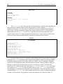
Constructing a cross-validated reflection file. This is an important step in your structure
determination. You are going to set aside a portion of your reflection data as a test data set that
will not be used in the construction of the model, but will be used to independently measure how
well your model fits the raw data. The nature of the iterative procedure of modeling and refining
biases the electron density map to conform to the model, no matter how wrong it may be. The
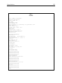
set-aside test data is your guard against falling too deeply into this trap. Modify the file
make_cv.inp so that it will set aside 5-10% of your reflections as test reflections. If your data
is nearly complete (>95%) you should use the maximum value (10% ). The input file should be
the .fobs file you created previously. The output file should be given the .cv extension to
uniquely identify it. This .cv file will be used to do all subsequent refinements.
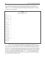
Generating CNS topology files. CNS requires, in addition to a PDB file, a molecular
topology (.mtf) file that contains information about molecular connectivity and geometrical
constraints necessary to guide the refinement. You must generate a new .mtf file whenever you
have add or delete atoms from your model. It is typical to generate a new .mtf file at the
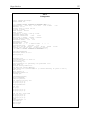
beginning of each refinement cycle. To generate an .mtf file, edit and run the script
generate_easy.inp. The required input is a .pdb file, and the outputs are a (new) .pdb
file and an associated .mtf file. Be sure you have included the necessary topology (.top) and
parameter (.par) files for ions, water, and hetero-compounds included in your model. Hetero
compound .pdb, .top, and .par files not included with the CNS distribution can usually be
downloaded from the HIC-UP server.
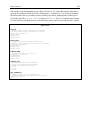
Fine-tuning the molecular replacement solution. The molecular replacement solution
should be fine-tuned by adjusting the position of the model, including the subunits independently
of each other, via a rigid-body refinement. This is accomplished by the CNS module
rigid.inp. Required inputs for rigid.inp are the .pdb, .mtf, and .cv files, the unit
cell parameters and space group, any extra .top or .par files required, the resolution range of
the reflection data to be used (typically 15.0–4.0 Å), the segid names to be minimized (typically
all of them), and the name of the output file (typically rigid.pdb). The highest resolution
shell should not be set too low a value else the refinement may not be able to move the model far
enough to find the global mininum best fit. Rigid body refinement needs only be run this one
time. It does not have to be run again during the refinement procedure. Normally, the R-factor
will decrease by 5% or more during rigid-body refinement, and this is usually a good sign that
things are going well. You should also monitor your R-test vs. your R-free values at this point
and after all subsequent refinement steps. R-test is the residual experimental data used for
refinement not explained by your model; R-free is the residual test data (the 10% you put aside
in your .cv file) that is not explained by your data. Normally R-test is lower than R-free
(presumably because of slight model bias) but generally these values are no more than 5% (0.05)
apart. If R-free–R-test > 0.05 you should investigate further or take steps to reduce model bias,
such as simulated annealing.
Calculating electron density maps. You should calculate two types of electron density
maps for modeling purposes. A 2Fo–Fc map is calculated from 2 × the observed minus the
calculated electron density. This map resembles the electron density of the target molecule and
should largely define the main and side chains of the model. A Fo–Fc map is calculated from the