1
LNAPL Distribution and Recovery
Model (LDRM)
Volume 2: User and Parameter
Selection Guide
Regulatory and Scientific Affairs Department
API PUBLICATION 4760
JANUARY 2007
LNAPL Distribution and Recovery
Model (LDRM)
Volume 2: User and Parameter
Selection Guide
Regulatory and Scientific Affairs Department
API PUBLICATION 4760
JANUARY 2007
Prepared by:
Randall Charbeneau, Ph.D., P.E.
The University of Texas at Austin
Austin, Texas
G.D. Beckett, R.G., C.HG.
AQUI-VER, INC.
Park City, Utah
SPECIAL NOTES
API publications necessarily address problems of a general nature. With respect to particular
circumstances, local, state, and federal laws and regulations should be reviewed.
Neither API nor any of API's employees, subcontractors, consultants, committees, or other
assignees make any warranty or representation, either express or implied, with respect to the
accuracy, completeness, or usefulness of the information contained herein, or assume any
liability or responsibility for any use, or the results of such use, of any information or process
disclosed in this publication. Neither API nor any of API's employees, subcontractors, consultants, or other assignees represent that use of this publication would not infringe upon privately owned rights.
API publications may be used by anyone desiring to do so. Every effort has been made by
the Institute to assure the accuracy and reliability of the data contained in them; however, the
Institute makes no representation, warranty, or guarantee in connection with this publication
and hereby expressly disclaims any liability or responsibility for loss or damage resulting
from its use or for the violation of any authorities having jurisdiction with which this publication may conflict.
API publications are published to facilitate the broad availability of proven, sound engineering and operating practices. These publications are not intended to obviate the need for
applying sound engineering judgment regarding when and where these publications should
be utilized. The formulation and publication of API publications is not intended in any way
to inhibit anyone from using any other practices.
Any manufacturer marking equipment or materials in conformance with the marking
requirements of an API standard is solely responsible for complying with all the applicable
requirements of that standard. API does not represent, warrant, or guarantee that such products do in fact conform to the applicable API standard.
All rights reserved. No part of this work may be reproduced, stored in a retrieval system, or
transmitted by any means, electronic, mechanical, photocopying, recording, or otherwise,
without prior written permission from the publisher. Contact the Publisher,
API Publishing Services, 1220 L Street, N.W., Washington, D.C. 20005.
Copyright © 2007 American Petroleum Institute
FOREWARD
Nothing contained in any API publication is to be construed as granting any right, by
implication or otherwise, for the manufacture, sale, or use of any method, apparatus, or
product covered by letters patent. Neither should anything contained in the publication be
construed as insuring anyone against liability for infringement of letters patent.
Suggested revisions are invited and should be submitted to the Director of Regulatory and
Scientific Affairs, API, 1220 L Street, NW, Washington, D.C. 20005.
iii
PREFACE
This manuscript documents use of the American Petroleum Institute LNAPL Distribution
and Recovery Model (LDRM), and is presented as a supplement to API Publication
Number 4682, Free-Product Recovery of Petroleum Hydrocarbon Liquids, which was
published in June 1999, and to API Publication Number 4729, Models for Design of FreeProduct Recovery Systems for Petroleum Hydrocarbon Liquids; A User’s Guide and Model
Documentation, which was published in August 2003 and included in the API Interactive
LNAPL Guide. This manuscript is Volume 2 of a two volume series providing background
and user information for LDRM. Guidance on use of the model is provided, along with
information to help in parameter selection. The appendix presents results from an
independent analysis of model performance. The API LDRM software can be downloaded
from API’s website at: groundwater.api.org/lnapl.
iv
TABLE OF CONTENTS
Section
Page
1
1.1
1.2
1.2.1
1.2.2
1.3
INTRODUCTION.................................................................................................... 1
Background and Objectives............................................................................. 1
Scenarios for Free-Product Hydrocarbon Liquid Recovery............................. 1
Scenarios for Recovery Well Systems...................................................... 2
Scenario for LNAPL Recovery Using Trenches........................................ 3
Overview.......................................................................................................... 4
2
2.1
2.2
2.3
2.4
2.4.1
2.4.2
2.4.3
2.4.4
2.4.5
2.4.6
2.5
2.5.1
2.5.2
USER GUIDE
Workspace Setup ............................................................................................ 6
Starting the Application.................................................................................... 7
Data Input Window .......................................................................................... 9
Menu Items.................................................................................................... 10
Add Field Data ........................................................................................ 13
LNAPL Recovery..................................................................................... 15
Graphs Output......................................................................................... 17
LNAPL Residual Saturation Models and Residual F-Factor Options ..... 24
Piecewise Linear Model Breakpoint Options .......................................... 25
Smear Correction Option ........................................................................ 27
Model Output Options.................................................................................... 29
Screen Output to the Main Application Window ..................................... 29
File Output from LDRM Application ........................................................ 30
3
3.1
3.2
PARAMETER SELECTION AND PROBLEM SOLVING GUIDE ........................ 32
Objectives and Overview............................................................................... 32
Oil Recovery Experiences: Oilfield Production versus
LNAPL Recovery ........................................................................................... 33
Parameter Limitations.................................................................................... 34
Model Conceptualization ............................................................................... 36
Multiphase Parameter Selection ................................................................... 38
Background to Multiphase Parameter Databases .................................. 38
Introduction to the API LNAPL Parameters Database............................ 39
Example Problems ........................................................................................ 41
Problem #1: Simple Skimming Recovery Evaluation.............................. 43
Parameter Selection ......................................................................... 43
Example Problem #1 Execution ....................................................... 44
Problem #2: Optimizing Remedial Options............................................. 49
Parameter Selection ......................................................................... 49
Problem #3: Parameter Bracketing Problem .......................................... 53
Parameter Selection Using the API LNAPL Parameter Database... 54
Example Problem #3: Execution ...................................................... 59
Problem #3: Conclusion ................................................................... 64
Problem #4: Case Study: LNAPL Recovery in Glacial
Outwash Sands (Adapted from API Publication #4715)......................... 66
Problem Overview ............................................................................ 66
Data Summary.................................................................................. 67
Model Conceptualization Summary.................................................. 68
Example Problem #4 Execution ....................................................... 69
Example Problem #4 Conclusions ................................................... 76
3.3
3.4
3.5
3.5.1
3.5.2
3.6
3.6.1
3.6.1.1
3.6.1.2
3.6.2
3.6.2.1
3.6.3
3.6.3.1
3.6.3.2
3.6.3.3
3.6.4
3.6.4.1
3.6.4.2
3.6.4.3
3.6.4.4
3.6.4.5
4
REFERENCES..................................................................................................... 77
APPENDIX A
REVIEW OF THE LNAPL DISTRIBUTION & RECOVERY MODEL
MATHEMATICAL VERIFICATION, CODE FIXES, & SENSITIVITY............. 79
v
LIST OF FIGURES
Figure
1.1
1.2
1.3
2.1
2.2
2.3
2.4
2.5
2.6
2.7
2.8
2.9
2.10
2.11
2.12
2.13
2.14
2.15
2.16
2.17
2.18
2.19
2.20
2.21
2.22
2.23
2.24
2.25
2.26
2.27
2.28
2.29
2.30
2.31
2.32
2.33
2.34
2.35
2.36
3.1
3.2
3.3
3.4
Page
Monitoring Well LNAPL Thickness, bn ................................................................................ 2
Recovery Well System with 7 Recovery Wells Showing the Radius of Capture
(Modified from Lefebvre, 2000)........................................................................................... 3
Simple Trench System for LNAPL Recovery ...................................................................... 4
Example Setup Folder Showing Project Workspace .......................................................... 6
API LDRM Logo .................................................................................................................. 7
Terms and Conditions Window ........................................................................................... 7
Initiation Message Box ........................................................................................................ 8
Standard Open File Dialog.................................................................................................. 8
Project Setup Dialog that Appears Only When “New” Simulation is Selected.................... 9
Data Input Window for a 1 Layer Model............................................................................ 10
Standard File Menu Items ................................................................................................. 10
Data Menu Items............................................................................................................... 11
Recovery Menu Items ....................................................................................................... 11
Graphs Menu Items........................................................................................................... 12
Options Menu Items .......................................................................................................... 12
Help Menu Items .............................................................................................................. 13
Input Field Data Options Message Window...................................................................... 14
Data Transfer Control Message Box................................................................................. 14
Application Folder with “field_data.csv” Spreadsheet....................................................... 14
“field_data.csv” Spreadsheet with Data ............................................................................ 15
Well Recovery Systems Data Entry Window .................................................................... 16
Interceptor Trench Data Entry Window............................................................................. 17
Data Input Window for Two-Layer Soil ............................................................................. 18
Saturation Profiles Graph Output...................................................................................... 18
Specific Volume/Transmissibility Graph Output................................................................ 19
Free Product Thickness Graph Output ............................................................................. 20
Drawdown/Buildup Graph Output ..................................................................................... 21
LNAPL Recovery Rate Graph Output ............................................................................... 22
LNAPL Recovery Volume Graph Output .......................................................................... 23
LNAPL Thickness Dialog Box for Later-Time Distributions .............................................. 23
LNAPL Distribution Graph Output..................................................................................... 24
Three Different LNAPL Residual Saturation Model Representations............................... 25
LNAPL Distribution Output Graph with Variable LNAPL Residual Saturation .................. 25
Pick Break Points: bn1, bn2 Message Box ....................................................................... 26
Piecewise Linear Model Representation with Alternative Breakpoints (Compare
with Figure 2.22) ............................................................................................................... 26
Initial LNAPL Saturation Distribution for Example with Smearing Option Selected.......... 27
New LNAPL Layer Saturation Distribution Following Drawdown of the
Water Table Using the Smear Correction Option ............................................................. 28
Summary Output Variables Written to the Main Window of the LDRM
Application......................................................................................................................... 30
Leading Part of the LDRM Simulation Output File............................................................ 31
Simple Conceptual Site Model.......................................................................................... 37
Complex Cross-Section Showing Heterogeneity (Based on Combined
Coring & Geophysics), Along with the Water Table Elevation Range and Site
Investigation Locations...................................................................................................... 37
Startup Box, with Selection Shown ................................................................................... 43
Startup Box, with Selection Shown ................................................................................... 44
vii
3.5
3.6
3.7
3.8
3.9
3.10
3.11
3.12
3.13
3.14
3.15
3.16
3.17
3.18
3.19
3.20
3.21
3.22
3.23
3.24
3.25
3.26
3.27
3.28
Input Parameters Controlling the LNAPL Distribution at Vertical Equilibrium................... 45
Results chart of Specific Volumes/Transmissibility for the Given Problem. Recall
that Dn is the specific volume, and Rn is the recoverable volume. Tn is the
LNAPL transmissibility. Paralleling that is a linearized “fit” that can be tuned
by the user as discussed in the text.................................................................................. 46
Input Parameters for Skimming Recovery Portion of Problem #1 .................................... 47
Summary Output for Skimming Recovery Using the Constant Residual Saturation
Option (Original Problem Definition) ................................................................................. 48
Summary Output for the F-factor Residual Saturation Conditions, with Other
Parameters Being the Basic Skimming Simulation........................................................... 49
Data Input Screen for a Recovery Time of 2 Years .......................................................... 51
Results for Vacuum-Assisted Skimming ........................................................................... 52
Site-specific Grain Size Data—Sample 1 ......................................................................... 55
Site-specific Grain Size Data—Sample 2 ......................................................................... 55
Capillary Fit Parameters for Samples with Soil Description.............................................. 56
Capillary Fit Parameters for Given Conductivity Range ................................................... 58
Grain Size Curves, Site Samples versus Database Samples .......................................... 59
Initial Data Input Screen for Example Problem #3............................................................ 60
Saturation Profiles for Data Input in Figure 3.17............................................................... 61
Saturation Profile for α = 3.5 x 10⁻² 1/cm and N =2.25 ..................................................... 61
Saturation Profile for α = 7.8 x 10⁻² 1/cm and N =1.50 ..................................................... 62
Data Input Screen for Example Problem #4 ..................................................................... 69
Saturation Profile for Example Problem #4 Input Data ..................................................... 70
Recovery Input Data for Example Problem #4 ................................................................. 71
Drawdown/Buildup Screen for Example Problem #4........................................................ 71
Data Input for Model with Two Layers .............................................................................. 72
Drawdown/Buildup for 2-Layer Model............................................................................... 73
LNAPL Recovery Rate versus Time ................................................................................. 74
LNAPL Recovery Volume versus Time............................................................................. 75
viii
LIST OF TABLES
Table
3.1
3.2
3.3
3.4
3.5
Page
USDA Soil Types and Multiphase Parameters (from M.G. Schaap, U.S.
Salinity Lab, 1999). Where: N is the number of samples; θr is the residual
volumetric moisture content; θs is the saturated volumetric moisture content
(total porosity); log (α) is the log of the van Genuchten model α parameter;
log (n) is the log of the van Genuchten model N parameter; and Ks is the log
of the saturated hydraulic conductivity. Abbreviations: S = sand; C = clay;
L = loam; Si = silt............................................................................................................... 39
Results of Initial Optimization Simulations ........................................................................ 51
Results for Vacuum-Assisted Skimming ........................................................................... 51
Results of the Smear Zone Correction Problem ............................................................... 52
Site-Specific Grain Size Data............................................................................................ 55
ix
EXECUTIVE SUMMARY
This document provides user and parameter selection guidance for application of the
American Petroleum Institute LNAPL Distribution and Recovery Model (LDRM). This is
Volume 2 of a two volume series; the first volume provides background information on
distribution and recovery of petroleum hydrocarbon liquids in porous media, and is
intended as an LNAPL primer. Section 1 of this volume discusses earlier releases of the
API LNAPL Recovery Model and describes the new features of the current release of the
model software application that is associated with this document series. Model scenarios
(wells and trenches) are also described. Section 2 is a detailed guide to use of the LDRM
software application. Workspace setup, program initiation, and data entry are described.
The various menu items which provide the basic navigation tools through the application
are discussed. Model options are described and model output using graphical screen output
and text files are presented. Section 3 provides background information on model
conceptualization, parameter selection (and limitations), and problem solving using the
LDRM. Four example problem applications are presented which highlight model use,
parameter estimation using the API LNAPL Parameters Database, and limitations of
scenario-based models.
xi
1
INTRODUCTION
1.1
BACKGROUND AND OBJECTIVES
The American Petroleum Institute (API) Publication Number 4682, Free-Product Recovery of
Petroleum Hydrocarbon Liquids (Charbeneau et al., 1999), provides an overview of recovery
technologies for petroleum hydrocarbon liquids that are released to the subsurface environment
and accumulate near the water table. The primary recovery technologies include skimmer wells
that produce hydrocarbon liquids and single- and dual-pump wells that produce both water and
hydrocarbon liquids. Hydrocarbon liquid recovery rates may also be enhanced by applying a
vacuum pressure to the well to increase the gradient towards the well within the hydrocarbon
layer. API Publ 4682 describes two (Excel spreadsheet) models that may be used to characterize
the subsurface distribution and mobility of liquid hydrocarbon (lighter-than-water nonaqueous
phase liquids, LNAPL), and to calculate the potential recovery rate and time using single- and
dual-pump wells, and vacuum-enhanced wells.
API Publication Number 4729, Models for Design of Free-Product Recovery Systems for
Petroleum Hydrocarbon Liquids (Charbeneau, 2003) describes scenario-based models for
LNAPL liquid recovery using skimmer wells, water and vacuum enhanced recovery wells, and
trenches. Soil capillary pressure characteristics are described using the van Genuchten (1980)
capillary pressure model (soil characteristics in API Publ 4682 are described using the Brooks
and Corey (1964) capillary pressure model). Implementation of the models through use of four
separate spreadsheets is presented, based on single or two-layer heterogeneity, and on selection
of relative permeability model (Burdine, 1953, or Mualem, 1976).
The objective of the present manuscript is to provide necessary background and user information
for application of scenario-based models describing LNAPL liquid recovery. Volume 1 of this
two-volume series provides model background information including the effects of capillarity in
porous media, distribution of LNAPL saturation under conditions of vertical equilibrium,
potential movement of LNAPL liquid, and mathematical model formulation and solution. The
model scope is similar to that presented in API Publ 4729, though the model formulation has
been generalized and additional capabilities have been added. The present Volume 2 describes
model implementation through a single executable program. This is a User Guide and includes
information and guidance on parameter selection and model testing.
1.2
SCENARIOS FOR FREE-PRODUCT HYDROCARBON LIQUID RECOVERY
Proven technologies for free-product recovery of petroleum hydrocarbon liquids are described in
API 4682. Models to provide quantitative estimates of system performance must necessarily be
based on simplifying assumptions that will not be applicable to all field conditions. Nevertheless,
the models provide insight and guidance that should be helpful in technology selection and
system design, and in analysis of system performance. The model scenarios for well systems and
trenches are discussed separately.
1
The subsurface porous media is assumed to be laterally homogeneous, but can have up to three
distinct layers (numbered with Layer 1 on top) with different soil characteristic and permeability
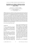
parameters. The vertical transition between layers is assumed to be abrupt. An example twolayer soil system is shown in Figure 1.1. This figure shows a monitoring well with an LNAPL
layer located between the air-NAPL interface zan and the NAPL-water interface znw. The total
monitoring well LNAPL thickness is bn. The elevation of the abrupt transition between the upper
and lower soil layers is designated z12. The elevation of the water table is designated zaw. While
the water table is not present because of the LNAPL layer, its elevation is easily determined from
the elevations zan and znw, and the LNAPL density ρn (see Section 2 of Volume 1).
Figure 1.1—Monitoring Well LNAPL Thickness, bn
The soil texture characteristics that must be defined for each layer of the porous medium include
the porosity n; the (water phase) hydraulic conductivity Kw; the van Genuchten parameters N and
α; and the irreducible water saturation, Swr. Selection of residual LNAPL saturation values
remains an elusive issue, and various options are described in Section 2.4.4. Fluid properties
include the LNAPL density, ρn (it is assumed that the water density is 1 g/cm3), and the water
and LNAPL surface and interfacial tensions, σaw, σan, and σnw.
1.2.1 Scenarios for Recovery Well Systems
The basic scenario for free-product recovery using well systems is the same for single- and dualpump wells, vacuum-enhanced wells, and skimmer wells. The performance of each well is
characterized in terms of its radius of capture Rc, with a typical scenario shown in Figure 1.2.
This figure depicts a plan view of an LNAPL lens (in gray color) with 7 recovery wells located
so that the pattern of wells with their radius of capture will cover most of the area of the lens. For
single- and dual-pump well systems, the radius of capture could extend out to the radius of
influence (water production) of the well. For vacuum-enhanced systems, the radius of influence
of the vacuum extraction well (which is typically on the order of 30 – 40 feet) limits the radius of
capture. For skimmer wells, the radius of capture is limited to a greater but unknown extent,
which is probably on the order of 10 – 30 feet.
2
Figure 1.2—Recovery Well System with 7 Recovery Wells Showing the Radius of Capture.
Scale on Right Side Shows Measured LNAPL Thickness in Wells.
(Modified from Lefebvre, 2000)
The data required for analysis of recovery-well-system performance includes the radius of
capture for the well, the LNAPL viscosity (the water viscosity is assumed to be 1 cp), and water
production rate for a water-enhanced system or wellhead vacuum pressure for a vapor-enhanced
system. For a water-enhanced system, the effective depth of penetration of the well into the
aquifer must be specified, while for a vacuum-enhanced system, the screened interval of the
vadose zone must be given. The effective relative permeability of the vadose zone due to the
presence of residual soil water is assumed to be kra = 0.9. If zero water production and wellhead
pressure are specified, then the well is assumed to function as a skimmer well.
1.2.2 Scenario for LNAPL Recovery Using Trenches
The modeling framework may also be used to represent a simple trench recovery system, such as
shown in Figure 1.3. The trench has a length LT transverse to the direction of groundwater flow.
The LNAPL lens is assumed to be of rectangular shape with length LT and width WT. The natural
groundwater hydraulic gradient Jw is transferred to the LNAPL layer and carries it into the trench
where LNAPL is removed by skimmer wells or other technology. The rate of LNAPL discharge
into the trench will depend on the effective lens thickness as observed in a monitoring well, soil
texture, natural groundwater hydraulic gradient, and whether groundwater is also produced from
the trench in order to increase the hydraulic gradient. If the trench cuts across an LNAPL lens,
then the upstream and downstream sections of the lens must be analyzed separately, with Jw
being negative on the downstream side.
3
Figure 1.3—Simple Trench System for LNAPL Recovery
1.3
OVERVIEW
The new features included in this release of the API LDRM include the following:
•
•
•
•
•
•
•
•
•
•
•
•
the model is a single, stand-alone executable application,
one may select either US Customary or metric units,
soil heterogeneity may be represented through use of 1, 2 or 3 soil layers,
soil profile data may be represented either as elevation above a datum or as depth below
the ground surface,
the capability for simulating LNAPL smearing associated with water table drawdown has
been added,
three different representations for LNAPL residual saturation are available, and the user
may change between representations during a modeling session,
the effects of vertical hydraulic gradient through surface fine-grain soil layers on LNAPL
distribution and recovery may be represented,
either the Burdine or Mualem relative permeability model may be selected for individual
soil layers,
measured field data on LNAPL saturation, LNAPL thickness, LNAPL recovery volume,
and LNAPL recovery rate may be added and displayed on model graphical output,
model formulation through use of the LNAPL layer transmissibility function is both more
rigorous and simpler than earlier model formulations,
the user may more directly specify the breakpoints for the piecewise linear fit of the
LNAPL transmissibility and specific volume functions,
more extensive and useful model output capabilities have also been added.
Section 2 of this document provides detailed user information on application of LDRM. Model
setup and data input are described. The user interacts with the application primarily through
menu items that are selected on the main application window. These are described in Section 2.4.
The method for adding field data is presented in Section 2.4.1, while the steps for simulating
LNAPL recovery using wells or trenches are described in Section 2.4.2. Seven different
graphical outputs are described in Section 2.4.3. Use of the different models for representing
LNAPL residual saturation are discussed in Section 2.4.4, while selection of piecewise linear
model breakpoints are described in Section 2.4.5. Section 2.4.6 discusses use of the smear
correction option. Section 2.5 describes the model output.
4
Section 3 provides guidance for model conceptualization, parameter selection, and problem
solving using the LDRM. Section 3.2 compares experience with oilfield production of
hydrocarbon liquids with LNAPL recovery for environmental management. Section 3.3
discusses limitations that may be associated with LDRM input parameters. Section 3.4 discusses
model conceptualization while Section 3.5 describes methods for parameter estimation when
detailed site data is limited. Finally, Section 3.6 provides four example problems showing model
application, methods for parameter estimation and bracketing, and an example where the
scenario-based model might not be appropriate.
2
USER GUIDE
The purpose of this section is to provide information on use of the API LNAPL Distribution and
Recovery Model (LDRM) and its various options. Model input and graphical and text output are
described. It is shown how field data may be entered and displayed on graphical output for
model testing and calibration. Various options are explained and demonstrated. The output file
format is also shown.
2.1
WORKSPACE SETUP
The API LNAPL Distribution and Recovery Model (LDRM) consist of a single executable
application that runs with the Windows ™ operating system. It is assumed that the user is
familiar with Windows, menus, the mouse, and folders for storage of files. The user should
create a folder for storage of work and copy the executable application (LDRM.exe) to a desired
location within the file structure (such as the primary work folder). Any additional
input/output/data files that are supplied with the application should also be copied into the work
folder. Subfolders can be created for each individual project. When running LDRM, the default
folder for opening active projects is the folder containing the application, while the default folder
for saving output is the active folder from which the input file was opened. An example setup is
shown in Figure 2.1.
5
Figure 2.1—Example Setup Folder Showing Project Workspace
2.2
STARTING THE APPLICATION
Like all Windows applications, the LDRM model can be initiated by ‘clicking’ on the executable
file icon (LDRM). The user is greeted briefly with the logo shown in Figure 2.2, and then is
required to agree to Terms and Conditions of model use before the program is initiated, as shown
in Figure 2.3.
Figure 2.2—API LDRM Logo
6
Figure 2.3—Terms and Conditions Window
Once the Terms and Conditions have been accepted (click on OK), the initiation message box
shown in Figure 2.4 appears and provides the user with options on how to proceed. The user may
open an existing simulation file, start a new simulation file, or exit the program. Select the
appropriate item and click OK. If the user selection the Open option, then the standard Open File
dialog appears (as shown in Figure 2.5), and one may navigate the file system and select the
desired simulation file to open. Only files with the “*.txt” extension may be used as input files.
No options are provided for opening input files with another extension. Thus input files are
standard ASCII text files and can be read and used by other text processing software, allowing
the experienced user to edit input files without running the application.
Figure 2.4—Initiation Message Box
7
Figure 2.5—Standard Open File Dialog
If in the initiation message box (Figure 2.4) the user selects to start a new simulation file, then
the Project Setup dialog appears, as shown in Figure 2.6. Basic choices for a given simulation
can only be made through this dialog, and cannot be changed later (the user would have to start a
new simulation). These choices include selection of units (English or Metric), number of layers
(1, 2, or 3), and elevation representation (elevation above a selected datum or depth below
ground surface, BGS). Other options that are selected through this dialog are whether to use a
drawdown correction for LNAPL smearing and the LNAPL residual saturation representation.
Both of these selections can be changed at a later time, and both are discussed in detail below
(Smear Correction in Section 2.4.6; LNAPL Residual Saturation in Section 2.4.4). Click OK to
continue.
Figure 2.6—Project Setup Dialog that Appears Only When “New” Simulation is Selected
8
2.3
DATA INPUT WINDOW
Once a selection has been made to Open an existing simulation or start a new simulation, the
Data Input window appears, such as shown in Figure 2.7. The appearance of this window differs
depending on the selected options, in particular Soil Heterogeneity (number of layers) and
Elevation representation. Figure 2.7 corresponds to English units, 1 layer, and Elevation above
Datum (options shown in Figure 2.6). The Data Input windows for 2 layer and 3 layer
simulations are shown in Figures 2.20 and 2.38 below. The basic data requirements should be
straightforward, based on the background information presented in Volume 1. A couple of items
are of note:
•
•
•
If a vertical gradient is specified, then it applies only for the uppermost layer. There is no
capability for specifying a vertical gradient in a lower layer.
The Burdine (default) or Mualem relative permeability model may be selected for any
layer, and a combination of models may be specified for a multiple-layer soil profile.
Required Residual LNAPL Saturation and Residual LNAPL f-factor data requirements
will vary with selected representation model, and these entry boxes may appear with
“Constant” or “Variable” for other options.
Figure 2.7—Data Input Window for a 1 Layer Model
2.4
MENU ITEMS
Access to most model options is achieved through use of the main menu and selection of menu
items. The File menu (Figure 2.8) contains standard items for control of files, including creation
9
of a New simulation file, Open an existing simulation file, file Save, and Exit the application.
The user is prompted to save an existing file if Exit is selected.
Figure 2.8—Standard File Menu Items
The Data menu contains three items, as shown in Figure 2.9. The first of these is to call the Edit
the basic input data for the simulation, and the standard Data Input window (Figure 2.7) is
opened. One may change input parameters during a simulation. The second menu item allows the
user to Add field data to the graphs that are generated by the application. Such input field data is
also added to the output data file. The detailed procedure for adding field data is presented in
Section 2.4.1. The third item allows the user to Remove all field data from output graphs and
from the output file.
Figure 2.9—Data Menu Items
The Recovery menu (Figure 2.10) allows the user to select the LNAPL recovery technology and
its characteristics for use during the simulation. Wells includes single and dual pump wells,
vacuum-enhanced wells, and skimmer wells. If the well water discharge and vacuum are
specified as 0, then the model assumes that a skimmer well is being used. A trench may also be
specified. The model input for wells or a trench are discussed in Section 2.4.2.
Figure 2.10—Recovery Menu Items
The Graphs menu (shown in Figure 2.11) has the available graphs listed as items. A total of 7
different graphs are available. However, graphs providing output on LNAPL recovery are active
only after the recovery option (Recovery menu item) has been selected and executed. The menu
shown in Figure 2.11 has the Saturation Profiles, Specific Volume, and LNAPL Distribution
10
graphs active. The Thickness, Drawdown, Rate and Volume graphs become active once the
recovery has been calculated. The specific graph output is described in detail in Section 2.4.3.
Figure 2.11—Graphs Menu Items
The Options menu (shown in Figure 2.12) provides access to two options that control calculation
of important model features. The first option allows the user to change between different models
for specifying the residual LNAPL saturation. These different models are explained in detail in
Section 2.4.4. The second option, Pick Break Points: bn1, bn2 (Alt-b), allows the user to specify
the piecewise linear segment breakpoint values of LNAPL thickness for the LNAPL specific
storage and transmissibility functions.
Figure 2.12—Options Menu Items
The Help menu (shown in Figure 2.13) provides limited help and model information for the user.
The Soil Parameters item refers to API documents and programs that are useful in selection of
model parameters relating to soil characteristics. The Rel. Perm. Models item is a warning that
for a specific soil, the van Genuchten soil characteristic parameters α and N will differ with
selection of the Burdine or Mualem relative permeability models. The other two items provide
information on model development and acknowledgements for model support.
Figure 2.13—Help Menu Items
11
The Exit menu provides direct access to model termination with a message box that inquires
whether the user wishes to save current work.
2.4.1 Add Field Data
The following field data values may be entered and displayed on the graphical output from
model simulations:
•
•
•
•
LNAPL saturation (Sn),
LNAPL monitoring well thickness (bn),
LNAPL cumulative recovery volume (Vn), and
LNAPL recovery rate (Qn).
Field data is entered through use of a spreadsheet. The spreadsheet is automatically formatted for
input. Field data is copied from another spreadsheet or text (ASCII) file. Upon saving and
closing the spreadsheet, the entered data is copied to the simulation model and will be displayed
when a figure is opened. All data is saved on the output file from a simulation.
To add field data select the Data Æ Add Field Data (Alt-d Æ Alt-a) item from the menu. The
options message box shown in Figure 2.14 will be displayed. Select the data-type for entry and
click OK. Two things then happen. First, the dialog shown in Figure 2.15 is displayed. Do not
click OK on this dialog until after the data has been entered and saved. The second thing that
happens is that a spreadsheet file field_data.csv is created in the folder from which the
application was launched (not the data folder if this is different), as shown in Figure 2.16. Open
this spreadsheet and enter the data (which may be copied and pasted from another data
spreadsheet). Once the data are entered, as shown in Figure 2.17, save field_data.csv, click Yes
on the “features” message box, close field_data.csv, and click No on the “save” message box.
One may now click OK on the dialog shown in Figure 2.15, and the data is copied to the
simulation application file.
Figure 2.14—Input Field Data Options Message Window
12
Figure 2.15—Data Transfer Control Message Box
Figure 2.16—Application Folder with “field_data.csv” Spreadsheet
13
Figure 2.17—“field_data.csv” Spreadsheet with Data
2.4.2 LNAPL Recovery
Once the basic input data (Section 2.3) has been entered, the user may select a recovery
technology using the menu Recovery (Alt-r) item. Two options are available, as shown in Figure
2.10. If the user selects the Well (Alt-w) item, then the Well Recovery Systems data entry
window shown in Figure 2.18 is displayed. The following parameters may be entered.
Recovery time (T) – time duration for simulated recovery
Radius of Pumping Well (L) – production or suction well effective radius
Radius of Recovery (L) – radius of capture (see discussion in Section 4.1 of Volume 1) of
groundwater-enhanced or skimmer well
Radius of Influence (L) – radial distance with significant water-table drawdown associated
with groundwater production
Water production rate (L3/T) – groundwater pumping discharge from single- or dual-pump
well
Water saturated thickness (L) – effective aquifer thickness of active flow towards the
groundwater pumping well. This may be approximated by the well screened interval
below the water table
Suction Pressure (fraction of atmospheric pressure) – well-suction applied for vacuumenhanced recovery. Entered as a positive number
14
Screen length (L) – length of the well screened interval above the water table
Air Radius of Capture (L) – effective radial distance of influence for air flow
Figure 2.18—Well Recovery Systems Data Entry Window
Discussion:
1. If both the Water production rate and the Suction Pressure are zero (0.0) then a skimmer
well is assumed. Further, if the downward hydraulic gradient within the upper soil layer
exceeds the critical value for LNAPL displacement (see Volume 1, Section 3.2.2), then
only residual LNAPL is assumed to exist in the upper layer and the model for recovery of
LNAPL beneath fine-grain zones using skimmer wells (see Volume 1, Section 3.3.6) is
assumed.
2. When a recovery well has both groundwater production and vacuum enhancement, then
the Radius of Recovery and Air Radius of Capture can differ, and the water table
drawdown/buildup is calculated using superposition.
3. The default Air Radius of Capture is calculated using equation (3.49) from Volume 1,
though the user can enter a different value that will be used in calculations.
If the user selects the Trench (Alt-t) item from the Recovery menu, then the Interceptor Trenches
data entry window shown in Figure 2.19 is displayed. The following parameters may be entered.
Recovery time (T) – time duration for simulated recovery
Qw (L3/T) – groundwater production rate that is used to enhance the natural hydraulic
gradient
Jw (-) – natural hydraulic gradient towards the trench
Trench length (L) – length of the trench or width of the LNAPL plume transverse to the
hydraulic gradient, whichever is smallest
15
Lens width (L) – longitudinal extent of the LNAPL plume in the flow direction
Screen depth (L) – effective depth of the trench beneath the water table. This is used in
conjunction with the Trench length and Qw to determine the additional hydraulic gradient
causing LNAPL migration to the trench (see equation 3.61 from Volume 1)
Figure 2.19—Interceptor Trench Data Entry Window
2.4.3 Graphs Output
As shown in Figure 2.11, seven different graphs may be displayed to summarize simulation
model output. All data that are used to generate these graphs are written to the output file, so that
graphical generation can be easily re-produced using alternative software. The first two and last
graph are available once the basic input data has been entered (Data Input window, Section 2.3).
The remaining four graphs require that a recovery technology be selected (menu Recovery item,
Section 2.4.2). The content of these graphs is described as follows.
The first graph, Saturation Profiles (Alt-p), shows the vertical distribution of LNAPL saturation
(red), LNAPL residual saturation (red-dashed), water saturation (blue), and LNAPL relative
permeability (grey). An example profile corresponding to the Data Input window of Figure 2.20
is shown in Figure 2.21. This represents a two-layer heterogeneous system with a low
permeability unit overlying a unit of higher permeability. The ground surface is located at an
elevation of 25 feet above the datum, while the water table is at an elevation of 22 feet. The
vertical facies transition occurs at an elevation of 20 feet (5 feet BGS). The heavy black line
drawn along the right border of the figure shows the 5-foot LNAPL thickness in the well
(extending from an elevation of 18 feet to 23 feet). The residual LNAPL saturation values are
calculated using the residual f-factor (see equation 2.2, Volume 1) and results in different
constant LNAPL residual saturation values for each layer. The maximum LNAPL saturation
occurs immediately below the facies interface. The largest LNAPL saturation in the upper unit
occurs at the elevation of the air-LNAPL interface in the well (elevation 23 feet). Because of
capillary forces, the LNAPL saturation remains above residual even at the ground surface. The
16
LNAPL relative permeability is calculated using the LNAPL and water saturation, with the
Mualem model for the upper layer and the Burdine model for the lower layer.
Figure 2.20—Data Input Window for Two-Layer Soil
Figure 2.21—Saturation Profiles Graph Output
17
The second graph, Specific Volume/Transmissibility (Alt-s), is shown in Figure 2.22. The three
curves present the specific volume functions Dn(bn) and Rn(bn) and the LNAPL transmissibility
function Tn(bn). The solid red, blue and grey curves are developed as follows. For twenty evenly
distributed values of bn ranging from zero to the maximum value specified on the Data Input
window, the functions are evaluated using equations (2.40), (2.41), and (3.31) from Volume 1.
For each bn value, the corresponding znw and zmax values are calculated using equations (2.20) and
(2.38). Using the sets of (bn, Rn) and (bn, Tn) values, a difference algorithm is used to select two
values (bn1 and bn2) to use at the breakpoints for the piecewise linear approximation models
specified by equations (4.3) and (4.4). These values are used to plot the piecewise linear
approximations (dashed segments) to Rn(bn) and Tn(bn) shown in Figure 2.22. As discussed in
Section 2.4.5, the user may select alternative breakpoint values to use in the recovery model
calculations.
Figure 2.22—Specific Volume/Transmissibility Graph Output
The third graph, Monitoring Well LNAPL Thickness (Alt-t), is shown in Figure 2.23. This graph
is available only after the recovery model has been run. This graph shows how the free product
thickness (bn) varies with time during the recovery time interval. For the example shown in
Figure 2.23, the LNAPL thickness decreases from 5 feet to about 3.7 feet over a time period of
two years.
18
Figure 2.23—Free Product Thickness Graph Output
The fourth graph, Drawdown/Buildup (Alt-d), is shown in Figure 2.24. This graph is available
only after the recovery model has been run, and only for groundwater or vacuum-enhanced
wells. This graph shows the water table drawdown (due to groundwater pumping) and rise or
buildup of the water table (due to an applied vacuum). Drawdown and buildup of the water table
are added to calculate the net water table change, which is also plotted. Finally, the average
drawdown/buildup within the radius of capture of the recovery well is shown. Drawdown and
buildup are calculated using the Thiem equation (equation 3.34 and 3.52, respectively, from
Volume 1). The average is a radial-distance weighted average. The example shown in Figure
2.24 corresponds to a radius of capture equal 60 feet (radius of influence equal 250 feet) and air
radius of capture equal 20 feet. The groundwater production rate is 1 gallon per minute and the
air-enhanced system suction pressure is 0.05 atmospheres. The average drawdown within the
radius of capture is 0.88 feet for this example.
19
Figure 2.24—Drawdown/Buildup Graph Output
The fifth graph, LNAPL Recovery Rate (Alt-r), is shown in Figure 2.25. This graph is available
only after the recovery model has been run. The LNAPL recovery rate, Qn, is shown as a
function of time during the recovery time period. For the example shown in this figure the
recovery rate decreases from about 60 gallons per day (gpd) to about 10 gpd after two years. This
corresponds directly to the nearly six-fold decrease in LNAPL transmissibility as the LNAPL
thickness decreases from 5 to 3.7 feet (see Figures 2.22 and 2.23).
20
Figure 2.25—LNAPL Recovery Rate Graph Output
The sixth graph, LNAPL Recovery Volume (Alt-v), is shown in Figure 2.26. This graph is
available only after the recovery model has been run. The cumulative LNAPL recovery volume,
Vn, is shown as a function of time during the recovery period. In the example shown in this figure
the recovery volume increases to approximately 20,000 gallons over two years. Also shown on
this figure (blue dashed line) is the total LNAPL volume (Ac Dn(bnmax)) within the area of capture
Ac. The maximum recoverable LNAPL volume within the capture area is Ac Rn(bnmax).
21
Figure 2.26—LNAPL Recovery Volume Graph Output
The seventh and final graph, LNAPL Distribution (Alt-l), shows the initial LNAPL and water
saturation distribution and the distributions at a later time. The later-time distribution is based on
a specified LNAPL thickness. If this graph is selected, then the dialog box in Figure 2.27 is
shown. The user enters the LNAPL thickness corresponding to the later-time distribution, and
then clicks OK. The saturation distribution graph is then display, such as shown in Figure 2.28.
In this example the initial saturation distribution corresponds to LNAPL thickness equal 5 feet
and the later-time distribution to 4-foot thickness. LNAPL thickness values are shown on the
right boundary of the figure. There is a fairly uniform decrease in LNAPL saturation within the
upper soil layer, but a large and nonuniform decrease in LNAPL saturation immediately below
the facies interface.
Figure 2.27—LNAPL Thickness Dialog Box for Later-Time Distributions
22
Figure 2.28—LNAPL Distribution Graph Output
2.4.4 LNAPL Residual Saturation Models and Residual F-Factor Options
The Options (Alt-o) menu shown in Figure 2.12 allows the user to change the LNAPL Residual
Saturation Model (Alt-r) that is used in the model calculations. Three different LNAPL residual
saturation models are available, as shown in Figure 2.29. The user may specify constant residual
LNAPL saturation values for each soil layer. The second choice also uses constant LNAPL
residual saturation values for each soil layer, but with the values determined by the maximum
initial LNAPL saturation in each layer and the f-factor fr that is specified for each soil layer on
the Data Input window (see Figure 2.20). For reference, see the discussion in Section 2.1.3 of
Volume 1. This is the representation used in Figures 2.20 and 2.21. The third choice is to use
LNAPL residual saturation that varies over the LNAPL thickness based on the initial LNAPL
saturation that varies with elevation and the constant f-factor fr for each soil layer. This is the
representation used in Figure 2.30, which is the same as Figure 2.28 except that a variable
LNAPL residual saturation model has been used. The values of the LNAPL residual f-factors for
each layer can be changed using the Data Input window.
23
Figure 2.29—Three Different LNAPL Residual Saturation Model Representations
Figure 2.30—LNAPL Distribution Output Graph with Variable LNAPL Residual Saturation
2.4.5 Piecewise Linear Model Breakpoint Options
The basis of the LNAPL recovery model formulation is piecewise linear representation of the
recoverable LNAPL specific volume and LNAPL transmissibility functions Rn(bn) and Tn(bn). As
discussed in association with Figure 2.22, these functions are evaluated for a range of LNAPL
thickness values and a difference algorithm is used to select breakpoints bn1 and bn2 for the
piecewise linear representation. These breakpoint values mark the terminal points of the interior
linear segments (the exterior terminal points are bn equal zero and bnmax). This algorithm often
leads to adequate representation of the storage and mobility functions as judged by a close visual
fit between the curves and piecewise linear segments shown in Figure 2.22. However, the user
may desire to select alternative breakpoint values. The Options Æ Pick Break Points: bn1, bn2
(Alt-o Æ Alt-b) menu item allows the user to select alternative points. If these options are
24
selected then the dialog of Figure 2.31 is shown. Based on visual inspection of the Specific
Volume/Transmissibility graph, the user may select alternative bn values for the segment
breakpoints. The next lowest values from the calculated range of bn-function values are then used
as breakpoints in subsequent calculations. A number of trial points can be inspected. When the
user is satisfied with the model fit, then the Fix break points box should be checked, which will
fix the breakpoint values until the option dialog is opened again. Figure 2.32 shows the selected
alternative piecewise linear model fit for the storage and mobility functions (Rn and Tn). Figure
2.32 can be compared with Figure 2.22.
Figure 2.31. Pick Break Points: bn1, bn2 Message Box
Figure 2.32—Piecewise Linear Model Representation with Alternative Breakpoints
(Compare with Figure 2.22)
2.4.6 Smear Correction Option
An option that is useful in some applications is to simulate the effect of LNAPL residual trapping
above the water table associated with water table drawdown due to groundwater pumping. This
“smearing” of the LNAPL above the water table results in a decrease in LNAPL specific volume
during recovery operations, and the amount of LNAPL smearing increases with increasing
groundwater pumping rate. The smearing simulation option may be invoked during project setup
for a new project (see Figure 2.8). Alternatively, one may open an existing output file as a text
25
(ASCII) file and edit the project options. During the simulation, the initial LNAPL distribution
and residual saturation are based on the conditions specified through the Data Input window. For
example, Figure 2.33 shows the saturation distribution corresponding to an initial LNAPL
thickness bn = 2 m with an initial water table elevation at depth 2 m below ground surface (bgs).
The corresponding LNAPL specific volume is Dn(initial) = 0.246 m.
Figure 2.33—Initial LNAPL Saturation Distribution for Example with Smearing Option Selected
When LNAPL recovery using groundwater pumping wells is selected, the average drawdown
within the radius of capture is calculated. For the new average water table elevation which is
lowered because of groundwater pumping, the new LNAPL thickness is calculated so that the
resulting LNAPL specific volume plus residual LNAPL volume in the region above the new
LNAPL layer is equal to the initial LNAPL specific volume. At any elevation, the LNAPL
residual saturation is specified as the maximum value based on the initial LNAPL thickness and
water table elevation, and the final LNAPL thickness and water table elevation. Specifically, the
new LNAPL thickness bn(new) is calculated from the following equation.
Dn (initial ) =
z max (initial )
∫ n S (z ) dz
nri
z max (bn ( new ))
+
z max (bn ( new ))
∫ n S (z ) dz
n
z nw (bn ( new ))
(2.1)
In equation (2.1) the elevation of maximum capillary rise, zmax(bn(new)), and the elevation of the
LNAPL-water interface in the well, znw(bn(new)), both depend on the new LNAPL thickness,
bn(new). The initial LNAPL residual saturation above the new LNAPL layer, Snri, is calculated
from the initial LNAPL thickness the water table elevation. The LNAPL saturation distribution,
Sn(z), in the second integral of equation (2.1) is based on the new LNAPL thickness and water
26
table elevation. Equation (2.1) is solved by first bracketing the range and then applying a bisection algorithm to find the bn(new) value for which equation (2.1) is satisfied.
Figure 2.34 shows results from application of the smear correction algorithm for the initial
distribution shown in Figure 2.33. Due to groundwater pumping (6 L/m for this example), the
water table elevation decreases from 2 m to 2.85 m bgs. The new LNAPL specific volume is
Dn(new) = 0.222 m. The difference Dn(initial) – Dn(new) = 0.024 m is associated with the
LNAPL residual saturation remaining trapped above the new LNAPL layer. The new LNAPL
layer thickness is bn(new) = 1.19 m. This is a significant decrease from the initial 2 m thickness,
and it is associated with lowering the LNAPL layer elevation towards a soil layer with coarsergrain texture which has a greater capacity for storage and mobility of LNAPL.
Figure 2.34—New LNAPL Layer Saturation Distribution Following Drawdown of the Water Table
Using the Smear Correction Option
Within the new LNAPL layer shown in Figure 2.34, two LNAPL residual saturation curves are
shown. These correspond to the initial and new LNAPL thickness values. The LNAPL residual
saturation values increased due to water table drawdown and the adjusted soil layer distribution
(relative to the new water table elevation). The larger values are used in calculation of the
LNAPL saturation distribution.
2.5
MODEL OUTPUT OPTIONS
Output of model simulation results is provided in three different forms. First, summary graphical
output is provided through the seven graphs described in Section 2.4.3. The second model of
27
output is through text information written to the main window of the LDRM application. The
third method of output is detailed simulation data written to the output file that can be viewed
and edited using most text processing applications. The latter two methods for output are
described in this section.
2.5.1 Screen Output to the Main Application Window
During application of the LDRM model it is useful for the user to have access to summary data
concerning a simulation. Such data is written to the computer screen on the main window of the
LDRM application. An example is shown in Figure 2.35. This figure shows the main window for
the example described in Figures 2.33 and 2.34. When the Data Input window is first closed,
only the first two lines are shown providing estimates of the LNAPL specific volume (Dn) and
recoverable volume (Rn) corresponding to the initial water table elevation and LNAPL thickness.
Once the Recovery Option is selected, the remaining variables are calculated and displayed. The
drawdown is the average drawdown within the radius of capture. A new water table elevation is
calculated and used only when the Smear Correction option has been selected. Similarly, the new
LNAPL thickness and specific volumes are calculated and used only with the Smear Correction
option. Otherwise, the original values are used. The initial and final LNAPL recovery rate (Qn)
and final LNAPL thickness (bn) and LNAPL recovery volume (Vn) are also presented. The
percent recovery is based on the initial LNAPL volume [the initial LNAPL specific volume (Dn)
provided on the first line multiplied by the area of capture (Ac)].
28
Figure 2.35—Summary Output Variables Written to the Main Window of the LDRM Application
2.5.2 File Output from LDRM Application
The user may save simulation results to an output text file that is expected to have “txt” as the
file extension (the file name is *.txt). All input and output data and variables are written to this
file, as are data for generating all of the graphical output from the simulation and any field data
that has been added for the simulation. Part of an example output file corresponding to Figures
2.33 through 2.35 is presented in Figure 2.36. Only the first part of the file has been copied. The
selected options and input data are shown in this figure. One may edit the output file to change
basic options; for example to invoke or cancel the Smear Correction option. The output file is
read by the program to initiate a new simulation with the same basic data. Parts of the output file
may also be copied to graphics programs (such as Excel) so that the user may create alternative
graphical images of the output.
29
Figure 2.36—Leading Part of the LDRM Simulation Output File
30
3
PARAMETER SELECTION AND PROBLEM SOLVING GUIDE
Section 3 of this User’s Guide provides guidance for model conceptualization, parameter
selection, and problem solving using the LDRM. The types of parameters required for the
LDRM can be observed simply by opening the model, and by review of prior sections of this
Guide. This section will cover several important background topics before working through four
example problems. First, an overview of hydraulic oil recovery field experience is presented to
provide a general overview and framework for interpreting model results. Next, an overview of
parameter selection and bracketing techniques is provided to help the user frame problems and
develop representative input parameter sets. As part of the discussion, an overview of the use of
the API LNAPL Parameters Database will be provided to assist in parameter selection in cases
when multiphase data are not available. The remainder of Section 3 will present four example
problems to illustrate the implementation of scenario-based models for LNAPL recovery. The
user is referred to Volume 1 of this document for background information and mathematical
development of the model and Section 2 of this volume for instructions on how to operate the
software.
3.1
OBJECTIVES AND OVERVIEW
The objectives of Section 3 are to ensure the user has adequate knowledge on the use of the
LDRM in applied, scenario-based problem solving, including:
•
•
•
•
Understanding the use of the LDRM for problem conceptualization and solving,
Guidance on input parameter selection, and identification of parameter sensitivity and
limitations,
Understanding the basis of the LDRM and the limitations and simplifications therein,
Recognizing conditions where the LDRM may be inapplicable
Clearly the most important steps in the modeling process, whether using the LDRM or others, is
conceptualization of the problem and the selection of the appropriate corresponding input
parameters. There is a meaningful difference between these two steps. Without a good selection
of input parameters, answers will be non-representative, irrespective of the problem
conceptualization. However, even with good parameter selection, poor conceptualization will
also generate non-representative estimates. For instance, if a site is well constrained with respect
to the input parameters, but the distribution of those parameters is not considered, the LDRM
would not likely produce representative results, though they may still be instructive. Similarly, if
hydraulic conditions are transiently variable, then the modeled system may not meet the key
vertical equilibrium assumptions. It should be clear that the requirements of the LDRM
approximations are not always met under real-world conditions, but in many cases are
sufficiently approximated that valuable insight can be obtained from its application. However, in
cases where any one of the approximations is poorly suited, one can expect results that at a
minimum require significant interpretation, and at worst, may be unrepresentative.
The importance of applying this or other models with sufficient thought and care is that the
process generally results in a refined or better understood conceptual site model (CSM).
Multiphase calculations and estimates are themselves an aid in CSM development and
understanding, as that problem solving requires constraining interrelated parameters, hydraulic
31
conditions, and other aspects of the problem being considered. For instance, do the model results
compare well with recovery data, but not with saturation data? If so, the results cannot be
correct. Do field measured LNAPL transmissivity values agree reasonably with the range
predicted by the model? If not, then the “answer” should be self-evident; the model is not
representative of the inputs and/or conceptualization specified by the user. Diligent and thorough
thought, as well as experience and professional judgment are required to produce useful results
in site-specific applications.
The following sections provide the user with the background needed to develop a sound model
conceptualization and provide guidance on parameter selection, with an emphasis on methods to
constrain parameter uncertainty where limited data exist. Before describing these approaches, an
overview of hydraulic oil recovery field experience is presented to provide a general overview
and framework for interpreting the LDRM results (Section 3.2) and several important parameter
limitations are presented to remind the user of key considerations in model conceptualization and
parameter selection (Section 3.3).
3.2
OIL RECOVERY EXPERIENCES: OILFIELD PRODUCTION VERSUS LNAPL
RECOVERY
It is illustrative to consider oil field and environmental experiences in context with the physics of
LNAPL recovery presented in this users guide. These experiences and data clearly indicate the
limits to the complete recovery of NAPL from geologic formations. Once in place, a fraction of
the oil tenaciously holds onto its pore space. The magnitude of this residual fraction and its
physical and chemical characteristics are key to site-specific risk.
In the oil industry there is economic incentive to optimize oil recovery efficiency. Consequently,
many field and laboratory investigations of the controls on oil mobility and recovery have been
undertaken that are relevant to environmental LNAPL recoverability. When oil displacement is
carried out by flooding the reservoir with water, air, or steam, capillary forces are responsible for
trapping some fraction of the oil initially in place. Studies of oil reservoir rocks have shown that
the residual oil left behind at the conclusion of water flooding typically ranges from 25 to 50% of
the pore volume (e.g., Chatzis et al., 1988; Melrose and Brandner, 1974). Pore structure and
wettability are two properties that strongly influence residual oil saturation. A tendency has been
observed for residual oil saturation to be greater where porosity is lower and the pore size (or
grain size) distribution is wider. As a reminder, the environmental case is one where water is
normally the wetting phase, except within certain types of geologic deposits. The same is not
true in oil reservoirs, where the wettability sequence depends on the specifics of each reservoir
setting.
Oil left behind in reservoirs can exist either as an immobile residual or as an unrecovered mobile
fraction. Unrecovered mobile oil in large, well-managed reservoirs can range from just 20 and up
to 70% of the initial mobile oil in place (Tyler and Finley, 1991). Unrecovered mobile oil exists
because of heterogeneities in the reservoir and the limitations of well recovery efficiency. In
comparing oil reservoirs to environmental conditions, it is important to consider that oil
reservoirs typically have greater initial oil saturations and mobility than observed in
environmental release conditions. Further, oil reservoirs are typically under confined conditions
allowing more effective application of standard pumping and enhanced recovery techniques such
as heating, water flooding, and chemical treatment methods. Offsetting factors are that crude oils
32
have viscosities that are typically higher than refined products (reducing flow), and reservoirs
often have intrinsic permeabilities that are smaller than unconsolidated alluvial sediments
prevalent in the environmental case. Thus, the reservoir comparison is for illustrative purposes
more than as a refined quantitative comparison. In general, the hydraulics of recovery and initial
oil conductivity are far better in reservoirs than for small volume LNAPL spills in unconfined,
unconsolidated sediments. However, other factors limit total recovery in reservoirs that may be
less restrictive under environmental release conditions.
Field and laboratory observations of environmental LNAPL recovery are different viewpoints of
the same multiphase phenomena observed in petroleum production. However, measuring
detailed subsurface LNAPL responses with respect to time and distance over the life of a
remediation project is rare for typical environmental operations. The cost is high and
interpretation of results is often difficult. Still, a few well-documented LNAPL remediation
examples are available in literature. In summary, for most of the hydraulic recovery cases
evaluated from literature and otherwise available to the authors, the total LNAPL recovery was
less than 30% of the original volume in-place with the upper end being as high as 60%. A few
other case studies are summarized by the EPA and others and are consistent with the theory and
examples above. The implication is that for most sites, hydraulic recovery of more than 30% of
the LNAPL in-place would be the exception rather than the rule. In finer-grained materials,
hydraulic recovery of more than 15% of the LNAPL in place would be unusual. These
generalizations are for overview purposes and certainly should not be arbitrarily applied to
specific sites. However, it is useful to remember these ranges to assist interpreting the LDRM
calculations.
3.3
PARAMETER LIMITATIONS
Before discussing the parameter selection process, it is useful to recognize some of the
limitations that may be associated with input parameters. While this discussion is not
comprehensive, it should caution the user regarding several important category limitations that
should be considered both in the model conceptualization process and during parameter
selection. The following categories are presented in no particular order, because the relative
importance is ultimately site-specific.
•
Data density limitations: The importance of multiphase conditions (parameters, boundary
conditions, etc.) has only recently been recognized as important to environmental
concerns. As a result, it is common for sites to have no multiphase data (e.g., capillarity,
interfacial tensions, relative permeability, and others), and even where available, those
data are generally sparse. The API LNAPL parameters database helps to bridge that gap,
but it is a reference database that may or may not have site-specific applicability (an
overview of the API LNAPL parameters database is presented in Section 3.5.2 and an
example of its use is provided in Section 3.6.3.1).
•
Sample scale limitations: Unlike many other hydrogeologic parameters, most multiphase
parameters cannot be measured using field-scale testing (e.g., capillarity, interfacial
tensions, relative permeability, and others). One can use the modeling to estimate these
factors, but the solutions are non-unique (several unknowns resulting in a single
solution). As a result, lab-scale testing is used, resulting in an unavoidable issue with
33
potential scale applicability. Lab-scale parameters are typically measured on small
volume core samples that may suffer from sampling disturbance. These factors can result
in challenges in the direct application of lab-test results. For instance, it is quite common
to observe lab-scale hydraulic conductivity values that are smaller than field-scale values.
Unfortunately, without field-scale tests for many of the important multiphase parameters
(such as capillarity), it is difficult to know whether or not scale issues exist. In summary,
measured multiphase parameters are useful, but are perhaps best viewed as a reasonable
starting point that may require interpretive adjustment by the user to better represent
observed field conditions.
•
Lab testing conditions: Separate from scale and sampling issues, lab-testing methods are
often performed under conditions that are unlikely to be present in the field (high
pressures, high saturations, etc.). An important and common problem is encountered with
lab measurement of LNAPL residual saturation values. Measured lab residuals are often
larger than the LNAPL saturations observed in the field. This condition results because
testing conditions are often run at higher initial LNAPL pressures and saturations than
present in the field. As a result, lab residual saturation values are often not applicable to
site LNAPL release and recovery conditions simulated by the LDRM (see Section 2.1.3;
Figure 2.5). In other words, one cannot always simply “plug-in” a lab result and get a
correct answer. Another important consideration is tested sample orientation. Most lab
samples are vertical while most field problems are dominated by radial horizontal flow. A
vertical orientation tends to bias the sample toward lower permeability horizons that may
be present in the core. This can result, for instance, in lower hydraulic conductivity
values, or higher capillarity than might be present in the lateral dimension.
•
Distribution of heterogeneity: Most earth scientists and engineers recognize that earth
systems are predominantly heterogeneous. The scale and distribution of that
heterogeneity strongly affects multiphase modeling and estimates, more so than other
forms of modeling. If the site is strongly heterogeneous, then one can expect that the
LDRM modeling (or other methods) to be limited to interpretive scenario building.
•
Vertical equilibrium conditions: The LDRM assumes vertical equilibrium conditions (see
Section 2.4). The constraints of those assumptions need to be met for useful application
of the model. It is often unknown whether the site is in vertical equilibrium, and in those
instances, it is equally unclear if the model calculations will be representative. For
instance, if one assumes that a well thickness of LNAPL represents the full vertical
interval of hydrocarbons, but the site has experienced significant variability in water table
levels, the vertical equilibrium assumption is possibly violated and the model results may
not be representative, even if the other model constraints are met. In other words, one
needs sufficient information about site conditions before applying the LDRM. In
summary, the user is cautioned in applying this or other models without sufficient
historical plume context and reasonable bracketing of potential hydraulic conditions
through time.
34
3.4
MODEL CONCEPTUALIZATION
The model conceptualization and parameter selection procedure is a simple guidance that may
assist the user, but is clearly not the only possible approach. The end result of suitable site
conceptualization and parameter selection process is a model that reasonably represents the
conditions of interest. Any process achieving that result is useful, with the converse also being
unfortunately true. Therefore, the recommendations herein are best viewed as a starting point;
other learning and methods may be useful to the problem-solver as they see fit.
The first step is to review the available geologic, hydrogeologic, and LNAPL data. One should
first inspect existing information for site-specific parameter availability. Next, one should find
secondary information that may be used to correlate the rest of the parameters necessary to
execute the LDRM. Perhaps there are nearby sites in public domain files with measured
parameters. Maybe local labs have experience in an area. In any case, it is convenient to divide
the site information and parameters into five general categories of information of interest for
users of the LDRM.
•
•
•
•
•
Physical properties of the aquifer materials (parameter inputs),
Physical properties of the LNAPL (parameter inputs),
The nature of the lateral and vertical extent of LNAPL, including saturations (LCSM),
The hydrogeologic and fluid level history (LCSM),
Existing historic LNAPL recovery data (LCSM)
Typically, this compilation is then reviewed for parameter availability, or other descriptive
features that may relate to those specific parameters (like soil texture, grain-size distribution,
bedding descriptions, LNAPL characteristics, etc.). There can be a range of values for each
physical parameter of the soil, LNAPL, or system geometry. It is generally useful to look at how
the range of variability of these parameters affects LDRM results; i.e., their sensitivity to the
particular set of calculations.
Following this compilation and review stage, it is useful to create hydrogeologic cross-sections
or other mapping showing the factors of interest (e.g., Figures 3.1 and 3.2). Other mapping might
include observable LNAPL thickness distribution through time, hydraulic conductivity and
gradient mapping, vadose zone thickness mapping, etc. The purpose of mapping is to enhance
the interpretive assessment of the LCSM. The level of mapping and its detail of course depends
on the site setting, complexity, risk/receptor pathways, and other considerations.
From this exercise, one would typically identify one or more “type” areas that are representative
of the broader site and encompass key facets for which LDRM estimates will be made. This
“type area” concept is analogous to that of classical geology: “…[it] serves as an objective
standard to which spatially separated parts may be compared and preferably shows the
maximally exposed strata” (adapted from AGI, 1984). For this purpose, the analogy means an
LNAPL type area represents (to an adequate degree) the soil, LNAPL, and hydraulic conditions
such that inferences from this type area and associated modeling results can be used elsewhere
across the site. The concept also recognizes that data collection efforts often have a bias toward
key areas of interest (i.e., type areas), and applications of these concepts are necessary to make
the most out of the evaluation effort. While there may be more than one type area for a given
35
site, a general need is for a type area in or around the release location and at off-site plume
locations (as applicable).
Representative
Well
Release Source
De
pt
h
(ft)
Water Table Range
Min & Max
LNAPL Thickness
LNAPL
Zone
K&i
Figure 3.1—Simple Conceptual Site Model
Flange Release
NORTHWEST
DEPTH BELOW GROUND SURFACE (ft)
(10 X Vertical Exaggeration)
L-1
SOUTHEAST
L-2
L-3
L-4
L-5
L-6
L-7
L-8
L-9
L-10
L-12
0
5
High Water
Table
10
15
Low Water
Table
20
GW Flow
25
0
100
200
300
400
500
600
700
800
900
1000
1100
DISTANCE (ft)
Cores
5
10
20
30
40
50
60
70
80
0
1
LIF INTENSITY
SANDS
2
4
5
6
3
CLAYEY SANDY SILT
SILT
SILTY SAND
SANDS
CLAYEY SILT
SILTY CLAY
CLAY
7
8
9
10
SLEEVE/TIP RATIO (%)
Figure 3.2—Complex Cross-Section Showing Heterogeneity (Based on Combined Coring and
Geophysics), Along with the Water Table Elevation Range and Site Investigation Locations
Once the site has been conceptualized, the LCSM needs to be inspected for consistency with the
LDRM constraining assumptions. Recall that this is a critical step in the application of this or
any model. If the site conditions do not meet the LDRM constraints, then a more complex model
(typically numerical methods) is required, or an alternate solution like field-pilot demonstrations
may be necessary to derive the desired understanding. Assuming the LDRM is sufficient and
useful for the expected LCSM, the next step is definition of the inputs needed to run the model.
3.5
MULTIPHASE PARAMETER SELECTION
For obvious reasons, site-specific multiphase parameters are preferred for model input.
Parameters should be measured for the range of soil types in the LNAPL plume, and the range of
parameters is then used to bracket possible recovery outcomes using the LDRM. The parameter
ranges should then be refined by tuning the model to data from a variety of related field
36
information. This may include comparing to LNAPL transmissivity, saturation, and recovery
data. Where such field data are not available, a bandwidth of LDRM results encompassing the
full range of measured parameters should be considered, and results from specific runs should
not be looked upon with a high degree of certainty.
The LDRM input parameters are not always available at sites when the calculations are to be
performed. A typical situation is where the capillary properties of the soils and LNAPL within
the LNAPL body have not been measured. The following sections describe resources for
multiphase parameter selection and suggested approaches for parameterization where sitespecific data are not available.
3.5.1 Background to Multiphase Parameter Databases
A typical approach for determining inputs when limited data are available is to consult a
published reference for guidance on parameter ranges to consider. There are several available
multiphase parameter databases in published literature that may be consulted for this purpose.
The following discussion focuses on those databases that have seen the most use in
environmental multiphase field problem solving.
One of the most commonly quoted parameter databases is that of Carsel and Parish (1988). This
database was derived from a wide number of soil samples from across the United States that
were analyzed using grain-size distribution relationships to estimate capillary and other soil
properties. There are two limitations of this dataset. First, there are no direct parametric
measurements (i.e., lab tests) to verify the parameter values. Second, the samples are not
representative of typical in situ environmental conditions due to the grain-size basis for the
estimations. As a result, many researchers have found that the values in this database generally
do a poor job of representing in situ environmental conditions, despite the quality of this
reference for other purposes.
Mualem (1976a) compiled a soil catalogue that contains measured capillary pressure, saturation
data, and some other unsaturated properties for a wide range of soils. Mualem also did
significant study in unsaturated mechanics and modeling, and one of the relative permeability
models used in LDRM comes from this related work (Mualem, 1976b). While the soil catalogue
is useful, it has two limitations for environmental application. First, these are generally
agricultural materials, and not in situ native soils. Second, as a practical matter, just the raw
laboratory data are provided, and one must fit capillary curves to these data and then attempt to
apply the results without a significant body of comparative petrophysical information. In other
words, one can generate a large amount of multiphase properties, but it is difficult to cross
correlate this data to site-specific environmental conditions.
Another literature database was prepared by the U.S. Salinity Lab for the distribution of general
USDA soil types (M.G. Schaap, U.S. Salinity Lab, 1999). Like the first database discussed, these
properties are based on empirical functions that translate physical and pedogenic properties of
the soil into predicted multiphase parameters. This database is more advanced than those
previously discussed, and may serve as a reasonable starting point for parameter selections, as
shown below in Table 3.1.
37
-- θr --
-- θs --
-- log(α) --
-- log(n) --
-- Ks --
cm3/cm3
cm3/cm3
log(1/cm)
log10
log(cm/day)
Texture
Class
N
Clay
84
0.098
-0.107
0.459
-0.079
-1.825
-0.68
0.098
-0.07
1.169
-0.92
C loam
140
0.079
-0.076
0.442
-0.079
-1.801
-0.69
0.151
-0.12
0.913
-1.09
Loam
242
0.061
-0.073
0.399
-0.098
-1.954
-0.73
0.168
-0.13
1.081
-0.92
L Sand
201
0.049
-0.042
0.39
-0.07
-1.459
-0.47
0.242
-0.16
2.022
-0.64
Sand
308
0.053
-0.029
0.375
-0.055
-1.453
-0.25
0.502
-0.18
2.808
-0.59
S Clay
11
0.117
-0.114
0.385
-0.046
-1.476
-0.57
0.082
-0.06
1.055
-0.89
SCL
87
0.063
-0.078
0.384
-0.061
-1.676
-0.71
0.124
-0.12
1.12
-0.85
S loam
476
0.039
-0.054
0.387
-0.085
-1.574
-0.56
0.161
-0.11
1.583
-0.66
Silt
6
0.05
-0.041
0.489
-0.078
-2.182
-0.3
0.225
-0.13
1.641
-0.27
Si Clay
28
0.111
-0.119
0.481
-0.08
-1.79
-0.64
0.121
-0.1
0.983
-0.57
Si C L
Si Loam
172
330
0.09
0.065
-0.082
-0.073
0.482
0.439
-0.086
-0.093
-2.076
-2.296
-0.59
-0.57
0.182
0.221
-0.13
-0.14
1.046
1.261
-0.76
-0.74
Table 3.1—USDA Soil Types and Multiphase Parameters (from M.G. Schaap, U.S. Salinity Lab,
1999). Where: N is the number of samples; θr is the residual volumetric moisture content; θs is
the saturated volumetric moisture content (total porosity); log (α) is the log of the van Genuchten
model α parameter; log (n) is the log of the van Genuchten model N parameter; and Ks is the
log of the saturated hydraulic conductivity. Abbreviations: S = sand; C = clay; L = loam; Si = silt.
To address the limitations of the databases discussed above, the API compiled the LNAPL
Parameters Database (2003, 2006). This database is comprised of lab measurements of hydraulic
and multiphase properties for the corresponding media of interest from environmental samples
collected from in situ site locations. Where the other databases correlate a general soil-type
description with the parameters, the LNAPL Parameters Database allows the user to query and
cross-compare ranges for a variety of measured parameters. For example, a common situation is
in which the user has petrophysical properties such as grain size and/or hydraulic conductivity
data but is lacking capillary properties. The user could use the database to define a range of
potentially representative van Genuchten parameters based on comparison to the measured
parameters. The use of LNAPL Parameters Database will be discussed in the following report
section and an example of its use is provided in Section 3.6.3.1. The current version of the
LNAPL Parameters Database, updated and extended with additional datasets in 2006, is
available at: www.api.org/lnapl.
3.5.2 Introduction to the API LNAPL Parameters Database
The following discussion provides a brief introduction to the API LNAPL Parameters Database.
Additional discussion is provided in the User’s Guide for the database, available from the
referenced API website (www.api.org/lnapl).
The API LNAPL Parameters database is a collection of information about samples with
measured capillary parameters, as well as other physical parameters. The capillary data
availability is key for inclusion in the database since these data are measured far less often than
other petrophysical properties. Furthermore, capillary properties are sensitive within the LDRM
and other multiphase calculations. The data come from a variety of sites, from service stations to
refineries, all having related LNAPL issues requiring data and analyses. The data that have been
included in this database were not collected for the purpose of populating a database. They were
collected by site technical teams to answer specific questions and to aid in the mitigation and
remediation of site-specific problems. Given these facts, it is not surprising that the range of tests
performed on each sample and the testing procedures used during the tests differ significantly.
Nevertheless, this is currently the most complete set of laboratory measurements of samples
38
whose properties have been analyzed for the purpose of understanding LNAPL remediation in
near-surface aquifers.
The API LNAPL database contains the following types of information:
•
•
•
•
•
•
•
Sample capillary parameters for the van Genuchten and Brooks-Corey capillary
functions, and the raw data from which they were derived. This information is available
for nearly all samples in the database.
Petrophysical data including density (bulk/grain), porosity, permeability, conductivity,
water and hydrocarbon saturations, as available.
Raw grain size distribution data (weight fraction vs. grain size)
Grain size at various percentages of the cumulative sample weight (i.e. the grain size at
the 10th, 50th, and 90th percentiles).
Grain size distribution statistics (mean, median, standard deviation).
Fraction of the sample in various grain size classifications (%sand, %silt, etc.). Typically,
if the full raw grain size distribution is available, then all of the summary parameters are
also available. For some samples, only summary data are available, while others have no
data available.
Fluid properties (viscosity, density, interfacial tensions). Typically, fluid properties
samples are not taken from the same samples where rock properties are measured. Fluid
properties samples are provided as a form of site characterization, rather than for direct
comparison with other samples within the site.
In many cases, the process of measuring one set of sample properties (grain size) makes the
sample useless for measuring other properties (porosity). In general, the collection of
measurements attributed to a single sample are collected from slices of a single core not
separated by more than 6 vertical inches from the slice where the sample capillarity was
determined.
The first step in use is opening the database with Microsoft Access 2000tm. Next, one would
typically go to the “Forms” menu, and select “Query Forms.” From this screen, one can explore
the multiphase parameters associated with samples based on the category options shown. The
first 3 or 4 general soil or parameter range queries are the most useful for initiating most
parameter searches. The remainder become sample-specific, which is useful after an initial
survey of parameter ranges has been made.
The API LNAPL Parameters database is used to develop a range of parameter values when one
or more soil properties have not been measured. As is the case where measured parameters are
available, a range of parameters should be used to bracket possible recovery outcomes using the
LDRM. The parameter ranges should then be refined by tuning the model to LNAPL saturation,
transmissivity, and recovery data from field (as available). Where field LNAPL data are not
available, a bandwidth of results encompassing the full range of measured parameters should be
considered and results from specific runs should not be held with a high degree of certainty.
For parameters that are absent in the site data, the first step is to identify other available site data
that are in one or more ways related to the missing parameters in question. For instance, grainsize distribution may be correlated to permeability and capillarity, and grain-size data can be
39
used to query the API LNAPL Parameters database for other parameters. More specific queries
are desirable, where possible. For instance, if soil parameters are needed and grain-size
distribution data are available, one could query the parameters database by those specific grainsize characteristics. Similarly, hydraulic conductivity could be another query factor that has
direct hydrogeologic applicability. The least specific query is through soil type description for
sites having only boring logs with USCS, USDA, Folk or other common soil designations. While
least specific, these are sometimes the only available site data to start from. Since the USCS,
USDA, and other soil description systems were developed primarily for purposes other than
environmental hydrogeologic applications, these soil designations are not always well correlated
to the hydrogeologic parameters of interest.
A high level of detail is not always a requirement because final parameter tuning will depend on
comparison of the LDRM predictions to site LNAPL data (recovery, saturation, transmissivity,
etc.). Therefore, one can perhaps expect that a detailed evaluation will provide a better starting
point for parameterization, but any method of querying the database should eventually be tuned
to site observations. In other words, the variations in methods to select the first range of selected
inputs are really just fine points that may not in the end make any difference to the final
parameter set selected. In any case, whether the database query is highly refined or not, the steps
of testing the resultant outcomes against site data will help to narrow potential ranges of
parameter input. Application of the database is exemplified in example problem #3 (Section
3.6.3).
3.6
EXAMPLE PROBLEMS
When solving problems using the LDRM (or others, for that matter), it is important to retain an
active understanding of the assumptions and limitations of the model. Several key assumptions
are critical in the LDRM, as detailed below. There are also other potential limitations stemming
from unconsidered site specifics or general unknowns in current scientific knowledge. Technical
considerations have been discussed in context with the mathematical development of the LDRM
in prior sections. Keeping these limitations in mind while using the LDRM will help generate
better answers.
The assumptions listed below are ordered in relative importance, based on experience and
scientific opinion, but the hierarchy at a particular site may be different. Further, certain
limitations apply only when specific evaluation conditions are selected in the LDRM. The key
assumptions are:
•
•
•
•
•
Uniform radial distribution and subsequent uniform drainage (recovery) of the LNAPL
within the radius of recovery (analogous to piston drainage),
All LNAPL within the radius of recovery will be captured at some point in time; using
too large a capture radius will result in unrealistically high recovery results,
Recovery is estimated by steady-state radial or 1-D flow equations,
Heterogeneity of earth materials or LNAPL properties is not considered (except for
simple uniformly layered soil horizons),
The background groundwater gradient is implicitly flat (zero), and has no affect on the
solution; capture is fully radial and equal in all directions (for recovery wells),
40
•
•
•
•
•
•
•
•
•
Groundwater drawdown will mathematically exceed the aquifer thickness when the
pumping rates are larger than the capacity of the aquifer as defined by the hydraulic
conductivity and thickness terms,
The groundwater and LNAPL gradients caused by recovery pumping are averaged across
the recovery domain,
LNAPL conductivity is averaged across the vertical saturation profile, which itself is
radially uniform across the zone of recovery,
LNAPL conditions are at all times under vertical equilibrium,
LNAPL is assumed to have been in-place for some time, and that the LNAPL saturations
estimated are additive to a residual saturation profile already in place,
Homogeneous or uniformly layered soil conditions, and homogeneous fluid and chemical
conditions,
Only a single recovery center is considered and interaction or interference of multiple
recovery centers is not considered,
Hysteresis is not explicitly considered, but a variable residual saturation is considered
with the “f-factor” approach described elsewhere in this Guide,
Hydraulic well efficiency is assumed to be 100%.
Given these assumptions, one can generate realistic and useful estimates from the LDRM simply
by making sound assumptions and consistent comparisons to available field information for all
pertinent aspects. The following list suggests some items that may be helpful in tuning the model
estimates to field conditions (known or expected).
•
•
•
•
Does the LNAPL saturation profile predicted by the LDRM reasonably match saturations
observed in the field (note, one may convert total petroleum hydrocarbon (TPH) values to
saturation). If predicted saturations are too large, one must change either the initial
thickness assumption, and/or the capillary properties of the soil.
Does the drawdown predicted by LDRM match that observed or expected in the field? If
the drawdown is too large, one must reduce the ground water pumping rate or increase
the hydraulic conductivity.
Do the predicted LNAPL recovery rates match those observed in the field?
Are the total specific and recoverable LNAPL volumes consistent with those observed in
the field and/or measured through other testing methods?
Based on the preceding discussion, one can quickly understand the importance of sound
judgment and critical thought in using the LDRM or other estimation codes. Multiphase
modeling is non-unique, and therefore only through a critical thought process may one generate
reasonable and useful results. Simply “pushing buttons” will not suffice, nor generate useful
answers. Comparison of model results with field data is of paramount importance. With these
caveats, proceed to the example problems below.
3.6.1 Problem #1: Simple Skimming Recovery Evaluation
This problem is designed to introduce the user to the LDRM and problem solving sequence. All
necessary parameter inputs will be given and the problem will be used to compare solutions
evaluating the skimming of LNAPL using different residual saturation assumptions; for these
41
purposes, skimming means pumping of LNAPL with no groundwater pumping. For the
conditions given (discussed below), the following questions will be considered:
•
•
•
•
How much LNAPL is present in the formation? How much would be present if the initial
observed thickness were doubled?
How much LNAPL is recoverable? In total gallons? As a percentage of the total initially
in-place?
How long does it take to recover 95% of the recoverable fraction?
How does changing the residual saturation assumptions in the model change these
values?
3.6.1.1
Parameter Selection
This initial problem setup will be a simple, single-layer homogeneous dune sand setting, with
diesel fuel as the LNAPL type. For the base case, it is assumed that the hydrogeologic and oil
properties are all known and homogeneous. The properties and conditions necessary to execute
the problem are given in the following screen shots from the LDRM. To start, double click the
LDRM icon or execute the LDRM from the Windowstm “Run” menu, then select the “Start a
New Simulation File”, as shown below.
Figure 3.3—Startup Box, with Selection Shown
Next, an options box is given that sets up the basic problem conditions, units of measurement,
and other aspects, as shown below. Ensure that the same selections as shown as those in Figure
3.4.
42
Figure 3.4—Startup Box, with Selection Shown
3.6.1.2
Example Problem #1 Execution
Once “OK” is selected on the screen above, the screen shown in Figure 3.5 will appear. Again,
the parameters shown are givens for this particular simple problem. The capillary parameters are
sensitive, and must be carefully selected and evaluated during a comprehensive problem solving
exercise.
After the inputs have been provided to the “Data Input” screen shown in Figure 3.5, click “OK”,
and the program will execute the LNAPL distribution component of the problem, and a summary
results screen will appear with the following values:
LNAPL Specific Volume, Dn (ft) = 0.2588
LNAPL Recoverable Volume, Rn (ft) = 0.1051
Note that although the units of specific and recoverable volume reduce to length, the real
meaning of the terms is volume per area (ft3/ft2; m3/m2; etc.). This is not a thickness exaggeration
term, nor is it a “length” term in the vertical direction. This is a volumetric term, not to be
confused with a linear measurement.
With the specific volume, one can integrate over an area represented by the observed thickness
and other parameters to estimate a total LNAPL volume. For instance, if this 2-ft thickness
contour represented a 50-ft radius around the point of measurement, the area would be 7,854 ft2
(πr2), and the corresponding LNAPL volume would be 2033 ft3, or equivalently, 15,205 gallons.
43
Figure 3.5—Input Parameters Controlling the LNAPL Distribution at VErtical Equilibrium. Recall
that the LNAPL thickness is that observed, at vertical equilibrium, in a monitoring well, which is
then used to define the capillary pressure as a function of elevation above the LNAPL/water
interface. The capillary properties control the associated saturations of water, LNAPL, and air.
The viscosity and hydraulic conductivity will influence the later recovery calculations. Note that
the default relative permeability model (Burdine) is selected.
From this first part of the problem, the first two questions on the problem list can be answered.
To perform the second part of the first question, simply go to the “File” menu, save the original
problem, then go to the “Data” menu and choose the “Edit Input Data” option. Change the
“Maximum Monitoring Well Thickness” to 4 ft (twice the original). Hit “OK”, and the problem
will run again, this time outputting the following answers:
LNAPL Specific Volume, Dn (ft) = 0.8034
LNAPL Recoverable Volume, Rn (ft) = 0.4959
All other things being equal, doubling the thickness results in a specific volume that is 3.10 times
greater than the original volume. The recoverable volume increases from about 41% to 62%.
These changes result from the non-linearity of the capillary expressions. The contrast would be
more pronounced when comparing very small well LNAPL thicknesses to larger thicknesses, or
when soil capillarity is greater (tighter pore space, finer-grained).
Using the results for a 2-ft initial thickness and framing above, about 825ft3, or 6,175 gallons are
potentially recoverable under the idealized conditions of the model. That is, the theoretical
endpoint of recovery is about 41% of the total LNAPL in-place (notice that the recovery model
44
does not need to be run to estimate this factor). Recall that many complicating factors affecting
hydraulic recovery are not considered by the model, and these values can be considered as an
ideal best-case endpoint that is not likely to be achieved in the field.
To find the answers to the remainder of the questions, the recovery aspects related to skimming
for the given problem need to be calculated. First, go to the “File” menu and open the problem
file that was saved in the steps above. It should have exactly the same inputs as were shown in
Figure 3.5. Verify those values and then hit the “OK” button. The distribution calculation will be
repeated, showing the same output as before.
The next step, prior to executing the recovery problem, is to inspect the output graphs,
particularly the “Specific Volumes/Transmissibility” chart found under the “Graphs” menu. That
chart is shown in Figure 3.6. On that chart is a “linearized fit” of the LNAPL transmissivity.
Notice that the default fit is not all that good. A good fit is needed before solving the recovery
problem because the solution is taken, in part, from this piecewise linear fit of transmissivity. To
better the fit, go to the “Options” menu and select “Pick Break Points: bn1, bn2". A submenu
appears and allows the user to select better-fit points. Perhaps 0.9 and 1.4 are better fits (try
those, and select the “fix break points” option to have the program accept the changes).
Inspection of the new output graph should show a better fit.
Figure 3.6—Results Chart of Specific Volumes/Transmissibility for the Given Problem. Recall
that Dn is the Specific Volume, and Rn is the Recoverable Volume. Tn is the LNAPL
Transmissivity. Paralleling that is a Linearized “fit” that can be Tuned by the User as Discussed
in the Text.
45
The recovery model (part 2 of the problem) is now ready to be executed. Go to the “Recovery”
menu, and select “Well”. A screen will appear (as shown in Figure 3.7), and all parameters
selected should be the same as shown below. Notice that the groundwater production rate is set
to zero for skimming and that there is no air-phase pressure drop to induce air movement. Since
one of the objectives is to determine how long it will take to recover 95% of the theoretically
recoverable LNAPL (Rn), a simulation time of 100 years is selected.
Figure 3.7—Input Parameters for Skimming Recovery Portion of Problem #1
When “OK” is selected, the skimming recovery problem will execute, and results will appear on
the screen, as shown in Figure 3.8. Notice that the first two outputs are the same as those given in
Part 1 of the problem (a way of verifying that inputs have not changed). The remainder of the
outputs are summaries for the end of the modeled timeframe (100 yrs). There are no meaningful
changes to the initial LNAPL thickness or water table in this simulation because skimming does
not use groundwater drawdown and LNAPL redistribution.
46
Figure 3.8—Summary Output for Skimming Recovery Using the Constant Residual Saturation
Option (Original Problem Definition)
The total percent recovery of about 41% at 100 years is more than the target of 95% of the
recoverable fraction; 95% of the recoverable volume is 38.7% of the total volume (Figure 3-8
above). By going to the “Graphs” menu and selecting “LNAPL recovery volume”, one can
inspect the asymptotic recovery curve that was generated by the inputs and see that the recovery
target is achieved on the order of 20 - 30 years. Iteratively running the calculation and selecting
smaller runtimes until the target is achieved can further refine this number. Doing so results in a
95% recovery target time of 25 years (by iteratively re-running the problem while changing the
time of recovery).
To answer the fourth question, change the residual saturation portion of the model to “Constant
(f-factors)”. To do this, one can either start a new problem, or change the residual saturation
model in the “Options” menu (recall Figure 2.12). After selecting the “Residual LNAPL
Saturation Model” and “Constant (f-factor)”, hit “OK”, and the “Data Input Box” will appear
(Figure 3.5). Make sure the “Residual LNAPL f-factor” is set to 0.3. Notice that the LNAPL
47
residual saturation values are now determined by the factors found during the referenced
research in the LDRM User’s Guide. The summary results for LNAPL distribution are shown
below in Figure 3.9. As seen, the potentially recoverable fraction is estimated to increase to 47%
(from 41% previously), but the specific volume is smaller under the new model.
LNAPL Specific Volume, Dn (ft) = 0.2331
LNAPL Recoverable Volume, Rn (ft) = 0.1092
The results shown in Figure 3.9 demonstrate a greater net recoverable volume under these
particular residual saturation assumptions. Re-iterating the steps above, it is found to require
about 14 years to reach 95% of the recoverable fraction. The user may choose to inspect
recovery and saturation graphs to review differences between the two simulation assumptions.
Figure 3.9—Summary Output for the F-factor Residual Saturation Conditions, with Other
Parameters Being the Basic Skimming Simulation
48
3.6.2 Problem #2: Optimizing Remedial Options
Problem #2 will use the properties given in Problem #1, and expand the analyses to address
issues pertaining to achieving remedial goals. For the conditions given in Problem #1, the
following questions are considered:
•
•
•
How can the remedial system be changed to achieve 90% recovery of the recoverable
fraction in 2 years? Will skimming alone reach the goal? If not, how much groundwater
pumping is needed?
How does applying a vacuum of 20 and 75 inches of water column affect results of the
first skimming calculations? Can the goal be reached without producing groundwater?
How does turning on the “smear zone correction” affect results of dual pumping at 1 and
10 gpm in terms of the total recoverable volume?
3.6.2.1
Parameter Selection
While still the simple, single-layer homogeneous dune sand setting as in Problem #1, this
problem asks questions related to remedial optimization of LNAPL source removal through
hydraulic and vacuum-assisted cleanup approaches. Costing and other aspects of optimization
are not covered, but clearly changing the recovery options to increase recovery rates has a
corresponding affect on the cost of cleanup. Since the basic conditions for this problem are the
same as those given in Problem 1, begin by opening the file that was saved for the first set of
conditions. Rerunning the LNAPL distribution portion of the problem should result in the
following values that were generated in the first problem. If that does not occur, the original
problem was not saved correctly, and that will need to be replicated.
LNAPL Specific Volume, Dn (ft) = 0.2588
LNAPL Recoverable Volume, Rn (ft) = 0.1051
Now, for the first question in Problem #2, how can the remedial system be changed to achieve
90% recovery of the recoverable fraction in 2 years? The 90% recoverable volume is 0.0946
ft3/ft2 (0.9 * 0.1051), and as a percentage of the total, that would equate to about 36.5%. To solve
the problem as given, the recovery time is set to 2 years as shown in Figure 3.10 below, and then
several remedial options are iteratively run to find out which will achieve the 2 year cleanup
goal.
Starting with the skimming example shown, 12.8% of the LNAPL is recovered in 2 years, so
obviously the gradients need to be increased. During this exercise, it may be useful to maintain a
separate spreadsheet with the remedial inputs variables and the key results. Iterating using dual
pumping (groundwater and LNAPL pumping), it is demonstrated that as 3-gpm groundwater
production is approached, 31.4% of the LNAPL has been recovered. Tuning further, 4.97 gpm
groundwater production results in the goal of 36.5% total recovery, as shown in Table 3.2 below.
Note, in this example the radius of recovery has not been adjusted with changes in pumping rate;
consideration of the radius of recovery is covered in subsequent problems.
49
Figure 3.10—Data Input Screen for a Recovery Time of 2 Years
Simulation
Number
1
2
3
4
Description
Skimming
Dual-Pump
Dual-Pump
Dual-Pump
Water
Production
Rate (gpm)
0.00
1.00
3.00
4.97
Suction
(atm)
0
0
0
0
% of Total
% of
LNAPL
Recoverable
Recovered
LNAPL
12.84%
32%
18.29%
45%
31.43%
77%
36.50%
90%
Table 3.2—Results of Initial Optimization Simulations
The 2-year, 90% recovery goal (90% of the recoverable fraction) has been achieved by using
groundwater pumping to increase the recovery gradient. The second question in the problem was
how the initial skimming scenario is affected by putting a vacuum on the recovery well; 20 and
75 inches water column, or equivalently, 0.049 and 0.184 atm (gauge). To put a vacuum in the
recovery calculation, one simply enters the given gauge suction into the “Air Enhanced System”
section of the “Well Recovery Systems input box” shown in Figure 3.10; for this case, assume a
screen length of 10 ft, and an air radius of capture of 40-ft. After entering the given vacuums for
skimming only, observe that the vacuum enhances recovery, and that the recovery goal is
reached in 2 years with skimming and an applied vacuum of 0.023 atm (9.4 inches of water
column; extended results are in Table 3.3). These results suggest that it may not be necessary to
produce water in this case to reach the stated goals; vacuum application may suffice instead.
Note also that the percent recoverable for the higher vacuums is greater than 100% of the initial
estimate because the remediation calculation itself results in a “new recoverable volume” term
(recall Figures 3.8 and 3.9).
Simulation
Number
Description
5
Vac-assist skimming
6
Vac-assist skimming
7
Vac-assist skimming
Water
Production
Rate (gpm)
0.00
0.00
0.00
Suction
(atm)
0.049
0.184
0.0236
% LNAPL
% of
Recovered Recoverable
41.97%
>100%
47.74%
>100%
36.54%
90%
Table 3.3—Results for Vacuum-Assisted Skimming
50
The 3rd part of the problem asks how the smear correction affects the recoverable fractions for
two different groundwater-pumping rates (1 and 10 gpm). Recall that the smear correction
accounts for LNAPL lost to residual storage as a function of drawdown. Therefore, the
expectation might be that there will be less recoverable volume at the higher pumping rates
because of the larger associated drawdown. To run the problem, start a new problem to access
the “Project Setup Input” screen with the “Smear Correction” turned on (shown below in Figure
3.11). Then proceed to re-enter the inputs from Problem 1 and verify through the Dn and Rn
terms, as done above.
Figure 3.11—Results for Vacuum-Assisted Skimming
Following the LNAPL distribution calculation, run the well recovery model at 1 and 10 gpm for
the same inputs as used above. With the increased pumping rate, a small amount of available and
recoverable specific volume is lost (Table 3.4 results). Of course, if the residual saturation were
greater, even more of the LNAPL would be lost to residual storage.
Simulation
Number
1
8
9
Description
Skimming
Dual-pump; smear correction
Dual-pump; smear correction
Reoverable % LNAPL
Water Production
Specific
Rate (gpm)
Volume (Dn) Volume (Rn) Recovered
0
1
10
0.261
0.106
0.255
0.245
0.103
0.096
12.8%
17.6%
37.1%
Table 3.4—Results of the Smear Zone Correction Problem
For the purposes of this simple but expanded problem, the implications of other factors used in
the recovery specification have not been discussed. Through experimentation, one will find that
the radius of influence term is not highly sensitive in the calculations, but clearly would increase
in the real world as the pumping rate increased. If desired, one could simply run the Theis
equation for late time to analytically determine the radius of influence term for a given
conductivity and pumping rate. However, the “Radius of Recovery” term is very important in the
calculations because it makes an explicit assumption about the zone over which recovery is
occurring, and therefore an implicit assumption about the volume in-place and the time to
recover that volume.
51
In reviewing the mathematical development, one will also recognize that the model will
eventually recover all recoverable LNAPL in the assumed “Radius of Recovery”; it will simply
take a longer time for larger radii and associated LNAPL volumes. Further, as with groundwater
capture zones, the capture function is not radial around a pumping well, drawdown is radial and
that is superimposed on the regional fluid gradients for both groundwater and LNAPL. Since the
“Radius of Recovery” is in effect a judgment term, one must be careful in selecting and
evaluating this factor. Despite all the sound technical work to produce the given estimates, the
complex hydraulics that occur for both groundwater and LNAPL flow under pumping conditions
cannot be accounted for in a simple radial flow model. The answers one generates are going to
be highly affected by the “Radius of Recovery” assumptions used in the estimates. The “Radius
of Recovery” term is examined further in Problem 4 where the model is fit against a wellcharacterized facility where LNAPL recovery has been closely tracked over time.
3.6.3 Problem #3: Parameter Bracketing Problem
The third problem is designed to demonstrate the use of LDRM to evaluate the cost-benefit of
multiple LNAPL recovery methods. There are three technical objectives of this example
problem. First, the use of the API LNAPL Parameters database for initial selection of multiphase
parameters is demonstrated. Secondly, the concept of parameter bracketing is illustrated. Lastly,
the problem will illustrate the importance of tuning the model to field data.
For this problem, the example site is an active truck stop and fueling station. During a recent
station reconstruction, it was discovered that fresh gasoline had been released to the subsurface,
resulting in an LNAPL body that occupies approximately 1250 m2 near the former underground
storage tanks. The core of the LNAPL body occupies approximately 900 m2 where 1 m of free
product is present in the monitoring wells. The observed free product thickness declines rapidly
with distance away form the core of the LNAPL body. The site is located in a non-beneficial use
groundwater aquifer and there are no complete risk pathways to other receptors. As such, the
only regulatory mandate is to recover LNAPL to the extent practicable. The regulatory authority
agreed that the remediation endpoint for the cleanup would be removal of 90% of the
recoverable LNAPL in the core of the plume.
Naturally, the site owner would like to minimize the cost of the LNAPL recovery efforts. To
achieve the site owner’s goals, the following questions must be answered:
•
•
•
How much LNAPL is present in the formation?
How much LNAPL is recoverable?
What is the most cost effective method for LNAPL recovery and how long will it take?
Multiple site investigations have been conducted to assess the lateral extent of LNAPL and
dissolved-phase impacts. Pilot testing of multiple LNAPL recovery methods has also been
performed. Data generated during these investigations are summarized in the following
paragraphs.
The soils beneath the site are fairly homogeneous and consist of well-graded, medium-grained
sands. These soils would be described in the Unified Soil Classification System (USCS) as SW
materials (well-graded sand with less than 5% fines). The grain size distribution of two aquifer
samples has been measured. Slug tests were conducted at the site, resulting in field-based
52
hydraulic conductivity estimates that range from about 1.7 x 10⁻³ to 1.5 x 10⁻² centimeters per
second (cm/sec) (approximately 1.5 to 13 meters per day (m/day)).
During the investigations, soil and fluid samples were collected for laboratory analysis. Soil
samples were submitted for chemical analysis of total petroleum hydrocarbons and volatile
constituents. Based on analyses of soil samples collected near wells with comparatively thin
product accumulations, the field residual LNAPL saturation is estimated to be approximately
15% in the capillary fringe and water table region. Test results in the vadose zone suggest a
much lower residual LNAPL saturation of approximately 7.5% or less. Test results in the core of
the LNAPL plume suggest peak saturations of approximately 40%-42%. The site fluids have
been analyzed to determine the physical properties of the LNAPL and water.
Monitoring wells have been installed within and outside of the LNAPL body to monitor fluid
levels and dissolved-phase plume transport. Fluid level monitoring has indicated that the water
table at the site has not fluctuated more than approximately 0.1 to 0.2 m during two years of
monitoring. This suggests that vertical equilibrium may be a satisfactory assumption for this site.
Wells in the core of the LNAPL body contain approximately 1 meter of hydrocarbons.
Short-term pilot testing of LNAPL recovery was performed to determine potential LNAPL
recovery rates. Skimming was conducted on several wells and recovery rates of approximately 1
liter per day (l/day) were observed. Dual-phase recovery was also tests by adding water
production of approximately 1 gallon per minute (3.8 liters per minute (l/min)), resulting in
recovery rates of approximately 600 l/day. Vacuum-enhanced product recovery was attempted,
but air leakage from the surface prevented significant enhancement of the recovery gradient.
Review of the required input parameters for the LDRM reveals that soil capillary properties,
residual (irreducible) water saturation, and porosity are missing. The following section describes
a method for estimating these parameters using the API LNAPL Parameters database. After the
parameters are estimated, the LDRM will be executed and the parameters will be bracketed and
tuned through a comparison to field recovery data. Then the site owner’s questions can be
answered.
3.6.3.1
Parameter Selection Using the API LNAPL Parameter Database
For this example site, it is known that the soils are well-graded, medium-grained sands that are
logged as SW soils under the USCS (Table 3.5; Figures 3.12 and 3.13). The hydraulic
conductivity of the soils is known from field measurements to be approximately between 1.7 x
10-3 to 1.5 x 10⁻² cm/sec.
53
Figure 3.12—Site-Specific Grain Size Data—Sample 1
18
100
16
90
Retained Weight, %
70
12
60
10
50
8
40
6
30
4
Cumulative Weight, %
80
14
20
PAN
400
270
200
120
Sieve Size
80
60
45
40
35
25
18
14
10
0
6
0
4
10
1/4
2
Figure 3.13—Site-Specific Grain Size Data—Sample 2
Sample ID
Depth (ft)
Grain Size
Description (1)
Particle Size Distribution (wt%)
Median Grain
Size (mm)
Gravel Coarse Medium Fine
Silt
Clay
Silt &
Clay
Sample 1
14.8
Med. Sand
1.461
9.01
27.30
46.37
14.67
NA
NA
2.66
Sample 2
15.9
Med. Sand
0.556
4.46
8.95
50.47
34.71
NA
NA
1.41
4.757
2.000
0.420
0.074
0.053
Seive Opening (mm)
Table 3.5—Site-Specific Grain Size Data
In the API database, initially query by the corresponding soil type for a first cut. Using the
“Query by Soil Type” option, the result is 7 matching samples. Given the measured field-testing
results for the site, query the database for soils with hydraulic conductivity ranging from 1.7 x
10-3 to 1.5 x 10⁻² cm/sec. Using the “Query by Conductivity Range” option, the result is 10
matching samples.
54
When the user selects the “Report: Samples and Stats” tab in the query options, the following
tables are returned for each of the queries:
Figure 3.14—Capillary Fit Parameters for Samples with Soil Description
55
56
Figure 3.15—Capillary Fit Parameters for Given Conductivity Range
Statistics of the capillary values are found at the bottom of both query reports. It can be seen that
the average capillary “α” value for the van Genuchten function are 2.87 x 10⁻² and 1.75 x 10⁻²
1/cm, respectively, with corresponding “N” values of 3.26 and 1.96. These values are probably a
reasonable starting point for LDRM calculations. However, because there is grain-size data, it is
also possible to review these data for potential similarities to the site-specific soils. In so doing,
only one database well-graded sand sample reasonably matches the grain-size distribution in the
site samples, Sample 162 (Figure 3.16-a). Similarly, an inspection of the grain size distribution
of the samples in the measured conductivity range reveals that most of the samples are much
finer-grained than the site soils (Figure 3.16-b). Although they are slightly more fine-grained,
database samples 11, 14, and 133 are similar to site sample #2 (Figure 3.16-b). Based on the
foregoing, the initial parameter estimates for the model can now be developed.
57
Grain-Size Curves, Soil based on Conductivity Range
100%
90%
90%
80%
80%
70%
60%
50%
40%
30%
20%
Cumulative Weight %
Cumulative Weight %
Grain-Size Curves, SW Soil
100%
DB #106
DB #107
DB #108
DB #162
DB #230
DB #235
Site Sample #1
Site Sample #2
60%
50%
40%
30%
20%
10%
0%
0.01
70%
10%
0.10
1.00
10.00
Screen Opening (mm)
0%
0.00001
DB #11
DB #14
DB #98
DB #99
DB #104
DB #127
DB #133
Site Sample #1
Site Sample #2
0.0001
0.001
0.01
0.1
1
10
Screen Opening (mm)
Figure 3.16-a and 3.16-b—Grain Size Curves, Site Samples versus Database Samples
Referring to the summary reports above, a range of property values based on samples 11, 14,
133, and 162 can be derived. The van Genuchten “α”of the samples range from 1.80 x 10⁻² and
7.83 x 10⁻² 1/cm with “N” values ranging between 1.2 and 2.25. The residual water saturation for
the samples ranges from 13% to 45%. The result for sample 11 (45%) appears to be somewhat
high compared to the expected range for sands, so that value will be eliminated from
consideration, leaving a range of 13% to 29%. Since the residual water saturation is not as
sensitive as the other capillary properties, the mid-point of the range (21%) will be selected for
the model input. There is now a range of capillary property inputs for the problem. The porosity
must now be estimated.
The porosity of samples can be found by re-running the above queries for the petrophysical
properties. Running these queries results in a porosity range of 33%-49% for SW soils and 22%50% for the selected hydraulic conductivity range. The overall range is, therefore, 22%-50%.
The low-end porosity results likely reflect samples that contain a comparatively higher fraction
of coarse sand and/or gravels. Similarly, the high-end porosity results are probably for samples
that contain fines. By focusing on that samples that most closely matched the site soils in the
queries above, it can be seen that the porosity ranges from 32% and 46%. The mid-point of the
range (39%) is selected for model input. Keep in mind that the porosity affects the total and
recoverable specific LNAPL volumes. Where data are available to independently calculate the
LNAPL volume, the specific volume can be checked against those calculations.
There is now a range of multiphase parameters for input to the LDRM, each of which will
generate a different initial basic distribution of LNAPL under vertical equilibrium conditions and
the variants offered in the LDRM.
3.6.3.2
Example Problem #3 Execution
The user is now ready to run the LDRM. First, the sensitive parameters need to be tuned based
on field observations. Once the user is comfortable with the parameter bracketing, the site
owner’s questions can then be answered.
The capillary properties are initially bracketed based on the saturations estimates from the field
sampling results. A starting point is the two multiphase data sets derived in Section 3.6.3.1.
Recalling that the peak saturations measured in the field were approximately 40% – 42%, the
58
user should look for the capillary values in this range that most closely match the observed peak
LNAPL saturation. The user should start with the low end van Genuchten “α” and “N”, as shown
in the following input screen. Note that the Mualem permeability model has been selected. The
van Genuchten “N” values in the API LNAPL Parameter database are derived using the Mualem
expression (M = 1 – 1/N). Recalling from Section 3.1.3 that while there are subjective trends
with grain-size, there is little published information to suggest which of the empirical relative
permeability models should be used for a specific site. In practice, the User should inspect the
effect of the different models and select the model that yields the most representative results. The
measured fluid properties are included in the input screen and other parameters are as presented
in the problem introduction.
Figure 3.17—Initial Data Input Screen for Example Problem #3
After clicking “OK” and graphing the saturation profile, the following screen is displayed in
Figure 3.1.8. Inspection of the profile reveals the predicted peak saturation is approximately
19%. This suggests that the van Genuchten “α” and/or “N” require adjustment. At this point, the
user would adjust the van Genuchten “α” and/or “N” until peak saturations are approximately
40%-42%. Doing so reveals that multiple combinations of “α” and “N” can generate the target
peak saturations. In fact, all that can be done at this point is to establish the minimum expected
“α” value for the given range of “N” values. Doing so reveals that “α” must be greater than 3.5 x
10-2 1/cm. At this point, “α” and “N” have been bracketed between two possible end member
combinations (3.5 x 10⁻² 1/cm, 2.25 and 7.8 x 10⁻² 1/cm, 1.50). The following screens show
LNAPL saturation profiles for these end members.
59
Figure 3.1.8—Saturation Profiles for Data Input in Figure 3.1.7
Figure 3.19—Saturation Profile for α = 3.5 x 10⁻² 1/cm and N =2.25.
60
Figure 3.20—Saturation Profile for α = 7.8 x 10⁻² 1/cm and N =1.50.
It is important to note that even though the saturation profiles are similar and have the same
peak saturation, the LNAPL relative permeability profiles are markedly different. The peak
relative permeability is almost 40% higher for the profile that uses the higher van Genuchten “α”
and lower “N” values. This is an important facet to consider because the LNAPL relative
permeability exerts a strong control on the LNAPL transmissivity and resulting recovery, but is
rarely measured. Where possible, hydrocarbon baildown tests or other data should be used to
constrain the LNAPL transmissivity and indirectly the capillary properties.
The capillary properties are now further tuned based on initial recovery rates from short-term
pilot tests of skimming and dual-phase recovery conducted at the site. This requires the user to
also tune hydraulic conductivity at the same time. Before proceeding, it is important to note that
when data are not available to constrain either hydraulic conductivity or the capillary properties
independently, it is may not possible to obtain a reasonably unique parameter set, as both exert a
strong control on the LNAPL transmissivity and resulting recovery.
The starting point is the range of capillary parameters from the previous bracketing work above
and the full range of hydraulic conductivity values from the slug tests. The bracketed “α” and
“N” end member combinations are 3.5 x 10⁻² 1/cm, 2.25 and 7.8 x 10⁻² 1/cm, 1.50. Hydraulic
conductivity ranges from approximately 1.5 to 13 m/day (note that the API LNAPL database
gives the “α” units as 1/cm; these will need to be converted to 1/m to enter into the LDRM).
Start by attempting to eliminate parameter sets that produce recovery results that are too high. To
do this, combine the end-member capillary data set that produced the large LNAPL relative
61
permeability with the low-end hydraulic conductivity (α = 7.8 1/m; N =1.50; and K = 1.5 m/day).
At this point, return to the data input screen and enter these parameters.
Next, run the skimming and dual-phase recovery calculations using the parameters set and
compare the recovery estimates to the pilot test recovery rates. After clicking “OK”, go to the
well recovery systems input and run the scenarios, starting with skimming. Only three
parameters must be entered to run a skimming scenario (recovery time, well radius, and radius of
recovery). Since only initial recovery rates are important in this step, enter any non-zero number
for recovery time. The well radius is 0.06 m. The radius of recovery is not known. Use the low
end of the recommended values in Section 1.2.1 of the user manual, i.e. 3 meters. All other
parameters should be set to zero. Click “OK” and graph the LNAPL recovery rate. Note the
initial recovery rate of approximately 1.45 l/day skimming. Now run the dual-phase recovery
scenario. For dual-phase recovery, the saturated thickness, radius of influence, and pumping rate
must also be input. The saturated well screens are 3 m long, so use this number for the saturated
thickness parameter. Drawdown was not observed beyond approximately 30 m from the
pumping well during pilot testing, so this value will be used for the radius of influence. The
radius of recovery is not known, but must be less than the groundwater radius of influences, so
20 m is assumed. Lastly, the dual-phase pilot test was conducted with 1 gallon per minute (3.8
l/m) of groundwater production. Click “OK” and graph the LNAPL recovery rate. Note the
initial recovery rate of approximately 1,100 l/day for dual-phase recovery.
After running the two scenarios above, it can be seen that the resulting initial recovery rates
predicted by the model are greater than those observed in the field (1 l/day and 600 l/day for
skimming and dual-phase recovery, respectively). At this point, one can conclude that the endmember capillary properties produce a LNAPL transmissivity that is too large, even with the
lowest conductivity value.
The next step is to attempt to eliminate parameter sets that produce recovery results that are too
low. To do this, combine the end member capillary data set that produced the small LNAPL
relative permeability with the high-end hydraulic conductivity (α =3.5 1/m; N =2.25; and K = 13
m/day). At this point, return to the data input screen and enter these parameters and then re-run
the skimming and dual-phase recovery scenarios. Doing this gives predicted initial recovery rates
of 5.4 l/day and 480 l/day for skimming and dual-phase recovery, respectively. It can be seen
that this parameter set results in a predicted skimmer rate that is greater than that observed in the
field. Conversely, the predicted dual-phase recovery rate is less than that observed in the field.
At this point, the user might consider changing the hydraulic conductivity to see what affect this
parameter has on the predicted recovery rates. Return to the data input screen and enter 2 m/day.
After clicking “OK” and re-running the recovery scenarios, the predicted recovery rates are 0.83
l/day and 480 l/day for skimming and dual-phase recovery, respectively. It is important to note
that the predicted recovery rate for dual-phase recovery did not change even though the hydraulic
conductivity was reduced. At first this may not make intuitive sense. This occurs because the
steady-state assumptions and mathematical development of this model dictate that for a given
groundwater production rate, any change in conductivity results in offsetting changes in gradient
and LNAPL transmissivity. The lesson here is that in order to tune dual-phase recovery
62
simulations, the user must be prepared to tune the model to groundwater drawdown and pumping
rates.
The capillary parameters and hydraulic conductivity are not yet fully constrained. At this point,
the model could be tuned by varying the capillary properties and conductivity. However, this
may lead to multiple, non-unique solutions. As suggested above, one should first constrain the
conductivity by looking at groundwater drawdown. During the dual-phase pilot test, it was noted
that drawdown in the pumping well was approximately 1.8 m. It is known that the well
efficiency is approximately 50% from a brief step test conducted as part of the overall pilot
testing program. Given this, one would expect approximately 0.9 m of drawdown in the
formation immediately adjacent to the well (i.e., at a radius of 0.06 m).
Next, the user should compare the predicted drawdown to the expected drawdown. This is
accomplished by executing multiple dual-phase recovery scenarios using a range of conductivity
values. After each run, the user can view the predicted drawdown by selecting the
“Drawdown/Buildup” option from the graphing menu. In some cases, it may be difficult to
estimate the exact drawdown from the graph, particularly as one gets closer to the target
drawdown. In these instances, the model file can be saved after executing the recovery scenario
and then opened using a text editor or other program to read the drawdown. After going through
the above-described process, the model predicts 0.9 m of drawdown at a radius of 0.06 m when a
conductivity of 2 m/day is input.
The model is now fine-tuned to hydraulic conductivity. The user should now re-visit the
capillary properties and finish tuning them to the field recovery rates. This is accomplished by
varying the capillary properties while holding the conductivity constant at 2.0 m/day. Again, the
capillary properties used must be such that the paired “α” and “N” generate the target peak
saturations, as previously discussed. For this problem, some example pairs that satisfy this
requirement are α =3.5 1/m, N =2.25; α =4.0 1/m, N =2.0; α =5.0 1/m, N =1.75; α =6.0 1/m, N
=1.6. After going through this process, the model predicts recovery rates for skimming and dualphase recovery of 1.06 l/day and 610 l/day, respectively, when α = 4.0 1/m and N = 2.0.
At this point, the input parameters are constrained and the model is considered tuned to field
data. For the purposes of concluding this example problem, assume that the model adequately
represents field conditions. In reality, some level of uncertainty remains and it would be prudent
to conduct a sensitivity analysis of those parameters that are least constrained. For example,
changing the radius of capture from 3 m to 10 m changes the predicted initial recovery rate by
approximately 20%. Also, the user may have noticed that the porosity and residual water content
parameters have not been revisited. Porosity affects the total and recoverable specific LNAPL
volumes but not LNAPL recoverability. Residual water saturation is inversely related to the
LNAPL volumes and recoverability, but is less sensitive than the other parameters controlling
these facets. These aspects will be left for the user to explore further.
3.6.3.3
Problem #3: Conclusion
Now that the model is tuned to field conditions, the site owner’s questions can be answered.
Again, the user is reminded that some level of uncertainty remains and it would be prudent to
conduct a sensitivity analysis of those parameters that are least constrained. In the framework of
63
this problem, the parameters that control the LNAPL total and recoverable volumes might be
looked at most closely since the remediation goal is defined by those volumes.
•
How much LNAPL is present in the formation? Input the final parameter set in the data
input screen and click OK. The LNAPL specific volume and recoverable volumes are
displayed on the main screen. The specific volume is 0.1312 m3/m2. For the 900 m2
LNAPL body, this translates to approximately 118,080 liters of product.
•
How much LNAPL is recoverable? The recoverable volume is .0606 m3/m2 or,
approximately 46%. This translates to approximately 54,540 liters of recoverable
product. Recalling that the regulatory mandate is to recover 90% of this volume, the
target is 49,086 liters.
•
What is the most cost effective method for LNAPL recovery and how long will it take?
To answer this question, one must first be determine the number of wells required and
how long it will take to recover 90% of the recoverable LNAPL in the core area of the
plume.
For dual-phase recovery, this question is relatively simple. The radius of recovery is 20 m, which
corresponds to an area of 1,250 m2. This area of recovery is greater than the release area of 900
m2, which roughly takes the shape of a 30 m by 30 m square. Therefore, only one dual-phase
well would be required. To determine the time required to recovery 90% of the LNAPL, run the
dual-phase scenario and save the model file. Open the model’s file in a text editor and find the
time needed to recover 49,086 liters. In this case, the time is approximately 4.4 months.
Assuming a system installation cost of $75,000, a total operation and maintenance cost of
$25,000, and $20,000 in discharge fees, the total estimated cost for dual-phase recovery is
$120,000. In practice, a single well may not suffice. Field experience strongly suggests that the
LDRM may over-predict LNAPL recovery from the distal portions of the recovery radius.
Simply stated, the model assumes that all recoverable LNAPL is removed and that this recovery
occurs uniformly across the recovery domain. In practice, the LNAPL saturation is typically
observed to decline more quickly near the recovery well. This results in a reduction in the
LNAPL relative permeability near the well, ultimately limiting the potential for recovery from
more distal areas. As such, it might be practical to consider adding a second or third well. If this
decision is made before the system is installed, the additional wells can be added for a small
incremental cost.
For skimming, the radius of recovery is 3 m. To ensure that the entire core of the LNAPL body
falls within the radius of recovery of a skimming well, there would need to be approximately
seventy-seven wells and skimmers. To determine the time required to recover 90% of the
LNAPL, run the skimmer scenario. The time required to recover 90% is approximately 21 years.
Assuming a system installation cost of approximately $100,000 and total operation and
maintenance cost of $100,000, the total estimated cost for skimming recovery is $200,000. If the
site owner can perform the operations and maintenance, the total cost might be reduced. Even if
the cost for skimming was less than that for dual-phase recovery, there may be practical issues
associated with the installation of seventy-seven wells in a 30 m x 30 m area. Furthermore, the
operation and maintenance plan would need to address potential well interference issues.
64
Overall, dual-phase recovery appears to be more cost effective than skimming, primarily due to
the larger number of skimmer wells required and the order-of-magnitude longer recovery period.
If the site owner can perform the operations and maintenance of the skimmer system, the cost of
the two alternatives might be similar. If that is the case, then time and the practical issues
discussed above become important factors.
3.6.4
Problem #4: Case Study: LNAPL Recovery in Glacial Outwash Sands
(Adapted from API Publication 4715)
The fourth problem compares the LDRM to a real world dual-phase recovery project. For this
example problem, the LDRM will be tuned using site-specific parameters and the recovery
history from a dual-phase recovery well. This problem emphasizes the importance of comparing
model results to field-based data and confirming that key model assumptions that form the basis
for scenario-based models such as LDRM are not violated. This problem will show that violating
two key model assumptions can lead to erroneous results if not realized and managed by the User
during the modeling process. Similarly, when the limitations are recognized, the modeling effort
can lead to additional insights and learning even when all the constraining assumptions are not
met.
3.6.4.1
Problem Overview
A former refinery in the U.S. has been extensively studied because LNAPL has migrated over a
significant area and potentially threatens a groundwater resource and an adjacent stream.
Pumping large amounts of groundwater is required to achieve hydraulic control of the
groundwater system to mitigate potential impacts at a stream. Soil saturation and petrophysical
measurements, laser fluorescence, cone penetrometer, and hydraulic tests have been combined to
produce a comprehensive data set. From these data, oil company scientists have estimated the
original LNAPL volume to be approximately 36 million gallons in predominantly permeable
outwash sand and gravel sediments. The high permeability outwash sands and gravels put this
site in the upper percentiles of probable LNAPL recovery success.
Of the LNAPL in-place at the former refinery, about 4 million gallons have been recovered
through aggressive groundwater and product pumping over 13 years. Approximately 90% of the
LNAPL was recovered over the first 3.5 years of operation. The cost of the system installation
and operation has been approximately $8.5 million, for a current net cost of a slightly more than
$2 per gallon recovered. However, because product recovery has diminished through time,
consistent with theory, the cost per gallon has increased from about $1 over the initial recovery
period to about $50 currently. The future cost per gallon recovered is expected to increase as a
greater percentage of costs are allocated to operation and water disposal per gallon of LNAPL
recovered.
Despite the large volume of LNAPL recovered, the adjacent stream could still potentially be
impacted by the LNAPL beneath the site during certain hydrologic events (e.g., a low water table
stand). Consequently, containment and alternate recovery strategies are being considered since
product recovery has not completely addressed the key impacts and potential risks of concern.
Thus we are reminded that limits to LNAPL recovery can sometimes preclude risk mitigation
goals even in permeable materials.
65
Early in the remediation history, between 1986 and 1989, three large-diameter, dual-phase
LNAPL recovery wells operated and accounted for approximately 75% of the LNAPL recovered
to date. Despite the addition of 10 recovery wells after the initial recovery period, LNAPL
recovery rates were strongly diminished, particularly during average to wet years. However,
during dry years, significant LNAPL recovery was still possible, with some years experiencing
as much as 4% of the LNAPL recovered to date.
3.6.4.2
Data Summary
As mentioned above, the former refinery has been extensively studied. The soil and fluid
properties that will be used in the calculations that follow are summarized in the following
paragraphs.
The soils beneath the site consist of high permeability outwash sands, gravels, and cobbles that
are most frequently described using the USCS as SP, SW, and GW materials. Numerous vadose
and aquifer zone samples have been sieved to determine gradation. Overall, the percentage of
fines is less than 10%, with most samples containing less than 5%. In sandy intervals, the gravel
percentage is generally in the 20-40% range. Highly conductive gravel zones containing as much
as 70% gravel and larger clasts are present starting at approximately 15 feet below the water
table or about 50 feet below ground surface. These zones are generally 5 to 10 feet thick and are
encountered below the LNAPL body. The significance of the above-described heterogeneity will
bear itself out during model calibration.
Numerous aquifer tests have been conducted at the site. Based on these tests, the field-based
transmissivity ranges from about 20,000 to 100,000 square feet per day (sq ft/day). Given an
average aquifer thickness of approximately 50 feet, these results translate to an average hydraulic
conductivity of 400 to 2,000 feet per day (ft/day). The prolific nature of the aquifer is further
evidenced by the specific capacity of the recovery wells, which ranges up to 500 gallons per
minute per foot drawdown (gpm/ft). As discussed above, the highly conductive gravel zones are
located beneath the LNAPL body. The conductivity of the shallow portion of the aquifer where
the LNAPL body is found has been estimated to be 300-600 ft/day based on tests conducted on
partially penetrating wells. The hydraulic conductivity of the aquifer below the LNAPL body
may be as high as 2,500 ft/day. The User should recall that a key model assumption for this
initial problem setup is that the aquifer is homogeneous with regard to groundwater pumping.
Where a layered system is selected, the layer-thickness weighted transmissivity controls the
groundwater pumping, and is therefore weighted to the thickest layers of greatest conductivity.
Therefore, the User should make a “mental note” regarding the above-described hydraulic
conductivity contrast and be prepared to compare the model results with field data to determine
if this condition significantly affects the calculations.
Soil samples have been collected for petrophysical and capillary properties. The porosity of fifty
soil samples was measured and ranges from 22% to 42%, with an average and standard deviation
of 33% and 5%, respectively. Capillary tests were performed on two soil samples. The predicted
van Genuchten “α” parameters for the two samples are both rather large (6.95 x 10⁻² and 7.50 x
10-2 1/cm (2.1 to 2.3 1/ft)). The van Genuchten “N” parameters for the samples are nearly
identical at 1.68 and 1.70. The predicted residual water saturation of the two samples is also very
similar 13% and 14%.
66
The site fluids were analyzed to determine the physical properties of the LNAPL and water. The
product density is 0.82 grams per cubic centimeter. The viscosity of the product is approximately
1.4 centipoise. Lastly, the interfacial tension pairs are as follows: Air/Water: 58 dynes/cm;
LNAPL/Air: 25 dynes/cm; and LNAPL/Water: 13.6 dynes/cm.
Fluid levels at the former refinery have been gauged since 1985, with LNAPL recovery
beginning in 1986. Prior to hydraulic recovery, the observed LNAPL well thickness near the
recovery well ranged from 0.13 to 0.96-foot and averaged 0.60-foot. Water levels fluctuate
seasonally as much as ten feet between spring and late fall. Since the early 1990s, a relatively
consistent relationship has been noted between water levels and free product appearance in wells.
In summary, there is a fairly well established water level altitude above which LNAPL does not
appear in wells. When the water table declines below this elevation, free product accumulates in
the monitoring wells in approximate proportion to the depth below the threshold elevation. Based
on these fluid level observations and the extensive laser-induced fluorescence and soil coring
work, the project team has concluded that a portion of the remaining LNAPL body is “stranded”
beneath the water table threshold elevation at saturations below the two-phase residual
saturation. When the water table falls below the threshold elevation, the LNAPL becomes mobile
due to the much lower residual saturation under three-phase conditions.
Extensive efforts have been undertaken to estimate the distribution and volume of LNAPL in the
subsurface beneath the former refinery. The morphology of the LNAPL body was first
characterized using standard investigation techniques and this understanding has been more
recently enhanced through the use of direct push laser-induced fluorescence techniques. The
LNAPL saturation distribution and volume has been studied through standard characterization
methods, LNAPL partitioning interwell tracer tests (PITT), and numerical multiphase modeling
efforts. In total, there is an estimated 32 million gallons of LNAPL remaining beneath the
approximately 175-acre plume footprint, corresponding to a specific volume of approximately
4.2 gallons per cubic foot (gal/ft2), or approximately 0.56 ft3/ft2. These estimates are based on
conditions present in the middle to late 1990s and, therefore, reflect a partially recovered and
smeared plume condition. The original volume would include the 4 million gallons recovered
and the original specific volume estimate is increased to 4.7 gal/ft2 or, approximately 0.63 ft3/ft2.
Peak LNAPL saturations have been estimated to be approximately 33%. Residual saturation
under three-phase conditions (air/NAPL/water) is estimated to be 2-4%. Under two-phase
conditions (NAPL/water), the residual saturation is much higher, approximately 20%.
The User should recall that the LDRM was not formulated to simulate field sites where water
table fluctuations are significant, regardless of whether conditions of vertical equilibrium exist.
The LDRM model-scenario formulation is based on an initial LNAPL distribution that is
calculated from the LNAPL thickness specified in the Data Input window, along with the water
table elevation and soil layer configuration. Even when the ‘smear correction’ option is selected,
the total LNAPL specific volume is determined by the initial LNAPL thickness; it is assumed
that there is no residual LNAPL initially present below or above the initial LNAPL layer.
Therefore, the User should make a “mental note” regarding the preceding discussion of water
table fluctuations and 2-phase to 3-phase transient drainage events. The User should be prepared
to compare the model results with field data to determine if this condition significantly affects
the calculations.
67
3.6.4.3
Model Conceptualization Summary
Recalling the discussion in Section 3.4, the key facets of the model conceptualization are:
•
•
•
•
Assess parameter availability,
Bracket parameter ranges and inspect for parameter variability,
Identify one or more “type” areas that are representative of the broader site,
Inspect the LCSM for consistency with the LDRM constraining assumptions.
In essence, the first two items are already complete. By reviewing the data summary in Section
3.6.4.2, it is seen that all input parameters are available from site-specific measurements or
modeling. The parameters are bracketed by multiple measurements and are mostly of low
variability. A notable exception is hydraulic conductivity, which ranges from 400 to 2,000 ft/day.
Drawdown data can be used to constrain the hydraulic conductivity in the area of pumping. The
type area (the third item) is defined in the framing of this example problem. That is, the predicted
recovery trend is being compared to that of one site recovery well.
The fourth item requires additional thought before proceeding. As discussed above, review of the
supporting field data has revealed that two key model assumptions should be carefully
considered. First, the soil descriptions and aquifer test results suggest a significant contrast in
hydraulic conductivity between the smear zone and the underlying aquifer materials. Because the
recovery wells at this site are fully penetrating, we should expect either the LNAPL recovery
rates and/or the drawdown to be incorrect if a single value of hydraulic conductivity value is
used in a single-layer simulation. The second key assumption concerns the significance of water
table fluctuations. As discussed above, there is a seasonal water table fluctuation of up to ten feet
at this facility. This fluctuation is by itself enough to suspect time periods with vertical disequilibrium, where hydrostatic conditions do not exist. However, vertical equilibrium conditions
are expected to exist for most time periods, but the LDRM formulation is not able to account for
residual LNAPL trapped beneath the fluctuating water table. The well-established relationship
between product thickness and water table elevation has been observed since the early 1990s and
the residual LNAPL saturation is known to be significantly different under 2-phase versus 3phase conditions. To proceed, it must be assumed that vertical equilibrium conditions were
approximated during the early recovery period (1986 – 1989). One must be vigilant during the
model-tuning process to verify that this assumption makes sense; otherwise the results may be
erroneous.
3.6.4.4
Example Problem #4 Execution
To begin model execution, enter the parameters presented in Section 3.6.4.2, as shown in the
following input screen.
68
Figure 3.21—Data Input Screen for Example Problem #4
The user should note that average porosity, van Genuchten “α”, hydraulic conductivity, and
LNAPL well thickness were used. The porosity directly affects the LNAPL specific volume and
less dramatically affects recovery rates, whereas “α” and hydraulic conductivity significantly
affect the recovery rates. The LNAPL well thickness affects both volume and recovery.
After clicking “OK”, the LNAPL specific volume is displayed as 0.0928 ft3/ft2. Plot the
saturation profile by selecting “Saturation Profiles” from the Graphs menu. The following screen
should appear:
69
Figure 3.22—Saturation Profile for Example Problem #4 Input Data
At this point, the peak LNAPL saturations are approximately 35%, which is reasonably close the
peak saturations observed in the field (~33%). However, the predicted specific volume is almost
an order-of-magnitude lower than that estimated from field data and other modeling. This is the
first clue that water table fluctuations and trapping of residual LNAPL beneath the water table
play a significant role. In fact, the user must enter a well thickness of approximately 3 feet to
approach the specific volume estimated from field data. However, when doing so, the peak
saturations are over double those observed in the field. A similar conclusion can be reached if the
user were to vary the capillary properties. Even increasing the porosity along with the well
thickness and/or capillary properties does not help. In essence, this situation is irreconcilable.
That is, the field-measured specific volume cannot be approached without changing the well
thickness or capillary properties far beyond their expected range and without obtaining peak
LNAPL saturations that greatly exceed field measurements. For now, assume that the fieldmeasured specific volume is higher than that predicted by the model because of LNAPL
smearing by the fluctuating water table. Move forward by assuming that the mobile fraction of
LNAPL (that observed in the wells) was in vertical equilibrium during the recovery period and is
adequately represented by the model.
Now compare the predicted drawdown to that observed in the field. At this point, proceed to the
well recovery systems input screen and input the following parameters:
70
Figure 3.23—Recovery Input Data for Example Problem #4
After clicking “OK” and plotting the Drawdown/Buildup, the user should see the following
screen:
Figure 3.24—Drawdown/Buildup Screen for Example Problem #4
The predicted drawdown at the recovery well is approximately 9 feet. This well’s efficiency is
known to be 80% and the field-measured drawdown in the pumping well at 800 gpm is 4.25 feet.
Accounting for well inefficiency, the actual drawdown adjacent to the well is approximately 3.4
feet under field conditions. Therefore, the model is over-predicting drawdown by approximately
5.6 feet.
71
At this point, the User could try increasing the hydraulic conductivity until the model predicts the
correct drawdown. Doing so reveals that the hydraulic conductivity must be increased to 1,200
ft/day. Although this value falls within the overall range of hydraulic conductivity measured at
the facility, recall that the hydraulic conductivity of the upper portion of the aquifer, where the
LNAPL is located, is only 300-600 ft/day. Accurate recovery results cannot be obtained using
1,200 ft/day because the model also uses this parameter to calculate the LNAPL transmissivity.
Clearly, recovery will be over predicted by using a hydraulic conductivity that is larger than that
of the materials through which the LNAPL is moving. At this point, the user should conclude
that the heterogeneity of the aquifer must be accounted for if reasonable simulation results are to
be made.
At this point, the user has two options. First, the hydraulic conductivity of the upper zone could
be used along with a lower groundwater production rate that generates the correct drawdown.
The other option would be to start over and build a two-layer model. For this example, the latter
option will be used.
Start a new simulation, select two layers and input the parameters shown on the following
screen:
Figure 3.25—Data Input for Model with Two Layers
Click “OK” and re-run the dual-phase recovery scenario and plot the Drawdown/Buildup. The
following screen should appear.
72
Figure 3.26—Drawdown/Buildup for 2-Layer Model
The drawdown at the recovery well is approximately 3.4 feet, which is the expected value. Note
that the correct hydraulic conductivities were provided in an effort to save time. In reality, these
values will need to be varied until a reasonable match to drawdown is achieved. The user should
also recognize that this answer is non-unique. That is, other combinations of hydraulic
conductivity values could have resulted in 3.4 feet of drawdown.
Now that the hydraulic conductivity has been tuned to field data, look at recovery rates and
volumes over time. If it is available, import field recovery rates and volumes into the LDRM by
following the procedures in Section 2.4.1 of this User’s Guide. For demonstration purposes, field
data from this site have been added and appear in the following figures.
Next, adjust the breakpoints for the transmissivity curves and then re-run the recovery scenarios.
The user might want to vary the radius of capture until it generates a total LNAPL volume that
matches the asymptotic endpoint of the field recovery curve. For this problem, this condition is
met with a radius of recovery of 1,350 feet. This is only one approach to estimating the radius of
capture. A better method of setting the radius of capture would be to estimate it from
measurements of LNAPL drawdown in the field, when available.
Using a radius of capture of 1350 feet, the model should generate the following recovery rates
and volumes over time:
73
Figure 3.27—LNAPL Recovery Rate Versus Time
74
Figure 3.28—LNAPL Recovery Volume Versus Time
Inspection of plots reveals that the predicted recovery rates are lower than expected during the
first two years and then are overestimated until approximately year 10. This results in a
cumulative recovery curve which falls well below the field curve until approximately the 10th
year.
At this point, the User could consider revisiting the input parameters in an effort to generate a
better match with the field data. Attempting this would reveal that an unreasonably large van
Genuchten “α”, hydraulic conductivity, and/or LNAPL well thickness values for layer one
would be needed to match the recovery trends. Similarly, the user might increase the radius of
capture to increase the recovery rate, only to find out that the model then over predicts the
recovery volume.
Clearly something is wrong. At this juncture, the User might recall that the model greatly under
predicted the LNAPL specific volume. Revisit the model conceptualization and consider the
implications of the water table fluctuations. The user should be wondering what condition could
explain why the model under predicted both the specific volume and recovery rates. Upon
careful consideration, one conclusion may be that the LNAPL that is “missing” from the
calculated specific volume might be oil (or LNAPL) that is actually present, but immobile under
two-phase conditions below the water table. This condition is suggested by the fluid level
observations discussed in Section 3.6.4.2. This oil, although present and contributing to the
measured specific LNAPL volume, did not appear in monitoring wells and, therefore, the
model’s specific volume estimates. However, upon lowering of the water table by pumping, a
75
fraction of this oil likely drained under three-phase conditions (due to the lower three-phase
residual LNAPL saturation), thereby increasing the recovery rates. This hypothesis is supported
by the LNAPL recovery “spikes” in the field data, which occurred when the water table was
much lower than normal due to very dry conditions (see recovery volume plot above). In
summary, the user should conclude that the water table fluctuations and trapping of residual
LNAPL beneath the water table play a significant role, and the LDRM should not be expected to
provide reliable results for this facility.
3.6.4.5
Example Problem #4 Conclusions
Example problem #4 exemplified the importance of comparing model results to field-based data
and confirming that key model assumptions are not violated. The problem execution process
showed that violation of two key model assumptions in later time periods significantly affected
the model results. The first violated assumption was homogeneity, which was violated by the
hydraulic conductivity contrast between the smear zone and the more permeable aquifer
materials beneath. This condition was managed by developing a two-layer model to account for
the hydraulic conductivity contrast. The second violated assumption was the significance of
residual LNAPL trapping beneath the fluctuating water table, particularly as it influences
recovery at later time frames in the data sequence. The User was left with a seemingly
irreconcilable situation where the field-measured specific volume cannot be approached without
changing the well thickness or capillary properties far beyond their expected range and without
obtaining peak LNAPL saturations that greatly exceed field measurements. The explanation for
this condition is stranded LNAPL under 2-phase conditions that becomes mobile under 3-phase
conditions when the water table drops during dry years. The User is left to explore methods for
producing a closer fit to the field data. Some possible methods might include piecewise fitting of
the recovery data over time or developing a method to accurately represent the correct LNAPL
specific volume while also maintaining representative LNAPL transmissivity values over time.
Due to the transient nature of this problem, the user might also consider using numerical
modeling methods to predict LNAPL recovery at this facility
As mentioned above, the main point of this example problem is the importance of comparing
model results to field-based data and confirming that key model assumptions are not violated.
Failure to do so can lead to erroneous forward predictions of LNAPL recovery. It is expected
that most Users will utilize the LDRM model to make forward predictions of LNAPL recovery
as part of a final remedy evaluation. These evaluations may be based on calibration to pilot test
or interim recovery data. Again, care must be taken to compare the model results to field-based
data and confirm that the key model assumptions are not violated. In this example, if all that we
had were “interim” recovery data from the early period between 1986 and 1989 and we forced
the model to match these data, the result would be over-prediction of the subsequent recovery
rates and volume. The outcomes of overpredicting recovery rates are the unnecessary cost
associated with remediation system over-design and the consequences of setting unattainable
LNAPL recovery goals with the regulatory agency and stakeholders.
76
4
REFERENCES
American Geological Institute, 1984. Dictionary of Geological Terms, 3rd Edition, 1984.
American Petroleum Institute, 2003. Light Non-Aqueous Phase Liquid (LNAPL) Parameters
Database (updated 2006), Available at: http://www.api.org/ehs/groundwater/lnapl/index.cfm.
Carsel, R.F. and Parish, R.S.,1988. “Developing joint probability distributions of soil water
retention characteristics.” Water Resources Research, 24(5), pp. 755- 769.
Chatzis, I., Kuntamukkala, M.S., Morrow, N.R., 1988. “Effect of capillary number on the
microstructure of residual oil in strongly water-wet sandstones,” SPE Reservoir Engineering.
August, 1988, pp. 902-912
Melrose, J.C, and Brandner, C.F.,1974. “Role of capillary forces in determination of microscopic
displacement efficiency for oil recovery by water flooding.” Journal of Canadian Petroleum
Technology, Vol. 13, No. 4, pp. 54-62.
Mualem, Y., 1976a. A catalogue of the hydraulic properties of unsaturated soils. Development of
methods, tools, and solutions for unsaturated flow with applications to watershed hydrology and
other fields. Israel Institute of Technology.
Mualem, Y., 1976b. “A new model for predicting the hydraulic conductivity of unsaturated
porous media.” Water Resources Research, Vol. 12, pp. 513-522.
M.G. Schaap, U.S. Salinity Lab,1999. Rosetta Model. Available at:
http://www.ars.usda.gov/Services/docs.htm?docid=8953#references
Tyler, N., and Finley, R.J., 1991. “Architectural controls on the recovery of hydrocarbons from
sandstone reservoirs: In Miall, A.D., and Tyler, N. (eds.), The three-dimensional facies
architecture of terrigenous clastic sediments and its implications for hydrocarbon discovery and
recovery: Society of Economic Paleontologists and Mineralogists,” Tulsa, Oklahoma, Concepts
in Sedimentology and Paleontology, Vol. 3, pp.1-5.
77
APPENDIX A
REVIEW OF THE LNAPL DISTRIBUTION & RECOVERY MODEL
MATHEMATICAL VERIFICATION, CODE FIXES, & SENSITIVITY
Prepared by:
AQUI-VER, INC.
Hydrologeology, Water Resources & Data Services
November 2006
79
AQUI-VER, INC.
Hydrogeology, Water Resources & Data Services
ii
TABLE OF CONTENTS
1.0 INTRODUCTION . . . . . . . . . . . . . . . . . . . . . . . . . . . . . . . . . . . . . . . . . . . . . . . . . . . . . . . . . . . . . . . . . . . . . . .
1.1 SCOPE AND OBJECTIVE . . . . . . . . . . . . . . . . . . . . . . . . . . . . . . . . . . . . . . . . . . . . . . . . . . . . . . . . . .
1.2 GENERAL METHODOLOGY . . . . . . . . . . . . . . . . . . . . . . . . . . . . . . . . . . . . . . . . . . . . . . . . . . . . . . .
1.3 LIMITATIONS . . . . . . . . . . . . . . . . . . . . . . . . . . . . . . . . . . . . . . . . . . . . . . . . . . . . . . . . . . . . . . . . . . .
1.4 MEMO STRUCTURE AND CONTENT . . . . . . . . . . . . . . . . . . . . . . . . . . . . . . . . . . . . . . . . . . . . . . .
1
1
1
3
3
2.0 GENERAL PROGRAM FUNCTIONALITY . . . . . . . . . . . . . . . . . . . . . . . . . . . . . . . . . . . . . . . . . . . . . . . .
2.1 CODE IRREGULARITIES . . . . . . . . . . . . . . . . . . . . . . . . . . . . . . . . . . . . . . . . . . . . . . . . . . . . . . . . . .
2.2 CODE FUNCTIONALITY . . . . . . . . . . . . . . . . . . . . . . . . . . . . . . . . . . . . . . . . . . . . . . . . . . . . . . . . . .
2.3 INPUT/OUTPUT COMMENTS . . . . . . . . . . . . . . . . . . . . . . . . . . . . . . . . . . . . . . . . . . . . . . . . . . . . . .
3
3
4
5
3.0 VERIFICATION OF MATHEMATICAL FUNCTIONS . . . . . . . . . . . . . . . . . . . . . . . . . . . . . . . . . . . . . . .
3.1 ESTIMATION OF SATURATION PROFILES . . . . . . . . . . . . . . . . . . . . . . . . . . . . . . . . . . . . . . . . . .
3.2 ESTIMATION OF RELATIVE PERMEABILITY FUNCTIONS . . . . . . . . . . . . . . . . . . . . . . . . . . . .
3.2.1 Mualem-Van Genuchten Relative Permeability Model . . . . . . . . . . . . . . . . . . . . . . . . . . . .
3.2.2 Burdine-Van Genuchten Relative Permeability Model . . . . . . . . . . . . . . . . . . . . . . . . . . . . .
3.3 DRAWDOWN AND LNAPL RECOVERY RATE . . . . . . . . . . . . . . . . . . . . . . . . . . . . . . . . . . . . . . .
3.4 CONCEPTUAL MODEL VERIFICATION . . . . . . . . . . . . . . . . . . . . . . . . . . . . . . . . . . . . . . . . . . . . .
3.5 COMPARISON TO NUMERICAL SIMULATIONS . . . . . . . . . . . . . . . . . . . . . . . . . . . . . . . . . . . . . .
6
7
7
7
7
8
8
9
4.0 PARAMETER SENSITIVITY . . . . . . . . . . . . . . . . . . . . . . . . . . . . . . . . . . . . . . . . . . . . . . . . . . . . . . . . . . . . . 9
4.1 LNAPL DISTRIBUTION INPUT PARAMETERS . . . . . . . . . . . . . . . . . . . . . . . . . . . . . . . . . . . . . . 10
4.1.2 LNAPL Density . . . . . . . . . . . . . . . . . . . . . . . . . . . . . . . . . . . . . . . . . . . . . . . . . . . . . . . . . 11
4.1.3 LNAPL/Water Interfacial Tension . . . . . . . . . . . . . . . . . . . . . . . . . . . . . . . . . . . . . . . . . . . 11
4.1.4 LNAPL/Air Interfacial Tension . . . . . . . . . . . . . . . . . . . . . . . . . . . . . . . . . . . . . . . . . . . . . 12
4.1.5 Monitoring Well LNAPL Thickness . . . . . . . . . . . . . . . . . . . . . . . . . . . . . . . . . . . . . . . . . . 12
4.1.6 Ground Surface Elevation . . . . . . . . . . . . . . . . . . . . . . . . . . . . . . . . . . . . . . . . . . . . . . . . . . 12
4.1.7 Vertical Groundwater Gradient . . . . . . . . . . . . . . . . . . . . . . . . . . . . . . . . . . . . . . . . . . . . . . 12
4.2 RECOVERY MODEL INPUT PARAMETERS . . . . . . . . . . . . . . . . . . . . . . . . . . . . . . . . . . . . . . . . . 12
4.2.1 Soil Properties . . . . . . . . . . . . . . . . . . . . . . . . . . . . . . . . . . . . . . . . . . . . . . . . . . . . . . . . . . . 13
4.2.1.1 Hydraulic Conductivity . . . . . . . . . . . . . . . . . . . . . . . . . . . . . . . . . . . . . . . . . . . 13
4.2.1.2 Residual LNAPL Saturations and "F-factors" . . . . . . . . . . . . . . . . . . . . . . . . . 14
4.2.2 LNAPL Viscosity . . . . . . . . . . . . . . . . . . . . . . . . . . . . . . . . . . . . . . . . . . . . . . . . . . . . . . . . 14
4.2.3 Recovery Time . . . . . . . . . . . . . . . . . . . . . . . . . . . . . . . . . . . . . . . . . . . . . . . . . . . . . . . . . . 15
4.2.4 Water Production Rate . . . . . . . . . . . . . . . . . . . . . . . . . . . . . . . . . . . . . . . . . . . . . . . . . . . . 15
4.2.5 Well Properties . . . . . . . . . . . . . . . . . . . . . . . . . . . . . . . . . . . . . . . . . . . . . . . . . . . . . . . . . . 15
4.2.5.1 Radius of the Pumping Well . . . . . . . . . . . . . . . . . . . . . . . . . . . . . . . . . . . . . . . 16
4.2.5.2 Radius of Capture . . . . . . . . . . . . . . . . . . . . . . . . . . . . . . . . . . . . . . . . . . . . . . . 16
4.2.5.3 Radius of Influence . . . . . . . . . . . . . . . . . . . . . . . . . . . . . . . . . . . . . . . . . . . . . . 16
4.2.5.4 Groundwater Thickness . . . . . . . . . . . . . . . . . . . . . . . . . . . . . . . . . . . . . . . . . . . 16
4.2.5.5 Air-Phase Vacuum . . . . . . . . . . . . . . . . . . . . . . . . . . . . . . . . . . . . . . . . . . . . . . . 17
4.2.5.6 Screen Length for Air Flow and Radius of Capture for Air Flow . . . . . . . . . . . 17
4.2.6 Trench Properties . . . . . . . . . . . . . . . . . . . . . . . . . . . . . . . . . . . . . . . . . . . . . . . . . . . . . . . . 17
4.2.6.1 Natural Hydraulic Gradient . . . . . . . . . . . . . . . . . . . . . . . . . . . . . . . . . . . . . . . . 18
4.2.6.2 Trench Length . . . . . . . . . . . . . . . . . . . . . . . . . . . . . . . . . . . . . . . . . . . . . . . . . . 18
4.2.6.3 LNAPL Lens Width . . . . . . . . . . . . . . . . . . . . . . . . . . . . . . . . . . . . . . . . . . . . . 18
4.2.6.4 Screen Depth . . . . . . . . . . . . . . . . . . . . . . . . . . . . . . . . . . . . . . . . . . . . . . . . . . . 18
4.2.7 Smear Correction . . . . . . . . . . . . . . . . . . . . . . . . . . . . . . . . . . . . . . . . . . . . . . . . . . . . . . . . 18
4.2.8 Relative Permeability Models . . . . . . . . . . . . . . . . . . . . . . . . . . . . . . . . . . . . . . . . . . . . . . . 19
5.0 SUMMARY AND CONCLUSIONS . . . . . . . . . . . . . . . . . . . . . . . . . . . . . . . . . . . . . . . . . . . . . . . . . . . . . . . 19
Y:\Clients\Gov&org\50300336\doc\TM100336.01q.wpd
AQUI-VER, INC.
Hydrogeology, Water Resources & Data Services
1
1.0 INTRODUCTION
Based on the work-plan dated November 1, 2004, and the subsequent contract issued December 9,
2004, Aqui-Ver, inc. (AVI) has prepared this memorandum to summarize the technical findings of
the LNAPL Distribution and Recovery Model (LDRM) verification. The beta Version 2 of LDRM
was verified through this work (April 2005), and the current release (Version 3.7) reflects fixes and
updates based on this work, and comments to the API by others. The fundamental numerical
calculations have not changed significantly, and the numerical verifications presented subsequently
herein are expected to hold for the most recent LDRM version.
The problem solving and parameter selection guide, which is also part of the December 9, 2004
contract, has been provided as a separate document. Key output and summary findings are provided
in the body of this report, with additional information provided in the appendices.
1.1 SCOPE AND OBJECTIVE
The objective of this memo is to summarize the LDRM validation process used to document any
errors, anomalies, or variability within the program. Additionally, the functionality of the program
was evaluated. The validation process described in this memorandum isolates each component of
the combined calculation (to the degree possible) and compares the intermediate calculations against
independent calculations and/or other analytic models with the same boundary conditions.
Additionally, a series of LDRM simulations were evaluated to demonstrate the sensitivity of each
key input parameter in the calculations and results for a set of generic simulations.
1.2 GENERAL METHODOLOGY
The LNAPL distribution and recovery model has been prepared for the API by Dr. Randall
Charbeneau of the University of Texas at Austin. In accordance with the API's request, the
following evaluations have been performed by AVI:
1.
The underlying mathematical framework was verified under a range of input conditions to
test important code algorithms against relevant benchmarks.
2.
The LDRM was tested to verify that the software represents the conceptual model.
3.
The code's operational features were tested to verify that input, output, and calculation
options work as intended
4.
The LDRM's parameter sensitivity was documented so that users may better understand
which parameters are critical to the LDRM results and how combinations of parameters can
affect outcomes.
6871 North 2200 West #8F, Park City, UT 84098 PH: 435-655-8024 FAX: 435-655-8026
AQUI-VER, INC.
Hydrogeology, Water Resources & Data Services
2
1.3 LIMITATIONS
Every effort was made to test and compare each feature and combination of options to ensure that
the program functions as intended. Each component of the LDRM has been explored and tested
independently. However, it was not possible nor practical to compare every possible combination
of options, components, and input parameters without reconstructing the full LDRM code.
Since the initial testing of the LDRM code (beta Verison 2), the code has been updated to the current
distribution Version 3.7. It is AVI's understanding that the current code is mathematically similar
and uses many of the same algorithms. As such, it is expected that the numerical verification
portions of this work hold for the current version. However, the newer LDRM versions have not
been explicitly tested.
1.4 MEMO STRUCTURE AND CONTENT
This memo is organized into three sections. First, the program functionality is described. Next, the
individual components of the LDRM that have been compared to independent calculations are
detailed (saturation profiles, relative permeability, etc.). Finally, the results of the sensitivity
analysis are presented.
2.0 GENERAL PROGRAM FUNCTIONALITY
Overall, the program is fairly easy for a typical user to navigate and understand. However, a number
of anomalies were noted throughout the testing process. These anomalies are discussed in detail in
the following sections. These sections also contain suggestions and clarifications that could improve
the usability of the program. It should be noted that these comments pertain to LDRM beta Version
2. As noted previously, most of the issues below have been addressed and incorporated into the
current distribution version of LDRM (Version 3.7).
2.1 CODE IRREGULARITIES
During the testing process, ten coding irregularities were noted. A brief description of each item is
provided below.
1.
When residual saturations are manually entered, values are re-computed without notifying
the user (the user must re-open the data input screen to determine if residual saturation
values are different than the ones entered). During the testing of this method, attempts were
made to force the residual saturation values into the LDRM; these attempts were
unsuccessful. Modifying the "F-factor" under the "Help" pull-down menu is the only way
that was found to alter the residual saturation values.
2.
The graphs (for example, "total volume recovered") only use six digits on the Y- scale
labels; therefore 1,800,000 appears as 800,000 on the display. In other instances, large
numbers print as "******", and the Y-axis text is not always legible.
3.
Each time the user makes parameter changes and re-prints the graphs, six additional
windows are displayed and the original graph windows do not automatically close. Once
6871 North 2200 West #8F, Park City, UT 84098 PH: 435-655-8024 FAX: 435-655-8026
AQUI-VER, INC.
Hydrogeology, Water Resources & Data Services
3
new graph windows are opened, the older windows are empty and cannot be closed
manually.
4.
The Sn, Sw, and Krn graph is color-coded incorrectly. Sn and Snr are red in the legend and
brown on the graph, and it may be difficult to differentiate the output.
5.
When the program is closed by the "X" in the upper right hand corner (or alt+F4), the
program is still listed in the "Running Programs" section of the Windows Task Manager.
Every time the program is open and closed in this manner, another copy is entered into the
Task Manager. Eventually, this affects Windows memory and the computer must be
re-booted (or the user can open the Task Manager and terminate each copy manually).
6.
When entering field data, the instructions read, "open the spreadsheet file (*.csv) and ...".
The associated file is named "field_data.csv". Providing the current path to the file and
additional instructions on the same screen would be helpful.
7.
The text in the main window becomes illegible if the window is re-sized. This problem is
more prominent in Windows 98 than in Windows XP, although it occurs in both operating
systems. Scroll bars and fixed text-size would be one method to correct this problem.
8.
The "Tab" order on the Data Input Screen is not sequential. For example, the conductivity
value is skipped while tabbing through inputs. It would be helpful if the user could tab
through the input screen in a logical and sequential manor.
9.
Many of the inputs lack error trapping. For example, porosity and residual saturations values
can be entered as 35 or 0.35. When values greater then 1 are entered (i.e., 35) the program
calculates erroneous values. Error trapping the inputs with easy to understand error
messages may help users successfully navigate the program.
10.
On a similar note to #9, positive vacuum on recovery wells are ignored. No warnings are
provided to indicate that the user has made an error.
2.2 CODE FUNCTIONALITY
As previously noted, the program is fairly easy to navigate and understand. However, a few
components of the program do not behave as a typical Windows user might expect. These items
are listed below, and again, have predominantly been addressed in the current release version of the
LDRM (Version 3.7).
1.
It is not immediately clear to the user that the LDRM works in two distinct, sequential steps:
1) LNAPL distribution and 2) LNAPL recovery. This may be confusing to some users.
2.
Upon startup, most programs open to a "start screen" where the user can either open an
existing file or begin a new file. When the LDRM program opens, the user is not presented
with a start screen. As a result, there is no clear starting point for calculations. Including
basic directions or a "file new" or "file open" option on the initial screen may help the
first-time user to begin.
6871 North 2200 West #8F, Park City, UT 84098 PH: 435-655-8024 FAX: 435-655-8026
AQUI-VER, INC.
Hydrogeology, Water Resources & Data Services
4
3.
The first three options under the "Help" menu ("LNAPL residual F-factor," "LNAPL
residual sat model," and "break points") are not really "Help" functions. The current location
for these items is confusing and they could be moved to a separate pull-down menu. They
might fit better under menus such as "Options," "Features," or "Program Settings."
4.
The graphing component of the program is an excellent method for the user to quickly view
the results of the calculations. However, when the user selects "graphs," all graphs (up to
six) are simultaneously displayed on the screen. This large amount of information is often
unnecessary and potentially confusing. Allowing the user to choose which graph(s) to
display could simplify the process. Similarly, a option to display tabular output may also
be useful to some users.
5.
Some of the pull-down menus do not function as a typical user would expect. The pull-down
menu for "well," "trench," "graphs," and "exit" do not display menu options. When these
menus are selected, the application is instantly launched, which may be confusing to some
users. As an alternative, the "well" and "trench" menus could be replaced with a "recovery
options" menu that contains "well" and "trench" options. The "graphs" menu could be
modified to provide a list of the available graphs, as well as allow the user to select a single
graph, multiple graphs, or all graphs. The "exit" menu can be removed, as the exit feature
is already available under the file menu (the location where most Windows users will first
look).
2.3 INPUT/OUTPUT COMMENTS
Parameters are directly entered into the LDRM through input screens. These screens are fairly easy
to understand and use, with a few exceptions noted below.
1.
The capillary soil properties (van Genuchten parameters) will have different values for the
same soil, depending on which relative permeability model is selected for the soil layer. The
input screen does not make any distinction between the Van Genuchten parameters (used
with the Mualem relative permeability) and the Burdine-Van Genuchten equation (used with
the Burdine-Van Genuchten relative permeability model). The multiphase soil properties
"n," ""," and "Srw" are dependent upon the relative permeability model selected and would
be better noted as different variables in the LDRM input and output.
2.
The process of entering field data may be confusing to some users. When the user begins
the process of entering field data, the program produces a file called "field_data.csv" in the
same directory in which the LDRM model .exe file is stored. The user is required to open
the .csv file, enter the data, and save the file while the LDRM is open. The user cannot close
or minimize the program while opening the .csv file. This potential point of confusion could
be eliminated if the program were to open the .csv file automatically.
3.
Currently, the help screens are not available without first closing the data input screen.
Including links to the help options from the input menus might be useful for many of the
users. These links could allow a user to look up typical values for a given parameter by
accessing the help screens from within the input screens.
6871 North 2200 West #8F, Park City, UT 84098 PH: 435-655-8024 FAX: 435-655-8026
AQUI-VER, INC.
Hydrogeology, Water Resources & Data Services
5
4.
The help screens, intended to aid users in selecting input parameters, do not reflect the most
recent values for the van Genuchten soil properties for in-situ environmental applications.
Updating the references within the help screens (perhaps by recommending the same default
values as the API-LNAPL guide) may help users better select input parameters.
5.
The water production rate used to increase the gradient in the vicinity of a well or trench is
a user-input parameter. This allows for input of unrealistic water recovery rates. It would
be helpful if the LDRM had an option to automatically calculate the water production rate
that will produce the optimal drawdown.
The output features within the program are somewhat limited. For example, the program lacks a
print feature, and graphs cannot be copied to the clipboard. The user has two output options: using
screen capture or copying and interpreting the tabular results from the .txt file. If the graphs will
be used or manipulated to produce report-quality graphics, the best option is to extract the output
from the .txt file and paste it into a spreadsheet to process the data. However, the current file
structure contains formatting inconsistencies that make it more difficult to import and plot the file
in another program. It would be helpful if the file were formatted in such a way that the results can
easily imported be into a spreadsheet. Recommendations for improving the formatting are listed
below.
1.
Two possible ways to improve the process of exporting files to another program would be
to: 1) store the input parameters in a constant column (for example, column 20) within the
data file; or 2) add an export feature to the program that would produce a delimited file of
the tabular data (e.g. tab or comma delimited).
2.
The table headings in the text file would be easier to understand if a consistent format were
used. The best method available (with the current LDRM files) is to import the output tables
by using a space delimiter (tab, comma, and other common delimiters are not able to
separate the columns). The header rows for these tables should be formatted consistently
such that the variable name, units, and data fall within the same column as the appropriate
header. The current structure uses two formats and the data is often not in the same column
as the header.
3.
The text file uses standard numbers with three digits of precision (0.000). If the text file
saved numbers in scientific notation, rounding errors could be minimized.
3.0 VERIFICATION OF MATHEMATICAL FUNCTIONS
Where possible, the individual mathematical functions were tested against analytic benchmarks to
compare for consistency. The results of these comparisons are discussed below and presented in
Appendix A. As mentioned previously, the mathematical aspects of the LDRM beta Version 2 are
generally the same as the current release Version 3.7, except as noted in the program documentation.
As such, the numerical verification results should hold, in general, for the current release version
except in limited areas where the program has changed from beta Version 2.
6871 North 2200 West #8F, Park City, UT 84098 PH: 435-655-8024 FAX: 435-655-8026
AQUI-VER, INC.
Hydrogeology, Water Resources & Data Services
6
3.1 ESTIMATION OF SATURATION PROFILES
The basic equations used in the LDRM code to compute the saturation profiles appear to be
consistent with published equations. The equations used within the LDRM code were isolated and
compared to published equations from Farr et al. (1990). The equations used to compute the
LNAPL saturation profiles are consistent with the equations from published sources. The complete
results are shown in Appendix A. Additionally, the results of the isolated equations were compared
to output from the LDRM. For the special case of 0 residual saturation values, with no advanced
options or features selected, the LDRM code output agrees with the associated published equations
from peer-reviewed literature.
The isolated equations were tested for the simple case of 1 layer. Multi-layer models are based on
the same equations verified above with different inputs for the individual layers. The LDRM was
also tested to confirm that the proper inputs were used for the different layers in the multi-layer
analysis. The feature also appears to function correctly.
3.2 ESTIMATION OF RELATIVE PERMEABILITY FUNCTIONS
Relative permeability is a function of the LNAPL saturation. To verify the accuracy of the LDRM,
the equations used to compute the relative permeability within the LDRM were compared to
published equations. The relative permeability is computed within the LDRM using either the
Burdine equation (the default) or the Mualem equation. The results of both equations are discussed
below and presented Appendix A. To further complicate the comparisons, when the Burdine model
is selected, the van Genuchten soil properties must be calculated differently than when the Mualem
model is selected. The results presented in Appendix A do not fully account for this complication.
Instead of recalculating the van Genuchten parameters, a value of 1 was added to the van Genuchten
"n" term to ensure that the criteria for the Burdine model would be satisfied for the purposes of this
mathematical verification.
3.2.1 Mualem-Van Genuchten Relative Permeability Model
When the Mualem relative permeability option is selected, the LDRM uses the equations shown in
Appendix A to calculate the relative permeability to LNAPL. As shown in Appendix A, the
equations produce an equivalent output to the Mualem equation published in van Genuchten 1980,
once it has been transformed to account for the presence of LNAPL. The results of the comparisons,
shown in Appendix A, demonstrate that both the LDRM and published equations produce the same
output. The Mualem model appears to function correctly within the LDRM.
3.2.2 Burdine-Van Genuchten Relative Permeability Model
When the Burdine relative permeability option is selected, the LDRM uses the equations shown in
Appendix A to calculate the relative permeability to LNAPL. Note that the subscript "b" has been
added to all the variables related to the Burdine model, including the water and LNAPL saturation
equations in Appendix A. The "b" denotes that the equations are specific to the Burdine model,
which uses alternate van Genuchten parameters to estimate fluid saturations and relative
permeability. The equations shown in Appendix A produce equivalent output to the Burdine
equation published in van Genuchten 1980, once it has been transformed to account for the presence
of LNAPL.
6871 North 2200 West #8F, Park City, UT 84098 PH: 435-655-8024 FAX: 435-655-8026
AQUI-VER, INC.
Hydrogeology, Water Resources & Data Services
7
3.3 DRAWDOWN AND LNAPL RECOVERY RATE
The LDRM predicted drawdown due to water production (dual phase extraction) as well as the
LNAPL production rate were compared to the Theim Equation (1906), shown below.
Q = 2 *π *T *
dH
Where: Q is the production rate; T is transmissivity; dH is the
ri
ln(
) change in head (drawdown); ri is the radius of the influence; and
rw rw is the effective radius of the well.
To test the accuracy of the drawdown estimate, the Theim Equation was solved for dH (drawdown)
and the water transmissivity, production rate, radius of influence, and radius of the well were input
for a range of conditions. The same conditions were entered in a series of LDRM runs and the
predicted drawdown at the well was compared between the LDRM and the Theim equation. The
drawdown between the two calculations showed no error over the tested range of conditions. The
LDRM code used to predict the steady state drawdown is consistent with the Theim Equation and
appears to functioning properly.
The Theim Equation was also applied to the LNAPL production rate over a range of conditions,
shown in Appendix B. The LNAPL transmissivity and water drawdown (verified above) were
calculated using the LDRM and used in the Theim Equation. The LDRM recovery rate was then
compared to the results from the Theim Equation. The results of the analysis demonstrate that the
LDRM recovery rates and the Theim Equation produce similar LNAPL production rates. The minor
differences (less then 0.05%) noted in Appendix B are due to rounding error associated with the
drawdown and LNAPL transmissivity calculations. It appears the LDRM code calculates LNAPL
production rate as intended according to the modifications of the Theim equation and variants.
3.4 CONCEPTUAL MODEL VERIFICATION
The LDRM uses a conceptual model of vertical equilibrium (VEQ) assumptions to define the
vertical extent and distribution of the LNAPL. When the well is selected as the recovery method,
the vertical extent and the radius of capture are used to define a cylindrical model domain. When
the trench is selected, the simulated domain is defined by the trench length, LNAPL lens width, and
vertical LNAPL extent. LNAPL is recovered uniformly from the domain, resulting in a decrease in
LNAPL thickness and saturation through time.
To verify that the LDRM accurately represents the conceptual model, the initial LDRM calculations
of LNAPL volume per unit area (Dn and Rn) were used to confirm that the total LNAPL volume
estimates for the model domain were accurate. Next, as the recovery operations removed LNAPL
from the domain, the updated LNAPL-specific volume numbers were used to determine the amount
of remaining LNAPL. The results of the conceptual model verification indicate that the LDRM
accurately represents the conceptual model.
6871 North 2200 West #8F, Park City, UT 84098 PH: 435-655-8024 FAX: 435-655-8026
AQUI-VER, INC.
Hydrogeology, Water Resources & Data Services
8
3.5 COMPARISON TO NUMERICAL SIMULATIONS
To further evaluate the recovery estimates from the LDRM, four scenarios have been compared to
numerical simulations. The results of the analysis are presented in Appendix C and discussed below.
The analysis indicates that the LDRM generally predicts higher early time recovery rates than the
numerical simulations. As a result, the LDRM estimates that more LNAPL can be recovered in a
shorter period of time than the equivalent numerical simulations. The analysis also demonstrates
that the LDRM results most closely agree with the numerical simulations when high conductivity
soils with high LNAPL saturation are input. The difference in LNAPL recovery for the course sand
is within 20% for both the LDRM simulations (Burdine and Mualem) and the numerical analysis.
The fine sand simulation indicates that the recovery for Burdine and Mualem models are 21% and
41%, respectively, more than the numerical simulation. For the silty sand, more than an order of
magnitude difference exists between the numerical simulations and the Mualem LDRM.
The differences between the LDRM and the numerical simulations are in part due to the LDRM's
simplification of the LNAPL distribution within the model domain. The LDRM averages the
LNAPL depletion over the model domain through time, while the numerical simulation computes
the LNAPL depletion at various points throughout the model domain. The LDRM also estimates
the LNAPL volume with the assumption that the LNAPL is in vertical equilibrium (VEQ). When
the LNAPL conductivity is high, which occurs in course-grained soils and high LNAPL saturations,
the VEQ assumptions are fairly accurate. However, when the LNAPL conductivity is low, the VEQ
is often not maintained, resulting in an over prediction of the LNAPL recovery.
Overall, the LDRM compares reasonably well to numerical simulations for relatively high
conductivity soils with moderate to high LNAPL saturations. However, as with other analytic
models that use VEQ assumptions, the LDRM results become less accurate when fine-grained soils
or low-LNAPL saturations are modeled for recovery.
4.0 PARAMETER SENSITIVITY
A parameter sensitivity screening is provided in this section to give the user a feeling for which
parameters are important and sensitive in the LDRM evaluations. The quantitative sensitivity to
each parameter obviously varies with problem conditions, so these sensitivity results are germane
only to the examples discussed. Sensitive parameters discussed below can be important at any site
for which LDRM or other multiphase evaluations are conducted. However, the degree of site
specific sensitivity may be different than that discussed in the examples that follow. Do not
arbitrarily apply these sensitivity results, or non-representative statements may result.
The parameter sensitivity analysis consists of a matrix of LDRM runs. A range of inputs for each
parameter is selected, based on parameter ranges from the API-LNAPL parameters database. The
first LDRM run is a "base case," for which the input is comprised of the middle value for each
varied parameter. The base case run provides a point of reference against which all subsequent
LDRM outputs are compared. The remainder of the matrix runs consist of inputs identical to the
base case except for one variable, which is either increased or decreased. The effect of increasing
or decreasing each variable is then determined relative to the base case for the given examples.
6871 North 2200 West #8F, Park City, UT 84098 PH: 435-655-8024 FAX: 435-655-8026
AQUI-VER, INC.
9
Hydrogeology, Water Resources & Data Services
The LDRM inputs and key outputs are presented in Appendix D. The effect of each parameter is
described in the following sections. The base case properties chosen for the well and trench
sensitivity analyses represent an LNAPL similar to a diesel fuel, with soil properties that are similar
to a sand (representing intermediate soil and fluid values).
The LDRM requires 22 input parameters to estimate the LNAPL saturation profile and LNAPL
volume. When a well is selected as the recovery method, an additional six parameters are required.
When a trench is selected as the recovery method, an additional four parameters are required. To
simplify the analysis, two separate parameter sensitivity matrices were used, the first with a well and
the second with a trench as the recovery method. This strategy resulted in 57 simulations in the well
matrix and 53 simulations in the trench matrix, for a total of 110 runs.
The sections below describe how each input parameter affects the LDRM output. The parameters
have been divided into two groups. The first group includes parameters that affect the fluid
saturation profiles (LNAPL distribution) and the LNAPL volume estimates. The second group of
parameters are necessary to compute the recovery rate.
4.1 LNAPL DISTRIBUTION INPUT PARAMETERS
The following section describes the effects that soil/fluid input properties and program settings have
on the LNAPL distribution (Smax and Savg) and specific volume estimates (Rn and Dn). To quantify
the effects of each parameter, the maximum and average saturation values from the well sensitivity
matrix are discussed below and shown in Table 1 below.
Table 1
Input values
Maximum Saturation
Average Saturation
Variable
Low
Base
High
Low
Base
High
Low
Base
High
1
3
6
0.05
0.4
0.63
0.03
0.23
0.39
van Genuchten n
2.1
3
4
0.06
0.4
0.59
0.04
0.23
0.33
Swr1
0.05
0.15
0.25
0.45
0.4
0.35
0.26
0.23
0.2
LNAPL Density
[g/cm3]
0.65
0.8
0.95
0.59
0.4
0.02
0.32
0.23
0.01
LNAPL/Water
Interfacial tension
15
25
35
0.58
0.4
0.26
0.33
0.23
0.14
LNAPL Surface
tension [dyne/cm]
15
25
35
0.39
0.4
0.41
0.23
0.23
0.23
Monitoring Well
LNAPL thickness
[m]
0.5
1
1.5
0.14
0.4
0.54
0.07
0.23
0.33
Ground surface
elevation [m]
1
3
5
0.4
0.4
0.4
0.23
0.23
0.23
Water vertical
gradient (+up)
-0.01
0
0.01
0.38
0.4
0.42
0.22
0.23
0.24
van Genuchten
alpha [m-1]
6871 North 2200 West #8F, Park City, UT 84098 PH: 435-655-8024 FAX: 435-655-8026
AQUI-VER, INC.
Hydrogeology, Water Resources & Data Services
10
4.1.1 Soil Capillary Parameters
The LDRM uses the van Genuchten equation to represent the soil capillary properties. The van
Genuchten equation has three key parameters: """, which is roughly inversely proportional to the
capillary fringe height; "n" (some scientists use “$” instead of “n”), which is a measure of pore-size
uniformity (with higher values indicating more uniform pore-sizing); and "Swr", which is the residual
saturation of the wetting phase. To test the LDRM model, each of the three parameters were varied
over a range of values. The effect of each input on the LDRM output is discussed below.
The """ parameter has a exponential effect on the average and peak LNAPL saturation calculations
because it is part of the capillary head calculation, which itself is exponential. When """ was
decreased from the base value of 3 m-1 to a value of 1 m-1, the average and peak LNAPL saturation
decreased by 88% and 86% from the base case values, respectively. When """ was increased from
the base value to 6 m-1, the average and peak LNAPL saturation increased by 71% and 57%,
respectively.
The "n" parameter is the exponent to which the capillary head/saturation equation is raised.
Therefore, the "n" parameter also has a exponential effect on the average and peak LNAPL
saturation calculations for the given conditions. When "n" was decreased from the base value of 3
to a value of 2.1, the average and peak LNAPL saturation decreased by 84% and 85% from the base
case values, respectively. When "n" was increased from the base value to 4, the average and peak
LNAPL saturation increased by 44% and 48%, respectively.
The "Swr" has a fractional effect on the average and peak LNAPL saturation calculations because
it affects only pore saturation volumetrics. When "Swr" was decreased from the base value of 15%
to a value of 5%, the average and peak LNAPL saturation increased by 12%. When "Swr" was
increased from the base value to 25%, the average and peak LNAPL saturation decreased by 12%.
4.1.2 LNAPL Density
The LNAPL density has a non-linear effect on the average and peak LNAPL saturation calculations
because it is used in the non-linear capillary head estimation. When LNAPL density was decreased
from the base value of 0.8g/cc to a value of 0.65 g/cc, the average and peak LNAPL saturation
increased by 38% and 48%, respectively. When the LNAPL density was increased from the base
value to 0.95 g/cc, the average and peak and LNAPL saturation decreased by 96% and 95%,
respectively.
4.1.3 LNAPL/Water Interfacial Tension
The LNAPL/water interfacial tension has an inverse, non-linear effect on the average and peak
LNAPL saturation calculations. This is because interfacial tension scales the non-linear capillary
function between different fluid couplets (air-water, oil-water). When LNAPL/water interfacial
tension was decreased from the base value of 25 dyne/cm to a value of 15 dyne/cm, the average and
peak LNAPL saturation increased by 45%. When LNAPL/water interfacial tension was increased
from the base value to 35 dyne/cm, the average and peak LNAPL saturation decreased by 39% and
35%, respectively.
6871 North 2200 West #8F, Park City, UT 84098 PH: 435-655-8024 FAX: 435-655-8026
AQUI-VER, INC.
Hydrogeology, Water Resources & Data Services
11
4.1.4 LNAPL/Air Interfacial Tension
The LNAPL/air interfacial tension has a fractional effect on the average and peak LNAPL
saturation calculations. This factor affects primarily the oil/water/air capillary fringe, and therefore
only affects a small portion of the saturation profile. When LNAPL/air interfacial tension was
decreased from the base value of 25 dyne/cm to a value of 15 dyne/cm, the average and peak
LNAPL saturation both decreased by 2%. When LNAPL/air interfacial tension was increased from
the base value to 35 dyne/cm, the average and peak LNAPL saturation increased by 1% and 2%,
respectively.
4.1.5 Monitoring Well LNAPL Thickness
At VEQ, the observed LNAPL well thickness is part of the non-linear capillary head/saturation
calculation. Therefore, the monitoring well LNAPL thickness has a non-linear effect on the average
and peak LNAPL saturation calculations. When the monitoring well LNAPL thickness was
decreased from the base value of 1 m to a value of 0.5 m, the average and peak LNAPL saturation
decreased by 68% and 65%, respectively. When the monitoring well LNAPL thickness was
increased from the base value to 1.5 m, the average and peak LNAPL saturation increased by 44%
and 37%, respectively. The total LNAPL volume in the formation is proportional to the LNAPL
thickness. A doubling of the LNAPL thickness results in slightly less than a doubling of the total
volume in place.
4.1.6 Ground Surface Elevation
When the LNAPL is near the ground surface, this factor will truncate the saturation functions at the
ground surface. The ground surface term may affect the LNAPL volume estimate when LNAPL is
near the surface. No effects from the ground surface elevation were noted in the sensitivity matrix.
4.1.7 Vertical Groundwater Gradient
The vertical groundwater gradient is used to alter the saturation profile to account for the different
capillary pressures under a vertical gradient. This can occur in fine-grained soils near the surface
(according to the LDRM documentation). The vertical water gradient has a minimal effect on the
average and peak LNAPL saturation calculations, with an approximately linear sensitivity as the
vertical water gradient is increased. When the vertical water gradient was decreased from the base
value of 0 to a value of -0.01, the average and peak LNAPL saturation decreased by 2% and 3%,
respectively. When the vertical water gradient was increased from the base value to +0.01, the
average and peak LNAPL saturation increased by 2% and 3%, respectively.
4.2 RECOVERY MODEL INPUT PARAMETERS
The input parameters discussed below are necessary to calculate the average fluid conductivity and
transmissivity, LNAPL recovery rate, total recoverable LNAPL volume, etc. from the LNAPL
saturation calculations that have been discussed above. The parameters discussed below do not
affect the initial conditions for the LNAPL (or water) saturation calculations. To simplify the
discussion, the values provided in the following sections are from the well sensitivity matrix, with
the exception of trench-specific parameters. Both the trench and well sensitivity matrices
demonstrate similar trends and values.
6871 North 2200 West #8F, Park City, UT 84098 PH: 435-655-8024 FAX: 435-655-8026
AQUI-VER, INC.
12
Hydrogeology, Water Resources & Data Services
The effects of the input parameters are described below and presented in Table 2 using the values
for total LNAPL recovery and initial recovery rate. The total LNAPL recovery is a measure of the
total recoverable LNAPL volume, given sufficient time. The initial recovery rate is an indication of
the rate that LNAPL will be recovered over the first modeled time interval. Since the model time
intervals are the same between simulations, the initial recovery rate provides some insight to which
parameters will speed up or impede the recovery rate of LNAPL. The initial recovery rate should
not be used to compare LDRM simulations with different time scales.
4.2.1 Soil Properties
The soil properties that effect the recoverability of LNAPL are conductivity and residual LNAPL
saturation. These input parameters are discussed below, with variable ranges presented in Table 2.
Table 2
Input values
Variable
Initial Recovery Rate
(L/day)
Total Recovery Volume (L)
Low
Base
High
Low
Base
High
Low
Base
High
Hydraulic conductivity
[m/d]
1
10
100
505
925
5,124
199,161
199,245
199,245
* LNAPL Residual
1
2
2
732
925
925
207,150
199,245
199,245
Residual-f (vadose)
0.1
0.2
0.3
896
925
956
202,952
199,245
195,531
Residual-f (saturated)
0.2
0.3
0.4
777
925
1,101
204,969
199,245
193,516
LNAPL Viscosity [cp]
0.5
2
5
3,699
925
370
199,245
199,245
198,590
Recovery time [yr]
2
10
20
925
925
925
188,304
199,245
199,245
Water production rate
[l/min]
10
50
100
558
925
1,383
199,208
199,245
199,245
4.2.1.1 Hydraulic Conductivity
The aquifer hydraulic conductivity affects the LNAPL recovery calculations in two ways. First, the
hydraulic conductivity is used to calculate the LNAPL transmissivity by integrating relative
permeability and fluid properties, which then directly controls the LNAPL recovery rate. Second,
the hydraulic conductivity affects the drawdown and gradient caused by water production in a
dual-phase extraction system. Given sufficient time, the same total volume of LNAPL can be
recovered, regardless of conductivity (except for minor variability due to LNAPL potential
smearing).
The effect of hydraulic conductivity is a fractionally proportional to the initial LNAPL recovery rate.
When conductivity was decreased from the base value of 10 m/day to a value of 1 m/day, initial
LNAPL recovery rate and total recovery estimates decreased by 45% and 0%, respectively. When
conductivity was increased from the base value to 100 m/day, the initial recovery rate and total
volume recovered increased by 454% and 0%, respectively. The total recovery volume is not
effected because 1) LNAPL smearing is not taken into account and 2) the simulations were run for
sufficient time.
6871 North 2200 West #8F, Park City, UT 84098 PH: 435-655-8024 FAX: 435-655-8026
AQUI-VER, INC.
Hydrogeology, Water Resources & Data Services
13
4.2.1.2 Residual LNAPL Saturations and "F-factors"
The residual LNAPL saturation parameters control the fraction of the total LNAPL volume that
is immobile and non-recoverable within the formation. The program uses two values for residual
saturation: 1) two-phase residual "Snrs" to quantify the residual or entrapped LNAPL below the
watertable; and 2) three-phase residual "Snrv" to quantify the residual LNAPL above the
watertable in the vadose zone (note: this has now been changed in Version 3.7). The residual
saturation values are calculated by the program as a fraction of the initial saturation (F-factors).
The user cannot directly input residual LNAPL values; however, the user can still control the
residual LNAPL values through "F-factors." The F-factors are simply the fraction of the initial
saturation that is residual LNAPL. There are two F-factors, one factor for the two-phase residual
or entrapped LNAPL and one for the three-phase residual LNAPL above the watertable.
The residual LNAPL saturations are calculated from the F-factors using one of two methods.
The first method, "constant residual saturation," computes the residual saturations as the
maximum saturation value multiplied by the F-factors to determine the two- and three-phase
residual saturation values.
When the constant residual saturation method is selected, the F-factors have a fractionally
proportional effect on the initial recovery rate and total LNAPL recovery, with a linear
sensitivity as the F-factors are increased. When the F-factors (vadose and saturated) are
decreased from the base values of 0.2 and 0.3, respectively, to values of 0.1 and 0.2, the initial
recovery rates decreased by 3% and 6%, while the total recovery volumes increased by 2% and
3%. When the F-factors (vadose and saturated) are increased from the base values to values of
0.3 and 0.4, respectively, the initial recovery rates increased by 3% and 19%, while the total
recovery volumes decreased by 2% and 3%. These findings are consistent with the anticipated
effect of altering the F-Factors.
The second option, "variable residual saturation," computes the residual saturation at every point
along the saturation profile. The variable method calculates a greater recoverable volume and
thus a greater total recovery than the constant residual saturation method. When the variable
residual saturation option was selected, the total LNAPL volume recovered increased by 4%.
Again, note that these results are very much specific to the simulations provided, and a much
wider range may be anticipated in site specific applications for other conditions.
4.2.2 LNAPL Viscosity
Viscosity has a inverse linear effect on the initial recovery rate. When the viscosity was
decreased from the base value of 2 cp to a value of 0.5 cp, the initial recovery rate increased by
300%. When viscosity was increased from the base value to 5 cp, the initial recovery rate is
decreased by 60%. Given sufficient time, the same total LNAPL recovery can be achieved,
though a higher viscosity LNAPL will require a longer design time. These findings are
consistent with the anticipated effect of altering the viscosity parameter.
6871 North 2200 West #8F, Park City, UT 84098 PH: 435-655-8024 FAX: 435-655-8026
AQUI-VER, INC.
Hydrogeology, Water Resources & Data Services
14
4.2.3 Recovery Time
The recovery time is the time the system is expected to operate. The LDRM creates 60
evenly-spaced time intervals from 0 to the design time in the data file. At each of the 60 time
steps, the program reports the LNAPL thickness, total volume recovered to date, and current
recovery rate. The percent recovery displayed on the main program window is computed as the
total volume recovered at the last time step divided by the total recoverable LNAPL. A display
of "100% recovery" indicates that all of the mobile fraction can potentially be removed. Within
the sensitivity analysis, three design times were explored. The results show no change in the
initial recovery rates for any of the design times, and only a small decrease (5%) in the total
volume recovered for the smallest design time (two years).
4.2.4 Water Production Rate
The water production rate is the rate at which water is extracted from a well or trench in an effort
to increase the LNAPL gradient (dual-phase extraction). A larger water production rate will
cause a larger drawdown and result in a higher gradient, which can increase the rate at which
LNAPL will be recovered. The larger drawdown can also cause additional smearing of the
LNAPL (provided the smear correction is on) that will decrease the total LNAPL recovery
volume.
The water production rate has a fractional effect (2:1) on the initial recovery rate calculations
when the smear correction is not active (well sensitivity matrix). When the water production rate
was decreased from the base value of 50 L/min to a value of 10 L/min, the initial recovery rate
decreased by 40%. When the water production rate was increased from the base value to 100
L/min, the initial recovery rate increased by 50%. The smear correction was not active for the
sensitivity matrix, so the total volume recovered was not affected for the well sensitivity matrix.
4.2.5 Well Properties
The following section discusses the input parameters that are specific to the well recovery
method. The effects of each input parameter are shown in Table 3 and discussed below.
6871 North 2200 West #8F, Park City, UT 84098 PH: 435-655-8024 FAX: 435-655-8026
AQUI-VER, INC.
15
Hydrogeology, Water Resources & Data Services
Table 3
Initial Recovery
Rate (L/day)
Input values
Variable
Total Recovery Volume (L)
Low
Base
High
Low
Base
High
Low
Base
High
0.03
0.06
0.12
862
925
1,011
199,245
199,245
199,245
Radius of capture [m]
10
30
60
925
925
925
22,138
199,245
775,330
Radius of influence [m]
20
60
120
925
925
925
199,245
199,245
199,245
Groundwater
[m]
1
5
15
2,758
925
619
199,245
199,245
199,231
Suction pressure [atm]
0
0.1
0.2
458
925
1,391
199,074
199,245
199,245
Screen length for air flow
[m]
1
5
10
925
925
925
199,245
199,245
199,245
Radius of pumping well
[m]
thickness
4.2.5.1 Radius of the Pumping Well
The well radius has a fractional effect on the initial recovery rate. When the well radius was
decreased from the base value of 0.06 m to a value of 0.03 m, the initial recovery rate decreased by
7%. When the well radius was increased from the base value to 0.12 m, the initial recovery rate
increased by 9%. Given sufficient time, the total recovery is unaffected.
4.2.5.2 Radius of Capture
The radius of capture is used to define the total volume of LNAPL in place that can be potentially
recovered by the well. The total recovery increases linearly with area within the radius. The radius
of capture has an exponential effect on the total recovery rate. When the radius of capture was
decreased from the base value of 30 m to a value of 10 m, the total recovery decreased by 89%.
When the well radius was increased from the base value to 60 m, the total recovery increased by
289%.
4.2.5.3 Radius of Influence
The radius of influence is used determine the drawdown and gradient. Radii of influence of 20 m,
60 m, and 120 m were utilized in the sensitivity matrix. No significant changes in the initial
production rate or the total production were noted. The radius of influence is not generally a
sensitive parameter unless it becomes small relative to the domain, and the results of the sensitivity
matrix support that finding.
4.2.5.4 Groundwater Thickness
The groundwater thickness parameter is used to determine the screened interval below the LNAPL.
A shorter screened interval results in a lower transmissivity that increases the drawdown for a given
pumping rate.
6871 North 2200 West #8F, Park City, UT 84098 PH: 435-655-8024 FAX: 435-655-8026
AQUI-VER, INC.
16
Hydrogeology, Water Resources & Data Services
Groundwater thickness has an inverse non-linear effect on the initial recovery rate, with a
decreasing sensitivity as the groundwater thickness is increased. When the groundwater thickness
was decreased from the base value of 5 m to a value of 1 m, the initial recovery rate increased by
198%. When the groundwater thickness was increased from the base value to 15 m, the initial
recovery rate decreased by 33%. Given sufficient time, total recovery is not affected by the
groundwater thickness. Additionally, groundwater thickness does not affect the LNAPL recovery
rate under ambient (no water pumping) conditions.
4.2.5.5 Air-Phase Vacuum
A vacuum can be applied to enhance LNAPL recovery. The vacuum is the negative pressure (in
atm) applied to the well head to enhance LNAPL recovery. The larger the vacuum, the higher the
initial rates of LNAPL recovery. However, given sufficient time, the same volume of LNAPL can
theoretically be recovered, regardless of the applied vacuum.
The vacuum has a linear effect on the initial recovery rate,. When the vacuum is decreased from the
base value of 0.1 atm to a value of 0 atm, the initial recovery rate decreased by 50%. When the
vacuum was increased from the base value to 0.2 atm, the initial recovery rate increased by 50%.
4.2.5.6 Screen Length for Air Flow and Radius of Capture for Air Flow
Two additional parameters that relate to the vacuum are screen length for air flow and the radius of
capture for air flow. These parameters are necessary to determine the air flow rate required to
maintain the vacuum pressure in the well. For example, when the screen length was decreased from
5 m to 1 m, the required air flow rate decreased from approximately 1018 L/min to approximately
509 L/min.
4.2.6 Trench Properties
The following sections and Table 4 describe the effects of each input parameter specific to trench
recovery. These parameters control the initial recovery rate and total volume of LNAPL that can
be recovered, but they do not affect the saturation distribution.
Table 4
Initial Recovery Rate
(L/day)
Input values
Variable
Total Recovery Volume (L)
Low
Base
High
Low
Base
High
Low
Base
High
Natural hydraulic
gradient (Jw)
0
0
0.01
41
63
256
438,475
460,222
467,228
Trench length [m]
50
75
100
56
63
70
310,281
460,222
604,573
LNAPL lens width
[m]
50
100
150
63
63
63
233,557
460,222
659,306
Screen depth [m]
1
5
10
228
63
42
467,228
460,222
440,054
6871 North 2200 West #8F, Park City, UT 84098 PH: 435-655-8024 FAX: 435-655-8026
AQUI-VER, INC.
Hydrogeology, Water Resources & Data Services
17
4.2.6.1 Natural Hydraulic Gradient
The natural gradient is the ambient gradient from the LNAPL body toward the trench. The program
assumes that the trench is installed directly down gradient from the LNAPL body. The gradient
affects the flow of water and LNAPL toward the trench.
The gradient has a fractional effect on the initial recovery rate, with a linear sensitivity as the
gradient is increased. When the gradient was decreased from the base value of 0.001m/m to a value
of 0.0001 m/m, the initial recovery rate decreased by 34%. When the gradient was increased from
the base value to 0.01m/m, the initial recovery increased by 308%. Given sufficient time, the same
volume can be recovered.
4.2.6.2 Trench Length
The trench length is used to define the width of the LNAPL body transverse to flow (similar to the
radius of capture for a well). The trench length has a linear effect on the total recovery and initial
recovery rate. When the trench length was decreased from the base value of 75 m to a value of 50
m, the total recovery decreased by 33%. When the trench length was increased from the base value
to 100 m, the total recovery increased by 31%.
4.2.6.3 LNAPL Lens Width
Lens width is the length of the LNAPL body parallel to the direction of flow (similar to the radius
of capture for a well). The longer the lens width, the more LNAPL is present. The LNAPL lens
width has a linear effect on the total recovery. When the lens width was decreased from the base
value of 100 m to a value of 50 m, the total recovery decreased by 49%. When the LNAPL lens
width was increased from the base value to 150 m, the total recovery increased by 43%. The longer
the lens width, the longer the recovery will take; the effects of the large LNAPL lens width have
been slightly skewed by an insufficient recovery time.
4.2.6.4 Screen Depth
The screen depth is equivalent to the groundwater thickness for the well. Larger screened intervals
result in larger water transmissivity values, which in turn results in less drawdown and a smaller
gradient. The screen length is not a sensitive parameter for a skimming trench (no water production).
4.2.7 Smear Correction
The smear correction is a feature used to account for LNAPL smearing that occurs from dual-phase
recovery by recalculating the saturation profile to account for the average drop in the watertable
across the domain. When the smear correction feature is selected, the program accounts for the
increased volume of soil that will be impacted by the LNAPL. The smear correction increases the
volume of residual LNAPL and results in slower and smaller recovery than when the option is not
selected. When this option is not selected, the program will compute increasingly faster recovery
rates as the water production rate is increased. Activating this parameter allows the user to explore
the effects of under/over pumping. As shown in Table 5, the total recovery and initial recovery rate
decreased by 9% and 5%, respectively, when the smear correction was activated in the well matrix.
6871 North 2200 West #8F, Park City, UT 84098 PH: 435-655-8024 FAX: 435-655-8026
AQUI-VER, INC.
18
Hydrogeology, Water Resources & Data Services
Table 5
Input values
Variable
Low Base High
Initial Recovery Rate
(L/day)
Total Recovery Volume (L)
Low
Base
High
Low
Base
High
* Smear Correction
0
0
1
925
925
810
199,245
199,245
182,147
Relative permeability
model
0
0
1
925
925
4,905
199,245
199,245
299,515
4.2.8 Relative Permeability Models
The LDRM program has two options to compute the relative permeability to LNAPL. The default
method is a modified Burdine model. Alternatively, the Mualem model can be selected to compute
the relative permeability. Given the same input parameters (which is not the recommended
procedure), the Mualem model results in a higher initial recovery rate than the Burdine model. As
shown in Table 5, the recovery rate for the Burdine model does not decrease as rapidly as the
Mualem model. When the Mualem model was selected, the initial recovery rate increased 430% over
the Burdine model, while the total recovery increased by 50%. The increase in total volume is a
result of the different soil property inputs required for the Burdine and Mualem models. This
example demonstrates the error that would occur if a user were to switch relative permeability
models without changing the soil properties. When the alternate van Genuchten parameters are
input, as recommended in LDRM documentation, both relative permeability functions produce the
same total volumes.
5.0 SUMMARY AND CONCLUSIONS
The objective of this report is to summarize the processes used to validate the LDRM and document
the anomalies within the program, the majority of which have been addressed through code updates
to beta Version 2 (current Version 3.7). The validation process isolated each component of the
combined calculations, to the degree possible, and compared the intermediate calculations to other
relevant calculations, analytic models, and numerical models. Additionally, LDRM simulations
were evaluated to determine the sensitivity that each input parameter had on the resulting
calculations. The general functionality of the program and recommended improvements have also
been discussed.
In general, the LDRM produced reasonable estimates for LNAPL recovery from a well and trench.
The intermediate calculations for the LNAPL saturation, relative permeability, and LNAPL recovery
rates are consistent with published methods. The LDRM's recovery rates compared reasonably well
to numerical simulations under certain conditions. When the LNAPL transmissivity is high, VEQ
assumptions are valid and the LDRM calculations agree with the numerical simulations. However,
when the LNAPL transmissivity is low, VEQ conditions are not maintained, and the LDRM predicts
more LNAPL recovery than the numerical simulations.
The results of the sensitivity analysis demonstrate that the LDRM generally performs as expected.
Varying input parameters affect the LDRM in a predictable and logical way. Additionally, the
different features of the LDRM have consistent and expected results.
6871 North 2200 West #8F, Park City, UT 84098 PH: 435-655-8024 FAX: 435-655-8026
AQUI-VER, INC.
Hydrogeology, Water Resources & Data Services
19
Overall, the program is fairly easy to understand and use. A few minor glitches, such as graphs not
printing correctly, were noted; however, none of these glitches causes serious errors in the final
results of the LDRM. With the implementation of some recommended improvements to the
user-interface, the program will be simple for most users to understand and use.
6871 North 2200 West #8F, Park City, UT 84098 PH: 435-655-8024 FAX: 435-655-8026
01/07
Product No. I47600