Download User`s Manual - i-Tree

Hydro
User’s Manual
v. 5.0
i-Tree is a cooperative initiative
About i-Tree
i-Tree is a state-of-the-art, peer-reviewed software suite from the USDA Forest Service that
provides urban and community forestry analysis and benefits assessment tools. The i-Tree
tools help communities of all sizes to strengthen their urban forest management and
advocacy efforts by quantifying the environmental services that trees provide and
assessing the structure of the urban forest.
i-Tree has been used by communities, non-profit organizations, consultants, volunteers,
and students to report on the urban forest at all scales from individual trees to parcels,
neighborhoods, cities, and entire states. By understanding the local, tangible ecosystem
services that trees provide, i-Tree users can link urban forest management activities with
environmental quality and community livability. Whether your interest is a single tree or an
entire forest, i-Tree provides baseline data that you can use to demonstrate value and set
priorities for more effective decision-making.
Developed by USDA Forest Service and numerous cooperators, i-Tree is in the public
domain and available by request through the i-Tree website (www.itreetools.org). The Forest
Service, Davey Tree Expert Company, the Arbor Day Foundation, Society of Municipal
Arborists, the International Society of Arboriculture, and Casey Trees have entered into a
cooperative partnership to further develop, disseminate, and provide technical support for
the suite.
i-Tree Products
The i-Tree software suite v. 5.0 includes the following urban forest analysis tools and utility
programs.
i-Tree Eco provides a broad picture of the entire urban forest. It is designed to use field
data from randomly located plots throughout a community along with local hourly air
pollution and meteorological data to quantify urban forest structure, environmental effects,
and value to communities.
i-Tree Streets focuses on the ecosystem services and structure of a municipality’s street
tree population. It makes use of a sample or complete inventory to quantify and put a
dollar value on the trees’ annual environmental and aesthetic benefits, including energy
conservation, air quality improvement, carbon dioxide reduction, stormwater control, and
property value increases.
i-Tree Hydro is the first vegetation-specific urban hydrology model. It is designed to model
the effects of changes in urban tree cover and impervious surfaces on hourly streamflows
and water quality at the watershed level.
i-Tree Vue allows you to make use of the freely available National Land Cover Database
(NLCD) satellite-based imagery to assess your community’s land cover, including tree
canopy, and some of the ecosystem services provided by your current urban forest. The
effects of planting scenarios on future benefits can also be modeled.
i-Tree Species Selector is a free-standing utility designed to help urban foresters select
the most appropriate tree species based on environmental function and geographic area.
i-Tree Storm helps you to assess widespread community damage in a simple, credible,
and efficient manner immediately after a severe storm. It is adaptable to various
community types and sizes and provides information on the time and funds needed to
mitigate storm damage.
i-Tree Design is a simple online tool that provides a platform for assessments of individual
trees at the parcel level. This tool links to Google Maps and allows you to see how tree
selection, tree size, and placement around your home affects energy use and other
benefits. This tool is in the early stages of development; more sophisticated options will be
available in future versions.
i-Tree Canopy offers a quick and easy way to produce a statistically valid estimate of land
cover types (e.g., tree cover) using aerial images available in Google Maps. The data can
be used by urban forest managers to estimate tree canopy cover, set canopy goals, and
track success; and to estimate inputs for use in i-Tree Hydro and elsewhere where land
cover data are needed.
Disclaimer
The use of trade, firm, or corporation names in this publication is solely for the information
and convenience of the reader. Such use does not constitute an official endorsement or
approval by the U.S. Department of Agriculture or the Forest Service of any product or
service to the exclusion of others that may be suitable. The software distributed under the
label “i-Tree Software Suite v. 5.0” is provided without warranty of any kind. Its use is
governed by the End User License Agreement (EULA) to which the user agrees before
installation.
Feedback
The i-Tree Development Team actively seeks feedback on any component of the project:
the software suite itself, the manuals, or the process of development, dissemination,
support, and refinement. Please send comments through any of the means listed on the
i-Tree support page: www.itreetools.org/support.
Acknowledgments
i-Tree
Components of the i-Tree software suite have been developed over the last few decades
by the USDA Forest Service and numerous cooperators. Support for the development and
release of i-Tree v. 5.0 has come from USDA Forest Service Research, State and Private
Forestry, and their cooperators through the i-Tree Cooperative Partnership of Davey
Tree Expert Company, the Arbor Day Foundation, Society of Municipal Arborists, the
International Society of Arboriculture, and Casey Trees.
i-Tree Hydro
The i-Tree Hydro model was originally developed by Drs. Jun Wang (SUNY-ESF), Ted
Endreny (SUNY-ESF), and David J. Nowak (USDA Forest Service). The model code has
been improved and integrated within i-Tree based on the work of Michael Kerr (Davey
Institute), Yang Yang (SUNY-ESF), Sanyam Chaudhary (Syracuse University), Rahul
Kumbhar (Syracuse University), Thomas Taggart (SUNY-ESF), and Shannon Conley
(SUNY-ESF).
Many other individuals have contributed to the design, development, testing process, and
revised manual including Andrew Lee (SUNY-ESF), Robert Hoehn (USDA Forest
Service), Tian Zhou (SUNY-ESF), Alexis Ellis (The Davey Institute), Mike Binkley (The
Davey Institute), Scott Maco (The Davey Institute), Allison Bodine (The Davey Institute),
and Lianghu Tian (The Davey Institute). The original manual was written and designed by
Kelaine Vargas.
Table of Contents
Introduction
1
Overview
1
About This Manual
2
Installation
4
System Requirements
4
Installation
4
Exploring i-Tree Hydro with the Sample Project
5
Phase I: Creating a New Project
Entering the Project Area Information
Phase II: Entering Model Parameters
6
6
9
Entering the Land Cover Parameters
9
Entering the Hydrological Parameters
9
Calibration process overview
10
Calibrating the model
10
Comparing the calibration results
12
Saving hydrological parameters for other i-Tree Hydro projects
12
Entering the Alternative Case Parameters
13
Phase III: Exploring i-Tree Hydro Outputs
14
Running the i-Tree Hydro Model
14
Executive Summary
14
Graphs and Tables
15
Water volume
16
Pollution estimates
17
Water flow
18
Water pollution
20
DEM 2D/3D Visualization
21
Calibration Comparison
22
Additional Information
Choosing Your Watershed and Gaging Station
Tools for choosing the best watershed and stream gage station
Gathering Data
23
23
23
27
Basic watershed characteristics
27
Observed streamflow
28
Weather station
29
Digital Elevation Model (DEM)
31
Topographic Index (TI)
31
Land cover parameters
32
Calibrating the Model Manually
33
Hydrological parameters
34
Appendix 1: Creating a Watershed Digital Elevation Model (DEM)
35
Appendix 2: Topographic Index Data (TI)
43
Appendix 3: Calculating Pollution Load
44
Appendix 4: International Support
48
References
50
Introduction
i-Tree Hydro is a simulation tool that analyzes how land cover influences the volume and
quality of runoff. It can analyze historical or future hydrological events and allow the user
to contrast runoff volume and quality from existing land cover (referred to as the Base
Case) with runoff from the Alternative Case land cover. The i-Tree Hydro model differs
from other i-Tree products in the following ways:
•
The model simulation area is loaded into the program either as a Digital Elevation
Model (DEM) file or as a Topographic Index (TI) file. It is not hand-delineated in
the program by the user. If you are interested in a watershed, you can load either
a DEM or TI file. If you are interested in a city or parcel that is not defined by a
single watershed, you would load a TI file.
•
The model simulation can be run in calibration mode or non-calibration mode. For
calibration mode, the user loads observed streamflow data from a gaging station
and the model will identify the optimal hydrological parameters to fit the observed
data. Streamflow gage data can be found for thousands of watershed areas. For
non-calibration runs, the user can employ previously calibrated parameters or
independently set the land cover and hydrological parameter values by adjusting
the default values that the model provides.
Any user with reasonable knowledge of the project area can choose the TI option and run
i-Tree Hydro in non-calibration mode with suggested hydrological parameters and the
weather station information included in i-Tree Hydro. However, superior estimates can be
derived with a watershed DEM calibrated against a USGS stream gage run in calibration
mode.
Overview
i-Tree Hydro models runoff volume and water quality using inputs of elevation, land
cover, weather, and various model parameters. The user can explore how the outputs
change with changes in model inputs such as tree and impervious cover.
Some additional data on inputs:
•
For elevation data – to simulate a watershed, the model is best suited to free
Digital Elevation Model (DEM) data from the USGS or Topographic Index (TI)
data prepared by the USGS. To simulate a city, you would use the TI data.
•
For land cover data – percent tree cover, shrub cover, impervious surface, and
other cover types are needed. These values can be obtained from updated
1
National Land Cover Data (NLCD) from the USGS. You can also derive these
values from i-Tree Canopy, available online at www.itreetools.org.
•
For weather – the model includes weather data from 2005-2012. With some
formatting, you can also load your own weather files.
•
For model parameters – the model provides Suggested Default Values that
should be modified to represent the specific analysis area.
•
i-Tree Hydro can be run for the Base Case to assess current conditions in your
project area. To contrast how land cover changes affect the runoff volume and
water quality, an Alternative Case can be run. To save time, both Base Case and
Alternative Case can be specified at the outset. The Alternative Case can be
changed and the model re-run at any time.
You can get a preview at File > Open the Sample Project.
When you are ready, get started with File > New Project.
For more information on the methodology that underlies i-Tree Hydro, visit
www.itreetools.org > Resources > Archives > i-Tree Hydro Resources.
About This Manual
This manual provides information needed to conduct an i-Tree Hydro project. After
installing the software and exploring a sample project, we’ll move on to three general
project phases:
Phase I: Creating a New Project. In this section, we’ll provide an overview of the steps
necessary to create a new project, input your Base Case data, and calibrate the model.
Phase II: Entering Model Parameters. In this section, we’ll explain how to adjust land
cover, hydrological, and Alternative Case parameters.
Phase III: Exploring Model Outputs. In the third phase, we get to the crux of i-Tree
Hydro – running the model, viewing the executive summary and other model outputs,
and interpreting the results.
Additional Information. This section explains some of the more challenging steps
involved with running i-Tree Hydro, such as choosing your watershed, gathering input
data, and calibrating the model.
2
The following appendices provide further detail on running i-Tree Hydro:
Appendix 1: Creating a Watershed Digital Elevation Model. This appendix describes
the necessary tools and steps involved in creating a Digital Elevation Model (DEM) for a
watershed using ArcGIS.
Appendix 2: Topographic Index Data. This appendix provides an overview of the
Topographic Index (TI) data that can be used in place of a DEM.
Appendix 3: Calculating Pollution Load. The methodology associated with estimating
how changes in hydrology affect water pollutant levels is presented here.
Appendix 4: International Support. This appendix includes a brief overview of the raw
data required to run i-Tree Hydro outside of the United States.
3
Installation
System Requirements
Minimum hardware:
• Pentium or compatible 1.6 GHz or faster processor
• 4 GB of available RAM
• Hard drive with at least 500 MB free space
• Monitor with resolution of at least 1024 x 768
Software:
• Windows XP service pack 2 or higher OS (including Windows 7)
• .NET 4.0 framework (included in i-Tree installation)
• Adobe Reader 9.0
Installation
To install i-Tree Hydro:
1 Visit www.itreetools.org to download the software or insert an i-Tree Installation
CD into your CD-ROM drive.
2 Follow the on-screen instructions to run i-Tree setup.exe. This may take several
minutes depending on which files need to be installed.
3 Follow the Installation Wizard instructions to complete the installation (default
location recommended).
You can check for the latest updates at any time by clicking Help > Check for Updates.
4
Exploring i-Tree Hydro with the Sample Project
Now that you’ve installed i-Tree Hydro, you would probably like to see a little of what the
software can do. To allow you to explore the program, we’ve included a sample project
based on the Harbor Brook Creek watershed near Syracuse, NY.
1 You begin by opening i-Tree Hydro using your computer’s Start menu > (All)
Programs > i-Tree > Hydro.
2 You will find the project under File > Open the Sample Project.
a Under Step 1) Project Area Information, you can review the input data
fields. Additional input parameters can also be viewed by going through
Step 2) Land Cover Parameters or Step 3) Hydrological Parameters.
b Tree and impervious cover parameters can be adjusted to see how these
changes affect the hydrology of the project area. Click Step 4) Define
Alternative Case and make adjustments as desired. On your first foray
into i-Tree Hydro, we recommend leaving these inputs as they are. You
can always return and make adjustments on Steps 2-4.
c Click Input > 5) Run Hydro Model to run the sample project and
calculate the outputs.
d Under the Output menu, review the graphs and tables that are available
for your watershed analysis over various time periods. For example:
• Executive Summary – a three-page summation of basic results.
• Water Volume – estimates of the water flowing out of your project
area.
• Pollutant Estimates – pollutant loads in the water flow.
• Water Flow – tables and graphs showing how water flow and rainfall
vary over time.
• Water Pollution – tables and graphs presenting the pollutant load
associated with Base and Alternative Case water flow.
We will, of course, explain all of these steps and outputs in greater detail, but for now,
feel free to explore and see what’s available.
5
Phase I: Creating a New Project
To begin working with i-Tree Hydro, click your computer’s Start menu > (All) Programs >
i-Tree > Hydro.
NOTE: The Additional Information section later in the manual provides directions for
choosing your watershed, gathering your data, and calibrating the Hydro model. It is
meant to supplement the more general directions provided in this section and you may
find it beneficial to explore that section before creating a new project.
To start a new project:
1 Click File > New Project. In the Save As window that appears, navigate to the
folder that you wish to save your project in.
2 Give your new project a name and click Save.
Now that your new project has been created, it is time to enter your input data and adjust
the parameters of the model. Review the Help text in the right-side panel of the window as
you navigate through each step. It will provide more detail about each of the model inputs
and parameters. The Help text for each variable appears when you hover over the
variable.
Entering the Project Area Information
Begin developing your i-Tree Hydro project by entering the Project Area Information.
1 Open the Step 1) Project Area Information window under the Steps menu. (This
window opens automatically when you create a new project.)
2 Enter the Project Location for your watershed or study area. Since watersheds are
not confined to political or parcel boundaries, it is important to choose the state,
county, and city in which the greatest portion of your watershed is located. If your
city is not listed, choose N/A in the alphabetical listing.
3 Enter the Basic Watershed Characteristics for your watershed or study area.
a The Watershed Land Area can be entered in either square kilometers (km 2)
or square miles (mi2). To toggle between the two options, simply check or
uncheck the box labeled Metric.
b Choose a Start Date/Time and End Date/Time. These will denote the first
6
and last recorded time step of the observed streamflow data and the
weather station data used in the model run.
If you are using the 2005-2012 data included in i-Tree Hydro, the weather
and stream gage data will be filtered by your chosen Start and End
Date/Time. If you are loading your own data, make sure you choose
appropriate Date/Times that are the same for both data sets. Projects
should be limited to three years or fewer, given the intensive amount of
processing.
4 In Steps 5 and 6 to follow, you will input your observed streamflow data and
weather station data. If you would like to save the raw streamflow and weather data
that you chose, check the box labeled Save raw source stream gage and
weather files before processing. You will be prompted for file names under which
to save the files.
5 This step relates to incorporating Observed Streamflow Data. Here you have three
options:
a If you will be using the standard i-Tree Hydro data (available for 20052012), click I need to pick a USGS gage from a map and a map of local
gaging stations will appear.
To select an appropriate station, you can enter the ID number directly in the
ID field or click on the station marker to select it. If you hover over each
marker, the station name will appear in the window status bar. After you
have selected an appropriate station, click OK.
In the window that appears, navigate to the folder where you saved your
project, give the gage data file a name (e.g., streamgage_data.dat), and
click Save. Processing will begin.
b If you gathered and formatted your own data, choose Browse for my own
file, navigate to the location where you saved the file and click Open.
c If you would like to conduct an analysis as a non-gaged stream, choose I
wish to predict streamflow for a non-gaged stream and the model will
use estimated values.
6 Accurate, complete, and nearby weather data are critical for the best i-Tree Hydro
estimates. In order to incorporate Weather Station Data, you have two options:
a If you will be using the standard i-Tree Hydro data for 2005-2012, click I
need to pick a weather station from a map and a map of local weather
7
stations will appear.
To select an appropriate station, you can enter the ID number directly in the
ID field or click on the station marker to select it. If you hover over each
marker, the station name will appear in the window status bar. After you
have selected an appropriate station, click OK.
In the window that appears, navigate to the folder where you saved your
project, give the weather and evaporation files names (e.g.,
weather_data.dat), and click Save. Processing will begin.
b If you gathered and properly formatted your own data, choose Browse for
my own file, navigate to the location where you saved the file, and click
Open.
7 In order to incorporate necessary elevation information, you have a few options:
a If you choose to represent a watershed model simulation area using a
digital elevation model (DEM), choose Browse for my own DEM file,
navigate to the location where you saved the file, and click Open.
For basic instructions on the process for creating a watershed DEM, see
the Additional Information section and Appendix 1.
b If you choose to represent the model simulation area using a topographic
index (TI), choose Use a Topographic Index.
In the window that appears, you can Browse for my own Topographic
Index file if you have prepared your own TI. Navigate to the location where
you saved the file and click Open. For detailed instructions on the process
of creating a TI, see the Additional Information section.
Alternatively, you can choose to Select Topographic Index data from the
i-Tree Hydro database. Select the desired TI boundary from the dropdown menus. In the window that appears, navigate to the folder where you
saved your project, give the file a name (e.g., TI_data.dat), and click Save.
Processing will begin.
Once you have finished in this window, click OK to close. It’s a good idea to save your
project at this time, so click File > Save Project. Be sure to save your project periodically.
NOTE: If you discover later that you made an error in any of the fields in the Step 1)
Project Area Information window, you must start over with a new project as changes
to these fields require i-Tree Hydro to reprocess the weather and stream gage data.
8
Phase II: Entering Model Parameters
Entering the Land Cover Parameters
To continue developing your i-Tree Hydro project, enter the Land Cover Parameters that
describe your project area.
1 Open the Step 2) Land Cover Parameters window under the Steps menu.
2 Enter the Surface Cover Types for your watershed or study area. These parameter
values are important as they help describe the land cover conditions of the study
area.
At this point, Tree Cover will already have been defined as the value set in the
Step 1) Project Area Information window, since it was needed for various initial
processing steps, such as calculating evapotranspiration, etc.
3 Enter the Cover Types Beneath Tree Cover for your watershed or study area.
NOTE: In this window, you are describing the entire watershed as best you can.
However, to avoid over- or underestimating, total surface cover types and total subtypes should both add up to 100%.
Again, be sure to save your current project periodically.
Entering the Hydrological Parameters
Calibrating your i-Tree Hydro project involves a multi-step process of adjusting model
parameters until the modeled streamflow resembles the actual streamflow. i-Tree Hydro
features an auto-calibration routine that uses the observed streamflow data from a gaging
station to identify the optimal hydrological parameters to fit the observed streamflow data.
The user can also manually enter hydrological parameter values by adjusting the default
values that the model provides. Ideally, you will then have a few parameter sets for
comparison and can select one to run the model. However, you can also choose to rely on
the default values and skip the calibration step altogether. In that case, simply click OK
and skip to Entering the Alternative Case Parameters below.
9
NOTE: Calibration cannot be performed on non-gaged watersheds as stream gage
data are required. However, you can adjust soil type, depth to root zone, and soil
saturation parameters if desired.
The model simulates various hydrologic processes (e.g., precipitation, interception,
infiltration, evaporation, transpiration, snowmelt, flow routing, and storage) in order to
simulate streamflow at the gaging station. It then checks the accuracy of the simulation by
comparing estimated model flow against actual flow. Results are considered in terms of
peak, base, and overall flow. Because water flow is dependent upon precipitation, weather
station data must be chosen with care. Model calibration can be significantly off if the local
precipitation data do not match the watershed. For example, if the precipitation data were
recorded too far from the watershed or if the precipitation events are very localized,
calibrations will be off as it may be raining in the watershed but not at the weather station
or vice versa.
Calibration process overview
1 Open the Step 3) Hydrological Parameters window under the Steps menu.
2 Create various parameter sets for comparison by first using the auto-calibration
routine and then manually adjusting your hydrological parameters. Repeated
adjustments and even re-running auto-calibration on adjusted values may be
required.
3 Compare the calibration results between these parameter sets to determine which
set produces the best fit between the estimated flow and the flow observed at the
gaging station.
4 When you have a parameter set with which you are satisfied, click OK. Remember
that the parameter set that is displayed in the Current parameter set drop-down
menu is the one that will be used for modeling.
Calibrating the model
As a first step, try running i-Tree Hydro’s auto-calibration option:
1 Select the Suggested Default Values parameter set from the Current parameter
set drop-down menu.
10
2 Click Auto-Calibrate Parameters at the bottom of the window.
NOTE: This process may take several minutes. Your anti-virus software may show
a warning regarding the file pest.exe. Allow that file to run – it is part of i-Tree
Hydro. Reminder: You cannot run auto-calibration on non-gaged watersheds.
3 At this point, you can choose to skip any manual calibration of the model and go
straight to the Comparing the calibration results section below. That will show you
how the auto-calibration results from the Suggested Default Values compare to
your observed streamflow. If you are not satisfied with the fit of the model for either
parameter set, you can return to the instructions below to manually adjust some
parameters and check the effects on the model.
To manually calibrate the model:
1 Select a parameter set from the Current parameter set drop-down menu on which
to base your adjustments. Ready these parameters by clicking Retain and Edit as
NEW parameter set and assigning a name in the window that appears. (Autocalibrated parameters cannot be edited without first retaining as a new parameter
set.)
2 Manually adjust the values of this new hydrological parameter set. If you want to
adjust the more advanced parameter settings, check the Advanced Settings box.
Ultimately, you can create different parameter sets for comparison purposes; you
may decide to return to an older parameter set if subsequent sets prove
unacceptable. Always remember to first click the Retain and Edit as NEW
parameter set button before making adjustments.
NOTE: Detailed knowledge of hydrology is required to properly make use of the
Advanced Settings. The option to adjust these settings is not available if you
used the auto-calibrated parameters as the Current parameter set without first
retaining as a new set.
3 Having too many parameter sets in your i-Tree Hydro project can slow down the
modeling. You can delete a parameter set by selecting it from the Current
parameter set drop-down menu and clicking Delete THIS parameter set.
11
Comparing the calibration results
i-Tree Hydro enables you to compare the results of the different parameter sets that you
created using the auto- and manual calibration options.
1 Click Compare Parameter Calibration Sets.
2 In the window that appears, you will see the process running. It should only take a
few minutes to run. Click OK when the top of the window reads Model run
complete!
3 In the Parameter Calibration Results window, the CRF1, CRF2, and CRF3
values are a measure of how well the estimated flow matches the flow observed at
the gaging station. With a very good fit, these CRF values will approach 1.0. The
full range for all values is anywhere from negative infinity to 1.0, so negative values
are not necessarily “bad.” Typically, “good” values range from 0.3 to 0.7, but higher
values are better. A value of 0.0 means the model is no better than just using the
observed average value to represent the observed data. In short, the calibration
process is to maximize the NSE (CRF1) value.
4 To move on with your i-Tree Hydro project, be sure that the desired parameter set
to run the model has been selected in the Current parameter set drop-down
menu, and click OK to close the Step 3) Hydrological Parameters window.
Be sure to save your current project periodically.
Saving hydrological parameters for other i-Tree Hydro projects
Once you have calibrated your model to your satisfaction and entered all the necessary
data, you have the option of saving all parameters, including Step 3) Hydrological
Parameters (currently visible calibration values as well as advanced settings) and Step 2)
Land Cover Parameters. This will allow you to use those same parameters in another
project.
To save parameters for future use on a new i-Tree Hydro project, click File > Save
Hydrological Parameters.
To start a new project using the saved parameters from a previous project, click File >
Build New with Hydrological Parameters.
12
Entering the Alternative Case Parameters
One of the primary uses of i-Tree Hydro is to show how changes in the amount of tree
canopy cover or changes in the surface cover (transforming impervious surface into
herbaceous cover, for example) would affect the hydrology of your watershed. Up to this
point, you have created a new project and defined the Base Case for your analysis area by
entering your input data and calibrating your model.
Although optional, the next logical step would be to define an Alternative Case. If you run
the i-Tree Hydro model without defining an Alternative Case, several outputs will not be
available for viewing. If you try to open these outputs, you will be prompted to follow the
steps below.
To model how different management scenarios affect a watershed’s hydrology:
1 Go to Step 4) Define Alternative Case.
2 To define the Alternative Case that you wish to model, change the surface cover
types, leaf area indexes, and/or cover types beneath tree cover. Make sure that the
covers total 100%. Click OK.
NOTE: The current version of i-Tree Hydro will allow only one Alternative Case to be
saved in the project at a time. If you wish to model several different scenarios, we
suggest saving each as a new project, under File > Save Project As, and giving each
scenario a different name – for example:
- Denver_IncreaseTreeCover30Percent.iHydro
- Denver_IncreaseTreeCover40Percent.iHydro
All variables, calibration settings, and inputs are saved with the project, so it is easy to
open each one after saving.
13
Phase III: Exploring i-Tree Hydro Outputs
i-Tree Hydro offers a variety of graphs, tables, and other model outputs that allow you to
take a closer look at the hydrology and water quality modeled for your study area. Once
you have run your model, you can explore these to interpret your results.
NOTE: Several outputs will not be available for viewing if you ran the Hydro model
without defining an Alternative Case. If you try to open these outputs, you will be
prompted to set the values in the 4) Define Alternative Case window. Refer to the last
section of Phase II: Entering Model Parameters for more information about defining an
Alternative Case.
Running the i-Tree Hydro Model
In Phases I and II, you described your project area and set up your Base Case hydrologic
parameters, and possibly specified an alternative case. The final step in the process is to
run the i-Tree Hydro model and view the results. Any changes to the Phase II inputs
require the model to be run again in order to update the outputs.
To run the i-Tree Hydro model:
1 Open Step 5) Run Hydro Model. In the window that appears, you will see the
process running. It should only take a few minutes to run. Click OK when the top of
the window reads Model run complete!
Executive Summary
One of the outputs provided by i-Tree Hydro is the Executive Summary. To open that
document, go to Outputs > Executive Summary.
The Executive Summary provides a broad overview of several model parameters,
including the watershed area, total rainfall, total runoff, and land cover (for both the Base
Case and Alternative Case, if defined). The table on the first page provides noteworthy
streamflow predictions, such as highest flow, lowest flow, and average flow for the
modeled Base Case and Alternative Case.
There are also several graphs included in the Executive Summary:
14
1 Water Volume – compares the total volume of observed discharge of the stream
gage (supplied as an input) to the total volume of predicted streamflow of the Base
Case (in cubic meters).
2 Predicted Runoff Volume Components – displays the breakdown of the
predicted streamflow of the Base Case according to the three types of streamflow
the model predicts: pervious flow, impervious flow, and baseflow.
3 Pollutants: Base Case vs. Alternative Case – displays the pollutant load
(kg/month) of ten pollutants for the modeled watershed. The different pollutant
loads are the predicted outputs for both the Base Case and Alternative Case.
Each output has a toolbar at the top of the window. In the Executive Summary toolbar, you
will find the following tools:
1 Print – to print the output that you are viewing. When you click this tool, the Print
window will appear. Select your printer name from the drop-down menu and click
OK.
2 Export – to export the output that you are viewing and save it to your computer.
Next to the Export button, you will see a drop-down menu with several format
options.
Outputs in a report form can be exported in RDP or RTF format. The RTF format is
compatible with Microsoft Office Word, which provides editing options.
Graphs and Tables
i-Tree Hydro produces multiple graphs and tables to display watershed hydrology. These
hydrology charts can be used to contrast and compare the total volume, total flow, and
streamflow components across the modeled time period. By observing the differences
between the Base Case and Alternative Case, users can explore the effect of changes in
land cover parameters.
i-Tree Hydro can also help clarify the impacts of changes in surface cover and vegetation
on pollutant load in streams by making use of a statistical parameter known as event
mean concentration (EMC) (see Appendix 3 for more information). An EMC value
represents the flow-proportional average concentration of a given pollutant during a storm
event and is measured in units of mass per volume, usually milligrams per liter. EMC can
be multiplied by actual flow to estimate the mass of pollutants entering a body of water,
such as grams per hour. Changes in flow owing to changes in cover and tree canopy will
15
therefore be reflected in changes in pollutant load. Below are the results that i-Tree Hydro
presents.
NOTE: EMC values can be derived from many sources, including actual measured data
from your watershed. Because such actual data are hard to come by, Hydro makes use
of average national values. More information about the methods used to estimate these
values can be found in Appendix 3.
It is important to note that these are national values and therefore do not take into
account local pollutant conditions and local management actions (such as street
cleaning). Therefore, it is not certain how well the national EMC values will represent
local conditions.
Water volume
The following Hydro outputs can be found under Outputs > Water Volume:
1 Total Streamflow – compares the total volume of observed discharge of the
stream gage (supplied as an input) to the total volume of predicted streamflow of
the Base Case (in cubic meters).
2 Base Case Predicted Streamflow Components – displays the breakdown of the
predicted streamflow of the Base Case according to the three types of streamflow
the model predicts: pervious flow, impervious flow, and baseflow.
3 Base Case vs. Alternative Case Total Runoff – compares the total volume of
predicted discharge of the Base Case and Alternative Case, in cubic meters.
4 Base Case vs. Alternative Case Predicted Streamflow Components –
compares the breakdown of the predicted streamflow of the Base Case and
Alternative Case according to the three types of streamflow the model predicts:
pervious flow, impervious flow, and baseflow.
Each of the water volume outputs has a toolbar at the top of the window, in which you will
find the following tools:
1 View – to change the view of your model output. Next to the View label, you will
see a drop-down menu with options to view All, By Month, or By Week.
The View All option means that you can see the total water volume for the entire
modeled time period. If you choose to view your output By Month or By Week, then
the total volume will be aggregated and displayed for each month or week,
16
respectively, of the modeled time period.
2 Export – to export the output that you are viewing and save it to your computer.
Next to the Export button, you will see a drop-down menu with several format
options.
Outputs in a graphic form can be exported as a JPG, GIF, or PNG image. Note that
the exported image will be of the current view that is displayed on your screen.
Graph legends are added automatically.
The water volume outputs are also customizable. Choose the colors for each bar by
clicking on the colored box next to each component and then choosing your new color in
the window that appears. To turn components on and off, click the check box next to the
name. It may take a minute for the chart to update.
Pollution estimates
The following Hydro outputs can be found under Outputs > Pollution Estimates:
1 Base Case – displays the pollutant load (kg/unit of time) of ten pollutants for the
modeled watershed. The different pollutant loads are the predicted outputs for the
Base Case.
2 Base Case vs. Alternative Case – displays the pollutant load (kg/unit of time) of
ten pollutants for the modeled watershed. The different pollutant loads are the
predicted outputs for both the Base Case and Alternative Case.
Each of the pollution estimate outputs has a toolbar at the top of the window, in which you
will find the following tools:
1 View – to change the view of your model output. Next to the View label, you will
see a drop-down menu with options to view All, By Month, or By Week.
The View All option means that you can see the total pollution load (kg) for the
modeled time period. If you choose to view your output By Month or By Week, then
the pollution load will be aggregated and displayed for each month or week,
respectively, of the modeled time period.
2 Export – to export the output that you are viewing and save it to your computer.
Next to the Export button, you will see a drop-down menu with several format
options.
Outputs in a graphic form can be exported as a JPG, GIF, or PNG image. Note that
17
the exported image will be of the current view that is displayed on your screen.
Legends are added automatically.
The pollution estimate outputs are also customizable. Choose the colors for each bar by
clicking on the colored box next to each component and then choosing your new color in
the window that appears. To turn components on and off, click the check box next to the
name. It may take a minute for the chart to update.
Water flow
The following Hydro outputs can be found under Outputs > Water Flow:
1 Base Case – displays the rainfall (mm/h) and total flow (m 3/h) for the modeled
watershed. The rainfall values are the recorded measurements that were inputs to
the model via the weather station data. The total flow is the predicted streamflow of
the Base Case, including its components: baseflow, pervious flow, and impervious
flow.
2 Alternative Case – displays the rainfall (mm/h) and total flow (m 3/h) for the
modeled watershed. The rainfall values are the recorded measurements that were
inputs to the model. The total flow is the predicted streamflow of the Alternative
Case, including baseflow, pervious flow, and impervious flow.
3 Base Case vs. Alternative Case – displays the rainfall (mm/h) and compares the
total flow (m 3/h) of both the Base Case and Alternative Case for the modeled
watershed. The rainfall values are the recorded measurements that were inputs to
the model. The total flow is displayed for the predicted streamflow of both the Base
Case and Alternative Case, including baseflow, pervious flow, and impervious flow.
4 Alternative Case - Base Case – displays the rainfall (mm/h) and result of the
predicted Alternate Case flows (m 3/h) minus the predicted Base Case flows (m 3/h)
for the modeled watershed. The rainfall values are the recorded measurements
that were inputs to the model. The results of subtracting the predicted Base Case
flows from the predicted Alternative Case flows are displayed to demonstrate the
increase or decrease in the flows (total and component) due to changes in land
cover parameters.
All of the water flow graphs show rainfall on the top of the graph, with larger rainfall events
stretching towards the bottom of the graph; the rainfall rates correspond to the graph’s
right-hand y-axis. Streamflow curves are on the bottom of the chart and are associated
with the values on the left-hand y-axis. The x-axis represents time.
18
Each water flow output has a toolbar at the top of the window, in which you will find the
following tools:
1 Show All – to return the graph view to full extent. For example, if you were to zoom
in on a specific segment of the graph, Show All would be used to quickly zoom
back out to display the graph in its entirety.
2 Zoom In/Zoom Out – to zoom in and out on specific segments of the graph and
view the output in more detail. This is particularly useful as the full extent of the
graph displays the entire modeled time period, oftentimes by month. Zooming in
would allow you to view the water flow at a more specific time period, such as a
day or week.
3 Pan – to move from side to side along the graph when zoomed in.
4 Export – to export the output that you are viewing and save it to your computer.
Next to the Export button, you will see a drop-down menu with several format
options.
Outputs in a graphic form can be exported as a JPG, GIF, or PNG image. Note that
the exported image will be of the current view that is displayed on your screen.
Legends are added automatically.
The water flow outputs are also customizable. Choose the colors for each line by clicking
on the colored box next to each component and then choosing your new color in the
window that appears. To turn components on and off, click the check box next to the name.
It may take a minute for the chart to update.
You can also view the water flow outputs in a tabular format:
1 Click on the Table tab located above the toolbar. These tables present the data
numerically on an hourly basis.
2 There are several tools available for the tables:
a Export – to export the output that you are viewing and save it to your
computer. Next to the Export button, you will see a drop-down menu with
several format options.
Outputs in a tabular form can be exported in Excel or comma-separated
values (CSV). Both of these file types are compatible with Microsoft Office
Excel, which provides relatively easy editing.
b Total by – to change the view of your model output. In the Total by drop19
down menu, you can choose to display daily totals, weekly totals, monthly
totals, or a total for the entire model run period (usually, but not always, one
year).
Water pollution
The following Hydro outputs can be found under Outputs > Water Pollution:
1 Base Case – displays the rainfall (mm/h) and pollutant load (kg/h) of ten pollutants
for the modeled watershed. The different pollutant loads are the predicted outputs
for the Base Case.
2 Alternative Case – displays the rainfall (mm/h) and pollutant load (kg/h) of ten
pollutants for the modeled watershed. The different pollutant loads are the
predicted outputs for the Alternative Case.
3 Alternative Case - Base Case – displays the rainfall (mm/h) and change in
pollutant load (kg/h) between the Base Case and Alternate Case for the modeled
watershed. The rainfall values are the recorded measurements that were inputs to
the model. The pollutants loads are the predicted model outputs for the Base Case
and Alternative Case. Displaying the pollutant loads against the rainfall allows the
user to observe how the pollutant load changes during and after a precipitation
event. This graph enables a user to compare the pollutant loads of the current
Base Case against the pollutant loads of an Alternative Case. Such a comparison
allows for observation of the effects (positive or negative) on the pollutant load
present in the total flow (discharge) associated with the proposed changes to tree
cover, land cover, etc.
All of the water pollution graphs show rainfall on the top of the graph, with larger rainfall
events stretching towards the bottom of the graph; the rainfall rates correspond to the
graph’s right-hand y-axis. Pollutant load measurements are on the bottom of the chart and
are associated with the values on the left-hand y-axis. The x-axis represents time.
Each water pollution output has a toolbar at the top of the window, in which you will find
the following tools:
1 Show All – to return the graph view to full extent. For example, if you were to zoom
in on a specific segment of the graph, Show All would be used to quickly zoom
back out to display the graph in its entirety.
2 Zoom In/Zoom Out – to zoom in and out on specific segments of the graph and
view the output in more detail. This is particularly useful as the full extent of the
graph displays the entire modeled time period, oftentimes by month. Zooming in
20
would allow you to view the pollutant load at a more specific time period, such as a
day or week.
3 Pan – to move from side to side along the graph when zoomed in.
4 Export – to export the output that you are viewing and save it to your computer.
Next to the Export button, you will see a drop-down menu with several format
options.
Outputs in a graphic form can be exported as a JPG, GIF, or PNG image. Note that
the exported image will be of the current view that is displayed on your screen.
Legends are added automatically.
The water pollution outputs are also customizable. Choose the colors for each line by
clicking on the colored box next to each component and then choosing your new color in
the window that appears. To turn components on and off, click the check box next to the
name. It may take a minute for the chart to update.
To view the water pollution outputs in a tabular format:
1 Click on the Table tab located above the toolbar. These tables present the data
numerically on an hourly basis.
2 There are several tools available for the tables:
a Export – to export the output that you are viewing and save it to your
computer. Next to the Export button, you will see a drop-down menu with
several format options.
Outputs in a tabular form can be exported in Excel or comma-separated
values (CSV). Both of these file types are compatible with Microsoft Office
Excel, which provides relatively easy editing.
b Total by – to change the view of your model output. In the Total by dropdown menu, you can choose to display daily totals, weekly totals, monthly
totals, or a total for the entire model run period (usually, but not always, one
year).
DEM 2D/3D Visualization
To view two-dimensional and three-dimensional representations of your Digital Elevation
Model (DEM) go to Outputs > DEM 2D/3D Visualization. Given the Universal Transverse
21
Mercator (UTM) projection of the DEM data, the watershed may appear distorted. This
option is not available for projects using a Topographic Index (TI) instead of a DEM.
When viewing the 3D simulation, press and hold the cursor in the viewing window while
moving the cursor to change the view of your DEM.
In the toolbar located near the top of the window:
1 Use the View drop-down menu to toggle back and forth between the 2D and 3D
views.
2 Click Reset Orientation to return to the default view of the DEM.
3 Use the Export tool to export the output that you are viewing and save it to your
computer. Next to the Export button, you will see a drop-down menu with several
format options.
Outputs in a graphic form can be exported as a JPG, GIF, or PNG image. Note that
the exported image will be of the current view that is displayed on your screen.
Calibration Comparison
Calibrating the model is an important step. i-Tree Hydro allows you to test different
parameter sets to see which will provide the best fit for your model.
The different calibration schemes can be displayed in graph form under Outputs >
Calibration Comparison. In the window that appears, you will see the process running. It
should only take a few minutes to run. Click OK when the top of the window reads Model
run complete!
A window will open that displays your calibration comparison graph. In the upper left-hand
corner, check or uncheck the calibration parameter sets that you would like to compare.
The resulting graph shows rainfall at the top with rainfall values along the graph’s righthand y-axis. Measured total streamflow (from the stream gage station) and predicted total
streamflow according to the different parameter sets are on the bottom of the chart and are
associated with the values on the left-hand y-axis. The recorded measurements are
displayed along with the results of different model runs using the weather data input and the
chosen or calibrated watershed and hydrological parameters. The x-axis represents time.
Similar to other i-Tree Hydro outputs, the Calibration Comparison has a toolbar at the top
of the window, in which you will find the following tools:
22
1 Show All – to return the graph view to full extent. For example, if you were to zoom
in on a specific segment of the graph, Show All would be used to quickly zoom
back out to display the graph in its entirety.
2 Zoom In/Zoom Out – to zoom in and out on specific segments of the graph and
view the output in more detail. This is particularly useful as the full extent of the
graph displays the entire modeled time period, oftentimes by month. Zooming in
would allow you to view the pollutant load at a more specific time period, such as a
day or week.
3 Pan – to move from side to side along the graph when the zoomed in.
4 Export – to export the output that you are viewing and save it to your computer.
Next to the Export button, you will see a drop-down menu with several format
options.
Outputs in a graphic form can be exported as a JPG, GIF, or PNG image. Note that
the exported image will be of the current view that is displayed on your screen.
Legends are added automatically.
23
Additional Information
Choosing Your Watershed and Gaging Station
If you pursue a watershed analysis instead of the Topographic Index (TI) option, then the
first, and perhaps most difficult, decision you have to make is selecting a watershed to
analyze. One challenge here is that many people are more accustomed to thinking in
terms of political or parcel boundaries (e.g., a city or a university campus) and considering
what impacts might result from changes within those areas. Hydrological modeling often
occurs at the watershed level, which is unlikely to align with political or parcel boundaries.
A second challenge relates to the availability of data. i-Tree Hydro makes use of hourly
stream gage data from the U.S. Geological Survey (USGS). Although there are many
stream gage stations across the country, data are not available for every stream and its
associated watershed.
A third challenge relates to scale. Gages are located in streams that capture water from
watersheds of vastly different scales. A stream gage in a small creek might be associated
with a watershed of a few square kilometers. A stream gage at the mouth of the
Mississippi River would be associated with a watershed that includes half of the United
States. Because changes in tree cover and impervious surface are unlikely to have
measurable effects over the scale of a very large watershed, you need to analyze a
watershed that is small enough to be influenced by changes in these factors.
With these limitations in mind, your goal in this first step is to choose the best stream gage
station in your area of interest and estimate the boundaries of the associated watershed.
You’ll use these boundaries in conjunction with obtaining your digital elevation model data.
Tools for choosing the best stream gage station and watershed
The easiest method for visualizing stream gage stations and their associated watersheds
is Google Earth. Begin by downloading the two files necessary:
1 At the EPA’s Waters website
(http://water.epa.gov/scitech/datait/tools/waters/tools/waters_kmz.cfm), download
the WATERS Data 1.5(Vector).kmz file (or the most current version posted).
NOTE: Links were correct at time of publication but may have changed. If
necessary, please use the EPA website’s search box and relevant key words
(“KMZ”) to search for updated links.
2 From www.itreetools.org > Resources > Archives under the Hydro section,
24
download the zip file of the stream gage stations available in Hydro:
i-Tree_Hydro_Gaging Stations_2005.
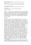
3 Open Google Earth on your computer (version 5.0 or higher) and open the two
files. Zoom in to your area of interest (see Fig. 1).
A few hints: (1) The EPA Waters file is live – that is, it updates from the internet
while you are using it. Therefore it can be very slow. You’ll know it is gathering data
when the little colored boxes next to the field names under Places are spinning. To
speed things up, uncheck every box under Surfacewater Features, except
Streams, and all boxes associated with Water Program Features, and zoom in to
your area. (2) The streams are only visible at very local scales. If you can’t see
them, continue zooming in until the scale at the bottom of the map is approximately
1 inch = 3 miles. Remember to wait for the data to load.
Fig. 1: Streams and stream gage stations around Denver
4 The next step is to explore the watersheds associated with each station to choose
the best one. To do this:
a Click on the stream itself just downstream of the station. A window will
appear describing the features of the stream. At the bottom, under Tools,
click Drainage Area Delineation.
b In the window that appears, choose Stop When: Maximum Distance (KM)
= 30 and click Start Search. The watershed upstream from that point for
25
the first 30 km will be identified. You might have to repeat this process a
few times, increasing the maximum distance to capture the entire
watershed (see Fig. 2).
Fig. 2: A watershed near Denver
Fig. 3: A smaller watershed near Denver
26
c Once you have determined the outline of the watershed, judge whether it is
appropriate for your study.
Does it capture your area of interest?
Is the watershed of a scale that would be appropriate for modeling changes
in canopy and impervious cover? (As explained above, if the watershed is
very large, changes in cover are unlikely to have a measurable impact.)
d Delineate the drainage areas for other stream gage stations until you have
found the best one (see Fig. 3).
5 Once you have made your selection:
a Note the name of the stream by clicking on the stream.
b Note the ID number of the stream gage station (SITENO), by clicking on its
red dot.
c Capture an image of the stream gage station and watershed using your
computer’s Print Screen function or Google Earth’s File > Save > Save
Image function.
Gathering Data
Now that you have selected your watershed of interest and the appropriate stream gage, it
is time to start gathering your input data. In Phase I: Creating a New Project, we described
the general input data that is needed for a new project in i-Tree Hydro. The tables and
directions below will assist you in collecting the data that you will need in order to run iTree Hydro, including some possible data sources or suggested default values.
Basic watershed characteristics
The following input data can be entered by going to Step 1) Project Area Information:
27
Table 1. Basic Watershed Characteristics
Category
Source
a
Default value
Units
2
2
Watershed Land Area
DEM
N/A
km or mi
Percent Tree Cover
Eco , Canopy,
UTC, GIS
N/A
%
Eco , Canopy,
UTC, GIS
5
none
Evergreen Tree Cover
Eco
10
%
Evergreen Shrub Cover
Eco
10
%
State Date/Time (Local)
N/A
N/A
mm/dd/yyyy
hh:mm:ss
End Date/Time (Local)
N/A
N/A
mm/dd/yyyy
hh:mm:ss
Tree Leaf Area Index
b
a
DEM = Digital Elevation Model data (see Appendix 1). Eco = An existing i-Tree Eco study; although it is
unlikely that the Eco study area and the Hydro study area will align exactly, your Eco results might offer some
insight. Canopy = i-Tree Canopy. Visit www.itreetools.org for more information on i-Tree Eco and i-Tree
Canopy. UTC = An existing urban tree canopy analysis. GIS = Your local government or university GIS
department.
b
Leaf area indexes (LAI) can be calculated from Eco results for leaf area, which are presented in units of
m 2/ha. Divide those results by 10,000, to get LAI.
Observed streamflow
Streamflow data are used in i-Tree Hydro to calibrate the model. Hydro tries to find the
best fit between the streamflow predicted by the model and the streamflow measured at
the stream gage station. However, stream gage availability varies and not every stream
has a gage located on it.
Within i-Tree Hydro, hourly streamflow data are available as standardized, complete data
sets. These data were obtained from the U.S. Geological Survey and pre-processed for
2005-2012. If you choose to use the available data, follow the steps provided in Phase
I:Creating a New Project to choose your gage from a map. If you are interested in using
data from a different year or you would like to use data for a gage that is not included in
Hydro, then you have the option of using your own streamflow data.
Once you have obtained your streamflow data, it is very important that the data are
properly formatted for use in i-Tree Hydro. Observed streamflow data must consist of the
following fields:
28
Table 2. Observed Streamflow Data Fields
Field name
a
Definition
b
Units
site_no
site identification number
N/A
date_time
date and time of observation
YYYYMMDDhhmmss
tz_cd
time zone
N/A
dd
data descriptor
N/A
accuracy_cd
accuracy code
N/A
value
discharge
cfs
precision
digits of precision in the discharge
N/A
remark
optional remark code
N/A
a
Required fields include: date_time, tz_cd, and value. See note below.
b
For a list of accuracy codes and optional remark codes, see the example at Resources > Archives > i-Tree
Hydro (beta) Resources > i-Tree Hydro at www.itreetools.org.
To make your data compatible with Hydro, the fields should be organized in tab-separated
columns using the field names listed above and saved as an .rdb file. When streamflow
data are properly formatted, you will be able to navigate to the folder in which you saved it
and load it into the 1) Project Area Information form as described in Phase I.
NOTE: Not all of the fields listed are used in i-Tree Hydro. If you cannot find certain
information, the field name still needs to be included, but you can populate the column
with dummy values. For example, i-Tree Hydro does not use the accuracy code, but
due to formatting of the data, a placeholder value is needed to keep the application on
track.
An example of correctly formatted streamflow data can be found at www.itreetools.org >
Resources > Archives > i-Tree Hydro Resources.
Weather station
Weather station data are an important input because they are used to simulate the
streamflow of your study area. When selecting your weather station be sure to select a
station that is representative of your entire study area. Bear in mind that precipitation
events may be highly localized, so there may be times when it is raining in the watershed
but not at the weather station or vice versa. For that reason, it can be difficult to choose
the best weather station and may mean that you have to try several different options.
29
Within i-Tree Hydro, hourly weather and evapotranspiration data are available as
standardized, complete data sets. These data are obtained from the National Oceanic and
Atmospheric Administration’s (NOAA) National Climatic Data Center (NCDC) and preprocessed for 2005-2012. If you choose to use the available data, then follow the steps
provided in Phase I: Creating a New Project to choose your station from a map. If you are
interested in using data from a different year or you would like to use data from a weather
station that is not included in Hydro, then you have the option of using your own weather
station data.
Required weather data include wind direction and speed, cloud ceiling, sky cover,
temperature, dewpoint, altimeter setting, pressure, and precipitation. Once you have
obtained your weather station data, it is very important that the data are properly
formatted for use in i-Tree Hydro. Weather station data must consist of the following fields:
Table 3. Weather Station Data Fields
Field name
a
Definition
b
Units
USAF
Air Force catalog station number
N/A
WBAN
NCDC WBAN number
N/A
YR--MODAHRMN
year-month-day-hour-minute in GMT
YYYYMMDDhhmm
DIR
wind direction in compass degrees
N/A
SPD
wind speed
mph
GUS
wind gust
mph
cloud ceiling – lowest opaque layer with
5/8 or greater coverage
sky cover (clr-clear, sct-scattered [1/8 4/8], bkn-broken [5/8 - 7/8], ovc-overcast,
obs-obscured, pob-partial obscuration)
CLG
SKC
hundreds of ft
N/A
L
low cloud type
N/A
M
middle cloud type
N/A
H
high cloud type
N/A
VSB
visibility in statute
mi (nearest tenth)
present weather
N/A
past weather indicator
N/A
TEMP
temperature
°F
DEWP
dewpoint
°F
WW WW WW
W
b
b
30
SLP
sea level pressure
mbar (nearest tenth)
ALT
altimeter setting
in (nearest hundredth)
STP
station pressure
mbar (nearest tenth)
MAX
maximum temperature
°F
MIN
minimum temperature
°F
PCP01
1-hour liquid precipitation
in (nearest hundredth)
PCP06
6-hour liquid precipitation
in (nearest hundredth)
PCP24
24-hour liquid precipitation
in (nearest hundredth)
PCPXX
liquid precipitation for a period other than
1, 6, or 24 hours
in (nearest hundredth)
SD
snow depth
in
a
Required fields include: date_time, tz_cd, and value. See note below.
For weather code tables, go to Resources > Archives > i-Tree Hydro (beta) Resources > i-Tree Hydro
weather abbreviation codes at www.itreetools.org.
b
To make your data compatible with Hydro, the fields should be organized in tab-separated
columns using the field names listed above and saved as an .rdb file. When your weather
station data are properly formatted, you will be able to navigate to the folder in which you
saved it and load it into the 1) Project Area Information form as described in Phase I.
NOTE: Not all of the fields listed are used in i-Tree Hydro. If you cannot find that
information, the field name still needs to be included, but you can populate the column
with dummy values. For example, i-Tree Hydro does not use the altimeter setting, but
due to formatting of the data, a placeholder value is needed to keep the application on
track.
An example of correctly formatted weather station data can be found at www.itreetools.org
> Resources > Archives > i-Tree Hydro Resources.
Digital Elevation Model (DEM)
Once you have identified your target watershed and noted the stream name and stream
gage station number, your next step is to create a Digital Elevation Model (DEM) of the
watershed. The end product should be a DEM clipped to the boundaries of your
watershed, projected in the proper Universal Transverse Mercator (UTM) coordinate zone
in meters, and converted to ASCII computer code format.
For more specifics on this process, see Appendix 1.
31
Topographic Index (TI)
The Topographic Index (TI) data were derived from DEM data within various polygon
boundaries. So if you opt to use a Topographic Index (TI), you can skip creating a DEM
for your watershed. In addition, going the TI route will enable you to pick project areas that
have boundaries other than actual watersheds, such as a city or college campus. i-Tree
Hydro contains a TI histogram database based on USGS calculations, with tables for
States, Counties, Places, gaged Watershed Basins, and HUC8 watersheds. In each table
there is a minimum and maximum topographic index value and a count of the number of
pixels in the area of interest. The B1 - B30 fields contain the proportion of the pixels in the
area of interest that fall within that histogram bin.
For a brief overview on how the TIs were constructed, see Appendix 2.
Land cover parameters
The following input data can be entered by going to Step > 2) Land Cover Parameters:
Table 4. Land Cover Parameters
Category
Source
a
Default value
Units
Surface Cover Types (should total 100%)
Eco , Canopy,
UTC, GIS
Eco , Canopy,
UTC, GIS
Eco , Canopy,
UTC, GIS
Eco , Canopy,
UTC, GIS
Eco , Canopy,
UTC, GIS
Eco , Canopy,
UTC, GIS
Tree Cover
Shrub Cover
Herbaceous Cover
Water Cover
Impervious Cover
Soil Cover
Tree Leaf Area Index
b
Shrub Leaf Area Index
b
Herbaceous Leaf Area Index
b
c
Directly Connected Impervious Cover
N/A
%
12.3
%
N/A
%
N/A
%
N/A
%
N/A
%
Eco, Literature
5.0
none
Eco, Literature
2.2
none
Eco, Literature
1.6
none
GIS
40
%
32
Cover Types Beneath Trees (should total 100%)
Pervious Cover
Eco
N/A
%
Impervious Cover
Eco
6.1
%
a
DEM = Digital Elevation Model data (see Appendix 1). Eco = An existing i-Tree Eco study; although it is
unlikely that the Eco study area and the Hydro study area will align exactly, your Eco results might offer some
insight. Canopy = i-Tree Canopy. Visit www.itreetools.org for more information on i-Tree Eco and i-Tree
Canopy. UTC = An existing urban tree canopy analysis. GIS = Your local government or university GIS
department. Literature = Some data may be available for certain locations in the scientific literature or from the
appropriate university department.
b
Leaf area indexes (LAI) can be calculated from Eco results for leaf area, which are presented in units of
m 2/ha. Divide those results by 10,000, to get LAI.
c
This value can be particularly difficult to find. One strategy is to adjust the value in the calibration process
until the model streamflow resembles the observed streamflow; see Calibrating the Model to learn more.
Calibrating the Model Manually
Calibrating the model involves a multi-step process of adjusting model parameters until
the modeled streamflow closely resembles the actual streamflow. The model simulates
various hydrologic processes (e.g., precipitation, interception, infiltration, evaporation,
transpiration, snowmelt, flow routing, and storage) in order to simulate streamflow at the
gaging station. It then checks the accuracy of the simulation by comparing estimated
model flow against actual flow. Results are considered in terms of peak, base, and overall
flow.
i-Tree Hydro features an auto-calibration routine that uses the observed streamflow data
from a gaging station to identify the optimal hydrological parameters to fit the observed
streamflow data. If you are not satisfied with the fit of the model, you can adjust some
parameters to see the effects on the model. See Table 5 below for ranges of possible
values.
Ideally, you create a few parameter sets for comparison and can select one to run the
model. However, having too many parameter sets saved can slow down the modeling.
You can delete a parameter set by selecting it from the Current parameter set dropdown menu and clicking Delete THIS parameter set.
Table 5. Hydrological Parameters
Category
Range
Default value
Units
Annual Average Flow at Gaging Station
N/A
0.000016
cms
Soil type
N/A
N/A
N/A
33
Wetting Front Suction
0.03 – 0.4
0.12
m
Wetted Moisture Content
0.1 – 0.7
0.48
m
Surface Hydraulic Conductivity
0.0001 – 0.3
0.002
cm/h
Depth of Root Zone
0.5
m
Initial Soil Saturation Condition
50
%
28
N/A
Advanced Settings
Leaf Transition Period (days)
N/A
Leaf-on Day (day of year, 1 - 365)
N/A
Leaf-off Day (day of year, 1 - 365)
N/A
Tree Bark Area Index
N/A
1.7
N/A
Shrub Bark Area Index
N/A
0.5
N/A
Leaf Storage
N/A
0.2
mm
Pervious Depression Storage
0.1 – 7.5
1.0
mm
Impervious Depression Storage
0.1 – 300
2.5
mm
Scale Parameter of Power Function
1–2
2
none
Scale Parameter of Soil Transmissivity
0.01 – 0.05
0.023
m
Transmissivity at Saturation
0.0005 – 100
0.13
m /h
Unsaturated Zone Time Delay
0.01 – 150
10
h
Time Constant for Subsurface Flow: B)
0.01 – 0.240
1.3
h
Time Constant for Surface Flow: Alpha
0.01 – 0.240
1
h
Time Constant for Surface Flow: Beta
0.01 – 0.240
2
h
Watershed area where rainfall rate can
exceed infiltration rate
0 – 100
30
%
34
defaults are
regionally
specific
defaults are
regionally
specific
N/A
N/A
2
Appendix 1: Creating a Watershed
Digital Elevation Model
In the Additional Information section, we discussed criteria for choosing a watershed and
some tools for doing so. This Appendix covers the steps necessary to create a Digital
Elevation Model (DEM) of that watershed using ArcGIS. These instructions assume that
you are familiar with DEM data, watershed concepts, and ArcGIS tools.
The basic steps of this procedure are as follows:
1 Download DEM data from the USGS for an area that covers the watershed
boundaries you determined in the Additional Information section.
2 Use ArcGIS to build a DEM from the downloaded data and clip it to the borders of
the watershed.
Tools
ArcGIS (v. 9.3.1. was used for this guide, but other versions can be used)
ArcGIS Spatial Analyst
Results
The end product of the steps described here will be a DEM clipped to the boundaries of
your watershed, projected in the proper UTM zone in meters, and converted to ASCII
format.
Downloading DEM Data from USGS
With your watershed and stream gage selected using the methods described in Phase I:
Creating a New Project, the first step in creating a DEM is to download the necessary data
from the USGS. If you have your own source of DEM data, it can certainly be used, but
keep in mind that DEM data should have a resolution of 10–30 m. Finer resolution data
are available, but are more likely to cause complications in modeling associated with
bridges and elevated roadways.
1 Navigate to the USGS DEM website: http://viewer.nationalmap.gov/viewer/.
NOTE: Links were correct at the time of publication but may have changed. If
necessary, please use Google and the relevant key words to search for the correct
35
links.
2 Display the Overlays tab on the left-hand side of the screen to manage visible
layers to help with orientation. (These choices do not affect which data are
downloaded.) The following are recommended:
a Under the Base Data Layers, turn on Hydrography.
b Under the Base Data Layers, expand Governmental Unit Boundaries.
Expand Features. Uncheck all of the boxes except County or Equivalent
and State or Territory.
3 Use the tools to zoom in or out and pan to your region.
4 Click on Download Data to choose the data that you want to download.
5 In the Download options window, choose Click here to define the area that you
want to download or choose a reference area from the pull-down menu. Now,
comparing the image you saved from Google Earth of the streams in your region
and your watershed of choice (Fig. 4), select an area of coverage that extends
comfortably beyond the boundaries of your watershed (Fig. 5).
6 In the USGS Available Data for download window, check the box for Elevation
then select Next.
7 Choose the National Elevation Dataset (1/3 arc second) in ArcGrid format then
select Next.
NOTE: It is much better to overestimate the size of your watershed when downloading
the DEM data than to underestimate because if you miss even a small corner of the
watershed you will have to begin again. On the other hand, the larger your download
size, the longer it will take and the more likely it is to “time out,” forcing you to begin
again, so don’t go overboard.
8 When you are satisfied with the dataset(s) that you have selected, click the
Checkout button in the panel on the left. Enter your email address as directed and
Place Order.
9 When you receive your order email, select the download link. Depending on the
size of your download, this request may take some time or require you to
download your order in several parts.
36
Fig. 4: Watershed boundaries determined using Google Earth, EPA stream file, and
Hydro stream gage file.
Fig. 5: The same stream system. The outlined area includes all of the yellow area in the
figure above.
37
Working with ArcGIS
Once you have your data downloaded and unzipped, you can begin the process of
transforming it into a hydrological model and clipping it in ArcGIS. You’ll need to load and
enable the ArcGIS Spatial Analyst Hydrology Tools.
1 Open the DEM data in ArcMap. Important: Do not set any projection information at
this time.
2 Open ArcToolBox and navigate to Spatial Analyst Tools > Hydrology.
3 First choose the option to fill the DEM model, using the Fill tool.
4 Next, compute flow direction on the filled DEM layer (from Step 3) using the Flow
Direction tool.
5 Next, compute flow accumulation on the flow direction layer (from Step 4) using the
Flow Accumulation tool.
6 Create a “pour point” for the watershed based on the location of your stream gage
station.
a On the ArcGIS Tools toolbar,
select the Go To XY tool.
38
b Enter the degrees, minutes, and seconds of your stream gage station in the
following format: Long: 81 37’48”W Lat: 41 23’43”N. (Use a space in place
of the degree symbol, use single quotes for minutes, double quotes for
seconds, and direction letters rather than negative signs.)
c Select the Add Point button to place a marker on the stream gage location/
watershed pour point.
d Because of the mechanics of creating a DEM, it is unlikely that your stream
gage marker will line up exactly with the stream created by the DEM. Drag
the point so that it sits within the primary outlet stream of your watershed.
The distance should be fairly small and the move obvious. If not, verify that
you have entered the coordinates correctly. Now, drag the pour point
slightly downstream ~50–100 feet to simplify later steps.
Move pour point
into stream
and 50–100 ft
downstream
Streamflow
7 Capture this pour point within a shapefile.
a In ArcCatalog create a new POINT shapefile.
b Set the projection system to that of the original DEM data projection system
via the Create New Shapefile > Spatial Reference > Edit > Import >
Browse to DEM data option.
39
c Open the pour point shapefile in the current ArcMap session.
d Edit the pour point shapefile and create a new point feature right on top of
the Pour Point marker. Stop editing and save edits.
8 Compute the watershed using the flow direction layer (created in Step 4) and the
pour point layer (created in Step 7), using the Watershed tool (not the Basins tool).
a For the pour point field, choose any of the numeric fields. (While the onscreen instructions indicate that this is optional, it is not.)
9 Compare the resulting image of the computed watershed with the image of your
watershed that you found in the Additional Information section. If they are not
similar:
a Try moving the pour point another 50–100 ft downstream and repeat Step
8.
b Verify that the spatial extent of the original downloaded DEM data covers
the entire watershed. If it does not, you’ll need to do another download and
perform these steps again.
10 Convert the derived watershed raster layer (from Step 8) into a polygon using
ArcToolbox > Conversion Tools > From Raster > Raster to Polygon.
40
11 Clip the original DEM (Step 1) with the converted watershed polygon (from Step
10) using ArcToolbox > Spatial Analyst Tools > Extraction > Extract by Mask.
NOTE: This is not the same process as ArcToolbox > Analysis Tools > Extract >
Clip.
12 Re-project the clipped DEM (from Step 11) to UTM meters using ArcToolbox >
Data Management Tools > Projections and Transformations > Raster >
Project Raster.
a The UTM zone is dependent on the project area. For UTM zones guidance:
http://egsc.usgs.gov/isb/pubs/factsheets/fs07701.html
b Output coordinate system should be: WGS_1984 datum
c Geographic transformation should be: NAD_1983_TO_WGS_1984_1
d Leave other values as defaults.
13 To calculate the area of the watershed, re-project the converted watershed layer
(from step 10) following the directions from step 12. Select Open Attribute Table.
Use the table tools to add a new field for area, then right-click on the added field
and select Calculate Geometry. Select Area and square kilometers.
41
14 Export the clipped, re-projected DEM (from step 13) to ASCII format using
ArcToolBox > Conversion Tools > From Raster > Raster to ASCII.
15 In Windows Explorer, change the file type extension of the ASCII file (from Step
14) from .TXT to .DAT for use within i-Tree Hydro.
42
Appendix 2: Topographic Index Data
A Topographic Index (TI) is constructed using a 30-meter DEM as follows:
1 TI approximates spatial distribution of the depth to water table. It is calculated using
the following formula:
TI = ln(a/tanB)
where:
a= specific catchment area defined = (# of upslope cells + 1) * grid cell length
tanB = slope gradient defined as the rise over run along the steepest path
from the cell center to its neighbor
2 This dataset was generated using a 30-meter resampled DEM. Output dataset was
100-meter resolution.
TI Histograms were generated in ESRI’s ArcGIS with the following input datasets:
Topographic Index Raster, Zone Boundary Files (State, County, Place, gaged and HUC8
watersheds), and NHD high-res water bodies.
1 The High Resolution National Hydrography Dataset water bodies dataset was used
to erase all portions of the zone boundary within a water body that crosses the
outline of the zone boundary. This was only done for States, Counties and Places.
2 ArcGIS SpatialAnalyst Tools >Zonal>Tabulate Area was run to compute the crosstabulated area between the Topographic Index dataset and the zones in the area
of interest boundary file (State, County, Place, gaged, and HUC8). This process
outputs a table containing a record for each location with fields containing the total
area of each pixel value.
3 ArcGIS SpatialAnalyst Tools >Zonal>Zonal Statistics As Table was run to
summarize the values (max, min, sum) of the TI raster within the zones of the
boundary file (State, County, Place, gaged, and HUC8).
4 The range of TI values in each zone was split into 30 bins (or histogram classes)
and the number of pixels in each bin is calculated.
43
Appendix 3: Calculating Pollution Load
The term “event mean concentration” (EMC) is a statistical parameter used to represent
the flow-proportional average concentration of a given parameter during a storm event. It is
defined as the total constituent mass divided by the total runoff volume, although EMC
estimates are usually obtained from a flow-weighted composite of concentration samples
taken during a storm. Mathematically (Sansalone and Buchberger, 1997; Charbeneau and
Barretti, 1998):
∑ 𝐶(𝑡)𝑄 (𝑡)∆𝑡
𝑀
∫ 𝐶 (𝑡)𝑄(𝑡) 𝑑
𝐸𝑀𝐶 = 𝐶 =
=
≈
∑ 𝑄(𝑡)∆𝑡
𝑉
∫ 𝑄(𝑡) 𝑑
where C(t) and Q(t) are the time-variable concentration and flow measured during the
runoff event, and M and V are pollutant mass and runoff volume as defined in Equation 1.
It is clear that the EMC results from a flow-weighted average, not simply a time average
of the concentration. EMC data is used for estimating pollutant loading into watersheds.
EMCs are reported as a mass of pollutant per unit volume of water (usually mg/l).
The pollution load (L) calculation from the EMC method is
𝐿 = 𝐸𝑀𝐶 ∗ 𝑄 = 𝐸𝑀𝐶 ∗ 𝑑𝛾 ∗ 𝐴
where EMC is event mean concentration (mg/l, mg/m 3, …), Q is runoff of a time period
associated with EMC (l/h, m 3/day…), d γ is runoff depth of unit area (mm/h, m/h,
m/day…),and A is the land area (m 2, …), which is catchment area in i-Tree Hydro.
Thus, when the EMC is multiplied by the runoff volume, an estimate of the loading to the
receiving water is provided. As is evident from Fig. 6, the instantaneous concentration
during a storm can be higher or lower than the EMC, but the use of the EMC as an event
characterization replaces the actual time variation of C versus t in a storm with a pulse of
constant concentration having equal mass and duration as the actual event. This process
ensures that mass loadings from storms will be correctly represented. EMCs represent the
concentration of a specific pollutant contained in stormwater runoff coming from a
particular land use type or from the whole watershed. Under most circumstances, the EMC
provides the most useful means for quantifying the level of pollution resulting from a runoff
event (USEPA, 2002).
Since collecting the data necessary for calculating site-specific EMCs can be costprohibitive, researchers or regulators will often use values that are already available in the
literature. If site-specific numbers are not available, regional or national averages can be
44
Fig. 6. Interstorm variation in pollutographs and EMCs.
used, although the accuracy of using these numbers is questionable. Due to the specific
climatological and physiographic characteristics of individual watersheds, agricultural and
urban land uses can exhibit a wide range of variability in nutrient export (Beaulac and
Reckhow 1982).
To understand and control urban runoff pollution, the U.S. Congress included the
establishment of the Nationwide Urban Runoff Program (NURP) in the 1977 Amendments
of the Clean Water Act (PL 95-217). The U.S. Environmental Protection Agency
developed the NURP to expand the state knowledge of urban runoff pollution by applying
research projects and instituting data collection in selected urban areas throughout the
country.
In 1983, the U.S. Environmental Protection Agency published the results of the NURP,
which nationally characterizes urban runoff for 10 standard water quality pollutants, based
on data from 2,300 station-storms at 81 urban sites in 28 metropolitan areas.
Two important conclusions from NURP investigations:
• The variance of the EMCs when data from sites are grouped by land use type
or geographic region is so great that difference in measures of central
tendency among groups statistically are not significant;
• Statistically, the entire sample of EMCs, and the medians of all EMCs among
sites, are lognormally distributed.
Thus the numbers in Table 6 do not distinguish between different urban land use types.
Subsequently, the USGS created another urban stormwater runoff base (Driver et al.
1985), based on data measured through mid-1980s for over 1,100 stations at 97 urban
sites located in 21 metropolitan areas. Additionally, many major cities in the United States
45
collected urban runoff quality data as part of the application requirements for stormwater
discharge permits under the National Pollutant Discharge Elimination System (NPDES).
The NPDES data are from over 30 cities and more than 800 station-storms for over 150
parameters (Smullen et al, 1999).
The data from the three sources (NURP, USGS, and NPDES) were used to compute new
estimates of EMC population means and medians for the 10 pollutants with many more
degrees of freedom than were available to the NURP investigators (Smullen et al, 1999).
A “pooled” mean was calculated representing the mean of the total population of sample
data. The NURP and pooled mean EMCs for the 10 constitutes are listed in Table 6
(Smullen et al, 1999). NURP or pooled mean EMCs were selected because they are
based on field data collected from thousands of storm events. These estimates are based
on nationwide data, however, so they do not account for regional variation in soil types,
climate, and other factors.
Table 6. National Pooled EMCs and NURP EMCs
Constituent
Data
a
source
EMCs
Mean
Median
No. of
events
Pooled
78.4
54.5
3047
NURP
17.4
113
2000
Pooled
14.1
11.5
1035
NURP
10.4
8.39
474
Pooled
52.8
44.7
2639
NURP
66.1
55
1538
Pooled
0.315
0.259
3094
NURP
0.337
0.266
1902
Pooled
0.129
0.103
1091
NURP
0.1
0.078
767
Pooled
1.73
1.47
2693
NURP
1.67
1.41
1601
Pooled
0.658
0.533
2016
NURP
0.837
0.666
1234
Pooled
13.5
11.1
1657
NURP
66.6
54.8
849
Total suspended solids: TSS
b
Biochemical oxygen demand: BOD5
Chemical oxygen demand: COD
Total phosphorus: TP
c
Soluble phosphorus: soluble P
Total Kjeldhal nitrogen: TKN
Nitrite and nitrate: NO2 and NO3
Copper: Cu
46
Pooled
67.5
50.7
2713
NURP
175
131
1579
Pooled
162
129
2234
NURP
176
140
1281
Lead: Pb
Zinc: Zn
a
Pooled data sources include: NURP, USGS, NPDES
No BOD5 data available in the USGS dataset; pooled includes NURP+NPDES
c
No TS data available in NPDES dataset; pooled includes NURP+USGS
b
For i-Tree Hydro, the pooled median and mean EMC value for each pollutant (Table 6)
were applied to the runoff regenerated from pervious and impervious surface flow, not the
baseflow values, to estimate effects on pollutant load across the entire modeling time
frame.
All rain events are treated equally using the EMC value, which means some events may
be overestimated and others underestimated. In addition, local management actions (e.g.,
street sweeping) can affect these values. However, across the entire season, if the
EMC value is representative of the watershed, the estimate of cumulative effects on water
quality should be relatively accurate. Accuracy of pollution estimates will be increased by
using locally derived coefficients. It is not known how well the national EMC values
represent local conditions.
47
Appendix 4: International Support
We recognize that users outside of the United States may wish to experiment with i-Tree
Hydro. It should be noted that the application and model have been built with specific U.S.
data in mind. Users in other countries will need to find and format appropriate data to meet
the requirements of i-Tree Hydro. This can be a difficult process; please review the following
suggestions for guidance. Please also periodically visit the online forums at
forums.itreetools.org to see if other users have posted additional information. Additional
support for users outside the U.S. may be added in future versions of i-Tree Hydro.
1 A DEM file should be created for the project watershed with GIS software. See
Appendix 1 for more information.
2 The user should select a U.S. location similar to the project location based on
latitude and elevation.
3 Weather data is required with the following fields:
•
•
•
•
•
•
•
•
•
DIR (wind direction)
SPD (wind speed in mph)
CLG (cloud ceiling – lowest opaque layer with 5/8 or greater coverage, in
hundreds of feet)
SKC (sky cover)
TEMP (temperature in Fahrenheit)
DEWP (dew point in Fahrenheit)
STP (station pressure in millibars; can be converted from ALT) or
ALT (altimeter setting in inches; can be converted to STP)
PCP01 (hourly precipitation in inches and hundredths)
The weather file must be a fixed-width text file. The model will interpolate gaps in
the data, though they should be kept under 72 hours. This data should be in GMT.
Example:
USAF WBAN YR--MODAHRMN DIR SPD GUS CLG SKC L M H VSB WW WW WW W TEMP DEWP SLP ALT STP MAX MIN PCP01 PCP06
PCP24 PCPXX SD
724666 99999 200701010053 150 5 *** 722 SCT * * * 10.0 ** ** ** * 18 5 1029.3 30.18 ****** *** *** ***** ***** ***** ***** **
724666 99999 200701010153 170 7 *** 722 SCT * * * 10.0 ** ** ** * 18 3 1029.4 30.18 ****** *** *** ***** ***** ***** ***** **
4 Stream gage data* is required if the user wants to calibrate the model. The file
must be tab-delimited and contain headers similar to the U.S. data.
48
Example:
# column
# ----------# site_no
# date_time
# tz_cd
# dd
# accuracy_cd
#
#
#
#
#
#
#
#
#
#
#
#
#
#
#
# value
#
#
site_no
15N
14N
06710150
06710150
06710150
06710150
column definition
----------------------------------------USGS site identification number
date and time in format (YYYYMMDDhhmmss)
time zone
internal USGS sensor designation (''data descriptor'')
accuracy code
0 - A daily mean discharge calculated from the instantaneous
data on this day is 0.01 cubic feet per second
or less and the published daily mean is zero.
1 - A daily mean discharge calculated from the instantaneous
data on this day matches the published daily mean
within 1 percent.
2 - A daily mean discharge calculated from the instantaneous
data on this day matches the published daily mean
from greater than 1 to 5 percent.
3 - A daily mean discharge calculated from the instantaneous
values on this day matches the published daily mean
from greater than 5 to 10 percent.
9 - The instantaneous value is considered correct by the
collecting USGS Water Science Center. A published daily
mean value does not exist and/or no comparison was made.
discharge in cubic feet per second
date_time
tz_cd
6S
2N
5S
20070101000000
20070101001500
20070101003000
20070101004500
dd
16N
MST
MST
MST
MST
accuracy_cd
1S
1S
2
1
2
1
2
1
2
1
value
prec
2.4
2.7
2.7
2.9
2
2
2
2
remark
* NOTE: The date_time value for this file should be converted from local time to
the time zone of the location you specified above. For example, if you selected an
EST location (GMT -5) and the project location is in GMT +1, the date_time should
have 6 hours subtracted from it. This is because the weather data are
automatically converted to local time and stream gage data are assumed to be in
local time already.
49
References
Beaulac, M. N., and Reckhow, K. H. 1982. An examination of land use-nutrient export
relationships. Water Resources Bulletin, 18(6), 1013-1024.
Charbeneau, R. J., and Barretti, M. 1998. Evaluation of methods for estimating
stormwater pollutant loads. Water Environ Res. 70: 1295-1302.
Driver, N. E., Mustard, M. H., Rhinesmith, R. B., and Middelburg, R. F. 1985. U.S.
Geological Survey urban-stormwater data base for 22 metropolitan areas throughout the
United States. United States Geological Survey, Open-File Report 85-337, Lakewood,
CO.
Sansalone, J. J., and Buchberger, S.G. 1997. Partitioning and first flush of metals in urban
roadway storm water. J Environ Eng ASCE 123: 134-143.
Smullen, J. T., Shallcross, A. L., and Cave, K. A. 1999. Updating the U.S. nationwide
urban runoff quality database. Water Science Technology 39(12), 9-16.
U.S. Environmental Protection Agency (USEPA). 1983. “Results of the Nationwide Urban
Runoff Program: Volume I – final report,” U.S. Environmental Protection Agency, PB84185552, Washington, DC.
U.S. Environmental Protection Agency (USEPA). 2002. Urban Stormwater BMP
Performance Monitoring, A Guidance Manual for Meeting the National Stormwater BMP
Database Requirements.
Wolock, D. M., and McCabe, G. J. 2000. Differences in topographic characteristics
computed from 100- and 1000-m resolution digital elevation model data. Hydrol. Process.
14, 987±1002.
Wolock, D. M., and Price, C. V. 1994. Effects of digital elevation model map scale and
data resolution on a topography-based watershed model. Water Resources Research,
30(11), 3041-3052.
50