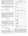
1
4.9 Laserresonator
Versuchsanleitung zum Fortgeschrittenen-Praktikum
Abteilung A
Version 2.2
Fachbereich Physik
Institut für Angewandte Physik
AG Nichtlineare Optik / Quantenoptik
Inhaltsverzeichnis
Versuchsanleitung
3
Anhang
The World of Fabry-Perots
10
The Spherical Mirror Fabry-Perot Interferometer
16
Laser Beams and Resonators
32
SA200-Series Scanning Fabry-Perot Interferometer Datenblatt
50
SA210-Series Scanning Fabry-Perot Interferometer Datenblatt
51
SA201 Spectrum Analyzer Controller Anleitung
56
S120C Leistungsmesskopf Datenblatt
67
PM100D Leistungsmessgerät Kurzanleitung
71
PicoScope 3000 PC-Oszilloskop Anleitung
83
2
Vorbereitung
Laserprinzip: Besetzungsinversion, Anregungsmechanismen, 3- und 4-NiveauSystem, Einwegverstärkung
Laseroszillatoren: Verstärkung durch Rückkopplung, Laseroszillator, Modenspektrum von Laseroszillatoren, Bandbreite, Eigenschaften der Laserstrahlung, HeNe-Gaslaser.
Resonatortheorie: Optische Resonatoren, Resonatorgeometrie, (planparallel,
konfokal, hemisphärisch) und deren Eigenschaften, Stabilitätsdiagramm, Verluste
optischer Resonatoren, Moden (transversal und longitudinal), Fabry-PerotInterferometer, Gauß-Optik.
Gefahren durch Laserstrahlung (siehe z.B. Wikipedia)
Vorbereitende Aufgaben: Gehen Sie die einzelnen Versuchsteile durch und
bearbeiten Sie die drei Vorbereitungsaufgaben.
Sollten Fragen zur Vorbereitung oder den Vorbereitungsaufgaben aufkommen,
können Sie sich bis einschließlich freitags vor dem Versuch per Mail an den
Betreuer wenden.
Überlegen Sie sich vor Versuchsbeginn welche Größen gemessen werden müssen
und erstellen Sie einen Messplan, der sämtliche zu messenden Größen inkl.
Fehlerangaben(!) jedes Aufgabenteils enthält.
Literatur
W. Demtröder:
„Laserspektroskopie:
Grundlagen
und
Techniken,“
Springer (2007)
F.K. Kneubühl, M.W. Sigrist: “Laser,” Vieweg + Teubner (2008)
J. Eichler, H.-J. Eichler:
„Laser:
Bauformen,
Strahlführung,
Anwendungen,“
Springer (2006)
M. Hercher:
“The Spherical Mirror Fabry-Perot-Interferometer,”
Applied Optics 7 951 (1968) (siehe Anhang)
H. Kogelnik, T. Li:
“Laser Beams and Resonators,” Applied Optics 5, 1550
(1966) (siehe Anhang)
W.S. Gornall
„The World of Fabry-Perots,“ Lasers & Applications, 47
(July 1983) (siehe Anhang)
3
Einleitung
Seit der Erfindung des Lasers (light amplification by stimulated emission of radiation) in den
1960er Jahren hat dieser weitreichende Anwendungen gefunden. Diese Anwendungen
beinhalten bspw. hochaufgelöste Spektroskopie, zeitlich aufgelöste Studien molekularer
Dynamik mittel Erzeugung ultrakurzer Lichtpulse, Fangen und Kühlen von Atomen zur
Erzeugung von Bose-Einstein Kondensaten, Medizin/Chirurgie (z.B. Laserskalpell),
Messtechnik (z.B. Abstandsmessung), Materialbearbeitung in der Industrie und
Unterhaltungselektronik (CD/DVD-Spieler).
Das Grundprinzip des Lasers lässt sich kurz folgendermaßen zusammenfassen:
Ein Laser besteht im Wesentlichen aus drei Komponenten:
- einem verstärkenden Medium, in das von
- einer „Energiepumpe“ selektiv Energie hineingepumpt wird und
- einem Resonator, der einen Teil dieser Energie in Form elektromagnetischer Wellen in
wenigen Resonatormoden speichert.
Die Energiepumpe erzeugt im Lasermedium eine vom thermischen Gleichgewicht extrem
abweichende Besetzung eines oder mehrerer Energieniveaus. Bei genügend großer
Pumpleistung wird zumindest für ein Energieniveau Ek die Besetzungsdichte Nk(Ek) größer als
die Besetzungsdichte Ni(Ei) für ein energetisch tiefer liegendes Niveau Ei, das mit Ek durch
einen erlaubten Übergang verbunden ist (Inversion). Da in einem solchen Fall die induzierte
Emissionsrate auf dem Übergang Ek Ei größer wird als die Absorptionsrate, kann Licht beim
Durchgang durch das aktive Medium verstärkt werden. Die Aufgabe des Resonators ist es nun,
Licht, das von den durch die Pumpe aktivierten Atomen des Lasermediums emittiert wird,
durch selektive, optische Rückkopplung wieder durch das verstärkende Medium zu schicken
und dadurch aus dem Laserverstärker einen selbstschwingenden Oszillator zu machen. Mit
anderen Worten: Der Resonator speichert das Licht in wenigen Resonatormoden, so dass in
diesen Moden die Strahlungsdichte groß wird und damit die induzierte Emission wesentlich
größer als die spontane Emission werden kann.
Während alle Laser auf diesem Prinzip basieren, ist die technische Realisierung der drei
Komponenten Resonator-Pumpe-Medium recht vielfältig. Die Pumpe lässt sich z.B. durch
Blitzlampen, Gasentladungen, Strom oder auch andere Laser implementieren. Aktive Medien
reichen von Gasen, dotierten Festkörperkristallen, Halbleitern, bis zu in Flüssigkeiten gelösten
Farbstoffen.
In diesem Versuch soll das Laserprinzip anhand eines Helium-Neon-Gaslasers veranschaulicht
werden. Durch Aufbau und Justage eines Resonators um das aktive Medium soll zuerst die
Laseroszillation erreicht und dann die im folgenden aufgeführten Aufgaben bearbeitet werden.
4
Versuchsdurchführung & Auswertung
WICHTIG: Dokumentieren Sie immer alle Messergebnisse der einzelnen Aufgaben! Die
Messdaten sind am Ende des Versuchs vom Betreuer unterzeichnen zu lassen.
WICHTIG: Die Gasentladung im Lasermedium wird über eine Hochspannung von
mehreren kV gezündet. Berühren Sie nicht die Anschlüsse! Das Lasermedium inkl.
Halterung darf nicht von der Schiene genommen und nur vom Betreuer bewegt werden!
WICHTIG: Die während der Versuchsdurchführung aufgenommenen Messwerte sind im
Original in die Auswertung einzufügen! Trennen Sie die Auswertung der Messwerte von der
Versuchsdurchführung! Es muss nachvollziehbar sein, wie die Auswertungsergebnisse aus
den Messdaten erhalten wurden!
Aufgaben:
1. Inbetriebnahme des Laserresonators
Benutzen Sie den Justierlaser sowie die Irisblende um eine optische Achse zu definieren.
Richten Sie dann das Laserrohr und die Resonatorspiegel bzgl. dieser Achse aus. Achten Sie
hierbei darauf, dass der Strahl des Justierlasers mittig durch das Laserrohr läuft und die
Resonatorspiegel zentrisch trifft.
Der Krümmungsradius der Spiegel beträgt R = 450 mm und der Spiegeldurchmesser beträgt
dM = 7.75 mm. Der Durchmesser des Laserrohrs beträgt ca. dR = 1.0 mm und seine Länge ca.
L = 20 cm.
Führen Sie nun die Aufgaben 2-4 für 10 Resonatorlängen jeweils nacheinander durch.
Das Lasermedium soll sich bei jeder Messung in der Mitte des Resonators befinden. Beginnen
Sie mit einem Spiegelabstand von 25 cm und vergrößern Sie diesen dann schrittweise bis 2 cm
unterhalb des größtmöglichen Abstands (Stabilitätsgrenze).
2. Ausgangsleistung des Lasers in Abhängigkeit von der Resonatorlänge
Aufgabe zur Vorbereitung: Erstellen Sie eine Messwert-Tabelle mit den 11 zu
untersuchenden Resonatorlängen. Die Tabelle sollte neben Feldern für die Messwerte und
den Fehler auch zwei Spalten für die Spiegelpositionen nebst Fehler, sowie eine Spalte für
Kommentare beinhalten.
Messen Sie die Ausgangsleistung des Lasers in Abhängigkeit von der Resonatorlänge und
bestimmen Sie so die Stabilitätsgrenze des Resonators. Nehmen Sie zusätzlich zu den normalen
Messwerten mindestens einen weiteren Messwert für eine Resonatorlänge auf, welche
weniger als 2 cm von der (theoretisch berechneten) Stabilitätsgrenze entfernt ist. Tragen Sie die
Ergebnisse graphisch auf. Diskutieren Sie die Ergebnisse.
Hinweise: Maximieren Sie die Ausgangsleistung für jeden Messpunkt durch Justage der
Spiegel und des Laserrohrs.
5
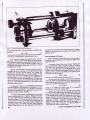
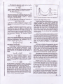
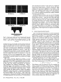
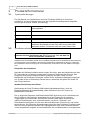
CCD-Sensor
Auskoppler
HR Spiegel
d
‘
‘
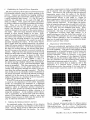
3. Strahlbreite der Grundmode in Abhängigkeit von der Resonatorlänge
Aufgaben zur Vorbereitung: Berechnen Sie für die beiden Resonatorlängen von 25cm und
88cm den Strahldurchmesser der TEM00-Mode am Auskoppelspiegel.
Bestimmen Sie für die beiden Resonatorlängen 25cm und 88cm den Fehler (in Prozent
vom erwarteten Messwert), der sich aus der Vereinfachung für einen Abstand d=8cm
ergibt. Diskutieren Sie später in der Auswertung gegebenenfalls dessen Relevanz.
(a) Aufnahme der Messdaten
Bestimmen Sie Strahlbreite w am Ort des Auskoppelspiegels in Abhängigkeit von der
Resonatorlänge. Nehmen Sie hierzu die Intensitätsverteilung der ausgekoppelten
Laserstrahlung mit Hilfe einer CCD-Kamera in festem und möglichst geringem Abstand d vom
Auskoppelspiegel auf (siehe Abb. 1). Die Maße der aktiven Sensorfläche betragen 4,8mm
horizontal und 3,6mm vertikal. Achten Sie bei der Aufnahme der Bilder darauf, dass der Chip
nicht übersättigt ist!
Für jede Resonatorlänge soll die TEM00-Mode des Lasers angeregt werden. Dies kann z.B.
durch verkippen des Laserrohres erreicht werden. Die Bildaufnahme erfolgt über das
Programm Beamscope. Die Messdaten befinden sich im Ordner „D:/Measurement
Data/Beamscope VGA/“ Das Programm erstellt automatisch einen horizontalen und einen
vertikalen Schnitt durch das Maximum der Intensitätsverteilung. Tragen Sie die aus einer
nichtlinearen Regression erhaltenen Strahlbreiten w in einem Diagramm über der
Resonatorlänge auf. Die Betrachtung eines vertikalen und horizontalen Schnitts ermöglicht
einen Rückschluss auf die Genauigkeit der Messung.
(b) Vergleich mit berechneten Werten.
Der Auskoppelspiegel besitzt eine gewölbte Außenfläche und kollimiert den Gauß´schen
Laserstrahl mit dem Strahlradius w(L/2). Das heißt, es bildet sich ein neuer Gauß´scher Strahl
mit der Strahltaille w0´=w(L/2) aus. Für kleine Abstände d können Sie daher zunächst davon
ausgehen, dass w´0=w´(d). Tragen Sie die berechneten Werte in das in 2(a) erzeugte Diagramm
ein. Diskutieren Sie das Ergebnis.
6
4. Longitudinale Modenstruktur in Abhängigkeit von der
Resonatorlänge
Beobachten Sie die longitudinale Modenstruktur des HeNe-Resonators in Abhängigkeit der
Resonatorlänge und vergleichen Sie die Ergebnisse mit der Theorie. Die longitudinale
Modenstruktur wird mit dem Fabry-Perot Interferometer (Thorlabs SA210 bzw. SA200 &
Steuergerät SA201) gemessen. Das Ausgangssignal des Interferometers kann mit einem
Digitaloszilloskop (Pico Modell 3204) auf den PC mittels des Programms PicoScope
übertragen werden.
Bestimmen Sie nun den Modenabstand in Abhängigkeit der Resonatorlänge. Vergleichen Sie
in einer Tabelle die gemessenen mit berechneten Werten.
Achten Sie darauf, während der Messung nur die TEM00-Mode anzuregen! Kalibrieren Sie
zunächst die Zeitskala des Oszilloskops mit Hilfe des freien Spektralbereichs des
Interferometers zur späteren Umrechnung von der Zeitbasis in den in Frequenzraum.
Achten Sie bei jeder Messung darauf, dass auf dem Oszilloskop klar separierbare,
symmetrische Lorenz-Linien erkennbar sind. Justieren Sie gegebenenfalls die Verkippung des
Interferometers im Bezug auf den Laserstrahl und stellen sie sicher, dass der Laserstrahl die
Eingangs-Iris des Detektors mittig trifft. Stellen Sie die Iris zur Messung auf den kleinsten
Durchmesser ein.
Speichern Sie die Daten jeweils im .txt und .png-Format (zur späteren Kontrolle).
Entfernen Sie bei der Justage des Fabry-Perot Interferometers nicht den Detektor, wie in dessen
Anleitung beschrieben wird!
5. Verstärkungsbandbreite des HeNe-Lasers.
(a) Aufnahme der Messdaten mithilfe der Persistenz-Funktion
Untersuchen Sie die Verstärkungsbandbreite des Lasers für mindestens eine Resonatorlänge.
Die „Persistenz“-Funktion des Oszilloskops eignet sich aufgrund des vorhandenen ModenJitters zur Aufnahme des Verstärkungsprofils. Es kann nur ein PNG-Bild der OszilloskopAnzeige gespeichert werden, die grafisch ausgewertet werden muss. Es empfiehlt sich, diese
Aufgabe bei einer Resonatorlänge von 60-81cm durchzuführen.
Nehmen Sie das Verstärkungsprofil bei maximaler Ausgangsleistung der TEM00-Mode auf.
Bestimmen Sie anschließend die Ausgangsleistung. Reduzieren Sie nun die Ausgangsleistung
durch Erhöhen der Beugungsverluste auf die Hälfte des Ausgangswertes. Wiederholen Sie die
Messung.
(b) Bestimmen der Verstärkungsbandbreite
Benutzen Sie die in Aufgabe 4 gemachte Kalibrierung der Zeitskala des Oszilloskops zur
Bestimmung der Frequenzbandbreite des Verstärkungsprofils. Erläutern Sie den Einfluss der
Verluste auf die Verstärkungsbandbreite anhand der Messung. Diskutieren Sie die erhaltenen
Werte im Hinblick auf die theoretisch zu erwartende Verstärkungsbandbreite.
7
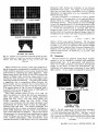
6. Beobachtung höherer transversaler Moden.
(a) Aufnahme der Messdaten mittels CCD-Kamera
Nehmen Sie mindestens vier Bilder der Intensitätsverteilung unterschiedlicher TEM-Moden
mit dem Programm Beamscope auf. Der Schalter „LIVE“ ermöglicht es, das Bild einer
Intensitätsverteilung zum Speichern einzufrieren. Wählen Sie möglichst Transversal, deren
Verteilung klar erkennbar ist und die Sie identifizieren können. Speichern Sie die Bilder als
BMP-Dateien. Notieren sie für jede Mode, auf welche Art und Weise sie erzeugt wurde und
welcher Resonatorlänge genutzt wurde.
Achten Sie auch hier auf eine gute Sensorbelichtung. Sie können durch Nutzung der
Mittelungsfunktion das Bildrauschen verringern. Achten Sie dabei jedoch darauf, dass nicht
verschiedene Transversalmoden zu einem Bild akkumuliert werden.
(b) Räumliche Intensitätsverteilung der Moden.
Legen Sie sinnvoll ausgerichtete Schnitte entlang der Symmetrieachsen durch die
Intensitätsverteilung der Moden. Hierzu dient das Programm SliceBMP. Die Position der
Schnitte lässt sich durch die Schieberegler rechts und oben am Bild anpassen. Die Drehung
durch Eingabe eines Winkels und Bestätigung mit Enter.
Mit Klick auf „Schnitt erstellen“ Werden sowohl das gedrehte Bild, als auch die beiden
Intensitätsprofile im angegebenen Ordner gespeichert.
(c) Vergleich der gemessenen Werte mit berechneten Intensitätsverteilungen.
Plotten Sie die berechneten Intensitätsverteilungen im jeweils zugehörigen Graph der
gemessenen Verteilung aus 6(a). Passen Sie für die Berechnung die Amplitude und die
Strahlbreite w der theoretischen Verteilung an die experimentellen Daten an.
Stellen Sie in der Auswertung links neben dem Graph die zweidimensionale
Intensitätsverteilung mit den Schnittgeraden dar, welche die Lage des benutzten Schnittes
innerhalb der Intensitätsverteilung aufzeigt. Diskutieren Sie die Qualität der Graphenanpassung
an die Messdaten.
Vergleichen sie den erhaltenen Radius mit dem Radius der Grundmode bei gleicher
Resonatorlänge aus Aufgabe 3(a). Diskutieren Sie die Ergebnisse im Hinblick auf die
theoretische Beschreibung der Transversalmoden.
8
Wichtige Punkte zum Laserschutz
Ganz allgemein gilt: Im Umgang mit Lasern ist der gesunde Menschenverstand nicht
zu ersetzen! Einige spezielle Hinweise werden im Folgenden angeführt.
1.
2.
3.
4.
5.
Die Laserschutzvorschriften sind immer zu beachten.
Halten Sie Ihren Kopf niemals auf Strahlhöhe.
Die Justierbrille immer aufsetzen.
Schauen Sie nie direkt in Strahl – auch nicht mit Justierbrille!
Achtung: praktisch alle Laser für Laboranwendungen sind mindestens Klasse 3, also
von vornherein für die Augen gefährlich, ggf. auch für die Haut – evtl.
auch hierfür Schutzmaßnahmen ergreifen. Zur Justage kann der Laserstrahl mittels
einem Stück Papier sichtbar gemacht werden.
6. Auch Kameras besitzen eine Zerstörschwelle!
7. Spiegel und sonstige Komponenten nie in den ungeblockten Laserstrahl einbauen! Vor
Einbau immer überlegen, in welche Richtung der Reflex geht! Diese Richtung zunächst
blocken, bevor der Strahl wieder frei gegeben wird.
8. Nie mit reflektierenden Werkzeugen im Strahlengang hantieren! Unkontrollierbare
Reflexe! Vorsicht ist z.B. auch mit BNC-Kabeln geboten, die in den Strahlengang
gelangen könnten! Gleiches gilt auch für Uhren und Ringe. Diese vorsichtshalber
ausziehen, wenn Sie mit den Händen im Strahlengang arbeiten.
9. Auch Leistungsmessgeräte können Reflexe verursachen! Unbeschichtete
Silizium-Fotodioden reflektieren über 30% des Lichtes!
10. Achtung im Umgang mit Strahlteilerwürfeln! Diese haben immer einen zweiten
Ausgang! Ggf. abblocken!
11. Warnlampen bei Betrieb des Lasers anschalten und nach Beendigung der Arbeit wieder
ausschalten.
12. Dafür sorgen, dass auch Dritte im Labor die richtigen Schutzbrillen tragen, oder sich
außerhalb des Laserschutzbereiches befinden.
13. Filtergläser in Laserschutzbrillen dürfen grundsätzlich nicht aus- oder umgebaut
werden!!!
14. In besonderem Maße auf Beistehende achten.
15. Optiken (Linsen, Spiegel etc.) nicht direkt mit den Fingern berühren!
Hiermit erkläre ich, dass ich die vorstehenden Punkte gelesen und verstanden habe. Ich
bestätige, dass ich eine Einführung in den Umgang mit Lasern sowie eine arbeitsplatzbezogene
Unterweisung erhalten habe.
Name:
Unterschrift:
Datum:
9
The World of
Fabry-Perots
TheseElegantrnstrumentsAre Versatile,High-Resolution
TunableWavelengthFilters
by William S. Gornalt
The Fabry-Psrot interferometer was invented by
two French opticians,Charles Fabry and Alfred Perotr in
1897. For decadesit receivedlimited use evenin spectroscopic researchbecausefew emissionsourceswere sufficiently monochromatic to take advantage of its high
resolving power. The advent of lasers in the early 1960s
produced a renaissanceof interest in Fabry-perot interferometry that continuesto grow as new applicationsand
techniquesare found.
The Fabry-Perot is the simplest of all interferometers, consisting of two partially transmitting mirrors
facing each other. Depending on the application, these
mirrors may be flat or spherical, and the distance
betweenthem can range anywhere from micrometers to
meters. All Fabry-Perot designs share some common
features, but there are important differences which
determine the right choice of interferometer for a particular application.
The author is manager of research and developmentat Burleigh
lnstruments,Inc., FishersNY 14453
How It Works
- - fh. Fabry-Perot mirrors form an opticat cavity in
which successivereflectionscrcate multiple beam inteference fringes.
The simplest and most versatile design is the flat
mirror cavity. As shownin Figure l, illumination by an
extended monochromatic light source produces bright
fringes of equal inclination in the focal plane of L2,
producing a characteristic "bull's-eye" pattcrn.
At the angle O where a bright fringe is observed,the
relationshipbetweenthe sourcewavelength), and the
mirror spacingd is
m.l, = 2nd cos O
(1)
wheren is the refractive index of the medium betweenthe
mirrors and, m is an integer identifying the order of
interference.A pinhole aperture on the optical axis at the
focal point of L: limits the light transmitted through the
pinhole to that passingthrough the Fabry-perot parallel
Bull's-Eye
I nterference
Pattern
Detector
Extended
Monochromatic
LightSource
*i
l l
l*d
Fabry-Perot
ln terferometer
lmage
Plane
Figure 1. Diagram of Fabry-Perot spectrometer.
Lasers & Appllcations July 1983
47
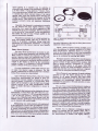
Figure 2. Super'lnvar Fabry'Perot interferomeler'
the
to the optical axis (O = 0), and therefore satisfying
condition
(2)
dt = 2nd
to
tuned
be
may
formed
so
The Fabry-Perotspectrom€ter
d'
n
or
either
varying
by
wavelength
änV
t*".*it
If the medium between the mirrors is air or some
gas pressure'
other gas, n can be varied by changin-gthe
becauseit is
now
used
rärely
is
scanning
Su.ft itotut"
n can be
solid,
a
is
"nd slow.-If the medium
;;üt;;;;
is slow
too
this
but
temperature,
the
;h;;c"d by "djusting
and difficult to control'
Modern interferometers are more often tuned by
changing the mirror spacing' d. The lPtical path length
the
Uetr"äen-the mirrors can be altered by rotating
in
nonrotation-results
but
i^6.y-i"tot interferometer'
the
iit""i tuoitg and must be limited to small anglesor
A
degraded'
is
pöwer of the interferometer
i"*r"i"i
one
to
mount
d
is
changing
for
technique
more veisätile
oo ift.ee piezoälectricelementsand translate that
.ü*t
while
riitot in a direction perpendicular to its surface
fixed.
remains
the other
As Equation 2 shows,any wavelengthcan be trans'
least
mittea tniöugh the interferomäterif d changesby at
ll)r. For visille wavelengths' it is possible to construct
jiezoelectric assembliesthat will move several waveiengths, providing ample tunability'
I
i
i
I
A modern Fabry-Perot interferometer with pieze'
electric tuning is pictured in Figure 2' The main structure
is heavy tupit-Inuut for mechanical rigidity and low
thermaf s"n.itiuity. The cavity spacing.can -bc set anyilt*"en 0 and 15 cenlimeters by adjusting tle
il;;
movable mirror mount. One mirror can be mechanically
"iig*a parallel to the other with tho large alignment
,"tätut. önce theseare set, fine alignment and tuning or
48
scanningcanbe performedby remotecontrolof voltages
ässemblythat supportsthe
ine piezoelectric
öi"J-t"
oppositemirror.
The Meaning of Finesse
further the criteriaforchoosinga
Beforediscussing
to definesome
it is necessary
interferometer,
Fabry-ierot
important terms.
illuminated
A scanningFabry-PcrotsPectrometer
in
a
transmits
light
"itft lnonocnräatic
ryak intensity
wavelJngthsatisfiesEquation2' The
;;'ä;;,h"
that can be displayedin the same
iunä of "uuelengths
"tnithoot
ordersis
overlapping-adjacent
t
otJtt
;;;ä;J
plane
mirror
a
(FSR)'
For
"'"inä ti" rt"" spectralrange
d,
sPacing
with
Fabry-Perot
(3)
FSR = 'lnd
(cm-t)'
If d is in cm, FSR is in wavenumbers
bandwidthor instrumentalresolution
The resolvable
profile
is the fuU width at half-maximumof the spectral
perfectly
monochromatic
a
from
ä"i "ltra be observed
source.It is definedarbitrarily as
(4)
Av = FSR/F
where F is called the finesse, and Az is resolvable
bandwidth measuredin wavenumbers'
Finesseis a measureof the interferomete-r'sability
the
to resoiuectoselyspacedlines; the higher the.finesse
number
ü"it". fin.tte cän'be thought of as the effective
oi iotttf*i"g beamsinvolved in forming the interference
which
iti"""r. itt" factors that limit finesseare tbose
of
number
as
the
ttrength of the interference
rJ,i*in"
mirror
are
examples
Important
itnattiont incre-ascsor
t"fi""ii"ity less than 100% and lack of parallelism
is
finesse
A
separate
surfacesor tn" mirror
iffi;;.
factors'
these
of
cach
with
associatsd
Lasere & APPllcations JulY 1983
- The reflecfivrty
finessefor a plane mirror interferometerwith mirror reflectivitiesR is
.^=?f
(5)
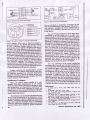
Typical intensity contours of Fabry-Perot fringcs for.
differentmirror reflectivitiesare shownin Figure3.
T\e flatnessfnesse ß
Fc = M/2
(6)
where M is the fractional wavelengthdeviation from true
flatnessor parallelisn acrossthe mirror aperture. Mirror
flatness is commonly spccified as l/M at a standard
wavelengthof 546 nanometers.
The net finesse due to flatness and reflectivity is
called the instrument finesse, F1, where
LlFtz = tfFRz + tlFF2
e)
A plot of F1 is shown in Figure 4 for mirrors with a
sphericalerror amounting to tr/100 and Ä/200 ovcr their
aperture.
When the Fabry-Perot interferometer is used in a
spsctrometer, as shown in Figure l, lbe pinhole size
determines the degree of collimation of light passing
through the interferometer that reachesthe detector. If
the pinhole is too large, rays passingthrough the FabryPerot at diferent angles are accepted,thus broadening
the instrumental linewidth. The associated pinholi
finesse is
u,:H
(s)
whcre D is the pinholc diameter and/is the focal length
of lens L2. To compute the total instrumental finesseof a
Fabry-Perot spestrometer, thc contribution from Fo
should be included with FR and Fp:
l
l + _ +l _
l
'
'
(e)
Fr' F^z 5.r
Prz
R=2t* Fß=2
R=6J* Fn'?
R = 9 0 ? 6F R = 3 0
Ordcr Numbct
Figure3. Fabry-Perot
transmission
lor difierentmirrorretrec-tivities.
Choosingthe Right Fabry-Perot
ThebestFabry-Perot
interferometer
for a particular
application depends on many factors, including size,
stability, tunability, free spectral range, resolution, lightgathering power, and price. Distinguishing features of
the various types of Fabry-Perot systems are outlined
below. (Note: The word "etalon" is usually usedfor small
Fabry-Pcrots that might serve as wavelength-selective
filters inside the laser cavity. The following discussion
uses the terms etalon and interferometer according to
gommon practice; for some dwices they are practically
interchangeable.)
Solid etalons arrdfxed-air-gap etalons are stablc
and compa.ct,making them ideal for wavelengthfiltering,
frrquency calibration, coherenceextension,and intracavity mode selectionin lasers.Solid etalons are made from
a piecc of optically homogeneousmaterial such as fused
quartz. Opposite faces are polishedflat and parallel, and
coated to any desired reflectivity. In a fixed-air-gap
ctalon, two mirrors are bonded to a solid spacer
element.
Throughput and ftendue
An advantageof Fabry-Perotinterferometers
over
other types of high resolutionspectrometers
is their
efficiency,both in transmission
and "6tendue,"or lightgatheringpower.For smallapefttrres
or perfectlyflat and
parallel mirrors, the transmisiionon the peak of a
fringe,
Both types are highly stable mechanically,but solid
etalons are more sensitive to temperature changes. A
solid etalon is best usedin a thermally controlled housing
where it can be temperature-tunedor stablized. Fixedair-gap etalons aro more stable thermally and, unlike
solid etalons, they can be pressure-tuned.Both types
allow no mechanical variability in spacing; the right
spacing must be preselectedfor a specific application.
(10)
Thesimplestway to tuneeitheretalonis bytilting. This
is a goodtechniqueprovidedtilt anglesare notsolargcas to
degradethe finesse.Theseetalonsare difficult to rnanufacture with very flat and parallel surfaces,especiallywith
large mirror spacings.They are best suited for optical
systemswith small-diameterlaserbeams.
T,"^=(t-r*Ä)'
dependson l, the scatteringand absorptionlossat the
mirrors, For modern multilayer dielectric mirrors
A <0.2Vo.Consequently,
mirror reflectivitiesas high as
98Vocan yield throughputclose rc 8A%over a small
aperture.The ötenduefor a planeFabry-Perotinterferometeris
U-o.o,=ffi
(11)
All the radiation at wavelengthl, within a solid angle O
subtendsdat a mirror aperture A, can be transmitted in
the bandpassdefined by the instrumental finesseF1.
The above formulae apply to Fabry-Perot interferome,
ters using plane mirrors. Similar formulae exist for
spherical mirror interferometers.2 The most common
interferometer of this type is the confocal dcsign, where
identical concave mirrors are spaced by precisely their
radius of curvature. For this casc the free spectral range
l/and, or half of a plane-mirror system.
Yariable-spacing air-gap etalons are similar to
fixed-air-gapetalons,except the spacingis cstablishedby
a mechanically adjustable frame in which thc etalon
plates are mounted. While adjustable mirror spacing is
an advantage,this design is less stable-both mechanically and thermally-than the bondedetalons. Applications are similar.
Piezoelectric mirror control is availablc for both
fixed-air-gap and variable-spacingetalons.In the former
the piezoelectric elements are carefully matched in
length and cemented directly to Fabry-Perot mirrors.
The latter consistsof a housing with a built-in piezoelec-
useful
Lar pe-frameFabry-Perotinterferometers-are
bighest
the
where
ttt""t"h
oth"t
and
in .äiääpv
A larse-framedesignsuchasthat
;rö;;;;;['aoit.a.
stable
"omuinÄa rigid,thcrmallv
ffiä^il'd;ie-i
adjustspacing
mirror
full
a
with
s?iu"tu."
;;;;#"i
found in small
;;;;J;it;or
insüuments.
100
98
96
94
(%)
ReflectivitY
lor differentplaleffalnessos'
teffectivity
versus
Finesse
4.
Figure
90
92
mirrors'
tric assemblythat supportsthe . Fabry-Perot
spaclng
mtrror
of
adjusting-the
means
Somemechanical
it -is
although
provided
mit.ors is
;;ä-"iüt.s--lh"
In
designs'
large-scale
than
manageable
senerallyless
is not
;t-ö;äses; this dilhcultv il initial alignment
oncethä adjustmentis settherangeof
imoortantbecause
is sufficient to subsequentlyopticontrol
#ä;tt"
mirror alignment'
mizethe interferometer
smallsizeand simpleintegrity of piezoelectric
-enhances
The
thermal and mechanicalstability'
ctalons
theseetalonsare electronicallytunablethey can
iü;;"
with activestabilizationsystems'Fixed-air-gap
b;;J
"irf""t *itn piezoelectriccontrol have becn built with
""pä"it"n"" d'isplaccmenttransducersthat can be used
r"Iäüiö*äti" aiignmentand cavity stabilization'l
tunable etalons
Applications for piezoelectrically
aclive optical
tuning,
laser
in"fuää"p""ttot analysis,
-niiri*g,
;nd spectroscopy-all "ryfplT whcre it's not
to trauelarge ipacing with full cavity adjust;äi;i
ment,high finesse,or high ätendue'
Confocaletalonshavetwo identicalconcavemirrors
,o"""d preciselyat their commonradius of curvature'
Hu"n*i*ot imägestheotherbackuponitselfsothat any
;;t;-iti ,"v "ntäing the interferometeris superimposed
foui reflections,resultingin a vcry hig!
iä"-iitiiät"r
t}'e mirrorsare spherical,the requireil"ause
aäa;;.
and on[
;;f;t
fuficl alignmentis greatlv ido$
confocal
is
necässary'-AjJnical
tuäing
."1äi pi"tä"i*ttic
iotertätottt"t"t bas cavity spacing of 50 cur and can
resolve1 megahertzConfocalinterferometersare coillmonlycalledspectrum-^n.iyzers when used for laser mode analysis'
*ittot alignmentis not critical, they are easier
-läptiu*t"
tu"uut"
täbilit" than other high resolution
to
Thus,theyareoftenusedas
i"ti"-i.tot interferometers'
laserfrequencyand
to
stabilize
cavities
;;*ilt"f";;;ce
oftunablelasers'Thehigh6tendue
[o "utiUtot"frequency
alsooffersan aävantagefor high resolutionspectroscopy
of diffusedlight sources50
alignmentcapabilitv not
The greatestadvantageof the large frame Fab1y'
providedbythe
p"totit tftiriittt iatheringpowerorötendue
are onlv
however'
mirrors'
Läge
i^;;;;t;;"pärture.
withoutdistortionsothat
läiui"ir tn"ytan uesuppo-rted
finesseis'not degradedb-rgdgced surface
;hJ;iJ.uÄä
dwelopedat Burleigh Instruments
technique
A
fl;d;t.
miror
,iJ"t ilt* f"var tabscemeniedto the rim of cach
with
align
labs
in
these
cenented
balls
bhss
ä;;;1).
spring
a
by
secured
are
and
cell
mirror
the
in
iniäV-päat
ring-tn"i-"it"les the mirror substrate'This kinematic
sotiat anystress
attowsthemirrortoself-locate
sus"penrion
"ri"ili.""f t"rce producedby the springring is relievedby
;he batt in the v-block' and doesnot warp the
;;;,ü-"f
Mirrors aslargeas70mm in diameterare
totfu"".
.it*i
this waywithoutaltering,theirsurface
;;i*lt;""ted
attaöhto the fixedandpiezoelectrimirrors
h*rt". ii *"
easy
änv Otiu"nmirror mounts.The mountingpermits
asnec€ssary.
mirrorchanges
The piezoelectricassemblyprovidessufficientalignment and scanningcontrol so ihat, oncemechanically
"ii*"a, the instrumentcan be thermallyisolatedin an
i;'t""hä b""and operatedcompletelyby r-emotecontrol'
for stabilityas the lab
i{rlJ p-ü"tt"rly advantageous
environmentsactive
Jxtreme
In
fluctüates.
t"Äo"t"tot"
conttot mav be addedinsidethe thermal
ä;;;;;;;
that iequire long.periodsof stable
;;: iil;;*ents
fiom an electronicstabilizabenefit
;"uld
;;;"tü
ihat actively corrects for spacing and
;;;-tyJ;
alignmcnt.
Mirrors and Coatings
With the exceptionof mirrors used in the farinfrared, most Fabry-Perotmirrors are madeof a highq"riitv iused silica-suchas SpectrosilB' Planc mirror
substratesare wedged-at an angle of about l0 arc
generminutesto Preventsecondaryinterferencefringes
;;äüt tbe-uactsurfacesof the mirrors' Also, the back
r"ti"öät "t" antireflectioncoated to reducc reflections
and to incroasethroughPut'
coatings
High-quality,low-lossmultilayer-die-legtric
These
infrared'
the
to
ultraviolet
^r" iu^t^bie from tbe
"soft coatings" give good spectral coveragc
so-called
itvoicallv with pass-baidsto0 nm or morein the visible)
i,iti toslat lessthan o.2% ar.d minimal flatnesserror'
gro"a"r-tand coatingsare available'but they requirea
n."ut"t numbcr of dielectric layers that may introduce
absorptionlosses
f,tinot errors (- I/100) and higher"hard
coatings,'l
(a.li"-ti o.4q"i. Alio available-are
sub'
mirror
the
warp
may
and
hot
,"hi"h ur" appfed
unless
mirrors
Fabry'Perot
for
advised
atä'not
,o
stätes,
necessaryfor resistanceto high-powerlaserbeams'
Ramp Generators
Piezoelectrictuning of an interferom€tcrrequiresa
specialelectroniccontroller'Its functionis to sweepthe
Lasers & APPlicatlonsJulY 1983
nrrrror sppcing in a repetitivs ssan by applying an
adjustable ramp voltage to the piezoelectiic elämenls,so
it is often called a "ramp generator." Modern FabryPerot ramp generatorsinclude many additional features.
A cornmon bias allows manual tuning of the mirror
spacing, while other bias controls permit changing the
voltage on individual piezoelectric clements to tili the
movable mirror. These controls also make it possible to
interfac€ automatic cavity and aligrrment siablization
systems.
Generally, the elements in a piezoelectricassembly
are not identical but have slightly different voltagä
sonsitivities.As a result, the-mirror supported by thät
assemblywill tilt as it is translated. Tilt-frce tranilation
can be restored by "trim controls" on the ramp generator
that adjust the ratio of ramp voltages appiiä to the
separate piezoelectric elements.
Piezoelectric materials do not extend perfectly linearly with applied voltage. One way to iinearizä the
motion is to produce a nonlinear voltage ramp that
counteracts the piezoelectric nonlinearity. In Bürleigh
ramp- gencrators this feature improves scan linearity
tenfold.
Fabry-Perot
Systems
_The Fabry-Perot interferomcter is actually an optical filter, passingsome frequenciesand rejecting othärs.
When tuned to transmit one frcquency of light, the
greatest rejection occurs for frequcncics that are displaced by one half of the free spectral range. Thc ratio of
maximum transmissionto maximum rejection contrast is
related to the finesse as shown by the transmission
profilas in Figure 3. A reflectivity of 93Vowill typically
produce a finesse of 40 and a contrast of 600.
For some applications a much bigher contrast ratio
or largcr frce spectral range is necessary. For this
purpose,combinationsof interferometers that constitute
Fabry-Perot systems have been devised.
Just as with other identical filters, when two or more
Fabry-Perot interferometers are placcd in scries the
transmission functions multiply to improve both resolution and contrast. [n practice, it is much easier, more
stable, and lessexpensiveto passthe light bcam through
different sections of the same interferometer several
times. A simple three-pass configuration is shown in
Figure 6.
Extremely high contrast can be obtained in this way.
Theoretically, a Fabry-Perot with 93% reflectivity miirors can have a contrast of -108 in three-passopeiation,
-l0ra in five-pass operation. Although othef factors,
such as stray reflections and mirror flatncss, limit the
ultimate contrast, performance approaching theoretical
can be obtained with careful design.
Multipassing was made practical and popularized
by the application of corner cubc retroreflectors.o Corner
cube retroreflectors displace the reflected beams lateral!1', ereatlf simplifying the separation of input beams.
They also have thc all-important featurc of producing a
reflected beam accurately parallel to thc inpul beam even
if the corner cube is tilted. This feature grätlysimplifies
Lasers & Applicatlons July 1983
,T\
MountirE
Holcs
f"firrJ,f rt t;;i"protrudes
aboutO.1mm
Figure5. Distortion-free
techniquetor mountingmirrorsh a large_
trameFabry-Perot.
the optical alignment so that only the Fabry-perot mirror
alignmcnt remains critical.
Figure 7 shows a schemeutilizing modified corner
cube retroreflectors for five-pass operation of a FabryPerot interferometer. Individual beams are well- sepärated on the minor surfaces so that cross-transmission
betweenbeam paths due to stray rcflcctions and scattering can be minimized by inserting light baffe$.
Multipass operation of Fabry-Perot interferometers
is now widely used, especially for experimcnts involving
spectral analysis of light scattered from surfaces, thin
films or opaque materials. Throughput of a properly
-93%
designed multipass s)ötem is very good. With
reflectivity mirrors, the actual l6prrghput compared to
single pass with the samc entrance ap€rture is approximately SQVofor three-passnd 30% for fivc-pass.
Mirror flatness is very important for good multipass
operation so that the mirror spacing can be made
identical for all passes; thereforc, only large frame
Fabry-Perot interferometers with distortion-free mirror
suspensionsare recommended. Special retroreflector
assembliesfor three-passor fivc-passoperation are commercially available.s
The use of two or more interferometerr in tandom to
alleviate thc problemsofoverlapping spectral orders has
often been proposd. One schemesimply utilizes a lowresolutionFabry-Perotinterferometerwith a fixed spacing
to prefilter a portion of the spectrum followed by a high
resolutionscanninginterferometerwith free spectalrange
equal toorgreatcr than the bandwidth oftheprefilter. The
transmissionprofile is that of thc high resolutionintcrferometer with a throughput modified by the prefilter that
servesto reject adjaccnt spectral orders. Oftcn an interference filter is added to such a system to provide complcte
blockagc of unwanted spectral orders beyond the free
spectral range of the prefilter interferometer.
- Another - way to eliminate overlapping spectral
orders is to increase the frce spectral iänge. inis is
possible w-itbout reducing the resolving powär by using
two intcrferometers in tandem with slightly differcni
I!
I
t
F.bry-P.rot
Retr@fhctot
i
tabry-Perot Inl6fem.ß.
Figur€ 6. Triple-pass Fabry-Perot interterometor'
Figure 8. Stabilized Fabry'Psrot sPecirom€ter'
that
The onc drawbackto capacitancetransdrtcers.is
msromeruu
(tyPicauy
rango
displacement
their limited
a
ters) precludeschangingthe mirror spacmgonoe
attached
been
has
elements
tt*äuä"r
;i ot
;rit",l*
to the mirrors.
--
-t/
interferometer'
Figure 7. Relror€f,€ctor design for a five'pass
a
mirror spacings.When each is tuned to transrrit
ttöencv the effectivefree spectralrangeof
iäiiäril
irt"'""it it intreaied becauseadjacentorders of one
ao not coincidein fie4uencywith thoseof
i"ätät"-"r";
Th" unjor difficultv in using such^atandem
il;;,;;;:
lrequencythe two interferometers
maintaining
svstemis
A
iäk:J;; """n otn"tätd scanningbothsync-hronously'
to
interferometers
two
allows
design6
roe"iaf mechanical
by mounting onc mirror of
ää;;;d-*"ultaneoisly
driven mount' The
;;mmon piezoälectricallv
;;-;;
to the ratio of
related
angle
at
an
set
ars
interferometers
mirror spacingsto achieve.synchroä" l"ttäii"*eter
scanning.Two separateFabrv-Perot
;;;-i;a;""cy
differät mirror spacingca1 also be
of
;;;f*;Ä;l;rs
äo"t"itO in synchronousfashionusingelectronicstabilithc scan
räii* "i.*itiy that couplesthemby referencing
of both instrumentsto the laserline frequency'
Tandem operation of piezoelectrically scanned
intetieto*"i"rs is not difficult whencertain simpleoptiproceduresare followed'? Synchronous
äi "fig"**t
ililentv t""*iog is achievedby driving the two intersiäultaneousrampvoltagesproportional
l;;;üt,"ith
to their respectivemirror spacings'
Stabilization Techniques
Often, tie passive thermal stability of a well'
desienediabry-Perot interferometeris not enough'
includecollectionof weakspectrawhere
äätitu"tioos
multi;
Ju1" "ou*utation over long periodsis necessary;
and
critical;
is
alignment
p"t. op.."tion wheremirrörfrequen'
in
correlation
where
accurate
operation
ä;4"mustbemaintained'Suchcasescdl for some
;;fu;g
form of activestabilization.
Onetechniqueusescapacitancedisplacementtransdu*rt on the cisumferenie of the Fabry-Perotmirrors
io monitorchangesin spacingor alignmentfrom a preset
**itiottt g*tteäely stabteandreliableinstrumentshavc
üä"- U"itt using this technique;they are particularly
roitta fot obseöationalastronomywhereno g1omilent
rp""tof featuresare availablefor optical stabilization'
52
The mostversatiletechniquefor activc Fabry-Perot
transstabilization is one that makes use of the light
cavity
the
to
control
interferomster
the
riü"alti""gh
l"ä"ü"ä"a "ltimize the mirror alignment $ Prominent
t,"n asthelaserlinein a lightscattering
ä;ä;fui",
is chosenas a referencefrequelc-yfor cavity
ä;;;ü;4,
stabilization.During setgpthis feature is
;;ä-;ä;il""t
designatedpositionin the frequency
some
at
;;;ä
"win;ä:'B; monitotingtte rclativc intcnsityin two
tittter siäe of this position, any drift of the
ä"*j;ä"
int.if"totn.t"r relativeto the referencefrequencycan be
ä"i""t"d ""0 correctedthroughthe cavity biascontrol on
Paraflelmirror alignmentcan bc
int-t".p generator-by
applying tiny angular changasto the
"oii-i"ä
mirror on successivescansand
oi."""i*i.l""lly'driven
ä"täti"e-th. ie.sultantchangein intensityof.the referÄfter eachtest alorrection is appliedto the
.iä""ät.
voltageson the ramp generatorin the
bias
;ilä;;t
dir-ectionthat producedthe greaterthroughprt'
The main advantageof the opticat stabilization
techniqucis that it may be usedwith any piezoelectricaluseof
it malces
in tätiorf"o Fabry-Perotsystembecause
separate
on
relying
than
rathcr
signal
tle transmitted
i.u*ao*t.. In eflict' it continually correctsfor cavity
manual"J-"iignt"nt
-that drift the sameway onewoulddo
can be
aligned
be
can
that
any
system
ly, so
ääi"Lio"O in'aüänment with this technique'If an
"ppiopti"rc refereice frequglcy does not exist in the
"6ä*""4 spectrum,one can be introducedas shownin
Fiilt 8. Sincethe'referencefrequencyis only usedfor a
smättiraction of the scan,it may beblockedby " tltt9
iilr-t"st of tn" dmeif it wouldotherwiseinterferewith the
collectionof spectralintensity from the light source' o
References
1. C. Fabry and A' Perot' Atn. Chem' Phys' 16' ll5'
r899.
2. M. Hercher,Appl. Opt' 7' 951' 1968'
r' Phys'E: Sci'
J. r.n. Hicks,N.k-.Reay,and R.J.Scaddan,
Instrum.T' 27, 1974.
4. lR. Sandircock,in Light Scatteing in Solids,M' Balkanski,Ed., FlammarionPress'Paris,1971p' 9'
consult Burleigh InstrumentsTech
5. For further dctails
"MultipassFabry-Pcrot.''
entitled
Memo
to RCA
O. Jß' Sana"tcock,U,S' Patent#4225236,assignod
CorP.,1980.
7. J.G: üit, N.C.f.a. van Hijningen,F. van Dorst,and R'M'
Aarts,APPI.OPL20,1374'l98l'
Laocrs & Appllcatlons JulY 1983
The Spherical Mirror Fabry-Perot Interferometer
Michael Hercher
The theory, design, and use of the confocalspherical mirror Fabry-Perot interferometer (FPS) is described
in detail. Topics covered include performance of an FPS for small departures from the confocal mirror
separation, optimization of the (resolution ) X (light gathering power) product, factors limiting realizable
finesse, mode matching considerations, alignment procedures, and general design considerations. Two
specific instruments are described. One is a versatile spectrum analyzer with piezo-electric scanning;
the other is a highly stable etalon with fixed spacing. Examples of the performance of these instruments
are given.
1.
Introduction
confocal arrangement
The spherical mirror Fabry-Perot interferometer
(FPS) was first described by Connes over ten years
ago. 1-3
Although this instrument is mentioned in some
recent texts,4' 5 Connes' papers contain the only detailed
descriptions of the spherical mirror Fabry-Perot interferometer.
This paper is intended to review and extend
Connes' treatments of the theory of operation of the
FPS, to describe specific instrument designs, and to
outline practical procedures for using this instrument in
both static and scanning modes. I have drawn freely
from the results obtained by Connes,particularly those
contained in Ref. 2. In those cases where our results
differ, it is generally because I consider only relatively
high reflection mirrors with uniform transmission,
whereas Connes described interferometers in which the
mirrors had zero transmission (and nearly complete
reflection) over half of their apertures.
Following the introduction of curved mirror resonators as laser cavities, it was found that with little modification they could effectively be used as spectrum
analyzers. Fork et al. have analyzed spherical mirror
interferometers in general terms, and have demon-
strated the extraordinarily high resolutions that can
be obtained, particularly when the interferometer has
optical gain as in a subthreshold laser.6 While they
recognized that confocal resonators (or spherical mirror
Fabry-Perot interferometers-the two terms are interchangeable) offer certain distinct advantages over nonconfocal arrangements, the tendency to date has been
to use nonconfocal cavities for high spectral resolution
with laser light sources. The advantages of a non-
The author is with the Institute of Optics, University of Rochester, Rochester, New York 14627.
Received 2 January
1968.
This work supported in part by the Air Force Cambridge Research Laboratories.
are (a) the relatively
loose
tolerance on the mirror separation, and (b) the ability
to select various free spectral ranges with a given pair
of mirrors. Its disadvantages are (a) the necessity to
match the input radiation field to a transverse mode of
the cavity, and (b) the relatively low light gathering
power of the resonator with spatially incoherent sources.
The FPS, on the other hand, requires a relatively precise
control of the mirror separation with a resulting fixed
free spectral range.
This disadvantage is largely offset
by the high light gathering power of the FPS (even at
very high resolution), freedom from mode matching con-
siderations, and the capability of the instrument to be,
used to display spectral information in the form of a
multiple beam interference fringe pattern.
The FPS
is clearly superior to a nonconfocal resonator for use-
with spatially incoherent sources and with fast pulsed
light sources.
It is also very much easier to use with
cw laser sources and permits the spectral analysis of
lasers operating in a number of different transverse
modes.
Section II deals with the theory of the FPS and
includes subsections on the localized fringe pattern,
spectral resolution and instrument profile with finite
apertures, light gathering power, and mode matching
considerations.
Section III contains descriptions of prototype
scanning and static FPS spectrum analyzers and practical procedures for their optimum use. We have been
able to achieve finesses well in excess of 150 with both
5-cm and 10-cm mirror spacings: both instruments are
thermally compensated and mechanically stable, and
the 5-cm FPS incorporates a piezoelectric scanning
device which permits its use in either a static or rapid
scan mode.
Table I lists the symbols used.
May 1968 / Vol. 7, No. 5 / APPLIED OPTICS 951
Mdoregenerally, if the mirror spacing is (r +
Table 1. List of Symbols
A
=
=
=
=
=
=
=
=
=
=
=
c
d
D
F
L
M
r
R
61
T
To
U
a
A
=
=
=
=
=
AP.
Apf
p
Pa
=
=
=
=
=
=
=
e),
the
four-transit ray path exceedsthe correspondingparaxial
ray path 4(r- + e) by an amount:
area of FPS entrance aperture
velocity of light
FPP mirror separation
aperture diameter (FPS or FPP)
finesse = (7rR/(1 - RI), (FPS)
cavity loss per transit
fringe pattern magnification factor
FPS mirror radii and confocal separation
mirror reflectivity
spectral resolving power
mirror transmission
FPS instrumental transmission
6tendue= QA
phase increment = 27rA/X
path difference
difference between FPS mirror separation and
confocal spacing r.
wavelength
optical frequency
minimum resolvable frequency difference, or
instrumental bandpass.
free spectral range, c/4r(FPS)
fringe radius
radius of central spot = (Xr'/F)I
solid angle subtended by source
A =
2
2
P1 P2
cos2/r'
+
2
2
e(pl
2
+ p2 )/r
+ higher order terms.
(2)
If we now restrict our attention to a small and distant
source, close to the axis of the interferometer, we may
write for Eq. (2):
2 2
A(p) - p4 /r' + 4p /r ,
(3)
where p is the height at which an entering ray crosses
the central plane of the FPS. Refering to Fig. 2(b) we
see that for each entering ray there are two sets of transmitted rays: those which have been reflected 4m times
(type 1), and those which have been reflected (4m + 2)
times (type 2), where m is an integer. The interference
11. Theory of Operation
A.
Fringes
Interference
A spherical mirror Fabry-Perot interferometer is
comprised of two identical spherical mirrors separated
Fig. 1. General ray path in a spherical mirror Fabry-Perot
interferometer.
by a distance very nearly equal to their common radius
When light from a source lying close to
of curvature.
the axis is incident on the FPS, a multiple beam interference pattern is produced in the vicinity of the central
To see how this interferplane of the interferometer.
ence pattern arises, consider an entering ray which
intersects the two mirrors at points P, and P2, which
are located at distances pi and P2 from the axis. As
shown in Fig. 1, 0 is the skew angle of the entering ray.
According to paraxial optics, each mirror serves to image
the other mirror back upon itself, so that a paraxial ray
is reentrant, i.e., falls back upon itself, after traversing
the interferometer
four times [Fig. 2(a)].
(a )
Owing to
aberration, however, a general ray is not reentrant but
follows a path such as that shown in Fig. 2(b).
Even
TYPE I
though it is not reentrant, if the incident ray is not at
too great an angle to the axis, it will continue to intersect
itself in the vicinity of a point P, located in the central
plane of the FPS at a distance p from the axis. The
position of the points at which rays continue to intersect
themselves determines the position of the fringe pattern.
If the axial mirror spacing is precisely r, the mirror
radius, it is straightforward to show that the fourtransit path, i.e., the path taken between successive
intersections at the point P, exceeds the paraxial path
4r by an amount:
Ao =
2
P2
2
cos2O/r3 + higher order terms.
952 APPLIED OPTICS / Vol. 7, No. 5 / May 1968
(1)
TYPE 2
(b )
Fig. 2. (a) Ray path in an FPS in the paraxial approximation
(reentrant rays), (b) aberrated ray path, showing intersection of
rays at point P.
1.0
is assumed, for convenience, to be an integer).
thus have radii given by:
0.8
Pm =
E
For
. 0.6
e
V}
<
[-2er
1=(4e'r
2
e > 0, Pm is single-valued
0, Pm is two-valued for m
+ mXr3)i]4 .
and m > 0.
Fringes
(7)
When
0, and single-valued
for m > 0. Figure 3 shows this fringe pattern in cross
section for different values of e with r and X fixed.
(Appendix I shows how to transform this curve, as well
as curves in later figures, so that it corresponds to
_z
0.4
L
0.2
0_
-.04
_,
---
-. 02
I I…
other values of r and/or X.)
The maximum radial dispersion in the fringe pattern
AT,..CENTRAL
FRINGE
_
iWIDTH
FOR FINESSE OF 100
--
.02
.04
.06
DEPARTURE FROM CONFOCAL POSITION,
.08
0.1
(cm)
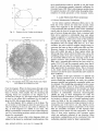
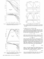
Fig. 3. Near confocal FPS fringe patterns. At each value of e,
the solid curves give the radii of the circular interference fringes
for the case of a monochromatic source and a bright fringe on
axis. The dashed line shows the spot size radius p for a finesse
of 100, and the dotted line defines the zone of best focus as a
function of . (Appendix I shows how to change the scales for
different wavelengths and mirror separations.)
(dp/dX) is obtained in the vicinity of the fringe corresponding to the lowest order of interference. For ay
given value of this fringe occurs at the value of p
which corresponds to the zone of best focus for the
spherical mirror. (By Fermat's principle, this is just
the value of p where d/dp is an extremum, or p =
(-2er).
No zone of best focus is defined for > 0.)
In the special case (very nearly approximated in most
applications) where e
0, the fringes have radii given
by:
patterns produced n the central plane of the interferometer are described by:
Type 1:
in the fringe pattern is markedly nonlinear near the axis
Ij(p,X) = Io[T/(1 - R2)2{1 + [2R/(1 -R2)]2
X sin 2 [8(p,X)/2]
}-1
(4a)
or,
Type 2:
I2(p,X)= R211(p,x)
(4b)
where,
5(p,X) = (27r/X)[A(p) + 4(r + e)].
(5)
(See Table I for a list of symbols.) The derivation of
these equations exactly follows the usual derivation for
a plane mirror Fabry-Perot interferometer (FPP).
When the mirror reflectivity R is close to unity, the
interference patterns for both types of rays are the same
and are superposed. When the two types of ray leave
the interferometer at a small angle, e.g., if the entering
beam is approximately collimated but at an angle to the
axis, they will form an additional interference pattern
made up of equally spaced straight fringes whose separations are determined by the angle at which the two
beams are brought to focus. This two-beam, i.e., sin2,
interference pattern modulates the multiple beam pat-
tern of circular fringes and, of course, arises only when
the two beams are coherent. Examples of this incidental two-beam pattern are shown in Sec. III.
From Eq. (4) we see that bright fringes are formed in
the central plane of the interferometer when
satisfies
(p,X)= 2m7r,or,
p4 /r + 4ep2/r
=
m,
Pm= [(m- t)Xr3],
(8)
where t < 1 and [4(r + e)/;\ is the exact order of interference on the axis.
It is obvious from Eq. (8) that the radial dispersion
(p,X)
(6)
where m is a positive or negative integer giving the
order of interference relative to the order on axis (which
when the interferometer is precisely confocal. This is,
of course, no real disadvantage and provides the basis
for the high tendue of which this type of instrument
is capable. If desired, the dispersion may be made
more nearly linear by slightly decreasing (or increasing)
the mirror separation. This is evident from Fig. 3 and
is illustrated in Sec. III.
B.
Spectral Resolving Power
In discussing spectral resolving power in this section,.
we assume that the interferometer is set at the confocal
spacing (el < X) and is used in the scanning mode with
a collimated light source. More specifically, we assume
that the central fringe pattern is imaged, 1 to 1, onto a
plane containing an axial aperture, coincident with the
center of the fringe pattern, behind which is located a
linear detector. Since the resonant wavelength of the
interferometer is a linear function of the mirror spacing,
it is possible to obtain a linear plot of the source spec-
trum simply by recording the output from the detector
as a function of the mirror separation.
A change of
X/4 in the mirror separation scans through a free
spectral range of c/ [4(r + )] Hz.
The spectral resolving power 61 of a spectroscopic
instrument is defined by:
(R_
V/Av", '=' X/Ax.,
(9)
where A.i is the minimum resolvable frequency increment in the vicinity of a frequency v. The classical
criterion for defining what is meant by minimum
resolvable increment is an extension of the criterion used by Rayleigh in discussing diffraction patMay 1968/ Vol. 7, No. 5 / APPLIED OPTICS 953
mains valid regardless of whether the finesse is de-
termined by the mirror reflectivity, or by other factors.
When the finesse is limited by a mirror reflectivity
whose value is close to unity, we have:
(15)
7/2(1 - R).
FR = 7rR/(1- R)
X
The fringe pattern described by Eq. (14) is shown in
Fig. 4 for representative values of the finesse.
t:
I
.1
11
In order to record the ultimate instrumental profile
in the scanning mode of operation, the detector aperture
would be vanishingly small and the resulting instrumental profile would be given by:
I
"r2
-1
(2-)[T_(]- R)-Io(v)
I(v - o)
0I
;\<"
0.10
I
I
0.40
0.30
0.20
RADIUS. p
1l
A
0.50
(IN FRINGE PLANE!
0.80
0.60
cm
Fig. 4. Calculated distribution of light i an FPS fringe pattern
for a monochromatic source and various values for F, the finesse.
Note the broad central fringe (e = 0, r = 10 cm).
terns. For convenience, we depart from this definition
slightly and define the minimum resolvablefrequency in-
crement as the apparent spectral width (full width at
half maximum) of a monochromatic line.
This is, of
course, just the width of the instrumental profile. In
practice, a large number of factors enter into the determination of the instrumental profile of a FabryPerot interferometer. These include mirror reflectivity, mirror figure, diffraction losses, and alignment.
One of the great advantages of the spherical FabryPerot interferometer over its plane parallel counterpart
is the relative ease with which reflectivity limited
resolution can be realized in practice. Neglecting all
but transmission losses at the mirrors, the instrumental
X
F
J
c/4r
II
(16)
If the detector aperture were increased, there would
initially be an increase in the amount of light collected
from a finite source, with little decrease in resolving
power (assuming perfectly spherical mirrors and confocal spacing). As the aperture was opened further,
the amount of light collected would increase less rapidly
and the resolving power would begin to decrease-becoming approximately 70% of the resolving power given
by Eq. (16) when the radius of the detector aperture
attained a value p, given by:
p = (r3X/F)I.
(17)
We will refer to p as the spot size or spot radius; p is
simply the radius of the mirror zone whose resonant
frequency is displaced from the axial resonance by an
ii
profile of an FPS is given by Eq. (4). The resulting
value for A\vn, the width of the instrumental profile, is
given by:
2
(10)
AV = c(l - R )/43ri1R.
LI
2
:t
At this point it is useful to introduce a quantity called
the finesse F of the interferometer, which we can define
as the ratio of the free spectral range to the instrumental
t:II
11
2
-4
11
width:
F =
(11)
Af/Avr.
In terms of the finesse F, the instrumental width and
spectral resolving power are given by:
AP, = C/4rF,
(12)
and
(13)
61 = 4rF/X.
Also, the expression for the interference pattern can be
written as:
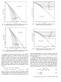
50
40
30
20
10
V0
10
20
30
40
50
FREQUENCY. MHz
(14)
Fig. 5. Calculated FPS instrumental profiles for two different
detector aperture radii. These correspond to the spectra which
Here we have simply made the substitution, F =
rR/(l -R 2) in Eq. (4). Note that this expression re-
would be recorded using a monochromatic source in the scanning
mode of operation (e = 0, r = 10 cm). (a) p = 0.05, (b) p = 0.2.
I=
(1
R
1 + (2F/r)
2
sin2 (3/2)
954 APPLIED OPTICS / Vol. 7, No. 5 / May 1968
amount equal to the minimum resolvable frequency
increment Avm. The actual instrumental profile that
is obtained when using a finite detector aperture is
given by:
I,(v
o) = 2 r
-
f
I(t)xdx,
(18)
[ - vo(l + x4/4r4)]
{(T/(1-
2
R)2I{ 1 + (2F/r)' sin- [rt/(c/4r)] -1
and where v is the frequency that would be recorded
using a vanishingly small aperture. Note that with a
finite aperture, the instrumental profile is no longer
centered on voand is asymetric. Figure 5 shows computed instrumental profiles for various values of F and
p, the aperture radius (cf., Fig. 14 in Sec. III).
OtherFactorsAffecting Instrumental Finesse
We have seen [Eq. (15) ] that in the absence of other
losses, the instrumental finesse is limited by the reflectivity of the mirrors to a value of approximately
7r/[2(1 - R) ]. In this section we consider the manner
in which the finesse is degraded by other factors,
namely, irregularities in the surfaces of the mirrors, and
diffraction. If we wish, we can associate with each
loss mechanism, e.g., mirror transmission or diffraction,
a contribution to the lifetime of the resonant cavity.
The finesse F associated with the ith loss mechanism,
is related to the corresponding contribution to the
cavity lifetime Ti by:
F = rcrT/2r.
(19)
Hence it is clear that the net instrumental finesse F
is related to the individual contributions Fi by:
F- = (Fi)-',
i
(20)
so that it is useful and meaningful to consider the in-
dividual contributions to the finesse independently.
First we consider the effect of irregularities in the
figure of the mirror on the finesse. Without knowledge
of the specific nature of these irregularities, it is impossible to be precise in predicting their effect on the
finesse. Generally, however, if the mirrors have a
smooth* irregularity on the order of X/m across the
aperture being used, then the figure-limited finesse
F- will be approximately:
Ff
m/2.
increased diffraction losses that
accompany the re-
duction of the etalon aperture set a limit to the improveNote also that in the case of the plane mirror FabryPerot, an angular misalignment of the plates is equivalent to a corresponding plate imperfection. For the
spherical Fabry-Perot, this is not the case: an angular
misalignment merely redefines the optical axis of the
and
I(Q)=
etalon; in the case of a plane
mirror Fabry-Perot etalon, however, the significantly
ment in finesse that can be realized by this technique.
rP
where
=
a spherical Fabry-Perot
(21)
Obviously, by reducing the aperture (or diameter of the
incident light beam) it is possible to minimize the reduction in instrumental finesse due to plate irregularities. This is indeed a practical expedient in the case of
* If the irregularity is not smooth, the loss incurred is more
appropriately treated as a scattering loss.
system. With regard to plate irregularities, it is
worthwhile pointing out another contrast between the
plate-mirror and spherical-mirror etalons. If the mirrors of an FPP have irregularities on the order of X/2,
the resultant pattern at infinity will be completely
washed out.
However, since the fringe pattern ob-
tained with an FPS is localized relatively close to the
surfaces of the mirrors, a similar mirror figure irregularity will not wash out the fringe pattern, but will instead distort it so that the fringes are no longer circular.
(These distorted fringes tend to define coutours of equal
path difference.)
As implied above, diffraction losses are much less in
the case of a spherical Fabry-Perot etalon than for its
plane mirror counterpart. The rigorous justification
of this statement lies in the analytical treatment of
confocal resonators given by Boyd and Gordon,7 in
which they show that for any case of practical interest
to us, i.e., those cases where D 2 /4r >> X, D being the
diameter of the mirror aperture, the diffraction losses
for a confocal resonator are orders of magnitude less
than for the corresponding plane parallel resonator.
The calculation of the exact diffraction loss in a confocal
resonator requires a fairly complex analysis in which
the incoming radiation field is decomposed into eigenmodes of the cavity, each of which has a different
diffraction loss. Absolute minimization of the diffraction losses requires proper mode matching (see Sec.
II.D). In this case, when the incoming radiation field
has a curvature and amplitude distribution identical to
that of the lowest order transverse mode of the confocal
resonator, the diffraction loss per pass LD is approximately given by7 :
LD ;
10-[5(po2/rX)+1]
(22)
where p is the radius of the mirror aperture. In any
case of practical interest, diffraction losses are completely negligible in comparison to other losses, so that
diffraction plays no significant role in determining the
over-all finesse. For a plane parallel Fabry-Perot
etalon, the diffraction limited finesse is approximately
given by:
FD(FPP)
D2/2Xd,
(23)
where d is the separation of the plane mirrors and D is
the aperture diameter.
Other types of loss, such as scattering at the mirror
surface (which is, of course, taken into account in FR),
can be treated separately very easily. If a small fraction L of the radiation incident on the mirror (or making
a transit of the resonator) is lost, then by analogy to
May 1968 / Vol. 7, No. 5 / APPLIED OPTICS 955
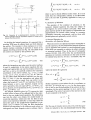
2. Transmission and Etendue of a Spherical FabryPerot Interferometer
In Sec. II.A it was pointed out that a single beam of
light incident on an FPS gives rise to two transmitted
beams, which are generally at a small angle to one
another. When both of these transmitted beams are
taken into account, the net transmission To at the
Fig. 6.
Generalized
picture
of a spectrometer
or monochro-
meter.
center of the instrument profile is found from Eq. (4a)
and (4b):
2[T/(1 - R)Y2, for
To = (1 + R')(T/[1 - R])'
1.
R
Eq. (15), the corresponding contribution to the finesse
is given by:
FL
7r/2L.
(24)
To summarize the implications of this section, we can
say that for a spherical Fabry-Perot interferometer, in
confocal adjustment, the significant factors in determining the finesse and resolving power are the reflectivity of the mirrors and their surface figure. This
is in contrast to the case of a plane parallel Fabry-Perot,
where diffraction and alignment can make significant
contributions to the degradation of finesse and resolving
power.
C.
Light Gathering Power
1.
Introduction
(27)
(When the two transmitted beams are precisely aligned,
the situation is somewhat different, as discussed in Sec.
II.D.) If we define A to be the sum of the absorption
and scattering at the mirrors, then (1 - R) = (T + A),
so that the peak transmission may be written as:
To -
[1 + (A/T)]-I
(28)
This function is plotted in Fig. 7, which clearly illus-
trates the drastic loss in net transmission whenever the
losses become comparable
absorption-plus-scattering
with, or exceed, the transmission loss at the mirror.
As a rule, very high reflectivities can be attained only
at the expense of increased values of (A/T), so that it is
often necessary in practice to make a compromise between finesse and transmission. This type of compromise is discussed further in Sec. III.
In the last section we found that the ultimate instru-
One of the major factors to consider in evaluating any
spectrometer is its ability to effectively gather light
from an incoherent extended source, filter it with the
instrumental bandpass, and transmit it to some radiation detector. In general, the situation can be represented by Fig. 6. Here, the spectrometer is depicted
as a bandpass filter: all of the radiation emanating from
within a solid angle Q subtended at an aperture of area
A, can be transmitted within the bandpass Avm of the
spectrometer. If the transmission of the spectrometer
at the center of the bandpass is To and the spectral
radiance of the source is N,, then the radiant power per
mental resolution, which we now call 6Ro,could be obtained only with an infinitesimally small axial aperture.
In this case, of course, the 4tendue is also infinitesimal.
A reasonable compromise between spectral resolving
power and 6tendue can be reached by increasing the
mirror aperture until the resolving power a is reduced
to a value of approximately 0.7 61o. This, as we have
seen, occurs when the mirror apertures have radii of
approximately p,. Under this condition, the 6tendue
is given by:
U =' [7rp,] [7rp'/r2] = 7r2rX/F,
(29)
unit bandwidth P, transmitted by the spectrometer is
given by:
p= N,AQT,.
Or.)
o.4
The product O2Ahas come to be known as 6tendue U of
the spectrometer. Thus the easily remembered expression:
0
.
.3
.
P = VUTo.
(26)
z
Of course, if the light source under investigation is a
laser, it is obvious that most of the emitted power can
be put into a beam with a small cross-sectional area
and a small divergence. In this case, the 6tendue of the
spectrometer provides a measure of the alignment
tolerance between the laser beam and spectrometer,
rather than being a measure of the spectrometer's light
gathering power.
956
APPLIED OPTICS / Vol. 7, No. 5 / May 1968
.
0
5
4
3
2
,
RATIO OF MIRROR ABSORPTION TO TRANSMISSION,
6
7
A/T
Fig. 7. FPS instrumental transmission as a function of the
(absorption:transmission) ratio of the mirror coatings.
I
g
0-~~~~~0
E 40
t~D
-
constant:
, 20
r,
((R/U)FPS
15
-i 30
02
-
In fact, the quotient (R/U is a
so also is the 6tendue.'
50
caI.10
I0o
lo
O
X
.1
.2
C6
5
v)
o
.1
Aperture radius, p(cm.)
(a )
.2
Aperture radius,p(cm.)
(30)
In writing this expression, we accept the 20%o to 30%
loss in resolution which accompanies the realization of
the tendue U. We also assume that, as the mirror
radius is increased to realize higher resolving powers, we
are able to maintain the required figure of
/F across
the central part of the mirror having a radius ps. It is interesting to compare this behavior with that of an FPP.
(b)
We assume that for an FPP, a net surface figure (including alignment error) of X/F can be maintained
across plates of diameter D, which are separated by a
5
distance d. For this FPP the tendue is (7rD2X/4dF),
C-
and the resolving power is (2df/X), so that it is the
product of the resolving power and tendue which re-
mains constant:
E
a-.
3
0.7(2F/rX)2 .
.E
.I
F =300
c
o
.1
(U(R)Fpp
E-
4E
.2
Aperture radius, p (cm)
(c )
0
.1
.2
Aperture radius, p (cm 1
(d)
Fig. 8. Computed FPS characteristics as a function of detector
aperture radius p for different values of F the finesse. Arrows
indicate the value of p in each case (e = 0, r = 10 cm). The
maxima in the curves shown in (d) define the aperture radius
giving the best compromise between resolving power and peak
transmitted power.
according to Eq. (17).
Figure 8 shows computed curves for the instrumental
bandwidth, spectral resolving power, peak transmitted
power, and the product (peak transmitted power) X
(resolving power), all plotted as a function of aperture
radius for finesses of 30, 100, and 300. These curves
(31)
(The factor of 0.7 again represents the loss in resolving
power associated with a useful 6tendue.) Thus an increase in light gathering power must be paid for by a
loss in resolution, and vice versa. The corresponding
product for an FPS is given by:
(UR)FPS
0.7(4ir2 r2 ).
(32)
From this expression we see that by increasing the
mirror radius of an FPS the tendue resolution product
may be increased indefinitely as long as the mirror figure
can be maintained to within X/F across an aperture of
diameter
where F is the finesse which determines the value of s
0.7( 7 D2 /2).
2
ps
-=
2(Xr3/F) l.
At this point, it should be quite clear that at high
resolution,
and correspondingly
small free spectral
range, the FPS excells over the FPP, both in terms of
6tendue and resolution. As the free spectral range is
increased, however, there will be some point at which
the FPP will become the better choice in terms of
6tendue.
The specific value of r, the mirror spacing of
show that the resolution drops to about 0.7R0 when the
the FPS, at which this transition occurs depends upon
both the desired finesse and the accuracy with which
the mirrors of the FPP can be figured and aligned. If
we define an angle a to represent the figure-plus-align-
and power transmitted is approximately 0.8p,. In
ment accuracy required to maintain a finesse F with
practice, the most convenient way to quickly attain a
useful compromise between resolution and transmitted
a= (x/FD),
aperture is opened up to a value of p = (Xr3/F) 1.
Figure (8d), however, shows that the value of p which
maximizes the product of the spectral resolving power
power is to start with a relatively large aperture and,
while observing the scanned spectrum of a narrow band
a plate diameter D:
then the ratio UFPS/UFPP
may be written:
source, to reduce the aperture size until the transmitted
power at the peak of a displayed spectral line is reduced
by between 20% and 30%. For this technique to be
useful, of course, the mirror spacing must be very
nearly confocal. This can be accomplished without
much difficulty, as described in Sec. III.
3. Comparisonof FPS and FPP
As Connes has pointed out, it is a unique characteris-
tic of the FPS, amongst all other types of spectrometers,
that, as the resolving power at constant finesse is in-
creased (by increasing the mirror radii and separation),
(33)
Upps/Uppp
= 4rdF2
2 2
ac /X ,
(34)
where d is the plate separation of the FPP and where we
tacitly assume that the spot size p on the FPS is small
enough so that there is no problem in maintaining the
necessary figure of X/F. If we now require that both
the FPP and FPS have the same free spectral range, so
that d = 2r, then Eq. (34) can be used to find the value
of r at which the FPP becomes the better choice with
regard to 6tendue:
r* = (X/a)/2F.
'(35)
May 1968 / Vol. 7, No. 5 / APPLIED OPTICS 957
called axial mode number giving the number of axial
modes in the intracavity standing wave. For the
general case of a resonator made up of two mirrors,
radii b and b, separated by a distance d, Boyd and
Kogelnik have shown that the resonant frequency
associated with a given TEllImn, mode is given by:
= (c/2d){q + (1/17)(1 + n + n)
vmnq
X cos'[(l
-
d/bl)(1 - d/b,) 1}.
(36)
(a)
We interpret this as follows: an arbitrary quasi-monochromatic field, of frequency v, which is incident on a
curved mirror resonator, is decomposed into a large
number of transverse modes TEMmn. Each of these
transverse modes will be resonant, i.e., will be transmitted by the high Q cavity, for mirror separations
satisfying:
d = (c/2vo){q + (1 +
X cos-'[(l
(b)
Fig. 9.
(a) Scan and fringe displays of an FPS in normal opera-
tion. Note the secondary fringe pattern. (b) Scan and fringe
displays of a very nearly mode-matched FPS. The alignment
of the FPS relative to the source has been adjusted to eliminate
the secondary fringe pattern, resulting in a doubling of both
the free spectral range and the instrumental transmission.
(e
20 u, r
=
5 cm; three-mode
laser source.)
For example, if the mirrors of an FPP can be maintained
plane and parallel to within a hundredth of a wavelength
per cm of aperture, so that (X/a) is 100, and a finesse
of 25 is desired, then an FPP offers the greater 6tendue
up to a mirror spacing of 4 cm. Rather than increasing
the FPP mirror spacing beyond 4 cm, one should in
principle, switch to an FPS in order to obtain higher
resolution and maximum 6tendue.
D.
n + n)
958 APPLIED OPTICS / Vol. 7, No. 5 / May 1968
d/bl)(1
-
d/b,)J1}.
(37)
In general, therefore, a given quasi-monochromatic
field will be decomposed into a large number of transverse modes, each of which is resonant for a different
mirror separation. In order for a general curved mirror
cavity to be useful as a scanning spectrum analyzer
(or static filter), the input field must be reduced to a
single transverse mode of the cavity, i.e., mode
matched, so that the transmission of the cavity, as a
function of mirror separation, can be unambiguously
interpreted in terms of the frequency content of the input field. This can be accomplished without considerable loss of light only in the case of a laser light source
operating in a single transverse mode.
For the special case of a confocal, or near confocal
resonator, such as an FPS, Eqs. (36) and (37) become:
n [4(r + e)][2q + (1 + m + n)],
Vmnq
(36a)
and
Mode Analysis of an FPS
The equations derived earlier in this section have
been based primarily on a geometrical analysis of a
confocal resonator, or FPS. This, as it turns out, is
adequate for most purposes. A more rigorous treatment, however, would involve a decomposition of the
incident radiation field into eigenmodes of the resonator, as defined (in the curved mirror case) by Boyd and
Gordon.7 In this section we outline an analysis of this
sort and to some extent justify the simpler geometrical
approach. We should point out that the aberrations of
a confocal spherical mirror resonator, which give rise
to the multiple beam interference fringes described
earlier, can be conveniently analyzed only by the
geometrical approach.
As shown by Boyd and Gordon, the eigenmodes
TEMmnq of a confocal resonator are closely approximated by Gaussian-Hermite functions [Ref. 7, Eq.
(20)]. The first two subscripts m and n denote the
amplitude distribution of the eigenmode on a surface
of constant phase, and the third subscript q is the so-
-
(c/4vo)[2q + (1 + m + n)],
(r + e)
(37b)
where the mirrors have radii r and are separated by
(r + e) - r. Thus, all transverse modeswill resonate at
cavity lengths of either,
(r +
e)
=
(c/4vo)(21 + 1); 1 an integer, (m + n) even,
(38a)
or
(r +
e)
= (c/4vo)(21); (n + n) odd.
(38b)
If we assume that an arbitrary input field of frequency
v is made up of an approximately equal number of
even and odd transverse modes (a good approximation
in any instance where mode-matching is not inten-
tionally accomplished),then the cavity will be resonant
for:
(r +
e)
= l/ 4 vo; 1an integer,
(39)
and the multimode free spectral range will be
Avf(multimode)- c/4r
(40)
If, on the other hand, the input field exactly matches a
single mode of the cavity, the free spectral range is
Avf(single transverse
mode)
c/2r.
(41)
The transition from multimode to single mode excitation can be observed without undue difficulty, as illustrated in Fig. 9. (Note that the free spectral range increases by a factor of two for both scanning and static
fringe modes of use of the FPS.) The tolerance on the
alignment of the light beam relative to the axis of the
FPS that is required for mode matched operation is
on the order of X/p8, so that it is highly unlikely that
this situation would be encountered inadvertently.
Mode matching of an FPS can also be considered from
a more direct point of view. We have already mentioned the additional interference pattern arising from
an angular misalignment of the two types of rays transmitted by the FPS. It is easy to show that, when these
two types of transmittkd beams are aligned, they are
in phase on axis (assuming r = mX/2), just out of phase
at the first fringe off axis, in phase again for the second
fringe, and so on. Thus the superposition of the two
transmitted beams results in constructive interference
in every other free spectral range, and destructive ineffectively
terference in the remaining orders-thereby
doubling the free spectral range and at the same time
doubling the amount of light transmitted at a given
resonance (when constructive interference occurs for
the transmitted beams, destructive interference occurs for
the two reflected beams).
The great advantage of the confocal FPS over a
general curved mirror resonator is the freedom from
the necessity to mode-match in order to observe a clean
spectrum. This, as we have just seen, is due to the
frequency degeneracy of even and odd transverse modes
of a confocal cavity. It can readily be shown from
Eq. (36) that the maximum value of el, the departure
from exact confocal mirror spacing, which can be
tolerated without allowing the TEMm,, transverse
mode to resonate at an observably different mirror
spacing from that at which the T1EMoomode is resonant,
is given by:
A. General Design Considerations
There are three separate aspects of the design
problem: (1) the mechanical design; (2) the attain-
ment of high finesse, and (3) the optical layout. Each
of these is briefly discussed in the following paragraphs.
1. MechanicalDesign
The key mechanical requirements are that the two
mirrors be accurately and rigidly fixed relative to each
other; that there be a provision for making fine
adjustments to the mirror separation (either during or
after fabrication); that the optical separation of the
mirrors be insensitive to temperature
and/or pressure
variation; and that the interferometer assembly be
mechanically isolated from vibration and acoustic
pickup. The requirements for rigidity and freedom
from vibration dictate that the mirrors be held in a
common structure, rather than mounted, for example,
on a lens bench. This, in turn, means that any transducer used for varying the mechanical separation of the
mirrors must be an integral part of the interferometer.
Mechanical isolation of the rigid interferometer assembly is readily accomplished by mounting it in an
outer case using a soft suspension (in the specific designs described later in this section, the outer case could
be sharply struck without producing a detectable
change in the observed spectrum-indicating a stability in the length of the optical cavity on the order of
a one hundredth of a wavelength or better).
Insensitivity to pressure variations can be accomplished only by sealing the container holding the interferometer. This must be done, in any event, if the
interferometer is to be pressure scanned. Insensitivity
to temperature variations can be achieved both by conventional compensation, in which the expansions of
dissimilar materials compensate for one another, and
by the use of very low expansion materials. In an
interferometer intended to serve as a passive frequency
standard, we have combined both methods. As long
as this interferometer is at a uniform temperature, its
the variation in the mirror separation which occurs
length can be maintained to within one part in 101over
a range of a few degrees centigrade.
The fine adjustment of mirror separation can easily
be obtained using a well-made threaded mount for one
mirror cell. For example, we found that a 12.7-mm
diam cell with 16 threads/cm could be manually adjusted with a precision of at least a tenth of a wave-
during direct scanning (less than a wavelength) is too
small to affect the transverse mode degeneracy. Of
course if pressure scanning is employed, it is the wave-
monitored by observing the spectrum from a stable
gas laser. (Most gas lasers are far less stable, both
IEas =
-rr/2(1
+ m + n)F
(42)
Thus an FPS with r = 10 cm and a finesse of 100 will
begin to suffer a loss in effective finesse for (m + n)
100 when I becomes greater than about 15 . Thus
length of the light which is changed, not the mirror
separation.
Ill.
Experimental Work with the FPS
This section is concerned with the practical aspects
of the FPS, including its design and fabrication, alignment procedures, and various modes of operation. A
number of applications are illustrated in the latter
parts of this section.
length providing that the mirror separation could be
mechanically and thermally, than the interferometers
described here.) We were pleasantly surprised to find
that the same precision of motion could also be obtained
with a relatively loose screw fit when the slop was taken
up with a thin Teflon tape commercially available as a
pipe dope.
2. Attainment of High Finesse
The attainment of high finesse requires that the
mirrors be of excellent optical quality and that they be
May 1968 / Vol. 7, No. 5 / APPLIED OPTICS
959
Table II.
Type
.4
B
C
power. This permits the use of mirrors with concentric
surfaces, which simplifies fabrication. More impor-
Characteristics of Some Multilayer
Reflective Coatings
tantly though, it means that the interferometer can be
Region of high
r-eflectivity
F
To
1?
6200 Xto 7000AX
4800AXto 6900AX
4900 A to 6800 A
225
150
180-200
0A45
0.35
0.02
0.993
0.99
0.992
used to spectrally filter a narrow collimated beam of
light without appreciably affecting the collimation of
the beam. If a further optical system is added to the
FPS, it should serve to facilitate the alignment of the
FPS with the light source, and to get light efficiently
through the interferometer and within the instrumental
coated with high reflectivity multilayer dielectric films.
For scanning applications, only the central spot, of
radius p, need satisfy these requirements. If the
interferometer is used to observe fringes, however, the
mirror figure should be good over a somewhat larger
area to ensure that the fringes will be circular. Mirror
blanks should be tested against the same master; they
generally require final polishing by hand if they are to
have the necessary figure-that is to say, if they are to
be spherical to within X/F, where F is the desired
finesse. Final evaluation of the mirror figure can only
be made after the mirror has been coated and tested
as an interferometer component. Not only must the
mirror figure be excellent, but the polished surface
must be free of microscopic scattering sites if the ultimate in reflectivity is to be realized. This is within
the present state of the art, and scattering losses of
less than 0.3% are attainable with fused quartz blanks.*
As we suggested in the last section, one is usually
forced to make some sort of compromise between finesse,
instrumental transmission, and possibly the spectral
bandwidth within which the mirrors have high reflectivity. For example, using commercially available
multilayer coatings (referred to as types A, B, and C)
we were able to obtain the performance summarized
in Table II. Type A is a narrow band coating covering
a rather restricted spectral range, but offers high finesse
combined with excellent transmission. Type B covers
a considerably broader portion of the spectrum with
fairly high instrumental transmission, but has a somewhat reduced finesse. Type C, on the other hand, has
broad band coverage and relatively high finesse, but
rather low transmission. By making fairly drastic
sacrifices in instrumental transmission, it is probably
possible to obtain finesses of up to 500 with commercially available coatings and a passive interferometer.
This limitation is not set by available reflectivity, but
by attainable mirror figure (or diff raction losses in the
case of very short cavities).
passband. Figure 10 illustrates an optical system
which has proved to be convenient and versatile. Consider first an incident collimated beam: lens Li brings
the incident radiation to focus at the center of the
(Note that the path of light within
interferometer.
the interferometer is just the reverse of the case where
the light incident on the interferometer is collimated.)
All of the light falling within a central circle of radius
on lens L, will pass through the detector aperture
2p~f/r
of radius p, and will thus be filtered by the instrumental
passband. In this mode of operation the FPS can be
used as a static or tunable filter, or as a scanning spectrum analyzer. If the incident light is not collimated,
there is no significant loss in resolution, but there may
be a reduction in the amount of light received by the
detector. This holds even for gross departures from
collimation in the incident beam of light. The entire
system should be free to rotate about the center of Li.
In this way the incoming beam can-be directed at the
center of Li and then the entire interferometer system
can be rotated about this point in order to attain alignment between the incoming beam of light and the axis
of the FPS. The detector aperture, which limits the
actual instrumental bandpass for incident beams with
a large diameter, is located just behind the interferometer.
APERTURE,
-ps
~~~~~RADIUS
(a)
(b
S. Optical Layout
By optical layout we mean the optical system which
brings the light into the interferometer and determines
the path of light leaving the interferometer. For a
number of reasons we have preferred to make the interferometer mirror blanks of very nearly zero optical
.* It is now generally recognized that essentially scatter-free
surfaces of excellent figure can be obtained by continuous and extended (12-36 h) final polishing of fused quartz blanks.
960 APPLIED OPTICS
DETECTOR
FPS
,-~~
LI
/
Vol. 7, No. 5
/
May 1968
LI
54}
FPS
RfT1
1
0
'
1.,-
INCIDENT
LIGHT
Mc
Fig. 10. A versatile FF8 instrument. (a) Optical layout showing the FPS etalon, lens LI, and detector aperture; (b) arrangement for scanning; (c) arrangement for observing and recording
fringe pattern (detector removed).
We have not yet established the lower limit on the
frequency stability of this system.
The interferometer assembly is held inside a pressure
chamber by means of phosphor-bronze finger-stock
springs, which provide adequate mechanical isolation.
The pressure chamber can be used for pressure scanning,
or it can be partially evacuated and sealed to eliminate
effects due to changes in atmospheric pressure.
Applications for this type of interferometer include
ultrahigh resolution spectroscopy, and use as a passive
feedback component in frequency stabilizing lasers.
Fig. 11. Schematic of a highly stable fixed mirror FPS etalon:
(1) outer case (Al alloy);
(2) end plates with
windows;
(3)
Cer-Vit etalon spacer; (4) fused quartz mirrors; (5) fixed mirror
cell (Invar);
(6), (7) adjustable
mirror cell (Invar);
(8) ports in
etalon spacer; (9) phosphor bronze springs holding etalon;
(10) fixture for evacuating chamber and pressure scanning.
This design facilitates the observation of the static
fringe pattern.
If the detector aperture is removed and
a quasi-collimated beam of light is incident on what was
the rear of the system, then the fringe pattern will be
formed in the focal plane of lens L. Thus an observer,
or camera focused on infinity, can readily view the
fringe pattern. If the incident beam is diverging,
rather than collimated, then the plane of the fringe pat-
tern will be slightly displaced towards the lens, and vice
versa. A low power focusing telescope is useful both
for observing the fringe pattern, and for photographing
it. In this mode of operation, the system should be
mounted so that it can be rotated about a point near
the right-hand interferometer mirror [Fig. 10(c) ]. To
use the interferometer as a narrow bandpass filter with
zero optical power, the lens is simply removed.
In order to eliminate ghost fringe patterns, the rear
surfaces of the FPS mirrors, and both surfaces of L,
should be antireflection coated.
C.
A Piezo-electrically Scanned FPS System
This instrument is designed along the lines illustrated
in Fig. 10, and can be used as a scanning spectrum
analyzer, as a tunable narrow bandpass filter with zero
optical power, or for direct observation of multiple beam
interference fringes. The key element in the instrument is the FPS etalon, which is comprised of a fixed
and an adjustable mirror cell, and a thermally compensated rigid spacer tube. The spacer tube includes, as
an integral component, a piezo-electric ceramic section
which increases in length by about 1.5 cm X 10- cm
with the application of 50 V across the inner and outer
surfaces of the tube (sufficient to scan a complete free
spectral range in the visible). The adjustable mirror
cell permits the mirror spacing to be easily set to within
a fraction of a micron. Further fine adjustment can
be accomplished by applying a dc voltage to the scan-
ning voltage terminal; this is the method of tuning in
the bandpass-filter mode of operation. Figure
shows a cut-away view of the entire instrument.
12
The FPS etalon is mechanically isolated from the
case by a mounting technique using two large silicone
rubber 0-rings which cushion the etalon from mechanical shocks (see Fig. 12). The outer case can be struck
sharply from any direction without noticeably affecting
the resonant frequency of the etalon. As shown in Fig.
B.
Design of a Static or Pressure Scanned FPS
This design, shown in Fig. 11, is intended primarily
to eliminate variation of the axial mirror separation
with temperature.
This FPS is thus well suited for
use as a secondary frequency standard with a long term
stability of better than 1 MHz with temperature control of - 1 C. This thermal stability is obtained by
making the mirror spacer of Cer-Vit* (thermal expansion coefficient no greater than zi 0.1 X 10⁻⁷/C), and
using the Invar mirror cells thermally to compensate
for the residual expansion of the Cer-Vit (this can
easily be done since the manufacturers of Cer-Vit
routinely supply accurate expansion data for each
blank). The quartz mirrors change radius by about a
wavelength for a 1 C temperature change, but this introduces a negligible change in the mirror separation,
which determines the resonant frequency of the FPS.
Cer Vit is a low expansion semitransparent gasslike ceramic
manufactured by Owens-Illinois.
*
Fig. 12. An FPS spectrum analyzer for scanning or static mode
of operation: (1) removable detector (photodiode); (2) soft
O-ring for mounting FPS etalon; (3) quartz mirrors (r = 5 cm);
(4) piezo-electric transducer/etalon spacer; (5) scanning voltage
terminal; (6) auxiliary lens (focal point is between mirrors);
(7) mounting
flange;
(8), (9) adjustable
mirror cell;
(10) fixed
mirror cell; (11) outer case. (The mirror cells are designed to
compensate for the thermal expansion of the etalon spacer.)
May 1968 / Vol. 7, No. 5 / APPLIED OPTICS 961
multilayer dielectric mirrors, we can obtain a finesse of
greater than 150 over a spectral range of about 1200 A,
and with an instrumental transmission of 40% to 45%
(compared with the maximum of 50% in the nonmodematched configuration). With careful mode matching,
the instrumental transmission goes to 80-90%, the free
spectral range becomes 3000 MHz, and the finesse is
the resolving power unchanged.
doubled-leaving
With broadband multilayer mirrors, a finesse of 150 can
be maintained from about 4900 A to 7000 A, with an
instrumental transmission of approximately 25% (or
50% when mode matched). With these mirrors, this
instrument has been used for high resolution spectroscopy with argon lasers (4880 A and 5145 A), He-Ne
lasers (6328 A) and Q-switched ruby lasers (6943 A).
A variety of experimental data is shown in Sec. III.E.
(a)
(b)
In the scanning mode, the instrument is very easy to
align to the incident
instrument is located
(preferably, but not
mated) falls close to
beam of light. First of all, the
so that the incident light beam
necessarily, more or less collithe center of the lens. The axis
of the instrument is then roughly aligned with the
incident beam.
(c)
Fig. 13. Typical fringe patterns in the vicinity of confocal
separation for a 10-cm FPS. In each case, the source is a single
mode Hle-Ne laser. Variations in the fringe patterns in each
horizontal row were obtained by making small changes (<X/4)
(a) e = -70,u, (b) e = 0, (c) e = 70 u.
in the mirror separation.
10, the lens at one end of the instrument serves either
of two functions: to direct an incident beam of radiation into the center of the FPS etalon (scanning or filter
modes of operation), or to image the interference fringe
pattern at infinity when light is incident on the other
end of the instrument (visual or photographic modes of
operation). In the scanning mode, a small photodetector is mounted directly behind the FPS. We have
used both a silicon photodiode and a photomultiplier as
the detector (the majority of the scans shown in Sec.
III.E were obtained with a photodiode operating in the
photovoltaic mode).
Since it is desirable-for
ease in
alignment-to rotate the entire instrument about the
entrance aperture, the mounting flange can be attached
at either end of the instrument. This flange then
serves to attach the instrument to a mirror-mount
which is adjustable in angle.
The mirror radius in the FPS is 5 cm, with a corresponding free spectral range of 1500 MHz.* Using
By replacing the 5-cm radius mirrors
one mirror cell to provide for
modifying
and
mirrors,
1-cm
with
*Note added in proof:
a 1-cm mirror separation, -we were recently able to extend the
free spectral range of this instrument to 7.5 GHz (or 0.09 A at
6000 A.). Using narrowband mirrors, a finesse in excess of 100
was easily attained with a 0.5-mm detector aperture. This
type of instrument has proved useful in examining ion laser
Comparable finesse in an FPP
spectra.
spectral range is very difficult to obtain.
This can be done most conveniently
by observingthe light that has been reflected from the
with the same free
962 APPLIED OPTICS / Vol. 7, No. 5 / May 1968
FPS back towards the source: the reflected beam should
be adjusted to lie fairly close to the incident beam. At
this point a high resolution scan display can be observed by monitoring the detector output at an oscilloscope. The display is peaked by further small adjustments to the alignment. The scanning voltage is conveniently provided by the sawtooth (or horizontal scan)
voltage from the oscilloscope. This voltage will
typically scan two or three free spectral ranges, and
assures synchronism between the applied scanning
voltage and the oscilloscope sweep. Moreover, this
technique provides a highly linear display of the optical
spectrum at the oscilloscope.
To observe interference fringes, the detector is removed and the incident beam is directed towards the
end of the instrument at which the detector was located.
The fringe pattern can then be viewed directly through
the lens, or an auxiliary telescope can be used. The
latter is particularly useful when the incident beam is
not collimated, resulting in a displacement of the plane
of the fringe pattern away from the focal plane of the
lens. The proper alignment of the instrument axis
relative to the incident beam of light can be made by
observing fringe pattern and making angular adjust-
ments to make the fringes circular. As mentioned
earlier, it may be desirable to change the mirror spacing
slightly to obtain a more nearly linear display of
frequency in the fringe pattern, although this entails a
reduction in the realizable spectral resolution (Fig. 14).
D.
Alignment Procedures
In assembling and using FPS interferometers, only a
few alignments or adjustments are required, and in this
section procedures for these are briefly described.
Establishing the Confocal Mirror Separation
We have pointed out that optimum performance of an
FPS depends critically upon the proper spacing of the
mirrors. Connes has described an imaging technique
for approximating this adjustment which requires only
a small incoherent light source.2 If a He-Ne laser is
available, the alignment can be made with high pre1.
cision as follows. First, adjust the mirror separation
to within a millimeter or so from knowledge of the mirror
radii. Then, set up the FPS etalon so that a quasicollimated beam from the gas laser is incident on one
mirror, and arrange to view the interference fringes
which are formed in the vicinity of the central plane of
the etalon. The laser beam diameter should be large
enough to allow several fringes to be seen. Next,
make a fine adjustment of the mirror separation to bring
the mirrors closer togetherby a fraction of a wavelength,
and observe the resulting change in the central fringe
radius. This fine adjustment can usually be made by
manually squeezing the etalon. If the mirror separa-
tion is greaterthan the confocal separation, the central
fringe will become smaller in diameter as the mirrors are
moved towards each other. If the mirror separation is
less than the confocal spacing, the central fringe diameter will increase as the mirrors are moved towards one
another. Figure 13 shows the appearance of the central
fringes on either side of exact confocal spacing, as well
as at the confocal spacing. As shown in Fig. 13(a),
when the mirrors are spaced by slightly less than conof
focal spacing, there is a zone [radius (2er)i]
high dispersion toward which all fringes gravitate as
the mirror spacing is slightly reduced (or, equivalently,
as the wavelength of the quasi-monochromatic light
source is increased). This zone approaches the center
of the fringe pattern as the mirror separation is increased, and disappears through the center of the pattern when the confocal spacing is exceeded. The location of this zone is an extremely sensitive indication of
the mirror separation, and when the mirrors are exactly
confocal it is at the center of the fringe pattern. The
radius of this zone, as a function of mirror separation,
is shown by the dotted line in Fig. 3.
If the FPS is set up in the scanning mode it is possible
to peak up the adjustment of the mirror separation
merely by maximizing the amplitude of a displayed
laser spectrum while at the same time minimizing the
apparent width of individual spectral components.
With very little practice it becomes a simple matter to
establish confocal separation to within a micron or so
using this technique. As the optimum mirror separation is approached, one should also make fine adjusta very small
ments to the angular alignment-unless
diameter beam is used, in which case the spectral display is relatively insensitive to alignment.
2.
Selecting the Optimum Detector Aperture
As mentioned earlier, the diameter of the detector
aperture [or, equivalently, the diameter of the incident
beam: see Fig. 10(a) serves to define both the actual
instrumental bandwidth and the tendue. As a rule,
one seeks a compromise in which a considerable 6tendue
can be attained with only slight sacrifice in resolving
power. The curves in Fig. 8(d) show that the optimum
compromise occurs when the radius of the detector
aperture (assuming it to be located adjacent to the rear
interferometer mirror) is just under p,. Figure 14
shows experimental data for the instrument profile of a
10-cm FPS, with a nominal finesse of just over 100, for
various detector apertures. In this figure the desirability of using the optimum detector aperture is obvious.
For larger apertures, the peak transmitted power goes
up very little, and the resolution goes down. Note,
however, that at larger apertures more total light is
transmitted: this may be an important consideration
in applications involving weak light sources. It is
worth pointing out that the finite time constant of a
high finesse FPS precludes the use of very high sweep
speeds without suffering a loss in resolution-in this
case, too, it would make sense to use a somewhat larger
detector aperture than normal.
S. Alignment for Mode Matching
There are undoubtedly applications where it might
prove useful to extend the free spectral range of an FPS
by mode matching. The gain in free spectral range is
accompanied by a twofold increase in both finesse and
instrumental transmission, so that there is no loss in
spectral resolution. There is, however, a very great
reduction in the tolerance of the alignment between
the FPS axis and the incident light beam, and there is
also the restriction that the incoming beam match a
lowest order transverse mode of the cavity.
This latter
restriction is less severe than it might be, due to the
degeneracy of a confocal cavity. Unlike a general
curved mirror cavity, the position of the beam waist of
the lowest order transverse mode is not uniquely de-
D =.I cm
D =.3 cm
D
D =.5 cm
7 cm
24 MHz/cm
Fig. 14. Observed instrumental profiles for different detector
aperture diameters D. Light source was a 1-cm wide collimated
The 0.3-cm aper(e - 0; r = 10 cm.)
single mode laser beam.
ture is clearly the best compromise between signal amplitude and
resolution.
May 1968 / Vol. 7, No. 5 / APPLIED OPTICS 963
than the detector aperture at the center of an image of
the circular fringe pattern. Finally, observe the scan
display and touch up the alignment as required. The
procedure is somewhat inefficient in that much of the
light in the collimated beam fails to reach the detector.
Note that the alignment precision is approximately
</p, and thus requires interferometric stability between
24MHz/cm
120 MHz/cm
330 MHz/cm
66 MHz/cm
the source and the FPS.
As an alternate procedure, one can use the technique
described by Fork et al. for mode matching to a general
curved mirror cavity.6 Also, we have found that with
practice one can set up the FPS in the normal scanning
mode and then hunt for the mode-matched condition
by making small lateral and angular adjustments while
observing the scan display. As the proper alignment is
approached, the spectral display in every other free
spectral range is slightly increased in amplitude, while
the remaining portion of the display is decreased in
amplitude. This hunting procedure is not very reliable,
and generally takes longer than the alignment described
above.
E. Some Experimental Results
One of the first characteristics of an FPS instrument
which one would like to determine experimentally is its
330MHz/cm
Fig. 15.
Spectra of a single mode laser obtained with 5-cm and
10-cm scanning FPS instruments. Top: 10-cm FPS, measured
148;
154; middle: 5-cm (broadband mirrors), F
finesse F
bottom:
single mode He-Ne gain profile, showing Lamb's dip
(see text).
termined, but can be located anywhere between the two
mirrors (the diffraction losses are minimized, however,
when the beam waist is at the center of the cavity).
This type of confocal cavity degeneracy is particularly
clear from the geometrical construction for gaussian
mode propagation described by Laures.5 Thus, for a
confocal laser, the problem of mode matching is largely
a problem of aligning the optical axis of the FPS, i.e.,
the line joining the centers of curvature of the two
mirrors, to that of the incoming light beam. Stated
in another way, the basic problem is to locate the source
(or its image) and both centers of curvature on a single
straight line.
The mode matching alignment problem, as just
stated, obviously requires both angular and lateral displacements of the FPS-regarding
the source as fixed.
When the source is at infinity (collimated), however, it
is clear that only angular adjustments are required.
This simplifies the problem considerably. Using a
collimated beam, the procedure is as follows. First,
set up the FPS in the same manner used for observing
multiple beam interference fringes [Fig. 10(c) ]. Then,
while viewing the fringe pattern, adjust the angular
alignment of the FPS until a two-beam interference
pattern of straight fringes can be seen superimposed on
the circular fringes [cf., Fig. 9(a)]. Next, make fine
adjustments to increase the straight-fringe spacing until
it is large compared to the spot size p,,or at least greater
964 APPLIED OPTICS / Vol. 7, No. 5 / May 1968
instrumental bandpass or, equivalently, its finesse.
This is conveniently accomplished by observing the
spectrum of a relatively stable gas laser, whose individual spectral components are generally orders of
magnitude narrower than one could hope to observe
directly. Figure 15 shows spectra of a stable single
mode He-Ne laser which were obtained with 5-cm and
10-cm scanning FPS instruments of the type described
in Sec. III.C. The 5-cm FPS had broadband mirrors
(4800 A to 6900 A), while the 10-cm FPS had con-
ventional narrowband mirrors peaked at approximately
6500 A. The finesse in both cases was about 150. The
scanning voltage was supplied directly from the oscilloscope's horizontal sweep, and the duration of each sweep
was 10 msec. Also shown in Fig. 15 is the gain profile
of the single mode He-Ne laser, clearly showing Lamb's
dip and thereby the collision-broadened homogeneous
linewidth in He-Ne (this gain profile was obtained by
slowly changing the laser cavity length and integrating
the displayed spectrum with a storage oscilloscope).
We also found that it was a simple matter to in-
directly determine the instrumental linewidth by making a direct measurement of the FPS cavity lifetime r:
r
=
2rr/7rc = (2rAv)-.
(43)
This lifetime could be observed with fair precision by
using a 10-nsec Q-switched laser pulse as a realizable
approximation to a temporal delta function, and detecting the transmission of the FPS as a function of
time with a fast phototube and scope. The resultant
trace was very nearly an exponential decay, and gave
results in good argreement with other measurements.
Note that it is not necessary that the Q-switchedpulse
have a narrow spectrum, although the alignment between the laser beam and FPS must be good.
frequency drift during the evolution of the 10-nsec
Q-switched laser pulse. The origin of the frequency
drift has not been clearly established, but it is power
dependent and approaches zero near threshold for the
Q-switched ruby laser.
In many instances it is desirable to make a precise
determination of the separation of two spectral lines or
I axial mode
2 axial modes
of the width of a single line, from a photograph of an
FPS fringe pattern.
This requires an exact knowledge
of both the magnification Ml of the fringe pattern in the
photograph and the departure from confocalseparation
e. If the two spectral lines in question give rise to
fringes of radii p and 2 in the photograph of the fringe
pattern (both in the same free spectral range), then it is
Axial & transverse modes
straightforward to show that their frequenciesdiffer by:
Av -( P2- ) = (/4r4)[(p24-p4)M-4
+ 4rpP22 - p2)M- 2 ]
(44)
where is the mean optical frequency. By the same
token, if a single spectral component gives rise to fringes
of radii p, P2, and p3 in adjacent free spectral ranges
(corresponding to spectral lines of known frequency difference, /41), then the equation above can be used to
solve for both ll and e in terms of p P2, p3, and r (the
MULTIMODEGAIN PROFILE
Fig. 16. Spectra of an adjustable multimode He-Ne gas laser.
Various numbers of modes were excited by adjusting the laser
mirrors. The 5-cm FPS shown in Fig. 12 was used. 330
MHz/cm.
Figure 16 shows the spectra which were obtained using an inexpensive commercially available He-Ne laser
which could be operated in one or many transverse and
axial modes by adjusting the mirror alignment. This
figure clearly shows the ability of the FPS to record the
spectra of higher order transverse modes (only by observing the laser spectrum can very weak higher order
transverse modes be detected). The gain profile shows
a raggedness due to competition effects between different modes, and an asymetry due to the presence of
more than one isotope of neon in the He-Ne mixture.
The spectra shown in Fig. 16 were all obtained with a
5-cm FPS with a free spectral range of 1500 MHz (or
approximately 0.02 A at 6328 A).
The fringe patterns shown in Fig. 17(a) and (b)
show the spectra of a 60-cm He-Ne laser operating in
mirror radius).
IV.
Summary
We have found the spherical Fabry-Perot interferometer to be an extremely versatile high resolution
spectroscopic tool. It is particularly well suited, because of its high resolution and limited, free spectral
range, to the study of laser and laser-derived, e.g.,
stimulated and spontaneous scattering of laser light,
light sources.
It can readily be adapted for pressure or
3 Axial modes
Aixiai and
transverse
modes
three axial modes, with just the TEl 0oo transverse
mode [see Fig. 17(a) ], and with both TEMoo and
TE3o 1 transverse modes [see Fig. 17(b)]. These
spectra were obtained with the same instrument used
in obtaining the spectra shown in Fig. 16, although a
different laser was used. The mirror separation was
approximately 50 A in excess of confocal, resulting in a
lower radial dispersion near the center of the pattern
than would otherwise be obtained. Figure 17(c) shows
the spectrum of a Q-switched laser operating in a single
mode (TEMoo), and was obtained with a 10-cm FPS in
exact confocal adjustment.
The anomalously large
recorded linewidth (>200 MHz) is due to a continuous
Single- mode
0-Switched ruby
Fig. 17. Top left: spectrum of a He-Ne gas laser operating in
three axial modes and the TEMootransverse mode. (e - 20 p,
r = 5 cm, free spectral range 1500 MHz). Top right: same as
above, but with an additional TEMol mode in oscillation. Bottom: spectrum of a 10-nsec single mode pulse from a Q-switched
ruby laser (see text). (e - 0, r = 10 cm, free spectral range
750 MHz).
May 1968 / Vol. 7, No. 5 / APPLIED OPTICS 965
mechanical scanning, fringe display, or tunable narrow
band filtering. The important limitations of an FPS
are its relatively narrow free spectral range (generally
less than a few thousand megahertz), and the inability
to vary the free spectral range attainable with a given
pair of mirrors. Some of the advantages of an FPS
over other types of optical spectrum analyzers are listed
below.
taking
(a) Ease in attaining high finesse-thereby
advantage of the high reflectivities now available with
commercially available dielectric coatings.
(b) Ease of alignment: once the initial mirror separation is set, no further adjustments are required. The
only alignment required is that of the entire FPS etalon
relative to the light source, and this alignment is not
critical.
(c) High tendue (light gathering power) without
sacrifice in spectral resolution.
(d) Large acceptance angle when used as an optical
filter (
4r(X/rF)4 sr).
(e) The transverse mode degeneracy of the confocal
cavity obviates the necessity for mode matching.
(f) Versatility: a single FPS instrument can be designed to serve in three modes of operation, i.e., scanning, fringe display, and optical filtering.
Using readily available mirror coatings, passive FPS
interferometers of reasonable length (50 cm) can easily
resolve down to a fraction of a megahertz arid, if properly stabilized and thermally compensated, can provide convenient and portable secondary optical wave-
length standards. In addition to spectroscopic applications, we plan to use FPS instruments as optical F-M
discriminators, and as passive elements in laser frequency stabilization servo loops.
Appendix 1. Normalized Equations for FPS
In illustrating the performance of an FPS with the
calculated curves shown in various figures, we chose to
use specific values for the pertinent parameters r e, A,
and p. This was done, rather than using dimensionless
normalized parameters, so the reader could get an idea
4(4,E
=(
(p.
If we wish, ve can define normalized dimensionless
e = /A, and p = p/A, so that
= r,
the normalized fringe radii are given by:
variables; r
r)
+
(Al)
where is the fractional order of interference on axis.
The spot size has a normalized radius,
(P8)n = (rn3/F)4 .
(A2)
With these equations, it is straightforward to convert
the calculated curves to normalized curves which apply
to any set of system parameters. As an alternative,
we list below recipes for converting the calculated curves
so that they may be used with different values of r
and/or X. (The distances r and Aa are 10 cm and
6.25 X 10- cm, respectively.)
if
Figure 3. If the mirror radii are each r = aro, and
= bo, then: (i) change each value of p to p' =
pa, and (ii) change each value of in, the order of
/
interference relative to the order on axis, to in' =
Note that
(ab), (iii) The e axis remains unchanged.
the curve defining p, corresponds to in = (1/F). ]
Figure 4. If r = ar0 arid A = bA0, then change p to
p = alblp.
Figure 5. If r = aro and X = bo, then: (i) change
p to p' = aiblp, and (ii) change ( - o) to ( - o)' =
(IJ- vo)/a.
Figure 8. Same as Fig. 4.
References
1.
2.
P. Connes, Rev. Opt. 35, 37 (1956).
P. Connes, J. Phys. RadiLm 19, 262 (1958).
3. P. Connes, in Quantum Electronics and Cohcrcnt Light
P. A. Miles, Ed. (Academic Press, Inc., New York, 1964), p.
198ff.
4.
W. H. Steel, Interferomnetry (Cambridge
University Press,
Cambridge, 1967), p. 123.
5. K. M. Baird and G. R. Hanes, in Applied Optics and Optical
Engineering, R. Kingslake, Ed. (Academic Press, Inc., New
York, 1967), Vols. 4 and 5, p. 350.
6. R. L. Fork, D. R. Herriott, and H. Kogelnik, Appl. Opt. 3,
of the actual values of these parameters in a typical
case: namely, r = 10 cm and A = 6250 A (v = 4.8 X
7.
1014Hz).
S.
1471 (1964).
G. D. Boyd and J. P. Gordon, Bell Sys. Tech. J. 40, 453
(1961).
P. Laures, Appl. Opt. 6, 747 (1967).
John S. Gailey is sales manager-technical optics in the
Optical Products Department of Corning Glass Works.
966 APPLIED OPTICS / Vol. 7, No. 5 / May 1968
-
Laser Beams and Resonators
H. KOGELNIK
Abstract-This
paper is a review of the theory-of laser beams and
resonators. It is meant to be tutorial in nature and useful in scope. No
attempt is made to be exhaustive in the treatment. Rather, emphasis is
placed on formulations and derivations which lead to basic understanding and on results which bear practical significance.
1. INTRODUCTION
rT
HE COHERENT radiation generated by lasers or
masers operating in the optical or infrared wavelength regions usually appears as a beam whose
transverse extent is large compared to the wavelength.
The resonant properties of such a beam in the resonator
structure, its propagation characteristics i free space, and
its interaction behavior with various optical elements and
devices have been studied extensively in recent years.
This paper is a review of the theory of laser beams and
resonators. Emphasis is placed on formulations and
derivations which lead to basic understanding and on
results which are of practical value.
Historically, the subject of laser resonators had its
origin when Dicke [1], Prokhorov [2], and Schawlow and
Townes [3] independently proposed to use the FabryPerot interferometer as a laser resonator. The modes in
such a structure, as determined by diffraction effects,
were first calculated by Fox and Li [4]. Boyd and Gordon
[5], and Boyd and Kogelnik [6] developed a theory for
resonators with spherical mirrors and approximated the
modes by wave beams. The concept of electromagnetic
wave beams was also introduced by Goubau and Schwering [7], who investigated the properties of sequences of
lenses for the guided transmission of electromagnetic
waves. Another treatment of wave beams was given by
Pierce [8]. The behavior of Gaussian laser beams as they
interact with various optical structures has been analyzed
by Goubau [9], Kogelnik [10], [11], and others.
.9The present paper summarizes the various thebries and
is divided into three parts. The first part treats the passage
of paraxial rays through optical structures and is based
on geometrical optics. The second part is an analysis of
laser beams and resonators, taking into account the wave
nature of the beams but ignoring diffraction effects due
to the finite size of the apertures. The third part treats the
resonator modes, taking into account aperture diffraction effects. Whenever applicable, useful results are presented in the forms off formulas, tables, charts, and
graphs.
Manuscript received July 12, 1966.
H. Kogelnik is with Bell Telephone Laboratories, Inc., Murray
Hill, N. Ji
T. Li is with Bell Telephone Laboratories, Inc., Holmdel, N. J.
1550 APPLIED OPTICS / Vol. 5, No. 10 / October 1966
AND
T. LI
2. PARAXIAL RAY ANALYSIS
A study of the passage of paraxial rays through optical
resonators, transmission lines, and similar structures can
reveal many important properties of these systems. One
such "geometrical" property is the stability of the structure [6], another is the loss of unstable resonators [12].
The propagation of paraxial rays through various optical
structures can be described by ray transfer matrices.
Knowledge of these matrices is particularly useful as they
also describe the propagation of Gaussian beams through
these structures; this will be discussed in Section 3. The
present section describes briefly some ray concepts which
are useful in understanding laser beams and resonators,
and lists the ray matrices of several optical systems of
interest. A more detailed treatment of ray propagation
can be found in textbooks [13] and in the literature on
laser resonators [14].
I
XI,,,
I
I
__
P!!tht -
- _
I
-"~
I
:
IP R NACI
PA L _ _e
PLANES
INPUT
PLANE
Fig. 1.
l
OUTPUT
PLANE
Reference planes of an optical system.
A typical ray path is indicated.
2.1 Ray TransferMatrix
A paraxial ray in a given cross section (z=const) of an
optical system is characterized by its distance x from the
optic (z) axis and by its angle or slope x' with respect to
that axis. A typical ray path through an optical structure
is shown in Fig. 1. The slope x' of paraxial rays is assumed
to be small. The ray path through a given structure depends on the optical properties of the structure and on the
input conditions, i.e., the position x and the slope x' of
the ray in the input plane of the system. For paraxial rays
the corresponding output quantities x2 and x2' are linearly
dependent on the input quantities. This is conveniently
written in the matrix form
X9
X2i
-A
C
B
D
xi
xi'
(1)
TABLE I
OPrICAL STRUCTURES
RAY TRANSFERMATRICESOFSix ELEMENTARY
RAY TRANSFER
OPTICAL SYSTEM
NO.
CC
f
D
MATRIX
(3)
=
C
A-i
1
aO
IIj
W
[8
2
where hi and h 2 are the distances of the principal planes
from the input and output planes as shown in Fig. 1.
In Table I there are listed the ray transfer matrices of
six elementary optical structures. The matrix of No. I
describes the ray transfer over a distance d. No. 2 describes the transfer of rays through a thin lens of focal
lengthf Here the input and output planes are immediately
to the left and right of the lens. No. 3 is a combination
of the first two. It governs rays passing first over a distance d and then through a thin lens. If the sequence is
reversed the diagonal elements are interchanged. The
1l
'
lf l
12
d
l
A
_
-!
l
1
matrix of No. 4 describes the rays passing through two
structures of the No. 3 type. It is obtained by matrix
multiplication. The ray transfer matrix for a lenslike
medium of length d is given in No. 5. In this medium the
refractive index varies quadratically with the distance r
from the optic axis.
d
-
f
Id
2
~2~ ~
d~~~~~~~~d
A
Id
d
1
+
dI _
d
f2
ftf 2
4
lf
2¶fl
d, d2 d, dd2
d2
f2 ff2
fl
aS - -d- cosdn
- >-
l5 : ..:::S
5
l t;.
S
:iifl.n I
f2 f2 ff2
nSI
no:
FI12
nd-
~
n~ = no~ -
n2r .
(4)
An index variation of this kind can occur in laser crystals
and in gas lenses. The matrix of a dielectric material of
index n and length d is given in No. 6. The matrix is
referred to the surrounding medium of index 1 and is
computed by means of Snell's law. Comparison with No.
1 shows that for paraxial rays the effective distance is
shortened by the optically denser material, while, as is
well known, the "optical distance" is lengthened.
no.;,
S
2.2 Periodic Sequences
K
n
n0o
2
n2 r
2
i
n
Nd
2
Light rays that bounce back and forth between the
cosd
no
spherical mirrors of a laser resonator experience a periodic
no
focusing action. The effect on the rays is the same as in a
periodic sequence of lenses [15] which can be used as an
optical transmission line. A periodic sequence of identical
optical systems is schematically indicated in Fig. 2. A
element of the sequence is characterized by its
XX/X/5X////@single
ABCD matrix. The ray transfer through n consecutive
elements of the sequence is described by the nth power
of this matrix. This can be evaluated by means of Sylvester's theorem
n -Id/n
6-
'_
o
/
2
where the slopes are measured positive as indicated in the
figure. The ABCD matrix is called the ray transfer matrix.
Its determinant is generally unity
AD-BC
= 1.
A
B
C
D
n
1
sin 0
(5)
(2)
The matrix elements are related to the focal length f of
the system and to the location of the principal planes by
A sin n@ - sin(n
C sin nO
-
1)0
B sin nI
D sin nO
-
sin(n
-
1)0
October 1966 / Vol. 5, No. 10 / APPLIED OPTICS 1551
where
cos ) =
(A + D).
(6)
Periodic sequences can be classified as either stable or
unstable. Sequences are stable when the trace (A+D)
obeys the inequality
-1 <
(A2+ D) < 1.
--- d---;
d------d---
(7)
Inspection of (5) shows that rays passing through a stable
sequence are periodically refocused. For unstable systems, the trigonometric functions in that equation become hyperbolic functions, which indicates that the rays
become more and more dispersed the further they pass
through the sequence.
---
f,
fz
f2
2f, , R = 2f2
Spherical-mirror resonator and the
equivalent sequence of lenses.
R =
'7
Xl')
A
f,
Fig. 3.
( )
II--- -
/~~~~~~~
Xn
Fig. 2. Periodic sequence of identical systems,
each characterized by its ABCD matrix.
I
ARA LL L
Ag
ONP C-_N42
-
-PLAEI
01
2.3 Stability of Laser Resonators
A laser resonator with spherical mirrors of unequal
curvature is a typical example of a periodic sequence that
can be either stable or unstable [6]. In Fig. 3 such a
resonator is shown together with its dual, which is a
sequence of lenses. The ray paths through the two structures are the same, except that the ray pattern is folded in
the resonator and unfolded in the lens sequence. The focal
lengths j; and f of the lenses are the same as the focal
lengths of the mirrors, i.e., they are determined by the
radii of curvature R and R2 of the mirrors (fi=R,/2,
f 2 =R 2/2). The lens spacings are the same as the mirror
spacing d. One can choose, as an element of the periodic sequence, a spacing followed by one lens plus another
spacing followed by the second lens. The ABCD matrix
of such an element is given in No. 4 of Table I. From this
one can obtain the trace, and write the stability condition
(7) in the form
0 < (I
) (1-)
< 1.
(8)
To show graphically which type of resonator is stable
and which is unstable, it is useful to plot a stability diagram on which each resonator type is represented by a
point. This is shown in Fig. 4 where the parameters d/R,
and d/R 2 are drawn as the coordinate axes; unstable
systems are represented by points in the shaded areas.
Various resonator types, as characterized by the relative
positions of the centers of curvature of the mirrors, are
indicated in the appropriate regions of the diagram. Also
entered as alternate coordinate axes are the parameters g 1
and 2 which play an important role in the diffraction
theory of resonators (see Section 4).
1552 APPLIED OPTICS / Vol. 5, No. 10 / October 1966
l
t
o
i
Z
z
w
w
w
w
r
w
w
Z
P
w
0~~~~~~~
:(ICONFOCAL-
I (RI= R 2 = d)
-
P
<
-
-
-
=II -
/ CONCENTRICX
(R = R 2 = d/2)
</WI
-1
Fig. 4. Stability diagram. Unstable resonator
systems lie in shaded regions.
3. WAVE ANALYSIS OF BEAMS AND RESONATORS
In this section the wave nature of laser beams is taken
into account, but diffraction effects due to the finite size
of apertures are neglected. The latter will be discussed in
Section 4. The results derived here are applicable to
optical systems with "large apertures," i.e., with apertures
that intercept only a negligible portion of the beam power.
A theory of light beams or "beam waves" of this kind was
first given by Boyd and Gordon [5] and by Goubau and
Schwering [7]. The present discussion follows an analysis
given in [11].
3.1 Approximate Solution of the Wave Equation
Laser beams are similar in many respects to plane
waves; however, their intensity distributions are not uniform, but are concentrated near the axis of propagation
and their phase fronts are slightly curved. A field component or potential
of the coherent light satisfies the
scalar wave equation
V2 u + k 2u = 0
(9)
where k = 27r/Xis the propagation constant in the medium.
For light traveling in the z direction one writes
iu = V,(x, y, z) exp(-jkz)
t
(10)
E
r
where 4' is a slowly varying complex function which
represents the differences between a laser beam and a
plane wave, namely: a nonuniform intensity distribution, expansion of the beam with distance of propagation,
curvature of the phase front, and other differences discussed below. By inserting (10) into (9) one obtains
,,
Go
Fig. 5. Amplitude distribution of the fundamental beam.
+ - 2jk - = °
Ox2
ay2
OZ
(11)
where it has been assumed that 4' varies so slowly with z
that its second derivative 02 4'/0z2 can be neglected.
The differential equation (11) for A/ has a form similar
to the time dependent Schrddinger equation. It is easy to
see that
4
exp {-
+2
r2
(12)
is a solution of (11), where
2
r2 =
+ y2 .
(13)
The parameter P(z) represents a complex phase shift which
is associated with the propagation of the light beam, and
q(z) is a complex beam parameter which describes the
Gaussian variation in beam intensity with the distance r
from the optic axis, as well as the curvature of the phase
front which is spherical near the axis. After insertion of
(12) into (11) and comparing terms of equal powers in r
one obtains the relations
q
=
I
(14)
When (17) is inserted in (12) the physical meaning of these
two parameters becomes clear. One sees that R(z) is the
radius of curvature of the wavefront that intersects the
axis at z, and w(z) is a measure of the decrease of the
field amplitude E with the distance from the axis. This
decrease is Gaussian in form, as indicated in Fig. 5, and
w is the distance at which the amplitude is l/e times that
on the axis. Note that the intensity distribution is Gaussian in every beam cross section, and that the width of
that Gaussian intensity profile changes along the axis.
The parameter w is often called the beam radius or "spot
size," and 2w, the beam diameter.
The Gaussian beam contracts to a minimum diameter
2wo at the beam waist where the phase front is plane. If
one measures z from this waist, the expansion laws for
the beam assume a simple form. The complex beam
parameter at the waist is purely imaginary
-rI
(18)
and a distance z away from the waist the parameter is
q=q + =j
-=
(15)
q
q1 + Z
3.2 Propagation Laws for the Fundamental Mode
A coherent light beam with a Gaussian intensity profile as obtained above is not the only solution of (11),
but is perhaps the most important one. This beam is often
called the "fundamental mode" as compared to the higher
order modes to be discussed later. Because of its importance it is discussed here in greater detail.
For convenience one introduces two real beam parameters R and w related to the complex parameter q by
1
q
1
R
*X
-
.2
7rW
+ .
(19)
W(Z)= W21 + (-2) ]
(20)
(16)
which relates the beam parameter q2 in one plane (output
plane) to the parameter q, in a second plane (input plane)
separated from the first by a distance z.
-
7rwo2
After combining (19) and (17) one equates the real and
imaginary parts to obtain
where the prime indicates differentiation with respect to z.
The integration of (14) yields
q2 =
2
qo =
and
P
f
(17)
and
R(Z)= Z[
(
.
(21)
Figure 6 shows the expansion of the beam according to
(20). The beam contour w(z) is a hyperbola with asymptotes inclined to the axis at an angle
0=-*
(22)
7rWo
This is the far-field diffraction angle of the fundamental
mode.
Dividing (21) by (20), one obtains the useful relation
Xz
rWI2
rwo 2
AR
October 1966 / Vol. 5, No. 10 / APPLIED OPTICS
(23)
1553
ilar properties, and they are discussed in this section.
These solutions form a complete and orthogonal set of
functions and are called the "modes of propagation."
Every arbitrary distribution of monochromatic light can
be expanded in terms of these modes. Because of space
limitations the derivation of these modes can only be
sketched here.
a) Modes in Cartesian Coordinates: For a system with
a rectangular (x, y, z) geometry one can try a solution for
(11) of the form
/
F
/ PHASE FRONT
Fig. 6.
Contour of a Gaussian beam.
g
h
which can be used to express w0 and z in terms of w and R:
[1 + (-)
wo2 = W2j
/ =R1
(R)
(24)
2
]
(25)
To calculate the complex phase shift a distance z away
from the waist, one inserts (1-9)into (15) to get
p,
I
(26)
j1
q
z + j(rwo
2
/X)
jP(z) = ln [1 - j(Xz/7rwo2)]
-
j arc tan(Xz/rwO2 ). (27)
The real part of P represents a phase shift difference cJbetween the Gaussian beam and an ideal plane wave, while
the imaginary part produces an amplitude factor w/w
which gives the expected intensity decrease on the axis due
to the expansion of the beam. With these results for the
fundamental Gaussian beam, (10) can be written in the
form
'
wO
it(r, z) =-
-
F[
j. P
2q
,
]}
-'(XI
2
2q
j).
(30)
where g is a function of x and z, and h is a function of y
and z. For real g and h this postulates mode beams whose
intensity patterns scale according to the width 2w(z) of a
Gaussian beam. After inserting this trial solution into
(11) one arrives at differential equations for g and h of the
form
d2 Hm
dx2
>
-
2x
dHrn
x + 2mHm = 0.
(31)
~~~dx
dx2
.g
J
= Hm./2
+ R)} (28)
where
D= arc tan(XZ/7rWO2 ).
(29)
It will be seen in Section 3.5 that Gaussian beams of this
kind are produced by many lasers, that oscillate in the
fundamental mode.
3.3 Higher Order Modes
In the preceding section only one solution of ( 1) was
discussed, i.e., a light beam with the property that its
intensity profile in every beam cross section is given by
the same function, namely, a Gaussian. The width of this
Gaussian distribution changes as the beam propagates
along its axis. There are other solutions of (11) with sim1554 APPLIED OPTICS / Vol. 5, No. 10 / October 1966
-)H
,~~~~
(,/2
&)
W
(32)
where m and n are the (transverse) mode numbers. Note
that the same pattern scaling parameter w(z) applies to
modes of all orders.
Some Hermite polynomials of low order are
Ho(x) = 1
Hl(x) = x
H3(x)
i
exp{-j(kz - ) -r2(
-+
H 2 (x) = 4X2 -
-\,*
"1
;ts
w
{
This is the differential equation for the Hermite polyftomial Hm(x) of order m. Equation (11) is satisfied if
Integration of (26) yields the result
= ln-\/l + (z/7rw2)2
,e
=
8x
3
-
2
12x.
(33)
Expression (28) can be used as a mathematical description of higher order light beams, if one inserts the product
g' h as a factor on the right-hand side. The intensity patternin a cross section of a higher order beam is, thus, described by the product of Hermite and Gaussian functions.
Photographs of such mode patterns are shown in Fig. 7.
They were produced as modes of oscillation in a gas laser
oscillator [16]. Note that the number of zeros in a mode
pattern is equal to the corresponding mode number, and
that the area occupied by a mode increases with the mode
number.
The parameter R(z) in (28) is the same for all modes,
implying that the phase-front curvature is the same and
changes in the same way for modes of all orders. The
phase shift 4, however, is a function of the mode numbers.
One obtains
4(m, n; z) = (m + n + 1) arc tan(Xz/7rwo2). (34)
As in the case of beams with a rectangular geometry, the
beam parameters w(z) and R(z) are the same for all cylindrical modes. The phase shift is, again, dependent on the
mode numbers and is given by
43(p, ; z) = (2p +
U
2
).
(39)
3.4 Beam Transformation by a Lens
__
___
___
___
A lens can be used to focus a laser beam to a small spot,
or to produce a beam of suitable diameter and phasefront curvature for injection into a given optical structure.
An ideal lens leaves the transverse field distribution of a
beam mode unchanged. i.e., an incoming fundamental
Gaussian beam will emerge from the lens as a fundamental beam, and a higher order mode remains a mode
of the same order after passing through the lens. However,
a lens does change the beam parameters R(z) and w(z).
As these two parameters are the same for modes of all
orders, the following discussion is valid for all orders;
the relationship between the parameters of an incoming
beam (labeled here with the index 1) and the parameters
of the corresponding outgoing beam (index 2) is studied in
detail.
An ideal thin lens of focal lengthf transforms an incoming spherical wave with a radius R1 immediately to the
left of the lens into a spherical wave with the radius R 2
immediately to the right of it, where
TEIMt
a
___
___
__
__
TEt9140
EN
TEMEl
___
TEM630
+ 1) arc tan(Xz/rwo
___
__
TEIM go
IEM2 1 ,
tM
I tM 3 3
22
Mode patterns of a gas laser oscil-
Fig. *4
lator (rectangular symmetry).
This means that the phase velocity increases with increasing mode number. In resonators this leads to differences
in the resonant frequencies of the various modes of oscillation.
b) Modes in Cylindrical Coordinates: For a system with
a cylindrical (r, , z) geometry one uses a trial solution
for (11) of the form
0I}t
1
1
1
t2
f1
f
(40)
Figure 8 illustrates this situation. The radius of curvature
is taken to be positive if the wavefront is convex as
viewed from z= -oc. The lens transforms the phase fronts
of laser beiafrs in eactly the same way as those of spherical
waves. As the diameter of a beam is the same immediately
to the left and to the right of a thin lens, the q-parameters
of the incoming and outgoing beams are related by
c(36)
=(v
Lj\/2.
-
(w = exp !
4 ' =
After some calculation
(a +
-rol+
q
(35)
)
one finds
Lp'(2
2 +(l +1-x)
dxl
dx
5)
+ p 'l= 0.
(37)
Some polynomials of low order are
Lo'(x)
= 1
Lll(x) = + 1-x
L 2 1(x) = 2'(l + 1)(I + 2) - (I + 2)x +
1
1
q2
qi
f
(41)
where the q's are measured at the lens. If q, and q2 are
measured at distances d 1 and d2 from the lens as indicated
in Fig. 9, the relation between them becomes
where Lp4 i a generalized Laguerre polynomial, and p
and I are the radial and angular mode numbers. L,'(x)
obeys the differential equation
X
1
x2.
(38)
q2 =
(1
-
d 2/f)qi + (d, + d2
-(il'f)
+ (
-
did2/f)
df)
(42)
This formula is derived using (16) and (41).
More complicated optical structures, such as gas lenses,
combinations of lenses, or thick lenses, can be thought of
as composed of a series of thin lenses at various spacings.
Repeated application of (16) and (41) is, therefore, sufficient to calculate the effect of complicated structures on
the propagation of laser beams. If the ABCD matrix for
the transfer of paraxial rays through the structure is
known, the q parameter of the output beam can be calculated from
October 1966 / Vol. 5, No. 10 / APPLIED OPTICS
1555
trip. If the complex beam
mediately to the right of
parameter q2, immediately
can be calculated by means
parameter is given by q,, ima particular lens, the beam
to the right of the next lens,
of (16) and (41) as
1
1
1
q2
q1 + d
f
(44)
f
Fig. 8. Transformationof wavefronts by a thin lens.
Self-consistency requires that qf=q2=q, which leads to
a quadratic equation for the beam parameter q at the lenses
(or at the mirrors of the resonator):
1
1
1
q2
fq
fd
_+-+-
= 0.
(45)
The roots of this equation are
q,
q2
Fig. 9. Distances and parameters for a
beam transformed by a thin lens.
Aq + B(43)
Cq + D
This is a generalized form of (42) and has been called the
ABCD law [10]. The matrices of several optical structures
are given in Section II. The ABCD law follows from the
analogy between the laws for laser beams and the laws
obeyed by the spherical waves in geometrical optics. The
radius of the spherical waves R obeys laws of the same
form as (16) and (41) for the complex beam parameter q.
A more detailed discussion of this analogy is given in [11] .
1
1
/ 1
q
2f
il'Vd
4f 2
(46)
where only the root that yields a real beamwidth is used.
(Note that one gets a real beamwidth for stable resonators
only.)
From (46) one obtains immediately the real beam
parameters defined in (17). One sees that R is equal to the
radius of curvature of the mirrors, which means that the
mirror surfaces are coincident with the phase fronts of
the resonator modes. The width 2w of the fundamental
mode is given by
W2 =
/R
_
/2 R
X
-
1.
(47)
3.5 Laser Resonators (Infinite Aperture)
The most commonly used laser resonators are composed of two spherical (or flat) mirrors facing each other.
The stability of such "open" resonators has been discussed
in Section 2 in terms of paraxial rays. To study the modes
of laser resonators one has to take account of their wave
nature, and this is done here by studying wave beams of
the kind discussed above as they propagate back and forth
between the mirrors. As aperture diffraction effects are
neglected throughout this section, the present discussion
applies only to stable resonators with mirror apertures
that are large compared to the spot size of the beams.
A mode of a resonator is defined as a self-consistent
field configuragion. If a mode can be represented by a
wave beam propagating back and forth between the
mirrors, the beam parameters must be the same after one
complete return trip of the beam. This condition is used
to calculate the mode parameters. As the beam that represents a mode travels in both directions between the mirrors
it forms the axial standing-wave pattern that is expected
for a resonator mode.
A laser resonator with mirrors of equal curvature is
shown in Fig. 10 together with the equivalent unfolded
system, a sequence of lenses. For this symmetrical structure it is sufficient to postulate self-consistency for one
transit of the resonator (which is equivalent to one full
period of the lens sequence), instead of a complete return
1556 APPLIED OPTICS / Vol. 5, No. 10 / October 1966
To calculate the beam radius wo in the center of the resonator where the phase front is plane, one uses (23) with
z=d/2 and gets
X
__
Wo=- \d(2R-d).
(48)
27r
The beam parameters R and w describe the modes of
all orders. But the phase velocities are different for the
different orders, so that the resonant conditions depend on
the mode numbers. Resonance occurs when the phase
shift from one mirror to the other is a multiple of r.
Using (28) and (34) this condition can be written as
kd
-
2(m + n + 1) arc tan(Xd/2rwo 2 ) = r(q + 1) (49)
where q is the number of nodes of the axial standing-wave
pattern (the number of half wavelengths is q+ 1),1and m
and n are the rectangular mode numbers defined in Section 3.3. For the modes of circular geoynetry one obtains
a similar condition where ( 2 p+l+ 1) replaces (m+n± 1).
The fundamental beat frequency vo, i e., the frequency
spacing between successive longitudinal resonances, is
given by
VO
c/2d
(50)
I This q is not to be confused with the complex beam parameter.
d(R 2
R1 + R 2
\
~~~~~~~~Z
1
d(R1
R =2f
R =2f
- -- d- -- d-<A--d
d)
-
-
-
2d
d)
R1 + R2 -2d
(55)
The resonant condition is
fi
f
f
or
Fig. 10. Symmetrical laser resonator and the equivalent sequence
of lenses. The beam parameters, q, and q2, are indicated.
,-------
t
+
W_
W, ff ,DV1T~IW
Fig. 1.
Mode parameters of interest for a resonator with
mirrors of unequal curvature.
where c is the velocity of light. After some algebraic
manipulations one obtains from (49) the following formula for the resonant frequenc" of a mode
1
v/V0=(qu)+-(m+n+
1) arc cos(1 -d/R).
Ir
(51)
For the special case of the confocal resonator (d= R = b),
the above relations become
2
W= Xb/r,
w0 = Xb/27r;
v/vo ==(q + 1) +
(?n+ n
+
1).
(52)
The parameter b is known as the confocal parameter.
Resonators with mirrors of unequal curvature can be
treated in a similar manner. The geometry of such a
resonator where the radii of curvature of the mirrors are
R 1 and R2 is shown in Fig. 11. The diameters of the beam
at the mirrors of a stable resonator, 2w1 and 2 2, are
given by
w14 = (R 1/7) 2
R 2 -d
_
=
(XR2
/1)
2
d
R - d R, + R2 -d
R, - d
wI 4
d
R 2 -d R1 +R 2 -d
(3
The diameter of the beam waist 2wo, which is formed
either inside or outside the resonator, is given by
d(R1 - d)(RI - d)(Ri + R 2 - d)
Wo4 = /X2).(54)
7r
(R + R2 -2d)
arc cosV/(l -d, /R 1 )(l - d/f 2 )
(56)
where the square root should be given the sign of (1 - dIR 1),
which is equal to the sign of ( -d/R 2 ) for a stable resona-
tor.
-------- d -- a
t-----
1
- (m + n + 1)
//Va= (q + :1)
~~~~~~~~~~~~~~~~~I
I
2
The distances t and t2 between the waist and the mirrors,
measured positive as shown in the figure, are
There are more complicated resonator structures than
the ones discussed above. In particular, one can insert a
lens or several lenses between the mirrors. But in every
case, the unfolded resonator is equivalent to a periodic
sequence of identical optical systems as shown in Fig. 2.
The elements of the ABCD matrix of this system can be
used to calculate the mode parameters of the resonator.
One uses the ABCD law (43) and postulates self-consistency by putting ql=q2=q. The roots of the resulting
quadratic equation are
1
q
D-A
-
2B-
172B ~
-
J 4
2B
\/4-(A+D)I
(57)
which yields, for the corresponding beam radius w,
W = (2XB/)/V4
-
(A-+ D)2 .
(58)
3.6 Mode Matching
It was shown in the preceding section that the modes of
laser resonators can be characterized by light beams with
certain properties and parameters which are defined by
the resonator geometry. These beams are often injected
into other optical structures with different sets of beam
parameters. These optical structures can assume various
physical forms, such as resonators used in scanning
Fabry-Perot interferometers or regenerative amplifiers,
sequences of dielectric or gas lenses used as optical transmission lines, or crystals of nonlinear dielectric material
employed in parametric optics experiments. To match
the modes of one structure to those of another one must
transform a given Gaussian beam (or higher order mode)
into another beam with prescribed properties. This transformation is usually accomplished with a thin lens, but
other more complex optical systems can be used. Although
the present discussion is devoted to the simple case of the
thin lens, it is also applicable to more complex systems,
provided one measures the distances from the principal
planes and uses the combined focal length f of the more
complex system.
The location of the waists of the two beams to be
transformed into each other and the beam diameters at
the waists are usually known or can be computed. To
ma tch the beams one has to choose a lens of a focal length
October 1966 / Vol. 5, No. 10 / APPLIED OPTICS
1557
that is larger than a characteristic length fo defined by
the two beams, and one has to adjust the distances between the lens and the two beam waists according to rules
derived below.
In Fig. 9 the two beam waists are assumed to be
located at distances di and d 2 from the lens. The complex
beam parameters at the waists are purely imaginary; they
are
f
q = frwi 2/X,
2
~rW
2 /X
q2 =
TABLE II
FORMULAS FOR THE CONFOCAL PARAMETER AND THE LOCATION OF
BEAMWAISTFORVARIOUSOPTICALSTRUCTURES
(59)
where 2w1 and 2w2 are the diameters of the two beams at
their waists. If one inserts these expressions for q, and q2
into (42) and equates the imaginary parts, one obtains
d 1 -f
W12
d 2 -f
W22
(60)
Equating the real parts results in
(di-f)(d2 -f) f2-fo2
(61)
fo = TwriW2/X-
(62)
where
Note that the characteristic lengthfo is defined by the waist
diameters of the beams to be matched. Except for the
term fog, which goes to zero for infinitely small wavelengths, (61) resembles Newton's imaging formula of
geometrical optics.
Any lens with a focal length f>fo can be used to perform the matching transformation. Once f is chosen, the
distances d and d 2 have to be adjusted to satisfy the
matching formulas [10]
d1 =f-+ Vy2I fo2,
W2
d 2 =f ± W- 2
2
WI
fo2.
(63)
These relations are derived by combining (60) and (61).
In (63) one can choose either both plus signs or both
minus signs for matching.
It is often useful to introduce the confocal parameters
b1 and b2 into the matching formulas. They are defined
by the waist diameters of the two systems to be matched
b2 = 27rW2 2/X.
bi °= 27rw,2/X,
(64)
Using these parameters one gets for the characteristic
lengthfo
fo2=
bib2,
(65)
and for the matching distances
di1
= f±
=f
1
_2b
+ 2b2
(f 2/fo
2
V(f2/fa 2)
)-1,
-
1.
(66)
Note that in this form of the matching formulas, the
wavelength does not appear explicitly.
Table II lists, for quick reference, formulas for the two
important parameters of beams that emerge from various
1558 APPLIED OPTICS / Vol. 5, No. 10 / October 1966
optical structures commonly encountered. They are the
confocal parameter b and the distance t which gives the
waist location of the emerging beam. System No. 1 is a
resonator formed by a flat mirror and a spherical mirror
of radius R. System No. 2 is a resonator formed by two
equal spherical mirrors. System No. 3 is a resonator
formed by mirrors of unequal curvature. System No. 4
This means that the parameter b2 of the beam emerging
from the lens changes with d according to a Lorentzian
functional form as shown in Fig. 12. The Lorentzian is
centered at d 1 =f and has a width of bl. The maximum
value of b 2 is 4f 2 /b1 .
If one inserts (67) into (60) one gets
I
-b f
\
/
_
1 - d2/f =
N1
1.0
0
Fig. 12.
I
_
d,/f
/
(1 - df)
2
+ (b1/2f) 2
(68)
which shows the change of d2 with d. The change is
reminiscent of a dispersion curve associated with a
Lorentzian as shown in Fig. 13. The extrema of this curve
occur at the halfpower points of the Lorentzian. The slope
2
of the curve at d 1 =f is (2f/b 1 ) . The dashed curves in the
figure correspond to the geometrical optics imaging relation between di, d2, and f [20].
The confocal parameter b2 as a function of the lens-waist spacing di.
2
1- d/f
,I
3.7 Circle Diagrams
-
____
sI
0
1
d,/f
3
2
Fig. 13. . The waist spacing d2 as a function of
the lens-waist spacing di,.
is, again, a resonator-ror-md by two equal spherical mirrors, but with the reflecting surfaces deposited on planoconcave optical plates of index n. These plates act as
negative lenses and change the characteristics of the
emerging beam. This lens effect is assumed not present in
Systems Nos. 2 and 3. System No. 5 is a sequence of
thin lenses of equal focal lengths f. System No. 6 is a
system of two irises with equal apertures spaced at a
distance d. Shown are the parameters of a beam that
will pass through both irises with the least possible beam
diameter. This is a beam which is "confocal" over the
distance d. This beam will also pass through a tube of
length d with the optimum clearance. (The tube is also
indicated
in the figure.) A similar situation is shown in
System No. 7, which corresponds to a beam that is
confocal over the length d of optical material of index n.
System No. 8 is a spherical mirror resonator filled with
material of index n, or an optical material with curved
end surfaces where the beam passing through it is assumed to have phase fronts that coincide with these surfaces.
When one designs a matching system, it is useful to
know the accuracy required of the distance adjustments.
The discussion below indicates how the parameters b2 and
d2 change when bi andf are fixed and the lens spacing di
to the waist of the input beam is varied. Equations (60)
and (61) can be solved for b2 with the result [9]
bl/f
b2/f - (1 - d/f)2 + (bl/2f)
2
(67)
The propagation of Gaussian laser beams can be represented graphically on a circle diagram. On such a diagram
one can follow a beam as it propagates in free space or
passes through lenses, thereby affording a graphic solution of the mode matching problem. The circle diagrams
for beams are similar to the impedance charts, such as the
Smith chart. In fact there is a close analogy between
transmission-line and laser-beam problems, and there are
analog electric networks for every optical system [17].
The first circle diagram for beams was proposed by
Collins [18]. A dual chart was discussed in [19]. The
basis for the derivation of these charts are the beam propagation laws discussed in Section 3.2. One combines
(17) and (19) and eliminates q to obtain
I
X
X
(w~fj
/7rW02
V-X--jz)
R"X-/
Irw2R
\
= 1.
(69)
=--
This relation contains the four quantities w, R, w0, and z
which were used to describe the propagation of Gaussian
beams in Section 3.2. Each pair of these quantities can be
expressed in complex variables W and Z:
IV
7rw
+j-
2
1
R
2
Z
=
7rWo
X
-jz = b/2-jz,
(70)
where b is the confocal parameter of the beam. For these
variables (69) defines a conformal transformation
IV =
I/Z.
(71)
The two dual circle diagrams are plotted in the complex
planes of W and Z, respectively. The W-plane diagram
[18] is shown in Fig. 14 where the variables X/7rw 2 and
I/R are plotted as axes. In this plane the lines of constant
b/2=7rw 2/X and the lines of constant z of the Z plane
appear as circles through the origin. A beam is represented
by a circle of constant b, and the beam parameters w and
R at a distance z from the beam waist can be easily read
October 1966 / Vol. 5, No. 10 / APPLIED OPTICS
1559
such transformation makes it possible to use the Smith
chart for determining complex mismatch coefficients for
Gaussian beams [20]. Other circle diagrams include those
for optical resonators [211 which allow the graphic determination of certain parameters of the resonator modes.
R
2>"~~,0
Z
4. LASER RESONATORS (FINITE APERTURE)
xxI
2
4.1 General Mathematical Formulation
77WW
~~~~~~~~z~0
2<0
Geometry for the W-plane circle diagram.
Fig. 14.
GAUSSIANBEAMCHART
iO
.
1 1 1b} -
,
11
...
0
p
O..
-
.
I¢...
Cr
...
,I ...
I ...
..
I20.
I
,I
~~~~~~~~~~
-O,
..
,,
.1.,..
I
Fig. 15, The Gaussian beam chart. Both W-plane and Z-plane
circle diagram are combined into one.
from the diagram. When the beam passes through a lens
the phase front is changed according to (40) and a new
beam is formed, which implies that the incoming and
outgoing beams are connected in the diagram by a
vertical line of length I/f. The angle cPshown in the figure
is equal to the phase shift experienced by the beam as
given by (29); this is easily shown using (23).
The dual diagram [19] is plotted in the Z plane. The
sets of circles in both diagrams have the same form, and
only the labeling of the axes and circles is different. In
Fig. 15 both diagrams are unified in one chart. The
labels in parentheses correspond to the Z-plane diagram,
and is a normalizing parameter which can be arbitrarily
chosen for convenience.
One can plot various other circle diagrams which are
related to the above by conformal transformations. One
1560 APPLIED OPTICS / Vol. 5, No. 10 / October 1966
In this section aperture diffraction effects due to the
finite size of the mirrors are taken into account; these
effects were neglected in the preceding sections. There,
it was mentioned that resonators used in laser oscillators
usually take the form of an open structure consisting of a
pair of mirrors facing each other. Such a structure with
finite mirror apertures is intrinsically lossy and, unless
energy is supplied to it continuously, the electromagnetic
field in it will decay. In this case a mode of the resonator
is a slowly decaying field configuration whose relative
distribution does not change with time [4]. In a laser
oscillator the active medium supplies enough energy to
overcome the losses so that a steady-state field can exist.
However, because of nonlinear gain saturation the medium will exhibit less gain in those regions where the
field is high than in those where the field is low, and so the
oscillating modes of an active resonator are expected to
be somewhat different from the decaying modes of the
passive resonator. The problem of an active resonator
filled with a saturable-gain medium has been solved recently [22], [23], and the computed results show that if
the gain is not too large the resonator modes are essentially unperturbed by saturation effects. This is fortunate
as the results which have been obtained for the passive
resonator can also be used to describe the active modes of
laser oscillators.
The problem of the open resonator is a difficult one
and a rigorous solution is yet to be found. However, if
certain simplifying assumptions are made, the problem
becomes tractable and physically meaningful results can
be obtained. The simplifying assumptions involve essentially the quasi-optic nature of the problem; specifically,
they are 1) that the dimensions of the resonator are large
compared to the wavelength and 2) that the field in the
resonator is substantially transverse electromagnetic
(TEM). So long as those assumptions are valid, the
Fresnel-Kirchhoff formulation of Huygens' principle can
be invoked to obtain a pair of integral equations which
relate the fields of the two opposing mirrors. Furthermore, if the mirror separation is large compared to mirror
dimensions and if the mirrors are only slightly curved,
the two orthogonal Cartesian components of the vector
field are essentially uncoupled, so that separate scalar
equations can be written for each component. The solutions of these scalar equations yield resonator modes
which are uniformly polarized in one direction. Other
polarization configurations can be constructed from the
uniformly polarized modes by linear superposition.
f
MIRROR I
2
MIRROR
. s
2a1
-
-
-
_
2a
2
-
j
Em(l)(s)En.()(sI)dSi = 0,
mF n
(
Em(2)(S2)E (2)(S2)dS2= 0,
m5 n
(73)
s2
d
.-
where m and n denote different mode orders. It is to be
noted that the orthogonality relation is non-Hermitian
and is the one that is generally applicable to lossy systems.
OPAQUE ABSORBING SCREENS
4
- d A
-
d
4.2 Existence of Solutions
4LENS
-2a~
-
-
2
-2a,
---
2a
-
__
Fig. 16. Geometry of a spherical-mirror resonator with finite
mirror apertures and the equivalent sequence of lenses set in
opaque absorbing screens.
The question of the existence of solutions to the
resonator integral equations has been the subject of
investigation by several authors [26]-[28]. They have
given rigorous proofs of the existence of eigenvalues and
eigenfunctions for kernels which belong to resonator
geometries commonly encountered, such as those with
parallel-plane and spherically curved mirrors.
4.3 Integral Equationsfor
In deriving the integral equations, it is assumed that a
traveling TEM wave is reflected back and forth between
the mirrors. The resonator is thus analogous to a transmission medium consisting of apertures or lenses set in
opaque absorbing screens (see Fig. 16). The fields at the
two mirrors are related by the equations [24]
y(t)E(l)(si) =
f
S2
Kl)(sl, s2 )E(2 )(s2)dS2
K(')(s 2 , sI)E(1)(si)dSi
(2 )E (2)(S2)=
(72)
Resonators with Spherical Mirrors
When the mirrors are spherical and have rectangular or
circular apertures, the two-dimensional integral equations
can be separated and reduced to one-dimensional equations which are amenable to solution by either analytical
or numerical methods. Thus, in the case of rectangular
mirrors [4]-[6], [24], [29], [30], the one-dimensional
equations in Cartesian coordinates are the same as those
for infinite-strip mirrors; for the x coordinate, they are
,(l)U(l)(xI)=
where the integrations are taken over the mirror surfaces
S2 and S1, respectively. In the above equations the subscripts and superscripts one and two denote mirrors one
and two; si and s2 are symbolic notations for transverse
coordinates on the mirror surface, e.g., sl=(xi, yi) and
S2 =(X 2 , y2) or si=(r,, 'k,) and s 2 =(r 2 , 42); E(') and E(2)
are the relative field distribution functions over the mirrors; 7ytl)and ya(2) give the attenuation and phase shift
suffered by the wave in transit from one mirror to the
other; the kernels K(1) and K(2) are functions of the distance between s1 and S2 and, therefore, depend on the
mirror geometry; they are equal [K(t)(s2,sl)=K(2)(sI, S2)]
but, in general, are not symmetric [K(l)(s2, si)KK(')(s 1 , S2),
K(2)(Sl,
(S2
s2)5dK(2)
S)]-
The integral equations given by (72) express the field
at each mirror in terms of the reflected field at the other;
that is, they are single-transit equations. By substituting
one into the other, one obtains the double-transit or
round-trip equations, which state that the field at each
mirror must reproduce itself after a round trip. Since the
kernel for each of the double-transit equations is symmetric [24], it follows [25]' that the field distribution
functions corresponding to the different mode orders are
orthogonal over their respective mirror surfaces; that is
j
K(x, x 2)u( 2 )(x2)dx2
- 2
Si
(2)U(2)(2) =
K(x, X2 )u(')(xl)dxi
(74)
where the kernel K is given by
K(x1 , X2) =
Vxd
{*exp
2
- 2xlX 2 )}.
2X2
(gqX12+
(75)
Similar equations can be written for the y coordinate, so
that E(x, y)=u(x)v(y) and y-=Tyxy. In the above equation a, and a2 are the half-widths of the mirrors in the x
2
direction, d is the mirror spacing, k is r/X, and X is the
wavelength. The radii of curvature of the mirrors R1 and
R 2 are contained in the factors
,9=1- -d
d
92 = 1
-- R2
(76)
For the case of circular mirrors [4], [31], [32] the equations are reduced to the one-dimensional form by using
October 1966 / Vol. 5, No. 10 / APPLIED OPTICS
1561
cylindrical coordinates and by assuming a sinusoidal
azimuthal variation of the field; that is, E(r, 4) = R1(r)e-i0.
The radial distribution functions R1 IM and R1(2) satisfy the
one-dimensional integral equations:
Yz
1)(ri)-\'ri
()2Rz(
=
7i
2
)R t 2 (r2)v'r
2 )-/r2
dr2
KI(r, r2)R(')(r) Vrdr
=
2
rir
22r
2)I
KI(ri, r 2 )Rz(2)(r
a2
0
4.5 Stability Conditionand Diagram
(77)
where the kernel K, is given by
K1 (r1 , r2) =
d(
*exp
3,
,k
~
-)
d
-\/lr
0 <
G1 G2 < 1
or
2
(78)
and Jz is a Bessel function of the first kind and th order.
In (77), a, and a2 are the radii of the mirror apertures and
d is the mirror spacing; the factors gi and g2 are given by
(76).
Except for the special case of the confocal resonator
[5] (gl=g2=0), no exact analytical solution has been
found for either (74) or (77), but approximate methods
and numerical techniques have been employed with success for their solutions. Before presenting results, it is
appropriate to discuss two important properties which
apply in general to resonators with spherical mirrors;
these are the properties of "equivalence" and "stability."
4.4 Equivalent Resonator Systems,
The equivalence properties [24], [331 of sphericalmirror resonators are obtained by simple algebraic manipulations of the integral equations. First, it is obvious that
the mirrors can be interchanged without affecting the
results; that is, the subscripts and superscripts one and
two can be interchanged. Second, the diffraction loss and
the intensity pattern of the mode remain invariant if both
gi and g2 are reversed in sign; the eigenfunctions E and
the eigenvalues y merely take on complex conjugate
values. An example of such equivalent systems is that of
parallel-plane(gl=g2=1) and concentric(gl=g2=-1)
resonator systems.
The third equivalence property involves the Fresnel
number N and the stability factors G1 and G2, where
a a2
xd
G1=
a'-al
a2
G2 =
Stability of optical resonators has been discussed in
Section 2 in terms of geometrical optics. The stability
condition is given by (8). In terms of the stability factors
G1 and G 2, it is
- (glr1 + q
!- 2d
+g2r-'
*-
same resonant frequency, and mode patterns that are
scaled versions of each other. Thus, the equivalence relations reduce greatly the number of calculations which are
necessary for obtaining the solutions for the various
resonator geometries.
2-*
a,
(79)
If these three parameters are the same for any two resonators, then they would have the same diffraction loss, the
1562 APPLIED OPTICS / Vol. 5, No. 10 / October 1966
0<
9192 <
1.
(80)
Resonators are stable if this condition is satisfied and
unstable otherwise.
A stability diagram [6], [24] for the various resonator
geometries is shown in Fig. 4 where gi and g2 are the coordinate axes and each point on the diagram represents a
particular resonator geometry. The boundaries between
stable and unstable (shaded) regions are determined by
(80), which is based on geometrical optics. The fields of
the modes in stable resonators are more concentrated
near the resonator axes than those in unstable resonators
and, therefore, the diffraction losses of unstable resonators are much higher than those of stable resonators. The
transition, which occurs near the boundaries, is gradual
for resonators with small Fresnel numbers and more
abrupt for those with large Fresnel numbers. The origin
of the diagram represents the confocal system with mirrors
of equal curvature (R 1 =R 2=d) and is a point of lowest
diffraction loss for a given Fresnel number. The fact that
a system with minor deviations from the ideal confocal
system may become unstable should be borne in mind
when designing laser resonators.
4.6 Modes of the Resonator
The transverse field distributions of the resonator
modes are given by the eigenfunctions of the integral
equations. As yet, no exact analytical solution has been
found for the general case of arbitrary G and G2, but
approximate analytical expressions have been obtained to
describe the fields in stable spherical-mirror resonators
[51, [6]. These approximate eigenfunctions are the same
as those of the optical beam modes which are discussed in
Section 2; that is, the field distributions are given approximately by Hermite-Gaussian functions for rectangular
mirrors [5], [6], [34], and by Laguerre-Gaussian functions for circular mirrors [6], [7]. The designation of the
resonator modes is given in Section 3.5. (The modes are
designated as TEMmnq for rectangular mirrors and
TEMPI, for circular mirrors.) Figure 7 shows photographs of some of the rectangular mode patterns of a
_
.,I
1l
, I, l7 *1+
iAissi.,
TEM,,
TEM,,
f
.I
TEM20
1 I1
TEM,,
TEM,,
'4
t it
t
TEM,2
TEM,,
TEM,,
TEM,,
( t
4;
TEM0 2
il
iL I
I
TEMQ
TEM,,
II
SQUARE MIRRORS
Fig. 17.
TEMo,
TEM,,
TEM20
TEM21
CIRCULAR
TEM22
MIRRORS
Linearly polarized resonator mode configurations
for square and circular mirrors.
I
+X
=FR
I
+m
Fig. 18.
Synthesis of different polarization configurations
from the linearly polarized TEMO mode.
laser. Linearly polarized mode configurations for square
mirrors and for circular mirrors are shown in Fig. 17.
By combining two orthogonally polarized modes of the
same order, it is possible to synthesize other polarization
configurations; this is shown in Fig. 18 for the TEMol
mode.
Field distributions of the resonator modes for any
value of G could be obtained numerically by solving the
integral equations either by the method of successive approximations [4], [24], [31] or by the method of kernel
expansion [30], [32]. The former method of solution is
equivalent to calculating the transient behavior of the
resonator when it is excited initially with a wave of arbitrary distribution. This wave is assumed to travel back
and forth between the mirrors of the resonator, undergoing changes from transit to transit and losing energy by
diffraction. After many transits a quasi steady-state condition is attained where the fields for successive transits
differ only by a constant multiplicative factor. This steadystate relative field distribution is then an eigenfunction of
the integral equations and is, in fact, the field distribution of the mode that has the lowest diffraction loss for
the symmetry assumed (e.g., for even or odd symmetry in
the case of infinite-strip mirrors, or for a given azimuthal
mode index number I in the case of circular mirrors); the
constant multiplicative factor is the eigenvalue associated
with the eigenfunction and gives the diffraction loss and
the phase shift of the mode. Although this simple form
of the iterative method gives only the lower order solutions, it can, nevertheless, be modified to yield higher
order ones [24], 135]. The method of kernel expansion,
however, is capable of yielding both low-order and highorder solutions.
Figures 19 and 20 show the relative field distributions
of the TEM0 0 and TEMo modes for a resonator with a
pair of identical, circular mirrors (N=o1, al=a 2, gl=g2
= g) as obtained by the numerical iterative method.
Several curves are shown for different values of g, ranging
from zero (confocal) through one (parallel-plane) to 1.2
(convex, unstable). By virtue of the equivalence property
discussed in Section 4.4, the curves are also applicable to
resonators with their g values reversed in sign, provided
the sign of the ordinate for the phase distribution is also
reversed. It is seen that the field is most concentrated
near the resonator axis for g=0 and tends to spread out
as Ig increases. Therefore, the diffraction loss is expected to be the least for confocal resonators.
Figure 21 shows the relative field distributions of some
of the low order modes of a Fabry-Perot resonator with
(parallel-plane)circularmirrors (N= 10,a1 = a2, gl =g2 = 1)
as obtained by a modified numerical iterative method
[35]. It is interesting to note that these curves are not
very smooth but have small wiggles on them, the number
of which are related to the Fresnel number. These wiggles
are entirely absent for the confocal resonator and appear
when the resonator geometry is unstable or nearly unstable. Approximate expressions for the field distributions of the Fabry-Perot resonator modes have also been
obtained by various analytical techniques [36], [37]. They
are represented to first order, by sine and cosine functions for infinite-strip mirrors and by Bessel functions for
circular mirrors.
For the special case of the confocal resonator (gl-=g2
= 0), the eigenfunctions are self-reciprocal under the
finite Fourier (infinite-strip mirrors) or Hankel (circular
mirrors) transformation and exact analytical solutions
exist [5], [38]-[40]. The eigenfunctions for infinite-strip
mirrors are given by the prolate spheroidal wave functions and, for circular mirrors, by the generalized prolate
spheroidal or hyperspheroidal wave functions. For large
Fresnel numbers these functions can be closely approximated by Hermite-Gaussian and Laguerre-Gaussian
functions which are the eigenfunctions for the beam
modes.
October 1966 / Vol. 5, No. 10 / APPLIED OPTICS
1563
lo MODE
TEMo,
MODE
TEM
TEM0 0
MODE
TEM 1
.6
.2 L
0.2
MODE
V
00
NO 1.0
-2
L
0
I
0.4
0.2
I
.6
0.6
I~~~~~~J
0.2
0.4
.00
0.0
0.0
1.0
TEM,, MODE
TEMQ, MODE
L~~~~~~~~~~~~~~~~~~~~~~~~~~~~~~~~~~~~~
0'
o
.0
2==._
... -
-60
I
-
I
_
ZI
0
0.2
0.6
0.4
0.8
1.0
'C-zo0
I
I
0.2
0.4
r/a
0
Relative field distributions of the TEMoo mode for
Fig. 19.
a resonator with circular mirrors (N= 1).
0.2
0.4
0.6
O.6
1.0
0
r/a
Fig. 21.
,
0.6
,
O.8
1.0
r/a
Relative field distributions of four of the low order modes
of a Fabry-Perot resonator with (parallel-plane) circular mirrors
(N
=
10).
4.7 Diffraction Losses and Phase Shifts
' .0
The diffraction loss a and the phase shift for a particular mode are important quantities in that they determine the Q and the resonant frequency of the resonator
for that mode. The diffraction loss is given by
ao= l-
Y12
(81)
which is the fractional energy lost per transit due to diffraction effects at the mirrors. The phase shift is given by
/3= angle of y
(82)
which is the phase shift suffered (or enjoyed) by the wave
in transit from one mirror to the other, in addition to the
geometrical phase shift which is given by 2rd/X. The
eigenvalue -y in (81) and (82) is the appropriate -y for the
mode under consideration. If the total resonator loss is
small, the Q of the resonator can be approximated by
AI
Q=
27rd
--
(83)
CiI
where ca,, the total resonator loss, includes losses due to
diffraction, output coupling, absorption, scattering, and
other effects. The resonant frequency v is given by
I
v/v = (q + 1) + o/h
0
Fig. 20.
0.2
0.4
r/a
0.6
0.5
(84)
1.0
Relative field distributions of the TEMot mode for
a resonator with circular mirrors (N= 1).
1564 APPLIED OPTICS / Vol. 5, No. 10 / October 1966
where q, the longitudinal mode order, and Po,the fundamental beat frequency, are defined in Section 3.5.
0.6
0.4
0
(L
6
0.21
0
0.10
0.06
0.04
0.02
0.01
0.1
I
0.2
I
I
0.4 0.6
1
1.0
I
1L
1 1
2
4
10
6
20
60
40
1
0.11
100
0.1
0.2
I,
!
1
0.4 0.6
1
I1
1
2
1.0
I
1 1
I
6
4
10
20
I
40
I
60
N= a2/Xd
a2/Xd
N=
Fig. 22.
'
1 1\ i .
Diffraction loss per transit (in decibels) for the TEMoo
mode of a stable resonator with circular mirrors.
Fig. 24. Phase shift per transit for the TEMoi mode of a
stable resonator with circular mirrors.
400
9-
200
D
100
0a9
620-
0
0
0.1
0.1
0.2
0.4 0.6
1.0
2
4
6
10
20
40
60
Fig. 25.
Fig. 23. Diffraction loss per transit (in decibels) for the TEMoi
mode of a stable resonator with circular mirrors.
The diffraction losses for the two lowest order (TEMoo
and TEMoi) modes of a stable resonator with a pair of
are given
identical, circular mirrors (ai=a2 , gl=g2=g)
in Figs. 22 and 23 as functions of the Fresnel number N
and for various values of g. The curves are obtained by
solving (77) numerically using the method of successive
approximations [31]. Corresponding curves for the phase
shifts are shown in Figs. 24 and 25. The horizontal portions of the phase shift curves can be calculated from the
formula
= (2p +
-go12
+ 1) arc cos g,
for 91 =
2
0.4
0.6
4
2
1.0
6
10
20
40
60
100
100
N= a2/Xd
d = (2p + I + 1) arc cos
0.2
(85)
which is equal to the phase shift for the beam modes
derived in Section 3.5. It is to be noted that the loss curves
are applicable to both positive and negative values of g
Phase shift per transit for the TEM00 mode of a
stable resonator with circullar mirrors.
while the phase-shift curves are for positive g only; the
phase shift for negative g is equal to 180 degrees minus
that for positive g.
Analytical expressions for the diffraction loss and the
phase shift have been obtained for the special cases of
and confocal (g= 0) geometries
parallel-plane (g =1.0)
when the Fresnel number is either very large (small diffraction loss) or very small (large diffraction loss) [36],
[38], [39], [41], [42]. In the case of the parallel-plane
resonator with circular mirrors, the approximate expressions valid for large N, as derived by Vainshtein [36], are
a8'1= -
(A + a)
[(Sit +
A=
/1f
a) 2 +
2] 2
a-I
a
October 1966 / Vol. 5, No. 10 / APPLIED OPTICS
(86)
(87)
1565
where 3=0.824, M= /8lrN, and Kp is the (p+)th zero
of the Bessel function of order . For the confocal resonator with circular mirrors, the corresponding expressions
are [39]
27r(8wN) 2p+1+le-4,IN
p!(p +
/ = (2p +
+
+ 1)!
(2r)]
+ 1)
(88)
(89)
Similar expressions exist for resonators with infinite-strip
or rectangular mirrors [36], [39]. The agreement between the values obtained from the above formulas and
those from numerical methods is excellent.
The loss of the lowest order (TEMoo) mode of an
unstable resonator is, to first order, independent of the
mirror size or shape. The formula for the loss, which is
based on geometrical optics, is [12]
1a= 1 ± 1 +
N1
-
(9192)'
\-(99)
(90)
where the plus sign in front of the fraction applies for g
values lying in the first and third quadrants of the stability
diagram, and the minus sign applies in the other two quadrants. Loss curves (plotted vs. N) obtained by solving the
integral equations numerically have a ripply behavior
which is attributable to diffraction effects [24], [43].I-lowever, the average values agree well with those obtained
from (90).
5. CONCLUDING REMARKS
Space limitations made it necessary to concentrate the
discussion of this article on the basic aspects of laser
beams and resonators. It was not possible to include such
interesting topics as perturbations of resonators, resonators with tilted mirrors, or to consider in detail the effect
of nonlinear, saturating host media. Also omitted was a
discussion of various resonator structures other than
those formed of spherical mirrors, e.g., resonators with
corner cube reflectors, resonators with output holes, or
fiber resonators. Another important, but omitted, field is
that of mode selection where much research work is currently in progress. A brief survey of some of these topics
is given in [44].
REFERENCES
[1] R. H. Dicke, "Molecular amplification and generation systems
and methods," U. S. Patent 2 851 652, September 9, 1958.
[2] A. M. Prokhorov, "Molecular amplifier and generator for submillimeter waves," JETP (USSR), vol. 34, pp. 1658-1659, June
1958; Sov. Phys. JETP, vol. 7, pp. 1140-1141, December 1958.
[3] A. L. Schawlow and C. H. Townes, "Infrared and optical
masers," Phys. Rev., vol. 29, pp. 1940-1949, December 1958.
[4] A. G. Fox and T. Li, "Resonant modes in an optical maser,"
Proc. IRE(Correspondence), vol. 48, pp. 1904-1905, November
1960; "Resonant modes in a maser interferometer," Bell .Sys.
Tech. J., vol. 40, pp. 453-488, March 1961.
[5] G. D. Boyd and J. P. Gordon, "Confocal multimode resonator
for millimeter through optical wavelength masers," Bell Sys.
Tech. J., vol. 40, pp. 489-508, March 1961.
[6] G. D. Boyd and H. Kogelnik, "Generalized confocal resonator
theory," Bell Sys. Tech. J., vol. 41, pp. 1347-1369, July 1962.
1566 APPLIED OPTICS / Vol. 5, No. 10 / October 1966
[7] G. Goubau and F. Schwering, "On the guided propagation of
electromagnetic wave beams," IRE Trans. o Antennas and
Propagation, vol. AP-9, pp. 248-256, May 1961.
[8] J. R. Pierce, "Modes in sequences of lenses," Proc. Nat'l Acad.
Sci., vol. 47, pp. 1808-1813, November 1961.
[9] G. Goubau, "Optical relations for coherent wave beams," in
Electromagnetic Theory and Antennas. New York: Macmillan,
1963, pp. 907-918.
with
[10] H. Kogelnik, "Imaging of optical mode-Resonators
internal lenses," Bell Sys. Tech. J., vol. 44, pp. 455-494, March
1965.
"On the propagation of Gaussian beams of light through
[11] -,
lenslike media including those with a loss or gain variation,"
Appl. Opt., vol. 4, pp. 1562-1569, December 1965.
[12] A. E. Siegman, "Unstable optical resonators for laser applications," Proc. IEEE, vol. 53, pp. 277-287, March 1965.
Design.
[13] W. Brower, Matrix Methods in Optical Istrument
New York: Benjamin, 1964. E. L. O'Neill, Itroduction to Statistical Optics. Reading, Mass.: Addison-Wesley, 1963.
[14] M. Bertolotti, "Matrix representation of geometrical properties of laser cavities," Nuovo Cimento, vol. 32, pp. 1242-1257,
June 1964. V. P. Bykov and L. A. Vainshtein, "Geometrical
optics of open resonators," JETP (USSR), vol. 47, pp. 508517, August 1964. B. Macke, "Laser cavities in geometrical
optics approximation," J. Pys. (Paris), vol. 26, pp. 104A112A, March 1965. W. K. Kahn, "Geometric optical derivation of formula for the variation of the spot size in a spherical
mirror resonator," Appl. Opt., vol. 4, pp. 758-759, June 1965.
[15] J. R. Pierce, Theory and Design of Electron Beams. New York:
Van Nostrand, 1954, p. 194.
[16] H. Kogelnik and W. W. Rigrod, "Visual display of isolated
optical-resonator modes," Proc. IRE (Correspondence), vol.
50, p. 220, February 1962.
[17] G. A. Deschamps and P. E. Mast, "Beam tracing and applications," in Proc. Symposium on Quasi-Optics. New York: Polytechnic Press, 1964, pp. 379-395.
[18] S. A. Collins, "Analysis of optical resonators involving focusing elements," Appl. Opt., vol. 3, pp. 1263-1275, November
1964.
[19] T. Li, "Dual forms of the Gaussian beam chart," Appl. Opt.,
vol. 3, pp. 1315-1317, November 1964.
[20] T. S. Chu, "Geometrical representation of Gaussian beam
propagation," Bell Sys. Tech. J., vol. 45, pp. 287-299, February 1966.
[21] J. P. Gordon, "A circle diagram for optical resonators," Bell
Sys. Tech. J., vol. 43, pp. 1826-1827, July 1964. M. J. Offerhaus, "Geometry of the radiation field for a laser interferometer," Philips Res. Rept., vol. 19, pp. 520-523, December 1964.
[22] H. Statz and C. L. Tang, "Problem of mode deformation in
optical masers," J. Appl. Phys., vol. 36, pp. 1816-1819, June
1965.
[23] A. G. Fox and T. Li, "Effect of gain saturation on the oscillating modes of optical masers," IEEE J. of Quantum Electronics,
vol. QE-2, p. xii, April 1966.
[24] -- , "Modes in a maser interferometer with curved and tilted
mirrors," Proc. IEEE, vol. 51, pp. 80-89, January 1963.
[25] F. B. Hildebrand, Methods of Applied Mathematics. Englewood
Cliffs, N. J.: Prentice Hall, 1952, pp. 412-413.
[26] D. J. Newman and S. P. Morgan, "Existence of eigenvalues of
a class of integral equations arising in laser theory," Bell Sys.
Tech. J., vol. 43, pp. 113-126, January 1964.
[27] J. A. Cochran, "The existence of eigenvalues for the integral
equations of laser theory," Bell Sys. Tech. J., vol. 44, pp. 77-88,
January 1965.
[28] H. Hochstadt, "On the eigenvalue of a class of integral equations arising in laser theory," SIAM Rev., vol. 8, pp. 62-65,
January 1966.
[29] D. Gloge, "Calculations of Fabry-Perot laser resonators by
scattering matrices," Arch. Elect. Ubertrag., vol. 18, pp. 197203, March 1964.
reflectors
[30] W. Streifer, "Optical resonator modes-rectangular
of spherical curvature," J. Opt. Soc. Ain., vol. 55, pp. 868-877,
July 1965
[31] T. Li, "Diffraction loss and selection of modes in maser resonators with circular mirrors," Bell Sys. Tech. J., vol. 44, pp.
917-932, May-June, 1965.
[32] J. C. Heurtley and W. Streifer, "Optical resonator modes-
[33]
[34]
[35]
[36]
[37]
[38]
[39]
circular reflectors of spherical curvature," J. Opt. Soc. Am.,
vol. 55, pp. 1472-1479, November 1965.
J. P. Gordon and H. Kogelnik, "Equivalence relations among
spherical mirror optical resonators," Bell Sys. Tech. J., vol.
43, pp. 2873-2886, November 1964.
F. Schwering, "Reiterative wave beams of rectangular symmetry," Arch. Elect. bertrag., vol. 15, pp. 555-564, December 1961
A. G. Fox and T. Li, to be published.
L. A. Vainshtein, "Open resonators for lasers," JETP (USSR),
vol. 44, pp. 1050-1067, March 1963; Sov. Phys. JETP, vol. 17,
pp. 709-719, September 1963.
S. R. Barone, "Resonances of the Fabry-Perot laser," J. Appl.
Phys., vol. 34, pp. 831-843, April 1963.
D. Slepian and H. 0. Pollak, "Prolate spheroidal wave funcBell Sys. Tech. J.,
tions, Fourier analysis and uncertainty-I,"
vol. 40, pp. 43-64, January 1961.
D. Slepian, "Prolate spheroidal wave functions, Fourier anal-
ysis and uncertainty-IV: Extensions to many dimensions;
generalized prolate spheroidal functions," Bell Svs. Tech. J.,
vol. 43, pp. 3009-3057, November 1964.
resonators
[40] J. C. Heurtley, "Hyperspheroidal functions-optical
with circular mirrors," in Proc. Symposium on Quasi-Optics.
New York: Polytechnic Press, 1964, pp. 367-375.
[41] S. R. Barone and M. C. Newstein, "Fabry-Perot resonances at
small Fresnel numbers," Appl. Opt., vol. 3, p. 1194, October
1964.
[42] L. Bergstein and H. Schachter, "Resonant modes of optic cavities of small Fresnel numbers," J. Opt. Soc. Am., vol. 55, pp.
1226-1233, October 1965.
[431 A. G. Fox and T. Li, "Modes in a maser interferometer with
curved mirrors," in Proc. Third International Congress ol
Quantum Electronics. New York: Columbia University Press,
1964, pp. 1263-1270.
[44] H. Kogelnik, "Modes in optical resonators,"
A. K. Levine, Ed. New York: Dekker, 1966.
in Lasers,
Modes, Phase Shifts, and Losses of Flat-Roof
Open Resonators
P. F. CHECCACCI, ANNA CONSORTINI, AND ANNAMARIA SCHEGGI
Abstract-The integral Squation of a "flat-roof resonator" is
solved by the Fox and Li method of iteration in a number of particular
cases.
Mode patterns, phase shifts, and power losses are derived. A good
overall agreement is found with the approximate theory previously
developed by Toraldo di Francia.
Some experimental tests carried out on a microwave model give a
further confirmation of the theoretical predictions.
Fig. 1.
The flat-roof resonator.
I. INTRODUCTION
A PARTICULAR
type of open resonator terminated
by roof reflectors with very small angles, the socalled "flat-roof resonator" (Fig. 1) was recently
described by Toraldo di Francia [1].
The mathematical approach consisted in considering
the solutions of the wave equation (for the electric or
magnetic field) in the two halves of a complete "diamond
cavity" whose normal cross section is shown in Fig. 2,
ignoring the fact that the reflectors are finite.
The two half-cavities were referred to cylindrical coordinates centered at G and H, respectively, and solutions
were given in terms of high-order cylindrical waves. The
field in the two half-cavities was matched over the median
Manuscript received May 4, 1966. The research reported here
was supported in part by the Air Force Cambridge Research Laboratories through the European Office of Aerospace Research (OAR),
U. S. Air Force, under Contract AF 61(052)-871.
The authors are with the Centro Microonde, Consiglio Nazionale delle Ricerche, Florence, Italy.
B
4:H
-
|
-- __
___-
H
E
Fig. 2.
The diamond cavity.
plane BE by simply requiring that this plane coincide
with a node or an antinode. Obviously the a angle of the
roof must be so small that the curvature of the nodal or
antinodal surfaces can be neglected. Due to the high order
of the cylindrical waves, the field in the central region of
the cavity approaches the form of a standing wave between the two roof reflectors, while it decays so rapidly
from the central region toward the vertices G and H,
that the absence of the complete metal walls of the diamond outside the resonator will have very little importance. This treatment, although approximate, allowed the
author to understand how the resonator actually worked
October 1966 / Vol. 5, No. 10 / APPLIED OPTICS
1567
435 Route 206 • P.O. Box 366
Newton, NJ 07860-0366
www.thorlabs.com
PH. 973-579-7227
FAX 973-300-3600
[email protected]
SA200-Series Scanning Fabry Perot Interferometer
DESCRIPTION:
The SA200 is a high finesse Spectrum Analyzer used to examine the fine structures of the spectral characteristics of
CW lasers. The spectrum analyzer consists of a confocal cavity that contains two high reflectivity mirrors; by varying
the mirror separation with a piezoelectric transducer the cavity acts as a very narrow band-pass filter. Knowing the
free spectral range of the SA200 allows the time-base of an oscilloscope to be calibrated to facilitate quantitative
measurements of a laser line shape.
SPECIFICATIONS:
1
Free Spectral Range (FSR)
Measured in milliseconds:
FWHM
Measured in microseconds:
(FSR/FWHM)
Actual Calculated Finesse:
Maximum Input Voltage:
Free Spectral Range:
Minimum Finesse:
Resolution:
Outer Housing Material:
2
Fabry Perot Cavity Material :
Dimensions:
1
150V
1.5Ghz
>200
7.5MHz
Black Anodized Aluminum
Low thermal expansion Invar ®
Ø 2” Flange
Total Length: 5.85”
FSR is set by the length of the confocal cavity and is given by: FSR=c/4d. Where d= the radius of curvature of the mirrors; in
this case d=50mm. (see drawing on next page)
2
A thermal design balances the small coefficient of thermal expansion of the Invar body with the negative coefficient of thermal
expansion of the piezo actuators.
Page 1 of 5
THORLABS, INC.
435 Route 206 • P.O. Box 366
Newton, NJ 07860-0366
www.thorlabs.com
PH. 973-579-7227
FAX 973-300-3600
[email protected]
SA210-Series Scanning Fabry Perot Interferometer
DESCRIPTION:
The SA210 is a high finesse Spectrum Analyzer used to examine the fine structures of the spectral characteristics of
CW lasers. The spectrum analyzer consists of a confocal cavity that contains two high reflectivity mirrors; by varying
the mirror separation with a piezoelectric transducer the cavity acts as a very narrow band-pass filter. Knowing the
free spectral range of the SA210 allows the time-base of an oscilloscope to be calibrated to facilitate quantitative
measurements of a laser line shape.
SPECIFICATIONS:
1
Free Spectral Range (FSR)
Measured in milliseconds:
FWHM
Measured in microseconds:
(FSR/FWHM)
Actual Calculated Finesse:
Maximum Input Voltage:
Free Spectral Range:
Minimum Finesse:
Resolution:
Outer Housing Material:
2
Fabry Perot Cavity Material :
Dimensions:
1
150V
10GHz
>150
> 67MHz
Black Anodized Aluminum
Low thermal expansion Invar ®
Ø 1” Flange
Total Length: 2.93”
FSR is set by the length of the confocal cavity and is given by: FSR=c/4d. Where d= the radius of curvature of the mirrors; in
this case d=7.5mm. (see drawing on next page).
2
A thermal design balances the small coefficient of thermal expansion of the Invar body with the negative coefficient of thermal
expansion of the piezo actuators.
Page 1 of 5
THORLABS, INC.
Confocal Cavity Configuration
Mirrors shown below are AR coated on the outer surfaces and HR coated on the inner surfaces.
FSR=c/4d
Other mirror sets are available for this instrument:
350nm - 535nm
535nm - 820nm
820nm - 1275nm
1275nm - 2000nm
1800nm – 2500nm
SETUP:
Knowing the FSR of the SA210 allows the time-base of an oscilloscope to be calibrated to facilitate
quantitative measurements of laser line shape. With a resolution of 67MHz, the fine structure resulting
from multiple longitudinal modes of a laser line can be resolved. Note: A saw tooth wave (0-20V) would
provide approximately 2 Free Spectral Ranges.
The SA210 should be mounted, so that it can be easily adjusted. It is recommended that Thorlabs 1inch Kinematic Mount KM100 be used to mount the interferometer at the 1-inch diameter flange.
The apparent beam size should be approximately 1mm. It is recommended that a fold mirror be used to
direct the beam into the Fabry-Perot interferometer. A lens with focal length of 100mm can be used,
with the focus set roughly at the center of the housing, approximately 25mm in from the flange.
The maximum voltage on the piezo (ramp in) is not to exceed 150V.
If the detector is connected directly to the scope, a 5kΩ terminator is needed. Offset adjustment
(SA201) is used to center the output on the scope.
OPERATION:
To set up the SA210-Series Fabry-Perot you should first mount the unit into a tip/tilt mirror mount (Thorlabs part#
KM100). Attach all of the connection according the drawing on page 4. Next you should remove the detector from
the back of the unit and mount it in it’s own mount, this will aid in the initial alignment. Then close the input iris and
center your beam on the iris opening. Leave the back iris completely open and start to scan the unit. Now using the
tip/tilt adjustment until the beam is center through the body of the SA210. Adjust the scope gain to maximum
sensitivity, position the detector close to the rear opening and slowly close the back iris as you correct the 2 angular
adjustments on the mirror mount. Once the beam is centered you can the replace the detector on the main body and
start to use the unit for measurements.
Page 2 of 5
THORLABS, INC.
OVER VIEW:
Free Spectral Range
To scan the spectra of the laser beam entering the Scanning Fabry–Perot interferometer small displacement is
applied to one of the cavity mirror mounted on piezoelectric transducers. This operation is done by fine tuning the
ramp voltage applied to the Piezoelectric elements using the controller SA201. When the mirror spacing becomes
equal to an integral number of half the wavelength of the laser, constructive interferences occur. That spectral
response of the signal can be visualized with a scope. A series of periodical peaks appear on the screen of the
scope. The distance between consecutive peaks is called the free spectral range (FSR) of the instrument.
From a users perspective a confocal cavity has a FSR that is given by c/4d instead of c/2d as would be the case for
a plano-plano cavity; the factor of 2 in the denominator can be understood by inspecting the ray trace shown below
in Figure II. Note that a ray entering the cavity at a height ‘h’ parallel to the optical axis of the cavity makes a
triangular figure eight pattern as it traverses the cavity. From this pattern it is clear that the ray makes four reflections
from the cavity mirrors instead of the two that would result in a plano-plano cavity. Hence the total round-trip path
through the cavity is given as 4d instead of 2d.
Figure II
Figure II: This figure shows a simplified ray-trace for a ray entering the cavity at height
‘h’. The curvature of the mirrors ‘R’ and the separation being set precisely to ‘R’ ensures
that the input ray is imaged back onto itself after traveling a distance of approximately
4R.
Additionally, in this configuration if a paraxial ray is traced through the system as shown in figure II, it is apparent that
in the confocal configuration each mirror serves to image the other mirror back onto itself so that a ray entering the
cavity will, after four traverses of the cavity, fall back onto itself, (note that the focal length of a spherical mirror is
R/2). This imaging of the beam back onto itself greatly simplifies the alignment of the cavity; just align your input to
within a few tenths of a millimeter of the center of the mirror set and restrict your input angles to less than a few
degrees. The SA200 series interferometer has two iris diaphragms that simplify this alignment requirement.
Finesse
The finesse of the Scanning Fabry-Perot interferometer is a quantity which characterizes the ability of the
interferometer to resolve closely spaced spectral features, it defines the resolution of the instrument. For an infinitely
narrow input spectrum, the finesse determines the width of the measured spectrum.
High finesse means high resolution capability, high finesse is obtained by increasing the reflectivity of the cavity
mirrors. However, high reflective mirrors reduce the transmission of the interferometer.
Page 3 of 5
THORLABS, INC.
In a typical application the SA210 Interferometer is used in conjunction with a signal generator and an oscilloscope,
as shown below in figure III. A signal generator (Thorlabs SA201 Fabry-Perot Controller is used for generating the
required scan signals for obtaining the data in this document) that can produce either a triangle or saw-tooth wave
with an adjustable frequency (5 to 50 Hz), an adjustable amplitude (15 to 40 volts), and an adjustable offset. The
signal generator is used to repetitively scan the length of the cavity by /4 in order to sweep through one FSR of the
interferometer. An oscilloscope is typically used to view the spectrum and make quantified measurements of
spectral features.
Recommended Set-up
MODEL #: SA201
S.N.
MANUFACTURED BY
WWW.THORLABS.COM
MAX POWER 15W
INPUT
OUTPUT
115VAC 50-60Hz 125mA TYPE 'T' FUSE
230VAC 50-60Hz 63mA TYPE 'T' FUSE
Figure III
Figure III: This figure shows a schematic diagram of a typical setup that is used to measure the spectrum of
a laser source. Please note that for this device to be useful the linewidth of the source must be less than the
FSR of the interferometer.
SPECTRUM ANALYZER CONTROLLER AND OTHER ACCESSORIES:
The SA201 controller generates a voltage ramp, which is used to scan the separation between the two
cavity mirrors. A photodiode is used to monitor transmission of the cavity. Using the output sync signal
from the controller, an oscilloscope can be used to display the spectrum of the input laser. The controller
provides adjustment of the ramp voltage (0 to 20V) and scan-time (1ms to 5s) to allow the user to choose
Page 4 of 5
THORLABS, INC.
the scan range and speed. An offset control is provided to allow the spectrum displayed on the oscilloscope
to be shifted right or left, zoom capability provides up to 100X increase in spectral resolution.
Thorlabs’ KM100, 1” kinematic mount can be used to mount the SA210 Scanning Fabry Perot
Interferometer.
TECHNICAL SUPPORT:
For further questions, or if you suspect a problem with your SA210, please contact Tech Support. An Applications
Engineer will gladly assist you.
Page 5 of 5
THORLABS, INC.
Ph: (973) 579-7227
Fax: (973) 300-3600
www.thorlabs.com
SA201
Spectrum Analyzer Controller
Operating Manual
Related Products
Model
SA200-5A
SA200-6A
SA200-7A
SA200-9A
SA200-12A
SA200-14A
525
650
780
900
1250
1450
–
–
–
–
–
–
Description
650nm Scanning Fabry Perot
800nm Scanning Fabry Perot
930 nm Scanning Fabry Perot
1100nm Scanning Fabry Perot
1400nm Scanning Fabry Perot
1625nm Scanning Fabry Perot
6679-D02, Rev. E
08-16-05
1
Table of Contents
WEEE STATEMENT . . . . . . . . . . . . . . . . . . . . . . . . . . . . . . . . . . . . . . . . . . . . . . . . . . . . . . . . . .3
SECTION 1.0: SPECIFICATIONS . . . . . . . . . . . . . . . . . . . . . . . . . . . . . . . . . . . . . . . . . .4
PHYSICAL FEATURES: . . . . . . . . . . . . . . . . . . . . . . . . . . . . . . . . . . . . . . . .4
POWER SUPPLY: . . . . . . . . . . . . . . . . . . . . . . . . . . . . . . . . . . . . . . . . . . . . .4
OUTPUT CHARACTERISTICS: . . . . . . . . . . . . . . . . . . . . . . . . . . . . . . . . . .4
TRIGGER CHARACTERISTICS: . . . . . . . . . . . . . . . . . . . . . . . . . . . . . . . . . .5
PHOTO DIODE AMPLIFIER CHARACTERISTICS: . . . . . . . . . . . . . . . . . . . .5
SA200-5A, 6A, AND 7A DETECTOR CHARACTERISTICS: . . . . . . . . . . . . .5
SA200-9A, 12A, AND 14A DETECTOR CHARACTERISTICS: . . . . . . . . . . .5
SECTION 2: OVERVIEW . . . . . . . . . . . . . . . . . . . . . . . . . . . . . . . . . . . . . . . . . . . . . . . . .6
SECTION 3: PARTS LIST . . . . . . . . . . . . . . . . . . . . . . . . . . . . . . . . . . . . . . . . . . . . . . . .6
SECTION 4: DESCRIPTION . . . . . . . . . . . . . . . . . . . . . . . . . . . . . . . . . . . . . . . . . . . . . .7
DETECTOR GAIN ADJUSTMENT (1) . . . . . . . . . . . . . . . . . . . . . . . . . . . . . .7
DC OFFSET CONTROL (2) . . . . . . . . . . . . . . . . . . . . . . . . . . . . . . . . . . . . . .7
SWEEP EXPANSION CONTROL (3) . . . . . . . . . . . . . . . . . . . . . . . . . . . . . . .7
WAVEFORM CONTROL (4) . . . . . . . . . . . . . . . . . . . . . . . . . . . . . . . . . . . . .7
POWER SWITCH (5) . . . . . . . . . . . . . . . . . . . . . . . . . . . . . . . . . . . . . . . . . . .7
POWER ON INDICATOR (6) . . . . . . . . . . . . . . . . . . . . . . . . . . . . . . . . . . . . .7
AMPLITUDE CONTROL (7) . . . . . . . . . . . . . . . . . . . . . . . . . . . . . . . . . . . . .8
RISETIME CONTROL (8) . . . . . . . . . . . . . . . . . . . . . . . . . . . . . . . . . . . . . . .8
TRIGGER OUTPUT BNC (9) . . . . . . . . . . . . . . . . . . . . . . . . . . . . . . . . . . . . .8
OUTPUT BNC (10) . . . . . . . . . . . . . . . . . . . . . . . . . . . . . . . . . . . . . . . . . . . .8
GROUND PLUG (11) . . . . . . . . . . . . . . . . . . . . . . . . . . . . . . . . . . . . . . . . . .9
AC INPUT CONNECTOR (12) . . . . . . . . . . . . . . . . . . . . . . . . . . . . . . . . . . .9
PD AMPLIFIER INPUT BNC (13) . . . . . . . . . . . . . . . . . . . . . . . . . . . . . . . . .9
PD AMPLIFIER OUTPUT BNC (14) . . . . . . . . . . . . . . . . . . . . . . . . . . . . . . .9
VOLTAGE SELECTOR SWITCH (15) . . . . . . . . . . . . . . . . . . . . . . . . . . . . . .9
PD BLANKING CIRCUIT . . . . . . . . . . . . . . . . . . . . . . . . . . . . . . . . . . . . . .10
SECTION 5: MAINTENANCE AND TROUBLESHOOTING . . . . . . . . . . . . . . . . . . . . .10
MATERIALS NEEDED . . . . . . . . . . . . . . . . . . . . . . . . . . . . . . . . . . . . . . . . .10
FUSE REPLACEMENT . . . . . . . . . . . . . . . . . . . . . . . . . . . . . . . . . . . . . . . .10
SELECTING THE LINE VOLTAGE . . . . . . . . . . . . . . . . . . . . . . . . . . . . . . .11
CLEANING . . . . . . . . . . . . . . . . . . . . . . . . . . . . . . . . . . . . . . . . . . . . . . . . .11
TECHNICAL SUPPORT . . . . . . . . . . . . . . . . . . . . . . . . . . . . . . . . . . . . . . .11
APPENDIX A: RECOMMENDED SETUP . . . . . . . . . . . . . . . . . . . . . . . . . . . . . . . . . . .11
6679-D02, Rev. E
08-16-05
2
Waste Electrical and Electronic Equipment Directive
As required by the WEEE (Waste Electrical and Electronic Equipment Directive) of the European
Community and the corresponding national laws, Thorlabs offers all end users in the EC the
possibility to return “end of life” units without incurring disposal charges.
This
•
•
•
•
•
offer is valid for Thorlabs electrical and electronic equipment
sold after August 13th 2005
marked correspondingly with the crossed out “wheelie bin” logo (see fig. 1)
sold to a company or institute within the EC
currently owned by a company or institute within the EC
still complete, not disassembled and not contaminated
As the WEEE directive applies to self contained operational electrical and electronic products, this “end
of life” take back service does not refer to other Thorlabs products, such as
• pure OEM products, that means assemblies to be built into a unit by the user (e.g. OEM laser driver
cards)
• components
• mechanics and optics
• left over parts of units disassembled by the user (PCB's, housings etc.).
If you wish to return a Thorlabs unit for waste recovery, please contact Thorlabs or your nearest dealer
for further information.
Waste treatment on your own responsibility
If you do not return an “end of life” unit to Thorlabs, you must hand it to a company specialized in waste
recovery. Do not dispose of the unit in a litter bin or at a public waste disposal site.
Ecological background
It is well known that WEEE pollutes the environment by releasing toxic products during decomposition.
The aim of the European RoHS directive is to reduce the content of toxic substances in electronic
products in the future.
The intent of the WEEE directive is to enforce the recycling of WEEE. A controlled recycling of end of live
products will thereby avoid negative impacts on the environment.
Crossed out “wheelie bin” symbol
6679-D02, Rev. E
08-16-05
3
Section 1.0 Specifications
Physical Features:
Dimensions (W x H x D):
Input and Output Connectors:
Offset Control:
5.8" x 2.8" x 12.5" (147mm x 71mm x 317.5mm)
BNC’s
10-turn Potentiometer
Amplitude Control:
10-turn Trim pot
Risetime Control:
10-turn Trim pot
Sweep Expansion Control:
7-Position Rotary Switch
Photodiode Gain Control:
3-Position Rotary Switch
Waveform Select:
PD Amp. Features:
Operating Temperature:
Storage Temperature:
Pushbutton w/ illuminated indicators
Blanking with Sawtooth Waveform Falling Edge
10ºC to 40ºC
0ºC to 85ºC
Power Supply:
Supply Type:
Voltage Selection:
Input Voltage:
Linear
Switch Selectable between 115 / 230VAC
100 / 115 / 230VAC
Line Frequency:
50 – 60Hz
Input Power:
15W max
Fuse Ratings:
125mA @ 100 / 115VAC
63mA @ 230VAC
Fuse Type:
Slow Blow Type ‘T’
Waveform:
Sawtooth / Triangle
Output Characteristics:
Default Waveform:
Sawtooth Fall Time:
Sawtooth
1ms typ.
Output Voltage Range:
1 to 45V (offset + amplitude)
Max Supply Current 1:
15mA
Short Circuit Current 2:
26mA max.
Duration2:
Continuous
Short Circuit
Offset Adj. Range:
0 to 15VDC
Amplitude Adj. Range:
1 to 30V
Risetime Adj. Range 3:
0.01 to 0.1s @ 1X Sweep Exp.
1 to 10s @ 100X Sweep Exp.
Sweep Expansion Settings:
1X, 2X, 5X, 10X, 20X, 50X, 100X
Sweep Scale Error
4:
+/- 0.5%
Output Noise
5:
1mVRMS (~6.6mVPP)
6679-D02, Rev. E
08-16-05
4
Section 1.0 Specifications
continued
Trigger Characteristics:
Trigger Output Voltage:
TTL levels
VOH (RL = 50W):
2V min.
VOL (RL = 50W):
0.5V max.
Trigger Load Impedance:
50W / Hi-Z
Trigger Rising
Edge6:
Ramp Start
Trigger Falling
Edge6:
Ramp Midpoint
Photo Diode Amplifier Characteristics:
Gain Steps:
0, 10, 20dB
Transimpedance Gain (Hi-Z):
10K, 100K, 1M V/A
Transimpedance Gain (50Ω) 7:
5K, 50K, 500K V/A
Gain Error7:
+/- 0.1% @ 10K (+/- 0.12%)
+/- 0.12% @ 100K (+/- 0.15%)
+/- 0.14% @ 1M (+/- 0.3%)
Output Impedance:
Load Impedance:
50Ω
50Ω / Hi-Z
Output Voltage (Hi-Z load):
0-10V min.
Output Voltage (50Ω load):
0-5V min.
Max Output Current8:
Bandwidth8:
Noise (RMS) 8:
100mA
250KHz
<0.1mV @ 10K
0.2mV @ 100K
1.5mV @ 1M
Offset
8:
+/- 1mV @ 10K
+/- 5mV @ 100K
+/- 20mV @ 1M
SA200-5A, 6A, and 7A Detector Characteristics:
Detector:
Silicon
Active Area:
Spectral Range:
Junction Cap (0V Bias):
NEP (@ 980nm):
13mm2 (3.6 x 3.6mm)
400 to 1100nm
110pF typ.
1.2 x 10⁻¹⁴ W/√Hz
SA200-9A, 12A, and 14A Detector Characteristics:
Detector:
InGaAs
Active Diameter:
φ1mm
Spectral Range:
700 to 1700nm
Junction Cap (0V Bias):
NEP (@ 980nm):
120pF (80pF typ.)
1 x 10-14 W/√Hz
6679-D02, Rev. E
08-16-05
5
Section 1.0 Specifications
continued
Notes:
1. Achieved during the sawtooth waveform fall time. This is calculated by I (mA) = Cpiezo (µF) x ∆Vmax / ∆tfall
2. The output drive amplifier will current limit the load to 26mA max. Although the unit may operate continuously under
these conditions, it is not recommended since the unit will heat up causing stress to the electronics.
3. The risetime adjustment range for each sweep setting is as follows:
Risetime Adj. Range = (0.01 x sweep expansion setting) to (0.1 x sweep expansion setting).
4. Defined as the scaling error between 1X and any other gain settings (ex. 2X +/- 0.5%).
5. Measures with SA200 series scanning head connected to output.
6. ‘Ramp’ refers to the rising, or scanning, edge of the ‘Output’ waveform.
7. The gain error does not apply when using a 50Ω load since the user-installed output terminator will probably have a
resistance tolerance greater than the gain errors above. Also note that the 50W output series resistance is 49.9W
+/-1%. This will also factor into gain error when using a 50Ω load.
8. Test performed with a 50Ω terminator and a 6’ (~1.8m) 50Ω coax cable.
Section 2.0 Overview
The SA201 is specifically designed to control Thorlabs SA200 Series Fabry Perot Interferometers. The
controller generates a voltage ramp, which is used to scan the separation between the two cavity mirrors.
The controller provides adjustment of the ramp voltage and scan time, allowing the user to choose the scan
range and speed. An offset control is provided to allow the spectrum displayed on the oscilloscope to be
shifted right or left. Another convenient feature of the controller is a zoom capability that provides a 1X, 2X,
5X, 10X, 20X, 50X and 100X increase in the spectral display resolution. The output TTL level trigger allows
the user to externally trigger an oscilloscope on either the beginning or midpoint of the ramp waveform.
The SA201 also includes a high precision photodetector amplifier circuit used to monitor the transmission
of the cavity. The amplifier provides an adjustable transimpedance gain of 10K, 100K, and 1M V/A when
driving a high impedance load, such as an oscilloscope. Using the output sync signal from the controller, an
oscilloscope can be used to display the spectrum of the input laser. The detector circuitry incorporates a
blanking circuit, which disables the photodiode response during the falling edge of the sawtooth waveform.
Section 3.0 Parts List
Below is a list of all components shipped with the SA201 Spectrum Analyzer Controller.
SA201 Spectrum Analyzer Controller
Operating Manual
US Power Supply Line Cord
63mA Fuse for use at 230VAC operation (125mA fuse installed in unit)
The following items are sold separately:
SA200-5A: 525-650nm Scanning Fabry Perot with Silicon Photodetector
SA200-6A: 650-800nm Scanning Fabry Perot with Silicon Photodetector
SA200-7A: 780-930nm Scanning Fabry Perot with Silicon Photodetector
SA200-9A: 900-1100nm Scanning Fabry Perot with InGaAs Photodetector
SA200-12A: 1250-1400nm Scanning Fabry Perot with InGaAs Photodetector
SA200-14A: 1450-1625nm Scanning Fabry Perot with InGaAs Photodetector
6679-D02, Rev. E
08-16-05
6
Section 4.0 Descriptions
Figure 1- SA201 Front Panel
Detector Gain Adjustment (1)
The SA201 includes a built in photodiode amplifier circuit. This amplifier is designed specifically to operate
with the detector provided with the SA200 series Fabry Perot Interferometer, allowing the user to monitor
the transmission of the cavity. While any photodetector may be connected to the amplifier the specifications,
listed in Section 1, apply only to detectors supplied with the SA200 series. The amplifier provides a
transimpedance gain (current to voltage gain) of 10K, 100K, and 1M V/A while driving a Hi-Z load, such as
an oscilloscope. For better noise and performance characteristics it is recommended that a 50W coax cable
with a 50Ω terminating resistor be used. The Photodetector input and output BNC’s are located on the
rear panel.
DC Offset Control (2)
The DC Offset provides a continuously adjustable offset voltage over the range of 0 to 15V using a 10-turn
potentiometer. This offset adds directly to the ramp signal. The DC offset control is used to adjust the
waveform from left to right across an oscilloscope viewing window, without affecting the calibration of the
cavity.
Sweep Expansion Control (3)
The sweep expansion provides a zoom capability to increase the spectral display resolution by a factor of
1x, 2x, 5x, 10x, 20x, 50x, and 100x. This is achieved by scaling the ramp rise time be the sweep expansion.
Waveform Control (4)
The SA201 allows the user to select between a sawtooth and triangular waveform. The sawtooth waveform
is desirable for most applications, however the triangle waveform is useful for cavity alignment. The SA201
will default to the sawtooth waveform during the system power-up. To change the waveform, simply press
the ‘WAVEFORM SEL’ button. The selected waveform is indicated by the illuminated symbol to the right of
the waveform select button.
Power Switch (5)
The power switch is used to toggle the unit on and off.
Power On Indicator (6)
The power on LED will light when the unit is powered up.
6679-D02, Rev. E
08-16-05
7
Section 4.0 Descriptions
continued
Amplitude Control (7)
The amplitude control allows the user to adjust the ramp amplitude from 1 to 30V peak to peak using a 10-turn
trimpot. Note, the ramp signal is added to the DC offset. This means that when the offset is set to 0V, the ramp
will start a 0V and increase to the amplitude limit setting. The amplitude is used to determine how far the mirror will be scanned, or to set the spectral range of the optical head.
Risetime Control (8)
The risetime control allows the user to continuously adjust the scan rate from 0.01ms to 0.1ms using a 10-turn
trimpot. Note, the risetime setting may be scaled by the sweep expansion setting. For example: If the scan rate
is set to 0.05s and the sweep expansion is adjusted from 1x to 100x then the scan rate will adjust to 5s. The
scaling error is typically less than +/-0.5%, providing excellent measurement capabilities.
Trigger Output BNC (9)
This trigger output signal may be used to externally trigger the oscilloscope. The trigger is capable of driving
50Ω terminated cables, as well as Hi Z loads such as oscilloscopes. The trigger will provide an edge on the
beginning and middle of the scanning ramp. See Figure 2 below.
Figure 2, Trigger Logic
Output BNC (10)
The output BNC is used to drive the SA200 scanning piezos from 1V to 45V. The output is capable of driving 0.6µF
piezo loads at a ramp rate of 1ms over the full voltage range. The output current is internally limited to prevent
damage to the output drive. Note: the output performance specifications assume a Thorlabs Fabry Perot
Interferometer module is connected.
Figure 4, Triangle Waveform
Figure 3, Sawtooth Waveform
6679-D02, Rev. E
08-16-05
8
Section 4.0 Descriptions
continued
Figure 5- SA201 Rear Panel
Ground Plug (11)
This ground plug is for use as a general-purpose ground connection. It is connected directly to the earth
ground connection of the input power plug.
AC Input Connector (12)
This is the line voltage input connection. IMPORTANT: The unit is configured for 100 / 115VAC, 50-60Hz
from the factory. To operate at 230VAC see Section 5.
PD Amplifier Input BNC (13)
This input BNC is used to interface the photodetector, provided with the SA200 scanning heads, to the
amplifier circuit. The photodiode amplifier is configured to operate with the Thorlabs supplied photo detectors; however it is possible to operate user supplied photo detectors. To do so, the BNC center contact must
be connected to the photo detector cathode and the BNC shell must be connected to the photodiode anode
(unbiased operation). If a biased detector is to be used the BNC shell must be connected to the bias ground
and the bias voltage must be negative for the circuit to operate properly.
PD Amplifier Output BNC (14)
This BNC is the amplifier output and may be connected directly to an oscilloscope to view the cavity
spectrum. The amplifier gain will be set using the front panel ‘DETECTOR’ control knob. The amplifier output
includes a 50Ω series resistor to minimize noise when operating with a 50Ω coax cable. For best results, a
50Ω load resistor is recommended at the oscilloscope. Note, the amplifier gain will be halved with a 50Ω
load connected.
Voltage Selector Switch (15)
The voltage selector switch allows the user to select the input line voltage they will be operating the system
at. the factory default setting is 100 / 115VAC as shown in figure 2. To operate at 230VAC, this switch will
have to be moved to the 230V position. The line fuse will also need to be changed to properly protect the
unit. See section 5 for detailed instructions.
6679-D02, Rev. E
08-16-05
9
Section 4.0 Descriptions
continued
PD Blanking Circuit
The detector amplifier includes a blanking circuit, which blocks any photo detector response during the
falling edge of the sawtooth waveform. This is very useful when triggering on the photo diode spectral
response, because unwanted signals while the cavity resets will be removed. The blanking is not available
when using the triangle waveform, since it is useful to see the rising and falling response overlapped during
system alignment. This feature may be disabled as described below:
1.
2.
3.
4.
Important – Disconnect the scanning head or any piezo device from the SA201 output.
Important – Disconnect the power cord. Do not open the unit if the power cord is connected.
Remove the two screws securing the enclosure cover with a Phillips head screwdriver. The screws are
located on the bottom side, rear corners of the unit. Do not lose the screws.
Carefully remove the cover by sliding toward the rear of the unit.
5.
Locate the JP3 header. It is positioned in front of the heat sink and will have a shorting jumper on pin 1.
6.
Remove the shorting jumper and place across (Shorting) the JP3 pins to disable the blanking circuit.
The default setting will be blanking enabled. The jumper will not be shorting the pins.
Replace the enclosure cover and secure with the enclosure screws.
7.
Section 5.0 Maintenance & Troubleshooting
DANGER! – The Thorlabs Spectrum Analyzer Controller, SA201, must be powered off, unplugged
from the AC input source, and disconnected from any piezo elements prior to replacing the fuse or
removal of the cover. Failure to do so may cause SERIOUS INJURY to the user, since high voltages
exist within the unit.
WARNUNG! - Sicherheitsanweisungen für den Thorlabs Spectrum Analyzer Controller ( SA201 ).
Bevor die Sicherung gewechselt oder die Gehäuseabdeckung entfernt werden darf, muß das Gerät
abgeschaltet und das Spannungsversorgungskabel von der Netzspannung getrennt werden. Das
nicht befolgen dieser Anweisungen, kann zu lebensgefährlichen Verletzungen führen, da das Gerät
intern unter Hochspannung steht.
Materials Needed
• SA201 Operating Manual – The most recent version of this operating manual will be available on Thorlabs web
site.
• 63mA Type ’T’ Slow Blow Fuse – The 63mA fuse is required for 230V operation only. Thorlabs supplies a 63mA
fuse with all of its SA201 units and must be installed when operating at 230VAC.
• 125mA Type ‘T’ Slow Blow Fuse – The 125mA fuse is installed from the factory. This must be installed when
operating the unit at 100 / 115VAC.
• Phillips Head Screwdriver (#2 Preferred) – We do not recommend using electrically powered screwdrivers.
Fuse Replacement
1.
2.
3.
4.
5.
6.
7.
8.
Important – Disconnect the scanning head or any piezo device from the SA201 output.
Important – Disconnect the power cord. Do not open the unit if the power cord is connected.
Remove the two screws securing the enclosure cover with a Phillips head screwdriver. The screws
are located on the bottom side, rear corners of the unit. Do not lose the screws.
Carefully remove the cover by sliding toward the rear of the unit.
Locate the fuse box between the input line voltage connector and the transformer.
Remove the fuse cover and slide the old fuse out.
Install the new fuse into the fuse cover and place back into the fuse box. (125mA @ 100/115VAC
and 63mA @ 230VAC)
Replace the enclosure cover and secure with the enclosure screws.
6679-D02, Rev. E
08-16-05
10
Section 5.0 Maintenance & Troubleshooting
continued
Selecting the Line Voltage
1. Important – Replace the line fuse as described above.2. Locate the voltage selector switch on the
rear panel. See Figure 5 leader 15.
3. Switch to the appropriate line voltage.
4. Install the appropriate line cord and turn the unit on.
Cleaning
The SA201 should only be cleaned with a soft cloth and a mild soap detergent or isopropyl alcohol. Do not use a
solvent-based cleaner.
Technical Support
You may use any of the following methods to contact Thorlabs in case of difficulty or if you have questions
regarding the SA201.
www.thorlabs.com
Thorlabs web site will have up to date application notes and frequently asked
questions regarding our products.
[email protected]
Send a detailed email message and one of our application engineers will
respond promptly (within 1 business day).
Mail:
Thorlabs, Inc.
435 Route 206N
Newton, NJ 07860
Phone: (973) 579-7227
Fax: (973) 300-3600
Appendix A: Recommended Setup
6679-D02, Rev. E
08-16-05
11
Spec Sheet
S120C Compact Photodiode Power Head with Silicon Detector
The S120C power head is designed for general purpose optical power measurements. The head is
optimized for small thickness to fit in tight spaces. The high sensitive photodiode with large active
area in combination with an absorptive ND filter enables power measurements up to 50 mW in freespace and fiber-based applications. A removable annular IR viewing target allows conveniently
centering the measured beam to the active area of the photo-diode. The target absorbs light from
400 to 640nm and 800 to 1700nm.
The S120C housing includes a threaded input in axis with the light input aperture that is compatible
with any number of Thorlabs 1” threaded accessories. This allows convenient mounting of external
optics, fiber adapters, light filters, and apertures. A 8-32 threaded mounting hole is provided to
accommodate posts and post holders (a M4 adapter for metric posts is included).
The S120C is compatible with the new Thorlabs PM100D and PM100A consoles. A non-volatile
memory in the sensor connector contains sensor information data and the NIST and PTB traceable
calibration data.
Technical Specifications
Detector Type
Silicon Photodiode
Wavelength Range
400 - 1100 nm
Optical Power Working Range
50 nW – 50 mW
Max Average Power Density
20 W/cm²
Max Pulse Energy
20 µJ
Linearity
± 0.5%
Resolution
1)
Measurement Uncertainty
1nW
±3% 451 – 1000 nm
±5% 400 – 450 nm, 1001 – 1100 nm
Low Power Lasers
2)
Typical Application
Laser Types
Diode, Diode Arrays, He-Ne, Dye, Ion Lasers (Ar+, Kr+)
Coating /Diffuser
Cooling
Absorptive ND (Schott NG3)
Convection
Head Temperature Measurement
Themistor 4.7kΩ
Console Compatibility
PM100D, PM100A
Response Time
Sensor Dimensions
Active Detector Area
Input Aperture
Cable Length
Connector
Weight
Ø9.5 mm
1.5 m
Sub-D 9p male
#8-32 thread, M4 Adapter included
Aperture Thread
Fiber Adapters (optional)
2)
9.7 mm x 9.7 mm
0.07 kg
Post
1)
< 1 µs
Ø30.5 mm x 12.7 mm
SM1, outer thread
FC, SC, LC, SMA, ST
Measured with PM100D console in bandwidth low setting.
Including uniformity failure
Please note that the S120C power meter head is not compatible with older Thorlabs power
meter consoles (PM100, PM30, PM300, PM300E, S100).
US:
Europe:
Web:
PO Box 366, 435 Route 206N, Newton, NJ 07860, Tel: +1 (973) 579-7227, Fax: +1 (973) 3600,
Hans-Boeckler-Str. 6, 85221 Dachau/Munich, Germany, Tel: +49 8131 59560, Fax +49 8131 595699
Mail: [email protected]
http://www.thorlabs.com
Doc 18356-S01.doc Rev A 1-Oct-08
1
Spec Sheet
Mechanical Drawing
Sensor Connector
Pin 3: Photodiode Anode
Pin 4: Photodiode Cathode
US:
Europe:
Web:
PO Box 366, 435 Route 206N, Newton, NJ 07860, Tel: +1 (973) 579-7227, Fax: +1 (973) 3600,
Hans-Boeckler-Str. 6, 85221 Dachau/Munich, Germany, Tel: +49 8131 59560, Fax +49 8131 595699
Mail: [email protected]
http://www.thorlabs.com
Doc 18356-S01.doc Rev A 1-Oct-08
2
Spec Sheet
Typical Spectral Response Graph
Available Accessories
S120-FC
S120-SMA
S120-SC
S120-LC
S120-ST
FC fiber adapter
SMA fiber adapter
SC fiber adapter
LC fiber adpter
ST fiber adapter
AS4M8E
SM1CP1
M4 to 8-32 Adapter
Dust cap
(included)
(included)
The S120C is also compatible to the Thorlabs imperial and metric post and post-holder series and
Thorlabs SM1 mechanics.
Cleaning and Maintenance
There are no serviceable parts in the S120C head. The housing may be cleaned by wiping with a
soft damp cloth. When cleaning the aperture filter, treat it as any other fine optic. Gently blow off
any debris using compressed air and wipe gently with an optic tissue wetted with propanol. If you
suspect a problem with your S120C please call Thorlabs and an engineer will be happy to assist
you.
As long as the sensor has not been exposed to excessive optical power (please pay attention to the
maximum ratings in the technical specifications), the calibration should be very stable over long
periods of time (well over a year). To keep the accuracy and performance of the S120C, Thorlabs
recommends a yearly recalibration, starting one year after purchase.
US:
Europe:
Web:
PO Box 366, 435 Route 206N, Newton, NJ 07860, Tel: +1 (973) 579-7227, Fax: +1 (973) 3600,
Hans-Boeckler-Str. 6, 85221 Dachau/Munich, Germany, Tel: +49 8131 59560, Fax +49 8131 595699
Mail: [email protected]
http://www.thorlabs.com
Doc 18356-S01.doc Rev A 1-Oct-08
3
Spec Sheet
WEEE
As required by the WEEE (Waste Electrical and Electronic Equipment Directive) of the European Community
and the corresponding national laws, Thorlabs offers all end users in the EC the possibility to return “end of
life” units without incurring disposal charges.
This offer is valid for Thorlabs electrical and electronic equipment
• sold after August 13th 2005
• marked correspondingly with the crossed out “wheelie bin” logo (see fig. 1)
• sold to a company or institute within the EC
• currently owned by a company or institute within the EC
• still complete, not disassembled and not contaminated
As the WEEE directive applies to self contained operational electrical and electronic products, this “end of life”
take back service does not refer to other Thorlabs products, such as
• pure OEM products, that means assemblies to be built into a unit by the user (e. g. OEM laser driver
cards)
• components
• mechanics and optics
• left over parts of units disassembled by the user (PCB’s, housings etc.).
If you wish to return a Thorlabs unit for waste recovery, please contact Thorlabs or your nearest dealer for
further information.
Waste treatment on your own responsibility
If you do not return an “end of life” unit to Thorlabs, you must hand it to a company specialized in waste
recovery. Do not dispose of the unit in a litter bin or at a public waste disposal site.
Ecological background
It is well known that WEEE pollutes the environment by releasing toxic products during decomposition. The
aim of the European RoHS directive is to reduce the content of toxic substances in electronic products in the
future.
The intent of the WEEE directive is to enforce the recycling of WEEE. A controlled recycling of end of live
products will thereby avoid negative impacts on the environment.
Crossed out “wheelie bin” symbol
US:
Europe:
Web:
PO Box 366, 435 Route 206N, Newton, NJ 07860, Tel: +1 (973) 579-7227, Fax: +1 (973) 3600,
Hans-Boeckler-Str. 6, 85221 Dachau/Munich, Germany, Tel: +49 8131 59560, Fax +49 8131 595699
Mail: [email protected]
http://www.thorlabs.com
Doc 18356-S01.doc Rev A 1-Oct-08
4
Quick Reference
Thorlabs Instrumentation
Optical Power and Energy Meter
PM100D
2009
Safety
Attention
All statements regarding safety of operation and technical data in
the instruction manual will only apply when the unit is operated
corectly.
The power meter PM100D must not be operated in explosion
endangered environments!
Sensor, photodiode and control inputs and outputs must only be
connected with duly shielded connection cables.
Only with written consent from Thorlabs may changes to single
components be carried out or components not supplied by
Thorlabs be used.
Do not remove covers!
Refer servicing to qualified personal!
Table of Content
1 General Information
2 Getting Started
2.1 Unpacking
2.2 Preparation
2.3 Physical Overview
3 Operating the PM100D
3.1 Connecting a Power or Energy Sensor
3.2 Controlling the PM100D
3.2.1 Navigating the Menus
3.2.2 Power and Energy Measurement in the Numeric Display
3.2.3 Display Options
3.2.4 Analog Output
3.2.5 Battery Charging
3.3 Computer Interface
4 Addresses
2
3
3
3
3
4
6
6
6
6
8
10
11
11
11
12
1 General Information
The PM100D Handheld Optical Power and Energy Meter is designed to measure
the optical power of laser light or other monochromatic or near monochromatic light
sources and the energy of pulsed light sources.
The space-saving, battery powered design and compatibility to all Thorlabs “CSeries” Photodiode, Thermal, Pyroelectric sensors, and custom Photodiode,
Thermal and Pyroelectric detectors, combined with a fast USB device interface
open a wide range of applications in Manufacturing, Quality Control, Quality
Assurance, and R&D for stationary and field use.
Please refer to the user manual on the data carrier supplied with the unit for
detailed function description.
2 Getting Started
2.1 Unpacking
Inspect the shipping container for damage.
If the shipping container seems to be damaged, keep it until you have inspected
the contents and you have inspected the PM100D mechanically and electrically.
Verify that you have received the following items within the hard-case:
1. PM100D power/energy meter console
2. 1GB SD memory card – installed in PM100D
3. Plug-In power supply with Interchangeable primary plug for USA, UK,
Europe, and Australia
4. USB cable, type ‘A’ to ‘mini-B’
5. Quick-start guide
6. USB memory stick with instrument drivers, user application and operation
manual
7. Certificate of Calibration
2.2 Preparation
Configure the plug-in power supply with the primary plug for your local power
supply.
Connect a suitable power or energy sensor. The sensors have a self-fixing
mechanism. To plug or unplug a sensor slightly press from both sides on the pins
in the connector housing.
Turn the unit on by pressing the power button in the side panel.
After switching on the unit, the graphics display will show the device status and
then jump to the last measurement screen before power down.
The PM100D is immediately ready to use after turning on.
3
2.3 Physical Overview
Function Keys:
Navigation: TSWX
Enter/Edit:
OK
Wavelength:
λ
Relative Measure: Δ
Backlight:
Figure 1
On/Off Switch
Front Panel
USB Connector
DC Input (Charger)
Figure 2
Analog Output (SMA)
Side Panel
Mounting Thread 1/4“-20
Figure 3
4
Sensor Connector
(DB9 female)
SD Card Slot
Bottom View
Pull here to lift the support
Removable protective
Rubber boot
Figure 4
Rear View
Header Line with Sensor Information, Date/Time and Battery state
Status Line with
Annunciators
Main Display
Configurable
Sub Display
Configurable
Sub Display
Tool Tip Text
Bar Graph
Menu Soft
Buttons
Figure 5
Numeric Display Setup
5
3 Operating the PM100D
3.1 Connecting a Power or Energy Sensor
The PM100D supports all Thorlabs ‘C-Series’ photodiode, thermal and pyroelectric
sensors. These can easily identified against older versions of Thorlabs power or
energy sensors by their red connector housing. The console will not recognize
sensors from the ‘A’ and ‘B’ series. Please contact Thorlabs for upgrading of old
sensors with ‘C-Series’ connectors.
To plug or remove a sensor slightly press the two bolts in the connector housing.
Sensors can be ‘hot-swapped’ to the console, after recognizing a new valid sensor
the type and calibration data will be downloaded to the console in approximately 2
seconds and the unit is ready to operate with the new sensor.
3.2 Controlling the PM100D
3.2.1 Navigating the Menus
Each measurement screen contains of eight soft buttons that are arranged in 2
rows in the bottom of the graphics display. These can be controlled by the four
navigation (STWX), and the enter/edit (OK) key. An interactive help text above
describes shortly the function of each selected button.
The soft buttons may be configured with the following functions:
Type
Menu
Indicator
X
Ring
Control
Function key
Radio
button
Numeric
6
Label in
capitals
3
Key label
contains a
number
Function when pressing ‘OK’
Shows a sub menu, by rearranging the soft
button labels
Scrolls up and down the ring with the up
and down navigation buttons. The changes
are valid immediately. A blinking button
frame indicates that the control is active.
Confirm with ‘OK’
Proceeds the described function
Selects the function of the pressed key.
The active key gets the ‘checked’ mark (3)
The button goes in the ‘edit’ mode. This is
indicated by a blinking frame and one digit
with a blinking underline. With the WX
buttons navigate the digit to change; with
the ST keys increment or decrement the
digit. Confirm with ‘OK’
Example
Meas
Config X
Range
RESET
3W
1.550µm
Button Appearance: Focus on Button Text Negative .
Edit Mode Blinking frame.
All sub menus can be left by navigating to the
EXIT
button at the downright
soft button location or to any empty … e … button, and pressing the OK key.
System Settings
-
-
-
The following sub menus will appear:
Measurement Settings
Remote state
PM100D can be switched back to local mode
Line filter
Sets the unit to the local line frequency 50Hz/60Hz
to avoid aliasing effects
Default sensor
Sets the PM100D in a mode to measure photo
current, thermal voltage or peak voltage from a pyroelectric detector. See user manual.
Console Settings
Language
User interface language setting
Backlight
Switches the LCD and key backlight on and off
(Same function as the key)
Brightness
Sets the brightness of the LCD and key backlight.
The setting range is 0 – 100% in 1% increments
LCD Contrast
Adjusts the LCD contrast.
The setting range is 0 – 100% in 1% increments
Sound
Switches on and off the key and warning sounds
Shutdown
The unit automatically powers off in battery
operation after a certain time without user action.
This feature can be set to 10 minutes, 1 hour or
switched off; and is not active when an external power
supply (AC adapter or USB) is connected.
Firmware Upload Needs to be ‘enabled’ before uploading a new
firmware version. The function will automatically reset
to ‘disabled’ when powering down.
Date and Time
Enters a submenu to set date and time. It is
possible to chose various date and time formats.
Console Info
Shows the console related information.
Sensor Info
Shows the related information of the currently
connected power or energy sensor.
7
3.2.2 Power and Energy Measurement in the Numeric Display
The numeric display contains a large configurable measurement value, two small
sub displays for additional measurement information, and a bar-graph that shows
the saturation degree of the chosen measurement range. To control and configure
the numeric display the soft buttons in the top level are arranged as following:
3.2.2.1 Range Control
Up to 6 power corresponding current and 4 power / energy corresponding voltage
ranges can be chosen manually with the S or T keys. For power measurements
an auto-ranging function is available.
3.2.2.2 Wavelength Correction
λ
The menu offers 8 individually configurable sensor independent wavelength
settings.
To edit a wavelength keep the OK key pressed for 1 second. Set the desired
wavelength with the STWX keys.
3.2.2.3 Readout Configuration
Depending on the connected sensor the units of measure for the large display can
be configured to Watt, dBm, Joule, Volt or Ampere.
For additional information two small displays are arranged below the main display
Min Val:
8
Minimum level until MAX RESET is pressed. Same unit as main
display.
Frequency:
Displays the frequency of a power signal or the repetition rate for
pulsed laser sources
Temperature: Shows the sensor head temperature.
Off:
Hides the left sub-display
Max Val:
Max/Min:
Area:
Alt Unit:
Off:
Maximum level until MAX RESET is pressed in main display unit.
Ratio between maximum and minimum.
Calculates power and energy density from the set beam diameter.
Shows the measurement in its alternate unit (e.g. W – dBm)
Hides the right sub-display
3.2.2.4 Measurement Configuration Menu
Photodiode Sensor
Thermal Sensor
Pyroelectric Sensor
Att:
BW:
Acc:
Trig:
∅ x.xxmm
ZERO
Sets an attenuation or gain factor
Sets the bandwidth of the photodiode input stage to High or Low
Switches the acceleration circuit for the thermal sensor input stage
Sets the trigger level for laser pulse detection.
Set the input beam diameter for power or energy density calculation
Performs a zeroing for thermal sensors and dark current adjustment
for photodiode sensors.
3.2.2.5 Max Reset Button
Sets back the Min, Max and Max/Min displays
3.2.2.6 Tuning Sound
Switches on and off an audible tone for laser tuning support
9
3.2.2.7 Relative Measurements
Δ
Switches on and off the relative measurement mode
The main display will set to zero, the offset and the absolute power or energy value
will be displayed in the sub displays. The bar graph and needle display will change
to a measurement range from -10% to +10% of the set range.
3.2.3 Display Options
3.2.3.1 Needle Display
Max value indicator
3.2.3.2
Data Logging Screens
After pressing the START button the data that are sampled in these screens will be
stored to the built in SD memory card on the selected file until STOP is pressed.
With START the selected file will be overwritten.
10
3.2.4 Analog Output
The analog output provides the amplified photo-diode current or the amplified
thermal or pyroelectric sensor voltage.
The signals from the analog outputs are not wavelength and zero corrected. The
analog output voltage is range dependent and can be calculated to:
UAnalog Out = 2V / full scale range value x measurement value
The analog output voltage can range from -0.3V to +2.3V.
3.2.5 Battery Charging
The PM100D is powered by a 1 cell LiPo+ battery that needs to be recharged
intermittently by plugging the AC adapter or plugging the USB cable to a
computer. To fully charge the battery it takes approximately 3-4 hours. A built in
charging circuit automatically regulates and terminates the charging.
Following battery icons in the display header show the charging state from empty
to full battery
The empty battery symbol starts blinking for one minute until the unit shuts off.
When an external power supply is plugged the symbols above change sequent
until the battery is fully charged.
3.3 Computer Interface
The PM100D optical power meter contains a USB 2.0 interface. When connecting
the PM100D to the PC first time, a new hardware will be found. For proper
installing the PM100D it requires a NI-VISA runtime version on the PC (available
on the National Instruments website www.ni.com) or from the data carrier that
comes with the instrument. Allow installing and follow the dialog instructions.
The PM100D comes with a utility software that easily enables remotely operating
the PM100D (also PM100A and PM100USB) and visualizing and logging
measurement data. Perform the setup.exe and follow the installing instructions.
The LabVIEW source code of this application is included on the data carrier as well
and can be used to build own applications or to modify the utility program to
specific requirements (LabVIEW 8.5.1 or higher required).
11
4 Addresses
Our Company is represented by several distributors and sales offices throughout
the world.
Europe
Thorlabs GmbH
Hans-Böckler-Str. 6
85221 Dachau
Germany
USA
Thorlabs, Inc.
435 Route 206 North
Newton, NJ 07860
USA
Sales and Support
Phone:
+49 (0)8131-5956-0
Fax:
+49 (0)8131-5956-99
Email:
[email protected]
Web:
www.thorlabs.com
Sales and Support
Phone:
1-973-579-7227
Fax:
1-973-300-3600
Email:
[email protected]
[email protected]
Web:
www.thorlabs.com
Japan
Thorlabs Japan, Inc.
Higashi Ikebukuro
Q Building 1st floor 2-23-2
Toshima-ku,
Tokyo 170-0013
Japan
China
Thorlabs China
Oasis Middlering Centre
3 Building 712 Room
915 Zhen Bei Road
Shanghai
China
Sales and Support
Phone:
+81-3-5979-8889
Fax:
+81-3-5979-7285
[email protected]
Email:
Web:
www.thorlabs.jp
Sales and Support
Phone:
+86 (0)21-32513486
Fax:
+86 (0)21-32513480
[email protected]
Email:
Web:
www.thorlabs.com
Please call our hotlines, send an Email to ask for your nearest distributor or just
visit our homepage
http://www.thorlabs.com
Copyright© 2009, Thorlabs, Germany
17654-D02 Rev D M0009-510-612
Series PicoScope 3000
PC-Oszilloskopen
Handbuch
PS3000049-2
Copyright 2005-7 Pico Technology Limited. All rights reserved.
I
Series PicoScope 3000 Handbuch
Inhaltsverzeichnis
1 Einführung
.............................................................................................1
1 Übersicht
...................................................................................................1
...................................................................................................1
2 Sicherheitszeichen
...................................................................................................2
3 Sicherheitshinweise
4 CE-Hinweis ...................................................................................................2
5 FCC-Hinweis ...................................................................................................3
6 Garantie
...................................................................................................3
...................................................................................................4
7 Rechtliche Hinweise
8 Warenzeichen...................................................................................................4
...................................................................................................5
9 Firmenanschrift
2 Produktinformationen
.............................................................................................6
...................................................................................................6
1 Systemanforderungen
...................................................................................................6
2 Installationsanleitung
...................................................................................................8
3 Technische Daten
3 Fehlerbehandlung .............................................................................................9
1 Fehlercodes ...................................................................................................9
...................................................................................................10
2 Stromversorgung
des PicoScope 3204/5/6
Index
PS3000049-2
......................................................................................................11
Copyright 2005-7 Pico Technology Limited. All rights reserved.
Einführung
1
Einführung
1.1
Übersicht
1
Die Serie PicoScope 3000 ist eine Reihe von High-Speed-PC-Oszilloskopen, die USB 2.0
vollständig unterstützen und abwärtskompatibel zu USB 1.1 sind.
Mit der Software von PicoScope können Oszilloskope der Serie PicoScope 3000 als
PC-Oszilloskope und Spektrumanalysatoren verwendet werden. Mit dem Programm
PicoLog können Oszilloskope der Serie PicoScope 3000 als Datenerfassungsgeräte
eingesetzt werden. Vielleicht sind Sie auch an der Alternative interessiert, die
verfügbaren API-Funktionen für die Entwicklung eigener Programme zum Erfassen und
Analysieren von Oszilloskopdaten zu verwenden.
Ein typisches PicoScope 3000-Oszilloskop wird mit folgendem Zubehör geliefert:
USB-Kabel passend zu beiden USB-Arten
Software-CD
Installationshandbuch
1.2
Sicherheitszeichen
Warnzeichen 1: Warndreieck
Dieses Sicherheitszeichen gibt an, dass an den angegebenen
Anschlüssen eine Sicherheitsgefahr vorliegt, wenn die
vorgeschriebenen Sicherheitsmaßnahmen nicht getroffen werden.
Stellen Sie sicher, dass alle Sicherheitsunterlagen im Zusammenhang
mit dem Produkt gründlich gelesen werden, bevor das Produkt
verwendet wird.
Warnzeichen 2: Äquipotential
Dieses Sicherheitszeichen gibt an, dass die Außengehäuse der
angezeigten BNC-Stecker das gleiche Potential haben (d.h.
kurzgeschlossen sind). Der Benutzer muss daher die notwendigen
Vorsichtsmaßnahmen ergreifen, um zu vermeiden, dass ein Potential
zwischen den Außengehäuseanschlüssen der BNC-Anschlüsse
angelegt wird, da dies zum Fließen eines hohen Stroms und damit zu
Beschädigung am Produkt und/oder angeschlossenen Geräten führen
kann.
Copyright 2005-7 Pico Technology Limited. All rights reserved.
PS3000049-2
2
1.3
Series PicoScope 3000 Handbuch
Sicherheitshinweise
Wir empfehlen dringend, vor dem ersten Verwenden des Oszilloskops die allgemeinen
Sicherheitsinformationen zu lesen. Die in das Gerät eingebauten Schutzvorrichtungen
können außer Kraft gesetzt werden, wenn das Gerät nicht richtig benutzt wird. Dies kann
zu einem Schaden am Computer oder zu Verletzungen bei Ihnen oder anderen führen.
Maximaler Eingangsspannungsbereich
Oszilloskope aus der PicoScope 3000-Palette sind auf die Messung von Spannungen im
Bereich von -20 V bis + 20 V ausgelegt. Spannungen über ± 100 V können physische
Schäden verursachen.
Netzspannung
Produkte von Pico Technology sind nicht für den Gebrauch mit Netzspannung ausgelegt.
Verwenden Sie zum Messen von Netzspannung eine isolierende Differenzsonde, die
speziell für hohe Quellspannungen ausgelegt ist.
Sicherheitserdung
Oszilloskope aus der Serie PicoSope 3000 werden über das mitgelieferte Kabel direkt mit
der Masse des Computers verbunden. Dadurch werden Interferenzstörungen minimiert.
Wie bei den meisten Oszilloskopen sollte es vermieden werden, den Erdungsanschluss
mit etwas anderem als Erde oder Masse zu verbinden. Verifizieren Sie im Zweifelsfall mit
einem Multimeter, dass keine bedeutende Gleich- oder Wechselspannung anliegt. Diese
Prüfung zu versäumen, kann zu Schäden am PC und zu Verletzungen bei Ihnen und
anderen führen.
Grundsätzlich sollte man davon ausgehen, dass ein Produkt keine Schutzerdung hat.
Reparaturen
Das Oszilloskop enthält keine zu wartenden Teile: Reparatur und Kalibrierung erfordern
spezielle Prüfgeräte und dürfen nur von Pico Technology durchgeführt werden.
1.4
CE-Hinweis
Die PC-Oszilloskope der Serie PicoScope 3000 entsprechen den Zielen der
EMC-Richtlinie 89/336/EWG und die folgende Norm wurde angewendet: EN61326-1
(1997) Klasse B Emissionen und Störfestigkeit.
Produkte aus der Reihe PicoScope 3000 entsprechen auch den Zielen der
Niederspannungsrichtlinie und die folgende Norm wurde angewendet: BS EN
61010-1:2001 IEC 61010-1:2001 (Sicherheitsanforderungen für elektrische Geräte,
Bedienelemente und Laboreinsatz).
PS3000049-2
Copyright 2005-7 Pico Technology Limited. All rights reserved.
Einführung
1.5
3
FCC-Hinweis
Dieses Gerät entspricht den FCC-Vorschriften, Teil 15 (FCC: US-Behörde für
Telekommunikation). Der Betrieb erfordert die Einhaltung der folgenden beiden
Bedingungen:
(1) Dieses Gerät darf keine schädlichen Störungen verursachen.
(2) Dieses Gerät muss jede empfangene Störung aufnehmen, einschließlich
Störungen, die unerwünschte Effekte verursachen.
Dieses Gerät wurde gemäß Teil 15 der FCC-Vorschriften geprüft und entspricht den
Grenzwerten für ein digitales Gerät der Klasse B. Diese Grenzwerte sind darauf
ausgelegt, einen angemessenen Schutz vor gesundheitsgefährdenden Störungen in
Wohngebäuden sicherzustellen. Dieses Gerät erzeugt und verwendet hochfrequente
Spannungen und kann diese ausstrahlen; wenn es nicht anweisungsgemäß betrieben
wird, kann es erhebliche Störungen des Funkverkehrs verursachen. Es gibt jedoch keine
Garantie, dass bei einer bestimmten Einrichtung keinerlei Störungen auftreten. Wenn
dieses Gerät den Radio- oder Fernsehempfang beeinträchtigt (was durch das Aus- und
Einschalten des Geräts überprüft werden kann), wird dem Benutzer der Versuch
empfohlen, diese Störungen durch eine oder mehrere der folgenden Maßnahmen zu
beseitigen:
Richten Sie die Empfangsantenne neu aus oder platzieren Sie diese an einer anderen
Stelle.
Vergrößern Sie den Abstand zwischen dem Gerät und dem Empfänger.
Verbinden Sie das Gerät mit einer Steckdose, die zu einem anderen Stromkreis gehört
als zu dem, an den das Empfangsgerät angeschlossen ist.
Fragen Sie Ihren Händler oder einen erfahrenen Radio/Fernsehtechniker um Rat.
weitere Informationen über Sicherheit und Wartung finden Sie in den
Sicherheitshinweisen.
1.6
Garantie
Pico Technology garantiert für einen Zeitraum von 24 Monaten ab Auslieferdatum, wenn
nicht anders angegeben, dass die Waren bei Lieferung frei von Material- und
Verarbeitungsfehlern sind.
Pico Technology übernimmt keine Haftung für eine Garantieverletzung, wenn der Defekt
durch angemessenen Verschleiß, absichtliche Beschädigung, Fahrlässigkeit, Missbrauch,
abnormale Arbeitsbedingungen oder Nichtbeachtung von Pico Technologys mündlichen
oder schriftlichen Hinweisen zu Lagerung, Installation, Inbetriebnahme, Gebrauch oder
Wartung der Waren oder (falls keine Hinweise vorliegen) gutem Handelsbrauch oder falls
der Kunde diese Waren ohne schriftliche Zustimmung von Pico Technology ändert oder
repariert.
Copyright 2005-7 Pico Technology Limited. All rights reserved.
PS3000049-2
4
1.7
Series PicoScope 3000 Handbuch
Rechtliche Hinweise
Das in dieser Version enthaltene Material wird nur lizenziert und nicht verkauft. Pico
Technology Limited gewährt der Person, die das Programm installiert, eine Lizenz miz
den folgenden Bedingungen:
Zugriff
Der Lizenznehmer stimmt zu, nur Personen Zugriff zur Software zu gewähren, die über
diese Bedingungen informiert wurden und diesen zugestimmt haben.
Verwendung
Diese Programmversion darf nur mit Pico-Produkten oder mit Daten, die mit Hilfe von
Pico-Produkten erstellt wurden, verwendet werden.
Copyright
Pico Technology Limited beansprucht das Copyright und behält sich alle Rechte an den
Materialien (Software, Dokumentationen usw.) dieser Version vor. Sie können diese
Version in ihrem Originalzustand kopieren und weitergeben, dürfen aber einzelne Teile
der Version nur zu Sicherungszwecken kopieren.
Haftung
Pico Technology und seine Bevollmächtigten sind, wenn nicht anders festgelegt, nicht
haftbar für Verluste, Schäden oder Verletzungen, wie auch immer verursacht, die durch
die Nutzung von Geräten oder Software von Pico Technology entstehen.
Zweckdienlichkeit
Zwei Anwendungen sind nie ganz gleich: Pico Technology kann keine Gewähr
übernehmen, dass Geräte oder Software für einen bestimmten Zweck geeignet sind.
Daher liegt es in Ihrer Verantwortung festzustellen, ob das Produkt für Ihre Anwendung
geeignet ist.
Kritische Anwendungen
Diese Software ist für die Ausführung auf Rechnern vorgesehen, auf denen auch andere
Software-Produkte ausgeführt werden. Aus diesem Grund ist es eine Bedingung dieser
Lizenz, dass die Benutzung bei kritischen Anwendungen, wie beispielsweise
Lebenserhaltungssystemen, ausgeschlossen wird.
Viren
Bei der Erstellung wurde diese Software ständig auf Viren überprüft. Wenn sie einmal
installiert ist, sind Sie jedoch selbst für die Überprüfung auf Viren verantwortlich.
Unterstützung
Sind Sie mit der Leistung dieser Software nicht zufrieden, nehmen Sie Kontakt mit
unserer technischen Abteilung auf. Sie wird versuchen, die Probleme innerhalb eines
angemessenen Zeitraums zu beheben. Sind Sie danach immer noch unzufrieden, geben
Sie Produkt und Software innerhalb von 28 Tagen an Ihren Händler zurück.
Upgrades
Sie können Upgrades kostenlos von unserer Internetseite www.picotech.com
herunterladen. Wir behalten uns jedoch das Recht vor, Updates oder Ersatzlieferungen,
die Ihnen zugesandt werden, zu berechnen.
1.8
Warenzeichen
Windows und Exel sind Schutzmarken der Microsoft Corporation. Pico Technology
Limited, DrDAQ und PicoScope sind international registrierte Handelsnamen.
PS3000049-2
Copyright 2005-7 Pico Technology Limited. All rights reserved.
Einführung
1.9
5
Firmenanschrift
Adresse:
Pico Technology Limited
The Mill House
Cambridge Street
St Neots
Cambridgeshire
PE19 1QB
Großbritannien
Telefon:
Fax:
+44 1480 396395
+44 1480 396296
E-Mail:
Technischer Support: [email protected]
Vertrieb:
[email protected]
Website:
www.picotech.com
Copyright 2005-7 Pico Technology Limited. All rights reserved.
PS3000049-2
6
Series PicoScope 3000 Handbuch
2
Produktinformationen
2.1
Systemanforderungen
Für den Betrieb von Oszilloskopen der Serie PicoScope 3000 ist ein Computer
erforderlich, auf dem Windows oder eines der folgenden Betriebssysteme ausgeführt
wird (es gilt die jeweils höhere Anforderung):
2.2
Prozessor
Mindestanforderung: Pentium-Prozessor oder vergleichbare
Leistungsklasse
RAM
256 MB Minimum.
Festplatte
10 MB Minimum.
Betriebssystem
Microsoft Windows XP SP2 oder Vista.
Ports
Mindestens kompatibel zu USB 1.1. Kompatibilität zu USB 2.0 wird
empfohlen. Muss direkt mit dem Port oder einem Aktiv-HUB
verbunden werden. Funktioniert nicht mit einem Passiv-Hub.
Installationsanleitung
Achtung:
Verbinden Sie kein Oszilloskop der Serie PicoScope 3000 mit dem PC,
bevor die Software installiert ist.
Installieren Sie die Software gemäß der im Installationshandbuch Ihres Oszilloskops beschriebenen
Vorgehensweise. Das Oszilloskop wird über das mitgelieferte USB-Kabel mit dem PC verbunden.
Eine zusätzliche Stromversorgung ist nicht erforderlich, da der Strom aus dem USB-Port bezogen
wird.
Überprüfen der Installation
Nachdem die Software installiert wurde, stellen Sie sicher, dass das Oszilloskop mit dem
PC verbunden ist und starten sie dann das Programm PicoScope oder PicoLog. Das
Programm sollte nun die angeschlossene Spannung anzeigen. Wenn Sie eine
Messsonde und PicoScope verwenden, sollten Sie ein schwaches Netzspannungssignal
von 50 oder 60 Hz im Oszilloskop-Fenster sehen, sobald Sie die Spitze der Sonde mit
dem Finger berühren.
Standard-Oszilloskopanschlüsse
Oszilloskope der Serie PicoScope 3000 haben Standardanschlüsse. Auch der
Eingangswiderstand ist standardmäßig, daher funktioniert die x10-Funktion mit
Messsonden einwandfrei.
Der im folgenden Diagramm mit E bezeichnete BNC-Anschluss und im Oszilloskop hat
zwei Funktionen. Bei normaler Verwendung ist es der Eingang für ein externes
Triggersignal mit einstellbarem Schwellwert. Alternativ kann dieser Anschluss bei
manchen Oszilloskopen auch verwendet werden, um Sinus-, Rechteck- und
Dreieckwellen auszugeben, die mit einer benutzerdefinierten Frequenz vor- und zurück
laufen können. Der integrierte Signalgenerator kann über das Programm PicoScope oder
über API-Aufrufe gesteuert werden. Der Signalgenerator kann auch verwendet werden,
um bei eingestellter Ausgabe von Rechteckwellen die x10-Messsonden zu kompensieren.
PS3000049-2
Copyright 2005-7 Pico Technology Limited. All rights reserved.
Produktinformationen
7
Anschlussdiagramm
3204
3205
3206
3224
3424
1
2
USB-Anschluss
LED. Zeigt durch Aufleuchten an, dass das Oszilloskop der Serie PicoScope 3000
Daten abtastet.
3
12-V-DC-, 500-mA-Eingang
A-D Eingangskanäle A-D.
E
Externer Trigger / Signalgenerator
Masseschleifen
Bei starkem Rauschen oder Fehlspannungen bei Verwendung der Varianten PicoScope
3204/5/6 könnte ein Masseschleifenfehler vorliegen. Zu Ratschlägen zur Beseitigung
dieses Problems siehe bitte "Stromversorgung des 3204/5/6".
Verlegung Ihres PicoScope-Oszilloskops an einen anderen USB-Anschluss
Wenn Sie das Oszilloskop der PicoScope Serie 3000 installieren, indem sie es in einen
USB-Anschluss stecken, verknüpft Windows die Pico-Treibersoftware mit diesem
Anschluss. Wenn Sie nun das Oszilloskop später an einen anderen USB-Anschluss
anschließen, zeigt Windows erneut den "Hardware-Assistent" an. Folgen Sie in diesem
Fall einfach den Schritten in der Kurzanleitung unter der Anweisung "Schließen Sie das
PC-gestützte Oszilloskop der Serie PicoScope 3000 an den PC an..." Da die Software,
die Sie benötigen, bereits auf Ihrem Computer installiert ist, müssen Sie die Pico
Software-CD nicht erneut einlegen.
Copyright 2005-7 Pico Technology Limited. All rights reserved.
PS3000049-2
8
2.3
Series PicoScope 3000 Handbuch
Technische Daten
Vertikale auflösung
Analog-bandbreite
Maximale abtastrate
1-Kanal
2-Kanal
3/4-Kanal
Repetitive Signale
Trigger-bandbreite
Puffergrösse
1-Kanal
2-Kanal
3/4-Kanal
Eingänge
3204
8 bits
50 MHz
3205
8 bits
100 MHz
3206
8 bits
200 MHz
3224
3424
12 bit
10 MHz
50 MS/s
50 MS/s
2.5 GS/s
50 MHz
100 MS/s
100 MS/s
5 GS/s
100 MHz
200 MS/s
100 MS/s
10 GS/s
150 MHz
20 MS/s 20 MS/s
10 MS/s 10 MS/s
5 MS/s
10 MHz
256 K
128 K
-
512 K
1M
256 K
512 K
2 Kanäle über BNC
512 K
256 K
-
512 K
256 K
128 K
4 Kanäle
über
BNC
1 MW Impedanz
AC/DC-Kopplung
20 pF Eingangskapazität
Ausgänge
Signalgenerator
Externer Trigger
Spannungsbereiche
Genauigkeit
Umgebungsbedingungen
Temperaturbereich
Feuchtigkeit
Überlastungsschutz
Kanäle
Externer Trigger
PC-Verbindung
(1)
(2)
1 BNC-Ausgang gemeinsam mit
Signalgenerator
Variabler Triggerschwellwert ± 20 V
ansteigend/abfallend
12,2 mV Auflösung
1 MW Impedanz
-
± 100 mV bis ± 20 V Bereiche in 1, 2, 5
Stufen
3 % Spannung
50 ppm Zeit
± 20 mV bis ± 20 V
0 °C bis 70 °C
(25 °C für die angegebene Genauigkeit)
0 °C bis 70 °C
(20 °C bis 30 °C für
die angegebene
Genauigkeit)
25 % bis 75 %
relative
Luftfeuchtigkeit
25 % bis 75 % relative Luftfeuchtigkeit
1 % Spannung
50 ppm Zeit
± 100 V
-
± 50 V
± 30 V
USB 2.0
Kompatibel mit USB 1.1
Stromversorgung
Aus USB-Port: 4,6 bis 5,25 V; 500 mA
Aus USB-Port
Externe Stromversorgung ist nicht
erforderlich.
Abmessungen
140 mm x 190 mm x 45 mm
Prüfzeichen
CE-Norm; FCC-Norm
(1) 1 BNC gemeinsam mit externem Trigger. Festfrequenz 1kHz. 5 V-Rechteckwelle. 600 W
Impedanz.
(2) 1 BNC gemeinsam mit externem Trigger. Variable Frequenz 100 Hz bis 1 MHz. 5
V-Rechteckwelle. 1 V-Sinuswelle und Dreiecksfunktionen. Wobbelwiederholungsfunktion. Dual
Slope-Funktion. 600 W Impedanz.
PS3000049-2
Copyright 2005-7 Pico Technology Limited. All rights reserved.
Fehlerbehandlung
3
Fehlerbehandlung
3.1
Fehlercodes
9
Sehen Sie in diesem Abschnitt nach, wenn Sie PicoScope oder PicoLog verwenden.
PicoLog meldet Fehlercode 1.
Dieser Fehler wird gemeldet, wenn mehr als 4 Oszilloskope auf einem PC geöffnet
werden. Mit PicoLog können nicht mehr als 4 Oszilloskope zugleich verwendet werden.
PicoScope oder PicoLog meldet Fehlercode 2.
Dieser Fehler wird gemeldet, wenn dem Treiber nicht ausreichend Speicher zur
Verfügung steht, um das Oszilloskop zu betreiben. Weitere Informationen finden Sie im
Abschnitt Systemanforderungen.
PicoScope oder PicoLog meldet Fehlercode 3.
Dieser Fehler zeigt an, dass auf Ihrem System kein Oszilloskop aus der Serie PicoScope
3000 gefunden wurde. Stellen Sie sicher, dass die Software installiert ist, bevor das
Oszilloskop mit der USB-Buchse verbunden wird und starten Sie Ihren Computer neu.
Stellen Sie sicher, dass das Oszilloskop im Geräte-Manager unter dem Eintrag USB
aufgeführt wird. Wenn das Oszilloskop hier nicht aufgeführt wird, wenden Sie sich an
den Technischen Support von Pico.
PicoScope oder PicoLog meldet Fehlercode 4, 5 oder 6.
Dieser Fehler wird gemeldet, wenn es ein Problem mit dem Oszilloskop selbst gibt.
Solche Probleme können daraus entstehen, dass die Konfigurationseinstellungen
beschädigt sind, ein Hardware-Fehler vorliegt oder ein spezielles Programm nicht richtig
funktioniert.
Ziehen Sie den Stecker des Oszilloskops, warten Sie ein paar Sekunden und stecken Sie
ihn wieder in die USB-Buchse. Wenn der Fehler immer noch gemeldet wird, fragen Sie
den Technischen Support von Pico.
PicoScope oder PicoLog meldet Fehlercode 7.
Dieser Fehler wird gemeldet, wenn das Betriebssystem zu alt ist, um das Oszilloskop der
Serie PicoScope 3000 zu unterstützen. Weitere Informationen finden Sie im Abschnitt
Systemanforderungen.
Copyright 2005-7 Pico Technology Limited. All rights reserved.
PS3000049-2
10
3.2
Series PicoScope 3000 Handbuch
Stromversorgung des PicoScope 3204/5/6
Die PC-gestützten Oszilloskope PicoScope 3204/5/6 werden normalerweise über die
USB-Schnittstelle des Computers mit Strom versorgt. Liegen jedoch der Computer und
der Prüfling beide in Bezug zur gleichen Masse, kann sich eine Masseschleife aufbauen.
Dies kann die Gleichstromgenauigkeit und Störfestigkeit beim Messen von Signalen mit
niedrigen Pegeln verschlechtern.
Eine Masseschleife baut sich normalerweise auf, wenn das PicoScope an einen vom
Netz gespeisten Computer angeschlossen ist und zum Messen eines Signals an einem
anderen netzgespeisten Gerät verwendet wird. In diesem Fall baut sich die Masseschleife
über die Netzerde auf, wie nachstehend abgebildet:
Die meisten Laptop-Netzteile (Ladegeräte) sind erdfrei und haben keinen Massebezug.
Verursacht jedoch der Anschluss Ihres geerdeten Laptop-Netzteils Störpegel-/
Versetzungsfehler, können Sie das Oszilloskop entweder verwenden, während der
Laptop im Akkubetrieb ist, oder das Oszilloskop über den Netzadapter im Lieferumfang
mit Strom versorgen.
Bei Bedarf sollte der Netzadapter in die Buchse hinten am Oszilloskop (neben der
USB-Buchse) eingesteckt werden. Sie können den Netzadapter im Betrieb ohne weiteres
anschließen und abziehen, ohne eine Beschädigung des Oszilloskops zu riskieren.
PS3000049-2
Copyright 2005-7 Pico Technology Limited. All rights reserved.
Index
Index
11
R
Rechteckwelle
Reparatur 2
A
API 1
API-Funktionen
S
1
Serie PicoScope 3000 2, 6
Sicherheitshinweis 3
Signalgenerator 6
Sonde 6
Spektrumanalysator 1
Systemanforderungen 6
B
BNC-Anschluss
6
6
D
Datenerfassungsgerät
T
1
E
Technische Daten
Externer Trigger
U
6
F
Firmenanschrift
8
USB 1, 6
USB 1.1 1, 6
USB 2.0 1, 6
5
H
Hochgeschwindigkeit
1
K
Kalibration
2
M
Maximaler Eingangsspannungsbereich
Messsonde 6
2
P
PC-Oszilloskope 1, 2
PicoLog-Programm 1
PicoScope 3000-Serie 1
PicoScope-Software 1, 6
Prüfgeräte 2
Copyright 2005-7 Pico Technology Limited. All rights reserved.
PS3000049-2
12
PS3000049-2
Series PicoScope 3000 Handbuch
Copyright 2005-7 Pico Technology Limited. All rights reserved.
Pico Technology Ltd
The Mill House
Cambridge Street
St Neots PE19 1QB
Großbritannien
Tel: +44 (0) 1480 396 395
Fax: +44 (0) 1480 396 296
Web: www.picotech.com
PS3000049-2 24.4.07
Copyright 2005-7 Pico Technology Limited. All rights reserved.