Download A Cardiovascular Simulator for Research User's Manual

A Cardiovascular Simulator for Research
User’s Manual and Software Guide
Ramakrishna Mukkamala
Harvard-MIT Division of Health Sciences and Technology
Massachusetts Institute of Technology, Cambridge, MA, 02139
February 3, 2004
Contents
1 Introduction
3
2 Human Cardiovascular Model
2.1 Pulsatile Heart and Circulation . . . . . . . . . . . . . . . . . . . . . . . . . . . .
2.2 Short-Term Regulatory System . . . . . . . . . . . . . . . . . . . . . . . . . . . .
2.3 Resting Physiologic Perturbations . . . . . . . . . . . . . . . . . . . . . . . . . .
3
4
7
8
3 Source Code
9
3.1 Flowchart and Functions . . . . . . . . . . . . . . . . . . . . . . . . . . . . . . . 10
3.2 Modifications and Extensions . . . . . . . . . . . . . . . . . . . . . . . . . . . . . 15
4 Software Installation and Compilation
16
4.1 Installation . . . . . . . . . . . . . . . . . . . . . . . . . . . . . . . . . . . . . . 17
4.2 Compilation . . . . . . . . . . . . . . . . . . . . . . . . . . . . . . . . . . . . . . 19
5 Software Execution
5.1 Help Option . . . . . . . . . . . . . . . . . . . . . .
5.2 Parameter File . . . . . . . . . . . . . . . . . . . . .
5.3 Viewing Waveforms . . . . . . . . . . . . . . . . . .
5.3.1 Setting Display Parameters . . . . . . . . . .
5.3.2 On-line Parameter Updating . . . . . . . . .
5.4 Viewing Cardiac Function and Venous Return Curves
5.5 Viewing Examples . . . . . . . . . . . . . . . . . .
.
.
.
.
.
.
.
.
.
.
.
.
.
.
.
.
.
.
.
.
.
.
.
.
.
.
.
.
.
.
.
.
.
.
.
.
.
.
.
.
.
.
.
.
.
.
.
.
.
.
.
.
.
.
.
.
.
.
.
.
.
.
.
.
.
.
.
.
.
.
.
.
.
.
.
.
.
.
.
.
.
.
.
.
.
.
.
.
.
.
.
.
.
.
.
.
.
.
.
.
.
.
.
.
.
.
.
.
.
.
.
.
19
20
22
22
24
24
25
27
6 A Research Example
47
A Other Models
50
2
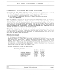
1 Introduction
Computational modeling and simulation studies can facilitate the advancement of cardiovascular
research by complementing experimental studies. Through computational studies, the researcher
may formulate hypotheses which may be subsequently tested through experimental studies or
the researcher may develop and evaluate inverse modeling algorithms for determining important
cardiovascular parameters from experimental data. Experimental studies, in turn, permit the researcher to construct more accurate computational models thereby improving the researcher’s understanding of the cardiovascular system and ability to devise new experimental hypotheses and
inverse modeling algorithms.
The general aim of this document is to introduce the Research CardioVascular SIMulator
(RCVSIM) software which may be downloaded from PhysioNet (www.physionet.org) – an NIHfunded national research resource that provides well characterized, experimental data sets and
open-source software for their analysis. RCVSIM is capable of generating reasonable human pulsatile hemodynamic waveforms, cardiac function and venous return curves, and beat-to-beat hemodynamic variability. The data simulated by RCVSIM is written in a format which is identical to
the experimental data sets. As such, the open-source data analysis software may be readily applied
to the simulated data as well. The data generated by RCVSIM may be viewed as they are being
calculated (on-line viewing) or any time after they have been calculated (off-line viewing) with the
WAVE display system (which is also provided by PhysioNet) and Gnuplot. The RCVSIM software
is open-source and extensively commented and includes Linux binaries that may be executed at
the Linux or MATLAB prompts. It should also be possible to compile the source code to create
binaries that may be executed on Unix platforms (e.g., Solaris, SunOS). (Note that MATLAB is
required for compiling the source code.) RCVSIM has been previously employed in cardiovascular research for the development and evaluation of system identification methods aimed at the
dynamical characterization of autonomic regulatory mechanisms [?, 4, 8].
This document specifically explains how to install and use the RCVSIM software and describes
the open-source code and each of its functions so that RCVSIM may be easily extended and modified by the researcher to achieve his desired research objective. In Section 2, a brief description of
the components and parameters of the human cardiovascular model is given. (A detailed description may be found in [?, 4, 7].) In Section 3, a description of the source code and an explanation of
how to alter it are provided. In Section 4, detailed instructions on software installation and compilation are outlined. In Section 5, instructions on software execution, including many examples,
are given. Finally, in Section 6, an example illustrating how the software may be utilized in cardiovascular research is provided. Note that if the researcher is interested in executing the software
but not editing it, then he may skip Section 3 without loss of continuity.
2 Human Cardiovascular Model
The human cardiovascular model upon which RCVSIM is based includes three major components.
The first component is a lumped parameter model of the pulsatile heart and circulation which may
be implemented as an intact preparation, a heart-lung unit preparation designed for measuring cardiac function curves, or a systemic circulation preparation designed for measuring venous return
curves. The second component is a short-term regulatory system model which includes an arterial
3
R pa
P pa(t)
.
q pa(t)
C pa
Rr
.
q r (t)
P pv(t)
.
q pv(t)
C pv
Pth
Pth
Pth
P r (t)
R pv
Pth
C r (t)
P l(t)
C l (t)
.
q l (t)
.
q a(t)
.
q v(t)
P v(t)
P "ra" (t)
Rl
Rv
P a (t)
Ra
Cv
Ca
Figure 1: Electrical circuit analog of the intact human pulsatile heart and circulation. Each box
encompassing a circuit element denotes a nonlinear element.
baroreflex system, a cardiopulmonary baroreflex system, and a direct neural coupling mechanism
between respiration and heart rate. The final component is a model of resting physiologic perturbations which includes respiration, autoregulation of local vascular beds (exogenous disturbance to
systemic arterial resistance), and higher brain center activity impinging on the autonomic nervous
system(1/f exogenous disturbance to heart rate).
2.1 Pulsatile Heart and Circulation
The lumped parameter model of the intact pulsatile heart and circulation is illustrated in Figure 1 in
terms of its electrical circuit analog. Here, charge is analogous to blood volume ( , ml), current,
to blood flow rate ( , ml/s), and voltage, to pressure ( , mmHg). The model consists of six
compartments which represent the left and right ventricles ( ), systemic arteries and veins ( ),
and pulmonary arteries and veins (
). Each compartment consists of a conduit for viscous
blood flow with resistance ( ) and a volume storage element with compliance ( ) and unstressed
4
R pa
C pa
Rr
R pv
C pv
Pth
Pth
Pth
Pth
C r (t)
C l (t)
.
q (t)
l
P "ra" (t)
Rl
P a (t)
Rv
Pv
Pa
Figure 2: Electrical circuit analog of the human heart-lung unit preparation designed for measuring
cardiac function curves. Each box encompassing a circuit element denotes a nonlinear element.
volume ( ). Two of the resistances and two of the compliances are nonlinear. The systemic
venous resistance is represented by a Starling resistor (with chamber pressure set to atmospheric
pressure), while the pulmonary arterial resistance is represented by an infinite number of parallel
Starling resistors (with chamber pressure equal to alveolar ( ) pressure), arranged vertically, one
on top of the other. The pressure-volume relationships of the left and right ventricles consist of an
essentially
linear regime (characterized by compliance
and unstressed volume), a diastolic volume
limit (
), and a systolic pressure limit ( ). The compliances of the linear regime of the
ventricular pressure-volume relationship vary periodically over time (time evolution is precisely
determined by the end-diastolic compliance ( ), the end-systolic ( ) compliance, and the heart
rate ( )) and are responsible for driving the flow of blood. The four ideal diodes represent the
ventricular inflow and outflow valves and ensure uni-directional blood flow. Finally, the reference
pressure is set to intrathoracic ( ) pressure for the ventricular and pulmonary compartments.
Figure 2 illustrates the electrical circuit analog of the lumped parameter model of the human
heart-lung unit preparation. The input pressure to the heart-lung unit here is defined to be the
5
P pa
Rr
.
q v(t)
Pth
P r (t)
C r (t)
.
q v(t)
P v(t)
P "ra" (t)
Rv
P a (t)
Ra
Cv
Ca
Figure 3: Electrical circuit analog of the human systemic circulation preparation designed for
measuring venous return curves. Each box encompassing a circuit element denotes a nonlinear
element.
node labelled “ ” – the location of where the right atrium would be if it were explicitly included in the model. Cardiac function curves may be obtained from this preparation
by varying
the independent voltage sources, and , and time-averaging the resulting and “ ” .
Figure 3 illustrates the electrical circuit analog of the lumped parameter model of the human
systemic circulation preparation.
Venous return curves may be measured from this preparation
by adjusting the value of at end-diastole ( ) in order to vary “ ” – the pressure
that
impedes flow into the right ventricle – and time-averaging
the resulting and “ ” . Note
that the independent current source here ( ) keeps the mean systemic ( ) pressure precisely
constant throughout the measurement period by pumping into the systemic circulation whatever is
pumped out.
6
F(t)
es
C l,r(t)
sp
Pa
ANS
Pulsatile
Heart
P a (t)
Q 0v(t)
Ra (t)
Circulation
Baroreceptors
Figure 4: Block diagram of the feedback system depicting the arterial baroreflex arc.
2.2 Short-Term Regulatory System
The arterial baroreflex arc is implemented according to the feedback system illustrated in Figure 4.
This system is aimed at tracking
a setpoint ( ) pressure through the following sequence of events.
The baroreceptors sense and relay this pressure to the autonomic nervous system (ANS). The
ANS compares the deviation between the sensed pressure and with zero and then responds
by adjusting four parameters of the pulsatile heart and circulation
in order to keep the
ensuing
,
near . The four adjustable parameters are , at end-systole ( ),
and . The ANS controls these parameters based on the history of specifically
according to the following nonlinear, dynamical mapping:
! (1)
where may represent any of the four adjustable parameters, the arctan
function
(which is
parametrized by the constant ) imposes arterial baroreflex saturation, and are unit-area
effector mechanisms which respectively represent the fast, parasympathetic limb of the ANS and
the slower, sympathetic limb (both - and -sympathetic sublimbs; see Figure 5), and
and reflect the respective static gain values of the effector mechanisms. Note that in order to map to the times of onset of ventricular contraction (which amounts to re-initiating the variable, ventricular compliance time evolution), an “integrate and fire” model of the sinoatrial node is incorporated
in the model.
The cardiopulmonary baroreflex arc is also implemented according to a feedback diagram analogous to Figure 4. However,
the sensed
pressure
here is defined to be the effective right atrial
transmural pressure ( “ ” “ ” ) of the pulsatile heart and circulation model.
The direct neural coupling mechanism between respiration and heart rate is characterized by
"
$
#
$&%
7
(b)
1
0.9
0.9
0.8
0.8
0.7
0.7
0.6
0.6
s(t)
p(t)
(a)
1
0.5
0.5
0.4
0.4
0.3
0.3
0.2
0.2
0.1
0.1
0
0
10
20
Time [s]
0
0
30
10
20
Time [s]
30
Figure 5: Unit-area effector mechanisms
representing (a) the fast, parasympathetic limb and
(b) the slower, sympathetic limb . These effector mechanisms characterize the dynamical
properties of the block labelled ANS in Figure 4.
a linear,
time-invariant impulse response which
maps fluctuations in instantaneous lung volume
. The impulse response is defined here by a linear
( ; see Section
2.3)
to
fluctuations
in
combination of and , each of which are advanced in time by 1.5 s in order to account for
the noncausality of this mechanism [6, 9].
2.3 Resting Physiologic Perturbations
Respiratory
activity, which may either be at fixed-rate or random-intervals [1], is modeled in terms
of
. Fixed-rate is represented
by a pure sinusoid, which is characterized by tidal
volume ( ) and respiratory period ( ), as well as a DC offset representing the functional reserve
volume of the lungs (
). Each respiratory cycle of random-interval is also represented
by one period of a sinusoid with the DC offset
. However, the period is not constant here but
rather determined based on the outcome of a probability experiment (which ranges from one to
15 seconds with a mean of five seconds), and the tidal volume is set such that the instantaneous
alveolar ventilation rate (which considers the dead space in the airways (
)) is identical to that
of fixed-rate breathing.
In order to account for the mechanical effects of on and , the simple model
of ventilation, illustrated in Figure 6 in terms of its electrical circuit analog, is also incorporated
in the model. The electrical components may be interpreted similarly to those in Figure 1 by
considering air here rather than blood. Hence, the resistor ( ) may be thought of as a conduit
for airflow between the atmosphere and the lungs, while the capacitor may be interpreted as an
air volume container representing the lung compartment, which is parametrized by an unstressed
$
$&%
8
dQ lu (t)
dt
R air
P atm(t)
P alv(t)
C lu
P th (t)
Figure 6: Electrical circuit analog of the human ventilatory mechanics model.
volume ( ) in addition to .
The systemic effects of the autoregulation of local vascular beds is represented with an exogenous disturbance to which is defined by a bandlimited Gaussian white noise process. This
process is created by convolving Gaussian white noise of zero mean and stdwr standard deviation
with a lowpass filter (truncated unit-area sinc function) of desired frequency cutoff (fco). Higher
brain center activity impinging on the ANS is modeled with a 1/f exogenous,
Gaussian disturbance
to convolved with a filter defined by a linear combination of ( -sympathetic sublimb)
and . The 1/f Gaussian disturbance is created by convolving
white noise of zero
Gaussian
mean and stdwf standard deviation with a unit-area filter of 1/f
magnitude squared frequency
response from Hz to 1 Hz, where alpha is set to one. Each of these exogenous disturbances
are treated as unobservable quantities.
%
#
3 Source Code
The RCVSIM source code was written predominantly in the MATLAB language (version 5.3.1;
R11.1) and includes some C language necessary for on-line viewing and parameter updating. The
source code may be compiled using the MATLAB compiler (version 1.2) with the libc5 development environment at the MATLAB prompt (see Section 4.2). Note that compilation permits
software execution at the Linux prompt and greatly improves execution speed. The source code
not only consists of code to implement the models described in Section 2 but also includes code
to implement other models. These latter models have been minimally tested and documented and
may only be executed in the MATLAB environment. A description of the code for implementing
the models of Section 2 and an explanation of how this code may be modified or extended to implement arbitrary lumped parameter cardiovascular models are provided below. See Appendix A
for a brief description of the other models and the source code for executing them.
9
3.1 Flowchart and Functions
The source code is based on the MATLAB function simulate.m. The input arguments to simulate.m include the desired parameter values characterizing the human cardiovascular
model
and its
execution,
while
the
outputs
are
the
simulated
data
–
all
pressures
(
), volumes (
), flow
rates ( ), ventricular elastances
, adjustable parameters ( ), cardiac function/venous
return curves ( ), and ventricular contraction times ( ). This function may also write
the simulated data to file (with a desired prefix file name also provided as an input argument) and
display the data as they are being calculated. The function is responsible for executing the models
described in Section 2 as well as in Appendix A. However, the flowchart of Figure 7 depicts how
the function simulates the data from the desired parameter values characterizing only the models
of Section 2. The pertinent details of each block of the flowchart are provided below.
Declaring and Initializing Variables (t=0). With the desired parameter values provided as
function input arguments, all variables of the simulation are declared and initialized. Memory is pre-allocated for all of the data to be simulated over their entire integration period
in order to increase execution speed with the MATLAB compiler. The respiratory-related
waveforms are pre-computed over the entire integration period.
Numerical Integration for Calculating . The pressures of the desired model of the pulsatile heart and circulation are calculated at the current time step ( ) from the pressures
at the previous time step ( ) by fourth-order Runge-Kutta integration of the set of ordinary
differential equations governing the model.
racy.
must be set to 0.005 s for reasonable accu-
Adjusting Parameters by Regulation/Perturbations. Parameters of the pulsatile heart and
circulation are adjusted by the short-term regulatory system and resting physiologic perturbations models. Because of the relatively narrow bandwidths of these models, the parameter
adjustments are calculated at a sampling period of 0.0625 s. First, the requisite waveforms
originally computed at a sampling period of are decimated to a sampling period of 0.0625
s by averaging over the past 0.25 s every 0.0625 s. Then, the mandated parameter adjustments are computed at a sampling period of 0.0625 s. Finally, the mandated parameter
adjustments are converted to a sampling period of
via linear interpolation (with the exception of the adjustments to which do not take effect until the initiation of the next
ventricular contraction) in order to compute the subsequent waveforms.
Establishing qrs via“Integrate and Fire.” The mandated changes to are mapped to the
times of onset of ventricular contraction by integrating (in units of bps) over time until
the integral is equal to one. Then, systole is initiated by resetting the variable, ventricular
elastance model, the integral is set to zero, and the integration is repeated.
Heart-Lung Unit or Systemic Circulation? Varying , , and Averaging “ra” ,
. Cardiac function or venous return curves are generated, if desired. Following every
fifth beat, and are varied in steps for generation of cardiac function
curves,
and is
varied for simulation of venous return curves. Time-averaged “ ” and and (for
cardiac function curves) are recorded over the beat preceding the step variation.
10
Parameters
Outputfile
Declaring and
Initializing Variables (t=0)
t=Ts
Numerical Integration for
Calculating P(t)
Adjusting Parameters by
Regulation/Perturbations
Establish qrs via
"Integrate and Fire"
Heart−Lung Unit or
Systemic Circulation?
Yes
Varying Pv , Pa , C ed
r. and
Averaging P"ra" (t), q v(t)
Yes
Correcting Qtot(t)
by Adjusting Pv (t)
No
Calculating Q(t) and
Storing E(t) and ap(t)
t=t+Ts
Intact Circulation?
No
Parameter Updates?
No
Conserving Q(t) and
Documenting Updates
Yes
Updated Parameters
.
Calculating q(t)
On−Line Viewing?
Yes
Writing Waveforms
to MIT Format Files
Outputfile.hea
Outputfile.dat
Outputfile.qrs
No
Displaying Waveforms
.
{P(t), Q(t), q(t), E(t), ap(t), qrs, numerics}
Figure 7: Flowchart of the MATLAB function simulate.m.
11
Calculating
and Storing
and . The blood volumes of each compartment
of the desired model of the pulsatile heart and circulation are computed at the current time
step from the pressures at the current time step, and the values of the ventricular elastances
and adjustable parameters at the current time step are stored into their pre-allocated memory
slots.
Intact Circulation? Correcting
by Adjusting . Total blood volume of the
$$
intact pulsatile heart and circulation at the current time step (
may vary due to
$ $ ), which
integration error, is conserved. The
difference
between
the
computed
and its assigned
$$
value is added/removed from and is altered accordingly.
Parameter Updates? Conserving and Documenting Updates. The parameter values
of a simulation may be updated after the initiation of each ventricular contraction by pausing
the simulation, updating the parameter values, and resuming the simulation. The newly chosen parameter values are documented to file if they are relevant to the current simulation, and
the blood volumes in each compartment at the current time step are conserved by adjusting
the pressures at the current time step (if necessary). Adjustments to the respiratory-related
waveforms are implemented for the remainder of the integration period.
Calculating . The flow rates of the pulsatile heart and circulation models are calculated
at the current time step from the pressures at the current time step.
On-Line Viewing? Writing Waveforms to MIT Format Files Displaying Waveforms.
When viewing simulated data as they are being calculated, the waveforms are periodically
written to file in MIT format (with a desired period). The newly written data are then immediately displayed with WAVE.
The
flow of each of the blocks is then repeated starting at Numerical Integration for Calculating
with . In order to execute the blocks in the flowchart, simulate.m calls upon many
MATLAB and C functions, each of which are briefly described below.
intact init cond.m computes the initial pressures, volumes, and flow rates of the intact pulsatile heart and circulation model from the desired parameter values. The initial values are
determined from the solution of a linear system of equations which are derived from the
application of steady-state conservation laws to a linearized version of the model.
hlu init cond.m computes the initial pressures, volumes, and flow rates of the heart-lung
unit preparation model from the desired parameter values. The initial values are determined
from the solution of a linear system of equations which are derived from the application of
steady-state conservation laws to a linearized version of the model.
sc init cond.m computes the initial pressures, volumes, and flow rates of the systemic circulation preparation model from the desired parameter values. The initial values are determined
from the solution of a linear system of equations which are derived from the application of
steady-state conservation laws to a linearized version of the model.
12
rk4.m computes the pressures of the pulsatile heart and circulation (any preparation) at the
current time step from the pressures of the previous time step, the current values of the
parameters, respiratory-related waveforms, and time surpassed in the current cardiac cycle
according to fourth-order Runge-Kutta integration.
intact eval deriv.m is called only by rk4.m and computes the derivative of the intact pulsatile
heart and circulation pressure values at a desired time step which is necessary for the fourthorder Runge-Kutta integration.
hlu eval deriv.m is called only by rk4.m and computes the derivative of the heart-lung unit
preparation pressure values at a desired time step which is necessary for the fourth-order
Runge-Kutta integration.
sc eval deriv.m is called only by rk4.m and computes the derivative of the systemic circulation preparation pressure values at a desired time step which is necessary for the fourth-order
Runge-Kutta integration.
var cap.m is also called by intact eval deriv.m, hlu eval deriv.m, and sc eval deriv.m and
computes a ventricular elastance value as well as its derivative at a desired time step from
the current values of , , the previous cardiac cycle length, and the time surpassed in
the current cardiac cycle.
&
vent vol.m is also called by intact eval deriv.m, hlu eval deriv.m, and sc eval deriv.m and
computes the current ventricular blood volume from the current ventricular pressure according to Newton’s search method with an initial guess given by the previous ventricular blood
volume.
rand int breath.m computes the time until the next respiratory cycle commences based on
the outcome of an independent probability experiment.
, $&% , $ $ , and )
over the entire integration period from the parameter values and the times of commencement
resp act.m computes the respiratory-related waveforms (
of each respiratory cycle.
ilv dec.m decimates
to a sampling period equal to 0.0625 s. This decimated waveform is convolved
with the filter created by dncm filt.m (see below) in order to establish the
changes in mandated by the direct neural coupling mechanism.
dncm filt.m generates a filter which characterizes the direct neural coupling mechanism be
tween
and .
bl filt.m generates a lowpass filter with a narrow transition band (truncated sinc function of
unit-area) and desired cutoff frequency which is utilized to bandlimit the exogenous disturbance to .
oneoverf filt.m generates a filter with a 1/f %
magnitude-squared frequency response over
a desired frequency range (in decades) and at a desired sampling period (see below).
13
ans filt.m creates a filter which is a linear combination of
and . This filter is convolved with the filter generated
by
oneoverf
filt.m
and
then
white
noise in order to create the
exogenous disturbance to .
abreflex.m computes the parameter adjustments mandated by the arterial baroreflex system
based on the current setpoint and static gain values.
cpreflex.m computes the parameter adjustments mandated by the cardiopulmonary baroreflex
system based on the current setpoint and static gain values.
param change.m determines whether the parameter updates are relevant to the status of the
current simulation based on the current parameter values, the previous parameter values, and
the status parameters (see Section 5.2).
conserve vol.m computes the pressures at the current time step necessary to conserve the
blood volume in each compartment at the current time step when parameter values are updated.
read param.m reads a file which contains the parameters values of the cardiovascular model
and its execution in a specific format and stores the values in a MATLAB vector.
read key.c reads the standard input, pauses the simulation if a “p” is entered followed by
RETURN , and resumes the simulation if a “r” is entered followed by
RETURN .
write param.c copies the parameter file to a new file of the same name but with the extension
.num. This function is implemented when the parameter update occurs. The extension is set
equal to the number of parameter updates that have been made during the simulation period.
wave remote.c plots the desired simulated waveforms and annotations with the WAVE display system. This function is called when the simulated data are written to file in MIT format
and plots the most recent desired window of written data.
The function simulate.m is called by a wrapper function rcvsim.m for execution at the Linux
prompt. This wrapper function takes two command line arguments: 1) the name of a file containing the desired parameter values and 2) the prefix name of the output files to be generated in
MIT format. The function rcvsim.m, which also includes a help option, reads in the parameter file
with read param.m (see above), creates a header file in MIT format, executes simulate.m, writes
the simulated data to MIT format files if the on-line viewing option is not chosen, and displays
cardiac function and venous return curves, if desired, with the function plot cfvr.c (which employs
Gnuplot). In order to execute rcvsim.m, the function must be compiled with the file make.m which
creates the binary file rcvsim. The function simulate.m may also be compiled independently of
rcvsim.m with the file makem.m which creates the binary file simulate.mexlx (in the Linux environment). Each of these make files greatly improve execution speed specifically through mcc
(MATLAB compiler) optimization arguments r (real numbers only) and i (no dynamic memory
allocation). Note that simulate.m may only be executed in the MATLAB environment without
on-line viewing and parameter updating capabilities.
14
3.2 Modifications and Extensions
Although the human cardiovascular model upon which RCVSIM is based accounts for a wide variety of hemodynamic behaviors, it certainly cannot address arbitrary cardiovascular research objectives. For example, if the researcher is interested in analyzing how stroke volume is compromised
at very high heart rates ( 150 bpm) in the absence of cardiovascular regulation, the model, as
described in Section 2, would not be adequate because contracting atrial compartments are not explicitly included. In such cases, the researcher may utilize the RCVSIM source code as a basis for
facilitating the construction of a model which can address his research objective. An outline of the
major steps necessary for the researcher to create different lumped parameter pulsatile heart and
circulation models and add new bandlimited regulatory systems (e.g., arterial chemoreflex) and
resting physiologic perturbations (e.g., central oscillator) is provided below. Note that additional
steps may also be necessary depending upon the particular extension.
Creating lumped parameter models of the pulsatile heart and circulation.
1. Name the new lumped parameter model (preparation) and assign a unique number to
it. This number will be used in conditional statements which must be added to the code
in order to distinguish the desired preparation to be executed from the other possible
preparations (see, for example, the rk4.m source code).
2. Extend the MATLAB parameter vector (th) to include any additional, necessary parameters. Add the new parameters (in the correct format) to the parameter file (see Section 5.2). Expand the function read param.m so that it can read these new parameters.
If the researcher would like to implement the new preparation in the MATLAB environment, the function header def.m must also be altered accordingly (see Appendix A).
3. Create a function called preparation init cond.m to generate the initial pressures, volumes, and flow rates. Call this newly created function at the same point in simulate.m
as the function call for intact init cond.m.
4. Create a function called preparation eval deriv.m to calculate the derivative of the pressure values at a desired time step. Call this newly created function from rk4.m analogous to the function calls for intact eval deriv.m.
5. Add code for calculating volumes and flow rates at the point in simulate.m in which
these waveforms are computed for the other preparations.
6. If necessary, pre-allocate additional memory for the simulated data in simulate.m, expand matrices to be written in MIT format in simulate.m and rcvsim.m, and extend code
for generating the MIT format header file in rcvsim.m.
7. Adjust parameter update code in simulate.m including conserve vol.m.
8. Add preparation init cond.m and preparation init cond.m to the make files (make.m
and makem.m) and recompile the code.
Adding bandlimited regulatory system/resting physiologic perturbation.
15
1. Name the new regulatory system/resting physiologic perturbation. This name will serve
as a flag indicating whether the new addition is to be activated or not. The MATLAB
vector flag at the start of simulate.m should be extended to incorporate this name.
2. Extend the MATLAB parameter vector (th) to include any additional, necessary parameters. Add the new parameters as well as the new flag name (in the correct format) to
the parameter file (see Section 5.2). Expand the function read param.m so that it can
read these new parameters and flag name. If the researcher would like to implement
the new model in the MATLAB environment, the function header def.m must also be
altered accordingly (see Appendix A).
3. Initialize the necessary variables at the beginning of simulate.m.
4. Create a function to compute the mandated change to the adjustable parameter. Call
this function every 0.0625 s. If this function requires a simulated waveform as input,
then this waveform must be averaged over the previous 0.25 s every 0.0625 s prior to
the function call.
5. If a parameter other than steps must be undertaken:
, ,
, and is adjusted, then the following
(a) Pre-allocate additional memory for the adjustable parameter matrix ap in simulate.m.
(b) Expand the thc vector in simulate.m to include the new parameter to be adjusted.
(c) Linearly interpolate the newly adjustable parameter.
(d) Assign the mandated adjustment to the ap matrix in simulate.m.
(e) Expand the ap matrix to be written in MIT format in simulate.m and rcvsim.m.
(f) Adjust the parameter update code in simulate.m accordingly.
(g) Extend code for generating the MIT format header file in rcvsim.m to include the
newly adjustable parameter.
6. Add the new function to the make files (make.m and makem.m) and recompile the code.
4 Software Installation and Compilation
The researcher may download the RCVSIM software from PhysioNet and install and execute the
pre-compiled binaries provided that he is running Linux. If the researcher also has access to MATLAB and its compiler (version 1.2), then he may modify and extend the source code as he wishes
and then recompile it to create new binaries. Alternatively, if the researcher is running any other
platform in which the WAVE display system is fully supported (e.g., Solaris, SunOS) and has
access to the MATLAB compiler (version 1.2), he may compile the source code and install and
execute the new binaries on that platform. (The binaries created for such platforms may then
be uploaded to PhysioNet so that they may be distributed to other researchers who do not own
MATLAB.) Detailed instructions on installing the RCVSIM binaries (and required libraries) and
compiling the source code are provided below.
16
4.1 Installation
The installation steps that the researcher must carry out in order to execute the RCVSIM precompiled Linux binaries are as follows:
1. Download the file rcvsim.tar.gz from the following web page:
http://www.physionet.org/physiotools/rcvsim
2. Type the following commands at the Linux prompt:
tar xvzf rcvsim.tar.gz
cd rcvsim
The contents of this directory – henceforth referred to as $DIR – are as follows:
README. This text file includes a brief introduction, references to the INSTALL file and the
doc sub-directory, and basic execution and compilation instructions.
INSTALL. This text file explains how to install/uninstall the RCVSIM software on Linux or
other platforms in which the WAVE display system is fully supported.
install. This shell, executable script automates some, or all, of the installation process.
uninstall. This shell, executable script is designed to undo what was done by the install
script.
src. This sub-directory includes all the source code described in Section 3.1 and Appendix A
as well as two other C files (check redhat.c and check wfdb.c) which are required by the
install and uninstall shell scripts. The Linux and MATLAB pre-compiled binaries (rcvsim
and simulate.mexlx) are also stored here.
bin. This sub-directory includes parameter files, parameters.def and header def.m (see Section 5.2 and Appendix A), which are respectively required for execution at the Linux and
MATLAB prompts, a wfdbcal file responsible for scaling the simulated waveforms displayed
by WAVE, and the two binaries, check redhat and check wfdb.
lib. This sub-directory consists of libraries which are required for executing the binaries.
These libraries include the dynamic MATLAB libraries which permit software execution in
the absence of MATLAB, two RPMs containing libc5 libraries and an old ld.so dynamic
linker (part of the Redhat 6.2 distribution which are necessary for dynamically linking
the MATLAB libraries), and a tar file consisting of the WFDB software package (version
10.1.6).
doc. This sub-directory includes this very document in HTML, PDF (manual.pdf), PostScript
(manual.ps) and LaTeX source (manual.tex) formats.
3. Login as root.
17
4. Download and install the WFDB software package and the WAVE display system, if this has
not already been done. See the following web page for instructions:
http://www.physionet.org/physiotools/wfdb-linux-quick-start.shtml
If the researcher is running Linux Redhat 6.2 or higher, then
5. Type the following command in the $DIR directory:
./install
The results of Step 5. are as follows:
The WFDB Software Package (version 10.1.6) in the $DIR/lib directory will be installed, if
an older version is currently installed.
The libc5 libraries and old ld.so dynamic linker RPMs in the $DIR/lib directory will also be
installed. (Note that recent Linux systems use libc and a new linker but will not be affected
by the installation of the older libraries and linker.)
An rcvsim executable shell script will be placed in the $DIR/bin directory. This script sets
the library and WFDB paths for its subsequent execution of the binary $DIR/src/rcvsim and
is linked to the directory /usr/local/bin which should already be in the researcher’s path.
The MATLAB binary executable simulate.mexlx will be linked to a directory in the MATLAB path, if MATLAB is present.
Or, if the researcher is running Linux Redhat 6.1 or lower or any other Linux distribution (e.g.,
Suse, Debian), then
5a. Acquire and install the necessary libc5 libraries and old dynamic linker, if they are not currently present on the system.
5b. Type the following command in the $DIR directory:
./install
For RPM-based distributions (e.g., Mandrake), the software required for Step 5a. may be found
on rpmfind.net as was the case for the RPMs provided in the directory $DIR/lib. Please see the
following web pages:
http://www.rpmfind.net/linux/rpm2html/search.php?query=ld.so
http://www.rpmfind.net/linux/rpm2html/search.php?query=libc
Note that the results of Step 5b. differ from those of Step 5. in that the RPMs of $DIR/lib will not
be installed.
6. To undo the install script, type the following command in the $DIR directory:
./uninstall
This will undo everything done by install except the removal of the WFDB Software Package
(version 10.1.6), if it were installed. This software can be removed manually (read INSTALL file
in the tar file wfdb-10.1.6.tar.gz which is located in the $DIR/lib directory).
18
4.2 Compilation
If the researcher is running Linux and wishes to modify/extend the RCVSIM source code or if the
researcher would like to run the RCVSIM software on another platform in which WAVE is fully
supported, then compilation is necessary. The steps required to compile the source code are are as
follows:
1. Acquire and install MATLAB with the MATLAB compiler (version 1.2), if they are not
currently available.
2. Establish a libc5 development environment. See the following web page for detailed instructions:
http://www.mathworks.com/support/solutions/data/11129.shtml
3. Launch MATLAB from the $DIR directory.
4. At the MATLAB prompt, execute the following commands:
cd src
make
makem
By implementing these steps in the Linux environment, new rcvsim and simulate.mexlx binaries
will be created in the $DIR/src directory. If the RCVSIM software has already been installed, then
re-installation is unnecessary after compilation. On platforms other than Linux, the above steps
must be carried out prior to software installation on platforms other than Linux. Additionally, the
install and uninstall scripts in the $DIR directory need to be slightly modified in order to include the
different MATLAB binary file extension name that results from compiling on a different platform.
For example, if compilation is achieved on the Solaris platform, simulate.mexlx in the install and
uninstall files must be replace with simulate.mexsol as the latter file will be created in the $DIR/src
directory. Then, the newly compiled software may be installed according to the previous section.
Note that it is possible to compile the source code with the latest MATLAB compiler (version
2.1). However, the binaries generated from this compiler are on the order of three magnitudes
slower than those generated with the MATLAB compiler (version 1.2). Mathworks is currently
trying to improve the latest compiler, so it may be possible in the future to use this compiler.
5 Software Execution
The researcher may view and record data simulated from the human cardiovascular model of
Section 2 by running the rcvsim executable file at the Linux prompt. Detailed instructions explaining how to execute this file including several examples, are provided below. Execution of
simulate.mexlx at the MATLAB prompt is touched upon in Appendix A. (Note that this section
requires some familiarity with the WAVE display system which may be acquired by either typing
more /usr/help/wave/wave.hlp at the Linux prompt or visiting the web page:
http://www.physionet.org/physiotools/wug/.)
19
5.1 Help Option
A help option may be implemented by running the rcvsim executable with the single argument -h
at the Linux prompt (that is, rcvsim -h; see Figure 8). The help option provides a description of
the major components of the human cardiovascular model, command line arguments, generated
output files, and on-line viewing options.
According to the help option, the executable file requires two arguments at the command line in
order to simulate hemodynamic data. The first argument must be the name of a file in the current
directory which contains the desired parameter values characterizing the human cardiovascular
model and its execution. This is the working parameter file which may be updated during the
simulation period (see Section 5.2). The second argument must be the desired prefix name of the
output files to be generated by the model.
By executing rcvsim with these two arguments, three MIT format files are always generated
in the current directory with extensions .dat, .qrs, and .hea. The .dat file is a binary (shorts) file
consisting of all of the generated waveforms; the .qrs file is a binary file consisting of annotations
which include the times of onset of ventricular contractions as well as any parameter updates; and
the .hea file is an ASCII header file necessary for reading, viewing, and analyzing the .dat and
.qrs files with the open-source software provided by PhysioNet. A fourth file with the extension
.txt may also be generated when the heart-lung unit preparation or systemic circulation preparation
is implemented. This file is in ASCII, multi-column format and constitutes the simulated cardiac
function or venous return curves. In order to document fully the simulation, the rcvsim executable
also saves the working parameter file in the current directory each time it is updated. The name
of the saved files is the first command line argument with the extension .num which denotes the
number of parameter updates that have been made during the simulation period. The name of each
saved file is also recorded in the annotation files at the time in which the parameters were updated.
At the beginning of the simulation, the rcvsim executable saves the initial working parameter file
with extension .0 to the current directory.
The rcvsim executable also permits the simulated waveforms (as a function of time) to be
viewed as they are being calculated (on-line viewing) through the WAVE display system. The simulation may be paused during on-line viewing by simply entering “p” followed by RETURN
at the standard input. Once the simulation is paused, any and all of the following three actions
may be carried out. 1) All the data that have been generated up to the time of the pause may be
scrolled through with the arrow buttons at the top of the WAVE display system. 2) Plots of one
generated waveform against another may be displayed by clicking the File button at the top of the
WAVE display system (with the right mouse button), and then clicking on the Analyze... option
followed by the VCG button (both with the left mouse button). The first two waveforms appearing
in the Signal List (first waveform is plotted on x-axis and the second waveform, on y-axis), which
may be adjusted as desired, will then be plotted against each other via Gnuplot. 3) The working
parameter file may be updated and saved. The simulation may be resumed, with the updated parameter values, by simply entering “r” followed by RETURN at the standard input. Note that
plots of one waveform versus another will not be automatically updated upon resuming the simulation. However, these plots may be manually updated by subsequently pausing the simulation and
regenerating the plot as described above.
20
Figure 8: Results of executing the rcvsim help option at the Linux prompt.
21
5.2 Parameter File
The parameter file ($DIR/parameters.def; see Figure 9) assigns the desired numerical values to
all of the parameters characterizing the human cardiovascular model and its execution. The syntax for parameter assignment must be precisely as written within the following squiggly brackets:
parameter: numerical value . Otherwise, the parameters will not be read in properly. The parameter file also includes definitions of each of the parameters and default or nominal parameter
values. Each line containing these definitions and default values as well as any other comments
must be preceded by a %. Parameter assignments should never be preceded by a %, else they
will not be read in properly. Each of the parameters in the file may be updated in the midst of a
simulation period with the exception of those labelled with * . Any update to these parameters
will simply be ignored.
The parameter file consists of integration and sampling parameters; display parameters; status
parameters; pulsatile heart and circulation parameters; short-term regulatory system parameters,
and resting physiologic perturbation parameters. The status parameters are flags which indicate the
preparation of the pulsatile heart and circulation to be implemented as well as whether a particular
short-term regulatory system or resting physiologic perturbation is to be activated or deactivated.
The status parameters, which cannot be adjusted in the midst of a simulation period, override any
of the other relevant parameters assignments. For example, if dra is set to zero, then the exogenous
disturbance to is deactivated and may not be activated during the simulation period regardless
of the value assigned to stdwr, which establishes the standard deviation of the disturbance to .
Note that a short-term regulatory system or resting physiologic perturbation may also be deactivated through the parameters that characterize them. For example, the exogenous disturbance to
may be deactivated by setting stdwr to zero. In this case, the exogenous disturbance to may be subsequently activated during the simulation period by setting stdwr to a value greater
than zero. However, if the researcher knows that a short-term regulatory system or resting physiologic perturbation is not required for his simulation, then the appropriate status parameter should
be deactivated for the purposes of increasing execution speed. Note that the pulsatile heart and
circulation parameters may be applicable to the intact circulation, heart-lung unit, and/or systemic
circulation preparations and are labelled accordingly.
5.3 Viewing Waveforms
Provided that the display parameters are properly set, the researcher may view the simulated waveforms and update the parameter values on-line by running the rcvsim executable which will make
repeated function calls to the WAVE display system. Alternatively, the waveforms, which are
recorded to MIT format files, may be viewed at any time after completion of the simulation (offline viewing) by directly running the wave executable file at the Linux prompt. An explanation on
how to set the display parameters and caveats to on-line parameter updating are provided below.
See also Examples 1-7 in Section 5.5 which illustrate how to view waveforms both on-line and
off-line.
22
Figure 9: The $DIR/parameters.def file which contains the parameter values characterizing the
human cardiovascular model of Section 2 and its execution.
23
5.3.1 Setting Display Parameters
The waveform parameter under the display parameters in the working parameter file determines
whether the simulated waveforms are to be viewed on-line. If the waveform parameter is assigned
the numerical value of -1, then the waveforms are not displayed as they are being calculated but
may be subsequently viewed and analyzed off-line. The researcher may choose this option, if, for
example, the data required for analysis are very time consuming to generate (e.g., Monte Carlo
simulations). If the waveform parameter is assigned one or more numerical values between 0 and
28 inclusive (with a single space inserted between each assigned numerical value), then the waveforms corresponding to those numerical values (see the $DIR/pararmeters.def file (Figure 9) or
the generated file with extension .hea for mapping key between waveforms and numerical values)
will be displayed as they are being calculated. For example, in Figure 9, the waveform parameter
is set such that left ventricle and systemic arterial pressures will be displayed on-line. Note that
the annotations parameter beneath the waveform parameter is simply a flag indicating whether the
contents of the annotations file, which include the times of onset of ventricular contractions and
parameter updates, will be viewed on-line with the waveforms selected by the waveform parameter. Note that if the waveform parameter is set to the numerical value of -1, then the contents of the
annotations file will not be displayed on-line regardless of the value assigned to the annotations
parameter.
The rcvsim executable file implements on-line viewing by periodically updating the WAVE
display with the most recently computed window of waveforms. The time duration of the window
and the update time period (both simulation times) may be respectively set to desired values with
the window and step parameters. For optimal on-line viewing, the window parameter should be set
equal to the time duration displayed by WAVE. This latter time duration is set by the physical size
of the WAVE window as well as the Time scale variable which is essentially a calibration factor
mapping this physical size to time duration. The Time scale variable may be altered by clicking
the VIEW option on the WAVE menu bar. The step parameter should be chosen to be sufficiently
small such that the displayed waveforms appear to scroll continuously through the WAVE window.
However, if the step parameter is chosen to be too small, then the actual time required to update
the display of the simulated data may not be sufficient and the quality of viewing may thus be
compromised.
5.3.2 On-line Parameter Updating
All of the parameter assignments in the working parameter file may be updated as waveforms
are being calculated and displayed on-line except those labelled with * . Any updates to these
parameters will be ignored. As soon as any parameter (not labelled with * ) is updated in the
working parameter file, the file is saved (with a new name) in order to document fully the simulation
(see Section 5.1). Some caveats to on-line parameter updating are provided below.
Since none of the display parameters are labelled with a * , they are permitted to be updated
on-line. Thus, the researcher may, for example, change the waveforms that he is currently viewing
without having to rerun rcvsim. However, when the working parameter file is updated only through
the display parameters, the update will not be documented to file.
Updates to the working parameter file are also not documented when the particular update is
not relevant to the status of the current simulation. For example, an update to the Cls parameter
24
is relevant when the intact circulation and heart-lung unit preparations are being implemented.
Thus, in this case, the update will be documented to file. However, when the systemic circulation
preparation is being executed, an update to the Cls parameter is irrelevant (see Figure 3) and is thus
not documented to file.
When implementing the heart-lung unit, the Pv and Pa parameters may be updated on-line provided that they are not being adjusted through the Pvs and Pas parameters, respectively. Otherwise,
the on-line adjustment of the Pv and Pa parameters will be ignored. Similarly, when implementing
the systemic circulation preparation, any update to the Crd parameter will be ignored unless it is
not being adjusted through the Crds parameter.
As described in Section 3.1, the volume in each of the capacitive elements of the pulsatile
heart and circulation (any preparation) is always conserved through a pressure adjustment. The
only exception to this rule is naturally when the researcher desires to adjust total blood volume
through the Qtot parameter (which is only applicable to the intact pulsatile heart and circulation
preparation). In this case, the volume is added to or subtracted from the systemic venous volume
and the systemic venous pressure is adjusted accordingly.
The instantaneous lung volume waveform may only be altered by updating the following parameters: Tr, Qt, Qfrs, and Qds. If parameters of the ventilatory model in Figure 6 are updated
(which includes the Pvc parameter), the value of intrathoracic pressure at the functional reserve
volume of the lungs will be adjusted instantaneously in order to preclude any change to instantaneous lung volume.
Finally, when updating the adjustable parameters of the pulsatile heart and circulation through
the F, Ra, Qvo, Crs, and Cls parameters, the current values and the setpoint values of these parameters will be adjusted. Note that updates to the Crs and Cls parameters will take effect at the start
of the subsequent ventricular contraction.
5.4 Viewing Cardiac Function and Venous Return Curves
Provided that the relevant parameters are properly set, the researcher may view cardiac function
and venous return curves immediately after they have been calculated (on-line viewing) by running
the rcvsim executable which will make a function call to Gnuplot. Since the time required for
generating a cardiac function or venous return curve is relatively short (within a few seconds), the
on-line viewing capability will usually suffice. However, it is possible that the researcher may
also desire to view the curves off-line. Since the curves are written to file in ASCII, multi-column
format, the researcher may view them any time after completion of the simulation by directly
executing gnuplot at the Linux prompt. A description of how to set the relevant parameters is
given below. See also Examples 8-13 in Section 5.5 which illustrate how to view the cardiac
function and venous return curves both on-line and off-line. (Note that this section requires some
familiarity with Gnuplot which may be garnered by typing man gnuplot at the Linux prompt.)
In order for the rcvsim executable to generate a cardiac function or venous return curve, either
the heart-lung unit preparation or systemic circulation preparation must be implemented by assigning the preparation parameter under the status parameters a numerical value of 1 or 2. Provided
that this has been done, then the numerics parameter under the display parameters determines
whether the cardiac function/venous return curve is to be viewed on-line. If the numerics parameter is assigned the numerical value of -1, then the curve will not be displayed as soon as it is
25
calculated but may be subsequently viewed off-line. If the numerics parameter is set to a numerical value between 0 and 3 inclusive which correspond to different plotting formats (see Figure 9),
then the cardiac function/venous return curve will be automatically displayed immediately following the completion of the simulation. The different plotting formats can be best understood by
recognizing that the on-line display of the curves is specifically implemented by writing gnuplot
commands to a file in the /tmp directory and executing these commands through a function call to
gnuplot. The single plot per window formats (corresponding to numerical values of 0 and 2) will
delete this file if it exists, write a new file to the /tmp directory, and thus display only the cardiac
function/venous return curve of the current simulation. The multiple plots per window formats
(corresponding to numerical values of 1 and 3) will add plotting instructions to the existing file in
the /tmp directory and thus display the curve of the current simulation as well as all other curves
that are instructed to be displayed in the file. In this way, multiple cardiac output and venous return
curves can be overlayed on the same axes. The mPra x-axis formats (corresponding to numerical
values of 0 and 1) will display either cardiac function or venous return curves. The mPa x-axis
formats (corresponding to numerical values of 2 and 3) will display average cardiac output as a
function of average systemic arterial pressure and is thus applicable only to the heart-lung unit
preparation.
Whether cardiac function and venous return curves are to be viewed on-line or off-line, the
simulation time is determined by the time parameter under integration and sampling parameters or
the time it takes to complete the calculation of the entire curve, which ever is less. Hence, the time
parameter should always be set to a value that is greater than the time it takes to calculate the entire
curve (1000 seconds is usually more than enough).
In order to generate venous return curves, the Crds parameter under pulsatile heart and circulation parameters must be properly selected. This parameter determines the increments in which the
Crd parameter is stepped from the value assigned to the Crs parameter to 60 ml/mmHg. Hence,
this parameter determines the number of points to be calculated on the venous return curve. For
example, if this parameter is set to five and all other parameters are also set to their default values,
then 12 points on the venous return curve will be calculated. If the Crds parameter is set to a value
greater than 60-Crs, then the Crd parameter will be held constant throughout the simulation and
only one point on the venous return curve will be generated.
In order to generate cardiac function curves, the Pvs and Pas parameters under pulsatile heart
and circulation parameters must be properly selected. Analogous to the Crds parameter, these parameters indicate the increments in which the Pv and Pa parameters are stepped. If the simulation
of a cardiac output curve is desired, the Pa parameter should be held constant by setting the Pas
parameter to a very large value (1000 mmHg will usually be more than sufficient), and the Pvs parameter should be set to a sufficiently small value in order to permit the generation of a reasonably
smooth curve (2 mmHg will usually do). If the generation of a curve of average cardiac output
versus average systemic arterial pressure is required, the Pv parameter should be held constant by
setting the Pvs parameter to a very large value (100 mmHg will usually be more than sufficient),
and the Pas parameter should be set to a sufficiently small value in order to allow the generation
of a reasonably smooth curve (30 mmHg will usually do). Finally, note that the researcher may
assign sufficiently small values to both Pvs and Pas such that a family of cardiac output curves at
different systemic arterial pressures will be generated.
26
5.5 Viewing Examples
The following examples illustrate how to view waveforms and cardiac function/venous return
curves on-line and off-line. Prior to implementing these examples, the researcher should set the
time duration displayed by the WAVE window to 20 seconds by resizing the window and/or adjusting the Time scale variable (click VIEW option at the top of the WAVE menu bar).
Ex. 1
Desired Execution:
– On-line display of left ventricle pressure, volume, and flow rate.
– Uncontrolled, unperturbed, intact pulsatile heart and circulation with default parameter
values.
Required Steps:
1. Copy file $DIR/bin/parameters.def to the current directory with the new file name parameters 1.
2. Open the file parameters 1 with any text editor (e.g., emacs).
3. Re-assign the following parameters: waveform: 0 9 17 and annotations: 0. Make sure
all of the status parameters are set to zero.
4. Save the file parameters 1.
5. Run the following command at the Linux prompt:
rcvsim parameters 1 foo1
Execution Output:
– The WAVE window in Figure 10 will initially appear and will automatically scroll
through the simulated data as they are being generated. This process will terminate
once 300 seconds of the data have been simulated.
– The following files will be created in the current directory: foo1.dat, foo1.qrs, foo1.hea,
and parameters 1.0 which may subsequently be viewed off-line (See Example 2).
Ex. 2
Desired Execution:
– Off-line display of left ventricle pressure, volume, and flow rate.
– Off-line display of left ventricle pressure versus volume.
– Uncontrolled, unperturbed, intact pulsatile heart and circulation with default parameter
values.
Required Steps:
27
Figure 10: Initial WAVE window generated according to Ex. 1 and Ex. 2.
28
1. Copy file $DIR/bin/parameters.def to the current directory with the new file name parameters 2.
2. Open the file parameters 2 with any text editor (e.g., emacs).
3. Re-assign the following parameter: waveform: -1. Make sure all of the status parameters are assigned the numerical value of zero.
4. Save the file parameters 2.
5. Run the following command at the Linux prompt:
rcvsim parameters 2 foo2.
6. Any time after the completion of the previous step, execute the following command at
the Linux prompt:
wave -r foo2 -s 0 9 17
7. Click on File button with right mouse button and then click Analyze... option with
left mouse button. Change first two waveforms in the Signal List to 9 0 followed by
RETURN . Then, click on the VCG button.
Or, if Ex. 1 has been previously implemented, then
1. Execute the following command at the Linux prompt:
wave -r foo1 -s 0 9 17
2. Click on File button with right mouse button and then click Analyze... option with
left mouse button. Change first two waveforms in the Signal List to 9 0 followed by
RETURN . Then, click on the VCG button.
Execution Output:
– If Ex. 1 has not been previously implemented, then the following files will be created
in the current directory: foo2.dat, foo2.qrs, foo2.hea, and parameters 2.0.
– When the wave executable is implemented, the WAVE window in Figure 10 will again
initially appear. The researcher may then use the arrow buttons at the top of the WAVE
display system to scroll through the 300 seconds of generated waveforms.
– When the VCG button is clicked, the Gnuplot in Figure 11 will appear illustrating left
ventricle pressure-volume loops. (As described in Section 5.1, plotting one waveform
against another can be carried out during on-line viewing provided that the simulation
is paused. Moreover, any two generated waveforms may be plotted against each other
through selection of the first two waveforms in the Signal List.)
Ex. 3
Desired Execution:
– On-line display of systemic arterial pressure, heart rate, and instantaneous lung volume
with annotations.
29
Figure 11: Gnuplot window generated according to Ex. 2.
– Fully controlled, fully perturbed (fixed-rate breathing), intact pulsatile heart and circulation with default parameter values.
Required Steps:
1. Copy file $DIR/bin/parameters.def to the current directory with the new file name parameters 3.
2. Open the file parameters 3 with any text editor (e.g., emacs).
3. Re-assign the following parameters: waveform: 1 15 26, baro: 3, dncm: 1, breathing:
1, dra: 1, and df: 1.
4. Save the file parameters 3.
5. Execute the following command at the Linux prompt:
rcvsim parameters 3 foo3
Execution Output:
– A WAVE window will appear and will automatically scroll through the simulated data
with annotations. Figure 12 illustrates the window after one minute of data has been
calculated. This process will terminate once 300 seconds of data have been simulated.
– The following files will be created in the current directory: foo3.dat, foo3.qrs, foo3.hea,
and parameters 3.0.
Ex. 4
30
Figure 12: WAVE window generated according to Ex. 3 and Ex. 4.
31
Desired Execution:
– Off-line display of systemic arterial pressure, heart rate, and instantaneous lung volume
with annotations.
– Fully controlled, fully perturbed (fixed-rate breathing), intact pulsatile heart and circulation with default parameter values.
Required Steps:
1. Copy file $DIR/bin/parameters.def to the current directory with the new file name parameters 4.
2. Open the file parameters 4 with any text editor (e.g., emacs).
3. Re-assign the following parameters: waveform: -1, baro: 3, dncm: 1, breathing: 1,
dra: 1, and df: 1.
4. Save the file parameters 4.
5. Run the following command at the Linux prompt:
rcvsim parameters 4 foo4
6. Any time after the completion of the previous step, execute the following command at
the Linux prompt:
wave -r foo4 -s 1 15 26 -a qrs
Or, if Ex. 3 have been previously implemented, then
1. Execute the following command at the Linux prompt:
wave -r foo3 -s 1 15 26 -a qrs
Execution Output:
– If Ex. 3 has not been previously implemented, then the following files will be created
in the current directory: foo4.dat, foo4.qrs, foo4.hea, and parameters 4.0.
– When the wave executable is implemented, a WAVE window will appear. The researcher may then use the arrow buttons at the top of the WAVE display system to
scroll through the 300 seconds of generated waveforms with annotations. Figure 12
will appear after clicking the forward double arrow button twice or by directly running
the wave executable with the following additional argument: -f 40.
Ex. 5
Desired Execution:
– On-line display of systemic arterial pressure and volume with annotations.
– Uncontrolled, unperturbed, intact pulsatile heart and circulation initially with default
parameter values.
– On-line reduction in systemic arterial compliance by a factor of two.
32
Required Steps:
1. Copy file $DIR/bin/parameters.def to the current directory with the new file name parameters 5.
2. Open the file parameters 5 with any text editor (e.g., emacs).
3. Re-assign the following parameter: waveform: 1 10. Make sure all of the status parameters are assigned the numerical value of zero.
4. Save the file parameters 5.
5. Run the following command at the Linux prompt:
rcvsim parameters 5 foo5
6. Some time in the midst of the simulation, type “p” followed by
dard input.
RETURN
at stan-
7. Re-assign the the following parameter: Ca: 0.8.
8. Save the file parameters 5.
9. Type “r” followed by
RETURN
at standard input.
Execution Output:
– A WAVE window will appear and will automatically scroll through the simulated data
with annotations. The automatic scrolling will stop once Step 6. is executed. (At this
point, the researcher may scroll backwards with the the arrow buttons at the top of the
WAVE display system.) After Steps 7.-9. are executed, automatic scrolling will resume
until a total of 300 seconds of data have been calculated. Figure 13 illustrates the
WAVE window during the time of reduction in systemic arterial compliance. Note that
this reduction is annotated with the name of the saved parameter file. (Also note how
systemic arterial volume is conserved through the instantaneous change in systemic
arterial pressure.)
– The following files will be created in the current directory: foo5.dat, foo5.qrs, foo5.hea,
parameters 5.0, and parameters 5.1.
Ex. 6
Desired Execution:
– On-line display of systemic arterial pressure, intrathoracic pressure, and instantaneous
lung volume with annotations.
– Uncontrolled, intact pulsatile heart and circulation initially with default parameter values perturbed by only fixed-rate breathing.
– First, an on-line reduction in lung compliance by a factor of two. Then, an on-line, 500
ml step increase in the functional reserve volume of the lungs.
Required Steps:
33
Figure 13: WAVE window generated according to Ex. 5.
34
1. Copy file $DIR/bin/parameters.def to the current directory with the new file name parameters 6.
2. Open the file parameters 6 with any text editor (e.g., emacs).
3. Re-assign the following parameters: waveform: 1 6 15 and breathing: 1.
4. Save the file parameters 6.
5. Run the following command at the Linux prompt:
rcvsim parameters 6 foo6
6. Some time in the midst of the simulation, type “p” followed by
dard input.
RETURN
at stan-
7. Re-assign the the following parameter: Clu: 126.25.
8. Save the file parameters 6.
9. Type “r” followed by
RETURN
at standard input.
10. At a subsequent time during the simulation, type “p” followed by
standard input.
RETURN
at
11. Re-assign the the following parameter: Qfrs: 500.
12. Save the file parameters 6.
13. Type “r” followed by
RETURN
at standard input.
Execution Output:
– A WAVE window will appear and will automatically scroll through the simulated data
with annotations. The automatic scrolling will stop once Step 6. is executed. After
Steps 7.-9. are executed, automatic scrolling will resume until Step 10. has been executed. When Steps 11.-13. are executed, the automatic scrolling will resume until a
total of 300 seconds of data have been simulated. Figure 14 illustrates the WAVE window during the reduction in lung compliance. (Note that this reduction does not alter
instantaneous lung volume; see Section 5.3.2). Figure 15 illustrates the WAVE window
during the time of the step increase in the functional reserve volume of the lungs. (Note
that the step increase occurs once the current respiratory cycle is complete.)
– The following files will be created in the current directory: foo6.dat, foo6.qrs, foo6.hea,
parameters 6.0, parameters 6.1, and parameters 6.2.
Ex. 7
Desired Execution:
– On-line display of systemic arterial pressure and heart rate with annotations.
– Uncontrolled, unperturbed, intact pulsatile heart and circulation initially with default
parameter values.
35
Figure 14: WAVE window generated according to the first parameter update of Ex. 6.
36
Figure 15: WAVE window generated according to the second parameter update of Ex. 6.
37
– First on-line hemmorhage of 500 ml. Then, on-line initiation of arterial and cardiopulmonary baroreflex control.
Required Steps:
1. Copy file $DIR/bin/parameters.def to the current directory with the new file name parameters 7.
2. Open the file parameters 7 with any text editor (e.g., emacs).
3. Re-assign the following parameters: waveform: 1 26, baro: 3, bgain: 0, again: 0, and
pgain: 0.
4. Save the file parameters 7.
5. Run the following command at the Linux prompt:
rcvsim parameters 7 foo7
6. Some time in the midst of the simulation, type “p” followed by
dard input.
RETURN
at stan-
7. Re-assign the the following parameter: Qtot: 4500.
8. Save the file parameters 7.
9. Type “r” followed by
RETURN
at standard input.
10. At a subsequent time during the simulation, type “p” followed by
standard input.
RETURN
at
11. Re-assign the the following parameters: bgain: 1, again: 1, and pgain: 1.
12. Save the file parameters 7.
13. Type “r” followed by
RETURN
at standard input.
Execution Output:
– A WAVE window will appear and will automatically scroll through the simulated data
with annotations. The automatic scrolling will stop once Step 6. is executed. After
Steps 7.-9. are executed, automatic scrolling will resume until Step 10. has been executed. When Steps 11.-13. are executed, the automatic scrolling will resume until a
total of 300 seconds of data have been simulated. Figure 16 illustrates the WAVE window once the simulation is complete. The Time variable of the WAVE window is set
such that the waveforms over the entire simulation period may be viewed all at once.
(Note how systemic arterial pressure has been returned to near normal values with the
baroreflex systems.)
– The following files will be created in the current directory: foo7.dat, foo7.qrs, foo7.hea,
parameters 7.0, parameters 7.1, and parameters 7.2.
Ex. 8
Desired Execution:
38
Figure 16: WAVE window generated according to Ex. 7 in which the time duration of the window
has been expanded to illustrate the entire simulation period.
39
– On-line display of a cardiac output curve.
– On-line display of systemic arterial and venous pressure and left ventricle flow rate.
– Uncontrolled, unperturbed, heart-lung unit preparation with default parameter values.
Required Steps:
1. Copy file $DIR/bin/parameters.def to the current directory with the new file name parameters 8.
2. Open the file parameters 8 with any text editor (e.g., emacs).
3. Re-assign the following parameters: time: 1000, waveform: 1 2 17, preparation: 1,
Pas: 1000, and Pvs: 2.
4. Save the file parameters 8.
5. Run the following command at the Linux prompt:
rcvsim parameters 8 foo8
Execution Output:
– A WAVE window will appear and will automatically scroll through the simulated data
as they are being calculated until the entire cardiac output curve has been measured.
Figure 17 illustrates the WAVE window at the end of the simulation. (As is always the
case with viewing waveforms on-line, the parameter values may be updated prior to
simulation termination, if desired.)
– Then, the Gnuplot window of Figure 18 will appear immediately following the calculation of the entire cardiac output curve.
– The following files will be created in the current directory: foo8.dat, foo8.qrs, foo8.hea,
foo8.txt and parameters 8.0.
Ex. 9
Desired Execution:
– On-line display of a venous return curve.
– Uncontrolled, unperturbed, systemic circulation preparation with default parameter
values.
Required Steps:
1. Copy file $DIR/bin/parameters.def to the current directory with the new file name parameters 9.
2. Open the file parameters 9 with any text editor (e.g., emacs).
3. Re-assign the following parameters: time: 1000, waveform: -1, preparation: 2, and
Crds: 5.
4. Save the file parameters 9.
40
Figure 17: WAVE window generated according to Ex. 8.
41
Figure 18: Gnuplot window generated according to Ex. 8, Ex. 10, and Ex. 11.
42
5. Run the following command at the Linux prompt:
rcvsim parameters 9 foo9
Execution Output:
– The Gnuplot window of Figure 19 will appear immediately following the calculation
of the entire venous return curve.
– The following files will be created in the current directory: foo9.dat, foo9.qrs, foo9.hea,
foo9.txt and parameters 9.0.
Ex. 10
Desired Execution:
– On-line display of multiple cardiac output and venous return curves.
– Uncontrolled, unperturbed, heart-lung unit and systemic circulation preparations with
default parameter values and after a 25% increase in systemic arterial resistance, mean
systemic pressure, heart rate, and contractility.
Required Steps:
1. Copy file $DIR/bin/parameters.def to the current directory with the new file name parameters 10.
2. Open the file parameters 10 with any text editor (e.g., emacs).
3. Re-assign the following parameters: time: 1000, waveform: -1, preparation: 1, Pas:
1000, and Pvs: 2.
4. Save the file parameters 10.
5. Run the following command at the Linux prompt:
rcvsim parameters 10 foo10a
6. Once the simulation is complete, re-assign the following parameters: numerics: 1,
preparation: 2, and Crds: 5.
7. Save the file parameters 10.
8. Run the following command at the Linux prompt:
rcvsim parameters 10 foo10b
9. Once the simulation is complete, re-assign the following parameters: Ra: 1.25 and
Pms: 8.625.
10. Save the file parameters 10.
11. Run the following command at the Linux prompt:
rcvsim parameters 10 foo10c
12. Once the simulation is complete, re-assign the following parameters: preparation: 1,
Cls: 0.3, Crs: 0.9, and F: 1.5.
13. Save the file parameters 10.
43
Figure 19: Gnuplot window generated according to Ex. 9.
44
Figure 20: Gnuplot window generated according to Ex. 10 and Ex. 11.
14. Run the following command at the Linux prompt:
rcvsim parameters 10 foo10d
Execution Output:
– A total of four Gnuplot windows will be displayed beginning with a window displaying
a single cardiac output curve (see Figure 18); then a window displaying the previous
cardiac output curve with a venous return curve; followed by a window displaying
these two previous curves with another venous return curve which is enhanced; and
ending with a window displaying each of these three curves and an additional enhanced
cardiac output curve (see Figure 20). (Note the increase in average cardiac output that
occurs due to the enhancement of the curves.) Each of the four windows will appear
immediately after the completion of each of the four rcvsim executions (Steps 5., 8.,
11., 14.).
– The following files will be created in the current directory: foo10a.dat, foo10a.qrs,
foo10a.hea, foo10a.txt, foo10b.dat, foo10b.qrs, foo10b.hea, foo10b.txt, foo10c.dat, foo10c.qrs,
foo10c.hea, foo10c.txt, foo10d.dat, foo10d.qrs, foo10d.hea, foo10d.txt and parameters 10.0.
Ex. 11
Desired Execution:
45
– Off-line display of the cardiac output and venous return curves generated from Ex. 10.
Required Steps:
1. Change directory to that which contains the simulated data of Ex. 10.
2. Run gnuplot at the Linux prompt.
3. At the Gnuplot prompt, enter the following commands:
set tics out
set xlabel ’mPra [mmHg]’
set ylabel ’mql,mqv [l/min]’
plot ’foo10a.txt’ using 1:2 notitle with lines
replot ’foo10b.txt’ using 1:2 notitle with lines
replot ’foo10c.txt’ using 1:2 notitle with lines
replot ’foo10d.txt’ using 1:2 notitle with lines
(Note that the plot command is similar to numerics: 0, while the replot command is
analogous to numerics: 1.)
Execution Output:
– A total of four Gnuplot windows will be displayed beginning with a window displaying
a single cardiac output curve (see Figure 18); then a window displaying the previous
cardiac output curve with a venous return curve; followed by a window displaying these
two previous curves with another venous return curve which is enhanced; and ending
with a window displaying each of these three curves and an additional enhanced cardiac
output curve (see Figure 20).
Ex. 12
Desired Execution:
– On-line display of average cardiac output as a function of average systemic arterial
pressure.
– Uncontrolled, unperturbed, heart-lung unit preparation with default parameter values.
Required Steps:
1. Copy file $DIR/bin/parameters.def to the current directory with the new file name parameters 12.
2. Open the file parameters 12 with any text editor (e.g., emacs).
3. Re-assign the following parameters: time: 1000, waveform: -1, numerics: 2, preparation: 1, Pas: 30, and Pvs: 100.
4. Save the file parameters 12.
5. Run the following command at the Linux prompt:
rcvsim parameters 12 foo12
46
Execution Output:
– The Gnuplot window of Figure 21 will appear immediately following the calculation
of the entire curve.
– The following files will be created in the current directory: foo12.dat, foo12.qrs, foo12.hea,
foo12.txt and parameters 12.0.
Ex. 13
Desired Execution:
– Off-line display of the curve of average cardiac output as a function of average systemic
arterial pressure generated from Ex. 12.
Required Steps:
1. Change directory to that which contains the simulated data of Ex. 12.
2. Run gnuplot at the Linux prompt.
3. At the Gnuplot prompt, enter the following commands:
set tics out
set xlabel ’mPa [mmHg]’
set ylabel ’mql [l/min]’
plot ’foo12.txt’ using 3:2 notitle with lines
Execution Output:
– The Gnuplot window of Figure 21 will again appear.
6 A Research Example
The human cardiovascular model upon which RCVSIM is based was originally constructed in order to advance research in the general area of beat-to-beat hemodynamic variability [?, 4, 8]. The
RCVSIM software enhances the potential of the original human cardiovascular model in facilitating
cardiovascular research by making the model more user friendly and compatible with the opensource software provided by PhysioNet. By further disseminating RCVSIM to the cardiovascular
research community through PhysioNet, researchers may conveniently utilize the computational
model to complement their studies with the experimental data sets available on PhysioNet. For
example, RCVSIM has been previously utilized to develop an algorithm for monitoring systemic
arterial resistance from only a peripheral arterial pressure waveforms which was subsequently validated with data from the MIMIC database on PhysioNet [4]. Another research example which
illustrates how RCVSIM may be utilized in conjunction with the open-source software and experimental data sets of PhysioNet in order to improve the accuracy of the model, and thus possibly
physiologic understanding, is provided below.
47
Figure 21: Gnuplot window generated according to Ex. 12 and Ex. 13.
48
The default or nominal parameter values of the human cardiovascular model are set such that
the power spectra of the simulated beat-to-beat hemodynamic variability resembles power spectra
measured from a group of normal humans in the standing posture [4, 5]. The objective of the research example here is to determine a set of parameter values which permit the model to generate
a realistic supine posture, heart rate power spectrum. In order to address this objective, it is necessary to obtain experimental data sets to define what is realistic and software to compute the heart
rate power spectrum – both of which are available from PhysioNet. The specific steps which were
implemented to achieve the research objective are given below.
1. Establish realistic supine posture, heart rate power spectrum.
(a) Visit the following web page:
http://www.physionet.org/physiobank/database/meditation/data/
which houses Exaggerated Heart Rate Oscillations During two Meditation Techniques:
Data.
(b) Download the data in the metronomic breathing group from the bottom of this web
page – M#.hea and M#.qrs, where # ranges from 1 to 14. (These data provide the qrs
times of 14 volunteer subjects in the supine posture breathing at a fixed-rate of 0.25
Hz.)
(c) Calculate an instantaneous heart rate tachogram from the qrs times for each subject by
executing the following command at the Linux prompt (14 times):
tach -r M# -a qrs -f hr#
(Note that tach is open-source software provided by PhysioNet. Type tach -h at the
Linux prompt for help.)
(d) Calculate the maximum entropy power spectrum of the instantaneous heart rate tachogram
for each subject by executing the following command at the Linux prompt (14 times):
memse -f 2 -Z -o 15 hr# phr#
(Note that memse is open-source software provided by PhysioNet. Type memse -h at
the Linux prompt for help. The generated files phr# are two-column, ASCII format
files in which the first column represents frequencies and the second column represents
the corresponding power spectral densities.)
(e) Average the power spectra over the 14 subjects and write the averaged spectra to a twocolumn ASCII file called avephr (by writing a simple program or using any pre-existing
software such as MATLAB).
(f) Plot the averaged power spectrum by executing the following command at the Linux
prompt:
plot2d avephr 0 1
(Note that plot2d, which is a simple program that controls Gnuplot, is open-source
software provided by PhysioNet. Type plot2d -h at the Linux prompt for help.)
2. Determine model parameter values which permit the model and averaged, experimental heart
rate power spectra to match.
(a) Copy file $DIR/bin/parameters.def to the current directory with the new file name parameters r.
49
(b) Open the file parameters r with any text editor (e.g., emacs).
(c) Re-assign the following parameters: waveform: -1, baro: 3, dncm: 1, breathing: 1,
dra: 1, df: 1, Tr: 4, and Qt: 430. (Since accompanying experimental respiratory data is
not available, the last parameter is arbitrarily set such that the alveolar ventilation rate
is 70 ml/s.)
(d) Save the file parameters r.
(e) Execute the following commands at the Linux prompt:
rcvsim parameters r foor
tach -r foor -a qrs -f hrsim
memse -f 2 -Z -o 15 hrsim phrsim
plot2d phrsim 0 1
(f) If this plot matches the experimental plot above, then the research objective has been
achieved. Otherwise, re-assign the following parameters: bgain, again, pgain, stdwr,
and stdwf, and repeat the steps above beginning with Step (d). (Note that these five
parameters have been identified based on a priori knowledge of the physiologic differences between supine and standing postures.)
When the values assigned to the parameters of Step (f) are set as follows: bgain: 0.5, again:
0.5, pgain: 1, stdwr: 0.04, and stdwf: 0.175, the averaged experimental and model supine posture,
heart rate power spectra match (see Figure 22). As expected, the parameter changes from the standing posture to supine posture reflected a shift in autonomic balance favoring the parasympathetic
nervous system. Interestingly, a further comparison of these parameter values with the nominal
values suggests that the posture peak in humans ( 0.1 Hz [10]; present in the model with default
parameter values) could be due to both a system resonance which is established by increased sympathetic nervous activity as well as increased fluctuations in local vascular resistance beds which
may be due to increased leg muscle activity.
A Other Models
In addition to the models of Section 2, other lumped parameter models of the pulsatile heart and
circulation and resting physiologic perturbation models may be implemented with the RCVSIM
source code. These models may only be implemented at the MATLAB prompt by executing simulate.mexlx. A brief description of each of these models and the relevant MATLAB functions is
given below.
Lumped parameter models of the pulsatile heart and circulation
– Left ventricle preparation. The electrical circuit analog of this preparation may be
visualized by replacing and in Figure 1 with the DC voltage sources and
, respectively. This preparation may be utilized for the analysis of the input-output
properties of the left ventricle model; however, there is currently no source code to
alter the DC voltage sources during a single simulation. The initial pressure, volume,
and flow rate of the preparation are computed with the function lv init cond.m, and
50
1
BPM2/Hz
0.8
0.6
0.4
0.2
0
0
0.1
0.2
0.3
Frequency [Hz]
0.4
0.5
Figure 22: Model (red) and experimental (blue) supine posture, heart rate power spectra at fixedrate breathing of 0.25 Hz. The dark blue line is the average spectrum computed from 14 volunteers,
while the two lighter blue lines are the corresponding 95% confidence intervals. See text for
additional details.
51
the derivative of the pressure at a desired time step is determined with the function
lv eval deriv.m.
– Intact circulatory preparation for measurement of single ventricular contraction response. The electrical circuit analog of this preparation is given by Figure 1and includes an additional parameter ( ) which represents the beat number after
which the
ventricles will no longer contract. The single ventricular contraction response
may then be determined by executing the preparation for , and then -1, ven
tricular contractions and then taking the difference between the two resulting waveforms.
– Intact circulatory preparation with only linear elements. The electrical circuit analog
of this preparation is given by Figure 1 in which the four nonlinear elements are replaced by purely linear elements. This model was previously presented by Davis [3].
The initial pressures, volumes, and flow rates of the preparation are computed with
the function init cond.m, and the derivative of the pressures at a desired time step is
determined with the function eval deriv.m.
– Intact circulatory preparation with third-order systemic arteries. The electrical circuit
analog of this preparation may be visualized by replacing the capacitor in Figure 1
with two grounded capacitors connected via an inductor. The capacitor proximal to the
left ventricle compartment represents the large, elastic ( ) arteries, the other capacitor
represents the small, muscular ( ) arteries, and the inductor ( ) accounts for the in
ertial effects of blood flow between the two lumped arteries. This third-order
model
of the systemic arteries was previously presented by Clark [2]. The waveform
may be considered as a first-order approximation of a peripheral arterial blood pressure waveform. The initial pressures, volumes, and flow rates of the preparation are
computed with the function third init cond.m, and the derivative of the pressures at a
desired time step is determined with the function third eval deriv.m.
– Intact circulatory preparation with nonlinear systemic arterial compliance. The electrical circuit analog of this preparation is given by Figure 1 with a box encompassing to denote its nonlinearity. This nonlinear element is characterized by the curvature ( ),
differential compliance ( ), and volume ( ) all at . Provided that , the
differential compliance decreases with increasing . The initial pressures, volumes,
and flow rates of the preparation are computed with the function nac init cond.m, and
the derivative of the pressures at a desired time step is determined with the function
nac eval deriv.m.
– Intact circulatory preparation with third-order systemic arteries and nonlinear, large
elastic arterial compliance. This preparation is a combination of the previous two
preparations with a nonlinear and linear . The initial pressured, volumes, and
flow rates of the preparation are computed with the function third nac init cond.m,
and the derivative of the pressures at a desired time step is determined with the function
third nac eval deriv.m.
– Intact circulatory preparation with an arterial pressure reservoir preparation. The
electrical circuit analog of this preparation may be visualized by replacing in Figure 1 with a DC voltage source . This preparation may be utilized to understand
52
hemodynamics while is held constant. The initial pressures, volumes, and flow
rates of the preparation are computed with the function apr init cond.m, and the derivative of the pressures at a desired time step is determined with the function apr eval deriv.m.
– Intact circulatory preparation with contracting atria. The electrical circuit analog of
this preparation may be visualized by inserting right atrial ( ) and left atrial ( ) compartments (linear resistor and linear, variable capacitor with an unstressed volume)
between the venous and ventricular compartments in Figure 1. The atrial and ventricular compliances at a desired time step are respectively computed by the functions
var vcap.m and var acap.m. The initial pressures, volumes, and flow rates of the preparation are computed with the function a init cond.m, and the derivative of the pressures
at a desired time step is determined with the function a eval deriv.m.
Resting physiologic perturbations
– Respiratory activity. In addition to
fixed-rate breathing and random-interval breathing
may also be represented as a step or impulse of
with varying tidal volumes,
desired amplitude or area (Qfrs) and at a desired time (Qfrt) as well as at randomintervals with a constant tidal volume. These breathing patterns are generated with the
function resp act.m.
– Autoregulation of local vascular beds. In addition to bandlimited white noise, autoregulation of local vascular beds may also be represented as bandlimited, 1/f noise or a
sinusoid of desired amplitude (ar) and frequency (fr). The former representation is
generated with the functions bl filt.m and oneoverf filt.m.
– Central oscillator. A central oscillator is represented as an exogenous, sinusoidal disturbance to of desired amplitude (ap) and frequency (fp).
– Non-baroreflex mediated fluctuations in . Fluctuations in not due to the
baroreflexes are represented as a white disturbance of desired standard deviation (stdwq)
that is bandlimited to a desired frequency ( ). These fluctuations may specifically
be due to, for example, fast acting hormonal loops. These fluctuations are generated
with the function bl filt.m.
In order to implement all of the above models, rather than using read param.m, the parameter vector th must be created by first copying the file $DIR/bin/header def.m to the current directory and
then executing th=header def; at the MATLAB prompt (Note that header def.m can be copied to
any name as long as it has the extension .m). Additionally, the appropriate option of the arguments
to simulate.mexlx (type help simulate at the MATLAB prompt) must be selected.
53
References
[1] Ronald D. Berger, J. Phillip Saul, and Richard J. Cohen. Assessment of autonomic response
by broad-band respiration. IEEE Trans. Biomed. Eng., 36(11):1061–1065, 1989.
[2] Kevin Patrick Clark. Extracting new information from the shape of the blood pressure pulse.
Master’s thesis, Massachusetts Institute of Technology, Cambridge, MA 02139, February
1990.
[3] Timothy L. Davis. Teaching physiology through interactive simulation of hemodynamics.
Master’s thesis, Massachusetts Institute of Technology, Cambridge, MA 02139, February
1991.
[4] Ramakrishna Mukkamala. A Forward Model-Based Analysis of Cardiovascular System Identification Methods. PhD thesis, Massachusetts Institute of Technology, Cambridge, MA
02139, June 2000.
[5] Ramakrishna Mukkamala and Richard J. Cohen. A forward model-based validation of cardiovascular system identification. Am J. Physiol., 281:H2714–H2730, 2001.
[6] Ramakrishna Mukkamala, Joanne M. Mathias, Thomas J. Mullen, Richard J. Cohen, and Roy
Freeman. System identification of closed-loop cardiovascular control mechanisms: Diabetic
autonomic neuropathy. Am J. Physiol., 276:R905–R912, 1999.
[7] Ramakrishna Mukkamala, Derin A. Sherman, Roger G. Mark, and Richard J. Cohen. A
nonlinear, computational model of the pulsatile heart and circulation. Submitted to Am J.
Physiol.
[8] Ramakrishna Mukkamala, Karin Toska, and Richard J. Cohen. Noninvasive identification of
the total peripheral resistance baroreflex. Am J. Physiol., 284(3):H947–H959, 2003.
[9] Thomas J. Mullen, Marvin L. Appel, Ramakrishna Mukkamala, Joanne M. Mathias, and
Richard J. Cohen. System identification of closed-loop cardiovascular control: Effects of
posture and autonomic blockade. Am J. Physiol., 272:H448–H461, 1997.
[10] Bruce Pomeranz, Robert J. B. Macaulay, Margaret A. Caudill, Ilan Kutz, Daniel C. Shannon,
Richard J. Cohen, and Herbert Benson. Assessment of autonomic function in humans by
heart rate spectral analysis. Am J. Physiol., 248(17):H151–H153, 1985.
54