Download AMESet User Manual

AMESet
Version 4.2 - September 2004
Copyright © IMAGINE S.A. 1995-2004
AMESim® is the registered trademark of IMAGINE S.A.
AMESet® is the registered trademark of IMAGINE S.A.
ADAMS® is a registered United States trademark of Mechanical Dynamics, Incorporated.
ADAMS/Solver™ and ADAMS/View™ are trademarks of Mechanical Dynamics,
Incorporated.
MATLAB and SIMULINK are registered trademarks of the Math Works, Inc.
Netscape and Netscape Navigator are registered trademarks of Netscape Communications Corporation in the United States and other countries. Netscape’s logos and
Netscape product and service names are also trademarks of Netscape Communications
Corporation, which may be registered in other countries.
PostScript is a trademark of Adobe Systems Inc.
UNIX is a registered trademark in the United States and other countries exclusively
licensed by X / Open Company Ltd.
Windows, Windows NT, Windows 2000, Windows XP and Visual C++ are registered trademarks of the Microsoft Corporation.
The GNU Compiler Collection (GCC) is a product of the Free Software Foundation.
See the GNU General Public License terms and conditions for copying, distribution
and modification in the license file.
X windows is a trademark of the Massachusetts Institute of Technology.
All other product names are trademarks or registered trademarks of their respective
companies.
AMESet 4.2
User Manual
Table of contents
Chapter 1:
Introduction . . . . . . . . . . . . . . . . . . . . . . . . . . . . . . . . . . . . . . . . . . . . . . . . . 1
1.1
What is AMESet? . . . . . . . . . . . . . . . . . . . . . . . . . . . . . . . . . . . . . . . . . . . . 1
1.2
AMESet functionality . . . . . . . . . . . . . . . . . . . . . . . . . . . . . . . . . . . . . . . . . 1
1.2.1
Add and remove a component category. . . . . . . . . . . . . . . . . . . . . . . . . . 1
1.2.2
Add, edit and remove a component icon in component category . . . . . . 1
1.2.3
Create a submodel specification . . . . . . . . . . . . . . . . . . . . . . . . . . . . . . . 2
1.2.4
Generate a submodel code skeleton. . . . . . . . . . . . . . . . . . . . . . . . . . . . . 2
1.3
Chapter 2:
Organization of this manual . . . . . . . . . . . . . . . . . . . . . . . . . . . . . . . . . . . . 2
AMESim Submodels . . . . . . . . . . . . . . . . . . . . . . . . . . . . . . . . . . . . . . . . . . 5
2.1
Introduction . . . . . . . . . . . . . . . . . . . . . . . . . . . . . . . . . . . . . . . . . . . . . . . . . 5
2.2
The structure of an AMESim simulation program . . . . . . . . . . . . . . . . . . . 5
2.3
Variables and parameters . . . . . . . . . . . . . . . . . . . . . . . . . . . . . . . . . . . . . . 6
2.4
Ports and external variables. . . . . . . . . . . . . . . . . . . . . . . . . . . . . . . . . . . . . 6
2.5
Inputs and outputs . . . . . . . . . . . . . . . . . . . . . . . . . . . . . . . . . . . . . . . . . . . . 7
2.6
Local variables and internal variables. . . . . . . . . . . . . . . . . . . . . . . . . . . . . 8
2.7
Types of variables . . . . . . . . . . . . . . . . . . . . . . . . . . . . . . . . . . . . . . . . . . . . 9
2.8
Basic Variables . . . . . . . . . . . . . . . . . . . . . . . . . . . . . . . . . . . . . . . . . . . . . 10
2.9
State Variables. . . . . . . . . . . . . . . . . . . . . . . . . . . . . . . . . . . . . . . . . . . . . . 12
2.9.1
Explicit state variables . . . . . . . . . . . . . . . . . . . . . . . . . . . . . . . . . . . . . . 12
2.9.2
Implicit state variables . . . . . . . . . . . . . . . . . . . . . . . . . . . . . . . . . . . . . . 13
2.10 Constraint variables. . . . . . . . . . . . . . . . . . . . . . . . . . . . . . . . . . . . . . . . . . 14
2.11 Duplicates, one-line and multi-line macro variables. . . . . . . . . . . . . . . . . 15
2.11.1 Duplicate variables. . . . . . . . . . . . . . . . . . . . . . . . . . . . . . . . . . . . . . . . . 15
2.11.2 One-line macro. . . . . . . . . . . . . . . . . . . . . . . . . . . . . . . . . . . . . . . . . . . . 16
2.11.3 Multi-line macro variables. . . . . . . . . . . . . . . . . . . . . . . . . . . . . . . . . . . 16
Use of duplicate and macro variables . . . . . . . . . . . . . . . . . . . . . . . . 17
2.12 Fixed variables . . . . . . . . . . . . . . . . . . . . . . . . . . . . . . . . . . . . . . . . . . . . . 18
2.13 Activity variables . . . . . . . . . . . . . . . . . . . . . . . . . . . . . . . . . . . . . . . . . . . 18
2.14 Scalars and arrays . . . . . . . . . . . . . . . . . . . . . . . . . . . . . . . . . . . . . . . . . . . 19
2.15 Complete classification of AMESim variables . . . . . . . . . . . . . . . . . . . . . 20
2.16 Units of external and internal variables. . . . . . . . . . . . . . . . . . . . . . . . . . . 21
2.17 Plot access to external and internal variables . . . . . . . . . . . . . . . . . . . . . . 23
i
Table of contents
2.18 Time as a submodel input . . . . . . . . . . . . . . . . . . . . . . . . . . . . . . . . . . . . . 23
2.19 Real, integer and text parameters . . . . . . . . . . . . . . . . . . . . . . . . . . . . . . . 23
2.20 Initialization and calculation routines. . . . . . . . . . . . . . . . . . . . . . . . . . . . 25
2.21 Real and integer stores . . . . . . . . . . . . . . . . . . . . . . . . . . . . . . . . . . . . . . . 26
2.22 Discontinuities . . . . . . . . . . . . . . . . . . . . . . . . . . . . . . . . . . . . . . . . . . . . . 26
2.23 Generation of code skeletons . . . . . . . . . . . . . . . . . . . . . . . . . . . . . . . . . . 29
Chapter 3:
Getting Started . . . . . . . . . . . . . . . . . . . . . . . . . . . . . . . . . . . . . . . . . . . . . 31
3.1
Introduction . . . . . . . . . . . . . . . . . . . . . . . . . . . . . . . . . . . . . . . . . . . . . . . 31
Submodel name conventions . . . . . . . . . . . . . . . . . . . . . . . . . . . . . . 32
3.2
A rack and pinion submodel with calculation of angular position . . . . . . 32
3.3
Comments on the code generated by AMESet . . . . . . . . . . . . . . . . . . . . . 48
Functions defined in the submodel code . . . . . . . . . . . . . . . . . . . . .
Calculation accuracy. . . . . . . . . . . . . . . . . . . . . . . . . . . . . . . . . . . . .
User reserved places in submodel code . . . . . . . . . . . . . . . . . . . . . .
Submodel description . . . . . . . . . . . . . . . . . . . . . . . . . . . . . . . . . . . .
AMESim integrator . . . . . . . . . . . . . . . . . . . . . . . . . . . . . . . . . . . . .
C language specific features . . . . . . . . . . . . . . . . . . . . . . . . . . . . . . .
Compilation flags for Fortran below Unix . . . . . . . . . . . . . . . . . . . .
Check statements . . . . . . . . . . . . . . . . . . . . . . . . . . . . . . . . . . . . . . .
Stopping a simulation from a submodel . . . . . . . . . . . . . . . . . . . . . .
Files associated with a submodel . . . . . . . . . . . . . . . . . . . . . . . . . . .
3.4
48
48
48
49
50
50
51
51
52
52
Prime mover with start up characteristics. . . . . . . . . . . . . . . . . . . . . . . . . 53
3.4.1
Introduction . . . . . . . . . . . . . . . . . . . . . . . . . . . . . . . . . . . . . . . . . . . . . . 53
3.4.2
Submodel with no discontinuity handling. . . . . . . . . . . . . . . . . . . . . . . 55
3.4.3
Submodel with discontinuity handling . . . . . . . . . . . . . . . . . . . . . . . . . 59
Modification of the submodel specification . . . . . . . . . . . . . . . . . . . 59
Modification of the submodel code . . . . . . . . . . . . . . . . . . . . . . . . . 62
Submodel test . . . . . . . . . . . . . . . . . . . . . . . . . . . . . . . . . . . . . . . . . . 66
3.5
Chapter 4:
Square wave submodel . . . . . . . . . . . . . . . . . . . . . . . . . . . . . . . . . . . . . . . 66
Advanced examples. . . . . . . . . . . . . . . . . . . . . . . . . . . . . . . . . . . . . . . . . . 75
4.1
Introduction . . . . . . . . . . . . . . . . . . . . . . . . . . . . . . . . . . . . . . . . . . . . . . . 75
4.2
Bouncing ball . . . . . . . . . . . . . . . . . . . . . . . . . . . . . . . . . . . . . . . . . . . . . . 75
4.2.1
Creating category and component icons in AMESet . . . . . . . . . . . . . . 77
4.2.2
Creating the submodel BL50 for the bouncing ball . . . . . . . . . . . . . . . 78
4.2.3
Creating the floor submodel FL50 . . . . . . . . . . . . . . . . . . . . . . . . . . . . 82
Use of an enumeration integer parameter. . . . . . . . . . . . . . . . . . . . . 90
Using AMELexicon to set parameters . . . . . . . . . . . . . . . . . . . . . . . 92
ii
AMESet 4.2
User Manual
4.2.4
Activity index computations . . . . . . . . . . . . . . . . . . . . . . . . . . . . . . . . . 96
4.2.5
Activity index in the ball submodel . . . . . . . . . . . . . . . . . . . . . . . . . 97
Activity index in the floor submodel. . . . . . . . . . . . . . . . . . . . . . . . . 98
Activity index computation in AMESim. . . . . . . . . . . . . . . . . . . . . . 99
BL51: a submodel employing a coefficient of restitution . . . . . . . . . . . 99
4.2.6
FL51: a floor submodel for BL51 . . . . . . . . . . . . . . . . . . . . . . . . . . . . 106
4.2.7
A final word on BL51 . . . . . . . . . . . . . . . . . . . . . . . . . . . . . . . . . . . . . 107
4.2.8
Use of disloc . . . . . . . . . . . . . . . . . . . . . . . . . . . . . . . . . . . . . . . . . . . . 109
4.3
A submodel using duplicate variables. . . . . . . . . . . . . . . . . . . . . . . . . . . 112
4.4
A submodel of an ideal crank . . . . . . . . . . . . . . . . . . . . . . . . . . . . . . . . . 117
4.5
Line submodels . . . . . . . . . . . . . . . . . . . . . . . . . . . . . . . . . . . . . . . . . . . . 129
4.6
Avoiding algebraic loops . . . . . . . . . . . . . . . . . . . . . . . . . . . . . . . . . . . . 129
Chapter 5:
Reference Guide for AMESet . . . . . . . . . . . . . . . . . . . . . . . . . . . . . . . . . 131
5.1
Introduction . . . . . . . . . . . . . . . . . . . . . . . . . . . . . . . . . . . . . . . . . . . . . . . 131
5.2
AMESim Nodes . . . . . . . . . . . . . . . . . . . . . . . . . . . . . . . . . . . . . . . . . . . 131
5.3
Using the category icons . . . . . . . . . . . . . . . . . . . . . . . . . . . . . . . . . . . . . 133
5.4
The AMESet menu bar . . . . . . . . . . . . . . . . . . . . . . . . . . . . . . . . . . . . . . 134
5.4.1
File menu . . . . . . . . . . . . . . . . . . . . . . . . . . . . . . . . . . . . . . . . . . . . . . . 135
5.4.2
Edit menu . . . . . . . . . . . . . . . . . . . . . . . . . . . . . . . . . . . . . . . . . . . . . . . 140
5.4.3
Options menu . . . . . . . . . . . . . . . . . . . . . . . . . . . . . . . . . . . . . . . . . . . . 143
5.4.4
Path List. . . . . . . . . . . . . . . . . . . . . . . . . . . . . . . . . . . . . . . . . . . . . . 143
Compiler settings. . . . . . . . . . . . . . . . . . . . . . . . . . . . . . . . . . . . . . . 144
Color preferences . . . . . . . . . . . . . . . . . . . . . . . . . . . . . . . . . . . . . . 145
AMESet preferences . . . . . . . . . . . . . . . . . . . . . . . . . . . . . . . . . . . . 146
Icons menu . . . . . . . . . . . . . . . . . . . . . . . . . . . . . . . . . . . . . . . . . . . . . . 150
5.4.5
Submodel menu . . . . . . . . . . . . . . . . . . . . . . . . . . . . . . . . . . . . . . . . . . 155
5.4.6
Code menu . . . . . . . . . . . . . . . . . . . . . . . . . . . . . . . . . . . . . . . . . . . . . . 157
5.4.7
Documentation menu . . . . . . . . . . . . . . . . . . . . . . . . . . . . . . . . . . . . . . 158
5.4.8
Tools menu. . . . . . . . . . . . . . . . . . . . . . . . . . . . . . . . . . . . . . . . . . . . . . 159
5.4.9
Windows menu . . . . . . . . . . . . . . . . . . . . . . . . . . . . . . . . . . . . . . . . . . 163
5.4.10 Help menu . . . . . . . . . . . . . . . . . . . . . . . . . . . . . . . . . . . . . . . . . . . . . . 163
5.5
The AMESet toolbars . . . . . . . . . . . . . . . . . . . . . . . . . . . . . . . . . . . . . . . 166
5.6
The AMESet main window. . . . . . . . . . . . . . . . . . . . . . . . . . . . . . . . . . . 167
5.6.1
Setting the basic features of a submodel . . . . . . . . . . . . . . . . . . . . . . . 168
Setting / Changing the submodel icon. . . . . . . . . . . . . . . . . . . . . . . 168
Setting a brief description . . . . . . . . . . . . . . . . . . . . . . . . . . . . . . . . 170
Right click menus associated with ports, variables and parameters 170
Ports. . . . . . . . . . . . . . . . . . . . . . . . . . . . . . . . . . . . . . . . . . . . . . . . . 171
iii
Table of contents
5.6.2
Inserting a port . . . . . . . . . . . . . . . . . . . . . . . . . . . . . . . . . . . . . . . .
Editing the number of ports . . . . . . . . . . . . . . . . . . . . . . . . . . . . . .
Removing a port . . . . . . . . . . . . . . . . . . . . . . . . . . . . . . . . . . . . . . .
Moving a port . . . . . . . . . . . . . . . . . . . . . . . . . . . . . . . . . . . . . . . . .
Setting port types . . . . . . . . . . . . . . . . . . . . . . . . . . . . . . . . . . . . . .
Declaring external variables . . . . . . . . . . . . . . . . . . . . . . . . . . . . . .
Declaring internal variables. . . . . . . . . . . . . . . . . . . . . . . . . . . . . .
Declaring real / integer / text parameters . . . . . . . . . . . . . . . . . . . .
Declaring integer / real stores . . . . . . . . . . . . . . . . . . . . . . . . . . . . .
Setting the submodel requirements. . . . . . . . . . . . . . . . . . . . . . . . .
Setting the characteristics of variables and parameters. . . . . . . . . . . .
171
172
172
173
173
173
174
174
174
175
175
Setting the characteristics of an external variable . . . . . . . . . . . . .
Setting the characteristics of an internal variable . . . . . . . . . . . . . .
Setting the characteristics of a real parameter . . . . . . . . . . . . . . . .
Setting the characteristics of an integer parameter . . . . . . . . . . . . .
Setting the characteristics of a text parameter . . . . . . . . . . . . . . . .
176
178
180
181
184
5.7
Debugging AMESim submodels . . . . . . . . . . . . . . . . . . . . . . . . . . . . . . 185
5.8
Summary of variable assignments . . . . . . . . . . . . . . . . . . . . . . . . . . . . . 186
5.9
Useful shortcuts for AMESet . . . . . . . . . . . . . . . . . . . . . . . . . . . . . . . . . 190
Appendix A: Creating your own Fluid Properties . . . . . . . . . . . . . . . . . . . . . . . . . . .
Introduction. . . . . . . . . . . . . . . . . . . . . . . . . . . . . . . . . . . . . . . . . . .
New Fluid Properties: mathematical model . . . . . . . . . . . . . . . . . .
Creating the new FP50 submodel . . . . . . . . . . . . . . . . . . . . . . . . . .
iv
191
191
191
192
AMESet 4.2
User Manual
Chapter 1: Introduction
1.1
What is AMESet?
If you are an advanced user, you can extend AMESim by adding both new icons
and submodels using the separate utility AMESet. It provides a comprehensive
graphical user interface for doing this. AMESet is the abbreviation of Advanced
Modeling Environment - Submodel editing tool.
AMESet allows you to integrate new icons and submodels into the AMESim
package so that they can be used just like standard AMESim icons and submodels.
Producing new submodels involves writing your own code that must be in the
correct format to allow AMESim to call it. AMESet creates a code skeleton in
this format to which you add your own statements to implement your submodel.
Using these facilities, an experienced AMESim user can create his own
submodels according to the needs of a particular application.
1.2
AMESet functionality
1.2.1
Add and remove a component category
The standard package provides the two following categories:
•
Mechanical:
•
Control signal and observer:
In addition you probably have one or more optional AMESim libraries. This
allows you to perform dynamic simulations of a variety of engineering systems.
However, you can add your own categories. You can also remove a category
completely from your local configuration when it is no longer needed.
1.2.2
Add, edit and remove a component icon in
component category
This involves creating icons using the built-in Icon designer and then defining type
and location for each of the ports in the icon. The setting of port details is fully
graphical.
1
Chapter 1
Introduction
In addition to adding new icons in a component category, you can also modify the
details of an existing component icon and its associated submodel. You can also
delete an icon or submodel from a category when it is no longer needed.
1.2.3
Create a submodel specification
For each submodel, there must be a specification file. AMESim relies on the
specification of a submodel to determine the details of the ports for exchanging
information between the submodel and the connected submodels. AMESet
provides you a graphical environment to set details of external variables and
internal variables, details of parameters for each of the types real, integer and text,
and also the requirement of discontinuities handling and time input. Once you have
specified your needs, AMESet creates a submodel specification for you
immediately.
1.2.4
Generate a submodel code skeleton
AMESim submodels must be written either in the programming language Fortran
77 or C. Of course, you can write AMESim submodels without using AMESet.
However, you can benefit a lot with the use of AMESet:
1. The submodel specification, the function call arguments and the declaration of
variables can be made totally consistent.
2. The description of the variables and parameters used in a submodel are
included automatically in comment statements in the source code.
3. A template for adding a description of submodel, usage, parameter setting and
code revision is also included in the source code.
4. A graphical environment for editing submodel details is provided.
5. You can set component icon port type and location interactively and
graphically.
6. A great deal of time can be saved when creating new submodels.
1.3
Organization of this manual
Chapter 2 - AMESim submodels. This chapter describes the nomenclature used
for AMESim submodels and how the code of a submodel is structured.
Chapter 3 - Getting started. This chapter shows you how to create your own
AMESim submodels and icons by presenting a series of tutorial examples. Before
reading this Chapter you should read Chapter 2.
Chapter 4 – Going Further. You should read it after Chapter 3. It gives a further
examples on the use of AMESet.
Chapter 5 - Reference Guide for AMESet. This chapter contains detailed
2
AMESet 4.2
User Manual
descriptions of the facilities available in AMESet. It is assumed that the reader of
this chapter already has some experience of using AMESet e.g. by doing the
tutorial examples in Chapters 3 and 4.
3
Chapter 1
Introduction
4
AMESet 4.2
User Manual
Chapter 2: AMESim Submodels
2.1
Introduction
Read this chapter if you are going to produce your own submodels for AMESim.
It describes the nomenclature used for AMESim submodels and how the code of
a submodel is structured. You must understand these concepts before you attempt
the tutorial examples of chapter 3.
2.2
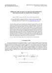
The structure of an AMESim simulation
program
Figure 2.1: The structure of the code generated by AMESim
When you perform a simulation using AMESim, computer code is produced
which is specific for the engineering system you have displayed in front of you. At
the core of AMESim is an integration algorithm, which advances the solution
through time. This integration algorithm calls the submodels, which are associated
with the components of the system as shown in Figure 2.1. These submodels may
have been selected by AMESim automatically or selected manually by you. In
either case, there will be computer code, which implements the mathematical
equations on which the submodel is based.
The order in which the submodels are called is not normally the same as the order
in which the corresponding components were added to the sketch. The submodels
are sorted into an order that is more efficient from a computational point of view.
We will return to this subject after some concepts are introduced.
5
Chapter 2
AMESim Submodels
The nomenclature of AMESim submodels will now be described.
2.3
Variables and parameters
During a simulation some quantities change with time. Typical examples are the
pressure in a pipe and the rotary speed of a load. These quantities are called
variables. Sometimes in a particular simulation, they are constant but, since in
principle they could vary with time, they are still called variables.
Other quantities are always fixed during a simulation run. These are called
parameters and these quantities normally indicate a size or dimension of a
component. Examples are the diameter of a pipe and mass of a load.
2.4
Ports and external variables
Figure 2.2: Port numbers of an icon
The icons of which the AMESim sketch of the system is built are connected
together at special points on the boundaries of the icon. These points are called
ports. There are some icons, which do not have any ports, but these are rare. Ports
are numbered in a special way. When the icon is in the form when it was originally
selected, the ports are numbered from the bottom left hand corner
counterclockwise around the icon. In Figure 2.2 the numbering of the port of the
displacement sensor icon is shown.
Figure 2.3: A typical simple system
6
AMESet 4.2
User Manual
A very simple mechanical system appears in Figure 2.3 with submodel names
added to the figure. The code of each component submodel has to calculate various
quantities associated with the component. The mass submodel MAS002 for
example calculates the velocity in m/s, the displacement in m and the acceleration
in m/s/s at each port. In order to do this, it requires information about the forces
applied at the two ports. Each of these quantities is associated with a particular port
and is called an external variable. External variables are normally available for
plotting.
2.5
Inputs and outputs
The value of the forces applied to this mass are supplied to MAS002 by the zero
force submodel F000 and the clearance submodel LSTP00A. This gives rise to the
concept of dividing submodel external variables into the categories inputs and
outputs.
Figure 2.4: The inputs and outputs of MAS002
The external variables calculated by a submodel are its outputs and for MAS002
they are:
•
velocity port 1.
•
displacement port 1.
•
acceleration port 1.
•
velocity port 2.
•
displacement port 2.
•
acceleration port 2.
whereas the inputs are:
•
force port 1.
•
force port 2.
Remember that external variables are either inputs or outputs and allow exchange
of information between submodels. The primary function of a submodel is to
calculate its outputs from its inputs.
7
Chapter 2
AMESim Submodels
In the previous section we stated that the order in which AMESim calls the
submodels during the integration is special. The idea is that AMESim tries to sort
the submodels into an order such when each submodel is called, all its inputs are
known. We say tries because sometimes no such order exists. In such
circumstances we say there is an algebraic loop also called an implicit loop.
AMESim gets over this problem by introducing special implicit variables that
break the algebraic loop. It is hoped that the elementary AMESim user never has
to think of these things. However, the submodel writer must be aware of this
problem and must try to minimize algebraic loops.
2.6
Local variables and internal variables
In a typical submodel there will be many variables including some that are not
external variables. Normally these are variables, which only exist inside the
submodel code and are totally inaccessible outside the submodel. These are known
as local variables.
Sometimes it is desirable to have a variable for plotting that is not an external
variable because it is not needed by any another submodel. AMESim allows for
this situation by having internal variables. These are like external variables but
are not associated with any port and are neither inputs nor outputs.
The angle sensor submodel ADT01, is an
example of a submodel with an internal
variable.
It has three ports each with one output:
•
torque at port 1,
•
signal output,
•
angular velocity at port 3.
and two inputs:
•
angular velocity at port 1,
•
torque at port 3.
One other variable is also calculated in ADT01:
•
angular displacement.
This variable is used with a gain and an offset to compute the signal output but it
is also useful in its own right. Variables like this are of sufficient significance to
justify making them internal variables. In consequence, the angular displacement
can be plotted if ADT01 is included in a simulation.
A much more spectacular example of a submodel with internal
variables is RSTAT. This has no ports and hence no external variables.
It monitors various statistics concerning the integration and stores them
using 14 internal variables!
8
AMESet 4.2
User Manual
There is no concept of input/output with an internal variable.
As you will see in the next section, variables can be classified into several types.
Sometimes there is a variable, which is an explicit state variable or an implicit
variable (either implicit state or constraint), but it is inappropriate to make it an
external variable. These three types of variable are not computed by the submodel
but rather by the integrator. In order to communicate values between the submodel
and the integrator, these variables must be made internal variables and cannot be
local variables, even if we are not interested in plotting graphs of them.
2.7
Types of variables
Further classification of external and internal variables is necessary. There are
eight special types of variables, which will now be introduced:
•
Explicit state variable.
•
Implicit state variable.
•
Constraint variable.
•
Duplicate variable (simple or reversed sign).
•
One-line macro variable.
•
Multi-line macro variable.
•
Fixed variable.
All of the above, if they are external variables, are outputs.
There is one type of variable which can only be an internal variable, this is an:
•
Activity variable.
Any external or internal variable that does not fit into one of these categories
AMESim refers to simply as a basic variable, giving a total of 9 variable types.
These can be used as follows:
Variable type
External variable
Internal variable
Basic
Yes
Yes
Explicit state
Yes
Yes
Implicit state
Yes
Yes
Constraint
Yes
Yes
Duplicate
Yes
No
One-line macro
Yes
No
Multi-line macro
Yes
Yes
9
Chapter 2
AMESim Submodels
Variable type
2.8
External variable
Internal variable
Fixed
Yes
Yes
Activity
No
Yes
Basic Variables
The basic variable, if it is an external variable, can be
1. an output,
2. an input,
3. an input with default,
4. an input unused.
If it is an output, it must be explicitly assigned a value. If it is an input, it will be
used in the submodel to calculate the submodel outputs. The third category, input
with default, is rare. The idea is that normally the value is supplied by another
submodel, but if the submodel connected does not supply the value, a default value
is used.
An example of submodel that uses an input with default is BHC11 in the HCD
library. This has external variables as follows:
Figure 2.5: The external variables of BHC11
The submodel represents a hydraulic chamber. At the 4 ports the inputs are a flow
rate in L/min and a volume in cm3. During normal usage we might want to connect
a BHC11 port toport 1 of the HCD piston submodel BAP11 shown on the left but
also to the hydraulic accumulator submodel HA000 shown on the right of Figure
2.6.
10
AMESet 4.2
User Manual
Figure 2.6: Submodels we want to connect to BHC11
The problem is that the accumulator HA000 does not supply a volume. The
solution was make all the volumes of BHC11 input with defaults (Figure 2.5), the
default being 0.0 cm3.
The fourth type of input/output status for a basic variable is input unused. An
example of this is SPR000RT. Submodels ending with the letters RT are designed
to be as fast as possible. Currently there are few of them but the number will grow
rapidly. Extensive use is made of duplicate variables and macro variables. They
have to be constructed very carefully to avoid algebraic loops and input unused
variables play a role in this.
Figure 2.7: The external variables of SPR000RT
The external variables of SPR000RT look the same as all the other spring
submodels but there is an important difference. The velocity is not used in
SPR000RT. However, it has to be there otherwise it would not connect to a large
number of other submodels. It is the convention that velocity comes before
displacement which comes before acceleration. The following are typical
mechanical submodels which we might hope to connect with the spring.
Figure 2.8: Typical variables on a linear shaft port
The one on the left would not connect with SPR000RT but the other two would. If
SPR00RT had only the displacement and not the velocity it would not connect with
any of them.
11
Chapter 2
AMESim Submodels
Internal variables can be basic variables. Remember there is no concept of input/
output with a internal variable but a basic internal variable behaves like an output
in that it must be assigned explicitly.
2.9
State Variables
State variables are explicit or implicit. In all cases there must be an initial value
also called a starting value for the state variable. State variables are not
computed directly by submodels. They are computed by the integrator.
A job of the submodel that is associated with the state is to directly or indirectly
define a value of the derivative of the state. Explicit and implicit state variables
differ solely in the way this assignment is made.
•
For explicit states a direct assignment is made.
•
For implicit states a quantity called a residual is defined. The integrator
tries to make this quantity as small as possible by varying both the state
variable and its derivative.
Both external and internal variables may be state variables. If an external
variable is classified as an explicit or implicit state, it is always an output.
All state variables have titles and units. The units of the time derivative of the state
can be derived from the units of the state by remembering that the simulation time
always has the units second.
Implicit state variables are rare in AMESim. It is in general far better to use
explicit state variables.
2.9.1
Explicit state variables
Almost all AMESim simulation runs involve solving differential equations. This
is because many submodels are based on differential equations. For example, most
of the mass submodels use a differential equation of the form
δv -----------force
=
δt
mass
where v is velocity and t is time. We say that v is an explicit state variable. In
AMESim nomenclature, we say that the velocity is an output of the submodel, but
strictly speaking, the submodel only calculates the velocity indirectly. What the
submodel does calculate is the time derivative of the velocity, dv/dt, as given in the
formula above. From this, the integration algorithm calculates v.
12
AMESet 4.2
User Manual
2.9.2
Implicit state variables
These have attributes which are a combination of explicit state and constraint
variables (which are described in the next section). The distinctive characteristics
are as follows:
•
The integrator gives the submodel an estimate for both the state variable and
its derivative. Submodels use these values to compute a residual. The
integrator then tries to make the residual zero.
•
The residual has units which can be unrelated to the units of the implicit state
variable.
The state is defined by a starting value and an implicit expression for the derivative
which is associated with the residual in the submodel code. An example of such an
expression is given below:
F+C
δx
δx
+ K δx = 0
δt
δt δt
This expression is used to define the residual in the submodel code:
ε = F+C
δx
δx
+ K δx
δt
δt δt
To underline the distinction we take a second example. Imagine the onedimensional motion of an object of mass M kg under the action of two forces f1 N
and f2 N so that it moves with velocity v1 m/s. If we used an explicit state we could
have the following code:
Here we explicitly define v1dot the derivative of v1. On the other hand we could
use an implicit state with the following C code:
The important point is that the same variable, v1dot, is used for the derivative and
the residual. On entry v1dot is an estimate (from the integrator) for the
derivative of v1 and has units m/s/s. On exit it is a residual and has units N. In
this case the first version is clearly better. There is only one small advantage of the
second version. This is that it can tolerate (no problem) the value M=0.
Only use implicit states if there is a very good reason for doing so.
13
Chapter 2
AMESim Submodels
2.10 Constraint variables
Figure 2.9: Constraint variables of the MAS000 submodel
v1
x1
a1
v2
x2
a2
F2
F1
These are much rarer than explicit state variables but are sometimes useful. A
simple example is in the load submodel MAS000. This submodel was developed
from MAS002, which computed the one-dimension motion of a mass subject to
two external forces (see Figure 2.9), in addition to its weight. For the purpose of
this description we will simplify the situation and only consider the velocity and
two external forces. Using the notation in the figure the time derivative of the
velocity at the right port v1 is given by
F2 ∠ F1
δv 1
= ------------------M
δt
The submodel works well under most circumstances but problems arise when the
mass M becomes very small. The simulation becomes slower and slower and
eventually unacceptably slow.
It is interesting to note that as the denominator tends to zero, so does the numerator.
This idea is implemented in MAS000 by adjusting v1 such that
F 2 ∠ F1 = 0
This is done by declaring v1 to be an algebraic or constraint variable. Constraint
variables may be internal or external variables. If they are external variables, they
are always regarded as outputs. However, submodels do not compute constraint
variables as these are computed by the integration algorithm. Instead, they
compute a quantity called the residual. This is the quantity that should be zero, but
in practice would be at best a very small quantity. In MAS000 the residual is
ε = F 2 ∠ F1
The integrator will adjust v1 in an attempt to make ε zero by an iterative process.
In order to do this a starting value must be provided. This is normally set using the
Change Parameters dialog box for the submodel. Sometimes it is difficult to set
this value to anything other than a very arbitrary value.
The equations being solved are now a mixture of differential and algebraic
equations and are referred to as differential algebraic equations (d.a.e.s) as
opposed to differential equations or more precisely ordinary differential
equations (o.d.e.s).
However, often the algebraic equation part of the whole model is far more difficult
to solve than the purely differential equation part. One of the problems is that an
algebraic equation may have:
14
AMESet 4.2
User Manual
•
a unique solution,
•
no solution,
•
multiple solutions or even
•
an infinite number of solutions.
A d.a.e. solver has a hard task to perform and can be excused for being less reliable
than an o.d.e. solver.
How does MAS000 compare with MAS002? Often when the mass is very small
compared with the forces it is spectacularly faster. It can fail, however, and it is
very easy to think of cases where this is guaranteed to happen. Suppose we set
constant values for the two forces as follows:
F 1 = 1000
F 2 = 2000
What value of v1 will make the residual zero? Clearly this is not possible and if you
try this example, you will find that the d.a.e. integrator gives up with an error
message.
To summarize, constraint variables of this type can be extremely useful but must
be used sparingly and with suitable warnings for the user.
Note that when AMESim detects an algebraic loop, it will alter the status of one
or more ordinary variable to make it an constraint variable. This will break the
algebraic loop.
2.11 Duplicates, one-line and multi-line macro
variables
These three types of variable are grouped together because they are great for
avoiding algebraic loops. They do this because the code that defines each of them
takes on the status of a submodel in its own right and is independent of the
submodel to which they belong.
Do not worry if you find this section a little confusing at first reading. As you begin
to develop your own submodels and your experience grows, read this section again
and it will become much clearer.
2.11.1 Duplicate variables
Sometimes external variables are calculated as outputs on one port but they are
also needed as outputs on other ports. On other occasions an input is received on
one port and is passed without modification to become an output on one or more
other ports. In both these situations, the copies of the original variable are known
as duplicate variables. The original is called the primary variable.
There is a further classification of duplicate variable: simple and reversed sign.
15
Chapter 2
AMESim Submodels
Often the duplicate variable has the same sign as the primary. However, it can be
convenient to have duplicate variables with the opposite sign to the primary. This
is because of the sign convention used by AMESim. If the primary variable was a
velocity state variable, the same variable but with reversed sign might be required
for another port. Note that in Figure 2.9 the variable v2 is a reversed sign
duplicate of the state variable v1. Similarly x2 is a reversed sign duplicate of x1 and
a2 is a reversed sign duplicate of a1. If there is no sign reversal, it is a simple
duplicate.
You do not make any assignment of a duplicate variable in your
submodel. This is done for you outside of the submodel.
Use duplicate variables as much as possible.
2.11.2 One-line macro
The concept of a duplicate variable involves taking the assignment of the variable
outside of the submodel. As you will later in this section, simple duplicates will
lead to AMESim (not AMESet) generating code like
v[23] = v[56];
for a simple duplicate and like
v[45] = -v[7];
for a reversed sign duplicate.
Sometimes we would like very much more complex assignments than this and the
two macro variables provide this facility.
The one-line macro variable is as its name suggests limited to a one line
assignment only. The assignment involves other suitable variables, real parameters
and real stores of the submodel, time and pi (π).
Here is an example of code generated by AMESim to implement a one-line macro.
v[12] = (v[23] - v[56])*v[78]/1.7027648993e0;
One-line macros are very useful but they make submodels difficult to debug.
Use them only when there is a strong reason for doing so. Usually this is to
break an algebraic loop.
The next variable is a heavy-weight version of the one-line macro.
2.11.3 Multi-line macro variables
The multi-line macro is an extension of the one-line macro. It is used when you
need to break up a submodel because it creates algebraic loops. It works like a oneline macro except that you write the associated code in as many lines as you need.
It is actually a double function and is stored in the file of the submodel code. It can
call other functions such as AMESim utilities or user made functions.
16
AMESet 4.2
User Manual
When a multi-line macro variable is declared, only its arguments must be entered.
These arguments are chosen from the list of the submodel variables. AMESet
writes the skeleton of the associated function automatically in the submodel code.
This function can then be completed according to your needs.
At this point it is necessary to pause to see why duplicate and macro variables are
useful.
Use of duplicate and macro variables
What is the point of introducing duplicate and macro variables? Previously we
stated that AMESim sorted submodels into a special order. We will qualify this
statement by saying that AMESim gives to duplicate variables and macro
variables the same status as a submodel. This greatly reduces the chance of
algebraic loops. Remember you can look at the code generated by AMESim. If the
system is NAME.ame, the generated source code is NAME_.c. In Figure 2. 5 is a
section of code generated (which has been edited slightly to remove lines of code
not strictly relevant to the present topic). Note the calls to the submodels and
interspersed with the assignment of the duplicates and macro variables. The
example has been taken from Chapter 4 where it is discussed in detail.
Why not make all variables duplicates or macros so that AMESim would not sort
submodels at all but solely equations? Putting all or most of the equations into the
submodel code has a lot of advantages. It makes the model much more modular
and much easier to debug. (You will be writing submodels soon. Do not expect to
always get them right first time.) AMESet actually restricts use of duplicate and
macro variables to cases where there is potentially an advantage of using them.
Figure 2.10: Duplicate and macro variables
The state variable from the integrator
The one-line macro for x only uses the
state variable which is v[5]
The mult-line macro for tfratio
only requires the state variable v[5]
The one-line macro for v uses tfratio
which is v[6]
The damper
Two one-line macros associated with the damper
The crank
One-line macro for torq
17
Chapter 2
AMESim Submodels
2.12 Fixed variables
This category of variable is the simplest. Its name, fixed variable, is rather a
contradiction! They are fixed in the sense that they retain the same value
throughout the simulation. They are variables in the sense that you can set them to
any (reasonable) value. You can also stop the simulation run, reset the value, and
then continue the run with the new value.
Since the value is fixed, you set the value of the fixed variable and AMESim will
leave the variable unchanged until the run stops naturally or is stopped by you.
AMESim derives many advantages from fixed variables and you are encouraged
to use them wherever appropriate.
An example of a submodel with a fixed variable is the
constant signal source submodel CONS0 which has a single
output constant value which is a fixed variable.
Internal variables may be fixed variables although it is difficult to see any
advantage from this arrangement.
Fixed variables should be used where appropriate instead of basic variables
because they help avoid algebraic loops.
2.13 Activity variables
The final category of variable is widely used in submodels where energy transfers
take place. The activity of an element i in a submodel is defined as a temporal
integration of the power absolute value
τ
A(τ) =
ò P(t)
⋅ dt
0
where P is the power in the element. The units are J. The activity represents a
quantity of energy that crosses the studied element. This is a different definition
from energy because it takes into account the absolute value of power.
An activity variable is always associated with a power variable. It is the user
responsibility to assign a value to the power variable in the submodel code. The
activity is then calculated by AMESim from the power.
Use this kind of variable when you want the activity of your submodel to be
calculated, this will allow you to know its index of activity in an AMESim model.
For more details on the index of activity facility, please refer to the Chapter
8:Activity index in the AMESim manual.
An activity variable is defined by a physical type:
•
18
R: dissipation.
AMESet 4.2
User Manual
•
C: capacitance.
•
I: inertia.
a physical domain:
•
hydraulic,
•
mechanical,
•
electrical,
•
thermal,
•
magnetic,
•
electric.
and a suffix which is used to generate the name for the power variable associated
with the activity. When an activity variable is declared, some extra code is
automatically added by AMESet at the end of the submodel code.
For more details on this topic, please refer to the Chapter 8:Activity index in the
AMESim manual.
2.14 Scalars and arrays
AMESim uses the term array to mean a collection of two or more related
quantities regarded as a single object. Scalars are simply single quantities but can
be regarded as arrays of dimension one (1).
Many AMESim libraries contain no arrays at all. We illustrate with an example
from the hydraulic library which contains many submodels with arrays of
variables. In the simple submodel of pipe, HL000, it is assumed that a single
representative value of pressure can be used. Variations in pressure with position
within the pipe are ignored.This is referred to as the lumped parameter approach.
Under many circumstances it is perfectly acceptable. However, if the pipe is long,
variations in pressure with position become too important to ignore. Under these
circumstances, a distributed parameter approach is used in which a series of
pressure values are computed.
The submodel HL020 is a distributive parameter pipe submodel that has an array
of 5 internal pressure nodes and an array of 5 internal flow rate nodes. All the pipe
submodels HL0xx, where xx is 10 or above, are distributed parameter submodels
with internal variables consisting of arrays of pressure and flow rate.
External variables can also be arrays although this is less common. An obvious
case where external array variables are useful is in mechanical submodels where
two or three-dimensional motion occurs. In such cases, arrays can be used to
specify position coordinates and components of velocity. These will be exchanged
between components.
Remember that all external and internal variables are either scalars or arrays.
19
Chapter 2
AMESim Submodels
2.15 Complete classification of AMESim
variables
AMESim variables have a number of classifications:
(i) they are either external or internal;
(ii) they are either scalars or arrays;
(iii) they are one of the following:
•
basic variables
•
explicit state variables
•
implicit state variables
•
constraint variables
•
duplicate variables (simple or reversed sign)
•
one-line macros
•
multi-line macros
•
fixed variables
(iv) if they are internal variables they may be:
•
activity variables
(v) if they are external variables they are either outputs, inputs, inputs with default or input unused.
AMESim insists that all variables have titles, units and a dimension. If they are
explicit state, implicit state, constraint or fixed variables, they also have special
values to be used at the start of the simulation. In the case of a fixed variable, the
value will stay the same throughout the simulation. For an implicit state or a
constraint variable the value is used as a starting value for an iterative process. For
explicit state variables, it is the initial value to be used at the start of the integration.
Four values are associated with this special value of a fixed, explicit state, implicit
state or constraint variable:
•
a minimum value
•
a default value
•
a maximum value and
•
the actual value set.
When you select a submodel, the actual value is set to the default value for all
explicit state, implicit state, constraint and fixed variables. Normally you can
change this value in the Change Parameters popup. The minimum and maximum
values are for guidance only and it is possible to set values outside of this range.
20
AMESet 4.2
User Manual
However, a submodel writer can set the minimum, default and maximum values
of an explicit state/implicit state/constraint/fixed variable to be the same.
AMESim takes this as a signal not to display the initial value on the Change
Parameters popup. By this device, the submodel writer can force a particular value
always to be used or set the initial value in the initialization section of the
submodel code.
2.16 Units of external and internal variables
Both external and internal variables have units. If a quantity such as Reynolds
number is dimensionless, you must set its units to ‘null’.
The SI system of units has won widespread acceptance in the scientific
community. In simulation work, use of these units has strong advantages and some
disadvantages. The problem is that some SI units are of a highly inappropriate size
for general and simulation use. We now consider some examples which illustrates
these advantages and disadvantages and describe the AMESim solution.
Use of SI units in calculations removes the need for conversion factors. Thus
the flow rate Q in m3/s from an ideal pump of displacement D m3 rotating at ω
rad/s is
Q = Dω
but if Q is in L/s, D in cm3/rev and ω in rev/min
Dω
Q = -----------------360x10
SI Units eliminate conversion factors and in consequence eliminate a common
source of error.
The disadvantage of the use of SI units in simulation is that they often lead to bad
scaling of state variables. This is particularly true in hydraulic applications. In
hydraulic systems, pressures of the order of 107 Pa and flow rates of 10-4 m3/s are
common but the fluid power engineer is much happier to refer to these as 100 bar
and 6 L/min respectively. Similarly it is extremely inconvenient to measure the
spool position in a servo-valve in m. It is better to use mm or a dimensionless
fractional spool position. Another bad example is in the field of magnetics where
the SI unit of magnetic flux is Wb where as most engineers would prefer to express
these quantities in µWb.
Units such as bar, L/min, rev/min and µWb will be referred to as Common units.
The problem is acute if the variable is a state or constraint variable since numerical
complexities can arise. The integrator must estimate the error εi in the step for each
state variable and constraint variable yi.
21
Chapter 2
AMESim Submodels
The most general error test for the variable is
τa+τr|yi| < εi
where τa and τr are error tolerances. There are three common error tests:
1. If τa=1 and τr=0, the test is called an absolute error test.
2. If τa=10-16 and τr=1, the test is called a relative error test. We use a small
value such as 10-16 instead of 0 to prevent problems when yi crosses zero.
3. If τa=1 and τr=1, the test is called a mixed error test. When |yi| is very large,
this is a relative error test and when |yi| is very small it is an absolute error test.
Normally the mixed or relative test is used. These works extremely well provided
the variables are well scaled. By this, we mean that the maximum value of a state/
implicit variable in the course of a simulation satisfies
10
∠3
< yi
Variables that are constant and zero are excluded from this test. This excludes
values in Wb and m3/s.
By having a different τa and τr for each state/constraint variable yi and manually
adjusting each tolerance value individually, it is normally possible to get good
results even if the state/constraint variables are badly scaled. However, this is a
tedious operation on a small system and totally impracticable on large systems.
AMESim adopts the strategy of encouraging the use of well-scaled variables and
using a default mixed error test. This implies the use of non-SI units on occasions.
To summarize:
SI units: no conversion necessary but sometimes badly scaled.
Common units: conversion factors necessary but well scaled.
To avoid calculations in non-SI units, the AMESet code generation facilities
give the option of automatic conversion between SI and common units. Use
this facility! This gives the advantages of both SI and common units.
AMESim extensively uses the following common units:
22
•
hydraulic flow rate [L/min]
•
pressure [bar]
•
spool position as a fractional value [null]
•
rotary speed [rev/min]
•
magnetic flux [µWb]
AMESet 4.2
User Manual
2.17 Plot access to external and internal
variables
It can be useful sometimes for the submodel writer to pass information through
variables at ports, and hide some variables from the AMESim user to make the
submodel clearer. AMESim/AMESet permits the submodel writer to specify that
a variable cannot be plotted by the user. Such a specification is made during the
design of the submodel.
2.18 Time as a submodel input
Sometimes submodels require time as an input. Usually they can be described as
duty cycle submodels. They provide an output variable, which is a prescribed
function of time. The current value of time is provided by the integration algorithm
and is updated as the simulation progresses.
Not all duty cycle submodels require time as an input. One could use another
variable on which to base the duty cycle.
2.19 Real, integer and text parameters
The size of components has to be defined. The characteristics of duty cycles have
to be set. You perform these tasks when you set submodel parameters. AMESim
sets default parameters when a submodel is selected and you can accept the
defaults or change them as you want.
These parameters can be real quantities, integer quantities or text expressions
being known as real parameters, integer parameters and text parameters
respectively. In computing terms, they are supplied to a submodel as arrays. They
are optional and can be omitted if not required.
The need for the real parameters is obvious. Integer parameters are normally used
for specifying which of several modes is selected. For example, many hydraulic
submodels include an orifice. There are two ways that AMESim uses to specify
the flow characteristics of a submodel:
(i) the user sets an orifice diameter and flow coefficient and these together
with the fluid density determine the flow;
(ii) a flow rate and corresponding pressure drop pair are set and used to determine the equivalent diameter.
23
Chapter 2
AMESim Submodels
In the orifice submodel OR000, an integer parameter is set to 1 to select
the flow rate - pressure drop method and 2 to select the diameter method.
This is called a standard integer parameter. There are two integer
parameters in OR000.
Figure 2.11: Two standard integer parameters in OR000.
The signal source submodel UDA01 uses a different type of integer
parameter. This is called an enumeration integer parameter. The
options are represented by meaningful text strings. UDA01 contains 3
enumeration parameters.
Figure 2.12: Changing an enumeration integer parameter.
Real and integer parameters have titles associated with them. They also have
minimum, default and maximum values. For real parameters, you can set a value
outside the range defined by the minimum and maximum value. This is not
allowed for integer parameters.
24
AMESet 4.2
User Manual
Integer parameters do not have units but AMESim insists that all real parameters
do have units. If you feel that a real parameter does not have units, set the field to
null. If the option of conversion to SI units is used, code will be inserted by the
automatic code generation facilities near the end of the initialization part. This
code will convert the real parameters from common units to SI units.
Text parameters are collections of one or more character arrays. The most common
use is to store the names of files. A more sophisticated use is to store an algebraic
expression in terms of one or more variables, which will be evaluated in the
submodel. Text parameters have four attributes:
•
a title that will be displayed in the Change parameters popup,
•
a default value for the text parameter
•
the current set value of the text parameter and
•
a Text type field which can take three values.
It is unfortunate that text arrays are stored rather differently
in the C language than in Fortran 77. For this reason, text
parameters are only allowed in submodels written in C. The
form of the initialization and calculation code will now be
described.
2.20 Initialization and calculation routines
The code of an AMESim submodel is written in C or Fortran 77 (F77). In either
case there will always be two modules of code (functions if it is written in C or
subroutines if in F77). One is called once only at the start of a simulation run and
will be referred to as the initialization routine. The other will be called many
times and will be called the calculation routine. In addition, if the submodels uses
multi-line macro variables, there will be one function for each multi-line macro.
For a submodel called NAME, both routines must be stored in a single source file,
which will be NAME.c for a C file and NAME.f for a F77 file.
In the initialization routine, access is provided to the real, integer and text
parameter arrays and to all explicit state, implicit state, constraint and fixed
variables. The following activities may be performed in this routine:
•
The real and integer parameters may be checked for valid values if you
think this is important.
•
The set values of explicit state, implicit state, constraint variables and
fixed variables can be checked.
•
If the minimum, default and maximum values of explicit state, implicit
state, constraint or fixed variables are the same, the values cannot be set
in the submodel Change parameters dialog box. They will be set to the
default value when the submodel is selected. You may wish to reset this
value in the initialization routine.
25
Chapter 2
AMESim Submodels
•
A file specified by a text parameter may be read and the values used in
some way.
•
If necessary real and integer stores may have their values set. These
variables are the subject of the next section.
2.21 Real and integer stores
An option available for submodels is to have real and/or integer arrays known as
real stores and integer stores. These arrays are accessible in both the initialization
and calculation routines. They can be used for whatever purpose you like. The
important point is that they retain their values between calls.
Here are some common uses of real stores:
•
Used to store expressions calculated in the initialization routine and
then used repeatedly in the calculation routine.
•
Used to store the final value of an iterative scheme calculated in the
calculation routine, which will be used as a starting value the next time
the submodel is called.
•
Used to store tables of information read from files in the initialization
routine and used for interpolation in the calculation routine.
The most common use of an integer store is to store an index number for a
particular mode that changes as the simulation progresses. This is extremely
important when the submodel features discontinuities. This important topic will
now be addressed.
2.22 Discontinuities
What is a discontinuity? A good example occurs in modeling a hydraulic actuator
or jack. The physical dimensions of the jack body limit the movement of the
piston. If the piston is moving within the jack body and reaches the limit of its
travel, it must be brought to rest. Often devices incorporate ‘cushion’ so that the
piston is brought to rest over a finite distance and in a finite time. If no such device
is incorporated, the piston will still be brought to rest over a finite distance and in
a finite time due to deformation of the parts involved in the collision.
Modeling of this situation is possible and extremely useful for detailed design of
hydraulic jacks. However, the transient behavior would be extremely rapid and
complex. Use of a hydraulic jack submodel incorporating these features in general
hydraulic simulation is unnecessary and might lead to unacceptable run times.
For general purposes, in the hydraulic jack submodel the assumption is made that
at the limits of its travel the jack comes instantaneously to rest. This is an example
of a discontinuity. A discontinuity is characterized by a physical quantity
26
AMESet 4.2
User Manual
jumping from one value to another instantaneously. In this example, the
physical quantity is the piston velocity.
Submodels incorporating discontinuities in physical quantities are quite rare.
However, there are related phenomena that are more common. A simple example
occurs in control systems that include saturation elements. There is an input x and
an output y. The output is limited to the range x min ≤ y ≤ x max otherwise y=x. A
typical example is shown graphically in Figure 2.13. The graph of y against x is
continuous. However, the derivative of y is discontinuous at two points also
shown in Figure 2.13. This function has a discontinuity in its first derivative. Other
functions have discontinuities in their second or higher derivative. These are not
artificially constructed examples but rather examples that do occur in modeling
work.
Figure 2.13: Saturation
Here are some other examples of discontinuities:
•
any form of backlash,
•
transition from linear to turbulent characteristics in an orifice,
•
frictional stick-slip,
•
any form of dead band,
•
a valve such as a check valve that has characteristics when open, which
are completely different to when closed,
•
any form of hysteresis,
•
any sort of duty cycle involving steps or ramps,
•
submodels which employ linear interpolation for empirical data.
Why is it necessary to stress the occurrence of discontinuities in simulation
submodels? The problem lies in the integration algorithms used for solving the
o.d.e. and d.a.e. equations that arise in simulation. They are based on integration
using methods, which assume that the state variables and some of their derivatives
are continuous. If this assumption is not true, special precautions have to be taken
at the discontinuity points. This can be illustrated by a simple graph shown in
Figure 2.14.
27
Chapter 2
AMESim Submodels
Figure 2.14: A function with a discontinuous derivative
The variable has two distinct characteristics resulting in two very different curves
C1 and C2. The variable is continuous but the derivative is discontinuous at the
point P. The integration methods have no problems when integrating along C1 but
at point P problems arise. If no special precautions are taken, as in the following
pseudo-code:
if(condition)
use formula for C1
else
use formula for C2
endif
The integrator will drastically reduce its step near the point P in a desperate attempt
to meet accuracy requirements. Many integrators will give up with an error
message when the step gets too small. Others will have a minimum step size and
when this is reached will carry on, even though the accuracy requirements are not
met. The first approach leads to frustration and the second can lead to highly
inaccurate results.
In the past many simulation packages accepted this situation but now it is almost
universally recognized that discontinuities should be handled in a more careful
manner. The idea is simple in concept. If the solution is on curve C1 and goes past
the point P then the equation for C2 is not used. Instead the equation for C1 is still
used so that effectively the curve C1’ is employed. This gives rise to a point Q
being predicted. The integrator must then realize that a discontinuity point has
been passed over and start trying to locate it. This can be done in two ways. Either
the integrator tries with a series of smaller steps sizes or some form of interpolation
is used. Either way, the point P is located within reasonable accuracy (or even to
machine accuracy). After this the integrator is restarted, forgetting all
information to the left of point P using the smooth curve C2.
This arrangement can be made to work very well but relies on cooperation between
the integration algorithm and the submodels. In practice, messages must be sent
between them so that submodels detect the discontinuity and inform the integrator.
28
AMESet 4.2
User Manual
The integrator informs the submodel when a restart is in progress so that various
initialization can be done.
2.23 Generation of code skeletons
AMESim submodels are written in either Fortran 77 or in C. By constructing new
icons and submodels you can greatly extent the capability of AMESim and
customize it to the needs of your particular application. Writing submodels is a
fascinating and rewarding activity but can be difficult and time consuming. To
ease the process, the AMESet (= AME Submodel editing tool) provides facility to
automate part of the code writing process.
In order that AMESim can use your submodel, just like standard AMESim
submodels, you must tell AMESim what icons it is associated with, what external
and internal variables it has, etc. To do this you effectively fill in a form. The
AMESet utility provides you with this form and checks your inputs to ensure that
they are reasonable and consistent.
When this process is complete, AMESet will allow you to assign variable names
to external and internal variables and optionally to real and integer parameters. It
will then generate a piece of code, the submodel skeleton, in Fortran 77 or C. This
will consist of the initialization and calculation functions or subroutines with their
declarations. In addition there will be extra functions if the submodel uses multiline macro variables.
The external and internal variables will be described in comment statements with
their titles and units. Similarly the real and integer parameters will be described.
The layout will be standardized so that the code will look the same regardless of
who wrote the submodel.
Within the code skeleton are at least six insertion points where your enter lines of
code for:
•
Private code section for own special purposes.
•
Initialization function (or subroutine) declaration statements.
•
Initialization function (or subroutine) checking statements.
•
Initialization function (or subroutine) executable statements.
•
Calculation function (or subroutine) declaration statements.
•
Calculation function (or subroutine) executable statements.
If in the course of development of the submodel you add or remove external or
internal variables or real or integer parameters, by rerunning AMESet, the
skeleton is regenerated keeping the statements you have added intact. This facility
has proved very popular with submodel writers as it removes much of the laborious
activity, allowing them to concentrate on the more creative aspects.
29
Chapter 2
AMESim Submodels
30
AMESet 4.2
User Manual
Chapter 3: Getting Started
3.1
Introduction
This chapter shows you how to create your own AMESim submodels and icons
by presenting a series of tutorial examples. However, before attempting to read this
chapter and doing the tutorial exercises, you should have experience at using
AMESim performing simple simulations using the standard AMESim submodel
libraries. You should also read Chapter 2, which gives a general background on
AMESim submodels.
The time taken to perform these tutorial exercises varies enormously. They are
open-ended in the sense that you can make your own minor modifications to the
submodels and to the experiments performed on them but allow at least three hours
to do a thorough job.
Creating an AMESim submodel involves constructing some code. This can be
done in either Fortran 77 (which will be referred to as F77) or C. However, do not
allow this to intimidate you. Much of the code can be generated automatically after
which you insert a relatively small number of lines of code. Note that there are a
lot of sections of code, which have been inserted in this chapter. They are similar
to that which is generated by AMESet but the code has been shortened slightly by
removing some comments.
The final version of each of the submodels described in this chapter is stored in the
following directory:
Using Unix:
$AME/tutorial/submodels
Using Windows:
%AME%\tutorial\submodels
You can of course copy these files into your own submodels area. However, it is
better if you generate the submodels and edit them to create the submodel code.
Remember that submodels rarely work first time and you will learn far more if you
make a few mistakes and correct them. When the author of this manual constructed
the submodels described, they certainly did not all work first time!
The development and refinements that can be applied to each submodel is almost
unlimited. In particular it is good practice to insert statements checking the values
of various parameters and to fill in the description section for each submodel. This
31
Chapter 3
Getting Started
does tend to be very time consuming and is perhaps too tedious for a tutorial
exercise. For this reason, at certain points in the exercises it is suggested that you
do copy the submodel code from the $AME/tutorial/submodels or
%AME%\tutorial\submodels directory and examine it in an editor.
Submodel name conventions
3.2
•
AMESim submodels have names of 4 to 23 characters comprising uppercase
letters and digits.
•
In all AMESim library submodel names, if there are any digits, the first digit
will be in the range 0 to 4.
•
Hence, if you create submodels with names that contain at least one digit and
if the first digit is in the range 5 to 9, there will be no name clashes with existing
standard submodels.
A rack and pinion submodel with
calculation of angular position
The rack and pinion submodel RACK00 is available in the AMESim mechanical
standard library. The first port requires a linear velocity in m/s as an input and
computes a force in N as output. The second port requires a torque in Nm as an
input and computes a rotary velocity in rev/min as output. The displacement of the
rack in mm is calculated as an internal explicit state variable. Other information
required is the radius of the pinion in mm.
Figure 3.1: The external variables of RACK00
A simple modification can be made to RACK00 to produce RACK50, which will
calculate the angular position of the pinion.
32
AMESet 4.2
User Manual
Step 1: First you use AMESet to load and examine the standard
RACK00.
1. Start AMESet as follows:
Using Unix:
Talk to your system administrator who will show you how to set up your
working environment so that you get access to AMESet. To start AMESet, in
a suitable window change to the directory where you wish to work (tutorial for
instance) and type:
AMESet
Using Windows:
Do one of the following:
•
Select AMESet from the menu Program u Imagine u AMESet produced
by the Start button, or
•
Double click on the AMESet icon on your desktop, or
•
Type AMESet in a MS DOS Command window from the directory where
you wish to work (tutorial for instance).
The display shown in will appear. It has been deliberately made similar to
AMESim but there are small differences in the display and AMESet performs
very different functions. The main display area, which in AMESim is used to
present the system sketch, will be used to display details of submodels and icons.
Figure 3.2: The AMESet display
33
Chapter 3
Getting Started
1. At the left hand side of the AMESet display are the Categories buttons. Select the Mechanical category and then click on the standard
rack and pinion icon. The dialog box below will appear.
Figure 3.3: Submodels associated with the icon rack2
Select the submodel RACK00 in the list and click on OK. Figure 3.4 shows the new
display.
Figure 3.4: RACK00 loaded into AMESet
34
AMESet 4.2
User Manual
2. Examine the details of the existing submodel. First concentrate on the tree
structure on the left shown below:
Figure 3.5: Ports, variables and parameters for RACK00
Currently Port 1, external variables and External variable 1 is selected and in
the right hand side of the display details of this external variable are displayed.
Figure 3.6: External variable
3. Examine other details as follows:
•
Select port 1 External variable 2.
•
Expand Port 2, external variables and select in turn each of the two external variables.
•
Expand Internal variables and select the single internal variable
•
Expand Real parameters and select the single real parameter.
•
Note the status of the Submodel requirements at the bottom left:
35
Chapter 3
Getting Started
Figure 3.7: Submodel requirements
4. Just in case you have made any accidental changes, do File u Close.
Step 1: The next stage is to plan carefully what you are going to do
1. You will use the standard rack and pinion icon, which has 2 ports.
2. You will base the new submodel on RACK00 which has four external variables
and one internal variable.
3. RACK50 will have the same external variables, but two internal variables. The
additional one being the angular position of the pinion. You are going to edit
the submodel RACK00 and alter it slightly in order to introduce this extra internal variable.
4. You will then save it as RACK50.
According to this plan, RACK50 will have the specifications listed below. They
are the same as RACK00 except the one in bold:
•
Field
36
There are 2 ports:
Port 1 variable
1
Port 1 variable
2
Port 2 variable
1
Port 2 variable
2
Type
one line macro
basic variable
input
one line macro
basic variable
input
Title
force at port 1
linear velocity
at port 1
rotary velocity
at port 2
torque at port 2
Unit
N
m/s
rev/min
Nm
Name
f1
v1
w2
t2
Expression
t2/radius
-
v1/radius
-
Dimension
-
1
-
1
AMESet 4.2
User Manual
•
There are 2 internal variables:
Field
•
Internal variable 1
Internal variable 2
Type
explicit state
basic variable
Can be plotted
-
True
Title
displacement of the
rack
angular position
Unit
mm
degree
Name
x
theta
Derivative name
dx
-
Dimension
1
1
Min value
0
-
Default value
0
-
Max value
0
-
There is 1 real parameters:
Field
Parameter 1
Title
radius of the pinion
Unit
mm
Variable name
x
Min.
-100000
Default
10
Max.
100000
•
The submodel does not generate discontinuities.
•
The submodel does not require time.
•
The submodel does require SI unit conversion.
Step 2: Create the new submodel
For this simple submodel the planning is complete and you can use AMESet to
create a specification of the submodel and generate a code skeleton. It is good idea
to create a special folder or directory called tutorial and do all the exercises in this
directory.
Note that for the rest of the tutorial exercises, you should save all your submodels
in the same area in which you are now working (tutorial directory). The process of
generating code for new submodels is largely a matter of filling forms. Here you
37
Chapter 3
Getting Started
are going to use the settings of the already existing submodel RACK00 and alter
them to get our own submodel you will call RACK50:
1. If necessary, reload RACK00 as you did in Step 1.
2. In the brief description field, type in the text shown below. The description
field contains text, which will be displayed when submodels are selected in
AMESim.
Figure 3.8: The brief description for the rack and pinion submodel
3. Below is a table in which you will find the list of the existing variables, parameters and stores. Select the item Internal variables and click on the column
Number. The current number of internal variable is 1: set it as 2.
Figure 3.9: Adjusting the numer of internal variables
4. Select the item Internal variable 2 and assign it the features shown in Figure
3.10 : The new internal variable characteristics.
Figure 3.10: The new internal variable characteristics
At this point a few words of explanation are needed:
•
The variable type is chosen in a list of possible types:
Figure 3.11: Setting the type of variable
38
AMESet 4.2
User Manual
You select basic variable because the angular position can be obtained directly
from the position of the rack and the radius of the pinion. The angular position
is explicitly defined by:
x
theta = ----------------radius
x is the linear position of the rack and radius is the radius of the pinion.
•
Another way of determining theta would be to use the fact that the derivative
of theta is omega. The angle theta could then be calculated from the angular
velocity omega by the AMESim integrator. This would involve setting up the
internal variable as follows:
Figure 3.12: Internal variable
However, this would be inefficient because you would be using 2 state variables when only one is needed. This is the reason why we define theta as a basic
variable.
•
The unit can be directly typed in or it can be chosen in the list below. This list
is obtained by clicking on the button
, to the right of the Value field:
Figure 3.13: Selecting a unit using the Unit Chooser
39
Chapter 3
Getting Started
•
AMESet can create code in Fortran 77 (F77) or in C. Since F77 is the most
restrictive of these languages in terms of variable names, AMESet uses the
F77 name restrictions on variable names. Hence names must
•
be of 12 characters or less (the strict standard says 6 but normally 12 is
accepted);
•
consist of either alphabetical characters or digits;
•
start with a letter.
Note:
There are some further restrictions due to reserved C and
F77 keywords such as if, else, for, call etc. If you enter a
wrong keyword, you are informed with the red light in
the upper right side of the interface, or with an error
message.
•
The dimension must be left at 1. Dimensions greater than 1 indicate an
array of variables. This feature is useful on occasions but its use is not
common.
5. You can also get a preview of the Change Parameters and Variable List dialog
boxes you would get in AMESim. Click on the buttons
and
the previews shown in Figure 3.14 and Figure 3.15 respectively:
Figure 3.14: Parameter Mode Preview
40
to get
AMESet 4.2
User Manual
Figure 3.15: Run Mode Preview
.
6. Select the programming language you want AMESet to use for creating the submodel code (either C or Fortran).
7. Generate the submodel code by clicking on
, then click on
in order
to edit this code. Below is an example of the code generated in C. The next section (3.3 Comments on the code generated by AMESet) gives more details on
the content of the following code.
Please note that the code is edited in the AMESet fallback editor, which is the
current default editor. If you wish to use another editor, please refer to the paragraph 5.4.3 Options menu, AMESet preferences in the Editors section.
41
Chapter 3
Getting Started
In C:
/* Submodel RACK50 skeleton created by AME Submodel editing utility
jeu. 27. mars 09:16:00 2003 */
#include <math.h>
#include <stdio.h>
#include <stdlib.h>
#include "ameutils.h"
/*****************************************************************************
TITLE : RACK50
-----------------------------------------------------------------------------DESCRIPTION :
This submodel of a rack and pinion converts a linear velocity v1
in m/s (port 1) into an angular velocity w2 in rev/min (port2) and
a torque t2 in Nm (port 2) into a linear force in N (port 1) f1.
w2 = v1 / radius
(S.I. units)
f1 = t2 / radius
(S.I. units)
where radius is the transformation ratio set by the user which corresponds
to the primitive radius of the pinion.
A rack displacement in mm (x) is calculated by integrating the linear
velocity (v1).
-----------------------------------------------------------------------------USAGE :
-----------------------------------------------------------------------------PARAMETER SETTINGS :
The transformation ratio (radius) must be different from zero! However,
a negative value will be accepted. This can be used to reverse the
sign of the rotary motion.
-----------------------------------------------------------------------------DATE OF CREATION/AUTHOR : 26/02/1999 R.RHOTE-VANEY
-----------------------------------------------------------------------------SOURCE :
IMAGINE Roanne (42)
5, rue Brison
42300 ROANNE
tel: (33).04.77.23.60.30
FRANCE
fax: (33).04.77.23.60.31
*****************************************************************************/
/* >>>>>>>>>>>>Insert Private Code Here. */
/* <<<<<<<<<<<<End of Private Code. */
/* There is 1 real parameter:
rp[0] = radius
radius of the pinion [mm -> m]
*/
/* There are 0 integer parameters:
*/
42
AMESet 4.2
User Manual
/* There are 0 text parameters:
*/
#ifdef _NO_PROTO
void rack50in_(n, rp, x)
int *n;
double rp[1];
double *x;
#else
void rack50in_(int *n, double rp[1], double *x)
#endif
{
int error = 0;
/* >>>>>>>>>>>>Extra Initialization Function Declarations Here. */
/* <<<<<<<<<<<<End of Extra Initialization declarations. */
double radius;
radius
= rp[0];
/*
If necessary, check values of the following:
rp[0..0]
*x
*/
/* >>>>>>>>>>>>Initialization Function Check Statements. */
if(radius == 0.0)
{
fprintf(stderr, "/nPinion radius cannot be = 0./n");
error = 2;
}
/* <<<<<<<<<<<<End of Initialization Check Statements. */
if(error == 1)
{
fprintf(stderr, "\nWarning in RACK50 instance %d.\n", *n);
}
else if(error == 2)
{
fprintf(stderr, "\nFatal error in RACK50 instance %d.\n", *n);
fprintf(stderr, "Terminating the program.\n");
AmeExit(1);
}
/* Common -> SI Conversions. */
rp[0]
radius
*= 1.00000000000000e-003;
= rp[0];
43
Chapter 3
Getting Started
/* >>>>>>>>>>>>Initialization Function Executable Statements. */
/* <<<<<<<<<<<<End of Initialization Executable Statements. */
}
/*
There are 2 ports.
Port number 1 has 2 variables:
Variable number 1 `f1' function expression is:
't2/radius'
force at port 1
[N]
Variable number 2 `v1' variable scalar input
linear velocity at port 1
[m/s]
Port number 2 has 2 variables:
Variable number 1 `w2' function expression is:
'v1/radius'
rotary velocity at port 2
[rev/min]
Variable number 2 `t2' variable scalar input
torque at port 2
[Nm]
*/
/*
There are 2 internal variables.
Variable number 1 (x) explicit state scalar derivative `dx'
displacement of the rack
[mm -> m]
Variable number 2 (theta) variable scalar
angular position
[degree -> rad]
*/
#ifdef _NO_PROTO
void rack50_(n, v1, t2, x, dx, theta, rp)
int *n;
double *v1;
double *t2;
double *x;
double *dx;
double *theta;
double rp[1];
#else
void rack50_(int *n, double *v1, double *t2, double *x, double *dx
, double *theta, double rp[1])
#endif
{
*theta
= ??;
*/
int logi;
/* >>>>>>>>>>>>Extra Calculation Function Declarations Here. */
/* <<<<<<<<<<<<End of Extra Calculation declarations. */
int loop;
double radius;
44
AMESet 4.2
User Manual
radius
= rp[0];
/* Common -> SI units conversions. */
*x
*= 1.00000000000000e-003;
/*
Set all submodel outputs below:
*dx
= ??;
/* >>>>>>>>>>>>Calculation Function Executable Statements. */
*dx = *v1;
/* <<<<<<<<<<<<End of Calculation Executable Statements. */
/* SI -> Common units conversions. */
*x
/= 1.00000000000000e-003;
*dx
/= 1.00000000000000e-003;
*theta
/= 1.74532925199433e-002;
}
1. Alter the code as follows in the Calculation Function Executable Statements:
In C:
/* >>>>>>>>>>>>Calculation Function Executable Statements. */
*dx = *v1;
*theta = *x/radius;
/* <<<<<<<<<<<<End of Calculation Executable Statements. */
In F77:
C>>>>>>>>>>>>Calculation Function Executable Statements.
dx = v1
theta = x/radius
C<<<<<<<<<<<<End of Calculation Executable Statements.
45
Chapter 3
Getting Started
As the automatic SI unit conversion is applied, you do not have to take care of
the units:
•
v1 is in m/s,
•
theta is in degree,
•
x and radius are in mm
These variables are all converted to SI units before the executable statements
so that the formula giving theta does not require any conversion coefficients.
At the end of the executable statements the variables are converted back to their
original units.
1. Next close the editor (File u Close for the fallback editor) and compile the
code by clicking on the button
. A dialog box similar to the one below will
appear indicating if the code is compiled properly:
Figure 3.16: Compiling RACK50
Step 1: Test your new submodel.
1. Start AMESim and build the small model below in order to test your new submodel:
Figure 3.17: The new submodel in AMESim
A piece wise linear torque profile is applied to the rack and the angular position
will respond to this.
46
AMESet 4.2
User Manual
2. In Submodel mode, select the submodels and in Parameter mode assign them
the following non-default parameters:
Submodel
UD00
RACK50
Title
Value
output at start of stage 1 [null]
-15
output at end of stage 1 [null]
-15
duration of stage 1 [s]
1
output at start of stage 2 [null]
15
output at end of stage 2 [null]
15
duration of stage 2 [s]
2
output at start of stage 3 [null]
-15
output at end of stage 3 [null]
-15
duration of stage 1 [s]
1
radius of the pinion [mm]
200
3. Run a simulation for 4 seconds with a communication interval of 0.01 second
and plot the angular position of the pinion and its velocity. You should get the
following curves:
Figure 3.18: Angular position and velocity of the pinion
47
Chapter 3
Getting Started
3.3
Comments on the code generated by
AMESet
Functions defined in the submodel code
The first thing to notice is that there are 2 Fortran subroutines or 2 C functions:
•
The first is for initialization and is called once at the beginning of the
simulation.
•
The second is for calculations and is called many times during the simulation.
Calculation accuracy
All arithmetic is performed to double precision accuracy.
In F77:
One consequence of this is that in F77 code you should always put real
constants in double precision form i.e. 0.39d0 rather than 0.39 or 0.39e0.
User reserved places in submodel code
There are six places in the code where you are invited to insert your own lines.
These start with <<<< and end with >>>> characters. These insertion points are
described below in Fortran:
1.
C >>>>>>>>>>>>Insert Private Code Here.
C <<<<<<<<<<<<End of Private Code.
The private parts section can be used for various purposes. You could for instance write a function or subroutine, which is called by your submodel.
2. C >>>>>>>>>>>>Extra Initialization Function Declarations Here.
C <<<<<<<<<<<<End of Extra Initialization declarations.
Here you are invited to make extra variable declarations you which to use in
the initialization subroutine or function.
3. C
If necessary, check values of the following:
C
rp(1..1)
C
x
C >>>>>>>>>>>>Initialization Function Check Statements.
C <<<<<<<<<<<<End of Initialization Check Statements.
Here you have the option to make checks on variable and parameters. This section is preceded by comments that suggest the things that you might like to
check. In this case it is the starting value of the state variable (the linear displacement of the rack) and the value of the real parameter (the radius of the pin48
AMESet 4.2
User Manual
ion).
4. C >>>>>>>>>>>>Initialization Function Executable Statements.
C <<<<<<<<<<<<End of Initialization Executable Statements.
Here you insert statements that assign variables. This will become clearer in
later examples.
5. C >>>>>>>>>>>>Extra Calculation Function Declarations Here.
C <<<<<<<<<<<<End of Extra Calculation declarations.
Here you can declare extra variables and functions for the calculation subroutine or function.
6. C
Set all submodel outputs below:
C
dx
= ??
C
theta
= ??
C >>>>>>>>>>>>Calculation Function Executable Statements.
C <<<<<<<<<<<<End of Calculation Executable Statements.
Here assignments are made for the outputs of the submodel. AMESet tells
which variables have to be set.
Submodel description
Note the lines of code which are near the beginning of the file, they are similar to
the following ones which are in Fortran:
C
****************************************************************
*
C TITLE :
C
C ---------------------------------------------------------------C DESCRIPTION :
C
C ---------------------------------------------------------------C USAGE :
C
C ---------------------------------------------------------------C PARAMETER SETTINGS :
C
C ---------------------------------------------------------------C REVISIONS :
C
C
****************************************************************
It is intended that you:
•
Modify this template if it is already filled with information on the submodel from which you create the current submodel. This is the case for
RACK50 which was made from RACK00.
49
Chapter 3
Getting Started
•
Complete this template if it is empty as shown above. This happens
when you create a submodel without starting from an existing one.
These lines give a description of the submodel you are currently constructing.
AMESim integrator
It is worth mentioning a small point, which does sometimes cause confusion to
beginners:
It is not the job of the submodel to do the integration.
There is a central integration algorithm for doing this. Thus you do not make an
assignment in the calculation code for the state variable (theta or *theta) using your
favorite integration method. Instead you must define the derivative of the state
variable (omega or *omega) and from this derivative, this is the AMESim
integrator which calculates the state.
C language specific features
If you ask AMESet to generate your submodel code in C, you must be aware of
conventions which are specific to this programming language:
•
AMESim generates calls to submodels without consideration as to whether
they are written in F77 or C. In practice this means that all variables on the
argument list will be referenced as pointers. If variables that are used in
assignment statements are on the argument list, they will have a ‘*’ in front of
them. Thus you have:
*dx = *v1;
*theta = *x/radius;
rather than
dx = v1;
theta = x/radius;
•
Some Unix versions of C conform to the ANSI standard and use full function
prototypes. Others do not. You will notice constructions of the type
#ifdef _NO_PROTO
some statements
#else
some different statements
#endif
The first set of statements is for versions of C which do not accept full function
prototypes and the second for those that do. If compilation is performed with a
-D_NO_PROTO
50
AMESet 4.2
User Manual
option, the first set of statements will be compiled otherwise the second set will be
compiled.
Compilation flags for Fortran below Unix
For F77 users under a Unix environment the following information may be of
interest.
When compiling, the following set of options is useful:
f77 -c -g -C -u ...
•
-g option prepares the code for use within a debugger.
•
-C enables array bound checking.
•
-u flags undeclared variables as errors.
Check statements
At this point, if you were to continue developing the submodel, you would check
the value of some variables and warn the user or even stop the simulation run if the
user had set completely unsatisfactory values. For the time being it is suggested
that you look at the code in the $AME/submodels (or %AME%/submodels) area to
see how check statements are inserted rather than actually do the operations
yourself.
You can look at the source code of any submodel (called NAME for instance) in
the AMESim system area. You will find that this code contains a description as
well as check statements that are very carefully filled. The easiest way is to load
the appropriate file into your preferred editor:
Using Unix:
$AME/tutorial/submodels/NAME.f or
$AME/tutorial/submodels/NAME.c or
$AME/submodels/NAME.c
Using Windows:
%AME%\tutorial\submodels\NAME.f or
%AME%\tutorial\submodels\NAME.c or
%AME%\submodels\NAME.c
You have read only access to these files and you can print them if you want. The
check statements test the value of some variables such as real parameters,
explicit state initial values, fixed variables etc. If it is an unacceptable value,
the program may be stopped. Note how the statements are placed in a special
checking section of the initialization routines between lines labeled:
51
Chapter 3
Getting Started
In F77:
C >>>>>>>>>>>>Initialization Function Check Statements.
C <<<<<<<<<<<<End of Initialization Check Statements.
or
In C:
/* >>>>>>>>>>>>Initialization Function Check Statements. */
/* <<<<<<<<<<<<End of Initialization Check Statements. */
In the current submodel (RACK50) the check statements come from RACK00 and
can be updated.
A special variable named error is declared for you and initialized to 0:
•
If you want the program to be stopped when an unacceptable value is
found, you must set the local variable error to 2.
•
If it is just a warning, set error to 1.
After the section for checking, the value is examined, a message printed and if
necessary the program is terminated.
Stopping a simulation from a submodel
Note that in the C code you do not use the function exit to stop the simulation but
rather the function AmeExit. Similarly in Fortran you do not use stop but rather the
subroutine famexit. You could use exit or stop but the alternatives provided enable
AMESim to terminate in a rather more graceful manner. This is very important
when your AMESim executable is interfaced with some other code (such as with
the Simulink interface).
We will repeat the following request several times in the manual:
•
If you use C, do not use the function exit (or abort). Use AmeExit(1) instead.
•
If you use F77, do not use the subroutine stop. Use call famexit(1) instead.
Note there is one integer argument to these functions. You normally set this to
1. The value 0 indicates a normal exit and any other value an abnormal exit (i.e.
on detecting an error).
Files associated with a submodel
Note that for each submodel you create (called NAME for instance) there are three
files associated with it:
52
•
The source file NAME.f or NAME.c.
•
The specification file NAME.spe.
•
The compiled version of the source NAME.o (or NAME.obj).
AMESet 4.2
User Manual
3.4
Prime mover with start up
characteristics
3.4.1
Introduction
The simplest prime mover submodel of the Mechanical library is
PM000 which is a constant speed source. There is only one external
variable which is a fixed variable with title shaft speed and units
rev/min. A typical graph of the shaft speed using the default
parameters is shown below:
Figure 3.19: The constant speed prime mover
It would be interesting to develop a submodel, which gave the start up
characteristics of the prime mover. Denoting the speed of the prime mover at time
t by ω , a simple model of the start up characteristics is:
ω = ϖ (1 − exp (− t / τ ))
where ϖ is the final speed of the prime mover in rev/min and τ is a time constant
in seconds. You could have taken the angular speed in rad/s so that everything was
in SI units, but the use of rev/min does not introduce any unpleasant conversion
factors.
The formula assumes the prime mover starts from rest at time t = 0 . It might be
useful to be able to modify this formula so that the prime mover could be started
after some time delay. If it starts at time t = t start , the equation becomes
∠ ( t ∠ t start ) ü
ì
ω = ϖ í 1 ∠ exp æè -----------------------------öø ý
τ
þ
î
for t ≥ tstart and ω = 0 otherwise.
53
Chapter 3
Getting Started
There will still be a single variable but it will be of type basic variable instead of
fixed variable. In addition, there will be three real parameters with the following
titles and units:
•
final speed [rev/min]
•
time constant [s]
•
startup time [s]
Figure 3.20: Prime mover with start up characteristic
A typical graph of ω against time is shown in Figure
3.19. It is clear that ω is a continuous function of time
but its derivative is not (discontinuity at time t = 2 s).
If the prime mover were connected to a rotary spring as shown, the discontinuity
would be transferred to the spring submodel RSPR00. The angular twist θ
calculated by the spring submodel is a state variable and ω would be used in
defining its derivative. Hence θ would have a discontinuity in its second
derivative. This is a relatively mild discontinuity and it is marginal as to whether
special precautions should be taken for this. Generally speaking:
54
•
it is essential to take special precautions if states or their first derivatives
are discontinuous;
•
if there is a discontinuity in the third or higher derivative of a state, no
special precautions are necessary;
•
for a discontinuous second derivative of a state it is wise, but not normally essential, to take special precautions. For this example, you will
try both approaches.
AMESet 4.2
User Manual
3.4.2
Submodel with no discontinuity handling
You will first create a prime mover submodel without any discontinuity handling:
1. Start AMESet, select the prime mover icon from the Mechanical library and
choose the submodel PM000 in the submodel list.
Note the following information about this submodel.
Figure 3.21: Calculation function Never called
PM000 is a very simple submodel. It is so simple that there is no need for a calculation function at all. Ticking the Never radio button ensures AMESim will
never attempt to call the calculation function.
2. Since you DO want AMESim to call our calculation function, tick the Always
radio button.
Figure 3.22: You do want the calculation function called
Note there is a third possibility: call the calculation function only When printing. This is useful when there are only information only variables.
3. Set the number of real parameters to 3 and set their titles, units, variable names
and minimum, default and maximum values as suggested in the following table:
Field
Parameter 1
Parameter 2
Parameter 3
Title
final speed
time constant
startup time
Unit
rev/min
s
s
Variable name
omegaf
tau
tstart
Min.
-5000
1e-6
-1e6
Default
1500
1
0
Max.
5000
1e3
1e6
55
Chapter 3
Getting Started
Below is what you should have for the first real parameter:
Figure 3.23: First real parameter
4. Specify that there is one external variable on port 1 with the characteristics
shown in Figure 3.23.
Figure 3.24: The external variable of PM50
5. For the submodel brief description use (see Figure 3.24):
‘prime mover with start up characteristics’
6. There is one important difference between PM50 and RACK50. PM50 requires
access to time. This can be achieved by clicking on the check box labeled
Submodel requires time.
7. As we will not deal with discontinuities for the time being, ensure that the
check box Submodel requires discontinuity flag is not ticked.
56
AMESet 4.2
User Manual
8. In this example it is definitely not worth converting to SI units so ensure that
the check box Convert to SI Units is not ticked.
Figure 3.25: Submodel requirements
9. Now select File from the menu bar and then Save. The dialog box below
should appear and you can then type the name of your submodel.
Figure 3.26: Type the name of your submodel
10. Generate the code skeleton by clicking on
with
and edit the generated code
.
57
Chapter 3
Getting Started
In the calculation routine omega must be defined. This involves inserting the
following lines of code:
In F77:
if (t .ge. tstart) then
omega = omegaf*(1- exp(-(t - tstart)/tau))
else
omega = 0.0
endif
In C:
if (*t >= tstart)
{
*omega = omegaf*(1- exp(-(*t - tstart)/tau));
}
else
{
*omega = 0.0;
}
1. Compile the submodel by clicking on
and then test it with a suitable system in AMESim. The following test system is satisfactory:
Figure 3.27: Test system for PM50
Note that while you are doing this you can exit AMESet or leave it running.
Try it with various final speeds, time constants and startup times. You will
probably find its performance is satisfactory despite the discontinuity. However, ignoring discontinuities like this can create problems and often leads to
longer simulation runs. Enable run Statistics from the Run parameters (see Figure 3.26) and perform a run making a note of:
•
The time for the simulation.
•
The maximum step size used.
•
The number of function evaluations.
The latter is the number of times each submodel is called.
58
AMESet 4.2
User Manual
Figure 3.28: Enable statistics
3.4.3
Submodel with discontinuity handling
Modification of the submodel specification
To modify PM50 to handle the discontinuity properly, restart AMESet if
necessary and select the prime mover. PM50 will appear as an existing submodel
and you must select it to read in the current specification. There are two changes
to be made to the specification:
1. Tick the check box Submodel requires discontinuity flag.
2. Set the number of Integer stores to 1.
Figure 3.29: Change submodel requirements
When you have done this, save this new version as PM51. You can then
generate F77 or C code without any further modification.
59
Chapter 3
Getting Started
In F77:
subroutine pm51(n, omega, rp, ic, flag, t)
integer n, ic(1)
double precision rp(3), omega
double precision t,tau, tstart
integer flag
logical logi
logical disimp
external disloc, disimp
external distim
C >>>>>>>>>>>>Extra Calculation Function Declarations Here.
C <<<<<<<<<<<<End of Extra Calculation declarations.
omegaf = rp(1)
tstart = rp(2)
tau = rp(3)
C Set all submodel outputs below:
C omega = ??
C >>>>>>>>>>>>Calculation Function Executable Statements.
if (t .ge. tstart) then
omega = omegaf*(1- exp(-(t - tstart)/tau))
else
omega = 0.0
endif
C <<<<<<<<<<<<End of Calculation Executable Statements.
end
60
AMESet 4.2
User Manual
In C:
#ifdef _NO_PROTO
void pm51_(n, omega, rp, ic, flag, t)
int *n;
double *omega;
double rp[3];
int ic[1];
int *flag;
double *t;
#else
void pm50_(int *n, double *omega, double rp[3], int ic[1],
int *flag , double *t)
#endif
{
int logi;
/* >>>>>>>>>>>>Extra Calculation Function Declarations Here. */
/* <<<<<<<<<<<<End of Extra Calculation declarations. */
double omegaf, tstart, tau;
omegaf = rp[0];
tstart = rp[1];
tau = rp[2];
/*
Set all submodel outputs here:
*omega = ??;
*/
/* >>>>>>>>>>>>Calculation Function Executable Statements. */
if(*t >= tstart)
{
*omega = omegaf*(1 - exp(-(*t - tstart)/tau));
}
else
{
*omega = 0.0;
}
/* <<<<<<<<<<<<End of Calculation Executable Statements. */
}
Note:
•
AMESet has kept your lines of executable code provided you put them
in the approved place.
•
An extra variable called flag has appeared on the argument list. This is
the discontinuity variable and plays an extremely important role in the
handling of discontinuities.
•
A variable named logi has been declared which is of type int in C code
and logical in the Fortran code.
•
In the Fortran code subroutines named disloc and distim are declared
on external statements and the logical function disimp is also declared
on an external statement. These utilities will be called to handle discontinuities as they occur.
61
Chapter 3
Getting Started
These functions are actually also declared in the C code but the declaration are in the header file ameutils.h. Strangely in C they are named
disloc_, distim_ and disimp_. There is a good reason for this. By adding the underscore, the same utility name_ can be called as name from
F77 code and name_ from C code.
•
The array ic dimensioned at 1 has appeared on the arguments list. This
is the integer store and in the present submodel it will be used to record
the current state of the prime mover i.e. whether the speed is a constant
zero before the start up time, or is rising with time.
•
The integer variable loop is introduced to deal with cases where some
external or internal variable is an array and is used as a ‘do’ or ‘for’ loop
parameter.
Modification of the submodel code
The modifications you must make to the code are as follows:
In F77:
subroutine pm51(n, omega, rp, ic, flag, t)
integer n, ic(1)
double precision rp(3), omega
double precision t,tau
integer flag
logical logi
logical disimp
external disloc, disimp
external distim
C >>>>>>>>>>>>Extra Calculation Function Declarations Here.
C <<<<<<<<<<<<End of Extra Calculation declarations.
omegaf = rp(1)
tstart = rp(2)
tau = rp(3)
C Set all submodel outputs below:
C omega = ??
C >>>>>>>>>>>>Calculation Function Executable Statements.
if(flag .eq. 0)then
if(t .ge. tstart)then
62
AMESet 4.2
User Manual
C Prime mover has started.
ic(1) = 1
else
C Prime mover has not started.
ic(1) = 0
endif
endif
if(ic(1) .eq. 1)then
C Prime mover has started.
omega = omegaf * (1 - exp(-(t-tstart)/tau))
else
C Prime mover has not started.
omega = 0
C Register discontinuity at time tstart
call distim(tstart)
endif
C <<<<<<<<<<<<End of Calculation Executable Statements.
end
In C:
#ifdef _NO_PROTO
void pm51_(n, omega, rp, ic, flag, t)
int *n;
double *omega;
double rp[3];
int ic[1];
int *flag;
double *t;
#else
void pm50_(int *n, double *omega, double rp[3], int ic[1], int *flag
, double *t)
#endif
{
int logi;
/* >>>>>>>>>>>>Extra Calculation Function Declarations Here. */
/* <<<<<<<<<<<<End of Extra Calculation declarations. */
63
Chapter 3
Getting Started
double omegaf, tstart, tau;
omegaf = rp[0];
tstart = rp[1];
tau = rp[2];
/*
Set all submodel outputs here:
*omega = ??;
*/
/* >>>>>>>>>>>>Calculation Function Executable Statements. */
if(*flag == 0)
{
/* Initialization call. Set the value of ic[0]. */
if(*t >= tstart)
{
/* Prime mover has started. */
ic[0] = 1;
}
else
{
/* Prime mover has not started. */
ic[0] = 0;
}
}
if(ic[0] == 1)
{
*omega = omegaf*(1 - exp(-(*t - tstart)/tau));
}
else
{
*omega = 0.0;
/* Register discontinuity at time tstart. */
distim_(&tstart);
}
/* <<<<<<<<<<<<End of Calculation Executable Statements. */
}
At this point a few words of explanation are needed:
•
64
Calls are made to the calculation routine with integer flag set to a variety of
values. The value indicates the purpose of the call. The only special value you
need worry about is flag = 0. This is a call to the routine for the purpose of
initialization. At the start of each run, the first call to each submodel which has
a discontinuity will have flag = 0. If any discontinuity occurs during a run,
immediately after the discontinuity is located there will be a further call to each
submodel with flag = 0. This allows the submodel to perform any initialization.
AMESet 4.2
User Manual
•
For the current submodel, ic(1) (in F77) or ic[0] (in C) is set to 0 if the prime
mover is in the pre-start up phase or 1 otherwise.
•
There are now two sections of code corresponding to each of the two values of
the ic state indicator. For each call to the submodel, only one section of code
will be visited.
•
A switch from one section of code to the other corresponds to a discontinuity.
In this case it is possible to switch from the pre-start up to the post-start up
phase but impossible to switch in the other direction.
•
The Fortran subroutine distim (or the C function distim_) is used to register
discontinuities which occur at a known time.
•
Note that great care is needed to ensure complete consistency. Thus if the
following statements had been used:
In F77:
if(t .gt. tstart)then
ic(1) = 1
endif
instead of
if(t .ge. tstart)then
ic(1) = 1
endif
In C:
if(*t > tstart)
{
ic[0] = 1;
}
instead of
if(*t >= tstart)
{
ic[0] = 1;
}
there could have been a major conflict. A discontinuity could have been located
at time tstart and a restart organized. The ic(1) or ic[0] variable would then
have been set to 0 and another discontinuity located at time tstart followed by
another restart. What would happen after this is rather unpredictable.
To summarize:
Discontinuities involve changing from one regime, mode or state to another.
Each regime has its own set of continuous equations. It is of the greatest impor65
Chapter 3
Getting Started
tance that the code for detecting a change of regime should be totally consistent
with the code for setting the regime. In the present example you are using:
ic(1)
condition for regime
condition for leaving regime
0
t .lt. tstart
t .ge. tstart
1
t .ge. tstart
t .lt. tstart
or:
ic[0]
condition for regime
condition for leaving regime
0
t < tstart
t >= tstart
1
t >= tstart
t < tstart
However, note that in this example, since time does not go backwards, you do
not need to test for leaving the region corresponding to ic(1)=1 (in F77) or
ic[0]=1 (in C).
Submodel test
Retest the submodel with the same system as before (Figure 3.25). Remove the old
submodel PM50 by selecting the new prime mover PM51 in Submodel mode.
After this, collect statistics for the run (see Figure 3.26) with the modified
submodel. You should find that the run:
•
is faster,
•
has fewer function evaluations and
•
uses a bigger maximum step size.
The cost is a slightly more complex submodel, which must be coded very
precisely. You can examine the files PM51.f and PM51.c files in the $AME/
tutorial/submodels or %AME%\tutorial\submodels areas (the same as with
RACK50).
3.5
Square wave submodel
This is the last exercise, which deals specifically with discontinuities. Clearly a
square wave is a discontinuous function. Here is some simple code for the square
wave:
66
AMESet 4.2
User Manual
In F77:
cycles = t/c(1)
if (cycles/2*2 .eq. cycles) then
C At minimum value.
output = minv
else
C At maximum value.
output = maxv
endif
In C:
cycles = (int)(*t/c[0]);
if (cycles/2*2 == cycles)
{
/* At minimum value. */
*output = minv;
}
else
{
/* At maximum value. */
*output = maxv;
}
You are going to create your own square wave submodel using the code
above and the icon shown.
This icon can be found in the Signal, Control and Observers category.
The following points give indications for constructing this submodel
which you will call SQ50.
67
Chapter 3
Getting Started
•
The submodel SQ50 has a single external variable, which we have referred to
as output:
Figure 3.30: The external variable for SQ50
•
The frequency in Hz is a real parameter, which can be denoted by f:
Figure 3.31: Frequency in Hz
•
The variables minv and maxv are also real parameters representing the
minimum and maximum values of the square wave. This gives three real
parameters:
frequency of square wave[Hz]
minimum value[null]
maximum value[null]
68
AMESet 4.2
User Manual
•
The variable cycles is local to the calculation routine of the submodel and must
be declared in the declaration section of the calculation routine as follows:
C >>>>>>>>>>>>Extra Calculation Function Declarations Here.
integer cycles
C <<<<<<<<<<<<End of Extra Calculation declarations.
or
/* >>>>>>>>>>>>Extra Calculation Function Declarations Here. */
int cycles;
/* <<<<<<<<<<<<End of Extra Calculation declarations. */
It is used to count the number of semi-periods that have been covered.
•
The variable c(1) or c[0] is a real store element and will be set to half of the
period. It will be set in the initialization code section for executable statements
as follows:
C >>>>>>>>>>>>Initialization Function Executable Statements.
c(1) = 0.5d0/f
C <<<<<<<<<<<<End of Initialization Executable Statements.
or
/* >>>>>>>>>>>>Initialization Function Executable Statements. */
c[0] = 0.5/f;
/* <<<<<<<<<<<<End of Initialization Executable Statements. */
•
Note that the device:
if (cycles/2*2 .eq. cycles) then
or
if (cycles/2*2 == cycles)
is used to determine whether cycles is even or odd. This is quite an old trick but
for those who have not seen it before, a short explanation is required. Suppose
cycles = 5. It follows that cycles/2 is 2 (as the rule is to round towards 0 for
integer division), cycles/2*2 is 4 and the test is false. If on the other hand cycles
= 6, cycles/2 is 3, cycles/2*2 is 6 and the test is true. This gives a very simple
test for an integer being even.
You now have enough information to introduce SQ50 using AMESet. Associate
it with the existing icon shown in Figure 3.26. Do not forget to declare the
submodel as requiring time and that there is 1 real store. At the moment it does not
need access to the discontinuity variable flag and so is declared as not having
discontinuities:
69
Chapter 3
Getting Started
Figure 3.32: Variables, parameters, stores and submodel requirements
Test the submodel with the systems shown in Figure 3.30.
Figure 3.33: Test systesm for SQ50
•
For the first system, there are no state variables. AMESim will limit the step
size to the communication interval unless this is larger than the declared
maximum step size. SQ50 can do nothing other than return the correct value. If
you reduce the communication interval to value of, say, one tenth of the period
of the square wave, the square wave will be represented very well in the plot.
•
For the second system, there are severe problems. If you set the following
values:
Submodel
SQW0
Title
Value
frequency of square wave [Hz]
10
minimum value [null]
-1
maximum values [null]
1
it is very easy to show that the output from the integrator should be a wave of
triangular form with minimum value -0.05 and maximum value 0. With a communication interval of 0.1 second and the default maximum step size, a typical
output from the integrator is shown in Figure 3.31.
70
AMESet 4.2
User Manual
Figure 3.34: Bad results for first version of SQ50
This is clearly unsatisfactory. What is happening is that since the integrator is
seeing a constant value from the square wave, the step size is going to grow
rapidly. Sometimes it may find that output from the square wave switches to a
completely different value. In these circumstances the step will be rejected on
accuracy grounds and be repeated with a smaller step size until the accuracy
requirement is meet.
Alternatively the step size may give the situation shown in Figure 3.32. Here P
corresponds to the time at the previous step and Q to the new step. The accuracy requirement is satisfied and integrator will probably increase the step size
even further.
Figure 3.35: AMESim takes a big step
Since there is now a state variable, reducing the Communication interval from
the Run Parameters dialog box will achieve little. Reducing the Maximum time
step to, say, one tenth of the period (0.01) will be more successful and you
should get results similar to what is shown in Figure 3.33. However, if the simulation is run for, say, 1000 seconds inaccuracies become apparent. Try this
with the Communication interval increased to 1 second to avoid over large result files.
•
Repeat these experiments with the standard square wave submodel SQW0. You
can do this by removing SQ50 and replace it by SQW0. Make sure you reset the
71
Chapter 3
Getting Started
Maximum time step back to its default (1.0e30), you will get the following
results:
Figure 3.36: Results using SQ50
How does this submodel achieve so much more accuracy? The answer is simply
that it employs the principles of locating discontinuities and ensuring the integrator
always integrates continuous functions.
Here are some simple modifications you can employ for SQ50 to make it perform
as well as SQW0:
1. Start AMESet and select SQ50.
2. Alter the submodel specification as follows:
•
Set the number of real stores as 2.
•
Set the number of integer stores as 1.
•
Declare the submodel as having discontinuities.
3. Regenerate the code.
4. Change the calculation routine as shown below.
5. Run a simulation with AMESim using SQ50 instead of SQW0 and check you
get proper results (as in Figure 3.33).
72
AMESet 4.2
User Manual
In F77:
if (flag .eq. 0) then
C The integration has just started or restarted.
cycles = t/c(1)
C Determine time of next discontinuity.
c(2) = (cycles + 1)*c(1)
C Determine which value will be used.
if (cycles/2*2 .eq. cycles) then
C At minimum value.
ic(1) = 0
else
C At maximum value.
ic(1) = 1
endif
endif
C Set output according current state.
if (ic(1) .eq. 0) then
output = minv
else
output = maxv
endif
C Check for discontinuity.
call distim(c(2))
73
Chapter 3
Getting Started
In C:
if(*flag == 0)
{
/* The integration has just started or restarted */
cycles = (int)(*t/c[0]);
/* Determine time of next discontinuity */
c[1] = (cycles +1)*c[0];
/* Determine which value will be used */
if (cycles/2*2 == cycles)
{
/* At minimum value. */
ic[0] = 0;
}
else
{
/* At maximum value. */
ic[0] = 1;
}
}
if (ic[0] == 0 )
{
*output = minv;
}
else
{
*output = maxv;
}
/* Check for discontinuity */
distim_(&c[1]);
74
AMESet 4.2
User Manual
Chapter 4: Advanced examples
4.1
Introduction
In this chapter you are introduced to:
•
more discontinuity facilities,
•
more on duplicate variables,
•
macro and activity variables,
•
in addition you are given advice on how to avoid algebraic loops.
We assume that most C programmers can understand Fortran 77 but probably the
reverse is not true. Hence we present the code of most examples in Fortran 77 but,
if there are subtle differences, the C code is also presented.
However, note that all submodels in the AMESim libraries are written in C. A
powerful facility in AMESet is that you can load a standard AMESim submodel,
modify it in some way and save it locally under a different name. To use this
facility you have to work in C.
We also illustrate the sort process used in AMESim by showing code generated
by AMESim. This is always in C.
4.2
Bouncing ball
The object of this exercise is to construct some submodels, which have a number
of interesting discontinuities. This is one feature that must be treated carefully in
AMESim and you will probably require a little practice before you master the
process. Another subject of interest is the activity variables that we will also
introduce in this chapter.
In Chapter 3 there were two examples with a discontinuity which occurred at a
known time. In practice AMESim goes past the discontinuity and then effectively
interpolates back to find the values of the state and implicit variables at the known
discontinuity time. In other situations it is more difficult because although it is easy
to detect that AMESim has gone past the discontinuity, the time at which the
discontinuity occurred is not known by the submodel and hence distim cannot be
used.
75
Chapter 4
Advanced examples
It is worth stressing at this stage the following points:
•
The AMESim integrator does not detect discontinuities.
•
It is the responsibility of AMESim submodels to detect discontinuities and
tell the AMESim integrator about them.
•
When a discontinuity has been registered by a submodel with the integrator, the integrator will locate the discontinuity.
Imagine a ball released from rest above a floor. The ball will bounce off the floor
until it comes to rest. This is a very familiar situation and it is a rich source of
modeling details. It is very instructive for modelers of all levels.
During the motion, there are two distinct stages:
1. the ball is moving freely under gravity;
2. the ball is in contact with the floor.
The equations governing the motion of the ball in these two stages are quite
different. The times at which the ball comes in contact with the floor and leaves
the floor are clearly discontinuity points. We do not know in advance (unless we
solved the equations analytically) the time at which the discontinuities occur.
You will construct two icons similar to those shown. One
icon represents the ball and the other the floor. This figure
also shows that each icon has one port and shows the
external variables for each of the two submodels that will be
constructed. For the ball submodel there are two output
variables corresponding to y and v and one input variable
corresponding to F. The situation is reversed for the floor
submodel.
All these variables have a direction associated with them. With the AMESim sign
convention positive quantities are in the direction of the arrow. This means a
positive velocity v and displacement y will be measured downwards and gravity
will assist them. A positive force F will oppose them.
It follows that the governing equations are:
δy
= v
δt
δv
F
= g ∠ ---δt
m
where m is the mass of the ball. The force F excludes the force due to gravity and
will be taken to be zero when the ball is free of the floor and non-zero when in
contact with the floor. We are making assumptions but this is always the case in a
76
AMESet 4.2
User Manual
modeling situation. In particular we are ignoring air resistance, which is
reasonable, since the speeds involved will be relatively small.
See the standard AMESim icon ports in Chapter 12: Facilities Available In Sketch
Mode of the AMESim manual. This convention is important and it is bad practice
to introduce new types of port without good reason.
Bearing in mind the units on the ports, we recommend you use linear
shaft (lshaft) ports.
You will construct a submodel BL50 for the ball and FL50 for the floor. However,
since none of the standard icons are suitable, you must construct two new ones.
There are AMESim categories which store the icons needed for libraries supplied
with the AMESim package. You are not allowed to add you own icons to these.
However, you can create one or more of your own categories in which you can
store your own component icons. You may have already created categories and
component icons for supercomponents using AMESim. The process is exactly the
same in AMESet, but the method of starting the process is different.
4.2.1
Creating category and component icons in
AMESet
In AMESet the processes are started from the Icons menu in the menu bar. The
steps to follow are:
Step 1: Decide if you need to create a new
category icon. If you already have a suitable
category, go to step 3.
Step 2: Create a new category icon.
1. IconsuAdd category ....
2. Create the new category icon. If necessary refer to section 11.4.7 Icons menu
of the AMESim manual.
If you have no idea what the icon should look like, here is a
suggestion.
Step 3: Create an icon for the ball with a single linear shaft port.
1. IconsuAdd component icon
2. Create the ball icon. If necessary refer to section 11.4.7 Icons menu of the
AMESim manual. Do not forget to add the style of the single linear shaft port
and to specify its position. Here are two suggestions for different levels of artistic competence.
77
Chapter 4
Advanced examples
Figure 4.37: Examples of ball icons
Step 4: Create an icon for the floor with a single shaft port.
1. Icons u Add component....
2. Create the floor icon. Do not forget to add the style
of the single linear shaft port and to specify its position. Here is a suggestion.
Step 5: Verify that the category exists and
the two icons are in it.
Step 6: Set suitable colors for the new
category using Options u Color preferences.
4.2.2
Creating the submodel BL50 for the bouncing ball
How will the submodel work? We have already decided that there are three external variables associated with the single port. We will work in SI units and give the
variables obvious titles. To summarize we have as our port 1 variables:
1. explicit state:
‘velocity of ball’[m/s]
2. explicit state:
‘displacement of ball’[m]
3. basic variable (input):‘external force on ball’[N]
Note the order of the variables. The port of the icon was set to type lshaft. Normally one of the variables on such a port is a force in N. The others will be one of
the following combinations:
78
AMESet 4.2
User Manual
Variable 1
Variable 2
Variable 3
velocity [m/s]
-
-
velocity [m/s]
displacement [m]
-
velocity [m/s]
displacement [m]
acceleration [m/s/s]
If a new submodel with linear shaft port is going to connect to an existing
AMESim model with an lshaft port, it is important to adhere to this order. Thus
velocity comes before displacement.
Are there any real parameters? Clearly the mass of the ball, m, must be a real
parameter. The acceleration due the gravity, g, could be another. However, the
value is unlikely to be set to anything other than 9.81. Hence for this exercise we
will stick to one real parameter with title, units, minimum, default and maximum
values as follows:
4. ‘mass of ball’[kg] 1.0e-3
0.1
0.5
Does the submodel generate discontinuities? The answer is that it does not.
Discontinuities occur in the force generated by the floor and they will be dealt with
there.
Step 1: Run AMESet, select the ball icon from its category and select
a new submodel.
Step 2: Set the number of external variables on port 1 as 3 and define
the 3 variables.
Suggested variable fields are:
Fields
Variable type
Port 1 variable 1
Port 1 variable 2
Port 1 variable 3
explicit states
explicit state
basic variable
(input)
Title
velocity of ball
displacement of
ball
external force
Unit
m/s
m
N
v
y
fext
Derivative name
vdot
ydot
-
Minimum
-1000
-10
-
0
0
-
1000
10
-
Variable name
Default
Maximum
79
Chapter 4
Advanced examples
Note that these variables are in the correct order. We must ask a question:
What happens if I get the order wrong?
Sooner or later you will do this and it is easy to correct!
1. First AMESet will impose the rule outputs before inputs before inputs with
default. You have no choice.
2. In the current example it is possible to get variables the wrong way round. To
correct this, click on the appropriate external variable with the right button and
select the item Move down or Move up.
Figure 4.38: Changing the order of external variables.
Step 3: Set the number of real parameters to 1. Define it as follows
Field
Title
mass of ball
Unit
kg
Variable name
mass
Min.
0.001
Default
1
Max.
10
The definition of the variables and
parameters is now complete. You do
not need time or the discontinuity flag.
You are already using SI units and so
the status of the Convert to SI units
check box is irrelevant. Hence you just
have to unselect it and you are ready to
save the submodel.
80
Value
AMESet 4.2
User Manual
Step 4: Set the submodel brief description as shown below:
Figure 4.39: Brief description.
Step 5: Save the submodel as BL50.
Step 6: Do a preview of Parameter mode, Simulation mode and
External variables as a check that all has been done well.
Step 7: Edit the code to complete the submodel.
1. Define the outputs in the Calculation Function Executable Statements section
as follows:
C >>>>>>>>>>>>Calculation Function Executable Statements.
vdot = 9.81d0 - fext/mass
ydot = v
C <<<<<<<<<<<<End of Calculation Executable Statements.
end
2. Optionally put checking code in the Initialization Function Check Statements
of the initialization code. There is a big temptation in these tutorial examples
to omit this but for serious submodels it is highly desirable to do it.
C >>>>>>>>>>>>Initialization Function Check Statements.
if(mass .le. 0.0d0)then
print*,’Mass should be greater than 0. Value is ’,mass
error = 2
endif
C <<<<<<<<<<<<End of Initialization Check Statements.
if(error .eq. 1)then
Step 8: Compile the code (and correct any errors found).
Step 9: Check that you can use it in AMESim.
1. First verify that it will connect to icons in the (green) Mechanical library. It
should connect to any linear shaft port of a green icon that supplies a force. Try
these.
81
Chapter 4
Advanced examples
Figure 4.40: Check that the ball connects.
2. Connect a single ball icon to a zero force source (ringed in Figure 4.40). In Submodel mode show the external variables of the BL50 are what they should be.
Figure 4.41: External variables of BL50.
3. With the default parameters, run a simulation. Plot various variables in the ball
submodel. Note how the ball falls freely under gravity.
Figure 4.42: The ball falls under gravity.
4.2.3
Creating the floor submodel FL50
The submodel we will use for the floor will be called FL50. It will effectively
provide a force corresponding to a spring damper system. This force will only
apply if the displacement received from the ball exceeds a certain value.
82
AMESet 4.2
User Manual
Step 1: Create a new submodel associated with the floor icon.
Step 2: Specify 3 external variables on the single port and set them as
follows:
Field
Variable 1
Variable 2
Variable 3
Type
basic variable
(output)
basic variable (input)
basic variable (input)
Title
force provided by
floor
velocity of impacting
object
displacement of
impacting object
Unit
N
m/s
m
name
fext
v
y
Remember the order is important!
Step 3: Set the number of real parameters to 3 and define them as
follows:
Field
Parameter 1
Parameter 2
Parameter 3
Title
displacement at
which impacting
object hits floor
spring rate between
impacting object and
floor
damping coefficient
between impacting
object and floor
Unit
m
N/m
N/(m/s)
Variable name
y0
k
damp
Min.
1
0
0
Default
10
1.0e5
1
Max.
100
1.0e8
100
Like all submodels, the purpose in life of FL50 is to compute its outputs from its
inputs. There is only one output. It is fext and the simplest way of defining fext is,
writing in Fortran 77:
83
Chapter 4
Advanced examples
if(y .ge. y0)then
C
C
C
The object is in contact with the floor.
fext = k*(y - y0) + damp*v
else
C
C
C
The object is free of the floor.
fext = 0.0d0
endif
Remember the sign convention, which is shown in Figure 4.43. If y, y-y0 and v are
positive which will be the case when the ball is in contact with the floor, both the
spring force and viscous force will act upwards i.e. will make a positive
contribution to fext.
Figure 4.43: The ball falls to the floor.
y
y0
fext
These lines of code are simple and express exactly what we want to do. However,
unfortunately they completely ignore the discontinuity. To handle the
discontinuity it is necessary to ensure the integrator always works on continuous
equations. We could modify the second branch of this code as follows:
else if(y .lt. y0)then
C
C
C
The object is free of the floor.
fext = 0.0d0
endif
84
AMESet 4.2
User Manual
Clearly this does exactly the same thing. Finally we modify the code as follows:
if( disimp(y .ge. y0, ic(1)) )then
C
C
C
The object is in contact with the floor.
fext = k*(y - y0) + damp*v
else if( disimp(y .lt. y0, ic(2)) )then
C
C
C
The object is free of the floor.
fext = 0.0d0
endif
and this achieves our objectives. There are two key features in this code, which
must now be explained. First there are two integer store array elements ic(1) and
ic(2). Remember that these elements have their values preserved between calls.
The function disimp will set these to either 1 or 0 which are taken to be true and
false respectively. The definition of the array elements is as follows:
•
ic(1) set to true if the object is in contact with the ground i.e. y ≥ y0 ,
•
ic(2) set to true if the object is NOT in contact with the ground i.e.
y < y0 .
Thus one will be set to 1 and the other to 0.
Next we must define the function disimp. Users of C have the advantage that there
is a header file called ameutils.h which is included in the code. This defines the
function disimp_ and a several hundred others. For Fortran users, if you declare a
submodel as having discontinuities, this function will always be declared as
follows:
logical disimp
external disimp
The first argument of disimp is of type logical and the second integer (and almost
always it is an integer store variable). The function does a great deal of work
managing discontinuities for you. The detail of this work is hidden and all you
need worry about are the following:
•
Make sure that AMESet knows that the submodel has discontinuities
so that disimp is declared properly.
•
Make sure that the logical conditions which form the first argument to
the function are exhaustive (cover every possible case) and exclusive
(have no overlap).
In C, since the first argument is a pointer to type int, it is necessary to declare two
variables for the conditions
int cond1, cond2;
85
Chapter 4
Advanced examples
and set them
cond1 = (*y) >= y0;
cond2 = (*y) < y0;
or even
cond1 = (*y) >= y0;
cond2 = !cond1;
The function disimp_ is then used as follows:
if( disimp_(&cond1, &ic[0]) )
{
/* Object is in contact with floor. */
*fext = k*((*y) - y0) + damp*(*v);
}
else if( disimp_(&cond2, &ic[1]) )
{
/* Object is free of floor. */
*fext = 0;
}
Knowledge of the full details of what happens within disimp is unnecessary.
However, you may find the following outline of the main stages useful:
At the start of the integration there is a special call and one of ic(1), ic(2) will be
set. This means one of the two possibilities is enabled.
After this the possibility selected will be used in calls to the submodel.
It may be that at some stage the logical condition of the selected branch becomes
false. If this happens, the integrator will interpolate backwards looking for the time
at which the discontinuity occurs. Eventually the discontinuity will be located as
accurately as possible. Two times will be found which are very very close together
one of which makes the condition true and the other false. In the code of the
integrator these are referred to as tl and tr with tl<tr. The integrator then shuts
down and restarts as if it where a completely new run with initial time tr. The
values of the state and implicit values at the time tr are used as starting values.
•
The first call to the submodels after the restart will be an initialization
call just like at the start of the integration. This will interchange the two
ic values, selecting the other branch.
•
Note that the first call at the start of the run and the call immediately after a restart has flag = 0. In the previous example and in some other example in this chapter this fact is important. However, in this example it
is not necessary to use the discontinuity variable flag.
Discontinuities involve changing from one regime, mode or state to another. Each
regime has its own set of continuous equations. It is of the greatest importance that
the conditions must be defined with great care. In the present example the
86
AMESet 4.2
User Manual
conditions are
y .ge. y0
y .lt. y0
Note we could have used conditions
y .gt. y0
y .le. y0
and these would have worked equally well. However, if we had used
y .ge. y0
y .le. y0
there would have been a lot of trouble. This is because these conditions are not
exclusive – they overlap. If we tried the conditions
y .gt. y0
y .lt. y0
there would also be trouble because the condition is not exhaustive. The condition
where y=y0 is not covered.
The important thing to remember is the conditions must not overlap and they
must cover all possibilities. Below is an example where there are three
possibilities:
if( disimp(x .le. xmin, ic(1)) )then
else if( disimp(x .ge. xmax, ic(2)) )then
else if( disimp(x .gt. xmin .and. x.lt.xmax, ic(3)) )then
endif
the code for each of the three branches being omitted. Provided xmin < xmax, the
three conditions are exclusive and exhaustive. Naturally the initialization function
should check that xmin < xmax.
You will now construct a submodel for our floor icon. The submodel will use the
code for handling the discontinuities in the manner described above and also code
which ignores discontinuities. This will enable you to see the two techniques
compared in terms of run times, accuracy etc. To enable us to switch from one
mode to the other, an integer parameter will be used. These are similar to real
parameters but, since they are integers, do not have units. They are chiefly used to
allow you to select from several options.
Step 4: Set the integer parameter in the same way as the real
parameters. A suggested name for this parameter is mode and for the
title, minimum, default and maximum values:
87
Chapter 4
Advanced examples
Field
Type of parameter
Parameter
standard
Name
mode
Title
1 for discontinuity handling 2
for ignore discontinuities
Minimum
1
Default
1
Maximum
2
Step 5: Generate the code in your preferred language and make
insertions in executable section of the calculation routine. In Fortran
these will be:
In F77:
if(mode .eq. 1)then
C
C
C
Full discontinuity handling selected.
if( disimp(y.ge.y0, ic(1)) )then
C
C
C
The object is in contact with the floor.
fext = k*(y - y0) + damp*v
else if( disimp(y.lt.y0, ic(2)) )then
C
C
C
The object is free of the floor.
fext = 0.0d0
endif
else
C
C
C
88
Living dangerously! No discontinuity handling.
AMESet 4.2
User Manual
if(y .ge. y0)then
C
C
C
The object is in contact with the floor.
fext = k*(y - y0) + damp*v
else
C
C
C
The object is free of the floor.
fext = 0.0d0
endif
endif
In C:
if(mode == 1)
{
/* Full discontinuity handling selected. */
cond1 = *y >= y0;
cond2 = !cond1;
if( disimp_(&cond1, &ic[0] ) )
{
/* The object in contact with the floor. */
*fext = k*(*y - y0) + damp*(*v);
}
else if( disimp_(&cond2, &ic[1] ) )
{
/* The object is free of the floor. */
*fext = 0.0;
}
}
else
{
/* Living dangerously! No discontinuity handling. */
if(*y >= y0)
{
/* The object in contact with the floor. */
*fext = k*(*y - y0) + damp*(*v);
}
else
{
/* The object is free of the floor. */
*fext = 0.0;
}
}
Step 6: Compile the code. If necessary, make corrections to any
errors detected by the compiler.
Step 7: Start AMESim and connect the ball icon to the floor icon.
The submodels should be selected automatically. Run several simulations with run
statistics enabled with and without discontinuity handling in FL50. You will
89
Chapter 4
Advanced examples
probably find that, for most but by no means all sets of parameters, the runs are
slightly faster with discontinuity handling. If you enable extra printout at
discontinuity points, you will find the points at which the ball contacts and leaves
the floor is located very precisely with discontinuity handling, even with a coarse
communication interval. To determine these points without discontinuity
handling, you must set a very small communication interval.
Figure 4.44: The displacement of the ball.
Increase the damping coefficient in the floor icon to 10 N/(m/s) and run the
simulation for at least 20 seconds. You will find that there are a finite number of
bounces and that eventually the ball comes to rest. It is much easier to identify the
individual bounces when there is discontinuity handling. You can save results
from one simulation and load them back after performing another simulation. You
will find that by zooming in you can see a difference between the results with and
without discontinuity handling. If you prefer, plot the displacement subtracted
from 10 m to get the height of the ball above the floor.
Use of an enumeration integer parameter
FL50 in its present state uses a standard integer parameter. It is also possible to
use an enumeration integer parameter. It is easy to convert from standard to
enumeration.
Step 1: If necessary, reload FL50 into AMESet.
Step 2: Select the integer parameter and modify it to make a suitable
enumeration integer parameter. Do this in the following stages:
90
AMESet 4.2
User Manual
1. Change the Type of Parameter field to enumeration.
2. Change the Title field to discontinuity handling.
3. The Configure enumeration field is currently displays not set. Click on the
button to create the Configure Enumeration dialog box shown in Figure 4.45.
Figure 4.45: The Configure Enumeration dialog box.
4. It is necessary to add two character strings that
will take the place of the values 1 and 2. Click
on the Add button twice.
5. Enter the text strings active and inactive in the
Text column.
6. Clicking on the Option button produces an expanded dialog box which offers
the possibility of hiding parameters according to value is set for the enumeration integer parameter. However, in this case this is not useful so click on the
OK button. Notice how the Parameter details have changed.
91
Chapter 4
Advanced examples
Figure 4.46: Parameter details for an enumeration integer parameter.
The Default value has been set to the first string in
the list which is active. This can be changed to any
of the string values the parameter can take.
However, leave the string as active.
Do a Parameter Mode Preview and note how you can change the text string for
the enumeration parameter.
Figure 4.47: Parameter mode preview for the enumeration integer parameter.
7. Save your submodel.
8. What changes need to be done to the code? Actually none. Look at the code in
your editor. You will find it looks very similar to how it did when it was a standard integer parameter. Within the generated code is a integer parameter taking
the value 1 to 2 just like when it was a standard integer parameter. The text
string active and inactive appear only in the Change Parameters dialog box.
9. Compile your submodel and reselect it in AMESim, verify than the Change
Parameter dialog box is different but it gives the same result.
Using AMELexicon to set parameters
AMELexicon is a tool dedicated to helping you achieve consistency in submodel
titles, units etc. Many submodels contain an enumeration integer parameter like the
one we want to create. We can use AMELexicon to find these and copy-paste into
FL50.
We now review the stages for changing the standard parameter to an enumeration
parameter using AMELexicon. We assume that starting point is the standard
integer parameter.
92
AMESet 4.2
User Manual
Figure 4.48: The standard integer parameter in FL50.
1. Start AMELexicon using Tools u AMELexicon....The AMELexicon dialog box appears as
shown in Figure 4.49.
Figure 4.49: The AMELexicon dialog box.
93
Chapter 4
Advanced examples
2. At the top is Path List which is constructed from
your current path list. Initially no items are
checked. Check the $AME item.
3. Under Submodel Filter is a ‘*’.
This is a wild card indicating all
submodels are to be searched.
Leave it like this but select the Parameters radio button. We want to
search all the parameters of all the
submodel in $AME.
4. Under Title Filter enter the text discontinuity handling. Tick the check
box Exact Match.
5. Click on Generate to create lists of parameter of submodels in $AME containing the exact text discontinuity handling.
Figure 4.50: AMELexicon with lists generated.
94
AMESet 4.2
User Manual
6. The parameter we want is
the first one and it is used in
15 submodels. Click on this
and The Submodel list reconstructs to show these 15
submodels.
7. Double click on FXA01 and
it is loaded into AMESet.
8. Locate integer parameter
number 3.
9. Right click on this parameter and select Copy.
10. Close FXA01 or use the
Windows menu to make
FL50 the active submodel.
11. Right click on the integer
parameter of FL50 and select Paste. The new details
appear
95
Chapter 4
Advanced examples
12. There is only one problem:
in the code generated the
variable name is mode
where in FXA01 it was disc.
Change disc to mode.
13. Save and compile the submodel.
In this example it was probably much quicker to do the changes without
AMELexicon. However, if you construct a lot of submodels it becomes very
important that titles and units are consistent. AMELexicon is very good for this.
4.2.4
Activity index computations
It is possible to create large numbers of very useful submodels that do not contain
activity variables. However, there are strong reasons for adding these features if
your submodels are to be used in serious big systems. This is illustrated in Chapter
8 of the AMESim manual. The current two submodels are certainly not likely to
be used in serious big systems! However to illustrate the process, we are going to
introduce activity index computations in both the ball and the floor submodels.
This is done by adding an internal variable of type activity variable. For this
variable we must define a physical type (R, C, I), a physical domain (hydraulic,
mechanical, electrical, ...) and a suffix. You do not have to give it a special title
because this is constructed from the other fields. The units are always J.
Note that none of the other submodels you have created so far need activity index.
•
The rack submodel RACK50 is an ideal transformer. There is no dissipation
(R), there is no inertia (I) and no energy is stored (C).
•
The prime mover PM50 is a pure source.
•
The square wave submodel SQ50, like all the submodels in the Signal, Control
and Observers does not involve energy exchange.
For each activity variable, AMESet automatically defines a power variable which
is declared at the beginning of the calculation function. This power variable must
be assigned in a special section of the calculation function/subroutine known as the
Activity Computation Statements. The power is then used by AMESet in order to
calculate the corresponding activity.
In the case of a linear mechanical submodel, the power is defined as follows:
P = F×V
where F is a force applied to the submodel and V its linear velocity.
96
AMESet 4.2
User Manual
Activity index in the ball submodel
Concerning the ball submodel, we need one activity variable that will be associated
with the inertial power of the ball.
Step 1: Open the ball submodel BL50.
Step 2: Set the number of internal variable to 1, set its type to activity
variable and define it as follows:
Field
Value
Physical type
Physical domain
Variable name suffix
I
Mechanical
mass
This activity variable will be related to the inertial power of the ball. As you
introduce an activity variable, you will find that the number of integer stores is
incremented by 1.
Step 3: Generate and examine the code.
1. Examine the calculation function/subroutine.
You will find that the power variable is a local variable declared as follows:
double precision powImass
and the activity variable is actImass which is passed through the argument list.
There is also a special section added near the end of the code:
if (isactivity().eq.1) then
C
Set the following power variables:
C
powImass = ??
C
>>>>>>>>>>>>Activity Computation Statements.
C
<<<<<<<<<<<<End of Activity Computation Statements.
call setactivity(ic(1), actImass, powImass, «BL50», n,
+
«mechanical», «I»)
endif
Note the call to the function isactivity. This is used to determine if the calculations are to be performed. The call to setactivity processes the powImass
variable and produces the activity actImass. Note that it uses an integer store.
1. Check that the integer store is declared properly with dimension 1.
97
Chapter 4
Advanced examples
Step 4: Edit the submodel code.
In the Activity Computation Statements section, define the power associated
with the mass of the ball. The power is obtained by multiplying the force
(mass*vdot) by the velocity (ydot).
C
>>>>>>>>>>>>Activity Computation Statements.
powImass = mass*vdot*ydot
C
<<<<<<<<<<<<End of Activity Computation Statements.
Step 5: Compile and save BL50.
Activity index in the floor submodel
Concerning the floor submodel, we will use two activity variables that will be
associated with the capacitive (spring) and dissipative (damper) power of the
submodel.
Step 1: Open the floor submodel FL50.
Step 2: Set the number of internal variables to 2, set their type to
activity variable and define them as follows:
Field
Variable 1
Variable 2
C
R
Mechanical
Mechanical
spring
damper
Physical type
Physical domain
Variable name suffix
Step 3: Edit the submodel code.
1. In the Activity Computation Statements section, define the power associated
with the capacitive and dissipative elements of the floor submodel.
In a linear mechanical submodel, the power is obtained by multiplying the
force by the velocity. For the dissipative (R) element, the force is damp*v and
the velocity is v. For the capacitive (C) element the force is k*(y-y0) and the
velocity is v. Thus we get:
C
>>>>>>>>>>>>Activity Computation Statements.
powCspring = k*(y-y0)*v
powRdamper = damp*v*v
C
<<<<<<<<<<<<End of Activity Computation Statements.
2. Check that the number of integer stores is correctly dimensioned at 4.
Step 4: Compile and save FL50.
98
AMESet 4.2
User Manual
Activity index computation in AMESim
Open the AMESim model using BL50 and FL50 and do Tools u Check
submodels in order to use the latest versions of these submodels. The activity
index calculations can be enabled from the Run parameters dialog box. If you run
a new simulation and then select the menu Tools u Activity index, an Activity
Index List dialog box appears showing the results below. As you can see, the
capacitive activity of the floor is 99.97% of the total activity of the model.
Figure 4.51: Look at the activity of the floor capacitance
4.2.5
BL51: a submodel employing a coefficient of restitution
Next you will construct two completely different submodels for the ball and floor
based on different modeling assumptions. These will be called BL51 and FL51
respectively. The assumptions are:
when the ball hits the ground, its velocity is reversed in sign and its magnitude is multiplied by a constant factor less than one.
This factor is sometimes called the coefficient of restitution.
BL50 dealt with the displacement and velocity and we
will do the same with BL51. Note that there is now no
concept of an external force and we can remove this
force from the port of BL51. This means that external
variables of BL51 look as shown on the right and that it
would still connect to the floor submodel FL50. This is
very bad because the purpose in life of FL50 is totally
unrelated to that of BL51.
99
Chapter 4
Advanced examples
To get over this we will remove the displacement external variable from
BL51 and make it an internal variable. BL51 will then have external
variables as shown on the right and will now be incompatible with FL50.
We will later build a special FL51 which is compatible with BL51.
Step 1: Ensure BL50 is loaded. To save time, you are going to base
the new submodel on the old.
Step 2: Use FileuSave as and save the submodel as BL51.
Remember there is now no external force. Hence we also have 2 variables on the
single port which are the velocity and displacement.
Step 3: We have to delete the last external variable.
There are two simple ways of doing this:
Figure 4.52: Deleting an external variable.
1. Right click on External variable 3 and select Delete. You can also select Cut.
(The difference is that with Cut you can always Paste it after.) Alternatively:
2. Edit the number of variables on
port 1 to 2. Check that the two variables left are what they should be.
Step 4: We want to move the displacement external variable to an
internal variable. This is done very easily.
1. Highlight external variable 2. Check that you really have got the right one: it is
the displacement. With the right button menu select Copy.
2. Select Internal variable 1.
3. With the right button menu select Paste: the previous activity variable is overwritten by the displacement variable.
4. Remove the second external variable as explained in Step 3.
100
AMESet 4.2
User Manual
Now we will consider the code for BL51. With the coefficient of restitution
represented by coefr, the most obvious way of coding this is as follows:
if(y .gt. y0)then
C
C
C
Ball has hit the floor.
y =
v =
endif
ydot =
vdot =
y0
-coefr*v
v
9.81
This is the most extreme form of discontinuity in which there are jump changes in
the state variables. It is almost guaranteed to cause severe problems and very likely
complete failure in the integration algorithm. It is common practice in simulation
code to protect against this sort of abuse by not allowing a model to change state
variables. AMESim always gives access to a copy of the state variables and so any
changes you might make to state variables do not normally reach the integrator.
The only exception to this is as follows:
!
When flag = 0, you are allowed to change the value of explicit states,
implicit states or constraint variables. At no other times are you
allowed to change these values.
Step 5: Tick the check box Submodel requires discontinuities flag.
Provided the submodel is declared as having discontinuities, we have access to the
flag variable and we can rewrite the calculation section as follows:
if(flag .eq. 0)then
C
C
C
C
Integration has just started or restarted.
Check value of y.
if(y .gt. y0)then
C
C
C
Ball has hit the floor.
y = y0
v = -coefr*v
101
Chapter 4
Advanced examples
endif
endif
if( disimp(y.le.y0, ic(1)) )then
C
C
C
Ball is still falling freely
ydot = v
vdot = 9.81
else if( disimp(y.gt.y0, ic(2)) )then
C
C
C
Ball is in illegal position
ydot = ??
vdot = ??
endif
There are two problems here. First it is not clear how we should set ydot and vdot
when y>y0. However, after a little thought it is clear that the second branch is
totally unnecessary. A little explanation is necessary:
•
At the start of the integration and after any restart flag will be 0 and
hence y will be changed so that y ≤ y0 . It follows that the first branch is
always selected.
•
When the condition y ≤ y0 is false, the first branch will still be executed.
This is essential to ensure that the equations are continuous. As soon as
the condition is false the function disimp will scream and the integrator
will locate the discontinuity and organize a restart.
•
During the first call after the restart, flag = 0 and y will be reset and so
the condition y ≤ y0 is true again.
It follows that we can delete the second branch completely.
If you are very observant, you will notice that if the starting value of y was set such
that y>y0 and in addition v<0, there would be a major problem. The value of v
would be reset to a positive value and the ball would be traveling downwards. This
would trigger a discontinuity immediately after the first integration step. We make
the following modification in an attempt to cope with this:
if(flag .eq. 0)then
C
C
C
C
Integration has just started or restarted.
Check value of y.
if(y gt. y0)then
C
C
C
Ball has hit the floor.
y = y0
102
AMESet 4.2
User Manual
if(v .gt. 0.0d0)then
v = -coefr*v
endif
endif
endif
if( disimp(y.le.y0, ic(1)) )then
C
C
C
Ball is still falling freely
ydot = v
vdot = 9.81
endif
Again, if you are very observant, you will notice that if initial value of y is set to
y0 and v = 0 there will be major problems. However, it is time to get started and
we will return to these problems when we have the model running and can study
the pathological cases in detail.
Notice that the only force applied to the ball in this equation is the weight of the
ball. There is no reference to any external force. Hence it is not necessary for the
floor submodel to return any value for the force between the ball and the floor. It
is probably more convenient to define the values of the displacement at which the
ball hits the floor and the coefficient of restitution within BL51 as real parameters.
Step 6: Alter the number of real parameters to 2. Set the new real
parameters as follows:
Field
Parameter 1
Parameter 2
Title
displacement at which ball hits floor
coefficient of restitution
Unit
m
null
Variable name
y0
coefr
Min.
1
0
Default
10
0.8
Max.
100
1.0
Step 7: Modify the new brief description to AMESet tutorial bouncing
ball 2. Generate the code for the submodel.
Step 8: Load the code into your favorite editor and insert the Fortran
code of the previous page into the calculation function/subroutine.
Alternatively, if you are using C, you are probably using an integer local variable
cond. Here is some code in C for this example. The extra definition of cond is
essential.
103
Chapter 4
Advanced examples
cond = *y <= y0;
if(*flag == 0)
{
/* Integration just started or restarted.
Check position of ball. */
if(*y > y0)
{
/* Displacement is invalid and must be reset.
Bounce the ball! */
*y = y0;
/* If necessary, reset velocity. */
if(*v >= 0.0)
{
*v = -coefr*(*v);
}
/* The state has changed and must be reset. */
cond = 1;
}
}
if(disimp_(&cond, &ic[0]))
{
*ydot = *v;
*vdot = 9.81;
}
Step 9: Compile your submodel. Be careful of any left over code from
BL50. For instance, any references to the old variable mass must be
removed.
Step 10: Use your new submodel in AMESim. It cannot
be connected to the old floor submodels. Connect it
instead to the general signal stopper. With the default
parameters run a simulation and plot a graph of
displacement of ball.
You will find all is well for a 10s run but if you increase the final time to 20s and
enable discontinuity the situation is very different! If you do this be ready with the
stop button!
104
AMESet 4.2
User Manual
Figure 4.53: The ball does not stop bouncing
Figure 4.54: The discontinuities get ever closer.
Note how the discontinuity handling picks out very sharply the instantaneous
changes in the velocity.
Figure 4.55: Instantaneous changes in velocity.
What is happening is that the modeling assumption imply equations which further
imply an infinite number of bounces before the ball comes to rest. Numerically this
is a disaster.
Which is the better submodel of the bouncing ball? Almost certainly BL50 but
BL51 is certainly interesting! Have you any ideas on how to overcome the
problem?
105
Chapter 4
Advanced examples
4.2.6
FL51: a floor submodel for BL51
The times at which the ball hits the ground will be very well picked out in plots if
we run the simulation with Discontinuities printout enabled. It would be
instructive to pick out the points where a maximum height is reached.
FL51 will accept the one variable from BL51 which is a velocity.We will integrate
the velocity to compute the total distance traveled by the ball as follows:
δs
= v
δt
Note that the function |v| has a discontinuity in its first derivative. If we use the
following code, we will pick out the points at which v changes sign as discontinuity
points:
if( disimp(v.ge.0.0d0, ic(1)) )then
C
C
C
The sign of v is positive.
sdot = v
else if( disimp(v.lt.0.0d0, ic(2)) )then
C
C
C
The sign of v is -ve.
sdot = -v
endif
Step 1: Load the old floor submodel FL50.
Step 2: Save it as FL51.
Step 3: Remove the output external variable and the displacement
input leaving just the velocity input. Remove all existing real
parameters and internal variables.
Step 4: Create a new internal variable as follows:
Field
106
Internal Variable 1
Type
explicit state variable
Title
total distance traveled by impacting object
Unit
m
name
s
derivative name
sdot
Min.
0.0
Default
0.0
Max.
0.0
AMESet 4.2
User Manual
Note that minimum, default and maximum values have been set to the same value.
This is a very useful ‘trick’ because it means that the initial value cannot be set
when the submodel is used under AMESim. Only the submodel writer can reset
this value directly. This is because there is access to all state variables in the
initialization routine of submodels. If the value is not reset in the initialization
routine, it will have the default value: 0.0 in this case. This technique can also be
used for implicit and fixed variables.
Step 5: Insert the code to perform the calculation of sdot. Compile
and debug as necessary.
Step 6: Use the submodel in AMESim together with BL51. Plot a
graph of the total distance traveled.
Note how the distance approaches a value asymptotically.
Figure 4.56: Asymptotic curve of the distance traveled
Note also how BL50 and FL50 are a compatible pair as are BL51 and FL51 but
you cannot pick and mix.
4.2.7
A final word on BL51
There are various ways of curing the problem. One example is given below. It
required several attempts before it worked properly!
107
Chapter 4
Advanced examples
if(flag .eq. 0)then
C
C
C
C
Integration has just started or restarted.
Check value of y.
if(y .gt. y0)then
C
C
C
Ball has hit the floor.
y = y0
if(v .gt. 0.0d0)then
v = -k*v
C
C
C
C
If bounce velocity is very small,
reset it to zero.
if(v .le. vtol)then
C
C
C
Ball has stopped bouncing.
v = 0.0d0
ic(2) = 1
endif
endif
endif
endif
if(ic(2) .eq. 0)then
C
C
Ball is bouncing.
C
if( disimp(y.le.y0, ic(1)) )then
C
C
Ball is still falling freely
C
ydot = v
vdot = 9.81d0
endif
else
C
C
Ball has stopped bouncing.
C
ydot = 0.0d0
vdot = 0.0d0
endif
This involves an extra real parameter with name vtol introduced into BL51. This
is set to a small value (e.g. 1.0e-6) and is used to stop the bounce and also a second
integer store ic(2).
Note that in this code ic(2) is not initialized to 0. This initialization can be done in
108
AMESet 4.2
User Manual
executable code section of the initialization routine.
The bouncing ball is a rich source of interesting modeling problems. An obvious
extension of the model is to make the motion two-dimensional introducing a
horizontal displacement x and velocity u. You can then have two walls introducing
a bounce in the horizontal direction. If you have time, you can develop this model
and simulate a game of squash!
4.2.8
Use of disloc
So far you have used the discontinuity handling functions distim and disimp. For
more than 95% of submodels with discontinuities these will provide all the
functionality necessary. However, there is a third discontinuity function disloc.
This does much the same as disimp but many features, which are automatic in
disimp, are left to the user in disloc. The function disimp was written as a much
easier to use replacement for disloc. However, many experienced AMESim
submodel developers continued to use disloc because they felt they had more
control and could employ a number of ‘tricks’ which were impossible with disimp.
The rest of this section comprises a description of disloc. It is suggested that, if you
are reading this chapter for the first time, you skip the rest of this section.
The classic use of disloc has the following form:
if(flag .eq. 0)then
C
C
C
C
Integration has just started or restarted.
Set value of ic(1).
if(condition)then
ic(1) = 1
else
ic(1) = 0
endif
endif
if(ic(1) .eq. 1)then
C
C
C
some statements here.
logi = .not.(condition)
call disloc(logi)
else
C
C
C
some other statements here.
logi = condition
call disloc(logi)
endif
109
Chapter 4
Advanced examples
where logi is automatically declared logical for F77 and type int for C and
condition is replaced by something like:
x.le.x0
in which case .not.(condition) will be replaced by
.not.(x.le.x0)
or equivalently
x.gt.x0
It is useful to construct a table from these values as follows:
ic(1)
Condition for being in region
Condition for leaving region
1
x.le.x0
x.gt.x0
0
x.gt.x0
x.le.x0
Note that the same rules about an exhaustive and exclusive set of conditions that
applied to disimp also apply to disloc.
if(flag .eq. 0)then
C
C
C
C
Integration has just started or restarted.
Check sign of v.
if(v .ge. 0.0d0)then
ic(1) = 1
else
ic(1) = -1
endif
endif
if( ic(1).eq.1)then
C
C
C
The sign of v is positive.
sdot = v
logi = v.lt.0.0d0
call disloc(logi)
else
C
C
C
The sign of v is -ve.
sdot = -v
logi = v.ge.0.0d0
call disloc(logi)
endif
110
AMESet 4.2
User Manual
Note that the code is slightly more complex and there are more opportunities for
getting it wrong. Only one integer store value is used instead of two but this is
hardly worth the greater complexity. In most cases it really is better to use disimp.
Why then do some users prefer to use disloc on occasions? Here is an example of
a section of code taken from the submodel of a check valve which employs
hysteresis.
dp = pin - pout
if(flag .eq. 0)then
if(dp .ge. 0.0d0)then
C
C
C
Check valve is open.
ic(1) = 1
else
C
C
C
Check valve is shut.
ic(1) = 0
endif
endif
if(ic(1) .eq. 1)then
C
C
C
Check valve is open.
qout = dp*k
C
C
C
Check for check valve shutting
logi = (dp .lt. -hys)
call disloc(logi)
else
C
C
C
Check valve is shut
qout = 0.0d0
C
C
C
Check for check valve opening.
log1 = (dp .gt. hys)
call disloc(logi)
endif
The hydraulic check valve submodel on rare occasions ‘chattered’. This means
that it opened and closed rapidly which generated many discontinuities resulting
in a slow simulation. This can occur when the system tries to achieve a steady state
111
Chapter 4
Advanced examples
with values, which give a pressure drop across the check valve corresponding to
the opening value. i.e. dp = 0. If this happens, variations in pressure due to
integrator ‘noise’ can open and close the valve. By reducing the integrator
tolerance a cure can often be obtained but the code above adopts a different
approach.
The quantity hys is a small pressure drop e.g. 0.00001 bar. The trick here is to
break the normal rules. Constructing a table for the two states we have:
ic(1)
condition for being in the
region
condition for leaving region
(logi)
1
dp.ge.0.0d0
dp.lt.-hys
0
dp.lt.0.0d0
dp.gt.hys
The conditions in the second column are exclusive and exhaustive but those in the
third column are not. In addition the conditions in the third column are not the
opposite to those in the second column.
Techniques like this can be very useful but naturally great care in coding and
testing are necessary.
4.3
A submodel using duplicate variables
Objectives
•
To see how duplicate variables can be used to break algebraic loops.
•
To gain some understanding of the AMESim sort process.
Step 1: Click on the icon shown (in the Mechanical
category) and select the existing submodel RL02.
Step 2: File u Save as and specify RL50.
Step 3: Examine all the external variables.
You will find that on port 2 the first external variable is a state variable.
112
AMESet 4.2
User Manual
Figure 4.57: External variable is an explicit state.
On port 1 the first external variable is a duplicate variable.
Figure 4.58: External variable is a duplicate.
Note that it must be specified
what it is a duplicate of. It is a
duplicate of the rotary speed
state variable.
State variable
Duplicate variable
113
Chapter 4
Advanced examples
Duplicate variables come in two types: simple and
reversed sign. The rotary speed is a quantity which has a
direction associated with it. With the AMESim sign
convention if the state variable on port 2 is 2000 rev/min,
the variable on port 1 is -2000 rev/min. This duplicate
variable is reversed sign.
Note:
With duplicates of variables that have a direction associated with
them, the type will be reversed sign. Other examples are mass flow
rate, volumetric flow rate, displacement, acceleration, force, torque.
With duplicates of variables that have no direction associated with
them, they will be of type simple. Examples are pressure, volume,
mass etc.
Step 4: Without changing anything, generate the code and view it in
an editor. For this example you should use C or will lose the executable
statements inherited from RL02.
The code will be identical to RL02 apart from the function names. Notice that the
duplicate variable wdup is not available. This is because AMESim manages
duplicate variables and will not give you an opportunity to mess things up!
Step 5: Change port 1 variable 1 to a basic variable output. Generate
the code and modify calculation function/subroutines as follow:
*wdot = ((*torq1) - (*torq2))/J;
*accel = *wdot;
*wdup = -(*w);
Note that the variable wdup is now known in the calculation function and we have
an explicit assignment of it.
Step 6: Using AMESim, create the
system shown. Make sure you select
the original submodel RL02. If the
system is called NAME, AMESim
will generate code called NAME_.c.
Load this code into an editor and
search for the call to the function
rl02_.
The code looks complex and there are special calls that deal with discontinuity
handling and with linear analysis. Below is a simplified version with lines of code
irrelevant for this discussion removed.
114
AMESet 4.2
User Manual
The important thing is the duplicate variables are taken out of the parent submodels
and become submodels in their own right. AMESim includes the duplicate
variables with the submodels into a calling sequence. Note that:
The reversed sign duplicate is ‘called’ before its parent submodel and
several other submodels are called between them. This is the feature that
makes duplicates useful.
The simple duplicate associated with RDAM0 is called after its parent
submodel. It is not useful in this system but could be very useful in other
systems.
Step 7: Change RL02 to RL50. Go to Parameter mode and reload the
code generated by AMESim into an editor.
Note that when AMESim
regenerated the code it
indicated there was an
implicit variable. Your
new submodel certainly
did not declare an implicit
state or a constraint. The
only possible way this
variable is created is by an
implicit or algebraic
loop.
Algebraic loop
115
Chapter 4
Advanced examples
When you examine the code created by AMESim, you will find the code is more
complex. Previously the LSODA integrator was used and now it is the DASSL
integrator. Stripping irrelevant lines of code the structure is as follows:
Remember:
AMESim uses the submodel as the basic unit with which it works. It never
looks inside the submodel.
Without the special constraint variable introduced by AMESim, it was impossible
to call rl50_ or rdam0_ but this solution adds complexity and the original RL02 is
better.
Duplicate variables, one-line macros and multi-line macros are submodels in
their own right.
4.4
A submodel of an ideal crank
Objectives
116
•
to create a simple submodel of a ideal crank
•
to show its capacity for creating algebraic loops
•
to use one-line and multi-line macro variables to improve it.
AMESet 4.2
User Manual
There is in the Mechanical library a crank icon and an associated
submodel CRANK0. This tutorial example follows the historical
evolution of this submodel.
The diagram above shows the geometry of the crank. The radius of the crank is R
and the length of the connecting rod is L.
Figure 4.59: Geometry of the crank
L
X
θ
R
A little bit of elementary trigonometry gives
2
2
2
X = R cos ( θ ) + L ∠ R sin ( θ )
X varies with the angle and we have
L∠R≤X≤L+R
We introduce an offset
2
2
2
x = X ∠ L + R = R cos ( θ ) + L ∠ R sin ( θ ) ∠ L + R
with x the displacement at port 2, so that
0 ≤ x ≤ 2R
This gives us the basic equation with which we will work. We introduce the
external variables for a 2 port submodel.
Figure 4.60: External variables of the crank
117
Chapter 4
Advanced examples
In addition we clearly need θ as an internal variable. We can now start to write
equations:
δθ
= ω
δt
2
2
2
x = X ∠ L + R = R cos ( θ ) + L ∠ R sin ( θ ) ∠ L + R
v =
R cos ( θ )
δx
= ∠ ωR sin ( θ ) 1 + -----------------------------------------δt
2
2
2
L ∠ R sin ( θ )
and since for our ideal crank ω T = Fv we have
Fv
T = -----ω
but we do have a problem when ω=v=0 so there is an alternative form
R cos ( θ )
T = ∠ FR sin ( θ ) 1 + -----------------------------------------2
2
2
L ∠ R sin ( θ )
Note that the crank is an example of a transformer converting between rotary and
linear motion. We could introduce a transformer ratio as follows:
R cos ( θ )
T rat = ∠ R sin ( θ ) 1 + -----------------------------------------2
2
2
L ∠ R sin ( θ )
so that we have T=FTrat and v=ωTrat.
Step 1: In AMESet select the crank icon and request a new submodel.
Note that port 1 is a rotary port and port 2 a linear port.
Step 2: Define the external variables on port 1 as follows:
Field
Variable 1
Variable 2
Type
basic variable (output)
basic variable (input)
Title
torque at port 1
angular velocity at port 1
Unit
Nm
rev/min
name
torq
omega
Note that, just in time, we remembered that the t is reserved for time and hence we
used torq. AMESet would not have allowed us to save the submodel with a
variable named t.
Step 3: Define the external variables on port 2 (which is the linear
port) as follows:
118
AMESet 4.2
User Manual
Field
Variable 1
Variable 2
Variable 3
Type
basic variable (output)
basic variable (output)
basic variable (input)
Title
velocity at port 2
displacement at port 2
force at port 2
Unit
m/s
m
N
name
vel
x
force
Step 4: Define two internal variables as follows:
Field
Internal Variable 1
Internal variable 2
Type
explicit state
basic variable
Title
angular position of crank
transformer ratio
Unit
degree
m
name
theta
tfratio
derivative name
dtheta
-
Min.
-1000
-
0.0
-
1000
-
Default
Max.
Step 5: Define two real parameters as follows:
Field
Parameter 1
Parameter 2
Title
stroke of crank
length of crank shaft
Unit
mm
mm
stroke
L
Min.
1
2
Default
30
50
1000
2000
Variable name
Max.
Note we use stroke rather than radius because this is a more usual engineering
term. The radius is clearly half the stroke. We can still use the radius by introducing a real store.
Step 6: Specify 1 real store. Ensure the Convert units to SI box is
ticked.
119
Chapter 4
Advanced examples
Step 7: Save as CRANK5 and generate the code.
Step 8: Edit the generated code as follows:
1. In the check statements section of the initialization function/subroutine:
C >>>>>>>>>>>>Initialization Function Check Statements.
if(L .le. stroke/2)then
print*,’Connecting rod length must be greater than stoke/2’
error = 2
endif
C <<<<<<<<<<<<End of Initialization Check Statements.
if(error .eq. 1)then
1. In the executable statements section of the initialization function/subroutine:
C >>>>>>>>>>>>Initialization Function Executable Statements.
C
Set crank radius
c(1) = stroke/2
C <<<<<<<<<<<<End of Initialization Executable Statements.
2. In the declaration statements section of the calculation function/subroutine:
C >>>>>>>>>>>>Extra Calculation Function Declarations Here.
double precision sint, cost, root
C <<<<<<<<<<<<End of Extra Calculation declarations..
3. In the executable statements of the calculation function/subroutine:
C >>>>>>>>>>>>Calculation Function Executable Statements.
C Set common quantities
sint = sin(theta)
cost = cos(theta)
root = sqrt(L*L - c(1)*c(1)*sint*sint)
C Set transformer ratio and hence the torque and linear velocity
tfratio = -c(1)*sint*(1.0d0 + c(1)*c(1)*sint*sint)
torq
= tfratio*force
vel
= tfratio*omega
C Set linear displacement
x = c(1)*cost + root -L + c(1)
C Set derivative of rotary speed
dtheta = omega
C <<<<<<<<<<<<End of Calculation Executable Statements.
C
120
SI -> Common units conversions.
AMESet 4.2
User Manual
Step 9: Compile the new submodel and debug as necessary.
Step 10: Test the new submodel in AMESim with the following system.
use all default values and run the simulation with a final time of 1
second.
Figure 4.61: System for testing the crank submodel.
The interesting point is the following information in the System compilation dialog
box:
Figure 4.62: AMESim detects an implicit loop.
Where did the one implicit variable come from? The answer is from another
algebraic loop! Create a State Count dialog box to find out what it is.
Figure 4.63: State count dialog box
Remember AMESim tries to sort the submodels into a calling sequence so that as
each submodel is called, all its inputs are known. In this case it is impossible:
•
We cannot call the damper submodel DAM000 and calculate the force output
until the velocity input is provided by CRANK5.
•
We cannot call CRANK5 to calculate this velocity until the force is provided by
DAM000.
AMESim breaks the deadlock by making either the force or the velocity a special
constraint variable and using a generalized Newton method to solve for it. In
Figure 4.63 it is the force but in your case it could be the velocity. This can depend
on the order in which you added the components to the sketch.
The system normally works OK with its algebraic loop but there can be a slight
loss in speed and reliability.
Remember that state variables are calculated by the integrator and not by the
submodels. It follows that the crank angle θ is available. Hence the outputs on port
121
Chapter 4
Advanced examples
1 of CRANK5, v and x, can be calculated freely. It follows that the input velocity
for DAM000 is known and there is no need for the algebraic loop at all! Remember
the following statement:
AMESim uses the submodel as the basic unit with which it works.
It never looks inside the submodel.
One possible solution is to split up the submodel into two or more parts. To take
this to an extreme we could build a supercomponent as follows:
Figure 4.64: Using the red library to build a crank.
This ignores the displacement but even that could be calculated if really needed.
We could associate this with a crank icon. We could even customize it with
AMECustom to make it appear similar to CRANK5.
However, AMESim provides another solution. We would like to extract some of
the equations from CRANK5 and allow them to behave like submodels in there
own right. This is precisely what we do.
There are three ways of extracting equations from AMESim submodels:
•
duplicate variables (simple or reversed sign) which you have seen already;
•
one-line macros;
•
multi-line macros.
Step 11: If necessary, reload CRANK5
Step 12: File u Save as specifying CRANK6
We have decided that there would be big advantages to extracting the calculation
of the linear velocity from CRANK5. We might as well extract the displacement as
well. If the damper had needed the displacement, this would have contributed to
the implicit loop.
Step 13: Load the details of port 2 external variable 2 specifying the
linear displacement. Change this to a one-line macro as follows:
122
AMESet 4.2
User Manual
Figure 4.65: Change the value to a one-line macro
The one-line macro is a ‘light weight’ version of the multi-line macro. We must
define the expression in a single line. The expression can contain the following:
•
suitable variables referenced by their name (theta in the current example);
•
suitable real parameters referenced by their name (L in the current example);
•
real stores references by c1, c2, etc. (c1 in the current example);
•
normal arithmetic operators like +, -, * ,/ and also ** and ^ for raised to
the power (be careful if your keyboard supports ^ as in â: it is safer to
use **);
•
parenthesis with their usual mathematical significance;
•
pi which is taken to be π;
•
simple mathematical function of one variable (sin and cos in the current
example).
•
t which is taken to be time.
Now we must define what we mean by an appropriate variable. It is easier to say
what variables are not allowed:
•
a variable cannot be defined in terms of itself;
•
basic variables which are outputs are not allowed,
•
duplicate variables are not allowed,
•
variables with dimension greater than 1 are not allowed.
These rules appear to be somewhat arbitrary. To understand why they exist, it is
interesting to see how the one-line macro works. If we saved CRANK6 in its
present state and used it in a simulation, the code generated by AMESim would
included a line like:
123
Chapter 4
Advanced examples
v[4] = c1[0]*cos(v[5]*1.74532925199433e-02)+sqrt(r1[0]*r1[0]-c1[0]*c1[0]
*sin(v[5]*1.74532925199433e-02)*sin(v[5]*1.74532925199433e-02));
This is similar to our one-line macro expression and if it had been
v[4] = c1[0]*cos(v[5])+sqrt(r1[0]*r1[0]
-c1[0]*c1[0]*sin(v[5])*sin(v[5]));
it would have had exactly the same structure as the expression. The difference is
there because we asked for conversion to SI units. The variable theta which
corresponds to v[5] is in degrees. AMESet has put a factor in to convert to radians.
This enables us to think in SI units in AMESet but have the convenience of
common units.
Also in the generated code is a call to the submodel function crank6_. Think of
one-line macros as a slightly more complex version of duplicate variables. If we
get a few other calls between the one-line macro and crank6_, we may break an
algebraic loop. However, it is not enough in the current case.
Step 14: Take the transformer ratio which is internal variable number
2 and modify as follows:
Figure 4.66: A multi-line macro.
What is a multi-line macro? In simple terms it is like a one-line macro but with the
possibility of more than one line of code. You can also call any function you have
access to including the full range of AMESim utility functions.
Instead of an Expression field there is an Argument field. In this field you give a
list of variables on which the multi-line macro depends referenced by their names
and separated by blanks and/or commas. Restrictions are the same as with one-line
macros.
124
AMESet 4.2
User Manual
Step 15: Take the linear velocity which is port 2 variable 1 and modify
as follows:
Figure 4.67: Velocity as a one-line macro.
Step 16: Take the torque which is port 1 variable 1 and modify as
follows:
Figure 4.68: Torque as a one-line macro.
Step 17: Generate code and load into an editor.
First note that a double precision (double in C) function has appeared in which we
must define tfratio. This function has a section where we can make declarations
and another where we insert executable statements. Note
•
The multi-line macro variable function/subroutine is like the calculation function/subroutine except that it returns a value.
•
It has access to all the same real, integer and text parameters and
real and integer stores.
125
Chapter 4
Advanced examples
•
If the Submodel requires time box is ticked, it has access to t.
•
If the Submodel requires discontinuity flag box is ticked, it has access
to flag.
In the crank6 subroutine (or crank6_ function) the definitions of the three one-line
macros must be removed since these will be written separately by AMESim. Code
for tfratio will be moved from crank6/crank6_ to crank6_macro0/crank6macro0.
Step 18: Move relevant code into the multi-line macro.
We have the declarations as follows:
external distim
C >>>>>>>>>>>>Extra Macro Function tfratio Declarations Here.
double precision sint, cost, root
C <<<<<<<<<<<<End of Extra Macro tfratio declarations.
integer loop
and executable statements as follows:
C >>>>>>>>>>>>Macro Function tfratio Executable Statements.
C Set common quantities
sint = sin(theta)
cost = cos(theta)
root = sqrt(L*L - c(1)*c(1)*sint*sint)
C Set transformer ratio.
tfratio = -c(1)*sint*(1.0d0 + c(1)*c(1)*sint*sint)
C <<<<<<<<<<<<End of Macro tfratio Executable Statements.
Step 19: Remove unnecessary code from crank6/crank6_.
The declaration section now contains nothing.
C >>>>>>>>>>>>Extra Calculation Function Declarations Here.
C <<<<<<<<<<<<End of Extra Calculation declarations.
The executable statement contains only the assign of the dtheta.
C >>>>>>>>>>>>Calculation Function Executable Statements.
C Set derivative of rotary speed
dtheta = omega
C <<<<<<<<<<<<End of Calculation Executable Statements.
126
AMESet 4.2
User Manual
Step 20: Compile and debug the submodel. Take your system
containing the crank and replace CRANK5 with CRANK6 and verify
the algebraic loop disappears.
We can now see how the multi-line macro and two one-line macros are treated like
submodels avoiding the algebraic loop.
This gives some ideas of how macro variables can be used to break algebraic loops
but a few words of advice:
•
Do not over use macro variable.
•
Start by constructing submodels in a very simple way. It is much easier to
debug a submodel that does not contain macros.
•
Only introduce macro variables if there are good reasons for doing so.
This usually means a tendency to produce algebraic loops.
•
Transformers in particular benefit from macro variable.
127
Chapter 4
Advanced examples
4.5
Line submodels
Hydraulic, pneumatic and any other lines are a little different from other AMESim
components. There is no special category in AMESim from which they can be
selected and their icon is not fixed. Its size and shape are determined when the line
is drawn.
To enable submodels of lines to be constructed in AMESet, a special
category for lines appears at the top of the other categories.
This produces a small collection of specific icons. You use these just like
any other specific icons.
Note that all line submodels have two ports.
4.6
Avoiding algebraic loops
The concept of the algebraic loop was introduced in this chapter. Briefly there is
an algebraic loop when there is no order in which the submodels can be called such
that all the inputs of each submodel are known when the submodel is called.
AMESim overcomes this problem by introducing implicit variables to break the
algebraic loop. The result is differential algebraic equations but they are generally
easy to solve using the DASSL integrator. Technically d.a.e.s are classified by an
integer known as the index of nil-potency or simply index. Algebraic loops
generate index 1 d.a.e.s which are the easiest to solve whereas the zero mass
submodel, MAS000 described in section 2.10, results in an index 2 problem which
is significantly more difficult. The infinite stiff spring submodel SPR1 is similar
whereas the differentiator submodel DIF00 gives rise to an index 1 problem.
To summarize there are two types of implicit variables:
•
Implicit variables declared in submodels as constraints or implicit
states. These usually result in index 1 or 2 d.a.e.s.
•
Constraints created by AMESim to resolve algebraic loops normally
resulting in index 1 d.a.e.s.
The ordinary differential solver used in AMESim is generally more reliable than
the d.a.e. solver. However, there is no point becoming pathological about d.a.e.s.
The best advice for submodel writer is to seek to reduce the number of implicit
variables rather than totally eliminate them. This can be done by observing two
rules.
1. Introduce declared implicit states and constraint variables in submodels sparingly and only when there is a genuine need. Warn users in the text of the description section of the code of the problems that can arise using these
submodels.
128
AMESet 4.2
User Manual
2. Construct all submodels in a way that minimizes the chances of algebraic loops
with generated implicit variables.
To expand the second rule:
•
Explicit states, fixed variables, implicit states and constraint variables as
external variables are extremely useful. Never have an useful variable like
this as an internal variable and make a copy to an external variable as a
basic variable output. This is a complete waste of a useful variable.
•
Use duplicate variables when the same variable occurs on more than one
port.
•
If you have an variable as an input to a
port and it is not used in the calculation,
remove it or make it an input unused.
•
In difficult cases where algebraic loops are generated, consider using macro variables.
•
Consider also a different subdivision of a subsystem into submodels with
smaller units.
129
Chapter 4
Advanced examples
130
AMESet 4.2
User Manual
Chapter 5: Reference Guide for AMESet
5.1
Introduction
This chapter is designed to be used for reference from the main index. It is
organized as follows:
5.2
•
a description of AMESim nodes,
•
features available from the menu bar,
•
features available from the tool bar,
•
facilities available in the main window including setting the
characteristics of ports, parameters and variables,
•
debugging submodels created in AMESet,
•
a summary of assignments of variables.
AMESim Nodes
It is important to be aware of the AMESim nodes to be efficient in the use of
AMESet.
An AMESim node is any folder or directory which is used as the root of a storage
area by
•
AMESet for generic submodels,
•
AMESim for generic supercomponents,
•
AMECustom for customized submodels and supercomponents.
Below is shown a typical structure of an AMESim node.
Figure 5.1: AMESim node
131
Chapter 5
Reference Guide for AMESet
The folders are used as follows:
Folder
Exists ...
Purpose
submodels
always.
Used to store details of submodels and
supercomponents associated with the
node
Icons
only if a category
has been created
specifically for
this node.
Used to store category icons and icons of
components stored in the category.
lib
only if a user
creates it
manually.
The preferred place to store an archive
library (.a or .lib).
data
only if a user
creates it
manually.
The preferred place for any data files.
doc
always.
The preferred place to store any
documentation files such as HTML.
The files in the AMESim node are as follows:
File
Exist ...
Purpose
submodels.inde
x
always.
Used to associate submodels and
supercomponents with icons.
AMEIcons
only if a
category is
created.
Used to specify the files of the category
associated with the node.
AME.make
only if created
manually.
Used to modify the behaviour of the
facility that creates or ‘makes’ the
executable of an AMESim model.
Files in the Icons folder
The .xbm files define the icons for categories. The .ico files define the icons for the
components in the category, the icon description and the position and type of their
ports.
Files and folders in the submodels folder
AMESet creates:
•
132
.spe files which specifies the characteristics of the submodel. These
files are read by AMESim and specify how the call is to be made to the
submodel.
AMESet 4.2
User Manual
•
.c or .f files which are the source code of the submodels.
•
.o or .obj files which are the object code of the submodels created when
the source is compiled. On some platforms these are stored in a special
sub-directory of submodels and in others directly in submodels.
Submodel Libraries
It is not a good idea to create submodels (and supercomponents) scattered around
the disk system in a random fashion. Concentrate them into a small number of
AMESim nodes grouping them together so that all objects in a node have a
unifying theme. The node can then be described as a submodel library. All
AMESim submodel libraries are organized in this way. Figure 5.1 is actually the
AMESim cooling system library.
5.3
Using the category icons
If you select a category icon you get a dialog box in exactly the same way as with
AMESim, AMERun and AMECustom.
Figure 5.2: The icons in the Mechanical category.
133
Chapter 5
Reference Guide for AMESet
If you click on one of the icons, you get a Submodel List dialog box.
Figure 5.3: The Submodel List dialog box.
You can select from the list an existing submodel or a new submodel with the icon
associated with it.
This is the most common way of initiating work on a new or existing submodels
but see also “New”, page 135 and “Open”, page 136.
5.4
The AMESet menu bar
Each menu allows you to access the main AMESet commands. See the details in
the following sections.
134
AMESet 4.2
User Manual
5.4.1
File menu
Figure 5.4: The file menu.
New
Use File u New... to initiate the process of opening a blank submodel
specification. It will not be associated with any icon and will have no proper
name (Figure 5.5). The short cut is Ctrl+N. The facility is also available by
clicking on the icon in the tool bar. See also 5.3 “Using the category icons”,
page 133.
Figure 5.5: A new submodel.
135
Chapter 5
Reference Guide for AMESet
Open
Use File u Open... to initiate the process of opening an existing submodel.
A file browser is displayed and allows you to search for the .spe file of an
existing submodel. The shortcut is Ctrl+O. The facility is also available by
clicking on the icon in the tool bar.
You are searching for .spe files and hence you look in the submodels
subdirectory of AMESim nodes.
Figure 5.6: Browsing for an existing submodel.
AMESet tries to find the corresponding submodels.index from which it can
deduce the icon to display.
Note:
You can also specify an existing submodel by opening the
appropriate category and selecting the icon with which it is
associated. See 5.3 “Using the category icons”, page 133.
You can only open .spe files of generic submodels. Use AMESim
to open generic supercomponents and AMECustom to open
customized objects.
Save
Use File u Save if you want AMESet to save your complete submodel
including the .spe file and source file. The shortcut is Ctrl+S. The facility
is also available by clicking on the icon in the tool bar.
The source generated will be of type (C or F77) corresponding to the source type
currently set. Note that you must have the appropriate write permission to save the
submodel in this way. This prevents you from overwriting the supplied AMESim
library submodels!
If the submodel is a new one, the Save facility behaves as Save as.
136
AMESet 4.2
User Manual
The traffic lights
The traffic light indicates if the submodel is in a fit state to save:
If the traffic light is green, the setup is complete.
If the traffic light is red, the setup is not complete or is wrong.
The setup can be complete and not totally wrong but some settings may not
relevant or could be improved. This will not prevent the submodel from being
saved but it is not totally satisfactory. In these cases, the traffic light will be
orange.
Save as
Select this item if you want AMESet to save your submodel under a new name.
Step 1: Select File u Save
as.
You are asked to define the name.
This must be unique i.e. not used
by any other submodels or
supercomponents.
Step 2: Select an AMESim node where it is to be stored.
Naturally you must have write permission.
Print
This item becomes active when a the source code of a submodel is displayed in the
AMESet fallback editor in which case File u Print... produces a dialog box to
enable you to print the source code.
137
Chapter 5
Reference Guide for AMESet
Using Windows.
Figure 5.7: The Windows Print dialog box.
138
AMESet 4.2
User Manual
Using Unix:
Figure 5.8: The Unix Setup Printer dialog box.
Restore backup
When you create submodels it is not normal
to get them all right at the first attempt!
Hence you continue to work on them and
overwrite the old source and .spe file with a
new and hopefully better version. AMESet
creates one level of backup when this is
done. If you use File u Restore backup... ,
you can restore this backup. You are asked
to confirm the request.
139
Chapter 5
Reference Guide for AMESet
Last opened files list
The File menu displays the last opened
files list. You can use the AMESet
Preferences to indicate the number of last
opened files you want to display.
Close
Use File u Close if you want AMESet to close the active submodel.
If the file is out of date, AMESet will ask you if you want to compile it before
closing it.
Quit
Use File u Quit if you want to terminate the AMESet session. If any submodels
have been changed without saving, you will be asked if you want to save them.
5.4.2
Edit menu
The first eight items operate on a selected or
highlighted object. This may be a:
•
port,
•
external variable,
•
internal variable,
•
real parameter,
•
integer parameter or
•
text parameter.
For Copy-Paste the source and destination
objects must be of the same type with the
single exception that you can Copy-Paste
between internal and external variables.
For a selected port the only operations that
are allowed are Move up and Move down.
Cut
The selected object is removed. The shortcut is Ctrl+X. The facility is also
available by clicking on the Cut current item button in the toolbar.
140
AMESet 4.2
User Manual
Copy
The selected object is copied into a special buffer or clipboard. The
shortcut is Ctrl+C. The facility is also available by clicking on the Copy
current item button in the tool bar.
Paste
The contents of the selected object are overwritten with the contents of the
clipboard. The shortcut is Ctrl+V. The facility is also available by clicking
on the Paste current item button in the tool bar.
Move up
If it is possible, the selected object is moved up one position in the list. The shortcut
is Ctrl+Up. Remember that with external variables the rule:
•
outputs first
•
inputs next
•
inputs with default last
is strictly enforced.
Move down
If it is possible, the selected object is moved down one position in the list. The
shortcut is Ctrl+Down. Remember that with external variables the rule:
•
outputs first
•
inputs next
•
inputs with default last
is strictly enforced.
The next three items operate
on the source code displayed
in the fallback editor.
Find
Use Edit u Find... to look for
text in the code editor. You
can also use the short cut
Cntrl+F. Enter the text you
are looking for and then click
on Find next.
141
Chapter 5
Reference Guide for AMESet
Replace
Use Edit u Replace... or the
short cut Cntrl+H to replace
occurrences of one text string
in the code editor by another.
Fill the text strings in the Find
& Replace dialog box.
Go to
Use Edit u Go to... or the
short cut Cntrl+G to scroll the
code editor to a specified line.
Fill the line number into the
Go To dialog box and click to
Go To.
The last three items in the Edit menu provide general
useful facilities.
View external variables
Use Edit u External
variables... to preview the
external variables as they will
appear in AMESim when the
submodel is saved.
Update categories
Edit u Update categories starts a reinitialization of the category icons, the
contents of the categories and associated data structures based on the current path
list. You will see the category icons disappear and be reconstructed.
List User Submodels
A user submodel is a generic submodel which is stored in an AMESim node
which is not the $AME (%AME%) node or a sub-directory of this node. In other
words it is not supplied as part of a standard AMESim product.
Selecting this item produces an Available User Submodels dialog box. The best
procedure is as follows:
Step 1: Adjust the path list if necessary using Options u Path list.
Step 2: Select Edit u List User Submodels.
142
AMESet 4.2
User Manual
Figure 5.9: The Available User Submodels dialog box.
Note: if you select a
submodel, the
Remove button
becomes active. If
you click on this
button, a Remove
User Submodel dialog
box appears. You can
remove the submodel
in two ways:
1. Submodel entry. The entry in submodels.index is removed which makes it
inaccessible in AMESim.
2. All files. This removes the entry in submodels.index and also removes the
specification (.spe) file. source (.c and/or .f) file, any backup (.bak) files of
these and any object (.o or .obj) files.
If you take the first option, you can restore the submodel using File u Open and
locating and loading the .spe file.
If you take the second option, the files really are deleted!
5.4.3
Options menu
Path List
Select this to change the AMESim path list. The functionality is precisely the
same as in AMESim.
143
Chapter 5
Reference Guide for AMESet
Figure 5.10: The Path List dialog box
Compiler settings
If you select this item, you get a dialog box as shown below:
Figure 5.11: The Compiler Settings dialog box.
144
AMESet 4.2
User Manual
Using Windows:
If the GCC compiler is selected as default instead of Figure 5.11 you will get
the following:
Figure 5.12: The Compiler settings for GCC.
The DEBUG option produces code appropriate for a debugger that can understand
the code produced by the compiler. The RELEASE option produces code which
is more efficient and compact but cannot be used with a debugger. The files
concerned are .bat files under NT and .sh files under Unix. Probably the supplied
files are all that is needed for 99% of users. If you really do want to change them,
copy them from the $AME system folder to another suitable folder and modify
them. Insert the name(s) into the appropriate slots and check that your
modifications work.
You can enter the full pathname of this executable or you can enter just the
executable name provided the path environment variable is set so that it can
be found.
Color preferences
This is exactly the same utility as in AMESim, AMERun and AMECustom. It
is useful when you create a new category. AMESet will display it initially in grey.
Use Color preferences to set a different color.
145
Chapter 5
Reference Guide for AMESet
Figure 5.13: The Color Preferences dialog box.
AMESet preferences
Selecting this produces a AMESet Preferences dialog box.
Figure 5.14: The General tab for AMESet Preferences.
Note the whatever changes have been made you can always click on Restore
standard.
Options are grouped under three tabs.
General
The Preview in file browsers check box applies to the Background area when the
Image button is selected.
The Application font button allows you to select the font to be used by AMESet.
You can change the background color of AMESet or use an image for it, with the
Color and Image radio buttons.
The function of the other facilities is obvious from their titles.
146
AMESet 4.2
User Manual
Editors
Figure 5.15: The Editor tab for AMESet Preferences.
If you are using AMESet for the first time, AMESet will use a built-in editor
known as the fallback editor. It was originally intended that this editor would be
rarely used and so it was kept very simple. However, experience has shown that it
is extremely convenient to work entirely within AMESet and hence it is now
much more powerful.
On the other hand, users have very individual tastes and preferences concerning
editors and if you want to use another editor, it is very easy to change. Use the
following procedure.
Step 1: Disable (untick) the Use AMESet fallback editor check box.
Step 2: Enter the name of the editor executable you wish to use.
You can enter the full pathname of this executable or you can enter just
the executable name provided the path environment variable is set so
that it can be found. Alternatively you can use the browse button to
search for it.
In this tab, you can also select the HTML editor you wish to use from
AMESet.
147
Chapter 5
Reference Guide for AMESet
If the fallback editor is enabled;
•
Two radio buttons control what
the tab key does.
If Keep tabs is enabled, an invisible tab character is inserted into
the text and the delete key removes it. If Insert spaces is enabled, the specified number of
spaces is inserted and the delete
key will remove one space.
•
Clicking on Select font... button creates the Select Font dialog box as shown in
Figure 5.16. Use this to select a font for the text appearing in the editor.
Figure 5.16: The Select Font dialog box.
•
Clicking on Code format... produces the Code Format dialog box as shown in
Figure 5.17. Use this to employ colors and styles for the selected item and make
the structure of the code clearer.
Figure 5.17: The Code Format dialog box.
148
AMESet 4.2
User Manual
Compilers
Using Windows.
Figure 5.18: The Compilers tab for AMESet Preferences.
Using Unix.
Figure 5.19: The Compilers tab for AMESet Preferences.
AMESet needs a compiler to produce object files for submodels. Under this tab
you can select C or F77 and Release or Debug. See also section 5.4.6 Code menu.
149
Chapter 5
Reference Guide for AMESet
Using Windows:
AMESet provides GCC as a free compiler. You may also use the Visual C++
compiler.
Changing the default compiler:
Do the following:
1. Go to Options u AMESet Preferences.
The AMESet Preferences dialog box appears.
2. Select the tab Compiler.
3. Click on the radio button for the compiler of your choice.
4. Click on the OK button.
What about the user submodels?
If you want to change the compiler and you have created your own submodels,
you must recompile all your submodels and libraries with new using the batch
command files (AMEcc_Debug.bat and AMEcc_Release.bat).
5.4.4
Icons menu
Add category
If you do not want to use a category icon in the supplied AMESim libraries, you
must create your own component icon. This must be stored in your own category
icon. Category icon are the ones you see at the left side of the AMESet window.
The steps involved in creating a new category icon are the following:
1. Select Icons u Add category.
A browser appears.
150
AMESet 4.2
User Manual
2. Select a directory for your category.
Figure 5.69: Browsing for a Folder for an AMESim category.
3. Click on OK.
If the selected directory is not in the AMESet path list, the following dialog
box is produced:
Figure 5.70: Adjusting the Path List.
You can then update your path list and you will be asked for the category name
and description. As soon as the description is validated, the Icon Designer appears. You can now create an icon for the new category.
Remove category
To be able to remove a category
•
you must have write permission for the appropriate .xbm and .ico files
to do the removal and write permission for the appropriate AMEIcons
file to modify it,
•
there must be no component icons in the category.
151
Chapter 5
Reference Guide for AMESet
1. Select Icons u Remove category.
The Remove Category dialog box appears:
Figure 5.71: Removing a Category.
2. Select the category you want to remove.
•
Check the box Remove icons files if you want to remove also the files
of the icon (.ico, .xbm).
Add component
Step 1: Create a new component
1. Use Icons u Add component. The dialog box shown in Figure 5.1 is
displayed:
Figure 5.1: Adding a New Component Icon.
2. Fill in the Name, Description and Parent category fields to give the necessary
information on your new icon.
Step 2: Specify an icon for the new component.
There are 3 different ways to assign an icon:
•
152
Draw a new icon: Click on the Draw icon button to produce the Icon
Designer. Design the icon and set its ports: please refer to the AMESim
manual section 6.5.2.Creating a supercomponent icon (step 1 to step 6) to learn
how to create an icon and add ports to it. Finally click on the Save icon to
AMESet 4.2
User Manual
AMESim files button of the Icon Designer dialog box.
•
Load a bitmap from a file: A file browser allows you to load a bitmap from
a file.
•
Select an existing icon from another category: Select the icon you want
within a list of existing icons.
When you have designed the icon and set its fields properly, click on the OK
button.
Remove component
To be able to remove a component icon:
•
you must have write permission (for the .ico file) to do the removal,
•
there must be no submodel associated with the icon.
Step 1: Select Icons u Remove component.
The Remove Icon dialog box appears.
Figure 5.2: Removing a Component Icons.
Step 2: You can select the icon in two ways.
1. If you know the icon name and the
category, enter the icon name and
select the Parent category
or
2. Click on the Select button and click on the component icon you want to
remove.
153
Chapter 5
Reference Guide for AMESet
Figure 5.3: The Icon Selection dialog box.
Icon designer
The Icon designer facility can be started as a general facility if you select Icons u
Icon designer. It can also be started when creating a new category icon or when
creating an icon for a submodel.
With the AMESet Icon Designer, you can create and save one or more icons and
specify their ports. Please refer to the AMESim manual section 6.5.2.Creating a
supercomponent icon (step 1 to step 6) to learn how to achieve this.
Change submodel icon
Use Icons u Change submodel icon... if you want
to replace the existing icon to which the current
active submodels is associated. You can do the
same thing by clicking on the Change icon button.
In either case a Icon selection dialog box is created.
Figure 5.4: The Icon selection dialog box.
154
AMESet 4.2
User Manual
Expand the tree structure and select the new icon.
Note that you will be presented with subset of icons. They are the ones that are
compatible with the active submodel. It is possible that no icons are suitable! In
this case you will have to create one or adjust the submodel ports so that it becomes
compatible with an existing one. Naturally you must create new icon before you
attach the submodel to it.
5.4.5
Submodel menu
Submodel requires time
This and the next two items can be set
to true (ticked) or false (unticked). The
status can also be set using the
Submodel requirements check boxes:
If Submode requires time is set to true, the time variable t will be included in the
calculation and multi-line macro functions/subroutines argument lists generated
by AMESet.
Discontinuity handling flag
If Discontinuity flag required is set to true, the flag variable will be included in the
calculation and multi-line macro functions/subroutines argument lists generated
by AMESet.
Use SI units
If Use SI units is set to true, AMESet will
•
convert real parameters and variables to SI units on entry to any functions/
subroutines and
•
convert them back to common units on exit.
Preview submodel parameters
This shows you how the active submodel will look in the AMESim in the
Change parameters dialog box. The facility is also available by clicking
on the button in the tool bar. Use this facility frequently to check that
what you are getting is really what you want.
155
Chapter 5
Reference Guide for AMESet
Figure 5.5: AMESim Parameter Mode Preview.
Preview submodel variables
This shows you how the active submodel will look in the AMESim in the
Variable list dialog box. The facility is also available by clicking on the
button in the tool bar. box. The facility is also available by clicking on the
button in the tool bar. Use this facility frequently to check that what
you are getting is really what you want.
Figure 5.6: AMESim Run Mode Preview.
156
AMESet 4.2
User Manual
5.4.6
Code menu
Type
Code u Type allows you to select the type of source code generated (C or F77)
and the type of object code generated (release or debug). Debug object type allows
you to use a suitable debugger if you include your submodel in an AMESim
system. Release object type does not.
Figure 5.7: The Code Type dialog box.
Generate
Use Code u Generate when you want to generate source code (.c or .f)
for the active submodel. The specification must be complete. The facility
is also available by clicking on the button in the tool bar.
Edit
Use Code u Edit when you want edit the code of the current submodel.
The facility is also available by clicking on the button in the tool bar.
Compile
Use Code u Compile when you want to compile the code of the current
submodel. The facility is also available by clicking on the button in the
tool bar.
157
Chapter 5
Reference Guide for AMESet
5.4.7
Documentation menu
Create HTML skeleton
Use Documentation u Create HTML documentation to create HTML
documentation for the active submodel.
Note:
•
The name of the file is inherited from the submodel
with an html extension.
•
This .html file is put in the doc directory of the
AMESim node in which the submodel is stored.
•
The .html file is constructed from the specification
(.spe) and source code (.c and .f) of the submodel. Fill
in the full description part of the source code as this
forms a major part of the documentation.
Edit HTML documentation
Use Documentation u Edit HTML documentation to modify the Sketches and
Equations section of your submodel documentation. If no HTML editor is
specified in the AMESet preferences (see section “AMESet preferences”,
page 146), you will be asked to select one.
View HTML documentation
Use Documentation u View HTML documentation to view the documentation
generated for the active submodel. In contrast if you use Help u OnLine, you get
documentation on all submodels.
158
AMESet 4.2
User Manual
Figure 5.8: Viewing HTML Submodel Documentation.
5.4.8
Tools menu
The function of the second and third items is obvious.
AMELexicon
Use this facility to help you make submodels with consistent titles and units for
Parameters and Variables.
When you use Tools u AMELexicon the starting point is the AMELexicon dialog
box.
159
Chapter 5
Reference Guide for AMESet
Figure 5.9: The AMELexicon dialog box under the Build tab.
Note there are two tabs:
Titles
Build
Titles is for showing the results of an AMELexicon analysis. Build is for defining
an analysis. Initially there is no completed analysis and hence the Titles tab is
insensitive.
The Build Tab for AMELexicon
The analysis to be performed is defined under the Build tab. To define an analysis
follow these steps:
Step 1: Set the path list.
A list of directories or folders of AMESim nodes is displayed each with
a check box. This is based on your current path list. The task is to check
the boxes of the nodes you are interested in. The analysis will only be
applied to the AMESim nodes that are checked.
The function of the Select None and Select All buttons is obvious. If you
do not like the current path list, use Options u Path list... to adjust it
and then click on Update Path List.
160
AMESet 4.2
User Manual
Step 2: Set the filters.
There are three: Submodel Filter, Title filter, Unit filter.
Submodel Filter. This specifies the submodels you want the analysis to
apply to. The wild cards ‘*’ (any string including null) and ‘?’ (any
character) may be used.
A further refinement is to specify whether you want the analysis to apply only to Variables, only to Parameters or to Both.
Title filter. This enables you to specify key words and complete substrings to search for in Parameters/Variables.
You can make the specification more precise using the Case Sensitive
and Exact Match check buttons. If Exact Match is selected, the string
must be a sub-string of a title otherwise the component words of the
specified string are key words.
Unit filter. This enables you to limit the analysis to Parameters/Variables having a specified unit.
Note that you can have very restrictive filters and very general filters
and both are useful.
•
If you select a single library with all parameters but no Title or Unit
filters, you will have all the parameters (real, integer and text) in that
library. You can then scroll through the lists looking for inconsistencies.
•
If you are certain there are inconsistencies associated with a particular
title, put a very restrictive Title filter to generate a short list. It is then
easy the make the titles consistent.
•
If you want to make your titles consistent with ones in an AMESim
library, use the method described in “Using AMELexicon to set
parameters”, page 92 to Copy-Paste the AMESim title onto your
submodel.
Step 3: Click on Generate.
The analysis is performed, the results are displayed under the Titles tab
(see Figure 5.10).
161
Chapter 5
Reference Guide for AMESet
The Titles Tab for AMELexicon
Figure 5.10: The AMELexicon dialog box under the Titles tab.
Under the Titles tab the results of an AMELexicon analysis are displayed. By
selecting a particular title the Submodel list is reconstructed to show the ones that
contain this title.
If you double click on a submodel in Submodel list it will be loaded into AMESet.
This gives a easy way to Copy/Paste variable or parameter between submodels.
License viewer
Select this item to see who is currently using AMESim product licenses. Normally
this is only useful for clients who have multiple licenses. Note that you do not use
a license for an AMESim library to use this library in AMESet. For example you
can use a pneumatic library icon and make a copy of a pneumatic library submodel
without using a pneumatic library license token.
162
AMESet 4.2
User Manual
Figure 5.11: The License Viewer dialog box.
5.4.9
Windows menu
This comprises permanent items:
•
Cascade.
•
Close all.
An extra item is added for each open submodel
specification. You can bring an open submodel
specification to the top, i.e. make it the active
submodel, by selecting it.
Cascade
Windows u Cascade arranges the windows corresponding to each open
submodel so that each is visible but they overlap.
Close all
Windows u Close all initiates the process of closing all the open submodel
specification. If there are unsaved changes, you will be asked if you want to save
them.
5.4.10 Help menu
OnLine
Use Help u OnLine to view documentation of AMESim submodels. These may
be in libraries supplied as an AMESim product, submodels produced by you or by
a colleague. Referring to Figure 5.3 on the left side of the screen you can find three
tabs:
163
Chapter 5
Reference Guide for AMESet
•
Contents, which shows the list of the documentation topics.
•
Index, from which you can type in a keyword and get the related entries.
•
Search, from which you can get the list of all the documents containing
at least one occurrence of a given keyword.
Figure 5.12: On-line Help.
You can also get information on AMESim utility functions that you can use in
your submodels. As an example, if you wish to use the utility dlimit, you can get
a description of it as in Figure 5.13.
Figure 5.13: On-line help for dlimit.
If you are writing a lot of AMESim submodels, you can probably save yourself a
lot of time in the long term by browsing through these utilities. (See Figure 5.14)
164
AMESet 4.2
User Manual
Figure 5.14: Selecting utilities for on-line documentation.
About
Figure 5.15: About AMESet
165
Chapter 5
Reference Guide for AMESet
This gives a lot of information on the version of AMESet you are using and the
libraries to which you have access. If you make a telephone support call, you may
need to create this dialog box to provide information requested by the support
team.
5.5
The AMESet toolbars
The toolbars consist of buttons all of which are equivalent to a menu item of the
menu bar. In addition there is one pulldown menu.
File u New or Ctrl+N (see page 135)
File u Open or Ctrl+O (see page 136)
File u Save or Ctrl+S (see page 136)
Edit u Cut or Ctrl+X (see page 140)
Edit u Copy or Ctrl+C (see page 141)
Edit u Paste or Ctrl+V (see page 141)
This is the Trash Can (see below).
Selection of the source code generated (C or F77).
Code u Generate code (see page 157)
Code u Edit code (see page 157)
Code u Compile code (see page 157)
Submodel u Preview submodel parameters (see page 155)
Submodel u Preview submodel variables (see page 156)
Use of the Trash Can
The Trash Can is a storage area were ports, variables and parameters which have
been subjected to Delete are stored. (See Figure 5.22.)
166
AMESet 4.2
User Manual
When you click to right of the Trash Can
you get a menu of two items.
Click here
1. Open/Close Trash Can... If the Trash Can dialog box is open, it will be closed
else it will be opened as shown in Figure 5.16.
Figure 5.16: The Trash Can dialog box.
Note the 6 tabs for selecting ports, various variable types and various parameter
types. You can select one or more items in the list and then:
•
Drag and drop them onto a submodel.
•
Click on the Restore button which will attempt to put them back from
whence they came.
If you feel the Trash Can has too much in it, click on Empty Trash Can.
2. You can also select Empty Trash Can in the Trash Can menu to do the same
thing.
5.6
The AMESet main window
This is the place where the submodel specifications are set. It is split up into two
parts as shown in Figure 5.17. To the left are shown the basic features of the
submodel which are:
•
The icon associated with the submodel.
•
A brief description.
•
The number of ports with their types.
•
The number of variables and parameters with their status.
•
The number of stores.
167
Chapter 5
Reference Guide for AMESet
•
The submodel requirements.
To the right are shown the characteristics of the selected variable or parameter
which are, for the variables:
•
The variable generalities: type of variable, plottability, input/output
status.
•
The variable details: title, unit, variable name, dimension...
and for the parameters:
•
The parameter details: title, unit, variable name...
Figure 5.17: The AMESet main window.
5.6.1
Setting the basic features of a submodel
Setting / Changing the submodel icon
When you start creating a new submodel specification you can either
•
168
select an icon in one of the available categories: this icon is then
assigned to the submodel you are dealing with (as in Figure 5.18),
AMESet 4.2
User Manual
Figure 5.18: All submodels must be associated with an icon.
or
•
you can use the menu File u New (or Ctrl+N, or click on
) and no
icon is assigned to your submodel for the time being (as shown in Figure
5.19).
Figure 5.19: For New there is initially no icon.
In both cases you can click on the button Change icon in order to replace the icon
currently assigned to the submodel, or to assign an icon to the submodel which has
no icon yet.
If you click on this button, the dialog box shown in Figure 5.20 appears. From there
you get a list of the available categories and if you select one of these you will be
able to choose an icon of the category you selected.
Figure 5.20: Selecting an icon for a submodel.
An important point is that you only have access to the icons for which the
number of ports and the port types are compatible with what you specified in
the basic features (see “Declaring external variables”, page 173).
169
Chapter 5
Reference Guide for AMESet
Setting a brief description
A field is at your disposal to type in a brief description for the submodel (see figure
below). This field contains text, which will be displayed when the submodel will
be selected in AMESim.
Figure 5.21: Entering a brief description.
Right click menus associated with ports, variables and parameters
If you select a variable or parameter and you click
on the mouse right button, a menu similar to the
one shown will appear.
If you select any port and you click on the mouse
right button, a slightly different menu will appear.
From there you can perform the actions on any
port, variable or parameter:
The possible actions are now described:
•
Delete: Select this menu item in order to remove the selected port, variable or
parameter. You are asked to confirm. If you click on Yes the deleted object is
put in the Trash Can.
Figure 5.22: Confirming a delete.
•
170
Insert new: Select this menu item in order to insert a new port, variable or
parameter
AMESet 4.2
User Manual
•
Cut: Select this item in order to remove the selected variable or parameter. It
is put into a buffer or clipboard and you can then use Paste to put it somewhere
else. This does not apply to ports.
•
Copy: Select this item in order to make a copy of the characteristics of the
selected variable or parameter in the clipboard. You can then use Paste to put
it somewhere else. This does not apply to ports.
•
Paste: Select this menu item in order to assign to a variable or a parameter the
same characteristics as in the clip board. This does not apply to ports.
•
Move up/down: Use these menu items if you want to change the place of the
selected port, variable or parameter. Note that for external variables, AMESet
prevents you from breaking the following rules:
•
•
Outputs must always be placed before Inputs.
•
Inputs must always be placed before Inputs with default.
Append new external variable: This only applies to ports. A new external
variable is added at the end of the existing ones.
Ports
Remember ports are used to connect components together. They are vitally
important in AMESim. It is necessary to be able add, remove, move and set port
types.
Inserting a port
There are three important points to consider.
•
If you have an icon for the submodel, this sets the number of ports.
•
If there is no icon, then the number of ports can easily be changed.
•
If there is an icon, you can still insert extra ports but the submodel will lose
it association with the icon.
Inserting a port when there are no ports
Do as follows:
1. Right-click on the Port item in the Type list.
A menu appears.
2. Select Append new port.
A new port is added. You now
have to define its external variables.
Inserting a port when there are one or more ports already
You can do as explained before. The port will go at the end of the existing ones.
171
Chapter 5
Reference Guide for AMESet
You can move it to a different position. See “Moving a port”, page 173.
You can also:
1. Right-click on one port in the
Type list. A menu appears.
2. Select Insert new.
A new port is added under the
port you selected. You now have
to define its external variables.
Editing the number of ports
This is way of adding or removing ports.:
1. Next to the Ports entry in the Type
column edit the value in the Number
column. Enter the number directly or use
the arrows in the ‘spin box’.
If you increase the number, ports are added at the end. If you decrease the number,
ports are deleted from the end. If you increase the number of ports and then
increase them back to the original number, you will find they are all there in
undamaged condition!
Removing a port
To remove a port:
1. Right-click on the port you want
to remove of the Type list.
2. Select Delete. You are asked to
confirm. Deleted ports are put in
the Trash Can.
172
AMESet 4.2
User Manual
Moving a port
To move a port up or down:
1. Right-click on the port you want
to move. A menu appears.
2. Use the items Move up and Move
down.
Note that is the submodel has already
been associated with an icon, the
move may make the submodel
incompatible with the icon. In this
case AMESet will remove the
association.
Setting port types
If you find under the Misc column of an item corresponding to a port the key word
undefined, you must change this to a standard port type. The simplest way to do
this is to select an icon for the submodel. The ports will inherit the port type from
the icon.
You can always edit the port type. Do this as follows:
Right click on the entry in the Misc column
and select the type of port you want.
Remember AMESet will not allow you to
save until the port type is defined.
Declaring external variables
These variables are associated with the ports of the submodel. If there are no ports,
there can be no external variables. Set up the ports before you declare external
variables. See “Ports”, page 171.
To declare external variables on a port:
1. Select the port.
2. Edit the Numbers field directly or using
the ‘spin box’ arrows.
173
Chapter 5
Reference Guide for AMESet
After this you must define further their characteristics. See “Setting the
characteristics of an external variable”, page 176.
Declaring internal variables
These variables are available for plotting but they are not associated with any ports
and they are neither inputs nor outputs.
To declare internal variables:
1. Select Internal variables.
2. Edit the Numbers field directly or using
the ‘spin box’ arrows.
After this you must define further their characteristics. See “Setting the
characteristics of an internal variable”, page 178.
Declaring real / integer / text parameters
These parameters are used to define the size or characteristics of the submodel.
They can be real quantities, integer quantities or text expressions. To declare
parameters:
1. Select Real parameters, Integer
parameters or Text parameters.
2. Edit the Numbers field directly or using
the ‘spin box’ arrows.
After this you must define further their characteristics. See “Setting the
characteristics of a real parameter”, page 180, “Setting the characteristics of an
integer parameter”, page 181 and “Setting the characteristics of a text parameter”,
page 184.
Declaring integer / real stores
Stores are arrays that are accessible in both the initialization, calculation routines
and from multi-line macros. Their main feature is they retain their values between
calls. To declared stores:
1. Select Real stores or Integer stores.
2. Edit the Numbers field directly or using the ‘spin
box’ arrows.
Note that there must be an integer store for each activity variable. When you
introduce an activity variable, AMESim increments the number of integer stores.
When you remove an activity variable, AMESim decrements the number of
integer stores.
174
AMESet 4.2
User Manual
If there are N activity variables, the last N integer stores are
reserved for these variables. Do not try to use them for any other
purpose.
!
Setting the submodel requirements
Figure 5.23: Submodel requirements.
You can indicate your submodel requires time, discontinuity flag or unit
conversions by putting a tick mark in the corresponding check box.
You can change the way the submodel calculation function will be called by
AMESim:
5.6.2
•
Always is the default setting and is convenient in most cases.
•
If the calculation function is empty, you should click on the Never
button. This will result in shorter simulation times when this submodel
is used, since its calculation function will not called by AMESim.
•
If you select When printing, the calculation function is only called when
new data is added by AMESim in the simulation result file.
Setting the characteristics of variables and parameters
After declaring a variable or a parameter you must set its characteristics from the
right part of the AMESet main window. If you select a variable or a parameter you
have just declared, you will find that default characteristics are assigned to it.
Information is given on the current selected variable or parameter number as
shown below:
Note that there is a single traffic light next to each variable or parameter in the Misc
column. It necessary expand items in the list to show individual parameters or
variable. This works like the facility for the lights for the complete submodel (see
“The traffic lights”, page 137). If it is orange or red you can get further information
by expanding the Misc column or putting you pointer in the Misc column.
175
Chapter 5
Reference Guide for AMESet
Figure 5.24: Determining the cause of an error.
Setting the characteristics of an external variable
There are two ways to select an external variable:
1. In the left part of the main menu expand the
tree structure in the Type column until you
see the external variable you want.
2. Click on it
or
3. In the right part of the main window click on
the External variables tab.
4. Adjust the port number and variable number
by using the arrows on the ‘spin boxes’.
In order to define an external variable, the following information must be given:
Variable generalities:
1. Type of variable: It is chosen in a list you get by clicking in
the column labeled Value. The default type is basic variable.
2. Input / output status: This characteristics is only available for
external variables the type of which is basic variable. It is
chosen from a list you get by clicking in the column labeled
Value. The default status is undefined but you must change it
to something else before you can save the submodel.
3. Variable can be plotted: This characteristics is only available
for external variables of type basic variable, fixed variable,
one line macro or multi line macro. It is chosen in a list you get
by clicking in the column labeled Value. It is either True or
False. The default state is True.
4. Duplicate type: This characteristics is only available for
external variables the type of which is duplicate variable. It is
chosen in a list you get by clicking in the column labeled
Value. It is either simple or reversed sign. The default type is
simple.
176
AMESet 4.2
User Manual
Variable details:
1. Title: This characteristics is common for all the types of external variables
except for the type duplicate variable. Click on the column Value and type in a
title for the external variable. This title will appear in AMESim when you will
use the submodel.
2. Unit: This characteristics is common for all the types of external variables
except for the type duplicate variable. Click on the column Value and type in
the unit of the external variable. Alternatively you can click on the button
in the column, and you will get a dialog box for selecting the unit:
Figure 5.25: The Unit Chooser
3. It is a difference: This is a boolean field which becomes available only when
the external variable has a unit set to either a pressure (bar, Pa, barA...) or a
temperature (degC, degF, ...). Set this field to True when the variable is either
a pressure drop or a temperature difference. Leave it to False, its default value,
otherwise. This characteristics is used in AMESim when preferred units are
required so that absolute units are replaced by relative ones (or the opposite).
If the variable is a difference and an offset is needed for the unit
conversion, then this offset will be ignored.
4. Variable name: This characteristics is common for all the types of external
variables except for the type duplicate variable. Click on the column Value and
type in a name for the external variable. This name will be used in the submodel
code.
5. Dimension: This characteristics is common for all the types of external
variables except for the types duplicate variable and one line macro. Click on
the column Value and type in a dimension for the external variable.
6. Minimum expected value, Default value and Maximum expected value:
These characteristics are available for external variables the type of which is
explicit state, implicit state, constraint or fixed variable. They are assigned by
clicking on the column Value. If the three values are identical, the external
177
Chapter 5
Reference Guide for AMESet
variable will not appear in AMESim and it will not be possible to change its
value.
7. Variable derivative name: This characteristics is only available for external
variables the type of which is explicit state. Click on the column Value and type
in a name for the derivative of the external variable. This name will be used in
the submodel code.
8. Variable residual name: This characteristics is only available for external
variables the type of which is implicit state or constraint. Click on the column
Value and type in a name for the residual associated with the external variable.
This name will be used in the submodel code.
9. Residual unit: This characteristics is only available for external variables the
type of which is implicit state or constraint. Click on the column Value and type
in the unit of the residual associated with the external variable. Alternatively
you can click on the button
in the column, and you will get a dialog box for
selecting the unit as in Figure 5.25.
Setting the characteristics of an internal variable
There are two ways to select an internal variable:
1. In the left part of the main menu expand the
tree structure in the Type column until you
see the internal variable you want.
2. Click on it
or
3. In the right part of the main window click on
the Internal variables tab.
4. Adjust the internal variable number by
using the arrows on the ‘spin box’.
In order to define an internal variable, the following information must be given:
Internal variable generalities:
1. Type of variable: It is chosen in a list you get by clicking in
the column labeled Value. The default type is basic variable.
178
AMESet 4.2
User Manual
2. Variable can be plotted: This characteristics is only
available for internal variables of type basic variable, fixed
variable or multi line macro. It is chosen in a list you get by
clicking in the column labeled Value. It is either True or
False. The default state is True.
Internal variable details:
1. Title: Click on the column Value and type in a title for the internal variable.
This title will appear in AMESim when you will use the submodel.
2. Unit: Click on the column Value and type in the unit of the internal variable.
Alternatively you can click on the button
in the column, and you will get a
dialog box for selecting the unit as in Figure 5.25.
3. It is a difference: This is a boolean field which becomes available only when
the internal variable has a unit set to either a pressure (bar, Pa, barA...) or a
temperature (degC, degF, ...). Set this field to True when the variable is either
a pressure drop or a temperature difference. Leave it to False, its default value,
otherwise. This characteristics is used in AMESim when preferred units are
required so that absolute units are replaced by relative ones (or the opposite).
If the variable is a difference and an offset is needed for the unit
conversion, then this offset will be ignored.
4. Variable name: Click on the column Value and type in a name for the internal
variable. This name will be used in the submodel code.
5. Dimension: Click on the column Value and type in a dimension for the internal
variable.
6. Minimum expected value, Default value and Maximum expected value:
These characteristics are available for internal variables the type of which is
explicit state, implicit state, constraint or fixed variable. They are assigned by
clicking on the column Value. If the three values are identical, the internal
variable will not appear in AMESim and it will not be possible to change its
value.
7. Variable derivative name: This characteristics is only available for internal
variables the type of which is explicit state. Click on the column Value and type
in a name for the derivative of the internal variable. This name will be used in
the submodel code.
8. Variable residual name: This characteristics is only available for internal
variables the type of which is implicit state or constraint. Click on the column
Value and type in a name for the residual associated with the internal variable.
This name will be used in the submodel code.
9. Residual unit: This characteristics is only available for internal variables the
type of which is implicit state or constraint. Click on the column Value and type
in the unit of the residual associated with the internal variable. Alternatively
you can click on the button
in the column, and you will get a dialog box for
selecting the unit as in Figure 5.25.
179
Chapter 5
Reference Guide for AMESet
10. Physical type, Physical domain, Variable name suffix: These characteristics
are only available for activity variables. The Physical type is selected from a
list, it can be set to R, C or I. The Physical domain is also selected from a list,
it can be set to hydraulic, mechanical, electrical, thermal, magnetic or
pneumatic. The Variable name suffix must be typed in, it will be used by
AMESet to generate the name of the power variable associated with the
activity variable.
Setting the characteristics of a real parameter
There are two ways to select an real parameter:
1. In the left part of the main menu expand the
tree structure in the Type column until you
see the real parameter you want.
2. Click on it
or
3. In the right part of the main window click on
the Real parameter tab.
4. Adjust the real parameter number by using
the arrows on the ‘spin box’.
Real parameter details
In order to define a real parameter, the following information must be given:
1. Title: Click on the column Value and type in a title for the real parameter. This
title will appear in AMESim when you will use the submodel.
2. Unit: Click on the column Value and type in the unit of the real parameter.
Alternatively you can click on the button
in the column, and you will get a
dialog box for selecting the unit as in Figure 5.25.
3. It is a difference: This is a boolean field which becomes available only when
the real parameter has a unit set to either a pressure (bar, Pa, barA...) or a
temperature (degC, degF, ...). Set this field to True when the parameter is either
a pressure drop or a temperature difference. Leave it to False, its default value,
otherwise. This characteristics is used in AMESim when preferred units are
required so that absolute units are replaced by relative ones (or the opposite).
If the parameter is a difference and an offset is needed for the unit
conversion, then this offset will be ignored.
4. Variable name: Click on the column Value and type in a name for the real
parameter. This name will be used in the submodel code.
5. Minimum expected fixed value, Default fixed value and Maximum
expected fixed value: These characteristics are assigned by clicking on the
column Value. If the three values are identical, the real parameter will not
appear in AMESim and it will not be possible to change its value.
180
AMESet 4.2
User Manual
Setting the characteristics of an integer parameter
There are two ways to select an integer parameter:
1. In the left part of the main menu expand the
tree structure in the Type column until you
see the integer parameter you want.
2. Click on it
or
3. In the right part of the main window click on
the Integer parameter tab.
4. Adjust the integer parameter number by
using the arrows on the ‘spin box’.
Integer parameter generalities
There are two types of integer parameter: standard and enumeration.
Set the integer parameter type.
Integer parameter details
Regardless of the integer parameter type, the following information must be given:
1. Title: Click on the column Value and type in a title for the integer parameter.
This title will appear in AMESim when you will use the submodel.
2. Variable name: Click on the column Value and type in a name for the integer
parameter. This name will be used in the submodel code.
The remaining information to be provided depends on the integer parameter type.
Parameter details for standard integer parameters
Minimum expected fixed value, Default fixed value and Maximum expected fixed value: These characteristics are assigned by clicking on the column
Value. If the three values are identical, the integer parameter will not appear in
AMESim and it will not be possible to change its value.
Parameter details for enumeration integer parameters
Note
The enumeration facility is extremely powerful. It require great care
to set it up well but the result is a submodel that is very easy to use.
When you use enumeration, make frequent use of Parameter Preview
to be sure you are really getting what you intended.
181
Chapter 5
Reference Guide for AMESet
There are two fields to set.
1. Configure enumeration. To set or edit
this click on the
button in the Value
field. The Configure Enumeration dialog
box appears.
Figure 5.26: The Configure Enumeration dialog box.
There is a list of text strings which can be set to anything reasonably. Embedded blanks are allowed. Four buttons allow you to edit the list.
Add. Click on this button to add a list item. It is added at
the bottom. Fill the text string. Embedded blanks are allowed.
Remove. Select an item in the list and click on an this button to remove it.
Select an item in the list and click on this button to move it one place up
the list.
Select an item in the list and click on this button to move it one place
down the list.
If you select an item in the enumeration list and then click on the Options button, you get an expanded dialog box. This is used to selectively hide or show
real parameters, text parameters and other integer parameters when this enumeration value is set. The following figure show the submodel UDA01 associated with the icon
.
182
AMESet 4.2
User Manual
Figure 5.27: The expanded Configure Enumeration dialog box.
Note the three tabs:
Real Parameters
Integer parameters
Text parameters
Note also the Hide all and Show all buttons. Individual hide/show values are set using a menu
under Status.
2. The Default value field by default is set to the
first enumeration string. It can be changed using
the menu available n the Value column.
Note that there are some restriction on enumeration integer parameters hiding
parameters:
•
An enumeration integer parameter cannot hide itself!
•
If an enumeration parameter can be hidden by another enumeration
parameter, it cannot hide any parameters. The Options button will be
insensitive.
183
Chapter 5
Reference Guide for AMESet
Setting the characteristics of a text parameter
There are two ways to select an text parameter:
1. In the left part of the main menu expand the tree
structure in the Type column until you see the
text parameter you want.
2. Click on it
or
3. In the right part of the main window click on the
Text parameter tab.
4. Adjust the text parameter number by using the
arrows on the ‘spin box’.
In order to define a text parameter, the following information must be given.
Text parameter generalities
Text type: It is chosen in a list you get by clicking in the column
labeled Value. The default type is undefined.
•
Use input file if the text parameter specifies a data file
that must be read when the simulation run.
•
Use expression if it is a mathematical expression in term
of some token(s) (e.g. x) that must be evaluated when the
simulation runs.
•
Use undefined for all other cases.
Parameter details:
1. Title: Click on the column Value and type in a title for the text parameter. This
title will appear in AMESim when you will use the submodel.
2. Default value: Click on the column Value and type in the text you want to
assign.
If the Text type is input file, you can use the button
file instead of typing its name and path:
184
to browse the default
AMESet 4.2
User Manual
Figure 5.28: Browsing for a data file.
If the Text type is set to expression type an expression in terms of the specified
tokens. The expression will be checked for validity.
3. If the type is expression:
Tokens: Click on the column Value and type in the token(s) that will be allowed in the expression of the parameter. If more than one token are declared,
these must be separated by comas or blank spaces.
5.7
Debugging AMESim submodels
No matter how carefully you construct submodels, you will eventually find
yourself in the situation of having a submodel that does not work. Finding out why
it does not work can be a time consuming and difficult task. The main techniques
in debugging the submodel are:
•
examining the submodel source code,
•
inserting print statements in the submodel code,
•
running the complete simulation in a source code debugger.
Much can be achieved with the first two techniques provided a systematic
approach is used. However, if you have access to a source code debugger, it is well
worth learning how to use it. It is not appropriate to give a tutorial on any particular
debugger in this manual but it is necessary to point out a few special aspects of
running an AMESim executable in a debugger.
The easiest way is to follow the procedure below:
1. Compile your submodel in debug mode (as opposed to release mode) in order
to get a special object file for your submodel:
•
Select the AMESet Code u Code type menu item, the dialog box
shown below will appear:
185
Chapter 5
Reference Guide for AMESet
Figure 5.29: Selecting the debug option.
•
Click on the button Debug in the Object type group box and click on
OK.
•
Compile your submodel by clicking on the button
he Code u Compile code menu item.
or by selecting
2. In AMESim, operate the Options menu. If it is
not ticked already, select Debug compilation.
3. Create a very simple model in AMESim that uses your submodel and save it:
this will produce a C file associated with this model. Note that if you save your
model as NAME.ame, then the C file will be called NAME_.c.
4. Do a quick run in AMESim to ensure all the data files are written.
5. Start this executable from your debugger.
5.8
Summary of variable assignments
The following two tables summarize how variables are assigned or checked in the
submodel initialization and calculation function or subroutine. To avoid use of ‘*’s
the code is presented in F77.
186
AMESet 4.2
User Manual
Type of variable
Basic variable:
that is an input
with default.
Explicit state
variable
Example of code in initialization
function/subroutine
Normally you do not write any code.
Comment
AMESet generates
code to set these to their
default value. You could
change the values but
not normally necessary.
if(x .gt. xmax)then
print*,’Illegal value of ‘
print*,’displacement. Resetting to ’
print*,xmax
x = xmax
if(error .ne. 2)error = 1
endif
Can check and reassign
values of explicit states.
Implicit state
variable
See above
Can check and reassign
values of implicit states.
Constraint
variable
Normally you do not write any code.
Can check and reassign
values of constraint
variables but this is not
normally necessary.
Duplicate
variable
No code.
There is no access to
duplicate variables in
the initialization
function.
On-line macro
variable
No code.
There is no access to
one-line macro variables
in the initialization
function.
Multi-line macro
variable
No code
There is no access to
multi-line macro
variables in the
initialization function.
Fixed variable
if(p .lt. -1.0d0)then
print*,’Pressure value to low’
print*,’Resetting to -1 bar’
p = -1.0d0
if(error .ne. 2)error = 1
endif
Can check and reassign
values of fixed
variables.
187
Chapter 5
Reference Guide for AMESet
Type of variable
Basic variable
which an output:
Example of code in calculation
function/subroutine
x = y + z
Comment
Explicit assignment.
any internal,
any external
output
Explicit state
variable
vdot = force/mass
if(flag .eq. 0)then
if(x .gt. xmax)then
x = xmax
endif
endif
Implicit state
variable
C
C
vdot is the derivative on entry
Set acceleration
accel = vdot
C
C
vdot must be reassigned to
the residual
Explicit assignment of
derivative of explicit
state.
The state variable may
be reassigned only if
flag = 0.
Derivative and residual
share the same name.
On entry set to
derivative.
On exit must be set to
the residual.
vdot = mass*vdot - force
if(flag .eq. 0)then
if(x .gt. xmax)then
x = xmax
v = 0.0
endif
endif
Constraint
variable
vres = f1 -f2
The state variable may
be assigned only if flag
= 0.
Explicit assignment of
residual.
Duplicate
variable
No code
There is no access to
duplicate variables in
the calculation function.
On-line macro
variable
No code
There is no access to
one-line macro
variables in the
calculation function.
Multi-line macro
variable
No code here but in the multi-line macro
variable function
188
AMESet 4.2
User Manual
Type of variable
Fixed variable
Activity variable
Example of code in calculation
function/subroutine
No code here
powImass = mass * accel * v
Comment
There is no access to
fixed variables in the
calculation function.
Explicit assignment of
associated power
variable.
189
Chapter 5
Reference Guide for AMESet
5.9
Useful shortcuts for AMESet
Facility
Create a new submodel
Ctrl+N
Open a file
Ctrl+O
Save configuration
Ctrl+S
Quit
Ctrl+Q
Cut
Ctrl+X
Copy
Ctrl+C
Paste
Ctrl+V
Move up
Ctrl+Up
Move down
Find
190
Shortcut
Ctrl+Down
Ctrl+F
Generate code
F5
Edit code
F6
Compile code
F7
AMESet 4.2
User Manual
Appendix A: Creating your own Fluid
Properties
Introduction
Please note that this appendix is intended only for users having access to the Hydraulic library.
If you have access to the Hydraulic library, AMESim permits you to simulate systems containing more than one fluid. FP04 is a standard fluid properties submodel
supplied in the AMESim Hydraulic Library.
If you have your own ideas on fluid properties, you have the opportunity to install
your own properties. There are two template submodels which are stored in the tutorial/submodels directory of the AMESim system directory. FP50 and FP51, and
the idea is to copy one or both of them to your local working area and use AMESet
to insert your equations. This means the density, the bulk modulus and the viscosity of this fluid submodel will be calculated by your own functions.
In its original form FP50 is set up with one integer parameter:
index of hydraulic fluid
The idea is you write your own rhoatp, bmatp and muatp functions.
In this appendix an example of the use of FP50 is given.
New Fluid Properties: mathematical model
We will assume we want to create a fluid with the following characteristics:
•
Density varies with the current pressure according to the formula:
2
ρ = ρ0( 1 + a × P + b × P )
See Ref. [1]
where ρ 0 is the density at atmospheric pressure, a and b are two coefficients and
P is the current pressure in Pa.
•
Bulk modulus is an iso-thermal value which is defined from the density as follows:
ρ
1+P ( a + b × P )
B = ----------------- = -------------------------------------a+2×b×P
d ρ ⁄ dP
•
Absolute viscosity is assumed to be constant and equal to 5 cP.
191
Appendix A
Creating the new FP50 submodel
Using this mathematical model you can now create the corresponding submodel.
First start AMESet and use File u Open... and browse for FP50.spe in the tutorial/submodels directory of the AMESim system directory. Start AMESet and
then select the file FP50.spe from your working area. A display similar to that
shown in Figure A. 1 should appear.
Figure A. 1: AMESet with FP50 loaded.
Note that an integer (the fluid index) is already defined, but you need three parameters ( ρ 0 , a and b). Declare them using the values as in Figure A. 2.
192
AMESet 4.2
User Manual
Figure A. 2: Values of the parameters
Save your submodel, create the C code skeleton, and edit it. You must now update
the DESCRIPTION section of the submodel, its PARAMETER SETTINGS section and fill in the private code part (the new text added is in bold):
/*
>>>>>>>>>>>>Insert Private Code Here. */
/* Global variables associated with the submodel parameters */
static double gdensity;
static double gpcoeff;
193
Appendix A
static double gp2coeff;
#ifdef _NO_PROTO
static double rhoatp(tcelsius, p)
double *tcelsius;
double *p;
#else
static double rhoatp(double *tcelsius, double *p)
#endif
{
double press;
double rho;
press = *p;
rho
= gdensity*(1+press*(gpcoeff+gp2coeff*press));
return rho;
}
#ifdef _NO_PROTO
static double bmatp(tcelsius, p)
double *tcelsius;
double *p;
#else
static double bmatp(double *tcelsius, double *p)
#endif
{
double press;
double bm;
press = *p;
bm
bm
= 1+press*(gpcoeff+gp2coeff*press);
/= gpcoeff+2*gp2coeff*press;
return bm;
}
#ifdef _NO_PROTO
static double muatp(tcelsius, p)
double *tcelsius;
double *p;
#else
static double muatp(double *tcelsius, double *p)
#endif
{
194
AMESet 4.2
User Manual
return 0.005;
}
/* <<<<<<<<<<<<End of Private Code. */
Finally add the following lines in the fp50in_ executable statements:
/* >>>>>>>>>>>>Initialization Function Executable Statements. */
/* Global variables used in the local ...atp functions are set here
*/
gpcoeff
= pcoeff;
gp2coeff = p2coeff;
gdensity = density;
/* Install the fluid properties */
fpuserd_( &fpi, rhoatp, bmatp, muatp );
sethdind_(&fpi);
/* <<<<<<<<<<<<End of Initialization Executable Statements. */
Save your modification in a suitable AMESim node and compile the new submodel. You are now ready to use your new personal fluid submodel.
Start AMESim in your working directory and build the system below:
Figure A. 3: Build this system
Select the FPROP submodel for the fluid props. icon and set the parameter index
of hydraulic fluid to 1. Change the parameters of the pressure input to get a ramp
from 0 to 200 bar in 10 seconds.
195
Appendix A
Start a simulation and plot the density, the bulk modulus and the viscosity against
the pressure:
Figure A. 4: See the results
You can now adjust the FP50 parameters in order to get closer to the characteristics
of the fluid you want to simulate.
The submodel skeleton FP51 is similar but it is constructed to make it easier to use
tables of values.
196
AMESet 4.2
User Manual
References
[1].
Blackburn J.F., G. Reethof and J.L. Shearer, Fluid Power Control, 1960,
New York: Technology Press of M.I.T. and Wiley.
197
Appendix A
198
AMESet 4.2
User Manual
INDEX
A
About . . . . . . . . . . . . . . . . . . . . . . . . . . . . . . . . . . . . . . . . . . . . . . . . . . . . . . . . . . . . . . . . . 165
Activity
Index . . . . . . . . . . . . . . . . . . . . . . . . . . . . . . . . . . . . . . . . . . . . . . . . . . . . . . . . . . . . . . . 96
Variables . . . . . . . . . . . . . . . . . . . . . . . . . . . . . . . . . . . . . . . . . . . . . . . . 18, 97, 98, 180
Add category . . . . . . . . . . . . . . . . . . . . . . . . . . . . . . . . . . . . . . . . . . . . . . . . . . . . . . . . . . . 150
Add component . . . . . . . . . . . . . . . . . . . . . . . . . . . . . . . . . . . . . . . . . . . . . . . . . . . . . . . . . 152
Algebraic loops . . . . . . . . . . . . . . . . . . . . . . . . . . . . . . . . . . . . . . . . . . . . . . . . . . . . . . . . . . . 8
Avoiding . . . . . . . . . . . . . . . . . . . . . . . . . . . . . . . . . . . . . . . . . . . . . . . . . . . . . . . . . . . 129
AMELexicon . . . . . . . . . . . . . . . . . . . . . . . . . . . . . . . . . . . . . . . . . . . . . . . . . . . . . . . . 92, 159
Submodel Filter . . . . . . . . . . . . . . . . . . . . . . . . . . . . . . . . . . . . . . . . . . . . . . . . . . . . . . 94
Title Filter . . . . . . . . . . . . . . . . . . . . . . . . . . . . . . . . . . . . . . . . . . . . . . . . . . . . . . . . . . . 94
Using to set parameters . . . . . . . . . . . . . . . . . . . . . . . . . . . . . . . . . . . . . . . . . . . . . . . . 92
AMELexicon dialog box . . . . . . . . . . . . . . . . . . . . . . . . . . . . . . . . . . . . . . . . . . . . . . . . . . . 93
AMESet
What is it? . . . . . . . . . . . . . . . . . . . . . . . . . . . . . . . . . . . . . . . . . . . . . . . . . . . . . . . . . . . 1
AMESim
Integrator . . . . . . . . . . . . . . . . . . . . . . . . . . . . . . . . . . . . . . . . . . . . . . . . . . . . . . . . . . . 50
Sort process . . . . . . . . . . . . . . . . . . . . . . . . . . . . . . . . . . . . . . . . . . . . . . . . . . . . . . . 5, 17
AMESim node
Files in Icon folder . . . . . . . . . . . . . . . . . . . . . . . . . . . . . . . . . . . . . . . . . . . . . . . . . . . 132
Files in submodel folder . . . . . . . . . . . . . . . . . . . . . . . . . . . . . . . . . . . . . . . . . . . . . . . 132
AMESim nodes . . . . . . . . . . . . . . . . . . . . . . . . . . . . . . . . . . . . . . . . . . . . . . . . . . . . . . . . . 131
C
C language specific features . . . . . . . . . . . . . . . . . . . . . . . . . . . . . . . . . . . . . . . . . . . . . . . . 50
Calculation accuracy in F77 . . . . . . . . . . . . . . . . . . . . . . . . . . . . . . . . . . . . . . . . . . . . . . . . 48
Calculation function
Called Always . . . . . . . . . . . . . . . . . . . . . . . . . . . . . . . . . . . . . . . . . . . . . . . . . . . . . . . 55
Called Never . . . . . . . . . . . . . . . . . . . . . . . . . . . . . . . . . . . . . . . . . . . . . . . . . . . . . . . . . 55
Calculation functions/subroutines . . . . . . . . . . . . . . . . . . . . . . . . . . . . . . . . . . . . . . . . . . . . 25
Callculation function
Called when printing . . . . . . . . . . . . . . . . . . . . . . . . . . . . . . . . . . . . . . . . . . . . . . . . . . 55
Cascade . . . . . . . . . . . . . . . . . . . . . . . . . . . . . . . . . . . . . . . . . . . . . . . . . . . . . . . . . . . . . . . 163
Category icon
Creating new . . . . . . . . . . . . . . . . . . . . . . . . . . . . . . . . . . . . . . . . . . . . . . . . . . . . . . . . 77
Category icons . . . . . . . . . . . . . . . . . . . . . . . . . . . . . . . . . . . . . . . . . . . . . . . . . . . . . . . . . . 133
Check statements . . . . . . . . . . . . . . . . . . . . . . . . . . . . . . . . . . . . . . . . . . . . . . . . . . . . . . . . . 51
Close . . . . . . . . . . . . . . . . . . . . . . . . . . . . . . . . . . . . . . . . . . . . . . . . . . . . . . . . . . . . . . . . . 140
Close all . . . . . . . . . . . . . . . . . . . . . . . . . . . . . . . . . . . . . . . . . . . . . . . . . . . . . . . . . . . . . . . 163
Code
Calculations . . . . . . . . . . . . . . . . . . . . . . . . . . . . . . . . . . . . . . . . . . . . . . . . . . . . . . . . . 48
Editors . . . . . . . . . . . . . . . . . . . . . . . . . . . . . . . . . . . . . . . . . . . . . . . . . . . . . . . . . . . . 147
Initialization . . . . . . . . . . . . . . . . . . . . . . . . . . . . . . . . . . . . . . . . . . . . . . . . . . . . . . . . . 48
199
Index
Menu . . . . . . . . . . . . . . . . . . . . . . . . . . . . . . . . . . . . . . . . . . . . . . . . . . . . . . . . . . . . . 157
Type . . . . . . . . . . . . . . . . . . . . . . . . . . . . . . . . . . . . . . . . . . . . . . . . . . . . . . . . . . . . . . 157
Code editor
Find . . . . . . . . . . . . . . . . . . . . . . . . . . . . . . . . . . . . . . . . . . . . . . . . . . . . . . . . . . . . . . 141
Go to . . . . . . . . . . . . . . . . . . . . . . . . . . . . . . . . . . . . . . . . . . . . . . . . . . . . . . . . . . . . . 142
Replace . . . . . . . . . . . . . . . . . . . . . . . . . . . . . . . . . . . . . . . . . . . . . . . . . . . . . . . . . . . 142
Code generation . . . . . . . . . . . . . . . . . . . . . . . . . . . . . . . . . . . . . . . . . . . . . . . . . . . . . . . . . 29
Color preferences . . . . . . . . . . . . . . . . . . . . . . . . . . . . . . . . . . . . . . . . . . . . . . . . . . . . . . . 145
Common units . . . . . . . . . . . . . . . . . . . . . . . . . . . . . . . . . . . . . . . . . . . . . . . . . . . . . . . . . . . 21
Compilation . . . . . . . . . . . . . . . . . . . . . . . . . . . . . . . . . . . . . . . . . . . . . . . . . . . . . . . . . . . 149
Compiler for Windows
GCC . . . . . . . . . . . . . . . . . . . . . . . . . . . . . . . . . . . . . . . . . . . . . . . . . . . . . . . . . . . . . . 150
Visual C++ . . . . . . . . . . . . . . . . . . . . . . . . . . . . . . . . . . . . . . . . . . . . . . . . . . . . . . . . 150
Compiler settings . . . . . . . . . . . . . . . . . . . . . . . . . . . . . . . . . . . . . . . . . . . . . . . . . . . . . . . 144
Component icon
Creating new . . . . . . . . . . . . . . . . . . . . . . . . . . . . . . . . . . . . . . . . . . . . . . . . . . . . . . . . 77
Configure enumeration dialog box . . . . . . . . . . . . . . . . . . . . . . . . . . . . . . . . . . . . . . . . . . . 91
Constraint variables . . . . . . . . . . . . . . . . . . . . . . . . . . . . . . . . . . . . . . . . . . . . . . . . . . . . . . 14
Copy . . . . . . . . . . . . . . . . . . . . . . . . . . . . . . . . . . . . . . . . . . . . . . . . . . . . . . . . . . . . . . . . . 141
Create a new component . . . . . . . . . . . . . . . . . . . . . . . . . . . . . . . . . . . . . . . . . . . . . . . . . . 152
Cut . . . . . . . . . . . . . . . . . . . . . . . . . . . . . . . . . . . . . . . . . . . . . . . . . . . . . . . . . . . . . . . . . . . 140
D
DEBUG option . . . . . . . . . . . . . . . . . . . . . . . . . . . . . . . . . . . . . . . . . . . . . . . . . . . . . . . . . 145
Differential algebraic equations . . . . . . . . . . . . . . . . . . . . . . . . . . . . . . . . . . . . . . . . . . . . . 14
Dimension of a variable . . . . . . . . . . . . . . . . . . . . . . . . . . . . . . . . . . . . . . . . . . . . . . . . . . . 19
Discontinuity . . . . . . . . . . . . . . . . . . . . . . . . . . . . . . . . . . . . . . . . . . . . . . . . . . . . . . . . . 26, 76
Flag . . . . . . . . . . . . . . . . . . . . . . . . . . . . . . . . . . . . . . . . . . . . . . . . . . . . . . . . . . . 59, 155
Regions (exclusive and exhaustive) . . . . . . . . . . . . . . . . . . . . . . . . . . . . . . . . . . . . . . 87
Responsibility of submodel to detect . . . . . . . . . . . . . . . . . . . . . . . . . . . . . . . . . . . . . 76
disimp . . . . . . . . . . . . . . . . . . . . . . . . . . . . . . . . . . . . . . . . . . . . . . . . . . . . . . . . . . . . . . 61, 85
disloc . . . . . . . . . . . . . . . . . . . . . . . . . . . . . . . . . . . . . . . . . . . . . . . . . . . . . . . . . . . . . . 61, 109
distim . . . . . . . . . . . . . . . . . . . . . . . . . . . . . . . . . . . . . . . . . . . . . . . . . . . . . . . . . . . . . . . . . 61
Distributed parameter approach . . . . . . . . . . . . . . . . . . . . . . . . . . . . . . . . . . . . . . . . . . . . . 19
Documentation menu . . . . . . . . . . . . . . . . . . . . . . . . . . . . . . . . . . . . . . . . . . . . . . . . . . . . 158
Duplicate variables . . . . . . . . . . . . . . . . . . . . . . . . . . . . . . . . . . . . . . . . . . . . . . . . . . . . . . . 15
Example of use . . . . . . . . . . . . . . . . . . . . . . . . . . . . . . . . . . . . . . . . . . . . . . . . . . . . . 112
Reversed sign . . . . . . . . . . . . . . . . . . . . . . . . . . . . . . . . . . . . . . . . . . . . . . . . . . . . . . . . 15
Simple . . . . . . . . . . . . . . . . . . . . . . . . . . . . . . . . . . . . . . . . . . . . . . . . . . . . . . . . . . . . . 15
E
Edit code . . . . . . . . . . . . . . . . . . . . . . . . . . . . . . . . . . . . . . . . . . . . . . . . . . . . . . . . . . . . . . 157
Edit menu . . . . . . . . . . . . . . . . . . . . . . . . . . . . . . . . . . . . . . . . . . . . . . . . . . . . . . . . . . . . . 140
Enumeration
Configuring . . . . . . . . . . . . . . . . . . . . . . . . . . . . . . . . . . . . . . . . . . . . . . . . . . . . . . . . 182
Hide/show . . . . . . . . . . . . . . . . . . . . . . . . . . . . . . . . . . . . . . . . . . . . . . . . . . . . . . . . . 183
Enumeration integer parameters
Restrictions . . . . . . . . . . . . . . . . . . . . . . . . . . . . . . . . . . . . . . . . . . . . . . . . . . . . . . . . 183
Explicit state variables . . . . . . . . . . . . . . . . . . . . . . . . . . . . . . . . . . . . . . . . . . . . . . . . . . . . 12
200
AMESet 4.2
User Manual
External variables . . . . . . . . . . . . . . . . . . . . . . . . . . . . . . . . . . . . . . . . . . . . . . . . . . . . .6, 176
F
File menu . . . . . . . . . . . . . . . . . . . . . . . . . . . . . . . . . . . . . . . . . . . . . . . . . . . . . . . . . . . . . . 135
Files associated with a submodel . . . . . . . . . . . . . . . . . . . . . . . . . . . . . . . . . . . . . . . . . . . . 52
Find . . . . . . . . . . . . . . . . . . . . . . . . . . . . . . . . . . . . . . . . . . . . . . . . . . . . . . . . . . . . . . . . . . 141
Fixed variables . . . . . . . . . . . . . . . . . . . . . . . . . . . . . . . . . . . . . . . . . . . . . . . . . . . . . . . . . . 18
Fluid Properties
Creating your own . . . . . . . . . . . . . . . . . . . . . . . . . . . . . . . . . . . . . . . . . . . . . . . . . . . 191
G
Generation of code skeleton . . . . . . . . . . . . . . . . . . . . . . . . . . . . . . . . . . . . . . . . . . . .29, 157
Go to . . . . . . . . . . . . . . . . . . . . . . . . . . . . . . . . . . . . . . . . . . . . . . . . . . . . . . . . . . . . . . . . . 142
H
Help menu . . . . . . . . . . . . . . . . . . . . . . . . . . . . . . . . . . . . . . . . . . . . . . . . . . . . . . . . . . . . . 163
Help on utility functions . . . . . . . . . . . . . . . . . . . . . . . . . . . . . . . . . . . . . . . . . . . . . . . . . . 164
Hiding variables . . . . . . . . . . . . . . . . . . . . . . . . . . . . . . . . . . . . . . . . . . . . . . . . . . . . . . . . . 23
HTML documentation
Create HTML skeleton . . . . . . . . . . . . . . . . . . . . . . . . . . . . . . . . . . . . . . . . . . . . . . . . 158
Edit . . . . . . . . . . . . . . . . . . . . . . . . . . . . . . . . . . . . . . . . . . . . . . . . . . . . . . . . . . . . . . . 158
View HTML documentation . . . . . . . . . . . . . . . . . . . . . . . . . . . . . . . . . . . . . . . . . . . 158
I
Icon designer . . . . . . . . . . . . . . . . . . . . . . . . . . . . . . . . . . . . . . . . . . . . . . . . . . . . . . . . . . . 154
Icons menu . . . . . . . . . . . . . . . . . . . . . . . . . . . . . . . . . . . . . . . . . . . . . . . . . . . . . . . . . . . . 150
Implicit loops . . . . . . . . . . . . . . . . . . . . . . . . . . . . . . . . . . . . . . . . . . . . . . . . . . . . . . . . . . . . . 8
Implicit state variables . . . . . . . . . . . . . . . . . . . . . . . . . . . . . . . . . . . . . . . . . . . . . . . . . . . . 13
Index of nil-potency . . . . . . . . . . . . . . . . . . . . . . . . . . . . . . . . . . . . . . . . . . . . . . . . . . . . . 129
Initialization functions/subroutines . . . . . . . . . . . . . . . . . . . . . . . . . . . . . . . . . . . . . . . . . . . 25
Input unused . . . . . . . . . . . . . . . . . . . . . . . . . . . . . . . . . . . . . . . . . . . . . . . . . . . . . . . . 10, 130
Input with default . . . . . . . . . . . . . . . . . . . . . . . . . . . . . . . . . . . . . . . . . . . . . . . . . . . . . . . . 10
Inputs . . . . . . . . . . . . . . . . . . . . . . . . . . . . . . . . . . . . . . . . . . . . . . . . . . . . . . . . . . . . . . . . . . . 7
Integer parameters . . . . . . . . . . . . . . . . . . . . . . . . . . . . . . . . . . . . . . . . . . . . . . . . . . . . 23, 181
Enumeration . . . . . . . . . . . . . . . . . . . . . . . . . . . . . . . . . . . . . . . . . . . . . . . . . . . . . .24, 90
Standard . . . . . . . . . . . . . . . . . . . . . . . . . . . . . . . . . . . . . . . . . . . . . . . . . . . . . . . . . 24, 87
Standard and Enumeration . . . . . . . . . . . . . . . . . . . . . . . . . . . . . . . . . . . . . . . . . . . . . 181
Integer stores . . . . . . . . . . . . . . . . . . . . . . . . . . . . . . . . . . . . . . . . . . . . . . . . . . . . . . . . . . . . 26
Internal variables . . . . . . . . . . . . . . . . . . . . . . . . . . . . . . . . . . . . . . . . . . . . . . . . . . . . . .8, 178
It is a difference . . . . . . . . . . . . . . . . . . . . . . . . . . . . . . . . . . . . . . . . . . . . . . . . .177, 179, 180
L
Last opened files list . . . . . . . . . . . . . . . . . . . . . . . . . . . . . . . . . . . . . . . . . . . . . . . . . . . . . 140
License viewer . . . . . . . . . . . . . . . . . . . . . . . . . . . . . . . . . . . . . . . . . . . . . . . . . . . . . . . . . . 162
Line submodels . . . . . . . . . . . . . . . . . . . . . . . . . . . . . . . . . . . . . . . . . . . . . . . . . . . . . . . . . 129
List User Submodels . . . . . . . . . . . . . . . . . . . . . . . . . . . . . . . . . . . . . . . . . . . . . . . . . . . . . 142
Local variables . . . . . . . . . . . . . . . . . . . . . . . . . . . . . . . . . . . . . . . . . . . . . . . . . . . . . . . . . . . 8
Lumped parameter approach . . . . . . . . . . . . . . . . . . . . . . . . . . . . . . . . . . . . . . . . . . . . . . . . 19
M
Macro variables
Do not over use . . . . . . . . . . . . . . . . . . . . . . . . . . . . . . . . . . . . . . . . . . . . . . . . . . . . . 128
201
Index
Menu bar . . . . . . . . . . . . . . . . . . . . . . . . . . . . . . . . . . . . . . . . . . . . . . . . . . . . . . . . . . . . . . 134
Minimum, default and maximum values . . . . . . . . . . . . . . . . . . . . . . . . . . . . . . . . . . . . . . 20
Move
Down . . . . . . . . . . . . . . . . . . . . . . . . . . . . . . . . . . . . . . . . . . . . . . . . . . . . . . . . . . . . . 141
Up . . . . . . . . . . . . . . . . . . . . . . . . . . . . . . . . . . . . . . . . . . . . . . . . . . . . . . . . . . . . . . . 141
Multi-line macro variables . . . . . . . . . . . . . . . . . . . . . . . . . . . . . . . . . . . . . . . . . . . . . . . . . 16
Example of use . . . . . . . . . . . . . . . . . . . . . . . . . . . . . . . . . . . . . . . . . . . . . . . . . 125, 126
N
New . . . . . . . . . . . . . . . . . . . . . . . . . . . . . . . . . . . . . . . . . . . . . . . . . . . . . . . . . . . . . . . . . . 135
O
One-line macro variables . . . . . . . . . . . . . . . . . . . . . . . . . . . . . . . . . . . . . . . . . . . . . . . . . . 16
Conversion to SI units . . . . . . . . . . . . . . . . . . . . . . . . . . . . . . . . . . . . . . . . . . . . . . . . 124
Example of use . . . . . . . . . . . . . . . . . . . . . . . . . . . . . . . . . . . . . . . . . . . . . . . . . . . . . 123
OnLine . . . . . . . . . . . . . . . . . . . . . . . . . . . . . . . . . . . . . . . . . . . . . . . . . . . . . . . . . . . . . . . 163
Open . . . . . . . . . . . . . . . . . . . . . . . . . . . . . . . . . . . . . . . . . . . . . . . . . . . . . . . . . . . . . . . . . 136
Options menu . . . . . . . . . . . . . . . . . . . . . . . . . . . . . . . . . . . . . . . . . . . . . . . . . . . . . . . . . . 143
Ordinary differential equations . . . . . . . . . . . . . . . . . . . . . . . . . . . . . . . . . . . . . . . . . . . . . . 14
Outputs . . . . . . . . . . . . . . . . . . . . . . . . . . . . . . . . . . . . . . . . . . . . . . . . . . . . . . . . . . . . . . . . . 7
P
Parameter Mode Preview
With enumeration . . . . . . . . . . . . . . . . . . . . . . . . . . . . . . . . . . . . . . . . . . . . . . . . . . . . 92
Parameters . . . . . . . . . . . . . . . . . . . . . . . . . . . . . . . . . . . . . . . . . . . . . . . . . . . . . . . . . . . . . . . 6
Paste . . . . . . . . . . . . . . . . . . . . . . . . . . . . . . . . . . . . . . . . . . . . . . . . . . . . . . . . . . . . . . . . . 141
Path List . . . . . . . . . . . . . . . . . . . . . . . . . . . . . . . . . . . . . . . . . . . . . . . . . . . . . . . . . . . . . . 143
Pi . . . . . . . . . . . . . . . . . . . . . . . . . . . . . . . . . . . . . . . . . . . . . . . . . . . . . . . . . . . . . . . . . . . . 123
Ports . . . . . . . . . . . . . . . . . . . . . . . . . . . . . . . . . . . . . . . . . . . . . . . . . . . . . . . . . . . . . . . . . . . 6
Power
Do not use circumflex sign . . . . . . . . . . . . . . . . . . . . . . . . . . . . . . . . . . . . . . . . . . . . 123
Preferences . . . . . . . . . . . . . . . . . . . . . . . . . . . . . . . . . . . . . . . . . . . . . . . . . . . . . . . . . . . . 146
Preview submodel
Parameters . . . . . . . . . . . . . . . . . . . . . . . . . . . . . . . . . . . . . . . . . . . . . . . . . . . . . . . . . 155
Variables . . . . . . . . . . . . . . . . . . . . . . . . . . . . . . . . . . . . . . . . . . . . . . . . . . . . . . . . . . 156
Primary variable for duplicate . . . . . . . . . . . . . . . . . . . . . . . . . . . . . . . . . . . . . . . . . . . . . . 15
Print . . . . . . . . . . . . . . . . . . . . . . . . . . . . . . . . . . . . . . . . . . . . . . . . . . . . . . . . . . . . . . . . . . 137
Q
Quit . . . . . . . . . . . . . . . . . . . . . . . . . . . . . . . . . . . . . . . . . . . . . . . . . . . . . . . . . . . . . . . . . . 140
R
Real parameters . . . . . . . . . . . . . . . . . . . . . . . . . . . . . . . . . . . . . . . . . . . . . . . . . . . . . 23, 180
Real stores . . . . . . . . . . . . . . . . . . . . . . . . . . . . . . . . . . . . . . . . . . . . . . . . . . . . . . . . . . . . . . 26
RELEASE option . . . . . . . . . . . . . . . . . . . . . . . . . . . . . . . . . . . . . . . . . . . . . . . . . . . . . . . 145
Remove category . . . . . . . . . . . . . . . . . . . . . . . . . . . . . . . . . . . . . . . . . . . . . . . . . . . . . . . 151
Remove component . . . . . . . . . . . . . . . . . . . . . . . . . . . . . . . . . . . . . . . . . . . . . . . . . . . . . 153
Replace . . . . . . . . . . . . . . . . . . . . . . . . . . . . . . . . . . . . . . . . . . . . . . . . . . . . . . . . . . . . . . . 142
Reserved places for user code . . . . . . . . . . . . . . . . . . . . . . . . . . . . . . . . . . . . . . . . . . . . . . . 48
Residual of constraint variable . . . . . . . . . . . . . . . . . . . . . . . . . . . . . . . . . . . . . . . . . . . . . . 14
Residual unit . . . . . . . . . . . . . . . . . . . . . . . . . . . . . . . . . . . . . . . . . . . . . . . . . . . . . . . 178, 179
202
AMESet 4.2
User Manual
Restore backup . . . . . . . . . . . . . . . . . . . . . . . . . . . . . . . . . . . . . . . . . . . . . . . . . . . . . . . . . 139
S
Save as . . . . . . . . . . . . . . . . . . . . . . . . . . . . . . . . . . . . . . . . . . . . . . . . . . . . . . . . . . . . . . . . 137
Scalars and arrays . . . . . . . . . . . . . . . . . . . . . . . . . . . . . . . . . . . . . . . . . . . . . . . . . . . . . . . . 19
SI system of units . . . . . . . . . . . . . . . . . . . . . . . . . . . . . . . . . . . . . . . . . . . . . . . . . . . . . . . . 21
Simulation program
Structure of . . . . . . . . . . . . . . . . . . . . . . . . . . . . . . . . . . . . . . . . . . . . . . . . . . . . . . . . . . . 5
Standard integer parameters . . . . . . . . . . . . . . . . . . . . . . . . . . . . . . . . . . . . . . . . . . . . . . . 181
Stopping a simulation from a submodel . . . . . . . . . . . . . . . . . . . . . . . . . . . . . . . . . . . . . . . 52
Submodel
Deleting . . . . . . . . . . . . . . . . . . . . . . . . . . . . . . . . . . . . . . . . . . . . . . . . . . . . . . . . . . . 143
Description . . . . . . . . . . . . . . . . . . . . . . . . . . . . . . . . . . . . . . . . . . . . . . . . . . . . . . . . . . 49
Extracting equations outside . . . . . . . . . . . . . . . . . . . . . . . . . . . . . . . . . . . . . . . . . . . 123
Line . . . . . . . . . . . . . . . . . . . . . . . . . . . . . . . . . . . . . . . . . . . . . . . . . . . . . . . . . . . . . . 129
Name conventions . . . . . . . . . . . . . . . . . . . . . . . . . . . . . . . . . . . . . . . . . . . . . . . . . . . . 32
Submodel Filter . . . . . . . . . . . . . . . . . . . . . . . . . . . . . . . . . . . . . . . . . . . . . . . . . . . . . . . . . 161
Submodel menu . . . . . . . . . . . . . . . . . . . . . . . . . . . . . . . . . . . . . . . . . . . . . . . . . . . . . . . . . 155
Submodels
Debugging . . . . . . . . . . . . . . . . . . . . . . . . . . . . . . . . . . . . . . . . . . . . . . . . . . . . . . . . . 185
They do not do the integration . . . . . . . . . . . . . . . . . . . . . . . . . . . . . . . . . . . . . . . . . . . 50
T
t means time . . . . . . . . . . . . . . . . . . . . . . . . . . . . . . . . . . . . . . . . . . . . . . . . . . . . . . . . . . . 124
Text parameters . . . . . . . . . . . . . . . . . . . . . . . . . . . . . . . . . . . . . . . . . . . . . . . . . . . . . . 23, 184
Expression . . . . . . . . . . . . . . . . . . . . . . . . . . . . . . . . . . . . . . . . . . . . . . . . . . . . . . . . . 184
Input file . . . . . . . . . . . . . . . . . . . . . . . . . . . . . . . . . . . . . . . . . . . . . . . . . . . . . . . . . . . 184
Text type . . . . . . . . . . . . . . . . . . . . . . . . . . . . . . . . . . . . . . . . . . . . . . . . . . . . . . . . 25, 184
Undefined . . . . . . . . . . . . . . . . . . . . . . . . . . . . . . . . . . . . . . . . . . . . . . . . . . . . . . . . . . 184
Time as a submodel input . . . . . . . . . . . . . . . . . . . . . . . . . . . . . . . . . . . . . . . . . . . . . . . . . . 23
Time as submodel input . . . . . . . . . . . . . . . . . . . . . . . . . . . . . . . . . . . . . . . . . . . . . . . . . . 155
Title filter . . . . . . . . . . . . . . . . . . . . . . . . . . . . . . . . . . . . . . . . . . . . . . . . . . . . . . . . . . . . . . 161
Toolbar . . . . . . . . . . . . . . . . . . . . . . . . . . . . . . . . . . . . . . . . . . . . . . . . . . . . . . . . . . . . . . . 166
Tools menu . . . . . . . . . . . . . . . . . . . . . . . . . . . . . . . . . . . . . . . . . . . . . . . . . . . . . . . . . . . . 159
U
Unit filter . . . . . . . . . . . . . . . . . . . . . . . . . . . . . . . . . . . . . . . . . . . . . . . . . . . . . . . . . . . . . . 161
Units
SI units . . . . . . . . . . . . . . . . . . . . . . . . . . . . . . . . . . . . . . . . . . . . . . . . . . . . . . . . . . . . 155
Units of external and internal variables . . . . . . . . . . . . . . . . . . . . . . . . . . . . . . . . . . . . . . . . 21
Update categories . . . . . . . . . . . . . . . . . . . . . . . . . . . . . . . . . . . . . . . . . . . . . . . . . . . . . . . 142
Use SI units . . . . . . . . . . . . . . . . . . . . . . . . . . . . . . . . . . . . . . . . . . . . . . . . . . . . . . . . . . . . 155
V
Variables . . . . . . . . . . . . . . . . . . . . . . . . . . . . . . . . . . . . . . . . . . . . . . . . . . . . . . . . . . . . . . . . 6
Changing the order . . . . . . . . . . . . . . . . . . . . . . . . . . . . . . . . . . . . . . . . . . . . . . . . . . . . 80
Complete classification . . . . . . . . . . . . . . . . . . . . . . . . . . . . . . . . . . . . . . . . . . . . . . . . 20
List of types . . . . . . . . . . . . . . . . . . . . . . . . . . . . . . . . . . . . . . . . . . . . . . . . . . . . . . . . . . 9
View external variables . . . . . . . . . . . . . . . . . . . . . . . . . . . . . . . . . . . . . . . . . . . . . . . . . . . 142
203
Index
W
Windows menu . . . . . . . . . . . . . . . . . . . . . . . . . . . . . . . . . . . . . . . . . . . . . . . . . . . . . . . . . 163
204
AMECustom 4.2
User Manual
Reporting Bugs and using the Hotline Service
AMECustom is a large piece of software containing many hundreds of thousands of
lines of code. With software of this size it is inevitable that it contains some bugs. Naturally we hope you do not encounter any of these but if you use AMECustom extensively at some stage, sooner or later, you may find a problem.
Bugs may occur in the pre- and post-processing facilities of AMESim, AMERun,
AMESet, AMECustom or in one of the interfaces with other software. Usually it is
quite clear when you have encountered a bug of this type.
Bugs can also occur when running a simulation of a model. Unfortunately it is not possible to say that, for any model, it is always possible to run a simulation. The integrators used in AMECustom are robust but no integrator can claim to be perfectly
reliable. From the view point of an integrator, models vary enormously in their difficulty. Usually when there is a problem it is because the equations being solved are
badly conditioned. This means that the solution is ill-defined. It is possible to write
down sets of equations that have no solution. In such circumstances it is not surprising
that the integrator is unsuccessful. Other sets of equations have very clearly defined
solutions. Between these extremes there is a whole spectrum of problems. Some of
these will be the marginal problems for the integrator.
If computers were able to do exact arithmetic with real numbers, these marginal problems would not create any difficulties. Unfortunately computers do real arithmetic to
a limited accuracy and hence there will be times when the integrator will be forced to
give up. Simulation is a skill which has to be learnt slowly. An experienced person will
be aware that certain situations can create difficulties. Thus very small hydraulic volumes and very small masses subject to large forces can cause problems. The State
count facility can be useful in identifying the cause of a slow simulation. An eigenvalue analysis can also be useful.
The author remembers spending many hours trying to understand why a simulation
failed. Eventually he discovered that he had mistyped a parameter. A hydraulic motor
size had been entered making the unit about as big as an ocean liner! When this parameter was corrected, the simulation ran fine.
It follows that you must spend some time investigating why a simulation runs slowly
or fails completely. However, it is possible that you have discovered a bug in an
AMESim submodel or utility. If this is the case, we would like to know about it. By
reporting problems you can help us make the product better.
On the next page is a form. When you wish to report a bug please photocopy this form
and fill the copy. You telephone us, having the filled form in front of you means you
have the information we need. Similarly include the information in an email.
To report the bug you have three options:
•
reproduce the same information as an email
•
telephone the details
•
fax the form
Use the fax number, telephone number or email address of your local distributor.
AMECustom 4.2
User Manual
HOTLINE REPORT
Creation date:
Created by:
Company:
Contact:
Keywords (at least one):
£ Bug
Problem type:
£ Improvement
£ Other
Summary:
Description:
Involved operating system(s):
£ All
£ Unix (all)
£ PC (all)
£ HP
£ Windows 2000
£ IBM
£ Windows NT
£ SGI
£ Windows XP
£ SUN
£ Linux
£ Other:
£ Other:
Involved software version(s):
£ All
£ AMESim (all)
£ AMERun (all)
£ AMESet (all)
£ AMECustom (all)
£ AMESim 4.0
£ AMERun 4.0
£ AMESet 4.0
£ AMECustom 4.0
£ AMESim 4.0.1
£ AMERun 4.0.1
£ AMESet 4.0.1
£ AMECustom 4.0.1
£ AMESim 4.0.2
£ AMERun 4.0.2
£ AMESet 4.0.2
£ AMECustom 4.0.2
£ AMESim 4.0.3
£ AMERun 4.0.3
£ AMESet 4.0.3
£ AMECustom 4.0.3
£ AMESim 4.1
£ AMERun 4.1
£ AMESet 4.1
£ AMECustom 4.1
£ AMESim 4.1.1
£ AMERun 4.1.1
£ AMESet 4.1.1
£ AMECustom 4.1.1
£ AMESim 4.1.2
£ AMERun 4.1.2
£ AMESet 4.1.2
£ AMECustom 4.1.2
£ AMESim 4.1.3
£ AMERun 4.1.3
£ AMESet 4.1.3
£ AMECustom 4.1.3
£ AMESim 4.2
£ AMERun 4.2
£ AMESet 4.2
£ AMECustom 4.2
AMECustom 4.2
User Manual
Web Site
http://www.amesim.com
Headquarter & Development Center
NORTH AMERICA
S.A. Roanne
Software, Inc.
Tel: +33 4-77-23-60-30
Fax: +33 4-77-23-60-31
E-mail: [email protected]
FRANCE - SWITZERLAND SPAIN - PORTUGAL - BENELUX
S.A. Paris
Tel: +33 1-39-43-08-12
Fax: +33 1-39-43-52-19
E-mail: [email protected]
ITALY - SWITZERLAND
S.A. Lyon
Tel: +33 4-37-69-72-30
Fax: +33 4-78-54-39-61
E-mail: [email protected]
UK
U.K.
Tel: +44 (0) 1869 351 994
Fax: +44 (0) 1869 351 302
E-mail: [email protected]
GERMANY - AUSTRIA - FINLAND DENMARK - NETHERLANDS NORWAY - SWEDEN SWITZERLAND - EASTERN
EUROPE
Software
GmbH
Tel: +49 (0) 89 / 548495-35
Fax: +49 (0) 89 / 548495-11
E-Mail: [email protected]
HUNGARY
Budapest University of
Technology & Economics
Tel: (36) 1 463 4072 / 463 2464
Fax: (36) 1 463 3464
E-Mail: [email protected]
Tel: (1) 734-207-5557
Fax: (1) 734-207-0117
E-Mail: [email protected]
SOUTH AMERICA
KEOHPS Ltd
Tel: (55) 48 239 – 2281
Fax: (55) 48 239 – 2282
E-Mail: [email protected]
JAPAN
Japan K.K.
Tel : +81 (0) 3 3351 9691
Fax : +81 (0) 3 3351 9692
E-mail: [email protected]
CHINA
China
Tel: + 86 21 34 12 34 58
E-mail: [email protected]
United Right Technology
Tel: (86) 10-67082450(52)(53)(54)
Fax: (86) 10-67082449
E-Mail: [email protected]
SOUTH KOREA
SHINHO Systems Co., Ltd
Tel: +82 31 608 0434
Fax: +82 31 608 0439
E.Mail: [email protected]
ISRAEL
Tel : +972 3534 4432
Fax : +972 3535 5514
E-mail: [email protected]