1
MATLAB/Simulink interface
Version 4.2 - September 2004
Copyright © IMAGINE S.A. 1995-2004
AMESim® is the registered trademark of IMAGINE S.A.
AMESet® is the registered trademark of IMAGINE S.A.
ADAMS® is a registered United States trademark of Mechanical Dynamics, Incorporated.
ADAMS/Solver™ and ADAMS/View™ are trademarks of Mechanical Dynamics,
Incorporated.
MATLAB and SIMULINK are registered trademarks of the Math Works, Inc.
Netscape and Netscape Navigator are registered trademarks of Netscape Communications Corporation in the United States and other countries. Netscape’s logos and
Netscape product and service names are also trademarks of Netscape Communications
Corporation, which may be registered in other countries.
PostScript is a trademark of Adobe Systems Inc.
UNIX is a registered trademark in the United States and other countries exclusively
licensed by X / Open Company Ltd.
Windows, Windows NT, Windows 2000, Windows XP and Visual C++ are registered trademarks of the Microsoft Corporation.
The GNU Compiler Collection (GCC) is a product of the Free Software Foundation.
See the GNU General Public License terms and conditions for copying, distribution
and modification in the license file.
X windows is a trademark of the Massachusetts Institute of Technology.
All other product names are trademarks or registered trademarks of their respective
companies.
MATLAB/Simulink interface 4.2
User Manual
Table of contents
Using the AMESim MATLAB/Simulink Interface . . . . . . . . . . 1
1.
Introduction . . . . . . . . . . . . . . . . . . . . . . . . . . . . . . . . . . . . . . . . . . . . . . . . . 1
2.
Preliminaries . . . . . . . . . . . . . . . . . . . . . . . . . . . . . . . . . . . . . . . . . . . . . . . . 2
2.1.
C compiler requirements2
2.2.
Supported versions of Simulink. . . . . . . . . . . . . . . . . . . . . . . . . . . . . . . . 3
2.3.
Setting up the environment . . . . . . . . . . . . . . . . . . . . . . . . . . . . . . . . . . . 3
2.4.
Configuration files . . . . . . . . . . . . . . . . . . . . . . . . . . . . . . . . . . . . . . . . . . 5
3.
Constructing the model in AMESim . . . . . . . . . . . . . . . . . . . . . . . . . . . . . . 7
4.
Importing the model into Simulink . . . . . . . . . . . . . . . . . . . . . . . . . . . . . . 12
5.
Co-simulation interface . . . . . . . . . . . . . . . . . . . . . . . . . . . . . . . . . . . . . . . 17
5.1.
Introduction18
5.2.
Usage of the co-simulation interface . . . . . . . . . . . . . . . . . . . . . . . . . . . 19
6.
Using more than one interface block. . . . . . . . . . . . . . . . . . . . . . . . . . . . . 24
7.
Concluding remarks and FAQs . . . . . . . . . . . . . . . . . . . . . . . . . . . . . . . . . 25
7.1.
Concluding remarks25
7.2.
Common problems and their solutions . . . . . . . . . . . . . . . . . . . . . . . . . 26
Compilation failure with a Line too long error message . . . . . . . . . . . . 26
Compilation window is blocked during the first use of the interface . . 26
Not possible to run sequential simulations . . . . . . . . . . . . . . . . . . . . . . 27
i
Table of contents
ii
MATLAB/Simulink interface 4.2
User Manual
Using the AMESim MATLAB/Simulink Interface
1.
Introduction
The AMESim MATLAB/Simulink interface enables you to construct a model of a
subsystem in AMESim and to convert it to a Simulink S-Function. The S-Function can
then be imported into Simulink and used within a Simulink system just like any other SFunction.
The interface is designed so that you can continue to use many of the AMESim facilities
while the model is running in Simulink. In particular you can change the parameters of the
AMESim model within AMESim in the normal way, examine the results within AMESim
by creating plots just as if they were produced in a regular AMESim run.
Normally you will have AMESim and Simulink running simultaneously so that you can
use the full facilities of both packages. The process is illustrated below:
Construct the AMESim model as a S-Function
Modify the AMESim submodel parameters
Complete the Simulink system
Run the simulation
Examine the AMESim
submodel results in AMESim
Examine the Simulink control
system results in Simulink
When the process is done, the AMESim model parameters may be changed within
AMESim, as well as the Simulink parameters within Simulink. A series of runs can be
performed. Typically, a controller can be designed for the system.
Organization of this manual
This manual describes both the standard interface (using the Simulink integrator) and the
co-simulation interface (where integrators from both Simulink and AMESim are used).
The main part of the manual deals with the standard interface and “Co-simulation
interface”, page 17 looks at the differences between the standard and the co-simulation
1
Using the AMESim MATLAB/Simulink Interface
interface.
The structure of this manual is the following:
•
Section 2 describes how you must set your working environment so that you can
use the interface.
•
Section 3 describes with a simple example how the AMESim submodel is
created and converted to an S-Function.
•
Section 4 describes how the AMESim model is imported into and run within
Simulink.
•
Section 5 describes the differences between the co-simulation interface and the
standard interface.
•
Section 6 shows how to use more than one interface block in an AMESim
model.
•
Section 7 gives a summary of the most important things to remember, as well as
as the answers to the most frequently asked questions (FAQ).
•
Sometimes a section of text is only applicable to a UNIX or Linux environment.
For such text the following presentation is used:
Using Unix:
Description for Unix/Linux environments.
•
Sometimes a section of text is only applicable to a Windows environment. For
such text the following presentation is used:
Using Windows:
Description for Windows environments.
Note that a collection of utilities also exists for MATLAB so as to import/export data to and
from AMESim. These are documented in chapter 7 of the main AMESim manual. It is
assumed that the reader of this manual is already familiar with AMESim, MATLAB and
Simulink.
2.
Preliminaries
2.1.
C compiler requirements
If you work on a UNIX or Linux platform, you will need an ANSI C Compiler that is
supported by Simulink for creating S-Functions.
If you work on a PC with Windows NT, Windows 2000 or Windows XP, you must use
Microsoft Visual C++ since it is the only compiler that can generate S-Functions for
Simulink. The GNU gcc compiler supplied with AMESim cannot be used.
2
MATLAB/Simulink interface 4.2
User Manual
2.2.
Supported versions of Simulink
MATLAB
2.3.
AMESim
6.1 (r12.1)
Simulink 4.1
6.5 (r13)
Simulink 5.0
4.1
Yes
Yes
4.2
Yes
Yes
Setting up the environment
In order to use the AMESim MATLAB/Simulink interface it is necessary to set an
environment variable that points out the MATLAB installation directory. If this is not set,
AMESim will not be able to find the files necessary to create S-Functions.
To find out if this environment variable is set, type the following line in a terminal window:
Using Unix:
echo $MATLAB_ROOT
This should result in something like:
/opt/matlabr13
being printed on screen. If nothing is printed, or the message "MATLAB_ROOT:
Undefined variable" is displayed, you must set this variable. To do this you need to know
where MATLAB is installed. If your working environment is set up properly to run
MATLAB, type either
which matlab
whence matlab
type matlab
(if you are using Cshell) or
(if you are using Korn shell (ksh) or Bourne shell (sh)) or
(for some versions of Bourne shells).
This will tell you the location of your version of MATLAB e.g.
/opt/matlabr13/bin/matlab
Remove the last two parts from this pathname to get the value to set for
MATLAB_ROOT, in this case /opt/matlabr13. If you are using the Unix C shell, you can
then set the environment variable as follows:
setenv MATLAB_ROOT /opt/matlabr13
This statement can also be added to your .cshrc file so that the environment variable is
set every time you login.
For Bourne or Korn shells the corresponding would be:
MATLAB_ROOT=/opt/matlabr13 ; export MATLAB_ROOT
Add these statements to your .profile file so that the environment variable is set every
time you login.
3
Using the AMESim MATLAB/Simulink Interface
Using Windows:
echo %MATLAB%
This should result in something like:
C:\MATLAB6p5
being printed on screen. If the environment variable is not set, %MATLAB% is printed and
you need to set the MATLAB environment variable to point to the MATLAB installation
directory. This can be done from the Windows Control Panel.
Another important point is that your path must contain the directory:
%windir%\System32
where %windir% is the Windows installation directory (a typical value for %windir%
is C:\WINNT). You can check the content of your path by typing the command below
and you can change it from the Windows Control Panel:
echo %Path%
2.4.
Configuration files
This section is intended to advanced users only. It can be skipped at a first reading.
The configuration files for the AMESim/Simulink interface supplied with a standard
AMESim installation assumes that all functions are written in C and that no extra libraries
with user written functions are needed. If you write your submodels in Fortran or you use
non-standard libraries in your model, some changes to the standard distribution files are
needed. These changes can as all AMESim configurations be performed in two ways:
globally for all users, or locally for the current directory (for a particular project).
The files that can be customized are simulink.conf and simulink.make. They normally exist
in the $AME/lib or (%AME%/lib) directory. For global customization, they should be
edited there. Your system administrator should normally handle this. For local
configuration, copy these files to your project directory and make the necessary changes to
these files. AMESim looks in the current directory before looking in the standard area
($AME/lib or %AME%/lib), any changes made to the local files will therefore override the
global configuration. The file simulink.conf contains instructions on which files are to be
used to create the S-Function for Simulink. This means that if you decide to make any local
configurations this file must be edited, otherwise the global configuration will be used. The
standard simulink.conf is shown in the following frame.
4
MATLAB/Simulink interface 4.2
User Manual
#########################################################
#
#
# This file specifies the AMESim export facility to
#
# Simulink. The entries are as follows:
#
#
#
# 1. the template to use for an explicit system.
#
# 2. the template to use for an implicit system.
#
# 3. the makefile to use.
#
# 4. the button title.
#
# 5. the script file to launch the companion software. #
#
#
#########################################################
$AME/lib/imulink.etemp
NULL
$AME/lib/simulink.make
Simulink\nInterface
$AME/lib/simulink.launch
The lines beginning with # are comments. The line that all local configurations needs to
change is the 3rd non-comment line (currently reading "$AME/lib/simulink.make"). This is
the name of a file with instructions on how to create the Simulink S-Function. If you want
AMESim to use your local configuration, change this line to "./simulink.make" for
instance.
In the standard distribution, this file ($AME/lib/simulink.make) contains two lines, as in:
Using Unix:
${AME}/lib/amemex -c -g -I${AME}/lib
${AME}/lib/amemex
Using Windows:
$(CC) -c -g -DWIN32 -I${MATLAB}/extern/include -I${MATLAB}/
simulink/include
${AME}/lib/amemex
The first line is the command for compiling the AMESim generated C file. This system is
dependent and may therefore be different on your installation.
The second line specifies the command used for creating the Simulink mex S-Function.
This is a small shell script (amemex) that runs the MATLAB utility mex. All arguments are
passed on to mex. By modifying amemex more advanced customizations can be made than
5
Using the AMESim MATLAB/Simulink Interface
are possible using lines 1 and 3 in simulink.make.
Using Unix:
If your model includes Fortran code simulink.make probably needs to be altered by
adding a 3rd line specifying the additional libraries needed. An example on such a line is:
-L/opt/SUNWspro/SC3.0.1/lib -lF77 -lsunmath
This is highly system dependent and you probably need to ask your system administrator
for the libraries used on your computer. If many users are using Fortran it is probably a
good idea to let your system administrator change the simulink.make in the standard area
($AME/lib/simulink.make).
Another reason to add a 3rd line is if your submodels use user written utilities or other
non-standard files or libraries; this would typically be a change that you would do
locally. For instance, if you would like to include a library called libmyfuncs.a which is
stored in /home/my_name/library add the following line:
-L/home/my_name/library –lmyfuncs
If there already is a 3rd line in simulink.make, for instance for using Fortran, add your
files at the beginning of the line as in:
-L/home/my_name/library -lmyfuncs -L/opt/SUNWspro/SC3.0.1/lib
-lF77 -lsunmath
Using Windows:
A reason to add a 3rd line is if your submodels use user written utilities or other nonstandard files or libraries; this would typically be a change that you would do locally.
For instance, if you would like to include a library called myfuncs.lib which is stored in
C:\home\my_name\library add the following line:
-link -libpath:C:\home\my_name\library myfuncs.lib
or
C:\home\my_name\library\myfuncs.lib
Each AMESim model ‘remembers’ which simulink.conf was specified when it was
created. This means that for any new simulation, the corresponding simulink.make will be
used. Hence, it is necessary to rebuild the special icon created for the AMESim/Simulink
interface, if you wish your model to use a different simulink.make.
6
MATLAB/Simulink interface 4.2
User Manual
3.
Constructing the model in AMESim
Figure 1: The model in AMESim.
The process of constructing the AMESim model is described with the help of a simple
example. You will understand the process better if you create and run the system yourself.
The exercise can be completed within about an hour.
Create the system shown in Figure 1: The model in AMESim. calling it skyhook. It consists
of two masses connected with a spring which represent a quarter car suspension.
Note:
•
Two transducers determine the positions of the wheel and the car body.
•
Connected to the wheel is a spring to which the road profile is applied.
7
Using the AMESim MATLAB/Simulink Interface
•
The system is incomplete with three ports unconnected.
Figure 2: The AMESim model with the interface block.
The force representing the damping in the suspension will be provided by Simulink and
the output from the velocity transducers will be sent to Simulink. To complete the system
it is necessary to add a special interface icon. Figure 2 shows this block added to the system.
Figure 3: First step in creating the interface icon.
To create the interface blocks, click on the Interface pulldown menu shown in Figure 3.
This menu is designed to be used with the Simulink interface and other interfaces but in
our case it will be Simulink. Select the item labeled Create interface icon. This is used to
define the variables which are provided and received by the companion software. From
AMESim these variables are seen as inputs and outputs respectively. The dialog box
8
MATLAB/Simulink interface 4.2
User Manual
shown in Figure 4 is produced.
Figure 4: Interface Icon Creation dialog box.
Notice that in this figure there is a field with the label Adams in it. This must be changed
by clicking on the arrow in the right of the field and by selecting Simulink as in Figure 5.
There is currently no input and output variable. By selecting the arrow buttons in the top
corners, the number of input or output variables can be adjusted. You can have any number
including 0 but a reasonable upper limit is 10. If you want more than this, it is better to use
more than one interface block. In our example, we require two input variables and one
output variables, so ensure that the fields have the values 2 and 3 respectively.
The next stage is to get AMESim to create a specific icon for the interface. The number of
ports is now specified but it is also necessary to add a label to each port. Hence, we will add
text to give a name to the variables. In addition, we will give a general name for the whole
interface block. Figure 5 shows text added in this way. Select each field and type an
9
Using the AMESim MATLAB/Simulink Interface
appropriate text string.
Figure 5: Specifying the interface block.
Note the three buttons labeled Clear all text, OK and Cancel.
•
Click on Cancel to abandon the process.
•
Click on Clear all text to remove any text you have entered.
•
Click on OK to obtain the icon produced by AMESim.
An icon similar to that shown in Figure 6 will appear. Note the port position is denoted by >.
Figure 6: The completed interface block.
The pointer will take on the appearance of the icon and can be treated like a normal
AMESim component icon. Thus it can be mirrored, rotated, deleted or added to system
sketch. All AMESim interface blocks have signal type ports.
Connect the block inputs and output to the other components of the model as shown in
Figure 2.
It is worth mentioning 2 important points:
10
•
You can have more than one interface block but if you do, they must all be of the
same type (all Simulink standard interface blocks in the current example);
•
the AMESim model must be explicit i.e. there cannot be any implicit variables,
unless the co-simulation interface is used.
MATLAB/Simulink interface 4.2
User Manual
Change now to Submodel mode. The interface block will automatically be associated with
a special submodel and you are not allowed to change these. For the other submodels select
Premier submodel so as to get the simplest submodels.
Figure 7: Compilation to create the S-Function.
Next, change to Parameter mode. Normally AMESim would create an executable program
that you would start in Run mode. However, because the system contains Simulink
interface blocks, an S-Function is created. The normal System Compilation window should
appear (as in Figure 7) and the Parameter mode should be entered. If any error occurs, it is
likely that the MATLAB environment variable is not properly set. In this case save the
system, exit from AMESim and carry out the instruction for setting this variable as
described in section 2.
Enter new parameters for the components to values shown in the table below, leave all other
parameters at their default values:
Submodel
MAS002
Name on
sketch if any
Body mass
SPR000A
Title
Value
mass [kg]
400
inclination (+90 port 1 lowest, -90
port 1 highest) [degree]
-90
spring rate [N/m]
15000
spring force with both
displacements zero [N]
400*9.81
mass [kg]
40
MAS002
Wheel mass
inclination (+90 port 1 lowest, -90
port 1 highest) [degree]
-90
SPR000A
Tire stiffness
spring rate [N/m]
200000
spring force with both
displacements zero [N]
440*9.81
11
Using the AMESim MATLAB/Simulink Interface
UD00
duration of stage 1 [s]
0.1
output at start of stage 2 [null]
0.1
output at end of stage 2 [null]
0.1
duration of stage 2 [s]
3
When you change from Parameter mode to Run mode, special data files containing the
parameters are written. When you run the S-Function within Simulink, these files will
be read. Hence, when you change any parameters, ensure you enter the Run mode. If
not, your changes will not be seen by Simulink.
At this point, you are ready to run the AMESim model within Simulink. In order to start
Simulink, you have two possibilities:
4.
•
In the normal way: from a suitable shell window (Unix) or by double-clicking
on its associated icon (Windows). If you do this you must ensure that the
Matlab Current Directory is set to the directory where the AMESim model
is stored. A browser button can help you for this:
•
Alternatively, you can use the Tools u Start Matlab menu from AMESim. In
this case the Matlab Current Directory is automatically set to the directory
where the AMESim model is stored.
Importing the model into Simulink
The AMESim model at this stage exists as an S-Function. It must be imported into
Simulink. Remember that when you quit AMESim, the files defining your system are
compressed into a single file. This means that Simulink would not have access to the SFunction. For this reason, it is normal to have AMESim and Simulink running
simultaneously when using the interface. This way, you can change the parameters in the
AMESim model and restart the simulation very rapidly. You can also examine the results
in AMESim.
Another mode of working is to quit AMESim but then to type in a terminal (Unix) or DOS
(Windows) window:
AMELoad skyhook
to expand the single file into its constituent parts. Simulink will then have access to all the
files it needs.
For the rest of this exercise it will be assumed you employ the first mode of working.
Figure 8: The S-Function in Simulink.
12
MATLAB/Simulink interface 4.2
User Manual
From within Simulink select the S-Function block (Figure 8) and add it to the display area,
then set the parameters as shown in Figure 9. The name of the S-Function is skyhook_ i.e.
the name of the system with an ‘_’ added. This name must be entered in the first box. In the
input box below this, two parameters must be entered. These are used to specify the
characteristics of the AMESim result files.
Figure 9: The S-Function parameters.
With a normal AMESim run, a print interval is specified whereby the size of the results file
can be controlled. Simulink runs in a somewhat different way and consequently the
AMESim result files can become unacceptably large. To prevent this from occurring a
special AMESim print interval is specified in the S-Function. The data added to the
AMESim results file will be spaced with a time interval not less than this value.
•
The first parameter indicates whether an AMESim results file is to be created. A value
of 1 indicates it is to be created and any other number indicates it is not to be created.
•
The second parameter indicates the special print interval. If a zero or negative value is
entered, Simulink will add to the AMESim results file whenever it adds to its own
results.
Add the values shown in Figure 9 so that there will be an AMESim results file but with a
print interval restriction of 0.01 s.
Complete the system as shown in Figure 10. Note that there are gain blocks, as well as
summing junctions. The outputs from the S-Function are passed through the Demux block
to split the output array from AMESim to form the two outputs Bspeed and Wspeed.
Users of previous versions of the AMESim-Simulink interface should notice that the
output dealing with discontinuities has been removed. The discontinuities are now dealt
13
Using the AMESim MATLAB/Simulink Interface
with internally in the S-Function.
Figure 10: The system ready to run.
Values of Gain and Gain 1 come from the car suspension example in Chapter 4 of the
AMESim manual.
Why has the transfer function been inserted? This is a consequence of the fact that the
AMESim S-Function is defined as having direct feed through. This means that the outputs
from the block may be directly dependent on the input. For most realistic AMESim
systems this is not true, there are normally state variable(s) between input and output. The
way the S-Function is created makes it necessary to specify that all systems have a direct
feed through anyway.
The transfer function (a first order lag) that is inserted is required to break the algebraic loop
that Simulink sees due to this direct feed through. For the current system it can be regarded
as the dynamics of the actuator that applies the damping force.
14
MATLAB/Simulink interface 4.2
User Manual
Important note:
If your AMESim model has more than one input coming from Simulink, the input
signals to AMESim have their order reversed when compared to what is sent from
Simulink. This is due to the fact that AMESim numbers the ports in counter-clockwise
order while the Mux block in Simulink numbers them starting at the top. The output
side of the interface block is not affected by this, since in this case the variables are
numbered from the top in both softwares. This can be seen by comparing the model in
AMESim and Simulink as shown in the figures below:
Figure 11: Order of inputs and outputs.
Next, set the simulation parameters to the values shown in Figure 12. Remember that
AMESim systems can be numerically stiff, this is particularly true for hydraulic and HCD
systems. This means that some of the time constants are very small and there can be very
fast dynamics. For this reason, the only integration methods likely to succeed are the ones
that are specially designed for this.
15
Using the AMESim MATLAB/Simulink Interface
Figure 12: Setting the simulation parameters.
In Simulink it seems that both solvers for stiff systems are possible to use for AMESim
models. In this particular case, use the ode15s (stiff/NDF) method (in older versions, Gear
and Adams/Gear were the ones most suitable). Set the stop time to 5 seconds, this will be
quite enough to produce some interesting results.
Initiate the Simulink run and watch the output from the Scope block. This will give the
input force supplied to the car suspension as shown in Figure 13: Force in Simulink..
Figure 13: Force in Simulink.
Notice that after starting the first run from Simulink, the appearance of the S-Function icon
is slightly altered: the name of the ports are added. If you want to see these names more
16
MATLAB/Simulink interface 4.2
User Manual
clearly you must adjust the size of this icon:
Figure 14 shows the same quantity plotted within AMESim. If you chose to generate an
AMESim result file, it is possible from within AMESim to access the full range of
variables of the AMESim model. These can be plotted as from a normal AMESim
simulation, Figure 15 shows the body and wheel displacements.
Figure 14: Force in AMESim.
Figure 15: Body and wheel displacements.
5.
Co-simulation interface
Two possibilities are offered to create an interface with Simulink: the standard interface
and the co-simulation interface. Here we will explain what the differences are between the
two, and describe how to use the co-simulation interface.
17
Using the AMESim MATLAB/Simulink Interface
5.1.
Introduction
The main difference between the two interfaces is that co-simulation interface uses two (or
more) solvers, while the standard interface uses only one. This means that AMESim and
Simulink use their own solver for the co-simulation interface whereas they both use the
Simulink solver for the standard interface. Another difference is that with the standard
interface the AMESim part is seen as a time continuous block in Simulink and in the cosimulation it is a time discrete block. Since the co-simulation block is seen as a discrete
block it makes this interface very suitable for discrete controllers implemented in Simulink
controlling an AMESim model.
The figure below shows in more detail how the interfaces work. In the standard interface
the AMESim part of the system gets state variables and input variables from Simulink and
calculates state derivatives and output variables. The process of exchanging this
information is controlled entirely by the Simulink solver. In this case one could say that we
import the equations into Simulink.
In the co-simulation case, the only exchanged variables are the input and output variables.
The rate of exchange is in this case decided by a parameter that the user decides. As the
name indicates the model is not entirely in the hands of one software (Simulink) but it is a
co-operation between two (or more) software. It is important to realize that by exchanging
only input and output variables at a certain sample rate there is a loss of information.
Figure 16: The two AMESim-Simulink interfaces, exchange of information.
State derivatives
AMESim
subsystem
Output variables
Simulink
subsystem+
solver
Input variables
State variables
Normal interface
AMESim
subsystem+
solver
Output variables
Simulink
subsystem+
solver
Input variables
Co-simulation interface
This can be compared with the difference between a continuous and a sampled controller.
Normally the smaller sample rate used the closer to the continuous result we get. Another
possible problem is that the we loose information about possible cross couplings between
the system since we do not communicate information about states and state derivatives.
18
MATLAB/Simulink interface 4.2
User Manual
All these factors mean that co-simulation can be difficult to set up if the two separate
systems are continuous. You should in that case try to find an interface between the
systems where the coupling is as weak as possible.
The obvious situation where co-simulation may be used is of course when the interface
between the system is sampled, for instance when using a sampled controller.
5.2.
Usage of the co-simulation interface
We will reuse the AMESim system created earlier (Figure 1: The model in AMESim.).
Save the system as skyhookcosim. Now we add the interface block. The process is similar
to the process creating the standard Simulink interface, except that we select SimulCosim
in the field labeled Type of interface instead of Simulink. See Figure 17:
Figure 17: Creating the icon for co-simulation.
Go into Parameter mode and then Run mode. Next we create the Simulink system as
shown in Figure 18: Simulink model - Co-simulation. We use the same basic system as
before with the difference that the name of the S-Function is now skyhookcosim_.
19
Using the AMESim MATLAB/Simulink Interface
In Simulink the only difference is the number and type of parameters of the S-Function.
Figure 18: Simulink model - Co-simulation
Looking at the parameters for the S-Function as shown in Figure 19 we can see that more
than two parameters are used. However it is possible to give it only two parameters; in that
case the other parameters will get default values.
Figure 19: The S-Function Parameters.
The list of parameters of the S-Function is shown in the following table. Note that if we
want to set a value for the 4th parameter, it is necessary to give a value to all parameters
before this one.
20
MATLAB/Simulink interface 4.2
User Manual
Parameter
Sample time
Description
Default value
Time between exchange
of
values
between
AMESim and Simulink
Required, no default value
AMESim communication
interval
As in AMESim
Tolerance
the same as in the
AMESim run parameters
popup
1.0e-5
the same as in the
AMESim run parameters
popup
1.0e20 s
Time range
Helps DASSL to decide
initialize the time step
100 s (do not change)
Show run statistics
0 or 1, 1 for displaying run
statistics
1
Extra discontinuity points
0 or 1, 1 for extra
discontinuity printouts
0
Output details
0 or 1, 1 for output of time
on screen (not useful on
PC)
0
Max time step
Required, no default value
The chosen sample time is on purpose chosen fairly large in this example to make the
effects of the sampling more obvious. The chosen sample time is for this case the maximal
sampling time possible to use. The damping force calculated by the Simulink model is
shown in Figure 20: Force as calculated by Simulink using a sample time of 0.01s, compare
this with the force in Figure 13: Force in Simulink.. The stability of the system has gone
21
Using the AMESim MATLAB/Simulink Interface
down due to the sampled controller.
Figure 20: Force as calculated by Simulink using a sample time of 0.01s
Looking more closely on the input to the AMESim system (Figure 21: Detailed view of
force input to AMESim model using sample time of 0.01s.) one clearly sees the time
discrete nature of the force. The sampled controller results in body and wheel
displacements that are more oscillatory (Figure 22: Body and wheel displacement with a
sample time of 0.01s.) than with the continuous controller (Figure 15: Body and wheel
displacements.). By selecting a smaller sample time we can get a result that is more similar
to the one we had with the standard interface (continuous controller). In Figure 23: Body
and wheel displacement with a sample time of 0.001s. and Figure 24: Actual input to the
AMESim model using a sample interval of 0.001s. the sample time is set to 0.001s and the
22
MATLAB/Simulink interface 4.2
User Manual
AMESim communication interval is set to 0.0002s.
Figure 21: Detailed view of force input to AMESim model using sample time of 0.01s.
Figure 22: Body and wheel displacement with a sample time of 0.01s.
Figure 23: Body and wheel displacement with a sample time of 0.001s.
23
Using the AMESim MATLAB/Simulink Interface
Figure 24: Actual input to the AMESim model using a sample interval of 0.001s.
6.
Using more than one interface block
Make sure you give each port a unique name.
When the S-Function is created, AMESim will concatenate
all the inputs and concatenate all the outputs. To see how this
is done, select Interface u Display interface status. A
dialog box (Figure 25) shows how the ports are arranged.
24
MATLAB/Simulink interface 4.2
User Manual
Figure 25: Concatenated inputs and outputs.
7.
Concluding remarks and FAQs
7.1.
Concluding remarks
This manual has presented a simple example to introduce the use of the Simulink interface.
Before you start developing your own models, we now summarize the most important
points:
•
If you work on a PC with Windows NT, Windows 2000 or Windows XP, you must use
Microsoft Visual C++ since it is the only compiler that can generate S-Functions for
Simulink. The GNU gcc compiler supplied with AMESim cannot be used.
•
The input of the interface block in AMESim has its ports in reverse order compared
with Simulink.
•
Remember to change from Parameters to Run mode in AMESim before running the
simulation in Simulink or to use File u Write aux. files.
•
For systems using the standard Simulink interface the following points are important:
•
•
The AMESim model must be explicit i.e. there cannot be any implicit variables.
The reason for this is that the Simulink integrators can handle only ordinary
differential equations.
•
Users of previous versions of the AMESim-Simulink interface should
notice that the output dealing with discontinuities (Hit Crossing) has been
removed.
For systems using the co-simulation interface it is important to think of the following:
•
Remember that the AMESim block is seen as a discrete block from Simulink.
•
The parameters to the S-Functions are as shown in the table in section 5.2.Usage
of the co-simulation interface, and they are not the same as the parameters for
the standard interface.
25
Using the AMESim MATLAB/Simulink Interface
7.2.
Common problems and their solutions
Compilation failure with a Line too long error message
Versions
All Matlab versions under Windows.
Situation
•
When compiling an AMESim system containing interface blocks, the compilation fails
and the following error message is displayed in the AMESim compilation window:
'...Line too long...'.
•
Furthermore, the DLL file representing the S-Function is not generated. And when
trying to run the simulation in Simulink, an error message indicates that the S-Function
does not exist.
Solution
•
Close the current AMESim session and login with Administrator privileges.
•
First check that the AME environment variable points to the AMESim installation
directory.
•
Go to the %MATLAB%\bin\win32\mexopts directory (where %MATLAB% is the
Matlab installation directory).
Depending on the MS Visual C++ version you use, copy the following file and paste it
into the %AME%\lib directory (where %AME% is the AMESim installation directory):
for Visual C++ 5, copy msvc50opts.bat,
for Visual C++ 6, copy msvc60opts.bat and
for Visual.NET, copy msvc70opts.bat.
•
Go to the %AME%\lib directory.
•
Drag the msvc..opts.bat file and drop it onto the install_big_simulink_interface.exe file:
one file is generated: mexopts.bat and
one file is modified: simulink.make.
•
Logout and login with your user account.
•
Launch AMESim and re-compile the system.
Compilation window is blocked during the first use of the interface
Versions
All Matlab versions under Windows.
Situation
26
•
The AMESim/Simulink interface is used for the first time.
•
When compiling the AMESim system with Simulink blocks, the compilation window
in AMESim seems to be blocked and the following pieces of information are displayed:
MATLAB/Simulink interface 4.2
User Manual
Select a compiler:
[1] Digital Visual Fortran version 6.0 in C:\Program Files\Microsoft Visual Studio
[2] Lcc C version 2.4 in C:\MATLAB6P5\sys\lcc
[3] Microsoft Visual C/C++ version 6.0 in C:\Program Files\Microsoft Visual Studio
[0] None
Solution
AMESim is waiting for the user to select a compiler:
•
Right click at the bottom of the compilation window.
•
A menu labeled Interactive compilation appears.
•
Select this menu: a blank field appears at the bottom of the compilation window.
•
Type the index corresponding to the Microsoft Visual C++ compiler in this field (3 in
this example) and hit the Enter key.
•
The compilation starts.
Not possible to run sequential simulations
This used to be a common problem but the solution has been partially automated and
fortunately now is much rarer.
Versions
Matlab r11, r12 and r13 under Unix, Linux and Windows.
Situation
•
A Simulink model containing the S-Function corresponding to an AMESim model
(.DLL, .mexsol, ...) is opened.
•
The first simulation in Simulink works fine.
•
When running a new simulation, the following error message (mdlInitializeConditions)
is systematically displayed:
Solutions
Under most circumstances it is necessary to force Simulink to reload the AMESim model
for each new simulation. To avoid any problem, it is recommended that this is done always.
One way to achieve this is to clear the AMESim mex function from (Matlab) memory
before starting a new simulation. This can be done in three ways, manually or
27
Using the AMESim MATLAB/Simulink Interface
automatically:
•
The manual way is to type "clear mex" or "clear xxxx_" where xxxx is the
AMESim system name. This needs to be done before each new simulation starts (or
after each simulation).
•
In Simulink version 2 and higher it is possible to specify a command to be executed
after each simulation. Taking the Simulink system in Figure 10: The system ready to
run. as an example we can type:
set_param('skyhook/S-Function','StopFcn','clear skyhook_')
at the Matlab command prompt. This makes Simulink unload the AMESim mex
function after each simulation, and thus forcing it to be reloaded when a new simulation
is run.
If the Java interface (Matlab 6 or higher) is used, a menu item File u Model properties
exists in the Simulink menu bar that does the same thing as the set_param command. In the
Simulation stop function zone add the expression "clear xxxx_" where xxxx is the
AMESim system name. Click on the Apply button. Save the Simulink model so that
modifications are definitely taken into account.
28
MATLAB/Simulink interface 4.2
User Manual
Reporting Bugs and using the Hotline Service
AME is a large piece of software containing many hundreds of thousands of lines of
code. With software of this size it is inevitable that it contains some bugs. Naturally
we hope you do not encounter any of these but if you use AME extensively at some
stage, sooner or later, you may find a problem.
Bugs may occur in the pre- and post-processing facilities of AMESim, AMERun,
AMESet, AMECustom or in one of the interfaces with other software. Usually it is
quite clear when you have encountered a bug of this type.
Bugs can also occur when running a simulation of a model. Unfortunately it is not possible to say that, for any model, it is always possible to run a simulation. The integrators used in AME are robust but no integrator can claim to be perfectly reliable. From
the view point of an integrator, models vary enormously in their difficulty. Usually
when there is a problem it is because the equations being solved are badly conditioned.
This means that the solution is ill-defined. It is possible to write down sets of equations
that have no solution. In such circumstances it is not surprising that the integrator is
unsuccessful. Other sets of equations have very clearly defined solutions. Between
these extremes there is a whole spectrum of problems. Some of these will be the marginal problems for the integrator.
If computers were able to do exact arithmetic with real numbers, these marginal problems would not create any difficulties. Unfortunately computers do real arithmetic to
a limited accuracy and hence there will be times when the integrator will be forced to
give up. Simulation is a skill which has to be learnt slowly. An experienced person will
be aware that certain situations can create difficulties. Thus very small hydraulic volumes and very small masses subject to large forces can cause problems. The State
count facility can be useful in identifying the cause of a slow simulation. An eigenvalue analysis can also be useful.
The author remembers spending many hours trying to understand why a simulation
failed. Eventually he discovered that he had mistyped a parameter. A hydraulic motor
size had been entered making the unit about as big as an ocean liner! When this parameter was corrected, the simulation ran fine.
It follows that you must spend some time investigating why a simulation runs slowly
or fails completely. However, it is possible that you have discovered a bug in an
AMESim submodel or utility. If this is the case, we would like to know about it. By
reporting problems you can help us make the product better.
On the next page is a form. When you wish to report a bug please photocopy this form
and fill the copy. You telephone us, having the filled form in front of you means you
have the information we need. Similarly include the information in an email.
To report the bug you have three options:
•
reproduce the same information as an email
•
telephone the details
•
fax the form
Use the email address, telephone number or fax number of your local distributor.
MATLAB/Simulink interface 4.2
User Manual
HOTLINE REPORT
Creation date:
Created by:
Company:
Contact:
Keywords (at least one):
£ Bug
Problem type:
£ Improvement
£ Other
Summary:
Description:
Involved operating system(s):
£ All
£ Unix (all)
£ PC (all)
£ HP
£ Windows 2000
£ IBM
£ Windows NT
£ SGI
£ Windows XP
£ SUN
£ Linux
£ Other:
£ Other:
Involved software version(s):
£ All
£ AMESim (all)
£ AMERun (all)
£ AMESet (all)
£ AMECustom (all)
£ AMESim 4.0
£ AMERun 4.0
£ AMESet 4.0
£ AMECustom 4.0
£ AMESim 4.0.1
£ AMERun 4.0.1
£ AMESet 4.0.1
£ AMECustom 4.0.1
£ AMESim 4.0.2
£ AMERun 4.0.2
£ AMESet 4.0.2
£ AMECustom 4.0.2
£ AMESim 4.0.3
£ AMERun 4.0.3
£ AMESet 4.0.3
£ AMECustom 4.0.3
£ AMESim 4.1
£ AMERun 4.1
£ AMESet 4.1
£ AMECustom 4.1
MATLAB/Simulink interface 4.2
User Manual
Web Site
http://www.amesim.com
FRANCE - ITALY SWITZERLAND - SPAIN - PORTUGAL BENELUX - SCANDINAVIA
S.A.
5, rue Brison
42300 ROANNE - FRANCE
Tel (from France): 04-77-23-60-30
Tel (international): +33 (0) 4-77-23-60-37
Fax: +33 (0) 4-77-23-60-31
E-mail: [email protected]
UK
Park Farm Technology Centre
Kirtlington, Oxfordshire
OX5 3JQ
ENGLAND
Tel: +44 (0) 1869 351 994
Fax: +44 (0) 1869 351 302
E-mail: [email protected]
USA - CANADA - MEXICO
Software, Inc.
44191 Plymouth Oaks Blvd – Suite 900
PLYMOUTH, MI 48170 - USA
Tel: (1) 734-207-5557
Fax: (1) 734-207-0117
E-Mail: [email protected]
SOUTH KOREA
SHINHO Systems Co., Ltd
#702
Ssyongyong IT Twin Tower
442-5, Sangdaewon-dong
Jungwon-gu
Seongnam-si
Gyeonggi, SOUTH KOREA <462-723 >
Tel: +82 31 608 0434
Fax: +82 31 608 0439
E.Mail: [email protected]
BRAZIL
KEOHPS Ltd
CELTA – Parc Tec ALFA
Rod. SC 401-km 01 – CEP 88030-000
FLORIANOPOLIS – SC – BRAZIL
Tel: (55) 48 239 – 2281
Fax: (55) 48 239 – 2282
E-Mail: [email protected]
HUNGARY
Budapest University of
Technology & Economics
Department of Fluid Mechanics
H-1111 BUDAPEST, Bertalan L.u. 4-6
HUNGARY
Tel: (36) 1 463 4072 / 463 2464
Fax: (36) 1 463 3464
E-Mail: [email protected]
GERMANY - AUSTRIA
Software GmbH
Elsenheimerstr. 15
D - 80687 München - DEUTSCHLAND
Tel: +49 (0) 89 / 548495-35
Fax: +49 (0) 89 / 548495-11
E-Mail: [email protected]
JAPAN
IMAGINE JAPAN K.K.
Satokura Akenobonashi Bldg. 2F
1-19, Sumiyoshi-cho,
Shinjuku-ku,
162-0065 TOKYO - JAPAN
Tel : +81 (0) 3 3351 9691
Fax : +81 (0) 3 3351 9692
E-mail: [email protected]
CHINA
United Right Technology
Room 716-717
North Office Tower Beijing, New World Center
No.3-B Chong Wen MenWai dajie,
BEIJING 100062, P.R CHINA
Tel: (86) 10-67082450(52)(53)(54)
Fax: (86) 10-67082449
E-Mail: [email protected]