1
I
AECL-7254
THERMAL-HYDRAULICS IN RECIRCULATING
STEAM GENERATORS
THIRST Code User's Manual
Model of steam generator used for analysis
THIRST code results. Prufi'es of mass flux and s'eam
quality
CARACTERISTIQUES THERMOHYDRAULIQUES
DES GENERATEURS DE VAPEUR A RECiRCULATION
Manuel de I'utilisateur du code THIRST
M.B. CARVER. L.N. CARLUCCI, W.W.R. INCH
April 1981 avril
ATOMIC ENERGY OF CANADA LIMITED
THERMAL-HYDRAULICS IN RECIRCULATING STEAM GENERATORS
THIRST Code User's Manual
by
M.B.
Carver, L.N. Carlucci, W.W.R. Inch
Chalk River Nuclear Laboratories
Chalk River, Ontario
1981 April
AECL-7254
L'ENERGIE ATOMIQUE DU CANADA, LIMITEE
Caractéristiques thermohydrauliques des générateurs de vapeur
â recirculation
Manuel de l'utilisateur du code THIRST
par
M.B. Carver, L.N. Carlucci et W.W.R. inch
Résumé
Ce manuel décrit le code THIRST et son utilisation pour
calculer les ëcnlaments tridimensionnels en deux phases et
les transferts ae chaleur dans un générateur de vapeur
fonctionnant à l'état constant. Ce manuel a principalement
pour but de faciliter l'application du code.S l'analyse des
générateurs de vapeur typiques des centrales nucléaires CANDU.
Son application à d'autres concepts de générateurs de vapeur
fait l'objet de commentaires. On donne le détail des
hypothèses employées pour formuler le modèle et pour appliquer
la solution numérique.
Laboratoires nucléaires de Chalk River
Chalk River, Ontario
KOJ 1J0
Avril 1981
AECL-7254
ATOMIC ENERGY OF CANADA LIMITED
THERMAL-HYDRAULICS IN RECIRClfLATIWG STEAM GENERATORS
THIRST CODE USER'S MANUAL
by
M.B. Carver, L.N. Carlucci, W.W.R. Inch
ABSTRACT
This manual describes the THIRST code and its use in computing
three-dimensional two-phase flow and heat transfer in a steam
generator under steady state operation.
The manual is intended
primarily to facilitate the application of the code to the
analysis of steam generators typical of CANDU nuclear stations.
Application to other steam generator designs is also discussed.
Details of the assumptions used to formulate the model and to
implement the numerical solution are also included.
Chalk River Nuclear Laboratories
Chalk River, Ontario
KOJ 1J0
1981 April
AECL-7254
(i)
TABLE OF CONTENTS
1.
INTRODUCTION
1.1
1.2
1.3
1.4
2.
Steam Generator Thermal-Hydraulics
The Hypothetical Prototype Steam Generator
The THIRST Standard Code and its Intended
Application
The Use of This Manual
. . . .
The Governing Equations
Modelling Assumptions
Boundary Conditions
Overview of the Solution Sequence
Thermal-Hydraulic Data
2
5
7
7
FOUNDATIONS OF THE MODEL
2.1
2.2
2.3
2.A
2.5
3.
1
9
.
9
11
12
12
16
2.5.1
Fluic1 Properties and Parameters
16
2.5.2
Empirical Relationships
17
IMPLEMENTATION FUNDAMENTALS
18
3.1
3.2
3.3
The Coordinate Grid
The Control Volumes
The Control Volume Integral Approach
3.3.1 Integration of the Source Terms
3.3.2 Integration of the Flux Terms
The 'Inner' Iteration
Stability of the Solution Scheme
18
19
24
24
25
26
28
3.5.1
3.5.2
28
29
3.4
3.5
3.6
3.7
Under-Relaxation
Upwind Biased Differencing
Notation used in THIRST
Formulation of the Source Terms
. -
32
33
- ii -
TABLE OF CONTENTS
(continued)
Page
4.
APPLICATION OF THIRST TO ANALYSE THE PROTOTYPE DESIGN
4.1
4.2
4.3
4.4
4.5
4.6
4.7
5.
6.
7.
. . . 34
Design Specification
Grid Selection
35
35
4.2.2
4.2.3
4.2.4
Baffles
Partition Platfi
Windows
36
36
38
4.2.5
4.2.6
4.2.7
4.2.8
Axial Layout (I Plane)
Radial Division (J Planes)
Circumferential Division (K Planes)
Final Assessment
38
40
42
42
Preliminary Data Specification
Preparation of the Input Data Cards
Sample Input Data Deck
The Standard Execution Deck
Job Submission
43
64
65
69
70
SOME FEATURES OF THE THIRST CODE
72
5.1
5.2
5.3
5.4
The RESTART Feature
The READIN Feature
Time Limit Feature
Advanced Execution Deck
72
75
77
78
5.4.1
Job Control Statements
79
5.4.2
Input Deck
81
THIRST OUTPUT
82
6.1
Printed Output Features
82
6.2
6.3
6.4
6.1.1 Preliminary Output
6.1.2
Individual Iteration Summary
6.1.3 Detailed Array Printout
Graphical Output Features
Interpretation of the Output
Treatment of Diverging Solutions
82
83
86
89
92
95
THERMAL-HYDRAULIC DATA
7.1
7.2
7.3
Therraodynamic Properties . . . . . .
Range of Application
Empirical Correlations for Flow and Heat Transfer
116
116
122
.
122
- iii TABLE OF CONTENTS (continued)
P-ge
8.
9.
GEOMETRICAL RESTRICTIONS AND POSSIBLE VARIATIONS
137
8.1
8.2
8.3
8.4
8.5
137
137
138
138
138
Tube Bundles
Preheater
Tube Supports
Downcomer Windows
Separators
ADAPTATION OF THIRST TO A NEW DESIGN
139
APPENDIX A - Logic Structure of the THIRST Code
150
APPENDIX B - References and Acknowledgements
157
- iv LIST OF FIGURES
Figure 1.1
Figure 1.2
Figure 3.1
Figure 3,2
Figure 3.3
Figure 3.4
Figure
Figure
Figure
Figure
Figure
Figure
Figure
4.1
4.2
4.3
4.4
4.5
6.1
6.2.1
Figure 6.2.2
Figure 6.2.3
Figure 6.3
Figure 6.4.1
Figure 6.4.2
Figure 6.4.3
Figure 6.4.4
Figure 6.4.5
Figure 6.5
Figure 6.6.1
Figure 6.6.2
Figure 6.6.3
Figure 6.7.1
Figure 6.7.2
Figure 6.7.3
Cutaway View of a Steam Generator
Simplified Model of the Steam Generator . .
Grid Layout showing Scalar and Vector
Locations
Control Volumes for Scalar Quantities . . .
Control Volumes for Radial Velocity
Vectors
Control Volumes for Circumferential
Velocity Vectors
Grid Layout at a Baffle Plate .
Grid Layout at a Shroud Window
Axial Grid Layout
Radial and Circumferential Grid
Execution Deck
THIRST OUTPUT - Summary of Input Data . . .
THIRST OUTPUT - Interpreted Data
(Summary of Operating Conditions)
THIRST OUTPUT - Interpreted Data
(Summary of Output Parameters)
THIRST OUTPUT - Interpreted Data
(Summary of Geometric Parameters)
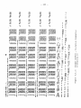
THIRST OUTPUT - Summary of Grid Locations .
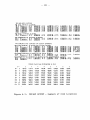
THIRST OUTPUT - Iteration Summaries
(Iteration 1)
THIRST OUTPUT - Iteration Summaries
(Iteration 2)
THIRST OUTPUT - Iteration Summaries
(Iteration 58)
THIRST OUTPUT - Iteration Summaries
(Iteration 59)
THIRST OUTPUT - Iteration Summaries
(Iteration 60)
THIRST OUTPUT - Detailed Output
(Velocity Field)
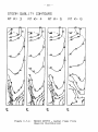
THIRST OUTPUT - Composite Plots
(Quality Distribution)
THIRST OUTPUT - Composite Plots
(Velocity Distribution) . . . . . . . . . .
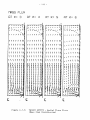
THIRST OUTPUT - Composite Plots
(Mass Flux Distribution)
THIRST OUTPUT - Radial Plane Plots
(Quality Distribution)
THIRST OUTPUT - Radial Plane Plots
(Velocity Distribution)
THIRST OUTPUT - Radial Plane Plots
(Mass Flux Distribution)
4
4
20
21
22
23
37
37
39
41
71
99
100
101
102
103
104
105
106
107
108
109
110
Ill
112
113
114
115
LIST OF FIGURES
Figure 7.1
Figure 7.2
Figure 7.3
Figure 7.4.1
Figure 7.4.2
Figure 7.4.3
(continued)
THIRST OUTPUT MODIFIED DESIGN
- Code Changes
THIRST OUTPUT MODIFIED DESIGN
- Data Summary
THIRST OUTPUT MODIFIED DESIGN
- Final Iteration Results Graphical
THIRST OUTPUT MODIFIED DESIGN
- Final Iteration Results Graphical
(Quality Distribution)
THIRST OUTPUT MODIFIED DESIGN
- Final Iteration Results Graphical
(Velocity Distribution)
THIRST OUTPUT MODIFIED DESIGN
- Final Iteration Results Graphical
(Mass H u x Distribution)
144
. . , .
145
Output .
146
Output
147
Output
148
Output
149
1.
INTRODUCTION
The THIRST* computer code is the latest in a series of
three-dimensional steady stato computer codes developed at CRNL
for the detailed analysis of steam generator thermal-hydraulics.
The original code, designated BOSS**, arose from the DRIP***
program of Spalding and Patankar [1], and was adapted for
application to CANDU**** type steam generators [2]. Although the
equations to be solved remain the same, extensive changes have
been made to the program structure, the numerical computation
sequence, the empirical relationships Involved, the treatment of
the U-bend, and the numerical and graphical presentation of
results.
The code has therefore been renamed THIRST.
In conjunction with these developments, the program has been used
to successfully analyse the thermal-hydraulic performance of a
number of different steam generator designs, from CANDU to
American PWR nuclear plants.
The program has also been used for
extensive design parameter surveys.
Some results of these
analyses have been released in publications [3-7].
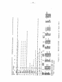
Steam
generator designs already analysed are summarized in Table 1.1.
As the structure of the THIRST code Is now well established, and
its flexibility and reliability have been illustrated by
extensive application, the time is now appropriate to present the
code In a formal manner.
It Is our intent in this manual to
present sufficient details of file THIRST code to permit a new
user to run the code, and to obtain parameter survey studies
based on variations of a reference hypothetical steam generator
design.
Suggested approaches to other basic designs are also
included.
*
**
***
THIRST: Thormal-I[ydraulics _In Recitculating SJTeam Generators
BOSS: BOiler Secondary £lde
DRIP: Distributed Resistance _In Porous Media
**** CANDU: CANada Deuterium Uranium
- 2 -
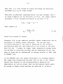
Before presenting details of the code implementation, and
discussing the input data .squired, some background knowledge of
the nature and function of steam generators must be established.
1. 1 Steam Generator Thermal-Hydraulics
The steam generator is a critical component in a nuclear power plant
because it provides the interface for heat exchange between the
high pressure reactor primary coolant circuit and the
secondary turbine circuit. The integrity of this interface
must be maintained to prevent mixing of fluids from the
two circuits, while thermal interaction must be maximizeo for
efficient transfer of energy to the turbine from the reactor.
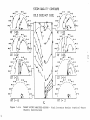
Figure 1.1 is, a cutaway view showing the salient features of a
typical CANDU steam generator.
The hot primary fluid from the
reactor circulates through the network of tubes, heating the
secondary flow which evaporates as it rises inside the shell.
Failure of any one of the tubes would lead to expensive downtime
for the station.
The most likely causes of such tube failure are
corrosion and fretting of the tube material.
Corrosion can be
minimized by regulating secondary fluid chemistry and by
optimizing secondary side flow to minimize flow stagnation areas
where corrosion tends to be highest.
I^etting of tube surfaces
due to flow-induced vibrational contact can also be analysed and
local flow conditions can be computed with sufficient accuracy.
The location of tube supports which minimize vibration can then
be specified.
In either case, a detailed picture of the flow
patterns under operating conditions is required.
provides such a picture.
The THIRST code
- 3 -
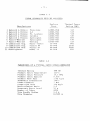
TABLE 1.1
STEAM CENERATOR DESIflNS ANALYSED
Nuclea r
Manufac ture r
1
2
3
4
5
6
7
8
9
10
11
Babcock & Wilccx
Babcock & Wilcox
Babcock & Wilcox
Babcock & Wilcox
Babcock & Wilcox
Foster-Wheeler
Foster-Wheeler
Combustion Eng.
Combustion Eng.
Combustion Eng.
Westinghouse
Plant
Pickering
G-2
P t . Lepreau
Cordoba
Darlington
Darlington
Wo 1 sung
Maine Yankee
System 80
Series 6 7
Model 5 1
CANDU-PWR
CANDU-PWR
CANDU-PWR
CANDU-PWK
CANDU-PWR
CANDU-PWR
CANDU-PWR
L'S-PWR
US-PWR
US-PWR
US-PWR
Th e rmal Powe r
Rating (Mw)
515
U5
5]0
6 60
670
515
845
1910
1260
850
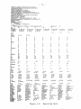
TABLE 1.2
PARAMETERS OF A TYPICAL CANDU STEAM CENERATOR
Thermal Rating
Primary Inlet Temperature
Primary Inlet Pressure
Primary Inlet Quality
Primary Flow Rate
Feedwater Temperature
Steam Pressure
Steam Flow Rate
Recirculation Ratio
Downcomer Water Level
Number of Tubes
Tube Bundle Radius
Tube Diameter
600 MW
315°C
10.7 MPa
0.034
2MK) kg/s
180°C
"> MVa
310 kg/s
5.5
15 m
4850
1.3 m
0.0125 m
SEPIHAIDKS
[
~f
Figure 1.1
Cutaway View of a Steam Generator
Figure 1.2
Simplified Model of the Steam
Generator
- 5 -
1.2
The Hypothetical Prototype Steam Generator
Although steam generators developed by different manufacturers
share a number of common features, it would be a prohibitive task
to attempt to write a computer code which would comprehensively
include all possible designs.
The bulk ->f this manual,
therefore, describes the standard version of the THIRST code
which has been written for analysis of a hypothetical steam
generator containing many features common to CANDU designs
(Figure 1.1).
In particular, it is a natural circulation steam generator with
Che following features
- integral preheater
- tube matrix with round U-bends
annular downcomer with re-entry through specified windows in
the circumference
Geometrical specifications and nominal operating conditions of
such
a
hypothetical design are listed in Table 1.2 for a
typical 600 MW thermal steam generator.
A simplified diagram of a natural circulation steam generator
with integral preheater is given in Figure 1.2.
The area inside
the shroud is completely filled with t-^bes except for the
central tube free lane between the hot and cold legs and
the annulus between the outer tube limit of the bundle and the
shroud.
The surface of the outer limit of the bundle in the
U-bend is spherical.
- 6 -
The primary fluid enters the right side of the sketch flowing up
inside the 'hot side1 tubes, transferring heat to the secondaryfluid en route.
The tubes turn through 180° in the U-bend
region, and the fluid returns down the cold side.
The secondary
fluid enters as subcooled water through the integral preheater,
where baffles force the flow to cross the tube bank in a zig-zag
pattern to enhance heat transfer.
At the preheater exit this
flow, now raised to saturation temperature, mixes with flow
recirculated from the hot side.
The resulting mixture undergoes
partial evaporation and rises as a two-phase mixture through the
remaining bundle section, into the riser,' and up into the
separator bank.
Here the two phases are separated.
The steam
leaves the vessel to enter the turbines, while the remaining
saturated liquid flows through the annular downcomer to the
bottom of the vessel.
Here it re-enters the heat transfer zone
through windows around the shroud circumference.
The downcomer flow entering through the windows on the hot side
partially penetrates the tube bundle before turning axially to
flow parallel to the tubes.
On the cold side, the downcomer flow
must pass under the preheater to the hot side before it can turn
axially.
Thus the downcomer flow converges on the center of the
hot side tube bundle.
As this fluid rises through the hot leg It absorbs heat from the
tube side fluid.
Quality develops very rapidly because the
downcomer flow Is very close to saturation.
Above the top of the
preheater, this mixture mixes with the fluid from the preheater.
The tubes are supported by broached plates located along straight
portions at the U-tubea.
the U-bend.
Further lattice supports are located in
The baffles in the preheater are drilled plates.
- 7 -
In this design, no feedwater
(floor of
leakage
through
the preheater) or the partition
the feedwater
The primary
must
exit at the top of the
fluid, heavy water, enters
the reactor circuit as a low quality
primary mass flow distribution
although
entry.
The secondary
fluid
at subcooled
preheater
at a uniform velocity.
circulation
is provided
conditions.
is assumed
It
by
The
the code,
to be uniform
It enters
is assumed
The driving
by the height
Ail
the tube bundle f-rom
two-phase mixture.
is light water.
preheater
plate
is allowed.
preheater.
is determined
the quality distribution
the thermal
plate
the
to enter
force
of water
at
for
in the
the
natural
downcomer
annul us•
1.3
The THIRST Standard
Code and its Intended
The THIRST computer
code, as evidenced
readil" adapted
numerical method
to a number
by Table 1.1, can be
of steam generator
is extremely
package, however, pertains
Application
robust.
The standard
to a hypothetical
The program models a region extending
designs as the
from
steam
THIRST
generator.
the face of
tubesheet
in Figure
1.2, up to the separator
downcomer
annulus.
Symmetry
the
deck, including
permits -analysis of only
the
one half of
the vessel.
1.4
The Use of This Manual
The THIRST package
steam generator
possible.
is designed
to make numerical
thermal-hydraulics
Thus a seasoned
modelling
as straightforward
the
input
data.
as
user of the code will normally
only chapters 4 and 5 of this report, which outline
procedures required
to layout
the computation
of
consult
in detail
grid and
prepare
the
However, to properly accomplish these tasks, the user must first
understand the fundamental principles of the relevant mathematical
formulation and numerical solution tecnniques.
summarized in chapters 2 and 3 which follow.
These are
- 9 -
2. FOUNDATIONS OF THE MODEL
The THIRST code computes the steady state thermal-hydraulics of
a steam generator by solving the well-known conservation
equations In three-dimensional cylindrical coordinates.
This chapter states the equations involved, outlines the overall
solution procedure, and lists the assumptions used to formulate
the model and the thermal-hydraulic data required.
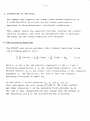
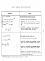
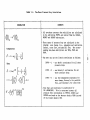
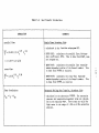
2 . 1 The Governing Equations
The THIRST code solves secondary side transport equations having
the following general fora:
i j^ (Srpv*) + ± -A (0pw<i>) + ~
(6pu4>) = SS^
(2.1)
Here v, w, and u are the velocity components in the r, 9 and z
directions, respectively, g is the volume-based porosity, p is the
mixture density, S, is the source term corresponding to the transport
parameter $.
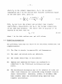
The latter two, for each of the five transport
equations, are listed in Table 2.1.
In the table, P is the pressure; Rr , R and Rz are the
0
flow resistances per unit volume offered by the tubes, baffles
and other obstacles; h is the secondary fluid enthalpy; S^ is
the rate of heat transferred per unit volume from the primary to
the secondary; and g is the acceleration due to gravity.
- 10 TABLE 2.1
i
( Transport
j Equation
i Continuity
1
Radial
momentum
V
j
Equation
Number
0
2.2
3P , pw 2
3r
r
2. 3
r
i
j Angular
momentum
w
1
• Ax i a1
j momentum
Energy
(secondary)
u
1 3P
" r 36
pvw
r
R
8
" If ' Pg " RZ
h
S
2.4
2.5
i
2.6
h
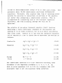
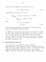
THIRST also solves the primary side energy equation which for a
differential length of tube Si is given by:
5h
(2.7)
where G p and h are the primary fluid
respectively, I is the distance along
outer diameter, d ± is the tube inside
heat flux at the outer tube surface.
from:
mass flux and enthalpy,
the tube, d is the tube
diameter, and <J/ is the
The heat flux Is calculated
- T
P •
s
(2.8)
- 11 -
where Tp is the primary temperature, T s is the secondary
temperature and U is the overall heat transfer coefficient based
on the tube outer area, given by:
d X,n(d/d.)
i
p
v
~1
w
Here, h p and h are the primary and secondary heat transfer
coefficients, respectively, and kw is the thermal conductivity
of the tube wall material.
The source term in equation 2.6 is
related to the heat flux by:
S h = \ty
(2.10)
where X is the tube surface area per unit volume.
2 . 2 Modelling Assumptions
The governing equations are based on the following assumptions and
ctmplifications:
(1)
The flow is steady, incompressible and homogeneous.
(2)
The shell and shroud walls are adiabatic.
(3)
The inside shroud wall is frictionless.
(4)
Laminar and turbulent diffusion are negligible in
comparison to the frictional resistances and heat
source.
(5)
The distributed resistances due to the presence of tubes and
other solid obstacles are calculated using standard friction
factor correlations. Similarly, primary to secondary side
heat transfer rates are calculated using empirical heat
transfer correlations.
- 12 -
(6)
Reductions of flow due to the presence of tubes and other
obstacles are accounted for by defining a volume-based
porosity.
(7)
The primary temperature distribution Is calculated from the
enthalpy distribution by using a polynomial curve fit (see
Chapter 7 ) .
(8)
Secondary subcooled values of temperature, viscosity, etc.,
are calculated by using polynomial curve fits of each
parameter expressed as a function of the secondary enthalpy
(see Chapter 7 ) .
2.3
Boundary Conditions
Boundary and start-up conditions such as primary flow and
temperature, secondary feedwater flow and temperature, downcomer
water level, etc., are described in detail in Chapter 4.
2.4
Overview of the Solution Sequence
The numerical solution sequence, apart from some variations
discussed later, follows the techniques outlined by Patankar and
Spalding in reference [8). A fair understanding of the
mechanics of the technique Is required for advanced use of the
THIRST code, and Appendix A contains details of the overall
formulation.
At this point, however, we present a brief exposition of the
philosophy of the method, including only a minimum of
mathematics.
THIRST solves the five secondary side transport equations (2.1)
in three dimensions to compute distributions of the dependent
variables u, v, w, h, and P. The mixture density p is calculated from the equation of state p - p(h,P). The variables are
- 13 -
stored in three-dimensional arrays of up to 5000 grid points. This
generates about 30,000 simultaneous non-linear differential
equations. Obviously, this requires some form of technique which
permits the solution to concentrate on portions of the equation
set rather than attempting a simultaneous solution. This is
accomplished by considering each of the transport equations
separately, and then iterating through the full set of
equations.
The solution of any given transport equation Itself Involves
developing a finite difference statement of the equation and
solving it in an inner iteration, but we will delay considering
this until later.
Suffice it to say that the transport equations
can be reduced to a set of linear matrix equations and written as
follows:
Continuity
A p U + B p V + C^W = 0
(2.11)
Momentum
DyU + E
+ F P = 0
(2.12)
DyV + E v + FyP = 0
(2.13)
= 0
(2.14)
D W -
w
Energy
State
+
+ G = 00
Hh +
p
P = f(P,h)
f ( P , h)
(2.15)
(2.16)
The coefficient matrices A to G are functions involving first
estimates of the dependent variables u, v, w, p, h, P.
We
wish to solve equations 2.11 to 2.16 in a sequence that will
eventually lead to all six equations being satisfied.
- 14 -
This is accomplished as follows:
i)
solve equation 2.12 to get new estimates of U
U = -Dy-l
= Ev*
ii) and ill)
E 0 + F0P
+ Fu*P
(2.17)
operate similarly on equations 2.15 and 2.14 to give
V = E v * + FV*P
(2.18)
W = E H * + F W *P
(2.19)
The new values of the U,V,W matrices have thus been computed from
the initial estimates using the momentum equations.
If the
original estimates of all the variables were correct, the values
would satisfy the continuity equation (2.11).
Invariably,
however, they will not satisfy (2.11) but will generate a mass
imbalance residual R.
As pressure is the dominant variable in
the momentum equations, it is logical to adjust the pressure
matrix in a direction that will reduce R to zero.
A logical method of adjusting pressure is to assess its effect on
the velocity components by differentiating equation 2.17 with
respect to pressure.
dU _ *
dP = U
Thus we can write
dO - F 0 *dP
dV - F v *dP
dW - Fw*dP
(2.20)
-
Now i f
the
the
pressure
new v e l o c i t y
15
"
adjustment
matrix
dP i n
(2.20)
is
correct,
matrix
U
NEW = "OLD + dU
will satisfy the continuity equation 2.11.
(2.21)
Substituting 2.21 and
similar equations for V N E W and WJJEW in 2.11, then gives
rise to the equation
+ BV
AU0LD
OLD +
CW
OLD
+(AFu* + BF V * + CF W *) dP = 0
(2.22)
Or more simply:
R + (F)dP = 0
(2.23)
Equation 2.23 thus illustrates the pressure correction matrix dP
required to eliminate the mass imbalance generated by the old
velocity values.
Thus the relevant steps are:
iv)
compute dP from 2.23
v)
compute U, V, W from 2.20 and 2.21
If the equation set were linear, steps iv) and v) would complete
the solution.
However, the linearized equations contain some
remnants of the initial estimate, so steps iv) and v) must be
repeated several times.
- 16 -
Finally, the energy equation must
vi)
compute h from equation 2.15
vii)
compute P from equation
also be incorporated:
2.16.
The sequence i) to vii) is now repeated
to convergence
The iteration sequence may be summarized
'i)
repeat
1
as follows:
compute U from equation 2.12
ii)
compute V from equation 2.13
iii)
compute W from equation 2.14
iv)
compute dp from equation 2.23
repeat
v)
compute dU, dV, dW from equat'
.20 and
2.21
vi)
compute h from equation
2.15
vii)
compute P from equation
2.16.
In the THIRST program, the outer
orchestrated
routine
by the executive
iteration
sequence is
routine, which calls a separate
to perform each of the above steps.
2.5
Thermal-Hydraulic
2.5.1
Fluid Properties and Parameters
As mentioned
Data
in Section 2.2, equations of state for both the
primary (heavy water) and secondary (light water) fluids are
required
in the analysis.
code using
relationships
These are incorporated
derived
from standard
details of these are given in Chapter 7.
in the THIRST
tables.
Full
- 17 -
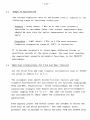
2.5.2
Empirical Relationships
In assembling the terms of the differential equations, any
thermal-hydraulic code must rely on empirical correlations to
approximate a number of phenomena which cannot be prescribed
analytically.
These empiricisms Include correlations for single
and two-phase heat transfer and pressure drop in rod bundle
arrays and for void fraction.
All correlations used in the THIRST code are summarized in
Chapter 7.
- 18 -
3.
IMPLEMENTATION FUNDAMENTALS
The previous chapter has discussed the governing equations,
developed a suitable solution philosophy, and mentioned the
thermal-hydraulic data required to complete the specification of
the model.
This chapter is concerned with the manner in which
these general principles are implemented in the THIRST code.
This Involves the establishment of the computational grid, the
conversion of the partial differential equations to discrete node
equations by means of control volume Integration, and the
technique used to perform the 'Inner' solution of individual
equations.
The control volume integration and equation solution are of
course built into THIRST, but in order to choose an effective
grid layout, the user needs some feeling of these procedures.
3.1
The Coordinate Grid
A three-dimensional cylindrical coordinate system Is used for
obvious reasons.
The entire flow domain between the tubesheet
and the separator bank is subdivided by planes of constant r, z
and 8.
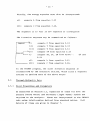
The grid arrangement is chosen to suit the geometry and
expected flow patterns of the steam generator.
Thus it is
usually not uniform, but is arranged to provide finer division in
the region where steep gradients are expected, for example near
the tubesheet.
- 19 -
Following
the now classical grid arrangement
Harlow, et al, [ 9 ] , scalar variables, such
and
enthalpy are centered at the points of Intersection
grid lines, or nodes*
pressure differences
As pressure
generate
velocities are centered
arrangement
is the driving
velocities
between nodes.
is shown in Figures 3.1
considered
3. 2
introduced
positive
by
s pressure, density
of the
force,
between nodes, thus
The
resulting
to 3.4.
grid
Velocities
in the direction of the coordinate
are
vector.
The Control Volumes
Finite difference approximations
to the partial
equations may be derived
in many ways.
volume
has proved
integral
approach
fluid modelling.
This
Is principally
variable mesh
continuity-
It does, however, introduce
Integrated
variable
equation
are centered
complexities,
must
on the
be
primary
to be constant
points, while
the axial
over a control volume centered
the radial and azimuthal momentum
on V and W, respectively.
for each of these four cases
3.4.
at grid
in
enforces
Thus scalars are considered
is integrated
the U velocity, and
centered
control
successful
it easily
additional
form of each equation
over control volumes centered
momentum
because
size, yet rigorously
using a control volume
concerned.
However, the
particularly
incorporates
as the finite difference
differential
Typical
are also shown
control
in Figures
equations
volumes
3.1
to
on
-
20 -
K RH
K +1
K- 1
J + 1
K - J ( r - 6 ) PLANE
X+
I x+
V(I,J,K)
1 + 1
I
hU.JJQ
<" I.CT
I
u ( I , J., KM\
)
t"-
T
J-I
K+ 1
I - J ( x - r ) PLANE
Figure
3.1:
K
I - K ( x -9)
Clrid Layout showing Scalar and Vector
K- 1
PLANE
Locations
-
21 -
1
r+
K+1
K -1
K)
r
\
\
K - J ( r -8)
/
J +1
/
/
PLANE
i
I +1
i
—-f-
—i
x
R~ r~
/
1
+
9
P/
i u(
/
+
J -1
I-J(x-r)
PLANE
i
i
0
B
x~
i
7-r-l
J
J +1
,J,
t
I-1
——
1
X
-
K +1
— i 1— —
K
—1
K - 1
I -K(x - 9 )
PLANE
Figure 3.2: Control Volumes for Scalar Quantities
i-
-
22
-
K +1
K- 1
J +1
K -J(r
~9)
PLANE
•i +
+V(I,J,K)
K)
I
I
i
r
-f—1-1
i
I
r
K +1
I - J(x - r)
Figure 3.3:
PLflNE
T~
I
4-1-1
I
K
I-K(x-0)
K- 1
PLANE
Control Volumes for Radial Velocity Vectors
- 23 -
K+1
K- 1
J+1
J- I
K - J (r - 8 ) PLANE
+-!•!
r-
Mfv
'/
W(I,J,K) |
tI-1
I
J -1
I -J (x - r)
Figure 3.4:
+4-I-HK +1
J
PLANE
K
K-1
I -K (x -6 )' PLANE
Control Volumes for Circumferential Velocitv Vectors
- 24 -
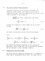
3. 3
The Control Volume Integral Approach
Although the equations to be solved are Integrated over
different control volumes, the procedure in each case Is
completely the same.
Thus, each equation may be written in the
form of equation 2.1 and integrated
[7 £
-0S
I ±
rdrdOdz = 0
(3.1)
Although the integration Is done formally by use of Gauss
theorem,
JJJ
^-<t>dv =/7"(n-<J>)ds
(3.2)
JJ
v
s
the result is Intuitively obvious from first principles.
It is
r,
I(grpv4i)n -
l
(grpvcf)
[
r
I A9Az + l(Bpw<}>)
I
I
- (Bpwc|>)wl
ArAz
rrr
(6pu<(i), - ( 6 p u < ( ) ) . | rA<J>Az • / / / B S . d v
(3.3)
%
h
The (quantities) obviously
represent
the Jflux through the
1
JJ
*
appropriate control volume face, and the [quantities] represent
the flux imbalance In each coordinate direction.
3.3.1
Integration of the Source Terms •
The source terms are frequently non-linear in 41 • Integration of
these terms is accomplished tsrm by term. The result can be
-
linearized
with
respect
25 -
to <b and
stated
in g e n e r a l
form
S v = Su + Sp<|>p
as
(3.4)
Here the term Sp normally contains all coefficients of (
J
> , and
Sy contains remaining terms which are generally (but not
always) unrelated to (
|
> .
Reexamining the equations in Table 2.1, it is apparent that the
greater part of the programming in the THIRST code is involved
with formulating and integrating the resistance components of
the source terms, using the appropriate empirical correlations.
This is done in subroutines with the generic name SOURC.
3.3.2
Integration of the Flux Terms
It is apparent from equation 3.3 and figure 3.2 that values at,
for example, control volume face n can be obtained to first
order accuracy by upwind approximation for any variable A, which
assumes that the velocity vector convects scalars from upwind
only.
Thus if all velocities are positive, inlet flows convect
neighbouring scalars, outlet flows convect the control volume
scalar.
Denoting the coefficients of <
f
> by C, and using the
upwind approximation, equation 3.3 is reduced to the i?orm
C
n
<f> - C <j> + C < t >
p
S3
e¥p
- C A
= S + S < f >
wYw
u
pYp
(
3
.
v
where C. is the flux evaluated at control volume face i.
5
)
'
_ 26 -
Collecting
terms
gives
i = n,s,e,w,h,£
(3.6)
A
n
= C
A
Once
the coefficients
standard
P
n
A
s
= C
s
etc.
= £A. - S
i
P
A have been computed,
linear equation
equation 3.6 is the
set
A <f> =- B
(3.7)
which can be readily solved
<(i - A " 1 ] !
(3.8)
Actually, the size of the matrices prohibits direct solution, so
iterative methods are used, and equation 3.8 is solved by an
'inner' iteration.
3.4
The 'Inner' Iteration
The matrices of equation (3.7) are too large to permit
direct
solution of the equation set by means of (3.8) even when sparse
matrix techniques are considered, so an Iterative technique is
used.
It is well known that the solution of equation sets in
which the matrix A is tridiagonal can be performed
quickly as the algorithm reduces to recursive
form.
extremely
- 27 -
Equation 3.7 can be converted to trldiagonal form by Including,
for example, only the coafficients along the r direction on the
left-hand side.
+
Vn
Vp
+
V s " ~(SV.i + V
(3.9)
j = e,w,5.,h
Similar expressions can be written for the 6 and z directions.
Ve
+
VP
+
V w " "(rVj +Su}
(3.10)
j = n,s,fc,h
Vh
+
\*P + V l " -(lAj*i
+
V
(3.11)
j = n,s,e,w
A one-dlmenslonal problem can be solved directly by (3.9).
A
two-dimensional problem Is solved by an alternating direction
Iteration ADI method.
This Involves solving 3.9 and 3.10
alternately until the solutions converge.
A three-dimensional
solution requires the solution of 3.11 in addition.
creates several possibilities.
This
For example, 3.9 and 3.10 could
be solved for a number of iterations for each time 3.11 is
solved.
The most suitable strategy depends on the nature of the
flow problem.
The THIRST code has a number of different
strategies designed to promote convergence in three dimensions.
These are discussed in Appendix A.
- 28 -
3. 5
Stability of the Solution Scheme
The outer iteration scheme discussed in Chapter 2 normally
proceeds to convergence in a stable manner, and converges
rapidly, providing each inner iteration is stable.
To promote stability of the iterations, three principal devices
are incorporated in THIRST. The first, that of under-relaxation,
is common to most iteration schemes. The second, upwind weighted
differencing, is frequently used to stabilize both steady state and
transient thermal-hydraulic calculations [10]. The third concerns
the formulation of the source terms to ensure stability.
.5.1 Under-Relaxation
Because the solution is obtained by iteration, there is a strong
likelihood that variable values may fluctuate unduly during the
initial stages.
It is common practice to stabilize these
fluctuations using under-relaxa tion •
Thus if (j)N is calculated
from 3.9 to 3.11 using previous values <j>
l>
+ (laH"1
- a*
Relax
, it is then replaced
Calc.
(3.12)
old
Relaxation factors a for each equation solution are supplied
with the THIRST code, but may be changed by data input if
necessary.
In practice, it is possible to impose under-relaxation before
attempting the linear equation solution instead of after Its
completion.
This is preferable as it minimizes the chances that
the linear equation solution itself may generate unlikely
values.
- 29 -
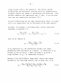
Recall that the equation to be solved is 3.6, or
(3.13)
Substitution of 3.13 into 3.14 gives
<drp
= -(EA c(> + S,.)(a/A )
Relax
l l
u
r
or
*p
= -(SAid)i + S
Relax
when
„
\
•
S
u
+
<
N
A p = A p /a
(3.14)
This pre-relaxed equation can obviously be solved using the
identical techniques already discussed.
In THIRST, all equations are pre-relaxed in this manner, except
for the pressure corrections and density calculation.
Equation
2.23 returns a pressure correction rather than the pressure
itself.
Pressures arising from this correction may be relaxed
according to 3.12, but this is not usually necessary.
Density
may also be relaxed by 3.12.
3.5.2 Upwind Biased Differencing
It is well known that symmetric central difference
representation of first derivative terms in transient equations
leads to unstable numeric behaviour
[10,11],
Stability is usually
ensured by incorporating one of two devices in the numeric
scheme.
The first, artificial dissipation, adds an artificially
- 30 -
large viscous term to the equations.
The second, upwind
differencing uses difference formulae which are asymmetrically
weighted towards the upwind or approaching flow direction.
Both
devices stabilize the computation and, in fact, it can be shown
that they are numerically equivalent [11].
Central differencing has the same destabilizing effect in steady
state, and computations can be stabilized by the same devices.
Consider, for example, a one-dimensional central difference
statement of equation 3.5.
- Cs
2
2
+ S
= 0
(3.15)
This can be reduced to
C'<t>r. ~ C <(>„ ~ 2 S J
As C B approaches C n , the denominator becomes very small,
generating undue excursions in efi values.
In particular if C s
exceeds C n very slightly, a small increase in <|>s gives a
large decrease in <);_ - an impossible situation.
However, if we add diffusion terms which involve the second
derivative, the resulting equation can be shown [13] to be
, _
*P
(D
s
+ C )<(>„ + (D - C )4T> - 2S,
s S
n
n N
A
D + D + C - C
n
s
n
s
,, , ,,.
(3<17)
- 31 -
Note that 3.17 will always be stable providing the diffusion
Influence D n + D s Is large enough.
Similarly on physical reasoning alone, one may consider that <J>
is swept primarily in the direction of flux.
The simple upwind
statement of 3.16 already introduced in section 3.5 is
C
This
reduces
n*P " C s*S
to
C <J>
t=p = - 2 - 2
-
S,
*
(3.18)
n
which will always be stable.
Equation 3.18 is the simplest possible upwind formulation and is
equivalent to adding excess viscosity.
Its use has been
criticized because it can lead to diffusion of the solution,
particularly when the flow direction is not normal to the grid
axes [14,15]-
A number of higher order difference schemes which
can be used to give more accuracy may be developed
[10,12] and
some of these may be implemented in schemes similar to that used
in THIRST [15].
In the THIRST code, the simple formulation is retained, however.
The large flow resistances and heat sourras due to the closely
packed tube bundles in the steam generators dominate the
computation to •rjch an extent that the differences which would
be caused by higher order methods are believed to be minor.
- 32 -
3.6
Notation used in THIRST
Finally, we have up to here been using single subscripts n, s,
etc.
for simplicity.
cylindrical
Ax_.
coordinates
The code,however, is written in
and uses terms such as AXM to denote
On this basis, equation 3.6 becomes
A<|>
= EA<J>+S
(3.19)
where:
A = A , + A
+ AQ, + A Q
+ A . + A
+ DIVG - SP
p
r+
r6+
9x+
xThe upwind f o r m u l a t i o n
direction
r+
automatically
r+
2
r2
1§±
2
r2
can be implemented
in
the
r+
following
(Bpav)
to c o n s i d e r
flow
manner:
r+
face area
C
(6pav)
CQ+
(@paw)
(3.20)
0+
etc .
t C , " mass flow through control volume face r,; depending on the
transport parameter <(>; 3> P> v ara either defined at that
face or interpolated
to that face.
- 33 -
DIVG = C r + - Cr_ + C e + - Ce_ + C x + - Cx_
= net accumulation of mass in the control volume
The table below defines A^ and <P± for each i:
i
„
A
i
A
r+
A
»1
\
+
r-
V
6+
A
6+
*0+
6
"
A
9-
*9-
X+
A
x+
A
*X +
<(>
x-
Note that this formulation also automatically handles possible
extreme cases In which all flow directions but one are in
towards (or out away from) a control volume.
3.7
Formulation of the Source Terms
For stability of the inner iteration, it is essential that the
coefficients remain positive after the source terms are incorporated.
Thus, in 3.20, SP must be negative.
Cases in which
SP tends to be positive are catered for by artificially
2
augmenting SU . For example, if S = -KpV , one may write
SP - -2Kp|v|, SU - +KpV 2 ; SU will then incorporate the old value
of V, and SP will ensure the formulation is both stable and
implicit.
This section completes the overall description of the model
implementation.
The following chapters contain detailed instruc-
tions on how to use the code.
- 34 -
4.
APPLICATION OF THIRST TO ANALYSE THE PROTOTYPE DESIGN
Specification of the three-dimensional model must include
details of all relevant geometrical, fluid flow and heat
transfer parameters.
It is emphasized that the process of
modelling a steam generator relieF heavily on diligent assembly
of the specifications, optimal choice of grid layout, and of
course correct preparation of the input data.
This chapter is
intended to guide the user step by step through the considerable
effort required.
By means of a detailed example, we illustrate the entire
procedure required to prepare a THIRST analysis of a particular
steam generator design.
We assume the user is familiar with the
fundamentals discussed in Chapters 2 and 3, and now discuss
Design Specification - the hypothetical steam generator
Grid Selection - arrangement of optimal grid layout
Preliminary Data Specification - procedure for assembling
the data specification sheets
Preparation of Input Data Cards
Sample Input Deck
Execution Deck - assembly of a THIRST job and submission
to the C£C computer
- 35 -
4. x
Design Specification
The particular case chosen for this example is the hypothetical
steam generator discussed in Chapter 1 and shown in Figure 1.2.
Design parameters used in the current example are summarized In
Table 1.2.
A large number of variations of this design can be investigated
using the standard THIRST code by specifying parameter
variation through input data.
Designs which deviate from the hypothetical model in major
aspects may require code modifications.
These are considered in
Chapter 5.
4,2
Grid Selection
The first task is to describe the geometry of the design to the
computer.
This is accomplished by superimposing a cylindrical
coordinate grid onto the design, and by specifying the location
of flow obstacles in terms of this grid.
THIRST accepts a
maximum of 40 axial planes, 20 radial planes and 20
circumferential planes; however,due to a storage limitation, the
maximum number of nodes must not exceed 4900.
In order to appreciate the selection of grid locations, the user
should understand the staggered grid arrangement used in THIRST
described in Chapter 3.
Essentially, velocities are centered
between gri<1 lines in their corresponding direction and centered
on grid lines in the other two directions, as shown in Figure 3.1
An axial velocity, for example, has
a control element with
- 36 -
boundaries as shown In Figure 3.2.
The cop boundary corresponds
to the I plane, the bottom to the 1-1 plane.
The left side
boundary is located midway between the J and J-l planes.
The
radial velocity has a control element that extends between J
planes and straddles I and K planes.
And similarly,
the
circumferential velocity extends between K-planes and straddles
the I and J planes.
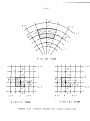
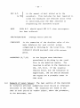
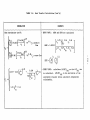
4.2.2
Baffles
Figure 4.1 shows how the code handles flow around a typical
baffle.
We observe a radial flow to the left under the baffle,
an axial flow around the baffle followed by a radial flow to the
right above the baffle.
Note that the baffle lies in the middle
of the U velocity control element and the radial control
elements lie on either side of the baffle.
We can see that
axial grid lines must be located such that the baffle plates lie
midway oatween them.
4.2.3
Partition Plate
Figure 4.1 also shows the code treatment of the partition plate.
The circumferential velocity W corresponding to the K plane is
blocked by this partition plate which is centered between the K
and K-l planes.
J +2
37 -
J - t
J +1
|
+
"(I+1,J,K) - c a r r i e s the
| flow out radially
-example of a
velocity blocked by
the baffle
U(1+1,J-1,K) -carries
the flow un past the
baffle
TYPICAL BflFFLE^
V(I,J,K) -carries the
flow in radially
SHROUD
PflRTITION PLATE
The I-planes are located so that baffles lie midway between them. The
location of the J-planes matches the baffle cuts for this particular
K-plane; however, the cut will not match other K-planes and the program
is set up to handle t h i s .
Figure
4.1:
Grid
Layout
SHROUD
J+ 2
at
a Baffle
Plate
J - I
SHELL
-downcomer velocity
-velocity inside
shroud
-shroud window
velocity
TU BESHEET
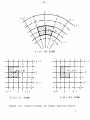
The I and 1-1 planes are located so that the top of the window lies
halfway between them. The J+l and J+2 planes center the shroud.
Generally, more grid would be located in the shroud window to handle
the sudden change in flow direction.
Figure 4.2:
Grid Layout at a Shroud Window
- 38 -
4.2.4 Windows
A third example (Figure 4.2) shows the grid layout required near
the shroud window opening.
The radial grid lines J+2 and J+l
are located to center the shroud.
The axial velocity at (1+1,
J+2, K) corresponds to the downcomer flow.
The radial velocity
at (I-1,J+2,K) corresponds to the window flow where the
downcomer flow enters the heat transfer area.
Thus the location
of the shroud and the location of the top of the window governs
the 1-1,1,J+l and J+2 grid selections.
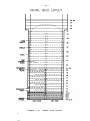
4.2.5 Axial Layout (I Plane)
When allocating the grid, the user is advised to start with the
axial planes.
Figure 4.3 shows the axial grid layout on the vertical cut of
the hypothetical model.
One can see the appropriate selection
of the axial grid location around the preheater baffles.
The
tube support plates cannot always be located midway between
planes because of the limit on the number of axial grid lines
available.
In such cases, support plates will be effectively
seen at lower or higher elevation than their actual location.
However, this will not unduly influence the model because the tube
support plates do not redirect the flow but simply add to the
pressure drop.
Two axial grid planes 1-7 and I«8 are positioned so that the top
of the shroud window on the hot side is located midway between
them.
The top of the shroud window on the cold side is lower
and thus the 1-6 plane is located such that the 1-6 and 1-7
staggers the top of the cold side shroud window.
- 39 -
PXIOL GRID LRYOUT
35,36
34
33
32
31
30
129
TT
I I
BUNXE
28
J.L.
27
SHROUD-
Tf
J-L
SHELL-
26
25
rr
TUBE
SUPPORTPLOTE
24
1L
-H-
23
PREHERTER
21,22
20
OBFTTJE-
PLBTE
D
J
19
18
17
16
15
14
- I
FEEDURTER
INLET
SHROUDWINDOW
13
r
±£
COLD SIDE
Figure
4.3:
HOT SIDE
Axial
Grid Layout
12
10,11
8,9
6,7
4,5
1-1,2,3
- 40 -
When the axial planes have been allocated to satisfy the axial
flow obstacles such as baffles, tube support plates, window
openings, etc., the user should then examine areas which are
critical to the analysis and ensure that a sufficient number of
grid planes are located in these areas.
For instance, the
region just above the tubesheet at the shroud window is
particularly important.
tubesheet.
The 1=2 plane is located just above the
The 1=3 to 1=5 are added to this region to provide
more detail.
The 1=22 plane is added above the preheater to
handle the migration of hot side flow to the cold side.
To enable the tracing routine used to calculate the heat
transfer in the U-bend, an axial plane must be located at the
start of the U-bend curvature.
At least 3 additional axial
planes should be located in the U-bend to ensure the accuracy of
the routine which calculates the pressure drop and heat transfer
in the U-bend.
linally the last plane should be located very
close to the second last plane so that the axial boundary values
which are based on the last Internal values can be calculated.
4.2.6
Radial Division (J Planes)
In our example, we have used 36 axial planes.
We have now
4900/36 » 136 more nodes available to share between the radial
and circumferential directions.
Figure 4.4 shows a horizontal
cross-sectional cut of our design.
Note that only one half of
the steam generator is modelled as the design is symmetric about
a line dividing the hot and cold sides.
The bundle boundaries
and baffle plate edges are marked as dashed lines.
and shell locations are shown as solid lines.
The shroud
RRDIPL OND CIRCUriFERENTIRL GRID
K-7
K-6
SHELL
DOWNCOMER
PNNULUS
SHROUD
TUBE
BUNDLE
K-B
K-9
FEEDUPTER
BUP3LE
K-tO
I
K-n
K-2
K-12
3
4
5
6
7
PREHEPTER BRFFLE
PLRTE EDGE
Figure 4.4:
Radial and Circumferential Grid
B
9 10
K-l
- 42 -
Figure 4.4 also
shows
to the center point.
very close
radial grid
second
so as to center
previously.
pattern.
the shroud
geometrical
inner
locations
it is the first
located
active
are
point
located
radius, as discussed
are positioned
are not dictated
(K
at
equal
by special
Planes)
We have now used 36 x 10 = 360 grid
4900/360 ~ 13 grid
planes
ential direction.
To simplify
left
accept unequal numbers of grid
if the geometry
they
requires
straddle
planes, the first and
close
to the boundary
inside
the boundary.
it.
planes
and we have
to be allocated
cold
side.
can
and hot
The K=6 and K=7 planes are
internal
remaining
side
located
The K=2 and K=ll
planes are located
points as they
The
circumfer-
The code
planes on the cold
the partition plate.
last
in the
the layout, we will only use 1 2 ,
with equal numbers on the hot and
that
corresponds
features.
4.2.7 Circumferential Division
such
J=l
The J=9 and J=10 points
The J=3 to J=8 points
as specific
layout.
radial position, J = 2 , is
to the J=l point because
in the radial grid
intervals
the
The
fairly
are the first active
points are spaced
points
equally;
however, this is not a requirement, and spacing may be adjusted
to fit particular
A.2.8 Final
geometrical
features.
Assessment
This then completes
number of planes
model the design.
the geometry of
the grid
layout.
in each direction
Once
the grid
One may find
could
be juggled
that
to
the
better
layout has been finalized
the design described
to the code relative
and
to
- 43 -
this grid, It is a major undertaking to alter the grid location.
Thus it is important at this stage to review the grid selection
carefully.
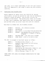
Preliminary Data Specification
Having examined the design layout and selected the optimum
grid location, we must now provide the code with the information
required to model the design.
contents of data sheets.
This section describes the
The specification sheets are included
In chart form to emphasize that specification must be completed
and verified before any actual input data cards are prepared.
Each chart Is divided into the following columns:
COLUMN 1:
DATA SO. - for reference purposes
COLUMN 2:
DESCRIPTION
COLUMN 3:
COLUMN 4:
DATA VALUES - to be taken from specifications
REMARKS - any manipulation of the DATA is
described or a summary of options
is given
COLUMN 5:
COLUMN 6:
VARIABLE NAME - code name used in THIRST
FINAL VALUE - value to be used as data
The data is arranged in functional groups as follows:
GROUP 1:
Preliminary Data (Items
GROUP 2:
Geometric Data Entered by Grid Indices
(Items 8 - 21)
Geometric Data Entered by Value
(Items 22 - 41)
GROUP 3:
1-7)
GROUP 4:
Correlations and Resistances (Items .42 - 60)
GROUP 5:
Operating Conditions (Items 61 - 69)
GROUP 6:
Utility Features (Items 70 - 85)
Items within each group are arranged alphabetically for ready
reference.
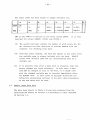
DATA
No.
DESCRIPTION
DATA
VALUE
REMARKS
ITEMS 1 - 7
PRELIMINARY DATA
RESTART " 1.0 - new run, no RESTART tape used
as input
Controls the use of the restart
ption (see Section 5.1)
1
VARIABLE
NAME
RESTART
RESTART = 2.0 - continue executing from a
point reached in a previous
run
RESTART = 3.0 - attach the data stored on tape
from a previous run and print
and/or plot the data
RESTART = - ( 1 or 2 or 3) - proceed as above
but write the final results
on a restart tape
2
Nuaber of axial planes
—
Must be an integer nuntoer
NI
3
Hiwber of radial planes
—
Must be an integer nunfcer
NJ
4
Nmfcer of circumferential planes
—
Must be an integer number
NK
5
Location of axial planes
—
Distance from the secondary side of the tubesheet surface to each axial plane - in meters
X
6
Location of radial planes
—
Distance from the center point to each radial
plane - in metres
Y
7
Location of circumferential grid
planes
—
The angle (In degrees) from a line passing
through the center of the hot side to each
circumferential plane
Z
VALUE
DATA
No.
DESCRIPTION
ITEMS
8
DATA
VALUE
VARIABLE
NAME
REMARKS
8 - 2 1 ARE GEOMETRIC DATA ENTERED ACCORDING TO GRID LOCATION USING GRID INDICES
Location of a l l baffles, tube
support plates and thermal plates
on the cold side
ee layout
This array is set up to indicate which axial
velocities are passing through a plate
resistance. Each axial plane, I , must be
specified as follows*
ICOLD
If ICOLD (r) = 1 -f no plates
ICOLD (I) - 2 -*• normal tube support
ICOLD (I) = 3 -*• outer baffle plate, see
data no. 23
ICOLD (I) = 4 -*• inner baffle plate, see
data no. 22
ICOLD (I) = 5 -*• thermal plate
ICOLD (I) » 6 •+ differentially broached
plate (usually first plate
on hot side)
9
10
Location of a l l baffles, tube
support plates, etc. on the hot
side
Shroud window height on the cold
side
See layout
This array is the same as data no. 8 except
that i t applies on the hot side.
The last axial plane lying
inside the window on the
cold side
n
1 1 = 1 DOMIC
IHOT
IDOWNC
VALUE
DATA
No.
.11
DESCRIPTION
ihroud window height on the hot
side
DATA
VALUE
REMARKS
The last axial plane lying
inside the window on Che
lot side
/ARIABLE
NAME
DOWNH
I = ( DOWKH
12
Top of the feedwater distribution
bubble
st axial plane passing
through the distribution
bubble
IFEEDB
13
Feedwater i n l e t window lower l i m i t
irst axial plane lying
inside the feedwater
window
IFSEDL
14
Feedwater i n l e t window upper l i m i t
Last axial plane lying
inside the feedwater
window
IFEEDU
15
Height of the preheater
Last axial plane inside
the preheater
IPKHT
VALUE
DATA
No.
DESCRIPTION
;ffective elevation where the
.owncomer annul us expands
DATA
VALUE
TRIABLE
NAME
REMARKS
The code treats the conical
section as a change in
porosity halfway through
:he expansion.
DASHED I W E
INDICATES
CODE
TREATMENT
17
19
starting elevation of the V-betid
The I-plauc located a t the s t a r t of the
urvature of the U-hend
The radial distance from the center
to the effective line dividing the
reduced broached side from the
normal broached size for different i a l l y broached plates
n some designs the f\rst
tube support plate
in the hot side i s di f f eri'nt i a l l v hrom'hod tc.
nduco flow into tin' contur
>f tht; steam generator. The
last r a d i a l grid Iinv c o r responding to Lhe l a r g e r
diameter holes i s used to
idt-nt i fy thi s point .
K-plane on the cold side noxt to
the 90° angle
p 1 'ir.t nunr the
s
ntt r of tlit-vk.K-t! r ^ i o n B u e b L E
I •!'
CO 1 C] S i d f
SH U L
K-plane on the hot side next to th
90° angle
A- 1" bur on
Angle at which the feedwater
d i s t r i b u t i o n bubble s t a r t s
k-pl.-inu thnt lie;: iuKt insult- t!
d i s t r i b u t ion buhl-. ].-
VALUE
DATA
No.
DATA
VALUE
DESCRIPTION
ITEMS 2 2 -
VALUE
4 1 ARE GEOMETRIC DATA ENTERED AS ACTUAL NUMBERS
Mstance from the partition p l a t e
:o the edge of the inner baffle
23
ARIABLE
NAME
REMARKS
listance from the partition p l a t e
:o the edge of the outer b a f f l e
Ised to determine which
:ontrol volumes contain
he baffle plate,
lontrol volumes which
xe partially exposed
o the baffle (partly
illed) have a weighed
jipedance.
BP(l)
Ised as above
BP(2)
:•)
00
•r 12)
I
Distance from the partition plate
to the edge of the inner baffle at
the exit of the pxeheater
(a)
25
One half of the width of tube free
lane between the hot and cold side
BP(3)
DATA
No.
DATA
VALUE
DESCRIPTION
VARIABLE
NAME
REMARKS
, 26
Outer diameter of the tubes
Cm)
DIA
27
Inner diameter of the tubes
(m)
DIAIN
28
lydraulic equivalent diameter in
the downcomer annulus at the feedwater bubble
(m)
hell inner
lam. 1 *
EDFEED = D S H E L L - D B U B B L E
EDFEED
luter bubble
diam.=
ffY/lKX11 SHROUD
^BU BBLt
29
Hydraulic equivalent diameter for
the normal downcomer amiulus below
the conical section
Cm)
30
Hydraulic equivalent diameter for
the downcomer annulus above the
conical expansion zone applies at
I planes greater than ISHRD (see
data no. 14)
(m)
Shell inner
dlam
EDN0RM
-'DSHEU
"
D
EDNORM
SHELL-DSHRQUD
Shroud o u t e r
diam
-
=D
SHROU
Upper s h e l l
i n n e r diam.
"
D
USHELL
EDSHRDX =
D
USHELL "
EDSHRDX
D
USHROUD
Upper shrout
o u t e r diam.
= D
USHROUD
31
HTAR
C2>
32
Distance between thf, outermost tub
and the shroud inner surface
(m)
^<53:——
^^/Yy^^9*
/Q*y'~
JAN
SHELL
OGAP
SHROUD
OUTER
TUBE
VALUE
DATA
No.33
DESCRIPTION
DATA
VALUE
'orosity in the downcomer at Che
:eedvater bubble
hell inner
dius
ubble outer
adius
ihroud outer
radius
R
REMARKS
rroally the downcomer
rosity i s equal to 1
idicating that the
ea i s entirely open,
r the region around
te bubble, one has to
alculate a porosity
hich when multiplied
imes the regular dovn;omer area will give the
reduced area
R
R
PFWB
"
R
BtfBBLE )
R
SHR0UD)
Distance between tubes (FITCH)
Porosity in the downcoaer annulus
above the expansion region
PITCH
inner radius As with data no. 28, porosity is used to
if the upper correct the flow area
ihell s e c t i
SHELL
)uter radius
upper
shroud
Lower s h e l l
Lnner rad.
Lower shroud
outer rad.
"SHROUD.
LO
36
Inner radius of the shroud
VALUE
SHROUD
PFWB =
35
'ARIABLE
NAME
PSHRD
SHROUD,,
UP
^p
R
2
SHROUDLQ)
o
i
DATA
Na
. 37
DESCRIPTION
alculated inner radius of the
hell
Cm)
DATA
VALUE
nner radius The code ignores the thickness of the shroud .
'o maintain the correct downcomer area, the
hell=R
SHELL nner radius of the shell has to be reduced to
uter radius ompensate for the added area contributed bv
he shroud thickness.
hroud
R UT
° SHM
nner r a d i u s
hroud
RADIUS
38
Height of thermal plate above leve
tubesheet (m)
39
Tubesheet thickness
40
Height of the dovncomer water
above the tubesheet (m)
41
Height at which the two-phase
mixture can be assumed to be
separated (relative to tubesheet)
VARIABLE
NAME
REMARKS
"SHELL - " " " ' B ^ - ^ H E I . L
-
R
RSHELL
ouiqHm)71
TPLATE
(m)
TUBSHET
XDOWN
This is used to calculate the gravity heaa
inside the shroud. Generally, one coula take
XVANE
VALUE
5ATA
No.
DATA
VALUE
DESCRIPTION
ITEMS 42 - 60
*2
loss factor for the centerline
>etween the hot and cold side,
MMV(I)
'araaeter -for selecting two-phase
Multipliers
ee layout
REMARKS
VARIABLE
NAME
CORRELATIONS AND RESISTANCES
This array is used to indicate the location of
AKDIV(I)
he partition plate AKDIV(I) = 1.0 E+15, the
-bend supports AKDIV(I) = k, or indicate
here no obstacles occur AKDIV(I) = 0. These
oss factors are used to calculate the pressure
oss relationship for the circumferential
velocity between the hot and cold sides <*se to
>lates or supports; the tubes are handled
ndependently.
If ITPPD = 1-THOM used for parallel, cross and
area change
ITPPD
If ITPPD - 2-BAROCZY-CHISHOLM used for parallel
cross and area change
If ITPPD = 3 - Separate correlations used
See Section 7.3
Parameter for selecting void
fraction correlation
If IVF • 1, homogeneous correlation
If IVF = 2, Chisholm correlation
If IVF » 3, Smith correlation
IVF
VALUE
DATA
No.
AS
DESCRIPTION
k shock loss factor for the baffle
)late resulting from area change
contraction and expansion)
DATA
VALUE
pproach
re a
)evice Area
evice Loss
actor
REMARKS
ne loss for the baffle
plate
ARIABLE
NAME
AKBL
(AKBL + f | ) e£
This data is the AKBL portion which is the
ressure drop due to the contraction into the
nnulus between the drilled plate and the tube
t i s based on the approach area.
Also see data no. 58)
46
k loss factor for the tube support
>roached plate - based on shock
atne as data The tube support plates result in a pressure
drop due to an area change. This value is
no. 45
based on the approach area.
AKBR
47
k loss factor for the larger
broached holes in a differentially
broached plate
Same as data In some designs, the first plate on the hot
side has smaller broached holes near the shrouc
no. 45
and larger broached holes near the center to
encourage flow penetration. This factor i s
for the area change in the central larger
holes.
AKBRL
48
k loss factor for the smaller
broached holes in a differentially
broached plate
S&me as data Shock loss for the outer small broached holes.
See data no. 18 for the radial position where
no. 45
the hole size changes.
AKBRS
Same as data For some designs the tubes are not rolled into
the thermal plate and leakage through the plat
no. 45
AKTP
plate
49
(AKTP + f^) ~~
a shock loss and a friction loss. This data ao. deals with the shock
loss. Again i t is based on the approach area
VALUE
DATA
No.
<50
DESCRIPTION
DATA
VALUE
Lndov area *
This pressure loss relationship i s based on a
Shock loss k factor for the shroud
mnular Area 0° flow direction change and an expansion
window on the cold side
rom the downcomer annulus into the shroud
*an
window. Both kgo° ant * kexp a r e based on A a n :
0° Elbow
^ s s » k 90
xpansion
AKWINDC = <kgo. + k
) (f^)2
oss - kexl>
an
ame as data Because the shroud window height may differ
o. 50
>etween the hot and cold s i d e , a second loss
factor may he required.
51
Shock loss k factor for the shroud
window on the hot side
52
Area ratio multiplier to determine Approach
Reynold's number In gap in baffles. area
(See also data no. 58)
" Aap
Gap area
53
REMARKS
Area ratio Multiplier to determine
Reynold's number in gap in thermal
plate
The local Reynolds number i s :
„ ._
R
'
D*v, *c
loc
0*AKATB*V *c
app
u
v
• Ag
Diametrical
clearance
= c
where:
See data
no. 52
ARATTP - (A /A )*c
ap g
ARIABLE
NAME
AKWINDC
AKWINDH
ARATB
ARATB = (A Ik )*c
ap g
ARATTP
VALUE
DATA
Na
,54
DESCRIPTION
Loss factor calculated for the
two-phase flow from the last
nodelied plane inside the shroud
to the separator exit, k
is
sep
normally given by the manufacturer
(based on V ) i s calculated
sep
by user, and i s generally much less
than k
sep
DATA
VALUE
TRIABLE
NAME
REMARKS
To calculate the recirculation ratio the flow from
the last modelled plane
Inside the shroud to the
last modelled plane outside the shroud is
modelled one-dimension- id.'
- total
.*ly.
CON1 is a
'P
combination of the loss
flow area
factors for the two-phase
lefore entei
mixture. It is based on
ng separatoi
the total flow as shown
below- C0N2 (data no. 55)
= total
sep
is the loss factor for the
leparator
saturated liquid flowing
irea
out of the separators.
ieparator
.ess Factor
k
sep
lontraction
'actor = k
VALUE
C0N1
From (1) to (2) - area contraction into
separators.
pvSEP
i
AP
A
where V
« velocity in
separator
SEP
FLOW2
P
A
SEP
2p
^EP
From (2) to (3) - separator loss
AP - k,
SEP
A
PV 2 .
2
SEP
SEP
FLOW2
2p
A
SEP
V
V
APP
I
DATA
No.
55
DESCRIPTION
DATA
VALUE
VARIABLE
NAME
REMARKS
Loss factor calculated for the
separated liquid flowing from the
water level to the l a s t modelled
plane in the downconer.
'his l o s s i s assumed to be a f r i c t i o n a l
and t r e a t e d as flow i n a p i p e .
-L pv2
L^
f j - 2 - fD *
. ,
..flP
1 FLOW2
2
2 p
-
loss
VALUE
CON2
CON2*FLOW2
2p. •
A
2 DC
where CON2 = f i (-r^-)
U
*DC
L - XDOWN-X(L)-*see data n o . 39
D = Hydraulic Diam. = Diam. Clearance
A^ = Downcomer Area
p = Saturation Density of Water
0.316
R
*
R
D
e
56
Parameter used to optimize the
estimate of the recirculation
ratio.
i s based on an estimate a t the
v e l o c i t y calculated from a r e c i r c u lation r a t i o estimate.
HPV
y
RECIR * FLOWC
P* A
DC
This r a t i o provides the code with an estimate
of how the pressure drop through the modelled
region changes with r e c i r c u l a t i o n r a t i o
( i . e . , t o t a l flow). The code uses t h i s value
to estimate the r e c i r c u l a t i o n r a t i o needed t o
balance the pressure l o s s against the driving
head.
C01M i s s e t a t 2000. If severe
convergence problems are encountered, other
estimates ( i . e . , 2000 + 1000) should be t r i e d
-
3I
FLOW
p*A^_c
"
CON4
DATA
No-
DESCRIPTION
57
Thermal conductivity of the tube
wall material
58
Friction pressure loss for the
baffle plate
DATA
VALUE
/ARIABLE
NAME
REMARKS
Obtain from material property data.
Baffle
thickness
L
FLDB
Also see data no. 45 and 52.
Ap •» [ARBL + ^ ] ~ Diametrical
clearance
=D
The variable i s concerned with the second
term - the frictional loss.
Area
approach
A
APP
Area gap
* A.
GAP
f = .316/Re*25
L = thickness of baffle
D = diametrical clearance
Because this loss is based on approach
velocities, the area correction is included.
Thus FLDB = .316 *
L
/ A APP\
\ GAP/
.. AP - [AKBL + FLDB * R
- 25
CWALL
5V
] *
VALUE
DATA
No.
59
DESCRIPTION
'
DATA
VALUE
VARIABLE
NAME
REMARKS
See data no. This variable stored the friction
58
mentioned in data no. 49 and 53.
Friction pressure loss for the
thermal plate
PLOT _ £ * /
coefficients
FLDT
W
2
/ . AP = [AKTP * FLDT * R£ ^
60
Resistance due to fouling on the
external surface of the tube
] -
^
Fouling is assumed to act uniformly over the
tube surface
RFOUL
ITEMS 6 1 - 69 ARE OPERATING CONDITIONS
61
Feedvater flow rate
(kg/s)
FLOWC
flow rate.
62
Eeheater flow rate
(kg/s>
Some designs include a reheater circuit.
The flow returning from the reheater is
assumed by the code to enter the steam
generator at the top of the downcomer. If
there is no reheater circuit, set this value
to zero.
FLOWRH
63
Prinary flow rate (kg/s)
Flow rate for the whole unit
FLOWTU
6A
Saturation pressure of the primary
(MPa)
Used to calculate priin^ry properties
PPRI
VALUE
DATA
No-
DATA
VALUE
DESCRIPTION
VARIABLE
NAME
REMARKS
Saturation pressure of the
secondary
(MPa)
Used to calculate secondary properties.
Take trie value at the normal water level.
PS EC
Inlet quality of the primjrv fluid
For a two-phase mixture, it is the actual
qualitv. For a subcooled primary flow this
value is calculated using
OLTU
n . _„
QLTu -
I n i t i a l estimate of recirculation
ratio
(°C)
*-•—•
*-::
Latent Heat
•
•
•
Tit a reci rculation r a t i o is not ad justed i or
the f i r s t 9 steps to allow the flow
to s e t t l e out. This* value serves ax ,in
ini t i a l condition.
Temperature of the feedwater
(°C)
Temperature of the reheater
flow
return
ITEMS 70 -
Enthaipv of Liquid-Saturation Entha
85 AKE UTILITY FEATURES AVAILABLE TO THK USER
The horizontal l i n e s of data which
are to be included on the v e r t i c a l
cut plots
In areas whore T pianes arc concentrated,
onv may decide to IpaVi* out some I lines from
v e r t i c a l plots so that tin* plotted arrows do
not overlap. Normallv a l l the l i n e ; would be
plotted.
IF IIPLOT(I) = I - plot tht' lintIF IIPf.OT(I) = 0 - skip the line
Note:
rTP[,OT(r) must have- M e n t r i e s
VALUE
DATA
No.
DESCRlPTluN
DATA
VALUE
REMARKS
ARIABLE
NAME
71
Selection of Che I position for
which the hot side and cold side
•ass flow will be calculated and
printed out
A subroutine MASSFLO has been set up to calulate the mass flow in the axial direction
for selected planes. This information is
rinted out any time the axial velocities or
tensities are adjusted.
Any number of I
planes may be specified up to NI.
IMASSF
72
Selection of the K-planes to be
plotted.
This variable allows the user to select any
number of Che circumferential planes for
plotting. Note the K=2 and K~N planes are
automatically plotted to give the t i r s t
frame and should not be requested again.
IPLOTK
73
Selection of the I axial planes to
be plotted
The plotting routine i s set up to plot up to
a maximum of 8 horizontal cuts. This variable
is used to specify the I planes of interest.
For example,
If IPLOTI
= +10, the 10th plane will be
plotted to the right of the
vertical cuts - see
Section 6.3 for more details
IPLOTI
If IPLOTI
= -10, the 10th plane will be
plotted on the left of the
vertical plot. Note there
must be only 4 specified for
the left side (negative
number) and 4 specified for
the right side (positive
number) .
VALUE
o
I
ATA
No.
74
DESCRIPTION
elect the variables to be printed
ut
DATA
VALUE
REMARKS
This parameter allows the user to trim the
utput down to variables cf s p e c i f i c i n t e r e s t .
VARIABLE
NAME
IPRINT
If IPRINT = 1, the variable i s p r i n t e d .
If IPRINT = 0, the variable i s skipped.
he order of variable s t o r a g e :
TPRINT(l) = axial velocity
IPRINT(2) = r a d i a l velocity
IPRINTO) = circumferential velocitv
IPRINTM « mass flux
IPRINTO) = steam quality
IPRLNT(fi) = primary temperature
IPRINTC7) = tube wall temperature
IPRINT(8) = s t a t i c pressure
IPRINT(9) = density of mixture
IPRINT(IO) = local heat flux
IPRINTU1) = porositv
75
Relaxation factors
"he order of variable s t o r a g e :
REI.AX(l)
RELA.X(2>
RELAXO)
RELAXC4)
RELAX(5>
RELAX ff>)
RKLAX(7)
RF.LAX(S)
RELAX O)
REijU(lll)
REIJUt(ll)
RELAX
= a x i a l velocity
= radial velocity
= circumferential velocity
= pressure correction
= enthalpv
' (inactive)
= tuhf wall temperature
= pressure
= denaitv
- wfdges and rings
= (inactive)
76
Contour intervals for the plotting
routines
Allows the user to specifv the q u a l i t v contours of inlftt'st
Can have up to 15 values.
Zero valut" "r tlu- end of the arrav are
i gnored.
TCON
77
Last execution step
Sots the last execution step. On completion
of I.ASTEP iterations, the computation ceases
and detailed printing and plotting s t a r t s .
LASTF.P
VALUE
JATA
Na
78
DESCRIPTION
DATA
VALUE
ARIABLEI
NAME
REMARKS
F PLOTO * 0, plots are never made
F PLOTO * 1, plots are made at the end of the
Job
F PLOTO * 2 , plots are made after each
iteration
arameter to specify when, during
he execution, plots are to be
made
Note:
PL070
If P1OTO - 2 , a very long plot f i l e
w i l l be produced. Careful s e l e c t i o n
of values for IPLOTI and IPLOTK are
necessary, (data no. 72 and 73)
79
arameter to specify when, during
the execution, the variables
pecified in IPRINT will be printed
out
R1NTO i s s e t up the same as PLOTO in data
o. 78. Note that PRINTO and PLOTO may be
reset i n the logic to turn the PLOTTING and
PRINTING routines on or off.
PRINTO
80
Parameter for overriding the time
limit routine
THIRST has been s e t up to print out a l l the
variables, make plots and write a RESTART
tape If the execution or INPUT/OUTPUT time has
been reached. To suppress this feature, set
TIMELT to zero.
TIMELT
81
Width of
I-plaues
the left
-vertical
the
are
and
cut
r\
• \/^
plotting frame when
to be plotted both on
on the right of the
(see data no. 73)
N
87.
Width of the plotting frame when
only 1-planes are plotted on the
right side of the verti"--" cut
—
r\
XLl
1—
T
1
XLl
•"
XL2
1
YI
83
Height of
.... plotting frame
YL
—
XL2 - ~ j
VALUE
DATA
No.
DESCRIPTION
DATA
VALUE
REMARKS
'84
Sxcra integer Input locations- Data put into
these variables is common to a l l subroutines
85
E>:tra real input locations.
VARIABLE
NAME
IEXTRA(I)
1=1,9
REXTRA(I)
1=1,9
VALUE
- 64 -
4.4
Preparation of the Input Data Cards
Once the data specification sheets have been completed, it is a
straightforward matter to transpose the requisite information
into data card form.
In THIRST, the data Is all processed through a routine called
READIN.
READIN not only reads the data into core, but also
performs a detailed check on the completeness and precision of
the data supplied.
The course of execution of the program is directed by the
RESTART feature which is described in Section 5.2.
The input cards are assembled from the variable names and values
already detailed in the last two columns of the charts in
Section 4.3, immediately preceding.
The cards must adhere to the following rules :
(1)
The first card must contain the title (1 to 40 columns) and
the RESTART value (word RESTART in columns 50 to 59 and
value in 60 to 69).
If the RESTART name and value are not
included, READIN assumes a RESTART value of 1.
(2)
All succeeding cards are read with the following format
s tatement
FORMAT (A9, 6 (A9, IX), A9)
- 65 -
The
ARP.YN
NAML
input cards for data arrays or single variables are,
10
20
30
40
50
60
70
NN
1
-1.
6.2
8750.5
1.0E+20
-.0068
-6.8E-4
1
NAM2
-1
ANAM3
1.3456789
ANAM3
180040.7
(NN Is the number of entries in the array called ARRYN.
It is only
required for arrays 1MASSF, IPLOTI and IPLOTK.)
(3)
The second card must contain the number of grid points NI, NJ,
NK,
selected for each direction to provide READIN with the
counters
(4)
for checking array data.
From this point onwards, the data may appear in any order since
the variable name is always included with the data.
READIN
treats each variable name and the corresponding data as a
variable set.
(5)
It is possible that after a data deck is prepared, some temporary changes are found necessary.
In this case, a data
item may be changed in situ in the deck, or a single card
with the changed variable may be inserted immediately after
the NINJNK card.
In such cases of multiple definition the
definition encountered earliest in the deck takes precedence,
so the new value will be used.
4.5
Sample Input Data Deck
The data deck sheets in Table 4.2 have been prepared from the
specification sheets of Section 4.3 according to rules outlined
in Section 4.4.
80
-
UJ
LL)
I
en
0.
I
66
-
-
67
-
THIRST INPUT DATA
SHEET
PAGE
1
0
1L
13 5
1 5 3l
l l
16
0 0
I A K B R
1.5
16
0 0
B
1 0
l A K B l
AK T P
A R A T T P
C0 N 4
0 . 0
E D F E E D
F 1 0 1
. 7 1 E +0 2
AK W I N D C
H e
2 0 0 0
0 . 0 6 5
16 0 0
1L
| l
1 1 1
. 8 E • 0 2
AKBRL
G A P
0 . 0 7
1 6 . 7
• E D N O R M
1 . 2 2
I
FI O W C
C 0 N 1
1
. 1 1 5 6
H
. 0 1 3 6 0 0 9
H
E D S H R O X
O . R
F I D B
?1I)I)O
H
3 0 6 . 1 8
F L O W R H
2 3 . 7
FLOWTIJ
2 4 8 4 . 9 3
H
6
I D O W N H
I F E E D U
1 0
I P R H T
I 7 P P 0
1
I U B E N D
3 0
K C E N T C
7
K C E N T H
6
P F W B
U 3 1 2 5
P I T C H
7
20
1
9
0 . 0 24 5
P R 1 1 1 0
1
P S F C
5.1
I V F
K F E E D L
F E E DB
I S H RD
J BR C H j
I I
A: T E P !
1 M" I 0 T n
I P S H R D
OL T U
0 . 0 4 4
R A D I U S
1 . 1 21
R E C I R
5.1
•
-
R S H E U
1 . 4 4
T I N C
1 7 6 . b 7
7 P I A T E
0.615
I T
R«
9
I x L :?
X VA N f
0 ..4| 1 9
1 6 .
0
X D O W N
VL T
1
1
T
• 1
H J
> 7 f» •; c . > B J
1
D I A [ If
I D O W N C
T U B S H E T
Hi
n
U N !
< 5 S 0
1 9 , 8 7 9
II
"•
O . O 1 5 S 7 5
8
P P R I
1
0 . 9 4 9 5
D I A
! r E E 0 L
0 . 0 3
fi
A Kp P S
ARATB
H I A 8
0 GA P
Ik
It*
1 . "
13
A K W I N D H
C M A L I
|
II*
1
I
3
5
.
0
X L 1
6 _[_
•
1
I;
13
31
4
|b 0
l l
i l l
1
0 .
M
1
-
I 1? 5 ' . 6 7
1
| h . 25
BJ
BJ
•
H
•
|
M
pj
1
-
1I
•
1
~~ti—i=5 5""3
;=|=
_
- .
.T
±::~!
t|t|
"17 .T. 1 , . —M
I
35
- 69 -
4. 6
The Standard Execution Deck
At this point, the major effort of preparing the data deck Is
complete.
It is now necessary to enter the ThIRST job into the
computer system.
Execution control cards can vary between CDC computer
ins tallatior. s .
However, the following decks are included as
examples, and operate satisfactorily on the CRNL system.
For a
full explanation of CDC control cards, see references 13 and
14.
The decks consist of the following:
JOBCARD containing job name and account information
CONTROL CARDS directing execution
7/8/9 END OF RECORD CARD
DATA DECK
7/8/9 END OF RECORD CARD
6/7/8/9 END OF JOB CARD
Card
1
Content
JOBNAME, BXXX-YYY, Tttt.IOiii.
Explanation
JOBNAME - 7 character job name
2
ATTACH, THIRST, ID-THIRST, CY-1.
Attach THIRST
object code
3
THIRST.
Execute THIRST
code
- 70 -
Card
4
5 to N
Content
Explanation
7/8/9 END OF RECORD CARD
COMPUTER DATA DECK
N+l
7/8/9 END OF RECORD CARD
N+2
6/7/8/9 END OF JOB CARD
The above simple execution deck will execute the standard THIRST
code without reading or saving any RESTART data.
Advanced
Execution Decks are discussed in Section 5.5.
4.7
Job Submission
A complete listing of the entire deck is given in Figure 4.5.
This may now be submitted to the CRNL system.
As turnaround time for a large job is not particularly fast, we
discuss in Chapter 5 some additional features of the code. Our
output will appear in Chapter 6.
-
71 -
THIRST,B652-EXAPPL,T50CiI<J100.
ATTACH < C L D P l , T H I RSTPLt ID = THI:<ST)
UP0ATEIC-DISC1
FTN( I = O I S C , e = Tt-IRPCD>
ATTACH(THIRST,ID=THI*ST)
COPYL<THIRST,THRI'OL>,TM5ST2)
ATTACH ( T A P E 6 0 . T h I R S T D A T A , I 0 = T
ATTACHIPLOTLIfl)
LOSET(LIB=PLOTLie,SlHST=PLOT-PLT>
THIRST2(PL=300C0)
IFE,Rl.NE.OiJUrP.
COHI1ENT.
CATALCG RESTART TAPE
CATALOG(TAPE60,THRST0ATA,n = T
ENOIF(JUfPt
7/8/9
•IDENT HYPOTH
*O KOMON.l
7/8/9
COMMON
F<432O.13I
HYPOTHETICAL
ri 1
AK^IV
1.OE-1Q
1.CE15
1.OF.15
1.8
BP
O.«3
ICOLD
1
1
4
2
1
IHOT
1
1
2
2
1
IIPLOT
0
0
1
1
1
IHASSF
3
11
19
27
35
I PLOT I
2
IPLOTK
3
IPRINT
0
RELAX
.5
.5
TCON
0.0
0.22
0.0
0.78
2.86
5.78
9.8
0.0
1.2845
0.0
135
AKBL
AKTP
*R*TTP
C0N4
EDFEED
FLDT
HTAR
IFEEOL
ITPPO
KCENTC
PPRI
OLTU
RSHELL
TUBSHET
XVANE
1/6/1
tCO Md S T E A 1
JO
l.oe-ic:
1.0E15
1.0E15
GENESATCH
J. Li
•> s i
l.OE-10
1.CE15
1.0E15
1.0S--10
1.01:15
1.0E15
0.16
0.56
1
1
3
2
1
4
2
I
1
1
3
2
1
1
1
2
2
1
0
1
1
1
1
1
1
1
2
1
1
0
1
1
0
5
13
21
29
6
14
l
i
I
2
1
1
1
1
1
1
33
4
12
20
28
8
-6
8
4
0
0
.5
.2
0.01
0.25
0.01
0.89
3.21
6.36
10.2
0.1
1.3575
9.0
153
1600
1600
0.0
2000
0.065
1600
4550
8
1
7
0.03
9.879
0.044
1.44
0.419
16.0
1
RESTART
l.OE-10
1.0E15
30
-21
1 • O c - 10
l.Otlb
I.CE15
1.CE15
l.OE 15
l.Cbli
1.0
1. t
1 .c
1
5
3
I
1
2
1
1
1
1
2
1
2
ft
1
1
2
1
0
1
1
1
1
1
1
0
0
1
1
1
1
0i
7
IS
23
31
8
16
24
32
<)
17
25
33
10
13
2o
25
-32
33
-35
7
H
0
0
0
0
.25
1
1
7
2
3
1
1
1
2
2
2
it
22
14
5
0
0
6
.5 .
1.
I.
1.
1.
0.03
0.35
0.23
1. 11
3.91
7.53
10.6
0.05
0.4
0.34
1.46
4.17
8.12
0.1
0.5
0
0.02
0.12
1.0
3.56
<j.94
10.5
0.27565
27.0
1.71£»02
AKrtR
AKHINOC
CGAP
CdALL
EONOR"
FLQUC
tOOttHC
IFEEDU
IUAEND
KCENTH
PFWB
PRINTO
RADIUS
TINC
XDO.N
YL
0.4513
45.0
l.BE*02
1.5
10
0.07
16.7
0.22
306.16
6
10
30
6
0.3125
1
1.321
176.67
15.0
6
Figure
-1
pi IN
4.5:
TPLATE
XL1
0.2
4.2b
8.7
0.5(? . lfa
4,61
9.C7
0. fc7
2.51
5.194
9.44
0.3026
O.97H
1.1539
B.1EI
S.9E1
63.0
RECIK
0.15
0.45
1.B1
0.6269
AK6KL
AKklNOH
C0N1
DIA
EDSHROX
FLO»RH
IDOKNH
IPRHT
IVF
KFEEDL
PITCH
PSEC
10
AKtRS
ASATJ
0.9495
CUN2
0.015^75 !) IA 1 ,\
1.0
13
0.8
23. 7
7
20
1
9
0.024511
5.1
5.3
0.615
9
Execution
Deck
FLOd
FLOWTU
(FEEDS
iSHRO
J8RCH
LASTEP
PLOTO
PSHkO
KFOUL
TRH
KL2
117.
o .C
1.2705c-2
. 115b
.0136i;C>)
21000
2 4 34 .'i3
13
31
60
1
1
10.1
Z.642E-5
251.6/
6.25
- 72 -
5.
SOME FEATURES OF THE THIRST CODE
While the Instructions included In the previous chapter are
sufficient to prepare an input deck, an understanding of some
additional features of THIRST is required for advanced use of
the code.
This chapter describes some of the THIRST input and
output options.
5.1
The RESTART Feature
RESTART Has been introduced very briefly in chapter 4.
This
feature was included in THIRST to reduce the repetition required
In making several runs with only slight data modification, and
to enable results to be stored so that later printouts and plots
can be made without re-executIng.
In THIRST, all the variables are initialized in START with, at
best, a rough guess.
Using RESTART, the variables can be
initialized with results saved from a previous run, resulting in
improved convergence.
RESTART has been set up so that a user can stop, at say the
twentieth step, examine the results and then proceed further if
desired.
The user can also run the code, examine the results,
make logic or input changes and continue running the program,
or merely change the clotting or numbering parameters, and
produce new output without executing the program.
- 73 The RESTART variable can have six values, three positive and
three negative.
RESTART=1 is used for a new run in which all variables and
arrays are initialized with rough guesses by the program. All
routines are executed to attain a solution.
RESTART must
always be set to 1 if the number of grids or the grid layout
is changed.
RESTART=2 is used to continue an old run.
All the variables in
common blocks are set to values calculated in a previous run,
which has been stored on a RESTART tape.
New values for selected
variables can be entered by including these in the input deck,
they then replace any stored values.
Variables which are not
to be changed are omitted from the input deck.
The new run is
then executed until a total of LASTEF iterations have been
completed.
RESTART=3 is used mainly to obtain new output from a previously
completed run.
With this option, all parameters except those
read in to specify the type of output required
values from the RESTART tape.
are set to their
The EXEC routine then passes the
control directly to the OUTPUT routine for the summary of the
last step, and a printout of all arrays requested through the
IPRINT(NN) parameter.
Finally, if PLOTO ¥ 0, the plot routine
generates the plots requested by IPLOTI and IPLOTK.
After this
output, the program terminates; no further execution is attempted.
RESTART«-n writes a RESTART tape on completion of a run.
The
absolute value of n (i.e., |n| = 1,2,3) determines the initial
conditions for the run.
On completion, a tape is written
through the WSTART routine ready for subsequent reading with
|RESTART| > 1.
- 74 -
Saving and Accessing a RESTART Tape
In WSTART a special global parameter "Rl" is set to 0 when the
tape is written.
A set of statements can be included in the
execution control cards to catalog the tape If this global
parameter is set.
IFE(R1.NE.O)JUMP
CATALOG(TAPE5O, THIRSTDATA, ID-THIRST)
ENDIF(JUMP)
If Rl«0, control jumps past the CATALOG card to the ENDl .JUMP)
card.
If WSTART has set R1»O, the CATALOG card is executed and
the RESTART tape is stored under the name THIRSTDATA, ID-THIRST
and CY=n,the lowest available number.
Thus each time a RESTART
tape is made, a new THIRSTDATA file is created.
The user will
have to exercise strict management of these files to avoid
confusion and the creation of unnecessary files.
To RESTART from this tape, the user includes the card
ATTACH(TAPE50, THIRSTDATA, ID-THIRST, CY-n)
before the execution card in the JOB control statements.
The
information stored on this file will then be used in the RESTART
routine to initialize the arrays and the variables providing
RESTART is set at 2 or 3 in the input deck.
- 75 -
5.2
The READIN Feature
To assist the user with the entry of data into the code, t
subroutine called READIN has been written .
READIN extracts
the variable name and its value from the data cards.
As each
piece of data is associated with the computer variable name,
READIN can:
(a)
ensure that all the data required are provided and
determine which data are missing
(b)
allow the user flexibility in choosing the order of the
data
(c)
initialize the variables with values on the restart tape.
READIN is set up to accept the title card with the RESTART value
as the first card.
columns 1 - 40.
The title can be set up to 40 characters in
The word RESTART sh
Id be located In columns
50 - 58 and the RESTART value in columns 60 - 68.
If the
RESTART name and value are left off, READIN assumes a value of
1.
If RESTART is set to 1, -the second card must specify NI,
NJ and. NK.
These variables spesify the array sizes
for all the variable arrays except IMASSF, IPLOTI and IPLOTK.
If NI, NJ and NK are not specified, an error message is sent and
the run erminates.
- 76 -
If (he RESTART is set at +2 or +3, the run will continue from a
print reached in an earlier execution.
Because the values are
stored in matrix arrays, the number of grids in each direction
must remain fixed.
Therefore, any attempt at re-specifying the
number of grids, i.e., changing the value of NI, NJ or NK, is
ignored.
All the remaining data can be introduced in any order.
In our
examples, we have elected to Rroup the data according to its
usage, i.e., geometric, correlation-related, operating
conditions and input/output parameter selection.
READIN contains li&Ls of all the variables required by the code.
As the data cards are read, READIN searches through the list to
match input variable names vith the ones on its list.
If the
subroutine can make the match, it stores the data in the
variable and removes the variable name from the list.
If READIN cannot match an input variable to one on Its list, it
issues the following message:
*** X CANNOT MATCH X VARNAME DATA ***
This message contains the input variable name and its value so
the user can trace the nature of the error.
This error could
result from a misspelling of the variable name, from reading the
same variable twice, or- using Improper data.
not result In a termination of the run.
This error does
If a variable appears
twice, .READIN stores the first value and disregards the second.
If a variable is mispelled, READIN Ignores the variable and its
value, and thus the intended variable name will not be removed
from the list.
- 77 -
When the end of the Input deck (END OF FILE) is encountered,
READIN checks that all the variables on its list have been
initialized.
Some variables may not be stroked off because they
are either mispelled or simply left out.
If a variable name
remains, but has not been initialized, READIN issues one of the
following messages:
* THE FOLLOWING VARIABLE(S) HAVE NO INPUT DATA:
VARNAME *
or * THE FOLLOWING ARRAY(S) HAVE NO INPUT DAT'.:
VARNAME *
READIN then checks the value of RESTART and:
If (RESTART-+1) - READIN terminates the run
If (RESTART-+2or±1) - READIN uses the values stored on the tape
iade from a previous run and continues
executing, thus only variables to be
changed are required as input data.
5.3
Time Limit Feature
If the code senses that insufficient time remains to complete
another Iteration step and to print ana plot the output, it will
automatically call FPRINT for a printout, and call the WSTART
routine to write a RESTART tape. The user can subsequently
attach the RESTART tape and continue executing with additional
time.
Both execution time and input/output time are monitored, but
the time limit feature can be suppressed by setting the
- 78 -
parameter TIMELT to zero. If TIMELT is not set in input or is
set to 1 in the input deck, time remaining is checked at the end
of each iteration.
The statements:
IFE(Rl.NE.0)JUMP
CATALOG (
ENDIF(JUMP)
should be included in the job control deck to catalog a RESTART
tape when a time limit is encountered.
5.4
Advanced Execution Deck
The simple execution deck introduced in Chapter 4 is sufficient
to run a standard '.HIRST job in which no RESTART tape Is read
or saved.
For more advanced use, we now include an execution
deck which will permit the use of a RESTART tape, and also
permit certain code changes to be made, using the CDC program
library editor, UPDATE.
This "advanced use" deck contains three major segments:
(1)
job control statements
(ii)
update correction set
(iii)
input data
Because the function of each section in the execution deck is
different, they will be explained separately.
It is assumed
that the reader has! a basic understanding of the job card
sequence and the update routines available through the computing
system.
A listing of the execution deck without explanations is
shown in Appendix C.
-
5.4.1
Job Control
79 -
Statements
Card
No.
Explanat ion
1
THIRST, B652-EXAMPLE,T500,I0100
2
ATTACH(OLDPL,THIRSTPL,ID=THIRST)
Attach
the code
stored on file name
THIRST
3
UPDATE(C=DISC)
Update the file
THIRST with any code
changes in the associated correction set
and list on disc
4
FTN(I=DISC, B=THIRMOD)
Compile the file
THIRST from DISC.
SLore compiled file on
THIRMOD
5
ATTACH(THIRST, ID=THIRST)
Access standard THIRST
code
6
COPYL(THIRST , THIRMOD, THIRST2)
Merge modifications
and standard code to
create new program
THIRST 2
7
ATTACH(PLOTLIB)
Attach library plotting package
8
COMMENT.
9
LDSET(LIB-PLOTLIB,
SUBST=PLOT-PLT)
-
80
Card
No.
10
-
Explanat ion
ATTACH(TAPE60, THIRSTDATA,
ID=THIRST)
This card is required
only when the RESTART option is used
(ABS(RESTART). GT.1)
The data catalogue
from a previous
run under file name
THIRSTDATA with ID=
THIRST and for CY=1
will be attached and
used to initialize the
variables.
If RESTART
is 1, this card wi11
have no useful purpose
and should be omitted.
11
THIRST2(PL=3OO0O)
Execute the job and
set the printing limit
at 30000 print lines
12
IFE(R1.NE .0)JUMP.
If a RESTART tape has
been written either
through a time limit
or a negative value of
RESTART then Rl is set
to one.
If the program has not written a
data RESTART tape then
Rl = 0 and the execution jumps to ENDIF
(JUMP).
Thus this
card controls the sequence to CATALOG only
when the data RESTART
tape exist s.
- 81 -
Card
No.
E x p l a n a t ion
13
CATALOG(TAPE60,
ID=THIRST)
14
ENDIF(JUMP)
P o i n t to which the
IFE( ) card d i r e c t s
control
15
7/8/9
End of
THIRSTDATA,
Catalog
tape
the RESTART
record
card
To enable the computer to allocate storage, the size of the grid
layout must be specified in the EXEC routine. The following
update correction may be used to change this allocation and is
included for example purposes.
Card
No.
Explanation
16
*D EXEC.4
Delete the
in EXEC
17
COMMON F(4320,13)
Reserve 13 a r r a y s (11
v a r i a b l e s plus 2 working s p a c e s ) •
Each
a r r a y c o n t a i n s NI*NJ
*NK - 36*10*12 - 4320
s t o r a g e places
18
7/8/9
END OF RECORD
5.4.2
fourth
card
Input Deck
Unless the changes made above incorporate new input data, no
form changes in the deck of Chapter 4 are required.
- 82 -
6.
THIRST
In this
OUTPUT
c h a p t e r , we present
THIRST code.
Output
Possible
the basic output
variations
from T H I R S T is in both
The following p a r a g r a p h s
consecutively
printed
obtained
are also
and g r a p h i c a l
refer to sample
P r i n t e i Output
6.1.1
Preliminary
from the
discussed.
form.
output which
at the end of this section s t a r t i n g
6.1
appears
on page 9 9 .
Features
Output
A f t e r the p r o g r a m
input deck.
l o g o , T H I R S T prints out the values
The arrays are printed
values s e c o n d and the single
messages
of output
related
to the input
f i r s t , the single
real values
last.
are printed
in the
integer
All the e r r o r
out in this
section,
Figure 6.1.
The next s e c t i o n of the p r i n t e d
all the input
of the p r o p e r t i e s w h i c h
Figures
output
received by the code
contains
for this
a summary of
run and a summary
T H I R S T has c a l c u l a t e d
from curve
6.2.1 to 6.2.3 c o n t a i n :
(a) Operating
Conditions
- Primary
-
Secondary
(b) Properties as Calculated by THIRST (using Curve Fits)
- Primary Saturation
- Secondary
Values
Saturation
Values
- Secondary Subcooled Inlet Properties
(c) Output Selection and Control Parameters
(d) Geometrical
Parameters
fits.
- 83 -
Figure 6.3 contains:
(a)
The Grid Locations for Scalar and Vector Components
- The Axial Positions in Metres
- The Radial Positions in Metres
- The Circumferential Positions in Degrees
(b)
Primary Fluid Flow Distribution per Typical Tube in kg/s
All the above output is generated in START before the
iteration procedure begins.
The user has no control over
the format without altering the program logic.
6.1.2
Individual Iteration Summary (Figures 6.4.1 to 6.4.5)
During the progression of the solution to convergence, the
following information is summarized on one page for each outer
iteration.
(a)
Iteration:
At the beginning of each iteration prior
to any further calculation, the EXEC routine prints the
outer iteration number.
(b)
Hew Estimate of RECIR (only after the ninth step):
After the ninth iteration, the program begins to calculate
the RECIRculation ratio.
Because the solution technique
is iterative, the value will change until the solution
approaches convergence.
(c)
Mass Flows at Planes of Interest: The mass flows are
calculated at I-planes selected by the user. The user
can chooBe any or all of the I-planes by using the IMASSF
- 84 -
parameter (see data no. 71, Table 4.1).
The mass flow
Information is preceded by a line indicating the point
within the iteration step at which these calculations were
performed.
The mass flows at designated I-planes are
plotted in five columns of eight entries each for a maximum
of forty positions, if required.
The mass flows are given
for both the hot and cold side.
The calculations are made
in MASSFLO.
MASSFLO is called whenever the axial velocity
or local density is changed.
(d)
Summary of Overall Performance Variables and the
Convergence Indicators:
At the end of an iteration step, a
summary of the overall performance variables and the
convergence indicators are printed.
control over this format.
The user has no direct
The information provided
Includes:
RECIR
Recirculation ratio used for this iteration
PRESS DROP
in Pa
is the pressure drop between the average
pressure at the last I-plane (1,-plane)
inside the shroud and the average
pressure at the last I plane (L-plane)
outside the shroud in the downcomer .
PRIM H.T.
in MW
Is the net amount of heat given up by the
primary fluid
- 85 -
SEC H.T.
is the amount of heat picked up by the
in MW
secondary.
This includes the heat required to
raise the feedwater and reheater drain flows
to saturation, plus the heat absorbed in
evaporating the secondary liquid.
NOTE
PRIM H.T. should equal SEC H.T. when convergence
has been achieved.
AVG/OUTLET/QUAL
SUMSOURCE
average outlet quality
is the summation of the absolute value of the
mass imbalance for each control volume
normalized by dividing by the total flow.
This
indicator should approach•?ero with convergence ,
MAXSOURCE (2,7,11)
is the largest mass imbalance
normalized by dividing by the total
flow in the modelled region.
The
location is gi"en in the brackets as
1-2, J-7, K-ll.
If the location
remains fixed, and the imbalance is
significant, the use should examine
the region for a possible error in
that area•
(e)
Summary of Local Values;
The last section of the iteration
by iteration printout summarizes local values at strategic
locations in the model.
The locations are fixed in the
code at such points as window inlets, above the preheater,
in the downcomer, etc.
- 86 -
Three sets of variables - AXIAL VELOCITY, CROSS FLOW
VELOCITIES and THERMAL VALUE are printed.
The location of
each variable is described including its (I,J,K) coordinates.
If the user wishes to change the locations to be
printed, the OUTPUT subroutine must be altered.
The overall values (d) and local values (e) are printed out
in OUTPUT.
OUTPUT can be called at any point in the.
execution if the user desires to.
At present it is called
at the end of each iteration step.
6.1,3
Detailed Array Printout (Figure 6.5)
The last type of printed output, again under user control, is
the complete printout of selected variables at every active node
in the model.
The format for the printout is
XXXXXXXXXX
VARIABLE NAME (1)
XXXXXXXXXX
K=2
1= 2
1= 3
1= 4
I
I=L
J =2
J= 3
J=4
J=M
- 87 -
K=3
1= 2
J=3
J=4
J=3
J=4
-J=M
1= 3
1=4
K=N
J =2
-J=M
1 =3
1=4
I
I-L
XXXXXXXXXX
VARIABLE NAME (2)
XXXXXXXXXX
etc •
This printout can be very long depending on how many variables
are specified for printout. Figure 6.5 shows the first page of
a detailed array printout of axial velocity obtained by setting
IPRINT(I) to 1. Each selected variable takes a similar format
and each generates five pages of output for K»12, so the feature
should be used with caution. Variables to be printed may be
selected by the input variable IPRINT.
If IPRINT(NV) is entered non zero, the array of values for
variable NV is printed, where NV is selected as follows:
-
NV = 1
NV = 2
-
88 -
axial velocity
r a d i a l velocity
NV = 3
-
circumferential
NV = 4
-
mass
NV = 5
-
steam
NV = 6
-
primary
NV = 7
NV
—
-
Q
—
NV = 9
-
velocity
flux
qual1ty
temperature
tube wall
static
temperature
pressure
density
NV = 10 -
heat
NV = 1 1 -
porosity
flux
This printout is generated by the FPRINT subroutine.
parameter calls FPRINT as follows:
The PRINTO
If PRINTO = 0 - the FPRINT array is never called
- this would be used where the user is interested
in the plots only
If PRINTO = 1 - che FPRINT array is called after exit from the
iteration loop at the end of the run
If PRINTO = N - the FPRINT array is called every (N-l) iteration
steps.
This tends to create large output files
and thus is only used for debugging p rposes.
Careful selection of the IPRINT (NV) parameter
is suggested.
-
6.2
89 -
Graphical Output Features
The plot routines have been set up to produce:
(a)
quality contours
(b)
velocity vectors
(c)
mass flux vectors
for any planes of interest.
Quality contour values are specified by TCON in the input deck.
Up to 15 contour intervals are allowed.
If less than 15
contours are desired, then set the remaining position of the
TCON array to zero and the plotting subroutine ignores them.
Velocity vectors are determined by first interpolating each
velocity component to the grid nodes.
The two velocity
component? lyli.% in the plane of interest are added vectorlally.
The resultant vector is printed as an arrow with its length
indicating magnitude ?nd angle indicating direction.
Mass flux
contours are determined by multiplying the velocity vector
calculated earlier by the local density.
Two plotting formats are available to the user:
(a)
(b)
Full Diameter/Horizontal Cut Composite
Vertical Cut Composite
Full Diameter/Horizontal Cut Composite
This composite includes plots of values of the K-2 and K-N
planes which lie next to the line of symmetry.
out by the plot routine automatically.
These are put
Included on this frame
-
are
up to eight
corresponding
parameter.
in
(maximum
to
deck,
otherwise
t h eright
specified,
are
given
in
mass
Vertical
Cut
Composite
plot
corresponding
of
K-planes
There
Examples
of
this
profiles
are
grid
flux
vectors
has
been
I-plane
0,
of
the
on
in
layouts,
introduced.
are
Figure
axial
Included
corresponding
an
If
on
the
of
thp
user
I-plancs
specified
Diameter
of t h e Full
f o r t h e left
four
a n d four
i - p l a m s
a r e
a sc h e
F. >: a m p i e s
depicts
of
tliis
quality,
of
four
planes.
The
of
cuts
and
indices
by the p a r a m e t e r
TP1.DTK.
K-planes
quality,
vertical
number
to
be
velocity
selected.
and
mass
flux
6.7.
planes
they
are
grouped
tend
to
when
IIPLOT
= 1,
(I)
vertical
values
cut
are
together
velocity
overlap.
plot
I-plane
by
desired
consecutively.
additional
the
IPI.OTI
on t h e right
Unfortunately,
plotted,
plots,
for
of
size.
are specified
number
detail.
are
the
the
the
of t h e Full
6.6, w h i c h
a composite
composite
given
greater
clarity
Figure
to b e p l o t t e d
limit
some
appear
region
is n a d e
front
I-plots
the frame
profiles
is
in
If only
should
by
cuts
o n t h e right
four
circumferential
no
In
flux
format
to
is
provide
sign
appears
reduce
and
specified
the number
m a yb e specified.
will
the modelled
o n t h e left
than
a l l t h e plots
second
lines
A negative
N o more
routine
composite
through
of h o r i z o n t a l
C h e plot
velocity
The
axial
t h eplot
Plot.
plotting
cuts
by specifying
positions
Diameter
for
eight
of e i g h t ) .
I-plane
Plot,
horizontal
The selection
the input
90 -
To
parameter
the
left
off
mass
ensure
called
values
plots.
to
or
If
the
on
11 P L O T
that
IIPLOT
plot.
(I) =
-
91 -
The user has control over the plotting frame size.
For the
first composite, the width is specified by "XL1" and "XL2".
If
horizontal plots are made on the left and on the right of the
vertical cut, the routine usss the wider plotting frame
specified In XL1.
If other horizontal plots appear only on the
right, the routine uses the narrow plot XL2.
plots is YL.
The height for all
The length to width ratios of the plots may not be
in proportion to the actual design,
increased to add clarity.
as the width may be
Scaling factors are determined by the
code .
The plotting routines can be called at any point in the code by
the statement CALL CONTOUR.
The parameter PLOTO has been
introduced to control the calling of the plot routines.
If FLOTO = 0 - the plot routine is never called.
This may ^e
used where the user wants only a printout.
If PLOTO * 1 - the plot routine Is called at the end of the
program.
If PLOTO « 2 - the plot routine is called at the end of each
iteration.
This leads to a very long plot life.
PLOTO is set in the input deck. PLOTO and PRINTO can be reset
In the program to initiate the plotting and printing function.
-
6.3
92 -
Interpretation of the Output
Having discussed the layout of printed output we now turn again
to the printed output, Figures 6.1 to 6.5, to examine its content
and its significance.
The first page of printout, Figure 6.1, contains a summary of
all the data introduced through the Input deck.
No error
messages of consequence were issued and a comparison with the
data sheets indicfcf.es that the data has been introduced
correctly•
The second, third and fourth pages (Figure 6.2) contain input
values and calculations made with the input.
The operating
conditions should be checked against the information sheets.
Property values generated by the code should be checked against
values in standard tables.
Correlation data should be verified.
The input/output parameters are simply informative.
Finally,
the geometric data should be verified against drawings or data
sheets.
The modelled heat transfer area should be examined to
ensure that it is not radically different than the prescribed
value.
Although the correction factor will correct the modelled
tube surface, a large discrepancy may indicate an error in
treating the tube-free lanes or in the location at the start of
the U-bend (IUBEND).
The main grid location (Figure 6.2) and particularly the
displaced grid locations should be checked to ensure proper
modelling of flow obstacles. For instance, the displaced grid
-
93 -
at 1=13 for the axial velocity should in this case correspond to
the elevation of the first inner baffle.
The primary fluid
flow, also Included on this page, is distributed to reflect the
different tube lengths.
Scanning the distribution, one should
see a drop in primary flow along the K=2 plane with increasing
J.
When satisfied with the validity of the Input, one can proceed
to examine the iteration by iteration output (Figure 6.4).
prime importance
is the line bounded by asterisks.
Of
Part of
this line contains the overall parameters which must converge on
single values - RECIR, PRESS DROP, PRIM and SEC HEAT TRANSFER
and QUAL.
The last two terms are the sum of the absolute value of
the mass imbalance over all control volumes and the maximum mass
imbalance at an indicated control volume.
approach zero at convergence.
These should
By examining the line of
printout as the solution proceeds, one can assess whether the
solution is converging to a single solution or oscillating
slowly about the solution.
Assuming that the run has completed normally without any
execution errors, we will concentrate on the last several
iterations to verify that a converged solution has been
obtained.
Later in this section we will discuss handling runs
that terminate in execution errors.
Comparing Iterations 58, 59 and 60, Figures 6.4.3, 4 and 5, we
observe that RECIR has converged to the fourth significant figure,
which Indicates that the pressure distribution has also
converged.
-
94 -
Examining the mass flows at various stages In the iteration
step, we see that the values are basically stable.
Minor
changes can be expected due to the nature of the finite
difference technique; however, a swinging from or.? value to
another would indicate an inconsistency in the modelling between
stages.
If the swinging is significant, further debugging of
the logic should take place.
In the middle of the mass flow printout is the SUM OF RING
(WEDGE) MASS IMBALANCE.
As explained in earlier sections,
continuity is enforced simultaneously over groups of control
volumes.
Control volumes are grouped alternatively into wedge
and ring geometries.
The MASS IMBALANCE should approach zero at
convergence; however, the level indicated is considered
acceptable.
At the end of the run we also should be satisfied that the
pressure drop value is stable, that the heat transferred out of
the primary (PRIM H.T.) is equal to that absorbed by the
secondary (SEC H.T.) and that the source terms are sufficiently
small.
The location of the maximum imbalance is given in
brackets after the MAX SOURCE.
This information can be useful
during debugging to indicate trouble areas.
If the location
remains fixed and the imbalance fairly high, one should examine
the region for a modelling error.
Tht last three lines on Figure 6.4.5
thermal and hydraulic variables.
contain local values of
These values should be
compared with earlier iterations to ensure that they have
converged.
The positions shown in brackets have been selected
to monitor variables because they are particularly sensitive
areas.
-
95 -
When we are content that the solution has converged, we should
examine the printouts to check numbers against Intuition and
then examine the plots to verify -hat flow and quality patterns
are consistent.
These outputs will not provide additional
evidence of convergence but will enable the user to intuitively
verify the results.
For instance, the quality profiles on the
1=2 plane could be superimposed over the velocity vectors to
verify that the velocities are concentrating near the point of
highest quality.
The velocity vectors in the D-bend should
indicate an outwards radial flow to the lower resistance
regions.
The flow around the baffles should be well defined-
Having examined the output, we conclude that, for this example,
the solution has converged.
6.4
Treatment of Diverging Solutions
If the solution has not converged, we should either restart the
program and continue for mjre iteration or examine the modelling
for errors. It may be necessary to use lower relaxation factor
to promote convergence.
If the solution terminates on an execution error or will not
converge, the user will be required to debug the model.
The
efficiency of the user's debugging methods will improve only
with experience.
To assist in debugging, the following
potpourri of examples is included:
(a)
If the program has terminated before completing one
Iteration, it Is likely that insufficient input data has
been given or that the array sizing doesn't match the
arrays referenced.
One can identify the line In which the
error occurred and generally find the error using an
"OPT-O" on the FTN card.
-
(b)
96 -
If the program fails after the eighth iteration, examine
the RECIR subroutine because it is called after the eighth
1teration.
(c)
If the program terminates with an error message
"ARGUMENT
LESS THAN ZERO", this is most likely generated by quality
values greater than 1 arising from a very high pressure
gradient (the user should refer to DENS to see how pressure
affects quality).
The high pressure gradient generally
occurs when a gross Inconsistency in the treatment of flow
obstacles occurs between various stages of the iteration
procedure.
Large pressure corrections are required to
maintain continuity.
The stage within the iteration that
contains the Inconsistency can be determined by examining
the mass flows printout.
(d)
Large swings in thermal values generally indicate a problem
in the heat transfer subroutine source terms, especially
if a new correlation has been introduced.
Reduce the
relaxation factor for T w to promote stability.
(e)
If the solution is not converging and the reason is not
clear, it may prove useful to call for plots for several
succeeding iterations.
The plots should then be super-
imposed to identify regions that are oscillating.
In this
way, the region(s) of possible modelling errors can be
pinpointed-
One could also call for FPRINT output for
several succeeding iteration?.
-
97 -
>
(f)
(g)
If the FPRINT array is called and columns of zeros appear
in the output or If a mode error occurs, check that the
common card in EXEC hich sets the size of the F-array has
been dimensioned correctly.
If the PRIM H.T. is different than the SEC H.T., the
problem is most likely located in the SOKRCH routine where
the heat transfer source terms are calculated.
Check that
the no-tube regions are bandied correctly and that any new
correlations are used correctly.
(h)
If the results seem to oscillate between two sets of
values, check the wedge and ring routines to ensure consistency of treatment. These routines are used on alternate steps.
(I)
If the flow oscillates between the hot and cold si.ie shroud
windows, examine the treatment of flow obstacles in the
downcomer.
(j)
If resistances appear to be incorrect, one can print out
the DU, DV and DW arrays after the CALCW subroutine.
arrays can be printed using the logic in FPRINT.
These
They
contain all the resistances in the model and can be checked
to see if any resistances are out of line.
(k)
The pressure correction generated in RINGS1 and WEDGES1 can
be printed out to Identify trouble spots.
Printing out the
pressure corrections for the CALCPK and CALCPIJ is more
involved since the control volumes are not grouped.
-
(1)
98 -
When RESTART Is set to - 1 , there should be no control card
that
attaches a RESTART tape to the program.
An ATTACH
statement is necessary when RESTART is set to +2 and +3.
If an ATTACH statement Is present when RESTART equals - 1 ,
the program will run and output will be printed, including
any plots, but the RESTART tape requested by negative value
of RESTART will not be made and you will get a DMPX.
The
dayfile will indicate "ILLEGAL I/O REQUEST", the "FILENAME
..." and "FET ADDRESS..." as well as "WRITE NOT AT EOI ON
PERMANENT FILE".
(m)
Finally, the user should document convergence problems and
their solution so that future problems will be easier to
track down.
- 99 -
i0aiA*W * ••*»
01
3
1=
~t
<0
Q.
a
e
3
us
-1 *IM <fU aWf^t
jaj
ozo
o
H
en
M
se
N
M
*4
»
«\»
rf
3
-i
an
s sis
. ESS
*1
»*
5
t,
§-'
Mum
s
a
a*
ru
u
• *
«
^ H S"
3"
Oft
(T > HuH
SK 5 '
HIP
W*ft H
utui
MO
*
*4
M
n
n
M
»<
n
ro
a^oooa
N»
8 *
IS fc*
^>
U1UJ
tumC '00014,0
*
«
•
^S;
5s:
o
o
K
HYPOTHETICAL 60U MH STEAH GENERATOR
OPERATING CONDITIONS:
PRIMARY
PPRI
9,8790000
N/H2
5,1000000
23.700000
N/H2
Ki»/S
4.40000000E-02
SECONDARY
PSEC
FLO«RH
PROPERTY VALUES CALCULATED BY THIRST
PRIMARY SATURATION
TSATU
VFU
VALUES
319,20115
CtL
1.3 206299E-03 M3/KS
SECONDARY SATURATION
TSAT
ALAT
AHUS
STEN
ENPS
1177907.6
1348548,5
J/KG
1.5976«798t-02 M3/KS
you
VALUES
265,17748
I63l9»b.l
1.010895S2E-04
2.26241O18E-02
CtL
J/M3
Kl>/M-S
N/M
25,903825
1.80500000E-05
•B564S620
6.22190564E-02
5.79814
51.0885
1.2
BTDP
R0/H3
KQ/H-S
IJ/KO/I
SECONDARY SUBCOOLED INLET PROPERTIES
ENFH
749868.28
J/KG
DENC
B93.52101
1094156.3
•• OTHER SUBCOOLED PROPERTIES ARE CALCuLATEO AS NEEDED • •
CONTROL VARIABLES
O
O
INPUT VARIABLES
AKBR
AKBL
ARATTP
CUALL
ooouoo
0.0000
0
16. 70Q000
Id
AKBRL
AKHINDC
CONl
FLDB
l.OOQOOOQ
tS,000000
.94950000
21000.000
AKbRS
AKVINDH
C0H2
FLOT
AKTP
ARATB
CON4
KFOUL
t
1
,11560000
1600.0000
i 1K?SSSSE-O 2
2000,0000
2.64200000E-05
AKOIV
I* 1
Hi
1.
1.
ir.\l
It:
t:ot.i5
o!
33
Figure 6.2.1:
OE-10
0E*15
OEMS
0E*15
1.0E-10
29
34
0
0
I>
I"
!•
I
I*
5
10
15
20
20
I" 25
I" 30
1« 35
1.0E-10
1.0£>15
1.0E.15
I.OE-15
THIRST OUTPUT - Interpreted Data
(Summary of Operating Conditions)
- 101 -
IKPUT/CUTPUT «NC CCNTFOL
FEATURES
Sn
ISTEF
1.0000000
9.COO0OO0
MflfS
XLl
F-ESTART
l.OvOOODO
&. CixJIi&JO
INCHES
Tcotim
0.
1.
23.
NVl 1> .£<1O
NVI 6 ) 1 . 0 0 0
r i l l l l l 1.C0O
NVl 1)
NVl 6>
NVdll
NVl 2 )
NVl 7 )
.!^U0
.250
NVl 3)
N V l S>
.500
.500
22.
25.
NVl M 1 . 0 0 0
NVl 91 . 5 0 3
1
C
»
IIPLOT< Zt
IIPLOK 7t
1IPL0K12)
IIPL0TI17)
IIPLOK 221
FLC
121)
I2F)
131)
t!(>
1
1
1
0
1
0
0
1
1
Hft8!!£l 3
IIPLOTI ») 1
_.J8!H1 1
IIPLCT(23) 1
J
IPLOTI 9) 0
IPLOTI14) 1
IPLOTI19) 1
IIPLOT124) 1
19
3
23
IPLCTK
3
IPLCTI
2
!<•
-21
25
-32
Figure 6.2.2:
33
-35
THIRST OUTPUT - Interpreted Data
(Summary of Output Parameters)
2C
21
KCENTC
IFEEOJ
IUBEIO
in'
INPL'T 5 ! 2 t S AND LOCATIONS
RADIU5
DIA
PSHBC
PF»e
1.3213Q01J
1.5P7F0U00E-C2
10.1C3G&0
.3)£?0ObC
•2200Q0C0
IF..003000
.8JOO0OJO
H
M
'.OOOQdQOOE-02
H
1J6S(>?9CG£-Ii2
M
rt
H
PITCH
TUESHET
HTAR
CSWO
H
XCOWN
BPI2)
CALCULATPC SIZES AN) LOCATIONS
XUBENC
n.TCQOOub
H
XPStHT
4.0*flC0(]0
HEAT TfrANSFES A^EA AS MOOELLED 31 THIRST = i . 5 3 l . 7619feilS£
CORPECTltN FACTOR kEQUIREO TO FOfCE MOCELLtC AtftAfO
'f
1*2
ACTUAt hEAT TSAHSFtR
LOCATION CF TUBE SUPPORTS ON HCT SIOE
IHCTI 1)
IHOT( f)
IHCT(JI)
IHCT(lf)
IHOTIZ11
IHOTU'.I
IHCT(31J
IKOT(3f)
IMOT( 2)
It-OT< 7)
IHOTtI?)
IBOT(17I
IH0TCJ2)
IH1T(27)
IH0T(32>
IHOTI 3)
:HCT( ei
IHCT (13)
IriOT (18J
IH0T(23>
IHOT(261
IHCT(33)
IhOTC 3)
IHOT(1H>
IHOTI1S)
IHOT (2*.)
IHOTI29)
IhOT (It,)
IHOT( 5
IHOT110
IHDT l i b
IHOTI20
LOCATION CF PJFFLESt TUG1; SUPPORTS, ANC THERfAL PLATE CN COLD SIOE
ICOLCI 1
ICCLU 6
ICCLGO1
ICCLCtit
ICCLCCil
ICCLCUf
ICCLC(3l
ICCLCdf
ICOLO(
7)
1
IC0L0(17>
ICOLO(22)
I COLO(2*1
ICCLD(3J)
»•
1
2
1
Figure 6.2.3:
ICOLCI 3)
ICCLC1 6)
ICOLDt13)
ICOLC(1«I
ICCLC123)
IC0LO(26l
ICCLDI33)
ICOLDI ->
COLDI 3)
COLD
— • " (I 1 U
:COLDI
ICOLU(
ICOLtl
ICOLO(
ICOLCI
ICOLC1
ICOLDC
ICOLOl
THIRST OUTPUT - Interpreted Data
(Summary of Geometric Parameters)
-
THE M I N GffIC
THE AXIAL
I» 1
0
103
-
LOCATIONS
OISTtKCE
5=11
THE RAOIAL OIST«NCES
THE
IN NiTERS
l.OOCE-01
9.7S0E-01
CIRCUHFEREKTIJI
«= 6
«*U
<= 4
«= 9
9.oooe»on ,
S.'lOOEtOl
1.710^X12
9.900EKI1
1.80GEt02
THE CISBLACEO GfilC LCCAT1ONS FOR VELOCITY
THE AXIAL OIST»I*CE:
"
1..5 00
1.350
COMPONENTS
I k METEFIS
ERS
S FOR THE A»IAL VELOCITY
1= 2
* .50UE-02
.5
.
= 1.
1.750E-01
1= K
E.15GE-O1
1
.
= 9
7.250E-01
. 2B5E»C0 .
=14
1.635E*0(I
•035E*00 * =19
3.385E»00
1 = 23 *.+i:
~ZH
<».9Q2F*00
1=28
1 = 33
\tDiai DISTAkCES IN METERS FOR THE
!
0.
. J= 3
l.ftl-ai
,
6.9D3E-C1 . J= 8
l.D6EE»0C .
= 29
3.9'. Cc-61
'^33. '.<00
• D^'.^'DO
i'.VAMl
7.82KJ0J
SACIAL VELOCITY
J= 14 3.63St-01 , J= 5
J= 9
l.Z19E»0C , J=10
HE CIUCUHF
3.600E»01
1.26DE»0
i .60£-01
:HiI;5J
PPICARY FLUIO FLO* OISTRI8UTION IN KG/S
2
J *
II
<
II •
X •
2
3
I
S
.5ECJB
.55ilE8
.551«!
.55266
r
.5!4<i!
.S92«<
.551.13
.550«S
II
K
II
•
X
>
s
K
11
•ssaot
Figure 6.3:
3
,!tllG
.S426:
.»«516
.54»72
•KS298
.!5J9«
."I.872
.'1.516
.•4262
.flllJO
i*
.53290
.S 31*95
. "5 3999
.51.1.66
.55151.
,!»46*
.5 3693
.13*96
.53290
5
.52»«6
.52763
. 5» 069
.55011
.55011
.5»C69
.53302
.52763
.52146
7
.51711,
.52055
.52722
.53679
• 51.470
.51.870
.53679
.52722
.5209!
.5171*
.50975
.51375
.5216C
.53299
.547J9
.5<i729
.93291
. 52160
.91375
.50975
«
.50 263
.50717
.51611.
.52923
.5<5«?
.5.589
.52923
.5161*
.50717
.50263
9
.1.9751
.5021.3
.51218
.52650
.5**8 6
.51.1.86
.52650
.51218
.C02H3
.49751
THIRST OUTPUT - Summary of Grid Locations
- 104 -
Ullft
£55
i ^ ^F TH
I
& rH
H C
a o
o -H
as OJ
w
as M
M
a
ooaN^mJiAj
3 aifitMSwiaerCfa1
3 amoKi^^'vioio*
t- air-oJiio<cir"r>M o
o-t^Doarvj^-ujh-
•1
S3
U. I
o
3
60
T O
c
u
o
»a •
o i ,-tu-ir
_.
u. 1
1
u. 1
...
^
—
i_,»H4r«no(rii\in
«
Hifl»rtSNN*J)
« *i(v * a
3 g'
O
x
tc X
Mdf^ctra m
o
•H tf) «
HOJ
s s
S
X
-
105 -
ft.
Ofw
rvmn
ui-i^orvmn
a
4
•9-inm
•
—
uniW^WnMH
naioHNM^
is
14
C3«]
D
U
=
ttfO •
,f~f».
JJ
I—<T><Sjh-CP.}««U!f!
u. tain«jj*»nwi»)
o x
a CM
(X
H C
P o
O -H
»fi
:r~:
• i> »
in
UI(P
_IW
4-1
CMft
H n!
^
UI
^ «
U3
U,
C/l •
•
•
g 38
•
•
*
•
»
Ut
(
/
)
>
•
•
•
•
•
M -U
a M
•
'ff1 >- O M J
i*4 | - -jwe\j
i "
I-H
t-
liJC
w.
4- V> *
1
O
T-t
.*•'
X •
4
SS 5* '
01
M
m
ni*>HF) x M H
IU>cr'*rtr>-UV<-«CM
aaacunDOH
•• o
j o^ivwjRft*j-m
u. i
t
MT
» •• ^ • • • •
• vjm*
• Ul<*4
• U.%4
-I
«
>
• urn*
«or •*
«
w
j o»*i
u. -
"-""'"-"°'° s
JO _ t n , u , t f > f f c .
^
Pi <D
• •- •«
M
a
- 106 -
O
( y > O
t U U
OO
'ijf*» J1 ^J^y^l^loT*
rt
^3
'*
3
«I
UI*^^J ^Hi^'^ ^^P^^
lij^iCQ^^J^^^» 4
(J
J -£^*^r*t ^'DC*J •-*
>H
•
«
'.JO
(iJ^ ^^fT* ^ «Ji^P^ 1
r
v
-
i
Q.^
-
CJI^-
UJ fr^tf)
O^
f_,
[D
-^
M
—
a
ifT
l f t O
„ i Oo
""""' g ST"
> o"
w
UJffl
a
•-tuii
»-r
•IO
t- u. i
s
o
i
z
MioK^-'vr^'^'
u. x
z
o
X
u - r
u-x
o
SS
X
" 2
*S
M O
o
u. i
u. x
a*)
</>
(/)
uir
-*££
Si
"S
M
>
_J
S*^S
»
*
«
<
IT
S V
Qt
*
vO
QQ
IQ
^P
-
107 -
3 *
j-HOO-
UJL3CJ
IU "9
EO
-Jin noting
T^ iQ i£ (O
r*>.*»
II si c
a
p in
P.
E-| C
P 0
O -H
lULnin
MM
li.
^3 ^^ CU ^^ ^9 *O *S11~4^4 3
i-tfM<\>(M(MtMN(Sj
p i CD
M W
S3 I - 1
li.
^D ^^ <tf M'O fO ^* ^ f^
3
^^ ^ ^ l\i ^ ^p (H ^i
ftj
f
.s
O
O O1 ^ »^
o o 1 fr <y- o^ (i* pi a- p 1
X
z
o
3
60
13 P
Z
_j
3
O4
VI
Mtttonn
a. o
IZ
UJUlt*'
M<9(0(Jtr^«0«J<O<U
si
•
UJT4*
UJM*
- i
s I
ITERATION NUM6ES = 6C
H8M ESTIMATE
OF PECIRCULATICN RATIO =
5.39756
MASS FLOHS AFTEF SOLUTION CF MOHENTUM EQUATION FCH U VELGCITY
WHS
eciD
••-"-—
COLC SIOE
530.(89
j?iJS
12.012
il-Ail
-21.694
28.723
79.918
450.644
496.760
MASS FLOU AFTER K-PLftNE SOLUTION OF CONTINUITY
HOT SIDE
9 Si.054
-llrSil
"•1:885
9
10
HOT SICE
913.060
913.054
913.055
913.106
913.060
11.788
17.517
14.431
40E'llC
3.051
EQUATICNFCR F ANG CORRECTION OF U
COLO SIDE
ISO.308
130.301
130.266
130.275
130.25b
130.303
130.342
130.391
MASS FLOK AFTER I-I-LAKE SOLUTION OF CONTINUITY
I
3
HC* SICE
,5.103
HOT SIC£
912.865
913,016
913.033
912.959
9U.037
912.886
9 3 0 6
CCLO SICE
t3.W7
17.3£0
., -n-.iv
o
SUN
10OF ililaki
RING r«SS lfS6lfKC€
JaW-sS
i«
AXIAL
RAOIAL
EOUATIONFOR
COLO SIDE
130.287
130.304
HO.287
130.258
28? Iff
9 1 3 '0?l
H3«?f
11
913 ^0!2
17
H8:it1
U:
i\
79.
912
18
.989
SOLUTION OF ENERGY EOU»T
CCLD S IDE
I HOT SIOE
7«7
913 • 332
093
913 !j«4
858
913 .311
913
13. 911
14
13
913 .326
16
913
17
913
7 9 . 281
16
913•:lil
IE!L VALUES
130.311
•An
• * • CrJ HOT S I D E
4.J.4723
• • • I K SHROUD
THERMAL VALUES AT ( Z*
5
COLO SIDE
530.S74
34
AND CORRECTICK OF U VELOCITY
I
HCT SICE
27
28
29
521.
521.334
50e.j93
33
'.84.17S
453.3^9
i5
HCT SIO£
913.Q17
9121936
913.0C5
673.337
801.592
67S.611
592.812
54b.664
22
25
26
COLO SIOE
130.288
ISO.306
1)0.289
130.257
130.281
130.269
130.306
130.371
( 2 3
5
5>
rflNDOK
-.63373
<
6 10
O
00
ABOVE
HC1 SIbE
521.4-.4
501.490
497.633
494.558
4S3.391
4 95.223
EC2.732
130.348
170.031
241.7(5
367.772
450.571
23
5
9)
O I V PLATE
.81795
I N U6END I
2.74979
( 2 1
5
7)
32
5
MALL T£MP
PRIMARY TEMP
HEAT FLUX
185901.37
273.28
296.06
.1725b
COLC SIDE
531.208
CCLO SIOE
621.919
535.158
61.1.873
5651
HOT SICt
912.186
C C L O SIOE
321.133
535.168
34 1.681
54E.517
546.610
=49.977
546.141
542.633
COLC SIOE
531.211
9 111
••••
51
I N PSEKEiTER
.ES23E
61 * • • SEC ENTHALPT
Figure 6.4.5:
4S7.9C7
494.61O
493.444
496.276
5C2.771
31
32
33
34
SUM SOURCE
HAX SOURCE ( 1C
.0233
.0002
****
***•
»*«•
Oh C O L O S I D E i
.98733
51
ULU SIOE
130.346
120.427
13 0.359
170.026
241.7'2
36?.752
450.55J
496.6S0
HOT SIDE
913.173
913.083
913.149
673.467
601.702
C75.696
546.746
PRESS CPCP PRIM h . T . SEC H . T . AvG OUTLET QUCL
-11720.€4
663.26
661.34
.15736
***«
««••
*«*v
****
•**«
VEL VALUES
HOT SICE
51£.lli
ECUATION USING MtOGES AND SING GEOMETRIES
HOT SICE
913. 0!7
913.059
913.076
913.105
IS!
I
35
915:
.Clu
a%
RECIR
S.3976
•#*•
675.658
1.92.670
E46.745
CCLO SICE
3.797
11.093
16.8S9
13.911
tkl-AR
COLO SIDE
120.467
130.*23
130.492
170.191
241.929
367.874
450.647
496.762
COLO SIOE
13b.210
129.991
tst.cir
130.165
130.031.
130.186
MASS FLOM AFTEF EXACT SOLUTICN OF CONTINUITY
1.791
HOT SICE
913.029
913.055
I N OCWNCOMER (
-2.3640B
( I f
5
61
2 3 10
5)
T
I I I U - S E N O SECT
.66502
THIRST OUTPUT - Iteration Summaries
(Iteration 60)
( 32 5 4)
-
109 -
0)
>
3
O
m i (J l | 11 (J l^ J Lxi UJ ^JI i j ]
HHOOsoeaeoeiaaaaoaaeaoaaaa
M ' - ' « j ' ^ i X t j oh-^trj)'jJiD
h^
P
CT10J(MO**raln»CTi J
^ J ^ ^ ^flDf J " > ^
HP^
^J T^ i-J M ^f ^* Ift^ I ^ft tn. ^ ^^ ' ^ I ^ ^ j
0^jf^Ou^^iv*^ f ^ ^ ^ r H
o
H
en
Pi
T W ^ ^ C J ^ ^ ' O ' J if IT
"• 1*. ir\ -1 \a w M in H <M »
j
IT, j'oj'tM j
11' l i t L^) ^ 1LU Ml l l J^J LL't^I l l j 1^1 ^-'l4J 111 ^ J I U
1
<UltVl4MJ t ^ f ^ K Q^T^O^U
STERM DURLITY CONTOURS
COLD SIDE HOT SIDE
RT 1=32
K- 7
K- 6
o
I
K- 8
flT 1= 6
K- 7
OT 1= 2
Figure 6.6.1:
THIRST OUTPUT - Composite Plots
(Quality Distribution)
K- 6
K- S
VELOCITY PLOTS 1 CM*
K- 7
K- 6
^ _ * - -fc ^ K-
K- 9
COLD SIDE HOT SIB
K- -4
-I-4K - l l1 ''
•
.
r
,
•>
I *
K- 7
K- 9
^
K- 6
'j
I
^
j
K-
4
t
4 >
.
,
.
/ * ,
A"
'
•
'
K- -4
N
\K-
«'
t
<
,
*
;
•
K- 6
-
*
.
. *
x
K - 3
flT I=25
K- 7
K- 9
V
/
•*,
K-ll'
•
'
PT 1=33
K-10
K- 6
K-10
'
i
K- *
g
N K-3
i t < 11«
K- S
4<
K-10
RT 1=21
QT 1 = 1 4
V» » -
K-
K- 7
-
K
"
a
-Tj- t
K-10
K-ll'
RT 1= 2
OT 1= 6
Figure
6.6.2:
\K-3
K- 2
4 « - ~ .. 4
T* K« 7
K- 8 _».
-",
K- 9
K-10 /
K- 7
K» G
r— *
K-S
K" 7
N
mil
mil
RT 1=32
K- 7
K- 8
f * • . I 4 > I * t t
\K\\\\w\\\l1i
OT 1=35
4.89 IVS
THIRST OUTPUT - C o m p o s i t e
(Velocity Distribution)
Plots
K- S
K
"
MOSS ^LUX
K- 8
K- 7
K- 6
_l — -{.
K- 5
•*
1
1905.1 KG/M**2-S
K- ?
K- S
^ _ ^.
K- S
K- 8
COLD SI DE HOT SIDE
K> 9
K-10 '
1 O1=
«
K- 3
•4-
4*
.
t
_
— H-
^
_
.
« »
i
K- 2
QT 1=35
K- 7
OT 1=33
!<• S
>C
K-10
OT 1=32
K- ?
?
K« S
>
*^ - *
K- 6
K-10
4
t
t
i
t
i
t n i i i i t i t i i i
1 H t t 1f 1 1 t t f t
m i i n n i t i !
t i m i m i i M
t i t i M M i i n t
i M l U t
QT 1 = 2 1
K« 7
a
K- 7
K- S
K- 8 ^ _ ; _ ^ _ K- S
X
I 4 •* ^ r _ ^ . ^ . .
K- fi
_v—> K. s
K- 9 ^ " 7 -
K
''^
X
-
*
K
- "' - ^
* -- *- -
r2
QT 1=25
K- 7
K« S
K- 8 ^ _ - = T , ~ » K- S
nu
—
—
» <
QT 1 = 1 4
K" S
K- 9
K« 7
K- S
_j _ _i
K" S
K"ll i
K- 4
K- Z
OT 1= 6
QT 1= 2
Figure 6 . 6 . 3 :
THIRST OUTPUT - Composite
(Mass Flux D i s t r i b u t i o n )
Plots
- 113 -
STERM QURLJTY CONTOURS
RT K= 3
RT K= 4 RT K = 5
Figure 6.7.1:
OT K = 6
THIRST OUTPUT - Radial Plane. Plots
(Quality Distribution)
UELOCITY PLOTS
OT K= 3
, OT K= 4
RT K= b
OT K= 6
• \ 1
..mil
lll
.mi i
t 1A
t
1 n
t tJ
\\\
Figure
6.7.2:
THIRST OUTPUT - Radial Plane Plots
(Velocity Distribution)
- 115 -
MRSS FLUX
RT K= 3
RT K= 4
Figure 6.7.3:
RT K= 5
RT K= G
THIRST OUTPUT - Radial Plane Plots
(Mass Flux Distribution)
- 116 7.
THERMAL-HYDRAULIC DATA
This chapter details the content and sources of (i) the
thermodynamic property data for light and heavy water, and
(ii) the empirical correlations used in the THIRST code.
Normally the user will not change these.
However, if it is
desired to investigate the possible effect of introducing
different correlations, this may be accomplished by simple
coding changes to the routines mentioned below.
The user can easily insert his own property functions to cover
different temperature and pres: ure ranges or different fluids.
Pertinent information related to each property or parameter
calculated in PROPRTY is listed in Table 7.1.
7 .1
Thermodynamic Properties
Heavy water and light water saturation and subcooled properties*
as well as property-related parameters are calculated in the
function subprogram PROPRTY.
Saturation properties are computed
from polynomial functions of user-specified
saturation
pressures** whereas subcooled properties are calculated from
polynomial functions of temperature and/or enthalpy.
The user can easily insert his own property functions to cover
different temperature and pressure ranges or different fluids.
Pertinent information related to each property or parameter
calculated in PROPRTY is listed in Table 7.1.
Heavy water primary properties are based on an AECL
proprietary program. Light water secondary properties are
based on the ASME steam tables.
THIRST is set up to handle a two-phase primary fluid. For
steam generators which have a subcooled primary fluid
entering the tube bundle, the primary inlet pressure is
specified rather than a saturation pressure. The subcooling
is specified by defining a negative thermodynamic quality.
TABLE 7.1:
Fluid Properties and Parameters
FORTRAN
NAME IN
PROPRTY
PROPERTY OR PARAMETER
ACCURACY OF
POLYNOMIAL
EXPRESSION
COMMENTS
(Z)
Secondary Fluid Saturation Properties:
Pressure (MPa)
PSEC
specified by
user
3
Liquid Density (kg/m )
DEN
0.00
Steam Density (kg/m )
DENSM
0.01
Saturation Temperature (°C)
TSAT
0.03
Enthalpy of Vaporization (j/kg)
ALAT
0.01
Liquid Saturation Enthalpy (J/kg)
ENSS
0.01
Liquid Viscosity (kg-m
AMUS
0.05
CPWS
0.00
Liquid Prandtl Number
PRWS
0.02
Steam Viscosity (kg*m~ -s~ )
AMUG
0.00
Surface Tension (N/m)
STEN
0.02
Change in Saturation Temperature per
Unit Change'in Pressure (°C/Pa)
DTDP
-s
Liquid Specific Heat (j-kg
)
-°C
)
- Secondary Fluid Saturation Properties are expressed as polynomial
functions of the user-specified
secondary saturation pressure PSEC.
Each function is valid over the
pressure range of 4 MPa to 6 MPa.
The properties are calculated in
the function subprogram PROPRTY,
ENTRY PR0P1.
- DTDP is the derivative of the TSAT
versus PSEC expression.
- DHDP is the derivative of the ENSS
versus PSEC expression.
TABLE 7.1:
PROPERTY OR PARAMETER
Fluid Properties and Parameters (Cont'd)
FORTRAN
NAME IN
PROPRTY
Change in Saturation Liquid Enthalpy
per Unit Change in Pressure
DHDP
Chen Correlation Parameters:
AKBO
XTTK
ACCURACY OF
POLYNOMIAL
EXPRESSION
(%)
COMMENTS
- The Chen correlation parameters are
defined in Section 7.3. The two
parameters are expressed as functions
of various saturation properties.
Primary Fluid Saturation Properties
(Heavy Water):
Pressure (MPa)
Saturation Temperature (CC)
Liquid Saturation Enthalpy (J/kg)
Enthalpy of Vaporization (J/kg)
Liquid Specific Volume (m3/kg)
3
Steam Specific Volume (m /kg)
PPRI
TSATU
ENPS
ALATU
VFU
VGV
user-specified - Primary Fluid Saturation Properties
are expressed as polynomial
0.01
functions of the user-specified
primary saturation pressure, PPRI.
0.02
Each function is valid for heavy
water over the pressure range of
0.03
7 MPa to 11 MPa. The properties are
calculated in PROPRTY, ENTRY PR0P1.
0.07
0.47
TABLE 7.1:
PROPERTY OR PARAMETER
Fluid Properties
FORTRAN
NAME IN
PROPRTY
and Parameters
ACCURACY OF
POLYNOMIAL
EXPRESSION
(Cont'd)
COMMENTS
Feedwater Subcooled Properties:
Feedwater Temperature (°C)
Reheater Drains
Temperature (°C)
TINC
TRH
ser-specified - The subcooled feedwater properties
are calculated from the userser-specified
specified temperatures TINC and
TRH.
The properties are calcula0.1 at 5 MPa
ted in PROPRTY, ENTRY PR0P1 and
are valid for the temperature range
0.2 at 4 to
of 150°C to saturation.
6 MPa
Feedwater Enthalpy (J/kg)
ENFW
Reheater Drains Enthalpy (J/kg)
ENRH
0.1 at 5 MPa
0.2 at 4 to
6 MPa
3
Feedwater Density (kg/m )
DENC
0.1 at 5 MPa
0.2 at 4 to
6 MPa
TABLE 7.1:
Fluid Properties
FORTRAN
NAME IN
PROPRTY
PROPERTY OR PARAMETER
and Parameters
ACCURACY OF
POLYNOMIAL
EXPRESSION
(%)
(Cont'd)
COMMENTS
Primary Subcooled Properties
(Heavy Water):
Temperature (°C)
Heat Transfer Coefficient Parameter,
RCONVA
r
i -l °-
67
(W-m -L-°C L)
-1
(j-kg
i i -°(kg-m
ROP (ENTRY
PROP 2)
0.01 at 9 MPa
0.30 at 7 to
11 MPa
PROP (ENTRY
PROP3)
0.12 at 9 HPa
0.50 at 7 to
11 MPa
47
- The primary temperature and the heat
transfer coefficient parameter are
calculated from polynomial functions
of enthalpy. They are valid over
the temperature range of 245°C to
saturation.
- The heat transfer coefficient
parameter (RCONVA) is defined in
Section 7.3.
-s l)
1 °-33l
A
--c )
I
Secondary Subcooled Properties
(Light Water) :
Liquid Viscosity (kg-nf1 -s~ 1 )
PROP (ENTRY
PROP4)
0.96 at 5 MPa
2.5 at 4 to
6 MPa
- All subcooled properties (ENTRY
PROP4 to PR0P8 inclusive) are calculated as polynomial functions of
enthalpy and are valid over the
temperature range of 150°C to saturation.
o
I
TABLE 7.1:
Fluid Properties and Parameters
PROPERTY OR PARAMETER
FORTRAN
NAME IN
PROPRTY
ACCURACY OF
POLYNOMIAL
EXPRESSION
Temperature (°C)
ROP (ENTRY
PROP 5)
Liquid Specific Heat (J*kg~ *°c" )
>ROP (ENTRY 0.3 at 5 MPa
PROP6)
0.6 at 4 to
6 MPa
Liquid Prandtl Number
PROP (ENTRY 0.5 at 5 MPa
PROP7)
1.1 at 4 to
6 MPa
Liquid Density (kg/m )
PROP (ENTRY 0.1 at 5 MPa
PROP8)
0.2 at 4 to
6 MPa
Derivative of Saturation Pressure
with Respect to Temperature for
Chen Correlation (Pa-'C" 1 ),
(Section 7.3).
?ROP (ENTRY
PROP9)
0.1 at 5 MPa
0.1 at 4 to
6 MPa
(Cont'd)
COMMENTS
- 122 -
7.2
Range of Application
The thermal-hydraulic data in the THIRST code is limited to the
following range of operating conditions:
Primary - heavy water; 7 MPa to 11 MPa inlet pressure;
subcooled to two-phase inlet (the overall temperature drop
should be such that the outlet temperature is not less than
245°C
Secondary - light water; 4 MPa to 6 MPa mean pressure;
feedwater temperature range of 150°C to saturation
If it becomes necessary to investigate different fluids or
conditions outside of the above ranges, the user must redefine
the appropriate property polynomial functions in the PROPRTY
subprogram*
7.3
Empirical Correlations for Flow and Heat Transfer
All the fluid flow and heat transfer correlations used in THIRST
are given In Tables 7.2 to 7.6.
The secondary side smooth bundle friction factors and heat
transfer coefficients are calculated in the function subprograms
FRIC and HTF, respectively.
These relationships are valid for
equilateral triangle tube bundle arrays with pitch-to-diameter
ratios ranging from 1.3 to 1.7.
The user can easily insert his
own correlations if those coded are unsuitable for his
application.
Tube support plates and baffle plates are assumed to resist the
flow only in the axial direction.
The tube support plate
pressure loss is assumed to result entirely from the sudden area
- 123 -
change through the plate; friction resistance is ignored.
baffle plate pressure loss Is a combination of
frictional loss in the reduced area.
factors are determined by the user.
The
shock loss plus
The value of the loss
The method for calculating
these factors is shown in the data sheets.
Two-phase pressure drop correlations, in the form of
multipliers, are coded in the subroutine TWOPH.
The user can
choose various combinations of these multipliers by setting the
appropriate value for the index ITPPD.
The mixture density distribution is calculated in the subroutine
DENS.
The user has the option of calculating density using the
homogeneous, the Smith*, or the Chlsholm* void fraction
relationships by setting the appropriate value of the index
IVF.
The Chen* correlation is the only two-phase heat transfer
relationship used in THIRST.
Because of their non-linear
nature, boiling heat transfer correlations require considerable
coding work to ensure convergence and stability.
In view of
this, it is recommended that the user consult with the authors
if he wishes to insert another boiling heat transfer
relationship •
These correlations are discussed in detail in reference 5.
TABLE 7.2:
Single Phase Pressure Drop Correlations*
CORRELATION
(-3.3 + 22.8 p / d ) / R e ;
for Rg < (-25 + 172.2 p / d ) 1 ' 4 1 6
f =' 0.132 Re " " ^
; Rp < 25000
0 227
0.066 R e " "
AP
AX.
fc=
Z
; Re > 25000
f
de
G2
pf
2 8 . 1 ( p / d ) ~ 6 - 8 Rcm
m = 0.62
[Jin ( p / d ) " 0 * 9 2 ]
AP
AJ,
f
„
c
' 0.866p
G
2
max
pf
COMMENTS
Smooth Bundle P a r a l l e l Flow Pressure Drop:
- calculated in the function subprogram FRIC.
- ENTRY FRIC1: calculates the p/d-dependent coefficient
PDA(l). This i s done from START, once per program
run.
- ENTRY FRIC11: calculates the f r i c t i o n factor as a
function of Reynolds number.
This i s done as
required from SOURCU, SOURCV, and SOURCW.
Smooth Bundle Cross-Flow Pressure Drop:
- calculated in the function subprogram FRIC.
- ENTRY FRIC2: calculates the p/d-dependent coefficient
PDA(2). This i s done from START, once per program
run.
- ENTRY FRIC3: calculates the p/d-dependent exponent
PDA(3). This i s done from START, once per program
run.
- ENTRY FRIC12: calculates the f r i c t i o n factor as a
function of Reynolds number. This i s done as required
from SOURCU, SOURCV, and SOURCW.
* The pressure gradient is related to the source term by
S = -AP/AP-.
TABLE 7.2:
Single Phase Pressure Drop Correlations (Cont'd)
CORRELATION
64/Re;
R g < 2000
COMMENTS
Downconier Annulus Pressure Drop:
r=
- calculated in the function subprogram FRIC.
0.316 R " ° ' 2 5 ;
e
AP
A*
R
> 2000
e —
- ENTRY FRIC13: calculates the friction factor as a
function of Reynolds number. This is done as
required from S0URCU, and S0URCW,
/ f ^ G2
\2dJ p f
Kt02
Tube Support or Broach Plate Pressure Drop:
- the loss factor is stored as AKBR in code.
K
= tube support loss factor based on
approach area
- K t based on the contraction into the support plate
and the expansion out of the plate, dt is based on
the approach area before the contraction.
TABLE 7.2:
Single Phase Pressure Drop Correlations (Cont'd)
CORRELATION
COMMENTS
Baffle Pressure Drop
- Kj, is the shock loss factor based on a contraction
into the baffle and expansion out of the baffle. It
is based on the approach area.
G2
2Pf
AP =
loss factor based
h = baffle
area
A
2
A
l
on approach
= approach area
= local area
t = baffle thickness
c = diametral clearance
l = 0.316 (-^-)
f
G
l
= local mass flux
local friction
factor
- fl is the friction factor which varies with Reynolds
number. The constant portion is stored in FLD (see
data sheets for discussion of FLD calculation).
TABLE 7 . 2 :
Single Phase Pressure Drop Correlations (Cont'd)
CORRELATION
COMMENTS
KG2
Downcomer Window Loss Factor
K = downcoraer window loss factor
w
- Kf, is determined by the user and is stored as AKWINDH
for the hot side and AKWINDC for the cold side.
- It includes the downcomer-to-window contraction
shock loss plus the 90° elbow (due to change in flow
direction) shock loss. K^ is based on the window
area.
TABLE 7 . 3 : S e p a r a t o r P r e s s u r e Loss
CORRELATION
c/
C = K /A2
1
s s
COMMENTS
C. = C0N1. CON1 is calculated by the user and read
in as input. The separator loss factor Ks and the
total separator area As should be available as design
specifications for the steam generator of interest.
Ks = separator loss factor
A
= t o t a l separator throat area
1
to
W = t o t a l mass flow through separators
p
= homogeneous mixture density
TABLE 7 . 4 :
CORRELATION
/AP\
[w
V /tp
.2 / A P \
- * [~Ki)0
\
homogeneous:
fio
Two-Phase P r e s s u r e Drop C o r r e l a t i o n s
COMMENTS
- All two-phase pressure drop m u l t i p l i e r s are calculated
i n the subroutine TWOPH, and c a l l e d from the SOURCU,
SOURCV and SOURCW subroutines.
- Three types of pressure drop are calculated i n the
program: area change ( i . e . , expansion and contraction
l o s s e s ) , cross flow, and p a r a l l e l flow. The c o r r e s ponding two-phase m u l t i p l i e r s are TWOA, TWOC and
TWOP.
- The user can use the l i s t e d c o r r e l a t i o n s as follows:
ITPPD = 1 - use Thorn's c o r r e l a t i o n for a l l three
pressure drops
Thom:
ITPPD = 2 - use Baroczy's c o r r e l a t i o n for a l l
three pressure drops
ITPVD = 3 - use the homogeneous expression for
area change, Baroczy's for p a r a l l e l
flow, and I s h i h a r a ' s for cross flow
- Note t h a t each m u l t i p l i e r i s multiplied by
DR (=RHOM/DEN). This i s necessary because a l l
pressure droo calculations in SOURCU, SOURCV and
SOURCW are based on the mixture density RHOM instead
of the l i q u i d density DEN.
I
TABLE 7 . 4 : Two-Phase P r e s s u r e Drop C o r r e l a t i o n s
CORRELATION
Baroczy:
J<{>
9
, +, (e
, 2 -1)
11 L
, x1-siJ
= 1
IBx°- t-,
(1-x)\°-9 _
+_
B = 55/*£
;
G > 500
= 2.45
;
G f 500
0.2
Ishihara:
*2 = (1-x)1-8 1 + 1 + 4
1
L
Y1
J
A
(Cont'd)
COMMENTS
TABLE 7.5:
Void Fraction Relationships
COMMENTS
CORRELATION
p = ap + (1-a) p_
m
g
r
a
- The mixture density, based on one of three different
void fraction relationships, is calculated in the subroutine DENS.
- The user can choose one of the three relationships
by setting IVF as follows:
6 + s(l-g)
IVF = 1
- homogeneous expression
IVF = 2
- Chisholm correlation
IVF = 3
- Smith correlation
x
n
x +
(1
Pf
~ x)
homogeneous:
S = 1
Chisholm:
Smith:
h
S = 0.4 + 0.6
Pg
1 +
" VX /
0 . 4 ^
TABLE 7.6:
CORRELATION
Heat Transfer Correlations
COMMENTS
Single Phase Secondary Side:
parallel flow:
- calculated in the function subprogram HTF.
M = (0.023) (C) R £ °- 8
C = 0.58 + 0.4
(p/d)
Pr0'4
- ENTRY HTF1: calculates the p a r a l l e l flow p/d-dependent coefficient, HT?L. This i s done from START, once
per program run.
- ENTRY HTF2: calculates the parallel flow Reynoldsnumber-dependent portion of the Nusselt number. This
i s done from SOURCH as required.
cross flow:
M
= o . 3 6 R c° - 6 P 0r - 3 6
tc
- ENTRY HTF3: calculates the cross-flow Reynolds number-dependent portion of the Nusselt number. This
i s done from SOURCH, as required.
Chen Correlation:
Saturated Boiling Heat Transfer, Secondary Side:
h
- calculated in the subroutine SOURCH. The saturation
pressure and temperature-dependent terms are calculated in the function PROP. These terms are valid for
l i g h t water in the range of A MPa to 6 MPa saturation
pressure.
tP " \
+
h
ab
TABLE 7.6: Heat Transfer Correlations (Cont'd)
CORRELATION
COMMENTS
Chen Correlation Cont'd:
- ENTRY PROP1:
/k v
r(1-x)Gde|
( / ) (0.023)
V e/
L
0.8
-
y
f
AKBO and XTTK a r e c a l c u l a t e d :
J
0 4
Pr ' * F ; parallel
°
flow
°P
AKBO = 0.00122
0.5
°
).36 F ; cross-floi
c
0.29 u
y
f
H
fR
0.24
0.24
P
g
0.1
XTTK
L0.73
0.199
0.35 + 2.'
be calculated.
exp
1 . 0 ; •—- < 0 . 1
X
tt
- ENTRY PR0P9:
calculates (dP/dT) gAT so that APgAT can
(dP/dT)
is the derivative of the
oAl
saturation pressure versus saturation temperature
relationship.
TABLE 7 . 6 :
Heat T r a n s f e r C o r r e l a t i o n s
CORRELATION
tt - u )
"
0.79
£
h
= 0.00122
nb
B — ATj,
1 0;
S
=<
c
('-
R
COMMENTS
©•«)-
x
0.45
0.49"
E
a0.5
V7 f
B
0-29
0.24 0.24
P
f
fg
g
T 24 ^ S A T 7 5
(RQ |
I ( -)t
/ \
S
c
< 2000
17 1
.mL-S^OT)"
c
e
'
L
\ /x-l /
> 2000
(Cont'd)
TABLE 7.6:
Heat Transfer Correlations (Cont'd)
CORRELATION
/MX 0 " 8 ,c
\
0
-
COMMENTS
3 3
Primary (tube-side) Heat Transfer Correlation:
The parameter X i s a cwo-phase heat transfer coefficient multiplier. I t i s activated when the primary
flow i s two-phase.
The temperature-dependent parameters kf, Uj and (C )
are calculated in the function subprogram
PROP (ENTRY PROP3) as:
RCONVA =
O
kf
-67yf-°-47(Cp)f0-33
= F (primary enthalpy)
RCONVA i s based on heavy water properties over the
temperature range of 245°C to 315°C. I t i s valid in
the pressure range of 7 MPa to 11 MPa to an accuracy
of 0.5%.
-Note that h i s the primary-side heat transfer
ient referred to the tube outside surface.
coeffic-
TABLE 7.6:
Heat Transfer Correlations (Cont'd)
CORRELATION
COMMENTS
2k
h
w
-
w
d JlnCd/dj)
Wall Heat Transfer Coefficient:
- The wall resistance referred to the tube outside
diameter, RWALL = — is calculated in START. CWALL =
w
k , the thermal conductivity of the tube wall material
is specified by the user in READIN.
RFOUL = 7 — i —
h
foul
Fouling Resistance:
- RFOUL is specified by the us~r in READIN.
I
I- 1
- 137 -
8.
GEOMETRICAL RESTRICTIONS AND POSSIBLE VARIATIONS
The basic steam generator geometry as Illustrated in Figure 1.1
has obvious geometric restrictions.
Foremost is the restriction
to cylindrical coordinate geometry.
However, a number of minor
geometrical changes can be made quite readily, enabling the code
to accept a wider variety of designs.
8. 1
Tube Bundles
The tube bundle is U-shaped with a spherical U-bend. Porosities
and control volume centroids for the U-bend region are
calculated in the subroutine VOLL. If the design of interest
has a non-spherical U-bend geometry (I.e., square - elliptic)
major modifications of NEW as well as some changes in SOURCU to
SOURCH will be necessary. The user is advised to consult the
authors before such modifications are undertaken.
The user can specify any tube bundle outer diameter and
tube-free lane width.
There are no provisions in the code to
handle cylindrical tube-free areas in the centre region,
however.
Porosities and single-phase fluid flow correlations are based on
an equilateral triangle pitch arrangement.
The user should
modify the correlations in FRIC and HTF if other arrangements
are of interest.
If the arrangement Is square, ATR in the
subroutine START must be redefined as ATR - 0.5 * PITCH ** 2.
8.2
Preheater
The preheater geometry is defined by specifying the following:
thermal-plate elevation, top of preheater, elevation, feedwater
inlet opening and baffle plate cuts.
The feedwater inlet
- 138 -
opening can extend over the full 90° circumferential arc on the
cold side*.
Baffle cuts must be parallel to the divider plate.
Code modifications are required if other types of cuts (i.e.,
normal to divider plate) or other baffles (i.e., triple
segmental) are considered.
8.3
Tube Supports
The user can specify any number of horizontal tube supports up
to the start of the U-bend.
The code can handle a vertical
U-bend tube support if it is located midway between the hot and
cold sides.
8. 4
Downcomer Windows
The downcomer window heights on the hot and cold sides can be
specified independently.
Once specified, each window extends
over the full 90° circumferential arcs on the hot and cold
sides .
8.5
Separators
The three-dimens4onal modelled region can be extended to just
below the separator deck.
The separators are treated as a
one-dimensional resistance.
*
Remembering that only h of the steam generator is modelled.
- 139 -
9.
ADAPTATION OF THIRST TO A NEW DESIGN
As discussed in earlier chapters, THIRST has been generalized to
accept minor geometric changes and most sizing changes. As the
user becomes more familiar with the code, alterations to handle
radically different designs will become easier to make.
Initially, tho user is advised to return to the authors for
advice on preparation of modification decks to handle radically
new designs. An example of such modification Is now considered.
In order to eliminate problems that can arise with a preheater, several steam generator designs introduce the feedwater
through a distribution ring located at the top of the downcomer
annulus, below the liquid free surface.
The colder relatively
dense feedwater mixes with the saturation liquid coming from the
separators and flows down the annulus to the shroud windows.
The average density in the downcomer Is increased thus the
recirculation ratio increases.
The log-mean temperature
difference (LMTD) of the units is reduced,however, and thus we
would expect a drop in overall heat transfer without the
preheater.
This section considers a design which does not contain a
preheater but introduces the feedwater at the top of the
downcomer. All dimensions remain the same as the original
values.
All operating conditions remain the same.
This unit
may not be well designed since the basic layout normally would
be altered when feedwater is Introduced at the top.
However, it
will serve to illustrate the extent of code modifications.
Altering the code to handle new geometries requires both data
and code logic changes*
To simplify the logic changes we will
locate the last I-plane just below the feedwater distribution
- 140 -
ring.
The downcomer flow rate is thus increased by the amount
of the feedwater flow.
The downcomer enthalpy is also reduced
because the feedwater is subcooled.
Both of these parameters
serve as boundary conditions to the modelTo illustrate the changes required, we must look at how the
downcomer flow is determined.
In the code, a subroutine called
RECIR estimates the recirculation ratio which will balance the
driving head against the flow-dependent pressure losses.
Recirculation ratio is defined as
RhclK
FLOW 0? SATURATED LIQUID OUT OF THE SEPARATORS
INLET FLOW
where the inlet flow is the sum of feedwater and reheater drain
flows.
If we add the feedwater flow to this liquid separator flow, we
have the flow In the downcomer annulus
DOWNCOMER FLOW = RECIR * (INLET FLOW) + FEEDWATER FLOW
In terms of code variables, we have
FLOWH = RECIR * (FLOWC + FLOWRH) + FLOWC
The code then determines the velocity at the boundary by
dividing the new downcomer volumetric flow rate by the annulus
area.
The downcomer enthalpy is calculated by summing the individual
flows coming into the downcomer multiplied by their enthalpy
values, and divided by the total downcomer flow
- 141 -
ENTH. OF D.C.
FLOW FROM SEP * SAT. ENTH. + PREHEATER FLOW
* PREH. ENTH. + FEEDWATER FLOW * FEEDWATER EHTH.
TOTAL DOWNCOMER FLOW
In THIRST the liquid saturation enthalpy is set to zero and all
other enthalpy values are relative to this zero level.
Thus,
the above expression reduces to the following form in terms of
code variables
_,_„
SUBH
"
FLOWRH * SUBRH + FLOWC * ENC
FLOWH
The enthalpy value at the I-plane is set to this value, and thus
the boundary conditions handle the introduction of feedwater
into the downcomer.
The code changes required to incorporate these changes are
In START - Initializing subroutine
*D START.112
FLOWH - RECIR * (FLOWC + FLOWRH) + FLOWC
(this statement initializes the downcomer flow rate to
Include the feedwater flow)
*D START.114
FLOTOT - FLOWH
(this statement tells the program that the total flow is
equal to the downcomer flow as all the inlet flows occur
at the top of the downcomer)
*D START.159, also *D START.260
SUBH - -(FLOWRH * SUBRH + FLOWC * ENC)/FLOWH
(this statement Initializes the downcomer enthalpy value)
- 142 -
In RECIR - calculating the recirculatIon ratio
*D RECIRC.65, RECIRC.66
FLOWH = RECIR * (FLOWC + FLOWR1) + FLOWC
FLOTOT = FLOWH
*D RECIRC.67
SUBH = -(FLOWRH * SUBRH + FLOW * ENC)/FLOWH
We now have introduced the feedvater in the top of the
downcomer.
Our next task is to eliminate the preheater and the
feedwater Inlet.
For the most part, we will leave the data the
same if it is not related to the preheater.
The following chart
contains the essential changes to remove the preheater.
Data
Ho.
Name
8
ICOLD
Set plate loss locations
to the same as in IHOT.
12
IFEEDB
Remove preheater bubble by
reducing its height to 1=1.
1
13
IFEEDU
Set upper limit of feedwater
window to the I»2.
2
14
IFEEDL
Make the lower limit feedwater
window greater than the upper
limit so that no control
volumes lie between the two.
10
15
IPRHT
Set the top of preheater to
1-1 for the plotting routine.
1
Reason for Change
Sew Values
7*1,6,3*1,
5*(1,2),2*1,
7*2,6*1
Other data values that deal with the preheater could be altered;
however, the changes made above ensure that these data values are
never used.
An example is AKBC, the baffle resistance, which is
not used because ICOLD never equals 3 or 4.
- 143 -
These changes were Inserted as Illustrated In Figures 7.1 and
7.2.
Results are summarized
In Figures 7.3 and 7.4.
Two major
prediction changes are evident:
(1)
The reclrculatlon climbed from 5.4 to 7.06.
(2)
The heat transfer dropped from 662 to 577.
The quality profiles undercut the larger subcooled region on the
cold side.
Mass flux plots indicate a uniform flow distribution
across the bundle.
In concluding this chapter, it should be pointed out again that
these changes were to illustrate the flexibility of the code and
not to compare two design types. Each design could be altered
to maximize its performance. Although the number of changes
required to handle this new configuration were small, it
required a good overall understanding of the code to Identify
them. We therefore stress that when faced with radically
different designs, the user is advised to consult with the
authors .
UPOATE 1 . 3 - t a 9 8 .
UM.«BECEO CLOU.
80-07-08
21.Ik.01.
•IDEST NFRHTF
IIIII
m//
EL
FLCkH=PEci«"IFLO»IC»FLOHRHKFLOHC
•CELETE S U R T . l l *
FLCTOT=FLOHH
•DELETE
•DELETE
m i l
FLOWRHI •FLOHC
•CELETE SCURCU.107
H00IFIC41I0NS /
ill
ART
4*T
T4FT
,T*RT
;IIVRT
CONTROL CAPOS
FLC*<H=F.ECIRMFLOMC*-FLOHRH)
FLCWH=PECIRMFLOMC+FLOWRH) +FLOWC
FLCTOT=FLOHC*FLOWH
FLCTOT=FLOMH
SueH=-FL CHrtH»St9RH/FL OHH
£ueH=-(FLOHRH*SU8RHt-FL0MC*ENC> /FLOHH
__ otPCt'4'_ a , , £ A S OCCUPI^O BY 6 A F F L £ S
C^LCULOTE
C
^^=l
INKE
9AFFL£
C
N*>=e
TLTC »AFFL£
C
^^ = J
LAS
CC =00 NK=
112
1
Hi*
j J-2.
= BA PT II
I"?
IBP(NN) .GT. YV(J+i)) GOTO 360
N
0
5t>7
SOB
lK
iF"iaR 7GfJ vi(j»in Goio 860
Tl=PI-ACOS(EP<NN»/YV(J*lt t
I F (8F(NN) . L T . YV<J)1 T2sPI-ACCS(B
I F <ZH(tc; , G T . T l ) n=ZMCK>
I F [ZH(K+1> . L T . T2) T2=2KO«;*1)
I F (T2 . L T . Tl> GOTO fl&Q
III
516
Us
aA & O ( Z h ( K l ) Z > < ( < ) )
CONTINUE
IF CNN ,EQ. 2> GOTO 883
I F (NN ,EQ. 3) GOTO 99Q
C
I^^Efi
FLES
I F I T 2 . L T . T l ) QAA=Q.O
8^0
9 F I N ( J - l , K - K C £ h T H ) =OAA/AA
r,OTO 900
FLES
I F (T2 . L T . TXJ 0AA=0.3
BFOU(J-1,K-KCENTH> = 1 , 0-OAfl/AA
GOTO 900
IF <T2 . L T . T l ) D£A=0.0
BLAST(J-t,<-KCEhT>'l=DAA/ftA
900 CONTINUE
519
66C
li'i
Iff
5^6
fii
5 32
533
53k
RECIRC
ZEC.iiC
StCIftC
NFfchTS
Figure 7.1:
THIRST OUTPUT MODIFIED DESIGN - Code Changes
»••••••••••••••«»•••»»*•••••••***•••»
RESTART
Nt
«.
NO PREHEATc" 6 0 0 MM STcAH GENESATO3
••»»•••••-
l.COOOCO
36
o."«.vo.
KJ
10
NK
12
o . 3 c . c . t . a . i . i . o. o . o. o . i . a . a . o . a . o . o . s . o. o . o . o . c . a. o . o .
1 1 1 1 1 1 1 6 1 1 1 1 J 1 2 1 2 1 2 1 2 1 1 2 Z 2 J 2 2 2 1 1 1 1 1 1
1 1 1 1 1 1 1 6 1 1 1 1 2 1 2 1 2 1 2 1 2 1 1 2 2 2 2 2 2 2 1 1 1 1 1 1
IJPIOT
3f
g i a i o i c i c i i o i i i i i t i i i i i i i i i i i o i a i i i o
;
i U
7 I 9 li u
i n n *
15 16 1? 18 19 zt 21 22 23 2"i 25 2t 27 28 29 3i si 32 33 :<<
35
J - 6 1* -21 25 -32 33 -3?
IFRINT
11
1 1 0 0 0 C C C C C 1
i-tZt 4.61 5.19*i 6.78 6»36
IFEfcOL
IUBENO
KF5EDL
IK
&KQR
BK
1KWINDH
C
O...
CON2
EdFEcC
FLCWC
FFXB
PStC
BFOUL
TUCSHET
K2*
LASTtP
1.530000
13,00000
.1166903
306.1900
?J«190000
t .3Q&003
1
60
A84TB
CON<.
FLOMRH
PITCf
P5HRC
fiSHELL
XOOMN
!OCu
2L0C
(CO
23? 7
NC DATA CAll.EC FC = ARCAY
NQ DATA CALLEO FCf ARRAY
fcEXTRA
Figure 7.2: THIRST OUTPUT MODIFIED DESIGN - Data Summary
EOSHSOX
FLOMTU
FLOTO
OLTU
6.000000
0•
16.70030
.8000000
248^.930
l.OOO&BG
176.6700
9.COO00O
ITEO.ATITO NU
NEK ESTIMATE OF =ECIRCUL4T I(W R 4 T I 0 =
M S S FLOHS AFTEP
HCT. SICE
77.835
209.146
3S7.278
MS.102
SH*13
7 . 062J9
SOLLTICN CF MOMENTUM ?i]LATXON FOH U JELOCITY
i
CCID SJCE
64.Sal
203.
ii
12
13
6?R.7?H
16
Crt5»l96
MOT SICE
6<*2,677
65«*.5«Q
673.
67 3 *
713.
COLD SIDE
689.057
SICE
"•I.70S
806,0*1
;o
77*.;£&?
799.82*
20
ei^Ǥ8l
£5*1.512
625.5?a
60 3.61.5
559.702
565.*27
M9.426
51
76U . 6 0 0
23
24
25
26
72*.813
6b1.807
6S2.743
55.:^l
HCT SICE
633.583
tel.Cl.li
611.999
£U.*>21
555.590
592353
27
23
527.312
516.348
5t7.251
5E2.080
601.516
S3
703." 710
7
I
36
HOT SIDE
650.085
35
646.579
COLC SIQE
7tt:Fi5
729.451
/32,4*tl
72£, 53$
702,204
MASS FLOM AFTEF K-PLANF SOLUTION OF CONTINUITY EOUATICNFOfi P AND CORRECTION CF u VELOCITY
I HOT SICt COLO SIDE
HCT SICE CCIO ?rCE
HCT SICi COLC SID£
11
641,640
688.119
80.058
70.619
688.119
771*.605
551.913
209.J6D
12
6*3.081
676.603
799.5*16
527.230
202.712
326.8=6
13
65**. 781
56£*-*83
343.0*1
760.801
429.61.6
14
625.211
565.878
762.025
532.777
6G*>. 01.3
776.135
5F1.513
559.283
601.5jfa
643.^01
6fl*5.369
!
724.362
565.57b
6*11*. 01*t
9
634.435
£91.. S2S
17
760.843
£81. Am
19.022
67271
10
634.339
E95.J64
652.
18
SO'.730
MSS FLO" AFTEF I-»L2N£ ! I O L I J T I C N OF COKTINUITY EOUATJCSFOR P AND COrfRECriCN CF u
I
OT SICE COLD SIOE
I
HCT SICE CCLO SIDE
)LC SIDE
74.674
7
4.674
53
8.5:*8
•J31.171
673. S*i•?
538.SiB
199.359
511.655
6*-2.5*.3
666.087
5i2.*i*i5
238.129
666.057
6*i5.6*ib
756.826
5.8.642
6
425.471.
6'".. 2 17
756.337
FMlfl
613.159
770.629
533.71*9
£1.630
'17.078
S93.238
720.696
f79.627
5e3.860
760.7ES
S
637."f{3
S45.516
677.111
e86.£**l
(32.B59
7' 6.207
9
625.150
55 3 2 9
b3Z.B56
t47.7ll
686.71.8
10
624.E55
801.'52
662.393
I!
WCT SIt.E
633.576
621.0C0
612.0J9
6{<4.544
tS5.4t6
592.3.0
27
23
29
HCT SICE
62d.*»k8
£15.7>O
I
27
12
729,296
732.436
725.937
33
3-1
S45.331
620.675
SUM OF RING "ASS IrBAL«NCI
UTION OF CONTMuITv -;c
"DT 31 C£ COLO SIDP
63'!.5(1
652.joa
fci-'. 31-3
6' C.f. 10
226.13
C4S.C2S
f,"«.''40
619.220
719.7qi
598.17<>
764.786
£79.776
553.173
"6.S2S
(69.2*9
5S9.4J2
S"S.2J7
(65.669
t 2 7
BASS FLOH AFTEt E>AC SOI
HCT SICE
76.537
196.234
?15.736
8
9
10
638,185
626.702
626.272
KI\SS FLO" AFTEF
HCT SICE
76.535
196.304
315,936
418.467
52 3.804
tn-.m
CCLO SIGE
SCLUTICN
Is
7?i'.865
722.315
679.495
6511.26*.
•IC'JATICf, Af4D
Or
s i c : COLO SlbE
682.274
S!5.£?;
670.500
l>-7.35?
648.909
CCIC SICE
(57.970
7 6
619.119
598.079
55 3.056
559.306
512.460
I .'" "!
689;557
ont;34o
21
l\
21
Ik
616,547
726. Jl*»
/21.F37
697.181,
595.1
63C.4
tt7.e
DENSITY
CCT SICE
772.536
797.369
752.942
755.809
-OT
(>^S(. ] = 7
699.132
DLD SIDE
5»5,3Ca
520,703
559,226
5S8.367
750.741
COLC
sic-:
544.617
519.592
557.470
556.4£(>
5*-1.981
592.581
635.847
665.202
679.731
65C.531
E:9.6f7
632.2C8
5 9 3.1
3.1-6
JO9.967
9.967
29
3U
w
6.719
CCLD S I O C
654.512
t97.166
706.297
/13.189
723. 17*.
?265E
j e i 7
£28.359
SECIR
#7jg62*
IHAt
RADIAL
PPfSE C'Cf
-86F2.12
PBIK H . r ,
,.,.57'.7tii
VEL lWH,tS • • • ON HOT SIDi
.llEO.
3iC H.T.
AVS OUTLET CUJL
573,0'^^
.10470
(
!
VEL VALUES • • • I K SHROUO M I N n o w
-,83»93
THTRHAL VALUES ST (
f
5
5
E)
(
6 10
SU» SOURCE
^.2463
ON COLO SIDE I
.11424
5)
3
5
3)
ABOVE O I V PLATE
-.07193
WALL TE«P
PP2MAHY TEMP
-18998.9*1
273.13
309.23
7.3:
IN UBENO I 32
2.75JJ7
( 1 0
6 ) • • • S f C ENTt-ALPY
FIGURE
Mix SOURCE i
.0036
3
2 11)
>s
5
71
HEAT
F
t!
IN O0»NC0HES (
-.35194
I N PREHE»TER
-.56361
(
7
5
41
3 13
51
I N U-BENO
SECT I 3 2
.66679
FLUX
.28888
THIRST OUTPUT MODIFIED DESIGN
Results Graphical Output
- Final
Iteration
5
4)
STEPM QUOLITY CONTOURS
COLD SIDE HOT SIDE
RT 1=33
K- 7
K- 8
K- G
K- 3 'f
N K- 4
\
PT 1=25
K- 7
K- 8
K- S
_,
K- S
,K- 3
K- S
K- 2
RT 1=14
K- 7
K- 8
K- 6
K- 5
N
PT 1= 6
Figure 7.4.1:
K- 4
\
N K- 3
\
K- 2
PT 1= 2
THIRST OUTPUT MODIFIED DESIGN - Final Iteration Results Graphical Output
(Quality Distribution)
UELOCITY PLOTS 1 CM=
K- 7
K- 6
K- S
K- S *»%
4.94
K-B
COLD SIDE HOT SIDE
K- 7
K- S
^ _ ^ ^ K- S
K- 4
K-10
K-11 '
* A, , .
/ M i l
QT 1=35
K- 7
K- 6
K-11
K-llI
' ' . * . ' " ' . ' ,
OT 1=32
K- B
K- 9
K- 7
K- 6
j — -=
K-S
'
*" v K-
. • »i \ \ \
*
/
K-10
l l l l l l l
QT 1-21
K- 7
K-B
_i
K- G
i
K- 5
K- 9
'\\></s
K-ll'
i i l l l l l ! [ (/ I 111 j
>> •
RT 1= G
Figure
7.4.2:
THIRST OUTPUT MODIFIED DESIGN - Final
(Velocity D i s t r i b u t i o n )
OT 1= 2
Iteration
Results
Graphical
Output
MRSS FLUX
K- 7
1 CM=
,
*
K- 0
K- 9
COLD SIDE HOT SIDE
\ K- 4
K-10
\K- 3
Tt
K-ll'
K-ll '
PT 1=33
K- 6
K- B
V
* /* . K- 4
in n n » M f f f t
t n n 11 it 11 m
V. . ' * / \
K-10 '
n
>
t ' ' 4
/
\K- 3
/ •W ' .
PT 1=32
K-
K- 7
K- S
e jt — -% '
K- 4
K-10
' *„
ilitliimttn
ttimmimt
*
•
iiuniiimit
mnuniittt
mini
\\w\\\
» • • • " ,
PT 1=21
K- 7
K- B
K- 6
_N
K- 9
:- 4
K-10
K- 3
K-ll
I M I M I
f I t f f 11
M »M M
t tIttt 1
tilt
I1
i tf tt i t I t
IM
v W ! ^.
i K" 2
RT 1= 6
figure 7.4.3:
K- 7
K- B
- _ .^
K- S
K-10 '
RT 1=35
K- 7
K- 8 ^ ^ _
K- 9 -", "
19B1.9 KG/M**2-S
K- 6
t
K- 7
«• 6
K- 8 ^j j __ K- S
K- 9 -*\
' - ^ N K- 4
,K- 2
« --"
I
RT 1=25
K- 7
K- B
j-__
K- 9 ''**
K- 6
^ ^ K- S
*
^*" N K- 4
K-10
K-ll '
i
>*t
>--.. .--^v.---y
RT 1 = 1 4
K- 4
K-ll /
RT
THIRST OUTPUT MODIFIED DESIGN - Final Iteration Results Graphical Output
(Mass Flux Distribution)
- 150 -
APPENDIX A
LOGIC STRUCTURE OF THE THIRST CODE
This appendix discusses the logic structure of the code, including the
outer and inner Iteration sequences, the pressure correction, and the
function of the subroutines.
A.1
The Outer Iteration Sequence
The executive subroutine orchestrates the outer iteration
sequence, computing in turn each velocity component from the
associated momentum equation to obtain velocity and pressure
corrections as described In Section 3, computing the enthalpy
from the energy equation and finally obtaining new densities
from the equation of state.
A.2
The Inner Iteration Sequence used in CALCU , CALCV, CALCW and
CALCH
Because it is possible to set up all the conservation equations
in general transport form, the solution of each equation follows
the same general sequence.
The problem is to solve the matrix
equation 3.6.
Vp
+ lA
ih " SV
i = n , s ,e f w,h,£
A
n
=
+C
n
A
•
p
A
S
=
"CS
= ZA. + S
i
p
etc
-
- 1.51 -
This is accomplished by setting up the alternating direction
tridiagonal solution in a plane as described in Section 3.4.
The general sequence used in CALCU and CALCV is given in Table
A-2.
However, as W is a 9 velocity, the K-planes must be
incorporated more implicitly in CALCW.
The sequence in CALCW is
identical to Table A-2, except that it is done by I-planes and
uses routines SOLVE3 and SOLVE4,which set up the tridiagonal
systems in KJ and I, respectively.
The energy equation solution CALCH also uses the same sequence
as Table A-2.
- 152 TABLE A-l
THIRST LOGIC STRUCTURE EXECUTIVE ROUTINE ITERATION SEQUENCE
Routine Called
Eguations
£ READIN )
Read al1 data.
(
TNIT
)
Initialize all array p o i n t e r s .
(
START
)
Compute all geometry and initial
co r re la t i ons
|—( RECIRC )
Compu fce recirculation.
(
CALCU
)
Compute U vector from axial
momentum equation
(
CALCV
)
Compute V vector from
momentum equation
radial
(
CALCW
)
Compute W vector
eq ua ti on
azimuthal
(
EXITT
)
Force exit axial velocities
pos i tive
C
CALCP
(^
CALCH
)
J
from
to be
Compute pressure and velocity
corrections from continuity equation
Compute enthalpy
energy equation
distribution
(
DE'NS
)
Compute densities
state
[
MASSFLO
)
Compute axial mass
{
BOUND
)
Impose exit plane boundary
I
OUTPUT
)
2.4
from
from equation of
flows
values
Output su mm a r y
Repeat unless time or n o . of iterations
is about to expi re
Final
( tfSTART
output
Write tape
for Restart
- 15 3 -
TABLE A-2
GENERAL SOLUTION OF TRANSPORT EQUATIONS
Purpose
Compute K = 1 boundary flux.
Start next K plane.
Call appropriate SOURCE routine to
evaluate resistances and assemble S
and S_ terms.
Compute all flux terms to complete
definition of Equation 3.6.
Incorporate under-relaxation. Set up
the system A<j> = B using tridiagonal in
x and solve using forward and backward
sweeps through r.
Repeat tridiagonal in r and sweep in
x. Assemble coefficients in the K plane
preparatory for a K block solution.
SOLVE 2 J
Set up the system A<|> = B using tridiagonal in 6. Perform one solution
using coefficients assembled above
thus correcting the above results for
K variation.
- 154 -
A.3
The Pressure and Velocity Correction Routine CALCP
The pressure and velocity correction obtains pressure
corrections by embedding the velocity corrections in the
continuity equation as described in Chapter 2.
The sequence is
shown in Table A-3.
First, the continuity equation is solved for the embedded
pressure corrections as in Section 2.4. Then, each velocity is
corrected following equation 2.21, and finally, the new values
of pressure are computed. As mentioned in Section 3, unlike the
other variables, pressure is under-relaxed if necessary after
the linear equation solution rather than before.
The solution of the embedded continuity equation in routine
CALCPK is performed exactly in the sequence of Table A-2, except
of course, there are no source terms to evaluate in the
continuity equation.
In standard applications of the Spalding and Patankar technique,
this pressure correction would be performed several times, and
then the sequence would pass on to the energy equation as shown
in Table A-l.
However, CRNL experience has shown that convergence can be
promoted more rapidly if further pressure correction is done
using an alternative iteration sequence.
In this sequence, a
further standard pressure correction Is performed in CALCPI.
This imposes continuity over the I-planes following the modified
sequence used in CALCW.
- 155 TABLE A-3
THE PRESSURE AND VELOCITY CORRECTION SEQUENCE
Routine
Purpose
CALCPK
Solve continuity equation for pressure
corrections by K planes.
(CORRECT")
Apply velocity corrections and compute
new pressures.
Solve continuity equation for pressure
corrections by I planes.
Apply velocity corrections and compute
new pressures .
RING 1
C CORRECTJ
RING
(
WEDGE 1 )
( CORRECT^
WEDGE 2 )
Solve continuity equation for pressure
corrections by rings.
Apply velocity corrections and compute
new pressures.
Adjust W velocities tor continuity in
neighbouring rings.
Solve continuity equation for pressure
correction by wedges.
Apply velocity corrections and compute
new pressures.
Adjust V velocities for continuity in
neighbouring wedges.
- 156
Finally, continuity
over 'wedges' and
resulting
and
A. 4
are not solved
set.
This
the decomposition
iteration
steps,
In the latter two cases, the
by alternating
iteration, but by direct
linear equation
using
is imposed, on alternate
'rings'.
equations
tridiagonal
-
direction
solution of the banded
is done fully by Gaussian
and back substitution
elimination
routines
MATSET
SOLN.
Auxiliary
Routines
The routines
that
form the inner and
call a number of auxiliary
described.
Routine
outer
routines,which
They are listed
iteration
have not yet
sequences
been
here:
Function
RSTART
Read Restart
tape
SOMOD
Find maximum .'ource term
FRIC
Multiple entry routine for all
single-phase friction factors
HTF
Multiple entry routine for all
single-phase heat transfer
PRPRTY
Multiple entry routine for all
fluid thermodynamic properties
TWOPH
Multiple entry routine for all
two-phase nressure drop correlations
VOLL
Compute control volume
in tube filled regions
parameters
BCUT
Compute fraction of control volume
in the tube free lane, or occupied
by a baffle
- 15 7 -
APPENDIX B
REFERENCES AND ACKNOWLEDGEMENTS
References
[1]
S.V. Patankar, "Computer Analysis of Distributed Resistance
Flows, 1.
Introduction to the DRIP Computer Program", CHAM
Report B262, Combustion Heat and Mass Transfer Ltd., 1975.
[2]
R.H. Shill, Private Communication, September, 1977.
[3]
W.W.R. Inch and R.H. Shill, "Thermal-Hydraulics of Nuclear
Steam Generators", ASME Nuclear Engineering Division Conference, San Francisco, August 1980.
[4]
W.W.R. Inch, D.A. Scott and M.B. Carver, "Steam Generator
Thermal-Hydraulics Analytical and Experimental", AECL-6885,
presented at the 5th Symposium on Engineering Applications of
Mechanics, University of Ottawa, 1980.
[5]
L.N. Carlucci, "Thermal-Hydraulic Analysis of the Combustion
Engineering System 80 Steam Generator", EPRI Report NF 1546,
project S-130-1, June 1980.
[6]
W.W.R. Inch, "Thermal-Hydraulic Analysis of the Combustion
Engineering Series 67 Steam Generator, EPRI Report NP 1678,
project S-130-1, Jan. 1981.
[7]
M.B. Carver, "Thermal-Hydraulic Analysis of the
stlnghouse
51 Steam Generator, EPRI report in press, proje
S-130-1,
March 1981.
- 158 -
[8]
S.V. Pacankar and D.B. Spalding, "A Calculation Procedure
for Heat, Mass and Momentum Transfer in Three-Dimensional
Parabolic Flows", Int. J• Heat Transfer, 15, p.1787, 1972.
[9]
F.H. Harlow and J.E. Welch, "Numerical Calculation of Time
Dependent Viscous Incompressible Flow", Physics Fluids, 8,
p.2182, 1965.
[10]
M.B. Carver and H.W. Hinds, "The Method of Lines and
Advective Equation", Simulation, 31, p.59, 1978.
[11]
M.B. Carver, "Pseudo-Characteristic Method of Lines Solution
of the Conservation Equations, J. Comp. Physics, 35, 1, p.57,
1980.
Acknowledgements
The authors wish to acknowledge the early work by R.H. Shill on
steam generator codes, much of which laid the foundations of the
current THIRST code.
N.M. Sandier has been of invaluable
assistance in the computer programming, among other contributions
he designed the plotting and read in sections.
D.G. Stewart
and C. Taylor have also contributed towards restructuring and
rationalizing code content.
The monumental task of deciphering, typing and revising this
manuscript might have foundered but for the efficient and
cheerful efforts of Mrs. M.L. Schwantz.
ISSN 0067 - 0367
ISSN 0067 - 0367
To identify individual documents in the series
Pour identifier les rapports individuels faisant
we have assigned an AECL-
partie de cette se>ie nous avons assign^
number to each.
un nume>o AECLPleass refer to the AECL-
number when re-
questing additional copies of this document
a chacun.
Veuillez faire mention du nume>o AECL-
si
vous demandez d'autres exemplaires de ce
rapport
from
Scientific Document Distribution Office
Service de Distribution des Documents Officiels
Atomic Energy of Canada Limited
L'Energie Atomique du Canada Limited
Chalk River, Ontario, Canada
Chalk River, Ontario, Canada
KOJ 1J0
KOJ 1J0
Price $9.00 per copy
Prix S9.00 par exemplaire