Download ArcUSA User's Guide - University of Waterloo Library

Contents
Preface
Getting started with ArcUSA
ix
Chapter 1:
What is ArcUSA?
A flexible U.S. database at two scales
U.S. regions and subregions
ArcUSA database layer summary tables
1-1
1-1
1-2
1-3
Chapter 2:
Exploring the ArcUSA database
Getting started
Exploring U.S. migration trends 1980 to 1986,
by state
Exploring U.S. migration trends 1980 to 1986,
by county
Bivariate mapping using ArcUSA 1:2M attributes
Landfall of a large oceanic storm
Data documentation views
Ideas for other ways to use ArcUSA
2-1
2-2
Database concepts and organization
Concepts and terms
Coverages
The ArcUSA database
Attributes
ArcUSA attributes
Naming conventions
Data sources
Coordinate systems
3-1
3-1
3-2
3-6
3-8
3-12
3-13
3-15
3-19
Chapter 3:
2-3
2-9
2-13
2-15
2-20
2-21
Contents
Chapter 4:
In greater detail: The ArcUSA 1:2M
layers
ArcUSA 1:2M cartographic layers
County Boundaries
Federal Lands
Lakes and Other Water Bodies
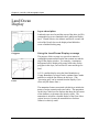
Land/Ocean Display
Map Elements
Place Names
Railroads
Rivers and Streams
Roads
State Boundaries
ArcUSA 1:2M index layers
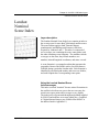
Landsat Nominal Scene Index
Latitude/Longitude Grids
USGS 1:24,000 Topographic Quadrangle
Series Index
USGS 1:100,000 Topographic Quadrangle
Series Index
USGS 1:250,000 Topographic Quadrangle
Series Index
Chapter 5:
vi
4-1
4-3
4-5
4-8
4-11
4-14
4-17
4-19
4-23
4-26
4-29
4-34
4-37
4-39
4-42
4-45
4-51
4-54
ArcUSA 1:2M state and county statistical attribute
layers4-59
1990 U.S. Census, Public Law 94-171 Data
Agricultural Product Inventory
Agricultural Product Market Value
Demographic and Health Attributes
Environmental Attributes
Government and Financial Attributes
Socioeconomic Attributes
4-61
4-70
4-80
4-89
4-100
4-107
4-115
The ArcUSA 1:25M layers
Cities
County Boundaries
Land/Ocean Display
Map Elements
Rivers
Roads
State Boundaries
Statistical Attributes
5-1
5-3
5-6
5-10
5-13
5-15
5-18
5-20
5-23
ArcUSA User's Guide and Data Reference
Contents
Chapter 6:
Appendix
6-1
6-1
6-3
6-6
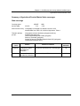
A: Database quality information
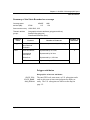
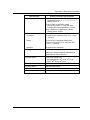
ArcUSA 1:2M data
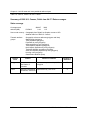
Summary of ArcUSA 1:2M characteristics
Lineage
Data derived from USGS Digital Line Graphs
Data derived from ESRI ArcWorld 1:3M data
Index coverages
Data derived from U.S. Government tabular
files
Positional accuracy
Attribute accuracy
Logical consistency
Completeness
A-1
A-2
A-3
A-5
A-5
A-12
A-12
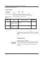
ArcUSA 1:25M data
Summary of ArcUSA 1:25M characteristics
Lineage
Data derived from USGS Digital Line Graphs
Data derived from ArcWorld 1:3M data
Data derived from U.S. Government tabular
files
Positional accuracy
Attribute accuracy
Logical consistency
Completeness
A-16
A-16
A-18
A-18
A-19
A-13
A-13
A-14
A-14
A-15
A-19
A-19
A-20
A-20
A-21
Appendix
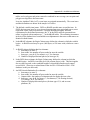
B: ArcUSA item definitions
B-1
Appendix
C: Federal Information Processing
Standards (FIPS) codes
C-1
Appendix
D: Bibliography
D-1
Appendix
E: Other data sources
E-1
Index
April 1992
Using the database
Optimizing performance
Working with attributes
Drawing with ArcUSA
Index-1
vii
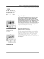
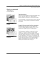
Getting started with ArcUSA
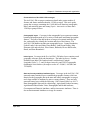
Welcome
The ArcUSA database contains the data needed to generate thematic maps of the
coterminous United States at the state and county levels. It contains
cartographic, tabular, and index information and is designed for a wide range of
business, educational, and scientific GIS applications. The ArcUSA database is
formatted for UNIX and MS-DOS systems.
Use ArcUSA data to. . .
•
•
•
•
•
•
•
•
•
Create county- and state-level thematic maps
Generate simple outline maps for use as insets or locators
Identify demographic and socioeconomic patterns by county and state
Display a road map of your state
Create basemaps for use with raster data
Serve as a cartographic base for your own tabular data
Find out which USGS topographic maps cover your study area
Observe how selected geographic features and patterns are related
Experiment with a variety of mapping techniques
What is in your ArcUSA package
• CD-ROM or other distribution medium that contains the ArcUSA database
and some preconstructed ArcView™ views
• ArcUSA 1:2M User's Guide and Data Reference
• ArcUSA 1:2M Installation Instructions
• ArcUSA license agreement
April 1992
ix
Getting started with ArcUSA
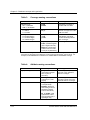
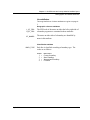
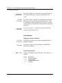
To get started, you'll need . . .
For UNIX systems:
For MS-DOS systems:
• ArcView or
ARC/INFO 6.0 or higher
• CD player (for CD-ROM) or drive
appropriate for the distribution
media you received
• Disk space appropriate to your
version of ArcUSA (see table
below), if you wish to copy the
entire database onto your hard drive
• ArcView for Windows, or
PC ARC/INFO 3.4D or higher, or
ArcCAD version 11 or higher
• CD-player (for CD-ROM) or drive
appropriate for the distribution
media you received
• Disk space appropriate to your
version of ArcUSA (see table
below), if you wish to copy the
entire database onto your hard drive
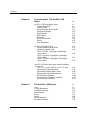
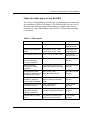
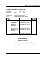
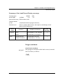
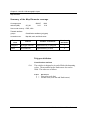
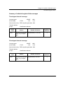
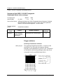
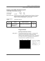
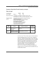
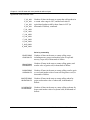
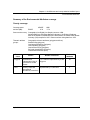
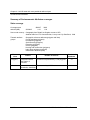
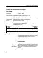
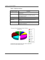
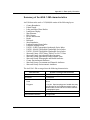
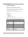
Table 1:
Disk space requirements for the
ArcUSA database
Size (MB)
Database
ArcUSA 1:2M, Full Extent
ArcUSA 1:25M
Sample data (views)
dBASE
215
13
3
UNIX
270
14
2
The database sizes shown in Table 1 apply to only one projection or coordinate
system; the second set of data for ArcUSA 1:2M requires approximately the same
amount of disk space. The ArcUSA 1:2M Installation Instructions give instructions
about copying individual coverages to another storage space.
x
ArcUSA User's Guide and Data Reference
Getting started with ArcUSA
How to access the database
Depending upon the amount of disk space you have available and the
applications you plan for your ArcUSA data, you may read data directly from
the CD-ROM or decide to copy all or some of the data to your hard drive.
Copying the data onto your hard drive will significantly improve performance,
but requires extra storage space. Data copying and storage options for your
particular hardware platforms are discussed in the ArcUSA 1:2M Installation
Instructions.
How to use this guide
If you're new to geographic information systems
If you've never worked with a geographic information system, you may want
to get an introduction to basic GIS concepts before you read this guide in detail.
You should also be familiar with the basic tools of the software you'll be using
(ArcView, ARC/INFO, or ArcCAD).
• To understand some basic concepts of GIS, see "What's GIS?" (Chapter 5 of
the ArcView User's Guide).
• The book Understanding GIS: The ARC/INFO Method is an excellent, more
extensive resource for novice ARC/INFO users.
• The ARC/INFO 6.0 handbook, ARC/INFO Data Model, Concepts, & Key
Terms will also be helpful.
• You can get excellent, detailed information from the numerous published
materials on geographic information systems. See the bibliography for
references to other materials that might prove useful.
April 1992
xi
Getting started with ArcUSA
Using ArcUSA data with ArcView
This user's guide assumes that you are familiar with the basic tools and
functionality of your ArcView software. Although this manual concentrates on
using the database with ArcView, all of the applications discussed, and more,
are possible using ARC/INFO.
• If you're new to ArcView and the ArcUSA database is the first database
you'll be exploring, begin by taking the ArcView guided tour (see Chapter 2
of the ArcView User's Guide).
• Once you've become familiar with ArcView, explore the ArcUSA database by
following the guided tour in Chapter 2. This hands-on tutorial will help you
learn the basic techniques for creating displays and querying the data.
• We have included several precomposed ArcUSA views. ArcView users can
immediately call these up to display and begin working with the data. These
displays are not accessible through ARC/INFO or ArcCAD™ software,
however.
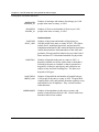
What is in this manual
Each chapter in this manual addresses a particular aspect of the database or its
use. The order in which you read the chapters is up to you, and you may wish
to defer reading a chapter until the information it contains is relevant to what
you are doing. The chapters are as follows:
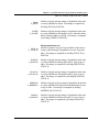
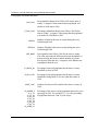
Chapter 1
What is ArcUSA?
Presents the geographic extent of the database and an overview of its contents.
Chapter 2
Exploring the ArcUSA database
Provides an ArcView tutorial that introduces you to the basic database
organization and illustrates fundamental techniques for selecting, displaying,
querying, and analyzing the data. Explores cartographic, index, and statistical
attribute data by leading you through sample applications.
xii
ArcUSA User's Guide and Data Reference
Getting started with ArcUSA
Chapter 3
Database concepts and organization
Discusses such data elements as coverages and attributes and explains how they
have been organized in the ArcUSA database. Presents basic database concepts
like projection and scale. Lists data sources.
Chapter 4
In greater detail: The ArcUSA 1:2M layers
Examines in detail the geographic features represented by each data layer.
Presents definitions and codes for all of the feature attributes. This is the
chapter you'll use most often during a work session.
Chapter 5
The ArcUSA 1:25M layers
Describes the features and attribute definitions for the ArcUSA 1:25M data set.
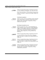
Chapter 6
Using the database
Suggests strategies for using the database to display and query, and gives
information about advanced applications like data export. Strategies apply to
both ArcView and ARC/INFO users.
Appendixes
A to E
Describe enhancements made during database development. Present attribute
field definitions for both INFO and dBASE formats for use with advanced
applications that use ARC/INFO and ArcCAD. List Federal Information
Processing Standards (FIPS) codes and sources of additional information.
Index
Provides information by a topic or key word.
April 1992
xiii
Chapter 1
What is ArcUSA?
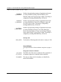
A flexible U.S. database at two scales
The ArcUSA database contains data for the coterminous United States at two
scales. The ArcUSA 1:2M data set is larger in both scale and content. It was
developed at a nominal scale of 1:2,000,000 (the "M" in "1:2M" stands for
"million"), and it contains representations of more than 100,000 features and
more than 1,000 attributes. The ArcUSA 1:25M data set represents a smallerscale map and contains a sample of the features and thematic attributes from the
1:2M database. It complements the larger data set by allowing a quick overview
of the ArcUSA database contents.
The ArcUSA database contains a broad range of data, including cartographic
features (state and county boundaries, roads, railroads, rivers, lakes, federal
land areas, county seats); indexes (latitude/longitude grids, USGS topographic
maps, Landsat scenes); and statistical attributes for states and counties
(population by age and race, income, hospitals and doctors, local government
spending, major soil types, agricultural products raised and sold). The user
may also add layers, either to tailor the database to a specific application or to
provide a more exhaustive treatment of any of the data types already present.
ArcUSA data are formatted in both UNIX ARC/INFO and PC ARC/INFO®
coverages and can be used with the following:
•
•
•
•
ArcView for UNIX and Windows
PC ARC/INFO Rev. 3.4D and higher
ARC/INFO Rev. 6.0 and higher on UNIX workstations
ArcCAD Version 11 and higher
PC ARC/INFO coverages store attributes in dBASE format. Thus, other
MS-DOS application software tools can be used with the ArcUSA database.
April 1992
1-1
Chapter 1—What is ArcUSA?
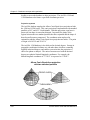
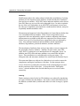
U.S. regions and subregions
U.S. regions and subregions
Some ArcUSA 1:2M data layers are divided into three major regions
encompassing states in the north, south, and west. Most ArcUSA features are
also assigned to a subregion (e.g., Pacific, Middle Atlantic) so you have an
easy means of selecting a small multistate area for display or study. These state
groups are the same as the Census Bureau's, except that the Census Bureau
considers New England to be a fourth major region instead of a subregion.
The ArcUSA 1:25M data set is for the full extent of the coterminous United
States only. It can function as a stand-alone database or as a complement of the
ArcUSA 1:2M database.
1-2
ArcUSA User's Guide and Data Reference
Chapter 1—What is ArcUSA?
The ArcUSA database you have licensed may contain either of the following
data sets:
• ArcUSA 1:2M (Full Extent), plus ArcUSA 1:25M
• ArcUSA 1:25M
The ArcUSA 1:2M data are delivered in two coordinate systems: the Albers
Conic Equal-Area projection in meters and geographic coordinates
(latitude/longitude) in decimal degrees. The ArcUSA 1:25M data are delivered
only in the Albers Conic Equal-Area projection.
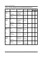
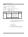
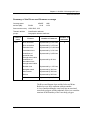
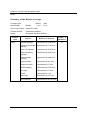
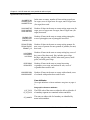
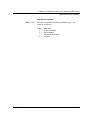
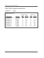
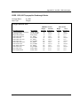
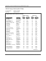
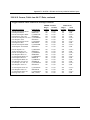
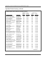
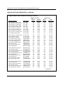
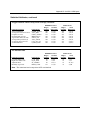
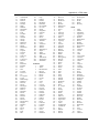
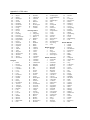
ArcUSA database layer summary tables
The four tables that begin on the next page summarize the ArcUSA database.
Tables 1 through 3 describe the 1:2M cartographic, index, and statistical
attribute layers; coverage names are listed for the entire United States as well as
for the three regions. (Regional coverage names end in "N" for north, "S" for
south, and "W" for west.) Table 4 describes the 1:25M layers.
The coverage sizes in the tables are approximate. In UNIX format, some
information is stored in a separate directory, so the overall database sizes listed
in Table 1 of "Getting Started" are larger than the sum of the component
coverages.
April 1992
1-3
Chapter 1—What is ArcUSA?
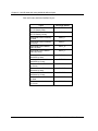
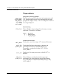
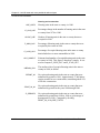
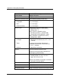
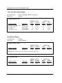
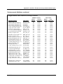
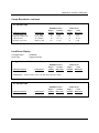
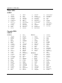
Table 1: ArcUSA 1:2M cartographic layers
Layer
County
Boundaries
Features
Polygons: 4,409
counties, independent
cities
Lines: 10,485
county and independent
city boundaries
Attributes
Polygon attributes: 7
county and state
names, FIPS codes,
U.S. subregion
Line attributes: 4
boundary type, geogr.
reference
Source,
Currency
Coverage
Names
Size (MB)
dBASE
UNIX
USGS—Digital
Line Graphs
(DLG), 1988
CTY2M
5.37
4.78
Federal Lands
Polygons: 2,741
Polygon attributes: 9
national parks, recreation
area type codes and
areas, Indian reservations names, state name,
FIPS, subregion
USGS—DLG,
1980
FED2M
2.24
2.33
Lakes and
Other Water
Bodies
Polygons: 6,365
lakes, reservoirs,
marshes, islands
Polygon attributes: 5
type, type name,
state, state FIPS,
subregion
USGS—DLG,
1980
LAK2M
LAK2M_N
LAK2M_S
LAK2M_W
3.97
1.78
1.30
0.92
3.93
1.81
1.35
0.95
Land/Ocean
Display
Polygons: 1,471
land, water
Lines: 1,860
features, grid
Annotation:
Canada, Mexico
Polygon attributes: 1
land/water code
Line attributes: 1
feature/grid code
ESRI—
ArcWorld, 1992
LAND2M
1.53
1.47
Map Elements
Polygons: 15
scale bar, North arrow
Lines: 43
scale bar, North arrow
Annotation:
map title, scale
Polygon attributes: 1
area fill code
Line attributes: 0
ESRI, 1992
SC_2M
0.02
0.03
Place Names
Points: 5,062
county seats, national
forest and park names,
lake locations
Point attributes: 10
feature name, type,
elevation, geogr.
reference
USGS—
Concise Digital
Database, 1973
NAM2M
1.10
0.96
Railroads
Lines: 12,182
railroad lines
Line attributes: 5
railroad line class,
state name, FIPS,
subregion
USGS—DLG,
1979
RR2M
4.94
4.37
Rivers and
Streams
Lines: 38,734
Line attributes: 5
perennial, intermittent,
river type, name,
and braided rivers, canals state name, FIPS,
subregion
USGS—DLG,
1973
RIV2M
16.48
14.50
Roads
Lines: 28,730
Interstates, U.S and state
highways, unimproved
roads
Line attributes: 22
road classes, route
numbers, geogr.
reference
USGS—DLG,
1980
RDS2M
15.81
14.31
State
Boundaries
Polygons: 1,295
states
Lines: 1,607
state and international
boundaries, shorelines
Polygon attributes: 4
state name
Line attributes: 4
boundary type, geogr.
reference
USGS—DLG,
1973
ST2M
1.67
1.59
1-4
ArcUSA User's Guide and Data Reference
Chapter 1—What is ArcUSA?
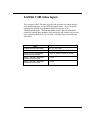
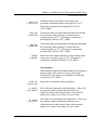
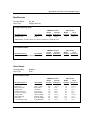
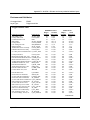
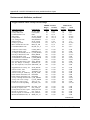
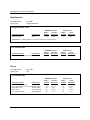
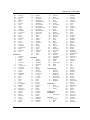
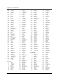
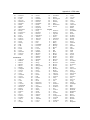
Table 2: ArcUSA 1:2M index layers
Layer
Landsat
Nominal Scene
Index
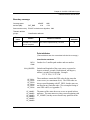
Latitude/
Longitude
Grids
Features
Attributes
Source,
Currency
Coverage
Names
Size (MB)
dBASE
UNIX
Points: 702
scene center points
Point attributes: 15
path, row, states
covered, lat./long.
of point
EOSAT—
algorithm
generated, 1992
SAT_PT
0.18
0.18
Lines: 702
scene coverages
Line attributes: 15
path, row, states
covered, lat./long.
of footprint
EOSAT—
algorithm
generated, 1992
SAT_BND
0.24
0.22
Lines: 1,225
2 by 2 degree grid
Line attributes: 3
ESRI—
latitude, longitude,
algorithm
U.S. or non-U.S. code generated, 1992
LTLG2
2.63
0.23
Lines: 314
5 by 5 degree grid
LTLG5
0.08
0.08
Lines: 134
10 by 10 degree grid
LTLG10
0.04
0.06
Q_24K
Q_24KN
Q_24KS
Q_24KW
26.41
8.82
7.47
10.52
26.01
8.82
7.49
10.47
USGS 1:24,000
Topographic
Quadrangle
Series Index
Polygons: 53,911
Polygon attributes: 19
1:24,000-scale map areas quad name and ID,
states covered, map
date, edition
USGS—various
ESRI—
algorithm
generated, 1986
USGS 1:100,000
Topographic
Quadrangle
Series Index
Polygons: 1,809
1:100,000-scale map
areas
Polygon attributes: 12
quad name and ID,
states covered, map
date,edition
USGS—various Q_100K
ESRI—
algorithm
generated, 1986
1.18
1.35
USGS 1:250,000
Topographic
Quadrangle
Series Index
Polygons: 488
1:250,000-scale map
series
Polygon attributes: 13
quad name and ID,
states covered, map
date, edition
USGS—various Q_250K
ESRI—
algorithm
generated, 1986
0.42
0.44
April 1992
1-5
Chapter 1—What is ArcUSA?
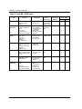
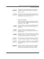
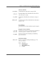
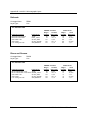
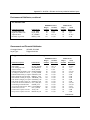
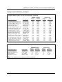
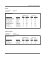
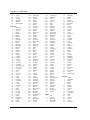
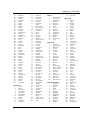
Table 3: ArcUSA 1:2M state and county statistical attribute layers
Layer
Features
1990 U.S.
Census
P-L 94-171 Data
by State
Polygons: 1,295
states
By
County
Agricultural
Product
Inventory
by State
Agricultural
Product Market
Value
by State
Demographic
and Health
Attributes
by State
1-6
Size (MB)
dBASE
UNIX
POP90S
2.49
1.87
Polygons: 4,409
counties
Lines: 10,485
county boundaries
Polygon attributes: 60
USGS—DLG,
1988
U.S. Census
Bureau, 1990
POP90C
8.17
5.69
Polygons: 1,295
states
Poly. attributes: 107
farm size, number,
products raised by
farm and area or
number
Line attributes: 4
boundary types
USGS—DLG,
1973
U.S. Census of
Agriculture,
1987
AGIN_S
3.94
2.64
Polygons: 4,409
counties
Lines: 10,485
county boundaries
Poly. attributes: 110
USGS—DLG,
1988
U.S. Census of
Agriculture,
1987
AGIN_C
13.11
8.33
Polygons: 1,295
states
Poly. attributes: 92
farms by value of
products; products by
value and quantity
sold
Line attributes: 4
boundary types
USGS—DLG,
1973
U.S. Census of
Agriculture,
1987
AGVL_S
3.61
2.49
Polygons: 4,409
counties
Lines: 10,485
county boundaries
Polygon attributes: 95
AGVL_C
11.97
7.81
Line attributes: 4
USGS—DLG,
1988
U.S. Census of
Agriculture,
1987
Polygons: 1,295
states
Polygon attributes: 48
population, vital
statistics, migration
Line attributes: 4
Boundary types
USGS—DLG,
POP88S
1973
U.S. Census—
County & City
Data Book, 1988
2.36
1.82
Polygon attributes: 55
USGS—DLG,
POP88C
1988
U.S. Census—
County & City
Data Book, 1988
7.91
5.67
Lines: 1,607
state boundaries
Lines: 1,607
state boundaries
By
County
Coverage
Names
USGS—DLG,
1973
U.S. Census
Bureau, 1990
Lines: 1,607
state boundaries
By
County
Source,
Currency
Polygon attributes: 57
population by race,
ethnicity, and age
Line attributes: 4
boundary types
Lines: 1,607
state boundaries
By
County
Attributes
Polygons: 4,409
counties
Lines: 10,485
county boundaries
Line attributes: 4
Line attributes: 4
Line attributes: 4
ArcUSA User's Guide and Data Reference
Chapter 1—What is ArcUSA?
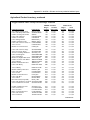
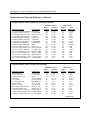
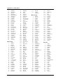
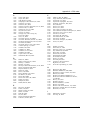
Table 3:
Layer
Environ-mental
Attributes
ArcUSA 1:2M state and county statistical attribute layers,
continued
Features
Polygons: 4,409
counties
Socioeconomic
Attributes
by State
April 1992
dBASE
UNIX
8.33
5.74
USGS—DLG,
GOV88S
1973
U.S. Census—
County & City
Data Book, 1988
2.13
1.74
Polygons: 4,409
counties
Lines: 10,485
county boundaries
Polygon attributes: 41
USGS—DLG,
GOV88C
1988
U.S. Census—
County & City
Data Book, 1988
7.12
5.43
Polygons: 1,295
states
Polygon attributes: 47
Social Security,
crime, education,
income and poverty,
housing
Line attributes: 4
boundary types,
geogr. reference
USGS—DLG,
SOC88S
1973
U.S. Census—
County & City
Data Book, 1988
1.00
1.82
Polygon attributes: 54
USGS—DLG,
SOC88C
1988
U.S. Census—
County & City
Data Book, 1988
7.80
5.67
Polygons: 4,409
counties
Lines: 10,485
county boundaries
Line attributes: 4
Line attributes: 4
ENVIR
Size (MB)
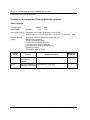
Polygon attributes: 34
Federal grants to
local gov'ts; local
gov't spending on
police, education,
highways
Line attributes: 4
boundary types,
geogr. reference
Polygons: 1,295
states
Lines: 1,607
state boundaries
By
County
Coverage
Names
USGS—DLG,
1988
Oak Ridge
National Lab.—
GeoEcology
database, 1967–
1979
Lines: 1,607
state boundaries
By
County
Source,
Currency
Polygon attributes: 63
land capability, land
use, soil orders,
surface mining
Line attributes: 4
boundary types
Lines: 10,485
county boundaries
Government &
Financial
Attributes
by State
Attributes
1-7
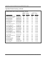
Chapter 1—What is ArcUSA?
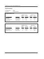
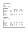
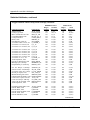
Table 4: ArcUSA 1:25M layers
Layer
Features
Attributes
Source,
Currency
Coverage
Names
Size (MB)
dBASE
UNIX
Cities
Points: 108
major cities, state
capitals
Point attributes: 9
city name, type
USGS—
Concise Digital
Database, 1973
CITIES
0.03
0.04
County
Boundaries
Polygons: 3,444
counties, independent
cities
Polygon attributes: 7
county and state
names, FIPS codes,
U.S. subregion
Line attributes: 4
boundary type, geogr.
reference
USGS—Digital
Line Graphs,
1988
CTY_25M
3.20
2.73
Lines: 9,496
county and state
boundaries, shorelines
Land/Ocean
Display
Polygons: 510
land, water
Lines: 749
features, grid
Annotation:
Canada, Mexico
Polygon attributes: 1
land/water code
Line attributes: 1
feature/grid code
ESRI—
ArcWorld, 1992
LAND25M
0.40
0.50
Map Elements
Polygons:
scale bar, North arrow
Lines:
scale bar, North arrow
Annotation:
map title, scale
Polygon attributes:
area fill code
Line attributes: 0
ESRI, 1992
SC_25M
0.02
0.03
Rivers
Lines: 2,162
perennial & intermittent
rivers, braided streams,
canals
Line attributes: 5
river types, geogr.
reference
USGS—DLG,
1973
RIV_25M
0.52
0.46
Roads
Lines: 4,658
Interstates, U.S. and
state highways
Line attributes: 11
road types, route
numbers, geogr.
reference
USGS—DLG,
1988
RDS_25M
0.93
0.75
State
Boundaries
Polygons: 336
states
Polygon attributes: 4
states,
geogr. reference
Line attributes: 4
boundary types,
geogr. reference
USGS—DLG,
1973
ST_25M
0.34
0.35
Lines: 472
state and international
boundaries, shorelines
1-8
ArcUSA User's Guide and Data Reference
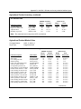
Chapter 1—What is ArcUSA?
Table 4: ArcUSA 1:25M layers, continued
Layer
Statistical
Attributes
by State
Features
Polygons: 336
states
Lines: 472
state and international
boundaries, shorelines
By
County
Polygons: 3,444
counties
Lines: 9,496
county boundaries,
shorelines
April 1992
Attributes
Source,
Currency
Coverage
Names
Size (MB)
dBASE
UNIX
Polygon attributes: 41
population by race
and age, income,
crime, farmland and
farm sales
Line attributes: 4
boundary type,
geogr. reference
USGS—
STATS_S
DLG,1973
Various attribute
sources
0.49
0.40
Polygon attributes: 50
population by race
and age, income,
crime, farmland and
farm sales, soils
Line attributes: 4
boundary types,
geogr. reference
USGS—DLG,
STATS_C
1988
Various attribute
sources
5.00
3.37
1-9
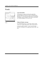
Chapter 2
Exploring the ArcUSA database
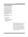
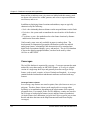
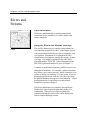
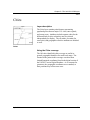
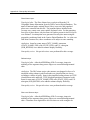
This guided tour introduces ArcView users to the ArcUSA database by
exploring the precomposed views included with the data. The tour does not
cover all aspects of the database, but it does illustrate some of the ways in
which the data at both the 1:2,000,000 and 1:25,000,000 scales can be used.
By following the exercises in this chapter, you will be better able to explore the
data on your own.
You will gain the most from these exercises if you are familiar with ArcView
functions. The emphasis of this tutorial is on exploring the database and not on
how to use the software tools, so it is recommended that you first do the
exercises in Chapter 2 of the ArcView User's Guide.
This chapter will
help you become
familiar with the
ArcUSA data, such
as the 1:25M
Roads coverage
shown in this
ArcView display.
April 1992
2-1
Chapter 2—Exploring the ArcUSA database
In the first two exercises, you will look at U.S. migration trends at the state and
county levels from 1980 to 1986, and explore potential relationships between
these migration trends and other statistical variables (or attributes) present in the
ArcUSA database. The third exercise teaches you how to create and analyze
bivariate maps. The fourth exercise involves preparing a coastal basemap, and
exploring the geographic factors involved in assessing the potential impact of a
large oceanic storm on a coastal area. The last exercise explores data
documentation views.
The exercises are independent of each other and can be done in any order.
However, because data display and query operations are described in more
detail in the first exercise, you are likely to gain more from the later exercises if
you try the "migration" exercises first.
Getting started
Begin by loading ArcView; if you haven't already loaded and started ArcView,
please see the ArcView installation instructions.
Next, load your ArcUSA data set (see the ArcUSA 1:2M Installation
Instructions). The "views" directory includes a series of precomposed ArcView
displays to guide you through the tour.
2-2
ArcUSA User's Guide and Data Reference
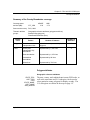
Chapter 2—Exploring the ArcUSA database
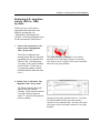
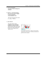
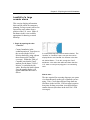
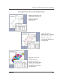
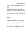
Exploring U.S. migration
trends 1980 to 1986,
by state
In this exercise, you'll explore
migration trends at the state level.
Begin by opening the view
"mig25mst.av" that displays the
ArcUSA 1:25M state boundaries layer
for the coterminous United States.
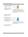
1. Click on the check box for the
theme named "Net Migration
1980 - 86, by state".
You will see a thematic map
showing states that lost or gained
population due to migration from
1980 to 1986. (Net migration,
"net_migr" is one of the variables
in the ArcUSA 1:25M "stats_s"
coverage that contains selected
statistical attribute data at the state
level.)
The upper peninsula of Michigan is not shaded
because it is not the largest polygon for the state.
See "Note to user" on page 2-4 for more information
about the "stat_flag" attribute.
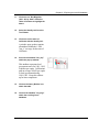
2. Double click on the theme "Net
Migration 1980 - 86, by state".
The Theme Property Sheet will
appear below the Table of
Contents. Notice that the attribute
"stat_flag" has been preset to
equal "1". Quit from the property
sheet to continue.
April 1992
Setting the "stat_flag" attribute equal to "1" through
the Query Builder provides accurate summary
statistics for any selected state. See the note on the
next page for more information about the "stat_flag"
attribute.
2-3
Chapter 2—Exploring the ArcUSA database
3. In the Table of Contents, select
the Table option from the themespecific menu for "Net Migration
1980 - 86, by state".
This allows you to access
information about the total
number of people who migrated
into or out of a given state from
1980 to 1986. Use the scroll bar
to view the full extent of the
attributes contained within the
"stat_s" coverage.
4. Select the Query Builder icon in
the "Net Migration
1980 - 86, by state" table.
Note to user...
The database includes one record for every polygon
included in a particular state or county. If a state
includes offshore islands, the database includes a
separate record for each individual island. The
geographic information for that state is repeated in
each polygon record for each island. To identify the
largest land area polygon in each state, use the Query
Builder in the theme's property sheet or table to
create a logical expression with the "stat_flag"
attribute set equal to "1". This will ensure that values
for each state are counted only once during tabular
queries.
2-4
ArcUSA User's Guide and Data Reference
Chapter 2—Exploring the ArcUSA database
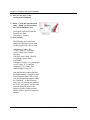
5. Click on the attribute
"net_migr" in the scrolling list of
attributes.
6. Choose ">" from the operators;
then enter the number "500000"
on the line below the
"Values/Attributes" box.
The logical expression now reads
( net_migr > 500000 ).
7. Click "Select."
Your map will now show
California, Texas, and Florida
highlighted (within the graphic
display and the table) as states that
gained more than 500,000 people
because of net migration from
1980 to 1986.
Use a logical expression to create a more focused
selection set; in this case, to identify the states that
gained the most people.
April 1992
2-5
Chapter 2—Exploring the ArcUSA database
8. Click on the "net_migr" attribute
in the table and select
"Statistics."
Use the scroll bar to scroll right to
the appropriate section of the
table. After "Statistics" for
"net_migr" is selected, a window
pops up that displays the count,
sum, minimum, maximum, and
mean values for the specified
attribute both for all records
contained in the layer and records
specific to the selected set. The
"sum" is not equal to zero because
this attribute reflects not only
migration from other states, but
also migration from other
countries.
When you set the "stat_flag" attribute equal to "1",
the proper total values display in the "Statistics"
window.
Within this statistics window,
you'll see that the maximum net
migration from 1980 to 1986 was
1,778,000.
9. Click "Dismiss."
10.
Enlarge the table window so that
the "state_name" and "net_migr"
attributes are contained within
the window area.
California gained 1,778,000 as a
result of net migration from 1980
to 1986. Move the table down
below the graphic display prior to
continuing.
2-6
ArcUSA User's Guide and Data Reference
Chapter 2—Exploring the ArcUSA database
11.
Click once on "Net Migration
1980 - 86, by State" within the
Table of Contents to highlight the
theme.
12.
Select the Identify tool from the
Tool Palette.
13.
Click once on the state of
California with the Identify tool.
A window pops up that contains
all attributes within the 1:25M
"stat_s" coverage for the state of
California.
14.
Scroll to the attribute "tax_cap"
within the pop-up window.
This attribute represents local
government taxes for 1981–1982,
in dollars per capita. Californians
paid an average of $429 per capita
to local government during
1981–1982. Keep this window
up for later comparison.
15.
Click on the Query Builder icon
within the table.
16.
Click on the attribute "net_migr"
within the scrolling list of
attributes.
April 1992
2-7
Chapter 2—Exploring the ArcUSA database
17.
Choose "<" from the
operators and enter
"–500000" on the line below
the "Values/Attributes" box.
The logical expression now
reads ( net_migr < –500000 ).
18.
Click "Select."
Michigan will be highlighted
as the only state that lost more
than 500,000 people because
of net migration from 1980 to
1986.
19.
Click once on the state of
Michigan with the Identify
tool from the palette.
A window pops up that
contains all attributes within
the "stat_s" coverage for
Michigan.
20.
Scroll to the attribute
"tax_cap" within the pop-up
window.
Comparing this figure to the
average of $429 for California
may help explain the
difference in net migration
between the two states. The
people of Michigan paid an
average of $560 per capita to
local government during
1981–1982.
2-8
ArcUSA User's Guide and Data Reference
Chapter 2—Exploring the ArcUSA database
Exploring U.S. migration
trends 1980 to 1986, by
county
You have seen how you can use the
ArcUSA database to look at
summary-level migration patterns by
state. You can also use the database
to see finer resolution patterns at the
county level. Begin by opening the
existing view "mig25mc.av". A
thematic map showing county-level
migration patterns in the Northeastern
region of the United States draws to
the screen.
1. Double click on the theme "Net
Migration 1980 - 86, by county".
The property sheet will appear
below the Table of Contents.
Notice that the attribute "stat_flag"
has been preset to equal "1" in
order to identify the largest land
area polygon for each county.
Quit from the property sheet prior
to continuing.
2. Pick the Table option from the
theme-specific menu for "Net
Migration 1980 - 86, by county".
A table pops up presenting all
attributes available in the 1:25M
"stat_c" coverage for each county
in the coterminous United States.
3. Click on the Query Builder icon
within the "Net Migration 1980 86, by county" table.
April 1992
2-9
Chapter 2—Exploring the ArcUSA database
4. Click on "net_migr" in the
scrolling list of attributes.
5. Select "<" from the operators and
enter "–50000" on the line below
the "Values/Attributes" box.
The logical expression within the
box will now read
( net_migr < –50000 ).
6. Click "Select."
The following nine counties are
identified as having lost more than
50,000 people from 1980 to 1986:
• Milwaukee County, Wis.
• Cook County, Ill. (Chicago)
• Lake County, Ind. (Greater
Chicago)
• Wayne County, Mich. (Detroit)
• Cuyahoga County, Ohio
(Cleveland)
• Allegheny County., Pa. (Pittsburgh)
• Erie County, N.Y. (Buffalo)
• Baltimore City County, Md.
• Philadelphia County, Pa.
Note that the nine counties that lost
the highest number of people because
of net migration from 1980 to 1986
were all metropolitan counties within
the "Rust Belt." In the following
steps, you will examine the attributes
for "loser" and "gainer" counties that
represent potential factors in the
negative growth of urban counties
and the positive growth of suburban
counties.
2-10
ArcUSA User's Guide and Data Reference
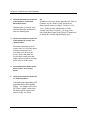
Chapter 2—Exploring the ArcUSA database
7. Use the "Zoom to Box" tool from
the palette to zoom in on the area
around Philadelphia,
Pennsylvania.
Philadelphia
8. Click once on "Net Migration
1980 - 86, by County" within the
Table of Contents to highlight the
theme.
9. Using the Identify tool from the
palette, click once on
Philadelphia, Pennsylvania.
A pop-up window containing
various attributes contained within
the "stats_c" coverage appears for
this "loser" county.
10.
Using the Identify tool again,
click once on Montgomery
County, Pennsylvania.
This county which borders
Philadelphia to the west, is a
"gainer" county.
11.
Scroll down to the attribute
"net_migr" in both pop-up
windows.
Notice that Philadelphia lost
78,400 people due to net
migration during 1980–86.
Montgomery County gained
13,600.
April 1992
2-11
Chapter 2—Exploring the ArcUSA database
12.
Scroll farther down to the
attribute "sr_cr_100k".
This attribute represents the
number of serious crimes per
100,000 people. The occurrence
of serious crime in Philadelphia
was higher than in Montgomery
County. (For comparison, the
average occurrence of serious
crime per 100,000 people within
the nine selected counties is 6,170
for this time period; the national
average is 2,706.) These figures
can be determined by using the
"Statistics" tool for "sr_cr_100k"
in the attribute table for "Net
Migration 1980 - 86, by county".
13.
Continue scrolling down in the
windows to the attribute
"inc_cap_85".
This attribute represents income
per capita (1985). Per capita
income was higher in Montgomery County than in
Philadelphia, and is another
possible factor in the difference in
migration between the two
counties.
14.
2-12
You may continue to explore
differences in attributes between
these two counties.
ArcUSA User's Guide and Data Reference
Chapter 2—Exploring the ArcUSA database
Bivariate mapping using
ArcUSA 1:2M attributes
The views presented thus far in this
tour have used data from the ArcUSA
1:25M coverages. The ArcUSA
1:2M coverages include a much
greater variety of statistical data, as
well as a much higher level of detail
for cartographic features like roads or
rivers. In the following exercise, a
sample data set using the 1:2M
attributes for the state of Georgia is
used to experiment with bivariate
mapping techniques.
For more information about bivariate
mapping, see Chapter 6.
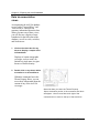
1. Open the view titled
"bivar2m.av".
Patterns representing positive and
negative net migration at the
county level are drawn in the
graphic display.
Tip
To increase drawing speed, use the ArcUSA 1:25M
coverages to draw state or county boundaries. The
state and county boundaries in the ArcUSA 1:2M
database are much more detailed than those in
ArcUSA 1:25M (although both versions contain the
same number of states and counties), so they take
longer to draw on the screen. (When you draw a
basemap, as opposed to a thematic map, you may
want the greater detail present in the 1:2M data; for
example, you may want to use the 1:2M data for the
"Storm" exercise that follows.)
April 1992
2-13
Chapter 2—Exploring the ArcUSA database
2. Click on the check box to the left of
the theme for "Income per Capita,
1985".
This variable is symbolized with color
and draws beneath the shade pattern
Use a pattern and a color to display two variables
that represents net migration.
Examine the relationship between net together. Note that the variable symbolized using a
migration and income per capita. The pattern must be placed above the second variable in
general pattern shows that counties the Table of Contents so that the patterns draw over
with the lowest income per capita also the colors.
experienced the highest loss due to
migration.
3. Click off the check box for
"Income per Capita, 1985".
4. Click on the check box for
"Unemployment Rate, 1986".
Again, examine the relationship
between the two variables. Did
the counties with high
unemployment rates also
experience high loss due to net
migration? The dark shade/light
pattern combination indicates
"loser" counties with high
unemployment.
On your own...
Explore the relationships between other 1:2M
"pop88c" and "soc88c" variables and net migration,
or introduce a new dependent variable and examine
its potential as a causal factor.
2-14
ArcUSA User's Guide and Data Reference
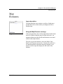
Chapter 2—Exploring the ArcUSA database
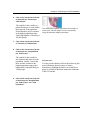
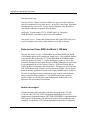
Landfall of a large
oceanic storm
This exercise displays information
that would be useful for emergency
planning if a large oceanic storm were
expected to come ashore along a
portion of the U.S. coast. Some of
the themes in this view would be
appropriate for drawing a coastal
basemap.
1. Begin by opening the view
"coast.av".
County boundaries in the
southern portion of Texas draw to
the screen with the Gulf of
Mexico shaded (by using a theme
that references the "land2m"
coverage). Within the Table of
Contents, note that the "land"
attribute for the theme "Gulf of
Mexico" is symbolized with
white. Because the land is drawn
first, the graphic display will
appear blank until the water is
drawn.
A coastal basemap with offshore water shaded. The
"land2m" or "land25m" layers can also be used to
display Mexico and Canada in a different color than
the United States. To do this, assign the "land"
attribute a color other than white and then draw the
U.S. state or county area polygons in a contrasting
color.
Note to user...
The time required for accessing data once you open a
view depends partly on the type of platform you are
using. Also, a view that references large data sets
(like those in the ArcUSA 1:2M coverages) requires
more time for data access than views that reference
smaller data sets (like those in the ArcUSA 1:25M
coverages).
April 1992
2-15
Chapter 2—Exploring the ArcUSA database
2. Click on the check box to the left
of the theme for "Parks and
Recreation Areas".
National parks, recreation areas,
and other federally administered
areas are shaded green.
Tip
To make room for new theme legends in the Table of
Contents, use the "Hide Legend" option in the
theme-specific menu (see page 2-9 in the ArcView
User's Guide for more information on "Hide
Legend" and "Show Legend"). Or, drag on the
lower right-hand corner of the Table of Contents box
to enlarge the available legend display space.
3. Click on the check box to the left
of the themes for "Parks" and
"County Seats".
The names and locations of all
county seats, as well as the names
of many coastal parks and
recreation areas, draw to the
screen. Notice that there are
several large coastal parks that
might require evacuation if a large
storm came in off the ocean.
4. Click off the check boxes to the
left of "Parks" and "County
Seats".
5. Click on the check box to the left
of "1990 Population".
A thematic map representing 1990
population draws in the graphic
display. You might want to select
the "Show Legend" option from
the theme-specific menu for the
themes as they are drawn.
2-16
ArcUSA User's Guide and Data Reference
Chapter 2—Exploring the ArcUSA database
6. Click on the check box to the left
of the theme for "Doctors per
100K People".
The symbol for this variable is a
pattern that draws over the shades
that represent 1990 population.
Notice that there are five counties
in the highest population range
with a high number of doctors per
100,000 people.
The relationship between population and number of
doctors per 100,000 people can be compared by
using the bivariate mapping technique.
7. Click off the check box to the left
of "Doctors per 100K People".
8. Click on the check box to the left
of the theme for "Hospital Beds
per 1000 People".
The symbol for this variable is
also a pattern that draws over the
population variable. Notice that
there are three counties in the
highest population range with a
high number of hospital beds per
1,000 people.
On your own...
You may use the Identify tool from the Palette to gain
more information about a county or feature.
Remember to highlight the theme you would like to
query by clicking on the theme name once within the
Table of Contents.
9. Click off the check box to the left
of the themes for "Hospital Beds
per 1000 People" and "1990
Population".
April 1992
2-17
Chapter 2—Exploring the ArcUSA database
10.
Click on the check box to the left
of the "Roads" and "Railroads"
themes.
Evaluate the transportation
network for routes out of the
coastal area should an evacuation
become necessary.
11.
Click off the check box for the
"Roads" and "Railroads"
themes.
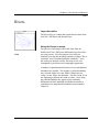
12.
Click on the check box to the left
of the "Rivers" theme.
The coastal transportation network is symbolized
using the simplified road classes (for more
information on the "road_class" attribute, see Chapter
4). The Digital Line Graph classifications carried in the
"dlg_class" attributes offer alternatives for symbolizing
the roads network.
This information is useful for
determining which areas might be
prone to flooding in the event of a
large oceanic storm.
A map of coastal rivers and estuaries. You may
draw the "Rivers" theme with the two transportation
themes to evaluate the probability of flooding on or
near transportation lines.
13.
2-18
Click off the check box to the left
of the "Rivers" theme.
ArcUSA User's Guide and Data Reference
Chapter 2—Exploring the ArcUSA database
14.
Click on the check box to the left
of the "100K Topo Quad Areas".
This theme displays areas covered
by USGS topographic
quadrangles. If you decide that
you need a more detailed source,
determine which quadrangle
covers your area of interest by
using the Identify tool from the
palette.
Locate the USGS 1:100,000-scale quadrangle that
covers your area of interest.
April 1992
2-19
Chapter 2—Exploring the ArcUSA database
Data documentation
views
Accompanying the ArcUSA database
are two views ("arcusa2M.av" and
"arcusa25M.av") that provide
summary information about the data.
When you enter one of these views,
you will first see a display of state
boundaries for the full extent of the
database, as well as a title, scale bar,
and North arrow.
1. Click on the check box for any
theme to display a sample of the
indicated data.
Displays of certain cartographic
coverages, such as roads, are
limited to a single state or region
because of feature density.
2. Double click on any theme within
arcusa2m.av or arcusa25m.av.
Within the comments box in the
Theme Property Sheet, you can
access basic information about the
content of any of the ArcUSA
coverages.
Note that when you enter the Theme Property
Sheet, the bottom portion of the comments text block
will appear. Use the scroll bar at the right of the
comments box to move to the top of the text block.
2-20
ArcUSA User's Guide and Data Reference
Chapter 2—Exploring the ArcUSA database
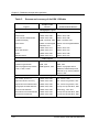
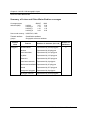
Ideas for other ways to use ArcUSA
The exercises in this guided tour provide only an introduction to the content and
the capabilities of the ArcUSA database. The following table lists just a few of
the many other issues you might want to explore by using the data. Next to
each issue are some of the attributes in the ArcUSA 1:2M coverages that might
be of interest.
Table 1: Other views
Issues
April 1992
Attributes
Layer
Planning new schools
% Pop. Under 5 Yrs., 1984
Demographic and
Health Attributes
Planning care facilities for
elderly
% Pop. 65 to 74 Yrs., 1984
% Pop. Over 74 Yrs., 1984
Demographic and
Health Attributes
Areas gaining political clout % Pop. 18 Yrs. or Older, 1990
1990 Census,
Public Law 94-171
Areas most concerned
about animal growth
hormone regulations
Farms with Beef Cows, 1987
Agricultural Product
Inventory
Areas where water
shortages may affect
agriculture
Irrigated Land in Acres, 1987
Farms with Irrigated Land, 1987
Agricultural Product
Inventory
Areas potentially most
affected by greater access
to Japanese rice market
Acres of Rice, 1987
Rice Harvested (100 lbs.)
Agricultural Product
Inventory
Areas potentially most
affected by changes in
federal tobacco subsidies
Farms with Tobacco, 1987
Acres of Tobacco Harvested,
1987
Agricultural Product
Inventory
Areas affected by potential
reclamation of mines
Total Disturbed Land
% Disturbed Land
Environmental
Attributes
Planning access to
materials for massive
highway construction
Land in Sand/Gravel Extraction
% Land in Sand/Gravel Extract.
Environmental
Attributes
Potential sites for mining
peat
% Land Area in Histosol Soils
Land Area in Histosol Soils
Environmental
Attributes
2-21
Chapter 3
Database concepts and
organization
This chapter defines several basic database terms and explains how the ArcUSA
database is organized. The standards and procedures employed during the
development of the database are discussed, and the sources for the ArcUSA
data are described. The information in this chapter applies to all components of
the database, so it may be helpful to read this chapter before reading Chapters 4
and 5, which contain a detailed descriptions of each data layer.
Concepts and terms
A map is a graphic display of spatially distributed elements called map features
which correspond to real-world geographic entities. These real-world entities
are located spatially on maps by means of points, lines, and areas.
• Points define discrete locations on a map for geographic phenomena that are
too small to be depicted as lines or areas, such as well locations, telephone
poles, and buildings. Points can also represent locations that have no area,
such as mountain peaks. In the ArcUSA database, points are used to
represent cities and satellite scene centers.
• Lines represent the shapes of geographic objects that are too narrow to depict
as areas (such as highways and streams).
• Areas are closed figures that represent the shapes and locations of
homogeneous features such as states, counties, parcels, and water bodies.
The characteristics, or attributes, of map features may also be conveyed by
using labels or graphic symbols. For example, streams and water bodies are
April 1992
3-1
Chapter 3—Database concepts and organization
drawn in blue to indicate water; city streets are labeled with their names; roads
are drawn with various line widths, patterns, and colors to represent different
road classes; and so on.
In addition to displaying feature locations and attributes, maps are typically
characterized by the following:
• Scale—the relationship between distance on the map and distance on the Earth
• Projection—the system used to transform the curved surface of the Earth to a
plane
• Coordinate system—the method used to relate feature locations by distance
and direction from other features
Until recently, maps were only available in paper (or analog) form. The
development of computerized geographic information systems has enabled
analog map features, relationships, and characteristics to be translated into
digital form for automated display, query, and analysis. The ArcUSA database
is just such a digital geographic database, one that can be used by either
ArcView or ARC/INFO.
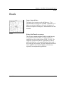
Coverages
The ArcUSA database is organized by coverage. Coverages represent the main
method for vector data storage in ARC/INFO format. A coverage is a digital
version of a single map sheet layer and generally describes one type of map
feature, such as roads, counties, or lines of latitude and longitude. A coverage
contains both the locational data and thematic attributes associated with map
features.
Coverage feature classes
In a coverage, map features are stored as points, lines (also known as arcs), or
polygons. The three feature classes can be employed in a coverage either
separately or in combination, depending on the requirements of the captured
geographic data. For example, in the ArcUSA database, counties are stored in
one coverage as both polygon features (areas) and line features (boundaries).
(A fourth feature class, annotation, is used in ArcUSA as a special way to store
the title and other characters in the Map Elements and Land/Ocean Display
coverages.)
3-2
ArcUSA User's Guide and Data Reference
Chapter 3—Database concepts and organization
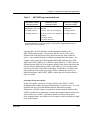
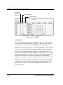
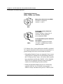
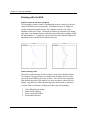
Coverage feature classes and attribute tables
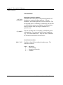
Points represent features like
named places. Points have no
length or area. A point is
defined as a single x,y
coordinate pair.
Lines represent linear
features like roads. Lines have
length but no area. A line is
defined as a string of x,y
coordinate pairs with beginning
and ending points.
Polygons represent area
features like counties.
Polygons have area and a
perimeter. A polygon is defined
as a string of x,y coordinate
pairs with the same beginning
and ending points.
April 1992
3-3
Chapter 3—Database concepts and organization
In the ArcUSA database, coverages are given names that reflect their content,
such as CTY2M (county boundary data at the 1:2,000,000 scale) and AGINC
(agricultural product inventory data by county).
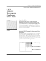
Two coverages, for the USGS1:24,000 Quadrangle Series Index layer and the
Lake and Other Water Bodies layer, contain a very large number of features.
For these layers three regional coverages are provided in addition to the
coverage that contains the full extent of the database. The smaller coverages
improve software performance during some operations. The extents of the
northern, southern, and western regional coverages are shown on the map in
Chapter 1.
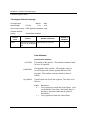
Feature attribute tables
The attributes of the polygons, lines, and points in a coverage are stored in
feature attribute tables. Each feature class in a coverage has its own table;
polygon attributes are stored in Polygon Attribute Tables (PATs); line attributes
are stored in Arc Attribute Tables (AATs); and point attributes are stored in
Point Attribute Tables (PATs).
The columns in a feature attribute table represent the attributes (imagine the
attribute names listed across the top of the table), and each contains information
about a row or feature (imagine the features listed down the side of the table).
Each entry in the table contains an attribute value for a particular record
(feature).
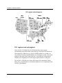
ARC/INFO-generated attributes
ARC/INFO-generated attributes are automatically created by ARC/INFO and are
different for each coverage type. The ARC/INFO-generated attributes are listed
in Table 1. (Since the ArcUSA database was developed using ARC/INFO
software, these attributes exist in the feature attribute tables even though they
are not apparent with ArcView software.)
Several of the ARC/INFO-generated attributes, such as length, area, and
perimeter, provide useful information about coverage features. They are all
calculated in the units used for the coverage coordinate system (in the ArcUSA
database, the Albers projection uses meters).
3-4
ArcUSA User's Guide and Data Reference
Chapter 3—Database concepts and organization
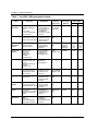
Table 1:
ARC/INFO-generated attributes
Attributes in Point
Attributes in Arc
Attribute Tables
AREA (set to "0")
Attribute Tables
FNODE#
Attributes in Polygon
Attribute Tables
AREA*
PERIMETER (set to "0") TNODE#
PERIMETER*
<coverage name>#
LPOLY# (set to "0" if no polygons)
<coverage name>#
<coverage name>-ID *
RPOLY# (set to "0" if no polygons)
<coverage name>-ID *
LENGTH *
<coverage name>#
<coverage name>-ID *
Note: Only the attributes marked with * appear in ArcView tables. The other ARC/INFOgenerated attributes are physically present in the ArcUSA coverage tables but are not
visible on the screen in ArcView.
Note that other ArcUSA attributes contain information similar to the
ARC/INFO-generated data. In such cases, the two sets of values will be
different from each other because they have been derived from a different
source—not calculated from the coordinate representation of the feature. For
example, in the county-level Demographic and Health Attributes layer, both
AREA and LAND_AREA give a value for county land area. Yet the values are
different because AREA is given in square meters (in the Albers projection) and
is derived from a digitized map, while LAND_AREA is given in square miles
and is derived from a Census Bureau database. Furthermore, in counties and
states made up of more than one polygon, AREA contains the value for an
individual polygon, while LAND_AREA contains the value for the county or
state as a whole.
Coverages in the user's guide
In this user's guide, a group of coverages like the four USGS 1:24,000
Quadrangle Series Index coverages mentioned above is called a layer. To avoid
repetition, the layer is described rather than the individual coverages.
Furthermore, ArcUSA county coverages that contain statistical attributes (like
AGINC) usually have a counterpart coverage that contains identical statistics for
states (in this case, AGINS—agricultural product inventory data by state).
Such counterpart state- and county-level coverages are also described as a single
layer in this manual.
April 1992
3-5
Chapter 3—Database concepts and organization
ArcUSA database organization
The ArcUSA database
The ArcUSA database includes data at two scales: 1:2,000,000 and
1:25,000,000. Data at both scales are presented in the Albers Conic Equal-Area
projection. The 1:2,000,000-scale data are also presented in geographic
coordinates expressed in decimal degrees, in a second set of coverages. (The
two sets of 1:2M coverages have identical names, but they are delivered in
different directories.) Any one coverage contains data at only one scale and in
one projection/coordinate system.
3-6
ArcUSA User's Guide and Data Reference
Chapter 3—Database concepts and organization
Characteristics of ArcUSA 1:2M coverages
The ArcUSA 1:2M coverages contain more detail and a greater number of
features and feature attributes than the 1:25M coverages. This user's guide
groups the coverages containing the 1:2,000,000-scale data into cartographic,
index, and statistical (state and county) layers. An overview of these three
1:2M layer groups follows.
Cartographic layers.
Coverages in the cartographic layers represent common
basemap information made up of a variety of man-made and natural geographic
features. The bulk of the data in these coverages is locational; attributes are
few, and usually they identify the location and class of the features. The
ArcUSA 1:2M database includes ten cartographic layers: County Boundaries,
Federal Lands, Lakes and Other Water Bodies, Land/Ocean Display, Map
Elements (title and scale bar), Place Names, Railroads, Rivers and Streams,
Roads, and State Boundaries.
Coverages in the five ArcUSA 1:2M index layers contain several
geographic reference grids and data indexes. The index layers are: Landsat
Nominal Scene Index (for Landsat 4 and 5 satellite data), Latitude/
Longitude Grids (2-, 5-, and 10-degree intervals), and USGS Topographic
Quadrangle Series Indexes (for maps at scales of 1:24,000, 1:100,000, and
1:250,000).
Index layers.
Coverages in the ArcUSA 1:2M
state and county statistical layers contain both geographic features (which are
identical to the geographic data in the state and county cartographic coverages)
and a large number of attributes for state or county statistics. There are both
state and county layers called the following: 1990 Census Public Law 94-171
Data (demographic data used for redistricting), Agricultural Product Inventory,
Agricultural Product Market Value, Demographic and Health Attributes,
Government and Financial Attributes, and Socioeconomic Attributes. There is
also an Environmental Attributes coverage for counties.
State and county statistical attribute layers.
April 1992
3-7
Chapter 3—Database concepts and organization
Characteristics of ArcUSA 1:25M coverages
The ArcUSA 1:25M layers contain data that are generalized from the 1:2M
coverages. Map features are less detailed, and there are fewer feature attributes.
The 1:25M coverages complement the more detailed coverages by providing a
quick overview of ArcUSA data. Because both are stored in the same
coordinate system, features from 1:25M coverages and features from 1:2M
coverages can be displayed together. For example, you might display 1:25M
roads as a basic interstate highway map, and simultaneously display a
latitude/longitude grid from a 1:2M coverage.
ArcUSA 1:25M has seven cartographic layers: Cities, County Boundaries,
Land/Ocean Display, Map Elements, Rivers and Streams, Roads, and State
Boundaries. There are two 1:25M statistical attribute layers, one for states and
one for counties. There are no index layers at this scale.
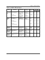
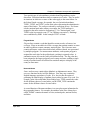
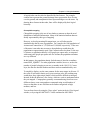
Attributes
The attributes (or items) in the ArcUSA feature attribute tables contain different
types of values; specifically, measurements, codes, flags, and names. The
values contained in an attribute determine the kinds of statistical operations that
can be performed on the data and influence the display of the data. The four
kinds of attribute values are discussed below.
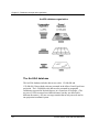
Measurement attributes
Measurement attributes have numeric values that indicate a measurement, such
as a number of people, cows, miles, bushels, or crimes, and not a code or
designation. For example, the values in the measurement attribute
PERS_HHLD (persons per household, 1985) represent the average number of
people per household. Measurement values are usually continuous (such as
3,145 or 6.2 or –43.8) but may be ordinal (first, second, etc.). In the ArcUSA
database, measurement attributes are most common in the statistical attribute
layers.
Measurements can be expressed either as raw values or as percentages. Raw or
nonstandardized attributes, such as the number of active physicians in
3-8
ArcUSA User's Guide and Data Reference
Chapter 3—Database concepts and organization
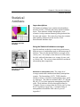
Flag attribute
Geographic
reference
attribute
Measurement
attribute
Nebraska, contain values indicating the original count or measurement. Such
attributes cannot be compared across counties or states because no standard for
comparison has been established. Raw values can be standardized to a unit of
area or population size. For example, the number of physicians in Nebraska
could be divided by the total number of people in the state, resulting in the value
for the number of physicians per capita. This standardized value can then be
meaningfully compared to the number of physicians per capita in other states.
Many raw values in the ArcUSA statistical attribute layers have been
standardized and are expressed as percentages.
Suppressed measurement values
Sometimes the measurement for a particular geographic area is missing or
suppressed in the database, such as when low response to a survey makes
it unreliable, or the privacy of individuals must be protected. In the four
coverages containing Census of Agriculture data, missing data in any of the
measurement attributes are represented by negative codes such as "–1" or "–2".
To perform statistical analyses with these attributes, first select only those
records that contain values greater than or equal to zero. (The codes follow the
census designations for missing data, except for the negative sign.) In the six
coverages containing data from the County and City Data Book, suppressed
measurements appear as zero values. This type of zero value is explained in
more detail in "Demographic and Health Attributes" in Chapter 4.
April 1992
3-9
Chapter 3—Database concepts and organization
ARC/INFOgenerated
attribute
Code attribute
Name attribute
Prioritized code attributes
Code attributes
Code attributes have either numeric or alphabetic codes. The codes are a short
form for text descriptions of groups or categories. In the ArcUSA database,
code attributes are most common in the cartographic and index layers.
Numeric codes generally begin with "1" and rise sequentially. The code order
may be random, in which case the codes have no inherent numeric meaning.
However, the order may also reflect frequency or relative significance. For
example, in the Railroads coverage, main lines are numbered "1" and "2," and
branch lines are numbered "3" and "4." Features that are inadvertently created
and are not the focus of the classification scheme, such as "background"
polygons, are usually represented by extreme value codes, such as "9" or "99."
Alphabetic codes are used sometimes instead of numeric codes. For example,
in the USGS 1:24,000 Topographic Quadrangle coverages, the MAP_EDIT
attribute has the codes "G" for "Surface management status" and "H" for
"Surface minerals."
3-10
ArcUSA User's Guide and Data Reference
Chapter 3—Database concepts and organization
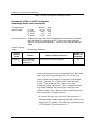
Two special types of code attributes, prioritized and flag attributes, require
discussion. Prioritized attributes share a common set of codes. They are useful
in situations in which two or more of the codes apply to the same feature. In
the Federal Lands coverage, for example, the set of prioritized attributes,
TYPE1, TYPE2, and TYPE 3, utilize nine codes representing the administrative
status of the feature. The codes are ordered by restrictions on use. If a feature
is both a national park and a military reservation, the TYPE1 attribute is
assigned to the more restrictive designation ("1" for "National park") and
TYPE2 to the less restrictive one ("5" for "Military reservation"). Rankings
were established by ESRI. In this example TYPE3 is blank.
Flag attributes
Flag attributes contain a code that identifies certain records, or features, in a
coverage. Flags are needed in ArcUSA coverages that contain counties or states
in order to generate accurate summary statistical data. This is because some
counties and states, such as those that include offshore islands, are represented
by multiple polygons. For measurement attributes, each separate polygon is
assigned the total value for the political unit, resulting in repeated values. A
summation across all records would yield inflated results. The flag value has
been assigned to the largest polygon in each county and state, enabling a single
record per political unit to be selected for statistical analysis or display of the
county or state name.
Name attributes
Name attributes may contain either alphabetic or alphanumeric names. They
serve two functions in the ArcUSA database. First, they may contain the
English-language equivalents of codes. If so, the user has the option of
generating an online display of attribute classes either by name or by code. For
example, in the Lakes and Other Water Bodies layer, TYPE contains the codes
for the different classes of water bodies, and WATER_TYPE contains the
names for the different classes of water bodies.
A second function of the name attributes is to store place name information for
the geographic features. For example, the attribute in the Place Names layer
called "NAME" contains the names of cities, national parks, national forests,
and lakes.
April 1992
3-11
Chapter 3—Database concepts and organization
ArcUSA attributes
In Chapters 4 and 5, the attributes within a coverage have been grouped by
topic, or theme, regardless of the type of values they contain. The thematic
attribute groups provide logical organization to the sometimes long lists of
coverage attributes and help the user locate data of interest in the online feature
attribute tables. The most common ArcUSA thematic attribute groups are
described below.
Geographic reference attributes
Geographic reference attributes allow the user to create displays that contain
features located in a geographic area of interest, such as one state. Many
ArcUSA layers include some geographic reference attributes, although the
specific attributes vary from one layer to another. The geographic reference
attributes used in the ArcUSA database are presented in Table 2.
Classification attributes
Classification attributes, which occur primarily in the cartographic layers,
contain codes or names that give a typology to geographic features. For
example, in the 1:2M Roads coverage, the attribute ESRI_CLASS contains
codes that specify whether a particular line represents an interstate, U.S. route,
state route, or other type of road. Categories in classification attributes are
generally mutually exclusive, although in certain cases, such as for prioritized
attributes, they may be used together.
Other attributes
The remaining attributes in ArcUSA layers are grouped by topic to assist in
locating the desired information. Most of them are measurement attributes.
Some attribute groups in the county-level Socioeconomic Attributes coverage
are, for example, Households, Social Security, Crime, Education, Income, and
Labor Force Attributes. Individual attributes in the Crime group include
SERIOUS_CR (number of serious crimes, by county, in 1985),
VIOLENT_CR (violent crimes), and SR_CR_100K (serious crimes per
100,000 population).
3-12
ArcUSA User's Guide and Data Reference
Chapter 3—Database concepts and organization
Table 2:
Geographic reference attributes
Attribute Name
Description
STATE_NAME
STATE_FIPS
The name of the state in which a feature is located, and the FIPS
code for the state.1
CNTY_NAME
CNTY_FIPS
The name of the county in which a feature is located, and the
FIPS code for the county.1
FIPS
The combined state/county FIPS code.1
SUB_REGION
An abbreviation for the U.S. subregion in which a feature is
located.2
MET_ST_AR
For metropolitan counties, the FIPS code for the Metropolitan
Statistical Area (MSA), Consolidated Metropolitan Statistical
Area (CMSA), or New England County Metropolitan Area
(NECMA).1
PR_MT_ST_A
For applicable metropolitan counties, the FIPS code for the
Primary Metropolitan Statistical Area (PMSA). 1
L_ST_FIPS
R_ST_FIPS
The FIPS codes for the states on the left and right sides of a
boundary.
ST_NAMES
The names for the states (or state) on either side of a boundary.
Notes: 1. A complete listing of state, county, and metropolitan area FIPS codes can be
found in Appendix C. 2. U.S. subregions are shown on the map in Chapter 1.
Naming conventions
To ensure consistency, naming conventions were adopted for ArcUSA
coverages and attributes. The names are intended to reflect the topic of the two
database components—features and map scale—while complying with DOS
restrictions on file name length. Tables 3 and 4 present the conventions used
for coverage and attribute names.
Attributes common to several different layers, such as state name, were
assigned the same attribute name in all layers (STATE_NAME). Conversely,
unique attributes were given names that are always unique within a layer and
generally unique across different layers. One exception is attributes in the
database that are generically named even though they refer to different features.
For example, both the water body and railroad classification code attributes are
April 1992
3-13
Chapter 3—Database concepts and organization
Table 3:
Coverage naming conventions
Convention
Examples
Applied to:
Database scale
2M = 1:2,000,000
25M = 1:25,000,000
RDS2M
RDS25M
Cartographic coverages in
ArcUSA 1:2M and 1:25M
Level of geography
S = States
C = Counties
POP90S
AGIN_C
State and county statistical
attribute coverages in ArcUSA
1:2M and 1:25M
U.S. region
N = Northern Region
S = Southern Region
W = Western Region
LAK2M_N
Q_24KS
Q_24KW
ArcUSA 1:2M Lakes and Other
Water Bodies, and USGS
1:24,000 Quadrangle Series
Index coverages
Content or source
R I V _25M (Rivers)
All coverages
LTLG5 (Latitude/longitude
grid, 5-degree intervals)
G O V 8 8 CW (Government
statistics from the 1988
County & City Data Book)
Note: The coverage files which contain feature attribute tables are assigned the coverage
name plus an extension for the table type (.PAT for polygons and points, .AAT for arcs). For
example, the file RDS2M.AAT contains the arc attribute table for the RDS2M coverage.
Table 4:
Attribute naming conventions
Convention
Examples
Applied to:
P_ = percentage
P _ HS_GRADS
(Percentage of people
with 12 years of
education)
All percentages, especially in
state and county statistical
attribute coverages
K = thousand
MARRIAG_1K (Number of Wherever applicable,
marriages per 1,000
especially in state and county
people)
statistical attribute coverages
Abbreviation
HOSP_BEDS (Number
of hospital beds)
All attributes
SICBEEF (Number of
farms falling under the
Standard Industrial
Code for beef farms)
TOT_Q_SQMI (Total
square miles of land
area represented by a
quadrangle map)
3-14
ArcUSA User's Guide and Data Reference
Chapter 3—Database concepts and organization
named TYPE. Another exception applies to some of the attributes derived from
the U.S. Census of Agriculture, which were given the same name in the
Agricultural Product Inventory layers and the Agricultural Product Market Value
layers, even though they are not identical. WHEATFARMS, for example,
indicates the number of farms that grew wheat during the census year in the
Inventory layers and the number of farms that sold wheat that year in the Market
Value layers.
Data sources
This section reviews the sources for ArcUSA data, discusses their currency,
and briefly indicates modifications or enhancements that were made to the
source data for the ArcUSA database. (Appendix A describes the development
of the ArcUSA database in detail, and the data sources and currency are
summarized in Table 5.) The name of the reference document for each source is
also noted where relevant (complete bibliographic references are listed in
Appendix D). These documents should be consulted by the user for
comprehensive definitions of the attributes included in this database.
The primary source for the ArcUSA geographic data was the USGS Digital
Line Graphs (DLGs) at a scale of 1:2,000,000. Other geographic data were
generated or compiled by ESRI, particularly the data for the index layers. U.S.
Bureau of the Census digital data from the 1990 Census of Population, the
1988 County and City Data Book, and the 1987 Census of Agriculture were the
sources for most of the statistical attributes. The Oak Ridge National
Laboratory's GeoEcology database was the source for the Environmental
Attributes layer.
Digital Line Graphs
The DLG is a digital map standard developed by the U.S. Geological Survey.
The data are offered at six scales ranging from 1:24,000 to 1:2,000,000. The
source for the 1:2,000,000-scale data (employed in the ArcUSA database) is the
1970 National Atlas of the United States of America. The data files contain
planimetric information about boundaries, hydrography, and transportation.
The DLG uses a system of major and minor codes to classify geographic
features. These cumbersome codes were revised and simplified for the
April 1992
3-15
Chapter 3—Database concepts and organization
Table 5:
Sources and currency of ArcUSA 1:2M data
Layers
Graphic Data
Source
Attribute Data Source
Cartographic Layers
County Boundaries
USGS—DLG, 1988
USGS—DLG, 1988
Federal Lands
USGS—DLG, 1980
USGS—DLG, 1980
Lakes and Other Water Bodies
USGS—DLG, 1980
USGS—DLG, 1988
Land/Ocean Display
ESRI—ArcWorld, 1992
ESRI—ArcWorld, 1992
Place Names
USGS—Concise Digital
Database, 1973
USGS—Concise Digital Database,
1973
Railroads
USGS—DLG, 1979
USGS—DLG, 1979
Rivers and Streams
USGS—DLG, 1973
USGS—DLG, 1973
Roads
USGS—DLG, 1980
USGS—DLG, 1980
State Boundaries
USGS—DLG, 1973
USGS—DLG, 1973
Index Layers
Landsat Nominal Scene Index
EOSAT algorithm, 1992
EOSAT algorithm, 1992
Latitude/Longitude Grids
ESRI, 1992
ESRI, 1992
USGS Topographic Map Indexes:
1:24K, 1:100K, 1:250K
ESRI algorithm, 1992
USGS—Topographic Names
Database; Published Map Sheet
Data File (T-70); various published
indexes, 1986
Statistical Layers
3-16
U.S. Census, P-L 94-171
USGS—DLG, 1988
U.S. Census, 1990
Agricultural Product Inventory
USGS—DLG, 1988
U.S. Census of Agriculture, 1987
Agricultural Product Market Value
USGS—DLG, 1988
U.S. Census of Agriculture, 1987
Demographic & Health Attributes
USGS—DLG, 1988
County and City Data Book, 1988
Environmental Attributes
USGS—DLG, 1988
GeoEcology, 1967–1979
Government & Financial Attributes
USGS—DLG, 1988
County and City Data Book, 1988
Socioeconomic Attributes
USGS—DLG, 1988
County and City Data Book, 1988
ArcUSA User's Guide and Data Reference
Chapter 3—Database concepts and organization
ArcUSA database. The reference work for the DLG data source is Digital Line
Graphs from 1:2,000,000-Scale Maps: Data Users Guide 3, U.S. Geological
Survey, Reston, Va., 1990.
The DLG data are the basis for features and attributes in the following ArcUSA
1:2M cartographic coverages: County Boundaries, Federal Lands, Lakes and
Other Water Bodies, Railroads, Rivers and Streams, Roads, and State
Boundaries. The DLG data are also the basis for the state and county features
in all the statistical coverages. The DLG data employed in the ArcUSA database
range in currency; the data for some of the coverages are as recent as 1988, but
date back to 1980.
Concise Digital Database
The Concise Digital Database is a digital compendium of U.S. place names
developed in 1973 in conjunction with the DLG. The translation to digital form
was made by the USGS's Geographic Names Information System (GNIS).
The Concise Digital Database references each place name through
latitude/longitude coordinates.
The Concise Digital Database was the source for the Place Names and Cities
cartographic layers. The latitude/longitude coordinates were used to generate
the point feature coverage. Some of the Concise Digital Database attributes,
such as the elevation attribute, were also retained.
Other USGS data
The USGS Topographic Names Database and the Published Map Sheet Data
File (also known as the T-70 file) were the two primary digital sources for the
attributes in the USGS Quadrangle Series index coverages. Where these
database were incomplete, various published USGS map indexes were
consulted to update the attributes. Further explanatory information about
USGS quadrangles can be found in the Catalog of Topographic and Other
Published Maps, and the Index to Topographic and Other Map Coverage, U.S.
Geological Survey, Reston, Va. These USGS companion publications are
available for every state.
Landsat nominal scene indexes
The Landsat satellites are operated by the Earth Observation Satellite Company
(EOSAT). EOSAT provided ESRI with an algorithm for generating two types
April 1992
3-17
Chapter 3—Database concepts and organization
of index information for Landsat 4 and 5 scenes: nominal scene center points
and nominal scene footprints. ("Nominal" indicates that the center points and
footprints represent an average, not an absolute, geographic location. The
center points and footprints are averaged because the orientation of the satellite
varies slightly from one orbit to the next.) Nominal scene center points were
calculated first; then scene footprints were mathematically generated with the
center points as the focus. The footprints are rectangular outlines whose exact
dimensions vary with satellite orientation. In the ArcUSA database, these data
are the basis for the Landsat Nominal Scene Index coverages.
U.S. Census of Population and Housing, 1990
The U.S. Census of Population and Housing is a compilation of statistical data
on population and housing that is developed every ten years by the U.S. Bureau
of the Census. The data are tabular and available in digital form. The ArcUSA
database employs a subset of the 1990 Census known as Public Law 94-171
data. These data support congressional and legislative redistricting and are the
first data to be released from the new census. The ArcUSA 1990 Census,
Public Law 91-171 Data layers contain these data for states and counties. The
reference document for this data source is Public Law 94-171, U.S. Bureau of
the Census, Washington, D.C., 1991.
U.S. Census of Agriculture, 1987
The U.S. Census of Agriculture is a statistical report developed at fixed
intervals by the U.S. Bureau of the Census. The census provides summary
statistical information for all farms with sales of $1,000 or more. The data are
presented in more than fifty tables and are available in digital form. Only a
subset of these data are included in the ArcUSA database: the Agricultural
Product Inventory layers contain state and county attributes from Table 1 of the
census, and the Agricultural Product Market Value layers contain attributes from
Table 2. The reference document for this data source is Census of Agriculture,
1987 on CD-ROM, U.S. Bureau of the Census, Data User Services Division,
Washington, D.C., 1990.
County and City Data Book, 1988
The County and City Data Books are interim (that is, non-census-year)
statistical products developed by the U.S. Bureau of the Census. They provide
data for states, counties, cities of 25,000 or more residents, and places with
2,500 or more residents. The data are tabular and available in digital form. The
3-18
ArcUSA User's Guide and Data Reference
Chapter 3—Database concepts and organization
ArcUSA database employs state and county data from the 1988 County and
City Data Book, which contains statistics that vary in currency from 1979 to
1986. These data are the basis for the attributes in three groups of ArcUSA
coverages: Demographic and Health Attributes, Government and Financial
Attributes, and Socioeconomic Attributes. The reference work for this data
source is the County and City Data Book, 1988: Files on CD-ROM Technical
Documentation, U.S. Bureau of the Census, Data Access and Use Staff, Data
User Services Division, Washington, D.C., 1989.
GeoEcology Database
The GeoEcology Database is a tabular digital database developed by the Oak
Ridge National Laboratory for the U.S. Department of Energy. The database
contains environmental data for the counties of the coterminous United States.
The GeoEcology database included research efforts spanning extended
geographic areas and addressing the long-term impact of human activity on
ecosystems in general. The currency of the data varies; the most recent entries
range from 1979. The ArcUSA Environmental Attributes coverage employs a
small subset of the GeoEcology data. The reference work for this data source is
GeoEcology: A County-Level Environmental Data Base for the Conterminous
United States, R. J. Olson, C. J. Emerson, and M. K. Nungesser, Oak Ridge
National Laboratory, Oak Ridge, Tenn., 1980.
ESRI in-house development
Several ArcUSA coverages do not have a specific source, but were developed
for the database by ESRI. For example, the 1:2,000,000-scale grids for the
three USGS topographic quadrangle indexes were mathematically generated by
ESRI; then the attribute information from USGS sources mentioned above was
added. Geographic and attribute data for the Latitude/Longitude Grids
coverages were also developed by ESRI. The Land/Ocean Display coverages,
which extend the U.S. ocean shorelines into Canada and Mexico, were created
from another ESRI product, the ArcWorld database. Special ArcUSA map
titles and scale bars were created for the Map Elements coverages.
Coordinate systems
The ArcUSA database is available in projections that promote usability as both
stand-alone data and in conjunction with other data sets. ARC/INFO users will
April 1992
3-19
Chapter 3—Database concepts and organization
be able to convert the database to other projections. The ArcUSA 1:2M and
1:25M databases also feature a specified coordinate precision.
Projection systems
The ArcUSA database employs the Albers Conic Equal-Area projection at both
the 1:2M and 1:25M scales. This conic projection is implemented with standard
parallels at 29.5° and 45.5° North latitude. With this projection, equal area is
preserved, but shape is somewhat distorted. In general, the shape of the
regions between the two standard parallels becomes expanded and the shape of
those beyond becomes compressed. The coordinate units employed in
conjunction with the Albers Conic Equal-Area projection are meters. The point
of origin is 96°00' W and 23°00' N.
The ArcUSA 1:2M database is also delivered in decimal degrees. Storage in
geographic coordinates facilitates use with other data, which are commonly
supplied in decimal degrees, and enables conversion into the projection of
choice for update or analysis. The units of measure used with the decimal
degrees are spherical latitude/longitude coordinates. For example, the
latitude/longitude coordinate of 37°30'15" is expressed as 37.50417.
Albers Conic Equal-Area projection
with two standard parallels
3-20
ArcUSA User's Guide and Data Reference
Chapter 3—Database concepts and organization
Datums
The horizontal datum used is the North American Datum of 1927 (NAD1927),
and the vertical datum used is the National Geodetic Vertical Datum of 1929
(NGVD 1929). The vertical datum applies only to the Place Names layer that
contains elevation information.
Coordinate precision
Coordinate precision refers to the maximum number of digits allocated within a
data file for the storage of an x, y, or z coordinate value. Single-precision maps
store as many as seven significant digits for each coordinate. All ArcUSA data
are in single precision. This means that any x,y coordinate in the ArcUSA
database has a locational accuracy at least to the nearest meter.
Projection conversion capability
ARC/INFO users can employ the PROJECT command to convert the ArcUSA
data into other projections. A coordinate system definition file (PRJ) is
included for each ArcUSA coverage and can be used in ARC/INFO for map
projection conversions. This option is not available to ArcView users.
April 1992
3-21
Chapter 4
In greater detail:
The ArcUSA 1:2M layers
This chapter describes the individual coverages in the ArcUSA 1:2M database.
To avoid repetition, all coverages that belong to the same layer are described
together, since coverages in the same layer have the same feature and attribute
definitions. As outlined in Chapter 3, the layer descriptions are presented in
three major groups (cartographic, index, and statistical attribute). Within each
group, the layers are listed in alphabetical order.
The description of each layer begins with a discussion of the map features and
attributes in that layer. The discussion continues with information about the use
of the coverages in that layer. Then a tabular summary of the layer is given.
The table lists the individual coverage names, coverage feature classes, map
feature counts (for the full U.S. coverage), and the number of database
attributes associated with each feature class. The last part of the layer
description, usually the longest, defines the individual attributes that appear in
the coverage feature attribute tables, and the coding schemes associated with the
attributes.
The summary tables for ArcUSA 1:2M layers may list four coverage names for
each layer. These coverage names correspond to the full U.S. coverage and
each of the three U.S. regional coverages.
The standard ARC/INFO-generated attributes described in Chapter 3 do not
appear, nor are they included in the attribute count in the layer summary tables.
April 1992
4-1
Chapter 4—In greater detail: The ArcUSA 1:2M layers
The layer descriptions do include geographic reference attributes, because the
list of those attributes differs slightly from one layer to the next (the geographic
reference attributes are described more thoroughly in Chapter 3).
Detailed attribute field definitions for both dBASE and INFO formats are given
for each layer in Appendix B.
4-2
ArcUSA User's Guide and Data Reference
ArcUSA 1:2M cartographic layers
The coverages in the cartographic layers contain geographic features like roads,
rivers, boundaries, and place names, which provide a general location context
for the data in other layers. The features in these coverages represent those that
are often placed on maps to orient the user. The cartographic coverages have
few attributes other than those used for classification and geographic reference.
The county and state boundary coverages described in this section are identical
to those used as the cartographic foundation for the state and county statistical
attribute coverages described later.
The ArcUSA 1:2M cartographic layers and coverages are listed in the table
below.
Coverage Names
Layer
County Boundaries*
CTY2M
Federal Lands
FED2M
Lakes and Other Water Bodies
LAK2M, LAK2M_N, LAK2M_S, LAK2M_W
Land/Ocean Display*
LAND2M
Map Elements
SC_2M
Place Names
NAM2M
Railroads
RR2M
Rivers and Streams*
RIV2M
Roads*
RDS2M
State Boundaries*
ST2M
* Generalized versions of these layers are provided with ArcUSA 1:25M. If you do
not need the detail of the 1:2M coverage, substituting a generalized coverage will
minimize display time.
April 1992
4-3
Chapter 4—ArcUSA 1:2M cartographic layers
County Boundaries
County
Boundaries
Layer description
The County Boundaries layer serves as a county base map
for the coterminous United States. Two new counties for
Arizona and New Mexico, as well as several independent
cities, primarily in Virginia, were added by ESRI to the DLG
source data. These additions brought the currency of the
layer from 1973 to 1988. More than 3,100 substate political
units are represented.
Polygons
A line attribute classifies boundaries as shorelines or as
county, state, or international boundaries. Attributes that
permit states or counties to be selected for display are
contained in both the line and polygon attribute tables.
Using the County Boundaries coverage
Lines
April 1992
Some counties, such as those that include offshore islands,
are represented by multiple polygons. A flag attribute is
provided so that the largest polygon can be used to represent
the county for choroplethic mapping or text labeling. The
county name attribute can be used to provide the text for
labeling the polygons in a base map.
4-5
Chapter 4—ArcUSA 1:2M cartographic layers
County Boundaries
Summary of the County Boundaries coverage
Coverage name
and size (MB):
CTY2M
dBASE
5.37
UNIX
4.78
Source and currency: USGS DLG, 1988
Thematic attribute
groups:
Feature
class
Geographic reference attributes (polygons and lines)
Statistical flag (polygons)
Classification attributes (lines)
Feature
Number of features
Number of
attributes
Polygons
Counties and
independent cities
3,111 features represented by 4,409
polygons
7
Lines
County and
independent city
boundaries
Represented by 7,504 lines
4
State boundaries
Represented by 1,204 lines
International
boundaries
Represented by 68 lines
Shorelines
Represented by 1,709 lines
All line features
Represented by 10,485 lines
Polygon attributes
Geographic reference attributes
STATE_FIPS
CNTY_FIPS
FIPS
STATE_NAME
CNTY_NAME
SUB_REGION
4-6
The state, county, and combined state/county FIPS codes, as
well as the state name and U.S. subregion, can be used to
select particular county polygons for display or study. The
U.S. subregions are shown on the map on page 1-2.
ArcUSA User's Guide and Data Reference
Chapter 4—ArcUSA 1:2M cartographic layers
County Boundaries
Statistical flag
STAT_FLAG
Flag to identify a unique polygon for each county. The
codes are as follows:
Codes
Definitions
0 = Other polygon
1 = Largest polygon
Line attributes
Geographic reference attributes
L_ST_FIPS
R_ST_FIPS
The FIPS codes of the states on either the left or right side of
a boundary are contained in these attributes. For county
boundaries inside a state, the left and right FIPS codes are
the same. For state boundaries, the left and right FIPS
codes are different. The left and right sides of a boundary
are defined by the direction in which that line segment was
digitized, so both attributes must be checked when querying
for the boundaries of a particular state.
ST_NAMES
This attribute contains the names of states adjacent to a
boundary. Two states are listed for state boundaries (e.g.,
"Wisconsin/Minnesota"). Only one state is identified for
county and international boundaries and shorelines.
Classification attribute
BNDY_TYPE
Each line is classified according to boundary type. This
attribute allows you to choose different symbols for political
boundaries and coastlines. Wherever boundaries are
coincident, rank is assigned beginning with coastlines in the
reverse order of the list below. Thus, a county boundary
that is also a state and international boundary will only be
coded as "3" for international boundary. The codes are as
follows:
Codes
1
2
3
4
April 1992
=
=
=
=
Definitions
County boundary
State boundary
International boundary
Coastline
4-7
Chapter 4—ArcUSA 1:2M cartographic layers
Federal
Lands
Layer description
The Federal Lands layer delimits those land areas that are
administered by the federal government. These include
national parks, monuments, and recreation areas; national
wildlife refuges; scenic waterways and wilderness areas;
national forests and grasslands; Indian reservations; and
military reservations. Each area contains three different
attributes to describe its administrative relationships.
Polygons
Using the Federal Lands coverage
Some types of federal land areas are "nested" within others.
For example, a scenic waterway may be located within a
wilderness area that is also part of a national forest. These
nested land areas may be administered by different
government agencies. Each land area classification has been
prioritized according to restrictions on use. The areas with
the most stringent restrictions on use (like scenic waterways)
were assigned the highest priority; the areas with the fewest
restrictions on use (like national forests) were assigned the
lowest priority. The names of national parks and forests are
included in the Place Names layer.
4-8
ArcUSA User's Guide and Data Reference
Chapter 4—ArcUSA 1:2M cartographic layers
Federal Lands
Summary of the Federal Lands coverage
Coverage name
and size (MB):
dBASE
2.24
FED2M
UNIX
2.33
Source and currency: USGS DLG, 1980
Thematic attribute
groups:
Feature
class
Polygons
Classification attributes (polygons)
Geographic reference attributes (polygons)
Feature
Number of features
National parks, etc.
Represented by 630 polygons
National wildlife
refuges, etc.
Represented by 640 polygons
National scenic
waterways, etc.
Represented by 139 polygons
Indian reservations
Represented by 381 polygons
Military reservations
Represented by 168 polygons
National forests and
grasslands
Represented by 619 polygons
Not a federal land area
Represented by 174 polygons
All polygon features
Represented by 2,741 polygons
Number of
attributes
9
Polygon attributes
Classification attributes
TYPE1
TYPE2
TYPE3
April 1992
These three attributes contain codes representing the
administrative type of the land area. Every land area is
assigned at least a TYPE1 code. If a land area is "nested"
within the limits of one or two other federal land areas, the
4-9
Chapter 4—ArcUSA 1:2M cartographic layers
Federal Lands
additional codes are stored in TYPE2 and TYPE3. Codes
are prioritized from most restrictions on use (beginning with
TYPE1) to fewest restrictions on use. Thus, if an area is
both a national park and an Indian reservation, TYPE1
contains "1," TYPE2 contains "4," and TYPE3 contains a
blank. The classification order is given below:
Codes
Definitions
1 = National park, monument, lakeshore, parkway,
battlefield, or recreation area
2 = National wildlife refuge, game preserve, or fish
hatchery
3 = National scenic waterway or wilderness area
4 = Indian reservation
5 = Military reservation
6 = National forest or grassland
9 = Not a federal land area
ADMN_TYPE1
ADMN_TYPE2
ADMN_TYPE3
These three attributes contain the abbreviated English
equivalents of the classifications defined above. They are as
follows:
•
•
•
•
•
•
•
Parks, monuments, etc.
Wildlife refuges, etc.
Waterways and wilderness areas
Indian reservation
Military reservation
National forest or grassland
Not a federal land area
Geographic reference attributes
STATE_FIPS
STATE_NAME
SUB_REGION
These attributes, which can be used for spatial selection,
store the state FIPS code, state name, and U.S. subregion in
which the federal land area is located.
A federal land area that is located in more than one state is
represented by multiple polygons, each of which is assigned
the appropriate state and subregional geographic reference
information. For example, Yellowstone National Park is
represented by three polygons, one each in Wyoming,
Idaho, and Montana.
4-10
ArcUSA User's Guide and Data Reference
Chapter 4—ArcUSA 1:2M cartographic layers
Lakes and Other Water Bodies
Lakes and
Other Water
Bodies
Layer description
The Lakes and Other Water Bodies layer contains more than
6,000 water body and island polygon features for the
coterminous United States. This number includes perennial
lakes, perennial reservoirs, intermittent lakes, intermittent
reservoirs, dry lakes, marshes, glaciers, and snowfields.
Islands within any of these water bodies are also included.
Polygons
Using the Lakes coverages
In some complex hydrologic situations, different types of
water bodies may be located completely within others. For
example, a perennial lake may be within a larger intermittent
lake, or a marsh may contain an island that in turn contains a
perennial pond. To clarify these displays, use areas instead
of lines to display water bodies and use different colors for
different classes.
Background polygons are present in the full U.S. and
northern region coverages. You can prevent them from
appearing in a display, if you wish, by selecting only
polygons with codes less than 9 (9 is defined as "not a water
body").
Names for selected lakes and reservoirs are contained in the
Place Names layer. The Great Lakes, which are outside the
extent of ArcUSA, can be displayed using the Land/Ocean
Display layer.
April 1992
4-11
Chapter 4—ArcUSA 1:2M cartographic layers
Lakes and Other Waterbodies
Summary of Lakes and Other Water Bodies coverages
Coverage names
and sizes (MB):
LAK2M
LAK2M_N
LAK2M_S
LAK2M_W
dBASE
3.97
1.78
1.30
0.92
UNIX
3.93
1.81
1.35
0.95
Source and currency: USGS DLG, 1980
Thematic attribute
groups:
Feature
class
Polygons
Classification attributes
Geographic reference attributes
Feature
Number of features (full U.S.)
Perennial lakes
Represented by 4,429 polygons
Marshes
Represented by 44 polygons
Intermittent lakes
Represented by 216 polygons
Dry lakes
Represented by 132 polygons
Reservoirs
Represented by 970 polygons
Intermittent reservoirs
Represented by 4 polygons
Number of
attributes
5
Glaciers and snowfields Represented by 35 polygons
4-12
Islands
Represented by 527 polygons
Background polygons
Represented by 8 polygons
All polygon features
Represented by 6,365 polygons
ArcUSA User's Guide and Data Reference
Chapter 4—ArcUSA 1:2M cartographic layers
Lakes and Other Water Bodies
Polygon attributes
Classification attributes
TYPE
WATER_TYPE
Each polygon is classified according to the following list of
categories. TYPE contains the code number, and
WATER_TYPE contains the English description.
Codes
1
2
3
4
5
6
7
8
9
=
=
=
=
=
=
=
=
=
Equivalents
Perennial lake or pond
Marsh
Intermittent lake or pond
Dry lake or pond
Reservoir
Intermittent reservoir
Glacier or snowfield
Island
Not a water body (background polygon)
Geographic reference attributes
STATE_FIPS
STATE_NAME
SUB_REGION
These attributes, which can be used for feature selection,
store the state FIPS code, state name, and U.S. subregion in
which the water body is located.
A water body located in more than one state is represented
by multiple polygons, each of which is assigned the
appropriate state and subregional geographic reference
information.
April 1992
4-13
Chapter 4—ArcUSA 1:2M cartographic layers
Land/Ocean
Display
Layer description
Land and water areas beyond the extent of the other ArcUSA
cartographic layers are contained in the Land/Ocean Display
layer. Canada, Mexico, the Atlantic and Pacific oceans, and
each of the Great Lakes can be displayed and labeled to
create a finished-looking map.
Polygons
Using the Land/Ocean Display coverage
The purpose of this coverage is to provide an attractive
cartographic treatment between the data content area and the
edge of the display window. For example, a continuous
background can be displayed by using solid colors for the
polygons in this layer, such as blue for water and beige for
land.
Lines
A U.S. coastline display using the State Boundaries or
County Boundaries coverages can be continued into Canada
and Mexico with the line features in this layer. (The
"processing grid" can be omitted from the display if you
select only the feature lines.)
The annotation features associated with this layer include the
names of major countries and water bodies. The annotation
for this layer looks best for displays that show the full extent
of the database, so the names are entirely visible. The
annotation is suited for a detailed display of the Great Lakes
region, however, because the annotation text for those
features is relatively small.
4-14
ArcUSA User's Guide and Data Reference
Chapter 4—ArcUSA 1:2M cartographic layers
Land/Ocean Display
Summary of the Land/Ocean Display coverage
Coverage name
and size (MB):
LAND2M
dBASE
1.53
UNIX
1.47
Source and currency: ESRI ArcWorld, 1992
Thematic attribute
groups:
Annotation text:
Feature
class
Polygons
Lines
Classification attributes (polygons and lines)
Mexico, Canada, Atlantic Ocean, Lake Superior, Lake Michigan, Gulf of
Mexico, Gulf of California, etc.
Feature
Number of features
Land
Represented by 1,431 polygons
Water
Represented by 40 polygons
Artificial grid lines
Represented by 103 lines
Feature boundaries
Represented by 1,757 lines
Number of
attributes
1
1
Polygon attributes
Classification attribute
LND_WAT
Each polygon is classified as either land or water (ocean and
the Great Lakes), as follows:
• Land
• Water
April 1992
4-15
Chapter 4—ArcUSA 1:2M cartographic layers
Land/Ocean Display
Line attributes
Classification attribute
BND_GRID
Each line segment is classified as either a feature boundary
(shorelines and international boundaries) or an artificial grid
line (a data processing line that divides the data into
geographic sections). The codes are as follows:
Codes
Definitions
0 = Artificial grid line
1 = Feature boundary or outer coverage extent line
4-16
ArcUSA User's Guide and Data Reference
Chapter 4—ArcUSA 1:2M cartographic layers
Map Elements
Map
Elements
Layer description
The Map Elements layer contains a scale bar, North arrow,
and a title that can be used to make your display look like a
finished map.
Using the Map Elements coverage
Polygons and Lines
Polygon attributes include codes for the scale bar and the
head of the North arrow so that they may be filled with
color. Annotation features provide the title and characters
associated with the other map elements.
The scale is given in kilometers, since the Albers Conic
Equal-Area projection uses meters. Because the scale bar is
in a predetermined location that cannot be changed, it is best
suited to maps that display the full extent of the database.
April 1992
4-17
Chapter 4—ArcUSA 1:2M cartographic layers
Map Elements
Summary of the Map Elements coverage
Coverage name
and size (MB):
SC_2M
dBASE
0.02
UNIX
0.03
Source and currency: ESRI, 1992
Thematic attribute
groups:
Classification attributes (polygons)
Annotation text:
Map title, scale, and North arrow
Feature
class
Feature
Number of features
Number of
attributes
Polygons
All polygon features
Represented by 15 polygons
1
Lines
All line features
Represented by 43 lines
0
Polygon attributes
Classification attribute
FILL
The scale bar is designed so it can be filled with alternating
colors. The arrowhead on the North arrow also can be
filled. The codes are as follows:
Codes
Definitions
1 = First color (scale bar)
2 = Second color (scale bar and North arrow)
4-18
ArcUSA User's Guide and Data Reference
Chapter 4—ArcUSA 1:2M cartographic layers
Place Names
Place
Names
Layer description
Point features representing major cities, state capitals, county
seats, national forests, national parks, lakes, and reservoirs
are contained in the Place Names layer. The point attributes
include the type and name of each feature. The elevation of
some features is also given.
Points
Using the Place Names coverage
The locations of the points in this coverage were taken from
latitude/longitude coordinates listed in the digital version of
the National Atlas Gazetteer. As is common for gazetteers,
the geographic coordinates were rounded, so their positions
may reflect some error.
Only one point has been coded for every unique place in this
layer, even though the feature itself may be an area that falls
into more than one state. For example, Lake Tahoe is
divided between California and Nevada, and it is represented
as two polygons in the Lakes layer. In the Place Names
layer, however, only a single point represents Lake Tahoe.
Since the point location lies in California, California is given
as the state of geographic reference.
Cities in this layer are coded as to whether they are major
U.S. cities, state capitals, and/or county seats. Cities can be
selectively displayed and symbolized for different purposes.
The point features and their place names are useful as general
geographic identifiers, especially for small-scale maps.
They can also be used to label the equivalent area features in
other layers. The national parks and forests named in this
layer correspond to the national parks and forests
April 1992
4-19
Chapter 4—ArcUSA 1:2M cartographic layers
Place Names
Summary of the Place Names coverage
Coverage name
and size (MB):
NAM2M
dBASE
1.05
UNIX
0.96
Source and currency: USGS Concise Digital Database, approximately 1973
Thematic attribute
groups:
Feature
class
Points
Classification attributes
Geographic reference attributes
Elevation
Feature
Number of features
Cities
Represented by 3,096 points
National forests
Represented by 174 points
National parks
Represented by 492 points
Lakes
Represented by 513 points
Reservoirs
Represented by 787 points
All point features
Represented by 5,062 points
Number of
attributes
10
represented as areas in the Federal Lands layer. The lakes
and reservoirs named here are represented as polygons in the
Lakes and Other Water Bodies layer.
Point attributes
Classification attributes
NAME
4-20
This attribute stores the name of the populated place or
named area feature that corresponds to a point location.
ArcUSA User's Guide and Data Reference
Chapter 4—ArcUSA 1:2M cartographic layers
Place Names
FEAT_TYPE
The name of the feature. The five feature types available in
this layer are as follows:
Names
Definitions
City
Forest
Park
Lake
Reservoir
MAJ_CITY
=
=
=
=
=
City or other populated place
National forest
National park
Lake
Reservoir
This attribute contains codes that identify the seventy-four
most populous cities in the coterminous United States.
Codes
Definitions
0 = Not a major city
1 = A major city
CAPITAL
This attribute contains codes that identify the capital cities of
the forty-eight states in the database, plus the national
capital.
Codes
Definitions
0 = Not a capital
1 = A state capital
2 = The national capital (Washington, D.C.)
CTY_SEAT
This attribute contains codes that identify which of the major
cities and state capital cities are also county seats. There are
ninety-six county seats in this coverage.
Codes
Definitions
0 = Not a county seat
1 = A county seat
Elevation
ELEVATION
April 1992
A feature's elevation with respect to sea level, expressed in
feet, is listed for some features.
4-21
Chapter 4—ArcUSA 1:2M cartographic layers
Place Names
Geographic reference attributes
CNTY_NAME
STATE_FIPS
STATE_NAME
SUB_REGION
4-22
The name of the county, state, and U.S. subregion in which
the point feature is located are provided in these attributes.
The state FIPS code is also given.
ArcUSA User's Guide and Data Reference
Chapter 4—ArcUSA 1:2M cartographic layers
Railroads
Railroads
Layer description
Railroad lines are represented in this layer. They are
identified as main or branch lines based on U.S. Department
of Transportation definitions, and are classified based on the
annual volume of traffic they bear. Other railroad lines, such
as sidings and railroad ferries, are also identified.
Lines
Using the Railroads coverage
The general decline of the U.S. railroad industry has resulted
in significant reduction in rail line usage since the National
Atlas was prepared in 1973. The features in this coverage
are those represented in the DLG database.
April 1992
4-23
Chapter 4—ArcUSA 1:2M cartographic layers
Railroads
Summary of the Railroads coverage
Coverage name
and size (MB):
RR2M
dBASE
4.94
UNIX
4.37
Source and currency: USGS DLG, 1979
Thematic attribute
groups:
Feature
class
Lines
4-24
Classification attributes
Geographic reference attributes
Feature
Number of features
Main lines, heavy use
Represented by 3,445 lines
Main lines, light use
Represented by 3,931 lines
Branch lines, heavy
use
Represented by 2,149 lines
Branch lines, light use
Represented by 2,763 lines
Other railroad
Represented by 883 lines
Railroad ferry
Represented by 11 lines
All line features
Represented by 12,182 lines
Number of
attributes
5
ArcUSA User's Guide and Data Reference
Chapter 4—ArcUSA 1:2M cartographic layers
Railroads
Line attributes
Classification attributes
TYPE
RAIL_TYPE
The railroad lines are classified according to volume of
traffic, measured in tons. The code number is stored in
TYPE, and the English equivalent is stored in RAIL_TYPE.
The codes are as follows:
Codes
Equivalents
1= Main line bearing more than 20 tons annually
2= Main line bearing less than 20 tons annually
3= Branch line bearing more than 1 but less than 5 tons
annually
4= Branch line bearing less than 1 ton annually
5= Other railroad
6= Railroad ferry
Geographic reference attributes
STATE_FIPS
STATE_NAME
SUB_REGION
April 1992
Railroads can be selected by the state name, state FIPS code,
and U.S. subregion in which they are located.
4-25
Chapter 4—ArcUSA 1:2M cartographic layers
Rivers and
Streams
Layer description
The Rivers and Streams layer contains perennial and
intermittent rivers, braided rivers, canals, ditches, and
stream centerlines.
Using the Rivers and Streams coverage
Lines
The ArcUSA database uses a simpler coding scheme for
rivers than the original DLG codes. In the simpler system,
codes are prioritized and only one code is assigned to each
river segment. Elimination of river length in the DLG
classifications also helped to simplify the scheme. In these
coverages, river length is contained in the ARC/INFOgenerated attribute, LENGTH. (More information about
ARC/INFO-generated attributes is given in Chapter 3.)
A number of spatial interactions are possible between rivers
and political boundaries. For example, a political boundary
may follow a river course precisely, follow a historical river
course, or follow one shoreline. For this reason, if you are
displaying a political unit, such as a state, the rivers along
the political boundary may appear to lack continuity. A more
detailed discussion of coincident rivers and political
boundaries is given in Chapter 5.
The Rivers and Streams layer and the Lakes and Water
Bodies layer can be displayed either individually or in
combination. When rivers are displayed alone, the
centerlines through the water bodies can be displayed to
form a complete drainage network.
4-26
ArcUSA User's Guide and Data Reference
Chapter 4—ArcUSA 1:2M cartographic layers
Rivers and Streams
Summary of the Rivers and Streams coverage
Coverage name
and size (MB):
RIV2M
dBASE
16.48
UNIX
14.50
Source and currency: USGS DLG, 1973
Thematic attribute
groups:
Feature
class
Lines
Classification attributes
Geographic reference attributes
Feature
Number of features
River shorelines
Represented by 2,361 lines
River centerlines
Represented by 3,253 lines
Perennial rivers
Represented by 23,456 lines
Intermittent rivers
Represented by 3,541 lines
Centerlines of
perennial rivers
through water bodies
Represented by 3,893 lines
Centerlines of
intermittent rivers
through water bodies
Represented by 46 lines
Braided rivers
Represented by 1,325 lines
Navigable canals
Represented by 304 lines
Other canals
Represented by 350 lines
Ditches
Represented by 205 lines
All line features
Represented by 38,734 lines
Number of
attributes
5
The Rivers and Streams layer and the Lakes and Water
Bodies layer are fully consistent with one another.
A river centerline through a water body has an associated
water body polygon, and the endpoints of the river centerline
terminate at the boundary of the water body polygon.
April 1992
4-27
Chapter 4—ArcUSA 1:2M cartographic layers
Rivers and Streams
At the original scale of 1:2,000,000, some rivers are wide
enough to be represented by two shorelines. Such
shorelines are coded "1." In addition, an artificial centerline
was digitized between the two shorelines (code = 2). This
centerline may be used to represent the river at smaller
scales.
Line attributes
Classification attributes
TYPE
RIVER_TYPE
The class number of the river or stream segment is stored in
TYPE; its English equivalent is stored in RIVER_TYPE.
The codes are as follows:
Codes
1
2
3
4
5
=
=
=
=
=
6 =
7
8
9
10
=
=
=
=
Equivalents
River shoreline
River centerline
Perennial river or stream
Intermittent river or stream
Centerline of perennial stream through a water
body
Centerline of intermittent stream through a water
body
Braided river or stream
Navigable canal
Other canal
Ditch
Geographic reference attributes
STATE_FIPS
STATE_NAME
SUB_REGION
4-28
Rivers can be selected by the state name, state FIPS code, or
U.S. subregion in which that part of the river or stream is
located.
ArcUSA User's Guide and Data Reference
Chapter 4—ArcUSA 1:2M cartographic layers
Roads
Roads
Layer description
The Roads layer contains roads and highways. Two
classifications of road type are available. (Interstates, U.S.
highways and state highways, toll roads, and improved
roads are examples of road types.) Route numbers are also
included.
Lines
Using the Roads coverage
This coverage contains attributes with the original twentyseven DLG road classes (DLG_CLASS) as well as a
simplified ten-class coding scheme (ESRI_CLASS). The
simplified classification scheme is particularly useful for
small-scale displays, or for regional displays where only a
few road types are required. The more detailed road classes
can be useful for more detailed displays of local areas,
especially for transportation applications.
April 1992
4-29
Chapter 4—ArcUSA 1:2M cartographic layers
Roads
Summary of the Roads coverage
Coverage name
and size (MB):
RDS2M
dBASE
15.81
UNIX
14.31
Source and currency: USGS DLG, 1980
Thematic attribute
groups:
Feature
class
Lines
Classification attributes
Geographic reference attributes
Feature
Number of features
Interstate highways
Represented by 5,406 lines
Limited access/divided
highways
Represented by 1,153 lines
Other U.S. highways
Represented by 6,720 lines
Other state primary
highways
Represented by 2,066 lines
State secondary
highways
Represented by 4,960 lines
Improved roads
Represented by 911 lines
Unimproved roads
Represented by 27 lines
Parallel highways
Represented by 7,238 lines
Toll roads
Represented by 31 lines
Tunnel
Represented by 1 line
Auto ferries
Represented by 217 lines
All line features
Represented by 28,730 lines
Number of
attributes
22
Note: This table is for the ESRI Roads coding scheme.
4-30
ArcUSA User's Guide and Data Reference
Chapter 4—ArcUSA 1:2M cartographic layers
Roads
Line attributes
Classification attributes
ESRI_CLASS
ROAD_CLASS
ESRI developed a simplified road classification system by
condensing the more than twenty-five road categories in the
source database (the DLG) to only ten classes. The code
numbers are stored in ESRI_CLASS, while the English
equivalent is stored in ROAD_CLASS. The codes are as
follows:
Codes
0
1
2
3
4
5
6
7
8
9
10
11
=
=
=
=
=
=
=
=
=
=
=
=
Equivalents
No class applies
Interstate highway
Limited access/divided highway
Other U.S. highway
Other state primary highway
State secondary highway
Improved road
Unimproved road
Parallel highway
Toll road
Tunnel
Auto ferry
Note: In this classification system, the parallel highway
class (code 8) includes those U.S., minor U.S., and state
highways that are through roads and generally within
ten kilometers (six miles) of an interstate or other type of
divided, limited-access highway.
CLASS1
DLG_CLASS1
CLASS2
DLG_CLASS2
CLASS3
DLG_CLASS3
April 1992
The CLASS1, 2, and 3 attributes contain the detailed road
segment classification codes used in the DLG source, and
the DLG_CLASS1, 2, and 3 attributes contain their English
word equivalents. CLASS1, 2, or 3 priority is assigned
based on the degree of multilane, limited access, and then by
decreasing jurisdictional control (interstate, U.S., state).
The highest priority code is stored in CLASS1. If a road
segment has no lower priority class, CLASS2 and/or
CLASS3 contains a code of 0. As an example, if a highway
is an "Interstate highway" (code = 1) and an "Other U.S.
route" (code = 16), then CLASS1 contains "1," CLASS2
contains "16," and CLASS3 contains "0."
4-31
Chapter 4—ArcUSA 1:2M cartographic layers
Roads
A relatively small number of lines are assigned CLASS2 and
CLASS3 codes:
Attribute
CLASS1
Number of lines assigned codes > 0
27,710 (all line features in the layer)
CLASS2
978
CLASS3
9
The codes are as follows:
Codes
0
1
2
3
4
5
6
7
8
9
10
11
=
=
=
=
=
=
=
=
=
=
=
=
12 =
13 =
14 =
15
16
17
18
19
20
21
22
23
24
25
26
27
4-32
=
=
=
=
=
=
=
=
=
=
=
=
=
Equivalents
No class applies
Interstate highway
Major U.S. route, limited access, divided
Major state route, limited access, divided
Major other route, limited access, divided
Toll road
Interstate connector
Limited access, divided connector
Toll connector
Interstate under construction
Interstate, proposed
Minor U.S. route, limited access, 310 km
(500 mi.) and longer
U.S., nonlimited access, 310 km (500 mi.) and
longer
Minor U.S., limited access, less than 310 km
(500 mi.)
U.S., nonlimited access, less than 310 km
(500 mi.)
Other minor U.S. limited access
Other U.S. route
Other minor state primary route, limited access
Other state primary route
Minor U.S. parallel, within 10 km (6 mi.)
U.S. parallel, within 10 km (6 mi.)
Minor state parallel, within 10 km (6 mi.)
State parallel, within 10 km (6 mi.)
State secondary route (all weather, hard surface)
Light duty (all weather, improved)
Unimproved (fair or dry weather)
Road tunnel
Auto ferry
ArcUSA User's Guide and Data Reference
Chapter 4—ArcUSA 1:2M cartographic layers
Roads
INTER_RTE1
INTER_RTE2
INTER_RTE3
Interstate highway route numbers. As many as three
interstate route numbers may be assigned to a highway
segment. If a segment of highway has multiple interstate
route numbers, the lowest number is stored in
INTER_RTE1. A code of "0" in either INTER_RTE2 or 3
means that the segment belongs to fewer than three interstate
routes. A code of "0" for all three attributes indicates that the
road segment is not part of the interstate highway system.
US_RTE1
US_RTE2
US_RTE3
US_RTE4
U.S. highway route numbers. As many as four U.S. route
numbers may be assigned to a road segment. If a road
segment has multiple U.S. route numbers, the numbers are
ordered from lowest to highest, with the lowest number
stored in US_RTE1. A code of "0" in US_RTE2, 3, or 4
means that the segment belongs to fewer than three U.S.
routes. A code of "0" for all four attributes indicates that the
road segment is not a U.S. route.
STATE_RTE1
STATE_RTE2
STATE_RTE3
STATE_RTE4
State route numbers. As many as four state route numbers
may be assigned to a road segment. If a road segment has
multiple state route numbers, the numbers are ordered from
lowest to highest, with the lowest number stored in
STATE_RTE1. A code of "0" in STATE_RTE2, 3, or 4
means that the segment belongs to fewer than three state
routes. A code of "0" for all four attributes indicates that the
road segment is not a state route.
Geographic reference attributes
STATE_FIPS
STATE_NAME
SUB_REGION
April 1992
Roads can be selected by the state name, state FIPS code, or
U.S. subregion in which they are located.
4-33
Chapter 4—ArcUSA 1:2M cartographic layers
State
Boundaries
Layer description
The State Boundaries layer serves as a state base map for the
coterminous United States. The lower forty-eight states plus
the District of Columbia are represented as polygons and
boundary lines. Boundaries are classified as state or
international boundaries, or as shorelines. Attributes for
selecting geographic areas for display are contained in both
the line and polygon attribute tables.
Polygons
Using the State Boundaries coverage
Lines
Some states, like Michigan and New York, are represented
by multiple polygons. Each of these polygons is assigned
the statistics for the entire state. The statistical flag attribute
(STAT_FLAG), which identifies only one polygon per state,
can be used to prevent state totals from being added
repeatedly during statistical analyses and to prevent text like
the state name from being drawn repeatedly in a display.
The statistical attribute flag value has been assigned to the
largest polygon in each state.
Political boundaries are terminated at the oceans and the
Great Lakes. In order to display the Great Lakes, the
oceans, or adjacent portions of Mexico and Canada, use the
Land/Ocean Display layer.
4-34
ArcUSA User's Guide and Data Reference
Chapter 4—ArcUSA 1:2M cartographic layers
State Boundaries
Summary of the State Boundaries coverage
Coverage name
and size (MB):
ST2M
dBASE
1.67
UNIX
1.59
Source and currency: USGS DLG, 1973
Thematic attribute
groups:
Feature
class
Geographic reference attributes (polygons and lines)
Statistical flag (polygons)
Classification attributes (lines)
Feature
Number of features
Number of
attributes
Polygons
Coterminous states
plus District of
Columbia
49 features represented by 1,295 polygons
4
Lines
State boundaries
Represented by 151 lines
4
International
boundaries
Represented by 24 lines
Shorelines
Represented by 1,432 lines
All line features
Represented by 1,607 lines
Polygon attributes
Geographic reference attributes
STATE_FIPS
STATE_NAME
SUB_REGION
April 1992
The state FIPS code, state name, or U.S. subregion can be
used to select one or more state polygons for display or
study. The U.S. subregions are shown on the map on
page 1-2.
4-35
Chapter 4—ArcUSA 1:2M cartographic layers
State Boundaries
Statistical flag
STAT_FLAG
This attribute is used to select a single polygon for each
state. The codes are as follows:
Codes
Definitions
0 = Other polygon
1 = Largest polygon
Line attributes
Geographic reference attributes
L_ST_FIPS
R_ST_FIPS
These attributes contain the FIPS codes of the states on
either side of a state boundary. The left and right sides of
the boundary are defined by the direction in which the line
segment was digitized, so both attributes must be checked
when querying for the boundaries of a particular state.
ST_NAMES
This attribute contains the names of states on both sides of a
boundary. Two states are listed for state boundaries (e.g.,
"Wisconsin/Minnesota"). Only one state is identified for
international boundaries and shorelines.
Classification attribute
BNDY_TYPE
Each line is classified according to boundary type. This
attribute allows you to choose different symbols for political
boundaries and coastlines. Wherever boundaries are
coincident, rank is assigned beginning with coastlines in the
reverse order of the list below. Thus, a state boundary that
is also a coastline will be coded as "4" for coastline. The
codes are as follows:
Codes
Equivalents
2 = State boundary
3 = International boundary
4 = Coastline
4-36
ArcUSA User's Guide and Data Reference
ArcUSA 1:2M index layers
The coverages in the 1:2M index layers provide reference to Landsat satellite
data, latitude/longitude, and to USGS topographic maps. Users can quickly
determine the location of geographic features by using one of the
latitude/longitude grids. The map and satellite indexes provide information
needed for ordering those products; they can also provide a handy way to zoom
in on a particular study area. The ArcUSA 1:2M index layers are listed in the
table below.
Coverage Names
Layer
Landsat Nominal Scene Index
SAT_PT, SAT_BND
Latitude/Longitude Grids
LTLG2, LTLG5, LTLG10
USGS 1:24,000 Topographic
Quadrangle Series Index
Q_24K, Q_24KN, Q_24KS, Q_24KW
USGS 1:100,000 Topographic
Quadrangle Series Index
Q_100K
USGS 1:250,000 Topographic
Quadrangle Series Index
Q_250K
April 1992
4-37
Chapter 4—ArcUSA 1:2M index layers
Landsat Nominal Scene Index
Landsat
Nominal
Scene Index
Layer description
Points and Lines
The Landsat Nominal Scene Index layer contains an index to
the coverage area for more than 700 nominal satellite scenes.
The scene outlines apply to both Thematic Mapper
(panchromatic) and Multispectral Scanner (color) data
acquired by Landsats 4 and 5. The index is composed of
two coverages, one containing the scene center points, and
the other containing scene footprints. The attributes in both
coverages are the same; they include numbers, row
numbers, latitude/longitude coordinates, and states covered.
A scene footprint is a rectangular outline that represents the
geographic extent of the Earth's surface for which data are
collected during a particular Landsat orbit. Each footprint is
identified by an orbital path number and scene row number,
and each footprint has a corresponding center point.
Using the Landsat Nominal Scene
Index coverages
This index is termed "nominal" because minor fluctuations in
the satellite's orbit from one pass to the next can cause the
actual scene center points and coverages to vary slightly.
The index itself was generated through an algorithm supplied
by EOSAT and indicates an average orbital pass. (Landsat 4
or 5 digital data and imagery are available from EOSAT at
the address listed in Appendix E.)
April 1992
4-39
Chapter 4—ArcUSA 1:2M index layers
Landsat Nominal Scene Index
Summary of the Landsat Nominal Scene Index coverages
Point coverage
Coverage name
and size (MB):
dBASE
0.18
SAT_PT
UNIX
0.18
Source and currency: EOSAT nominal scene algorithm, 1992
Thematic attribute
groups:
Feature
class
Points
Classification attributes
Feature
Number of features
Landsat 4 or 5 nominal
scene center points
702 scene centers represented by 702
points
Number of
attributes
15
A scene footprint resembles a polygon but is represented by
a single self-closing line. The footprint boundary lines may
be queried, but because the footprints overlap somewhat, we
recommend that you query this layer by using the scene
center points.
4-40
ArcUSA User's Guide and Data Reference
Chapter 4—ArcUSA 1:2M index layers
Landsat Nominal Scene Index
Boundary coverage
Coverage name
and size (MB):
dBASE
0.24
SAT_BND
UNIX
0.22
Source and currency: EOSAT nominal scene algorithm, 1992
Thematic attribute
groups:
Feature
class
Lines
Classification attributes
Feature
Number of features
Landsat 4 or 5 nominal
scene footprints
702 scenes represented by 702 lines
Number of
attributes
15
Point attributes
(These attributes are also associated with the line coverage.)
Classification attributes
PATH
ROW
SCN_CENTER
ST_FIPS1
ST_FIPS2
ST_FIPS3
ST_FIPS4
ST_FIPS5
ST_FIPS6
ST_NAME1
ST_NAME2
ST_NAME3
ST_NAME4
ST_NAME5
ST_NAME6
April 1992
Landsat 4 or 5 satellite path number and row number.
Latitude and longitude of the scene center, expressed as
degrees, minutes, seconds, North latitude, and degrees,
minutes, seconds West longitude. Example:
135 35 35N, 135 35 35W
These attributes contain the FIPS codes for the states the
scene covers (to a maximum of six). The FIPS codes are
always stored beginning with ST_FIPS1, but the states are
not listed in any particular order. (For a complete listing of
state FIPS codes, see Appendix C.)
The names of the states the scene covers are stored in these
attributes. The state names are always stored beginning with
ST_NAME1, but they are not listed in any particular order.
4-41
Chapter 4—ArcUSA 1:2M index layers
Latitude/
Longitude
Grids
Layer description
Lines
The Latitude/Longitude Grids layer contains lines that
represent geographic parallels (lines of latitude) and
meridians (lines of longitude) at intervals of 2 degrees,
5 degrees, and 10 degrees. The grids for the three intervals
are contained in separate coverages. Attributes include the
latitude or longitude value of each line and codes indicating
whether a line segment is inside the continental United
States.
Using the Latitude/Longitude
Grids coverages
The "U.S./Non-U.S." attribute gives you the flexibility to
symbolize the latitude/longitude grid differently in the
foreground and background of a display. For example, you
might choose to display the graticule in the ocean areas
(background), and to exclude it from the area inside the
United States to avoid obscuring other map features.
The scale of a map and the extent to which the grid will be
used for reference will determine the most suitable grid
interval. The 10-degree grid is appropriate for small-scale
displays, such as maps showing the full extent of the United
States. The 5-degree grid is excellent for regional displays,
while the 2-degree grid is best for large-scale maps showing
a state or local area.
To create grid resolutions that are finer than 2 degrees, the
latitude/longitude grids can be supplemented with the USGS
topographic map sheet grids.
4-42
ArcUSA User's Guide and Data Reference
Chapter 4—ArcUSA 1:2M index layers
Latitude/Longitude Grids
Summary of Latitude/Longitude Grids coverages
Two-degree-interval coverage
Coverage name
and size (MB):
LTLG2
dBASE
2.63
UNIX
0.23
Source and currency: ESRI, algorithm generated, 1992
Thematic attribute
groups:
Feature
class
Lines
Classification attributes
Feature
Number of features
Latitude and longitude
lines, 2- by 2-degree
grid
Represented by 1,225 lines
Number of
attributes
3
Five-degree-interval coverage
Coverage name
and size (MB):
LTLG5
dBASE
0.08
UNIX
0.08
Source and currency: ESRI, algorithm generated, 1992
Thematic attribute
groups:
Feature
class
Lines
April 1992
Classification attributes
Feature
Latitude and longitude
lines, 5- by 5-degree
grid
Number of features
Represented by 314 lines
Number of
attributes
3
4-43
Chapter 4—ArcUSA 1:2M index layers
Latitude/Longitude Grids
Ten-degree-interval coverage
Coverage name
and size (MB):
LTLG10
dBASE
0.04
UNIX
0.06
Source and currency: ESRI, algorithm generated, 1992
Thematic attribute
groups:
Feature
class
Lines
Classification attributes
Feature
Number of features
Latitude and longitude Represented by 134 lines
lines, 10- by 10-degree
grid
Number of
attributes
3
Line attributes
Classification attributes
LATITUDE
The latitude of the grid line. This attribute contains a blank
for lines of longitude.
LONGITUDE
The longitude of the grid line. All longitude values in
ArcUSA begin with a minus sign that indicates West
longitude. This attribute contains a blank for lines of
latitude.
US_NONUS
Classification code for the line segment. The codes are as
follows:
Codes
Definitions
0 = Line segment lies outside the United States. (Over
oceans and the Great Lakes, the United States is
defined by shorelines rather than by political
boundaries.)
1 = Line segment lies inside the United States.
4-44
ArcUSA User's Guide and Data Reference
Chapter 4—ArcUSA 1:2M index layers
USGS 1:24,000 Topographic Quadrangle Series
USGS
1:24,000
Topographic
Quadrangle
Series Index
Layer description
The polygons in the USGS 1:24,000 Topographic
Quadrangle Series Index layer contain the outlines of the
U.S. Geological Survey 1:24,000-scale topographic maps
(7.5-minute quadrangles). Quadrangle name, USGS map
reference code, publication data, and map coverage by state
are given for each quadrangle.
Polygons
Using the USGS Topographic Quadrangle Series
Index layers
The USGS 1:24,000 Topographic Quadrangle Series Index
layer is one of three quadrangle index layers in the 1:2M
ArcUSA database. Indexes to maps at scales of 1:100,000
(30 by 60 minutes) and 1:250,000 (1 by 2 degrees) are also
included. The relationship between these map scales and the
graticule are illustrated in the diagram below.
April 1992
4-45
Chapter 4—ArcUSA 1:2M index layers
USGS 1:24,000 Topographic Quadrangle Series
Summary of USGS 1:24,000 Topographic
Quadrangle Series Index coverages
Coverage names
and sizes (MB):
Q_24K
Q_24KN
Q_24KS
Q_24KW
dBASE
26.41
8.82
7.47
10.52
UNIX
26.01
8.82
7.49
10.47
Source and currency: Attributes and origin from USGS Topographic Names Database, Published
Map Sheet Data File (also known as the T-70 file), and various published
indexes. Grid from an ESRI algorithm. Current for map sheet information to
1986.
Thematic attribute
groups:
Feature
class
Polygons
Classification attributes
Feature
Areas covered by
USGS 1:24,000
quadrangles
Number of features (full U.S.)
Represented by 53,911 polygons
Number of
attributes
19
In general, these map series systematically divide the United
States into units of regular space and size. However, in
order to minimize the number of maps that would contain
mostly open water, the USGS deviated from the regular
system in four different ways: rotation, over edge
extensions, offsets, and inserts. These irregularities in the
map sheet boundaries are restricted to coastal areas and
offshore islands. More than one of these modifications may
have been made to a single map sheet.
• In rotation, the long east–west axis of the map sheet is
reoriented north–south in order to parallel the direction of a
long section of coastline. This technique is restricted to the
1:250,000 and 1:100,000 map series.
4-46
ArcUSA User's Guide and Data Reference
Chapter 4—ArcUSA 1:2M index layers
USGS 1:24,000 Topographic Quadrangle Series
• In an over edge extension, one edge of a map sheet is
extended in order to enlarge the coverage area for a single
sheet.
• In an offset, the location of a whole map sheet is shifted in
order to create the best fit between the map sheet and the
land area.
• The use of inserts refers to showing small, isolated areas
on unused portions of nearby map sheets.
The quadrangle boundaries in the ArcUSA database are
entirely regular; that is, none of the modifications of map
sheet size or location are reflected in the grids. Therefore,
the quadrangles in the index do not necessarily correspond to
the map sheets on which the land area is published. Also,
note that because the index data were developed at a scale of
1:2,000,000, the location of the quadrangle boundaries on a
zoomed-in display may not correspond exactly to the
boundary of the published map sheet.
Using the USGS 1:24,000 Topographic
Quadrangle Series coverages
The 1:24,000 map series index coverage for the full
coterminous United States (Q_24K) is made up of nearly
54,000 polygons representing the locations of the 1:24,000scale quadrangles. The grid does not replicate offset, overedge, and insert sheet layouts that occur near the shorelines,
but correct map sheet information is included for all land
areas.
To optimize software performance, query this large layer
using the regional coverages instead of the full U.S.
coverage, and, whenever possible, break logical expressions
for selecting quadrangles into several simple statements
instead of using a single complex expression. For example,
to select the quadrangles that cover Ohio, first select the
records where ST_NAME1 contains Ohio; then select
April 1992
4-47
Chapter 4—ArcUSA 1:2M index layers
USGS 1:24,000 Topographic Quadrangle Series
records where ST_NAME2 contains Ohio; and so on.
Using a single expression that searches all four state name
attributes at once reduces performance.
The detail in this layer makes it especially appropriate for
display at more detailed scales, such as creating a
topographic map index for a study area.
If the 2-degree latitude/longitude grid and this index are
overlaid, a 2-degree-by-2-degree area will be 16 quadrangles
wide by 16 quadrangles high.
Polygon attributes
Quadrangle identification attributes
4-48
USGS_QD_ID
The quadrangle identification number. As shown in the
sketch below, the ID number incorporates latitude,
longitude, and an alphanumeric grid cell code. ID numbers
are included for theoretical quadrangles (those that do not
correspond exactly to published map sheets).
QUAD_NAME
The quadrangle name. The names of theoretical quadrangles
indicate the quadrangle's relationship to the published map
ArcUSA User's Guide and Data Reference
Chapter 4—ArcUSA 1:2M index layers
USGS 1:24,000 Topographic Quadrangle Series
on which the land area appears ("Charleston OE W," for
example). The word "(digital)" in a quadrangle name also
indicates that the quadrangle is theoretical. It is usually used
for quadrangles that show islands that are distant from the
map sheets on which they are inserted.
MAP_EDIT
A single number or letter code for the type of map. If several
types of maps exist for the same quadrangle, the lowest code
value is listed. The codes are as follows:
Codes
1
3
9
G
Definitions
=
=
=
=
Topographic contour
Planimetric
Slope
Surface management status (Bureau of Land
Management)
H = Surface minerals (Bureau of Land Management)
K = Topography–bathymetry, line map
L = Topography–bathymetry, orthophoto map
Quadrangle coverage attributes
ST_FIPS1
ST_FIPS2
ST_FIPS3
ST_FIPS4
ST_NAME1
ST_NAME2
ST_NAME3
ST_NAME4
These attributes contain the FIPS codes for the states the
quadrangle covers (up to four). The FIPS codes are always
stored beginning with ST_FIPS1, but the states are not listed
in any particular order. (For a complete listing of state FIPS
codes, see Appendix C.) If a quadrangle covers fewer than
four states, one or more attributes contain a blank.
The names of the states the quadrangle covers are stored in
these attributes. The state names are always stored
beginning with ST_NAME1, but they are not listed in any
particular order. If a quadrangle covers fewer than four
states, one or more attributes contain a blank.
Note that the information in the ST_NAME attributes is
derived from the published map sheets, and not from the
quadrangle boundaries in this index. Therefore, if there is
any discrepancy between the information conveyed by the
ST_NAME attributes and by a display of the quadrangle
April 1992
4-49
Chapter 4—ArcUSA 1:2M index layers
USGS 1:24,000 Topographic Quadrangle Series
index as to which states are covered by a given map sheet,
the information conveyed by the ST_NAME attributes
should be considered more accurate.
ST1_SQ_MI
ST2_SQ_MI
ST3_SQ_MI
ST4_SQ_MI
TOT_Q_SQMI
The area of the states represented by the quadrangle,
expressed in square miles. If a quadrangle covers fewer
than four states, one or more attributes are blank.
The total area represented by the quadrangle, expressed in
square miles.
Publication data
DATE_REV
Most recent date of revision, expressed as the last two digits
of the year. This information was not available for some
quadrangles.
DATE_PUB
Most recent date of publication, expressed as the last two
digits of the year. This information was not available for
some quadrangles.
PHOTO_R_DT
4-50
Most recent date of photo revision, if applicable, expressed
as the last two digits of the year. This information was not
available for some quadrangles.
ArcUSA User's Guide and Data Reference
Chapter 4—ArcUSA 1:2M index layers
USGS 1:100,000 Topographic Quadrangle Series
USGS
1:100,000
Topographic
Quadrangle
Series Index
Layer description
The USGS 1:100,000 Topographic Quadrangle Series Index
layer contains polygons that represent the geographic extent
of USGS 1:100,000 topographic maps (30- by 60-minute
quadrangles). Quadrangle names, publication data, and map
coverage by state are given for each quadrangle.
Polygons
Using the USGS 1:100,000 Topographic
Quadrangle Series Index coverages
The quadrangle index contained in this layer is a systematic
grid based on the graticule. One 1:100,000-scale map sheet
covers the same area as thirty-two 1:24,000 quadrangles.
The relationship between this quadrangle index, the
graticule, and the other two quadrangle series in the ArcUSA
database are further explained in "Using the USGS
Topographic Quadrangle Index Layers" (page 4-45).
In addition to being useful as an index for determining the
geographic coverage or names of particular quadrangles, this
medium-scale index grid can be a handy visual reference for
regional displays. Setting the map extent to the limits of one
or more quadrangle units is also a simple way to display an
area of interest.
The 2- or 5-degree grids can be overlaid on this index to aid
in geographic reference or to create displays of blocks of
quadrangles.
April 1992
4-51
Chapter 4—ArcUSA 1:2M index layers
USGS 1:100,000 Topographic Quadrangle Series
Summary of the USGS 1:100,000 Topographic
Quadrangle Series Index coverage
Coverage name
and size (MB):
Q_100K
dBASE
1.18
UNIX
1.35
Source and currency: Attributes and origin from USGS Topographic Names Database, Published
Map Sheet Data File (also known as the T-70 file), and various published
indexes. Grid from an ESRI algorithm. Current to 1986.
Thematic attribute
groups:
Feature
class
Polygons
Classification attributes
Feature
Areas covered by
USGS 1:100,000
quadrangles
Number of features
Represented by 1,809 polygons
Number of
attributes
12
Polygon attributes
Quadrangle identification attributes
USGS_QD_ID
4-52
The quadrangle identification number. As shown in the
sketch below, the ID number incorporates latitude,
longitude, and an alphanumeric grid cell code. ID numbers
are included for theoretical quadrangles (those that do not
correspond exactly to published map sheets).
ArcUSA User's Guide and Data Reference
Chapter 4—ArcUSA 1:2M index layers
USGS 1:100,000 Topographic Quadrangle Series
QUAD_NAME
The quadrangle name. The names of theoretical quadrangles
indicate the quadrangle's relationship to the published map
on which the land area appears ("Charleston OE W," for
example). The word "(digital)" in a quadrangle name also
indicates that the quadrangle is theoretical. It is usually used
for quadrangles that show islands that are distant from the
map sheets on which they are inserted.
MAP_EDIT
A single number or letter code for the type of map. If several
types of maps exist for the same quadrangle, the lowest code
value is listed. The codes are as follows:
Codes
1
3
G
H
K
=
=
=
=
=
Definitions
Topographic contour
Planimetric
Surface management status (BLM)
Surface minerals (BLM)
Topography–bathymetry, line map
Quadrangle coverage attributes
ST_FIPS1
ST_FIPS2
ST_FIPS3
ST_FIPS4
ST_NAME1
ST_NAME2
ST_NAME3
ST_NAME4
These attributes contain the FIPS codes for the states the
quadrangle covers (up to four). The FIPS codes are always
stored beginning with ST_FIPS1, but the states are not listed
in any particular order. (For a complete listing of state FIPS
codes, see Appendix C.) If a quadrangle covers fewer than
four states, one or more attributes are blank.
The names of the states the quadrangle covers are stored in these
attributes. The state names are always stored beginning with
ST_NAME1, but they are not listed in any particular order.
Publication data
DATE_PUB
April 1992
Most recent date of publication, expressed as the last two
digits of the year.
4-53
Chapter 4—ArcUSA 1:2M index layers
USGS 1:250,000 Topographic Quadrangle Series
USGS
1:250,000
Topographic
Quadrangle
Series Index
Layer description
The USGS 1:250,000 Topographic Quadrangle Series Index
layer contains polygons that represent the geographic extent
of USGS 1:250,000 topographic maps. Quadrangle names,
publication data, and map coverage by state are given for
each quadrangle.
Polygons
Using the USGS 1:250,000 Topographic
Quadrangle Series Index coverages
The quadrangle index contained in this layer is a systematic
grid based on the graticule. The relationship between this
quadrangle index, the graticule, and the other two
quadrangle series in the ArcUSA database are explained in
"Using the USGS Topographic Quadrangle Index Layers"
(page 4-45).
In addition to its being useful as an index for determining the
geographic coverage or names of particular quadrangles, this
small-scale index grid can be a handy visual reference for
regional displays. Setting the map extent to the limits of one
or more quadrangle units is also a simple way to display an
area of interest.
The 5- or 10-degree grids can be overlaid with this index to
aid in geographic reference or to create displays of blocks of
quadrangles.
4-54
ArcUSA User's Guide and Data Reference
Chapter 4—ArcUSA 1:2M index layers
USGS 1:250,000 Topographic Quadrangle Series
Summary of the USGS 1:250,000 Topographic
Quadrangle Series Index coverage
Coverage name
and size (MB):
Q_250K
dBASE
0.42
UNIX
0.44
Source and currency: Attributes and origin from USGS Topographic Names Database, Published
Map Sheet Data File (also known as the T-70 file), and various published
indexes. Grid from an ESRI algorithm. Current to 1986.
Thematic attribute
groups:
Feature
class
Polygons
Classification attributes
Feature
Areas covered by
USGS 1:250,000
quadrangles
Number of features
Represented by 488 polygons
Number of
attributes
13
Polygon attributes
Quadrangle identification attributes
USGS_QD_ID
April 1992
The quadrangle identification number. As shown in the
sketch below, the ID number incorporates latitude,
longitude, and an alphanumeric grid cell code. ID numbers
are included for theoretical quadrangles (those that do not
correspond exactly to published map sheets).
4-55
Chapter 4—ArcUSA 1:2M index layers
USGS 1:250,000 Topographic Quadrangle Series
QUAD_NAME
The quadrangle name. The names of theoretical quadrangles
indicate the quadrangle's relationship to the published map
on which the land area appears ("Charleston OE W," for
example). The word "(digital)" in a quadrangle name also
indicates that the quadrangle is theoretical. It is usually used
for quadrangles that show islands that are distant from the
map sheets on which they are inserted.
MAP_EDIT
A single-letter code for the type of map. If several types of
maps exist for the same quadrangle, the lowest code value is
listed. The codes are as follows:
Codes
1
3
4
6
8
J
K
=
=
=
=
=
=
=
Definitions
Topographic contour
Planimetric
Orthophoto map with contours
Shaded relief
Other
Satellite imagery
Topography–bathymetry, line map
Quadrangle coverage attributes
ST_FIPS1
ST_FIPS2
ST_FIPS3
ST_FIPS4
ST_NAME1
ST_NAME2
ST_NAME3
ST_NAME4
These attributes contain the FIPS codes for the states the
quadrangle covers (up to four). The FIPS codes are always
stored beginning with ST_FIPS1, but the states are not listed
in any particular order. (For a complete listing of state FIPS
codes, see Appendix C.) If a quadrangle covers fewer than
four states, one or more attributes are blank.
The names of the states the quadrangle covers are stored in these
attributes. The state names are always stored beginning with
ST_NAME1, but they are not listed in any particular order.
Publication data
DATE_REV
4-56
Most recent date of revision, expressed as the last two digits
of the year.
ArcUSA User's Guide and Data Reference
Chapter 4—ArcUSA 1:2M index layers
USGS 1:250,000 Topographic Quadrangle Series
DATE_PUB
April 1992
Most recent date of publication, expressed as the last two
digits of the year.
4-57
ArcUSA 1:2M state and county
statistical attribute layers
The coverages in the ArcUSA 1:2M statistical attribute layers provide a diverse
set of statistics from a variety of sources for both the states and counties. The
sources are the U.S. Census, the County and City Data Book, the Census of
Agriculture, and the GeoEcology Database. These diverse data permit the user
to study the United States from a number of disciplinary viewpoints and to
establish relationships between them.
All state and county rankings in ArcUSA 1:2M are based on data from all fifty
states plus the District of Columbia, even though information for only fortyeight states plus the District of Columbia are included in the database. For
example, the rank of states by population is based on fifty-one political units,
but two ranks (the ranks of Alaska and Hawaii) will be missing from the list.
Each statistical attribute coverage contains either state or county boundaries so
that the statistical attributes can be displayed on an appropriate cartographic
base. The state and county boundaries in the statistical attribute layers are
identical to those provided in the cartographic layers (coverages ST2M and
CTY2M).
The state and county statistical attribute layers are listed on the next page.
April 1992
4-59
Chapter 4—ArcUSA state and county statistical attribute layers
State and county statistical attribute layers:
4-60
Layer
1990 U.S. Census, Public Law
94-171 Data by State
Coverage Names
1990 U.S. Census, Public Law
94-171 Data by County
POP90C
Agricultural Product Inventory
by State
AGIN_S
Agricultural Product Inventory
by County
AGIN_C
Agricultural Product Market
Value by State
AGVL_S
Agricultural Product Market
Value by County
AGVL_C
Demographic and Health
Attributes by State
POP88S
Demographic and Health
Attributes by County
POP99C
Environmental Attributes
by County
ENVIR
Government and Financial
Attributes by State
GOV88S
Government and Financial
Attributes by County
GOV88C
Socioeconomic Attributes
by State
SOC88S
Socioeconomic Attributes
by County
SOC88C
POP90S
ArcUSA User's Guide and Data Reference
Chapter 4—ArcUSA state and county statistical attribute layers
1990 U.S. Census, Public Law 94-171 Data
1990
U.S. Census,
Public Law
94-171 Data
Layer descriptions
The coverages in the state and county 1990 U.S. Census,
Public Law 94-171 Data layers contain state or county
population statistics from the 1990 Census. The coverages
include population counts by race, age, and ethnicity, which
are known as "Public Law 94-171 data" because that law
requires that these statistics be the first released from the new
census and that they be utilized in the decennial process of
congressional and legislative redistricting.
Polygons and lines
for states
Using the 1990 U.S. Census,
Public Law 94-171 coverages
The only category of population by age group included in
this data set is people 18 years of age and older. Hispanic
origin is the only ethnic category, and it is treated as an
entirely separate variable from race. In other words,
someone of Hispanic origin can belong to any one of the five
race categories.
Polygons and lines
for counties
April 1992
4-61
Chapter 4—ArcUSA state and county statistical attribute layers
1990 U.S. Census, Public Law 94-171 Data
Summary of 1990 U.S. Census, Public Law 94-171 Data coverages
State coverage
Coverage name
and size (MB):
POP90S
dBASE
2.49
UNIX
1.87
Source and currency: Cartography from Digital Line Graphs; current to 1973
Attribute data from 1990 U.S. Census
Thematic attribute
groups:
Feature
class
Geographic reference attributes (polygons and lines)
Statistical flag (polygons)
Total population (polygons)
Population by race (polygons)
Adult population by race (polygons)
Total Hispanic population (polygons)
Non-Hispanic population by race (polygons)
Total adult Hispanic population (polygons)
Adult non-Hispanic population by race (polygons)
Housing units (polygons)
Classification attributes (lines)
Feature
Number of features
Polygons
Coterminous states
plus District of
Columbia
Lines
State and international Represented by 1,607 lines
boundaries, shorelines
4-62
49 features represented by 1,295
polygons
Number of
attributes
57
4
ArcUSA User's Guide and Data Reference
Chapter 4—ArcUSA state and county statistical attribute layers
1990 U.S. Census, Public Law 94-171 Data
County coverage
Coverage name
and size (MB):
POP90C
dBASE
8.17
UNIX
5.69
Source and currency: Cartography from Digital Line Graphs; current to 1988
Attribute data from 1990 U.S. Census
Thematic attribute
groups:
Feature
class
Same as for state-level coverage (above)
Feature
Number of features
Polygons
Counties and
independent cities of
coterminous United
States
3,111 features represented by 4,409
polygons
Lines
County, state, and
Represented by 10,485 lines
international
boundaries, shorelines
Number of
attributes
60
4
The polygon and line attributes described below are present
in both the state and the county coverages, except where
specifically noted.
Polygon attributes
Geographic reference attributes
STATE_FIPS
STATE_NAME
SUB_REGION
April 1992
The state FIPS code, state name, and U.S. subregion can be
used to select particular state or county polygons for display
or study. The U.S. subregions are shown on the map in
Chapter 1.
4-63
Chapter 4—ArcUSA state and county statistical attribute layers
1990 U.S. Census, Public Law 94-171 Data
These geographic reference attributes appear only in the
county-level coverages.
CNTY_FIPS
FIPS
CNTY_NAME
The county polygon coverages contain the county FIPS code,
the combined state and county FIPS code, and the county name.
Statistical flag
STAT_FLAG
Flag to identify a unique polygon for each state or county.
The codes are as follows:
Codes
Definitions
0 = Other polygon
1 = Largest polygon
Total population
POP1990
POP90_SQMI
Total population of the state or county.
Average number of people per square mile. Computed by
dividing TOTAL by the land area of the state or county.
Population by race
4-64
WHITE
P_WHITE
Number of people and percentage of population in the state
or county identified as white. Percentage is computed by
dividing WHITE by POP1990.
BLACK
P_BLACK
Number of people and percentage of population in the state
or county identified as black. Percentage is computed by
dividing BLACK by POP1990.
AMERIND
P_AMERIND
Number of people and percentage of population in the state
or county identified as American Indian. Percentage is
computed by dividing AMERIND by POP1990.
ArcUSA User's Guide and Data Reference
Chapter 4—ArcUSA state and county statistical attribute layers
1990 U.S. Census, Public Law 94-171 Data
ASIAN
P_ASIAN
Number of people and percentage of population in the state
or county identified as Asian. Percentage is computed by
dividing ASIAN by POP1990.
OTHER
P_OTHER
Number of people and percentage of population in the state
or county identified as belonging to a race other than white,
black, American Indian, or Asian. Percentage is computed
by dividing OTHER by POP1990.
Adult population by race
April 1992
TOTAL18
P_TOTAL18
Number of people 18 years of age and older in the state or
county; and percentage of population 18 years of age and
older. Percentage is computed by dividing TOTAL18 by
POP1990.
WHITE18
P_WHITE18
Number of people and percentage of population in the state
or county identified as being white and 18 years of age or
older. Percentage is computed by dividing WHITE18 by
TOTAL18.
BLACK18
P_BLACK18
Number of people and percentage of population in the state
or county identified as being black and 18 years of age or
older. Percentage is computed by dividing BLACK18 by
TOTAL18.
AMERIN18
P_AMERIN18
Number of people and percentage of population in the state
or county identified as being American Indian and 18 years
of age or older. Percentage is computed by dividing
AMERIN18 by TOTAL18.
ASIAN18
P_ASIAN18
Number of people and percentage of population in the state
or county identified as being Asian and 18 years of age or
older. Percentage is computed by dividing ASIAN18 by
TOTAL18.
4-65
Chapter 4—ArcUSA state and county statistical attribute layers
1990 U.S. Census, Public Law 94-171 Data
OTHER18
P_OTHER18
Number of people and percentage of population in the state
or county identified as belonging to a race other than white,
black, American Indian, or Asian, and being 18 years of age
or older. Percentage is computed by dividing OTHER18 by
TOTAL18.
Total Hispanic population
HISPANIC
P_HISPANIC
Number of people of all races identified as being of Hispanic
origin, and percentage of population identified as being of
Hispanic origin. Percentage is computed by dividing
HISPANIC by POP1990.
Non-Hispanic population by race
4-66
NHISPAN
P_NHISPAN
Number of people in the state or county identified as not
being of Hispanic origin (computed by adding NHWHITE,
NHBLACK, NHAMIND, NHASIAN, and NHOTHER),
and percentage of population identified as not being of
Hispanic origin (computed by dividing NHISPAN by
POP1990).
NHWHITE
P_NHWHITE
Number of people and percentage of population in the state
or county identified as being white and not of Hispanic
origin. Percentage is computed by dividing NHWHITE by
NHISPAN.
NHBLACK
P_NHBLACK
Number of people and percentage of population in the state
or county identified as being black and not of Hispanic
origin. Percentage is computed by dividing NHBLACK by
NHISPAN.
NHAMIND
P_NHAMIND
Number of people and percentage of population in the state
or county identified as being American Indian and not of
Hispanic origin. Percentage is computed by dividing
NHAMIND by NHISPAN.
ArcUSA User's Guide and Data Reference
Chapter 4—ArcUSA state and county statistical attribute layers
1990 U.S. Census, Public Law 94-171 Data
NHASIAN
P_NHASIAN
NHOTHER
P_NHOTHER
Number of people and percentage of population in the state
or county identified as being Asian and not of Hispanic
origin. Percentage is computed by dividing NHASIAN by
NHISPAN.
Number of people and percentage of population in the state
or county identified as being of a race other than white,
black, American Indian, or Asian, and not being of Hispanic
origin. Percentage is computed by dividing NHOTHER by
NHISPAN.
Total adult Hispanic population
HISPAN18
P_HISPAN18
Number of people in the state or county identified as being
18 years of age or older, and of Hispanic origin; percentage
of population identified as such. Percentage is computed by
dividing HISPAN18 by POP1990.
Adult non-Hispanic population by race
April 1992
NHISPN18
P_NHISPN18
Number of people in the state or county identified as being
18 years of age and older and not of Hispanic origin
(computed by adding NHWHIT18, NHBLACK18,
NHAMIN18, NHASIA18, and NHOTHE18), and
percentage of population identified as being 18 years of age
and older and not of Hispanic origin (computed by dividing
NHISPN18 by POP1990).
NHWHIT18
P_NHWHIT18
Number of people and percentage of population in the state
or county identified as being white, not of Hispanic origin,
and 18 years of age or older. Percentage is computed by
dividing NHWHIT18 by TOTAL18.
NHBLK18
P_NHBLK18
Number of people and percentage of population in the state
or county identified as being black, not of Hispanic origin,
and 18 years of age or older. Percentage is computed by
dividing NHBLACK18 by TOTAL18.
4-67
Chapter 4—ArcUSA state and county statistical attribute layers
1990 U.S. Census, Public Law 94-171 Data
NHAMIN18
P_NHAMIN18
Number of people and percentage of population in the state
or county identified as being American Indian, not of
Hispanic origin, and 18 years of age or older. Percentage is
computed by dividing NHAMIN18 by TOTAL18.
NHASIA18
P_NHASIA18
Number of people and percentage of population in the state
or county identified as Asian, not of Hispanic origin, and
18 years of age or older. Percentage is computed by
dividing NHASIA18 by TOTAL18.
NHOTHE18
P_NHOTHE18
Number of people and percentage of population in the state
or county identified as being of a race other than white,
black, American Indian, or Asian, as not being of Hispanic
origin, and as being 18 years of age or older. Percentage is
computed by dividing NHOTHE18 by TOTAL18.
Housing units
HSE_UNITS
Total number of housing units in the state or county in 1990.
Line attributes
Thorough definitions of these attributes are given on page 47.
Geographic reference attributes
4-68
L_ST_FIPS
R_ST_FIPS
The FIPS code of the states on either the left or right side of
a boundary segment are contained in these attributes.
ST_NAMES
The states on either side of a boundary are identified by
name in this attribute.
ArcUSA User's Guide and Data Reference
Chapter 4—ArcUSA state and county statistical attribute layers
1990 U.S. Census, Public Law 94-171 Data
Classification attribute
BNDY_TYPE
Each line is classified according to boundary type. The
codes are as follows:
Codes
1
2
3
4
April 1992
=
=
=
=
Definitions
County boundary
State boundary
International boundary
Coastline
4-69
Chapter 4—ArcUSA state and county statistical attribute layers
Agricultural
Product
Inventory
Layer descriptions
Polygons and lines
for states
Agricultural Product Inventory coverage attributes include
general farm statistics for states and counties, such as the
total number of farms, the number of farms of a given size,
and total acres of harvested crops. Other attributes give
more specific information about the number of farms,
acreage, and yield for various agricultural products ranging
from cattle to pineapples. (The next layer, Agricultural
Product Market Value, focuses on the amount and value of
products sold.)
Using the agricultural statistics layers
The attributes in the Agricultural Product Inventory and
Agricultural Product Market Value layers come from the
U.S. Census of Agriculture. The agricultural census does
not recognize or summarize statistics for independent cities.
Such places may have a blank or zero value for some
agricultural attributes.
Polygons and lines
for counties
Complete information about how agricultural census data are
collected is available in Census Bureau publications. For
your convenience, a few general definitions of some
important Census Bureau terms are included below.
A farm is defined as any place from which $1,000 or more
of agricultural products were produced and sold, or normally
would have been sold, during the census year.
Farm size is calculated by including land owned and
operated as well as land rented from others. Land rented to a
tenant was considered the tenant's farm and not the owner's.
4-70
ArcUSA User's Guide and Data Reference
Chapter 4—ArcUSA state and county statistical attribute layers
Agricultural Product Inventory
Summary of Agricultural Product Inventory coverages
State coverage
Coverage name
and size (MB):
AGIN_S
dBASE
3.94
UNIX
2.64
Source and currency: Cartography from Digital Line Graphs; current to 1973
Attribute data from 1987 U.S. Census of Agriculture, Table 1
Thematic attribute
groups:
Feature
class
Geographic reference attributes (polygons and lines)
Statistical flag (polygons)
General farm description attributes (polygons)
Farms by value of sales (polygons)
Farm operators (polygons)
Farm production expenses (polygons)
Farm inventory attributes (polygons)
Classification attributes (lines)
Feature
Number of features
Polygons
Coterminous states
plus District of
Columbia
49 features represented by 1,295
polygons
Lines
State and international Represented by 1,607 lines
boundaries, shorelines
Number of
attributes
107
4
Acres harvested. If two or more crops were harvested from
the same land during the year, the acres were counted for
each crop. Therefore, the total number of acres of all crops
harvested generally exceeds the number of acres of cropland
harvested. An exception is land used for hay; when more
than one cutting of hay was taken from the same acres, the
acres were counted only once but the quantity harvested
includes all cuttings. If a crop was planted but not
harvested, the acres were not reported as harvested.
However, acres of land in fruit orchards (including citrus
and other groves) are counted as harvested whether the crop
was harvested or failed.
April 1992
4-71
Chapter 4—ArcUSA state and county statistical attribute layers
Agricultural Product Inventory
County coverage
Coverage name
and size (MB):
AGINC
dBASE
13.11
UNIX
8.33
Source and currency: Cartography from Digital Line Graphs; current to 1988
Attribute data from 1987 U.S. Census of Agriculture, Table 1
Thematic attribute
groups:
Feature
class
Same as for state-level coverage (above)
Feature
Number of features
Polygons
Counties and
independent cities of
coterminous United
States
3,111 features represented by 4,409
polygons
Lines
County, state, and
Represented by 10,485 lines
international
boundaries, shorelines
Number of
attributes
110
4
Market value of agricultural products. Values given for
agricultural products represent the gross market value before
taxes and production expenses of all agricultural products
sold or removed from the place in 1987 regardless of who
received the payment. They do not include payments
received for participation in federal farm programs. The
value of crops sold in 1987 does not necessarily represent
the sales from crops harvested in 1987 due to sale of stored
crops or storage of new crops. Sales figures are reported in
current (1987) dollars and have not been adjusted for
inflation.
4-72
ArcUSA User's Guide and Data Reference
Chapter 4—ArcUSA state and county statistical attribute layers
Agricultural Product Inventory
Using the Agricultural Product Inventory coverages
Some attributes in these layers have the same names as
attributes in the Agricultural Product Market Value layers,
but they contain a slightly different statistic. For example, in
these layers COTTONFARM contains the number of farms
that raised cotton during 1987; in the Agricultural Product
Market Value layers, COTTONFARM contains the number
of farms that sold cotton.
An attribute containing a negative number indicates that no
data exist, or that data were suppressed, by the Census
Bureau for that particular geographic unit. Lack of data may
result from a number of situations, such as the suppression
of information to maintain the privacy of individual farms.
The polygon and line attributes described below are present
in both the state and county coverages, except where
specifically noted.
Polygon attributes
Geographic reference attributes
STATE_FIPS
STATE_NAME
SUB_REGION
April 1992
The state FIPS code, state name, and U.S. subregion can be
used to select particular state or county polygons for display
or study. The U.S. subregions are shown on the map in
Chapter 1.
4-73
Chapter 4—ArcUSA state and county statistical attribute layers
Agricultural Product Inventory
These geographic reference attributes appear only in the
county-level coverages.
CNTY_FIPS
FIPS
CNTY_NAME
The county polygon coverages contain the county FIPS
code, the combined state and county FIPS code, and the
county name.
Statistical flag
STAT_FLAG
Flag to identify a unique polygon for each state or county.
The codes are as follows:
Codes
Definitions
0 = Other polygon
1 = Largest polygon
General farm description attributes
4-74
NO_FARMS
FARM_ACRES
AVG_SIZE
Number of farms, amount of farmland in acres, and average
farm size in acres for the state or county.
LAND_BLD_F
LAND_BLD_A
MACHINE_F
The average value in dollars of the land and buildings per
farm and per acre for the state or county; and the average
estimated market value in dollars of machinery per farm for
the state or county.
F_1_9ACRE
F_10_49
F_50_179
F_180_499
F_500_999
F_OVER_999
The number of farms between 1 acre and more than
999 acres in size in the state or county.
CROP_FARMS
CROP_ACRES
The number of farms in the state or county with cropland,
and total area of cropland, in acres.
HARVSTED_F
HARVSTED_A
Number of farms in the state or county with harvested
cropland; area of harvested cropland, in acres.
ArcUSA User's Guide and Data Reference
Chapter 4—ArcUSA state and county statistical attribute layers
Agricultural Product Inventory
IRRIGATE_F
IRRIGATE_A
Number of farms in the state or county with irrigated land;
area of irrigated land, in acres. Irrigated land includes all
land watered by any artificial or controlled means, such as
sprinklers, furrows or ditches, and spreader dikes.
Value of crop and livestock sales
VAL_CROPS
VAL_ANIMAL
Market value of crops sold for the state or county, including
nursery and greenhouse crops; market value of livestock,
poultry, and their products sold. Both values in thousands
of dollars.
Farm operators
FARMERS
OTH_OPERS
Number of farm operators in the state or county for whom
farming is the principal occupation; number of farm
operators for whom farming is not the principal occupation.
OTHJOB_ANY
OTHJOB_200
Number of farm operators in the state or county who have
worked one or more days off the farm; number of farm
operators who have worked 200 or more days off the farm.
AVG_AGE
The average age of farm operators, in years, for the state or
county.
Farm production expenses
PROD_EXP
AVG_EXP
April 1992
Total farm production expenses for the state or county, in
thousands of dollars.
Average farm production expenses per farm for the state or
county, in dollars.
4-75
Chapter 4—ArcUSA state and county statistical attribute layers
Agricultural Product Inventory
Farm inventory attributes
4-76
CATTLEFARM
CATTLE
Number of farms in the state or county with an inventory of
cattle and calves, and number of cattle and calves.
BEEFFARMS
BEEFCOWS
Number of farms in the state or county with beef cows, and
number of beef cows.
MILKFARMS
MILKCOWS
Number of farms in the state or county with dairy cows, and
number of dairy cows.
COWSOLDFAR
CATTLESOLD
Number of farms in the state or county that sold cattle and
calves, and number of cattle and calves sold.
HOGFARMS
HOGS
HOGSOLDFAR
HOGS_SOLD
Number of farms in the state or county with hogs and pigs,
number of hogs and pigs, number of farms that sold hogs
and pigs, and number of hogs and pigs sold.
SHEEPFARMS
SHEEP
Number of farms in the state or county with sheep and
lambs, and number of sheep and lambs.
CHICKENFAR
CHICKENS
BROILSLD_F
BROIL_SOLD
Number of farms in the state or county with chickens,
number of chickens, number of farms that sold broilers, and
number of broilers sold.
CORNFARMS
CORNACRES
CORN_BU
Number of farms in the state or county raising corn for grain
or seed, acres in corn for grain or seed, and bushels of corn
harvested.
SILAGEFARM
SILAGEACRE
SILAGE_TON
Number of farms in the state or county raising corn for
silage, acres in corn for silage, and tons of silage produced.
SORGHMFARM
SORGHMACRE
SORGHM_BU
Number of farms in the state or county raising sorghum for
grain or seed, acres in sorghum for grain or seed, and
bushels of sorghum harvested.
ArcUSA User's Guide and Data Reference
Chapter 4—ArcUSA state and county statistical attribute layers
Agricultural Product Inventory
WHEATFARMS
WHEATACRES
WHEAT_BU
Number of farms in the state or county raising wheat for
grain, acres in wheat for grain, and bushels of wheat
harvested.
BARLEYFARM
BARLEYACRE
BARLEY_BU
Number of farms in the state or county raising barley for
grain, acres in barley for grain, and bushels of barley
harvested.
OATSFARMS
OATSACRES
OATS_BU
RICEFARMS
RICEACRES
RICE_CWT
April 1992
Number of farms in the state or county raising oats for grain,
acres in oats for grain, and bushels of oat grain harvested.
Number of farms in the state or county raising rice; acres in
rice; and rice harvested, in hundreds of pounds.
SUNFLWFARM
SUNFLWACRE
SUNFLW_LB
Number of farms in the state or county raising sunflowers
for seed, acres in sunflowers for seed, and pounds of
sunflower seed harvested.
COTTONFARM
COTTONACRE
COTTONBALE
Number of farms in the state or county raising cotton or
cottonseed, acres of cotton, and bales of cotton harvested.
TOBACOFARM
TOBACOACRE
TOBACO_LB
Number of farms in the state or county raising tobacco, acres
of tobacco, and pounds of tobacco harvested.
SOYBEANFAR
SOYBEANACR
SOYBEAN_BU
Number of farms in the state or county raising soybeans for
beans, acres of soybeans for beans, bushels of soybeans
harvested.
DRYBEANFAR
DRYBEANACR
DRYBEANCWT
Number of farms in the state or county raising dry edible
beans (excluding dry lima beans); acres of dry edible beans
(excluding dry lima beans); and dry edible beans harvested
(excluding dry lima beans), in hundreds of pounds.
POTATOFARM
POTATOACRE
POTATO_CWT
Number of farms in the state or county raising Irish potatoes;
acres of Irish potatoes; and Irish potatoes harvested, in
hundreds of pounds.
4-77
Chapter 4—ArcUSA state and county statistical attribute layers
Agricultural Product Inventory
SUGBEETFAR
SUGBEETACR
SUGBEETTON
In the state or county, number of farms raising sugar beets
for sugar; acres of sugar beets for sugar; tons of sugar beets
(for sugar) harvested.
SUGCANEFAR
SUGCANEACR
SUGCANETON
Number of farms in the state or county raising sugar cane for
sugar; acres of sugar cane for sugar; tons of sugar cane (for
sugar) harvested.
PINEAPLFAR
PINEAPLACR
PINEAPLTON
Number of farms in the state or county raising pineapples;
acres of pineapples; tons of pineapples harvested.
PEANUTFARM
PEANUTACRE
PEANUT_LB
Number of farms in the state or county raising peanuts for
nuts; acres of peanuts for nuts; pounds of peanuts (for nuts)
harvested.
HAYFARMS
HAYACRES
HAYTONS
Number of farms in the state or county raising hay; acres of
hay; tons of hay harvested. Hay includes grass silage,
haylage, and green hay, alfalfa, other tame grasses, small
grain, and wild grass silage.
VEGFARMS
VEGACRES
Number of farms in the state or county harvesting
vegetables, sweet corn, and melons for sale; acres of
vegetables harvested for sale.
ORCHRDFARM
ORCHRDACRE
Number of farms in the state or county with orchards; acres
of orchards with produce harvested for sale.
Line attributes
Thorough definitions of these attributes are given on page 47.
Geographic reference attributes
4-78
L_ST_FIPS
R_ST_FIPS
The FIPS code of the states on either the left or right side of
a boundary segment are contained in these attributes.
ST_NAMES
The states on either side of a boundary are identified by
name in this attribute.
ArcUSA User's Guide and Data Reference
Chapter 4—ArcUSA state and county statistical attribute layers
Agricultural Product Inventory
Classification attribute
BNDY_TYPE
Each line is classified according to boundary type. The
codes are as follows:
Codes
1
2
3
4
April 1992
=
=
=
=
Definitions
County boundary
State boundary
International boundary
Coastline
4-79
Chapter 4—ArcUSA state and county statistical attribute layers
Agricultural
Product
Market Value
Layer descriptions
The state and county Agricultural Product Market Value
layers contain statistical data about the market value of
various agricultural products, including the number of farms
reporting sales of given products and the sales value of those
products. Products range from grains to cash crops, from
poultry to mutton. (The previous layer, Agricultural Product
Inventory, focuses on the amount of crops or the number of
animals raised, but not necessarily sold.)
Polygons and lines
for states
Using the Agricultural Product
Market Value coverages
Some of the attributes in these layers have the same name as
attributes in the Agricultural Product Inventory layer, but
contain a slightly different statistic. For example, in this
layer COTTONFARM contains the number of farms that
sold cotton in 1987; in the Agricultural Product Inventory
layers, COTTONFARM contains the number of farms that
raised cotton.
Polygons and lines
for counties
4-80
An attribute containing a negative number indicates that no
data exist, or that data were suppressed, for that particular
geographic unit. Lack of data may result from a number of
situations, such as the suppression of information to
maintain the privacy of individual farms.
ArcUSA User's Guide and Data Reference
Chapter 4—ArcUSA state and county statistical attribute layers
Agricultural Product Market Value
Summary of Agricultural Product Market Value coverages
State coverage
Coverage name
and size (MB):
AGVLS
dBASE
3.61
UNIX
2.49
Source and currency: Cartography from Digital Line Graphs; current to 1973
Attribute data from 1987 U.S. Census of Agriculture, Table 2
Thematic attribute
groups:
Feature
class
Geographic reference attributes (polygons and lines)
Statistical flag (polygons)
General agricultural product sales (polygons)
Sales by commodity (polygons)
Number of farms by Standard Industrial Code (SIC) (polygons)
Classification attributes (lines)
Feature
Number of features
Number of
attributes
49 features represented by 1,295 polygons
92
Polygons
Coterminous states
plus District of
Columbia
Lines
State and international Represented by 1,607 lines
boundaries, shorelines
April 1992
4
4-81
Chapter 4—ArcUSA state and county statistical attribute layers
Agricultural Product Market Value
County coverage
Coverage name
and size (MB):
AGVLC
dBASE
11.97
UNIX
7.81
Source and currency: Cartography from Digital Line Graphs; current to 1988
Attribute data from 1987 U.S. Census of Agriculture, Table 2
Thematic attribute
groups:
Feature
class
Same as for state-level coverage, above
Feature
Number of features
Polygons
Counties and
independent cities of
coterminous United
States
3,111 features represented by 4,409
polygons
Lines
County, state, and
Represented by 10,485 lines
international
boundaries, shorelines
Number of
attributes
95
4
The polygon and line attributes described below are present in
both the state and county coverages, except where specifically
noted.
Polygon attributes
Geographic reference attributes
STATE_FIPS
STATE_NAME
SUB_REGION
4-82
The state FIPS code, state name, and U.S. subregion can be
used to select particular state or county polygons for display
or study. The U.S. subregions are shown on the map in
Chapter 1.
ArcUSA User's Guide and Data Reference
Chapter 4—ArcUSA state and county statistical attribute layers
Agricultural Product Market Value
These geographic reference attributes appear only in the
county-level coverages.
CNTY_FIPS
FIPS
CNTY_NAME
The county polygon coverages contain the county FIPS code,
the combined state and county FIPS code, and the county name.
Statistical flag
STAT_FLAG
Flag to identify a unique polygon for each state or county. The
codes are as follows:
Codes
Definitions
0 = Other polygon
1 = Largest polygon
General agricultural product sales
SALESFARMS
SALES_1K
AVG_SALES
FARM_UND1K
SALE_UND1K
F_1K_2500
S_1K_2500
F_2500_5K
S_2500_5K
FARM_5_10K
SALE_5_10K
F_10_20K
S_10_20K
The total number of farms in the state or county that sold
agricultural products.
Total sales of agricultural products in the state or county, and
average sales of agricultural products per farm, both in
thousands of dollars.
The next twelve attribute pairs contain the number of farms
in the state or county that sold products in a certain value
range in 1987, and the total value of agricultural products
sold by those farms in 1987 (in thousands of dollars).
For example, FARM_UND1K is the number of farms in the
state or county that sold less than $1,000 worth of
agricultural products; and SALE_UND1K is the total value
of agricultural products sold by farms that individually sold
less than $1,000 worth of produce (in thousands of dollars).
F_20_25K
S_20_25K
April 1992
4-83
Chapter 4—ArcUSA state and county statistical attribute layers
Agricultural Product Market Value
F_25_40K
S_25_40K
F_40_50K
S_40_50K
Number of farms in the state or county that sold products in
a certain value range in 1987, and the total value of
agricultural products sold by those farms in 1987 (in
thousands of dollars), continued.
F_50_100K
S_50_100K
F_100_250K
S_100_250K
F_250_500K
S_250_500K
F_OVR_500K
S_OVR_500K
Sales by commodity
4-84
CROPFARMS
CROPSALES
Number of farms in the state or county selling crops,
including nursery crops; total market value of crops and
nursery crops sold, in thousands of dollars.
GRAINFARMS
GRAINSALES
Number of farms in the state or county selling grains; total
market value of grains sold, in thousands of dollars.
CORNFARMS
CORNSALES
Number of farms in the state or county selling corn for grain
or seed; total market value of corn sold for grain or seed, in
thousands of dollars.
WHEATFARMS
WHEATSALES
Number of farms in the state or county selling wheat for
grain; total market value of wheat sold, in thousands of
dollars.
SOYBEANFAR
SOYBEANSAL
Number of farms in the state or county selling soybeans for
beans; total market value of soybeans sold, in thousands of
dollars.
ArcUSA User's Guide and Data Reference
Chapter 4—ArcUSA state and county statistical attribute layers
Agricultural Product Market Value
SORGHMFARM
SORGHMSAL
BARLEYFARM
BARLEYSALE
OATSFARMS
OATSSALES
April 1992
Number of farms in the state or county selling sorghum for
grain or seed; total market value of sorghum sold, in
thousands of dollars.
Number of farms in the state or county selling barley for
grain; total market value of barley sold, in thousands of
dollars.
Number of farms in the state or county selling oats for grain;
total market value of oats sold, in thousands of dollars.
OTHGRNFARM
OTHGRNSALE
Number of farms in the state or county selling other grain
crops; total market value of other grain crops sold, in
thousands of dollars.
COTTONFARM
COTTONSALE
Number of farms in the state or county selling cotton and
cottonseed; total market value of cotton and cottonseed sold,
in thousands of dollars.
TOBACOFARM
TOBACOSALE
Number of farms in the state or county selling tobacco; total
market value of tobacco sold, in thousands of dollars.
HAYSILGFAR
HAYSILGSAL
Number of farms in the state or county selling hay; total
market value of hay sold, in thousands of dollars. Hay
includes grass silage, haylage, and green hay, alfalfa, other
tame grasses, small grain, and wild grass silage.
VEGFARMS
VEGSALES
Number of farms in the state or county selling vegetables,
sweet corn, and melons; total market value of vegetables,
sweet corn, and melons sold, in thousands of dollars.
FRUITNUTFA
FRUITNUTSA
Number of farms in the state or county selling fruits, nuts,
and berries; total market value of fruits, nuts, and berries
sold, in thousands of dollars.
NURSRYFARM
NURSRYSALE
Number of farms in the state or county selling nursery and
greenhouse crops; total market value of nursery and
greenhouse crops sold, in thousands of dollars.
4-85
Chapter 4—ArcUSA state and county statistical attribute layers
Agricultural Product Market Value
OTHCROPFAR
OTHCROPSAL
Number of farms in the state or county selling other crops;
total market value of other crops sold, in thousands of
dollars.
LVSTPOUL_F
LVSTPOUL_S
Number of farms in the state or county selling livestock,
poultry, and related products; total market value of livestock,
poultry, and related products sold, in thousands of dollars.
POULTRYFAR
POULTRYSAL
Number of farms in the state or county selling poultry and
poultry products; total market value of poultry and poultry
products sold, in thousands of dollars.
DAIRYFARMS
DAIRYSALES
Number of farms in the state or county selling dairy
products; total market value of dairy products sold, in
thousands of dollars.
CATTLEFARM
CATTLESALE
Number of farms in the state or county selling cattle and
calves; total market value of cattle and calves sold, in
thousands of dollars.
HOGFARMS
HOGSALES
4-86
Number of farms in the state or county selling hogs and
pigs; total market value of hogs and pigs sold, in thousands
of dollars.
SHEEPFARMS
SHPWOOLSAL
Number of farms in the state or county selling sheep, lambs,
and wool; total market value of sheep, lambs, and wool
sold, in thousands of dollars.
OTHLVSTFAR
OTHLVSTSAL
Number of farms in the state or county selling other
livestock and products; total market value of other livestock
and products sold, in thousands of dollars.
ArcUSA User's Guide and Data Reference
Chapter 4—ArcUSA state and county statistical attribute layers
Agricultural Product Market Value
Number of farms by Standard Industrial Code (SIC)
Farms in SIC for:
SICCASHGRN
Cash grains (SIC 011). Includes wheat, rice, corn,
soybeans, barley, buckwheat, cowpeas, dry field and seed
beans and peas, emmer field seeds, flaxseed, lentils,
mustard seed, oats, popcorn, rye, safflower, sorghum, and
other small grains.
SICFLDCROP
Field crops other than cash grains (SIC 013).
SICCOTTON
SICTOBACCO
SICOTHFLD
SICVEG
Tobacco (SIC 0132).
Other field crops (SIC 0133, 0134, 0139). Includes sugar
cane, sugar beets, Irish potatoes, alfalfa, broomcorn, clover,
flax, hay, hops, mint, peanuts, sweet potatoes, and timothy.
Vegetables and melons (SIC 016).
SICFRTNUT
Fruits and tree nuts (SIC 017). Includes berries, grapes,
tree nuts, citrus fruits, deciduous tree fruits, avocados,
dates, figs, olives, pineapples, and tropical fruit.
SICHORTSP
Horticultural specialties (SIC 018). Includes ornamental
plants; nursery products, such as bulbs, florists' greens,
flowers, shrubbery, flower and vegetable seeds and plants,
and sod; mushrooms and vegetables grown under cover.
SICGENCROP
General farms that primarily raise crops (SIC 019). Includes
crop farms where less than 50% of sales came from any
single three-digit industry group.
SICLVSTOCK
Livestock, except specialties (SIC 021). Includes cattle,
calves, hogs, sheep, goats, goat's milk, wool, and mohair.
SICBEEF
April 1992
Cotton and cottonseed (SIC 0131).
Beef cattle, except feedlots (SIC 0212).
4-87
Chapter 4—ArcUSA state and county statistical attribute layers
Agricultural Product Market Value
SICDAIRY
Dairy (SIC 024). Includes production of cow's milk and
other dairy products, and raising of dairy heifer
replacements.
SICPOULTRY
Poultry and eggs (SIC 025). Includes chickens, chicken
eggs, turkeys, duck, geese, pheasants, pigeons, and quail.
SICANIMLSP
Animal specialties (SIC 027). Includes fur-bearing animals,
rabbits, horses, ponies, bees, fish in captivity (except those
in fish hatcheries), worms, and laboratory animals.
SICGENLVST
General farms that primarily focus on special livestock (SIC
029). Includes livestock farms where less than 50% of sales
came from any single three-digit industry group.
Line attributes
Thorough definitions of these attributes are given on page 47.
Geographic reference attributes
L_ST_FIPS
R_ST_FIPS
The FIPS code of the states on either the left or right side of
a boundary segment are contained in these attributes.
ST_NAMES
The states on either side of a boundary are identified by
name in this attribute.
Classification attribute
BNDY_TYPE
Each line is classified according to boundary type. The
codes are as follows:
Codes
1
2
3
4
4-88
=
=
=
=
Definitions
County boundary
State boundary
International boundary
Coastline
ArcUSA User's Guide and Data Reference
Chapter 4—ArcUSA state and county statistical attribute layers
Demographic and Health Attributes
Demographic
and Health
Attributes
Layer descriptions
The Demographic and Health Attributes layers contain
detailed total population counts and vital statistics data for
states and counties. Also, important health indicators are
provided. These layers include some racial data but
emphasize the total population dynamics for the geographic
units represented.
Polygons and lines
for states
Using the Census coverages from the
County and City Data Book
Coverages containing Demographic and
Health Attributes, Government and Financial Attributes, and
Socioeconomic Attributes contain U.S. Bureau of the
Census data published in 1988. Note that even though these
data were published in the same year, they do not all apply to
the same year. For example, some data are for 1986, some
are for 1984, and still other data cover a range of years, such
as 1980 to 1986. This variety in dates should be considered
when making data comparisons.
Attribute dates.
For some of the attributes in these County
and City Data Book layers, a zero value may represent
something other than a measurement of zero. It may
represent an approximate value of zero (measurements of
greater than zero but less than half the measurement unit, like
less than half a hectare, were rounded down to zero).
However, a zero entry may also mean that data were
unavailable, that the actual value was suppressed by the
Census Bureau for reasons of confidentiality or publication
standards, or that the measurement did not apply to that
political unit.
Zero values.
Polygons and lines
for counties
April 1992
4-89
Chapter 4—ArcUSA state and county statistical attribute layers
Demographic and Health Attributes
Summary of Demographic and Health Attributes coverages
State coverage
Coverage name
and size (MB):
POP88S
dBASE
2.36
UNIX
1.82
Source and currency: Cartography from Digital Line Graphs; current to 1973
Attribute data from U.S. Census Bureau, County and City Data Book, 1988
Thematic attribute
groups:
Feature
class
Geographic reference attributes (polygons and lines)
Statistical flag (polygons)
Demographic attributes (polygons)
Vital statistics (polygons)
Health attributes (polygons)
Classification attributes (lines)
Feature
Number of features
Number of
attributes
49 features represented by 1,295 polygons
48
Polygons
Coterminous states
plus District of
Columbia
Lines
State and international Represented by 1,607 lines
boundaries, shorelines
4
A zero in a group of closely related attributes often shares the
same meaning. For example, in all nine population age
group attributes in the county-level data (P_UNDER_5,
etc.), a zero indicates that the actual value has been
suppressed because the data did not meet publication
standards. Zeros representing suppressed data constitute
35% of each of the nine population age group attributes (the
largest percentage of this type of data in the database). The
second highest instance, again for county-level data, is for
the attributes for new private housing units authorized by
permit (PERMITS_86, etc.), where zeros occur in 19% of
the entries. County-level crime-occurrence-related items
have the third highest percentage (VIOLENT_CR,
SERIOUS_CR), with 4% of the data represented by zero
entries indicating that data were unavailable.
4-90
ArcUSA User's Guide and Data Reference
Chapter 4—ArcUSA state and county statistical attribute layers
Demographic and Health Attributes
County coverage
Coverage name
and size (MB):
POP88C
dBASE
7.91
UNIX
5.67
Source and currency: Cartography from Digital Line Graphs; current to 1988
Attribute data from U.S. Census Bureau, County and City Data Book, 1988
Thematic attribute
groups:
Feature
class
Metropolitan area attributes (polygons)
County land area (polygons)
Plus, the attribute groups listed for states (above)
Feature
Number of features
Polygons
Counties and
independent cities of
coterminous United
States
3,111 features represented by 4,409
polygons
Lines
County, state, and
Represented by 10,485 lines
international
boundaries, shorelines
Number of
attributes
55
4
Those sixty attributes for which zero indicates something
other than a measurement of zero are marked with an asterisk
in the attribute listings.
The county-level
coverages from the County and City Data Book contain three
attributes that identify metropolitan counties. The first
attribute, county type (CNTY_TYPE), identifies whether a
county is considered a Primary Metropolitan Statistical Area
(PMSA), part of a Consolidated Metropolitan Statistical Area
(CMSA), part of a Metropolitan Statistical Area (MSA), part
of a New England County Metropolitan Area (NECMA), or
none of the above. The other two attributes, MET-ST-AR
and PR_MT_ST_A, contain the four-digit FIPS codes for
metropolitan areas.
Attributes for metropolitan areas.
April 1992
4-91
Chapter 4—ArcUSA state and county statistical attribute layers
Demographic and Health Attributes
Relationship between
MSAs, PMSAs, and CMSAs
3
1
2
Metropolitan Statistical Area (MSA)
This MSA is composed of
counties 1, 2, and 3.
MSA
6
4
5
Primary Metropolitan Statistical
Area (PMSA)
County 5 contains a "Central City" of
more than 100,000 population,
so is considered a PMSA.
Central City
PMSA
CMSA
Consolidated Metropolitan Statistical
Area (CMSA)
This CMSA is composed of counties
4, 5, and 6. A CMSA always includes
at least one PMSA.
U.S. Bureau of the Census publications should be consulted
for complete information on how these areas are defined. In
general, though, these areas can be defined as follows:
• Metropolitan Statistical Areas are composed of one or more
counties that are considered to be metropolitan in nature by
the U.S. Bureau of the Census. All cities in MSA counties
have populations smaller than 100,000. In New England,
MSAs may be composed of partial county units where
counties are divided along city and town lines.
• Primary Metropolitan Statistical Areas are counties that
contain at least one city of 100,000 or more people. A
PMSA is always considered to be part of a CMSA as well.
4-92
ArcUSA User's Guide and Data Reference
Chapter 4—ArcUSA state and county statistical attribute layers
Demographic and Health Attributes
• Consolidated Metropolitan Statistical Areas are composed
of one or more counties that are considered to be
metropolitan in nature, and that include at least one city of
100,000 population.
• New England County Metropolitan Areas apply to the six
New England States (Maine, New Hampshire, Vermont,
Massachusetts, Connecticut, and Rhode Island). Because
MSAs in New England may be composed of partial county
units, NECMAs were created in order to define the same
metropolitan areas based on entire counties.
When you use ArcUSA data to compare New England
metropolitan areas with metropolitan areas in other states, it
is recommended that you select NECMA counties for the
New England states and MSA counties elsewhere. This is
because in CNTY_TYPE, a New England county that is part
of a NECMA is classified as a NECMA county even if it also
is part of an MSA. If all or part of a New England county
belongs to an MSA but not to a NECMA, it is classified as
an MSA county. As a result, a selection of MSA counties in
New England will result in a set of seven "fringe" counties
rather than complete MSAs.
The attribute MET_ST_AR contains the FIPS code for the
MSA or CMSA to which a metropolitan county belongs.
This attribute is blank for counties that are not included in an
MSA or CMSA, and for MSA counties in New England. If
a county is also considered a Primary Metropolitan Statistical
Area, the attribute PR_MT_ST_A contains the PMSA FIPS
code. A complete listing of metropolitan areas and their
FIPS codes is given in Appendix C.
Using the Demographic and Health
Attributes coverages
These coverages can be used to explore recent population
changes at the county and state levels. Information about
migration, births, deaths, and other vital statistics is
April 1992
4-93
Chapter 4—ArcUSA state and county statistical attribute layers
Demographic and Health Attributes
contained here. Also, broad health indicators, such as the
number of doctors and health care facilities by state and
county, can be found in these coverages. In conjunction
with the Socioeconomic Attributes coverages, relationships
between population change components and social and
economic indicators, such as crime occurrence or percentage
of unemployment, can be analyzed.
The polygon and line attributes described below are present
in both the state and county coverages, except where
specifically noted.
Polygon attributes
Geographic reference attributes
STATE_FIPS
STATE_NAME
SUB_REGION
The state FIPS code, state name, and U.S. subregion can be
used to select particular state or county polygons for display
or study. The U.S. subregions are shown on the map in
Chapter 1.
These geographic reference attributes appear only in the
county-level coverages.
CNTY_FIPS
FIPS
CNTY_NAME
The county polygon coverages contain the county FIPS code,
the combined state and county FIPS code, and the county name.
Statistical flag
STAT_FLAG
Flag to identify a unique polygon for each state or county.
The codes are as follows:
Codes
Definitions
0 = Other polygon
1 = Largest polygon
4-94
ArcUSA User's Guide and Data Reference
Chapter 4—ArcUSA state and county statistical attribute layers
Demographic and Health Attributes
Metropolitan area attributes
These attributes appear only in the county-level coverages.
CNTY_TYPE
This attribute allows the user to select counties according to
census geography. The metropolitan area terms are
explained on page 4-91. The codes are as follows:
•
•
•
•
MET_ST_AR
PR_MT_ST_A
County within a CMSA/PMSA
County within an MSA
County within an NECMA
County not in a metro area
Metropolitan Statistical Area (MSA) or Consolidated MSA
(CMSA) FIPS code. This attribute is blank for counties that
are not included in an MSA or CMSA, and for MSA
counties in New England.
Primary Metropolitan Statistical Area (PMSA) FIPS code.
In general, a PMSA is a county that contains a city of over
100,000 population.
County land area
This attribute appears only in the county-level coverages.
*LAND_AREA
The land area of the county in 1980. Land area excludes the
areas of water bodies. The value in this item is measured in
square miles.
Demographic attributes
*POP1986
*POP_RANK
POP_SQMILE
POP1980CR
April 1992
Total population for the state or county, estimated for 1986.
Rank of state or county by 1986 population.
State or county population per square mile, for 1986.
Corrected state or county population for 1980.
4-95
Chapter 4—ArcUSA state and county statistical attribute layers
Demographic and Health Attributes
POP_CHG
P_POP_CHG
Percentage population change from 1980 to 1986 for the
state or county. A negative value means that the population
was smaller in 1986 than in 1980.
BIRTHS
Number of births in the state or county during the years
1980 through 1986.
DEATHS
Number of deaths in the state or county during the years
1980 through 1986.
NET_MIGR
Net migration from 1980 to 1986 for the state or county.
This value represents the difference between the number of
persons moving into an area and the number of persons
moving away from the area. A negative value indicates net
outmigration from the area.
*P_WHITE_84
Percentage of the total population for the state or county
identified as white in 1984.
*P_BLK_OTH
Percentage of the total population for the state or county
identified as being black or of a race other than white in
1984.
MALE_100F
*P_UNDER_5
*P_5_14
*P_15_24
*P_25_34
*P_35_44
*P_45_54
*P_55_64
*P_65_74
*P_OVER_74
4-96
Net population change from 1980 to 1986 for the state or
county. A negative value means that the population was
smaller in 1986 than in 1980.
Number of males per 100 females in the state or county, in
1984.
Percentage of the state or county population between a given
age range in 1984. For example, P_5_14 is the percentage
of population between 5 and 14 years of age.
ArcUSA User's Guide and Data Reference
Chapter 4—ArcUSA state and county statistical attribute layers
Demographic and Health Attributes
*POP1984
P_AMERIND
P_ASIAN
P_HISPANIC
POP1980
Total state or county population in 1984. This value was
used to compute 1984 race and age population percentages.
Percentage of state or county population identified as
American Indian, Eskimo, and Aleut in 1980.
Percentage of state or county population of Asian and Pacific
Island origin in 1980.
Percentage of state or county population of Hispanic origin
in 1980.
Total state or county population in 1980. This value was
used to compute 1980 population percentages for race and
Hispanic origin.
Vital statistics
BIRTHS_84
P_BIR_TEEN
April 1992
Number of births in the state or county during 1984.
Percentage of total births to mothers under 20 years old in
the state or county, in 1984.
BIR_1KPOP
Number of births per 1,000 persons in the state or county, in
1984.
DEATHS_84
Number of deaths in 1984 in the state or county.
INFANT_DTH
Number of infant deaths in the state or county in 1984.
Figures for infant deaths include deaths of children under
one year of age; they exclude fetal deaths.
DEATH1KPOP
Number of deaths per 1,000 persons in the state or county,
in 1984.
INF_DTH_1K
Number of infant deaths per 1,000 live births in the state or
county, in 1984.
4-97
Chapter 4—ArcUSA state and county statistical attribute layers
Demographic and Health Attributes
*MARRIAGES
*MARRIAG_1K
*DIVORCES
*DIVORC_1K
Number of marriages and number of marriages per 1,000
people in the state or county, in 1984.
Number of divorces and number of divorces per 1,000
people in the state or county, in 1984.
Health attributes
*DOCTORS
*DOCT_100K
HOSPITALS
HOSP_BEDS
HBEDS_1000
NURSEHOMES
4-98
Number of physicians and number of physicians per
100,000 people in the state or county in 1985. The figures
include active, nonfederal physicians, and are based on
information maintained by the American Medical Association
(AMA) about members and nonmembers of the AMA and
graduates of foreign medical schools who are in the United
States and meet U.S. educational standards for physicians.
Number of hospitals in the state or county in 1985. A
hospital is defined as a facility with at least six beds that is
licensed by the state as a hospital, or that is operated as a
hospital by a federal or state agency and is therefore not
subject to state and local licensing laws. The data cover
hospitals of all types.
Number of hospital beds and number of hospital beds per
1,000 people in the state or county in 1985. Hospital beds
comprise beds, cribs, and pediatric bassinets regularly set up
and staffed for use of inpatients. They exclude newborn
infant bassinets.
Number of nursing homes in the state or county, and
number of nursing home beds in 1986. Homes with fewer
than three beds are not counted.
ArcUSA User's Guide and Data Reference
Chapter 4—ArcUSA state and county statistical attribute layers
Demographic and Health Attributes
Line attributes
Thorough definitions of these attributes are given on page 47.
Geographic reference attributes
L_ST_FIPS
R_ST_FIPS
The FIPS code of the states on either the left or right side of
a boundary segment are contained in these attributes.
ST_NAMES
The states on either side of a boundary are identified by
name in this attribute.
Classification attribute
BNDY_TYPE
Each line is classified according to boundary type. The
codes are as follows:
Codes
1
2
3
4
April 1992
=
=
=
=
Definitions
County boundary
State boundary
International boundary
Coastline
4-99
Chapter 4—ArcUSA state and county statistical attribute layers
Environmental
Attributes
Layer description
Polygons and lines
for counties
The Environmental Attributes layer contains a variety of
attributes related to soils (land capability and soil taxonomy)
as well as land use and surface mining attributes. All of the
environmental attributes are summarized by county.
Using the Environmental Attributes
coverages
Since these data are organized by county, and usually by
percentage of county area, only general patterns about
individual attributes are discernible. For example, selecting
the attribute for "percent aridisols" and displaying the data on
a choroplethic map will show a general distribution area in
the western United States but will not indicate exact soil
boundaries.
4-100
ArcUSA User's Guide and Data Reference
Chapter 4—ArcUSA state and county statistical attribute layers
Environmental Attributes
Summary of the Environmental Attributes coverage
County coverage
Coverage name
and size (MB):
ENVIR
dBASE
8.33
UNIX
5.74
Source and currency: Cartography from Digital Line Graphs; current to 1988.
Attribute data from Oak Ridge National Laboratory, GeoEcology Database.
Most of the statistics included here were derived from the Conservation Needs
Inventory (CNI) compiled in 1967. Data on surface mining date from 1975.
Thematic attribute
groups:
Feature
class
Geographic reference attributes (polygons and lines)
Statistical flag (polygons)
Land area and land use (polygons)
Land capability (polygons)
Land surface mining (polygons)
Soil order classification (polygons)
Classification attributes (lines)
Feature
Number of features
Polygons
Counties and
independent cities of
coterminous United
States
Lines
County, state, and
Represented by 10,485 lines
international
boundaries, shorelines
April 1992
3,111 features represented by 4,409
polygons
Number of
attributes
63
4
4-101
Chapter 4—ArcUSA state and county statistical attribute layers
Environmental Attributes
Polygon attributes
Geographic reference attributes
STATE_FIPS
STATE_NAME
SUB_REGION
CNTY_FIPS
FIPS
CNTY_NAME
The state and county FIPS codes, state and county names, and
U.S. subregion can be used to select particular state or county
polygons for display or study. The U.S. subregions are shown
on a map in Chapter 1.
Statistical flag
STAT_FLAG
Flag to identify a unique polygon for each county or county
equivalent. The codes are as follows:
Codes
Definitions
0 = Other polygon
1 = Largest polygon
Land area and land use
CNTY_AREA
CNTY_FED
P_CNTY_FED
CNTY_LND
FED_R_LD
P_FED_R_LD
4-102
Total surface area of the county, 1977, measured in hectares.
Total federal land area in the county (in hectares) and
percentage of county area in federal land, in 1977.
Percentage is computed by dividing CNTY_FED by
CNTY_AREA.
Land area of the county (water area excluded), 1977, in
hectares.
Federal land area considered rural (in hectares) and
percentage of the county land area in rural federal land, in
1977. Percentage is computed by dividing FED_R_LD by
CNTY_AREA.
ArcUSA User's Guide and Data Reference
Chapter 4—ArcUSA state and county statistical attribute layers
Environmental Attributes
NFD_R_LD
P_NFD_R_LD
Nonfederal land in rural land use (in hectares) and
percentage of nonfederal land in rural land use, in 1977.
Percentage is computed by dividing NFD_R_LD by
CNTY_AREA.
RUR_LND
P_RUR_LND
Total county land area (federal and nonfederal) in rural land
use (in hectares) and percentage of county land area
considered rural, in 1977. Percentage is computed by
dividing RUR_LND by CNTY_AREA.
URB_LND
P_URB_LND
Total county land area (federal and nonfederal) in urban land
use (in hectares) and percentage of county land area
considered urban, in 1977. Percentage is computed by
dividing URB_LND by CNTY_AREA.
WATER
P_WATER
Water area of the county (in hectares) and percentage of the
county area covered by water, in 1977. Percentage is
computed by dividing WATER by CNTY_AREA.
Land capability
These attributes contain the nonfederal land area (in hectares)
and percentage of the county area in soils with certain
characteristics. Percentages are calculated by dividing the
soil area by CNTY_AREA.
April 1992
SOILS_OK
P_SOILS_OK
Soils with few limitations restricting land use.
SL_SMLTS
P_SL_SMLTS
Soils with some limitations restricting land use. These soils
are generally capable of producing cultivated crops.
Limitations may include dryness, high erosion potential,
shallowness, salinity, low fertility, or excess water.
SL_SVLTS
P_SL_SVLTS
Soils with severe limitations restricting land use. These soils
are generally capable of producing cultivated crops.
Limitations may include dryness, high erosion potential,
shallowness, salinity, low fertility, or excess water.
4-103
Chapter 4—ArcUSA state and county statistical attribute layers
Environmental Attributes
SL_VSLTS
P_SL_VSLTS
Soils with very severe limitations restricting land use. These
soils are generally capable of producing cultivated crops.
Limitations may include dryness, high erosion potential,
shallowness, salinity, low fertility, or excess water.
SL_WET
P_SL_WET
Soils that are generally level, but wet or stony. These soils
are generally capable of sustaining managed natural
vegetation. Other limitations may include dryness (for stony
soils), high erosion potential, shallowness, salinity, or low
fertility.
SL_RANGE
P_SL_RANGE
SL_WILD
P_SL_WILD
SL_NO_AG
P_SL_NO_AG
Soils that are suitable for rangeland, forest, or other
managed natural vegetation. These soils are generally
capable of sustaining managed natural vegetation.
Limitations may include dryness, wetness, high erosion
potential, shallowness, salinity, or low fertility.
Soils most suitable for forest or wildlife habitat. Generally,
these soils are not appropriate for cultivated crops or
managed natural vegetation. Limitations may include
dryness, high erosion potential, shallowness, salinity, low
fertility, or excess water.
Soils where cultivation is precluded.
Land surface mining
DIST_LND
P_DIST_LND
COAL_MNS
P_COAL_MNS
4-104
Total land area (in hectares) and percentage of county land
area disturbed by surface mining activities (coal,
sand/gravel, and other), as of 1975.
Land area (in hectares) and percentage of county land area
disturbed by activities related to surface mining for coal, as
of 1975.
ArcUSA User's Guide and Data Reference
Chapter 4—ArcUSA state and county statistical attribute layers
Environmental Attributes
SAND_EXT
P_SAND_EXT
Land area (in hectares) and percentage of county land area
disturbed by activities related to extraction of sand and
gravel, as of 1975.
OTH_MINE
P_OTH_MINE
Land area (in hectares) and percentage of county land area
disturbed by activities related to surface mining for materials
other than coal, sand, or gravel, as of 1975.
Soil order classification
Land area (in hectares) and percentage of the county area in
certain soil orders. Percentages are calculated by dividing
the soil area by CNTY_AREA.
April 1992
ALFISOL
P_ALFISOL
Soil order "alfisol." Alfisols are fertile soils that develop in
humid regions. They are typically highly productive for
agriculture.
ARIDISOL
P_ARIDISOL
Soil order "aridisol." Aridisols develop in desert
environments. They are poor in organic matter and have a
high salt content.
ENTISOL
P_ENTISOL
Soil order "entisol." These soils are fertile and are found in
many different climates. Entisols are characterized by a lack
of horizons (layers) because they are of recent origin.
HISTOSOL
P_HISTOSOL
Soil order "histosol." Histosols develop in poorly drained
areas such as peat bogs, and they are rich in organic matter.
INCEPTSL
P_INCEPTSL
Soil order "inceptisol." Inceptisols are very young soils that
are just beginning to form. They are commonly found in
tundra areas.
MOLLISOL
P_MOLLISOL
Soil order "mollisol." These dark soils are rich in organic
matter and are very productive for agriculture. Mollisols
typically develop in grasslands, such as the Great Plains.
4-105
Chapter 4—ArcUSA state and county statistical attribute layers
Environmental Attributes
SPODOSOL
P_SPODOSOL
ULTISOL
P_ULTISOL
VERTISOL
P_VERTISOL
Soil order "spodosol." Spodosols are commonly found in
cool, humid forest areas. They are acidic and not very
fertile.
Soil order "ultisol." Ultisols are commonly found in warm,
humid areas such as the southeastern United States. They
are weathered, acidic, and typically red or yellow. Ultisols
can be productive for agriculture when treated with lime and
fertilizers.
Soil order "vertisol." Vertisols are rich in clay and form
cracks when they become dry.
Line attributes
Geographic reference attributes
L_ST_FIPS
R_ST_FIPS
The FIPS code of the states on the left and right sides of a
boundary segment.
ST_NAMES
The states on either side of a boundary are identified by
name in this attribute.
Classification attribute
BNDY_TYPE
The type of boundary the line represents. The codes are as
follows:
Codes
1
2
3
4
4-106
=
=
=
=
Definitions
County boundary
State boundary
International boundary
Coastline
ArcUSA User's Guide and Data Reference
Chapter 4—ArcUSA state and county statistical attribute layers
Government and Financial Attributes
Government and
Financial
Attributes
Layer descriptions
These layers contain attributes pertaining to local government
financing and employment. Local governments include
county, municipal, town, and township governments; data
for these entities are summarized to the county and state
levels. Some national election data are also included in these
layers.
Pol ygons and lines
for states
Using the Government and Financial
Attributes coverages
Information about using these coverages and the other
coverages that contain attributes from the County and City
Data Book is explained on pages 4-88 through 4-90.
Polygons and lines
for counties
April 1992
State and county information in these coverages represents a
summary of the data for municipal, county, town, and
township government figures. In other words, the value for
"local government general revenue" (LOC_GEN_RV) in a
county coverage represents the county revenue plus revenue
of towns and cities within the county. In a state coverage,
LOC_GEN_RV represents the summary of the county and
municipal government data for the whole state. It does not
represent the general revenue of the state government.
4-107
Chapter 4—ArcUSA state and county statistical attribute layers
Government and Financial Attributes
Summary of Government and Financial Attributes coverages
State coverage
Coverage name
and size (MB):
GOV88S
dBASE
2.13
UNIX
1.74
Source and currency: Cartography from Digital Line Graphs; current to 1973
Attribute data from U.S. Census Bureau, County and City Data Book, 1988
Thematic attribute
groups:
Feature
class
Geographic reference attributes (polygons and lines)
Statistical flag (polygons)
County land area (polygons)
Federal funds and grants (polygons)
Local government finance (polygons)
Local government employment (polygons)
Elections (polygons)
Classification attributes (lines)
Feature
Number of features
Number of
attributes
49 features represented by 1,295 polygons
34
Polygons
Coterminous states
plus District of
Columbia
Lines
State and international Represented by 1,607 lines
boundaries, shorelines
4-108
4
ArcUSA User's Guide and Data Reference
Chapter 4—ArcUSA state and county statistical attribute layers
Government and Financial Attributes
County coverage
Coverage name
and size (MB):
GOV88C
dBASE
7.12
UNIX
5.43
Source and currency: Cartography from Digital Line Graphs; current to 1988
Attribute data from U.S. Census Bureau, County and City Data Book, 1988
Thematic attribute
groups:
Feature
class
Metropolitan area attributes (polygons)
County land area (polygons)
Plus, the attribute groups listed for states (above)
Feature
Number of features
Polygons
Counties and
independent cities of
coterminous United
States
3,111 features represented by 4,409
polygons
Lines
County, state, and
Represented by 10,485 lines
international
boundaries, shorelines
Number of
attributes
41
4
The polygon and line attributes described below are present in
both the state and county coverages, except where specifically
noted otherwise.
Polygon attributes
Geographic reference attributes
STATE_FIPS
STATE_NAME
SUB_REGION
April 1992
The state FIPS code, state name, and U.S. subregion can be
used to select particular state or county polygons for display
or study. The U.S. subregions are shown on the map in
Chapter 1.
4-109
Chapter 4—ArcUSA state and county statistical attribute layers
Government and Financial Attributes
These geographic reference attributes appear only in the
county-level coverages.
CNTY_FIPS
FIPS
CNTY_NAME
The county polygon coverages contain the county FIPS code,
the combined state and county FIPS code, and the county name.
Statistical flag
STAT_FLAG
Flag to identify a unique polygon for each state or county.
The codes are as follows:
Codes
Definitions
0 = Other polygon
1 = Largest polygon
Metropolitan area attributes
These attributes appear only in the county-level coverages.
CNTY_TYPE
This attribute allows the user to select counties according to
census geography. The metropolitan area terms are
explained on page 4-88. The codes are as follows:
•
•
•
•
MET_ST_AR
PR_MT_ST_A
4-110
County within a CMSA/PMSA
County within an MSA
County within an NECMA
County not in a metro area
Metropolitan Statistical Area (MSA) or Consolidated MSA
(CMSA) FIPS code. This attribute is blank for counties that
are not included in an MSA or CMSA, and for MSA
counties in New England.
Primary Metropolitan Statistical Area (PMSA) FIPS code.
In general, a PMSA is a county that contains a city of over
100,000 population.
ArcUSA User's Guide and Data Reference
Chapter 4—ArcUSA state and county statistical attribute layers
Government and Financial Attributes
County land area
This attribute appears only in the county-level coverages.
*LAND_AREA
The land area of the county in 1980. Land area excludes the
areas of water bodies. The value in this item is measured in
square miles.
Federal funds and grants
April 1992
FEDFUNDGRT
Federal funds and grants to local governments within a state
or county, for 1986, in millions of dollars.
P_CHG_FNGR
Percent change in federal funds and grants to local
governments within a state or county, from 1985 to 1986.
FNDGRT_CAP
Federal funds and grants to local governments or other
organizations within a county, summarized to the county or
state level. Figures are for 1986, in dollars per capita.
DIRPAY_CAP
Direct payment of federal funds for individuals (e.g.,
retirement and disability benefits), summarized to the county
or state level. Figures are for 1986, in dollars per capita.
AWARDS_CAP
Federal procurement contract awards to organizations within
a county, summarized to the county or state level. Figures
are for 1986, in dollars per capita.
FWAGES_CAP
Federal funds for salaries and wages, summarized to the
county or state level. Figures are for 1986, in dollars per
capita.
GRANTS_CAP
Federal grants awarded to local governments or other
organizations within a county, summarized to the county or
state level. Figures are for 1986, in dollars per capita.
4-111
Chapter 4—ArcUSA state and county statistical attribute layers
Government and Financial Attributes
Local government finance
All quantities are for 1981–1982.
*LOC_GEN_RV
Local government general revenue, in millions of dollars,
summarized to the state and county levels.
*INTER_GVT
Local government intergovernmental revenue, in millions of
dollars, summarized to the state and county levels.
*P_STATEREV
Percentage of local government intergovernmental revenue
that came from the state, summarized to the state and county
levels.
*LOC_TAXES
TAX_CAP
Local government taxes within a state or county; in millions
of dollars, and in dollars per capita.
*PROPTAX_CP
Local government property taxes within a state or county, in
dollars per capita.
*GEN_EXP
Local government direct general expenditures, in millions of
dollars, summarized to the state and county levels.
*P_CHG_EXP
*GEN_EXP_CP
Percentage of change in local government direct general
expenditures from 1977 to 1982, for local governments
within a state or county.
Local government direct general expenditures, in dollars per
capita, summarized to the state and county levels.
Percentage of 1981–1982 local government expenditures,
averaged to the state and county levels, for the following:
*P_EDUC
4-112
Education.
*P_HEALTH
Health and hospitals.
*P_POLICE
Police protection.
ArcUSA User's Guide and Data Reference
Chapter 4—ArcUSA state and county statistical attribute layers
Government and Financial Attributes
*P_WELFARE
*P_HIGHWAY
*DEBT
*DEBT_CAP
Public welfare.
Highways.
Outstanding local government debt for 1981–82, for local
governments within a state or county; in millions of dollars,
and in dollars per capita.
Local government employment
*LOCGVT_EMP
*LG_EMP_10K
*FEDCIV_EMP
FEDCV_EARN
Local government employment, and local government
employment per 10,000 population; as of October 1982.
Federal government civilian employment, and federal
government civilian employee earnings, in thousands of dollars;
1984.
Elections
For the 1984 presidential election:
*PRESVOTE84
*P_VTE_LEAD
Total vote cast for President in the state or county;
percentage of the total vote cast that was for the party that
had a majority or plurality.
*LEAD_PARTY
The leading party (the party for which the percentage is given in
P_VTE_LEAD). The codes are as follows:
Codes
Definitions
1= Democratic
2= Republican
April 1992
4-113
Chapter 4—ArcUSA state and county statistical attribute layers
Government and Financial Attributes
Line attributes
Thorough definitions of these attributes are given on page 47.
Geographic reference attributes
L_ST_FIPS
R_ST_FIPS
The FIPS code of the states on either the left or right side of
a boundary segment are contained in these attributes.
ST_NAMES
The states on either side of a boundary are identified by
name in this attribute.
Classification attribute
BNDY_TYPE
Each line is classified according to boundary type. The
codes are as follows:
Codes
1
2
3
4
4-114
=
=
=
=
Definitions
County boundary
State boundary
International boundary
Coastline
ArcUSA User's Guide and Data Reference
Chapter 4—ArcUSA state and county statistical attribute layers
Socioeconomic Attributes
Socio-economic
Attributes
Layer descriptions
These layers contain attributes describing households, family
structure, education, and income. Other population
attributes include the incidence of certain crimes and labor
force participation. Also included in these layers are housing
characteristics. These attributes are reported for both states
and counties.
Polygons and lines
for states
Using the Socioeconomic Attributes coverages
Information about using these coverages and the other
coverages containing attributes from the County and City
Data Book is explained on pages 4-89 through 4-93.
Polygons and lines
for counties
April 1992
The Socioeconomic Attributes coverages can be used to
compare U.S. counties or regions according to broad
socioeconomic indicators such as percentage of households
with female family householders, Social Security recipients
per 1,000 population, violent crime, college graduates, and
median household income. Limited time-series analysis can
be done using some attributes, such as percent change in
number of households between 1980 and 1985. Other
attributes provide statistics for a single year.
4-115
Chapter 4—ArcUSA state and county statistical attribute layers
Socioeconomic Attributes
Summary of Socioeconomic Attributes coverages
State coverage
Coverage name
and size (MB):
SOC88S
dBASE
1.00
UNIX
1.82
Source and currency: Cartography from Digital Line Graphs; current to 1973
Attribute data from U.S. Census Bureau, County and City Data Book, 1988
Thematic attribute
groups:
Feature
class
Geographic reference attributes (polygons and lines)
County land area (polygons)
Households (polygons)
Social Security (polygons)
Education (polygons)
Income (polygons)
Housing and construction (polygons)
Labor force attributes (polygons)
Classification attributes (lines)
Feature
Number of features
Number of
attributes
49 features represented by 1,295 polygons
47
Polygons
Coterminous states
plus District of
Columbia
Lines
State and international Represented by 1,607 lines
boundaries, shorelines
4-116
4
ArcUSA User's Guide and Data Reference
Chapter 4—ArcUSA state and county statistical attribute layers
Socioeconomic Attributes
County coverage
Coverage name
and size (MB):
SOC88C
dBASE
7.80
UNIX
5.67
Source and currency: Cartography from Digital Line Graphs; current to 1988
Attribute data from U.S. Census Bureau, County and City Data Book, 1988
Thematic attribute
groups:
Feature
class
Metropolitan area attributes (polygons)
County land area (polygons)
Plus, the attribute groups listed for states (above)
Feature
Number of features
Polygons
Counties and
independent cities of
coterminous United
States
3,111 features represented by 4,409
polygons
Lines
County, state, and
Represented by 10,485 lines
international
boundaries, shorelines
Number of
attributes
54
4
The polygon and line attributes described below are present
in both the state and the county coverages, except where
specifically noted.
Polygon attributes
Geographic reference attributes
STATE_FIPS
STATE_NAME
SUB_REGION
April 1992
The state FIPS code, state name, and U.S. subregion can be
used to select particular state or county polygons for display
or study. The U.S. subregions are shown on the map in
Chapter 1.
4-117
Chapter 4—ArcUSA state and county statistical attribute layers
Socioeconomic Attributes
These geographic reference attributes appear only in the
county-level coverages.
CNTY_FIPS
FIPS
CNTY_NAME
The county polygon coverages contain the county FIPS code,
the combined state and county FIPS code, and the county name.
Statistical flag
STAT_FLAG
Flag to identify a unique polygon for each state or county.
The codes are as follows:
Codes
Definitions
0 = Other polygon
1 = Largest polygon
Metropolitan area attributes
These attributes appear only in the county-level coverages.
CNTY_TYPE
This attribute allows the user to select counties according to
census geography. The metropolitan area terms are
explained on page 4-91. The codes are as follows:
•
•
•
•
MET_ST_AR
PR_MT_ST_A
4-118
County within a CMSA/PMSA
County within an MSA
County within an NECMA
County not in a metro area
Metropolitan Statistical Area (MSA) or Consolidated MSA
(CMSA) FIPS code. This attribute is blank for counties that
are not included in an MSA or CMSA, and for MSA
counties in New England.
Primary Metropolitan Statistical Area (PMSA) FIPS code.
In general, a PMSA is a county that contains a city of over
100,000 population.
ArcUSA User's Guide and Data Reference
Chapter 4—ArcUSA state and county statistical attribute layers
Socioeconomic Attributes
County land area
This attribute appears only in the county-level coverages.
*LAND_AREA
The land area of the county in 1980. Land area excludes the
areas of water bodies. The value in this item is measured in
square miles.
Households
HSEHOLD_85
Number of households in the state or county, in 1985.
P_CHG_HHLD
The percentage of change in the number of households in the
state or county between 1980 and 1985.
PERS_HHLD
Average number of people per household in the state or
county, in 1985.
HSEHOLD_80
Number of households in the state or county in 1980.
P_FEM_HHLD
Percentage of households with a female family householder
in the state or county, in 1980.
P_1PER_HH
Percentage of all households that were comprised of one
person in the state or county, in 1980.
Social Security
*SSEC_RECIP
The number of Social Security beneficiaries in the state or
county, in 1985. This figure includes retired and disabled
workers and their dependents, and survivors of insured
workers who receive monthly benefits under the Social
Security program.
*SSRECIP_1K
The number of Social Security beneficiaries per 1,000
population in the state or county, in 1985.
*SSPAYMT_1K
April 1992
Social Security payments to people in the state or county, in
thousands of dollars; 1985.
4-119
Chapter 4—ArcUSA state and county statistical attribute layers
Socioeconomic Attributes
*SUPP_RECIP
Supplemental Security Income program recipients in the state
or county, in June 1986. This program provides cash
payments to persons with limited income and resources who
are aged, blind, or disabled.
Crime
*SERIOUS_CR
Serious crimes known to police in 1985, for states and
counties. The seven serious crimes included in this figure
are as follows:
• Murder and nonnegligent manslaughter (includes deaths
caused by negligence, suicide, or accident; justifiable
homicide; and attempted murder)
• Forcible rape—excludes statutory rape
• Robbery
• Aggravated assault
• Burglary
• Larceny–theft
• Motor vehicle theft
*VIOLENT_CR
Violent crimes known to police in 1985, for states and
counties. The first four serious crimes listed above are
considered to be violent crimes.
*SR_CR_100K
Serious crimes known to police per 100,000 population, by
state and county, in 1985.
Education
*PUPILS86
Public school enrollment for 1986–1987, by state and
county.
PUPILS80
Public school enrollment in 1980, by state and county.
P_HS_GRADS
4-120
Percentage of people in the state or county who were
25 years of age and older with 12 years or more education
in 1980.
ArcUSA User's Guide and Data Reference
Chapter 4—ArcUSA state and county statistical attribute layers
Socioeconomic Attributes
P_COL_GRAD
AGE_25_UP
*ED_DOL_1M
ED_DOL_CAP
Percentage of people in the state or county who were
25 years of age and older with 16 years or more education
in 1980.
Number of people in the state or county who were aged
25 years and older in 1980. This figure was used to
compute P_HS_GRADS and P_COL_GRAD.
Local government expenditures for education in 1982,
summarized for states and counties, in millions of dollars,
and in dollars per capita.
Income
April 1992
INC_CAP_85
Money income per capita in 1985, by state and county.
RNK_INCCAP
State or county rank by money income per capita in 1985.
INC_CAP_79
Money income per capita in 1979, in current dollars (i.e.,
1979 dollars), by state and county.
INC_CNST79
Money income per capita in 1979, in constant dollars (i.e.,
1967 dollars), by state and county. This figure is computed
using the Consumer Price Index. The index for the base
year, 1967, equals 100; the index for 1979 equals 217.4.
MED_INC_79
Median household income by state and county for 1979.
P_POVERTY
POV_STATUS
Percentage of people below poverty level, and number of
people assigned poverty status, for 1979. Percentage is
computed using POV_STATUS.
P_FAM_POV
Percentage of families below poverty level in the state or
county, in 1979.
FAMILYHHLD
Family households in the state or county, in 1980. This
figure was used to compute P_FAM_POV.
4-121
Chapter 4—ArcUSA state and county statistical attribute layers
Socioeconomic Attributes
Housing and construction
HSE_UNITS
*P_CHG_HSE
Percentage change in the number of housing units in the state
or county from 1970 to 1980.
OCCUP_HSE
Number of housing units in the state or county that were
occupied in 1980.
P_OWN_OCC
Percentage of housing units in the state or county that were
occupied by the owner in 1980.
P_2CAR_OCC
Percentage of occupied housing units in the state or county
that included two or more automobiles in 1980.
OCC_SAMPLE
Estimated total number of occupied housing units in the state
or county in 1980. This figure is based on a sample. It was
used to compute P_OWN_OCC and P_2CAR_OCC.
*MEDIAN_DOL
The median value of occupied housing units in the state or
county in 1980, in dollars.
*PERMIT_86
*PRMT_80_86
*P_PERMITS
4-122
Housing units in the state or county, in 1980.
New private housing units in the state or county that were
authorized by permit in 1986. Approximately 17,000 places
require permits for new construction, constituting about 95%
of all new construction.
New private housing units in the state or county that were
authorized by permit for the years 1980 through 1986.
New private housing units in the state or county that were
authorized by permit from 1980 to 1986 as a percentage of
housing units in 1980. Computed by dividing
PRMT_80_86 by HSE_UNITS.
ArcUSA User's Guide and Data Reference
Chapter 4—ArcUSA state and county statistical attribute layers
Socioeconomic Attributes
Labor force attributes
CIVLABOR86
Civilian labor force in the state or county, in 1986.
P_CHG_CIV
Percentage change in the civilian labor force from 1985 to
1986, in the state or county.
CIV_UNEMP
Unemployed civilian labor force in the state or county, in
1986.
UNEMP_RATE
Unemployment rate of the civilian labor force in the state or
county, in 1986.
Line attributes
Thorough definitions of these attributes are given on page 47.
Geographic reference attributes
L_ST_FIPS
R_ST_FIPS
The FIPS code of the states on either the left or right side of
a boundary segment is contained in these attributes.
ST_NAMES
The states on either side of a boundary are identified by
name in this attribute.
Classification attribute
BNDY_TYPE
Each line is classified according to boundary type. The
codes are as follows:
Codes
1
2
3
4
April 1992
=
=
=
=
Definitions
County boundary
State boundary
International boundary
Coastline
4-123
Chapter 5
The ArcUSA 1:25M layers
The ArcUSA 1:25M coverages represent generalized versions of some of the
larger-scale USA 1:2M coverages. The ArcUSA 1:25M coverages have fewer
attributes than the 1:2M coverages and are designed for people interested in
either national-level analysis or a quick exploratory reconnaissance before
delving into the ArcUSA 1:2M layers for more detailed state- or region-level
analysis. The ArcUSA 1:25M layers are listed in the table below.
Layer
Cities
County Boundaries
Land/Ocean Display
Map Elements
Rivers
Roads
State Boundaries
Statistical Attributes by State
Statistical Attributes by County
April 1992
Coverage names
CITIES
CTY_25M
LAND25M
SC_25M
RIV_25M
RDS_25M
ST_25M
STATS_S
STATS_C
5-1
Chapter 5—The ArcUSA 1:25M layers
Cities
Cities
Layer description
The Cities layer contains point features representing
populated places that are major U.S. cities, state capitals,
and county seats. Attributes include separate codes for the
different kinds of cities so that they may be selected
independently for display. The city name, elevation (for
some cities) and geographic reference attributes are included
as well.
Points
Using the Cities coverage
The 108 cities identified in this coverage are useful as
general geographic identifiers for small-scale maps. The
location of the points in this coverage was taken from
latitude/longitude coordinates listed in the digital version of
the USGS's Concise Digital Database. As is common for
gazetteers, the geographic coordinates were rounded, so
their positions may reflect some error.
April 1992
5-3
Chapter 5—The ArcUSA 1:25M layers
Cities
Summary of the Cities coverage
Coverage name
and size (MB):
CITIES
dBASE
0.03
UNIX
0.04
Source and currency: USGS, Concise Digital Database, approximately 1973
Thematic attribute
groups:
Feature
class
Points
Classification attributes
Geographic reference attributes
Feature
Cities
Number of features
Represented by 108 points
Number of
attributes
9
Point attributes
Classification attributes
NAME
MAJ_CITY
The name of the city is stored in this attribute.
This attribute contains codes that identify the seventy-four
most populous cities in the coterminous United States.
Codes
Definitions
0 = Not a major city
1 = A major city
CAPITAL
This attribute contains codes that identify the capital cities of
the forty-eight states in the database, plus the national
capital.
Codes
Definitions
0 = Not a capital
1 = A state capital
2 = The national capital (Washington, D.C.)
5-4
ArcUSA User's Guide and Data Reference
Chapter 5—The ArcUSA 1:25M layers
Cities
CTY_SEAT
This attribute contains codes that identify which of the major
cities and state capital cities are also county seats. There are
ninety-six county seats in this coverage.
Codes
Definitions
0 = Not a county seat
1 = A county seat
Elevation
ELEVATION
A city's elevation with respect to sea level, expressed in feet.
Elevation is listed for some cities only.
Geographic reference attributes
CNTY_NAME
STATE_FIPS
STATE_NAME
SUB_REGION
April 1992
Cities can be selected by the county name, state name, state
FIPS code, or the subregion in which they are located.
5-5
Chapter 5—The ArcUSA 1:25M layers
County
Boundaries
Layer description
The County Boundaries layer serves as a small-scale county
basemap for the coterminous United States. The
cartographic representation of political boundaries and
shorelines has been generalized from the ArcUSA 1:2M
County Boundaries layer. This layer contains the same
number of counties and county equivalent areas as the
ArcUSA 1:2M layer (more than 3,100 entities).
Polygons
The layer contains new counties for Arizona and New
Mexico, as well as several independent cities, primarily in
Virginia, that were added by ESRI to the DLG source data.
These additions brought the currency of the layer from 1973
to 1988.
In the line theme, boundaries are classified as to whether
they are county, state, or international boundaries, or
shorelines. Attributes that may be used to select certain
geographic areas for display are contained in both the line
and polygon themes.
Lines
Using the County Boundaries coverage
The more generalized cartography and fewer offshore
islands in this layer make it especially useful for fast display
of small-scale thematic maps with the ArcUSA 1:2M
statistical attribute data.
Some counties, such as those that include offshore islands,
are represented by multiple polygons. A flag attribute is
provided so that the largest polygon can be used to represent
the county for choroplethic mapping or text labeling. The
county name attribute can be used to provide the text for
labeling the polygons in a base map.
5-6
ArcUSA User's Guide and Data Reference
Chapter 5—The ArcUSA 1:25M layers
County Boundaries
Summary of the County Boundaries coverage
Coverage name
and size (MB):
CTY_25M
dBASE
3.20
UNIX
2.73
Source and currency: DLG, 1988
Thematic attribute
groups:
Feature
class
Geographic reference attributes (polygons and lines)
Statistical flag (polygons)
Classification attributes (lines)
Feature
Number of features
Number of
attributes
Polygons
Counties and
independent cities
3,111 features represented by 3,444
polygons
7
Lines
County and
independent city
boundaries
Represented by 7,491 lines
4
State boundaries
Represented by 1,203 lines
International
boundaries
Represented by 68 lines
Shorelines
Represented by 734 lines
Polygon attributes
Geographic reference attributes
STATE_FIPS
CNTY_FIPS
FIPS
STATE_NAME
CNTY_NAME
SUB_REGION
April 1992
The state, county, and combined state/county FIPS codes, as
well as the state name and U.S. subregion, can be used to
select particular county polygons for display or study. The
U.S. subregions are shown on the map on page 1-2.
5-7
Chapter 5—The ArcUSA 1:25M layers
County Boundaries
Statistical flag
STAT_FLAG
Flag used to identify a single polygon for each county. The
codes are as follows:
Codes
Definitions
0 = Additional polygon
1 = Largest polygon
Line attributes
Geographic reference attributes
5-8
L_ST_FIPS
R_ST_FIPS
The FIPS codes of the states on the left and right sides of a
boundary are contained in these attributes. For county
boundaries inside a state, the left and right FIPS codes are
the same. For state boundaries, the left and right FIPS
codes are different. The left and right sides of a boundary
are defined by the direction in which that line segment was
digitized, so both attributes must be checked when querying
for boundaries of a particular state.
ST_NAMES
This attribute contains the names of states on both sides of a
boundary. Two states are listed for state boundaries (e.g.,
"Wisconsin/Minnesota"). Only one state is identified for
county and international boundaries and shorelines.
ArcUSA User's Guide and Data Reference
Chapter 5—The ArcUSA 1:25M layers
County Boundaries
Classification attribute
BNDY_TYPE
Each line is classified according to boundary type. This
attribute allows you to choose unique symbols for different
political boundaries and coastlines. Wherever boundaries
are coincident, rank is assigned in the reverse order of the
list below (beginning with coastlines). Thus, a county
boundary that is also a state and international boundary will
only be coded as "3" for international boundary. The codes
are as follows:
Codes
1
2
3
4
April 1992
=
=
=
=
Definitions
County boundary
State boundary
International boundary
Coastline
5-9
Chapter 5—The ArcUSA 1:25M layers
Land/Ocean
Display
Layer description
Land and water areas beyond the extent of the other ArcUSA
cartographic layers are contained in the Land/Ocean Display
layer. Canada, Mexico, the Atlantic and Pacific oceans, and
each of the Great Lakes can be displayed and labeled to
create a finished-looking map.
Polygons
Using the Land/Ocean Display coverage
The primary purpose of this layer is to provide an attractive
cartographic treatment between the data content area and the
edge of the display window. For example, a continuous
background can be displayed by symbolizing the polygons
in this layer with solid colors, such as blue for water and
beige for land.
A U.S. coastline display using the State Boundaries or
County Boundaries layer can be continued into Canada and
Mexico with the line theme in this layer. (The "processing
grid" can be omitted from display if you select only the
feature lines.)
The annotation theme associated with this layer contains
labels for the major country and water features. Annotation
is best for displays showing the full extent of the database,
so that names will be entirely visible. The annotation is
suited for a detailed display of the Great Lakes region,
however, because the annotation text for those features is
relatively small.
5-10
ArcUSA User's Guide and Data Reference
Chapter 5—The ArcUSA 1:25M layers
Land/Ocean Display
Summary of the Land/Ocean Display coverage
Coverage name
and size (MB):
LAND25M
dBASE
0.40
UNIX
0.50
Source and currency: ESRI ArcWorld, 1992
Thematic attribute
groups:
Annotation:
Mexico, Canada, Atlantic Ocean, Lake Superior, Lake Michigan, Gulf of
Mexico, Gulf of California, and so on.
Feature
class
Polygons
Lines
Classification attributes (polygons and lines)
Feature
Number of features
Land
Represented by 471 polygons
Water
Represented by 39 polygons
Artificial grid lines
Represented by 96 lines
Feature boundaries
Represented by 653 lines
Number of
attributes
1
1
Polygon attributes
Classification attribute
LND_WAT
Each polygon is classified as either land or water (ocean and
the Great Lakes), as follows:
• Land
• Water
April 1992
5-11
Chapter 5—The ArcUSA 1:25M layers
Land/Ocean Display
Line attributes
Classification attribute
BND_GRID
Each line segment is classified either as a feature boundary
(shorelines and international boundaries) or an artificial grid
line (a data processing line that divides the data into
geographic sections). The codes are as follows:
Codes
Definitions
0 = Artificial grid line
1 = Feature boundary or outer coverage extent line
5-12
ArcUSA User's Guide and Data Reference
Chapter 5—The ArcUSA 1:25M layers
Map Elements
Map
Elements
Layer description
The Map Elements layer contains a scale bar, North arrow,
and title that can be used to make your display look like a
finished map.
Using the Map Elements coverage
Polygons and Lines
In the polygon theme, the scale bar and the head of the North
arrow are coded so that they may be filled with color. An
annotation theme provides the title and characters associated
with the other map elements.
The scale is given in kilometers, since the Albers Conic
Equal-Area Projection uses meters. Because the scale bar is
in a predetermined location that cannot be changed, it can
only be used for maps that display the full extent of the
database.
April 1992
5-13
Chapter 5—The ArcUSA 1:25M layers
Map Elements
Summary of the Map Elements coverage
Coverage name
and size (MB):
SC_25M
dBASE
0.02
UNIX
0.03
Source and currency: ESRI, 1992
Thematic attribute
groups:
Classification attributes (polygons)
Annotation text:
Map title, scale, and North arrow characters
Feature
class
Feature
Number of features
Number of
attributes
Polygons
All polygon features
Represented by 15 polygons
1
Lines
All line features
Represented by 43 lines
0
Polygon attributes
Classification attribute
FILL
The scale bar is designed so that it can be filled with
alternating colors. The arrowhead on the North arrow can
also be filled. The codes are as follows:
Codes
Definitions
1 = First color (scale bar)
2 = Second color (scale bar and North arrow)
5-14
ArcUSA User's Guide and Data Reference
Chapter 5—The ArcUSA 1:25M layers
Rivers
Rivers
Layer description
The Rivers layer is a subset and a generalized version of the
ArcUSA 1:2M Rivers and Streams layer.
Using the Rivers coverage
Lines
The process of selecting rivers for this layer from the
detailed ArcUSA 1:2M Rivers and Streams layer involved a
two-step process. First, the longest rivers and river
branches were selected, including segments coded as "River
centerline" and "Centerline through a waterbody." Next,
this result was checked visually, and some rivers were
reintegrated to provide an even cartographic appearance.
A number of spatial interactions between rivers and political
boundaries are possible. For example, a political boundary
may coincide with a river, may follow a historical river
course, or may follow one shoreline. For this reason, if you
are displaying a political unit, such as a state, a river along
the political boundary may appear to lack continuity.
Illustrations of these situations and further discussion of
coincident rivers and political boundaries are presented in
Chapter 6.
April 1992
5-15
Chapter 5—The ArcUSA 1:25M layers
Rivers
Summary of the Rivers coverage
Coverage name
and size (MB):
RIV_25M
dBASE
0.52
UNIX
0.46
Source and currency: DLG, 1973
Thematic attribute
groups:
Feature
class
Lines
5-16
Classification attributes
Geographic reference attributes
Feature
Number of features
River shorelines
Represented by 3 lines
River centerlines
Represented by 978 lines
Perennial rivers
Represented by 899 lines
Intermittent rivers
Represented by 12 lines
Centerlines of
perennial streams
through water bodies
Represented by 213 lines
Centerlines of
intermittent streams
through water bodies
Represented by 2 lines
Braided rivers
Represented by 50 lines
Navigable canals
Represented by 2 lines
Other canals
Represented by 3 lines
All features
Represented by 2,162 lines
Number of
attributes
5
ArcUSA User's Guide and Data Reference
Chapter 5—The ArcUSA 1:25M layers
Rivers
Line attributes
Classification attributes
TYPE
RIVER_TYPE
The class number of the river or stream segment is stored in
TYPE; its English equivalent is stored in RIVER_TYPE.
The codes are as follows:
Codes
1
2
3
4
5
6
Equivalents
=
=
=
=
=
=
River shorelines
River centerlines
Perennial river or stream
Intermittent river or stream
Centerline of perennial stream through a waterbody
Centerline of intermittent stream through a
waterbody
7 = Braided river or stream
8 = Navigable canal
9 = Other canal
Geographic reference attributes
STATE_FIPS
STATE_NAME
SUB_REGION
April 1992
Rivers can be selected by the state name, FIPS code, or the
subregion in which they are located.
5-17
Chapter 5—The ArcUSA 1:25M layers
Roads
Layer description
The Roads layer contains selected roads, particularly
interstate highways, from the ArcUSA 1:2M Roads layer.
Interstate, U.S., and state route numbers have been retained.
Geographic reference attributes for the selection and display
of a certain geographic area are given, also.
Lines
Using the Roads coverage
This simplified Roads layer is especially useful for smallscale U.S. or regional maps where a basic road network is
needed for visual orientation. It can be used with other
ArcUSA 1:25M layers or in conjunction with ArcUSA 1:2M
data.
5-18
ArcUSA User's Guide and Data Reference
Chapter 5—The ArcUSA 1:25M layers
Roads
Summary of the Roads coverage
Coverage name
and size (MB):
RDS_25M
dBASE
0.93
UNIX
0.75
Source and currency: DLG, 1980
Thematic attribute
groups:
Feature
class
Lines
Route numbers
Geographic reference attributes
Feature
All roads
Number of features
Represented by 4,658 lines
Number of
attributes
11
Line attributes
Route numbers
INTER_RTE1
INTER_RTE2
INTER_RTE3
US_RTE1
US_RTE2
US_RTE3
STATE_RTE1
STATE_RTE2
Federal interstate route numbers. If a road segment has
multiple federal route numbers, the lowest numeral will be
present in INTER-RTE1. A zero indicates that the interstate
does not have additional route numbers or that the road
segment is not part of the interstate highway system.
U.S. route numbers. If a road segment has multiple U.S.
route numbers, the lowest numeral will be present in
US_RTE1. A zero indicates that no U.S. route number
applies.
State route numbers. If a road segment has multiple state
route numbers, the lowest numeral will be present in
STATE_RTE1. A zero indicates that no state route number
applies.
Geographic reference attributes
STATE_FIPS
STATE_NAME
SUB_REGION
April 1992
Roads can be selected by the state name, FIPS code, or the
subregion in which they are located.
5-19
Chapter 5—The ArcUSA 1:25M layers
State
Boundaries
Layer description
The State Boundaries layer serves as a basemap for the
coterminous United States. The cartographic representation
of boundaries and shorelines has been generalized from the
ArcUSA 1:2M State Boundaries layer. The polygon and line
attributes and attribute values are identical to those in the
ArcUSA 1:2M layer.
Lines
Using the State Boundaries coverage
The more generalized cartography in this layer makes it
particularly useful for the fast display of small-scale thematic
maps with ArcUSA 1:2M statistical attribute data.
Some states, such as Michigan and New York, are
represented by multiple polygons. Each of these polygons is
assigned the statistics for the entire state. The statistical flag
attribute (STAT_FLAG), which identifies only one polygon
per state, can be used to prevent state totals from being
added repeatedly during statistical analyses and to prevent
text like the state name from being drawn repeatedly in a
display. The statistical flag attribute value has been assigned
to the largest polygon in each state.
To create a base map with state names, you can use the state
name attribute as text to label the polygons. Again, you can
use the flag attribute to select only one polygon per state for
text labeling.
5-20
ArcUSA User's Guide and Data Reference
Chapter 5—The ArcUSA 1:25M layers
State Boundaries
Summary of the State Boundaries coverage
Coverage name
and size (MB):
ST_25M
dBASE
0.34
UNIX
0.35
Source and currency: DLG, 1973
Thematic attribute
groups:
Feature
class
Geographic reference attributes (polygons and lines)
Statistical flag (polygons)
Classification attributes (lines)
Feature
Number of features
Number of
attributes
Polygons
Coterminous states
plus District of
Columbia
49 features represented by 336 polygons
4
Lines
All boundaries
Represented by 472 lines
4
Polygon attributes
Geographic reference attributes
STATE_FIPS
STATE_NAME
SUB_REGION
The state FIPS code, state name, or U.S. subregion can be used
to select one or a group of state polygons for display or study.
The U.S. subregions are shown on the map on
page 1-2.
Statistical flag
STAT_FLAG
Flag to identify a unique polygon for each county and county
equivalent. The codes are as follows:
Codes
Definitions
0 = Additional polygon
1 = Largest polygon
April 1992
5-21
Chapter 5—The ArcUSA 1:25M layers
State Boundaries
Line attributes
Geographic reference attributes
L_ST_FIPS
R_ST_FIPS
The FIPS codes of the states on the left and right sides of a
boundary are contained in these attributes. For state
boundaries, the left and right FIPS codes are different. The
left and right sides of a boundary are defined by the direction
in which that line segment was digitized, so both attributes
must be checked when querying for boundaries of a
particular state.
ST_NAMES
The state on either side of a boundary is identified by name
in this attribute. Two states are listed for state boundaries
(e.g., "Wisconsin/Minnesota"). Only one state is identified
for international boundaries and shorelines.
Classification attribute
BNDY_TYPE
Each line is classified according to boundary type. The
codes are as follows:
Codes
Definitions
2 = State boundary
3 = International boundary
4 = Coastline
5-22
ArcUSA User's Guide and Data Reference
Chapter 5—The ArcUSA 1:25M layers
Statistical Attributes
Statistical
Attributes
Layer descriptions
The Statistical Attributes layers contain selected attributes
from the ArcUSA 1:2M state and county statistical attribute
layers. These attributes include demographic, socioeconomic, local government financing, and agricultural data
for states and counties. The county-level layer also contains
land capability attributes from the ArcUSA 1:2M
Environmental Attributes layer.
Polygons and lines
for states
Using the Statistical Attributes coverages
Since the attributes in this layer come from several sources,
different types of considerations apply to different groups of
attributes. Note also that the data in these coverages are for
various years. For example, some data are for 1980, others
for 1984, while still other data cover a range of years, such
as 1980 to 1986. This variety in dates should be considered
when making data comparisons.
Polygons and lines
for counties
The county-level
coverage contains three attributes that identify metropolitan
counties. The first attribute (CNTY_TYPE) identifies
whether a county is considered a metropolitan county, and if
so, which type. The other two attributes (MET_ST_AR and
PR_MT_ST_A) list the appropriate metropolitan area FIPS
codes. These attributes are more thoroughly defined in
"Using the Census coverages from the County and City Data
Book," beginning on page 4-89. A complete listing of
metropolitan areas and their FIPS codes is given in
Appendix C.
Attributes for metropolitan areas.
April 1992
5-23
Chapter 5—The ArcUSA 1:25M layers
Statistical Attributes
For some of the attributes in these coverages,
particularly the county-level coverage, a zero value may
represent something other than a measurement of zero. It
may represent an approximate value of zero (measurements
of greater than zero but less than half the measurement unit,
like less than half a hectare, were rounded down to zero).
However, a zero entry may also mean that data were
unavailable, that the actual value was suppressed for reasons
of confidentiality or publication standards, or that the
measurement did not apply to that political unit.
Zero values.
Additional information about attributes with zero values is
given on pages 4-89 and 4-91. Those attributes for which
zero indicates something other than a measurement of zero
are marked with an asterisk in the attribute listings.
State and county
information in these attributes represents a summary of the
data for municipal, county, town, and township government
figures. In other words, the value for "local government
taxes per capita" (TAX_CAP) in the county coverage
represents the county taxes plus taxes levied by towns and
cities within the county. In the state coverage, TAX_CAP
represents the summary of the county and municipal
government data for the whole state. It does not represent
the taxes levied by the state government.
Definition of local government.
The agricultural attributes in this
layer come from the U.S. Census of Agriculture. The
agricultural census does not recognize or summarize
statistics for independent cities. Such places may have a
blank or zero value for some of these attributes. Additional
general information about agricultural attributes begins on
page 4-70.
Agricultural attributes.
5-24
ArcUSA User's Guide and Data Reference
Chapter 5—The ArcUSA 1:25M layers
Statistical Attributes
Summary of the Statistical Attributes coverages
State coverage
Coverage name
and size (MB):
STATS_S
dBASE
0.49
UNIX
0.40
Source and currency: Cartography from Digital Line Graphs; current to 1973
Attribute data selected from various sources, which are:
U.S. Census Bureau, 1990 Census and Digital County and City Data Book,
1988; U.S. Census of Agriculture, Tables 1 and 2, 1987.
Thematic attribute
groups:
Feature
class
Geographic reference attributes (polygons and lines)
Demographic attributes (polygons)
Socioeconomic attributes (polygons)
Government and financial attributes (polygons)
1990 Census attributes (polygons)
Farm and agricultural attributes (polygons)
Classification attribute (lines)
Feature
Number of features
Number of
attributes
Polygons
Coterminous states
plus District of
Columbia
49 features represented by 336 polygons
41
Lines
All boundaries
Represented by 472 lines
4
The polygon and line attributes described below are present
in both the state and county coverages, except where
specifically noted otherwise.
Polygon attributes
Geographic reference attributes
STATE_FIPS
STATE_NAME
SUB_REGION
April 1992
The state FIPS code, state name, and U.S. subregion can be
used to select particular state or county polygons for display
or study. The U.S. subregions are shown on the map in
Chapter 1.
5-25
Chapter 5—The ArcUSA 1:25M layers
Statistical Attributes
County coverage
Coverage name
and sizes(MB):
STATS_C
dBASE
5.00
UNIX
3.37
Source and currency: Cartography from Digital Line Graphs; current to 1988
Attribute data selected from various sources, which are:
U.S. Census Bureau, 1990 Census and Digital County and City Data Book,
1988; U.S. Census of Agriculture, Tables 1 and 2, 1987; Oak Ridge National
Laboratory, GeoEcology Database, various dates, 1967 to 1979.
Thematic attribute
groups:
Feature
class
Geographic reference attributes (polygons and lines)
County land area (polygons)
Demographic attributes (polygons)
Socioeconomic attributes (polygons)
Government and financial attributes (polygons)
1990 Census attributes (polygons)
Farm and agricultural attributes (polygons)
County land capability (polygons)
Classification attribute (lines)
Feature
Number of features
Polygons
Counties and
independent cities of
coterminous United
States
3,111 features represented by 3,444
polygons
Lines
County, state, and
Represented by 9,496 lines
international
boundaries, shorelines
Number of
attributes
50
4
These geographic reference attributes appear only in the
county-level coverages.
CNTY_FIPS
FIPS
CNTY_NAME
5-26
The county polygon coverages also contain the county FIPS
codes, the combined state and county FIPS codes, and the
county name.
ArcUSA User's Guide and Data Reference
Chapter 5—The ArcUSA 1:25M layers
Statistical Attributes
Statistical flag
STAT_FLAG
Flag to identify a unique polygon for each county and county
equivalent. The codes are as follows:
Codes
Definitions
0 = Additional polygon
1 = Largest polygon
Metropolitan area attributes
These attributes appear only in the county-level coverage.
CNTY_TYPE
This attribute allows the user to select counties according to
census geography. The metropolitan area terms are
explained on page 4-91. The codes are as follows:
•
•
•
•
MET_ST_AR
PR_MT_ST_A
County within a CMSA/PMSA
County within an MSA
County within an NECMA
County not in a metro area
Metropolitan Statistical Area (MSA) or Consolidated MSA
(CMSA) FIPS code. This attribute is blank for counties that
are not included in an MSA or CMSA, and for MSA
counties in New England.
Primary Metropolitan Statistical Area (PMSA) FIPS code.
In general, a PMSA is a county that contains a city of over
100,000 population.
County land area
This attribute appears only in the county-level coverage.
*LAND_AREA
April 1992
The land area of the county in 1980. Land area excludes the
areas of water bodies. The value in this item is measured in
square miles.
5-27
Chapter 5—The ArcUSA 1:25M layers
Statistical Attributes
Demographic attributes
BIRTHS_84
NET_MIGR
*P_UNDER_5
*P_5_14
*P_15_24
*P_25_34
*P_35_44
*P_45_54
*P_55_64
*P_65_74
*P_OVER_74
*POP1984
PERS_HHLD
Number of births in the state or county during 1984.
Net migration in or out of the state or county from 1980 to
1986. This value represents the difference between the
number of persons moving into an area and the number of
persons moving away from the area. A negative value
indicates net outmigration from the area.
Percentage of the state or county population between a given
age range in 1984. For example, P_5_14 is the percentage
of population between 5 and 14 years of age.
Total state or county population in 1984. This value was
used to compute 1984 race and age population percentages.
Average number of persons per household in the state or
county, in 1985.
*MARRIAG_1K
Number of marriages per 1,000 people in the state or
county, in 1984.
HBBDS_1000
Number of hospital beds per 1,000 persons in the state or
county, in 1985.
Socioeconomic attributes
5-28
*SSRECIP_1K
The number of Social Security beneficiaries per 1,000
population in the state or county, in 1985.
*SR_CR_100K
Serious crimes known to police per 100,000 population in
the state or county, in 1985.
ArcUSA User's Guide and Data Reference
Chapter 5—The ArcUSA 1:25M layers
Statistical Attributes
P_COL_GRAD
INC_CAP_85
*MEDIAN_DOL
Percentage of state or county population 25 years of age and
older with 16 years or more education in 1980.
Money income per capita in the state or county, in 1985.
The median value of occupied housing units in the state or
county; 1980, in dollars.
Government and financial attributes
FEDFUNDGRT
TAX_CAP
Federal funds and grants to local governments in 1986,
summarized to the state or county level; in millions of
dollars.
Local government taxes in 1981–1982, in dollars per capita,
summarized to the state or county level.
*LG_EMP_10K
Local government employment per 10,000 population as of
October 1982, summarized to the state or county level.
*PRESVOTE84
Votes cast for President in the 1984 presidential election.
1990 Census attributes
POP1990
TOTAL_SQMI
April 1992
Total population of the state or county in 1990.
Average population per square mile in the state or county.
Computed by dividing TOTAL by the land area of the state
or county.
P_WHITE
Percentage of the state or county population identified as
white. Computed by dividing WHITE by TOTAL.
P_BLACK
Percentage of the state or county population identified as
black. Computed by dividing BLACK by TOTAL.
5-29
Chapter 5—The ArcUSA 1:25M layers
Statistical Attributes
P_AMERIND
Percentage of the state or county population identified as
American Indian. Computed by dividing AMERIND by
TOTAL.
P_ASIAN
Percentage of the state or county population identified as
Asian. Computed by dividing ASIAN by TOTAL.
P_OTHER
Percentage of the state or county population identified as
belonging to a race other than white, black, American
Indian, or Asian. Computed by dividing OTHER by
TOTAL.
Farm and agricultural attributes
FARM_ACRES
AVG_SIZE
CROP_ACRES
IRRIGATE_A
SALES_1K
AVG_SALES
The amount of farmland in the state or county, in acres.
Average farm size in the state or county, in acres.
Total area of cropland in the state or county, in acres.
Area of irrigated land in the state or county, in acres.
Market value of agricultural products sold from the state or
county, in thousands of dollars.
Average sales of agricultural products per farm in the state or
county, in dollars.
County land capability
These attributes appear only in the county-level coverage.
P_SL_NO_AG
5-30
Percentage of the county land area with soils that are
inappropriate for cultivation.
ArcUSA User's Guide and Data Reference
Chapter 5—The ArcUSA 1:25M layers
Statistical Attributes
P_DIST_UND
Percentage of the county land area that has been disturbed by
surface mining activities.
Line attributes
Geographic reference attributes
L_ST_FIPS
R_ST_FIPS
The FIPS code of the states on either the left or right side of
a boundary segment are contained in these attributes.
ST_NAMES
The states on either side of a boundary are identified by
name in this attribute.
Classification attribute
BNDY_TYPE
Each line is classified according to boundary type. The
codes are as follows:
Codes
1
2
3
4
April 1992
=
=
=
=
Definitions
County boundary
State boundary
International boundary
Coastline
5-31
Chapter 6
Using the database
This chapter contains information that will help you use the ArcUSA database
successfully. The information covers three general areas: techniques for
selecting data in order to improve software performance, information about
working with attributes in order to analyze data, and suggestions for creating
attractive, functional graphic displays.
Optimizing performance
Reduce the number of features
To improve performance when you use a large database like ArcUSA, reduce
the amount of data you are dealing with as soon as possible. This will improve
performance for subsequent search operations (logical operations) as well as
reduce drawing times. Many layers in the database have been coded by
geographic region and by state. Thus, if you know that your need for
cartographic or attribute information is limited to one state or region, selecting
first by the appropriate values will speed up subsequent operations. Any of the
geographic reference attributes, such as state and county names, can be used for
this selection. The use of FIPS codes eliminates the need to spell out long state
names like "Massachusetts." In ArcView, use the Definition tool in the Theme
Property Sheet to select the states or counties with which to work.
Reduce the number of attributes
You can also reduce the number of attributes you work with. If you are an
ARC/INFO user, you can use commands like DROPITEM or PULLITEMS to
eliminate unnecessary attributes. If you use ArcView for Windows, you can
April 1992
6-1
Chapter 6—Using the database
use commercially available PC software like Q + E, dBASE, or FoxPro for this
purpose.
Use simple selection statements
Break complex selection logic statements into simpler statements. For example,
to select all counties in Ohio in which the percentage of population between the
ages of 5 and 14 is greater than 10%, you could use the following complex
statement:
STATE_NAME = Ohio and P_5_14 > 10
However, the same selection logic can be expressed in the following two
statements:
STATE_NAME = Ohio
P_5_14 > 10
and these statements will search the database in less time than a single complex
statement.
Use the 1:25M database whenever possible
As noted in Chapter 2, another way to decrease drawing time is to use the
1:25,000,000-scale data whenever possible. For small-scale representations of
the attribute information present in the 1:2,000,000-scale data, the cartographic
level of detail may be served better by the 1:25M layers. Be aware, however,
that even though you can zoom in to display data at any scale desired, the
cartographic level of detail remains consistent with the scale at which the
database was constructed.
For use with ARC/INFO, normalize the database
ARC/INFO users may want to create a series of smaller, more compact tables
for tabular information in order to take advantage of the relate capability in
ARC/INFO. The process of creating compact related tables is called
normalization; explanations can be found in standard database design textbooks.
The present design of the ArcUSA database allows the ArcView user to access
tables that are not normalized.
6-2
ArcUSA User's Guide and Data Reference
Chapter 6—Using the database
Working with attributes
Flag attributes
Some of the states and counties in the database are represented by multiple
polygons. The state of Michigan, with its upper peninsula and many islands, is
a good example. In these cases, the polygons in the layer have been coded with
a statistical flag named STAT_FLAG that can be used to select the largest
polygon of the group. The flag allows a single polygon to be selected so that
the state or county name will appear only once in a display. The flag also
allows attribute values to be added correctly. The same attribute values are
stored for every polygon that composes the political entity. If a state is
represented by four polygons, the same attribute record is coded for each of the
four polygons. Unless data are selected using STAT_FLAG, statistical
operations in the software will return a total population (for example) for that
state four times the true population figure. First selecting only the flagged
polygons will result in the correct statistic.
Data export
Attribute data from ArcUSA may be downloaded into other software programs
like spreadsheets or database management systems, where charts, graphs, and
other graphic displays can be generated. ArcView users can save a selected
tabular data set to a file by clicking on the "save the table as a file" icon at the
top of a Theme Table. A dialog box appears that you can use for navigating to a
directory into which you can write the file. By default, ArcView saves a tabseparated ASCII file. You can change this setting by choosing "Preferences" in
the File menu. See Chapter 3 in the ArcView User's Guide for more
information on saving tabular data.
A list of Windows software for use with ArcUSA appears in Table 1. This list
of software is included to illustrate the types of packages with which ArcView
for Windows can be used. It is not an endorsement of any particular software
product, nor is it inclusive; many other products will work as effectively.
These are merely the products that we have tried at ESRI and have found to be
effective for use with ArcUSA.
April 1992
6-3
Chapter 6—Using the database
Table 1: Windows software
Software Program
Functions
dBASE
Used to manage and manipulate feature attribute and
related tables
Excel
Spreadsheet tools for manipulating selected attribute
records, business graphics, summaries, and other
spreadsheet functions
Q+E
Joins dBASE attribute tables
CorelDRAW
Graphics editor for Windows
Paintbrush
Graphics editor for Windows (and delivered as part of
Windows)
ObjectVision
Used to build front ends to dBASE files
Publisher
A word processing and publishing package that is
integrated with Windows
ArcUSA data can be imported into other software applications
like Excel for further statistical analysis.
6-4
ArcUSA User's Guide and Data Reference
Chapter 6—Using the database
Units of measure
A number of different units are used for the various measurement attributes.
The units used for area, length, volume, and weight are listed in Table 2. Other
units used in the database include decimal degrees (used for all geographic
coordinate layers and in the latitude/longitude grids) and dollars (which may be
expressed in different denominations, like thousands of dollars).
Table 2: Units of measure in the ArcUSA database
Units
Layers in Which Used
Common
Equivalents
Area
Square miles
USGS 1:24,000 Topographic Quadrangle
Series Index
Demographic and Health Attributes
Government and Financial Attributes
Socioeconomic Attributes
640 acres
259 hectares
2.59 square km
Square meters
All polygon layers
10.76 square feet
Hectares
Environmental Attributes
2.471 acres
Acres
Agricultural Product Inventory
0.405 hectares
Length
Meters
All layers
3.281 feet
Kilometers
Map Elements (scale bar)
0.621 miles
Volume
Bushels
Agricultural Product Inventory
Bales
Agricultural Product Inventory
35.238 liters
1.244 cubic feet
Weight
April 1992
Pounds
Agricultural Product Inventory
Hundredweight
(CWT)
Agricultural Product Inventory
100 pounds
Tons
Agricultural Product Inventory
2,000 pounds
6-5
Chapter 6—Using the database
Drawing with ArcUSA
Graphic results of selection operations
The geographic features in most of the database layers are coded by state and
region to facilitate selection operations. Sometimes this type of coding can
produce unexpected graphic results. For example, because rivers often
meander in and out of a state, a selection of features by state name will display
only those river segments that are within the state, and not those slightly outside
the state boundary. To make the river network look more familiar, display the
Boundaries layer with the Rivers and Streams layer.
Feature drawing order
The order in which features are drawn on the screen affects the final display.
For example, if polygon features are shaded last, the shades will cover any
previously drawn shades, line work, and text. You will need to experiment
with the drawing order of the features you select in order to achieve the best
display. In general, the following drawing order (from bottom to top in the
ArcView Table of Contents) can help you achieve the desired display:
1.
2.
3.
4.
6-6
Color-filled polygon shades
Pattern-filled polygons
Lines or polygon borders
Point features and text
ArcUSA User's Guide and Data Reference
Chapter 6—Using the database
A logical order can also often be identified for line features. For example,
contour lines represent the ground, drainage lines represent the flow of water
over the ground, and transportation lines represent bridges over the water. By
drawing these features in that order, lines will be displayed by their logical
hierarchy.
Choroplethic mapping
Choroplethic mapping is the use of area shades or patterns to show the areal
distribution of statistical information. Many of the statistical attribute data are
ideally represented by this type of mapping.
However, to develop meaningful comparisons, you will often need to
standardize the data by area or population. For example, the 1986 population of
Arizona and Connecticut is 3,279,000 and 3,189,000, respectively. If the area
of the states is not taken into account, a choropleth map would show the
populations as approximately equal. But Connecticut has less than 5% the area
of Arizona, so population density is 654 people per square mile, as compared
with twenty-nine people per square mile for Arizona; the population situations
are very different.
In this instance, the population density for both states is listed in an attribute
named POP_SQMILE. For other population variables, however, such as the
number of people belonging to one race or another in the 1990 U.S. Census
layer, the data are absolute numbers and have not been standardized by area.
To simplify a display, use the same patterns for the same ranges in all areas. If
the value of each state's density were given a unique value, the resulting map
would show forty-eight unique shades, which would be difficult to interpret.
Instead, divide the data into a few classes, which are easier to understand when
they are mapped. Cartographers generally recommend using from four to ten
different classes; some cartographers recommend using an odd number of
classes so that there is one class that can be further categorized as high,
medium, and low.
You can form classes by using the "class values" option in the ArcView legend
window, or by using the ARCPLOT CLASS command in ARC/INFO.
April 1992
6-7
Chapter 6—Using the database
Bivariate mapping
A variation of choroplethic mapping, which was referred to in Chapter 2 as
"bivariate mapping," is simultaneously displaying two variables using different
symbols over the same geographic area. In ArcView, bivariate mapping can be
accomplished by displaying one variable in a color and the other variable in a
pattern. This technique is commonly used to investigate relationships, or
correlations, between two different attributes. For example, net migration out
of an area may be related to a high rate of crime, high unemployment, or a high
local tax rate. In statistical terms, the variable being explained, net migration, is
called the "dependent" variable, and the others are called "independent"
variables. Because ArcView makes it so easy to generate color ramps (colors of
gradually changing hue or of gradually increasing intensity, which can be made
to correspond to gradual increases in a variable), it is recommended that you use
colors to display the independent variables and a pattern to display the
dependent variable; using color and pattern in this way makes it easy to create a
series of bivariate maps.
6-8
ArcUSA User's Guide and Data Reference
Appendix A
Data quality information
This appendix summarizes quality information and technical details about the
ArcUSA database. The information is presented to assist users in determining
the suitability of ArcUSA data for their applications. The information about
ArcUSA data characteristics is generally presented in the format recommended
by the Digital Cartographic Data Standards Task Force as part of the
development of the Spatial Data Transfer Standard (SDTS). ESRI is providing
data quality–related information in this format to facilitate communication
between providers and users of digital geographic data.
April 1992
A-1
Appendix A—Data quality information
ArcUSA 1:2M data
During ArcUSA development, several modifications were made to the source
data in order to generate a database in which the data had the following
characteristics:
•
•
•
•
Common scale
Uniform level of resolution
Consistent coding scheme
Comparable (standardized) measurement data
Production of the ArcUSA database involved:
•
Joining multiple-panel data into a single panel covering the coterminous
United States
•
Modifying source cartographic information and attribution schemes
•
Associating tabular data with a cartographic base
In addition, a second, smaller-scale (1:25,000,000) data set was produced from
the larger 1:2,000,000 one.
A-2
ArcUSA User's Guide and Data Reference
Appendix A—Data quality information
Summary of ArcUSA 1:2M characteristics
ArcUSA data at the scale of 1:2,000,000 consist of the following layers:
•
•
•
•
•
•
•
•
•
•
•
•
•
•
•
•
•
•
•
•
•
•
County Boundaries
Federal Lands
Lakes and Other Water Bodies
Land/Ocean Display
Map Elements
Place Names
Rivers and Streams
Roads
Railroads
State Boundaries
Landsat Nominal Scene Index
Latitude/Longitude Grids
USGS 1:24,000 Topographic Quadrangle Series Index
USGS 1:100,000 Topographic Quadrangle Series Index
USGS 1:250,000 Topographic Quadrangle Series Index
State and County 1990 Census, Public Law 94-171 Data
State and County Agricultural Product Inventory
State and County Agricultural Product Market Value
State and County Demographic and Health Attributes
County Environmental Attributes
State and County Government and Financial Attributes
State and County Socioeconomic Attributes
The ArcUSA 1:2M coverages have the following characteristics:
Characteristic
Format
ARC/INFO coverages
Input scale
1:2,000,000
Resolution:
Lines
50.8 m
Polygons
April 1992
ArcUSA coverage characteristics
2.3 sq km. Spurious polygons of smaller size may
exist because of the overlay processing used to
attribute state names and FIPS codes to features
in cartographic layers
Resolution of statistical data
To county level
Generalization tolerance
Not applicable
A-3
Appendix A—Data quality information
Characteristic
ArcUSA coverage characteristics
Feature classes
Polygon, line, point
Feature attribute tables
Polygon, arc, point
Database normalization status
Unnormalized (repeating records exist)
Number of layers:
Cartographic
10 (13 coverages)
Index
5 (11 coverages)
Statistical attribute
13 (13 coverages)
Attribute types
Naming conventions:
Coverages
Measurement (interval or ordinal values)
Suppressed values: 0, -1, -2, -3, -4, -5, -6
Missing values: 0
Code (numeric or alphabetic codes)
Null values (numeric): 9, 99, 999, 9999
Not applicable values (alphabetic): blanks
Name (alphabetic or alphanumeric names)
Missing values: blanks
10 alphanumeric characters (only "A-Z", "1-9" or
"_" allowed)
Tables
10 primary and 3 extension alphanumeric
characters (xxxxxxxx.PAT or .AAT with "A-Z",
"1-9" or "_" allowed)
Attributes
10 alphanumeric characters
Indexing
Tabular (all attributes sorted by value)
Spatial (all coverages spatially subdivided into
quadrangles by feature density)
Projection system
Albers Conic Equal-Area
Standard parallels: 25° 30' N, 45° 30' N
Origin: 96° 00' W, 23° 00' N
Data are also available in geographic coordinates,
expressed in decimal degrees
A-4
Units of measure
Meters
Horizontal datum
NAD 1927
Vertical datum
NGVD 1929
Coordinate precision
Single (coordinates rounded to the nearest meter)
ArcUSA User's Guide and Data Reference
Appendix A—Data quality information
Lineage
The lineage of the ArcUSA 1:2M data includes four main sources:
•
•
•
•
Data derived primarily from 1:2,000,000-scale USGS DLG
Data derived from ESRI's ArcWorld 1:3M database
Mathematically generated indexes
Data derived from tabular files published by the U.S. Bureau of the Census
Data derived from USGS Digital Line Graphs
Basic production process
The following general processing methods are applicable to all layers derived
from DLG data. For a description of the characteristics of the DLG source data,
refer to the DLG user guide, Digital Line Graphs from 1:2,000,000-Scale
Maps: Data Users Guide 3. Special processing techniques applicable to a
single database layer are described separately under the heading appropriate for
the layer.
The 1:2,000,000-scale DLG optional files of the coterminous United States
(fifteen panels) were converted into single-precision ARC/INFO coverages,
using the DLGARC command in ARC/INFO Rev. 5.0.1. The coverages were
then projected to a common coordinate space (Albers Conic Equal-Area
projection; see technical specifications for projection parameters). Following
projection, the coverages were appended using the ARC/INFO APPEND
command. After all topological edits were completed for each layer, topology
was established in the APPENDed coverage using the ARC/INFO command
CLEAN with a fuzzy tolerance of 50.8 m. This resulted in a single 1:2M
coverage of the coterminous United States for each database layer. All linework
and attribute processing and all data quality reviews occurred on the
APPENDed coverage. Once attribute processing and all data reviews were
complete, the APPENDed coverages for the USGS 1:24,000 Topographic
Quadrangle Series Index layer and the Lakes and Other Water Bodies layer were
split into three tiles (regions) corresponding to the northern, southern, and
western portions of the coterminous United States using the ARC/INFO
command SPLIT with a fuzzy tolerance of 50.8 m.
April 1992
A-5
Appendix A—Data quality information
Attribution
Modifications made to the coding scheme included the consolidation of existing
attributes, the development of new attributes, and the introduction of attributes
from one layer to another. USGS DLG major and minor attribute codes derived
from DLG data were reviewed for each cartographic layer. In order to optimize
the use of the ArcUSA database in an ARC/INFO environment, in most cases
the codes were simplified, restructured into a nonhierarchical scheme, and given
sequentially numbered attribute codes.
Measurement and suppressed value flag attributes in Census Bureau tabular data
were consolidated into one attribute. In the Census of Agriculture layers,
suppressed values are indicated by negative numbers, indicating either that no
measurement was available or that data were suppressed for various reasons.
In the County and City Data Book layers, suppressed values are indicated by
zeros. New attributes introduced into the database include standardized
attributes, flag attributes, prioritized attributes, and name attributes.
The introduction of attributes from one layer into others was most common for
the geographic reference attributes. Attributes for state names, state FIPS
codes, and U.S. subregions were introduced into all cartographic layers. In
addition, state FIPS codes and name attributes were entered into the index
layers. These attributes were coded through overlay processing. U.S.
subregion codes and state name attributes were entered into the statistical layers.
The restructured data were subjected to a limited review in order to assess the
completeness and logical consistency of the data. For the most part, these
reviews focused on verifying the correctness of the restructuring process and
not the correctness of the source data. As described under "Data quality
review," selected attribute codes for individual layers were reviewed more
extensively.
Indexing
Display and query times for the ArcUSA database were reduced by introducing
two types of indexes into the database. One index is for the individual items in
the database (a tabular index), and the other index is for the coverages (a spatial
index).
A-6
ArcUSA User's Guide and Data Reference
Appendix A—Data quality information
In the tabular index (which applies to data in UNIX format only), all attributes
are sorted by value. Such sorting facilitates user operations like logical
reselections. It permits fast binary searches of item values in place of slower
sequential ones; values of interest are identified and then matched with the
corresponding record numbers.
In the spatial index, all coverages are spatially subdivided into quadrangles
using a modified quadtree approach. The size and number of the quadrangles
vary across the different coverages according to feature density. Spatial
indexing supports subsequent user operations like spatial reselections and
drawing efforts. It permits the speedy identification of the quadrangles in
which the features of interest lie.
Data quality review
No independent evaluation of the attribute or positional accuracy of the source
data was undertaken. However, a series of coverage-based (global) diagnostic
tests were run on each ArcUSA coverage to ensure data quality and integrity.
Code attributes were reviewed by checking for invalid codes in the database
using the ARC/INFO CODEFIND command. Invalid code combinations were
checked using the ARC/INFO CONSIST command (codes were deemed invalid
if they were undefined in the ArcUSA data dictionary). Zero measurement
values in the agricultural attribute layers were checked to see whether they were
true zero values or indicators of missing or suppressed data. This was
accomplished by checking the Census statistical attributes against their
companion flag attributes. The zero entries with no corresponding flag were
retained, and those with flags were replaced with the appropriate missing data
identifier.
State and county name attributes were checked for spelling against the National
Bureau of Standards Guideline: Codes for Named Populated Places . . . (FIPS
Publication 55-2). Discrepancies in spelling between Publication 55 and the
U.S. Census digital tabular files were resolved by adopting the spelling from
Publication 55.
Visual tests involved the review of check plots. The check plots were matched
against the source map book for the 1:2,000,000 DLG data (The National Atlas
of the United States of America) to verify the validity of particular codes. Plots
consisted of single attribute code plots. Depending on the complexity of the
codes, either all codes or only a subset of valid codes was plotted to facilitate
the review. For example, the "Reservoir" and "Lake" code classification might
April 1992
A-7
Appendix A—Data quality information
be plotted together to ensure that no reservoir feature had been coded as a lake
or vice versa. Cartographically nested codes (for example, an island enclosed
by a lake that, in turn, was surrounded by a marsh) were closely reviewed.
Codes found to be illegitimate were corrected.
State and county FIPS codes were very closely reviewed. The reason for this
close scrutiny was that these codes played a key role in the association of the
statistical attribute data with the graphic data. Both the state and county
coverages were plotted out in full, and each individual FIPS code (state,
county, combined) was checked. All FIPS codes found to be invalid or
missing were corrected.
The FIPS codes were checked again after the graphic and the statistical attribute
data were associated to ensure that the attribute data were assigned to the
appropriate state and county. This check represented a rigorous countyby-county review that entailed querying the FIPS codes associated with each
county in each statistical attribute layer.
Layer-specific processing
County Boundaries layer
Topological edits. In instances where a county boundary was coincident with a
state or international boundary or coastline, multiple arcs were occasionally
present in the DLG source data (i.e., one arc for each boundary type). For the
ArcUSA database, all such duplicates were eliminated, leaving only one arc
representing the feature. The DLG source data were updated by ESRI to
contain two new counties for Arizona and New Mexico as well as several
independent cities (primarily in Virginia).
Attribution. County names (CNTY_NAME) and U.S. subregions
(SUB_REGION) were added to the database as new items. All lines in the
layer were attributized, with boundary type (BNDY_TYPE) identifying the type
of boundary. Some boundaries were coincident; for example, a county
boundary might also be a state boundary and an international boundary. Thus,
the boundary mentioned above would be attributized as an international
boundary. In such cases, priority was assigned as follows: (1) coastline,
(2) international boundary, (3) state boundary, (4) county boundary.
Data quality review. County and combined state and county FIPS codes were
reviewed visually and corrected when found to be invalid or missing.
A-8
ArcUSA User's Guide and Data Reference
Appendix A—Data quality information
Federal Lands layer
Topological edits. The Federal Lands data were integrated with the State
Boundaries data through an overlay process.
Attribution. The multiple coding scheme employed by the DLG was retained,
because some federal land areas may belong to more than one category. Unlike
the DLG source data, however, ArcUSA prioritized the assignment of type
codes (TYPE1, TYPE2, TYPE3). The category with the most stringent
restrictions on use (such as scenic waterway) is listed first, and the category
with the fewest restrictions on use (such as national forest) is listed last. Items
for state name (STATE_NAME), FIPS code (STATE_FIPS), and U.S.
subregion (SUB_REGION) were added to enhance cartographic flexibility.
Items containing the name of the land type (ADMN_TYPE1, ADMN_TYPE2,
ADMN_TYPE3) were added as an online aid to the user.
Data quality review. No special reviews were performed for this coverage.
Lakes and Other Water Bodies layer
Topological edits. In cases where inland water shorelines (e.g., marshes)
abutted coastlines or international boundaries, inland water polygons were
edited to have coordinate coincidence with the boundary or coastline.
Attribution. The complex coding structure for lakes and other water bodies in
the DLG source database permitted a feature to be coded with multiple codes.
This coding scheme was replaced with a simpler scheme for the ArcUSA
database. In the new system, an inland water body could only be assigned one
code, according to a set priority (rank). The DLG source data contained
attributes for area and length. These were eliminated, because both these
attributes are software generated in ARC/INFO every time topology is
established in a coverage. Items for state name (STATE_NAME), FIPS code
(STATE_FIPS), and U.S. subregion (SUB_REGION) were added to enhance
display flexibility.
Data quality review. After code restructuring, the water bodies were plotted by
class, and DLG miscodes were corrected. "Nested cartography," such as
marsh on an island within a lake, was carefully verified.
April 1992
A-9
Appendix A—Data quality information
Place Names layer
Topological edits. The Place Names layer was derived from the U.S.
Geographic Names Information System (GNIS) Concise Digital Database. The
names of national parks, national forests, lakes, reservoirs, and populated
places were extracted from this file. The populated places included in the
coverage were county seats, state capitals, and major cities. For the remaining
four types of place names, only the names of features present in ArcUSA layers
were retained. Location points were generated for each place name using the
geographic coordinates listed in the Concise Digital Database file. As is the case
with most Gazetteer files, these coordinates were subject to some rounding.
Attribution. Items for county name (CNTY_NAME), state name
(STATE_NAME), FIPS code (STATE_FIPS), and U.S. subregion
(SUB_REGION) were added to enhance display flexibility.
Data quality review. No special reviews were performed for this coverage.
Railroads layer
Topological edits. After the APPENDing of DLG coverages, imprecise
matching of line segments along source edges was corrected through manual
edits.
Attribution. The DLG minor–major code structure was dropped in favor of a
simplified coding scheme in which railroads were classified into six classes
according to volume of traffic. Items in the simplified coding scheme are TYPE
(classification code) and RAIL_TYPE (English equivalent of numerical code).
Items for state name (STATE_NAME), FIPS code (STATE_FIPS), and U.S.
subregion (SUB_REGION) were added to enhance display flexibility.
Data quality review. No special reviews were performed on this coverage.
Rivers and Streams layer
Topological edits. After the APPENDing of DLG coverages, imprecise
matching of line segments along source edges was corrected through manual
edits. Centerlines were digitized for all rivers that were wide enough to be
A-10
ArcUSA User's Guide and Data Reference
Appendix A—Data quality information
represented as two inland shorelines in the DLG source data. Where gaps
existed in the rivers and streams coverage because of inland water bodies,
centerlines were added to achieve connectivity in the coverage. Display of
centerlines is therefore necessary in order to view a complete hydrological
network.
Attribution. River codes in the DLG source database consisted of a complex
coding structure permitting a feature to be coded with multiple codes. This
coding scheme was replaced with a simpler scheme for the ArcUSA database.
In the new system, a river segment can only be assigned one code, according to
a set priority (rank). The code for intercoastal waterways was dropped entirely
because of its low frequency of use. Also dropped were any codes that are
ordinarily software generated, such as the length of a river segment. Items for
state name (STATE_NAME), FIPS code (STATE_FIPS), and U.S. subregion
(SUB_REGION) were added to enhance display flexibility.
Data quality review. No special reviews were performed on this coverage.
Roads layer
Topological edits. No special topological edits were performed.
Attribution. The twenty-seven DLG road classes were restructured into a
simplified ten-class coding scheme (ESRI_CLASS) suitable for small-scale or
regional displays requiring less detail. New items (DLG_CLASS1 to 3) were
added; they contained class descriptions rather than just road class code
numbers. Also added were items for state name (STATE_NAME), FIPS code
(STATE_FIPS), and U.S. subregion (SUB_REGION). These geographic
identifiers were added to enhance display flexibility.
Data quality review. Automated diagnostic checks were performed on the
database for invalid and missing codes. The coverage was also reviewed for
roads that crossed water bodies. Roads and interstates were plotted, and a
general visual review of road classes and route numbers was performed.
Inconsistent or invalid codes were corrected.
April 1992
A-11
Appendix A—Data quality information
State Boundaries layer
Topological edits. Where state and coastline arcs were coincident, duplicate
arcs were eliminated, leaving only one arc. In the DLG source data, boundaries
extended into the Great Lakes. For the ArcUSA database, these boundaries
were edited so that they terminated at the shoreline.
Attribution. County names (CNTY_NAME) and U.S. subregions
(SUB_REGION) were added as new items to the database.
Data quality review. County and combined state and county FIPS codes were
reviewed visually and corrected when found to be invalid or missing.
Data derived from ESRI ArcWorld 1:3M data
The only data in the ArcUSA 1:2M database derived from ESRI's ArcWorld
1:3M database appear in the Land/Ocean Display layer. The ArcWorld database
was originally derived from the 1973 World Data Bank II (WDBII) database,
which was produced by the U.S. Central Intelligence Agency (CIA). Little
formal documentation exists on the lineage of WDBII, although it is known that
it was automated from a wide variety of sources. ESRI received the data as
ASCII flat files of coordinates and related tables. The data were converted into
ARC/INFO format using a simple conversion routine at ESRI. The ArcWorld
database includes significant revisions to the original WDBII source, mainly in
the areas of topology correction, spurious polygon removal, and coordinate
density reduction (of line primitives). The Land/Ocean Display coverage
consists of those ArcWorld land, ocean, and coastline features that occur
adjacent to the coterminous United States.
Index coverages
Latitude/longitude grids and index grids that correspond to the 1:24,000,
1:100,000, and 1:250,000 USGS Topographic Quadrangle Series were
mathematically generated using the ARC/INFO GENERATE command with the
GRID option. In this manner, the theoretical location of the quadrangles was
computed. Occasionally, USGS actual quadrangles depart from a completely
A-12
ArcUSA User's Guide and Data Reference
Appendix A—Data quality information
rectangular format, mainly because of map sheet production considerations.
Especially near shorelines, this results in offset, over edge, and insert sheet
layouts. These are not represented precisely by the ArcUSA grid, but the
correct attribute information is included. The USGS Topographic Names
database was used as the source for quadrangle names and the geographic
coordinates that were used to calculate the identification number for each map.
The ArcUSA map edition numbers, publication dates, and state FIPS codes
were derived from the USGS Published Map Sheet File. Indexes are current to
1986. The generated indexes were spot checked visually to verify the validity
of the generated quadrangle coordinates.
The Landsat Nominal Scene Index was generated mathematically by using the
nominal scene center points and an algorithm provided by EOSAT. The
nominal scene index generated by the algorithm was spot checked visually to
verify the validity of the scene footprints.
Data derived from U.S. Government tabular files
The state and county statistical attribute layers are a combination of the
cartography presented in the layers for State and County Boundaries and an
additional set of statistical attributes. The attributes were derived from the
Census of Population and Housing, 1990; the Digital County and City Data
Book, 1988; the U.S. Census of Agriculture, Tables 1 and 2, 1987; and the
Oak Ridge National Laboratory GeoEcology Database, 1967–1979. Each of
these sources was acquired by ESRI as flat ASCII files, which were loaded into
INFO after empty INFO templates with the appropriate field widths were
prepared. Each of these tables was linked to the State and County Boundaries
coverages through state and county FIPS codes.
Positional accuracy
The positional accuracy of the ArcUSA 1:2M database is affected by the
accuracy of sources of cartographic data, the USGS DLGs, and the ArcWorld
data. The accuracy of the database components that originated in the USGS
DLGs can be inferred to have the same accuracy as the original plus the
cumulative effects of the data processing performed at ESRI. The original DLG
data met the criteria for inclusion in the National Digital Cartographic Database:
April 1992
A-13
Appendix A—Data quality information
"90 percent of a minimum of 20 tested points must be within plus or minus
.005 inch (.127 mm) from the true (correct) position of the map feature as
indicated on the stable base copy of the USGS source graphic." The original
USGS source conformed to the requirement that 90% of the well-defined points
tested be in error by no more than 1/30 in (0.85 mm). A root-sum-square
calculation indicates that the expected positional error of the DLGs is 0.034 in
(0.86 mm), or a ground distance of 1720 m. Additional ESRI processes that
could introduce error include the application of "fuzzy" tolerances of 50.8 m.
Fuzzy tolerances have the potential of offsetting lines from their original
positions by the amount specified, although the effects are extremely localized.
Therefore, a conservative estimate of the accuracy of the ArcUSA 1:2M data
derived from the DLGs is SQRT[(1720 m)2 + 2*(50.8 m) 2] or 1722 m.
The positional accuracy of the ArcWorld 1:3M data is not known. No detailed
evaluation of the positional accuracy of this database has been made, and
knowledge of the source of the WDBII data is insufficient to make a
determination in this regard.
Attribute accuracy
The accuracy of most attributes in the ArcUSA 1:2M database has not been
explicitly tested against independent sources. However, all of the data have
been reviewed for anomalous visual patterns both on line and in hard copy.
Before attribute restructuring (into the 1:2M design), road, rail, and drainage
features were plotted (with various attribute combinations symbolized) and
reviewed against source lithographs for consistency in attribute coding.
Logical consistency
All data were found to be topologically correct using ARC/INFO Rev. 5.0.1.
No duplicate features are present. All polygons are closed, and all lines
intersect where intended. No undershoots or overshoots are present.
A-14
ArcUSA User's Guide and Data Reference
Appendix A—Data quality information
Completeness
The ArcUSA data were closely reviewed to ensure completeness of shorelines
and of state and county boundaries. River and road layer completeness is less
well defined, since cartographic judgment has been used to create a visually
pleasing product. Statistical data are incomplete in the sense that selected
records in the database may not have data for some attributes.
April 1992
A-15
Appendix A—Data quality information
ArcUSA 1:25M data
Summary of ArcUSA 1:25M characteristics
The 1:25M data set is intended to serve as a basemap for display and analysis at
very small scales. Its smaller file size and coordinate density also allow for
more rapid drawing when viewed graphically.
ArcUSA data at the scale of 1:25,000,000 consist of the following layers:
•
•
•
•
•
•
•
•
Cities
County Boundaries
Rivers
Roads
Land/Ocean Display
Map Elements
State Boundaries
State and County Statistical Attributes
The ArcUSA 1:25M coverages have the characteristics shown in the following
tables:
Characteristic
Format
ARC/INFO coverages
Input scale
1:25,000,000
Resolution:
Lines
50.8 m
Polygons
5.1 sq km
Resolution of statistical data
To county level
Generalization tolerance
500 m
Feature classes
Polygon, line
Feature attribute tables
Polygon, arc
Database normalization status
Unnormalized (repeating records exist)
Number of layers:
Cartographic
7 (7 coverages)
Statistical attribute
A-16
ArcUSA coverage characteristics
2 (2 coverages)
ArcUSA User's Guide and Data Reference
Appendix A—Data quality information
Characteristic
Attribute types
Naming conventions:
Coverages
ArcUSA coverage characteristics
Measurement (interval or ordinal values)
Suppressed values: 0, -1, -2, -3, -4, -5, -6
Missing values: 0
Code (numeric or alphabetic codes)
Null values (numeric): 9, 99, 999, 9999
Not applicable values (alphabetic): blanks
Name (alphabetic or alphanumeric names)
Missing values: blanks
10 alphanumeric characters (only "A-Z", "1-9" or
"_" allowed)
Tables
10 primary and 3 extension alphanumeric
characters (xxxxxxxx.PAT or .AAT with "A-Z",
"1-9" or "_" allowed)
Attributes
10 alphanumeric characters
Indexing
Tabular (all attributes sorted by value)
Spatial (all coverages spatially subdivided into
quadrangles by feature density)
April 1992
Projection system
Albers Conic Equal Area
Standard parallels: 25o 30' N, 45o 30' N
Origin: 96o 00' W, 23o 00' N
Units of measure
Meters
Horizontal datum
NAD 1927 (horizontal)
Vertical datum
Not applicable
Coordinate precision
Single (coordinates rounded to the nearest meter)
A-17
Appendix A—Data quality information
Lineage
The lineage of ArcUSA 1:25M data includes three main sources:
•
•
•
Data derived primarily from 1:2,000,000-scale USGS DLG
Data derived from ESRI's ArcWorld 1:3M database
Data derived from tabular files published by the U.S. Bureau of the Census
ArcUSA 1:25M coverages are generally derived from a combination of these
sources.
Data derived from USGS Digital Line Graphs
State boundaries, county boundaries, rivers, and roads layers were all derived
from USGS 1:2,000,000-scale DLG. The original data were dated 1973,
although ESRI has updated the county data to 1988. DLG data are distributed
in distinct thematic coverages whose extent corresponds to the National Atlas
Sectional Maps, a 1:2,000,000-scale hard copy map series produced by the
USGS. Production processes for creating the ArcUSA 1:2M data set are
described in detail in the lineage section for the 1:2M data.
Following processing of the 1:2M coverages, the data were subjected to a
generalization process to create the 1:25M coverages. All polygonal features
less than 5.1 sq km in area were eliminated from the database. No elimination
of line features based on minimum length criteria was performed. Lines were
subjected to a coordinate generalization process using the ARC GENERALIZE
command with a tolerance of 500 m. Thematic simplification rules were also
applied to the Roads and Rivers coverages by eliminating certain codes. For
example, all road features were eliminated with the exception of interstate
highways and interstate highway connectors. After the 1:25M data were
reviewed, some additional features were eliminated from the most dense
regions, particularly in and around major metropolitan areas. This last step was
performed to support the effective cartographic display of the data. River
features were originally limited to the centerlines of double line features present
in the original DLG data. This criterion, however, did not result in a consistent
river network. As a result, cartographic judgment was used to eliminate and to
add features to create a more pleasing appearance and to provide a more even
distribution of features across the database.
A-18
ArcUSA User's Guide and Data Reference
Appendix A—Data quality information
Data derived from ArcWorld 1:3M data
The Land/Ocean Display coverage is the only 1:25M coverage derived from
ESRI's ArcWorld database. The initial creation of this coverage was identical
to the creation of the 1:2M Land/Ocean Display coverage (see the explanation on
p. A-12). These have been further generalized using the ARC GENERALIZE
command with a tolerance of 500 m. Additionally, extraneous attribute items
have been dropped to conform to the ArcUSA 1:25M database specification.
Data derived from U.S. Government tabular files
The Statistical Attributes layer is a combination of the same cartography as that
presented in the State and County Boundaries layers, and an additional set of
statistical attributes. The attributes were derived from the 1:2M state and county
statistical attribute layers (see p. A-13). The ArcUSA 1:25M version has
significantly fewer attributes than the fully detailed 1:2M version.
Positional accuracy
The positional accuracy of the ArcUSA 1:25M database is affected by the
accuracy of the two primary sources of cartographic data, the USGS DLGs and
the ArcWorld data. The accuracy of the database components that originated in
the USGS DLGs can be inferred to have the same accuracy as the original plus
the cumulative effects of the data processing performed by ESRI. The original
DLG data met the criteria for inclusion in the National Digital Cartographic
Database: "90 percent of a minimum of 20 tested points must be within plus or
minus .005 inch (.127 mm) from the true (correct) position of the map feature
as indicated on the stable base copy of the USGS source graphic." The original
USGS source conformed to the requirement that 90% of the well-defined points
tested be in error by no more than 1/30 in (0.85 mm). A root-sum-square
calculation indicates that the expected positional error of the 1:2M DLGs is
0.034 in (0.86 mm), or a ground distance of 1720 m. Additional ESRI
processes that could introduce error include two applications of "fuzzy"
tolerances at 50.8 m. Fuzzy tolerances have the potential of offsetting lines
from their original positions by the amount specified, although the effects are
extremely localized.
April 1992
A-19
Appendix A—Data quality information
A more significant effect on positional accuracy is the use of the ARC
GENERALIZE command, which uses a Douglas-Peuker algorithm to remove
vertices along arcs. The tolerance used in this command (500 m) represents a
true offsetting of lines from their original positions. Therefore, a conservative
estimate of the accuracy of the ArcUSA 1:2M data derived from the DLG 1:2M
(using a root-sum-square calculation) is
SQRT[(1720 m)2 + 2*(50.8 m) 2 + (500 m)2] or 1792 m.
The positional accuracy of the ArcWorld 1:3M data is not known. No detailed
evaluation of the positional accuracy of this database has been made, and
knowledge of the source of the WDBII data is insufficient to make a
determination in this regard.
Attribute accuracy
The accuracy of most attributes in the ArcUSA 1:25M database has not been
explicitly tested against independent sources. However, all of the data have
been reviewed for anomalous visual patterns both on line and in hard copy.
Before generalization and attribute restructuring (into the 1:25M design), road,
rail, and drainage features were plotted (with various attribute combinations
symbolized) and reviewed against source lithographs for consistency in attribute
coding. After generalization and attribute restructuring, the data were again
subjected to the same process at the smaller scale.
Logical consistency
All data were found to be topologically correct using ARC/INFO Rev. 6.0.1.
No duplicate features are present. All polygons are closed, and all lines
intersect where intended. No undershoots or overshoots are present.
A-20
ArcUSA User's Guide and Data Reference
Appendix A—Data quality information
Completeness
The ArcUSA data were closely reviewed to ensure completeness of shorelines
and of state and county boundaries. River and road layer completeness are less
well defined, since some cartographic judgment has been used to create a
visually pleasing product. Statistical data are incomplete in the sense that
selected records in the database may be not have data for some attributes.
April 1992
A-21
Appendix B
ArcUSA item definitions
The tables in this appendix present the definition of each item in the ArcUSA database.
The sample feature attribute tables immediately below illustrate the way in which the
item definitions are presented. The columns in all tables are the same, but the
ARC/INFO-generated items for point and polygon features differ somewhat from the
ARC/INFO-generated items for line features. The notes below the sample tables
provide information about these and other table characteristics.
Item definitions are presented for each set of ArcUSA coverages. The coverages
appear in the same order as in Chapters 4 and 5: first the 1:2M cartographic, index, and
statistical attribute layers, and then the 1:25M layers. In order to reduce repetition, the
ARC/INFO-generated items are omitted from the feature attribute tables in this
appendix.
Polygon (or point) feature tables
Coverage Names:1
Layer Type:2
FTP2M, FTP2M_N, FTP2M_S, FTP2M_W
Polygon (or Point)
Polygon (or Point) Attribute Table
dBASE Columns
Item Description 3,4
Area
Perimeter
Arc Internal Number
User Assignable ID
April 1992
Item Name 5
AREA
PERIMETER
(coverage name)#
(coverage name)-ID
Begin
Column
Column 6 Definition 7
1
14
27
38
13,N,6
13,N,6
11,N,0
11,N,0
INFO Items
Begin
Item
Column 8 Definition 9
1
5
9
13
4,12,F,3
4,12,F,3
4,5,B
4,5,B
B-1
Appendix B—ArcUSA item definitions
Line feature tables
Coverage Names:1
Layer Type:2
FTA2M, FTA2M_N, FTA2M_S, FTA2M_W
Line
Arc Attribute Table
dBASE Columns
Item Description 3,4
Item Name 5
From Node Number
To Node Number
Left Polygon Number
Right Polygon Number
Arc Length
Arc Internal Number
User Assignable ID
FNODE#
TNODE#
LPOLY#
RPOLY#
LENGTH
(coverage name)#
(coverage name)-ID
Begin
Column
Column 6 Definition 7
1
12
23
34
45
58
69
11,N,0
11,N,0
11,N,0
11,N,0
13,N,6
11,N,0
11,N,0
INFO Items
Begin
Item
Column 8 Definition 9
1
5
9
13
17
21
25
4,5,B
4,5,B
4,5,B
4,5,B
4,12,F,3
4,5,B
4,5,B
Notes:
1. The coverage directory names. For the ArcUSA 1:2M database, the first coverage listed is
for the full U.S. coverage. The next three coverages listed represent the north, south, and
west regions, respectively. (The final letter of the regional coverages designates the
region.) Where both state- and county-level coverages exist for a particular layer, the letter
"S" designates state, and "C" designates county.
2. The type of coverage. Coverages that contain only polygons, lines (arcs), or points require
only one feature attribute table. Many of the ArcUSA coverages contain both polygon and
line features and thus require two feature attribute tables.
3. A brief descriptive variable (item) name. The attribute descriptions in Chapters 4 and 5
provide complete definitions for the attributes and the attribute codes.
4. In all feature attribute tables, the first few items are generated automatically by the
ARC/INFO software.
In a Polygon Attribute Table (PAT), four items are software generated. The four items and
their definitions are shown in the PAT example above.
In a Point Attribute Table (PAT), the ARC/INFO-generated items are the same as in a
polygon attribute table, and the area and perimeters are set to zero. Although some
documentation refers to the point attribute table as XAT to differentiate it from the polygon
attribute table, INFO software does not distinguish between point and polygon attribute
B-2
ArcUSA User's Guide and Data Reference
Appendix B—ArcUSA item definitions
tables, and so polygons and points cannot be combined in one coverage, nor can point and
polygon coverages have the same name.
In an Arc Attribute Table (AAT), seven items are assigned automatically. The seven items
and their definitions are shown in the sample AAT above.
5. The defined variable (item) name. INFO or dBASE uses this name to read the item. In
INFO, the item name may be up to sixteen characters long, may not include spaces, must
begin with a letter, and is case sensitive. Because dBASE has slightly different
requirements for the defined item names, the "#" in the INFO software-generated item
names is replaced with an underscore "_" in the dBASE tables. The remaining item names
in the ArcUSA database have been limited to ten alphanumeric characters so that names are
identical in both formats.
6. In the dBASE columns, the Begin Column entry defines the column in which the variable
begins. A dBASE record may be up to 4,000 bytes, or 128 items wide (whichever comes
first).
7. A dBASE column definition has four elements:
a. Item name (see note 5)
b. Item width—the number of bytes needed to store the variable
c. Item type—may be N, for numeric, or C, for character
d. Number of displayed decimal places (for item type N)
8. In the INFO Items columns, the Begin Column entry defines the column in which the
variable begins. An INFO record may be 4,096 columns (bytes) wide. This limit applies
also to related records, so the combined length of selected and related records cannot
exceed 4,096. (There are no related items in the ArcUSA 1:2M and ArcUSA 1:25M
databases as they are delivered.)
9. An INFO item definition has five elements:
a. Item name (see note 5)
b. Item width—the number of bytes needed to store the variable
c. Output width—the number of columns needed to display the item value
d. Item type—may be B, for binary; C, for character; F, for floating decimal;
I, for integer; or N, for numeric
e. Number of displayed decimal places (for item types F, N, and on some
platforms, B)
April 1992
B-3
Appendix B—ArcUSA 1:2M cartographic layers
County Boundaries
Coverage Name:
Layer Type:
CTY2M
Polygon and Line
Polygon Attribute Table
dBASE Columns
Item Description
Item Name
State FIPS Code
County FIPS Code
Combined FIPS Code
State Name
County Name
U.S. Subregion Code
Statistical Flag
STATE_FIPS
CNTY_FIPS
FIPS
STATE_NAME
CNTY_NAME
SUB_REGION
STAT_FLAG
Begin
Column
49
52
55
61
81
113
120
Column
Definition
3,N,0
3,N,0
6,C,0
20,C,0
32,C,0
7,C,0
1,N,0
INFO Items
Begin
Column
Item
Definition
17
20
23
29
49
81
88
3,3,I
3,3,I
6,6,I
20,20,C
32,32,C
7,7,C
1,1,I
Arc Attribute Table
dBASE Columns
Item Description
Item Name
Begin
Column
Left State FIPS Code
Right State FIPS Code
Adjacent States
Boundary Type Code
L_ST_FIPS
R_ST_FIPS
ST_NAMES
BNDY_TYPE
80
83
86
127
B-4
Column
Definition
3,N,0
3,N,0
41,C,0
11,N,0
INFO Items
Begin
Column
Item
Definition
29
32
35
76
3,3,I
3,3,I
41,41,C
4,5,B
ArcUSA User's Guide and Data Reference
Appendix B—ArcUSA 1:2M cartographic layers
Federal Lands
Coverage Name:
Layer Type:
FED2M
Polygon
Polygon Attribute Table
dBASE Columns
Item Description
Item Name
Federal Land Type Code One
Type Code One Name
Federal Land Type Code Two
Type Code Two Name
Federal Land Type Code Three
Type Code Three Name
State FIPS Code
State Name
U.S. Subregion Code
TYPE1
ADMN_TYPE1
TYPE2
ADMN_TYPE2
TYPE3
ADMN_TYPE3
STATE_FIPS
STATE_NAME
SUB_REGION
April 1992
Begin
Column
49
50
78
79
107
108
136
139
159
Column
Definition
1,N,0
28,C,0
1,N,0
28,C,0
1,N,0
28,C,0
3,N,0
20,C,0
7,C,0
INFO Items
Begin
Column
17
18
46
47
75
76
104
107
127
Item
Definition
1,1,I
28,28,C
1,1,I
28,28,C
1,1,I
28,28,C
3,3,I
20,20,C
7,7,C
B-5
Appendix B—ArcUSA 1:2M cartographic layers
Lakes and Other Water Bodies
Coverage Names:
Layer Type:
LAK2M, LAK2M_N, LAK2M_S, LAK2M_W
Polygon
Polygon Attribute Table
dBASE Columns
Item Description
Item Name
Waterbody Classification Code
Waterbody Code Name
State FIPS Code
State Name
U.S. Subregion Code
TYPE
WATER_TYPE
STATE_FIPS
STATE_NAME
SUB_REGION
Begin
Column
49
50
75
78
98
Column
Definition
1,N,0
25,C,0
3,N,0
20,C,0
7,C,0
INFO Items
Begin
Column
Item
Definition
17
18
43
46
66
1,1,I
25,25,C
3,3,I
20,20,C
7,7,C
Land/Ocean Display
Coverage Name:
Layer Type:
LAND2M
Polygon and Line
Polygon Attribute Table
dBASE Columns
Item Description
Item Name
Land/Water Identifier
LND_WAT
Begin
Column
49
Column
Definition
5,C,0
INFO Items
Begin
Column
17
Item
Definition
5,5,C
Annotation: Includes country, water body, and other major place names.
Arc Attribute Table
dBASE Columns
Item Description
Item Name
Feature/Grid Identifier
BND_GRID
B-6
Begin
Column
80
Column
Definition
1,N,0
INFO Items
Begin
Column
29
Item
Definition
1,1,I
ArcUSA User's Guide and Data Reference
Appendix B—ArcUSA 1:2M cartographic layers
Map Elements
Coverage Name:
Layer Type:
SC_2M
Polygon and Line
Polygon Attribute Table
dBASE Columns
Item Description
Item Name
Fill Area Code
FILL
Begin
Column
49
Column
Definition
2,N,0
INFO Items
Begin
Column
17
Item
Definition
2,2,I
Annotation: Includes labels for scale bar, North arrow, and display title.
Arc Attribute Table
dBASE Columns
Item Description
Item Name
Begin
Column
Column
Definition
INFO Items
Begin
Column
Item
Definition
All items are ARC/INFO generated.
Place Names
Coverage Name:
Layer Type:
NAM2M
Point
Point Attribute Table
dBASE Columns
Item Description
Item Name
Name of Feature
Feature Type
Major City Code
Capital Code
County Seat Code
Elevation of Feature
County Name
State FIPS Code
State Name
U.S. Subregion Code
NAME
FEAT_TYPE
MAJ_CITY
CAPITAL
CTY_SEAT
ELEVATION
CNTY_NAME
STATE_FIPS
STATE_NAME
SUB_REGION
April 1992
Begin
Column
49
100
111
112
113
114
120
151
154
170
Column
Definition
51,C,0
11,C,0
1,N,0
1,N,0
1,N,0
6,N,0
31,C,0
3,N,0
16,C,0
7,C,0
INFO Items
Begin
Column
17
68
79
80
81
82
88
119
122
138
Item
Definition
51,51,C
11,11,C
1,1,I
1,1,I
1,1,I
6,6,I
31,31,C
3,3,I
16,16,C
7,7,C
B-7
Appendix B—ArcUSA 1:2M cartographic layers
Railroads
Coverage Name:
Layer Type:
RR2M
Line
Arc Attribute Table
dBASE Columns
Item Description
Item Name
Rail Line Classification
Rail Line Class Name
State FIPS Code
State Name
U.S. Subregion Code
TYPE
RAIL_TYPE
STATE_FIPS
STATE_NAME
SUB_REGION
Begin
Column
80
81
153
156
176
Column
Definition
1,N,0
72,C,0
3,N,0
20,C,0
7,C,0
INFO Items
Begin
Column
29
30
102
105
125
Item
Definition
1,1,I
72,72,C
3,3,I
20,20,C
7,7,C
Rivers and Streams
Coverage Name:
Layer Type:
RIV2M
Line
Arc Attribute Table
dBASE Columns
Item Description
Item Name
River Classification Code
River Classification Code Name
State FIPS Code
State Name
U.S. Subregion Code
TYPE
RIVER_TYPE
STATE_FIPS
STATE_NAME
SUB_REGION
B-8
Begin
Column
80
84
122
125
145
Column
Definition
4,N,0
38,C,0
3,N,0
20,C,0
7,C,0
INFO Items
Begin
Column
Item
Definition
29
33
71
74
94
4,4,I
38,38,C
3,3,I
20,20,C
7,7,C
ArcUSA User's Guide and Data Reference
Appendix B—ArcUSA 1:2M cartographic layers
Roads
Coverage Name:
Layer Type:
RDS2M
Line
Arc Attribute Table
dBASE Columns
Begin
Column
Column
Definition
INFO Items
Begin
Column
Item
Definition
Item Description
Item Name
Simplified Road Class
Road Class Name
Road Class One
Road Class One Name
Road Class Two
Road Class Two Name
Road Class Three
Road Class Three Name
Federal Interstate Route #1
Federal Interstate Route #2
ESRI_CLASS
ROAD_CLASS
CLASS1
DLG_CLASS1
CLASS2
DLG_CLASS2
CLASS3
DLG_CLASS3
INTER-RTE1
INTER-RTE2
80
82
120
122
186
188
252
254
318
321
2,N,0
38,C,0
2,N,0
64,C,0
2,N,0
64,C,0
2,N,0
64,C,0
3,N,0
3,N,0
29
31
69
71
135
137
201
203
267
270
2,2,I
38,38,C
2,2,I
64,64,C
2,2,I
64,64,C
2,2,I
64,64,C
3,3,I
3,3,I
Federal Interstate Route #3
U.S. Route Number One
U.S. Route Number Two
U.S. Route Number Three
U.S. Route Number Four
State Route Number One
State Route Number Two
State Route Number Three
State Route Number Four
State FIPS Code
INTER-RTE3
US_RTE1
US_RTE2
US_RTE3
US_RTE4
STATE_RTE1
STATE_RTE2
STATE_RTE3
STATE_RTE4
STATE_FIPS
324
327
330
333
336
339
342
345
348
351
3,N,0
3,N,0
3,N,0
3,N,0
3,N,0
3,N,0
3,N,0
3,N,0
3,N,0
3,N,0
273
276
279
282
285
288
291
204
297
300
3,3,I
3,3,I
3,3,I
3,3,I
3,3,I
3,3,I
3,3,I
3,3,I
3,3,I
3,3,I
State Name
U.S. Subregion Code
STATE_NAME
SUB_REGION
354
374
20,C,0
7,C,0
303
323
20,20,C
7,7,C
April 1992
B-9
Appendix B—ArcUSA 1:2M cartographic layers
State Boundaries
Coverage Name:
Layer Type:
ST2M
Polygon and Line
Polygon Attribute Table
dBASE Columns
Item Description
Item Name
State FIPS Code
State Name
U.S. Subregion Code
Statistical Flag
STATE_FIPS
STATE_NAME
SUB_REGION
STAT_FLAG
Begin
Column
49
52
72
79
Column
Definition
3,N,0
20,C,0
7,C,0
1,N,0
INFO Items
Begin
Column
Item
Definition
17
20
40
47
3,3,I
20,20,C
7,7,C
1,1,I
Arc Attribute Table
dBASE Columns
Item Description
Item Name
Begin
Column
Left State FIPS Code
Right State FIPS Code
Adjacent States
Boundary Type Code
L_ST_FIPS
R_ST_FIPS
ST_NAMES
BNDY_TYPE
80
83
86
127
B-10
Column
Definition
3,N,0
3,N,0
41,C,0
11,N,0
INFO Items
Begin
Column
Item
Definition
29
32
35
76
3,3,I
3,3,I
41,41,C
4,5,B
ArcUSA User's Guide and Data Reference
Appendix B—ArcUSA 1:2M index layers
Landsat Nominal Scene Center Points
Coverage Name:
Layer Type:
SAT_PT
Point
Point Attribute Table
dBASE Columns
Item Description
Item Name
Path Number
Row Number
Scene Center
State FIPS Code One
State Name One
State FIPS Code Two
State Name Two
State FIPS Code Three
State Name Three
State FIPS Code Four
State Name Four
State FIPS Code Five
State Name Five
State FIPS Code Six
State Name Six
PATH
ROW
SCN_CENTER
ST_FIPS1
ST_NAME1
ST_FIPS2
ST_NAME2
ST_FIPS3
ST_NAME3
ST_FIPS4
ST_NAME4
ST_FIPS5
ST_NAME5
ST_FIPS6
ST_NAME6
Begin
Column
49
53
57
78
81
101
104
124
127
147
150
170
173
193
196
Column
Definition
4,C,0
4,C,0
21,C,0
3,N,0
20,C,0
3,N,0
20,C,0
3,N,0
20,C,0
3,N,0
20,C,0
3,N,0
20,C,0
3,N,0
20,C,0
INFO Items
Begin
Column
17
21
25
46
49
69
72
92
95
115
118
138
141
161
164
Item
Definition
4,4,C
4,4,C
21,21,C
3,3,I
20,20,C
3,3,I
20,20,C
3,3,I
20,20,C
3,3,I
20,20,C
3,3,I
20,20,C
3,3,I
20,20,C
Landsat Nominal Scene Footprints
Coverage Name:
Layer Type:
SAT_BND
Line
Arc Attribute Table
dBASE Columns
Item Description
Item Name
Path Number
Row Number
Scene Center
State FIPS Code One
State Name One
PATH
ROW
SCN_CENTER
ST_FIPS1
ST_NAME1
Begin
Column
80
84
88
109
112
Column
Definition
4,C,0
4,C,0
21,C,0
3,N,0
20,C,0
INFO Items
Begin
Column
Item
Definition
29
33
37
58
61
4,4,C
4,4,C
21,21,C
3,3,I
20,20,C
continued...
April 1992
B-11
Appendix B—ArcUSA 1:2M index layers
Landsat Nominal Scene Footprints, continued
Arc Attribute Table, continued
dBASE Columns
Item Description
Item Name
Begin
Column
State FIPS Code Two
State Name Two
State FIPS Code Three
State Name Three
State FIPS Code Four
State Name Four
State FIPS Code Five
State Name Five
State FIPS Code Six
State Name Six
ST_FIPS2
ST_NAME2
ST_FIPS3
ST_NAME3
ST_FIPS4
ST_NAME4
ST_FIPS5
ST_NAME5
ST_FIPS6
ST_NAME6
132
135
155
158
178
181
201
204
224
227
Column
Definition
3,N,0
20,C,0
3,N,0
20,C,0
3,N,0
20,C,0
3,N,0
20,C,0
3,N,0
20,C,0
INFO Items
Begin
Column
81
84
104
107
127
130
150
153
150
153
Item
Definition
3,3,I
20,20,C
3,3,I
20,20,C
3,3,I
20,20,C
3,3,I
20,20,C
3,3,I
20,20,C
Latitude/Longitude Grids
Coverage Names:
LTLG2, LTLG5, LTLG10
Layer Type:
Line
Arc Attribute Table
dBASE Columns
Item Description
Item Name
Latitude
Longitude
U.S./Non-U.S. Area Code
LATITUDE
LONGITUDE
US_NONUS
B-12
Begin
Column
80
84
88
Column
Definition
4,C,0
4,C,0
1,N,0
INFO Items
Begin
Column
29
33
37
Item
Definition
4,4,C
4,4,C
1,1,I
ArcUSA User's Guide and Data Reference
Appendix B—ArcUSA 1:2M index layers
USGS 1:24,000 Topographic Quadrangle Series
Coverage Names:
Layer Type:
Q_24K, Q_24KN, Q_24KS, Q_24KW
Polygon
Polygon Attribute Table
dBASE Columns
Item Description
Item Name
USGS Quadrangle ID Number
Quadrangle Name
Map Edition Number
State FIPS Code One
State Name One
Area in State One
State FIPS Code Two
State Name Two
Area in State Two
State FIPS Code Three
State Name Three
Area in State Three
State FIPS Code Four
State Name Four
Area in State Four
Total Quadrangle Area
Date of Revision
Date of Publication
Date of Photo Revision
USGS_QD_ID
QUAD_NAME
MAP_EDIT
ST_FIPS1
ST_NAME1
ST1_SQ_MI
ST_FIPS2
ST_NAME2
ST2_SQ_MI
ST_FIPS3
ST_NAME3
ST3_SQ_MI
ST_FIPS4
ST_NAME4
ST4_SQ_MI
TOT_Q_SQMI
DATE_REV
DATE_PUB
PHOTO_R_DT
April 1992
Begin
Column
49
57
98
99
102
122
124
127
147
150
153
173
176
179
199
201
204
206
208
Column
Definition
8,C,0
41,C,0
1,C,0
3,N,0
20,C,0
2,N,0
3,N,0
20,C,0
3,N,0
3,N,0
20,C,0
3,N,0
3,N,0
20,C,0
2,N,0
3,N,0
2,C,0
2,C,0
4,C,0
INFO Items
Begin
Column
17
25
66
67
70
90
92
95
115
118
121
141
144
147
167
169
172
174
176
Item
Definition
8,8,C
41,41,C
1,1,C
3,3,I
20,20,C
2,2,I
3,3,I
20,20,C
3,3,I
3,3,I
20,20,C
3,3,I
3,3,I
20,20,C
2,2,I
3,3,I
2,2,C
2,2,C
4,4,C
B-13
Appendix B—ArcUSA 1:2M index layers
USGS 1:100,000 Topographic Quadrangle Series
Coverage Name:
Layer Type:
Q_100K
Polygon
Polygon Attribute Table
dBASE Columns
Item Description
Item Name
USGS Quadrangle ID Number
Quadrangle Name
Map Edition Number
State FIPS Code One
State Name One
State FIPS Code Two
State Name Two
State FIPS Code Three
State Name Three
State FIPS Code Four
State Name Four
Date of Publication
USGS_QD_ID
QUAD_NAME
MAP_EDIT
ST_FIPS1
ST_NAME1
ST_FIPS2
ST_NAME2
ST_FIPS3
ST_NAME3
ST_FIPS4
ST_NAME4
DATE_PUB
B-14
Begin
Column
49
57
89
90
93
113
116
136
139
159
162
182
Column
Definition
8,C,0
32,C,0
1,C,0
3,N,0
20,C,0
3,N,0
20,C,0
3,N,0
20,C,0
3,N,0
20,C,0
2,C,0
INFO Items
Begin
Column
17
25
57
58
61
81
84
104
107
127
130
150
Item
Definition
8,8,C
32,32,C
1,1,C
3,3,I
20,20,C
3,3,I
20,20,C
3,3,I
20,20,C
3,3,I
20,20,C
2,2,C
ArcUSA User's Guide and Data Reference
Appendix B—ArcUSA 1:2M index layers
USGS 1:250,000 Topographic Quadrangle Series
Coverage Name:
Layer Type:
Q_250K
Polygon
Polygon Attribute Table
dBASE Columns
Item Description
Item Name
USGS Quadrangle ID Number
Quadrangle Name
Map Edition Number
State FIPS Code One
State Name One
State FIPS Code Two
State Name Two
State FIPS Code Three
State Name Three
State FIPS Code Four
State Name Four
Date of Revision
Date of Publication
USGS_QD_ID
QUAD_NAME
MAP_EDIT
ST_FIPS1
ST_NAME1
ST_FIPS2
ST_NAME2
ST_FIPS3
ST_NAME3
ST_FIPS4
ST_NAME4
DATE_REV
DATE_PUB
April 1992
Begin
Column
49
57
77
78
81
101
104
124
127
147
150
170
172
Column
Definition
8,C,0
20,C,0
1,C,0
3,N,0
20,C,0
3,N,0
20,C,0
3,N,0
20,C,0
3,N,0
20,C,0
2,C,0
2,C,0
INFO Items
Begin
Column
17
25
45
46
49
69
72
92
95
115
118
138
140
Item
Definition
8,8,C
20,20,C
1,1,C
3,3,I
20,20,C
3,3,I
20,20,C
3,3,I
20,20,C
3,3,I
20,20,C
2,2,C
2,2,C
B-15
Appendix B—ArcUSA 1:2M state and county statistical attribute layers
1990 U.S. Census, Public Law 94-171 Data
Coverage Names:
Layer Type:
POP90S, POP90C
Polygon and Line
Polygon Attribute Table—State-Level Coverage
dBASE Columns
Begin
Column
Begin
Column
Item
Definition
3,N,0
20,C,0
7,C,0
1,N,0
11,N,0
13,N,6
11,N,0
13,N,6
11,N,0
13,N,6
17
20
40
47
48
52
56
60
64
68
3,3,I
20,20,C
7,7,C
1,1,I
4,9,B
4,9,F,2
4,9,B
4,6,F,2
4,9,B
4,5,F,2
152
163
176
187
200
211
224
235
248
259
11,N,0
13,N,6
11,N,0
13,N,6
11,N,0
13,N,6
11,N,0
13,N,6
11,N,0
13,N,6
72
76
80
84
88
92
96
100
104
108
4,9,B
4,5,F,2
4,9,B
4,5,F,2
4,9,B
4,5,F,2
4,9,B
4,5,F,2
4,9,B
4,5,F,2
BLACK18
P_BLACK18
AMERIN18
P_AMERIN18
ASIAN18
P_ASIAN18
OTHER18
P_OTHER18
HISPANIC
P_HISPANIC
272
283
296
307
320
331
344
355
368
379
11,N,0
13,N,6
11,N,0
13,N,6
11,N,0
13,N,6
11,N,0
13,N,6
11,N,0
13,N,6
112
116
120
124
128
132
136
140
144
148
4,9,B
4,5,F,2
4,9,B
4,5,F,2
4,9,B
4,5,F,2
4,9,B
4,5,F,2
4,9,B
4,5,F,2
NHISPAN
P_NHISPAN
NHWHITE
392
403
416
11,N,0
13,N,6
11,N,0
152
156
160
4,9,B
4,6,F,2
4,9,B
Item Description
Item Name
State FIPS Code
State Name
U.S. Subregion Code
Statistical Flag
Total 1990 Population
1990 Pop. per Square Mile
Total White
Percent White
Total Black
Percent Black
STATE_FIPS
STATE_NAME
SUB_REGION
STAT_FLAG
POP1990
POP90_SQMI
WHITE
P_WHITE
BLACK
P_BLACK
49
52
72
79
80
91
104
115
128
139
Total American Indian
Percent American Indian
Total Asian
Percent Asian
Total Other
Percent Other
Total 18 Years and Older
Percent 18+ of Total Pop.
White 18+
Percent White 18+
AMERIND
P_AMERIND
ASIAN
P-ASIAN
OTHER
P_OTHER
TOTAL18
P_TOTAL18
WHITE18
P_WHITE18
Black 18+
Percent Black 18+
American Ind. 18+
Percent Amer. Ind. 18+
Asian 18+
Percent Asian 18+
Other 18+
Percent Other 18+
Total Hispanic
Percent Hispanic of Total Pop.
Total Non-Hispanic
Percent Non-Hispanic
Non-Hispanic White
Column
Definition
INFO Items
continued...
B-16
ArcUSA User's Guide and Data Reference
Appendix B—ArcUSA 1:2M state and county statistical attribute layers
1990 U.S. Census, Public Law 94-171 Data, continued
Polygon Attribute Table—State-Level Coverage, continued
dBASE Columns
Begin
Column
Column
Definition
INFO Items
Begin
Column
Item
Definition
Item Description
Item Name
Percent Non-Hispanic White
Non-Hispanic Black
Percent Non-Hispanic Black
Non-Hispanic Amer. Ind.
Percent Non-Hispanic Am. Ind.
Non-Hispanic Asian
Percent Non-Hispanic Asian
Non-Hispanic Other
Percent Non-Hispanic Other
Total Hispanic 18 and older
P_NHWHITE
NHBLACK
P_NHBLACK
NHAMIND
P_NHAMIND
NHASIAN
P_NHASIAN
NHOTHER
P_NHOTHER
HISPAN18
427
440
451
464
475
488
499
512
523
536
13,N,6
11,N,0
13,N,6
11,N,0
13,N,6
11,N,0
13,N,6
11,N,0
13,N,6
11,N,0
164
168
172
176
180
184
188
192
196
200
4,6,F,2
4,9,B
4,5,F,2
4,9,B
4,5,F,2
4,9,B
4,5,F,2
4,9,B
4,5,F,2
4,9,B
Percent Hispanic 18+
Total Non-Hispanic 18+
Percent Non-Hispanic 18+
Non-Hispanic White 18+
% Non-Hispanic White 18+
Non-Hispanic Black 18+
% Non-Hispanic Black 18+
Non-Hispanic Am. Ind. 18+
% Non-Hisp. Am. Ind. 18+
Non-Hispanic Asian 18+
P_HISPAN18
NHISPN18
P_NHISPN18
NHWHIT18
P_NHWHIT18
NHBLK18
P_NHBLK18
NHAMIN18
P_NHAMIN18
NHASIA18
547
560
571
584
595
608
619
632
643
656
13,N,6
11,N,0
13,N,6
11,N,0
13,N,6
11,N,0
13,N,6
11,N,0
13,N,6
11,N,0
204
208
212
216
220
224
228
232
236
240
4,5,F,2
4,9,B
4,5,F,2
4,9,B
4,6,F,2
4,9,B
4,5,F,2
4,9,B
4,5,F,2
4,9,B
% Non-Hispanic Asian 18+
Non-Hispanic Other 18+
% Non-Hispanic Other 18+
Housing Units, 1990
P_NHASIA18
NHOTHE18
P_NHOTHE18
HSE_UNITS
667
680
691
704
13,N,6
11,N,0
13,N,6
11,N,0
244
248
252
256
4,5,F,2
4,9,B
4,5,F,2
4,9,B
April 1992
B-17
Appendix B—ArcUSA 1:2M state and county statistical attribute layers
1990 U.S. Census, Public Law 94-171 Data, continued
Polygon Attribute Table—County-Level Coverage
dBASE Columns
Begin
Column
Begin
Column
Item
Definition
3,N,0
3,N,0
6,C,0
20,C,0
32,C,0
7,C,0
1,N,0
11,N,0
13,N,6
11,N,0
17
20
23
29
49
81
88
89
93
97
3,3,I
3,3,I
6,6,C
20,20,C
32,32,C
7,7,C
1,1,I
4,9,B
4,9,F,2
4,9,B
156
169
180
193
204
217
228
241
252
265
13,N,6
11,N,0
13,N,6
11,N,0
13,N,6
11,N,0
13,N,6
11,N,0
13,N,6
11,N,0
101
105
109
113
117
121
125
129
133
137
4,6,F,2
4,9,B
4,5,F,2
4,9,B
4,5,F,2
4,9,B
4,5,F,2
4,9,B
4,5,F,2
4,9,B
P_TOTAL18
WHITE18
P_WHITE18
BLACK18
P_BLACK18
AMERIN18
P_AMERIN18
ASIAN18
P_ASIAN18
OTHER18
276
289
300
313
324
337
348
361
372
385
13,N,6
11,N,0
13,N,6
11,N,0
13,N,6
11,N,0
13,N,6
11,N,0
13,N,6
11,N,0
141
145
149
153
157
161
165
169
173
177
4,5,F,2
4,9,B
4,5,F,2
4,9,B
4,5,F,2
4,9,B
4,5,F,2
4,9,B
4,5,F,2
4,9,B
P_OTHER18
HISPANIC
P_HISPANIC
NHISPAN
P_NHISPAN
396
409
420
433
444
13,N,6
11,N,0
13,N,6
11,N,0
13,N,6
181
185
189
193
197
4,5,F,2
4,9,B
4,5,F,2
4,9,B
4,6,F,2
Item Description
Item Name
State FIPS Code
County FIPS Code
Combined FIPS Code
State Name
County Name
U.S. Subregion Code
Statistical Flag
Total 1990 Population
1990 Pop. per Square Mile
Total White
STATE_FIPS
CNTY_FIPS
FIPS
STATE_NAME
CNTY_NAME
SUB_REGION
STAT_FLAG
POP1990
POP90_SQMI
WHITE
49
52
55
61
81
113
120
121
132
145
Percent White
Total Black
Percent Black
Total American Indian
Percent American Indian
Total Asian
Percent Asian
Total Other
Percent Other
Total 18 Years and Older
P_WHITE
BLACK
P_BLACK
AMERIND
P_AMERIND
ASIAN
P_ASIAN
OTHER
P_OTHER
TOTAL18
Percent 18+ of Total Pop.
White 18+
Percent White 18+
Black 18+
Percent Black 18+
American Ind 18+
Percent Amer. Ind. 18+
Asian 18+
Percent Asian 18+
Other 18+
Percent Other 18+
Total Hispanic
Percent Hispanic of Total Pop.
Total Non-Hispanic
Percent Non-Hispanic
Column
Definition
INFO Items
continued...
B-18
ArcUSA User's Guide and Data Reference
Appendix B—ArcUSA 1:2M state and county statistical attribute layers
1990 U.S. Census, Public Law 94-171 Data, continued
Polygon Attribute Table—County-Level Coverage, continued
dBASE Columns
Begin
Column
Column
Definition
INFO Items
Begin
Column
Item
Definition
Item Description
Item Name
Non-Hispanic White
Percent Non-Hispanic White
Non-Hispanic Black
Percent Non-Hispanic Black
Non-Hispanic Amer. Ind.
Percent Non-Hispanic Am. Ind.
Non-Hispanic Asian
Percent Non-Hispanic Asian
Non-Hispanic Other
Percent Non-Hispanic Other
NHWHITE
P_NHWHITE
NHBLACK
P_NHBLACK
NHAMIND
P_NHAMIND
NHASIAN
P_NHASIAN
NHOTHER
P_NHOTHER
457
468
481
492
505
516
529
540
553
564
11,N,0
13,N,6
11,N,0
13,N,6
11,N,0
13,N,6
11,N,0
13,N,6
11,N,0
13,N,6
201
205
209
213
217
221
225
229
233
237
4,9,B
4,5,F,2
4,9,B
4,5,F,2
4,9,B
4,5,F,2
4,9,B
4,5,F,2
4,9,B
4,5,F,2
Total Hispanic 18 Years and Older
Percent Hispanic 18+
Total Non-Hispanic 18+
Percent Non-Hispanic 18+
Non-Hispanic White 18+
% Non-Hispanic White 18+
Non-Hispanic Black 18+
% Non-Hispanic Black 18+
Non-Hispanic Am. Ind. 18+
% Non-Hisp. Am. Ind. 18+
HISPAN18
P_HISPAN18
NHISPN18
P_NHISPN18
NHWHIT18
P_NHWHIT18
NHBLK18
P_NHBLK18
NHAMIN18
P_NHAMIN18
577
588
601
612
625
636
649
660
673
684
11,N,0
13,N,6
11,N,0
13,N,6
11,N,0
13,N,6
11,N,0
13,N,6
11,N,0
13,N,6
241
245
249
253
257
261
265
269
273
277
4,9,B
4,5,F,2
4,9,B
4,5,F,2
4,9,B
4,6,F,2
4,9,B
4,5,F,2
4,9,B
4,5,F,2
Non-Hispanic Asian 18+
% Non-Hispanic Asian 18+
Non-Hispanic Other 18+
% Non-Hispanic Other 18+
Housing Units, 1990
NHASIA18
P_NHASIA18
NHOTHE18
P_NHOTHE18
HSE_UNITS
697
708
721
732
745
11,N,0
13,N,6
11,N,0
13,N,6
11,N,0
281
285
289
293
297
4,9,B
4,5,F,2
4,9,B
4,5,F,2
4,9,B
April 1992
B-19
Appendix B—ArcUSA 1:2M state and county statistical attribute layers
1990 U.S. Census, Public Law 94-171 Data, continued
Arc Attribute Table
dBASE Columns
Item Description
Item Name
Begin
Column
Left State FIPS Code
Right State FIPS Code
Adjacent States
Boundary Type Code
L_ST_FIPS
R_ST_FIPS
ST_NAMES
BNDY_TYPE
80
83
86
127
Column
Definition
3,N,0
3,N,0
41,C,0
11,N,0
INFO Items
Begin
Column
Item
Definition
29
32
35
76
3,3,I
3,3,I
41,41,C
4,5,B
Note: The state-level and county-level AATs are identical.
Agricultural Product Inventory
Coverage Names:
Layer Type:
AGIN_S, AGIN_C
Polygon and Line
Polygon Attribute Table—State-Level Coverage
dBASE Columns
Item Description
Item Name
State FIPS Code
State Name
U.S. Subregion Code
Statistical Flag
Number of Farms
Acres of Farmland
Average Farm Size in Acres
Value of Land, etc. per Farm
Value of Land, etc. per Acre
Value of Machinery per Farm
Farms 1 to 9 Acres in Size
Farms 10 to 49 Acres in Size
Farms 50 to 179 Acres in Size
Farms 180 to 499 Acres in Size
Farms 500 to 999 Acres in Size
Farms Over 999 Acres in Size
STATE_FIPS
STATE_NAME
SUB_REGION
STAT_FLAG
NO_FARMS
FARM_ACRES
AVG_SIZE
LAND_BLD_F
LAND_BLD_A
MACHINE_F
F_1_9ACRE
F_10_49
F_50_179
F_180_499
F_500_999
F_OVER_999
Begin
Column
49
52
72
79
80
97
114
131
148
165
182
199
216
233
250
267
Column
Definition
3,N,0
20,C,0
7,C,0
1,N,0
17,N,6
17,N,6
17,N,6
17,N,6
17,N,6
17,N,6
17,N,6
17,N,6
17,N,6
17,N,6
17,N,6
17,N,6
INFO Items
Begin
Column
17
20
40
47
48
56
64
72
80
88
96
104
112
120
128
136
Item
Definition
3,3,I
20,20,C
7,7,C
1,1,I
8,11,F,0
8,11,F,0
8,11,F,0
8,11,F,0
8,11,F,0
8,11,F,0
8,11,F,0
8,11,F,0
8,11,F,0
8,11,F,0
8,11,F,0
8,11,F,0
continued...
B-20
ArcUSA User's Guide and Data Reference
Appendix B—ArcUSA 1:2M state and county statistical attribute layers
Agricultural Product Inventory, continued
Polygon Attribute Table—State-Level Coverage, continued
dBASE Columns
Begin
Column
Column
Definition
INFO Items
Begin
Column
Item
Definition
Item Description
Item Name
No. of Farms with Cropland
Cropland, in Acres
Farms with Harvested Cropland
Harvested Cropland, in Acres
Farms with Irrigated Land
Irrigated Land, in Acres
Value of Crops Sold ($1,000)
Value of Livestock, etc. Sold
Farmer as Principal Occupation
Farmer as Other Occupation
CROP_FARMS
CROP_ACRES
HARVSTED_F
HARVSTED_A
IRRIGATE_F
IRRIGATE_A
VAL_CROPS
VAL_ANIMAL
FARMERS
OTH_OPERS
284
301
318
335
352
369
386
403
420
437
17,N,6
17,N,6
17,N,6
17,N,6
17,N,6
17,N,6
17,N,6
17,N,6
17,N,6
17,N,6
144
152
160
168
176
184
192
200
208
216
8,11,F,0
8,11,F,0
8,11,F,0
8,11,F,0
8,11,F,0
8,11,F,0
8,11,F,0
8,11,F,0
8,11,F,0
8,11,F,0
Farmers with Days Off Farm
Farmers with 200+ Days Off
Average Age of Farmers
Farm Expenses ($1,000)
Avg. Expenses per Farm
Farms with Cattle and Calves
Number of Cattle and Calves
Farms with Beef Cows
Number of Beef Cows
Farms with Dairy Cows
OTHJOB_ANY
OTHJOB_200
AVG_AGE
PROD_EXP
AVG_EXP
CATTLEFARM
CATTLE
BEEFFARMS
BEEFCOWS
MILKFARMS
454
471
488
505
522
539
556
573
590
607
17,N,6
17,N,6
17,N,6
17,N,6
17,N,6
17,N,6
17,N,6
17,N,6
17,N,6
17,N,6
224
232
240
248
256
264
272
280
288
296
8,11,F,0
8,11,F,0
8,11,F,1
8,11,F,0
8,11,F,0
8,11,F,0
8,11,F,0
8,11,F,0
8,11,F,0
8,11,F,0
Number of Dairy Cows
Farms Selling Cattle & Calves
No. of Cattle and Calves Sold
Farms with Hogs and Pigs
Number of Hogs and Pigs
Farms Selling Hogs and Pigs
Number of Hogs and Pigs Sold
Farms with Sheep and Lambs
Number of Sheep and Lambs
Farms with Chickens
MILKCOWS
COWSOLDFAR
CATTLESOLD
HOGFARMS
HOGS
HOGSOLDFAR
HOGS_SOLD
SHEEPFARMS
SHEEP
CHICKENFAR
624
641
658
675
692
709
726
743
760
777
17,N,6
17,N,6
17,N,6
17,N,6
17,N,6
17,N,6
17,N,6
17,N,6
17,N,6
17,N,6
304
312
320
328
336
344
352
360
368
376
8,11,F,0
8,11,F,0
8,11,F,0
8,11,F,0
8,11,F,0
8,11,F,0
8,11,F,0
8,11,F,0
8,11,F,0
8,11,F,0
Number of Chickens
Farms Selling Broilers
Number of Broilers Sold
Farms with Corn for Grain, etc.
Acres of Corn
Bushels of Corn Harvested
CHICKENS
BROILSLD_F
BROIL_SOLD
CORNFARMS
CORNACRES
CORN_BU
794
811
828
845
862
879
17,N,6
17,N,6
17,N,6
17,N,6
17,N,6
17,N,6
384
392
400
408
416
424
8,11,F,0
8,11,F,0
8,11,F,0
8,11,F,0
8,11,F,0
8,11,F,0
continued...
April 1992
B-21
Appendix B—ArcUSA 1:2M state and county statistical attribute layers
Agricultural Product Inventory, continued
Polygon Attribute Table—State-Level Coverage, continued
dBASE Columns
Begin
Column
Column
Definition
INFO Items
Begin
Column
Item
Definition
Item Description
Item Name
Farms with Corn for Silage
Acres of Corn for Silage
Tons of Corn Silage Produced
Farms with Sorghum
Acres of Sorghum
Bushels of Sorghum Harvested
Number of Farms with Wheat
Acres of Wheat
Bushels of Wheat Harvested
Farms with Barley
SILAGEFARM
SILAGEACRE
SILAGE_TON
SORGHMFARM
SORGHMACRE
SORGHM_BU
WHEATFARMS
WHEATACRES
WHEAT_BU
BARLEYFARM
896
913
930
947
964
981
998
1015
1032
1049
17,N,6
17,N,6
17,N,6
17,N,6
17,N,6
17,N,6
17,N,6
17,N,6
17,N,6
17,N,6
432
440
448
456
464
472
480
488
496
504
8,11,F,0
8,11,F,0
8,11,F,0
8,11,F,0
8,11,F,0
8,11,F,0
8,11,F,0
8,11,F,0
8,11,F,0
8,11,F,0
Acres of Barley
Bushels of Barley Harvested
Farms with Oats
Acres of Oats
Bushels of Oats Harvested
Farms with Rice
Acres of Rice
Rice Harvested (100 pounds)
Farms with Sunflowers for Seed
Acres of Sunflowers for Seed
BARLEYACRE
BARLEY_BU
OATSFARMS
OATSACRES
OATS_BU
RICEFARMS
RICEACRES
RICE_CWT
SUNFLWFARM
SUNFLWACRE
1066
1083
1100
1117
1134
1151
1168
1185
1202
1219
17,N,6
17,N,6
17,N,6
17,N,6
17,N,6
17,N,6
17,N,6
17,N,6
17,N,6
17,N,6
512
520
528
536
544
552
560
568
576
584
8,11,F,0
8,11,F,0
8,11,F,0
8,11,F,0
8,11,F,0
8,11,F,0
8,11,F,0
8,11,F,0
8,11,F,0
8,11,F,0
Pounds of Sunflower Seed
Farms with Cotton
Acres of Cotton
Bales of Cotton Harvested
Farms with Tobacco
Acres of Tobacco
Pounds of Tobacco Harvested
Farms with Soybeans for Beans
Acres of Soybeans for Beans
Bushels of Soybeans
SUNFLW_LB
COTTONFARM
COTTONACRE
COTTONBALE
TOBACOFARM
TOBACOACRE
TOBACO_LB
SOYBEANFAR
SOYBEANACR
SOYBEAN_BU
1236
1253
1270
1287
1304
1321
1338
1355
1372
1389
17,N,6
17,N,6
17,N,6
17,N,6
17,N,6
17,N,6
17,N,6
17,N,6
17,N,6
17,N,6
592
600
608
616
624
632
640
648
656
664
8,11,F,0
8,11,F,0
8,11,F,0
8,11,F,0
8,11,F,0
8,11,F,0
8,11,F,0
8,11,F,0
8,11,F,0
8,11,F,0
Farms with Dry Beans
Acres of Dry Beans
Dry Beans Harvested (100 lbs.)
Farms with Potatoes
Acres of Potatoes
Potatoes Harvested (100 lbs.)
DRYBEANFAR
DRYBEANACR
DRYBEANCWT
POTATOFARM
POTATOACRE
POTATO_CWT
1406
1423
1440
1457
1474
1491
17,N,6
17,N,6
17,N,6
17,N,6
17,N,6
17,N,6
672
680
688
696
704
712
8,11,F,0
8,11,F,0
8,11,F,0
8,11,F,0
8,11,F,0
8,11,F,0
continued...
B-22
ArcUSA User's Guide and Data Reference
Appendix B—ArcUSA 1:2M state and county statistical attribute layers
Agricultural Product Inventory, continued
Polygon Attribute Table—State-Level Coverage, continued
dBASE Columns
Begin
Column
Column
Definition
INFO Items
Begin
Column
Item
Definition
Item Description
Item Name
Farms with Sugar Beets
Acres of Sugar Beets
Tons of Sugar Beets Harvested
Farms with Sugar Cane
Acres of Sugar Cane
Tons of Sugar Cane Harvested
Farms with Pineapples
Acres of Pineapples
Tons of Pineapples Harvested
Farms with Peanuts (for Nuts)
SUGBEETFAR
SUGBEETACR
SUGBEETTON
SUGCANEFAR
SUGCANEACR
SUGCANETON
PINEAPLFAR
PINEAPLACR
PINEAPLTON
PEANUTFARM
1508
1525
1542
1559
1576
1593
1610
1627
1644
1661
17,N,6
17,N,6
17,N,6
17,N,6
17,N,6
17,N,6
17,N,6
17,N,6
17,N,6
17,N,6
720
728
736
744
752
760
768
776
784
792
8,11,F,0
8,11,F,0
8,11,F,0
8,11,F,0
8,11,F,0
8,11,F,0
8,11,F,0
8,11,F,0
8,11,F,0
8,11,F,0
Acres of Peanuts
Pounds of Peanuts Harvested
Farms with Hay
Acres of Hay
Tons of Hay Harvested
Farms with Vegetables
Acres of Vegetables
Farms with Orchards
Acres of Orchards
PEANUTACRE
PEANUT_LB
HAYFARMS
HAYACRES
HAYTONS
VEGFARMS
VEGACRES
ORCHRDFARM
ORCHRDACRE
1678
1695
1712
1729
1746
1763
1780
1797
1814
17,N,6
17,N,6
17,N,6
17,N,6
17,N,6
17,N,6
17,N,6
17,N,6
17,N,6
800
808
816
824
832
840
848
856
864
8,11,F,0
8,11,F,0
8,11,F,0
8,11,F,0
8,11,F,0
8,11,F,0
8,11,F,0
8,11,F,0
8,11,F,0
Polygon Attribute Table—County-Level Coverage
dBASE Columns
Item Description
Item Name
State FIPS Code
County FIPS Code
Combine FIPS Code
State Name
County Name
U.S. Subregion Code
Statistical Flag
Number of Farms
Acres of Farmland
STATE_FIPS
CNTY_FIPS
FIPS
STATE_NAME
CNTY_NAME
SUB_REGION
STAT_FLAG
NO_FARMS
FARM_ACRES
Begin
Column
49
52
55
61
81
113
120
121
138
Column
Definition
3,N,0
3,N,0
6,C,0
20,C,0
32,C,0
7,C,0
1,N,0
17,N,6
17,N,6
INFO Items
Begin
Column
17
20
23
29
49
81
88
89
97
Item
Definition
3,3,I
3,3,I
6,6,C
20,20,C
32,32,C
7,7,C
1,1,I
8,11,F,0
8,11,F,0
continued...
April 1992
B-23
Appendix B—ArcUSA 1:2M state and county statistical attribute layers
Agricultural Product Inventory, continued
Polygon Attribute Table—County-Level Coverage, continued
dBASE Columns
Begin
Column
Column
Definition
INFO Items
Begin
Column
Item
Definition
Item Description
Item Name
Average Farm Size in Acres
Value of Land, etc. per Farm
Value of Land, etc. per Acre
Value of Machinery per Farm
Farms 1 to 9 Acres in Size
Farms 10 to 49 Acres in Size
Farms 50 to 179 Acres in Size
Farms 180 to 499 Acres in Size
Farms 500 to 999 Acres in Size
Farms Over 999 Acres in Size
AVG_SIZE
LAND_BLD_F
LAND_BLD_A
MACHINE_F
F_1_9ACRE
F_10_49
F_50_179
F_180_499
F_500_999
F_OVER_999
155
172
189
206
223
240
257
274
291
308
17,N,6
17,N,6
17,N,6
17,N,6
17,N,6
17,N,6
17,N,6
17,N,6
17,N,6
17,N,6
105
113
121
129
137
145
153
161
169
177
8,11,F,0
8,11,F,0
8,11,F,0
8,11,F,0
8,11,F,0
8,11,F,0
8,11,F,0
8,11,F,0
8,11,F,0
8,11,F,0
No. of Farms with Cropland
Cropland, in Acres
Farms with Harvested Cropland
Harvested Cropland, in Acres
Farms with Irrigated Land
Irrigated Land, in Acres
Value of Crops Sold ($1,000)
Value of Livestock, etc. Sold
Farmer as Principal Occupation
Farmer as Other Occupation
CROP_FARMS
CROP_ACRES
HARVSTED_F
HARVSTED_A
IRRIGATE_F
IRRIGATE_A
VAL_CROPS
VAL_ANIMAL
FARMERS
OTH_OPERS
325
342
359
376
393
410
427
444
461
478
17,N,6
17,N,6
17,N,6
17,N,6
17,N,6
17,N,6
17,N,6
17,N,6
17,N,6
17,N,6
185
193
201
209
217
225
233
241
249
257
8,11,F,0
8,11,F,0
8,11,F,0
8,11,F,0
8,11,F,0
8,11,F,0
8,11,F,0
8,11,F,0
8,11,F,0
8,11,F,0
Farmers with Days Off Farm
Farmers w/ 200+ Days Off
Average Age of Farmers
Production Expenses ($1,000)
Avg. Expenses per Farm
Farms with Cattle and Calves
Number of Cattle and Calves
Farms with Beef Cows
Number of Beef Cows
Farms with Dairy Cows
OTHJOB_ANY
OTHJOB_200
AVG_AGE
PROD_EXP
AVG_EXP
CATTLEFARM
CATTLE
BEEFFARMS
BEEFCOWS
MILKFARMS
495
512
529
546
563
580
597
614
631
648
17,N,6
17,N,6
17,N,6
17,N,6
17,N,6
17,N,6
17,N,6
17,N,6
17,N,6
17,N,6
265
273
281
289
297
305
313
321
329
337
8,11,F,0
8,11,F,0
8,11,F,1
8,11,F,0
8,11,F,0
8,11,F,0
8,11,F,0
8,11,F,0
8,11,F,0
8,11,F,0
Number of Dairy Cows
Farms Selling Cattle & Calves
No. of Cattle and Calves Sold
Farms with Hogs and Pigs
Number of Hogs and Pigs
Farms Selling Hogs and Pigs
MILKCOWS
COWSOLDFAR
CATTLESOLD
HOGFARMS
HOGS
HOGSOLDFAR
665
682
699
716
733
750
17,N,6
17,N,6
17,N,6
17,N,6
17,N,6
17,N,6
345
353
361
369
377
385
8,11,F,0
8,11,F,0
8,11,F,0
8,11,F,0
8,11,F,0
8,11,F,0
continued...
B-24
ArcUSA User's Guide and Data Reference
Appendix B—ArcUSA 1:2M state and county statistical attribute layers
Agricultural Product Inventory, continued
Polygon Attribute Table—County-Level Coverage, continued
dBASE Columns
Begin
Column
Column
Definition
INFO Items
Begin
Column
Item
Definition
Item Description
Item Name
No. of Hogs and Pigs Sold
Farms with Sheep and Lambs
Number of Sheep and Lambs
Farms with Chickens
Number of Chickens
Farms Selling Broilers
Number of Broilers Sold
Farms with Corn for Grain, etc.
Acres of Corn
Bushels of Corn Harvested
HOGS_SOLD
SHEEPFARMS
SHEEP
CHICKENFAR
CHICKENS
BROILSLD_F
BROIL_SOLD
CORNFARMS
CORNACRES
CORN_BU
767
784
801
818
835
852
869
886
903
920
17,N,6
17,N,6
17,N,6
17,N,6
17,N,6
17,N,6
17,N,6
17,N,6
17,N,6
17,N,6
393
401
409
417
425
433
441
449
457
465
8,11,F,0
8,11,F,0
8,11,F,0
8,11,F,0
8,11,F,0
8,11,F,0
8,11,F,0
8,11,F,0
8,11,F,0
8,11,F,0
Farms with Corn for Silage
Acres of Corn for Silage
Tons of Corn Silage Produced
Farms with Sorghum
Acres of Sorghum
Bushels of Sorghum Harvested
Number of Farms with Wheat
Acres of Wheat
Bushels of Wheat Harvested
Farms with Barley
SILAGEFARM
SILAGEACRE
SILAGE_TON
SORGHMFARM
SORGHMACRE
SORGHM_BU
WHEATFARMS
WHEATACRES
WHEAT_BU
BARLEYFARM
937
954
971
988
1005
1022
1039
1056
1073
1090
17,N,6
17,N,6
17,N,6
17,N,6
17,N,6
17,N,6
17,N,6
17,N,6
17,N,6
17,N,6
473
481
489
497
505
513
521
529
537
545
8,11,F,0
8,11,F,0
8,11,F,0
8,11,F,0
8,11,F,0
8,11,F,0
8,11,F,0
8,11,F,0
8,11,F,0
8,11,F,0
Acres of Barley
Bushels of Barley Harvested
Farms with Oats
Acres of Oats
Bushels of Oats Harvested
Farms with Rice
Acres of Rice
Rice Harvested (100 pounds)
Farms with Sunflowers for Seed
Acres of Sunflowers for Seed
BARLEYACRE
BARLEY_BU
OATSFARMS
OATSACRES
OATS_BU
RICEFARMS
RICEACRES
RICE_CWT
SUNFLWFARM
SUNFLWACRE
1107
1124
1141
1158
1175
1192
1209
1226
1243
1260
17,N,6
17,N,6
17,N,6
17,N,6
17,N,6
17,N,6
17,N,6
17,N,6
17,N,6
17,N,6
553
561
569
577
585
593
601
609
617
625
8,11,F,0
8,11,F,0
8,11,F,0
8,11,F,0
8,11,F,0
8,11,F,0
8,11,F,0
8,11,F,0
8,11,F,0
8,11,F,0
Pounds of Sunflower Seed
Farms with Cotton
Acres of Cotton
Bales of Cotton Harvested
Farms with Tobacco
Acres of Tobacco
SUNFLW_LB
COTTONFARM
COTTONACRE
COTTONBALE
TOBACOFARM
TOBACOACRE
1277
1294
1311
1328
1345
1362
17,N,6
17,N,6
17,N,6
17,N,6
17,N,6
17,N,6
633
641
649
657
665
673
8,11,F,0
8,11,F,0
8,11,F,0
8,11,F,0
8,11,F,0
8,11,F,0
continued...
April 1992
B-25
Appendix B—ArcUSA 1:2M state and county statistical attribute layers
Agricultural Product Inventory, continued
Polygon Attribute Table—County-Level Coverage, continued
dBASE Columns
Begin
Column
Column
Definition
INFO Items
Begin
Column
Item
Definition
Item Description
Item Name
Pounds of Tobacco Harvested
Farms with Soybeans for Beans
Acres of Soybeans for Beans
Bushels of Soybeans
Farms with Dry Bean
Acres of Dry Beans
Dry Beans Harvested (100 lbs.)
Farms with Potatoes
Acres of Potatoes
Potatoes Harvested (100 lbs.)
TOBACO_LB
SOYBEANFAR
SOYBEANACR
SOYBEAN_BU
DRYBEANFAR
DRYBEANACR
DRYBEANCWT
POTATOFARM
POTATOACRE
POTATO_CWT
1379
1396
1413
1430
1447
1464
1481
1498
1515
1532
17,N,6
17,N,6
17,N,6
17,N,6
17,N,6
17,N,6
17,N,6
17,N,6
17,N,6
17,N,6
681
689
697
705
713
721
729
737
745
453
8,11,F,0
8,11,F,0
8,11,F,0
8,11,F,0
8,11,F,0
8,11,F,0
8,11,F,0
8,11,F,0
8,11,F,0
8,11,F,0
Farms with Sugar Beets
Acres of Sugar Beets
Tons of Sugar Beets Harvested
Farms with Sugar Cane
Acres of Sugar Beets
Tons of Sugar Beets Harvested
Farms with Pineapples
Acres of Pineapples
Tons of Pineapples Harvested
Farms with Peanuts (for Nuts)
SUGBEETFAR
SUGBEETACR
SUGBEETTON
SUGCANEFAR
SUGCANEACR
SUGCANETON
PINEAPLFAR
PINEAPLACR
PINEAPLTON
PEANUTFARM
1549
1566
1583
1600
1617
1634
1651
1668
1685
1702
17,N,6
17,N,6
17,N,6
17,N,6
17,N,6
17,N,6
17,N,6
17,N,6
17,N,6
17,N,6
761
769
777
785
793
801
809
817
825
833
8,11,F,0
8,11,F,0
8,11,F,0
8,11,F,0
8,11,F,0
8,11,F,0
8,11,F,0
8,11,F,0
8,11,F,0
8,11,F,0
Acres of Peanuts
Pounds of Peanuts Harvested
Farms with Hay
Acres of Hay
Tons of Hay Harvested
Farms with Vegetables
Acres of Vegetables
Farms with Orchards
Acres of Orchards
PEANUTACRE
PEANUT_LB
HAYFARMS
HAYACRES
HAYTONS
VEGFARMS
VEGACRES
ORCHRDFARM
ORCHRDACRE
1719
1736
1753
1770
1787
1804
1821
1838
1855
17,N,6
17,N,6
17,N,6
17,N,6
17,N,6
17,N,6
17,N,6
17,N,6
17,N,6
841
849
857
865
873
881
889
897
905
8,11,F,0
8,11,F,0
8,11,F,0
8,11,F,0
8,11,F,0
8,11,F,0
8,11,F,0
8,11,F,0
8,11,F,0
B-26
ArcUSA User's Guide and Data Reference
Appendix B—ArcUSA 1:2M state and county statistical attribute layers
Agricultural Product Inventory, continued
Arc Attribute Table
dBASE Columns
Item Description
Item Name
Begin
Column
Left State FIPS Code
Right State FIPS Code
Adjacent States
Boundary Type Code
L_ST_FIPS
R_ST_FIPS
ST_NAMES
BNDY_TYPE
80
83
86
127
Column
Definition
3,N,0
3,N,0
41,C,0
11,N,0
INFO Items
Begin
Column
Item
Definition
29
32
35
76
3,3,I
3,3,I
41,41,C
4,5,B
Note: The state-level and county-level AATs are identical.
Agricultural Product Market Value
Coverage Names:
Layer Type:
AGVL_S, AGVL_C
Polygon and Line
Polygon Attribute Table—State-Level Coverage
dBASE Columns
Item Description
Item Name
State FIPS Code
State Name
U.S. Subregion Code
Statistical Flag
Farms with Agricultural Sales
Total Ag. Sales ($1,000)
Average Sales per Farm ($)
Farms Selling <$1,000 Products
Product Value, Farms w/ <$1K
Farms Selling $1,000–$2,500
Sales by Farms w/ $1K–2.5K
Farms Selling $2,500–5,000
Sales by Farms w/ $2,500–5K
Farms Selling $5,000–10,000
Sales by Farms w/ $5K–10K
Farms Selling $10,000–20,000
Sales by Farms w/ $10K–20K
Farms Selling $20,000–25,000
STATE_FIPS
STATE_NAME
SUB_REGION
STAT_FLAG
SALESFARMS
SALES_1K
AVG_SALES
FARM_UND1K
SALE_UND1K
F_1K_2500
S_1K_2500
F_2500_5K
S_2500_5K
FARM_5_10K
SALE_5_10K
F_10_20K
S_10_20K
F_20_25K
INFO Items
Begin
Column
Column
Definition
Begin
Column
Item
Definition
49
52
72
79
80
97
114
131
148
165
182
199
216
233
250
267
284
301
3,N,0
20,C,0
7,C,0
1,N,0
17,N,6
17,N,6
17,N,6
17,N,6
17,N,6
17,N,6
17,N,6
17,N,6
17,N,6
17,N,6
17,N,6
17,N,6
17,N,6
17,N,6
17
20
40
47
48
56
64
72
80
88
96
104
112
120
128
136
144
152
3,3,I
20,20,C
7,7,C
1,1,I
8,11,F,0
8,11,F,0
8,11,F,0
8,11,F,0
8,11,F,0
8,11,F,0
8,11,F,0
8,11,F,0
8,11,F,0
8,11,F,0
8,11,F,0
8,11,F,0
8,11,F,0
8,11,F,0
continued...
April 1992
B-27
Appendix B—ArcUSA 1:2M state and county statistical attribute layers
Agricultural Product Market Value, continued
Polygon Attribute Table—State-Level Coverage, continued
dBASE Columns
Item Description
Item Name
Begin
Column
Sales by Farms w/ $20K–25K
Farms Selling $25,000–40,000
Sales by Farms w/ $25K–40K
Farms Selling $40,000–50,000
Sales by Farms w/ $40K–50K
Farms w/ $50,000–$100,000
Sales by Farms w/ $50K–100K
Farms w/ $100,000–250,000
Sales by Farms w/ $100K–250K
Farms Selling $250K–500K
S_20_25K
F_25_40K
S_25_40K
F_40_50K
S_40_50K
F_50_100K
S_50_100K
F_100_250K
S_100_250K
F_250_500K
318
335
352
369
386
403
420
437
454
471
Sales by Farms w/ $250K–500K
Farms Selling $500,000+
Sales by Farms w/ $500K+
No. of Farms Selling Crops
Total Value, Crops Sold ($1K)
No. of Farms Selling Grain
Total Value, Grain Sold ($1K)
Farms Selling Corn
Value of Corn Sold ($1,000)
Farms Selling Wheat
S_250_500K
F_OVR_500K
S_OVR_500K
CROPFARMS
CROPSALES
GRAINFARMS
GRAINSALES
CORNFARMS
CORNSALES
WHEATFARMS
Value of Wheat Sold ($1,000)
Farms Selling Soybeans
Value of Soybeans Sold ($1,000)
Farms Selling Sorghum
Value of Sorghum Sold ($1,000)
Farms Selling Barley
Value of Barley Sold ($1,000)
Farms Selling Oats
Value of Oats Sold ($1,000)
Farms Selling Other Grains
Value, Other Grains Sold ($1K)
Farms Selling Cotton
Value of Cotton Sold ($1,000)
Farms Selling Tobacco
Value of Tobacco Sold ($1,000)
Farms Selling Hay or Silage
Column
Definition
INFO Items
Begin
Column
Item
Definition
17,N,6
17,N,6
17,N,6
17,N,6
17,N,6
17,N,6
17,N,6
17,N,6
17,N,6
17,N,6
160
168
176
184
192
200
208
216
224
232
8,11,F,0
8,11,F,0
8,11,F,0
8,11,F,0
8,11,F,0
8,11,F,0
8,11,F,0
8,11,F,0
8,11,F,0
8,11,F,0
488
505
522
539
556
573
590
607
624
641
17,N,6
17,N,6
17,N,6
17,N,6
17,N,6
17,N,6
17,N,6
17,N,6
17,N,6
17,N,6
240
248
256
264
272
280
288
296
304
312
8,11,F,0
8,11,F,0
8,11,F,0
8,11,F,0
8,11,F,0
8,11,F,0
8,11,F,0
8,11,F,0
8,11,F,0
8,11,F,0
WHEATSALES
SOYBEANFAR
SOYBEANSAL
SORGHMFARM
SORGHMSAL
BARLEYFARM
BARLEYSALE
OATSFARMS
OATSSALES
OTHGRNFARM
658
675
692
709
726
743
760
777
794
811
17,N,6
17,N,6
17,N,6
17,N,6
17,N,6
17,N,6
17,N,6
17,N,6
17,N,6
17,N,6
320
328
336
344
352
360
368
376
384
392
8,11,F,0
8,11,F,0
8,11,F,0
8,11,F,0
8,11,F,0
8,11,F,0
8,11,F,0
8,11,F,0
8,11,F,0
8,11,F,0
OTHGRNSALE
COTTONFARM
COTTONSALE
TOBACOFARM
TOBACOSALE
HAYSILGFAR
828
845
862
879
896
913
17,N,6
17,N,6
17,N,6
17,N,6
17,N,6
17,N,6
400
408
416
424
432
440
8,11,F,0
8,11,F,0
8,11,F,0
8,11,F,0
8,11,F,0
8,11,F,0
continued...
B-28
ArcUSA User's Guide and Data Reference
Appendix B—ArcUSA 1:2M state and county statistical attribute layers
Agricultural Product Market Value, continued
Polygon Attribute Table—State-Level Coverage, continued
dBASE Columns
Begin
Column
Column
Definition
INFO Items
Begin
Column
Item
Definition
Item Description
Item Name
Value of Hay, etc.. Sold ($1K)
Farms Selling Vegetables
Value of Vegetables Sold ($1K)
Farms Selling Fruits or Nuts
Value, Fruits, Nuts Sold ($1K)
Farms Selling Nursery Crops
Nursery Crops Sold ($1,000)
Farms Selling Other Crops
Value, Other Crops Sold ($1K)
Farms Selling Livestock, etc.
HAYSILGSAL
VEGFARMS
VEGSALES
FRUITNUTFA
FRUITNUTSA
NURSRYFARM
NURSRYSALE
OTHCROPFAR
OTHCROPSAL
LVSTPOUL_F
930
947
964
981
998
1015
1032
1049
1066
1083
17,N,6
17,N,6
17,N,6
17,N,6
17,N,6
17,N,6
17,N,6
17,N,6
17,N,6
17,N,6
448
456
464
472
480
488
496
504
512
520
8,11,F,0
8,11,F,0
8,11,F,0
8,11,F,0
8,11,F,0
8,11,F,0
8,11,F,0
8,11,F,0
8,11,F,0
8,11,F,0
Value, Livestock/Poultry ($1K)
Farms Selling Poultry
Value of Poultry Sold ($1,000)
Farms Selling Dairy Products
Value, Dairy Products ($1K)
Farms Selling Cattle
Value of Cattle Sold ($1,000)
Farms Selling Hogs and Pigs
Value of Hogs Sold ($1,000)
Farms Selling Sheep, etc.
LVSTPOUL_S
POULTRYFAR
POULTRYSAL
DAIRYFARMS
DAIRYSALES
CATTLEFARM
CATTLESALE
HOGFARMS
HOGSALES
SHEEPFARMS
1100
1117
1134
1151
1168
1185
1202
1219
1236
1253
17,N,6
17,N,6
17,N,6
17,N,6
17,N,6
17,N,6
17,N,6
17,N,6
17,N,6
17,N,6
528
536
544
552
560
568
576
584
592
600
8,11,F,0
8,11,F,0
8,11,F,0
8,11,F,0
8,11,F,0
8,11,F,0
8,11,F,0
8,11,F,0
8,11,F,0
8,11,F,0
Value of Sheep Sold ($1,000)
Farms Selling Other Livestock
Value of Other Livestock Sold
Farms by SIC Cash Grain
Farms in SIC Field Crops
Farms in SIC Cotton
Farms in SIC Tobacco
Farms in SIC Other Field Crops
Farms in SIC Vegetables
Farms in SIC Fruits/Nuts
SHPWOOLSAL
OTHLVSTFAR
OTHLVSTSAL
SICCASHGRN
SICFLDCROP
SICCOTTON
SICTOBACCO
SICOTHFLD
SICVEG
SICFRTNUT
1270
1287
1304
1321
1338
1355
1372
1389
1406
1423
17,N,6
17,N,6
17,N,6
17,N,6
17,N,6
17,N,6
17,N,6
17,N,6
17,N,6
17,N,6
608
616
624
632
640
648
656
664
672
680
8,11,F,0
8,11,F,0
8,11,F,0
8,11,F,0
8,11,F,0
8,11,F,0
8,11,F,0
8,11,F,0
8,11,F,0
8,11,F,0
Farms in SIC Horticulture
Farms in SIC General, Crops
Farms in SIC Livestock
Farms in SIC Beef Cattle
Farms in SIC Dairy
Farms in SIC Poultry
Farms, SIC Animal Specialties
Farms, SIC General, Livestock
SICHORTSP
SICGENCROP
SICLVSTOCK
SICBEEF
SICDAIRY
SICPOULTRY
SICANIMLSP
SICGENLVST
1440
1457
1474
1491
1508
1525
1542
1559
17,N,6
17,N,6
17,N,6
17,N,6
17,N,6
17,N,6
17,N,6
17,N,6
688
696
704
712
720
728
736
744
8,11,F,0
8,11,F,0
8,11,F,0
8,11,F,0
8,11,F,0
8,11,F,0
8,11,F,0
8,11,F,0
April 1992
B-29
Appendix B—ArcUSA 1:2M state and county statistical attribute layers
Agricultural Product Market Value, continued
Polygon Attribute Table—County-Level Coverage
dBASE Columns
Item Description
Item Name
Begin
Column
Column Definition
INFO Items
Begin
Column
Item
Definition
State FIPS Code
County FIPS Code
Combined FIPS Code
State Name
County Name
U.S. Subregion Code
Statistical Flag
Farms with Agricultural Sales
Total Agricultural Sales ($1,000)
Average Sales per Farm ($)
STATE_FIPS
CNTY_FIPS
FIPS
STATE_NAME
CNTY_NAME
SUB_REGION
STAT_FLAG
SALESFARMS
SALES_1K
AVG_SALES
49
52
55
61
81
113
120
121
138
155
3,N,0
3,N,0
6,C,0
20,C,0
32,C,0
7,C,0
1,N,0
17,N,6
17,N,6
17,N,6
17
20
23
29
49
81
88
89
97
105
3,3,I
3,3,I
6,6,C
20,20,C
32,32,C
7,7,C
1,1,I
8,11,F,0
8,11,F,0
8,11,F,0
Farms with <$1,000 in Products
Product Value, Farms w/ <$1K
Farms Selling $1,000–$2,500
Value by Farms w/ $–2,500
Farms Selling $2,500–5,000
Sales by Farms w/ $2,500–5K
Farms Selling $5,000–10,000
Sales by Farms w/ $–10K
Farms Selling $10,000–20,000
Sales by Farms w/ $10K–20K
FARM_UND1K
SALE_UND1K
F_1K_2500
S_1K_2500
F_2500_5K
S_2500_5K
FARM_5_10K
SALE_5_10K
F_10_20K
S_10_20K
172
189
206
223
240
257
274
291
308
325
17,N,6
17,N,6
17,N,6
17,N,6
17,N,6
17,N,6
17,N,6
17,N,6
17,N,6
17,N,6
113
121
129
137
145
153
161
169
177
185
8,11,F,0
8,11,F,0
8,11,F,0
8,11,F,0
8,11,F,0
8,11,F,0
8,11,F,0
8,11,F,0
8,11,F,0
8,11,F,0
Farms Selling $20,000–25,000
Sales by Farms w/ $20K–25K
Farms Selling $25,000–40,000
Sales by Farms w/ $25K–40K
Farms Selling $40,000–50,000
Sales by Farms w/ $40K–50K
Farms Selling $50K–$100K
Sales by Farms w/ $50K–100K
Farms Selling $100K–250K
Sales by Farms w/ $100K–250K
F_20_25K
S_20_25K
F_25_40K
S_25_40K
F_40_50K
S_40_50K
F_50_100K
S_50_100K
F_100_250K
S_100_250K
342
359
376
393
410
427
444
461
478
495
17,N,6
17,N,6
17,N,6
17,N,6
17,N,6
17,N,6
17,N,6
17,N,6
17,N,6
17,N,6
193
201
209
217
225
233
241
249
257
265
8,11,F,0
8,11,F,0
8,11,F,0
8,11,F,0
8,11,F,0
8,11,F,0
8,11,F,0
8,11,F,0
8,11,F,0
8,11,F,0
Farms Selling $250K–500K
Sales by Farms w/ $250K–500K
Farms Selling $500,000+
Sales by Farms w/ $500K+
No. of Farms Selling Crops
Total Value of Crops ($1K)
F_250_500K
S_250_500K
F_OVR_500K
S_OVR_500K
CROPFARMS
CROPSALES
512
529
546
563
580
597
17,N,6
17,N,6
17,N,6
17,N,6
17,N,6
17,N,6
273
281
289
297
305
313
8,11,F,0
8,11,F,0
8,11,F,0
8,11,F,0
8,11,F,0
8,11,F,0
continued...
B-30
ArcUSA User's Guide and Data Reference
Appendix B—ArcUSA 1:2M state and county statistical attribute layers
Agricultural Product Market Value, continued
Polygon Attribute Table—County-Level Coverage, continued
dBASE Columns
Begin
Column
Column
Definition
INFO Items
Begin
Column
Item
Definition
Item Description
Item Name
Number of Farms Selling Grain
Total Value of Grain ($1,000)
Farms Selling Corn
Value of Corn Sold ($1,000)
Farms Selling Wheat
Value of Wheat Sold ($1,000)
Farms Selling Soybeans
Value of Soybeans Sold ($1,000)
Farms Selling Sorghum
Value of Sorghum Sold ($1,000)
GRAINFARMS
GRAINSALES
CORNFARMS
CORNSALES
WHEATFARMS
WHEATSALES
SOYBEANFAR
SOYBEANSAL
SORGHMFARM
SORGHMSAL
614
631
648
665
682
699
716
733
750
767
17,N,6
17,N,6
17,N,6
17,N,6
17,N,6
17,N,6
17,N,6
17,N,6
17,N,6
17,N,6
321
329
337
345
353
361
369
377
385
393
8,11,F,0
8,11,F,0
8,11,F,0
8,11,F,0
8,11,F,0
8,11,F,0
8,11,F,0
8,11,F,0
8,11,F,0
8,11,F,0
Farms Selling Barley
Value of Barley Sold ($1,000)
Farms Selling Oats
Value of Oats Sold ($1,000)
Farms Selling Other Grains
Value of Other Grains ($1K)
Farms Selling Cotton
Value of Cotton Sold ($1,000)
Farms Selling Tobacco
Value of Tobacco Sold ($1,000)
BARLEYFARM
BARLEYSALE
OATSFARMS
OATSSALES
OTHGRNFARM
OTHGRNSALE
COTTONFARM
COTTONSALE
TOBACOFARM
TOBACOSALE
784
801
818
835
852
869
886
903
920
937
17,N,6
17,N,6
17,N,6
17,N,6
17,N,6
17,N,6
17,N,6
17,N,6
17,N,6
17,N,6
401
409
417
425
433
441
449
457
465
473
8,11,F,0
8,11,F,0
8,11,F,0
8,11,F,0
8,11,F,0
8,11,F,0
8,11,F,0
8,11,F,0
8,11,F,0
8,11,F,0
Farms Selling Hay or Silage
Value of Hay, etc. Sold ($1K)
Farms Selling Vegetables
Value of Vegetables Sold ($1K)
Farms Selling Fruits or Nuts
Value, Fruits/Nuts Sold ($1K)
Farms Selling Nursery Stock
Value, Nursery Crops ($1K)
Farms Selling Other Crops
Value of Other Crops ($1K)
HAYSILGFAR
HAYSILGSAL
VEGFARMS
VEGSALES
FRUITNUTFA
FRUITNUTSA
NURSRYFARM
NURSRYSALE
OTHCROPFAR
OTHCROPSAL
954
971
988
1005
1022
1039
1056
1073
1090
1107
17,N,6
17,N,6
17,N,6
17,N,6
17,N,6
17,N,6
17,N,6
17,N,6
17,N,6
17,N,6
481
489
497
505
513
521
529
537
545
553
8,11,F,0
8,11,F,0
8,11,F,0
8,11,F,0
8,11,F,0
8,11,F,0
8,11,F,0
8,11,F,0
8,11,F,0
8,11,F,0
Farms Selling Livestock, etc.
Value, Livestock/Poultry ($1K)
Farms Selling Poultry
Value of Poultry Sold ($1,000)
Farms Selling Dairy Products
Value, Dairy Products ($1K)
LVSTPOUL_F
LVSTPOUL_S
POULTRYFAR
POULTRYSAL
DAIRYFARMS
DAIRYSALES
1124
1141
1158
1175
1192
1209
17,N,6
17,N,6
17,N,6
17,N,6
17,N,6
17,N,6
561
569
577
585
593
601
8,11,F,0
8,11,F,0
8,11,F,0
8,11,F,0
8,11,F,0
8,11,F,0
continued...
April 1992
B-31
Appendix B—ArcUSA 1:2M state and county statistical attribute layers
Agricultural Product Market Value, continued
Polygon Attribute Table—County-Level Coverage, continued
dBASE Columns
Begin
Column
Column
Definition
INFO Items
Begin
Column
Item
Definition
Item Description
Item Name
Farms Selling Cattle
Value of Cattle Sold ($1,000)
Farms Selling Hogs and Pigs
Value of Hogs Sold ($1,000)
Farms Selling Sheep, etc.
Value of Sheep Sold ($1,000)
Farms Selling Other Livestock
Value of Other Livestock Sold
Farms by SIC, Cash Grain
Farms in SIC Field Crops
CATTLEFARM
CATTLESALE
HOGFARMS
HOGSALES
SHEEPFARMS
SHPWOOLSAL
OTHLVSTFAR
OTHLVSTSAL
SICCASHGRN
SICFLDCROP
1226
1243
1260
1277
1294
1311
1328
1345
1362
1379
17,N,6
17,N,6
17,N,6
17,N,6
17,N,6
17,N,6
17,N,6
17,N,6
17,N,6
17,N,6
609
617
625
633
641
649
657
665
673
681
8,11,F,0
8,11,F,0
8,11,F,0
8,11,F,0
8,11,F,0
8,11,F,0
8,11,F,0
8,11,F,0
8,11,F,0
8,11,F,0
Farms in SIC Cotton
Farms in SIC Tobacco
Farms in SIC Other Field Crops
Farms in SIC Vegetables
Farms in SIC Fruits/Nuts
Farms in SIC Horticulture
Farms in SIC General, Crops
Farms in SIC Livestock
Farms in SIC Beef Cattle
Farms in SIC Dairy
SICCOTTON
SICTOBACCO
SICOTHFLD
SICVEG
SICFRTNUT
SICHORTSP
SICGENCROP
SICLVSTOCK
SICBEEF
SICDAIRY
1396
1413
1430
1447
1464
1481
1498
1515
1532
1549
17,N,6
17,N,6
17,N,6
17,N,6
17,N,6
17,N,6
17,N,6
17,N,6
17,N,6
17,N,6
689
697
705
713
721
729
737
745
753
761
8,11,F,0
8,11,F,0
8,11,F,0
8,11,F,0
8,11,F,0
8,11,F,0
8,11,F,0
8,11,F,0
8,11,F,0
8,11,F,0
Farms in SIC Poultry
SICPOULTRY
Farms in SIC Animal Spec.
SICANIMLSP
Farms in SIC General Livestock SICGENLVST
1566
1583
1600
17,N,6
17,N,6
17,N,6
769
777
785
8,11,F,0
8,11,F,0
8,11,F,0
Arc Attribute Table
dBASE Columns
Item Description
Item Name
Begin
Column
Left State FIPS Code
Right State FIPS Code
Adjacent States
Boundary Type Code
L_ST_FIPS
R_ST_FIPS
ST_NAMES
BNDY_TYPE
80
83
86
127
Column
Definition
3,N,0
3,N,0
41,C,0
11,N,0
INFO Items
Begin
Column
Item
Definition
29
32
35
76
3,3,I
3,3,I
41,41,C
4,5,B
Note: The state-level and county-level AATs are identical.
B-32
ArcUSA User's Guide and Data Reference
Appendix B—ArcUSA 1:2M state and county statistical attribute layers
Demographic and Health Attributes
Coverage Names:
Layer Type:
POP88S, POP88C
Polygon and Line
Polygon Attribute Table—State-Level Coverage
dBASE Columns
Begin
Column
Begin
Column
Item
Definition
3,N,0
20,C,0
7,C,0
1,N,0
11,N,0
11,N,0
13,N,6
11,N,0
11,N,0
13,N,6
17
20
40
47
48
52
54
58
62
66
3,3,I
20,20,C
7,7,C
1,1,I
4,9,B
2,4,B
4,9,F,1
4,9,B
4,8,B
4,7,F,1
150
161
172
183
196
209
222
235
248
261
11,N,0
11,N,0
11,N,0
13,N,6
13,N,6
13,N,6
13,N,6
13,N,6
13,N,6
13,N,6
70
74
78
82
86
90
94
98
102
106
4,8,B
4,8,B
4,7,B
4,7,F,2
4,7,F,2
4,7,F,1
4,6,F,1
4,6,F,1
4,6,F,1
4,6,F,1
P_35_44
P_45_54
P_55_64
P_65_74
P_OVER_74
POP1984
P_AMERIND
P_ASIAN
P_HISPANIC
POP1980
274
287
300
313
326
339
350
363
376
389
13,N,6
13,N,6
13,N,6
13,N,6
13,N,6
11,N,0
13,N,6
13,N,6
13,N,6
11,N,0
110
114
118
122
126
130
134
138
142
146
4,6,F,1
4,6,F,1
4,6,F,1
4,6,F,1
4,6,F,1
4,9,B
4,7,F,2
4,7,F,2
4,7,F,2
4,9,B
Births, 1984
BIRTHS_84
% Births to Mothers <20 Years P_BIR_TEEN
Births per 1000 Pop., 1984
BIR_1KPOP
400
411
424
11,N,0
13,N,6
13,N,6
150
154
158
4,7,B
4,6,F,1
4,6,F,1
Item Description
Item Name
State FIPS Code
State Name
U.S. Subregion Code
Statistical Flag
Total Population, 1986
Population Rank, 1986
Population per Square Mile
Population, 1980, Corrected
Population Change, 1980–1986
Pop. % Change, 1980–1986
STATE_FIPS
STATE_NAME
SUB_REGION
STAT_FLAG
POP1986
POP_RANK
POP_SQMILE
POP1980CR
POP_CHG
P_POP_CHG
49
52
72
79
80
91
102
115
126
137
Births, 1980–1986
Deaths, 1980–1986
Net Migration, 1980–1986
Percent White Population, 1984
% Black & Other Races, 1984
Males per 100 Females, 1984
% Persons Under 5 Years, 1984
Percent Persons 5 to 14 Years
Percent Persons 15 to 24 Years
Percent Persons 25 to 34 Years
BIRTHS
DEATHS
NET_MIGR
P_WHITE_84
P_BLK_OTH
MALE_100F
P_UNDER_5
P_5_14
P_15_24
P_25_34
Percent Persons 35 to 44 Years
Percent Persons 45 to 54 Years
Percent Persons 55 to 64 Years
Percent Persons 65 to 74 Years
Percent Persons 65 to 74 Years
Total Population 1984
Percent American Indian, 1980
Percent Asian, 1980
Percent Hispanic, 1980
Population, 1980
Column
Definition
INFO Items
continued...
April 1992
B-33
Appendix B—ArcUSA 1:2M state and county statistical attribute layers
Demographic and Health Attributes, continued
Polygon Attribute Table—State-Level Coverage, continued
dBASE Columns
Item Description
Item Name
Deaths, 1984
Infant Deaths, 1984
Deaths per 1,000 Pop., 1984
Infant Deaths per 1,000 Births
Marriages, 1984
Marriages per 1,000 Pop., 1984
Divorces, 1984
Divorces per 1,000 Pop., 1984
Active Physicians, 1985
Physicians per 1,000 Pop., 1985
Hospitals, 1985
Hospital Beds, 1985
Hospital Beds per 1,000 Pop.
Nursing Homes, 1986
Nursing Home Beds, 1986
DEATHS_84
INFANT_DTH
DEATH1KPOP
INF_DTH_1K
MARRIAGES
MARRIAG_1K
DIVORCES
DIVORC_1K
DOCTORS
DOCT_100K
HOSPITALS
HOSP_BEDS
HBEDS_1000
NURSEHOMES
NURSHM_BED
Begin
Column
437
448
459
472
485
496
509
520
533
544
555
566
577
588
599
Column
Definition
11,N,0
11,N,0
13,N,6
13,N,6
11,N,0
13,N,6
11,N,0
13,N,6
11,N,0
11,N,0
11,N,0
11,N,0
11,N,0
11,N,0
11,N,0
INFO Items
Begin
Column
162
166
170
174
178
182
186
190
194
198
200
202
206
208
212
Item
Definition
4,7,B
4,5,B
4,6,F,1
4,6,F,1
4,7,B
4,7,F,1
4,7,B
4,7,F,1
4,6,B
2,4,B
2,4,B
4,7,B
2,4,B
4,5,B
4,7,B
Polygon Attribute Table—County-Level Coverage
dBASE Columns
Item Description
Item Name
State FIPS Code
County FIPS Code
Combined FIPS Code
State Name
County Name
U.S. Subregion Code
Statistical Flag
County Type Code
Metro. Statistical Area Code
Consolidated MSA Code
County Land Area in Sq. Mi.
Total Population, 1986
Population Rank, 1986
STATE_FIPS
CNTY_FIPS
FIPS
STATE_NAME
CNTY_NAME
SUB_REGION
STAT_FLAG
CNTY_TYPE
MET_ST_AR
PR_MT_ST_A
LAND_AREA
POP1986
POP_RANK
Begin
Column
49
52
55
61
81
113
120
121
147
151
155
166
177
Column
Definition
3,N,0
3,N,0
6,C,0
20,C,0
32,C,0
7,C,0
1,N,0
26,C,0
4,C,0
4,C,0
11,N,0
11,N,0
11,N,0
INFO Items
Begin
Column
17
20
23
29
49
81
88
89
115
119
123
127
131
Item
Definition
3,3,I
3,3,I
6,6,C
20,20,C
32,32,C
7,7,C
1,1,I
26,26,C
4,4,C
4,4,C
4,7,B
4,9,B
2,4,B
continued...
B-34
ArcUSA User's Guide and Data Reference
Appendix B—ArcUSA 1:2M state and county statistical attribute layers
Demographic and Health Attributes, continued
Polygon Attribute Table—County-Level Coverage, continued
dBASE Columns
Begin
Column
Column
Definition
INFO Items
Begin
Column
Item
Definition
Item Description
Item Name
Population per Square Mile
Population, 1980, Corrected
Population Change, 1980–1986
Pop. % Change, 1980–1986
Births, 1980–1986
Deaths, 1980–1986
Net Migration, 1980–1986
Percent White Population, 1984
% Black & Other Races, 1984
Males per 100 Females, 1984
POP_SQMILE
POP1980CR
POP_CHG
P_POP_CHG
BIRTHS
DEATHS
NET_MIGR
P_WHITE_84
P_BLK_OTH
MALE_100F
188
201
212
223
236
247
258
269
282
295
13,N,6
11,N,0
11,N,0
13,N,6
11,N,0
11,N,0
11,N,0
13,N,6
13,N,6
13,N,6
133
137
141
145
149
153
157
161
165
169
4,9,F,1
4,9,B
4,8,B
4,7,F
4,8,B
4,8,B
4,7,B
4,7,F
4,7,F
4,7,F
% Persons under 5 Years, 1984
Percent Persons 5 to 14 Years
Percent Persons 15 to 24 Years
Percent Persons 25 to 34 Years
Percent Persons 35 to 44 Years
Percent Persons 45 to 54 Years
Percent Persons 55 to 64 Years
Percent Persons 65 to 74 Years
Percent Persons Over 74 Years
Total Population 1984
P_UNDER_5
P_5_14
P_15_24
P_25_34
P_35_44
P_45_54
P_55_64
P_65_74
P_OVER_74
POP1984
308
321
334
347
360
373
386
399
412
425
13,N,6
13,N,6
13,N,6
13,N,6
13,N,6
13,N,6
13,N,6
13,N,6
13,N,6
11,N,0
173
177
181
185
189
193
197
201
205
209
4,6,F
4,6,F
4,6,F
4,6,F
4,6,F
4,6,F
4,6,F
4,6,F
4,6,F
4,9,B
Percent American Indian, 1980
Percent Asian, 1980
Percent Hispanic, 1980
Population, 1980
Births, 1984
% Births to Mothers <20 Years
Births per 1,000 Pop., 1984
Deaths, 1984
Infant Deaths, 1984
Deaths per 1,000 Pop., 1984
P_AMERIND
P_ASIAN
P_HISPANIC
POP1980
BIRTHS_84
P_BIR_TEEN
BIR_1KPOP
DEATHS_84
INFANT_DTH
DEATH1KPOP
436
449
462
475
486
497
510
523
534
545
13,N,6
13,N,6
13,N,6
11,N,0
11,N,0
13,N,6
13,N,6
11,N,0
11,N,0
13,N,6
213
217
221
225
229
233
237
241
245
249
4,7,F
4,7,F
4,7,F
4,9,B
4,7,B
4,6,F
4,6,F
4,7,B
4,5,B
4,6,F
Infant Deaths per 1,000 Births
Marriages, 1984
Marriages per 1,000 Pop., 1984
Divorces, 1984
Divorces per 1,000 Pop., 1984
Active Physicians, 1985
INF_DTH_1K
MARRIAGES
MARRIAG_1K
DIVORCES
DIVORC_1K
DOCTORS
558
571
582
595
606
619
13,N,6
11,N,0
13,N,6
11,N,0
13,N,6
11,N,0
253
257
261
265
269
273
4,6,F
4,7,B
4,7,F
4,7,B
4,7,F
4,6,B
continued...
April 1992
B-35
Appendix B—ArcUSA 1:2M state and county statistical attribute layers
Demographic and Health Attributes, continued
Polygon Attribute Table—County-Level Coverage, continued
dBASE Columns
Item Description
Item Name
Physicians per 1,000 Pop., 1985
Hospitals, 1985
Hospital Beds, 1985
Hospital Beds per 1,000 Pop.
Nursing Homes, 1986
Nursing Home Beds, 1986
DOCT_100K
HOSPITALS
HOSP_BEDS
HBEDS_1000
NURSEHOMES
NURSHM_BED
INFO Items
Begin
Column
Column
Definition
Begin
Column
Item
Definition
630
641
652
663
674
685
11,N,0
11,N,0
11,N,0
11,N,0
11,N,0
11,N,0
277
279
281
285
287
291
2,4,B
2,4,B
4,7,B
2,4,B
4,5,B
4,7,B
Arc Attribute Table
dBASE Columns
Item Description
Item Name
Begin
Column
Left State FIPS Code
Right State FIPS Code
Adjacent States
Boundary Type Code
L_ST_FIPS
R_ST_FIPS
ST_NAMES
BNDY_TYPE
80
83
86
127
Column
Definition
3,N,0
3,N,0
41,C,0
11,N,0
INFO Items
Begin
Column
Item
Definition
29
32
35
76
3,3,I
3,3,I
41,41,C
4,5,B
Note: The state-level and county-level AATs are identical.
B-36
ArcUSA User's Guide and Data Reference
Appendix B—ArcUSA 1:2M state and county statistical attribute layers
Environmental Attributes
Coverage Name:
Layer Type:
ENVIR
Polygon and Line
Polygon Attribute Table
dBASE Columns
Begin
Column
Begin
Column
Item
Definition
3,N,0
3,N,0
6,C,0
20,C,0
32,C,0
7,C,0
1,N,0
11,N,0
11,N,0
13,N,6
17
20
23
29
49
81
88
89
93
97
3,3,I
3,3,I
6,6,C
20,20,C
32,32,C
7,7,C
1,1,I
4,8,B
4,8,B
4,6,F,2
156
167
178
191
202
215
226
239
250
263
11,N,0
11,N,0
13,N,6
11,N,0
13,N,6
11,N,0
13,N,6
11,N,0
13,N,6
11,N,0
101
105
109
113
117
121
125
129
133
137
4,8,B
4,8,B
4,6,F,2
4,8,B
4,6,F,2
4,8,B
4,6,F,2
4,8,B
4,6,F,2
4,8,B
274
287
298
311
322
335
346
359
370
383
394
407
418
13,N,6
11,N,0
13,N,6
11,N,0
13,N,6
11,N,0
13,N,6
11,N,0
13,N,6
11,N,0
13,N,6
11,N,0
13,N,6
141
145
149
153
157
161
165
169
173
177
181
185
189
4,6,F,2
4,8,B
4,6,F,2
4,9,B
4,6,F,2
4,9,B
4,6,F,2
4,9,B
4,6,F,2
4,9,B
4,6,F,2
4,9,B
4,6,F,2
Item Description
Item Name
State FIPS Code
County FIPS Code
Combined FIPS Code
State Name
County Name
U.S. Subregion Code
Statistical Flag
Total Surface Area of County
Federal Land Area in County
% County Area in Federal Land
STATE_FIPS
CNTY_FIPS
FIPS
STATE_NAME
CNTY_NAME
SUB_REGION
STAT_FLAG
CNTY_AREA
CNTY_FED
P_CNTY_FED
49
52
55
61
81
113
120
121
132
143
County Land Area
Rural Federal Land Area, 1977
Percent Rural Federal Land Area
Rural Non-Federal Area, 1977
% Rural Non-Federal Land Area
Total Rural Land Area, 1977
Percent Rural Land Area
Total Urban Land Area, 1977
Percent Urban Land Area
Census Water Area, 1977
CNTY_LND
FED_R_LD
P_FED_R_LD
NFD_R_LD
P_NFD_R_LD
RUR_LND
P_RUR_LND
URB_LND
P_URB_LND
WATER
Percent Water Area
Soils with No Limitations
% Soils with No Limitations
Soils with Some Limitations
% Soils with Some Limitations
Soils with Severe Limitations
% Soils with Severe Lmts.
Soils with Very Severe Lmts.
% Soils w/ Very Severe Lmts.
Soils Level but Wet/Stoney
% Soils Level but Wet/Stony
Soil for Range, Forest, etc.
% Soil for Range, Forest, etc.
P_WATER
SOILS_OK
P_SOILS_OK
SL_SMLTS
P_SL_SMLTS
SL_SVLTS
P_SL_SVLTS
SL_VSLTS
P_SL_VSLTS
SL_WET
P_SL_WET
SL_RANGE
P_SL_RANGE
Column
Definition
INFO Items
continued...
April 1992
B-37
Appendix B—ArcUSA 1:2M state and county statistical attribute layers
Environmental Attributes, continued
Polygon Attribute Table, continued
dBASE Columns
Begin
Column
Column
Definition
INFO Items
Begin
Column
Item
Definition
Item Description
Item Name
Soil for Forest, Wildlife
% Soil for Forest, Wildlife
Soil Not Good for Cultivation
% Soil Not Good for Cult.
Total Disturbed Land
Percent Disturbed Land
Land in Coal Mines
Percent Land in Coal Mines
Land in Sand/Gravel Extraction
% Land in Sand/Gravel Extr.
SL_WILD
P_SL_WILD
SL_NO_AG
P_SL_NO_AG
DIST_LND
P_DIST_LND
COAL_MNS
P_COAL_MNS
SAND_EXT
P_SAND_EXT
431
442
455
466
479
490
503
514
527
538
11,N,0
13,N,6
11,N,0
13,N,6
11,N,0
13,N,6
11,N,0
13,N,6
11,N,0
13,N,6
193
197
201
205
209
213
217
221
225
229
4,9,B
4,6,F,2
4,9,B
4,6,F,2
4,8,B
4,6,F,2
4,9,B
4,6,F,2
4,9,B
4,6,F,2
Land in Other Mines
Percent Land in Other Mines
Alfisol
Percent Alfisol
Aridisol
Percent Aridisol
Entisol
Percent Entisol
Histosol
Percent Histosol
OTH_MINE
P_OTH_MINE
ALFISOL
P_ALFISOL
ARIDISOL
P_ARIDISOL
ENTISOL
P_ENTISOL
HISTOSOL
P_HISTOSOL
551
562
575
586
599
610
623
634
647
658
11,N,0
13,N,6
11,N,0
13,N,6
11,N,0
13,N,6
11,N,0
13,N,6
11,N,0
13,N,6
233
237
241
245
249
253
257
261
265
269
4,9,B
4,6,F,2
4,8,B
4,6,F,2
4,8,B
4,6,F,2
4,8,B
4,6,F,2
4,8,B
4,6,F,2
Inceptisol
Percent Inceptisol
Mollisol
Percent Mollisol
Spodosol
Percent Spodosol
Ultisol
Percent Ultisol
Vertisol
Percent Vertisol
INCEPTSL
P_INCEPTSL
MOLLISOL
P_MOLLISOL
SPODOSOL
P_SPODOSOL
ULTISOL
P_ULTISOL
VERTISOL
P_VERTISOL
671
682
695
706
719
730
743
754
767
778
11,N,0
13,N,6
11,N,0
13,N,6
11,N,0
13,N,6
11,N,0
13,N,6
11,N,0
13,N,6
273
277
281
285
289
293
297
301
305
309
4,8,B
4,6,F,2
4,8,B
4,6,F,2
4,8,B
4,6,F,2
4,8,B
4,6,F,2
4,8,B
4,6,F,2
B-38
ArcUSA User's Guide and Data Reference
Appendix B—ArcUSA 1:2M state and county statistical attribute layers
Environmental Attributes, continued
Arc Attribute Table
dBASE Columns
Item Description
Item Name
Begin
Column
Left State FIPS Code
Right State FIPS Code
Adjacent States
Boundary Type Code
L_ST_FIPS
R_ST_FIPS
ST_NAMES
BNDY_TYPE
80
83
86
127
Column
Definition
3,N,0
3,N,0
41,C,0
11,N,0
INFO Items
Begin
Column
Item
Definition
29
32
35
76
3,3,I
3,3,I
41,41,C
4,5,B
Government and Financial Attributes
Coverage Names:
Layer Type:
GOV88S, GOV88C
Polygon and Line
Polygon Attribute Table—State-Level Coverage
dBASE Columns
Item Description
Item Name
State FIPS Code
State Name
U.S. Subregion Code
Statistical Flag
Federal Funds and Grants, 1986
% Change in Funds etc. 85–86
Federal Funds/Grants per Capita
Direct Payments of Fed. Funds
Procurement Awards per Capita
Fed. Salaries, Wages per Capita
Fed. Grant Awards /Capita, '86
Local Gen. Revenue (million $)
Local Intergovernmental Rev.
% Local Gov't Revenue fr. State
Local Taxes,1981–82
Local Taxes /Capita, 1981–82
Prop. Taxes /Capita, 1981–82
STATE_FIPS
STATE_NAME
SUB_REGION
STAT_FLAG
FEDFUNDGRT
P_CHG_FNGR
FNDGRT_CAP
DIRPAY_CAP
AWARDS_CAP
FWAGES_CAP
GRANTS_CAP
LOC_GEN_RV
INTER_GVT
P_STATEREV
LOC_TAXES
TAX_CAP
PROPTAX_CP
Begin
Column
49
52
72
79
80
93
106
117
128
139
150
161
174
187
200
213
224
Column
Definition
3,N,0
20,C,0
7,C,0
1,N,0
13,N,6
13,N,6
11,N,0
11,N,0
11,N,0
11,N,0
11,N,0
13,N,6
13,N,6
13,N,6
13,N,6
11,N,0
11,N,0
INFO Items
Begin
Column
Item
Definition
17
20
40
47
48
52
56
60
64
68
72
76
80
84
88
92
94
3,3,I
20,20,C
7,7,C
1,1,I
4,10,F,1
4,7,F,1
4,5,B
4,5,B
4,5,B
4,5,B
4,5,B
4,10,F,1
4,10,F,1
4,6,F,1
4,10,F,1
2,4,B
2,4,B
continued...
April 1992
B-39
Appendix B—ArcUSA 1:2M state and county statistical attribute layers
Government and Financial Attributes, continued
Polygon Attribute Table—State-Level Coverage, continued
dBASE Columns
Item Description
Item Name
Loc. Gov't General Expenditures
% Change, Expend. 1977–82
General Expenditure per Capita
% Expenditure for Education
Percent Expenditure for Health
Percent Expenditure for Police
% Expend. for Public Welfare
% Expenditure for Highways
Local Gov't Debt Outstanding
Local Gov't Debt per Capita
Local Gov't Employment, 1982
Local Gov't Empl. /10K Pop.
Fed. Civilian Employment, '84
Fed. Civ. Emp. Earnings, '84
Votes Cast for President, 1984
% Vote for Leading Party, 1984
Votes for Pres., Leading Party
GEN_EXP
P_CHG_EXP
GEN_EXP_CP
P_EDUC
P_HEALTH
P_POLICE
P_WELFARE
P_HIGHWAY
DEBT
DEBT_CAP
LOCGVT_EMP
LG_EMP_10K
FEDCIV_EMP
FEDCV_EARN
PRESVOTE84
P_VTE_LEAD
LEAD_PARTY
Begin
Column
235
248
261
272
285
298
311
324
337
350
361
372
385
396
407
418
431
Column
Definition
13,N,6
13,N,6
11,N,0
13,N,6
13,N,6
13,N,6
13,N,6
13,N,6
13,N,6
11,N,0
11,N,0
13,N,6
11,N,0
11,N,0
11,N,0
13,N,6
1,N,0
INFO Items
Begin
Column
96
100
104
106
110
114
118
122
126
130
132
136
140
144
148
152
156
Item
Definition
4,10,F,1
4,7,F,1
2,4,B
4,6,F,1
4,6,F,1
4,6,F,1
4,6,F,1
4,6,F,1
4,10,F,1
2,4,B
4,7,B
4,8,F,1
4,7,B
4,8,B
4,8,B
4,6,F,1
1,1,I
Polygon Attribute Table—County-Level Coverage
dBASE Columns
Item Description
Item Name
State FIPS Code
County FIPS Code
Combined FIPS Code
State Name
County Name
U.S. Subregion Code
Statistical Flag
County Type Code
Metro. Statistical Area Code
Consolidated MSA Code
County Land Area in Hectares
Federal Funds and Grants, 1986
% Change, Funds/Grants 85–86
STATE_FIPS
CNTY_FIPS
FIPS
STATE_NAME
CNTY_NAME
SUB_REGION
STAT_FLAG
CNTY_TYPE
MET_ST_AR
PR_MT_ST_A
LAND_AREA
FEDFUNDGRT
P_CHG_FNGR
Begin
Column
49
52
55
61
81
113
120
121
147
151
155
166
179
Column
Definition
3,N,0
3,N,0
6,C,0
20,C,0
32,C,0
7,C,0
1,N,0
26,C,0
4,C,0
4,C,0
11,N,0
13,N,6
13,N,6
INFO Items
Begin
Column
17
20
23
29
49
81
88
89
115
119
123
127
131
Item
Definition
3,3,I
3,3,I
6,6,C
20,20,C
32,32,C
7,7,C
1,1,I
26,26,C
4,4,C
4,4,C
4,7,B
4,10,F
4,7,F
continued...
B-40
ArcUSA User's Guide and Data Reference
Appendix B—ArcUSA 1:2M state and county statistical attribute layers
Government and Financial Attributes, continued
Polygon Attribute Table—County-Level Coverage, continued
dBASE Columns
Begin
Column
Column
Definition
INFO Items
Begin
Column
Item
Definition
Item Description
Item Name
Federal Funds & Grants /Capita
Direct Payments of Fed. Funds
Procurement Awards per Capita
Fed. Salaries, Wages per Capita
Fed. Grant Awards /Capita, '86
Local Gen. Revenue (million $)
Local Intergovernmental Rev.
% Local Gov't Revenue fr. State
Local Taxes, 1981–82
Local Taxes /Capita, 1981–82
FNDGRT_CAP
DIRPAY_CAP
AWARDS_CAP
FWAGES_CAP
GRANTS_CAP
LOC_GEN_RV
INTER_GVT
P_STATEREV
LOC_TAXES
TAX_CAP
192
203
214
225
236
247
260
273
286
299
11,N,0
11,N,0
11,N,0
11,N,0
11,N,0
13,N,6
13,N,6
13,N,6
13,N,6
11,N,0
135
139
143
147
151
155
159
163
167
171
4,5,B
4,5,B
4,5,B
4,5,B
4,5,B
4,10,F
4,10,F
4,6,F
4,10,F
2,4,B
Property Taxes /Capita, '81–82
Loc. Gov't General Expenditures
% Change, Expend. 1977–82
General Expenditure per Capita
% Expenditure for Education
Percent Expenditure for Health
Percent Expenditure for Police
% Expenditure, Public Welfare
% Expenditure for Highways
Local Gov't Debt Outstanding
PROPTAX_CP
GEN_EXP
P_CHG_EXP
GEN_EXP_CP
P_EDUC
P_HEALTH
P_POLICE
P_WELFARE
P_HIGHWAY
DEBT
310
321
334
347
358
371
384
397
410
423
11,N,0
13,N,6
13,N,6
11,N,0
13,N,6
13,N,6
13,N,6
13,N,6
13,N,6
13,N,6
173
175
179
183
185
189
193
197
201
205
2,4,B
4,10,F
4,7,F
2,4,B
4,6,F
4,6,F
4,6,F
4,6,F
4,6,F
4,10,F
Local Gov't Debt per Capita
Local Gov't Employment, 1982
Local Gov't Empl. /10K Pop.
Fed. Civilian Employment, '84
Fed. Civ. Emp. Earnings, '84
Votes Cast for President, 1984
% Vote for Leading Party, 1984
Vote for Pres., Leading Party
DEBT_CAP
LOCGVT_EMP
LG_EMP_10K
FEDCIV_EMP
FEDCV_EARN
PRESVOTE84
P_VTE_LEAD
LEAD_PARTY
436
447
458
471
482
493
504
517
11,N,0
11,N,0
13,N,6
11,N,0
11,N,0
11,N,0
13,N,6
1,N,0
209
213
217
221
225
229
233
237
4,6,B
4,7,B
4,8,F
4,7,B
4,8,B
4,8,B
4,6,F,1
1,1,I
April 1992
B-41
Appendix B—ArcUSA 1:2M state and county statistical attribute layers
Government and Financial Attributes, continued
Arc Attribute Table
dBASE Columns
Item Description
Item Name
Begin
Column
Left State FIPS Code
Right State FIPS Code
Adjacent States
Boundary Type Code
L_ST_FIPS
R_ST_FIPS
ST_NAMES
BNDY_TYPE
80
83
86
127
Column
Definition
3,N,0
3,N,0
41,C,0
11,N,0
INFO Items
Begin
Column
Item
Definition
29
35
35
76
3,3,I
3,3,I
41,41,C
4,5,B
Note: The state-level and county-level AATs are identical.
Socioeconomic Attributes
Coverage Names:
Layer Type:
SOC88S, SOC88C
Polygon and Line
Polygon Attribute Table—State-Level Coverage
dBASE Columns
Item Description
Item Name
State FIPS Code
State Name
U.S. Subregion Code
Statistical Flag
Total Households, 1985
% Change, Households 1980–85
Persons per Household, 1985
Total Households, 1980
% Households w/ Female Head
% One-person Households
Soc. Security Recipients, 1985
Soc. Sec. Recips. /1,000 Pop.
Soc. Sec. Payments, 1985, $1K
Supplemental Sec. Recip., '86
Serious Crimes, 1985
STATE_FIPS
STATE_NAME
SUB_REGION
STAT_FLAG
HSEHOLD_85
P_CHG_HHLD
PERS_HHLD
HSEHOLD_80
P_FEM_HHLD
P_1PER_HH
SSEC_RECIP
SSRECIP_1K
SSPAYMT_1K
SUPP_RECIP
SERIOUS_CR
Begin
Column
49
52
72
79
80
91
104
117
128
141
154
165
178
189
200
Column
Definition
3,N,0
20,C,0
7,C,0
1,N,0
11,N,0
13,N,6
13,N,6
11,N,0
13,N,6
13,N,6
11,N,0
13,N,6
11,N,0
11,N,0
11,N,0
INFO Items
Begin
Column
Item
Definition
17
20
40
47
48
52
56
60
64
68
72
76
80
84
88
3,3,I
20,20,C
7,7,C
1,1,I
4,8,B
4,7,F,1
4,7,F,2
4,8,B
4,6,F,1
4,6,F,1
4,8,B
4,7,F,1
4,8,B
4,7,B
4,8,B
continued...
B-42
ArcUSA User's Guide and Data Reference
Appendix B—ArcUSA 1:2M state and county statistical attribute layers
Socioeconomic Attributes, continued
Polygon Attribute Table—State-Level Coverage, continued
dBASE Columns
Begin
Column
Column
Definition
INFO Items
Begin
Item
Column Definition
Item Description
Item Name
Violent Crimes, 1985
Serious Crimes per 100K Pop.
Public School Enrollment, '86
Public School Enrollment, '80
% Pop. with High School Educ.
% Pop. with 4 Yrs. College
Persons 25+ Years of Age
Loc. Gov't. Education Spending
Per Capita Education Spending
Income per Capita, 1985
VIOLENT_CR
SR_CR_100K
PUPILS86
PUPILS80
P_HS_GRADS
P_COL_GRAD
AGE_25_UP
ED_DOL_1M
ED_DOL_CAP
INC_CAP_85
211
222
233
244
255
268
281
292
305
316
11,N,0
11,N,0
11,N,0
11,N,0
13,N,6
13,N,6
11,N,0
13,N,6
11,N,0
11,N,0
92
96
100
104
108
112
116
120
124
126
4,7,B
4,5,B
4,8,B
4,8,B
4,6,F,1
4,6,F,1
4,9,B
4,10,F
2,4,B
4,5,B
State Rank, Income/Capita, '85
Income per Capita, 1979
Income /Capita, '79, Constant $
Median Household Income, '79
% Persons Below Poverty, '79
Persons of Poverty Status, '79
% Families Below Poverty, '79
Family Households, 1980
Housing Units, 1980
% Chg., Housing Units '70–80
RNK_INCCAP
INC_CAP_79
INC_CNST79
MED_INC_79
P_POVERTY
POV_STATUS
P_FAM_POV
FAMILYHHLD
HSE_UNITS
P_CHG_HSE
327
338
349
360
371
384
395
408
419
430
11,N,0
11,N,0
11,N,0
11,N,0
13,N,6
11,N,0
13,N,6
11,N,0
11,N,0
13,N,6
130
132
136
140
144
148
152
156
160
164
2,4,B
4,5,B
4,5,B
4,5,B
4,6,F,1
4,9,B
4,6,F,1
4,9,B
4,8,B
4,6,F,1
Occupied Housing Units, '80
% Owner Occupied Housing
% Housing Units, 2+ Cars
Occupied Housing Units (Est.)
Median Housing Unit Value
Authorized New Units, 1986
Authorized New Units, 1980–86
% 1980 Units w/ Permits 80–86
Civilian Labor Force, 1986
% Chg., Labor Force, 1985–86
OCCUP_HSE
P_OWN_OCC
P_2CAR_OCC
OCC_SAMPLE
MEDIAN_DOL
PERMIT_86
PRMT_80_86
P_PERMITS
CIVLABOR86
P_CHG_CIV
443
454
467
480
491
502
513
524
537
548
11,N,0
13,N,6
13,N,6
11,N,0
11,N,0
11,N,0
11,N,0
13,N,6
11,N,0
13,N,6
168
172
176
180
184
188
192
196
200
204
4,8,B
4,6,F,1
4,6,F,1
4,8,B
4,6,B
4,7,B
4,7,B
4,6,F,1
4,9,B
4,7,F,1
Unemployed Civ. Labor Force
Unemployment Rate, 1986
CIV_UNEMP
UNEMP_RATE
561
572
11,N,0
13,N,6
208
212
4,7,B
4,6,F,1
April 1992
B-43
Appendix B—ArcUSA 1:2M state and county statistical attribute layers
Socioeconomic Attributes, continued
Polygon Attribute Table—County-Level Coverage
dBASE Columns
Begin
Column
Column
Definition
INFO Items
Begin
Column
Item
Definition
Item Description
Item Name
State FIPS Code
County FIPS Code
Combined FIPS Code
State Name
County Name
U.S. Subregion Code
Statistical Flag
County Type Code
Metro. Statistical Area Code
Consolidated MSA Code
STATE_FIPS
CNTY_FIPS
FIPS
STATE_NAME
CNTY_NAME
SUB_REGION
STAT_FLAG
CNTY_TYPE
MET_ST_AR
PR_MT_ST_A
49
52
55
61
81
113
120
121
147
151
3,N,0
3,N,0
6,C,0
20,C,0
32,C,0
7,C,0
1,N,0
26,C,0
4,C,0
4,C,0
17
20
23
29
49
81
88
89
115
119
3,3,I
3,3,I
6,6,C
20,20,C
32,32,C
7,7,C
1,1,I
26,26,C
4,4,C
4,4,C
Land Area of the County
Total Households, 1985
% Change, Households, '80–85
Persons per Household, 1985
Total Households, 1980
% Households w/ Female Head
% One-Person Households
Soc. Security Recipients, 1985
Soc. Sec. Recips. /1,000 Pop.
Soc. Sec. Payments, 1985, $1K
LAND_AREA
HSEHOLD_85
P_CHG_HHLD
PERS_HHLD
HSEHOLD_80
P_FEM_HHLD
P_1PER_HH
SSEC_RECIP
SSRECIP_1K
SSPAYMT_1K
155
166
177
190
203
214
227
240
251
264
11,N,0
11,N,0
13,N,6
13,N,6
11,N,0
13,N,6
13,N,6
11,N,0
13,N,6
11,N,0
123
127
131
135
139
143
147
151
155
159
4,7,B
4,8,B
4,7,F,1
4,7,F,2
4,8,B
4,6,F,1
4,6,F,1
4,8,B
4,7,F,1
4,8,B
Supplemental Sec. Recip., '86
Serious Crimes, 1985
Violent Crimes, 1985
Serious Crimes per 100K Pop.
Public School Enrollment, '86
Public School Enrollment, '80
% Pop. with High School Educ.
% Pop. with 4 Yrs. College
Persons 25+ Years of Age
Local Gov't. Educ. Spending
SUPP_RECIP
SERIOUS_CR
VIOLENT_CR
SR_CR_100K
PUPILS86
PUPILS80
P_HS_GRADS
P_COL_GRAD
AGE_25_UP
ED_DOL_1M
275
286
297
308
319
330
341
354
367
378
11,N,0
11,N,0
11,N,0
11,N,0
11,N,0
11,N,0
13,N,6
13,N,6
11,N,0
13,N,6
163
167
171
175
179
183
187
191
195
199
4,7,B
4,8,B
4,7,B
4,5,B
4,8,B
4,8,B
4,6,F,1
4,6,F,1
4,9,B
4,10,F,1
Per Capita Education Spending
Income per Capita, 1985
County Rank, Income /Capita
Income per Capita, 1979
Income /Capita, '79 Constant $
Median Household Income, '79
ED_DOL_CAP
INC_CAP_85
RNK_INCCAP
INC_CAP_79
INC_CNST79
MED_INC_79
391
402
413
424
435
446
11,N,0
11,N,0
11,N,0
11,N,0
11,N,0
11,N,0
203
205
209
211
215
219
2,4,B
4,5,B
2,4,B
4,5,B
4,5,B
4,5,B
continued...
B-44
ArcUSA User's Guide and Data Reference
Appendix B—ArcUSA 1:2M state and county statistical attribute layers
Socioeconomic Attributes, continued
Polygon Attribute Table—County-Level Coverage, continued
dBASE Columns
Item Description
Item Name
% Persons Below Poverty, '79
Persons of Poverty Status, '79
% Families Below Poverty, '79
Family Households, 1980
Housing Units, 1980
% Chg., Housing Units '70–80
Occupied Housing Units, 1980
% Owner Occupied Housing
% Housing Units, 2+ Cars
Occupied Housing Units (Est.)
Median Housing Unit Value
Authorized New Units, 1986
Authorized New Units, 1980–86
% 1980 Units w/ Permits 80–86
Civilian Labor Force, 1985–86
% Chg., Labor Force, 1985–86
Unemployed Civ. Labor Force
Unemployment Rate, 1986
P_POVERTY
POV_STATUS
P_FAM_POV
FAMILYHHLD
HSE_UNITS
P_CHG_HSE
OCCUP_HSE
P_OWN_OCC
P_2CAR_OCC
OCC_SAMPLE
MEDIAN_DOL
PERMIT_86
PRMT_80_86
P_PERMITS
CIVLABOR86
P_CHG_CIV
CIV_UNEMP
UNEMP_RATE
Begin
Column
Column
Definition
457
470
481
494
505
516
529
540
553
566
577
588
599
610
623
634
647
658
13,N,6
11,N,0
13,N,6
11,N,0
11,N,0
13,N,6
11,N,0
13,N,6
13,N,6
11,N,0
11,N,0
11,N,0
11,N,0
13,N,6
11,N,0
13,N,6
11,N,0
13,N,6
INFO Items
Begin
Column
Item
Definition
223
227
231
235
239
243
247
251
255
259
263
267
271
275
279
283
287
291
4,6,F,1
4,9,B
4,6,F,1
4,9,B
4,8,B
4,6,F,1
4,8,B
4,6,F,1
4,6,F,1
4,8,B
4,6,B
4,7,B
4,7,B
4,6,F,1
4,9,B
4,7,F,1
4,7,B
4,6,F,1
Arc Attribute Table
dBASE Columns
Item Description
Item Name
Begin
Column
Left State FIPS Code
Right State FIPS Code
Adjacent States
Boundary Type Code
L_ST_FIPS
R_ST_FIPS
ST_NAMES
BNDY_TYPE
80
83
86
127
Column
Definition
3,N,0
3,N,0
41,C,0
11,N,0
INFO Items
Begin
Column
Item
Definition
29
32
35
76
3,3,I
3,3,I
41,41,C
4,5,B
Note: The state-level and county-level AATs are identical.
April 1992
B-45
Appendix B—ArcUSA 1:25M layers
Cities
Coverage Name:
Layer Type:
CITIES
Point
Point Attribute Table
dBASE Columns
Item Description
Item Name
Name of Feature
Major City Code
Capital Code
County Seat Code
Elevation of Feature
County Name
State FIPS Code
State Name
U.S. Subregion Code
NAME
MAJ_CITY
CAPITAL
CTY_SEAT
ELEVATION
CNTY_NAME
STATE_FIPS
STATE_NAME
SUB_REGION
Begin
Column
49
100
101
102
103
109
140
143
159
Column
Definition
51,C,0
1,N,0
1,N,0
1,N,0
6,N,0
31,C,0
3,N,0
16,C,0
7,C,0
INFO Items
Begin
Column
17
68
69
70
71
77
108
111
127
Item
Definition
51,51,C
1,1,I
1,1,I
1,1,I
6,6,I
31,31,C
3,3,I
16,16,C
7,7,C
County Boundaries
Coverage Name:
Layer Type:
CTY_25M
Polygon and Line
Polygon Attribute Table
dBASE Columns
Item Description
Item Name
State FIPS Code
County FIPS Code
Combined FIPS Code
State Name
County Name
U.S. Subregion Code
STATE_FIPS
CNTY_FIPS
FIPS
STATE_NAME
CNTY_NAME
SUB_REGION
STAT_FLAG
B-46
Begin
Column
49
52
55
61
81
113
120
Column
Definition
3,N,0
3,N,0
6,C,0
20,C,0
32,C,0
7,C,,0
1,N,0
INFO Items
Begin
Column
Item
Definition
17
20
23
29
49
81
88
3,3,I
3,3,I
6,6,C
20,20,C
32,32,C
7,7,C
1,1,I
ArcUSA User's Guide and Data Reference
Appendix B—ArcUSA 1:25M layers
County Boundaries, continued
Arc Attribute Table
dBASE Columns
Item Description
Item Name
Begin
Column
Left State FIPS Code
Right State FIPS Code
Adjacent States
Boundary Type Code
L_ST_FIPS
R_ST_FIPS
ST_NAMES
BNDY_TYPE
80
83
86
127
Column
Definition
3,N,0
3,N,0
41,C,0
11,N,0
INFO Items
Begin
Column
Item
Definition
29
32
35
76
3,3,I
3,3,I
41,41,C
4,5,B
Land/Ocean Display
Coverage Name:
Layer Type:
LAND25M
Polygon and Line
Polygon Attribute Table
dBASE Columns
Item Description
Item Name
Land/Water Identifier
LND_WAT
Begin
Column
49
Column
Definition
5,C,0
INFO Items
Begin
Column
17
Item
Definition
5,5,C
Annotation: Includes country, water body and other major place names.
Arc Attribute Table
dBASE Columns
Item Description
Item Name
Feature/Grid Identifier
BND_GRID
April 1992
Begin
Column
80
Column
Definition
1,N,0
INFO Items
Begin
Column
29
Item
Definition
1,1,I
B-47
Appendix B—ArcUSA 1:25M layers
Map Elements
Coverage Name:
Layer Type:
SC_25M
Polygon and Line
Polygon Attribute Table
dBASE Columns
Item Description
Item Name
Fill Area Code
FILL1
Begin
Column
49
Column
Definition
2,N,0
INFO Items
Begin
Column
17
Item
Definition
2,2,I
Annotation: Includes labels for scale bar, North arrow, and display title.
Arc Attribute Table
dBASE Columns
Item Description
Item Name
Begin
Column
Column
Definition
INFO Items
Begin
Column
Item
Definition
All items are ARC/INFO generated.
Rivers
Coverage Name:
Layer Type:
RIV_25M
Line
Arc Attribute Table
dBASE Columns
Item Description
Item Name
River Classification Code
River Classification Code Name
State FIPS Code
State Name
U.S. Subregion Code
TYPE
RIVER_TYPE
STATE_FIPS
STATE_NAME
SUB_REGION
B-48
Begin
Column
80
84
122
125
145
Column
Definition
4,N,0
38,C,0
3,N,0
20,C,0
7,C,0
INFO Items
Begin
Column
Item
Definition
29
33
71
74
94
4,4,I
38,38,C
3,3,I
20,20,C
7,7,C
ArcUSA User's Guide and Data Reference
Appendix B—ArcUSA 1:25M layers
Roads
Coverage Name:
Layer Type:
RDS_25M
Line
Arc Attribute Table
dBASE Columns
Item Description
Item Name
Federal Interstate Route #1
Federal Interstate Route #2
Federal Interstate Route #3
U.S. Route Number 1
U.S. Route Number 2
U.S. Route Number 3
State Route Number One
State Route Number Two
State FIPS Code
State Name
U.S. Subregion Code
INTER_RTE1
INTER_RTE2
INTER_RTE3
US_RTE1
US_RTE2
US_RTE3
STATE_RTE1
STATE_RTE2
STATE_FIPS
STATE_NAME
SUB_REGION
Begin
Column
80
83
86
89
92
95
98
101
104
107
127
Column
Definition
3,N,0
3,N,0
3,N,0
3,N,0
3,N,0
3,N,0
3,N,0
3,N,0
3,N,0
20,L,0
7,L,0
INFO Items
Begin
Column
Item
Definition
29
32
35
38
41
44
47
50
53
56
76
3,3,I
3,3,I
3,3,I
3,3,1
3,3,I
3,3,I
3,3,I
3,3,I
3,3,I
20,20,C
7,7,C
State Boundaries
Coverage Name:
Layer Type:
ST_25M
Polygon and Line
Polygon Attribute Table
dBASE Columns
Item Description
Item Name
State FIPS Code
State Name
U.S. Subregion Code
Statistical Flag
STATE_FIPS
STATE_NAME
SUB_REGION
STAT_FLAG
April 1992
Begin
Column
49
52
72
79
Column
Definition
3,N,0
20,C,0
7,C,0
1,N,0
INFO Items
Begin
Column
Item
Definition
17
20
40
47
3,3,I
20,20,C
7,7,C
1,1,I
B-49
Appendix B—ArcUSA 1:25M layers
State Boundaries, continued
Arc Attribute Table
dBASE Columns
Item Description
Item Name
Begin
Column
Left State FIPS Code
Right State FIPS Code
Adjacent States
Boundary Type Code
L_ST_FIPS
R_ST_FIPS
ST_NAMES
BNDY_TYPE
80
83
86
127
Column
Definition
3,N,0
3,N,0
41,C,0
11,N,0
INFO Items
Begin
Column
Item
Definition
29
32
35
76
3,3,I
3,3,I
41,41,C
4,5,B
Statistical Attributes
Coverage Names:
Layer Type:
STATS_S, STATS_C
Polygon and Line
Polygon Attribute Table–State-Level Coverage
dBASE Columns
Item Description
Item Name
State FIPS Code
State Name
U.S. Subregion Code
Statistical Flag
Births, 1984
Net Migration, 1980–86
% Persons Under 5 Years, 1984
% Persons 5 to 14 Years, 1984
% Persons 15 to 24 Years, '84
% Persons 25 to 34 Years, '84
% Persons 35 to 44 Years, '84
% Persons 45 to 54 Years, '84
% Persons 55 to 64 Years, '84
% Persons 65 to 74 Years, '84
% Persons 75+ Yrs., 1984
Total Population, 1984
Persons per Household, 1985
Marriages, 1984
STATE_FIPS
STATE_NAME
SUB_REGION
STAT_FLAG
BIRTHS_84
NET_MIGR
P_UNDER_5
P_5_14
P_15_24
P_25_34
P_35_44
P_45_54
P_55_64
P_65_74
P_OVER_74
POP1984
PERS_HHLD
MARRIAG_1K
Begin
Column
49
52
72
79
80
91
102
115
128
141
154
167
180
193
206
219
230
243
Column
Definition
3,N,0
20,L,0
7,L,0
1,N,0
11,N,0
11,N,0
13,N,6
13,N,6
13,N,6
13,N,6
13,N,6
13,N,6
13,N,6
13,N,6
13,N,6
11,N,0
13,N,6
13,N,6
INFO Items
Begin
Column
17
20
40
47
48
52
56
60
64
68
72
76
80
84
88
92
96
100
Item
Definition
3,3,I
20,20,C
7,7,C
1,1,I
4,7,B
4,7,B
4,6,F,1
4,6,F,1
4,6,F.1
4,6,F,1
4,6,F,1
4,6,F,1
4,6,F,1
4,6,F,1
4,6,F,1
4,9,B
4,7,F,2
4,7,F,1
continued...
B-50
ArcUSA User's Guide and Data Reference
Appendix B—ArcUSA 1:25M layers
Statistical Attributes, continued
Polygon Attribute Table–State-Level Coverage, continued
dBASE Columns
Begin
Column
Column
Definition
INFO Items
Begin
Column
Item
Definition
Item Description
Item Name
Hospital Beds per 1,000 Pop.
Soc. Sec. Recips. /1,000 Pop.
Serious Crimes per 100K Pop.
% Persons with 4 Yrs. College
Income per Capita, 1985
Median Housing Unit Value
Federal Funds and Grants, 1986
Local Taxes /Capita, 1981–82
Local Gov't Empl. /10K Pop.
Vote Cast for President, 1984
HBEDS_1000
SSRECIP_1K
SR_CR_100K
P_COL_GRAD
INC_CAP_85
MEDIAN_DOL
FEDFUNDGRT
TAX_CAP
LG_EMP_10K
PRESVOTE84
256
267
280
291
304
315
326
339
350
363
11,N,0
13,N,6
11,N,0
13,N,6
11,N,0
11,N,0
13,N,6
11,N,0
13,N,6
11,N,0
104
106
110
114
118
122
126
130
134
138
2,4,B
4,7,F,1
4,5,B
4,6,F,1
4,5,B
4,6,B
4,10,F,1
4,5,B
4,8,F,1
4,8,B
Total Population, 1990
Population/Square Mile, 1990
Percent White, 1990
Percent Black, 1990
Percent American Indian, 1990
Percent Asian, 1990
Percent Other Race, 1990
Acres of Farmland
Average Size of Farm in Acres
Cropland, in Acres
POP1990
TOTAL_SQMI
P_WHITE
P_BLACK
P_AMERIND
P_ASIAN
P_OTHER
FARM_ACRES
AVG_SIZE
CROP_ACRES
374
385
398
411
424
437
450
463
474
485
11,N,0
13,N,6
13,N,6
13,N,6
13,N,6
13,N,6
13,N,6
11,N,0
11,N,0
11,N,0
142
146
150
154
158
162
166
170
174
178
4,9,B
4,9,F,2
4,6,F,2
4,5,F,2
4,5,F,2
4,5,F,2
4,5,F,2
4,11,B
4,11,B
4,11,B
Irrigated Land, in Acres
Ag. Products Sold, ($1,000)
Average Sales per Farm ($)
IRRIGATE_A
SALES_1K
AVG_SALES
496
507
518
11,N,0
11,N,0
11,N,0
182
186
190
4,11,B
4,11,B
4,11,B
Polygon Attribute Table–County-Level Coverage
dBASE Columns
Item Description
Item Name
State FIPS Code
State Name
County FIPS Code
State Name
County Name
U.S. Subregion Code
STATE_FIPS
CNTY_FIPS
FIPS
STATE_NAME
CNTY_NAME
SUB_REGION
Begin
Column
49
52
55
61
81
113
Column
Definition
3,N,0
3,N,0
6,L,0
20,L,0
32,L,0
7,L,0
INFO Items
Begin
Column
Item
Definition
17
20
23
29
49
81
3,3,I
3,3,I
6,6,C
20,20,C
32,32,C
7,7,C
continued...
April 1992
B-51
Appendix B—ArcUSA 1:25M layers
Statistical Attributes, continued
Polygon Attribute Table–County-Level Coverage, continued
dBASE Columns
Begin
Column
Column
Definition
INFO Items
Begin
Column
Item
Definition
Item Description
Item Name
Statistical Flag
County Type Code
Metro. Statistical Area Code
Consolidated MSA Code
County Land Area
Births, 1984
Net Migration, 1980–86
% Persons Under 5 Years, '84
% Persons 5 to 14 Years, '84
% Persons 15 to 24 Years, '84
STAT_FLAG
CNTY_TYPE
MET_ST_AR
PR_MT_ST_A
LAND_AREA
BIRTHS_84
NET_MIGR
P_UNDER_5
P_5_14
P_15_24
120
121
147
151
155
166
177
188
201
214
1,N,0
26,C,0
4,L,0
4,L,0
11,N,0
11,N,0
11,N,0
13,N,6
13,N,6
13,N,6
88
89
115
119
123
127
131
135
139
143
1,1,I
26,26,C
4,4,C
4,4,C
4,7,B
4,7,B
4,7,B
4,6,F,1
4,6,F,1
4,6,F,1
% Persons 25 to 34 Years, '84
% Persons 35 to 44 Years, '84
% Persons 45 to 54 Years, '84
% Persons 55 to 64 Years, '84
% Persons 65 to 74 Years, '84
% Persons 75+ Yrs., '84
Total Population, 1984
Persons per Household, 1985
Marriages per 1,000 Pop.
Hospital Beds per 1,000 Pop.
P_25_34
P_35_44
P_45_54
P_55_64
P_65_74
P_OVER_74
POP1984
PERS_HHLD
MARRIAG_1K
HBEDS_1000
227
240
253
266
279
292
305
316
329
342
13,N,6
13,N,6
13,N,6
13,N,6
13,N,6
13,N,6
11,N,0
13,N,6
13,N,6
11,N,0
147
151
155
159
163
167
171
175
179
183
4,6,F,1
4,6,F,1
4,6,F,1
4,6,F,1
4,6,F,1
4,6,F,1
4,9,B
4,7,F,2
4,7,F,1
2,4,B
Soc. Sec. Recips. /1,000 Pop.
Serious Crimes /100,000 Pop.
% Persons with 4 Yrs. College
Income per Capita, 1985
Median Housing Unit Value
Federal Funds and Grants, 1986
Local Taxes /Capita, 1981–82
Local Gov't Empl. /10K Pop.
Votes Cast for President, 1984
Total Population, 1990
SSRECIP_1K
SR_CR_100K
P_COL_GRAD
INC_CAP_85
MEDIAN_DOL
FEDFUNDGRT
TAX_CAP
LG_EMP_10K
PRESVOTE84
POP1990
353
366
377
390
401
412
425
436
449
460
13,N,6
11,N,0
13,N,6
11,N,0
11,N,0
13,N,6
11,N,0
13,N,6
11,N,0
11,N,0
185
189
193
197
201
205
209
213
217
221
4,7,F,1
4,5,B
4,6,F,1
4,5,B
4,6,B
4,10,F,1
4,5,B
4,8,F
4,8,B
4,9,B
Population/Square Mile, 1990
Percent White, 1990
Percent Black, 1990
Percent American Indian, 1990
Percent Asian, 1990
Percent Other Race, 1990
TOTAL_SQMI
P_WHITE
P_BLACK
P_AMERIND
P_ASIAN
P_OTHER
471
484
497
510
523
536
13,N,6
13,N,6
13,N,6
13,N,6
13,N,6
13,N,6
225
229
233
237
241
245
4,9,F,2
4,6,F,2
4,5,F,2
4,5,F,2
4,5,F,2
4,5,F,2
continued...
B-52
ArcUSA User's Guide and Data Reference
Appendix B—ArcUSA 1:25M layers
Statistical Attributes, continued
Polygon Attribute Table–County-Level Coverage, continued
dBASE Columns
Item Description
Item Name
Acres of Farmland
Average Size of Farm in Acres
Cropland, in Acres
Irrigated Land, in Acres
Ag. Products Sold, ($1,000)
Average Sales per Farm ($)
% Soil Not Good for Cult.
% Disturbed Land
FARM_ACRES
AVG_SIZE
CROP_ACRES
IRRIGATE_A
SALES_1K
AVG_SALES
P_SL_NO_AG
P_DIST_LND
Begin
Column
Column
Definition
549
560
571
582
593
604
615
628
11,N,0
11,N,0
11,N,0
11,N,0
11,N,0
11,N,0
13,N,6
13,N,6
INFO Items
Begin
Column
249
253
257
261
265
269
273
277
Item
Definition
4,11,B
4,11,B
4,11,B
4,11,B
4,11,B
4,11,B
4,6,F,2
4,6,F,2
Arc Attribute Table
dBASE Columns
Item Description
Item Name
Begin
Column
Left State FIPS Code
Right State FIPS Code
Adjacent States
Boundary Type Code
L_ST_FIPS
R_ST_FIPS
ST_NAMES
BNDY_TYPE
80
83
86
127
Column
Definition
3,N,0
3,N,0
41,L,0
11,N,0
INFO Items
Begin
Column
Item
Definition
29
32
35
76
3,3,I
3,3,I
41,41,C
4,5,B
Note: The state-level and county-level AATs are identical.
April 1992
B-53
Appendix C
Federal Information
Processing Standards
(FIPS) codes
Federal Information Processing Standards (FIPS) codes are standard international
codes that have been developed to facilitate the transfer of information between
systems, to reduce data coding error, and to reduce waste in data storage by
eliminating duplication. The codes were developed by the National Computer
Systems Laboratory at the National Institute of Standards and Technology.
There are FIPS codes for place names throughout the world; for the United States,
the codes include the place names for incorporated places, Indian reservations,
airports, and U.S. Post Offices. The ArcUSA database uses the U.S. state and
county FIPS codes. Each state has a unique two-digit numeric code, and each
county has a three-digit numeric code that is unique within the state. In
combination, these codes give each county a unique five-digit code.
The ArcUSA database also uses the four-digit FIPS codes for census metropolitan
areas. These areas are Metropolitan Statistical Areas (MSAs), Primary Metropolitan
Statistical Areas (PMSAs), Consolidated Metropolitan Statistical Areas (PMSAs),
and New England County Metropolitan Areas (NECMA).
To allow for the addition of new entries (e.g., the names of new counties or states),
intervals were left between the FIPS codes. For that reason, the code list is not
sequential even though it is complete.
April 1992
C-1
Appendix C—FIPS codes
State FIPS
codes
1
4
5
6
8
9
10
11
-
12
13
16
17
-
Alabama
Arizona
Arkansas
California
Colorado
Connecticut
Delaware
District of
Columbia
Florida
Georgia
Idaho
Illinois
18
19
20
21
22
23
24
25
26
27
28
29
30
-
Indiana
Iowa
Kansas
Kentucky
Louisiana
Maine
Maryland
Massachusetts
Michigan
Minnesota
Mississippi
Missouri
Montana
67
69
71
73
75
77
79
81
83
85
87
89
91
93
95
97
99
101
103
105
107
109
111
113
115
117
119
121
123
125
127
129
131
133
-
Henry
Houston
Jackson
Jefferson
Lamar
Lauderdale
Lawrence
Lee
Limestone
Lowndes
Macon
Madison
Marengo
Marion
Marshall
Mobile
Monroe
Montgomery
Morgan
Perry
Pickens
Pike
Randolph
Russell
St. Clair
Shelby
Sumter
Talladega
Tallapoosa
Tuscaloosa
Walker
Washington
Wilcox
Winston
31
32
33
34
35
36
37
38
39
40
41
42
44
-
Nebraska
Nevada
New Hampshire
New Jersey
New Mexico
New York
North Carolina
North Dakota
Ohio
Oklahoma
Oregon
Pennsylvania
Rhode Island
45
46
47
48
49
50
51
53
54
55
56
-
South Carolina
South Dakota
Tennessee
Texas
Utah
Vermont
Virginia
Washington
West Virginia
Wisconsin
Wyoming
33
35
37
39
41
43
45
47
49
51
53
55
57
59
61
63
65
67
69
71
73
75
77
79
81
83
85
87
89
91
93
95
97
99
-
Crawford
Crittenden
Cross
Dallas
Desha
Drew
Faulkner
Franklin
Fulton
Garland
Grant
Greene
Hempstead
Hot Spring
Howard
Independence
Izard
Jackson
Jefferson
Johnson
Lafayette
Lawrence
Lee
Lincoln
Little River
Logan
Lonoke
Madison
Marion
Miller
Mississippi
Monroe
Montgomery
Nevada
County FIPS
codes
Alabama
1 - Autauga
3 - Baldwin
5 - Barbour
7 - Bibb
9 - Blount
11 - Bullock
13 - Butler
15 - Calhoun
17 - Chambers
19 - Cherokee
21 - Chilton
23 - Choctaw
25 - Clarke
27 - Clay
29 - Cleburne
31 - Coffee
33 - Colbert
35 - Conecuh
37 - Coosa
39 - Covington
41 - Crenshaw
43 - Cullman
45 - Dale
47 - Dallas
49 - De Kalb
51 - Elmore
53 - Escambia
55 - Etowah
57 - Fayette
59 - Franklin
61 - Geneva
63 - Greene
65 - Hale
C-2
Arizona
1 - Apache
3 - Cochise
5 - Coconino
7 - Gila
9 - Graham
11 - Greenlee
12 - La Paz
13 - Maricopa
15 - Mohave
17 - Navajo
19 - Pima
21 - Pinal
23 - Santa Cruz
25 - Yavapai
27 - Yuma
Arkansas
1 - Arkansas
3 - Ashley
5 - Baxter
7 - Benton
9 - Boone
11 - Bradley
13 - Calhoun
15 - Carroll
17 - Chicot
19 - Clark
21 - Clay
23 - Cleburne
25 - Cleveland
27 - Columbia
29 - Conway
31 - Craighead
ArcUSA User's Guide and Data Reference
Appendix C—FIPS codes
101
103
105
107
109
111
113
115
117
119
121
123
125
127
129
131
133
135
137
139
141
143
145
147
149
-
Newton
Ouachita
Perry
Phillips
Pike
Poinsett
Polk
Pope
Prairie
Pulaski
Randolph
St. Francis
Saline
Scott
Searcy
Sebastian
Sevier
Sharp
Stone
Union
Van Buren
Washington
White
Woodruff
Yell
California
1 - Alameda
3 - Alpine
5 - Amador
7 - Butte
9 - Calaveras
11 - Colusa
13 - Contra Costa
15 - Del Norte
17 - El Dorado
19 - Fresno
21 - Glenn
23 - Humboldt
25 - Imperial
27 - Inyo
29 - Kern
31 - Kings
33 - Lake
35 - Lassen
37 - Los Angeles
39 - Madera
41 - Marin
43 - Mariposa
45 - Mendocino
47 - Merced
49 - Modoc
51 - Mono
53 - Monterey
55 - Napa
57 - Nevada
59 - Orange
61 - Placer
April 1992
63
65
67
69
71
73
75
77
79
81
83
85
87
89
91
93
95
97
99
101
103
105
107
109
111
113
115
-
Plumas
Riverside
Sacramento
San Benito
San Bernardino
San Diego
San Francisco
San Joaquin
San Luis Obispo
San Mateo
Santa Barbara
Santa Clara
Santa Cruz
Shasta
Sierra
Siskiyou
Solano
Sonoma
Stanislaus
Sutter
Tehama
Trinity
Tulare
Tuolumne
Ventura
Yolo
Yuba
Colorado
1 - Adams
3 - Alamosa
5 - Arapahoe
7 - Archuleta
9 - Baca
11 - Bent
13 - Boulder
15 - Chaffee
17 - Cheyenne
19 - Clear Creek
21 - Conejos
23 - Costilla
25 - Crowley
27 - Custer
29 - Delta
31 - Denver
33 - Dolores
35 - Douglas
37 - Eagle
39 - Elbert
41 - El Paso
43 - Fremont
45 - Garfield
47 - Gilpin
49 - Grand
51 - Gunnison
53 - Hinsdale
55 - Huerfano
57 - Jackson
59
61
63
65
67
69
71
73
75
77
79
81
83
85
87
89
91
93
95
97
99
101
103
105
107
109
111
113
115
117
119
121
123
125
-
Jefferson
Kiowa
Kit Carson
Lake
La Plata
Larimer
Las Animas
Lincoln
Logan
Mesa
Mineral
Moffat
Montezuma
Montrose
Morgan
Otero
Ouray
Park
Phillips
Pitkin
Prowers
Pueblo
Rio Blanco
Rio Grande
Routt
Saguache
San Juan
San Miguel
Sedgwick
Summit
Teller
Washington
Weld
Yuma
Connecticut
1 - Fairfield
3 - Hartford
5 - Litchfield
7 - Middlesex
9 - New Haven
11 - New London
13 - Tolland
15 - Windham
Delaware
1 - Kent
3 - New Castle
5 - Sussex
District of
Columbia
1 - Washington
Florida
1 - Alachua
3 - Baker
5 - Bay
7
9
11
13
15
17
19
21
23
25
27
29
31
33
35
37
39
41
43
45
47
49
51
53
55
57
59
61
63
65
67
69
71
73
75
77
79
81
83
85
87
89
91
93
95
97
99
101
103
105
107
109
111
113
115
117
119
121
-
Bradford
Brevard
Broward
Calhoun
Charlotte
Citrus
Clay
Collier
Columbia
Dade
De Soto
Dixie
Duval
Escambia
Flagler
Franklin
Gadsden
Gilchrist
Glades
Gulf
Hamilton
Hardee
Hendry
Hernando
Highlands
Hillsborough
Holmes
Indian River
Jackson
Jefferson
Lafayette
Lake
Lee
Leon
Levy
Liberty
Madison
Manatee
Marion
Martin
Monroe
Nassau
Okaloosa
Okeechobee
Orange
Osceola
Palm Beach
Pasco
Pinellas
Polk
Putnam
St. Johns
St. Lucie
Santa Rosa
Sarasota
Seminole
Sumter
Suwannee
C-3
Appendix C—FIPS codes
123
125
127
129
131
133
-
Taylor
Union
Volusia
Wakulla
Walton
Washington
Georgia
1 - Appling
3 - Atkinson
5 - Bacon
7 - Baker
9 - Baldwin
11 - Banks
13 - Barrow
15 - Bartow
17 - Ben Hill
19 - Berrien
21 - Bibb
23 - Bleckley
25 - Brantley
27 - Brooks
29 - Bryan
31 - Bulloch
33 - Burke
35 - Butts
37 - Calhoun
39 - Camden
43 - Candler
45 - Carroll
47 - Catoosa
49 - Charlton
51 - Chatham
53 - Chattahoochee
55 - Chattooga
57 - Cherokee
59 - Clarke
61 - Clay
63 - Clayton
65 - Clinch
67 - Cobb
69 - Coffee
71 - Colquitt
73 - Columbia
75 - Cook
77 - Coweta
79 - Crawford
81 - Crisp
83 - Dade
85 - Dawson
87 - Decatur
89 - De Kalb
91 - Dodge
93 - Dooly
95 - Dougherty
97 - Douglas
99 - Early
101 - Echols
C-4
103
105
107
109
111
113
115
117
119
121
123
125
127
129
131
133
135
137
139
141
143
145
147
149
151
153
155
157
159
161
163
165
167
169
171
173
175
177
179
181
183
185
187
189
191
193
195
197
199
201
205
207
209
211
213
215
217
219
-
Effingham
Elbert
Emanuel
Evans
Fannin
Fayette
Floyd
Forsyth
Franklin
Fulton
Gilmer
Glascock
Glynn
Gordon
Grady
Greene
Gwinnett
Habersham
Hall
Hancock
Haralson
Harris
Hart
Heard
Henry
Houston
Irwin
Jackson
Jasper
Jeff Davis
Jefferson
Jenkins
Johnson
Jones
Lamar
Lanier
Laurens
Lee
Liberty
Lincoln
Long
Lowndes
Lumpkin
McDuffie
McIntosh
Macon
Madison
Marion
Meriwether
Miller
Mitchell
Monroe
Montgomery
Morgan
Murray
Muscogee
Newton
Oconee
221
223
225
227
229
231
233
235
237
239
241
243
245
247
249
251
253
255
257
259
261
263
265
267
269
271
273
275
277
279
281
283
285
287
289
291
293
295
297
299
301
303
305
307
309
311
313
315
317
319
321
-
Idaho
1 3 5 7 9 -
Oglethorpe
Paulding
Peach
Pickens
Pierce
Pike
Polk
Pulaski
Putnam
Quitman
Rabun
Randolph
Richmond
Rockdale
Schley
Screven
Seminole
Spalding
Stephens
Stewart
Sumter
Talbot
Taliaferro
Tattnall
Taylor
Telfair
Terrell
Thomas
Tift
Toombs
Towns
Treutlen
Troup
Turner
Twiggs
Union
Upson
Walker
Walton
Ware
Warren
Washington
Wayne
Webster
Wheeler
White
Whitfield
Wilcox
Wilkes
Wilkinson
Worth
Ada
Adams
Bannock
Bear Lake
Benewah
11
13
15
17
19
21
23
25
27
29
31
33
35
37
39
41
43
45
47
49
51
53
55
57
59
61
63
65
67
69
71
73
75
77
79
81
83
85
87
-
Bingham
Blaine
Boise
Bonner
Bonneville
Boundary
Butte
Camas
Canyon
Caribou
Cassia
Clark
Clearwater
Custer
Elmore
Franklin
Fremont
Gem
Gooding
Idaho
Jefferson
Jerome
Kootenai
Latah
Lemhi
Lewis
Lincoln
Madison
Minidoka
Nez Perce
Oneida
Owyhee
Payette
Power
Shoshone
Teton
Twin Falls
Valley
Washington
Illinois
1 - Adams
3 - Alexander
5 - Bond
7 - Boone
9 - Brown
11 - Bureau
13 - Calhoun
15 - Carroll
17 - Cass
19 - Champaign
21 - Christian
23 - Clark
25 - Clay
27 - Clinton
29 - Coles
31 - Cook
33 - Crawford
ArcUSA User's Guide and Data Reference
Appendix C—FIPS codes
35
37
39
41
43
45
47
49
51
53
55
57
59
61
63
65
67
69
71
73
75
77
79
81
83
85
87
89
91
93
95
97
99
101
103
105
107
109
111
113
115
117
119
121
123
125
127
129
131
133
135
137
139
141
143
145
147
149
-
Cumberland
De Kalb
De Witt
Douglas
Du Page
Edgar
Edwards
Effingham
Fayette
Ford
Franklin
Fulton
Gallatin
Greene
Grundy
Hamilton
Hancock
Hardin
Henderson
Henry
Iroquois
Jackson
Jasper
Jefferson
Jersey
Jo Daviess
Johnson
Kane
Kankakee
Kendall
Knox
Lake
La Salle
Lawrence
Lee
Livingston
Logan
McDonough
McHenry
McLean
Macon
Macoupin
Madison
Marion
Marshall
Mason
Massac
Menard
Mercer
Monroe
Montgomery
Morgan
Moultrie
Ogle
Peoria
Perry
Piatt
Pike
April 1992
151
153
155
157
159
161
163
165
167
169
171
173
175
177
179
181
183
185
187
189
191
193
195
197
199
201
203
-
Pope
Pulaski
Putnam
Randolph
Richland
Rock Island
St. Clair
Saline
Sangamon
Schuyler
Scott
Shelby
Stark
Stephenson
Tazewell
Union
Vermilion
Wabash
Warren
Washington
Wayne
White
Whiteside
Will
Williamson
Winnebago
Woodford
Indiana
1 - Adams
3 - Allen
5 - Bartholomew
7 - Benton
9 - Blackford
11 - Boone
13 - Brown
15 - Carroll
17 - Cass
19 - Clark
21 - Clay
23 - Clinton
25 - Crawford
27 - Daviess
29 - Dearborn
31 - Decatur
33 - De Kalb
35 - Delaware
37 - Dubois
39 - Elkhart
41 - Fayette
43 - Floyd
45 - Fountain
47 - Franklin
49 - Fulton
51 - Gibson
53 - Grant
55 - Greene
57 - Hamilton
59
61
63
65
67
69
71
73
75
77
79
81
83
85
87
89
91
93
95
97
99
101
103
105
107
109
111
113
115
117
119
121
123
125
127
129
131
133
135
137
139
141
143
145
147
149
151
153
155
157
159
161
163
165
167
169
171
173
-
Hancock
Harrison
Hendricks
Henry
Howard
Huntington
Jackson
Jasper
Jay
Jefferson
Jennings
Johnson
Knox
Kosciusko
Lagrange
Lake
La Porte
Lawrence
Madison
Marion
Marshall
Martin
Miami
Monroe
Montgomery
Morgan
Newton
Noble
Ohio
Orange
Owen
Parke
Perry
Pike
Porter
Posey
Pulaski
Putnam
Randolph
Ripley
Rush
St. Joseph
Scott
Shelby
Spencer
Starke
Steuben
Sullivan
Switzerland
Tippecanoe
Tipton
Union
Vanderburgh
Vermillion
Vigo
Wabash
Warren
Warrick
175
177
179
181
183
-
Washington
Wayne
Wells
White
Whitley
Iowa
1
3
5
7
9
11
13
15
17
19
21
23
25
27
29
31
33
35
37
39
41
43
45
47
49
51
53
55
57
59
61
63
65
67
69
71
73
75
77
79
81
83
85
87
89
91
93
95
97
99
101
-
Adair
Adams
Allamakee
Appanoose
Audubon
Benton
Black Hawk
Boone
Bremer
Buchanan
Buena Vista
Butler
Calhoun
Carroll
Cass
Cedar
Cerro Gordo
Cherokee
Chickasaw
Clarke
Clay
Clayton
Clinton
Crawford
Dallas
Davis
Decatur
Delaware
Des Moines
Dickinson
Dubuque
Emmet
Fayette
Floyd
Franklin
Fremont
Greene
Grundy
Guthrie
Hamilton
Hancock
Hardin
Harrison
Henry
Howard
Humboldt
Ida
Iowa
Jackson
Jasper
Jefferson
C-5
Appendix C—FIPS codes
103
105
107
109
111
113
115
117
119
121
123
125
127
129
131
133
135
137
139
141
143
145
147
149
151
153
155
157
159
161
163
165
167
169
171
173
175
177
179
181
183
185
187
189
191
193
195
197
-
Johnson
Jones
Keokuk
Kossuth
Lee
Linn
Louisa
Lucas
Lyon
Madison
Mahaska
Marion
Marshall
Mills
Mitchell
Monona
Monroe
Montgomery
Muscatine
O'Brien
Osceola
Page
Palo Alto
Plymouth
Pocahontas
Polk
Pottawattamie
Poweshiek
Ringgold
Sac
Scott
Shelby
Sioux
Story
Tama
Taylor
Union
Van Buren
Wapello
Warren
Washington
Wayne
Webster
Winnebago
Winneshiek
Woodbury
Worth
Wright
Kansas
1 - Allen
3 - Anderson
5 - Atchison
7 - Barber
9 - Barton
11 - Bourbon
13 - Brown
15 - Butler
C-6
17
19
21
23
25
27
29
31
33
35
37
39
41
43
45
47
49
51
53
55
57
59
61
63
65
67
69
71
73
75
77
79
81
83
85
87
89
91
93
95
97
99
101
103
105
107
109
111
113
115
117
119
121
123
125
127
129
131
-
Chase
Chautauqua
Cherokee
Cheyenne
Clark
Clay
Cloud
Coffey
Comanche
Cowley
Crawford
Decatur
Dickinson
Doniphan
Douglas
Edwards
Elk
Ellis
Ellsworth
Finney
Ford
Franklin
Geary
Gove
Graham
Grant
Gray
Greeley
Greenwood
Hamilton
Harper
Harvey
Haskell
Hodgeman
Jackson
Jefferson
Jewell
Johnson
Kearny
Kingman
Kiowa
Labette
Lane
Leavenworth
Lincoln
Linn
Logan
Lyon
McPherson
Marion
Marshall
Meade
Miami
Mitchell
Montgomery
Morris
Morton
Nemaha
133
135
137
139
141
143
145
147
149
151
153
155
157
159
161
163
165
167
169
171
173
175
177
179
181
183
185
187
189
191
193
195
197
199
201
203
205
207
209
-
Neosho
Ness
Norton
Osage
Osborne
Ottawa
Pawnee
Phillips
Pottawatomie
Pratt
Rawlins
Reno
Republic
Rice
Riley
Rooks
Rush
Russell
Saline
Scott
Sedgwick
Seward
Shawnee
Sheridan
Sherman
Smith
Stafford
Stanton
Stevens
Sumner
Thomas
Trego
Wabaunsee
Wallace
Washington
Wichita
Wilson
Woodson
Wyandotte
Kentucky
1 - Adair
3 - Allen
5 - Anderson
7 - Ballard
9 - Barren
11 - Bath
13 - Bell
15 - Boone
17 - Bourbon
19 - Boyd
21 - Boyle
23 - Bracken
25 - Breathitt
27 - Breckinridge
29 - Bullitt
31 - Butler
33 - Caldwell
35
37
39
41
43
45
47
49
51
53
55
57
59
61
63
65
67
69
71
73
75
77
79
81
83
85
87
89
91
93
95
97
99
101
103
105
107
109
111
113
115
117
119
121
123
125
127
129
131
133
135
137
139
141
143
145
147
149
-
Calloway
Campbell
Carlisle
Carroll
Carter
Casey
Christian
Clark
Clay
Clinton
Crittenden
Cumberland
Daviess
Edmonson
Elliott
Estill
Fayette
Fleming
Floyd
Franklin
Fulton
Gallatin
Garrard
Grant
Graves
Grayson
Green
Greenup
Hancock
Hardin
Harlan
Harrison
Hart
Henderson
Henry
Hickman
Hopkins
Jackson
Jefferson
Jessamine
Johnson
Kenton
Knott
Knox
Larue
Laurel
Lawrence
Lee
Leslie
Letcher
Lewis
Lincoln
Livingston
Logan
Lyon
McCracken
McCreary
McLean
ArcUSA User's Guide and Data Reference
Appendix C—FIPS codes
151
153
155
157
159
161
163
165
167
169
171
173
175
177
179
181
183
185
187
189
191
193
195
197
199
201
203
205
207
209
211
213
215
217
219
221
223
225
227
229
231
233
235
237
239
-
Madison
Magoffin
Marion
Marshall
Martin
Mason
Meade
Menifee
Mercer
Metcalfe
Monroe
Montgomery
Morgan
Muhlenberg
Nelson
Nicholas
Ohio
Oldham
Owen
Owsley
Pendleton
Perry
Pike
Powell
Pulaski
Robertson
Rockcastle
Rowan
Russell
Scott
Shelby
Simpson
Spencer
Taylor
Todd
Trigg
Trimble
Union
Warren
Washington
Wayne
Webster
Whitley
Wolfe
Woodford
Louisiana
1 - Acadia
3 - Allen
5 - Ascension
7 - Assumption
9 - Avoyelles
11 - Beauregard
13 - Bienville
15 - Bossier
17 - Caddo
19 - Calcasieu
21 - Caldwell
April 1992
23
25
27
29
31
33
-
35
37
39
41
43
45
47
49
51
53
55
57
59
61
63
65
67
69
71
73
75
77
79
81
83
85
87
87
89
91
93
95
-
97
99
101
103
105
107
109
111
113
115
117
119
121
-
123
125
127
-
Cameron
Catahoula
Claiborne
Concordia
De Soto
East Baton
Rouge
East Carroll
East Feliciana
Evangeline
Franklin
Grant
Iberia
Iberville
Jackson
Jefferson
Jefferson Davis
Lafayette
LaFourche
La Salle
Lincoln
Livingston
Madison
Morehouse
Natchitoches
Orleans
Ouachita
Plaquemines
Pointe Coupee
Rapides
Red River
Richland
Sabine
St. Bernard
St. Bernard
St. Charles
St. Helena
St. James
St. John the
Baptist
St. Landry
St. Martin
St. Mary
St. Tammany
Tangipahoa
Tensas
Terrebonne
Union
Vermilion
Vernon
Washington
Webster
West Baton
Rouge
West Carroll
West Feliciana
Winn
Maine
1 3 5 7 9 11 13 15 17 19 21 23 25 27 29 31 -
27
Androscoggin
Aroostook
Cumberland
Franklin
Hancock
Kennebec
Knox
Lincoln
Oxford
Penobscot
Piscataquis
Sagadahoc
Somerset
Waldo
Washington
York
Maryland
1 - Allegany
3 - Anne Arundel
5 - Baltimore
9 - Calvert
11 - Caroline
13 - Carroll
15 - Cecil
17 - Charles
19 - Dorchester
21 - Frederick
23 - Garrett
25 - Harford
27 - Howard
29 - Kent
31 - Montgomery
33 - Prince George's
35 - Queen Anne's
37 - St. Mary's
39 - Somerset
41 - Talbot
43 - Washington
45 - Wicomico
47 - Worcester
510 - Baltimore City
Massachusetts
1 - Barnstable
3 - Berkshire
5 - Bristol
7 - Dukes
9 - Essex
11 - Franklin
13 - Hampden
15 - Hampshire
17 - Middlesex
19 - Nantucket
21 - Norfolk
23 - Plymouth
25 - Suffolk
- Worcester
Michigan
1 - Alcona
3 - Alger
5 - Allegan
7 - Alpena
9 - Antrim
11 - Arenac
13 - Baraga
15 - Barry
17 - Bay
19 - Benzie
21 - Berrien
23 - Branch
25 - Calhoun
27 - Cass
29 - Charlevoix
31 - Cheboygan
33 - Chippewa
35 - Clare
37 - Clinton
39 - Crawford
41 - Delta
43 - Dickinson
45 - Eaton
47 - Emmet
49 - Genesee
51 - Gladwin
53 - Gogebic
55 - Grand Traverse
57 - Gratiot
59 - Hillsdale
61 - Houghton
63 - Huron
65 - Ingham
67 - Ionia
69 - Iosco
71 - Iron
73 - Isabella
75 - Jackson
77 - Kalamazoo
79 - Kalkaska
81 - Kent
83 - Keweenaw
85 - Lake
87 - Lapeer
89 - Leelanau
91 - Lenawee
93 - Livingston
95 - Luce
97 - Mackinac
99 - Macomb
101 - Manistee
103 - Marquette
105 - Mason
107 - Mecosta
109 - Menominee
C-7
Appendix C—FIPS codes
111
113
115
117
119
121
123
125
127
129
131
133
135
137
139
141
143
145
147
149
151
153
155
157
159
161
163
165
-
Midland
Missaukee
Monroe
Montcalm
Montmorency
Muskegon
Newaygo
Oakland
Oceana
Ogemaw
Ontonagon
Osceola
Oscoda
Otsego
Ottawa
Presque Isle
Roscommon
Saginaw
St. Clair
St. Joseph
Sanilac
Schoolcraft
Shiawassee
Tuscola
Van Buren
Washtenaw
Wayne
Wexford
Minnesota
1 - Aitkin
3 - Anoka
5 - Becker
7 - Beltrami
9 - Benton
11 - Big Stone
13 - Blue Earth
15 - Brown
17 - Carlton
19 - Carver
21 - Cass
23 - Chippewa
25 - Chisago
27 - Clay
29 - Clearwater
31 - Cook
33 - Cottonwood
35 - Crow Wing
37 - Dakota
39 - Dodge
41 - Douglas
43 - Faribault
45 - Fillmore
47 - Freeborn
49 - Goodhue
51 - Grant
53 - Hennepin
55 - Houston
C-8
57
59
61
63
65
67
69
71
73
75
77
-
79
81
83
85
87
89
91
93
95
97
99
101
103
105
107
109
111
113
115
117
119
121
123
125
127
129
131
133
135
137
139
141
143
145
147
149
151
153
155
157
159
161
163
165
167
169
-
Hubbard
Isanti
Itasca
Jackson
Kanabec
Kandiyohi
Kittson
Koochiching
Lac Qui Parle
Lake
Lake of the
Woods
Le Sueur
Lincoln
Lyon
McLeod
Mahnomen
Marshall
Martin
Meeker
Mille Lacs
Morrison
Mower
Murray
Nicollet
Nobles
Norman
Olmsted
Otter Tail
Pennington
Pine
Pipestone
Polk
Pope
Ramsey
Red Lake
Redwood
Renville
Rice
Rock
Roseau
St. Louis
Scott
Sherburne
Sibley
Stearns
Steele
Stevens
Swift
Todd
Traverse
Wabasha
Wadena
Waseca
Washington
Watonwan
Wilkin
Winona
171
173
- Wright
- Yellow
Medicine
Mississippi
1 - Adams
3 - Alcorn
5 - Amite
7 - Attala
9 - Benton
11 - Bolivar
13 - Calhoun
15 - Carroll
17 - Chickasaw
19 - Choctaw
21 - Claiborne
23 - Clarke
25 - Clay
27 - Coahoma
29 - Copiah
31 - Covington
33 - De Soto
35 - Forrest
37 - Franklin
39 - George
41 - Greene
43 - Grenada
45 - Hancock
47 - Harrison
49 - Hinds
51 - Holmes
53 - Humphreys
55 - Issaquena
57 - Itawamba
59 - Jackson
61 - Jasper
63 - Jefferson
65 - Jefferson Davis
67 - Jones
69 - Kemper
71 - Lafayette
73 - Lamar
75 - Lauderdale
77 - Lawrence
79 - Leake
81 - Lee
83 - Leflore
85 - Lincoln
87 - Lowndes
89 - Madison
91 - Marion
93 - Marshall
95 - Monroe
97 - Montgomery
99 - Neshoba
101 - Newton
103 - Noxubee
105 - Oktibbeha
107
109
111
113
115
117
119
121
123
125
127
129
131
133
135
137
139
141
143
145
147
149
151
153
155
157
159
161
163
-
Panola
Pearl River
Perry
Pike
Pontotoc
Prentiss
Quitman
Rankin
Scott
Sharkey
Simpson
Smith
Stone
Sunflower
Tallahatchie
Tate
Tippah
Tishomingo
Tunica
Union
Walthall
Warren
Washington
Wayne
Webster
Wilkinson
Winston
Yalobusha
Yazoo
Missouri
1 - Adair
3 - Andrew
5 - Atchison
7 - Audrain
9 - Barry
11 - Barton
13 - Bates
15 - Benton
17 - Bollinger
19 - Boone
21 - Buchanan
23 - Butler
25 - Caldwell
27 - Callaway
29 - Camden
31 - Cape Girardeau
33 - Carroll
35 - Carter
37 - Cass
39 - Cedar
41 - Chariton
43 - Christian
45 - Clark
47 - Clay
49 - Clinton
51 - Cole
53 - Cooper
ArcUSA User's Guide and Data Reference
Appendix C—FIPS codes
55
57
59
61
63
65
67
69
71
73
75
77
79
81
83
85
87
89
91
93
95
97
99
101
103
105
107
109
111
113
115
117
119
121
123
125
127
129
131
133
135
137
139
141
143
145
147
149
151
153
155
157
159
161
163
165
167
169
-
Crawford
Dade
Dallas
Daviess
De Kalb
Dent
Douglas
Dunklin
Franklin
Gasconade
Gentry
Greene
Grundy
Harrison
Henry
Hickory
Holt
Howard
Howell
Iron
Jackson
Jasper
Jefferson
Johnson
Knox
Laclede
Lafayette
Lawrence
Lewis
Lincoln
Linn
Livingston
McDonald
Macon
Madison
Maries
Marion
Mercer
Miller
Mississippi
Moniteau
Monroe
Montgomery
Morgan
New Madrid
Newton
Nodaway
Oregon
Osage
Ozark
Pemiscot
Perry
Pettis
Phelps
Pike
Platte
Polk
Pulaski
April 1992
171
173
175
177
179
181
183
185
187
189
193
195
197
199
201
203
205
207
209
211
213
215
217
219
221
223
225
227
229
510
-
Putnam
Ralls
Randolph
Ray
Reynolds
Ripley
St. Charles
St. Clair
St. Francois
St. Louis
Ste. Genevieve
Saline
Schuyler
Scotland
Scott
Shannon
Shelby
Stoddard
Stone
Sullivan
Taney
Texas
Vernon
Warren
Washington
Wayne
Webster
Worth
Wright
St. Louis City
Montana
1 - Beaverhead
3 - Big Horn
5 - Blaine
7 - Broadwater
9 - Carbon
11 - Carter
13 - Cascade
15 - Chouteau
17 - Custer
19 - Daniels
21 - Dawson
23 - Deer Lodge
25 - Fallon
27 - Fergus
29 - Flathead
31 - Gallatin
33 - Garfield
35 - Glacier
37 - Golden Valley
39 - Granite
41 - Hill
43 - Jefferson
45 - Judith Basin
47 - Lake
49 - Lewis and Clark
51 - Liberty
53
55
57
59
61
63
65
67
69
71
73
75
77
79
81
83
85
87
89
91
93
95
97
99
101
103
105
107
109
111
113
-
Lincoln
McCone
Madison
Meagher
Mineral
Missoula
Musselshell
Park
Petroleum
Phillips
Pondera
Powder River
Powell
Prairie
Ravalli
Richland
Roosevelt
Rosebud
Sanders
Sheridan
Silver Bow
Stillwater
Sweet Grass
Teton
Toole
Treasure
Valley
Wheatland
Wibaux
Yellowstone
Yellowstone
National
Park (Part)
Nebraska
1 - Adams
3 - Antelope
5 - Arthur
7 - Banner
9 - Blaine
11 - Boone
13 - Box Butte
15 - Boyd
17 - Brown
19 - Buffalo
21 - Burt
23 - Butler
25 - Cass
27 - Cedar
29 - Chase
31 - Cherry
33 - Cheyenne
35 - Clay
37 - Colfax
39 - Cuming
41 - Custer
43 - Dakota
45 - Dawes
47
49
51
53
55
57
59
61
63
65
67
69
71
73
75
77
79
81
83
85
87
89
91
93
95
97
99
101
103
105
107
109
111
113
115
117
119
121
123
125
127
129
131
133
135
137
139
141
143
145
147
149
151
153
155
157
159
161
-
Dawson
Deuel
Dixon
Dodge
Douglas
Dundy
Fillmore
Franklin
Frontier
Furnas
Gage
Garden
Garfield
Gosper
Grant
Greeley
Hall
Hamilton
Harlan
Hayes
Hitchcock
Holt
Hooker
Howard
Jefferson
Johnson
Kearney
Keith
Keya Paha
Kimball
Knox
Lancaster
Lincoln
Logan
Loup
McPherson
Madison
Merrick
Morrill
Nance
Nemaha
Nuckolls
Otoe
Pawnee
Perkins
Phelps
Pierce
Platte
Polk
Red Willow
Richardson
Rock
Saline
Sarpy
Saunders
Scotts Bluff
Seward
Sheridan
C-9
Appendix C—FIPS codes
163
165
167
169
171
173
175
177
179
181
183
185
-
Sherman
Sioux
Stanton
Thayer
Thomas
Thurston
Valley
Washington
Wayne
Webster
Wheeler
York
27
29
31
33
35
37
39
41
New
1
3
5
7
9
11
13
15
17
19
Hampshire
- Belknap
- Carroll
- Cheshire
- Coos
- Grafton
- Hillsborough
- Merrimack
- Rockingham
- Strafford
- Sullivan
New
1
3
5
6
7
9
11
13
15
17
19
21
23
25
27
28
29
31
33
35
37
39
41
43
45
47
49
51
53
55
57
59
61
New
1
3
5
7
9
11
13
15
17
19
21
23
25
Jersey
- Atlantic
- Bergen
- Burlington
- Camden
- Cape May
- Cumberland
- Essex
- Gloucester
- Hudson
- Hunterdon
- Mercer
- Middlesex
- Monmouth
New
1
3
5
7
9
11
13
15
17
19
21
23
25
Nevada
1 - Churchill
3 - Clark
5 - Douglas
7 - Elko
9 - Esmeralda
11 - Eureka
13 - Humboldt
15 - Lander
17 - Lincoln
19 - Lyon
21 - Mineral
23 - Nye
27 - Pershing
29 - Storey
31 - Washoe
33 - White Pine
510 - Carson City
C-10
-
Morris
Ocean
Passaic
Salem
Somerset
Sussex
Union
Warren
Mexico
- Bernalillo
- Catron
- Chaves
- Cibola
- Colfax
- Curry
- De Baca
- Dona Ana
- Eddy
- Grant
- Guadalupe
- Harding
- Hidalgo
- Lea
- Lincoln
- Los Alamos
- Luna
- McKinley
- Mora
- Otero
- Quay
- Rio Arriba
- Roosevelt
- Sandoval
- San Juan
- San Miguel
- Santa Fe
- Sierra
- Socorro
- Taos
- Torrance
- Union
- Valencia
York
- Albany
- Allegany
- Bronx
- Broome
- Cattaraugus
- Cayuga
- Chautauqua
- Chemung
- Chenango
- Clinton
- Columbia
- Cortland
- Delaware
27
29
31
33
35
37
39
41
43
45
47
49
51
53
55
57
59
61
63
65
67
69
71
73
75
77
79
81
83
85
87
89
91
93
95
97
99
101
103
105
107
109
111
113
115
117
119
121
123
-
Dutchess
Erie
Essex
Franklin
Fulton
Genesee
Greene
Hamilton
Herkimer
Jefferson
Kings
Lewis
Livingston
Madison
Monroe
Montgomery
Nassau
New York
Niagara
Oneida
Onondaga
Ontario
Orange
Orleans
Oswego
Otsego
Putnam
Queens
Rensselaer
Richmond
Rockland
St. Lawrence
Saratoga
Schenectady
Schoharie
Schuyler
Seneca
Steuben
Suffolk
Sullivan
Tioga
Tompkins
Ulster
Warren
Washington
Wayne
Westchester
Wyoming
Yates
North Carolina
1 - Alamance
3 - Alexander
5 - Alleghany
7 - Anson
9 - Ashe
11 - Avery
13 - Beaufort
15
17
19
21
23
25
27
29
31
33
35
37
39
41
43
45
47
49
51
53
55
57
59
61
63
65
67
69
71
73
75
77
79
81
83
85
87
89
91
93
95
97
99
101
103
105
107
109
111
113
115
117
119
121
123
125
127
129
-
Bertie
Bladen
Brunswick
Buncombe
Burke
Cabarrus
Caldwell
Camden
Carteret
Caswell
Catawba
Chatham
Cherokee
Chowan
Clay
Cleveland
Columbus
Craven
Cumberland
Currituck
Dare
Davidson
Davie
Duplin
Durham
Edgecombe
Forsyth
Franklin
Gaston
Gates
Graham
Granville
Greene
Guilford
Halifax
Harnett
Haywood
Henderson
Hertford
Hoke
Hyde
Iredell
Jackson
Johnston
Jones
Lee
Lenoir
Lincoln
McDowell
Macon
Madison
Martin
Mecklenburg
Mitchell
Montgomery
Moore
Nash
New Hanover
ArcUSA User's Guide and Data Reference
Appendix C—FIPS codes
131
133
135
137
139
141
143
145
147
149
151
153
155
157
159
161
163
165
167
169
171
173
175
177
177
179
181
183
185
187
189
191
193
195
197
199
-
Northampton
Onslow
Orange
Pamlico
Pasquotank
Pender
Perquimans
Person
Pitt
Polk
Randolph
Richmond
Robeson
Rockingham
Rowan
Rutherford
Sampson
Scotland
Stanly
Stokes
Surry
Swain
Transylvania
Tyrrell
Tyrrell
Union
Vance
Wake
Warren
Washington
Watauga
Wayne
Wilkes
Wilson
Yadkin
Yancey
North Dakota
1 - Adams
3 - Barnes
5 - Benson
7 - Billings
9 - Bottineau
11 - Bowman
13 - Burke
15 - Burleigh
17 - Cass
19 - Cavalier
21 - Dickey
23 - Divide
25 - Dunn
27 - Eddy
29 - Emmons
31 - Foster
33 - Golden Valley
35 - Grand Forks
37 - Grant
39 - Griggs
April 1992
41
43
45
47
49
51
53
55
57
59
61
63
65
67
69
71
73
75
77
79
81
83
85
87
89
91
93
95
97
99
101
103
105
-
Hettinger
Kidder
La Moure
Logan
McHenry
McIntosh
McKenzie
McLean
Mercer
Morton
Mountrail
Nelson
Oliver
Pembina
Pierce
Ramsey
Ransom
Renville
Richland
Rolette
Sargent
Sheridan
Sioux
Slope
Stark
Steele
Stutsman
Towner
Traill
Walsh
Ward
Wells
Williams
Ohio
1
3
5
7
9
1
13
15
17
19
21
23
25
27
29
31
33
35
37
39
41
43
45
-
Adams
Allen
Ashland
Ashtabula
Athens
Auglaize
Belmont
Brown
Butler
Carroll
Champaign
Clark
Clermont
Clinton
Columbiana
Coshocton
Crawford
Cuyahoga
Darke
Defiance
Delaware
Erie
Fairfield
47
49
51
53
55
57
59
61
63
65
67
69
71
73
75
77
79
81
83
85
87
89
91
93
95
95
97
99
101
103
105
107
109
111
113
115
117
119
121
123
125
127
129
131
133
135
137
139
141
143
145
147
149
151
153
155
157
159
-
Fayette
Franklin
Fulton
Gallia
Geauga
Greene
Guernsey
Hamilton
Hancock
Hardin
Harrison
Henry
Highland
Hocking
Holmes
Huron
Jackson
Jefferson
Knox
Lake
Lawrence
Licking
Logan
Lorain
Lucas
Lucas
Madison
Mahoning
Marion
Medina
Meigs
Mercer
Miami
Monroe
Montgomery
Morgan
Morrow
Muskingum
Noble
Ottawa
Paulding
Perry
Pickaway
Pike
Portage
Preble
Putnam
Richland
Ross
Sandusky
Scioto
Seneca
Shelby
Stark
Summit
Trumbull
Tuscarawas
Union
161
163
165
167
169
171
173
175
-
Van Wert
Vinton
Warren
Washington
Wayne
Williams
Wood
Wyandot
Oklahoma
1 - Adair
3 - Alfalfa
5 - Atoka
7 - Beaver
9 - Beckham
11 - Blaine
13 - Bryan
15 - Caddo
17 - Canadian
19 - Carter
21 - Cherokee
23 - Choctaw
25 - Cimarron
27 - Cleveland
29 - Coal
31 - Comanche
33 - Cotton
35 - Craig
37 - Creek
39 - Custer
41 - Delaware
43 - Dewey
45 - Ellis
47 - Garfield
49 - Garvin
51 - Grady
53 - Grant
55 - Greer
57 - Harmon
59 - Harper
61 - Haskell
63 - Hughes
65 - Jackson
67 - Jefferson
69 - Johnston
71 - Kay
73 - Kingfisher
75 - Kiowa
77 - Latimer
79 - Le Flore
81 - Lincoln
83 - Logan
85 - Love
87 - McClain
89 - McCurtain
91 - McIntosh
93 - Major
95 - Marshall
C-11
Appendix C—FIPS codes
97
99
101
103
105
107
109
111
113
115
117
119
121
123
125
127
129
131
133
135
137
139
141
143
145
147
149
151
153
-
Mayes
Murray
Muskogee
Noble
Nowata
Okfuskee
Oklahoma
Okmulgee
Osage
Ottawa
Pawnee
Payne
Pittsburg
Pontotoc
Pottawatomie
Pushmataha
Roger Mills
Rogers
Seminole
Sequoyah
Stephens
Texas
Tillman
Tulsa
Wagoner
Washington
Washita
Woods
Woodward
Oregon
1 - Baker
3 - Benton
5 - Clackamas
7 - Clatsop
9 - Columbia
11 - Coos
13 - Crook
15 - Curry
17 - Deschutes
19 - Douglas
21 - Gilliam
23 - Grant
25 - Harney
27 - Hood River
29 - Jackson
31 - Jefferson
33 - Josephine
35 - Klamath
37 - Lake
39 - Lane
41 - Lincoln
43 - Linn
45 - Malheur
47 - Marion
49 - Morrow
51 - Multnomah
53 - Polk
C-12
55
57
59
61
63
65
67
69
71
-
Sherman
Tillamook
Umatilla
Union
Wallowa
Wasco
Washington
Wheeler
Yamhill
Pennsylvania
1 - Adams
3 - Allegheny
5 - Armstrong
7 - Beaver
9 - Bedford
11 - Berks
13 - Blair
15 - Bradford
17 - Bucks
19 - Butler
21 - Cambria
23 - Cameron
25 - Carbon
27 - Centre
29 - Chester
31 - Clarion
33 - Clearfield
35 - Clinton
37 - Columbia
39 - Crawford
41 - Cumberland
43 - Dauphin
45 - Delaware
47 - Elk
49 - Erie
51 - Fayette
53 - Forest
55 - Franklin
57 - Fulton
59 - Greene
61 - Huntingdon
63 - Indiana
65 - Jefferson
67 - Juniata
69 - Lackawanna
71 - Lancaster
73 - Lawrence
75 - Lebanon
77 - Lehigh
79 - Luzerne
81 - Lycoming
83 - McKean
85 - Mercer
87 - Mifflin
89 - Monroe
91 - Montgomery
93 - Montour
95
97
99
101
103
105
107
109
111
113
115
117
119
121
123
125
127
129
131
133
-
Northampton
Northumberland
Perry
Philadelphia
Pike
Potter
Schuylkill
Snyder
Somerset
Sullivan
Susquehanna
Tioga
Union
Venango
Warren
Washington
Wayne
Westmoreland
Wyoming
York
Rhode
1 3 5 7 9 -
Island
Bristol
Kent
Newport
Providence
Washington
South Carolina
1 - Abbeville
3 - Aiken
5 - Allendale
7 - Anderson
9 - Bamberg
11 - Barnwell
13 - Beaufort
15 - Berkeley
17 - Calhoun
19 - Charleston
21 - Cherokee
23 - Chester
25 - Chesterfield
27 - Clarendon
29 - Colleton
31 - Darlington
33 - Dillon
35 - Dorchester
37 - Edgefield
39 - Fairfield
41 - Florence
43 - Georgetown
45 - Greenville
47 - Greenwood
49 - Hampton
51 - Horry
53 - Jasper
55 - Kershaw
57 - Lancaster
59
61
63
65
67
69
71
73
75
77
79
81
83
85
87
89
91
-
Laurens
Lee
Lexington
McCormick
Marion
Marlboro
Newberry
Oconee
Orangeburg
Pickens
Richland
Saluda
Spartanburg
Sumter
Union
Williamsburg
York
South Dakota
3 - Aurora
5 - Beadle
7 - Bennett
9 - Bon Homme
11 - Brookings
13 - Brown
15 - Brule
17 - Buffalo
19 - Butte
21 - Campbell
23 - Charles Mix
25 - Clark
27 - Clay
29 - Codington
31 - Corson
33 - Custer
35 - Davison
37 - Day
39 - Deuel
41 - Dewey
43 - Douglas
45 - Edmunds
47 - Fall River
49 - Faulk
51 - Grant
53 - Gregory
55 - Haakon
57 - Hamlin
59 - Hand
61 - Hanson
63 - Harding
65 - Hughes
67 - Hutchinson
69 - Hyde
71 - Jackson
73 - Jerauld
75 - Jones
77 - Kingsbury
79 - Lake
ArcUSA User's Guide and Data Reference
Appendix C—FIPS codes
81
83
85
87
89
91
93
95
97
99
101
103
105
107
109
111
113
115
117
119
121
123
125
127
129
135
137
-
Lawrence
Lincoln
Lyman
McCook
McPherson
Marshall
Meade
Mellette
Miner
Minnehaha
Moody
Pennington
Perkins
Potter
Roberts
Sanborn
Shannon
Spink
Stanley
Sully
Todd
Tripp
Turner
Union
Walworth
Yankton
Ziebach
Tennessee
1 - Anderson
3 - Bedford
5 - Benton
7 - Bledsoe
9 - Blount
11 - Bradley
13 - Campbell
15 - Cannon
17 - Carroll
19 - Carter
21 - Cheatham
23 - Chester
25 - Claiborne
27 - Clay
29 - Cocke
31 - Coffee
33 - Crockett
35 - Cumberland
37 - Davidson
39 - Decatur
41 - De Kalb
43 - Dickson
45 - Dyer
47 - Fayette
49 - Fentress
51 - Franklin
53 - Gibson
55 - Giles
57 - Grainger
April 1992
59
61
63
65
67
69
71
73
75
77
79
81
83
85
87
89
91
93
95
97
99
101
103
105
107
109
111
113
115
117
119
121
123
125
127
129
131
133
135
137
139
141
143
145
147
149
151
153
155
157
159
161
163
165
167
169
171
173
-
Greene
Grundy
Hamblen
Hamilton
Hancock
Hardeman
Hardin
Hawkins
Haywood
Henderson
Henry
Hickman
Houston
Humphreys
Jackson
Jefferson
Johnson
Knox
Lake
Lauderdale
Lawrence
Lewis
Lincoln
Loudon
McMinn
McNairy
Macon
Madison
Marion
Marshall
Maury
Meigs
Monroe
Montgomery
Moore
Morgan
Obion
Overton
Perry
Pickett
Polk
Putnam
Rhea
Roane
Robertson
Rutherford
Scott
Sequatchie
Sevier
Shelby
Smith
Stewart
Sullivan
Sumner
Tipton
Trousdale
Unicoi
Union
175
177
179
181
183
185
187
189
-
Texas
1 3 5 7 9 11 13 15 17 19 21 23 25 27 29 31 33 35 37 39 41 43 45 47 49 51 53 55 57 59 61 63 65 67 69 71 73 75 77 79 81 83 85 87 89 91 93 95 -
Van Buren
Warren
Washington
Wayne
Weakley
White
Williamson
Wilson
Anderson
Andrews
Angelina
Aransas
Archer
Armstrong
Atascosa
Austin
Bailey
Bandera
Bastrop
Baylor
Bee
Bell
Bexar
Blanco
Borden
Bosque
Bowie
Brazoria
Brazos
Brewster
Briscoe
Brooks
Brown
Burleson
Burnet
Caldwell
Calhoun
Callahan
Cameron
Camp
Carson
Cass
Castro
Chambers
Cherokee
Childress
Clay
Cochran
Coke
Coleman
Collin
Collingsworth
Colorado
Comal
Comanche
Concho
97
99
101
103
105
107
109
111
113
115
117
119
121
123
125
127
129
131
133
135
137
139
141
143
145
147
149
151
153
155
157
159
161
163
165
167
169
171
173
175
177
179
181
183
185
187
189
191
193
195
197
199
201
203
205
207
209
211
-
Cooke
Coryell
Cottle
Crane
Crockett
Crosby
Culberson
Dallam
Dallas
Dawson
Deaf Smith
Delta
Denton
De Witt
Dickens
Dimmit
Donley
Duval
Eastland
Ector
Edwards
Ellis
El Paso
Erath
Falls
Fannin
Fayette
Fisher
Floyd
Foard
Fort Bend
Franklin
Freestone
Frio
Gaines
Galveston
Garza
Gillespie
Glasscock
Goliad
Gonzales
Gray
Grayson
Gregg
Grimes
Guadalupe
Hale
Hall
Hamilton
Hansford
Hardeman
Hardin
Harris
Harrison
Hartley
Haskell
Hays
Hemphill
C-13
Appendix C—FIPS codes
213
215
217
219
221
223
225
227
229
231
233
235
237
239
241
243
245
247
249
251
253
255
257
259
261
263
265
267
269
271
273
275
277
279
281
283
285
287
289
291
293
295
297
299
301
303
305
307
309
311
313
315
317
319
321
323
325
327
C-14
-
Henderson
Hidalgo
Hill
Hockley
Hood
Hopkins
Houston
Howard
Hudspeth
Hunt
Hutchinson
Irion
Jack
Jackson
Jasper
Jeff Davis
Jefferson
Jim Hogg
Jim Wells
Johnson
Jones
Karnes
Kaufman
Kendall
Kenedy
Kent
Kerr
Kimble
King
Kinney
Kleberg
Knox
Lamar
Lamb
Lampasas
La Salle
Lavaca
Lee
Leon
Liberty
Limestone
Lipscomb
Live Oak
Llano
Loving
Lubbock
Lynn
McCulloch
McLennan
McMullen
Madison
Marion
Martin
Mason
Matagorda
Maverick
Medina
Menard
329
331
333
335
337
339
341
343
345
347
349
351
353
355
357
359
361
363
365
367
369
371
373
375
377
379
381
383
385
387
389
391
393
395
397
399
401
403
405
407
409
411
413
415
417
419
421
423
425
427
429
431
433
435
437
439
441
443
-
Midland
Milam
Mills
Mitchell
Montague
Montgomery
Moore
Morris
Motley
Nacogdoches
Navarro
Newton
Nolan
Nueces
Ochiltree
Oldham
Orange
Palo Pinto
Panola
Parker
Parmer
Pecos
Polk
Potter
Presidio
Rains
Randall
Reagan
Real
Red River
Reeves
Refugio
Roberts
Robertson
Rockwall
Runnels
Rusk
Sabine
San Augustine
San Jacinto
San Patricio
San Saba
Schleicher
Scurry
Shackelford
Shelby
Sherman
Smith
Somervell
Starr
Stephens
Sterling
Stonewall
Sutton
Swisher
Tarrant
Taylor
Terrell
445
447
449
451
453
455
457
459
461
463
465
467
469
471
473
475
477
479
481
483
485
487
489
491
493
495
497
499
501
503
505
507
-
Terry
Throckmorton
Titus
Tom Green
Travis
Trinity
Tyler
Upshur
Upton
Uvalde
Val Verde
Van Zandt
Victoria
Walker
Waller
Ward
Washington
Webb
Wharton
Wheeler
Wichita
Wilbarger
Willacy
Williamson
Wilson
Winkler
Wise
Wood
Yoakum
Young
Zapata
Zavala
Utah
1
3
5
7
9
11
13
15
17
19
21
23
25
27
29
31
33
35
37
39
41
43
45
47
-
Beaver
Box Elder
Cache
Carbon
Daggett
Davis
Duchesne
Emery
Garfield
Grand
Iron
Juab
Kane
Millard
Morgan
Piute
Rich
Salt Lake
San Juan
Sanpete
Sevier
Summit
Tooele
Uintah
49
51
53
55
57
-
Utah
Wasatch
Washington
Wayne
Weber
Vermont
1 - Addison
3 - Bennington
5 - Caledonia
7 - Chittenden
9 - Essex
11 - Franklin
13 - Grand Isle
15 - Lamoille
17 - Orange
19 - Orleans
21 - Rutland
23 - Washington
25 - Windham
27 - Windsor
Virginia
1 - Accomack
3 - Albemarle
5 - Alleghany
7 - Amelia
9 - Amherst
11 - Appomattox
13 - Arlington
15 - Augusta
17 - Bath
19 - Bedford
21 - Bland
23 - Botetourt
25 - Brunswick
27 - Buchanan
29 - Buckingham
31 - Campbell
33 - Caroline
35 - Carroll
36 - Charles City
37 - Charlotte
41 - Chesterfield
43 - Clarke
45 - Craig
47 - Culpeper
49 - Cumberland
51 - Dickenson
53 - Dinwiddie
57 - Essex
59 - Fairfax
61 - Fauquier
63 - Floyd
65 - Fluvanna
67 - Franklin
69 - Frederick
71 - Giles
ArcUSA User's Guide and Data Reference
Appendix C—FIPS codes
73
75
77
79
81
83
85
87
89
91
93
95
97
99
101
103
105
107
109
111
113
115
117
119
121
125
127
131
133
135
137
139
141
143
145
147
149
153
155
157
159
161
163
165
167
169
171
173
175
177
179
181
183
185
187
191
193
195
-
Gloucester
Goochland
Grayson
Greene
Greensville
Halifax
Hanover
Henrico
Henry
Highland
Isle of Wight
James City
King and Queen
King George
King William
Lancaster
Lee
Loudoun
Louisa
Lunenburg
Madison
Mathews
Mecklenburg
Middlesex
Montgomery
Nelson
New Kent
Northampton
Northumberland
Nottoway
Orange
Page
Patrick
Pittsylvania
Powhatan
Prince Edward
Prince George
Prince William
Pulaski
Rappahannock
Richmond
Roanoke
Rockbridge
Rockingham
Russell
Scott
Shenandoah
Smyth
Southampton
Spotsylvania
Stafford
Surry
Sussex
Tazewell
Warren
Washington
Westmoreland
Wise
April 1992
197
199
510
515
520
530
540
550
560
570
-
580
590
595
600
610
620
630
640
650
660
670
678
680
683
685
690
700
710
720
730
735
740
750
760
770
775
780
790
800
810
820
830
840
-
Wythe
York
Alexandria
Bedford
Bristol
Buena Vista
Charlottesville
Chesapeake
Clifton Forge
Colonial
Heights
Covington
Danville
Emporia
Fairfax
Falls Chruch
Franklin
Fredericksburg
Galax
Hampton
Harrisonburg
Hopewell
Lexington
Lynchburg
Manassas
Manassas Park
Martinsville
Newport News
Norfolk
Norton
Petersburg
Poquoson
Portsmouth
Radford
Richmond
Roanoke
Salem
South Boston
Staunton
Suffolk
Virginia Beach
Waynesboro
Williamsburg
Winchester
Washington
1 - Adams
3 - Asotin
5 - Benton
7 - Chelan
9 - Clallam
11 - Clark
13 - Columbia
15 - Cowlitz
17 - Douglas
19 - Ferry
21 - Franklin
23 - Garfield
25
27
29
31
33
35
37
39
41
43
45
47
49
51
53
55
57
59
61
63
65
67
69
71
73
75
77
West
1
3
5
7
9
11
13
15
17
19
21
23
25
27
29
31
33
35
37
39
41
43
45
47
49
51
53
55
57
-
Grant
Grays Harbor
Island
Jefferson
King
Kitsap
Kittitas
Klickitat
Lewis
Lincoln
Mason
Okanogan
Pacific
Pend Oreille
Pierce
San Juan
Skagit
Skamania
Snohomish
Spokane
Stevens
Thurston
Wahkiakum
Walla Walla
Whatcom
Whitman
Yakima
Virginia
- Barbour
- Berkeley
- Boone
- Braxton
- Brooke
- Cabell
- Calhoun
- Clay
- Doddridge
- Fayette
- Gilmer
- Grant
- Greenbrier
- Hampshire
- Hancock
- Hardy
- Harrison
- Jackson
- Jefferson
- Kanawha
- Lewis
- Lincoln
- Logan
- McDowell
- Marion
- Marshall
- Mason
- Mercer
- Mineral
59
61
63
65
67
69
71
73
75
77
79
81
83
85
87
89
91
93
95
97
99
101
103
105
107
109
-
Mingo
Monongalia
Monroe
Morgan
Nicholas
Ohio
Pendleton
Pleasants
Pocahontas
Preston
Putnam
Raleigh
Randolph
Ritchie
Roane
Summers
Taylor
Tucker
Tyler
Upshur
Wayne
Webster
Wetzel
Wirt
Wood
Wyoming
Wisconsin
1 - Adams
3 - Ashland
5 - Barron
7 - Bayfield
9 - Brown
11 - Buffalo
13 - Burnett
15 - Calumet
17 - Chippewa
19 - Clark
21 - Columbia
23 - Crawford
25 - Dane
27 - Dodge
29 - Door
31 - Douglas
33 - Dunn
35 - Eau Claire
37 - Florence
39 - Fond Du Lac
41 - Forest
43 - Grant
45 - Green
47 - Green Lake
49 - Iowa
51 - Iron
53 - Jackson
55 - Jefferson
57 - Juneau
59 - Kenosha
C-15
Appendix C—FIPS codes
61
63
65
67
69
71
73
75
77
78
79
81
83
85
87
89
91
-
Kewaunee
La Crosse
Lafayette
Langlade
Lincoln
Manitowoc
Marathon
Marinette
Marquette
Menominee
Milwaukee
Monroe
Oconto
Oneida
Outagamie
Ozaukee
Pepin
93
95
97
99
101
103
105
107
109
111
113
115
117
119
121
123
125
-
Pierce
Polk
Portage
Price
Racine
Richland
Rock
Rusk
St. Croix
Sauk
Sawyer
Shawano
Sheboygan
Taylor
Trempealeau
Vernon
Vilas
127
129
131
133
135
137
139
141
-
Walworth
Washburn
Washington
Waukesha
Waupaca
Waushara
Winnebago
Wood
Wyoming
1 - Albany
3 - Big Horn
5 - Campbell
7 - Carbon
9 - Converse
11 - Crook
13 - Fremont
15
17
19
21
23
25
27
29
31
33
35
37
39
41
43
45
-
Goshen
Hot Springs
Johnson
Laramie
Lincoln
Natrona
Niobrara
Park
Platte
Sheridan
Sublette
Sweetwater
Teton
Uinta
Washakie
Weston
Metropolitan area
FIPS codes
A
0040
0080
0120
0160
0200
0220
0240
0280
0320
0360
0380
0400
0405
0440
0450
0460
0480
0500
0620
0560
0600
0620
0640
Abilene, TX, MSA
Akron, OH, PMSA
Albany, GA, MSA
Albany–Schenectady–Troy, NY, MSA
Albuquerque, NM, MSA
Alexandria, LA, MSA
Allentown–Bethlehem, PA–NJ, MSA
Easton, PA)
Altoona, PA, MSA
Amarillo, TX, MSA
Anaheim–Santa Ana, CA, PMSA
Anchorage, AK, MSA
Anderson, IN, MSA
Anderson, SC, MSA
Ann Arbor, MI, PMSA
Anniston, AL, MSA
Appleton–Oshkosh–Neenah, WI, MSA
Asheville, NC, MSA
Athens, GA, MSA
Atlanta, GA, MSA
Atlantic City, NJ NSA
Augusta, GA–SC, MSA
Aurora–Elgin, IL, PMSA
Austin, TX, MSA
B
0680
0720
0730
0760
0780
0840
C-16
Bakersfield, CA, MSA
Baltimore, MD, MSA
Bangor, ME, MSA
Baton Rouge, LA, MSA
Battle Creek, MI, MSA
Beaumont–Port Arthur, TX, MSA
0845
0860
0870
0875
0880
0920
0960
1000
1010
1020
1040
1080
1120
1122
1123
1200
1125
1140
1145
1150
1160
1163
1170
1200
1240
1260
1280
1282
1300
1303
1305
Beaver County, PA, PMSA
Bellingham, WA, MSA
Benton Harbor, MI, MSA
Bergen–Passaic, NJ, PMSA
Billings, MT, MSA
Biloxi–Gulfport, MS, MSA
Binghamton, NY, MSA
Birmingham, AL, MSA
Bismarck, ND, MSA
Bloomington, IN, MSA
Bloomington–Normal, IL, MSA
Boise City, ID, MSA
Boston, MA, PMSA
Boston–Lawrence–Salem, MA–NH, CMSA
Boston–Lawrence–Salem–Lowell–Brockton,
MA, NECMA
Brockton, MA, PMSA
Boulder–Longmont, CO, PMSA
Bradenton, FL, MSA
Brazoria, TX, PMSA
Bremerton, WA, MSA
Bridgeport–Milford, CT, PMSA
Bridgeport–Stamford–Norwalk–Danbury,
CT, NECMA
Bristol, CT, PMSA
Brockton, MA, PMSA
Brownsville–Harlingen, TX, MSA
Bryan–College Station, TX, MSA
Buffalo, NY, PMSA
Buffalo–Niagara Falls, NY, CMSA
Burlington, NC, MSA
Burlington, VT, NECMA
Burlington, VT, MSA
ArcUSA User's Guide and Data Reference
Appendix C—FIPS codes
C
1320
1350
1360
1400
1440
1480
1520
1540
1560
1580
1600
1602
1620
1640
1642
1660
1680
1692
1720
1740
1760
1800
1840
1880
1900
F
Canton, OH, MSA
Casper, WY, MSA
Cedar Rapids, IA, MSA
Champaign–Urbana–Rantoul, IL, MSA
Charleston, SC, MSA
Charleston, WV, MSA
Charlotte–Gastonia–Rock Hill, NC–SC, MSA
Charlottesville, VA, MSA
Chattanooga, TN–GA, MSA
Cheyenne, WY, MSA
Chicago, IL, PMSA
Chicago–Gary–Lake County (IL),
IL–IN–WI, CMSA
Chico, CA, MSA
Cincinnati, OH–KY–IN, PMSA
Cincinnati–Hamilton, OH–KY–IN, CMSA
Clarksville–Hopkinsville, TN–KY, MSA
Cleveland, OH, PMSA
Cleveland–Akron–Lorain, OH, CMSA
Colorado Springs, CO, MSA
Columbia, MO, MSA
Columbia, SC, MSA
Columbus, GA–AL, MSA
Columbus, OH, MSA
Corpus Christi, TX, MSA
Cumberland, MD–WV, MSA
D
1920
1922
1930
1950
1960
2000
2020
2040
2080
2082
2120
2160
2162
2180
2200
2240
Dallas, TX, PMSA
Dallas–Fort Worth, TX, CMSA
Danbury, CT, PMSA
Danville, VA, MSA
Davenport–Rock Island–Moline, IA–IL, MSA
Dayton–Springfield, OH, MSA
Daytona Beach, FL, MSA
Decatur, IL, MSA
Denver, CO, PMSA
Denver–Boulder, CO, CMSA
Des Moines, IA, MSA
Detroit, MI, PMSA
Detroit–Ann Arbor, MI, CMSA
Dothan, AL, MSA
Dubuque, IA, MSA
Duluth, MN–WI, MSA
E
2290
2320
2330
2335
2340
2360
2400
2440
Eau Claire, WI, MSA
El Paso, TX, MSA
Elkhart–Goshen, IN, MSA
Elmira, NY, MSA
Enid, OK, MSA
Erie, PA, MSA
Eugene–Springfield, OR, MSA
Evansville, IN–KY, MSA
April 1992
2480
2520
2560
2580
2600
2640
2650
2655
2670
2680
2700
2710
2720
2750
2760
2800
2840
Fall River, MA–RI, PMSA
Fargo–Moorhead, ND–MN, MSA
Fayetteville, NC, MSA
Fayetteville–Springdale, AR, MSA
Fitchburg–Leominster, MA, MSA
Flint, MI, MSA
Florence, AL, MSA
Florence, SC, MSA
Fort Collins–Loveland, CO, MSA
Fort Lauderdale–Hollywood–Pompano, FL, PMSA
Fort Myers–Cape Coral, FL, MSA
Fort Pierce, FL, MSA
Fort Smith, AR–OK, MSA
Fort Walton Beach, FL, MSA
Fort Wayne, IN, MSA
Fort Worth–Arlington, TX, PMSA
Fresno, CA, MSA
G
2880
2900
2920
2960
2975
2985
3000
3040
3060
3080
3120
3160
Gadsden, AL, MSA
Gainesville, FL, MSA
Galveston–Texas City, TX, PMSA
Gary–Hammond, IN, PMSA
Glens Falls, NY, MSA
Grand Forks, ND, MSA
Grand Rapids, MI, MSA
Great Falls, MT, MSA
Greeley, CO, MSA
Green Bay, WI, MSA
Greensboro–Winston-Salem–
HighPoint, NC, MSA
Greenville–Spartanburg, SC, MSA
H
3180
3200
3240
3280
3282
3283
3290
3320
3350
3360
3362
3400
3440
Hagerstown, MD, MSA
Hamilton–Middletown, OH, PMSA
Harrisburg–Lebanon–Carlisle, PA, MSA
Hartford, CT, PMSA
Hartford–New Britain–Middletown, CT
Hartford–New Britain–Middletown–Bristol,
CT, NECMA
Hickory, NC, MSA
Honolulu, HI, MSA
Houma–Thibodaux, LA, MSA
Houston, TX, PMSA
Houston–Galveston–Brazoria, TX, CMSA
Huntington–Ashland, WV–KY–OH, MSA
Huntsville, AL, MSA
I
3480
3500
Indianapolis, IN, MSA
Iowa City, IA, MSA
C-17
Appendix C—FIPS codes
J
3520
3560
3580
3600
3605
3620
3640
3660
3680
3690
3710
Jackson, MI, MSA
Jackson, MS, MSA
Jackson, TN, MSA
Jacksonville, FL, MSA
Jacksonville, NC, MSA
Janesville–Beloit, WI, MSA
Jersey City, NJ, PMSA
Johnson City–Kingsport–Bristol (TN),
TN–VA, MSA
Johnstown, PA, MSA
Joliet, IL,, PMSA
Joplin, MD, MSA
K
3720
3740
3760
3800
3810
3840
3850
Kalamazoo, MI, MSA
Kankakee, IL, MSA
Kansas City, MO–KS, MSA
Kenosha, WI, PMSA
Killeen–Temple, TX, MSA
Knoxville, TN, MSA
Kokomo, IN, MSA
La Crosse, WI, MSA
Lafayette, LA, MSA
Lafayette–West Lafayette, IN, MSA
Lake Charles, LA, MSA
Lake County, IL, PMSA
Lakeland–Winter Haven, FL, MSA
Lancaster, PA, MSA
Lansing–East Lansing, MI, MSA
Laradeo, TX, MSA
Las Cruces, NM, MSA
Las Vegas, NV, MSA
Lawrence, KS, MSA
Lawrence–Haverhill, MA–NH, PMSA
Lawton, OK, MSA
Lewiston–Auburn, ME, MSA
Lewiston–Auburn, ME, NECMA
Lexington–Fayette, KY, MSA
Lima, OH, MSA
Lincoln, NE, MSA
Little Rock–North Little Rock AR, MSA
Longview–Marshall, TX, MSA
Lorain–Elyria, OH, PMSA
Los Angeles–Anaheim–Riverside, CA, CMSA
Los Angeles–Long Beach, CA, PMSA
Louisville, KY–IN, MSA
Lowell, MA–NH, PMSA
Lubbock, TX, MSA
Lynchburg, VA, MSA
M
4680
4720
4760
C-18
Manchester–Nasua, NH, NECMA
Mansfield, OH, MSA
McAllen–Edinburg–Mission, TX, MSA
Medford, OR, MSA
Melbourne–Titusville–Palm Bay, FL, MSA
Memphis, TN–AR–MS, MSA
Merced, CA, MSA
Miami–Fort Lauderdale, FL, CMSA
Miami-Hialeah, FL, PMSA
Middlesex–Somerset–Hunterdon, NJ, PMSA
Middletown, CT, PMSA
Midland, TX, MSA
Milwaukee, WI, PMSA
Milwaukee–Racine, WI, CMSA
Minneapolis–St. Paul, MN–WI, MSA
Mobile, AL, MSA
Modesto, CA, MSA
Monmouth–Ocean, NJ, PMSA
Monroe, LA, MSA
Montgomery, AL, MSA
Muncie, IN, MSA
Muskegon, MI, MSA
N
L
3870
3880
3920
3960
3965
3980
4000
4040
4080
4100
4120
4150
4160
4200
4240
4243
4280
4320
4360
4400
4420
4440
4472
4480
4520
4560
4600
4640
4363
4800
4880
4890
4900
4920
4940
4992
5000
5015
5020
5040
5080
5082
5120
5160
5170
5190
5200
5240
5280
5320
Macon–Warner Robins, GA, MSA
Madison, WI, MSA
Manchester, NH, MSA
5345
5350
5360
5380
5400
5403
5440
5480
5483
5520
5623
5560
5600
5602
5640
5700
5720
5760
Naples, FL, MSA
Nashua, NH, PMSA
Nashville, TN, MSA
Nassau–Suffolk, NY, PMSA
New Bedford, MA, MSA
New Bedford–Fall River–Atteboro, MA, NECMA
New Britain, CT, PMSA
New Haven–Meriden, CT, MSA
New Haven–Waterbury–Meriden, CT, NECMA
New London–Norwich, CT–RI, MSA
New London–Norwich, CT, NECMA
New Orleans, LA, MSA
New York, NY, PMSA
New York–Northern New Jersey–Long Island,
NY-NJ-CT, CMSA
Newark, NJ, PMSA
Niagara Falls, NY, PMSA
Norfolk–Virginia Beach–Newport News,
VA, MSA
Norwalk, CT, PMSA
O
5775
5790
5800
5880
5910
5920
5950
5960
5990
6000
Oakland, CA, PMSA
Ocala, FL, MSA
Odessa, TX, MSA
Oklahoma City, OK, MSA
Olympia, WA, MSA
Omaha, NE-IA, MSA
Orange County, NY, PMSA
Orlando, FL, MSA
Owensboro, KY, MSA
Oxnard–Ventura, CA, PMSA
P
ArcUSA User's Guide and Data Reference
Appendix C—FIPS codes
6015
6020
6025
6060
6080
6120
6160
6162
6200
6240
6280
6282
6320
6323
6400
6403
6440
6442
6450
6453
6460
6480
6482
6483
6520
6560
Panama City, FL, MSA
Parkersburg–Marietta, WV–OH, MSA
Pascagoula, MS, MSA
Pawtucket–Woonsocket–Attleboro, RI–MI,
PMSA
Pensacola, FL, MSA
Peoria, IL, MSA
Philadelphia, PA–NJ, PMSA
Philadelphia–Wilmington–Trenton,
PA–NJ–DE–MD, CMSA
Phoenix, AZ, MSA
Pine Bluff, AR, MSA
Pittsburgh, PA, PMSA
Pittsburgh–Beaver Valley, PA, CMSA
Pittsfield, MA, MSA
Pittsfield, MA, NECMA
Portland, ME, MSA
Portland, ME, NECMA
Portland, OR, PMSA
Portland–Vancouver, OR–WA, CMSA
Portsmouth–Dover–Rochester, NH–ME, MSA
Portsmouth–Dover–Rochester, NH, NECMA
Poughkeepsie, NY, MSA
Providence, RI RMSA
Providence–Pawtucket–Fall River, RI–MA, CMSA
Providence–Pawtucket–Woonsocket, RI, NECMA
Provo–Orem, UT, MSA
Pueblo, CO, MSA
7362
7400
7480
Racine, WI, PMSA
Raleigh–Durham, NC, MSA
Rapid City, SD, MSA
Reading, PA, MSA
Redding, CA, MSA
Reno, NV, MSA
Richland–Kennewick–Pasco, WA, MSA
Richmond–Petersburg, VA, MSA
Riverside–San Bernardino, CA, PMSA
Roanoke, VA, MSA
Rochester, MN, MSA
Rochester, NY, MSA
Rockford, IL, MSA
T
7485
7490
7500
7510
7520
7560
7600
7602
7610
7620
7640
7680
7720
7760
7800
7840
7880
7920
8000
8003
8040
8050
8080
8120
8160
San Francisco–Oakland–San Jose, CA, CMSA
San Jose, CA, PMSA
Santa Barbara–Santa Maria–Lompoc,
CA, MSA
Santa Cruz, CA, PMSA
Santa Fe, NM, MSA
Santa Rosa–Petaluma, CA, PMSA
Sarasota, FL, MSA
Savannah, GA, MSA
Scranton–Wilkes-Barre, PA, MSA
Seattle, WA, PMSA
Seattle–Tacoma, WA, CMSA
Sharon, PA, MSA
Sheboygan, WI, MSA
Sherman–Denison, TX, MSA
Shreveport, LA, MSA
Sioux City, IA–NE, MSA
Sioux Falls, SD, MSA
South Bend–Mishawaka, IN, MSA
Spokane, WA, MSA
Springfield, IL, MSA
Springfield, MO, MSA
Springfield, MA, MSA
Springfield, MA, NECMA
Stanford, CT, PMSA
State College, PA, MSA
Steubenville–Weirton, OH–WV, MSA
Stockton, CA, MSA
Syracuse, NY, MSA
R
6600
6640
6660
6680
6690
6720
6740
6760
6780
6800
6820
6840
6880
S
6920
6960
6980
7000
7040
7080
7090
7120
7160
7200
7240
7320
7360
8200
8240
8280
8320
8360
8400
8440
8480
8520
8560
8600
8640
Tacoma, WA, PMSA
Tallahassee, FL, MSA
Tampa–St. Petersburg–Clearwater, FL., MSA
Terre Haute, IN, MSA
Texarkana, TX–Texarkana, AR, MSA
Toledo, OH, MSA
Topeka, KS, MSA
Trenton, NJ, PMSA
Tucson, AZ, MSA
Tulsa, OK, MSA
Tuscaloosa, AL, MSA
Tyler, TX, MSA
U
Sacramento, CA, MSA
Saginaw–Bay City–Midland, MI, MSA
St. Cloud, MN, MSA
St. Joseph, MO, MSA
St. Louis, MO–IL, MSA
Salem, OR, MSA
Salem–Gloucester, MA, PMSA
Salinas–Seaside–Monterey, CA, MSA
Salt Lake City–Ogden, UT, MSA
San Angelo, TX, MSA
San Antonio, TX, MSA
San Diego, CA, MSA
San Francisco, CA, PMSA
April 1992
8680
Utica–Rome, NY, MSA
V
8720
8725
8750
8760
8780
Vallejo–Fairfield–Napa, CA, PMSA
Vancouver, WA, PMSA
Victoria, TX, MSA
Vineland–Millville–Bridgeton, NJ, PMSA
Visalia–Tulare–Porterville, CA, MSA
C-19
Appendix C—FIPS codes
W
8800
8840
8880
8920
8940
8960
9000
9040
9080
C-20
Waco, TX, MSA
Washington, DC–MD–VA, MSA
Waterbury, CT, MSA
Waterloo–Cedar Falls, IA, MSA
Wausau, WI, MSA
West Palm Beach–Boca Raton–Delray Beach,
FL, MSA
Wheeling, WV–OH, MSA
Wichita, KS, MSA
Wichita Falls, TX, MSA
9140
9160
9200
9240
9243
Williamsport, PA, MSA
Wilmington, DE–NJ–MD, PMSA
Wilmington, NC, MSA
Worcester, MA, MSA
Worcester–Fitchburg–Leominster, MA, NECMA
Y
9260
9280
9320
9340
Yakima, WA, MSA
York, PA, MSA
Youngstown–Warren, OH, MSA
Yuba City, CA, MSA
ArcUSA User's Guide and Data Reference
Appendix D
Bibliography
Source data
The following publications contain further information about the data sources
for this database:
Data Access and Use Staff, Data User Services Division. 1990. Census of
Agriculture, 1987 on CD-ROM. Washington, D.C.: U.S. Bureau of the
Census.
Data Access and Use Staff, Data User Services Division. 1989. County and
City Data Book, 1988: Files on CD-ROM Technical Documentation.
Washington, D.C.: U.S. Bureau of the Census.
National Bureau of Standards. 1987. Guideline: Codes for Named Populated
Places, Primary County Divisions, and Other Locational Entities of the United
States and Outlying Areas. Gaithersburg, Md.: U.S. Department of
Commerce. [FIPS Publication 55-2.]
Olson, R. J., C. J. Emerson, and M. K. Nungesser. 1980. Geoecology: A
County-Level Environmental Data Base for the Conterminous United States.
ORNL/TM-7351. Oak Ridge, Tenn.: Oak Ridge National Laboratory.
U.S. Bureau of the Census. 1991. Public Law 94-171. Washington, D.C.
[1990 Census data on total population, age, sex, race, available in listings and
computer files.]
U.S. Geological Survey. 1990. Digital Line Graphs from 1:2,000,000-Scale
Maps: Data Users Guide 3. Reston, Va. [Political boundaries and other
geographic data were derived from the 1972–73 update of the National Atlas
sectional maps.]
U.S. Geological Survey. 1970. The National Atlas of the United States of
America. Washington, D.C.
April 1992
D-1
Appendix D—Bibliography
U.S. Geological Survey. Catalog of Topographic and Other Published Maps
and the Index to Topographic and Other Map Coverage. Reston, Va. [Book
pairs for all fifty states; dates vary.]
Reference data
The following printed publications were used to verify the accuracy and
consistency of the database:
Atlas of North America—Space Age Portrait of a Continent. 1985.
Washington, D.C.: National Geographic Society.
Handy Railroad Atlas of the United States. 1988. Chicago: Rand McNally &
Company.
National Geographic Atlas of the World—Sixth Edition. 1990.
Washington, D.C.: National Geographic Society.
Rand McNally Road Atlas. 1990. Chicago: Rand McNally & Company.
The New International Atlas. 1987. Chicago: Rand McNally & Company.
The Times Atlas of the World—Eighth Comprehensive Edition. 1990. New
York: Random House.
1:2,000,000-Scale National Atlas Sectional Maps. 1972–73. Reston, Va.:
U.S. Geological Survey.
Further reading
All materials listed below are available from ESRI Book Sales, 380 New York
Street, Redlands, California 92373. Telephone: (714) 793-2853.
Aronoff, S., ed. 1989. Geographic Information Systems: A Management
Perspective. Ottawa: WDL Publications.
Burrough, P. A. 1986. Principles of Geographical Information Systems for
Land Resources Assessment. New York: Oxford University Press.
Butterfield, B., and R. McMaster. 1991. Map Generalization: Making Rules
for Knowledge Representation. New York: John Wiley & Sons.
ESRI. 1992. ArcView User's Guide. Redlands, Calif.: Environmental
Systems Research Institute, Inc.
D-2
ArcUSA User's Guide and Data Reference
Appendix D—Bibliography
ESRI. 1991. ARC/INFO User’s Guide: Map Projections & Coordinate
Management. 1991. Redlands, Calif.: Environmental Systems Research
Institute, Inc.
ESRI. 1991. ARC/INFO 6.0 User's Guide: ARC/INFO Data Model,
Concepts, & Key Terms. Redlands, Calif.: Environmental Systems Research
Institute, Inc.
ESRI. 1990. Understanding GIS: The ARC/INFO Method. Redlands, Calif.:
Environmental Systems Research Institute, Inc.
Goodchild, M., and S. Gopal, eds. 1989. Accuracy of Spatial Databases.
New York: Taylor & Francis. [Detailed treatment of error and accuracy,
particularly of modeling uncertainty and reliability, testing accuracy, and the
practical implications for use of spatial data.]
Huxhold, W. E. 1991. Introduction to Urban Geographic Information
Systems. New York: Oxford University Press. [Basic concepts and
applications of GIS in local government. Useful for students and practitioners.]
Intelligent Infrastructure—The Movie: A Management-Level Overview of GIS.
1990. Englewood, Colo.: UGC Corporation. [15 min. video.]
Intelligent Infrastructure Workbook—A Management-Level Primer on GIS.
1990. Englewood, Colo.: UGC Corporation.
Maguire, D. J., M. F. Goodchild, and D. W. Rhind. 1991. Geographical
Information Systems: Principles and Applications. New York: John Wiley &
Sons.
Marx, R. W., ed. "The Census Bureau's TIGER System." Jan. 1990.
Cartography and Geographic Information Systems 17 (no. 1): 17–113.
Bethesda, Md.: American Congress on Surveying and Mapping.
Monmonier, M., and G. A. Schnell. 1988. Map Appreciation. Englewood
Cliffs, N.J.: Prentice Hall.
Mounsey, H., ed. 1988. Building Databases for Global Science. New York:
Taylor & Francis. [Proceedings of the first meeting of the International
Geophysical Union Global Database Planning Project. Roger Tomlinson, gen.
ed.]
Onsrud, H. J., and D. W. Cook. 1990. Geographic and Land Information
Systems for Practicing Surveyors: A Compendium. Bethesda, Md.: American
Congress on Surveying and Mapping.
April 1992
D-3
Appendix D—Bibliography
Peuquet, D., and D. Marble. 1990. Introductory Readings in Geographic
Information Systems. New York: Taylor & Francis.
Raper, J., ed. 1989. Three Dimensional Applications in Geographical
Information Systems. New York: Taylor & Francis.
Ripple, W. J., ed. 1989. Fundamentals of Geographic Information Systems:
A Compendium. Bethesda, Md.: American Congress on Surveying and
Mapping. [Collection of papers.]
Ripple, W., ed. 1987. GIS for Resource Management: A Compendium.
Bethesda, Md.: American Congress on Surveying and Mapping.
Star, J. L., and J. E. Estes. 1990. Geographic Information Systems: An
Introduction. Englewood Cliffs, N.J.: Prentice Hall.
Tomlin, D. 1990. Geographic Information Systems and Cartographic
Modelling. Englewood Cliffs, N.J.: Prentice Hall.
D-4
ArcUSA User's Guide and Data Reference
Appendix E
Other data sources
The Landsat satellite imagery indexed in the ArcUSA 1:2M database can be
obtained from the Earth Observation Satellite Company (EOSAT), Lanham,
Maryland. (Digital data in ARC/INFO-compatible format for specified areas
can be obtained by calling 800-344-9933.)
The U.S. Geological Survey topographic maps indexed in the ArcUSA 1:2M
database can be purchased by writing to: USGS Map Sales, Box 25286,
Denver, CO 80225 (telephone 303-236-7477).
The ArcData Catalog, distributed by ESRI, is a handy reference to high-quality
database products distributed in ARC/INFO-compatible format. It includes
database products marketed by ESRI and those offered by premier data publishers
under the auspices of the ArcData program. To obtain a copy of this valuable data
guide, contact the ESRI Regional Office nearest you, or call the ESRI Marketing
Department in Redlands, California, at 714-793-2853.
April 1992
E-1
Index
1:2M data See ArcUSA 1:2M data layers
1:25M data See ArcUSA 1:25M data layers
1990 U.S. Census, Public Law 94-171 Data layer
(1:2M) 4-61 to 4-69
data sources for 3-16, 3-17, 3-18, 4-61
item definitions B-16 to B-20
types of population counts 4-61
Access, database xi
Agricultural Product Inventory layer (1:2M) 4-70
to 4-79
data sources for 3-16, 3-17, 3-18
item definitions B-20 to B-27
meaning of negative numbers in 4-73
ArcUSA 1:2M data layers 4-1 to 4-123
characteristics 3-7, 4-1, A-3 to A-4 (table)
lists of 1-4 to 1-7, 4-3, 4-37, 4-59, A-3
resolution of A-3
units of measure used in 6-5
ArcUSA 1:25M data layers 5-1 to 5-31
characteristics 3-8, 5-1, A-16 to A-17 (table)
lists of 1-8 to 1-9, 5-1, A-16
resolution of A-16
units of measure used in 6-5
use of to optimize performance 2-13, 2-15, 5-6,
6-2
Albers Conic Equal-Area projection 1-3, 3-20,
4-17; see also Projection systems
ArcUSA database
applications ix
data sources and currency (table) 3-16
introduced 1-1
modifications made to source data A-2
positional accuracy of A-13 to A-14, A-19 to
A-20
production process for A-5 to A-7, A-8 to A-12
quality assurance review procedures A-7 to A-8
regions and subregions for 1-2
units of measure in 6-5
use with other software 1-1, 6-4
Alphabetic codes 3-10
ArcView, use with ArcUSA xii
Annotation
drawing order for 6-6
of cities 5-3
of counties 4-5, 5-6
of countries 4-14, 5-10
of polygons that cross political boundaries 4-19
of states 4-34, 5-20
of water bodies 4-14, 5-10
suppression of redundant See Flag attribute
ArcWorld 1:3M data A-12, A-19
Agricultural Product Market Value layer (1:2M)
4-80 to 4-88
data sources for 3-16, 3-17
item definitions B-27 to B-32
meaning of negative numbers in 4-80
ARC/INFO-generated attributes 3-4 to 3-5, B-1
Arc attribute table
explanation of columns in B-2 to B-3
use of 3-4
April 1992
Area, defined 3-1, 3-3
Asterisk, meaning of in Demographic and Health
Attributes layer 4-91
Attributes
accuracy of A-7 to A-8, A-14, A-20
alphabetic, use of 3-10
classification, defined 3-12
code, defined 3-10 to 3-11
downloading 6-3
flag See Flag attribute
Index-1
Index
Attributes (cont.)
geographic reference
defined 3-12
introduction into index and statistical layers
A-6
listed 3-13
measurement
defined 3-8
lack of standardization 3-8 to 3-9
suppression of 3-9
metropolitan area 4-91 to 4-93, 5-23
name 3-11
numeric 3-10
prioritized 3-11, 4-8, 4-10
types of 3-8 to 3-12
Background polygons, suppression of 4-11
Bivariate mapping 2-13 to 2-14, 6-8
Cartographic data layers (1:2M) 4-3 to 4-36
characteristics 3-7
source and currency 3-16
lists of 1-4, 4-3
Choroplethic mapping 6-7 to 6-8
Cities layer (1:25M) 5-3 to 5-5
data source for 3-16, 3-17, 5-3
elevations 4-21
item definitions B-46
characteristics of and layers employed in 3-18 to
3-19
currency of data derived from 4-89
meaning of zero values in data derived from 4-89
to 4-91
metropolitan area attributes used in data from
4-91 to 4-93
Concise Digital Database, characteristics of and
layers employed in 3-17
Coordinate precision 3-21, A-4, A-17
Coordinate system 3-19 to 3-21; see also
Projection systems
defined 3-2
used for ArcUSA 1:2M data 1-3
County Boundaries layer (1:2M) 4-5 to 4-8
data quality review procedures for A-8
data source for 3-15, 3-16, 3-17
item definitions B-4
production procedures for A-5 to A-6, A-8
County Boundaries layer (1:25M) 5-6 to 5-9
data source for 3-15, 3-16, 3-17
item definitions B-46 to B-47
Coverages see also ArcUSA 1:2M data layers,
ArcUSA 1:25M data layers
defined 3-2
in ArcUSA database 1-4 to 1-9
Classification attribute, defined 3-12
CMSA (Consolidated Metropolitan Statistical
Area), defined 4-91, 4-92, 4-93
Coastlines and political boundaries
extending beyond U.S. borders 5-10
priority of coding 4-7, 4-36
Code attribute 3-10
Color
drawing order for when used with patterns, lines,
points, and text 6-6
use for background display 5-10
use to distinguish countries 2-15
use to distinguish variables 2-14, 4-11, 6-8
use with North arrow and scale bar 4-17, 4-18,
5-13, 5-14
Data quality review procedures
for accuracy of attribution A-14, A-20
for completeness A-15, A-21
for correctness of topology A-14, A-20
for DLG-derived data A-6, A-7
for logical consistency A-14, A-20
for nominal scene footprints A-13
layer-specific
County Boundaries (1:2M) A-8
Lakes and Other Water Bodies A-9
Roads A-11
State Boundaries (1:2M) A-12
Data sources 3-15 to 3-19, D-1 to D-2, A-5 to
A-13, A-18 to A-19
table listing 3-16
Data, suppressed 3-9, 4-73, 4-80, 4-89 to 4-90
Database size x, 1-4 to 1-9
County and City Data Book
Index -2
ArcUSA User's Guide and Data Reference
Index
Datums 3-21, A-4, A-17
GeoEcology Database, characteristics of and layers
employed in 3-19
Decimal degrees See Projection systems
Geographic coordinates See Projection systems
Demographic and Health Attributes layer (1:2M)
4-89 to 4-99
data sources for 3-16, 3-17, 3-18 to 3-19, 4-98
item definitions B-33 to B-36
meaning of zero values in 4-89
"(digital)," meaning of in quadrangle name 4-48,
4-53, 4-56
Digital Line Graphs
characteristics of 3-15, 3-17
layers employed in 3-17
production processing applied to A-5 to A-12,
A-18
Geographic reference attributes
defined 3-12
introduction into index and statistical layers A-6
listed 3-13
Government and Financial Attributes layer (1:2M)
4-107 to 4-114
data sources for 3-16, 3-19, 3-18 to 3-19
item definitions B-39 to B-42
Downloading the database 6-3 to 6-4
Graphics 6-6 to 6-8; see also Color
optimizing
through data selection 6-6
through drawing order 6-6
through suppression of redundant annotation
See Flag attribute
through use of data ranges 6-7
suppression of background polygons 4-11
use of latitude/longitude grids 4-42
Drainage network, how to display 4-26
Hardware requirements x
Drawing order 6-6
Index data layers (1:2M) 4-37 to 4-57
characteristics 3-7, 4-37
generation of A-12 to A-13
lists of 1-5, 4-37
source and currency 3-16
Disk space requirements for ArcUSA database x
Display See Color, Graphics
Environmental Attributes layer (1:2M) 4-100 to
4-106
data sources for 3-16, 3-17, 3-19
item definitions B-37 to B-39
EOSAT (Earth Observation Satellite Company)
3-17 to 3-18, 4-39, E-1; see also Landsat
Nominal Scene Index coverage
Feature attribute tables 3-4
Feature classes 3-2
Features that cross political boundaries See
Polygons that cross political boundaries
Federal Lands layer (1:2M) 4-8 to 4-10
data sources for 3-15, 3-16, 3-17
item definitions B-5
production procedures for A-5 to A-6, A-9
Flag attribute 2-3, 2-4, 2-6, 3-11, 4-5, 4-34, 5-6,
5-20, 6-3
April 1992
Inserts, use of in USGS topographic map sheets
4-46, 4-47
Item definitions B-1 to B-53
Lakes and Other Water Bodies layer (1:2M) 4-11 to
4-13
data quality review procedures for A-9
data sources for 3-15, 3-16, 3-17
item definitions B-6
production procedures for A-5 to A-6, A-9
relationship to Rivers and Streams layer 4-26 to
4-27
Land/Ocean Display layer (1:2M) 4-14 to 4-16
generation of 3-16, 3-19, A-12
item definitions B-6
Index-3
Index
Land/Ocean Display layer (1:25M) 5-10 to 5-12
generation of 3-16, 3-19
item definitions B-47
Land use classification, coding for 4-8, 4-10
Metropolitan area attributes See Attribute
Multispectral Scanner data See Landsat Nominal
Scene Index layer
Landsat Nominal Scene Index layer (1:2M) 4-39 to
4-41
generation of 3-17 to 3-18
item definitions B-11 to B-12
relationship to Thematic Mapper and
Multispectral Scanner data 4-39
NECMA (New England County Metropolitan
Area), defined 4-91, 4-93
Latitude/longitude grids See also
Latitude/Longitude Grids layer
display in foreground and background polygons
4-42
relationship of grid interval to map scale 4-42
use with USGS topographic map sheet grids
4-42
Negative numbers, meaning of 3-9, 4-73, 4-80;
see also Data, suppressed
Latitude/Longitude Grids layer (1:2M) 4-42 to
4-44
generation of 3-19
item definitions B-12
Layer see also ArcUSA 1:2M data layers, ArcUSA
1:25M data layers
definition of 3-5
Name attribute 3-11
Naming conventions 3-13 to 3-15
Nested land areas, classification of 3-11, 4-8
Nominal scene center points see also Landsat
Nominal Scene Index layer
defined 4-39
query using 4-40
Nominal scene footprints, defined 4-39, 4-40; see
also Landsat Nominal Scene Index layer
Nominal scene index See Landsat Nominal Scene
Index layer
Normalization 6-2
Layer summary tables 1-3 to 1-9
North arrow 4-17, 5-13
Line, definition of 3-1, 3-3
Numeric codes, use of 3-10
Line feature table B-2
Logical consistency See Data quality review
procedures
Offsets, use of in USGS topographic map sheets
4-46, 4-47
Logical expression 2-8, 2-10
Over edge extension, use of in USGS topographic
map sheets 4-46, 4-47
MSA (Metropolitan Statistical Area), defined 4-91,
4-92, 4-93
PMSA (Primary Metropolitan Statistical Area),
defined 4-91, 4-92, 4-93
Map Elements layer (1:2M) 4-17 to 4-18
generation of 3-19
item definitions B-7
Package components ix, 1-3
Map Elements layer (1:25M) 5-13 to 5-14
generation of 3-19
item definitions B-48
Measurement attributes 3-8 to 3-9
Index -4
Performance, optimizing 6-1 to 6-2
by normalizing the database 6-2
by reducing number of attributes 6-1
by reducing number of features 6-1
by using the ArcUSA 1:25M layers 6-2
by using simple selection statements 6-2
ArcUSA User's Guide and Data Reference
Index
Place Names layer (1:2M) 4-19 to 4-22
elevations for features in 4-21
generation of 3-17, 4-19
item definitions B-7
production procedures for A-5 to A-6, A-10
Resolution, database A-3, A-16
Restrictions on use, as coding criterion 3-11, 4-8,
4-9 to 4-10
Rivers and political boundaries 4-26, 5-15, 6-6
Point, defined 3-1, 3-3
Point attribute table
use of 3-4
explanation of columns in B-1
Political boundaries see also State Boundaries
layers and County Boundaries layers
and coastlines, priority of coding for 4-7, 4-36
and rivers 4-26, 5-15, 6-6
outside U.S., display of 4-14, 4-34, 5-10
Polygon attribute table
explanation of columns in B-1
use of 3-4
Polygons that cross political boundaries
annotation of 4-19
coding of federal land areas 4-10
coding of water bodies 4-13
Positional accuracy of database A-13 to A-14,
A-19 to A-20
Processing grid, suppression of 4-14, 5-10
Projection systems
Albers Conic Equal-Area projection 1-3, 3-20,
4-17
conversion capability 3-21
definition of 3-2
used for ArcUSA database 1-3, 3-20
Rivers and Streams layer (1:2M) 4-26 to 4-28; see
also Rivers and political boundaries
drainage network, how to generate using 4-26
generation of 3-15, 3-17
item definitions B-8
production procedures for A-5 to A-6, A-10 to
A-11
relationship to Lakes and Water Bodies layer
4-26 to 4-27
Rivers layer (1:25M) 5-15 to 5-17
generation of 5-15
item definitions B-48
Roads layer (1:2M) 4-29 to 4-33
data quality review procedures for A-11
data sources for 3-15, 3-16, 3-17
item definitions B-9
production procedures for A-5 to A-6, A-11
relationship of simplified and DLG classification
systems 4-29, 4-31 to 4-32, A-11
Roads layer (1:25M) 5-18 to 5-19
generation of 5-18
item definitions B-49
Rotation, use of in USGS topographic map sheets
4-46
Scale bar 4-17, 5-13
Selection statements 6-2, 6-6
Published Map Sheet Data File 3-17
Simplified road classes 4-29, 4-31
Railroads layer (1:2M) 4-23 to 4-26
criterion for classification 4-23
data sources for 3-15, 3-16, 3-17
Railroads layer (1:2M) (cont.)
item definitions B-8
production procedures for A-5 to A-6, A-10
Socioeconomic Attributes layer (1:2M) 4-115 to
4-123
data sources for 3-16, 3-17, 3-18 to 3-19
item definitions B-42 to B-45
Regions and subregions, defined 1-2
Software, compatible with ArcUSA data 6-3 to 6-4
Regions and subregions, ArcUSA data, map of 1-2
Software-generated attributes 3-4 to 3-5, B-1
April 1992
Index-5
Index
Units of measure used in data layers 6-5
Software requirements x
Source data See Data sources
Standardizing data 3-8 to 3-9
U.S. Census of Agriculture, characteristics of and
layers employed in 3-18
U.S. Census of Population and Housing,
characteristics of and layers employed in 3-18
"stat_flag" attribute See Flag attribute
STAT_FLAG attribute See Flag attribute
State Boundaries layer (1:2M) 4-34 to 4-36
data quality review procedures for A-12
data sources for 3-15, 3-16, 3-17
item definitions B-10
production procedures for A-5 to A-6, A-12
State Boundaries layer (1:25M) 5-20 to 5-22
generation of 3-8
item definitions B-49 to B-50
Statistical Attributes layer (1:25M) 5-23 to 5-31
data sources and currency 5-23
generation of 5-23, A-19
item definitions B-50 to B-53
Statistical attribute layers (1:2M) 4-59 to 4-123
characteristics 3-7
generation of A-13
list of 1-6 to 1-7
source and currency 3-16
Statistical flag attribute See Flag attribute
USGS 1:24,000 Topographic Quadrangle Series
layer (1:2M) 4-45 to 4-50
generation of 3-16, 3-19, A-12 to A-13
item definitions B-13
recommended methods for query 4-47 to 4-48
relationship to USGS map sheets 4-47, 4-48,
4-49 to 4-50
and ST_NAME attributes 4-49
USGS 1:100,000 Topographic Quadrangle Series
layer (1:2M) 4-51 to 4-53
generation of 3-16, 3-19, A-12 to A-13
item definitions B-14
relationship to USGS map sheets 4-52, 4-53
USGS 1:250,000 Topographic Quadrangle Series
layer (1:2M) 4-54 to 4-57
generation of 3-16, 3-19, A-12 to A-13
item definitions B-15
relationship to USGS map sheets 4-55, 4-56
Zero values, meaning of
in Demographic and Health Attributes layer
(1:2M) 4-89 to 4-91
in Statistical Attributes layer (1:25M) 5-24
Suppressed data See Data, suppressed
T-70 file 3-17
Thematic Mapper See Landsat Nominal Scene
Index layer
Title, map 4-17, 5-13
Topographic Names Database 3-17
Topographic quadrangle indexes see also USGS
1:24,000 Topographic Quadrangle Series layer,
USGS 1:100,000 Topographic Quadrangle
Series layer, and USGS 1:250,000
Topographic Quadrangle Series layer
deviations from USGS map sheets 4-46 to 4-47
generation of 3-16, 3-19
relationship to latitude and longitude 4-45
Index -6
ArcUSA User's Guide and Data Reference