Download Simics User Guide for Unix

Simics User Guide
for Unix
Simics Version
3.0
Revision
Date
1376
2007-01-24
© 1998–2006 Virtutech AB
Norrtullsgatan 15, SE-113 27 STOCKHOLM, Sweden
Trademarks
Virtutech, the Virtutech logo, Simics, and Hindsight are trademarks or registered trademarks
of Virtutech AB or Virtutech, Inc. in the United States and/or other countries.
The contents herein are Documentation which are a subset of Licensed Software pursuant
to the terms of the Virtutech Simics Software License Agreement (the “Agreement”), and
are being distributed under the Agreement, and use of this Documentation is subject to the
terms the Agreement.
This Publication is provided “as is” without warranty of any kind, either express or implied,
including, but not limited to, the implied warranties of merchantability, fitness for a particular
purpose, or non-infringement.
This Publication could include technical inaccuracies or typographical errors. Changes are
periodically added to the information herein; these changes will be incorporated in new editions of the Publication. Virtutech may make improvements and/or changes in the product(s)
and/or the program(s) described in this Publication at any time.
Contents
I
Simics Documentation
11
1
About Simics Documentation
1.1
Conventions . . . . . . . . . . . . . . . . . . . . . . . .
1.2
Simics Guides and Manuals . . . . . . . . . . . . . . .
Simics Installation Guide for Unix and for Windows
Simics User Guide for Unix and for Windows . . . .
Simics Eclipse User Guide . . . . . . . . . . . . . . . .
Simics Target Guides . . . . . . . . . . . . . . . . . . .
Simics Programming Guide . . . . . . . . . . . . . . .
DML Tutorial . . . . . . . . . . . . . . . . . . . . . . .
DML Reference Manual . . . . . . . . . . . . . . . . .
Simics Reference Manual . . . . . . . . . . . . . . . .
Simics Micro-Architectural Interface . . . . . . . . . .
RELEASENOTES and LIMITATIONS files . . . . . .
Simics Technical FAQ . . . . . . . . . . . . . . . . . .
Simics Support Forum . . . . . . . . . . . . . . . . . .
Other Interesting Documents . . . . . . . . . . . . . .
13
13
13
13
14
14
14
14
14
14
14
14
15
15
15
15
2
II
3
.
.
.
.
.
.
.
.
.
.
.
.
.
.
.
.
.
.
.
.
.
.
.
.
.
.
.
.
.
.
.
.
.
.
.
.
.
.
.
.
.
.
.
.
.
.
.
.
.
.
.
.
.
.
.
.
.
.
.
.
.
.
.
.
.
.
.
.
.
.
.
.
.
.
.
.
.
.
.
.
.
.
.
.
.
.
.
.
.
.
.
.
.
.
.
.
.
.
.
.
.
.
.
.
.
.
.
.
.
.
.
.
.
.
.
.
.
.
.
.
.
.
.
.
.
.
.
.
.
.
.
.
.
.
.
.
.
.
.
.
.
.
.
.
.
.
.
.
.
.
.
.
.
.
.
.
.
.
.
.
.
.
.
.
.
.
.
.
.
.
.
.
.
.
.
.
.
.
.
.
.
.
.
.
.
.
.
.
.
.
.
.
.
.
.
Glossary
17
Simulating with Simics
Introduction
3.1
Hosts and Targets . . .
3.2
Host Recommendations
3.3
Simics Targets . . . . .
3.3.1 AlphaPC 164LX
3.3.2 ARM SA1110 . .
3.3.3 Ebony . . . . . .
3.3.4 Fiesta . . . . . .
3.3.5 IA-64 460GX . .
3.3.6 Malta/MIPS4kc
3.3.7 PM/PPC . . . .
3.3.8 Simple PPC64 .
21
.
.
.
.
.
.
.
.
.
.
.
.
.
.
.
.
.
.
.
.
.
.
.
.
.
.
.
.
.
.
.
.
.
.
.
.
.
.
.
.
.
.
.
.
.
.
.
.
.
.
.
.
.
.
.
.
.
.
.
.
.
.
.
.
.
.
.
.
.
.
.
.
.
.
.
.
.
3
.
.
.
.
.
.
.
.
.
.
.
.
.
.
.
.
.
.
.
.
.
.
.
.
.
.
.
.
.
.
.
.
.
.
.
.
.
.
.
.
.
.
.
.
.
.
.
.
.
.
.
.
.
.
.
.
.
.
.
.
.
.
.
.
.
.
.
.
.
.
.
.
.
.
.
.
.
.
.
.
.
.
.
.
.
.
.
.
.
.
.
.
.
.
.
.
.
.
.
.
.
.
.
.
.
.
.
.
.
.
.
.
.
.
.
.
.
.
.
.
.
.
.
.
.
.
.
.
.
.
.
.
.
.
.
.
.
.
.
.
.
.
.
.
.
.
.
.
.
.
.
.
.
.
.
.
.
.
.
.
.
.
.
.
.
.
.
.
.
.
.
.
.
.
.
.
.
.
.
.
.
.
.
.
.
.
.
.
.
.
.
.
.
.
.
.
.
.
.
.
.
.
.
.
.
.
.
.
.
.
.
.
.
.
.
.
.
.
.
.
.
.
.
.
.
.
.
.
.
.
.
.
.
.
.
.
.
.
.
.
.
.
.
.
.
.
.
.
.
.
.
.
.
.
.
.
.
.
.
.
.
.
.
.
23
24
24
25
25
25
25
25
25
25
26
26
CONTENTS
.
.
.
.
.
.
.
.
.
.
.
.
.
.
.
.
.
.
.
.
.
.
.
.
.
.
.
.
.
.
.
.
.
.
.
.
.
.
.
.
.
.
.
.
.
.
.
.
.
.
.
.
.
.
.
.
.
.
.
.
.
.
.
.
.
.
.
.
.
.
.
.
.
.
.
.
.
.
.
.
.
.
.
.
.
.
.
.
.
.
.
.
.
.
.
.
.
.
.
.
.
.
.
.
.
.
.
.
.
.
.
.
.
.
.
.
.
.
.
.
26
26
26
26
27
First Steps
4.1
Launch Simulation . . . . . . . . . . .
4.2
Running the Simulation . . . . . . . .
4.3
Checkpointing . . . . . . . . . . . . .
4.4
Hindsight . . . . . . . . . . . . . . . .
4.5
Getting Files into a Simulated System
4.6
Debugging . . . . . . . . . . . . . . .
4.7
Tracing . . . . . . . . . . . . . . . . .
4.8
Scripting . . . . . . . . . . . . . . . .
4.9
Simple Virtual Network . . . . . . . .
4.10 Connect to a Real Network . . . . . .
.
.
.
.
.
.
.
.
.
.
.
.
.
.
.
.
.
.
.
.
.
.
.
.
.
.
.
.
.
.
.
.
.
.
.
.
.
.
.
.
.
.
.
.
.
.
.
.
.
.
.
.
.
.
.
.
.
.
.
.
.
.
.
.
.
.
.
.
.
.
.
.
.
.
.
.
.
.
.
.
.
.
.
.
.
.
.
.
.
.
.
.
.
.
.
.
.
.
.
.
.
.
.
.
.
.
.
.
.
.
.
.
.
.
.
.
.
.
.
.
.
.
.
.
.
.
.
.
.
.
.
.
.
.
.
.
.
.
.
.
.
.
.
.
.
.
.
.
.
.
.
.
.
.
.
.
.
.
.
.
.
.
.
.
.
.
.
.
.
.
.
.
.
.
.
.
.
.
.
.
.
.
.
.
.
.
.
.
.
.
.
.
.
.
.
.
.
.
.
.
.
.
.
.
.
.
.
.
.
.
.
.
.
.
.
.
.
.
.
.
.
.
.
.
.
.
.
.
.
.
29
29
30
31
31
33
34
39
42
43
45
3.4
3.5
4
3.3.9 Serengeti . . . .
3.3.10 SunFire . . . . .
3.3.11 x86 440BX . . .
Simics Version Number
Simics Compatibility .
.
.
.
.
.
.
.
.
.
.
.
.
.
.
.
.
.
.
.
.
.
.
.
.
.
.
.
.
.
.
.
.
.
.
.
5
Command-line Interface: Basics
49
6
Configuration and Checkpointing
6.1
Basics . . . . . . . . . . . . . . . . . . . . . . . . . .
6.2
Checkpointing . . . . . . . . . . . . . . . . . . . . .
6.2.1 Attributes . . . . . . . . . . . . . . . . . . .
6.2.2 Images . . . . . . . . . . . . . . . . . . . . .
Image Search Path . . . . . . . . . . . . . .
6.2.3 Saving and Restoring Persistent Data . . . .
6.2.4 Modifying Checkpoints . . . . . . . . . . .
6.2.5 Merging Checkpoints . . . . . . . . . . . . .
6.3
Inspecting the Configuration . . . . . . . . . . . . .
6.4
Components . . . . . . . . . . . . . . . . . . . . . .
6.4.1 Component Definitions . . . . . . . . . . . .
6.4.2 Importing Component Commands . . . . .
6.4.3 Creating Components . . . . . . . . . . . . .
6.4.4 Connectors . . . . . . . . . . . . . . . . . . .
6.4.5 Instantiation . . . . . . . . . . . . . . . . . .
6.4.6 Inspecting Component Configurations . . .
6.4.7 Accessing Objects from Components . . . .
6.4.8 Available Components . . . . . . . . . . . .
6.5
Ready-to-run Configurations . . . . . . . . . . . . .
6.5.1 Customizing the Configurations . . . . . .
6.5.2 Adding Devices to Existing Configurations
4
.
.
.
.
.
.
.
.
.
.
.
.
.
.
.
.
.
.
.
.
.
.
.
.
.
.
.
.
.
.
.
.
.
.
.
.
.
.
.
.
.
.
.
.
.
.
.
.
.
.
.
.
.
.
.
.
.
.
.
.
.
.
.
.
.
.
.
.
.
.
.
.
.
.
.
.
.
.
.
.
.
.
.
.
.
.
.
.
.
.
.
.
.
.
.
.
.
.
.
.
.
.
.
.
.
.
.
.
.
.
.
.
.
.
.
.
.
.
.
.
.
.
.
.
.
.
.
.
.
.
.
.
.
.
.
.
.
.
.
.
.
.
.
.
.
.
.
.
.
.
.
.
.
.
.
.
.
.
.
.
.
.
.
.
.
.
.
.
.
.
.
.
.
.
.
.
.
.
.
.
.
.
.
.
.
.
.
.
.
.
.
.
.
.
.
.
.
.
.
.
.
.
.
.
.
.
.
.
.
.
.
.
.
.
.
.
.
.
.
.
.
.
.
.
.
.
.
.
.
.
.
.
.
.
.
.
.
.
.
.
.
.
.
.
.
.
.
.
.
.
.
.
.
.
.
.
.
.
.
.
.
.
.
.
.
.
.
.
.
.
.
.
.
.
.
.
.
.
.
.
.
.
.
.
.
.
.
.
.
.
.
.
.
.
.
.
.
.
.
.
.
.
.
.
.
.
.
.
.
.
.
.
.
.
.
53
53
54
55
56
57
58
58
59
59
60
60
60
60
61
62
63
63
64
64
65
66
CONTENTS
7
8
Managing Disks, Floppies, and CD-ROMs
7.1
Working with Images . . . . . . . . . . . . . . . . . . . . .
7.1.1 Saving Changes to an Image . . . . . . . . . . . . .
7.1.2 Reducing Memory Usage Due to Images . . . . . .
7.1.3 Using Read/Write Images . . . . . . . . . . . . . .
7.1.4 Editing Images Using Mtools . . . . . . . . . . . .
7.1.5 Editing Images Using Loopback Mounting . . . .
7.1.6 Constructing a Disk from Multiple Files . . . . . .
7.1.7 The Craff Utility . . . . . . . . . . . . . . . . . . . .
7.2
CD-ROMs and Floppies . . . . . . . . . . . . . . . . . . . .
7.2.1 Accessing a Host CD-ROM Drive . . . . . . . . . .
7.2.2 Accessing a CD-ROM Image File . . . . . . . . . .
7.2.3 Accessing a Host Floppy Drive . . . . . . . . . . .
7.2.4 Accessing a Floppy Image File . . . . . . . . . . . .
7.3
Using SimicsFS . . . . . . . . . . . . . . . . . . . . . . . . .
7.3.1 Installing SimicsFS on a Simulated Linux System .
7.3.2 Installing SimicsFS on a Simulated Solaris System
7.3.3 Using SimicsFS . . . . . . . . . . . . . . . . . . . .
7.4
Importing a Real Disk into Simics . . . . . . . . . . . . . .
.
.
.
.
.
.
.
.
.
.
.
.
.
.
.
.
.
.
Simics Scripting Environment
8.1
Script Support in CLI . . . . . . . . . . . . . . . . . . . . . .
8.1.1 Variables . . . . . . . . . . . . . . . . . . . . . . . . .
8.1.2 Command Return Values . . . . . . . . . . . . . . . .
8.1.3 Control Flow Commands . . . . . . . . . . . . . . . .
8.1.4 Integer Conversion . . . . . . . . . . . . . . . . . . .
8.1.5 Accessing Configuration Attributes . . . . . . . . . .
8.1.6 Script Branches . . . . . . . . . . . . . . . . . . . . .
Introduction to Script Branches . . . . . . . . . . . .
Waiting for Haps in Script Branches . . . . . . . . .
How Script Branches Work . . . . . . . . . . . . . . .
Script Branch Commands . . . . . . . . . . . . . . .
Variables in Script Branches . . . . . . . . . . . . . .
Canceling Script Branches . . . . . . . . . . . . . . .
Script Branch Limitations . . . . . . . . . . . . . . .
8.2
Scripting Using Python . . . . . . . . . . . . . . . . . . . . .
8.2.1 Python in Simics . . . . . . . . . . . . . . . . . . . . .
8.2.2 Accessing CLI Variables from Python . . . . . . . . .
8.2.3 Accessing the Configuration from Python . . . . . .
Configuration Objects . . . . . . . . . . . . . . . . . .
Creating Configurations in Python . . . . . . . . . .
8.2.4 Accessing Command-Line Commands from Python
8.2.5 The Simics API . . . . . . . . . . . . . . . . . . . . .
8.2.6 Haps . . . . . . . . . . . . . . . . . . . . . . . . . . .
Example of Python Callback on a Hap . . . . . . . .
5
.
.
.
.
.
.
.
.
.
.
.
.
.
.
.
.
.
.
.
.
.
.
.
.
.
.
.
.
.
.
.
.
.
.
.
.
.
.
.
.
.
.
.
.
.
.
.
.
.
.
.
.
.
.
.
.
.
.
.
.
.
.
.
.
.
.
.
.
.
.
.
.
.
.
.
.
.
.
.
.
.
.
.
.
.
.
.
.
.
.
.
.
.
.
.
.
.
.
.
.
.
.
.
.
.
.
.
.
.
.
.
.
.
.
.
.
.
.
.
.
.
.
.
.
.
.
.
.
.
.
.
.
.
.
.
.
.
.
.
.
.
.
.
.
.
.
.
.
.
.
.
.
.
.
.
.
.
.
.
.
.
.
.
.
.
.
.
.
.
.
.
.
.
.
.
.
.
.
.
.
.
.
.
.
.
.
.
.
.
.
.
.
.
.
.
.
.
.
.
.
.
.
.
.
.
.
.
.
.
.
.
.
.
.
.
.
.
.
.
.
.
.
.
.
.
.
.
.
.
.
.
.
.
.
.
.
.
.
.
.
.
.
.
.
.
.
.
.
.
.
.
.
.
.
.
.
.
.
.
.
.
.
.
.
.
.
.
.
.
.
.
.
.
.
.
.
.
.
.
.
.
.
.
.
.
.
.
.
.
.
.
.
.
.
.
.
.
.
.
.
.
.
.
.
.
.
.
.
.
.
.
.
.
.
.
.
.
.
.
.
.
.
.
.
.
.
.
.
.
.
.
.
.
.
.
.
.
.
.
.
.
.
.
.
.
.
.
.
.
.
.
.
.
.
.
.
.
.
.
.
.
.
.
.
.
.
.
.
.
.
.
.
.
.
.
.
.
.
.
.
.
.
.
.
.
.
.
.
.
.
.
.
.
.
.
.
69
70
70
71
72
73
73
74
75
76
76
76
77
77
78
78
79
80
80
.
.
.
.
.
.
.
.
.
.
.
.
.
.
.
.
.
.
.
.
.
.
.
.
83
83
83
84
84
86
86
86
86
87
87
87
88
89
89
89
89
90
90
90
91
92
92
93
93
CONTENTS
III
9
Simics Networking
Network Simulation
9.1
Ethernet Links . . . . . . . . . .
9.2
Link Object Timing . . . . . . .
9.3
IP Services . . . . . . . . . . . .
9.3.1 IP Based Routing . . . .
9.3.2 DHCP and BOOTP . . .
9.3.3 DNS . . . . . . . . . . . .
9.3.4 TFTP . . . . . . . . . . .
9.4
Distributed Network Simulation
9.5
Serial Links . . . . . . . . . . . .
95
.
.
.
.
.
.
.
.
.
.
.
.
.
.
.
.
.
.
.
.
.
.
.
.
.
.
.
.
.
.
.
.
.
.
.
.
.
.
.
.
.
.
.
.
.
.
.
.
.
.
.
.
.
.
.
.
.
.
.
.
.
.
.
.
.
.
.
.
.
.
.
.
.
.
.
.
.
.
.
.
.
.
.
.
.
.
.
.
.
.
.
.
.
.
.
.
.
.
.
.
.
.
.
.
.
.
.
.
.
.
.
.
.
.
.
.
.
.
.
.
.
.
.
.
.
.
.
.
.
.
.
.
.
.
.
.
.
.
.
.
.
.
.
.
.
.
.
.
.
.
.
.
.
.
.
.
.
.
.
.
.
.
.
.
.
.
.
.
.
.
.
.
.
.
.
.
.
.
.
.
97
97
98
99
100
101
102
102
103
103
10 Connecting to a Real Network
10.1 Accessing Host Ethernet Interfaces . . . . .
10.1.1 Raw Access . . . . . . . . . . . . . . .
10.1.2 TAP Access . . . . . . . . . . . . . . .
10.2 Selecting Host Ethernet Interface . . . . . .
10.3 Preparing for the Examples . . . . . . . . . .
10.4 Connection Types . . . . . . . . . . . . . . .
10.4.1 Port Forwarding . . . . . . . . . . . .
The connect-real-network Command
Example . . . . . . . . . . .
Incoming Port Forwarding . . . . . .
Example . . . . . . . . . . .
Outgoing Port Forwarding . . . . . .
Example . . . . . . . . . . .
NAPT . . . . . . . . . . . . . . . . . .
Example . . . . . . . . . . .
DNS Forwarding . . . . . . . . . . .
Example . . . . . . . . . . .
10.4.2 Ethernet Bridging . . . . . . . . . . .
Example . . . . . . . . . . . . . . . .
10.4.3 IP Routing . . . . . . . . . . . . . . .
Example . . . . . . . . . . . . . . . .
10.4.4 Host Connection . . . . . . . . . . . .
Example . . . . . . . . . . . . . . . .
10.5 Performance . . . . . . . . . . . . . . . . . .
10.6 Troubleshooting . . . . . . . . . . . . . . . .
.
.
.
.
.
.
.
.
.
.
.
.
.
.
.
.
.
.
.
.
.
.
.
.
.
.
.
.
.
.
.
.
.
.
.
.
.
.
.
.
.
.
.
.
.
.
.
.
.
.
.
.
.
.
.
.
.
.
.
.
.
.
.
.
.
.
.
.
.
.
.
.
.
.
.
.
.
.
.
.
.
.
.
.
.
.
.
.
.
.
.
.
.
.
.
.
.
.
.
.
.
.
.
.
.
.
.
.
.
.
.
.
.
.
.
.
.
.
.
.
.
.
.
.
.
.
.
.
.
.
.
.
.
.
.
.
.
.
.
.
.
.
.
.
.
.
.
.
.
.
.
.
.
.
.
.
.
.
.
.
.
.
.
.
.
.
.
.
.
.
.
.
.
.
.
.
.
.
.
.
.
.
.
.
.
.
.
.
.
.
.
.
.
.
.
.
.
.
.
.
.
.
.
.
.
.
.
.
.
.
.
.
.
.
.
.
.
.
.
.
.
.
.
.
.
.
.
.
.
.
.
.
.
.
.
.
.
.
.
.
.
.
.
.
.
.
.
.
.
.
.
.
.
.
.
.
.
.
.
.
.
.
.
.
.
.
.
.
.
.
.
.
.
.
.
.
.
.
.
.
.
.
.
.
.
.
.
.
.
.
.
.
.
.
.
.
.
.
.
.
.
.
.
.
.
.
.
.
.
.
.
.
.
.
.
.
.
.
.
.
.
.
.
.
.
.
.
.
.
.
.
.
.
.
.
.
.
.
.
.
.
.
.
.
.
.
.
.
.
.
.
.
.
.
.
.
.
.
.
.
.
.
.
.
.
.
.
.
.
.
.
.
.
.
.
.
.
.
.
.
.
.
.
.
.
.
.
.
.
.
.
.
.
.
.
.
.
.
.
.
.
.
.
.
.
.
.
.
.
.
.
.
.
.
.
.
.
.
.
.
.
.
.
.
.
.
.
.
.
.
.
.
.
.
.
.
.
.
.
.
.
.
.
.
.
.
.
.
.
.
.
.
.
.
.
.
.
.
.
.
.
.
.
.
.
.
.
.
.
.
.
.
.
.
.
105
105
106
106
107
108
111
113
113
114
114
115
116
116
117
118
119
119
120
122
123
124
126
127
128
128
11 Distributed Simulation
11.1 Synchronization . . . . . . . . . . . . . . . . . . .
11.2 Architecture . . . . . . . . . . . . . . . . . . . . .
11.3 Running distributed . . . . . . . . . . . . . . . . .
11.4 Example of Distributed Simulation and Network
.
.
.
.
.
.
.
.
.
.
.
.
.
.
.
.
.
.
.
.
.
.
.
.
.
.
.
.
.
.
.
.
.
.
.
.
.
.
.
.
.
.
.
.
.
.
.
.
.
.
.
.
.
.
.
.
.
.
.
.
.
.
.
.
131
131
132
132
133
.
.
.
.
.
.
.
.
.
.
.
.
.
.
.
.
.
.
6
.
.
.
.
.
.
.
.
.
.
.
.
.
.
.
.
.
.
.
.
.
.
.
.
.
.
.
.
.
.
.
.
.
.
.
.
CONTENTS
IV
Developing with Simics
137
12 Debugging Tools
12.1 Breakpoints . . . . . . . . . . . . . . . . . . . . . . .
12.1.1 Memory Breakpoints . . . . . . . . . . . . .
12.1.2 Temporal Breakpoints . . . . . . . . . . . .
12.1.3 Control Register Breakpoints . . . . . . . .
12.1.4 I/O Breakpoints . . . . . . . . . . . . . . . .
12.1.5 Graphics Breakpoints . . . . . . . . . . . . .
12.1.6 Text Output Breakpoints . . . . . . . . . . .
12.1.7 Magic Instructions and Magic Breakpoints .
12.2 Using GDB with Simics . . . . . . . . . . . . . . . .
12.2.1 Remote GDB and Shared Libraries . . . . .
12.2.2 Using GDB with Hindsight . . . . . . . . .
12.2.3 Compiling GDB . . . . . . . . . . . . . . . .
12.3 Symbolic Debugging Using Symtable . . . . . . . .
12.3.1 Symtables and Contexts . . . . . . . . . . .
12.3.2 Sample Session . . . . . . . . . . . . . . . .
12.3.3 Source Code Stepping . . . . . . . . . . . .
12.3.4 Symbolic Breakpoints . . . . . . . . . . . . .
12.3.5 Reading Debug Information from Binaries .
12.3.6 Loading Symbols from Alternate Sources .
12.3.7 Multiple Debugging Contexts . . . . . . . .
12.3.8 Scripted Debugging . . . . . . . . . . . . . .
.
.
.
.
.
.
.
.
.
.
.
.
.
.
.
.
.
.
.
.
.
.
.
.
.
.
.
.
.
.
.
.
.
.
.
.
.
.
.
.
.
.
.
.
.
.
.
.
.
.
.
.
.
.
.
.
.
.
.
.
.
.
.
.
.
.
.
.
.
.
.
.
.
.
.
.
.
.
.
.
.
.
.
.
.
.
.
.
.
.
.
.
.
.
.
.
.
.
.
.
.
.
.
.
.
.
.
.
.
.
.
.
.
.
.
.
.
.
.
.
.
.
.
.
.
.
.
.
.
.
.
.
.
.
.
.
.
.
.
.
.
.
.
.
.
.
.
.
.
.
.
.
.
.
.
.
.
.
.
.
.
.
.
.
.
.
.
.
.
.
.
.
.
.
.
.
.
.
.
.
.
.
.
.
.
.
.
.
.
.
.
.
.
.
.
.
.
.
.
.
.
.
.
.
.
.
.
.
.
.
.
.
.
.
.
.
.
.
.
.
.
.
.
.
.
.
.
.
.
.
.
.
.
.
.
.
.
.
.
.
.
.
.
.
.
.
.
.
.
.
.
.
.
.
.
.
.
.
.
.
.
.
.
.
.
.
.
.
.
.
.
.
.
.
.
.
.
.
.
.
.
.
.
.
.
.
.
.
.
.
.
.
.
.
.
.
.
.
.
.
.
.
.
.
.
.
.
.
.
.
.
.
.
.
.
139
139
139
141
141
141
142
142
143
146
147
148
150
151
151
151
154
155
156
156
156
159
13 Profiling Tools
13.1 Instruction Profiling . . . . . . . . .
13.1.1 Virtual Instruction Profiling
13.2 Data Profiling . . . . . . . . . . . .
13.3 Examining the Profile . . . . . . . .
.
.
.
.
.
.
.
.
.
.
.
.
.
.
.
.
.
.
.
.
.
.
.
.
.
.
.
.
.
.
.
.
.
.
.
.
.
.
.
.
.
.
.
.
.
.
.
.
.
.
.
.
.
.
.
.
.
.
.
.
161
161
162
163
164
V
.
.
.
.
.
.
.
.
.
.
.
.
.
.
.
.
.
.
.
.
.
.
.
.
.
.
.
.
.
.
.
.
.
.
.
.
Advanced Simics Usage
167
14 Startup Options
14.1 Simulation Modes . . . . . . . . . . . . . . . . . .
14.1.1 Normal mode . . . . . . . . . . . . . . . .
14.1.2 Memory Timing with -stall . . . . . . . . .
14.1.3 Micro Architectural Simulation with -ma
14.2 Common Options . . . . . . . . . . . . . . . . . .
.
.
.
.
.
.
.
.
.
.
.
.
.
.
.
.
.
.
.
.
.
.
.
.
.
.
.
.
.
.
.
.
.
.
.
.
.
.
.
.
.
.
.
.
.
.
.
.
.
.
.
.
.
.
.
.
.
.
.
.
.
.
.
.
.
.
.
.
.
.
.
.
.
.
.
.
.
.
.
.
169
169
170
170
170
170
15 The Command Line Interface
15.1 Invoking Commands . . . . . . . . . .
15.1.1 How are Arguments Resolved?
15.1.2 Namespace Commands . . . .
15.1.3 Expressions . . . . . . . . . . .
.
.
.
.
.
.
.
.
.
.
.
.
.
.
.
.
.
.
.
.
.
.
.
.
.
.
.
.
.
.
.
.
.
.
.
.
.
.
.
.
.
.
.
.
.
.
.
.
.
.
.
.
.
.
.
.
.
.
.
.
.
.
.
.
173
173
174
175
175
7
.
.
.
.
.
.
.
.
.
.
.
.
.
.
.
.
.
.
.
.
.
.
.
.
CONTENTS
.
.
.
.
.
.
.
.
.
.
.
.
.
.
.
.
.
.
.
.
.
.
.
.
.
.
.
.
.
.
.
.
.
.
.
.
.
.
.
.
.
.
.
.
.
.
.
.
.
.
.
.
.
.
.
.
.
.
.
.
.
.
.
.
.
.
.
.
.
.
.
.
.
.
.
.
.
.
.
.
.
.
.
.
.
.
.
.
.
.
.
.
.
.
.
.
.
.
.
.
.
.
.
.
.
.
.
.
.
.
.
.
.
.
.
.
.
.
.
.
176
176
176
179
181
16 Memory Transactions
16.1 Observing Memory Transactions . .
16.2 Stalling Memory Transactions . . . .
16.3 Observing Instruction Fetches . . . .
16.4 Simulator Translation Cache (STC) .
16.5 Summary of Simics Memory System
.
.
.
.
.
.
.
.
.
.
.
.
.
.
.
.
.
.
.
.
.
.
.
.
.
.
.
.
.
.
.
.
.
.
.
.
.
.
.
.
.
.
.
.
.
.
.
.
.
.
.
.
.
.
.
.
.
.
.
.
.
.
.
.
.
.
.
.
.
.
.
.
.
.
.
.
.
.
.
.
.
.
.
.
.
.
.
.
.
.
.
.
.
.
.
.
.
.
.
.
.
.
.
.
.
.
.
.
.
.
.
.
.
.
.
183
184
185
185
186
186
.
.
.
.
.
.
.
.
.
189
189
190
190
190
190
190
191
192
193
15.2
15.3
15.4
15.5
15.1.4 Interrupting Commands
Tab Completion . . . . . . . . .
Help System . . . . . . . . . . .
Simics’s Search Path . . . . . . .
Using the Pipe Command . . .
17 Understanding Simics Timing
17.1 Events . . . . . . . . . . . . . . .
17.2 Instruction Execution Timing . .
Simics in-order . . . . . . . . .
Stalling . . . . . . . . . . . . . .
Simics MAI . . . . . . . . . . .
Choosing an Execution Mode .
Changing the Step Rate . . . .
Suspending Time or Execution
17.3 Multiprocessor Simulation . . .
.
.
.
.
.
.
.
.
.
.
.
.
.
.
.
.
.
.
.
.
.
.
.
.
.
.
.
.
.
.
.
.
.
.
.
.
.
.
.
.
.
.
.
.
.
.
.
.
.
.
.
.
.
.
.
.
.
.
.
.
.
.
.
.
.
.
.
.
.
.
.
.
.
.
.
.
.
.
.
.
.
.
.
.
.
.
.
.
.
.
.
.
.
.
.
.
.
.
.
.
.
.
.
.
.
.
.
.
.
.
.
.
.
.
.
.
.
.
.
.
.
.
.
.
.
.
.
.
.
.
.
.
.
.
.
.
.
.
.
.
.
.
.
.
.
.
.
.
.
.
.
.
.
.
.
.
.
.
.
.
.
.
.
.
.
.
.
.
.
.
.
.
.
.
.
.
.
.
.
.
.
.
.
.
.
.
.
.
.
.
.
.
.
.
.
.
.
.
.
.
.
.
.
.
.
.
.
.
.
.
.
.
.
.
.
.
.
.
.
.
.
.
.
.
.
.
.
.
.
.
.
.
.
.
.
18 Cache Simulation
18.1 Introduction to Cache Simulation with Simics
18.2 Simulating a Simple Cache . . . . . . . . . . .
18.3 Example Machines . . . . . . . . . . . . . . . .
18.4 A More Complex Cache System . . . . . . . .
18.5 Workload Positioning and Cache Models . . .
18.6 Using g-cache . . . . . . . . . . . . . . . . . .
18.7 Understanding g-cache Statistics . . . . . . . .
18.8 Speeding up g-cache simulation . . . . . . . .
18.9 Cache Miss Profiling . . . . . . . . . . . . . . .
18.10 Using g-cache with Several Processors . . . .
18.11 g-cache Limitations . . . . . . . . . . . . . . .
.
.
.
.
.
.
.
.
.
.
.
.
.
.
.
.
.
.
.
.
.
.
.
.
.
.
.
.
.
.
.
.
.
.
.
.
.
.
.
.
.
.
.
.
.
.
.
.
.
.
.
.
.
.
.
.
.
.
.
.
.
.
.
.
.
.
.
.
.
.
.
.
.
.
.
.
.
.
.
.
.
.
.
.
.
.
.
.
.
.
.
.
.
.
.
.
.
.
.
.
.
.
.
.
.
.
.
.
.
.
.
.
.
.
.
.
.
.
.
.
.
.
.
.
.
.
.
.
.
.
.
.
.
.
.
.
.
.
.
.
.
.
.
.
.
.
.
.
.
.
.
.
.
.
.
.
.
.
.
.
.
.
.
.
.
.
.
.
.
.
.
.
.
.
.
.
.
.
.
.
.
.
.
.
.
.
.
.
.
.
.
.
.
.
.
.
.
.
197
197
198
199
199
203
203
204
205
206
208
208
19 Memory Spaces
19.1 Memory Space Basics . . . .
19.2 Memory Space Commands .
19.3 Memory Mapping Types . .
19.4 Avoiding Circular Mappings
.
.
.
.
.
.
.
.
.
.
.
.
.
.
.
.
.
.
.
.
.
.
.
.
.
.
.
.
.
.
.
.
.
.
.
.
.
.
.
.
.
.
.
.
.
.
.
.
.
.
.
.
.
.
.
.
.
.
.
.
.
.
.
.
.
.
.
.
.
.
.
.
211
211
213
213
214
.
.
.
.
.
.
.
.
.
.
.
.
.
.
.
.
8
.
.
.
.
.
.
.
.
.
.
.
.
.
.
.
.
.
.
.
.
.
.
.
.
20 PCI Support in Simics
20.1 Introduction . . . . . . . . . . . . .
20.2 Configuration Space . . . . . . . . .
20.3 Memory and I/O Spaces . . . . . .
20.4 PCI Interrupts . . . . . . . . . . . .
20.5 Expansion ROM . . . . . . . . . . .
20.6 PCI Express . . . . . . . . . . . . . .
20.7 Other PCI Features . . . . . . . . .
20.7.1 Master Abort . . . . . . . . .
20.7.2 Target Abort . . . . . . . . .
20.7.3 Message Signaling Interrupt
20.7.4 Special Cycles . . . . . . . .
20.7.5 System Error (SERR#) . . . .
20.7.6 Parity Error (PERR#) . . . .
20.7.7 Interrupt Acknowledge . . .
20.7.8 VGA Palette Snooping . . .
.
.
.
.
.
.
.
.
.
.
.
.
.
.
.
215
215
217
218
219
219
219
219
219
220
220
220
220
220
220
220
21 Driving Context Changes
21.1 Switching Contexts Manually . . . . . . . . . . . . . . . . . . . . . . . . . . .
21.2 Process Trackers . . . . . . . . . . . . . . . . . . . . . . . . . . . . . . . . . . .
21.3 Switching Contexts Automatically . . . . . . . . . . . . . . . . . . . . . . . . .
221
221
222
225
.
.
.
.
.
.
.
.
.
.
.
.
.
.
.
.
.
.
.
.
.
.
.
.
.
.
.
.
.
.
.
.
.
.
.
.
.
.
.
.
.
.
.
.
.
.
.
.
.
.
.
.
.
.
.
.
.
.
.
.
.
.
.
.
.
.
.
.
.
.
.
.
.
.
.
.
.
.
.
.
.
.
.
.
.
.
.
.
.
.
.
.
.
.
.
.
.
.
.
.
.
.
.
.
.
.
.
.
.
.
.
.
.
.
.
.
.
.
.
.
.
.
.
.
.
.
.
.
.
.
.
.
.
.
.
.
.
.
.
.
.
.
.
.
.
.
.
.
.
.
.
.
.
.
.
.
.
.
.
.
.
.
.
.
.
.
.
.
.
.
.
.
.
.
.
.
.
.
.
.
.
.
.
.
.
.
.
.
.
.
.
.
.
.
.
.
.
.
.
.
.
.
.
.
.
.
.
.
.
.
.
.
.
.
.
.
.
.
.
.
.
.
.
.
.
.
.
.
.
.
.
.
.
.
.
.
.
.
.
.
.
.
.
.
.
.
.
.
.
.
.
.
.
.
.
.
.
.
.
.
.
.
.
.
.
.
.
.
.
.
.
.
.
.
.
.
.
.
.
.
.
.
.
.
.
.
.
.
.
.
.
.
.
.
.
.
.
.
.
.
.
.
.
.
.
.
.
.
.
.
.
.
.
.
.
.
.
.
.
.
.
.
.
.
.
.
.
.
.
.
.
.
.
.
.
.
.
.
.
.
.
.
.
.
.
22 Understanding Hindsight
227
22.1 Command Overview . . . . . . . . . . . . . . . . . . . . . . . . . . . . . . . . 227
22.2 Performance . . . . . . . . . . . . . . . . . . . . . . . . . . . . . . . . . . . . . 228
Index
229
9
10
Part I
Simics Documentation
11
Chapter 1
About Simics Documentation
1.1
Conventions
Let us take a quick look at the conventions used throughout the Simics documentation.
Scripts, screen dumps and code fragments are presented in a monospace font. In screen
dumps, user input is always presented in bold font, as in:
Welcome to the Simics prompt
simics> this is something that you should type
Sometimes, artificial line breaks may be introduced to prevent the text from being too
wide. When such a break occurs, it is indicated by a small arrow pointing down, showing
that the interrupted text continues on the next line:
This is an artificial
line break that shouldn’t be there.
The directory where Simics is installed is referred to as [simics], for example when
mentioning the [simics]/README file. In the same way, the shortcut [workspace] is
used to point at the user’s workspace directory.
1.2
Simics Guides and Manuals
Simics comes with several guides and manuals, which will be briefly described here. All
documentation can be found in [simics]/doc as Windows Help files (on Windows),
HTML files (on Unix) and PDF files (on both platforms). The new Eclipse-based interface
also includes Simics documentation in its own help system.
Simics Installation Guide for Unix and for Windows
These guides describe how to install Simics and provide a short description of an installed
Simics package. They also cover the additional steps needed for certain features of Simics
to work (connection to real network, building new Simics modules, . . . ).
13
1.2. Simics Guides and Manuals
Simics User Guide for Unix and for Windows
These guides focus on getting a new user up to speed with Simics, providing information on
Simics features such as debugging, profiling, networks, machine configuration and scripting.
Simics Eclipse User Guide
This is an alternative User Guide describing Simics and its new Eclipse-based graphical user
interface.
Simics Target Guides
These guides provide more specific information on the different architectures simulated by
Simics and the example machines that are provided. They explain how the machine configurations are built and how they can be changed, as well as how to install new operating
systems. They also list potential limitations of the models.
Simics Programming Guide
This guide explains how to extend Simics by creating new devices and new commands. It
gives a broad overview of how to work with modules and how to develop new classes and
objects that fit in the Simics environment. It is only available when the DML add-on package
has been installed.
DML Tutorial
This tutorial will give you a gentle and practical introduction to the Device Modeling Language (DML), guiding you through the creation of a simple device. It is only available when
the DML add-on package has been installed.
DML Reference Manual
This manual provides a complete reference of DML used for developing new devices with
Simics. It is only available when the DML add-on package has been installed.
Simics Reference Manual
This manual provides complete information on all commands, modules, classes and haps
implemented by Simics as well as the functions and data types defined in the Simics API.
Simics Micro-Architectural Interface
This guide describes the cycle-accurate extensions of Simics (Micro-Architecture Interface
or MAI) and provides information on how to write your own processor timing models. It is
only available when the DML add-on package has been installed.
14
1.2. Simics Guides and Manuals
RELEASENOTES and LIMITATIONS files
These files are located in Simics’s main directory (i.e., [simics]). They list limitations,
changes and improvements on a per-version basis. They are the best source of information
on new functionalities and specific bug fixes.
Simics Technical FAQ
This document is available on the Virtutech website at http://www.simics.net/support.
It answers many questions that come up regularly on the support forums.
Simics Support Forum
The Simics Support Forum is the main support tool for Simics. You can access it at http://
www.simics.net.
Other Interesting Documents
Simics uses Python as its main script language. A Python tutorial is available at http://
www.python.org/doc/2.4/tut/tut.html. The complete Python documentation is located at http://www.python.org/doc/2.4/.
15
1.2. Simics Guides and Manuals
16
Chapter 2
Glossary
This is a list of terms that have a special meaning in Simics documentation.
• callback — A user-defined function installed so that it will be called from Simics, for
example when a hap occurs.
• checkpoint — The state of simulation, saved as a number of files, that can be loaded
to continue simulation at the point the checkpoint was saved.
• CLI — See Command Line Interface.
• Command Line Interface — The default Simics command-line (user interface). It uses
a simple language implemented in Python, and is variously called the Simics “front
end” or the “CLI”.
• component — A component is typically the smallest hardware unit that can be used
when configuring a real machine, and examples include motherboards, PCI cards,
hard disks, and backplanes. Components are usually implemented in Simics using
several configuration objects.
• configuration — A configuration is a description of a target architecture, and is loaded
into Simics with the read-configuration command. Note that a configuration can also include the state of the target, and saved from within Simics using the write-configuration
command, in which case it provides a portable checkpoint facility.
• configuration object — Simics’s configuration system is object-oriented: a simulated
machine is represented as a set of components, which are implemented by configuration
objects.
• context — Each processor has a current context, which represents the virtual address
space currently visible to code running on the processor.
• craff — Compressed Random Access File Format, used to save raw data for objects,
such as disk dumps and target memory contents. A separate utility allows you to
compress input data to Simics, such as target disk dumps, in a format that Simics can
use directly.
17
• cycle — The smallest unit of time in Simics. When using Simics in its default mode,
the cycle count is usually the same as the step count, but this can be changed in various
ways to improve the fidelity of the simulation.
• device — A module modeling a hardware device.
• event — A Simics event occurs at some predefined point of simulated time. Time
can be specified either as a number of steps on a simulated processor, or a number of
simulated clock cycles.
• extension — A module which is not a device, but adds features to Simics; e.g., a statistics collection module.
• hap — Defined simulation or simulator state changes that may trigger callback functions.
• Hindsight™ — The technology utilized by Simics to achieve reverse execution.
• host addresses — Logical memory addresses on the host machine; i.e., addresses in
the virtual memory space that the simulator itself is running in.
• host — The machine the simulator (Simics) is running on.
• logical addresses — Memory addresses corresponding to virtual or logical addresses
on the target machine. These are typically translated by a memory management unit
(MMU) to physical addresses.
• memory hierarchy — A user defined module that simulates caches and timing of
memory operations. Interfaces to Simics using a memory transaction data structure.
• module — A dynamically linked library or a script that interfaces to Simics and extends the functionality of the simulator. A module is either an extension or a device.
• object — See Configuration object.
• physical addresses — Memory addresses corresponding to physical/real addresses
on the target machine; i.e., the actual address bits put out on the memory bus.
• Python — An object oriented script language. See http://www.python.org for
more info.
• reverse execution — Execution of a simulation backwards in simulated time.
• Simics console — The Simics console is a text console where you can issue commands
to Simics, and where Simics will display status information, log messages, and printout from issued commands. The Simics console is available in all Simics user interfaces
but in slightly different versions.
• SimicsFS — A “magic” feature allowing simple accesses from a simulated system to
the host’s real file system. Pre-configured disk dumps use the /host mount point for
the magic device. This is presently only supported when running Solaris or Linux on
the target machine.
18
• Simics object — See Configuration object.
• STC — Simulator Translation Cache. A mechanism in the simulator to improve simulator performance. Among other things, it filters uninteresting memory accesses from
the memory hierarchy.
• step — An issued instruction that completes or causes an exception, or an external
interrupt.
• system level instruction set simulation — The effect of every single instruction is
simulated both on user and supervisor level. At any instruction, the simulation can be
stopped and state can be inspected (and changed).
• target — The simulated machine.
• virtual machine — The simulated machine.
• workspace — The primary area where the user’s files (scripts, checkpoints, source
code, etc.) are placed.
19
20
Part II
Simulating with Simics
21
Chapter 3
Introduction
Simics is an efficient, instrumented, system level instruction set simulator.
• Whereas an emulator is focused on executing a program as quickly and accurately as
possible, a simulator, in addition, is designed from the ground up to gather information on the execution and in general be a flexible tool. Simics is not a monolithic
program, it is a complete platform on which simulation-based tools can be built.
• efficient means that Simics is designed to run simulations very fast. Often, a Simics
simulation will run as fast as the real hardware, or even faster. In fact, in its class of
tools, Simics is the fastest simulator ever implemented.
• instrumented means that Simics was designed not to run just the target system programs, but to gather a great deal of information during runtime. Many simulators
are simply fast emulators with instrumentation added as an afterthought, making the
tool slow down considerably when running with high levels of information-gathering
enabled.
Simics, by contrast, is specifically designed to achieve good performance even with a
high level of instrumentation and very large workloads. Simics provides a variety of
statistics in its default configuration and allows various add-ons to be developed by
power users and plugged into the simulator.
• Simics is system level, meaning that it models a target computer at the level that an
operating system acts. Thus, Simics models the binary interfaces to buses, interrupt
controllers, disks, video memory, etc. This means that Simics can run anything that
the target system can, i.e., arbitrary workloads. Simics can boot unmodified operating
system kernels from raw disk dumps.
• instruction set simulator means that Simics models the target system at the level of
individual instructions, executing them one at a time. This is the lowest level of the
hardware that software has ready access to. Simulating at this level allows Simics to
be system level, yet still permits an efficient design.
Simics fully virtualizes the target computer, allowing simulation of multiprocessor systems as well as a cluster of independent systems, and even networks, regardless of the
23
3.1. Hosts and Targets
simulator host type. The virtualization also allows Simics to be cross platform. For instance,
Simics/SunFire can run on a Linux/x86 system, thus simulating a 64-bit big-endian system
on a 32-bit little endian host.
The end uses for Simics include program analysis, computer architecture research, and
kernel debugging. The analysis support includes code profiling and memory hierarchy simulation (i.e., cache hierarchies). Debugging support includes a wide variety of breakpoint
types. The support for system-level simulation allows operating system code to be developed and analyzed.
3.1
Hosts and Targets
Two fundamental terms used throughout the Simics manuals are host and target:
• host defines the computer on which you are running Simics. It can also refer to the
architecture (x86) or the model (Sun SunFire) of computer that runs the simulator,
or to the host platform (combination of an architecture and an operating system, like
x86-linux).
• target refers to the computer simulated by Simics. It can also refer to the architecture
or the model of computer simulated.
You can find a full list of terms used in the glossary (Chapter 2).
The standard host platforms for Simics are:
Linux/x86
Built for Red Hat Linux 7.3. Simics also runs on many other Linux distributions.
Linux/AMD64
Built for SuSE Linux 9.0. Simics also runs on many other AMD64 Linux distributions.
Solaris/UltraSPARC 64-bit
Built for Solaris 8. Simics also runs on Solaris 9 and 10.
Windows/x86
Built for Windows 2000. Simics also runs on newer versions of Windows.
3.2
Host Recommendations
Requirements on memory and disk sizes depends on the workload, but at least 512MB RAM
and several GB of free disk is recommended. In general, it helps to have at least as much
memory as what is being used on the simulated machine to avoid unnecessary swapping.
A fast disk system speeds up loading and saving of disk images and checkpoints.
If you are running Simics on a laptop and want to reduce the power consumption, you
can try to use the enable-real-time-mode command to prevent Simics from simulating faster
than real time (see the Simics Reference Manual for more information on this command). To
further reduce the CPU usage of Simics, you can pass an argument to enable-real-timemode that is less than 100 (in percent of real time).
24
3.3. Simics Targets
3.3
Simics Targets
The following section lists all Simics targets that are publicly available, i.e., available for
evaluation and academic use. Not all processor models are available in the public distribution; contact Virtutech for information on other models. Refer to the Simics target guide
corresponding to a specific target to get a full list of all the processor models available.
3.3.1
AlphaPC 164LX
This target models the Alpha 21164 (also known as EV5) implementation of the Alpha architecture. It includes device models and configurations for systems based on the 21174 (Pyxis)
chipset, similar to the AlphaPC 164LX.
This target is capable of booting Red Hat Linux 6.0 and 6.2. It has been tested with Linux
Miniloader (MILO).
3.3.2
ARM SA1110
This target models a generic ARMv5 processor with minimal implementations of the devices from the Intel StrongARM processor that are needed to boot a minimal Linux configuration.
3.3.3
Ebony
This target models a PPC-based Ebony card with a PPC440GP 32-bits processor. Other
processor models are available, like the 405GP and 440GX. It boots Linux 2.4 and VxWorks.
This target supports Hindsight.
3.3.4
Fiesta
This target simulates the Sun Blade 1500 workstation from Sun Microsystems, running Solaris. The processor modeled is UltraSPARC IIIi. A variety of PCI based devices are supported, such as SCSI and Fibre Channel. This target supports Hindsight.
The Micro Architectural Interface (MAI) is available for the Fiesta target (see chapter 17
and the Simics Micro-Architectural Interface for more information).
3.3.5
IA-64 460GX
This target models the Intel Itanium and Itanium2 processors. It includes device models to
simulate a complete system based on the 460GX chipset, and is capable of booting Linux 2.4.
3.3.6
Malta/MIPS4kc
This target models the 32 bit MIPS-4Kc processor with a limited set of devices from the
MIPS Malta reference board. Only the devices needed in order to boot Linux have been
implemented. This targets boots Linux 2.4.
25
3.4. Simics Version Number
3.3.7
PM/PPC
This target models a 32 bit PowerPC 750 processor on an Artesyn’s PM/PPC card with PCI
support. It boots Linux 2.4. Other processors available include the 74xx family. This target
supports Hindsight.
3.3.8
Simple PPC64
This target models a 64-bit PowerPC 970FX processor along with a few standard devices
necessary to boot Linux. It boots Linux 2.4. This target supports Hindsight.
3.3.9
Serengeti
This target simulates the Sun Fire 3800–6800 server series from Sun Microsystems, running
Solaris. The processors modeled are UltraSPARC III, UltraSPARC III Cu and UltraSPARC
IV. A variety of PCI based devices are supported, such as SCSI and Fibre-Channel. This
target supports Hindsight.
The Micro Architectural Interface (MAI) is available for the Serengeti target (see chapter
17 and the Simics Micro-Architectural Interface for more information).
3.3.10
SunFire
This target simulates the Sun Enterprise 3000–6500 server series from Sun Microsystems,
running Solaris or Linux. The processor modeled is UltraSPARC II. A variety of SBus and
PCI based devices are supported, such as SCSI, Fibre Channel, and graphics cards. This
target supports Hindsight.
The Micro Architectural Interface (MAI) is available for the SunFire target (see chapter 17
and the Simics Micro-Architectural Interface for more information).
3.3.11
x86 440BX
This target simulates various x86 compatible processors, ranging from 486sx to Pentium 4
and AMD64 processors, and it is capable of booting several Linux versions, Windows NT
4.0, 2000 and XP in both single-processor and multi-processors (SMP) configurations. It
includes standard PC devices, such as graphic devices, north and south bridges, floppy and
hard disks.
The Micro Architectural Interface (MAI) is available for this target (see chapter 17 and the
Simics Micro-Architectural Interface for more information).
3.4
Simics Version Number
Each release of Simics has a unique three digit version number, e.g. 2.2.7. A change in the
first or second number is defined as a major release. Changing the third number is a minor
release. Major releases are generally distributed to provide significant product improvements. Minor releases are generally distributed when adding new simulation models or for
error corrections.
26
3.5. Simics Compatibility
A release with an odd second number or with a letter in the version e.g. 2.3.2 or 3.1b.0 is
a development release and is not subject to any support commitment. Development releases
are generally distributed to provide early access to new functionality.
3.5
Simics Compatibility
In general, Simics strives for compatibility between major releases. However, different parts
of Simics will provide different level of compatibility.
The following interfaces are backward compatible between major releases. Any exceptions is listed in the release notes:
• Configurations and checkpoints
• Simics API
• CLI commands
The following parts may change in major release and warnings may not be listed in the
release notes:
• Simics file structure
• Simics library source code
The following parts are likely to change in major release without any warning:
• Configuration scripts
• Module source code
• Example code
• Simics ABI
Platform support may change at a major release.
For minor releases, the Simics ABI is backward compatible with rare exceptions due to
error corrections. Error corrections causing incompatibility are noted in the release notes
while backward compatible ABI extensions are not guaranteed to be mentioned. Thus, device models will usually only have to be re-compiled for a new major release and it should
be possible to load them directly into a newer minor release. Note that there may be direct
dependencies between modules unrelated to the Simics ABI that force two or more modules
to be updated simultaneously.
Processor models are not guaranteed to be be movable even between minor releases.
Instead a new version of the processor module is supplied with each new minor release.
Communication between Simics simulation processes is only guaranteed to work when
running the same version of Simics.
DML code has a version number which is recognized or rejected by the DML compiler.
DMLC generates code for the Simics version it is distributed with. However, the user can
27
3.5. Simics Compatibility
write DML code that runs with an older minor version of Simics by avoiding using interfaces introduced in later minor versions.
Target model functionality may have been be extended and corrected between minor
releases. Target timing may have been changed between minor releases. Important updates
and changes will be noted in the release notes.
28
Chapter 4
First Steps
First Steps is a step-by-step guide describing how to perform some common tasks with Simics. The guide is based on a target computer known as Ebony. Ebony is a simulated PowerPC
440GP machine running a very small Linux Montavista installation.
4.1
Launch Simulation
The installation of Simics is made to be shared among several users, and therefore you first
need to create your own workspace. A workspace is a place where you have write permission
and can save your own Simics files.
Type the following commands in a terminal, to create a workspace called simicsworkspace in your home directory. Replace [simics] with your Simics installation directory.
joe@computer: ˜$ [simics]/bin/workspace-setup ˜/simics-workspace
Setting up Simics workspace directory: /home/joe/simics-workspace
[..]
joe@computer: ˜$ cd simics-workspace
joe@computer: simics-workspace$
The preconfigured Ebony machines reside under the directory targets/ebony/. Launch
the firststeps configuration in the command-line environment of Simics.
joe@computer: simics-workspace$ ./simics targets/ebony/ebony-linux-firststeps.simics
Simulation starts in suspended mode, and the Simics prompt will appear, waiting for
you to give further commands.
In this guide, interaction with the Simics console will be presented in monospace font.
User input will be presented in bold font.
simics>
this is something that you should type
This is output from Simics
29
4.2. Running the Simulation
Ebony’s screen will be shown in an additional window. It is initially empty before the
machine is started.
4.2
Running the Simulation
You start the simulation with the command continue.
[...]
simics>
continue
As the simulation is running, you will see the boot process in the terminal connected to
Ebony.
At any time you can pause the simulation by pressing control-C. Simics will stop between two instructions and bring you back to the prompt.
[press control-C]
[cpu0] v:0xc0003d0c p:0x000003d0c
simics>
beq- cr4,0xc0003d1c
continue
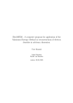
After some time Linux will be up and running and you arrive at the command line
prompt. See figure 4.1.
Figure 4.1: A booted Montavista Linux
You can now try typing a few commands on the prompt:
root@firststeps: ˜# pwd
/root
root@firststeps: ˜# ls /
LICENSE
dev
host
lost+found
proc
tmp
bin
etc
lib
mnt
root
usr
boot
home
linuxrc
opt
sbin
var
30
4.3. Checkpointing
root@firststeps: ˜#
Note: If the terminal console does not respond, make sure that the simulation is actually
running.
4.3
Checkpointing
In order to avoid booting First Steps every time, we use the facility known as configuration checkpointing or simply checkpointing. This enables Simics to save the entire state of the
simulation to disk. The files are saved in a portable format and can be loaded at a later time.
To write a checkpoint, use the write-configuration command. The command expects a
filename as argument. Name the checkpoint after_boot.conf.
[control-C]
simics>
write-configuration after_boot.conf
simics>
The state is now saved, and you can safely terminate the simulation.
simics>
quit
joe@computer: simics-workspace$
All that remains of the simulation is the checkpoint we just created. To load the checkpoint,
use the -c flag when starting Simics.
joe@computer: ebony$ ./simics -c after_boot.conf
[...]
simics>
The terminal contents is also restored and you should end up in the same state as before.
Remember to resume the simulation (by entering continue) before typing more commands
at the console.
You can read more about configuration and checkpointing in chapter 6.
4.4
Hindsight
Note: Hindsight requires a special license. This section can be skipped if Hindsight is not
available.
Hindsight enables the simulation to run backwards in time. To enable Hindsight, we have
to set an initial time bookmark. Time bookmarks are set with the set-bookmark command.
31
4.4. Hindsight
simics>
set-bookmark booted
simics>
c
Note: Typing c is a shorthand for continue.
To demonstrate the possibilities Hindsight gives, we will accidentally remove an important file on the simulated system. Enter the following commands in the simulated system’s
terminal:
root@firststeps: ˜# rm /bin/ls
root@firststeps: ˜# ls /
ls: No such file or directory
The program ls has been removed. You can no longer list the contents of a directory. Let
us use Hindsight to recover ls.
ptime is a useful command that shows the number of executed instructions and the
current simulated time. We will use it to show that the time have advanced backwards.
[press control-C]
simics>
ptime
processor
cpu0
steps
cycles
time [s]
16667617210
16667617210
166.676
simics>
The skip-to command can be used to quickly jump to a previous point in time. We
will use the bookmark we created before as our time-travel destination. Note that it is not
possible to reverse past the first bookmark.
simics>
skip-to bookmark = booted
simics>
ptime
processor
cpu0
steps
cycles
time [s]
13586370338
13586370338
135.864
simics>
The system is now in the state it was before the file was erased. Now, we run forward
again.
simics>
c
When you type something in the terminal, you will notice that it does not respond any
longer! Instead the same commands as before will be replayed.
This behavior is intentional, and keeps the deterministic property of the simulation,
which is invaluable when debugging. Keystrokes, network traffic and any other input is
replayed until the last known time is reached.
32
4.5. Getting Files into a Simulated System
In our example, this is not what we want. To erase all knowledge about the future, run
the clear-recorder command.
[press control-C]
simics>
skip-to bookmark = booted
simics>
clear-recorder
Replay of recorded input finished; Simics is now running normally
simics>
c
Resume the simulation and enter the following command:
root@firststeps: ˜# ls /
LICENSE
dev
host
lost+found
proc
tmp
bin
etc
lib
mnt
root
usr
boot
home
linuxrc
opt
sbin
var
root@firststeps: ˜#
ls works again!
You can read more about Hindsight in chapter 22.
4.5
Getting Files into a Simulated System
A full systems simulation can be run completely isolated, but Simics also provides a way
for the simulated system to access files that are located on the host, i.e, your real computer.
SimicsFS is a Linux kernel filesystem module that talks to a simulated device, namely a
corresponding Simics module. Our firststeps machine is prepared with simicsfs support; just mount /host to access it.
root@firststeps: ˜# mount /host
[simicsfs] mounted
root@firststeps: ˜# ls /host
bin
etc
lost+found
net
root
sys
boot
home
media
opt
sbin
tmp
[...]
root@firststeps: ˜#
Note: Support for SimicsFS have to be installed in the target system, which means it have
to be modified. Modules exists for the Linux 2.4 and 2.6 series. On other systems a module
has to be written in order to get SimicsFS to work.
As write support is experimental, SimicsFS is mounted read-only by default. To be able
to transfer files from the simulation to the host, mount it read-write.
root@firststeps: ˜# mount /host -o remount,rw
33
4.6. Debugging
root@firststeps: ˜# cp /proc/cpuinfo /host/tmp/cpuinfo
root@firststeps: ˜# umount /host
root@firststeps: ˜#
Now, we can read the file on our host machine.
[press control-C]
simics>
!cat /tmp/cpuinfo
processor
: 0
cpu
: 440GP Rev. C
revision
: 4.129 (pvr 4012 0481)
bogomips
: 799.53
vendor
: IBM
machine
: Ebony
simics>
Note: The ! command will interpret the rest of the command line as if it was given in a
shell.
Sometimes it is desirable to limit the accessible files to a certain directory. This is done
with the hhostfsi.root command. Set the root to the Simics installation directory.
[press control-C]
simics>
hfs0.root sim->simics_base
simics>
c
Now transfer the file to be used in next section into the simulated system.
root@firststeps: ˜# mount /host
[simicsfs] mounted
root@firststeps: ˜# cp /host/targets/ebony/images/debug_example .
root@firststeps: ˜#
You can read more about SimicsFS/hostfs and other ways to transfer files in chapter 7.
4.6
Debugging
Note: Some steps in this section require Hindsight. However, you will grasp the basic
debugging commands even if Hindsight is not available.
This section demonstrates some source-level debugging facilities that Simics provides.
Your Simics distribution contains an example code snippet called debug_example.c.
34
4.6. Debugging
Copy the source file and corresponding compiled executable into your workspace using
the following commands.
simics>
!cp [simics]/targets/ebony/debug_example.c .
simics>
!cp [simics]/targets/ebony/images/debug_example .
simics>
c
Replace [simics] with the Simics installation directory.
We recommend opening the file debug_example.c in an editor of your choice to easier
follow the debugging example. This file contains the code that we are going to debug. The
program is supposed to print some information about the users on a system.
In the previous section we copied the executable into the simulated system by using
SimicsFS. Now, run that program by starting it in the simulated terminal.
root@firststeps: ˜# ./debug_example
[...]
Got segmentation fault!
root@firststeps: ˜#
This output indicates that our program crashed. Let us use Simics features to debug it.
Simics needs to know the mapping between addresses and line numbers, and this information is stored in the executable. The symtable module in Simics contains commands
related to symbolic debugging.
[press control-C]
simics>
new-symtable file = debug_example
Created symbol table ’debug_example’
[symtable] Symbols loaded at 0x10000000
ABI for debug_example is ppc-elf-32
debug_example set for context primary_context
simics>
Note: Remember to write file =, otherwise you will create an empty symtable named
debug_example. You can add files to an existing symtable with the hsymtablei.addsymbol-file command.
To help debugging your programs, we have introduced magic instructions. These are
instructions that have no side-effects on a real machine, but can be programmed to do things
when run inside Simics, for example stop the simulation.
The debug example code contains such an instruction in the beginning of the main function. Enable break on magic instruction by the command magic-break-enable:
simics>
magic-break-enable
simics>
c
35
4.6. Debugging
Now rerun debug_example:
root@firststeps: ˜# ./debug_example
Simics will stop at the magic instruction and show the corresponding source code line
and assembly opcode.
[cpu0] v:0x10000634 p:0x00737b634
magic instruction (or r0,r0,r0)
main (argc=1, argv=0x7ffffe34) at /tmp/debug_example.c:73
73
MAGIC_BREAKPOINT;
simics>
As you can see, this magic instruction is effectively a no-operation, which means that
the simulation will run as usual on real hardware, or when magic breakpoints are disabled
in Simics.
Now let us find the cause of the segmentation fault. Place a breakpoint in the sigsegv_
handler() function. The sigsegv_handler() function is called when the program receives the
segmentation fault and will allow the program to gracefully exit.
simics>
break (sym sigsegv_handler)
Breakpoint 1 set on address 0x10000520 with access mode ’x’
1
simics>
Resume the simulation. It will stop at the signal handler, and by giving the stack-trace
command, you can also see the chain of function calls leading up to this point. This list
gives you useful hints about where the crash occurred.
simics>
c
Code breakpoint 1 reached.
[cpu0] v:0x10000520 p:0x00737b520
stwu r1,-32(r1)
sigsegv_handler (sig=0) at /tmp/debug_example.c:35
35
simics>
{
stack-trace
#0 0x10000520 in sigsegv_handler (sig=0) at /tmp/debug_example.c:35
#1 0x7ffff3d8 in ?? ()
#2 0xff06a44 in ?? ()
#3 0xff0ff60 in ?? ()
#4 0x100006ac in main (argc=1, argv=0x7ffffe34) at /tmp/debug_example.c:82
#5 0xfed5fdc in ?? ()
#6 0x0 in ?? ()
simics>
36
4.6. Debugging
Simics prints question marks when no symbol could be found at the address. This can
either be a bogus address or a function inside the standard library, to which no symbols
have been loaded.
A few frames down you have the main() function, which caused the crash. Now we run
the simulation backward into that function. reverse-step-line will run backwards until the
previous known source line is reached.
simics>
reverse-step-line
[cpu0] v:0x100006a8 p:0x00737b6a8
bl 0x10010c54
main (argc=1, argv=0x7ffffe34) at /tmp/debug_example.c:82
82
printf("Type: %s\n", user.type);
simics>
This line cause the crash. Let us examine what user.type contains:
simics>
psym user.type
(char *) 0xa94 (unreadable)
simics> psym user
{name = 0x7ffffdc0 "shutdown", type = (char *) 0xa94 (unreadable)}
simics>
As you can see, the type member points to an unreadable address, which caused the
crash. Where does this pointer come from? What we want to do is to find where the last
write to this pointer occurred.
Using Hindsight, we can first set a write-access breakpoint on the memory of interest,
and run backward (using reverse) until the breakpoint is reached. After some time will find
the place where the write takes place.
simics>
break -w (sym "&user.type") (sym "sizeof user.type")
Breakpoint 2 set on address 0x7ffffdc8, length 4 with access mode ’w’
2
simics>
reverse
Breakpoint on write to address 0x7ffffdc8 in primary_context.
Completing instruction @ 0xff365e0 on cpu0.
[cpu0] v:0x0ff365e4 p:0x0075275e4
beqlr
simics>
Now, examine the stack trace:
simics>
stack-trace
#0 0xff365e4 in ?? ()
#1 0x100005d8 in read_developer (p=0x7ffffdc0, f=0x10010ca0)
at /tmp/debug_example.c:60
#2 0x10000674 in main (argc=1, argv=0x7ffffe34) at /tmp/debug_example.c:80
37
4.6. Debugging
#3 0xfed5fdc in ?? ()
#4 0x0 in ?? ()
simics>
In the stack trace, you will see that a call from read_developer() have caused the
crash. Switch to that frame and display the code being run.
simics>
frame 1
#1 0x100005d8 in read_developer (p=0x7ffffdc0, f=0x10010ca0)
at /tmp/debug_example.c:60
simics>
48
list read_developer 15
{
49
char line[100], *colon;
50
51
if (fgets(line, 100, f) == NULL)
52
return 0;
/* end of file */
53
54
/* Type is always developer */
p->type = "developer";
55
56
57
/* Everything until the first colon is the name */
colon = strchr(line, ’:’);
58
60
59
*colon = ’\0’;
strcpy(p->name, line);
61
return 1;
62
}
simics>
On line 60 you can see that while the name field was filled in using strcpy, our failing
pointer was accidentally overwritten (remember that the breakpoint was placed on the type
member). If you write psym line you will see that the string copied is "shutdown". A
look into the declaration of struct person shows that the name field is only 8 bytes big,
and hence has no space for the trailing null byte.
Check the contents of p after and before the actual write to verify it is overwritten.
simics>
psym "*p"
{name = 0x7ffffdc0 "shutdown", type = (char *) 0xa94 (unreadable)}
simics> reverse-step-instruction
Completing instruction @ 0xff365e0 on cpu0.
Breakpoint on write to address 0x7ffffdc8 in primary_context.
[cpu0] v:0x0ff365e0 p:0x0075275e0
stb r0,4(r5)
simics>
frame 1; psym "*p"
#1 0x100005d8 in read_developer (p=0x7ffffdc0, f=0x10010ca0)
at /tmp/debug_example.c:60
{name = 0x7ffffdc0 "shutdown\020", type = (char *) 0x10000a94 "developer"}
38
4.7. Tracing
simics>
To clean up after our debug session, we must remove the breakpoints that we have set.
They are identified with a number and can be shown using list-breakpoints.
simics>
delete 1
simics>
delete 2
simics>
magic-break-disable
simics>
You can read more about debugging in chapter 12. Magic instructions are described in
section 12.1.7.
4.7
Tracing
Tracing is a way to observe what is going on during the simulation. This section describes
how to trace memory accesses, I/O accesses, control register writes, and exceptions in Simics.
The tracing facility provided by the trace module will display all memory accesses, both
instruction fetches and data accesses.
First, launch the ebony-linux-firststeps.simics configuration, but not boot it.
Second, create a tracer:
simics>
new-tracer
Trace object ’trace0’ created. Enable tracing with ’trace0.start’.
simics>
Now we are going to trace a few of instructions executed when booting Ebony. We execute 300 instructions without tracing first to reach a sequence of instructions that includes
memory accesses:
simics>
continue 300
[cpu0] v:0xfffff160 p:0x1fffff160
simics>
tlbwe r1,r4,1
trace0.start
Tracing enabled. Writing text output to standard output.
simics>
continue 6
inst: [
1] CPU
0 <v:0xfffff160> [...] 7c240fa4 tlbwe r1,r4,1
inst: [
2] CPU
0 <v:0xfffff164> [...] 7c4417a4 tlbwe r2,r4,2
inst: [
3] CPU
0 <v:0xfffff168> [...] 38840001 addi r4,r4,1
inst: [
4] CPU
0 <v:0xfffff16c> [...] 4200ffdc bdnz+ 0xfffff148
inst: [
5] CPU
0 <v:0xfffff148> [...] 84050004 lwzu r0,4(r5)
data: [
1] CPU
0 <v:0xfffff1b8> [...] Read
1 bytes
0xc0
data: [
2] CPU
0 <v:0xfffff1b9> [...] Read
1 bytes
0x0
data: [
3] CPU
0 <v:0xfffff1ba> [...] Read
1 bytes
0x12
data: [
4] CPU
0 <v:0xfffff1bb> [...] Read
1 bytes
0x10
39
4.7. Tracing
inst: [
6] CPU
0 <v:0xfffff14c> [...] 2c000000 cmpwi r0,0
[cpu0] v:0xfffff150 p:0x1fffff150
beq- 0xfffff170
simics>
Lines beginning with inst: are executed instructions. Each line contains the address
(both virtual and physical) and the instruction itself, in both hexadecimal form and the
mnemonic.
Lines beginning with data: indicate that some instructions are performing memory
operations. Each line contains the operation address (again, both virtual and physical), the
type of operation (read or write), the size and the value.
Note: In the trace you can see one four-byte memory read that is split into four single-byte
reads. This reflects how Simics models the accesses to the flash memory it reads from.
It is also possible to only trace accesses to a certain device. This is done with the trace-io
command. In this example we are looking at in the interaction with the UART device.
simics>
trace0.stop
Tracing disabled
simics>
trace-io uart0
simics>
continue 30_000
[cpu0 -> uart0] Write: 0x140000203 1 0x80
[cpu0 -> uart0] Write: 0x140000200 1 0x48
[cpu0 -> uart0] Write: 0x140000201 1 0
[cpu0 -> uart0] Write: 0x140000203 1 0x3
[cpu0 -> uart0] Write: 0x140000202 1 0
[cpu0 -> uart0] Write: 0x140000204 1 0
[cpu0 -> uart0] Read: 0x140000205 1 0x60
[cpu0 -> uart0] Read: 0x140000200 1 0
[cpu0 -> uart0] Write: 0x140000207 1 0
[cpu0 -> uart0] Write: 0x140000201 1 0
[cpu0 -> uart0] Read: 0x140000205 1 0x60
[cpu0 -> uart0] Write: 0x140000200 1 0xd
[cpu0 -> uart0] Read: 0x140000205 1 0
[cpu0] v:0xfff8a634 p:0x1fff8a634
bl 0xfff8a608
simics>
Note: You can use underscores anywhere in numbers to make them more readable. The
underscores have no other meaning and are ignored when the number is read.
trace-cr turns on tracing of changes in the processor’s control registers.
simics>
untrace-io uart0
simics>
trace-cr -all
40
4.7. Tracing
simics>
continue 6_500_000
[cpu0] tcr <- 0
[cpu0] dec <- 0
[cpu0] decar <- 0
[cpu0] tsr <- 0x8000000
[cpu0] decar <- 0x51615
[cpu0] dec <- 0x51615
[cpu0] tcr <- 0x4400000
[cpu0] ivpr <- 0
[cpu0] msr <- 0x29000
[cpu0] msr <- 0
[...]
[cpu0] [cpu0] v:0x07fd8634 p:0x007fd8634
bl 0x7fd8608
simics>
We can single-step with the -r flag, to see what registers each instruction changes.
simics>
untrace-cr -all
simics>
step-instruction -r 10
[cpu0] v:0x07fd8608 p:0x007fd8608
mftbu r3
[cpu0] v:0x07fd860c p:0x007fd860c
mftbl r4
r4 <- 6529678
[cpu0] v:0x07fd8610 p:0x007fd8610
mftbu r5
[cpu0] v:0x07fd8614 p:0x007fd8614
cmpw r3,r5
[cpu0] v:0x07fd8618 p:0x007fd8618
bne+ 0x7fd8608
[cpu0] v:0x07fd861c p:0x007fd861c
blr
[cpu0] v:0x07fd8638 p:0x007fd8638
subfc r4,r4,r7
r4 <- 1384
[cpu0] v:0x07fd863c p:0x007fd863c
subfe. r3,r3,r6
[cpu0] v:0x07fd8640 p:0x007fd8640
bge+ 0x7fd8634
[cpu0] v:0x07fd8634 p:0x007fd8634
bl 0x7fd8608
simics>
Simics can also monitor exceptions. Here we will trace all system calls.
simics>
trace-exception System_call
simics>
c
[cpu0] (@ cycle 203963506) Exception 8: System_call
[cpu0] (@ cycle 205608905) Exception 8: System_call
[cpu0] (@ cycle 205617423) Exception 8: System_call
[...]
[control-C]
[cpu0] v:0xc01bc12c p:0x0001bc12c
simics>
addi r10,r10,1
untrace-exception -all
41
4.8. Scripting
simics>
Note:
There are variants of trace-io, trace-cr and trace-exception that will stop the simulation
when respective event occur. These commands begin with break-.
Why do we need to create an object to trace instructions? This is because the tracing
should be easy to customize to your needs. By changing some attributes, it is possible to
choose what to trace on, and control the output format. You can also build your own tracer
based on the source of this tracer. All attributes are described in the Reference Manual.
4.8
Scripting
The Simics command line interface (CLI) has some built-in scripting capabilities. When that is
not enough, Python can be used instead.
We will use a trace object as our example object:
simics>
new-tracer
Trace object ’trace0’ created. Enable tracing with ’trace0.start’.
simics>
There are two commands available for this object: htracei.start and htracei.stop.
For example, to start tracing:
simics>
trace0.start
Tracing enabled. Writing text output to standard output.
simics>
It is also possible to access an object’s attributes using CLI. The state of an object is contained in its attributes.
simics>
trace0->classname
base-trace-mem-hier
simics>
trace0->enabled
1
simics>
Variables in CLI are prefixed with $, and can hold a string, a number, or an object reference. In the following example the variable my_tracer references our trace0 object (i.e. it is
not a copy).
simics>
$my_tracer = trace0
simics>
$my_tracer->enabled
1
42
4.9. Simple Virtual Network
simics>
It is also possible to access the tracer from Python. All lines begin with a @ are evaluated
as a Python statement.
simics>
@trace_obj = SIM_get_object("trace0")
simics>
@trace_obj
<the base-trace-mem-hier ’trace0’>
simics>
@trace_obj.enabled
1
simics>
The Simics API is directly accessible from Python. The script below counts the number of
instructions that are executed until the register msr is modified. It imitates the functionality
of break-cr msr.
simics>
@start_cycle = SIM_cycle_count(conf.cpu0)
simics>
@msr = conf.cpu0.msr
simics>
@while conf.cpu0.msr == msr: SIM_continue(1)
[...]
simics>
@end_cycle = SIM_cycle_count(conf.cpu0)
simics>
@print "Executed", end_cycle - start_cycle, "instructions"
Executed 56 instructions
simics>
After you enter @while conf.cpu0.msr [. . . ] command, the simulation starts, and continues until the msr register is modified. When that happens (which should not take any
noticeable time), the simulation stops and the rest of the commands can be entered.
You can read more about scripting in chapter 8. The full description of the Simics API is
available in the Reference Manual.
4.9
Simple Virtual Network
Simics can simulate several machines simultaneously. These machines can be connected
together using a simulated Ethernet link.
This chapter uses a different launch configuration than the rest of the First Steps chapters. Before continuing, launch the ebony-linux-firststeps-multi.simics configuration.
joe@computer: simics-workspace$ ./simics targets/ebony/ebony-linux-firststeps-multi.simics
This configuration contains two similar machines, with their own CPU. Simics will run
the machines synchronized, by executing some instructions on one CPU and then switch to
the other.
Boot the two simulated machines by starting the simulation.
43
4.9. Simple Virtual Network
simics>
c
One of them will be assigned the Internet Protocol (IP) address 10.10.0.50 and the other
one 10.10.0.51. If you try to ping from one of the machines to the other, it will fail. This is
because the two machines have not yet been connected to the simulated network.
An Ethernet link is simulated using ethernet-link module. You can connect any number
of simulated network cards to the link.
[control-C]
simics>
new-ethernet-link
[ethlink0 info] Adjusting latency to 1e-05 s [...]
Created ethernet-link ethlink0
simics>
Next, we must connect the simulated network cards to this link:
simics>
ebony0_emac0.connect ethlink0
simics>
ebony1_emac0.connect ethlink0
simics>
ethlink0.info
Information about ethlink0 [class ethernet-link]
================================================
Latency : 10 us
Distribution : local
Filtering : enabled
Devices:
Local devices : <0:0> ebony0_emac0, <1:1> ebony1_emac0
Remote devices : none
Real network connection:
Connected : No
simics>
c
Now it should be possible to ping between the two simulated machines. Enter the following commands in the first machine.
root@firststeps: ˜# ping -c 2 10.10.0.51
PING 10.10.0.51 (10.10.0.51): 56 data bytes
64 bytes from 10.10.0.51: icmp_seq=0 ttl=64 time=0.0 ms
64 bytes from 10.10.0.51: icmp_seq=1 ttl=64 time=0.0 ms
--- 10.10.0.51 ping statistics --2 packets transmitted, 2 packets received, 0% packet loss
44
4.10. Connect to a Real Network
round-trip min/avg/max = 0.0/0.0/0.0 ms
root@firststeps: ˜#
You can read more about network simulation in chapter 9.
4.10
Connect to a Real Network
A simulation can be connected to a real network. By doing this, simulated computers and
real computers are able to communicate with each other.
Note: If you experience timing problems, for example TCP timeouts, when using real
network, the simulation is running too fast. In these cases, slow it down by using the enablereal-time-mode command.
Before following the steps in this example, launch a new ebony-linux-firststeps.
simics. Don’t boot it yet.
Connecting a simulated machine to a real network is done with one command:
simics>
connect-real-network 10.10.0.50
No ethernet-link found, creating ’ethlink0’.
No service-node found, creating ’ethlink0_sn0’ with IP ’10.10.0.1’.
Connecting device ’emac1’ to ’ethlink0’
Connecting device ’emac0’ to ’ethlink0’
NAPT enabled with gateway 10.10.0.1 on link ethlink0.
Host TCP port 4021 −> 10.10.0.50:21 on link ethlink0
Host TCP port 4023 −> 10.10.0.50:23 on link ethlink0
Host TCP port 4080 −> 10.10.0.50:80 on link ethlink0
Real DNS enabled at 10.10.0.1 on link ethlink0.
simics>
continue
Note: Note that the IP address specified in the connect-real-network command is the IP
address of the simulated machine
This command will create a new ethernet-link, connect it to both the simulated network
cards, and to the real network. It will also enable NAPT, network address port translation.
Finally, it will forward ports 4021, 4023 and 4080 to the simulated machine’s telnet, FTP and
HTTP ports.
To actually make the real network accessible from the simulated machine, the simulated
system must be configured. These commands set up the service node as gateway and domain name server:
root@firststeps: ˜# route add default gw 10.10.0.1
root@firststeps: ˜# echo nameserver 10.10.0.1 > /etc/resolv.conf
45
4.10. Connect to a Real Network
root@firststeps: ˜#
This tells the simulated system to direct all accesses outside the local network to the
gateway at 10.10.0.1 (which is the service node connect-real-network created for us).
Now, if your computer is connected to Internet, we can try to telnet to a real computer
on Internet. In this example we use gnu.org.
root@firststeps: ˜# telnet gnu.org 80
GET /
<!DOCTYPE HTML PUBLIC "-//IETF//DTD HTML 2.0//EN">
<HTML><HEAD>
<TITLE>301 Moved Permanently</TITLE>
</HEAD><BODY>
<H1>Moved Permanently</H1>
The document has moved <A HREF="http://www.gnu.org/">here</A>.<P>
<HR>
<ADDRESS>Apache/1.3.31 Server at gnu.org Port 80</ADDRESS>
</BODY></HTML>
Connection closed by foreign host.
root@firststeps: ˜#
Since connect-real-network forwards ports to the telnet, FTP and HTTP ports of the simulated machine, it is possible to telnet into the simulated machine, or access its web server
from a web browser. To access the web server, enter the address http://localhost:4080
in a web browser on your real machine.
In an new shell on your computer, you can also try to telnet into the simulated machine:
joe@computer: ˜$ telnet -l root localhost 4023
Trying 127.0.0.1...
Connected to localhost.localdomain.
Escape character is ’ˆ]’.
Welcome to MontaVista Linux 2.1, Professional Edition
BusyBox v0.60.2 (2002.08.28-16:54+0000) Built-in shell (ash)
Enter ’help’ for a list of built-in commands.
# exit
Connection closed by foreign host.
joe@computer: ˜$
You can read more about real network in chapter 10.
46
4.10. Connect to a Real Network
Figure 4.2: Montavista Linux HTTP server front page
47
4.10. Connect to a Real Network
48
Chapter 5
Command-line Interface: Basics
The Simics command-line uses GNU Readline to provide command-line editing and a command history buffer.
Let us go through a list of handy commands for Simics common usage:
Simulation
At the Simics prompt, you can run the simulation with the continue (c) command,
followed by the number of steps you want to run. If no argument is provided, the
simulation will run until control-C is pressed in the Simics console.
You can also use stepi (si) to make the simulation progress step by step. You can use
the step-cycle (sc) command to make the simulation progress cycle by cycle. Note
that as long as you do not use timing models, si and sc are equivalent. For more
information, see chapter 17.
Simulation State
All processors support the pregs command to show the state of the main registers. The
argument -all will allow you to inspect all the registers instead of the usual working
set.
If the processor has floating-point registers, pfregs can be used to print them out. By
default, the pregs command (and other commands dependent on the CPU) uses the
current CPU scheduled by the simulation. You can change the current selected CPU
by using the pselect command. This won’t affect the simulation scheduling.
You can inspect and change the contents of a register by using the read/write-reg commands. Using % is equivalent to the read-reg command (i.e., %pc, %eax, ...). You
can inspect and change the contents of the memory by using the commands get, x and
set.
To get statistics concerning the current CPU, you can use the ptime and pstats commands.
Scripts
Simics can execute Python commands directly at the prompt; they just need to be
prefixed by the symbol @. You can also evaluate Python expressions in the middle of
a command by placing them between backquotes:
49
--- this is Python’s print()
simics> @print conf.cpu0.name
cpu0
--- this is CLI’s echo
simics> echo ‘conf.cpu0.name‘
cpu0
simics>
Note: ’@’ will only be recognized as starting a python command if it is the first character
on the command-line. It will be treated normally otherwise.
Simics can load both Simics scripts (a file containing a list of acceptable commands
for the Simics frontend) or Python script with the commands run-command-file and
run-python-file. You can read more about Simics scripting in chapter 8.
Modules
Simics usually handles modules automatically when loading a configuration. You
may however want to load a specific module by yourself with the load-module command.
The modules currently loaded are available through the list-modules command. If a
module fails to be loaded, it will be listed by the list-failed-modules command, along
with an explanation of the problem. You can use the -v argument to get the exact error
message preventing the module from loading.
Command-Line Interface
You can ask Simics to run command every time it returns at the prompt, using the
display command. For example:
simics> display ptime
display 1: ptime
simics> si
[cpu0] v:0xfffffffff0000024 p:0x000007fff0000024 nop
processor
steps
cycles
time [s]
cpu0
1
1
0.0
simics> c 100
[cpu0] v:0x000007fff0102190 p:0x000007fff0102190 sub %o2, 8, %o2
processor
steps
cycles
time [s]
cpu0
101
101
0.0
simics> undisplay 1
simics>
50
To stop the command from being run every time, use undisplay number where number
is the number that was returned by display for this specific command (in the example,
1).
The print command allows you to print out a value in different ways (binary, hexadecimal, etc.). You can control the way the command-line handles numbers with the
following commands: output-radix allows you to choose a default base for printing
numbers; digit-grouping can be used to group digits in a number in a more readable
way.
The CLI also supports the following Unix shell-like commands: cd, date, dirs, echo,
ls, popd, pushd, pwd. All of them are performed of the host machine, not on the
simulated machine.
51
52
Chapter 6
Configuration and Checkpointing
Simics includes a configuration system used to describe the state of the simulated machines.
Simics’s configuration system is object-oriented: a simulated machine is represented as
a set of objects that interact when the simulated time advances. Typically, processors, memories and devices are modeled as objects. Each object is defined by a number of properties
that are called attributes. A processor object, for example, will have an attribute called freq_
mhz to define its clock frequency (in MHz).
Simics’s configuration system is flexible: it is possible to create and delete objects dynamically, as well as access the attributes of all objects for reading and writing at any time.
Simics’s configuration system allows its elements to be saved so that a complete simulated machine state can be written to a set of files. This set of files is called a checkpoint.
This chapter describes the Simics configuration system as well as the different layers
built on top of it to handle more specific tasks:
• Checkpoints: how a simulated state is saved and restored via checkpointing;
• Inspection: how the simulated state can be examined and changed during simulation;
• Start Scripts: the components and scripts used to define the initial state of a machine
in the examples provided with Simics.
6.1
Basics
As mentioned above, Simics’s configuration system is object-oriented. A Simics object is
instantiated from a Simics class. The core of Simics defines some useful classes, but most
of the classes (processors, device models, statistic gathering extensions) are provided by
modules that are loaded by the simulator when requested.
For example, the x86-p4 module defines, surprisingly, the x86-p4 class. Note that a module may define several classes. Since modules advertise the classes they define, Simics can
load modules transparently as objects are instantiated.
A class defines attributes that represent both the static and dynamic state of the instantiated objects. The static state includes information that doesn’t change during the simulation
(like a version number in a register) while the dynamic state covers the part of the device
that are affected by the simulation (registers, internal state, buffers, etc.).
53
6.2. Checkpointing
Let us take the example of an x86-p4 processor and have a closer look:
• We can create an object instantiated from the class x86-p4. Let us call it cpu0
• The attribute freq_mhz can be set to 1500. It defines the processor clock frequency (in
MHz)
• The attribute physical_memory can be set to a memory space object, such as phys_
mem0. This attribute points to the object that will answer to the memory accesses
coming from the processor.
• etc.
As you noticed, attributes may be of various types. A complete description is available
in the next section.
6.2
Checkpointing
Simics’s configuration system can save the complete state of a simulation in a portable way.
This functionality is known as checkpointing, and the set of files that represent the elements
of the systems are called a checkpoint.
Saving and restoring a checkpoint can be done on the command-line with the writeconfiguration and read-configuration commands.
A checkpoint consists of the following files:
• A main file called configuration file (usually terminated by .conf, but this is only a
convention). This file is a text representation of the objects present in the system.
• An optional raw data file (described below), having the same name as the configuration file, with the suffix .raw appended.
• Optional image files (described in section 6.2.2), having the same name as the configuration file, with the suffix .object_image appended.
Below is a portion of a checkpoint file showing an object. Saved objects are always
represented as OBJECT object-name TYPE class-name { attributes }. In this case we have an
instance of the AM79C960 class (a 10Mbits ISA Ethernet card with on-board DMA) named
lance0. The irq_dev and the irq_level attributes connect the device to a controller that will
handle the interrupts it generates. Since this device has on-board DMA, it is also connected
to memory with the memory attribute.
...
}
OBJECT lance0 TYPE AM79C960 {
mac_address: "10:10:10:10:10:30"
irq_dev: isa0
irq_level: 7
54
6.2. Checkpointing
memory: pci_mem0
...
}
OBJECT ... TYPE ... {
...
Objects are saved in the main checkpoint file in no specific order.
6.2.1
Attributes
The short example of the lance0 description only uses three types of attribute values: strings,
objects, and (signed 64-bit) integers. The possible attribute types are:
string
Strings are enclosed in double quotes, with C-style control characters: "a string\n"
integer
Integers can be in hexadecimal (0xfce2) or signed decimal (-17) notation.
boolean
One of TRUE or FALSE.
floating-point
Specified in decimal (1.0e-2) or hexadecimal (0x5.a21p-32) style, just like in C.
object
The name of a configuration object: cpu0.
raw data
Arbitrary data; typically used to save large dumps of binary information. The data
itself is stored in the raw data file. The syntax is [R length-in-bytes filename file-offset].
list
Comma-separated list of any attribute values, enclosed in parentheses. Example: ("a
string", 4711, (1, 2, 3), cpu0)
dictionary
The format is a comma-separated list of key/value pairs, like in: { "master-cpu"
: cpu0, "slave-cpu" : cpu1 }. The key should be a string, integer or object,
while the value can be of any attribute type. Dictionaries are typically used to save
Python dictionaries in a checkpoint. Keys must be unique, although Simics does not
enforce this.
Each attribute belongs to one of the following categories. Note that only attributes of the
first two categories are saved in checkpoints.
Required
Required attributes must be set when creating an object. They are saved in checkpoints. If you edit a checkpoint, you should never remove a required attribute—Simics
will complain and refuse to load the checkpoint if you do.
55
6.2. Checkpointing
Optional
If no other value is provided, optional attributes take their default value when the
object is created. They are saved in checkpoints, but if you edit them out they will
revert to their default value when the checkpoint is loaded.
Session
Session attributes are only valid during a Simics session. They are not saved in checkpoints. They are usually used for statistics gathering or values that can be computed
from the rest of the object state.
Pseudo
Pseudo attributes are not saved in checkpoints and usually contain read-only information that does not change, or that is calculated when the attribute is accessed. Pseudo
attributes are in some cases used to trigger state changes in the object when written.
There are two special cases in the attribute checkpointing process. The first one, described above, concerns raw data. Raw data is saved in a separate file that belongs to the
checkpoint file set. The main configuration file only contains a pointer to the corresponding
data in the raw data file.
The second one concerns images.
6.2.2
Images
Simics implements a special class called image for objects that potentially need to save a
huge amount of state, like memories and disks. An image represents a big amount of raw
data using pages and compression to minimize disk usage.
To save space and time, images do not save their entire state every time a checkpoint is
written. They can work in two ways:
• Images can save their state incrementally. At each checkpoint, an image saves the difference between its current state and the previously saved state (either the previous
checkpoint or the initial state). This is the default behavior implemented by Simics.
This allows several checkpoints to be saved and restored using the same base image
and a series of difference files.
• Images can be used as read-write media. In that case the file representing the data is
always up to date to the current state. However, this prevents the image from being
used in a previously saved checkpoint or initial state, since its contents are modified
as the simulation advances.
It is important to understand that when used in incremental mode, images create dependencies between checkpoints. A checkpoint can only be loaded if all previous checkpoints
are intact.
To re-use the example above, let us have a look at the disk image of the same x86 computer:
...
56
6.2. Checkpointing
}
OBJECT disk0_image TYPE image {
...
files: (("enterprise3-rh73.craff", "ro", 0, 0x4c5abc000, 0),
("checkpoint-1.disk0_image", "ro", 0, 0x4c5abc000, 0))
size: 0x4c5abc000
...
}
...
The checkpointed image is based on the file enterprise3-rh73.craff, on top of
which is added the file checkpoint-1.disk0_image that contains the difference between the checkpoint checkpoint-1 and the initial state.
Files like checkpoint-1.disk0_image are often called diff files because they contain
the difference between the new state and the previous state.
Image Search Path
This section contains more in-depth explanations about image handling that you may skip when
reading this guide for the first time.
When successive checkpoints are saved, an image object may become dependent on
several diff files present in different directories. To keep track of all files, Simics stores in the
checkpoint a checkpoint path list that contains the absolute directory paths where image files
may be found. Images filenames are then saved as %n%/filename where %n% represents the
number of the entry in the checkpoint path, counting from zero.
Note: Simics’s checkpoint path is different from Simics’s search path (see section 15.4),
although both will be used when looking for image files, as show below.
To summarize, when loading a checkpoint or a new configuration, Simics looks for images in the following way:
• If the filename doesn’t contain any path information (like image.craff) or contains a
relative path (like test/image.craff), the file is looked up first from the checkpoint
directory, then from all the path entries in Simics’s search path, in order (see also section
15.4 for more information).
For example, if Simics’s search path contains [workspace]/targets/sunfire/
and the checkpoint is located in /home/joe/checkpoints/, Simics will look for
the file test/image.craff in the following places:
1. /home/joe/checkpoints/test/image.craff
2. [workspace]/targets/sunfire/test/image.craff
• If the filename contains a checkpoint path marker (%n%), the marker is translated using
Simics’s checkpoint path and the file is looked up in the corresponding path.
57
6.2. Checkpointing
For example, if Simics’s checkpoint path contains /home/joe/c1:/home/joe/c2,
the file %1%/image.craff will be translated into /home/joe/c2/image.craff.
• If the filename contains an absolute path (like /home/joe/image.craff), the file
path is used as is.
Note: The reason why Simics’s search path is involved in the process is that it makes
writing new configurations easier. Adding a path to the place where all initial images are
located allows you to just specify the image names.
6.2.3
Saving and Restoring Persistent Data
As an alternative to checkpointing, Simics allows you to only save the persistent state of a
machine, i.e., data that survive when the machine is powered-down. This typically consists
of disk images and flash memory or NVRAM contents. A persistent data checkpoint is
handled exactly like any other checkpoint and contains the same file set, but only objects
containing persistent data are saved. This persistent data checkpoint can be loaded on top
of a corresponding configuration later on.
The commands save-persistent-state and load-persistent-state respectively save and
load the persistent data in a configuration.
Note: These commands are often used to save the state and reboot a machine after the
disk contents have been modified. Remember that the target OS might have cached disk
contents in memory. In order to have a clean disk that can be used at boot, you should
synchronize the disk, for example by running init 0 on a Unix target system, or shutting
down the operating system, before you issue the save-persistent-state command.
6.2.4
Modifying Checkpoints
Checkpoints are usually created by saving a configuration inside Simics, but it is possible to
edit or even create checkpoints yourself.
Because a minimal checkpoint only has to include required attributes, creating a checkpoint from scratch works relatively well for small configurations. We suggest you use an
existing checkpoint as a starting point if you wish to do that. Note that more advanced
layers have been built on top of the configuration system to make the creation of a new
machine much easier. Refer to section 6.5 for more information.
Modifying checkpoints require some extra care. Adding or removing devices may confuse the operating system, which does not expect devices to appear or disappear while the
system is running, and cause it to crash.
Changing the processor frequency may be enough to confuse the operating system.
Many operating systems check the CPU frequency at boot time, and base their waiting loops
and timing on the value they got. Saving a checkpoint and changing the frequency after boot
may affect the simulation and confuse the system. Devices that use processor frequency to
58
6.3. Inspecting the Configuration
trigger events at specific times may also behave strangely when the frequency suddenly
changes.
6.2.5
Merging Checkpoints
If you want to make a checkpoint independent from all previous checkpoints, for example
to distribute it, you can use the small checkpoint-merge program in [simics]/bin from
your system command line. It merges the checkpoint with all its ancestors to create a checkpoint that has no dependencies. Specify the checkpoint you want to distribute as the first
parameter and the name of the new stand-alone checkpoint as the second. This tool can
be used in both Unix and Windows environments, but it can not handle Cygwin paths on
Windows.
6.3
Inspecting the Configuration
Object attributes that are of type integer, string or object are directly accessible at the
command-line with the notation object->attribute:
# reading the EAX register in an x86 processor
simics> cpu0->eax
0
# writing a new value to EAX
simics> cpu0->eax = 10
simics> cpu0->eax
10
simics>
More information about the command-line and scripting is available in chapter 8.
The Eclipse-based User Interface includes a Configuration Browser that allows you to visually browse the complete state of the simulation.
Finally, objects and attributes (of all types) are also available when scripting Simics directly
in Python. Configuration objects are available under the conf namespace:
# reading the EAX register in an x86 processor
simics> @conf.cpu0.eax
0
# writing a new value to EAX
simics> @conf.cpu0.eax = 10
simics> @conf.cpu0.eax
10
simics>
More information about scripting Simics in Python is available in chapter 8.
59
6.4. Components
6.4
Components
All machines in [simics]/targets/architecture use components to create configurations.
A component is typically the smallest hardware unit that can be used when configuring a
real machine, and examples include motherboards, PCI cards, hard disks, and backplanes.
Components are usually implemented in Simics using several configuration objects.
Components are intended to reduce the large configuration space provided by Simics’s
objects and attributes, by only allowing combinations that match real hardware. This greatly
simplifies the creation of different systems by catching many misconfigurations.
Components themselves are also configuration objects in Simics. But to avoid confusion, they will always be referred to as components and the objects implementing the actual
functionality will be called objects.
6.4.1
Component Definitions
All machines are based on a top-level component. The top-level component is the root of the
component hierarchy and is often a motherboard, backplane, or system chassis.
When a component is created, it is in a non-instantiated state. At this stage only the
component itself exists, not the configuration objects that will implement the actual functionality. Once a complete configuration has been created, all included components can be
instantiated. When this happens, all objects are created and their attributes are set.
A standalone component is a component that can be instantiated without being connected
to a component hierarchy. A typical example is a hotplug device, such as a PC Card (PCMCIA) or an Ethernet link.
6.4.2
Importing Component Commands
Components in Simics are grouped by machine architecture, or by type, into several collections. Before a component can be used in Simics, the corresponding component collection
has to be imported. What the import actually does, is to add CLI commands for creating
components in the collection. The most common collections, that are not architecture specific, are memory, pci, std and timing. To import all collections that are used by the
Ebony machine for example, issue the following commands:
simics>
simics>
simics>
simics>
6.4.3
import-pci-components
import-std-components
import-memory-components
import-ppc440gp-components
Creating Components
The create-<component> command is used to create non-instantiated components. There
is one create command for each component class. The arguments to the create command
60
6.4. Components
represent attributes in the component. Standalone components can be created both noninstantiated and instantiated. To create instantiated components, there are new- commands,
similar to the create- commands.
The following code creates a non-instantiated ’ebony-board’ component representing an
Ebony Reference Board, called ’board’
simics> (create-ebony-board board cpu_frequency = 100
.......
mac_address0 = "00:04:ac:00:50:00"
.......
mac_address1 = "00:04:ac:00:50:01"
.......
rtc_time = "2003-09-03 11:17:00 UTC")
.......
The parentheses are needed to allow multi-line input. The command arguments set the
processor frequency, the MAC addresses of the on-board network adapters, and the time
and date of the real-time clock.
In multi machine configurations it is often useful to separate objects from the different machines by name. The command set-component-prefix str causes all following createcommands to prefix all created object names—including the names of the components themselves—
with the string str.
6.4.4
Connectors
A connector provides a means for a component to connect to other components. Connectors
have a defined direction: up, down, or any. The direction is up if it needs an existing hierarchy
to connect to; for example, the PCI-bus connector in a PCI device must connect to a PCI slot.
A connector has a down direction if it extends the hierarchy downwards; for example, a PCI
slot is a connection downward from a board to a PCI device. There are also non-directed
connectors, with direction any. You can only connect an up to a down connector or to an any
connector, and similar for down connectors. Connectors with the any direction can not be
connected together.
Many connectors have to be connected before the component is instantiated, while others can be empty. A standalone component, as described above, may have all connectors
empty.
A hotplug connector supports connect and disconnect after instantiation. Other connectors can only be connected, or left unconnected, when the configuration is created and may
not be modified after that point. A multi connector supports connections to several other
connectors. A typical example of a hotplug multi connector is the Ethernet link.
It is not possible to connect instantiated components with non-instantiated ones. The
reason is that the instantiated component expects the other to have all objects already created, and need to access some of them to finish the connection.
The info command of a component lists all connectors and some information about
them:
simics> board.info
Information about board [class ebony-board]
===========================================
61
6.4. Components
Implementing objects:
Connectors:
ddr-slot0
ddr-slot1
emac0
emac1
pci-slot0
pci-slot1
pci-slot2
pci-slot3
uart0
uart1
:
:
:
:
:
:
:
:
:
:
mem-bus
mem-bus
ethernet-link
ethernet-link
pci-bus
pci-bus
pci-bus
pci-bus
serial
serial
down
down
down
down
down
down
down
down
down
down
hotplug
hotplug
hotplug
hotplug
Since the component in the example isn’t instantiated yet, the list of implementing objects is
empty. The ebony-board has two slots for DDR SDRAM modules, four PCI slots, two serial
ports and two Ethernet ports. The memory slot is not listed as hotplug since DDR modules
have to be inserted when the machine is configured initially, while serial and Ethernet ports
support connect and disconnect in run-time. As the ebony-board is a top-level component,
there are no up connectors.
To enable input and output for the simulated machine, the following commands create a
serial text console and connects it to the uart0 connector of the Ebony board. Since the text
console only has a single connector, it does not have to be specified in the connect command.
simics> board.connect uart0 (create-std-text-console)
Created non-instantiated ’std-text-console’ component ’text_console_cmp0’.
Since no name is given the console component, a unique name will be assigned to it by
the configuration system. The create- command returns the name of the newly created
component, allowing it to be used as in the example above.
If the board only had a single serial connector, the uart0 connector name could have
been left out as well.
Since the machine needs some memory to run, we also add a DDR memory module to
our example. A CLI variable is used to hold the name of the memory component.
simics> $ddr = (create-ddr-memory-module rank_density = 128 module_data_width = 64)
Created non-instantiated ’ddr-memory-module’ component ’ddr_memory_module_cmp0’.
simics> board.connect ddr-slot0 $ddr
6.4.5
Instantiation
When a component hierarchy has been created, it can be instantiated using the instantiatecomponents command. This command will look for all non-instantiated top-level components and instantiate all components below them. The instantiate-components command
62
6.4. Components
can also be given a specific component as argument. Then only that component will be
instantiated, including its hierarchy if it is a top-level component.
simics> instantiate-components
If there are unconnected connectors left that may not be empty, the command will return
with an error.
When the instantiation is ready, all object and attributes have been created and initialized. In our example, a text console window should have opened. The hardware of the
simulated Ebony board is now properly configured, but since no software is loaded, it will
not show any output on the console if the machine is started.
6.4.6
Inspecting Component Configurations
The list-components command prints a list of all components in the system. All connectors
are included, and information about existing connections between them.
The info name-space command provides static information about a component, such as
the implementing objects and a list of connectors.
The status name-space command provides dynamic information about a component,
such as attribute values and a list of all current connections. The output from status in the
Ebony example:
simics> board.status
Status of board [class ebony-board]
===================================
Attributes:
rtc_time
cpu_frequency
mac_address0
mac_address1
:
:
:
:
2003-09-03 11:17:00 UTC
100
00:04:ac:00:50:00
00:04:ac:00:50:01
Connections:
uart0 : text_console_cmp0
ddr-slot0 : ddr_memory_module_cmp0
The Eclipse-based User Interface includes a Configuration Browser where the configuration can be browsed visually.
6.4.7
Accessing Objects from Components
When doing more advanced configuration of a machine, it may be necessary to access configuration objects and their attributes directly. Since the objects are created by the component system automatically during instantiation, the names of the implementing objects are
not known in advance. For this reason it is possible to query a component about what configuration objects are used to implement it, using get-component-object. The argument is
63
6.5. Ready-to-run Configurations
a name for the object that is the same for all components of the same class. A list of such
names, and their mapping to actual configuration object names, is available in the output
from the info command. The next example prints the pc attribute from the cpu object.
simics> p -x (board.get-component-object cpu)->pc
The get-component-object is mainly useful in scripts, when running interactively it is easy
to find object names using the info command, or list-objects.
The get-component-object command does not work for non-instantiated components
since they do not have any associated configuration objects. But it is possible to access
the pre_conf_objects of the non-instantiated component from Python using the get_
component_object() function. This functions works for both instantiated and noninstantiated components, and Python code as in the following example works in both cases:
@print "0x%x" % get_component_object(conf.board, ’cpu’).pc
6.4.8
Available Components
The Simics Target Guide for each architecture lists and describes all components that are
available.
6.5
Ready-to-run Configurations
Simics includes many customizable ready-to-run configurations. Because checkpoint files
are by definition very static, these example configurations are not checkpoint-based, but
rather build on components and scripts to generate a working simulated machine.
The example configurations are located in separate directories for each system architecture: [simics]/targets/architecture. Each of these directories contains a number of
Simics scripts (i.e., files containing Simics commands):
<machine>-common.simics
Script that defines a complete simulated machine, i.e., both hardware and software,
that can be run by Simics directly. The common script use the -system.include
script to define the hardware, and the -setup.include script for software configuration. The -common.simics scripts may add additional hardware in some cases.
These are the files you want to use to start the standard example machines in this directory.
<machine> in the script name is either a Unix machine name, or a some other name
that defines the hardware/software combination.
<machine>-<feature>-common.simics
A script that extends the -common.simics script with a new feature. Many minor
features, such as the processor frequency, can be controlled using parameters to the
common script, but features that are mutually exclusive are added as separate scripts.
Typical examples are scripts that add different diff-files to the same disk image in the
system setup.
64
6.5. Ready-to-run Configurations
<architecture-variant>-system.include
Script that defines the hardware of a machine. This script can be shared by several
simulated machines that are based on the same hardware. The hardware setup is
typically configurable using some standard parameters.
<machine>-setup.include
Script that defines the software and possibly configures the machine to run the selected
software, for example setting boot path, and scripting automatic login.
The example configurations are designed to work with the disk images distributed by
Virtutech. The machines are described in the Target Guides corresponding to each architecture.
Several machines may be defined for a given architecture, and thus the corresponding
architecture directory will contain several machine-common.simics scripts.
Note: The [simics]/home/machine directory contains deprecated example machines
provided for backward compatibility reasons. These machine configurations are based
on a combination of Simics and Python scripts. It is highly recommended to use
the component-based scripts defined in [simics]/targets/architecture rather than the
scripts in [simics]/home/machine.
6.5.1
Customizing the Configurations
There are several ways to customize the examples provided with Simics. The table below
shows them sorted by how simple they are to use.
Parameters
The machine scripts distributed with Simics can be modified by setting parameters
(CLI variables) before the script is actually run. This is the easiest way to change the
default configuration. Parameters can typically be used to change properties such as
the amount of memory, the number of processors and the primary MAC address. The
available parameters are listed in each Target Guide.
Scripts
A simulated machine is defined by several scripts, as described above. By replacing the -common.simics file with a user defined one, the system can be configured in more details while keeping the machine definition provided by the -system.
include file. Similarly the -setup.include can be replaced to configure different
software on the same machine.
Components
Components represents real hardware items such as PCI cards, motherboards, and
disks. Using components to configure a machine provides freedom to set up the
simulated machine in any way that is supported by the architecture. The -system.
include files use components to create their machine definitions. A complete description of components is provided earlier in this chapter.
65
6.5. Ready-to-run Configurations
Objects and Attributes
A component is implemented by one or more configuration objects in Simics, and
each object has several attributes describing it. Configuring machines on the object
and attribute level is not supported in Simics, and such configurations may not work
in future versions.
Below is an example of a simple configuration based on ebony, that uses parameters to
configure two machines slightly differently that both run in the same Simics session.
$freq_mhz = 100
$memory_megs = 128
$host_name = "ebony0"
set-component-prefix "ebony0_"
run-command-file "ebony-linux-common.simics"
$freq_mhz = 200
$memory_megs = 256
$host_name = "ebony1"
set-component-prefix "ebony1_"
run-command-file "ebony-linux-common.simics"
6.5.2
Adding Devices to Existing Configurations
The parameters available for each predefined machine allows the user to do minor modifications. It is also possible to extend the ready-to-run configurations with additional components without creating new machine setups from scratch. This is done by adding components and connecting them to the machine before the instantiate-components command is
run.
Since the machine setup scripts are located in the read-only master installation of Simics,
they should not be modified. User files that add new components should instead be placed
in the corresponding [workspace]/targets/architecture directory.
The following commands adds a SCSI controller, and one SCSI disk, to one of the PCI
slots in the predefined ebony-linux-common.simics file. The commands should be
placed in a file in the target directory for ebony in the workspace, for example in [workspace]
/targets/ebony/ebony-linux-scsi.simics
script-branch {
wait-for-variable machine_defined
$sym = (create-pci-sym53c810)
$scsi_bus = (create-std-scsi-bus)
$system.connect pci-slot2 $sym
$scsi_bus.connect $sym
$scsi_bus.connect (create-std-scsi-disk scsi_id = 0 size = 3221225472)
}
66
6.5. Ready-to-run Configurations
run-command-file "%script%/ebony-linux-common.simics"
The script works by starting a script branch that waits for the CLI variable $machine_
defined to be written. All machine defining scripts distributed with Simics sets this variable, by convention, when the complete machine has been created but before the components are instantiated. Since many script branches can wait for the same variable, it is possible to extend the same configuration from different scripts in this way.
When the machine has been created, and machine_defined variable is written, the
script branch continues to execute. It creates a SCSI controller, a SCSI bus and a 3GB disk,
and then connects them. The $system variable is defined in the ebony-system.include
where the machine is created. When the script branch has finished executing, the main script
will continue and run instantiate-components.
The example above extends the ebony-linux-common.simics file in the workspace
target directory. To access files in the target directory of the main Simics installation, the
%simics% path shortcut can be used:
run-command-file "%simics%/targets/ebony/ebony-system.include"
Here’s another example that adds a network card in PCI slot 3 and connects it to the
same network as the primary ethernet cards:
$create_network = yes
script-branch {
# wait for machine to be setup and connect the new eth before instantiation
wait-for-variable machine_defined
$add_eth = (create-pci-dec21143 mac_address = "10:10:10:10:10:28")
$system.connect pci-slot3 $add_eth
}
run-command-file "%script%/ebony-linux-common.simics"
ethernet_link_cmp0.connect $add_eth
67
6.5. Ready-to-run Configurations
68
Chapter 7
Managing Disks, Floppies, and
CD-ROMs
In order to use Simics, you must have images (also called disk dumps) with the operating system and the applications you plan to run. Depending on the type of machine you are using,
these images will corresponds to the contents of a disk, a flash memory, a CD-ROM, etc.
Virtutech provides images that work with the example machines located in the targets
directory.
Simics images are usually stored in a special format called craff (for Compressed Random Access File Format) to save disk space. Simics also accepts a raw binary dump as an
image. This is sometimes more practical if you are manipulating images outside Simics.
Simics comes with the craff utility to manipulate and convert images in craff format
(see section 7.1.7).
This chapter will explain the following:
• How to work with images in general
• How to use CD-ROMs and floppies with Simics
• How to use the SimicsFS filesystem
• How to import the contents of a real disk inside Simics
To provide you with a more practical overview, here are the ways you can install and
modify the operating system and the applications you wish to run:
Using Simics:
• You can install a completely new OS or simply copy files using a simulated CDROM drive, by linking it to a real CD-ROM drive on your host machine or by
using a CD image file (refer to sections 7.2.1 and 7.2.2).
• You can copy files from the simulated floppy drive by linking it to the real host
floppy device or by using a floppy image file (see sections 7.2.3 and 7.2.4).
• You can use SimicsFS to directly access your real file systems from the simulated
machine (see section 7.3).
69
7.1. Working with Images
• You can download files over the simulated network (see chapter 10).
Don’t forget to read more about images in section 7.1.1 to learn how to save or re-use
your changes.
Using External Programs
• You can install a new OS along with new programs on a real machine and create
an image from the real machine storage (disk, flash memory, etc.). Section 7.4
shows how to perform this with a disk.
• You can modify an image directly with Mtools (see section 7.1.4).
• You can modify an image directly via a loopback device (see section 7.1.5).
7.1
7.1.1
Working with Images
Saving Changes to an Image
If you modify or create new files on a storage device within Simics, you should remember
that by default images are read-only. This means that the alterations made when running
Simics are not written to the image, and will last only for the current Simics session. As
described in the 6.2.2 section, this behavior has many advantages. You may however want
to save your changes to the image to re-use them in future simulations.
The first thing you should do is to make sure that all the changes are actually written to
the media you are using. In many cases, the simulated operating system caches operations
to disks or floppies. A safe way to ensure that all changes are written back is to shutdown
the simulated machine.
When all changes have been written to the media in the simulation, you can save the
new contents of the image in different ways:
• Using the save-persistent-state command, all image changes for persistent storage
media are saved to disk as a persistent state. This is the recommended way of saving
your image changes.
• Using the himagei.save-diff-file command, you can manually save a diff file for the
images you are interested in.
• Using the himagei.save command, you can create a raw binary dump of the image that
is completely independent of all previous images and diff files. Note that this is not
the best way to get a new and shiny image, since the image is saved uncompressed,
which can take a lot of time and disk space.
Note: The himagei.save actually allows you to save a partial dump of an image, which may
be useful to dump a specific part of a disk or a floppy.
Once you have saved the images, you can do the following:
70
7.1. Working with Images
• If you used save-persistent-state, you can issue the load-persistent-state command
just after starting the original configuration. This will add the new changes to the
persistent storage media images and the machine will boot with the changes included.
This is the recommended way of using a saved persistent state.
For example, let us suppose that you saved some new files on the disk of the enterprise machine (started with the enterprise-common.simics script). You saved
the persistent state of the machine after stopping it to the persistent state file newfiles-added. You can easily create a small script to start enterprise with the new
files:
# enterprise-new-files.simics
run-command-file enterprise-common.simics
load-persistent-state new-files-added
• You can also load the original configuration and add the diff files manually to the
images, using the himagei.add-diff-file command.
• If you are building your own configurations (either as scripts or as checkpoints), you
can add the diff files to the files attribute of the corresponding image object. This
corresponds to what the himagei.add-diff-file command does.
If you save several persistent states or image diff files that are dependent on each other, it
may become cumbersome to take care of all these dependencies and to remember which files
are important or not. You can merge the states or image diff files to create a new independent
state:
• If you are working with persistent states, you can use the checkpoint-merge utility to create a persistent state that is independent of all previous files, including the
original images provided by Virtutech. This is the recommended way of creating
a new independent image. You can load it as usual with the load-persistent-state
command.
• If you saved some image diff files manually, you can use the craff utility described
below to merge the diff files yourself.
7.1.2
Reducing Memory Usage Due to Images
Although images are divided into pages that are only loaded on request, Simics can run out
of host memory if very big images are used, or if the footprint of the software running on
the simulated system is bigger than the host memory. To prevent these kind of problems,
Simics implements a global image memory limitation controlled by the set-memory-limit
command.
When the memory limit is reached, Simics will start swapping out pages to disk very
much like an operating system would do. The set-memory-limit command let you specify
the maximum amount of memory that can be used, and where swapping should occur.
71
7.1. Working with Images
Note: This memory limitation only applies to images. Although this is unlikely, Simics can
run out of memory due to other data structures becoming too large (for example memory
profiling information) even though a memory limit has been set.
7.1.3
Using Read/Write Images
As mentioned in section 6.2.2, images can also work as read-write media, although this is
not recommended. It can be useful sometimes when planning to make large changes to an
image (like installing an operating system on a disk).
To make an image read-write in your own configurations, simply set the second parameter (the “read-only” flag) of the files attribute in the image object to "rw".
In a ready-to-run example like enterprise, you can change this attribute after the configuration is completed:
# read the ’files’ attribute
simics> @files = conf.disk0_image.files
simics> @files
[[’enterprise3-rh73.craff’, ’ro’, 0, 20496236544L, 0]]
# provide the complete path to the file
simics> @files[-1][0] = "[workspace]/targets/enterprise/images/
enterprise3-rh73.craff"
# change the second element to make the file read-write
simics> @files[-1][1] = "rw"
simics> @files
[[’[workspace]/targets/enterprise/images/enterprise3-rh73.craff’,
’rw’, 0, 20496236544L, 0]]
# set the ’files’ attribute to its new value
simics> @conf.disk0_image.files = files
Note that by indexing files with the index -1, the last element of the array is accessed,
which is always the one that should be set read-write, in case files is a list of several files.
As you can see in the example above, Simics by default does not look for files in the
Simics search path when the files are used in read-write mode. If you do not provide a
complete path to a read-write file, a new file will be created in the current directory.
Use this feature with caution. Make sure to take a copy of the original image before
running Simics with the image in read-write mode. Remember to synchronize the storage
device within the target OS before exiting Simics, for example by shutting down the simulated machine.
72
7.1. Working with Images
Note: You can not access directly the files attributes by doing
@conf.disk0_image.files[-1][0] = "rw"
because the files attribute is not an indexed attribute. In this case, Python will read the
files attribute and change the element [-1][0] in the resulting list, but this list is then
discarded and the change produces no effect. The Simics Programming Guide contains a
longer discussion explaining the ambiguities introduced by indexed attributes and the []
location.
7.1.4
Editing Images Using Mtools
If you have an image that contains a FAT filesystem, you can use Mtools (http://mtools.
linux.lu) to get read-write access to the image. You must have a raw binary dump of the
image for Mtools to work. This can be obtained using the craff utility (see section 7.1.7).
If your image is partitioned (a complete disk for example), you may need to give Mtools
special parameters like an offset or a partition. Refer to the Mtools documentation for more
information.
7.1.5
Editing Images Using Loopback Mounting
If the host OS supports loopback devices, like, e.g., Linux and Solaris, you can mount an
image on your host machine and get direct read/write access to the files within the image.
If you have root permissions this allows you to easily and quickly copy files.
Note: Remember that the image must be a raw binary dump. Disk dumps supplied by
Virtutech are normally in craff format but you can use the craff utility to unpack the
disk image to a raw image. The resulting images have the same size as the simulated disk,
so you need to have sufficient free space on your host disk to contain the entire simulated
disk image.
Note: Do not try to loopback mount an image over NFS. This does not work reliably on all
operating systems (Linux, for example). Instead, move the image to a local disk and mount
it from there.
On Solaris 8 or later:
lofiadm -a disk_dump /dev/lofi/1
mount /dev/lofi/1 mnt-point
...
umount mnt-point
lofiadm -d /dev/lofi/1
On Linux:
73
7.1. Working with Images
mount <disk_dump> mnt_pnt -o loop=/dev/loopn,offset=m
Example:
# mount /disk1/rh6.2-kde-ws /mnt/loop -o loop=/dev/loop0,offset=17063424
# cd /mnt/loop
# ls
bin
dev
home
lost+found
opt
root
tmp
boot
etc
lib
mnt
proc
sbin
usr
var
#
As shown in the example, the disk dump containing a Red Hat 6.2 KDE WS is mounted
on the /mnt/loop directory. The file system mounted on / starts on the offset 17063424 on
the disk. Linux autodetects the file system type when mounting (ext2 in this example). If
you want to access another kind of file system, use the -t fs option to the mount command.
Once the file system is mounted, you can copy files in and out of the disk image.
The offset can be calculated by examining the partition table with fdisk (from within
Simics). Use mount to find the partition you want to edit or examine (e.g., /dev/hda2 is
mounted on /usr which you want to modify). Next, run fdisk on the device handling
this partition (such as fdisk /dev/hda). From within fdisk, change the display unit to
sectors instead of cylinders with the u command and print the partition table with p. You
will now see the start and end sectors of the partitions; you can get the offset by taking the
start sector multiplied with the sector size (512).
When you have finished examining or modifying the disk, unmount it and touch the
disk image. For example:
cd
umount /mnt/loop
touch /disk1/rh6.2-kde-ws
The modification date of the disk image does not change when if you modify the disk via
the loopback device. Thus, if you have run Simics on the disk image earlier, the OS might
have cached disk pages from the now modified disk image in RAM. This would cause a new
Simics session to still use the old disk pages instead of the newly modified pages. Touching
the image file should ensure that the OS rereads each page.
7.1.6
Constructing a Disk from Multiple Files
In some cases, you may want to populate a simulated disk from multiple files covering
different parts of the disk. For example, the partition table and boot sectors could be stored
in a different disk image file than the main contents of the disk. If that is the case, you
cannot use the himagei.add-diff-file command: you must set manually the disk image files
attribute to put each image file at its appropriate location.
Assume you are simulating a PC and want to build a disk from a main file called hda1_
partition.img and a master boot record image file called MBR.img. The main partition
74
7.1. Working with Images
will start at offset 32256 of the disk, and the MBR (Master Boot Record) covers the first 512
bytes of the disk (typically, you would get the contents of these image files from the real disk
as detailed in section 7.4). The following command in Simics’s start-up script will build the
disk from these two files.
create-std-ide-disk disk2 size = 2559836160
@image = get_component_object(conf.disk2, ’hd_image’)
@image.files = [["hda1_partition.img", "ro", 32256, 1032151040, 0],
["MBR.img",
"ro",
0,
512, 0]]
Note that the two image files cover non-overlapping sections of the disk.
7.1.7
The Craff Utility
The images distributed by Virtutech, and in general most of the images created by Simics
are in the craff file format. The craff utility can convert files to and from the craff
format, and also merge several craff files into a single file.
In your Simics distribution you will find craff in [simics]/bin. The examples below
assume that craff is present in your shell path.
Convert a raw dump to craff format
shell$ craff -o mydisk.craff mydisk.img
Convert a single craff file to a raw file
shell$ craff --decompress -o mydisk.img mydisk.craff
Merge multiple checkpoint files into a single craff file
If more than one input file is specified, they will be merged so that later files override
earlier files on the command line.
shell$ craff -o merged.craff chkpt1.craff chkpt2.craff chkpt3.craff
Add a craff file to a raw dump, producing a new dump
shell$ craff --decompress -o new.img mydisk.img diff.craff
The input files can be any combination of raw and craff files.
Make a file of the differences of two dumps
shell$ craff --diff -o diff.craff dump1.img dump2.img
The resulting file, diff.craff, will contain only what is needed to add to dump1.
img in order to get dump2.img. This is useful to save space if little has been changed.
75
7.2. CD-ROMs and Floppies
See also the Simics Reference Manual for a full description of the craff utility and its
parameters.
7.2
CD-ROMs and Floppies
7.2.1
Accessing a Host CD-ROM Drive
Accessing the CD-ROM of the host machine from inside the simulation is supported on
Linux and Solaris hosts. This is done by creating a file-cdrom object using the new-filecdrom command. First, you should insert the CD in the host machine and figure out which
device name it uses.
On a Linux host, this is typically /dev/cdrom, which is a symbolic link to the actual
CD-ROM device, e.g., /dev/hdc. Note that you need read/write access to the CD-ROM
device for this to work.
On a Solaris host, you need to specify the raw disk device, which can be found by using
the mount command. The line that shows where the CD is mounted will look something
like this:
/cdrom/mydisk on /vol/dev/dsk/c0t2d0/mydisk read only/nosuid
on Fri Jul 26 11:52:52 2002
This means that the corresponding raw disk device will be called /vol/dev/rdsk/
c0t2d0/mydisk. Note the rdsk instead of dsk.
When you have the correct device file name, you create a file-cdrom object and insert it
into the simulated CD-ROM drive:
simics> new-file-cdrom /dev/cdrom file-cd0
cdrom ’file-cd0’ created
simics> cd0.insert file-cd0
Inserting media ’file-cd0’ into CDROM drive
Note that you must replace /dev/cdrom with the correct host device name as mentioned above, and cd0 with the correct Simics object name. Use the list-objects command
to find the correct object of class scsi-cdrom or ide-cdrom.
The cd0.insert command simulates inserting a new disk into the CD-ROM drive, and
there is also a corresponding cd0.eject command that simulates ejecting the disk.
7.2.2
Accessing a CD-ROM Image File
A file containing an ISO-9660 image can be used as medium in the simulated CD-ROM. This
image file can be created from real CD-ROM disks, or from collections of files on any disk.
An image can be created from a set of files with the mkisofs program, which is available
on both Linux and Solaris. For example:
76
7.2. CD-ROMs and Floppies
mkisofs -l -L -o image -r dir
Once you have an image file, a file-cdrom object can be created, and then inserted into a
simulated CD-ROM device in the same way as above:
simics> new-file-cdrom myimage.iso
cdrom ’myimage’ created
simics> cd0.insert myimage
Inserting media ’myimage’ into CDROM drive
Note that cd0 above refers to the Simics object name of the CD-ROM drive. This may, or
may not be called cd0. To see which object name to use, try the list-objects command and
look for an object of class scsi-cdrom or ide-cdrom.
7.2.3
Accessing a Host Floppy Drive
It is possible to access a floppy on the host machine from within Simics if the host is running
Linux or Solaris. For example (assuming the floppy device object is called flp0):
simics> flp0.insert-floppy A /dev/fd0
Note: To boot directly from the floppy on a simulated x86 architecture you need to select
the “A” drive to be the boot device (in, for example, enterprise-common.simics):
simics> system_cmp0.cmos-boot-dev A
7.2.4
Accessing a Floppy Image File
Sometimes it can be convenient to have copies of boot floppies as image files. To create an
image of a floppy you can use the Unix command dd:
dd if=/dev/fd0 of=floppy.img
It is then possible to use this image file in Simics:
simics> flp0.insert-floppy A floppy.img
77
7.3. Using SimicsFS
Note: To boot directly from the floppy on a simulated x86 architecture you need to select
the “A” drive to be the boot device (in, for example, enterprise-common.simics):
simics> system_cmp0.cmos-boot-dev A
Floppies are also a convenient way to move small amounts of data out of the simulated
machine. Write the data to the simulated floppy inside the simulated machine, and then
extract it from the image.
If it is formatted as FAT filesystem, a floppy image can be manipulated with Mtools (see
section 7.1.4 for more information).
7.3
Using SimicsFS
SimicsFS gives you access to the file system of your real computer inside the simulated
machine. This greatly simplifies the process of importing files into the simulated machine.
SimicsFS is supported for targets running Solaris 7, 8, 9 and 10, and Linux kernel versions 2.0, 2.2 and 2.4.
SimicsFS is installed on disk dumps distributed by Virtutech. For users booting from
other disks, there are a number of steps needed to configure the target system. This process
is target OS specific, and is described in the following sections.
SimicsFS is not fully functional on all simulated operating systems. The following limitations apply:
Simulated OS
Linux
Solaris
Other
7.3.1
Limitations
Access is read-only. (Write support experimental.)
Truncating files does not work.
SimicsFS is not currently available.
Installing SimicsFS on a Simulated Linux System
For Linux kernel versions prior to 2.4, the SimicsFS kernel module is called hostfs rather
than simicsfs, so for those kernels just replace the simicsfs part in file names with
hostfs in the following description. When the instructions ask you to copy files into the
simulated machine, one of the methods described elsewhere must be used (e.g., network,
loopback disk access, or CD-ROM).
• Since there are lots of different Linux kernels, and a module has to match the kernel
version, Simics does not provide any pre-compiled simicsfs modules. To build your
own simicsfs module, download the SimicsFS source code from https://www.
simics.net/pub/simicsfs.tar.gz. The README_2.4 and README_2.6 files
in the archive will explain how to add the SimicsFS sources to the Linux kernel tree
and compile it with the kernel you want to use.
78
7.3. Using SimicsFS
• Create a new directory /lib/modules/version/kernel/fs/simicsfs/ on the simulated machine, where version is the simulated machine’s kernel version.
• Copy the newly compiled SimicsFS module file to the directory /lib/modules/version/kernel/
fs/simicsfs/ on the simulated machine, and make sure it is called simicsfs.o for
Linux 2.4 (and older), and simicsfs.ko for Linux 2.6.
• Create the mount point on the simulated machine with mkdir /host.
• Add the following line in the simulated machine’s /etc/fstab (replace /host with
your mount point):
special
/host
simicsfs
noauto,ro
0 0
Note: To use the experimental write support, change ro into rw.
• Mount SimicsFS with the command mount /host on the simulated machine.
SimicsFS should now be working, and by issuing ls /host on the simulated machine,
you should get a listing of the host machine’s files.
7.3.2
Installing SimicsFS on a Simulated Solaris System
These are the steps needed to install SimicsFS on a simulated Solaris, version 7, 8, 9 and 10.
When the instructions ask you to copy files into the simulated machine, one of the methods
described above must be used (network, loopback disk access, CD-ROM. . . ). Note that the
driver included with earlier Simics distributions was called hostfs and not simicsfs.
• Create a new directory /usr/lib/fs/simicsfs/ on the simulated machine.
• Copy the file [simics]/import/sun4u/mount_simicsfs to /usr/lib/fs/simicsfs/
on the simulated disk, and rename it to mount.
• Copy the file [simics]/import/sun4u/simicsfs-solversion (where version matches
the version of Solaris running on your simulated machine) to /usr/kernel/fs/
sparcv9/ on the simulated machine, and rename it to simicsfs.
• Add the following line to /etc/vfstab on the simulated disk:
simicsfs
-
/host
simicsfs
-
no
-
• Create the mount point on the simulated machine with mkdir /host.
79
7.4. Importing a Real Disk into Simics
• When the simulated system is running, issue the command:
mount /host
You should now be able to do ls /host on the simulated system to get a list of the files
on the host.
7.3.3
Using SimicsFS
By default, the simulated machine can access the entire file tree of the host computer from
the mount point (typically /host).
This can sometimes be inconvenient (or dangerous, if the simulator runs untrusted or
unreliable code), so it is recommended to set the directory that is visible to the simulated
machine using the hhostfsi.root command, e.g.:
simics> hfs0.root /home/alice/sandbox
The command will take effect next time SimicsFS is mounted.
Because of implementation limitations, it is recommended that SimicsFS be chiefly used
to copy files into and out from the target machine. In particular, executing binaries residing
on the host machine may be unreliable.
Note: When saving a checkpoint while a SimicsFS is mounted, take care that the host files
that were used at that time are kept unchanged when the checkpoint is loaded.
7.4
Importing a Real Disk into Simics
It is possible to create an image by copying data from a real disk. If the disk to be copied
contains an operating system, you must have at least two operating systems on the machine,
since the partition that should be copied should not be in use or mounted.
Before making a copy of a disk, some information about the disk should be gathered:
• The number of disk cylinders
• The number of sectors per track
• The number of disk heads
• The offset where the specific partition starts (optional)
• The size of a specific partition (optional)
These numbers can be obtained using the fdisk utility.
You can choose to make a copy of the whole disk or just a partition from the disk using
the dd utility. Example:
80
7.4. Importing a Real Disk into Simics
dd if=/dev/hdb of=hdb_disk.img
Note: To save space, you may want to compress the disk image using the craff utility.
See section 7.1.7.
The next step is to prepare the target configuration so it can use the new disk. For x86
targets, the dredd machine has a $disk_files parameter that can be set to a list of files to
use in the image object of the boot disk, and also $disk_size that specifies the size of that
disk.
$disk_size = 1056964608
$disk_files = [["hdb_disk.img", "ro", 0, 1056964608, 0]]
For other machines, that do not have these parameters, attributes in the the disk object
and its corresponding image objects have to be set instead.
Make sure to set the $disk_size correctly to reflect the size of the disk that has been
copied. If only a partition has been copied, the offset where the partition starts, and the size
of the partition, should be set in the file list. If the whole disk has been copied, the offset is
zero and the size should be the size of the whole disk. Several partitions can be combined
to form the complete disk, as described in section 7.1.6.
For an x86 machine, the system component will automatically set the BIOS geometry for
the C: disk. It can also be set manually:
simics> system_cmp0.cmos-hd C 1023 16 63
81
7.4. Importing a Real Disk into Simics
82
Chapter 8
Simics Scripting Environment
The Command-Line Interface in Simics has simple scripting capabilities that can be used
when writing parameterized configurations and scripts with conditional commands. For
more advanced scripting, the Python language can be used.
This chapter describes how to write simple scripts in the Simics command line interface
(CLI), using control flow commands, and variables. It also explains how the configuration
system can be accessed from scripts, and how Python can be used for more advanced scripting.
All commands can be executed either by typing them at the prompt in the Simics console, or by writing them to a file, e.g. example.simics, and executing the command runcommand-file example.simics, or for Python examples: run-python-file example.py.
8.1
8.1.1
Script Support in CLI
Variables
The Simics command line has support for string and integer variables. Variables are always
prefixed with the $ character. Variables that are not set have a value of 0.
simics> $foo = "some text"
simics> $foo
some text
simics> echo $not_used_before
0
There is also support for indexed variables (arrays). This is useful in loops for example.
simics> $foo[0] = 10
simics> $foo[1] = 20
simics> echo $foo[0] + $foo[1]
30
CLI also has support for local variables, described later in this chapter.
83
8.1. Script Support in CLI
8.1.2
Command Return Values
The return value of a command is printed on the console, unless it is used as argument
to some other command. Parenthesis () are used to group a command with arguments
together, allowing the return value to be used as argument. The return value can also be
used as name-space in another command. Variables can be used in the same way.
simics> $address = 0
simics> set $address 20
simics> echo "The Value at address " + $address + " is " + (get $address)
The Value at address 0 is 20
simics> $id = 0
simics> ("cpu" + $id).print-time
processor
steps
cpu0
0
cycles
0
time [s]
0.0
simics> $cpu = cpu0
simics> $cpu.print-time
processor
cpu0
cycles
0
time [s]
0.0
steps
0
Parenthesis can also be used to enter a multi-line command, making it easier to read
scripts with nested command invocations. In the text console, the prompt will change to
....... for code spanning more than one line.
simics> (echo 10
.......
+ (20 - 5)
.......
+ (max 4 7))
.......
32
8.1.3
Control Flow Commands
The script support in CLI has support for standard if, else and while statements.
simics> $value = 10
simics> if $value > 5 { echo "Larger than five!" }
Larger than five!
The if statement has a return value:
simics> $num_cpus = 2
simics> (if $num_cpus > 1 { "multi" } else { "single" }) + "-pro"
84
8.1. Script Support in CLI
multi-pro
Note: Multi-line if-else statements must have } else { on the same line.
It is also possible to have else followed by another if statement.
simics>
.......
.......
.......
.......
.......
.......
.......
20
if $b == 1 {
echo 10
} else if $b == 0 {
echo 20
} else {
echo 30
}
Loops can be written with the while command.
simics> $loop = 3
simics> while $loop {
.......
echo $loop
.......
$loop -= 1
....... }
.......
3
2
1
In if and while statements, it can be useful to have variables that are local to the scope
and thus do not collide with the names of global variables. By adding local before the first
assignment of a variable, the variable is made local.
simics>
simics>
.......
.......
.......
.......
20
10
$global = 10
if 1 > 0 {
local $global = 20
echo $global
}
echo $global
85
8.1. Script Support in CLI
8.1.4
Integer Conversion
In some cases it is useful to interpret an integer as a signed value of a specific bit size, for
example when reading four bytes from memory that should be interpreted as a signed 32
bit integer. The signed8, signed16, . . . , signed64 commands can be used in to perform the
conversion. argument.
simics> phys_mem.set 0 0xffffffff 4
simics> phys_mem.get 0 4
4294967295
simics> signed32 (phys_mem.get 0 4)
-1
8.1.5
Accessing Configuration Attributes
Simics configuration attributes that are of string and integer type can be accessed directly
from CLI using the -> operator.
simics> echo "Will switch cpu every " + (sim->cpu_switch_time) + " cycles"
Will switch cpu every 1000000 cycles
8.1.6
Script Branches
Introduction to Script Branches
Script branches allow the user to write sequences of CLI commands that can wait for Simics
haps at anytime without breaking the sequential flow of commands. This is typically used
to avoid breaking a script into many small sections, each installed as a hap callback written
in Python.
A simple example from a Simics script:
script-branch {
echo "This is a script branch test - going to sleep."
cpu0.wait-for-step 10
echo "Processor registers after 10 steps:"
cpu0.pregs
}
The example above will execute the first echo command at once, and then go to sleep
waiting until the first 10 instructions (steps) have run. When the step counter for cpu0 has
reached 10, the branch will wake up and run the next two commands, echo and pregs.
Some commands can not be run while Simics is executing. One example is the writeconfiguration command. To issue such commands from a script branch, it is possible to
stop the execution, issue the command and then resume the simulation. The following is
86
8.1. Script Support in CLI
an example that writes a checkpoint when the simulation reaches a login prompt, and then
continues running. It assumes that a text-console called con0 is used.
script-branch {
con0.wait-for-string login
stop
write-configuration login.conf
run
}
Waiting for Haps in Script Branches
A common use of script branches is to wait for a hap to occur before continuing the script
execution. Most haps have some data associated with them, such as the exception number
for the Core_Exception hap used in the example below. This data can be accessed from
CLI by telling the wait-for-hap command to save it into a named indexed variable with local
scope. See the hap documentation for information on what data is associated with each hap
type.
script-branch {
wait-for-hap Core_Exception info
echo "Processor " + $info[0] + " got exception " + $info[1]
}
How Script Branches Work
When a script branch is started (using script-branch), it begins executing immediately, and
runs until a wait-for-, command is issued. Execution is then resumed in the main script;
i.e., there is never any concurrent activity. When a hap, or some other activity, occurs that
a script branch is waiting for, the branch continues executing once the currently simulated
instruction is ready.
Note: Since only one branch can be active at once, any callback to Python from Simics will
execute in the currently active branch, i.e., if a branch installs a callback, it is most likely that
it will be called when the main branch is active.
Script Branch Commands
The following is a list of the commands related to script branches.
script-branch
Create a new script branch and start it.
87
8.1. Script Support in CLI
list-script-branches
List all existing, but suspended, branches.
interrupt-script-branch
Interrupt a script-branch, causing it to exit.
wait-for-hap hap [object] [index|range-start] [range-end]
Suspend branch waiting for a hap to occur.
wait-for-variable variable
Suspend branch until a specified CLI variable is modified. This can be used for synchronization between script branches.
<processor>.wait-for-cycle cycle
Suspend branch until the specified cycle on the processor has been reached.
<processor>.wait-for-step step
Suspend branch until the specified step on the processor has been reached.
<text-console>.wait-for-string string
Suspend branch until string is printed on the text console.
Variables in Script Branches
Variable references in CLI are evaluated when accessed. This is important to remember
when writing script branches, since some commands are executed when the branch has
been suspended, and variables may have been changed. To make sure that CLI variables in
script branches are untouched by other scripts, they should be made local.
The following example
script-branch {
$foo = 20
cpu0.wait-for-step 10
echo "foo is " + $foo
}
$foo = 15
run
will produce the output foo is 15 while the following script will print foo is 20.
script-branch {
local $foo = 20
cpu0.wait-for-step 10
echo "foo is " + $foo
}
$foo = 15
run
88
8.2. Scripting Using Python
Canceling Script Branches
It is possible to cancel a suspended script branch by interrupting it using the interruptscript-branch command. Each branch has an ID associated that can be found using listscript-branches, and that is returned by the script-branch command.
$id = (script-branch {
wait-for-variable trigger
})
...
simics> interrupt-script-branch $id
Command ’wait-for-variable’ interrupted.
Script branch 1 interrupted.
Script Branch Limitations
There are some limitations to script branches. The first two in the list are enforced by Simics:
• Script branches may not start new branches.
• The main branch may not issue the wait-for- commands.
• Breaking the simulation with multiple control-C, which forces Simics back to prompt,
may confuse the Python interpreter about what thread is active. (Interrupting Simics
this way typically destroy the simulation state anyway.)
8.2
Scripting Using Python
Simics provides support for the script language Python (http://www.python.org). By
using Python the user can extend Simics, and control it in greater detail. Python can interface with Simics using functions in the Simics API.
8.2.1
Python in Simics
Python is normally hidden from the user by the command line interface (CLI). But since
CLI is implemented in Python, it also provides simple access to the Python environment,
making it easy to write your own functions and scripts.
Note: All commands in Simics are implemented as Python functions; the source code of
the commands is available in the distribution.
To execute some Python code from the command line, the @ character is used to prefix
the line. Example:
89
8.2. Scripting Using Python
simics> @print "This is a Python line"
This is a Python line
simics>
For code spanning more than one line, the prompt will change to ....... and more
code can be inserted until an empty line is entered. The full code block will then be executed.
(Note that whitespace is significant in Python.) Example:
simics> @if SIM_number_processors() > 1:
.......
print "Wow, an MP system!"
....... else:
.......
print "Only single pro :-("
.......
Wow, an MP system!
simics>
Entering more than one line is useful for defining Python functions. It is also possible to
execute Python code from a file, which is done with the run-python-file command.
If the Python code is an expression that should return a value to the CLI, the python
command can be used, or the expression can be back-quoted. The following example selects
a file with Python commands to execute depending on the number of processors in the
system:
simics> run-python-file ‘"abc-%d.py" % SIM_number_processors()‘
If the system has 2 processors, the file abc-2.py will be executed.
8.2.2
Accessing CLI Variables from Python
CLI variables can be accessed from Python via the simenv name space, for example:
simics> $cpu = "processor"
simics> @simenv.cpu = simenv.cpu.capitalize()
simics> $cpu
Processor
8.2.3
Accessing the Configuration from Python
Configuration Objects
All configuration objects are visible as objects in Python. The global Python module conf
holds all such objects. Attribute values can be both read and written using attributes in
Python. Example: (print the pci_devices attribute in a pci-bus object that is called pcibus25B
in the machine where the example was taken from)
90
8.2. Scripting Using Python
simics> @print conf.pcibus25B.pci_devices
[[2, 0, ’glm0’]]
To try this example in an arbitrary configuration, run list-objects pci-bus to find possible
pci-bus objects to use instead of pcibus25B.
Any ’-’ (dash) character in the object name, or in an attribute name, is replaced by ’_’
(underscore).
Indexed attributes can be accessed using [] indexing in Python. It is also possible to
index other list attributes this way, but it is inefficient since the full list is converted to a
Python list before the element is extracted. Here are some examples of indexed attributes
access (sb0 is a scsi-bus object, and phys_mem0 a memory-space object):
simics> @print conf.sb0.scsi_phases[1]
Arbitration
simics> @print conf.phys_mem0.memory[0x100000:0x10000f]
(157, 227, 191, 80, 3, 0, 0, 0, 130, 16, 96, 0, 131, 40, 112)
simics> @conf.phys_mem0.memory[0x100000:0x100003] = (100,101,102)
Warning: Python only supports 32 bit integers in keys when doing sliced indexing (no long
integers). However, the Simics API treats [m:n] synonymous to [ [m, n-1] ], so instead of
conf.phys_mem0.memory[0x1fff80082f0:0x1fff80082f8]
(which won’t work), write
conf.phys_mem0.memory[[0x1fff80082f0,0x1fff80082f7]]
Creating Configurations in Python
In addition to using .conf files, it is also possible to create and load configurations from
Python. The main advantage is that the configuration can be parameterized without the
need of multiple .conf files. A part of a configuration in Python, typically written as part
of a low-level machine setup, may look like:
scsi_bus = pre_conf_object(’sb5’, ’scsi-bus’)
sd_image = pre_conf_object(’sd5_image’, ’image’)
sd_image.size = 2128486400
sd = pre_conf_object(’sd5’, ’scsi-disk’)
sd.image = sd_image
sd.scsi_bus = scsi_bus
sd.scsi_target = 1
sd.geometry = [4157200, 1, 1]
91
8.2. Scripting Using Python
scsi_bus.targets = [[1, sd, 0]]
This will create one scsi-disk, one image and one scsi-bus pre-configuration object with
the names sd5, sd5_image and sb5. The pre-configuration objects are Python objects that
are used to build a configuration before it is actually loaded in Simics.
When all relevant pre-configuration objects have been added, they can be loaded into
Simics using the SIM_add_configuration() function.
SIM_add_configuration((sd_image, sd, scsi_bus), None)
This example can be run from a Python (.py) file.
Most configurations supplied with Simics are component based and written in Python.
However, the way configurations are created differs between targets. Refer to the corresponding Simics Target Guide for more information. Python files that are used to create
configurations can be found in the file:
[simics]/<host>/lib/<architecture>_components.py and, to some extent, in
each target architecture directory.
8.2.4
Accessing Command-Line Commands from Python
At times, it can be useful to access command-line commands from a Python script file. This
is done using the run_command(cli_string) function, which takes a string which is then
evaluated by the command-line front-end. For example, write run_command("pregs")
to execute the pregs command. Any return value from the command is returned to Python.
8.2.5
The Simics API
The Simics API is a set of functions that provide access to Simics functionality from loadable
modules (i.e., devices and extensions), and Python scripts. All functions in the Simics API
have a name that starts with “SIM_”. They are described in details in the Simics Reference
Manual.
By using the api-help and api-apropos commands you can get the declarations for API
functions and data types. api-help identifier will print the declaration of identifier. apiapropos identifier lists all declarations where identifier appears.
The Simics API functions are available in the sim_core Python module. This module is
imported into the Python environment in the frontend when Simics starts; for user-written
.py files however, the module must be imported explicitly, i.e.,
from sim_core import *
Errors in API functions are reported back to the caller using frontend exceptions. The exception is thrown together with a string that describes the problem more in detail. Examples
of exceptions are General, Memory, Index, IOError. . .
For the Python environment, Simics defines an exception subclass for each of its defined
exceptions in the sim_core module. These are raised to indicate exceptions inside the
92
8.2. Scripting Using Python
API functions. When errors occur in the interface between Python and the underlying C
API function, the standard Python exceptions are used; e.g., if the C API function requires
an int argument, and the Python function is called with a tuple, a Python TypeError
exception is raised.
8.2.6
Haps
A hap is an event or occurrence in Simics with some specific semantic meaning, either related
to the target or to the internals of the simulator.
Examples of simulation haps are:
• Exception or interrupt
• Control register read or write
• Breakpoint on read, write, or execute
• Execution of a magic instruction (see section 12.1.7)
• Device access
There are also haps which are related to the simulator, e.g., (re)starting the simulation or
stopping it and returning to prompt.
Note: In Simics documentation, the word event is used exclusively for events that occur at a
specific point in simulated time, and hap for those that happen in response to other specific
conditions (like a state change in the simulator or in the simulated machine).
Callback functions from any supported language can be tied to a certain hap. The callback can be invoked for all occurrences of the hap, or for a specified range. This range can
be a register number, an address, or an exception number, depending on the hap.
A complete reference of the haps available in Simics can be found in the Simics Reference
Manual.
Example of Python Callback on a Hap
This example uses functions from the Simics API to install a callback on the hap that occurs
when a control register is written. It is intended to be part of a .simics script, that extends
an UltraSPARC machine setup. The SIM_hap_add_callback_index() function sets the index
of the control register to listen to, in this case the %pil register in an UltraSPARC processor.
@pil_reg_no = SIM_get_register_number(conf.cpu0, "pil")
# print the new value when %pil is changed
@def ctrl_write_pil(user_arg, cpu, reg, val):
print "[%s] Write to %%pil: 0x%x" % (cpu.name, val)
# install the callback
93
8.2. Scripting Using Python
@SIM_hap_add_callback_index("Core_Control_Register_Write",
ctrl_write_pil, None, pil_reg_no)
In CLI, the same example would look like:
script-branch {
local $reg = ((current-processor).register-number pil)
while 1 {
wait-for-hap Core_Control_Register_Write $reg info
echo "[" + $info[0] + "] Write to %pil: " + $info[2]
}
}
94
Part III
Simics Networking
95
Chapter 9
Network Simulation
This chapter describes how Simics models networking. In the simulated environment, two
or more target systems may be connected together, forming a simulated network that is fully
virtualized. There are also ways to connect the simulated environment to outside systems,
by creating networks that connect to simulated systems at one end, and real systems at the
other.
This chapter focuses on networking based on simulated Ethernet links, but the principles
for network virtualization is not limited to Ethernet. Simple communication links, such as
serial connections can be simulated similarly.
9.1
Ethernet Links
Connecting simulated machines over a simulated Ethernet connection is done by creating
an ethernet-link object that connects to the Ethernet devices in the machines. The link object
can be thought of as modeling an Ethernet cable that is plugged in to the connectors on the
devices.
The link object models Ethernet at the frame level, in that it performs delivery of complete frames sent from one device to any other device connected to the link, and doesn’t
model collisions or lower-level signaling details. This means that it can be used either to
model point-to-point twisted-pair or fiber cables running at any speed, or even a 10BASE2
or 10BASE5 traditional coaxial bus, without any changes to the model. Another way of
viewing ethernet-link is to see it as an Ethernet hub or switch to which can be connected
two or more devices.
Traffic sent over the link can be anything, including TCP/IP or any other protocol stack
that works on top of Ethernet. The link object doesn’t need to be configured with any information about how it will be used.
New ethernet-link objects can be added with the new-ethernet-link command:
simics> new-ethernet-link
Created ethernet-link ethlink0
97
9.2. Link Object Timing
9.2
Link Object Timing
All frames that are sent over a link are delivered to the receiving device/devices at a point
in simulated time after the time when it was sent. The delay is the same for every frame,
and is called the latency of the link. The latency is a configuration parameter that can be set
individually for each link object.
Link objects are most often used to communicate between network devices using separate clocks, and because of how Simics handles simulated time, the clocks are not always
completely synchronized. To avoid strange causality effects and indeterministic simulation,
the latency of any link must not be set so low that data sent over it might reach the recipient
at a point in time that it has already passed. This imposes a lower boundary on the latency,
called the min-latency of the link. The value of the min-latency depends on the simulation
setup, in particular whether the simulation is distributed between several Simics processes
or not. See Chapter 11 for information about distributing the simulation.
The latency of a link can be displayed by the hethernet-linki.info command:
simics> ethlink0.info
Information about ethlink0 [class ethernet-link]
================================================
Latency : 1 us
Distribution : local
Filtering : enabled
Devices:
Local devices : none
Remote devices : none
Real network connection:
Connected : No
As can be seen from the example above, the default latency for an Ethernet link object is
one microsecond.
The latency of a link can be specified in the new-ethernet-link command as a number
of nanoseconds. If the latency of a link is set too low, it will be automatically adjusted to the
lowest value allowed by the setup. For example, if you launch a new multi machine setup,
such as ebony-linux-multi, and try to create a link with too low latency, Simics will adjust the
latency automatically:
simics> new-ethernet-link latency = 100
[ethlink0 info] Adjusting latency to 1e-005 s because the
min-latency changed
Created ethernet-link ethlink0
simics> ethlink0.info
Information about ethlink0 [class ethernet-link]
================================================
98
9.3. IP Services
Latency : 10 us
...
9.3
IP Services
It is often useful to be able to let the simulated machines use services available on the simulated network, especially for boot-time configuration. Instead of adding a full system simulation of servers running these services, a more efficient implementation is provided as a
Simics service node.
The service-node class provides a virtual network node that acts as a server for a number
of protocols, and it can act as a IP router between networks. The services supported are:
• IP Based Routing
• RARP
• DHCP/BOOTP
• DNS
• Bootparam/Whoami RPC (simplified)
• TFTP
• Real network connections (see section 10)
There can be any number of service-node objects, and each object can be connected to
any number of Ethernet links. In most configurations, however, there will usually be a
single service node object. The links themselves do not provide any services, so a service
node is needed to make the services available to target machines connected to the link.
A service node can be created using the new-service-node command:
simics> new-service-node
Created service-node sn0
This service node can then be connected to an Ethernet link object. For example, if
you already have an ethernet-link called ethlink0 and want the service-node to use the
IP address 10.10.0.1 on it:
simics> sn0.connect ethlink0 10.10.0.1
Connecting sn0 to ethlink0
Setting IP address of sn0 on network ethlink0 to 10.10.0.1
Note: The service node needs to have an IP address on each link it is connected to.
99
9.3. IP Services
The link to attach the service node to can also be specified when creating the service
node. This will make the default name given to the service reflect which link object it is
connected to. For example, if you already have an ethernet-link called ethlink0 and want
the service-node to use the IP address 10.10.0.1 on it:
simics> new-service-node link = ethlink0 ip = 10.10.0.1
Created service-node ethlink0_sn0
Connecting ethlink0_sn0 to ethlink0
Setting IP address of ethlink0_sn0 on network ethlink0 to 10.10.0.1
For each link that the service node connects to, a service-node-device will be automatically created to act as an Ethernet interface. The name of these device objects are a combination of the service node name and the link object name.
9.3.1
IP Based Routing
A service-node object can provide IP based routing between Ethernet links, allowing machines attached to different networks to communicate with each other.
Note: To use the routing mechanisms, simulated machines must use the IP address of
the service node as a gateway for IP based traffic. Configuring a gateway requires system
administration skills, and the exact procedure depends on the target operating system.
The service node contains an internal IP routing table that is used for packet routing
between connected links. The routing table can be viewed using the hservice-nodei.route
command:
simics> sn0.route
Destination Netmask
Gateway Port
----------------------------------------------------10.10.0.0
255.255.255.0
sn0_ethlink0_dev
The output is quite similar to route command available on many systems. The destination and netmask fields specify a target that can be either a network (i.e., a range of addresses) or a single host (with netmask 255.255.255.255). For packets with this target as
their destination, the port field specifies the service node network device on which link the
packet should be sent.
New entries can be added to the routing table with the hservice-nodei.route-add command. If you have a service-node called sn0 connected to two links called ethlink0 and
ethlink1, you could, for example, set up routes like this:
simics>
simics>
simics>
simics>
simics>
sn0.route-add
sn0.route-add
sn0.route-add
sn0.route-add
sn0.route
192.168.0.0 255.255.0.0 link = ethlink0
192.168.1.0/26 link = ethlink1
10.10.0.0 255.255.0.0 192.168.0.1 ethlink0
0.0.0.0 255.255.255.255 192.168.1.1 ethlink1
100
9.3. IP Services
Destination Netmask
Gateway
Port
----------------------------------------------------------192.168.0.0 255.255.255.0
sn0_ethlink0_dev
192.168.1.0 255.255.255.192
sn0_ethlink1_dev
10.10.0.0
255.255.0.0
192.168.0.1 sn0_ethlink0_dev
default
192.168.1.1 sn0_ethlink1_dev
The destination address and the netmask identify the target, and should be given as
strings in dotted decimal form. If the target is a single host, the netmask should be given as
"255.255.255.255".
9.3.2
DHCP and BOOTP
A service node can act as a Dynamic Host Configuration Protocol (DHCP) or Bootstrap Protocol
(BOOTP) server, responding to requests from clients that can read their network configuration from such a server. The DHCP protocol is an extension of the BOOTP protocol, and for
many uses the feature set used are more or less the same. The Simics implementation uses
the same configuration for both services.
The service node has a table that maps MAC addresses to IP addresses and domain
name. This is used to answer DHCP or BOOTP request. An entry to this table can be added
with the hservice-nodei.add-host command:
simics> sn0.add-host 10.10.0.1 node1 mac="10:10:10:10:10:01"
Adding host info for IP 10.10.0.1: node1.network.sim MAC: 10:10:10:10:10:01
The current contents of the table can be viewed with the hservice-nodei.list-host-info
command:
simics> sn0.list-host-info
IP
name.domain
MAC
----------------------------------------------10.10.0.1 node1.network.sim 10:10:10:10:10:01
A pool of IP addresses for dynamic DHCP leases can be added with the hservice-nodei.dhcpadd-pool command. This is used for dynamically assigning IP addresses to new clients.
When an entry from the pool is used, the new mapping is stored in the internal host info
table, including an automatically generated name that can be found through DNS queries.
If a DHCP client’s MAC address matches an entry in the table, it is assigned the corresponding IP address. If there is no matching MAC address, the dynamic address pools will
be searched for an available IP address.
The DHCP implementation in service-node is simple, and might not work with all
DHCP clients.
101
9.3. IP Services
9.3.3
DNS
The service node includes the functionality of a simple Domain Name Server (DNS), that a
simulated client can use to translate a host/domain name into an IP address and vice versa.
The DNS service is based on the same host table as the DHCP service, and only answers
requests for A and PTR records.
For entries in the table that will only be used for DNS requests, and not for assigning IP
address by means of DHCP, the MAC address can be left out. The hservice-nodei.add-host
command can be used to add table entries, and the hservice-nodei.list-host-info command
prints the current table. By default, all host entries will use the network.sim domain.
simics> sn0.add-host 10.10.0.1 donut
Adding host info for IP 10.10.0.1: donut.network.sim
simics> sn0.add-host 10.11.0.1 foo other.domain
Adding host info for IP 10.11.0.1: foo.other.domain
simics> sn0.list-host-info
IP
name.domain
MAC | IP
name.domain
MAC
----------------------------------+---------------------------------10.10.0.1 donut.network.sim
| 10.11.0.1 foo.other.domain
For dynamically added DHCP addresses, a DNS name will be added for the new IP
number, so that any address handed out by a DHCP server can be found by the DNS service.
When connected to a real network, the DNS service can do external lookups for names
it does not recognize.
9.3.4
TFTP
The service node also supports the Trivial File Transfer Protocol (TFTP, see RFC 1350) and can
be used to transfer files between the host system (running the simulation) and a simulated
(target) client. The TFTP functionality is often used in network booting, together with the
BOOTP facilities, to load OS kernels and images, and can also be used interactively from
the tftp command found on many systems.
Files that should be transferred from the host system to the simulated client should be
located in a directory on the Simics path.
Note: This is the same path as used by image objects and can be viewed with list-directory
command and modified with the add-directory command.
Files transferred from the simulated client to the host, will also end up in the same directory.
Note: TFTP is based on UDP, and each package is acknowledged individually before the
transfer is allowed to continue. Depending on the latency of the link, the transfer of large
files can be slow. In that case, ensuring that the link can use a lower latency will increase
performance.
102
9.4. Distributed Network Simulation
9.4
Distributed Network Simulation
The simulation of systems connected over an Ethernet network can be distributed over several Simics instances in a distributed simulation, as described in Chapter 11. A link object
can be configured to have global distribution, which means that several link object in separate Simics instances can form a shared link, over which all connected systems can communicate even if they are simulated by different Simics instances.
A link object with global distribution is automatically joined with any other link object
in another Simics instance if it also has global distribution and has the same name.
The way to make a link object have global distribution is to set its central attribute to
point to the central-client object. The hethernet-linki.info shows the current setting. (Note
that you must set up a central server and client as described in Chapter 11 for these examples
to work.)
simics> @conf.ethlink0.central = conf.central_client
simics> ethlink0.info
Information about ethlink0 [class ethernet-link]
================================================
Latency : 1 us
Distribution : global
Filtering : enabled
9.5
Serial Links
Connecting simulated machines over a simulated serial connection is done by creating a
serial-link object that connects to the serial devices in the machines. The link object can be
thought of as modeling a serial cable that is plugged in to the connectors on the devices.
The link object models serial communication at the character level in a simplified way.
The bandwidth for the connection is configured in the link object, which means that the
serial devices do not need to be explicitly configured by software.
New serial-link objects can be added with the new-serial-link command:
simics> new-serial-link
Created serial-link serlink0
The serial devices can then connect to that link instead of connecting to another device:
simics> com0->link = serlink0
103
9.5. Serial Links
104
Chapter 10
Connecting to a Real Network
Connecting a simulator to a real network opens many new possibilities. You can, for example, easily download files to simulated machines using FTP, access the simulated machines
remotely through telnet, or test software on simulated machines against real machines.
Before you can connect to a real network you may need to make some preparations
on the simulation host to allow Simics to access the host’s Ethernet interfaces. These are
described in section 10.1. Section 10.2 describes how to select the correct host interface
when running on a host with multiple Ethernet interfaces.
The examples in section 10.4 all start from a checkpoint, so if you want to try the examples you will need to prepare a checkpoint according to the instructions in section 10.3.
Simics is very flexible when it comes to connecting to real networks. There are four
different types of connections, to cover almost any use. Section 10.4 describes the connection
types, and how to choose which one to use.
Finally, section 10.5 describes how you can tune real network connections to improve
their performance, and section 10.6 contains a troubleshooting guide in case you run into
problems.
Note: Connecting a simulated network to a real network requires some knowledge of
network administration issues.
10.1
Accessing Host Ethernet Interfaces
When connecting to a real network using other connection types than port forwarding, Simics needs low-level access to the simulation host’s Ethernet interfaces to send and receive
packets. However, operating systems do not usually allow user programs low-level access
to Ethernet interfaces. You therefore have to configure the simulation host to allow Simics
low-level access.
This can be done in two ways. You can give administrative privileges to a small helper
program called openif, which will access the simulation host’s Ethernet interface for Simics. This is called raw access in Simics. Or, you can create a virtual Ethernet (TAP) interface
that Simics can access with user privileges. This is called TAP access in Simics.
105
10.1. Accessing Host Ethernet Interfaces
Different connection types can use different access types. Ethernet bridging connections
can use either raw or TAP access, IP routing connections can only use raw access, and host
connections can only use TAP access.
To tell Simics to use raw or TAP access when creating an Ethernet bridging connection,
specify raw or tap as the host-access argument to connect-real-network-bridge.
10.1.1
Raw Access
With raw access, Simics uses a small helper program, openif, to access the simulation
host’s Ethernet interfaces. openif is launched from Simics and executes with administrative privileges. This way you do not need administrative privileges to connect Simics to the
real network once openif has been installed. Simics Installation Guide contains instructions
for installing openif.
If openif is not installed in its default location, you can use the command networkhelper to tell Simics where to find it. This command needs to be issued before connecting
to the real network, for example:
simics> network-helper /usr/local/sbin/openif
Note: If openif is not installed so that it will run with administrative privileges, the
connection to the real network will fail.
Usually, an Ethernet interface only receives packets addressed to the host itself, and
ignores other packets. However, when you use Ethernet bridging without MAC address
translation and raw access, the interface also needs to receive packets addressed to the simulated machines. This can be achieved be enabling promiscuous mode on the interface.
On Linux, this is done by specifying the promisc argument to ifconfig, which requires
administrative privileges. For example, if you want to use the eth0 interface:
computer# ifconfig eth0 promisc
Enabling promiscuous mode on an interface means that the operating system will have
to process all incoming packets. On a network with a lot of traffic, this may therefore cause
a performance degradation on the simulation host. To disable promiscuous mode when it
is no longer needed, use the -promisc argument to ifconfig:
computer# ifconfig eth0 -promisc
10.1.2
TAP Access
Note: TAP access is not supported on Solaris host.
106
10.2. Selecting Host Ethernet Interface
With TAP access Simics will connect the simulated network to a virtual Ethernet (TAP)
interface provided by the operating system. Accessing the TAP interface does not require
administrative privileges, so once the TAP interface has been configured you can connect
Simics to the real network without administrative privileges.
The TAP interface can either be bridged to a real Ethernet interface to create an Ethernet
bridging connection, or configured with an IP address to create a host connection. Either
way, creating a TAP interface that Simics can use is done in two simple steps. These commands require administrative privileges:
1. Give the user running the simulation access to the /dev/net/tun device.
computer# chmod 666 /dev/net/tun
2. Create the TAP interface. Here the name of the user that will be using the TAP interface
is assumed to be joe and the name of the TAP interface will be sim_tap0, but you
should of course replace them with the correct user name and the name of the TAP
interface that you want.
computer# tunctl -u joe -t sim_tap0
Set ’sim_tap0’ persistent and owned by uid 4711
To remove a TAP interface when you are done with it, use the -d argument to tunctl.
Again, this requires administrative privileges:
computer# tunctl -d sim_tap0
Set ’sim_tap0’ nonpersistent
Note: The tunctl utility is usually not present in default Linux installations, so you may
therefore have to install it yourself. It is usually included in the User Mode Linux package.
For convenience, a pre-built version is included in [simics]/hosttype/sys/bin/ (replace
hosttype with x86-linux or amd64-linux depending on your host type).
10.2
Selecting Host Ethernet Interface
When you connect to a real network on a host with multiple network interfaces installed,
Simics will select one of them for the real network connection. If the default selection is
incorrect, you can use the interface argument of the command you use to connect to select
the desired interface.
The interface name expected by the interface argument is the ordinary interface name
used by the host operating system. You can list all network interfaces by running /sbin/
ifconfig -a on the simulation host:
107
10.3. Preparing for the Examples
joe@computer$ /sbin/ifconfig -a
eth0
Link encap:Ethernet HWaddr 00:10:18:0A:DE:EF
BROADCAST MULTICAST MTU:1500 Metric:1
RX packets:0 errors:0 dropped:0 overruns:0 frame:0
TX packets:0 errors:0 dropped:0 overruns:0 carrier:0
collisions:0 txqueuelen:1000
RX bytes:0 (0.0 b) TX bytes:0 (0.0 b)
Interrupt:21
eth1
Link encap:Ethernet HWaddr 00:0C:F1:D1:FF:09
inet addr:10.0.0.140 Bcast:10.0.0.255 Mask:255.255.255.0
UP BROADCAST RUNNING MULTICAST MTU:1500 Metric:1
RX packets:671467287 errors:0 dropped:0 overruns:0 frame:0
TX packets:647635204 errors:0 dropped:0 overruns:0 carrier:0
collisions:0 txqueuelen:1000
RX bytes:3725791210 (3553.1 Mb) TX bytes:217046405 (206.9 Mb)
Interrupt:20 Base address:0xdf40 Memory:fceef000-fceef038
lo
Link encap:Local Loopback
inet addr:127.0.0.1 Mask:255.0.0.0
UP LOOPBACK RUNNING MTU:16436 Metric:1
RX packets:24929 errors:0 dropped:0 overruns:0 frame:0
TX packets:24929 errors:0 dropped:0 overruns:0 carrier:0
collisions:0 txqueuelen:0
RX bytes:4164218 (3.9 Mb) TX bytes:4164218 (3.9 Mb)
For example, to use the first interface listed above you would specify eth0 as the interface argument.
10.3
Preparing for the Examples
The examples in section 10.4 use the simulated machine enterprise. It is a simulated x86
machine (PC) with a Red Hat Linux 7.3 installation. Unfortunately enterprise does not have
any services running that can be used to test access from the real network to the simulated
machine by default. To get around this we can turn on the echo service on TCP port 7.
To be able to try more than one example without repeating the configuration steps, you
can prepare a checkpoint that you can then start from when trying the examples. Simply
follow these steps:
1. Start Simics with enterprise-common.simics script in [simics]/targets/x86440bx directory.
2. The simulation of the enterprise machine can be very fast, so you may want to run the
enable-real-time-mode command at the Simics prompt. This will limit the simulation
speed to real-time speed, so that the screen saver will not kick in annoyingly fast.
108
10.3. Preparing for the Examples
3. Start the simulation and let the enterprise machine boot. Log in as root when you get
to the login prompt. No password is required.
4. Start pico, a simple text editor, to edit the file /etc/xinetd.d/echo:
[root@enterprise root]# pico /etc/xinetd.d/echo
If you prefer Emacs or vi, those editors are also available.
5. Change the line that reads
disable
= yes
disable
= no
to
You can use the arrow keys to navigate in the file.
6. Press Ctrl and o to save the file. Press return when asked for the file name.
7. Press Ctrl and x to exit pico.
8. Restart the server handling the echo port:
[root@enterprise root]# /etc/init.d/xinetd restart
You should see a couple of messages about the xinetd service stopping and starting
again.
9. To verify that the echo service started successfully, telnet to the echo port.
[root@enterprise root]# telnet localhost 7
Type a line of text and press enter, and it should be echoed on the simulated console.
To quit the telnet session, first press Ctrl and 5, and then type q and press enter at
the telnet> prompt that appears.
10. Save a checkpoint using the write-configuration command now that the simulated
machine has been configured. You can then restart from this point if you want to try
several of the examples, or if you run into problems.
109
10.3. Preparing for the Examples
In the examples, the simulated machine sometimes needs to be reconfigured. Since it is
running Linux, the Linux configuration commands are used. If you are using a simulated
machine with a different operating system you should configure the simulated machine
similarly, but the commands may of course be different.
In the examples, the simulation host has the IP address 10.0.0.129 and the real host that
communicates with the simulated network has the IP address 10.0.0.240. You should generally replace these addresses with the address of your simulation host and another host on
the your real network.
The enterprise machine uses its default IP address 10.10.0.15.
The examples assume that you have a host on the real network that you can telnet to.
You should check that you can telnet from the simulation host to the other real host. Just
run telnet <ip> in a terminal window, where <ip> is the IP address of the other real
host. If that does not work, you should not expect to be able to telnet from the simulated
machine either.
If you do not have any hosts that accept telnet connections on your network, you can test
the connection by entering GET / HTTP/1.0 and a blank line to port 80 of a web server on
your network instead. This should return the HTML content of the start page of the server.
Here 64.233.161.104 (www.google.com) is used, replace it with the IP address of your web
server:
[root@enterprise root]# telnet 64.233.161.104 80
Trying 64.233.161.104...
Connected to 64.233.161.104.
Escape character is ’ˆ]’.
GET / HTTP/1.0
HTTP/1.0 302 Found
Location: http://www.google.se/cxfer?c=PREF%3D:TM%3D1118841789:S%3DumC
Vbug84n5uBWAo&prev=/
Set-Cookie: PREF=ID=a5e237e2402bdcac:CR=1:TM=1118841789:LM=1118841789:
S=HQ3jOc8_1peVGj98; expires=Sun, 17-Jan-2038 19:14:07 GMT; path=/;
domain=.google.com
Content-Type: text/html
Server: GWS/2.1
Content-Length: 214
Date: Wed, 15 Jun 2005 13:23:09 GMT
Connection: Keep-Alive
<HTML><HEAD><TITLE>302 Moved</TITLE></HEAD><BODY>
<H1>302 Moved</H1>
The document has moved
<A HREF="http://www.google.se/cxfer?c=PREF%3D:TM%3D1118841789:S%3DumC
Vbug84n5uBWAo&amp;prev=/">here</A>.
</BODY></HTML>
Connection closed by foreign host.
110
10.4. Connection Types
[root@enterprise root]#
Make sure that the telnet or web server you use is on the same IP subnet as the simulation
host, since you may not be able to access other subnets, depending on what connection type
you are using.
10.4
Connection Types
There are a four different types of connections between simulated networks and real networks in Simics. Each connection type has its advantages and drawbacks, and which one
you should use depends on what you want to do.
All connection types except port forwarding require low-level access to the simulation
host’s Ethernet interfaces, and therefore require administrative privileges to set up. In most
cases, however, you no longer need administrative privileges to access the real network
from Simics once low-level access has been set up. See section 10.1 for details.
To help you select what type of connection to use, here is a short description of each
connection type:
Port forwarding
Port forwarding is the easiest connection type to set up for simple uses. It does not
require administrative privileges and does not require you to configure the simulation
host or other hosts in any way.
However, port forwarding is limited to TCP and UDP traffic. Other traffic, for example, ping packets that use the ICMP protocol, will not pass through the connection.
Since the port forwarding uses ports on the simulation host you will also not be able
to use incoming ports that are already used by the simulation host, or ports below
1024 unless you have administrative privileges.
You need to set up a separate forwarding rule for each incoming TCP port and each
incoming or outgoing UDP port. This means that if you are using an application that
uses many ports, or random ports, the configuration will become cumbersome or impossible.
Outgoing TCP connections on many or random ports can be handled by NAPT, so
that is not a problem.
Port forwarding allows communication between the simulated machines and both the
simulations host and other hosts on the real network.
Ethernet bridging connection
With an Ethernet bridging connection it appears like the simulated machines are directly connected to the real network, both to the simulated machines and the real hosts.
The connection allows any kind of Ethernet traffic between the simulated and real networks.
Usually IP addresses from the IP subnet of the real network are used by the simulated
machines. In that case you do not have to configure the hosts on the real network in
any way.
111
10.4. Connection Types
You can not access the simulation host from the simulated machines using an Ethernet
bridging connection.
IP routing connection
An IP routing connection acts just like an IPv4 router between the simulated and real
networks. The connection will therefore allow any kind of IPv4 traffic between the the
simulated network and the real network. Other protocols, for example, IPv6 or IPX,
are not supported.
Since the simulated machines and real hosts will be on different subnets, you need to
configure routes to the simulated network on real hosts that need to access it.
You can not access the simulation host from the simulated machines using an IP routing connection.
Host connection
With a host connection you connect the simulation host to a simulated network, allowing any kind of Ethernet traffic between the simulation host and the simulated
machines.
Host connections do not enable the simulated machines to access other hosts on the
real network, unless you enable IP routing on the simulation host. In that case you
need to configure routes to the simulated network on real hosts that need to access it.
Basically, if you are only going to use simple TCP services like FTP, HTTP or telnet, you
should probably use port forwarding. If you can not use port forwarding but have available
IP addresses on the IP subnet of the real network, or if you use other network protocols
than IPv4, you should probably use an Ethernet bridging connection. If you do not have
available IP addresses on the IP subnet of the real network, but can configure routes on the
other hosts on the real network, you should probably use an IP routing connection. Finally,
if you want to access the simulated machines from the simulation host but can not use port
forwarding, you have to use a host connection.
The commands to create a connection to the real network start with connect-real-network,
with different suffixes depending on the connection type. They come in two variants.
For each connection type there is a global command that assumes that there is at most
one ethernet-link object. If there is no ethernet-link object one is created. All Ethernet
interfaces of all simulated machines in the Simics process are then automatically connected
to the ethernet-link, and the ethernet-link is connected to the real network. This is an
easy way to connect all simulated machines in the Simics process to the real network with
a single command. For example, to connect all simulated machines to the real network
using an Ethernet bridging connection, you would use the global command connect-realnetwork-bridge.
If you have a more complex simulated network setup, you probably do not want to
connect all simulated Ethernet interfaces to the same network. In that case, you first create
your simulated network setup, and then connect specific ethernet-links to the real network.
For each connection type there is a command with the same name as the global command
that you can run on an ethernet-link object to connect it to the real network. For example, if you have an ethernet-link object named ethlink0, you would use the command
112
10.4. Connection Types
ethlink0.connect-real-network-bridge to create an Ethernet bridging connection between
that particular link and the real network.
The commands related to port forwarding are an exception to this rule. They do not
come in variants that can be run on ethernet-link objects, but instead have an ethernet-link
argument that can be used to specify a link.
10.4.1
Port Forwarding
Port forwarding forwards traffic on TCP and UDP ports between the simulated network
and the real network. There is also support for forwarding DNS queries from the simulated
network to the real network. Port forwarding can be used with any kind of IP network on
the host, it is not limited to Ethernet networks.
Port forwarding is probably the easiest way to access the real network if you only need
simple TCP or UDP connectivity, for example, for telnet or FTP. Port forwarding is easy to
set up. Simics does not need administrative privileges to run port forwarding, and you do
not need to configure the simulation host or other hosts on the real network in any way.
The port forwarding is managed by a service-node on the ethernet-link. It is the servicenode that listens for traffic both on the real and simulated networks and forwards it to the
other side. All port forwarding commands except connect-real-network therefore require
an ethernet-link with a service-node as argument.
There are really four distinct parts to Simics’s port forwarding solution. There is forwarding of specific ports from the real network to the simulated network, there is forwarding of specific ports from the simulated network to the real network network, there is NAPT
from the simulated network to the real network, and there is forwarding of DNS queries to
the real network.
There is also a convenience command named connect-real-network that automatically
sets up NAPT for outgoing traffic, forwarding of DNS queries to the real network, and
incoming port forwarding for some common services.
If you want to view the current port forwarding setup, you can use the list-port-forwardingsetup command. It will list all incoming and outgoing ports, NAPT and DNS forwarding.
Note: Pinging between the simulated network and the real network will not work when
using port forwarding, so ping should not be used to test if the connection is working. Ping
uses the ICMP protocol, but only TCP and UDP traffic is supported with port forwarding.
The connect-real-network Command
The connect-real-network command is a convenience command that sets up NAPT for outgoing traffic, enables forwarding of DNS queries to the real network, and opens incoming
ports for FTP, HTTP and telnet to a simulated machine. This is an easy way to get inbound
and outbound access for common services on a simulated machine.
The command requires a target-ip argument that specifies the IP address of the simulated
machine that should be targeted by the incoming traffic. If you have multiple simulated machines you can run connect-real-network once for each machine. Simics will select different
113
10.4. Connection Types
ports on the simulation host for the incoming services for each simulated machine, and the
selected ports are printed in the Simics console.
The connect-real-network command does not require you to specify an ethernet-link,
unless there is more than one. If there is no ethernet-link or service-node, they will be
created automatically.
Example The connect-real-network lets us set up all connections that are needed for most
simple real network uses with one simple command. We can start from the checkpoint prepared in section 10.3, and then run the connect-real-network command with the IP address
10.10.0.15, which is the default address of the enterprise machine:
simics> connect-real-network 10.10.0.15
No ethernet-link found, creating ’ethlink0’.
No service-node found, creating ’ethlink0_sn0’ with IP ’10.10.0.1’.
Connecting device ’lance0’ to ’ethlink0’
NAPT enabled with gateway 10.10.0.1 on link ethlink0.
Host TCP port 4021 -> 10.10.0.15:21 on link ethlink0
Host TCP port 4023 -> 10.10.0.15:23 on link ethlink0
Host TCP port 4080 -> 10.10.0.15:80 on link ethlink0
Real DNS enabled at 10.10.0.1 on link ethlink0.
From the output you can see that an ethernet-link and a service-node have been automatically created and connected to the simulated machine. NAPT, DNS forwarding, and
incoming port forwarding for FTP, HTTP and telnet have been also enabled.
You should now be able configure the service node as default gateway on the enterprise
machine and to telnet to a host on the real network as described in the example of section
10.4.1, and to configure the service node as DNS server on the enterprise machine and use
it to look up real DNS names as described in the example of section 10.4.1.
If you have FTP, HTTP or telnet servers on your simulated machine, which the enterprise
machine does not have by default, you should also be able to access these servers from the
real network through the ports they have been assigned on the simulation host.
Incoming Port Forwarding
The connect-real-network-port-in command sets up port forwarding from a port on the
host machine to a specific port on a simulated machines. It takes required three arguments
ethernet-link, target-ip and target-port, that specify the ethernet-link, IP address and port the
traffic should be forwarded to.
You can also specify what port on the simulation host should be used to receive the incoming traffic by specifying the host-port argument. If you do not, Simics will automatically
select a port and print it on the Simics console.
The command can also take the flags -tcp and -udp, that let you specify whether you
want to set up forwarding for a TCP or UDP port. If neither is specified forwarding will be
set up for both the TCP and UDP port.
114
10.4. Connection Types
The service-node acts as a proxy for incoming traffic, so when you want to connect to
a port on the simulated machine from the real network, you should connect to the corresponding port on the simulation host. You should not use the simulation host as gateway
for the simulated network.
Any UDP packets sent to port on the simulation host are forwarded to the specified
port and IP address on the simulated network. For the simulated machine to be able to
return UDP packets to the real network, a separate forwarding rule must be set up using the
connect-real-network-port-out command.
Any TCP connections to the port on the simulation host are forwarded to the specified
port and IP address on the simulated network. Since TCP connections are two-way, once a
connection has been established, data can be sent in both directions.
The FTP protocol needs to open additional ports when transferring files. Simics handles
this by automatically opening outgoing ports for FTP when needed, so FTP will work as
long as you use active mode FTP.
Example In the checkpoint we prepared in section 10.3 we started the echo service on port
7 of the simulated machine. We can now set up a port forwarding rule that lets us access
the echo service from the real network. Start from the checkpoint, create an ethernet-link
and service-node, connect the simulated machine to the ethernet-link and run the connectreal-network-port-in command like this:
simics> new-ethernet-link
Created ethernet-link ethlink0
simics> new-service-node link = ethlink0 ip = 10.10.0.1
netmask = 255.255.255.0
Created service-node ethlink0_sn0
Connecting ethlink0_sn0 to ethlink0
Setting IP address of ethlink0_sn0 on network ethlink0 to 10.10.0.1
simics> lance0.connect ethlink0
simics> connect-real-network-port-in ethernet-link = ethlink0
target-ip = 10.10.0.15 target-port = 7 host-port = 2007 -tcp
Host TCP port 2007 -> 10.10.0.15:7 on link ethlink0
The enterprise machine uses the IP address 10.10.0.15 and the echo service runs on TCP
port 7. We use port 2007 on the simulation host, but you can use any free port.
Start the simulation. You should now be able to telnet from a real host to the echo port
of the simulated machine by telnetting to port 2007 of the simulation host. In our case
the simulation host has the IP address 10.0.0.129, replace it with the IP address of your
simulation host:
bash-2.05# telnet 10.0.0.129 2007
Trying 10.0.0.129...
Connected to 10.0.0.129.
Escape character is ’ˆ]’.
Echo this!
115
10.4. Connection Types
Echo this!
Press Ctrl and 5.
ˆ]
telnet> q
Connection to 10.0.0.129 closed.
bash-2.05#
Outgoing Port Forwarding
The connect-real-network-port-out command sets up port forwarding from a port on a
service-node to a specific port on a host on the real network. It takes three required arguments ethernet-link, target-ip and target-port, that specify the ethernet-link the service-node
is connected to, and the IP address and port on the real network the traffic should be forwarded.
You can also specify what port on the service-node should be used to receive the outgoing traffic by specifying the service-node-port argument. If you do not, Simics will automatically select a port and print it on the Simics console.
The command can also take the flags -tcp and -udp, that let you specify whether you
want to set up forwarding for a TCP or UDP port. If neither is specified forwarding will be
set up for both the TCP and UDP port.
The service-node acts as a proxy for outgoing traffic, so when you want to connect to a
port on the host on the real network from a simulated machine, you should connect to the
corresponding port on the service-node. You should not use the service-node as gateway
for the real network.
Any UDP packets sent to port on the service-node are forwarded to the specified port
and IP address on the real network. For the real host to be able to return UDP packets to
the simulated network, a separate forwarding rule must be set up using the connect-realnetwork-port-in command.
Any TCP connections to the port on the service-node are forwarded to the specified port
and IP address on the real network. Since TCP connections are two-way, once a connection
has been established, data can be sent in both directions.
Example By setting up forwarding from a port on a service-node to port 23 of a host on
the real network, we should be able to telnet to the real host by telnetting to the port on the
service-node from the enterprise machine. We can start from the checkpoint we prepared in
section 10.3, and create an ethernet-link and service-node, connect the simulated machine
to the ethernet-link and run the connect-real-network-port-out command. Here we use a
host on the real network with IP address 10.0.0.240, replace it with the IP address of a real
host on your network:
simics> new-ethernet-link
Created ethernet-link ethlink0
116
10.4. Connection Types
simics> new-service-node link = ethlink0 ip = 10.10.0.1
netmask = 255.255.255.0
Created service-node ethlink0_sn0
Connecting ethlink0_sn0 to ethlink0
Setting IP address of ethlink0_sn0 on network ethlink0 to 10.10.0.1
simics> lance0.connect ethlink0
simics> connect-real-network-port-out ethernet-link = ethlink0
service-node-port = 2323 target-ip = 10.0.0.240 target-port = 23 -tcp
Got service node ethlink0_sn0 for ethlink0
10.10.0.1 TCP port 2323 on link ethlink0 -> host 10.0.0.240:23
Now start the simulation. We used the IP address 10.10.0.1 and the port 2323 for the
service-node, so we should be able to telnet to the real host by telnetting to port 2323 of
10.10.0.1 from the enterprise machine:
[root@enterprise root]# telnet 10.10.0.1 2323
Trying 10.10.0.1...
Connected to 10.10.0.1.
Escape character is ’ˆ]’.
SunOS 5.9
login: joe
Password:
No directory! Logging in with home=/
Last login: Sun Jun 2 07:45:58 from 10.0.0.211
Sun Microsystems Inc.
SunOS 5.9
$ exit
[root@enterprise root]#
Generic May 2002
NAPT
The connect-real-network-napt command sets up NAPT (network address port translation,
also known as just NAT or network address translation) from the simulated network to the
real network. With NAPT enabled, the service-node will act as a gateway on the simulated
network and automatically forward TCP connections to the real network.
The connect-real-network-napt only has one required argument, ethernet-link, that specifies the Ethernet link that should be connected to the real network.
You must configure the simulated machines to use the service-node as gateway for the
real network, so that it is able to capture the outgoing traffic. The simulated machines will
then be able to access hosts on the real network using their real IP addresses. If you combine
NAPT with DNS forwarding, described in section 10.4.1, you will be able to use the real DNS
names of hosts on the real network too.
117
10.4. Connection Types
The NAPT setup is not specific to a simulated machine, so you only need to run connectreal-network-napt once for each ethernet-link, and all simulated machines on the link get
outbound access.
Since NAPT only allows new TCP connections to be opened from the simulated network
to the real network, and the FTP protocol need to open new ports when transferring files,
you should use passive mode FTP if you connect to an FTP server on a host on the real
network from a simulated machine.
Example To try NAPT, we can start from the checkpoint we prepared in section 10.3, create an ethernet-link and service-node, connect the simulated machine to the ethernet-link
and run the connect-real-network-napt command like this:
simics> new-ethernet-link
Created ethernet-link ethlink0
simics> new-service-node link = ethlink0 ip = 10.10.0.1
netmask = 255.255.255.0
Created service-node ethlink0_sn0
Connecting ethlink0_sn0 to ethlink0
Setting IP address of ethlink0_sn0 on network ethlink0 to 10.10.0.1
simics> lance0.connect ethlink0
simics> connect-real-network-napt ethernet-link = ethlink0
NAPT enabled with gateway 10.10.0.1 on link ethlink0.
Now start the simulation. Since we gave the service-node the IP address 10.10.0.1, the
enterprise machine should be configured with 10.10.0.1 as default gateway. This is already
the default, which you can see by running route in the the simulated console:
[root@enterprise root]# route
Kernel IP routing table
Destination
Gateway
10.10.0.0
*
127.0.0.0
*
default
10.10.0.1
Genmask
255.255.255.0
255.0.0.0
0.0.0.0
Flags
U
U
UG
Metric
0
0
0
Ref
0
0
0
If this had not been the case, we could have added 10.10.0.1 as default gateway with the
command route add default gw 10.10.0.1.
You should now be able to telnet from the simulated machine to hosts on the real network. In this case we telnet to a Solaris machine with IP address 10.0.0.240, replace this with
the address of another host on your real network:
[root@enterprise root]# telnet 10.0.0.240
Trying 10.0.0.240...
Connected to 10.0.0.240.
Escape character is ’ˆ]’.
118
Use
0
0
0
Iface
eth0
lo
eth0
10.4. Connection Types
SunOS 5.9
login: joe
Password:
Sun Microsystems Inc.
SunOS 5.9
$ exit
Connection closed by foreign host.
[root@enterprise root]#
Generic May 2002
DNS Forwarding
The enable-real-dns and disable-real-dns commands of the service-node class enable and
disable forwarding of DNS requests to the real network by a service-node. This allows
simulated machines to look up names and IP addresses of hosts on the real network, using
the service-node as DNS server.
Example To try DNS forwarding, we can start from the checkpoint we prepared in section
10.3, and create an ethernet-link and service-node, connect the simulated machine to the
ethernet-link and run the enable-real-dns command like this:
simics> new-ethernet-link
Created ethernet-link ethlink0
simics> new-service-node link = ethlink0 ip = 10.10.0.1
netmask = 255.255.255.0
Created service-node ethlink0_sn0
Connecting ethlink0_sn0 to ethlink0
Setting IP address of ethlink0_sn0 on network ethlink0 to 10.10.0.1
simics> lance0.connect ethlink0
simics> ethlink0_sn0.enable-real-dns
Now start the simulation. To tell the simulated machine to use the service-node as DNS
server, the line nameserver 10.10.0.1 is needed in the file /etc/resolv.conf on the
simulated machine. However, this is already the default, so nothing needs to be done.
You should now be able to look up the addresses of real hosts on the simulated machine,
for example, www.google.com:
[root@enterprise root]# nslookup www.google.com
Note: nslookup is deprecated and may be removed from future releases.
Consider using the ‘dig’ or ‘host’ programs instead. Run nslookup with
the ‘-sil[ent]’ option to prevent this message from appearing.
Server:
10.10.0.1
Address:
10.10.0.1#53
119
10.4. Connection Types
Name:
www.google.com
Address: 216.239.59.104
10.4.2
Ethernet Bridging
Simics can act as a bridge between simulated Ethernet networks and the real Ethernet networks of the host. With this type of connection it will appear that the simulated machines
are directly connected to the real network, both to the simulated machines and to the hosts
on the real network. Because of this you should configure your simulated machines with IP
addresses from the same subnet as the real hosts.
Since the simulated machines appear to be located on the real network, there is no need
to configure routes on real hosts that communicate with it. They can find the simulated
machines by sending ARP requests, just like they would find other real hosts. You will not
be able to access the simulated network from the simulation host.
To create a bridged connection to the real network, use the connect-real-network-bridge
command. It takes an argument interface that specifies what Ethernet interface on the host
should be used. It also takes an argument host-access that specifies how Simics should access
the host’s Ethernet interface, see section 10.1. If you omit the arguments, Simics will use raw
access to the first interface it finds.
By default Simics will translate MAC addresses between the simulated network and the
real network, so that the host’s MAC address is used for all packets sent on the real network.
This has two advantages. First of all, the simulation host does not have to listen on the real
network in promiscuous mode, reducing the load on it. It also avoids problems with MAC
address collisions between multiple simulations connected to the same real network. Each
simulated machine communicating with the real network must still be configured with a
unique IP address, though.
There are a couple of drawbacks with MAC address translation. One is that it is limited to ARP and IPv4 packets; other kinds of packets will not be bridged. There may also
be problems with setting up routing on simulated machines. Since the destination MAC
addresses are translated, the packets may not go where you expect them.
To be able to bridge other kinds of traffic than ARP and IPv4, for example, DHCP, IPv6,
or IPX, you can turn off MAC address translation by specifying the -no-mac-xlate flag to
connect-real-network-bridge. This enables all kinds Ethernet traffic to be bridged between
the simulated network and the real network. You must then make sure that each simulated
machine connected to the real network is configured with a unique MAC address, to avoid
MAC address collisions on the real network.
A big drawback with disabling MAC address translation is that the host must listen on
the real network in promiscuous mode. This increases the risk of dropping packets from the
real network that were intended for the simulated network, because unrelated traffic will be
bridged to the simulated network. It is therefore recommended that bridging without MAC
address translation only be used on dedicated networks, or on network interfaces with very
little unrelated traffic.
120
10.4. Connection Types
Note: To use bridging without MAC address translation with raw access you must set the
host’s Ethernet interface to promiscuous mode, as described in section 10.1.1. If you do not,
traffic will be bridged from the simulated network to the real network, but not the other
way around.
When you run the connect-real-network-bridge command with TAP access, the operating system must be configured to act as a bridge between the virtual interface and the real
interface. That is done by the following steps:
Note: When you set up bridging between a TAP interface and a real Ethernet interface, the
host will no longer accept traffic on the real interface. All connections the host has open on
the interface will be lost. We therefore strongly recommend that you only set up bridging
on dedicated host interfaces.
1. Create a TAP interface, as described in 10.1.2
2. Create a bridge interface and connect the TAP interface and the real interface. You
may also want to turn off STP (Spanning Tree Protocol) in the bridge, otherwise you
will get STP traffic from the bridge into both the simulated and the real network. Here
the name of the created bridge interface is sim_br0 and the interface used is eth1,
but you can of course use other names and interfaces.
computer#
computer#
computer#
computer#
brctl
brctl
brctl
brctl
addbr sim_br0
addif sim_br0 sim_tap0
addif sim_br0 eth1
stp sim_br0 off
3. Bring up the TAP interface and the bridge interface.
computer# ifconfig sim_tap0 promisc up
computer# ifconfig sim_br0 promisc up
To remove the bridging when you are done, do the following:
1. Bring down the TAP interface and the bridge interface.
computer# ifconfig sim_tap0 down
computer# ifconfig sim_br0 down
2. Delete the bridge interface.
computer# brctl delbr sim_br0
121
10.4. Connection Types
Note: The brctl utility is usually not present in default Linux installations, so you may
therefore have to install it yourself. It is usually included in the bridge-utils package.
For convenience, a pre-built version is included in [simics]/hosttype/sys/bin/ (replace
hosttype with x86-linux or amd64-linux depending on your host type).
Example
This example assumes that you are starting from the checkpoint prepared in section 10.3,
and that you have installed the openif helper program according to the instructions in
Simics Installation Guide.
To set up an Ethernet bridging connection between the real network and the simulated
network, run the connect-real-network-bridge command. This will automatically create an
ethernet-link, connect it to the simulated machine and set up bridging to the real network:
simics> connect-real-network-bridge host-access = raw
Created ethernet-link ethlink0
Connecting lance0 to ethlink0
[real_net0 info] Receive buffer size 262142 bytes.
[real_net0 info] Using mmap packet capture.
Ethernet-link ’ethlink0’ connected to real network.
When using Ethernet bridging, the simulated machine should be configured with an
unused IP address and netmask from the real network. In this case we use 10.0.0.241 and
255.255.255.0, replace it with an unused IP address and netmask from your real network:
[root@enterprise root]# ifconfig eth0 10.0.0.241 netmask 255.255.255.0
The simulated machine is now connected to the real network. Any kind of IP traffic is
bridged between the simulated network and the real network. You should be able to ping
any real host from the simulated machine. Replace 10.0.0.240 with the address of a host on
your real network.
[root@enterprise root]# ping 10.0.0.240 -c 5
PING 10.0.0.240 (10.0.0.240) from 10.0.0.241
64 bytes from 10.0.0.240: icmp_seq=1 ttl=255
64 bytes from 10.0.0.240: icmp_seq=2 ttl=255
64 bytes from 10.0.0.240: icmp_seq=3 ttl=255
64 bytes from 10.0.0.240: icmp_seq=4 ttl=255
64 bytes from 10.0.0.240: icmp_seq=5 ttl=255
: 56(84) bytes of data.
time=28.0 ms
time=60.9 ms
time=40.9 ms
time=50.9 ms
time=1.10 ms
--- 10.0.0.240 ping statistics --5 packets transmitted, 5 received, 0% loss, time 4047ms
rtt min/avg/max/mdev = 1.106/36.409/60.950/20.734 ms
122
10.4. Connection Types
Of course, it should also be possible to ping from the real host to the simulated machine.
Running traceroute shows that the simulated machine is connected directly to the real
network; there are no routers between it and the real host. Again, replace 10.0.0.240 with
another host on your real network.
[root@enterprise root]# traceroute 10.0.0.240
traceroute to 10.0.0.240 (10.0.0.240), 30 hops max, 38 byte packets
1 10.0.0.240 (10.0.0.240) 2.568 ms 1.291 ms 1.292 ms
If the IP address of the simulated machine itself is printed and !H is printed after the
response times, it means the simulated machine can not reach the real host, and you need
to check your configuration.
You should also, for example, be able to telnet from the simulated machine to a real host.
Again, replace 10.0.0.240 with another host on your real network.
[root@enterprise root]# telnet 10.0.0.240
Trying 10.0.0.240...
Connected to 10.0.0.240.
Escape character is ’ˆ]’.
SunOS 5.9
login: joe
Password:
Last login: Sun Jun 2 07:21:44 from 10.0.0.129
Sun Microsystems Inc.
SunOS 5.9
Generic May 2002
$ exit
Connection closed by foreign host.
10.4.3
IP Routing
Simics can act as an IP router between simulated Ethernet networks and the real Ethernet
networks of the host. This allows any kind of IPv4 traffic between the simulated machines
and hosts on the real network. It will appear to both the simulated machine and the real
hosts that there is an ordinary IP router between them.
To create a routed connection to the real network, use the connect-real-network-router
command. The arguments ip and netmask specify what IP address and netmask the real
network router should use on the simulated network. It will always use the simulation
host’s IP address on the real network. The gateway argument tells the real network router
what machine on the simulated network should be used as gateway to other simulated
networks, in case there are multiple simulated networks with routers between them. The
interface argument specifies what Ethernet interface on the host should be used, if there are
more than one.
123
10.4. Connection Types
Simics creates a new real network router object, typically named real_net0, that performs
the routing. It is independent of any service-node on the ethernet-link, and should use a
unique IP address.
When acting as an IP router, Simics will always use raw access to the host’s Ethernet
interface; see section 10.1 for more information.
For the routing to work, you have to configure the simulated machine with a route to the
real network with the real network router’s IP address as gateway. You will also have to set
up a route to the simulated network with the simulation host as gateway on all real hosts
that are going to communicate with the simulated machines. Also, you will probably not
be able to access the simulated network from the simulation host unless you set up fairly
complicated routing rules.
Note: The real network router routes ICMP packets between the real network and the
simulated network, but it does not implement the ICMP protocol itself. This means that it
will not respond to ping. It also means that it will only show up as an unknown router if
you run traceroute between the real and simulated network.
Example
This example assumes that you are starting from the checkpoint prepared in section 10.3,
and that you have installed the openif helper program according to the instructions in
Simics Installation Guide.
To set up an IP routing connection between simulated network to the real network, run
the connect-real-network-router command. This will automatically create an ethernet-link
and real network router, and connect the simulated machine and real network router to the
ethernet-link. Here the IP address 10.10.0.1 is used for the real network router.
simics> connect-real-network-router ip = 10.10.0.1
Created ethernet-link ethlink0
Connecting lance0 to ethlink0
[real_net0 info] Receive buffer size 262142 bytes.
[real_net0 info] Using mmap packet capture.
Ethernet-link ’ethlink0’ connected to real network.
The simulated machine must have a route to the real network with the real network
router as gateway, so add one using the route command:
[root@enterprise root]# route add -net 10.0.0.0 netmask 255.255.255.0
gw 10.10.0.1
We also need to create a route to the simulated network with the simulation host as
gateway on the real hosts that are going to communicate with the simulated network. The
command to do this is different depending on the operating system of the real host. In
this case 10.10.0.0 and 255.255.255.0 are the IP address and the netmask of the simulated
network, and 10.0.0.129 is the IP address of the simulation host. Replace these with the
124
10.4. Connection Types
correct addresses and netmask for your setup. Note that you must have administrative
privileges to run these commands.
Linux
/sbin/route add -net 10.10.0.0 netmask 255.255.255.0 gw 10.0.0.129
Solaris
/sbin/route add -net 10.10.0 10.0.0.129
Windows
route add 10.10.0.0 mask 255.255.255.0 10.0.0.129
Once this is done, you should be able to ping the real host from the simulated machine.
Replace 10.0.0.240 with the address of another host on your real network:
[root@enterprise root]# ping 10.0.0.240 -c 5
PING 10.0.0.240 (10.0.0.240) from 10.10.0.15
64 bytes from 10.0.0.240: icmp_seq=1 ttl=255
64 bytes from 10.0.0.240: icmp_seq=2 ttl=255
64 bytes from 10.0.0.240: icmp_seq=3 ttl=255
64 bytes from 10.0.0.240: icmp_seq=4 ttl=255
64 bytes from 10.0.0.240: icmp_seq=5 ttl=255
: 56(84) bytes of data.
time=158 ms
time=10.9 ms
time=1.10 ms
time=1.10 ms
time=1.10 ms
--- 10.0.0.240 ping statistics --5 packets transmitted, 5 received, 0% loss, time 4047ms
rtt min/avg/max/mdev = 1.106/34.582/158.650/62.150 ms
Of course it should also be possible to ping from the real host to the simulated machine
too. By running traceroute from the simulated machine to the real host, we can see
the real network router. It shows up as an unknown router (1 * * *), since it does not
implement the ICMP protocol. Again, replace 10.0.0.240 with the address of another host
on your real network:
[root@enterprise root]# traceroute 10.0.0.240
traceroute to 10.0.0.240 (10.0.0.240), 30 hops max, 38 byte packets
1 * * *
2 10.0.0.240 (10.0.0.240) 100.883 ms 939.796 ms 1.288 ms
If this works, the IP routing between the real and simulated network is working, so any
kind of IP traffic can pass between them. You should, for example, be a able to telnet from
the real host to the echo port on the simulated machine, using the simulated machine’s IP
address:
125
10.4. Connection Types
bash-2.05# telnet 10.10.0.15 7
Trying 10.10.0.15...
Connected to 10.10.0.15.
Escape character is ’ˆ]’.
Echo echo echo echo!
Echo echo echo echo!
Press Ctrl and 5.
ˆ]
telnet> q
Connection to 10.10.0.15 closed.
10.4.4
Host Connection
Simics can connect a simulated network to a virtual Ethernet (TAP) interface on the simulation host. The simulation host and the simulated machines will then be able to communicate
as if they were connected to the same Ethernet network. For example, by configuring the
simulation host with an IP address on the TAP interface, the simulation host and the simulated machines will be able to send IP traffic to each other.
Host connection is not supported on Solaris host, since it can only use TAP access, and
TAP access is not supported on Solaris.
To connect the simulated network to the TAP interface, you first have to configure the
TAP interface on the simulation host, as described in section 10.1.2. You then use the
connect-real-network-host command, which simply takes the name of the TAP interface
as the interface argument. The simulation host will now appear on the simulated network. It
should be configured with an IP addresses from the same subnet as the simulated machines.
The simulated machines will then be able to communicate with it without any further configuration.
If you enable IP routing on the simulation host you will also be able to access other hosts
on the real network, very similar to using an IP routing connection as described above. You
must then configure the simulated machines to use the simulation host’s IP address on the
TAP interface as gateway for the real network, and real hosts to use the simulation host’s IP
address on the real network as gateway for the simulated network.
To enable IP traffic between the simulation host and the simulated machines, you have
to set up an IP address on the TAP interface. The simulation host will use this address on the
simulated network. Here the IP address 10.10.0.1 and the netmask 255.255.255.0 are used,
replace them with an IP address from the subnet used by the simulated machines and the
corresponding netmask. This requires administrative privileges:
computer# ifconfig sim_tap0 10.10.0.1 netmask 255.255.255.0 up
126
10.4. Connection Types
Simulated machine configurations provided with Simics usually use IP addresses from
the 10.10.0.x subnet, so you should typically select an IP address on the form 10.10.0.x and
the netmask 255.255.255.0.
If you enable IP forwarding on the simulation host, you will also be able to access the
simulated network from other hosts on the real network by routing the traffic through the
simulation host:
computer# sysctl -w net.ipv4.ip_forward=1
net.ipv4.ip_forward = 1
To disable IP forwarding again:
computer# sysctl -w net.ipv4.ip_forward=0
net.ipv4.ip_forward = 0
Example
This example assumes that you are starting from the checkpoint prepared in section 10.3,
that you have set up a TAP interface on the simulation host for host connection according to
section 10.1.2, and that you have configured it with the the IP address 10.10.0.1 as described
above. Here the name if the TAP interface is assumed to be sim_tap0, replace it with the
name of your TAP interface.
Since host connection is not supported supported on Solaris host, this example will not
work if your simulation host is running Solaris.
To connect the TAP interface to the simulated network, use the connect-real-networkhost command:
simics> connect-real-network-host interface = sim_tap0
Created ethernet-link ethlink0
Connecting lance0 to ethlink0
[real_net0 info] Connecting to existing TUN/TAP device ’sim_tap0’
Ethernet-link ’ethlink0’ connected to real network.
Any kind of Ethernet traffic can now pass between the simulated network and the simulation host. You should, for example, be able to ping the simulation host from the simulated
machine, at the IP address you configured on the TAP interface:
[root@enterprise root]# ping 10.10.0.1 -c 5
PING 10.10.0.1 (10.10.0.1) from 10.10.0.15 : 56(84) bytes of data.
64 bytes from 10.10.0.1: icmp_seq=1 ttl=64 time=1.15 ms
64 bytes from 10.10.0.1: icmp_seq=2 ttl=64 time=1.11 ms
64 bytes from 10.10.0.1: icmp_seq=3 ttl=64 time=10.9 ms
64 bytes from 10.10.0.1: icmp_seq=4 ttl=64 time=1.11 ms
64 bytes from 10.10.0.1: icmp_seq=5 ttl=64 time=1.11 ms
127
10.5. Performance
--- 10.10.0.1 ping statistics --5 packets transmitted, 5 received, 0% loss, time 4037ms
rtt min/avg/max/mdev = 1.113/3.085/10.932/3.923 ms
10.5
Performance
When using other connection types than port forwarding, Simics has to prevent the simulated network from being flooded with packets from the real network. If Simics buffered all
incoming traffic while the simulated machine was handling it slower than it was arriving,
or while the simulation was stopped, Simics would require arbitrarily large buffers for the
incoming traffic.
This is prevented by limiting the amount of traffic that is allowed to enter the simulated network per simulated second. The amount of traffic allowed to enter the simulated
network is determined by the tx_bandwidth and tx_packet_rate attributes of the real network
object created for the connection, typically named real_net0. The unit of the tx_bandwidth
attribute is bits per simulated second, and the unit of the tx_packet_rate attribute is packets
per simulated second. You can set either to unlimited by setting them to 0, but this is not recommended unless you know that only a very limited amount of data will be received. The
default is to allow 10 megabits per simulated second and an unlimited number of packets.
In addition to allowing the selected rate of traffic into the simulated network, Simics
buffers traffic for an additional 0.1 seconds simulated time. This avoids dropping packets if
there is a short peak in the traffic. If more packets arrives once this buffer is full, Simics will
drop them.
If you want to get better performance out of the connection to the real network, you may
want to alter the the tx_bandwidth and tx_packet_rate attributes. A good strategy is to set the
tx_bandwidth attribute to the amount of traffic you would expect the simulated machine to
be able to handle per simulated second, and then try to increase the tx_packet_rate from
about 5000 and see at what packet rate you get the best performance.
For example, this will set the limit to 100 megabits and 10000 packets per simulated
second:
simics> @conf.real_net0.tx_bandwidth = 100000000
simics> @conf.real_net0.tx_packet_rate = 10000
10.6
Troubleshooting
A network monitoring tool such as Ethereal is invaluable when debugging problems with
the real network connections. It is a graphical traffic analyzer that can analyze most common
network protocols. Ethereal is available from http://www.ethereal.com.
There are some pitfalls one might encounter when trying to connect a simulated network
to a real one:
128
10.6. Troubleshooting
Trying to access the simulation host
Accessing the simulation host from the simulated network, or the other way around,
is only supported with port forwarding and host connection. You will not be able
to access the simulation host from the simulated network if you set up an IP routing
connection or an Ethernet bridging connection.
Real host has no route
If you are using an IP routing connection and trying to communicate with the simulated network from a real host that does not have a route to the simulated network,
the real host will drop the packets intended for the simulated network or send them
to the wrong router. Running Ethereal on the Ethernet interface of the real host will
show you if, and in that case where, the packets are sent. They should be sent to the
simulation host, but if a route is missing they will usually be sent to the real host’s
default gateway, which will probably ignore them.
Simulated OS has no route
If you are using a NAPT connection or an IP routing connection and the operating
system of the simulated machine does not have a correct route to the real network,
the simulated machine will drop the packets or send them to the wrong address. To
view the routing setup on the simulated machine, use the command netstat -r on
Linux and Solaris, or route print on Windows. Note that these commands should
be executed on the simulated machines. The simulated OS should have a default route
to the service node in the case NAPT connections, or the real network router in the
case of IP routing connections.
Real host and simulation host not on the same subnet
If you are using an IP routing connection, all real hosts that should be communicating
with the simulated network need to be on the same IP subnet as the simulation host.
Otherwise, the real routers between the real host and the simulation host will not be
aware of the simulated network and will drop any packets to it, or confuse it with a
real subnet with the same address and route the packets there.
Of course, you can configure the real routers to be aware of the simulated network if
you really have to communicate with the simulated network from other subnets.
This restriction does not apply to port forwarding connections and Ethernet bridging
connections where the simulated machines use IP addresses from the real subnet.
Simics uses the wrong host network interface
On a host with multiple network interfaces installed, Simics will only use one of them
for a real network connection. If the default selection is incorrect, use the interface
argument of the connect command to select the desired network interface. See the
Selecting Host Interface part of section 10.2.
129
10.6. Troubleshooting
130
Chapter 11
Distributed Simulation
When simulating more than one target system, Simics will simulated one system at a time,
and periodically switch between them so that the simulation will advance similarly for all
of them.
However, to better use the computing resources of a multi-CPU simulation host, or a
cluster of simulation hosts, it is possible to connect a number of simulation processes so that
they form a single distributed simulation session. This can be done on both a single host
machine to take advantage of multiple CPUs, or over a network where the processes can
connect over a TCP/IP network.
11.1
Synchronization
Ideally, the parallel simulation processes should be completely synchronized, so that anything that happens simultaneously in simulated time also happens simultaneously in real
time. This would allow events triggered in one process to almost immediately have a deterministic effect in another process.
Unfortunately, this is not realistic. The amount of overhead to keep the processes synchronized would be overwhelming, leaving little time to do real work. Furthermore, the
speed of the simulation varies over time, so that the second 1000 cycles of simulated time
may take longer or shorter time to simulate than the first 1000 cycles etc. If all simulation
processes were executed in lock-step synchronization, it would mean that most processes
would constantly be waiting for the one that was currently slowest.
The remedy for this is to allow the processes some slack. The distributed simulation
is not kept completely synchronized, but there is an upper bound placed on the allowed
difference in time. If one process is simulating at a certain point in simulated time, all other
processes must be kept at a point in simulated time that is close enough to that process.
To put it more mathematically, the absolute difference |Tn − Tm| is always less than or
equal to the maximum slack D for any two processes n and m.
The effect of this is that any event in the simulation can not have any deterministic
effect in a simulation process other than the one triggering it, unless the effect happens long
enough in simulated time after the event that triggered it. The delay that must pass is the
same as the maximum slack allowed by the synchronization protocol, and the reason is that
131
11.2. Architecture
the other process may already be that much ahead in simulated time, so it is impossible to
make the event have any effect any sooner.
The maximum slack thus defines the minimum latency for inter-process communication.
11.2
Architecture
Synchronization in Simics is implemented by the central module. It defines two classes, the
central-server class and the central-client class.
One Simics process is assigned the role of server for the distributed simulation. In this
process, a central-server object is added, and in every Simics process that takes part in the
distributed simulation, a central-client object is added.
The client objects are connected to the server object, and then makes sure that the Simics
processes they belong to are kept synchronized with each other.
If the Simics process that contains the server will run any simulation, it too needs a
central-client object. An alternative is to place the server in a completely dedicated Simics
process without any target machine configuration. In that case it does not need a client
object.
All inter-process communication that is part of the simulation is handled by link objects,
typically Ethernet links, as described in chapter 10.
11.3
Running distributed
To create a central server object in a Simics instance, the new-central-server can be used:
simics> new-central-server
[central_server info] Listening to port 1909
[central_server info] Listening to unix socket /tmp/simics-central.user
Created central_server
Without arguments, this command will listen for TCP connections on the standard port
(1909), and on the standard file socket name. This can be changed by specifying on the
command line where it should listen for connections.
The minimum latency is by default set to 10 milliseconds, but this can also be changed
when creating the central server object. It is not possible to change the minimum latency
after the server is created.
Creating a central server like this does not automatically make the Simics instance in
which the server runs part of the distributed simulation. If any simulation is to be done in
the Simics instance acting as a central server, a central client is required in the same Simics,
and can be added with the connect-central command:
simics> connect-central obj=central_server
Created central_client
[central_server info] New connection with id 0
132
11.4. Example of Distributed Simulation and Network
Connected to Simics Central
Other Simics instances can be connected using TCP connections. This works both for
instances on the same host or over the host network:
simics> connect-central hostname
Created central_client
[central_client info] Connected to server
Connected to Simics Central
When running a client Simics on the same host as the server, it is better to use file sockets.
This can be done by specifying the socket file name to the connect-central, but if the server
uses the default socket file name, and runs as the same user as the client, it is simpler to
specify localhost as the server. This will automatically be changed to a file socket if the
socket is found, otherwise a TCP connection to local host is tried.
simics> connect-central localhost
Created central_client
[central_client info] Connected to server
Connected to Simics Central
simics> central_client.info
Information about central_client [class central-client]
=======================================================
Identification : a string
Server : /tmp/simics-central.user
Another way to specify that a Simics instance should connect to a Central server is to use
the -central flag to start Simics. This makes it very simple to use the same Simics script
without modification even when running with different servers.
11.4
Example of Distributed Simulation and Network
This section is an extension of the First Steps guide in Chapter 4.
Simics allows you to distribute a simulation on several computers. The typical setup is
to simulate one or more machines on each node. Simics will synchronize the nodes so that
they will have the same simulated time elapsed, and also provides a way to share Ethernet
links.
In this guide we will start two Simicses on the same computer and connect them together.
Create two terminals, and launch the ebony-linux-firststeps.simics in both
shells. To be able distinguish the machines, we change the Simics prompt.
joe@computer: ebony$ ./simics ebony-linux-firststeps.simics
[...]
133
11.4. Example of Distributed Simulation and Network
simics>
@SIM_set_prompt("simics1>
")
simics1>
Likewise, in the second terminal:
joe@computer: ebony$ ./simics ebony-linux-firststeps.simics
[...]
simics>
@SIM_set_prompt("simics2>
")
simics2>
Select the first simulation again, and enter the following commands in the Simics console:
simics1>
new-central-server
[central_server info] Listening to port 1909
[central_server info] Listening to unix socket [...]
Created central_server
simics1>
This will create the central_server object, which acts as the hub in our distributed simulation. All simulations will connect to the central server. The next step is to actually connect
the first simulation to the server:
simics1>
connect-central obj = central_server
Created central_client
[central_server info] New connection with id 0
Connected to Simics Central
simics1>
connect-central will create a central-client object named central_client and connect it to
our central_server object. Note the usage of the obj argument. Normally, we would supply
the host name of the computer running the central server. However, since the client and
server are running in the same Simics process, we connect directly to the central_server
object.
Note: You can at any time run central_server.info or central_client.info to view the current
status.
Now we are going to connect the other simulation to the central as well.
simics2>
connect-central localhost
Created central_client
[central_client info] Connected to server
Connected to Simics Central
simics2>
central_client.info
134
11.4. Example of Distributed Simulation and Network
Information about central_client [class central-client]
=======================================================
Identification : computer (process 2013)
Server : /tmp/simics-central.joe
simics2>
Since the central-server is running in another Simics process, on the same computer, we
supply localhost as the host name.
Now both simulations are synchronized. However, the simulated machines are not able
to talk to each other yet.
Both machines need a simulated Ethernet link. Create a ethernet-link to which we connect the simulated network card.
simics2>
new-ethernet-link
Created ethernet-link ethlink0
simics2>
emac0.connect ethlink0
simics2>
ethlink0.info
Information about ethlink0 [class ethernet-link]
================================================
[...]
Distribution : local
[...]
simics2>
The first command will create the ethlink0 object, and the second command connects it
to the simulated network card. The hethernet-linki.info shows two important things: the
link is connected to the simulated network card, but not shared via the central yet. We will
do that now:
simics2>
ethlink0->central = central_client
[ethlink0 info] Adjusting latency to 0.01 s [...]
simics2>
ethlink0.info
[...]
Distribution : global
[...]
simics2>
Distribution has now changed from local to global.
Finally, we must also connect the first simulation to the simulated network. Switch to
the first Simics instance and enter the following commands:
simics1>
new-ethernet-link
Created ethernet-link ethlink0
simics1>
emac0.connect ethlink0
simics1>
ethlink0->central = central_client
135
11.4. Example of Distributed Simulation and Network
[ethlink0 info] Adjusting latency to 0.01 s [...]
simics1>
ethlink0.info
[...]
Local devices : <0:0> emac0
Remote devices : <1:0> emac0
[...]
simics1>
Here we see that the network card on the other simulated machine is added to the device
list. Hopefully, the two machines are now able to talk to each other. Before we try anything,
there is one more thing we must do. Since the two simulated machines are identical, they
are assigned the same IP address. Thus, we must change the IP address on one of them.
Boot both machines by giving the continue command.
Note: You must resume both simulations. If you resume only one simulation it will appear
to hang. This is because the simulations are synchronized through the central server.
Then, in one of the consoles, enter the following command:
root@firststeps: ˜# ifconfig eth0 10.10.0.51
root@firststeps: ˜#
This will change the IP on that machine to 10.10.0.51. The other machine should have
the IP address 10.10.0.50. Try pinging (from 10.10.0.51):
root@firststeps: ˜# ping -c 2 10.10.0.50
PING 10.10.0.50 (10.10.0.50): 56 data bytes
64 bytes from 10.10.0.50: icmp_seq=0 ttl=64 time=10.0 ms
64 bytes from 10.10.0.50: icmp_seq=1 ttl=64 time=10.0 ms
--- 10.10.0.50 ping statistics --1 packets transmitted, 1 packets received, 0% packet loss
round-trip min/avg/max = 10.0/10.0/10.0 ms
root@firststeps: ˜#
You can read more about distributed simulation in chapter 11.
136
Part IV
Developing with Simics
137
Chapter 12
Debugging Tools
12.1
Breakpoints
Like an ordinary debugger, Simics can run user binaries, allowing the user to set breakpoints, inspect state, single step, etc. Some difficult bugs are easier to find using various
esoteric breakpoint types. In Simics you can set breakpoints on:
• memory accesses: any range and combination of read/write/execute
• time (number of cycles or instructions executed)
• instruction types, such as control register accesses
• device accesses
• output in the console
Simics is fully deterministic, allowing you to narrow down the location of difficult bugs.
If your session has interactive input, you can record it using the recorder and replay when
you need to reproduce the same execution. If Hindsight is available, you can of course freely
go forward and backward in time until you found the location of the problem.
12.1.1
Memory Breakpoints
A memory breakpoint stops the simulation whenever a memory location in a specified address interval is accessed. The address interval can be of arbitrary length and the type of the
memory access can be specified as any combination of read, write, and execute.
Physical memory breakpoints refer to addresses within a memory space, so the breakpoint itself is always connected to a specific memory space object in Simics. If this object is
known by name (as phys_mem0 in the following example), the breakpoint can be set with
the break command:
simics> phys_mem0.break address = 0x10000 length = 16 -w
Breakpoint 1 set on address 0x10000, length 16 with access mode ’w’
139
12.1. Breakpoints
Virtual memory breakpoints are handled by context objects:
simics> primary_context.break 0x1ff00
Breakpoint 1 set on address 0x1ff00 with access mode ’x’
Note that by default, all simulated processors in one Simics process share one context.
If you want a virtual breakpoint to apply only to a subset of the processors, create a new
context just for them:
simics>
simics>
simics>
simics>
new-context foo
cpu1.set-context foo
cpu7.set-context foo
foo.break 0xffffffffbfc008b8
The break command can also be used without explicitly specifying an address space or
context object. Instead you can prefix the address with p: for a physical address, or v:
for a virtual address. The breakpoint will refer respectively to the memory space (physical
address) or context (virtual address) connected to the current front-end processor (as specified with the pselect command). Note that, unless you have created a new context for the
current processor, the breakpoint will apply to all processors.
As you can see in the following example, Simics interprets a breakpoint address as virtual unless p: is explicitly specified:
simics> break v:0x4711
Breakpoint 2 set on address 0x4711 with access mode ’x’
simics> break p:0x4711
Breakpoint 3 set on address 0x4711 with access mode ’x’
simics> break 0x4711
Breakpoint 4 set on address 0x4711 with access mode ’x’
Note: overlaps with breakpoint 2
Execution breakpoints can be modified with filter rules to only trigger when instructions
match certain syntactical criteria. This feature is mainly useful with breakpoints covering
large areas of memory. The commands available are set-prefix (to match the start of an
instruction), set-substr (to match a particular substring), and set-pattern (to match the bit
pattern of the instruction). The commands work by modifying an existing breakpoint, so
you first have to set an execution breakpoint and then modify it to match only particular
expressions.
For example, to stop when an instruction with the name add is executed in a memory
range from 0x10000 to 0x12000, use the following commands:
simics> break 0x10000 0x2000 -x
Breakpoint 1 set on address 0x10000, length 8192 with access mode ’x’
simics> set-prefix 1 "add"
140
12.1. Breakpoints
Simics will stop when the first add instruction is encountered. For more information,
see the Simics Reference Manual or use the help break command.
12.1.2
Temporal Breakpoints
Unlike an ordinary debugger, Simics can handle temporal breakpoints, i.e., breakpoints in
time. As the concept of time is based on steps and cycles, a temporal breakpoint refers to a
specific step or a cycle count for a given processor object:
simics> cpu0.cycle-break 100
simics> cpu0.step-break 100
In the example above, the breakpoints are specified relative to the current time. It is also
possible to set temporal breakpoints in absolute time (where 0 refers to the time when the
original configuration was set up in Simics). When Hindsight is available, you can freely set
time breakpoints in the past as well as in the future.
simics> cpu0.cycle-break-absolute 100
simics> cpu0.step-break-absolute 100
All the commands cycle-break, step-break, cycle-break-absolute, and stepbreak-absolute, can be given without prefixing them with the CPU. Note that the in this
case the commands will plant a breakpoint for current front-end processor (and not all processors).
12.1.3
Control Register Breakpoints
A control register breakpoint is triggered when a selected control register is accessed. The
control register is specified either by name or number, and the access type can be any combination of read or write. For example:
simics> break-cr reg-name = asi
Note that the exact arguments to this command depend on the target architecture. A list
of available control registers can be obtained by tab-completing the reg-name argument. See
the documentation for break-cr in the Simics Reference Manual for more information..
12.1.4
I/O Breakpoints
An I/O breakpoint is always connected to a specific device object. The breakpoint is triggered when that device is accessed. The breakpoint is set using the break-io command,
which take the device name as a parameter. For example, to break on accesses to the hme0
device, we would use the following syntax:
simics> break-io object-name = hme0
141
12.1. Breakpoints
A list of devices can be obtained by tab-completing the object-name argument.
12.1.5
Graphics Breakpoints
The graphics-console can be used to save and set graphical breakpoints. A graphical breakpoint is a rectangular area on the simulated display that triggers a hap (Gfx_Break_String)
whenever the pixels inside the saved breakpoint rectangle exactly match those on the display.
The following commands can be used to save and set breakpoints for a graphics console:
<gfx-console>.save-break filename [comment]
Let the user select a rectangular area inside the graphics console using the mouse
pointer. To cancel the select operation press the right mouse button. The selected area
will be saved as a graphical breakpoint file. You can add an optional comment that
will be put in the beginning of the (binary) breakpoint file.
<gfx-console>.save-break-xy filename left top right bottom [comment]
Let the user specify a rectangular area inside the graphics console using the top left
and bottom right corners coordinates. The selected area will be saved as a binary
graphical breakpoint file. You can add an optional comment that will be put at the
beginning of the breakpoint file.
<gfx-console>.break filename
Activate a previously saved breakpoint and return a breakpoint id. When a graphical breakpoint is reached, it is immediately deleted and a Gfx_Break_String hap
is triggered. If no callbacks for this hap were registered, Simics halts execution and
returns to the command prompt.
<gfx-console>.delete id
Delete the breakpoint associated with id.
12.1.6
Text Output Breakpoints
The text console can set breakpoints on the occurrence of certain character sequences in the
output sent to the screen.
• To set a breakpoint, use the command console.break string. Simics will stop when
string appears in the output.
• Use console.unbreak string to remove a particular breakpoint.
• All breakpoints can be listed using the console.list-break-strings command.
Note: To find out if a specific simulated machine uses a text console, look for an object of
class text-console in the list provided by list-objects once the configuration is loaded.
142
12.1. Breakpoints
12.1.7
Magic Instructions and Magic Breakpoints
For each simulated processor architecture, a special no-operation instruction has been chosen to be a magic instruction for the simulator. When the simulator executes such an instruction, it triggers a Core_Magic_Instruction hap and calls all the callbacks functions
registered on this hap (see chapter 8 to get more information about haps).
If the architecture makes it possible, an immediate value is encoded in the magic instruction. When the hap is triggered, this value is passed as an argument to the hap handlers.
This provides the user with a rudimentary way of passing information from the simulated
system to the hap handler.
Magic instructions have to be compiled in the binary files that are executed on the target. The file magic-instruction.h in [simics]/src/include/simics/ defines a
MAGIC(n) macro that can be used to place magic instructions in your program, where n is
the immediate value to use.
Note: The declaration of the macros are heavily dependent on the compiler used, so you
may get an error message telling you that your compiler is not supported. You will need to
write by yourself the inline assembly corresponding to the magic instruction you want to
use. The GCC compiler should always be supported.
Note: Using magic instructions in other languages than C requires the ability to insert inline
assembler in a program, or at least the ability to call arbitrary functions written in assembly.
For example, in Java it would be necessary to use the JNI interface. As always, check your
compiler and language documentation for details on how to enter inline assembly.
A complete definition of magic instructions and the values the parameter n can take is
provided in figure 12.1.
Target
Alpha
ARM
IA-64
MIPS
MSP430
PowerPC 32-bit
PowerPC 64-bit
SPARC
x86
Magic instruction
binary: 0x70000000
orreq rn, rn, rn
nop (0x100000 + n)
li %zero, n
bis r0,r0
mr n, n
fmr n, n
sethi n, %g0
xchg %bx, %bx
Conditions on n
n=0
0 6 n < 15
0 6 n < 0x100000
0 6 n < 0x10000
n=0
0 6 n < 32
0 6 n < 32
1 6 n < 0x400000
n=0
Figure 12.1: Magic instructions for different Simics Targets
Here is a simple pseudo-code example:
143
12.1. Breakpoints
#include "magic-instruction.h"
int main(int argc, char **argv)
{
initialize();
MAGIC(1);
tell the simulator to start
the cache simulation
do_something_important();
MAGIC(2);
tell the simulator to stop
the cache simulation
clean_up();
}
This code needs to be coupled with a callback registered on the magic instruction hap
to handle what happens when the simulator encounters a magic instruction with the arguments 1 or 2 (in this example, to start and stop the cache simulation).
Simics implements a special handling of magic instructions called magic breakpoints.
A magic breakpoint occurs if magic breakpoints are enabled and if the parameter n of a
magic instruction matches a special condition. When a magic breakpoint is triggered, the
simulation stops and returns to prompt.
Magic breakpoints can be enabled and disabled with the commands magic-break-enable
and magic-break-disable . The condition on n for a magic instruction to be recognized as a
magic breakpoint is the following:
n == 0 || (n & 0x3f0000) == 0x40000
Note that the value 0 is included for architectures where no immediate can be specified. The file magic-instruction.h defines a macro called MAGIC_BREAKPOINT that
places a magic instruction with a correct parameter value in your program.
On architectures that only offer a single magic instruction (x86 and Alpha), more information can be passed from the simulation to the magic instruction hap handler by putting
data values in machine registers prior to triggering the magic instruction.
As a concrete example, on the x86, the hap argument can only be 0. This can be worked
around by putting extra information into register eax before executing the MAGIC(0) magic
instruction. The hap handler for magic instructions then needs to read the value from eax
and do different things depending on its contents.
The following is an example program implementing this technique, using the gcc compiler’s syntax for inserting inline assembler:
#include "stdio.h"
#include "magic-instruction.h"
#define MY_MAGIC(n) do {
asm volatile ("movl %0, %%eax" : : "g" (n) : "eax");
144
\
\
12.1. Breakpoints
MAGIC(0);
} while (0)
\
int main(void)
{
printf("Hello,\n");
MY_MAGIC(1);
printf("World!\n");
MY_MAGIC(2);
return 0;
}
The hap handler for this would look something like the following:
@def call_back_1(cpu):
pr("call back one triggered\n")
@def call_back_2(cpu):
pr("another one here\n")
@def hap_callback(user_arg, cpu, arg):
eax = cpu.eax
# read value passed from program
if eax == 1:
# take appropriate action
call_back_1(cpu)
elif eax == 2:
call_back_2(cpu)
else:
print "Unknown callback, eax is", eax
SIM_break_simulation("snore")
@SIM_hap_add_callback("Core_Magic_Instruction", hap_callback, None)
The same technique can be applied to other architectures, but you need to adapt the
names of the registers involved.
Note: This method is slightly intrusive since a register will change its value. It is thus
important to make sure that the compiler is aware of the change to the register so that no
broken code is emitted; in the gcc compiler, this is specified in the last argument to the
asm() statement.
145
12.2. Using GDB with Simics
12.2
Using GDB with Simics
This chapter describes how to use gdb-remote, a Simics module that lets you connect a
GDB session running on your host machine to the simulated machine using GDB’s remote
debugging protocol, and use GDB to debug software running on the target machine.
If you load the gdb-remote module in Simics, you can use the remote debugging feature
of GDB, the GNU debugger, to connect one or more GDB processes to Simics over TCP/IP. In
order to do this, you need a GDB compiled to support the simulation’s target architecture on
whichever host you’re running. The gdb-remote module only supports version 5.0 or later
of GDB, but other versions may work as well. Unfortunately GDB’s remote protocol does
not include any version checking, so the behavior is undefined if you use other versions.
For information on how to obtain and compile GDB, see section 12.2.3.
To connect a GDB session to Simics, start your Simics session and run the new-gdbremote command, optionally followed by a TCP/IP port number, which defaults to 9123
otherwise. This will automatically load the gdb-remote module.
When a configuration is loaded, Simics will start listening to incoming TCP/IP connections on the specified port. Run the simulated machine up to the point where you want to
connect GDB. To inspect a user process or dynamically loaded parts of the kernel, the easiest
solution might be to insert magic instructions at carefully chosen points. For static kernel
debugging, a simple breakpoint on a suitable address will solve the problem.
Note: When debugging the start-up phase of an operating system, it might happen that
gdb gets confused by the machine state and disconnects when you try to connect. In this
case, execute a few instructions and try again.
Once Simics is in the desired state, start your GDB session, load any debugging information into it, and then connect it to Simics using the target remote host:port command, where
host is the host Simics is running on, and port is the TCP/IP port number as described above.
Here is a short sample session using bagle, a Sun UltraSPARC machine running Linux:
(gdb) set architecture sparc:v9a
(gdb) symbol-file vmlinux
Reading symbols from vmlinux...done.
(gdb) target remote localhost:9123
Remote debugging using localhost:9123
time_init () at /usr/src/linux/include/asm/time.h:52
(gdb)
Note: For some architectures, you need to give a command to GDB before connecting
(the set architecture command in the session above). These are tabulated in the reference
manual’s section on gdb-remote, and will also be printed on the Simics console when you
run new-gdb-remote.
From this point, you can use GDB to control the target machine by entering normal GDB
commands such as continue, step, stepi, info regs, breakpoint, etc.
146
12.2. Using GDB with Simics
Note that while a remote GDB session is connected to Simics, the Simics prompt behaves
a little differently when it comes to stopping and resuming the simulation. While the GDB
session is at prompt, it is impossible to continue the simulation from within Simics (e.g.,
by using the continue command). However, once you continue the execution from GDB,
you can stop it from GDB (by pressing control-C), which causes the simulation to stop and
makes both GDB and Simics return to their prompts, or you can stop the simulation from
the Simics prompt (also by pressing control-C). This only makes Simics return to prompt,
while GDB will still think the target program is running. In this state, you should continue
the simulation from the Simics prompt before attempting to use GDB.
You can also force GDB back to prompt using the gdb0.signal 2 command in Simics,
which tells the GDB session that the simulated machine got a SIGINT signal. gdb0 here
refers to the configuration object created on the fly when the GDB session connected to Simics. You can connect several GDB sessions to one Simics; each connection will be associated
to one gdbnn object.
Since GDB isn’t the most stable software, especially when using remote debugging, it
unfortunately hangs now and then. To force Simics to disconnect a dead connection, you
can use the gdb0.disconnect command.
Note that the gdb-remote module does not have any high-level information about the
OS being run inside Simics. This means that in order to examine memory or disassemble
code, the data or code you want to look at has to be in the active TLB.
Note: When using gdb-remote with targets supporting multiple address sizes (such as
x86-64 and SPARC), you must have a GDB compiled for the larger address size. For SPARC,
run GDB’s configure script with the --target=sparc64-sun-solaris2.8 option.
12.2.1
Remote GDB and Shared Libraries
It takes some work to figure out how to load symbol tables at the correct offsets for relocatable object modules in GDB. This is done automatically for normal (non-remote) targets, but
for the remote target, you have to do it yourself. You need to find out the actual address at
which the shared module is mapped in the current context on the simulated machine, and
then calculate the offset to use for GDB’s add-symbol-file command.
To find the addresses of the shared libraries mapped into a process’ memory space under
Solaris, use the /usr/proc/bin/pmap pid command. The start address of the text segment can
be obtained from the Addr field in the .text line of the output from dump -h file.
Under Linux, the list of memory mappings can be found in the file /proc/pid/maps
(plain text format). The VMA column of the .text line of the output from objdump -h file
contains the start address of the text segment.
Using these two values, map address and text address, you should use map address + text
address as the offset to add-symbol-file (it has to be done this way to compensate for how
GDB handles symbol loading).
The following example uses a SPARC running Linux (sim-sh# denotes the shell in the
simulated computer):
sim-sh# ps
147
12.2. Using GDB with Simics
PID TTY
TIME CMD
:
461 ttyS0
00:00:00 bash
sim-sh# cat /proc/461/maps
0000000000010000-0000000000060000 r-xp 0000000000000000 08:11 90115
/bin/bash
000000000006e000-0000000000076000 rwxp 000000000004e000 08:11 90115
/bin/bash
:
0000000070040000-0000000070138000 r-xp 0000000000000000 08:11 106505 /lib/libc-2.1.3.so
0000000070138000-0000000070140000 ---p 00000000000f8000 08:11 106505 /lib/libc-2.1.3.so
0000000070140000-000000007014e000 rwxp 00000000000f0000 08:11 106505 /lib/libc-2.1.3.so
:
sim-sh# objdump -h /lib/libc-2.1.3.so
/lib/libc-2.1.3.so:
file format elf32-sparc
Sections:
Idx Name
Size
VMA
LMA
File off
Algn
000ce338
000000000001e400
000000000001e400
0001e400
2**9
:
14 .text
From this output, we derive that the bash process with PID 461 has /lib/libc-2.
1.3.so located at starting address 0x70040000. The .text symbols starts at address
0x1e400, so if we connect GDB to Simics we have to add the symbols with an offset of
0x70040000 + 0x1e400 = 0x7005e400. Before running the following commands, we
stopped Simics using control-C while it was executing code in the bash process:
(gdb) dir ˜/glibc-2.1.2/malloc
Source directories searched: /home/joe/glibc-2.1.2/malloc:$cdir:$cwd
(gdb) add-symbol-file libc.so.6 0x7005e400
add symbol table from file "libc.so.6" at
.text_addr = 0x7005e400
(y or n) y
Reading symbols from libc.so.6...done.
(gdb) target remote localhost:9123
Remote debugging using localhost:9123
__libc_malloc (bytes=0x14) at malloc.c:2691
2691
if (victim == q)
(gdb) next
2693
q = next_bin(q);
(gdb)
12.2.2
Using GDB with Hindsight
gdb-remote supports an extension to the GDB remote protocol that allows the debugger to
control the Hindsight functions in Simics. An unmodified GDB does not know about this ex148
12.2. Using GDB with Simics
tension, however; if you compile GDB yourself, you will need to start from patched sources,
available at https://www.simics.net/pub/ (see section 12.2.3). Some Simics packages
come with a pre-compiled GDB with Hindsight support; you can find it in host/sys/bin/.
The patch adds a number of Hindsight commands to GDB; they all have the reverseprefix, and are more or less just the reverse version of the standard commands:
reverse-continue
Run in reverse until a breakpoint or watchpoint is hit, or to the point where Hindsight
runs out of history.
reverse-next
Run in reverse and stop at the previous source code line. Will skip subfunction calls.
reverse-nexti
Run in reverse and stop at the previous instruction. Will skip subfunction calls.
reverse-step
Run in reverse and stop at the previous source code line. Will enter subfunction calls.
reverse-stepi
Run in reverse and stop at the previous instruction. Will enter subfunction calls.
reverse-finish
Run in reverse till the point where the current function is called.
Normal break- and watchpoints set with break and watch will also be triggered when
running in reverse using reverse-continue
A small example of how to use reverse-next:
22
for (i = 0; i < 10; i++)
(gdb) p i
$2 = 0
(gdb) n
24
c = foo (i) + c;
(gdb) p i
$3 = 1
(gdb) reverse-next
22
for (i = 0; i < 10; i++)
(gdb) p i
$4 = 0
The amount of history that Hindsight keeps is limited; it is only possibly to reverse
back to the point where Hindsight was started. If GDB recognizes that Hindsight has ran
out of history, it will report an error. Note that this is not a fatal error, and the debugging
session can continue, without the possibility to reverse further than to the point where GDB
reported the error.
(gdb) reverse-continue
149
12.2. Using GDB with Simics
Continuing.
No more history to reverse further.
_start () at start.c:17
17
{
12.2.3
Compiling GDB
If you do not want to (or cannot) use one of the GDB executables in host/sys/bin/, you
will most likely have to compile GDB from source, even if your system already has GDB
installed. The reason for this is that a given GDB executable is specialized both for the architecture of the computer you run it on (host), and the architecture of the computer that
runs the programs you want to debug (target). Any GDB already installed on your computer will have target identical to host, but this is often not what you want when your
target is a simulated machine.
The first step is to get the GDB source code. You can either get the unmodified GDB
from ftp://ftp.gnu.org/, or a Hindsight-aware GDB from https://www.simics.
net/pub/. In either case, the source will be packaged in a .tar.gz file.
The second step is to make sure you have all the tools necessary to compile GDB, such
as GNU Make and a C compiler. On a Linux or Solaris system, you probably have them
already. On Windows, you will have to install Cygwin; get it at http://www.cygwin.
com/.
That done, unpack and configure GDB like this:
˜> tar zxfv gdb-6.3.tar.gz
˜> cd gdb-6.3
˜/gdb-6.3> ./configure --target=powerpc64-elf-linux
(On Windows, be sure to enter these commands in the bash shell installed as part of
Cygwin.)
The --target flag to configure specifies which target architecture your new GDB binary
will be specialized for (in this example, a 64-bit PowerPC). These flags are tabulated in the
reference manual’s section on gdb-remote, and will also be printed on the Simics console
when you run new-gdb-remote.
˜/gdb-6.3> make
The build process takes a while; when done, it will have left a gdb executable in the
“gdb” subdirectory. You can execute it directly from that location:
˜/gdb-6.3> ./gdb/gdb
150
12.3. Symbolic Debugging Using Symtable
12.3
Symbolic Debugging Using Symtable
As an alternative to gdb-remote, Simics comes with some symbolic debugging facilities of
its own in the symtable module. It is less full-featured than GDB but is easy to use, and it
can be scripted in Python.
Note: Not all Simics targets have full symtable support implemented. Check the reference
manual for more information.
12.3.1
Symtables and Contexts
Each processor in the simulated system has a current context, which represents the virtual
address space currently visible to code running on the processor. This context is embodied
by a context object. A context object has various attributes, such as virtual-address breakpoints and symbolic information for the address space (contained in a symtable object).
The correctness of the simulation does not depend on contexts in any way; the concept
of multiple virtual address spaces is useful for understanding the simulated software, but not
necessary for just running it. What contexts to create and how to use them is entirely your
business; Simics does not care.
By default, each processor has the object primary-context as its current context. You may
create new contexts and switch between them at any time. This allows you, for example,
to maintain separate debugging symbols and breakpoints for different processes in your
target machine. When a context is used in this manner (active when and only when a certain
simulated process is active), the context is said to follow the process.
One handy tool when trying to make a context follow a simulated process is process
trackers. A process tracker knows something about the target machine and its operating
system—just enough to be able to tell when a given process is active (Simics itself knows
nothing about the abstractions—such as processes—implemented by the simulated software). When listening to the haps triggered by the process tracker, switching contexts at the
right moment is a breeze.
Simics comes with process trackers for some targets, but far from all. Chapter 21 describes process trackers in more detail, including how to build your own.
12.3.2
Sample Session
Here we inspect a user-space program—the zsh shell—running on a 32-bit PowerPC target.
Two things are required for this session: a zsh binary built with debug info (see section
12.3.5), and its source code.
Start by creating a process tracker:
simics> new-linux-process-tracker kernel = ppc32-linux-2.4.17
Using parameters suitable for ppc32 Linux 2.4.17.
New process tracker tracker0 created.
simics> tracker0.add-processor cpu0
simics> new-context-switcher tracker = tracker0
151
12.3. Symbolic Debugging Using Symtable
New context switcher switcher0 created.
Note that we had to tell the process tracker which kernel we use—or rather, what we
have to tell it is the value of a number of numerical parameters:
simics> tracker0.status
Status of tracker0 [class linux-process-tracker]
================================================
Processors : cpu0
Processor type : ppc32
Process tracking parameters:
ts_comm
ts_next
ts_next_relative
ts_pid
ts_prev
ts_state
ts_thread_struct
:
:
:
:
:
:
:
582
72
0
128
76
0
624
ppc32-linux-2.4.17 is simply a convenient name for the set of parameters that work
with the 32-bit PowerPC Linux 2.4.17 kernel; such predefined parameter sets exist for some
of the kernels in the machines shipped by Virtutech. If you want to do process tracking on
a kernel for which there is no such predefined parameter set, you will want to look up the
process tracker’s autodetect-parameters command in the Reference Manual.
We also created a context switcher. It handles the rather boring task of listening to the
process tracker and actually switching contexts at the right moment, so that one context will
follow the process that runs zsh. (Context switchers are covered in more detail in section
21.3.)
Now create the symbol table and load the symbols. Note that for this to work, the zsh
binary must have been built with debug info.
simics> new-symtable zsh_sym
Created symbol table ’zsh_sym’
zsh_sym set for context primary_context
simics> zsh_sym.load-symbols ˜/zsh-4.2.3/Src/zsh
found load segment at 0x10000000
[symtable] Symbols loaded at 0x10000000
Tell the context switcher to use a special context for the zsh process. Make sure that the
new context uses the symbol table:
simics> switcher0.track-bin zsh zsh_context
Context ’zsh_context’ will be tracking the first process
152
12.3. Symbolic Debugging Using Symtable
that executes the binary ’zsh’.
simics> @conf.zsh_context.symtable = conf.zsh_sym
We would like to start debugging the program at the beginning of its main function.
The symbol table can tell us where that is:
simics> psym main
{int (int, char **)} 0x100001f8
simics> whereis (sym main)
in main() at /home/jane/zsh-4.2.3/Src/main.c:92
sym is like psym, except that it only returns the value, and not its type—which is exactly
what other commands are expecting as input.
Let us set a breakpoint at main, and let the simulation run:
simics> zsh_context.break -x (sym main)
Breakpoint 1 set on address 0x100001f8 with access mode ’x’
1
simics> c
Note that as long as you do not execute a binary named “zsh”, you can run whatever
program you want without triggering this breakpoint. That is because it is set on the zsh_
context context, which will not be activated until zsh is run:
$ ls /
bin
dev home lib
boot etc host lost+found
$ sh -c ’echo foo’
foo
$ zsh
mnt
opt
proc
root
sbin
tmp
usr
var
Now the simulation stops:
Code breakpoint 1 reached.
main (argc=0, argv=0x0) at /home/jane/zsh-4.2.3/Src/main.c:92
92
{
[cpu0] v:0x100001f8 p:0x079d41f8 stwu r1,-32(r1)
We can single-step through the code:
simics> zsh_context.step
93
simics>
return (zsh_main(argc, argv));
153
12.3. Symbolic Debugging Using Symtable
zsh_main (argc=1, argv=0x7ffffe14) at /home/jane/zsh-4.2.3/Src/init.c:1205
1205
{
simics>
1206
simics>
char **t;
1209
simics>
setlocale(LC_ALL, "");
1212
simics>
init_jobs(argv, environ);
init_jobs (argv=0x1, envp=0x7ffffe14) at /home/jane/zsh-4.2.3/Src/jobs.c:1465
1465
{
(Just pressing Return at the prompt repeats the last stepping command.)
Note how the function setlocale was skipped. It is part of the C library linked into
zsh, which was not compiled with line number information.
We can also examine the contents of variables (note that some C expressions must be
quoted to prevent the command-line parser from trying to parse them):
simics> psym envp
(char **) 0x7ffffe14
simics> psym "envp[0]"
(char *) 0x7ffffefa "zsh"
Looking at the stack, we can see that we have made two function calls that have not
returned since we started single-stepping:
simics> stack-trace
#0 0x10043914 in init_jobs (argv=0x1, envp=0x7ffffe14)
at /home/jane/zsh-4.2.3/Src/jobs.c:1465
#1 0x1003d394 in zsh_main (argc=1, argv=0x7ffffe14)
at /home/jane/zsh-4.2.3/Src/init.c:1219
#2 0x10000220 in main (argc=1, argv=0x7ffffe14)
at /home/jane/zsh-4.2.3/Src/main.c:93
#3 0x10129830 in __libc_start_main () in zsh
#4 0x0 in ?? ()
12.3.3
Source Code Stepping
There are other source code stepping functions besides step. next, for example, steps to the
next source line without descending into function calls like step does. (This is exactly what
happened when step skipped setlocale, but next will do this with every function call
154
12.3. Symbolic Debugging Using Symtable
whether or not we have line number information for them.) And finish runs the simulation
until the current function returns:
simics> zsh_context.finish
zsh_main (argc=1, argv=0x7ffffe14) at /home/jane/zsh-4.2.3/Src/init.c:1219
1219
typtab[’\0’] |= IMETA;
If Hindsight is enabled, all these stepping commands have reverse counterparts: rstep,
rnext, and uncall.
Note: The stepping commands expect to step through a single single-threaded process. If
the context does not properly follow a single process, or if that process is multi-threaded,
they may terminate too soon, or too late, or not at all.
The reason for this is that all but the simplest stepping commands rely on the stack pointer
to be well-behaved – in particular, that it keeps pointing to the same stack. The presence
of multiple threads – or multiple processes not hidden by a process tracker – breaks this
assumption.
12.3.4
Symbolic Breakpoints
We saw earlier how sym could be used to set a breakpoint on a function. pos can be used to
set a breakpoint on a source line:
simics> pos jobs.c:1465
268712212
simics> hex (pos jobs.c:1465)
0x10043914
simics> zsh_context.break -x (pos jobs.c:1465)
Breakpoint 26 set on address 0x10043914 with access mode ’x’
26
It is also possible to set a breakpoint on data (a watchpoint). The following example
sets a data breakpoint on the variable “argc”, causing the simulation to stop whenever this
variable is read from or written to. The second parameter is the extent of the breakpoint, in
bytes.
simics> zsh_context.break -r -w (sym "&argc") (sym "sizeof argc")
Breakpoint 27 set on address 0x7ffffd88, length 4 with access mode ’rw’
27
See section 12.1 for more information about how to use breakpoints.
155
12.3. Symbolic Debugging Using Symtable
12.3.5
Reading Debug Information from Binaries
Symbolic information is normally read from file using the hsymtablei.load-symbols command as in the example above. Currently only ELF binaries can be used, and the debug info
must be in the STABS format. Also, the files must be present on the host machine—Simics
cannot read directly from the file system of the simulated machine.
Here are some things to think about when preparing a binary for debugging:
• On some platforms, the GCC compiler does not use the STABS format by default. Use
the -gstabs+ option to force STABS (with some GCC extensions) to be used.
• Some versions of the Sun WorkShop (Forte) C compiler do not put the debug information in the final executable, but expect a debugger to read it from the object files
directly. This is not supported by Simics, so be sure to use the -xs option when compiling.
• If getting sensible stack traces is important, adhere to the target machine’s calling and
stack frame conventions. In other words, avoid optimizations such as GCC’s -fomitframe-pointer.
• Currently, only C is supported, not C++. It is possible to debug programs built from
a mixture of C and C++ source, but then only symbols from the C part (and those
declared extern "C") will be reliably recognized, for name mangling reasons.
• It is possible to debug dynamically loaded code by specifying the base address of each
module when using load-symbols, but it is easier to just link the code statically when
possible. See section 12.2.1 for how to find the base address on some systems.
12.3.6
Loading Symbols from Alternate Sources
Sometimes it is desirable to read symbols from a source other than a binary file—perhaps all
you have is a text file listing the symbols. The hsymtablei.plain-symbols command reads
symbols from a file in the output format of the BSD nm command. Example:
000000000046b7e0 T iunique
000000000062ba40 B ivector_table
00000000005a6338 D jiffies
The hexadecimal number is the symbol value, usually the address. The letter is a type
code; for this purpose, D, B, and R are treated as data and anything else as code.
The symbols do not have any C type or line number information associated with them,
but you will at least be able to print stack traces and find the location of statically allocated
variables.
12.3.7
Multiple Debugging Contexts
The process tracker and context switcher can without problem handle separate contexts
(and symbol tables) for two or more processes at once:
156
12.3. Symbolic Debugging Using Symtable
simics> new-symtable encode_sym
Created symbol table ’encode_sym’
encode_sym set for context primary_context
simics> encode_sym.load-symbols ˜/sharutils-4.3.80/src/uuencode
[symtable] Symbols loaded at 0x10000000
simics> switcher0.track-bin uuencode context = encode_context
Context ’encode_context’ will be tracking the first process
that executes the binary ’uuencode’.
simics> @conf.encode_context.symtable = conf.encode_sym
simics> new-symtable decode_sym
Created symbol table ’decode_sym’
simics> decode_sym.load-symbols ˜/sharutils-4.3.80/src/uudecode
[symtable] Symbols loaded at 0x10000000
simics> switcher0.track-bin uudecode context = decode_context
Context ’decode_context’ will be tracking the first process
that executes the binary ’uudecode’.
simics> @conf.decode_context.symtable = conf.decode_sym
Here, we have created separate contexts for the programs uuencode and uudecode,
loaded their symbols into two symtables, and asked the context switcher to associate these
contexts with the first processes that execute “uuencode” and “uudecode”, respectively.
We would like to step through uudecode first:
simics> decode_context.step
The simulation just runs freely now, waiting for us to reach a source line while decode_
context is active—which will happen as soon as we start uudecode:
$ ls -laR / | uuencode - | uudecode | wc
main (argc=0, argv=0x0) at /home/jane/sharutils-4.3.80/src/uudecode.c:432
432
{
We started four programs at once, here. First, ls prints a listing of every file on the target
machine. This listing is fed to uuencode, which encodes it, then feeds the coded result to
uudecode, which decodes it. The decoded file listing (which is identical to the original
listing produced by ls) is then fed to wc, which counts the number of words in it and prints
the result on the terminal.
This description makes it sound like the four programs are run in sequence, one after
the other. This is not the case. They all run simultaneously—or rather, since this is a singleprocessor system, they run interleaved. It works more or less like this:
157
12.3. Symbolic Debugging Using Symtable
1. ls runs, accumulating output in a buffer. When that buffer is full, it makes a system
call that passes the buffered output to the next process, uuencode.
2. uuencode runs until it has consumed all available input, or until it has to flush its
output buffer.
3. uudecode runs until it has consumed all available input, or until it has to flush its
output buffer.
4. wc runs until it has consumed all available input.
5. Repeat until wc has finished.
Things may not happen in exactly that order; the only constraint is that a process that is
waiting for input cannot be run until some input is available. As long as the amount of data
to be passed is large enough to fill the programs’ output buffers several times over (and
a directory listing of the entire file system should be large enough), execution will alternate between the different programs. So, when we reach the first source line in uudecode,
uuencode should still be running.
Let’s first step a few lines in uudecode:
simics> decode_context.step
433
simics>
int opt;
437
program_name = argv[0];
This is just like when we were debugging a single program. Now, let’s test our assumption by stepping to the next line in uuencode. The step command will let the simulation
run until we reach a new line in that context, so we will either stop when uuencode gets to
run again, or continue running forever if uuencode has already finished.
simics> encode_context.step
try_putchar (c=34) at /home/jane/sharutils-4.3.80/src/uuencode.c:130
130
if (putchar (c) == EOF)
As expected, uuencode was still running. In fact, it was busy outputting text for uudecode
when it was interrupted so that uudecode could be started.
If we step to the next line in uudecode again, we see that it has now run to the point
where it was blocking, waiting for uuencode to produce more output:
simics> decode_context.step
read_stduu (inname=0x100464ec "stdin", outname=0x7fffbcf8 "-")
at /home/jane/sharutils-4.3.80/src/uudecode.c:126
158
12.3. Symbolic Debugging Using Symtable
126
12.3.8
if (fgets ((char *) buf, sizeof(buf), stdin) == NULL)
Scripted Debugging
It is often useful to access data symbolically from Python scripts. Scripts access the debugging facilities using the symtable interface and attributes of the symtable class. These are
documented in the Simics Reference Manual.
For instance, here is a short script to print out the contents of one of the linked lists
that zsh uses. It uses the eval_sym function, which takes a C expression and returns a
(type, value) pair. The expression parsed by eval_sym may contain casts, struct member
selection and indexing.
eval_sym = SIM_get_class_interface("symtable", "symtable").eval_sym
def eval_expr(cpu, expr):
return eval_sym(cpu, expr, [], ’v’)
def ptr_str(typed_val):
(type, val) = typed_val
return "((%s)0x%x)" % (type, val)
def print_linklist(list):
cpu = current_processor()
ll = eval_expr(cpu, list)
first = eval_expr(cpu, ptr_str(ll) + "->first")
l = []
def print_tail(node):
type, val = node
if val == 0:
return # end of list
type, val = eval_expr(cpu, ptr_str(node) + "->dat")
type, val = eval_expr(cpu, ptr_str(("char *", val)))
l.append(val)
next = eval_expr(cpu, ptr_str(node) + "->next")
print_tail(next)
print_tail(first)
print l
zsh uses these lists for lots of things, among them to store the directory stack. After having given the command pushd a few times on the zsh prompt, we can inspect the directory
stack by stopping in the bin_cd function and printing the linked list “dirstack”:
simics> zsh_context.break -x (sym bin_cd)
Breakpoint 1 set on address 0x1000282c with access mode ’x’
1
159
12.3. Symbolic Debugging Using Symtable
simics> c
Code breakpoint 1 reached.
bin_cd (nam=0x300001a8 "/usr/bin", argv=0x0, ops=0x101b0000, func=2147481984)
at /home/jane/zsh-4.2.3/Src/builtin.c:772
772
{
simics> @print_linklist("dirstack")
[’/var/tmp’, ’/tmp’, ’/usr’, ’/home’, ’/sbin’, ’/bin’, ’/root’]
160
Chapter 13
Profiling Tools
Unlike most profiling tools, which instrument the target source code or object code, Simics
can profile a workload non-intrusively. This allows you to profile without disturbing the
execution. Simics will profile arbitrary code, including device drivers, dynamically generated code, and code for which you do not have the source. Also unlike most profiling tools,
Simics collects profiling data exactly, not by sampling the execution and relying on statistics.
The following sections describe how to make Simics collect profiles of instruction execution and memory reads and writes, and how to examine the collected data.
13.1
Instruction Profiling
Note: Instruction profiling is not yet implemented for targets other than SPARC, PowerPC,
x86, and MIPS, and is only available when Simics is started with -stall.
Simics can maintain an exact execution profile: every single taken branch is counted,
showing you exactly what code was executed and how often branches were taken.
To get started with instruction profiling, type cpu0.start-instruction-profiling at the
prompt (assuming the machine you are simulating has a processor called cpu0). This has
the same effect as if you had executed the following two commands:
simics> new-branch-recorder cpu0_branch_recorder physical
simics> cpu0.attach-branch-recorder cpu0_branch_recorder
These commands create a branch recorder and attach it to the cpu0 processor. All
branches taken by cpu0 will now be recorder in cpu0_branch_recorder.
You need to use these separate commands instead of start-instruction-profiling if you
want a branch recorder with a particular name, or if you want to record virtual instead of
physical addresses.
A branch recorder remembers the source and destination address of each branch, as well
as the number of times the branch has been taken. It does not remember in which order the
branches happened, so it cannot be used to reconstruct an execution trace (if you want that,
you have to use the trace module, which is slower and generates much more profiling data).
161
13.1. Instruction Profiling
There is however enough information to compute a number of interesting statistics. To get
a list of what the branch recorder can do, type:
simics> cpu0_branch_recorder.address-profile-info
cpu0_branch_recorder has 6 address profiler views:
View 0: execution count
64-bit addresses, granularity 4 bytes
View 1: branches from
64-bit addresses, granularity 4 bytes
View 2: branches to
64-bit addresses, granularity 4 bytes
View 3: interrupted execution count
64-bit addresses, granularity 4 bytes
View 4: exceptions from
64-bit addresses, granularity 4 bytes
View 5: exceptions to
64-bit addresses, granularity 4 bytes
An address profiler is an object whose data can be meaningfully displayed as a count for
each address interval. The output of the last command indicates that cpu0_branch_recorder
is an address profiler with six separate views; i.e., there are six separate ways of displaying
its data as counts for each four-byte interval.
View 0 is the execution count per instruction, conveniently represented as one count
per four-byte address interval since the instructions of the simulated machine (a SPARC
in this case) are all four bytes long and aligned on four-byte boundaries. Views 1 and 2
count the number of times the processor has branched from and to each instruction, except
when the branch is caused by an exception (or exception return); those branches are counted
separately by views 4 and 5. View 3, finally, counts the number of times an instruction was
started but not completed because an exception occurred.
When you are done recording for the moment, type:
simics> cpu0.detach-branch-recorder cpu0_branch_recorder
to detach the branch recorder; it will stop recording new branches, but the already collected branches will remain in the branch recorder (until you type cpu0_branch_recorder.clean
at the prompt). You can reattach it again at any time:
simics> cpu0.attach-branch-recorder cpu0_branch_recorder
Section 13.3 explains how to access the recorded data.
13.1.1
Virtual Instruction Profiling
Branch recorders can record virtual instead of physical addresses; just say so when you
create them:
162
13.2. Data Profiling
simics> new-branch-recorder ls_profile virtual
Once it has been created, the new branch recorder object behaves just the same as a physical profiler would, except for one thing: when you want a physical profile, you typically
expect the profiler to collect statistics from the whole system, but when you want a virtual
profile, you probably are interested in one process (or the kernel) only.
To be consistent with the name of the branch recorder we just created, let us collect a
virtual profile of a run of the ls program. The problem is to have the branch recorder
attached when ls is running, and detached when other processes are running. This is the
same problem that we had in chapter 12.3, when we wanted a context object to be active
precisely when a given process was active.
Unfortunately, we cannot use the same convenient tools for branch recorders as we did
for contexts, since Simics does not yet support that. We can use the process tracker directly,
though, with Python scripts very similar to those in section 21.2:
def exec_hap(user_arg, tracker, tid, cpu, binary):
if binary.endswith("ls"):
def set_profiler(user_arg, tracker, tid, cpu, active):
if active:
cpu.branch_recorders = [conf.ls_profile]
else:
cpu.branch_recorders = []
SIM_hap_add_callback_obj_index("Core_Trackee_Active", tracker,
0, set_profiler, None, tid)
SIM_hap_add_callback_obj("Core_Trackee_Exec", conf.tracker0,
0, exec_hap, None)
This script assumes the existence of a process tracker called tracker0, and the branch
recorder ls_profile that we created above.
Note: Remember to use the CLI command <tracker>.activate (or, equivalently, call the
activate function of the tracker interface) before trying to use a tracker.
First, it listens for the Core_Trackee_Exec hap, which is triggered when any process
in the system calls the exec system call. When that happens, and the binary being executed
is called “ls”, the script starts listening for the Core_Trackee_Active hap for that process,
attaching the branch recorder ls_profile to the processor when the process becomes active,
and detaching it when the process becomes inactive.
13.2
Data Profiling
In addition to recording branches, Simics can record memory reads and writes by physical
address—all of it simultaneously if you like. Start it like this:
163
13.3. Examining the Profile
simics> cpu0.add-memory-profiler read
[cpu0] New read memory profiler added: cpu0_read_mem_prof
This creates a new data profiler called cpu0_read_mem_prof, which will keep track of
all reads performed by cpu0 until you detach it:
simics> cpu0.remove-memory-profiler read
Like branch recorders, data profilers retain their recorded data after being detached, and
may be reattached later. They may also be attached to another processor, even while they
are still attached to the first one.
And, like branch recorders, data profilers are also address profilers. This means that
while they may be different under the hood, they present their data the same way:
simics> cpu0_read_mem_prof.address-profile-info
cpu0_read_mem_prof has 1 address profiler view:
View 0: data profiler
64-bit addresses, granularity 32 bytes
However, unlike branch recorders, data profilers can only record physical addresses.
Section 13.3 explains how to access the recorded data.
Cache models provide profiling on cache hits and misses. See chapter 18 for more information.
13.3
Examining the Profile
Examining the collected profile is the same for any address profiler, no matter if it is really
a data profiler, a branch recorder, or something else. For the examples, we use the branch
recorder from section 13.1.
Run a few million instructions or so with the branch profiler attached to the processor to
get some data to look at, and then type:
simics> cpu0_branch_recorder.address-profile-data
View 0 of cpu0_branch_recorder: execution count
64-bit physical addresses, profiler granularity 4 bytes
Each cell covers 36 address bits (64 Gigabytes).
column offsets:
0x1000000000*
0x0
0x1
0x2
0x3
0x4
0x5
0x6
0x7
--------------------------------------------------------------------------0x0000000000000000: 17000k
.
.
.
.
.
.
.
0x0000008000000000:
.
.
.
.
.
.
.
.
0x0000010000000000:
.
.
.
.
.
.
.
.
0x0000018000000000:
.
.
.
.
.
.
.
.
164
13.3. Examining the Profile
0x0000020000000000:
.
.
.
.
.
.
.
.
0x0000028000000000:
.
.
.
.
.
.
.
.
0x0000030000000000:
.
.
.
.
.
.
.
.
0x0000038000000000:
.
.
.
.
.
.
.
.
0x0000040000000000:
.
.
.
.
.
.
.
.
0x0000048000000000:
.
.
.
.
.
.
.
.
0x0000050000000000:
.
.
.
.
.
.
.
.
0x0000058000000000:
.
.
.
.
.
.
.
.
0x0000060000000000:
.
.
.
.
.
.
.
.
0x0000068000000000:
.
.
.
.
.
.
.
.
0x0000070000000000:
.
.
.
.
.
.
.
.
0x0000078000000000:
.
.
.
.
.
.
.
141
16999781 (17000k) counts shown. 0 not shown.
(View 0 is the default, so we did not have to specify it explicitly.) This gives us an
overview of the address space. Since we did not specify what address interval we wanted to
see, we got the smallest interval that contained all counts. By giving arguments to addressprofile-data, we can zoom in on the interesting part where almost all the action is. A few
orders of magnitude closer, it looks like this:
simics> cpu0_branch_recorder.address-profile-data address = 0x1f800000 table-bits = 19
View 0 of cpu0_branch_recorder: execution count
64-bit physical addresses, profiler granularity 4 bytes
Each cell covers 12 address bits (4 kilobytes).
column offsets:
0x1000*
0x0
0x1
0x2
0x3
0x4
0x5
0x6
0x7
--------------------------------------------------------------------------0x000000001f800000:
31
760
.
.
.
0x000000001f808000:
14380
39728
420
1
2751
0x000000001f810000:
375
301
5979k
1036
.
.
.
.
0x000000001f818000:
.
.
390
.
.
.
.
.
0x000000001f820000:
.
.
.
.
.
.
.
.
0x000000001f828000:
.
.
.
.
.
.
.
.
0x000000001f830000:
.
.
.
.
.
.
.
.
16
.
.
.
.
.
. 129960
16048 194576
12930
.
.
.
.
0x000000001f838000:
0x000000001f840000:
.
9472k 204633
38226 119215 560668
.
0x000000001f848000:
.
1264
152
.
.
18930
0x000000001f850000:
5736
.
.
.
.
.
.
6
0x000000001f858000:
52
.
.
.
.
.
.
.
0x000000001f860000:
.
.
.
.
.
.
.
.
0x000000001f868000:
.
.
.
.
.
.
.
.
0x000000001f870000:
.
.
.
.
.
.
.
.
0x000000001f878000:
.
.
.
.
.
.
.
.
165
12338 174868
13.3. Examining the Profile
16999640 (17000k) counts shown. 141 not shown.
Here, we have zoomed in on the 19 bits of address space containing the address 0x1f800000.
It is also possible to specify exactly what address interval you are interested in; see the Simics
Reference Manual or the online help for address-profile-data.
If you want to see the current numbers every time you disassemble code, use the command aprof-views to select the views you want:
simics> cpu0.aprof-views add = cpu0_branch_recorder view = 0
simics> si 5
[cpu0] <v:0x00000000f00066b4> <p:0x000000001f8066b4> 1183160 sllx %o1, 63, %o1
[cpu0] <v:0x00000000f00066b8> <p:0x000000001f8066b8> 1183160 jmpl [%o7 + 8], %g0
[cpu0] <v:0x00000000f00066bc> <p:0x000000001f8066bc> 1183160 andn %o0, %o1, %o0
[cpu0] <v:0x00000000f0012358> <p:0x000000001f812358> 1181028 cmp %o0, %i0
[cpu0] <v:0x00000000f001235c> <p:0x000000001f81235c> 1181028 bcs,pt %xcc, 0xf0012350
Note that since the disassembly printed by commands such as c and si are the instruction just about to execute, the statistics reflect the way things were immediately before that
instruction executed.
For most real-world profiling tasks, the above methods of looking at profile data are
inadequate. Unfortunately, Simics does not currently offer a way to display large sets of
profiling data in a user-friendly way; what it does offer is a few primitive operations (such
as accessing individual counters and summing all counters in an interval) that users can
call from their own scripts. See the Profiling API section in the Simics Reference Manual for
details.
166
Part V
Advanced Simics Usage
167
Chapter 14
Startup Options
This chapter describes the most important command-line options accepted by Simics. A
complete list can be found in the Simics Reference Manual.
The common way of starting Simics from the command line is to run the ./simics
script in your workspace directory. Simics can also be started by running a similar start
script in the [simics]/bin directory.
joe@computer:[workspace]$ ./simics targets/x86-440bx/enterprise-common.simics
This will run the enterprise-common.simics script, which will start the Enterprise
machine with its default configuration.
14.1
Simulation Modes
The simulation mode (or execution mode) is used to control the availability of certain features:
instruction and data profiling, memory timing, and the micro-architectural interface. To allow for maximum performance when these features are not used, they are compiled as separate processor implementations. By default, Simics uses the fastest possible mode (“normal”).
To select a simulation mode, the corresponding command line flag (-stall or -ma) is
passed to Simics. For example, to select “Stall mode”:
$ cd [workspace]
$ ./simics -stall ...
Simics does not support switching processor implementations at runtime. To change
from one mode to another, use Simics’s checkpoint feature to save the simulation state and
restart Simics in the new mode from the checkpoint:
simics> write-configuration at-workload-start
simics> quit
and then start from the new checkpoint in the new simulation mode:
169
14.2. Common Options
$ ./simics -stall -c at-workload-start
14.1.1
Normal mode
Normal mode is the fastest execution mode, and is optimized for emulation-style usage.
The following features are not available in Normal mode:
• Instruction and data profiling is not available.
• Attaching timing-models and snoop devices to memory spaces is not supported. This
means that the tracing and cache modules do not work correctly, and that stalling is
not possible.
• The micro-architectural interface is not available.
14.1.2
Memory Timing with -stall
Stall mode supports stalling and instruction/data profiling.
Note that not all Simics processor models implement a complete support for stalling and
profiling. Refer to chapter 13 (Profiling) and chapter 16 (Stalling) for more information.
14.1.3
Micro Architectural Simulation with -ma
The micro-architecture mode selects in implementation with support for micro-architectural
simulation. For performance reasons, this mode is usually only used for those subsets of
the workload for which micro-architectural modeling is relevant. Typically, the system is
booted in normal mode until the workload starts. A checkpoint is then taken, and Simics is
restarted in micro-architecture mode from that checkpoint.
Changing to micro-architectural mode usually requires additional configuration information (like a processor timing model for example) before the simulation can be run. See
chapter 17 and Simics Micro-Architectural Interface document for more information.
14.2
Common Options
Below is a list of the most common options used when starting Simics. All possible startup
options are listed in the Simics Reference Manual.
-c file
Reads a specified configuration file. This is equivalent to running the command readconfiguration file after starting Simics.
-central <addr[:port]>|:<file>
Connects to an existing Simics instance with a Simics Central server running. This
option takes an IP address and an optional port number (the default is 1909), or a
Unix domain socket (a file name). If no port number is supplied, and the local host’s
address is supplied, Simics will try to connect to the default Unix domain socket.
170
14.2. Common Options
-h
Prints a list of the possible startup flags along with a short description.
-v
Print the Simics version number.
171
14.2. Common Options
172
Chapter 15
The Command Line Interface
The Simics Command Line Interface (CLI) is an advanced text based user interface with
built-in help system, context sensitive tab-completion, and scripting support (both built-in
and using Python).
15.1
Invoking Commands
Commands are invoked by typing them at the command line followed by their arguments.
The synopsis part of a command documentation (you can see many examples in the Simics
Reference Manual) explains how to call a command. Here are two examples:
SYNOPSIS
command1 -x -y -small [cpu-name] address (size|name)
SYNOPSIS
command2 files . . .
Arguments starting with a hyphen are flags and are always optional. Flags can be more
than one character long so it is not possible to write -xy for -x -y. The order of the flags is not
significant and they can appear anywhere in the argument list.
Arguments enclosed within square brackets are optional; in the example above, it is not
necessary to specify cpu-name. address, on the other hand, is required. The last argument to
command1 is either a size or a name, but not both. Such arguments are called polyvalues and
can be of different types. Size and name are called sub-arguments.
If an argument is followed by three dots as the file argument in command2 it indicates
that the argument can be repeated one or more times.
The type of the arguments, e.g., if they are integers or strings, should be evident from
their names. For example size should be an integer and name a string if not documented
otherwise.
Integers are written as a sequence of digits beginning with an optional minus character
for negative numbers. Hexadecimal numbers can be written by prefixing them with 0x, octal numbers with 0o, and binary numbers with with 0b. Integers may contain “_” characters
to make them easier to read. They are ignored during parsing. For example:
173
15.1. Invoking Commands
simics> 170_000
170000
simics> 0xFFFF_C700
4294952704
Strings are written as is or within double quotes if they contain spaces or begin with a
non-letter.
Here are some possible invocations of the commands above:
simics> command1 -small cpu0 0x7fff_c000 14 -y
simics> command1 0x7fffc000 foo
simics> command1 -x "Pentium 4" 0x7fff_c000 -8
simics> command2 "/tmp/txt" "../bootdisk" floppy
In the first example cpu-name is passed as the string cpu0 and size as the integer 14.
In the second invocation cpu-name has been omitted and name is set to the string foo. The
third example illustrated the use of a string containing a space. In all command1 examples
the address is set to the hexadecimal value 0x7fffc000. command2 takes a list of at least
1 string.
A few commonly used commands have aliases. For example, it is possible to write c for
continue and si for step-instruction for example. Command aliases are documented with
their corresponding command in the Simics Reference Manual.
15.1.1
How are Arguments Resolved?
Simics tries to match the provided arguments in same order as they appear in the synopsis.
If the type of the next argument is identical to what is typed at the command line the argument will match. If there is a mismatch and the argument is optional, the argument will
be skipped and the next argument will be matched, and so on. If a mismatching argument
is not optional, the interpreter will fail and explain what it expected. For polyvalues, the
argument will match if one of its sub-arguments matches.
There are situations however when this method is not sufficient. For example, when
two arguments both have the same type and are optional, there is no way to know which
argument to match if only one is given. This is resolved by naming the arguments: argname=value. For example command1 in the example above can be invoked like this:
simics> command1 size=32 -y address = 0xf000 -small cpu-name=cpu0
Thus there is no ambiguity in what is meant and in fact this is the only way to specify
a polyvalue with sub-arguments of the same type. Note also that named arguments can be
placed in any order.
174
15.1. Invoking Commands
15.1.2
Namespace Commands
Configuration objects (such as devices or CPUs) that define user commands usually place
them in a separate namespace. The namespace is the name of the object. Interfaces may also
define commands, in which case all objects implementing these interfaces will inherit of the
commands in their own namespace.
Namespace commands are invoked by typing the name of the object, followed by a dot
and the command name: object.command, e.g.,
simics> cache0.print-status
All namespace commands are listed in the Simics Reference Manual under the class or
interface they belong to.
15.1.3
Expressions
The CLI allows expressions to be evaluated, for example:
print -x 2*(0x3e + %g7) + %pc
The precedence order of the operators is as follows (highest first):
$
%
[]
->
pow
˜
*, /
+, <<, >>
&
ˆ
|
<, <=, ==, !=, >=, >
not
and
or
read Simics variable
get register value
variable indexing
attribute access
power of
bitwise not
multiplication, division
addition, subtraction
left, right shift
bitwise and
bitwise xor
bitwise or
comparison
boolean not
boolean and
boolean or
Parentheses can be used to override the priorities. Commands which return values can
also be used in expressions if they are enclosed within parentheses:
print -x (cpu0.read-reg g7)
Values can be saved in variables for later use. You set a variable by simply giving an
assignment command such as $var = 15.
175
15.2. Tab Completion
15.1.4
Interrupting Commands
Any command which causes the simulation to advance can be interrupted by typing controlC. The simulator will gracefully stop and prompt for a new command. If Simics hangs for
some reason, possibly due to some internal error, you can usually force a return to the command line by pressing control-C two or more times in a row.
Note: Pressing control-C several times may damage some internal state in the simulator so
should be used only in last resort.
15.2
Tab Completion
The command line interface has a tab-completion facility (if the readhist helper program
has been started—Simics should do that automatically when supported). It works not only
on commands but on their arguments as well. The philosophy is that the user should be
able to press the tab key when uncertain about what to type, and Simics should fill in the
text or list alternatives.
For example com<tab> will expand to the command beginning with com or list all
commands with that prefix if there are several. Similarly, disassemble <tab> will display
all arguments available for the command. In this case Simics will write:
address =
count =
cpu-name =
to indicate that these alternatives for arguments exists. Typing disassemble cp<tab>
will expand to disassemble cpu-name = and a further tab will fill in the name of the CPU
that is defined (or list all of them).
15.3
Help System
The most useful Simics commands are grouped into categories. To list these categories, just
type help at the command prompt. The list should look like this:
simics> help
[...]
To get you started, here is a list of command categories:
Breakpoints
Changing Simulated State
Command-Line Interface
Configuration
Debugging
Disk
Ethernet
Execution
Files and Directories
176
15.3. Help System
Haps
Help
Inspecting Simulated State
Light Edition
Logging
Memory
Modules
Output
Profiling
Python
Real Network
Registers
Remote Access
Simics Central
Simics Search Path
Speed
Symbolic Debugging
Test
Tracing
[...]
Note that since Simics’s configuration can change between sessions and even dynamically through loading modules, the commands and command categories may look different.
Type help category for a list of commands, e.g., help “Changing Simulated State” will
list all commands belonging to that category:
simics> help "Changing Simulated State"
Commands available in category Changing Simulated State
set-pc
set the current processor’s program counter
set
set physical address to specified value
<image>.set
set bytes in image to specified value
load-file
load file into memory
load-binary
load binary (executable) file into memory
<processor>.write-reg
write to register
write-reg
write to register
penable
switch processor on
Type help command to print the documentation for a specific command.
The help command can do much more than printing command documentation: it gives
you access to nearly all Simics documentation on commands, classes, modules, interfaces,
API types and functions, haps and more according to the configuration loaded in the simulator. All documentation is also available in the Simics Reference Manual.
Here are some more examples of usage of the help command:
simics> help ptime
177
15.3. Help System
[... ptime command documentation ...]
simics> help cpu0.disassemble
[... <processor>.disassemble command documentation ...]
simics> help <processor>.disassemble
[... <processor>.disassemble command documentation ...]
simics> help cpu0
[... <ultrasparc-iii-i> class documentation ...]
simics> help ultrasparc-iii-i
[... <ultrasparc-iii-i> class documentation ...]
simics> help processor
[... <processor> interface documentation ...]
simics> help cpu0.reorder_buffer_size
[... <ultrasparc-iii-i>.reorder_buffer_size attribute documentation ...]
simics> help ultrasparc-iii-i.windowed_registers
[... <ultrasparc-iii-i>.windowed_registers attribute documentation ...]
simics> help Core_Exception
[... Core_Exception hap documentation ...]
simics> help SIM_get_mem_op_type
[... SIM_get_mem_op_type() function declaration ...]
simics> help sparc-u3-turbo
[... sparc-u3-turbo module documentation ...]
When a name matches several help topics (for example, a command and an attribute, or
a module and a class), help will print out the first topic coming in this order: command categories, commands, classes, interfaces, haps, modules, attributes, API functions and symbols. It will also inform you at the end of the documentation output that other topics were
matching your search:
simics> help cheerio-hme
[... cheerio-hme class documentation ...]
Note that your request also matched other topics:
module:cheerio-hme
178
15.4. Simics’s Search Path
If you type help module:cheerio-hme, the module documentation will be printed instead:
simics> help module:cheerio-hme
[... cheerio-hme module documentation ...]
You can use specifiers like module: or class: at any time. It will also allow the help
command to provide you better tab-completion, since only items in the selected category of
documentation will be proposed. The following specifiers are available: object:, class:,
command:, attribute:, interface:, module:, api:, hap: and category:.
Note: By default, help does not propose tab-completion for modules and API symbols,
because they tend not to be the most searched for and would clutter the tab-completion
propositions unnecessarily. You can get tab-completion for those by specifying module: or
api: in front of what you are looking for.
The apropos command can search for keywords in the documentation provided by help.
Type apropos keyword to get a list of all documentation topics matching this keyword.
simics> apropos step
The text ’step’ appears in the documentation
for the following items:
Command
Command
Command
Command
Command
Command
[...]
Attribute
Hap
<processor>.cycle-break-absolute
<processor>.step-break
<processor>.step-break-absolute
cycle-break-absolute
log-setup
print-event-queue
<ultrasparc-iii>.steps
Core_Step_Count
simics>
15.4
Simics’s Search Path
Many Simics commands will look up files based on the current directory. This may be
impractical when writing scripts or building new configurations, so Simics provides two
features to ease directory handling:
• Simics recognizes some special path markers that are translated before being used:
%simics%
Translated to the current Simics installation directory, so that %simics%/scripts/
179
15.4. Simics’s Search Path
foo.simics will be translated to, for example, /home/joe/simics/scripts/
foo.simics. Note that if you change the version of Simics you are using,
%simics% will change as well, so you should use it to refer only to files that
you know are present in all Simics versions..
%script%
Translated to the directory where the currently running script is located. A possible usage is to let a script call another one in the same directory, independently
of what the current directory is.
For example, if the directory /home/joe/scripts/ contains the scripts foo.
simics and bar.simics, even if the user uses Simics with /home/joe/workspace/
as current directory, it will be possible for foo.simics to call bar.simics by
issuing the command:
run-command-file %script%/bar.simics
%simics% and %script% are always translated to absolute paths, so they never interact with the next feature, called Simics’s search path.
• Simics has a list of paths called Simics’s search path where files will be looked up when
using some specific commands (among others, load-binary, load-file, run-commandfile, and run-python-file). The file is first looked up in the current directory, then in
all entries of Simics’s search path, in order.
Let us assume for example that Simics’s search path contains
/home/joe/scripts/ and that the current directory is /home/joe/workspace. If
the command:
simics> run-command-file test/start-test.simics
is issued, Simics will look for the following files to run:
1. /home/joe/workspace/test/start-test.simics
2. /home/joe/scripts/test/start-test.simics
Simics’s search path can be manipulated using the add-directory, clear-directories and
list-directories commands. Simics’s search path is also used when looking for images files
belonging to checkpoints or new configuration. This is described in section 6.2.2.
Note: Although the Simics search path is saved in the sim object in checkpoints, allowing
image files that were found through it to be opened again by the checkpoint, it is not available until the object creation phase. Module initialization code should not rely on the Simics
path since that code is run before the simobject object from the checkpoint has been created.
180
15.5. Using the Pipe Command
15.5
Using the Pipe Command
The pipe command, which only is available on Unix hosts, lets you send the output of a
Simics command to a shell command through a pipe:
simics> pipe "help" "grep Tracing"
This will run help (which lists all Simics commands categories) and send its output to the
standard input of the grep trace process. grep will discard all lines not containing “Tracing”
and forward the rest to its standard output, which will be printed on the Simics terminal.
The pipe command can be used to send all the output of a command to a file:
simics> pipe "stepi 1000" "cat > trace.txt"
Or you can use it to view information using the shell command more:
simics> pipe "pregs -all" more
Note that you have to enclose both the Simics command (the first argument) and the
shell command (the second argument) in double quotes if they contain whitespace or other
non-letter characters.
A related command is !, which runs a shell command from the Simics prompt:
simics> !uname -a
This will run the uname -a shell command and print its output in the Simics console.
181
15.5. Using the Pipe Command
182
Chapter 16
Memory Transactions
Both CPUs and devices can initiate memory transactions in Simics. For a CPU, the requested
virtual address is first translated by the MMU, and an access is performed using the physical
address obtained. Device transactions usually skip the translation phase, but are otherwise
handled in the same way.
In order to know what a given physical address corresponds to, Simics uses a concept
called memory-space. A memory-space maps a physical address to an object that can accept
a memory transaction, like RAM, a flash-memory or a device. An access performed in a
memory-space is automatically propagated to the right target (device or memory).
Memory-spaces can also contain other memory-spaces as targets which will in-turn
map the physical address to a specific object, thus creating a hierarchical organization of
memory-spaces. This is often used to separate different types of mapping, or to implement
architecture specific differences.
For example, the memory mappings of a one-processor Serengeti system (in this case
sarek-common.simics) at boot time is based on two memory-spaces: phys_io0 (the I/O
space) and phys_mem0 (the memory space). They contain the following mappings:
simics> phys_mem0.map
base
object
0x0000000000000000 memory
0x000007fff07ffff0 hfs
fn offs
0 0x0
0 0x0
length
0x10000000
0x10
simics> phys_io0.map
base
object
0x0000040000400000 mmu0
0x000004000c000000 schizo24
0x000004000c800000 schizo25
0x000007fff0000000 cpuprom
0x000007fff0102000 fpost_code
0x000007fff0104000 fpost_data
0x000007fff0800060 empty0
0x000007fff091e000 empty1
fn
0
0
0
0
0
0
0
0
length
0x48
0x800000
0x800000
0xbd3b0
0x2000
0x2000
0x10
0x120
183
offs
0x0
0x0
0x0
0x0
0x0
0x0
0x60
0x0
16.1. Observing Memory Transactions
Simics allows you to observe and sometimes modify the behavior of the transactions
that go through the memory system. The rest of this chapter will present the basic concepts
behind Simics’s memory system and how to interact with it.
16.1
Observing Memory Transactions
Memory-spaces provide a memory hierarchy interface for observing and modifying memory
transactions passing through them. This interface is in fact composed of two different interfaces acting at different phases of a memory transaction execution:
• The timing-model interface provides access to a transaction before it has been executed (i.e., it has just arrived at the memory-space).
To connect an object to the timing model interface, just set the timing_model attribute
of the corresponding memory-space with the value of the object you want to connect:
simics> @conf.phys_mem0.timing_model = conf.listening_object
The timing model interface can also be used to change the timing and the execution of
a memory transaction, as well as to modify the value of a store going to memory. This
is described in more detail in section 16.2 and in the Simics Programming Guide.
• The snoop-memory interface provides access to a transaction after it has been executed.
Connecting an object to the snoop memory interface is done in the same way as for
the timing model interface:
simics> @conf.phys_mem0.snoop_device = conf.listening_object
The trace module, for example, automatically connects itself (or rather one of its objects) to this interface when a trace is started. The advantage of using this interface
is that the value of load operations is accessible, since the operation has already been
performed.
The snoop memory interface can also be used to modify the value of a load operation.
This is described in more detail in the Simics Programming Guide.
Note: Both interfaces can be used simultaneously, even by the same object. This property
is used by the trace module, which is in fact connected both to the timing-model and the
snoop-memory interfaces. The reason for this double connection is explained later in this
chapter.
184
16.2. Stalling Memory Transactions
16.2
Stalling Memory Transactions
When an object attached to the timing-model interface receives a memory-transaction, it is
allowed to modify the timing of the transaction by returning a stall time (as a number of
processor cycles). Upon receiving a non-zero stall time, Simics will block the transaction for
that number of processor cycles before executing it.
This behavior is a key to modeling caches and memory hierarchies in Simics, particularly in multi-processor simulations. A complete description of cache simulation in Simics
is available in chapter 18. The Simics Programming Guide explains how to make your own
timing-model object to observe and stall memory transactions, and provides more information about the different types of stalling available.
To be able to stall transactions, the simulation must be started with the -stall flag. This
will tell Simics to set up the processors so that stalling is allowed. It is otherwise disabled
for performance reasons.
Stalling a transaction is not always possible, depending on the processor model you are
using in the simulation:
• UltraSPARC processors can stall both data accesses and instruction fetches.
• x86, PowerPC and MIPS processors can stall data accesses.
Note: As mentioned above, a transaction may go through several memory-spaces in hierarchical order before being executed. Each of these memory-spaces may have a timing-model
connected to them. However, if the transaction is stalled by one timing model, the other
timing models may see the transaction being reissued before it is executed.
16.3
Observing Instruction Fetches
For performance reasons, instruction fetches are not sent to the memory hierarchy interface
by default. You can activate instruction fetches for each processor by using the command
<cpu>.instruction-fetch-mode. It can take several values:
no-instruction-fetch
No instruction fetches are sent to the memory hierarchy interface.
instruction-cache-access-trace
An instruction fetch is sent every time a different cache line is accessed by the processor. The size of the cache line is set by the processor attribute instruction-fetch-line-size.
This option is available for UltraSPARC processors.
This option is meant to be used for cache simulation where successive accesses to the
same cache line do not modify the cache state.
instruction-fetch-trace
All instruction fetches are sent to the memory hierarchy interface. This option is often
185
16.4. Simulator Translation Cache (STC)
implemented as instruction-cache-access-trace with a line size equal to the size of one
instruction. This option is available for UltraSPARC and x86 processors.
This option is meant to provide a complete trace of fetch transactions.
16.4
Simulator Translation Cache (STC)
In order to improve the speed of the simulation, Simics does not perform all accesses through
the memory spaces. The Simulator Translation Caches (STCs) try to serve most memory
operations directly by caching relevant information. In particular, an STC is intended to
contain the following:
• The current logical-to-physical translation for the address;
• A count of number of accesses to the address.
The general idea is that the STC will contain information about “harmless” memory
addresses, i.e., addresses where an access would not cause any device state change or sideeffect. A particular memory address is mapped by the STC only if:
• The given logical-to-physical mapping is valid.
• An access would not affect the MMU (TLB) state.
• There are no breakpoints, callbacks, etc associated with the address.
The contents of the STCs can be flushed at any time, so models using them to improve
speed can not rely on a specific address being cached. They can however let the STCs cache
addresses when further accesses to these addresses do not change the state of the model
(this is used by cache simulation with g-cache; see chapter 18).
The STCs are activated by default. They can be turned on or off at the command prompt,
using the stc-enable/disable functions. An object connected to the timing model interface can also mark a memory transaction so that it won’t be cached by the STCs. For example, the trace module uses that method to ensure that no memory transaction will be cached,
so that the trace will be complete.
Note that since transactions are inserted into the STCs when they are executed, only
objects connected to the timing model interface can influence the STCs’ behavior. The Simics
Programming Guide provides a complete description of the changes authorized on a memory
transaction when using the memory hierarchy interface.
16.5
Summary of Simics Memory System
To summarize the different concepts introduced in this chapter, here is a description of the
path followed by a processor transaction through Simics memory system.
1. The CPU executes a load instruction.
2. A memory transaction is created.
186
16.5. Summary of Simics Memory System
CPU executes
memory instruction
CPU
CPU stalls
Reissue
transaction
Stall
Memory
Space
Call
timing−model
No stall
RAM
CPU initiates
memory transaction
Check if address
is in STC
STC
Miss in STC
Yes
Data returned to CPU
Check if
timing model
connected
Hit in STC
No
Check if
snoop memory
connected
Yes
No
Perform
memory access
Insert address
in STC
if possible
Figure 16.1: Transaction Path through Simics Memory System
187
Call
snoop memory
16.5. Summary of Simics Memory System
3. If the address is in the STC, the data is read and returned to the CPU using the cached
information.
4. If the address is not in the STC, the transaction is passed along to the CPU memoryspace.
5. If a timing-model is connected to the memory-space, it receives the transaction.
(a) If the timing model returns a non-zero stalling time, the processor is stalled and
the transaction will be reissued when the stall time is finished.
(b) If the timing model return a zero stall time, the memory-space is free to execute
the transaction.
6. The memory-space determines the target object (in this example, a RAM object).
7. The RAM object receives the transactions and executes it.
8. If possible, the transaction is inserted in the STC.
9. If a snoop-memory is connected to the memory-space, it receives the transaction.
10. The transaction is returned to the CPU with the correct data.
Store operations works in the same way, but no data is returned to the CPU.
Note: Simics’s memory system is more complex than what is presented here, but from the
point of view of a user timing-model or snoop-memory, this diagram explains correctly at
which point the main different events happen.
188
Chapter 17
Understanding Simics Timing
This chapter provides an overview of the mechanisms behind Simics simulation system,
and gives more formal definitions to some terms and concepts used in previous chapters.
17.1
Events
Simics is an event driven simulator with a maximum time resolution of a clock cycle. In a singleprocessor system, the length (in seconds) of a clock cycle is easily defined as 1 divided by
the processor frequency set by the user. As described later in this chapter, Simics can also
handle multiprocessor systems with different clock frequencies, but we will focus on singleprocessor systems for the rest of this section.
As Simics makes the simulated time progress, cycle by cycle, events are triggered and
executed. Events include device interrupts, internal state updates, as well as step executions. A step is the unit in which Simics divides the execution of a flow of instructions going
through a processor; it is defined as the execution of an instruction, an instruction resulting
in an exception, or an interrupt. Steps are by far the most common events.
Steps and cycles are fundamental Simics concepts. Simics exposes two types of events
to users: events linked to a specific step, and events linked to a specific cycle. Step events
are useful for debugging (execute 1 step at a time, stop after executing 3 steps, etc.), whereas
time events are rather independent from the flow of execution (sector read operation on the
hard disk will finish in 1 ms).
For each executed cycle, events are triggered in the following order:
1. All events posted for this specific cycle, except step execution.
2. For each step scheduled for execution on this cycle:
(a) All events scheduled for that specific step.
(b) A step execution.
Events belonging to the same category are executed in FIFO order: posted first is executed first.
189
17.2. Instruction Execution Timing
17.2
Instruction Execution Timing
Simics in-order
In the default model, the execution of a step takes no time by itself, and steps are run in program order. This is called the Simics in-order model. It implements the basic instruction set
abstraction that instructions execute discretely and sequentially. This minimalistic approach
makes simulation fast but does not attempt to model execution timing in any way.
Normally one step is executed every cycle, so that the step and cycle counts are the same.
See the section Changing the Step Rate for how to change this.
Stalling
The in-order model can be extended by adding timing models to control the timing of memory operations, typically using the memory hierarchy interface described in chapter 16.
When timing models are introduced, steps are no longer atomic operations taking no time.
A step performing a memory operation (whether an instruction fetch or a data transaction)
can stall for a number of cycles. Cycle events are performed during the stalling period as
time goes forward. Step events are performed just before the step execution, as in the default model. Note that in this mode, Simics still executes one step at a time, with varying
timing for each step, so the simulation is still performing an in-order execution of the instruction flow. The basic step rate can also be changed; see the section Changing the Step
Rate below.
Simics MAI
Simics also has an extended timing control mode called Micro-architectural Interface (MAI).
When running in MAI mode, step execution is completely under user control. Cycle events
are still executed one cycle at a time, but no step execution is performed unless a user processor timing model is driving it. This user timing model is usually called every cycle to make
instructions advance in the processor pipeline, stall, allocate resources, etc. Whenever an
instruction is committed by the processor timing model, Simics increases the step counter,
executes all step events related to this step and finally commits the step execution. From the
point of view of event handling, Simics MAI is similar to the standard model, but the number of steps executed (or, in this case, committed) per cycle is entirely under user control.
Simics MAI transcends the standard model by providing an infrastructure for parallelized and speculative execution, allowing a much more accurate timing simulation of
complex processors. Simics MAI mode is also called Simics out-of-order mode. A complete
description of Simics MAI is available in the Simics Micro-Architectural Interface document.
Note that Simics MAI is only available for the UltraSPARC and x86/x86-64 processor models.
Choosing an Execution Mode
Choosing an execution mode is matter of trade-off between performance and accuracy. As
the timing control becomes more refined, the simulation slows down. Simics allows you to
choose the execution mode dynamically (using checkpoints), so it is possible to use a simple
190
17.2. Instruction Execution Timing
model to reach interesting parts of the simulation quickly, then switch to a more complex
model.
Changing the Step Rate
The step rate is the number of steps executed each cycle, disregarding any stalling. It is
expressed as the quotient q/p. By default, p = q = 1; this schedules one step to run in
each cycle. This can be changed by setting the step_rate processor attribute to [q, p, r] where
the last r parameter is a remainder to keep track of the relative phase of the cycle and step
counters; set it to zero if you are not interested in sub-cycle accuracy. For example,
@conf.cpu0.step_rate = [3, 4, 0]
will set the step rate of cpu0 to 3/4; that is, three steps every four cycles.
If q < p, then some cycles will execute no step at all; if q > p, then some cycles will
execute more than one step. The step rate parameters are currently limited to 1 6 p 6 128
with p = 2k for some integer k, and 1 6 q 6 128.
Setting a non-unity step rate can be used to better approximate the timing of a target
machine averaging more or less than one instruction per cycle. It can also be used to compensate for Simics running instructions slower than actual hardware when it is desirable to
have the simulated time match real time; specifying a lower step rate will cause simulated
time go faster.
The step rate is sometimes called IPC (instructions per cycle), and its inverse, the cycle
rate, may be called CPI (cycles per instruction). The actual rates will depend on how many
extra cycles are added by stalling.
Let us look at an example using a single Ebony card. We will first run 1 million steps
with the default settings:
+----------------+
|
Virtutech
|
|
Simics
|
+----------------+
www.simics.com
Copyright 1998-2005 by Virtutech, All Rights Reserved
Version:
Build:
"Virtutech" and "Simics" are trademarks of Virtutech AB
simics> c 1000000
[cpu0] v:0xfff8a610 p:0x1fff8a610
simics> ptime
processor
steps
cpu0
1000000
mftbu r5
cycles
1000000
time [s]
0.010
The processor has run 1 million steps, taking 1 million cycles to execute them. Let us set
the cycle rate to the value mentioned above, 3 steps for every 4 cycles:
simics> @conf.cpu0.step_rate = [3, 4, 0]
simics> cb 1200000
191
17.2. Instruction Execution Timing
simics> c
Caught time breakpoint
[cpu0] v:0xfff8a634 p:0x1fff8a634
simics> ptime
processor
steps
cpu0
1900000
simics>
bl 0xfff8a608
cycles
2200000
time [s]
0.022
When running the next 1.2 million cycles, the processor executes only 900000 steps,
which corresponds to the 3/4 rate that we configured.
Suspending Time or Execution
It is possible to set the step rate to infinity, or equivalently, to suspend simulated time while
executing steps. This is done by setting the step_per_cycle_mode processor attribute to one of
the following values:
"constant"
Steps are executed at the constant and finite rate specified in the step_rate attribute
"infinite"
Steps are executed with no progress in simulated time
While time is suspended, the cycle counter does not advance, nor are any time events
run. To the simulated machine this appears as if all instructions are run infinitely fast.
Conversely, it is possible set the step rate to zero, thus suspending execution while
letting simulated time pass. This can be done by stalling the processor for a finite time
(see Stalling above) or by disabling the processor for an indefinite time. Disabling and reenabling processors is done with the commands hprocessori.enable and hprocessori.disable.
Using the same example as above, we set the step per cycle mode to “infinite” to prevent
the simulated time from advancing:
simics> @conf.cpu0.step_per_cycle_mode = "infinite"
simics> c 1000000
[cpu0] v:0xfff8a614 p:0x1fff8a614 cmpw r3,r5
simics> ptime
processor
steps
cycles
cpu0
1000000
0
simics>
time [s]
0.000
The processor has executed 1 million steps but the simulated time has not advanced.
Note that setting this mode would probably prevent a machine like Ebony from booting
since many hardware events (like interrupts) are time-based.
192
17.3. Multiprocessor Simulation
17.3
Multiprocessor Simulation
Simics can model systems with several processors, each with their own clock frequency. In
this case the definition of how long a cycle is becomes processor-dependent. Ideally, Simics
would make time progress and execute one cycle at a time, scheduling processors according
to their frequency. However, perfect synchronization is exceedingly slow, so Simics serializes
execution to improve performance.
Simics does this by dividing time into segments and serializing the execution of separate
processors within a segment. The length of these segments is referred to as the quantum and
is specified in seconds (this is similar to the way operating systems implement multitasking
on a single-processor machine: each process is given access to the processor and runs for a
certain time quantum). The processors are scheduled in a round-robin fashion, and when a
particular processor P has finished its quantum, all other processors will finish their quanta
before execution returns to P. The length of the time quantum can be set by using the command cpu-switch-time. The argument to cpu-switch-time is specified in cycles (referring
to the first processor in the system) rather than absolute time.
As in the single-processor case, instruction execution and latency are defined with execution modes and timing interfaces. Simics does not define the order in which the processors are serialized, which means that if causality is to be preserved, processor-to-processor
communications must have a minimum latency of one quantum. Another consequence of
serializing the execution is that Simics will maintain strict sequential consistency. However,
through careful use of the memory hierarchy interface, the user can choose to simulate other
consistency models.
As an example, consider a dual-processor system where the first processor runs at 4 MHz
and the second at 1 MHz. Setting cpu-switch-time to 10 will give a quantum of 2.5 simulated microseconds. During each quantum, the first processor will execute 10 steps, and the
second 2 or 3 steps, not necessarily in that order. Breakpoints do not affect this schedule, so
that interaction remains non-intrusive.
Note that if you are single-stepping (step-instruction) on a processor P, which has just
executed the last cycle of a quantum, the next single-step will cause all other processors
to advance an entire quantum and then P will stop after one step. This behavior makes it
convenient to follow the execution of instructions on a particular processor. You can use
the hprocessori.ptime command to see the flow of time on each particular processor in the
simulated machine.
For a multi-processor simulation to run efficiently, the quantum should not be set too
low, since a CPU switch causes simulator overhead. It should not be set below 10, and
should preferably be set to 50 or higher. The default value is 1000. For a perfectly synchronized simulation, set the switch time to 1 (which will give a very slow simulation but is
useful for detailed cache studies, for example). Note that all of the above remains essentially
the same when running a distributed simulation (see next section).
Time events in Simics are executed when the processor on which they were posted run
the triggering cycle during its quantum. However, it is possible to post synchronizing time
events that will ensure that all processors have the same local time when the event is executed, independently of the time quantum. Synchronizing events can not be posted less
than one time quantum in the future unless the simulation is already synchronized.
193
17.3. Multiprocessor Simulation
Simics MAI has limited support for multiprocessor simulation; processors are always
scheduled in a round-robin fashion, one cycle at a time.
Let us have a look at a 2-machines setup containing two SPARC SunFire machine (with
one processor each) to illustrate multiprocessor simulation. The processor in the first machine runs at 168MHz; the other runs at 56MHz (equal to 168/3). The time quantum (configured via the cpu-switch-time command) is 1000 cycles of the first processor, or 6 microseconds.
+----------------+
|
Virtutech
|
|
Simics
|
+----------------+
www.simics.com
Copyright 1998-2005 by Virtutech, All Rights Reserved
Version:
Build:
"Virtutech" and "Simics" are trademarks of Virtutech AB
simics> @conf.d1_cpu0.freq_mhz
168
simics> @conf.d2_cpu0.freq_mhz
56
simics> @conf.sim.cpu_switch_time
1000
simics> c 10000
[d1_cpu0] v:0xfffffffff0001364 p:0x1fff0001364 bne,pt %xcc, 0xfffffffff0001360
simics> ptime -all
processor
steps
cycles
time [s]
d1_cpu0
10000
10000
0.000
d2_cpu0
3333
3333
0.000
While the first processor executed 10000 steps, the second processor completed 3333
steps, which corresponds to the ratio between the two frequencies (168MHz compared to
56MHz). Let us now examine the effects of the time quantum:
simics> c 30
[d1_cpu0] v:0xfffffffff0001364 p:0x1fff0001364 bne,pt %xcc, 0xfffffffff0001360
simics> ptime -all
processor
steps
cycles
time [s]
d1_cpu0
10030
10030
0.000
d2_cpu0
3333
3333
0.000
Although the first processor ran 30 steps further, the second processor has not run the
10 steps that we would expect, and the frequency ratio is not respected anymore. This is
the effect of the 1000 cycles time quantum: the first processor is scheduled for the next 1000
cycles and no other processor will be run until the quantum is finished. If we switch to the
second processor and try to make it run one step further, we will observe the following:
194
17.3. Multiprocessor Simulation
simics> pselect d2_cpu0
simics> c 1
[d2_cpu0] v:0xfffffffff0001364 p:0x1fff0001364 bne,pt %xcc, 0xfffffffff0001360
simics> ptime -all
processor
steps
cycles
time [s]
d1_cpu0
11000
11000
0.000
d2_cpu0
3334
3334
0.000
The second processor has run 1 step further as requested, but the first had to finish its
time quantum before the second processor could be allowed to run, which explains its step
count of 11000 compared to 10030 before. Let us now set the time quantum to 1:
simics> cpu-switch-time 1
The switch time will change to 1 cycles (for CPU-0) once all
processors have synchronized.
simics> c 1
[d2_cpu0] v:0xfffffffff0001368 p:0x1fff0001368 nop
simics> ptime -all
processor
steps
cycles
time [s]
d1_cpu0
11000
11000
0.000
d2_cpu0
3335
3335
0.000
Note that the new time quantum length will only become valid once all processors have
finished their current time quantum. This is why stepping one more step forward with the
second processor hasn’t affected the first yet. Now let us select the first processor again, and
run three steps:
simics> pselect d1_cpu0
simics> c 3
[d1_cpu0] v:0xfffffffff0001368 p:0x1fff0001368 nop
simics> ptime -all
processor
steps
cycles
d1_cpu0
11003
11003
d2_cpu0
3668
3668
simics> c 3
[d1_cpu0] v:0xfffffffff0001368 p:0x1fff0001368 nop
simics> ptime -all
processor
steps
cycles
d1_cpu0
11006
11006
d2_cpu0
3669
3669
simics>
195
time [s]
0.000
0.000
time [s]
0.000
0.000
17.3. Multiprocessor Simulation
All processors finished their 1000 cycles time quantum and started to run with the new
1 cycle value, which means that they are now advancing in lockstep. For every 3 steps
performed by the first processor, the second executes 1.
196
Chapter 18
Cache Simulation
18.1
Introduction to Cache Simulation with Simics
By default, Simics does not model any cache system. It uses its own memory system to
obtain high speed simulation, and modeling a hardware cache model would only slow it
down.
Note: Although it is often said that Simics models a processor, such as an UltraSPARC III
or an x86 P4, remember that Simics is an instruction-set simulator, not a processor simulator.
Transactions coming out of a real x86 P4 processor have already gone through the L1 and
L2 caches, so they consist mainly of cache misses to be fetched from memory. In Simics, all
transactions performed by the processor execution core are made visible.
For simplicity and performance, Simics does not model incoherence. In Simics, the memory is always up to date with the latest CPU and device transactions. Memory accesses take
no time to execute and are always atomic.
The possibility to observe and alter memory transactions (both in timing and in execution) makes Simics very suitable for cache simulation:
Cache Profiling
The goal is to gather information about the cache behavior of a system or an application. Unless the application runs on multi-processors, takes a lot of interrupts or runs a
lot of system-level code, the timing of the memory operations is often irrelevant, thus
no stalling is necessary. The timing-model interface is a good place to be informed
of all transactions sent by the processor.
Note that this type of simulation does not modify the execution of the target program.
It could be done by using Simics as a simple memory transaction trace generator, and
then computing the cache state evolution afterward. However, doing the cache simulation at the same time as the execution enables a number of optimizations that Simics
models make good use of.
Cache Timing
The goal is to study the timing behavior of the transactions, in which case a transaction
197
18.2. Simulating a Simple Cache
to memory should take much more time than, for example, a transaction to an L1
cache. This is useful when studying interactions between several CPUs, or to grossly
estimate the CPI of an application. To be able to stall the processor, a cache timing
model should be connected to the timing-model interface. Simics models can be
used for such a simulation.
This type of simulation modifies the execution, since interrupts and multi-processor
interaction will be influenced by the timing provided by the cache model. However,
unless the target program is not written properly, the execution will always be correct,
although different from the execution obtained without any cache model.
Cache Content Simulation
It is possible to change Simics coherency model by allowing a cache model to contain
data that is different from the contents of the memory. Such a model needs to use
both the timing-model and the snoop-memory interfaces to properly handle the
memory transactions (it must be able to change the values of loads and stores or to
prevent their execution to main memory).
Note that this kind of simulation is difficult to do and requires a well-written, bug-free
cache model, since it can prevent the target program from executing properly.
Simics comes with cache models that allow for the two first types of cache simulation:
• g-cache is the standard cache model. It handles one transaction at a time in a flat way:
all needed operations (copy-back, fetch, etc.) are performed in order and at once. The
cache returns the sum of the stall times reported for each operation.
• g-cache-ooo is a more complex model adapted to Simics MAI. It handles multiple outstanding transactions and keeps track of their current status (copy-back or fetch ongoing). g-cache-ooo is the standard cache model for Simics out-of-order; it is described
in detail in Simics Micro-Architectural Interface.
The source code of these caches is available in [simics]/src/extensions/.
18.2
Simulating a Simple Cache
Adding a g-cache to a system is pretty straightforward. You can append the following code
to the script creating your simulated machine:
@cache = pre_conf_object(’cache’, ’g-cache’)
@cache.cpus = conf.cpu0
@cache.config_line_number = 256
@cache.config_line_size = 32
@cache.config_assoc = 1
@cache.config_virtual_index = 0
@cache.config_virtual_tag = 0
@cache.config_replacement_policy = ’random’
@cache.penalty_read = 0
198
18.3. Example Machines
@cache.penalty_write = 0
@cache.penalty_read_next = 0
@cache.penalty_write_next = 0
@SIM_add_configuration([cache], None)
This command will tell Simics to create a new object called cache, of type g-cache. It
also sets some parameters to describe the cache (number of lines, size, associativity, type of
index and tag, replacement policy, and stall penalties).
Now start Simics with the -stall flag to load the configuration with the cache in a
mode where cache simulation is working properly. The only thing left is to connect the
cache somewhere so that it will receive memory accesses. To connect it to the main memory,
execute:
@conf.phys_mem0.timing_model = conf.cache
Note: The name of the main physical memory space can be different from one simulated
machine to another, but the names phys_mem and phys_mem0 are the most commonly
used.
From now on, accesses to main memory will go through the cache and cache hits/misses
will be simulated. If you run the simulation for a while, you will get information about the
cache with the cache.status and cache.statistics commands.
Note: For performance reasons, instruction fetches are not sent to the caches unless you
explicitly ask for it. Refer to section 16.3 for more information.
18.3
Example Machines
Some machines in the [simics]/targets/ directories are pre-configured with a simple
data/instruction cache per processor. You will recognize them by their name: name-gcachecommon.simics.
18.4
A More Complex Cache System
Using g-cache, we can simulate more complex cache systems. Let us consider the structure
described by figure 18.1.
What we want to simulate is a system with separate instruction and data caches at level
1 backed by a level 2 cache. We will connect this memory hierarchy to an x86 processor.
The dotted components in the diagram represent elements that are introduced in Simics to
complete the simulation. Let us have a look at these components:
199
18.4. A More Complex Cache System
CPU
id−splitter
splitter
splitter
L1 Instruction Cache
L1 Data Cache
L2 Cache
trans−staller
Figure 18.1: A More Complex Cache System
200
18.4. A More Complex Cache System
id-splitter
This module is used by Simics to separate instruction and data accesses and send them
to separate L1 caches.
splitter
Since we are simulating an x86 machine, accesses can cross a cache-line boundary.
To avoid that, we connect two splitters before the caches. The splitters will let uncacheable and correctly aligned accesses go through untouched, whereas others will
be split in two accesses.
trans-staller
The trans-staller is a very simple device that will simulate the memory latency. It will
stall all accesses by a fixed amount of cycles.
In terms of script, this configuration gives us the following:
#
# Transaction staller for memory
#
@staller = pre_conf_object(’staller’, ’trans-staller’)
@staller.stall_time = 200
#
# l2 cache: 512Kb Write-back
#
@l2c = pre_conf_object(’l2c’, ’g-cache’)
@l2c.cpus = conf.cpu0
@l2c.config_line_number = 4096
@l2c.config_line_size = 128
@l2c.config_assoc = 8
@l2c.config_virtual_index = 0
@l2c.config_virtual_tag = 0
@l2c.config_write_back = 1
@l2c.config_write_allocate = 1
@l2c.config_replacement_policy = ’lru’
@l2c.penalty_read = 10
@l2c.penalty_write = 10
@l2c.penalty_read_next = 0
@l2c.penalty_write_next = 0
@l2c.timing_model = staller
#
# instruction cache: 16Kb
#
@ic = pre_conf_object(’ic’, ’g-cache’)
@ic.cpus = conf.cpu0
@ic.config_line_number = 256
@ic.config_line_size = 64
@ic.config_assoc = 2
201
18.4. A More Complex Cache System
@ic.config_virtual_index = 0
@ic.config_virtual_tag = 0
@ic.config_replacement_policy = ’lru’
@ic.penalty_read = 3
@ic.penalty_write = 0
@ic.penalty_read_next = 0
@ic.penalty_write_next = 0
@ic.timing_model = l2c
#
# data cache: 16Kb Write-through
#
@dc = pre_conf_object(’dc’, ’g-cache’)
@dc.cpus = conf.cpu0
@dc.config_line_number = 256
@dc.config_line_size = 64
@dc.config_assoc = 4
@dc.config_virtual_index = 0
@dc.config_virtual_tag = 0
@dc.config_replacement_policy = ’lru’
@dc.penalty_read = 3
@dc.penalty_write = 3
@dc.penalty_read_next = 0
@dc.penalty_write_next = 0
@dc.timing_model = l2c
#
# transaction splitter for instruction cache
#
@ts_i = pre_conf_object(’ts_i’, ’trans-splitter’)
@ts_i.cache = ic
@ts_i.timing_model = ic
@ts_i.next_cache_line_size = 64
#
# transaction splitter for data cache
#
@ts_d = pre_conf_object(’ts_d’, ’trans-splitter’)
@ts_d.cache = dc
@ts_d.timing_model = dc
@ts_d.next_cache_line_size = 64
#
# instruction-data splitter
#
@id = pre_conf_object(’id’, ’id-splitter’)
@id.ibranch = ts_i
@id.dbranch = ts_d
202
18.5. Workload Positioning and Cache Models
@SIM_add_configuration([staller, l2c, ic, dc, ts_i, ts_d, id], None)
Once this is done, we can simply plug the id-splitter to the main memory:
@conf.phys_mem0.timing_model = conf.id
Note the way the penalties have been set: we don’t use _next penalties but let the next
level report penalties in case they are accessed. In this configuration, a read hit in L1 would
take 3 cycles; a read miss that goes to memory would take 3 + 10 + 200 = 213 cycles if no
copy-back is performed in the L2 cache. There’s no best way to set up the penalties so it’s
up to you to decide how your model should behave.
18.5
Workload Positioning and Cache Models
You may have noticed that connecting the caches to the memory-space can be done separately from defining the caches. It is possible to connect and disconnect the caches at any
time during the simulation. You may, for example, boot an operating system and set up
the workload with Simics in -fast mode, save a checkpoint and reload it in -stall mode
when you want to start cache simulation.
To get decent cache statistics, you should run a few million instructions to warm up the
caches before actually starting to do measurements on the cache behavior of your workload.
Note that this is only a rough advice; the precise warm-up time needed will depend on the
cache model and the workload.
18.6
Using g-cache
Let us have a more detailed look at g-cache. It has the following features:
• Configurable number of lines, line size and associativity. Note that the line size must
be a power of 2, but the only restriction on the cache structure is that the number of
lines divided by the associativity must be a power of two.
• Physical/virtual index and tag.
• Configurable write allocate/write back policy.
• Random, true LRU or cyclic replacement policies. It is easy to add new replacement
policies.
• Sample MESI protocol.
• Support for several processors connected to one cache.
• Configurable penalties for read/write accesses to the cache, and read/write accesses
initiated by the cache to the next level cache.
• Cache miss profiling.
203
18.7. Understanding g-cache Statistics
Transactions are handled one at a time; all operations are done in order, at once, and
a total stall time is returned. The transaction is not reissued afterward. Here’s a short description of the way g-cache handles a transaction (we assume a write-back, write allocate
cache):
• If the transaction is uncacheable, g-cache ignores it.
• If the transaction is a read hit, g-cache returns penalty_read cycles of penalty.
• If the transaction is a read miss, g-cache asks the replacement policy to provide a cache
line to allocate.
• The new cache line is emptied. If necessary, a copy-back transaction is initiated to the
next level cache. In this case, a penalty of penalty_write_next is counted, added to the
penalty returned by the next level.
• The new data is fetched from the next level, incurring penalty_read_next cycles penalty
added to the penalty returned by the next level.
• The total penalty returned is the sum of penalty_read, plus the penalties associated with
the copy-back (if any), plus the penalties associated with the line fetch.
Note the usage of penalty_read/write and penalty_read/write_next: a write-through cache
would always take a penalty_write_next penalty independently of the fact that a write is a
hit or a miss, but g-cache always reports hits and misses according to the line lookup, not
based on the fact that a transaction is propagated to the next level.
18.7
Understanding g-cache Statistics
The following statistics are available in a g-cache:
Total number of transactions
Count of all transactions received by the cache, including all transactions listed below.
Device data read/write
Number of transactions, e.g., DMA transfers, performed by devices against the memoryspace to which the cache is connected. Device accesses are otherwise ignored by the
cache and passed as-is to the next level cache.
Uncacheable data read/write, instruction fetch
Number of uncacheable transactions performed by the processor. Uncacheable transactions are otherwise ignored by the cache and passed as-is to the next level cache.
Data read transactions
Cacheable read transactions counted by the cache.
Data read misses
Cacheable read transactions that missed in the cache.
204
18.8. Speeding up g-cache simulation
Data read hit ratio
1 − (cacheable read misses / cacheable read transactions)
Instruction fetch transactions
Cacheable instruction fetch transactions counted by the cache.
Instruction fetch misses
Cacheable instruction fetch transactions that missed in the cache.
Instruction fetch hit ratio
1 − (cacheable instruction fetch misses / cacheable instruction fetch transactions)
Data write transactions
Cacheable write transactions counted by the cache.
Data write misses
Cacheable write transactions that missed in the cache. This is not directly related to
the number of transactions sent to the next level cache, which also depends on the
write allocation and write-back policies selected for the cache.
Data write hit ratio
1 − (cacheable write misses / cacheable write transactions)
Copy-back transactions
Copy-back transactions performed by the cache to flush modified cache lines.
18.8
Speeding up g-cache simulation
By default, g-cache will try to use the STCs to minimize the number of transactions that it
has to handle while still providing correct statistics and behavior.
Simulating a data cache
If you are only interested in data accesses, g-cache can use the Data STC and still
provide correct statistics. To allow g-cache to use the Data STC, you should set the
penalty_read and penalty_write to 0 (so that cache hits do not take any penalty). g-cache
will then allow cache hit transactions to be saved in the Data STC and use its internal
counters to report a correct number of total transactions, and thus correct ratios.
Note that when using the Data STC counters, g-cache can not determine to which
memory space the accesses reported by the DSTC belong to, so you need to connect
g-cache to all the memory spaces to which the processor is talking. In practice, the
processor often talks to one main memory space and nothing special needs to be done.
Sun’s UltraSPARC machines, however, have separate physical memory and physical
I/O spaces. The cache should then be connected to both of them. Another way of
solving this problem is to connect a small module that will prevent accesses to other
memory spaces from being cached in the Data STC.
205
18.9. Cache Miss Profiling
Simulating an instruction cache
When simulating an instruction cache, g-cache is able to use the Instruction STC to
speed up the simulation and report the number of instruction misses, but it won’t
report the correct number of total transactions. If you wish to have a correct total
amount of instruction fetches, you need to disable ISTC usage at the command-line
with the istc-disable command.
You can always prevent g-cache from using the STCs if you encounter one of the limitations mentioned later in this chapter, by setting the config_block_STC attribute of the cache
to 1.
18.9
Cache Miss Profiling
g-cache can use Simics’s data profiling support to profile cache misses. You can use the
add-profiler and remove-profiler commands to add and remove profiler to the cache for a
specific type of events.
g-cache can profile the following type of events:
• number of data read misses per virtual address, physical address, or instruction
• number of data write misses per virtual address, physical address, or instruction
• number of instruction fetch misses per virtual or physical address
For example, if you would like to see which parts of the code are responsible for read
and write misses, you could create profilers that count read and write misses per instruction.
(This example assumes that your cache is called dc.)
simics> dc.add-profiler type = data-read-miss-per-instruction
[dc] New profiler added for data-read-miss-per-instruction:
dc_prof_data-read-miss-per-instruction
simics> dc.add-profiler type = data-write-miss-per-instruction
[dc] New profiler added for data-write-miss-per-instruction:
dc_prof_data-write-miss-per-instruction
This creates two profiler objects and attaches them to the proper slots in the cache object.
The profilers are initially empty, so we have to run for a while to give them time to collect
some interesting data:
simics> c 10_000_000
[cpu0] v:0x0000000000002590 p:0x0000000003c7e590
sll %i0, 1, %o1
Now, we can ask either profiler what data it has gathered:
simics> dc_prof_data_read_miss_per_instruction.address-profile-data
View 0 of dc_prof_data_read_miss_per_instruction: dc prof: data-read-miss-per-instruction
206
18.9. Cache Miss Profiling
64-bit virtual addresses, profiler granularity 4 bytes
Each cell covers 2 address bits (4 bytes).
column offsets:
0x1*
0x00
0x04
0x08
0x0c
0x10
0x14
0x18
0x1c
--------------------------------------------------------------------------0x0000000000002480:
.
.
.
23331
.
.
.
.
0x00000000000024a0:
.
.
15492
545
.
.
90
.
0x00000000000024c0:
.
.
.
112
.
.
.
.
0x00000000000024e0:
.
.
.
.
.
.
.
.
0x0000000000002500:
.
.
.
.
.
.
.
.
0x0000000000002520:
.
.
.
.
.
.
.
.
0x0000000000002540:
.
.
.
.
.
.
.
.
0x0000000000002560:
.
.
.
.
.
.
.
.
0x0000000000002580:
.
.
.
.
.
.
.
.
0x00000000000025a0:
.
.
.
.
.
.
.
.
0x00000000000025c0:
.
.
.
.
.
.
.
.
0x00000000000025e0:
.
.
.
.
.
.
136
.
39706 counts shown. 0 not shown.
Since these two profilers are instruction indexed, it also makes sense to display their
counts in a disassembly listing:
simics> cpu0.aprof-views add = dc_prof_data_read_miss_per_instruction
simics> cpu0.aprof-views add = dc_prof_data_write_miss_per_instruction
simics> cpu0.disassemble %pc 32
v:0x0000000000002590 p:0x0000000003c7e590
0 0
sll %i0, 1, %o1
v:0x0000000000002594 p:0x0000000003c7e594
0 0
lduh [%o1 + %o2], %o1
v:0x0000000000002598 p:0x0000000003c7e598
0 0
and %l0, %o1, %o1
v:0x000000000000259c p:0x0000000003c7e59c
0 0
sll %o1, 16, %i0
v:0x00000000000025a0 p:0x0000000003c7e5a0
0 0
sra %i0, 16, %i0
v:0x00000000000025a4 p:0x0000000003c7e5a4
0 0
jmpl [%i7 + 8], %g0
v:0x00000000000025a8 p:0x0000000003c7e5a8
0 0
restore %g0, %g0, %g0
v:0x00000000000025ac p:0x0000000003c7e5ac
0 0
jmpl [%i7 + 8], %g0
v:0x00000000000025b0 p:0x0000000003c7e5b0
0 0
restore %g0, -1, %o0
v:0x00000000000025b4 p:0x0000000003c7e5b4
0 0
illtrap 0
v:0x00000000000025b8 p:0x0000000003c7e5b8
0 0
illtrap 0
v:0x00000000000025bc p:0x0000000003c7e5bc
0 0
illtrap 0
v:0x00000000000025c0 p:0x0000000003c7e5c0
0 0
illtrap 0
v:0x00000000000025c4 p:0x0000000003c7e5c4
0 0
illtrap 0
v:0x00000000000025c8 p:0x0000000003c7e5c8
0 0
save %sp, -96, %sp
v:0x00000000000025cc p:0x0000000003c7e5cc
0 0
sethi %hi(0x41c00), %o0
v:0x00000000000025d0 p:0x0000000003c7e5d0
0 0
add %o0, 840, %o1
v:0x00000000000025d4 p:0x0000000003c7e5d4
0 0
lduw [%o1 + 0], %o0
207
18.10. Using g-cache with Several Processors
v:0x00000000000025d8 p:0x0000000003c7e5d8
0 0
subcc %o0, 1, %o0
v:0x00000000000025dc p:0x0000000003c7e5dc
0 0
stw %o0, [%o1 + 0]
v:0x00000000000025e0 p:0x0000000003c7e5e0
0 0
bpos 0x25f0
v:0x00000000000025e4 p:0x0000000003c7e5e4
0 0
mov -1, %i0
v:0x00000000000025e8 p:0x0000000003c7e5e8
0 0
jmpl [%i7 + 8], %g0
v:0x00000000000025ec p:0x0000000003c7e5ec
0 0
restore %g0, %g0, %g0
v:0x00000000000025f0 p:0x0000000003c7e5f0
0 0
sethi %hi(0x4f000), %o0
v:0x00000000000025f4 p:0x0000000003c7e5f4
0 0
add %o0, 616, %o0
v:0x00000000000025f8 p:0x0000000003c7e5f8
136 0
v:0x00000000000025fc p:0x0000000003c7e5fc
0 0
add %o2, 1, %o1
v:0x0000000000002600 p:0x0000000003c7e600
0 0
stw %o1, [%o0 + 0]
v:0x0000000000002604 p:0x0000000003c7e604
0 0
ldub [%o2 + 0], %o2
v:0x0000000000002608 p:0x0000000003c7e608
0 0
and %o2, 255, %i0
v:0x000000000000260c p:0x0000000003c7e60c
0 0
jmpl [%i7 + 8], %g0
lduw [%o0 + 0], %o2
In the listing above, we see that in the 32 instructions following the current program
counter, one load instruction is responsible for 136 read misses, and no instructions have
caused any write misses.
For more on getting information out of profilers, see section 13.3.
18.10
Using g-cache with Several Processors
Support for several processors talking to one cache is integrated in g-cache. You just need to
specify the list of CPUs connected to the cache in the cpus attribute. Note that it is possible
for the cache to use the STCs as described above even with several processors.
You can use the sample MESI protocol to connect several caches in a multiprocessor
system. You need to provide the cache with a list of the other caches snooping on the bus
using the snoopers attribute. If you have higher-level caches that are not snooping on the bus,
you need to set the higher_level_caches attribute so that invalidation is done properly. Note
that the sample MESI protocol was written to handle simple cases such as several L1 writethrough caches with L2 caches synchronizing via MESI. To model more complex protocol,
you will need to modify g-cache.
If you use LRU replacement with several processors, you may have problems with the
way Simics schedules processor execution (read the chapter 17 for more information). You
may want to lower the CPU switch time from its default value to prevent accesses “in the
future” from changing the way LRU replacement is behaving.
18.11
g-cache Limitations
Virtually tagged caches are usually informed of the state of the MMU in order to immediately invalidate lines whose virtual-to-physical mapping changes. g-cache is not MMUaware, so when looking for a hit with virtual tags, it tries to match both the virtual tag and
the physical tag. This approach prevents cache accesses from triggering a hit on lines with
invalid translations, but it makes it possible for some invalid mappings to be present in the
cache (and shown by the status command for example).
208
18.11. g-cache Limitations
Some special instructions (atomic instructions in particular) can cause the STC counters
to be off by about one memory access per million, which influences the total number of
transactions reported by the cache. The UltraSPARC architecture should be free of this bug,
while others may still trigger it in some circumstances. The workaround is to avoid using
the STC if a very precise total transaction count is needed.
g-cache doesn’t understand control transactions like cache flushes and cache line locking.
209
18.11. g-cache Limitations
210
Chapter 19
Memory Spaces
19.1
Memory Space Basics
Simics memory-spaces are handled by the generic memory-space class. A memory-space
object implements interface functions for memory accesses, and it has attributes specifying
how the mappings are setup.
The most important attribute in a memory-space is the map attribute. This is a list of
mapped objects that may contain devices, RAM and ROM objects, and other memoryspaces. In addition to the map attribute, there is also a default_target attribute that is used
for accesses that don’t match any of the targets in the map list.
Python example of a memory-space object where already created objects are mapped
into a new memory space:
@mem = pre_conf_object(’phys_mem’, ’memory-space’)
@mem.map = [[0x00000000, conf.ram0,
0, 0,
0xa0000],
[0x000a0000, conf.vga0,
1, 0,
0x20000],
[0x000c0000, conf.rom0,
0, 0,
0x10000],
[0x000f0000, conf.rom0,
0, 0,
0x10000],
[0x00100000, conf.ram0,
0, 0x100000, 0xff00000],
[0xfee00000, conf.apic0,
0, 0,
0x4000],
[0xffe81000, conf.hfs0,
0, 0,
16],
[0xffff0000, conf.rom0,
0, 0,
0x10000]]
@mem.default_target = [conf.pci_mem0, 0, 0, conf.pci_mem0]
@SIM_add_configuration([mem], None)
The fields for an entry in the map list are as follows:
base
The start address of the mapping in the memory space.
object
Reference to the mapped object.
function
An object specific identification number for this mapping. The function number is
211
19.1. Memory Space Basics
typically used by objects that have several mappings. When an object is accessed, it
can use the function number to figure out what mapping it was accessed through.
offset
The start offset in the target object. This is often used when a memory-space is mapped
in another memory-space. Example: memory-space B is mapped in space A at base
0x4000 with length 0x1000, and with offset 0x2000. If an access is made in space A at
address 0x4010, it will be forwarded to space B at address 0x2010. Without any offset
in the mapping, the resulting address would have been 0x10.
length
The size of the mapping in bytes.
target
(optional) If object isn’t the final destination for the access, then target is a reference to
the actual target object. This is described in more details in the section about different
mapping types.
priority
(optional) The priority of the mapping. Default is 0 (highest priority), and the lowest
is 256. If mappings overlap, then the priority field specified what mapping that has
precedence. It is an error if overlapping mappings have the same priority. Usually
overlapping mappings should be avoided, but for bridges that catch unclaimed accesses in specific address ranges the priority field is useful. There are also devices that
have overlapping mappings that have different priorities, and in that case the priority
field in the map list can be used.
align-size
(optional) The align-size can be be used if a target does not support large accesses.
Accesses that crosses an alignment boundary will be split into several transactions by
the Simics memory system. By default this will be set to 4 bytes for port space devices,
8 bytes for other devices and 4096 or 8192 for memory.
reverse-endian
(optional) Some device mappings reverse the byte order of data, to support mixedendian environments. The reverse-endian field can be used to model this behavior. It
will reverse the byte-order of data for mappings that have an align-size of 2, 4 or 8
bytes.
Note: In Simics versions prior to 2.0, the priority field was a “reverse-endian” flag. Old
checkpoints will automatically be updated with this field cleared, since the handling of endian swapping has changed. This old “reverse-endian” flag was obsoleted since devices in
2.0 read and write data with explicit endianness, and reversing the byte-order of all accesses
in a memory-space often was incorrect.
212
19.2. Memory Space Commands
19.2
Memory Space Commands
All mappings in a memory-space can be viewed with the <memory-space>.map command. Example:
simics> phys_io0.map
base
object
fn offs
0x0000040000400000 chmmu0
0 0x0
0x000004000c000000 schizo24
0 0x0
0x000004000c800000 schizo25
0 0x0
0x000007fff0000000 serengeti_cpuprom
0 0x0
0x000007fff0102000 serengeti_fpost_code 0 0x0
0x000007fff0104000 fpost_data0
0 0x0
0x000007fff0800060 empty0_0
0 0x60
0x000007fff091e000 empty1_0
0 0x0
length
0x48
0x800000
0x800000
0xbd3b0
0x2000
0x2000
0x10
0x120
Another useful command is devs, that lists all mapped devices in the system.
simics> devs
Count
Device
Space
Range
0
chmmu0
phys_io0
0x0000040000400000 - 0x0000040000400047
Func
0
0
e2bus24B_1
bus_pcicfg24B
0x0000000000000800 - 0x00000000000008ff
255
0
empty0_0
phys_io0
0x000007fff0800060 - 0x000007fff080006f
0
0
empty1_0
phys_io0
0x000007fff091e000 - 0x000007fff091e11f
0
0
fpost_data0
phys_io0
0x000007fff0104000 - 0x000007fff0105fff
0
0
glm0
bus_pcicfg25B
0x0000000000001000 - 0x00000000000010ff
255
...
19.3
Memory Mapping Types
There are a few different kinds of mappings that can be specified in the map attribute. All
use the format described in the previous section.
Device Mapping
The most common kind of mapping. It is used for devices, RAM and ROM objects.
The target field is not set.
Translator Mapping
Sometimes the address has to be modified between memory-spaces, or the destination memory-space depends on the address or some other aspect of the access such
as the initiating processor. In these cases a translator can be used. A translator mapping is specified with the translator in the object field, and the default target as target.
The translator has to implement the TRANSLATE interface. When an access reaches
a translator mapping, the translate function in the TRANSLATE interface is called.
The translator can then modify the address if necessary, and specify what destination
213
19.4. Avoiding Circular Mappings
memory-space to use. If it doesn’t specify any new memory-space, the default one
from the configuration is used. The following fields can be changed by the translator:
physical_address, ignore, block_STC, inverse_endian and user_ptr.
Translate to RAM/ROM Mapping
Used to map RAM and ROM objects with a translator first. The object field is set to the
translator, and target is set to the RAM/ROM object.
Space-to-space Mapping
Map one memory-space in another. Both object and target should be set to the destination memory-space object.
Bridge Mapping
A bridge mapping is typically used for mappings that are setup by some kind of
bridge device. The purpose of a bridge mapping is to handle accesses where nothing is
mapped, in a way that corresponds to the bus architecture. For a bridge mapping, the
object field is set to the bridge device, implementing the BRIDGE interface. The target
field is set to the destination memory-space. If both a translator and bridge is needed,
they must be implemented by the same object. If an access is made where nothing is
mapped, the memory-space by default returns the Sim_PE_IO_Not_Taken pseudo
exception. But if the access was made through a bridge mapping, the bridge device
will be called to notify it about the unmapped access. It can then update any internal status registers, specify a new return exception, and set the data that should be
returned in the case of a read access. Since the bridge is associated with the mapping
and not the memory-space itself, several bridges can exist for one space, and devices
doing accesses directly to the memory-space in question will not affect the bridge for
non-mapped addresses. In the latter case, the device itself has to interpret the Sim_
PE_IO_Not_Taken exception. The Sim_PE_IO_Error exception, indicating that
a device returned an error is also sent to the bridge. Finally, bridges are called for
accesses that generate Sim_PE_Inquiry_Outside_Memory, i.e. an inquiry access
where nothing is mapped. In this case the bridge may have to set a default return
value, such as −1.
19.4
Avoiding Circular Mappings
Since memory-spaces can be mapped in other memory-spaces, it is possible to create loops
where accesses never reach any target device. One typical case is a PCI memory-space with
bridges that has both downstream and upstream mappings. In a real system, the bridge typically doesn’t snoop its own transactions and there will be no loop. But in Simics there are
usually n bridge devices mapped between different memory-spaces. Instead the bridge will
create space-to-space mappings. To avoid loops in this case, bridges should be careful when
setting up memory-space mappings. Simics will make sure that an access does not loop by
terminating it after 512 memory-space transitions. If this limit is reached, it is considered a
configuration error and Simics will stop.
214
Chapter 20
PCI Support in Simics
20.1
Introduction
Simics models a PCI bus using several objects of various kinds:
• A pci-bus object that models the bus to which PCI devices are connected, keeping
track of which device is in which slot.
• Three memory-space objects that model the three different access types to the PCI bus:
one for configuration accesses, one for I/O accesses and one for memory accesses.
• An object acting as a bridge, linking the PCI bus to the rest of the system. This can be
a host-to-PCI bridge (like a Northbridge chipset) or a PCI-to-PCI bridge (linking the
PCI bus to a parent PCI bus).
• A number of PCI devices connected to the PCI bus object. Note that in Simics, each
function of a multi-function PCI device must be represented by a separate object.
Let us look at a more concrete example from the simulated Ebony board:
OBJECT pcibus0 TYPE pci-bus {
conf_space: pciconf0
memory_space: pcimem0
io_space: pciio0
bridge: pci0
interrupt: (pci0)
pci_devices: ((0, 0, pci0, 1), (3, 0, dec0, 1))
}
OBJECT pciconf0 TYPE memory-space {
}
OBJECT pciio0 TYPE memory-space {
}
OBJECT pcimem0 TYPE memory-space {
}
OBJECT pci0 TYPE ppc440gp-pci {
215
20.1. Introduction
pci_bus: pcibus0
...
}
OBJECT dec0 TYPE DEC21140A-dml {
pci_bus: pcibus0
...
}
• The pcibus0 object represents the PCI bus. The pci-devices attribute shows that two
PCI devices are connected: pci0 is the bridge (presented below), inserted as function
0 in slot 0; dec0 is a DEC21140A network card inserted as function 0 in slot 3.
• The three memory-spaces are pciconf0 for configuration, pciio0 for I/O and pcimem0
for memory. Note that these memory-spaces are empty. The configuration memoryspace will be filled in automatically as devices are connected to the PCI slots. The other
two spaces will be filled in when software enables different base address registers in
the PCI devices. In most cases, these spaces need never be manipulated manually.
• The pci0 object is a host-to-PCI bridge present in the 440GP chipset. It creates a bridge
between the PPC 440GP processor and the PCI devices.
• The dec0 PCI device is connected to the PCI bus in slot 3, function 0.
Once the configuration presented above is loaded into Simics, a number of parameters
will be configured automatically. Let us look at the result of this automatic configuration.
The PCI bus object now reports the devices that are connected:
simics> pcibus0.info
Information about pcibus0 [class pci-bus]
=========================================
Bridge device : pci0
Interrupt devices : pci0
PCI Bus Number : 0x0
Config space : pciconf0
IO space : pciio0
Memory space : pcimem0
Connected devices:
Slot 0 function 0 : pci0
Slot 3 function 0 : dec0
The configuration memory-space has been automatically configured to include the configuration registers defined by the devices connected on the bus. The exact addresses where
216
20.2. Configuration Space
the configuration registers are mapped are determined using the PCI configuration address
described in the next section.
simics> pciconf0.map
base
object
0x0000000000000000 pci0
0x0000000000001800 dec0
fn offs
255 0x0
255 0x0
length
0x100
0x100
The PCI I/O and memory spaces are empty since no base address registers have been
configured yet. The bridge, however, catches all unmapped accesses in the PCI memory
space to redirect them towards the main memory. This enables PCI devices to perform
DMA accesses to and from other PCI devices or main memory.
simics> pciio0.map
base
object
simics> pcimem0.map
base
object
- default pci0
target -> plb
20.2
fn offs
length
fn offs
5 0x0
length
-
Configuration Space
The PCI configuration accesses are implemented with a generic Simics memory-space object. The space is populated by the pci-bus object based on the list provided by the pci_
devices attribute. It does not need to be configured manually.
31
24 23
Reserved
16 15
11 10
Device
Number
Bus Number
8 7
Fn
Number
0
Register Offset
Figure 20.1: PCI Type 1 Configuration Address in Simics
The configuration space in Simics uses the Type 1 addressing layout (see figure 20.1), but
with the lower bits used for byte addressing. No IDSEL signals are used. This is done to
simplify the implementation, and does not impose any restriction of the PCI model.
In the previous example, the configuration space was configured with two devices as
follow:
base
object
0x0000000000000000 pci0
0x0000000000001800 dec0
fn offs
255 0x0
255 0x0
217
length
0x100
0x100
20.3. Memory and I/O Spaces
The addresses are computed as explained by figure 20.1, which gives an address of 0x0
for pci0 (bus 0, device or slot 0, function 0) and an address of 0x1800 for dec0 (bus 0, device
or slot 3, function 0).
In many systems, typically 32-bit ones, the configuration space is not visible in the global
memory-space of the processor. Instead the bridge has a register pair that is used to access
the configuration space: one register for the address and one for data.
PCI-to-PCI bridges will automatically add mappings to the configuration space of the
primary bus for all subordinate buses. This is done at run-time, since both the secondary
and subordinate bus is configured by the simulated software.
20.3
Memory and I/O Spaces
The PCI memory and I/O spaces are implemented as generic Simics memory-spaces where
the spaces controlled by the base address registers of the PCI devices will be mapped.
Let us imitate the transactions that the simulated software would issue to map the space
controlled by the base address register 1 of the dec0 object above:
# Issue a write to BAR1 register (offset 0x14)
simics> pciconf0.set address = 0x1814 value = 0xFF000000 size = 4 -l
# Enable memory mappings in Command register (offset 0x4)
simics> pciconf0.set address = 0x1804 value = 0x0002 size = 2 -l
# Print the PCI memory mappings
simics> pcimem0.map
base
object
0x00000000ff000000 dec0
- default pci0
target -> plb
fn offs
0 0x0
5 0x0
length
0x80
-
The address space controlled by the BAR1 register is now mapped at address in 0xFF000000
in the PCI memory.
PCI bridges in Simics typically create space-to-space mappings when adding a PCI
memory space to the global memory-space in a system. This way memory transactions go
directly between memory-spaces without having to pass the bridge object. There are, however, cases when the bridge is needed, for example for accesses where nothing is mapped.
In these cases, the bridge is associated with the mapping (see section on memory mapping
types), and the bridge will be called for non-mapped accesses.
The bridge mapping is also used to prevent memory mappings loops. A bridge typically
doesn’t forward upstream a transaction that it sent downstream previously. But in Simics
the memory-spaces are connected directly to each other, and there is no bridge doing the
forwarding. Since the bridge creates the mappings as “bridge mappings”, Simics will make
sure that the transaction isn’t forwarded using the same bridge twice in a row. Circular
mappings are not a problem in a correctly configured system, but can occur for memory
accesses to a non-existing device.
218
20.4. PCI Interrupts
In the same way as with the configuration space, a PCI-to-PCI bridge will create mappings in the memory and I/O spaces for upstream and downstream accesses. These mappings are created at run-time, since they are dynamic and set up by the simulated software.
20.4
PCI Interrupts
There are four interrupt pins defined for PCI (A, B C and D). A PCI device uses the pci-bus
object to raise and lower the interrupt signal for a specific interrupt pin. The pci-bus object
then passes the interrupt to the host-to-PCI bridge that translates the interrupt to a system
architecture specific interrupt.
20.5
Expansion ROM
All PCI devices that are based on the generic PCI device code in Simics can have support
for expansion ROMs, depending on the device implementation. To add an expansion ROM
image, a rom object should be created that contains the ROM memory image. This rom object is then referenced from the expansion_rom attribute in the PCI device. The Expansion
ROM base address registers are handled automatically.
20.6
PCI Express
At the level of simulation provided by Simics, there is very little difference between a PCI
bus and a PCI Express switch. The major change is the extension of the configuration registers to 4096 bytes per device instead of 256. This is taken into account if you define a PCI
Express system using the pcie-switch class instead of the pci-bus class. The PCIe switch will
check if the device claims to be PCIe compatible (whether it implements the pci_express
interface or not) before allowing it to be connected. Other PCIe features depend on the
device used as root complex for the system.
20.7
Other PCI Features
20.7.1
Master Abort
Accesses that pass a host-to-PCI bridge, or a PCI-to-PCI bridge, but have a non-mapped address as target will call the master abort handling in the bridge. This is implemented in Simics using the bridge mapping, where the most recent bridge will be called signaling that the
access wasn’t claimed by any device. The bridge can then perform the appropriate master
abort semantics, and return a Sim_PE_No_Exception pseudo exception. If a PCI device
issues a transaction on the local bus that is not claimed by any device, the memory-space access will return the pseudo exception Sim_PE_IO_Not_Taken directly to the device. This
is the same exception that the bridge will get in case of a bridge mapping. It is important to
use bridge mappings for PCI memory-spaces, since the processor should not get the Sim_
PE_IO_Not_Taken exception on accesses, but instead get informed by the bridge about
the error.
219
20.7. Other PCI Features
20.7.2
Target Abort
A PCI device can signal a target abort by returning the Sim_PE_IO_Error pseudo exception on accesses. It should also be prepared to receive this error when doing memory
accesses itself on the PCI bus. PCI bridges implemented in Simics may receive the Sim_
PE_IO_Error exception from the PCI_BRIDGE interface if the access was done through a
bridge mapping, for example a CPU-initiated access to a PCI device below the bridge.
20.7.3
Message Signaling Interrupt
There is no generic support in Simics for Message Signaling Interrupts (MSI). This is something that can be implemented on a per device (or bridge) basis.
20.7.4
Special Cycles
The PCI system in Simics does support PCI Special Cycles. However, most PCI bridges and
devices modeled do not have Special Cycles support implemented.
20.7.5
System Error (SERR#)
System Error is used in PCI to signal unrecoverable errors. A PCI device can assert the
SERR# line on the PCI bus upon errors, and the host-to-PCI bridge informs the Operating
System of the error. System Error is supported by the PCI system in Simics, but not all
modeled bridges and devices implement it.
20.7.6
Parity Error (PERR#)
Simics currently does not support PCI Parity Error signaling. Please contact Virtutech if you
need this modeled.
20.7.7
Interrupt Acknowledge
Interrupt Acknowledge is a rarely used feature of PCI. It is implemented in Simics’s pci-bus
object, but most bridges and devices do not support it.
20.7.8
VGA Palette Snooping
Simics currently does not support VGA Palette Snooping. Please contact Virtutech if you
need this modeled.
220
Chapter 21
Driving Context Changes
As explained in section 12.3.1, each processor has a current context, which represents the
virtual address space currently visible to code running on the processor. Things such as
virtual-address breakpoints and symbol information are properties of contexts, so when the
current context of a processor is changed, those things change with it.
Chapter 12.3 explains how this is used in practice. This chapter focuses on another issue:
how to actually change the current context.
As a general guideline, you probably want a separate context for each userspace process and kernel that you are interested in (and a default context for everything you are not
interested in). After all, one of the abstractions maintained by most operating systems is
that each process has its own virtual address space, so if you, for example, set a virtual
breakpoint at an address in one process, you probably do not want it to trigger in other
processes.
The bad news is that since Simics does not need to know about the abstractions—such as
processes—implemented by the operating system, it (quite correctly) does not try to. This
is actually very good news most of the time, since Simics can then run any and all code
without having to be modified, but in this case it is bad news: Simics knows nothing about
processes on the simulated machine, and so cannot change contexts automatically. You will
have to do that, and section 21.1 explains how.
The good news is that Simics comes with add-on modules, process trackers, that each
understand a particular architecture/OS combination, and can help you tell which process
is active when. They even come with source code, which is helpful if you want to write
your own process tracker for some architecture/OS combination that does not yet have
one. Process trackers are covered in section 21.2.
Simics also comes with a context-switcher module. It automates the task of listening
to what the process tracker says and switching contexts accordingly. Section 21.3 describes
how to use it.
21.1
Switching Contexts Manually
Changing the current context of a processor is very simple. Every processor starts out with
primary-context as current context, so for this to be interesting we will need to create another context first:
221
21.2. Process Trackers
simics> new-context my-little-context
Then, simply set the current-context attribute of the processor, either directly, or via the
set-context command:
simics> cpu0.set-context my-little-context
And we are all done.
The tricky thing is to know when to change the context. This generally involves monitoring the state of the simulated machine, and looking for more or less subtle signs of relevant
change. For example, assume that we are interested in the kernel. What we would like to
do then is to change to the kernel context when the processor enters supervisor mode, and
change back to primary-context when it enters user mode.
Conveniently, Simics triggers a Core_Mode_Change hap whenever the privilege level
changes. The following Python script listens for that hap, and changes context accordingly.
def set_context(user_arg, cpu, old_mode, new_mode):
if new_mode == Sim_CPU_Mode_Supervisor:
cpu.current_context = conf.my_little_context
else:
cpu.current_context = conf.primary_context
SIM_hap_add_callback_obj("Core_Mode_Change", conf.cpu0,
0, set_context, None)
Note that, in this example, all of userspace is covered by a single context (primarycontext). Distinguishing between different userspace processes is, as mentioned earlier, not
something that Simics can do by itself. It needs a process tracker for that; this is the topic of
the next section.
21.2
Process Trackers
As mentioned in the previous section, Simics triggers haps for hardware events such as
processor privilege level changes, making it easy to change contexts in response to those. It
does not trigger haps in response to software events, such as when the currently executing
process changes, because it knows nothing about things such as processes. But if you know
how the operating system works, you can inspect the information that Simics does provide,
and figure out all kinds of stuff.
A process tracker does just that; inspects the simulated operating system, and triggers
haps when interesting things occur.
Typically, a new tracker needs to be written for each architecture/OS combination. Simics comes with two trackers:
• cpu-mode-tracker, which only distinguishes between user and supervisor mode (but
works on all targets and operating systems).
222
21.2. Process Trackers
• linux-process-tracker, which tracks processes on Linux on PowerPC, UltraSPARC and
x86 targets.
Their source code can be found in src/extensions. The intention is that this will be
helpful if you would like to write a tracker for some other architecture/OS combination.
Note that a tracker is watching over a specific set of processors. This set should typically
contain all processors that run an operating system together, and no other processors. That
way, processes that migrate between processors will not get lost, and processes running
in different operating system instances will not be mixed up. If there is more than one
operating system running in the simulation, they will need separate trackers.
A new cpu-mode-tracker can be created like this:
simics> new-cpu-mode-tracker name = tracker0
New cpu mode tracker tracker0 created.
simics> tracker0.add-processor cpu0
Creating a linux-process-tracker requires a little more work:
simics> new-linux-process-tracker name = tracker0
New process tracker tracker0 created.
simics> tracker0.add-processor cpu0
simics> tracker0.autodetect-parameters
Notice the added command tracker0.autodetect-parameters. This makes the process
tracker examine memory to figure out what operating system the target machine is actually
running. This means that the target system must be booted before this command is issued.
If that is not an option, the OS version can be specified explicitly as an argument to newlinux-process-tracker. The process tracker just created should be suitable to try out the
examples below.
If the trackers distributed with Simics do not fit your needs, there are some things to
think about when creating a new tracker. (This part is beneficial to read even if you use
the trackers shipped with Simics, as it explains the interface to the tracker, with some usage
examples.) A tracker must do two things:
• Monitor a specific set of processors, and trigger the Core_Trackee_Active hap
when a trackee becomes active or inactive on one of them.
• Answer questions about trackees by implementing the tracker interface.
(It says “tracker” instead of “process tracker”, and “trackee” instead of “process” in
the text above because the things being tracked are not necessarily processes. cpu-modetracker, for example, tracks processor privilege levels.)
If the tracker tracks processes on a Unix-like operating system, it may additionally do
the following:
• Monitor the processors, and trigger the Core_Trackee_Exec hap when a process
calls the exec system call on one of them.
223
21.2. Process Trackers
• Answer questions about processes by implementing the tracker_unix interface.
And if it wants to play nice with automatic configuring of process trackers, there is one
more thing to do:
• Expose any parameter settings it requires through the tracker_settings interface.
These haps and interfaces are documented in the Reference Manual. The tracker typically implements this functionality by listening to haps such as Core_Mode_Change and
Core_Exception, and knowing in which registers and memory locations the operating
system stores interesting information.
Clearly, using just the basic interface (the Core_Trackee_Active hap and the tracker
interface), it is easy to make a context follow the currently active trackee (this example assumes that there is a tracker called tracker0):
def set_context(user_arg, tracker, tid, cpu, active):
if active:
cpu.current_context = conf.my_little_context
else:
cpu.current_context = conf.primary_context
current_tid = conf.tracker0.iface.tracker.active_trackee(
conf.tracker0, conf.cpu0)
SIM_hap_add_callback_obj_index("Core_Trackee_Active", conf.tracker0,
0, set_context, None, current_tid)
Here, current_tid is set to the ID of the trackee that is active when we run this code.
SIM_hap_add_callback_obj_index is then used to cause our callback function set_context
to be called every time the trackee with this ID becomes active or inactive. For example, if
tracker0 is a process tracker, current_tid will be an ID representing the currently executing process (or the operating system—whichever was executing at the time). The callback
function then ensures that my_little_context is active whenever that process is active, and
that primary_context is active at all other times.
Using the Unix process tracker interface as well (the Core_Trackee_Exec hap and
the tracker_unix interface), we can do more complicated things, such as waiting for a
specific binary (ifconfig in this example) to be executed, then follow any process that
executes it:
def exec_hap(user_arg, tracker, tid, cpu, binary):
if binary.endswith("ifconfig"):
def active_hap(user_arg, tracker, tid, cpu, active):
if active:
cpu.current_context = conf.my_little_context
else:
cpu.current_context = conf.primary_context
SIM_hap_add_callback_obj_index("Core_Trackee_Active", tracker,
0, active_hap, None, tid)
224
21.3. Switching Contexts Automatically
SIM_hap_add_callback_obj("Core_Trackee_Exec", conf.tracker0,
0, exec_hap, None)
Section 21.3 reveals how to do this without having to write scripts.
Switching contexts is not all that can be done with process trackers. Here is another
example that prints the number of steps a user process is running continuously in user
mode. In this case we are looking at the program “ls”.
start_cycle = 0
def exec_hap(user_arg, tracker, tid, cpu, binary):
global total_cycles, start_cycle
if binary.endswith("ls"):
def active_hap(user_arg, tracker, tid, cpu, active):
global total_cycles, start_cycle
if active:
start_cycle = SIM_cycle_count(cpu)
else:
print "ls ran for", (SIM_cycle_count(cpu) - start_cycle), "cycles"
start_cycle = SIM_cycle_count(cpu)
SIM_hap_add_callback_obj_index("Core_Trackee_Active", tracker,
0, active_hap, None, tid)
SIM_hap_add_callback_obj("Core_Trackee_Exec", conf.tracker0,
0, exec_hap, None)
Section 12.3 has an example of how to use process trackers in symbolic debugging.
Note: Remember to use the CLI command <tracker>.activate (or, equivalently, call the
activate function of the tracker interface) before trying to use a tracker.
21.3
Switching Contexts Automatically
If all you want to do is let a context follow a process with a given PID, or follow processes
that execute a given binary, you do not have to program elaborate scripts like the ones at the
end of section 21.2. There is a module called context-switcher that will do these common
tasks for you so that you do not have to talk to the tracker directly:
simics> switcher0.track-pid pid = 4711 context = my-little-context
Context ’my_little_context’ is now tracking process 4711.
simics> switcher0.track-bin binary = "emacs" context = emacs-context
Context ’emacs_context’ will be tracking the first process
that executes the binary ’emacs’.
(These commands assume the existence of a context-switcher object called switcher0.)
225
21.3. Switching Contexts Automatically
Of course, you might want to do more complicated things; in that case, feel free to write
all the scripts you want, or modify context-switcher to fit your needs; it, too, comes with
source code.
226
Chapter 22
Understanding Hindsight
22.1
Command Overview
Hindsight™ is the technology utilized by Simics to achieve reverse execution.
Before any reverse operations can be performed, at least one time bookmark must be
added. Depending upon how Simics is invoked (and various user preferences), a time bookmark denoted “start” is sometimes added automatically at the beginning of the simulation.
Reverse operations are possible in the region following the first (i.e. oldest) bookmark.
Bookmarks can be managed through the commands
simics> set-bookmark label
simics> list-bookmarks
simics> delete-bookmark [label | -all].
The main reverse execution commands are
simics> reverse
simics> reverse-to position
simics> skip-to position.
The reverse and reverse-to commands run the simulation backwards until a breakpoint occurs or till the oldest time bookmark is reached. Skipping is somewhat similar to reversing;
the main difference is that intermediate breakpoints are ignored. Skipping can also be much
faster than reversing.
The skip-to and reverse-to commands take either an absolute step count or a time bookmark as argument.
Many forward executing commands used for debugging has a corresponding reverse
variant obtained by adding a reverse prefix. The reverse variant of step-instruction is for
instance reverse-step-instruction.
Any external input (like a human typing on a virtual serial console) is replayed when
the simulation is being run forward after a reversal; this guarantees that the simulation will
follow the same path as originally. For the same reason, all external input is ignored until
227
22.2. Performance
the point is reached where the first reverse operation was initiated. It is possible to override
this behavior with the
simics> clear-recorder
command. This command discards all recorded input and allows an alternate future to take
place.
Note that external changes to the simulation not under the control of the recorder can
make Hindsight operate somewhat unpredictably. It is recommended that any time bookmarks before a non-replayable change of the simulation state is deleted explicitly. Examples
of such external changes are the modification of a CPU register by hand or loading a boot
image from the command line.
22.2
Performance
Hindsight optimizes for certain reverse operations that are expected to be common. One
example of this is that skipping to bookmarks can be faster than skipping to some other
location.
The usage of time bookmarks has a certain impact on overall performance since it implicitly enables Hindsight support. Normal performance is always obtained if all time bookmarks are removed.
It is possible to tune certain reverse execution parameters in order to optimize operations for a particular usage pattern (although the default settings should work well in most
situations). Tradeoffs exists between:
• reverse performance
• forward performance
• memory utilization
• scope of reversibility
The rexec-limit command is the primary tool for adjusting the balance, e.g.
simics> rexec-limit steps = 20000000
simics> rexec-limit size_mb = 200
The steps limit indicate that the scope of interest is at most the specified number of steps.
By imposing a steps limit, resources can be spent more effectively with the drawback that
reversal past the limit may not possible. By default, no steps limit is imposed.
The size limit imposes a limit on the amount of memory Hindsight may use. If the limit
is exceeded, reverse performance will be traded for less memory consumption.
228
Index
Symbols
cd, 51
CD-ROM, 76
image files, 76
checkpoint, 17, 58
CLI, 83
-> operator, 86
attributes, 86
if-else statement, 84
local variable, 85, 88
script branch, 86
variable, 83
while statement, 84
clock cycle, 189
command line interface, 17, 173
accessing commands from Python, 92
argument resolving, 174
commands, 50
expression, 175
help system, 176
namespace commands, 175
operators, 175
tab completion, 176
variable, 175
commands
namespace, 175
component, 17, 60, 61, 64
configuration, 17, 53
access from Python, 90
object, 90
scripted, 91
configuration object, 17
connecting to a real network, 105
connector, 61
context, 17, 151, 221
context switcher, 152, 225
current, 17, 151, 221
changing, 221
!, 181
-ma, 170
-stall, 170
@, 89
%, 49
[simics], 13
[workspace], 13
A
address space, 18
api-apropos, 92
api-help, 92
apropos, 179
B
BOOTP, 101
Bootstrap Protocol, 101
branch recorder, 161
brctl, 121, 122
breakpoint, 139
control register access, 141
graphics, 142
I/O, 141
memory, 139
set-pattern, 140
set-prefix, 140
set-substr, 140
symbolic, 155
temporal, 141
text output, 142
C
c, 49
caches
simulation, 197
workload positioning, 203
callback, 17, 93
229
INDEX
context switcher, 152, 225
context-switcher, 221
continue, 49
CPI, 191
CPU usage, 24
craff, 17, 75
current context, 17, 151, 221
cycle, 18, 189
cycle rate, 191
execution timing, 190
extension, 18
D
G
date, 51
debug information, 156
debugging, 146, 151, 221
GDB, 146, 150
hindsight, 148
memory spaces, 156
remote, 146
scripted, 159
shared libraries, 147
symbolic, 146, 151
device, 18
DHCP, 101
dirs, 51
disabling processors, 192
disks, 69
building from multiple files, 74
CD-ROM images, 76
copying real, 80
floppy, 77
host CD-ROM, 76
images in craff format, 75
loopback mounting, 73
MBR, 74
display, 50
Dynamic Host Configuration Protocol, 101
g-cache, 197
workload positioning, 203
GCC, 156
GDB, 146
compiling, 150
gdb-remote, 146
generic-cache, 197
get, 49
glossary, 17
graphics breakpoints, 142
E
laptop, 24
latency, 98, 132
link object, 97, 103, 132
list-failed-modules, 50
list-modules, 50
list-script-branches, 88
load-module, 50
load-persistent-state, 58
local, 85
F
file-cdrom, 76
floppy, 77
images, 77
Forte
C compiler, 156
H
hap, 18, 93
help system, 176
Hindsight, 18, 227
host machine, 24
I
if, 84
in-order, 190
interrupt-script-branch, 88
IP address, 99, 100
IP addresses, 101
IPC, 191
L
echo, 51
ELF, 156
enable-real-time-mode, 24
enabling processors, 192
Ethernet, 97, 132
event, 18, 189
execution
suspending, 192
230
INDEX
P
loopback mounting, 73
ls, 51
pfregs, 49
pipe, 181
plain-symbols, 156
popd, 51
port forwarding, 111, 113
pregs, 49
print, 51
process
follow, 151
process tracker, 151, 221, 222
processor
disabling, 192
enabling, 192
profiling, 161
pselect, 49
pstats, 49
ptime, 49
pushd, 51
pwd, 51
Python, 18, 89, 159
M
MAC addresses, 101
magic instruction, 35
passing arguments, 143
magic-break-disable, 144
magic-break-enable, 144
memory mappings, 147
micro architectural mode, 170
min-latency, 98
minimum latency, 132
module, 18
commands, 50
N
namespace
commands, 175
NAPT, 117
NAT, 117
network
BOOTP, 101
bridging, 111, 120
connecting to real network, 105
DHCP, 101
distribution, 103
DNS, 102
Ethernet, 97
gateway, 100
host connection, 112
latency, 98
NAPT, 117
NAT, 117
port forwarding, 111, 113
routing, 100, 112
Serial, 103
TAP, 105
TFTP, 102
nm
output format, 156
R
read-reg, 49
recorder, 139
remote GDB, 146
reverse execution, 18, 227
run-command-file, 50
run-python-file, 50, 90
run_command, 92
S
save-persistent-state, 58
sc, 49
script, 83
commands, 49
script branch, 86
commands, 87
local variable, 88
wait-for, 87
wait-for-hap, 87
serial, 103
service node, 99
service-node, 99
set, 49
set-pattern, 140
O
openif, 105
operators
precedence, 175
231
INDEX
set-prefix, 140
set-substr, 140
si, 49
Simics Central, 170
SimicsFS, 18
simulated time, 189, 192
STABS, 156
stall, 190
stall mode, 170
stalling, 192
stalling period, 190
STC, 19
step, 19, 189
step rate, 191, 192
step-cycle, 49
stepi, 49
Sun Workshop
C compiler, 156
symbols
loading, 156
symtable, 151
wait-for-variable, 88
watchpoint, 155
while, 84
workspace, 19
write-reg, 49
X
x, 49
Z
zsh, 151
T
tab completion, 176
TAP, 105
TCP/IP, 97
TFTP, 102
time
suspending, 192
timing models, 190
trackee, 223
tracker, 223
tunctl, 107
tutorial, 29
U
undisplay, 51
V
variable, 83, 88, 90
W
wait-for-cycle, 88
wait-for-hap, 87, 88
wait-for-step, 88
wait-for-string, 87, 88
232
Virtutech, Inc.
1740 Technology Dr., suite 460
San Jose, CA 95110
USA
Phone +1 408-392-9150
Fax +1 408-608-0430
http://www.virtutech.com