Download Felix2 User Manual

Andreas Knoblauch
Department of Neural Information Processing, University of Ulm, Germany
Felix2 User Manual
C++ simulation tool for
biological neural networks
Version 0.1 / 0.1
March 5, 2004
ii
Contents
I
Getting started
1
1
Introduction
1.1 History of Felix and Felix2 . . . . . . . . . . . . . . . . . . . . . . . . . . . . . .
1.2 How to read this book . . . . . . . . . . . . . . . . . . . . . . . . . . . . . . . .
3
3
3
2
Installing Felix2
5
3
Compiling and Running Felix2 simulations
3.1 The structure of a Felix2 simulation program . . . . . . . . . . . . . . . . . . .
3.2 Compiling a Felix2 simulation . . . . . . . . . . . . . . . . . . . . . . . . . . . .
3.3 Running a Felix2 simulation . . . . . . . . . . . . . . . . . . . . . . . . . . . . .
7
7
10
10
4
Overview
4.1 Basic architecture of Felix++ . . . . . . . . . . . . . . . . . . . . . .
4.1.1 The core modules of Felix++ . . . . . . . . . . . . . . . . .
4.1.2 Auxiliary modules of Felix++ . . . . . . . . . . . . . . . . .
4.1.3 Component classes of Felix++ . . . . . . . . . . . . . . . . .
4.2 Simulation environment and components: Code examples . . . .
4.2.1 Simulation environment: Class TSimulationEnvironment .
4.2.2 Components: Class TComponent . . . . . . . . . . . . . . .
4.2.3 Class TSSNeuron: a simple spiking neuron model . . . . .
4.3 Structure of a Felix++ simulation . . . . . . . . . . . . . . . . . . .
4.3.1 A skeleton simulation program . . . . . . . . . . . . . . . .
4.3.2 The parameter file . . . . . . . . . . . . . . . . . . . . . . .
4.3.3 Compiling and running simulations . . . . . . . . . . . . .
11
11
12
13
15
17
18
19
21
23
23
25
26
II
The Graphical User Interface (GUI) of Felix
.
.
.
.
.
.
.
.
.
.
.
.
.
.
.
.
.
.
.
.
.
.
.
.
.
.
.
.
.
.
.
.
.
.
.
.
.
.
.
.
.
.
.
.
.
.
.
.
.
.
.
.
.
.
.
.
.
.
.
.
.
.
.
.
.
.
.
.
.
.
.
.
.
.
.
.
.
.
.
.
.
.
.
.
29
5
The program structure of GUI simulations
31
6
Using the GUI elements of Felix
33
III
7
Fundamentals of Felix2
35
Type conventions
37
iii
iv
CONTENTS
8
Layouts and multi-dimensional arrays
39
9
Parameters and parsing
41
10 Parameters and parsing
43
11 Basic numerics
11.1 Time . . . . . . . . . . . . . . . . . . . . . . . . . . . . . . . . . . . . . . . . . .
11.2 Random generators . . . . . . . . . . . . . . . . . . . . . . . . . . . . . . . . . .
11.3 Constants, functions, and look-up-tables . . . . . . . . . . . . . . . . . . . . . .
45
45
45
45
12 Ports
47
13 Kernels
49
14 Simulation environment and components
51
IV
53
Modelling the environment: input and output
15 Vectors and patterns
55
16 Modelling objects and the space around
57
17 Recording of simulation data
59
V
61
Further elements of Felix2
18 Integrators for differential equations
63
19 Delays
65
20 Receptors
67
21 A library for associative memory
69
VI
71
Components of Felix2
22 Noise populations
22.1 TMUniformNoise: the standard noise population . . . . . . . . . . . . . . . .
22.2 TMCorrelatedNoise: noise correlated in space and time . . . . . . . . . . . . .
73
73
73
23 Neuron populations
23.1 IFNeuron: a simple integrate-and-fire neuron model
23.2 SGNeuron: . . . . . . . . . . . . . . . . . . . . . . . .
23.3 SSNeuron: . . . . . . . . . . . . . . . . . . . . . . . .
23.4 SSCOscillator: . . . . . . . . . . . . . . . . . . . . . .
23.5 InpNeuron: . . . . . . . . . . . . . . . . . . . . . . . .
75
75
75
75
75
75
.
.
.
.
.
.
.
.
.
.
.
.
.
.
.
.
.
.
.
.
.
.
.
.
.
.
.
.
.
.
.
.
.
.
.
.
.
.
.
.
.
.
.
.
.
.
.
.
.
.
.
.
.
.
.
.
.
.
.
.
.
.
.
.
.
.
.
.
.
.
.
.
.
.
.
CONTENTS
24 Connections
24.1 TopoConnection: . . . . . . .
24.2 GaussConnection: . . . . . . .
24.3 BlankTopoConnection: . . . .
24.4 DemoBlankTopoConnection:
24.5 AssoConnection: . . . . . . .
24.6 V1Connection: . . . . . . . . .
24.7 RandomConnection: . . . . .
24.8 DelayKernelConnection: . . .
v
.
.
.
.
.
.
.
.
77
77
77
77
77
77
77
77
77
25 Learner
25.1 STDPLearner: . . . . . . . . . . . . . . . . . . . . . . . . . . . . . . . . . . . . .
79
79
VII
81
.
.
.
.
.
.
.
.
.
.
.
.
.
.
.
.
.
.
.
.
.
.
.
.
.
.
.
.
.
.
.
.
.
.
.
.
.
.
.
.
.
.
.
.
.
.
.
.
.
.
.
.
.
.
.
.
.
.
.
.
.
.
.
.
.
.
.
.
.
.
.
.
.
.
.
.
.
.
.
.
.
.
.
.
.
.
.
.
.
.
.
.
.
.
.
.
.
.
.
.
.
.
.
.
.
.
.
.
.
.
.
.
.
.
.
.
.
.
.
.
.
.
.
.
.
.
.
.
.
.
.
.
.
.
.
.
.
.
.
.
.
.
.
.
.
.
.
.
.
.
.
.
.
.
.
.
.
.
.
.
.
.
.
.
.
.
.
.
.
.
.
.
.
.
.
.
.
.
.
.
.
.
.
.
.
.
.
.
.
.
.
.
.
.
.
.
.
.
.
.
.
.
.
.
.
.
.
.
.
.
.
.
.
.
.
.
Simulation examples
26 Integrating Felix2 and the GUI of Felix1
83
27 A simple network of oscillating neurons
85
VIII
87
Appendices
A The GUI reference of Felix
89
B The C++ classes of Felix2
91
C Parameter scopes for Felix2 components
C.1 Noise populations . . . . . . . . . . . .
C.2 Neuron populations . . . . . . . . . .
C.2.1 Class TIFNeuron . . . . . . . .
C.2.2 Class TSSNeuron . . . . . . . .
C.3 Connections . . . . . . . . . . . . . . .
C.3.1 Template TMGaussConnection
C.3.2 Template TMAssoConnection .
C.4 Learner . . . . . . . . . . . . . . . . . .
93
93
93
93
94
95
95
97
98
.
.
.
.
.
.
.
.
.
.
.
.
.
.
.
.
.
.
.
.
.
.
.
.
.
.
.
.
.
.
.
.
.
.
.
.
.
.
.
.
.
.
.
.
.
.
.
.
.
.
.
.
.
.
.
.
.
.
.
.
.
.
.
.
.
.
.
.
.
.
.
.
.
.
.
.
.
.
.
.
.
.
.
.
.
.
.
.
.
.
.
.
.
.
.
.
.
.
.
.
.
.
.
.
.
.
.
.
.
.
.
.
.
.
.
.
.
.
.
.
.
.
.
.
.
.
.
.
.
.
.
.
.
.
.
.
.
.
.
.
.
.
.
.
.
.
.
.
.
.
.
.
.
.
.
.
.
.
.
.
.
.
.
.
.
.
.
.
.
.
.
.
.
.
.
.
.
.
.
.
.
.
.
.
vi
CONTENTS
Part I
Getting started
1
Chapter 1
Introduction
1.1
History of Felix and Felix2
1.2
How to read this book
3
4
CHAPTER 1. INTRODUCTION
Chapter 2
Installing Felix2
Installing Felix2 on a Linux system is fairly simple:
1. Make sure that you have installed the ’xview’ package which is contained, for example,
in the SuSe Linux distribution.
2. Get the Felix2 source code package Felix2.tar.gz, for example, from
http://www.informatik.uni-ulm.de/ni/mitarbeiter/AKnoblauch.html
under item “software” and put the file into the directory where you want to install
Felix2
3. In your shell, apply the commands gunzip Felix2.tar.gz and tar xf Felix2.tar
which creates a directory “Felix2” containing all files.
4. Add something like
# Felix2
setenv FELIX2HOME
setenv OPENWINHOME
setenv LD_LIBRARY_PATH
alias Felix2
/private/aknoblau/neuro/Felix2
/usr/openwin
${LD_LIBRARY_PATH}:$OPENWINHOME/lib:{$FELIX2HOME}/lib
${FELIX2HOME}/Felix2
to your .cshrc file in your home directory.
5. Go into directory Felix2HOME/test and apply at the command-line: Felix2 tdel
which compiles a test simulation for Felix1. Start the simulation with ./tdel. If there
pop-ups a window with some sliders then all is ok. you can start the simulation by
pressing the ’run’ button.
6. Make a second test for Felix2 by entering directory Felix2HOME/test and apply at
the command-line: Felix2 exampleSS which compiles a test simulation for simple
spiking neurons. Start the simulation with ./exampleSS similarly as before.
If problems occur with compiling or linking of the test simulation, you may try to recompile
Felix2. For this you have to do the following:
1. enter directory FELIX2HOME/xview, clear all old object files by rm *.o and recompile with make all.
5
6
CHAPTER 2. INSTALLING FELIX2
2. enter directory FELIX2HOME/src, clear all old object files by rm *.o and recompile
with make all.
3. enter directory FELIX2HOME/src Felix2, clear all old object files by rm *.o and
recompile with make all. This may take some minutes.
Chapter 3
Compiling and Running Felix2
simulations
Every Felix2 simulation is esentially a C++ program which uses the Felix2 library. In so far
it is up to the programer to write a C++ program in an ingenious way and use (or even
use not) the Felix2 libraries which deliver just classes for neurons, network connections and
other things. However, in this chapter we want to give some guidelines how we do think a
typical simulation program should be structured, and moreover, how the whole process of
simulating should be structured to make use of Felix2 in an optimal way.
3.1
The structure of a Felix2 simulation program
We recommend that a Felix2 simulation program typically should be structured like this:
0:
1:
2:
3:
4:
5:
6:
7:
8:
9:
10:
11:
12:
13:
14:
15:
16:
17:
18:
19:
20:
21:
22:
// Part 1: Felix2 declarations
// -----------------------------------#include "F2_simenv.h"
...
// further includes
#define STANDALONE 1
...
// further macro definitions
int nArgs;
char** args;
TSimulationEnvironment* senv;
TSSNeuron* popPe;
...
// further declarations
// Part 2: Felix1 (GUI) declarations
// -----------------------------------#if FELIX_GUI==1
extern "C" {
# include <stdio.h>
# include "nn.h"
# include "vector.h"
// include the Felix headers
7
8
23:
24:
25:
26:
27:
28:
29:
30:
31:
32:
33:
34:
35:
36:
37:
38:
39:
40:
41:
42:
43:
44:
45:
46:
47:
48:
49:
50:
51:
52:
53:
54:
55:
56:
57:
58:
59:
60:
61:
62:
63:
64:
65:
66:
67:
68:
69:
70:
71:
72:
73:
74:
75:
CHAPTER 3. COMPILING AND RUNNING FELIX2 SIMULATIONS
# include "random.h"
# include "delay.h"
}
#endif
char
...
*outPe;
#if FELIX_GUI==1
#if STANDALONE
NO_DISPLAY
#else
BEGIN_DISPLAY
reparseSWITCH((*senv));
...
// field to be displayed by GUI
// further declarations
// declaration of reparse-switch
// further switches and sliders
WINDOW("out")
// declare image in window
IMAGE("outPe",NR,AC,&outPe,POINTER TO bMATRIX,PeX,PeY,-0.1f,1.2f,1);
...
// further GUI declarations
END_DISPLAY
#endif
NO_OUTPUT
#endif
// no Felix1 output
// Part 3: main_init()
// -----------------------------------int main_init() {
senv = new TSimulationEnvironment(parameterFile,nArgs,args);
...
// further declarations/creations
popPe = new TSSNeuron(*senv,"popPe",popLT_Pe,0,integrator1,1);
...
// further creation of objects
senv->allocate();
outPe
= (char*)popPe->y;
...
// further assigning GUI variables
cout << "maininit completed...\n";
return 0;
}
// Part 4: init()
// -----------------------------------int init() {
senv->init();
...
// further initialization
cout << "init completed...\n";
return 0;
}
// Part 5: step()
// -----------------------------------int step() {
senv->step();
...
// further step()-stuff
3.1. THE STRUCTURE OF A FELIX2 SIMULATION PROGRAM
76:
77:
78:
79:
80:
81:
82:
83:
84:
85:
86:
87:
88:
89:
90:
91:
92:
93:
94:
95:
96:
9
cout << "init completed...\n";
return 0;
}
// Part 6: main()
// -----------------------------------#if STANDALONE
int main(int nArgs_, char** args_) {
nArgs=nArgs_-1;
if(nArgs_>1) args=&(args_[1]);
main_init();
init();
for(i=0;i<1000;i++) step();
...
// further stuff, e.g. saving simulation data
}
#endif
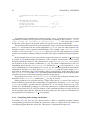
As illustrated the typical Felix2 simulation consists of 6 parts:
• Part 1 (lines 0-14) contains all the declarations for the simulation except the declarations for the graphical user interface (GUI). It should include at least the F2 simenv.h
but also the headers of other Felix2 components that are used in the program. The
macro definition STANDALONE serves to switch between two simulation modes: For
STANDALONE=0 the GUI is used and simulation variables can be displayed online
and simulation parameters can be modified online e.g. via the switches, sliders, or
most easily using the reparse-switch and the parameter file (see also section ?? on page
??). The variables nArgs and args are used for the transfer of parameters from the
call of the C++ program to the simulation environement in standalone simulations
(STANDALONE=1, cf. Part 6). Although it is possible to declare the Felix2 components
as the simulation environment or neurons statically as global variables, it is strongly
recommended that the Felix2 components are declared dynamically as pointers in Part 1,
while the creation of the actual objects is placed in main init() (Part 3). One reason
why to do so is the handling of the parameter transfer via nArgs and args. If the
Felix2 components are declared as static global objects then they are already created
and parsed(!) before the call to main(nArgs ,args ) is performed. Consequently it is not
possible to adjust constants in the parameter file via a the nArgs /args parameters
of main(), see also section ?? on page ??. Another reason why to use pointer declarations in part 1 is that certain free parameters can only be adequately reparsed if they
were declared as pointers (see section ?? on page ??).
• Part 2 (lines 15-47) contains the GUI declarations of Felix1. First the Felix1 headers
must be included as extern C. Then there should be declared variables which are
used to display simulation data online. Finally Part 2 contains the declaration of the
GUI components of Felix1, such as the reparse-switch, sliders, images, graphs, functions, etc. See section ?? on page ?? for more details.
10
CHAPTER 3. COMPILING AND RUNNING FELIX2 SIMULATIONS
• Part 3 (lines 48-61) is esentially the main init() procedure as required by Felix1.
First the simulation environment should be created which initiates the parsing of the
remaining objects using correctly possibly modified constant of the parameter file. The
remaining objects are created and parsed from the parameter file as soon as they allocated. After creating the Felix2 objects, a call to senv->allocate() may be necessary to allocate certain integrator objects (see section ?? on page ??). Finally the display
pointer variables (like outPe in line 56) must connected with the correct component
fields.
• Part 4 (lines 62-70) is the init() procedure as required by Felix1. In the simplest case
it may only contain the call to senv->init(); which will call the init() methods
of all the previously created Felix2 objects.
• Part 5 (lines 71-79) is the step() procedure as required by Felix1. In the simplest case
it may only contain the call to senv->step(); which will call the step() methods
of all the previously created Felix2 objects. In addition senv->step(); will check
sliders and the reparse-switch (line 36), and react to possible events as parameter updates.
• Finally Part 6 (lines 80-96) contains the main(nArgs,args) procedure which is only
used for standalone simulations with STANDALONE=1.
3.2
Compiling a Felix2 simulation
3.3
Running a Felix2 simulation
Chapter 4
Overview
The following is unedited text from my dissertation ‘‘Synchronization
and pattern separation in spiking associative memories and visual cortical
areas.’’
All simulations described in this work have been implemented using the Felix or Felix++
simulation tools. Originally the C based simulation tool Felix has been developed by Thomas
Wennekers at the University of Ulm [?] as a universal simulation environment for physical
and, in particular, neural systems. The development of Felix was motivated by the need
for a fast implementation of multi-layer one- or two-dimensional neural structures such as
neuron populations. For this purpose, Felix provides elementary algorithms for single-cell
dynamics, inter-layer connections, and learning. Additionally, there exist also libraries for
non-neural applications, e.g., for general dynamical systems and elementary image processing.
Simulations can be observed and influenced online via the X11/XView-based graphical
user interface (GUI) of Felix. The Felix GUI provides elements such as switches for conditional
execution of code fragments, sliders for online-manipulation of simulation parameters (like
connection strengths, time constants, etc.), and graphs for the online observation of the states
of a simulated system in xy-plots or gray-scale images (see [?, ?] for more details).
During this work the simulation tool Felix++ has been developed as a C++ based objectoriented extension of Felix. Felix++ provides additionally classes for neuron models, n dimensional connections, pattern generation, and data recording. Current installations of
Felix++ are running on PC/Linux as well as on 64bit-SunFire/Solaris9 systems. In the following the architecture of Felix++ is briefly sketched (for more details see [?]).
4.1
Basic architecture of Felix++
Essentially Felix++ is a collection of C++ libraries supporting fast development of neural
networks in C++ [?, ?]. Thus Felix++ comprises a number of modules each consisting of a
header (with the suffix “.h”) and a corpus (with the suffix “.cpp” for Felix++/C++ or ”.c” for
Felix/C). The header files contain declarations of classes, types, and algorithms, whereas in
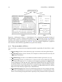
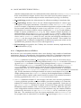
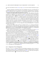
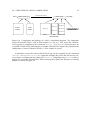
the corpus files the declarations are implemented. Figure 4.1 illustrates the architecture of
Felix++ by classifying all the modules of Felix++ and Felix in a hierarchy.
11
12
CHAPTER 4. OVERVIEW
SIMULATION.cpp
#include
#include
UniformNoise.h/cpp
Simulation Components CorrelatedNoise.h/cpp
IFNeuron.h/cpp
TopoConnection.h/cpp
SGNeuron.h/cpp
GaussConnection.h/cpp
BlankTopoConnection.h/cpp
SSNeuron.h/cpp
DemoBlankTopoConnection.h/cpp
GNeuron.h/cpp
SSCOscillator.h/cpp F2_association.h/cpp V1Connection.h/cpp
AssoConnection.h/cpp
InpNeuron.h/cpp
RandomConnection.h/cpp
F2_integrator.h/cpp
DelayKernelConnection.h/cpp
STDPLearner.h/cpp
Library
nn.h/c
numerics.h/c
vector.h/c
images.h/c
random.h/c
Driver/Communication
Auxiliary Modules
F2_numerics.h/cpp F2_kernel.h/cpp
F2_vector.h/cpp
F2_pattern.h/cpp
F2_delay.h/cpp
F2_object.h/cpp
F2_record.h/cpp
F2_receptor.h/cpp F2_libasso.h/cpp
gen_sim.h/c
Core
Core
F2_simenv.h/cpp F2_types.h/cpp
F2_random.h/cpp F2_parser.h/cpp F2_parameter.h/cpp
F2_time.h/cpp
F2_layout.h/cpp F2_port.h/cpp
Felix++
gen_obj.c/h
sim_graph.c/h output.c/h
file_graph.c/h
Felix
Figure 4.1: Architecture of Felix++: A simulation is a C++ program that includes headers of
Felix and Felix++. Felix++ contains core modules (e.g., F2 simenv.h/cpp; cf. Fig. 4.2), auxiliary
modules, and modules for simulation components such as neuron populations and connections between neuron populations (cf. Fig. 4.3). The Felix modules implement a graphical
user interface and elementary algorithms (see [?] for more details).
4.1.1
The core modules of Felix++
The core of Felix++ contains the most important modules required by all other Felix++ modules.
• F2 types.h/cpp declares some elementary type conventions and some global objects.
• F2 time.h/cpp declares classes for time, for example to evaluate the time necessary for
computing a simulation.
• F2 random.h/cpp provides several different random number generators (see [?]).
• F2 layout.h/cpp declares so-called layouts. A layout can be used to define the topology
of a vector (or in terms of C++, an array). For example a population of 1000 neurons
can be arranged as a 10×10×10 cuboid. Apart from cuboid layouts also ellipsoid layouts
are defined which are useful in particular for saving memory when modeling isotropic
local connectivity (in three dimensions, for example, an ellipsoidal kernel saves almost
50 percent of the memory required by a cuboid kernel).
• F2 parameter.h/cpp declares classes for simulation parameters. For example, the membrane time constant field of a neuron class is usually declared as such a parameter. This
allows conveniently parsing and online reparsing of the parameters from a parameter
4.1. BASIC ARCHITECTURE OF FELIX++
13
file as well as online manipulation via sliders of the Felix GUI (including updating of
other dependent parameters). The parameters declared in this module are essentially
arrays equipped with a cuboid layout (see above). Therefore they can be used not only
for single parameter values, but as well for multi-dimensional parameter collections
such as parameter vectors or matrices.
• F2 parser.h/cpp provides the classes for parsing parameters from a parameter file.
Usually, in Felix++ a component class (e.g., a neuron class) is designed in such a way
that a construction of an object is paralleled by parsing the corresponding parameters
from a file. Furthermore, during the simulation the parameter file can be modified and
reparsed by pressing the reparse-button.
• F2 port.h/cpp declares interfaces for the communication between different simulation
components, so-called ports. For example, a neuron class may contain an output port
representing the spikes of the neuron, and an input port representing synaptic input to
the neuron. Correspondingly, the constructor of a connection component class requires
as parameters the output port of a neuron population and the input port of another
neuron population such that the spikes from the first population can be propagated to
the dendrites of the second population.
• F2 simenv.h/cpp declares the simulation environment class TSimulationEnvironment
and the component base class TComponent as well as some base classes for special
components such as neurons (TNeuron) and connections (TConnection). This module should be included by any simulation program using Felix++. The simulation environment is essentially a container for the simulation components (see below for more
details; cf. Fig. 4.2), but provides also additional infrastructure such as look-up tables
(for example for Gaussians), random number generators, and much more. Usually, the
construction of a simulation component requires a TSimulationEnvironment as an
argument, such that the component is automatically inserted. After construction of all
the components, calls to methods allocate() will allocate memory shared by multiple components (for example when integrating differential equations via TIntegrator
objects; see below). Before starting the simulation all the components can be initialized
by calling the init() method of the simulation environment. Similarly, during the
simulation a call to the step() method will compute one simulation step.
4.1.2
Auxiliary modules of Felix++
Besides the core modules there are a number of auxiliary modules that provide additional
functionality required by only some of the Felix++ component modules, and perhaps also
by the programmer developing a simulation.
• F2 numerics.h/cpp provides a number of useful constants (e.g., π, e, and ln 2) and
functions (e.g., density function of Binomials or Gaussians, information and transinformation functions for binary random variables, etc.). Further declarations provide
classes for look-up-tables and interpolation.
• F2 kernel.h/cpp declares classes for kernels that can be used, for example, for implementing synaptic connections. Kernels are essentially arrays (e.g., of synaptic weights
14
CHAPTER 4. OVERVIEW
Simulation Environment
Components:
− neuron populations
− connections
− etc.
allocate()
init()
step()
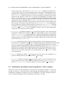
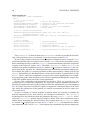
Figure 4.2: The simulation environment object (of class TSimulationEnvironment) is
essentially a container object containing all the simulation components such as neuron populations or connections. The components are inserted during construction. Before starting a
simulation a call to method allocate() is necessary to allocate memory. A call to init()
initializes the components, and each call to step() results in the computation of one simulation step.
or delays) that have been assigned a topology via layouts (see F2 layout.h/cpp). The
classes defined in this module enable, for example, the coordination of a neuron population (layout) to a set of kernels. This happens in a rather flexible manner such that
each neuron can be assigned individually a kernel index, where also certain regularities of kernel arrangements can be exploited (such as the regularities occurring for the
orientation modules in our visual model; cf. Fig. ??a).
• F2 vector.h/cpp provides basic vector functionality. This module also declares classes
for numerical vector parameters (cf. F2 parameter.h/cpp).
• F2 pattern.h/cpp implements classes for various types of patterns. From the pattern
base type (TMPattern) which corresponds simply to a multi-dimensional array there
are derived specialized pattern types such as binary patterns (TMbPattern), sparse binary patterns (TMsbPattern), sparse patterns (TMsPattern), or sparse binary spatiotemporal patterns (TMsbSTPattern). Additionally, further auxiliary classes have been
implemented in order to facilitate the use of patterns. For example, pattern container
classes are declared (TMPatternStock and derivatives of TMPatternGroup) for convenient construction and parsing of pattern groups from parameter files. The TMPatternRanking
class can be used for analyzing neural activity with respect to a set of patterns (i.e., to
determine the pattern in the set that is most similar to the neural activity pattern).
Similarly, the TMPatternHistogram class can be used to create pattern-specific histograms of state variables (as used, for example, for the threshold distance histograms
in Fig. ??d-h).
• F2 delay.h/cpp provides classes based on the definitions in F2 kernel.h/cpp for efficient
implementation of synaptic delays.
• F2 object.h/cpp declares classes for generating stimulus objects. Further classes can be
used to put static or moving objects in space (derivatives of TMSpace), or to project the
4.1. BASIC ARCHITECTURE OF FELIX++
15
stimulus configuration onto a two-dimensional surface (derivatives of TMSpaceRepresentation).
In the visual model of chapter ?? these classes have been used in order to project a visual scene of several stimulus objects onto the retinal area R (see Figs. ??a and ??a).
• F2 record.h/cpp provides the infrastructure for efficient recording of simulation data.
• F2 receptor.h/cpp declares classes for the efficient implementation of various types
of receptors for synaptic transmitters. Derivatives of class TMReceptorPort can be
used, for example, to implement certain transmitter-dependent synaptic conductances.
For our neuron model described in section ?? we used class TMOffDynamics for implementation of excitatory AMPA currents (conductance gex ; cf. eq. ??) and inhibitory
GABA-A currents (conductance gin ; cf. eq. ??). More complex receptor dynamics are
implemented by classes TMOnOffDynamicsRP and TMSimpleNMDARP where the latter can be used to model NMDA receptor dependent currents (cf. [?]). Actually neuron
classes such as TSSNeuron (which we have used for our biological simulations) or
TGNeuron use the receptor port classes provided by this module. These models can
be equipped with an arbitrary configuration of different receptor ports which can be
specified in the parameter file (see below code fragment 4.5).
• F2 libasso.h/cpp encapsulates the C-library for associative memory implemented by
Friedrich Sommer (cf. [?]).
4.1.3
Component classes of Felix++
Based on the core and auxiliary modules there exists already a large number of simulation
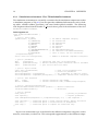
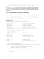
components. Figure 4.3 illustrates the class hierarchy of the Felix++ simulation components.
They can be divided into the following component base classes derived from TComponent:
• TNeuron (defined in module F2 simenv.h/cpp) is the base class for all neuron classes.
Currently there are implementations for gradual neurons (TSGNeuron in module SGNeuron.h/cpp and TGNeuron in module GNeuron.h/cpp), spiking neurons (TIFNeuron in module
IFNeuron.h/cpp and TSSNeuron in module SSNeuron.h/cpp), and oscillators (TSSCOscillator in module SSCOscillator.h/cpp) which all can be used for biological modeling.
Additionally, there are classes adequate for technical implementations of associative
memory (TMAssociationPopulation and TMAutoWillshawTAMP in module F2 association.h/cpp). For the simulations of biological models in section ?? and chapter ?? we used the
simple spiking neuron class TSSNeuron, whereas for the implementation of Willshaw
associative memory and the spike counter model in section ?? the technical associative
memory population class TMAutoWillshawTAMP has been used.
• TMNoise (defined in module F2 simenv.h/cpp) is the base class for noise populations.
A noise population provides random numbers generated according to a certain distribution for another component object such as a neuron population. Derivatives of
type TMUniformNoise (defined in module UniformNoise.h/cpp) provide uniformly
distributed random numbers with a certain power (or variance). While this type generates independent random numbers in each simulation step the random numbers
generated by derivatives of type TMCorrelatedNoise can be correlated in space
and time. The standard noise type for neuron populations such as TSSNeuron (or
for synaptic noise in connections; see module F2 receptor.h/cpp) is TMUniformNoise,
16
CHAPTER 4. OVERVIEW
TComponent
TNeuron
TNoise
TIFNeuron
TMUniformNoise
TSGNeuron
TMCorrelatedNoise
TSSNeuron
TConnection
TMIntegrator
TMTopoConnection
TMGaussConnection
TMSTDPLearnerSMA2000
TMRK4cIntegrator
TMSTDPLearnerFD2002
TMDemoBlankTopoConnection
TMAssoConnection
TMInpNeuron
TMV1Connection
TMAssociationPopulation
TMAutoWillshawTAMP
TMPatternRanking
TMPatternHistogram
TMBlankTopoConnection
TSSCOscillator
TMInputHandleNeuron
TMSpace TObserver
TMEulerIntegrator
TGNeuron
TMFileInpNeuron
TLearner
TMRandomConnection
TMDelayKernelConnection
TMAssociation
TMWillshawAssociation
TMcWillshawAssociation
Figure 4.3: The class hierarchy for the currently implemented simulation components of Felix++. From the base class TComponent specialized sub-classes are derived for neuron populations (TNeuron), noise generators (TMNoise), connections between neuron populations
(TConnection), integration of differential equations (TMIntegrator), synaptic plasticity
(TLearner), representations of stimulus space (TMSpace), and on-line observation of the
simulation state (TObserver).
whereas for the primary visual area P (see chapter ??) correlated noise of type TMCorrelatedNoise
has been used.
• TConnection (defined in module F2 simenv.h/cpp) is the base class for connections between neuron populations (or more exactly, between ports; see module F2 port.h/cpp).
The function of derivatives of this type is to propagate information from an output
port to an input port, for example, to propagate the spikes from the output port of one
neuron population through the network to the input port of another neuron population. The most important derived type for biological modeling is TMTopoConnection
(defined in module TopoConnection.h/cpp). This generic type is the base class for many
further derived classes. Here a synapse is defined by two state values: A synaptic
weight, and a synaptic delay. Correspondingly, an object of type TMTopoConnection
essentially contains two kernel arrays of type TKernel (defined in F2 kernel.h/cpp) representing weights and delays. The kernel classes can be applied in a very flexible manner allowing implementation of full, sparse, topographical schemes in multiple dimensions. Additionally, efficient algorithms are implemented for several special cases
(e.g., for non-sparse bit-packed binary topographical connectivity). The derivatives of
TMTopoConnection merely specify how the synaptic weight and delay kernels are
generated. For example, class TMGaussConnection (defined in module GaussConnection.h/cpp) implements simple topographical connections with Gaussian kernels. A
further derived class TMBlankTopoConnection (defined in module BlankTopoConnection.h/cpp) provides an interface to TMTopoConnection in order to allow a more
convenient derivation of further connection classes. While TMDemoBlankTopoConnection (defined in module DemoBlankTopoConnection.h/cpp) is merely a demonstration how to derive from TMBlankTopoConnection, also a number of important con-
4.2. SIMULATION ENVIRONMENT AND COMPONENTS: CODE EXAMPLES
17
nection classes have been derived. TMAssoConnection (defined in module AssoConnection.h/cpp) can be used to implement fully connected or multi-dimensional topographically confined associative connections, for example, of the Willshaw type.
TMV1Connection (defined in module V1Connection.h/cpp) is a specialized connection
scheme for the primary visual cortex as used for the simulations in chapter ?? (see
Fig. ??). And TMRandomConnection (defined in module RandomConnection.h/cpp)
can be used conveniently for implementing connections with random connectivity.
Another class derived directly from TConnection is TMDelayKernelConnection
(defined in module DelayKernelConnection.h/cpp) which provides a much simpler and
faster scheme for delayed connections than TMTopoConnection. For implementation of technical associative memory derivatives from class TMAssociation (defined
in module F2 association.h/cpp) can be used, such as TMWillshawAssociation and
TMcWillshawAssociation for the Willshaw model, where the latter implements
compression of the binary memory matrix.
• TMIntegrator (defined in module F2 integrator.h/cpp) is the base class for numerical
integration of differential equations. Derived classes (defined in the same module)
are TMEulerIntegrator which implements a simple first order Euler method, and
TMRK4cIntegrator which implements the fourth order Runge-Kutta method with
constant step size (see [?]). Normally, these integrator objects are used by some of the
neuron classes (e.g., TSSNeuron).
• TLearner (defined in module F2 simenv.h/cpp) is the base class for plasticity of synaptic connections. Currently, two derivatives are implemented in the module STDPLearner.h/cpp.
TMSTDPLearnerSMA2000 implements a model of spike-timing dependent synaptic
plasticity (STDP) described by Song, Miller, and Abbott [?], while TMSTDPLearnerFD2002
implements an extended model suggested by Froemke and Dan [?]. Both classes are interfaced with connection classes via the kernel classes defined in F2 kernel.h/cpp. Therefore it is easy to endow connections (e.g., derived from TMTopoConnection) with
synaptic plasticity.
• TMSpace (defined in module F2 object.h/cpp) is the base class for the definition of a
space for stimulus objects (see above module F2 object.h/cpp).
• TObserver (defined in module F2 simenv.h/cpp) is the base class for components observing on-line the state of the simulation. Derived classes are TMPatternRanking
and TMPatternHistogram (for more details see above module F2 pattern.h/cpp).
4.2
Simulation environment and components: Code examples
In the last section we have obtained an overview over the modules of Felix++. In the following we will have a closer look at the code defining some important Felix++ classes, the
simulation environment, and the base class for components. The code examples shown below are shortened fragments of the declarations in the Felix++ headers.
18
4.2.1
CHAPTER 4. OVERVIEW
Simulation environment: Class TSimulationEnvironment
The simulation environment is essentially a container for the simulation components used in
a simulation program (cf. Fig. 4.2), but also provides additional infrastructure such as lookup tables, random number generators, and some further global variables. The following
code fragment taken from the header F2 simenv.h shows parts of the declaration of the class
TSimulationEnvironment.
Code fragment 4.1
class TSimulationEnvironment {
public:
// part 1: local types
typedef enum { CC_NOISE,
CC_CONNECTION,
CC_INTEGRATOR,
CC_NEURON,
CC_LEARNER,
CC_SPACE,
CC_SPACEREPRESENTATION,
CC_OBSERVER,
CC_ASYNCHRONY
} TComponentCategory;
static const int nCategories=9;
// part 2: parameters
TPar
parStepSize;
TsPar
parDataDirectory;
TsPar
parDataPostFix;
//
//
//
//
//
//
//
//
//
for TNoise component category
for TConnection
for TIntegrator
for TNeuron
for TLearner
for TSpace
for TSpaceRepresentation
for observers like TMPatternRanking
calls to step() are not controlled
// number of different component categories
// simulation step size (in milliseconds)
// default directory where simulation data is recorded
// post fix for data file names
// part 3: object fields
const char* parameterFile;
TParser parser;
vector<TComponent*> allComponents;
vector<TComponent*> components[nCategories];
// part 4: time reference
TInt
steps;
TFloat simTime;
//
//
//
//
name of root parameter file
parser for parameters
all components in order of constr.
components ordered after categories
// current simulation step number
// current simulation time, simTime:=steps*stepSize;
// part 5: constructors/destructors
TSimulationEnvironment(const char* parFile); // default constructor
˜TSimulationEnvironment();
// destructor
// part 6: methods
void parse();
// parsing of parameters
void reparse();
// reparse parameters
void addComponent(TComponent *c, TComponentCategory cc); // add component c
void allocate(); // simulation phase 2 (after creation phase): memory allocation
void init();
// simulation phase 3: Initialization of TComponents
void step();
// simulation phase 4: compute one simulation step
};
In part 1 an enumeration type is declared for the different component categories such as
neurons, connections, or observers. This corresponds approximately to the different compo-
4.2. SIMULATION ENVIRONMENT AND COMPONENTS: CODE EXAMPLES
19
nent classes described in section 4.1.3 (see Fig. 4.3; see also the container declarations in part
3).
In part 2 parameters are declared such as the simulation step size, or the directory for
recorded simulation data. These parameters are parsed from a parameter file (see code fragment 4.5) during the first execution phase of the simulation program when the simulation
environment is created by calling the constructor (see part 5).
In part 3 some object fields are declared such as the name of the parameter file (which
is passed as an argument to the constructor; see part 5), or the parser used for parsing the
parameters (see module F2 parser.h/cpp in section 4.1.1). Here there are also the declarations
of the containers for the simulation components (vectors of the STL library; cf. [?, ?]). The
first container field allComponents contains references to the components in order of the
construction of the components (which is important for reparsing the parameter file), while
the second container field components contains the components ordered for the different
categories (see part 1). The latter ordering is important to assert a defined synchronization
of object of the same component category. For example, the calls to the step() methods
of neuron objects should be before the step() calls of connection objects (cf. part 6). This
synchronization will become even more important when parallelizing Felix++ as planned
for future work (cf. [?]).
In part 4 some fields for time reference are defined. Felix++ is a step-based simulation
tool (in contrast to event-based tools). This means that the state of the simulated system is
updated step by step where one simulation step corresponds to a fixed time interval. The
parameter parStepSize (see part 2) defines this time interval. The field steps is initialized
by 0, and incremented for each call to the step() method (see part 6).
Part 5 contains the declarations of the constructors and destructors. In section 4.3 an
example is given how and when to apply the constructor in a simulation program.
In part 6 the methods are declared. Method parse() is normally called by the constructor in order to parse the parameter file. Method reparse() is called for reparsing a modified parameter file, for example, when pressing the reparse-button in an online-simulation.
With addComponent() new simulation components can be added to the component containers (see part 3) which is usually done by the constructor of TComponent (see section 4.2.2).
Then there are further three important methods (cf. Fig. 4.2): In order to allocate memory shared by different simulation components (for example state variables of neurons integrated by components of type TIntegrator; see module F2 integrator.h/cpp) a call from
the simulation program to allocate() must occur after the construction of the simulation
components (see procedure main init() in code fragment 4.4). A call to method init()
initializes the simulated system essentially by calling the init() method of each simulation
component. Similarly, a call to method step() computes one simulation step by calling the
step() method of each simulation component. The calls to the simulation environment’s
init() and step() methods occur normally from the simulation program’s init() and
step() procedures (see code fragment 4.4).
4.2.2
Components: Class TComponent
The class TComponent is the base class for all simulation components such as neurons or
connections (see Figs. 4.3 and 4.1) and implements essentially a common interface of simulation components to the simulation environment (section 4.2.1). The following code fragment
taken from the header F2 simenv.h shows parts of the declaration.
20
CHAPTER 4. OVERVIEW
Code fragment 4.2
class TComponent : public TParamOwner {
public:
// part 1: object fields
string name;
// name of the component
TSimulationEnvironment& simEnv; // reference to the simulation environment
TComponentCategory category;
// component category
vector<TfPort*> gradualPorts;
// gradual i/o ports of the component
vector<TbPort*> binaryPorts;
// binary ports
// part 2: constructors/destructors
TComponent(TSimulationEnvironment& simEnv_arg, const char* name_arg,
TComponentCategory cc_arg);
TComponent(TComponent& pattern, const char* name_arg, TComponentCategory cc_arg);
˜TComponent();
// part
virtual
virtual
virtual
virtual
3: methods
void reparse();
void allocate();
void init();
void step();
virtual void derivs() {};
//
//
//
//
reparse parameters
allocate memory for TIntegrator
initialize component
compute one simulation step of component
// compute derivatives for TIntegrator
};
Class TComponent is derived from class TParamOwner in order to provide the functionality of the parameter classes (see module F2 parameter.h/cpp in section 4.1.1).
In part 1 object fields are declared. Each simulation component can be assigned a name
which considerably relieves search for errors. Field simEnv refers to the simulation environment containing the object, and field category contains information about the component
category of the object (cf. section 4.2.1). The fields gradualPorts and binaryPorts are
containers for gradual and binary ports (see module F2 port.h/cpp in section 4.1.1) and constitute thereby the interface for communication between different simulation components.
For example, the spikes of a neuron population will be represented by a binary port of type
TbPort and similarly the dendritic inputs will be represented by a gradual port of type
TfPort. Thus a connection component can connect two neuron populations, for example,
by propagating spikes from the binary port of the first population through the synaptic network to the gradual input port of the second population.
In part 2 the constructors and destructors are declared. There are generally two constructor types for a simulation component. The default (or complete) constructor constructs a
simulation component by parsing the parameters from the parameter file (see code fragment
4.5). In contrast, the pattern constructor requires as argument a simulation object of the same
type where the parameters of this pattern are used for construction of the new object (see
also section 4.2.3).
In part 3 a number of virtual methods is defined which are normally overridden by
derived component classes and called by the simulation environment. The reparse()
method reparses the parameters from the parameter file using simEnv → parser. If necessary the allocate() method requests memory shared with other components from a
further object managing the shared memory (for example from an TIntegrator object;
see module F2 integrator.h/cpp in section 4.1.3). A call to init() will initialize the simulation component, and a call to step() will compute one simulation step for the component.
4.2. SIMULATION ENVIRONMENT AND COMPONENTS: CODE EXAMPLES
21
The method derivs() can be used in derived classes to compute the (numerical) derivatives of some of the state variables of the component. This method is normally called by a
TIntegrator object in order to integrate the differential equation associated with a component state.
4.2.3
Class TSSNeuron: a simple spiking neuron model
To illustrate how a concrete simulation component can be derived from the base class TComponent we will have a closer look at the class TSSNeuron implementing a simple spiking
neuron model. Actually, this class (with a parameter file as shown in code fragment 4.5) has
been used to implement the model described in section ?? for the biological simulations in
section ?? and chapter ??. The following code fragment taken from the header SSNeuron.h
shows parts of the declaration.
Code fragment 4.3
class TSSNeuron : public TNeuron, public TIntegratorClient {
public:
// part 1: parameters
string scopeID;
// scope id for parsing parameters
TVecPar tau_x;
// membrane time constant
TVecPar theta;
// asymptotic threshold
TVecPar refAbs;
// absolute refractory time
TVecPar refRel;
// relative refractory parameter
TVecPar tau_h;
// decay time constant of habituation
TVecPar thetaInc_h;
// threshold increment after each spike
TCompartmentReceptors* receptorPorts; // receptorPorts
// part 2: integrator for membrane potential
TDerivScope derivScope;
TIntegrator* integrator;
// integrator
// part 3: ports
TbPort *out;
TfPort *lastOut;
TfPort* excIn;
TfPort* inhIn;
//
//
//
//
output queue for spikes
output queue for last spikes
default excitatory in-port
default inhibitory in-port
// part 4: state variables
TFloat *current;
TFloat *x;
TByte *y;
TFloat *last;
TFloat *habituation;
//
//
//
//
//
synaptic currents
membrane potential
output variable (refers to out)
last spike time (refers to lastOut)
habituation (fatigue) - increased threshold
// part 5: constructors/destructors
TSSNeuron(TSimulationEnvironment& simEnv_arg, const char* name_arg,
TLayout* layout_arg, vector<TNoise*>* noiseSources_arg);
TSSNeuron(TSimulationEnvironment& simEnv_arg, const char* name_arg,
TLayout* layout_arg, vector<TNoise*>* noiseSources_arg,
TIntegrator* integrator_arg, int parse);
TSSNeuron(TSSNeuron& pattern, const char* name_arg,
TLayout* layout_arg, vector<TNoise*>* noiseSources_arg);
˜TSSNeuron();
// part 6: methods
// complete cnstr.
// default
"
// patterned
"
// destructor
22
CHAPTER 4. OVERVIEW
void allocate();
// get memory from integrator
void derivs() {};
// compute ...
void derivs(int id, TFloat t,TFloat* x,TFloat* dxdt); // derivatives for integrator
void init();
// initialize states to zero values
void step();
// one simulation step
void reparse();
// reparse parameters
void handleUpdatedParameters();
// handle updated parameters
void setParameterValues();
// update parameter values
friend ostream & operator<<(ostream& os
, const TSSNeuron & neuron); // output op.
friend istream & operator>>(istream& parser,
TSSNeuron & neuron); // input op.
};
Class TSSNeuron is derived from TNeuron (which in turn is derived from TComponent;
see Fig. 4.3) and from TIntegratorClient. The derivation from the latter class is necessary for any class requiring integration of differential equations by a TIntegrator object
(see module F2 integrator.h/cpp in section 4.1.3).
In part 1 of code fragment 4.3 parameters of the neuron model are declared. When comparing with the notation used in section ?? (cf. table ?? and code fragment 4.5) parameter
field tau x corresponds to parameter τx , theta to Θ∞ , refAbs to Ra , refRel to Rr , tau h
to τh , and thetaInc h to H. Field scopeID contains information about which parameter scope (see below) in the parameter file has been used to parse the parameters for this
object. Field receptorPorts points to a container object for receptor ports (see module
F2 receptor.h/cpp in section 4.1.2) which becomes allocated during object construction. This
field is used for implementing different excitatory or inhibitory synaptic currents (see code
fragment 4.5).
In part 2 field integrator declares the integrator object for integrating the differential
equation for the membrane potential (cf. eq. ??). Currently, either a Euler or a Runge-Kutta
method can be used (see module F2 integrator.h/cpp in section 4.1.3). The field derivScope
just serves to identify the memory for the state variable x (see part 4) which is administrated
by the integrator object.
Part 3 declares the ports of the object (see module F2 port.h/cpp in section 4.1.1). Port out
is the output queue for the spikes of the neuron population, port lastOut contains information about the time of the last spike for each neuron. Input ports excIn and inhIn are
essentially queues for synaptic input from other neuron populations mediated by connection
objects (see type TConnection in section 4.1.3).
In part 4 the state variables of the neurons are declared. Array current is essentially the
sum of the synaptic input currents for each neuron as computed by receptorPorts (see
part 1). Array x corresponds to the membrane potential x of the neuron model in section ??
(cf. eq. ??). Similarly y corresponds to the spike output variable y (eq. ??), last corresponds
to the time point s of the last spike for each neuron (cf. eq. ??), and habituation corresponds to the neuronal habituation or fatigue h (cf. eq. ??).
In part 5 the constructors and destructors are declared (cf. part 2 in section 4.2.2). The
first constructor is the so-called complete constructor which is normally used in a simulation
program for creating an object of type TSSNeuron for the first time. The third constructor
is the pattern constructor which is normally used for further creations of TSSNeuron objects.
While for the complete constructor the parameters (see part 1) are parsed from the parameter file (see code fragment 4.5), the pattern constructor copies the parameters from a pattern
4.3. STRUCTURE OF A FELIX++ SIMULATION
23
object passed as the first argument. The second constructor in the code fragment is the socalled default constructor which is normally used by the constructor of another class derived
from TSSNeuron. In contrast to the complete constructor, automatic parsing (which should
be done only by the constructor of the derived class) can be suppressed by passing an additional flag argument parse.
Finally part 6 contains the declarations of the methods allocate(), derivs(), init(),
step(), and reparse() which override the declarations explained above for the base class
TComponent (see part 3 in section 4.2.2). There are a few remaining methods: handleUpdatedParameters() and setParameterValues() manage updating of the object state if
one of the parameters (see part 1) is changed (for example when reparsing the parameter
file), while the input/output operators operator>>() and operator<<() are used for
parsing the object parameters from the parameter file, or for printing the parameter data, for
example, when debugging.
4.3
4.3.1
Structure of a Felix++ simulation
A skeleton simulation program
A Felix++ simulation is basically a C++ program that includes header files of Felix and/or
Felix++. The structure of a Felix++ simulation typically looks similar to the following code
fragment:
Code fragment 4.4
// Part 1: Felix2 declarations
// -----------------------------------#include "F2_simenv.h"
...
// further includes (e.g., of Felix++ headers)
#define STANDALONE 1
...
// further macro definitions
TSimulationEnvironment* senv;
TSSNeuron* popPe;
...
// declaration of further simulation components
// Part 2: Felix1 (GUI) declarations
// -----------------------------------extern "C" {
#include "nn.h"
...
// include of further Felix headers
}
#if STANDALONE
NO_DISPLAY
#else
BEGIN_DISPLAY
...
// declaration of Felix GUI (switches, sliders, graphs, etc.)
END_DISPLAY
NO_OUTPUT
// Felix1 output mechanisms usually not used
#endif
// Part 3: main_init()
// -----------------------------------int main_init() {
senv = new TSimulationEnvironment(parameterFile);
24
CHAPTER 4. OVERVIEW
...
// further utility declarations/creations
popPe = new TSSNeuron(*senv,"popPe",popLT_Pe,0,integrator1,1);
...
// further creation of objects
senv->allocate();
...
// assigning of GUI variables
return 0;
}
// Part 4: init()
// -----------------------------------int init() {
senv->init();
...
// further initialization
return 0;
}
// Part 5: step()
// -----------------------------------int step() {
senv->step();
...
// further step()-stuff
return 0;
}
// Part 6: main()
// -----------------------------------#if STANDALONE
int main(int nArgs, char** args) {
main_init();
init();
for(int i=0;i<1000;i++) step();
...
// further stuff, e.g. saving simulation data
}
#endif
In part 1 Felix++ header files (and also other headers) are included, macros are defined
such as STANDALONE (which switches between online and batch mode; see below parts 2
and 6), and the simulation environment and the simulation components are declared. For
the sake of flexibility it is recommended to declare the simulation environment and the components as pointer variables which are allocated in the main init() method (see part 3).
For example, if the simulation environment and components would be already constructed
here, it would not be possible to pass the name of the parameter file as an argument to the
simulation program. In this example only the simulation environment senv and a neuron
population popPe of type TSSNeuron (see section 4.2.3) are declared. Usually the construction of the simulation environment and the simulation components is paralleled with the
parsing of a parameter file (see below the code fragment 4.5)
In part 2 the graphical user interface (GUI) of the simulation is declared (only necessary
for online simulations, i.e., if the flag macro STANDALONE is inactive). For this purpose, first
the Felix headers (see Fig. 4.1) must be included (in extern ‘‘C’’ brackets since Felix has
been implemented in C). Then the GUI components of Felix can be specified in the #else
branch of the #if directive (see [?] for details).
Part 3 is the main init() procedure. Here the simulation environment and subsequently the simulation components are created by calling the corresponding constructors.
4.3. STRUCTURE OF A FELIX++ SIMULATION
25
After constructing all simulation components a call to the allocate() method of the simulation environment might be necessary (e.g., for simulation components such as TSSNeuron
employing integrators; see module F2 integrator.h/cpp in section 4.1.3; cf. section 4.2.3). The
main init() procedure is normally called only once at the beginning of the simulation to
construct the simulation objects. This is done either by the main() procedure (see part 6) for
batch simulations (for activated flag macro STANDALONE=1) or by the Felix GUI for online
simulations (for STANDALONE=0).
In part 4 the init() procedure is defined. It contains normally at least the call to the
init() method of the simulation environment, but possibly also further initialization code
for the simulation. The init() procedure should be called after main init() to initialize
the states of the simulation objects before the actual simulation computations start (see part
5). In contrast to main init() the init() procedure can be called more than once either
from the main() procedure (see part 6) for batch simulations or for online simulations by
pressing the init button (or the run button) in the main simulation window [?].
Part 5 is the step() procedure which computes one simulation step. It contains normally at least the call to the step() method of the simulation environment, but possibly also
further code for the simulation. The step() procedure is called either from the main() procedure (see part 6) for batch simulations or for online simulations by pressing the step button
(or the run button) in the main simulation window.
Part 6 defines the main() procedure for batch simulations with activated macro flag
STANDALONE=1 (see part 1). This procedure must contain calls to main init() and init()
before the calls to the step() procedure.
4.3.2
The parameter file
The construction of the simulation environment and the simulation components in main init()
(see part 3 in section 4.3.1) is usually paralleled by the parsing of the parameter file in order to
read in the parameters to be used for the respective simulation objects. The following code
fragment shows parts of the parameter file for our skeleton simulation program above (code
fragment 4.4).
Code fragment 4.5
#{ TSimulationEnvironment Simulation1
% parameter scope for simulation environment
stepSize
: 0.1
dataDirectory : /private/aknoblau/simdata/BC2
}
#{ SSNeuron popPe
tau_x(exp,sig,min,max)
theta(exp,sig,min,max)
refAbs(exp,sig,min,max)
refRel(exp,sig,min,max)
tau_h(exp,sig,min,max)
thetaInc_h(exp,sig,min,max)
% parameter scope for neuron population
: 10 0 1 0
: 10 0 1 0
:
2 0 1 0
: 3 0.5 1.75 4.25
: 150 0 1 0
: 0.6 1.0 0.2 1.0
#{ TMCompartmentReceptors receptors
nReceptorPorts : 2
#{ TMOffDynamicsRP AMPA
tau_OFF(exp,sig,min,max)
E(exp,sig,min,max)
g0(exp,sig,min,max)
:
:
:
5 0 1 0
80 0 1 0
0 0 1 0
26
CHAPTER 4. OVERVIEW
powerInpNoise(exp,order,sig,min,max) :
0.025 1 0 1 0
qLen
: 600
}
#{ TMOffDynamicsRP GABAA
tau_OFF(exp,sig,min,max)
E(exp,sig,min,max)
g0(exp,sig,min,max)
powerInpNoise(exp,order,sig,min,max)
qLen
}
:
7 0 1 0
: -10 0 1 0
:
0 0 1 0
:
0.02 1 0 1 0
: 100
}
}
A parameter file is divided into various parameter scopes. A parameter scope is a group
of parameters which has been put into scope brackets according to the syntax #{ <scope
type> <scope ID> <parameter1> <parameter2> ... }. The scope type is given
by the class of the object to be parsed, while the scope ID can be chosen arbitrarily.
This parameter file contains two global parameter scopes, one for the simulation environment senv and another for the neuron population popPe (cf. part 3 in code fragment 4.4).
Parameter scopes can be organized hierarchically: For example scope SSNeuron popPe
contains a sub-scope for the receptorPorts object (see part 1 in code fragment 4.4) which
in turn can contain an arbitrary number of further sub-scopes for different receptor dynamics.
In the example there are two scopes for the receptor dynamics (cf. module F2 receptor.h/cpp
in section 4.1.2) implementing the dynamics of the synaptic conductances of the neuron
model described in section ??. The parameters in scope TMOffDynamicsRP AMPA specify
the dynamics of the excitatory conductance gex (eq. ??) which is implemented by the corresponding object of type TMOffDynamicsRP. Parameter tau OFF corresponds to τex (see
eq. ??) and parameter E corresponds to Eex (see eq. ??). The additional parameters determine
conductance baseline (g0), noise power (powerInpNoise), and the queue length (qLen;
measured in simulation steps) for incoming spikes propagated by connection objects (see
class TConnection in section 4.1.3). The latter parameter determines the maximal possible
axonal delay for the connection projecting onto this receptor port.
The parameters in scope TMOffDynamicsRP GABAA have the analogous relation to the
dynamics of the inhibitory conductance gin (see eqs. ?? and ??).
Many parameters are specified not by a single value but by a vector of four values to
define individual parameters for each member of a population. Parameter refRel (in scope
popPe), for example, specifies that the parameter Rr of our neuron model (see eq. ?? in
section ??) is distributed according to a Gaussian with mean 3, standard deviation 0.5, but
limited to the interval [1.75; 4.25]. In contrast, if the standard deviation is 0 and/or the left
interval border larger than the right one then the parameter is the same for all members of
the population (see parameter tau x, for example).
4.3.3
Compiling and running simulations
In sections 4.3.1 and 4.3.2 we have discussed how a Felix++ simulation program and the
corresponding parameter file should be structured. Here we explain how one obtains an
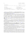
executable program from the source file. This process is illustrated in Figure 4.4.
4.3. STRUCTURE OF A FELIX++ SIMULATION
source
SIMULATION.cpp
"Felix2 SIMULATION"
27
SIMULATION
executable
libolgx.so
Felix++
headers
Felix
headers
libf_f2.so
libf2_f2.so
libX11.so
SIMULATION.par
parameter file
libxf_f2.so
libxview.so
Felix++
Felix
XView etc.
shared libraries
Figure 4.4: Compilation and Linkage of a Felix++ simulation program. The simulation
source file includes Felix++ and/or Felix headers (cf. Fig. 4.1). The source file SIMULATION.cpp then is compiled by the command “Felix2 SIMULATION” which generates an
executable SIMULATION. Running the executable SIMULATION requires the parameter file
and dynamic (“shared”) libraries of Felix++, Felix, and the X system.
A simulation source file named SIMULATION.cpp can be compiled by the command
“Felix2 SIMULATION”. Felix2 is a script that compiles the source file and sets the correct include- and link-paths by calling the Makefile. Compiling using Felix2 yields as
output the executable SIMULATION. When running this requires the dynamic (or shared)
libraries as shown in Figure 4.4.
28
CHAPTER 4. OVERVIEW
Part II
The Graphical User Interface (GUI) of
Felix
29
Chapter 5
The program structure of GUI
simulations
31
32
CHAPTER 5. THE PROGRAM STRUCTURE OF GUI SIMULATIONS
Chapter 6
Using the GUI elements of Felix
33
34
CHAPTER 6. USING THE GUI ELEMENTS OF FELIX
Part III
Fundamentals of Felix2
35
Chapter 7
Type conventions
37
38
CHAPTER 7. TYPE CONVENTIONS
Chapter 8
Layouts and multi-dimensional arrays
39
40
CHAPTER 8. LAYOUTS AND MULTI-DIMENSIONAL ARRAYS
Chapter 9
Parameters and parsing
41
42
CHAPTER 9. PARAMETERS AND PARSING
Chapter 10
Parameters and parsing
43
44
CHAPTER 10. PARAMETERS AND PARSING
Chapter 11
Basic numerics
11.1
Time
11.2
Random generators
11.3
Constants, functions, and look-up-tables
45
46
CHAPTER 11. BASIC NUMERICS
Chapter 12
Ports
47
48
CHAPTER 12. PORTS
Chapter 13
Kernels
49
50
CHAPTER 13. KERNELS
Chapter 14
Simulation environment and
components
51
52
CHAPTER 14. SIMULATION ENVIRONMENT AND COMPONENTS
Part IV
Modelling the environment: input and
output
53
Chapter 15
Vectors and patterns
55
56
CHAPTER 15. VECTORS AND PATTERNS
Chapter 16
Modelling objects and the space
around
57
58
CHAPTER 16. MODELLING OBJECTS AND THE SPACE AROUND
Chapter 17
Recording of simulation data
59
60
CHAPTER 17. RECORDING OF SIMULATION DATA
Part V
Further elements of Felix2
61
Chapter 18
Integrators for differential equations
63
64
CHAPTER 18. INTEGRATORS FOR DIFFERENTIAL EQUATIONS
Chapter 19
Delays
65
66
CHAPTER 19. DELAYS
Chapter 20
Receptors
67
68
CHAPTER 20. RECEPTORS
Chapter 21
A library for associative memory
69
70
CHAPTER 21. A LIBRARY FOR ASSOCIATIVE MEMORY
Part VI
Components of Felix2
71
Chapter 22
Noise populations
22.1
TMUniformNoise: the standard noise population
22.2
TMCorrelatedNoise: noise correlated in space and time
73
74
CHAPTER 22. NOISE POPULATIONS
Chapter 23
Neuron populations
23.1
IFNeuron: a simple integrate-and-fire neuron model
23.2
SGNeuron:
23.3
SSNeuron:
23.4
SSCOscillator:
23.5
InpNeuron:
75
76
CHAPTER 23. NEURON POPULATIONS
Chapter 24
Connections
24.1
TopoConnection:
24.2
GaussConnection:
24.3
BlankTopoConnection:
24.4
DemoBlankTopoConnection:
24.5
AssoConnection:
24.6
V1Connection:
24.7
RandomConnection:
24.8
DelayKernelConnection:
77
78
CHAPTER 24. CONNECTIONS
Chapter 25
Learner
25.1
STDPLearner:
79
80
CHAPTER 25. LEARNER
Part VII
Simulation examples
81
Chapter 26
Integrating Felix2 and the GUI of
Felix1
83
84
CHAPTER 26. INTEGRATING FELIX2 AND THE GUI OF FELIX1
Chapter 27
A simple network of oscillating
neurons
85
86
CHAPTER 27. A SIMPLE NETWORK OF OSCILLATING NEURONS
Part VIII
Appendices
87
Appendix A
The GUI reference of Felix
89
90
APPENDIX A. THE GUI REFERENCE OF FELIX
Appendix B
The C++ classes of Felix2
91
92
APPENDIX B. THE C++ CLASSES OF FELIX2
Appendix C
Parameter scopes for Felix2
components
This appendix contains descriptions of the parameter scopes for all Felix2 components. The
descriptions consist of example parameter scopes and a brief explanations of its use and the
role of the parameters.
C.1
Noise populations
C.2
Neuron populations
C.2.1
Class TIFNeuron
The following example is taken from the simulations in []. The description of the TIFNeuron
model should be clear by the comments. For more details see section ?? on page ??.
#{ IFNeuron TrigExNeuron
tau_x
: 0.5
tau_gex
: 0.25
tau_gin
: 0.25
tau_h
: 1
gexMax
: 100
ginMax
: 100
theta
: 10
ahp
: 108
habituation
: 0
exConstInput
: 0
inConstInput
: 10.45
noise(power,order) : 0 0
eInLen
: 20
iInLen
: 20
eInGradLen
: 20
iInGradLen
: 20
}
%
%
%
%
%
%
%
%
%
%
%
%
%
%
%
%
time constant of membr.potential
time constant excit.conductance
time constant inhib.conductance
time constant of habituation
maximal excitatory conductance
maximal inhibitory conductance
(asymptotic) threshold
after-hyperpolarization (reset x)
habituation (increase of h)
excitatory constant input
inhibitory constant input
noise power and order
length excit. spike input queue
length inhib. spike input queue
length excit. gradual inp.queue
length inhib. gradual inp.queue
93
94
APPENDIX C. PARAMETER SCOPES FOR FELIX2 COMPONENTS
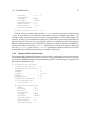
C.2.2
Class TSSNeuron
The TSSNeuron model consists of basic neuron parameters similar to the TIFNeuron (see
section C.2.1 on page 93). In contrast, however, input parameters are specified via an TMCompartmentReceptors container (see section ?? on page ??). Thus one can define an arbitrary number of receptors where spikes or gradual input can be directed to (e.g. AMPA-,
GABA-, or NMDA- receptors). Another difference to the TIFNeuron is the more detailed
refractory mechanism. The following example is taken from the simulations in []. ??.
#{ SSNeuron popPe
tau_x(exp,sig,min,max)
theta(exp,sig,min,max)
refAbs(exp,sig,min,max)
refRel(exp,sig,min,max)
tau_h(exp,sig,min,max)
thetaInc_h(exp,sig,min,max)
: 10 0 1 0
: 10 0 1 0
:
2 0 1 0
:
3 0.5 1.75 4.25
: 150 0 1 0
:
0.6 1.0 0.2 1.0
#{ TMCompartmentReceptors receptors
nNoiseSources : 0
nReceptorPorts : 2
noiseIndices : size : 2
DEFAULT DEFAULT
#{ TMOffDynamicsRP AMPA
tau_OFF(exp,sig,min,max)
E(exp,sig,min,max)
g0(exp,sig,min,max)
powerInpNoise(exp,order,sig,min,max)
pSynNoise(exp,sig,min,max)
cSynNoise(exp,sig,min,max)
qLen
qLen_gradual
}
noiseIndices : size : 2
DEFAULT DEFAULT
#{ TMOffDynamicsRP GABAA
tau_OFF(exp,sig,min,max)
E(exp,sig,min,max)
g0(exp,sig,min,max)
powerInpNoise(exp,order,sig,min,max)
pSynNoise(exp,sig,min,max)
cSynNoise(exp,sig,min,max)
qLen
qLen_gradual
}
:
5 0 1 0
: 80 0 1 0
:
0 0 1 0
:
0.025 1 0 1 0
:
0.5 0 1 0
:
0.05 0 1 0
: 600
: 100
:
7 0 1 0
: -10 0 1 0
:
0 0 1 0
:
0.02 1 0 1 0
:
0.5 0 1 0
:
0.05 0 1 0
: 100
: 100
}
}
The basic neuron model parameters are the decay time constant tau x of the membrane
potential, the asymptotic threshold theta, the absolute refractory period refAbs, the relative refractory period refRel, the decay time constant tau h of the habituation, and the
C.3. CONNECTIONS
95
threshold increase per spike thetaInc h. All these parameters can be defined to be distributed for the neuron population according to a Gaussian with expectation exp and standard deviation sig where the values are restricted to the interval [min;max]. For min≥max
all neurons will have the same parameter value exp. For further details of the neuron model
see section ?? on page ??. For the parameter scope of TMCompartmentReceptors see section
?? on page ??.
C.3
Connections
C.3.1
Template TMGaussConnection
The template class TMGaussConnection is a topographic connection derived from TMTopoConnection (see section ?? on page ??) where the kernels are simply Gaussians of an arbitrary
dimension. The parameters of a TMGaussConnection can be divided into five parts, where
(i) the scope weightsMapping (cf. section ?? on page ??) defines the mapping of the
weight kernels, i.e. which neuron uses which afferent or efferent weight kernel, (ii) the
scope weightsParameters (cf. section ?? on page ??) defines the weight kernels, i.e. the
weights of each kernel are according to a certain Gaussian, (iii) the scope delaysMapping
(cf. section ?? on page ??) defines the mapping of the delay kernels which is similar to the
mapping of the weight kernels, (iv) the scope TMKernelDY (cf. section ?? on page ??) defines
the delays, and (v) the strength parameters define factors which are multiplicated to the
kernel weights when a spike is propagated, for example. The following example is taken
from the simulations in [] and is as simple as possible.
#{ GaussConnection linkCorrNoisePePs
#{ weightsMapping wm
direction : EFFERENT
kernelMap :
size : d2(1 1)
0
}
#{ weightsParameters wp
exp :
size : 1 2
0.0 0.0
sig :
size : 1 2
10.0 10.0
phi :
size : 1 2
0.0 0.0
}
#{ delaysMapping dm
direction : EFFERENT
kernelMap :
size : d2(1 1)
0
}
#{ TMKernelDY kerneldelay1
nModes
: 1
baseDelay
: 0
96
APPENDIX C. PARAMETER SCOPES FOR FELIX2 COMPONENTS
distDelay
straightDist
distType
noiseType
powerDelayNoise
minDelayNoise
maxDelayNoise
limitsDelayNoise
:
:
:
:
:
:
:
:
0
0
RECT
FIXED
0
0
10
1 1
}
strength p[0;1000]/0.001: 1.5
}
This simple example uses a single two-dimensional non-rotated (phi=(0,0)) Gaussian
weight kernel with a centered peak (exp=(0,0)), and standard deviation (s.d.) 10 in both
dimensions. Similarly it uses a single unimodal delay kernel.
In the following variant there are used two different weight kernels, one with s.d. 10, the
other with s.d. 5. Further a special mapping of the weight kernels is used.
#{ weightsMapping wm
direction : EFFERENT
kernelMap :
size : d2(3 4)
0 0 1 0
0 1 0 0
1 0 0 0
}
#{ weightsParameters wp
exp :
size : 2 2
0.0 0.0
0.0 0.0
sig :
size : 2 2
10.0 10.0
5.0 5.0
phi :
size : 2 2
0.0 0.0
0.0 0.0
}
The 3x4 mapping of scope weightsMapping can be adapted to an arbitrary-sized twodimensional neuron population by repeating the 3x4 blocks in both dimensions. The weights
mapping specifies how many differnet kernels are actually needed (one plus the largest index in the index block - 2 in this example). Accordingly, the parameters in scope weightsParameters
must contain for each kernel a separate line.
For multi-modal delays (see section ?? on page ??) the corresponding scopes would look
like this:
#{ TMKernelDY kerneldelay1
nModes
: 2
baseDelay
: 4 7
C.3. CONNECTIONS
distDelay
straightDist
distType
noiseType
powerDelayNoise
minDelayNoise
maxDelayNoise
limitsDelayNoise
97
:
:
:
:
:
:
:
:
0.1 0.2
0
RECT
FIXED
0 0
0 0
10 30
1 1
}
strength p[0;1000]/0.001: 1.5 0.5
Note that for an m-modal connection the strength parameter must be a m-dimensional
vector. It is possible that one TMGaussConnection is used in a multiplexing fashion. For
example, if the connections from presynaptic neuron population A to the postsynaptic connections B and C (or two different receptor ports of the same postsynaptic population) are
identical, then it is not necessary to propgate a spike in a A-neuron two times through two
different TMGaussConnections. Instead it is possible to call the constructor of TMGaussConnection with two (or more) postPorts arguments (see section ?? on page ??). However,
then for p postPorts there are also p strength parameters required, one line for each. For
more details about TMGaussConnection see section ?? on page ??.
C.3.2
Template TMAssoConnection
The template class TMAssoConnection is derived from a topographic or full connection derived from TMBlankTopoConnection (see section ?? on page ??) where the kernel are usually
generated by Hebbian learning of a priori defined patterns. The following is a simple example from the simulations in [].
#{ AssoConnection assoLinkC
flagEllipsoidConstraint
:
threshEllipsoidConstraint :
flagMask
:
expMask
:
sigMask
:
phiMask
:
nDelayKernels
:
flagZeroCenteredDelays
:
#{ fullDimFlags fdf1
fullDimFlags : 0 0
}
#{ TMKernelDY kerneldelay1
nModes
: 1
baseDelay
: 0.8
distDelay
: 0.05
straightDist
: 0
distType
: RECT
noiseType
: FIXED
powerDelayNoise : 0
minDelayNoise
: 0
maxDelayNoise
: 10
limitsDelayNoise : 1 1
}
0
1
1
0 0
200 200
0 0
1
0
98
APPENDIX C. PARAMETER SCOPES FOR FELIX2 COMPONENTS
strength p[0;1000]/0.001: 1.0
% AMPA
}
The flag flagEllipsoidConstraint determines if only the ellipsoid of the weight
kenrnels are used (if set), or if the whole cuboid is used (if unset). If set, then threshEllipsoidConstrain
determines how the ellipsoid is defined (see section ?? on page ??). The flag flagMask determines if the kernels are additionally multiplied by a mask for example to express weight
decay with increasing distance from the center. If the flag is set the Gaussian mask kernel
is defined by the parameters expMask, sigMask, and phiMask. nDelayKernels determines how many different delay kernels are generated that are randomly mapped to the
neuron population. And the flag flagZeroCenteredDelays determines if the delays in
the delay kernels are represented zero-centered or not (see section ?? on page ??). Parameter
scope fullDimFlags determines which dimensions are topographic and wich dimensions
are full (see section ?? on page ??), and scope TMKernelDY specifies the delays (see section
?? on page ??). Finally parameter strength specifies a global factor multiplicated to the
weights of the kernels when presynaptic input is actually propagated to the postsynaptic
target (cf. section ?? on page ??).
C.4
Learner