1
Scientific Excellence • Resource Protection & Conservation • Benefits for Canadians
Excellence scientifique • Protection et conservation des ressources • Benefices aux Canadiens
Software to Complement HTI's Model240
Split-Beam Echosounder: A User's Guide to
HAFU (Hydro-Acoustic File Utilities) and
QTS (Qualark Tools for S-Pius).
Norm Olsen
Biological Sciences Branch
Department of Fisheries and Oceans
Pacific Biological Station
Nanaimo, British Columbia V9R 5K6
January 1995
Canadian Technical Report of
Fisheries and Aquatic Sciences
No. 2037
1+1
Fisheries
and Oceans
Pec hes
et Oceans
Canadian Technical Report of
Fisheries and Aquatic Sciences
Technical reports contain scientific and technical information that contributes to
existing knowledge but which is not normally appropriate for primary literature.
Technical reports are directed primarily toward a worldwide audience and have an
international distribution. No restriction is placed on subject matter and the series
reflects the broad interests and policies of the Department of Fisheries and Oceans,
namely, fisheries and aquatic sciences.
Technical reports may be cited as full publications. The correct citation appears
above the abstract of each report. Each report is abstracted in Aquatic Sciences and
Fisheries Abstracts and indexed in the Department's annual index to scientific and
technical publications.
Numbers 1-456 in this series were issued as Technical Reports of the Fisheries
Research Board of Canada. Numbers 457-714 were issued as Department of the
Environment, Fisheries and Marine Service, Research and Development Directorate
Technical Reports. Numbers 715-924 were issued as Department of Fisheries and the
Environment, Fisheries and Marine Service Technical Reports. The current series
name was changed with report number 925.
Technical reports are produced regionally but are numbered nationally. Requests
for individual reports will be filled by the issuing establishment listed on the front cover
and title page. Out-of-stock reports will be supplied for a fee by commercial agents.
Rapport technique canadien des
sciences halieutiques et aquatiques
Les rapports techniques contiennent des renseignements scientifiques et techniques qui constituent une contribution aux connaissances actuelles, mais qui ne sont
pas normalement appropries pour la publication dans un journal scientifique. Les
rapports techniques sont destines essentiellement a un public international et ils sont
distribues a cet echelon. 11 n'y a aucune restriction quant au sujet; de fait, la serie reflete
la vaste gamme des interets et des politiques du ministere des Peches et des Oceans,
c'est-A-dire les sciences halieutiques et aquatiques.
Les rapports techniques peuvent etre cites comme des publications completes. Le
titre exact parait au-dessus du résumé de chaque rapport. Les rapports techniques sont
résumés dans la revue Résumés des sciences aquatiques et halieutiques, et ils sont
classes dans l'index annual des publications scientifiques et techniques du Ministere.
Les numeros 1 a 456 de cette serie ont ete publies a titre de rapports techniques de
]'Office des recherches sur les pecheries du Canada. Les numeros 457 a 714 sont parus
titre de rapports techniques de la Direction generale de la recherche et du developpement, Service des peches et de la mer, ministere de l'Environnement. Les numeros 715 a
924 ont ete publies a titre de rapports techniques du Service des peches et de la mer,
ministere des Peches et de l'Environnement. Le nom actuel de la serie a ete etabli lors
de la parution du numero 925.
Les rapports techniques sont produits a ]'echelon regional, mais numerotes
]'echelon national. Les demandes de rapports seront satisfaites par l'etablissement
auteur dont le nom figure sur la couverture et la page du titre. Les rapports epuises
seront fournis contre retribution par des agents commerciaux.
Canadian Technical Report of
Fisheries and Aquatic Sciences 2037
1995
SOFIWARE TO COMPLEMENT HTI'S MODEL 240
SPLIT-BEAM ECHOSOUNDER:
A USER'S GUIDE TO HAFU (HYDRO-ACOUSTIC FILE UTILITIES)
AND QTS (QUALARK TOOLS FOR S-PLUS).
Norm Olsen
Biological Sciences Branch
Department of Fisheries and Oceans
Pacific Biological Station
Nanaimo, British Columbia V9R 5K6
SfP 13 1995
- 11 -
(c) Minister of Supply and Services Canada 1995
Cat. No. Fs 97-6/2037E
ISSN 0706-6457
Correct citation for this publication:
Olsen, N. 1995; Software to complement HTI's model240 split-beam echosounder: A
user's guide to HAFU (hydro-acoustic file utilities) and QTS (Qualark tools for
S-Plus). Can. Tech. Rep. Fish. Aquat. Sci. 2037: 45p.
-iii-
TABLE of CONTENTS
LIST OF FIGURES ..................................................................................... ..
v
LIST OFTABLES.........................................................................................
vi
ABSTRACT ..................................................................................................
Vll
INTRODUCTION .........................................................................................
1
Chapter 1 - HAFU. THE HYDRO-ACOUSTIC FILE UTILITIES...............
A) Overview ................ .................................................................... ... ...
B) HAFUUser's Manual.......................................................................
B.1) Screen Elements.....................................................................
B.1.1) The Main Menu............................................................
B.l.2) The Input Window ........................................ ......... .... ..
B.l.3) The Status Window......................................................
B.1.4) The Help Window........................................................
B.l.5) The Read Window........................................................
B.2) M~nu Items.............................................................................
B.2.1) Compress Daily Files...................................................
B.2.2) Convert HTI RAW files to PBS RAW file ..................
B.2.3) Convert HTI ECHO files to PBS ECHO file...............
B.2.4) Convert PBS ECHO file to PBS FISH file..................
B.2.5) Merge HTI RAW files..................................................
B.2.6) Display Upstream Tracked Fish Counts.......................
B.2.7) View Results................................................................
B.2.8) Shell to DOS................................................................
B.2.9) Quit...............................................................................
4
4
6
6
6
7
7
8
8
9
9
10
11
12
12
13
13
13
13
Chapter 2- OTS- Oualark Tools for S-Plus..................................................
A) Overview..........................................................................................
B) QTS User's Manual..........................................................................
B.1) The Main Menu......................................................................
B.l.1) View On-Line Help......................................................
B.1.2) Data Manipulation........................................................
B.1.3) Images..........................................................................
B.1.4) Histograms...................................................................
B.1.5) Echograms and Trackers..............................................
B.1.6) Quit ................... ;...........................................................
B.2) The Data Manipulation Menu................................................
B.2.1) Launch HAFU ..............................................................
B.2.2) Scan a Data File............................................................
B.2.3) Remove Noise from a Data Frame...............................
14
14
16
16
16
17
17
17
18
18
18
18
18
18
- ivB.2.4) Generate a Passage Report...........................................
B.2.5) Directory of Data Frames.............................................
B.2.6) Make a RAW Object Current.......................................
B.2.7) Make an ECHO Object Current...................................
B.2.8) Make a FISH Object Current........................................
B.3) The Images Menu...................................................................
B.3.1) Z vs. Y ..........................................................................
B.3.2) Z vs. X..........................................................................
B.3.3) X vs. Y .........................................................................
B.3.4) TS vs. Off-Axis Angle.................................................
B.4) The Histograms Menu............................................................
B.4.1) Up/Down Tracks by Range..........................................
B.4.2) Targets by Vert/Horiz Angle........................................
B.4.3) TS vs. Off-Axis Angle .................................................
B.4.4) TS vs. Range ................................................................
B.5) The Echograms and Trackers Menu.......................................
B.5.1) Simple Echogram.........................................................
B.5.2) Echogram Examiner.....................................................
B.5.3) Target Track Examiner.................................................
20
21
21
22
22
23
23
24
25
26
27
27
28
29
30
31
31
32
33
Appendix A - DATA FILE TYPES AND FORMATS .................................
A.1) HTIRAWfiles .......................... ·~...................................................
A.2) PBS RAW files..............................................................................
A.3) HTI ECHO files.............................................................................
A.4) PBS ECHO files.............................................................................
A.5) HTI FISH files...............................................................................
A.6) PBS FISH files .. ... .. ..... .. ... .. ..... ..... ..... ..... ..... ..... ..... ... .. ... ..... ... ... .....
34
34
35
37
38
38
39
Appendix B- FILE NAMING CONVENTIONS..........................................
42
Appendix C - INPUT CONVENTIONS USED IN HAFU ..........................
43
Appendix D - MISCELANEOUS HAFU UTILITIES ........ ....... ... .. ... .. .......
43
REFERENCES
...........................................................................................
44
ACKNOWLEDGEMENTS...........................................................................
45
-v-
LIST of FIGURES
Fig. 1.
Fig. 2.
Fig. 3.
Fig. 4.
Fig. 5.
Fig. 6.
Fig. 7.
Fig. 8.
Fig. 9.
Fig. 10.
Fig. 11.
Fig. 12.
Fig.
Fig.
Fig.
Fig.
Fig.
13.
14.
15.
16.
17.
Fig. 18.
Fig.·19.
Fig. 20.
Fig. 21.
Fig. 22.
Fig. 23.
Fig. 24.
Fig. 25.
Fig. 26.
Fig. 27.
Fig. 28.
Fig. 29.
Schematic diagram of HTI's model 240 split-beam hydroacoustic
system as configured at Qualark....... ...... ... ... ... ... ...... ... .... ... ... ... .... ...
Example on-screen display of HTI' s DSBP software .. .... ... ... ... ... ...
Example on-screen display of HAFU, the Hydro-Acoustic
File Utilities.....................................................................................
Flow diagram of HAFU's operation................................................
The main menu of HAFU................................................................
The input window of HAFU............................................................
The status window of HAFU...........................................................
The help window of HAFU ............................................ ... ... ... ... .... .
File compression verification screen...............................................
"Convert HTI RAW files to PBS RAW file" verification screen .. .
The RESULTS directory with two PBS RAW files listed...............
The status window upon completion of PBS ECHO file to PBS
FISH ftle conversion........................................................................
The QTS icon in a Program Manager group....................................
Overview ofthe QTS menu structure..............................................
The layout of S-Plus for Windows when QTS is running...............
The QTS help system.......................................................................
Screen display of the brush and spin plot from the "Remove noise
from a data frame" menu option......................................................
Plot produced by the "Generate a passage report" menu option.....
Z vs. Y density image......................................................................
Z vs. X density image......................................................................
X vs. Y density image ...................................... ... ....... ... .... ... ... ... .... .
Target strength vs. off-axis angle density image.............................
Histogram of upstream and downstream tracked targets
by range...........................................................................................
Histograms showing target frequency vs. vertical angle (degrees)
and target frequency vs. horizontal angle (degrees) ........................
Histograms of target strength (dB) for each degree of off-axis
angle spanned by the data................................................................
Histograms of target strength (dB) for each meter of range spanned
by the data........................................................................................
Echogram produced by the "Simple Echogram" menu option........
Screen-display of the "Echogram Examiner" routine .....................
Plots produced by the ''Target-Track Examiner" routine................
1
3
4
6
7
7
8
8
10
10
11
12
14
15
16
17
19
21
23
24
25
26
27
28
29
30
31
32
33
-viLIST ofTABLES
Table 1.
Table 2.
The function of each menu item in HAFU .............................. .
Summary table produced by the "Generate a passage r((port"
procedure ................................................................................. .
4
19
CONVENTIONS USED IN THIS MANUAL
Words printed in bold, upper-case, fix-pitched typeface indicate commands or key-names
that are typed into the computer exactly as written.
E.g.
ESC (The escape key)
ENTER (The enter key)
HAFt1 (The command "HAFU")
Words printed in upper-case, proportional typeface indicate data file types. These are
always one of:
RAW
ECHO
FISH
SUMMARY
INTEGRATION
Words printed in upper-case, fix-pitched typeface indicate the names of directories on the
hard drive.
E.g.
\RESULTS
Words printed in upper-case, bold-faced italics refer to the names of programs.
E.g.
HAFU
QTS
PKZIP
Phrases surrounded by quotations (" ") refer to specific menu items or data-entry prompts.
E.g.
"Convert HTI RAW files to PBS RAW file"
"Is this information correct (YIN)?"
-vii-
ABSTRACT
Olsen, N. 1995. Software to complement HTI's model240 split-beam echosounder: A
user's guide to HAFU (Hydro-Acoustic File Utilities) and QTS (Qualark Tools
for S-Plus). Can. Tech. Rep. Fish. Aquat. Sci. 2037: 45p.
Hydroacoustic Technology Inc.'s (HTI) model240 split-beam
echosounder represents the state-of-the-art in split-beam hydroacoustic technology. The
split-beam technique provides several advantages over traditional echosounder design,
including the ability to accurately estimate target strength, and the ability to track and
enumerate salmon as they migrate upstream to their spawning grounds. We have been
using this system extensively since 1993 at a site near Qualark Creek on the Fraser River,
just north of Hope, British Columbia, Canada. During this time we have developed
several software packages to help us deal with the large volume of data produced by the
system, and to aid us in analyzing and processing these data. The software is grouped
into two categories; file management utilities, including utilities to compress,
concatenate, and convert HTI data files, and data analysis routines, focusing primarily on
graphical representations of the data. These categories are presented here as HAFU
(Hydro-Acoustic File Utilities) and QTS (Qualark Tools for S-Plus), respectively. HAFU
is a DOS program and requires no special hardware or software to run. QTS is written
for S-Plus for Windows and therefore requires Windows 3.1 and S-Plus for Windows. A
floppy disk containing the software discussed in this document can be obtained from us,
free of charge.
- Vlll-
RESUME
Olsen, N. 1995. Software to complement HTI's model240 split-beam echosounder: A
user's guide to HAFU (Hydro-Acoustic File Utilities) and QTS (Qualark Tools
for S-Plus). Can. Tech. Rep. Fish. Aquat. Sci. 2037: 45p.
L'echosondeur a faisceau divise modele 240 de l'Hydroacoustic
Technology Inc. (HTI) est l'appareil a la fine pointe de la technologie en matiere
d'hydroacoustique a faisceau divise. Les appareils a faisceau divise presentent plusieurs
avantages par rapport aux echosondeurs classiques dont la possibilite d'estimation precise
de l'intensite des cibles et des possibilites de reperage et d'enumeration des saumons
migrant vers l'amont jusqu'a leur frayere. Nous avons abondamment utilise ce systeme
depuis 1993 a un emplacement situe sur le Fraser pres du ruisseau Qualark juste au nord
de Hope, (Colombie-Britannique) au Canada. Pendant cet intervalle, nous avons mis au
point plusieurs progiciels facilitant la manipulation des imposants volumes de donnees
produits par le systeme ainsi que I'analyse et le traitement de ces donnees. Les logiciels
sont regroupes en deux categories : des utilitaires de gestion de fichiers, incluant des
utilitaires de compression, de concatenation et de conversion de fichiers de donnees HTI
et des sous-programmes d'analyse de donnees axes principalement sur Ia representation
graphique de ces donnees. Ces deux categories sont ici respectivement designees par les
acronymes HAFU (Hydro-Acoustic File Utilities) et QTS (Qualark Tools for S-Plus). Le
HAFU est un programme DOS et son execution n'exige aucun materiel ou logiciel
special. Le QTS est ecrit pour le S-Plus pour Windows et son execution exige done le SPlus et le Windows 3.1. Nous foumissons sans frais une disquette comportant les
logiciels ici presentes.
- 1-
INTRODUCTION
This report is a user's manual for a set of software tools designed to
complement *HTI's model240 split-beam digital echo sounding system. Two packages
are covered in this manual, a DOS-based set of file management utilities called HAFU
(Hydro-Acoustic File Utilities), and a Windows-based set of S-Plus routines called QTS
(Qualark Tools for S-Plus). Both sets of software are accessible from a menu system that
runs from within S-Plus for Windows and, additionally, HAFU can be accessed as a
stand-alone DOS program.
HTI'S SPLIT-BEAM ECHOSOUNDING SYSTEM.
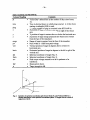
HTI's Model240, 200KHz Split Beam Hydroacoustic System consists of
a split-beam echosounder, a monitor and keyboard, two transducers, an oscilloscope, a
chart recorder, a digital audio tape recorder, a 486DX personal computer, and a 24-pin
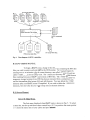
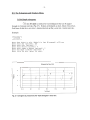
dot-matrix computer printer (Fig. 1).
Echosounder
Model 402 Digital
Chart Recorder
Printer
lool
Rotator
Control
Fig. 1:
Digital Audio
0
0
Schematic diagram of HTI's model 240 split-beam hydroacoustic system as configured at
Qualark. (From HTI, 1993).
Unlike conventional echosounders that can only determine the range of a
target, a split beam echosounder can measure the three-dimensional position of a target.
Therefore, it is possible to accurately track and enumerate fish as they migrate through the
echosounder beam. The receiver contained in the split-beam echosounder provides
simultaneous 20 log(R) and 40 log(R) time-varied-gain (TVG) output, so echo-integration
and target tracking can be accomplished concurrently.
The digital split-beam processor (DSBP) board processes signals received
from the split-beam echosounder. This board interfaces with the 486 computer attached
• Hydroacoustic Technology Inc., Seattle Washington, USA.
- 2-
to the echosounder, via a standard ISA slot. The 486 computer also runs HTI's real-time
software and stores data files collected during echosounding.
The digital chart recorder located in the echosounder prints echograms
using a standard 24-pin dot-matrix printer. Echogram printing is controlled through a
menu system accessible via the keyboard and monitor attached to the echosounder. The
keyboard is also used to input various echosounder settings such as time-varied-gain, and
ping rate.
The digital audio tape (DAT) recorder records raw echosounder output on
tape. If desired, tapes can later be re-processed through the DSBP using modified
echosounder parameters.
The oscilloscope provides the primary feedback for aiming the acoustic
beam. It displays the return signal voltage vs. time (in effect, the return signal strength
vs. range).
The rotator control remotely actuates a rotator to which the transducers are
attached. This allows positioning of the beam both vertically, with respect to the river
bottom, and horizontally, in the up-stream or down-stream direction.
HTI'S SOFTWARE.
HTI provides real-time and post-processing software that reside on the 486
computer connected to the echosounder. Integral to this group of programs are DSBP
which performs echo integration and DSBPTRAK which performs target tracking. These
two programs multitask under the DesQView operating environment, processing output
from the DSBP board and producing output in the form of ASCII data files and real-time
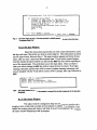
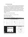
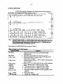
graphical displays. A variety of graphs can be displayed while data are collected (Fig. 2).
- 3START
EHD
BOTTa« TRACKING
GRAPH
Tracked Fish by Range
ROTATE 3D
~
PRIHT PLOT
MAIH MEHU
Target Strength
D
D
10.0
D
D
D
D
D
8.0
6.0
D
D
D
D
D
4.0
0.0
-2.0
D
D
-4.0
D
-6.0
-2o:-2 2
-22:-24
-24:-26
-26:-28
-28:-3o
-3o:-32
-32:-34
-34:-36
-36:-38
-38:-4o
-4o:-42
-42:-44
-44:-46
-46 :-48
-48:-so
TS Bins (dB)
-8.04----------.----------.---------.----------.~---
0.0
3.0
6.0
9.0
12.0
Current OUtput Fi1es: A2411600.RAW A2411600.ECH A2411600.FSH
Real T~e Res~ts: Raw Echoes 1 Tracked Targets 35 Average TS -29.2 dB
Current Settings: Run
Hot Speciried
Bottom Range: 11.0 meters
Port 2
Fig. 2:
Example on-screen display of HTI's DSBP software. Several real-time graphical displays are
available. This one shows a histogram of tracked targets by range.
- 4-
CHAPTER 1 - HAFU, THE HYDRO-ACOUSTIC FILE UTILITIES
A) OVERVIEW.
Although HTI's software is necessary for real-time data acquisition and
analysis, we have found that their post-processing software is cumbersome to use with
large volumes of data and often does not meet our requirements for detailed data analysis.
Thus, we have developed our own software tools. These are grouped under two main
categories: utilities to concatenate and convert HTI data files into a more useful format,
and routines to analyze and graphically display the data.
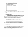
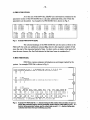
The first category of software is accessible from the DOS program HAFU
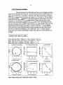
which is a menu-driven front end for several command-line utilities. A screen-display of
HAFU is shown in Fig. 3.
Co~p~ess Daily Piles
~ Conue~t HTI Raw Piles to PBS Raw Piles
Conue~t HTI Echo Piles to PBS Echo Piles
Conue~t PBS Echo Pile to PBS Fish Pile
Me~ge HTI Raw Files
Display Upst~a~ T~acked Fish Counts
Uiew Results
Shell to DOS
Quit
Fig. 3:
Example on-screen display of HAFU, Hydro-Acoustic File Utilities.
The function of each HAFU menu item is outlined in Table 1.
- 5Table 1. The function of each menu Item In HAFU. Command arguments are shown In <brackets>.
Menu Item
User Input
Compress Daily
Files.
Year and day of
the year.
Convert HTI Raw
Files to PBS Raw
File.
Convert HTI
Echo Files to
PBS Echo File.
Year, days of the
year, and start and
end times.
Year, days of the
year, and start and
end times.
Convert PBS
Echo File to PBS
Fish File.
Merge HTI Raw
Files.
Name of PBS echo
file.
Year, days of the
year, and start and
end times.
Shell to DOS.
None
Quit.
None
Output
A PKZIP-format compressed
file containing all data files for
xear and dax .
PBS-format raw file containing
all HTI Raw file data for
~riod seecified.
PBS-format echo file
containing all HTI Echo file
data for period specified.
PBS-format fish file containing
conversion of specified PBS
echo file.
HTI-format raw files split into
output for each multiplexer
port. New files are written
each time a parameter change
is encountered.
View output files from any of
the above procedures. This
item launches the shareware
erogram called LIST.
Exits temporarily to DOS.
Ty~ 'exit' to return to HAFU.
Quits HAFU.
Command-Line Equivalent
pkzip <zipfile>
<datafiles>
rawfiltr <HTirawfile>
<rnuxloutput>
<rnux2output>
echfiltr
<HTiechofile>
<rnuxloutput>
<rnux2output>
ech2fsh <echofile>
<fishfile>
None.
command
Not applicable.
The primary value of HAFU is its ability to deal efficiently with large
amounts of data from numerous files. For example, during an operational day at Qualark
the echosounder may produce up to 120 separate data files (5 file-types x 24 hours)
equaling on a low passage day, perhaps 10 megabytes of data. Using HAFU, the user can
compress all of these files into a single file approximately 10-30% of the original size.
HAFU then operates from the compressed file, avoiding the need to decompress the files
directly. For instance, if the user wishes to look at the raw data for a particular time
frame, she needs to enter only the dates and times desired and the relevant files will be
decompressed from the compressed file, converted to PBS-format, and concatenated into
a single flat-file that can be read into a spreadsheet or other analysis software. Any
intermediate stages between the compressed file and the PBS-format file are deleted
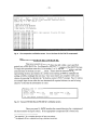
during the process. Fig. 4 schematizes the operation of HAFU. Refer to appendix A for
a complete description of HTI and PBS file types and their formats .
- 6HTI-format data files.
~~~~~
RAW
ECHO
FISH
SUMMARY INTEGRATION
PKZIP compressed
file.
RAW
Fig. 4:
FISH
ECHO
PBS-format data files.
HTI-format RAW files.
Flow-diagram of HAFU 's operation.
B) HAFU USER'S MANUAL.
To begin a HAFU session, change to the directory containing the HTI data
files you wish to analyze and enter HAFU at the DOS prompt. The program begins by
creating two sub-directories under the current directory, one called \RESULTS and one
called \TEMP, if they do not already exist. The \RESULTS directory stores PBS-format
files resulting from any of HAFU's conversions of HTI files. The \TEMP directory is a
temporary storage location for any HTI files that are extracted from a compressed file,
and for intermediate files between HTI and PBS formats. You may delete the \TEMP
directory after your HAFU session is completed. If you wish to delete the \RESULTS
directory, first move the files you want to keep into an alternate directory.
B.l) Screen Elements.
B.l.l) The Main Menu.
The first menu displayed when HAFU starts is shown in Fig. 5. To select
a menu item, use the up and down cursor control keys ( "fr .JJ.) to position the menu-pointer
(=>) next to the menu item of your choice and press ENTER.
-7-
HAFU Hydro=acoustic file utilities-==========-=========n
-> Compress Daily Files
Convert HTI RAW Files to PBS RAW File
Convert HTI ECHO Files to PBS ECHO File
Convert PBS ECHO File to PBS FISH File
Merge HTI RAW Files
Display Upstream Tracked Fish Counts
View Results
Shell to DOS
Quit
t! =Move. ENTER= Select. Fl =Help. FlO =README
Fig. 5:
The main menu of HAFU. The menu-pointer Is Initially positioned next to the first Item,
"Compress Dally Files".
B.1.2) The Input Window.
Most of the menu items require that you enter certain information, usually
the days and times of the period you wish to extract data for. This information is entered
into the input window, shown in Fig. 6. The input window appears just below the main
menu, after you select a menu item that requires input. If you wish to cancel the menu
item that initiated the input window you must hit the BSC key first, before responding to
any of the input prompts. This will return you to the main menu. Once you begin to
enter your choices, hitting the BSC key will not cause the item to cancel. If you begin
entering information and then later wish to cancel, continue entering information until
you are prompted with the "Is the above correct (YIN)?" prompt, then type N followed by
BSC.
Input: ESC to cancel-=--==-====-===-==================;
Enter system (1/2): 1
Enter year (format=nnnn): 1994
Enter start julian day (format=nnn) :
Fig. 6: The Input window of HAFU. Information Is entered line by line In response to the prompts
displayed.
B.1.3) The Status Window.
The status window is designed to keep you informed of a specific task's
progress, since certain tasks can take several minutes to complete. This window is also
helpful for locating when and where a task fails, if an error is encountered. Fig. 7 shows
the status window displaying a task in progress.
- 8Status==========================~
Finished decompressin9.
Processing, please wa~t ...
Done: A2380000.RAW => A2380000.SPR
B2380000.SPR
Done: A2380100.RAW => A2380100.SPR
B2380100.SPR
Fig. 7:
The status window of HAFU. The progress of the task being performed is displayed in this
window.
B.1.4) The Help Window.
The help window displays a brief description of each menu item. To view
help on a particular menu item, position the menu-pointer next to the menu item and
press the Pl key. Fig. 8 shows the help window displaying help on the "Quit" menu
item. To view a more detailed help file, press FlO while in the main menu.
Help - Press 'ESC' to clear---------------------------,
Quits HAFU and returns you to the operating system.
Fig. 8:
The help window of HAFU. A brief description of each menu Item is available via this
window.
B.l.S) The Read Window.
HAFU uses the shareware program called LIST to display various ASCII
files, including HTI and PBS data files. A full description of LISTs features are not
included in this discussion. Refer to the UST documentation in the \HAFU\LIST
directory for more information regarding it's use.
- 9B.2) Menu Items.
B.2.1) Compress Daily Files.
This menu item is used to compress all HTI files for a given day of a given
year, into a single file. To begin this procedure, enter the number of the echosounder
system, and the year and day that the HTI files were collected. The echosounder system
number indicates which system the data were collected on. Currently it can only be 1 or
2 as an historical consequence of our use of two echosounders at Qualark. If you use
only one echosounder system, the system number will always be 1. If you use more than
2 systems, contact us to have your version of HAFU modified. The year must be entered
as 4 digits, for example, 1995. The day is defined as a sequence starting at 1 on January
1st of each year. It must be entered as 3 digits, for example 013 for January 13th. When
you have finished entering all the required information, verify your entries by pressing Y
after the "Is the above correct (YIN)?" prompt. If you wish to change one or more of your
entries press N after this prompt.
Once you have verified your entries, HAFU searches the current directory
for all HTI files that match the system, year, and day that you specified, and compresses
them using PKZIP, into a single ftle. While this is happening the display switches to a
plain DOS screen that allows you to view the compression as it occurs. When
compression is complete the resulting file is checked for errors by PKUNZIP and the
results are displayed on the screen. You can use the Page Up and Page Down keys to
view these results and look for any compression errors that may have occurred. Each
compressed file is listed down the left side of the screen with either an "OK" to the right
of it or an error message (Fig. 9). Press ESC when you have finished viewing this
information. The display then switches back to HAFU and you are asked if you wish to
delete the original HTI files. Press Y if you are satisfied that the file compression
operation was successful (i.e. if no error messages were displayed) or N if an error
occurred. If errors were encountered you may wish to retry the compression procedure or
quit HAFU and take other steps. Compression errors are very rare, in fact we have yet to
encountered one while working with our data (the error shown in Fig. 9 is a simulation).
- 10-
:.J r ::.·r
J
·
:•
.~
r
~)
t
~
:
~
(.
•
~.·
1 .J
•
~ •t
•
•
••
PKUNZIP (R)
FAST!
Extract Utility
Version 2 .04g 02-01 - 93
Copr . 1989-1993 PKWARE Inc . All Rights Reserved . Registered ver s i o n
PKUNZIP Reg. U. S. Pat. and Tm . Off.
80486 CPU detected.
EMS version 4.00 detected.
XMS version 2. 00 detected.
DPMI version 0 . 90 detected .
Searching ZIP: 94A238 . ZIP
Testing: A2380000.RAW PKUNZIP : (W15) Warning! file fails CRC check
Testing: A2380000.ECH OK
Testing: A2380000.FSH OK
Testing : A2380000.INT OK
Testing: A2380100.RAW OK
Testing: A2380100.ECH OK
Testing: A2380100.FSH OK
Testing: A238 0100.INT OK
Testing: A2380200 . RAW OK
Testing: A2380200.ECH OK
Testing: A2380200 . FSH OK
Testing: A2380200 .INT OK
Fig. 9:
File compression verification screen. An error is shown for the first file compressed.
B.2.2) Convert HTI RAW files to PBS RAW file.
This item converts all HTI RAW files that fall within a user specified
period, into a PBS RAW file. See appendix A for a full description of the RAW file type.
To begin this procedure enter the system number (1 or 2), the start and end day, and start
and end times of the data you are interested in. Times must be entered as 4 digits
representing the hour and minute on a 24 hour clock starting at 0000 at midnight and
ending at 2400 at midnight the next day.* Once your entries are complete verify your
choices by pressing Y or N after the "Is the above correct (YIN)?" prompt. Fig. 10. shows
an example input screen after the user has entered all required information and is being
asked to verify that the information is correct.
Inpu t : ESC t o cance l =====================================9
System = 1
Year = 1994
Start Jul i an Day = 231
End Julian Day
234
Start time
= 2230
End time
0030
Is the above correct (Y/N)?
Fig. 10: "Convert HTI RAW files to PBS RAW file" verification screen.
Once you press Y, HAFU searches the current directory for a compressed
file that matches the input criteria.** If the appropriate compressed file is found, any
• See appendix C for a complete description of input conventions.
•• See appendix B for a complete description of naming conventions.
- 11 -
RAW files that fall within the period specified are extracted and converted to PBS
format. HAFU uses information found in each file's parameter section to calculate
additional variables of interest such as beam pattern factor and target strength. The
parameter sections are then left out of the resulting PBS RAW files. When all
conversions are complete the PBS RAW files are concatenated together into two files
containing the information for the specified period of interest. One file contains data
collected on port 1 and the other contains data collected on port 2. Note that if only one
port was used to collect data, the file representing data from the other port consists of
only a single header line. This file should later be deleted. ·
When the conversion process is complete, the display switches to a view
of the RESULTS directory, showing a list of the files contained there (Fig. 11 ). This list
includes the PBS RAW files that were just produced, as well as any PBS files from
previous procedures. To view any of these files, use the cursor control keys ( 1::t .0. ¢:n:~) to
position the highlight bar over the file name and then press ENTER. When you have
finished viewing files, continue to press ESC until you are back at the HAFU main menu .
..
A2380000.ALR
B2380000.ALR
Fig. 11: The IUISULTS directory with two PBS RAW flies listed. One represents data collected on
port 1 (A2380000.ALR) , the other represents data collected on port 2 (B2380000.ALR).
B.2.3) Convert HTI ECHO files to PBS ECHO tlle.
This item operates identically to the "Convert HTI RAW files to PBS
RAW file" item, except that the resulting files are ECHO format, not RAW. Follow the
steps outlined in B.2.2 to use this procedure.
- 12B.2.4) Convert PBS ECHO file to PBS FISH file.
This item converts PBS ECHO files (created with the item "Convert HTI
ECHO files to PBS ECHO file") to PBS FISH files. To use this item, enter the name of
the PBS ECHO file you wish to convert and the ping rate used to collect the data. You
are asked to verify your entries before the conversion takes place. During the conversion
the status window displays the prompt "Processing ... " and when completed, the source
PBS ECHO file and target PBS FISH file names are displayed (Fig. 12). When the
conversion is complete, press any key to return to the HAFU main menu.
Status===--======--=============~
Processing ...
Done: a2380000.ale -> a2380000.alf
at 10 pings/sec.
Conversion complete.
Press a key to continue.
Fig. 12: Status window upon completion of PBS ECHO file to PBS FISH file conversion.
B.2.5) Merge HTI RAW files.
Occasionally it's necessary to reprocess RAW data using HTI's DSBP
software. This software will accept any HTI RAW file and re-track the data, creating
ECHO, FISH, and SUMMARY files as output. This procedure can be very time
consuming when one is dealing with dozens of RAW files. The menu item "Merge HTI
RAW files" is designed to expedite reprocessing of HTI RAW files by concatenating all
HTI RAW files that fall within a user-specified time frame. The concatenated files are
split into separate files for each port and a new set of files is produced each time a change
in a parameter value is encountered in the original HTI RAW files. This can greatly
reduce the number of HTI RAW files you must deal with and also provides a clear
indication of when a parameter change occurred. For example, suppose you have six HTI
RAW files representing data collected from two ports over a period of six hours, and that
the same parameters were used to collect all of these data. The "Merge HTI RAW files"
procedure will create two HTI RAW files from these data, one file containing the data
from port 1 and one file containing the data from port 2.
As with previous menu-items, you must enter the system number, year,
starting and ending day, and starting and ending times. HAFU then searches the
appropriate compressed files for HTI RAW files that fall within the period specified.
- 13-
B.2.6) Display Upstream Tracked Fish Counts.
This item is not yet implemented as it requires that HTI make some small
modifications to the way that the SUMMARY file is written. However, you can still use
this procedure provided that your SUMMARY files summarize all of the data collected
on a specific day, and only the data for that day.
B.2. 7) View Results.
This item executes the shareware program called UST, in the RESULTS
directory under the current working directory. This allows you to view any of the results
from your HAFU session by positioning the highlight bar over a file name and pressing
ENTER. You can also perform several file management activities from within UST.
Refer to the UST documentation or press the Fl key from within UST for more
information.
B.2.8) Shell to DOS.
This item allows you to temporarily exit HAFU and access the DOS
command-line. When you are ready to return to HAFU, enter EX:IT.
B.2.9) Quit.
This item quits HAFU and returns you to the operating system.
- 14-
CHAPTER 2- QTS, QUALARK TOOLS FOR S-PLUS
A) OVERVIEW.
QTS is a collection of S-Plus routines that we developed while working at
our hydroacoustic site near Qualark Creek on the Fraser River, just north of Hope. These
tools are primarily designed to graph data, but they also provide options for producing
summaries of fish passage and for editing data interactively. QTS is written in the S
language and requires the Windows version of S-Plus to run. A full description of the S
language is given in Becker et al, 1988.
Like HAFU, QTS provides a menu-driven interface. You can access this
menu by double-clicking on the QTS icon in the Program Manager of Windows, just as
you would any Windows application. Double-clicking on the QTS icon launches S-Plus
for Windows and executes the appropriateS code to initialize the QTS menu. Fig. 13
shows the QTS icon in a program group with other application icons.
r~~,...:'(~'"":Y.~'mX>W&:«::11.:'Z
fJ
1
•
.,~~"""
... ,.., •..,.....
""..,_#.-
""'
Hydroacoustics
~
QTS Help
HAFU
>:'U~
aa1
,..-~-~
..... ~
=~
Ill
WinZip
Fig. 13: The QTS icon in a Program Manager group.
When the QTS main menu appears, activate a menu item by doubleclicking on the menu item text. For example to view a Windows help file concerning
QTS, double click on the text that reads "View on-line help". To leave a sub-menu and
return to the main menu, double-click on the text that reads "Leave this menu". There is
only one level of sub-menu under the main menu so selecting "Leave this menu" will
always return you to the main menu. The complete menu structure of QTS is shown in
Fig. 14.
In addition to the QTS menu, S-Plus also displays a graphics window and
a command window. The graphics window displays various graphs selected from the
QTS menu such as histograms and images. The command window displays text
messages and prompts, and also accepts text input. Most of the QTS menu items require
that you enter some information into the command window, such as the names of data
frames and labels for plots. Fig. 15 shows the S-Plus display when QTS is running.
- 15 -
"~
Data Manipulation
Select one:
.!::.!!!.!:!.!:!.~_l:! ..l::t.Af.IJ...... ..... ············-···· ·····
Scan a data file
Remove noise from a data frame
Generate a passage report
Directory of data frames
Make a RAW object current
Make an ECHO object current
Make a FISH object current
Leave this menu
Access QTS Help File.
~.Y.l?_.Y_._........·-·····················-··· ····-····-·········-····-·········-····-··· · · ·-···
ZvsX
-----------+--11~ Xvs Y
TS vs off-Axis angle
Leave this menu
Select one:
Select one:
~imP.k..!t'!.M..!I.!:!!_I.!'L_ ____.....·-----·--·····-··············-·········
.!,l.P..l!!.!tl!f..!:!..!!!!f~!!...~.Y.-I!!!.!:!.Q.!L. _________......·-····-·········-···
Targets by vert,lhoriz angle
TS vs off-axis angle
TS vs range
Leave this menu
Echogram examiner
Target track examiner
Leave this menu
Fig. 14: Overview of the QTS menu structure.
- 16 -
HISTOGRAM OF UPSTREAM AHD DOWHST
nter FISH data frame to plot (def
nter direction of water flow, lef
default is left_to_right):
nter title for plot: Test
Select one:
Up/down tracks by range
Targets by vert/horiz angle
TS vs off-axis angle
TS vs range
Leave this menu
....
1,:?;;::
Fig. 15: The layout of S-Pius for Windows when QTS is running. Note the command window,
graphics window, and QTS menu.
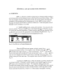
B) QTS USER'S MANUAL.
B.l) Main Menu Items.
B.l.l) View on-line help.
This item accesses a Windows help file on QTS. The help system includes
standard Windows help features such as hypertext links that allow you to to jump to
topics by clicking on certain words or phrases indicated by green, underlined text. See
the Windows user manual for more information on using this help system. Fig. 16 shows
the Windows help system running the QTS help file.
- 17-
Qualark Tools for S·Pius: Contents
Scanning in a data file.
Interactively removing noise from data
Images
Histograms
Echograms and Tra ckers
Fig. 16: The QTS help system.
B.1.2) Data manipulation.
This item brings up the sub-menu called "Data Manipulation" which
provides items to convert data files to S-Plus format, to edit data sets interactively, and to
create summaries of fish passage.
B.1.3) Images.
This item brings up the sub-menu called "Images" which allows you to
choose from several different image plots. Images are two-dimensional histograms in
which two variables form a grid of some pre-defined spacing. The number of
observations falling within each cell of the grid is summed, and the relative difference in
frequencies among cells is indicated by differences in cell colour or shades of gray. For
gray-scale images, cells with no observations are coloured black while the the cells with
the highest number of observations are coloured white. For all of these routines you may
plot a RAW, ECHO, or FISH data frame. Note that when using a FISH data frame, all
coordinates are defined as the initial position that each fish was detected in the beam.
B.1.4) Histograms
This item brings up the sub-menu called "Histograms" which allows you
to choose from several different histogram plots. Histograms graphically display the
freqency of observation of some variable summed over regular intervals. The freqeuncy
at each interval is represented by a bar of variable height where the interval with the
greatest frequency is represented by the tallest bar. Unless otherwise indicated, a RAW,
ECHO, or FISH data frame may be plotted.
- 18-
B.l.S) Echograms and trackers.
This item brings up the sub-menu called "Echograms and Trackers" which
allows you to choose from echograms and tracker plots. Echograms are plots of detected
echoes shown on a time (horizontal axis) vs. range (vertical axis) display. Trackers
display the trajectory of individual tracked targets.
B.1.6) Quit.
This item quits QTS and ends your S-Plus session.
B.2) The Data Manipulation Menu.
B.2.1) Launch HAFU.
This item launches HAFU. Enter the name of the directory that you wish
to run HAFU from. This should be the name of the directory containing the HTI files
you wish to analyze. Note that HAFU can also be run as a stand-alone DOS program, by
entering HAFU at the DOS prompt.
B.2.2) Scan a data file.
This item allows you to convert a data file produced by HAFU, into SPlus binary format. This step is necessary before any plots or summaries can be produced
since S-Plus can only work with it's own format of data file. Enter the name of the
source data file and a name for the target data frame (data frames are a particular kind of
S-Plus data set).
Example:
**************************************
* SCAN A DATA FILE INTO A DATA FRAME *
**************************************
Enter a name for the target data frame : a244 . fsh
Enter the source file name (give full path): c: \ 94sysl \ results \ a2440000 . alf
B.2.3) Remove noise from a data frame.
This item allows you to remove echoes from a data frame using visual
tools. This is useful for eliminating rocks or other non-fish targets. The display consists
of two windows, one titled brush that shows selected variables from the given data frame
- 19 -
plotted against each other, and one titled spin that shows any three of these variables in a
3-D plot that can be rotated and expanded. Use the left mouse button to highlight any
echoes that you wish to remove from the data. A small box in the lower right of the
display lists the target strength, in decibels, of all echoes displayed. As you highlight
echoes with the mouse, the corresponding target strength is highlighted in this box. This
is useful for checking the target strength of individual echoes. Fig. 17 shows a display of
this routine. See S-Plus documentation for more information on using the brush/spin
display.
Example:
**********************************
* REMOVE NOISE FROM A DATA FRAME *
**********************************
Enter a name for the target data frame: newa244.fsh
Enter the name of the source data frame: a244.fsh
D
Big Points
[]
•
•
0
Fig. 17: Screen-display of the brush and spin plot from the "Remove noise from a data frame" menu
option.
- 20-
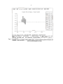
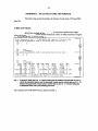
B.2.4) Generate a passage report.
This item generates a table, output to an Excel spreadsheet, of upstream
and downstream passage per hour for a given time frame (Table 2). The data are also
displayed graphically (Fig. 18). This is a useful tool for producing daily summaries of
fish passage through the beam. The count is automatically expanded for the portion of
each hour that the beam was not operated. For example, if two beams were multiplexed*
at 15 minute intervals, each beam would collect data for 30 minutes out of each hour.
This procedure multiplies the count in each beam to make an estimate of the total number
of fish that passed through the beam each hour. Thus, the count would be expanded by a
factor of 2 for a beam that operated for 30 minutes out of each hour. The direction of
water flow past the beam must be entered so that upstream and downstream passing fish
can be correctly identified. Water flow direction is defined as left_to_right or
right_to_left, as seen from the river bank looking out into the river.
Example:
*************************
* GENERATE DAILY REPORT *
*************************
Enter source FISH data frame (default is last FISH file scanned): a255.fsh
Enter number of minutes of data collected per hour (default is 60 min): 30
Enter the direction of water flow (right_to_left or left_to_right)
Default is left_to_right: left_to_right
Enter title:
Table 2: Summary table produced by the "Generate a passage report" procedure.
Unvalidated Expanded Fish Passage.
Julian Day(s): 244 to 244 . Flow = Left to right. Expansion Factor = 2
Julian
Start
End
Up
Down
Avg
Avg
Day
Hour
Hour
Stream
Stream
TS
Speed
244
0
244
1
2
244
244
244
244
244
2
3
4
5
3
4
5
6
7
6
Total Passage:
Hourly Mean Passage:
228
28
-29.58
1.23
278
218
260
356
120
102
60
56
58
140
14
14
-28.59
-28.75
-28.6
-28.23
-27.33
-27.55
1.45
1.39
1.39
1.48
1.45
1.42
1562
370
223.14
52.86
-28.38
1.4
• Multiplexing refers to switching echousounder operation between two transducers at some regular interval.
- 21 -
Unvalidaled Expanded Fish Passage.
JuHan Day( s): 244 to 244 . Flow = Left to right. Expansion Factor = 2
0
a
3
4
6
Hoqr
(Dowo<tr..,. p••<ioglioll oro ollowoloclow oxi•)
Fig. 18: Plot produced by the "Generate a passage report" menu Item.
B.2.5) Directory of data frames.
This item lists all available data frames (data objects that can be passed as
arguments to the various plotting routines).
Example:
**************************************
* DIRECTORY OF AVAILABLE DATA FRAMES *
**************************************
CURRENT.ECH
CURRENT.FSH
CURRENT.RAW
a244.ech
a244.fsh
a244.raw
newa244.fsh
extent object.size
dataset.date
data.c1ass storage.mode
1268743 95.01.09 15:42
data. frame
list 9263 X 16
data. frame
list 1076 X 22
199030 95.01.09 15:42
1726472 95.01.09 15:42
data.frame
list 13360 X 15
list 9263 X 16
1268743 95.01.09 14:02
data. frame
data. frame
list 1076 X 22
199030 95.01.09 14:03
data. frame
list 13360 X 15
1726472 95.01.09 14:50
970 X 22
179449 95.01.10
data. frame
list
9:05
B.2.6) Make a RAW object current.
This item allows you to make a RAW data frame the current RAW data
frame. Use this procedure when you wish to pass the same RAW data frame as an
argument to several different routines without having to retype the name of the data frame
each time. This only applies to routines that use a RAW data frame as a default
argument.
- 22- .
B.2. 7) Make an ECHO object current.
This item is the same as B.2.6 but applies to an ECHO data frame.
B.2.8) Make a FISH object current.
This item is the same as B.2.6 but applies to a FISH data frame.
- 23-
B.3) The Images Menu.
B.3.1) Z vs Y.
This item produces a density image of target frequency in the Z (Distance
from the transducer face, in meters) vs Y (vertical coordinate in meters) plane (Fig. 19).
A scatter plot of the same data is shown below the image.
Example:
**************************************
* IMAGE OF Z (RANGE) VS Y (VERTICAL) *
**************************************
Enter data frame to plot (default is current ECHO): a244.ech
Enter title for plot: Echo Data.
hrg<!t Diotril>vtion in Zf'i Jll•••
D•~ ass · Troc~ed J:c'hoeo.
Density Image
N
~
j
~
D
~
>
c
-;
~
a
4
6
Di~.:a1111ct:
e·
10
8
10
lrom T~n~duce:r
Scatter Plot
N
~
j
~
D
~
>
c
-;
~
a
6
Di~~nce
Fig. 19: Z vs. Y density image.
lrorn
Tnn~ducer
- 24-
B.3.2) Z vs X.
This item produces a density image of target frequency in the Z (Distance
from the transducer face , in meters) vs X (horizontal coordinate in meters) plane (Fig.
20). A scatter plot of the same data set is shown below the image.
Example:
****************************************
* IMAGE OF Z (RANGE) VS X (HORIZONTAL) *
****************************************
Enter data frame to plot (default is current ECHO): a244. ec h
Enter title for plot: Echo Data.
hrget Diotribution in ZIX ll>nt
D•y 355 • Troc\td J:cllo• •·
Density Image
~
~
~
li
~
0
e.
X
"'
c
..
~
Di~;)fiiCC
rrom
hn~duccr
Scatter Plot
.:·~·', .~:.· .,.:_:._: /·;:.- ~- .·.~:.>:_:·::- :~-~.-: :=, .-·
....
··:\;·,:: .-: ..·.::._·/:.(.;/.:·,: ..· .' :.:;, :< :' ·...:
·. • .
a
8
Di~::lln cc
Fig. 20: Z vs. X density image.
lrom
Tr~n::;d\lct:r
10
-25-
B.3.3) X vs Y.
This item produces a density image of target frequency in the X
(horizontal coordinate in meters) vs Y (vertical coordinate in meters) plane (Fig. 21). A
scatter plot of the same data set is shown to the right of the image.
Example:
*******************************************
* IMAGE OF X (HORIZONTAL) VS Y (VERTICAL) *
*******************************************
Enter data frame to pl ot (default is current ECHO): a244.ec h
Enter title for plot : Echo Data .
hrget D•••ity l>y Op/Dow•·Ltltlltigllt ,.,.gle
D•y 355 • Tr•c\td Zc'hoeo.
Density Image
Scatter Plot
5!
M
.."'
"'
"'
<
~
II)
<
~
c
~
~
:::>
:::>
'I'
'I'
!j!
!j!
·10
·5
0
Ltfti:Rigllt Aoglt
Fig. 21: X vs. Y density Image.
10
·.·
c
...
·... ...
: ·.
.. ;
...
·.•. ;:_:;·~':{:~;],}·;;+•. •
·10
·S
0
10
-26-
B.3.4) TS vs off-axis angle.
This item produces a density image of target strength, in decibels, vs. offaxis angle (angle from the centre of the beam, in degrees), (Fig. 22. A scatter plot of the
same data set is shown below the image. Note that this plot is only appropriate for beams
with circular cross-sections.
Example:
************************************ * *********
* IMAGE OF TARGET STRENGTH VS OFF-AXIS ANGLE *
**********************************************
Enter data frame to plot (default is current ECHO): a244.ech
Enter title for plot: Echo Data.
hrgc:t 3trtngl'h lrtq•••cy by Ofi·Axio Anglt
Doy 355 • Tr>c\td J:c'hoeo.
Density Image
"'
c
·35
·30
·30
·35
·15
·10
·15
·10
hrgc:t 3trtngl'h (dB)
Scatter Plot
S!
"'
c
· 35
-30
·30
· 35
hrgc:t 3trtnglh (dB)
Fig. 22: Target strength vs. off-axis angle density image.
- 27 -
B.4) The Histograms Menu.
B.4.1) Up/down tracks by range.
This item produces a histogram of tracked targets by range, in meters (Fig.
23). Upstream-migrating targets are shown above the x-axis, downstream-migrating
targets are shown below the x-axis. Only FISH data frames may be used with this
routine.
Example:
*****************************************************************
* HISTOGRAM OF UPSTREAM AND DOWNSTREAM TRACKED TARGETS BY RANGE *
*****************************************************************
Enter FISH data frame to plot (default is current): a255.fsh
Enter direction of water flow, left_to_right or right_to_left.
(default is left_to_right): left_to_right
Histogram of tracked fish vs . range
Day 255 .
0
CD
>-
(0
0
cQ)
::I
C"
Q)
&t
,.,.
N
0
3.0
3 .5
4 .0
4.5
5.0
5.5
6 .0
6 .5
7.0
Range (m)
Fig. 23: Histogram of upstream and downstream tracked targets by range.
7 .5
8 .0
8.5
- 28-
B.4.2) Targets by vert/horiz angle.
This item produces histograms of target frequency vs vertical angle and
horizontal angle, in degrees (Fig. 24).
Example:
********************************************************
* TARGET DISTRIBUTION BY VERTICAL AND HORIZONTAL ANGLE *
********************************************************
Enter data frame to plot (default is last ECHO scanned): a244.ech
Enter title for plot : Day 255 .
Vertic~!
::lind Horio:orrt~l hrgt't Di~ribution
n.v a55.
Vertical Distribution
5!
...
"' "'
<
c
~
--
$
~
0
ao
10
40
30
50
60
lrcquc:ncy
Horizontal Distribution
·10
·5
0
Horioontol Angl•
···---
Fig. 24: Histograms showing target frequency vs. vertical angle (degrees) and target frequency
horizontal angle (degrees).
10
vs.
- 29 -
B.4.3) TS vs off-axis angle.
This item produces histograms of target strength, in decibels, for each
degree of off-axis angle spanned by the data (Fig. 25). Note that this plot is only
appropriate for beams with circular cross-sections.
Example:
****************************************************
* HISTOGRAMS OF TARGET STRENGTH PER OFF-AXIS ANGLE *
****************************************************
Enter data object to plot (default is last ECHO scanned): a244 . ech
Enter title for plot: Echo Data.
Pili= 0 to 1
~
..
..
..
..
..
Pili• 1 to
.
.
.
... ... -··
Pili=
a to
3
!:'
.
.
.
"
.
.
....
, ..... 'Sit-alii I~
II I I
..
,..... ,
,.
... -··
.....
!'
.
.
.
I 1.1111
.
....
... ... -··
.....,.
,.....
Pili= 5 to 6
Plli=4to5
!'
!'
.
.
.
.
"
II
II
... ...
I
.
....
... . "'....,. -··
,
.....
I1,.....
...
..
.
'•lllf'Stt.Uhl~
Pili= 6 to 7
Pili= 7 to 8
R
!.'
!.'
.
.
!!'
!'
"
.
.
.
~
!:'
!:'
Pili= 3 to 4
.
-
....
a
I... ...
..
..
111
....
-··
' •glii 'Sft-.:lll hl-
I
....
...
I...
II
.... ,....,.. ,.-··
,
..
.
I
.....
1•.
... ... -··
' •lllf 'SII .U tl l ~
Fig. 25: Histograms of target strength (dB) for each degree of off-axis angle spanned by the data.
- 30 -
B.4.4) TS vs range.
This item produces histograms of target strength, in decibels, for each
meter of range spanned by the data (Fig. 26).
Example:
*************************************************
* HISTOGRAMS OF TARGET STRENGTH PER METER RANGE *
*************************************************
Enter data objec t to plot (default is last ECHO scanned) : a244.ech
Enter title for plot: Echo Data.
'•IJIIII
~••9•
= 3 to 4 M
D
~••9•
= 4 to 5 M
~._,
.. .,.,,_,.,.
~
RIIVI
O.,~ · '•a..Ea- .
~••9•
= 5 to 6 M
~••9•
= 6 to 7 M
!'
"
!'
!'
~
!i'
~
D
D
D
!i'
p
D
...
I
.II Ill
... ... . •
... ..•
'•1111'511-alhl~
~••9•
1.1
'•P "'•-alh IAt'
= 7 to 8 M
~••9•
IIIII
... ...
1,. ..
.
.
'•giiiii'Sh-clhl~
.•11
....
= 8 to 9 m
!'
!i'
!i'
.hi ... ln....
...
.
' •IIIII
'S1 1 -.:Ih l~
1.1
I.
... ...
II
..
.
'•"'"'...... ,~
!'
R
...
1~~.
I
.
'·-~•.Vhl~
Fig. 26 : Histograms of target strength (dB) for each meter of ran ge spanned by the data.
- 31 -
B.5) The Echograms and Trackers Menu.
B.S.l) Simple echogram.
This item produces a standard on-screen echogram that can be paged
through in 6 minute intervals (Fig. 27). Echoes are displayed as short, black vertical bars.
Grid lines divide the x-axis into !-minute intervals and the y-axis into 1 metre intervals.
Example:
************
*
ECHOGRAM
*
************
Enter
Enter
Enter
Enter
Enter
Enter
Enter
data object to plot (default is last RAW scanned) : a255 . raw
start day (optional) : 255
start hour (optional ): 2
start minute (optional) : 0
start range in meters (optional) : 2
end range in meters (optional) : 9
title for p lo t (enter for none ) :
Echogram for Day 255
"'
r---·----·-- -
..·-------..- ·-·--·--··------ -------·-· ·-···-······-····--··-····-
···· ~
-·········---·············-··········-··
··- - - - - · · - ··-······-····---·--!--··-·-·-·-·---·-········--· --···---r ----·- ............................ ·····-·····-· --····-·-····-r ·-
.
~
"';;;
1
,1
"'
I
I
a:
I
18 : 0
18 : 1
18 :a
18 : 3
18 : 4
Tim< (llb:mm)
Fig. 27: Echogram as produced by the "Simple echogram" menu item.
18 : 5
· ·1t
- 32-
B.5.2) Echogram Examiner.
This item produces an echogram of a RAW and an ECHO data frame (Fig.
28). Echoes are shown as short vertical bars with untracked echoes (from the RAW data
frame) displayed in black and tracked echoes (from the ECHO data frame) displayed in
some other colour. To view the trajectories of individual tracked targets, use the left
mouse button to click on each highlighted track with the mouse pointer. When you have
selected all the tracks you wish to view, click the right mouse button. You can then view
the trajectories of each tracked target, on a horizontal vs. vertical angle display. When
you have finished viewing tracks, select "Forward" to move on to the next echogram
segment, "Backward" to move to the previous echogram segment, or "Pause" to rerun the
current echogram segment.
Example:
******** * * ** ********************* ** *********
* EXAMINE TRACKS SELECTED FROM AN ECHOGRAM *
******************** * ************ * * * * * * ** ***
Enter
Enter
Enter
Enter
Enter
Enter
Enter
RAW data object (default is last scanned): a244.raw
ECHO data object (default is last scanned): a244.ech
start day (o ptional): 244
start hour (optional) : 2
start minute (optional): 30
start range in meters (opti onal) : 2
end range in meters ( optional): 10
beam x-section width
ional
PBS TRACKMAN (raw echos with tracked echos highlighted) . JD 244
I
I
,,,
.
I
~~
I
I
'"
I
'
2 :1
2 0
2 :2
23
II
~
~
I
,
I
j
2.5
2 :fo
Tmt(W\:mm}
Beam cro ss-Section . Fish· 330
Select one:
s>
--
Pause
Reverse
Quit
t
~
I11
~
1---.
II~
"1
·"
Fig. 28: Screen-display of the "Echogram examiner" routine.
·•
"
- 33-
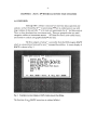
B.5.3) Target track examiner.
This item produces a set of six plots that allow you to compare a tracked
target with surrounding echoes (Fig. 29). The top left plot shows the tracked target in the
beam cross-section (X vs. Yin meters). The plot to the right of this shows the tracked
target with respect to horizontal position and range (X vs. Z in meters). The top right plot
shows the ping sequence represented by the tracked target (the ping number of each echo
returned from the target, relative to the total number of pings since the start of data
collection) vs. the horizontal coordinate, in meters. The circles surrounding each point
represent the relative target strength of each returned echo. The 3 bottom plots mirror the
top ones but include a user-specified "buffer" period, in seconds, before and after the
period during which the target was tracked. On these 3 plots the 'o' symbol represents
echoes that were returned during the tracked target's passage (plus the buffer time) but
that were not identified as belonging to any tracked fish. The'*' symbol represents
echoes that were tracked but that belong to targets other than the currently displayed one.
Example:
***********************************
* EXAMINE TRACKS TARGET BY TARGET *
***********************************
Enter
Enter
Enter
Enter
Enter
RAW data object (default is last scanned): a244.raw
ECHO data object (default is last scanned): a244.ech
starting fish number (optional, default = 1): 35
buffer time in seconds (optional, default = 2): 2
beam width in degrees (optional, default= 8:) 8
z vs X: Beam top-down view
Yvs X: Beam Cross-section
li
!:g.
.,
:c
>
Iii
"..i -
N
-
"I
N
t
t
'•
"'
li
"i
!
x
<:'
X vs Ping Number
"' a
~
I
::S
...-s
"i
Iii
•x
IS.
::>
<:'
l'l
5'
~
"'q
OQ
q
-a
-1
0
a
"'"'
.Ill
1:1
.
>
~
:c
8.8a
8.84
3015
301?
3019
Z: Diot•••• lr- tr•••d•c•r (M)
PiogJ'hMlo•r
Yvs X: Beam Cross-section
z vs X: Beam top-down view
Xvs Ping Number
li
•i..
~
~
8.80
X: Upotr..., -(•)·> Dowootr••,.
'
"'
I
~
~,..-.r--
"'"' <:~
.....,_........_,
a: 1
........_- ...
IS.
.&3
x
I
-1.0
I
0.0
0.5°
1.0
X: Upotr ..., ·(•)·> Downotr••,.
~
I
"'
i
q
IS.
::>
1:1
"'
t
1:1
"'
."Ili
..
OQ
~\
<'1
<'1
'--...~..
::>
x
1:1
"i
8.?8
8.82
8.86
8.90
Z: Diotooc•lr- tr•••d•c•r (M)
Fig. 29: Plots produced by the "Target track examiner" routine.
~
·4.
3000
3005
3010
Piogl'hMlo•r
3015
- 34-
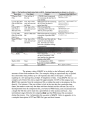
APPENDIX A -DATA FILE TYPES AND FORMATS
The following section describes the format of each type of HTI and PBS
data file.
1) HTI RAW FILES:
RAW files include all detected echoes that pass a point-source target
selection criteria. This can include echoes from fish, rocks, or other point-source targets.
An example RAW file is shown in Fig. 1
* Start Processing at Port 1 C:\SB\SBPORTl.PAR Wed Oct 12 00:00:02 1994
* Data processing parameters used in collecting this file for Port 1
100
101
-1
-1
1
0
A
610
-1 OFF
611
-1 D:\94SYS2\B
* Data processing parameters used in collecting this file for Port 2
100
-1
2
101
-1
0
8
*
*
*
*
*
-1 OFF
610
-1 D:\94SYS2\B
611
Range Sum Chan. -6dB -12dB -18dB
Lf-Rt
Mux
Ping
Up-Dn
Angle
P.W.
P.W. P.W.
Angle
Port
Number meters
Volts
10
-3.3843
12
563
3.16
0.5359
10
2.1950
1
564
3.16
0.3034
7
8
8
2.7752
-3.2484
1
End Sample Block for Port 1 C:\SB\SBPORTl.PAR Wed Oct 12 00:02:00 1994
264
7.38
0.2173
-3.9969
-5.6333
2
8
8
8
-2.1934
265
3.91
0.2454
8
8
8
6.4172
2
End Sample Block for Port 2 C:\SB\SBPORT2.PAR Wed Oct 12 01:00:00 1994
Stop Processing. C:\SB\SBPORTl.PAR Wed Oct 12 01:00:00 1994
Fig. 1:
c
Example HTI RAW data file. A = Section listing the file creation time and date, the port on
which data collection begins, and the parameter values used to collect data on port 1. B =
Section listing parameter values used to collect data on port 2. C =Section listing data
collected and times when port switching occurred.
The contents of the HTI RAW file are listed in Table 1.
-35Table 1: Contents of the HTI RAW data file.
Column Heading
Ping Number
Range meters
Sum Chan. Volts
•
•
•
-6dB P.W.
-12dB P.W.
-18dB P.W.
Up-DnAngle
•
•
•
•
Lf-Rt Angle
•
Mux Port
•
Contents
Sequential ping number since the file start time .
Range of target in meters from the face of the transducer.
Peak output voltage summed over all 4 quadrants of the
transducer.
Pulse width at -6dB from peak voltage .
Pulse width at -12dB from peak voltage .
Pulse width at -18dB from peak voltage .
Horizontal position of target in degrees to the left or right of the
vertical axis.
Vertical position of target in degrees above or below the
horizontal axis.
Multiplexer port on which data were collected.
2) PBS RAW FILES.
HAFU uses the parameter values for each port to calculate several
additional fields. The parameter values are then discarded. An example of a PBS RAW
file is shown in Fig. 2.
jd
285
285
285
285
time
0.016194
0.016222
0.016250
0.016306
horiz
-3.3843
-3.2484
-2.3359
2.6008
Fig. 2:
phi
4.0310
4.2686
3.8181
6.7508
ping
563
564
565
567
y
0.1208
0.1528
0.1618
-1.1235
X
-0.1864
-0.1789
-0.1250
0.4669
theta
147.0509
139.5000
127.6786
292.5654
scv
0.5359
0.3034
0.3650
0.2130
z
3.1522
3.1512
3.0632
10.2782
bpf
-5.7504
-6.4053
-5.1088
-18.0709
range
3.1600
3.1600
3.0700
10.3500
ts
-26.3579
-30.6444
-30.3354
-22.0515
Example PBS RAW file (split).
The contents of the PBS RAW file are listed in Table 2.
pw
0.000208
0.000146
0.000167
0.000167
vert
2.1950
2.7752
3.0235
-6.2382
-36-
Table 2: Contents of the PBS RAW file.
Column Heading
jd
•
time
•
ping
X
•
•
y
z
•
•
range
pw
vert
•
•
•
horiz
•
phi
theta
scv
•
•
•
bpf
ts
•
•
Contents
"Julian Day" defined here as the number of days since January
1st.
Time in decimal hours on which ping occurred. A 24 hour clock
starting at midnight (0.00) is used.
Sequence number of ping as recorded in the HTI RAW file.
X position of target in meters to the left or right of the vertical
axis.
Y position of target in meters above or below the horizontal axis.
Z position of target (range projected onto beam axis) in meters
from the face of the transducer.
Range of target in meters from the face of the transducer.
Pulse width at -12dB from peak voltage.
Vertical position of target in degrees above or below the
horizontal axis.
Horizontal position of target in degrees to the left or right of the
vertical axis.
Spherical coordinate of target (Fig. 3).
Spherical coordinate of target (Fig. 3).
Peak output voltage summed over all 4 quadrants of the
transducer.
Beam pattern factor.
Target strength in dB.
z
X
Fig. 3:
Illustration of spherical coordinates phi (0) and theta (6). See Peterson, 1960 for a
complete description of the spherical coordinate system. 0 ranges from 0 to 1t while
ranges from 0 to 21t.
6
-37-
3) HTI ECHO FILES.
ECHO files contain information on each ping returned from targets that
are tracked An example ECHO file is shown in Fig. 4
* Start Processing at Port 1 C:\SB\SBPORTl.PAR Wed Oct 12 00:00:02 1994
* Data processing parameters used in collecting this file for Port 1
100
-1
1
101
-1
0
-1 OFF
610
611
-1 D:\94SYS2\B
* Data processing parameters used in collecting this file for Port 2
100
-1
2
101
-1
0
*
*
*
*
*
610
-1 OFF
611
-1 D:\94SYS2\B
Fish Ping X dir. Y Dir. Range
-6 -12 -18 Sum Ch. Beam P. Target
Num. Num. Coord. Coord. meters PW PW PW Volts
Factor Strength
352
563 -0.19
0.12
3.16 10 1~ 12 0.5359 -5.7482 -26.36
352
564 -0.18
0.15
3.16
7
8
8 0.3034 -6.4021 -30.65
End Sample Block for Port 1 C:\SB\SBPORTl.PAR Wed Oct 12 00:02:00 1994
354
264 -0.72 -0.51
7.38
8 .. 8
8 0.2173 -18.3223 -21.63
354
268 -0.52 -0.29
7.38
8
8
8 0.2960 -7.8267 -29.44
End Sample Block for Port 2 C:\SB\SBPORT2.PAR Wed Oct 12 01:00:00 1994
Stop Processing. C:\SB\SBPORTl.PAR Wed Oct 12 01:00:00 1994
Fig. 4:
Example HTI ECHO data file. A = Section listing the file creation time and date, the port on
which data collection begins, and the parameter values used to collect data on port 1. B =
Section listing parameter values used to collect data on port 2. C Section listing data
collected and times when port switching occurred.
=
The contents of the HTI ECHO flle are listed in Table 3.
Table 3: Contents of the HTI ECHO data file.
Contents
Column Heading
FishNum.
•
PingNum.
X Dir. Coord.
•
•
Y Dir. Coord.
•
Range meters
-6dBPW
-12d.B PW
-18d.B PW
Sum Ch. Volts
•
•
•
•
•
Beam P. Factor
Target Strength
•
•
Sequential fish number since echosounder began
collecting data.
Sequential ping number since the file start time .
Horizontal position of target to the left or right of the
vertical axis, in meters.
Vertical position of target above or below the horizontal
axis, in meters.
Range of target in meters from the face of the transducer.
Pulse width received at -6d.B from peak voltage .
Pulse width received at -12d.B from peak voltage .
Pulse width received at -18d.B from peak voltage .
Peak output voltage summed over all 4 quadrants of the
transducer.
Beam pattern factor.
Acoustic size of target in dB .
-384) PBS ECHO FILES.
As is the case with RAW files, HAFU uses information contained in the
parameter section of the HTI ECHO file to calculate additional fields, after which the
parameters are discarded. An example of a PBS ECHO file is shown in Fig. 5.
jd
285
285
285
285
time
0.016194
0.016222
0.016250
0.016333
phi
4.0780
4.2523
3.8504
2.4753
horiz
-3.4496
-3.2691
-2.4302
-0.9526
Fig. 5:
fish
1
1
1
1
ping
563
564
565
568
theta
147.7244
140.1944
129.0939
112.6199
X
-0.1900
-0.1800
-0.1300
-0.0500
scv
0.5359
0.3034
0.3650
0.5408
y
0.1200
0.1500
0.1600
0.1200
bpf
-5.7482
-6.4021
-5.1053
-2.0752
z
3.1520
3.1513
3.0631
3. 0072
range
3.1600
3.1600
3.0700
3.0100
pw
0.000208
0.000146
0.000167
0.000229
vert
2.1803
2.725
2.990
2.285
ts
-26.3600
-30.6500
-30.3400
-29.9500
Example PBS ECHO file (split).
The column headings of the PBS ECHO file are the same as those in the
PBS RAW file with one additional column, fish, which is the sequence number of fish
since the start of the requested period of data. In other words, no matter what period of
time the user chooses, the first fish detected in that time frame is numbered as 1.
5) HTI FISH FILES.
FISH files contain summary information on each target tracked by the
system. An example FISH file is shown in Fig. 6.
* Start Processing at Port 1 C:\SB\SBPORTl.PAR Wed Oct 12 00:00:03 1994
* Data processing parameters used in collecting this file for Port 1
100
101
-1
-1
1
0
610
-1 OFF
611
-1 D:\94SYS2\B
* Data processing parameters used in collecting this file for Port 2
100
-1
2
101
-1
0
-1 OFF
610
611
-1 D:\94SYS2\B
* Fish Start
End Num. Start Start Range Dist. Dist. Dist. Swim. Target Mx
* Num. Ping Ping Ech. Xcoord Ycoord meters X Dir Y Dir z Dir Speed Streng Pt
352
563
576
7 -0.19
0.12
3.16
0.37 -0.00 -0.34 0.47 -30.51
353
890
911 17 -0.39 -0.23
4.90
0.46 -0.02 -0.25 1.14 -28.42
* End Sample Block for Port 1 C:\SB\SBPORTl.PAR Wed Oct 12 00:02:00 1994
354
264
286 14 -0.72 -0.51
7.38
1.27
0.29
0.08 1.35 -30.37
355
985
1001 10 -0.33 -0.36
4.18
0.51
0.17
0.02 0.95 -27.10
* End Sample Block for Port 2 C:\SB\SBPORT2.PAR Wed Oct 12 01:00:00 1994
* Stop Processing. C:\SB\SBPORT1.PAR Wed Oct 12 01:00:00 1994
Fig. 6:
1
1
~
c;'
~
2
2
Example HTI FISH data file. A = Section listing the file creation time and date, the port on
which data collection begins, and the parameter values used to collect data on port 1. B =
Section listing parameter values used to collect data on port 2. C = Section listing data
collected and times when port switching occurred.
-39-
The contents of the HTI FISH file are listed in Table 4.
Table 4: Contents of the HTI FISH data file.
Column Heading
FishNum.
•
Start Ping
•
End Ping
•
Num.Ech.
•
Start Xcoord
•
Start Y coord
•
Range meters
•
Dist. X Dir
•
Dist. Y Dir
•
Dist Z Dir
Swim. Speed
Target Streng
MxPt
•
•
•
•
Contents
Sequential fish number of the tracked target, since
echosounder began collecting data.
Sequential ping number on which the tracked target was first
seen.
Sequential ping number on which the tracked target was last
seen.
Total number of echoes detected from the current tracked
target.
Initial horizontal position of the current tracked target in
meters to the left or right of the vertical axis.
Initial vertical position of the current tracked target in meters
above or below the horizontal axis.
Range in meters of the current tracked target's initial
position.
Total horizontal distance traveled by the current tracked
target, in meters.
Total vertical distance traveled by the current tracked target,
in meters.
Total range traveled by the current tracked target, in meters.
Mean swim speed of the tracked target in meters per second.
Mean swim speed of the tracked target in dB.
Multiplexer port on which the target was tracked.
6) PBS FISH FILES.
PBS FISH files are not generated from HTI FISH files. Instead, they are a
conversion of PBS ECHO files. This is done because it is much quicker to convert a PBS
ECHO file to a FISH file than it is to convert and concatenate HTI FISH files. An
example PBS FISH file is shown in Fig. 7.
-40jd
285
285
285
285
fish
1
2
3
4
startp endp
576
563
890
911
264
286
985
1001
z
3.1520
4.8790
7. 3271
4.1514
range
3.1600
4.9000
7.3800
4.1800
phi
4.0780
5.3018
6.8665
6.7094
theta
147.7244
210.5297
215.3112
227.4896
Fig. 7:
distx
0.3700
0.6200
1. 2700
0.4000
scv
0.5359
0.2551
0.2173
0.2454
stime
0.016194
0.025278
0.040667
0.060694
etime
0.016556
0.025861
0.041278
0.061139
disty
0.0000
-0.0700
0.2900
0.1400
distz
-0.3403
-0.1842
0.1093
0.0122
bpf
-5.7482
-10.1784
-18.3223
-16.8153
ts
-30.5114
-28.4194
-30.3729
-27.1000
nump
7
17
14
10
speed
0.4623
1. 0541
1. 3452
0.8859
Example PBS FISH data file.
The contents of the PBS FISH file are listed in Table 5.
X
-0.1900
-0.3900
-0.7200
-0.3300
vert
2.1803
-2.6990
-3.9816
-4.9562
y
0.1200
-0.2300
-0.5100
-0.3600
horiz
-3.4496
-4.5702
-5.6122
-4.5450
-41-
Table 5: Contents of the PBS FISH file.
Contents
Column
Heading
jd
fish
•
•
startp
•
endp
stime
•
•
etime
•
nump
X
•
•
y
•
z
•
range
•
distx
disty
distz
•
•
•
speed
vert
•
•
horiz
•
phi
theta
scv
bpf
ts
•
•
•
•
•
"Julian Day", defined here as the number of days since January 1st.
Sequence number of the tracked target. Always starts at 1 for any
given file.
Sequential ping number on which the tracked target was first
detected.
Sequential ping number on which the tracked target was last detected.
Time in decimal hours, that the tracked target was first detected. A
24 hour clock starting at midnight is used.
Time in decimal hours, that the tracked target was last detected. A 24
hour clock starting at midnight is used.
Total number of pings detected from the tracked target.
Initial horizontal position of the tracked target, in meters to the left or
right of the vertical axis.
Initial vertical position of the tracked target, in meters above or below
the horizontal axis.
Initial z coordinate (range projected onto the beam axis) of the
tracked target, in meters from the face of the transducer.
Initial range of the tracked target, in meters from the face of the
transducer.
Total horizontal distance traveled by the tracked target, in meters.
Total vertical distance traveled by the tracked target, in meters.
Total z distance (range projected onto the beam axis) traveled by the
tracked target, in meters.
Mean speed of the tracked target, in meters per second.
Initial vertical position of the tracked target, in degrees above or
below the horizontal axis.
Initial horizontal position of the tracked target, in degrees to the left
or right of the vertical axis.
Initial spherical coordinate of target (see Fig. 3).
Initial spherical coordinate of target (see Fig. 3).
Peak output voltage summed over all4 quadrants of the transducer.
Beam pattern factor.
Mean target strength of the tracked target in dB.
Neither HAFU nor QTS use the HTI SUMMARY or HTI
INTEGRATION files so they are not covered here. Refer to HTI documentation for
details on these file types.
-42APPENDIX B -FILE NAMING CONVENTIONS
HAFU was originally designed to deal with the specific configuration that
we use at our site at Qualark Creek, on the Fraser River. Thus, the program expects file
names to be in a specific format. If you wish to use HAFU you must follow these
naming conventions or else obtain a modified copy of HAFU from us. The naming
conventions are as follows:
Table 1: File naming conventions used In HAFU.
File Type
HTIRAW
* Concatenated HTI RAW
PBS RAW
HTI ECHO
PBSECHO
HTIASH
PBS ASH
HTISUMMARY
HTI INTEGRATION
Compressed HTI Files
Where: S =
P=
Naming Convention
SDDDHHMM
SDDDHHMM
PDDDHHMM
SDDDHHMM
PDDDHHMM
SDDDHHMM
PDDDHHMM
SDDDHHMM
SDDDHHMM
YYSDDD
Extension
RAW
RW2
ALR
ECH
ALE
FSH
ALF
SUM
INT
ZIP
A letter that refers to the echosounder system on which data were
collected. (A = System 1; B = System 2).
A letter that refers to the port on which the data were collected. (A =
Port 1; B =Port 2). Note that this can cause some confusion with the
S convention used for HTI files, which refers to system number. In
general you should keep data from each system in separate locations.
DDD = The day of the year on which the data were collected, beginning at 1 on
January 1st of each year and ending on the last day of the year (usually
365). We define this as the Julian Day, although Julian Day is not
technically defined this way.
HH =
The hour that the data file began, based on a 24 hour clock starting at
00 at midnight of each day and ending at 24 at midnight on the next
day.
MM = The minute that the data file began, from 00 to 59.
YY =
The year that the data were collected on (e.g. 94 = 1994).
• After concatenation with the "Merge HTI RAW files" procedure of HAFU.
-43-
APPENDIX C ·INPUT CONVENTIONS USED IN HAFU
When entering data into HAFU's input window, the following
conventions are always used.
•
•
•
•
System number is entered as a 1 or a 2, corresponding to the first or second
echosounding system, respectively. This is an historical consequence of our use of
two systems at Qualark.
The year is entered as a 4 digit number, for example, 1995.
The day is entered as a 3 digit number beginning at 001 on January 1st of each year,
and ending at 365 on non-leap years and 366 on leap years. We use the term Julian
Day to describe this number, although this is not a technically correct definition of
Julian Day.
The time is entered as a 4 digit number representing hours and minutes, beginning at
0000 at midnight and ending at 2400.
APPENDIX D ·MISCELLANEOUS HAFU UTILITIES
Two useful utilities can be found in the \HAFU program directory. These
are designed to be run from the DOS command-line and convert a given Julian Day to a
calendar date, and vice versa. The program to convert a Julian Day to a calendar date is
called JD2DA'l'B and the program to convert a calendar date to Julian Day is called
DA~B2JD. They are used as follows:
JD2DA'l'E <julian day> <year>
Where:
<julian day> = the Julian Day.
<year> = the year.
e.g.
C:\> jd2date 201 1995
Julian Day 201, 1995 => July 20, 1995
DA'l'E:ZJD <JIIIIJ./dd/yy>
Where:
<mm/dd/yy> = the calendar date in the format month/day/year.
e.g.
C:\> date2jd 07/20/95
The Julian Day on 07/20/95 is: 201
-44-
REFERENCES
Becker, R. A., John M. Chambers, and Allan R. Wilks. 1988. The newS language, a
programming environment for data analysis and graphics. Wadsworth and
Brooks/Cole, California. 702p.
Hydroacoustic Technology, Inc. 1933. Model240 split beam digital echo sounder
operator's manual, ver 1.03. Hydroacoustic Technology, Inc. Seattle,
Washington. 72p.
Peterson, T. S. 1960. Calculus with analytic geometry. Harper and Brothers. New
York. 487-488.
-45-
ACKNOWLEDGEMENTS
I thank the following people, in alphabetical order, for their many
suggestions that helped in the design and implementation HAFU and QTS.
George Cronkite, Hermann Enzenhoffer, Sam Johnston, Dr. Robert Kieser, and Dr. Tim
Mulligan.