Download User's manual for Ecolego Toolbox and the Discretisations Block

SSI Rapport
2008:10
Rapport från Statens strålskyddsinstitut
tillgänglig i sin helhet via www.ssi.se
User’s manual for Ecolego Toolbox
and the Discretization Block
Robert Broed and Shulan Xu
SSI's Activity Symbols
Ultraviolet, solar and optical radiation
Ultraviolet radiation from the sun and solariums can result in both long-term and
short-term effects. Other types of optical radiation, primarily from lasers, can also be
hazardous. SSI provides guidance and information.
Solariums
The risk of tanning in a solarium are probably the same as tanning in natural sunlight.
Therefore SSI’s regulations also provide advice for people tanning in solariums.
Radon
The largest contribution to the total radiation dose to the Swedish population comes
from indoor air. SSI works with risk assessments, measurement techniques and advises
other authorities.
Health care
The second largest contribution to the total radiation dose to the Swedish population
comes from health care. SSI is working to reduce the radiation dose to employees and
patients through its regulations and its inspection activities.
Radiation in industry and research
According to the Radiation Protection Act, a licence is required to conduct activities
involving ionising radiation. SSI promulgates regulations and checks compliance with these
regulations, conducts inspections and investigations and can stop hazardous activities.
Nuclear power
SSI requires that nuclear power plants should have adequate radiation protection for the
generalpublic, employees and the environment. SSI also checks compliance with these
requirements on a continuous basis.
Waste
SSI works to ensure that all radioactive waste is managed in a manner that is safe from the
standpoint of radiation protection.
Mobile telephony
Mobile telephones and base stations emit electromagnetic fields. SSI is monitoring
developments and research in mobile telephony and associated health risks.
Transport
SSI is involved in work in Sweden and abroad to ensure the safe transportation of
radioactive substances used in the health care sector, industrial radiation sources and
spent nuclear fuel.
Environment
“A safe radiation environment” is one of the 15 environmental quality objectives that the
Swedish parliament has decided must be met in order to achieve an ecologically sustainable
development in society. SSI is responsible for ensuring that this objective is reached.
Biofuel
Biofuel from trees, which contains, for example from the Chernobyl accident, is an issue
where SSI is currently conducting research and formulating regulations.
Cosmic radiation
Airline flight crews can be exposed to high levels of cosmic radiation. SSI participates in joint
international projects to identify the occupational exposure within this job category.
Electromagnetic fields
SSI is working on the risks associated with electromagnetic fields and adopts countermeasures when risks are identified.
Emergency preparedness
SSI maintains a round-the-clock emergency response organisation to protect people and
the environment from the consequences of nuclear accidents and other radiation-related
accidents.
SSI Education
is charged with providing a wide range of education in the field of radiation protection.
Its courses are financed by students' fees.
editors / redaktörer :
Robert Broed* and Shulan Xu
*Facilia consulting AB, Sweden
Title / Titel:
User’s manual for Ecolego Toolbox and the Discretization Block /
Användarmanual för Ecolego Toolbox och diskretiseringsblocket.
Department / Avdelning:
of Nuclear Facilities and Waste Management / Avdelningen för kärnteknik och avfall
Summary: The CLIMB modelling team (Catchment LInked Models of radiological
effects in the Biosphere) was instituted in 2004 to provide SSI with an independent modelling capability when reviewing SKB’s assessment of long-term safety for a geological
repository. Modelling in CLIMB covers all aspects of performance assessment (PA) from
near-field releases to radiological consequences in the surface environment. Software used
to implement assessment models has been developed within the project. The software
comprises a toolbox based on the commercial packages Matlab and Simulink used to
solve compartment based differential equation systems, but with an added user friendly
graphical interface. This report documents the new simulation toolbox and a newly developed Discretisation Block, which is a powerful tool for solving problems involving a
network of compartments in two dimensions
Sammanfattning: År 2004 initierade SSI modelleringsgruppen CLIMB (Catchment LInked
Models of radiological effects in the Biosphere) för att bygga upp en oberoende modelleringskompetens för granskning av SKB:s säkerhetsanalyser. Modelleringen inom CLIMB täcker alla
aspekter av säkerhetsanalysen från utläckage från de tekniska barriärerna till radiologiska konsekvenser i ytmiljön. En mjukvara för implementeringen av säkerhetsanalysmodeller utvecklades
inom CLIMB-projektet. Mjukvaran är en Toolbox baserad på det kommersiella paketet Matlab och Simulink för att lösa differentialekvationssystem kopplade till compartment-modeller,
men med mer användarvänligt användargränssnitt. Den här rapporten dokumenterar den nya
Toolbox:en och ett nyligen utvecklat diskretiseringsblock som är ett kraftfullt verktyg för att lösa
problem med en serie av compartments i två dimensioner.
SSI rapport: 2008:10
mars 2008
issn 0282-4434
Contents
1.
Ecolego Toolbox....................................................................................................... 3
1.1
Introduction............................................................................................................... 3
1.2
Blocks in the Ecolego Toolbox................................................................................. 3
1.2.1 Compartment ............................................................................................................ 3
1.2.2 Function Block.......................................................................................................... 5
1.2.3 Radionuclide Manager Block ................................................................................... 5
1.2.4 Transfer Function Block ........................................................................................... 7
1.2.5 Conversion Blocks.................................................................................................... 9
1.2.6 Parameter Input......................................................................................................... 9
1.3
Interface with MS Excel ......................................................................................... 11
1.4
Installation and use ................................................................................................. 11
1.5
Verification of the Toolbox .................................................................................... 12
2.
The Discretisation Block ........................................................................................ 13
2.1
Introduction............................................................................................................. 13
2.2
1-D Discretisation Block ........................................................................................ 13
2.3
2-D Discretisation Block ........................................................................................ 13
3.
Application of Discretisation Block ....................................................................... 15
3.1
Radionuclide transport in far field .......................................................................... 15
3.1.1 A dual porosity model for radionuclide transport................................................... 15
3.1.2 The Representation of radionuclide transport by compartment model................... 16
3.1.3 Implementation of compartment model in the Block and comparison of the results
with the semi-analytical solutions........................................................................... 18
3.2
Radionuclide transport in streams........................................................................... 22
3.2.1 Description of the stream model ............................................................................. 22
3.2.2 Derivation of compartment model for description of radionuclide transport in
streams .................................................................................................................... 23
3.2.3 Model implementation and discretisation............................................................... 25
i
ii
1. Ecolego Toolbox
1.1 Introduction
Ecolego Toolbox is a set of Simulink blocks created to facilitate the creation and
modelling of compartment based systems in the Simulink environment. Specifically the
blocks has been designed to be used in the field of radionuclide transport modelling. The
name Ecolego Toolbox comes from the fact that the underlying principle for how the
blocks function is the same as that of the blocks constituting a Simulink model created in
the tool Ecolego (Avila et al., 2003). Thus a user of the Ecolego Toolbox will
immediately recognize the structure and functionalities in an Ecolego created Simulink
model, even though some layout and design differences exists between the two tools.
Also, a model created with the Ecolego Toolbox can be imported to Ecolego. This allows
for the use of Ecolego’s data visualization capabilities and parameter handling as well as
its, probabilistic simulation engine, etc.
1.2 Blocks in the Ecolego Toolbox
Except for those functionalities which are included in Simulink, the following Blocks
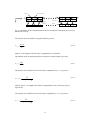
shown in Fig. 1-1 are used in the Ecolego Toolbox to facilitate model construction:
•
•
•
•
•
Compartment Block
Function Block
Radionuclide Block
Transfer Function Block
Conversion Blocks (Bq to Mole, Mole to Bq)
Below follows a description of each block in the Ecolego Toolbox library.
1.2.1 Compartment Block
The Compartment block represents a section of the system in which the concentration of
the radionuclides are homogenously distributed, i.e. a single Compartment has exactly
one value of the concentration for any given radionuclide. Each Compartment has an
unlimited number of inputs and outputs, as selected by the user. The inputs represent the
time-dependent flux of radionuclides into the Compartment, and the outputs the timedependent outflux of radionuclides over time. Mathematically the Compartment
integrates the difference between the total influx and total outflux over time. In addition
to this, the radioactive decay, including ingrowth of possible daughter nuclides, is
calculated inside the Compartment.
3
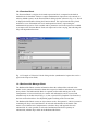
The compartment has an Initial Condition setting, that by default is zero. If the user
wishes to have an initial condition other than this, it is possible to select “Display Initial
Condition Port” on “Compartment” window (see Fig. 1-2). The “Compartment” window
will be displayed by double-clicking on the Compartment symbol. This adds an additional
input port to the Compartment block and whatever value(s) are input here becomes the
new initial conditions for the Compartment.
U-234 245500
Th-230 75380
Bq Mole
Inflow
Inf
low
Connected to
0 TF
Level
Lev el
Radionuclides
Mole Bq
Compartment
output
transfer
Function Block
Fig. 1-1 Symbols of various Blocks in Ecolego Toolbox library.
Fig. 1-2 Example of “Compartment” block dialog window.
4
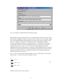
1.2.2 Function Block
The Function Block is a higher level maths expression block, compared to the built-in
maths blocks in Simulink. It allows complex mathematical expressions to be entered (in
ordinary Matlab syntax) on the Function Block dialog window (shown in Fig. 1-3), which
is displayed when double-clicking the Function Block. The expressions then are parsed
and built as a set of Simulink low-level math operations blocks, representing the
mathematical expression. Each variable and/or parameter used in the expression is added
as an input to the Function Block. Each such input can be time-varying, thus allowing for
fully time-dependent functions.
Fig. 1-3 Example of “Function” block dialog window (mathematical expressions can be
typed in the Expression field).
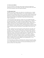
1.2.3 Radionuclide Manager Block
The Radionuclide Block contains information about the radionuclides selected in the
model. It also contains information about their respective halflives and about any eventual
decay-chains. The Radionuclide Block is required in all models making use of the
Compartment or Conversion blocks in a model. All information can be accessed and
edited directly in the block itself (Fig. 1-4), but a special GUI (Graphical User Interface)
has been written that allows for simplified graphical editing of the relevant data.
The Radionuclide Block creates an object known as the “Decaymatrix”, which is a matrix
containing all decay-associated data for all selected radionuclides in the model. This
matrix is used within each Compartment to calculate decay and ingrowth for each
radionuclide. It is also possible to select the fundamental unit for the quantity of
radionuclide, whether Bq or Mole in the Radionuclide Block.
5
Fig. 1-4 Example of “Radionuclide” block dialog window.
Radionuclide transport models often have to consider multiple nuclides, most often when
the ingrowth of daughter nuclides is of interest, but also when two or more nuclides might
have some relationship other than belonging to the same decay chain, for instance when
there are similarities in the physico-chemical properties which might lead them to
compete in adsorption processes or root-uptake processes. To handle this effectively, it
was decided to look at the models implemented as being vectorised. Since a signal in
Simulink can either be a scalar or a vector, this raises no big problems. Instead of
multiplying the signal corresponding to one nuclide, a matrix multiplication is performed
with the vector-signal. The matrix contains all information about the decay-times and also
about decay chains. The goal is to calculate the change in each nuclide per time unit,
either in units of nuclei or activity.
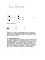
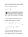
If N1, N2 and N3 are the number of nuclei [Mole] in a decay chain where N1 is the parent
nuclide, and λ1, λ2 and λ3 are the decay-constants, we have:
⎧ dN1
⎪ dt = −λ1 N1
⎪ dN
⎪ 2 = λ N −λ N
1 1
2 2
⎨ dt
⎪
⎪ dN3 = λ N − λ N
2 2
3 3
⎪⎩ dt
(1-1)
Which, in matrix form, can be written as:
6
0
⎡− λ1
dN ⎢
= λ1 − λ2
dt ⎢
⎢⎣ 0
λ2
0 ⎤ ⎡ N1 ⎤ ⎡ − λ1 ⋅ N1
⎤
⎢
⎥
⎢
⎥
0 ⎥ × ⎢ N 2 ⎥ = ⎢ λ1 ⋅ N1 − λ2 ⋅ N 2 ⎥⎥
− λ3 ⎥⎦ ⎢⎣ N 3 ⎥⎦ ⎢⎣λ2 ⋅ N 2 − λ3 ⋅ N 3 ⎥⎦
(1-2)
If the unit used in the model is activity, Ai = λi Ni [Bq], we can multiply both sides of
equation (1-1) with decay-constants to obtain:
⎧ dN1
dA1
= −λ1 A1
⎪λ1 dt = λ1 (−λ1 N1 )
dt
⎪ dN
dA2
⎪λ
2
= λ2 A1 − λ2 A2
⎨ 2 dt = λ2 (λ1 N1 − λ2 N 2 ) ⇔
dt
⎪
dA3
⎪λ dN 3 = λ (λ N − λ N )
= λ3 A2 − λ3 A3
3
3
2
2
3
3
⎪⎩ dt
dt
(1-3)
Which now is equivalent to:
0
⎡− λ1
dA ⎢
= λ2 − λ2
dt ⎢
⎢⎣ 0
λ3
0 ⎤ ⎡ A1 ⎤ ⎡ − λ1 ⋅ A1 ⎤
0 ⎥⎥ × ⎢⎢ A2 ⎥⎥ = ⎢⎢λ2 ⋅ A1 − λ2 ⋅ A2 ⎥⎥
− λ3 ⎥⎦ ⎢⎣ A3 ⎥⎦ ⎢⎣λ3 ⋅ A2 − λ3 ⋅ A3 ⎥⎦
(1-4)
In the equations above, the vectors N and A are the state-vectors of any individual
compartment, i.e. compartment inventories. In the example a decay-chain consisting of
three nuclides is used, but the same principle holds for any number and mix of nuclides
and decay chains used in a model.
1.2.4 Transfer Function Block
The Transfer Function block is what is used to make a connection (representing transfer
of radionuclides) between any two Compartments, or to be used as a sink accounting for
losses from the system. The Transfer Function block is basically a Function Block but
with added functionality in that it automatically identifies what block is the so called
donor Compartment, i.e., the Compartment from which the radionuclides are to be
removed by the rate governed by the Transfer Function Block. This is accomplished via
the use of a pair of matching Goto and From blocks, and a callback function that is
executed whenever the connection is changed on the Transfer Function Block.
Several Transfer Function Blocks can be connected to the same donor Compartment.
Further, the block allows for direct input of mathematical expressions, describing the
transfer rate in either Bq/Yr or Mole/Yr depending on the selected unit in the
Radionuclide Block. However, these functions all assume that any parameter in the
expression is a constant. To use time-varying parameters the user has to select the “Show
External Rate Port” checkbox in the blocks dialog window (Fig. 1-5). When this is
7
Fig. 1-5 Example of “Transfer Function” block dialog window.
selected, a new port is made available on the block where the user can input the output of
a Function Block or any other required signal representing the transfer rate. Note that the
expressions are not automatically assumed to be proportional to the donor Compartments
value, so the donor Compartments value has to be used in the expression if this is the
goal.
Example:
The expression “(a+b)” entered in the Transfer Function block (or fed as an input as
described above) would mean that the amount of “(a+b)” will be removed from the
donor Compartment each time-step. Thus the value of the Transfer Function Block is not
proportional to the value of the donor Compartment.
On the other hand, if the expression was instead “(a+b) * INVENTORY”, where
INVENTORY is the value of the donor Compartment, then the value of the Transfer
Function Block will be directly proportional to the value of the donor Compartment.
Note: the variable INVENTORY can be used to automatically access the donor
Compartments value IF the expression is written directly in the Transfer Function Block,
and not using the external rate port option. If the external rate port is used, this value has
to be connected manually like any parameter to the inputs of the Function Block.
8
1.2.5 Conversion Blocks
The Conversion Blocks, when being connected with an output from another block,
automatically converts the value between either Mole to Bq or Bq to Mole. These blocks
also uses the information stored in the Radionuclide Block.
1.2.6 Parameter Input
Although a parameter in Simulink can be defined in several different ways, to simplify
the use of Ecolego Toolbox, model parameters are by convention defined in so called
subsystem masks. By following this convention, it is possible to import and export model
parameters to and from Ecolego Toolbox (for example to/from MS Excel). The user still
has the option of suing any valid Simulink method to define parameters, however,
parameters defined in this way cannot then be included when interfacing Ecolego
Toolbox with MS Excel.
A subsystem mask basically represents a workspace for a given Simulink subsystem
(note: a mask also has other functionalities, that are not presented here), in which the user
can define the parameters. This is similar to the ordinary Matlab workspace, the only
difference being the manner in which the user defines the parameters, and how these are
available in the model. In contrast to the Matlab workspace, parameters defined in a
masked subsystem are only available to blocks contained within such a subsystem. In this
way it is possible to construct hierarchical structures when building a model, and even use
parameters with the same names but different values depending on their location in the
model.
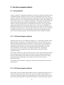
To define a parameter, the user must right-click a masked subsystem in the model, and
then select “edit mask”. This opens a dialog window, where the user should select the
“Parameters” tab. In this view, the user can add, remove and edit the order of the list of
defined parameters. Each parameter has a “prompt” and a “variable” which needs to be
defined. The “prompt” is the text that will appear when the user left double-clicks on the
masked subsystem after the parameter has been defined. The “variable” contains a
variable name that is used by the model. For instance, if a parameter has assigned the
variable “kd”, the value for kd is available anywhere within the masked subsystem in
question by simply writing “kd” in the appropriate location (this could be in the “value”
field of a constant block, in any dialog parameter for any Simulink block, or in an
expression of a transfer function block).
Once the parameters are defined in a masked subsystem, and the user has pressed “apply”
or “ok”, the mask dialog will open the next time the user left double-clicks the subsystem.
For an example of this see Fig. 1-6a and 1-6b. In the opened mask dialog, the user can
specify any values to the listed parameters. 9
Fig. 1-6a Example of the editing of a masked subsystems parameters.
Fig. 1-6b The resulting opened mask dialog of the parameters defined according to fig. 16a.
10
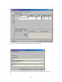
1.3 Interface with MS Excel
In addition to the block-library in Ecolego Toolbox, described in section 1.2, two Matlab
functions are included in the toolbox, simplifying the handling of model parameters. The
two files are:
•
•
Simulink_xls.m
xls_simulink.m
The functions are called from the Matlab prompt and works on the currently active
Ecolego Toolbox model.
The goal of these functions is to assist in editing and viewing the parameters of a model.
Since a parameter in Simulink can be defined in many different ways, these files work
under the assumption that the user has defined the model parameters in so called Masked
Subsystems in Simulink. A Masked Subsystem is basically a set of blocks grouped
together hierarchically, and having a local workspace associated with it. The Masked
Subsystems workspace can be edited to include any number of parameters. Any
parameter defined in a Masked Subsystem, is available for all blocks below it in the
model hierarchy via references.
The function “simulink_xls.m” scans through the model for any Masked Subsystems, and
extracts the data for any defined parameters. The data is summarized in a MS Excel file,
containing the parameter name, location in the model, and value if specified. To use the
function the user enters “simulink_xls” at the Matlab prompt, after which a dialog asks
the user to enter a name of the MS Excel file to be created.
The function “xls_simulink.m” works the opposite way, by reading the data in an MS
Excel file, and then for all matching parameters and Masked Subsystems in an active
Ecolego Toolbox model, updates the parameters. The major benefit of this is that a user
created model can have different parameter sets, stored in MS Excel files. To use the
function, the user enters “xls_simulink” at the Matlab prompt, after which a dialog asks
the user to select an MS Excel file.
1.4 Installation and use
To install Ecolego Toolbox, simply copy the folder containing the harddrive. Then in
Matlab, add this path with subfolders to the Matlab path. This is done by selecting (in
Matlab) the following menu items: File > Set Path… In the window that appears, press
the button labeled “Add with Subfolders”, then locate the folder where the files were
copied to and press ok. After that press the button labeled “Save” and close.
11
Once the Ecolego Toolbox is installed, the Simulink blockset will appear in the Simulink
Library browser window the next time Simulink is started. To use a block from the
library simply click-and-drag it into the model window from the library window.
1.5 Verification of the Toolbox
The Toolbox was verified by comparing the results with the results obtained from the
Ecolego, for the same problem. In the test the results agreed perfectly. The problem used
in the verification is taken from assessment of long-term safety for a spent nuclear fuel
repository (Lindgren and Lindström, 1999) to calculate the release of radionuclide from
the near field due to the leakage from a damaged canister through the bentonite buffer to
the fracture. The reason for choosing this problem is that the results have been verified in
a comparison of Ecolego and AMBER (Maul et al., 2003).
12
2. The Discretisation Block
2.1 Introduction
In many situations in compartment modelling it is the goal to model the transport of some
contaminant through a medium of some sort. Since a compartment represents a unit of
volume in which the contaminants entering are immediately assumed to be homogenously
distributed, this gives rise to a problem when the total volume is large. This problem can
be solved by using a series of connected compartments, all together representing the total
volume of the medium. In this manner the dependency on the spatial variable can be
obtained. Often the optimal number of compartments required to correctly approximate
transport through the medium in question can be large. It can also vary depending on
radionuclide properties or some other parameter in the system. Thus, the need to connect
the number of compartments via the many transfer function connections can be both timeconsuming and prone to error since the number of interconnections rapidly becomes
large. To get around this problem a Discretisation Block was developed for Simulink.
2.2 1-D Discretisation Block
This block only consists of one underlying integrator (i.e. Compartment), which is being
fed the product of its output (i.e. the states) with a matrix of size N×N where N is the
number of required discretisations. The matrix is set up to represent a one-dimensional
and sequential transport between the discretisation nodes (states). Both forward and
backward transport is allowed, as well as specifying initial conditions for any of the
states. Furthermore, the block allows for multiple radionuclides, including the
calculations for decay and ingrowth, in the same manner as is performed in the
Compartment Block.
The transfer coefficients are fed as inputs to the block, and can thus describe any required
process affecting the overall transport, for instance advection, dispersion, diffusion etc.
As for the Function Block, these inputs (the transfer coefficients) can be time-varying,
allowing for full time-dependency. Also, inputs can be fed to any of the given
discretisation nodes.
The number of discretisations is changed by entering the required number in the blocks
dialog window.
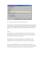
2.3 2-D Discretisation Block
The original version of the Discretisation Block was for 1 dimensional transport only. To
be able to model systems with 2 dimensions, such as for example water transport in a
rock fracture with matrix diffusion, the original block had to be extended. Due to the fact
that only 2D matrix operations are allowed in Simulink, a workaround solution had to be
13
devised. The solution was to write code that added a Compartment for each of the
discretisations along the second dimension, while maintaining the original single of the
discretisation along the first dimension. Thus if the system is discretised in 10 levels
along the first dimension, and 5 along the second dimension, the total number of
Compartments would be 60 (10 + 5 * 10). Were this to be constructed manually, 60
Compartments, with 120 Transfer Functions linking them, would need to be set up. In
such modelling it is often the case that the effect of discretisation on system behaviour is
part of the study and therefore a manual method is impractical. The task is greatly
simplified by just changing the values given for the number of required discretisation
elements in the two dimensions (x and y) to get the required size of the system (see figure
2-1).
Fig. 2-1: An example of the mask dialog for the 2D Discretisation Block.
14
3. Application of Discretisation Block
3.1 Radionuclide transport in far field
3.1.1 A dual porosity model for radionuclide transport
Transport of radionuclide by groundwater in fractured rock is known as far field transport
in assessments of the long-term safety of spent nuclear fuel repositories in crystalline
bedrock. The processes involved in the transport are advection and dispersion along
preferential flow paths and diffusion into the rock matrix as well as sorption on to the
solid matrix. A dual porosity model for radionuclide transport along a stream tube is often
used for describing radionuclide transport in far field (Norman and Kjellbert, 1990):
∂C p
∂C i
∂C i
∂ 2C i
+u
− D 2 + λi C i − λi−1C i−1 − aw Dei
∂t
∂x
∂x
∂z
i
Ri
∂C ip
∂t
− Dei
where
t
Ci
=
=
C ip
=
u
D
aw
=
=
=
x
z
=
=
=
Dei
λi
R
i
ρ
K di
θ
∂ 2C ip
∂z 2
=0
(3-1)
z =0
+ R i λi C ip − R i−1λi −1C ip−1 = 0
(3-2)
time [y]
an effective stream tube average of the concentration of radionuclide i in
the mobile liquid [moles m-3]
a surface and stream tube averaged concentration of radionuclide i in the
stagnant pore liquid in the impervious rock matrix [moles m-3]
velocity of the mobile liquid [m y-1]
longitudinal dispersion coefficient [m2 y-1]
total surface area of the boundary of the flow porosity per unit volume of
mobile liquid [m-1]
distance along stream direction [m]
penetration depth into matrix orthogonal to stream direction [m]
effective matrix diffusion coefficient for radionuclide i [m2 y-1]
=
=
decay constant for radionuclide i [y-1]
retardation factor [-] due to sorption into the rock matrix, which is defined
i
i
by R = θ + K d ρ
=
=
bulk density of rock matrix [kg m-3]
distribution coefficient for radionuclide i inside rock matrix [m3 kg-1]
=
matrix porosity [-]
For a solute pulse travelling in the fracture (a delta source), the initial and boundary
conditions are:
15
C i (x, t = 0) = C ip ( x, t = 0) = 0
(3-3)
M0
Q
(3-4)
C ip ( z = 0, t ) = C i (x, t )
(3-5)
∂C ip
(3-6)
C i (x = 0, t ) = δ (t )
∂z
=0
z =Z
C i (x, t = ∞) = 0
(3-7)
in which Q is the water flux [m3 y-1], M0 is the total mass of solute inserted into the
fracture [moles], δ(t) is the Dirac delta function [y-1] and Z is the maximum penetration
depth [m].
3.1.2 The Representation of radionuclide transport by compartment model
There is similarity between a finite difference approximation of an advection-dispersion
(A/D) type equation and compartmental models. Therefore, compartmental models can be
used to obtain identical solutions to analytical solutions of A/D equations when certain
criteria are fulfilled (Xu et al., 2007). The corresponding transport problem modelled by a
compartmental model as a two dimensional array of compartments is schematically
shown in Fig. 3-1. In the x-direction (along the stream flow), compartments are linked
together to represent advective and dispersive fluxes both forwards and backwards. In the
y-direction (perpendicular to the stream flow), compartments are represent the process of
matrix diffusion in a stagnant liquid. The transfer rates shown in Fig. 3-1 are given below,
taken from Maul and Robinson, (2002). The symbols used in the following expressions
have the same definitions as in (3-1) and (3-2).
The transfer rate of advection from compartment i to i+1 is given by:
λadv =
u
X nx
(3-8)
where X is length of transport domain and nx is number of compartments in the xdirection.
The transfer rate for dispersion (both forward or backward) is given by:
λdis _ f = λdis _ b =
(X
D
2
nx )
(3-9)
16
λdis_f
x
y
λadc +λdis_b
λm_s
λm_down
λs_m
λm_up
Fig. 3-1 Schematic of the compartmental model for description of transport processes in a
stream tube concept.
The transfer rate from mobile to stagnant liquid is given by:
λm _ s =
2aw Dei
d1
(3-10)
where d1 is the length of the first layer (compartment) in y-direction.
The transfer rate from stagnant liquid (rock matrix) to mobile liquid is given by:
λs _ m =
2 Dei
R i d12
(3-11)
The transfer rate of diffusion from rock matrix compartment j to j+1 is given by
λm _ down =
Dei
R i d j (d j + d j +1 ) 2
(3-12)
where dj and dj+1 are length of the matrix compartments in the y-direction j and j+1,
respectively.
The transfer rate of diffusion from rock matrix compartment j+1 to j is given by
λm _ up =
Dei
R d j +1 (d j + d j +1 ) 2
(3-13)
i
17
3.1.3 Implementation of compartment model in the Block and comparison
of the results with the semi-analytical solutions
We take as an example the pin-hole failure case in SR-Can assessment of long-term
safety for a spent nuclear fuel repository (SKB, 2006) as a calculation example.
Calculated release from near field due to the leakage from the damaged canister through
bentonite buffer to the fracture is shown in Fig. 3-2. Details of near field transport
calculation are found in (SKB, 2006) and Maul et. al., (2003). The near field release flux
was used as the boundary condition for the far field transport problem. Input data to the
problem are shown in Table 3-1 and 3-2. The same parameter values were used in both
the dual porosity model and the compartment model calculations except the numbers of
compartments, which are only used for the compartment model. The dual porosity model
is solved by means of Laplace transforming of (3-1) and (3-2) (Maul et. al., 2003).
Transformation back to the real domain is performed numerically by means of the series
expansion algorithm of De Hoog et al., (1982) implemented in a Matlab code developed
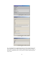
by Hollenbeck (1998). Implementation of the compartment model in the Discretisation
Block simply requires that the expressions for the transfer rates in the “Function” block
dialog windows are filled in (see Fig. 3-3a) together with the parameter values and the
number of compartments required in both the x- and y-directions using the “Masked
subsystem” dialog windows (see Fig. 3-3b and 3-3c), respectively.
The numbers of compartments for both x- and y-directions in the compartment model
were tuned until the solution convergence. This was done in two steps. Firstly, we kept
number of compartments in the y-direction constant and tuned number of compartments
in the x-direction until the solution no longer changed with the number of compartments.
Secondly, we set number of compartments in x-direction as obtained in the first step and
tuned the number of compartments in y-direction until the solution became stable. The
simulated breakthrough curve remains unchanged when the number of compartments in
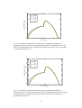
the x-direction was tuned to be more than 40 while the number of compartments in the ydirection was kept constant (see Fig. 3-4). The length of the compartments in both
directions was equally divided. We used 60 compartments for the discretisation of rock
matrix in the x-direction and then tuned the number of compartments in the y-direction.
As can be seen from Fig. 3-5 when the number of compartments is more than 12 the
solution converges, i.e., the breakthrough curves obtained with 10 and 12 compartments
are almost overlapped.
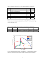
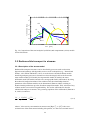
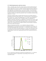
Fig. 3-6 shows the far field release fluxes calculated from both models for five
radionuclides in pin-hole failure case. It can be seen that the agreement between two
model solutions is excellent.
18
Table 3-1 Parameter values used in far field transport calculation (Hedin, 2007)
Symbols
[I]
X
[I]
u
[I]
Definitions
Units
Values
length of transport domain
[m]
500
-1
velocity of the mobile liquid
[m y ]
12.5
2
-1
D
longitudinal dispersion coefficient
[m y ]
625
aw
half width of fracture
[m]
1×104
ρ
bulk density of rock matrix
[kg m-3]
2700
θ
matrix porosity
[-]
0.001
Z
the maximum penetration depth
[m]
0.03
[I]
In Hedin (2007) the values of the transport time (tw) and Peclet (Pe) number are given as tw =40
[y] and Pe=10. tw and Pe have been interpreted into corresponding parameters u and D in our
calculation based on assuming X=500 [m] and the relationship of t w = X u and D u 2 = t w Pe
(Norman and Kjellbert, 1990).
Table 3-2 Distribution and diffusivity coefficients used in calculations (Hedin, 2007).
14
C
36
135
Cl
129
Cs
59
I
Ni
Kd [kg m-3]
1×10-3
0
4.2×10-2
0
1×10-2
De [m2 y-1]
8.138×10-8
1.356×10-7
1.424×10-6
5.629×10-8
4.611×10-7
10
Near field release [Bq/y]
10
10
10
10
10
6
C-14
Cl-36
I-129
Cs-135
Ni-59
5
4
3
2
1
0
10 3
10
10
4
10
Time
5
10
6
[years]
Fig. 3-2 Calculated near-field releases from pathway Q1 for the deterministic pin-hole
failure case, which are used as boundary condition for far field release calculations.
19
a)
b)
c)
Fig. 3-3 Implementation of compartmental model representing far field transport in the
discretisation Block, a) an example of transfer rate, Eq. (3-10), is filled in “Function”
block window, b) parameter values are filled in “Masked subsystem” dialog window, c)
the number of compartments in the x- and y-directions is filled in “Masked subsystem”
dialog window.
20
5
10
4
Far field release [Bq/y]
10
n=5
n=10
n=20
n=40
n=60
3
10
2
10
1
10
0
10
3
10
4
10
Time
[years]
5
10
Fig. 3-4 Comparison of calculated far field release by using different number of
compartments in the x-direction representing mobile liquid in compartment model. The
number of compartments in the y-direction representing rock matrix is set to be constant
(6 compartments in this case).
5
10
4
Far field release [Bq/y]
10
n=4
n=6
n=8
n=10
n=12
3
10
2
10
1
10
0
10
3
10
4
10
Time
[years]
5
10
Fig. 3-5 Comparison of calculated far field release by using different number of
compartments in y-direction representing rock matrix in compartment model. The number
of compartments in x-direction representing mobile liquid is set to be constant (60
compartments in this case).
21
6
10
5
10
Far field release [Bq/y]
36
Cl
4
59
Ni
10
3
10
14
C
2
10
135
Cs
1
10
129
I
0
10
3
10
4
5
10
10
Time
6
10
[years]
Fig. 3-6 Comparison of the semi-analytical (solid line) and compartment (circles) models
for far field release.
3.2 Radionuclide transport in streams
3.2.1 Description of the stream model
Radionuclide transport in streams can be described by processes such as advection,
dispersion and exchange with hyporheic zones as well as adsorption (e.g., Bencala and
Walters, 1983; Elliott and Brooks, 1997). Over the last two decades different models
describing transport processes in streams have been developed, such as the first-order
mass transfer model (FOT model), the impermeable model (IS model), the water
infiltration model (WI model) and advective-storage-path model (ASP model). By using
the method of temporal moments of the residence time the relationships between
parameters of the different models can be determined (Wörman, 2000), resulting in
identical model predictions up to the first three temporal moments. Thus, selection of any
of these models is not critical for predictability. We use the ASP model to describe
radionuclide transport in streams. The governing equations of the ASP model (Wörman et
al., 2002) is written as:
∂ 2C
∂C 1 ∂( AUC )
− D 2 = JS
+
∂x
∂t AT
∂x
(3-14)
where C is the activity concentration in stream water [Bq m-3], AT [m2] is the crosssectional area of the main stream including side pockets, A is the cross-sectional area of
22
the main stream excluding side pockets, U is the flow velocity in the main stream [m s-1],
Q( = UA) is the discharge [m3 s-1], and D is the main stream dispersion coefficient [m2 s1
]. The effective flow velocity in the main stream channel corrected for side pockets with
stagnant water is given by Ue=Q/AT (Wörman, 1998).
The net solute mass flux [Bq/(m3s)] in the dissolved phase in the stream water can be
written, integrating over the distribution of transport pathways:
JS =
(
)
1 ∞
P
f (T ) ξ − VZ (τ , T ) τ =0 cd + (VZ (τ , T )) τ =T g d dT
∫
2 0
A
(3-15)
where gd is solute mass per unit volume of water in the hyporheic zone [Bq m-3], Vz is the
infiltration velocity [m s-1] into the bed in the direction of the streamlines denoted by
VZ (τ , T ) τ =0 and exfiltration velocity out of the bed in the direction of the streamlines by
VZ (τ , T ) τ =T , f(T) is the probability density function (PDF) of T weighted by the velocity
component normal to the bed surface, Vn, T is the total residence time from inlet to exit of
hyporheic flow path [s], τ is the exfiltration residence time [s] (0<τ<T), P is the wetted
perimeter [m], A is the cross-sectional area of the stream [m2], and ξ is an area reduction
factor equal to Vn/VZ that accounts for the fact that the streamlines are not necessarily
always perpendicular to the bed surface.
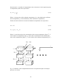
3.2.2 Derivation of compartment model for description of radionuclide
transport in streams
Similar to the APS model the mass balance for the compartments in the stream and the
sediment based on the conceptual description in Fig. 3-7 can be written as:
dM i
U
D
D
ξVz
ξVZ m j
=−
Mi −
Mi +
M i +1 −
Mi +
− λM i
2
2
dt
L nriv
2h
2(Z nsed ) R j
(L42
(L42
nriv )
nriv )
{
123
1
4
2
4
3
1
4
3
1
4
3
TRwat _ sed
TRadv
TRdis
TRsed _ wat
TRdis
(3-16)
dm j
dt
=−
ξVz
mj
2(Z nsed ) R j
1424
3
TRup _ down
+
ξVz
m j +1
2(Z nsed ) R j +1
1424
3
TRdown _ up
−
ξVz
mj
2(Z nsed ) R j
1424
3
TRsed _ wat
+
ξVZ
2h
{
M i − λm j
TRwat _ sed
(3-17)
Where Mi is the total inventory in stream compartment i [Bq] or [kg], mj is the total
inventory in sediment compartment j [Bq] or [kg], U is the advective velocity, D is
dispersion coefficient, VZ is the infiltration velocity, ξ is the area reduction factor as
described previously for ASP model, h is the depth of the river [m] and equivalent to A/P
in ASP model, λ is decay constant for radionuclide [s-1], L is the transport length in the xdirection [m], Z is the depth of the sediment [m], nriv is number of compartments in the x23
direction and nsed is number of compartments in the z-direction, Ri is the sorption capacity
of compartment j and can be expressed as
R j = 1 + kd , j ρ ε j
(3-18)
Where εj is the porosity of the sediment compartment j, kd,j is the distribution coefficient
in the compartment j, ρ is the bulk density of the sediment in compartment j.
Further, the total inventories in stream and sediment compartments are expressed as:
M i = CiVi
(3-19)
m j = g j (ε j v j + k d , j ρ )
(3-20)
Where Ci is the dissolved activity concentration in the stream compartment i [Bq m-3], Vi
is the volume of compartment i [m3], gj is the solute concentration in the sediment pore
water in the compartment j [Bq m-3], vj is the volume of the sediment compartment j [m3].
TRadv + TRdis
TRdis
x
Mi
Mi+11 Vi+1
Vi
TRwat_sed
z
TRwat_sed
mj
vj
TRupp_down
TRdown_upp
mj+1 vj+1
Fig. 3-7 Schematic of the compartmental model for conceptual description of transport
processes in a stream.
24
3.2.3 Model implementation and discretisation
Table 3-3 summarises the expressions of those transfer rates derived from the previous
section. Data obtained from a tracer experiment performed in Säva Brook in Uppland
County (Johansson et al., 2001) was used to verify the compartment model of the stream.
In the experiment, moderately sorbing 51Cr, was used as the tracer. The concentrationtime-distributions were obtained at eight stations along a distance of 30 km. The input
data used in this application are based on the distance between station C and D. The data
are shown in Table 3-4, in which some parameter values are obtained from model fitting
(Wörman et. al., 2002).
Following a similar procedure to that described in the previous section the model was
implemented in the Discretisation Block. First, we tuned the number of compartments in
the x-direction. Fig. 3-8 shows the breakthrough curve converges when the number of
compartments is large than 200. Then, we tuned the number of compartments in
sediments (z-direction). The number of compartments in z-direction is not sensitive either
the depth of the sediment on the model predictions in this case. The reason for this might
be the residence time of radionuclide in the studied domain is much shorter than the
residence time of radionuclide in the sediment, therefore, the discretisation of sediment
has no effect on the model response.
Finally, the lumped parameter TRwat_sed was obtained by fitting the simulated
breakthrough curve with experimental data when 250 compartments are used (Fig. 3-8).
The calibrated lumped parameter value of TRwat_sed is 0.033 [hour-1] which is a factor of
0.55 of the value used for ASP model (Wörman, et. al., 2002). The reason for this is that
in ASP model mass flux from water into sediment is integrated over the distribution of
transport pathways while in the compartmental model no such a distribution function is
employed.
Concentration (cpm/g sample)
400
350
nriv=50
300
nriv=100
250
nriv=150
200
nriv=200
150
250
100
50
0
0
10
20
30
Time
40
50
60
70
(hours)
Fig. 3-8 Comparison of calculated concentration-time distribution for 51Cr at station D
by using different number of compartments in representing stream water in the
compartment model.
25
Table 3-3 Description of transfer rates in compartmental models (definitions and values
of the parameters in the descriptions are found in Table 3-4).
Transfer rate
Description of transfer rate
TRadv
U
L nriv
TRdis
D
(L nriv )2
TRwat_sed
VZ ξ
2h
TRsed_wat
(VZ ξ 2) ,
R( z nsed )
TRupp_down
(VZ ξ 2)
R (Z nsed )
TRdown_upp
(VZ ξ 2)
R (Z nsed )
where R = 1 + kd ρ ε
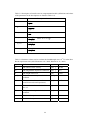
Table 3-4 Parameter values used to evaluate the breakthrough curve of 51Cr in the Säva
Brook experiment 1998 (after Johansson et al., 2000; Wörman et. al., 2002).
Symbol
Definitions
unit
values
U
The effective flow velocity
[m s-1]
0.088
D
The longitudinal dispersion coefficient
[m s-2]
0.8
L
The length of the river
[m]
3980
ξ<Vz>/2
The advective velocity into the bed
sediment
[m/s]
3.96×10-6
h
The hydraulic radius (ratio of cross
section area and wetted perimeter)
[m]
0.77
R
The retardation factor in bed sediment
for 51Cr
[-]
20 000
Z
The penetration depth in the bed
sediment
[m]
0.4
nriv
Number of compartments in stream
[-]
250
nsed
Number of compartments in sediments
[-]
4
26
600
Station C
Concentration (cpm/g sample)
500
400
300
Station D
200
100
0
0
10
20
30
Time
40
50
60
70
(hours)
Fig. 3-9. Measured concentration-time distribution for 51Cr at station D (marked with '{')
in Säva Brook experiment (Johansson et al., 2001) and predicted curve (solid line) at
station D using compartmental river model with 250 compartments and TRwat_sed as 0.033
[hour-1].
27
References
Avila, R., Broed, R. and Pereira, A. (2003). Ecolego ⎯ a Toolbox for radioecological
risk assessments. International conference on protection of the environment from the
effects of ionising radiation, 6-10 October 2003, Stockholm, Sweden.
Bencala, K. E. (1983). Simulation of solute transport in a mountain pool- and-riffle
stream with kinetic mass transfer model for sorption. Water Resource Research, 19(3),
732-738.
De Hoog, F. R., Knight, J. H. and Stokes, A. N. (1982). An improved method for
numerical inversion of Laplace transforms. J. Sci. Stat. Compt., 3 357-366.
Elliott, A. H. and Brooks, N. H. (1997). Transfer of nonsorbing solutes to a streambed
with bed forms: Theory. Water Resource Research, 33(1), 123-136.
Hedin, A. (2007). E-mail to Björn Dverstorp and Bo Strömberg dated 19/3/07 on the
subject of input files for SR-Can calculations.
Hollenbeck, K. J. (1998). INVLAP.M: A Matlab function for numerical inversion of
Laplace transforms by De Hoog Algorithm, http://www.isva.dtu.dk/staff/karl/invlap.htm.
Johansson, H., Jonsson, K., Forsman, K.J., Wörman, A. (2001). Retention of conservative
and sorptive solutes in streams – simultaneous tracer experiment. The Science of the Total
Environment. 266 (1–3), 229–238.
Lindgren, M. and Lindström, F. (1999). SR 97 radionuclide transport calculations. SKB
Report TR-99-23. Svensk Kärnbränslehantering AB.
Maul, P. R. and Robinson, P. C. (2002). Exploration of important issues for the safety of
SFR 1 using performance assessment calculations. SKI Report 02:62. Statens
Kärnkraftinspektion (SKI), Sweden.
Maul, P., Robinson, P., Avila, R., Broed, R., Pereira, A. and Xu, S. (2003). AMBER and
Ecolego intercomparisons using calculations from SR-97. SKI report 2003:28, SSI report
2003:11.
28
Norman, S. and Kjellbert, N. (1990). FARF31 ― A far field radionuclide migration code
for use with the PROPER package. SKB TR-90-01, Svensk Kärnbränslehantering AB.
SKB (2006). Long-term safety for KBS-3 repositories at Forsmark and Laxemar ― a first
evaluation, Main report of the SR-Can project. SKB TR-06-09. Svensk
Kärnbränslehantering AB.
Wörman, A. (1998). Analytical solution and timescale for transport of reactive solutes in
rivers and streams, Water Resources Research. 34(10), 2703-2716.
Wörman, A. (2000). Comparison of models for transient storage of solutes in small
streams. Water Resources Research. 36(2), 455-468.
Wörman, A., Packman, A. I., Johansson, H. and Jonsson, K. (2002). Effect of flowinduced exchange in hyporheic zones on longitudinal transport of solutes in streams and
rivers. Water Resources Research. Vol. 38, N0. 1, 10.1029/2001WR000769.
Xu, S., Wörman, A. and Dverstorp, B. (2007). Criteria for resolution-scales and
parameterisation of compartmental models of hydrological and ecological mass flow in
watersheds. Journal of Hydrology. 335, 364-373.
29
SSI-rapporter 2008
SSI reports 2008
2008:01 Myndigheternas granskning av SKB:s preliminära säkerhetsbedömningar för Forsmark och
Laxemar
Avdelningen för kärnteknik och avfall och SKI
Maria Nordén, Öivind Toverud, Petra Wallberg, Bo
Strömberg, Anders Wiebert, Björn Dverstorp, Fritz Kautsky, Eva Simic och Shulan Xu
90 SEK
2008:02 Patientstråldoser vid röntgendiagnostik i
Sverige – 1999 och 2006
Avdelningen för personal- och patientstrålskydd
Wolfram Leitz och Anja Almén
110 SEK
2008:03 Radiologiska undersökningar i Sverige
under 2005
Avdelningen för personal- och patientstrålskydd
Anja Almén, Sven Richter och Wolfram Leitz 110 SEK
2008:04 SKI:s och SSI:s gemensamma granskning
av SKB:s Säkerhetsrapport SR-Can Granskningsrapport
Avdelningen för kärnteknik och avfall
Björn Dverstorp och Bo Strömberg
110 SEK
2008:04 E SKI's and SSI's review of SKB's safety
report SR-Can
Avdelningen för kärnteknik och avfall
Björn Dverstorp och Bo Strömberg
110 SEK
2008:05 International Expert Review of Sr-Can:
Safety Assessment Methodology; External review
contribution in support of SSI's and SKI's review
of SR-Can
Avdelningen för kärnteknik och avfall
Budhi Sagar, et al
110 SEK
2008:06 Review of SKB's Safety Assessment SRCan: –Contributions in support of SKI’s and SSI’s
review by external consultants
Avdelningen för kärnteknik och avfall
Pierre Glynn et.al.
110 SEK
2008:07 Modelling of long term geochemical evolution and study of mechanical perturbation of
bentonite buffer of a KBS-3 repository
Avdelningen för kärnteknik och avfall
Marsal F. et al.
110 SEK
2008:08 SSI's independent consequence calculations in support of the regulatory review of the
SR-Can safety assessmenty
Avdelningen för kärnteknik och avfall
Shulan Xu, Anders Wörman, Björn Dverstorp, Ryk Kłos,
George Shaw och Lars Marklund
110 SEK
2008:09 The Generalised Ecosystem Modelling Approach in radiological assessment
Avdelningen för kärnteknik och avfall
Ryk Kłos
110 SEK
2008:10 User’s manual for Ecolego Toolbox and
the Discretization Block
Avdelningen för kärnteknik och avfall
Robert Broed and Shulan Xu
110 SEK
S
TATENS STRÅLSKYDDSINSTITUT, SSI,
är en central tillsynsmyndighet som verkar för ett gott strålskydd för
människan och miljön, nu och i framtiden.
SSI sätter gränser för stråldoser till allmänheten och
för dem som arbetar med strålning, utfärdar föreskrifter
och kontrollerar att de efterlevs. SSI håller beredskap
dygnet runt mot olyckor med strålning. Myndigheten
informerar, utbildar och utfärdar råd och rekommendationer samt stöder och utvärderar forskning. SSI
bedriver även internationellt utvecklingssamarbete.
Myndigheten, som sorterar under Miljödepartementet,
har 110 anställda och är belägen i Solna.
THE SWEDISH RADIATION PROTECTION AUTHORITY (SSI) is a central
regulatory authority charged with promoting effective
radiation protection for people and the environment today
and in the future.
SSI sets limits on radiation doses to the public and to
those that work with radiation. SSI has staff on standby
round the clock to respond to radiation accidents.
Other roles include information, education, issuing
advice and recommendations, and funding and
evaluating research.
SSI is also involved in international development
cooperation. SSI, with 110 employees located at Solna near
Stockholm, reports to the Ministry of Environment.
Adress: Statens strålskyddsinstitut; S-171 16 Stockholm
Besöksadress: Solna strandväg 96
Telefon: 08-729 71 00, Fax: 08-729 71 08
Address: Swedish Radiation Protection Authority
SE-171 16 Stockholm; Sweden
Visiting address: Solna strandväg 96
Telephone: + 46 8-729 71 00, Fax: + 46 8-729 71 08
www.ssi.se