1
A user’s guide for identifying rice
paddocks using GIS and remote sensing
at Coleambally Irrigation Area, NSW
Thomas G. Van Niel and Tim R. McVicar
CSIRO Land and Water
CSIRO Land and Water Client Report
A report for Coleambally Irrigation Co-operative Limited
(CICL) for research conducted by the CRC for Sustainable Rice
Production Project 1105
November 2004
A user’s guide for identifying rice paddocks using GIS and remote sensing at
Coleambally Irrigation Area, NSW
Thomas G. Van Niel a,c, Tim R. McVicar b
a CSIRO Land and Water, Private Bag No. 5, Wembley, WA 6913, Australia.
b CSIRO Land and Water, GPO Box 1666, Canberra, ACT 2601, Australia.
c Cooperative Research Centre for Sustainable Rice Production, Yanco, NSW 2703,
Australia.
CSIRO Land and Water Client Report
November 2004
Copyright and Disclaimer
© 2004 CSIRO To the extent permitted by law, all rights are reserved and no part of this
publication covered by copyright may be reproduced or copied in any form or by any means
except with the written permission of CSIRO Land and Water.
Important Disclaimer:
CSIRO Land and Water advises that the information contained in this publication comprises
general statements based on scientific research. The reader is advised and needs to be
aware that such information may be incomplete or unable to be used in any specific situation.
No reliance or actions must therefore be made on that information without seeking prior
expert professional, scientific and technical advice. To the extent permitted by law, CSIRO
Land and Water (including its employees and consultants) excludes all liability to any person
for any consequences, including but not limited to all losses, damages, costs, expenses and
any other compensation, arising directly or indirectly from using this publication (in part or in
whole) and any information or material contained in it.
Cover Photograph:
Description: Enhanced Thematic Mapper (ETM) image over the Coleambally Irrigation Area
acquired on 13 February 2002. Wavelengths displayed are 0.7199 µm (red colour gun),
0.6614 µm (green colour gun), and 0.5610 µm (blue colour gun).
© 2004 CSIRO
CSIRO Land and Water
-i-
Acknowledgements
This research was funded by the CRC for Sustainable Rice Production (Rice CRC) and
CSIRO Land and Water. Please note, mention of commercial products in this work does not
imply an endorsement of these products by either CSIRO or the Rice CRC. Many thanks to
Reuben Robinson and David Klienert of Coleambally Irrigation Co-operative Limited (CICL)
who provided helpful comments on the manuscript and learned rice identification from
remote sensing over the telephone. The new section 8 about rice administration was written
by Rueben Robinson and David Klienert during their review of the manuscript.
CSIRO Land and Water
- ii -
Executive Summary
Rice administration at the Coleambally Irrigation Area (CIA), New South Wales (NSW), is an
important aspect of yearly management. This process relies upon identification of rice
paddocks and summarisation of each landholder’s rice area. In the past, rice administration
has been strictly based on high resolution aerial photography because, although satellite
remote sensing can accurately identify rice, (1) its spatial accuracy has not been suitable for
paddock-level management and (2) image processing has required a great deal of training.
Recently, greatly simplified techniques have been developed to accurately classify rice
removing one of the impediments to using satellite remote sensing for rice administration. If
these results can be merged with spatially accurate paddock boundaries, then the other
impediment is also removed. This report describes the methods required to both accurately
classify rice from satellite remote sensing and merge these results with highly accurate
vector paddock boundaries, thus providing high attribute and spatial accuracy in a way that is
both more automated, and less expensive.
The format of this paper and the description of the procedures are informal and non-technical
wherever possible. The examples provided are from data acquired in the 2002-03 growing
season and are conducted solely in ArcView, the generic GIS software already used by
Coleambally Irrigation Co-operative Limited (CICL). However, these general techniques
could easily be adapted to other GIS or image processing software packages in the future.
Also, these techniques are specifically designed to work best under the management
practices existing at the CIA at the time of publication. That is, under the current
management practices, rice is easily identified from all other crops in late November when
the water of the permanently flooded rice paddocks is drastically different from the other
paddock’s surfaces. If management practices significantly change in the future (e.g., if rice is
predominantly grown on beds) then the specifics of this research will need to be adjusted.
For more details, see the associated scientific publications of this work regarding: (1) spatial
accuracy of aerial photography and GIS data (Van Niel and McVicar 2000, 2001, 2002); and
(2) rice identification using satellite remote sensing (Van Niel and McVicar 2003; Van Niel et
al. 2003).
CSIRO Land and Water
- iii -
Table of Contents
Copyright and Disclaimer
i
Acknowledgements
ii
Executive Summary
iii
1 Introduction
1
2 Selection and Purchase of TM Imagery from ACRES Website
3
2.1
Introduction
3
2.2
ACRES website
3
3 Rudimentary Geometric Offset
7
3.1
Introduction
7
3.2
Importing Images into ArcView
7
3.3
Comparison of imagery with DGPS roads GIS data
4 Ground Validation, Classification Accuracy, and Training Sets
10
13
4.1
Introduction
13
4.2
Defining the ground validation dataset
13
4.3
Defining the rice and non-rice training sets
14
4.4
Estimating classification accuracy
15
5 Updating Paddock Boundaries
19
5.1
Introduction
19
5.2
Defining flooded areas on the imagery
20
6 Identifying Summer Rice Paddocks (Optional Step)
24
6.1
Introduction
24
6.2
Calculating the mean ETM band 5 value for every paddock
24
6.3
Classifying each paddock to rice or non-rice
26
7 Identifying Winter Cereal Paddocks for Exclusion (Optional Step)
28
7.1
Introduction
28
7.2
Calculating the NDVI on an October ETM image
28
7.3
Define small training set of known winter cereal and non-cropped paddocks
30
7.4
Calculate mean NDVI for each paddock using the sum_grid.ave program
33
7.5
Identify and eliminate rice paddocks that had a winter crop
35
8 Rice administration
38
8.1
Adding attributes to rice areas
38
8.2
Location of rice paddocks on suitable ground
39
8.3
Total rice area and rice water usage
39
References
40
Appendix A
42
Appendix B
43
Appendix C
51
CSIRO Land and Water
- iv -
CSIRO Land and Water
-v-
1
Introduction
The strengths of moderate to coarse resolution satellite remote sensing in both identifying
crop types and estimating crop area has resulted in the widespread use of this technology for
the monitoring of agriculture (e.g., Barbosa et al. 1996; Fang 1998). Although the spectral
information and cost of these remote sensing data are attractive, their spatial resolutions are
often perceived as being inadequate for agricultural management at either the individual
holding or the paddock level (Quarmby et al. 1992). Conversely, fine resolution remote
sensing (e.g., aerial photography) very often contain spatial detail that will allow management
decisions to be made at the paddock level (Van Niel and McVicar 2001), but these data can
be expensive to acquire and subsequent manual digitisation of crop areas is labour intensive
when done every year.
Because agricultural systems are generally very structured when compared to natural
systems, land cover and management practices can be assigned within discrete paddock
boundaries. Also, the more regulated agricultural systems (e.g., irrigation areas) have
paddock boundaries that are practically temporally invariant. The combination of these
characteristics can result in both very high attribute and spatial accuracies when fine
resolution imagery is used. However, mapping relatively large areas every year to such a
fine detail can be particularly costly. Also, it is an inefficient spatial exercise to map invariant
features at a high spatial resolution more than once. Given the ordered nature of agricultural
systems, the relative strengths of fine and coarse resolution spatial data can often be
integrated successfully for optimising accuracy, cost, and effort of crop area assessment
(although this is rarely done).
High crop identification accuracy can be achieved using relatively coarse resolution satellite
remote sensing data, especially when it is merged with contextual information (Pedley and
Curran 1991; Moody 1997; Aplin et al. 1999; Tso and Mather 1999; Stuckens et al. 2000).
Furthermore, spatially accurate paddock boundaries delineated from either fine resolution
remote sensing or Global Positioning System (GPS) data can then be merged with this high
accuracy crop identification information. In this example, the temporally invariant features
(the paddock boundaries) need to be mapped very accurately only once (or infrequently).
Conversely, the temporally variant features (uniform crop types) found within the invariant
boundaries can be mapped at a more coarse spatial resolution without loss of classification
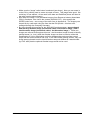
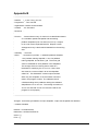
accuracy. In this way temporally variant and invariant features can be mapped more
efficiently while resultant crop classifications maintain both high attribute and spatial
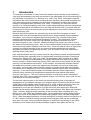
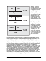
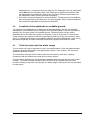
accuracy (see figure 1). This is the common situation for most farms at the Coleambally
Irrigation Area (CIA), where paddock boundaries change very little from year to year, but the
crop attribute is frequently changing.
The accurate measurement of rice area to the individual holding level is important for
management of groundwater recharge in the irrigation areas of southern New South Wales
(NSW) (Barrs and Prathapar 1994; Humphreys et al. 1994), and has resulted in yearly rice
administration responsibilities of the local irrigation managers. Both the accurate
identification of rice and the estimation of its total area have been achieved in NSW with
satellite remote sensing (McCloy et al. 1987; Barrs and Prathapar 1994; Barrs and Prathapar
1996). However, highly accurate estimation of total rice area, often exceeding 99% (e.g.,
McCloy et al. 1987; Barrs and Prathapar 1996), can be attributed to compensating negative
and positive errors at the paddock level (Barrs and Prathapar 1996; Van Niel and McVicar
2001). Wide discrepancies between rice area estimations at both the district level (McCloy et
al. 1987), and the individual holding level (Barrs and Prathapar 1996) can be exceedingly
large and, in the past, has prevented the adoption of satellite remote sensing for the yearly
monitoring of rice areas in both the Murrumbidgee Irrigation Area (MIA) and the CIA.
CSIRO Land and Water
-1-
Rice
Rice
Year 1
Soybeans
Rice
Rice
Year 2
Maize
Soybeans
Rice
Year 3
Fallow
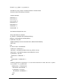
Figure 1. The idea of
temporally variant and
invariant features can allow
for efficient and accurate
mapping of crops at the
Coleambally Irrigation Area
(CIA). Most farms in the
CIA are typified by paddock
boundaries which change
very little from year to year,
but where the crop type
inside the boundary may
change frequently. In this
hypothetical example which
looks at the same farm over
three consecutive summer
growing seasons, only one
of the paddock boundaries
changes (depicted by the
dashed line in year 3).
However, the crops grown
in these static boundaries
tend to change often. If the
boundaries are updated
yearly with a GPS, then
moderately coarse remote
sensing data can be used
to map the crop type every
year for less expense than
high resolution aerial
photographs.
Because high spatial accuracy is important for management, both the MIA and CIA have
primarily used the interpretation of high-resolution aerial photography to monitor rice crop
areas every year. However, recent research at the CIA regarding: (1) spatial accuracy of
aerial photography and GIS data (Van Niel and McVicar 2000, 2001, 2002); and (2) rice
identification using satellite remote sensing (Van Niel and McVicar 2003; Van Niel et al.
2003) has moved satellite-based remote sensing one step closer to an operational system in
the region. This research has been further refined and simplified in collaboration with staff
from the Coleambally Irrigation Co-operative Limited (CICL) over the 2002-03 and 2003-04
growing seasons during which satellite remote sensing was used to complete rice
administration at the CIA. The reader is also referred to a review of remote sensing of ricebased systems, where these and other issues are described (Van Niel and McVicar 2004a).
This report, then, outlines the steps required to merge the high spatial accuracy paddock
boundaries defined from either high-resolution digital aerial photography or a GPS in the
field, with high attribute accuracy rice classifications from moderately coarse (and relatively
inexpensive) satellite imagery in order to accomplish yearly rice administration. It also
demonstrates that by taking advantage of certain strengths of coarse- and fine-scale spatial
data, the relationship between cost and accuracy can be improved by the use of satellite
remote sensing in conjunction with highly accurate paddock boundaries.
CSIRO Land and Water
-2-
2
Selection and Purchase of TM Imagery from ACRES
Website
2.1
Introduction
The timing of image acquisition can greatly influence the results of satellite image
classifications (Van Niel and McVicar 2004b). The first problem in any remote sensing
application is defining when discrimination of the particular target of interest (e.g., rice) is
best. We have seen at the CIA that best rice discrimination occurs in late November due to
the water of the ponded rice paddocks being easily identified when compared to all other
areas. The second problem is acquiring an image during the desired temporal window. This
is not usually a problem at the CIA, however, because it is completely contained within the
overlap area of two Landsat scenes. This means that the main CIA is imaged about every 8
days instead of every 16 days (like in non-overlap areas). This provides twice as many
opportunities to acquire cloud-free imagery in the desired timeframe, and thus greatly
enhances the operational management of satellite remote sensing at the CIA. To define
what images have been acquired and to order an image, the Australian Centre for REmote
Sesning (ACRES) website is extremely useful because they provide estimates of cloud cover
and a “quicklook” image of the entire scene. In this section, we describe the steps necessary
to access the ACRES website and how to define imagery for purchasing.
ACRES website
2.2
•
•
•
•
•
Go to the ACRES website: http://www.ga.gov.au/acres/
Click on the “Digital Catalogue” link on the left-hand side of the homepage
Click on the “Please Log In” link in the green tab along the bottom of this page
Click on the “Guest User” radio button and Click “Connect”
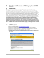
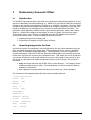
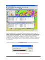
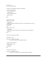
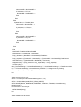
Now that you are into the main search page, the first thing to do is to close the
“Location” tab so your screen looks like the picture below. This is so we can refine
the search.
CSIRO Land and Water
-3-
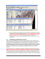
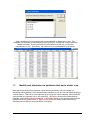
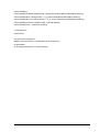
• Now Click on the “Databases” tab along the top of the page.
• On the databases page, select “ACRES [Landsat 4, 5, and 7] – Australian Centre for
Remote Sensing”, but DO NOT click on Search yet.
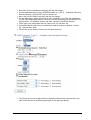
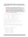
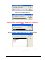
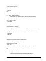
• Next, click on the “Refine” tab along the top of the page.
• On the refine page, adjust the search so only “Landsat 5” and “TM” are highlighted
(for the 2002-03 growing season, Landsat 7 was still operating and was chosen, see
picture below. For 2003-04 season and after, Landsat 5 should be chosen.).
• Then, type in the valid paths and row, Path: 92 to 93, and Row: 84
• Choose the Month and Year you would like to search under the “Season” section,
e.g., Oct and Nov, 2002.
• Then Click on the “Search” button (see the picture below).
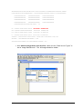
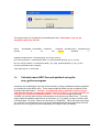
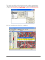
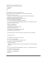
• This brings up a list of images within the specified criterion with relevant info in the
table on the left and a quicklook jpeg image on the right (see below).
CSIRO Land and Water
-4-
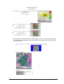
• If you click on one of the quicklook small images, you go to a new page, where you
can zoom in on the image to make sure there are no small clouds or haze over the
CIA (see below)
CSIRO Land and Water
-5-
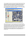
• Make sure the “Image” radio button is selected (see above). Now you can zoom in
to the CIA by clicking near its centre a couple of times. This image looks good. We
could buy it if we wanted. All we need is the date and Path/Row (these are listed in
the table, see the above image).
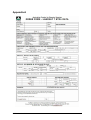
• Now order the image. CICL purchases imagery from Resource Industry Associates
(RIA) in Canberra. John Lee is the contact (02 6260 5377). John accepts the
ACRES order form – see a copy of the order form in Appendix A. The imagery can
be paid for by credit card using the form that the RIA provide – this has to be
arranged through the Company Secretary.
• By going through this process for the 2002-2003 growing season, we purchased
both an early October image (henceforth called, ‘the October image’), and a
late November image (henceforth called, ‘the November image’). These two
images are referred to throughout this text – the November image is used to identify
ponded areas (i.e., rice), while the October image can then be used to refine this
classification of rice by eliminating confusion between the previous winter cereal
crops and the current summer rice crop. In the 2003-2004 growing season, only one
image was purchased near the late November temporal window as it was decided
(by CICL staff) that the optional October image would not be used.
CSIRO Land and Water
-6-
3
Rudimentary Geometric Offset
3.1
Introduction
The ACRES map-oriented data is provided with a geometric model already applied to it, and
results in reasonably accurate positioning (e.g., within 50 to 100 metres) within the projection
defined in the selection and purchase of imagery (e.g., AMG66, see above). However, when
comparing any subsequent paddock boundaries to the imagery (especially if more than one
image is considered) it is advisable to have a better correction that what is provided. The
geometric model applied by ACRES results in good internal geometry, which means that a
simple x, y offset can be applied to the imagery in order to “nudge” the image into place.
This nudge is easy, it only requires a positionally accurate GIS dataset as a reference,
ArcView, and a text editor. In order to apply the shift we will cover:
• Importing images into ArcView; and
• Comparison of imagery to DGPS roads GIS layer.
Importing Images into ArcView
3.2
ArcView recognises uncompressed, band interleaved by line (bil), band interleaved by pixel
(bip), and band sequential (bsq) image data. These images, however, require a standard
header (text) file specifying image parameters. To demonstrate, we will be using Band 5
(central wavelength, 1650 nm) for the late November 2002 image you purchased as this will
be the main input into the rice/non-rice classification later. This image was in bsq format but
your image will likely be in bil format. Whenever you see a bsq image in the pictures in this
document you will need to be aware that this also refers to your bil image. This requires a
few steps.
• Copy the image data from the ACRES CD to a local directory. The imagery comes
as band interleaved by line (BIL). This format allows one file to contain the data for
all bands of reflectance.
• Next, open the template header file using a text editor (e.g., Word, Notepad).
The contents of the template header file should look something like this:
; ArcView Image Information
NCOLS
2722
NROWS
2080
NBANDS
1
NBITS
8
LAYOUT
BSQ
BYTEORDER I
SKIPBYTES 0
MAPUNITS
METERS
ULXMAP
351712.500
ULYMAP
6168837.500
XDIM
25.00000
YDIM
25.00000
CSIRO Land and Water
-7-
Where NCOLS, NROWS, NBANDS, and NBITS represents the number of columns, rows,
bands, and bits represented in the image, LAYOUT is the file format, ULXMAP, ULYMAP
are the upper left x and y coordinates in map space and XDIM and YDIM are the pixel size in
map units (i.e., metres).
• Now, you need to put the initial ULXMAP and ULYMAP coordinates based on the
ACRES geometric correction into the hdr file (if not already there)
• This requires copying and pasting the coordinates from the file called “header.hrf”
which is found in the same directory as the imagery for 27 November 2002. The
“header.hrf” file is a text file and can be opened in any text editor or even Word. The
contents of this file for the November image are shown below with the UL
coordinates coloured red. These are the values that need to be pasted into
“nov_bnd5.hdr”. As can be seen, the template was made with these coordinates, so
we don’t have to worry about actually changing it this first time (but you will need to
do it next year, or for this year’s October image):
REQ ID =01026_02
LOC =093/0840000
SATELLITE =LANDSAT7 SENSOR =ETM+
LOCATION =
SATELLITE =
LOCATION =
SENSOR MODE =
LOOK ANGLE =
ACQUISITION DATE =
SENSOR =
LOCATION =
SATELLITE =
SENSOR MODE =NORMAL LOOK ANGLE = 0.00
ACQUISITION DATE =
SENSOR =
SATELLITE =
ACQUISITION DATE =20021127
SENSOR MODE =
LOOK ANGLE =
ACQUISITION DATE =
SENSOR =
PRODUCT TYPE =MAP ORIENTED
SENSOR MODE =
LOOK ANGLE =
PRODUCT SIZE =SUBSCENE
TYPE OF PROCESSING =SYSTEMATIC RESAMPLING =CC
VOLUME #/# IN SET =01/01 PIXELS PER LINE = 2722 LINES PER BAND = 2080/ 2080
START LINE # =
1 BLOCKING FACTOR = 1 REC SIZE =
2722 PIXEL SIZE = 25.00
OUTPUT BITS PER PIXEL = 8 ACQUIRED BITS PER PIXEL = 8
BANDS PRESENT =123457
FILENAME =L71093084_08420021127_B10.FSTFILENAME =L71093084_08420021127_B20.FST
FILENAME =L71093084_08420021127_B30.FSTFILENAME =L71093084_08420021127_B40.FST
FILENAME =L71093084_08420021127_B50.FSTFILENAME =L72093084_08420021127_B70.FST
REV
L7A
BIASES AND GAINS IN ASCENDING BAND NUMBER ORDER
-6.199996948242188
0.775686264038086
-6.399993896484375
0.795686244964600
-5.000000000000000
0.619215667247772
-5.100006103515625
0.965490221977234
-0.999998092651367
0.125725477933884
-0.350000381469727
0.043725494295359
0.000000000000000
0.000000000000000
0.000000000000000
0.000000000000000
CSIRO Land and Water
-8-
GEOMETRIC DATA MAP PROJECTION =UTM ELLIPSOID =AustralianNational DATUM =AGD66
USGS PROJECTION PARAMETERS = 6378160.000000000000000 6356774.719195305400000
0.000000000000000
0.000000000000000
0.000000000000000
0.000000000000000
0.000000000000000
0.000000000000000
0.000000000000000
0.000000000000000
0.000000000000000
0.000000000000000
0.000000000000000
0.000000000000000
0.000000000000000 USGS MAP ZONE =
55
UL = 1452257.5446E 343641.3657S
351712.500 6168837.500
UR = 1460728.1294E 343708.6552S
419737.500 6168837.500
LR = 1460710.2050E 350515.7448S
419737.500 6116862.500
LL = 1452224.4454E 350447.9781S
351712.500 6116862.500
CENTER = 1450519.0279E 344516.3703S
325051.989 6152498.930 -1065 655
OFFSET = -336 ORIENTATION ANGLE = 0.00
SUN ELEVATION ANGLE =59.2 SUN AZIMUTH ANGLE = 72.3
• Now add the image theme into ArcView, make sure the “Data Source Types:” is
set to “Image Data Source”. The .bil image should be visible.
CSIRO Land and Water
-9-
• When the image is added to the view you will need to double click on the legend to
change it to single band, Band 5.
• The image should appear as a grey scale with approximate map coordinates
(AMG66 – see below)
• This process will need to be repeated until it matches with the DGPS data
(described below).
3.3
Comparison of imagery with DGPS roads GIS data
Now that the initial geometric coordinates are placed in the header file and the image is read
into ArcView, we want to compare it to a very accurate GIS layer. This layer is the roads
network digitised using NSW Department of Agriculture’s DGPS unit in February 2001.
These lines should be within about 1 to 2 metres of the centreline of almost every road within
the main CIA boundary, so they provide lots of reference points to compare the placement of
our imagery. The roads shapefile is also in AMG66. For details of this dataset see Van Niel
and McVicar (2002). This step requires adding the GPS roads theme to the same view that
the imagery is in, changing the colour to something easily seen, and then altering the
ULXMAP and ULYMAP values in the image header file until you are satisfied with how the
roads lines up with the image. Please note, the match should be good throughout the
CSIRO Land and Water
- 10 -
entire main CIA boundary. Also, be careful not to mix up canals and side roads with
the main roads which are represented in the shapefile.
• Add the GPS roads shapefile to the view
• Zoom in to an appropriate scale (make sure the view map units are set to meters – I
like about 1:20000 and usually start somewhere around Anderson and Frazer
Roads, but this is arbitrary)
• As can be seen below, the ACRES correction is not too bad, but the roads don’t
quite line up. It looks like the Y direction is worse than the X.
• Change the coordinates until you are happy with the match over the whole CIA.
Note, you will have to delete the theme and add it again to the view each time
you change the header file coordinates or ArcView will not make note of the
change to the coordinates. Also, it probably doesn’t make sense to be more
precise than about 0.5 of a pixel or in this case 12.5 metres.
• I did this and was happy with the following coordinates (see pic below) :
• ULXMAP
• ULYMAP
351762.500
6168937.500
• This represents a shift of 50 metres in the x direction and 100 metres in the y
direction, resulting in a good match
CSIRO Land and Water
- 11 -
• Note that an addition to the X coordinate will result in the image moving right and a
subtraction will result in it moving left. An addition to the Y coordinate will result in it
moving up and a subtraction will result in it moving down.
CSIRO Land and Water
- 12 -
4
Ground Validation, Classification Accuracy, and
Training Sets
4.1
Introduction
One of the most important things in the classification of rice is defining an appropriate ground
validation or reference dataset. This reference dataset will be used for two purposes: (i)
estimation of rice classification accuracy; and (ii) defining two small training sets which will be
used to determine the threshold used to classify paddocks as either rice or non-rice. The
following topics, then, need more detailed discussion:
•
•
•
4.2
Defining the ground validation dataset;
Defining the rice and non-rice training sets; and
Estimating classification accuracy.
Defining the ground validation dataset
The first step is to define the base ground validation set of paddocks. This can be done by
sending out simple surveys to landholders. Since this has been done for several years in a
row, there is a set of Word documents to use including the surveys and farm maps. These
can be faxed to the landholders, who usually respond quickly if the survey is relatively
simple. Maps can be found in “NRE on Sol”:\Rice\Survey forms-cropping. Before faxing and
mailing the forms out to the landholders it is necessary to update the year at the top of the
form, and the covering note. For the 2002-2003 growing season, we had a good response
where the crop types of 73 paddocks were known. Since 40 of these were rice, a fairly even
sample of rice and non-rice was also achieved, which is one of the goals. Arbitrarily, it
would be good to have at least 30 rice and 30 non-rice paddocks to estimate the
classification accuracy from. Since 5 rice paddocks and 5 non-rice paddocks are used for
training the classification (see below) and cannot be used for both training the classification
and estimating it’s accuracy, we will (ideally) need at least 35 rice and 35 non-rice paddocks
from this survey. If we do have 30 of each class for accuracy estimation, it means that
although a bit course, the precision of our accuracy measurement is good enough to detect
changes of 1.67% (1/60). That is, the smallest increment of change in our accuracy estimate
is 1.67%, so if one paddock out of the 60 is misclassified, our estimate will be 100 – 1.67, or
98.33%, if 2 are misclassified it will be 100 – 3.33, or 96.67%.
• The known paddocks should be put into a shapefile. These known paddocks should
also have current boundaries. Therefore, the boundaries might need updating (for
details, see section 5 regarding updating paddock boundaries).
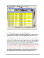
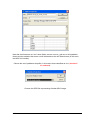
• Also, it is good to make sure that the attributes of this shapefile are in order. For the
subsequent classification accuracy assessment, below, a field of crop types using
the code of “R” for rice and “NR” for non-rice is required. In my shapefile, this
field is called “Crop2003”, see the figure below. It is not a bad idea also to keep
track of which areal photos the paddock was digitised from, who digitised it, and
other details as you see fit (e.g., variety if known, etc…).
CSIRO Land and Water
- 13 -
4.3
Defining the rice and non-rice training sets
Next, two shapefiles containing a small number of paddocks (e.g., 5) whose boundaries
are known to be current and whose crop types are also known will be defined. These
small subsets of paddocks are known as training sets and will be used to derive the
threshold that will be used to define which pixels or paddocks are rice and which are nonrice. These training sets can be defined in various ways. For example, they can come
from landholder surveys, or from field observations. In this case, we used landholder
surveys to determine paddocks where the crop types were known (as above). From these,
5 rice and 5 non-rice paddocks were arbitrarily selected and saved to separate shapefiles,
see figure below (e.g., 02_03_r_trn.shp and 02_03_nr_trn.shp, where 02-03 represents
the year, r and nr stands for rice or non-rice, and trn stands for training set).
The non-rice training set was selected with a stratified sample in mind. That is, various
crop types were selected to very roughly represent their proportion in the non-rice crops (2
maize, 1 soybean, 1 sorghum, 1 millet). It is important that both the rice and non-rice
training sets do not include paddocks that are grossly unrepresentative of the
overall class response. For example a very small proportion of the rice paddocks are not
flooded by late November. So, if by chance we include one of these paddocks in our
training set, the statistics developed from it will not really represent the normal case and
may result in poor classification accuracy. Therefore, particular care must be taken to
select a representative training set in order to achieve the required accuracies.
CSIRO Land and Water
- 14 -
• Once these shapefiles are organised, we will estimate the classification accuracy of
rice based on the remaining known paddocks. The final validation shapefile will
include all of the original paddocks from step 1 above minus those paddocks
used for training in step 2. That is, the paddocks used for training the
classification should not be used to estimate it’s accuracy, since they are no longer
independent.
4.4
Estimating classification accuracy
Finally, these three shapefiles will be used in conjunction with an Avenue script and the
GRID representation of ETM band 5 to define both the threshold used to classify rice versus
non-rice and the accuracy defined from the final validation set of paddocks. The script
summarises the mean ETM band 5 value for each paddock in the three shapefiles. It then
calculates the threshold value as the average of the mean rice and mean non-rice responses
from the two training sets. Then, it compares the validation paddocks known crop types to
what this newly defined threshold would classify the paddock as in order to estimate
accuracy.
The script called r_nr.ave should be loaded into a script editor window, and then compiled.
Make sure that all three of the above shapefiles are loaded into the ArcView View and
that all the records in the validation shapefile are selected. If there is no selection, the
script will complain. The script also assumes that the view is the last thing to be active prior
to running the script (this is due to the first line in the script where the view variable is set to
the active document using the “av.GetActiveDoc” request). Therefore, if an error occurs right
CSIRO Land and Water
- 15 -
off the bat and say’s something like “A(n) Table does not recognise request GetThemes”,
then make the View active, then make the script active and then run it again – it should work
this time. Another solution would be to attach this script to a button directly on the View’s
GUI (see ArcView help for details). Also make sure that a GRID of ETM band 5 is in the
view. To convert the image to a GRID, simply click on Theme/Convert to Grid… from the
View’s GUI and follow the prompts (the ArcView Spatial Analyst extension must also be
already loaded).
The script is included in Appendix B as a backup of the original file and can be cut and
pasted into the script window directly. The script depends on a common field defined by
the user in each of the three shapefiles. This common field must contain an R in it for any
paddocks that are rice and an NR in it for any paddocks that are non-rice. Currently, if the
field has something different, then this script will need to change. Also, make sure that
these shapefiles all have unique ids or the summary may not be correct. For example,
when a new paddock is added to a current shapefile, the attributes of the new record will be
set to zero; if 5 new paddocks are added, and their ids are all left zero, the last four will be
classified the same as the first rather than each separately, resulting in a false estimate of
the accuracy reported by this script (see Appendix B).
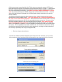
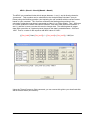
• Run the script as shown below:
Choose the validation paddock shapefile (This works off of the selection, so if you want
all the paddocks to be considered within this shapefile, then they should all be selected):
Then, the rice training set:
Then, the non-rice training set:
CSIRO Land and Water
- 16 -
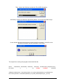
Then, choose the field that contains the R and NR information:
And finally, choose the GRID file representing Band 5 of the late November image:
A new window should reveal where the output excel file is located. In this file is the
threshold information and the estimation of accuracy:
The output from running this program should look like this:
Name
NumNRasR
Nov_bnd5
NumRasNR TotalCount
2
1
63
Threshold
75.5838
OverallAccuracy KappaAccuracy
0.952381
0.903226
Validation Paddocks file: c:\vanniel\tmp\rueben_rice_2002_2003\shapes\02_03_validation.shp
Rice Training Set file: C:\VanNiel\tmp\Rueben_rice_2002_2003\shapes\02_03_r_trn.shp
CSIRO Land and Water
- 17 -
Non-rice Training Set file: C:\VanNiel\tmp\Rueben_rice_2002_2003\shapes\02_03_nr_trn.shp
Common Validation Field: Crop2003
Time: Mon Aug 04 13:04:15 2003
• The NumNRasR reveals the number of NonRice paddocks that were classified as
Rice (errors of commission), the NumRasNR shows how many Rice paddocks were
classified as NR (errors of omission), the Threshold will be used later to classify the
rice, and the Overall Accuracy (as a proportion) is the estimate of the accuracy
based on the validation paddocks. The Kappa accuracy is another accuracy statistic
useful when the sample sizes are very uneven.
CSIRO Land and Water
- 18 -
5
Updating Paddock Boundaries
5.1
Introduction
The methods outlined for identification of rice depend on placing the remotely sensed signal
within some sort of ‘context’. Basically, this means that we don’t just use the information
from all the pixels in the image separately (per-pixel classification), but rather we also make
use of the information that is surrounding these points at the same time. One of the most
common ways to put remote sensing data into context for agricultural applications is by
summarising the entire paddock (per-paddock classification). This requires a GIS layer of
paddock boundaries.
As usually the hardest part of a mapping project is defining boundaries, this per-paddock
method has a distinct advantage over per-pixel classifications. That is, since we know the
potential boundaries of the phenomena that we wish to map before we map it, the hardest
part of the mapping procedure is done before we start. This is also one of the reasons why
we are able to get such high accuracies using such simple techniques (there are also other
reasons, like homogeneous management practices of the landholders and the fact that we
are really mapping standing water versus non-water, which is not too hard compared to lots
of other things).
Unfortunately, there is also a distinct disadvantage to this per-field method: if the GIS
boundaries are not spatially accurate or up-to-date (temporally accurate), then the results
can be worse than a per-pixel classification. Therefore, assuring that the paddocks are both
spatially accurate as well as appropriate for the current time period (growing season) is
essential. Normally, drastic differences to paddock boundaries do not occur from year to
year at the CIA, which means that keeping the GIS boundaries up-to-date is not a huge job.
However, the more common changes where parts of paddocks (e.g., rice bays) are
alternately included or omitted can be enough to alter the mean statistics of the paddock
enough to misclassify the paddock. Therefore, these changes need to be updated in the GIS
paddock boundary every year, or the resulting accuracies will not be as high as expected.
There are a number of ways that this updating of paddocks could take place, so this section
is not really a definitive ‘recipe book’ for updating paddocks. The methods introduced here
can be altered as need be.
The methods we used concentrated on updating ONLY the boundaries of those paddocks
that were suspected of being rice. Since this included any paddocks that had any standing
water, it was a pretty safe starting point:
1. First flooded areas on the November ETM image are defined using per-pixel
classification of band 5 (1650nm), and subsequently converted to an ArcView
shapefile.
2. Once these areas suspected of being ponded water (i.e., rice) are defined, they are
then compared to the previously digitised paddock boundary GIS dataset.
3. Next, a decision is made about whether or not each of these paddocks needs to be
updated using the following rather subjective rule:
• If one of the previous year’s rice boundaries matches well with the area of ponded
water defined from step 1, above, then this boundary can be used in the
classification.
• However, if the previously defined boundary and the classification from step 1,
above provides a poor match, then the boundary will need to be updated.
Ultimately, these boundaries need to be of high accuracy, which means digitising
from previous aerial photos or by using a GPS unit in the field. However, if the
analyst chooses, the initial digitisation of these changed paddocks can occur from
the satellite imagery, which allows for an “approximate” boundary for classification.
CSIRO Land and Water
- 19 -
These “approximate” boundaries should be identified separately so that the ones
that are classified as rice can be updated in the future from either a previous aerial
photograph or by using a GPS in the field. When the difference is small (for
example, due to a missing rice bay in a paddock), this defines a change that can
probably be fixed from past aerial photos. When the change is too big to be
identified properly from previous photos, someone will need to update the boundary
using a GPS unit in the field. Remember, the date of update, who recorded the GPS
data, and who updated the GIS boundary could be recorded in the GIS paddock
boundary file.
These three steps are outlined below.
5.2
Defining flooded areas on the imagery
The purpose of this initial pass is only to assess which paddocks may need updating and
requires a per-pixel classification. Since water absorbs light in the wavelengths around
1650 nm where band 5 is centred, the rice areas during this time of year have very low
values. Also, non-rice paddocks are predominantly some much drier surface (e.g., soil,
stubble, or green crops that are not near canopy closure), revealing very high values in ETM
band 5. Therefore, it is generally very easy to classify water versus non-water (which is
really what we are doing); we assume that all the flooded paddocks are rice. We will put
these values in a per-paddock context later. Be careful to note whether a heavy rainfall
occurred just prior to image acquisition as this might influence the results of this analysis.
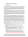
• First, the GRID of ETM band 5, generated in the Ground Validation section, above is
classified using the threshold value determined in that same section. As determined
above, the threshold between rice/non-rice from our training sets was 75.5838.
• This entails using the “Map Calculator” in the Analysis/ menu. Set up the equation
to define the classes based on the above threshold (see figure below):
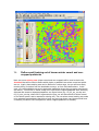
• This will result in the calculation of a GRID that has a two classes: zero’s for nonwater areas and one’s for water (see below).
CSIRO Land and Water
- 20 -
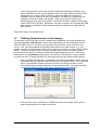
• This GRID can then be saved to a temporary shapefile using Theme/Convert to
Shapefile… command. Once this is complete, use the shapefile Query Builder to
select only the polygons with Gridcode = 1, as seen below :
CSIRO Land and Water
- 21 -
•
Run Theme/Convert to Shapefile again with this selection and this will result in a
shapefile of the areas predominantly covered by water on this image date (see
below).
.
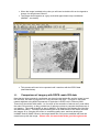
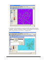
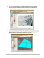
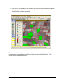
•
This shapefile can then be used to compare the extent of water for this current date to
previously digitised paddocks. If the match is good, then the old paddock boundary is
OK to use (see below for an example of a good match between three previously
defined boundaries in red to the water classification of this year).
CSIRO Land and Water
- 22 -
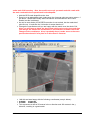
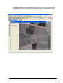
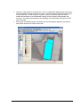
•
•
However, if the match is not good (e.g., due to a change like adding more rice bays in
this year when compared to previous years - see below) then these boundaries need
to be UPDATED. In this example, a previous year’s air photos might be used to
extend the boundary as a fundamental change to the boundary has probably not
occurred. For other circumstances, the updating of the boundary will require a GPS
unit in the field.
Every area of classified water will need to be checked against paddock boundaries
and similar decision will need to be made.
CSIRO Land and Water
- 23 -
6
Identifying Summer Rice Paddocks (Optional Step)
The procedures in this chapter are optional. For the 2003/04 season, all rice paddocks were
classified by looking at the map of standing water (generated by the steps in the last chapter)
and using it to select paddock measurements from previous years for this year's rice. The
per-paddock classification process is still described in detail for completeness and is thus
available for use in this or other similar applications if the user so chooses. There is no need
to perform this task, however, if the per-pixel visual inspection approach is taken.
Remember, if you are not going to perform the following per-paddock classification, then it is
a good idea to make use of the "Waterways" database that CICL records for every farm. In
this database, the landholder's estimated rice area and the volume of water applied to rice
are recorded and can be used as a guide in determining the area of rice for each farm. When
we know the area, determination of rice paddocks by visual assessment is easier.
Introduction
6.1
As discussed before, the methods outlined for identification of rice depend on placing the
remotely sensed signal within a per-paddock context, which requires the updating of some
boundaries every year (see above). After the publication of research using a moisture index
based on the ‘depth’ of ETM band 5 reflectance compared to that of ETM bands 4 and 7, it
was found that simply using ETM band 5 alone provides just as accurate (or better) results.
Also, the added benefit is that using a single band is even easier to process. The methods
here depend on the previous sections already being accomplished. That is, the ground
validation should be compiled, the rudimentary geometric offset should be applied, the rice
and non-rice training sets should be defined, the threshold should be calculated, and the
paddock boundaries should be updated. The basic steps that will be covered in this section
include:
•
•
Calculate the mean ETM band 5 value for every paddock; and
Classify each paddock into a rice or non-rice class by comparing the threshold
defined from the training sets to the mean paddock values.
Using a subset of the r_nr.ave Avenue script called sum_grid.ave (see Appendix C), the
mean value of each paddock will be summarised and will be saved to a separate shapefile
(saved to your ArcView working directory – to change this, look in File/Set Working
Directory). The inputs are a paddock theme (this time, it is the full set of paddocks over
the entire CIA instead of the validation set of paddocks), and the GRID of ETM band 5.
Calculating the mean ETM band 5 value for every paddock
6.2
Previously, (in the ground validation section) we used a similar script to calculate a per-pixel
classification for the purposes of updating paddock boundaries. Now, we will rerun the
same basic steps using the information from that original processing (i.e., the threshold
determined from the training sets, and the ETM band 5 GRID). Whatever paddock
boundaries are input into this sum_grid.ave program will be summarised statistically,
including the mean of each paddock (which is what we will subsequently use to classify the
paddocks as either rice or non-rice). Therefore, we want at least all of the boundaries
suspected of being rice, defined previously. In this example, we use all of the paddock
boundaries. Remember, the paddock theme should have all of its records selected.
Also make sure that the GRID of ETM band 5 is in the view.
•
First, the script will need to be loaded, compiled, and ran (see ESRI and previous
section for details).
CSIRO Land and Water
- 24 -
•
Once the script is run, follow the prompts:
Choose the full set of paddocks shapefile (should all be selected):
Choose the GRID file representing Band 5 of the late November image:
After completion of running this script a new shapefile is added to the view. This
shapefile is a duplicate of the paddock theme input into it, except that a set of fields are
added to the database file (dbf). These new fields are the statistics we will use to
classify rice – specifically, the mean value for each paddock (see below).
CSIRO Land and Water
- 25 -
Classifying each paddock to rice or non-rice
6.3
Previously (ground validation section 4), the threshold was calculated as 75.5838. This
threshold will be used to select any paddocks that are less than or equal to this value. It is
these paddocks that we will classify as rice. There are various ways to approach this last
step, so this is more of a guide than a definitive list of instructions. In this case, we use
the query builder to select only those paddocks that are less than or equal to the threshold
and then save them out to a separate shapefile.
First, use the query builder to select any paddocks in the new theme (generated above,
step 1 of this section) that are less than or equal to the previously defined threshold of
75.5838 (of coarse, this threshold will change every year or if different training
sets are used).
•
Click on “New Set”. This results in a subset of the original number of paddocks being
selected (see below) :
CSIRO Land and Water
- 26 -
•
Now that the rice paddocks are selected, if we click on Theme/Convert to Shapefile…
, the rice paddocks can be saved out to a separate shapefile – I called mine
02_03_classif_rice.shp (see below).
These are our final rice paddocks. Optionally, these can be adjusted by preventing
paddocks which contained previous winter cereals from being classified as rice. This
optional section is discussed below.
CSIRO Land and Water
- 27 -
7
Identifying Winter Cereal Paddocks for Exclusion
(Optional Step)
7.1
Introduction
An optional processing tactic is to adjust the previously classified rice paddocks (defined
from the step above) by not allowing any paddocks to be classified as rice if they contained a
crop during the preceding winter growing season. The premise is that the winter crops are
not usually harvested until late November; since the recommended time for planting rice is
early October, almost no farmers will ever plant a rice crop immediately after a winter crop.
Since it is very easy to define cropped areas from non-cropped areas using the Normalised
Difference Vegetation Index (NDVI), we are able to detect any paddocks that were winter
cereals and prevent them from being classified as summer rice. An October image should
be ideal for this since the winter crops should still be green, while the summer paddocks
should be in some state of preparation for planting (if they have not been sown yet), but not
yet green. Also, during this time, most winter pasture should be dried out and being
prepared if there is going to be a summer crop.
If you have purchased an October image, then all of the previously discussed steps will need
to be applied to this image. That is, importing (in this case) ETM bands 3 (red) and 4 (NIR)
into ArcView, calculating and applying the geometric offset (it should be the same for all
bands within the October image), and defining two more training sets (one winter cereal,
and one non-cropped training set). Please see the previous notes on all of these steps. The
steps for doing this follow the methods for identifying rice, so they will only be covered very
briefly. The steps include:
•
•
•
•
7.2
Calculation of NDVI on an October ETM image;
Define small training set of known winter cereal and non-cropped paddocks and
determine threshold for classifying winter cereals from the October NDVI image;
Calculate mean NDVI for each paddock using the sum_grid.ave program; and
Identify and eliminate paddocks previously classified as rice which are also classified
as having a winter cereal crop (these are most likely not rice).
Calculating the NDVI on an October ETM image
Using the techniques discussed previously, ETM bands 3 (red waveband) and 4 (NIR
waveband) of the October image should be imported into ArcView and a different geometric
offset should be applied. Note, the steps for calculating the geometric offset will be the
same, but will need to be redone for the different image (before we were using a November
image). Then, convert both of these bands to GRIDs as before and add them to the view.
The formula for the NDVI is:
NDVI = (NIR - red)/(NIR + red)
or for ETM bands,
CSIRO Land and Water
- 28 -
NDVI = (Band4 – Band3)/(Band4 + Band3)
The NDVI is a normalised index which ranges between -1 and 1, and is directly related to
“greenness”. This equation can be calculated in the Analysis/“Map Calculator” (see pic
below) using the following equation (and replacing the red variables with the correct names
based on your own data. The .float term maintains the floating point precision in the
calculation (otherwise everything is converted to either 1’s or 0’s by default. The * 1000 term
is a scalar (scales the values of the NDVI between -1000 and 1000 (instead of between -1
and 1), and the .int term converts this result to integer data. The resulting data is integer
data (with a precision of 3 decimal places) because the data is scaled between -1000 and
1000. That is, a value of 459 equals a real NDVI value of 0.459 :
(( [Oct_bnd4] .float- [Oct_bnd3]) / ( [Oct_bnd4] + [Oct_bnd3]) * 1000).int
Using the Theme/Convert to Grid command, you can convert this grid to your local hard disk
with a relevant name (like octndvi):
CSIRO Land and Water
- 29 -
7.3
Define small training set of known winter cereal and noncropped paddocks
Next, two more training sets (winter cereal and non-cropped) will be used to derive the
threshold that will be used to define which pixels or paddocks are winter cereal and which
are not. Again, these training sets can be defined in various ways, but you will most likely
receive plenty of choices from the landholder surveys, or from field observations. In this
case, we used landholder surveys to determine paddocks where the crop types were known
(as above). From these, 5 winter cereal and 5 non-winter-cropped paddocks were arbitrarily
selected and saved to separate shapefiles, see figure below (e.g., 02_03_wc_trn.shp and
02_03_nwc_trn.shp, where 02-03 represents the year, wc and nwc stands for winter cereal
or non-winter cereal, and trn stands for training set). The non-winter cereal training set needs
to be selected from paddocks that did not have any previous winter crop (these should have
a relatively low NDVI value compared to winter cropped paddocks in October).
CSIRO Land and Water
- 30 -
Now, the threshold needs to be calculated. This can be done in a number of ways. For
example, you could run the sum_grid.ave script and then calculate the average of the means
between the two training sets “manually”. Otherwise, you can run the r_nr.ave script and
disregard the accuracy information. That is, have the script calculate the threshold for you.
If using the script to calculate the threshold, ignore the accuracy statistics, they are
meaningless. See the menus below for the input for this option. If using the r_nr.ave script,
the rice and non-rice prompts will need to be replaced (in your mind) by winter cereal and
non-winter cereal:
Choose the shapefile containing the paddocks that have already been classified as rice
(should all be selected):
Then, the winter cereal training set:
CSIRO Land and Water
- 31 -
Then, the non-winter cereal training set:
Then, choose the field that contains the R and NR information (This actually doesn’t
matter for the winter cereal processing, but has to be filled in for the script to
finish):
And finally, choose the GRID file representing the NDVI of the October image:
A new window should reveal where the output excel file is located. In this file is the
threshold information (and the estimation of accuracy, which is meaningless for the
winter cereal application):
CSIRO Land and Water
- 32 -
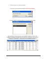
The output excel csv file should look something like this. Remember, only use the
threshold value from this file:
Name
Octndvi
NumNRasR NumRasNR
0
39
TotalCount
Threshold OverallAccuracy
381
182.912
KappaAccuracy
0.897638
0
Validation Paddocks file: c:\vanniel\tmp\02_03_classif_rice.shp
Rice Training Set file: c:\vanniel\tmp\rueben_rice_2002_2003\shapes\02_03_wc_trn.shp
Non-rice Training Set file: c:\vanniel\tmp\rueben_rice_2002_2003\shapes\02_03_nwc_trn.shp
Common Validation Field: Crop2003
Time: Mon Aug 25 11:50:56 2003
7.4
Calculate mean NDVI for each paddock using the
sum_grid.ave program
As before, the classification is put into a field context by using a paddock boundary shapefile
to calculate the mean NDVI value. These mean paddock values are then compared to the
threshold calculated above. However, an additional step is required if you are using a
shapefile that already contains the statistics fields in it (that is, if you have already run
sum_grid.ave on the input paddock theme). You will need to make these fields
“invisible” so ArcView does not get confused later as to which mean field to use. To do this,
simply make the paddock theme active (in this case, 01_03_classif_rice.shp, and then open
it’s theme table. Go to the Table menu and click on “Properties”. When this new menu pops
up, “uncheck” the checkboxes next to all of the statistics fields that were generated from the
previous run of sum_grid.ave (most importantly, the “Mean” field, see below):
CSIRO Land and Water
- 33 -
Now that ArcView does not “see” these fields, we can run sum_grid.ave on this paddock
theme and the statistics that come out will be based on the new index theme (in this case,
the NDVI for October):
Choose the set of paddocks shapefile, in this case, those classified as rice (should all
be selected):
Choose the GRID file representing October NDVI image:
CSIRO Land and Water
- 34 -
After completion of running this script a new shapefile is added to the view. This
shapefile is a duplicate of the paddock theme input into it, except that a set of fields are
added to the dbf. These new fields are the statistics we will use to refine the
classification of rice – specifically, the mean value for each paddock (see below).
7.5
Identify and eliminate rice paddocks that had a winter crop
Now that we have the mean paddock values and the threshold, it is just a matter of
identifying which paddocks from those already classified as rice are now identified as having
a winter cereal. This can be accomplished by querying the output shapefile, above with the
query builder (the hammer icon in the view GUI). As before, select those paddocks that
meet the criteria defined by the threshold. In this case, however, we are interested in those
paddocks that are greater than or equal to the threshold (those paddock previously
classified as rice that had very high NDVI in October):
CSIRO Land and Water
- 35 -
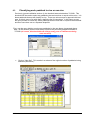
First, use the query builder to select any paddocks in the new theme (generated above,
step 1 of this section) that are greater than or equal to the previously defined threshold
of 182.912 (of coarse, this threshold will change every year or if different training
sets are used)
In this case, two paddocks are selected (see image below).
CSIRO Land and Water
- 36 -
These two paddocks had mean values well above the threshold (both greater than 375), and
are most probably not rice (that is, they were heavily vegetated in October). Because of this,
the final shapefile representing the classification of rice should be saved out with these
adjustments. To do this, from the Table GUI click on the Edit/Switch Selection option, and
then from the View GUI, click on Theme/Save to Shapefile. This selects all the other
paddocks except these two which have been classified as winter cereals, and then saves
them to a separate shapefile. Remember to use a name for the output that makes sense to
you. I have used the name, 02_03_classif_rice_wc_mask.shp. And, as you can see below,
these two paddocks are not included in my new shapefile:
If these paddocks (the ones that have been removed) coincide with the original paddocks
that were used for validation (i.e., accuracy assessment), then our estimation of accuracy will
now need to be reassessed. In this case, these two paddocks were not in our validation set,
so our estimate of accuracy remains the same. In other words, we don’t really know whether
we have just improved the accuracy or made it worse. However, from past studies, it is
reasonably safe to assume that we have just made it better. If we look at the mean
November Band5 values for these two paddocks, they were just barely under our November
Band5 threshold of 75 (one was 67 and the other was 74) – this also makes us more
confident that we have done the right thing, since not only did both paddocks show a strong
crop signal in October, but neither paddock showed a very strong water signal in our
November image.
CSIRO Land and Water
- 37 -
8
Rice Administration
Once the rice areas have all been completed and you are satisfied that they are correct, you
can start to generate the information from them required for rice administration.
8.1
Adding attributes to rice areas
The first step is to add a field listing areas in hectares to the attributes table of the rice area
shapefile. This can be achieved by running the “AreaMeasurement” script, a copy of which
can be found at m:\esri\AV_GIS30\ARCVIEW\Samples\Scripts. This is a very simple script to
use.
This script will add two new fields to the shapefile – area (in square metres) and perimeter (in
metres). To view the area of each polygon in hectares, add a new field called “Area_ha” with
one decimal place. You will first need to start editing the table and make the heading
“Area_ha” active. Under the “Field, Calculate” option you can run a calculation in which you
divide the values in the “Area” field by 10,000. All the values will be automatically filled in.
Next you will need to append the attributes from the shapefile “cia_external” to the rice areas.
In particular the attributes that we require are farm numbers, property ID and outlet numbers.
It might be expected that this could be achieved by straightaway doing a simple spatial join
(using the Geoprocessing Wizard). However, this option relies on the rice polygons being
entirely contained within the farm boundaries. Due to slight differences in the georeferencing
of our GIS layers, including the aerial photographs, this is not possible. You will therefore
need to convert the rice areas to centroids (points at the centre of each polygon) to enable
the spatial join to occur. The spatial join is performed as follows:
• Ensure that there is a field in the attributes table of the rice areas called ID and that
every record in the attributes table has a unique ID number. You can add these
numbers to the table if they are not already there by running the increment script.
This can be found in m:\esri\AV_GIS30\ARCVIEW\Samples\Scripts. This will
generate a field called “Inc”. By doing a field calculation as described above for
hectares, you can give the field called ID the same numbers as in “Inc”. Delete the
“Inc” field.
• Load the “Xtools” extension in the ArcView project. A window will appear in which
you can change the default units to metres and hectares. Close the window.
• An “Xtools” option will appear as one of the headings at the top of the ArcView
window. When you click on the heading there is a long list of options. Click on
“Convert shapes to centroids”. Follow the instructions and select the rice areas
theme as the theme to convert to centroids. Store the new file “Cntrs” in X:\Temp.
• Open the attributes table of Cia_external. Click on Table\Properties and un-tick the
data that you do not need. As stated earlier, the attributes you will need are farm
numbers, property ID and outlet numbers. Click OK.
• You can now use the Geoprocessing Wizard to perform a spatial join. You may need
to load the “Geoprocessing” extension. Then go to View\GeoProcessing Wizard.
Select the option “Assign data by location (Spatial Join)” and click Next. Assign data
to “Cntrs” and assign data from “Cia_external”. Click Finish.
• Open the attributes table of “Cntrs”. You will see that the three fields we require
have been appended with data for every record in the table. If you wish to redo the
spatial join for some reason, remove the join by clicking on Table\Remove All Joins.
• You now need to export the attributes table for “Cntrs” as a dbase file to X:\Temp.
• In the project window, click on Tables and then Add. Navigate to the table you
exported. The table will appear when you add it in. In the table properties ensure
only the farm numbers, property IDs and outlet numbers are displayed. Make the
“ID” heading active. Open the attributes table for the rice areas and make the “ID”
CSIRO Land and Water
- 38 -
heading active. It is important that you make the “ID” heading for the rice areas table
active after that for the dbase table. Click Table\Join to append the attributes from
the dbase table to the attributes table of the rice areas. Close the tables when you
are satisfied the table join has occurred successfully.
• Convert the rice areas shapefile to a new shapefile. This will preserve the attributes
that were generated by the table join in the new shapefile. All the required attributes
have now been appended to the rice areas shapefile.
8.2
Location of rice paddocks on suitable ground
The location of rice paddocks on suitable ground as delineated by the rice soil suitability
classification can be determined by using the GeoProcessing Wizard. Use the clip option to
identify if any rice was grown on unsuitable ground. The same option can be used to
determine which rice areas were grown on marginal (1 year in 4) ground. For these areas
further overlays are required to see if they were grown with rice in any of the previous three
years. To perform each clip the rice suitability shapefile should be displayed by “type” (using
the theme properties) to isolate unsuitable areas from marginal areas and vice versa.
8.3
Total rice area and rice water usage
The rice areas can now be exported for use in rice administration. Open the attributes table
of the new shapefile and export to an appropriate location on the network. The file can be
modified and saved in Excel.
The information exported can be used to sum the rice areas for each farm, enabling
comparison with the allowed rice areas for the current season.
A report can be obtained from the Waterways database with rice water use by block (outlet
number). The outlet numbers relating to the rice areas can be matched with the outlet
numbers relating to rice water use, and the rice water usage in ML/ha can then be calculated
for each block.
CSIRO Land and Water
- 39 -
References
Aplin P, Atkinson PM, Curran PJ (1999) Fine spatial resolution simulated satellite sensor
imagery for land cover mapping in the United Kingdom. Remote Sensing of Environment 68,
206-216.
Barbosa PM, Casterad MA, Herrero J (1996) Performance of several Landsat 5 Thematic
Mapper (TM) image classification methods for crop extent estimates in an irrigation district.
International Journal of Remote Sensing 17, 3665-3674.
Barrs HD, Prathapar SA (1994) An inexpensive and effective basis for monitoring rice areas
using GIS and remote sensing. Australian Journal of Experimental Agriculture 34, 10791083.
Barrs HD, Prathapar SA (1996) Use of satellite remote sensing to estimate summer crop
areas in the Coleambally Irrigation Area, NSW. CSIRO, Division of Water Resources,
Consultancy Report 96/17.
Fang HL (1998) Rice crop area estimation of an administrative division in China using remote
sensing data. International Journal of Remote Sensing 19, 3411-3419.
Humphreys L, Van Der Lely A, Muirhead W, Hoey D (1994) The development of on-farm
restrictions to minimise recharge from rice in New South Wales. Australian Journal of Soil
and Water Conservation 7, 11-20.
McCloy KR, Smith FR, Robinson MR (1987) Monitoring rice areas using Landsat MSS data.
International Journal of Remote Sensing 8, 741-749.
Moody A (1997) Using landscape spatial relationships to improve estimates of land-cover
area from coarse resolution remote sensing. Remote Sensing of Environment 64, 202-220.
Pedley MI, Curran PJ (1991) Per-field classification: an example using SPOT HRV imagery.
International Journal of Remote Sensing 12, 2181-2192.
Quarmby NA, Townshend JRG, Settle JJ, White KH, Milnes M, Hindle TL, Silleos N (1992)
Linear mixture modelling applied to AVHRR data for crop area estimation. International
Journal of Remote Sensing 13, 415-425.
Stuckens J, Coppin PR, Bauer ME (2000) Integrating contextual information with per-pixel
classification for improved land cover classification. Remote Sensing of Environment 71,
282-296.
Tso B, Mather PM (1999) Crop discrimination using multi-temporal SAR imagery.
International Journal of Remote Sensing 20, 2443-2460.
Van Niel TG, McVicar TR (2000) Assessing and improving positional accuracy and its effects
on areal estimation at Coleambally Irrigation Area. Cooperative Research Centre for
Sustainable Rice Production, P1-01/00, Yanco, NSW, Australia.
Van Niel TG, McVicar TR (2001) Assessing positional accuracy and its effects on rice crop
area measurement: an application at Coleambally Irrigation Area. Australian Journal of
Experimental Agriculture 41, 557-566.
CSIRO Land and Water
- 40 -
Van Niel TG, McVicar TR (2002) Experimental evaluation of positional accuracy estimates
from a linear network using point- and line-based testing methods. International Journal of
Geographical Information Science 16, 455-473.
Van Niel TG, McVicar TR (2003) A simple method to improve field-level rice identification:
Toward operational monitoring with satellite remote sensing. Australian Journal of
Experimental Agriculture 43, 379-387.
Van Niel TG, McVicar TR (2004a) Current and potential uses of optical remote sensing in
rice-based irrigation systems: a review. Australian Journal of Agricultural Research 55, 155185.
Van Niel TG, McVicar TR (2004b) Determining temporal windows of crop discrimination with
remote sensing: a case study in south-eastern Australia. Computers and Electronics in
Agriculture In Press.
Van Niel TG, McVicar TR, Fang H, Liang S (2003) Calculating environmental moisture for
per-field discrimination of rice crops. International Journal of Remote Sensing 24, 885-890.
CSIRO Land and Water
- 41 -
Appendix A
CSIRO Land and Water
- 42 -
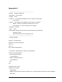
Appendix B
' ---------------------------------------------------------------------' DiskFile
: r_nr.ave : Rice_non-rice
' Programmer : Tom Van Niel
' Orgainization: CSIRO Land and Water
' Created
: 24-June-2003
' Revisions
:
'
' Function
: Summarise accuracy of rice/non-rice classification based
'
on a validation paddock shapefile and two training
'
paddock shapefiles (one rice and one non-rice). Outputs
'
to an excel comma separated text file. Reports overall
'
& Kappa accuracy & the threshold defined from the training
'
sets.
' Called By
' Notes
: View GUI
: Assumes 4 input files - 1 validation paddock shapefile,
'
1 rice paddock training shapefile, 1 non-rice paddock
'
training shapefile, and at least 1 grid. The mean grid
'
value is calculated for each paddock in the shapefiles.
'
The average of the two training sets is used as a
'
threshold for classifying rice vs non-rice. Note, there
'
also must be a common field in all of the shapefiles
'
called "Id". This field MUST contain unique numbers
'
within any one shapefile, or the zonal stats command
'
used in this program chokes. The validation field is
'
a field describing which paddocks withing the validation
'
shapefile are rice or non-rice. The naming convention of
'
"R" for rice and "NR" for non-rice must be used for the
'
program to work properly.
'
' ----------------------------------------------------------------------
'Sumgrid - summarise grid statistics for input shapefile - output new shapefile with statistics
' Initialize Variables
theView = av.GetActiveDoc
thethemes = theView.GetThemes
GrList = {}
FList = {}
CSIRO Land and Water
- 43 -
AccuracyLst = {}
aPrj = theView.GetProjection
' Put themes in separate lists for feature and Grid themes
For each Thm in theThemes
If (Thm.Is(GTheme)) then
GrList.add(Thm)
Elseif( Thm.Is(fTheme)) then
FList.add(Thm)
End
End
' ERROR CHECK LISTS
If (Flist.Count = 0) then
System.Beep
MsgBox.info("No feature Themes to Select From, must add Paddock Theme to the
View","ERROR")
Return NIL
End
If (GrList.Count = 0) then
System.Beep
MsgBox.info("No Grids to Select From, must add a Grid to the View","ERROR")
Return NIL
End
' Get info from User and Error Handle
' Get Paddock Theme
Padd_theme = MsgBox.Choice(FList,
"Choose the Paddock Theme","Paddock Selection")
' Check for Cancel, Exit if true
If (Padd_theme = NIL) then
System.Beep
Return NIL
End
' Get Rice Training Set theme
r_ts_theme = MsgBox.Choice(FList,
"Choose the Rice Training Set Theme","RICE training set Selection")
CSIRO Land and Water
- 44 -
' Check for Cancel, Exit if true
If (r_ts_theme = NIL) then
System.Beep
Return NIL
End
' Get Non-Rice Training Set theme
nr_ts_theme = MsgBox.Choice(FList,
"Choose the Non-Rice Training Set Theme","Non-Rice Training Set Selection")
' Check for Cancel, Exit if true
If (nr_ts_theme = NIL) then
System.Beep
Return NIL
End
' Get the field to use for validation
FldLst = Padd_theme.GetFtab.GetFields
vldnFld = MsgBox.Choice(FldLst,"Choose Field used for validation","CROP Type Field Selection")
vldnStrng = vldnFld.AsString
If (vldnFld = NIL) then
System.Beep
Return NIL
End
' Make sure there is a feature selection on Paddock Theme
PaddFtab = Padd_Theme.GetFtab
OrigPaddBit = PaddFtab.GetSelection.Clone
If (OrigPaddBit.Count = 0) then
System.Beep
MsgBox.info("No Paddock Theme features selected, please try again.","ERROR")
Return NIL
End
' Get Index (GRID) theme to summarize
IndexLst =
MsgBox.MultiList(GrList,
"Choose the Index (Grid) Theme(s) to Summarize","Index Selection")
CSIRO Land and Water
- 45 -
' Check for Cancel or no selection, Exit if true
If ((IndexLst = Nil) or (IndexLst.Count = 0)) then
System.Beep
Return Nil
End
' Run ZonalStats on Index Grid for paddocks theme
'Export paddock theme to a new shapefile so it can be joined with zstats later
For each Index_Theme in IndexLst
p_basename = Index_Theme.GetGrid.GetSrcName.GetFileName.GetBaseName
newPaddFtab = Padd_Theme.ExportToFTab
(av.GetProject.GetWorkDir.MakeTmp(p_basename,"shp"))
zoneField = newPaddFTab.FindField("Id")
aFN = av.GetProject.GetWorkDir.MakeTmp("zstat","dbf")
zt = Index_Theme.GetGrid.ZonalStatsTable(newPaddFtab, aPrj, zoneField, FALSE, aFN)
if (zt.HasError) then return NIL end
ztJoinFld = zt.FindField("Id")
' Join Shape file's FTab to zt
newPaddFtab.Join(zoneField,zt,ztJoinFld)
' Add new padd shapefile to view
'newPaddFTheme = FTheme.Make(newPaddFTab)
'theview.addtheme(newPaddFTheme)
'summarise training sets - get mean and std for rice training set and for nr training set
' Summarise Rice first
' Run ZonalStats on Index Grid for rice training set
r_ts_FTab = r_ts_theme.GetFtab
rFN = av.GetProject.GetWorkDir.MakeTmp("zstat","dbf")
r_zoneField = r_ts_FTab.FindField(vldnStrng)
If (r_zoneField = Nil) then
MsgBox.Info("Rice training set field not the same as paddock theme, exiting","ERROR")
Return Nil
End
r_zt = Index_Theme.GetGrid.ZonalStatsTable(r_ts_Ftab, aPrj, r_zoneField, FALSE, rFN)
if (r_zt.HasError) then return NIL end
rzCountField = r_zt.FindField("Count")
rzSumField = r_zt.FindField("Sum")
rzTotCount = 0
CSIRO Land and Water
- 46 -
rzTotSum = 0
rzCount = 0
rzSum = 0
For each r in r_zt
rzCount = r_zt.ReturnValue(rzCountField,r)
rzSum = r_zt.ReturnValue(rzSumField,r)
rzTotSum = rzTotSum + rzSum
rzTotCount = rzTotCount + rzCount
End
r_ts_Mean = rzTotSum/rzTotCount
'summarise training sets - get mean and std for NON-RICE training set and for nr training set
' Summarise Non-Rice
' Run ZonalStats on Index Grid for non-rice training set
nr_ts_FTab = nr_ts_theme.GetFtab
nrFN = av.GetProject.GetWorkDir.MakeTmp("zstat","dbf")
nr_zoneField = nr_ts_FTab.FindField(vldnStrng)
If (r_zoneField = Nil) then
MsgBox.Info("Non-rice training set field not the same as paddock theme, exiting","ERROR")
Return Nil
End
nr_zt = Index_Theme.GetGrid.ZonalStatsTable(nr_ts_Ftab, aPrj, nr_zoneField, FALSE, nrFN)
if (nr_zt.HasError) then return NIL end
nrzCountField = nr_zt.FindField("Count")
nrzSumField = nr_zt.FindField("Sum")
nrzTotCount = 0
nrzTotSum = 0
nrzCount = 0
nrzSum = 0
For each nr in nr_zt
nrzCount = nr_zt.ReturnValue(nrzCountField,nr)
nrzSum = nr_zt.ReturnValue(nrzSumField,nr)
nrzTotSum = nrzTotSum + nrzSum
nrzTotCount = nrzTotCount + nrzCount
End
nr_ts_Mean = nrzTotSum/nrzTotCount
'Calculate Threshold value based on these means:
CSIRO Land and Water
- 47 -
Threshld = (r_ts_Mean + nr_ts_Mean) / 2
' Calculate Accuracy of Rice vs NonRice based on Threshld values
' Assumes certain field naming convention
' Initialise Variables
TotalCount = 0
NumClassR =0
NumClassNR = 0
NumNRasR = 0
NumRasNR = 0
TotalNumR = 0
TotalNumNR = 0
' Get Paddock Shapefile from user
' Query Ftab based on Threshld
np_vldnFld = newPaddFTab.FindField(vldnStrng)
MeanFld = newPaddFtab.FindField("Mean")
If (MeanFld = NIL) then
MsgBox.ERROR("Could not find Mean field","MEAN FIELD ERROR")
Return NIL
End
For each record in newPaddFtab
TotalCount = TotalCount + 1
vldnValue = newPaddFTab.ReturnValue (np_vldnFld, record)
MeanValue = newPaddFTab.ReturnValue (MeanFld, record)
If (vldnValue = "R") then
TotalNumR = TotalNumR + 1
Else
TotalNumNR = TotalNumNR + 1
End
'Determine Direction of comparison, i.e., if rice mean is lower than nr mean, than use <= symbol
If (r_ts_Mean <= nr_ts_Mean) then
If (MeanValue <= Threshld) then
NumClassR = NumClassR + 1
If (vldnValue <> "R") then
NumNRasR = NumNRasR + 1
End
Else
CSIRO Land and Water
- 48 -
NumClassNR = NumClassNR + 1
If (vldnValue = "R") then
NumRasNR = NumRasNR + 1
End
End
Else
If (MeanValue >= Threshld) then
NumClassR = NumClassR + 1
If (vldnValue <> "R") then
NumNRasR = NumNRasR + 1
End
Else
NumClassNR = NumClassNR + 1
If (vldnValue = "R") then
NumRasNR = NumRasNR + 1
End
End
End
End
NumRasR = TotalNumR - NumRasNR
NumNRasNR = TotalNumNR - NumNRasR
Prop_observed = (NumRasR + NumNRasNR)/TotalCount
Prop_expected = ((TotalNumR * NumClassR) + (TotalNumNR * NumClassNR))/(TotalCount^2)
OverallAccuracy = ((NumNRasNR + NumRasR) / TotalCount)
KappaAccuracy = (Prop_observed - Prop_expected)/(1 - Prop_expected)
AccuracyStrng =
Index_Theme.AsString+","++NumNRasR.AsString+","++NumRasNR.AsString+","++TotalCount.AsStri
ng+","++Threshld.AsString+","+OverallAccuracy.AsString+","++KappaAccuracy.AsString
AccuracyLst.Add(AccuracyStrng)
End
' Write accuracy info to a text
outFN = av.GetProject.GetWorkDir.MakeTmp("acc","csv")
outFile = LineFile.Make(outFN,#FILE_PERM_WRITE)
outFile.WriteElt("Name, NumNRasR, NumRasNR, TotalCount, Threshold, OverallAccuracy,
KappaAccuracy")
For Each Strng in AccuracyLst
outFile.WriteElt(Strng)
End
' Write metadata info at the end
CSIRO Land and Water
- 49 -
outFile.WriteElt("")
outFile.WriteElt("Validation Paddocks file: "+padd_theme.GetSrcName.GetFileName.asString)
outFile.WriteElt("Rice Training Set file: "+r_ts_theme.GetSrcName.GetFileName.asString)
outFile.WriteElt("Non-rice Training Set file: "+nr_ts_theme.GetSrcName.GetFileName.asString)
outFile.WriteElt("Common Validation Field: "+vldnFld.asString)
outFile.WriteElt("Time: "+Date.Now.AsString)
' Close output file
outFile.Close
'Tell user where output file is
MsgBox.Info("Output file is"++outFN.asstring,"OUTPUT FILE")
av.ClearStatus
av.ShowMsg("Output file is"++outFN.asstring)
CSIRO Land and Water
- 50 -
Appendix C
' ---------------------------------------------------------------------' DiskFile : Sumgrid: sumgrd.ave
' Programmer : Tom Van Niel
' Created
: 2002
' Revisions : 11-June-2004/TVN/added more error traps and made code
'
more general
' Function : Summarises a grid dataset by each polygon in a polygon
'
dataset. Performs a zonalstats, resulting in min, mean,
'
max, majority, etc. values of the grid for ea. polygon
' Called By : View GUI
' Calls
: None
' Assumptions: Assumes that the view was the last active document before
'
running the script.
'
Must have a selection on the polygon theme.
' ---------------------------------------------------------------------' Initialize Variables
theView = av.GetActiveDoc
thethemes = theView.GetThemes
GrList = {}
FList = {}
aPrj = theView.GetProjection
' Put themes in separate lists for feature and Grid themes
For each Thm in theThemes
If (Thm.Is(GTheme)) then
GrList.add(Thm)
Elseif( Thm.Is(fTheme)) then
FList.add(Thm)
End
End
' ERROR CHECK LISTS
If (Flist.Count = 0) then
System.Beep
MsgBox.info("No feature Themes to Select From, must add Polygon Theme to the View","ERROR")
Return NIL
CSIRO Land and Water
- 51 -
End
If (GrList.Count = 0) then
System.Beep
MsgBox.info("No Grids to Select From, must add a Grid to the View","ERROR")
Return NIL
End
' Get info from User and Error Handle
' Get Polygon Theme
Plygn_theme = MsgBox.Choice(FList,
"Choose the Paddock Theme","Paddock Selection")
' Check for Cancel, Exit if true
If (Plygn_theme = NIL) then
System.Beep
Return NIL
End
' Make sure there is a feature selection on PlygN Theme
PlygnFtab = Plygn_Theme.GetFtab
OrigPlygnBit = PlygnFtab.GetSelection.Clone
If (OrigPlygnBit.Count = 0) then
System.Beep
MsgBox.info("No Polygon Theme features selected, please try again.","ERROR")
Return NIL
End
' Put Fields from Plygn theme in a list and allow user to select the field to summarize
' Make sure they are only numeric fields
tmpFldList = PlygnFTab.GetFields
theFldList = {}
For each Fld in tmpFldList
If (Fld.IsTypeNumber) then
theFldList.Add(Fld)
End
End
theFld = MsgBox.List(theFldList,
"Choose Field to summarize","Summary Field")
' Get Index (GRID) theme to summarize
CSIRO Land and Water
- 52 -
IndexLst =
MsgBox.MultiList(GrList,
"Choose the Index (Grid) Theme(s) to Summarize","Index Selection")
' Check for Cancel or no selection, Exit if true
If ((IndexLst = Nil) or (IndexLst.Count = 0)) then
System.Beep
Return Nil
End
' Run ZonalStats on Index Grid
For Each Index_Theme in IndexLst
aFN = av.GetProject.GetWorkDir.MakeTmp("zstat","dbf")
zoneField = PlygnFtab.FindField(theFld.AsString)
If (zoneField = NIL) then Return NIL End
zt = Index_Theme.GetGrid.ZonalStatsTable(PlygnFtab, aPrj, zoneField, FALSE, aFN)
if (zt.HasError) then
System.Beep
MsgBox.info("Problem calculating zonal stats, please try again or contact author.","ERROR")
Return NIL
End
ztJoinFld = zt.FindField(theFld.AsString)
If (ztJoinFld = NIL) then
System.Beep
MsgBox.info("ztJoinFld not found, please try again or contact author.","ERROR")
Return NIL
End
' Temporarily join Shape file's FTab to zt
PlygnFtab.Join(zoneField,zt,ztJoinFld)
' Export joined FTAB to a new shapefile
basename = Index_Theme.GetGrid.GetSrcName.GetFileName.GetBaseName
newPlygnFtab = Plygn_Theme.ExportToFTab
(av.GetProject.GetWorkDir.MakeTmp(basename,"shp"))
' Add new Plygn shapefile to view
newPlygnFTheme = FTheme.Make(newPlygnFTab)
theview.addtheme(newPlygnFTheme)
End
CSIRO Land and Water
- 53 -