1
Estuarine, Coastal and Marine (ECM)
National Habitat Mapping Project
ECM National Habitat Map Series
User Guide
Version 1.1 February 2008
Principal Authors
Richard Mount1, 2 and Phillippa Bricher2
1
2
National Estuarine, Coastal and Marine Information Coordinator, NLWRA
Spatial Science Group, School of Geography and Environmental Studies, University of
Tasmania
This project is a component of the
Australian “First Pass Coastal Vulnerability Assessment” Project
and is also supporting
NRM reporting on the ecological integrity of key ECM habitats
Agency Support
Department of Climate Change, Australian Government
National Land and Water Resources Audit
School of Geography and Environmental Studies, University of Tasmania
Contents
ECM National Habitat Map Series User Guide overview..................................... 5
Acronyms ................................................................................................ 5
Citation ................................................................................................... 5
1. Agency partners and contributors.............................................................. 6
2. ECM National Habitat Map Series components ............................................ 7
3. Introduction and Map Series Objectives ..................................................... 8
3.1. Map Series scope.............................................................................. 9
4. Information Product Descriptions .............................................................11
4.1. Map Series Information Products overview ........................................11
4.2. Defining the Map Series coastal zone ................................................11
4.3. Map Series classification schemes .....................................................12
4.4. The NISB Habitat Map .....................................................................13
4.5. The ECM Key Habitat Distribution Map Series.....................................15
4.6. The National Habitat Map Series Collections.......................................17
5. Data characteristics.................................................................................19
5.1. Coordinate System (CS) ...................................................................19
5.2. Data Dictionary for the National Intertidal/Subtidal Benthic (NISB)
Habitat Map Series Fields .................................................................20
5.3. Data Dictionary for the National Dune Vegetation Collection................25
6. Data Quality Information .........................................................................27
6.1. Metadata ........................................................................................27
6.2. Feature level metadata pointer (FMP)................................................37
7. Data Licensing ........................................................................................38
Acknowledgements .................................................................................40
References .............................................................................................41
Appendix 1: National Intertidal/Subtidal Benthic (NISB) Habitat Classification
Scheme..................................................................................................43
Appendix 2. Data Sources Acknowledgement List ...........................................75
2.1. NISB Habitat Map Collection .............................................................76
2.2. Estuaries collection ..........................................................................79
2.3. Dunes Collection..............................................................................80
National ECM Habitat Map Series User Guide_v7.doc
30/04/2008
Page 3 of 156
2.4. Coastal Wetlands Collection..............................................................83
Appendix 3: Inventory of Data Sources..........................................................84
3.1. New South Wales ............................................................................84
3.2. Northern Territory ...........................................................................85
3.3. Queensland.....................................................................................90
3.4. South Australia..............................................................................101
3.5. Tasmania......................................................................................101
3.6. Victoria .........................................................................................103
3.7. Western Australia ..........................................................................129
Appendix 4: Listing of potential Wetlands data sets ......................................149
National ECM Habitat Map Series User Guide_v7.doc
30/04/2008
Page 4 of 156
ECM National Habitat Map Series User Guide overview
The User Guide includes the following:
• Map Series definition, background and objectives
• A brief description of each component and information product
• Data Characteristics and Data Dictionary
• Data quality information including data set and feature level metadata
• The NISB Habitat Classification Scheme (see Appendix 1)
• Acknowledgements of the Data Suppliers (see Appendix 2)
• Summary metadata of the input Data Sources (see Appendix 3)
Acronyms
AGO
ASDD
ASRIS
CMA
CS
CSIRO
CVA
DCC
DEM
ECM
ERIN
FMP
GIS
GCS
ICAG
ISB
IMCRA
MQ
NISB
NLWRA
NOO
NRM
NVIS
OSDM
OSRA
SMB
WMS
Australian Greenhouse Office (now within the DCC)
Australian Spatial Data Directory
Australian Soil Resource Information System
Catchment Management Authority
Coordinate System
Commonwealth Scientific and Industrial Research Organisation
Coastal Vulnerability Assessment Project
Department of Climate Change, Australian Government
Digital Elevation Model
Estuarine, Coastal and Marine
Environmental Resources Information Network
Feature level metadata pointer
Geographic Information System
Geographic Coordinate System
Intergovernmental Coastal Advisory Group
Intertidal/Subtidal Benthic
Integrated Marine and Coastal Regionalisation of Australia
Mixed Quality
National Intertidal/Subtidal Benthic
National Land and Water Resources Audit (Audit)
National Oceans Office
Natural Resource Management
National Vegetation Information Systetm
Office of Spatial Data Management
Oil Spill Response Atlas
Structural Macrobiota
Web Mapping Services
Citation
Mount, R.E. and P.J. Bricher, 2008. Estuarine, Coastal and Marine (ECM) National
Habitat Map Series User Guide Version 1 February 2008. Spatial Science Group,
School of Geography and Environmental Studies, University of Tasmania. Report
to the Department of Climate Change and the National Land and Water Resources
Audit, Canberra, ACT. Pp.
National ECM Habitat Map Series User Guide_v7.doc
30/04/2008
Page 5 of 156
1. Agency partners and contributors
National: An adjective describing something that is produced or agreed by jurisdictions at all
levels including the Australian Government, State/NT Governments, NRM Regions and Local
Governments.
A very large number of agencies at the national and state level participated in this national
project. In terms of the actual data sets, the project was dependent on the goodwill and
cooperation of these partners and contributors. Acknowledgements of the individuals involved is
covered elsewhere later in this report; however, we wish to start this report by acknowledging and
appreciating the following Agencies:
Summary List of Data Custodians
For the whole ECM National Habitat Map Series all the following contributors must be
acknowledged:
Subset of contributors for the National Intertidal/Subtidal (NISB) Habitat Map:
Department of Natural Resources, Environment and the Arts, Northern Territory Government of
Australia
Queensland Department of Primary Industries and Fisheries
Queensland Parks and Wildlife Services Environmental Protection Agency
Great Barrier Reef Marine Park Authority
National Oceans Office
Western Australia Department of Environment and Conservation
South Australian Department of Environment and Heritage
New South Wales Department of Environment and Conservation
New South Wales Department of Primary Industries: Fisheries
Conservation Commission of the Northern Territory Land Conservation Unit
Victorian Department of Primary Industries
Parks Victoria
Tasmanian Aquaculture and Fisheries Institute
Subset of contributors for the Coastal Wetlands Collection:
Queensland Environmental Protection Agency
Australian Government Department of the Environment and Heritage
NSW Department of Planning
Subset of contributors for the Estuaries Collection:
Geoscience Australia
Subset of contributors for the Dune and Dune Vegetation Collection:
Australian Government Department of the Environment and Heritage
Department of Natural Resources, Environment and the Arts, Northern Territory Government of
Australia
Queensland Department of Primary Industries and Fisheries
WA Department of Industry and Resources
WA Department of Minerals and Energy
WA Department of Mineral and Petroleum Resources
Victorian Department of Primary Industries
SA DEH - Natural and Cultural Heritage
Queensland Herbarium, Environmental Protection Agency
NSW Department of Primary Industries, Mineral Resources
NSW Department of Mineral Resources (DMR)
National ECM Habitat Map Series User Guide_v7.doc
30/04/2008
Page 6 of 156
2. ECM National Habitat Map Series components
The following components together comprise the Estuarine, Coastal and Marine
National Habitat Map Series:
•
The ECM National Habitat Mapping Project Final Report (Mount and Bricher,
2008a)
•
The derived information products (data sets):
1. The National Intertidal/Subtidal benthic (NISB) Habitat Map (and associated
NISB Habitat MQ (NISB_plus) data set)
2. The National ECM Key Habitat Distribution Map Series (10 km and 50 km
grid cell maps)
3. A National Coastal Wetlands Map Collection
4. A National Estuaries Map Collection
5. A National Dune and Dune Vegetation Map Collection, and
6. A National Shoreline Map (derived from the National Geomorphic Shoreline
Map or “Smartline” (Sharples and Mount, 2008, in prep.)
•
User Guide and metadata for each product (i.e. this document)
•
The NISB Habitat Classification Scheme Version 1 (Mount et al, 2007) (Appendix
1 of this document)
•
Data sources acknowledgement list (Appendix 2 of this document)
•
Inventory of habitat mapping data sets (Appendix 3 of this document)
National ECM Habitat Map Series User Guide_v7.doc
30/04/2008
Page 7 of 156
3. Introduction and Map Series Objectives
The production of the ECM National Habitat Map Series was driven by a number of
immediate policy needs including supporting an assessment of the vulnerability of
Australia’s coastal ecosystems to the effects of climate change. It is also clear that there
are a large number of other purposes for which the maps can be used including the
following:
•
Support for the development of national key habitat extent and distribution
indicators by the National Land and Water Resources Audit (Audit) for reporting
on coastal habitats.
•
A consistent national input to future marine bioregionalisation processes,
particularly supporting the development of IMCRA Bioregion sub-regions (or
“ecoregions”)
•
Upgraded, nationally consistent Oil Spill Response Atlas (OSRA) habitat
mapping for all states
•
Enhanced information inputs to coastal planning including the flagging of the
location of key coastal habitats at potentially higher risk of impact from
development pressures
•
An inventory of key habitat natural assets to assist NRM projects and activities
•
Underpinning of improved wildlife management requiring detailed habitat type
mapping
In more detail, the Department of Climate Change (DCC; formerly the Australian
Greenhouse Office) is working with the States and Territories through the
Intergovernmental Coastal Advisory Group (ICAG) to assess Australia’s coastal
vulnerability to climate change. An early objective of the Department is to deliver a
“First Pass” Coastal Vulnerability Assessment (CVA) of the Australian coast and priority
coastal systems (natural and artificial) by June 2008. This will identify risks and
priorities and build foundational capacity towards future, more detailed assessments.
A key part of the CVA is the identification and mapping of coastal ecosystems and
habitat types that have greater or lesser susceptibility to potential coastal impacts of
climate change and sea level rise, such as accelerated erosion and increased marine
inundation. These hazards may contribute to impacts including the direct loss of habitats
(e.g. seagrass and mangroves), interruptions to biotic and chemical processes (e.g. coral
bleaching) and progressive inland migration of ecosystems (e.g. mangrove and
saltmarsh). These ecosystems and habitat types have undergone a detailed gap analysis
of data and methods via an Australian Greenhouse Office consultancy (Voice et al.,
2006).
Assessment of the potential rates and magnitudes with which these hazards may affect
particular coastal ecosystems requires detailed measurement and modelling of a range of
locally-variable factors (e.g., wave climate & energy, exposure, local bathymetry, littoral
drift & sediment budget, and biotic responses). An important initial step is to be able to
identify the location of those ecosystems which may be susceptible in some significant
degree to such hazards. This, in turn, requires the availability of coastal habitat maps. The
National ECM Habitat Map Series User Guide_v7.doc
30/04/2008
Page 8 of 156
maps need to be in a format that enables the rapid and flexible extraction of the required
information, such as a well designed GIS spatial database.
At the time this project was initiated, a significant number of coastal habitat maps existed
for various discrete sections of the Australian coast. These were prepared for a wide
range of purposes, by numerous researchers and agencies, and they existed in a variety of
formats, at differing scales and resolutions. Moreover, these maps thematically classified
and mapped coastal habitats using a variety of different classification schemes that
included a mix of biotic, geomorphic and environmental factors. There was no
consistently-classified coastal habitat mapping of the entire Australian coastline, except
at scales too coarse to be of practical use in a vulnerability assessment.
In order to provide the basis for a First Pass vulnerability assessment of the whole
Australian coastline, the DCC has contracted the National Land and Water Resources
Audit (Audit) to prepare a national map of the Australian intertidal/subtidal benthic
habitats using a nationally-consistent habitat classification that is capable of being readily
interrogated to identify habitats that are potentially sensitive to a range of physical
hazards related to climate change and sea-level rise. The Audit is involved as it has an
interest in compiling national extent and distribution mapping of key estuarine, coastal
and marine habitats to support one of the nationally agreed NRM indicators. The seaward
boundary of the NRM estuarine, coastal and marine areas is the outer edge of the State
Coastal Waters (i.e. 3 nm limits). The indicator will be delivered via the OzCoasts web
site managed by Geoscience Australia.
The Audit coordinated a team of coastal habitat mapping specialists in the Spatial
Science Group, School of Geography and Environmental Studies, University of Tasmania
to undertake the bulk of the practical work involved in creating the nationally-consistent
coastal classification system and map. The team works through UTAS Innovation Ltd.,
and is led by Dr Richard Mount (GIS, Remote Sensing and coastal monitoring and
mapping specialist and the Audit’s National Estuarine, Coastal and Marine (ECM)
Information Coordinator). Via the services of the team, the Audit will produce the
following coastal ecosystem and habitat data layers:
beaches (shorelines)
estuaries
coastal wetlands
dune vegetation
saltmarsh
mangroves
seagrasses
macroalgae
coral reefs
rocky reefs
The broad class of “sediment” (i.e. unconsolidated substrates such as sand, silt etc) has
been added to the project’s list of classes as it is regularly mapped and is an important
habitat type, particularly for the project’s primary objectives.
In practice, a series of information products have been developed to meet the project
requirements (see Section 4).
3.1.
Map Series scope
By necessity the project began by defining more closely the scope of the map series.
Many of the tasks for producing the national maps were open ended and given the
imperative for a rapid “first pass” assessment, limitations were placed on the project to
National ECM Habitat Map Series User Guide_v7.doc
30/04/2008
Page 9 of 156
enable delivery of the products within the required time frame. These constraints are as
follows:
•
The project was designed to collate existing habitat data sets only
•
Existing classification schemes should be used when available and, ideally,
collected data needs to be translated into nationally consistent schemes. However,
where a national scheme is not in place or cannot be produced in the time
available, we will need to accept the source data’s classification scheme i.e. create
a compilation or collection of data sets consisting of data coded with various
schemes rather than translating the data into a single national scheme. Coastal
wetlands and dune vegetation are good cases in point. The same applies where
significant information will be lost through the translation process. Estuaries are a
good case in point here.
•
The map series’ definition of the “coastal zone” includes:
o The marine influenced waters within the State Coastal Waters (i.e. 3 nm
limit, which constitutes the seaward boundary for NRM), and
o The land that is either below 10 m elevation (i.e. 10 m above AHD) or
within 500 m of the coastline as defined by the mean high water mark. In
the low lying areas, this area broadly equates to the distribution of coastal
vegetation such as mangroves and, in the environments with more relief
than 10 m, this area broadly equates to the extent of habitats subject to a
marine influence, for example coastal dunes or coastal cliff habitats. The
Shuttle Radar Topography Mission (SRTM) Version 2 digital elevation
model (DEM) was used to generate the elevation portion of the coastal
zone area.
•
Given that many issues that arise when comparing mapped data sets of multiple
scales, two derived information products were generated to provide a simplified
spatial representation of the distribution of each of the key habitats. These
derived products enable the visualisation of the habitat distributions at the
regional and national extents. It is extremely important to note that they are
definitely NOT able to be used to calculate areas of habitat types. The map
format selected for distribution maps was the grid cell format and the two grid cell
sizes are 10 km (state and regional) and 50 km (national), respectively.
National ECM Habitat Map Series User Guide_v7.doc
30/04/2008
Page 10 of 156
4. Information Product Descriptions
4.1.
Map Series Information Products overview
The ECM National Habitat Map Series consists of 2 main groups of information
products. Firstly, a series of national habitat distribution maps were produced for the
habitat types of saltmarsh, mangrove, seagrass, macroalgae, sediment, coral reef and rock
substrate including the three following information products:
1. A thematically simplified, high spatial resolution National Intertidal/Subtidal
Benthic (NISB) Habitat Map
2. A set of 10 km grid cell ECM Key Habitat Distribution Maps depicting the
regional and statewide distribution of each key habitat type
3. A set of 50 km grid cell ECM Key Habitat Distribution Maps depicting the
national distribution of each key habitat type
Four additional information products covering the remaining habitat types of dune
vegetation, estuaries, coastal wetlands and shorelines (beaches) are identified as follows:
4. A Dune and Dune Vegetation Map collection
5. A National Estuaries Map collection
6. A National Coastal Wetlands Map collection, and
7. A National Shoreline Map
Together, the information products form the ECM National Habitat Map Series. The
coastal ecosystem and habitat layers are as nationally comprehensive and consistent as is
practical with current data, that is, legacy data from all States and the Northern Territory.
Where appropriately licensed by the data suppliers, these layers are intended to form part
of a coastal vulnerability spatial information system that will underpin the national
coastal vulnerability assessment process. Where appropriately licensed or permitted by
the data suppliers, the derived information products are intended to be made available
through the proposed OzCoast portal housed at Geoscience Australia. The final
nationally-consistent coastal habitat map series is intended to be a public domain data set
managed by the Australian Government with full attribution of the various original
mapping sources used to build the final map.
4.2.
Defining the Map Series coastal zone
The map series’ definition of the “coastal zone” includes:
o The marine influenced waters within the State Coastal Waters (i.e. 3 nm
limit, which constitutes the seaward boundary for NRM), and
o The land that is either below 10 m elevation (i.e. 10 m above AHD) or
within 500 m of the coastline as defined by the mean high water mark. In
the low lying areas, this area broadly equates to the distribution of coastal
vegetation such as mangroves and, in the environments with more relief
than 10 m, this area broadly equates to the extent of habitats subject to a
marine influence, for example coastal dunes or coastal cliff habitats. The
Shuttle Radar Topography Mission (SRTM) Version 2 digital elevation
National ECM Habitat Map Series User Guide_v7.doc
30/04/2008
Page 11 of 156
model (DEM) was used to generate the elevation portion of the coastal
zone area.
The zone is important to define for geoprocessing purposes as many of the spatial data
sets classes are not defined with reference to the coastal zone. For example, the NVIS
saltmarsh classes extend inland across the continent, well beyond the coastal influence. It
was therefore necessary to clip the NVIS saltmarsh layers with the coastal zone polygon
defined for this project. On the other hand, the mangrove data sets almost completely fell
within the coastal zone polygon. The coastal zone layer is called coastal_buffers_04.shp
and is found in the Data_Delivery\Reference_Layers directory.
4.3.
Map Series classification schemes
Any method of reporting and assessment that seeks to compare ecological units of
interest must address the issue of classification. Classification schemes ideally organise
and group information about distinguishable components of ecological systems so that
comparisons can be made between the extent and distribution of the components across
space and time.
In Australia, there are a large number of habitat classification schemes; for example,
there are more than 15 schemes for wetland classification systems (including marine and
estuarine wetlands). The estuarine, coastal and marine environments are extremely
diverse and there is currently no classification scheme that covers all three environments.
They must, therefore, be split into areas that have sufficient features in common to enable
the application of classification schemes.
For the purposes of this map series, the habitats are split into onshore environments (i.e.
dunes and dune vegetation) and the subtidal and intertidal environments (i.e. whether
estuarine, nearshore or marine) including saltmarsh, mangroves, seagrasses, macroalgae,
sediment, rock and coral reef. These classes of habitat types broadly equate to land cover
mapping in the terrestrial environment. The intertidal and subtidal habitats did not
have a single national classification scheme and it was necessary to produce one during
the project. Details of the process for developing the scheme and the resulting scheme are
available in National Intertidal/Subtidal Benthic (NISB) Habitat Classification Scheme
Version 1 (Mount, Bricher and Newton, 2007) (see Figure 1 below and Appendix 1).
Estuaries are treated separately as a higher order habitat as they include elements of the
other habitat classes and are considered a useful organising entity and have their own
classification schemes. Similarly, coastal wetlands are treated separately as they overlap
with other categories, such as mangroves, saltmarshes and estuaries. Both estuaries and
coastal wetlands are, therefore, dealt with as separate data sets with their own
classifications. Where there are additional data sets with conflicting classification
schemes, they are simply treated by including them on a stand alone basis within a
“collection”. This also applies to the dune vegetation data set.
The shoreline (beaches) category will also be treated separately because a
complementary concurrent project (the National Geomorphic and Shoreline Stability
Mapping Project (Sharples and Mount, 2008)) is producing a comprehensive shoreline
classification scheme and mapping and will effectively deliver the “Beach” habitat data
sets to the CVA project.
National ECM Habitat Map Series User Guide_v7.doc
30/04/2008
Page 12 of 156
4.4.
The NISB Habitat Map
The NISB Habitat Map layers form the primary data sets of the ECM National Habitat
Map Series. They conform to the definitions, classes and standards defined in the
National Intertidal/Subtidal Benthic (NISB) Habitat Classification Scheme Version 1
(Mount, Bricher and Newton, 2007) (see Figure 1 below and Appendix 1). The data were
processed on a state-by-state basis as many characteristics were similar within states but
not among states. In addition, the production of the 10 km grid cell distribution maps was
implemented on a state-by-state basis as they are designed to assist with the extent of a
whole state or larger NRM Region. While this approach may bring some minor problems
at state boundaries, the advantages were considered to outweigh these.
One of the main tasks of the project was to derive the maps based on the NISB Habitat
Classification Scheme (Scheme) from the various intertidal/subtidal benthic habitat data
sets supplied by the contributing state and research agencies. This required a
comprehensive and thorough matching of the source data set attributes with the classes
defined by the Scheme. The decision rules defined in the Scheme were also used to
establish the destination class to which the source class belonged. Usually there was a
considerable simplification of the source data’s classes into the nationally consistent
classes. For example, some Victorian data sets had over 90 classes for mapping seagrass.
This reduced thematic resolution is necessary as it enables a map to be derived that is
comparable across the entire continent.
Further NISB Habitat information products, the 10 km and 50 km grid cell ECM Key
Habitat Distribution Map Series (see the next section for details) and the NISB Habitat
MQ data set, was developed as it became clear there were considerable differences in the
quality and resolution of the candidate data sets. In response to this issue, criteria were set
for deciding whether a data set “qualified” for inclusion in the NISB Habitat Map.
Drawing on the NISB Habitat Classification Scheme, the data needed to fall within the
accuracy range typically achieved by the leading state mapping agencies. This broadly
equates to a resolution that is at least 1:50,000 scale or, preferably, more detailed. Other
criteria included an assessment of the data collection methods and coverage. Some data
were highly detailed at the quadrat and transect extent, but had very limited coverage.
Other data consisted of single samples spaced more than 10 km apart. Some data had
little or no field assessment (“ground truthing”) and these were regarded as consisting of
lower quality for the purposes of the project.
National ECM Habitat Map Series User Guide_v7.doc
30/04/2008
Page 13 of 156
NISB Habitats
1 Consolidated Substrate
1.1 Coral Reef Substrate
1.2.1 Rock
Dominated
2 Unconsolidated Substrate
1.2 Rock Substrate
2.0 Unconsolidated Substrate
1.2.2 Structural Macrobiota
(SMB) Dominated
2.0.1 Sediment
Dominated
2.0.2 Structural Macrobiota
(SMB) Dominated
1.2.1.1 Unbroken Rock
Dominated
1.2.2.1 Macroalgae
Dominated
2.0.1.1 Pebble
Dominated
2.0.2.1 Seagrass
Dominated
1.2.1.2 Boulder
Dominated
1.2.2.2 Filter Feeder
Dominated
2.0.1.2 Gravel
Dominated
2.0.2.2 Mangrove
Dominated
1.2.1.3 Cobble
Dominated
1.2.2.3 Coral
Dominated
2.0.1.3 Sand
Dominated
2.0.2.3 Saltmarsh
Dominated
1.2.2.4 Seagrass
Dominated
2.0.1.4 Silt
Dominated
2.0.2.4 Macroalgae
Dominated
Target classes for the Audit/DCC NISB Habitat Map
2.0.2.5 Filter Feeder
Dominated
Figure 1. National Intertidal/Subtidal Benthic (NISB) Habitat Classification Scheme Version 1 (Mount et al, 2007)
National ECM Habitat Map Series User Guide_v7.doc
30/04/2008
Page 14 of 156
While the standard NISB Habitat Map consists of the higher quality data, there were
significant amounts of information that would be lost, especially for the habitat
distribution maps, if the coarser and lower quality data sets were not included in some
way. The approach taken was to add the coarser data to the standard NISB Habitat Map
data set and use it for the production of the 10 km and 50 km grid cell ECM Key
Habitat Distribution Maps. The data are often labelled as “NISB_plus”, indicating that
it is the NISB Habitat layer plus other lower quality layers. It is referred to as the NISB
Habitat MQ data set, where the “MQ” refers to “Mixed Quality”.
Data set name
NISB Habitat Map
NISB Habitat MQ data
set (“NISB_plus”)
4.5.
Purpose
Supporting detailed extent and
distribution mapping at the local,
state and regional scale
Supporting distribution mapping at
the regional and national scale
through the production of grid cell
distribution maps
Quality comment
Scale generally better than
1:50,000 and usually with
substantial ground truthing
Mixed scales including
broad coarse scales,
sometimes with limited
ground truthing
The ECM Key Habitat Distribution Map Series
The grid cell maps were produced specifically to assist with visualisation of the data at
the regional, state and national scales. The fine, resolution NISB Habitat data is not
easily visible when creating maps at these broader coverages. Careful logic was applied
to the process as there were concerns that there should neither be an overstatement of
the distribution of ECM key habitats and misconceptions arise that the mapping of the
continent’s key habitats was competed, nor that the distributions be understated.
Firstly, a standard set of grid cells were developed based on the successful use of the
1:100,000 map sheets for a sister weed mapping project within the Audit. Standard
50 km and 10 km cells were produced for the whole of Australia and then subset with
the project’s coastal zone polygon. This created the ECM set of grid cells depicted in
Figure 2 and Figure 3. The 10 km and 50 km grid cells are precisely nested and have
the characteristic of being evenly sized the across the whole continent, both east-west
and north-south (See Figure 2 and Figure 3 for an example).
For each key habitat distribution map, each grid cell depicts where the following occurs
in the NISB Habitat MQ data set:
• Firstly, if any of the specified key habitat type occurs, then attribute the cell
with “present”
• Secondly, if there is none of the habitat mapped yet the whole area is mapped,
mark the cell with “absent”
• Thirdly, if there is none of the habitat mapped and the whole cell is not
mapped, then mark the cell as “unknown”.
• Finally, if the entire cell is located in an environment where the habitat could
not occur, such as saltmarsh below the high water mark, then mark the cell as
“not applicable”.
National ECM Habitat Map Series User Guide_v7.doc
30/04/2008
Page 15 of 156
Key ECM Habitat Distribution Maps
50 km grid cells
The national coastal zone
grid cell coverage
Map Authors: Richard Mount and Philippa Bricher, UTAS 2008
Coordinate System - Albers Equal Area Conic, GDA94
Legend
50 km Grid Cells
0
500
1,000
Kilometres
2,000
°
Figure 2. The 50 km grid cells (here blank) used for displaying the distribution key ECM habitats
Figure 3. An example of the 10 km habitat distribution grid cells nested within the 50 km grid cells.
Clearly, there will be exceptions to these rules and they are completely dependent on
the quality of the spatial data, however, they are considered to be robust in a number of
ways. Firstly, they are built for the purpose of showing where a habitat has been
National ECM Habitat Map Series User Guide_v7.doc
30/04/2008
Page 16 of 156
mapped, no matter how small the patch or the mapping effort. This means the
approach will honour the mapper’s observations. Secondly, the method also indicates
where further mapping work could be required (i.e. the “unknown” class), thus helping
to indicate where significant work remains to be done.
It is notable that the classes included in the NISB Habitat Map are drawn from a
number of levels within the hierarchy. This is quite acceptable and is regarded as a
useful feature of the Classification Scheme, however, when applying the logic
described above to a series of nested classes a complex series of logic tests need to be
applied. For the purposes of the distribution maps, all coral was lumped together (i.e.
both “coral reef substrate” and “coral dominated habitat on a rock substrate” as was all
seagrass (i.e. a few seagrasses occur on a rock substrate).
It should also be noted that mapping macroalgae via acoustics (i.e. single beam and
multi-beam sonar systems) is usually not achievable for technical reasons. This means
that, while much of the mapped rock substrate is highly likely to be covered in
macroalgae and/or filter feeders, and while it may be reasonable to assume that that is
the case, without adequate ground truthing via, for example, a video camera or diver
observations, it must be recorded as rock, not macroalgae. This means that the
macroalgae mapping is not comprehensive enough to be included in the habitat
distribution maps, though with the application of careful assumptions, a reasonable
map could be made for particular purposes.
4.6.
The National Habitat Map Series Collections
A series of map compilations, or collections, were developed for both the higher level
organising entities, such as estuaries and coastal wetlands, and for the less well defined
data sets, such as dune vegetation. It is important to note that a different approach was
taken to creating each collection.
Coastal wetlands
Firstly, there are a very large number of wetlands spatial databases in Australia.
Another Audit project is currently compiling a list of the databases and assessing them
for their quality with regard to showing the extent, or area, of Australia’s wetlands. The
project is finding that the standards and methodologies for mapping wetlands are very
variable. There is also a Wetlands Classification Scheme being developed, again with
the assistance of the Audit. As such, it was considered prudent to simply compile the
data sets that were available within the project’s time frame and document the
remaining data sets. See Appendix 4 for a list of potential wetlands data sets.
Given the range of approaches to wetland mapping it was considered reasonable to
intersect the available data with this project’s coastal zone polygon. This means that if a
small part of the wetland falls within the coastal zone the entire wetland is included in
the final mapped layer. This approach is based on the assumption that a wetland is
usually level and that if any part of the wetland is subject to, for example, inundation or
erosion, the whole wetland is potentially affected.
Dune vegetation
The dune vegetation data sets were in many ways the least developed of all the target
data sets. There is little actual mapping of dune vegetation per se, rather the collection
National ECM Habitat Map Series User Guide_v7.doc
30/04/2008
Page 17 of 156
has proceeded by firstly compiling the available mapping of dunes from sources such as
geomorphological and geological maps and then intersecting those with vegetation
maps, such as the National Vegetation Information Systems (NVIS). While the
approach is practical given the timeframe of this project, it does not guarantee capture
dune vegetation as there may be differences in the mapping methods and classification
schemes of the source data sets. This means that caution should be exercised in the
interpretation of this collection.
Unlike the coastal wetlands, the dune and dune vegetation data sets were clipped, or
limited, to the extent of the coastal zone buffer polygon. This decision was based on the
assumption that this habitat type is found in non-coastal areas as well as the coastal
zone and that, while there is unlikely to be a crisp dividing boundary between coastal
and non-coastal areas, it was not possible to accurately delineated this boundary with
the evidence to hand. In the absence of higher level evidence, the coastal zone polygon
boundary was used.
Estuaries
For estuaries, there is well founded national classification scheme based on
geomorphic principles (Ryan et al, 2003). This scheme has considerable relevance to
the assessment of coastal vulnerability as it capture information about the energy
regimes operating within each estuary and the national data set using the scheme
(OzEstuaries) has been included here. The data set’s classes were also easily mapped
across to the NISB Habitat Classification Scheme classes. This was done and the
resulting polygons added to the NISB Habitat Mixed Quality (MQ) data set (or AKA
NISB_plus).
Other estuary data sets largely depict the topographic boundaries of the estuaries;
however, they do so without reference to a consistent classification scheme. For this
reason they are not included in this collection.
Shoreline (Beaches)
For the shoreline itself, the National Shoreline Geomorphic and Stability Mapping
Project (Sharples and Mount, 2008, in prep) is running in parallel to this project and is
producing a nationally consistent “smartline” map for all shoreline types that
comprehensively maps a large number of shoreline attributes including information
about the intertidal zone and the immediate backshore and foreshore. These are
considered suitable for defining shoreline habitat types including for example, the
location of the sandy beaches suitable for shorebird habitat. Details are provided in the
National Shoreline Geomorphic and Stability Map User Guide (Sharples, 2008, in
prep) that accompanies that data set.
A key component of that project is the linking (joining) of the “Smartline” to Andy
Short’s Australian Beach Safety and Management Program (ABSAMP) database of
12,000 sandy beaches. This linkage will provide easy access to the large store of
ecological and geophysical information contained in that database.
The Shoreline Habitat Map Collection will be available as soon as that project delivers
its data sets in March 2008.
National ECM Habitat Map Series User Guide_v7.doc
30/04/2008
Page 18 of 156
5. Data characteristics
5.1.
Coordinate System (CS)
Two standard coordinate systems were selected based on the Australian Government
agencies, especially including Geoscience Australia. The geographic coordinate system
(GCS) based on the GDA94 datum is preferred for most purposes. Where area needs to
be calculated, the Albers Equal Area Conic Projection based on the GDA94 datum is
used with the standard meridians and parallels as specified in the standards used by
Geoscience Australia (GA, 200?).
The standard geographical CS (GCS) (i.e. latitude and longitude) is based on the
Geocentric Datum of Australia 1994 (GDA94). In ArcGIS it is called
GCS_GDA_1994.
Angular Unit
Prime Meridian
Datum
Spheroid
Degree (0.017453292519943299)
Greenwich (0.000000000000000000)
D_GDA_1994
GRS_1980
Semimajor Axis
6378137.000000000000000000
Semiminor Axis
6356752.314140356100000000
Inverse Flattening
298.257222101000020000
The standard projected CS (PCS) is based on the GDA94 datum as well and is an
Albers equal area conic projection. It was chosen to enable Australia-wide
representations of the geographic data that conform closely to the true shape of the
continent and to enable delivery of spatial data in measurement units of metres. The
projected CS has input values as detailed below.
Projection
Datum
Spheroid
Unit of measurement
Albers
GCS_GDA_1994
GRS80
Meter, 1.0
False_Easting
0.0
False_Northing
0.0
Central_Meridian
134°
Standard_Parallel_1
-36°
Standard_Parallel_2
-18°
Latitude_Of_Origin
0°
National ECM Habitat Map Series User Guide_v7.doc
30/04/2008
Page 19 of 156
5.2.
Data Dictionary for the National Intertidal/Subtidal Benthic (NISB) Habitat Map Series Fields
Field Name
NISB_sub01
Type
Text
Width
Attribute Description
Range
Definition
30
Classification under the first
tier (substrate) of the NISB
Habitat Classification Scheme
1 Consolidated
Any habitat in which the substrate is predominantly made
up of particles of cobble size (>64 mm diameter) or
larger. This includes coral reefs, solid rock and boulders
A substrate that is predominantly made up of particles of
pebble size (<64 mm diameter) or smaller. This includes
gravels, sands and silts
Could not be mapped across to the NISB Habitat
Classification Scheme (usually, either because it was
unidentified or because it's a mixed rock/sediment site)
Could not be classified any further than 1 Consolidated
2 Unconsolidated
3 Unknown
NISB_sub02
Text
26
Classification under the 2nd
tier (substrate) of the NISB
Habitat Classification Scheme
1.0 Consolidated
1.1 Coral Reef
1.2 Rock Substrate
2.0 Unconsolidated
3.0 Unknown
NISB_dom01
Text
40
Classification under the 3rd
tier (dominant habitat) of the
NISB Habitat Classification
Scheme
1.0.0 Consolidated
1.1.0 Coral Reef
1.2.0 Rock Substrate
National ECM Habitat Map Series User Guide_v7.doc
30/04/2008
Any habitat in which the structure is predominantly
formed by a coral framework. As all coral reef has some
kind of rock substrate, coral reef is here defined as an
object that has more than 50% coral cover.
A structure that is predominantly formed by a rock
framework. Here it is defined as a consolidated substrate
that has 50% or less coral cover
A dummy class “holder” at the second level of the
hierarchy to enable consistency in the numbering
throughout the class hierarchy
Could not be mapped across to the NISB Habitat
Classification Scheme (usually, either because it was
unidentified or because it's a mixed rock/sediment site)
Could not be classified any further than 1 Consolidated
This scheme does not classify beyond 1.1 Coral Reef
Could not be classified any further than 1.2 Rock
Substrate
Page 20 of 156
1.2.1 Rock Dominated
1.2.2 Structural Macrobiota
Dominated
2.0.0 Unconsolidated
2.0.1 Sediment Dominated
2.0.2 Structural Macrobiota
Dominated
3.0.0 Unknown
NISB_dom02
Text
33
Classification under the 4th
tier of the NISB Habitat
Classification Scheme
1.0.0.0 Consolidated
1.1.0.0 Coral Reef
1.2.0.0 Rock Substrate
1.2.1.0 Rock Dominated
1.2.1.1 Unbroken Rock
Dominated
1.2.1.2 Boulder Dominated
1.2.1.3 Cobble Dominated
1.2.2.0 Structural Macrobiota
Dominated
1.2.2.1 Macroalgae Dominated
1.2.2.2 Filter Feeder Dominated
1.2.2.3 Coral Dominated
National ECM Habitat Map Series User Guide_v7.doc
30/04/2008
A rocky substrate on which there is less than 5%
seagrass or 10% other SMB cover
A habitat in which seagrass covers more than 5% of the
substrate or one or more groups of other SMB cover
more than 10% of the substrate
Could not be classified any further than 2 Unconsolidated
An unconsolidated habitat with either <5% seagrass
cover or <10% other SMB cover
A habitat in which >= 5% the substrate is covered by
seagrass or >=10% by any other SMB (Seagrass has a
lower threshold than other SMB because a significant
amount of the biomass occurs below the surface (Duarte
and Chiscano, 1999).
Could not be mapped across to the NISB Habitat
Classification Scheme (usually, either because it was
unidentified or because it's a mixed rock/sediment site)
Could not be classified any further than 1 Consolidated
This scheme does not classify beyond 1.1 Coral Reef
Could not be classified any further than 1.2 Rock
Substrate
Could not be classified any further than 1.2.1 Rock
Dominated
A rock dominated substrate where the cover is dominated
by continuous outcropping rock.
A rock dominated substrate where the cover is dominated
by rocks larger than 256 mm diameter.
A rock dominated substrate where the cover is dominated
by rocks between 64 mm and 256 mm diameter.
Could not be classified any further than 1.2.2 Structural
Macrobiota Dominated
SMB dominated habitat in which macroalgae has greater
substrate cover than other SMB
SMB dominated habitat in which sessile filter feeders
(e.g. sponges, ascidians and tunicates) have greater
substrate cover than other SMB
SMB dominated habitat in which coral has greater
Page 21 of 156
1.2.2.4 Seagrass Dominated
2.0.0.0 Unconsolidated
2.0.1.0 Sediment Dominated
2.0.1.1 Pebble Dominated
2.0.1.2 Gravel Dominated
2.0.1.3 Sand Dominated
2.01.4 Silt Dominated
2.0.2.0 Structural Macrobiota
Dominated
2.0.2.1 Seagrass Dominated
2.0.2.2 Mangrove Dominated
2.0.2.3 Saltmarsh Dominated
2.0.2.4 Macroalgae Dominated
2.0.2.5 Filter Feeder Dominated
3.0.0.0 Unknown
National ECM Habitat Map Series User Guide_v7.doc
30/04/2008
substrate cover than other SMB
SMB dominated habitat in which seagrass has greater
substrate cover than other SMB
Could not be classified any further than 2 Unconsolidated
Could not be classified any further than 2.0.1 Sediment
Dominated
A sediment dominated habitat which predominantly
consists of particles 4 to 64 mm diameter
A sediment dominated habitat which predominantly
consists of particles 2 to 4 mm diameter
A sediment dominated habitat which predominantly
consists of particles 63 μm to 2 mm diameter
A sediment dominated habitat which predominantly
consists of particles <63 μm diameter
Could not be classified any further than 2.0.2 Structural
Macrobiota Dominated
An SMB dominated habitat in which seagrasses have
greater substrate cover than other SMB. For seagrass,
dominance is defined at 5%, compared with 10% for
other SMB.
Intertidal tall forests to shrublands, in areas with low wave
energy. This habitat comprises more than 30 species,
with most concentrated in Australia’s north (DEWR,
2007). NB: Even though mangroves can occur on rocky
shores, the substrate under mangroves is rarely mapped.
Therefore, an arbitrary decision has been made here to
class all mangroves as occurring on unconsolidated
substrates.
Extensive damp and water-logged flats, mostly in nearestuarine areas. The vegetation is dominated by hardy
low shrubs, especially samphire communities (DEWR,
2007).
An SMB dominated habitat in which macroalgae have
greater substrate cover than other SMB.
An SMB dominated habitat in which filter feeders have
greater substrate cover than other SMB.
Could not be mapped across to the NISB Habitat
Classification Scheme (usually, either because it was
Page 22 of 156
unidentified or because it's a mixed rock/sediment site)
ANZLIC_ID
Text
20
DSource
Text
100
DOrig_File
Text
100
DMeta_File
Text
100
Area
HOI_1
Double
String
20
20
HOI_2
String
20
S_Roc
String
254
S_Unc
String
254
ANZLIC Metadata unique
identifying number (if
applicable)
The custodians of the original
file from which the features
presented here were derived
The original shapefile, geodatabase or raster from which the
features presented here were derived
The name under which the
metadata for the DOrig_File
was saved
Area in m²
0-1000
Habitat of Interest (a
Rock, Unconsolidated
relabelling of NISB
classifications for the purpose
of generating 10km and 50km
tile maps)
Habitat of Interest (a
Seagrass, Sediment, Coral,
relabelling of NISB
Saltmarsh, Mangrove
classifications for the purpose
of generating 10km and 50km
tile maps)
Distribution status of rock
Presence, Absence, Unknown,
substrates (NISB class 1.2)
N/A
Distribution status of
unconsolidated substrates
(NISB class 2.0)
National ECM Habitat Map Series User Guide_v7.doc
Presence, Absence, Unknown,
N/A
30/04/2008
Any polygon containing rock/unconsolidated substrates
Any polygon containing
seagrass/sediment/coral/saltmarsh/mangrove dominated
habitats
•
•
Presence = the HOI is found within that tile.
Absence = the entire area covered by the tile has
been mapped and the HOI is not found within it.
• N/A = The area covered by the tile has not been
completely mapped, but the area is unlikely to
contain the HOI, because it is terrestrial (in the case
of rock, sediment, coral, seagrass) or below the tide
line (in the case of saltmarsh).
• Unknown = The HOI is not found in the mapped
portion of the tile, but the tile is not completely
mapped. Therefore, its presence or absence cannot
be ascertained.
As above
Page 23 of 156
S_Sea
String
254
S_Sed
String
254
S_Cor
String
254
S_Sal
String
254
S_Man
String
254
Distribution status of seagrass
dominated habitats (NISB
class 1.2.2.4 or 2.0.2.1)
Distribution status of sediment
dominated habitats (NISB
class 2.0.1)
Distribution status of coral
dominated habitats (NISB
class 1.1 or 1.2.2.3)
Distribution status of
saltmarsh dominated habitats
(NISB class 2.0.2.3)
Distribution status of
mangrove dominated habitats
(NISB class 2.0.2.2)
National ECM Habitat Map Series User Guide_v7.doc
Presence, Absence, Unknown,
N/A
As above
Presence, Absence, Unknown,
N/A
As above
Presence, Absence, Unknown,
N/A
As above
Presence, Absence, Unknown,
N/A
As above
Presence, Absence, Unknown,
N/A
As above
30/04/2008
Page 24 of 156
5.3.
Data Dictionary for the National Dune Vegetation Collection
Field Name
Type
Width
Attribute Description
ANZLIC_ID
Text
20
DSource
Text
100
DOrig_File
Text
100
DMeta_File
Text
100
Dune_Dsc1
Text
150
Dune_Dsc2
Text
150
State
Text
3
Dune
Text
3
ANZLIC Metadata unique
identifying number (if
applicable) for original dune
presence data
The custodians of the original
file from which the dune
features presented here were
derived
The original shapefile,
geodatabase or raster from
which the dune features
presented here were derived
The name under which the
metadata for the DOrig_File
was saved
The primary descriptive
information used to determine
dune presence
Secondary descriptive
information used to determine
dune presence, where
applicable
The State (or Territory) in
which the dune polygon falls
A classification of the
reliability of dune presence
Range
Definition
y
Yes: Dunes, beach ridges or dune fields specified in
original data source
Maybe: Dunes potentially present but not specified in
original data source; this classification was used only
when no other data was available for a location
m
DOrig_Scal
Text
30
The spatial scale of the
original dune presence data
file
National ECM Habitat Map Series User Guide_v7.doc
30/04/2008
Page 25 of 156
NVIS_mvs
Text
150
V_ANZLICID
Text
20
V_DSource
Text
100
V_DOrigFil
Text
100
V_DMetaFil
Text
100
V_DOrigScl
Text
30
Descriptions of major
vegetation subgroups derived
from the National Vegetation
Information System
ANZLIC Metadata unique
identifying number (if
applicable) for original
vegetation data
The custodians of the original
data file from which the
vegetation features presented
here were derived
The original shapefile,
geodatabase or raster from
which the vegetation features
presented here were derived
The name under which the
metadata for the V_DOrigFil
was saved
The spatial scale of the
original vegetation data file
National ECM Habitat Map Series User Guide_v7.doc
30/04/2008
Page 26 of 156
6. Data Quality Information
The concept of “quality” is a relative one as the quality of an individual data set will
change depending on the purpose for which it is used. In the spatial sciences, assessing
the quality of a data set is usually done in the context of the specified purpose and is
referred to as assessing the data set’s “fitness-for-purpose”. This is a challenging
concept when all the exact purposes are not able to be specified, as is the case here.
While a number of purposes are specified (e.g. for the First Pass Coastal Vulnerability
Assessment and the NRM Key Habitat Distribution Indicator), there are likely to be
many other uses for this data set. The approach taken in this situation is to ensure that
the data is labelled according to its known characteristics. This is referred to as a “truthin-labelling” approach and provides information to those who intend to use the data in
the future for currently non-specified purposes.
The data quality information for the Map Series works differently for each component
of the data. The NISB Habitat Map and the ECM Key Habitat Distribution Map Series
qualify as data sets in their own right and have a full metadata record and data
dictionary. The source data for these data sets are comprehensively listed and the data
suppliers and any metadata associated with the original data sets are acknowledged at
every level – that is in this report, in the metadata and, for the NISB Habitat Map, in the
data itself as Feature level Metadata Pointer (FMP). For the Map Collections, each
collected data set has its own metadata record (where available) and FMP was added.
6.1.
Metadata
Metadata statements are presented here for the following National ECM Map Series
components:
• The NISB Habitat Map
• The 10 km and 50 km NISB Habitat Distribution Grid Cell Maps
All other metadata is documented within the body of this User Guide.
DATASET CITATION
Title: National Intertidal/Subtidal Benthic (NISB) Habitat Map
Custodian: ERIN for Department of Climate Change (TBA)
Creator: Dr Richard Mount and Phillippa Bricher, Spatial Science Group, School of
Geography, University of Tasmania
Jurisdiction: Australia
DESCRIPTION
Abstract:
The NISB Habitat Map was created by the University of Tasmania for a partnership
between the Department of Climate Change and the National Land and Water
Resources Audit. It supports the DCC/Audit partnership by providing a nationally
National ECM Habitat Map Series User Guide_v7.doc
30/04/2008
Page 27 of 156
consistent set of the available mapping data for those habitats that occur between the
approximate position of the highest astronomical tide mark (HAT) and the location of
the outer limit of the photic benthic zone (approximately at the 50-70 m depth contour).
This area is broadly equivalent to the “inner” and “mid-shelf” regions identified by
Geoscience Australia. The resulting map data set forms a core component of the ECM
National Habitat Map Series.
The habitat classes include: coral reef, rock dominated habitat, sediment dominated
habitat, mangroves, saltmarsh, seagrass, macroalgae and filter feeders (e.g. sponges), as
defined in the NISB Habitat Classification Scheme. The scheme is designed to support
the development of marine ‘ecoregions’ or bioregional subregions. Details of the
scheme and the process of its development are available in National Intertidal/Subtidal
Benthic (NISB) Habitat Classification Scheme Version 1 (Mount, Bricher and Newton,
2007).
The NISB Habitat Map consists of two layers for each state.
<STATENAME>_NISB.shp consists of the entire available habitat mapping at a
resolution finer than 1:50 000 (with a few exceptions, outlined in the data quality
section below). <STATENAME>_NISB_PLUS.shp consists of all the data in
<STATENAME>_NISB.shp along with coarser resolution data, including NVIS and
OzEstuaries data. These layers were used to produce the National ECM Key Habitat
Distribution Map Series 10 km and 50 km tile maps.
Datum: Geodetic Datum of Australia 1994
Projection: Geographic coordinates
GEOGRAPHIC EXTENT NAME
Australia excluding external territories – AUS - Australia – Australia
GEOGRAPHIC BOUNDING BOX
North bounding latitude: 8.912920° S
South bounding latitude: 55.326655° S
East bounding latitude: 112.609896° E
West bounding latitude: 159.810665° E
DATA CURRENCY
Start date: 1984
End date: 2007
National ECM Habitat Map Series User Guide_v7.doc
30/04/2008
Page 28 of 156
DATA STATUS
Progress: Complete
Maintenance and update frequency: Not scheduled.
ACCESS:
Format: ArcGIS shapefile (.shp)
Access constraints:
XXXX (TBA by Custodian)
DATA QUALITY
Lineage:
The NISB Habitat Map is a composite data set of the best available habitat mapping
data for Australia’s intertidal and subtidal benthos. Using ArcGIS 9.2, all the input
layers were imported into geodatabases for processing. Fields were added to each
layer’s attribute table, listing the data source (DSource), original file name
(DOrig_File), metadata file name (DMeta_File) and ANZLIC ID number
(ANZLIC_ID).
Each layer then had NISB fields added, which correspond to the four tiers in the NISB
Habitat Classification Scheme (2007). NISB_Sub01 and NISB_Sub02 refer to the first
two tiers of the classification, which are based on the substrate. NISB_Dom01 and
NISB_Dom02 refer to the dominant land cover, as described in the third and fourth
tiers. The scheme is hierarchical, so where insufficient information was available to
fully classify a polygon, it was classified to the finest tier possible.
The NISB Habitat Classification Scheme includes decision rules that describe the limits
of each habitat class. For example, for a polygon to be described as class 1.2.2
Structural Macrobiota Dominated, SMBs (Structural Macrobiota such as seagrass or
mangrove) must cover more than 10% of the substrate. However, many of the source
data sets do not include information on percent cover, and so the original classifications
were accepted on face value. That is, if the data provider identified a polygon as
seagrass dominated sediment, we classified it as 2.0.2.1 Seagrass Dominated, without
information about how precisely the original category fit the NISB classes. Microsoft
Access was used to reclassify the layers.
Where habitat types extended inland (e.g. saltmarsh or mangrove), a buffer was used to
select those that are “coastal”. The coastal zone is defined here as being within 500 m
of the coast or less than 10 m above sea level. A 500 m buffer was created around the
coastline as defined by the Geodata Coast 100k (Geoscience Australia 2004). The
Shuttle Radar Topography Mission (SRTM) v2 Digital Elevation Model was used to
determine all areas below 10 m ASL. These two areas were merged to create the coastal
zone buffer.
Once all the layers for a state had been converted to the NISB Habitat Classification
scheme, they were merged into a single layer. Where layers overlapped, a decision was
National ECM Habitat Map Series User Guide_v7.doc
30/04/2008
Page 29 of 156
made as to which was considered to be more reliable. This decision was based on a
combination of the metadata records and a visual inspection of the data sets. Then, the
erase and merge functions were used to combine the layers.
The layers were then tested to ensure that the classifications were translated correctly
from the source data and that there were no overlapping polygons. Overlaps were
discovered in some of the source data for Victoria and were left as they were. The
layers were not tested topologically. The maps were not independently ground-truthed.
All areas were calculated in m², using Albers equal area projection.
The contributing agencies must be acknowledged with each use of this derived data set
are:
Contributors to the National Intertidal/Subtidal (NISB) Habitat Map:
Department of Natural Resources, Environment and the Arts, Northern Territory Government of
Australia
Queensland Department of Primary Industries and Fisheries
Queensland Parks and Wildlife Services Environmental Protection Agency
Great Barrier Reef Marine Park Authority
National Oceans Office
Western Australia Department of Environment and Conservation
South Australian Department of Environment and Heritage
New South Wales Department of Environment and Conservation
New South Wales Department of Primary Industries: Fisheries
Conservation Commission of the Northern Territory Land Conservation Unit
Victorian Department of Primary Industries
Parks Victoria
Tasmanian Aquaculture and fisheries Institute
Positional Accuracy:
As this is a multi-scale dataset, it is impossible to give a single value for positional
accuracy. Most layers in the NISB dataset were mapped at scales finer than 1:50 000,
which translates to a positional accuracy of approximately ±25 m. However, some
seagrass mapping for Queensland and South Australia has errors up to ±100 m. It is
recommended that the user reads the metadata for the source layers for more specific
accuracy information.
Attribute Accuracy:
After the NISB habitat classification scheme was applied to the data, MS Access
queries were used to confirm that all records had been reclassified correctly. However,
it was not possible to test the accuracy of the source datasets, and the original
classifications were taken on trust. A pragmatic approach was used in applying the
scheme, as there was rarely sufficient information to test whether any given record met
the criteria for classes (e.g. percent cover was often not listed). For this reason, if the
source dataset stated that a polygon contained sparse seagrass, then it was classified as
2.0.2.1 Seagrass Dominated Habitat, even though it have had less than 5% seagrass
cover. Conservative assumptions were made about the substrate, where this was not
listed. For example, it was generally assumed that a seagrass site had a sediment
National ECM Habitat Map Series User Guide_v7.doc
30/04/2008
Page 30 of 156
substrate. The only state where it was believed that this assumption would not hold was
Victoria and Tasmania, where Amphibolis occurs on both rock and sediment substrates
in very limited locations. In those sites, substrate information was provided and no
assumptions were made.
Logical consistency:
A single person conducted all classifications, using a consistent classification scheme.
After merging, the datasets were visually inspected for overlaps, but were not tested for
topological consistency.
Completeness:
Complete
CONTACT INFORMATION
Contact organisation:
Contact position:
Mail address:
Locality:
State:
Country:
Postcode:
Telephone:
Facsimile:
Email:
METADATA INFORMATION
Metadata date:
28/2/2008
Metadata author:
Phillippa Bricher
Spatial Information Science
School of Geography and Environmental Studies
University of Tasmania
Private Bag 76
Sandy Bay
TAS 7005
National ECM Habitat Map Series User Guide_v7.doc
30/04/2008
Page 31 of 156
DATASET CITATION
Title: National ECM Key Habitat Distribution Map Series
Custodian: ERIN for Department of Climate Change (TBA)
Creator: Dr Richard Mount and Phillippa Bricher, Spatial Science Group, School of
Geography, University of Tasmania
Jurisdiction: Australia
DESCRIPTION
Abstract:
The National ECM Key Habitat Distribution Map Series were derived from the NISB
Habitat Map created by the University of Tasmania for a partnership between the
Department of Climate Change and the National Land and Water Resources Audit. It
supports the DCC/Audit partnership by providing a nationally consistent set of the
available mapping data that show the distribution of habitats that occur between the
approximate position of the highest astronomical tide mark (HAT) and the location of
the outer limit of the photic benthic zone (approximately at the 50-70 m depth contour).
This area is broadly equivalent to the “inner” and “mid-shelf” regions identified by
Geoscience Australia. The resulting map data set forms a core component of the ECM
National Habitat Map Series.
The habitat classes include: coral reef, rock dominated habitat, sediment dominated
habitat, mangroves, saltmarsh, seagrass, macroalgae and filter feeders (e.g. sponges), as
defined in the NISB Habitat Classification Scheme. The scheme is designed to support
the development of marine ‘ecoregions’ or bioregional subregions. Details of the
scheme and the process of its development are available in National Intertidal/Subtidal
Benthic (NISB) Habitat Classification Scheme Version 1 (Mount, Bricher and Newton,
2007).
The 10 km and 50 km tiles distribution maps that form the National ECM Key Habitat
Distribution Map Series were derived from the NISB Habitat Map in order to produce
maps at resolutions that are easy to interpret at state and national extents. For each state,
two layers were produced, one with 10 km and one with 50 km tiles. In each layer, new
fields were created listing the presence, absence, unknown distribution or nonapplicability of the Habitats of Interest (HOI). The HOI are rock substrate (Class 1.2),
unconsolidated substrates (Class 2.0), coral habitat (classes 1.1 and 1.2.2.3), sediment
dominated habitats (Class 2.0.1), seagrass dominated habitats (Classes 1.2.2.4 and
2.0.2.1), mangrove dominated habitats (Class 2.0.2.2) and saltmarsh dominated habitats
(Class 2.0.2.3).
There are technical geographic and cartographic issues that arise when comparing
mapped data sets of multiple scales, as is the case for this compiled and derived data
set. The two derived information products were generated to provide a simplified
spatial representation of the broad distribution patterns of each of the key habitats
National ECM Habitat Map Series User Guide_v7.doc
30/04/2008
Page 32 of 156
across large areas. These derived products are designed to enable the visualisation of
the habitat distributions at the regional and national extents. It is extremely important
to note that they are definitely NOT able to be used to calculate areas of habitat
types.
Datum: Geodetic Datum of Australia 1994
Projection: Albers Equal Area Projection (Geoscience Australia Standard)
Spheroid: GRS 80
Std parallel 1: -18°N
Std parallel 2: -36°N
Central Meridian: 134°E
Latitude of origin: 0°
Usage: For calculating areas at national extents
GEOGRAPHIC EXTENT NAME
Australia excluding external territories – AUS - Australia – Australia
GEOGRAPHIC BOUNDING BOX
North bounding latitude: 8.912920°S
South bounding latitude: 55.326655°S
East bounding latitude: 112.609896°E
West bounding latitude: 159.810665°E
DATA CURRENCY
Start date: 1984
End date: 2007
DATA STATUS
Progress: Complete
Maintenance and update frequency: Not scheduled.
ACCESS:
Format: ArcGIS shapefile (.shp)
Access constraints:
XXXX (TBA by Custodian)
DATA QUALITY
Lineage:
National ECM Habitat Map Series User Guide_v7.doc
30/04/2008
Page 33 of 156
The National ECM Key Habitat Distribution Map Series are derivatives from the NISB
Habitat Map.
The NISB Habitat Map is a composite data set of the best available habitat mapping
data for Australia’s intertidal and subtidal benthos. Using ArcGIS 9.2, all the input
layers were imported into geodatabases for processing. Fields were added to each
layer’s attribute table, listing the data source (DSource), original file name
(DOrig_File), metadata file name (DMeta_File) and ANZLIC ID number
(ANZLIC_ID).
Each layer then had NISB fields added, which correspond to the four tiers in the NISB
Habitat Classification Scheme (2007). NISB_Sub01 and NISB_Sub02 refer to the first
two tiers of the classification, which are based on the substrate. NISB_Dom01 and
NISB_Dom02 refer to the dominant land cover, as described in the third and fourth
tiers. The scheme is hierarchical, so where insufficient information was available to
fully classify a polygon, it was classified to the finest tier possible.
The NISB Habitat Classification Scheme includes decision rules that describe the limits
of each habitat class. For example, for a polygon to be described as class 1.2.2
Structural Macrobiota Dominated, SMBs (Structural Macrobiota such as seagrass or
mangrove) must cover more than 10% of the substrate. However, many of the source
data sets do not include information on percent cover, and so the original classifications
were accepted on face value. That is, if the data provider identified a polygon as
seagrass dominated sediment, we classified it as 2.0.2.1 Seagrass Dominated, without
information about how precisely the original category fit the NISB classes. Microsoft
Access was used to reclassify the layers.
Where habitat types extended inland (e.g. saltmarsh or mangrove), a buffer was used to
select those that are “coastal”. The coastal zone is defined here as being within 500 m
of the coast or less than 10 m above sea level. A 500 m buffer was created around the
coastline as defined by the Geodata Coast 100k (Geoscience Australia 2004). The
Shuttle Radar Topography Mission (SRTM) v2 Digital Elevation Model was used to
determine all areas below 10 m ASL. These two areas were merged to create the coastal
zone buffer.
Once all the layers for a state had been converted to the NISB Habitat Classification
scheme, they were merged into a single layer. Where layers overlapped, a decision was
made as to which was considered to be more reliable. This decision was based on a
combination of the metadata records and a visual inspection of the data sets. Then, the
erase and merge functions were used to combine the layers.
The layers were then tested to ensure that the classifications were translated correctly
from the source data and that there were no overlapping polygons. Overlaps were
discovered in some of the source data for Victoria and were left as they were. The
layers were not tested topologically. The maps were not independently ground-truthed.
To create the tile layers, tessellated grids with tiles of 10km and 50km that cover the
extent of state coastal waters were created using Jenness Tools’ Repeating Shapes tool
(www.jennessent.com). Then, we used a script written by Dominik Jaskerniak and
Luke Wallace, from the University of Tasmania, to classify these grids according to the
habitat types found within them, as defined in the layer
<STATENAME>_NISB_PLUS.shp.
National ECM Habitat Map Series User Guide_v7.doc
30/04/2008
Page 34 of 156
The logic of the script was as follows: If a habitat of interest (HOI) occurs anywhere
within a tile, that HOI is listed as Present. If the entire tile has been mapped and the
HOI does not occur anywhere within that tile, it is labeled Absent (Note: due to the
patchy nature of coastal habitat mapping, this is a very rare class). If the tile covers an
area where it is extremely unlikely that the HOI exists (e.g. rock, sediment, coral,
seagrass and macroalgae are only mapped below the high tide line, and are therefore
unlikely to occur on land) then the tile is labeled N/A. If the tile is incompletely
mapped, but the area that is mapped does not include any of the HOI, the tile is labeled
Unknown.
The contributing agencies must be acknowledged with each use of this derived data set
are:
Contributors to the National Intertidal/Subtidal (NISB) Habitat Map:
Department of Natural Resources, Environment and the Arts, Northern Territory Government of
Australia
Queensland Department of Primary Industries and Fisheries
Queensland Parks and Wildlife Services Environmental Protection Agency
Great Barrier Reef Marine Park Authority
National Oceans Office
Western Australia Department of Environment and Conservation
South Australian Department of Environment and Heritage
New South Wales Department of Environment and Conservation
New South Wales Department of Primary Industries: Fisheries
Conservation Commission of the Northern Territory Land Conservation Unit
Victorian Department of Primary Industries
Parks Victoria
Tasmanian Aquaculture and fisheries Institute
Positional Accuracy:
As this is a multi-scale dataset, it is impossible to give a single value for positional
accuracy. Most layers in the NISB dataset were mapped at scales finer than 1:50 000,
which translates to a positional accuracy of approximately ±25 m. However, some
seagrass mapping for Queensland and South Australia has errors up to ±100 m. It is
recommended that the user reads the metadata for the source layers for more specific
accuracy information.
Attribute Accuracy:
After the NISB habitat classification scheme was applied to the data, MS Access
queries were used to confirm that all records had been reclassified correctly. However,
it was not possible to test the accuracy of the source datasets, and the original
classifications were taken on trust. A pragmatic approach was used in applying the
scheme, as there was rarely sufficient information to test whether any given record met
the criteria for classes (e.g. percent cover was often not listed). For this reason, if the
source dataset stated that a polygon contained sparse seagrass, then it was classified as
2.0.2.1 Seagrass Dominated Habitat, even though it have had less than 5% seagrass
cover. Conservative assumptions were made about the substrate, where this was not
listed. For example, it was generally assumed that a seagrass site had a sediment
National ECM Habitat Map Series User Guide_v7.doc
30/04/2008
Page 35 of 156
substrate. The only state where it was believed that this assumption would not hold was
Victoria and Tasmania, where Amphibolis occurs on both rock and sediment substrates
in very limited locations. In those sites, substrate information was provided and no
assumptions were made.
Visual inspections were used to confirm that the script had assigned the correct values
to tiles, based on the values in the NISB_Plus layers.
Logical consistency:
A single person conducted all classifications, using a consistent classification scheme.
After merging, the datasets were visually inspected for overlaps, but were not tested for
topological consistency.
Completeness:
Complete
CONTACT INFORMATION
Contact organisation:
Contact position:
Mail address:
Locality:
State:
Country:
Postcode:
Telephone:
Facsimile:
Email:
METADATA INFORMATION
Metadata date:
28/2/2008
Metadata author:
Phillippa Bricher
Spatial Information Science
School of Geography and Environmental Studies
University of Tasmania
Private Bag 76
Sandy Bay
TAS 7005
National ECM Habitat Map Series User Guide_v7.doc
30/04/2008
Page 36 of 156
6.2.
Feature level metadata pointer (FMP)
One of the primary objectives of the FMPs is to ensure that the data supplier is
acknowledged at the finest level of the data set. It also will enable a number of other
functions:
• Discovery of the current version of the data set via the Australian Spatial Data
Directory (ASDD)
• Updated data sets to be added more easily
• Support the ability of the user to “drill down” to the feature’s original data set
metadata.
• Enable the data supplier to be contacted about the data set if needed.
Each feature in the National ECM Habitat Map Series has had 4 new attributes added.
These are as follows:
ANZLIC_ID
DSource
Text
Text
20
100
DOrig_File
Text
100
DMeta_File
Text
100
ANZLIC Metadata unique identifying number (if applicable)
The custodians of the original file from which the features
presented here were derived
The original shapefile, geodatabase or raster from which the
features presented here were derived
The name under which the metadata for the DOrig_File was
saved
An example entry is a follows:
ANZLIC_ID
unavailable
DSource
Tasmanian Aquaculture and Fisheries
Institute University of Tasmania
DOrig_File
SEAMAP_habitats_
mga.shp
DMeta_File
Seamap_ACV_
Metadata.doc
See Section 5.2 Data Dictionary for the National Intertidal/Subtidal Benthic (NISB)
Habitat Map Series Fields for the complete definition of all the added fields.
National ECM Habitat Map Series User Guide_v7.doc
30/04/2008
Page 37 of 156
7. Data Licensing
Data licensing revolves around the uses to which the data will be put. The 2 primary
uses are for the DCC’s First Pass Coastal Vulnerability Assessment project and the
production of the NRM Habitat Extent and Distribution Indicator by the Audit. While
the vulnerability of the coast to climate change has provided the impetus for this work,
the ECM Habitat Map will be useful for a very large range of other uses. Some of these
are as follows:
•
A consistent national input to future marine bioregionalisation processes,
particularly supporting the development of IMCRA Bioregion sub-regions (or
“ecoregions”)
•
Upgraded, nationally consistent Oil Spill Response Atlas (OSRA) habitat
mapping for all states
•
Enhanced information inputs to coastal planning including the flagging of the
location of key coastal habitats at potentially higher risk of impact from
development pressures
•
An inventory of key habitat natural assets to assist NRM projects and activities
•
Underpinning of improved wildlife management requiring detailed habitat type
mapping
In the first instance, data licensing was completed that allowed the primary uses to
proceed and, secondly, data licensing was facilitated that allowed further uses of the
data by open viewing of the derived information products via web mapping services
(e.g. OzCoasts) and open access via downloading of the data sets facilitated by, for
example, an Office of Spatial Data Management’s (OSDM) license. These uses were
grouped into three tiers, summarised as follows:
1. That UTAS use the supplied data to produce the ECM Habitat Map and provide
the derived information products to the DCC via the Audit including:
a. The ECM Habitat map
b. The national 10 km grid cell map
c. The national 50 km grid cell map
2. That the DCC and the Audit (representing the Australian Government) publish
the resulting information products via simple visual representations of the data,
such as hard copy figures in reports and via Web Mapping Services (WMS)
including OzCoasts, the web site managed by Geoscience Australia.
3. That the DCC and Audit (representing the Australian Government) distribute
the resulting information products via standard Office of Spatial Data
Management’s (OSDM) data licenses as used by the AG for other nationally
produced data sets, such as the National Vegetation Information System
(NVIS), the Australian Soil Resource Information System (ASRIS) and award
winning MapConnect.
This tiered approach to data licensing means that some of the data in the ECM National
Habitat Map Series may be more accessible to a wider range of users than others. This
National ECM Habitat Map Series User Guide_v7.doc
30/04/2008
Page 38 of 156
is an almost inevitable outcome given the complex process of obtaining data licenses
for multiple data sets from a wide range of government and research agencies, each
operating with their own data licensing policies.
Data licenses are stored in the data license folder within each data set folder.
National ECM Habitat Map Series User Guide_v7.doc
30/04/2008
Page 39 of 156
Acknowledgements
A large undertaking such as this requires goodwill and commitment from many people.
We are very grateful for all the support provided to us by the many partners in this truly
national (in the inclusive sense of the word!) project.
The NISB Habitat Classification Scheme is the result of the work of many people
including those who, over the years, have led the development of habitat mapping in
the challenging coastal and marine environments. We would like to particularly
acknowledge the following people who have directly contributed to the production of
this scheme: David Ball, Victoria; Ewan Buckley, Chris Simpson and Kevin Bancroft,
WA; Alan Jordan, NSW; Vanessa Lucieer, Tasmania; Len McKenzie, QLD; David
Miller, SA; Elvira Poloczanska, CSIRO; David Ryan, GA; Neil Smit, NT; Rob
Thorman, Audit; and Gina Newton. Most of these people were also key contacts in the
state agencies who smoothed the way to obtaining access to the data sets and have
provided willingly of their time in explaining the detail of their data – many thanks to
you all.
Daniel Ierodiaconou was very responsive in tight circumstances – thanks Dan. Jo
Klemke and Anth Boxshall have also been helpful in Victoria. Stuart Phinn and Mike
Ronan look like picking up the classification ball in Queensland and run with it some
more and Ewan Buckley is a total gem and doing a similar job in WA. Rob Williams
does what he knows best in NSW – map macrophytes. The likes of Matthew Royal,
David Miller, Bryan McDonald, Sam Gaylard and Doug Fotheringham have done some
great work in SA. Neil Smit and the others in NT managed to come up with some great
data sets for the project.
At the Audit, Rob Thorman steered the ship skilfully through its many stages and was
particularly able in scoping the project in a realistic way.
Data licensing gurus including Peter Wilson, Audit, Robyn Gallagher, ERIN (then GA),
Damian Woolcombe, ERIN and Brian Burbridge, GA provided excellent advice about
how to tackle the minefield that is data licensing. We all dream of whole of government
licensing made easy!
The core UTAS team consists of Richard Mount, Phillippa Bricher, Jenny Newton,
Katherine Tattersall and Simon File. They were magnificently supported by the
following generous colleagues: Tore Pedersen, Luke Wallace, Dom Jaskierniak, Chris
Sharples and Samya Jabbour. The UTAS team would also like to acknowledge the
support they have received from the School of Geography, especially Jon Osborn and
Elaine Stratford.
At UTAS Innovation we would particularly like to appreciate the boundless enthusiasm
and enabling approach of Tony Baker and his team, including the legal advice from
Richard Atkins.
National ECM Habitat Map Series User Guide_v7.doc
30/04/2008
Page 40 of 156
References
ACLUMP (2006). Guidelines for land use mapping in Australia: principles, procedures and definitions,
Australian Government Bureau of Rural Sciences
Ball, D., S. Blake and A. Plummer (2006). Review of Marine Habitat Classification Systems. No. 26,
Parks Victoria.
Bancroft, K. P. (2002). A standardised classification scheme for the mapping of shallow-water marine
habitats in Western Australia., Marine Conservation Branch, Department of Conservation and
Land Management, WA.
Banks, S. A. and G. A. Skilleter (2002). "Mapping intertidal habitats and an evaluation of their
conservation status in Queensland, Australia.” Ocean and Coastal Management 45: 485-509.
Burrough, P. A. and R. A. McDonnell (1998). Principles of Geographical Information Systems. Oxford
University Press.
Butler, A., P. Harris, V. Lyne, A. Heap, V. Passlow and R. Porter-Smith (2001). An Interim
Bioregionalisation for the continental slope and deeper waters of the South-East Marine
Region of Australia., National Oceans Office.
Cocito, S. (2004). "Bioconstruction and biodiversity: their mutual influence." Scientia Marina
68(Supplement 1): 137-144.
Cowardin, L. M., V. Carter, F.C. Golet and E.T. LaRoe (1979). Classification of wetlands and deepwater
habitats of the United States. Washington, D.C, U.S. Department of the Interior, Fish and
Wildlife Service: 79.
Delaney, J. and K. Van Neil (2007). Geographical Information Systems - An Introduction. Melbourne,
Oxford University Press.
DEWR (2007). Australia’s Native Vegetation – A Summary of Australia’s Major Vegetation Groups,
2007. Australian Government
Department of the Environment and Water Resources.
Diaz, R. J., M. Solan and R. Valente. (2004). "A review of approaches for classifying benthic habitats
and evaluating habitat quality." Journal of Environmental Management(73): 165-181.
Duarte, C.M. and C.L. Chiscano. (1999) “Seagrass biomass and production: a reassessment”, Aquatic
Botany (65:1): 159-174.
Gregorio, A. D. and L. J. M. Jansen (2005). Land Cover Classification System - Classification concepts
and user manual. Rome, Food and Agriculture Organization of the United States.
Hilbert, D. W., L. Hughes, J. Johnson, J. M. Lough, T. Low, R.G. Pearson, R.W. Sutherst and S.
Whittaker (2007). Biodiversity conservation research in a changing climate, Australian
Government Department of the Environment and Water Resources: 72.
IMCRA (1997). Interim Marine and Coastal Regionalisation for Australia: an ecosystem-based
classification for marine and coastal environments. Version 3.2. Canberra, Environment
Australia, Commonwealth Department of the Environment.
National ECM Habitat Map Series User Guide_v7.doc
30/04/2008
Page 41 of 156
Kvitek, R., P. Iampietro, E. Sandoval, M. Castleton, C.Bretz, T. Manouki and A. Green (1999). Final
Report Early Implementation of Nearshore Ecosystem Database Project, Institute for Earth
Systems Science and Policy
Lilley, S. E. and D. R. Schiel (2006). "Community effects following the deletion of a habitat-forming
alga from rocky marine shores" Oecologia 148: 672–681
NOO (2006). Version 4.0 A Guide to the Integrated Marine and Coastal Regionalisation of Australia,
Australian Government Department of the Environment and Heritage: 15.
Mount, R., P. Bricher and J. Newton (2007). National Intertidal/Subtidal Benthic (NISB) Habitat
Classification Scheme Version 1. Hobart, University of Tasmania: 29.
Mount, R. and P. Bricher (2008). Estuarine, Coastal and Marine (ECM) National Habitat Mapping
Project Report. Hobart, School of Geography and Environmental Studies, University of
Tasmania. Report to the Department of Climate Change and the National Land and Water
Resources Audit, Canberra, ACT.: 86.
NOO (2002). Ecosystems - nature's diversity. The South-east Regional Marine Plan Assessment Reports.
Hobart, National Oceans Office: 214.
Roy, P. S., Williams, R. J., Jones, A. R., Yassini, R., Gibbs, P. J., Coates, B., West, R. J., Scanes, P. R.,
Hudson, J. P., and Nichol, S., (2001). “Structure and function of southeast Australian
estuaries.” Estuarine, Coastal and Shelf Science. 53:351-384.
Rule, M., A. Jordan, A. McIlgorm (2007). The Marine Environment of Northern New South Wales - A
review of current knowledge and existing datasets, Northern Rivers Catchment Management
Authority: 202.
Ryan, D., A. Heap, L. Radke and D. Heggie (2003). Conceptual Models of Australia's Estuaries and
Coastal Waterways: Applications for Coastal Resource Management, Record 1003/09,
Geoscience Australia: 136.
Sharples, C. (2008, in prep.). National Shoreline Geomorphic and Stability Mapping Project: User Guide.
Hobart, School of Geography and Environmental Studies, University of Tasmania. Report to
the Department of Climate Change and the National Land and Water Resources Audit,
Canberra, ACT.
Sharples, C. and R. Mount (2008, in prep.). National Shoreline Geomorphic and Stability Mapping
Project Report. Hobart, School of Geography and Environmental Studies, University of
Tasmania. Report to the Department of Climate Change and the National Land and Water
Resources Audit, Canberra, ACT.
Voice, M., N. Harvey, K.Walsh (2006). Vulnerability to Climate Change of Australia's Coastal Zone:
analysis of gaps in methods, data and system thresholds, AGO.
National ECM Habitat Map Series User Guide_v7.doc
30/04/2008
Page 42 of 156
Appendix 1: NISB Habitat Classification Scheme
Appendix 1:
National Intertidal/Subtidal Benthic
(NISB)
Habitat Classification Scheme
Version 1
October 2007
Principal Authors
Richard Mount1, 2, Phillippa Bricher2 and Jenny Newton2
1
2
National Estuarine, Coastal and Marine Information Coordinator, NLWRA
Spatial Science Group, School of Geography and Environmental Studies, University of
Tasmania
Contributors
David Ball, Kevin Bancroft, Ewan Buckley, Alan Jordan, Vanessa Lucieer,
Len McKenzie, David Miller, Elvira Poloczanska, David Ryan, Neil Smit, and Rob
Thorman
This scheme was collaboratively produced at the
NISB Habitat Classification Workshop, Hobart 7-8 August 2007
(as part of the Australian Coastal Vulnerability Project)
Agency Support
Australian Greenhouse Office
National Land and Water Resources Audit
School of Geography and Environmental Studies, University of Tasmania
National ECM Habitat Map Series User Guide_v7.doc
30/04/2008
Page 43 of 156
Appendix 1: NISB Habitat Classification Scheme
National ECM Habitat Map Series User Guide_v7.doc
30/04/2008
Page 44 of 156
Contents
Executive Summary .....................................................................................46
Acronyms ...............................................................................................47
1. Introduction ...........................................................................................47
1.1. Background to the development of the scheme..................................48
1.2. Classification scheme objectives........................................................48
1.3. Purposes for habitat mapping:..........................................................49
2. Definitions..............................................................................................50
3. The Scheme Conceptual Basis..................................................................52
3.1. Current classification systems ...........................................................53
3.1.1. National approaches.................................................................53
3.1.2. State approaches .....................................................................53
3.2. Ideal characteristics of a marine habitat classification scheme .............55
3.3. The basis for a national approach .....................................................55
4. The National Intertidal/Subtidal Benthic (NISB) Habitat Classification
Scheme..................................................................................................57
4.1. Draft National Intertidal/Subtidal Benthic (NISB) habitat classification
scheme...........................................................................................58
4.2. Class descriptions and decision rules for the classification scheme .......59
4.3. Modifiers.........................................................................................63
4.4. Decision rules for the modifiers.........................................................65
Acknowledgements ......................................................................................66
References ..................................................................................................66
National ECM Habitat Map Series User Guide_v7.doc
30/04/2008
Page 45 of 156
Appendix 1: NISB Habitat Classification Scheme
Executive Summary
•
There are a series of uses for a national intertidal/subtidal benthic habitat
classification scheme. These include supporting the assessment of the
vulnerability of Australia’s shores to climate change impacts. Currently, a number
of habitat classification schemes are in use around Australia. These schemes have
many characteristics in common, though they are implemented differently to
reflect current practise and management needs within each state and territory.
•
The scheme is focused on the surface of the land and the seafloor between the
highest astronomical tide (HAT) and the maximum depth at which approximate
outer limit of the photic benthic zone (approximately 50-70 m deep). It is
concerned with defining local scale “habitats” or “communities” for mapping
purposes.
•
The national scheme was developed by decomposing the state schemes into their
component parts, establishing a conceptual model for habitat mapping and then
synthesising a national scheme. This scheme is designed to be applied around the
nation; be consistent with the existing schemes; and meet the requirements of
producing a national map.
•
It should be noted that while there are a large number of habitat properties that
could be mapped, this scheme has focused on a subset of properties that are both
feasible to map and are ecologically relevant; i.e. substrate and habitat-forming
macrobiota. Mapping biodiversity or mobile biota is resource intensive and not
usually undertaken across large areas. Environmental properties, such as depth,
tidal limits, exposure and temperature are more available but are treated as
“modifiers” rather than core properties for this classification. This provides
simplicity in the core scheme and the flexibility to include them if required.
•
A new term, structural macrobiota (SMB), was developed to more accurately
describe the marine biota that fulfil the habitat-forming role played by vegetation
in terrestrial environments. SMB covers macroalgae (protists), corals and other
filter feeders (animals with algal symbionts), and marine plants (macrophytes such
as seagrasses).
•
The resulting scheme is hierarchical in structure with class descriptions defined
for the higher level classes and the capacity to add classes further down the
hierarchy. The classes are defined at the highest levels of the hierarchy by
substrate properties, such as rock and sediment, and, at the lower levels, by the
presence and dominance of various SMB. The SMB classes targeted for the
national map include mangroves, saltmarsh, coral, macroalgae and seagrass.
Decision rules are defined for most boundaries between classes, though further
refinement is required, in particular the definition of reference areas for some
classes. If required, attributes of any observed substrate, biotic and environmental
properties can be added at any level of the hierarchy in the form of “modifiers”.
There are a very large number of potential modifiers and a small subset is
addressed here.
•
Great flexibility is conferred by the hierarchical nature of the scheme as maps can
be produced that represent classes from differing levels of the hierarchy. This
means that where greater resolution data is available, or particular purposes need
to be met, the maps can display a matching amount of detail.
National ECM Habitat Map Series User Guide_v7.doc
30/04/2008
Page 46 of 156
Appendix 1: NISB Habitat Classification Scheme
Acronyms
AGO
CMA
CSIRO
ECM
GRU
HAT
ISB
MDU
MMU
NISB
NISBHCS
NLWRA
NOO
NRM
NVIS
SMB
Australian Greenhouse Office
Catchment Management Authority
Commonwealth Scientific and Industrial Research Organisation
Estuarine, Coastal and Marine
Ground Resolution Unit
Highest Astronomical Tide
Intertidal/Subtidal Benthic
Minimum Discernable Unit
Minimum Mapping Unit
National Intertidal/Subtidal Benthic
National Intertidal/Subtidal Benthic Habitat Classification Scheme
National Land and Water Resources Audit (Audit)
National Oceans Office
Natural Resource Management
National Vegetation Information System
Structural Macrobiota
1. Introduction
Intertidal and shallow water benthic habitat mapping is conducted in all Australian
states and the Northern Territory by a variety of agencies and for a range of purposes.
The various classification schemes used are designed for these specific purposes and
there is not necessarily consistency between the resultant mappings. Typically, the
States and NT have focused their mapping efforts on defining habitat extent at various
resolutions (see discussion below), while Commonwealth Government agencies have
been focused on bioregionalisation at very broad extents and resolutions, such as
biomes, bioregions and upwards to provinces (Butler et al., 2001). A series of national
initiatives would benefit from access to finer resolution estuarine, coastal and marine
(ECM) key habitat maps that have a nationally consistent classification and, ideally,
national coverage. These include the Australian Greenhouse Office’s Australian
Coastal Vulnerability to Climate Change project and the Audit’s national ECM
resource condition assessments (see Project Aims below). At the same time, a
nationally consistent system would enable comparisons among state and regional
habitat maps.
Given the continuing development of many states’ and NT’s mapping programs and
the increasing interest of NRM regions (CMAs) in the marine environment, a
nationally consistent classification scheme is considered a useful tool for habitat
reporting. The primary focus is on achieving consistency at a high level of the
intertidal/subtidal benthic habitat classification hierarchy (e.g. mangrove, reef,
sediment and seagrass) rather than the more detailed levels (e.g. species, modifiers,
etc). However, a nationally consistent scheme needs to be flexible enough that the
existing habitat classification schemes can be mapped across to it, so as to avoid
National ECM Habitat Map Series User Guide_v7.doc
30/04/2008
Page 47 of 156
Appendix 1: NISB Habitat Classification Scheme
undermining the substantial and valuable body of habitat classification work that has
been completed and is continuing around Australia.
The wide variety of benthic sensing techniques used across Australia poses an
additional challenge to creating a consistent scheme. For example, definitions of
seagrass density vary according to whether the seagrass is mapped from aerial
photographs, acoustic soundings, underwater video or dive samples (Bancroft, 2003;
Ball et al., 2006). The decision rules associated with the various classes need to be
framed so that they are as independent of platform sensor as possible.
1.1.
Background to the development of the scheme
The development of a national habitat classification scheme has been pursued for a
number of years in many different forums…
[More needed here re current schemes and the previous workshops and the
reports by Bancroft (2003) and Ball (2006).]
1.2.
Classification scheme objectives
The objective of this scheme is to enable the creation of a national level map
including the National Habitat Map identified by the AGO/NLWRA Partnership
Project. Thus agreement by the various state and NRM regions is not needed on all
levels within the national scheme; though classes lower in the hierarchy (i.e. more
detailed classes) needed to be considered to ensure that the existing data produced
with state classification schemes could map across to a national scheme.
This objective requires the definition of both habitat classes and decision rules for
differentiating classes in the resulting scheme.
The key estuarine, coastal and marine (ECM) intertidal/subtidal benthic habitat types
identified for inclusion in the National Habitat Map include, at least:
a.
b.
c.
d.
e.
f.
g.
mangroves
saltmarshes
seagrasses
macroalgae
rocky reefs
coral reefs
unconsolidated sediments
The National Intertidal/Subtidal Benthic (NISB) Habitat Classification Scheme will
support the AGO/NLWRA partnership project by providing a nationally consistent
National ECM Habitat Map Series User Guide_v7.doc
30/04/2008
Page 48 of 156
Appendix 1: NISB Habitat Classification Scheme
scheme for those habitats between the highest astronomical tide mark (HAT) and the
approximate outer limit of the photic benthic zone (approximately 50 – 70 m depth
contour). This area is broadly equivalent to the “inner” and “mid-shelf” regions
identified by Geoscience Australia (REFS XXXX).
1.3.
Purposes for habitat mapping:
At a workshop held in Hobart in August 2007, attended by representatives of state
marine habitat mapping agencies, the following groups of purposes were identified:
Low Resolution Mapping (<1:40 000):
• Marine regional planning
Medium Resolution Mapping (1:25 000 – 1:40 000):
This resolution of mapping is regarded as “general purpose” mapping and has many
uses, including
• Aquaculture planning
• Emergency response (for example, oil spills)
• Natural Resource Management Regions
• Marine Protected Areas (planning
• Fisheries Management
High Resolution Mapping (>1:25 000):
• Environmental Impact Assessment
• Environmental monitoring
National ECM Habitat Map Series User Guide_v7.doc
30/04/2008
Page 49 of 156
Appendix 1: NISB Habitat Classification Scheme
2. Definitions
Accuracy: The closeness of an observed value to a true value. This term is here used in
two ways:
•
Positional accuracy: The difference between observed and true location
(usually expressed as ± X distance).
•
Attribute accuracy: The likelihood that the attribute label is correct at any
location.
Extent: The total area under consideration. This term is here used in three ways:
•
Observational extent: The area covered by a given sensor.
•
Representational extent: The area covered by a map/data layer.
•
Management extent: The area of interest to a particular management body
(e.g. all of Australia’s coasts, or all the waters in a particular NRM region).
Habitat: This term is used in two primary senses.
(1) Most strictly, “habitat” is an environment used by a particular organism or
assemblage, e.g. habitat for dugongs or habitat for seagrass (Kvitek et al., 1999).
(2) “Habitat” can also be used to denote a relatively homogeneous environment that is
inhabited either permanently or temporarily by organisms. This is the sense in
which generalised habitat mapping is conducted by Australian government
agencies (e.g. Ball et al., 2006; Rule et al., 2007) and the meaning which is used
throughout this document, unless otherwise stated. Diaz et al (2004) identify
habitat as the intersection of three components:
•
The substrate (i.e. topography and textural characteristics)
•
The biota (species life histories and preferences)
•
The environmental processes acting on the location (e.g. temperature, salinity,
pressure, exposure, etc.)
It should be noted that habitats are repetitive physical or biophysical units found
within ecosystems, so the same habitat could be found in more than one bioregion
(Kvitek et al., 1999). For the purposes of this scheme, “habitat” is broadly equivalent
to Biotope (primary or secondary) and Biological Facies (Butler et al, 2001).
Habitat mapping: This term can refer to either species-specific habitat mapping (e.g.
seagrass beds as dugong habitat) or, as in this scheme, generalised mapping of broad
habitat types, as is practised by state and territory agencies around Australia and the
world. This involves classifying landscape into relatively homogeneous units
(Bancroft, 2003; Ball, 2006).
Habitat mapping classifications: The classification schemes that are applied at state,
territory and Natural Resource Management (NRM) Region scales.
Modifiers: Attributes of a habitat or ecosystem that are not used for primary
classification. This may be because they are considered to be less significant
ecological forcers, or because they are not so easily mapped and hence data are only
available for some areas of the total extent to which a classification scheme is being
applied.
National ECM Habitat Map Series User Guide_v7.doc
30/04/2008
Page 50 of 156
Appendix 1: NISB Habitat Classification Scheme
Resolution: A measure of the closest distance between two unique identifiable features or
the size of the smallest feature that can be mapped or sampled (Burrough and
McDonnell, 2000; Delaney and Van Niel, 2007). It is here divided into four
subcategories:
•
Observational resolution: the size of the smallest feature that can be mapped
or sampled (also known as Ground Resolution Unit (GRU) or Minimum
Discernable Unit (MDU)).
•
Representational resolution: The smallest object that can be shown in a
map/data layer (also known as the Minimum Mapping Unit (MMU)).
•
Management resolution: The smallest unit of relevance to a given
management consideration (e.g. a biotope or a microcommunity).
•
Temporal resolution: The frequency of observations through time.
Scale: Within habitat mapping circles many different and often contradictory meanings
are given to the term “scale”. Scale generally involves some kind of measure of
extent, area and/or resolution. For clarity, this document uses the terms extent,
resolution and accuracy in place of scale.
Scale ratio: Many available datasets do not contain specific metadata on accuracy or
resolution. Instead, data is described as being mapped at “1:25,000 scale” or
“1:1,000,000 scale”. In the absence of more explicit metadata, it is assumed that this
refers to a paper map scale ratio. As a rule of thumb, the smallest object that can be
drawn on a paper map is 0.5 mm wide (Longley et al., 2005). Thus the accuracy of
data can be calculated as ½ the second integer in the scale. For example, a 1:25,000
scale map is likely to be accurate to ±12,500 mm (or ±12.5 m). This assumes that the
data was originally gathered at an appropriate level of accuracy, and this assumption
often cannot be assessed.
Structural Macrobiota (SMB): Sessile habitat-forming species that, by their presence,
increase spatial complexity and alter local environmental conditions, often facilitating
a diversified assemblage of organisms (Lilley and Schiel, 2006). This class is similar
to the “vegetated” class used in terrestrial habitat classifications. In the marine
environment, this class includes seagrasses, macroalgae, stromatolites, corals, sponges
and other macroinvertebrates that form large enough patches to provide places for
other organisms to live (Cocito 2004). These structures and patches may be
monospecific; formed by a single primary species such as serpulid reefs, or may
consist of a number of primary species such as coral reefs. More specifically, the term
“macrobiota” implies that an organism must be visible to the naked eye. The
structuring role of SMB can include both three dimensional structure, as provided by
coral or macroalgae, and two-dimensional structure, as provided by crust- or matforming biota (e.g. turfing algae and encrusting sponges).
Environment
Structural Macrobiotic Groups
Terrestrial
Plants
Aquatic
Plants (macrophytes), Protists (macroalgae), Animals (e.g. corals,
sponges, ascidians and tunicates)
National ECM Habitat Map Series User Guide_v7.doc
30/04/2008
Page 51 of 156
Appendix 1: NISB Habitat Classification Scheme
3. Conceptual Basis of the Scheme
It is widely recognised that ecosystems and their management need to be viewed as
multi-scale processes (Butler et al., 2001). It has also long been recognised that any
classification system involves an attempt to impose artificial boundaries on natural
continuums for the purposes of inventory, evaluation and management (Cowardin,
1979). However, classification provides a valuable framework that allows habitats to
be quantified and monitored.
Habitat and land cover classification maps are widely used in both terrestrial and
marine environments and a large range of schemes have been created for specific
purposes and environments. These are most strongly developed for terrestrial
environments. In Australia, such schemes include the National Vegetation
Information System (NVIS) and the Land Cover classification scheme (DEWR, 2007;
ACLUMP, 2006). Globally, the UN’s Land Cover Classification System (Gregorio,
2005) is used to classify land, including those areas of land that are permanently or
regularly flooded (e.g. wetlands, shallow marine waters).
In its strictest sense, the term habitat mapping refers to habitat for a particular species
or assemblage (e.g. shark habitat). However, in a more general sense, habitat mapping
is used to refer to a system of classifying landscape into relatively homogeneous units
(Bancroft, 2003; Ball, 2006). This definition is used here, so that an area which is
spatially dominated by seagrass is classed as “seagrass dominated habitat” whereas an
area which contains small amounts of seagrass is classed as “sediment dominated
habitat”. For a particular species, e.g. dugongs, both of these sites may form valuable
habitat.
In the marine environment, the difficulty of gathering data about the benthos means
that many of the environmental and biotic attributes that contribute to a habitat cannot
be readily quantified or mapped. Therefore, a mixture of geomorphological and
structural macrobiotic attributes form the basis of most aquatic habitat classification
schemes, including the one presented here.
Conceptually, a number of steps are involved in the creation of any kind of
classification scheme can be created. Gregorio (2005) warned against conflating land
use, habitat and land cover classifications, despite their superficial similarities. While
they all involve the classification of the “real-world” into relatively uniform units, the
purposes are different. As a result, the classification rules differ, as do the final maps.
After a comparison of existing classification schemes from around Australia, we came
to a similar conclusion. The way in which any kind of classification scheme is created
can be conceptualised as:
1. With a given purpose in mind,
2. Make observations (with sensors) of “real world” properties (attributes) in
time and space
3. Map observations using decision rules as
–
discrete (polygon) maps via
•
Categorising (classification scheme), OR
National ECM Habitat Map Series User Guide_v7.doc
30/04/2008
Page 52 of 156
Appendix 1: NISB Habitat Classification Scheme
–
continuous field (surface) maps via
•
Modelling
•
Interpolation
•
Categorising (classification scheme)
“Real world” properties are grouped along the lines of Diaz et al. (2004) into
substrate, biotic and environmental processes. Note that some sensors allow more
properties to be observed. The collected observations can then be classed in many
ways including into habitat, geomorphological or land cover classes. Some worked
examples of this conceptual model are presented in Appendix B.
3.1.
Current classification systems
3.1.1.
National approaches
In Australia, national approaches to classifying coastal and marine ecosystems have
involved very coarse spatial resolutions and have been limited by lack of data (Hilbert
et al., 2007). These have typically involved bioregionalisation rather than habitat
mapping. Bioregionalisation involves dividing up the environment into large (3000 –
240 000 km²) units, each of which is unique (IMCRA 1997). However, in a recent
national review of biodiversity conservation research in the face of climate change,
Hilbert et al (2007) argue that the mesoscale IMCRA bioregions are “too coarse to
detect change or loss of individual habitats and communities”. The authors
recommended a need:
• To identify a “uniform definition of communities, habitats and ecosystems”,
and
• To “define ‘ecoregions’ to provide spatial units suitable for integrating both
science and management around critical climate change issues”.
Habitat mapping, in contrast, is focused on finer resolutions and smaller extents –from
10s m² to multiple km². It attempts to identify non-contiguous areas of similar
substrate, biota and environment. The definition of habitats as “repetitive physical or
biophysical units found within ecosystems” means that individual habitats may be
found in more than one biogeographical province (Kvitek et al., 1999).
3.1.2.
State approaches
Habitat classification schemes have been individually developed in several Australian
states and these have been tailored to local conditions and needs (e.g. Bancroft, 2003;
Ball et al., 2006; SEAMAP, 2007). It should be noted that there are many ways to
explore, measure and describe the marine environment, and that there is no single best
method for dividing it into homogeneous regions (Butler et al., 2001). One result of
the diversity of schemes is that existing habitat maps cannot be compared among the
states, territory and regions.
Scheme Similarities:
The available schemes are typically hierarchical – both in terms of the detail of the
categories and in terms of the spatial extent and resolution (e.g. Banks and Skilleter,
2002; Bancroft, 2003; Ball et al, 2006). There are commonalities between many of the
systems, especially at the more general levels of the classification. For example, the
National ECM Habitat Map Series User Guide_v7.doc
30/04/2008
Page 53 of 156
Appendix 1: NISB Habitat Classification Scheme
distinction between consolidated substrate (rock/reef) and unconsolidated substrate
(sediment) is typically the first step in a classification process (e.g. Butler et al., 2001;
Banks and Skilleter, 2002; Bancroft, 2003; SEAMAP, 2007). However, some
schemes recognise three distinct classes at this level – consolidated, unconsolidated
and mixed (Ball et al., 2006). Most schemes also make use of so-called “modifiers”,
which are properties of the habitat under observation that are not central to the chosen
classification scheme. Note that any of the modifiers could be used to derive distinct
classification schemes (e.g. a geological map of marine habitats). The properties
chosen as key classifiers for the habitat classification scheme, rather than modifiers,
are typically those that are strong ecological forcers and that are readily observed and
mapped using existing technologies.
Scheme Differences:
There are also some key differences between the available schemes. These include the
relative importance assigned to variables such as:
• Water depth (including intertidal/subtidal divisions)
• continuity/patchiness,
• high/low profile (reefs),
• geology and
• biotic groups.
These variables are considered to be primary classifiers in some schemes and either
modifiers or subsidiary classifiers in others. For a national scheme, primary classifiers
need to be features that are readily mapped for all or most of Australia’s marine
environments as well as being ecologically significant. A key characteristic of habitat
classification schemes is the respective contribution of biotic and abiotic features. For
example, Diaz et al. (2004) point out that it is relatively easy to conduct broad
mapping of geomorphic structure with remote sensing techniques but harder to detect
biological features (e.g. video drops may be required). The variety of sensing
techniques used around Australia creates a range of mapping methods that will allow
greater or lesser detail in reporting the ecological condition of any specific mapping
unit.
Extent:
Another issue that limits comparisons among existing classification schemes is that
they are designed for different spatial extents. Some schemes investigate the transition
zone between terrestrial and marine environments, including the intertidal zone (e.g.
Bancroft, 2003; Gregorio, 2005; Ball et al., 2006) while others are concerned
exclusively with the subtidal zones (e.g. Butler et al., 2001; SEAMAP). The outer
depth limit also varies significantly, and is dependent on water clarity, sensing
techniques and the extent of the area of interest for a particular mapping agency. It
may not be specified (Bancroft, 2003) but can be anywhere between 25 m and 100 m
(D. Ball, V. Lucieer and D. Miller, pers. comm.).
There is also considerable overlap with terrestrial vegetation classification schemes,
especially for the mangrove and saltmarsh classes (DEWR, 2007).
National ECM Habitat Map Series User Guide_v7.doc
30/04/2008
Page 54 of 156
Appendix 1: NISB Habitat Classification Scheme
Resolution:
No state in Australia relies on a single sensing technique for its benthic habitat
mapping efforts. Therefore, all mapping efforts involve an amalgamation of data with
different resolutions. This variation within and among states and NT means that
decision rules on classifiers need to be drafted in such a way that they can be mapped
using all, or at least the majority of the available sensing techniques.
Geographic consistency of classes:
Each scheme is designed for a particular geographical area, purpose and set of
available data. Each of these criteria potentially limits the applicability of an
individual scheme to other areas, datasets and uses. For example, the SEAMAP
scheme does not classify coral, because there is so little coral in Tasmania. A national
scheme needs to be drawn broadly enough to encompass all possible habitats
occurring in Australia, as well as the range of mapping purposes and the wide variety
of sensing equipment used around the coast.
3.2.
Ideal characteristics of a marine habitat classification
scheme
In a review of habitat classifications, Ball et al. (2006) identified the following
characteristics of successful classification schemes:
•
•
•
•
•
•
•
•
3.3.
The scheme should be hierarchical (to avoid duplication of categories)
Classes should be mutually exclusive and exhaustive at each level in the
hierarchy (so that each habitat type is accounted for and unique)
The scheme should be comprehensive (at least at the upper levels of the
scheme)
The scheme should provide a common and easily-understood language for
descriptions
All sensing techniques should result in the same classifications, though the
level to which a habitat can be classified will be dependent on the resolution
of the sensor
Habitat variables that change slowly (e.g. substrate) should be placed higher
in the scheme than those that change rapidly (e.g. biota)
Classes should be sufficiently fine to be of practical use for local managers,
but also be sufficiently broad (through the hierarchy) as to allow summary
information to be presented at national or international scales or to nonspecialists
The scheme should be flexible enough that it can be modified when new
information is presented, but also be stable enough that it can support ongoing
use. Changes should be clearly documented and related back to earlier
categories.
The basis for a national approach
The proposed National Intertidal/Subtidal Benthic Habitat Classification Scheme
(NISBHCS) has been designed to integrate the existing classification schemes. It does
this by creating a common system for the highest levels of hierarchy. These broad
classes meet the criteria of being hierarchical, comprehensive, mutually exclusive,
relatively sensor independent and well defined. It is designed to allow national
National ECM Habitat Map Series User Guide_v7.doc
30/04/2008
Page 55 of 156
Appendix 1: NISB Habitat Classification Scheme
reporting and comparisons, while leaving space for states, NT and regions to define
finer levels of classifications for local condition reporting. Thus the scheme meets the
criterion of being both sufficiently broad and (by proxy of the states/NT) detailed
enough to meet a range of uses. At the same time, it is designed to operate in parallel
with the existing schemes, so that each state and region can continue to use the
classifications it has already developed.
Marine habitat mapping is conducted in both vector and raster data models. It is
anticipated that the new classification can be implemented as extra attributes in
vector-based data models or as straightforward reclassifications of existing raster
datasets.
Extent:
The proposed scheme covers all of Australia’s territorial waters between the High
Astronomical Tide (HAT) mark and the approximate outer limit of the photic zone
(50 – 70 m depth). It thus incorporates data from all existing shallow-water benthic
habitat classification schemes. It also covers some vegetation classes already by
NVIS. To maintain consistency, the proposed scheme will use the NVIS class
descriptions for mangrove and salt marsh habitats.
Resolution:
Decision rules for the classes have been framed so as to be as sensor-independent as
possible. A reference area of 9m² is used for determining dominance of substrate or
biota. At the Hobart workshop (the workshop report is in Appendix A), this area was
determined to be appropriate for a range of sensing techniques, either as a 3 m by 3 m
quadrat, or its equivalent in transect mapping.
Geographic consistency of classes:
Because the proposed scheme was designed for use in all Australian intertidal and
shallow water subtidal areas, the classes were created to account for all the major
habitat types that are known to occur in these waters.
National ECM Habitat Map Series User Guide_v7.doc
30/04/2008
Page 56 of 156
Appendix 1: NISB Habitat Classification Scheme
4. The National Intertidal/Subtidal Benthic (NISB)
Habitat Classification Scheme
The National Intertidal/Subtidal Benthic Habitat Classification Scheme (NISB Habitat
Classes) is designed to support the production of maps for the purpose of representing
areas of marine and coastal habitats at the national scale. To achieve this, the scheme
must be compatible with the mapping classification schemes used by the major
producers of habitat maps in Australia, that is, state and NT agencies and, more
recently, NRM regional bodies.
The scheme is hierarchical and initially divides habitats according to broad substrate
type, and then according to whether they are spatially dominated by “structural
macrobiota” (SMB) or by the substrate (i.e. largely “bare” of visible biota).
For consolidated substrates, there is a primary division between coral reef and rocky
substrates. This split is determined on the substrate or structure of the reef, rather than
its ecology. The rocky substrates are divided into SMB dominated or rock dominated
habitats. The SMB dominated category is divided into classes according to the
dominant habitat-forming life forms of macroalgae, sponges, corals, ascidians or
seagrass respectively.
For unconsolidated substrates, the SMB dominated class is then divided according
to the spatially dominant life form (seagrass, mangrove, saltmarsh, macroalgae or
filter feeders). The non-SMB dominated class is also divided, this time according to
particle size using the Wentworth Scale.
The modifiers can be applied at any level of the hierarchy and can be used as the
basis of other classification schemes. It is worth noting that maps can legitimately be
created using virtually any combination of classes and modifiers to meet a required
purpose. Indeed, the intention of defining this national scheme is to provide some
consistency for national mapping projects.
The scheme is presented as a flow chart and then a series of tables listing the class
descriptions, the decision rules dividing the classes and a partial list of the “modifiers”
used by various mapping agencies.
National ECM Habitat Map Series User Guide_v7.doc
30/04/2008
Page 57 of 156
Appendix 1:: NISB Habitat Classification Scheme
4.1.
National Intertidal/Subtidal Benthic (NISB) habitat classification scheme Version 1
NISB Habitats
2 Unconsolidated Substrate
1 Consolidated Substrate
1.1 Coral Reef Substrate
1.2.1 Rock
Dominated
1.2 Rock Substrate
2.0 Unconsolidated Substrate
1.2.2 Structural Macrobiota
(SMB) Dominated
2.0.1 Sediment
Dominated
2.0.2 Structural Macrobiota
(SMB) Dominated
1.2.1.1 Unbroken Rock
Dominated
1.2.2.1 Macroalgae
Dominated
2.0.1.1 Pebble
Dominated
2.0.2.1 Seagrass
Dominated
1.2.1.2 Boulder
Dominated
1.2.2.2 Filter Feeder
Dominated
2.0.1.2 Gravel
Dominated
2.0.2.2 Mangrove
Dominated
1.2.1.3 Cobble
Dominated
1.2.2.3 Coral
Dominated
2.0.1.3 Sand
Dominated
2.0.2.3 Saltmarsh
Dominated
1.2.2.4 Seagrass
Dominated
2.0.1.4 Silt
Dominated
2.0.2.4 Macroalgae
Dominated
Target classes for the Audit/AGO national map
National ECM Habitat Map Series User Guide_v7.doc
30/04/2008
2.0.2.5 Filter Feeder
Dominated
Page 58 of 156
Appendix 1: NISB Habitat Classification Scheme
4.2.
Class descriptions and decision rules for the classification scheme
Table 1: Class descriptions for habitats on consolidated substrates
Class
No.
1
Class Name
Description
Consolidated
1.1
Coral reef
1.2
Rock substrate
1.2.1
1.2.1.1
1.2.1.2
1.2.1.3
1.2.2
1.2.2.1
1.2.2.2
Rock dominated
Unbroken rock dominated
Boulder dominated
Cobble dominated
Structural macrobiota
(SMB) dominated
Macroalgae dominated
Filter feeder dominated
1.2.2.3
Coral dominated
Any habitat in which the substrate is predominantly made up of particles of cobble size (>64 mm diameter) or larger. This
includes coral reefs, solid rock and boulders
Any habitat in which the structure is predominantly formed by a coral framework. As all coral reef has some kind of rock
substrate, coral reef is here defined as an object that has more than 50% coral cover.
A structure that is predominantly formed by a rock framework. Here it is defined as a consolidated substrate that has 50%
or less coral cover
A rocky substrate on which there is less than 5% seagrass or 10% other SMB cover
A rock dominated substrate where the cover is dominated by continuous outcropping rock.
A rock dominated substrate where the cover is dominated by rocks larger than 256 mm diameter.
A rock dominated substrate where the cover is dominated by rocks between 64 mm and 256 mm diameter.
A habitat in which seagrass covers more than 5% of the substrate or one or more groups of other SMB cover more than
10% of the substrate
SMB dominated habitat in which macroalgae has greater substrate cover than other SMB
SMB dominated habitat in which sessile filter feeders (e.g. sponges, ascidians and tunicates) have greater substrate cover
than other SMB
SMB dominated habitat in which coral has greater substrate cover than other SMB
1.2.2.4
Seagrass dominated
SMB dominated habitat in which seagrass has greater substrate cover than other SMB
Important note: definitions that include percent cover or predominant cover imply a reference extent within which the percent cover is estimated. For the purposes of the
NISB Habitat Classification Scheme, the reference extent is 9 m² - either a 3 x 3 m quadrat, a 9 x 1 m transect or an equivalent - unless otherwise stated. This area equates to
a practical measure that can be easily made in the field with the current observation sensors and methods, such as videography and diver observations.
National ECM Habitat Map Series User Guide_v7.doc
30/04/2008
Page 59 of 156
Appendix 1: NISB Habitat Classification Scheme
Table 2: Decision rules for dividing habitat classes on consolidated substrates
Class Names
Consolidated / Unconsolidated
Decision Rule
These classes are separated according to the size of the particles with majority cover, using the Wentworth scale.
Particles the size of cobbles or larger (>64 mm diameter) are consolidated, while pebbles and smaller particles are
unconsolidated.
Coral reef / Rock substrate
These classes are separated according the substrate, as determined by the relative cover of corals. If corals cover >
50% of the surface, the substrate is classed as coral reef. If there is any doubt about the dominance of coral, then the
habitat is to be classed as rock substrate.
SMB dominated / Rock dominated
SMB dominated habitat is classed as habitat with 10% or more of the rocky substrate covered by structural
macrobiota. Less than 10% SMB cover is classified as rock dominated. (Note: as this classification sits at a lower level
in the hierarchy than the split between coral reef and rock substrates, any habitat with more than 50% coral cover
would be classified as coral reef, not SMB dominated rock.)
Unbroken rock / Boulder / Cobble
dominated
These classes are separated according to the size of the substrate particles with majority cover, according to the
Wentworth scale. Unbroken rock is defined as a habitat predominantly covered by a continuous rock surface.
Macroalgae / Seagrass / Coral /
Filter feeder dominated
In an SMB dominated habitat, the group (macroalgae / seagrass / coral / filter feeders) with the greatest proportion of
cover determines the class into which a habitat is placed.
National ECM Habitat Map Series User Guide_v7.doc
30/04/2008
Page 60 of 156
Appendix 1: NISB Habitat Classification Scheme
Table 3: Class descriptions for habitats on unconsolidated substrates
Class
Number
2
Class Name
Description
Unconsolidated
2.0.1
Unconsolidated
substrate
Sediment dominated
A substrate that is predominantly made up of particles of pebble size (<64 mm diameter) or smaller. This includes
gravels, sands and silts
A dummy class “holder” at the second level of the hierarchy to enable consistency in the numbering throughout the
class hierarchy
An unconsolidated habitat with either <5% seagrass cover or <10% other SMB cover
2.0.1.1
2.0.1.2
2.0.1.3
2.0.1.4
Pebble dominated
Gravel dominated
Sand dominated
Mud dominated
A sediment dominated habitat
A sediment dominated habitat
A sediment dominated habitat
A sediment dominated habitat
2.0.2
Structural macrobiota
(SMB) dominated
2.0.2.1
Salt marsh dominated
2.0.2.2
Mangrove dominated
2.0.2.3
Seagrass dominated
A habitat in which >= 5% the substrate is covered by seagrass or >=10% by any other SMB (Seagrass has a lower
threshold than other SMB because a significant amount of the biomass occurs below the surface (Duarte and
Chiscano, 1999).
Extensive damp and water-logged flats, mostly in near-estuarine areas. The vegetation is dominated by hardy low
shrubs, especially samphire communities (DEWR, 2007).
Intertidal tall forests to shrublands, in areas with low wave energy. This habitat comprises more than 30 species, with
most concentrated in Australia’s north (DEWR, 2007). NB: Even though mangroves can occur on rocky shores, the
substrate under mangroves is rarely mapped. Therefore, an arbitrary decision has been made here to class all
mangroves as occurring on unconsolidated substrates.
An SMB dominated habitat in which seagrasses have greater substrate cover than other SMB. For seagrass,
dominance is defined at 5%, compared with 10% for other SMB.
2.0.2.4
Macroalgae
dominated
Filter feeder
dominated
2.0
2.0.2.5
which predominantly consists of particles 4 to 64 mm diameter
which predominantly consists of particles 2 to 4 mm diameter
which predominantly consists of particles 63 μm to 2 mm diameter
which predominantly consists of particles <63 μm diameter
An SMB dominated habitat in which macroalgae have greater substrate cover than other SMB.
An SMB dominated habitat in which filter feeders have greater substrate cover than other SMB.
National ECM Habitat Map Series User Guide_v7.doc
30/04/2008
Page 61 of 156
Appendix 1: NISB Habitat Classification Scheme
Table 4: Decision rules for habitats on unconsolidated substrates
Class Names
Consolidated / Unconsolidated
SMB / Sediment dominated
Pebble / Gravel / Sand / Mud
dominated
Mangrove / Saltmarsh / Seagrass /
Filter feeder / Macroalgae dominated
Decision Rule
These classes are separated according to the size of the particles which cover the majority of a habitat. Particles
larger than cobbles (>64 mm diameter) fit in the consolidated class, while pebbles and smaller particles are
considered to be unconsolidated.
These classes are separated according to the proportion of SMB cover. If either seagrasses cover 5% or more of the
substrate, or other SMB cover more than 10% of the substrate then the habitat is classed as SMB dominated.
Otherwise, the habitat is classed as sediment dominated.
Sediment dominated habitats are classified according to the particle size, as defined on the Wentworth scale. The
classification is applied to the particle size with the greatest cover.
SMB dominated habitats are classified according to the SMB group with the greatest cover.
National ECM Habitat Map Series User Guide_v7.doc
30/04/2008
Page 62 of 156
Appendix 1: NISB Habitat Classification Scheme
4.3.
Modifiers
This section presents a list of the most common modifiers used by existing Australian
habitat classification schemes, along with decision rules, where these could be agreed
at the Hobart workshop. The modifiers and their decision rules vary significantly
among agencies, so this list is provided here as a guide to the kinds of modifiers
available.
Table 5: Geomodifiers
Class
Rock (> 64 mm
grains; basement
outcrop)
Modifier Group
Profile/Morphometry/Tex
ture/etc
(geomorphology?)
Potential Descriptors
High/low; gutters, cracks,
crevices, cliff, platform,
peak, pit, ridge, pass etc
etc. Could include
Vanessa’s scheme or
other quantitative texture
descriptors/measurements.
Slope
Angle in degrees; or slight,
moderate, steep classes.
The sky’s the limit here:
e.g.’s sandstone,
calcarenite, granite,
concrete breakwall etc. Or
even more detailed such
as Ordovician turbidites, or
garnet schist….. Origins
and some properties are
implied in name.
Continuous/patchy; %
cover?
Udden-Wentworth size
classes; actual quantitative
grain size descriptors
Poor, moderate, well etc.,
or quantitative grain size
standard deviation.
%CaCO3, quartz, feldspar
etc; fossil content e.g.
mollusc fragments,
foraminiferal ooze
Bulk Density (g/cc);
penetrometer readings;
inferred from acoustics.
Ripples/dunes, ridges,
ribbons, channels, gutters,
flats, mounds,
pits/depressions etc etc.
Sediment areas could also
be described using
quantitative textural
analyses.
Angle in degrees; or slight,
moderate, steep classes.
Composition
Spatial distribution
Sediment (<64 mm)
Grain size
Sorting
Composition
Density/geotechnical
properties
Geomorphology
Slope
National ECM Habitat Map Series User Guide_v7.doc
30/04/2008
Comments
The scale of
the texture is
also
important – a
crack could
be 1 mm
across or
100’s
metres!!
Page 63 of 156
Appendix 1: NISB Habitat Classification Scheme
Table 6: Biomodifiers
DENSITY
Biomodifiers
Dense
Moderate
Sparse
SPATIAL
DISTRIBUTION
(BIOTA)
Continuous
Patchy
SPONGE
CORAL
RHODOLITHS
ETC ETC
Table 7: Environmental modifiers
Environmental Modifiers
EXPOSURE
High
Medium
Low
WATER CLARITY
PLUS DEPTH
CURRENT FLOW
DEPTH ZONE
ESTUARINE/RIVERINE
PLUMES
TEMPERATURE
Intertidal
Subtidal
Plume influenced
Not plume
influenced
Tropical
Subtropical
Warm Temperate
Cold Temperate
ETC ETC
National ECM Habitat Map Series User Guide_v7.doc
30/04/2008
Page 64 of 156
Appendix 1: NISB Habitat Classification Scheme
4.4.
Decision rules for the modifiers
Table 8. Decision rules for Geomodifiers
Geomodifier
Origin
Spatial Distribution
(substrate)
Topography / Macropattern /
Morphometry (consolidated
substrates)
Topography / Macropattern /
Morphometry (unconsolidated
substrates)
Slope
Profile / Morphometry
Texture
Complexity
Decision Rule
Geology maps
[TBC]
[TBC]
Ripples are defined as dune systems with a
wavelength =< 0.6 m. If the wavelength > 0.6 m and
the height >= 0.075, the substrate is classed as a
dune (Ashley, 1990).
[TBC (Wilson et al. (2007) talk about multi-scale
slope analysis, but do not provide guidelines on an
appropriate rise/horizontal distance ratio.)]
[High profile reefs are >=1 m above the surrounding
substrate. Low profile reefs are <1 m above the
surrounding substrate. Is this correct?]
Wentworth Scale
[The scheme used in Vanessa Lucieer’s PhD (to be
published soon)]
Table 9. Decision rules for Biomodifiers
Biomodifier
Density
Spatial
Distribution
(biota)
Sponge
Coral
Rhodoliths
Decision Rule
[This varies between species and agencies. For Victorian seagrass,
dense = benthos cannot be seen; medium = leaves of adjacent
plants touch but benthos can be seen; sparse = leaves of individual
plants do not touch. For SA: sparse = 0-25%; Medium = 26-85%;
Dense = >85% cover ]
[Continuity/patchiness is driven by resolution of mapping units. TBC]
[These categories were listed as biomodifiers. However, we are
unsure as to how they’d be used to modify the categories listed in
the classification scheme.]
Table 10. Decision rules for Environmental modifiers
Environmental Modifier
Wave Exposure
Water Clarity + Depth
Current Flow
Depth Zone
Estuarine / Riverine Plumes
Temperature
Decision Rule
[TBC]
[TBC]
[TBC]
Inner-shelf: 0-20 m; Mid-shelf: 20-60 m; Outer-shelf:
60-200 m.
[TBC]
These categories are distinguished using the IMCRA
bioregionalisation (IMCRA, V 4.0, 2006)
National ECM Habitat Map Series User Guide_v7.doc
30/04/2008
Page 65 of 156
Appendix 1: NISB Habitat Classification Scheme
Acknowledgements
This scheme is the result of the work of many people including those who, over the
years, have led the development of habitat mapping in the challenging coastal and
marine environments. We would like to particularly acknowledge the following
people who have directly contributed to the production of this scheme: Gina Newton,
AGO; Chris Simpson and Kevin Bancroft, WA; and, especially, all the NISB habitat
classification workshop participants.
The UTAS contingent would also like to acknowledge the support they have received
from the School of Geography, especially Jon Osborn and Elaine Stratford.
References
ACLUMP (2006). Guidelines for land use mapping in Australia: principles,
procedures and definitions, Australian Government Bureau of Rural Sciences
Ball, D., S. Blake and A. Plummer (2006). Review of Marine Habitat Classification
Systems. No. 26, Parks Victoria.
Bancroft, K. P. (2002). A standardised classification scheme for the mapping of
shallow-water marine habitats in Western Australia., Marine Conservation
Branch, Department of Conservation and Land Management, WA.
Banks, S. A. and G. A. Skilleter (2002). "Mapping intertidal habitats and an
evaluation of their conservation status in Queensland, Australia. ." Ocean and
Coastal Management 45: 485-509.
Burrough, P. A. and R. A. McDonnell (1998). Principles of Geographical Information
Systems. Oxford University Press.
Butler, A., P. Harris, V. Lyne, A. Heap, V. Passlow and R. Porter-Smith (2001). An
Interim Bioregionalisation for the continental slope and deeper waters of the
South-East Marine Region of Australia., National Oceans Office.
Cocito, S. (2004). "Bioconstruction and biodiversity: their mutual influence." Scientia
Marina 68(Supplement 1): 137-144.
Cowardin, L. M., V. Carter, F.C. Golet and E.T. LaRoe (1979). Classification of
wetlands and deepwater habitats of the United States. Washington, D.C, U.S.
Department of the Interior, Fish and Wildlife Service: 79.
Delaney, J. and K. Van Neil (2007). Geographical Information Systems - An
Introduction. Melbourne, Oxford University Press.
National ECM Habitat Map Series User Guide_v7.doc
30/04/2008
Page 66 of 156
Appendix 1: NISB Habitat Classification Scheme
DEWR (2007). Australia’s Native Vegetation – A Summary of Australia’s Major
Vegetation Groups, 2007. Australian Government Department of the
Environment and Water Resources.
Diaz, R. J., M. Solan and R. Valente. (2004). "A review of approaches for classifying
benthic habitats and evaluating habitat quality." Journal of Environmental
Management(73): 165-181.
Duarte, C.M. and C.L. Chiscano. (1999) “Seagrass biomass and production: a
reassessment”, Aquatic Botany (65:1): 159-174.
Gregorio, A. D. and L. J. M. Jansen (2005). Land Cover Classification System Classification concepts and user manual. Rome, Food and Agriculture
Organization of the United States.
Hilbert, D. W., L. Hughes, J. Johnson, J. M. Lough, T. Low, R.G. Pearson, R.W.
Sutherst and S. Whittaker (2007). Biodiversity conservation research in a
changing climate, Australian Government Department of the Environment
and Water Resources: 72.
IMCRA (1997). Interim Marine and Coastal Regionalisation for Australia: an
ecosystem-based classification for marine and coastal environments. Version
3.2. Canberra, Environment Australia, Commonwealth Department of the
Environment.
Kvitek, R., P. Iampietro, E. Sandoval, M. Castleton, C.Bretz, T. Manouki and A.
Green (1999). Final Report Early Implementation of Nearshore Ecosystem
Database Project, Institute for Earth Systems Science and Policy
Lilley, S. E. and D. R. Schiel (2006). "Community effects following the deletion of a
habitat-forming alga from rocky marine shores " Oecologia 148: 672–681
Longley, P. A., G. A. Goodchild, D.J.Maguire, D.W Rhind, (2005). Geographical
Information Systems and Science. Chichester, UK, John Wiley and Sons.
NOO (2006). Version 4.0 A Guide to the Integrated Marine and Coastal
Regionalisation of Australia, Australian Government Department of the
Environment and Heritage: 15.
NOO (2002). Ecosystems - nature's diversity. The South-east Regional Marine Plan
Assessment Reports. Hobart, National Oceans Office: 214.
DEPWR (2007). Australia’s Native Vegetation – A Summary of Australia’s Major
Vegetation Groups, 2007. Australian Government Department of the
Environment and Water Resources.
National ECM Habitat Map Series User Guide_v7.doc
30/04/2008
Page 67 of 156
Appendix 1: NISB Habitat Classification Scheme
Rule, M., A. Jordan, et al. (2007). The Marine Environment of Northern New South
Wales - A review of current knowledge and existing datasets, Northern
Rivers Catchment Management Authority: 202.
National ECM Habitat Map Series User Guide_v7.doc
30/04/2008
Page 68 of 156
Appendix 1: NISB Habitat Classification Scheme
An Australian Greenhouse Office and NLWRA Partnership project
Appendix A: Workshop Report
National Intertidal/Subtidal Benthic Habitat Classification
Workshop
August 7/8 2007, CSIRO Headquarters, Castray Esplanade, Hobart
Executive Summary
There were two objectives for the workshop. The first was:
• To identify a practical, valid habitat classification scheme (including the decision
rules) that will enable the collation of data sets into a national map of key
intertidal and subtidal estuarine, coastal and marine (ECM) habitat types,
including mangroves, saltmarshes, seagrasses, macroalgae, rocky reefs and coral
reefs.
The second objective was:
• To identify a pathway towards the adoption and application of such a scheme,
including identifying ECM habitat data sets and their custodians and identifying a
work plan.
The scope of the workshop subject matter was limited to the habitats between the
highest astronomical tide (HAT) and approximately 50 - 70 m depth. The classes of
the scheme are those typically used for habitat mapping and are conceptually similar
to terrestrial land cover mapping. They are not bioregionalisation or ecosystem classes
though they may contribute to the development of both. They are also not microcommunity classes, as the intention is to limit the scheme to habitat mapping rather
than species mapping.
Participants came from each of the states, the NT and the project partners: the
Australian Greenhouse Office, the National Land and Water Resources Audit,
Geoscience Australia and the CSIRO (See Appendix A for a complete list). Each
participant identified the purposes (uses) of a habitat classification scheme within the
state or territory that they represented. Common definitions were established,
conceptual models of habitat mapping were outlined and a benthic habitat
classification scheme synthesised from existing state schemes was presented as a
starting point. The participants then proceeded to develop a new national scheme
including decision rules to assist with defining the boundary between classes.
The outcomes of the workshop included:
• A draft national intertidal/subtidal benthic habitat classification scheme with
decision rules.
• In principle agreement by the participants to the national classification scheme.
National ECM Habitat Map Series User Guide_v7.doc
30/04/2008
Page 69 of 156
Appendix 1: NISB Habitat Classification Scheme
•
•
The agreement of the participants to form a reference group for the continued
development and oversight of the national classification system.
A work plan was formed for establishing the national scheme and implementing
the scheme through the collation of a national habitat map.
Note: the national scheme itself will be written up in detail in the scheme
documentation – the following is a brief record of the workshop.
Workshop Preparation
During the preparation phase of the workshop, key habitat mapping experts were
contacted and consulted besides the workshop participants including Chris Simpson,
Kevin Bancroft, Gary Kendrick, Doug Fotheringham, Bryan McDonald, Rob
Williams, Ray Lawrie, Malcolm Dunning and John Beumer. This group provided
input into the collation of habitat classifications and their decision rules. Potential
workshop participants were also identified. Prior to the workshop, participants were
asked to provide resource documents and respond to questions about both the
purposes to which habitat mapping is put in their state or territory as well as the
sensors used to map the habitats. Based on this knowledge, a habitat mapping
conceptual model was produced to assist the workshop. A draft national classification
scheme was synthesised from the existing state schemes by identifying both the
commonalities and ambiguous or unresolved aspects of the schemes. A discussion
paper was distributed to all participants prior to the workshop.
Workshop Agenda
Day 1:
- Introduction
- Discussion of purposes for habitat mapping (AGO, NLWRA, GA, state agencies,
research)
- Workshop scope (physical and thematic)
- Definitions
- Presentation of conceptual model for habitat, geomorphological and biotic
mapping
- Presentation of proposed national habitat classification scheme
- Group discussion of proposed national habitat classification scheme
Day 2:
- Group discussion about decision rules for the classification scheme
- In principle agreement on classification scheme and decision rules?
- Identification of a work plan for adoption and implementation
Purposes for Habitat Classification
Collation of responses from participants resulted in the following broad categories:
Low Resolution Mapping (<1:40 000):
• Marine regional planning
National ECM Habitat Map Series User Guide_v7.doc
30/04/2008
Page 70 of 156
Appendix 1: NISB Habitat Classification Scheme
Medium Resolution Mapping (1:25 000 – 1:40 000):
• This resolution of mapping is regarded as “general purpose” mapping and
has many uses, such as aquaculture planning and emergency response (for
example, oil spills)
• Natural Resource Management Regions
• Marine Protected Areas (planning
• Fisheries Management
High Resolution Mapping (>1:25 000):
• Environmental Impact Assessment
• Environmental monitoring
Workshop Presentations, Processes and Discussions
Please note: the entire scheme will be written up in detail in the scheme
documentation – the following is a brief record of the workshop.
Workshop Scope:
Benthic habitats from the Highest Astronomical Tide (HAT) to a depth of
approximately 50 - 70 metres were recognised as the scope of the scheme. This is
commonly regarded as the most productive region biologically and is broadly related
to the photic zone or “inner shelf”.
In terms of the broad Australian hierarchal classification scheme for marine habitats
presented by the National Oceans Office (NOO, 2002; adapted from Butler et al,
2001), the workshop focussed on the primary and secondary biotope and biological
facies levels. This is the usual domain of “habitat mapping” as carried out on a
broadscale by state and territory governments. The conceptual similarity of this form
of mapping to terrestrial land cover mapping was noted a number of times during the
workshop, and assisted in making decision about classes and decision rules.
Definitions:
To establish common understandings among the workshop participants the workshop
discussed and adopted some common definitions. These will be presented in the
Scheme documentation. A key definition introduced a new term – “structural
macrobiota”, which is, in essence, an attempt to define the marine version of the role
that terrestrial vegetation (i.e. plants) plays in forming habitats. Structural macrobiota
are habitat-forming species (i.e. those that create habitats for other species by
significantly altering the spatial complexity of a site) and include plants (e.g.
seagrasses, mangroves), attached protists (e.g. macroalgae) and attached macrofauna
(e.g. corals, sponges, ascidians).
Habitat Mapping Conceptual Model:
After a comparison of existing classification schemes from around Australia, a
conceptual scheme was synthesised using the component parts of the schemes. The
model is defined verbally as:
4. With a given purpose in mind,
5. Make observations (with sensors) of “real world” properties (attributes) in
time and space
6. Map observations using decision rules as
National ECM Habitat Map Series User Guide_v7.doc
30/04/2008
Page 71 of 156
–
Appendix 1: NISB Habitat Classification Scheme
discrete (polygon) maps via
•
–
Categorising (classification scheme)
continuous field (surface) maps via
•
Categorising (classification scheme)
•
Modelling
•
Interpolation
“Real world” properties were grouped along the lines of Diaz et al (2004) into
substrate, biota and environmental processes. Note that some sensors allow more
properties to be observed. The collected observations can then be classed in many
ways including into “habitat map” classes.
National Habitat Classification Scheme:
The synthesised national scheme was proposed to the workshop as a starting point for
discussion. The participants then proceeded to evaluate the proposed scheme and
modify it to make it consistent with their respective individual schemes. This process
was designed to enable the collation of the various agencies’ data into a national data
set. It involved identifying the scheme classes and their position in the hierarchy. A
key point to note here is that almost any of the observable properties (attributes) could
be used at any point in the classification. For example, reef profile could be placed
high in the hierarchy or be simply added to the list of modifiers. Those attributes
incorporated into the scheme are those that are easily and widely mapped as well as
being ecologically significant.
A suggestion was made to develop a national catalogue of reference images that
would hold images that represented clear examples of the agreed classes
Decision rules were defined to provide guidance on where the class boundaries
should occur. This is a particularly challenging process as most classes intergrade, and
specific examples can often be found that confound the rules. This is the nature of
crisp classification systems and some divisions are more arbitrary than others.
Boundaries between the classes were defined using observable or readily mapped
properties. These properties included, primarily, percentage coverage and particle
size. Note that percent cover estimates require a reference size for the area used to
define the percent cover – in most cases reference areas were also set.
The following morning, the National Tidal/Subtidal Benthic Habitat Classification
Scheme for habitats between the HAT and 50 – 70 metres, was agreed to in principle.
Decision rules to separate classes were also agreed upon. Extensive discussion of
properties (referred to as modifiers) identified national standards wherever possible.
Further work is required on the definition of these modifiers.
The participants all identified the most suitable data sources and custodians.
Colour schemes for mapping were discussed, though no firm conclusions were
reached – however it was noted that there was a preference for colour schemes that
were intuitively easy to interpret i.e. greens for seagrass, yellows for sand and browns
for rock.
Work Plan:
1. The workshop participants agreed to form a reference group for the further
development of the national scheme.
National ECM Habitat Map Series User Guide_v7.doc
30/04/2008
Page 72 of 156
Appendix 1: NISB Habitat Classification Scheme
2. The NLWRA/AGO partnership will be the secretariat to the reference group
and will facilitate the creation of the National Scheme, including:
•
Documenting the national scheme (classes, decision rules, modifiers),
•
Facilitate the development of a national habitat mapping reference image
catalogue. This could be modelled on, for example, the representative
photos on the SEAMAP web page (http://www.utas.edu.au/tafi/seamap/).
3. The NLWRA/AGO partnership will generate a National ECM Habitat Map.
Firstly, they will collaborate with the workshop participants and the key
custodians to collate a national ECM data set. Then, the national classification
scheme will be applied to the data set to produce a National ECM Habitat
Map. It was noted that some participants anticipated applying the scheme to
their own data sets as simply another set of attributes.
Workshop Outcomes
1. Unanimous agreement, in principle, to the adoption of the National
Intertidal/Subtidal Benthic Habitat Classification Scheme developed at the
workshop.
2. A reference group to oversee the documentation of the National Habitat
Classification Scheme was established.
3. A Work Plan for creating the National Habitat Map was produced.
References
Butler, A., P. Harris, V. Lyne, A. Heap, V. Passlow and R. Porter-Smith (2001). An
Interim Bioregionalisation for the continental slope and deeper waters of the
South-East Marine Region of Australia., National Oceans Office.
Diaz, R. J., M. Solan and R. Valente (2004). "A review of approaches for classifying
benthic habitats and evaluating habitat quality." Journal of Environmental
Management(73): 165-181.
Appendix A. Workshop Participants:
Name
Richard Mount
David Ball
Alan Jordan
Vanessa Lucieer
Neil Smit
Len McKenzie
Ewan Buckley
Elvira Poloczanska
David Miller
Rob Thorman
David Ryan
Phillippa Bricher
Jenny Newton
Org
UTAS/NLWRA
PIRVic
NSW
TAFI, UTAS
NRETA
DPI
DEC
CSIRO
NLWRA, AG
Geoscience
Australia, AG
UTAS
UTAS
State
Tas
Vic
NSW
Tas
NT
Qld
WA
Tas
SA
ACT
ACT
Phone
03 6226 2106
03 5258 0210
02 4916 3874
03 6227 7219
08 8920 9271
07 4057 3731
08 9336 0108
03 6226 1708
08 8124 4899
02 6263 6039
02 6274
email
[email protected]
[email protected]
[email protected]
[email protected]
[email protected]
[email protected]
[email protected]
[email protected]
[email protected]
[email protected]
[email protected]
Tas
Tas
03 6226 1981
03 6226 1981
[email protected]
[email protected]
National ECM Habitat Map Series User Guide_v7.doc
30/04/2008
Page 73 of 156
Appendix 1: NISB Habitat Classification Scheme
Appendix B. Components of the habitat mapping process, which moves from left to right across the table.
“Real
world”
Sand
Habitat
Potentially observable properties
Sensor/s
(i.e. attributes)
Substrate
Biota
Processes
Soft sediment
depth
fine sand
benthic
microalgae
diatoms
calcareous
invertebrates
exposure
vertebrates
hydrology
etc
salinity
macropattern/
relief
etc
e.g. aerial
photography
Observed
properties
Soft sediment
e.g. u/water
video
Soft sediment
Sand
fine sand
algae
temperature
silicaceous
invertebrates
exposure
vertebrates
hydrology
macropattern/
relief
etc
fish
etc
salinity
light
Biodiversity
Geomorphology
1- Soft sediment (O)
soft bottom
assemblage (A)
Fabric: sand (A)
soft bottom
assemblage (O)
Fabric: fine sand (O)
soft bottom
assemblage (A)
Fabric: sand (A)
1- Soft sediment (O)
Re biota
2 - no structural
macrobiota (O)
3 – sand (O)
Fine sand
Soft sediment
macropattern
depth
Habitat Mapping
Re particle sizes
Benthic
microalgae
invertebrates
e.g. acoustic
swath mapper
seagrass
Classifications
A = Assumed, O = Observed
2 - no structural
macrobiota (O)
3 – sand (A)
offshore/
nearshore
Soft sediment
Re feature detection
(i.e. with depth)
temperature
light
Seagrass
Habitat
Decision
Rules
e.g. aerial
photography
Submerged
aquatic vegetation
(SAV)
Mod – fine sand (O)
Re hardness/
roughness
Re topographic
definitions
1- Soft sediment (O)
Re density,
patchiness, percent
cover
1 - Soft sediment (A)
2 - no structural
macrobiota (A)
3 – sand (A)
Form: mega ripples
(O)
Processes: paleo
inundation (A)
seagrass associated
assemblage (A)
Fabric: sand (A)
seagrass associated
assemblage (O)
Fabric: fine sand (A)
2 - structural
macrobiota (O)
3 – seagrass (A)
e.g. u/water
video
Soft sediment
Sand
seagrass
seagrass spp.
Re epiphytic loading
1 - Soft sediment (A)
Re density,
patchiness, percent
cover
Re biota
2 - structural
macrobiota (O)
3 – seagrass (O)
Mod – seagrass spp.
(O)
Epiphytic
macroalgae
vertebrates
National ECM Habitat Map Series User Guide_v7.doc
30/04/2008
Page 74 of 156
Appendix 2: Data Suppliers
2. Appendix 2. Data Sources Acknowledgement List
Summary List of Data Custodians
For the whole ECM National Habitat Map Series all the following contributors must be acknowledged:
Subset of contributors for the National Intertidal/Subtidal (NISB) Habitat Map:
Department of Natural Resources, Environment and the Arts, Northern Territory Government of Australia
Queensland Department of Primary Industries and Fisheries
Queensland Parks and Wildlife Services Environmental Protection Agency
Great Barrier Reef Marine Park Authority
National Oceans Office
Western Australia Department of Environment and Conservation
South Australian Department of Environment and Heritage
New South Wales Department of Environment and Conservation
New South Wales Department of Primary Industries: Fisheries
Conservation Commission of the Northern Territory Land Conservation Unit
Victorian Department of Primary Industries
Parks Victoria
Tasmanian Aquaculture and Fisheries Institute
Subset of contributors for the Coastal Wetlands Collection:
Queensland Environmental Protection Agency
Australian Government Department of the Environment and Heritage
NSW Department of Planning
Subset of contributors for the Estuaries Collection:
Geoscience Australia
Subset of contributors for the Dune and Dune Vegetation Collection:
Australian Government Department of the Environment and Heritage
Department of Natural Resources, Environment and the Arts, Northern Territory Government of Australia
Queensland Department of Primary Industries and Fisheries
WA Department of Industry and Resources
WA Department of Minerals and Energy
WA Department of Mineral and Petroleum Resources
Victorian Department of Primary Industries
SA DEH - Natural and Cultural Heritage
Queensland Herbarium, Environmental Protection Agency
NSW Department of Primary Industries, Mineral Resources
NSW Department of Mineral Resources (DMR)
National ECM Habitat Map Series User Guide_v7.doc
30/04/2008
Page 75 of 156
Appendix 2: Data Suppliers
2.1.
NISB Habitat Map Collection
Custodians
Department of Natural Resources,
Environment and the Arts, Northern
Territory Government of Australia
PO Box 30
Palmerston, NT 0831
General Enquiries
Tel: (08) 8999 5511
Datasets
Contact person
Cape Arnhem Vegetation Survey
Athina Pascoe-Bell
[email protected]
Ludmilla Creek Mangrove Survey
Mangrove Mapping Bynoe Harbour
Mangrove Mapping of Darwin Harbour
Northern Territory Coastal Wetlands
Rapid Creek Catchment Vegetation Survey
Classification, distribution and environmental relationships of coastal
floodplain vegetation, Northern Territory, Australia, March-May 1990
Conservation Commission of the
Northern Territory
Land Conservation Unit
PO Box 496
Palmerston, NT 0813
Queensland Department of Primary
Industries and Fisheries
GPO Box 46
Brisbane Qld 4001
Classification, distribution and environmental relationships of coastal
floodplain vegetation, Northern Territory, Australia, March-May 1990
Northern Territory Coastal Wetlands
Queensland Coastal Wetland Vegetation
Queensland Wetland Data Version 1.0 – Wetlands
Queensland Wetland Data Version 1.1 – Wetlands
Queensland Parks and Wildlife
Services
Environmental Protection Agency
PO Box 15155
City East QLD 4002
1300 130 372
Moreton Bay Coral 2004
Great Barrier Reef Marine Park
Authority
2-68 Flinders Street
PO Box 1379
Townsville QLD 4810
National Oceans Office
Edgar Waite Building
203 Channel Highway
Kingston TAS 7050
Dryreef_2003
Moreton Bay Seagrass 2004
Nadia Engstrom, 07 3224 2175
[email protected]
Katherine Zamel
[email protected]
Mike Ronan
07 3227 6147
[email protected]
The Riparian Assessment Program – Mapping the Status of Estuarine Habitat
Pumicestone Passage Seagrass 2002
ATT N04 Arnhem Land meadows_region
ATT N04 Kakadu meadows_region
Steve Jones07 3227 6447
[email protected]
Sharon King
[email protected]
Alicja Mosbauer
03 6208 2912
[email protected]
ATT N04 Gulf of Carpentaria meadows_region
National ECM Habitat Map Series User Guide_v7.doc
30/04/2008
Page 76 of 156
Appendix 2: Data Suppliers
Western Australia Department of
Environment and Conservation
Locked Bag 104
Bentley Delivery Centre
Western Australia 6983
Marine Habitats of the Recherché Archipelago
Marine Benthic Habitats of the Rowley Shoals Marine Park and Mermaid Reef
National Marine Nature Reserve
Ewan Buckley
08 9336 0108
[email protected]
Marine Benthic Habitats of the Shark Bay Region
Marine Benthic Habitats of the Jurien Bay Marine Park
Marine Benthic Habitats of the Marmion Marine Park
Marine Benthic Habitats of the Swan Estuary Marine Park
Marine Benthic Habitats of the Shoalwater Islands Marine Park
Regional Marine Benthic Habitat Mapping: Geographe Bay/Capes Area
Major Marine Habitats of Ningaloo Reef Area
Major Marine Habitats of the Montebello/Lowendal/Barrow Island’s Area
Major Marine Habitats of the Cape Preston/Dampier Archipelago/Cape
Lambert Area
Shoreline Habitats of the Marmion Marine Park
Shoreline Habitats of Ningaloo Reef Area
Onshore Coastline Habitats of Shark Bay Area
Onshore Coastline Habitats of the Swan Estuary Marine Park
Onshore Coastline Habitats of the Shoalwater Islands Marine Park
South Australian Department for
Environment and Heritage,
Coast and Marine Conservation
Branch
GPO Box 1047
Adelaide SA 5001
New South Wales Department of
Environment and Conservation
Waters and Catchment Section,
Port Stephens Fisheries Centre,
Locked Bag 1,
Nelson Bay, NSW 2315
New South Wales Department of
Primary Industries: Fisheries
PO Box 21,
Cronulla, NSW 2230
Nearshore Marine Benthic Habitat Mapping
David Miller
08 8124 4899
[email protected]
Marine Park Habitat Mapping
Alan Jordan
02 4916 3874
[email protected]
Estuarine Macrophytes of the Northern and Southern CCA regions
Rob Williams
02 9527 8535
[email protected]
Extract of Estuarine Macrophytes for the Central Region of New South Wales,
Australia
National ECM Habitat Map Series User Guide_v7.doc
30/04/2008
Page 77 of 156
Appendix 2: Data Suppliers
Victorian Department of Primary
Industries
PO Box 114,
Cape Howe General Biota Map, Smoothed
David Ball
Cape Howe General Substrate Map, Smoothed
Queenscliff, Victoria 3225
Discovery Bay General Biota Map, Smoothed
03 5258 0210
[email protected]
Discovery Bay General Substrate Map, Smoothed
Point Addis General Substrate Map, Smoothed
Point Addis General Biota Map
Point Hicks General Biota Map, Smoothed
Point Hicks General Substrate Map, Smoothed
Twelve Apostles General Biota Map, Smoothed
Twelve Apostles General Substrate Map, Smoothed
Eastern Minor Inlet Seagrass Distribution
Port Phillip Bay Seagrass
Western Port Seagrass Distribution
Parks Victoria
Level 10/535, Bourke Street
Melbourne, Victoria 3000
Cape Howe General Biota Map, Smoothed
Cape Howe General Substrate Map, Smoothed
Rae Poules
[email protected]
Discovery Bay General Biota Map, Smoothed
Discovery Bay General Substrate Map, Smoothed
Point Addis General Substrate Map, Smoothed
Point Addis General Biota Map
Point Hicks General Biota Map, Smoothed
Point Hicks General Substrate Map, Smoothed
Twelve Apostles General Biota Map, Smoothed
Twelve Apostles General Substrate Map, Smoothed
Eastern Minor Inlet Seagrass Distribution
Port Phillip Bay Seagrass
Western Port Seagrass Distribution
Department of Sustainability &
Environment
2/8 Nicholson St, East,
Melbourne, Victoria 3002
Cape Howe General Biota Map, Smoothed
Cape Howe General Substrate Map, Smoothed
Jo Klemke
[email protected]
Discovery Bay General Biota Map, Smoothed
National ECM Habitat Map Series User Guide_v7.doc
30/04/2008
Page 78 of 156
Appendix 2: Data Suppliers
Discovery Bay General Substrate Map, Smoothed
Point Addis General Substrate Map, Smoothed
Point Addis General Biota Map
Point Hicks General Biota Map, Smoothed
Point Hicks General Substrate Map, Smoothed
Twelve Apostles General Biota Map, Smoothed
Twelve Apostles General Substrate Map, Smoothed
Eastern Minor Inlet Seagrass Distribution
Port Phillip Bay Seagrass
Western Port Seagrass Distribution
Victorian Wetland Environments and Extent - up to 1994
(WETLAND_1994/WET1994)
Tasmanian Aquaculture and Fisheries
Institute
Private Bag 49,
Hobart, Tasmania 7053
2.2.
SeaMap Tasmania Merged Habitat Layers for the Australian Coastal
Vulnerability Project 2007
Vanessa Lucieer
62 277219
[email protected]
Estuaries collection
Custodians
Datasets
Geoscience Australia
GPO Box 378
Canberra
ACT
Australia
2601
+61 2 6249 9966
+61 2 6249 9960
[email protected]
Contact person
New South Wales coastal waterways geomorphic habitat mapping
(1:100 000 scale digital data)
Northern Territory coastal waterways geomorphic habitat mapping
(1:100 000 scale digital data)
South Australian coastal waterways geomorphic habitat mapping
(1:100 000 scale digital data)
Tasmanian coastal waterways geomorphic habitat mapping (1:100 000
scale digital data)
Victorian coastal waterways geomorphic habitat mapping (1:100 000
scale digital data)
Western Australia coastal waterways geomorphic habitat mapping
(1:100 000 scale digital data)
Queensland coastal waterways geomorphic habitat mapping, Version 2
(1:100 000 scale digital data)
National ECM Habitat Map Series User Guide_v7.doc
30/04/2008
Page 79 of 156
Appendix 2: Data Suppliers
2.3.
Dunes Collection
Custodians
Datasets
Contact person
Department of Natural Resources,
Environment and the Arts, Northern
Territory Government of Australia
PO Box 30
Palmerston, NT 0831
General Enquiries
Tel: (08) 8999 5511
Queensland Department of Primary
Industries and Fisheries
GPO Box 46
Brisbane Qld 4001
Australian Government Department of
the Environment and Heritage
North_NT_94
Athina Pascoe-Bell
[email protected]
WA Department of Industry and
Resources
Survey and Mapping of 2003 Remnant Vegetation Communities and
Regional Ecosystems of Queensland, Version 5.0 (December 2005).
NVIS Stage 1, Version 3.1 - Albers
1:50 000 environmental map - ALBANY (2427-I, 2428-II, 2527-IV, 2528-III)
1:50 000 environmental map - BROOME_ROEBUCK PLAINS (3362 II and
PT 3362 III and 3361 IV)
1:50 000 environmental map - BUSSELTON (1930-I)
1:50 000 environmental map - FREMANTLE (2033-I, 2033-IV)
1:50 000 environmental map - LAKE CLIFTON - HAMEL (2032-II, 2032-III)
1:50 000 environmental map - PERTH (2034-II, 2034-III, 2134-III)
1:50 000 environmental map - ROTTNEST ISLAND (1934-II, 2034-III, 1933-I,
2033-IV)
1:50 000 environmental map - TORBAY (2427-IV, 2428-III)
1:50 000 environmental map - YALLINGUP (1930-IV, 1830-I)
1:50 000 environmental map - YANCHEP (2034-IV)
1:50 000 urban map - Bunbury - Burekup (2031-III, 2031-II)
National ECM Habitat Map Series User Guide_v7.doc
30/04/2008
Page 80 of 156
Appendix 2: Data Suppliers
1:50 000 urban map - Harvey - Lake Preston (2031-I, 2031-IV)
1:50 000 urban map - Mandurah (2032-IV)
1:50 000 urban map - Moore River - Cape Leschenault (1935-II, 2035-III)
1:100 000 geological map - ARROWSMITH-BEAGLE ISLANDS (1938), first
edition
1:100 000 geological map - COCANARUP (2830), first edition
1:100 000 geological map - DAMPIER (2256), first edition
1:100 000 geological map - DE GREY (2757), first edition - version 2
1:100 000 geological map - HILL RIVER-GREEN HEAD (1937 and 1938),
first edition
1:100 000 geological map - MINGENEW-DONGARA (1939 and part 1839),
first edition
1:100 000 geological map - PARDOO (2857), first edition - version 2
1:100 000 geological map - PRESTON (2156), first edition
1:100 000 geological map - RAVENSTHORPE (2930), first edition
1:100 000 geological map - RIVERINA (3038), first edition
1:100 000 geological map - ROEBOURNE (2356), first edition
1:100 000 geological map - SHERLOCK (2456), first edition
1:100 000 geological map - WEDGE ISLAND (1936), first edition
1:250 000 geological map - BALLADONIA (SI51-03), first edition
1:250 000 geological map - BUSSELTON-AUGUSTA (part SI50-05 and part
SI50-09), first edition
1:250 000 geological map - DAMPIER_BARROW ISLAND (SF50-02 & PT
SF50-01), second edition
National ECM Habitat Map Series User Guide_v7.doc
30/04/2008
Page 81 of 156
Appendix 2: Data Suppliers
1:250 000 geological map - PERTH (SH50-14 and part SH50-13), first edition
1:250 000 geological map - ROEBOURNE (SF50-03), second edition
1:250 000 geological map - WINNING POOL - MINILYA (SF50-13 and part
SF49-16), second edition
WA Dept. of Mineral and Petroleum
Resources
WA Dept. of Mineral and Energy
Victorian Department of Primary
Industries
1:500 000 regolith map of Western Australia south of the 26th parallel
1:2 500 000 Atlas of Mineral Deposits and Petroleum Fields 2001
1:50 000 environmental map - Capel (2030-IV)
Geological polygons and lines (1:250,000)
Arthur – Pieman Conservation Area Tracks Map (apcatracks_v1gda)
Chris Sharples
Coastal Quaternary Sediments and Landforms Map (apcaquat_v1gda)
Tasmanian Quaternary Coastal Sediments Digital Polygon Map version 5.0
(2007)
(TASCOASTSED_V5GDA)
SA DEH - Natural and Cultural
Heritage,
GPO Box 1047,
ADELAIDE
SA 5001
Coastal Hazard Areas
NSW Department of Primary
Industries, Mineral Resources
Comprehensive Coastal Assessment Coastal
Quaternary Geology – Northern
Doug Fotheringham
Comprehensive Coastal Assessment Coastal
Quaternary Geology – Southern
Port Hacking 1:100,000 geological map
Newcastle Coalfield Regional Geology 1:100,000 geological map
Wollongong 1:100,000 geological map
National ECM Habitat Map Series User Guide_v7.doc
30/04/2008
Page 82 of 156
Appendix 2: Data Suppliers
2.4.
Coastal Wetlands Collection
Custodians
Australian Government
Department of the Environment
and Heritage
GPO Box 787
Canberra
ACT
Australia
2601
Datasets
Australia - A Directory of Important Wetlands in Australia Spatial
Database
Queensland Environmental Protection
Agency
Queensland Wetland Data Version 1.0 – Springs
Queensland Wetland Data Version 1.0 – Streams
Queensland Wetland Data Version 1.0 – Wetlands
Queensland Wetland Data Version 1.1 – Streams
Queensland Wetland Data Version 1.1 – Wetlands
Floor 6, 160 Ann St
Contact person
Directory of Ramsar Wetlands in Australia
BRISBANE
QLD
AUSTRALIA
4000
07 3277 8765
[email protected]
NSW Department of Planning
GPO 39
23-33 Bridge Street
Sydney
NSW
Australia
2001
Coastal Wetlands (State Environmental Planning Policy No. 14) SEPP 14
Coastal Protection (State Environmental Planning Policy No. 71) SEPP 71
National ECM Habitat Map Series User Guide_v7.doc
30/04/2008
Page 83 of 156
Appendix 3: Inventory of Data Source
3. Appendix 3: Inventory of Data Sources
3.1.
New South Wales
Data Set
Extent
Accuracy
Details
Further contact
New South Wales Department of
Primary Industries (NSW DPI)
Scientific Officer – Habitat Mapping
Port Stephens Research Centre
Private Bag 1
Nelson Bay
NSW
NSWDPI
Data Manager
202 Nicholson Parade
Cronulla
NSW 2230
Estuarine Macrophytes
of the Northern and
Southern CCA regions
Northern and
southern thirds of
New South
Wales coastline.
All data was mapped at a scale of 1:1500
derived from orthorectified aerial
photographs with a positional accuracy of
less than 10 metres.
Distribution and abundance
of seagrass,
mangrove and saltmarsh in
the Northern and
Southern CCA regions.
Extract of Estuarine
Macrophytes for the
Central Region of New
South Wales,
Australia.
Central estuaries
and embayments
of the New South
Wales coast.
Distribution and abundance
of seagrass, mangrove and
saltmarsh in 11 central
estuaries and embayments
of the New South Wales
coast.
nearreef_v5
Entire NSW coast
Positional accuracy: All data was
mapped at a scale of 1:1500 derived from
orthorectified aerial photographs with a
positional accuracy of approximately 6
metres.
Attribute accuracy: Vegetation
boundaries were identified on
orthorectified aerial photographs (1997 2004). Boundary location and species
identification were verified in the field.
Families or in some case species of
vegetation were mapped in the following
categories: Posidonia australis,
Zosteraceae (including Zostera capricorni,
Zostera muelleri and Heterozostera
tasmanica), Halophila, Ruppia
megacarpa, Mangrove (Avicennia marina,
Aegiceras corniculatum, Bruguiera
gymnorrhiza, Rhizophora stylosa),
Mangrove Fern (Acrostichum speciosum)
and saltmarsh (all species combined).
Area calculations were determined in
Arcview using XTools.
Scale of source map 1:25 000
Attribute accuracy remains unvalidated.
National ECM Habitat Map Series User Guide_v7.doc
30/04/2008
Distribution of reef, sand,
emergents, urchin barrens
and fringe reefs to the
AMBIS low water mark.
NPWS GIS Support Manager or
Ron Avery c/o National Parks &
Wildlife Service
Hurstville NSW
Page 84 of 156
Appendix 3: Inventory of Data Source
3.2.
Northern Territory
Data Set
Extent
ATT N04 Arnhem Land
meadows_region
Arnhem Land;
Goulburn Islands;
Coastal Northern
Territory
ATT N04 Gulf of
Carpentaria
meadows_region
Gulf of Carpentaria;
Coastal Northern
Territory; Westcoastal Queensland.
ATT N04 Kakadu
meadows_region
Kakadu; Van Dieman
Gulf; Coastal
Northern Territory
Cape Arnhem
Vegetation Survey
Cape Arnhem
Accuracy
Details
Further contact
Generally less than 100 metres for
seagrass meadow boundaries.
Determined through a combination
of GPS fix, aerial photography,
1:250,000 topographical maps and
satellite imagery (30 metre pixel
accuracy).
Generally less than 100 metres for
seagrass meadow boundaries.
Determined through a combination
of GPS fix, aerial photography,
1:250,000 topographical maps and
satellite imagery (30 metre pixel
accuracy).
Generally less than 100 metres for
seagrass meadow boundaries.
Determined through a combination
of GPS fix, aerial photography,
1:250,000 topographical maps and
satellite imagery (30 metre pixel
accuracy).
Positional Accuracy: Good Linework digitised and
georeferenced using GPS ground
control points. Registration/location
information has been derived from
topographic base map, NT
cadastre and GPS based field
survey. The summation of errors
from all sources results in data with
a standard deviation defined by
scale used as ï¾±20m for welldefined points.
Intertidal seagrass
meadows within coastal
bounds from Goulburn
Islands to Milingimbi in
Arnhem Land, Northern
Territory.
Queensland Department of Primary
Industries & Fisheries
Principal Senior Scientist
P.O. Box 5396
Cairns
Qld 4870
Intertidal seagrass
meadows in Gulf of
Carpentaria within coastal
bounds from Gove,
Northern Territory, to
Horn Island, Queensland.
Queensland Department of Primary
Industries & Fisheries
Principal Senior Scientist
P.O. Box 5396
Cairns
Qld 4870
Intertidal seagrass
meadows within coastal
bounds of Kakadu
National Park.
Queensland Department of Primary
Industries & Fisheries
Principal Senior Scientist
P.O. Box 5396
Cairns
Qld 4870
A floristic survey (1:5,000
scale dataset)
describing/mapping
vegetation communities
for the Cape Arnhem
area of the NT. Mapped
information describes
vegetation units and their
attributes and provides a
basis for identifying the
extent and distribution of
vegetation resources.
(Vegetation Unit - A
reasonably homogeneous
part of the land surface,
distinct from surrounding
terrain with constant
Department of Natural Resources,
Environment and The Arts
Manager, Spatial Data and Mapping
Branch - Land & Water Division
GPO Box 30
Palmerston
NT 0831
Attribute Accuracy: High - The
accuracy of the attribute
information is considered high and
conforms to the 'Australian Soil and
National ECM Habitat Map Series User Guide_v7.doc
30/04/2008
Page 85 of 156
Appendix 3: Inventory of Data Source
Land Survey Field Handbook' at
time of capture. Analysis of site
data to provide community
information.
properties in landform
and vegetation)
This survey was carried
out as a joint project with
Dhimurru Aboriginal
Association to produce
floristic and
environmental data for
Cape Arnhem area.
Floristic and
environmental data. A
joint project with
Dhimurru Aboriginal
Association.
See report
The vegetation of
floodplains of the
major river systems of
the Northern Territory
between the Moyle and
Clyde Rivers was
surveyed over the
period March to May
1990. Maps showing
the distribution of plant
communities are
presented.
a high resolution
survey (1:5,000 scale
dataset)
describing/mapping
vegetation communities
for the upper region of
Ludmilla Creek and its
environs. Mapped
information describes
mangrove
communities/vegetation
units and their
Classification,
distribution and
environmental
relationships of
coastal floodplain
vegetation, Northern
Territory, Australia,
March-May 1990
Floodplains of the
major river systems
of the Northern
Territory between
the Moyle and
Clyde Rivers
Ludmilla Creek
Mangrove Survey
Ludmilla Creek and Positional Accuracy: Good its environments
Derived from topographic
basemap, NT cadastre and GPS.
The summation of errors from
all sources results in data with a
standard deviation defined by
scale used as ï¾±25m for welldefined points.
Attribute Accuracy: High The accuracy of the attribute
information is considered high
National ECM Habitat Map Series User Guide_v7.doc
30/04/2008
Land Conservation Unit
Conservation Commission of the
Northern Territory
PO Box 496
Palmerston
NT 0813
Department of Natural Resources,
Environment and The Arts
Manager, Spatial Data and Mapping
Branch - Land & Water Division
GPO Box 30
Palmerston
NT 0831
Page 86 of 156
and conforms to the 'Australian
Soil and Land Survey Field
Handbook' at time of capture.
Analysis of site data to provide
community information.
Mangrove Mapping
Bynoe Harbour
Bynoe Harbour
Positional Accuracy: Good Derived from topographic
basemap, NT cadastre and GPS.
The summation of errors from
all sources results in data with a
standard deviation defined by
scale used as ï¾±50m for welldefined points.
Attribute Accuracy: High The accuracy of the attribute
information is considered high
and conforms to the 'Australian
Soil and Land Survey Field
Handbook' at time of capture.
National ECM Habitat Map Series User Guide_v7.doc
30/04/2008
Appendix 3: Inventory of Data Source
attributes as floristic
and environmental data
and provides a basis for
identifying the extent
and distribution of
vegetation resources.
(Vegetation Unit - A
reasonably
homogeneous part of
the land surface,
distinct from
surrounding terrain
with constant properties
in landform and
vegetation)
Department of Natural Resources,
A high resolution
survey (1:25,000 scale Environment and The Arts
Manager, Spatial Data and Mapping
dataset)
Branch - Land & Water Division
describing/mapping
GPO Box 30
mangrove communities Palmerston
for Bynoe Harbour and NT 0831
its environs. Mapped
information describes
mangrove
communities/vegetation
units and their
attributes as floristic
and environmental data
and provides a basis for
identifying the extent
and distribution of
mangrove community
resources for Bynoe
Harbour and its
environs. (Vegetation
Unit - A reasonably
Page 87 of 156
Mangrove Mapping of
Darwin Harbour
Darwin Harbour
Positional Accuracy: Good Derived from topographic
basemap, NT cadastre and GPS.
The summation of errors from
all sources results in data with a
standard deviation defined by
scale used as ï¾±50m for welldefined
Attribute Accuracy: High The accuracy of the attribute
information is considered high
and conforms to the 'Australian
Soil and Land Survey Field
Handbook' at time of capture.
National ECM Habitat Map Series User Guide_v7.doc
30/04/2008
Appendix 3: Inventory of Data Source
homogeneous part of
the land surface,
distinct from
surrounding terrain
with constant properties
in landform and
vegetation)
Department of Natural Resources,
A high resolution
survey (1:25,000 scale Environment and The Arts
Manager, Spatial Data and Mapping
dataset)
Branch - Land & Water Division
describing/mapping
mangrove communities GPO Box 30
Palmerston
for Darwin Harbour
NT 0831
and its environs.
Mapped information
describes mangrove
communities/vegetation
units and their
attributes as floristic
and environmental data
and provides a basis for
identifying the extent
and distribution of
mangrove community
resources for Darwin
Harbour and its
environs. (Vegetation
Unit - A reasonably
homogeneous part of
the land surface,
distinct from
surrounding terrain
with constant properties
in landform and
vegetation)
Page 88 of 156
Appendix 3: Inventory of Data Source
Northern Territory
Coastal Wetlands
Northern Territory
Coast
Positional Accuracy: Base data
Landsat ETM+ imagery. Problems
with the positional accuracy of
Landsat imagery at the Zone 52/53
boundary and the WA border
required that mapping be
registered to Northern Territory
coastline data.
Attribute Accuracy: Various.
Reliability field indicates the
reliability of the attribute assigned
based on the level of ground truth
data available. A - highest
reliability,B - high reliability, C
average reliability, D - reliability
unknown, further grouth truthing
required. See report for more
details.
A coastal wetland
community classification
produced as the first
phase of the FRDC
funded project, Methods
for monitoring the
abundance and habitat of
the northern Australian
mud crab, Scylla serrata.
The Landsat TM/ETM+
derived classification
includes mangroves and
saltmarsh communities.
Assessment & Monitoring Unit
Fisheries Data Coordinator
Level 2 80 Ann Street
Brisbane
Qld 4001
Rapid Creek
Catchment Vegetation
Survey
Rapid Creek
catchment
Positional Accuracy: Good Derived from cadastrel
basemap, GPS and NT cadastre.
The summation of errors from
all sources results in data with a
standard deviation defined by
scale used as ï¾±20m for welldefined points.
A high resolution
survey (1:5,000 scale
dataset)
describing/mapping
vegetation for the
Rapid Creek catchment
area. Mapped
information describes
vegetation units and
their attributes as
floristic and
environmental data and
provides a basis for
identifying the extent
and distribution of
vegetation resources for
the Rapid Creek
catchment area.
(Vegetation Unit - A
reasonably
Department of Natural Resources,
Environment and The Arts
Manager, Spatial Data and Mapping
Branch - Land & Water Division
GPO Box 30
Palmerston
NT 0831
Attribute Accuracy: High The accuracy of the attribute
information is considered high
and conforms to the 'Australian
Soil and Land Survey Field
Handbook' at time of capture.
Analysis of site data to provide
community information.
National ECM Habitat Map Series User Guide_v7.doc
30/04/2008
Page 89 of 156
Appendix 3: Inventory of Data Source
homogeneous part of
the land surface,
distinct from
surrounding terrain
with constant properties
in landform and
vegetation)
3.3.
Queensland
Data Set
Extent
Central Queensland
Coast Biodiversity
Planning Assessment
Version 1.3 Released on
29 January 2007
Central Queensland
Coast Bioregion,
Queensland
National ECM Habitat Map Series User Guide_v7.doc
Accuracy
Details
Further contact
Positional Accuracy:
The positional accuracy is
primarily dependant on the
accuracy of the Herbarium
Regional Ecosystem Mapping
Version 5.0 (December 2005)
recorded in that metadata as a
scale of 1:100,000 which has a
minimum remnant polygon area
of 5 hectares or minimum
remnant width of 75 metres. The
precision of polygon boundaries
or positional accuracy of linework
is 100 metres. Positional
accuracies of other datasets is
unknown, but at 1:100000 scale,
at least 100 metres should be
anticipated.
Attribute Accuracy:
Accuracy of Status and level of
conservation is dependent on the
Herbarium Regional Ecosystem
Mapping..
This dataset represents
Version 1.3 of the
Central Queensland
Coast Biodiversity
Planning Assessment.
The methodology has
application for
identifying areas with
various levels of
significance solely for
biodiversity reasons.
These include
threatened ecosystems
or taxa, large tracts of
habitat in good
condition and buffers to
wetlands or other types
of habitat important for
the maintenance of
biodiversity or
ecological processes.
While natural resource
values such as dryland
salinity, soil erosion
potential or land
capability are not dealt
with explicitly, they are
included to some extent
within the Biodiversity
Environmental Protection Agency
Queensland
Data Coordinator
PO Box 155
Brisbane
Queensland 4002
30/04/2008
Page 90 of 156
Appendix 3: Inventory of Data Source
Status of REs
recognised by the EPA.
DPA M99 Meadows
Great Barrier Reef
Marine Park (Central
Section); East-Coastal
Queensland
Positional Accuracy:
Varies up to 15 to 70 metres
Largest variation mostly
dependent on distances between
sites.
Attribute Accuracy:
Contains Biomass attributes
which refer to a visual estimate of
aboveground seagrass biomass
(grams dry weight) of seagrass in
a square metre. Area_in_ha
attribute refers to our estimate of
the total meadow area. Seagrass
species names updated.
Information finalized.
DPA O99 Meadows
Great Barrier Reef
Marine Park (Central
Section); East-Coastal
Queensland.
Positional Accuracy:
Varies up to 15 to 70 metres
Largest variation mostly
dependent on distances between
sites.
Attribute Accuracy:
Seagrass meadows in
the Dugong Protection
Areas of Upstart Bay,
Newry Region and
Sand Bay, Llewellyn
and Ince Bays and the
Clairview Region,
April/May 1999
Seagrass meadows in
the Dugong Protection
Areas of Upstart Bay,
Newry Region and
Sand Bay, and
Llewellyn and Ince
Bays: October 1999.
Contains Biomass attributes
which refer to a visual estimate of
aboveground seagrass biomass
(grams dry weight) of seagrass in
a square metre. Area_in_ha
attribute refers to our estimate of
the total meadow area. Seagrass
species names updated.
Information finalized.
Dryreef_2003
Great Barrier Reef
World Heritage Area
National ECM Habitat Map Series User Guide_v7.doc
Positional Accuracy: varies
considerably but coverage can be
regarded as having a nominal
scale of 1:250 000
Attribute Accuracy: estimated to
be better than 95% correct
30/04/2008
Len McKenzie
Department of Primary Industries and
Fisheries
Principal Scientist
P.O. Box 5396
Cairns
Queensland 4870
Len McKenzie
Department of Primary Industries and
Fisheries
Principal Scientist
P.O. Box 5396
Cairns
Queensland 4870
Major coral reef
structures (as defined
by the reef shoal edge)
and tidal, drying or
emergent reef areas
within the Great Barrier
Great Barrier Reef Marine Park
Authority
Data Administrator
Spatial Data Centre
PO Box 1379
TOWNSVILLE
Page 91 of 156
Appendix 3: Inventory of Data Source
Dunk-Cleveland Oct96 meadows
Great Barrier Reef
Marine Park (Cairns
and Central sections);
East-Coastal
Queensland.
Positional Accuracy:
Estimates of mapping reliability
were assigned to each meadow,
based on the range of mapping
techniques used and associated
spatial errors. Boundaries of
meadows in intertidal depths were
usually mapped with greatest
reliability (identified from surface
observations, from dive sites
usually less than 100 m apart,
and sometimes interpreted from
aerial photos). Boundaries in
sub-tidal depths (e.g., the outer
boundaries of large meadows)
were mapped with less reliability
because of a) very gradual
changes in habitat and b) poor
underwater visibility. Where the
depth of outer boundaries were
established, bathymetry was used
to help outline the meadow
boundary between survey sites.
Estimates of mapping reliability
ranged from 10 m to 500 m and
were recorded in the GIS.
Reef World Heritage
Area.
QLD 4810
Seagrass communities
of the coastal and
island waters from
Dunk Island to
Cleveland Bay
surveyed 7 - 16
October 1996.
Len McKenzie
Department of Primary Industries and
Fisheries
Principal Scientist
P.O. Box 5396
Cairns
Queensland 4870
Attribute Accuracy:
Contains Av_mdw_biomass and
Area attributes which refer to
mean above ground biomass (g
DW m-2) of seagrass in a
meadow and the distribution of
the meadow (ha), respectively.
Codes for seagrass species
names are: CR6 = Cymodocea
rotundata, CS1 = Cymodocea
serrulata , HP11 = Halodule
pinifolia, HUW5 = Halodule
uninervis (wide), HUT7 =
National ECM Habitat Map Series User Guide_v7.doc
30/04/2008
Page 92 of 156
Appendix 3: Inventory of Data Source
Halodule uninervis (thin), SI8 =
Syringodium isoetifolium, ZC14 =
Zostera capricorni, HD10 =
Halophila decipiens, HO4 =
Halophila ovalis, HM16 =
Halophila minor, HS3 = Halophila
spinulosa, HT13 = Halophila
tricostate, H 15 = Halophila spp.,
TH9 = Thalassia
hemprichiiupdated. Meadow
habitat and community types are
listed in the source publication.
Information finalized.
Moreton Bay Coral 2004
Moreton Bay
Positional Accuracy: Polygons +/10m. Positional accuracy of
polygon linework noted in the field
“Pos_Acc” which gives a reliability
code as either A, B, C or D for
high, moderate, low and very low
confidence in accuracy. The level
is derived on the basis of
positioning and the frequency of
survey sites and the
distinctiveness of discrete
boundaries.
Attribute Accuracy: Attribute
accuracy of polygons, in particular
the fields denoting species and
cover, is noted in the field
“Att_Acc”. This reliability code is
given as either A, B, C or D for
high, moderate, low and very low
confidence
in accuracy. The level is
determined on the basis of
reliability of field observations and
interpretation from the oblique
aerial photos.
Benthic habitat
mapping of Moreton
Bay, from Comboyuro
Point to Jacobs Well.
Mapping conducted as
part of the Ecosystem
Health Monitoring
Program.
Environmental Protection Agency
Queensland
Data Coordinator
PO Box 155
Brisbane
Queensland 4002
Moreton Bay Seagrass
2004
Bribie Island bridge to
Kangaroo Island.
Positional Accuracy: Polygons +/10m. Positional accuracy of
polygon linework is noted in the
Seagrass mapping of
Moreton Bay between
the Bribie Island bridge
Environmental Protection Agency
Queensland
Data Coordinator
National ECM Habitat Map Series User Guide_v7.doc
30/04/2008
Page 93 of 156
Appendix 3: Inventory of Data Source
Northern Territory
Coastal Wetlands
Northern Territory
Coast
National ECM Habitat Map Series User Guide_v7.doc
field 'Pos_Acc' which gives a
reliability code of high, moderate,
or low confidence in accuracy for
polygons derived from the EHMP
field survey sites. The level is
derived on the basis of positioning
and the frequency of survey sites,
the distinctiveness of discrete
boundaries evident from the field
surveys and the georeferencing
accuracy of the satellite image.
Attribute Accuracy: Attribute
accuracy for the field denoting
cover, is provided in the field
“Att_acc”. It gives, for the
polygons derived from the EHMP
survey sites, a reliability code of
high, moderate, or low confidence
in accuracy. The level is
determined on the basis of
reliability of field observations. For
polygons derived from the
classification of the satellite
image, attribute accuracy is
denoted as “OA 60%” or “OA
72%”. Where OA stands for
“Overall Accuracy” which is
commonly expressed as the
probability that a classified image
pixel actually represents that
category on the ground.
Attribute accuracy for the field
denoting seagrass species is
provided in the field “Att_acc_sp”
which gives a reliability code of
high, moderate, or low confidence
in accuracy. This level is
determined on the basis of
reliability of field observations.
and Kangaroo Island:
Mapping conducted as
part of the Ecosystem
Health Monitoring
Program (EHMP) in
conjunction with
research by the
CRSSIS, UQ (funded
by Coastal CRC).
PO Box 155
Brisbane
Queensland 4002
Positional Accuracy: Base data
Landsat ETM+ imagery.
A coastal wetland
community
Department of Primary Industries and
Fisheries - Assessment & Monitoring
30/04/2008
Page 94 of 156
Appendix 3: Inventory of Data Source
Problems with the positional
accuracy of Landsat imagery at
the Zone 52/53 boundary and the
WA border required that mapping
be registered to Northern Territory
coastline data.
Attribute Accuracy: Various.
Reliability field indicates the
reliability of the attribute assigned
based on the level of ground truth
data available. A - highest
reliability,B - high reliability, C
average reliability, D - reliability
unknown, further grouth truthing
required. See report for more
details.
classification produced
as the first phase of the
FRDC funded project,
Methods for monitoring
the abundance and
habitat of the northern
Australian mud crab,
Scylla serrata. The
Landsat TM/ETM+
derived classification
includes mangroves
and saltmarsh
communities.
Unit
Fisheries Data Coordinator
Level 2 80 Ann Street
Brisbane
Qld 4001
Pumicestone Passage
seagrass 2002
Pumicestone Passage
between Caloundra and
the Bribie Island bridge,
including several of the
major creeks
Positional Accuracy: Polygons
+/- 10m
Attribute accuracy of polygons,
in particular the fields denoting
species and cover, is noted in the
field “Att_Acc”.
Seagrass mapping of
Pumicestone Passage
between Caloundra and
the Bribie Island bridge,
including several of the
major creeks: Mapping
conducted as part of
the Ecosystem Health
Monitoring Program.
Environmental Protection Agency
Queensland
Data Coordinator
PO Box 155
Brisbane
Queensland 4002
Queensland Coastal
Wetland Vegetation
Queensland Coast
Positional Accuracy:
Mangroves: +/- 100 meters
Attribute Accuracy:
Mangroves: approximately 80%
1:100,000 coastal
wetland vegetation
mapping for
Queensland including
mangrove communities,
saltpans and saline
grasslands. Mapping
taken from Landsat TM
images with ground
truthing.
Department of Primary Industries and
Fisheries - Assessment & Monitoring
Unit
Remote Sensing Officer
Level 2 80 Ann Street
Brisbane
Qld 4001
Queensland Seagrass
Meadows 1984-1988
Queensland Coast
Positional Accuracy:
Coastal seagrass
meadows along the
Queensland coast.
Survey Dates: Tarrant
Point to Cape York -
Len McKenzie
National ECM Habitat Map Series User Guide_v7.doc
Boundaries of meadows were
determined based on the
positions of survey sites and the
presence of seagrass, coupled
30/04/2008
Department of Primary Industries and
Fisheries
Principal Scientist
Page 95 of 156
Appendix 3: Inventory of Data Source
with depth contours and other
available information. Accuracy
varies from 10-100 metres, as it
relies partly on locational
accuracy of RADAR.
Attribute Accuracy:
Information finalized.
Queensland Wetland
Data Version 1.0 –
Wetlands
Great Barrier Reef
Catchment
Queensland Wetland
Data Version 1.1 –
Wetlands
Wide Bay
National ECM Habitat Map Series User Guide_v7.doc
Positional accuracy of wetland
data mapped at a scale of 1:100
000 is +/-100 metres with a
minimum polygon size of 5 ha or
75 metres wide for linear features,
except for areas along the east
coast which are mapped at the
1:50 000 scale with a positional
accuracy of +/-50 metres, with a
minimum polygon size of 1 ha or
35 metres wide for linear features.
Wetlands smaller than 1 ha are
not delineated on the wetland
data.
Positional accuracy of wetland
data mapped at a scale of 1:100
000 is +/-100 metres with a
minimum polygon size of 5 ha or
75 metres wide for linear features,
except for areas along the east
30/04/2008
October/November
1986 Cape York to
Cairns - November
1984 Cairns to Bowen October/November
1987 Bowen to Water
Park Point - March/April
1987 Water Park Point
to Hervey Bay October/November
1988 Noosa to
Coolangatta August/December 1987
Please note that recent
seagrass survey data
may be available and
that users should
ensure that they are
using the most recent
data available. Please
contact the custodian
for further information.
P.O. Box 5396
This dataset provides
mapping of water
bodies and wetland
regional ecosystems at
1:100,000 scale across
the Great Barrier Reef
Catchment.
Department of Primary Industries and
Fisheries - Environmental Protection
Agency
Wetland Project Support Officer
Floor 6, 160 Ann St
BRISBANE
QLD 4000
This dataset provides
mapping of water
bodies and wetland
regional ecosystems at
1:100,000 scale across
the Wide Bay area.
Department of Primary Industries and
Fisheries - Environmental Protection
Agency
Wetland Project Support Officer
Floor 6, 160 Ann St
BRISBANE
Cairns
Queensland 4870
Page 96 of 156
Appendix 3: Inventory of Data Source
coast which are mapped at the
1:50 000 scale with a positional
accuracy of +/-50 metres, with a
minimum polygon size of 1 ha or
35 metres wide for linear features.
Wetlands smaller than 1 ha are
not delineated on the wetland
data.
South East Queensland
Biodiversity Planning
Assessment Version 3.4
Released 7 March 2005
South East Queensland
Bioregion, Queensland
Positional Accuracy:
The positional accuracy is
primarily dependant on the
accuracy of the Herbarium
Regional Ecosystem Mapping
(Version 4.0 (September 2003)
and in part, version 4.1 (March
2004)) recorded in that metadata
as a scale of 1:100,000 which has
a minimum remnant polygon area
of 5 hectares or minimum
remnant width of 75 metres. The
precision of polygon boundaries
or positional accuracy of linework
is 100 metres. Positional
accuracies of other datasets is
unknown, but at 1:100000 scale,
at least 100 metres should be
anticipated.
Attribute Accuracy:
Accuracy of Status and level of
conservation is dependent on the
Herbarium Regional Ecosystem
Mapping.
Swbsep95 (Shoalwater
Bay seagrass meadows
September 1995)
Shoalwater Bay; EastCoastal Queensland.
National ECM Habitat Map Series User Guide_v7.doc
Positional Accuracy:
A differential Global Positioning
System (dGPS) was used to
accurately determine geographic
location of sampling sites (±5 m)
(see also Table 2 in source
30/04/2008
QLD 4000
The methodology has
application for
identifying areas with
various levels of
significance solely for
biodiversity reasons.
These include
threatened ecosystems
or taxa, large tracts of
habitat in good
condition and buffers to
wetlands or other types
of habitat important for
the maintenance of
biodiversity or
ecological processes.
While natural resource
values such as dryland
salinity, soil erosion
potential or land
capability are not dealt
with explicitly, they are
included to some extent
within the Biodiversity
Status of REs
recognised by the EPA.
Environmental Protection Agency
Queensland
Data Coordinator
PO Box 155
Brisbane
Queensland 4002
Seagrass meadows in
Shoalwater Bay coastal
waters mapped from
1068 ground truth sites
examined between 13
September 1995 and
Len McKenzie
Department of Primary Industries and
Fisheries
Principal Scientist
Page 97 of 156
Appendix 3: Inventory of Data Source
document).
Attribute Accuracy:
Contains seagrass biomass
(average for all species pooled) in
a 50cmx50cm quadrat and extent.
Information finalized.
Coulmns are: ID=unique meadow
code, SPECIES= seagrass
community,
MAPPING_QU=boundary
mapping quality (see Table 2 in
source document),
AREA=hectares,
BIOMASS_AV=mean seagrass
biomass m-2, BIOMASS_SE=
mean seagrass biomass standard
error, BIOMASS_MI= minimum
seagrass biomass m-2,
BIOMASS_MA= maximum
seagrass biomass m-2,
NUMBER_OF_=number of
ground truth sites within meadow.
20 September 1995.
13,076 +/-800 ha of
seagrass habitat was
mapped in September
1995 between
Macdonald Point
(north-western
Shoalwater Bay) and
Port Clinton (south-east
of Shoalwater Bay).
P.O. Box 5396
Seagrass meadows in
Shoalwater Bay coastal
waters mapped from
1799 ground truth sites
examined between 4
March 1996 to 10 April
1996.
Len McKenzie
Cairns
Queensland 4870
Biomass is mean above ground
biomass (g DW m-2) of seagrass
in a quadrat. Meadow habitat and
community types are listed in the
source publication. Information
finalized.
swbapr96 (Shoalwater
Bay seagrass meadows
April 1996)
Shoalwater Bay; EastCoastal Queensland
Positional Accuracy:
A differential Global Positioning
System (dGPS) was used to
accurately determine geographic
location of sampling sites (±5 m)
(see also Table 2 in source
document).
Attribute Accuracy:
Contains seagrass biomass
(average for all species pooled) in
National ECM Habitat Map Series User Guide_v7.doc
30/04/2008
13,001 +/-890 ha of
seagrass habitat was
mapped in April 1996
between Macdonald
Department of Primary Industries and
Fisheries
Principal Scientist
P.O. Box 5396
Cairns
Queensland 4870
Page 98 of 156
Appendix 3: Inventory of Data Source
a 50cmx50cm quadrat and extent.
Information finalized.
Coulmns are: ID=unique meadow
code, SPECIES= seagrass
community,
MAPPING_QU=boundary
mapping quality (see Table 2 in
source document),
AREA=hectares,
BIOMASS_AV=mean seagrass
biomass m-2, BIOMASS_SE=
mean seagrass biomass standard
error, BIOMASS_MI= minimum
seagrass biomass m-2,
BIOMASS_MA= maximum
seagrass biomass m-2,
NUMBER_OF_=number of
ground truth sites within meadow.
Point (north-western
Shoalwater Bay) and
Port Clinton (south-east
of Shoalwater Bay),
and including the
Cannibal Island group
(north of Shoalwater
Bay).
Biomass is mean above ground
biomass (g DW m-2) of seagrass
in a quadrat. Meadow habitat and
community types are listed in the
source publication. Information
finalized.
The Riparian
Assessment Program –
Mapping the Status of
Estuarine Habitat
Estuaries in South East
Queensland
NA
A software -based
monitoring tool which
allows an operator with
limited exposure to
riparian assessment
techniques and
vegetation knowledge
to rapidly assess the
riparian habitat.
Queensland Environmental Protection
Agency
Data Coordinator
PO Box 155
Brisbane
Queensland 4002
Whitsunday Jan99_00 meadows
Great Barrier Reef
Marine Park (Central
section); East-Coastal
Queensland
Positional Accuracy:
Seagrass Resources of
the coastal and island
waters from Hydeaway
Bay to Midge Point
surveyed 8 - 15
January 1999 and 24 –
30 January 2000.
Len McKenzie
National ECM Habitat Map Series User Guide_v7.doc
Estimates of mapping reliability
(Mapping_quality) were assigned
to each meadow, based on the
range of mapping techniques
used and associated spatial
errors (see Table 1 in citation).
30/04/2008
Department of Primary Industries and
Fisheries
Principal Scientist
P.O. Box 5396
Page 99 of 156
Appendix 3: Inventory of Data Source
Boundaries of meadows in
intertidal depths were usually
mapped with greatest reliability
(identified from surface
observations, from dive sites
usually less than 100 m apart,
and sometimes interpreted from
aerial photos). Boundaries in
sub-tidal depths (e.g., the outer
boundaries of large meadows)
were mapped with less reliability
because of a) very gradual
changes in habitat and b) poor
underwater visibility. Where the
depth of outer boundaries were
established, bathymetry was used
to help outline the meadow
boundary between survey sites.
Estimates of mapping reliability
ranged from 10 m to 500 m and
were recorded in the GIS.
Cairns
Queensland 4870
Attribute Accuracy:
Contains Average_biomass and
Area_in_ha attributes which refer
to mean above ground biomass
(g DW m-2) of seagrass in a
meadow and the distribution of
the meadow (ha), respectively.
Codes for seagrass species
names are: CR6 = Cymodocea
rotundata, CS1 = Cymodocea
serrulata , HP11 = Halodule
pinifolia, HUW5 = Halodule
uninervis (wide), HUT7 =
Halodule uninervis (thin), SI8 =
Syringodium isoetifolium, ZC14 =
Zostera capricorni, HD10 =
Halophila decipiens, HO4 =
Halophila ovalis, HM16 =
Halophila minor, HS3 = Halophila
spinulosa, HT13 = Halophila
tricostata, H15 = Halophila spp.,
National ECM Habitat Map Series User Guide_v7.doc
30/04/2008
Page 100 of 156
Appendix 3: Inventory of Data Source
TH9 = Thalassia hemprichii
updated. Meadow habitat and
community types are listed in the
source publication. Information
finalized.
3.4.
South Australia
Data Set
Extent
Accuracy
Details
Further contact
Nearshore Marine
Benthic
Habitat Mapping
Mapping for this project was
undertaken at scales between
1: 5000 and 1: 10 000.
A number of data sets
complement the marine
benthic habitat
mapping. These
include:
• Benthic Survey Data,
2006 (DEH)
• SA Saltmarsh
Mangrove Habitat
Mapping, 2006
(DEH)
• SA Benthic Habitat
Mapping, 2004
(DEH - CSIRO/SARDI)
• Benthic Survey Sites,
1996 (DEH CSIRO/SARDI)
Coast and Marine Conservation Branch
Department for Environment and
Heritage
GPO Box 1047 Adelaide SA 5001
Website:
www.environment.sa.gov.au/coasts
Northern and Yorke
Region including
Spencer Gulf and Gulf
St. Vincent
3.5.
Tasmania
Data Set
Extent
SeaMap Tasmania
Merged Habitat Layers
for the Australian
Coastal
Vulnerability Project
2007
Tasmania
Seasonal variations, depending
on the time of year that the aerial
photos were taken, can also be
quite significant. The process
becomes increasingly subjective
as the water deepens.
Due to the difficulties associated
with discerning features on aerial
photography in deep water, a
bathymetry map was used to
highlight those areas that were
deeper than 15m. Areas deeper
than 15m were considered
unreliable and not mapped.
Accuracy
Details
Further contact
Positional Accuracy:
The positional accuracy of the GPS
was found to vary 1.5m in the
horizontal plane when left to record
for a period of 60minutes.
Attribute Accuracy:
The attributes assigned to the
1:25000 Habitat Mapping Series
were based on the interpretation of
The SeaMap Tasmania merged
marine habitat layer depicts
marine habitats mapped by the
Tasmanian Aquaculture and
Fisheries Institute from the year
2000 to 2007. The datasets have
been merged for the purposes of
the National Land and Water
Resources Audit for the
Tasmanian Aquaculture and Fisheries
Institute
Geographical Information Systems
Officer
Nubeena Cresent
Taroona
Tasmania
National ECM Habitat Map Series User Guide_v7.doc
30/04/2008
03 62277 277
Page 101 of 156
Appendix 3: Inventory of Data Source
Tasmanian Oil Spill
Response Wetlands
Susceptible to Marine
Oiling
Tasmania
the acoustic signal using EchoView
software (Sonar Data TM). These
attributes were cross-referenced
with
underwater video information used
to
ground truth the sounder
interpretations.
Australian Coastal Vulnerability
Project. The habitat types
depicted in the dataset include
rocky reef, unconsolidated
substrates and seagrass. The
use of underwater camera
equipment, echo sounder data,
side scan sonar and a
Differential GPS unit allowed for
the extensive area to be
surveyed. The dataset is
intended to be used to fulfil
coastal management objectives
according to The Living Marine
Resources Act 1995.
Positional Accuracy:
This data set spatially depicts
wetlands susceptible to
marine oiling necessary for
any response to an oil spill in
Tasmanian State coastal
waters as specified by the Oil
Spill Response Atlas project.
The need for identifying
coastal wetland areas that are
subject to marine influence is
important in the management
and their protection and for
the protection of the
vulnerable and endemic
species that utilise them. This
data set contains the point
locations of the centre of both
actual and probable coastal
wetland areas within
Tasmania that are susceptible
to a marine oil spills. Coastal
The positional accuracy of the
LIST data is well defined and has
an accuracy of 17.5m to true
geographic position. The
centroids assigned to each
wetland were generated
automatically using GIS software
routines. These were checked
visually and with spatial queries
to ensure they fell within the
originating wetland. Becuase the
data consists of point locations no
indication of the size of the
polygon is provided. it is
assumed this coverage will be
used in conjunction with the
LIST data with which it was
created.
Attribute Accuracy: Attribute
[email protected]
Resource Management and
Conservation
Wildlife Biologist, Nature
Conservation
GPO Box 44
Hobart TAS 7001
Australia
03 6233 [email protected]
accuracy is estimated to be
National ECM Habitat Map Series User Guide_v7.doc
30/04/2008
Page 102 of 156
Appendix 3: Inventory of Data Source
95%.The RAMSAR sites are very wet areas such as wetlands,
accurately attributed. The
saline flats, estuaries,
Wetlands of National Importance watercourses and waterbodies
had some problems in the source that are below 10 metres
data are slightly less accurately
above Mean High Water
attributed. The accuracy of the
Mark (MHWM) and are either
attribute JAMBA and CAMBA
connected to, or within 250
metres of, the MHWM were
all identified as having the
potential for oil damage if a
spill was to occur nearby. Any
wetlands with international,
national and state significance
have been attributed as such.
For example, where known,
the points are attributed with
the conservation significance
of the wetlands including
RAMSAR sites and areas
frequented by Japanese
Australia Migratory Bird
Agreement (JAMBA) and
China Australia Migratory
Bird Agreement (CAMBA)
bird species. The base data is
currently held in AGD66
geographicals (ie Latitude
Longitude).
3.6.
Victoria
Data Set
ADDIS_HAB
Extent
Accuracy
Details
Further contact
Point Addis Marine National
Park
Positional Accuracy:
Shallow marine habitat
mapping at Point Addis
Marine National Park by
PIRVic Marine and
David Ball
National ECM Habitat Map Series User Guide_v7.doc
PIRVic orthorectified the 2002 and 2004
aerial photography for Point Addis using
30/04/2008
DPI
Page 103 of 156
Appendix 3: Inventory of Data Source
ground-control points (GCPs) primarily
derived from the Vicmap Transport and
Property layers. Additional ground-control
points were collected with a GPS by
PIRVic scientists at Bells Beach and Point
Addis. The DEM was created from the
Vicmap Elevation layer and bathymetry
from the Depth_250 layer.
Freshwater Systems from
aerial photography and
underwater video.
PO Box 114
Shallow marine habitat
mapping atBarwon Bluff
Marine Sanctuary by
PIRVic Marine and
David Ball, PIRVic Marine
and Freshwater Systems
Queenscliff
Victoria 3225
RMS error (Root Mean Square) denotes
the difference between an output location
for a GCP and the real coordinates for the
same point when the point is transformed.
The RMS error is expressed in the
image’s pixel size. The ortho-rectification
of the 2002 photography had an average
RMS error of 3.6 with a pixel size of 0.9
m, and the 2004 photography had an
average RMS error of 3.2 with a pixel size
0.4 m.
Attribute Accuracy: The classification
scheme primarily differentiates between
reef and sediment and these habitats
typically presented very different pixel
values (colour and texture) in the
photography raster images. The
comparison of the initial habitat
classifications from the manual digitising
with the underwater video showed a high
degree of accuracy in differentiating reef
from sediment (typically >90% accuracy).
The mapping represents the distribution
of habitats at the time the aerial
photography and underwater video was
collected and is a baseline against which
future changes can be compared.
BARWON_HAB
Barwon Bluff Marine
Sanctuary
National ECM Habitat Map Series User Guide_v7.doc
Positional Accuracy:
The metadata for the source Fugro orthorectified aerial photography stated that it
achieved a target accuracy of +/- 1.5 m
30/04/2008
Page 104 of 156
Appendix 3: Inventory of Data Source
for areas with 10 m contour intervals
where the supplied DEM surface was
accurate to half the contour interval and
this is believed to apply to the Barwon
Bluff area. The Fugro metadata also
noted that every 1 m error in the supplied
DEM might result in a plan error of up to
0.5 m in the ortho-imagery.
FreshwaterSystems from
Aerial photography and
underwater video.
Attribute Accuracy:
Ball et al. (2006) adopted a two-stage
approach to marine habitat classification
whereby a primary habitat classification
scheme was used to classify observations
from the underwater video and a reduced
set of modifiers was used to classify the
habitats mapped from the aerial
photography in the GIS. The GIS mapping
classification scheme consisted of a
hierarchy with two levels of modifiers. The
first level (substratum type) was
consistent with the primary habitat
classification table. The second level
(substratum/biota category) was divided
into intertidal and subtidal habitats and
featured elements of the substratum
category and texture for reef and
dominant biota for sediments from the
primary classification table. The habitat
polygons mapped from the aerial
photography in this layer were only
classified according to these modifiers.
The habitat polygons could be further
classified in the future through the use of
acoustic mapping systems and additional
ground-truthing to include all levels of the
primary habitat classification table.
The classification scheme primarily
differentiates between reef and sediment
and these habitats typically present very
different pixel values (colour and texture)
in the photography raster images.
National ECM Habitat Map Series User Guide_v7.doc
30/04/2008
Page 105 of 156
Appendix 3: Inventory of Data Source
However, differences in depth may
influence pixel reflectance values for
similar habitats within a site in aerial
photography (e.g. sediment in deeper
water may have a similar appearance to
low-profile reef in shallow water). As a
consequence the aerial photography was
divided into shallow (<2 m) and deep (2-5
m) mapping regions to reduce
misclassification of habitats due to light
attenuation in the water column.
The comparison of the initial habitat
classifications from the unsupervised
classification process with the underwater
video showed a high degree of accuracy
in differentiating reef from sediment and
seagrass from bare sediment (typically
>90% accuracy). Differentiating dense
seagrass on sediment from reef was more
difficult and we relied on contextual
editing where sites known to have large
areas of seagrass from previous studies
(e.g. Corner Inlet MNP) could be reliably
classified as being seagrass with
confirmation of the classification from the
underwater video.
Sites where beds of seagrass grew over
reef and amongst sandy sediment
between patches of reef were assigned a
combined category of Seagrass / Reef –
Sediment where it was not possible to
accurately delineate separate seagrass
and reef features from the aerial
photography. The seagrass in this
category was predominantly Amphibolis
antarctica, particularly where it extended
from patchy reef into adjacent sediment.
Small stands of Zostera spp. were also
observed in more sheltered areas (e.g.
Mushroom Reef and Nepean Bay).
It should be noted that marine habitats
National ECM Habitat Map Series User Guide_v7.doc
30/04/2008
Page 106 of 156
Appendix 3: Inventory of Data Source
are highly dynamic and some habitat
boundaries and characteristics are
constantly changing due to influences
such as erosion and accretion of
sediments, wave erosion of rocky reefs
and variation in distribution and/or density
of biota. The mapping represents a ‘bestfit’ of linear boundaries to natural features,
which in some cases may show a gradual
transition from one feature to another or
are constantly varying over time. The
mapping therefore represents the
distribution of habitats at the time the
aerial photography and underwater video
was collected and is a baseline against
which future changes can be compared.
Cape Howe General Biota
Map, Smoothed
Cape Howe MNP
Positional accuracy is dependent on
hydroacoustic survey accuracy (average
+/- 3 m), and tow video locational
accuracy (maximum of +/- 5 m)
Attribute accuracy is dependent on
modelling accuracy and errors
compounded from combining multiple
modelled surfaces- please refer to the
Habitat Mapping Technical Report.
This grid shows the
distribution of the basic
categories identifiable from
tow video for Biota at Cape
Howe, assembled from
modelled binary grids and
smoothed by assigning the
marjority cell value in a 10m radius circle.
Parks Victoria
Cape Howe General
Substrate Map, Smoothed
Cape Howe MNP
Positional accuracy is dependent on
hydroacoustic survey accuracy (average
+/- 3 m), and tow video locational
accuracy (maximum of +/- 5 m)
This grid shows the
distribution of the basic
categories identifiable from
tow video for Substrate at
Cape Howe, assembled
from modelled binary grids
and smoothed by assigning
the marjority cell value in a
10-m radius circle.
Parks Victoria
Shallow marine habitat
mapping at Corner Inlet
David Ball, PIRVic Marine
and Freshwater Systems
Attribute accuracy is dependent on
modelling accuracy and errors
compounded from combining multiple
modelled surfaces- please refer to the
Habitat Mapping Technical Report.
Corner Inlet Marine National
Park
Corner Inlet Marine National
Park
National ECM Habitat Map Series User Guide_v7.doc
Positional Accuracy:
QASCO orthorectified the aerial
30/04/2008
Page 107 of 156
Appendix 3: Inventory of Data Source
photography using ground-control points
(GCPs) primarily derived from Vicmap
layers and positions of navigation
structures provided by Gippsland Ports.
The DEM was created from the Vicmap
Elevation layer and depths from the
Corner Inlet bathymetry layer.
RMS error (Root Mean Square) denotes
the difference between an output location
for a GCP and the real coordinates for the
same point when the point is transformed.
The RMS error is expressed in the
image’s pixel size. There were limited
ground-control points visible in the Corner
Inlet photography and ortho-rectification
of the northern site had an average RMS
error of 24.5 with a pixel size of 0.6 m,
and ortho-rectification for the southern
site had an average RMS error of 20.9
also with a pixel size 0.6 m.
Marine National Park by
PIRVic Marine and
Freshwater Systems from
aerial photography and
underwater video.
Attribute Accuracy:
Ball et al. (2006) adopted a two-stage
approach to marine habitat classification
whereby a primary habitat classification
scheme was used to classify observations
from the underwater video and a reduced
set of modifiers was used to classify the
habitats mapped from the aerial
photography in the GIS. The GIS mapping
classification scheme consisted of a
hierarchy with two levels of modifiers. The
first level (substratum type) was
consistent with the primary habitat
classification table. The second level
(substratum/biota category) was divided
into intertidal and subtidal habitats and
featured elements of the substratum
category and texture for reef and
dominant biota for sediments from the
primary classification table. The habitat
polygons mapped from the aerial
National ECM Habitat Map Series User Guide_v7.doc
30/04/2008
Page 108 of 156
Appendix 3: Inventory of Data Source
photography in this layer were only
classified according to these modifiers.
The habitat polygons could be further
classified in the future through the use of
acoustic mapping systems and additional
ground-truthing to include all levels of the
primary habitat classification table.
The comparison of the initial habitat
classifications from the unsupervised
classification process with the underwater
video showed a high degree of accuracy
in differentiating reef from sediment and
seagrass from bare sediment (typically
>90% accuracy). Differentiating dense
seagrass on sediment from reef was more
difficult and we relied on contextual
editing where sites known to have large
areas of seagrass from previous studies
(e.g. Corner Inlet MNP) could be reliably
classified as being seagrass with
confirmation of the classification from the
underwater video.
The aerial photography for Corner Inlet
MNP was flown at low-tide under calm
conditions and provided a clear view of
the seagrass habitat up to depths of about
5 m. The northern site was characterised
by extensive beds of Posidonia australis
with small areas of Zostera spp. on the
very shallow sections of the central bank.
The consistent colour and texture of the
P. australis seagrass beds mapped from
the aerial photography supported giving
them a single habitat classification and
this was confirmed by the ground-truthing.
However, it is possible that small patches
of Zostera spp. exist amongst the
medium-dense P. australis at this site.
The southern site displayed a more
complex mosaic of seagrass patches of
varying densities and sizes. It was not
possible to ground-truth every patch of
National ECM Habitat Map Series User Guide_v7.doc
30/04/2008
Page 109 of 156
Appendix 3: Inventory of Data Source
seagrass visible in the photography, so
we matched different colours, texture and
shapes of seagrass patches in the aerial
photography with the ground-truthing. We
then extrapolated our field observations
across the aerial photography to classify
the habitat polygons. As a consequence
there may be some differences in the
species or density of seagrass at specific
sites within the Park when compared to
the mapping.
The ground-truthing found very little P.
australis in the southern site and as a
consequence most of the seagrass was
classified as Zostera spp. An area of
seagrass on the northern boundary of the
southern site, to the east of Bennison
Island was classified as P. australis in the
mapping. Although this area of seagrass
was not ground-truthed, it displayed a
similar colour and texture in the aerial
photography to areas found to be P.
australis at the northern site.
It should be noted that marine habitats
are highly dynamic and some habitat
boundaries and characteristics are
constantly changing due to influences
such as erosion and accretion of
sediments, wave erosion of rocky reefs
and variation in distribution and/or density
of biota. The mapping represents a ‘bestfit’ of linear boundaries to natural features,
which in some cases may show a gradual
transition from one feature to another or
are constantly varying over time. The
mapping therefore represents the
distribution of habitats at the time the
aerial photography and underwater video
was collected and is a baseline against
which future changes can be compared.
National ECM Habitat Map Series User Guide_v7.doc
30/04/2008
Page 110 of 156
Appendix 3: Inventory of Data Source
DANGER_HAB
Point Danger Marine
Sanctuary
Positional Accuracy:
The 2003 Surf Coast Shire aerial
photography used for the mapping had a
positional accuracy of approximately +/1.5 m.
Attribute Accuracy: The classification
scheme primarily differentiates between
reef and sediment and these habitats
typically presented very different pixel
values (colour and texture) in the
photography raster images. The
comparison of the initial habitat
classifications from the manual digitising
with the underwater video showed a high
degree of accuracy in differentiating reef
from sediment (typically >90% accuracy).
Shallow marine habitat
mapping at Point
DangerMarine
Sanctuary by PIRVic
Marine and Freshwater
Systems from aerial
photography and
underwater video.
David Ball
Shallow marine habitat
mapping at Discovery Bay
Marine National Park by
PIRVic Marine and
Freshwater Systems from
aerial photography and
underwater video.
David Ball, PIRVic Marine
and Freshwater Systems
DPI
PO Box 114
Queenscliff
Victoria 3225
The mapping represents the distribution
of habitats at the time the aerial
photography and underwater video was
collected and is a baseline against which
future changes can be compared.
DBAY_HAB
Discovery Bay Marine
National Park
Positional Accuracy:
PIRVic orthorectified the 2006 aerial
photography for Discovery Bay using
ground-control points (GCPs) derived
from an aerial photography mosaic
produced for the Glenelg Hopkins
Catchment Management Authority with
photography flown in November 2003.
The DEM was created from the
Vicmap Elevation layer and
bathymetry from the Depth_250 layer.
The positional accuracy of the 2003
GHCMA aerial photography was not
stated in the documentation provided
National ECM Habitat Map Series User Guide_v7.doc
30/04/2008
Page 111 of 156
Appendix 3: Inventory of Data Source
with this photography. It is estimated
that the positional accuracy is < 10 m.
RMS error (Root Mean Square)
denotes the difference between an
output location for a GCP and the real
coordinates for the same point when
the point is transformed. The RMS
error is expressed in the image’s pixel
size. The ortho-rectification of the
2006 photography against the 2003
photography had an average RMS
error of 1.7 with a pixel size of 0.3 m.
Attribute Accuracy:
Ball et al. (2006) adopted a two-stage
approach to marine habitat classification
whereby a primary habitat classification
scheme was used to classify observations
from the underwater video and a reduced
set of modifiers was used to classify the
habitats mapped from the aerial
photography in the GIS. The GIS mapping
classification scheme consisted of a
hierarchy with two levels of modifiers. The
first level (substratum type) was
consistent with the primary habitat
classification table. The second level
(substratum/biota category) was divided
into intertidal and subtidal habitats and
featured elements of the substratum
category and texture for reef and
dominant biota for sediments from the
primary classification table. The habitat
polygons mapped from the aerial
photography in this layer were only
classified according to these modifiers.
The habitat polygons could be further
classified in the future through the use of
acoustic mapping systems and additional
ground-truthing to include all levels of the
primary habitat classification table.
The classification scheme primarily
National ECM Habitat Map Series User Guide_v7.doc
30/04/2008
Page 112 of 156
Appendix 3: Inventory of Data Source
differentiated between reef and sediment
and these habitats typically presented
very different pixel values (colour and
texture) in the photography raster images.
The comparison of the initial habitat
classifications from the manual digitising
with the underwater video showed a high
degree of accuracy in differentiating reef
from sediment (typically >90% accuracy).
It should be noted that marine habitats
are highly dynamic and some habitat
boundaries and characteristics are
constantly changing due to influences
such as erosion and accretion of
sediments, wave erosion of rocky reefs
and variation in distribution and/or density
of biota. The mapping represents a ‘bestfit’ of linear boundaries to natural features,
which in some cases may show a gradual
transition from one feature to another or
are constantly varying over time. The
mapping therefore represents the
distribution of habitats at the time the
aerial photography and underwater video
was collected and is a baseline against
which future changes can be compared.
Discovery Bay General Biota
Map, Smoothed
Discovery Bay MNP
Positional accuracy is dependent on
hydroacoustic survey accuracy (average
+/- 3 m), and tow video locational
accuracy (maximum of +/- 5 m)
Attribute accuracy is dependent on
modelling accuracy - please refer to the
Habitat Mapping Technical Report.
This grid shows the
distribution of all categories
identifiable from tow video
for Biota at Discovery Bay,
assembled from modelled
binary grids and smoothed
by assigning the marjority
cell value in a 10-m radius
circle.
Parks Victoria
Discovery Bay General
Substrate Map, Smoothed
Discovery Bay MNP
Positional accuracy is dependent on
hydroacoustic survey accuracy (average
+/- 3 m), and tow video locational
accuracy (maximum of +/- 5 m)
This grid shows the
distribution of all categories
identifiable from tow video
for Substrate at Discovery
Parks Victoria
National ECM Habitat Map Series User Guide_v7.doc
30/04/2008
Page 113 of 156
Appendix 3: Inventory of Data Source
EAGLE_HAB
Eagle Rock Marine Sanctuary
Attribute accuracy is dependent on
modelling accuracy - please refer to the
Habitat Mapping Technical Report.
Bay, assembled from
modelled binary grids and
smoothed by assigning the
marjority cell value in a 10m radius circle.
Positional Accuracy:
Shallow marine habitat
mapping at Eagle Rock
Marine Sanctuary by
PIRVic Marine and
Freshwater Systems from
aerial photography
and underwater video.
The 2003 Surf Coast Shire aerial
photography used for the mapping had a
positional accuracy of approximately +/1.5 m.
Vertical Accuracy: Attribute Accuracy:
David Ball,
PIRVic Marine and
Freshwater Systems
Ball et al. (2006) adopted a two-stage
approach to marine habitat classification
whereby a primary habitat classification
scheme was used to classify observations
from the underwater video and a reduced
set of modifiers was used to classify the
habitats mapped from the aerial
photography in the GIS. The GIS mapping
classification scheme consisted of a
hierarchy with two levels of modifiers. The
first level (substratum type) was
consistent with the primary habitat
classification table. The second level
(substratum/biota category) was divided
into intertidal and subtidal habitats and
featured elements of the substratum
category and texture for reef and
dominant biota for sediments from the
primary classification table. The habitat
polygons mapped from the aerial
photography in this layer were only
classified according to these modifiers.
The habitat polygons could be further
classified in the future through the use of
acoustic mapping systems and additional
ground-truthing to include all levels of the
primary habitat classification table.
The comparison of the initial habitat
classifications from the unsupervised
classification process with the underwater
National ECM Habitat Map Series User Guide_v7.doc
30/04/2008
Page 114 of 156
Appendix 3: Inventory of Data Source
video showed a high degree of accuracy
in differentiating reef from sediment
(typically >90% accuracy).
The aerial photography for Eagle Rock
MS was flown under almost optimum
conditions for marine habitat mapping
with predominantly clear water and a low
tide. Despite this, some small waves
could be observed breaking on the
seaward edge of the rocky platforms and
some sediment in the water mobilised by
these waves partially obscured the
seabed at these areas. The intertidal zone
is a dynamic system and evidence of a
pattern of sand accretion and erosion at
the pocket beach between Split Point and
Eagle Rock was confirmed by comparing
aerial photography flown at the site 12
months apart. The habitat at this location
was classified as sand beach/low profile
platform to account for the constantly
changing coastline.
It should be noted that marine habitats
are highly dynamic and some habitat
boundaries and characteristics are
constantly changing due to influences
such as erosion and accretion of
sediments, wave erosion of rocky reefs
and variation in distribution and/or density
of biota. The mapping represents a ‘bestfit’ of linear boundaries to natural features,
which in some cases may show a gradual
transition from one feature to another or
are constantly varying over time. The
mapping therefore represents the
distribution of habitats at the time the
aerial photography and underwater video
was collected and is a baseline against
which future changes can be compared.
Eastern Minor Inlet
Seagrass Distribution
Anderson Inlet, Shallow Inlet,
Sydenham Inlet, Tamboon
National ECM Habitat Map Series User Guide_v7.doc
Positional Accuracy:
Precision:Horizontal accuracy of 5m to
30/04/2008
This layer contains
polygons
Parks Victoria
Page 115 of 156
Appendix 3: Inventory of Data Source
GL_SEAGSS_97G
Inlet,
Wingan Inlet and Mallacoota
Inlet
10m.
Vertical Accuracy: NA
Attribute Accuracy:
Attributes have been verified by MAFRI.
definingthe spatial extent,
species
distribution and density of
seagrass
meadows within Victoria’s
minor
inlets east of Western Port.
Gippsland Lakes, Lake Tyers
Positional Accuracy:
Precision:Horizontal accuracy of 510 m.
Vertical accuracy NA
This layer presents the
David Ball
spatial extent, species
DPI
distribution and density
PO Box 114
Determination:Digital: Any
departure between the digital and
source material (measured
between centrelines) will not
exceed 1 mm at the map scale of
1:25,000.
of seagrass/submerged
aquatic vegetation at
Gippsland Lakes mapped
Queenscliff
Victoria 3225
from 1997 aerial
photography and field
observations.
Attribute Accuracy:
There has been no assessment of
attribute accuracy.
HICKS_HAB
Point Hicks Marine National
Park
Positional Accuracy:
The IKONOS imagery was supplied in a
geo-corrected format with a positional
accuracy of approximately 15 m,
excluding the effects of terrain (Space
Imaging 2004). We used Imagine
OrthoBase to ortho-rectify this imagery
with its rational polynomial coefficient
(rpc) file and a DEM derived from the
Vicmap topographic data. We used the
position of the Point Hicks lighthouse,
roads and other buildings identified from
Vicmap layers to identify ground-control
points to further improve the positional
accuracy of the ortho-rectification to be
approximately 5–10 m.
Shallow marine habitat
mapping at Point Hicks
Marine National Park by
PIRVic Marine and
Freshwater Systems from
aerial photography and
underwater video.
David Ball
DPI
PO Box 114
Queenscliff
Victoria 3225
We used the ortho-rectified Ikonos image
National ECM Habitat Map Series User Guide_v7.doc
30/04/2008
Page 116 of 156
Appendix 3: Inventory of Data Source
as a base map to ortho-rectify the 2004
aerial photography. RMS error (Root
Mean Square) denotes the difference
between an output location for a GCP and
the real coordinates for the same point
when the point is transformed. The RMS
error is expressed in the image’s pixel
size. The ortho-rectification of the 2004
photography using the Ikonos imagery as
a base map had an average RMS error of
5.8 with a pixel size of 0.3 m.
Attribute Accuracy: The classification
scheme primarily differentiates between
reef and sediment and these habitats
typically presented very different pixel
values (colour and texture) in the
photography raster images. The
comparison of the initial habitat
classifications from the manual digitising
with the underwater video showed a high
degree of accuracy in differentiating reef
from sediment (typically >90% accuracy).
The mapping represents the distribution
of habitats at the time the aerial
photography and underwater video was
collected and is a baseline against which
future changes can be compared.
HOWE_HAB
Cape Howe Marine National
Park
National ECM Habitat Map Series User Guide_v7.doc
Positional Accuracy:
The IKONOS imagery was supplied in a
geo-corrected format with a positional
accuracy of approximately 15 m,
excluding the effects of terrain (Space
Imaging 2004). There were no identifiable
ground-control points for this area in
either the Vicmap or cadastral GIS data
which prevented us from improving the
positional accuracy of the IKONOS
imagery. The aerial photography was
orthorectified against the IKONOS
imagery and as a result the positional
accuracy of mapping at this site is lower
30/04/2008
Shallow marine habitat
mapping at Cape Howe
Marine National Park by
PIRVic Marine and
Freshwater Systems from
aerial photography and
underwater video.
David Ball, PIRVic Marine
and Freshwater Systems
Page 117 of 156
Appendix 3: Inventory of Data Source
than other sites in this study where
accurate ground control points were
available.
We used the ortho-rectified Ikonos image
as a base map to ortho-rectify the 2004
aerial photography. RMS error (Root
Mean Square) denotes the difference
between an output location for a GCP and
the real coordinates for the same point
when the point is transformed. The RMS
error is expressed in the image’s pixel
size. The ortho-rectification of the 2004
photography using the Ikonos imagery as
a base map had an average RMS error of
2.8 with a pixel size of 0.3 m.
Attribute Accuracy:
Ball et al. (2006) adopted a two-stage
approach to marine habitat classification
whereby a primary habitat classification
scheme was used to classify observations
from the underwater video and a reduced
set of modifiers was used to classify the
habitats mapped from the aerial
photography in the GIS. The GIS mapping
classification scheme consisted of a
hierarchy with two levels of modifiers. The
first level (substratum type) was
consistent with the primary habitat
classification table. The second level
(substratum/biota category) was divided
into intertidal and subtidal habitats and
featured elements of the substratum
category and texture for reef and
dominant biota for sediments from the
primary classification table. The habitat
polygons mapped from the aerial
photography in this layer were only
classified according to these modifiers.
The habitat polygons could be further
classified in the future through the use of
acoustic mapping systems and additional
National ECM Habitat Map Series User Guide_v7.doc
30/04/2008
Page 118 of 156
Appendix 3: Inventory of Data Source
ground-truthing to include all levels of the
primary habitat classification table.
The classification scheme primarily
differentiated between reef and sediment
and these habitats typically presented
very different pixel values (colour and
texture) in the photography raster images.
The comparison of the initial habitat
classifications from the manual digitising
with the underwater video showed a high
degree of accuracy in differentiating reef
from sediment (typically >90% accuracy).
It should be noted that marine habitats
are highly dynamic and some habitat
boundaries and characteristics are
constantly changing due to influences
such as erosion and accretion of
sediments, wave erosion of rocky reefs
and variation in distribution and/or density
of biota. The mapping represents a ‘bestfit’ of linear boundaries to natural features,
which in some cases may show a gradual
transition from one feature to another or
are constantly varying over time. The
mapping therefore represents the
distribution of habitats at the time the
aerial photography and underwater video
was collected and is a baseline against
which future changes can be compared.
LONSDALE_HAB
Port Phillip Heads Marine
National Park - Point
Lonsdale
National ECM Habitat Map Series User Guide_v7.doc
Positional Accuracy:
QASCO orthorectified the 1997 and 2004
aerial photography for Point Lonsdale
using ground-control points (GCPs)
derived from the Vicmap Transport and
Property layers. The DEM was created
from the Vicmap Elevation layer. RMS
error (Root Mean Square) denotes the
difference between an output location for
a GCP and the real coordinates for the
30/04/2008
Shallow marine habitat
mapping at Port
Phillip Heads Marine
National Park - Point
Lonsdale by PIRVic Marine
and
David Ball
DPI
PO Box 114
Queenscliff
Victoria 3225
Freshwater Systems from
aerial
photography and
Page 119 of 156
Appendix 3: Inventory of Data Source
same point when the point is transformed.
The RMS error is expressed in the
image’s pixel size. The ortho-rectification
of the 1997 photography had an average
RMS error of 5.1 with a pixel size of 0.4
m, and the 2004 photography had an
average RMS error of 7.6 with a pixel size
0.6 m.
underwater video.
Attribute Accuracy:
The classification scheme primarily
differentiates between reef and sediment
and these habitats typically presented
very different pixel values (colour and
texture) in the photography raster images.
The comparison of the initial habitat
classifications from the manual digitising
with the underwater video showed a high
degree of accuracy in differentiating reef
from sediment (typically >90% accuracy).
The mapping represents the distribution
of habitats at the time the aerial
photography and underwater video was
collected and is a baseline against which
future changes can be compared.
MARENGO_HAB
Marengo Reefs Marine
Sanctuary
Positional Accuracy:
The digital ortho-rectified aerial
photography for Marengo Reefs MS flown
by AEROmetrex Pty Ltd on 1st November
2004 and used in the marine habitat
mapping had a positional accuracy of +/4 m.
Shallow marine habitat
mapping at Marengo Reefs
Marine Sanctuary
by PIRVic Marine and
Freshwater Systems from
aerial photography
and underwater video.
David Ball
DPI
PO Box 114
Queenscliff
Victoria 3225
Attribute Accuracy:
Ball et al. (2006) adopted a two-stage
approach to marine habitat classification
whereby a primary habitat classification
scheme was used to classify observations
from the underwater video and a reduced
set of modifiers was used to classify the
habitats mapped from the aerial
National ECM Habitat Map Series User Guide_v7.doc
30/04/2008
Page 120 of 156
Appendix 3: Inventory of Data Source
photography in the GIS. The GIS mapping
classification scheme consisted of a
hierarchy with two levels of modifiers. The
first level (substratum type) was
consistent with the primary habitat
classification table. The second level
(substratum/biota category) was divided
into intertidal and subtidal habitats and
featured elements of the substratum
category and texture for reef and
dominant biota for sediments from the
primary classification table. The habitat
polygons mapped from the aerial
photography in this layer were only
classified according to these modifiers.
The habitat polygons could be further
classified in the future through the use of
acoustic mapping systems and additional
ground-truthing to include all levels of the
primary habitat classification table.
The comparison of the initial habitat
classifications from the unsupervised
classification process with the underwater
video showed a high degree of accuracy
in differentiating reef from sediment
(typically >90% accuracy).
The aerial photography for Marengo
Reefs MS had excellent visibility for
marine mapping. Despite the relatively
calm conditions on the day of the
photography, a small area of the seabed
around the exposed coast on the outer
island was obscured by small breaking
waves
It should be noted that marine habitats
are highly dynamic and some habitat
boundaries and characteristics are
constantly changing due to influences
such as erosion and accretion of
sediments, wave erosion of rocky reefs
and variation in distribution and/or density
National ECM Habitat Map Series User Guide_v7.doc
30/04/2008
Page 121 of 156
Appendix 3: Inventory of Data Source
of biota. The mapping represents a ‘bestfit’ of linear boundaries to natural features,
which in some cases may show a gradual
transition from one feature to another or
are constantly varying over time. The
mapping therefore represents the
distribution of habitats at the time the
aerial photography and underwater video
was collected and is a baseline against
which future changes can be compared.
MERRI_HAB
Merri Marine Sanctuary
Positional Accuracy:
The digital ortho-rectified aerial
photography for Merri MS flown by
QASCO Pty Ltd on 1st December 2004
and used in the marine habitat mapping
had a positional accuracy of +/- 4 m.
Shallow marine habitat
mapping at Merri Marine
Sanctuary by PIRVic
Marine and Freshwater
Systems from aerial
photography.
David Ball
DPI
PO Box 114
Queenscliff
Victoria 3225
Attribute Accuracy:
Ball et al. (2006) adopted a two-stage
approach to marine habitat classification
whereby a primary habitat classification
scheme was used to classify observations
from underwater video and a reduced set
of modifiers was used to classify the
habitats mapped from the aerial
photography in the GIS. The GIS mapping
classification scheme consisted of a
hierarchy with two levels of modifiers. The
first level (substratum type) was
consistent with the primary habitat
classification table. The second level
(substratum/biota category) was divided
into intertidal and subtidal habitats and
featured elements of the substratum
category and texture for reef and
dominant biota for sediments from the
primary classification table. The habitat
polygons mapped from the aerial
photography in this layer were only
classified according to these modifiers.
National ECM Habitat Map Series User Guide_v7.doc
30/04/2008
Page 122 of 156
Appendix 3: Inventory of Data Source
The habitat polygons could be further
classified in the future through the use of
acoustic mapping systems and additional
ground-truthing to include all levels of the
primary habitat classification table.
The classification scheme primarily
differentiated between reef and sediment
and these habitats typically presented
very different pixel values (colour and
texture) in the photography raster images.
We did not have underwater video for this
site to ground-truth the habitat
classification from the aerial photography.
However, comparison of the mapping of
reef habitat from aerial photography with
underwater video at the other MNP and
MS sites showed a high degree of
accuracy in differentiating reef from
sediment (typically >90% accuracy).
It should be noted that marine habitats
are highly dynamic and some habitat
boundaries and characteristics are
constantly changing due to influences
such as erosion and accretion of
sediments, wave erosion of rocky reefs
and variation in distribution and/or density
of biota. The mapping represents a ‘bestfit’ of linear boundaries to natural features,
which in some cases may show a gradual
transition from one feature to another or
are constantly varying over time. The
mapping therefore represents the
distribution of habitats at the time the
aerial photography and underwater video
was collected and is a baseline against
which future changes can be compared.
MUSHROOM_HAB
Mushroom Reef Marine
Sanctuary
National ECM Habitat Map Series User Guide_v7.doc
Positional Accuracy:
QASCO orthorectified the aerial
30/04/2008
Shallow marine habitat
mapping at Mushroom Reef
David Ball
Page 123 of 156
Appendix 3: Inventory of Data Source
photography using ground-control points
(GCPs) derived from the Vicmap
Transport and Property layers. The DEM
was created from the Vicmap Elevation
layer. RMS error (Root Mean Square)
denotes the difference between an output
location for a GCP and the real
coordinates for the same point when the
point is transformed. The RMS error is
expressed in the image’s pixel size. The
ortho-rectification of the 1998
photography had an average RMS error
of 8.8 with a pixel size of 0.27 m, and the
2004 photography had an average RMS
error of 15.9 with a pixel size 0.6 m.
Attribute Accuracy: The classification
scheme primarily differentiates between
reef and sediment and these habitats
typically present very different pixel
values (colour and texture) in the
photography raster images. The
Marine Sanctuary by
PIRVic Marine and
Freshwater Systems from
aerial photography and
underwater video.
DPI
Shallow marine habitat
mapping at Port Phillip
Heads Marine National
Park - Point Nepean by
PIRVic Marine and
Freshwater Systems from
David Ball
PO Box 114
Queenscliff
Victoria 3225
comparison of the initial habitat
classifications from the unsupervised
classification process with the underwater
video showed a high degree of accuracy
in differentiating reef from sediment and
seagrass from bare sediment (typically
>90% accuracy).
The mapping represents the distribution
of habitats at the time the aerial
photography and underwater video was
collected and is a baseline against which
future changes can be compared.
NEPEAN_HAB
Port Phillip Heads Marine
National Park - Point Nepean
National ECM Habitat Map Series User Guide_v7.doc
Positional Accuracy:
The 2003 aerial photography was sourced
from Hydro Tasmania and was provided
as an ortho-
30/04/2008
DPI
PO Box 114
Queenscliff
Page 124 of 156
Appendix 3: Inventory of Data Source
rectified digital mosaic.
The metadata provided with the 2003
aerial photography states that the
Orthophoto
aerial photography and
underwater video.
Victoria 3225
TriangulationResiduals include: Easting:
0.95 m, Northing: 0.975 m,
Elevation: 1.1 m. The ground sample
distance was 0.15 m and ground control
locations identified to +/- 1 pixel (pixel size
0.2 m). Intended Scale of the orthorectified photography was 1:1,500.
PIRvic orthorectified the 2000 and 2001
aerial photography using ground-control
points identified from the 2003 Hydro
Tasmania photography and a DEM also
created by Hydro Tasmania. RMS error
(Root Mean Square) denotes the
difference between an output location for
a GCP and the real coordinates for the
same point when the point is transformed.
The RMS error is expressed in the
image’s pixel size. The ortho-rectification
of the 2000 photography had an average
RMS error of < 5 with a pixel size of 0.4
m, and the 2001 photography had an
average RMS error of 3.8 with a pixel size
0.35 m.
Attribute Accuracy: The classification
scheme primarily differentiates between
reef and sediment and these habitats
typically presented very different pixel
values (colour and texture) in the
photography raster images. The
comparison of the initial habitat
classifications from the manual digitising
with the underwater video showed a high
degree of accuracy in differentiating reef
from sediment (typically >90% accuracy).
The mapping represents the distribution
of habitats at the time the aerial
National ECM Habitat Map Series User Guide_v7.doc
30/04/2008
Page 125 of 156
Appendix 3: Inventory of Data Source
photography and underwater video was
collected and is a baseline against which
future changes can be compared.
Point Addis General Biota
Map
Point Addis MNP
Positional accuracy is dependent on
hydroacoustic survey accuracy (average
+/- 3 m), and tow video locational
accuracy (maximum of +/- 5 m)
Attribute accuracy is dependent on
modelling accuracy - please refer to the
Habitat Mapping Technical Report.
This grid shows the
distribution of the basic
categories identifiable from
tow video for Biota classes
at Point Addis, assembled
from modelled binary grids.
Parks Victoria
Point Addis General
Substrate Map, Smoothed
Point Addis MNP
Positional accuracy is dependent on
hydroacoustic survey accuracy (average
+/- 3 m), and tow video locational
accuracy (maximum of +/- 5 m)
Attribute accuracy is dependent on
modelling accuracy - please refer to the
Habitat Mapping Technical Report.
This grid shows the
distribution of the basic
categories identifiable from
tow video for Substrate at
Point Addis, assembled
from modelled binary grids
and smoothed by assigning
the marjority cell value in a
10-m radius circle.
Parks Victoria
Point Hicks General Biota
Map, Smoothed
Point Hicks MNP
Positional accuracy is dependent on
hydroacoustic survey accuracy (average
+/- 3 m), and tow video locational
accuracy (maximum of +/- 5 m)
Attribute accuracy is dependent on
modelling accuracy and errors
compounded from combining multiple
modelled surfaces- please refer to the
Habitat Mapping Technical Report.
This grid shows the
distribution of the basic
categories identifiable from
tow video for Biota at Point
Hicks, assembled from
modelled binary grids and
smoothed by assigning the
marjority cell value in a 10m radius circle.
Parks Victoria
Point Hicks General
Substrate Map, Smoothed
Point Hicks MNP
Positional accuracy is dependent on
hydroacoustic survey accuracy (average
+/- 3 m), and tow video locational
accuracy (maximum of +/- 5 m)
Attribute accuracy is dependent on
modelling accuracy and errors
compounded from combining multiple
modelled surfaces- please refer to the
Habitat Mapping Technical Report.
This grid shows the
distribution of the basic
categories identifiable from
tow video for Substrate at
Point Hicks, assembled
from modelled binary grids
and smoothed by assigning
the marjority cell value in a
10-m radius circle.
Parks Victoria
National ECM Habitat Map Series User Guide_v7.doc
30/04/2008
Page 126 of 156
Appendix 3: Inventory of Data Source
Port Phillip Bay
Port Phillip
Positional Accuracy:
Precision:
to 10 m.
Seagrass
Horizontal accuracy of 5
Vertical accuracy NA
Attribute Accuracy:
Attributes were verified by MAFRI.
PP_SGRASS2000 is a
polygon
layer defining the spatial
extent, species distribution
and
density of seagrass and
David Ball
DPI
PO Box 114
Queenscliff
Victoria 3225
macroalgae within Port
Phillip
Bay mapped from aerial
photography in 2000.
SEAGRASS25
Anderson Inlet, Shallow Inlet,
Sydenham Inlet, Tamboon
Inlet, Wingan Inlet and
Mallacoota Inlet
Positional Accuracy:
Precision:
Vertical accuracy NA
Attribute Accuracy:
Attributes have been verified by
MAFRI.
Seagrass at Corner Inlet and
Nooramunga
Twelve Apostles General
Biota Map, Smoothed
Corner Inlet and Nooramunga
Positional Accuracy:
Precision:Horizontal accuracy of 5 - 10m.
Vertical accuracy NA
Determination: Digital: Any departure
between the digital and source material
(measured between centrelines) will not
exceed 1mm at the map scale of
1:25,000.
Attribute Accuracy:
There has been no assessment of
attribute accuracy.
Twelve Apostles MNP
National ECM Habitat Map Series User Guide_v7.doc
Positional accuracy is dependent on
hydroacoustic survey accuracy (average
+/- 3 m), and tow video locational
accuracy (maximum of +/- 5 m)
Attribute accuracy is dependent on
30/04/2008
This layer contains
polygons defining the
spatial extent, species
distribution and density of
seagrass meadows within
Victoria’s minor inlets east
of Western Port.
David Ball
MAFRI, Weeroona Parade,
Queenscliff 3225
This layer presents the
spatial extent, species
distribution and density of
seagrass meadows at
Corner
Inlet and Nooramunga
mapped from 1998 aerial
photography and field
observations.
David Ball
This grid shows the
distribution of the basic
categories identifiable from
tow video for Biota at
Twelve Apostles,
Parks Victoria
DPI
PO Box 114
Queenscliff
Victoria 3225
Page 127 of 156
Appendix 3: Inventory of Data Source
modelling accuracy and errors
compounded from combining multiple
modelled surfaces- please refer to the
Habitat Mapping Technical Report.
assembled from modelled
binary grids and smoothed
by assigning the marjority
cell value in a 10-m radius
circle.
Twelve Apostles General
Substrate Map, Smoothed
Twelve Apostles MNP
Positional accuracy is dependent on
hydroacoustic survey accuracy (average
+/- 3 m), and tow video locational
accuracy (maximum of +/- 5 m)
Attribute accuracy is dependent on
modelling accuracy and errors
compounded from combining multiple
modelled surfaces- please refer to the
Habitat Mapping Technical Report.
This grid shows the
distribution of the basic
categories identifiable from
tow video for Substrate at
Twelve Apostles,
assembled from modelled
binary grids and smoothed
by assigning the marjority
cell value in a 10-m radius
circle.
Parks Victoria
UWA_2006(1)
Cape Howe MNP, Discovery
Bay MNP, Point Addis MNP,
Point Hicks MNP, Twelve
Apostles MNP, Wilson’s
Promontory MNP
Positional accuracy is dependent on
hydroacoustic survey accuracy (average
+/- 3 m), and tow video locational
accuracy (maximum of +/- 5 m)
Attribute accuracy is dependent on
modelling accuracy and errors
compounded from combining multiple
modelled surfaces- please refer to the
Habitat Mapping Technical Report.
A collection of datasets
showing the distribution of
macroalgae, ascidians,
boulders, broken reef,
sand, reef, sessile
invertebrates, gravel, sea
whips and sediments.
Datasets have been
developed from either
towed video, multibeam,
hydroacoustics or modeled
data.
Parks Victoria
Positional Accuracy:
Precision:10m to 100m
Determination: Deductive estimate.
Ad-hoc comparisons with 1:25,000
layer data and various sorts of imagery
indicated good correlation in terms of
shape and size but with errors of the
order indicated above in terms of
position and/or rotation. When
resources permit, the 1:25,000 library
hydrology and roads layers should be
Polygons showing the
extent and types of
wetlands in Victoria
based on photography
taken during the 1970's
and 80's. Wetlands are
classified into primary
categories based on water
regimes and subdivided
into sub areas based on
vegetation or hydologic
Department of
Sustainability and
Environment
Victorian Wetland
Victoria
Environments and Extent up to 1994
(WETLAND_1994/WET1
994)
National ECM Habitat Map Series User Guide_v7.doc
30/04/2008
mark.o'[email protected]
ov.au
PO Box 500
East Melbourne
Victoria 3002
(03) 8636 2385
Page 128 of 156
Western Port Seagrass
Distribution
Western Port
3.7.
Western Australia
Data Set
Extent
Major Marine Habitats of
Ningaloo Reef Area
Ningaloo IMCRA
region
National ECM Habitat Map Series User Guide_v7.doc
Appendix 3: Inventory of Data Source
used to identify layer inconsistencies
attributes.
which may indicate specific wetlands The polygon boundaries
which require translation, rotation or
were derived from
boundary modifications.
digitizing marked up
Attribute Accuracy: The classification
aerial photography
scheme used is based on photo
interpretation.
interpretation and ground surveys
carried out by Departmental research
staff under the direction of research
scientist Andrew Corrick
David Ball
Positional Accuracy:
WP_SGRASS99 is a
DPI
Precision:
Horizontal accuracy of 5
polygon layer defining
to 10 m.
the spatial extent, species PO Box 114
Vertical accuracy NA
Queenscliff
distribution and density
Attribute Accuracy:
Victoria 3225
of seagrass and
Attributes were verified by MAFRI.
macroalgae in Western
Port mapped from aerial
photography in
1999.
Accuracy
Details
Further
contact
Positional accuracy:
The rectified Landsat image used as a
base to digitise the habitat boundaries is
generally considered accurate to within 4
pixels or better. This equates to a
positional accuracy of linework of +- 100
metres.
Linework was digitised at scale 1:30 000
or better.
While every effort was made to digitise
This dataset consists of polygons
detailing the major marine habitats of
WA's Ningaloo reef area and covers
the offshore waters of approximately
370 kilometers of coastline from Red
Bluff to Exmouth. Broad scale
habitats extend from the shoreline to
the boundary of the Ningaloo Marine
Park over the northern part of the
dataset, and from the shoreline to
Conservation Branch
Marine GIS Coordinator
47 Henry Street
Fremantle
WA 6160
30/04/2008
Page 129 of 156
Appendix 3: Inventory of Data Source
the datasets accurately, the large pixel
size (25 m) of the Landsat image, and the
resultant spectral response, sometimes
made it difficult to interpret corresponding
locations on aerial photography and
Landsat image. Some positional inaccuracies may have resulted, however
these are estimated to be in-frequent.
Since this work was undertaken, high
quality digital ortho-rectified aerial
photography has become available over
much of the area. The habitat mapping
should be reviewed using this
photography to provide significantly
improved positional accuracy of habitat
boundaries.
Attribute accuracy:
The classification system used for this
project is broad scale only, and designed
for interpretation at regional scales of
1:100 000. The development of the
standard broad scale habitat classification
system on a statewide basis is a large
and ongoing task. This system is close to
a robust system, but will be refined and
improved as anomalies arise that warrant
modification to the system.
Several habitat polygons need further
ground-truth work due to the potential for
mis-interpretation from aerial photography
as a result of using hard copy, unrectified
photography and attempting to visually
align this with 25m pixel satellite imagery.
These are identified within a Processing
dataset (see hab2_poly) in the field
GT_NEEDED.
Some polygons were difficult to attribute
using the aerial photography, and the
current knowledge and ground-truthing of
the area. An interpretation of the marine
habitat has been made on these polygons
based on expert knowledge of marine
biologists. This interpretation will remain
National ECM Habitat Map Series User Guide_v7.doc
30/04/2008
the Limit of Coastal Waters of the
State over the southern extension to
the Ningaloo Marine Park. The
dataset is complemented by a
linework dataset detailing shoreline
habitats of the Ningaloo reef area.
Habitats are identified at a broad
scale only and are suitable for
regional analysis and representation
at 1:50 000. Habitats were
delineated on a rectified Landsat 5
TM base using hard copy aerial
photographs as a guide. Habitats
were attributed using a combination
of aerial photography, expert
knowledge, and ground-truthing from
several field trips.
The original dataset was compiled
by Mark Sheridan under direction
from Ray Lawrie. The habitat
classification system was developed
by Dr Chris Simpson and Kevin
Bancroft. Habitat attribution was
undertaken by Kevin Bancroft. The
project was undertaken in November
1999 - January 2000. Further
refinement of the original dataset
was carried out by Oliver Looker,
under direction from Ray Lawrie,
with additional habitat determination
from Kevin Bancroft and Jennie
Cary. This refinement was
undertaken in April - May 2000. The
dataset was further upgraded in
June 2005.
Page 130 of 156
Appendix 3: Inventory of Data Source
until further work verifies otherwise.
Since this work was undertaken, high
quality digital ortho-rectified aerial
photography has become available over
much of the area. The habitat mapping
should be reviewed using this
photography to provide significantly
improved accuracy of habitat
interpretation.
Major Marine Habitats of the
Cape Preston/Dampier
Archipelago/Cape Lambert
Area
Pilbara (nearshore)
IMCRA region
National ECM Habitat Map Series User Guide_v7.doc
Positional accuracy:
Habitats are identified at a broad scale
only and are suitable for regional analysis
and representation. The spatial accuracy
varies across the dataset depending on
the accuracy of the source dataset used
in a particular area. Ideally orthorectified
digital aerial photography would be used
as a base on which to assess positional
accuracy, however this was not available
over the full extent of the study area.
Further metadata was requested with
supplied datasets, but was not readily
available. Data suppliers informed us that
information existed in several reports
which would have to be located and
interrogated for relevant metadata. Even
then it would be difficult attaching each
dataset to the detail in a particular report.
Thus to acquire metadata as per the
ANZLIC standard would require
substantial work and resources.
Due to the absence of detailed metadata,
source data could not be assessed for
spatial accuracy based on the
methodology used to collect the data.
Source dataset ground-truthing point data
and a description of how this was
collected was not available. Details of the
backdrop used to delineate the
boundaries of the source data habitat was
also not available. As such, data
processing had to proceed in the absence
30/04/2008
This dataset consists of polygons
detailing the major marine habitats of
WA's Cape Preston/Dampier
Archipelago/Cape Lambert area.
This dataset was developed to assist
in the planning process for the
implementation of a proposed
Dampier Archipelago/Cape Preston
marine reserve.
Habitats are identified at a broad
scale only and are suitable for
regional analysis and representation.
Conservation Branch
Marine GIS Coordinator
47 Henry Street
Fremantle
WA 6160
Page 131 of 156
Appendix 3: Inventory of Data Source
of this information.
Additional linework was added to the
unioned dataset from a variety of
reference sources, particularly for CALM
interpolated habitats. Reference datasets
were used based on the most accurate,
or only available relevant data, and
include bathymetry data from Dept of
Transport and Apache Energy, coastline
data from Dept of Land Administration
(DOLA), cadastre data from DOLA,
pipeline data from Dept of Minerals and
Energy, hydrographic chart data from the
Australian Hydrographic Office, digital
satellite imagery from DOLA, and hard
copy aerial photography from DOLA.
Reference datasets were used by either
incorporating original linework into the
unioned dataset, or digitising linework
using the source dataset as a guide.
Linework was digitised at scale 1:30 000
or better.
The spatial accuracy of these reference
datasets varies both between and within
these datasets. Detailed accuracy
information is not readily available with
most datasets. Available information on
spatial accuracies is detailed below;
- the Landsat imagery is generally
considered accurate to within 4 pixels or
better, i.e +- 100 metres.
Major work still needs to be undertaken to
align the data with the DOLA coast. This
is particularly relevant to nearshore
habitats, eg mangrove, salt marsh,
beach, mudflat habitats. The DOLA coast
high water mark, mean high water mark,
and low water mark will be a useful
surrogate for improving the spatial
accuracy of the delineation of these
habitats.
Attribute accuracy:
The classification system used for this
National ECM Habitat Map Series User Guide_v7.doc
30/04/2008
Page 132 of 156
Appendix 3: Inventory of Data Source
project is broad scale only, and designed
for interpretation at regional scales. The
development of the standard broad scale
habitat classification system on a
statewide basis is a large and ongoing
task. This system is being developed to
facilitate a more systematic and
standardised approach to marine habitat
classification and will be refined and
improved as anomolies arise that warrant
modification to the system.
Due to the absence of detailed metadata,
source data could not be assessed for
attribute accuracy based on the
methodology used to collect the data. The
ground-truthing point data and a
description of how this was collected was
not available. As such, data processing
had to proceed in its absence. It was thus
assumed that attribute classification was
correct.
For every polygon in the unioned dataset,
there were up to four habitat attributes.
As part of the prioritising process, source
data layers were assessed for their
habitat attribute accuracy, and the priority
layer moved into the group of primary
attributes.
Attribute accuracy of habitat polygons
could potentially be affected by a shift in
positional location in the source dataset.
This was taken into account (where
possible) by visual inspection and
identification of corresponding habitat
shapes on aerial photography/Landsat
imagery.
While every effort was made to accurately
attribute habitat polygons, a balance had
to be maintained between achieving
accuracy on a regional scale (versus a
local scale) and the time available to
produce this dataset. Some polygons
were difficult to attribute accurately using
National ECM Habitat Map Series User Guide_v7.doc
30/04/2008
Page 133 of 156
Appendix 3: Inventory of Data Source
the available data, aerial photography,
and the current knowledge and groundtruthing of the area. In these cases,
habitat boundary delineation was
modelled based on either linear
interpolation between points of known
habitat type, or field verified bathymetric
modelling. See Bancroft et al., (2000) for
further details. This interpretation will
remain until further field work verifies
otherwise.
The delineation between habitats is
shown by abrupt changes in habitat
classification. In reality some changes are
more often a gradual transition from one
habitat to another. As a result the location
of some habitat boundaries should be
considered as approximate only. These
habitats include many of the extensive
deeper subtidal (>10m depth) and
nearshore subtidal habitats which were
difficult to distinguish with remotely
sensed information. In addition, relatively
limited ground-truthing data has been
used in determining these habitats due to
their extensive area. See Bancroft et al.,
(2000) for further details.
Major Marine Habitats of the
Montebello/Lowendal/Barrow
Island's Area
Pilbara (offshore)
IMCRA region
National ECM Habitat Map Series User Guide_v7.doc
Positional accuracy:
Additional linework was added to the
unioned dataset from a variety of
reference sources, particularly for CALM
interpolated habitats. Reference datasets
were used based on the most accurate,
or only available relevant data, and
include bathymetry data from Dept of
Transport and Apache Energy, coastline
data from Dept of Land Administration
(DOLA) and Apache Energy, habitat data
from Australian Petroleum Production and
Exploration Association Ltd (APPEA),
digital satellite imagery from DOLA, hard
copy aerial photography from DOLA, and
30/04/2008
This dataset consists of polygons
detailing the major marine habitats of
WA's Montebello/Lowendal/Barrow
Island's area. The dataset is
complemented by a linework dataset
detailing onshore coastline habitats
of the same area
(hab_montes_onshoreddmmyyyy_a
mg50_agd84). These datasets were
developed to assist in the planning
process for the implementation of a
proposed Montebello/Barrow Island
marine reserve.
Habitats are identified at a broad
scale only and are suitable for
Conservation Branch
Marine GIS Coordinator
47 Henry Street
Fremantle
WA 6160
Page 134 of 156
Appendix 3: Inventory of Data Source
digital multi-spectral video(DMSV) data
from Apache Energy.
Reference datasets were used by either
incorporating original linework into the
unioned dataset, or digitising linework
using the source dataset as a guide (see
the field SOURCE_D* in the dataset for
details). Linework was digitised at scale
1:30 000 or better.
The spatial accuracy of these reference
datasets varies both between and within
these datasets. Detailed accuracy
information is not readily available with
most datasets. Available information on
spatial accuracies is detailed below;
- the Landsat imagery is generally
considered accurate to within 4 pixels or
better, i.e +- 100 metres.
Attribute accuracy:
The classification system used for this
project is broad scale only, and designed
for interpretation at regional scales. The
development of the standard broad scale
habitat classification system on a
statewide basis is a large and ongoing
task. This system is being developed to
facilitate a more systematic and
standardised approach to marine habitat
classification and will be refined and
improved as anomolies arise that warrant
modification to the system. Specific subcategories are being developed to
provide the appropriate level of detail
required for the marine reserve planning
process.
Due to the absence of detailed metadata,
source datasets could not be assessed
for attribute accuracy based on the
methodology used to collect the data. The
ground-truthing point data for these
datasets, and a description of how this
was collected was not available. As such,
data processing had to proceed in its
National ECM Habitat Map Series User Guide_v7.doc
30/04/2008
regional analysis and representation.
Page 135 of 156
Appendix 3: Inventory of Data Source
absence. It was thus assumed that
attribute classification was correct.
For every polygon in the unioned dataset,
there were up to four habitat attributes.
As part of the prioritising process, source
data layers were assessed for their
habitat attribute accuracy, and the priority
layer moved into the group of primary
attributes. The source dataset from which
every individual polygon was derived is
detailed in the field SOURCE_D* in the
dataset. When a new line was added to
the data, the details of how it was derived
are also detailed in the field
SOURCE_D*.
Attribute accuracy of habitat polygons
could potentially be affected by a shift in
positional location in the source dataset.
This was taken into account (where
possible) by visual inspection and
identification of corresponding habitat
shapes on aerial photography/Landsat
imagery.
While every effort was made to accurately
attribute habitat polygons, a balance had
to be maintained between achieving
accuracy on a regional scale (versus a
local scale) and the time available to
produce this dataset. Some polygons
were difficult to attribute accurately using
the available data, aerial photography,
and the current knowledge and groundtruthing of the area. In these cases,
habitat boundary delineation was
modelled based on either linear
interpolation between points of known
habitat type, or field verified bathymetric
modelling. See Bancroft et al., (2000) for
further details. This interpretation will
remain until further field work verifies
otherwise.
The delineation between habitats is
shown by abrupt changes in habitat
National ECM Habitat Map Series User Guide_v7.doc
30/04/2008
Page 136 of 156
Appendix 3: Inventory of Data Source
classification. In reality some changes are
more often a gradual transition from one
habitat to another. As a result the location
of some habitat boundaries should be
considered as approximate only. These
habitats include many of the extensive
deeper subtidal (>10m depth) and
nearshore subtidal habitats which were
difficult to distinguish with remotely
sensed information. In addition, relatively
limited ground-truthing data has been
used in determining these habitats due to
their extensive area. See Bancroft et al.,
(2000) for further details.
Marine Benthic Habitats of
the Jurien Bay Marine Park
Central West Coast
(CWC) IMCRA
Region
National ECM Habitat Map Series User Guide_v7.doc
Positional Accuracy:
The broad scale habitats for Beagle
Islands to Two Rocks were digitised
using 1:20000 aerial photos and a TM
image (30m pixel). The TM image was
processed by RSAC and is derived from
113-081 and 113-082 collected
19901115. Spatial accuracy of 50m. The
original survey initially utilised a hardcopy
of the TM image that had poorer
resolution than on screen.
Given the regional nature of the field work
undertaken, use of the data at a local
scale should be undertaken with caution.
Attribute Accuracy:
Marine habitats by their very nature are
dynamic and subject to change due to
natural and man-made forces, as such,
the classification of habitats were
attributed as at the time of the
Further ground-truthing would need to be
undertaken to determine habitats with
greater accuracy.
Application of the MCB classifaction
scheme difficult due to lack of profile
information for the habitat areas.
Given the regional nature of the field work
30/04/2008
This dataset consists of polygons
detailing the marine benthic habitats
of WA's Jurien Bay Marine Park at a
regional scale. The data covers
WA's Coastal Waters between
Knobby Head and Two Rocks and is
from two sources, Marine
Conservation Branch field surveys
and BSD, that meet at Wedge
Island. The habitats are classified as
Intertidal Reef, Sand, Seagrass
(dense or medium), Subtidal Reef,
Subtidal Reef (macroalgae
dominated) and Subtidal Reef
Pavement / Sand.
Department of
Conservation and
Land Management,
Marine Conservation
Branch
Marine GIS Coordinator
47 Henry Street
Fremantle
WA 6160
Page 137 of 156
Appendix 3: Inventory of Data Source
undertaken, use of the data at a local
scale should be undertaken with caution.
Marine Benthic Habitats of
the Marmion Marine Park
Marmion Marine Park,
Perth, Western
Australia
Central West Coast
(CWC) IMCRA region
Marine Benthic Habitats of
the Rowley Shoals Marine
Park and Mermaid Reef
National Marine Nature
Reserve
WA's Rowley Shoals
Marine Park (Clerke
and Imerpieuse
Reefs) and Mermaid
Reef National Marine
Nature Reserve.
National ECM Habitat Map Series User Guide_v7.doc
Positional Accuracy:
Habitat extents were delineated using
automated techniques developed by the
Dept. of Agriculture, Dept. of Transport
and DOLA's Remote Sensing Application
Centre and have not undergone field
verification. As such the positional
accuracy of the dataset can only be
described as approximate until groundtruthing has been undertaken.
Attribute Accuracy:
Marine habitats by their very nature are
dynamic and subject to change due to
natural and man-made forces, as such,
the classification of habitats were
attributed as at the time of the Geoscan
imagery (Feb 1993) and digital
orthophotos (Jan 2001).
Positional Accuracy:
Habitat extents were delineated as
accurately as is possible to determine
from digital orthophotos (3/7/1996) and
hardcopy water penetration aerial
photography (4/7/96). The accuracy of
the orthophotos is stated as being within
2-4m and as such the overall accuracy
could not be better than this. Further
ground-truthing would need to be
undertaken to determine them with
greater accuracy.
Attribute Accuracy:
Marine habitats by their very nature are
dynamic and subject to change due to
natural and man-made forces, as such,
the classification of habitats were
attributed as at the time of the
orthophotos (3/7/1996), hardcopy water
penetration aerial photography (4/7/96)
and field surveys (Sept/Oct 1996 and Oct
2001). Further ground-truthing would
30/04/2008
This dataset consists of polygons
detailing the marine benthic habitats
of Perth's Marmion Marine Park and
was developed from the Geoscan
habitat classification made by Alex
Wiley and Associates. It has not yet
undergone field verification.
Hardcopy maps were generated
containing the geoscan habitat
classification, bathymetry and
coastline. The hardcopy maps were
then updated by Kevin Bancroft and
the digital dataset modified by Ben
Lamb in June 2002 using Arcview
3.2.
Department of
Conservation and
Land Management,
Marine Conservation
Branch
Marine GIS Coordinator
47 Henry Street
Fremantle
WA 6160
This dataset consists of polygons
detailing the marine benthic habitats
of WA's Rowley Shoals Marine Park
(Clerke and Imerpieuse Reefs) and
Mermaid Reef National Marine
Nature Reserve.
Department of
Conservation and
Land Management,
Marine Conservation
Branch
Marine GIS Coordinator
47 Henry Street
Fremantle
WA 6160
Page 138 of 156
Appendix 3: Inventory of Data Source
need to be undertaken to determine
habitats with greater accuracy.
Marine Benthic Habitats of
the Shark Bay Region
Shark Bay and
Zuytdorp IMCRA
regions
Marine Benthic Habitats of
the Shoalwater Islands
Marine Park
Shoalwater Islands
Marine Park, Perth,
Western Australia
Leeuwin-Naturaliste
(LNE) IMCRA region
Positional Accuracy:
Habitat extents were delineated as
accurately as is possible to determine
from landsat imagery, unrectified aerial
photography and field survey results.
Further ground-truthing would need to be
undertaken to determine them with
greater accuracy.
Attribute Accuracy:
Marine habitats by their very nature are
dynamic and subject to change due to
natural and man-made forces, as such,
the classification of habitats were
attributed as at the time of the landsat
imagery (1992) and subsequent field
surveys
Positional Accuracy:
Habitat extents were delineated using
automated techniques developed by the
Dept. of Agriculture, Dept. of Transport
and DOLA's Remote Sensing Application
Centre, Cell size 10 metre 10 metre,
and have not undergone field verification.
As such the positional accuracy of the
dataset can only be described as
approximate until ground-truthing has
been undertaken.
Furthermore : Rectification checked by
CALM MCB against DOLA coastline,
rectified imagery and other known
features. There are some positional
discrepancies (up to approx 100 metres,
more than the 10m-30m accuracy error
quoted) existing in the data. The islands
seem to line up quite well however. The
dataset needs to be rectified further
before analysis in relation to other
datasets.
This dataset consists of polygons
detailing the marine benthic habitats
of WA's Shark Bay region and was
developed from the existing habitat
dataset based on ground truthing
from several surveys.
Department of
Conservation and
Land Management,
Marine Conservation
Branch
Marine GIS Coordinator
47 Henry Street
Fremantle
WA 6160
This dataset consists of polygons
detailing the marine benthic habitats
of Perth's Shoalwater Islands Marine
Park and was developed from the
Geoscan habitat classification made
by Alex Wiley and Associates. It has
not yet undergone field verification.
Department of
Conservation and
Land Management,
Marine Conservation
Branch
Marine GIS Coordinator
47 Henry Street
Fremantle
WA 6160
Attribute Accuracy:
National ECM Habitat Map Series User Guide_v7.doc
30/04/2008
Page 139 of 156
Appendix 3: Inventory of Data Source
Marine Benthic Habitats of
the Swan Estuary Marine
Park
Swan Coastal Plain
IBRA region
Marine Habitats of the
Recherché Archipelago
WA South Coast
(WSC) and Eucla
(EUC) IMCRA regions
Onshore Coastline Habitats
of Shark Bay Area
Shark Bay and
Zuytdorp IMCRA
regions
National ECM Habitat Map Series User Guide_v7.doc
Marine habitats by their very nature are
dynamic and subject to change due to
natural and man-made forces, as such,
the classification of habitats were
attributed as at the time of the Geoscan
imagery (Feb 1993) and digital
orthophotos (Jan 2001).
Positional Accuracy:
Habitat extents were delineated as
accurately as is possible to determine
from the digital orthophoto mosaic. The
accuracy of the orthophoto was stated by
DOLA as being +/- 3m with a resolution of
0.4m. Further ground-truthing would
need to be undertaken to determine them
with greater accuracy..
Attribute Accuracy:
Marine habitats by their very nature are
dynamic and subject to change due to
natural and man-made forces, as such,
the classification of habitats were
attributed as at the time of aerial photos
(Dec 2001/Jan 2002).
Positional accuracy:
Habitat extents were delineated as
accurately as is possible to determine
from the available digital and hardcopy
sources. Further Ground-truthing would
need to be undertaken to determine them
with greater accuracy
Attribute accuracy:
Classified as per habitat classification
system held by CALMs Marine
Conservation Branch -"draft as at time of
capture"(See Additional Metadata).
Positional accuracy:
Habitats extents were delineated as
accurately as is possible to determine
from 1:50 000 scale aerial photography,
and are estimated to be within 50 metres.
Ground-truthing needs to be undertaken
to determine them with greater accuracy.
Accuracy of DOLA's coastline linework is
30/04/2008
This dataset consists of polygons
detailing the marine benthic habitats
of WA's Swan Estuary Marine Park.
The habitat map covers the three
areas of Pelican Point, Alfred Cove
and Milyu which form the Swan
Estuary Marine Park.
Department of
Conservation and
Land Management,
Marine Conservation
Branch
Marine GIS Coordinator
47 Henry Street
Fremantle
WA 6160
This dataset consists of polygons
detailing the offshore marine habitats
of Southern Western Australia's
Recherché Archipelago and covers
an area extending from Stokes Inlet
(121oE) eastward to Israelite Bay
(124o15'E) and seawards to
Western Australia's Coastal Waters
boundary.
Department of
Conservation and
Land Management,
Marine Conservation
Branch
Marine GIS Coordinator
47 Henry Street
Fremantle
WA 6160
This dataset consists of linework
detailing the onshore coastline
habitats of WA's Shark Bay Marine
Park and extensions and covers
approximately 2324 kilometers of
coastline extending from Carnarvon
(24deg 30'S) around to Tamala
(27deg S). Only 1077km (Bernier
Conservation Branch
Marine GIS Coordinator
47 Henry Street
Fremantle
WA 6160
Page 140 of 156
Appendix 3: Inventory of Data Source
Onshore Coastline Habitats
of the Shoalwater Islands
Leeuwin-Naturaliste
(LNE) IMCRA region
National ECM Habitat Map Series User Guide_v7.doc
not stated. DOLA has compiled this
dataset from a number of sources of best
available information including 1:2 000,
1:50 000 and 1:100 000 scale datasets.
These source datasets were collected at
various levels of positional accuracy, and
as such each individual line is as
accurate as its source data. The source
attribute in the shapefile identifies these
sources.
The DOLA coastline was modified in only
a few small areas in order to generate a
single continous polyline to represent the
coastline.
Attribute accuracy:
Habitat classifications were determined
visually from aerial photography, and
while every effort has been made to
assign these correctly, there may be
some errors. The habitats are accurate as
best determined at the time of aerial
photography (29 June 1998). Coastlines
by their very nature are dynamic and
subject to change due to natural and
man-made forces. This is particularly the
case with the movement of sand up and
down the coast, and as such beaches
may form and dissappear with the
passing of time.Ground-truthing needs to
be undertaken to determine habitats with
greater accuracy.
- Beach widths were estimated from the
aerial photography using a scaled
adjustable magnifying glass. These
widths are estimated to be accurate to
within 5 metres. Ground-truthing needs to
be undertaken to determine them with
greater accuracy.
Island, Dorre Island, Dirk Hartog
Island, Steep Point, Zuytdorp Cliffs,
Bellefin Prong and other areas) of
the total 2324 has been attributed
with coastline habitat due to a lack of
current aerial photography.
The coastline is delineated into
areas of Beach, Rocky intertidal, or
Beach + Rocky intertidal and
attributed accordingly (there are also
small areas of Mangal, Mudflat and
Salt marsh). Any habitats that could
not be identified from the aerial
photography have been attributed
with an unknown until verification
can be carried out to identify the
habitat. Lines are further attributed
with the direction the habitat is
facing, habitat length (metres),
beach width (maximum and average
in metres). The base coastline
linework was provided by DOLA. A
source attribute has been added to
each line based on DOLA's coastline
source and/or method used to derive
the coastline in any area.
Habitats were identified from aerial
photography. Beach widths were
measured from the aerial
photography using a scaled
adjustable magnifying glass. Habitat
facing directions were determined
using an avenue script to compute a
bearing from North. The dataset
was compiled by Ben Lamb in
January 2002.
Positional accuracy:
Habitat extents were delineated as
This dataset consists of linework
detailing the onshore coastline
30/04/2008
Conservation Branch
Marine GIS CoPage 141 of 156
Appendix 3: Inventory of Data Source
Marine Park
National ECM Habitat Map Series User Guide_v7.doc
accurately as is possible to determine
from the 0.4m resolution digital
orthophoto mosaics. Ground-truthing
needs to be undertaken to determine
them with greater accuracy.
Accuracy of DOLA's coastline linework is
not stated. DOLA has compiled this
dataset from a number of sources of best
available information including 1:2 000,
1:50 000 and 1:100 000 scale datasets.
These source datasets were collected at
various levels of positional accuracy, and
as such each individual line is as
accurate as its source data. The source
attribute in the shapefile identifies these
sources.
The DOLA coastline was modified in only
a few small areas in order to generate a
single continous polyline to represent the
coastline or correct areas of gross
deviation from the orthophotos.
Attribute accuracy:
Habitat classifications were determined
visually from digital orthophoto mosaics,
and while every effort has been made to
assign these correctly, there may be
some errors. The habitats are accurate as
best determined at the time of aerial
photography (January 2001) from which
the orthophoto mosaics are derived.
Coastlines by their very nature are
dynamic and subject to change due to
natural and man-made forces. This is
particularly the case with the movement
of sand up and down the coast, and as
such beaches may form and dissappear
with the passing of time.Ground-truthing
needs to be undertaken to determine
habitats with greater accuracy.
- Beach widths were estimated from the
orthophotos using Arcviews measure
distance tool. These widths are estimated
to be accurate to within 5 metres.
30/04/2008
habitats of Western Australia's
Shoalwater Islands Marine Park and
covers approximately 33 kilometers
of coastline extending from Mangles
Bay, southward to Becher Point.
The proposed extensions over
Garden Island and Carnac Island
have not yet been classified.
The coastline is delineated into
areas of beach, rocky shore,
unclassified, groyne or beach +
rocky shore and attributed
accordingly. Lines are further
attributed with the direction the
habitat is facing, habitat length
(metres), beach width (maximum
and average in metres). The base
coastline linework was provided by
DOLA. A source attribute has been
added to each line based on DOLA's
coastline source and/or method used
to derive the coastline in any area.
Habitats were identified from digital
orthophoto mosaics and unrectified
digital aerial photography. Beach
widths were measured from the
digital orthophoto mosaics and
digital aerial photography using the
measure distance tool in Arcview.
Habitat facing directions were
determined by visually assessing the
facing direction in conjunction with a
transperancy of compass rose. The
dataset was compiled by Ben Deeley
in November 2001 and
completed/modified by Ben Lamb in
May 2002.
ordinator
47 Henry Street
Fremantle
WA 6160
Page 142 of 156
Appendix 3: Inventory of Data Source
Ground-truthing needs to be undertaken
to determine them with greater accuracy.
Onshore Coastline Habitats
of the Swan Estuary Marine
Park
Swan Coastal Plain
IBRA region
National ECM Habitat Map Series User Guide_v7.doc
Positional accuracy:
Habitat extents were delineated as
accurately as is possible to determine
from the digital orthophoto, and are
estimated to be within ?? metres. Further
Ground-truthing would need to be
undertaken to determine them with
greater accuracy.
Accuracy of DOLA's coastline linework is
not stated. DOLA has compiled this
dataset from a number of sources of best
available information including 1:2 000,
1:50 000 and 1:100 000 scale datasets.
These source datasets were collected at
various levels of positional accuracy, and
as such each individual line is as
accurate as its source data. The source
attribute in the shapefile identifies these
sources.
Attribute accuracy:
Habitat classifications were determined
visually from aerial photography, and
while every effort has been made to
assign these correctly, there may be
some errors. The habitats are accurate as
best determined at the time of aerial
photography (December 2001/January
2002). Coastlines by their very nature are
dynamic and subject to change due to
natural and man-made forces. This is
particularly the case with the movement
of sand up and down the coast, and as
such beaches may form and disappear
with the passing of time.Ground-truthing
needs to be undertaken to determine
habitats with greater accuracy.
- Beach widths were estimated from the
aerial photography using a scaled
adjustable magnifying glass. These
widths are estimated to be accurate to
within 5 metres. Ground-truthing needs to
30/04/2008
This dataset consists of linework
detailing the onshore coastline
habitats of WA's Swan Estuary
Marine Park.
The coastline is delineated into
areas of Beach and Salt marsh.
Lines are further attributed with the
direction the habitat is facing, habitat
length (metres), beach width
(maximum and average in metres).
The base coastline linework was
provided by DOLA. A source
attribute has been added to each
line based on DOLA's coastline
source and/or method used to derive
the coastline in any area.
Habitats were identified from a digital
orthophoto mosaic. Beach widths
were measured from the digital
orthophoto mosaic using ArcView's
measure tool. Habitat facing
directions were determined using an
avenue script to compute a bearing
from North. The dataset was
compiled by Ben Lamb in March
2002.
Conservation Branch
Marine GIS Coordinator
47 Henry Street
Fremantle
WA 6160
Page 143 of 156
Appendix 3: Inventory of Data Source
be undertaken to determine them with
greater accuracy.
Regional Marine Benthic
Habitat Mapping of the
Geographe Bay/Capes Area
Leeuwin/Naturaliste
(LNE) IMCRA Region
National ECM Habitat Map Series User Guide_v7.doc
Positional accuracy:
The rectified Landsat image used as a
base to digitise the habitat boundaries is
generally considered accurate to within 4
pixels or better. This equates to a
positional accuracy of linework of +- 100
metres.
Linework was digitised at scale 1:20 000
or better.
While every effort was made to digitise
the datasets accurately, the large pixel
size (25 m) of the Landsat image, and the
resultant spectral response, sometimes
made it difficult to interpret corresponding
locations on aerial photography and
Landsat image. Some positional inaccuracies may have resulted, however
these are estimated to be in-frequent.
Attribute accuracy:
The classification system used for this
project is broad scale only, and designed
for interpretation at regional scales of
1:100 000. The development of the
standard broad scale habitat classification
system on a statewide basis is a large
and ongoing task. This system is close to
a robust system, but will be refined and
improved as anomolies arise that warrant
modification to the system.
Some polygons were difficult to attribute
using only the aerial photography, and
the current knowledge and groundtruthing of the area. An educated
interpretation of the marine habitat has
been made on these polygons. This
interpretation will remain until further field
work verifies otherwise.
30/04/2008
The classification system used for
this project is broad scale only, and
designed for interpretation at
regional scales of 1:100 000. The
development of the standard broad
scale habitat classification system on
a statewide basis is a large and
ongoing task. This system is close to
a robust system, but will be refined
and improved as anomolies arise
that warrant modification to the
system.
Some polygons were difficult to
attribute using only the aerial
photography, and the current
knowledge and ground-truthing of
the area. An educated interpretation
of the marine habitat has been made
on these polygons. This
interpretation will remain until further
field work verifies otherwise.
Conservation Branch
Marine GIS Coordinator
47 Henry Street
Fremantle
WA 6160
Page 144 of 156
Appendix 3: Inventory of Data Source
Shoreline Habitats of the
Marmion Marine Park
Marmion Marine Park,
Perth, Western
Australia
Central West Coast
(CWC) IMCRA region
National ECM Habitat Map Series User Guide_v7.doc
Positional accuracy:
Habitat extents were delineated as
accurately as possible from the orthorectified mosaic, utilising a minimum
scale of 1:4000. Habitats were delineated
with a maximum length of two kilometres
and a minimum length of 20 metres.
Accuracy of DOLA's coastline linework is
not stated. DOLA has compiled this
dataset from a number of sources of best
available information including 1:2 000,
1:50 000 and 1:100 000 scale datasets.
These source datasets were collected at
various levels of positional accuracy, and
as such each individual line is as
accurate as its source data. The source
attribute in the shapefile identifies these
sources.
The DOLA coastline was modified in only
a few small areas where there was large
conflict with the Landsat image data and
the aerial photography (eg Little Island).
Attribute accuracy:
Habitat classifications were determined
visually from the ortho-rectified mosaic,
and while every effort has been made to
assign these correctly, there may be
some errors. The habitats are accurate as
best determined at the time of aerial
photography (12-27 September 1994). It
must also be appreciated that coastlines
by their very nature are dynamic and
subject to temoral and spatial change.
Beach widths and habitat lengths were
calculated using Arcview's 'measure'
functionality. Habitats classified as beach
+ rocky shore were considerably harder
to attribute beach width to compared to
areas of uninterupted sand and thus
measurements may exhibit a lower level
of accuracy.
30/04/2008
This dataset consists of linework
detailing the shoreline habitats of
WA's Marmion Marine Park and
covers approximately 23 kilometres
of coastline, extending from Trigg
Point to Burns Beach.
The coastline is delineated into
areas of Beach, Rocky Intertidal, or
Beach + Rocky Intertidal and
attributed accordingly. Lines are
further attributed with direction the
habitat is facing, habitat length
(metres), beach width (maximum
and average in metres). The base
coastline linework was provided by
DOLA. A source attribute has been
added to each line based on DOLA's
coastline source and/or method used
to derive the coastline in any area.
Habitats were identified from an
ortho-rectified mosaic of aerial
photographs, which was viewed
using Arcview 3.2. Beach widths
were measured from the orthorectified mosaic using Arcview's
'measure' functionality. Habitat
aspect was determined using a
transparency of a compass rose
(360 degree circle), which was
overlaid upon the computer screen.
The dataset was compiled by Ben
Deeley under the supervision of Ray
Lawrie and Kevin Bancroft (MCB) in
the months of September and
October 2001.
The dataset was modified on
7/6/2002 by Ben Lamb to remove an
xy shift error and bring the
classification into line with the
current classification as used for the
other shoreline classifications
Conservation Branch
Marine GIS Coordinator
47 Henry Street
Fremantle
WA 6160
Page 145 of 156
Appendix 3: Inventory of Data Source
Shoreline Habitats of
Ningaloo Reef Area
Ningaloo IMCRA
region
Positional accuracy:
Habitats extents were delineated as
accurately as is possible to determine
from 1:20 000 scale hard copy aerial
photography, and are estimated to be
within 20 metres of true position at the
date of photography. Ground-truthing
needs to be undertaken to verify and
improve habitat positional accuracy.
Since this work was undertaken, high
quality digital ortho-rectified aerial
photography has become available over
much of the area. The habitat mapping
should be reviewed using this
photography to provide significantly
improved positional accuracy of habitat
delineation.
Accuracy of DLI's 1999 coastline linework
is not stated. DLI has compiled this
dataset from a number of sources of best
available information including 1:2 000,
1:50 000 and 1:100 000 scale datasets.
These source datasets were collected at
various levels of positional accuracy, and
as such each individual line is as
accurate as its source data. The source
attribute in the dataset identifies these
sources.
The DLI coastline was modified in only a
few small areas where there was large
conflict with the Landsat image data and
the aerial photography (eg Cape
Farquhar).
Since this work was undertaken, DLI
have subsequently reviewed the
delineation of the coastline along this
stretch of WA coast. The habitat mapping
needs to be upgraded to match this
delineation.
Attribute accuracy:
Habitat classifications were determined
visually from hard copy aerial
National ECM Habitat Map Series User Guide_v7.doc
30/04/2008
Habitat classifications were
determined visually from hard copy
aerial photography, and while every
effort has been made to assign
these correctly, there may be some
errors. The habitats are accurate as
best determined at the time of aerial
photography (mainly 12-27
September 1994). Coastlines by
their very nature are dynamic and
subject to change due to natural and
man-made forces. This is particularly
the case with the movement of sand
up and down the coast, and as such
beaches may form and disappear
with the passing of time. Groundtruthing needs to be undertaken to
determine habitats with greater
accuracy.
Since this work was undertaken,
high quality digital ortho-rectified
aerial photography has become
available over much of the area. The
habitat mapping should be reviewed
using this photography to provide
significantly improved accuracy of
habitat interpretation.
Conservation Branch
Marine GIS Coordinator
47 Henry Street
Fremantle
WA 6160
The classification Beach + Rocky
shore included both the following
areas:
1) where there was a beach that had
a rocky shore abutting it from the
landward side, and may also have
had the rocky shore extending into
the beach,
2) where a beach was divided along
its extent by the emergence of a rock
platform through the beach.
These classifications have not been
discerned in the dataset. To
determine which category a
particular Beach + Rocky shore
Page 146 of 156
Appendix 3: Inventory of Data Source
photography, and while every effort has
been made to assign these correctly,
there may be some errors. The habitats
are accurate as best determined at the
time of aerial photography (mainly 12-27
September 1994). Coastlines by their
very nature are dynamic and subject to
change due to natural and man-made
forces. This is particularly the case with
the movement of sand up and down the
coast, and as such beaches may form
and disappear with the passing of time.
Ground-truthing needs to be undertaken
to determine habitats with greater
accuracy.
Since this work was undertaken, high
quality digital ortho-rectified aerial
photography has become available over
much of the area. The habitat mapping
should be reviewed using this
photography to provide significantly
improved accuracy of habitat
interpretation.
classification falls into, the relevant
aerial photograph would need to be
viewed.
Beach widths were estimated from
the hard copy aerial photography
using a scale rule, and a scaled
adjustable magnifying glass where
necessary. These widths are
estimated to be accurate to within 5
metres. Ground-truthing needs to be
undertaken to determine them with
greater accuracy.
The classification Beach + Rocky shore
included both the following areas:
1) where there was a beach that had a
rocky shore abutting it from the landward
side, and may also have had the rocky
shore extending into the beach,
2) where a beach was divided along its
extent by the emergence of a rock
platform through the beach.
These classifications have not been
discerned in the dataset. To determine
which category a particular Beach +
Rocky shore classification falls into, the
relevant aerial photograph would need to
be viewed.
Beach widths were estimated from the
hard copy aerial photography using a
scale rule, and a scaled adjustable
National ECM Habitat Map Series User Guide_v7.doc
30/04/2008
Page 147 of 156
Appendix 3: Inventory of Data Source
magnifying glass where necessary.
These widths are estimated to be
accurate to within 5 metres. Groundtruthing needs to be undertaken to
determine them with greater accuracy.
National ECM Habitat Map Series User Guide_v7.doc
30/04/2008
Page 148 of 156
Appendix 4: Potential Coastal Wetlands data sets
4. Appendix 4: Listing of potential Wetlands data sets
Source: Doug Watkins, Wetlands International
Note: These 144 data sets are not necessarily coastal wetlands
Acid Sulfate Soil Risk Map, Albany-Torbay
Acid Sulphate Soils - Planning Maps
Acid Sulphate Soils (ASS) Priority Management Areas (Hot Spots) - North Coast
Additional Flora Studies for Homebush Bay: Abattoir Site and Brick Pit
An Estuarine Inventory for New South Wales, Australia
Annual Waterfowl Counts in the South-West of Western Australia
Aquatic invertebrates, waterbirds and water chemistry
AUSLIG Hydrological polygon information at 1:250,000 (HYDROP250/HYDRP250)
Barratta Wetland Study (BWS)
BARTRAM RD WETLAND BEENYUP RD SWAMP
BARTRAM RD WETLAND COMPLEX BEENYUP RD SWAMP
Bathymetry survey of the Lake Warden Wetland System, Esperance
BENGER SWAMP WETLAND
Biodiversity Significance Brigalow Belt
Biodiversity Significance Central Queensland Coast
Biodiversity Significance Desert Uplands
Biodiversity Significance South East Queensland
Biological Wetlands of the River Murray for South Australia Based on the Wetlands Atlas
Bioregional Corridor Buffers - New England Tableland
Bioregional Corridor Buffers - Southeast Queensland
Bore monitoring program in the Lake Warden Wetland System, Esperance
Brisbane Water Area Wetlands Management Study
Broadscale Classification of Marine Ecosystem and Habitat Classes
Catchments, Department of Environment, 2003.
Centennial Parklands Management Units 1998
Central Coast Heritage Inventory Report
Changes in peripheral vegetation of the Peel-Harvey Estuary 1994-1995
Changes in Peripheral Vegetation of the Peel-Harvey estuary 1994-1995, 1997
National ECM Habitat Map Series User Guide_v7.doc
30/04/2008
Page 149 of 156
Appendix 4: Potential Coastal Wetlands data sets
Clarence River Catchment Wetlands Inventory
Class Modification AML
Classification, Survey and Mapping of South Australias Coastal Saltmarsh and Mangrove habitats
Clearing Regulations - Schedule One Areas
Coastal Wetlands (State Environmental Planning Policy No. 14) - SEPP 14
Coastal Wetlands and Associated Communities Tweed Shire, Northern NSW
COASTAL, WETLAND FAUNA - SEABIRD BREEDING COLONIES, WATERBIRD BREEDING COLONIES AND ALL OTHER COASTAL WETLAND FAUNA
Conservation Status of Rare Plants in the Lake Macquarie area
Corangamite CMA: IWC Condition assessments - generates wetland maps; - Inventory (includes a mapping component)
CSIRO Wildlife and Ecology - Estimated Areas of Wetlands
Digital Multi Spectral Video (DMSV) over the Woody Lake Nature Reserve, Esperance
Directory of Important Wetlands in Australia (DIWA) Spatial Database
Directory of Important Wetlands Spatial Database including Wetlands Type and Criteria
Drainage Catchment Maps
Ecological Assessment and Evaluation of Wetlands in the System 5 Region, 1994
Ecological studies of the Canning River Wetland, 1984
Environmental Assessment - Werkenbergal Swamp
Environmental Flow Requirements of the Lower Darling River-Interim Report on Wetland Commence-to-Flow Levels
Environmental Flows - Summary of 1992/93 Findings - Lower Darling River
Environmental Impact Assessment Number - 1007, CRN: 94962
Environmental Impact Assessment Number - 1076, CRN: 103511
Environmental Impact Assessment Number - 1200, CRN: 122316
Environmental Impact Assessment Number - 1223, CRN: 127696
Environmental Impact Assessment Number - 1268, CRN: 138167
Environmental Impact Assessment Number - 1439, CRN: 181831
Environmental Impact Assessment Number - 616, CRN: 46943
Environmental Impact Assessment Number - 621, CRN: 47529
Environmental Impact Assessment Number - 729, CRN: 56556
Environmental Impact Assessment Number - 788, CRN: 63158
EPP, South West Agricultural Zone Wetlands
Estuarine Macrophytes of New South Wales, Australia
Estuarine Wetlands
Estuarine Wetlands
National ECM Habitat Map Series User Guide_v7.doc
30/04/2008
Page 150 of 156
Evaluation of Flora and Fauna Constraints - Paterson Valley - June 1995
Appendix 4: Potential Coastal Wetlands data sets
Eve Street Wetland, Arncliffe - Draft Plan of Management
Extant Fauna Habitats - Adelaide Plains
Final Report of the Amphibians and Reptiles at Homebush Bay
Flinders Island Vegetation Mapping
Flood Extent Mapping Index (FLMI_{YYYYMM}/)
Flood Mapping Limit of Study (FLD_LOS/)
FLOODPLAIN WETLANDS SURVEY OF THE NORTHERN TERRITORY
Floodways (FLOODWAY25/)
Flora and Fauna of the Eastern Part of the RANAD, Newington
Flora and Fauna Survey - Lake Coolah
Freshwater lagoons in the Darwin region have been documented in a desktop study based on aerial photography (Schult 2005)
Freshwater Wetland Survey - North Coast
Geodata Waterbodies, Geoscience Australia, 2004 1:250,000.
Geomorphic mapping of the River Murray floodplain, Lake Hume to the South Australia Border.
Geomorphic Wetlands, Augusta to Walpole
Geomorphic Wetlands, Swan Coastal Plain
Goulburn/Broken CMA: Mapped bogs, soaks; IWC Condition assessments - generates wetland maps)
Gwydir Watercourse Vegetation
Gwydir wetlands - mapped using landsat MSS and TM data since 1987 (1:100000)
Hawkesbury - Nepean Wetlands Assessment Database
Homebush Bay Avifauna Study: Part 1 - Waterbirds
Homebush Bay Ecological Studies : Fish Study
Homebush Bay Pilot Study : Wetlands and Benthos
Homebush Bay Saltmarsh Ecology and Transplantability Study
Hunter Central Coast CMA – Compilation of layers obtained from state and local government and environmental organisations
Hydrographic Catchments – Basins. Custodian: Department of Water (DoW) 1:25,000.
Hydrographic Catchments – Catchments. Custodian: Department of Water (DoW) 1:25,000.
Hydrography, Linear. Custodian: Department of Water (DoW) 1:25,000.
Indicators of Catchment Condition in the Intensive Land Use Zone of Australia - Impoundment density
Interpreted Environmental Sensitivity, Comprehensive Version
Investigation of Pest Mosquito Populations in the Homebush Bay Area
JANDAKOT (BARTRAM BEENYUP RD WETLAND COMPLEX)
National ECM Habitat Map Series User Guide_v7.doc
30/04/2008
Page 151 of 156
Appendix 4: Potential Coastal Wetlands data sets
Jandakot Structure Plan (DRAFT) - October 2001
Key Plan of Flood Geology Data (FLGI/)
KONDININ LAKES WETLAND
Lake - Vicmap Reference (LAKEVR/LAKEVR)
LAKE EGANU WETLAND
LAKE HINDS WETLAND
LAKE VIEW FARM WETLAND
Land Use in Queensland
Land Use in the Maroochy catchment, Queensland
Land Use in the Mary River catchment, Queensland
LIST Hydrographic Closure Digital Topographic Series
LIST Water Body Digital Topographic Series
LIST Water Line Digital Topographic Series
LIST Wetland Digital Topographic Series
Listing of Bird Species for the Lowbidgee Wetlands
Local Environmental Study - Belmont - Redhead
Local Environmental Study - Jewells Wetland
Lowry & Finlayson (2004) gives a comparison of wetland datasets for Northern Australia and Kakadu National Park and contains a good map of AUSLIG Topo
1:250,000 map of wetlands
Macquarie Marshes – mapped using landsat MSS and TM data every year since 1979 (1:100000)
Mallee CMA: Corrected old mapping; IWC Condition assessments - generates wetland maps)
Merrowie Creek Wetland Management Plan Draft Document for Public Comment (June 1993)
Monitoring River Health Initiative
Multi Attribute Data - Landform and Condition Dataset - Richmond River Catchment
Multi Attribute Data - Landform and Condition Dataset - Tweed/Brunswick River Catchments
Murray Riparian Vegetation Mapping
NARROGIN LAKE WETLAND
Native Vegetation (Floristic) - Coongie
Native Vegetation (Floristic) - Kanowana Wetlands
Native Vegetation Assessment Database
Natural Area Study - Lake Macquarie
Natural Diversity Recovery Catchment - South West and Buntine Marchagee
Natural Resources of the Murrumbidgee Irrigation Area, Tabbita and Benerembah Irrigation Districts.
National ECM Habitat Map Series User Guide_v7.doc
30/04/2008
Page 152 of 156
Natural Vegetation of Homebush Bay - two hundred years of changes.
Appendix 4: Potential Coastal Wetlands data sets
North Scarborough Park Remedial Works Report
Northeast CMA: IWC Condition assessments - generates wetland maps
Northern Rivers CMA - Compilation of layers obtained from state and local government and environmental organisations
Northern Territory Ramsar sites
Percentage area of land adjacent to waterways within SEPP14 wetlands
Phytosociology of Coastal Saltmarsh Vegetation in NSW.
Plan of Management - Jerrara Dam - Draft
Plan of Management - Mason Park Wetlands
Plan of Management - Significant Areas
Plan of Management - Spring Creek - Draft
Plan of Management - Warriewood Wetlands - Draft
Plant Species - Richness and Invasion by exotics in relation to disturbance of wetland communities on the Riverine Plain, NSW
Priority 5 Mapping Area (P5MA) - Vegetation Extent
Proposed Jandakot Botanical Park; Overview of Botanical Communities and their Significance I Anstey Road Wetlands 1993
Queensland Coastal Wetland Vegetation
Rainforest Remnants on headlands in the Manning Valley: their composition and conservation significance
Ramsar Sites Western Australia
Ramsar Sites Western Australia
Ramsar Wetland Areas
Regional Environmental Plan - REP 17 - Kurnell Peninsula - Revised
Regional NRM Investment Plan-South Coast Wetlands - Albany, Esperance urban- future urban areas, South Coast
Resource Map
Restoration of Estuarine Fisheries Habitat
Richmond Catchment Wetlands Inventory
Riparian Health Report - Wetland Inundation - Barwon-Darling River
River Murray (Below Lake Hume) Wetlands GIS 1996
River Murray Flood Mapping
Riverine Rainforest Remnants in the Manning Valley
Salinity Action Plan (SAP) - Wetland Monitoring
Salinity Action Plan Monitoring Project - Wheatbelt and Southwest focus
Salinity Action Plan Survey Project
Saltmarsh Vegetation in the Homebush Bay Study Area
National ECM Habitat Map Series User Guide_v7.doc
30/04/2008
Page 153 of 156
Appendix 4: Potential Coastal Wetlands data sets
South Coast Significant Wetlands
South Coast Wetland Mapping
South Coast Wetland Survey - Field Data
Southeast NSW Native Vegetation Classification and Mapping - SCIVI
Springs of Queensland - Distribution and Assessment (v3.0)
State of the Environment Report - Gunnedah Council - 1993
State of the Environment Report 1993 - City of Bankstown
State of the Rivers and Estuaries Report
Structures Impeding Tidal Flow
Study of Selected South West Wetlands
Subtidal Seaweed Communities of Bare Island, Botany Bay
Survey of Wetlands in the Bega Valley
Survey of Wetlands on the Lower Hunter Flood Plain
Swan River Algal Bloom Data 1994-1995
Sydney Olympic Park Ecosystem Distribution
Sydney Regional Environmental Plan (Sydney Harbour Catchment) 2005
Tasmania - CRA/RFA - Forests - National Estate - Fauna Key Habitats
Tasmanian Oil Spill Response Wetlands Susceptible to Marine Oiling
Tasmanian Waterline - 1:250 000 Digital Topographic Statewide Series
Tasmanian Wetland - 1:250 000 Digital Topographic Statewide Series
TASVEG, the Tasmanian Vegetation Map
Terrestrial vertebrates of Weipa, Cape York Peninsula
The Ecology and Management of Shorebirds in the Homebush Bay Wetlands
Threatened Ecological Communities
Threatened Ecological Communities, CALM, 2005.
Threatened Fauna, CALM 2005.
Threatened Flora, CALM 2005.
Tweed and Brunswick River Catchment Wetlands Inventory
Vegetation and Flora of Wetlands Near Busselton 1980
Vegetation Assessment - Lake Victoria
Vegetation of Driftway Reserve, Hawkesbury Campus, University of Western Sydney
Vegetation of Kooragang Island, NSW
Vegetation of Three Headlands of the Central Coast of NSW - Norah, Wamberal and Wybung Heads
National ECM Habitat Map Series User Guide_v7.doc
30/04/2008
Page 154 of 156
Appendix 4: Potential Coastal Wetlands data sets
Vegetation: Wetlands (below 1000m)
Vesicular-arbuscular mycorrhizal fungi in Natural Vegetation and Sand-Mined Dunes at Bridge Hill, NSW
VICTORIAN DRYLAND SALINITY ASSESSMENT 2000 - d01cac_ramsar_final.xls
VICTORIAN DRYLAND SALINITY ASSESSMENT 2000 - d05cac_wetland_final.xls
Victorian Wetland Environments and Extent - up to 1994 (WETLAND_1994/WET1994)
WAGIN LAKE WETLAND
Wastewater artificial wetlands listed as important wetlands in Australia - point locations
Water Quality and Wetland Evaluation - Final Report
Waterbird Counts in Nature Reserve Wetlands
Waterfowl counts
West Gippsland CMA: Mapped wetlands on river floodplains; IWC Condition assessments - generates wetland maps
Wetland Inventories - Statewide (Incomplete)
Wetland Inventory - Longneck Lagoon
Wetland Rehabilitation Project - Kooragang
Wetland Requirements and River Operations in the Murray Region
Wetland Vegetation
Wetlands
Wetlands - Boundaries
Wetlands - Murray River (Wetlands Atlas)
Wetlands - Murray river Thompson and Pressey
Wetlands and Recreation Corridor Study - Rockdale
Wetlands Coastal of South-eastern Queensland
Wetlands Database - Botany Bay Wetlands
Wetlands Database for WA
Wetlands Directory of Important
Wetlands Extent for Victoria Prior to European Settlement - Deduced (WETLAND_1788/WET1788)
Wetlands GIS of the Murray-Darling Basin Series 2.0
Wetlands in arid parts of the Northern Territory, listed in Duguid et al. (2002). This report includes methodology on ground surveys, aerial surveys, and remote
sensing.
Wetlands in the Alligator Rivers Region were mapped by ERISS (Saynor et al. 2001)
Wetlands Inventory - Lake Macquarie
Wetlands of part of the Daly Catchment have been mapped, based on 1:50,000 topo maps, land unit maps and aerial photography (Begg et al. 2001)
Wetlands of South Australia
National ECM Habitat Map Series User Guide_v7.doc
30/04/2008
Page 155 of 156
Appendix 4: Potential Coastal Wetlands data sets
Wetlands of the Barwon-Darling River (Mungundi to Menindee)
Wetlands of the Gwydir Valley
Wetlands of the Jemalong and Wyldes Plains Irrigation District
Wetlands of the Lachlan Valley
Wetlands of the Lower Clarence Floodplain, Northern Coastal NSW
Wetlands of the Lower Darling River and Great Darling Anabranch
Wetlands of the Lower Macleay Floodplain Northern Coastal NSW
Wetlands of the Murrumbidgee Valley
Wetlands of the Namoi Valley
Wetlands of the Paroo River and Cuttaburra Creek
Wetlands of the Warrego River
Wetlands Report - Plumpton Park
Wetlands Species List - Botany
Wetlands Survey - Monaro - MDBVNRBG0020
Wheatbealt Wetland Mapping
Willandra Creek Wetlands Proposed Management Plan - Draft document for Public Comment (March 1994)
Wimmera CMA: - Groundwater modelling, Wetlands and wetland catchment mapping, DEM developed, Geomorphic classification developed – wetlands mapped
according to geomorphic category
Woodada Gas Project 1981 Environmental Review and Management Programme, Vegetation
WWF Kimberley Wetlands Project
Yalgorup National Park Management Plan
National ECM Habitat Map Series User Guide_v7.doc
30/04/2008
Page 156 of 156


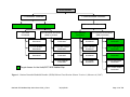


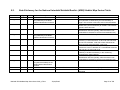
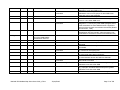

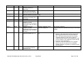
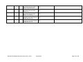
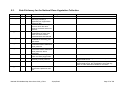
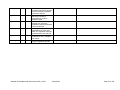
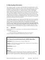


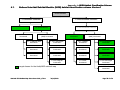

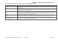
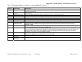
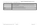


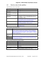
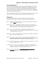


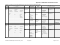
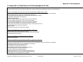
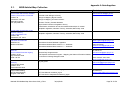
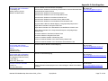

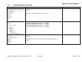
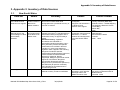
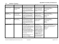

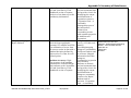


![[In]Sight User Guide - Regional Australia Institute](http://vs1.manualzilla.com/store/data/006869990_1-7c0e7afba9e4f1981156fce7684759c4-150x150.png)