Download Consistent Climate Scenarios User Guide- Version 2.2

Consistent Climate Scenarios User Guide
AR4 ‘Change factor’ and ‘Quantile-matching’ based
climate projections data
Grazing Land Systems – Science Delivery
May 2015 / Version 2.2
Department of Science, Information Technology and Innovation
Prepared by
Grazing Land Systems
Science Division
Department of Science, Information Technology and Innovation
PO Box 5078
Brisbane QLD 4001
© The State of Queensland (Department of Science, Information Technology and Innovation) 2015
The Queensland Government supports and encourages the dissemination and exchange of its information. The copyright in
this publication is licensed under a Creative Commons Attribution 3.0 Australia (CC BY) licence.
Under this licence you are free, without having to seek permission from DSITI, to use this publication in accordance with the licence
terms.
You must keep intact the copyright notice and attribute the State of Queensland, Department of Science, Information Technology and
Innovation as the source of the publication.
For more information on this licence visit http://creativecommons.org/licenses/by/3.0/au/deed.en
Disclaimer
This document has been prepared with all due diligence and care, based on the best available information at the time of publication.
The department holds no responsibility for any errors or omissions within this document. Any decisions made by other parties based on
this document are solely the responsibility of those parties. Information contained in this document is from a number of sources and, as
such, does not necessarily represent government or departmental policy.
Some of the pages in this document contain links to pages and/or sites which are not under the control of the State of Queensland. No
representation or warranty is made by the State of Queensland regarding the content of any such pages or sites. Merely because links
are made to third party sites does not mean that the State of Queensland through the Department of Science, Information Technology
and Innovation promotes or endorses any of those sites. It is possible that adverse consequences including viruses or loss of privacy
may result from use of third party sites.
Furthermore, in regard to material or information provided by the CSIRO, the CSIRO does not guarantee that the material or information
it has provided is complete or accurate or without flaw of any kind, or is wholly appropriate for your particular purposes and therefore
disclaims all liability for any error, loss or other consequence which may arise directly or indirectly from you relying on any information or
material it has provided (in part or in whole). Any reliance on the information or material CSIRO has provided is made at the reader's
own risk.
The same disclaimers that apply to SILO historical data apply to the CCS projections data.
If you need to access this document in a language other than English, please call the Translating and Interpreting Service (TIS National)
on 131 450 and ask them to telephone Library Services on +61 7 3170 5725
Citation
Content from this document should be attributed as: The State of Queensland (Department of Science, Information Technology and
Innovation), Consistent Climate Scenarios User Guide Version 2.2, 2015.
Acknowledgements
The Consistent Climate Scenarios Project (CCSP) was initially undertaken by the former Queensland Climate Change Centre of
Excellence (QCCCE), now under the Queensland Government’s Department of Science, Information Technology and Innovation
(DSITI). DSITI acknowledges that the development of the Consistent Climate Scenarios (CCS) User Guide and the daily climate
projections data referred to herein was supported by funding from the Australian Government Department of Agriculture Forestry and
Fisheries (DAFF) under the Australia’s Farming Future - Climate Change Research Program (CCRP). DSITI also acknowledges
guidance provided by Dr Stephen McMaugh (DAFF) and the project’s Expert Panel chaired by Mr Steven Crimp (CSIRO). The authors
also thank Dr Ian Smith (formerly CSIRO) for his assistance in reviewing this document. Furthermore, this User Guide has benefitted
from feedback and advice of data users, in particular from the CCRP project teams who have applied CCS projections data in their
projects.
May 2015
Consistent Climate Scenarios User Guide - Version 2.2
About this document
The intent of this User Guide is to provide users (previously restricted to project teams under the CCRP program (see Appendix), but
now extended to all users) with background input and guidelines for using the Consistent Climate Scenarios (CCS) projections data.
The User Guide aims to assist users in interpreting the data that has been provided.
This updated User Guide (V2.2) which supersedes the previous draft (V2.1) released in August 2012, includes additional information
about:




the availability of CCS datasets through the Long Paddock Climate Change Projections web portal
updated CF and QM file-naming conventions
additional projections data for four Representative Future Climate partitions (RFCs)
maps showing projected 21st Century temperature changes for the four RFCs
This User Guide was supported by the project’s Chair and Expert Panel. In addition, User feedback has also played an important role in
the development and improvement of the information that this User Guide contains.
Referencing Consistent Climate Scenarios (CCS) Data
The data source should be acknowledged as the Queensland Government SILO database (http://www.longpaddock.qld.gov.au/silo).
The SILO database is operated by DSITI.
The climate ‘change factors’ used to calculate CCS data have been estimated using:

Coupled Model Intercomparison Research Program 3 (CMIP3) patterns of change data (projected changes per degree of 21st
Century global warming) supplied by the CSIRO and the UK Met Office/Hadley Centre; and

data from AR4 SRES scenario temperature response curves (projected amounts of global warming) supplied by the CSIRO.
As such, the following data sources should also be acknowledged:

The CMIP3 global model database (http://www-pcmdi.llnl.gov/ipcc/about_ipcc.php)

OzClim http://www.csiro.au/ozclim)

UK Met Office/Hadley Centre (http://www.metoffice.gov.uk/climate-change/resources/hadley)
Related publications
Further information, describing the infilling of trends per degree of global warming for missing climate variables, is documented in:
Ricketts, J.Ha., Kokic, P.Nb. and Carter, J.Oa. (2011). Estimating trends in monthly maximum and minimum temperatures in GCMs for
which these data are not archived. aQueensland Climate Change Centre of Excellence, Queensland Government. bCSIRO,
Mathematics, Informatics and Statistics. 19th International Congress on Modelling and Simulation (MODSIM), Perth, Australia 12-16
December 2011, http://www.mssanz.org.au/modsim2011/F5/ricketts.pdf.
Further information, describing the ‘quantile-matching’ approach, is documented in:
Kokic, P., Jin, H. and Crimp, S. (2012). Statistical Forecasts of Observational Climate Data. Extended Abstract, International conference
on “Opportunities and Challenges in Monsoon Prediction in a Changing Climate” (OCHAMP-2012), Pune, India 21-25 February 2012.
Additional information, summarising the Consistent Climate Scenarios Project, is documented in:
Ricketts, J.Ha., Kokic, P.Nb. and Carter, J.Oa. (2013). Consistent Climate Scenarios: projecting representative future daily climate from
global climate models based on historical data. aDepartment of Science, Information Technology, Innovation and the Arts. Queensland
Government. bCSIRO, Mathematics, Informatics and Statistics, Australia. 20th International Congress on Modelling and Simulation
(MODSIM), Adelaide, Australia, 1–6 December 2013, http://www.mssanz.org.au/modsim2013/L11/ricketts.pdf.
i
Department of Science, Information Technology and Innovation
Contents
1
Introduction ......................................................................................................................................... 1
2
Accessing and interpreting data ...................................................................................................... 4
3
4
5
6
7
ii
2.1
‘Change factor’ (CF) data
2.2
‘Quantile-matched’ (QM) data
12
2.3
Historical baseline climate data files
17
2.4
An end-user example
19
8
Files with additional information .................................................................................................... 20
3.1
Multiplier files
20
3.2
CO2 matching files
23
3.3
CO2 concentrations files
24
3.4
Log warning files
28
3.5
Historical time series plots
30
3.6
CF Frequency distribution plots
32
3.7
Comparison of model projections plots
34
th
st
3.8
Plots of simulated 20 and 21 Century climate
36
3.9
Quantile trend plots
39
3.10 Histograms of ‘quantile-matched’ climate projections
41
3.11 Transient climate data test set for 1889-2100
43
‘Change factor’ (CF) methodology ................................................................................................. 45
4.1
‘Change factor’ definition
45
4.2
Background
45
4.3
Calculation of ‘change factors’
46
4.4
A worked example – projecting climate data for 2050 for a specific location
49
‘Quantile-matching’ (QM) methodology ......................................................................................... 50
5.1
Steps involved to calculate QM projections data for 2030
50
5.2
Variation of methodology for calculating 2050 QM projections data
52
5.3
Post-projection clamping
53
5.4
Transforms applied
54
Description of daily climate variables ............................................................................................ 55
6.1
SILO data
55
6.2
Patched Point and drilled data
56
Emissions scenarios and climate warming sensitivity ................................................................ 57
7.1
Emissions scenarios - background information
57
7.2
Selecting emissions scenarios
60
7.3
Climate warming sensitivity
60
Consistent Climate Scenarios User Guide - Version 2.2
8
9
Global Climate Models ..................................................................................................................... 64
8.1
Selecting Global Climate Models
66
8.2
Composite (HI, HP, WI and WP) climate projections data
69
Infilling of trends per degree of global warming .......................................................................... 70
9.1
Estimating trends in daily maximum and minimum temperature
71
9.2
Estimating vapour pressure
76
9.3
Estimating potential evaporation and pan evaporation
82
9.4
Estimating solar radiation
82
9.5
Summary of infilling
84
10 Known limitations of CF projections data ..................................................................................... 86
10.1
Base-period selection
86
10.2
Capture of anomalous data in Log warning files
88
10.3
Emissions and CO2 -stabilisation scenarios
88
10.4
Downscaling from Global Climate Models
89
10.5
The calculation of trends per degree of global warming
89
10.6
Known issues related to the calculation of ‘change factors’
91
10.7
Issues important to biological modelling
92
11 Differences between CF and QM projections data, including versioning ................................. 94
11.1
GCMs, emissions scenarios, climate sensitivities and projections years
94
11.2
Historical baseline and training period
94
11.3
Latitude and longitude in file names
94
11.4
Changes in SILO historical data
94
11.5
Quality control measures
94
11.6
Calculation of pan evaporation
95
11.7
Projected CF and QM means and standard deviations
95
11.8
Non-uniformity of perturbations
96
11.9
Differences between CF and QM projections
96
11.10 Changes between QMV2.2.0 and QMV3.0
96
11.11 Summary of differences between CF and QM versioning
97
12 Glossary ............................................................................................................................................ 98
13 References ...................................................................................................................................... 101
14 Contact details ................................................................................................................................ 103
15 Appendix ......................................................................................................................................... 104
DAFF Climate Change Research Program Projects
104
Consistent Climate Scenarios – Web Portal
105
iii
Consistent Climate Scenarios User Guide - Version 2.2
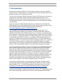
1 Introduction
Researchers conducting studies of climate change impacts on primary industries
have previously not had access to a consistent set of climate change projections in a
suitable format for use in biophysical models.
The aim of the Consistent Climate Scenarios Project (CCSP) has been to develop a
consistent set of synthetic climate projections data across Australia for use in
biophysical models, which maintain ‘weather-like’ properties and also account for
uncertainties and biases in climate change projections, as well as different methods
of downscaling.
Since July 2012, the CCSP has been delivering a consistent set of model-ready
(AR4-based) 2030 and 2050 Australia-wide climate change projections data, via the
Long Paddock website’s Climate Change Projections web portal
http://www.longpaddock.qld.gov.au/climateprojections/.
The first phase of the project used CSIRO’s OzClimTM ‘change factor’ (CF)
approach (described in Section 4) to transform historical climate data, based on
projections information from CSIRO’s OzClim tool. CF (Version 1) projections data
were released for eight Global Climate Models (GCMs) in September 2010, followed
by CF (Version 1.1) projections data for 17 GCMs in April 2011. As at April 30, 2012,
a considerable amount of CF (Version 1.1) projections data had been provided to
end-users, exceeding 650 individual Australian locations, 1.3 million data files and
850GB data volume. The latest version of the CF projections data (V1.2), released in
June 2012, is the same as V1.1, except that it now includes data for two highly
ranked Hadley Centre GCMs (HADCM3 and HADGEM1) and has been adapted for
delivery via the Long Paddock website’s Climate Change Projections web portal.
The second phase of the project, which incorporated a more sophisticated approach
called ‘quantile-matching’ (QM, see Section 5), supplied by Dr Phil Kokic and Mr
Steven Crimp (CSIRO), was implemented and enhanced by Dr Andrej Panjkov
(QCCCE). QM considers projected changes in the cumulative distribution function of
the climate projections (Kokic et al. 2012). The method used to calculate the 2030
projections data (Version QMV2.2.0 released in June 2011, updated to Version
QMV3.0 in May 2015) does this by incorporating significant observed trends in 10th,
50th and 90th percentile values that have been extrapolated to 2030. QM 2030
projections are available for the same GCMs as the CF data. QM 2030 projections
data are also available via the Climate Change Projections web portal.
A variation in the QM method, to incorporate daily GCM data, has been used to
calculate QM based projections data for 2050 (Version QM2.2.10, 2050, released
mid-November 2011). The QM 2050 projections, which were limited to a single
GCM, due to the availability of raw daily GCM data for 2050, are available via:
ftp://climate.mft.derm.qld.gov.au/Climate_Scenarios/QM_2050_TestData/.
Users are encouraged to consider the limitations of both the CF and QM approaches
when interpreting model output based on these climate change projections data.
1
Department of Science, Information Technology and Innovation
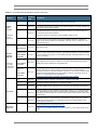
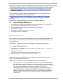
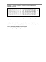
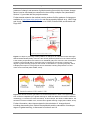
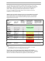
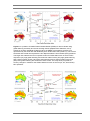
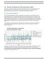
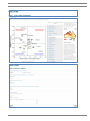
Figure 1.1 indicates the relationship between the CCSP partners and their roles in
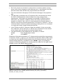
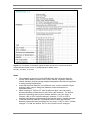
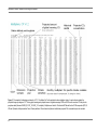
delivering the project outputs. Table 1.1 presents the CCSP versioning.
Figure 1.1 Relationships between Consistent Climate Scenarios Project partners and project
outputs.
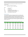
In the AR4 CCS projections data, 2030 (or 2050) represents a period (e.g. 30 years)
centred on that year. The length of the period will be the same as the user’s
selected SILO historical base period.
For applications model evaluation, we recommend usage of a 1960-2010 base
period (the quality of post-1960 historical climate data is higher than that of earlier
data). The period from 1960 to 2010 also encompasses a wide range of natural
climate variability (i.e. droughts and floods) due to fluctuations in the El Niño
Southern Oscillation phenomenon (ENSO), as well as opposite phases of the
Interdecadal Pacific Oscillation (IPO).
2
Consistent Climate Scenarios User Guide - Version 2.2
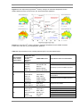
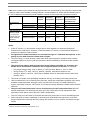
Table 1.1 Consistent Climate Scenarios Project Versioning
Product
‘Change
factor’
(CF) data
Version
Release
date
Comments
V0
Apr 2010
Initial CF 2030 and 2050 projections test data for format checks, etc.
V1
Sep 2010
Eight GCMs, eight emissions scenarios, three climate sensitivities, six climate variables and
two projections years (2030 and 2050).
V1.1
Apr 2011
These files
have no
method tag.
17 GCMs, eight emissions scenarios, three climate sensitivities, six climate variables and
two projections years (2030 and 2050).
Some improvements on evaporation. Historical baseline 1899 to current.
Jun 2012
This is the version running under the web. Historical baseline 1960-2010. Includes two
Hadley Centre GCMs (HADCM3 and HADGEM1). Otherwise, there is no difference in the
data, from that of V1.1.
Jun 2011
Initial 2030 test set.
Jul 2011
Initially 17 GCMs, eight emissions scenarios, three climate sensitivities, six climate variables
and one projections year (2030). Two extra GCMs (HADCM3, HADGEM1 added for the web
version in June 2012.
May 2015
Code adjusted to fix a trivial error in QMV2.2.0, for which an insignificant amount of daily
rainfall data had been affected and to negligible extent.
Nov 2011
2050 only. Limited to a 52 station test set, for a single GCM (ECHAM 5), one emissions
scenario (A1B) and one climate sensitivity (median). Approach for 2050 rainfall and
temperature projections uses daily GCM data. Projections for other climate variables based
on QM 2030 method extended to 2050. 2050_QM2.2 in filename, but internally known as
QMV2.2.10, to reflect different data, available via
ftp://climate.mft.derm.qld.gov.au/Climate_Scenarios/QM_2050_TestData/
V1.0
Nov 2010
Development version, supporting ‘change factor’(V1) data for eight GCMs.
V1.1
May 2011
Development version, supporting CF V1.1 data for 17 GCMs.
V2
Oct 2011
Information added to support QM 2030 test set. Includes CF and QM 2030 methodologies.
V2.1
Aug 2012
Information added to support HADCM3 and HADGEM1 GCMs, CF V1.2 and QM 2050 data
sets, updated filenames, descriptions for QM trend plots and QM 2050 methodology. Brief
notes about transient data sets, the Climate Change Projections data interactive web portal
and the ftp site.
V2.2
May 2015
Additional information on the availability of CCS datasets through the web portal, updated
file-naming conventions (Section 2) and projections data for four Representative Future
Climate partitions (Section 8).
V1.2
QMV2.1.0 2030
QM in filename
QMV2.2.0 2030
‘Quantilematching’
(QM) data
2030 & QMv2.2
in filename
QMV3.0
These files
have a QM
method tag in
the filename.
2030
2030 & QMv3.0
in filename
QMV2.2.10
2050
2050 & QM2.2
in filename
User Guide
http://longpaddock.qld.gov.au/climateprojections/
Web-based
data portal
Aug 2012
Portal on the Long Paddock website, from which requests for CCS projections data can be
made.
3
Department of Science, Information Technology and Innovation
2 Accessing and interpreting data
What is available?
The 2030 and 2050 daily (AR4-based) climate projections data are available for six
climate variables useful for biological modelling, including:





rainfall
maximum and minimum temperature
solar radiation
vapour pressure
pan evaporation.
Users can order projections data based on:
 the ‘Change factor’ or ‘Quantile-matching’ method (see Sections 4 and 5)
 eight emissions scenarios (see Section 7.1)
 three climate warming sensitivities (see Section 7.3)
 19 global climate models (see Section 8).
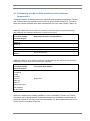
Registration
The climate projections data are password protected. To access to these data, a new
user must complete and submit the registration form at:
http://www.longpaddock.qld.gov.au/climateprojections/registration.php
Login details are provided by email, once registered (allow three working-days).
Ordering data
The climate projections data can be ordered by clicking the REQUEST DATA link at:
http://www.longpaddock.qld.gov.au/climateprojections/registration.php
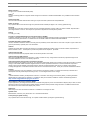
The CCS login page (Figure 2.1) will then appear:
Figure 2.1 CCS login page.
4
Consistent Climate Scenarios User Guide - Version 2.2
Following login, the steps required to order data are:
Step 1: Select order type
Choose the type of data. Data can be for ‘Weather stations’, or point locations (by
‘Latitude and Longitude’), with an option for ‘Full data’ (daily projections) or ‘Summary
data’ (i.e. plots showing comparisons of GCM model projections for 2030 based on
the A1B emissions scenario).
Step 2: Select weather station locations
Select the required weather stations (by station Name or ID Code), or point-locations
(by latitude and longitude).
Step 3: Select data parameters
Choose ‘Change factor’ (CF) or ‘Quantile-matching’ (QM) projections, the historical
baseline period (start and end years), the projections year (2030 or 2050), and
choice of up to three emissions scenarios, up to three global warming sensitivities
and up to 23 climate models.

Projections data are always packaged with the following ancillary information,
which can be used with or independently of the projections data:
– historical-baseline climate data files
– multiplier files (containing the information used to calculate ‘change factors’)
– comparison of model projections plots (showing change in rainfall and
temperature at 2030 for 19 GCMs based on ‘change factors’)
– a CO2 matching file (look-up table)
– log warning files (only with CF orders).
Step 4: Select delivery details
Enter a unique label to assist in identification of the ZIP archive that will be created
for your projections data files. Then select the projections data file format (APSIM or
p51), option to include ‘diagnostic charts’ or not, and finally how you wish to receive
the data (FTP is preferred).
 If ‘diagnostic charts’ is selected, the user will receive the following, which can be
used with or independently of the projections datasets:
– historical time series plots of histograms showing historical and ‘quantilematched’ distributions for each climate variable (only with QM orders)
– monthly quantile trend plots, for selected climate variables (only with QM
orders).
Step 5: Confirm order
Your order is summarised, with an option to submit or revise it.

Once submitted, the option is available for a user to track the progress of the
order.
An example of the web portal process for ordering CCS data is provided in the
Appendix. Further information is available in the ‘Data Order Online Help’ page in
the CCS web portal.
5
Department of Science, Information Technology and Innovation
FTP data collection site
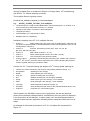
The user will be notified by email, as soon as the data order has been processed.
The email will provide a link to the specific location of the data under
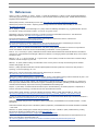
‘CCCS_Web_Data_Outputs’ on the FTP data collection site (Figure 2.2).
Ancillary information hosted on the FTP data collection site, includes the following:
 the User Guide
 a 52-station QM 2050 test-set (see Section 2.2), based on a single GCM, one
emissions scenario and one climate sensitivity
 a single-station 1899-2100 CF-based transient data set (see Section 3.11).
Figure 2.2 Information available at the CCS FTP Data collection site (as at May 1, 2015).
Important notes for users, regarding ZIP archives
Windows
Self-extracting ZIP archives (file extension .zip.exe) only work for the Windows
environment. They won’t work when downloaded to non-Linux/x86, Unix systems
(e.g. HP-UX, AIX, Solaris, DG-UX, IRIX, TRU64, OSF/1).
Unix and Linux
Standard ZIP files (file extension .zip) can be provided for Unix and Linux users. Unix
users can extract the projections data files by typing unzip filename.zip in the Unix
command line.
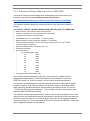
ZIP archive file-sizes
When ordering data, the user needs to consider the size of zipped archives and the
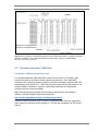
number of files that will be produced. Table 2.1 shows typical zip archive file sizes
and the number of files that will be produced.
6
Consistent Climate Scenarios User Guide - Version 2.2
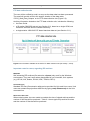
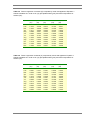
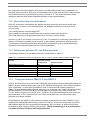
Table 2.1 Typical ZIP archive file sizes and number of files (based on the selection of the
default 1960-2010 climate baseline, including diagnostic plots).
Projections
type
CF 2030 or
2050
projections
CF 2030 or
2050
projections
with diagnostic
plots
QM 2030
projections
User selection
User selection
User selection
1 location
10 locations
10 locations
1 GCM
1 GCM
19 GCMs
1 emissions scenario
1 emissions scenario
3 emissions scenarios
1 climate sensitivity
1 climate sensitivity
3 climate sensitivities
0.5 MB, 5 files
4.8 MB, 50 files
322 MB, 2470 files
1 projections file
10 projections files
1710 projections files
1 SILO file
10 SILO files
190 SILO files
1 multiplier file
10 multiplier files
190 multiplier files
1 CO2 matching file
10 CO2 matching files
190 CO2 matching files
1 log file
10 log files
190 log files
0.7 MB, 7 files
6.7 MB, 70 files
324 MB, 2490 files
Includes the same files as
those above, plus:
Includes the same files as
Includes the same files as
those above, plus:
those above, plus:
1 comparison of model
projections plot
10 comparison of model
projections plots
10 comparison of model
projections plots
1 time series plot
10 time series plots
10 time series plots
0.5 MB, 4 files
5.3 MB, 40 files
369 MB, 2280 files
1 projections file
10 projections files
1710 projections files
1 SILO file
10 SILO files
190 SILO files
1 multiplier file
10 multiplier files
190 multiplier files
2
QM 2030
projections
with diagnostic
plots
2
1 CO matching file
10 CO matching files
190 CO2 matching files
5.9 MB, 17 files
59 MB, 170 files
443 MB, 2410 files
Includes the same files as
those above, plus:
Includes the same files as those
above, plus:
Includes the same files as those
above, plus:
1 comparison of model
projections plot
10 comparison of model
projections plots
10 comparison of model
projections plots
1 time series plot
10 time series plots
10 time series plots
5 quantile trend plots
50 quantile trend plots
50 quantile trend plots
6 QM histogram plots
60 QM histogram plots
60 QM histogram plots
7
Department of Science, Information Technology and Innovation
2.1 ‘Change factor’ (CF) data
Availability
‘Change factor’ (CF) based projections data can be ordered through the Long
Paddock website’s Climate Change Projections web portal:
http://www.longpaddock.qld.gov.au/climateprojections/.
Users have a choice of CF projections data files for 2030 and 2050, 19 GCMs (see
Section 8), eight emissions scenarios (see Section 7.1) and three climate warming
sensitivities (see Section 7.3). Each projections file contains projections data for six
climate variables (see Section 6) using the CF methodology (see Section 4). CF
projections data can be made available for any weather station or point location
(latitude and longitude) within Australia.
For small orders, the average delivery time to the ftp server is 60 minutes from being
submitted. For large orders, delivery time is usually within 24 hours. Users are
notified by email, with a link to their data on ftp server, as soon as an order has been
processed and is ready for download.
All CCS files on the ftp server are contained in ZIP format archives. Users should
note that the ZIP format archives will be deleted seven days after having been
processed. This is to ensure that the ftp site does not reach capacity, enabling new
file-space to be created for additional orders.
CF ZIP archives - containing daily projections
CF climate projections data files (as well as historical baseline climate data files,
monthly multiplier files, CO2 matching files and log warnings files) for each selected
climate site are contained in a ZIP format archive named as follows:
User.name_JobNumber_FileLabel_Archivetype
e.g.




john.smith_its138_FileLabel_zip.exe
Username (derived from your email address)
JobNumber (i.e. its138, its139, its140, etc.)
FileLabel (1-8 character label, specified by the user, i.e. cf2030, testdata, etc.)
Archivetype (i.e. .zip.exe for Windows or .zip for Unix/Linux)
File types packaged in CF ZIP archives containing daily projections data (including
filename examples) are:
o CF projections
–
051039_A1F1_2030_M_CSIRO-MK35_-31.5495_147.1961_V1.2.met (details in this Section)
o Historical baseline climate data
–
051039_SILO_-31.5495_147.1961_V1.2.met (described in Section 2.3)
o Multiplier files
–
051039_-31.5495_147.1961_V1.2.multiplier (described in Section 3.1)
o CO2 matching files
–
051039_-31.5495_147.1961_NamesList.txt (described in Section 3.2)
o Log warning files
–
8
051039_-31.5495_147.1961_V1.2.log (described in Section 3.4)
Consistent Climate Scenarios User Guide - Version 2.2
CF ZIP archives - containing diagnostic plots
CF 2030 diagnostic charts (which include comparison of model projections plots for
2030 based on the A1B emissions scenario and historical time series plots) for each
selected climate site are contained in a ZIP format archive as follows:
User.name_JobNumber_FileLabel_Plots_Archivetype
e.g.





john.smith_its138_plots_zip.exe
Username (derived from your email address)
JobNumber (i.e. its138, its139, its140, etc.)
FileLabel (1-8 character label, specified by the user, i.e. cf2030, testdata, etc.)
Plots (shows that plot files are included)
Archivetype (i.e. .zip.exe for Windows or .zip for Unix/Linux)
File types packaged in CF ZIP archives containing diagnostics plots (including
filename examples) are:
o Comparison of model projections plots
–
051039_A1B_M_2030_31.5495_147.1961_mdlperf_V1.2.png (described in Section 3.7)
o Historical time series plots
–
051039_-31.5495_147.1961_V1.2.png (described in Section 3.5)
CF Projections files
Once the ZIP archive is opened, individual CF climate projections data files and
ancillary files are then accessible. The CF climate projections data files are named
as follows:
LocationCode_Scenario_ProjectionsYear_ClimateWarmingSensitivity_ModelName_Latitu
de_Longitude_VersionNumber.SILOformat
e.g.








1
051039_A1FI_2030_M_CSIRO-MK35_-31.5495_147.1961_V1.2.met
‘LocationCode’ is a six digit number (BoM station code if patched-point, i.e.
051039, or all zeros if drilled (from interpolated surfaces), i.e. 000000)
Scenario (emissions scenario1, i.e. A1B, A1FI, etc.)
Projections year (i.e. 2030 or 2050)
Climate warming sensitivity (rate of global warming, i.e. L, M, H)
– ‘L’, ‘M’ and ‘H’ refer to the 10th, 50th and 90th percentile values respectively.
ModelName2 (i.e. CSIRO-MK35, HADGEM1, HI, HP, etc.)
Latitude and longitude of the station, or location, in decimal degrees (rounded to 4
decimal places)
CF Version (i.e. V1.2)
SILO format (either ’met’ for APSIM or ’p51’ for GRASP)
Emissions scenarios and climate warming sensitivities used in the project are discussed in Section 7.
2
More information about the AR4 GCMs and Representative Future Climate partition model composites used in this
project is available in Section 8.
9
Department of Science, Information Technology and Innovation
CF Projections file metadata
The CF projections files, in APSIM format, contain the following metadata in the first
21 rows of each file:

Station number
This is the same as the ‘Location code’, following the same convention as is used
by the Bureau of Meteorology (BoM), which consists of six digits, containing
leading zeros. For example station 51039 in the SILO database adopts the BoM
station identifier convention and becomes LocationCode 051039 for this project.

Station name
‘None’ is listed if the location is selected by latitude and longitude.

Latitude and longitude (decimal degrees)

Long-term annual average ambient temperature (tav, ºC)
Perturbed tav, based on the default period (currently 1960 to 2010).
If 1970 to 2000 is selected, the calculation will be based on 1970 to 2000.

Annual amplitude in mean monthly temperature (amp, ºC).The difference
between the long-term mean of the warmest month of the year and the long-term
mean of the coolest month of the year. Statistical period the same as tav.

The date that the projections data were computed

Projections year (2030 or 2050)

Emissions scenario (Eight are available, see Section 7.1)

GCM model or RFC composite
19 Global Climate Models (see Section 8, Table 8.2) and four Representative
Future Climate composites (see Section 8, Table 8.3) are available. The CCS
project’s file naming convention for AR4 GCMs (documented in Section 8, Table
8.2) uses abbreviations of the formal model names used by the Program for
Climate Model Diagnosis and Intercomparison (PCMDI) Coupled Model
Intercomparison Project phase 3 (CMIP3).

Model sensitivity (low, median or high), refer to ‘climate warming sensitivity’
(Section 7).

Ambient CO2 in year of projection (ppm, see Section 3.3)
Notes

Each file contains projections data for six climate variables based on the CF
methodology (see Section 4).

The projections data are synthetic and do not represent a forecast.

The projections data have been developed for use as input to agricultural
simulation models.

In the projections data, the intensity of the rain on rain days is perturbed, but the
sequence of rain/no-rain days remains unchanged from the source historical data.
Days without rain in the historical time series are projected to days without rain.

The SILO climate database http://www.longpaddock.qld.gov.au/silo can be used
to assist in the selection and identification of climate stations.
10
Consistent Climate Scenarios User Guide - Version 2.2

SILO daily climate are checked for quality and are constantly updated (at least
twice a year), hence changes to some data may occur. Any changes in the SILO
base-line climate data will affect the projected 2030 and 2050 data.

The same disclaimers that apply to SILO historical data apply to the projections
data.

The daily dates, presented in the CF projections files, are the dates from which
the 2030 or 2050 projections data are drawn from (using ‘change factor’
methodology). These dates are essentially an ensemble of individual 2030 or
2050 years. For example, if 19600101 were to be used to represent the first
instance of 20300101, then 19610101 would represent the second instance of
20300101 and 20100101would represent the 51st instance of 20300101. The use
of historical dates creates the practical advantage of being able to run an analysis
in a single pass using a single climate data input file.

In the CF data, at least 51 instances of data are available, if using source data
from 1960-2010. Source data prior to 1960 are less useful due to issues related
to low climate station density and uncorrected climate trends.

The date-formatting in the APSIM and p51 files differs, as follows:
APSIM
YYYY DayNumber(1-365/6)
p51
YYYYMMDD
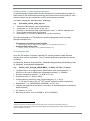
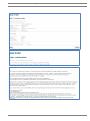
Examples of information presented in CF climate projections data files are presented
in Figures 2.3 and 2.4. Figure 2.3 is a screenshot of projections data for 2050, based
on output from the HADCM3 GCM forced by the A1FI emissions scenario with high
climate warming sensitivity, formatted for use in APSIM. Figure 2.3 provides an
example of information presented in a climate projections data file in the ‘p51’ format
suitable for use in the GRASP pasture model.
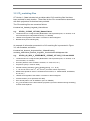
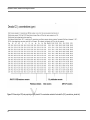
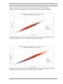
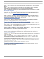
Figure 2.3 A snapshot of information (projections for 2030) presented in a climate projections
data file, suitable for use in APSIM (filename 040428_A1FI_2030_H_HADCM3_25.6550_151.7450_V1.2.met).
11
Department of Science, Information Technology and Innovation
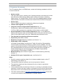
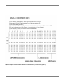
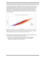
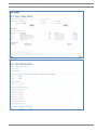
Figure 2.4 A snapshot of information (projections for 2030) presented in a climate projections
data file, suitable for use in GRASP (filename 051039_A1FI_2030_M_CSIRO-MK35_31.5495_147.1961_V1.2.p51).
2.2 ‘Quantile-matched’ (QM) data
Availability of QM 2030 projections data
For ‘Quantile-Matched’ (QM) 2030 data, users have a choice of 19 GCMs, eight
emissions scenarios and three climate warming sensitivities. Each QM 2030
projections file contains projections data for six climate variables using the QM 2030
methodology (see Section 5.1). QM 2030 projections data can be requested for any
weather station in Australia. However, drilled data (derived from interpolated
surfaces) are not currently available.
QM 2030 based projections data can be ordered through the Long Paddock
website’s Climate Change Projections web portal:
http://www.longpaddock.qld.gov.au/climateprojections/.
Users are notified by email once an order, for QM 2030 data, has been processed
and is ready for download (refer to page 6). The files are contained in a ZIP format
archive.
12
Consistent Climate Scenarios User Guide - Version 2.2
QM 2030 ZIP archives – containing daily projections
QM climate projections data files (as well as a set of historical baseline climate data
files, monthly multiplier files, CO2 matching files) for each selected climate site are
contained in a ZIP format archive named as follows:
User.name_JobNumber_FileLabel_Archivetype
e.g.




john.smith_its138_FileLabel_zip.exe
Username (derived from your email address)
JobNumber (i.e. its138, its139, its140, etc.)
FileLabel (1-8 character label, specified by the user, i.e. qm2030, qmdata, etc.)
Archivetype (i.e. .zip.exe for Windows or .zip for Unix/Linux)
File types packaged in the QM ZIP archive containing daily projections (including
filename examples) for each selected climate site are:
o QM projections (for 2030)
–
051039_A1F1_2030_M_CSIRO-MK35_-31.5495_147.1961_QMv3.0.met (described in this Section)
o Historical baseline climate data
–
051039_SILO_-31.5495_147.1961_QMv3.0.met (described in Section 2.3)
o Multiplier files
–
051039_-31.5495_147.1961_V1.2.multiplier (described in Section 3.1)
o CO2 matching files
–
051039_-31.5495_147.1961_NamesList.txt (described in Section 3.2)
QM 2030 ZIP archives - containing diagnostic plots
QM 2030 diagnostic plots (which include comparison of model projections plots for
2030 based on the A1B emissions scenario, historical time series plots, QM
histograms plots and quantile trend plots) for each selected climate site are
contained in a ZIP format archive as follows:
User.name_JobNumber_FileLabel_Plots_Archivetype
e.g.





john.smith_its138_plots_zip.exe
Username (derived from your email address)
JobNumber (i.e. its138, its139, its140, etc.)
FileLabel (1-8 character label, specified by the user, i.e. qm2030, testdata, etc.)
Plots (shows that plot files are included)
Archivetype (i.e. .zip.exe for Windows or .zip for Unix/Linux)
13
Department of Science, Information Technology and Innovation
File types packaged in QM 2030 ZIP archives containing diagnostics plots (including
filename examples) are:
o Comparison of model projections plots
–
o
051039_A1B_M_2030_31.5495_147.1961_mdlperf_V1.2.png (described in Section 3.7)
Historical time series plots
–
051039_-31.5495_147.1961_V1.2.png (described in Section 3.5)
o Quantile trend plots (files for 5 climate variables) *
–
RadnPropOfEtlogit_051039_[10,50,90]_1957_2010_2030_QuantileTrends_051039.png
–
RainCubeRoot_051039_[10,50,90]_1957_2010_2030_QuantileTrends_051039.png
–
SH_051039_[10,50,90]_1957_2010_2030_QuantileTrends_051039.png
–
T.Max_051039_[10,50,90]_1957_2010_2030_QuantileTrends_051039.png
–
T.Min_051039_[10,50,90]_1957_2010_2030_QuantileTrends_051039.png
(described in Section 3.9)
o Histograms of QM projections (files for 6 climate variables) *
–
RadnPropOfEtlogit_051039_[10,50,90]_1957_2010_2030_Histograms_051039_HADCM3_A1FI_high.png
–
Rain_051039_[10,50,90]_1957_2010_2030_Histograms_051039_HADCM3_A1FI_high.png
–
RainCubeRoot_051039_[10,50,90]_1957_2010_2030_Histograms_051039_HADCM3_A1FI_high.png
–
VP_051039_[10,50,90]_1957_2010_2030_Histograms_051039_HADCM3_A1FI_high.png
–
T.Max_051039_[10,50,90]_1957_2010_2030_Histograms_051039_HADCM3_A1FI_high.png
–
T.Min_051039_[10,50,90]_1957_2010_2030_Histograms_051039_HADCM3_A1FI_high.png
(described in Section 3.10)
* File naming syntax for Quantile trend and Histogram plots supersedes that presented in earlier User Guides.
QM 2030 Projections files
Once a ZIP archive is opened, individual QM 2030 climate projections data files and
ancillary files are then accessible. The QM 2030 climate projections data files are
named as follows:
LocationCode_Scenario_ProjectionsYear_ClimateWarming
sensitivity_ModelName_Latitude_Longitude_VersionNumber.SILOformat
e.g.








051039_A1FI_2030_M_CSIRO-MK35_-31.5495_147.1961_QMv3.0.met
‘LocationCode’ is a six digit number (BoM station code if patched-point, i.e. 051039, or all
zeros if drilled (from interpolated surfaces), i.e. 000000)
Scenario (emissions scenario, i.e. A1B, A1FI, etc.)
Projections year (2030)
Climate warming sensitivity (rate of global warming, i.e. L, M, H)
th
th
th
– ‘L’, ‘M’ and ‘H’ refer to the 10 , 50 and 90 percentile values respectively.
Model Name (i.e. CSIRO-MK35, HADGEM1, HI, HP, etc.)
Latitude and longitude of the station or location in decimal degrees
Version Number (where QMv2.2 or QMv3.0 represents QM data)
SILO format (either ’met’ for APSIM or ’p51’ for GRASP)
Data contained in the QM 2030 projections data files are formatted the same as
those in the CF projections data files (Figures 2.3 and 2.4). However, metadata
provided in QM projections data files includes an additional column containing
reference codes for QM synthesis methods.
14
Consistent Climate Scenarios User Guide - Version 2.2
Notes (where different from caveats in Section 2.1 associated with the CF data)



The QM projections use a 1957-2010 training period to compute the
perturbation rules that are applied to that historical baseline. The tav (annual
average ambient temperature) and amp (annual amplitude in mean monthly
temperature) parameters shown in the QM metadata in the APSIM files are
calculated based on the 1957-2010 training period.
The daily dates, presented in the QM projections files, indicate only the
historical date that was the source of the associated perturbed data before
the QM methodology was applied. The month day and Julian day fields in the
projection files are correct.
QMv3.0 represents a code upgrade from QMv2.2 (see section 11.10).
Availability of QM 2050 Projections files
Due to a lack of raw daily GCM data, QM 2050 projections data are only available for
a single GCM (ECHAM5), the A1B emissions scenario and median climate warming
sensitivity. Each QM 2050 file contains projections data for rainfall, maximum and
minimum temperature projections are based on the QM 2050 methodology (see
Section 5.2), while and vapour pressure, evaporation and solar radiation projections
are based on the QM 2030 methodology(see Section 5.1).
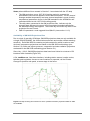
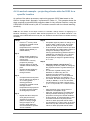
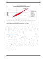
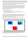
Since July 1, 2012, QM 2050 projections data have been limited to a test-set of 52
locations within Australia (Figure 2.5).
A file, testSites.csv, lists those locations, including station names, location codes,
latitudes and longitudes. Access to more locations is expected, via the Climate
Change Projections web portal, at some stage in the future.
Figure 2.5 Map showing 52 locations for which ‘quantile-matched’ projections data for 2050
are available.
15
Department of Science, Information Technology and Innovation
The QM 2050 station location file and QM 2050 projections data can be downloaded
via ftp://climate.mft.derm.qld.gov.au/Climate_Scenarios/QM_2050_TestData/.
QM 2050 ZIP archives
QM 2050 climate projections data and diagnostic files for each climate site are
contained in self-extracting ZIP format archives at
ftp://climate.mft.derm.qld.gov.au/Climate_Scenarios/QM_2050_TestData/
as follows:
LocationCode_ProjectionsMethod_ProjectionsYear_DEMO.Archivetype
e.g.
002012_QM_2050_DEMO.zip.exe

‘LocationCode’ is a 6 digit number (BoM station code if patched-point, i.e. 051039, or all
zeros if drilled (from interpolated surfaces), i.e. 000000)

ProjectionsMethod (QM, represents ‘quantile-matched’ projections)

ProjectionsYear (2050)

DEMO (represents QMV2.2.10 2050 test dataset)

Archivetype (.zip.exe for Windows)
QM 2050 Projections files
Once a ZIP archive is opened, individual QM 2050 climate projections data files and
ancillary files are then accessible. The QM 2050 climate projections data files are
named as follows:
LocationCode_ProjectionsYear_ProjectionsMethod_VersionNumber.SILOformat
e.g.
002012_2050_QM2.2.met

‘LocationCode’ is a six digit number (BoM station code if patched-point, i.e. 051039, or all
zeros if drilled, i.e. 000000)

Projections year (2050)

Version Number (where QM2.2 represents QM 2050 test data)

SILO format (either ’met’ for APSIM or ’p51’ for GRASP)
Data contained in the QM 2050 projections data files are formatted the same as
those in the QM projections data files.
Note (applies in addition to caveats associated with the QM 2030 data)

16
The QM projections data for 2050 are available for a single GCM (ECHAM5)
one, emissions scenario (A1B) and one climate warming sensitivity (median).
Each file contains projections data for six climate variables (rainfall, maximum
and minimum temperature projections are based on the QM 2050
methodology (see Section 5) and vapour pressure, evaporation and solar
radiation projections are based on the QM 2030 methodology). ECHAM5 is
unique, in that it is the only GCM that has both a high rank (as assessed by
the Expert Review Panel) and a complete set of raw GCM daily data from
1900 to 2100.
Consistent Climate Scenarios User Guide - Version 2.2
2.3 Historical baseline climate data files
Along with projections data, the ZIP archive also contains files of historical climate
data for baseline comparison. The historical data have been extracted from the SILO
database.
The SILO historical database, as it currently exists, is relied upon by the scientific
community across Australia and provides researchers and modellers with seamless
spatially and temporally complete Australia-wide daily climate data from 1889 to
current. CCS historical baseline climate datasets are available from 1960 onwards,
since this is the period of highest quality data. SILO grew from a need for climate
data in various formats suitable for systems modelling. The SILO datasets are based
on historical data provided by the Bureau of Meteorology (BoM), which DSITI has
enhanced by error checking, interpolating across Australia on a 5km grid, and on this
basis, ‘ infilling’ missing data at each station.
Both CF and QM historical data files are named as follows:
LocationCode_SILO_Latitude_Longitude_VersionNumber.SILOformat
e.g.
056002_SILO_-30.5167_151.6681_V1.2.met

LocationCode is a six digit number (BoM station code if patched-point, i.e. 051039, or all
zeros if drilled (from interpolated surfaces), i.e. 000000)

Obs (indicates observed/historical data)

SILO (indicates SILO baseline data)

Latitude (of your station in decimal degrees)

Longitude (as above)

Version Number (i.e. V1.2 as used in CF data, QMv2.2 or QMv3.0 as used in QM data)

SILO_format (either ‘met’ for APSIM or ‘p51’ for GRASP)
Note the different date formats in the APSIM and p51 files:

APSIM
YYYY DayNumber(1-365/6)

p51
YYYYMMDD
An example of information presented in an historical baseline climate data file is
presented in Figure 2.6. This format is suitable for use in APSIM.
17
Department of Science, Information Technology and Innovation
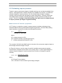
Figure 2.6 A snapshot of information (observed data) presented in a historical-baseline
climate data file suitable for use in APSIM (filename 056002_SILO_30.5167_151.6681_V1.2.met).
Notes




18
The metadata at the start of each APSIM format SILO historical data file
include station details (location code, name, latitude, longitude), baseline
climate statistics (annual average ambient temperature and annual amplitude
in mean monthly temperature).
In the QM historical data files, an additional ‘code’ column contains 6 digits
outlining codes used to distinguish between actual observations or
interpolated data.
When ordering CF 2030 or CF 2050 projections data, users can select
historical baseline climate data for years from 1960 onwards. The default
period for calculating the long term climate statistics (‘tav’ and ‘amp’) is
currently 1960 to 2010,’climate-changed’. However, if 1970 to 2000 is
selected, calculations will be based on that specific period, ’climate-changed’.
In the QM historical data files, the default period for both the historical
baseline climate data and calculated ‘tav’ and ‘amp’ is 1957 to 2010, ‘climatechanged’. For QM, the default 1957 to 2010 period can’t be changed.
Consistent Climate Scenarios User Guide - Version 2.2
2.4 An end-user example
A typical sequence for an end user is provided by the following example.
An end-user is interested in studying the impacts on grape vines near Mildura due to
a change in the frequency of hot days (days where the maximum temperature
exceeds 35oC). They would like to know what change could be expected around the
year 2030 assuming a worst case emissions scenario (A1FI) and high climate
sensitivity to global warming. However, they are only interested in the projections
from a few (five) GCMs which are recommended as being relatively good performers.
They would also like to compare the differences based on the ‘change factor’ (CF)
and ‘quantile-matched’ (QM) methods.
The end-user will first need to place a data order, based on the above-mentioned
variables, via the Long Paddock website’s Climate Change Projections web portal
http://www.longpaddock.qld.gov.au/climateprojections/. Once the projections
data have been processed, the end-user will receive an email containing an ftp link
for collection of the data. In most cases, ZIP archives containing the data will be
ready for collection within 2 hours (may take longer for large orders). When
projections data, without diagnostics are requested, there will be one ZIP archive per
order. In this example, there would be two sets of ZIP archives (one for CF data and
one for QM data).
If the user were to open either the CF or QM ZIP archive, the user will have access to
many files. For example, in the CF ZIP archive, the CF projections data files refer to
the GCMs, emissions scenarios, target years, climate sensitivity values, and output
formats that were selected during the order process. In this case, the user will have
received for each of the five GCMs, just those files corresponding to the specified
location, year 2030, A1FI emissions scenario and high climate sensitivity. That
equates to a total of five CF projections data files (one for each GCM). For each
location requested, the ZIP archives contain a range of additional files. In the ZIP
archives, these additional files include the corresponding observed data as contained
in the SILO data base (see Section 2.3), CO2 matching files, log warning files,
monthly multiplier files, historical time-series plots and comparison of model
projections plots (see Section 3).
As at January 20, 2015, by default the years in the SILO observed daily data file and
the CF projected daily data file, are dated from January 1, 1960 to December 31,
2010. However, if desired, the end-user can select a shorter or longer period when
making their web-based order (the latest end year can be 2013). For example, in
calculating the frequency of hot days, the end-user can select a window of years (e.g.
1971 to 2000) from the observations, and compare the results with the same window
(1971 to 2000) from the 2030 projections data files. The selected historical baseline
for the QM data is fixed, from January 1, 1957 to December 31, 2010.
The data from each file can be imported directly into a spread sheet or other program
and the user can focus, in this case, on just the daily temperatures. It is
recommended that the end-user perform some basic calculations and plots of the
data and then refer to the corresponding ancillary files that are contained in each
archive. This can provide a check that the correct data has been accessed for the
19
Department of Science, Information Technology and Innovation
specific purpose. In some cases the ancillary files may contain the exact information
that the end-user is interested in.
3 Files with additional information
Many ancillary files are supplied in the ZIP archives to supplement the climate
projections data. The information contained in these ancillary files can be used
independently from the 2030/50 projections data files.
‘Change factor’ (CF) based ancillary files include:

multiplier files

CO2 matching files

log warning files

historical time series plots

comparison of model projections plots.
Additional to these, ‘quantile-matched’ (QM) based ancillary files include:

monthly quantile trend plots

histograms of projected frequency distributions.
In addition, the following ancillary files (not available via the CCS web portal) can be
made available, if requested:

an historical and projected CO2 concentrations file

CF based frequency distribution plots

plots of simulated 20th and 21st Century climate according to available GCM runs

a single-station CF based transient climate data test set for 1889-2100.
3.1 Multiplier files
The data, or ‘multipliers’, contained in these files include:

projected amounts of global warming for each emissions scenario at 2030 and
2050

projected rates of change per degree of 21st Century global warming for a range
of climate variables for each GCM.
The multipliers are listed for each of the 19 GCMs (Section 8, Table 8.2), four GCM
composites based on the Representative Future Climate partitions (WP, WI, HP and
HI) described in Section 8 (Table 8.3), eight emissions scenarios (Table 7.1) and
three climate sensitivities (Table 7.3). These multipliers are the ones that have been
used to calculate the climate ‘change factors’ that have been applied to the SILO
historical daily climate data to produce the 2030 and 2050 CF climate projections
data. The multiplier files include both monthly and annual values.
The ’change factors’ are calculated, for specific climate variables, by multiplying
amounts of global warming by rates of change per degree of 21st Century global
warming. Further detail, related to the application of the data contained in the
20
Consistent Climate Scenarios User Guide - Version 2.2
monthly multiplier files, is contained in Section 4 ‘Change factor’ (CF) methodology
and Section 7.3 ‘Climate warming sensitivity’.
The multiplier files are typically named:
LocationCode_Latitude_Longitude_VersionNo.multiplier
e.g.
051039_-31.5495_147.1961_V1.2.multiplier

LocationCode is a six digit number (BoM station code if patched-point, i.e. 051039, or all
zeros if drilled (from interpolated surfaces), i.e. 000000)

Latitude (of the station or location in decimal degrees)

Longitude (as above)

VersionNumber (V1.2 represents CF data)

Multiplier (this is a notepad file)
Variables contained in the CF V1.2 multiplier files are:

Column 1:
Model: Model name (for each of the 19 GCMs listed in Table 8.2 and
four GCM composites based on the Representative Future Climate partitions (WP, WI, HP
and HI) listed in Table 8.3).

Column 2:
Scenario: Emissions scenario (A1FI, A1B, A1T, A2, B1,
B2, CO2_450 and CO2_550)

Column 3:
Mnth: Month (numeric 1-12, 13)

Column 4:
Month: Month (alpha-numeric Jan to Dec, Annual)

Column 5:
Year: Projections year (2030 and 2050)

Column 6 and 7:
Sensitivity: Climate warming sensitivity (‘low, median, high’) refers to
th
th
th
the 10 , 50 and 90 percentile values respectively and a value indicating the projected
amount of global warming (ºC) at 2030 or 2050.
Column 8 to 18: Projected change per degree of 21st Century global warming for:

Tasmax and Tasmin: Maximum and minimum temperature (absolute change, ºC)

Precipitation:
Rainfall (per cent change)

RSDS:
Solar radiation (per cent change)

huss_tpc:
Specific humidity (per cent change)

RH:
Relative humidity (per cent change) if available

WVap:
Water vapour (per cent change), 0 if not available

WSP:
Wind speed (per cent change), o if not available

Taverage:
Mean temperature (absolute change, ºC)

SILORain:
SILO rainfall (observed mean for the selected baseline period, mm)

CO2Conc:
Projected CO2 concentration (ppm).
Values listed in the SILORain column are not projections, but are the observed
means for the historical climate baseline, as selected by the user (which is displayed
in the second line of the data file). In some cases ‘nan’ may be displayed where a
numerical value has been expected, indicating that the computed values were out of
range.
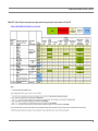
An example of information presented in a CF V1.2 multiplier file is presented in
Figure 3.1.
21
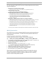
Department of Science, Information Technology and Innovation
Figure 3.1 A snapshot of information contained in a CF V1.2 multiplier file. For the selected location multipliers include, for each climate variable, the
st
projected change per degree of 21 Century global warming and projected amount of global warming at 2030 and 2050 used to construct CF daily climate
projections data (filename 056002_30.5167_151.6681_V1.2.multiplier). Multipliers are listed for 19 individual GCMs and the four GCM composites (WP, WI,
HP and HI) based on Representative Future Climate partitions. Other information (historical rainfall and projected CO2 concentration) are also included.
22
Consistent Climate Scenarios User Guide - Version 2.2
3.2 CO2 matching files
CF Version 1.2 data includes look-up tables called ‘CO2 matching files’ that have
been provided for each location. These files list the CO2 concentrations associated
with each projections file that has been provided.
The CO2 matching files are named as follows:
LocationCode_Latitude_Longitude_NamesList.txt
e.g.
051039_-31.5495_147.1961_NamesList.txt

LocationCode is a six digit number (BoM station code if patched-point, i.e. 051039, or all
zeros if drilled (from interpolated surfaces), i.e. 000000)

Latitude and longitude of the station or location in decimal degrees

NamesList.txt (CO2 matching file)
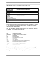
An example of information presented in a CO2 matching file is presented in Figure
3.2, with metadata, as follows:
LocationCode_Scenario_ProjectionsYear_ClimateWarming
sensitivity_ModelName_Latitude_Longitude_VersionNumber.SILOformat CO2
e.g.
051039_A2_2030_L_CSIRO-MK35_-35.5495_147.1961_V1.2.met 444.00

LocationCode is a six digit number (BoM station code if patched-point, i.e. 051039, or all
zeros if drilled, i.e. 000000)

Scenario (listed for each emissions scenario, i.e. A1B, A1FI, etc.)

Projections year (i.e. 2030 or 2050)

Climate warming sensitivity (rate of global warming, i.e. L, M, H)

‘L’, ‘M’ and ‘H’ refer to the 10 , 50 and 90 percentile values respectively.

Model Name (listed for each of 19 GCMs and four RFCs, i.e. CSIRO-MK35, HADGEM1,
HI, HP, etc.)

Latitude and longitude of the station or location in decimal degrees

Version Number (V1.2 represents CF data)

SILO format (either ’met’ for APSIM or ’p51’ for GRASP)

CO2 (concentration for the listed climate projections year and climate warming sensitivity),
to three decimal places.
th
th
th
23
Department of Science, Information Technology and Innovation
Figure 3.2 A snapshot of information presented in a CO2 matching file (filename 056002_30.5167_151.6681_NamesList.txt).
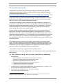
3.3 CO2 concentrations files
Two CO2 concentrations files are available. These are:
 an annual file, named CO2_concentrations_annual.dat containing CO2
concentrations for each year from 1970 to 2100
 a decadal file, named CO2_concentrations_decadal.dat containing CO2
concentrations for each decade from 1970 to 2100.
These files can be downloaded from:
ftp://climate.mft.derm.qld.gov.au/Climate_Scenarios/Documentation
The CO2 data used in the CCS project, and listed in these CO2 concentrations files, is
sourced from the IPCC . The IPCC has documented a range of emission scenarios
featured in the ‘Special Report on Emissions Scenarios (SRES)’ (IPCC, 2000). Six of
the scenarios documented by the IPCC (used in both AR3 and AR4) are utilised in
this project, representing outcomes of distinct narratives of economic development,
demographic and technological change. The SRES scenarios are: A1FI, A1B, A1T,
A2, B1 and B2 (see additional technical details describing these emissions scenarios
in Section 7.1).
In addition to the SRES scenarios, the CO2 concentrations files include two
‘stabilisation scenarios’ (CO2-450 and CO2-550) based on the work of Wigley et al.
(1996) and the CCS web portal includes these as options when ordering data. The
stabilisation scenarios examine the implications of stabilising CO2 at 2100 at various
concentrations.
The CO2 concentration files also contain the preliminary IPCC AR3 CO2 estimates
headed with the subscript ‘p’ and two older scenarios IS92A and IS92A/SAR.
Users should be aware that projected futures CO2 concentration pathways are
uncertain and may ‘undershoot’ or ‘overshoot’ the proposed trajectories.
24
Consistent Climate Scenarios User Guide - Version 2.2
Furthermore, the CO2 concentration files also include CO2 data for four scenarios
based on Representative Concentration Pathways (RCP 3-PD, RCP 4.5, RCP6.0
and RCP8.5). These RCPs that have been determined by projected radiative forcing
and have been used for the development of information for the IPCC Fifth
Assessment Report (AR5). Further documentation about these RCPs is available
from:

the IPCC Expert Meeting Report on New Scenarios (Noordwijkerhout report)
http://www.aimes.ucar.edu/docs/IPCC.meetingreport.final.pdf

the "Representative Concentration Pathways (RCPs) Draft Handshake"
http://www.aimes.ucar.edu/docs/RCP_handshake.pdf

the IPCC website at
http://sedac.ciesin.columbia.edu/ddc/ar5_scenario_process/RCPs.html.
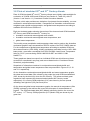
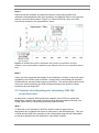
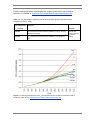
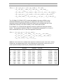
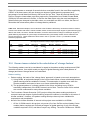
The information contained in the decadal CO2 concentrations file is shown in Figure
3.3 and Figure 3.4.
Notes

Projected 2030 CO2 concentrations for:
- A1FI (449ppm) are equivalent to RCP 8.5
- A1T (435ppm) are equivalent to RCP 4.5

Projected 2050 CO2 concentrations for:
- A1FI (555ppm) slightly exceed RCP 8.5 (541ppm)

Users should note that AR3 and AR4 based CO2 concentration data is
derived from the BERN model. Some GCM models used CO2 from the ISAM
model for their atmospheric forcing. The difference between the ISAM and
BERN models for the year 2050 for each SRES scenario is about 10ppm,
which is less than the difference between the ‘high’ and ‘low’ versions of each
model. Since more GCM models use CO2 derived from the BERN model we
supply this estimate with the climate data.

The preliminary IPCC AR3 CO2 estimates, two older scenarios IS92A and
IS92A/SAR and the new RCP CO2 data are for reference – there are no
corresponding CF or QM climate files.
25
Department of Science, Information Technology and Innovation
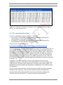
Figure 3.3 Observed (pre 2010) and projected (post 2010) decadal CO2 concentrations contained in the decadal file (CO2_concentrations_decadal.dat).
26
Consistent Climate Scenarios User Guide - Version 2.2
Figure 3.4 A snapshot of information contained in the annual CO2 concentrations data file (CO2_concentrations_annual.dat).
27
Department of Science, Information Technology and Innovation
3.4 Log warning files
Log warning files (see naming convention below) accompany the CF data, for each
point-location and model run. The log warning files hold information to alert users to
any problematic data. For example, data are generated for inclusion in log warning
files when projections data lie outside the bounds of what may reasonably be
expected.
The log warning files are typically named:
LocationCode_Latitude_Longitude_VersionNo.log
e.g.
056002_-30.5167_151.6681_V1.2.log

LocationCode is a six digit number (BoM station code if patched-point, i.e. 051039, or all
zeros if drilled (from interpolated surfaces), i.e. 000000)

Latitude (of the station or location in decimal degrees)

Longitude (as above)

VersionNumber (V1.2 represents CF data)
The log warning files include:

ModelName (i.e. CSIRO-MK35, HADGEM1, HI, HP, etc.)

Emissions ‘Scenario’ (A1FI, A1B, A1T, A2, B1, B2, CO2_450 or CO2_550)

Climate Warming sensitivity (low, median or high)
th
th
th
– ‘L’, ‘M’ and ‘H’ refer to the 10 , 50 and 90 percentile values respectively

Projections year (2030 or 2050)

Number of projected Tmin greater than projected Tmax
– Instances when the projected minimum temperature is greater than the maximum
projected temperature for the day.

Number of projected Vp greater than VpSat
– Instances where the projected vapour pressure is checked against the saturated
vapour pressure using WMO 2008 recommended functions without pressure
corrections.

Number of clamped projected radiation greater than ET radiation
– Instances where the projected radiation are clamped to 0.81% of the calculated extra
terrestrial maximum solar radiation on a horizontal surface and clear sky radiation.

Warning: Potential (or Implausible) Extreme Percent Change Rate
– Month affected
– Climate element affected (i.e. rain)
– Change from the historical baseline climate as a percentage change for rain,
radiation, relative humidity and pan evaporation, but an absolute change for
temperature, e.g. for rain a change of -75, means a 75 percent decline.
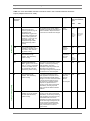
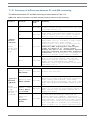
The thresholds for which log warnings are assessed are presented in Table 3.1.
28
Consistent Climate Scenarios User Guide - Version 2.2
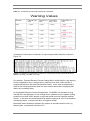
Table 3.1 Thresholds for which log warnings are assessed.
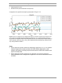
A snapshot of information contained in a log warning ancillary data file is shown in
Figure 3.5.
Figure 3.5 Snapshot of information contained in a log warning ancillary data file (filename
056002_-30.5167_151.6681_V1.2.log).
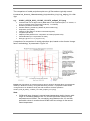
For example, ‘Potential Extreme Percent Change Rate’ will be listed in a log warning
file if the application of the ‘change factor’ produces more than a 50% decline in
projected rainfall from the historical baseline climate. In this case no adjustment is
made to the rainfall projections data, but users need to be cautious if applying that
data in any modelling study.
An ‘Implausible Extreme Percent Change Rate - CLAMPED’ will be listed in a log
warning file if the application of the ‘change factor’ obtained from the pattern scaling
produces more than a 90% decline in projected rainfall from the historical baseline
climate. In this case the rainfall projections data are clamped at 10% of the baseline
climatology values, to avoid occurrence of negative rainfall.
Information about limitations related to the capture of anomalous data in the Log
Warning files, is presented in Section 10.2.
29
Department of Science, Information Technology and Innovation
Notes

Users should note that the precision of the values listed in the Log warning files is
for calculation purposes only and will not occur in reality.

In some cases (usually individual days) anomalous values may occur. These
values may be derived from one of three sources, which are: 1) the raw data, 2)
interpolation, or 3) the modification to “climate changed data”.
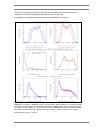
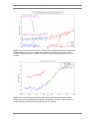
3.5 Historical time series plots
Historical time series plots, for the six climate variables used in the CCS project,
have been provided as part of the user information framework. The plots provide
users with representations for specific locations showing the historical annual
variability, as well as a longer-term trend (i.e. rising mean annual temperature).
The plots are location-specific and show the daily average for each year, as an
annual time series, extracted from historical SILO climate data.
Although users can select any period from 1960 onwards, 1960 to 2010 is the
recommended historical baseline. Periods of less than 30 years are
insufficient for climate-change trend analysis.
The historical time series plots are .png files and are typically named:
LocationCode_Lat_Long_V1.2.png
e.g.
040112_-26.5544_151.8456_V1.2.png

LocationCode is a six digit number (BoM station code if patched-point, i.e. 040112, or all
zeros if drilled (from interpolated surfaces), i.e. 000000)

Latitude (of the station or location in decimal degrees)

Longitude (as above)

VersionNumber (V1.2 represents CF data)
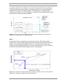
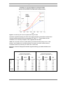
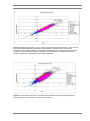
A snapshot of a historical time series plot is presented in Figure 3.6.
30
Consistent Climate Scenarios User Guide - Version 2.2
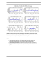
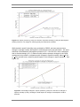
Figure 3.6 Historical time series plot for Mt Brisbane, Queensland (LocationCode 040140),
(filename: 040140_-27.1492_152.5781_V1.2.png). Annual variability is shown is black. The
linear trend for the selected base period (in this case 1960-2010) is shown in blue. Historical
time-series plots are not produced for periods of less than six years.
Notes



Pan evaporation data from 1970 onwards are from daily ‘class A’ pan
evaporation measurements. Prior to this the data is synthetic pan.
Linear trend lines showing the selected long-term trend are not plotted for
periods of 30 years or less.
The historical time-series plots are not produced for periods of less than six
years.
31
Department of Science, Information Technology and Innovation
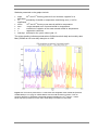
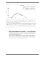
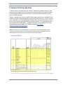
3.6 CF Frequency distribution plots
CF v1.1 based frequency distribution plots, based on the A1B emissions scenario for
six climate variables, were initially provided as test data as part of the user
information framework for the Consistent Climate Scenarios project. The plots
provide users with a visual impression of historical and projected frequency
distribution changes. Initial inspection of the plots shows that the output is as
expected (i.e. increased temperatures). These plots are not currently available
through the CCS web-portal (see Section14 for contact details).
The plots are designed to inform users of the change in frequency distributions
(shown on the y-axis) for both the observed (1960-2009 baseline) and the projected
(2050) climate data. The frequency distribution plots provide users with an analysis
of the occurrence of discrete values of specified climate variables, expressed as a
percentage of the total distribution for that variable.
The CF based frequency distribution plots are not provided with the CF V1.2 datasets
via the web Climate Change Projections web portal, as not all users will request the
A1B scenario with their data order. However, plots are for specific locations in
Australia and can be made available on request for 17 GCMs, the A1B emissions
scenario, high climate warming sensitivity and six climate variables. The climate
variables are:





rainfall
maximum and minimum temperature
solar radiation
vapour pressure
pan evaporation.
The frequency distribution plots are .gif files and are typically named:
ModelName_Scenario_ClimateSensitvity_ProjectionsYear_LocationCode_Lat_Long_fdist_
v1.1.gif
e.g.









32
CSIRO-Mk35_A1B_H_2050_051039_-31.5495_147.1961_fdist_v1.1.gif
ModelName (BCCR, CCCMA-47, CCCMA-63, CNRM, CSIRO-MK30, CSIROMK35, ECHAM5, ECHO-G, GFDL-20, GFDL-21, GISS-AOM, HADCM3,
HADGEM1, IAP-FGOALS, INMCM, MIROC-H, MIROC-M, MRI-GCM232, NCARCCSM)
Scenario (emissions scenario: A1B)
Climate Warming sensitivity (high)
– ‘H’ refers to the 90th percentile value
Projections year (2050)
’LocationCode’ is a six digit number (BoM station code if patched-point, i.e.
051039, or all zeros if drilled (from interpolated surfaces), i.e. 000000)
Latitude (of the station or location in decimal degrees)
Longitude (as above)
fdist (frequency distribution file)
VersionNumber (v1.1 represents CF data )
Consistent Climate Scenarios User Guide - Version 2.2
Change in frequency is greatest where there are large differences between the
observed (coloured) and projected (black) points on the plots.
A snapshot of a frequency distribution plot is presented in Figure 3.7.
Figure 3.7 Frequency distribution plots, observed with 2050 projections, for Nyngan Airport
(LocationCode 051039) in South Australia (filename CSIRO-MK35_A1B_H_2050_051039_ 31.5495_147.1961_fdist_v1.1.gif), from a run of the CSIRO-Mk3.5 GCM forced by the A1B
emissions scenario with high climate warming sensitivity. Observed values are coloured,
projections are shown in black.
33
Department of Science, Information Technology and Innovation
Spikes in pan evaporation frequency distribution plots
Bureau of Meteorology Class A pan evaporation site data has been used since 1970.
Bird cages were installed then, to reduce errors, (e.g. evaporation readings were
occasionally too high, due to animals drinking or splashing water). The frequency
spikes that occur in the observed pan evaporation frequency distribution plots are
due largely to lack of precision in some (post 1970) manually recorded observations.
For example, during measurement, evaporation has been rounded down to the
nearest full can (which holds 4 mm), giving spikes at 4 mm and 8 mm on the x-axis,
rather than providing more precise values. Spikes in the observed data also occur on
high rainfall days, especially if the pan overflows, or there is a reading error in the
rainfall, which is subsequently transferred to the pan reading.
3.7 Comparison of model projections plots
Comparison of model projections plots are provided, in the ZIP archives, as part of
the user information framework, to assist users in GCM model selection.
Each plot is location specific and shows projected changes (i.e. climate ‘change
factors’) at 2030 from a 1960-2010 base period climate, for both annual mean
temperature and rainfall. The changes in temperature and rainfall are presented for
each of 19 GCMs and three climate warming sensitivities (low, median and high).
The GCMs were all forced by the A1B emissions scenario.
The projected changes have been calculated using amounts of global warming from
MAGICC applied to the mean annual rate of change for rainfall and temperature per
degree of global warming.
On each plot:







34
change in annual mean rainfall is shown on the x-axis
change in annual mean temperature is shown on the y-axis
GCM model names are abbreviated (i.e. CCCMA, GISS)
the mean change from the 1960 to 2010 base period for the aggregate of all
seventeen GCMs models is shown by the blue circle
changes in the median, from the base period, for individual models are shown by
red squares
changes in rainfall, based on 10th and 90th percentile climate warming sensitivities
are indicated by the horizontal barbs
changes in temperature for 10th and 90th percentile climate warming sensitivities
are indicated by the vertical barbs.
Consistent Climate Scenarios User Guide - Version 2.2
The comparison of model projections plots are .gif files and are typically named:
LocationCode_Scenario_ClimateSensitvity_ProjectionsYear_Lat_Long_mdlperf_V1.2.File
Type
e.g.









014901_A1B_M_2030_-13.8345_131.1872_mdlperf_V1.2.png
LocationCode is a six digit number (BoM station code if patched-point, i.e. 014901, or
all zeros if drilled (from interpolated surfaces), i.e. 000000)
Scenario (emissions scenario: A1B)
Climate Warming sensitivity (default ‘M’ place holder only)
Projections year (2030)
Latitude (of the station or location in decimal degrees)
Longitude (as above)
mdlperf (model performance: comparison of model projections file)
VersionNumber (V1.2 represents CF data )
FileType (.gif for v1.1 or .png for V1.2)
A snapshot of a comparison of model projections plot, based on the climate ‘change
factor’ methodology, is presented in Figure 3.8.
Figure 3.8 Comparison of model projections plot for 2030 for Douglas River (LocationCode
014901) in Northern Territory. Plot generated using Version 1.2 projections data climate
‘change factors’ for GCMs forced by the A1B emissions scenario (filename
014901_A1B_M_2030_-13.8345_131.1872_mdlperf_V1.2.png).
Note

GCMs with large changes in annual mean temperature tend to have a wide
range of uncertainty between the 10th and 90th percentile values for both
temperature and rainfall. The uncertainty range between the 10th and 90th
percentile values is smaller where GCMs have less change in the annual
mean temperature.
35
Department of Science, Information Technology and Innovation
3.8 Plots of simulated 20th and 21st Century climate
Plots of GCM simulated 20th and 21st Century climate were initially made available for
a selection of 23 AR4 A1B forced GCM runs (see Section 8, Table 8.2), with CF
(Version 1 and Version 1.1) Consistent Climate Scenarios datasets.
The plots, which also provide some indication of projected climate variability, are now
contained in a draft document entitled, “Comparisons of Australian continental areaweighted mean rainfall and temperature, and global mean temperature according to
available AR4 A1B forced GCM runs”.
Each plot included graphs showing time-series of the observed and GCM simulated
20th Century and GCM simulated 21st Century for:



Australian continental area-weighted mean rainfall;
Australian continental area-weighted mean temperature; and
global mean temperature.
The monthly mean precipitation and temperature data used to produce the Australian
continental graphics were accessed from DSITIA copies of the IPCC CMIP3 data set.
For the comparisons of global mean temperature according to available GCM runs,
the measured series (1901-2009), initially provided as anomalies from the 1951-1980
base period, were taken unmodified from GISS GLOBAL Land-Ocean Temperature
Index in 0.01ºC (sources being GHCN 1880-2010+SST and 1880-11/1981
HadSST1).
These graphs are based on output from individual GCM runs which have not been
re-scaled or normalised in any way (and are not based on the ‘Consistent Climate
Scenarios’ projections data).
Snapshots of information contained in continental area-weighted rainfall and
temperature and global mean temperature files are presented in Figures 3.9, 3.10
and 3.11 respectively.
On the Australian continental area-weighted rainfall and mean temperature graphs,
the observed annual data (Obs, shown by the purple line) and GCM simulated data
(20C, shown by the blue line) cover the 20th Century. The yellow and dark green
regression lines represent the observed and simulated 20th Century trends
respectively. 21st century GCM projections (21C) are shown by the red (annual
variability) and light blue (100 year trend) lines.
On the observed global mean temperature graphs, the annual air temperature (Obs
(GISS)) is shown by the red line and covers the time-span of measured data to
present. The GCM simulated data (20C (Model)) shown by the blue line cover the
20th century. 21st Century GCM projections (21C (Model A1B)) are shown by the
green line.
36
Consistent Climate Scenarios User Guide - Version 2.2
Statistics presented on the graphs include:







slope
20th and 21st Century (positive for an increase, negative for a
decrease)
Pr
probability of rainfall or temperature trend being zero (< 0.05 is
significant)
mean
20th and 21st Century mean annual rainfall or temperature
mse
mean standard error of annual rainfall or temperature
cv
coefficient of variation of the mean annual rainfall or temperature
r:
regression coefficient
intercept intercept on the y-axis, where year = 0
The yellow shading indicates periods where GCMs have both daily and monthly data.
Many GCMS do not have daily data prior to 1945.
Figure 3.9 Time series presented in a continental area-weighted mean rainfall file (filename
CSIRO-Mk30.pr.run1.png) for CSIRO-Mk3.0 with the A1B emissions scenario. This run
st
shows a decrease in Australian continental weighted rainfall in the 21 Century. Yellow
bands represent periods for which DSITI holds daily information for that GCM.
37
Department of Science, Information Technology and Innovation
Figure 3.10 Time series presented in a continental area-weighted temperature file (filename
CSIRO-Mk30.tas.run1.png) for CSIRO-Mk3.0 with the A1B emissions scenario. This run
st
shows a marked increase in Australian continental weighted mean temperature in the 21
Century.
Figure 3.11 Time series presented in a global mean temperature file (filename CSIROMk30.gw.run1.png) for CSIRO-Mk3.0 with the A1B emissions scenario. This run shows a
st
marked increase in global mean temperature in the 21 Century.
38
Consistent Climate Scenarios User Guide - Version 2.2
3.9 Quantile trend plots
If diagnostics are selected, when ordering through the web-portal, the QM 2030
datasets will include plots of location-specific quantile3 trends. QM 2050 quantile
trend plots can be downloaded via
ftp://climate.mft.derm.qld.gov.au/Climate_Scenarios/QM_2050_TestData/. These
are the trends that have been used to estimate target cumulative distribution
frequencies (CDFs) for 2030 for projected rainfall, maximum temperature, minimum
temperature, solar radiation and specific humidity (or their transforms) and target
CDFs for 2050 for solar radiation and specific humidity.
The plots are arranged by month and show historical time-series for quantiles 0.1,
0.5 and 0.9, of daily data for each month, including1957 to 2010 training-period linear
trends as well as forward extrapolation of these trends (to 2030/2050). Computed
statistical significance of each trend (represented by p-values) over the training
period is given as well for each climate variable,
Quantile trends have been classed as significant when the computed statistical
significance, called the p-value statistic (shown on each graphic) is 0.1 or less (i.e.
when there is at most a 10 per cent probability that the observed data arose from an
underlying stationary distribution). If a computed p-value for a quantile trend exceeds
the 0.1 cut-off, the trend is not used in the QM projections and no trend is applied.
This represents a null model in which the future quantiles are the same as those over
the training period.
In the QM processing, corrections are made in cases where future trends would
cross. This does not apply to rainfall and temperature variables in the QMV2.2.10
datasets for 2050 which utilise a future CDF based on daily GCM data and not trend
extrapolation, but does apply to QM 2050 solar radiation and specific humidity for
which future CDFs are estimated using trend extrapolation.
The quantile trend plots are .png files and are typically named:
ClimateVariable_LocationCode_PivotQuantiles_1957_2010_ProjectionsYear_QuantileTrends_Loc
ationCode.png
e.g. T.Min_040428_[10,50,90]_1957_2010_2030_QuantileTrends_040428.png

ClimateVariable
– RadnPropOfEtlogit (solar radiation transformed by ground level
proportion of extra-terrestrial, then logit transform used)
– RainCubeRoot (rainfall transformed by cube root)
– SH (specific humidity transformed from vapour pressure)
– T.Max (maximum temperature, no transform)
– T.Min (minimum temperature, no transform)

LocationCode is a six digit number (BoM station code if patched-point, i.e. 002012, or all
zeros if drilled (from interpolated surfaces) i.e. 000000)

PivotQuantiles [10,50,90] denotes 0.1, 0.5 and 0.9 quantiles

1957_2010 (historical training period)
3
Quantiles differ from percentiles, in that quantiles are expressed in sample fractions rather than
sample percentages. Quantile 0.1 is equivalent to the 10 th percentile.
39
Department of Science, Information Technology and Innovation

2030 (projections year)

QuantileTrends (denotes Quantile trend plot file)
A snapshot of a quantile trend plot is presented in Figure 3.12.
Figure 3.12 An example from a quantile trend plot for a specific showing time series for the
0.1, 0.5 and 0.9 quantiles (and the statistical significance, i.e. p-values) of daily minimum
temperature for Augusts, with trends computed over the 1957-2010 period location (filename:
T.Min_040428_[10,50,90]_1957_2010_2030_QuantileTrends_040428.png). Plotting scales
may change between stations.
Notes

Where observed quantile trends are statistically significant (p <0.1), the ‘quantilematched’ approach is used to produce the 2030 rainfall, temperature, solar
radiation and specific humidity projections data and the 2050 solar radiation and
specific humidity data.

Where observed quantile trends are not significant, the climate projections
method defaults to the ‘change factor’ approach for the above-mentioned climate
variables.
40
Consistent Climate Scenarios User Guide - Version 2.2
3.10 Histograms of ‘quantile-matched’ climate projections
If diagnostics are selected, when ordering through the web-portal, the QM 2030
datasets will include plots of histograms of QM climate projections. QM 2050 quantile
trend plots can be downloaded via
ftp://climate.mft.derm.qld.gov.au/Climate_Scenarios/QM_2050_TestData/.
These histograms, arranged by month, are location-specific and show frequency
distributions for specified climate variables (or their transforms). The frequency
distributions include ‘quantile-matched’ 2030 or 2050 projections data in comparison
to an observed 1957-2010 baseline climate.
Months where no significant quantile trends are computed will be apparent in the
histogram plots as a simple horizontal translation between the historical (black
shaded) and ‘quantile-matched’ (orange shaded) data, due to OzClim ‘change factor’
based trends only.
The means (µ) and sample standard deviations (sN) of the historical and ‘quantilematched’ data are shown on each plot.
Users should note that the plotting scales may differ between stations.
The histograms are .png files and are typically named:
ClimateVariable_LocationCode_PivotQuantiles_1957_2010_ProjectionsYear_Histograms_
LocationCode_ModelName_Scenario_ClimateWarmingSensitivity.png
e.g.
T.Min_040428_[10,50,90]_1957_2010_2030_Histograms_040428_HADCM3_A
1FI_high.png

ClimateVariable
– Radn (solar radiation transformed by ground level
proportion of extra-terrestrial, then logit transform used)
– Rain (rainfall not-transformed)
– RainCubeRoot (rainfall transformed by cube root)
– VP (transformed to specific humidity, then back to vapour pressure)
– T.Max (maximum temperature, no transform)
– T.Min (minimum temperature, no transform)

LocationCode is a six digit number (BoM station code if patched-point, i.e. 002012, or all
zeros if drilled (from interpolated surfaces), i.e. 000000)

PivotQuantiles [10,50,90], denotes 0.1, 0.5 and 0.9 quantiles

1957_2010 (historical training period)

Projections year (2030 or 2050)

Histograms (denotes Histograms trend plot file)

Model Name (i.e. CSIRO-MK35)

Scenario (emissions scenario, i.e. A1B, A1FI, etc.)

Climate warming sensitivity (rate of global warming) i.e. low, med, high, referring to the
th
th
th
10 , 50 and 90 percentile values respectively.
A snapshot of a quantile-based historgam is presented in Figure 3.13.
41
Department of Science, Information Technology and Innovation
Figure 3.13 Minimum temperature information displayed in a histogram of ‘quantile-matched’
(QM) projections data for Augusts for a specific location, showing differences between the
observed 1957 to 2010 baseline climate and QM 2030 climate projections data. This plot
(filename: T.Min_040428_[10,50,90]_19572010_2030_Histograms_040428_HADCM3_A1FI_high.png) shows a positive shift in the QM
th
th
frequency distribution. The blue semi circles on the x-axis represent projected 10 , 50 and
th
90 percentile values of the mean daily minimum temperature for 2030, using QM trends.
Observed 1957-2010 and projected 2030 means and corresponding standard deviations are
presented in the top right panel.
Notes


42
Where observed quantile trends are significant (p <0.05), the QM approach is
used to produce the 2030 rainfall, temperature, solar radiation and specific
humidity projections data and the 2050 solar radiation and specific humidity
data and the projected standard deviation shown in the plot will differ from
that of the historical baseline data.
Where observed quantile trends are not significant, the climate projections
method defaults to the ‘change factor’ approach for the above-mentioned
climate variables and the projected standard deviation shown in the plot will
be the same as that of the historical baseline data.
Consistent Climate Scenarios User Guide - Version 2.2
3.11 Transient climate data test set for 1889-2100
A test set of transient climate change files, and background documentation, are
located in a zip archive named transient_data_test_set.zip at
ftp://climate.mft.derm.qld.gov.au/Climate_Scenarios/Transient_TestData/
The transient climate change files contained within the zip archive are named as
follows:
e.g. 035149_-24.8353_149.8003_NCAR-CCSM_CO2-550_med_CF1.2EM09.wth

Station number, also called Location Code (035194)

Latitude of the station in decimal degrees (24.8353 South)

Longitude of the station (149.8003 East)

GCM Model Name (17 are available, i.e. NCAR_CCSM)

SRES emissions scenario (eight are available, i.e. CO2-550)

Climate warming sensitivity (i.e. low, med, high), referring to the 10 , 50 and 90
percentile values respectively.

Projections Method Code and Version (CF 1.2)

Ensemble Code (EM)

Ensemble number
–
e.g. 01 starting point 1962
–
02 “
” 1963
–
03 “
” 1968
–
04 “
” 1972
–
05 “
” 1975
–
06 “
” 1985
–
07 “
” 1986
–
08 “
” 1996
–
09 “
” 2001
–
10 “
” 2009

File type (transient climate data .wth)
th
th
th
The transient climate change files have been constructed for a single location
(Brigalow Research Station, Central Queensland), and formatted for use in the
CENTURY model, as “proof of concept”, prior to further systems development.
The transient climate change files include historical data back to 1889 and CF based
projections data to 2100. The test data are for the same range of seventeen GCMs,
eight emissions scenarios and three climate warming sensitivities as the CF Version
1.1 2030 and 2050 projections datasets. Ten ensemble members, with starting years
between 1962 and 2009 are provided.
The data files contain the projections year, and for each month, precipitation total, mean
daily minimum and mean daily maximum temperatures, and at the end of each data row,
the source year, the index (1-10) to the analogue start year, and the expected degrees
of global warming (ºC). These extra data fields are not read by the CENTURY model and
are for diagnostic purposes in this data set.
43
Department of Science, Information Technology and Innovation
An example of information presented in a transient climate change data file is
presented in Figure 3.14.
Figure 3.14 A snapshot of information presented in a transient climate change data file,
suitable for use in CENTURY (filename 035149_-24.8353_149.8003_NCAR-CCSM_CO2550_med_CF1.2EM09.wth).
In addition to the transient climate change data files, the zip archive includes
multiplier files, from which ‘change factors’ have been calculated. The multiplier files,
which are described in Section 3.1 of this User Guide, are named as follows:
LocationCode_Latitude_Longitude_VersionNo.multiplier
e.g.
44
035149_-24.8353_149.8003_v1.2.multiplier
Consistent Climate Scenarios User Guide - Version 2.2
4 ‘Change factor’ (CF) methodology
This section of the User Guide describes the methodology, employed by CSIRO, to
prepare the OzClim climate ‘change factors’ (CSIRO, 2010). The section also
outlines how climate ‘change factors’ are applied to historical data to produce climate
estimates for the future.
The climate ‘change factors’ used to calculate CCS data have been estimated using

Coupled Model Intercomparison Research Program 3 (CMIP3) patterns of
change data (projected changes per degree of 21st Century global warming)
supplied by the CSIRO and the UK Met Office/Hadley Centre; and

data from SRES scenario temperature response curves (projected amounts of
global warming) supplied by the CSIRO.
4.1 ‘Change factor’ definition
The term climate ‘change factor’ refers to the change in the climatological mean of a
specific climate variable (e.g. temperature) between the current climate (defined in
terms of a suitable 20th Century base period) and a projected time in the future (for
example, the 30 years centred on 2050).
Calculated on a monthly basis, ‘change factors’ may be used as scalars to transform
historical daily climate time-series to produce time-series of projected future climate
for use in biophysical models. Climate ‘change factors’ have been calculated, using
the OzClim4 methodology, and applied to SILO historical baseline climate data to
produce the Consistent Climate Scenarios CF (Version 1,Version 1.1 and Version
1.2) projections datasets for 2030 and 2050. In OzClim, ‘change factors’ are applied
to a 1975 to 2004 baseline climate (CSIRO, 2010).
4.2 Background
The CMIP3 (Coupled Model Intercomparison Project 3) database includes
experiments from the 23 GCM models submitted to the International Panel for
Climate Change (IPCC) Fourth Assessment Report (AR4). IPCC AR4 represents a
global scientific consensus on the issue of climate change and is accepted as the
highest authority for policy makers. The CMIP3 database has been freely available
to the global research community resulting in unprecedented levels of evaluation and
analysis.
OzClim (CSIRO, 2010) is a CSIRO product, used to explore climate change
scenarios from 2020 to 2100 for Australia and has an interactive website at
http://www.csiro.au/ozclim. OzClim provides climate change projections information
based on the results of experiments from 23 GCM projections, which are a subset
from the International Panel for Climate Change Fourth Assessment Report (IPCC
AR4).
For any one GCM, the experiments in the CMIP3 database do not cover the full
range of emissions scenarios (eight) which were considered by the IPCC in its
4
OzClim version 3
45
Department of Science, Information Technology and Innovation
Special Report on Emissions Scenarios (SRES) (IPCC, 2000). The experiments also
did not include a desirable level of replication.
The IPCC employed a relatively straight-forward methodology to extrapolate AR4
model outputs across all SRES scenarios and to quantify the sensitivity of the
warming response to a particular emissions scenario. This method involves the use
of a coupled gas/climate model called MAGICC (Model for the Assessment of
Greenhouse-gas Induced Climate Change) (Wigley, 2000), which uses emissions
scenarios for greenhouse gases, reactive gases and sulphur dioxide, to calculate
projected global warming for the eight SRES emissions scenarios.
For each emissions scenario, the IPCC provides low, moderate and high warming
responses (equivalent to the 10th, 50th and 90th percentile projections) representing
the range of sensitivity of global temperature rise to each emissions scenario.
4.3 Calculation of ‘change factors’
The calculation of ‘change factors’ for individual GCMs is relatively straight forward.
CSIRO employ a ‘pattern scaling’ approach, as used in OzClim (described briefly
below), to calculate, for each surface grid-point5 of a GCM, the projected change
(over the 21st Century) in a given climate variable per degree global warming. This is
termed the ‘pattern of change’. Patterns of change differ according to specific
emissions scenarios, climate warming sensitivities and GCM runs.
Whereas temperature change per degree global warming is expressed in absolute
terms, (i.e. degrees Celsius change per degree global warming), projected change in
other climate variables (e.g. rainfall, evaporation, solar radiation and vapour
pressure) is expressed in relative terms (i.e. as percentage change per degree global
warming). To produce a ‘change factor’, the pattern of change (i.e. projected change
per degree global warming) for a given climate variable is then multiplied by the
warming curve from each of the eight SRES scenarios and climate warming
sensitivities established using MAGICC. This ‘change factor’ can then be applied to
a suitable 20th Century baseline climatology to produce projections of a given climate
element.
The patterns of change used in the Consistent Climate Scenarios project have been
obtained from OzClim patterns of change files and raw GCM files, provided by
CSIRO Marine and Atmospheric Research (CMAR). The source files for the patterns
of change computations are monthly averages of GCM derived model output for
individual climate variables and for specific runs.
Further detail, on the use of patterns of change, to calculate estimates for specified
climate variables at a particular point in the future, is described in detail in several
papers (Mitchell, et al. (1999), Mitchell (2003), Whetton, et al. (2005) and Ricketts
(2009)).
The pattern scaling approach employed by CSIRO (2010), and adopted for use in
this project, can be summarised as follows:
5
A GCM grid-point (which is typically 150-250km2) is the essentially the same as a grid-‘cell’.
46
Consistent Climate Scenarios User Guide - Version 2.2
Using output from individual runs of a given GCM forced by a specific emissions
scenario:
Step 1
Extract global annual averages of 21st Century surface temperature projections
(Figure 4.1a).
Step 2
For an individual GCM model’s grid-point (typically 150-250km2), extract monthly
projections of a given climate variable (e.g. temperature or rainfall, Figure 4.1b).
Step 3
Using a simple linear regression approach, compute the linear trend (slope) between
the global annual average surface temperature (Step 1) and the average monthly
values of a given climate variable for that grid-point (Step 2). The calculated slope
for each grid-point represents the mean rate of change of that climate variable per
degree global warming’ (Figure 4.1c).
Step 4
Repeat the above steps for each grid-point across Australia to produce the projected
pattern of change per degree of 21st Century global warming across Australia for that
climate variable (Figure 4.1d).
Step 5
As GCMs vary in their spatial resolution, interpolate the pattern of change obtained in
Step 4 to a finer (regional) scale. It should be noted that representing GCM output
on a common 25km x 25km base provides utility in terms of application but does not
imply increased accuracy over the native resolution of the GCM outputs. [Patterns of
change for specific locations are available in the monthly multiplier ancillary files
supplied with CF data].
Step 6
Calculate ‘change factors’, by applying the above ‘pattern of change’ (change per
degree global warming) to global warming projections (from MAGICC) for each of the
eight SRES emissions scenarios (that part of the equation shown in brackets in
Figure 4.2).
Step 7
Apply ‘change factors’ for specific locations to a suitable 20th Century baseline
climatology to produce projections for a given climate variable (Figure 4.2). In
OzClim, ‘change factors’ are applied to a 1975 to 2004 baseline climate (CSIRO,
2010).
Monthly climate ‘change factors’ for individual locations have been calculated for
seventeen individual GCMs (see Section 6) using amounts of global warming at 2030
and 2050 for eight emissions scenarios (A1FI, A1B, A1T, A2, B1, B2, C02-450 and
C02-550) and three climate warming sensitivities (low, median and high). The
47
Department of Science, Information Technology and Innovation
‘patterns of change’ and amounts of global warming (from which the climate ‘change
factors’ can be calculated) are contained in the monthly multiplier files (described in
Section 3.1) provided with the projections data.
Further details related to the method used to produce OzClim patterns of change are
available at: http://www.csiro.au/ozclim and documented by Mitchell et al. 1999; Page
and Jones 2001, Michell 2003; Whetton et al. 2005; Ricketts 2009, and Ricketts and
Page 2007.
Figure 4.1 Steps to producing OzClim patterns of change for an individual month and single
Global Climate Model (GCM). Panel A is the annual global temperature for the GCM. Panel B
is the monthly temperature time-series for an individual grid-point. Panel C is the combination
of Panel A and Panel B (with a regression line from which the annual rate of change per
degree of global warming (slope) for that month is calculated for a specific grid-point). Panel
D displays the slope for each grid-point across Australia, following interpolation to a finer
scale across Australia (after CSIRO, 2010).
Figure 4.2 Climate scenario generation for annual temperature in 2060. The regional pattern
from a GCM is multiplied by the global warming for 2060 and added to the observed baseline
climatology (i.e. OzClim has used 1975-2004). In this example, the GCM is CSIRO Mk3.0, the
emissions scenario is SRES A1FI, and the rate of global warming is high (after CSIRO, 2010).
Further information, about issues related in the calculation of ‘change factors’,
including downscaling from Global Climate Models and the calculation of trends per
degree of global warming, is discussed in Section 9 and 10.
48
Consistent Climate Scenarios User Guide - Version 2.2
4.4 A worked example – projecting climate data for 2050 for a
specific location
An outline of the above processes, required to generate CCSP data based on the
OzClim ‘change factor’ approach, is presented in Table 4.1. This example shows the
steps required to calculate 2050 projections data for July at Brian Pastures, using the
CSIRO-Mk3.5 GCM forced by the A1T emissions scenario with low climate warming
sensitivity.
Table 4.1 An outline of the steps involved, to calculate ‘change factors’ for applying to a
baseline climatology, to produce 2050 climate projections for July at Brian Pastures. This
example uses CSIRO-Mk3.5 forced by the A1T emissions scenario with low climate warming
sensitivity.
Step 1
•
Step 5
st
Extract 21 Century GCM
projections of global annual
average surface
temperature from a selected
Global Climate Model (i.e.
CSIRO-Mk3.5).
•
•
Step 2
•
•
•
Select climate variable (i.e.
rainfall or temperature) and
month (July).
st
Extract the 21 Century
projections (average
monthly values) of climate
variable at GCM model gridpoint.
Climate variable infilled by
DSITIA, if not available
through OzClim.
Step 6
•
•
Step 3
•
Compute linear trend (mean
rate of change per degree of
st
21 Century global
warming) between
projections of global annual
average surface
temperature and projections
of monthly climate variable
at GCM grid-point level.
•
•
•
Repeat the above steps for
each grid-point across
Australia to produce the
pattern of change (mean
st
rate) per degree of 21
Century global warming
across Australia for specific
climate variables.
Calculate climate ‘change factor’ by
multiplying the above ‘pattern of change’ by
the projected amount of global warming at
2050.
The amount of global warming, from
MAGGIC, for 2050 using the A1T
emissions scenario with low climate
warming sensitivity is +1.24ºC (obtained
from the multiplier file, see Section 3.1).
For rainfall, the 2050 ‘change factor’ (1.24 x
-18.68) is -23.16, i.e. a 23.16% decrease.
For temperature, the 2050 ‘change factor’
(1.24 x 1.12) is 1.39, i.e. a 1.39ºC increase.
Step 7
•
•
Step 4
Interpolate regional ‘pattern of change’ to a
uniform (25km x 25km) base, then select
pattern of change for a specific location.
In this example, at Brian Pastures (Location
Code 040428), the CSIRO-Mk3.5 pattern of
st
change for rainfall per degree of 21
Century global warming (obtained from the
multiplier file, see Section 3.1) is -18.68%,
and the pattern of change for minimum
temperature per degree of global warming
is +1.12ºC.
•
•
Apply clamping if the ‘change factor’ is
outside the acceptable range.
Apply the ‘change factors’ to suitable 20th
Century baseline climatology to produce
projections for the given climate variables.
In this example, for rainfall we take 23.16%
off all SILO historical July daily rainfall
values to obtain projected data for 2050.
For temperature, we add 1.39ºC to all SILO
historical July daily minimum temperature
values to obtain projected data for 2050.
49
Department of Science, Information Technology and Innovation
5 ‘Quantile-matching’ (QM) methodology
This section of the User Guide provides an outline of the methodology that DSITI has
used to prepare QM climate projections data for 2030 and 2050. Further information
describing the ‘quantile-matching’ approach is documented in Kokic et al. (2012) and
Panjkov (2012).
The QM method produces projected daily data for the future by mapping historical
cumulative distribution functions (CDFs), sourced from a 1957 to 2010 training
period, to a supposed future CDF. A variation in the QM method is used, depending
on whether projections for 2030 or 2050 are required. Different methods are required,
as there is almost no daily data for GCMs around 2030. In addition, even where data
do exist, no daily data for surface water vapour and solar radiation are available.
For 2030, the future CDF is estimated by the forward projection of historical trends in
monthly quantiles out to that year. However, beyond 2030, there is a risk that
historically-based quantile trends may meet or cross each other at some point in
time, particularly under emissions scenarios associated with high climate sensitivity
to global warming. Therefore, to acquire 2050 projections datasets, future CDFs for
rainfall and temperature variables have been computed differently, using daily data
obtained from GCMs instead of extrapolating historical quantile trends.
As with CF data, QM 2030 projections have been computed for 19 GCMs, eight
emissions scenarios, three climate sensitivities and six climate variables. However,
due to limited daily GCM data, QM 2050 projections have only been prepared for a
single GCM (ECHAM 5), emissions scenario (A1B) and climate sensitivity (median).
While the approach for 2050 rainfall and temperature projections uses daily GCM
data, QM 2050 projections for other climate variables use the QM 2030 method
extended to 2050 (discussed further in Section 5.2).
5.1 Steps involved to calculate QM projections data for 2030
Step 1
Compute the quantile ranking of a climate variable for each historical day in its
containing month, based on a 1957 to 2010 training period.
Step 2
To construct a plausible future CDF (to represent future variability), project the
historical trends in three or more "pivot" quantiles (usually 0.1, 0.5 and 0.9) out to the
target projection year (usually 2030). These historical trends (Figure 5.1) are not
used if their computed statistical significance exceeds a cut-off threshold, currently pstatistic = 0.1. Interpolation and use of conservative extrapolation methods has been
used to estimate the future CDF at quantiles other than the pivot quantiles. This
process is carried out for most6 of the climate variables, but some of the climate
variables will have been pre-transformed to limit any non-physical projections, such
6
Pan evaporation is not computed by ‘Quantile-matching’, but uses the ‘Change factor’ methodology
based on synthetic pan evaporation functions (Rayner, 2005) using ‘Change factors’ for vapour
pressure and solar radiation.
50
Consistent Climate Scenarios User Guide - Version 2.2
as negative rainfall or solar radiation in excess of extraterrestrial incoming radiation.
The pre-transformation is also done to normalise the data, i.e. make the regression
residuals more nearly normally distributed. The QM procedure is applied to the
transformed variables. An inverse transform is applied to the resulting projected data
to generate the projected climate variables.
Figure 5.1 Quantile trend plot for September daily maximum temperature, showing how
quantiles 0.1,0.5 and 0.9 are computed for 2030.
Step 3
Each historical value is replaced by a value from the future CDF with the same
quantile rank, using ‘quantile-matching’ functions that have been computed for each
location, month and climate variable (Figure 5.2). Projected values in the lower
(upper) end of the target distribution (i.e. beyond pivot quantile 0.1 (0.9)), are based
on the same shift that has been applied to the 0.1 (0.9) quantile.
Figure 5. 2 Example of a ‘quantile-matching’ function for a specific month for daily maximum
temperature, showing the target CDF for 2030 (black line).
51
Department of Science, Information Technology and Innovation
Step 4
Historical climate variability is projected forward by computing quantile trend
residuals (interpolated about the pivot quantiles), and applying these to the projected
data by a second QM procedure (Figure 5.3). Without this step, there is too little
inter-annual variation in the projected time series.
Figure 5. 3 Quantile trend plot for September daily maximum temperature, showing
residuals. The projected data are adjusted by the residuals using a second qauntile matching
pass.
Step 5
Lastly, the entire projected data stream is renormalised to conform to the mean value
indicated by the OzClim trend coefficient (‘change factor’) associated with a specific
GCM/emissions scenario/climate warming sensitivity. The resulting QM output should
honour the mean implied by the GCM and (approximately) the spread of values
implied by the new target CDF.
5.2 Variation of methodology for calculating 2050 QM
projections data
As discussed, to acquire 2050 projections datasets, future CDFs for rainfall and
temperature variables have been computed using daily data obtained directly from
GCMs, rather than by extrapolating historical quantile trends.
Step 1
To start with, pivot quantiles for 2050 for rainfall, maximum and minimum
temperature are computed and saved for each point in the GCM data grid. This grid
of GCM derived 2050 pivot quantiles is then interpolated using bilinear interpolation
so that pivot quantiles can be obtained for each station location.
52
Consistent Climate Scenarios User Guide - Version 2.2
Step 2
The 2050 CDF is then computed from the station-specific pivot quantiles and
interpolation and conservative extrapolation methods are applied so that the 2050
CDF can be estimated at other quantiles besides the pivot quantiles. This
interpolation process is carried out for most of the climate variables, but some of the
climate variables will have been pre-transformed to limit any non-physical
projections, such as negative rainfall. The pre-transformation is also done to
normalise the data (i.e. make the regression residuals more nearly normally
distributed). The QM procedure is applied to the transformed rainfall and
temperature variables. An inverse transform is applied to the resulting projected data
to generate the projected climate variables.
After this, steps 3 to 5 are applied, as per the 2030 QM method.
Caution





The QM 2050 projections data should be used with care, as these projections
are only available for a single GCM (ECHAM 5), emissions scenario (A1B)
and climate sensitivity (median).
QM 2050 projections are limited to the ECHAM 5 GCM. Of the 17 GCMs
used in this project (i.e. CF and QM 2030 projections), ECHAM 5 is the only
GCM that is both noted by the Expert Panel as being more likely to produce
credible projections and having a complete set of raw daily rainfall, maximum
and minimum temperature data available from 1900 to 2100, particularly 15
years either side of 2050.
Users should note that QM 2050 projections are currently limited to the A1B
emissions scenario, which, while being recommended for use, does not
represent the most extreme risk.
Furthermore, while QM 2050 projections for daily rainfall, maximum and
minimum temperature projections are sourced from daily GCM data, other
daily climate variables were not available in GCMs, due to limited holdings of
daily data around 2050.
Placeholder columns in the QM 2050 .met files for the missing vapour
pressure, pan evaporation and solar radiation have been infilled with
projections data for 2050 based on the QM 2030 methodology, using
extrapolation of historical quantile trends to 2050, with renormalisation to the
GCM mean by using ‘change factors’ with median sensitivity to global
warming. The QM 2050 pan evaporation has been computed using Rayner
(2005) synthetic pan evaporation functions, using vapour pressure as an
input.
5.3 Post-projection clamping
The projection method can result in occasional non-physical values (i.e. values that
will not occur in reality), such as negative rainfalls, evaporations or vapour pressures,
or radiation data that exceed incoming solar radiation. The occurrence of such nonphysical values is reduced by pre-transforming the data, but some non-physical
values may still occur. Where such data occurs, it is corrected by a brute-force
clamping back to the physical range. In the QM datasets, currently supplied, such
values are rare. In the prototype data, most of the 312 variables/stations showed no
53
Department of Science, Information Technology and Innovation
clamping. Of the 35 variables/stations that required clamping, the number of
clamped values was less than 87 in 19723 days (<0.4%), apart from four cases
where the counts were 115 (0.58%), 255 (1.3%), 146 (0.74%) and (2.6%).
5.4 Transforms applied
Some climate variables are transformed before applying the ‘quantile-matched’
projection. The currently used transforms (and their inverses) are provisional only,
and may be later changed.
Maximum and minimum temperature
No transforms.
Evaporation
Evaporation is computed using synthetic pan evaporation formulae (described in
Rayner, 2005) and no transforms have been applied. However, clamping is applied,
after having ‘quantile-matched’ the projection, to ensure that evaporation values are
not negative.
Rainfall
Only positive rainfall data are projected. Positive rainfall data are transformed by
taking the cube root. The immediate goal is to reduce the leverage of the high
rainfall events in the regressions. Post-projected data is then back-transformed to
rainfall by cubing. This is followed by a procedure which is consistent with the CF
based projections clamping algorithm, to ensure that all rainfalls are positive.
Vapour Pressure
Vapour pressure (VP) has been transformed to specific humidity (SH) using WMO
2008 formulae and then transformed back to VP post-projection. The immediate goal
is to reduce the spread of data to decrease leverage of any outliers. A final
clamping, post-projection, occurs to ensure that vapour pressures are strictly
positive. The lower cut-off is arbitrarily chosen as the saturation VP at the lowest
recorded temperature in the Australian observed record (-23.0ºC, 29 June 1994,
Charlotte Pass, NSW).
Solar radiation
Solar radiation is first scaled by the extra-terrestrial incoming radiation, to produce a
ground level proportion of extra-terrestrial radiation between 0 and 1 inclusive. This
proportion is transformed by the logit transform to allow values to range over
negative infinity to positive infinity. The post-projected data is back-transformed by
the inverse of the logit function, the logistic function. The goal of these transforms is
to confine the projected proportional data to the [0,1] interval, with the main effect at
the high and low end of the range. The proportion data is then restored to unscaled
solar radiation data. No clamping is needed as the transform/projection/backtransform sequence is guaranteed to return values in the physical range.
54
Consistent Climate Scenarios User Guide - Version 2.2
6 Description of daily climate variables
6.1 SILO data
The SILO historical data sets, to which the OzClim7 scaling approach has been
applied to produce the 2030 and 2050 projections data, include the following six daily
climate variables, useful for biological modelling:






Rainfall (mm), for the 24 hours to 9am on the date listed
Maximum air temperature (ºC), for the 24 hours from 9am on the date listed
Minimum air temperature (ºC), for the 24 hours to 9am on the date listed
Solar radiation (megajoules per square metre), on the date listed
Vapour pressure (hectopascals), at 9am on the date listed
Pan evaporation (mm), for the 24 hours from 9am on the date listed
While rainfall is captured in standard 203 mm (eight inch) diameter gauges at the
majority of Australian recording sites, some sites have automated gauges. A
standard rain gauge can hold 300 mm of water before overflowing. Accumulated
rainfall totals (i.e. for periods of more than a day) are not included in the SILO
patched point datasets, unless they have already been apportioned.
Maximum and minimum air temperatures are measured using thermometers or
electronic temperature sensors. The instruments, which are standardised at 1.3
metres above level ground, are located inside a Stevenson screen or other standard
enclosure (to protect them from exposure to direct sunlight). As with rainfall, SILO
does not include accumulated maximum or minimum temperatures in its patched
point data sets, unless they have been apportioned.
Solar radiation is radiant energy emitted by the sun. The measured data is the
combined total of both direct and diffuse solar radiation, per day, received on a
horizontal surface.
Vapour pressure is the partial pressure exerted by the water in the atmosphere. The
vapour pressure is dependant on the dry bulb air temperature and the coincident
relative humidity.
Pan evaporation, which integrates the evaporative effects of temperature, humidity,
solar radiation and wind, is normally highest when it is hot, windy and dry. Pan
evaporation is measured using a Bureau of Meteorology ‘Class A’ evaporimeter,
which is a water-filled circular pan of galvanized iron, 121 cm in diameter and 25 cm
deep, mounted on an open wooden platform. Manually observed Bureau of
Meteorology Class A pan evaporation site data are used in the SILO historical data
files (i.e. APSIM and p51 formats) from 1970 to current. It is worth noting that bird
cages were installed in the early 1970s to reduce errors (e.g. evaporation readings
were occasionally too high, due to animals drinking or splashing water). Prior to
1970, the SILO historical pan evaporation data have been interpolated from long
term averages.
7
OzClim version 3
55
Department of Science, Information Technology and Innovation
Notes
 The accuracy of the historical daily data depends on many factors, including
date, location and how the climate variable has been measured.
 Although SILO data is supplied to one decimal place to maintain consistency,
in some cases it may not be accurate to that precision ( i.e. an observer
measuring the temperature to the nearest 0.5ºC).
 All SILO historical data are provided by the Australian Bureau of Meteorology
and are collected and are prepared to their standards.
6.2 Patched Point and drilled data
The SILO historical datasets are available as either ‘Patched Point’ or ‘Drilled’. While
both datasets provide continuous daily climate data, suitable for use in simulation
models, there are subtle but important differences between the two sets.
Patched Point data uses original Bureau of Meteorology measurements for a
particular meteorological station, but with interpolated data used to fill ("patch") any
gaps in the observation record.
Drilled data is based on grids of data, derived by interpolating the Bureau of
Meteorology's station records. Interpolations are calculated by splining and kriging
techniques. The drilled data are all synthetic; there are no original meteorological
station data left in the calculated grid fields. However, the drilled data does have the
advantage of being available for any set of coordinates in Australia.
The Patched Point data would typically be used when an analysis or simulation is
needed quite close to a meteorological station. However, if an analysis is required for
a location which has no meteorological station nearby, then the drilled data is the
more relevant product. Drilled data sets can be processed when a specific latitude
and longitude is provided.
56
Consistent Climate Scenarios User Guide - Version 2.2
7 Emissions scenarios and climate warming
sensitivity
Available CF data includes 2030 and 2050 climate projections data, based on
nineteen GCMs for approximately 4700 Australian patched-point climate stations. To
better inform users about the projections datasets and assist in dataset selection, this
section provides users with some background information about emissions scenarios
and associated climate warming sensitivity, including brief recommendations.
7.1 Emissions scenarios - background information
Economic development, demographic and technological change play critical roles in
the outcome of future greenhouse gas emissions and potentially climate change. As
such, the IPCC documented a range of greenhouse gas emissions scenarios for the
future (used in both AR3 and AR4 modelling) in their ‘Special Report on Emissions
Scenarios (SRES)’ (IPCC, 2000). The emissions scenarios are grouped into four
categories termed ‘families’ (A1, A2, B1 and B2) each family having a storyline based
on specific socio-economic and environmental characteristics.
The six IPCC AR4 emissions scenarios considered in the Consistent Climate
Scenarios Project are described in Table 7.1. Additional to the six A and B family
SRES emissions scenarios, this project considers two CO2 ‘stabilisation scenarios’,
based on the work of Wigley et al. (1996), listed in Table 7.2. Projections to 2100 for
all eight scenarios are presented in Figure 7.1.
57
Department of Science, Information Technology and Innovation
Table 7.1 IPCC AR4 SRES emissions scenarios used in the Consistent Climate Scenarios
Project (adapted from IPCC, 2000).
SRES
Emissions
Scenario
Looking increasingly unlikely
Recommended
A1FI
Remarks
Most recommended
Represents the most
extreme global warming risk
analysed to date.
Observations suggest A1FI
most closely represents the
current trend in global CO2
emissions. Only a few runs
have been made. Not
available through PCMDI.
Data obtained by patternscaling.
Storyline
Very rapid economic growth. Global
population that peaks around 2050 and
declines thereafter. Rapid introduction
of new and more efficient technologies.
Energy use
Fossil
intensive
Median of projected
CO2 concentrations,
ppm
2030
2050
449
555
Same
value as
RCP8.5
(AR5)
Slightly higher
than RCP 8.5
(541ppm)
A1B
This model has the most
variables. Submitted to IPCC
for PCMDI. Data obtained
by pattern-scaling.
Balance
across all
sources
447
522
A1T
Not available through
PCMDI. Data obtained by
pattern-scaling.
Emphasis on
non-fossil
sources
435
496
A2
Preferred alternative to
A1FI. Similar to A1FI for the
early 21st Century. Submitted
to IPCC for PCMDI, but not
as complete as A1B. Data
obtained by pattern-scaling.
Self-reliance and preservation of local
identities. Continuously increasing
global population. Economic
development regionally oriented. Per
capita economic growth and
technological change more fragmented
and slower than for other storylines.
B1
Not available through
PCMDI. Data obtained by
pattern-scaling.
A convergent world with the same
global population that peaks around
2050 and declines thereafter. Rapid
changes in economic structures toward
a service and information economy,
with reductions in material intensity.
Emphasis on global solutions to
economic, social, and environmental
sustainability, including improved
equity, but without additional climate
initiatives.
B2
58
Submitted to IPCC for
PCMDI, but not as complete
as A1B. Data obtained by
pattern-scaling.
Emphasis on local solutions to
economic, social, and environmental
sustainability. Continuously increasing
global population (rate lower than A2).
Intermediate levels of economic
development and less rapid and more
diverse technological change than B1
and A1 storylines. Oriented toward
environmental protection and social
equity, but focused on local and
regional levels.
Introduction of
clean and
resourceefficient
Same
value as
RCP4.5
444
522
432
482
425
473
Technologies
Consistent Climate Scenarios User Guide - Version 2.2
Further reading and details regarding the full range of greenhouse gas emissions
scenarios is available at: http://www.ipcc.ch/pdf/special-reports/spm/sres-en.pdf .
Table 7.2 CO2-stabilisation scenarios used in the Consistent Climate Scenarios Project
(adapted from IPCC, 2000).
CO2-stabilisation
Storyline
Remarks
scenario
CO2-450
CO2 emissions increase and then stabilise by 2100 (a ‘very low’
emissions scenario).
CO2-550
CO2 emissions increase and then stabilise by 2150 (similar to
B1).
Data for this
project obtained
by patternscaling.
Figure 7.1 Historical and projected CO2 concentrations for the emissions scenarios used in
the CCSP (data source: http://www.ipcc-data.org/ancilliary/tar-bern.txt).
59
Department of Science, Information Technology and Innovation
For all GCMs, the experiments in the CMIP3 database do not cover the full range of
emissions scenarios which were considered by the IPCC in its Special Report on
Emissions Scenarios (SRES). The suite of model runs in CMIP3 are forced by a
limited number of SRES emissions scenarios including SRES A1B, a slightly smaller
set from SRES A2, and a still smaller set from SRES B1. The A1FI high emissions
scenario which is increasingly being adopted in policy development was not run for
CMIP3. The experiments also did not include a desirable level of replication.
The IPCC employed a relatively straight-forward methodology to extrapolate AR4
model outputs across all SRES scenarios and to quantify the sensitivity of the
warming response to a particular emissions scenario. This method involved
calculating projected global warming for the eight SRES emissions scenarios using a
single climate model (MAGICC). For each emissions scenario, the IPCC provides
three warming responses (low, moderate and high) representing the range of
sensitivity of global temperature rise to each emissions scenario. These are
discussed in the following section.
7.2 Selecting emissions scenarios
Although the 21st Century concentration pathways for the six emissions scenarios
and two CO2-stabilisation scenarios described remain uncertain, we strongly
recommend the use of A1FI, since recent observations show that A1FI (which carries
the most extreme risk) is the emissions scenario that most closely represents the
present-day situation. A1FI depicts a socio-economic future of very rapid economic
growth and rapid introduction of new and more efficient technologies. The A2
emissions scenario is often preferred as an alternative to A1FI.
The low-end ‘B’ family of SRES emissions may be overly optimistic. Inclusion of lowend scenarios in modelling the range of uncertainties for climate change projections
has the potential to bias final output and hence under-estimate the effects of climate
change.
Thus, the use of mid to high-end ‘A’ family of SRES emissions scenarios, which
produce higher rates of global warming, is recommended as being more realistic than
using those from the low-end, low rate of global warming, ‘B’ family of emissions
scenarios (Table 5.1).
Further reading, about limitations in emissions scenarios, is presented in Section
10.3.
7.3 Climate warming sensitivity
Climate warming sensitivity is a simple but useful measure of the strength of the
effect of CO2 concentrations on climate, particularly global temperature.
Rahmstorf (2008) noted that a doubling of CO2, from the pre-industrial 280 ppm to the
560 ppm estimate for the mid-to-late 21st Century (the classic IPCC range), would
lead to between 1.5°C and 4.5°C of global warming, but added that this range could
now have narrowed to 2°C to 4°C. The US National Academies (2010) confirm a
similar range (2.1°C to 4.4°C) with a best estimate of 3.2°C. The pre-industrial value
refers to the period circa 1750 (IPCC, 2007). Ramsdorf (2008) also states that global
60
Consistent Climate Scenarios User Guide - Version 2.2
warming at a particular time depends on the time-history of past CO2 (and other
forcing) changes, not just anthropogenic climate change. As such, climate warming
sensitivity may not be constant over time and is usually grouped into three ranges
(low, median and high).
Climate warming sensitivities used for the projections data
The CF projections data provided in the Consistent Climate Scenarios Project utilise
climate warming sensitivities (low, median and high) calculated from estimates of
global warming, due to the effect of global CO2 concentrations, at both 2030 and
2050. These climate warming sensitivities are provided for each of the six SRES
emissions and two CO2-stabilisation scenarios listed in Tables 7.1 and 7.2.
Note

These climate warming sensitivity options should not be confused with those
provided on the OzClim website which refer to the emissions scenarios per se.
That is, OzClim offers SRESscenarios B1, A1B and A1FI as low, medium and
high warming sensitivity options respectively.
To present this possible range of outcomes in a useful manner, the emissions
projections were ranked and the 10th, 50th (median) and 90th percentile projections
were chosen to represent, respectively, a low ‘L’, median ‘M’’ and high ‘H’ global
warming sensitivity to a given emissions scenario.
The process used to select an amount of global warming from MAGICC is
represented in Figure 7.2 and is as follows:
1) Select a scenario (e.g. SRES A1FI) – this yields a family of three curves.
2) Select a year of interest (e.g. 2050).
3) Select a climate warming sensitivity (low ‘L’, medium ‘M’, or high ‘H’).
In this particular example, the result for A1FI with high climate warming sensitivity is
a single global warming offset of 2.35ºC’.
61
Department of Science, Information Technology and Innovation
Figure 7.2 Selecting the amount of global warming for 2050.
Amounts of global warming for each of the eight emissions scenarios and the three
climate warming sensitivities are presented in Table 7.3. These data are also
available in the ‘monthly multiplier’ files supplied with the data.
Table 7.3 Projected amounts of global warming at 2030 and 2050 (change from a 1990
baseline, from MAGICC) for the eight emissions scenarios and three climate warming
sensitivities utilised in producing CF 2030 and CF 2050 data.
Emissions scenarios and projected amounts of global warming (ºC) at 2030 and 2050, from
MAGICC
2030
2050
Climate warming sensitivity
(Change from 1990 baseline, ºC)
Climate warming sensitivity
(Change from 1990 baseline, ºC)
Low
th
Median
th
High
th
Low
th
Median
th
High
th
Scenario
10 percentile
50 percentile
90 percentile
10 percentile
50 percentile
90 percentile
A1F1
A1B
A1T
A2
B1
B2
C02-450
C02-550
0.63
0.66
0.73
0.57
0.54
0.65
0.52
0.57
0.87
0.90
1.00
0.79
0.74
0.89
0.71
0.78
1.13
1.17
1.30
1.02
0.96
1.15
0.89
0.96
1.31
1.12
1.24
1.05
0.82
0.97
0.83
0.98
1.81
1.53
1.71
1.44
1.13
1.33
1.15
1.34
2.35
1.99
2.22
1.87
1.47
1.72
1.43
1.66
62
Consistent Climate Scenarios User Guide - Version 2.2
We recommend the combined use of all three climate warming sensitivities (low,
median and high) as these sensitivity values will incorporate some of the uncertainty
about the range of potential biosphere carbon feedbacks. These biosphere carbon
feedbacks could be as large as the difference in the SRES scenarios.
Further reading, related to aspects of climate warming sensitivity, is available in
Wigley (2000) as well as:




https://wiki.csiro.au/confluence/display/ozclim/Science#Science-Development
http://www.nap.edu/catalog/12877.html
http://www.ipcc.ch/pdf/assessment-report/ar4/syr/ar4_syr_spm.pdf
http://en.wikipedia.org/wiki/Climate_sensitivity
63
Department of Science, Information Technology and Innovation
8 Global Climate Models
To better inform users about the use of the CF datasets and dataset selection, this
section provides users with brief background information about the range of Global
Climate Models (GCMs) that we have used, including recommendations to assist
users on GCM selection.
Table 8.1 indicates the full set of CMIP3 GCM model runs that were available to the
CCSP to consider (including climate forcings and spatial resolution) of which 19 have
been selected for use. The CSIRO-Mk3.5 GCM, hasn’t been assessed with a rank, in
terms of skill, by the CCSP Expert Review Panel. However, it is expected to be an
improvement over CSIRO-Mk3.0. Detailed information on all available IPCC AR4
listed GCMs is documented on the PCMDI website at http://wwwpcmdi.llnl.gov/ipcc/about_ipcc.php.
Table 8.1 IPCC AR4 GCM characteristics, including their official PCMDI CMIP3 name,
number of ensemble members, specific climate forcings, spatial resolution and rank as
assessed by the Consistent Climate Scenarios Project Expert Panel.
64
Consistent Climate Scenarios User Guide - Version 2.2
The CCSP Expert Panel classified the available GCMs according to each model’s
reliability in the Australian region (Table 8.2; Crimp et al. 2010) based on Smith and
Chiew (2009). Table 8.2 also compares this ranking with that of Suppiah et al.
(2007). Similar rankings provided by other studies are shown in Table 8.4.
As a result, the panel recommended nineteen of these models for use in the
preparation of CCSP projections data.
Table 8.2 Twenty-three GCMs categorised in terms of their overall performance in simulating
climate variables, derived from an aggregate of global and regional statistics, adapted from
Smith and Chiew (2009), Crimp et al. (2010) and Suppiah et al. (2007). The grey-shaded
panels highlight both the Consistent Climate Scenarios Project Expert Review Panel and
Suppiah’s more-favoured models.
GCMs
Name used in
Consistent
Climate
Scenarios Project
HADCM3
MIROC-H
GFDL-21
GFDL-20
MIROC-M
ECHO-G
HADGEM1
ECHAM5
MRI-GCM232
NCAR-CCSM
CCCMA-63
PCMDI CMIP3
GCM name
Weighted
failure rate (%)
Smith and
Chiew (2009)
UKMO-HadCM3
MIROC3.2(hires)
GFDL-CM2.1
GFDL-CM2.0
MIROC3.2(medres)
ECHO-G
UKMO-HadGEM1
ECHAM5/MPI-OM
MRI-CGCM2.3.2
CCSM3
0%
8%
13%
20%
25%
33%
33%
38%
40%
44%
GISS-AOM
INMCM
CCCMA-47
IAP-FGOALS-G10
CSIRO-MK30
CNRM
Not used in project
BCCR
Not used in project
Not used in project
Not used in project
CGCM3.1(T63)
GISS-AOM
INM-CM3.0
CGCM3.1(T47)
FGOALS-g1.0
CSIRO-Mk3.0
CNRM-CM3
IPSL-CM4
BCCR-BCM2.0
GISS-ER
PCM
GISS-EH
50%
58%
59%
63%
63%
73%
75%
75%
88%
88%
89%
100%
CSIRO-MK35
CSIRO-Mk3.5
Consistent Climate
Scenario Project
Expert Review Panel
recommendation
Crimp et al. (2010)
Demerit points based
on Australian rainfall,
temperature and MSLP
(Suppiah et al. 2007)
More likely to produce
credible projections
Likely to be less reliable
Not recommended
Likely to be less reliable
Consistently under
performed
Not recommended
6
7
2
2
7
4
2
1
3
2
10
8
7
8
2
7
4
14
5
8
11
14
Not assessed, but expected to be better than CSIRO-Mk3.0
Note

The INMCM GCM, previously rated ‘likely to be less reliable’, is no longer
recommended for use due to unstable drift in the model.
The CF Version 1.0 projections data provided in September 2010 included
projections data from only eight models for which infilling of any trend per degree of
global warming data has been reasonably straight forward. By April 2011, projections
data from nine additional GCMs had been progressively infilled enabling the
65
Department of Science, Information Technology and Innovation
production of the CF Version 1.1 data. As at June 2012, the latest CF Version 1.2
and QM 2030 datasets are available from a total of nineteen GCMs.
Detail on the ‘infilling’ methodology is discussed in Section 9, with the infilling status
for each model summarised in Table 9.10.
8.1 Selecting Global Climate Models
The issue of Global Climate Model (GCM) selection is an important one and various
views exist as to the best approach to take. It is desirable that end-users can relate
their results, based on their choice of GCMs, to the results from another user who
has chosen a different set of GCMs - particularly if the results differ.
A DAFF-sponsored workshop was held in June 2011 where participants were asked
to consider how to ensure comparability between projects, via use of GCMs linked to
a common set of climate change scenarios. The workshop agreed that a common
approach to selecting model projections should be one based on the work of
Watterson (2011). Watterson’s paper describes how projected Australian 21st
Century rainfall responses cluster, for the range of CMIP3 GCMs, according to global
warming sensitivity and East Indian verses West Pacific Ocean temperature
responses. The rainfall responses, which can be split into four Representative
Future Climate (RFC) partitions (Figure 8.1), are based on:

HI: A high level of global warming, where the Eastern Indian Ocean warms faster
than the Western Pacific Ocean.

HP: A high level of global warming, where the Western Pacific Ocean warms
faster than Eastern Indian Ocean.

WI: A low level of global warming, where the Eastern Indian Ocean warms
fasters than Western Pacific Ocean.

WP: A low level of global warming, where the Western Pacific Ocean warms
fasters than Eastern Indian Ocean.
Considering the above, a mean 21st Century climate response (for rainfall and other
climate variables), has been derived for the CCS project, by compositing modelled
data (based on selected GCMs) within each of Watterson’s four RFC partitions
(Figures 8.1, 8.2 and 8.3). The groups of GCMs that are being used to produce ‘CCS
Composite’ climate projections data for each RFC are listed in Table 8.3.
While the CCS Expert Panel has recommended use of the complete set of 19 GCMs
that are available in CCS for climate projections analysis, the use of data based on
the mean RFC related climate response patterns (HI, HP, WI and WP) has been
offered as a secondary option where this is not practicable. In cases where single
GCMs are selected, the selection of at least one GCM from each RFC partition will
provide coverage of a range of possible outcomes.
DSITI, the Expert Panel and DAFF see the use of projections data based on these
RFC related climate response patterns as an important step in ensuring
comparability between projects.
66
Consistent Climate Scenarios User Guide - Version 2.2
Figure 8.1 A partition of CMIP3 Global Climate Models (GCMs) for future climate using
global warming sensitivity and ocean warming indices (adapted from Watterson, 2011).
Values for nineteen individual GCMs (forced by the SRES A1B emissions scenario) are
represented by the small dots and labelled by their GCM model code (Table 8.2). The central
horizontal and vertical lines separate the four Representative Future Climate (RFC) partitions.
The larger dots indicate the CCS composite means for GCMs within each of the four RFC
responses: (HI) high global warming and a warmer Indian Ocean; (HP) high global warming
and a warmer Pacific Ocean; (WI) lower global warming and a warmer Indian Ocean and;
st
(WP) lower global warming and a warmer Pacific Ocean. The maps show projected 21
Century changes in rainfall for the GCMs clustered in each of the four (HI, HP, WI and WP)
RFC partitions.
67
Department of Science, Information Technology and Innovation
st
Figure 8.2 The maps show projected 21 Century changes in maximum temperature for the
GCMs clustered in each of the four (HI, HP, WI and WP) RFC partitions.
st
Figure 8.3 Projected 21 Century changes in minimum temperature for the GCMs clustered
in each of the four (HI, HP, WI and WP) RFC partitions.
Table 8.3 Representative Future Climate partitions (RFC) and associated GCMs
Representative
Future Climate
partition (RFC).
HI
HP
WI
WP
68
GCM name used
in Consistent
Climate
Scenarios
Project
PCMDI CMIP3 name
Expert Review Panel recommendation
CCCMA-63
CGCM3.1(T63)
Likely to be less reliable
ECHAM5
ECHAM5/MPI-OM
ECHO-G
ECHO-G
MIROC-H
MIROC3.2(hires)
MIROC-M
MIROC3.2(medres)
CNRM
CNRM-CM3
Consistently under performed
CSIRO-MK35
CSIRO-Mk3.5
Not assessed, but expected to be better than
CSIRO-Mk3.0
GFDL-20
HADCM3 *
HADGEM1*
GFDL-CM2.0
UKMO-HadCM3
UKMO-HadGEM1
More likely to produce credible projections
CCCMA-47
GISS-AOM
MRI-GCM 232
CGCM3.1(T47)
GISS-AOM
MRI-CGCM2.3.2
Likely to be less reliable
BCCR
BCCR-BCM2.0
Not recommended
CSIRO-MK30
CSIRO-Mk3.0
Consistently under performed
GFDL-21
GFDL-CM2.1
More likely to produce credible projections
IAP-FGOALS-G10
FGOALS-g1.0
Likely to be less reliable
INMCM
INM-CM3.0
Not recommended
NCAR-CCSM
CCSM3
Likely to be less reliable
More likely to produce credible projections
Consistent Climate Scenarios User Guide - Version 2.2
* UK Met Office Hadley Centre models added in June 2012
8.2 Composite (HI, HP, WI and WP) climate projections data
It is well known that individual GCMs are subject to individual model bias. For this
reason the CCS Expert Panel recommends either: 1) running the 19 GCMs supplied,
or 2) if this is not practicable, short-cutting this processing by ordering composite
data based on RFCs.
Composite daily climate projections data for 2030 and 2050 can be ordered for each
of the four RFCs (HI, HP, WI and WP) through the CCS web-portal (see Appendix,
Data Order Step 3). In addition, for each RFC, the multiplier files (Section 3.1) that
are provided list monthly and annual projected rates of change per degree of 21st
Century global warming for a range of climate variables.
Notes

Before running composite projections, it may help to become familiar with the
‘Plots of simulated 20th and 21st Century climate’ provided in this project. These
plots have been provided for individual runs of all 19 GCMs, used in the CCS
project, based on the A1B emissions scenario for Australian continental area
weighted rainfall and mean temperature and are discussed in Section 3.8 of the
User Guide.

Users should note that the partitioning approach described by Watterson (2011),
is focused on annual climate change over the whole of the 21st Century,
nominally for 2100 relative to 2000 using 23 CMIP3 GCMs forced by the SRES
A1B emissions scenario, for which the best estimate for global warming was an
increase of 2.8ºC. The Consistent Climate Scenarios projections data do not
extend to 2100. They are for 2030 and 2050, and are not restricted to the A1B
emissions scenario.

We caution that composite temperature projections, based on GCMs grouped into
each of the four RFC partitions, may show ‘unexpected’ temperature results for
Australian locations, as the amount of warming (as shown on the Y-axis of Figure
8.1) is for the globe and will vary on local and regional scales. For example, the
projected change in the mean temperature in Brisbane over the 21st Century will
differ from mean global warming. Projected climates will also differ due to
choices of emissions scenario and sensitivity to global warming.
69
Department of Science, Information Technology and Innovation
9 Infilling of trends per degree of global
warming
To produce the CF projections data, trends per degree of 21st Century global warming
are required for each climate variable of interest for each GCM of interest. These trends
per degree of global warming are then applied to historical observations to give future
projections. However, in many cases OzClim trends per degree of global warming were
not available for specific climate variables. Therefore, trends for those climate variables
were estimated by the Queensland Climate Change Centre of Excellence and then
‘infilled’.
Of the 19 GCMs selected for use in the CCS project, only five have a complete set of
trends per degree of global warming (also called ‘patterns of change’) from OzClim for
all the required climate variables. In addition, since June 1, 2012, trends per degree of
global warming have been obtained for two extra highly ranked Hadley Centre GCMs
(HADCM3, HADGEM1). The seven GCMs, for which no infilling was required, are listed
in Table 9.1.
Table 9.1 GCMs that did not require any infilling, as trends per degree of global warming were
available for all the climate variables needed to produce the ‘change factors’ used in the
calculation of the Consistent Climate Scenarios projections data.
GCM name used in
Consistent Climate
Scenarios Project
Expert Review Panel recommendation
HADCM3
HADGEM1
MIROC-H
MIROC-M
More likely to produce credible projections
GISS-AOM
Less likely to be reliable
INMCM
Not recommended
CSIRO-MK35
Not assessed, but expected to be better than CSIRO-Mk3.0
Most of the infilling required to produce the CF projections data used quite complex
methods. For some GCMs, infilling was almost entirely derived from single model runs,
rather than ensembles.
The following information describes the infilling methods used for estimating trends in
daily maximum and minimum temperature, vapour pressure, potential evaporation, pan
evaporation and solar radiation.
70
Consistent Climate Scenarios User Guide - Version 2.2
9.1 Estimating trends in daily maximum and minimum
temperature
Trends per degree of global warming for maximum and minimum temperature (Tasmax
and Tasmin) were only available from OzClim for seven GCMs (Table 9.2). Trends for
these two climate variables have been estimated for all of the other GCMs (Table 9.3).
Table 9.2 GCMs that did not require any infilling for trends per degree of global warming for
daily maximum and minimum temperature (Tasmax and Tasmin).
GCM name used in
Consistent Climate
Scenarios Project
Expert Review Panel recommendation
CSIRO-MK35
Not assessed, but expected to be better than CSIRO-Mk3.0
MIROC-H
MIROC-M
More likely to produce credible projections
GIS-AOM
Less likely to be reliable
CSIRO-MK30
Consistently underperformed
BCCR
INMCM
Not recommended
Table 9.3 GCMs for which trends per degree of global warming daily maximum and minimum
temperature (Tasmax and Tasmin) have been estimated.
GCM name used in
Consistent Climate
Scenarios Project
CCCMA-47
CCCMA-63
CNRM
ECHAM5
ECHO-G
GDFL-20
GDFL-21
IAP-FGOALS-G10
MRI-GCM232
NCAR-CCSM
Trend estimation method
Regressed
While two methods were initially available for use in calculating Tasmax and Tasmin
(the mean ratios method and the regression method), the regression method was the
preferred method of use, as it used more information (i.e. precipitable water and cloud
cover) from the individual GCM runs.
71
Department of Science, Information Technology and Innovation
Regression method
A regression method, developed by Ricketts (2011), has been used to produce a
single multiple regression model, which would apply to trends in both maximum and
minimum temperature.
As a first step towards estimating these trends, the relationship between the trends in
maximum and minimum temperatures, and other climate variables were surveyed
using Eureqa™ (Schmidt & Lipson, 2009). Eureqa™ (from Cornell Creative
Machines Lab) is a symbolic regression/genetic programming package used to
determine a set of candidate predictive relationships. The climate variables and
combinations that had the best predictive power were found to be cloud cover (clt),
precipitable water (prw), mean temperature at surface (tas), and the two
combinations tasclt and tasprw.
Data were tested on a set of 13 locations around Australia, representing a range of
conditions, to derive the ‘shape’ of the function.
Multiple linear regression was performed for each month using all continental native
model grid points, fitted to the following equation. Although OzClim output are
available for the INMCM GCM, these were omitted (i.e. not used in the equation)
after cross validation diagnostics revealed a severe skewing effect on the regression.
T p ,G*,m  P1,m  tas p ,G ,m  P2,m  prw p ,G ,m  P3,m  clt p ,G ,m
 P4,m  tas p ,G ,m  clt p ,G ,m  P5,m  tas p ,G ,m  prw p ,G ,m
Equation 1 General regression model fitted.
Where T is one of Tasmax and Tasmin, p is an individual grid point, G is a GCM from
the set with known Tasmax and Tasmin, p denotes individual points selected at native
GCM resolution, and G* denotes all GCMs; m is a month and P is a set of parameters
estimated by multiple linear regression. Note that for each month a single set of
regression parameters is computed and this regression model is fitted for the same
month to all regression models over all grid points. Tables 9.4 and 9.5 present Tasmax
and Tasmin regression constants computed by month and applied to Equation 1.
Finally, the parameters of the function were then applied to all pixels over all
available Australian grid points.
72
Consistent Climate Scenarios User Guide - Version 2.2
Table 9.4 Tasmax regression constants (P) computed by month and applied to Equation 1.
Climate variables are: cloud cover (clt), precipitable water (prw) and mean temperature at
surface (tas).
Month
tas
(P1)
prw
(P2)
clt
(P3)
tas*clt
(P4)
tas*prw
(P5)
Jan
Feb
Mar
Apr
May
Jun
Jul
Aug
Sep
Oct
Nov
Dec
1.0750
1.0444
1.0844
1.0171
0.9986
0.9903
1.0049
1.0535
1.0077
1.0778
1.0786
1.0925
-0.0001
-0.0128
-0.0096
-0.0245
-0.0311
-0.0545
-0.1167
-0.0225
0.0218
-0.0037
-0.0044
-0.0110
-0.0845
-0.0514
-0.0686
-0.0465
-0.0460
-0.0378
-0.0302
-0.0096
-0.0462
-0.0485
-0.0818
-0.0641
0.0379
0.0155
0.0258
0.0032
0.0091
-0.0205
-0.0293
-0.0327
-0.0036
0.0157
0.0323
0.0213
-0.0238
-0.0017
-0.0221
0.0004
0.0208
0.0395
0.0818
-0.0188
-0.0199
-0.0305
-0.0242
-0.0200
Table 9.5 Tasmin regression constants (P) computed by month and applied to Equation 1.
Climate variables are: cloud cover (clt), precipitable water (prw) and mean temperature at
surface (tas).
Month
tas
(P1)
prw
(P2)
clt
(P3)
tas*clt
(P4)
tas*prw
(P5)
Jan
Feb
Mar
Apr
May
Jun
Jul
Aug
Sep
Oct
Nov
Dec
0.9325
0.9481
0.9205
0.9751
1.0215
0.9719
0.9662
0.9115
0.9573
0.8802
0.9045
0.8893
0.0018
0.0171
0.0267
0.0402
0.0290
0.1185
0.1829
0.0800
-0.0101
0.0199
0.0218
0.0114
0.0455
0.0367
0.0475
0.0168
0.0258
0.0321
0.0097
-0.0056
0.0216
0.0101
0.0464
0.0384
-0.0075
-0.0028
-0.0056
0.0229
0.0157
0.0142
0.0399
0.0409
0.0203
0.0077
-0.0058
-0.0029
0.0261
0.0064
0.0126
-0.0062
-0.0205
-0.0673
-0.1136
0.0046
0.0534
0.0530
0.0272
0.0340
73
Department of Science, Information Technology and Innovation
Figure 9.1 presents a comparison of minimum temperature (Tasmin) trends to
regression derived estimates of the trends for all months for each of the six GCMs.
Figure 9.2 Comparison of minimum temperature (Tasmin) trends (x-axis) to regression derived
estimates of the trends (y-axis) for all months for each of the six GCMs.
Figure 9.3 Comparison of maximum temperature (Tasmax) trends (x-axis) to regression derived
estimates of the trends (y-axis) for all months for each of the six GCMs.
74
Consistent Climate Scenarios User Guide - Version 2.2
A comparison with the ratios method was performed to demonstrate improvements over
the ratios methods (Figure 9.2 and Figure 9.3). This comparison shows that: (a) there
was a significant reduction in scatter for the regression method compared to the ratios
method; and (b) the ratios method had a lower regression coefficient for maximum
temperature. The resulting gridded data were checked to ensure the computed tmax
and tmin (Tasmax, Tasmin) values correctly bracketed the original tmean (tas) values,
and range checked.
Figure 9.3 Comparison of maximum temperature (Tasmax) trends (x-axis) to ratios-method
2
derived estimates of the trends for all months (y-axis) for each of the six GCMs (r = 0.8987).
Note: the slope is lower than in Figure 9.2 and there is increased scatter.
Further information, describing the infilling of trends per degree of global warming
for missing climate variables, has been documented in:

Ricketts, J.H. (2011). Estimating trends in monthly maximum and minimum
temperatures in GCMs for which these data are not archived. MODSIM
Congress, Perth, Australia 12-16 December 2011.
75
Department of Science, Information Technology and Innovation
9.2 Estimating vapour pressure
Trends in vapour pressure per degree of global warming, are not directly available from
OzClim. Although trends in relative humidity are available from OzClim, it is difficult to
estimate changes in vapour pressure, due to corresponding changes in relative
humidity, without knowing the simultaneous (9am) temperature. Instead, CSIRO has
calculated trends per degree of global warming for surface specific humidity for this
project. Therefore, changes in specific humidity have been used to compute trends
in vapour pressure per degree of global warming.
Method used in CF Version 1 projections
In CF Version 1 projections, trends in vapour pressure had been estimated using
standard WMO functions (World Meteorological Organization, Geneva 2008) relating
vapour pressure to specific humidity and atmospheric pressure:
VP 
SH  P
0.62198  1  SH   SH
where
VP = vapour pressure in hPa
SH = specific humidity in g(water)/g(moist air)
P = surface atmospheric pressure in hPa.
The constant 0.62198 is the WMO value for the ratio of the molecular weight of water to
the average molecular weight of dry air.
As Figure 9.4 shows, over the range of specific humidities and pressures typically
encountered in Australia, this function is very nearly linear. A linear approximation is
used to compute changes in vapour pressure as a function of changes in specific
humidity:
VP  P 
0.62198  VP  SH
SH  P
where
VP, SH and P are as above
VP, SH and P are all relative (percentage) changes.
76
Consistent Climate Scenarios User Guide - Version 2.2
Figure 9.4 Vapour pressure (y-axis) as a function of specific humidity (x-axis) and atmospheric
surface pressure, over ranges of values typically encountered in Australia.
While trends in specific humidity were provided by CSIRO, we have assumed zero
change in average monthly atmospheric surface pressure for this calculation. We have
assumed a fixed baseline atmospheric pressure of P = 1013.25 hPa, with no alteration
due to climate change (P = 0). Mean monthly surface pressure changes in the GCM
models tend to be small in comparison with changes in specific humidity (about +0.3%
c.f. +5%) and will have a relatively small impact on the change in vapour pressure. See
Figure 9.5
Figure 9.5 Percentage changes in vapour pressure (y-axis) as a function of changes in
specific humidity (x-axis), showing the small impact of changes in atmospheric surface
pressure.
77
Department of Science, Information Technology and Innovation
Method used in CF Version 1.1 and CF Version 1.2 projections
In the Consistent Climate Scenarios project, the climate variable screen specific
humidity (huss) is an important input into calculation of vapour pressure deficit. This
climate variable was not available for a number of GCMs of importance (in fact only four
of the ten most preferred GCMs), and hence it becomes necessary to estimate trends.
Butler 1998 gives the following relationship between precipitable water and water
vapour partial pressure,
h
mw P0 H
l kT0
, where
h is precipitable water
mw , H , l , k
are constants
P0 is water vapour partial pressure at the surface
T0 is temperature at the surface.
From this we can derive the following for the derivative of P0 which should be similar to
the trends in huss,
dP0 1  dT0
dh 
 h
 T0  , where B subsumes the constants.
dt B  dt
dt 
So trends in huss ought to be related to trends in precipitable water and surface
temperature. However, this is a static model, and climate models involve mobile parcels
of air. Furthermore, we are dealing with monthly averaged data.
Technique
As in the estimation of temperature trends, climate model monthly trends were extracted
for 13 selected sites distributed within Australia for all climate variables, their present
day averages (ave), trend in change per degree global warming and percentage trend
per degree of warming (tpc) if available.
The CSIRO supplied climate variables deemed likely to be predictands of huss were
precipitable water (prw), cloud cover (clt), temperature (tas), precipitation (pr) and solar
radiation (rsds). Additionally, DSITI holds the monthly values for atmospheric specific
humidity at standard pressures (hus) and a separate investigation was carried out to
determine the feasibility of predicting huss directly from trends in huss at some low
pressure level. In the later event the relationship seems to break down near the coast,
and so a measure of distance from coast was added to compensate for this.
After experimentation, the GCMs listed in Table 9.6 were selected for the availability of
huss plus the nominated predictands.
78
Consistent Climate Scenarios User Guide - Version 2.2
Table 9.6 GCMs selected for the availability of specific humidity (huss).
GCM name used in
Consistent Climate
Scenarios Project
Expert Review Panel recommendation
CSIRO-MK35
Not assessed, but expected to be better than CSIRO-Mk3.0
MIROC-H
MIROC-M
CCCMA-47 (added later)
CCCMA-63
GIS-AOM
IAP-FGOALS-G10
MRI-GCM232 (omitted later)
More likely to produce credible projections
Less likely to be reliable
CNRM
Consistently underperformed
BCCR
INMCM
Not recommended
EuriquaTM was used to select candidate variables and simple combinations of variables
for each month from 13 candidate sites within Australia. The final runs of EuriquaTM
attempted to fit the following relation.
huss_tpc = f(hus_92500_trend, hus_92500_ave, pr_tpc, prw_tpc, prw_ave, tas_trend,
clt_trend, tas_prw, tas_pr, pr_prw, rsds_tpc, dist)
where
huss
hus_92500
pr
prw
tas
clt
rsds
“_tpc”
“_ave”
“_trend”
dist
= screen specific humidity
= air column specific humidity at 925 HP
= precipitation
= precipitable water
= mean temperature at surface
= cloud cover
= solar radiation
= percentage trend per degree of global warming
= model average of present (1975-2004)
= trend per degree of global warming
= distance from coast.
For each month, EuriquaTM ran the above model for 10 minutes and then the partial
functions from the resulting “fitted” equations and the equation with the highest r2 were
recorded. Note that differing months yielded somewhat differing results, and hence the
following regression model was tested using multiple linear regression.
79
Department of Science, Information Technology and Innovation
Hussp ,G*,m  P1, m  prw _ tpc p ,G , m  P2, m  tas _ trend p ,G , m  P3, m  dist p
 P4, m  pr _ tpc p ,G , m  dist p  P5, m  prw _ tpc p ,G , m  tas _ trend p ,G , m
 P6, m  hus _ ave92500
 tas _ trend p ,G , m  dist p  P7, m  clt _ avep ,G , m  tas _ trend p ,G , m
p ,G , m
 P8, m  prw _ tpc p ,G , m  clt _ trend p ,G , m  P9, m  tas _ trend p ,G , m  hus _ trend 92500
p ,G , m
 P10, m  hus _ trend 92500
 P11, m  prw _ tpc p ,G , m  pr _ tpc p ,G ,m  P12, m  rsds _ tpc p ,G , m
p ,G , m
The CCCMA-47 (CGCM3.1(T47)) model was added to the above GCMs, using
estimated RSDS tpcs (since rsds was not supplied for this model). Huss trends
associated with the MRI-GCM232 GCM were totally non-correlated with any of the
predictands (contrary to all other models), so this model was omitted.
As in Section 9.1, multiple linear regression was then performed using the chosen
model. The regression statistics (Table 9.7) indicated that parameters 3, 4, 6 and 11
were not different from zero, so the final regression used was:
Hussp ,G*,m  P1,m  prw _ tpc p ,G ,m  P2,m  tas _ trend p ,G ,m
 P5,m  prw _ tpc p ,G ,m  tas _ trend p ,G ,m  P7 ,m  clt _ avep ,G ,m  tas _ trend p ,G ,m
 P8,m  prw _ tpc p ,G ,m  clt _ trend p ,G ,m  P9,m  tas _ trend p ,G ,m  hus _ trend 92500
p ,G , m
 P10,m  hus _ trend 92500
 P12,m  rsds _ tpc p ,G ,m
p ,G , m
Table 9.7 Final values for the multiple linear regression coefficients (P) for each month. Climate
variables are: precipitable water (prw), mean temperature at surface (tas), cloud cover (clt), air
column specific humidity at 925 HP (hus_92500) and solar radiation (rsds).
Month prw_tpc Tas_trend
prw_tpc
tas_trend
Jan
Feb
0.8158
0.7709
-0.3472
-0.2694
-0.0474
0.0048
0.0642 -0.0302
0.3657 -0.0418
558.9261
588.6248
-607.9183
-564.2603
0.1705
0.2041
Mar
Apr
0.9153
0.9238
-1.1877
0.2712
-0.0368
-0.1711
-0.1795 -0.0086
0.2522 -0.0566
994.6107
671.7763
-971.3263
-636.5437
0.0919
-0.1546
May
Jun
1.0603
1.0133
0.1438
0.5494
-0.2990
-0.3136
-0.3151 0.0036
-0.5790 -0.0198
762.1897
1597.5352
-575.5986
-1268.8066
-0.1726
-0.8551
Jul
Aug
1.0176
0.9297
0.0242
1.3073
-0.1713
-0.3551
-0.7287 0.0034
-0.6341 -0.0028
-2122.3183
1612.0010
2320.9253
-1155.6561
-0.7793
-0.7550
Sep
Oct
Nov
0.9173
0.9639
0.9230
-0.1568
-2.0256
-1.8634
-0.1663
-0.0366
0.0214
-0.2789 -0.0643
-1.1688 0.0234
-0.1456 -0.0265
384.0680
774.2827
-344.7397
-315.6471
-888.5436
422.3786
-0.4853
-0.6362
0.2942
Dec
0.9806
-2.2829
0.0658
-0.4819
411.5138
-446.5273
0.3866
80
*clt_ave prw_tpc
* clt_trend
0.0318
hus_92500_trend
* tas_trend
hus_92500_trend rsds_tpc
Consistent Climate Scenarios User Guide - Version 2.2
Figure 9.6 Regression models (y-axis) vs huss (screen height specific humidity, x-axis) showing
each GCM plotted against the prediction if each model is regressed against only its own
predictands. For example, MIROC3.2 (medres) huss predicted from coefficients derived for that
GCM only. This measures the internal consistency of the regression, and shows that for the
models included in the calculation huss is highly predictable.
Figure 9.7 The same as Figure 8.6, but showing the GCM huss (x-axis) plotted against the
predicted values (y-axis) using the coefficients in Table 9.7.
81
Department of Science, Information Technology and Innovation
9.3 Estimating potential evaporation and pan evaporation
As pan evaporation is not a variable directly available from GCMs, pan evaporation data
were initially calculated using OzClim Areal Wet Area “potential evaporation” trends,
based on Morton’s method (Morton, 1983). This initial approach was taken, since trends
in Areal Wet Area potential evaporation should be highly correlated with trends in pan
evaporation. A refinement was made in CF Version 1.1, with OzClim trends for solar
radiation and vapour pressure being adopted to calculate trends in pan evaporation. CF
Version 1.1, daily pan evaporation has been re-computed using the same synthetic pan
evaporation calculation method that is used in SILO (Rayner, 2005).
9.4 Estimating solar radiation
In this project, the climate variable downward short wave radiation (rsds) is an important
input into calculation of vapour pressure deficit. As rsds was not readily available on
PCMDI for two GCMs of interest (CCCMA-47 and ECHO-G), it became necessary to
estimate trends for those GCMs.
The first step in estimating solar radiation took an approach to find candidate
relationships between the available climate variables and rsds, using a correlation
relationship to give reasonable estimates of trends in rsds. This included using the
reciprocal top of atmosphere radiation (Ra) being added to the standard climate
variables. After experimentation, several GCMs (Table 9.8) were selected for the
availability of rsds plus the nominated predictands.
Table 9.8 GCMs selected for the availability of downward short wave radiation (rsds).
GCM name used in
Consistent Climate
Scenarios Project
Expert Review Panel recommendation
CSIRO-MK35
Not assessed, but expected to be better than CSIRO-Mk3.0.0
MIROC-H
MIROC-M
More likely to produce credible projections
CCCMA-63
GISS-AOM
IAP-FGOALS-G10
MRI-GCM 232
Less likely to be reliable
CNRM
Consistently underperformed
BCCR
INMCM
Not recommended
82
Consistent Climate Scenarios User Guide - Version 2.2
Trends in solar radiation as a percentage of the average are computed from the
following equation:
rsds_tpc = clt_ave*(P1 + P2*clt_trend + P3*pr_tpc)
+(P4*clt_trend + P5*pr_tpc + P6*prw_tpc)/Ra
where
clt
pr
prw
Ra
“_tpc”
“_ave”
“_trend”
= total cloud fraction
= precipitation
= precipitable water
= reciprocal top of atmosphere radiation
= percentage trend per degree of global warming
= model average of present (1975-2004)
= trend per degree of global warming.
Multiple regression
The next step taken to estimate solar radiation was drawn from the GCMs at model
native resolution. All data points over Australia for each of the climate variables from
each Global Climate Model were extracted. The data was separated into months and
the above regression equation was fitted to all of the data points for that month, pooling
all the available points from all of the GCMs. The result was a set of regression
coefficients for each month (Table 9.9). Additionally, the multiple linear regression was
performed on a per GCM basis to allow us to test the strength of the regression model
predictions (Figure 9.8).
Table 9.9 Regression parameters found for each of the parts of the regression model.
Month
Clt_ave
Clt_ave*clt
clt_ave*pr
clt/Ra
Pr/Ra
Prw/Ra
Residue
Jan
Feb
Mar
0.0003
0.0004
0.0097
-0.0032
-0.0017
-0.0006
-0.0007
-0.0019
-0.0008
-14.4229
-12.0832
-10.7869
0.1190
0.7943
-0.2588
-0.9620
-1.2286
-2.1887
543.1265
948.7009
555.5375
Apr
May
0.0033
0.0052
0.0000
-0.0196
-0.0001
-0.0005
-17.0826
5.6363
-0.5170
-0.3182
-1.5816
-1.2720
549.2540
871.0217
Jun
Jul
0.0094
-0.0205
-0.0325
-0.0212
0.0001
-0.0006
4.8687
-6.9712
0.0072
-0.0339
-2.0298
0.7876
1996.3467
2369.9871
Aug
Sep
0.0059
0.0040
-0.0042
0.0043
-0.0013
-0.0004
-11.4853
-26.0600
0.1778
-0.0607
-0.4918
-1.6455
1280.0288
624.5360
Oct
Nov
0.0032
0.0039
-0.0091
-0.0017
-0.0004
-0.0002
-10.1548
-15.3375
0.0931
0.1875
-1.3102
-2.5574
451.3216
326.1852
Dec
0.0179
-0.0001
0.0000
-16.8268
-0.2668
-3.9200
543.2014
83
Department of Science, Information Technology and Innovation
Figure 9.8 Plot of rsds (% trend, x-axis) for individual GCMs against the prediction for that
GCM (y-axis) if the regression parameters are derived for each individual GCM (and month).
This allows us to say, in this case, that all GCMs show the same general relationship between
climate variables, and the regression model produces a linear trend.
It should be noted that trends in downward short wave solar radiation appear to relate to
trends in cloudiness and related water variables. Note also, that despite the signs being
shown as positive above, when the signs of the coefficients are taken into account, the
trends in rsds are generally inverse to trends in cloudiness as expected. It is also
consistent to find that the trends are inversely proportional to the top of atmosphere
radiation. Lastly, an analysis of multiple regression residues showed that the winter
months are not as well estimated as other months.
9.5 Summary of infilling
In summary, of the 19 GCMs currently available in the Consistent Climate Scenarios
project, no infilling of trends per degree of 21st Century global warming was required in
order to compute ‘change factors’ for the associated rainfall projections data.
However, several GCMs did not have trends per degree of 21st Century global warming
for specific climate elements, which include solar radiation, humidity and maximum and
minimum air temperature, so the DSITI has adopted multiple regression techniques to
formulate these missing trends. Of those GCMs that had missing trends per degree of
21st Century global warming, 10 GCMs required infilling for maximum and minimum
temperature and five GCMs required infilling for humidity. Less infilling was required for
other climate variables. Further information related to the infilling for individual GCMs is
presented in Table 9.10.
84
Consistent Climate Scenarios User Guide - Version 2.2
Table 9.10 State of infilling for missing trends per degree of global warming for specific climate variables at 30 May 2012.
85
Department of Science, Information Technology and Innovation
10 Known limitations of CF projections data
This section of the User Guide provides users with information about known limitations of the CF
data projections data, accompanied by some caveats and guidelines. It remains the user’s
responsibility to fully evaluate inputs to, and outputs from, biophysical models.
10.1 Base-period selection
The CF projections data have not been de-trended in any way and users of the data need to be
aware that their choice of historical base-period data can make a difference in the statistics of the
climate variables. This is because climate fluctuates over time, particularly due to the influence of
annual and decadal climate drivers (i.e. El Niño- Southern Oscillation (ENSO) and the Interdecadal
Pacific Oscillation (IPO)) and also due to longer term natural and anthropogenic climate influences.
The compilation of statistics using a relatively long base-period is more likely to capture these
trends.
The examples presented in Figure 10.1 and Table 10.1 show how the University of Queensland
(Gatton) historical climate data and CF projections data can differ according to the selected
historical base-period.
Figure 10.1 Graph showing how the University of Queensland - Gatton (Location Code 040082) CF Version
1.1 projections data differ for 2050, depending on the historical base-period that is selected. The SILO
historical data (black) are overlaid with Consistent Climate Scenarios CF Version 1.1 projections data (green)
for July 2050. The projections data use MIROC-H, A1FI and high climate warming sensitivity. Data will differ
for other sites and projections scenarios.
86
Consistent Climate Scenarios User Guide - Version 2.2
Table 10.1 Analysis of SILO historical and projected 2050 July climate data for the University of Queensland
- Gatton (Location Code 040082), showing changes in climate statistics for several climate variables due to
the use of different historical base-periods. Statistics will differ for other sites and projections scenarios.
July
Base-period
Mean
monthly
Rainfall
Mean daily
maximum
temperature
Mean daily
minimum
temperature
Mean days with
frost per month
(screen minimum
less than 2.0ºC)
SILO historical
data
1889-2010 (122-yrs)
45.6 mm
20.5ºC
5.9ºC
3.8
1961-2010 (50-yrs)
45.9 mm
20.8ºC
6.2ºC
1.5
1980-2010 (30-yrs)
36.0 mm
21.1ºC
6.6ºC
0.7
1889-2010 (122-yrs)
39.1 mm
22.6ºC
8.4ºC
0.5
1961-2010 (50-yrs)
39.3 mm
22.9ºC
8.7ºC
0.3
1980-2010 (30-yrs)
30.9 mm
23.2ºC
9.1ºC
0.1
2050 projections
(MIROC-H GCM,
A1F1 emissions
scenario and high
climate warming
sensitivity)
Notes

In the CF Version 1.1 data climate ‘change factors’ were applied to a measured (historical)
sequence from 1889-2010. However, in the web-based CF Version 1.2 the historical baseline is
restricted to data from 1960 onwards.

For applications model evaluation, we recommend usage of a 1960-2010 base period, as the
quality of post-1960 historical climate data is higher.

The use of long (i.e. multi-decadal), rather than short, time sequences will allow users to better
investigate impacts of year-to-year and decade-to-decade variability in rainfall and other climate
elements.

The period from 1960 to 2010 encompasses natural climate variability (i.e. droughts and
floods) due to fluctuations in ENSO as well as opposite phases of the IPO. For example:
–
IPO phase changes from ‘Cool’ to ‘Warm’ in 1978 and from ‘Warm’ to ‘Cool’ in 1999;
–
strong El Niño’s8 in 1965, 1972/73, 1982/83, 1991/92, 1997/98 and 2009/10; and
–
strong La Niña’s in 1973/74, 1975/76 and 1988/89, based on the NOAA Oceanic Niño Index
(NOAA, 2011).

The mean and shape of the probability distribution will vary according to the base-period used.

We recommend the use of patched-point data sets, rather than interpolated (gridded) data, where
available. Interpolated data, although useful, may have low accuracy in isolated station-poor
regions, especially in the pre 1957 period, due to the low density Australian climate station network
until then.

The post 1957 interpolated data is more accurate than pre 1957 interpolated data (QCCCE,
2009 in preparation). Un-detected ‘bad data’ can have a large effect on the interpolated data,
especially in data sparse areas (QCCCE, 2008 in preparation).

The use of the post 1957 data is consistent with the base-period that is used in the QM approach.

Users may wish to further subsample or randomise the 2030/2050 time sequences to suit their
project requirements, although this may change the statistics of runs of above and below average
rainfall.
8
based on the NOAA Oceanic Niño Index (NOAA, 2011).
87
Department of Science, Information Technology and Innovation
10.2 Capture of anomalous data in Log warning files
Log warning files have been provided, with the CF data, for each point-location and GCM model
run. The Log warning files hold information to alert users to any problematic data and have been
described earlier (see Section 3.4 of the User Guide). For example, a log will be generated in a
Log warning file whenever pattern scaling produces negative projections or where data lie outside
the bounds of what may reasonably be expected:

In the cases where trends in climate variables have been logged as ‘Implausible’, the
associated projections data have been re-set to more realistic values (according to Table 3.1).
For example, this means that negative rainfall totals will not occur (such values could case
biological models to fail).

In some cases, usually individual days, anomalous values may occur. These values may be
derived from one of three sources, which are: 1) the raw data; 2) interpolation; or 3) the
modification to “climate changed data”.

Users should also note that any precision in the values (i.e. change rates) listed in the Log
warning files is for calculation purposes only and that this precision will not occur in reality.
10.3 Emissions and CO2 -stabilisation scenarios
Climate projections data using six SRES emissions scenarios and two CO2-stabilisation scenarios
are available for use in the Consistent Climate Scenarios project. Users should be aware that:

We strongly recommend using the A1FI emissions scenario, as it most closely represents the
current trend in global CO2 emissions. A1FI also represents the most extreme global warming
risk analysed to date.

A1B is the scenario for which amounts of global warming and associated climate warming
sensitivities were available for the greatest number of GCM runs through PCMDI. Whilst runs
for A2 and B2 were also submitted to PCMDI, these were not as complete. Where there was
any missing data for any climate variable in A1B runs, A2 runs were used for that GCM.

Pattern-scaling has been used to derive amounts of global warming and associated climate
warming sensitivities for all emissions scenarios, normalising them to the responses computed
using the MAGICC simple climate model. This includes the A1B and A2 scenarios.

The low-end, less extreme, ‘B’ family of SRES emissions scenarios are looking increasingly
unlikely. The inclusion of these low-end scenarios, in modelling the range of uncertainties for
climate change projections, has the potential to bias outputs and hence under-estimate the
effects of climate change.
As the 21st Century concentration pathways for the six emissions scenarios and two CO2stabilisation scenarios are uncertain, it is possible that they may under or over shoot the proposed
trajectories.
88
Consistent Climate Scenarios User Guide - Version 2.2
10.4 Downscaling from Global Climate Models
A typical coarse-grained Global Climate Model (GCM) is computed at a resolution of about 2o,
giving about 16,200 grid points over the whole globe, of which, some 350 grid points are likely to
occur within the Australian bounding rectangle (10S to 45S, 115E to 155E) and less over the
Australian continental land area9.
Therefore, in attempting to produce analyses of future trends over the Australian continent, we are
constrained to using less than two percent of the available information from GCMs. As a
consequence, this creates increased sample variance and:


the range of available GCMs produce widely differing estimates of both simulated 20th Century
and projected 21st Century trends in rainfall over Australia; and similarly
GCMs also give a diversity of 20th Century Australian continental mean temperature trends.
We assume the spatial variation in climate variable response is:


more related to a GCM itself than individual runs, or the forcing scenario; and
is approximately linear in response to global warming in the model.
Therefore, we can scale the local climate response according to global warming.
In this project, information obtained from GCM grid-points has been interpolated over Australia on
a common 25km x 25km base. However:

the downscaling produced by this interpolation provides utility in terms of application, but it
does not imply any increase in accuracy over the native, typically 150-250km2 GCM resolution.
10.5 The calculation of trends per degree of global warming
Regression has been used to calculate trends per degree of global warming for 2000-2100, against
GCM data, which may:



contain “outliers”; or
may be inherently non-linear; and/or
the base-line GCM model data may be implausibly low.
The following may produce impossible percentage trends per degree of global warming values:
 an implausible trend value is divided by a plausible base-line value; or

a plausible trend value is divided by an implausibly low base-line value.
In either event, when the trend per degree of global warming value is then multiplied by the
observed value, the error is propagated.
9
Australia has a land area equivalent to 1.5% of the Earth’s total area.
89
Department of Science, Information Technology and Innovation
In cases where OzClim trends per degree of global warming for some climate variables are not
available for particular GCMs, the data for those climate variables have been estimated and then
‘in-filled’, using either ratios or multiple regression techniques.
Various anomalies were found in some of the trend per degree of global warming files supplied by
CSIRO for this project. A search of monthly trend per degree of global warming on a grid-cell by
grid-cell basis over all GCM models, using a filter of +/- 50% (for a nominal degree of global
warming), revealed some anomalous large magnitude ‘change factors’ that would become much
larger when scaled by one to four degrees of global warming. The anomalies discovered were
mainly in rainfall and evaporation trend files.
The most common effects are:



projections of extreme drying trends;
unreasonably large increases in wet area evaporation at some locations; and
significant errors, not only of scale of trend but also potentially of sign of trend, leading to a
reduction in confidence in projections.
As an example, one GCM model had an implausibly low base-line 30-year monthly average rainfall
of 7.9 x 10-6 mm (Fig. 10.2a). The resulting trend per degree of global warming was a -2.6 x 107
percent change from base per degree of global warming (Fig. 10.2b). This corresponds to an
original trend of -2.1 mm per degree of global warming which is almost, but not quite plausible given an observed monthly average of 2 mm (Fig. 10.2c).
Note that wet area evaporation is not used in the final calculation, in which changes in pan
evaporation are estimated as a function of changes in vapour pressure deficit and changes in solar
radiation.
Figure 10.2 Illustrating limitations associated with downscaling from GCMs: (a) An extract of "pre-OzClim"
model simulated base-line climate, showing the mean rainfall at one location; (b) a consequential
anomalously extreme downward trend in percentage change per degree of global warming and (c) Bureau of
Meteorology observational data from the same region, showing a 2 mm average rainfall for the month as
compared to 1 nanometre shown by the GCM model observed monthly average.
90
Consistent Climate Scenarios User Guide - Version 2.2
Table 10.2 presents an example of several obvious anomalies found in the trend files supplied by
CSIRO. In all these cases, they are change per degree of global warming expressed as a
percentage of model base-line climate, and known as “tpc” files. These are derived directly from
OzClim, being the intermediate trend files produced by interpolation from Global Climate Model
(GCM tpc) files and cached in OzClim. In OzClim the data output using the trend and degree of
global warming are clamped to plausible values, so anomalies are often not visible; the issue of
anomalies then arises when pattern-of-change data is published.
Table 10. 2 Selected examples, where rainfall in a few GCMs are affected by anomalous trends in OzClim.
Columns are GCM model name, Climate variable, Month, and for all trend per degree of global warming (tpc)
data for the month, the mean, standard deviation, minimum and maximum change in rainfall per degree of
global warming expressed as a percentage of GCM base-line (1975-2004) climate. Errors marked in red
exceed 100 percent. These GCMs have been used in the CF (Version 1 and 1.1) Consistent Climate
Scenarios projection data.
Error flags for anomalous trends per degree of global warming
GCM
Climate
Name
variable
CCCMA-63
CSIRO-MK35
MRI-GCM232
Month
Mean trend
in rain
Standard
deviation
%
%
Minimum
Maximum
Error flag
%
%
Rainfall
6
6.43
11.99
-7.53
101.46
extremes out of range in tpc
Rainfall
9
-19.49
22.01
-99.33
131.09
extremes out of range in tpc
Rainfall
10
-34.32
57.77
-545.89
15.98
extremes out of range in tpc
Rainfall
10
-14.48
30.14
-338.43
13.26
extremes out of range in tpc
10.6 Known issues related to the calculation of ‘change factors’
The following matters need to be considered in regard to the pattern-scaling technique and GCM
ensemble members, from which trends per degree of global warming (also called patterns of
change) and hence ‘change factors’ are calculated:
Pattern-scaling

Pattern scaling, the basis of the ‘change factor’ approach, is based on two main assumptions:
1) Using GCMs, all projected changes in the future climate follow a linear relationship between
global warming and the variables of interest. This assumption is applied even when the
climate variables are known to have a non-linear relationship between them.
2) The projected pattern of a climate variable in the future, according to any GCM, is
essentially independent of the SRES scenario and of time. The error limits of this method
are not well understood for many climate variables.

The Consistent Climate Scenarios (CCS) project utilises the pattern-scaling technique to
compute trends per degree of global warming at specific locations in Australia for a number of
climate variables. However, the pattern-scaling technique has only been validated for
temperature and precipitation.

Not all of the climate variables of interest to this project were available in all GCMs:
– Of the 19 GCMs used in this project, only seven (five from OzClim and two Hadley Centre
models) had a complete set of trends per degree of global warming, for all of the climate
variables required in CCS, and did not require any infilling. The seven GCMs were: CSIRO-
91
Department of Science, Information Technology and Innovation
Mk3.5, GISS-AOM, HADCM3, HADGEM1, INM-CM3.0, MIROC3.2(hires) and
MIROC3.2(medres).
– Trends in vapour pressure were not directly available from OzClim, so changes in specific
humidity have been used to compute those.
– Trends per degree of global warming for missing climate variables have been estimated
(infilled) using suitable methods, and these are noted in the metadata.

Trends per degree of global warming are computed from GCM monthly averaged data. They do
not include information about changes in extremes, daily mean or variance.

Trends per degree of global warming are spatially interpolated to higher resolution using
bilinear interpolation. Topography is not taken into account, neither are any other factors. Thus,
as no further information is added, small scale differences on small spatial scales may be
deceptive.
10.7 Issues important to biological modelling
The initial scaling approach, using ‘change factors’, has several known limitations which need to be
considered when applying the CF data to biological modelling. These limitations are important,
since the application of a simple scaling approach can lead to unintended consequences in some
biophysical models, especially those which are threshold dependant.
Users should note that uncertainty and errors in climate projections data can propagate from many
sources, including:




the underlying climate data;
GCM models;
spatial downscaling (from a coarse to fine grid); and
temporal down scaling (i.e. from monthly to daily).
Furthermore, additional errors can occur when the computed climate projections data are then
applied to biological models, due to:


biology with inadequate functionality / parameterisation; and
systems responses (management adaptation, natural selection / adaptation).
The following caveats, related to unrealistic outcomes that can occur with the OzClim ‘change
factor’ approach, need to be considered in regard to the usage of ‘change factors’ and climate
projections data based on these:

In the underlying historical climate data, many stations may have a high degree of “patching”
prior to 1957, in order to produce seamless data files back to 1889. The patching is based on
spatial interpolation and other techniques (Jeffrey et al., 2001). The accuracy of patched data
is lowest in isolated ‘station poor’ regions and is not improved in the ‘change factor’ based
projections data.

In the projections data, there is no change in the probability distribution function (PDF) of
temperature, other than a uniform shift. However;
– in reality some amount of change is likely in the PDF, which could lead to increased or
decreased variability, and hence, a change in the frequency or high or low temperatures.
92
Consistent Climate Scenarios User Guide - Version 2.2

A uniformly applied increase in minimum temperature may completely eliminate the occurrence
of frost, at some locations, as:
– complete elimination of frost may not occur in reality; and
– this outcome could be unreasonable, since normal climate variability, even after global
warming has occurred, is still likely to include a small probability of near/sub zero
temperatures that would result in frost.

In cases where a GCM shows a decreasing 21st Century trend in rainfall, a uniformly applied
percentage decrease in rainfall may generate negative rainfall at some point in the future,
particularly under a high emissions scenario, but this outcome is non-physical:
– In initial Brian Pastures CF Version 0 test data, we found that the CSIRO-Mk3.5 GCM
generated future projections (early in the 21st Century) containing negative rainfall under a
high emissions scenario due to a rapid decline in rainfall per degree of global warming.
– An analysis of other GCMs showed that this problem was widespread across Australia,
especially in the drier months of the year.
– To avoid this problem, in CF Version 1, we have truncated rainfall to a minimum 90%
decline so it cannot ever be negative. The same constraint is applied to other climate
variables that cannot be negative by definition. The application of these rules appears in the
log warning ancillary files.

While changes in daily rainfall intensity occur, the approach also assumes no change in the
occurrence of the number of dry days, which would be important to germination/harvest and
irrigation.

Simultaneously applying simple changes to daily climate variables may, or may not, consistent.
For example:
– wet days tend to be associated with lower than average maximum temperatures, and dry
days with higher than average maximum temperatures; and
– a uniform increase in both daily rainfall and temperature may not fully capture this
interdependence.
Other climate-related factors affecting biological response worth consideration are:
 The variability in the CO2 responses of plants relative to climate warming sensitivities. The
stabilisation of CO2 will result in reduced changes in rainfall, temperature and soil moisture
(Dai, Wigley, Meehl and Washington (2001));

Changes in average wind speed, which may be an important for potential evaporation;

Heat stress on growing points, especially close to ground surface;

The effect of fire and flood on insects, pathogens, plant competition (e.g. weeds), trees relative
to grasses. The responses for these may be unknown.

Insufficient data on the impacts of extremes to correctly parameterise models. In some
locations there may only be data for a single extreme event (i.e. damaging frost).
We recommend coupling the OzClim ‘change factor’ based projections data in the context of the
broader range of current climate change risk assessment information.
93
Department of Science, Information Technology and Innovation
11 Differences between CF and QM projections data,
including versioning
Users should note that there are differences between the CF and QM climate projections data.
The following discussion, including Tables 11.1 and 11.2, outline these differences.
11.1 GCMs, emissions scenarios, climate sensitivities and projections
years
Differences between CF and QM Versions, related to available GCMs, emissions scenarios,
climate sensitivities and projections years are listed in Table 11.1. The range of GCMs, emissions
scenarios and climate sensitivities are described in Sections 7 and 8. Details on infilling of the
missing trends per degree of 21st Century global warming for selected climate variables are
provided in Section 9.
11.2 Historical baseline and training period
The CF projections data have not been de-trended in any way.
In the CF Version 1.1 projections, ‘change factors’ could be applied to daily data from 1889 to
present. However, in considering applications model evaluation, we have since adopted the
recommended use of a 1960 to 2010 baseline (which has been applied in the options for ordering
CF Version 1.2 projections data via the web). The 1960 to 2010 baseline, as a default, is based on
the improved quality of the historical data from 1960 onwards. Users should note that OzClim
(CSIRO, 2010) uses a fixed 1975 to 2004 baseline.
All QM projections have been de-trended. In the QM projections, a 1957-2010 training period has
been used to compute the perturbation rules that are applied to that historical baseline.
11.3 Latitude and longitude in file names
In the CF file names, station latitudes and longitudes which were rounded to two decimal places
prior to August 2011 are now rounded to four decimal places.
11.4 Changes in SILO historical data
Regular updates and quality control measures are applied to the SILO climate database and some
changes may affect both CF and QM projections data. For example, on 26 January 2012 there
was a significant update to the SILO climate database, improving the precision of rainfall
normalisation procedures. This update involved recalculation of normalisation parameters and an
update to the station dictionary, affecting all variables within SILO. Furthermore, in CF Version 1.1
and 1.2, more accurate daily synthetic pan estimates have replaced the previous average daily pan
evaporation values in APSIM files prior to 1970.
11.5 Quality control measures
Additional quality control measures were applied to each climate variable in the CF Version 1.1
and 1.2 data, over and above those applied in CF Version 1, so that application of change patterns
94
Consistent Climate Scenarios User Guide - Version 2.2
will not produce climate projections values outside the bounds of what may be reasonably
expected. The additional quality control measures include clamping to calculated thresholds if:

the projected vapour pressure is greater than the saturated vapour pressure at maximum
temperature (reset to this value); and

the projected solar radiation is greater than the maximum clear sky radiation for the day (reset
to this value).
11.6 Calculation of pan evaporation
SILO can deliver a number of different estimates of potential evaporation. The historical data
supplied in SILO files for APSIM (.met) and GRASP (.p51) consists of two estimates merged in
time. Class A pan evaporation estimates either actual or in-filled by interpolated Class A pan is
supplied for the period 1970 to current. Prior to widespread use of Class A pans in 1970, the SILO
files contain a synthetic estimate of Class A pan based on monthly, spatially parameterised linear
equations using vapour pressure deficit and solar radiation calibrated against actual pan
measurements.
Estimates of pan evaporation under climate change are difficult, as only estimates of Morton’s wet
area evaporation (Morton, 1983) are available for a small subset of models. ‘change factors’ were
previously applied to SILO baseline data in the initial CF V0 set. As this estimate of evaporation
trends was for large water bodies and only available for a subset of GCM’s it was decided not to
use this ‘change factor’ and instead use ‘change factors’ for temperature, vapour pressure (from
specific humidity) and solar radiation to compute an empirical equation to estimate a new synthetic
pan estimate using the SILO spatial parameters (Rayner, 2005). While this was consistent with the
pre-1970 synthetic pan data it introduced an inconsistency between the baseline SILO data set
(which contains actual pan estimates post 1970) and the climate changed data which produced a
synthetic pan estimate for this period. This inconsistency was eliminated in data sets supplied
after July 2011 by applying the ratio of climate changed synthetic pan to baseline synthetic pan to
the post 1970 actual pan data.
It should be noted that while synthetic pan is on average good proxy for measured pan, it is less
variable due to lack of wind effects and does have areas of biases, but is much better than using
long term average data for the pre 1970 period. In the future it is hoped to produce an improved
synthetic pan estimate by incorporating wind run from GCM re-analysis data fields as an additional
predictor variable.
11.7 Projected CF and QM means and standard deviations
To calculate the CF 2030 and 2050 projections, ‘change factors’ are applied uniformly to each of
the historical daily datum. This means that while the means of the CF projected datum (i.e. for
2030 or 2050) will differ from the historical datum, the standard deviations of the CF projected
datum will remain the same as that of the historical baseline data.
In calculating the QM 2030 projections, the method takes into account the variance implied by the
target 2030 CDF (refer to Section 5.1). This means that we should expect changes in both the QM
projected means and standard deviations.
In calculating the QM 2050 projections for rainfall and temperature, the method uses raw daily
GCM data (refer to Section 5.2). This means that there will be changes in both the QM 2050
projected means and standard deviations. QM 2050 projections are limited to the ECHAM 5 GCM,
A1B emissions scenario and median climate sensitivity. QM 2050 projections for vapour pressure,
95
Department of Science, Information Technology and Innovation
pan evaporation and solar radiation are based on the QM 2030 method, using extrapolation of
historical quantile trends to 2050, with renormalisation to the GCM mean by using ‘change factors’
with median sensitivity to global warming (refer to Section 5.2). This means that there will be
changes in both the mean and the standard deviation of the projected datum.
11.8 Non-uniformity of perturbations
In the CF projections, perturbations are applied uniformly across the time series (within each
month family). However, in the QM projections, the applied perturbations come from three
sources, being:
1) the initial projection onto the target CDF
2) the transport of historical residuals from the projection trends to the projection
3) the final debiasing of the projected sequence to honour the OzClim trends.
Sources (1) and (3) are uniform, but source (2) is not. For example, a month that is abnormally low
relative to its historical quantile trends may end up with negative perturbations after projecting.
The likelihood of downward perturbations lessens as the projection year (or global warming) is
increased, but the data will always be non-uniformly perturbed.
11.9 Differences between CF and QM projections
A comparison between CF and QM projections in summarised in Table1.1.
Table 11. 1 Comparison between ‘change factor’ (CF V 1.2) and ‘quantile-matched’ (QM) projections data.
Property
Projections method
‘Change factor’
‘Quantile-matched’
Applies shifts to the mean
Yes
Yes
Altered Cumulative frequency distribution
No
Yes, where p-value is significant
Applies changes to the standard deviation
No
Yes, where p-value is significant
Carries historical trends
Yes
Only if p-value not significant
Historical base line climate
1960 to 2010
1957 to 2010
Available projections years
2030 and 2050
2030 and 2050
11.9
Changes between QMV2.2.0 and QMV3.0
In 2014, an insignificant error was found in QM 2030 daily rainfall projections data produced by the
QMV2.2.0 code, when developing the code for the QM with bootstrapping. Other climate variables
were not affected. In testing the new QMV3.0 code, it was found that a small proportion of
QMV2.2.0 generated data were affected, and only to an extremely minor extent (80 individual daily
rainfall instances out of 912,500 days). Of those data, the average error in daily rainfall was
0.1 mm, with the largest error being 0.3 mm. Therefore, projections data based on both codes are
almost identical. In fact, improvements to raw SILO climate data over time would more likely
generate much larger changes.
Output based on the QMV3.0 code represents a slight improvement from that of QMV2.2.0, as it
integrates the original QM methodology (outlined in Section 5 of this User Guide) with a modified
QM method called ‘Q5’ that incorporates bootstrapping. Q5 is currently (as at May 2015) being
developed for AR4, and then AR5 projections data. The Q5 methodology is to be addressed in
a separate CCS User Guide for AR5 projections data.
96
Consistent Climate Scenarios User Guide - Version 2.2
11.10 Summary of differences between CF and QM versioning
The differences between CF and QM versioning are summarised in Table 11.2.
Table 11.2 Difference between Consistent Climate Scenarios projections data versioning.
Product
Version
Release
date
V0
Apr 2010
Initial CF 2030 and 2050 projections test data
for format checks, etc.
V1
Sep 2010
Eight GCMs, eight emissions scenarios, three
climate sensitivities, six climate variables
and two projections years (2030 and 2050).
‘Change
factor’
(CF)data
These
files have
no method
tag.
V1.1
Apr 2011
V1.2
Jun 2012
QMV2.1.0 2030
Jun 2011
Comments
Improvement over V1, including 17 GCMs, eight
emissions scenarios, three climate
sensitivities, six climate variables and two
projections years (2030 and 2050). The
additional GCMs required more infilling for
trends per degree of 21st Century global
warming than the V1 set. Incorporates improved
infilling techniques and additional diagnostic
information. Some improvements on evaporation.
Historical baseline option 1899 to current.
This is the version running under the web.
Historical baseline 1960-2010. Includes two
Hadley Centre GCMs(HADCM3 and HADGEM1).
Otherwise, there is no difference in the data,
from that of V1.1.
Initial 2030 test set.
QM in filename
‘Quantilematched’
(QM)data
These
files have
a QM
method tag
in the
filename.
QMV2.2.0 2030
QMv2.2 in filename
QMV3.0
2030
2030 & QMv3.0
in filename
QMV2.2.10
2050
2050_QM2.2 in
filename
Jul 2011
Initially 17 GCMs, eight emissions scenarios,
three climate sensitivities, six climate
variables and one projections year (2030). Two
extra GCMs (HADCM3 and HADGEM1) added in June
2012.
May 2015
Code adjusted to fix a trivial error in
QMV2.2.0, for which an insignificant amount of
daily rainfall data had been affected and to
negligible extent.
Nov 2011
Test set (2050 only), for a single GCM (ECHAM
5), one emissions scenario (A1B) and one
climate sensitivity (median). Approach for
2050 rainfall and temperature projections uses
daily GCM data. Projections for other climate
variables based on QM 2030 method extended to
2050. 2050_QM2.2 in filename, but internally
known as QMV2.2.10, to reflect different data.
97
Department of Science, Information Technology and Innovation
12 Glossary
Agricultural Production Systems Simulator (APSIM)
An intensive grazing and crop modelling framework, used primarily to investigate the management of climate variability at a farm scale.
Amount of global warming
The estimated amount of global warming at a future point in time (i.e. 2050) occurring with a specified SRES emissions scenario.
AR3, AR4, AR5
International Panel for Climate Change (IPCC) Third, Fourth and Fifth Assessment Reports.
Australian Government Department of Agriculture, Fisheries and Forestry (DAFF)
An agency of the Australian Government, responsible for developing and implementing policies and programs that ensure Australia's
agricultural, fisheries, food and forestry industries remain competitive, profitable and sustainable.
Australian Grassland and Rangeland Assessment by Spatial Simulation (AussieGRASS)
A leading Australian climate and biological modelling system run by the Department of Science, Information Technology and Innovation
(DSITI), using advanced spatial simulation techniques and super computing facilities.
http://www.longpaddock.qld.gov.au/about/researchprojects/aussiegrass
Bureau of Meteorology (BoM)
An agency of the Australian Government, responsible for providing weather services to Australia and surrounding areas.
Carbon dioxide (CO2)
A naturally occurring gas, which is also a by-product of burning fossil fuels and biomass, as well as land-use changes and other
industrial processes. Changes in CO2 concentrations have been linked to changes in the earth's temperature.
‘Change factor’
The change in the climatological mean of a specific climate variable (e.g. temperature) between the current climate (defined in terms of
a suitable 20th Century base period) and a projected time in the future (for example, the 30 years centred on 2050). ‘Change factors’
are based on the amount of global warming at a future point in time and the 21st Century pattern (or rate) of change.
‘Change factor’ (CF) approach
An OzClim based statistical approach, whereby monthly climate ‘change factors’ are used to scale historical climate data sets to
produce daily climate projections for 2030 and 2050. The ‘change factors’ have been derived for a range of GCMs, emissions scenarios
and climate sensitivities.
Climate Change Research Program (CCRP)
The DAFF Climate Change Research Program funds research projects and on–farm demonstrations to help prepare Australia’s primary
industries for climate change and build the resilience of our agricultural sector into the future.
Climate warming sensitivity
A simple measure of the strength of the effect of CO2 concentrations on climate, particularly global temperature. In this project this term
is expressed in terms of the uncertainty spread of the amount of global warming (under a specified SRES emissions scenario) at future
point in time, i.e. ‘low’ (10th percentile), ‘median’ (50th percentile) or ‘high’ (90th percentile).
Commonwealth Scientific and Industrial Research Organisation (CSIRO)
Australia's national science agency.
Consistent Climate Scenarios Project (CCSP)
A DAFF funded program formed to develop a consistent set of synthetic climate projections data across Australia for use in biophysical
models, which maintain ‘weather-like’ properties and also account for uncertainties and biases in climate change projections, as well as
different methods of downscaling.
Coupled Model Intercomparison Project Phase 3 (CMIP3)
The database formed by CMIP3 includes experiments from the 23 GCM models submitted to the International Panel for Climate Change
(IPCC) Fourth Assessment Report (AR4).
Cumulative distribution function (CDF)
The cumulative distribution function gives the probability that an observation X is less than or equal to a given value x and gives the
percentile (or quantile) rank of an observation.
Debiasing
Removal of systematic error.
Department of Environmental and Resource Management (DERM)
DERM handled environmental issues facing Queensland, including securing water for the future, managing land use, meeting the
challenges of climate change, and conserving the state’s natural and cultural heritage.
Department of Science, Information Technology and Innovation (DSITI)
Formed in February 2015, DSITI works closely with all agencies to drive the Queensland government’s priorities in research, science,
innovation, technology, intellectual property, service delivery.
98
Consistent Climate Scenarios User Guide - Version 2.2
Department of Science, Information Technology, Innovation and the Arts (DSITIA)
Formed in May 2012, DSITIA brought together science, information and technology, innovation and the arts in one portfolio to help drive
Queensland’s economy. The department was a critical enabler, to support tourism, agriculture, mining and construction. In February
2015, DSITIA transferred to DSITI.
Downscaling
The process of transforming numerical output from a coarse to a finer scale, i.e. from GCM model grid-point to regional scale.
El Niño
El Niño represents the warm phase of the El Niño–Southern Oscillation (ENSO) cycle (the opposite of a La Niña). This large-scale
periodic warming of the central and central-east tropical Pacific results in changes in the atmosphere that affect weather patterns across
much of the Pacific Basin, including Australia. During El Niño episodes the SOI is negative, due to lower-than-average air pressure at
Tahiti and higher-than-average pressure at Darwin.
El Niño–Southern Oscillation (ENSO)
The coupled ocean-atmosphere phenomenon that produces year-to-year oscillations between opposite states of atmospheric pressure
and rainfall, associated with the large-scale warming and cooling of the oceans in the central and east-central tropical Pacific. ENSO
has three phases: warm (El Niño), cold (La Niña) and neutral. Common measures of ENSO are the Southern Oscillation Index (SOI)
and Niño region ocean temperatures.
Emissions scenarios
Categorised outcomes, of greenhouse gas emissions, based on potential economic development, demographic and technological
changes.
Ensemble
A group of realisations (runs) from a Global Climate Model (GCM).
Expert Review Panel
This panel provides expert scientific advice to the Consistent Climate Scenarios project.
File Transfer Protocol (FTP)
A protocol used for transferring files from one computer to another.
Global Climate Model (GCM)
A GCM is built on a sophisticated computer program, which uses mathematical equations, based on the physical laws governing the
behaviour of the earth-climate system, to simulate the global climate. GCMs are used to produce climate projections for the 21st
Century.
Grass Production Model (GRASP)
A pasture simulation and water balance model, specific to point locations, integrating climate, soil, plant, animal and management
processes related to perennial grasses of Northern Australia. http://www.longpaddock.qld.gov.au/GRASP
Greenhouse Gases (GHG)
Natural and anthropogenic (man-made) gases in the atmosphere, that absorb and emit infrared or heat radiation, causing the
greenhouse effect. The main greenhouse gases are water vapour (H2O), carbon dioxide (CO 2), nitrous oxide (NO) and methane (CH4).
Interdecadal Pacific Oscillation (IPO)
The IPO, which has similarities to the Pacific Decadal Oscillation, is a slow background change in Pacific Ocean sea-surface
temperatures, which fluctuates (between ‘warm’ and ‘cool’ phases) on an inter-decadal time scale and affects the relationship between
the El Niño-Southern Oscillation (ENSO) and Queensland summer rainfall. During cool phases of the IPO, La Niña events tend to be
more frequent during cool phases of the IPO. Phase-changes of the IPO occurred in 1909 to cool, 1922 to warm, 1945 to cool, 1978 to
warm and 1999 to cool.
Intergovernmental Panel on Climate Change (IPCC)
The leading international body for the assessment of climate change, established by the United Nations Environment Programme
(UNEP) and the World Meteorological Organization (WMO) to provide the world with a clear scientific view on the current state of
knowledge in climate change and its potential environmental and socio-economic impacts.
La Niña
La Niña represents the cool phase of the ENSO cycle (the opposite of an El Niño) and is sometimes referred to as a Pacific cold
episode. The large-scale periodic cooling of the central and east-central tropical Pacific results in changes in the atmosphere that affect
weather patterns across much of the Pacific Basin, including Australia. During La Niña episodes the SOI is positive due to higher-thanaverage air pressure at Tahiti and lower-than-average pressure at Darwin.
Logit transformation
Used with logit regression, where the predicted values for the dependent or response variable will never be less than (or equal to) 0, or
greater than (or equal to) 1, regardless of the values of the independent variables.
Long Paddock
An award-winning website, providing climate information and outlooks, to improve understanding and management of climate and
variability in Queensland.
Model-ready
Data in a ready-to-use format (i.e. can be implemented into a modelling system without further adjustment).
99
Department of Science, Information Technology and Innovation
Model realisation
A single run of a Global Climate Model (GCM).
OzClimTM
A system containing patterns of regional climate change from a selection of Global Climate Models run by CSIRO and other research
centres.
Patched point data
The term used where data that are either missing or suspect have been ‘patched’ with interpolated data.
Pattern of change
The projected mean annual rate of change for a particular climate variable per degree of 21 st Century global warming.
Percentile
Percentiles are points taken at regular intervals from the cumulative distribution function (CDF) of a random variable, expressed as a
percentage between 0 and 100. The sample 50th percentile is equivalent to the sample 0.5 quantile.
Perturb
To modify (i.e. scale).
Program for Climate Model Diagnosis and Intercomparison (PCMDI)
A research organisation in the USA, who’s mission is to develop improved methods and tools for the diagnosis and intercomparison of
GCMs that simulate global climate. The PCMDI archives the WCRP CMIP3 and CMIP5 Multi-Model Datasets.
Probability distribution function (PDF)
Like the, Cumulative distribution function, the PDF gives the probability that an observation X is less than or equal to a given value x and
gives the percentile (or quantile) rank of an observation.
Quantile
Quantiles are points taken at regular intervals from the cumulative distribution function (CDF) of a random variable, expressed as a
fraction between 0 and 1. The sample 0.5 quantile is equivalent to the sample 50th percentile.
Quantile-matching (QM)
QM maps historical values to projected values with the same quantile in each class.
Quantile-matching (QM) approach
QM is more sophisticated than the CF approach, in that it considers not only ‘change factors’ but also the projected changes in the
cumulative distribution function of the climate projections.
Queensland Climate Change Centre of Excellence (QCCCE)
QCCCE existed from April 2009 to April 2012), as an Australian state-based climate science research centre within the Office of Climate
Change, under DERM. DERM undertook targeted research to deliver specialised information to inform Queensland's response to
climate change, climate variability and climate extremes. QCCCE provided information and science on climate change impacts,
including the application of international research and science to the Queensland context. In May 2012, QCCCE transferred to DSITIA.
Scenario
A plausible description, but not a predication, of how the future may develop, based on a coherent and internally consistent set of
assumptions about key relationships and driving forces, i.e. technological and economic change.
SILO
A climate database hosted by the Department of Science , Information Technology and Innovation (DSITI), containing Australian
climate data from 1889 current to yesterday, in a number of ready-to-use formats, suitable for research and climate applications.
http://www.longpaddock.qld.gov.au/SILO
Special Report on Emissions Scenarios (SRES)
A report prepared by the Intergovernmental Panel on Climate Change (IPCC) for the Third Assessment Report (TAR) in 2000, on future
emission scenarios to be used for driving global circulation models to develop climate change scenarios. The SRES Scenarios were
also used for the Fourth Assessment Report (AR4) in 2007.
Stationarity
Stationarity occurs when the mean and variance of a statistic do not change over time.
Synthetic data
Best estimates, used as a proxy where either no or anomalous data exists.
Trend per degree global warming
The projected mean annual rate of change, for a specific climate variable, per degree of global warming.
100
Consistent Climate Scenarios User Guide - Version 2.2
13 References
Crimp, S., Kokic, P., McKeon, G., Smith, I. ,Syktus, J., Timbal, B. and Whetton, P. (2010). A review of appropriate statistical
downscaling approaches to apply as part of Phase 2 of the Consistent Climate Projection project. CSIRO, National Research
Flagships Climate Adaptation
CSIRO (2009). Glossary, retrieved May 23, 2011 from https://wiki.csiro.au/confluence/display/ozclim/Glossary.
CSIRO (2010). Welcome to OzClim – Exploring climate change scenarios for Australia. Retrieved May 23, 2011 from
http://www.csiro.au/ozclim
Dai, A., Wigley, T., Meehl, G. and Washington, W. (2001). Effects of stabilizing atmospheric CO 2 on global climate in the next
two centuries. Geophysical Research Letters, Vol. 28. No. 23, (pp 4511-4514).
Department of Science, Information Technology, Innovation and the Arts. Queensland Government. SILO Enhanced
Meteorological Datasets, from http://www.longpaddock.qld.gov.au/silo/
Intergovernmental Panel on Climate Change (2000). Special Report on Emissions Scenarios, retrieved from
http://www.ipcc.ch/pdf/special-reports/spm/sres-en.pdf .
Intergovernmental Panel on Climate Change (2007). IPCC Fourth Assessment Report, retrieved May 23, 2011 from
http://www.ipcc.ch/publications_and_data/ar4/wg1/en/spmsspm-human-and.html.
Jeffrey, S.J., Carter, J.O., Moodie, K.M and Beswick, A.R. (2001). Using spatial interpolation to construct a comprehensive
archive of Australian climate data, Environmental Modelling and Software, Vol 16/4, pp 309-330.
Kokic, P., Jin, H. and Crimp S. (2012). Statistical Forecasts of Observational Climate Data. Extended Abstract, International
conference on “Opportunities and Challenges in Monsoon Prediction in a Changing Climate” (OCHAMP-2012), Pune, India 2125 February 2012.
Mitchell, J. F. B., T. C. Johns, M. Eagles, W. J. Ingram and R. A. Davis (1999). Towards the Construction of Climate Change
Scenarios. Climatic Change 41(3): 547-581.
Mitchell, T. D. (2003). Pattern Scaling: An Examination of the Accuracy of the Technique for Describing Future Climates.
Climatic Change 60(3): 217-242.
Morton F. (1983) "Operational estimates of areal evapotranspiration and their significance to the science and practice of
hydrology", Journal of Hydrology, 66, 1-76.
NOAA (2010). Trends in Atmospheric Carbon Dioxide, retrieved July 21, 2010 from
http://www.esrl.noaa.gov/gmd/ccgg/trends/#global_data
NOAA (2011). National Weather Service, Climate Prediction Centre. Cold & Warm Events by Season. Retrieved July 2011, from
http://www.cpc.ncep.noaa.gov/products/analysis_monitoring/ensostuff/ensoyears.shtml
Page, C.M. and Jones, D. (2001) 'OzClim: The development of a climate scenario generator for Australia.' In A. Zerger and
R.M. Argent (eds.) MODSIM 2001 International Congress on Modelling and Simulation. (Modelling and Simulation Society of
Australia and New Zealand). http://www.mssanz.org.au/MODSIM01/Vol%202/Page.pdf.
Panjkov, A. (2012 draft). Consistent Climate Scenarios Project: ‘Quantile-matching’ for climate projections. Department of
Science, Information Technology, Innovation and the Arts. Queensland Government.
People & Place (2009). Glossary of Climate Adaptation and Decision-Making. (2009). Retrieved May 21, 2010, from
http://www.peopleandplace.net/media_library/text/2009/5/19/glossary_of_climate_adaptation_and_decision-making
Program for Climate Model Diagnosis and Intercomparison (2011). About WCRP CMIP3 Model Output. Retrieved December 3,
2009, from http://www-pcmdi.llnl.gov/ipcc/info_for_analysts.php
Queensland Climate Change Centre of Excellence (2008 in preparation). AussieGRASS Environmental Calculator – Product
Descriptions.
Queensland Climate Change Centre of Excellence (2009 in preparation). AussieGRASS Environmental Calculator & FORAGE
– User Guide.
Rahmstorf, S. (2008). Anthropogenic Climate Change: Revisiting the Facts. In Zedillo, E. (PDF). Global Warming: Looking
Beyond Kyoto. Brookings Institution Press. pp. 34–53 http://www.pikpotsdam.de/~stefan/Publications/Book_chapters/Rahmstorf_Zedillo_2008.pdf
Rayner, D.P. (2005). Australian synthetic daily Class A pan evaporation. Queensland Department of Natural Resources and
Mines. Technical Report, December 2005, from
http://www.longpaddock.qld.gov.au/silo/documentation/AustralianSyntheticDailyClassAPanEvaporation.pdf
101
Department of Science, Information Technology and Innovation
Reichler, T., and J. Kim (2008), How well do coupled models simulate today’s climate?. Bull. American Meteorological Society,
89, 303-311
Reichler, T., and J. Kim (2008), Uncertainties in the climate mean state of global observations, reanalyses, and the GFDL
climate model. Journal of Geophysical Research, vol. 113, D05106, doi:10.1029/2007JD009278, 2008
Ricketts, J.H. (2009). OzClim for the MTSRF region. 18th World IMACS/MODSIM Congress, Cairns, Australia 13-17 July 2009
http://www.mssanz.org/modsim09
Ricketts, J.Ha., Kokic, P.Nb. and Carter, J.Oa. (2011). Estimating trends in monthly maximum and minimum temperatures in
GCMs for which these data are not archived. aQueensland Climate Change Centre of Excellence, Queensland Government.
b
CSIRO, Mathematics, Informatics and Statistics. 19th International Congress on Modelling and Simulation (MODSIM), Perth,
Australia 12-16 December 2011, http://www.mssanz.org.au/modsim2011/F5/ricketts.pdf
Ricketts, J.Ha., Kokic, P.Nb. and Carter, J.Oa. (2013). Consistent Climate Scenarios: projecting representative future daily
climate from global climate models based on historical data. aDepartment of Science, Information Technology, Innovation and
the Arts. Queensland Government. bCSIRO, Mathematics, Informatics and Statistics, Australia. 20th International Congress on
Modelling and Simulation (MODSIM), Adelaide, Australia, 1–6 December 2013,
http://www.mssanz.org.au/modsim2013/L11/ricketts.pdf
Ricketts, J., and Page, C.M. (2007) 'A web based version of OzClim for exploring climate change impacts and risks in the
Australian region.' In L. Oxley and D. Kulasiri (eds.) MODSIM 2007 International Congress on Modelling and Simulation.
November 2007 (Modelling and Simulation Society of Australia and New Zealand).
http://www.mssanz.org.au/MODSIM07/papers/10_s61/AWebBasedVersion_s61_Ricketts.pdf.
Schmidt M., Lipson H. (2009) "Distilling Free-Form Natural Laws from Experimental Data," Science, Vol. 324, no. 5923, pp. 8185.
Smith, I. and Chiew, F. (2009). Document and assess methods for generating inputs to hydrological models and extend delivery
of projections across Victoria. Final report for SEACI Phase 1 Project 2.2.5P.
http://www.seaci.org/publications/documents/SEACI-1%20Reports/S1_FR225P.pdf
Suppiah, R., Hennessy, K.J., Whetton, P.H., McInnes, K., Macadam, I., Bathols, J., Ricketts, J., & Page, C.M. (2007). Australian
climate change projections derived from simulations performed for the IPCC 4th Assessment Report. Aust.
Met. Mag. 56 (2007) 131-152. CSIRO Marine & Atmospheric Research, Australia.
US National Academies (2010, prepublication copy). Climate Stabilization Targets: Emissions, Concentrations, and Impacts
over Decades to Millennia. Committee on Stabilization Targets for Atmospheric Greenhouse Gas Concentrations - Board on
Atmospheric Sciences and Climate Division on Earth and Life Studies. The National Academies Press. Washington, D.C.
http://www.nap.edu/catalog/12877.html
Watterson, I.G. (2011). Understanding and partitioning future climates for Australian regions from CMIP3 using ocean warming
indices. Climatic Change.
Whetton, P. H., R. N. Jones, K. L. McInnes, K. J. Hennessy, R. Suppiah, C. M. Page, J. Bathols and P. J. Durack (2005).
Australian climate change projections for impact assessment and policy application : a review P. H. Whetton et al . Series:
CSIRO Marine and Atmospheric Research paper,1. Aspendale, Vic.
Wigley,T.M.L., Raper,S.C.B., Hulme,M. and Smith,S. 2000. The MAGICC/SCENGEN Climate Scenario Generator: Version 2.4,
Technical Manual, Climatic Research Unit, UEA, Norwich, UK, 48pp.
Wigley, T.M.L., Richels, R, & Edmonds, J.A. (1996). Economic and environmental choices in the stabilization of atmospheric
CO2 concentrations. Nature 379, 240 - 243.
Wikipedia (2010). Special Report on Emissions Scenarios. Retrieved May 24, 2010, from
http://en.wikipedia.org/wiki/Special_Report_on_Emissions_Scenarios
World Meteorological Organization. (2008) Guide to Meteorological Instruments and Methods of Observation, Appendix 4B,
WMO-No. 8 (CIMO Guide), Geneva 2008.
102
Consistent Climate Scenarios User Guide - Version 2.2
14 Contact details
Feedback about the contents of this document is encouraged and most welcome. All comments
related to this document, including data access and data derivation, should be directed to
[email protected]
103
Department of Science, Information Technology and Innovation
15 Appendix
DAFF Climate Change Research Program Projects

A national research program for climate ready cereals – performance of wheat and sorghum
under current and future climates (CSIRO)

Adaptation of a range of wheat types to elevated atmospheric CO2 concentration (University of
Melbourne)

Developing climate change resilient cropping and mixed cropping/grazing businesses in
Australia (CSIRO)

Relocation of intensive crop production systems to northern Australia: Costs and opportunities
(DEEDI, Qld)

Agriculture transforming to adapt to climate change: Peanut industry expansion in the NT as a
blueprint (CSIRO)

Development of effective management strategies to adapt production to mitigate climate
change challenges in the wine industry Grape and Wine Research and Development
Corporation (GWRDC)

Developing improved on-ground practices and institutional policies for managing climate
variability and climate change within beef production enterprises across northern Australia
(DEEDI, Qld)

Climate Change Adaptation in the Southern Livestock Industries (Meat & Livestock Australia)

Amelioration of thermal stress impacts on animal performance and welfare in southern
Australian dairy, beef and sheep industries (University of Melbourne)

Adaptation of fisheries and fisheries management to climate change in south-eastern Australia
– a national case study (DPI, Vic)

Consistent Climate Scenarios (QCCCE/DSITIA, Qld)
104
Consistent Climate Scenarios User Guide - Version 2.2
Consistent Climate Scenarios – Web Portal
http://www.longpaddock.qld.gov.au/climateprojections/access.html
This example shows the process required to order 2030 daily projections data for Brisbane Airport,
based on the Change Factor method, using the UKMO-HadGEM1 GCM forced by the A1FI
emissions scenario with medium climate warming sensitivity.
105
Department of Science, Information Technology and Innovation
106
Consistent Climate Scenarios User Guide - Version 2.2
107
Department of Science, Information Technology and Innovation
108
Consistent Climate Scenarios User Guide - Version 2.2
109