1
A
Guide to Dynamical
Downscaling of Climate and
Scenario generation using
climate models
PREFACE
IGAD Climate Prediction and Applications Centre (ICPAC) under the Planning for
Resilience in East Africa through Policy, Adaptation, Research, and Economic
Development (PREPARED) project, held its first training of scientists from the region on
dynamical downscaling of climate in Nairobi, Kenya, 27 April-01 May 2015.
The main objective of this training was to build capacity of National Meteorological and
Hydrological Services (NMHSs) climate scientists from East Africa member countries on
downscaling techniques of low resolution Global Climate Models (GCMs) using high
resolution Regional Climate Models (RCMs). The participants were also trained on
analysis of daily rainfall and temperature extremes for their respective countries using
observed in-situ data.
The training guidelines were modified and developed into a training manual on
dynamical climate downscaling and scenario development. This was in response to
participants request for a follow-up tool to help scientists from the region learn on their
own skills and knowledge on climate downscaling. The manual is simple and straight
forward for a beginner to use and become expert without necessarily participating in a
formal training.
This manual is composed of four main parts. The first part introduces users to the basics
of Linux commands, its structure, where files and directories are located to enable
navigate around, giving one a better idea of how Linux systems works. The second part
gives guidance on how to format climate data and carry out basic analysis using the
Climate Data Operator (CDO). The third part is on data analysis and visualization using
Ferret. The fourth part is dedicated to creating future climate scenarios and analyzing
change (using CDO and ferret). The fifth part is based on the use of R- software in
constructing climate extremes indices for use in climate change monitoring and detection
studies. This is through computation of daily rainfall and temperature extreme indices
using observed in-situ data.
The basic scripts used for the computations of the regional climatology, mean annual
cycle and the models bias from mean observed data are provided in the annexes. All other
downscaling procedures can be built from these basic scripts.
2|Page
Part I: Linux Commands and Administration for Beginners
The goal of this article is to help introduce new users to the basics of Linux. After reading
this article you will have an understanding of how the Linux system is structured, where
files and directories are located making it easier for you to navigate around, giving you a
better idea of how your systems works. We’ll then move on to some basic Linux
navigation, copy, showing your files and directories, etc.
Whether you’re new to Linux or already using it, you’ll need to have some basic
knowledge of the Shell, the Kernel, the Terminal, and File Hierarchy Standard (FHS),
among others. There’s actually quite a bit of other things you’ll need to know, but let’s
start with the basics.
The Kernel
The Kernel is what controls everything on a system; think of it as the heart of Linux. It
performs tasks that create and maintain the Linux environment. The Kernel receives
instructions from the shell and engages the appropriate hardware (processors, memory,
disks, enforces security, etc.). It is a bridge between applications and the actual data
processing done at the hardware level.
The Shell
The shell is the interface between you and Linux. We issue commands through the
command line interface which is interpreted and passed on to the kernel for processing.
When we log onto the computer the shell will automatically start. It will then monitor the
terminal for any commands.
3|Page
This is the Terminal (command line interface).
There are a number of shells you can use, each differing slightly. Most Linux distros use
Bourne-Again shell (bash) but support various others: Korn Shell, Bourne shell, C shell,
etc. For all intensive purposes you can just stick with bash but I will show you how to
change this if you want to. As you advance you can use shells to create scripts to
automate tasks, making your daily routine all the more easier.
Filesystem Hierarchy Standard
Next important aspect is the FHS. Everything in Linux is either a file or a directory. The
Filesystem Hierarchy Standard (FSH) is the way that these files and directories are
structured. More importantly though is how they are structured. Looks intimidating at
first glance but when you realize that there is a method to this madness, you will find it’s
so much simpler because everything is organized in the proper place and you can find
where you want go much easier.
/ – The root directory. This is where your directory structure starts. Everything is housed
under the root directory.
4|Page
/bin – Essential user command binaries used for general operations: Copy, show
directory, etc. (ls, cp, and cat – we’ll get to these commands soon)
/boot – Static files of the boot loader. Files here are necessary for a Linux system to start
(Kernel & GTUB information)
/dev – Where the device files are located
/etc – Configuration files for all programs. Things like an apache web server, users &
groups on your system, or printer configuration. Think of this as a control panel for
Windows users. We will edit these text files later (These files should remain static and
text based).
/home – Home directories for all the users to store personal files (i.e. /home/roman) –
Windows equivalent of Documents & Settings.
/lib – Essential shared libraries and kernel modules
/media – Mount point for removable media
/mnt – Temporary mounted file systems
5|Page
/opt — Add on application software packages – (i.e. Program files for windows users)
/sbin — Essential system binaries
/tmp – Programs write their temporary files here.
/usr – Multi-user utilities & Applications. It contains application source codes,
documentation, & config files they use. It’s the largest directory on the system.
/var – Variable data on a system. Data that will change as the system is running (Log
files, backups, cache, etc.)
/root – Home directory for root
/proc – Virtual directory containing process information (system memory, hardware
configuration, devices mounted, etc.)
The directories that one would be most concerned in starting with are /etc, /home, /dev,
/mnt and as your skills progress you’ll venture off into other areas. There are directories
that extend, but those will come later.
Navigation and Issuing Commands
The first thing you want to do is open a terminal. Depending on the distribution you are
using this may differ but you should find it in Utilities. If one is new to Linux, it is
recommended that you download a distro and try it Live without having to install. Check
out the blog’s Linux section and other lists of Linux distros.
Let’s start with some basic commands
pwd – Print working directory will tell you what directory you are in.
Notice that the use of pwd to tell where one is while cd (change directory) is used to
move into another folder.
6|Page
cd – Change Directory. Can be used with “/” and then the folder you want to go to. For
example, cd /home/roman will take you to the directory that exits for user Roman.
ls – Lists files and directories that you are in.
It may help to use the ls command to list what files and directories exist in the directory
you are in. It’s vital to know the difference between ls & pwd. pwd tells you where are, ls
tells you what you have to work with.
whoami – Tells you which user is logged in
7|Page
You’ll notice the use of the su command to change from user roman, to root, then to igby,
though igby does not exist. Use “exit” to go back to user roman.
su – Substitute user. There are some rules and additional features that we’ll be explored
in the next session.
Let’s go to your home directory and finish off a few other commands. This will be cd
/home/roman.
Let’s make a file and delete it.
touch – A command you can use to quickly create a file that you can also “touch” on
existing files.
You’ll notice that “createfile” wasn’t there before but when is used with the “touch”
command it will be created. Nothing is in createfile but it exists.
rm – Removes the file for you
clear – Clears the terminal for you
Those are some of the basic commands. There are plenty more where that came from.
Hopefully this article has been informative and insightful. The next article will follow up
on this one with more information on Linux as well as commands to really get you going.
8|Page
Useful shortcuts
To copy double click with left mouse button and paste by pressing middle mouse button.
ctrlA
Control + A to go to beginning of typed line.
ctrlE
Control + E to go to the end of typed line.
ctrlK
Control + K deletes the line
ls e*
lists all files that start with e
ls *.nc
lists all files that end in pdf
ls file?.dat
list files such as file1.dat and file7.dat but will not list file001.dat
cat
Concatenate and display
less
Can move through a file when viewing it
man
Manual
touch
Makes a new file
clear
Clears the terminal screen
emacs
Editor
pico
Editor
vi
Editor
acroread
Acrobat Reader
Some useful websites:
i. Doctor Bobs Lowfat Linux http://lowfatlinux.com/
ii. Getting started with Linux http://www.linux.org/lessons/beginner/toc.html
iii. Unix Tutorial for beginners http://www.ee.surrey.ac.uk/Teaching/Unix/index.html
9|Page
Part II: Climate data formats and analysis tools
Contents
o
Formats used for climate data
o
Software for climate data analysis
o
Introduction to netCDF and ncdump
1. Formats used for climate data
Different types of data formats are used in climate/atmospheric science. The most
commonly used data format types are ASCII, Binary and Self-describing data formats.
1.1 ASCII data formats:
Data usually organized in rows and columns
Advantages:
o
o
Easy to look at: can use tools like Excel, Notepad, or any UNIX editor to look at files
Can print it out
Disadvantages:
o
o
o
o
o
Inefficient way to store data
Hard to tell what kind of grid the data is on
Can get unwieldy very quickly
No standards
Potential lack of descriptive info
1.2 Binary data formats
Examples: “Fortran sequential”, “Fortran direct”
Advantages:
o
Usually smaller file sizes than ASCII
Disadvantages:
o
o
o
o
Not easily portable across computers – need to know “big endian” versus “little
endian”
Need special program to look at binary data
What happens if you lose description of what’s on the file? You won’t know how to
read it.
No standards
1.3 Self-describing data formats
Self-describing data is data that has descriptive data (“metadata”) associated with it. The
metadata is optional, but highly useful. Metadata can include information about the file
itself and about the variables on the file.
Metadata generally consists of three features:
10 | P a g e
o
o
o
Attributes (descriptive information about file or variables)
Named dimensions (names for dimensions in arrays)
Coordinate arrays (one-dimensional arrays that indicate lat/lon locations,
levels, time, etc, of data points).
Advantages:
o
o
o
Well-written files have all the information you need, hence easier to share with others
You can query what’s on the file before reading the whole file
You can easily ask for subsets of data: “Give me all the rainfall values for this lat/lon
range”
Disadvantages:
o
o
Files can get large if you have lots of variables and/or lots of metadata
Some standards, but not always adopted
Global attributes– Information about the file itself
o
o
o
o
o
o
“title” : one-line description of what’s in the file
“institution”: where original data file was created
“source”: method used to produce the data file
“history”: history of mods to the data, timestamps
“references”: publications, web-based references for data
“comment” : miscellaneous information
Variable attributes – Information about the variable
o
o
o
o
o
“units”: one-line description of what’s in data
“long_name”: a long descriptive name
“standard_name”: shorter name with no spaces
“_FillValue”: special attribute value that represents missing values (-9999.9 etc)
“scale_factor” and “add_offset”: used for packing data, making it more compact
Dimension names – naming each dimension of an array
o
o
“time”, “lev”, “lat”, “lon” are very common
E.g. “This variable is dimensioned time x lev x lat x lon (1 x 194 x 201 x 300)”
Coordinate variables – gives the coordinate values for a particular dimension of an array
o
Has the same name as dimension it represents
Examples of self-describing data formats
o
o
o
NetCDF (Network Common Data Form) - most commonly used in climate sciences
HDF (Hierarchical Data Format) - used by NASA and common format for satellite
data
GRIB (Gridded Binary)
- Historical and forecast weather data; WMO standard
highly compressed. Can be complicated to read, requires supplemental files
2. Software for climate data analysis
o
11 | P a g e
CDO (http://www.mpimet.mpg.de/fileadmin/software/cdo/)
o
o
o
o
o
o
o
o
o
o
o
Ferret (http://www.ferret.noaa.gov/Ferret/)
GrADS (http://www.iges.org/grads/)
IDL (http://www.ittvis.com/ProductServices/IDL.aspx)
Matlab (http://www.mathworks.com/)
ncdump (http://www.unidata.ucar.edu/software/netcdf)
NCL (http://www.ncl.ucar.edu/)
NCO (http://nco.sourceforge.net/)
R (http://www.r-project.org/)
Panoply (http://www.giss.nasa.gov/tools/panoply/)
gnuplot (http://www.gnuplot.info/)
wgrib (http://www.cpc.noaa.gov/products/wesley/wgrib.html)
3. Introduction to netCDF and ncdump
netCDF - the acronym stands for network Common Data Form (not Format). It’s selfdescribing, portable, metadata friendly, supported by many languages including fortran,
C/C++, Matlab, ferret, GrADS, NCL, IDL; viewing tools like ncview/ncdump; and tool
suites of file operators (NCO, CDO).
ncdump - is a netcdf utility that allows one to dump the contents of the netcdf file to
screen or file. Files are often too big to dump to screen, but one can look at subsets of the
file using the different ncdump options.
ncdump options
$ ncdump input.nc - dump entire contents of netCDF to screen (generally not used:
too much information)
$ ncdump –h input.nc - dump header from netCDF file to screen (see the next E.g.)
$ ncdump –v input.nc - dump the variable to the screen, after the header
$ ncdump –v time input.nc | less - display the time array using the UNIX command
less, which allows one to page up/down using the arrows on the keyboard
Example: output using ncdump –h input.nc
12 | P a g e
4.
Data manipulation and analysis using CDO
The following data manipulation procedures shall be covered using CDO under part B of
this manual
o Introduction to CDO
o Installation and usage
o Explore data Information
o Climatological mean calculation
o Mean annual cycle calculation
o Computing statistical values
o Interpolation
4.1 Introduction to CDO
CDO – stands for climate data operators. It is a Collection of command line operators to
analyze and manipulate climate and numerical weather prediction model output. It can be
used for netCDF, GRIB and other data formats (like SERVICE, EXTRA & IEG).
CDO was developed at the Max Planck Institute for Meteorology in Hamburg. It is a free
open source tool, can be run on Linux, Windows and MacOS. Documentation and
support forums can be found at https://code.zmaw.de/projects/cdo
5. Installation and usage
5.1 Installation
First go to the download page (http://code.zmaw.de/projects/cdo) to get the latest
distribution.
13 | P a g e
After downloading CDO from internet, performing the following steps to compile
and install:
$ gunzip cdo.tar.gz # uncompress the archive
$ tar xf cdo.tar # unpack it
$ cd cdo
$. /configure
$. /configure --with-netcdf=/usr/local/lib # type ncdump to know where netCDF is
$ make
#compile the program
$ make install
N.B: Additional libraries (netCDF, GRIB_API, HDF5) should be installed and compiled
to take full advantage of cdo.
5.2 Usage
$ cdo <options><operator> input.nc output.nc # This is all you need to know about
CDO
5.2.1 Options
All options have to be placed before the first operator.
Here are some of the options available for operators:
-h
help information for the operators
$ cdo -h <operator>
-f<format> Set the output file format
$ cdo -f nc copy input.grb out.nc
-g <grid> Define the default grid description by name or from file
-m<missval> Set the default missing value (default: -9e+33).
-a converts from relative to absolute time axis
$ cdo –a –f nc copy input.grb out.nc
-r converts from absolute to relative time axis
$ cdo –r –f nc copy input.grb out.nc
5.2.2 Operators
There are more than 600 operators available. The table below shows some of the
operators and their description. A full list of operators can be found from the manual.
14 | P a g e
Operators
There are more than 600 operators available
Categories*
Descrip. on
Example
File information (Info, sinfo, diff, nvar,
…)
Print information about datasets
cdo sinfo file.nc
File operators (copy, merge, split ...)
Copy, merge and split datasets
cdo mergetime f2001.nc f2002.nc out.nc
Selection (selcode, selvar, sellevel,
seltimestep, ...)
Select parts of a dataset
cdo seldate,2001-08-15 f2001.nc out.nc
Comparison (eq, ne, le, ge, gt, …)
Compare datasets
cdo eq
Arithmetic (add, sub, mul, div, …)
Arithmetically process datasets
cdo sub f2002.nc f2001.nc out.nc
Missing values (setmissval, setctomiss,
setmisstoc, setrtomiss, …)
Set missing value
setmissval,newmiss ifile.nc out.nc
Mathematical functions (sqrt, exp, log,
sin, cos, …)
Standard mathematical functions
cdo sqrt ifile.nc out.nc
Field interpolation (remapbil, remapcon,
remapdis, …)
Interpolate datasets in space
cdo remapbil,n32 ifile.nc out.nc
Time interpolation (intime, intyear)
Interpolate datasets in time
cdo intyear,2002,2003 f2001.nc f2004.nc year
6. Explore data Information
Now let’s see the structure and content of the netcdf file you have: infov and sinfo
operators write information about the structure and content of the netCDF file to screen.
Go to the directory where the data is, and then apply these operators, and see what comes
out.
bash$ cdo info file.nc
bash$ cdo sinfo file.nc
You may compare these results with the result from NCO operator (i.e ncdump)
$ ncdump –h input.nc
7. Climatological mean calculation
Let’s calculate the annual and seasonal mean (JJAS, OND, MAM) values for the period
15 | P a g e
of 1989 to 2008. Note: First you need to go to the directory where you stored the data.
selyear allow you to select years
timmean calculates the mean over all timesteps in a file (e.g. annual mean clim)
selmon allow you to select months
yearmean calculates yearly mean
7.1 Computing the annual mean step by step:
$ cdo selyear,1989/2008 input.nc out_1989_2008.nc
$ cdo timmean out_1989_2008.nc out_1989_2008_clim.nc
Piping: All operators with a fixed number of input streams and one output stream can
pipe the result directly to another operator. The operator must begin with ”–”, in order to
combine it with others. This can improve the performance by reducing unnecessary disk
I/O and parallel processing.
Piping:
$ cdo timmean –selyear,1989/2008 input.nc out_1989_2008_clim.nc
Note sometimes commands are too long to fit on one line. If a line does not start with $,
the command is continued on the next line and you should not press enter until it is
complete.
7.2 Computing the seasonal mean (JJAS) step by step:
Step-by-step computation of JJAS mean season:
$ cdo selyear,1989/2008 input.nc out_1989_2008.nc
$ cdo selmon,6,7,8,9 out_1989_2008.nc out_1989_2008_jjas.nc
$ cdo timmean out_1989_2008_jjas.nc out_1989_2008_jjas_clim.nc
Or use Piping:
$cdo timmean -selmon,6/9 -selyear,1989/2008 out_1989_2008_jjas_clim.nc
Figure 1: Annual mean (left) and seasonal mean (right) rainfall over East Africa,
units in mm/day
16 | P a g e
Note that we will use ferret for the visualization, not cdo. We will start the ferret session
once we complete the cdo tutorial.
8. Mean annual cycle calculation
sellonlatbox allows you to extract an area from fields by choosing lon1,lon2,lat1,lat2.
fldmeancalculates field mean (e.g area average)
ymonmean computes the mean of all the time steps of multiple years in each month (e.g.
annual cycles)
Step-by-step computation of mean annual cycle:
$ cdo sellonlatbox,33.75,40.25,7.25,15.25 input.nc out_box.nc
$ cdo fldmean out_box.nc out_box_fldmean.nc
$ cdo ymonmean out_box_fldmean.nc out_box_ymonmean.nc
Piping:
$ cdo ymonmean –fldmean -sellonlatbox, 33.75,40.25,7.25,15.25
out_box_ymonmean.nc
input.nc
Figure 2: Annual Cycle of Rainfall over Ethiopian highlands
9. Computing statistical values
This section contains some of the operators to compute statistical values of datasets.
Standard deviation
bash$ cdo timstd input.nc output.nc#Twime standard deviation with divisor n
bash$ cdo timstd1 input.nc output.nc#Time standard deviation with divisor is n-1
Bash$ cdo fldstd input.nc output.nc#Field standard deviation with devisor n
Correlation and covariance
bash$ cdo timcor input1.nc input2.nc output.nc#Correlation over time
bash$ cdo fldcor input.nc input.nc output.nc#Correlation in grid space
bash$ cdo timcovar input.nc input.nc output.nc#Covariance over time
17 | P a g e
Bash$ cdo fldcovar input1.nc input2.nc output.nc#Covariance in grid space
Climate indices
bash$ cdo eca_cdd input.nc output.nc#Consecutive dry days index per time period
bash$cdo eca_cwd input.nc output.nc#Consecutive wet days index per time
period
bash$cdo eca_r10mm input.nc output.nc#Heavy precipitation index per time
period
bash$ cdo eca_rr1 input.nc output.nc #Wet days index per time period
10. Interpolation/regridding
Note that to compare spatial model and observation fields they must firstly be on the
same grid. So we will regrid the datasets to the same grid. Theobserved datasets we use
for this training (i.e GPCC) isat 0.5-degree resolution. The resolution of the CORDEX
simulations is 0.44-degree so we will regrid the model data onto the observation grid.
There are several operators to interpolate horizontal fields to a new grid (E.g. remapbil,
remapbic,remapdis …)
Thefollowing example shows you how to remap all model fields to an observed
horizontal grid using griddes and remapbil.
$ cdo griddes obs_data.nc > obsgrid
$ cdo remapbil,obsgrid mod_data.nc mod_data_obsgrid.nc
* griddes prints a description of the input field(s) grid (i.e the observed grid in this case)
* remapbil - remaps all input fields to a new horizontal grid using bilinear interpolation.
Note: obsgrid is used as the target grid for remapping.
Alternatively, you can remap all input fields to a new horizontal grid by using the
following command.
Bash$ cdo remapbil, griddescription.txt inputfile.nc outputfile.nc
The file “griddescription.txt” must look like the following:
gridtype=lonlat
xsize=194
ysize=201
xfirst=-24.64
yfirst=-45.76
xinc=0.44
yinc=0.44
18 | P a g e
Part III: Data analysis and visualization using Ferret
Contents:
o
Introduction to ferret
o
Most common and useful commands
o
Importing and manipulating data
o
Create maps
o
Saving output
o
Writing your own script
1. Introduction to ferret
Ferret is an interactive analysis and visualization environment that allows users to explore
large and complex gridded data sets.It is a free open source tool; can be run on Linux,
Windows and MacOS.It can be used for netCDF, GRIB, ASCII and other binary formats.
Download and documentation can be found at: http://www.ferret.noaa.gov/Ferret/.
NB: Ferret User's Group provides a venue to ask experienced ferret users for advice
solving problems.
Note that ferretis not case-sensitive, i.e., commands and variable names may be entered
in upper or lower case. Commands may be entered either entered interactively at the
prompt or by a script file (filename.jnl in Ferret).
2. Most common and useful commands
Here's a list of the most common and useful commands:
Command
USE
Description:
Names the data set to be analyzed (alias for “SET DATA”)
SHOW DATA
SHOW GRID
Produces a summary of variables in a data set
Examines the coordinates of a grid
SET REGION
Sets the region to be analyzed/plotted
LET
Defines a new variable
PLOT
Produces a plot
CONTOUR
Produces a contour plot
FILL
Produces a color-filled contour plot
SHADE
Produces a shaded-area plot
VECTOR
Produces a vector arrow plot
GO
Executes Ferret commands in a .jnl file
STATISTICS
Produces summary statistics about vars and expressions
SAVE
Saves data in NetCDF format
LIST
Produces a listing of data (also outputs to a file)
!
19 | P a g e
Comment in a .jnl file
The sequence of operations in ferret is simply:
Specify the data set
Specify the region
Define the desired variable or expression (optional)
Request the output
3. Getting started
To start ferret, type “ferret” at the Unix prompt. Once you do that, you will see the ferret
“yes?” prompt.
home@icpaclab:~$ ferret
NOAA/PMEL TMAP
FERRET v6.82
Darwin 9.8.0 – 08/06/12
28-Apr-15 12:36
cancel mode journal sp rm –f ferret.jnl
yes?
To execute a journal file (filename.jnl), which is just a sequence of Ferret commands in a
file, type GO filename at the Ferret prompt. A quick way to get to know ferret is to run
the tutorial provided with the distribution.
yes? go tutorial
The tutorial demonstrates many of ferret's features, showing the user both the commands
given and ferret's textual and graphical output.
4. Importing and manipulating data
Let's look at an example using the COADS (Comprehensive Ocean/Atmosphere Data
Set), and suppose we want to shade the sea surface temperature in the equatorial Indian
Ocean using this climatology.
First, we load or specify the data set:
yes? use coads_climatology! you can use “set data” instead of “use”
What variables are contained in this data set? What is the resolution of the data?
To answer these questions, the commands: SHOW DATA and SHOW GRID variable are
useful. These commands should also be used for diagnosing problems and debugging.
yes? show data! produces a summary of a variable
20 | P a g e
yes? show grid sst !produces the coordinates of the variable
5. Create maps
Now we know what the variables are and that the resolution of the data, we can define a
region which is in the tropical Indian ocean for the month of January and then shade the
sea surface temperature (sst) for that region. Note: A region can be defined either in terms
of the X, Y, Z or T value, or in terms of the corresponding indices, I, J, K and L.
yes? SHADE SST [X=30E: 80E,Y=30S: 30N,L=1]
yes? go land 1 “” 1
The purpose of the “go land” command is to overlay the continental and national
boundaries.
Exercise:
a. Analyse and plot the observed seasonal rainfall climatology over Greater Horn of
Africa (JJAS, MAM and OND)?
b. Analyse and plot the observed annual cycle over three homogeneous rainfall subregions?
You have already calculated the climatology and annual cycle using cdo before, so you
just use ferret only for visualization.
6. Saving output
Graphical Output:
A quick way to save images in ferret is using the frame qualifier:
yes?frame/file=filename.gif
To create a publication-quality postscript file, type the following command in ferret, prior
to creating the plot
yes? SET MODE METAFILE
21 | P a g e
This creates a file called metafile.plt in the current directory. Once you exit Ferret and
have a Unix prompt, type:
Fprint -o filename.ps metafile.plt
This Unix command creates a postscript file called filename.ps from the metafile.plt.
Data file:
Data or computations from ferret may be saved into files using the LIST command, e.g.:
yes? LIST/file=precipitation.output/format=(20E11.3)/order=xy/L=7 pr
The file qualifier lets you specify a filename for the output. The format qualifier lets you
specify a format for ASCII output. Format can also be "UNFORMATTED", which
creates a fortran-compatible binary file, or "CDF" which produces NetCDF formatted
output.
7. Write your own ferret script
It is not necessary to re-type Ferret commands every time you want to generate a plot.
Especially if you are analyzing large climate model outputs, typing ferret commands into
ferret command line would be very time very time consuming. So we will write a ferret
script instead. A script contains a series of Ferret commands
and comment lines (lines
beginning with!). A Ferret script can be identified by a file name ending in .jnl. To run a
script, use the go command. Example:
To start with, open an empty file using a gedit editor (a different editor) with a *.jnl
extension. You can use a different edior other than gedit if you are comfortable with it.
gedit filename.jnl & # this will open an empty file
Now you can write the computation within the script
! Example Type the following commands:
use file.nc !N.B use quotation marks if you are importing files from a different
directory.
sh d
shade var[x=x1:x2,y1:y2,l=1]
go land 1 “” 1
frame/file=filename.gif
To run the script:
yes? go myscript.jnl
8. Comparing models and observation(s)
At this stage, we believe the basic syntaxes of CDO and ferret analysis of climate data are
22 | P a g e
understandable. Thus our next task is to evaluate the performance of CORDEX models in
reproducing the recent-past climate over the region.
First we will evaluate the Era-Interim driven CORDEX RCMs (10 RCMs) in simulating
climate of the region. Secondly we will assess the performance of one regional climate
model (i.e RCA model) driven by different CMIP5 GCMs in representing the climate of
the region.
Exercise 1: Evaluating Era-Interim driven CORDEX RCMs over the region
How the models reproduce the seasonal mean rainfall over GHA (JJAS, OND, MAM)?
How the models represent the annual cycles over different homogeneous rainfall subregions (NEA, EEA, and SEA)? NEA (lon=33.75, lon2= 40.25 lat1=7.25, lat2= 15.25),
EEA (lon1=44.25, lon2=51.75, lat1=2.25, lat2=11.75), SEA (lon1=28.75, lon2=35.25,
lat1=-15.25, lat2=-2.25). Some portion of EEA fall over the ocean, so you may apply a
land mask to EEA region (a value of 0 for water, 1 for land using a file landmask.nc,
$cdo mul model.nc landmask.nc out.nc)
Figure 3: Rainfall sub-regions over Greater Horn of Africa
Do the models show a wet or dry bias from observation over the GHA region?
Exercise 2: Evaluation of historical simulations (RCA driven by different CMIP5
GCMs)
How different boundary forcing from GCMs affects the RCM’s ability in reproducing the
regional climate?
To see the effect of boundary condition, compare GCM driven results (RCM(GCM) –
23 | P a g e
GPCC) with ERA-interim driven results (RCM(ERA) – GPCC)
Assess the added value by RCM. To assess the added value by the RCM use this
following formula
RCM AV = (GCM-GPCP)**2 - (RCM(GCM)-GPCP)**2
9. More ferret commands
Setting up the plot window:
set window n
set window/size=1.0
set window/aspect=0.7
Plot layout:
set viewport ll
set viewport left
set viewport upper
Colour palettes:
palette blue_darkred
spawn Fpalette ‘*’
go try_palette blue_darkred
Send graphics to window n
Resize window to 1.0 of full
Change aspect ratio to 0.7
Lower left of window [also: lr, ul, ur]
Left half of window [also: right]
Upper half of window [also: lower]
User colour palette blue_darkred
List all available palettes
Display palette blue_darkred
Customizing plots:
shade/set_up/options data Set up a plot
ppl commands
Customise the plot using ppl
ppl shade
Generate the plot
fill, plot and shade options:
shade/hlimits=0:10:1 Horizontal axis range and interval
shade/vlimits=0:10:1 Vertical axis range and interval
fill/title="My title"
Specifies a plot title
contour/over/nolab
Overlay contours without adding a label
go land
Overlay continental boundaries
contour/over
Overlay contours
ppl commands:
ppl labset Sets character heights for labels
ppl axlsze Sets axis label heights
ppl shakey Controls the shade key
ppl axlint Sets numeric label interval for axes
ppl xfor Sets format of x-axis numeric labels
ppl yfor Sets format of y-axis numeric labels
ppl xlab Sets label of x-axis
ppl ylab Sets label of y-axis
Much more ferret commands found at:
http://ferret.pmel.noaa.gov/Ferret/documentation/users-guide
24 | P a g e
Part IV: Creating future climate scenarios and analyzing change (using CDO and
ferret)
Contents
o
Creating climate change fields
o
Future time series
o
Creating a future scenario
1. Creating climate change fields
In this section we will calculate the climate change signals for the nearer future (20312060) and the end of the 21st century (2070-2099) with respect to thebaseline (1976–
2005)
Example:Calculate the future change in OND precipitation (2070-2099)in rcp4.5
projection.
$ cdo remapbil,obsgrid -mulc,86400 -timmean -selmon,10/12 selyear,1976/2005model1_baseline.nc
model1_baseline_1976_2005_OND_timmean_rg.nc
$ cdo remapbil,obsgrid -mulc,86400 -timmean -selmon,10/12 selyear,2070/2099model1_future_rcp45.nc
model1_future_rcp45_2070_2099_OND_timmean_rg.nc
Now find the change
$ cdo sub model1_future_rcp45_2070_2099_OND_timmean_rg.nc
model1_baseline_1976_2005_OND_timmean_rg.ncmodel1_future_baseline_OND_diff.nc
Calculate the future change in OND precipitation as a percentage.
Calculate 100*(diff/baseline)
$ cdo mulc,100 -div model1_future_baseline_OND_diff.nc
model1_baseline_1976_2005_OND_timmean_rg.nc
model1_future_baseline_OND_diff_perc.nc
Exercise:
Calculate the seasonal climate change signals (JJAS, OND, MAM)in each model for the
nearer future (2031-2060) and the end of the 21st century (2071-2099) with respect to the
baseline (1976 – 2005) in both rcp4.5 and rcp8.5 projection.
Modify and use the bash script that you used for historical simulations.
2. Future time series
Now let’s calculate 2070-2099 monthly time series of precipitationrelative to the 19762005 baseline monthly mean.
25 | P a g e
ymonsub command subtracts multi-year monthly time series
$cdo ymonsub model1_future_rcp45.nc -ymonmean
model1_baseline_1971_2000.nc model1_future_rcp45_tseries_diff.nc
$ cdo mulc,86400 -fldmean -sellonlatbox,33.75,40.25,7.25,15.25
model1_future_rcp45_tseries_diff.nc model1_future_rcp45_tseries_diff_NEA.nc
3. Creating a future scenario
There are several different possible approaches to create climate change scenarios from
model projections. This is just one example to demonstrate how CDO tools can be
implemented to do this.
For example let’s create a climate change scenario over east Africafor 2070 to 2099,
which comprises a timeseries of monthly mean rainfall which has a mean derived from
the observed mean plus the modelled change but has variability directly simulated by the
model.
Note: This example assumes that model biases are systematic.
The first step is to create the monthly mean annual cycle from both observation and
model baseline.
Create the monthly mean annual cycle from the model baseline.
$ cdo ymonmean model1.nc model1_ymonmean.nc
Create the monthly mean annual cycle from the observation
$ cdo ymonmean obs.nc obs_ymonmean.nc
Calculate the monthly mean annual cycle model bias (model minus observations).
$ cdo sub model1_ymonmean.nc obs_ymonmean.nc model_ymonmean_bias.nc
Remove the monthly mean bias from the modelled future monthly (daily) timeseries
$ cdoymonsub model_future.nc model_baseline_ymonmean_bias.nc
model_future_scinario.nc
Note: If you use daily data the first step is to put all of each month's daily fields into one
file.
To create the climate change scenario for eastern Africa(blue nile) is to find the model
bias by subtracting the model monthly means from the observation monthly means.
$ cdo model_monmean_baseline.degC.nc > mygrid
$ cdo remapnn,mygrid cru_monmean_baseline.nccru_monmean_baseline_rg.nc
$ cdo sub cru_monmean_baseline_rg.ncmodel_monmean_baseline.degC.nc
run_mod_bias.nc
26 | P a g e
Now from the future time series of monthly precipitation, take the monthly model bias.
You will also need to extract the blue nile area and convert from K into degrees C. This
can all be done in one command:
$ cdo ymonsub -subc,273.15 -sellonlatbox,lon1,lon2,lat1,lat2
model_rcp45.nc run_mod_bias.ncrun_ccscenario.nc
$ cdo infov model_ccscenario.nc
2 ) Plot the climate change scenario for temperature over eastern Africa/blue nile.
Can you explain another method which could be used to produce a future temperature
scenario?
27 | P a g e
Part V: R- User Manual
1.0 Introduction
R is a powerful statistical program and environment for computing graphics. It can be run
on Windows and Linux and other platforms and is freely available. You can download
the program and user manuals from the Comprehensive R Archive Network (CRAN)
website: http://cran.r-project.org/.
1.1 Installation Guide
From the CRAN website, download R by double clicking on the icon of choice and
follow the instructions:
Download R for Linux
Download R for (Mac) OS X
Download R for Windows.
Ensure you install the latest version (R-3.2.0 for Windows -32/64 bit)
For linux installation you can install R in Ubuntu (Others include: open suse,
linux mint etc). Press Ctrl+Alt+T to launch the terminal and type the following;
> sudo apt-get install r-base-core ##step 1 is to ensure that the internet
is connected to your system
> sudo apt-get install r-base-dev ##Enter this command if you
want more than the standard packages
> R ## You can now type R to launch the program.
> update.packages ()
## This will update your packages.
R prompts you to type the commands using the greater than (>) symbol on the RConsole.
For example, to quit R, the command is > q ( ). On quitting you will be asked whether
you want to save the data from your R session. Say know unless you need the data.
[ The RConsole allows command editing through left and right arrow keys, home, end,
backspace, insert, and delete keys and a command history through the up and down arrow
keys ]
1.2 Installing Tinn-R editor
The Tinn-R is an editor/word processor ASCII/UNICODE generic for the Windows
operating system, very well integrated into the R, with Graphical User Interface (GUI)
and Integrated Development Environment (IDE). Tinn-R can be freely available from:
http://sourceforge.net/projects/tinn-r/. Download and save in your computer and then
install.
28 | P a g e
The R-Language recognizes Rgui.exe and Rterm.exe which simply put are the two
alternative RConsoles. A screen-shot of the R Editor, Console (RGui) and Graphics
Inter-phase is shown below.
Figure 3: R working Space, Console and Graphics interface
1.3 Starting R
Step1
After completing the installation process, you should see a “Tinn-R” icon on your
desktop (you should have saved this during installation). Clicking on this would start up
the standard Tinn-R editor interface, from where you can launch the RConsole (see
below).
##
Alternatively,
one
may
download
and
install
RStudio
((http://rprogramming.net/download-and-install-rstudio/). It is similar to the above only
that it comes “all in one window” but with some slight modifications.
Step 2
Once you have the two panels ready, you can start a new working space from the Tinn-R
editor…File menu …New. You can write down your commands/scripts in this and save
as a file for future use.
29 | P a g e
1.3.1 Expressions and Assignments
The basic operators in R are ‘+’, ‘-‘, ‘/’, ‘*’, ‘^’, which stands for addition, subtraction,
division, multiplication and the exponent (power). You can enter expressions directly in
RConsole the way one does in the calculator. For example,
> 5*10
# multiplication
Note that for more extensive/complex analysis you need to write/type the commands in
the editor in order to edit, review and store for future reference or use.
You can assign a value, a vector, table, data series, or matrix of values to a variable
(name). R is case sensitive i.e. x ≠ X,
Basic Data Types: You can have or create
1.
Vectors and assignment to a variable (x)
# assigns the values to x
# assigns the values to y
Using the function c ()
The vectors above can also be used in arithmetic expressions (x & y) i.e.
# assigns the arithmetic to v
Calculating the mean of the vector x you can simply use the function mean ()
This is same as:
Character vector
Can be converted to factors by using the function factor () :
2.
> factor (State)
Data frames
You can add another variable/Column to the data frame as follows:
30 | P a g e
If you are interested in selecting the first column only you can use the “[ ]” or the “$”
operator to slice off the first column as follows:
To retrieve elements from the first column of the data frame-‘d’, you add “[[ ]]” operator
after selecting the column (d [,1]) and then define which element you want to select e.g.
for the first element choose…. “[[1]]” .
Create a data frame from vector and calculate mean
***** We can try this out with own data e.g. rainfall for MAM, JJA or any other data
3. Matrix
A matrix is a collection of data elements arranged in a two-dimensional rectangular
layout. The following is an example of a matrix with 2 rows and 3 columns. We
reproduce a memory representation of the matrix in R with the matrix function. The data
elements must be of the same basic type.
31 | P a g e
Re
trieving Elements of a Matrix
An element at the mth row, nth column of A can be accessed by the expression A [m, n].
1.4 Loading your data into R
Step 1: Set your working directory to where all your data and script should be
stored.
Type in the command window:
. e.g.
Step 2: Load the file you wish to use
R can read a wide range of data input files / formats including text (.txt), excel (.xlsx),
comma separated values (.csv) files, SYSTAT (.dta), STATA, SPSS files and even netcdf
(.nc) files.
To read a text or .csv file type:
To read in the worksheet named mysheet (excel) you first need to install the package /
library “xlsx” and then load the file:
32 | P a g e
Similarly, for NetCDF file require the library “ncdf”
install.packages (“ncdf”)
Summarizing DATA
You can summarize your data with mean, standard deviation, etc.), broken down by
group and so on. To view some statistics you can use the function summary ().
Recall: data “d”, and data frame “df”
1.5 Plotting in R
33 | P a g e
Once the data has been loaded, one can plot the raw data or output from the analysis of
the data
To plot data, use the plot ( ) function.
For example, you may wish to plot the monthly rainfall data file. You will go like
plot(Rain, Years, type='l', col="blue",lwd=0.9, lty=1, xlab="Years", ylab="Seasonal
Rainfall (mm)", main="Plot of Monthly rainfall for Kitale")
You may wish to do the seasonal sums and plot
> First do seasonal sum for MAM and then plot
> MAM=rowSums(Kitale[,3:5])
## Performs the seasonal sum for MAM (y data)
> Years=Kitale$Years
## Defines the x-values and reads the years column in
Kitale
> To plot
plot(MAM, Years, type='l', col="blue", xlab="Years", ylab="Seasonal Rainfall (mm)",
main="Plot of MAM rainfall for Kitale")
Resources for further reading
1.
http://cran.r-project.org/doc/manuals/R-intro.pdf
2.
http://www.r-tutor.com/r-introduction
3.
http://www.computerworld.com/article/2497143/business-intelligence-beginner-sguide-to-r-introduction.html
4.
http://cran.r-project.org/doc/contrib/usingR.pdf
34 | P a g e
Annexes I: To compute climatology of GHA region
define
define
define
define
view/ylim=0.56,1.000
view/ylim=0.56,1.000
view/ylim=0.56,1.000
view/ylim=0.56,1.000
/xlim=0.00,0.30
/xlim=0.23,0.53
/xlim=0.46,0.76
/xlim=0.69,0.99
A1
A2
A3
A4
define
define
define
define
view/ylim=0.28,0.72
view/ylim=0.28,0.72
view/ylim=0.28,0.72
view/ylim=0.28,0.72
/xlim=0.00,0.30
/xlim=0.23,0.53
/xlim=0.46,0.76
/xlim=0.69,0.99
B1
B2
B3
B4
define
define
define
define
view/ylim=0.00,0.44
view/ylim=0.00,0.44
view/ylim=0.00,0.44
view/ylim=0.00,0.44
/xlim=0.00,0.30
/xlim=0.23,0.53
/xlim=0.46,0.76
/xlim=0.69,0.99
C1
C2
C3
C4
use
"/Volumes/External/Training_workshop/data_analysed/GPCC/1986_2005/pr_GPCC_MM_50km_1
986-2005_mam_timmean_rg.nc" !d=1
use "/Volumes/External/Training_workshop/data_analysed/RCA/climatology/pr_AFR44_CCCma-CanESM2_historical_r1i1p1_SMHI-RCA4_v1_mon_19862005_mam_timmean_rg.nc"!d=2
use "/Volumes/External/Training_workshop/data_analysed/RCA/climatology/pr_AFR44_CNRM-CERFACS-CNRM-CM5_historical_r1i1p1_SMHI-RCA4_v1_mon_19862005_mam_timmean_rg.nc" !d=3
use "/Volumes/External/Training_workshop/data_analysed/RCA/climatology/pr_AFR44_ICHEC-EC-EARTH_historical_r12i1p1_SMHI-RCA4_v1_mon_1986-2005_mam_timmean_rg.nc"
!d=4
use "/Volumes/External/Training_workshop/data_analysed/RCA/climatology/pr_AFR44_MIROC-MIROC5_historical_r1i1p1_SMHI-RCA4_v1_mon_1986-2005_mam_timmean_rg.nc"!d=5
use "/Volumes/External/Training_workshop/data_analysed/RCA/climatology/pr_AFR44_MOHC-HadGEM2-ES_historical_r1i1p1_SMHI-RCA4_v1_mon_1986-2005_mam_timmean_rg.nc"
!d=6
use "/Volumes/External/Training_workshop/data_analysed/RCA/climatology/pr_AFR44_MPI-M-MPI-ESM-LR_historical_r1i1p1_SMHI-RCA4_v1_mon_1986-2005_mam_timmean_rg.nc"
!d=7
use "/Volumes/External/Training_workshop/data_analysed/RCA/climatology/pr_AFR44_NCC-NorESM1-M_historical_r1i1p1_SMHI-RCA4_v1_mon_1986-2005_mam_timmean_rg.nc"
!d=8
use "/Volumes/External/Training_workshop/data_analysed/RCA/climatology/pr_AFR44_NOAA-GFDL-GFDL-ESM2M_historical_r1i1p1_SMHI-RCA4_v1_mon_19862005_mam_timmean_rg.nc" !d=9
use "/Volumes/External/Training_workshop/data_analysed/RCA/climatology/pr_AFR44_ECMWF-ERAINT_evaluation_r1i1p1_SMHI-RCA4_v1_mon_1986-2005_mam_timemean_rg.nc"
!10
SET WINDOW/SIZE=1.0
SET WINDOW/ASPECT=0.74
!ppl tics,0,0,0,0
!ppl axlsze,0,0
SET VIEWPORT A1
fill/nolabel/nokey/level=(-inf)(2,30,2)(inf)
pr[d=1,x=24.20E:51.92E,y=12.32S:18.04N]
!ppl fill
go focean 5 white
go land 1 " " 1
label 38,18.7,0,0,0.19 @as GPCC
35 | P a g e
SET VIEWPORT A2
ppl tics,0,0,0,0
ppl axlsze,0,0
fill/nolabel/nokey/level=(-inf)(2,30,2)(inf)
pr[d=2,x=24.20E:51.92E,y=12.32S:18.04N]
go focean 5 white
go land 1 " " 1
label 38,18.7,0,0,0.19 @as RCA(CCCma-CanESM2)
SET VIEWPORT A3
fill/nolabel/nokey/level=(-inf)(2,30,2)(inf)
pr[d=3,x=24.20E:51.92E,y=12.32S:18.04N]
go focean 5 white
go land 1 " " 1
label 38,18.7,0,0,0.19 @as RCA(CNRM-CM5)
SET VIEWPORT A4
fill /nolabel/nokey/level=(-inf)(2,30,2)(inf)
pr[d=4,x=24.20E:51.92E,y=12.32S:18.04N]
go focean 5 white
go land 1 " " 1
label 38,18.7,0,0,0.19 @as RCA(EC-EARTH)
SET VIEWPORT B1
fill /nolabel/nokey/level=(-inf)(2,30,2)(inf)
pr[d=5,x=24.20E:51.92E,y=12.32S:18.04N]
go focean 5 white
go land 1 " " 1
label 38,18.7,0,0,0.19 @as RCA(MIROC5)
SET VIEWPORT B2
fill /nolabel/nokey/level=(-inf)(2,30,2)(inf)
pr[d=6,x=24.20E:51.92E,y=12.32S:18.04N]
go focean 5 white
go land 1 " " 1
label 38,18.7,0,0,0.19 @as RCA(HadGEM2-ES)
SET VIEWPORT B3
fill /nolabel/nokey/level=(-inf)(2,30,2)(inf)
pr[d=7,x=24.20E:51.92E,y=12.32S:18.04N]
go focean 5 white
go land 1 " " 1
label 38,18.7,0,0,0.19 @as RCA(MPI-ESM-LR)
SET VIEWPORT B4
fill /nolabel/nokey/level=(-inf)(2,30,2)(inf)
pr[d=8,x=24.20E:51.92E,y=12.32S:18.04N]
go focean 5 white
go land 1 " " 1
label 38,18.7,0,0,0.19 @as RCA(NorESM1-M)
SET VIEWPORT C1
fill /nolabel/nokey/level=(-inf)(2,30,2)(inf)
pr[d=9,x=24.20E:51.92E,y=12.32S:18.04N]
go focean 5 white
go land 1 " " 1
label 38,18.7,0,0,0.19 @as RCA(GFDL-ESM2M)
SET VIEWPORT C2
fill /nolabel/set_up/level=(-inf)(2,30,2)(inf)
pr[d=10,x=24.20E:51.92E,y=12.32S:18.04N]
PPL SHAKEY 1, 0, 0.18, 1, 3, 12, -2.8, 11.2, 0.75, 1.1
PPL fill
36 | P a g e
go focean 5 white
go land 1 " " 1
label 38,18.7,0,0,0.19 @as RCA(ERAINT)
frame/file=climatology_historical_mam_pr_historical.gif
Annexes II: To compute mean annual cycle of GHA region
use
"/Volumes/External/Training_workshop/data_analysed/GPCC/1986_2005/pr_GPCC_MM_50
km_1986-2005_annualcycle_EEA.nc" !d=1
use "/Volumes/External/Training_workshop/data_analysed/RCA/annual_cycle/pr_AFR44_CCCma-CanESM2_historical_r1i1p1_SMHI-RCA4_v1_mon_19862005_annualcycle_EEA.nc"!d=2
use "/Volumes/External/Training_workshop/data_analysed/RCA/annual_cycle/pr_AFR44_CNRM-CERFACS-CNRM-CM5_historical_r1i1p1_SMHI-RCA4_v1_mon_19862005_annualcycle_EEA.nc" !d=3
use "/Volumes/External/Training_workshop/data_analysed/RCA/annual_cycle/pr_AFR44_ICHEC-EC-EARTH_historical_r12i1p1_SMHI-RCA4_v1_mon_19862005_annualcycle_EEA.nc" !d=4
use "/Volumes/External/Training_workshop/data_analysed/RCA/annual_cycle/pr_AFR44_MIROC-MIROC5_historical_r1i1p1_SMHI-RCA4_v1_mon_19862005_annualcycle_EEA.nc"!d=5
use "/Volumes/External/Training_workshop/data_analysed/RCA/annual_cycle/pr_AFR44_MOHC-HadGEM2-ES_historical_r1i1p1_SMHI-RCA4_v1_mon_19862005_annualcycle_EEA.nc" !d=6
use "/Volumes/External/Training_workshop/data_analysed/RCA/annual_cycle/pr_AFR44_MPI-M-MPI-ESM-LR_historical_r1i1p1_SMHI-RCA4_v1_mon_19862005_annualcycle_EEA.nc" !d=7
use "/Volumes/External/Training_workshop/data_analysed/RCA/annual_cycle/pr_AFR44_NCC-NorESM1-M_historical_r1i1p1_SMHI-RCA4_v1_mon_19862005_annualcycle_EEA.nc" !d=8
use "/Volumes/External/Training_workshop/data_analysed/RCA/annual_cycle/pr_AFR44_NOAA-GFDL-GFDL-ESM2M_historical_r1i1p1_SMHI-RCA4_v1_mon_19862005_annualcycle_EEA.nc" !d=9
use "/Volumes/External/Training_workshop/data_analysed/RCA/annual_cycle/pr_AFR44_ECMWF-ERAINT_evaluation_r1i1p1_SMHI-RCA4_v1_mon_19862005_annualcycle_EEA.nc" !10
!SET MODE METAFILE:seasonal-R4.plt
SET WINDOW/SIZE=1.0
SET WINDOW/ASPECT=0.65
let
let
let
let
let
let
let
let
let
let
pr1=pr[d=1]
pr2=pr[d=2]
pr3=pr[d=3]
pr4=pr[d=4]
pr5=pr[d=5]
pr6=pr[d=6]
pr7=pr[d=7]
pr8=pr[d=8]
pr9=pr[d=9]
pr10=pr[d=10]
plot/vlimits=0:6:0.5/nolabel/line=13 pr1
plot/vlimits=0:6:0.5/over/nolabel/line=14 pr2[gt=pr1@asn]
plot/vlimits=0:6:0.5/over/nolabel/line=15 pr3[gt=pr1@asn]
plot/vlimits=0:6:0.5/over/nolabel/line=16 pr4[gt=pr1@asn]
plot/vlimits=0:6:0.5/over/nolabel/line=17 pr5[gt=pr1@asn]
plot/vlimits=0:6:0.5/over/nolabel/line=18 pr6[gt=pr1@asn]
plot/vlimits=0:6:0.5/over/nolabel/line=14/dashed pr7[gt=pr1@asn]
37 | P a g e
plot/vlimits=0:6:0.5/over/nolabel/line=15/dashed pr8[gt=pr1@asn]
plot/vlimits=0:6:0.5/over/nolabel/line=16/dashed pr9[gt=pr1@asn]
plot/vlimits=0:6:0.5/over/nolabel/line=17/dashed pr10[gt=pr1@asn]
LET tt = T[GT=pr1]
! tt is the coordinates along the T axis
! place an "X" at the value exactly at 7-aug
! "@ITP" causes interpolation to exact location
LET t0
= tt[T="01-JAN-2005"@itp]
LET t1
= tt[T="15-FEB-2005"@itp]
!LET t2
= tt[T="20-OCT-2005"@itp]
LET t2=10000
plot /over/vs/nolabel/line=13 {`t0`,`t1`},{4.75,4.75}; label `t2`, 4.75,1,0,0.11 @AS GPCC
plot /over/vs/nolabel/line=14 {`t0`,`t1`},{4.5,4.5}; label `t2`, 4.5,-1,0,0.11
@AS RCA(CCCma-CanESM2)
plot /over/vs/nolabel/line=15 {`t0`,`t1`},{4.25,4.25}; label `t2`, 4.25,1,0,0.11 @AS RCA(CNRM-CM5)
plot /over/vs/nolabel/line=16 {`t0`,`t1`},{4,4}; label `t2`, 4,-1,0,0.10 @AS
RCA(EC-EARTH)
plot /over/vs/nolabel/line=17 {`t0`,`t1`},{3.75,3.75}; label `t2`, 3.75,1,0,0.11 @AS RCA(MIROC5)
plot /over/vs/nolabel/line=18 {`t0`,`t1`},{3.5,3.5}; label `t2`, 3.5,-1,0,0.11
@AS RCA(HadGEM2-ES)
plot /over/vs/nolabel/line=14/dashed {`t0`,`t1`},{3.25,3.25}; label `t2`,
3.25,-1,0,0.11 @AS RCA(MPI-ESM-LR)
plot /over/vs/nolabel/line=15/dashed {`t0`,`t1`},{3,3}; label `t2`, 3,-1,0,0.11
@AS RCA(NorESM1-M)
plot /over/vs/nolabel/line=16/dashed {`t0`,`t1`},{2.75,2.75}; label `t2`,
2.75,-1,0,0.11 @AS RCA(GFDL-ESM2M)
plot /over/vs/nolabel/line=17/dashed {`t0`,`t1`},{2.5,2.5}; label `t2`, 2.5,1,0,0.11 @AS RCA(ERAINT)
label/nouser
-0.5, 2.0, 0, 90, 0.15 @AS mm/day
frame/file=annual_cycle_EEA.gif
Annexes III: To compute RCM bias from observed
define
define
define
define
view/ylim=0.56,1.000
view/ylim=0.56,1.000
view/ylim=0.56,1.000
view/ylim=0.56,1.000
/xlim=0.00,0.30
/xlim=0.23,0.53
/xlim=0.46,0.76
/xlim=0.69,0.99
A1
A2
A3
A4
define
define
define
define
view/ylim=0.28,0.72
view/ylim=0.28,0.72
view/ylim=0.28,0.72
view/ylim=0.28,0.72
/xlim=0.00,0.30
/xlim=0.23,0.53
/xlim=0.46,0.76
/xlim=0.69,0.99
B1
B2
B3
B4
define
define
define
define
view/ylim=0.00,0.44
view/ylim=0.00,0.44
view/ylim=0.00,0.44
view/ylim=0.00,0.44
/xlim=0.00,0.30
/xlim=0.23,0.53
/xlim=0.46,0.76
/xlim=0.69,0.99
C1
C2
C3
C4
use "/home/icpaclab/Downscaling/data_analysed/RCA/pr_CCCma-CanESM245_ond_timmean_rg_diff.nc"
use "/home/icpaclab/Downscaling/data_analysed/RCA/pr_CNRM-CERFACS-CNRM-CM545_ond_timmean_rg_diff.nc"
use "/home/icpaclab/Downscaling/data_analysed/RCA/pr_ICHEC-EC-EARTH45_ond_timmean_rg_diff.nc"
38 | P a g e
use "/home/icpaclab/Downscaling/data_analysed/RCA/pr_MIROC-MIROC545_ond_timmean_rg_diff.nc"
use "/home/icpaclab/Downscaling/data_analysed/RCA/pr_MOHC-HadGEM2-ES45_ond_timmean_rg_diff.nc"
use "/home/icpaclab/Downscaling/data_analysed/RCA/pr_MPI-M-MPI-ESM-LR45_ond_timmean_rg_diff.nc"
use "/home/icpaclab/Downscaling/data_analysed/RCA/pr_NCC-NorESM1-M45_ond_timmean_rg_diff.nc"
use "/home/icpaclab/Downscaling/data_analysed/RCA/pr_NOAA-GFDL-GFDL-ESM2M45_ond_timmean_rg_diff.nc"
use "/home/icpaclab/Downscaling/data_analysed/RCA/pr_ENSEMBLE45_ond_timmean_rg_diff.nc"
SET WINDOW/SIZE=1.0
SET WINDOW/ASPECT=0.74
!ppl tics,0,0,0,0
!ppl axlsze,0,0
SET VIEWPORT A1
ppl tics,0,0,0,0
ppl axlsze,0,0
fill/nolabel/nokey/pal=purple_orange/level=(-inf)(-10)(-8)(-6)(-5)(-4)(-3)(2)(-1)(0)(1)(2)(3)(4)(5)(6)(8)(10)(inf) pr[d=1,x=24.20E:51.92E,y=12.32S:18.04N]
go focean 5 white
go land 1 " " 1
label 38,18.7,0,0,0.19 @as RCA(CanESM2)
SET VIEWPORT A2
fill/nolabel/nokey/pal=purple_orange/level=(-inf)(-10)(-8)(-6)(-5)(-4)(-3)(2)(-1)(0)(1)(2)(3)(4)(5)(6)(8)(10)(inf) pr[d=2,x=24.20E:51.92E,y=12.32S:18.04N]
go focean 5 white
go land 1 " " 1
label 38,18.7,0,0,0.19 @as RCA(CNRM-CM5)
SET VIEWPORT A3
fill /nolabel/nokey/pal=purple_orange/level=(-inf)(-10)(-8)(-6)(-5)(-4)(-3)(2)(-1)(0)(1)(2)(3)(4)(5)(6)(8)(10)(inf) pr[d=3,x=24.20E:51.92E,y=12.32S:18.04N]
go focean 5 white
go land 1 " " 1
label 38,18.7,0,0,0.19 @as RCA(EC-EARTH)
SET VIEWPORT A4
fill /nolabel/nokey/pal=purple_orange/level=(-inf)(-10)(-8)(-6)(-5)(-4)(-3)(2)(-1)(0)(1)(2)(3)(4)(5)(6)(8)(10)(inf) pr[d=4,x=24.20E:51.92E,y=12.32S:18.04N]
go focean 5 white
go land 1 " " 1
label 38,18.7,0,0,0.19 @as RCA(MIROC5)
SET VIEWPORT B1
fill /nolabel/nokey/pal=purple_orange/level=(-inf)(-10)(-8)(-6)(-5)(-4)(-3)(2)(-1)(0)(1)(2)(3)(4)(5)(6)(8)(10)(inf) pr[d=5,x=24.20E:51.92E,y=12.32S:18.04N]
go focean 5 white
go land 1 " " 1
label 38,18.7,0,0,0.19 @as RCA(HadGEM2-ES)
SET VIEWPORT B2
fill /nolabel/nokey/pal=purple_orange/level=(-inf)(-10)(-8)(-6)(-5)(-4)(-3)(2)(-1)(0)(1)(2)(3)(4)(5)(6)(8)(10)(inf) pr[d=6,x=24.20E:51.92E,y=12.32S:18.04N]
go focean 5 white
go land 1 " " 1
label 38,18.7,0,0,0.19 @as RCA(MPI-ESM-LR)
39 | P a g e
SET VIEWPORT B3
fill /nolabel/nokey/pal=purple_orange/level=(-inf)(-10)(-8)(-6)(-5)(-4)(-3)(2)(-1)(0)(1)(2)(3)(4)(5)(6)(8)(10)(inf) pr[d=7,x=24.20E:51.92E,y=12.32S:18.04N]
go focean 5 white
go land 1 " " 1
label 38,18.7,0,0,0.19 @as RCA(NorESM1-M)
SET VIEWPORT B4
fill /nolabel/nokey/pal=purple_orange/level=(-inf)(-10)(-8)(-6)(-5)(-4)(-3)(2)(-1)(0)(1)(2)(3)(4)(5)(6)(8)(10)(inf) pr[d=8,x=24.20E:51.92E,y=12.32S:18.04N]
go focean 5 white
go land 1 " " 1
label 38,18.7,0,0,0.19 @as UC-WRF311
SET VIEWPORT C1
fill /nolabel/nokey/pal=purple_orange/level=(-inf)(-10)(-8)(-6)(-5)(-4)(-3)(2)(-1)(0)(1)(2)(3)(4)(5)(6)(8)(10)(inf) pr[d=9,x=24.20E:51.92E,y=12.32S:18.04N]
go focean 5 white
go land 1 " " 1
label 38,18.7,0,0,0.19 @as UCT-PRECIS
SET VIEWPORT C2
fill /nolabel/set_up/pal=purple_orange/level=(-inf)(-10)(-8)(-6)(-5)(-4)(-3)(2)(-1)(0)(1)(2)(3)(4)(5)(6)(8)(10)(inf)
pr[d=10,x=24.20E:51.92E,y=12.32S:18.04N]
PPL SHAKEY 1, 0, 0.18, 1, 3, 12, -2.8, 11.2, 0.75, 1.1
PPL fill
go focean 5 white
go land 1 " " 1
label 38,18.7,0,0,0.19 @as UQAM-CRCM5
frame/file=bias_historical_ond_pr.gif
40 | P a g e