1
Desmond User’s Guide
Desmond Version 3.0 /Document Version 0.5.3
D. E. Shaw Research
1 April 2011
Notice
The Desmond User’s Guide and the information it contains is offered solely for educational purposes, as a service to users. It is subject to change without notice, as is the
software it describes. D. E. Shaw Research assumes no responsibility or liability regarding the correctness or completeness of the information provided herein, nor for damages
or loss suffered as a result of actions taken in accordance with said information.
No part of this guide may be reproduced, displayed, transmitted, or otherwise copied
in any form without written authorization from D. E. Shaw Research. The software
described in this guide is copyrighted and licensed by D. E. Shaw Research under separate
agreement. This software may be used only according to the terms and conditions of
such agreement.
Copyright
2011 by D. E. Shaw Research. All rights reserved.
Trademarks
Ethernet is a trademark of Xerox Corporation.
InfiniBand is a registered trademark of systemI/O Inc.
Intel and Pentium are trademarks of Intel Corporation in the U.S. and other countries.
Linux is the registered trademark of Linus Torvalds in the U.S. and other countries.
All other trademarks are the property of their respective owners.
Preface
Intended audience
This guide is intended for computational scientists using Desmond to prepare configuration and structure files for molecular dynamics simulations. It assumes a broad
familiarity with the concepts and techniques of molecular dynamics simulation.
Prerequisites
Desmond runs on Intel based Linux systems with Pentium 4 or more recent processors;
running CentOS 5.4 (RHEL5) or later. Linux clusters can be networked with either
Ethernet or InfiniBand. To build the source code, Desmond is known to work with gcc
Version 4.5.1 and glibc Version 2.5. Certain python scripts require a recent version of
Python; we recommend Version 2.7.1 or greater. This guide assumes that someone has
prepared the Desmond executable for you, either by installing a binary release or by
building the executable.
Preliminary support is provided for Windows 7, 64 bit, using the Microsoft Visual
Studio 2010 compiler. Desmond using MPI is not supported under Windows.
Format conventions
Command lines appear in a typewriter font; in some cases, bolding draws your attention to a particular part of the command:
desmond --include equil.cfg
Placeholders intended to be replaced by actual values are obliqued:
desmond --tpp 4 --restore checkpoint_file
Configuration file examples also appear in a typewriter font:
mdsim = {
title = w
last_time = t1
checkpt = { ... }
plugin = { ... }
}
i
ii
Configuration files are divided into sections, which can in turn contain other sections;
parameters occur at all levels. When discussed in the context of their particular section,
configuration parameters appear by name in a typewriter font, thus: plugin. When discussed outside of the context of their sections, however, configuration parameters appear
as a keypath, in which the name of each enclosing section appears in order from outermost to innermost, separated by periods. For example, force.nonbonded.far.sigma
refers to the sigma configuration parameter in the far subsection of the nonbonded
subsection of the force section of the configuration file.
About the equations
The equations in this document are concerned with scalars, vectors, and matrices of
various sorts. To help clarify the type of a quantity, equations in this manual use the
following conventions:
• An upper or lowercase letter without bolding or arrows, such as A or a, is a scalar.
~ or ~a, indicates three variables as a three• An arrow over a variable, such as A
dimensional vector.
• A boldfaced lowercase letter, such as a, is a vector of unspecified dimension, with
ai indicating the ith element of the vector.
• A boldfaced uppercase letter is a matrix of unspecified dimensions, though usually
3 × 3, with Aij being the element of row i and column j in matrix A.
Certain quantities that are 3n dimensional vectors, such as r, the positions of n
particles, are indexed differently. The manual does not use ri to refer to one of its
3n components, but instead ~ri denotes the ith three-dimensional vector in r, which is
the position of the ith particle in this case.
Contents
1 Key Concepts
1.1 What is Desmond? . . . . . . .
1.1.1 Forces . . . . . . . . . .
1.1.2 Particles . . . . . . . . .
1.1.3 Force fields . . . . . . .
1.1.4 Space . . . . . . . . . .
1.1.5 Time . . . . . . . . . . .
1.1.6 Dynamics . . . . . . . .
1.2 Using Desmond . . . . . . . . .
1.2.1 Input . . . . . . . . . .
1.2.2 Applications and scripts
1.2.3 Output . . . . . . . . .
1.2.4 Workflow . . . . . . . .
1.2.5 Customizing Desmond .
.
.
.
.
.
.
.
.
.
.
.
.
.
.
.
.
.
.
.
.
.
.
.
.
.
.
2 Running Desmond
2.1 About configuration . . . . . . . .
2.2 Invoking Desmond . . . . . . . . .
2.2.1 Using plugins . . . . . . . .
2.3 Running Desmond in parallel . . .
2.4 Configuring Desmond applications
2.4.1 mdsim . . . . . . . . . . . .
2.4.2 remd . . . . . . . . . . . . .
2.4.3 minimize . . . . . . . . . .
2.4.4 vrun . . . . . . . . . . . . .
2.5 Naming output files . . . . . . . .
2.6 Configuring the built-in plugins . .
2.6.1 anneal . . . . . . . . . . . .
2.6.2 Biasing Force . . . . . . . .
2.6.3 e bias . . . . . . . . . . . .
2.6.4 energy groups . . . . . . . .
2.6.5 compute forces . . . . . . .
2.6.6 eneseq . . . . . . . . . . . .
iii
.
.
.
.
.
.
.
.
.
.
.
.
.
.
.
.
.
.
.
.
.
.
.
.
.
.
.
.
.
.
.
.
.
.
.
.
.
.
.
.
.
.
.
.
.
.
.
.
.
.
.
.
.
.
.
.
.
.
.
.
.
.
.
.
.
.
.
.
.
.
.
.
.
.
.
.
.
.
.
.
.
.
.
.
.
.
.
.
.
.
.
.
.
.
.
.
.
.
.
.
.
.
.
.
.
.
.
.
.
.
.
.
.
.
.
.
.
.
.
.
.
.
.
.
.
.
.
.
.
.
.
.
.
.
.
.
.
.
.
.
.
.
.
.
.
.
.
.
.
.
.
.
.
.
.
.
.
.
.
.
.
.
.
.
.
.
.
.
.
.
.
.
.
.
.
.
.
.
.
.
.
.
.
.
.
.
.
.
.
.
.
.
.
.
.
.
.
.
.
.
.
.
.
.
.
.
.
.
.
.
.
.
.
.
.
.
.
.
.
.
.
.
.
.
.
.
.
.
.
.
.
.
.
.
.
.
.
.
.
.
.
.
.
.
.
.
.
.
.
.
.
.
.
.
.
.
.
.
.
.
.
.
.
.
.
.
.
.
.
.
.
.
.
.
.
.
.
.
.
.
.
.
.
.
.
.
.
.
.
.
.
.
.
.
.
.
.
.
.
.
.
.
.
.
.
.
.
.
.
.
.
.
.
.
.
.
.
.
.
.
.
.
.
.
.
.
.
.
.
.
.
.
.
.
.
.
.
.
.
.
.
.
.
.
.
.
.
.
.
.
.
.
.
.
.
.
.
.
.
.
.
.
.
.
.
.
.
.
.
.
.
.
.
.
.
.
.
.
.
.
.
.
.
.
.
.
.
.
.
.
.
.
.
.
.
.
.
.
.
.
.
.
.
.
.
.
.
.
.
.
.
.
.
.
.
.
.
.
.
.
.
.
.
.
.
.
.
.
.
.
.
.
.
.
.
.
.
.
.
.
.
.
.
.
.
.
.
.
.
.
.
.
.
.
.
.
.
.
.
.
.
.
.
.
.
.
.
.
.
.
.
.
.
.
.
.
.
.
.
.
.
.
.
.
.
.
.
.
.
.
.
.
.
.
.
.
.
.
.
.
.
.
.
.
.
.
.
.
.
.
.
.
.
.
.
.
.
.
.
.
.
.
.
.
.
.
.
.
.
.
.
.
.
.
.
.
.
.
.
.
.
.
.
.
.
.
.
.
.
.
.
.
.
.
.
.
.
.
.
.
.
.
.
.
.
.
.
.
.
.
.
.
.
.
.
.
.
.
.
.
.
.
.
.
.
.
.
.
.
.
.
.
.
.
.
.
.
.
.
.
.
.
.
.
.
.
.
.
.
.
.
.
.
.
.
.
.
.
.
.
.
.
.
.
.
.
.
.
.
.
.
.
.
.
.
.
.
.
.
.
.
.
.
1
1
2
3
4
4
5
5
7
7
7
8
8
10
.
.
.
.
.
.
.
.
.
.
.
.
.
.
.
.
.
11
11
12
14
16
17
17
19
21
22
23
24
24
25
29
30
31
32
CONTENTS
2.7
3 The
3.1
3.2
3.3
iv
2.6.7 maeff output . . . . .
2.6.8 posre schedule . . . .
2.6.9 pprofile . . . . . . . .
2.6.10 randomize velocities .
2.6.11 remove com motion .
2.6.12 trajectory . . . . . . .
2.6.13 status . . . . . . . . .
Configuring optional sections
2.7.1 profile . . . . . . . . .
.
.
.
.
.
.
.
.
.
.
.
.
.
.
.
.
.
.
.
.
.
.
.
.
.
.
.
.
.
.
.
.
.
.
.
.
.
.
.
.
.
.
.
.
.
.
.
.
.
.
.
.
.
.
.
.
.
.
.
.
.
.
.
.
.
.
.
.
.
.
.
.
.
.
.
.
.
.
.
.
.
.
.
.
.
.
.
.
.
.
.
.
.
.
.
.
.
.
.
.
.
.
.
.
.
.
.
.
.
.
.
.
.
.
.
.
.
.
.
.
.
.
.
.
.
.
.
.
.
.
.
.
.
.
.
.
.
.
.
.
.
.
.
.
.
.
.
.
.
.
.
.
.
.
.
.
.
.
.
.
.
.
.
.
.
.
.
.
.
.
.
.
.
.
.
.
.
.
.
.
.
.
.
.
.
.
.
.
.
.
.
.
.
.
.
.
.
.
.
.
.
.
.
.
.
.
.
.
.
.
.
.
.
.
.
.
.
.
.
.
.
.
.
.
.
33
34
34
37
37
38
40
40
40
Global Cell
Parallelization . . . . . . . . . . . . . . . . . . . . . . . . . . . . . . . . . .
Configuration . . . . . . . . . . . . . . . . . . . . . . . . . . . . . . . . . .
Migration . . . . . . . . . . . . . . . . . . . . . . . . . . . . . . . . . . . .
43
43
45
47
4 Preparing a structure file
4.1 Converting a Desmond 2.0/2.2 structure file . . . .
4.2 Preparing a Desmond DMS file . . . . . . . . . . .
4.2.1 Constructing an input DMS file for Viparr .
4.2.2 Running Viparr . . . . . . . . . . . . . . . .
4.2.3 Adding constraints . . . . . . . . . . . . . .
4.2.4 Running the build constraints program . .
.
.
.
.
.
.
.
.
.
.
.
.
.
.
.
.
.
.
.
.
.
.
.
.
.
.
.
.
.
.
.
.
.
.
.
.
.
.
.
.
.
.
.
.
.
.
.
.
.
.
.
.
.
.
.
.
.
.
.
.
.
.
.
.
.
.
.
.
.
.
.
.
.
.
.
.
.
.
49
50
50
50
51
52
52
5 Calculating Force and Energy
5.1 Configuring force fields . . . . . . . . . . . .
5.1.1 Force terms . . . . . . . . . . . . . .
5.2 Bonded, pair, and excluded interactions . .
5.3 Van der Waals and electrostatic interactions
5.3.1 Near interactions . . . . . . . . . . .
5.3.2 Nonbonded tail corrections . . . . .
5.4 Nonbonded far interactions . . . . . . . . .
5.4.1 Electrostatic self-energy correction .
5.4.2 Virtual sites . . . . . . . . . . . . . .
.
.
.
.
.
.
.
.
.
.
.
.
.
.
.
.
.
.
.
.
.
.
.
.
.
.
.
.
.
.
.
.
.
.
.
.
.
.
.
.
.
.
.
.
.
.
.
.
.
.
.
.
.
.
.
.
.
.
.
.
.
.
.
.
.
.
.
.
.
.
.
.
.
.
.
.
.
.
.
.
.
.
.
.
.
.
.
.
.
.
.
.
.
.
.
.
.
.
.
.
.
.
.
.
.
.
.
.
.
.
.
.
.
.
.
.
.
53
53
55
55
61
64
66
67
69
70
.
.
.
.
.
.
.
.
.
.
.
.
.
.
.
.
.
.
.
.
.
.
.
.
.
.
.
.
.
.
.
.
.
.
.
.
6 Constraints
73
6.1 Single precision resolution and constraints . . . . . . . . . . . . . . . . . . 75
7 Dynamics
7.1 Particles and mechanics .
7.1.1 Particles . . . . . .
7.1.2 Chemical systems .
7.2 Integrator . . . . . . . . .
7.3 RESPA . . . . . . . . . .
7.4 Pressure . . . . . . . . . .
.
.
.
.
.
.
.
.
.
.
.
.
.
.
.
.
.
.
.
.
.
.
.
.
.
.
.
.
.
.
.
.
.
.
.
.
.
.
.
.
.
.
.
.
.
.
.
.
.
.
.
.
.
.
.
.
.
.
.
.
.
.
.
.
.
.
.
.
.
.
.
.
.
.
.
.
.
.
.
.
.
.
.
.
.
.
.
.
.
.
.
.
.
.
.
.
.
.
.
.
.
.
.
.
.
.
.
.
.
.
.
.
.
.
.
.
.
.
.
.
.
.
.
.
.
.
.
.
.
.
.
.
.
.
.
.
.
.
.
.
.
.
.
.
.
.
.
.
.
.
.
.
.
.
.
.
.
.
.
.
.
.
77
77
77
78
78
79
80
v
CONTENTS
7.5
7.6
Temperature . . . . . . . . . . . . . . . . . . . . . . . . . . . . . . . . .
Dynamical systems . . . . . . . . . . . . . . . . . . . . . . . . . . . . . .
7.6.1 V NVE: Verlet constant volume and energy . . . . . . . . . . . .
7.6.2 NH NVT: Nosé-Hoover constant volume and temperature . . . .
7.6.3 L NVT: Langevin constant volume and temperature . . . . . . .
7.6.4 Piston NPH: constant pressure and enthalpy . . . . . . . . . . .
7.6.5 MTK NPT: Martyna-Tobias-Klein, constant pressure and temperature . . . . . . . . . . . . . . . . . . . . . . . . . . . . . . . . . .
7.6.6 L NPT: Langevin constant pressure and temperature . . . . . . .
7.6.7 Ber NVT: Berendsen constant volume and temperature . . . . .
7.6.8 Ber NPT: Berendsen constant temperature and pressure . . . . .
7.6.9 Brownian motion integrators . . . . . . . . . . . . . . . . . . . .
7.6.10 The Multigrator integrator . . . . . . . . . . . . . . . . . . . . .
.
.
.
.
.
.
81
82
82
83
84
86
.
.
.
.
.
.
89
90
92
93
95
96
8 Free Energy Simulations
101
8.1 Configuring free energy simulations . . . . . . . . . . . . . . . . . . . . . . 101
9 Enhanced Sampling and Umbrella Sampling
9.1 Introduction . . . . . . . . . . . . . . . . . . .
9.1.1 Who should read this chapter? . . . .
9.1.2 Enhanced sampling functionality . . .
9.2 Using the Enhanced Sampling Plugin . . . . .
9.2.1 Workflow . . . . . . . . . . . . . . . .
9.2.2 Output format . . . . . . . . . . . . .
9.2.3 Example configuration . . . . . . . . .
9.3 Interpreter . . . . . . . . . . . . . . . . . . . .
9.3.1 Syntax . . . . . . . . . . . . . . . . . .
9.3.2 Interpreter values . . . . . . . . . . . .
9.3.3 Static Variables . . . . . . . . . . . . .
9.3.4 Function classes . . . . . . . . . . . .
9.3.5 Functions . . . . . . . . . . . . . . . .
9.3.6 Periodic Images . . . . . . . . . . . . .
9.4 Metadynamics . . . . . . . . . . . . . . . . .
9.4.1 Usage . . . . . . . . . . . . . . . . . .
9.4.2 Metadynamics example . . . . . . . .
9.5 Examples . . . . . . . . . . . . . . . . . . . .
9.5.1 Center of mass restraint . . . . . . . .
9.5.2 Metadynamics for a dihedral angle . .
9.5.3 Well-tempered metadynamics . . . . .
9.5.4 Metadynamics with a wall . . . . . . .
.
.
.
.
.
.
.
.
.
.
.
.
.
.
.
.
.
.
.
.
.
.
.
.
.
.
.
.
.
.
.
.
.
.
.
.
.
.
.
.
.
.
.
.
.
.
.
.
.
.
.
.
.
.
.
.
.
.
.
.
.
.
.
.
.
.
.
.
.
.
.
.
.
.
.
.
.
.
.
.
.
.
.
.
.
.
.
.
.
.
.
.
.
.
.
.
.
.
.
.
.
.
.
.
.
.
.
.
.
.
.
.
.
.
.
.
.
.
.
.
.
.
.
.
.
.
.
.
.
.
.
.
.
.
.
.
.
.
.
.
.
.
.
.
.
.
.
.
.
.
.
.
.
.
.
.
.
.
.
.
.
.
.
.
.
.
.
.
.
.
.
.
.
.
.
.
.
.
.
.
.
.
.
.
.
.
.
.
.
.
.
.
.
.
.
.
.
.
.
.
.
.
.
.
.
.
.
.
.
.
.
.
.
.
.
.
.
.
.
.
.
.
.
.
.
.
.
.
.
.
.
.
.
.
.
.
.
.
.
.
.
.
.
.
.
.
.
.
.
.
.
.
.
.
.
.
.
.
.
.
.
.
.
.
.
.
.
.
.
.
.
.
.
.
.
.
.
.
.
.
.
.
.
.
.
.
.
.
.
.
.
.
.
.
.
.
.
.
.
.
.
.
.
.
.
.
.
.
.
.
.
.
.
.
.
.
.
.
.
.
.
.
.
.
.
.
.
.
.
.
.
.
.
.
.
.
.
.
.
.
.
.
.
.
.
.
.
.
.
.
.
.
109
109
109
109
110
110
110
110
111
111
112
113
114
114
115
116
116
117
118
118
118
119
119
CONTENTS
vi
10 Extending Desmond
121
10.1 Implementation . . . . . . . . . . . . . . . . . . . . . . . . . . . . . . . . . 121
10.1.1 Plugin interface . . . . . . . . . . . . . . . . . . . . . . . . . . . . . 122
10.2 Running your plugin . . . . . . . . . . . . . . . . . . . . . . . . . . . . . . 122
11 Trajectory Format and Analysis
11.1 Structure of frameset directories . . . . . . .
11.2 Soft catenation option . . . . . . . . . . . . .
11.3 Command line tools for framesets . . . . . . .
11.3.1 fsdump . . . . . . . . . . . . . . . . .
11.3.2 framedump . . . . . . . . . . . . . . .
11.3.3 fstime . . . . . . . . . . . . . . . . . .
11.3.4 fskeycheck . . . . . . . . . . . . . . . .
11.3.5 rebuild timekeys . . . . . . . . . . . .
11.4 Python tools for trajectories and framesets .
11.4.1 framesettools module for direct access
11.4.2 generictrajectory module for simplified
11.4.3 molfile module . . . . . . . . . . . . .
. . . .
. . . .
. . . .
. . . .
. . . .
. . . .
. . . .
. . . .
. . . .
. . . .
access
. . . .
.
.
.
.
.
.
.
.
.
.
.
.
.
.
.
.
.
.
.
.
.
.
.
.
.
.
.
.
.
.
.
.
.
.
.
.
.
.
.
.
.
.
.
.
.
.
.
.
.
.
.
.
.
.
.
.
.
.
.
.
.
.
.
.
.
.
.
.
.
.
.
.
.
.
.
.
.
.
.
.
.
.
.
.
.
.
.
.
.
.
.
.
.
.
.
.
.
.
.
.
.
.
.
.
.
.
.
.
.
.
.
.
.
.
.
.
.
.
.
.
.
.
.
.
.
.
.
.
.
.
.
.
125
. 125
. 127
. 127
. 127
. 128
. 128
. 128
. 128
. 128
. 129
. 132
. 133
A Units
137
B Configuration syntax
139
B.1 Examples . . . . . . . . . . . . . . . . . . . . . . . . . . . . . . . . . . . . 141
C Clone Radius Restrictions
145
D DMS file format
D.1 Molecules . . . . . . . . . . . . . . . . . . . . . . . . . . . . . . . . . . .
D.2 Forcefields . . . . . . . . . . . . . . . . . . . . . . . . . . . . . . . . . . .
D.3 Alchemical systems . . . . . . . . . . . . . . . . . . . . . . . . . . . . . .
147
. 148
. 149
. 152
E Legacy Applications: Preparing a Maestro structure file
E.1 Format . . . . . . . . . . . . . . . . . . . . . . . . . . . . . .
E.1.1 Global cell . . . . . . . . . . . . . . . . . . . . . . .
E.1.2 Particles and pseudoparticles . . . . . . . . . . . . .
E.1.3 Force field sections . . . . . . . . . . . . . . . . . . .
E.2 Preparing the structure file for Free Energy Simulations . .
E.2.1 Ligand-binding free energy simulations . . . . . . . .
E.2.2 Alchemical free energy simulations . . . . . . . . . .
.
.
.
.
.
.
.
F Enhanced sampling function reference
.
.
.
.
.
.
.
.
.
.
.
.
.
.
.
.
.
.
.
.
.
.
.
.
.
.
.
.
.
.
.
.
.
.
.
.
.
.
.
.
.
.
.
.
.
.
.
.
.
155
155
157
157
158
159
159
160
169
vii
G Licenses and Third-Party Software
G.1 Licensing Desmond for Non-Commercial Research . . . . . . . .
G.2 Licensed Companion Software . . . . . . . . . . . . . . . . . . . .
G.2.1 Boost C++ Libraries . . . . . . . . . . . . . . . . . . . . .
G.2.2 SunPro Error Function . . . . . . . . . . . . . . . . . . . .
G.2.3 ANTLR . . . . . . . . . . . . . . . . . . . . . . . . . . . .
G.2.4 Standard C compliant headers — stdint.h and inittypes.h
CONTENTS
.
.
.
.
.
.
.
.
.
.
.
.
.
.
.
.
.
.
.
.
.
.
.
.
181
. 181
. 185
. 185
. 185
. 186
. 186
CONTENTS
viii
Chapter 1
Key Concepts
This chapter explains the basic ideas underlying Desmond and describes how Desmond
fits into a workflow.
1.1
What is Desmond?
Desmond is a suite of computer programs for carrying out molecular dynamics simulations. Such simulations model the motion of a collection of atoms—a chemical system—
over time, according to the laws of classical physics.
A collection of atoms representing such real-world components as a protein molecule
in water undergoing a structural change, or a drug molecule interacting with a protein.
Desmond models solvents such as water explicitly, as individual water molecules.
The chemical system exists in a thermodynamic environment, which represents the
conditions under which the simulation is carried out. This environment mimics the
experimental conditions: whether the temperature or pressure is regulated, for example,
or whether the system is isolated so that it cannot exchange energy with its environment.
The chemical system occupies a three-dimensional volume of space of a specified size,
and each atom is generally represented by a particle at a specific position in that space.
Motion is simulated in discrete timesteps like the frames of a film. From one step to the
next, a tiny slice of time goes by, and atom positions update accordingly. Atoms move;
time advances; atoms move again. Frame by frame, the simulation builds a movie: for
example, a microsecond in the life of a protein.
How the atoms move—in which direction? by how much?—is determined by:
• the initial atom positions and velocities,
• the thermodynamic environment, and
• a molecular mechanics force field.
The molecular mechanics force field is a set of functions and parameters that describe
the potential energy of the interactions between the particles in a chemical system.
1
CHAPTER 1. KEY CONCEPTS
2
In addition to its position, each particle has an associated charge and atomic number,
as well as a list of the bonds that it participates in. Using this information, the force
field models the forces exerted on each particle by every other particle, thus determining
each particle’s acceleration.
Simulations such as Desmond’s that use the laws of classical physics can only approximate full quantum mechanical reality. They bow to the limits of computer performance:
solving the full set of quantum mechanical equations would take far too long. Though
merely an approximation, integrating Newton’s laws of motion for so many particles still
means a great many computations for each step forward. Molecular dynamics simulations therefore face a dilemma:
For accurate results, the simulation timestep must be short enough to capture the
vibrational frequency of the atoms you’re modeling. Yet the shorter the timestep, the
less simulated time you can compute in a practical period of clock time.
To enhance performance as much as possible, Desmond implements a variety of
features. Some, such as an algorithm used to minimize interprocessor communication,
are built into Desmond and require no action on your part. Others require you to
specify their use; for example, you can run Desmond in parallel, using as many processes
as your parallel environment can support. Spreading the many computations among
many processes can yield a significant increase in speed.
Still other performance features, however, don’t make sense for every simulation;
therefore, part of configuring a simulation is to set them as you require. In order to
make most effective use of Desmond, then, you’ll need to learn certain details about the
way it works. Where relevant, such performance issues are noted below and throughout
the manual.
In addition to the simulations described above, Desmond has the ability to perform
Gibbs free energy simulations, which compute the change in free energy of a chemical
system as it evolves from one state to another. These are described in detail in Chapter 8.
1.1.1
Forces
The total force on a particle is the sum of bonded and nonbonded forces. A bonded
force is a force due to two or more atoms that are chemically bound. Bonded forces are
of at least three kinds:
stretch Depends on the distance between the centers of two atoms sharing a bond.
bend Depends on the angle between two bonds shared by one atom with two other
atoms.
torsion Depends on the torsion angle between two planes each defined by a group of
three atoms where two of the atoms are shared between the groups. A normal
torsion is defined by a sequentially connected set of four atoms, and an improper
torsion has a more general relationship among its atoms.
In addition, some force fields define other bonded terms.
3
CHAPTER 1. KEY CONCEPTS
Nonbonded force is the sum of two forces: electrostatic and van der Waals. Both
kinds of nonbonded forces are a function of the distance between the two atoms.
In principle, electrostatic and van der Waals forces must be computed between every pair of atoms in the system. In practice, however, the magnitude of van der Waals
forces falls off rapidly with distance, becoming negligible between pairs of atoms separated by more than a certain distance, referred to as the cutoff radius. Therefore, the
simulation can restrict van der Waals calculations to only nearby atoms, thus improving
performance by reducing the number of computations Desmond must perform.
The cutoff radius cannot be used to limit electrostatic interactions, however, without
seriously compromising accuracy. Instead, the electrostatic interactions are split into
those between particles within the cutoff radius, and those between more distant particles. Modified electrostatic interactions are computed explicitly for the closer particle
pairs, while the distant particle pairs are computed according to a more efficient method,
thus further improving performance.
Interactions between pairs of particles separated by less than the cutoff radius are
called nonbonded near interactions or more briefly the near interactions. They comprise
both van der Waals forces and the short-range electrostatic forces.
Electrostatic forces between pairs of particles separated by more than the cutoff
radius are referred to as nonbonded far interactions or far interactions. Instead of computing each pair wise interaction explicitly, Desmond computes far interactions more
efficiently in Fourier space, thus:
1. The application maps charges from particles to nearby grid points needed for the
Fourier transform: charge-spreading.
2. Using this charge density, it determines the nonbonded far potential at each mesh
point via Fourier space techniques.
3. It calculates the resulting forces on the particles from the results at the nearby
grid points: force interpolation.
Even with optimizations such as the Fourier space computation, far interactions are
expensive to compute. Because the overall force these interactions exert on a particle
varies more slowly in time than other interactions, you can configure Desmond to compute them less often to further accelerate the computation; this is discussed below in
Section 1.1.6.
1.1.2
Particles
Desmond represents each atom in the chemical system as a particle. (Special cases for
molecules such as water are discussed below; see the discussion of “pseudoparticle” on
page 4.)
The particle:
• models key real-world aspects of an atom: its mass, charge, position, and velocity;
CHAPTER 1. KEY CONCEPTS
4
• participates in bonds of specified types; and
• can be a member of one or more groups.
You can assign particles to groups for various purposes:
• To understand how energy is distributed throughout the system, particles can
belong to different energy groups.
• To control the temperature of subsets of particles independently, particles can
belong to different temperature groups.
• To restrain them to a predetermined position relative to another particle group
or to the simulation coordinate system, particles can belong to a center-of-mass
group.
• To hold them motionless in the simulation, particles can belong to the frozen group.
• To define a ligand, used in free energy simulations, particles can belong to the
ligand group.
1.1.3
Force fields
A force field is a model of the potential energy of a chemical system. It’s a set of
functions and parameters used to model the potential energy of the system, and thereby
to calculate the forces on each particle.
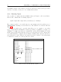
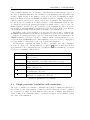
To accurately simulate different kinds of systems, Desmond supports several variants
of the Amber, CHARMM, and OPLS-AA force field models; see Table 4.1.
To more accurately simulate the behavior of water or other molecules, certain force
fields add electrostatic or van der Waals interaction sites located where no atom is.
Desmond implements these as pseudoparticles. Desmond supports the most common
kinds of pseudoparticles, including those needed for common water models such as SPC,
TIP3P, TIP4P, and TIP5P. See details in Section 5.4.2. Like particles, pseudoparticles
have a mass, charge, position, and velocity; however, their mass is often zero.
1.1.4
Space
The volume of space in which the simulation takes place is called the global cell . A threedimensional volume of space containing the chemical system. This volume is ordinarily
visualized as a three-dimensional rectangular box, though Desmond can simulate other
shapes.
The simulation can change dimensions in the course of running—for example, to
satisfy a requirement for a constant pressure.
Positions within the global cell are specified in x, y, z coordinates.
Desmond employs a technique known as periodic boundary conditions to wrap each
face of the global cell to its opposite face. That is, particles that move leftwards out
of the global conditions cell appear to be moving in at a corresponding spot on the
5
CHAPTER 1. KEY CONCEPTS
right-hand face, and vice versa; particles that move out the top appear to enter at the
bottom, and vice-versa; and finally, particles that move out the front appear at the back,
and vice-versa. Thus, you can picture your simulation as an arbitrarily large space tiled
by the global cell repeating periodically.
Because the global cell tiles the simulation volume, it must be a shape that can tile
a three-dimensional space without gaps, such as a parallelepiped, a hexagonal prism, or
a truncated octahedron.
The global cell also has specified dimensions. It must be large enough that the
molecule of interest doesn’t interact with its counterparts—its periodic images—in other
repetitions of the global cell.
When you run a simulation in parallel, Desmond apportions the work among processes by breaking the global cell into smaller boxes. Therefore, how you configure the
global cell can have a significant effect on how efficiently your simulation runs in parallel.
Details of these parallelization parameters, and related ones, are discussed in Section 3.2.
1.1.5
Time
The simulation begins at a specified reference time and advances by timesteps. The time
at which the simulation begins.
Ordinarily, a simulation begins at time 0.0, but it need not. For example, if you wish
to use the output of one simulation as the input for the next, thus effectively continuing
a simulation, you can specify a reference time equal to the time at which the previous
simulation finished.
Starting with the initial chemical system, Desmond:
1. computes forces on each particle based on all the other particles in the system, and
2. moves the particles according to the results of these computations.
This sequence, forming the basis of the timestep, is repeated again and again. The
period of simulated time computed between each update of the particle positions. The
action of the force field on the atoms is a continuous function of position and time which
the simulation samples at regular intervals. Thus, the timestep is analogous to the
resolution of an image in pixels, or the sampling rate of an analog to digital converter.
And like those, it presents trade-offs—too long a timestep sacrifices accuracy; too short,
performance.
For accurate results, the timestep must be short enough to resolve the highest frequency vibrations present in your system sufficiently for the timestepping scheme you
are using. For typical Desmond simulations, timesteps around 1 to 2 femtoseconds (fs)
are sufficient. To allow larger timesteps in common situations, Desmond also provides
constraints, discussed in Section 1.1.6.
1.1.6
Dynamics
The action of the force field on the particles is described by a differential equation that
Desmond integrates—numerically solves—at every timestep, thus computing a new po-
CHAPTER 1. KEY CONCEPTS
6
sition and velocity for every particle in the system. The differential equation is based on
the laws of Newtonian mechanics applied to particles in the system, but modeling some
physical systems requires augmenting the differential equations. Desmond implements
three broad categories:
• Ordinary differential equations that hold certain measures constant—Verlet constant volume and energy, Nosé-Hoover constant volume and temperature, MTK
constant pressure and temperature, and Piston constant enthalpy.
• Stochastic differential equations that hold certain measures constant and in which
one or more of the terms is a stochastic process—Langevin constant volume and
temperature, and Langevin constant pressure and temperature.
• Ordinary differential equations coupled to feedback control systems that keep a
certain measure within a certain range—Berendsen constant temperature, and
Berendsen constant temperature and pressure.
The particular algorithm that Desmond uses to solves the differential equation is
called the integrator . Integrators are described in detail in Section 7.2. Desmond allows
you to specify other aspects of the motion in your simulation, as well. For example, if
you’re using certain integrators, you may wish to remove the center-of-mass motion of
the chemical system.
Even with optimizations such as the Fourier space computation, far interactions are
expensive to compute. They also change more slowly in time than the other forces.
For many simulations, then, you can improve performance by configuring Desmond to
compute the far interactions less often—for example, on alternating timesteps. The
integrator still computes the near interactions every timestep, but it skips the far-range
computations half the time, weighting the results accordingly to compensate for not
including them at every timestep.
Typically, near interactions vary at a rate intermediate between bonded forces and far
interactions. Given their often dominant computational expense, Desmond also allows
these to be scheduled less often. Desmond allows timestep scheduling as follows:
• Bonded forces are computed at every timestep. This is then called the inner
timestep.
• Nonbonded near forces can be computed at every nth timestep, as configured.
• Nonbonded far forces can be computed at the same interval as nonbonded near
forces, or a multiple of it. This is then called the outer timestep.
Timestep scheduling appears as a configuration parameter called RESPA, an acronym
that stands for reference system propagator algorithm.
Constraints among particles let you lengthen the timestep by not modeling the very
fastest vibrations; the integrator moves these constrained particles in unison. A variety
of geometries can be constrained this way:
7
CHAPTER 1. KEY CONCEPTS
• a fan of 1–8 particles, each bonded to a central particle, such as the three hydrogen
atoms connected to a carbon atom in a methyl group; and,
• three particles arranged in a rigid triangle, such as a water molecule.
These constraints are described in detail in Chapter 6.
When you prepare your structure file, you specify the types of constraints, if any,
and the atoms involved in them. When you configure your simulation, you can specify
how precisely to compute the constraints. Whether and how to use constraints depends
on simulation specific factors or the force field you’re using.
1.2
Using Desmond
Desmond is a suite of computer programs. It uses a standard format for input—structure
(DMS) files—-and an open format for output—trajectory files, or frame files. So you
can also use other applications with Desmond, both public domain and commercial.
1.2.1
Input
Desmond requires two files for input: a structure file that defines the chemical system,
and a configuration file that sets simulation parameters.
The structure file specifies what to simulate, the initial state of the system: the size
of the global cell; the particles it contains, their positions and other properties; the force
fields to employ; and possibly other details.
Structure files are also called DMS files (file name suffix .dms for DESRES Molecular
System).
The configuration file specifies how you want to simulate the chemical system: the
reference temperature and pressure, if any; the integrator to use; the length of the
timestep; the fineness of the grid to use for charge-spreading; how many processes to
assign to a given dimension of the global cell; and possibly many other such parameters.
By using different configuration files with the same structure file, you can run different
simulations.
1.2.2
Applications and scripts
Desmond consists of three main applications and several companion Python scripts:
mdsim The application that performs the molecular dynamics simulation.
minimize The application that prepares the molecular dynamics simulation, if necessary, by minimizing energetic strains in the system so that they don’t destabilize
the simulation at the first few steps.
vrun The application used to analyze framesets output by mdsim.
Viparr The Python script that adds force field information to the structure file.
CHAPTER 1. KEY CONCEPTS
8
build constraints The Python script that adds constraint information to the structure
file.
1.2.3
Output
Timestep by timestep, an atom traces a path through the global cell as the simulation
advances.
The path that molecules take through the global cell is the trajectory. Trajectories
are writ ten out in a set of files representing a time series, like the frames of a movie.
Each frame is a file containing the positions and velocities of all the particles and
pseudoparticles in the chemical system at that particular timestep. In addition to particle
positions and velocities, frames can include system characteristics such as its total energy,
temperature, volume, pressure, and dimensions of the global cell.
You can configure Desmond to output frames—typically at an interval corresponding
to a multiple of the outer timestep, when nonbonded far interactions are computed.
A time-ordered series of frame files representing the dynamics of the chemical system
for the specified time period. Framesets are ordinarily the meaningful unit of analysis
for vrun or other analysis applications such as VMD.
1.2.4
Workflow
The following typical workflow illustrates the roles of Desmond’s three main applications,
as well as those of other cooperating applications:
1. Prepare the structure file. Typically, start with a Protein Data Base (.pdb) file
and produce a DMS file.
(a) Depending on its contents, and the manner in which it was created, it may
need some repair of artifacts (e.g. due to x-ray crystallography). Maestro
is one tool that can do this; others also exist. Maestro or a comparable
application outputs a structure file typically containing:
the solute proteins, ligands, or other molecules of interest; and
the solvent water; and often ions such as sodium, potassium, or chloride
to ensure that the overall chemical system is neutral with respect to
charge. (A charge-neutral system is desirable for computing long-range
electrostatic interactions.)
The structure file contains all particle and bond information, but has as yet no
information about the force field describing the interactions between particles.
(b) To add the force field information, the structure file is input to Viparr.
You specify the force field you wish to use, and Viparr outputs a structure
file with the force field information added. It can access a set of databases
specifying the required force terms for the various molecules in the chemical
system. Viparr reads the structure file and appends the necessary force terms
in a separate section of the file.
9
CHAPTER 1. KEY CONCEPTS
You now have a structure file that defines the particles and forces in your
simulation.
(c) If you wish to use constraints in your simulation, you now run build constraints.
By default, the script constrains the bond length of all bonds involving hydrogen atoms, as well as the angle in all water molecules. The out put is a
new structure file with the constraint terms added. You now have a structure
file that describes the particles and forces in your simulation, as well as any
constraints you wish to apply.
2. The simulation still needs to be configured, which involves specifying the values of
parameters in a configuration file. The simplest way is to start with an existing
con figuration file and edit it.
Chapter 2 provides an overview of configuring the simulation. For details about
specific configuration file parameters, see the chapters that discuss the applicable
configuration file sections.
3. Most simulations now require that the energy of the system be equilibrated so
that initial forces between atoms are small. One way to do this is to minimize the
potential energy of the system. Desmond provides two means of doing this. The
first is by Brownian motion, through the use of the brownie NVT or brownie NPT
integrators, or by gradient minimization, through the minimize application. You
may not need to use equilibrated if your system was prepared with care to avoid
energetic strains, or if it has already been equilibrated with another tool.
On the other hand, depending on how the structure file was obtained, you may
wish to use minimize even if you don’t intend to run mdsim, in order to rectify
strange conformations resulting from the homology model, or undesired artifacts
resulting from x-ray crystallography.
To minimize the energy of the system, the structure file and associated configuration file are input to minimize, which changes the atom positions slightly as
needed. It then outputs another structure file but does not change the configuration file.
4. The new structure and the configuration file are now input to mdsim, which executes the simulation (possibly for days or weeks), writing the results as frame files
at the configured intervals of simulated time.
Analyze the results
5. The frameset and configuration file can now be input to vrun, which analyzes the
results according to the manner specified in the configuration. For example, you
can specify that vrun print the energy of the system for each frame, or the forces
on each particle at each frame.
Other tools such as VMD, a freely available visualization application, can be used to
analyze results in addition to, or instead of, vrun.
CHAPTER 1. KEY CONCEPTS
1.2.5
10
Customizing Desmond
Desmond modularizes its functionality in the form of extensions.
An extension is a software module that implements a discrete set of capabilities, compiled separately so that it can be added to, or removed from, an existing application.
The capabilities are further divided logically into units of functionality called plugins. As
it runs, the Desmond executable calls plugins as specified in the configuration file for its
application. In this way you can execute the functions that you need while skipping those
that you don’t. Each Desmond application has a main loop which it repeats: one step
in the minimization process, one simulation timestep, or one trajectory frame loaded.
Plugins can be called during this loop to perform their work repeatedly as the simulation unfolds. For example, the plugin eneseq computes system energy, temperatures,
pressures, and other data, breaking down the energy into various categories, then writes
the result to the specified output file. For example, randomize velocities reinitializes
the velocities of the particles in the simulation according to the Boltzmann distribution
for a specified temperature, something you may wish to do once, at the start of the
simulation. On the other hand, trajectory writes all particle positions to the specified
output file at specified intervals, which you probably wish to do more than once, but
less often than at every timestep.
The main loop plugins are configured in the section of the configuration named after
the application being run (e.g. mdsim or remd). Not all plugins are active in the main
loop. Some plugins provide integrators and additional force terms. They are either
partly or wholly configured in these sections of the configuration.
Plugins provided with Desmond are described in Section 2.6.
Desmond already has most or all the functionality required for typical molecular dynamics simulations, but you can extend this functionality by writing your own plugins
to, for example, support new force field terms, add new integrators, or apply arbitrary
steering forces to the simulation, all without recompiling the Desmond executable. Implement the functionality you need as a plugin; then specify the parameters for your
plugin in the configuration file. Other requirements are discussed in Chapter 10.
Chapter 2
Running Desmond
This chapter explains the basics of working with configuration files; describes how to
invoke the various Desmond applications, including in parallel; and describes how to
configure Desmond applications and built-in plugins, as well as the optional profiling
mechanism.
2.1
About configuration
Desmond reads configuration parameters from a configuration file, specified on the command line.
The simplest way to configure a simulation is to copy one of the sample configuration
files provided and edit it. See the README.txt file for the location of these files. For those
who wish to edit extensively or create their own, configuration file syntax is described
in Appendix B.
Configuration files are divided into sections, with the configuration information for
a given application going into the section named for that application. In addition, other
sections configure other aspects of the simulation, such as the global cell, the force field,
constraints (if any), and the integrator. The same configuration file can apply to any
Desmond application.
Configuration file sections are:
app = mdsim|remd|minimize|vrun|...
boot = { file = p } # the structure file
global cell = { ... }
force = { ... }
migration = { ... }
integrator = { ... }
profile = { ... } # for debugging
mdsim = { ... }
vrun = { ... }
minimize = { ... }
remd = { ... }
11
CHAPTER 2. RUNNING DESMOND
12
Each application reads a particle system and a force field from a structure file located
at the path p, the details of which can be found in Chapter 4. The structure file defines
the global cell dimensions, initial particle properties, and the specific parameters of the
force field.
Many Desmond objects share the following configuration idiom:
object = {
first = tf
interval = ti
...
}
This describes the pattern of activity of the object, acting only at specific times, the first
time at tf and thereafter periodically with period ti . Setting ti = 0 causes the object to
act at every opportunity after tf .
Note: The application might modify tf and ti slightly from their configuration values
to make them a multiple of the current timestep.
Setting tf to inf meaning infinity (see Appendix A) declares that the activity never
occurs; but beware: some plugins use the Boolean parameter write last step that
when set causes output to occur at the end of the simulation regardless.
2.2
Invoking Desmond
Desmond applications are invoked from the command line by the desmond executable.
Use the --include to specify the configuration file. For example, to invoke desmond
with the configuration file equil.cfg:
Example 2.1
desmond --include equil.cfg
As indicated above, the configuration specifies the application and the structure file,
as in:
Example 2.2
app = mdsim
boot = {
file = /path/to/my/input.dms
}
The --cfg option allows you to append additional configuration information to the
command line. It’s often used to specify the structure file. For example, to invoke
desmond with the structure file /path/to/my/input.dms:
Example 2.3
desmond --include equil.cfg --cfg boot.file=/path/to/my/input.dms
13
CHAPTER 2. RUNNING DESMOND
This has the same effect as the line from the configuration file above.
Note: Use quotation marks around the parameter to --cfg if it contains any special
characters (such as spaces) that are interpreted by the shell.
You can specify multiple configuration files; this can be useful for configuring a simulation in a modular way. For example, you might choose to have alternative integrator
configurations in two files named nve.cfg and ber nvt.cfg, with other configuration
parameters in the base configuration file in base.cfg. Then, for a simulation in which
you intend to use the Verlet constant volume and energy integrator, you’d invoke:
Example 2.4
desmond --include base.cfg --include nve.cfg --cfg boot.file=input.dms
Whereas, for a simulation in which you intended to use the Berendsen constant
volume and temperature integrator, the command line would instead be:
Example 2.5
desmond --include base.cfg --include ber nvt.cfg --cfg boot.file=input.dms
You cannot specify multiple structure files. The --include and --cfg arguments
are evaluated in order, and the last specified name for the structure file overrides any
previous ones.
The --tpp command line option sets the number of threads per process. If your
application is to run on a processor with multiple cores, you may benefit by setting this
value to other than its default of one. Otherwise, the command line can omit it. The
--cpc command line option sets the number of cores per physical chip and as a side
effect ties Desmond threads to processor cores. If --cpc N, where N ≥ 1, is used master
and worker threads are bound to processor cores. If --spin 1 or --spin 2 is used, a
faster but more processor intensive thread idle strategy using spin-locks is employed.
When 1, foreground threads will spin, and background threads will sleep; when 2, all
worker threads will spin.
Note: If you run more than one Desmond job on a multiprocessor node, make sure
that --cpc is set to 0, otherwise Desmond processes in the different jobs will use the
same core resulting in significant performance degradation.
Note: When running on an interactively used workstation and with more than one
Desmond thread, it is better to set --spin 0.
For example, to start a Desmond application with four threads per process:
Example 2.6
desmond --tpp 4 --include example.cfg --cfg boot.file=input.dms
Note: Under most circumstances, it’s best to run desmond with one thread per
process and one process per processor core.
Each application logs its configuration at startup, so users can observe the net result
of the configuration options. This includes displaying a list of the loaded plugins with full
paths, so that you can see all the code that Desmond can access. (Plugins are described
in Section 2.6.)
CHAPTER 2. RUNNING DESMOND
14
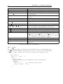
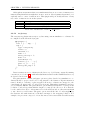
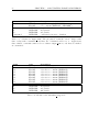
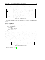
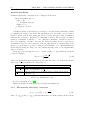
Table 2.1 lists the full set of supported options. All command line options have the
same effect for all applications except --restore, which pertains to the mdsim and remd
applications only, enabling them to start from a checkpoint file. It is an error to provide
a command line option that is not recognized by Desmond or one of its components.
Command line options can be given in any order.
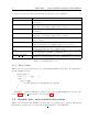
argument
--tpp N
--cpc N
--spin N
description
Sets the number of threads per process. Defaults to 1.
Gives the number of cores per physical chip. Defaults to 0.
Sets the worker thread idle strategy. Defaults to 0. If 1 or 2 then use
spin-lock based idle strategies. Sets the name of the communications
plugin to use for parallel jobs.
Defaults to serial.
Adds configuration information from the given file. Can be given
any number of times.
Adds configuration information from the given string. Can be given
any number of times.
Restarts the mdsim or remd applications from a checkpoint. Because
these applications are expected to run for long periods of time, during
which hardware might fail, they can be set to produce a checkpoint
file periodically, from which you can restart
--destrier name
--include file name
--cfg string
--restore file
Table 2.1: Desmond command line options
Restoring from a checkpoint
You can configure the mdsim or remd applications to create a checkpoint file at regular
intervals as it runs. When you wish desmond to start from a checkpoint file created
during an earlier run, use the restore flag to specify the file name.
For example, to restore from a checkpoint:
desmond --tpp 4 --restore checkpoint_file
Note: To avoid an application error, set the --tpp and other thread specific flags
the same way it was set for the original simulation. desmond must initialize the parallel
environment before it can read the checkpoint file.
You need not specify other configuration options; they’ve been saved. When restoring
from a checkpoint file, only certain options can be changed from the configuration of the
original simulation: last time (see Section 2.4.1 and Section 2.4.2), checkpt.interval
(see Section 2.4.1), and certain plugin options (for example, the name and interval for
eneseq and trajectory).
2.2.1
Using plugins
Desmond applications use certain plugins for various diagnotics and interventions. Plugins can be implemented as part of an application (called built-in plugins), or in external
15
CHAPTER 2. RUNNING DESMOND
files (called extensions).
Desmond locates extensions (files containing plugins) by means of either of two environment variables DESMOND PLUGIN PATH and DESRES PLUGIN PATH. You can specify
more than one path to search for plugins by separating them with colons, as in:
Example 2.7
DESMOND_PLUGIN_PATH=/this/is/the/first/path:/this/is/the/second
The line above specifies two directories, which are searched for plugins in the given
order. Many plugins are compiled with Desmond already and are therefore available to all
its applications; these are discussed in Section 2.6. In addition, you can implement your
own plugins, or use those developed by third parties. Extending Desmond’s functionality
in this way is discussed in Chapter 10.
Each application has a main loop, consisting of one minimization or simulation step
(mdsim, remd, and minimize) or processing one trajectory frame (vrun). You can configure a plugin to run once at the beginning of a simulation, or periodically at an interval
of one or more steps.
Each application’s plugin section of the configuration contains a list under the key
plugin that gives the names of main loop objects to create.
For example, the plugins to call when the mdsim application runs appear in a list like
the one below:
mdsim = {
plugin = {
list = [ key1 ... keyn ]
key1 = {
type= type1
...
}
...
keyn = {
type= typen
...
}
...
}
}
The key names appearing in the plugins list are arbitrary (though, for a given section,
they must be unique). For each key, keyi , Desmond creates a main loop object of type
typei . The remainder of the table under keyi contains the object’s configuration:
mdsim = {
plugin = {
list = [ my_status ]
my_status = {
CHAPTER 2. RUNNING DESMOND
16
type=status
first=0
interval=1
}
}
}
In this case, the mdsim application will create an object of type status, which is set to
run every picosecond.
Note: Main loop plugin objects are evaluated in the order in which they’re listed in
the configuration. In certain circumstances, listing plugins in a different order can yield
different results: for example, if your simulation calls both the randomize velocities
and eneseq plugins. Because randomize velocities generally changes the kinetic
energy of the system, different kinetic energies and temperatures are reported if the
randomize velocities plugin is listed before eneseq rather than after—the dynamics
of the system will be the same, but the reported temperatures will be different. Section 2.6 describes the built-in main loop plugins.
2.3
Running Desmond in parallel
Desmond can be run either in serial or in parallel, in environments ranging from laptops
to large Linux clusters. High-performance parallel systems consist of nodes connected
together in a network, containing one or more processors each of which consisting of one
or more processor cores or cores. In the following we will frequently refer to processor
cores as processors where confusion is unlikely.
When you run Desmond in parallel, specify the number of Desmond processes you
want to run according to the particulars of your parallel environment.
You can run Desmond in parallel—that is, run multiple Desmond processes—and also
run each process with multiple threads (using the --tpp command line parameter). In
order to run Desmond in multi-threaded mode efficiently, you’ll need to request as many
total processor cores as the total number of threads. For example, if you are running on
a system with 8 processors cores per node, and specify 2 processes per node, then you
should set the --tpp parameter no larger than 4. The details of selecting the number
of nodes and processes per node are system dependent and are not discussed further.
When running a simulation in parallel, Desmond processes exchange the information
by means of a parallel communication interface (typically, MPI), implemented with a
plugin called a destrier. That implementation is registered under a symbol (normally,
either mpi or serial) by which it can be selected by giving an application the destrier
flag:
Example 2.8
desmond --destrier mpi --tpp 1 --include example.cfg
Without the --destrier flag, a Desmond application defaults to serial. The details
of Desmond installations and parallel environments vary, but a plugin containing a de-
17
CHAPTER 2. RUNNING DESMOND
strier implementation in a file named destrier.so, and registered as mpi, must either be
built-in (that is, compiled as part of the Desmond executable), or located in an extension
specified by the path given in your DESMOND PLUGIN PATH environment variable.
--destrier serial: runs Desmond applications with a single process. This gives you
a means to check your code and find any other problems while your installation
creates a usable parallel environment.
--destrier mpi: uses the MPI destrier variant, a common parallel programming specification, implemented as a library of C, C++, or Fortran functions.
--destrier other: You can create your own destrier plugin by modifying the examples
provided for the serial and mpi plugins. Register the resulting plugin under the
name of your choice, supplying that name as the argument to the --destrier
parameter.
The parallel environment is initialized before checkpoint information is read. Therefore, if you’re restoring from a checkpoint, the --destrier flag must be set in the same
way it was when you started the original simulation.
Note: The mpi destrier plugin requires Open MPI version 1.4.3 or later. If you
wish to use a different parallel communication interface, you’ll need to compile your own
plugin.
2.4
Configuring Desmond applications
The main Desmond applications are mdsim, minimize, remd, and vrun, as described
in Section 1.2.2. Configuration parameters for each of these applications are described
below.
2.4.1
mdsim
mdsim is Desmond’s main molecular dynamics simulation code. It’s configured as shown
in:
mdsim = {
title = w
last_time = t1
plugin = { ... }
checkpt = { ... }
}
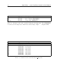
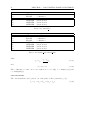
CHAPTER 2. RUNNING DESMOND
name
title
last time
plugin
checkpt
18
description
A short string to include in various output files—by default,
“(no title)”. [string]
Time at which to stop the simulation, in picoseconds, relative to the reference time given as part of the global cell
configuration (see Section 3.2). [time]
Description of the main loop plugins to call during simulation.
See Using plugins. [configuration]
Checkpoint configuration. See Checkpointing. [Configuration]
Table 2.2: Parameters for mdsim
Checkpointing
Because mdsim can run for a long time, during which hardware can fail, checkpointing
allows you to restart a simulation from a backup file called a checkpoint. A checkpoint
file is a snapshot of the entire state of the computation and can therefore be quite a large
file. However, because their purpose is to restart an interrupted simulation, checkpoint
files can be discarded after the simulation completes. Desmond checkpoints are designed
such that the state of a simulation restarted from checkpoint is bitwise identical to the
state of simulation at the point when the checkpoint file is written.
Configuration information for checkpointing appears as shown in:
checkpt = {
first = tf
interval = ti
wall_interval = tw
name = p
write first step = bf
write last step = b1
}
Setting checkpt = none shuts off checkpointing.
A checkpoint is written at simulation time tf and thereafter with a period ti or at
the wall clock interval tw as measured from the start of each invocation of the simulator.
The output file name convention is followed for the checkpoint files; see Section 2.5.
You can cause mdsim to write a checkpoint file initially and finally by setting bi and
bf respectively to true.
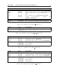
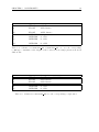
19
CHAPTER 2. RUNNING DESMOND
name
first
interval
wall interval
name
write first step
write last step
description
First time to create a checkpoint. [time]
Periodic interval at which to create checkpoints. [time]
Periodic interval at which to create checkpoints; wall clock
time in units of seconds. [time]
Output filename to use for the checkpoint files. [filename]
Whether to write a checkpoint file before the first step is
taken. [Boolean]
Whether to write a checkpoint file after the last step is taken.
[Boolean]
Table 2.3: Parameters for checkpointing
2.4.2
remd
The remd application in Desmond implements the replica exchange protocol, sometimes
known as parallel tempering. The number of replicas that can be simulated is limited
only by the number of processors available and that an equal number of processors
must be assigned to each replica. The only restriction on the replicas themselves is
that they must all have the same number of particles. Thus, remd can be used for the
usual temperature exchange method, as well as exchanges between systems with different
Hamiltonian parameters.
remd runs as a single parallel application, just like mdsim and vrun, producing a single
checkpoint file if checkpointing is enabled. Each replica runs as a normal simulation,
with swaps of coordinates taking place as specified by the user through the configuration.
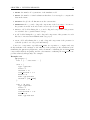
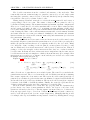
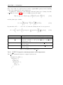
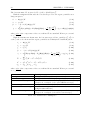
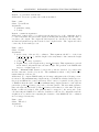
When an exchange is attempted between two replicas, the usual Metropolis criterion is
applied to determine if the exchange should be accepted or accepted, according to the
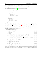
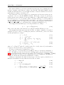
fol lowing prescription: with
Q = (β1 U11 + β2 U22 − β1 U12 − β2 U21 ) + (β1 P1 − β2 P2 )(V1 − V2 ) ,
(2.1)
where randN is a random variate on (0, 1], Uij is the potential energy of replica i in the
Hamiltonian of replica j, Pi is the instantaneous pressure of replica i, Vi is instantaneous
volume of replica i, and βi is the inverse temperature of replica i. If Q > 0 accept the
exchange, or if Q < −20 reject it, otherwise accept the exchange if randN < exp(Q).
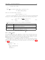
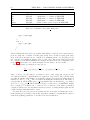
An example remd configuration is shown in following Example; all parameters are
required. The parameters are summarized in Table 2.4.
Example 2.9
remd = {
title = w
last_time = t1
checkpt = { ... }
plugin = { ... }
first = tf
CHAPTER 2. RUNNING DESMOND
20
interval = ti
seed = s
exchange_type = neighbors|random
cfg = [ c1 ... cr ]
}
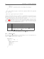
name
title
last time
checkpt
plugin
first
interval
type
seed
cfg
description
A short string to include in various output files. Optional—
by default, “(no title)”. [string]
Time at which to stop the simulation, in picoseconds, relative to the reference time given as part of the global cell
configuration (see Section 3.2). [time]
Checkpoint configuration. See Checkpointing. [configuration]
See Using plugins. [configuration]
Time of first exchange attempt [Time]
Time between exchange attempts [Time]
Either exchanges only between neighboring replicas or exchanges between any pair of replicas [neighbors /random ]
random number seed for the Metropolis criterion [Integer ]
configuration overrides for each replica [List of configurations]
Table 2.4: Parameters for remd
The actual exchange policies and parameters are implemented through a special
built-in plugin of type remd. Exchanges are attempted starting at chemical time given
by first, and at intervals of interval thereafter. If type is neighbors, then on each
exchange attempt, all replicas will attempt an exchange with either of their neighbors in
a linear order with 50% probability, and accept based on the Metropolis criterion above.
If type is random, then only two out of all replicas will attempt an exchange, but those
two replicas could be any of the replicas in the ensemble. Exchanges are implemented by
swapping the positions of a pair of replicas. If an exchange is accepted, the velocities of
the replicas are rescaled to the temperature of the host replica; otherwise, the positions
are simply swapped back. Thus, in any replica, the temperature and Hamiltonian will
stay the same, but the dynamics will be discontinuous as new coordinates are swapped
in via exchanges.
The cfg configuration in remd serves two purposes. First, the number of entries in
the list, r, serves to specify how many replicas are to be run in the simulation. Second,
each entry in remd.cfg overrides the configuration for the corresponding replica, in the
same way that the cfg command line option overrides a setting for an mdsim run. For
example,
Example 2.10
cfg = [
21
CHAPTER 2. RUNNING DESMOND
{integrator.temperature.T_ref=300
{integrator.temperature.T_ref=303.3333
{integrator.temperature.T_ref=306.6667
{integrator.temperature.T_ref=310
plugin.eneseq.name=0.ene}
plugin.eneseq.name=1.ene}
plugin.eneseq.name=2.ene}
plugin.eneseq.name=3.ene}
]
has four replicas: replica 0 will see a configuration with the integrator temperature set
to 300, replica 1 will get a temperature of 303.3333, and so forth. Also in this example,
a plugin variable is overridden on a per replica basis. Overrides to the remd section itself
should not qualified with the prefix remd. as one would have expected.
2.4.3
minimize
minimize performs steepest descent minimization followed by LBFGS minimization.
Configuration parameters are shown in following example; all parameters are optional;
the defaults should be adequate for most systems.
minimize = {
migrate_interval = i
m = m
maxsteps = smax
tol = τ
stepsize = l
switch = g
sdsteps = s0
debug = d
dt = t
plugin = { ... }
}
minimize requires an integrator section, even though all parameters in that section are
ignored during the calculation. We recommend that you use the same configuration for
minimization and dynamics, appending the minimize section to the mdsim configuration
discussed above.
minimize handles constraints differently from mdsim; for a discussion, see Section 4.2.3.
CHAPTER 2. RUNNING DESMOND
name
plugin
migrate interval
m
maxsteps
tol
stepsize
switch
sdsteps
debug
dt
22
description
See Using plugins. [configuration]
Number of minimization steps between each migration event.
Optional—by default, 1. [Integer > 0]
Number of state vectors to use during L-BFGS minimization.
Optional—by default, 3. [Integer > 0]
Maximum number of steps to iterate. Optional—by default,
200. [Integer ]
Stopping tolerance for gradient norm. Optional—by default,
1.0. [Energy/Length > 0]
Norm of first step. Optional—by default, 0.005. [Length > 0]
Minimum gradient before switching to L-BFGS. Optional—
by default, 100.0. [Energy/Length > 0]
Minimum number of initial steepest descent steps.
Optional—by default, 0. [Integer ]
Debug level. Optional—by default, 0. If debug=1, Desmond
prints additional minimization information. [Integer ]
A fake time scale for the minimize step. Optional—by default, 1.0. [time > 0]
Table 2.5: Parameters for minimize
2.4.4
vrun
The vrun application is used to analyze structure files and trajectories. It loads successive trajectory frames (written by mdsim or per-replica frames written by remd) and
triggers plugins to act on those frames.
Configuration information is shown in:
vrun = {
title = w
plugin = { ... }
input = bootfile | frameset
frameset = {
name = p
first = tf
interval = ti
last_time = t1
}
}
Loads a configuration, or sequence of configurations, given by the set of frames from a
trajectory file. p is expected to be a path to a frameset, a trajectory output. If not
given, then the initial configuration is processed as loaded.
23
CHAPTER 2. RUNNING DESMOND
name
plugin
title
input
frameset.name
frameset.first
frameset.interval
frameset.last time
description
See Using plugins. [configuration]
A string to be included in various output files. Optional—by
default, “(no title)”. [string]
Input mode: either ‘frameset’ or ‘bootfile’. [String]
Path to the input trajectory. Optional. [filename]
Start processing frames after this chemical time. [time]
Skip this much chemical time between frames. [time]
Stop processing after this chemical time. [time]
Table 2.6: Parameters for vrun
2.5
Naming output files
Output files are created according to a format string having terms that are expanded
on a per-file basis. These terms are of the form @X, where X is a single character; they
expand as listed in Table 2.7
Term
@B
@S
@P
@R
@FS
@@
Expands to
A boot timestamp: a date string, resolved to the second, taken from the
start time of one of the parallel processes.
A sequence number: an integer, starting at zero and incrementing each time
this filename is expanded, producing an ordered sequence of files rather
than overwriting the same file.
The UNIX process ID of the process writing the file, as a hexadecimal integer.
The rank—a unique identifier within a parallel run—of the process writing
the file.
The result of passing S to strftime.
The @ character.
Table 2.7: Terms for naming output files
For example, if you wish to write an output file several times during a run, the
filename my output-@S creates a sequence of files named my output-0, my output-1,
and so on. The last-used value of the sequence number is saved in the checkpoint file.
To ensure that unique files are created with each Desmond run, give files names such as:
my output-@B, thus causing each to be named with a unique timestamp. (If the runs
are expected to take less than one second to complete, unique file names would require
a different strategy; perhaps: my output-@B-@P.)
A filename can encode the current date and time in various formats. For example,
you can use a file name of the form my output-@F{%Y-%m-%d} to name a file according
to current date: my output-2010-04-23. You could name your checkpoint file in this
way if you wanted to ensure that no more that one checkpoint file is written per day.
Plugins that periodically update an output file—for example, eneseq, compute forces,
CHAPTER 2. RUNNING DESMOND
24
energy groups, and gibbs.output—can use an empty string as a filename; in this
case, data is written to the standard output. However, maeff output and checkpt
require real file names.
2.6
Configuring the built-in plugins
Desmond is compiled with various plugins, which are therefore available to all Desmond
applications. These plugins offer a range of commonly useful functionality; configuration
information for them all is discussed below.
2.6.1
anneal
The Desmond anneal plugin periodically updates the temperature setting of the anneal
integrator during an mdsim run. The anneal integrator is actually a thin shell around
any other Desmond integrator. Hence, there are two places in the configuration that
need to be changed in order to use the anneal plugin.
Integrator setup
The integrator section of the configuration normally has the following form:
integrator = {
type = name
name = { ... } # integrator-specific options
# ... other non-specific integrator options
}
In order to enable the anneal plugin, the above should be changed as follows:
Example 2.11
integrator = {
type = anneal
anneal = { type = name
name = { ... } } # integrator-specific options
# ... other integrator options
}
This wraps whatever integrator symbol was asking for inside the anneal integrator and
thereby makes it responsive to requests for temperature changes.
Plugin setup
Within the application specific plugin section, the following specifies the component of
annealing that schedules the temperature changes:
25
CHAPTER 2. RUNNING DESMOND
app.plugin = {
list = [ ... key ... ]
key = {
type = anneal
first = t0
interval = δ
schedule = {
time = [ t1 t2 ... tN ]
value = [ T1 T2 ... TN ]
}
}
}
t0 : first time to reset the thermostat temperature
δ: interval between thermostat resets. There is a small performance cost to resetting the
thermostat, so its recommended that the delta be set no smaller than the natural
thermalization time of the system, typically on the order of 1 ps.
schedule: When the plugin is invoked, as specified by first and interval, a target
temperature is computed based on the current chemical time t. If t < t1 , no action
is taken. If t ≥ tN , the target temperature will be TN , the last temperature in
values. Otherwise, the target temperature is computed by linearly interpolation
between the time points ti , ti+1 that bracket the current time:
T = Ti + (Ti+1 − Ti )
(t − ti )
(ti+1 − ti )
(2.2)
For example, the following schedule would heat a system from 0 to 500 K during the
first 20 ps, then cool it to 300 K during the subsequent 80 ps, and maintain it at 300 K
thereafter:
Example 2.12
mdsim.plugin.key.schedule = {
time = [ 0 20 100 ]
value = [ 0 500 300 ]
}
2.6.2
Biasing Force
The BiasingForce plugin can be used to restrain two groups of atoms within a chemical
system with respect to each other, in displacement, distance, and/or orientation. It can
also be used to restrain the position and orientation of a group of atoms within the molecular system with respect to the simulation box. Unlike most plugins, its configuration
is given in the force section of the configuration (note below).
CHAPTER 2. RUNNING DESMOND
force.term = {
list = [ ... key ... ]
key = {
type = BiasingForce
cm_moi = [ {
groups
= [ A B ]
displace_coeff = [ kx ky
displacement
= [ x0 y0
distance_coeff = kd
distance
= R0
orient_coeff
= [ ω1 ω2
Euler_angles
= [ θ0 φ0
26
kz
z0
]
]
ω3 ]
ψ0 ]
use_lab_frame_for_displacement = Boolean
pull_displacement = [ vx vy vz ]
pull_distance
= vd
dφ dψ
]
pull_Euler
= [ dθ
dt dt dt
} # Multiple biasing potentials, supplied as a list, can be applied.
... ]
output = {
first = tf
interval = ti
name = filename
}
t0 = t0
}
... # Other force terms
}
The units of the parameters in the configuration are given in Table. 2.8.
The biasing force in the above configuration will restrain particles in cm moi group B
with respect to particles in cm moi group A. Group A consists of all atoms whose
grp bias property is set to the integer value A; Group B those set to the integer value B
(see Chapter 4). The allowed values of grp bias are 0, 1, 2, and 3 and by default all
particles in the chemical system are in center of mass group 0. If A = −1, however,
BiasingForce will restrain group B with respect to the simulation box.
The BiasingForce plugin works by imposing the following restraining potential on
the molecular system:
Ebiasing =
+
+
κy ~
κx ~
κz ~
(RAB · ~qA1 − x)2 + (R
qA2 − y)2 + (R
qA3 − z)2
AB · ~
AB · ~
2
2
2
κd
(RAB − R)2
(2.3)
2
ω1
ω2
ω3
((G~qB1 ) · ~qA1 − 1)2 + ((G~qB2 ) · ~qA2 − 1)2 + ((G~qB3 ) · ~qA3 − 1)2
2
2
2
27
CHAPTER 2. RUNNING DESMOND
quantity
t0
kx , ky , kz
x0 , y0 , z0
kd
R0
ω1 , ω2 , ω3
θ0 , φ0 , ψ0
vx , vy , vz
vd
dθ dφ dψ
,
,
dt dt dt
unit
picosecond
−2
kcal·mol−1 · Å
Å
−2
kcal·mol−1 · Å
Å
kcal·mol−1
degree (not radian)
Å·picosecond−1
Å·picosecond−1
degree·picosecond−1
Table 2.8: Units of the parameters in biasing force.
where RA (RB ) is the center of mass of group A (B), RAB = (xAB , yAB , zAB ) = RB −RA ,
qAα , α = 1, 2, 3 (qBα ) are the principal axis of group A (B), and G is the rotational matrix
that will superimpose the qB ’s onto qA ’s when B is in the relative orientation with respect
to A, as specified by the Euler angles (θ, φ, ψ).
In Ebiasing , the first three terms restrain the relative displacement between the centers
of mass of groups B and A, to the desired displacement (x, y, z). The term in the second
line restrains the scalar center-of-mass distance RAB of the two groups A and B and
R is the target displacement. The three terms in the third line restrain the relative
orientations of the particles in group B with respect to those in group A.
If the parameters pull displacement are set to 0, the desired displacement—(x, y, z)
in Equation 2.3—are taken to be (x0 , y0 , z0 ) in the configuration, and they will not change
in the course of the simulation. But if they are not zero, the biasing force will be used
to pull the two groups from the initial positions at the specified rates v = (vx , vy , vz ),
and the target displacement, R(t), at time t is given by
~
~ AB (0) + ~v t
R(t)
= (x(t), y(t), z(t)) = R
(2.4)
where RAB (0) is the initial displacement between A and B at the beginning of the
simulation.
The same convention applies to pull distance and pull Euler.
The parameter use lab frame for displacement is false by default. If it is set to
true, the displacement between groups B and A will be measured in the reference frame
of the simulation box, and will not be projected onto the reference frame formed by the
principal axes of group A. Namely, the three terms in the first line of Equation 2.3 are
replaced in this case by
κy
κx
κz
(xAB − x)2 + (yAB − y)2 + (zAB − z)2
(2.5)
2
2
2
A maximum of 4 cm moi groups can be defined for a chemical system. Because the
center-of-mass and moment-of-inertia are computed for these groups of atoms in order
CHAPTER 2. RUNNING DESMOND
28
to apply the biasing potential, the user must avoid imposing the biasing potential upon
a group of atoms that can wrap around the periodic box since in this case, the center-ofmass and the moment-of-inertia are ill-defined. There is a limit of 4 biasing potentials
in the cm moi list of the force.BiasingForce configuration.
The user can monitor the action of the biasing potential from the data written at
the specified time intervals to the output file. The header in the output file reports
the number of atoms in each cm moi group; the user should verify that these match
the intended grouping. Following this is a header line that labels each column of the
subsequent data. Each row of data corresponds to one moment in time, beginning with
the properties of the first cm moi group, followed by those of the ensuing groups. The
data reported are as follows:
xci, yci, zci, where i = 0, 1, . . . : the center-of-mass coordinates of the ith cm moi
group in units of Å.
p1xi, p1yi, p1zi : the unit vector of the first principal axis of the ith cm moi group.
p2xi, p2yi, p2zi, p3xi, p3yi, p3zi : the unit vectors of the second and third principal
axes of the ith cm moi group.
I1i, I2i, I3i : the diagonal moment-of-inertia tensor of the ith cm moi group, corre2
sponding to the principal axes in the same order. They are in units of amu × Å .
From these data together with the parameters in the biasing potential configuration,
it is straightforward to compute the energy contributions from the biasing potential at
each recorded moment.
29
CHAPTER 2. RUNNING DESMOND
name
cm moi
groups
displace coeff
displacement
distance coeff
distance
orient coeff
Euler angles
use lab frame for displacement
pull displacement
pull distance
pull Euler
t0
output.first
output.interval
output.name
description
Biasing force definition for a list of cm moi groups [List]
The groups to restrain [List]
Force coefficients for displacement restraints [List of 3
Energy/Length2 ]
Relative displacement between the two groups [List of 3
Lengths]
Force coefficient for distance restraint [Energy/Length2 ]
Distance between the two groups [Length]
Force coefficients for orientational restraints [List of 3 Energies]
Euler angles between the two groups [List of 3 Degrees]
If true, the displacement between the groups are measured in
the reference frame of the simulation box [Boolean]
Velocity of pulling in displacement [List of 3 Length/Time]
Velocity of pulling in distance [Length/Time]
Velocity of pulling in orientation [List of 3 Degree/Time]
The time to begin apply pulling, as specified by
pull displacement, pull distance, and pull Euler. This is not
to be confused with the biasing force itself, which is applied
from the beginning of the simulation. [Time]
The time to write the first biasing results [Time]
The interval at which to write the biasing results [Time]
The name of the file to which to write the energy estimates
[Filename]
Table 2.9: Parameters for BiasingForce
2.6.3
e bias
The e bias plugin applies a constant electric field with the direction and magnitude given
by E applied. The schedule subsection is can be set to none; if so, the field remains
constant over time; otherwise, it’s scaled by the values given in schedule.value.
force.term = {
list = [ ... key ... ]
key = {
type = e_bias
E_applied = [Ex Ey Ez ] # Applied field in kcal/mol/A/e
schedule = {
time = [ t1 t2 ... tN ] # Times in picosecond
value = [ S1 S2 ... SN ]
}
}
CHAPTER 2. RUNNING DESMOND
30
... # other force terms
}
With e bias, a particle carrying charge q experiences a force
F~ = (qEx (t), qEy (t), qEz (t))
where the electric field at time t is given by
Eα (t) = Eα S(t) for α = x, y, z
The time-dependent scaling factor S(t) is determined by the schedule. If schedule=none,
then S(t) = 1 for all t. Otherwise, S(t) at time t is given by piecewise linear interpolation:
t−ti
if t ∈ [ti , ti+1 )
Si + (Si+1 − Si ) ti+1 −t
i
S(t) =
(2.6)
S
if t < t1
1
SN
if t ≥ tN
e bias is often used to model electric potentials across membranes.
name
E applied
schedule.time
schedule.value
description
Applied electric field in kcal/mol/Å/e [List of 3 Energy/Length/ElectronCharge]
Times at which scale factors are specified [List of Times]
Scale factors to apply at corresponding times. Same length
as schedule.time list [List of Scalars]
Table 2.10: Parameters for e bias
2.6.4
energy groups
Periodically writes energy to the output file p, broken down both by the energy group
property of the particles and the Hamiltonian category of the potential energy term.
(Energy groups are assigned in the structure file, while the string identifiers of various
Hamiltonian categories are set by their computational pipelines.)
Additionally, the 3 × 3 instantaneous pressure tensor and the nonbonded correction
energy are printed if specified. The nonbonded correction energy is the sum of the
nonbonded tail correction and the electrostatic self-energy correction (see sections 5.3.2
and 5.4.1).
app.plugin = {
list = [ ... key ... ]
key = {
type = energy_groups
first = tf
interval = ti
31
CHAPTER 2. RUNNING DESMOND
name = p
options = [ pressure_tensor corr_energy self_energy ]
}
}
The output format is a sequence of ascii blocks of plain text. Each block begins with
a line of the form
time=t en=εv E_p=εp E_k=εk E_x=εx P=P V=V
giving the chemical time, the raw potential, the potential, kinetic, and extended energies,
as well as the pressure and volume. The raw potential energy is potential energy without
the electrostatic self-energy or the nonbonded tail corrections.
What follows is then a break down of the raw potential energy by energy group (see
Section 2.6.4). The kinetic energy is broken down into the kinetic energy per group.
The potential energies are broken down (by column) according to their interacting pairs
of groups and (by row) their Hamiltonian category.
name
first
interval
name
options
description
First time for this action. [Time]
Time between actions. [Time]
The output file name. [String]
Whether to print pressure tensor (pressure tensor), the
correlation energy (corr energy), and/or the self energy
(self energy) [List of strings]
Table 2.11: Parameters for energy groups
2.6.5
compute forces
The compute forces plugin Writes a per-particle listing of forces to an output trajectory
frameset p. It is primarily useful for diagnostics.
app.plugin = {
list = [ ... key ... ]
key = {
type = compute_forces
first = tf
interval = ti
name = p
mode = m
}
}
CHAPTER 2. RUNNING DESMOND
name
first
interval
name
mode
32
description
First time for this action. [Time]
Time between actions. [Time]
The directory name of the trajectory frameset. [String]
append/noclobber/clobber, see discussion in Table 2.19
[String]
Table 2.12: Parameters for compute forces
2.6.6
eneseq
The eneseq plugin Writes energy, temperatures, pressures, and other summary data to
an output file. Configuration information is given in:
app.plugin = {
list = [ ... key ... ]
key = {
type = eneseq
first = tf
interval = ti
sync_io = bs
name = p
}
}
The energy is broken down into components and printed in columns of the eneseq
file indexed by simulation time (column time):
conserved The sum of potential, kinetic, and extended system energy. For many integration methods, this quantity is asymptotically conserved as the simulation
timestep goes to 0 and serves as a check on the correctness of the trajectory (column E).
potential The value of U (r) (column E p).
P
kinetic The value of K(p) = i kpi k2 /(2mi ) (column E k).
extended The energy associated with the extended variables of the dynamical system
being integrated (column E x).
P
force correction The value of −δt2 i kf~i k2 /(8mi ), where f~i is the force on particle i.
Because its addition to the energy gives an exactly (up to arithmetic) conserved
quantity in systems where the potential is purely harmonic integrated with velocity
Verlet, this quantity is sometimes of technical interest (column E f).
The eneseq plugin also reports pressure P, volume V and temperature T, as well as
a temperature for each temperature group identified in the structure file T N.
33
CHAPTER 2. RUNNING DESMOND
The header of the eneseq, excerpted with a few columns below, gives the number
of particles N atoms, the number of degrees of freedom N dof, the total charge q i and
squared charge q i, together with other sometimes pertinent information.
# 5dhfr production parameters
# Simulation started on Wed May 19 15:36:52 2010
#
#
#
#
#
sum_i q_i = -10.999998, sum_i q_i^2 = 7582.727781
N_atoms = 23558
N dof = 70674 ( 70674 )
n_pressure_grp = 23558
n_frozen_atoms = 0
# 0:time (ps)
0.000
0.050
1:E
(kcal/mol)
-7.24497189e+04
-7.39533259e+04
2:E_p (kcal/mol)
-7.24497189e+04
-8.30207059e+04
3:E_k (kcal/mol) ...
0.00000000e+00 ...
9.06738003e+03 ...
Note: Not all integration schemes have a conserved energy. Details are discussed in
Chapter 7.
Note: When performing initial velocity thermalization, place this plugin before the
eneseq plugin on the list of plugin names.
name
first
interval
name
description
First time for this action. [Time]
Time between actions. [Time]
The output file name. [String]
Table 2.13: Parameters for eneseq
2.6.7
maeff output
The maeff output plugin writes a structure file in the deprecated Maestro file format
using current simulation coordinates. It preserves non-coordinate information from the
structure file. Configuration information is given in:
app.plugin = {
list = [ ... key ... ]
key = {
type = maeff_output
first = tf
interval = ti
name = p
write last step = b1
periodicfix = bp
}
}
CHAPTER 2. RUNNING DESMOND
name
first
interval
name
write last step
periodicfix
34
description
First time for this action. [Time]
Time between actions. [Time]
The output file name. [String]
Whether to write a structure file at the last step. [Boolean]
Whether to wrap atom positions across periodic boundaries
to minimize bond lengths. [Boolean]
Table 2.14: Parameters for maeff output
2.6.8
posre schedule
The posre schedule plugin scales the strength of position restraints according to a time
schedule. It is useful for slowly turning off position restraints during a simulation. The
following Example shows the configuration:
Example 2.13
app.plugin = {
list = [ ... key ... ]
key = {
type = posre_schedule
schedule = {
time = [ t1 t2 ... tN ]
value = [ S1 S2 ... SN ]
}
}
}
name
time
value
description
Times at which scale factors are specified. [List of Times]
(must be same Scale factor to apply to position restraints.
Required. length as time list) [List of Scalars]
Table 2.15: Parameters for posreschedule
The scale factor S used at time t is given by piecewise linear interpolation as in
Equation 2.6.
For example, if a schedule has time points [1 10] and values [1.0 0.0], then the
scale factor will be 1.0 for times before 1 ps, 0.0 for times after 10 ps, and in between,
the scale factor will decrease linearly.
2.6.9
pprofile
The pprofile plugin computes pressure profiles, which gives the surface tension in a
molecular system as a function of the z coordinate. Pressure profile analysis can give
35
CHAPTER 2. RUNNING DESMOND
insight into the role of the lipid environment on embedded proteins. Configuration of
the pprofile plugin is shown in the Example.
Example 2.14
app.plugin = {
list = [ ... key ... ]
key = {
type = pprofile
first = tf
interval = ti
eval_interval = te
nslabs = N
name = p
include = [ ... ] # optional
exclude = [ ... ] # optional
}
}
name
first
interval
eval interval
nslabs
name
include
exclude
description
first output time [Time]
interval between outputs [Time]
time interval between virial calculations [Time]
number of simulation cell partitions [Integer ]
frameset output directory [String]
if present, include only the given force terms in the virial
calculation [List of strings]
if present, do not include the given force terms in the virial
calculation; it is an error to specify both include and
exclude in the same pprofile instance [List of strings]
Table 2.16: Parameters for pprofile
At each application, the pprofile plugin divides the simulation cell into a number of
slabs parallel to the z axis. Contributions to the pressure from particles located within
each slab are computed, where each particle’s position is wrapped to the central global
cell. These values are output to a frameset.
The time between pressure profile calculations can be specified; in addition, the time
between profile output can be given separately, in which case the average of the values
collected over the preceeding interval will be written.
Output frameset contains the following fields:
• FORMAT: the string “PPROFILE V1”.
• CHEMICALTIME: the simulation time at which the data was written.
CHAPTER 2. RUNNING DESMOND
36
• NSLABS: the number N of partitions of the simulation cell.
• NEVALS: the number of virial evaluations that have been averaged to compute the
data in the frame.
• UNITCELL: the global cell dimensions at the current time.
• CORRECTION: the x, y, and z diagonal components of the long range correction to
the pressure from the nonbonded tail correction (see Section 5.3.2).
• kinetic: 3N doubles listing the x, y, and z diagonal components of the pressure
for each slab due to particle kinetic energy.
• C : 3N doubles listing the x, y, and z diagonal components of the pressure for each
slab due to interactions in Hamiltonian category C.
• total: 3N doubles listing the x, y, and z diagonal components of the pressure for
each slab (totaled over categories and kinetic).
Some force components, especially far terms, are expensive to compute and vary
slowly with time. One can improve the efficiency of the pressure profile calculation by instantiating the pprofile plugin twice, with one instance evaluating the non-far terms
components relatively frequently, and the other instance evaluating the far terms components relatively infrequently. For example:
Example 2.15
app.plugin = {
list = [ ... slow fast ... ]
slow = {
type = pprofile
first = 0
interval = 10
eval interval = 0.2
nslabs = 8
name = pp-slow.dtr
include = [far terms]
}
fast = { # fast
type = pprofile
first = 0
interval = 10
eval interval = 0.01
nslabs = 8
name = pp-fast.dtr
37
CHAPTER 2. RUNNING DESMOND
exclude = [far terms]
}
}
2.6.10
randomize velocities
The randomize velocities plugin periodically thermalizes velocities. Configuration is
shown in:
app.plugin = {
list = [ ... key ... ]
key = {
type = randomize_velocities
first = tf
interval = ti
seed = s
temperature = T
}
}
You can use this plugin to perform initial velocity randomization, by setting the value
of first to zero, interval to infinity, and temperature to the desired temperature.
The plugin can also serve as a rough implementation of an Andersen thermostat.
name
first
interval
seed
temperature
description
First time for this action. [Time]
Time between actions. [Time]
Seed for the random number generator. [Integer ]
The target temperature. [temperature]
Table 2.17: Parameters for randomize velocities
2.6.11
remove com motion
The remove com motion plugin periodically removes net center of mess motion from the
system velocities. Configuration is shown in:
app.plugin = {
list = [ ... key ... ]
key = {
type = remove_com_motion
first = tf
interval = ti
}
}
CHAPTER 2. RUNNING DESMOND
38
Although most systems in their exact mathematics have no net center of mass motion,
numerical implementations might have nonzero motion. Most dynamical systems do not
explicitly remove center of mass motion. This plugin will periodically subtract off any
net center of mass motion from the system.
name
first
interval
description
First time for this action. [Time]
Time between actions. [Time]
Table 2.18: Parameters for remove com motion
2.6.12
trajectory
The trajectory plugin writes trajectory data using current simulation coordinates. It
is configured as shown in the Synopsis.
app.plugin = {
list = [ ... key ... ]
key = {
type = trajectory
first = tf
interval = ti
name = d
write_velocity = bv
mode = m
periodicfix = bp
center = [ c1 ... cm ]
glue = [ g1 ... gn ]
write_last_step = bl
}
}
Data is written as a set of frames in the directory, d, (following output file naming
conventions; see Section 2.5), with individual frames written as files within that directory
as described in Section 11.
The periodicfix, center, and glue options together describe how simulation coordinates should be preprocessed before being written to the frameset. If periodicfix is
turned off and no centering or glue is applied, all atom coordinates are wrapped to the
central unit cell, irrespective of bonds between atoms. This makes visualization and trajectory analysis difficult. The periodicfix option instructs Desmond to re-wrap atoms
so that no bond is longer than half the length of of any global cell vector. Note that the
bonds considered are those of the bond section of the structure file, not the stretch harm
or any other force field terms. The glue option extends the list of bonds supplied by
the structure file with fictitious bonds that can improve the wrapping behavior. For
example, if a protein is composed of four disconnected monomers that nevertheless stay
39
CHAPTER 2. RUNNING DESMOND
non-covalently bound to each other during a simulation, it will be desirable to keep
them together during wrapping. Without glue, however, if one monomer strays close
to the edge of the periodic cell, it will be wrapped to the other side while the other
three monomers remain where they are. To correct this behavior, one could use a glue
configuration of the form glue=[ [n1 n2 n3 n4] ], where each n is from a different
monomer. This would create fictitious bonds n1 − n2, n1 − n3, and n1 − n4. Note that
it is important to choose particles for the glue that are as close as possible to each other
in the input structure.
After the bond fixing step, the centering step is performed if any particles in the
center configuration have been specified. A single translation is applied to the entire
system in order to bring the geometric center of the center atoms to the origin.
The last transformation applied to the coordinates, assuming periodicfix is enabled, is to take connected sets of atoms and translate each set as a group so that their
geometric centers are located within the central unit cell. Here, again, the definition of
connected use both the input structure bonds as well as bonds supplied by glue.
name
first
interval
name
write velocity
mode
description
First time for this action. [Time]
Time between actions. [Time]
The output directory name for the frameset. [String]
Whether to include velocity information in output frames.
[Boolean]
Open mode for the frameset.
‘append’ open for append,
‘noclobber’ open for writing, fails if the directory exists,
and
‘clobber’ open for writing, recursively deleting the directory
if it exists
periodicfix
center
glue
write last step
[String]
Whether to wrap atom positions across periodic boundaries
to minimize bond lengths. [Boolean]
Set of atoms specified by global ids (GIDs) whose coordinates should be used to center trajectory frames. Requires
periodicfix to be true. [List]
A list whose elements are lists of GIDs; each GID list is to be
kept together during centering and periodicfix application.
Requires periodicfix to be true. [List of lists]
Whether to write a frame at the last step. [Boolean]
Table 2.19: Parameters for trajectory
CHAPTER 2. RUNNING DESMOND
2.6.13
40
status
The status plugin periodically outputs to the log the simulation speed in terms of
simulation time per unit of wall clock time, and at the end of the simulation writes a
cumulative speed. It’s configured as shown in:
app.plugin = {
list = [ ... key ... ]
key = {
type = status
first = tf
interval = ti
verbose = bv
}
}
name
first
interval
verbose
description
First time for this action. [Time]
Time between actions. [Time]
Print out running cumulative speed information. Optional—
by default, false. [Boolean]
Table 2.20: Parameters for status
2.7
Configuring optional sections
Certain sections of the configuration can be omitted entirely. One such section is the
profile section, which can sometimes be useful for debugging and tuning performance.
2.7.1
profile
Each Desmond application can generate a runtime profile of time spent in various activities, output at the end of the run, thus helping you to tune your simulation for
best performance. These activities usually correspond to functions, families of related
functions, or blocks of code dedicated to a particular task.
This feature is primarily to assist developers; the activities are described by short
names that are somewhat self-explanatory.
The profile section is optional. If omitted, no profile is generated. Profile configuration is given in:
profile = {
show_tree
show_flat
min_calls
max_depth
=
=
=
=
bt
bf
cmin
dmax
41
CHAPTER 2. RUNNING DESMOND
}
Two profile views can be output: a tree view and a flat view, both analogous to the
output of the well-known profiler gprof.
The tree view gives times for various activities in a hierarchy, since activities can
contain sub-activities (or children). The accumulated time for each activity is the total
time spent in that activity and its children. An activity can occur in more than one
place in the hierarchy.
The flat view removes the hierarchy and lists one line per activity, accumulating times
spent in an activity which may be the result of different parent activities. Additionally,
the time printed for the flat view is given as the difference between the time spent in
that activity and the total time spent in the children of that activity, and hence the total
time in the flat view should be roughly equal to the total runtime of the application,
minus some startup and shutdown overhead.
The Boolean variables bt and bf control which views are presented. By default, both
are true.
To control the complexity of the output, users can pick a maximum depth of the
tree view, dmax , and a minimum number of occurrences, cmin , below which the activity
is not reported. (For example, most initialization activities occur just once, so cmin = 2
suppresses them.)
When profiling a simulation run in parallel, profile prints the profile for process 0. If
the simulation is sufficiently load-balanced, this is representative of the whole computation.
name
max depth
min calls
show tree
show flat
description
Maximum depth of the tree view. Optional—by default infinite [Integer ]
Minimum number of occurrences to report. Optional—by
default 1 [Integer ]
Whether to display the tree view. Optional—by default, true.
[Boolean]
Whether to display the flat view. Optional—by default, true.
[Boolean]
Table 2.21: Parameters for profile
CHAPTER 2. RUNNING DESMOND
42
Chapter 3
The Global Cell
This chapter discusses Desmond’s parallelization strategies and describes how to configure the global cell.
3.1
Parallelization
As described in Section 1.1.4, the global cell is Desmond’s representation of the space
occupied by the chemical system. It fills an infinite volume by tiling the space periodically
with repetitions of the global cell.
To parallelize the computations, Desmond decomposes the work spatially. Therefore, configuring the global cell appropriately requires an understanding of several of
Desmond’s parallelization mechanisms.
The global cell is divided into regular three-dimensional volumes called boxes. Each
box is assigned to a single Desmond process, which maintains the information describing
each particle located within that box.
Note: For an efficiently parallelized simulation in Desmond, we recommend no more
than one process (one box) per processor.
The box encompassing the volume of space in which a particle is located is called its
home box. The home box determines which process owns the particle—that is, maintains
its mass, charge, position, velocity, and other associated data.
Interactions between particles can cross box boundaries, of course; communication
across box boundaries can be necessary for other reasons, too. This means that communication must occur between processes. Interactions that require communication between
processes have a strong effect on how well your simulation performs in parallel—how
much it can take advantage of the multiple processes available to it. Communication
between processes is necessary to resolve two common situations:
• A particle near the face of a box is bonded with a particle in a neighboring box,
or close enough to it that the electrostatic or van der Waals forces between them
are computed explicitly—that is, within the cutoff radius (see page 3).
43
CHAPTER 3. THE GLOBAL CELL
44
• A particle that was not originally inside the cutoff radius drifts inside it from one
timestep to the next.
To ensure that a given process can access all the data it needs to compute such
interactions, Desmond copies data for any particle that’s outside the home box, but
within a given distance of its edge. Such copies are called clones, and this distance is
the clone radius.
For example, if particle A near the edge of its home box A participates in a bond
with particle B just outside home box A, then process A has access to data associated
with both particles: A, which it owns; and B, which it clones. Because each face of the
global cell wraps to its opposite, particles are also cloned when they are close enough to
particles on the opposite face of the global cell, as well as the edges of their home box. If
you’re running Desmond serially (a single process), the home box equals the global cell,
and this is the only manifestation of clones in the simulation. In the example illustrated
in Figure 3.1, either process could, in principle, compute the interaction. In Desmond,
the process that does so is the one whose home box contains the midpoint between the
two particles. After computing forces on the clone, it sends the result to process B,
which sums A’s result with its own before computing B’s new position and velocity.
The process that computes an interaction between two particles is the one whose
home box contains the midpoint between those particles.
At the end of a timestep, after new particle positions are computed, some particles
will have moved out of their previous home boxes into neighboring ones. Migration is
the process by which particles are reassigned to the processes responsible for their new
home boxes.
You can configure Desmond to migrate particles every time it updates particle
positions—at each inner timestep—a setting called eager migration. However, during
migration, processes need to exchange a lot of data, so it’s desirable to minimize its
occurrence.
Lazy migration lets you avoid some communication overhead by reassigning particles
to home boxes less often than every time particle positions are updated. Position updates
can then occur without migration. (The migration schedule is described in Section 3.3.)
But if particles aren’t reassigned to new processes every time positions are updated,
then inevitably, between migration events, some particles will approach each other and
drift within the cutoff radius. Then the near interactions between the pair will have to
be calculated.
How often this happens depends on the size of the cutoff radius, and how volatile
the simulation is: the faster particles move, the more often pairs of particles will end up
in separate home boxes.
For efficiency, Desmond maintains a list—the pairlist—of particle pairs that might
need to be used to evaluate the effects of nonbonded near interactions. The pairlist must
contain particle pairs that are now outside the cutoff radius, but might approach each
other closely enough to interact in upcoming timesteps, before the next migration.
Instead of the cutoff radius, therefore, the pairlist contains particle pairs separated
by less than the lazy radius. The lazy radius sets the maximum distance of all pairs of
45
CHAPTER 3. THE GLOBAL CELL
particles included in the pairlist at the time of its assembly (the most recent migration).
The lazy radius is determined implicitly from the margin parameter, ∆, by Rlazy =
Rcut + ∆. If no particle has moved a distance more than ∆/2 since the last update, the
pairlist still contains all pairs of particles within Rcut of each other. In typical simulations
it is highly unlikely that particles move faster than 50 Å/ps (by a probabilistic argument
involving the number and masses of all particles, based on the Maxwell-Boltzmann
distribution), hence ∆ ≥ 50ti , where ti is the interval between migrations, is sufficient
to ensure correct calculations. Because Rlazy ≥ Rcut , additional work (roughly of order
2 ∆)) is needed to iterate over uninteresting pairs for near interactions, so, for
O(Rcut
good performance, you must strike a balance. A typical value used is ∆ = 0.625 Å with
a pairlist update every 12 fs, though this can miss pairs occasionally. The pairlist is
updated at each migration event.
The cutoff radius is a therefore key factor in setting the correct lazy radius, and the
lazy radius in turn is a key factor in setting the clone radius, in particular. For correct
pairlist assembly Rlazy ≤ Rclone .
To determine which process computes an interaction between two particles, Desmond
uses the midpoint method: it’s the process whose home box contains the midpoint
between the two. If the midpoint of a pair of particles within the lazy radius lies in a
particular home box, then in order for both particles (owned and cloned) to be accessible
to the appropriate process, the clone radius must be at least half of the lazy radius. While
the clone radius is set as part of configuring the global cell, the cutoff and lazy radii are
specified in the force section of the configuration; for details, see Chapter 5.
Note: When migrating eagerly (ti = 0), one can set ∆ = 0, Rcut = 2 · Rclone .
Note: Ordinarily, near interactions restrict the size of the clone radius more than any
other consideration. For all restrictions on the size of the clone radius, see Appendix C.
For setting these three radii, the following rule of thumb is useful for most simulations:
1. Choose the cutoff radius Rcut .
2. Choose the margin ∆.
3. Set the clone radius Rclone to half of Rlazy = Rcut + ∆.
3.2
Configuration
Configuring the global cell involves setting:
• the reference time, and
• the clone radius.
In addition, if you’re running Desmond in parallel, you can also:
• specify how you wish to partition the global cell among the processes, and
• provide an estimate of average particle density per homebox.
CHAPTER 3. THE GLOBAL CELL
46
These parameters are discussed below. The global cell’s section in the configuration file
appears as shown in the following Synopsis, Configuring the global cell:
global_cell = {
reference_time = tr
r_clone = Rclone
partition = [ n1 n2 n3 ]
margin = ∆
est_pdens = d
}
The global cell is centered at the origin, with edge vectors given by the lattice vectors,
~a, ~b, ~c, read from the structure file. This is described Section E.1.1.
The global cell is responsible for the time coordinate, t, initialized to tr . The integers
n1 , n2 , n3 specify how the global cell is partitioned among processes, with each process
assigned a home box:
• n1 is the number of processes along the X axis of the global cell.
• n2 is the number of processes along the Y axis of the global cell.
• n3 is the number of processes along the Z axis of the global cell.
By definition, then, n1 n2 n3 is the total number of Desmond processes.
Note: The number of processes along each axis may be constrained by the requirements of the nonbonded terms if a discrete Fourier transform is used to implement Ewald
summation (see Section 5.4); if not, it outputs an error message and halts.
Assuming a homogeneous particle density throughout the global cell, it’s most efficient if the relative number of boxes along each axis is as close as possible to the relative
proportions of the global cell, so that each box is as close as possible to a cube. This
minimizes the surface-to-volume ratio of each box. A surface represents a boundary
between boxes, so a minimal surface minimizes interprocessor communication. For example, for a relatively homogeneous system with dimensions 90 Å × 90 Å × 50 Å running
on 32 processes, a partition of n1 = 4, n2 = 4, n3 = 2 is most efficient.
If you’d like Desmond to set the number of processes assigned to a given axis, then
instead of setting it explicitly set the corresponding parameter to zero. To allow Desmond
to determine how to partition the global cell along all three axes, therefore, set n1 , n2 ,
n3 to 0, 0, 0. Desmond can nearly always determine an efficient global cell partitioning.
When the global cell isn’t a rectangular volume, Desmond issues a warning. For
example, a hexagonal prism has X and Y vectors of the same length, but the Z axis
could be any length. In this case, if you set n1 , n2 , n3 to 0, 0, 0, Desmond generates a
partition, but prints: Automatic partitioning is untested for global cells with off-diagonal
boxes. If you see this warning, check the partitioning to ensure that it meets the criteria
discussed above.
The margin, ∆, is a user provided upper bound on the maximum distance any particle
will move between migration steps events. Certain data structures within Desmond (such
as pairlists) will rely on ∆ to be faithful.
47
CHAPTER 3. THE GLOBAL CELL
To tune various internal parameters for best performance, Desmond needs an estimate of particle density est pdens per home box. By default, Desmond sets d by
computing an average density from the structure file. For most simulations, it’s safe
to omit est pdens, in which case Desmond uses its default. However, if the density of
particles in the system is highly inhomogeneous, set d to:
• the maximum number of particles that could exist in a single home box,
• multiplied by the number of home boxes,
• divided by the volume of the global cell.
Configuring the global cell is summarized in:
name
reference time
r clone
margin
partition
est pdens
description
Start time for the simulation. [Time]
Radius of particle / home box visibility. [Length > 0]
A user-promised maximum displacement of any particle between migration events. [Length > 0]
Number of process subdivisions along each axis. Optional;
by default, 0,0,0—meaning that Desmond sets them. [List of
three Integers]
Average number of particles per unit volume. Optional; by
default, computed from the structure file. [1/length3 > 0]
Table 3.1: Parameters for global cell
3.3
Migration
Migration is configured as shown in:
migration = {
first = tf
interval = ti
}
Desmond partitions particles across processors by a spatial decomposition. As such,
when particle positions change, home box ownership must be recalculated and interprocess communication must occur to make each process aware of new particles in its view.
This is called migration. Since it is a significant computational and communicative task,
which need not be performed at every position update, this task is scheduled independently of position changes. The parameters tf and ti set the time for the first migration
update and the interval of time between later migration update.
CHAPTER 3. THE GLOBAL CELL
name
first
interval
description
Approximate amount of time of the first migration. [Time
≥ 0]
Approximate amount of time between subsequent migrations.
[Time ≥ 0]
Table 3.2: Parameters for migrate
48
Chapter 4
Preparing a structure file
Starting with version 2.4, Desmond switched the format of its structure file from Maestro
to a new format called DMS. The DESRES Molecular Structure (DMS) file format is a set
of schemas for storing coordinate and forcefield information about a single biomolecular
system in an SQLite-format database. SQLite[13] is a in-process library that implements
a self-contained, serverless, zero-configuration, transactional SQL database engine. The
code for SQLite is in the public domain and is thus free for use for any purpose, commercial or private.
Note: Section E provides additional information on the format and contents of MAE
files.
SQLite reads and writes directly to ordinary disk files. A complete SQLite database
with multiple tables, indices, triggers, and views, is contained in a single disk file. The
database file format is cross-platform—it is portable between 32- and 64-bit systems,
between big- and little-endian architectures, and between Unix and Windows operating
systems.
All data in a DMS file lives in a flat list of two-dimensional tables. Each table
has a unique name. Columns in the tables have a name, a datatype, and several other
attributes, most importantly, whether or not the column is the primary key for the table.
Rows in the tables hold a value for each of the columns. Table names, column names,
and datatypes are case-preserving, but case-insensitive: thus “pArTiCLE” is the same
table as “particle”, and “NAME” is the same column as “name”.
For more about the DMS format, see Appendix D.
There are two main ways to prepare a DMS file for Desmond. The first method is
to convert an existing MAE file and all its forcefield data to DMS using the mae2dms
tool described below. The second method is to construct a DMS file containing just the
minimal set of molecular structure information, and build a forcefield for that structure
using Viparr.
49
CHAPTER 4. PREPARING A STRUCTURE FILE
4.1
50
Converting a Desmond 2.0/2.2 structure file
If you already have an MAE file, prepared either with viparr.py from Desmond 2.0/2.2
or with Schrodinger’s Maestro tool, you can convert to to DMS using mae2dms. mae2dms
preserves all forcefield information, including bonded terms, vdw tables energy and temperature groups, constraints, cmap tables, and position restraints. Force field terms that
were present and supported in Desmond 2.2 should be properly handled by mae2dms;
any forcefield type that was not present in Desmond 2.2 is not likely to be recognized
and converted.
Alchemical MAE files require special attention. Before running mae2dms, run the
prep alchemical mae program on the MAE file. This program interprets the fepio fep
sections of the MAE file and converts the MAE file to a form more amenable to conversion
to DMS format.
Once you have successfully converted a forcefield-containing MAE file to DMS, you
are ready to begin equilibration and minimization.
4.2
Preparing a Desmond DMS file
Preparing a DMS file from scratch can be divided into four main steps. First a DMS file
must be constructed that contains all the atoms and bonds in the structure, including
ions, waters, protons, etc., along with a specification of the global cell. Second, this
DMS file serves as the input to Viparr, which adds forcefield information. Third, the
build constraints program is used to constrain bonds between hydrogen and heavy
atoms. Finally, additional atom properties may be specified in order to perform specialized tasks such as energy group analysis or biasing force application.
4.2.1
Constructing an input DMS file for Viparr
The simplest method for preparing an input DMS file for Viparr is to use VMD. VMD
provides a number of tools for building structures in psf/pdb format. Once you have
a molecule in VMD containing the full set of atoms and bonds, you can write out the
structure in DMS format using the dms file plugin.
Alternatively, a DMS file may be produced by any tool that can write to the SQLite
file format. The input DMS file for Viparr must contain particle, bond, and global cell
tables. The particle table must contain at a minimum the anum column for atomic
number; resid, resname, chain, and segid columns will also be used if provided to distinguish residues from each other. See Appendix D for the specification of these columns
and tables.
Viparr uses atomic numbers and bond structure (graph isomorphism) to match
residues to templates. Thus if you have nonstandard atom or residue PDB names,
you do not need to modify them, and you do not need to be concerned about the atom
and residue names used in the force field. You can, however, modify atom and residue
names for your own purposes, if you wish. In particular, Viparr identifies the N- and
51
CHAPTER 4. PREPARING A STRUCTURE FILE
C-terminus versions of the residues correctly, as well as protonated and deprotonated
versions of a residue, even if you do not identify them as such.
4.2.2
Running Viparr
Once you have a complete structure in DMS format, use Viparr to add forcefield information. The command line for running Viparr is:
viparr input.dms output.dms [-d ffdir]* [-f ffname]*
Here, ffdir is path to a forcefield directory, and ffname is the the subdirectory of
$VIPARR FFDIR containing a forcefield directory. The available force fields are listed in
Table 4.1.
Multiple forcefields can be provided; this allows one, for example, to use either
tip3p or tip4p with the charmm27 forcefield by specifying -f charmm27 -f tip3p or -f
charmm27 -f tip4p, respectively, as command line options. When multiple force fields
match a given residue in the structure, the first forcefield takes precedence. All specified
force fields must have consistent van der Waals combining rules; water models can be
used with any force field. When a bond exists between two residues, both residues must
be matched by exactly one of the specified force fields.
Force field name
amber03
amber94
amber96
amber99
amber99SB
charmm27
charmm22nocmap
charmm31
oplsaa impact 2001
oplsaa impact 2005
spc
spce
tip3p
tip3p charmm
tip4p
tip4pew
tip5p
Description
Amber
Amber
Amber
Amber
Amber
CHARMM 27
CHARMM 22 without CMAP terms
CHARMM 31
OPLS-AA 2001
OPLS-AA 2005
Water model
Water model
Water model
Water model
Water model
Water model
Water model
Table 4.1: Force fields built into Viparr
CHAPTER 4. PREPARING A STRUCTURE FILE
4.2.3
52
Adding constraints
Like other force field terms, constraint terms must be specified explicitly; in this way,
Desmond is unlike other molecular dynamics applications that infer the existence of
constraints based on molecular topology and configuration options. You add constraints
to a structure file using the build constraints program provided with Desmond.
Note: Viparr does not update the constraint tables in a dms file, so if you use Viparr
to update a structure file that included constraints, you’ll need to add the constraints
again.
build constraints examines a structure file for atom groups of the following forms:
AHn An atom other than hydrogen, bonded to n hydrogen atoms.
HOH An oxygen atom bonded to two hydrogen atoms and no other atoms.
Desmond’s implementation of constraints is described in Chapter 6.
The atom identities are determined from the atomic number of each atom, while the
bonds are determined from the bond table. build constraints then constructs a new
constraints table (replacing any existing table by that name) and populates it with
the detected constraint groups.
By default, the stretch and angle force terms corresponding to groups that are
constrained by the constraint groups are also modified: the constrained column of
stretch harm and angle harm records is set to 1. This is done because evaluating
forces on constrained groups is wasted effort: the constrained lengths and angles are not
allowed to change. However, the constrained bonds and angles cannot be completely
removed from the structure file, because the minimize application does not currently
evaluate constraint terms, but instead evaluates the forces in the constrained bond and
angle terms.
The mdsim application, on the other hand, ignores the constrained bond and angle
terms, and prints a message at startup indicating how many terms have been ignored.
4.2.4
Running the build constraints program
To run build constraints:
build_constraints [options] input.dms output.dms
The options are:
-k Leave constrained bonds and angle terms unmodified rather than setting their constrained
column to 1.
-x C Don’t build any constraints of type C.
Chapter 5
Calculating Force and Energy
This chapter provides a high-level overview of configuring force fields; then discusses
the computations involved in, and how to configure, the various interactions. It also
describes additional off-atom interaction sites.
5.1
Configuring force fields
Force fields are configured as shown in:
force = {
bonded = {
exclude = [ ... ] # optional
include = [ ... ] # optional
}
virtual = {
exclude = [ ... ] # optional
include = [ ... ] # optional
}
constraint = {
exclude = [ ... ] # optional
include = [ ... ] # optional
...
}
nonbonded = { ... } # vdW and es
term = { ... } # force plugins
ignore_com_dofs = bi
}
Molecular force fields approximate the total potential energy of a chemical system
as a sum of the form:
U = Ubonded + UvdW + Ues
(5.1)
These are the bonded, van der Waals, and electrostatic terms, respectively.
53
CHAPTER 5. CALCULATING FORCE AND ENERGY
54
The bonded term arises from the covalent bond structure of the molecules. This
term includes stretch terms involving two particles connected by a bond, angle terms
involving three particles connected by two bonds, and dihedral (torsion) terms involving
four particles connected by a chain of three bonds.
During startup, Desmond scans the records in the bond term table and creates a
corresponding bonded force term. The names of these terms are printed to the log
by Desmond during startup. The bonded.include and bonded.exclude configurations
allow you to override the set of bonded terms that will be created. These entries are lists,
and are empty by default. A value of “*” in bonded.exclude will turn off all bonded
force terms. Putting the name of a specific term in bonded.exclude will turn off just that
term. Putting the name of the term in bonded.include will override bonded.exclude
and ensure that the force term gets evaluated. Similarly for the include and exclude
lists in virtual (records from the virtual term table) and Constraint (records from
the constraint term table).
The van der Waals and electrostatic terms are known as nonbonded terms because
they include all pairs of particles in the system that are not bonded. More precisely, they
include all pair interactions that are not explicitly excluded by the force field. Many
force fields also define a scaling for the 14 (that is, atoms separated by three bonds)
van der Waals and electrostatic interactions, called partial 14 interactions. This is a
scaling to reduce the strength of these interactions since they are correlated with the
bonded terms. In Desmond, these 14 interactions are implemented in the same way as
bonded interactions and it is simplest to think of them in this way. (For example, their
interactions are not subject to a distance cutoff, and they are treated as bonded terms
in multiple timestepping integration.)
Equation 5.1 can now be refined:
X
X
√
(5.2)
U = Ubonded +
UvdW +
qi qj erfc(rij / 2 σ)/rij
(i,j)∈N
+
X
(i,j)∈N
√
(i,j)∈N
qi qj erf(rij / 2 σ)/rij −
X
√
qi qj erf(rij / 2 σ)/rij
(5.3)
(i,j)∈N
/
where N is the set of pairs that are non-excluded pairs. The term Ubonded includes the
partial-14 interactions. The second term is the van der Waals term and the remaining
three terms comprise the electrostatic term. The near nonbonded terms (2) and (3) for
pairs in N are calculated together in the same cutoff-limited compute kernel in Desmond
and is called the nonbonded near calculation. The far nonbonded term (4) is computed
by means of the PME or k-GSE algorithms. Finally, the term (5) represents the far
exclusion, which subtracts the far term contribution of excluded pairs.
Most molecular dynamics force fields have the property that the dynamics they
produce has no net center of mass translation. Hence, the degrees of freedom of the
system are effectively reduced by 3. The flag ignore com dofs causes 3 to be subtracted
from any appropriate degree of freedom counters within Desmond (such counters are
used by some integrators and by some output diagnostics). Changing this flag would,
for example, alter reported simulation temperatures obtained by dividing kinetic energy
55
CHAPTER 5. CALCULATING FORCE AND ENERGY
by degrees of freedom. For large systems, its effects become negligible.
name
bonded.exclude
bonded.include
virtual.exclude
virtual.include
constraint.exclude
constraint.include
nonbonded
term
ignore com dofs
description
bonded terms to turn off. Optional—by default, empty [List
of names]
bonded terms which must be turned on (overrides exclude).
Optional—by default, empty [List of names]
virtual terms to turn off. Optional—by default, empty [List
of names]
virtual terms which must be turned on (overrides exclude).
Optional—by default, empty [List of names]
constraint terms to turn off. Optional—by default, empty
[List of names]
constraint terms which must be turned on (overrides exclude). Optional—by default, empty [List of names]
configuration of the nonbonded forces. Can be set to none
for no nonbonded forces. [configuration]
configuration of a set of special force terms provided typically
by a general force plugin. [configuration]
A user assertion that, at least up to exact arithmetic, the dynamics do not have any net center of mass motion. [Boolean]
Table 5.1: Parameters for force
5.1.1
Force terms
This section is a specification of force term plugins similar in layout to the application
specific plugin section.
force.term = {
list = [ ... key ... ]
key = {
type = type
... # term specific configuration options
}
}
Examples of such terms that we have seen so far are BiasingForce, described in
Section 2.6.2 and e bias, described in Section 2.6.3.
5.2
Bonded, pair, and excluded interactions
This section describes the built-in bonded term objects that can be used in a Desmond
application, specified by records in the bond term table of the DMS file.
CHAPTER 5. CALCULATING FORCE AND ENERGY
name
r0
fc
p0
p1
constrained
type
FLOAT
FLOAT
INTEGER
INTEGER
INTEGER
56
description
equilibrium separation (LENGTH)
force constant (ENERGY / LENGTH2 )
1st particle
2nd particle
if nonzero, constrained; default 0
Table 5.2: Schema for stretch harm. Stretch terms that overlap with constraints should
have the constrained field set to 1. Applications that evaluate constraint terms need not
evaluate stretch harm records that are marked as constrained.
Stretch terms
The vibrational motion between two atoms (i, j) is represented by a harmonic potential
as:
Vs (rij ) = fc (rij − r0 )2
(5.4)
where fc is the bond force constant in units of Energy/Length2 and r0 is the equilibrium
bond distance. Terms in stretch harm are evaluated using this potential.
These terms are in the stretch Hamiltonian category.
Angle terms
The angle vibration between three atoms (i, j, k) is evaluated as:
Va (θijk ) = fc (θijk − θ0 )2
(5.5)
where fc is the angle force constant in Energy/Radians2 and θ0 is the equilibrium angle
in radians. Beware, the explicit use of the θijk angle will introduce discontinuities in the
potential at θijk = ±π. Terms in angle harm are evaluated using this potential.
These terms are in the angle Hamiltonian category.
Proper dihedral terms
Desmond implements two functional forms for calculating proper and improper torsion
potential terms. The first is:
Vt (φijkl ) = fc0 +
6
X
fcn cos(nφijkl − φ0 )
(5.6)
n=1
where fc0 . . . fc6 are dihedral angle force constants in units of Energy and φ0 is the
equilibrium dihedral angle in radians. The φ angle is formed by the planes p0–p1–p2
and p1–p2–p3. Terms in dihedral trig are handled by this potential function.
These terms are in the dihedral Hamiltonian category.
57
name
theta0
fc
p0
p1
p2
constrained
CHAPTER 5. CALCULATING FORCE AND ENERGY
type
FLOAT
FLOAT
INTEGER
INTEGER
INTEGER
INTEGER
description
equilibrium angle (DEGREES)
force constant (ENERGY / DEGREE2 )
1st particle
2nd particle
3rd particle
constrained if nonzero; default 0
Table 5.3: Schema for angle harm. The p0 particle forms the vertex. Angle terms
that overlap with constraints should have the constrained field set to 1. Applications
that evaluate constraint terms need not evaluate angle harm records that are marked
as constrained.
name
phi0
fc0
fc1
fc2
fc3
fc4
fc5
fc6
p0
p1
p2
p3
type
FLOAT
FLOAT
FLOAT
FLOAT
FLOAT
FLOAT
FLOAT
FLOAT
INTEGER
INTEGER
INTEGER
INTEGER
description
phase (DEGREES)
order-0 force constant
order-1 force constant
order-2 force constant
order-3 force constant
order-4 force constant
order-5 force constant
order-6 force constant
1st particle
2nd particle
3rd particle
4th particle
(ENERGY)
(ENERGY)
(ENERGY)
(ENERGY)
(ENERGY)
(ENERGY)
(ENERGY)
Table 5.4: Schema for the dihedral trig table.
CHAPTER 5. CALCULATING FORCE AND ENERGY
name
phi0
fc
p0
p1
p2
p3
type
FLOAT
FLOAT
INTEGER
INTEGER
INTEGER
INTEGER
58
description
equilibrium separation (DEGREES)
force constant (ENERGY / DEGREE2̂)
1st particle
2nd particle
3rd particle
4th particle
Table 5.5: Schema for the improper harm table.
Improper dihedral terms
The second dihedral functional form is:
Vt (φijkl ) = fc (φijkl − φ0 )2
(5.7)
where fc is the dihedral angle force constant in units of Energy/radians2 and φ0 is the
equilibrium dihedral angle in radians. The φ angle is formed by the planes p0–p1–p2
and p1–p2–p3. Terms in improper harm are handled by this potential function.
The harmonic dihedral term given in Eq 5.7 can lead to accuracy issues if fc is too
small, or if initial conditions are poorly chosen due to a discontinuity in the definition
of the first derivative with respect to i in φijkl near φ0 ± π.
These terms are in the improper Hamiltonian category.
CMAP torsion terms
CMAP is a torsion-torsion cross-term that uses a tabulated energy correction. It is found
in more recent versions of the CHARMM forcefield. The potential function is given by:
Vc (φ, ψ) =
4 X
4
X
n=1 m=1
Cnm
ψ − ψL
∆ψ
n−1 φ − φL
∆φ
m−1
(5.8)
where Cnm are bi-cubic interpolation coefficients derived from the supplied energy table,
φ is the dihedral angle formed by particles p0 . . . p3, and ψ is the dihedral angle formed
by particles p4 . . . p7. The grid spacings are also derived from the supplied energy table.
Terms in torsiontorsion cmap are handled by this potential function.
The cmap tables for each term can be found in cmapN, where N is a unique integer
identifier for a particular table (multiple cmap terms in torsiontorsion cmap can refer
to a single cmapN block). The format of the cmap tables consists of two torsion angles
in degrees and an associated energy. cmap tables must begin with both torsion angles
equal to -180.0 and increase fastest in the second torsion angle. The grid spacing must
be uniform within each torsion coordinate, but can be different from the grid spacing in
other torsion coordinates. More information can be found in [1].
These terms are in the cmap Hamiltonian category.
59
name
phi
psi
energy
CHAPTER 5. CALCULATING FORCE AND ENERGY
type
FLOAT
FLOAT
FLOAT
description
phi coordinate (DEGREES)
psi coordinate (DEGREES)
energy value (ENERGY)
Table 5.6: Schema for the each of tables holding the 2D cmap grids. The CHARMM27
forcefield uses six cmap tables, which have names cmap1, cmap2, . . . , cmap6 in DMS.
name
cmap
p0
p1
p2
p3
p4
p5
p6
p7
type
INTEGER
INTEGER
INTEGER
INTEGER
INTEGER
INTEGER
INTEGER
INTEGER
INTEGER
description
name of cmap table
1st particle
2nd particle
3rd particle
4th particle
5th particle
6th particle
7th particle
8th particle
Table 5.7: Schema for the torsiontorsion cmap table.
CHAPTER 5. CALCULATING FORCE AND ENERGY
name
fcx
fcy
fcz
p0
x0
y0
z0
type
FLOAT
FLOAT
FLOAT
INTEGER
FLOAT
FLOAT
FLOAT
60
description
X force constant in ENERGY/LENGTH2
Y force constant in ENERGY/LENGTH2
Z force constant in ENERGY/LENGTH2
restrained particle
x reference coordinate
y reference coordinate
z reference coordinate
Table 5.8: Schema for the posre harm table.
name
p0
p1
type
INTEGER
INTEGER
description
1st particle
2nd particle
Table 5.9: Schema for the exclusion table.
Position restraint terms
Particles can be restrained to a given global coordinate by means of the restraining
potential:
1
Vr (x, y, z) = (fcx (x − x0 )2 + fcy (y − y0 )2 + fcz (z − z0 )2 )
2
(5.9)
where fcx , fcy , fcz are the force constants in Energy/Length2 and x0 , y0 , z0 are the
desired global cell coordinates (units of Length). Terms in posre harm are evaluated
using this potential.
These terms are in the posre Hamiltonian category.
Exclusions
Exclusion terms in exclusion are used to prevent calculation of certain non bonded
interactions at short ranges. The excluded interactions are typically those that involve
particles separated by one or two bonds, as these interactions are assumed to be adequately modeled by the stretch and angle terms described above.
Desmond requires that p0 < p1 for each term, and every p0, p1 pair should be unique.
Exclusions are in the far exclusion Hamiltonian category.
Pair 12–6 terms
Pair terms in pair 12 6 es allow for modifying the normally calculated nonbonded
interactions either by scaling the interaction energy, or by specifying new coefficients
61
CHAPTER 5. CALCULATING FORCE AND ENERGY
name
aij
bij
qij
p0
p1
type
FLOAT
FLOAT
FLOAT
INTEGER
INTEGER
description
scaled LJ12 coeff in ENERGY LENGTH12
scaled LJ6 coeff in ENERGY LENGTH6
scaled product of charges in CHARGE2
1st particle
2nd particle
Table 5.10: Schema for the pair 12 6 es table.
to use for a particular pair. This partial or modified energy is calculated in addition to
the normally calculated interaction energy.
The functional form of the pair potential is:
Vp (rij ) =
bij
qij
aij
+ 6 +
12
rij
rij
rij
(5.10)
The aij , bij , and qij coefficients are specified in the pair 12 6 es table.
Pair terms contribute the van der Waals interaction to the pair vdw Hamiltonian
category and the electrostatic interaction to pair elec.
Flat-bottomed harmonic well
Desmond supports a variant of the usual harmonic stretch, angle, improper, and position
restraint terms in which a region of the potential near the equilibrium position is flat. In
addition, the flat-bottomed harmonic stretch term supports specification of an interaction between groups of particles, where the force acting on the particles is based on the
distance between the geometric centers of the particles in the respective groups. A given
particle can participate in multiple groups. The flat-bottomed harmonic stretch term
also differs from the other potentials in that it transitions from a harmonic to a linear
potential at large separation. All flat-bottomed potentials transition to the harmonic
region with a continuous first derivative; i.e., forces are everywhere continuous.
The Hamiltonian categories of the flat-bottomed terms are, correspondingly, stretch fbhw,
angle fbhw, improper fbhw, and posre fbhw.
5.3
Van der Waals and electrostatic interactions
The nonbonded forces are configured as shown in:
force.nonbonded = {
n_zone = nz
sigma = σ
r_cut = Rcut
near = {
CHAPTER 5. CALCULATING FORCE AND ENERGY
name
lower
upper
sigma
type
FLOAT
FLOAT
FLOAT
beta
fc
FLOAT
FLOAT
group1
group2
INTEGER
INTEGER
62
description
lower bound for flat-bottomed region in LENGTH
upper bound for flat-bottomed region in LENGTH
width of harmonic region in LENGTH for r >
upper
slope of linear region in ENERGY/LENGTH
overall
proportionality
constant
in
ENERGY/LENGTH2
tag for first group with specified parameters
tag for second group with specified parameters
Table 5.11: Schema for the stretch fbhw table.
name
p0
group
type
INTEGER
INTEGER
description
particle id
group for given particle
Table 5.12: Schema for the stretch fbhw term table.
name
fc
theta0
sigma
p0
p1
p2
type
FLOAT
FLOAT
FLOAT
INTEGER
INTEGER
INTEGER
description
force constant in ENERGY/RADIANS2
equilibrium angle in DEGREES
half-width of flat-bottomed region in DEGREES
first particle
second particle
third particle
Table 5.13: Schema for the angle fbhw table.
name
fc
phi0
sigma
p0
p1
p2
p3
type
FLOAT
FLOAT
FLOAT
INTEGER
INTEGER
INTEGER
INTEGER
description
force constant in ENERGY/RADIANS2
equilibrium improper dihedral angle in DEGREES
half-width of flat-bottomed region in DEGREES
first particle
second particle
third particle
fourth particle
Table 5.14: Schema for the improper fbhw table.
63
CHAPTER 5. CALCULATING FORCE AND ENERGY
name
fc
x0
y0
z0
sigma
p0
type
FLOAT
FLOAT
FLOAT
FLOAT
FLOAT
INTEGER
description
force constant in ENERGY/LENGTH2
equilibrium x coordinate in LENGTH
equilibrium y coordinate in LENGTH
equilibrium z coordinate in LENGTH
radius of flat-bottomed region in LENGTH
restrained particle
Table 5.15: Schema for the posre fbhw table.
type = near-type
...
}
far = {
type = far-type
...
}
}
Van der Waals interactions decay rapidly with distance, whereas electrostatic interactions are split into a rapidly decaying part (near) and a slowly decaying part (far).
Near nonbonded interactions are computed by summing them over all pairs (except
the excluded ones) within a distance Rcut of each other. Far electrostatic interactions
are computed by an Ewald summation technique specified in the far configuration (see
Section 5.4) and a sum over certain designated electrostatic correction terms.
The electrostatic potential is decomposed as:
√
√
qi qj
= qi qj erfc(rij / 2σ)/rij + qi qj erf(rij / 2σ)/rij
rij
(5.11)
where qi and qj are the charges of particles i and j, and erf(r) and erfc(r) are the
error function and the complementary error function, respectively. The term involving
erfc falls off quickly with distance; it is usually computed by an interpolating function,
truncated to 0 for rij > Rcut . The erf √
term is essentially the far interaction. The value of
σ is typically chosen such
that
erfc(r/
2 σ) is small at the cutoff radius Rcut (a common
√
choice is σ = Rcut /(3 2 which assumes erfc(3) = 2.209 × 10⁻⁵ is sufficiently small).
Note: setting σ = ∞ makes erfc = 1 and erf = 0, so that the electrostatic potential is
computed entirely as a cutoff pairwise interaction; users operating in this regime should
consider setting nonbonded.far to none.
Because the nonbonded forces are partitioned into near (van der Waals and electrostatic) and far (electrostatic) components, they share a number of arguments in common,
such as the splitting parameter, σ and the near cutoff radius Rcut .
CHAPTER 5. CALCULATING FORCE AND ENERGY
name
r cut
n zone
sigma
near
far
64
description
Distance at which near interactions vanish. [Length > 0]
Number of polynomial regions for potential interpolation
functions. [Integer > 0]
Electrostatic splitting parameter. [Length > 0]
Configuration for the near nonbonded. Can be set to none.
[configuration]
Configuration for the far nonbonded. Can be set to none.
[configuration]
Table 5.16: Parameters for nonbonded
5.3.1
Near interactions
force.nonbonded.near = {
type = default|table|force-only
taper = none|shift|c1switch|c2switch
r_tap = Rtap
average_dispersion = ν # optional
}
nonbonded.near.type specifies the method used to compute nonbonded near interactions. Some of these methods are built-in and some are provided by extensions. The
built-in ones:
default van der Waals using a tuned Lennard-Jones computational pipeline and an
interpolating function for electrostatics.
table an alternate implementation providing greater flexibility at the expense of performance by using interpolating functions for both.
force-only similar to the default, but without energy evaluations. Provides increased
performance.
Where energies do not need to be calculated you can achieve significantly greater
performance by using the force-only form of the nonbonded interaction. This form of
the nonbonded interaction cannot be used where energies need to be evaluated as with
the energy groups plugin.
table is an alternative to default which employs an interpolation scheme for both
van der Waals and electrostatic computations. This allows a tapering method to be
applied to all near nonbonded interactions. This is computationally slower.
The Lennard-Jones 12–6 potential between two particles is:
VLJ (rij ) =
aij
bij
+ 6
12
rij
rij
(5.12)
65
CHAPTER 5. CALCULATING FORCE AND ENERGY
where rij = kri −rj k is the distance between two particles i and j. Coefficients aij and bij
depend on the types of the particles i and j. Desmond reads per-particle van der Waals
properties, ai and bi for particle i, and constructs aij and bij by a function of the perparticle coefficients called a combining rule (specified in the structure file).
Each near nonbonded potential function (electrostatic or van der Waals), φ(r), is
truncated by a cutoff to φ = 0 for r > Rcut . If Rcut is selected too aggressively Rcut < 9,
then discontinuities in at r = Rcut can have detrimental effects on the simulation.
You can alleviate this detrimental effect somewhat by choosing a tapering strategy,
where the potential φ, being approximated by φ̃ is replaced with a function φT and φ̃
constructed to approximate φT , instead. Three strategies are available for constructing
φT : shift,
φT (r) = φ(r) − φ(Rcut )
(5.13)
which vertically shifts the function so that φT (r) = 0 for r = Rcut , c1switch and
c2switch,
φT (r) = (1 − x)2 (1 + 2x)φ(r)
3
(5.14)
2
φT (r) = (1 − x) (1 + 3x + 6x )φ(r)
(5.15)
respectively, for Rtap ≤ r < Rcut where x = (r − Rtap )/(Rcut − Rtap ), and φT (r) = φ(r)
for r < Rtap .
In practice, tapering is not usually necessary for typical cutoff values (Rcut = 10Å is
typical).
Note: Currently, tapering is only performed for near electrostatics in default (table
tapers all near nonbonded terms).
Additionally, the near nonbonded electrostatic potential is approximated by a piecewise polynomial interpolation function, φ which is implemented as a function of distance
2 ). The interval [0, R2 ] is divided uniformly into n polysquared, that is, φ(rij ) ∼ φ(rij
z
cut
√
nomial domains in which φ(x) is computed by a polynomial approximation of φ( x)
and φ̃(x) = 0 for x > Rcut .
The near nonbonded force calculation skips over excluded pairs, if any. Additionally,
for all excluded pairs (i, j), a √
far exclusion calculation subtracts the contribution from
the potential term qi qj erf(rij / 2 σ)/rij , and its associated force from the energy and the
forces. Like the near nonbonded terms, this function is evaluated by a cutoff interpolation
function. Because the calculation is cut off for large r, in practice the distance between
excluded pairs of particles is always within a sensible Rcut .
name
taper
r tap
average dispersion
description
Tapering strategy to use.
[none/shift/c1switch/
c2switch ]
Distance at which to begin the tapering strategy. [Length
≤ rcut ]
Correction factor for long-range van der Waals interactions.
Optional—by default, calculated. [Length6 > 0]
Table 5.17: Parameters for near
CHAPTER 5. CALCULATING FORCE AND ENERGY
name
sigma
epsilon
type
FLOAT
FLOAT
66
description
VdW radius in LENGTH
VdW energy in ENERGY
Table 5.18: Schema for the vdw 12 6 nonbonded type, with the functional form V =
aij /|r|12 + bij /|r|6 , where aij and bij are computed by applying either the combining rule
from nonbonded info or the value from nonbonded combined param to obtain σ and ,
then computing aij = 4σ 12 and bij = −4σ 6 .
For both default and table, the van der Waals contributions are in the nonbonded vdw
Hamiltonian category, while the near electrostatic contributions are in nonbonded elec.
(force-only contributes to no category, and this is debatably a bug.)
5.3.2
Nonbonded tail corrections
The truncation of van der Waals forces to a cutoff neglects the energy of the r−6 term
over the volume beyond r > Rcut . This term decays as Rcut , and thus can be significant
enough to warrant a tail correction term to the total energy of the system (as well as
an associated correction to the pressure). The tail correction represents an averaged
r−6 interaction between particles outside of Rcut from each other. The term depends on
the number of particles in the system, the average dispersion, and the current system
volume, the precise form depending on the means by which the term has been tapered.
none
Utail = −
2π N 2 1
ν
3
3 V Rcut
(5.16)
Utail = −
4π N 2 1
ν
3
3 V Rcut
(5.17)
shift
c1switch or c2switch
Utail
2π N 2 1
=− ν
3
3 V Rtap
Z
1−3
0
1
αt(x)
dx
(1 + αx)4
(5.18)
where α = Rtap /Rcut − Rtap and t(x) = (1 − x)2 (1 + 2x) or t(x) = (1 − x)3 (1 + 3x + 6x2 )
correspond to c1switch or c2switch respectively.
The average dispersion, ν, is used to calculate energy and virial corrections due to
cutoff in the van der Waals interactions whenever such interactions are present in the
force field and used by the selected nonbonded type. If omitted, Desmond calculates ν
based on the van der Waals terms and the atom types in the system.
67
5.4
CHAPTER 5. CALCULATING FORCE AND ENERGY
Nonbonded far interactions
The nonbonded far electrostatic forces are configured as shown in:
force.nonbonded.far = {
type = gse|pme
n_k = [ kx ky kz ]
transform = c2c|r2c|r2c_2round|auto # optional
keep_nyquist = bn # optional
... # gse or pme specific options
}
The far interactions are computed by using an Ewald mesh calculation. The built-in
methods support both smooth particle mesh Ewald (PME) and k-space Gaussian split
Ewald (k-GSE) according to the type parameter. In these methods, particle charges
are spread onto a three-dimensional Cartesian mesh and a Poisson equation is solved on
this mesh. The resulting potentials are used to compute the forces and energy of each
particle. The Poisson equation is solved efficiently using fast Fourier transforms.
The splitting parameter, σ, first referenced in Section 5.3, determines the far electrostatic potential:
√
qi qj
erf(rij /( 2 σ))
(5.19)
Vfar =
rij
Both methods compute the sum of far interactions for all pairs of particles, including
those pairs that are excluded. Thus it is necessary to subtract the portion of the energy
and forces due to the exclusions with a far exclusion computation.
The Ewald mesh dimensions are specified as the number of subdivisions ki along the
axes of the global cell. The spacing of mesh points along the ~a axis, for example, is
k~ak/k1 . A mesh spacing between 0.6 Åand 1.5 Åusually gives a good balance between
accuracy and efficiency. The subdivisions are required to be integers of the form ki =
2a 3b 5c 7d (for nonnegative integers a, b, c, and d) that are also multiples of the global cell
partition along the corresponding axes (see Chapter 3); the smallest such integer that
provides a suitable mesh spacing is recommended.
The Fourier c2c and r2c differ in their efficiency depending on the underlying networking hardware. Since the type of the network is not available to Desmond, the user
is responsible for picking the correct value of transform. For low-latency networks such
as available with InfiniBand, we have found that setting transform=c2c gives the best
performance at high levels of parallelism, with transform=r2c performing better at low
levels of parallelism and transform=r2c-2round at very low levels. For high-latency
networking hardware such as Gigabit Ethernet, setting transform=r2c has been found
to give good performance in most cases. The default setting of transform=auto uses
a heuristic method to set the value according to the above advice, but the user is still
responsible for ensuring that this selection is optimal for his situation. Almost never
should it be required to set keep nyquist=true, since the amplitude of the farfield electrostatics should be small at the Nyquist frequency and if it is not signals a problem
with the configuration of the simulation.
CHAPTER 5. CALCULATING FORCE AND ENERGY
68
Additional parameters particular to the method type are also specified in this configuration section, as described below.
name
type
nk
transform
keep nyquist
description
Type of Ewald summation method to use. [gse/pme ]
Number of fourier mesh points along each global cell axis.
[List of Integers > 0]
c2c: complex-to-complex transform, r2c/r2c-2round variants of real-to-complex transform. Optional—by default
auto. [c2c/r2c/r2c 2round/auto ]
If true keep Nyquist value in transform, default is false.
[Boolean]
Table 5.19: Parameters for far
Both PME and GSE nonbonded far computations are in the far terms Hamiltonian
category.
Particle mesh Ewald
Particle-mesh Ewald computations are configured as shown in:
force.nonbonded.far = {
type = pme
... # common options
order = [ ox oy oz ]
}
For PME, point charges are spread to the mesh by convolving them with cardinal Bspline functions (scaled to the mesh dimensions) in real space and then sampled on the
mesh. The Fourier transform then implements a spectral convolution with a kernel.
Finally, forces and energies are accumulated using another B-spline convolution in real
space. The spectral convolution kernel is that of a Gaussian charge density of width
deconvolved twice by the B-spline functions.
It is necessary to choose an order for the B-splines i, for each dimension. Orders
of 4–7 are supported. As a balance between accuracy and efficiency, order 5 (quartic
interpolation) is recommended for most applications.
name
order
description
Order of interpolation along each axis.
4 ≤ integer ≤ 7]
Table 5.20: Parameters for pme
For more information, see [4].
[List of Integers:
69
CHAPTER 5. CALCULATING FORCE AND ENERGY
Gaussian split Ewald
Gaussian split Ewald computations are configured as shown in:
force.nonbonded.far = {
type = gse
... # common options
sigma_s = σs
r_spread = Rspread
}
k-GSE spreads the point charges by a real-space convolution with a Gaussian of width
σs , sampling the result on the mesh. The mesh charges are spectrally convolved with a
kernel by means of the Fourier transform. The forces and energies are then accumulated
using another real-space convolution by a Gaussian of width s. The spectral convolution
kernel is a Gaussian of width k = −2σs , which is a Gaussian of width deconvolved
twice by a Gaussian of width s. Because the charge-spreading and force and energyaccumulation steps are done in real space with a localized (but not compactly supported)
function, a cutoff, Rspread , is used to truncate the Gaussian to zero. Experiments have
shown that spreading the charge onto more than 250 mesh points does not significantly
improve accuracy.
Thus Rspread is typically selected to contain a sphere of approximately 250 mesh
points; for example:
1
250 3
(5.20)
Rspread = h
4π/3
where h is the
√ smallest mesh spacing along any axis. The value of σs is then chosen such
that erfc(r/ 2 σs ) is small at the radius Rspread .
name
sigma s
r spread
description
Bandwidth parameter for
√ Gaussian charge density interpolation. [0 < Length < σ/ 2]
Cutoff parameter for Gaussian charge density interpolation.
[Length > 0]
Table 5.21: Parameters for gse
For more information, see [11].
Note: Normally, the GSE is not used in Desmond simulations.
5.4.1
Electrostatic self-energy correction
√
Uself = −(πσq12 /V + q2 / 2πσ)
where q2 =
2
i qi
P
and q1 =
P
i qi
(5.21)
with the sums taken over all the particles in the system.
CHAPTER 5. CALCULATING FORCE AND ENERGY
name
c1
p0
p1
p2
type
FLOAT
INTEGER
INTEGER
INTEGER
70
description
coefficient 1
pseudoparticle id
parent atom 1
parent atom 2
Table 5.22: Schema for virtual lc2 records, in which pseudoparticle p0 is placed at
the fractional position c1 along the interpolated line between p1 and p2.
5.4.2
Virtual sites
Virtual sites, a form of pseudoparticle, are additional off-atom interaction sites that can
be added to a molecular system. These sites can have charge or van der Waals parameters
associated with them; they are usually massless. The TIP4P and TIP5P water models
are examples that contain one and two off-atom (virtual) sites, respectively. Because
these sites are massless, it is necessary to redistribute any forces acting on them to the
particles used in their construction. (A consistent way to do this can be found in [6].)
The virial in most cases must also be modified after redistributing the virtual site force.
The types of virtual site placement routines are described below.
lc2 virtual site
The lc2 virtual site is placed some fraction a along the vector between two particles
(i, j).
~rv = ~ri + a~rij
(5.22)
lc3 virtual site
The lc3 virtual site is placed some fraction a and b along the vectors between particles
(i, j) and (i, k) respectively. The virtual particle lies in the plane formed by (i, j, k).
~rv = ~ri + a~rij + b~rik
(5.23)
fdat3 virtual site
The fdat3 virtual site is placed at a fixed distance d from particle i, at a fixed angle θ
defined by particles (v, i, j) and at a fixed torsion φ defined by particles (v, i, j, k).
~rv = ~ri + a
~rp
~rq
~rij
+b
+c
|~rij |
|~rp |
|~rq |
(5.24)
71
name
c1
c2
p0
p1
p2
p3
CHAPTER 5. CALCULATING FORCE AND ENERGY
type
FLOAT
FLOAT
INTEGER
INTEGER
INTEGER
INTEGER
description
coefficient 1
coefficient 2
pseudoparticle id
parent atom 1
parent atom 2
parent atom 3
Table 5.23: virtual lc3
name
c1
c2
c3
p0
p1
p2
p3
type
FLOAT
FLOAT
FLOAT
INTEGER
INTEGER
INTEGER
INTEGER
description
coefficient 1
coefficient 2
coefficient 3
pseudoparticle id
parent atom 1
parent atom 2
parent atom 3
Table 5.24: virtual out3,virtual fdat3
where
~rp = ~rjk −
~rij · ~rjk
~rij
~rij · ~rij
(5.25)
and
~rq = ~rjk × ~rij
(5.26)
The coefficients a, b and c above are defined as a = d cos(θ), b = d sin(θ) cos(φ) and
c = d sin(θ) sin(φ).
out3 virtual site
The out3 virtual site can be placed out of the plane of three particles (i, j, k).
~rv = ~ri + a~rij + b~rik + c(~rij × ~rik )
(5.27)
CHAPTER 5. CALCULATING FORCE AND ENERGY
72
Chapter 6
Constraints
This chapter describes the constraints available to eliminate the fastest vibrational motions and how to configure them.
By applying constraints that eliminate the fastest vibrational motions, simulations
can be run using longer timesteps—typically 2 or 2.5 fs instead of 1 fs. Constraints are
configured as shown in:
force.constraint = {
tol = δ
maxit = m
use_reshake = br
use_Reich = bR
exclude = [ ... ] # optional
include = [ ... ] # optional
}
Constraints fix the distances between pairs of particles according to a topology of
rigid rods:
||ri − rj || = dij
(6.1)
||rk − rl || = dkl
(6.2)
...
(6.3)
The topologies that can be constrained are:
AHn n particles connected to a single particle, with 1 ≤ n ≤ 8.
HOH three mutually connected particles.
The schemas in the DMS file for AHn and HOH constraints are shown in Tables 6.1 and
6.2, respectively.
A constrained particle is no longer free; each such particle has 3 − m/2 degrees of
freedom, where m is the number of independent constraints involved; for example, a
73
CHAPTER 6. CONSTRAINTS
name
r1
r2
...
rN
p0
p1
p2
...
pN
74
type
FLOAT
FLOAT
description
A-H1 distance
A-H2 distance
FLOAT
INTEGER
INTEGER
INTEGER
A-HN distance
id of parent atom
id of H1
id of H2
INTEGER
id of HN
Table 6.1: Schema for constraint ah1, constraint ah2, etc. records corresponding
to AHn-type constraints on the lengths of the bonds between a single parent atom and n
child atoms.
name
theta
r1
r2
p0
p1
p2
type
FLOAT
FLOAT
FLOAT
INTEGER
INTEGER
INTEGER
description
H-O-H angle in DEGREES
O-H1 distance
O-H2 distance
id of heavy atom (oxygen)
id of H1
id of H2
Table 6.2: Schema for constraint hoh records, corresponding to rigid water.
75
CHAPTER 6. CONSTRAINTS
pair of particles having only one distance constraint between them has five degrees of
freedom. Constraints thus affect the calculation of the instantaneous temperature and
pressure, which depend on the number of degrees of freedom. Constraints are implemented in Desmond by the M-SHAKE algorithm, iteratively obtaining corrections to
particle positions (as well as secondary corrections to momenta). The implementation
is controlled by two parameters, a relative tolerance, δ, and a maximum iteration count,
m. Iteration ceases if each particle-pair distance is within a factor of 1 + δ of its constrained distance. A value of δ = 10−8 is suitable for most simulations. The convergence
rate is high enough that usually fewer than five steps are needed. In the event that the
constraint iteration fails, Desmond prints a warning to the simulation log.
Regardless of the precision (single or double) used for the atomic coordinates, the
M-SHAKE implementation performs its calculations in double precision. If the atomic
coordinates are in single precision, some error is inevitably introduced when these MSHAKE results are converted to atomic coordinates, which could, in principle be recovered at the next M-SHAKE update. This cumulative error is recovered by employing a
novel algorithm we call reshake, at the cost of additional arithmetic.
An alternative constraint algorithm for water constraints, since the constrained
molecule is a rigid body. An algorithm due to Reich [10] derives a fixed rigid motion
approximation to the constrained motion, generally needing fewer arithmetic operations
to preserve constraints to full precision.
name
exclude
include
tol
maxit
use Reich
use reshake
description
constraint terms to turn off. Optional—by default, empty
[List of names]
constraint terms which must be turned on (overrides exclude). Optional—by default, empty [List of names]
Relative tolerance for the constraint algorithm. [Real > 0]
Maximum number of iterations to use in the constraint algorithm. [Integer > 0]
employ Reich’s rigid motion constraint algorithm. Optional–
by default true. [Boolean]
Compensate for double to single precision rounding effects.
Optional—by default true. [Boolean]
Table 6.3: Parameters for constraint
6.1
Single precision resolution and constraints
The degree to which a set of distance constraints can possibly be satisfied is a function of
the resolution of the representation of particle positions. When the atomic coordinates
are represented by single precision numbers, there is some possibility that numerical
errors, coming from constraints with poor position resolution, can accumulate during
the course of the simulation.
CHAPTER 6. CONSTRAINTS
step/size
2.0 fs
1.0 fs
0.5 fs
0.25 fs
10 Å
-0.08(0.44)
-0.25(0.47)
-0.10(0.55)
-1.7(2.3)
20 Å
0.01(0.19)
0.01(0.27)
-0.57(0.28)
-14.3(2.3)
76
30 Å
0.03(0.13)
-0.09(0.17)
-1.97(0.26)
-42.0(3.2)
40 Å
-0.04(0.10)
-0.07(0.14)
-4.58(0.62)
-80.6(1.3)
60 Å
-0.04(0.11)
-0.46(0.14)
-14.21(0.48)
-166.6(2.1)
80 Å
0.02(0.07)
-1.22(0.07)
-31.06(0.62)
-238.6(3.0)
Table 6.4: Influence of finite precision resolution and timestep on energy drift
Particle positions are represented in a local coordinate system whose origin depends
on the owning process. The dimensions of that local cell are proportional to the distances,
along Cartesian axes, between representable positions in real space, and thus inversely
proportional to resolution. Thus, when the dimensions of the local cell increase, by
running on larger systems or with fewer processors, the resolution decreases.
Time resolution is also relevant. Clearly, the more time steps used for a given simulated time, the more space resolution errors accumulate, but empirically, the relationship
is not as linear as this rationale suggests (see below). In terms of an overall energy drift,
more constraint errors manifest as a negative (downward) drift in conserved energy. In
fact, should one see a substantial negative energy drift, one should suspect constraint
accuracy.
In order to guide users away from such problems, we have made a table of the energy
drifts (in Kelvin/ns) which result from the simulation of a cubic cell of water at standard
density for various local cell sizes and (inner) timesteps. For each size and step, ten NVE
simulations were run with random initial velocities (drawn from a Maxwell-Boltzmann
distribution at 300 K). All force interactions were shut off and the constraint convergence
tolerances were set very stringently (twelve M-SHAKE iterations always), and thus the
simulation is purely that of free motion of rigid water molecules, the only possible source
of energy being the resolution errors from the constraint calculations. The simulations
were run for 25 ps of simulated time. With the first 5 ps discarded, the total (kinetic)
energy profile of each simulation was fit to a line and the drift reported is the mean
slope of the ten simulations (standard deviation in parentheses). For larger time steps
and smaller box sizes, the simulation energy profiles resembled unbiased random walks
and fit poorly to lines, as indicated by standard deviations which are larger than their
means in these regimes.
Although real simulations will include interactions and other molecules, we believe
that for simulations where water is the solvent, running at typical temperatures, Table 6.4 captures the ballpark drift contribution one can expect to see from constraint
resolution issues.
Chapter 7
Dynamics
This chapter summarizes the basic concepts of particle dynamics and describes how to
configure the migration interval, timestep scheduling, pressure, and temperature. It also
describes each of the available dynamical systems, and how to configure them.
7.1
Particles and mechanics
Molecular systems are collections of particles evolved by some variant of the dynamics
of Newtonian mechanics. Newtonian mechanics can be summarized by a few conserved
quantities (usually a scalar with units of energy and a probability density). Certain
variations to the equations of motion can be used to control certain macroscopic parameters of the system; for example, the volume of cell or the temperature of the particles.
This section reviews basic mechanical and statistical concepts of particle motion; later
sections describe these different kinds of dynamics.
7.1.1
Particles
The basic data describing each particle are its position and momentum vectors, r and
p, and a set of (usually) fixed particle properties ranging from the parameters of certain particle interactions (charge, mass, van der Waals radius) to discrete parameters
indicating membership in some group or another (for example, this particle is part of a
ligand and this particle is not).
Given a set of particles, the kinetic energy is:
K(p) =
N
X
k~
pi k2 /(2mi )
(7.1)
i=1
where mi is the mass of the particle i. A force field refers to a potential energy function
U (r) = U (~r1 , . . . , ~rN ), which makes the total energy, E, of the particles:
E(r, p) =
N
X
k~
pi k2 /(2mi ) + U (r)
i=1
77
(7.2)
CHAPTER 7. DYNAMICS
78
A basic problem of molecular dynamics is the time-integration of the Newton equations
of motion,
~r˙i = p~i /mi
p~˙i = −∇~ri U (r) = Fi (r)
(7.3)
(7.4)
whose exact solutions conserve E(r, p).
In Desmond, particles are placed in the global cell with periodic boundary conditions.
This means that long-range interactions (for example, electrostatic interactions) are, in
principle, summed over all periodic images of the global cell, making the potential energy
properly a function of both r and the 3 × 3 matrix B = [~a, ~b, ~c], where ~a, ~b, and ~c are the
lattice vectors of the cell. Usually this dependence on B is suppressed, unless variations
in the cell shape need to be considered.
7.1.2
Chemical systems
In addition to the energy of the particles, a number of other macroscopic properties of
the system are of interest, particularly pressure and temperature. These quantities are
only properly defined in reference to very large systems with ergodic dynamics, aver
aged over statistically significant lengths of time. However, instantaneous microscopic
versions of these quantities can be defined.
The instantaneous temperature, T , of a group of particles is given by:
1
1 X
k~
pi k2 /(2mi )
kB T =
2
Nf
(7.5)
i
where kB is the Boltzmann constant and Nf counts the number of degrees of freedom
of the particles (for N free particles Nf = 3N ). The instantaneous pressure is given by
P = Tr {P} /3, the average of the main diagonal components of the 3 × 3 tensor:
!
−1
P(r, p, B) = |B|
X
p~i p~i /mi −
∇~ri U (r, B)~rit
− ∇B U (r, B)B
t
(7.6)
i
Variations of the Newton equations are often made through additional ordinary or
stochastic variables coupled dynamically to the positions and momenta or via feedback
control interventions which adjust the positions and momenta. These variations are
typically designed to ensure certain statistical properties of the macroscopic quantities.
7.2
Integrator
Simulation dynamics are specified in a section named integrator, in which one specifies
the conditions for evolving the system forward in time. The integrator is configured as
shown in:
79
CHAPTER 7. DYNAMICS
integrator = {
dt = δt
respa = { ... }
pressure = { ... }
temperature = { ... }
type = key
# dynamics type
key = { ... } # specific options
}
The type value specifies the dynamical system defining the system’s evolution (see
Section 7.6). Additionally, the type value is used as a key for any additional parameters
that the selected system requires.
δt is the amount of simulated time between particle position updates. Every position
update is:
~ri (t + δt ) = ~ri (t) + p~i (t + δt /2)δt /mi
(7.7)
followed by a modification to account for any constraints (see Section 6).
Because Desmond supports multiple timestepping, the full timestep, ∆t , between
successive simulation steps might not be δt but instead some integer multiple of it. δt is
sometimes called the inner timestep and ∆t = nδt is called the outer timestep.
name
dt
respa
pressure
temperature
type
description
The time length of a position update step. [Time > 0]
breakdown of the integrator timestep. [configuration]
configuration of the system pressure. [configuration]
configuration of the system temperature. [configuration]
Type of dynamical system to integrate. [Symbol ]
Table 7.1: Parameters for integrate
7.3
RESPA
Timestep scheduling is configured as shown in:
integrator.respa = {
near_timesteps = in
far_timesteps
= if
outer_timesteps = io
}
Most Desmond integrator types (and force configurations) support a splitting of the force
field into three computational categories with separate scheduling of each. The divisions
are bonded, nonbonded near (van der Waals and short-range electrostatic interactions),
and nonbonded-far (long-range electrostatic interactions). Additionally, certain dynamical events, typically corresponding to the dynamics of thermostat extended variables,
CHAPTER 7. DYNAMICS
80
can occur at an even longer time scale. The scheduling of these different categories is
controlled by these values. During the course of a simulation, positions and momenta
are updated according to the velocity Verlet algorithm:
p~i (t + δt /2) = p~i (t) + f~i (t)/2
~ri (t + δt ) = ~ri (t) + p~i (t + δt /2)/mi
p~i (t + δt ) = p~i (t + δt /2) + f~i (t + δt)δt /2
(7.8)
(7.9)
(7.10)
The force is split into three components f (t) = f b (t) + f n (t) + f f (t), where each of f b , f n ,
and f n is computed every δt , in δt , and if δt units of time based on the current value of
r(t) for if phases of time repeated io /if times for a total of io phases, or an outer time
step of ∆t = io δt . It is required that in divide if and that if divide io .
Multiple timestepping is effectively disabled by setting in = if = io = 1, which makes
the force and extended dynamics purely a function of current position, f (t) = f (r(t)),
and not the phase of time.
name
near timesteps
far timesteps
outer timesteps
description
Period of nonbonded near force calculation. [Integer > 0,
divides far timesteps]
Period of nonbonded far force calculation.
[Integer > 0,
divides the outer timesteps]
Period of outer dynamics, total number of bonded steps in a
full integrator. [Integer > 0 ]
Table 7.2: Parameters for respa
7.4
Pressure
Some dynamical systems change the unit cell vectors of the global cell, thus changing
the size and possibly the shape of the cell during the integration to realize a constant
pressure ensemble. The pressure section gives the parameters for such systems.
Pressure is configured as shown in:
integrator.pressure = {
isotropy = isotropic|semi_isotropic|anisotropic|constant_area
max_margin_contraction = cmax
P_ref = P0
tension_ref = [t11 t12 t13
t21 t22 t23
t31 t32 t33]
}
isotropy constrains the changes allowed for the global cell:
isotropic The cell scales uniformly along all three axes.
81
CHAPTER 7. DYNAMICS
semi-isotropic The X and Y axes scale uniformly, while the Z axis scales independently.
anisotropic The cell scales independently along all three axes.
constant area The cell scales along its Z axis only.
As the cell changes shape, its clone radius changes as well. If the new radius is less
than a factor of cmax times the old radius, certain lazily updated quantities (such as
particle pairlists) are immediately recomputed. P0 and tij are parameters that appear
in the equations of certain dynamical systems. Their roles in those systems are described
in Section 7.6.
name
isotropy
max margin contraction
P ref
tension ref
description
The allowed class of cell changes. [Symbol ]
The amount of relative contraction beyond which all particle
ownerships must be recalculated. [Real ]
The reference pressure for the cell. [Pressure > 0]
The reference tension for the cell. Optional—by default, 0.
[Pressure*Length > 0]
Table 7.3: Parameters for pressure
7.5
Temperature
Each particle in a structure file is assigned a property called its temperature group. The
following synopsis shows how to assign reference temperatures to sets of temperature
groups:
integrator.temperature = {
T_ref = T
T_groups = [ {
T_ref = T1
groups = [g1 ... ]
} ... {
T_ref = Tk
groups = [gk ... ]
} ]
}
The reference temperature T is taken as the temperature of any component in the system
which does not have some other temperature assignment that overrides it. For nearly
all uses this is the only variable that needs to be set. However, for certain exceptional
applications it is possible to assign alternative temperatures to system components (what
this means physically is the province of the user). It is also sometimes desirable, in
systems sampling from contant temperature ensembles to assign separate thermostats
CHAPTER 7. DYNAMICS
82
(or no thermostat) to subsets of the particles. The T groups section is an optional
means for exercising this fine control. The elements of the T groups list correspond to
logically distinct thermostats that apply to the temperature groups listed in groups and
these groups can be assigned their own reference temperatures, Tj . Subsequent sections
in this chapter will be written at this finer level of control and use χ(i) to denote the
element of temperature in which the ith particle’s temperature group occurs (in other
words, χ(i) = j means particle i is governed by thermostat j in temperature- controlled
simulations). We set χ(i) = 0 when the group is not assigned a reference temperature.
Note: Desmond prints a warning if some particles in the simulation have not been
assigned a reference temperature.
name
T ref
T groups[i].T ref
T groups[i].groups
description
The global reference temperature. [Temperature > 0]
The reference temperature for thermostat i. Optional–
defaults to the global reference temperature. [Temperature
> 0]
The temperature groups regulates by thermostat i. [List of
Integers ≥ 0]
Table 7.4: Parameters for temperature
7.6
Dynamical systems
Three kinds of dynamical systems are available in Desmond:
• ordinary differential equations (ODEs) with certain energy and measure-conserving
properties,
• stochastic differential equations (SDEs) with invariant measures, and
• stochastic differential equations coupled to feedback control systems
This section describes the supported systems in a mathematically exact and unconstrained form, omitting the details of the integration method and the complexities of
incorporating constraints.
A simulation is evolved according to a dynamical system specified by the integrator.type variable, which is a name. This name selects the system to be used and is also
treated as a key in the integrator section under which the parameters for the specified
system can be found.
7.6.1
V NVE: Verlet constant volume and energy
The V NVE dynamical system is configured as shown in:
integrator.V_NVE = {}
83
CHAPTER 7. DYNAMICS
No parameters are needed. The system is the ODE:
~r˙i = p~i /mi
p~˙i = −∇~ri U (r)
(7.11)
(7.12)
which conserves the scalar:
Ho (r, p) =
X
k~
pi k2 + U (r)
(7.13)
i
and the phase space density (differential form):
Ω0 =
Y
d3~ri d3 p~i
(7.14)
i
where d3~ri and d3 p~i are the volume elements of the position and momentum of particle i. Thus, the trajectory, if ergodic, is expected to sample uniformly from a surface of
constant H0 (r, p).
7.6.2
NH NVT: Nosé-Hoover constant volume and temperature
The NH NVT dynamical [7] system is configured as shown in:
integrator.NH_NVT = {
thermostat = {
mts = m
tau = [τ1 ... τn ]
}
}
This system supplies a thermostat using a Nosé-Hoover chain (with extended system
variables) for each of the elements of the integrator.temperature list (the length
of which must match that of the thermostat list). For each thermostat and each τi
parameter, a pair of variables ζi , νi ) is introduced for a total of 2nk additional variables
(k being the number of thermostats). The dynamics are given by the ODE:
~r˙i = p~i /mi
(7.15)
ζ̇ij
νij /wij
(7.16)
χ(i)
χ(i)
−∇~ri U (r) − p~i ν1 /w1
X
k~
pi k2 /mi − C1j − ν1j ν2j /w2j
i|χ(i)=j
(7.17)
=
p~˙i =
ν̇1j
=
(7.18)
j
j
j
ν̇ij = (νij )2 /wi−1
− Cij − νij νi+1
/wi+1
(7.19)
j
ν̇nj = (νnj )2 /wn−1
− Cnj
(7.20)
CHAPTER 7. DYNAMICS
84
j
where wij = Cij (τi )2 with C1j = kB Tj Nj and Ci>1
= kB Tj , where Nj is the number of
degrees of freedom of the governed particles j. Recall from Section 7.5 that χ(i) denotes
the thermostat which governs particle i.
This system preserves the scalar:
H(r, ζ, p, ν) = H0 (r, p) +
X
(νij )2 /(2wij ) +
X
ij
Cij ζij
(7.21)
ij
and the phase space density:
Ω = exp
X
(kB Tj )−1
X
j
i
Y
j
Ci
dζij dνij Ω0
(7.22)
ij
In particular, if T1 = . . . = Tk = T , then the density,
Ω0 = exp −(kB T )−1 H0 (r, p) +
X
(νij )2 /(2wij )
Y
ij
dζij dνij Ω0
(7.23)
ij
is preserved. Hence, the trajectories of these equations, if ergodic, sample (r, p) from the
canonical ensemble with temperature T .
The current numerical implementation of the ODE updates each Nosé-Hoover chain
as a separate step from the governed position and momentum variable updates. Because
these updates are inexpensive, they can be done multiple times, m, with a smaller
timestep proportionate to 1/m, for higher accuracy. In practice, we usually set m = 2.
name
thermostat.mts
thermostat.tau
description
The number of discrete updates within the chain. Required.
[Integer > 0]
The time constants determining the length and masses of the
chain variables. [List of Time > 0]
Table 7.5: Parameters for NH NVT
7.6.3
L NVT: Langevin constant volume and temperature
The L NVT dynamical system is configured as shown in:
integrator.L_NVT = {
thermostat = {
tau = τ
seed = s
}
}
85
CHAPTER 7. DYNAMICS
It supplies a thermostat using the Langevin method for all of the elements of the
integrator.temperature list.
This dynamical system adds a damping term and a stochastic force to the atoms.
The amount of stochastic force used is a function of the Tj for the j th thermostat, while
the damping 1/τ is uniform across all thermostats. The mean collision time for water,
roughly 1/62 ps, is often used for τ .
The dynamics are given by the SDE:
~r˙i = p~i /mi
p~˙i
(7.24)
~˙ i (t))/τ
= −∇r~i U (r) − (~
pi + σ i S
(7.25)
~
where each component of the random vector S(t)
is a standard Weiner process, W (t),
having the probability density:
P rob(w ≤ W (t) ≤ w + dw) = √
1
exp(−w2 /(2t))dw
2πt
(7.26)
p
and σi = mi kB Tj where particle i is in the j th thermostat (temperature Tj ). The
Weiner distribution is seeded by s.
Although this SDE does not have a conserved scalar, it does have an invariant phase
space density, given by:
Y
Ω = f (r, p)
d3~ri d3 p~i
(7.27)
i
where f satisfies the PDE:
X 1
1
0=
pi f ) + σi2 ∇2p~i f /τ
p~i · ∇~ri f − ∇~ri U (r) · ∇p~i f + ∇p~i · (~
mi
2
(7.28)
i
If T1 = . . . = Tk = T , then:
f = exp(−H0 (r, p)/(kB T ))
(7.29)
Thus, the trajectories of this system are expected to produce samples from the canonical
ensemble with temperature T .
In Desmond, the net energy (or heat) subtracted by the stochastic portions of the
SDE are accounted for in the extended variable energy term, which results in a conserved
energy useful for diagnostic purposes.
name
thermostat.tau
thermostat.seed
description
The decay time (inverse damping constant) of the particle
momenta. [Time > 0]
The random number seed for normally distributed random
variables. [Integer ]
Table 7.6: Parameters for L NVT
CHAPTER 7. DYNAMICS
7.6.4
86
Piston NPH: constant pressure and enthalpy
The Piston NPH dynamical system is configured as shown in:
integrator.Piston_NPH = {
barostat={
tau = τp
T_ref = Tb # optional
}
}
This is the simplest dynamical system that changes the cell according to a conservative
dynamics. More complex systems that change the cell have many similarities with
Piston NPH and share its definitions.
Usually energy is the conserved quantity, but in this case the conserved quantity is
enthalpy.
To describe the equations of motion in Piston NPH, recall the definition B = [~a, ~b, ~c],
a 3 × 3 matrix with the system’s unit cell vectors as columns; the volume of the system
is the determinant |B|.
Since changes in the global cell affect long-range interactions, we expose the dependence of the potential
P function on B, writing U (r, B) for the potential energy (and
writing H0 (r, B, p) = i kpi k2 /(2mi )+U (r, B)). The dynamics of the cell are expressed
through some number of new scaling variables, s1 , . . . , sd , and their relative momenta,
η1 , . . . , ηd , depending on the pressure.isotropy. For a given isotropy, we define the
maps B, A, and a (a is the adjoint of A), as shown in Equation 7.21 through Equation
7.24:
Isotropic
m11 m12
a m21 m22
m31 m32
s1 0 0
B(s1 ) = 0 s1 0 [~a, ~b, ~c]
0 0 s1
η1 0 0
A(η1 ) = 0 η1 0
0 0 η1
m13
m23 = m11 + m22 + m33
m33
(7.30)
(7.31)
(7.32)
87
CHAPTER 7. DYNAMICS
Semi-isotropic
m11
a m21
m31
s1 0 0
B(s1 , s2 ) = 0 s1 0
0 0 s2
η1 0 0
A(η1 , η2 ) = 0 η1 0
0 0 η2
m12 m13
m11 + m22
m22 m23 =
m33
m32 m33
[~a, ~b, ~c]
(7.33)
(7.34)
(7.35)
Anisotropic
m11
a m21
m31
s1 0
B(s1 , s2 , s3 ) = 0 s2
0 0
η1 0
A(η1 , η2 , η3 ) = 0 η2
0 0
m12 m13
m11
m22 m23 = m22
m32 m33
m33
0
0 [~a, ~b, ~c]
s3
0
0
η3
(7.36)
(7.37)
(7.38)
Constant area
m11 m12
a m21 m22
m31 m32
1 0
B(s1 ) = 0 1 0 [~a, ~b, ~c]
0 0 s1
0 0 0
A(η1 ) = 0 0 0
0 0 η1
m13
m23 = m33
m33
(7.39)
(7.40)
(7.41)
The ODE for the Piston NPH dynamical system is:
~r˙i = p~i /mi + A(η)~ri /W
(7.42)
ṡi = ηi si /W
pi /W
p~˙i = −∇~ri U (r, B(s)) − (1 + 1/Ng )A(η)~
(7.43)
η̇ = a (P(r, p, B(s)) − P0 (B(s)))|B(s)| +
(7.44)
1 X t
p~i p~i /mi
Ng
i
!
(7.45)
CHAPTER 7. DYNAMICS
88
where:
P0 (B) = (P0 − Tr TB−1 )I + (TB−1 )t
with P0 given by the pressure.p ref parameter and
t11 t12 t13
T = t21 t22 t23
t31 t32 t33
(7.46)
(7.47)
given by the pressure.tension ref parameters. The barostat mass, W , is given by
W = (3Ng + d)kB Tb τp2 , where Ng is the number of constraint terms (or molecular
groups) of the system and d is the number of independent η variables. This system is
not thermostated, so the roles of Tb and τp are redundant for this system. However, other
systems use the same barostat framework and do apply a thermostat to the barostat.
This system preserves the scalar:
X
Hp (r, s, p, η) = H0 (r, B(s), p) +
ηi2 /(2W ) + P0 − Tr TB(s)−1 |B(s)| (7.48)
i
and the phase space density (by isotropy type):
isotropic
Ωp = s21 ds1 dη1 Ω0
(7.49)
semi-isotropic
Ωp = s1
d
Y
dsj dηj Ω0
(7.50)
j=1
anisotropic
Ωp =
d
Y
dsj dηj Ω0
(7.51)
j=1
constant area
Ωp = ds1 dη1 Ω0
(7.52)
Like a V NVE simulation, the exact trajectory, if ergodic, is expected to sample from
a surface of constant Hp (r, s, p, η), weighted by Ωp .
name
tau
barostat.T ref
description
Used to set the mass. [barostat.Time > 0]
Equilibrium temperature (used to set the mass). Optional–
defaults to the global reference temperature. [Temperature
> 0]
Table 7.7: Parameters for Piston NPH
89
CHAPTER 7. DYNAMICS
7.6.5
MTK NPT: Martyna-Tobias-Klein, constant pressure and temperature
The MTK NPT dynamical system [8] is configured as shown in:
integrator.MTK_NPT = {
barostat = {
tau = τp
T_ref = Tb
thermostat = {
mts = mb
tau = [ τ1b . . . τnb ]
}
}
thermostat = {
mts = m1
tau = [ τ1 . . . τn ]
}
}
The Martyna-Tobias-Klein dynamical system is a combination of Piston NPH (see Section 7.6.4) and NH NVT (see Section 7.6.2) dynamics. There is also an additional
Nosé-Hoover chain, with nb additional pairs of variables (ζib , νib ) that govern the barostat degrees of freedom. To include this chain in sums or products over chains, treat
the index of the sum or product as ranging over the numbers 1, . . . , k (for the particle
Nosé-Hoover chains) and the letter b.
The ODE for this system is
pi /mi + A(η)~ri /W
~r˙i =~
(7.53)
ṡi =ηi si /W
(7.54)
ζ̇ij
(7.55)
=νij /wij
χ(i)
χ(i)
p~˙i = − ∇~ri U (r, B(s)) − (1 + 1/Ng )A(η)~
pi /W − p~i ν1 /w1
!
1 X t
p~i p~i /mi − ην1b /w1b
η̇ =a (P(r, p, B(s)) − P0 (B(s)))|B(s)| +
Ng
i
X
j6=b
j
j j
j
2
ν̇1 =
k~
pi k /mi − C1 − ν1 ν2 /w2
(7.56)
(7.57)
(7.58)
i|χ(i)=j
ν̇1b =
ν̇ij
ν̇nj
X
ηi2 /W − C1b − ν1b ν2b /w2b
(7.59)
i
j
j
j
j
=(νi−1
)2 /wi−1
− Cij − νij νi+1
/wi+1
j
j
=(νn−1
)2 /wn−1
− Cnj
(7.60)
(7.61)
b
where C1b = kB Tb d and Ci>1
= kB Tb , where d is the number of independent variables in
the barostat (according to its isotropy type) and wij = Cij (τij )2 . (Note: the astute reader
CHAPTER 7. DYNAMICS
90
may observe that our equations vary from the original MTK equations in the handling
of the 1/Ng -terms in the p~˙i and η̇ equations.)
Recalling the definitions of the invariant scalar and phase space density from Piston NPH (see Section 7.6.4), the above ODE preserves the scalar:
X j
X j j
H(r, s, ζ, p, η, ν) = Hp (r, s, p, η) +
(vi )2 /(2wij ) +
Ci ζi
(7.62)
ij
ij
and the phase space density:
Ω = exp
X
j
(kB Tj )−1
X
i
Cij ζij
Y
dζij dνij Ωp
(7.63)
ij
In particular, if T1 = . . . = Tk = Tb = T , then the density shown below is preserved:
Y j j
X j
dζi dνi Ωp
(7.64)
Ω0 = exp −(kB T )−1 Hp (r, s, p, η) +
(νi )2 /(2wij )
ij
name
barostat.tau
barostat.T ref
barostat.thermostat
thermostat
ij
description
Used to set the mass (see Piston NPH). [Time > 0]
Equilibrium temperature (see Piston NPH and NH NVT).
Optional—defaults to the global reference temperature.
[Temperature > 0]
Description of the barostat chain (see NH NVT). [NoséHoover chain]
Description of the particle thermostat (see NH NVT). [NoséHoover chain]
Table 7.8: Parameters for MTK NPT
7.6.6
L NPT: Langevin constant pressure and temperature
The L NPT dynamical system is configured as shown in:
integrator.L_NPT = {
barostat = {
tau = τp
T_ref = Tb
thermostat = {
tau = τb
seed = sb
}
}
91
CHAPTER 7. DYNAMICS
thermostat = {
tau = τ
seed = s
}
}
The Langevin constant pressure and temperature dynamical system [5] is a combination of the L NVT (see Section 7.6.3) stochastic dynamics and Piston NPH (see Section 7.6.4). An additional stochastic differential equation governs the barostat degrees
of freedom.
The SDE for this system is:
~r˙i = p~i /mi + A(η)ri /W
(7.65)
ṡi = ηi si /W
(7.66)
˙
~
pi /W − (~
pi + σi S(t))/τ
(7.67)
p~˙i = −∇~ri U (r, B(s)) − (1 + 1/Ng )A(η)~
!
1 X t
p~i p~i /mi − (η + σb Ṡ(t))/τ
η̇ = a (P(r, p, B(s)) − P0 (B(s)))|B(s)| +
(7.68)
b
Ng
i
~i is a standard Weiner process and
where√each of the components of the vectors S and S
σb = W kB Tb .
Although this SDE does not have a conserved scalar, it does have an invariant phase
space density, given by:
(7.69)
Ω = f (r, s, p, η)Ωp
where f satisfies the PDE:
X 1
0 =
p~i + A(η)~ri /W · ∇~ri U (r)
mi
i
X
+
(1 + 1/Ng ) (A(η)~
pi /W ) · ∇p~i f
i
+
X
i
1
pi f ) + σi2 ∇2p~i f
∇p~i · (~
2
/τ
1 X t
+a (P (r, s, B(s)) − P0 (B(s)))|B(s)| +
p~i p~i /mi
Ng
i
X
1
ηi si /W ∇si f + ((∇η · (ηf ) + σb2 ∇2η f ))/τb
+
2
!
· ∇η f
i
If T1 = . . . = Tk = Tb = T , then:
f = exp(−Hp (r, s, p, η)/(kB T )))
is the invariant phase space density.
(7.70)
CHAPTER 7. DYNAMICS
92
As with L NVT, the energy (or heat) added or subtracted by the stochastic portions of the SDE are accounted for in the extended variable energy term, resulting in a
conserved energy useful for diagnostic purposes.
name
barostat.tau
barostat.T ref
barostat.thermostat
thermostat
description
Used to set the mass (see Piston NPH). [Time > 0]
Equilibrium temperature (see Piston NPH and L NVT).
Optional–defaults to the global reference temperature. [Temperature > 0]
Description of the thermostat of the barostat (see L NVT).
[Langevin parameters]
Description of the thermostat for the particles (see L NVT).
[Langevin parameters]
Table 7.9: Parameters for L NPT
7.6.7
Ber NVT: Berendsen constant volume and temperature
The Ber NVT dynamical system [3] is configured as shown in:
integrator.Ber_NVT = {
tau = τ
min_velocity_scaling = smin
max_velocity_scaling = smax
}
Berendsen constant volume and temperature simulations do not sample microstates according to their probability distribution in a canonical ensemble. Instead, this dynamics
keeps the kinetic energy of the system close to the average kinetic energy in the corresponding canonical ensemble by means of feedback control. It can be used to equilibrate
a system in short simulations.
It is recommended that Berendsen integrators be run with the net center of mass
motion periodically removed from the system to prevent certain long-term degenerate
behaviors.
The instantaneous temperature, Tj∗ , of the atoms governed by thermostat j (with
reference temperature Tj ) is related to their kinetic energy by:
Kj =
X
i|χ(i)=j
1
k~
pi k2 /(2mi ) = Nj kB TJ∗
2
(7.71)
where Nj is the number of degrees of freedom of thermostat j.
In a Berendsen constant volume and temperature simulation, the particle velocities
are rescaled at each full timestep, ∆t, to bring the instantaneous temperature Tj∗ closer
to the target temperature Tj : if Tj∗ > Tj , the particle velocities are scaled down; if the
93
CHAPTER 7. DYNAMICS
Tj∗ < Tj , the particle velocities are scaled up. Velocities are rescaled gradually, according
to a linear rate given by τ .
∆t
∆Tj∗ =
(Tj − Tj∗ )
(7.72)
τ
To elaborate, scaling the particle velocities by sj scales the kinetic energy and instantaneous temperature by s2j , thus ∆T ∗j = (s2j − 1)Tj∗ serves to determine sj . However,
such a procedure tends to be unstable unless the center of mass motion of the entire system is simultaneously removed. With the mass and velocity of each thermostat defined
by:
X
Mj =
mi
(7.73)
i|χ(j)=j
and
~j =
Mj V
X
p~i /mi
(7.74)
X
~j
~ (s) = 1
sj Mj V
V
M
(7.75)
i|χ(j)=j
The velocity of the system, after rescaling, is:
j
where M =
P
j
Mj . The new particle momenta are given by:
~ (s)
p~new
= sχ(i) p~i − mi V
i
where s is determined by solving the following nonlinear equation:
1
∆i 1
2
2
~
~
~
∆KJ = sj Kj − sj Mj Vj · V (s) + Mj kV (s)k − Kj =
kB Tj Nj − Kj
2
τ
2
name
tau
min velocity scaling
max velocity scaling
thermostat
(7.77)
description
Relaxation time. [Time > 0]
Minimum factor for scaling particle velocities in one timestep.
[0 < Real < 1]
Maximum factor for scaling particle velocities in one
timestep. [1 < Real ]
Description of the thermostat for the particles (see
NH NVT). [List of Langevin parameters]
Table 7.10: Parameters for Ber NVT
7.6.8
(7.76)
Ber NPT: Berendsen constant temperature and pressure
The Ber NPT dynamical system is configured as shown in:
CHAPTER 7. DYNAMICS
94
integrator.Ber_NPT = {
barostat = {
tau = τp
kappa = κ
min_contraction_per_step = spmin
max_expansion_per_step = spmax
}
tau = τ
min_velocity_scaling = smin
max_velocity_scaling = smax
}
Just as a Berendsen NVT simulation does not sample according to canonical distributions, a Berendsen NPT simulation does not sample according to probability distributions in isothermal-isobaric equilibrium ensemble. It employs feedback control systems
which try to keep the instantaneous temperature and pressure close to their reference
values. Temperature control is carried out similarly to Ber NVT; we discuss only the
pressure control here.
Pressure control is performed by scaling the dimensions of the cell at each full
timestep ∆t . If the instantaneous scalar pressure P = Tr {P} /3 is greater than the
target pressure P0 , the cell is expanded to release the extra pressure; if P < P0 , the cell
is contracted to build up pressure. The scaling is done gradually, according to a given
parameter, κ, which estimates of the compressibility of the system:
κ=
1 ∂|B|
|B| ∂P
(7.78)
and a relaxation time τp :
∆P =
∆t
∆|B| 1
(P0 − P ) = −
τp
|B| κ
(7.79)
In the isotropic case, this is achieved by scaling each axis of the global cell by a factor
s, given by:
1
∆t 3
1
∆t
≈ 1 − κ(P0 − P )
(7.80)
s = 1 − κ(P0 − P )
τp
3
τp
More generally (for non-isotropic cases), we scale B to B(s), where s satisfies:
κ∆t
a(A(s))= a I −
(Po I − P)
(7.81)
3τp
and the forms of a, A, and B are determined by the isotropy.
Note: Berendsen is not expected to work with constant area isotropy.
To avoid changing the box dimensions too much in a single step, each scaling factor
s is constrained to smin < s < smax .
95
CHAPTER 7. DYNAMICS
name
barostat.tau
barostat.kappa
barostat.min contraction per step
barostat.max expansion per step
tau
min velocity scaling
max velocity scaling
description
Relaxation time for Berendsen pressure control. [Time > 0]
Estimated compressibility of the system. [Pressure−1 > 0]
Minimum factor for scaling the box in one timestep. [0 <
Real < 1]
Maximum factor for scaling the box in one timestep. [1 <
Real ]
Relaxation time. [Time > 0]
Minimum factor for scaling particle velocities in one timestep.
[0 < Real < 1]
Real maximum factor for scaling particle velocities in one
timestep. [1 < Real ]
Table 7.11: Parameters for Ber NPT
7.6.9
Brownian motion integrators
integrator.brownie_NVT = {
thermostat = {
seed = i
}
delta_max = ∆max
}
integrator.brownie_NPT = {
thermostat = {
seed = i
}
barostat = {
thermostat = {
seed = ib
}
tau = τp
T_ref = Tb
}
delta_max = ∆max
}
Desmond provides two Brownian dynamics integrators whose primary purpose is to
equilibrate systems which might be in high potential energy configurations due to system
preparation artifacts, brownie NVT and brownie NPT. They differ in that the latter will
sample global cell dimensions as well as particle positions.
Mathematically, the dynamics of these integrators are no different from that of the
corresponding Langevin integrators (L NVT and L NPT) of Sections 7.6.3 and 7.6.6 in
the limit as τ = τb → 0. In this limit, all inertial information is lost and the equations
CHAPTER 7. DYNAMICS
96
proceed as either V NVE or Piston NPH dynamics with particle and piston momenta being
sampled independently from Maxwell-Boltzmann distributions.
While it is possible to obtain the mathematical behavior of these integrators by
taking τ = τb → 0 in previously discussed integrators, obtaining samples from the
same stationary distribution, the Brownian dynamics integrators have been modified to
stabilize the equilibration process from starting points with very large potential energies
(and forces). Specifically, all particle and piston velocities are clipped so that no particle
is displaced by more than a length of ∆max in any direction on position update. We
typically set ∆max = 0.1Å. This additional safety feature prevents run-away particles or
a collapsing/exploding global cell during the initial steps of the simulation and becomes
superfluous later.
As per the corresponding Langevin integrators, the Brownian dynamics integrators
track the net heat transferred from the stochastic processes in their extended variable
energies, which creates a useful conserved diagnostic quantity. The velocity clipping
process (which removes kinetic energy from the system) is not accounted for, and will
cause the diagnostic quantity and extended variable energy to increase when clipping
takes place.
name
delta max
thermostat.seed
barostat.thermostat.seed
description
maximum displacement of any particle position per step.
[Length> 0]
random seed for normally distributed random variables of the
particles. [Integer ]
random seed for normally distributed random variables of the
global cell. [Integer ]
Table 7.12: Parameters for brownian
7.6.10
The Multigrator integrator
integrator.Multigrator = {
nve = {
type = none | Verlet | PLS
}
thermostat= {
type = Langevin | NoseHoover
timesteps = nT
Langevin = {
tau = τ
seed = s
}
NoseHoover = {
mts = m
tau = [ τ1 ... τn ]
97
CHAPTER 7. DYNAMICS
}
}
barostat = {
type = MTK
interval = nB
MTK = {
T_ref = Tb
tau = τp
thermostat = {
type = none|Langevin|NoseHoover
Langevin = {
tau = τb
seed = sb
}
NoseHoover = {
mts = mb
tau = [ τ1b ...τnbb ]
}
}
}
}
}
The multigrator is an integrator developed in-house to allow greater flexibility in
the design of the integration step, combining the features of the dynamical system and
stochastic integrators. It also allows the user the option of carrying out thermostat
and barostat updates less frequently than once per outer RESPA timestep, reducing the
performance overhead of extended system dynamics.
The integration update steps vary periodically with a full period of nB updates
spanning a chemical time of nB δt . Every update contains a full NVE step, which updates
positions and momentum to approximate the solution of
~r˙i = p~i /mi
p~˙i = −∇~ri U (r).
(7.82)
(7.83)
according to the selected nve.type and the integrator.respa schedule (only certain
RESPA schedules are currently compatible with the multigrator: 1:1:1, 1:1:2, 1:1:3, 1:1:4,
1:2:2, 1:3:3, 1:4:4, 1:2:4, and 1:3:6) (Note: the none NVE type performs no position or
momentum changes). For every sequence of nT inner NVE steps, a pair of thermostat
steps are added to the beginning of the first and to the end of the last such that the full
sequence is an NVT step spanning a chemical time of nT δt . Every nB inner NVE steps,
or nB /nT NVT steps, a pair of barostat steps are added to the beginning of the first and
the end of the last such that the full sequence is an NPT step spanning a chemical time
of nB δt .
CHAPTER 7. DYNAMICS
98
The Verlet NVE type performs a standard respa integrator step, splitting the force
field into weighted components according to the schedule. The PLS is similar, but the
weights and schedule have been somewhat modified so that true harmonic motions are
approximated to higher order than ∝ δt2 .
The timescales of the steps employed for thermostat and barostat updates are independent of nB , nT , and the RESPA schedule. Each pair of steps of a given type
updates its associated variables by an approximation to a differential equation evolved,
as described below, for a total time equal to an inner timestep, δt . In the limit as
δt → 0, a multigrator configuration that corresponds to one of the previous integrators
(NH NVT, MTK NPT, L NPT, etc.) approaches the results of that integrator with barostat τ
parameters multiplied by nB and thermostat τ parameters multiplied by nT .
The Langevin thermostat steps evolve the p variables according to
~˙ i (t))/(nB τ ),
p~˙i = −(~
pi + σ i S
(7.84)
~
where each component of the random vector S(t)
is a standard Weiner process.
The NoseHoover thermostat steps add Nosé-Hoover chains consisting of 2 extended
variables (ζij , νij ) for each τij , governing the particles of thermostat j, and evolve them
and the p variables according to
ζ̇ij = νij /wij
χ(i)
χ(i)
p~˙i = −~
pi ν1 /w1
X
ν̇1j =
k~
pi k2 /mi − C1j − ν1j ν2j /w2j
(7.85)
(7.86)
(7.87)
i|χ(i)=j
ν̇ij
ν̇nj
j
j
j
= (νij )2 /wi−1
− Cij − νij νi+1
/wi+1
(7.88)
j
= (νnj )2 /wn−1
− Cnj
(7.89)
j
where wij = Cij (nT τij )2 with C1j = kB Tj Nj and Ci>1
= kB Tj , where Nj is the number
of degrees of freedom of the governed particles j.
To have no thermostat set thermostat = none.
The only type of barostat supported is MTK (to have no barostat set barostat =
none). The MTK type introduces extended variables
in Section
P s 2and η (as described
7.6.4), and add an extended variable energy equal to i ηi /(2W )+ P0 − Tr TB(s)−1 |B(s)|.
The MTK barostat’s velocities, η, can be thermostated by one of Langevin or NoseHoover
(to have no thermostat set barostat.thermostat = none).
Without a thermostat the MTK barostat steps evolve the r, p, s, η variables as a
Martyna-Tobias-Klein barostat without its Nosé-Hoover chain,
~r˙i = A(η)~ri /W
(7.90)
ṡi = ηi si /W
p~˙i = − (1 + 1/Ng ) A(η)~
pi /W
(7.91)
η̇ = a (P(r, p, B(s)) − P0 (B(s)))|B(s)| +
(7.92)
1 X p~i p~ti
Ng
mi
i
!
(7.93)
99
CHAPTER 7. DYNAMICS
The barostat mass, W , is given by W = (3Ng + d)kB Tb (nB τp )2 ,
With the Langevin thermostat, the barostat steps evolve the r, p, s, η variables as a
Langevin piston,
~r˙i = A(η)~ri /W
(7.94)
ṡi = ηi si /W
p~˙i = − (1 + 1/Ng ) A(η)~
pi /W
(7.95)
(7.96)
η̇ = a (P(r, p, B(s)) − P0 (B(s)))|B(s)| +
1 X p~i p~ti
Ng
mi
!
− (η + σb Ṡ(t))/(nB(7.97)
τb )
i
~i is a standard Weiner process and
where√each of the components of the vectors S and S
σb = W kB Tb .
With the NoseHoover thermostat, the barostat steps add two variables (ζjb , νjb ) for
each τjb and evolve them and the r, p, s, η variables as a Martyna-Tobias-Klein piston,
~r˙i = A(η)~ri /W
(7.98)
ṡi = ηi si /W
(7.99)
ζ̇ij
νij /wij
=
˙p~i = − (1 + 1/Ng ) A(η)~
pi /W
η̇ = a (P(r, p, B(s)) − P0 (B(s)))|B(s)| +
(7.100)
(7.101)
1 X p~i p~ti
Ng
mi
!
− ην1b /w1b (7.102)
i
ν̇1b
=
X
ηi2 /W
−
C1b
−
ν1b ν2b /w2b
(7.103)
i
ν̇ij
j
j
j
j
= (νi−1
)2 /wi−1
− Cij − νij νi+1
/wi+1
j
j
ν̇nj = (νn−1
)2 /wn−1
− Cnj
(7.104)
(7.105)
~i is a standard Weiner process and
where√each of the components of the vectors S and S
σb = W kB Tb .
name
nve.type
thermostat.type
thermostat.timesteps
barostat.type
barostat.thermostat.type
barostat.timesteps
description
the type of NVE step. [none|Verlet|PLS ]
the type of thermostat step. [Langevin|NoseHoover ]
Number of innermost time steps per full thermostat step.
[Integer> 0 a multiple of the outer RESPA timesteps]
the type of barostat step. [MTK ]
thermostat
type
of
the
barostat
step.
[Langevin|NoseHoover ]
Number of innermost time steps per full barostat step.
[Integer> 0 a multiple of the thermostat timesteps]
Table 7.13: Parameters for Multigrator
CHAPTER 7. DYNAMICS
100
The particular parameters for the various kind of thermostat and barostat steps are
discussed in sections on other integrators.
Chapter 8
Free Energy Simulations
This chapter explains the concepts necessary to configure ligand-binding and alchemical
free-energy simulations and those using the Bennett acceptance ratio method, as well as
describing how to prepare a structure file for free energy simulations.
8.1
Configuring free energy simulations
Free energy simulations are configured as shown in:
force.term = {
list = [ ... key ... ]
key = {
type = alchemical|binding
alpha_vdw = α
window = iw
output = {
first = tf
interval = ti
name = filename
}
weights = { ... }
}
}
The free energy F of a thermodynamic system with Hamiltonian H is related to the
partition function Z of the corresponding ensemble by:
F = −kB T ln(ZH )
(8.1)
where kB is the Boltzmann constant and T is the temperature and ZH is the partition
function for the Hamiltonian H. The free energy is not an average of some quantity over
the phase space; therefore it can not be computed from molecular dynamic simulations
or other importance sampling techniques. Fortunately, what matters in problems of
101
CHAPTER 8. FREE ENERGY SIMULATIONS
102
chemistry and biology is the relative free energy: the difference between two systems
acting through different Hamiltonians. This difference in free energy can be expressed
as an ensemble average and is thus amenable to computation by importance sampling.
Consider two systems with different Hamiltonians H0 and H1 . In the canonical
ensemble at temperature T , the free-energy difference between the two systems is:
F
= F1 − F0 = −kB T ln(Z0 /Z1 )
Z
Y
= −kB T ln Z0−1 e−βH1 (r)
d3~ri
(8.2)
(8.3)
i
Z
= −kB T ln
Z0−1 e−βH0 (r) eβ(H0 (r)−H1 (r))
Y
d3~ri
(8.4)
i
D
E
= −kB T ln eβ(H0 (r)−H1 (r))
(8.5)
0
where d3~ri is the volume elements of the position of particle i.
This equation suggests that, at least in theory, we can compute ∆F by sampling r according to the canonical distribution e−βH0 (x) and computing the average of eβ(H0 (x)−H1 (x)) .
In practice, we use better estimators, such as the Bennett acceptance ratio (BAR)
method (see Section 8.1), to compute ∆F because of its lower statistical variance.
The variance in the computed ∆F is small only when the two Hamiltonians are
similar such that the two systems overlap significantly in phase space. In order to
compute ∆F when H0 and H1 are very different, we introduce n − 1 interpolating
Hamiltonians, Hλ , where λ ∈ {i/n : 0 ≤ i ≤ n}, between H0 and H1 , such that each
pair of adjacent Hamiltonians is similar enough that the corresponding systems overlap
significantly in phase space. This family of Hamiltonians therefore provides a smooth
and gradual transition from the initial state H0 to the final state H1 .
To compute the free energy difference between H0 and H1 , n independent simulations
are run for each λ = iw /n. Each such simulation computes a pair of energy differences,
(w(iw ,+) , w(iw ,−) ), where w(iw ,+) = H(iw +1)/n − Hiw /n and w(iw ,−) = H(iw −1)/n − Hiw /n ,
sampled at a prescribed time interval ti . The free energy differences between the associated consecutive pair of Hλ is then estimated from the (w(iw ,+) , w(iw ,−) ) samples using
the Bennett acceptance ratio method. These estimates W (iw ,±) are written to the output
file by the name specified in force.gibbs.output.name in the format shown in:
tf
tf + ti
tf + mti
(i ,−)
(i ,+)
W0 w
W0 w
(iw ,−)
(i ,+)
W1
W1 w
...
(iw ,−)
(i ,+)
Wm
Wm w
(8.6)
Combining two outputs from simulation iw and iw + 1, we can estimate the free energy
difference ∆Fiw /n,(iw +1)/n between systems Hiw /n and H(iw +1)/n . The desired free energy
difference between H0 and H1 is then given by ∆F = ∆F0,1/n + · · · + ∆F(n−1)/n,1 .
103
CHAPTER 8. FREE ENERGY SIMULATIONS
name
type
alpha vdw
window
output.first
output.interval
output.name
description
The type of free energy simulation to run.
[
alchemical|binding ]
The parameter in the softcore potential. [ Real ≥ 0 ]
Selecting the values to use in this simulation. [ Integer ∈
{0, 1, . . . , n} ]
The time to write the first energy difference value. [ Time
≥0]
The interval at which to write the energy difference estimates.
[ Time ≥ 0 ]
The name of the file to which to write the energy estimates.
[ Filename ]
Table 8.1: Parameters for FEP
Bennett acceptance ratio method
Consider a simulation under Hamiltonian Ha and another under Hb , both at temperature
T . Na samples of W (+) = Hb (r) − Ha (r) are accumulated in the former simulation and
Nb of W (−) = Ha (r) − Hb (r) in the latter. The free energy difference between systems
a and b is estimated by solving the following nonlinear equation for ∆F :
Na
X
i=1
1
1+
(+)
Na
Nb exp(β(Wi
−
− ∆F ))
Nb
X
j=1
1
1+
Na
Nb
(−)
exp(β(∆F + Wj
=0
(8.7)
))
Charles Bennett (see [2]) first demonstrated that this solution provides the minimumvariance estimate of ∆F . Two decades later, Michael Shirts et al. (see [12]) proved that
it is also the maximum-likelihood estimator of ∆F .
The Bennett acceptance ratio method is implemented in the script bennett.py. It
is tailored to work with output files of the above form.
Binding free energy simulations
force.term.key = {
type = binding
...
weights = {
es = [C0 C1/n ... C1 ]
vdw = [v0 v1/n ... v1 ]
}
}
force.nonbonded.near = {
type=binding:softcore
... # same parameters as default
CHAPTER 8. FREE ENERGY SIMULATIONS
104
}
force.nonbonded.far = {
type=binding:pme|binding:gse
... # same parameters as pme or gse
}
Binding free energy simulations compute the free energy of adding a molecule (called
the ligand ) to the chemical system. Effectively, this free energy is the difference between:
• the system in which the ligand is fully interacting with the rest of the system, and
• the system in which the ligand is not interacting at all with the rest of the system.
Denoting the ligand degrees of freedom by rL and those of the rest of the system by rS ,
the Hamiltonian of the system can be separated into three components:
H(r) = HL (rL ) + HS (rS ) + V (rL , rS ),
(8.8)
where HL and HS are the Hamiltonians of the ligand and the rest in isolation and V is
the interaction potential between the particles of the ligand and the rest.
We introduce a family of interpolating Hamiltonians:
Hλ (r) = HL (rL ) + HS (rS ) + Vλ (rL , rS ),
(8.9)
such that V0 (rL , rS ) = 0 and V1 (rL , rS ) = V (rL , rS ).
At present, Desmond handles only the most common case where ligand molecules
do not have covalent interactions with the rest of the system. In terms of a classical
force field, this means that the interaction between the ligand and the rest of the system
consists of nonbonded (van der Waals and electrostatic) interactions only. Desmond uses
the following form for the interaction potential Vs :
X
X
qi qj
Vλ (rL , rS ) =
fvλ (k~ri − ~rj k; ij , σij , α) + Cλ
(8.10)
k~ri − ~rj k
i∈i,j∈s
i∈L,j∈S
where fv is the following softcore potential governed by parameter α:
fv (r; , σ, α) = 4v
σ6
α(1 − v)2 σ 6 + r6
2
σ6
−
α(1 − v)2 σ 6 + r6
!
,
(8.11)
where ij and σij are the usual Lennard-Jones parameters. The soft-core potential is
used so that the energy difference W (iw ,+) is always bounded for v = 0, even when
non-ligand atoms are infinitesimally close to the ligand atoms.
In theory, the path of changing (v, C) from (0, 0) to (1, 1) should not affect the computed ∆F , because free energy is a state variable, independent of history and determined
only by the thermodynamic state. Practically, however, the choice of the (v, C) path
affects both the convergence and the stability of simulations. Most importantly, when
the ligand and the rest of the system interact through the softcore potential (that is,
105
CHAPTER 8. FREE ENERGY SIMULATIONS
v 6= 1), non-ligand atoms can overlap with ligand atoms in space, causing the Coulombic
interaction between their partial charges to diverge, unless this electrostatic interaction
has been turned off (that is, C = 0). Hence, it is always necessary to turn off Coulombic
interactions before turning off Lennard-Jones interactions.
An example of a sensible λ schedule for a binding free energy simulation is given in:
weights = {
vdw = [0.00 0.25 0.50 0.75 1.00 1.00 1.00 1.00 1.00]
es = [0.00 0.00 0.00 0.00 0.00 0.25 0.50 0.75 1.00]
}
To carry out ligand-binding free energy simulations, you must specify which atoms in
the system belong to the ligand by setting grp ligand for these atoms to 1, and for all
other atoms to 0 in the structure file.
name
weights.vdw
weights.es
description
parameterizes intermediate Lennard-Jones interactions. [
List of 0 ≤ Reals ≤ 1 ]
parameterizes intermediate electrostatic interactions. [ List
of 0 ≤ Reals ≤ 1 ]
Table 8.2: Parameters for binding FEP
Alchemical free energy simulations
Alchemical free energy simulations are configured as shown in:
force.term.key = {
type = alchemical
...
weights = {
A
A
bondA = [bA
0 b1/n ... b1 ]
B
B
bondB = [bB
0 b1/n ... b1 ]
A
A
qA = [cA
0 c1/n ... c1 ]
B
B
qB = [cB
0 c1/n ... c1 ]
A
vdwA = [v0A v1/n
... v1A ]
B
vdwB = [v0B v1/n
... v1B ]
}
}
force.nonbonded.near = {
type=alchemical:softcore
... # same parameters as default
}
CHAPTER 8. FREE ENERGY SIMULATIONS
106
In alchemical free energy simulations, a part of the system (called A) is changed into
something else (called B). In this transformation, some atoms change their LennardJones parameters and partial charges, and some bonded interactions change their parameters. We introduce a family of interpolating potential functions parameterized by
λ and (v A , v B , cA , cB , bA , bB ). The potential function of Hλ is the sum of electrostatic,
softcore Lennard-Jones, and bonded terms
Vλ (r) = Vλelec (r) + Vλvdw (r) + Vλbond (r).
(8.12)
The interpolating electrostatic interaction is computed using partial charges linearly
interpolated between A and B. In other words, it is computed using the charges:
A
B B
qi = cA
λ qi + cλ qi
(8.13)
(the alchemical charges, q A , q B are taken from the structure file). The Lennard-Jones
interactions for a pair of atoms, i and j, changing their combined Lennard-Jones paramA
B
B
eters from (A
ij , σij ) to (ij , σij ), the following intermediate potential is used:
A
B
Vλvdw (~ri , ~rj ) = fvA (k~ri − ~rj k, A
ri − ~rj k, B
ij , σij ) + fv B (k~
ij , σij )
λ
λ
(8.14)
where f is the softcore potential defined in Equation 8.11. The intermediate bonded
interactions are the linear interpolations between the interactions with parameters in A
and B:
bond
bond
Vλbond (r) = bA
(r) + bB
(r)
(8.15)
λ VA
λ VB
where the A state and B state bonded interactions, VAbond and VBbond , are taken from
the structure file.
Although the path of changing Vλ from V0 to V1 should not, in theory, affect the
outcome of the free energy calculation, in practice, the choice of λ path determines the
precision of calculated ∆F , as well as the stability of the simulations. For instance, if
an atom has different Lennard-Jones parameters in states A and B, at intermediate vλ ,
it is interacting with other atoms through the soft-core potential. Unlike the LennardJones potential that rises steeply to infinity as the inter atomic distance r decreases to
zero, the soft-core potential remains bounded for r = 0.This means that other atoms
can be infinitesimally close to this atom. If the concerned atom has a nonzero partial
charge, infinite electrostatic energy results; therefore, it’s important to turn off the partial
charges on mutating atoms before changing their Lennard-Jones interactions. Here is a
sensible schedule of alchemical transformation:
weights
bondA
bondB
qA
qB
vdwA
vdwB
}
=
=
=
=
=
=
=
{
[1.00
[0.00
[1.00
[0.00
[1.00
[0.00
1.00
0.00
0.75
0.00
1.00
0.00
1.00
0.00
0.50
0.00
1.00
0.00
0.75
0.25
0.25
0.00
1.00
0.00
0.50
0.50
0.00
0.00
0.75
0.25
0.50
0.50
0.00
0.00
0.50
0.50
0.50
0.50
0.00
0.00
0.25
0.75
0.25
0.75
0.00
0.25
0.00
1.00
0.00
1.00
0.00
0.50
0.00
1.00
0.00
1.00
0.00
0.75
0.00
1.00
0.00]
1.00]
0.00]
1.00]
0.00]
1.00]
107
name
lambda.vdwA
lambda.vdwB
lambda.chargeA
lambda.chargeB
lambda.bondedA
lambda.bondedB
CHAPTER 8. FREE ENERGY SIMULATIONS
description
values to parameterize the Lennard-Jones interactions in the
A state. [ List of 0 ≤ Real ≤ 1 ]
values to parameterize the Lennard-Jones interactions in the
B state. [ List of 0 ≤ Real ≤ 1 ]
values to scale the partial charges in A state. [ List of 0 ≤
Real ≤ 1 ]
values to scale the partial charges in B state. [ List of 0 ≤
Real ≤ 1 ]
values to scale the bond terms in A state. [ List of 0 ≤ Real
≤1]
values to scale the bond terms in B state. [ List of 0 ≤ Real
≤1]
Table 8.3: Parameters for alchemical
CHAPTER 8. FREE ENERGY SIMULATIONS
108
Chapter 9
Enhanced Sampling and Umbrella
Sampling
9.1
9.1.1
Introduction
Who should read this chapter?
This document is intended to provide all the information needed for a Desmond user
to perform umbrella sampling and metadynamics using the enhanced sampling plugin.
Basic understanding of the theory of umbrella sampling and metadynamics is assumed.
Though the information in this document will be of interest to developers, the primary
developer documentation is the Doxygen comments in the source code.
9.1.2
Enhanced sampling functionality
The enhanced sampling plugin is capable of performing umbrella sampling for potentials
that can be expressed as functions of the coordinates of a subset of particles, expressed
as VMD selections. To support complex potentials, a simple interpreter for symbolic
expressions has been developed. The interpreter allows the user to specify the potential
using a set of primitive operations, such as norm and arithmetic operators, which will be
transformed into a Desmond configuration file. The advantage of symbolic expressions
is that the user needs only to specify the potential, and the force associated with the potential will be calculated automatically. The expressions may also include more complex
primitives, such as RMSD computation, that specialize the expressions to handle common chemistry potentials. It is expected that the number of available chemistry-specific
primitives will grow as awkward or frequently-used constructs are identified.
Metadynamics is supported through the same interpreter as umbrella sampling, and
the collective coordinates needed for metadynamics are specified using the same symbolic
expressions. The metadynamics coordinates may also be arbitrary functions of the
particle positions, so long as they are expressible using the expression primitives. Support
for metadynamics is provided through the meta keyword in the symbolic expressions,
109
CHAPTER 9. ENHANCED SAMPLING AND UMBRELLA SAMPLING
110
and umbrella sampling may be used in conjunction with metadynamics (e.g. to provide
“walls” to bound the collective coordinates).
It is important to understand that whether being used for umbrella sampling or
metadynamics, the action of the enhanced sampling plugin is always applied at the outer
RESPA timestep. For a discussion of how Desmond applies plugins see the Desmond
User’s Guide.
9.2
9.2.1
Using the Enhanced Sampling Plugin
Workflow
Enhanced sampling potentials must be specified using the imperative m-expression syntax described below. The user will then run the enhsamp program to transform the
potential description into an s-expression form suitable to use as a Desmond configuration file. The enhsamp is also responsible for resolving VMD atom selections using a
Maestro structure file specified in its command line arguments.
A typical usage of the enhanced sampling plugin is given below.
edit enh.pot
enhsamp structure-file.dms enh.pot > enh.ark
mdsim --include desmond-config.ark --include enh.ark
# write potential file
# run parser
# launch Desmond
The output of the enhsamp program is a valid Desmond configuration file, and including
the enhsamp output with a standard Desmond configuration file is all that is required
to use the enhanced sampling plugin. The structure file used with Desmond must be
the same as the structure file given to the enhsamp program.
9.2.2
Output format
By default, the only output generated is the chemical time and the value of the enhanced
sampling potential. The user may specify additional output using the print function in
symbolic expressions. This allows the user to print the value of an arbitrary expression
to aid in debugging and interpreting results. Because of looping and other constructs in
the symbolic expressions, the amount of output generated may not be the same every
time the interpreter is called. In addition, if print is called within a loop, a large amount
of output may be generated on each step. For these reasons, a structured output format
is used instead of column output. This output occurs only every interval picoseconds
to a file whose name is given by the name parameter.
Each line of output represents one evaluation of the enhanced sampling plugin and is
of the format [[name1 value1 ] [name2 value2 ] ...]. Each value is a list of floating
point numbers.
9.2.3
Example configuration
The following is an example of a simple configuration that creates a harmonic potential
between atoms with GIDs 10 and 20.
111
CHAPTER 9. ENHANCED SAMPLING AND UMBRELLA SAMPLING
declare_output( name
= "cvseq",
first
= 0.0,
interval = 0.020 );
p = atomsel("index 10 20");
7.5 * dist(p[1], p[0])^2;
# output file
# first output occurs at time 0.0 ps
# output every 0.020 ps
# select the needed particles
# compute the potential
The syntax of this m-expression code is explained below.
9.3
Interpreter
This section documents the m-expression syntax and semantics. The complete function
reference is given in Appendix F.
9.3.1
Syntax
Potentials are specified in the interpreter using an imperative syntax. The program is
divided into a header where global declarations are made, and a body where executable
statements are written. Both the header and the body are semicolon-separated lists of
statements, and the header is distinguished from the body only by the type of statements
allowed in each section. In the example configuration above, the only header statement
was the declare output statement, and the rest of the statements constituted the body.
Each statement in the body is either an assignment or an expression. Each assignment is a variable name, followed by an equal sign, and then an expression. Each variable
may only be bound once (i.e. this is a single assignment language), and later references
to the variable use the stored value of the variable. The only exception to the single
binding rule is if the variables are at different scopes, as explained below.
Expressions are written in a style similar to C or Python. Functions are called by
writing the function name followed by a comma-separated list of arguments enclosed
by parentheses. The binary operators +, −, ∗, /, and ^ are available, and they obey
the normal precedence rules. Unary negation is indicated by writing a negative sign
at the front of an expression. Importantly, the subtraction operator does not perform
a minimum image computation. See the section 9.3.6 for more information. Array
subscripts are indicated by using the syntax a[i], where both the array and the index
may be arbitrary expressions. Array subscripts have higher precedence than the binary
arithmetic operators.
Expressions may indicate conditionals with the notation
if condition then positive-branch else nonpositive-branch
Note that if returns a value and may be used in expressions. The condition must be a
single number, and the positive branch is used if that number is greater than zero. An
example is
CHAPTER 9. ENHANCED SAMPLING AND UMBRELLA SAMPLING
interaction = if time() - 10
then k * x^2
else 0;
112
# if time > 10, use harmonic potential
# otherwise, use zero potential
The unneeded branch is not executed.
The only looping construct in the m-expression language is the series expression,
which sums its body over a set of iterators. As an example, the following series computes
the sum of all harmonic pairwise interactions between sets of particles a and b.
s = series (i=0:length(a), j=0:length(b))
k * dist(a[i], b[j])^2;
Each iterator is specified as
iter name = lower bound :upper bound
and the iteration is carried out for all integers i where lower bound ≤ i < upper bound.
Expression blocks and scoping are available. Blocks are indicated by wrapping a
sequence of statements in braces, and blocks may appear anywhere within expressions.
The only requirement is that the last statement in a block must be an expression and not
an assignment. The value of the block is then the value of its last statement. Each block
introduces a nested scope so that assignments made within a block are only available
inside the block and shadow assignments made outside the block. An example that uses
blocks is the following all-pairs interaction.
s = series (i=0:length(a), j=0:length(b)) {
r = dist(a[i], b[j]);
if r - 5
then {
r2 = (r-5)^2;
k * r2;
} else {
0;
};
};
Note that the entire body of the enhanced sampling program is treated as if it is wrapped
in a block.
Integer and floating point literals may be used in the normal manner. Some functions
take strings as arguments. This is a special behavior, and strings do not exist anywhere
else within the interpreter.
9.3.2
Interpreter values
All values within the interpreter are arrays of germs. A germ is a double-precision
value and its differential. The differentials are not manipulated directly by the user;
instead, every function uses the differentials of its arguments to compute the differential
113
CHAPTER 9. ENHANCED SAMPLING AND UMBRELLA SAMPLING
of its return value. In this way, the force associated with the user-specified potential is
computed automatically.
Numeric literals in a symbolic expression are converted internally to arrays of length 1
with zero differential.
Some functions take an integer argument. Since there are no integers in the interpreter, a length one array should be used instead. The element of this array will be
rounded to get an integer, and the differential of the germ will be discarded. If a function requires a particle identifier, then this should be a reference to a particle obtained
by the atomsel function.
9.3.3
Static Variables
The interpreter has the ability to retain the value of certain variables for use on later
time steps. The variables that should be preserved for future time steps are declared
in the header with the static keyword. The type (array length) of each static variable
must be specified in parentheses after the variable name. Static variables can be read
like any other variable, but storing values in static variables must be done with the
store function. The first argument to the store function is the variable name, while the
second argument to the function is the value to be stored. It is important to note that
the action of store is delayed, and the values of static variables do not change until the
end of the time step. For this reason, all references to a static variable on the same time
step will give the same value, regardless of stores executed on that time step. By the
next time step, any stores will have had their effect and changed the value of the static
variable. If a variable is referenced before a value has been stored in it, then the value
of the variable will be a zero array of the correct length. For the purpose of derivative
computation, the derivative of a static variable is always zero, even if the value stored
had a nonzero derivative.
As an example of two uses of static variables, the following potential restrains a
particle to its initial location and prints the displacement vector of the particle on this
time step.
static x0(3), x_last(3);
k = 10;
p = atomsel("index 10");
x = pos(p[0]);
store(x_last, x);
print("x_diff", min_image(x-x_last));
if time()
then {
k * norm2(min_image(x-x0));
}
CHAPTER 9. ENHANCED SAMPLING AND UMBRELLA SAMPLING
114
else {
store(x0, x);
0;
};
Note that the printed difference will not make sense for the initial step because static
variables are initialized with zeros.
9.3.4
Function classes
There are four classes of functions which differ in the way they evaluate their arguments. The classes are Normal, Threaded, Binary Threaded, and Special Forms. Unless
otherwise noted, arguments are evaluated in left-to-right order.
Normal functions evaluate all their arguments before the function body is entered.
After the arguments are evaluated, the function executes with the value of the arguments.
Threaded functions take exactly one argument and compute their return value elementwise over the elements of their argument. For example, if cos is applied to an array of
angles, the result is an array of cosine values in the same order as the input array. This
behavior should be familiar to users of software packages like MATLAB.
Binary Threaded functions take exactly two arguments, and represent an underlying
function of two scalar arguments. If the two arguments to the Binary Threaded function
are the same length, then the n-th element of the return value is the underlying binary
function applied to the n-th elements of each of the two arguments. For example, a+b is
just the element-wise sum of a and b. If a binary threaded function has an argument of
length 1, then that argument is paired with each of the elements of the other argument.
For example, the return value of a*5 is the array whose n-th element is 5 times the n-th
element of a. The behavior of Binary Threaded functions is similar, but not identical,
to MATLAB’s treatment of addition.
Special Forms evaluate some or all their arguments in a non-standard manner. The
output statement print is an example. The documentation for these functions explain
their argument evaluation rules.
9.3.5
Functions
Below is a list of the available functions with brief descriptions of their behavior. Full
descriptions of the functions are available in Appendix F.
*
+
/
^
acos
angle
multiplication
addition
subtraction
division
raise to integer power
arccosine
cosine of angle for 2 vectors
115
CHAPTER 9. ENHANCED SAMPLING AND UMBRELLA SAMPLING
angle gid
angle gid radians
angle radians
array
atan2
center of geometry
center of mass
cos
cross
delta
dihedral
dihedral gid
dihedral gid radians
dihedral radians
dist
dot
exp
length
log
mass
meta
min image
mod
norm
norm2
pos
pos inner prod
pow
print
rmsd
sign
sin
sqrt
store
sum
time
9.3.6
cosine of angle for 3 particles
angle of 3 particles (unstable for angles near 0 or π)
angle of 2 vectors (unstable for angles near 0 or π)
create array
arctangent for two arguments
center of geometry for a group of particles
center of mass for a group of particles
cosine
cross product
min-image vector between two particles
cosine and sine of dihedral angle for 3 vectors
cosine and sine of dihedral angle for 4 particles
dihedral angle for 4 particles (problematic for angles near ±π)
dihedral angle for 3 vectors (problematic for angles near ±π)
min-image distance between two particles
dot product
exponent
array length
logarithm
mass of particle in amu
metadynamics
minimum image of vector
modulus
norm of vector
squared norm
lookup particle position
weighted sum of particles positions
positive base raise to arbitrary power
create output
RMS displacement from model structure
sign function with sign(0) = +1
sine
square root
store value for use at a later time step
sum an array
chemical time
Periodic Images
The interpreter does not distinguish between vectors representing atom coordinates and
arbitrary length-3 arrays, and the user is responsible for considering periodic images
when computing collective variables. In particular, the code pos(gid[2]) - pos(gid[1])
will not compute the minimum image displacement due to wrapping of periodic coordinates. The function min image will compute the minimum image of an arbitrary length-3
CHAPTER 9. ENHANCED SAMPLING AND UMBRELLA SAMPLING
116
array for the current simulation box. As a convenience, the functions delta and dist
cover the most common coordinate differences that are needed. They are defined as
follows.
delta(gid2, gid1) == min_image( pos(gid2) - pos(gid1) )
dist(gid2, gid1) == norm( min_image( pos(gid2) - pos(gid1) ) )
For algorithms that operate on widely separated parts of the protein, such as center
of mass, the user is strongly encouraged to consider carefully how periodic images will
be handled. Note that functions like the Enhanced Sampling implementation of RMSD
have carefully specified behavior with respect to periodic images, and the user should
review this behavior to ensure that the correct periodic images are chosen.
9.4
Metadynamics
Metadynamics is a free energy perturbation method which enhances sampling of the
underlying free energy space by biasing against previously-visited values of user-specified
collective variables. The biasing is achieved by dropping kernels (only Gaussian kernels
have been implemented) at the current location of the simulation in the phase space
of the collective variables. This history-dependent potential encourages the system to
explore new values of the collective variables, and the accumulation of potential allows
the system to cross potential barriers much more quickly than would occur in standard
dynamics.
9.4.1
Usage
The enhanced sampling plugin implements metadynamics by using the declare meta
header to define the accumulator for the history-dependent potential and using the
meta function to compute the potential for the interpreter. Each call to declare meta
creates an independent kernel accumulator, which does not share kernels with any other
accumulator. The accumulators are indexed in the order that they are declared. The
parameters to declare meta are as follows.
dimension: defines the dimension of the collective variable space, which must be a
positive integer.
cutoff: If the collective variables in the current configuration are more than cutoff number of kernel widths away from the center of a kernel, the kernel is not computed.
If the cutoff is 0.0, an infinite cutoff is used.
first: determines the first time at which a Gaussian is added.
interval: determines the time between Gaussian drops. A value of 0.0 indicates that a
Gaussian is dropped on every time step.
name: If non-empty, this gives the name of the kernel sequence file, which logs every
kernel added to the simulation. See below.
117
CHAPTER 9. ENHANCED SAMPLING AND UMBRELLA SAMPLING
initial: If non-empty, gives the location of a file containing kernels to be added at the
beginning of a simulation. See below.
All kernels that are added to the simulation are logged to the kernel sequence file,
where each kernel is described by the time it was added, its height, and its widths.
Lines that begin with a hash, #, are comments. This same format may be used to
define an initial kernels file, which is loaded at Desmond boot. The logged kernels can
be used to initialize a new simulation with the metadynamics potential produced by a
previous simulation or to start the simulation with a potential defined by an arbitrary
kernel mixing model. When the kernels are loaded, the time values are required but are
ignored in the computation—all initial kernels are used, regardless of the current value
of chemical time. All initial kernels are written to the kernel sequence file before any
new kernels are written.
The syntax of the meta keyword is
meta(meta acc, height width, collective vars )
where meta acc is an integer that references a member of the set of metadynamics
accumulators, height width is an array of height and widths to use for newly-inserted
kernels, and collective vars is an expression for the collective variables. The length
of the collective variables array is equal to the dimension of the accumulator, and the
length of the height width array is one more than the dimension of the accumulator.
The height is the value of the kernel at its center. The height width array is only
evaluated when a kernel is added to the potential.
9.4.2
Metadynamics example
An example configuration for a simple metadynamics simulation is given below. This
configuration file biases the inter-atomic distance of the atoms given by GIDs 0 and 1.
# define the accumulator
declare_meta( dimension =
cutoff
=
first
=
interval =
name
=
initial
=
1,
9,
0.0,
0.200,
"kerseq",
"" );
#
#
#
#
#
#
only one collective variable
in units of widths
begin dropping immediately
wait 0.2 picoseconds between drops
log kernels to kerseq
no initial kernel file
p = atomsel("index 0 1");
meta(0,
array(0.2, 0.1),
dist(p[1], p[0]));
# use accumulator 0
# height is 0.020 kcal/mole, width is 0.1 A
# coordinate is distance between atoms 0 and 1
More examples of metadynamics can be found in the next section.
CHAPTER 9. ENHANCED SAMPLING AND UMBRELLA SAMPLING
9.5
118
Examples
The following sections give examples of enhanced sampling configurations to illustrate
the uses of the enhanced sampling plugin.
9.5.1
Center of mass restraint
This example shows the use of an umbrella potential to harmonically restrain the center
of mass for a group of particles. In this example, the masses of all particles are assumed
to be the same.
declare_output( name = "cvseq", first = 0.0, interval = 0.1 );
spring = 1.0;
center = array(4.0, 5.0, 6.0);
p = atomsel("index 21 22 23 25 26 29");
sum_val = series( i=0:length(p) ) {
diff = pos(p[i]) - center;
norm2(min_image(diff));
};
disp2 = sum_val / length(p);
print("sqr_disp", disp2);
spring * disp2;
9.5.2
Metadynamics for a dihedral angle
This example demonstrates the use of metadynamics on dihedral angles. In this case,
the sine and cosine of the angle are biased to avoid the derivative singularities associated
with inverse trigonometry.
Biasing angles based on sine and cosine can be understood in the following way. For
a Gaussian centered at sin(φ) and cos(φ) with width w, we have
cos (θ − φ) − 1
(sin(θ) − sin(φ))2 (cos(θ) − cos(φ))2
−
=
exp
.
exp −
2w2
2w2
w2
In the case that the width is small, this function is approximately a Gaussian in the angles
with width w. This function differs only by normalization from the normal distribution
on the circle, also known as the von Mises distribution.
declare_meta( dimension=2,
cutoff = 9,
first = 0.0,
interval = 0.200,
name = "kerseq",
#
#
#
#
#
for sine and cosine
in units of widths
begin dropping immediately
wait 0.2 picoseconds between drops
log kernels to kerseq
119
CHAPTER 9. ENHANCED SAMPLING AND UMBRELLA SAMPLING
initial = "" );
# no initial kernel file
p = atomsel("index 14 15 16 17");
# height is 0.2 and widths are both 0.1
meta(0, array(0.2, 0.1, 0.1), dihedral_gid(p[0], p[1], p[2], p[3]));
9.5.3
Well-tempered metadynamics
This example will use well-tempered metadynamics to demonstrate metadynamics with
dynamically varying heights. For well-tempered metadynamics, the height of a Gaus−
Vt (x)
sian added at time t is given by h0 e kT1 where h0 is the initial height, Vt (x) is the
metadynamics potential at the center position, and T1 is a user-specified temperature.
Since the metadynamics potential must be known before the Gaussian is added, a small
trick is used. To evaluate the metadynamics potential without changing the potential,
metadynamics is called with a height of 0.0. In this case, Gaussian kernels are added by
this evaluation, but they do not contribute to the potential. They are, however, present
in the kernel sequence file.
declare_meta( dimension=1, cutoff = 9, first = 0.0, interval = 0.200,
name = "kerseq", initial = "" );
p
= atomsel("index 0 1");
h_0 = 0.020;
w
= 0.1;
kT1 = 2.4;
cv
# initial height of gaussians
# width of gaussians
# sampling temperature
= dist(p[1], p[0]);
# collective variable is interatomic distance
meta(0,
array(h_0 * exp( meta(0, array(0,0), cv) / -kT1 ), w),
cv)
9.5.4
Metadynamics with a wall
This example demonstrates the use of a wall to prevent metadynamics from driving the
collective coordinates too far. The form of this wall is
hwall
x0 −c ,
1 + exp( w
)
wall
where hwall is the wall height, x0 is the location of the wall, c is the collective variable,
and wwall is the width of the wall. The wall potential is added as an umbrella potential
to the enhanced sampling symbolic expression.
CHAPTER 9. ENHANCED SAMPLING AND UMBRELLA SAMPLING
declare_meta( dimension=1, cutoff = 9, first = 0.0, interval = 0.200,
name = "kerseq", initial = "" );
p
= atomsel("index 0 1");
cv
x0
w_wall
h_wall
=
=
=
=
dist(p[1], p[0]);
14;
0.2;
1000;
#
#
#
#
collective variable
wall location
wall width
wall height
wall = h_wall / (1 + exp( (x0-cv)/w_wall ));
wall + meta(0, array(0.2, 0.1), cv);
120
Chapter 10
Extending Desmond
This chapter provides a sketch for implementing extensions for Desmond. Full technical
specifications are difficult to accomplish or keep current in a document removed from
the source files. Hence, this chapter can only provide an outline and some pointers for
further information.
10.1
Implementation
Desmond’s built-in plugins are compiled with the application itself, but you can include
your own plugins in the application by implementing them in an extension, a shared
library (.so file) which is dynamically linked into an application at runtime. All plugins
for Desmond must be organized into extensions.
You can create an extension with nothing more than GNU make. To create an
extension:
• Put the root of the Desmond tree (containing the plugins subdirectory) into the
include path, and add #include <Desmond/Desmond.hxx> to the top of the extension’s header file.
• Compile and link the plugin as a shared library, without linking against any
Desmond libraries. Be sure to compile and link with -fPIC (required in Linux
when loading shared libraries).
• Other compiler flags and preprocessing directives may have to be set in accordance
with the particulars of the Desmond installation. This may require recording the
flags passed to Desmond during installation, unfortunately.
• Extensions are loaded into Desmond with RTLD GLOBAL, so place all classes defined
by the extension into either an anonymous namespace, or a namespace unique to
your development environment.
• If you wish to checkpoint your simulation, all API subclasses must be serializable.
These classes need to follow conventions layed out in base/desmond src/util/desurrection.
121
CHAPTER 10. EXTENDING DESMOND
factory (in namespace Desmond)
MainPlugin::factory()
Integrator::factory()
Hamiltonian::factory()
App::abstract driver::factory()
122
description
main-loop plugins
integration algorithms
force terms
Application type (e.g. mdsim, remd)
Table 10.1: List of some of Desmond’s factories and their call signatures.
10.1.1
Plugin interface
Desmond provides a number of APIs which can be extended to provide additional functionality, following the abstract factory pattern. These APIs take the form of abstract
C++ classes, which are subclassed to create the new functionality, and extensible factories that can construct instances of these classes. When an extension is loaded the
plugins in the extension add new concrete types in the extension to various factories in
Desmond. The most common factories are listed in Table 10.1.
10.2
Running your plugin
If your plugin resides in a separately compiled extension, Desmond must find it and load
it before it can be used. When Desmond starts, it searches for extensions by parsing the
environment variable DESMOND PLUGIN PATH and searching for shared libraries created
according to the compilation guidelines outlined in Section 10.1.
Extensions are loading immediately after the Desmond executable starts. Desmond
processes extensions in three steps:
1. Desmond reads the extension’s type, description, boot, and halt methods. This
information is created by a static instance of the desres::plugin::declaration
class. When Desmond loads the extension, it examines this information and checks
to see if a plugin of that type has already been loaded; if it has, this plugin is not
used, the declaration is ignored. In this manner, the plugins of all extensions in
the DESMOND PLUGIN PATH are loaded and examined. Desmond then unloads any
extensions who contributed no plugins and calls the boot method of each plugin
declaration.
2. Among other thing, a plugin’s boot method typically registers a concrete subclass
of some interface class with an abstract factory under some name, so that this
subclass can be produced by the factory as directed by the configuration or the
structure file.
3. At some point in the parsing of the configuration file or the structure file, a string
identifying the subclass by its abstract type and registered name will direct an
instance of the subclass to be created through the appropriate factory.
When Desmond shuts down, the steps occur in reverse:
123
CHAPTER 10. EXTENDING DESMOND
1. Desmond calls the halt method, as given in the plugin declaration, for each booted
plugin; and
2. Desmond unloads the shared libraries.
CHAPTER 10. EXTENDING DESMOND
124
Chapter 11
Trajectory Format and Analysis
Desmond writes time sampled data into trajectory collections. These collections are
stored in the file system and are called framesets. These trajectories are a series of
frames that represent snapshots of the simulation a various times. Each frame has a
collection of simulation data. The data contains (at a minimum) information about
chemical time, the unit cell, atom positions and atom velocities.
11.1
Structure of frameset directories
Framesets are stored in standard file system directories. At the top level of the directory
are the timekeys file, the metadata file, a clickme file, and the not hashed directory
which holds the .ddparams file. The frame data is held in frame files of the form
frameXXXXXXXXX which are either at the top level (normally) or under a nest of numbered
subdirectories.
The timekeys file contains version information, the number of frames contained in
each frame file, and a map into the frame files. The number of total frames in the
frameset is sizeof((timekeys) − 12)/24.
The metadata file is a frame file, but rather than containing time centered data, it
contains data common to all frames in a trajectory. The metadata file may contain an
empty frame. Typical fields in this file include TITLE and INVMASS.
The clickme file is an artifact of selecting files in a GUI browser like VMD. The file
browser won’t allow a user to select a directory, rather it clicks through to the underlying
files. Selecting the clickme file results in VMD actually selecting the enclosing directory.
Very large framesets (100’s of thousands of frames) can exceed directory files storage
limits, so framesets can use a DeepDir hierarchical subdirectory structure to get around
that limit. The .ddparams file contains two ASCII integers, ndir1 and ndir2, that
describe a two-level subdirectory system. ndir1 is the number of directories at the
top level while ndir2 is the number of directories at the second level. For typical
framesets, these numbers are 0 and 0 (i.e. framefiles are stored directly under the top
level directory).
Desmond frames contain the following fields:
125
CHAPTER 11. TRAJECTORY FORMAT AND ANALYSIS
FORMAT
char[*]
126
WRAPPED V 2
(FLT = float) or
DBL WRAPPED V 2
(FLT = double)
CREATOR
char[*]
DESMOND
VERSION
char[*]
Desmond version
ELAPSED
double
wallclock from start
TITLE
char[*]
Title from configuration
PROVENANCE
char[*]
Build source info
BUILDCLASS
char[*]
real or double (will
match FORMAT)
KERNEL
char[*]
e.g. linux
PROCESSOR
char[*]
e.g. x86 64
ISROGUE
uint32
1 for releases, 0 for internal builds
CHEMICALTIME
double
simulation time in picoseconds
ENERGY
double
in kcal/mole
POT ENERGY
double
in kcal/mole
KIN ENERGY
double
in kcal/mole
double
in kcal/mole
EX ENERGY
FORCE ENERGY
double
in kcal/mole
TEMPERATURE
double
in kcal/mole
VOLUME
double
in cubic angstroms
PRESSURE
double
in Bar
PRESSURETENSOR
double[9]
in Bar
TEMPERATURE PER GROUP
double[ngroups] in kcal/mole
DEGREES OF FREEDOM
double
dimensionless
DEGREES OF FREEDOM PER GROUP double[ngroups] dimensionless
CHARGE SUM
double
electron charge
CHARGE SQUARED SUM
double
electron
charge
squared
POSITION
FLT[3*natoms] in Ångströms
VELOCITY
FLT[3*natoms] in
Ångströms/picosecond
UNITCELL
FLT[9]
Unit cell shift vectors as Ax,Bx,Cx,
Ay,By,Cy, Az,Bz,Cz
127
11.2
CHAPTER 11. TRAJECTORY FORMAT AND ANALYSIS
Soft catenation option
Multiple frameset directories can be soft catenated by listing the directory pathnames in
a STK file (ess-tee-kay) (file name suffix .stk) file separated by newlines. Tools like the
Python frameset tools (see below), the VMD trajectory reader, and molfile can read
STK files anywhere a DESRES trajectory file (DTR, file name suffix .dtr) is expected.
11.3
Command line tools for framesets
Frameset files have internal binary structure and are difficult to interpret manually. The
frameset library includes some programs that allow users to inspect, view, and correct
framesets.
11.3.1
fsdump
fsdump is used to look at the times, fields, and data contained in every frame in a
frameset. Command line options control begin/end frames, which fields are viewed, and
the maximum number of items in each field to view.
Example 11.1
$ fsdump [--begin=n] [--end=n] [--match=xxx] [--matchnot=xxx]
[--max=n] [--hexfloat] [--json] framesetdir framesetdir ...
The --begin option defaults to frame 0, --end defaults to -1 (negative indices count
from the back, so the -1th frame is the last frame, -2nd is second to last frame, etc. . . ).
The --match and --matchnot options signify fields to pick or fields to skip. You
may use multiple --match options together. So, to select only the potential and kinetic
fields of a frameset, run:
Example 11.2
$ fsdump --match=POT ENERGY --match=KIN ENERGY foobar.dtr
The --max option is used to trim very long output fields if you simply want to see
a truncated view of a field. So, for example, --max=12 will allow you to see the first 3
position triples.
By default, floats and doubles are printed in decimal using default formats that,
while they use a sufficient number of digits, can not precisely represent all the bits of
precision stored internally in the frame. Using the --hexfloat option will print the
floating point values in %a (hex) format that, while not easily readable, does perfectly
represent all bits of precision in the double and float values.
The --json option creates json (Javascript object notation) compatible output that
can be fed into any standard json reader. While slightly less readable, json output is
easier to machine parse.
CHAPTER 11. TRAJECTORY FORMAT AND ANALYSIS
11.3.2
128
framedump
The framedump command works just like fsdump, but works on a single frame file. The
command can be used to examine the common fields in the metadata frame file, for
instance.
Example 11.3
$ framedump [--begin=n] [--end=n] [--match=xxx] [--matchnot=xxx]
[--max=n] [--hexfloat] [--json] framefile framefile ...
11.3.3
fstime
fstime lists the number of frames and the last time contained in a frameset directory.
Example 11.4
$ fstime framesetdir
105 10.5
11.3.4
fskeycheck
Occasionally, frameset files can be corrupted on disks. The fskeycheck tool will check
the integrity of the timekeys and frame files. Using the --fix option will output a
new timekeys file (in the current working directory) that truncates any bad frames. The
frameset can be updated by replacing the original timekeys file with the newly generated
one.
Example 11.5
$ fskeycheck [--fix] framesetdir
11.3.5
rebuild timekeys
The information in the timekeys file is redundant. It is used to make a quick association
between times and the bytes that represent the associated frames in the frame files. If
the timekeys file is corrupt, broken, or missing, the rebuild timekeys tool will scan
all the frame files and create a new timekeys file in the current working directory.
Example 11.6
$ rebuild timekeys
11.4
framesetdir
Python tools for trajectories and framesets
Command line tools are useful for a quick look at the data contained in trajectories, but
it is difficult to write analysis tools from the text tools or the raw format itself. Desmond
provides a library of C++ and Python tools to access frame data.
The Python modules make it easy to write high performance scripts to analyze
trajectory data. The data are accessible via numpy arrays.
129
CHAPTER 11. TRAJECTORY FORMAT AND ANALYSIS
11.4.1
framesettools module for direct access
The framesettools module allows Python scripts access to the raw field data contained
in the frames of a frameset. Desmond can write either its floating point positition data
in a bitwise precise internal form or a simpler to access floating point form.
In its simplest form, Python framesets provide a frame iterator and numpy array
access to data fields.
Example 11.7
import framesettools
fs = framesettools.FrameSet(’myframeset.dtr’)
print ’myframeset has’, len(fs), ’frames from time’, fs.times()[0],
’to’fs.times()[-1]
# assumes a normal WRAPPED_V_2 Desmond trajectory
for frame in fs:
x = frame.POSITION[0:3]
print ’ ’,frame.CHEMICALTIME,’atom 0 has position’,x
Users can also write (’w’), overwrite (’w!’), or extend (’a’) trajectories. By default,
framesets opened in write mode will fail if the file already exists (Use ’w!’ if you wish to
rewrite an existing frameset). Here is a sample program that will randomize positions.
Example 11.8
import framesettools
import random
fs = framesettools.FrameSet(’foobar.dtr’)
out = framesettools.FrameSet(’output.dtr’,’w’)
for frame in fs: # This iterates over all the frames
pos = frame.POSITION # This is a 1-D (3*natoms) numpy array
delta = [random.gauss(0,.1) for i in range(len(pos))]
pos += delta
out.push_back(frame,frame.CHEMICALTIME)
An example that writes out all the ENERGY fields:
Example 11.9
import framesettools
import random
fs = framesettools.FrameSet(’foobar.dtr’)
out = framesettools.FrameSet(’output.dtr’,’w’)
CHAPTER 11. TRAJECTORY FORMAT AND ANALYSIS
for frame in fs:
print ’AT TIME’,frame.CHEMICALTIME
for attr in frame: # This iterates over the labels
if attr.endswith(’ENERGY’):
print ’ ’,attr,getattr(frame,attr)
130
131
CHAPTER 11. TRAJECTORY FORMAT AND ANALYSIS
name
size
[index]
hierarchicalName(
filename )
framefile(frameindex)
frameinfo(frameindex)
fileinfo(frameindex)
metainfo()
time(frameindex)
times()
rewind(time)
nearest(time)
le(time)
lt(time)
ge(time)
gt(time)
push back(frame,t)
meta()
FrameSet attributes and methods
file name used to open this frameset
number of frames in a frameset (also len(fs))
get index’th frame
DeepDir hierarchical name of filename
path to filename holding the frameindex’th frame
framefile, filesize, time, offset, framesize
of
frameindex’th frame.
framefile is the file (of size
filesize bytes) holding the frame at time. The framesize
serialized bytes for this frame are at position offset within
the file.
filepath, offset, framesize, first, lastp1,
filesize of the frameindex’th frame.
filepath is
the full path name to the file that contains frame index.
offset is the starting bytes of the frame in the file.
framesize is the size (in case there are varible length frames
in a file). first is the lowest frame number contained in
the same file. lastp1 is 1 plus the highest frame number
contained in the file (lastp1 itself is not included in the
file). filesize is the size of the file.
path to metadata frame file
Time associated with the frameindex’th frame
numpy array of times associated with all frames
For a writeable frameset, truncate any times after time
Return frame object with associated time x where abs(x −
time) is minimal
Return frame object with largest associated time x where
x <= time
Return frame object with largest associated time x where
x < time
Return frame object with smallest associated time x where
x >= time
Return frame object with smallest associated time x where
x > time
Append frame to a writeable frameset. Time must be greater
than previous last time entered.
Get the metaframe. On writeable framesets, changes here
will be flushed to disk on closing.
CHAPTER 11. TRAJECTORY FORMAT AND ANALYSIS
labels
endianism
machineEndianism
sameendianism
has (fieldname)
knowsType (typename)
framesize ()
serialize ()
type (fieldname)
count (fieldname)
elementsize (
fieldname)
nbytes (fieldname)
11.4.2
132
Frame attributes and methods
list of all field names
endianism of the data in this frame (integer)
endianism of this machine (integer)
true iff endianism of this frame matches machine endianism
(Boolean)
true iff frame has an attribute fieldname (Boolean)
true iff frame understands named C type (Boolean)
Number of bytes required for serialization
string serialization
C type name for this field (string)
Number of elements in this field
Size of individual elements in the named field
Number of bytes used to hold a field
generictrajectory module for simplified access
The generic trajectory module provides an interface to the unified trajectory reader
object. We use this reader object to open any of the variety of trajectory files (and
trajectory-like files) that are supported by Desmond. The module provides Trajectory
and Frame types.
Not all frameset based trajectories have convenient POSITION and VELOCITY fields.
Frames with the FORMAT field set to WRAPPED V 2 for DBL WRAPPED V2 will have those
fields, but frames in other formats will not. To simplify access, the generictrajectory
module understands all Desmond formats and auto-converts frames into Python objects
with position, velocity, box, title, and time attributes. Position and velocity are
numpy arrays of double[natoms][3], box is double[3][3], title is a Python string,
and time is a Python float (C double).
The generictrajectory frames are similar to the full frameset frames above, but have
only the fixed attributes listed. These Frame objects are, however, pickleable.
The generictrajectory trajectory objects also have simplified time accessors. For
instance you can access and iterate from frames based on their times, for example. To
look at all frames whose times are between 20.5 and 30.5
Example 11.10
from generictrajectory import *
T = Trajectory(’/path/to/somewhere.dtr’)
for frame in T.at_time_ge(20.5):
if frame.time > 30.5: break
# process frame ...
133
CHAPTER 11. TRAJECTORY FORMAT AND ANALYSIS
The iterators can be accessed via the at time near, at time lt, at time le, at time gt,
at time ge methods.
11.4.3
molfile module
The molfile module is a Python interface to the set of file I/O plugins that are included
with the program VMD, developed at the University of Illinois. The Python interface
provides methods for creating, loading and saving molecular structures and coordinates
to all the file formats supported by VMD.
Below is a synopsis of how to perform common tasks using molfile.
Example 11.11
import molfile
# Reading a structure file:
reader = molfile.mae.read(’/path/to/foo.mae’)
# Iterating through the frames in a file:
for frame in molfile.dtr.read(’/path/to/foo.dtr’).frames():
function( frame.pos, frame.vel, frame.time, frame.box )
# Random access to frames (only dtr files support this currently):
f27 = molfile.dtr.read(’/path/to/foo.dtr’).frame(27) # 0-based index
# Convert an mae file to a pdb file:
input=molfile.mae.read(’foo.mae’)
output=molfile.pdb.write(’foo.pdb’, atoms=input.atoms)
output.frame(input.frames().next())
output.close()
# Write every 10th frame in a dtr to a trr:
input=molfile.dtr.read(’big.dtr’)
output=molfile.trr.write(’out.trr, natoms=input.natoms)
for i in range(0,input.nframes, 10):
output.frame( input.frame(i) )
output.close()
CHAPTER 11. TRAJECTORY FORMAT AND ANALYSIS
134
All data is read to and from molfile objects in terms of a small number of classes
defined within the module:
• Atom: Represents fixed particle attributes; i.e. no position or velocity! Atoms hold
references to other atoms through their bonds member; use Atom.addbond and
Atom.delbond to change the bond topology.
• Frame: Data from a single timestep. Contains position, velocity, unit cell, and
physical time.
• Plugin: For each supported file type, e.g., ‘pdb’, ‘mae’, ‘trr’, there is a Plugin
object with that name in the module. A Plugin can be queried for its capabilities
using its can * methods. Nearly all plugins can read files, but only some can write.
Use the Plugin.read method to create a Reader, and Plugin.write to create a
Writer. Some plugins, e.g., ‘psf’, read only structure data (atoms), while others,
e.g., ‘dtr’, read only coordinate data (frames). If you try to read atoms from a
‘dtr’, or frames from a ‘psf’, you’ll get an error.
• Reader: A Reader is a handle to an open file. Use the atoms member to fetch the
atomic structure from the file, assuming it exists. To access frames, there are two
methods. Reader.frames() returns a FrameIter object for iteration over frames.
FrameIter has two methods: the usual next() method which returns a Frame, and
skip(n=1), which advances the iterator by n frames without (necessarily) reading
anything. FrameIter is a very poor iterator: once a frame has been read or skipped,
it can’t be loaded again; you have use a brand new Reader. Reader.frame(n) —
returns the nth frame (0-based index). Currently only the ‘dtr’ plugin supports
this method.
• Writer: Writers are initialized with a path and either an array of Atoms or an
atom count. If the Writer supports structure writing, Atoms must be provided;
if the Writer only writes frames, either one will do. If the writer supports frame
writing, Writer.frame(f) appends frame f to the end of the file. Writer.close()
will be invoked when the Writer goes out of scope, but it’s not a bad idea to invoke
it explicitly.
Finally, there is a guess filetype(path, default=None) function in the molfile
module which returns a Plugin based on the file name, or the default if none found.
135
Atom.altloc
Atom.anum
Atom.bfactor
Atom.bonds
Atom.chain
Atom.charge
Atom.insertion
Atom.mass
Atom.name
Atom.occupancy
Atom.radius
Atom.resid
Atom.resname
Atom.segid
Atom.type
Atom.addbond(atom)
Atom.delbond(atom)
Frame.box
Frame.pos
Frame.time
Frame.vel
Frame. init (natoms)
Frame.moveby(x,y,z)
Frame.select(inds)
Reader.atoms
Reader.natoms
Reader.nframes
Reader.topology
Reader.frame(i)
Reader.frames()
Writer.natoms
Writer.path
Writer.close()
Writer.frame(f)
Plugin.can read
Plugin.can write
Plugin.name
Plugin.prettyname
Plugin.version
Plugin.read(path)
Plugin.write(path, ...)
CHAPTER 11. TRAJECTORY FORMAT AND ANALYSIS
molfile object properties and methods
PDB altloc value
atomic number
temperature factor
set of bonded neighbor atoms
chain name
charge in e
PDB insertion value
mass in AMU
atom name
PDB occupancy
a vdw radius value
PDB residue id
residue name
segment name
VMD atom type
add bond between self and atom
remove bond between self and atom
unit cell vectors as ROWS of 3x3 matrix
positions as rows of Nx3 matrix
physical time
velocities as rows of Nx3 matrix
new Frame with given number of atoms
shift the positions by the given amount
new Frame with selected atoms
copy of the atoms in the structure
number of atoms
number of frames; -1 if not known
bond neighbor list
Frame at index i
iterator over frames
number of atoms in output file
path of output file
close the writer
write Frame f
can create a Reader
can create a Writer
name of the plugin
pretty name
(major, minor) version
new Reader for given path
new Writer for path; supply natoms or atoms
CHAPTER 11. TRAJECTORY FORMAT AND ANALYSIS
136
Appendix A
Units
This appendix explains how numbers provided as configuration parameters are interpreted.
Many configuration parameters are real numbers that are interpreted as dimensioned
quantities. Desmond code uses the 2002 CODATA adjustment for units as given by the
National Institute for Standards [9]. For a given dimension, Desmond always uses the
same kind of units:
• Time is in picoseconds (ps).
• Length is in Ångströms (Å).
• Energy is in (thermochemical) kilocalories per mole.
• Pressure is in Bar.
• Temperature is in degrees Kelvin (K).
• Charge is in multiples of the absolute electron charge.
These units are sometimes referred to as “PEAK” units (Picoseconds, Electron, Ångström,
Kilocalorie).
Boolean values are either true or false.
Integers are assumed to be in the range of two’s complement 32bit representations.
Real-valued quantities can be given in decimal or scientific ‘e’ notation. ±infinity
and ±inf are also recognized real values, as is ±nan. See strtod(3) for a full description
of the acceptable values for real-valued quantities.
137
APPENDIX A. UNITS
138
Appendix B
Configuration syntax
This appendix describes the configuration file syntax.
All Desmond applications are configured by means of command line options or configuration file parameters according to a uniform syntax. The command line options can
be summarized and stored in plain text files, called configuration files, which represent
a summary of the state of the configuration. This is discussed in Section 2.2.
This appendix describes configuration file syntax in formal terms and provides additional examples.
In Backus-Naur Form (BNF), a configuration is:
CONFIG -> KEYVAL *
KEYVAL -> key = VALUE
VALUE -> {CONFIG} |[VALUE*] |"atom"| ?
The terminals are:
key A valid key name—a string consisting of alphanumerical and underscore characters
with a nonnumerical leading character.
atom An arbitrary string
? A nil value. Not commonly used.
The keys of a CONFIG are assumed to be distinct and its KEYVAL terms are considered
unordered.
A configuration is therefore a table of atoms, lists, and more tables. Because of this
tree structure, leafs and subtrees can be referenced by a path starting from the root.
KEYPATH -> key INDEX *
INDEX -> [number] |. key
A key indexes a table. A subscript, [ number ], accesses a zero-based list. This is
identical to the member/vector indexing notation used in many programming languages.
A subscript expression of the form [+] can be used in assignments.
139
APPENDIX B. CONFIGURATION SYNTAX
140
A keypath is a path to a configuration parameter. For example, force.nonbonded.far.sigma
is a keypath referring to the sigma configuration parameter in the far subsection of the
nonbonded subsection of the force section of the configuration file.
Note: The internal data structure used to implement configurations is called ark,
and error messages referring to it most likely indicate either bad syntax or missing values.
In addition, a configuration can include comments. A comment starts with a # mark
and continues until the end of the line.
When producing a configuration with either the --include and --cfg options (discussed in Section 2.2, the contents of files (for the former) and string arguments (for the
latter) are concatenated and parsed as a single text, with comments removed.
The text is parsed according to a more complex grammar:
CONFIG -> KEYVAL *
KEYVAL -> KEYPATH = VALUE/KEYPATH CONFIG/INCLUDE
KEYPATH -> key INDEX *
INDEX -> [number] |. key
VALUE -> {CONFIG}| [VALUE*] |QATOM|?
QATOM -> "atom"|’atom’|‘atom‘|atom
INCLUDE -> ! include QATOM
QATOM Resolves to either a quote-delimited string using any of the standard quotation
marks, or a bare string—a sequence of characters containing no white space or syntactic
tokens. Within a quote-delimited string, internal quotes can be escaped with a backslash
as per the common convention.
The KEYVAL terms are interpreted in the order given; later terms can have affects on
previous terms.
The KEYPATH term expands to a key which can be extended by a list ([number]) or
table (.key) indexes. New lists or tables are created when necessary to accommodate
these indexes. The KEYPATH term resolves to a (possibly newly created) subtree of the
configuration. An assignment, KEYPATH = VALUE, obliterates the previous subtree, if
any, and replaces it with the expansion of the VALUE term. A list KEYPATH term can be
extended with an assignment of the form KEYPATH[+] = VALUE. An enclosure, KEYPATH
{ CONFIG }, changes the subtree to an empty table, unless it is already a table, and
merges the two tables by appending to the subtree’s table the KEYVAL terms of the
CONFIG. This is analogous to the behavior of namespaces in C++.
An INCLUDE term expands into the text of the file indicated by the QATOM in its
production rule, with comments removed. This text is presumed to be a CONFIG term
and its sequences of KEYVAL terms are inserted into the stream of terms in which the
text is included. Inclusion is properly nested: an included file can include other files,
referring to it by paths relative to itself. The --include FILE command line option is
equivalent to --cfg ’!include FILE’.
Table B.1 summarizes the information above:
141
APPENDIX B. CONFIGURATION SYNTAX
Terminals
Terms
atom
Combinations
nil
table
list
Definitions
A string, bare or quoted (any of the three standard quotation
marks—single or double quotation marks, or backticks), with internal quotes escaped with the \ character.
written as ?.
An unordered set of (key,value) pairs with distinct keys written: {key1=value1 key2=value2 ...keyN=valueN} A key is an alphanumeric unquoted string that can also include underscores.
A sequence of values written: [value1 value2 ...valueN] Syntax
does not require that the values of a list be of similar type, though
for clarity, we recommend following this convention.
Table B.1: Summary of terms
Examples using enclosure and keypaths are given the next section.
B.1
Examples
Below is an example of a configuration file.
Example B.1
title=’this is an example’ # an atom, quoted string
pi =3.14159 # an atom, bare string
file=myDoc.txt # an atom, bare string
matrix=[ [1 0 0] [0 1 0] [0 0 1] ] # a list (of lists)
options={
verbose=yes
Nsteps=100
vec=[1 2 3] # a table
}
This configuration could be given to a Desmond application with either the --include
or --cfg options as follows.
Example B.2
desmond --include config_file
or:
Example B.3
desmond --cfg "title=’this is an example’ \
pi =3.14159 file=myDoc.txt \
matrix=[ [1 0 0] [0 1 0] [0 0 1] ] \
options={ verbose=yes Nsteps=100 vec=[1 2 3]}"
APPENDIX B. CONFIGURATION SYNTAX
142
The first of these reads a file named config file, which we assume holds the contents
of the example. The second gives the contents of the previous example as a string.
Configuration flags can be combined arbitrarily:
Example B.4
desmond --include config_file --cfg "last_time=10.0"
which is equivalent to the following configuration text:
Example B.5
title=this is an example
pi =3.14159
file=myDoc.txt
matrix=[ [1 0 0] [0 1 0] [0 0 1] ]
options={
verbose=yes
Nsteps=100
vec=[1 2 3]
}
last_time=10.0
Repeated key assignments override previous ones. In the following Example, both assignments have the effect of producing the configuration X="2".
Example B.6
desmond --cfg ’X=1 X=2’
desmond --cfg ’X=1’ --cfg ’X=2’
Through keypaths, elements of a configuration can be individually overridden from the
command line
Example B.7
desmond --include config_file --cfg ’matrix[2]=[1 1 1]
options.verbose=no’
which results in a configuration equivalent to:
Example B.8
title=’this is an example’
pi =3.14159
file=myDoc2.txt
matrix=[ [1 0 0] [0 1 0] [1 1 1] ]
options={
verbose=no
Nsteps=100
vec=[1 2 3]
}
143
APPENDIX B. CONFIGURATION SYNTAX
The enclosure syntax can be used to extend a table.
Example B.9
desmond --include config_file --cfg ’options {verbose=no Nsteps=50 }’
which results in a configuration equivalent to:
Example B.10
title=’this is an example’
pi =3.14159
file=myDoc2.txt
matrix=[ [1 0 0] [0 1 0] [1 1 1] ]
options={
verbose=no
Nsteps=50
vec=[1 2 3]
}
Conversely, an assignment such as in the next Example results in the configuration shown
in
Example B.11
desmond --include config_file --cfg ’options={ verbose=no Nsteps=50 }’
Example B.12
title=’this is an example’
pi =3.14159
file=myDoc2.txt
matrix=[ [1 0 0] [0 1 0] [1 1 1] ]
options={
verbose=no Nsteps=50
}
APPENDIX B. CONFIGURATION SYNTAX
144
Appendix C
Clone Radius Restrictions
This appendix provides the full set of restrictions on the size of the clone radius, for
those who need more than the practical guidelines given in Chapter 3.
The clone radius must be chosen large enough to ensure that a process can access all
the particles it needs to compute force interactions. There are, however, also practical
limits on the size of the clone radius. This Appendix collects all the restrictions placed
on the clone radius.
For correct pairlist reconstruction, Desmond requires
2Rclone ≥ Rlazy = Rcut + ∆,
(C.1)
(recall that Rcut is a parameter in force.nonbonded and ∆ is global cell.margin).
This is normally how the clone radius is chosen; it is set to half of the lazy radius (plus
a small fudge factor of about 10−6 to allow for roundoff error).
To correctly compute bonded interactions and constraints, Rclone should be large
enough that every such group of bonded or constrained particles fit within some sphere
of radius Rclone . When a violation of this condition would prevent correct computation
Desmond halts with an error. For practical values of the cutoff radius (Rcut ≤ Rlazy ≤
2 · Rclone ), Rclone should be large enough to guarantee that each process has all the
particles it requires for bonded force and constraint calculations.
For far electrostatic force calculations, there are additional restrictions on the clone
radius. These restrictions are usually weaker than the above, but are included for completeness.
In the case of PME,
q
1
∆
Rclone ≥
(hx (σx − 1))2 + (hy (σy − 1))2 + (hz (σy − 1))2 + √
(C.2)
2
2
where hi is the Ewald mesh spacing in the ith direction, ∆ is the margin defined in on
page 45. and ωi is the PME interpolation order in the ith direction.
In the case of k-GSE,
∆
Rclone ≥ Rspread + √
(C.3)
2
145
APPENDIX C. CLONE RADIUS RESTRICTIONS
146
where Rspread is the k-GSE spreading radius.
It is generally not necessary and is inefficient to choose the clone radius larger than
what the above restrictions require. There are also upper limits to the size of the
clone radius. These come from the parallelization of the global cell and particle image
tracking, which does not allow greater than nearest neighbor communications or certain
kinds of self-overlapping clone regions. First, because Desmond communicates only with
immediately adjacent boxes during migration, the clone radius cannot be larger than
the box dimension in any direction, in other words,
Rclone < Li
(C.4)
where Li is the home box dimension in the ith direction. This condition may restrict
how many processes you can use to parallelize your chemical system. At low levels of
parallelism, if a dimension i has been partitioned into only two boxes, then we have the
more strict limitation
3
(C.5)
Rclone < Li
4
because clone regions cannot overlap. Finally, if a dimension i has not been partitioned
at all
1
(C.6)
Rclone < Li .
4
These restrictions have been phrased in terms of a Cartesian global cell. For a triclinic
cell, the concerns are analogous, though the mathematical conditions more difficult to
summarize.
Appendix D
DMS file format
All data in a DMS file lives in a flat list of two-dimensional tables. Each table has
a unique name. Columns in the tables have a name, a datatype, and several other
attributes, most importantly, whether or not the column is the primary key for the
table. Rows in the tables hold a value for each of the columns. Table names, column
names, and datatypes are case-preserving, but case-insensitive: thus “pArTiCLE” is the
same table as “particle”, and “NAME” is the same column as “name”.
Of the five datatypes available in SQLite, DMS uses three: INTEGER, a signed
64-bit int; FLOAT, a 64-bit IEEE floating point number; and TEXT, a UTF8 string. In
addition, any value other than a primary key can be NULL, indicating that no value is
stored for that row and column. A NULL value is allowed in the DMS file but might be
regarded as an invalid value by a particular application; for example, Desmond make no
use of the atomic number column in the particle table, but Viparr requires it.
Because DMS is used to store dimensionful quantities, we must declare a system of
units. The units in DMS, summarized in Table D.1, reflects a compromise between an
ideal of full consistency and the reality of practical usage; in particular, the mass unit
is amu, rather than an algebraic combination of the energy, length, and time units.
In addition to tables, DMS files may contain stored queries known as views. A view
combines data from one or more tables, and may apply a predicate as well a sorting
criterion. How this is actually done in SQL will be obvious to database afficiandos; for
this specification it suffices to note that a view looks just like a table when reading a
DMS file, so the views will be described in terms of the data in their columns, just as for
TIME
CHARGE
LENGTH
ENERGY
MASS
picosecond
electron charge
Angstrom
thermochemical kcal/mol
atomic mass unit (amu)
Table D.1: DMS system of units
147
APPENDIX D. DMS FILE FORMAT
name
id
anum
x
y
z
type
INTEGER
INTEGER
FLOAT
FLOAT
FLOAT
148
description
unique particle identifier
atomic number
x-coordinate in LENGTH
y-coordinate in LENGTH
z-coordinate in LENGTH
Table D.2: Schema for the particle table.
name
p0
p1
order
type
INTEGER
INTEGER
FLOAT
description
1st particle id
2nd particle id
bond order
Table D.3: Schema for the bond table.
tables. Importantly, views cannot be written to directly; one instead updates the tables
to which they refer.
D.1
Molecules
The DMS file contains the identity of all particles in the structure as well as their
positions and velocities in a global coordinate system. The particle list includes both
physical atoms as well as pseudoparticles such as virtual sites and drude particles. The
most important table has the name particle; all other tables containing additional
particle properties or particle-particle interactions refer back to records in the particle
table. References to particles should follow a naming convention of p0, p1, p2, ... for
each particle referenced.
Particles
The particle table associates a unique id to all particles in the structure. The ids of
the particles must all be contiguous, starting at zero. The ordering of the particles in a
DMS file for the purpose of, e.g., writing coordinate data, is given by the order of their
ids. The minimal schema for the particle table is given in Table D.2.
Bonds
The bond table specifies the chemical topology of the system. Here, the topology is
understood to be independent of the forcefield that describes the interactions between
particles. Whether a water molecule is described by a set of stretch and angle terms,
149
APPENDIX D. DMS FILE FORMAT
name
id
x
y
z
type
INTEGER
FLOAT
FLOAT
FLOAT
description
vector index (0, 1, or 2)
x component in LENGTH
y component in LENGTH
z component in LENGTH
Table D.4: Schema for the global cell table.
or by a single constraint term, one would still expect to find entries in the bond table
corresponding to the two oxygen-hydrogen bonds. Bonds may also be present between
a pseudoatom and its parent particle or particles; these bonds aid in visualization.
The p0 and p1 values correspond to an id in the particle table. Each p0, p1 pair
should be unique, non-NULL, and satisfy p0 < p1.
The global cell
The global cell table specified in Table D.4 specifies the dimensions of the periodic cell
in which particles interact. There shall be three records, with id 0, 1, or 2; the primary
key is provided since the order of the records matters, and one would otherwise have
difficulty referring to or updating a particular record in the table.
Additional particle properties
Additional per-particle properties not already specified in the particle table should be
added to the particle table as columns. Table D.5 shows the schema for the additional
properties expected and/or recognized by Desmond and by Viparr.
D.2
Forcefields
A description of a forcefield comprises the functional form of the interactions between
particles in a chemical system, the particles that interact with a given functional form,
and the parameters that govern a particular interaction. At a higher level, interactions
can be described as being local or nonlocal. Local particle interactions in DMS are those
described by a fixed set of n-body terms. These include bonded terms, virtual sites,
constraints, and polar terms. Nonlocal interactions in principle involve all particles in
the system, though in practice the potential is typically range-limited. These include
van der Waals (vdw) interactions as well as electrostatics.
Local particle interactions
In order to evaluate all the different forces between particles, a program needs to be
able to find them within a DMS file that may well contain any number of other auxiliary tables. The DMS format solves this problem by providing a set of “metatables”
APPENDIX D. DMS FILE FORMAT
name
mass
charge
vx
vy
vz
nbtype
grp temperature
grp energy
grp ligand
grp bias
resid
resname
chain
name
formal charge
occupancy
bfactor
type
FLOAT
FLOAT
FLOAT
FLOAT
FLOAT
INTEGER
INTEGER
INTEGER
INTEGER
INTEGER
INTEGER
TEXT
TEXT
TEXT
FLOAT
FLOAT
FLOAT
150
description
Desmond: particle mass in MASS
Desmond: particle charge in CHARGE
Desmond: x-velocity in LENGTH/TIME
Desmond: y-velocity in LENGTH/TIME
Desmond: z-velocity in LENGTH/TIME
Desmond: nonbonded type
Desmond: temperature group
Desmond: energy group
Desmond: ligand group
Desmond: force biasing group
Viparr: residue number
Viparr: residue name
Viparr: chain identifier
Viparr: atom name
Viparr: format particle charge
pdb occupancy value
pdb temperature factor
Table D.5: Optional particle properties that may be added as additional columns in the
particle table.
151
APPENDIX D. DMS FILE FORMAT
metatable name
bond term
constraint term
virtual term
polar term
description
Interactions representing bonds between atoms, including
stretch, angle, and dihedral terms, as well as 1-4 pairs and
position restraints.
Constraints on bonds and/or angles involving a reduction in
the number of degrees of freedom of the system.
Similar to a constraint; a set of parameters describing how a
pseudoparticle is to be positioned relative to a set of parent
atoms.
Similar to a virtual site; a set of parametere describing how a
pseudoparticle moves relative to its parent atoms.
Table D.6: Metatables for local particle interactions.
name
name
type
TEXT
description
name of the table for an interaction form
Table D.7:
Schema for the bond term, constraint term, virtual term, and
polar term tables described in Table D.6.
containing the names of force terms required by the forcefield as well as the names of
the tables in which the force term data is found. The force terms are placed into one of
four categories: bonded terms, constraints, virtual sites, polar terms. Table D.6 shows
the names and descriptions of those tables. The first four tables, all of which refer to
local particle interactions, have the same schema shown in Table D.7. Each row in any
of these four metatables corresponds to a unique functional form, documented in later
sections.
Each table name corresponding to the values in the local term metatables is the
designated string for a particular functional form. The required columns for these tables
is given in the next section. Note that creators of DMS files are free to implement the
schema as an SQL view, rather than as a pure table; a reader of a DMS file should not
assume anything about how the columns in the table name have been assembled.
Nonbonded interactions
The functional form for nonbonded interactions, as well as the tables containing the interaction parameters and type assignments, are given by the fields in the nonbonded info
table, shown in Table D.8.
There should exactly one record in the nonbonded info table. Like the local interaction tables described by Table D.7, the name field indicates the functional form of
the nonbonded interaction type. If the particles have no nonbonded interactions, name
APPENDIX D. DMS FILE FORMAT
name
name
rule
type
TEXT
TEXT
152
description
nonbonded functional form
combining rule for nonbonded parameters
Table D.8: Schema for the nonbonded info table.
name
param1
param2
coeff1
...
type
INTEGER
INTEGER
FLOAT
description
1st entry in nonbonded param table
2nd entry in nonbonded param table
first combined coefficient
other combined coefficients...
Table D.9: Schema for the nonbonded combined param table. Only param1 and param2
are required; the remaining columns provide the interaction-dependent coefficients.
should have the special value none.
The parameters for nonbonded interactions will be stored in a table called nonbonded param,
whose schema depends on the value of name in nonbonded info. All such schemas must
have a primary key column called id; there are no other restrictions.
The nbtype column in the particle table gives the nonbonded type assignment.
The value of the type assignment must correspond to one of the primary keys in the
nonbonded param table.
Typically, the parameters governing the nonbonded interaction between a pair of
particles is a simple function of the parameters assigned to the individual particles.
For example, in a Lennard-Jones functional form with parameters sigma and epsilon,
the combined parameters are typically the arithmetic or geometric mean of sigma and
epsilon. The required approach is obtained by the application from the value of rule
in nonbonded info.
For the interaction parameters that cannot be so simply derived, a table called
nonbonded combined param may be provided, with a schema shown in Table D.9. Like
the nonbonded param table, the schema of nonbonded combined param will depend on
the functional form of the nonbonded interactions, but there are two required columns,
which indicate which entry in nonbonded param are being overridden.
D.3
Alchemical systems
Methods for calculating relative free energies or energies of solvation using free energy
perturbation (FEP) involve mutating one or more chemical entities from a reference
state, labeled “A”, to a new state, labeled “B”. DMS treats FEP calculations as just
another set of interactions with an extended functional form. In order to permit multiple
independent mutations to be carried out in the same simulation, a “moiety” label is
153
APPENDIX D. DMS FILE FORMAT
name
p0
moiety
nbtypeA
nbtypeB
chargeA
chargeB
type
INTEGER
INTEGER
INTEGER
INTEGER
FLOAT
FLOAT
description
alchemical particle id
moiety assignment
entry in nonbonded param for A state
entry in nonbonded param for B state
charge in the A state
charge in the B state
Table D.10: Schema for the alchemical particle table .
name
r0A
fcA
r0B
fcB
p0
p1
moiety
type
FLOAT
FLOAT
FLOAT
FLOAT
INTEGER
INTEGER
INTEGER
description
equilibrium separation in A state
force constant in A state
equilibrium separation in B state
force constant in B state
1st particle
2nd particle
chemical group
Table D.11: Schema for alchemical stretch harm records, corresponding to alchemical harmonic stretch terms with a functional form given by interpolating between the
parameters for states A and B.
applied to each mutating particle and bonded term.
Alchemical particles
Any particle whose charge or nonbonded parameters changes in going from state A to
state B, is considered to be an alchemical particle and must have a moiety assigned to
it. The set of distinct moieties should begin at 0 and increase consecutively. The set of
alchemical particles, if any, should be provided in a table called alchemical particle
shown in Table D.10.
Bonded terms
Alchemical bonded terms are to be treated by creating a table analogous to the nonalchemical version, but replacing each interaction parameter with an “A” and a “B”
version. An example is given in Table D.11. As a naming convention, the string “alchemical ” should be prepended to the name of the table.
APPENDIX D. DMS FILE FORMAT
154
Constraint terms
No support is offered for alchemical constraint terms at this time. If particles A, b, and
c are covered by an AH2 constraint in the A state, and particles A, d, and e are covered
by an AH2 constraint in the B state, then the set of constraint terms in the alchemical
DMS file should include an AH4 constraint between A and b, c, d and e.
Virtual sites
No support is offered for alchemical virtual sites at this time.
Polar terms
No support is offered for alchemical polar terms at this time.
Appendix E
Legacy Applications: Preparing a
Maestro structure file
As discussed in Section 1.2.1, Desmond requires two files for input: a structure file that
defines the chemical system, and a configuration file that sets simulation parameters.
The details of setting configuration parameters are described in Chapter 2. This chapter
describes how Desmond prior to version 2.4 specified the structure file.
E.1
Format
A structure file—also known as a Maestro file or MAE file, file name suffix .mae—is
organized as a set of nested blocks. Each block has a set of attributes and can contain
other blocks. Some blocks, called arrays or indexed-blocks, contain multiple records.
Blocks start and end with curly braces: { }. Within each block, attribute names are
listed first, followed by :::, and finally the values of those attributes. A typical structure
file starts with an unnamed block, as shown in:
Example E.1
{
s m m2io_version
:::
2.0.0
}
The unnamed block specifies the version of the format of the structure file and is
other wise not used. The unnamed block is followed by one or more connection tables.
These are called f m ct blocks, or simply ct blocks:
Example E.2
f_m_ct {
s_m_title
r_chorus_box_ax
155
APPENDIX E. LEGACY APPLICATIONS: PREPARING A MAESTRO
STRUCTURE FILE
156
r_chorus_box_ay
r_chorus_box_az
:::
"this is the title"
25.0
0.0
0.0
m_atom[2] {
i_m_mmod_type
r_m_x_coord
r_m_y_coord
r_m_z_coord
:::
1 0.326 0.704 0.726
2 1 -0.431 1.245 1.295
:::
}
}
The ct block in the previous Example shows four attributes, plus an array block called
m atom. The attributes are m title, chorus box ax, chorus box ay, and chorus box az.
The array block called m atom has three attributes and two records. The attribute
names are prepended by s , r , or i , depending on whether the corresponding value is
a string (text), real number, or integer, respectively.
Note: In the discussion below, these prefixes are ordinarily excluded.
Attributes names also encode the owner of the attribute—that is, the name of the
application responsible for managing that quantity. For example, the attribute name
prefix m indicates that Maestro is responsible for managing that attribute. In an array,
each record has a one-based index, followed by values for the attributes of the block, one
for each record. The size of the array block is given by the number in square brackets
after the name. In the Example above, the value corresponding to chorus box ax is
25.0, and the m x coord attribute takes on the values of 0.326 and -0.431 in the first and
second m atom records, respectively.
Note: Two kinds of ct blocks exist: full or partial, indicated by the respective name
components f and p . Partial blocks contain only attributes and values that override
the corresponding values in the preceding full block. Desmond makes no use of this
feature.
You can think of each ct block as containing a complete description of a chemical
system and the interaction between its particles. Desmond reads all the ct blocks in a
structure file and simulates them together in one chemical system, with two exceptions:
• ct blocks with the attribute ffio ct type equal to full system are not included
in the simulation. Such ct blocks are used by Maestro for visualization.
APPENDIX E. LEGACY APPLICATIONS: PREPARING A MAESTRO
STRUCTURE FILE
157
• ct blocks corresponding to alchemical stages are combined into a single block
before being loaded into the simulation. More about preparing structure files for
alchemical simulations can be found in Section E.2.
E.1.1
Global cell
Desmond carries out simulations in a three-dimensional region of space called the global
cell, described in Section 1.1.4. The dimensions of the global cell are specified by the
three shift vectors ~a, ~b, and ~c, which together determine the shape of the global cell.
These shift vectors are specified in the ct attributes given in Table E.1.
Global cell component
X component of a vector
Y component of a vector
Z component of a vector
X component of b vector
Y component of b vector
Z component of b vector
X component of c vector
Y component of c vector
Z component of c vector
Attribute
r chorus
r chorus
r chorus
r chorus
r chorus
r chorus
r chorus
r chorus
r chorus
box
box
box
box
box
box
box
box
box
ax
ay
az
bx
by
bz
cx
cy
cz
Table E.1: Global cell specification
Note: Each ct block in a structure file must contain the same global cell specification
as every other ct block in that file, if any.
E.1.2
Particles and pseudoparticles
After loading the structure file, Desmond scans the ct blocks looking for particles to
include in the simulation. Each ct block must contain one or more atoms; depending
on the force field to be used, it can also contain pseudoparticles representing additional
charge sites. (Pseudoparticles are described in general in Section 1.1.3; specific implementations are described in Section 5.4.2.) The atoms in a ct block are specified by
the records in the m atom array. Pseudoparticles, if any, are given by the records in the
ffio pseudo array within the ffio ff subblock of the ct block.
Each atom and pseudoparticle record can contain any number of attributes; however,
Desmond reads only:
• the positions and velocities using the attributes listed in Table E.2, and
• a set of integer-valued properties ffio grp name. Desmond makes use of energy,
temperature, cm moi, ligand, and frozen groups, described in Section 1.1.2.
APPENDIX E. LEGACY APPLICATIONS: PREPARING A MAESTRO
STRUCTURE FILE
particle property
X position
Y position
Z position
X velocity
Y velocity
Z velocity
m atom attribute
m x coord
m y coord
m z coord
ffio x vel
ffio y vel
ffio z vel
ffio
ffio
ffio
ffio
ffio
ffio
ffio
158
pseudo attribute
x coord
y coord
z coord
x vel
y vel
z vel
Table E.2: Initial particle position and velocity specification
Particles are loaded into Desmond in the order in which they appear in the structure
file. Within a given ct, all atoms are injected, followed by all pseudoparticles, if any.
This is also the order in which the particles appear in trajectory output. For alchemical
systems, the order is that of the internally constructed alchemically combined ct block
E.1.3
Force field sections
Bonded and nonbonded interactions between particles are determined by the contents of
the force field section of the structure file. Desmond requires that each ct block (except
the full system block) contain a sub-block named ffio ff, containing at least two
sub-items:
• an array block called ffio sites, whose attributes are summarized in Table E.3,
and
• a string attribute named ffio comb rule, the value of which specifies how LennardJones interactions are computed.
Site property
particle type (ATOM or PSEUDO)
charge (units of e)
mass (atomic units)
van der Waals type (string key)
ffio
ffio
ffio
ffio
ffio
sites attribute
type
charge
mass
vdwtype
Table E.3: Particle properties obtained from ffio sites block
Note: The value of ffio comb rule must be same for all ct blocks.
All other interactions are determined by additional subsections of the ffio ff block.
For example, two-body stretch harmonic stretch terms are found in a subblock called
ffio bonds, and van der Waals interactions are specified by the VDW type and by a
subblock called ffio vdwtypes.
Note: Because the Maestro file format is designed to be extensible, many other
interaction types are possible; consult the documentation for the specific force terms
you wish to employ to determine which structure file records contribute to those terms.
159
APPENDIX E. LEGACY APPLICATIONS: PREPARING A MAESTRO
STRUCTURE FILE
Note: The Maestro file is sometimes referred to as a MaeFF file when it has force
field parameter assignments present. The Maestro Desmond system builder tool will
output MaeFF files with the file name suffix .cms.
Note: The DMS file can not be directly converted into a MAE file. A workaround
is to use VMD to convert a DMS file to a MAE file. This conversion will not include
force field parameters present in the DMS file, however. Force field parameters can be
added to the MAE file using versions of Viparr provided with Desmond 2.2
E.2
Preparing the structure file for Free Energy Simulations
Structure file preparation in general is discussed in Chapter E. The sections below describe additional steps needed to prepare a structure file for ligand-binding free energy
simulations and for alchemical free energy simulations.
E.2.1
Ligand-binding free energy simulations
To prepare the structure file for ligand binding free energy simulations, specify the atoms
that belong to the ligand. To do so, set the ffio grp ligand field in the m atoms records
to 1 for the ligand atoms, and to 0 for other atoms.
The following Example shows an excerpt from a structure file for simulating the
solvation free energy of methanol, highlighting the ffio grp ligand field. The first ct
block describes the solute—methanol, having all the atoms in its ffio grp ligand set
to 1. The second ct block describes the solvent—water, having all the atoms in its
ffio grp ligand set to 0.
Example E.3
... # lines omitted
f_m_ct {
... # lines omitted
s_ffio_ct_type
:::
... # lines omitted
solute
m_atom[6] {
i_m_mmod_type
r_m_x_coord
r_m_y_coord
r_m_z_coord
s_m_pdb_atom_name
i_m_atomic_number
i_ffio_grp_ligand
:::
13
-0.683143 -0.071748 0.090914 "C1" 6 1
APPENDIX E. LEGACY APPLICATIONS: PREPARING A MAESTRO
STRUCTURE FILE
2 16
3 41
4 41
5 41
6 42
:::
0.463103
-1.138147
-1.450629
-0.403379
0.858372
160
0.750632 -0.140535 "O2" 8 1
-0.383230 -0.876254 "H3" 1 1
0.486326 0.674057
"H4" 1 1
-0.990407 0.655399 "H5" 1 1
0.916697 0.724639
"H5" 1 1
}
... # lines omitted
}
f_m_ct {
... # lines omitted
s_ffio_ct_type
:::
... # lines omitted
solvent
m_atom[2484] {
i_m_mmod_type
r_m_x_coord
r_m_y_coord
r_m_z_coord
s_m_pdb_atom_name
i_m_atomic_number
i_ffio_grp_ligand
:::
1 16
-7.429789 -7.792630 4.945186 "OW" 6 0
2 42
-6.709420 -8.366949 4.498097 "HW1" 1 0
3 42
-7.200478 -6.819860 4.736009 "HW2" 1 0
... # lines omitted
:::
}
}
E.2.2
Alchemical free energy simulations
The structure file used for alchemical free energy simulations consists of the following
components:
• original ct (system in state A)
• perturbed ct (system in state B)
• environment ct’s
The original ct contains the unperturbed version of the molecule in the alchemical transformation, and the perturbed ct contains what the original ct becomes. They both contain ffio information to describe the force field parameterization in their respective
161
APPENDIX E. LEGACY APPLICATIONS: PREPARING A MAESTRO
STRUCTURE FILE
states. They also both contain FEPIO information specific to alchemical free energy
simulation.
The environment ct’s are component CTs or multicomponent CTs that do not undergo alchemical transformation. These CTs have only ffio information, but not FEPIO
information.
CT-level MMFEPIO properties
Both the original ct and the perturbed ct must contain a user-specified name for the
FEP transformation, and whether it corresponds to the original or the perturbed state.
Property name
s fepio name
i fepio stage
Description
Arbitrary name used to distinguish the original perturbed pair from
other pairs.
1 for the original ct; 2 for the perturbed ct.
Table E.4: CT level MMFEPIO properties
The fepio fep block
The perturbed CT has an fepio fep block to indicate how atoms and interactions map
from the original ct onto the perturbed ct. The top-level properties in the fepio fep
block are shown in Table E.5:
Property name
s fepio name
i fepio stage
Description
Should be the same as the s fepio name used in the original ct.
Normally 1, indicating transformation from the ct with s fepio stage
= 1 to the ct with s fepio stage = 2.
Table E.5: fepio fep properties
Inside fepio fep block are the following blocks:
• fepio atommaps
• fepio bondmaps
• fepio anglemaps
• fepio dihedralmaps
• fepio exclmaps
• fepio pairmaps
APPENDIX E. LEGACY APPLICATIONS: PREPARING A MAESTRO
STRUCTURE FILE
162
fepio atommaps
This indexed block maps the alchemically transformed atoms. Specifically, it maps the
atom number from the original ct onto the perturbed ct.
Property name
i fepio ai
i fepio aj
Description
The atom index in the original ct being mapped
The atom index in the perturbed ct being mapped.
Table E.6: fepio atommaps properties
For atoms in the original ct (i fepio ai) that map onto dummy atoms in the perturbed ct (that is, that disappear in the perturbed ct), i fepio aj is set to 1. For
atoms in the perturbed ct that map onto dummy atoms in the original ct, we assign
atom numbers i fepio ai counting from -(the number of real atoms in the original ct
+ 1). For instance, if ten real atoms are in the original ct, these dummy atoms are
numbered i fepio ai = -11, -12, and so on.
fepio bondmaps
This indexed block maps the bond potentials from the original ct onto the perturbed ct.
Property name
i fepio ti
i fepio tj
i fepio ai
i fepio ai
Description
Bond potential number in original ct. Negative bond number indicates a bond involving at least one dummy atom.
Bond potential number in perturbed ct. Negative bond number indicates a bond involving at least one dummy atom.
The first atom in the bond in original ct. Negative atom numbers
can appear here, by the same convention as in atommaps.
The second atom in the bond in orignal ct. Negative atom numbers
can appear here, by the same convention as in atommaps.
Table E.7: fepio bondmaps properties
fepio anglemaps
This indexed block maps the angle potential from original ct onto perturbed ct.
163
APPENDIX E. LEGACY APPLICATIONS: PREPARING A MAESTRO
STRUCTURE FILE
Property name
i fepio ti
i fepio tj
i fepio ai
i fepio aj
i fepio ak
Description
Angle potential number in original ct. Negative angle numbers indicate an angle involving at least one dummy atom; 0 indicates that
this potential should disappear in the corresponding ct.
Angle potential number in perturbed ct. Negative angle numbers
indicate an angle involving at least one dummy atom; 0 indicates
that this potential should disappear in the corresponding ct.
The first atom in the angle in original ct. Negative atom number
can appear here, by the same convention as in atommaps.
The second atom in the angle in orignal ct. Negative atom number
can appear here, by the same convention as in atommaps.
The third atom in the angle in orignal ct. Negative atom number
can appear here, by the same convention as in atommaps.
Table E.8: fepio anglemaps properties
fepio dihedralmaps
This indexed block maps the dihedral angle potentials from original ct onto perturbed ct.
Property name
i fepio ti
i fepio tj
i fepio ai
i fepio aj
i fepio ak
i fepio al
Description
Dihedral potential number in original ct. Negative dihedral numbers
indicate a dihedral involving at least one dummy atom; 0 indicates
that this potential should disappear in the corresponding ct.
Dihedral potential number in perturbed ct. Negative dihedral numbers indicate a dihedral involving at least one dummy atom; 0 indicates that this potential should disappear in the corresponding ct.
The first atom in the dihedral in original ct. Negative atom number
can appear here, by the same convention as in atommaps.
The second atom in the dihedral in orignal ct. Negative atom number
can appear here, by the same convention as in atommaps.
The third atom in the dihedral in orignal ct. Negative atom number
can appear here, by the same convention as in atommaps.
The fourth atom in the dihedral in orignal ct. Negative atom number
can appear here, by the same convention as in atommaps.
Table E.9: fepio dihedralmaps properties
fepio exclmaps
This indexed block maps the exclusions from original ct onto perturbed ct.
APPENDIX E. LEGACY APPLICATIONS: PREPARING A MAESTRO
STRUCTURE FILE
Property name
i fepio ti
i fepio tj
i fepio ai
i fepio aj
164
Description
Exclusion number in original ct. Negative exclusion number indicates that this exclusion does not exist in the original ct, and it
involves at least one dummy atom.
Exclusion number in perturbed ct. Negative exclusion number indicates that this exclusion does not exist in the perturbed ct, and it
involves at least one dummy atom. If both i fepio ti and i fepio tj are
-1, this exclusion does not exist in either the original or perturbed
ct, and is an extra exclusion to prevent dummy atoms in original ct
from interacting with dummy atoms in perturbed ct.
The first atom in the exclusion in original ct. Negative atom numbers
can appear here, by the same convention as in atommaps.
The second atom in the exclusion in orignal ct. Negative atom numbers can appear here, by the same convention as in atommaps.
Table E.10: fepio exclmaps properties
fepio pairmaps
This indexed block maps the pairs from original ct onto perturbed ct.
Property name
i fepio ti
i fepio tj
i fepio ai
i fepio aj
Description
Pair number in original ct. Negative exclusion number indicates a
pair involving at least one dummy atom.
Pair number in perturbed ct. Negative exclusion number indicates a
pair involving at least one dummy atom.
The first atom in the pair in original ct. Negative atom numbers can
appear here, by the same convention as in atommaps.
The second atom in the pair in orignal ct. Negative atom numbers
can appear here, by the same convention as in atommaps.
Table E.11: fepio pairmaps properties
The next Example shows an excerpt from a structure file for an alchemical free energy
simulation in which a methyl group in ethane vanishes and is replaced by another methyl
group.
The first ct block describes the original ethane molecule, and the second ct block describes the ethane molecule with one methyl group replaced by another—albeit identical—
methyl group. The second ct block contains the fepio fep section that details the mapping of the second molecule onto the first one.
The third ct block describes the solvent, in which the transformation takes place
from the ethane in the first ct block to the ethane in the second.
Example E.4
165
APPENDIX E. LEGACY APPLICATIONS: PREPARING A MAESTRO
STRUCTURE FILE
...
f_m_ct {
...
s_fepio_name
i_fepio_stage
:::
...
ethane_to_ethane
1
m_atom[8] {
... # lines omitted
}
ffio_ff {
... # lines omitted
}
}
... # lines omitted
f_m_ct {
...
s_fepio_name
i_fepio_stage
:::
ethane_to_ethane
2
m_atom[8] {
... # lines omitted
}
ffio_ff {
... # lines omitted
}
fepio_fep {
s_fepio_name
i_fepio_stage
:::
ethane_to_ethane
1
fepio_atommaps[13] {
i_fepio_ai
i_fepio_aj
:::
111
222
333
4 4 -1 # The 4, 5, 6, 7, and 8th atoms in state A
APPENDIX E. LEGACY APPLICATIONS: PREPARING A MAESTRO
STRUCTURE FILE
166
vanish and become dummy atoms in state B
5 5 -1
6 6 -1
7 7 -1
8 8 -1
9 -9 4 # The 4, 5, 6, 7, and 8th atoms in state B don’t
exist and are dummy atoms in state A
10 -10 5
11 -11 6
12 -12 7
13 -13 8
:::
}
fepio_bondmaps[12] {
i_fepio_ti
i_fepio_tj
i_fepio_ai
i_fepio_aj
:::
11112
22213
3 3 -1 1 4 # The bond between atoms 1 and 4 in state A
does not exist in state B, but will not be changed
... # lines omitted
}
fepio_anglemaps[23] {
i_fepio_ti
i_fepio_tj
i_fepio_ai
i_fepio_aj
i_fepio_ak
:::
1 1 -1 6 5 1 # The angle between atoms 6-5-1 in state A does
not exist in state B, but will not be changed
2 2 0 7 5 1 # The angle between atoms 7-5-1 in state A does
not exist in state B, and will vanish
... # lines omitted
}
fepio_dihedmaps[18] ...
fepio_exclmaps[78] ...
fepio_pairmaps[36] ...
}
}
f_m_ct {
APPENDIX E. LEGACY APPLICATIONS: PREPARING A MAESTRO
STRUCTURE FILE
167
...
s_ffio_ct_type
:::
... # lines omitted
solvent
m_atom[915] {
s_m_pdb_atom_name
s_m_pdb_residue_name
s_m_chain_name
i_m_residue_number
r_m_x_coord
r_m_y_coord
r_m_z_coord
i_m_atomic_number
:::
1 " OWS" SOL X 2 5.690000 12.750000 11.650000
2 " HWS" SOL X 2 4.760000 12.680000 11.280001
3 " HWS" SOL X 2 5.800000 13.639999 12.090000
4 " OWS" SOL X 3 15.549999 15.110001 7.030000
5 " HWS" SOL X 3 14.980000 14.950000 7.840000
6 " HWS" SOL X 3 14.960001 15.210000 6.230000
... # lines omitted
}
... # lines omitted
}
8
1
1
8
1
1
APPENDIX E. LEGACY APPLICATIONS: PREPARING A MAESTRO
STRUCTURE FILE
168
Appendix F
Enhanced sampling function
reference
Name: *
Class: Binary Threaded
Arguments:
• a, array
• b, array
Return: a ∗ b computed element-wise by the binary threading rules
Additional:
Name: +
Class: Binary Threaded
Arguments:
• a, array
• b, array
Return: a + b computed element-wise by the binary threading rules
Additional:
Name: Class: Binary Threaded
Arguments:
• a, array
• b, array
Return: a − b computed element-wise by the binary threading rules
Additional:
Name: /
Class: Binary Threaded
Arguments:
• a, array
169
APPENDIX F. ENHANCED SAMPLING FUNCTION REFERENCE
170
• b, array
Return: a/b computed element-wise by the binary threading rules
Additional:
Name: ˆ
Class: Binary threaded
Arguments:
• a, array
• b, integer
Return: ab performed element-wise by the binary threading rules
Additional: Note that b will be rounded to get an integer. If this is not the desired
behavior, then pow should be used instead.
Name: acos
Class: Threaded
Arguments:
• a, array
Return: the element-wise arccosine of a
Additional: note that this function is not numerically stable for arguments near +1 or
-1
Name: angle
Class: Normal
Arguments:
• a, 3-element array
• b, 3-element array
Return: The cosine of the angle between a and b
Additional: This function does not return the angle directly due to numerical issues
that arise due to the periodicity of angles. In particular, inverse trigonometric functions
often have singularities in their derivatives.
Name: angle gid
Class: Normal
Arguments:
• p1, particle
• p2, particle
• p3, particle
Return: The cosine of the angle of p1, p2, and p3
Additional: This function does not return the angle directly due to numerical issues
that arise due to the periodicity of angles. In particular, inverse trigonometric functions
often have singularities in their derivatives.
Name: angle gid radians
171
APPENDIX F. ENHANCED SAMPLING FUNCTION REFERENCE
Class: Normal
Arguments:
• p1, particle
• p2, particle
• p3, particle
Return: Angle of a and b in radians. Result is in the range [0, pi].
Additional: This function is not safe to use if the angle is near 0 or π because the
derivative of this function diverges. It is preferable to use the function “angle” when
possible.
Name: angle radians
Class: Normal
Arguments:
• a, 3-element array
• b, 3-element array
Return: Angle of a and b in radians. Result is in the range [0, pi].
Additional: This function is not safe to use if the angle is near 0 or π because the
derivative of this function diverges. It is preferable to use the function “angle” when
possible.
Name: array
Class: Normal
Arguments:
• An arbitrary number of array arguments
Return: the concatenation of all arguments
Additional: This function is useful for the creation of data arrays. For example, [array
1.0 2.0 3.0 4.0] is a 4-element array because scalar literals are 1-element arrays.
Name: atan2
Class: Binary Threaded
Arguments:
• y, array
• x, array
Return: arctangent of y/x computed according to the binary threading rules with the
quadrants chosen according to the signs of x and y. The range of this function is [−π, π].
Additional: The derivative of this function does not capture the discontinuity of the
function at ±π. If the angle crosses ±π, there can be a discrete change in the potential without a corresponding derivative divergence. This can cause energy drift in the
simulation. The user is advised to exercise caution if using atan2 in enhanced sampling
potentials.
Name: center of geometry
Class: Normal
Arguments:
APPENDIX F. ENHANCED SAMPLING FUNCTION REFERENCE
172
• gids, array of gids
Return: center of geometry with periodic image handling
Additional: To compute the center of geometry with periodic image ambiguities, the
following convention is used. The minimum image displacement of each GID is calculated
with respect to the previous GID in the gids array. The location of a particle for
the purposes of the center of geometry is then the sum of all these minimum image
displacements for each adjacent pair in the gid array going back to the first particle.
The user must guarantee that each adjacent pair in the position gid array is less than
1/2 of the unit cell apart. If this condition is violated, then particles may be wrapped
to the wrong side of the cell, distorting the center of geometry.
Name: center of mass
Class: Normal
Arguments:
• gids, array of gids
Return: center of mass with periodic image handling
Additional: To compute the center of mass with periodic image ambiguities, the following convention is used. The minimum image displacement of each GID is calculated
with respect to the previous GID in the gids array. The location of a particle for the
purposes of the center of mass is then the sum of all these minimum image displacements
for each adjacent pair in the gid array going back to the first particle. The user must
guarantee that each adjacent pair in the position gid array is less than 1/2 of the unit
cell apart. If this condition is violated, then particles may be wrapped to the wrong side
of the cell, distorting the center of mass.
Name: cos
Class: Threaded
Arguments:
• a, array
Return: the element-wise cosine of a
Additional:
Name: cross
Class: Normal
Arguments:
• a, 3-element array
• b, 3-element array
Return: the cross product of a and b
Additional:
Name: delta
Class: Normal
Arguments:
173
APPENDIX F. ENHANCED SAMPLING FUNCTION REFERENCE
• gid1, particle
• gid2, particle
Return: the minimum image displacement from particle gid1 to particle gid2
Additional:
Name: dihedral
Class: Normal
Arguments:
• a, 3-element array
• b, 3-element array
• c, 3-element array
Return: A 2-element array. The first element is the cosine of the dihedral angle of
vectors a, b, and c, and the second element is the sine of the dihedral angle.
Additional:
Name: dihedral gid
Class: Normal
Arguments:
• p1, particle
• p2, particle
• p3, particle
• p4, particle
Return: A 2-element array. The first element is the cosine of the dihedral angle for
particles p1, p2, p3, and p4, and the second element is the sine of the dihedral angle.
Additional:
Name: dihedral gid radians
Class: Normal
Arguments:
• p1, particle
• p2, particle
• p3, particle
• p4, particle
Return: Dihedral angle in radians for particle p1, p2, p3, and p4. Result is in the range
[−π, π].
Additional: This function is based internally on atan2. Please see the documentation
for atan2 for more information. In particular, this function is discontinuous when the
dihedral angle is near ±π, and the derivative of the function does not describe this
singularity. This can cause significant energy drift when the dihedral angle crosses ±π.
Users are advised to exercise caution when using dihedral gid radians. It is preferable
to use the function “dihedral gid” when possible.
Name: dihedral radians
APPENDIX F. ENHANCED SAMPLING FUNCTION REFERENCE
174
Class: Normal
Arguments:
• a, 3-element array
• b, 3-element array
• c, 3-element array
Return: Angle in radians for vectors a, b, and c. Result is in the range [−π, π].
Additional: This function is based internally on atan2. Please see the documentation
for atan2 for more information. In particular, this function is discontinuous when the
dihedral angle is near ±π, and the derivative of the function does not describe this
singularity. This can cause significant energy drift when the dihedral angle crosses ±π.
Users are advised to exercise caution when using dihedral radians. It is preferable to use
the function “dihedral” when possible.
Name: dist
Class: Normal
Arguments:
• gid1, particle
• gid2, particle
Return: the minimum image distance from particle gid1 to particle gid2
Additional:
Name: dot
Class: Normal
Arguments:
• a, array
• b, array of the same length as a
Return: the dot product of a with b
Additional:
Name: exp
Class: Threaded
Arguments:
• a, array
Return: the element-wise exponent of a
Additional:
Name: length
Class: Normal
Arguments:
• a, array
Return: the number of elements in a
Additional:
175
APPENDIX F. ENHANCED SAMPLING FUNCTION REFERENCE
Name: log
Class: Threaded
Arguments:
• a, array
Return: the element-wise logarithm of a
Additional:
Name: mass
Class: Threaded
Arguments:
• a, array of gids
Return: the element-wise mass of a
Additional:
Name: meta
Class: Special Form
Arguments:
• mid, integer index of a metadynamics accumulator, zero-indexed
• array of the gaussian height followed by the gaussian widths
• array of the collective variables
Return: the metadynamics potential at the current location in the collective variables
Additional: Note that the height and the widths of the gaussian may be an arbitrary
expression, and the height and widths expression is only evaluated when a gaussian is
added to the potential. On each gaussian addition, the height, width, and center of the
resulting gaussian is written to a file as specified in the declare meta statement in the
header of the potential.
Name: min image
Class: Normal
Arguments:
• a, 3-element array
Return: the minimum image of a with respect to the unit cell
Additional:
Name: mod
Class: Binary Threaded
Arguments:
• a, array
• b, array
Return: mod(a, b) computed element-wise by the binary threading rules. Answer is
between 0 and b, including 0 and excluding b.
Additional:
APPENDIX F. ENHANCED SAMPLING FUNCTION REFERENCE
176
Name: norm
Class: Normal
Arguments:
• a, array
Return: Magnitude(norm) of a. Equivalent to [sqrt [norm2 $a]]
Additional:
Name: norm2
Class: Normal
Arguments:
• a, array
Return: the dot product of a with itself
Additional: note that if a is a scalar, this is simply the square of the scalar
Name: pos
Class: Normal
Arguments:
• gid, particle
Return: the position of the particle whose GID is given by gid
Additional:
Name: pos inner prod
Class: Normal
Arguments:
• gids, array of gids
• weigths, array, same length as gids
Return: sum from i=0 to length(gids) of weights[i]*pos(gids[i]) after periodic image
correction
Additional: This function is useful for computing center of mass, center of geometry
and dipole moments. To compute the inner product with periodic image ambiguities, the
following convention is used. The minimum image displacement of each GID is calculated
with respect to the previous GID in the gids array. The location of a particle for the
purposes of the inner product is then the sum of all these minimum image displacements
for each adjacent pair in the gid array going back to the first particle. The user must
guarantee that each adjacent pair in the position gid array is less than 1/2 of the unit
cell apart. If this condition is violated, then particles may be wrapped to the wrong side
of the cell, distorting the inner product.
Name: pow
Class: Normal
Arguments:
• a, array of positive numbers
• b, length-1 array
177
APPENDIX F. ENHANCED SAMPLING FUNCTION REFERENCE
Return: ab performed element-wise
Additional: If a is not positive, the result is undefined.
Name: print
Class: Special Form
Arguments:
• printname, string
• a, array
Return: returns its argument a
Additional: print is used to log values from the interpreter to a file. printname is used
to control the name associated with output from this print statement, and the value of
a is sent to the output. The output file and frequency is controlled by the name, first,
and interval parameters specified in the declare output header. The output side-effect
occurs only on the rank 0 process.
Name: rmsd
Class: Normal
Arguments:
• model, array of the model coordinates. This argument should be of the form
[x 1 y 1 z 1 x 2 y 2 ...], and the length of the array must be three times the length
of position gids.
• position gids, array of particles
• weights, array of the length as the position gids array. This argument is optional
and if omitted, all particles have the same weight. The gradient of the RMSD with
respect to weights is ignored.
Return: Minimum RMS distance between the positions described by position gids
and the structure described by model. The minimum is taken of all possible affine
transformations of the model.
Additional: To compute RMSD with periodic image ambiguities, the following convention is used. The minimum image displacement of each GID is calculated with respect to
the previous GID in the position gids array. The location of a particle for the purposes
of RMSD is then the sum of all these minimum image displacements for each adjacent
pair in the position gid array going back to the first particle. The user must guarantee
that each adjacent pair in the position gid array is less than 1/2 of the unit cell apart.
If this condition is violated, then particles may be wrapped to the wrong side of the
cell, distorting the RMSD. Note that the derivatives of the model configuration and the
weights are not considered in computing the derivative of the RMSD. Model coordinates
are not wrapped in any way.
Name: sign
Class: Threaded
Arguments:
• a, array
APPENDIX F. ENHANCED SAMPLING FUNCTION REFERENCE
178
Return: For each element x of a, returns +1 if x >= 0, -1 if x < 0, and x otherwise.
Sign is computed element-wise.
Additional:
Name: sin
Class: Threaded
Arguments:
• a, array
Return: the element-wise sine of a
Additional:
Name: sqrt
Class: Threaded
Arguments:
• a, array
Return: the element-wise square root of a
Additional:
Name: store
Class: Special Form
Arguments:
• storename, see description
• a, array
Return: returns its argument a
Additional: This operation stores its second argument under the name given by the
first argument. The storename must be declared in a “static” statement of the enhanced
sampling configuration, and the length of the array a must be the same as the length
declared in the static statement. Note that the store does not actually occur until the
end of the potential evaluation, so that the stored value is not accessible until the next
potential evaluation.
Name: sum
Class: Normal
Arguments:
• a, array
Return: the sum of the elements of a
Additional:
Name: time
Class: Normal
Arguments:
• None
179
APPENDIX F. ENHANCED SAMPLING FUNCTION REFERENCE
Return: the chemical time for this step
Additional:
APPENDIX F. ENHANCED SAMPLING FUNCTION REFERENCE
180
Appendix G
Licenses and Third-Party
Software
G.1
Licensing Desmond for Non-Commercial Research
Desmond can be licensed at no charge for non-commercial use subject to the following
license conditions. The terms of the license below are as of the time this document
was prepared but is subject to change. Consult the terms of the license agreement you
obtained with your distribution.
DESMOND LICENSE AGREEMENT
FOR NON-COMMERCIAL RESEARCH
1. License Grant. Subject to the terms and conditions of this license
agreement (the "Agreement"), D. E. Shaw Research, LLC ("DESRES") grants to
LICENSEE a limited, royalty-free license, on a non-exclusive,
non-transferable, non-assignable, and non-sublicensable basis, to install and
use for non-commercial research (as defined below) the molecular dynamics
software program known as Desmond and any associated
documentation (any such documentation and any such version collectively
referred to herein as the "SOFTWARE"). The SOFTWARE may be accessed, held, or
otherwise used only with a valid license and this Agreement confers a valid
license only to (a) academic or other not-for-profit research entities and (b)
individuals who are affiliated with such entities, in each case (a) and (b),
provided that such entities and/or individuals use the SOFTWARE exclusively
for non-commercial research purposes. Upon any change in LICENSEE’s status as
or affiliation with a not-for-profit research organization, or in LICENSEE’s
use of the SOFTWARE exclusively for non-commercial research, all licenses
granted hereunder shall terminate immediately with or without any notice by
DESRES. If LICENSEE wishes to continue using the SOFTWARE after any such
termination, LICENSEE must apply for a new SOFTWARE license, any approval of
which application shall be at DESRES’ sole discretion. Use of the SOFTWARE is
restricted to non-commercial research conducted by LICENSEE and, if LICENSEE
181
APPENDIX G. LICENSES AND THIRD-PARTY SOFTWARE
182
is an organization, LICENSEE’s employees, research advisees, and students
("Authorized Users"). The term "non-commercial research" means any academic
or other research which (x) is not undertaken for profit and (y) is not
intended to produce results, works, services, or data for commercial use by
anyone. Any other parties (including, without limitation, any collaborators
of LICENSEE) wishing to install or use the SOFTWARE may do so only if such
parties have executed a separate license agreement with DESRES giving such
parties the right to do so. DESRES reserves all rights not expressly granted
herein.
2. Representations and Warranties. LICENSEE hereby represents and warrants
that: a. LICENSEE has the necessary authority to enter into this Agreement; b.
all information that LICENSEE has provided or will hereafter provide in
connection with this Agreement is and will be correct and complete; c.
LICENSEE qualifies for the non-commercial license granted hereunder on the
basis of the criteria specified herein; and d. LICENSEE will abide by, and
will ensure that all of its Authorized Users abide by, the terms and
conditions set forth in this Agreement.
3. Restrictions. LICENSEE may make copies of the SOFTWARE only as necessary
for bona fide backup or archival purposes. LICENSEE shall not: (a) modify,
translate, adapt, create derivative works from (except in accordance with the
Derivative Work Permissions set forth in this paragraph), or decompile the
SOFTWARE, or any portion thereof, or create or attempt to create, by reverse
engineering or otherwise, the source code ("Source Code") from the object code
supplied hereunder; (b) rent, lease, loan, sell, transfer, publish, display,
or distribute the SOFTWARE, or make the SOFTWARE available to third parties,
or use the SOFTWARE, or any portion thereof, in a service bureau,
time-sharing, or outsourcing service, or otherwise use the SOFTWARE for the
benefit of third parties; (c) remove or alter any proprietary rights notices
on the SOFTWARE; (d) export, import, or re-export the SOFTWARE in violation of
any applicable law, rule, or regulation of any jurisdiction; (e) disclose,
without DESRES’s prior written approval, the SOFTWARE or any code,
information, or materials contained in or related to the SOFTWARE ("RELATED
MATERIALS") other than as expressly authorized hereunder. LICENSEE shall
notify DESRES immediately of any actual or imminent unauthorized access to, or
use or disclosure of, the SOFTWARE and/or any RELATED MATERIALS. LICENSEE
recognizes that the unauthorized use or disclosure of any of the foregoing
will give rise to irreparable injury to DESRES, its affiliates, and/or its
licensors for which monetary damages may be an inadequate remedy; and LICENSEE
agrees that DESRES, its affiliates, and/or its licensors may seek and obtain
injunctive relief against the breach or threatened breach of LICENSEE’s
obligations hereunder, in addition to any other legal and equitable remedies
which may be available. The "Derivative Work Permissions" relate only to any
Source Code provided by DESRES to LICENSEE and permit LICENSEE to create only
the following types of derivative works: (i) any complementary code that
interoperates with the SOFTWARE, provided that any such code is provided to
users free of charge and distributed only with a disclaimer that conspicuously
states that D. E. Shaw Research, LLC and its affiliates did not create,
183
APPENDIX G. LICENSES AND THIRD-PARTY SOFTWARE
approve, or authorize such code, and (ii) any modification to the code
comprising the SOFTWARE itself ("Software Modification"), provided that any
such Software Modification may in no case be distributed by the LICENSEE.
4. Acknowledgement and Citation. LICENSEE agrees to acknowledge the use of
the SOFTWARE in any reports or publications of results obtained with the
SOFTWARE as follows:
"Desmond Molecular Dynamics System, version X.Y, D. E. Shaw Research, New
York, NY."
Where ’X’ and ’Y’ are to be replaced with the major- and minor-release number
of the version used in the published research. If the published research is
based on results obtained with any Software Modification or any complementary
code not developed by DESRES, then those variants must be acknowledged as
such. LICENSEE is also requested to include a citation to the following
paper:
"K. J. Bowers, E. Chow, H. Xu, R. O. Dror, M. P. Eastwood, B. A. Gregersen,
J. L. Klepeis, I. Kolossvry, M. A. Moraes, F. D. Sacerdoti, J. K. Salmon,
Y. Shan, and D. E. Shaw. Scalable algorithms for molecular dynamics
simulations on commodity clusters. Proceedings of the 2006 ACM/IEEE
Conference on Supercomputing (SC06), Tampa, FL, 11 to 17 November 2006
(ACM Press, New York, 2006)."
5. Disclaimer of Warranties and Liabilities. LICENSEE acknowledges that the
SOFTWARE is a research tool. The SOFTWARE is provided "as is." For the
avoidance of doubt, DESRES and its licensors shall have no maintenance,
upgrade, or support obligations with respect to the SOFTWARE. DESRES, ITS
AFFILIATES, AND ITS LICENSORS DISCLAIM ALL WARRANTIES, EXPRESS OR IMPLIED,
INCLUDING WITHOUT LIMITATION ANY WARRANTIES OF MERCHANTABILITY, FITNESS FOR A
PARTICULAR PURPOSE, TITLE, AND NON-INFRINGEMENT, OR THAT THE SOFTWARE WILL
OPERATE UNINTERRUPTED OR ERROR-FREE OR MEET LICENSEE’S PARTICULAR
REQUIREMENTS. LICENSEE AGREES THAT DESRES AND ITS AFFILIATES SHALL NOT BE
HELD LIABLE FOR ANY DIRECT, INDIRECT, SPECIAL, CONSEQUENTIAL, EXEMPLARY,
PUNITIVE, OR INCIDENTAL DAMAGES WITH RESPECT TO ANY CLAIM BY LICENSEE OR ANY
THIRD PARTY ARISING OUT OF OR RELATING TO THIS AGREEMENT OR USE OF THE
SOFTWARE OR ANY DERIVATIVE WORK BASED ON THE SOFTWARE.
6. Ownership Rights. LICENSEE acknowledges that the SOFTWARE is the sole and
exclusive property of, and is valuable, confidential, and proprietary to,
DESRES and its licensors, including, without limitation, all rights to
patents, copyrights, trademarks, trade secrets, and any other intellectual
property and proprietary rights inherent therein or appurtenant thereto, in
all media now known or hereinafter developed, and LICENSEE shall protect the
foregoing to at least the same extent that it protects its own confidential
information, but using no less than a reasonable standard of care. LICENSEE
is not purchasing title to the SOFTWARE or copies thereof, but rather is being
granted only a limited license to use the SOFTWARE only in accordance with
APPENDIX G. LICENSES AND THIRD-PARTY SOFTWARE
184
this Agreement. LICENSEE shall not use DESRES or its affiliates or licensors’
names or marks or employee names, or adaptations thereof, in any advertising,
promotional, sales, or other materials without the prior written consent of
DESRES or, if and as applicable, of DESRES’s affiliates or licensors.
LICENSEE shall inform DESRES promptly in writing of any actual or alleged
infringement of DESRES or its licensors’ rights and of any available evidence
thereof.
7. Term and Termination. LICENSEE’s license with respect to the SOFTWARE
shall be perpetual, subject to DESRES’s rights to terminate this Agreement.
Any and all rights granted to LICENSEE hereunder shall terminate immediately
upon LICENSEE’s breach of, or non-compliance with, any provisions of this
Agreement. In the event of any termination of this Agreement for any reason,
LICENSEE shall discontinue all use of the SOFTWARE and shall either (a)
promptly return all copies of the SOFTWARE and any RELATED MATERIALS to
DESRES, or (b) subject to DESRES’s prior consent, provide DESRES with a
certificate of destruction of all copies of the SOFTWARE and any RELATED
MATERIALS. Notwithstanding the foregoing, only Paragraph 1 of this Agreement
shall not survive the termination of this Agreement.
8. Government Use. The SOFTWARE and the accompanying documentation are
"commercial items" as that term is defined in 48 C.F.R. 2.101 consisting of
"commercial computer software" and "commercial computer software
documentation" as such terms are used in 48 C.F.R. 12.212. Consistent with 48
C.F.R. 12.212 and 48 C.F.R. 227.7202-1 through 227.7202-4, if LICENSEE
hereunder is the U.S. Government or any agency or department thereof, the
SOFTWARE and the documentation are licensed hereunder (i) only as commercial
items, and (ii) with only those rights as granted to all other end users
pursuant to the terms and conditions hereof.
9. General. This Agreement and its enforcement shall be governed by, and
construed in accordance with, the laws of the State of New York, without
regard to conflicts-of-law principles. LICENSEE acknowledges that (x) DESRES
may enter into agreements with one or more third parties (each an "Independent
Commercial Distributor") to distribute the SOFTWARE for commercial use; (y) as
of the date of this Agreement DESRES has entered into one such agreement,
designating Schrdinger, LLC as an Independent Commercial Distributor; and (z)
any such Independent Commercial Distributor (including without limitation
Schrdinger, LLC) is a third-party beneficiary of this Agreement. The
exclusive venue for any action relating to this Agreement shall be the state
and federal courts situated in the State of New York, County of New York, and
each party expressly consents to the jurisdiction of such courts. This
Agreement constitutes the entire agreement between the parties and supersedes
all prior agreements, written or oral, relating to the subject matter hereof.
This Agreement may not be modified or altered except by written instrument
duly executed by both parties. If any provision of this Agreement is deemed
to be unenforceable, that provision shall be enforced to the maximum extent
permitted to effect the parties’ intentions hereunder, and the remainder of
this Agreement shall continue in full force and effect. The failure of either
185
APPENDIX G. LICENSES AND THIRD-PARTY SOFTWARE
party to exercise any right provided for herein shall not be deemed a waiver
of any right hereunder.
G.2
Licensed Companion Software
Desmond and its related software makes use of several software packages prepared by
organizations and individuals outside of D. E. Shaw Research. We include here the
licensing terms for two of those packages.
G.2.1
Boost C++ Libraries
Desmond 3.x uses Boost version 1.45.0, available from the Boost website http://www.
boost.org, under the terms of the Boost Software License, Version 1.0.
Boost Software License - Version 1.0 - August 17th, 2003
Permission is hereby granted, free of charge, to any person or organization
obtaining a copy of the software and accompanying documentation covered by
this license (the "Software") to use, reproduce, display, distribute,
execute, and transmit the Software, and to prepare derivative works of the
Software, and to permit third-parties to whom the Software is furnished to
do so, all subject to the following:
The copyright notices in the Software and this entire statement, including
the above license grant, this restriction and the following disclaimer,
must be included in all copies of the Software, in whole or in part, and
all derivative works of the Software, unless such copies or derivative
works are solely in the form of machine-executable object code generated by
a source language processor.
THE SOFTWARE IS PROVIDED "AS IS", WITHOUT WARRANTY OF ANY KIND, EXPRESS OR
IMPLIED, INCLUDING BUT NOT LIMITED TO THE WARRANTIES OF MERCHANTABILITY,
FITNESS FOR A PARTICULAR PURPOSE, TITLE AND NON-INFRINGEMENT. IN NO EVENT
SHALL THE COPYRIGHT HOLDERS OR ANYONE DISTRIBUTING THE SOFTWARE BE LIABLE
FOR ANY DAMAGES OR OTHER LIABILITY, WHETHER IN CONTRACT, TORT OR OTHERWISE,
ARISING FROM, OUT OF OR IN CONNECTION WITH THE SOFTWARE OR THE USE OR OTHER
DEALINGS IN THE SOFTWARE.
G.2.2
SunPro Error Function
Desmond uses an implementation of the error function that includes the following notice:
Copyright (C) 1993 by Sun Microsystems, Inc. All rights reserved.
Developed at SunPro, a Sun Microsystems, Inc. business.
Permission to use, copy, modify, and distribute this
software is freely granted, provided that this notice
is preserved.
APPENDIX G. LICENSES AND THIRD-PARTY SOFTWARE
G.2.3
186
ANTLR
The directory src/port/export/antlr3 contains run-time files from the ANTLR version 3.1.3 distribution. The entire distribution is available from the URL: http://www.
antlr.org
LICENSE:
Copyright (c) 2005-2008 Terence Parr
All rights reserved.
Redistribution and use in source and binary forms, with or without
modification, are permitted provided that the following conditions
are met:
1. Redistributions of source code must retain the above copyright
notice, this list of conditions and the following disclaimer.
2. Redistributions in binary form must reproduce the above copyright
notice, this list of conditions and the following disclaimer in the
documentation and/or other materials provided with the distribution.
3. The name of the author may not be used to endorse or promote products
derived from this software without specific prior written permission.
THIS SOFTWARE IS PROVIDED BY THE AUTHOR ‘‘AS IS’’ AND ANY EXPRESS OR
IMPLIED WARRANTIES, INCLUDING, BUT NOT LIMITED TO, THE IMPLIED WARRANTIES
OF MERCHANTABILITY AND FITNESS FOR A PARTICULAR PURPOSE ARE DISCLAIMED.
IN NO EVENT SHALL THE AUTHOR BE LIABLE FOR ANY DIRECT, INDIRECT,
INCIDENTAL, SPECIAL, EXEMPLARY, OR CONSEQUENTIAL DAMAGES (INCLUDING, BUT
NOT LIMITED TO, PROCUREMENT OF SUBSTITUTE GOODS OR SERVICES; LOSS OF USE,
DATA, OR PROFITS; OR BUSINESS INTERRUPTION) HOWEVER CAUSED AND ON ANY
THEORY OF LIABILITY, WHETHER IN CONTRACT, STRICT LIABILITY, OR TORT
(INCLUDING NEGLIGENCE OR OTHERWISE) ARISING IN ANY WAY OUT OF THE USE OF
THIS SOFTWARE, EVEN IF ADVISED OF THE POSSIBILITY OF SUCH DAMAGE.
G.2.4
Standard C compliant headers — stdint.h and inittypes.h
The Windows version of Desmond makes use of two headers files developed by Alexander
Chemeris.
inttypes.h license
//
//
//
//
//
//
//
//
//
ISO C9x compliant inttypes.h for Microsoft Visual Studio
Based on ISO/IEC 9899:TC2 Committee draft (May 6, 2005) WG14/N1124
Copyright (c) 2006 Alexander Chemeris
Redistribution and use in source and binary forms, with or without
modification, are permitted provided that the following conditions are met:
1. Redistributions of source code must retain the above copyright notice,
187
APPENDIX G. LICENSES AND THIRD-PARTY SOFTWARE
// this list of conditions and the following disclaimer.
//
// 2. Redistributions in binary form must reproduce the above copyright
// notice, this list of conditions and the following disclaimer in the
// documentation and/or other materials provided with the distribution.
//
// 3. The name of the author may be used to endorse or promote products
// derived from this software without specific prior written permission.
//
// THIS SOFTWARE IS PROVIDED BY THE AUTHOR ‘‘AS IS’’ AND ANY EXPRESS OR IMPLIED
// WARRANTIES, INCLUDING, BUT NOT LIMITED TO, THE IMPLIED WARRANTIES OF
// MERCHANTABILITY AND FITNESS FOR A PARTICULAR PURPOSE ARE DISCLAIMED. IN NO
// EVENT SHALL THE AUTHOR BE LIABLE FOR ANY DIRECT, INDIRECT, INCIDENTAL,
// SPECIAL, EXEMPLARY, OR CONSEQUENTIAL DAMAGES (INCLUDING, BUT NOT LIMITED TO,
// PROCUREMENT OF SUBSTITUTE GOODS OR SERVICES; LOSS OF USE, DATA, OR PROFITS;
// OR BUSINESS INTERRUPTION) HOWEVER CAUSED AND ON ANY THEORY OF LIABILITY,
// WHETHER IN CONTRACT, STRICT LIABILITY, OR TORT (INCLUDING NEGLIGENCE OR
// OTHERWISE) ARISING IN ANY WAY OUT OF THE USE OF THIS SOFTWARE, EVEN IF
// ADVISED OF THE POSSIBILITY OF SUCH DAMAGE.
//
///////////////////////////////////////////////////////////////////////////////
stdint.h license
//
//
//
//
//
//
//
//
//
//
//
//
//
//
//
//
//
//
//
//
//
//
//
//
//
ISO C9x compliant inttypes.h for Microsoft Visual Studio
Based on ISO/IEC 9899:TC2 Committee draft (May 6, 2005) WG14/N1124
Copyright (c) 2006 Alexander Chemeris
Redistribution and use in source and binary forms, with or without
modification, are permitted provided that the following conditions are met:
1. Redistributions of source code must retain the above copyright notice,
this list of conditions and the following disclaimer.
2. Redistributions in binary form must reproduce the above copyright
notice, this list of conditions and the following disclaimer in the
documentation and/or other materials provided with the distribution.
3. The name of the author may be used to endorse or promote products
derived from this software without specific prior written permission.
THIS SOFTWARE IS PROVIDED BY THE AUTHOR ‘‘AS IS’’ AND ANY EXPRESS OR IMPLIED
WARRANTIES, INCLUDING, BUT NOT LIMITED TO, THE IMPLIED WARRANTIES OF
MERCHANTABILITY AND FITNESS FOR A PARTICULAR PURPOSE ARE DISCLAIMED. IN NO
EVENT SHALL THE AUTHOR BE LIABLE FOR ANY DIRECT, INDIRECT, INCIDENTAL,
SPECIAL, EXEMPLARY, OR CONSEQUENTIAL DAMAGES (INCLUDING, BUT NOT LIMITED TO,
PROCUREMENT OF SUBSTITUTE GOODS OR SERVICES; LOSS OF USE, DATA, OR PROFITS;
OR BUSINESS INTERRUPTION) HOWEVER CAUSED AND ON ANY THEORY OF LIABILITY,
APPENDIX G. LICENSES AND THIRD-PARTY SOFTWARE
188
// WHETHER IN CONTRACT, STRICT LIABILITY, OR TORT (INCLUDING NEGLIGENCE OR
// OTHERWISE) ARISING IN ANY WAY OUT OF THE USE OF THIS SOFTWARE, EVEN IF
// ADVISED OF THE POSSIBILITY OF SUCH DAMAGE.
//
///////////////////////////////////////////////////////////////////////////////
Bibliography
[1] C. L. Brooks III A. D. MacKerell Jr., M. Feig. Extending the treatment of backbone
energetics in protein force fields: limitations of gasphase quantum mechanics in reproducing protein conformational distributions in molecular dynamics simulations.
J. Comput. Chem., 25:1400–1415, 2004.
[2] Charles H. Bennett. Efficient estimation of free energy differences from Monte Carlo
data. J. Comp. Phys., 22:245–268, 1976.
[3] H. J. C. Berendsen, J. P. M. Postma, W. F. van Gunsteren, A. Dinola, and J. R.
Haak. Molecular dynamics with coupling to an external bath. J. Chem. Phys.,
81:3684–3690, October 1984.
[4] U. Essman, L. Perera, M. L. Berkowitz, T. Darden, H. Lee, and L. G. Pedersen. A
smooth particle mesh Ewald method. J. Chem. Phys., 103(19):8577–8593, 1995.
[5] S. E. Feller, Y. Zhang, R. W. Pastor, and B. R. Brooks. Constant pressure molecular
dynamics simulation: The Langevin piston method. J. Chem. Phys., 103:4613–4621,
September 1995.
[6] W. F. van Gunsteren H. J. C Berendsen. Molecular dynamics simulations: Techniques and approaches. In A. J. Barnes et al., editor, Molecular Liquids: Dynamics
and Interactions, NATO ASI C 135, pages 475–500. Reidel Dordrecht, The Netherlands, 1984.
[7] G. J. Martyna, M. L. Klein, and M. Tuckerman. Nosé-Hoover chains: The canonical
ensemble via continuous dynamics. J. Chem. Phys., 97:2635–2643, August 1992.
[8] G. J. Martyna, D. J. Tobias, and M. L. Klein. Constant pressure molecular dynamics
algorithms. J. Chem. Phys., 101:4177–4189, September 1994.
[9] P. J. Mohr and B. N. Taylor. CODATA recommended values of the fundamental
physical constants: 2002. Rev. Mod. Phys., 77(1):1–107, 2005.
[10] Sebastian Reich. Momentum conserving symplectic integrators. Physica D, 76:375–
383, 1994.
189
BIBLIOGRAPHY
190
[11] Yibing Shan, John L. Klepeis, Michael P. Eastwood, Ron O. Dror, and David E.
Shaw. Gaussian split Ewald: A fast Ewald mesh for molecular simulation. J. Comp.
Phys., 122(5), 2005.
[12] Michael R. Shirts, Eric Bair, Giles Hooker, and Vijay S. Pande. Equilibrium free energies from nonequilibrium measurements using maximum-liklihood methods. Physical Review Letters, 91, 2003.
[13] http://www.sqlite.org. SQLite home page.