Download NCO User Guide

NCO User Guide
A suite of netCDF operators
Edition 4.5.3-alpha03, for NCO Version 4.5.3-alpha03
September 2015
by Charlie Zender
Departments of Earth System Science and of Computer Science
University of California, Irvine
c 1995–2015 Charlie Zender.
Copyright This is the first edition of the NCO User Guide,
and is consistent with version 2 of texinfo.tex.
Published by Charlie Zender
Department of Earth System Science
3200 Croul Hall
University of California, Irvine
Irvine, CA 92697-3100 USA
Permission is granted to copy, distribute and/or modify this document under the terms of
the GNU Free Documentation License, Version 1.3 or any later version published by the Free
Software Foundation; with no Invariant Sections, no Front-Cover Texts, and no Back-Cover
Texts. The license is available online at http://www.gnu.org/copyleft/fdl.html
The original author of this software, Charlie Zender, wants to improve it with the help of
your suggestions, improvements, bug-reports, and patches.
Charlie Zender <surname at uci dot edu> (yes, my surname is zender)
Department of Earth System Science
3200 Croul Hall
University of California, Irvine
Irvine, CA 92697-3100
i
Table of Contents
Foreword . . . . . . . . . . . . . . . . . . . . . . . . . . . . . . . . . . . . . . . . . . . . 1
Summary . . . . . . . . . . . . . . . . . . . . . . . . . . . . . . . . . . . . . . . . . . . . 5
1
Introduction . . . . . . . . . . . . . . . . . . . . . . . . . . . . . . . . . . . . . 7
1.1
1.2
1.3
Availability . . . . . . . . . . . . . . . . . . . . . . . . . . . . . . . . . . . . . . . . . . . . . . . . . . . . 7
How to Use This Guide . . . . . . . . . . . . . . . . . . . . . . . . . . . . . . . . . . . . . . . . 7
Operating systems compatible with NCO . . . . . . . . . . . . . . . . . . . . . . . 8
1.3.1 Compiling NCO for Microsoft Windows OS . . . . . . . . . . . . . . . 10
1.4 Symbolic Links . . . . . . . . . . . . . . . . . . . . . . . . . . . . . . . . . . . . . . . . . . . . . . . 10
1.5 Libraries . . . . . . . . . . . . . . . . . . . . . . . . . . . . . . . . . . . . . . . . . . . . . . . . . . . . . . 11
1.6 netCDF2/3/4 and HDF4/5 Support . . . . . . . . . . . . . . . . . . . . . . . . . . . 11
1.7 Help Requests and Bug Reports . . . . . . . . . . . . . . . . . . . . . . . . . . . . . . . 15
2
Operator Strategies . . . . . . . . . . . . . . . . . . . . . . . . . . . 17
2.1
2.2
2.3
2.4
2.5
2.6
Philosophy . . . . . . . . . . . . . . . . . . . . . . . . . . . . . . . . . . . . . . . . . . . . . . . . . . . .
Climate Model Paradigm . . . . . . . . . . . . . . . . . . . . . . . . . . . . . . . . . . . . . .
Temporary Output Files . . . . . . . . . . . . . . . . . . . . . . . . . . . . . . . . . . . . . .
Appending Variables . . . . . . . . . . . . . . . . . . . . . . . . . . . . . . . . . . . . . . . . . .
Simple Arithmetic and Interpolation. . . . . . . . . . . . . . . . . . . . . . . . . . .
Statistics vs. Concatenation . . . . . . . . . . . . . . . . . . . . . . . . . . . . . . . . . . .
2.6.1 Concatenators ncrcat and ncecat. . . . . . . . . . . . . . . . . . . . . . . .
2.6.2 Averagers nces, ncra, and ncwa . . . . . . . . . . . . . . . . . . . . . . . . . .
2.6.3 Interpolator ncflint . . . . . . . . . . . . . . . . . . . . . . . . . . . . . . . . . . . . .
2.7 Large Numbers of Files. . . . . . . . . . . . . . . . . . . . . . . . . . . . . . . . . . . . . . . .
2.8 Large Datasets . . . . . . . . . . . . . . . . . . . . . . . . . . . . . . . . . . . . . . . . . . . . . . . .
2.9 Memory Requirements . . . . . . . . . . . . . . . . . . . . . . . . . . . . . . . . . . . . . . . .
2.9.1 Single and Multi-file Operators . . . . . . . . . . . . . . . . . . . . . . . . . . .
2.9.2 Memory for ncap2 . . . . . . . . . . . . . . . . . . . . . . . . . . . . . . . . . . . . . . .
2.10 Performance . . . . . . . . . . . . . . . . . . . . . . . . . . . . . . . . . . . . . . . . . . . . . . . . .
3
17
17
17
19
19
20
20
21
21
21
23
24
24
25
26
Shared Features . . . . . . . . . . . . . . . . . . . . . . . . . . . . . . . 27
3.1
3.2
3.3
3.4
3.5
3.6
3.7
Internationalization . . . . . . . . . . . . . . . . . . . . . . . . . . . . . . . . . . . . . . . . . . .
Metadata Optimization . . . . . . . . . . . . . . . . . . . . . . . . . . . . . . . . . . . . . . .
OpenMP Threading . . . . . . . . . . . . . . . . . . . . . . . . . . . . . . . . . . . . . . . . . . .
Command Line Options . . . . . . . . . . . . . . . . . . . . . . . . . . . . . . . . . . . . . . .
Specifying Input Files . . . . . . . . . . . . . . . . . . . . . . . . . . . . . . . . . . . . . . . . .
Specifying Output Files . . . . . . . . . . . . . . . . . . . . . . . . . . . . . . . . . . . . . . .
Accessing Remote Files . . . . . . . . . . . . . . . . . . . . . . . . . . . . . . . . . . . . . . .
3.7.1 OPeNDAP . . . . . . . . . . . . . . . . . . . . . . . . . . . . . . . . . . . . . . . . . . . . . . . .
3.8 Retaining Retrieved Files . . . . . . . . . . . . . . . . . . . . . . . . . . . . . . . . . . . . .
27
27
27
29
30
32
33
35
37
ii
NCO 4.5.3-alpha03 User Guide
3.9
File Formats and Conversion . . . . . . . . . . . . . . . . . . . . . . . . . . . . . . . . . . 38
3.9.1 File Formats . . . . . . . . . . . . . . . . . . . . . . . . . . . . . . . . . . . . . . . . . . . . . 38
3.9.2 Determining File Format . . . . . . . . . . . . . . . . . . . . . . . . . . . . . . . . . 39
3.9.3 File Conversion . . . . . . . . . . . . . . . . . . . . . . . . . . . . . . . . . . . . . . . . . . 41
3.9.4 Autoconversion. . . . . . . . . . . . . . . . . . . . . . . . . . . . . . . . . . . . . . . . . . . 41
3.10 Large File Support . . . . . . . . . . . . . . . . . . . . . . . . . . . . . . . . . . . . . . . . . . . 42
3.11 Subsetting Files . . . . . . . . . . . . . . . . . . . . . . . . . . . . . . . . . . . . . . . . . . . . . . 43
3.12 Subsetting Coordinate Variables. . . . . . . . . . . . . . . . . . . . . . . . . . . . . . 47
3.13 Group Path Editing . . . . . . . . . . . . . . . . . . . . . . . . . . . . . . . . . . . . . . . . . . 48
3.13.1 Deletion, Truncation, and Flattening of Groups . . . . . . . . . . 49
3.13.2 Moving Groups . . . . . . . . . . . . . . . . . . . . . . . . . . . . . . . . . . . . . . . . . 50
3.13.3 Dismembering Files . . . . . . . . . . . . . . . . . . . . . . . . . . . . . . . . . . . . . 51
3.13.4 Checking CF-compliance . . . . . . . . . . . . . . . . . . . . . . . . . . . . . . . . 54
3.14 C and Fortran Index conventions . . . . . . . . . . . . . . . . . . . . . . . . . . . . . 57
3.15 Hyperslabs. . . . . . . . . . . . . . . . . . . . . . . . . . . . . . . . . . . . . . . . . . . . . . . . . . . 58
3.16 Stride. . . . . . . . . . . . . . . . . . . . . . . . . . . . . . . . . . . . . . . . . . . . . . . . . . . . . . . . 60
3.17 Record Appending . . . . . . . . . . . . . . . . . . . . . . . . . . . . . . . . . . . . . . . . . . . 61
3.18 Subcycle . . . . . . . . . . . . . . . . . . . . . . . . . . . . . . . . . . . . . . . . . . . . . . . . . . . . . 62
3.19 Multislabs . . . . . . . . . . . . . . . . . . . . . . . . . . . . . . . . . . . . . . . . . . . . . . . . . . . 64
3.20 Wrapped Coordinates . . . . . . . . . . . . . . . . . . . . . . . . . . . . . . . . . . . . . . . . 66
3.21 Auxiliary Coordinates . . . . . . . . . . . . . . . . . . . . . . . . . . . . . . . . . . . . . . . . 67
3.22 Grid Generation . . . . . . . . . . . . . . . . . . . . . . . . . . . . . . . . . . . . . . . . . . . . . 69
3.23 Regridding . . . . . . . . . . . . . . . . . . . . . . . . . . . . . . . . . . . . . . . . . . . . . . . . . . . 73
3.24 UDUnits Support . . . . . . . . . . . . . . . . . . . . . . . . . . . . . . . . . . . . . . . . . . . . 79
3.25 Rebasing Time Coordinate . . . . . . . . . . . . . . . . . . . . . . . . . . . . . . . . . . . 82
3.26 Multiple Record Dimensions . . . . . . . . . . . . . . . . . . . . . . . . . . . . . . . . . 83
3.27 Missing values . . . . . . . . . . . . . . . . . . . . . . . . . . . . . . . . . . . . . . . . . . . . . . . 84
3.28 Chunking . . . . . . . . . . . . . . . . . . . . . . . . . . . . . . . . . . . . . . . . . . . . . . . . . . . . 85
3.29 Compression . . . . . . . . . . . . . . . . . . . . . . . . . . . . . . . . . . . . . . . . . . . . . . . . . 91
3.30 Deflation . . . . . . . . . . . . . . . . . . . . . . . . . . . . . . . . . . . . . . . . . . . . . . . . . . . 101
3.31 MD5 digests . . . . . . . . . . . . . . . . . . . . . . . . . . . . . . . . . . . . . . . . . . . . . . . . 102
3.32 Buffer sizes . . . . . . . . . . . . . . . . . . . . . . . . . . . . . . . . . . . . . . . . . . . . . . . . . 103
3.33 RAM disks . . . . . . . . . . . . . . . . . . . . . . . . . . . . . . . . . . . . . . . . . . . . . . . . . 104
3.34 Packed data . . . . . . . . . . . . . . . . . . . . . . . . . . . . . . . . . . . . . . . . . . . . . . . . 105
Packing Algorithm . . . . . . . . . . . . . . . . . . . . . . . . . . . . . . . . . . . . . . . . . . . . . 105
Unpacking Algorithm . . . . . . . . . . . . . . . . . . . . . . . . . . . . . . . . . . . . . . . . . . 106
Default Handling of Packed Data . . . . . . . . . . . . . . . . . . . . . . . . . . . . . . . 106
Default Handling of Packed Data . . . . . . . . . . . . . . . . . . . . . . . . . . . . . . . 107
3.35 Operation Types . . . . . . . . . . . . . . . . . . . . . . . . . . . . . . . . . . . . . . . . . . . . 107
3.36 Type Conversion . . . . . . . . . . . . . . . . . . . . . . . . . . . . . . . . . . . . . . . . . . . . 113
3.36.1 Automatic type conversion . . . . . . . . . . . . . . . . . . . . . . . . . . . . . 113
3.36.2 Promoting Single-precision to Double. . . . . . . . . . . . . . . . . . . 115
3.36.3 Manual type conversion . . . . . . . . . . . . . . . . . . . . . . . . . . . . . . . . 121
3.37 Batch Mode . . . . . . . . . . . . . . . . . . . . . . . . . . . . . . . . . . . . . . . . . . . . . . . . 121
3.38 Global Attribute Addition . . . . . . . . . . . . . . . . . . . . . . . . . . . . . . . . . . 122
3.39 History Attribute . . . . . . . . . . . . . . . . . . . . . . . . . . . . . . . . . . . . . . . . . . . 122
3.40 File List Attributes . . . . . . . . . . . . . . . . . . . . . . . . . . . . . . . . . . . . . . . . . 123
3.41 CF Conventions . . . . . . . . . . . . . . . . . . . . . . . . . . . . . . . . . . . . . . . . . . . . . 124
iii
3.42 ARM Conventions . . . . . . . . . . . . . . . . . . . . . . . . . . . . . . . . . . . . . . . . . . . 127
3.43 Operator Version . . . . . . . . . . . . . . . . . . . . . . . . . . . . . . . . . . . . . . . . . . . 127
4
Reference Manual . . . . . . . . . . . . . . . . . . . . . . . . . . . . 129
4.1 ncap2 netCDF Arithmetic Processor . . . . . . . . . . . . . . . . . . . . . . . . .
4.1.1 Syntax of ncap2 statements . . . . . . . . . . . . . . . . . . . . . . . . . . . . .
4.1.2 Expressions . . . . . . . . . . . . . . . . . . . . . . . . . . . . . . . . . . . . . . . . . . . . .
4.1.3 Dimensions . . . . . . . . . . . . . . . . . . . . . . . . . . . . . . . . . . . . . . . . . . . . .
4.1.4 Left hand casting . . . . . . . . . . . . . . . . . . . . . . . . . . . . . . . . . . . . . . .
4.1.5 Arrays and hyperslabs. . . . . . . . . . . . . . . . . . . . . . . . . . . . . . . . . . .
4.1.6 Attributes . . . . . . . . . . . . . . . . . . . . . . . . . . . . . . . . . . . . . . . . . . . . . .
4.1.7 Number literals . . . . . . . . . . . . . . . . . . . . . . . . . . . . . . . . . . . . . . . . .
4.1.8 if statement . . . . . . . . . . . . . . . . . . . . . . . . . . . . . . . . . . . . . . . . . . . . .
4.1.9 print statement . . . . . . . . . . . . . . . . . . . . . . . . . . . . . . . . . . . . . . . . .
4.1.10 Missing values ncap2 . . . . . . . . . . . . . . . . . . . . . . . . . . . . . . . . . . .
4.1.11 Methods and functions . . . . . . . . . . . . . . . . . . . . . . . . . . . . . . . . .
4.1.12 RAM variables . . . . . . . . . . . . . . . . . . . . . . . . . . . . . . . . . . . . . . . . .
4.1.13 Where statement. . . . . . . . . . . . . . . . . . . . . . . . . . . . . . . . . . . . . . .
4.1.14 Loops . . . . . . . . . . . . . . . . . . . . . . . . . . . . . . . . . . . . . . . . . . . . . . . . . .
4.1.15 Include files . . . . . . . . . . . . . . . . . . . . . . . . . . . . . . . . . . . . . . . . . . . .
4.1.16 sort methods . . . . . . . . . . . . . . . . . . . . . . . . . . . . . . . . . . . . . . . . . .
4.1.17 Irregular Grids . . . . . . . . . . . . . . . . . . . . . . . . . . . . . . . . . . . . . . . . .
4.1.18 Bilinear interpolation . . . . . . . . . . . . . . . . . . . . . . . . . . . . . . . . . .
4.1.19 GSL special functions . . . . . . . . . . . . . . . . . . . . . . . . . . . . . . . . . .
4.1.20 GSL interpolation . . . . . . . . . . . . . . . . . . . . . . . . . . . . . . . . . . . . . .
4.1.21 GSL least-squares fitting . . . . . . . . . . . . . . . . . . . . . . . . . . . . . . .
4.1.22 GSL statistics . . . . . . . . . . . . . . . . . . . . . . . . . . . . . . . . . . . . . . . . . .
4.1.23 GSL random number generation . . . . . . . . . . . . . . . . . . . . . . . .
4.1.24 Examples ncap2 . . . . . . . . . . . . . . . . . . . . . . . . . . . . . . . . . . . . . . .
4.1.25 Intrinsic mathematical methods . . . . . . . . . . . . . . . . . . . . . . . .
4.1.26 Operator precedence and associativity . . . . . . . . . . . . . . . . . .
4.1.27 ID Quoting . . . . . . . . . . . . . . . . . . . . . . . . . . . . . . . . . . . . . . . . . . . .
4.2 ncatted netCDF Attribute Editor . . . . . . . . . . . . . . . . . . . . . . . . . . .
4.3 ncbo netCDF Binary Operator . . . . . . . . . . . . . . . . . . . . . . . . . . . . . . .
4.4 nces netCDF Ensemble Statistics . . . . . . . . . . . . . . . . . . . . . . . . . . . .
4.5 ncecat netCDF Ensemble Concatenator. . . . . . . . . . . . . . . . . . . . . .
4.6 ncflint netCDF File Interpolator . . . . . . . . . . . . . . . . . . . . . . . . . . .
4.7 ncks netCDF Kitchen Sink. . . . . . . . . . . . . . . . . . . . . . . . . . . . . . . . . . .
Options specific to ncks . . . . . . . . . . . . . . . . . . . . . . . . . . . . . . . . . . . . . . . .
4.7.2 Filters for ncks . . . . . . . . . . . . . . . . . . . . . . . . . . . . . . . . . . . . . . . . .
4.8 ncpdq netCDF Permute Dimensions Quickly . . . . . . . . . . . . . . . . .
Packing and Unpacking Functions . . . . . . . . . . . . . . . . . . . . . . . . . . . . . .
Dimension Permutation . . . . . . . . . . . . . . . . . . . . . . . . . . . . . . . . . . . . . . . .
4.9 ncra netCDF Record Averager . . . . . . . . . . . . . . . . . . . . . . . . . . . . . . .
4.10 ncrcat netCDF Record Concatenator . . . . . . . . . . . . . . . . . . . . . . .
4.11 ncrename netCDF Renamer . . . . . . . . . . . . . . . . . . . . . . . . . . . . . . . . .
4.12 ncwa netCDF Weighted Averager . . . . . . . . . . . . . . . . . . . . . . . . . . .
4.12.1 Mask condition . . . . . . . . . . . . . . . . . . . . . . . . . . . . . . . . . . . . . . . .
130
131
131
135
136
136
139
140
142
143
144
145
149
149
151
152
152
157
159
161
169
170
172
174
176
178
180
181
183
189
194
197
200
203
204
211
217
217
220
225
228
230
235
236
iv
NCO 4.5.3-alpha03 User Guide
4.12.2
5
Normalization and Integration. . . . . . . . . . . . . . . . . . . . . . . . . . 237
Contributing . . . . . . . . . . . . . . . . . . . . . . . . . . . . . . . . . . 241
5.1
5.2
5.3
6
Contributors . . . . . . . . . . . . . . . . . . . . . . . . . . . . . . . . . . . . . . . . . . . . . . . . . 241
Citation . . . . . . . . . . . . . . . . . . . . . . . . . . . . . . . . . . . . . . . . . . . . . . . . . . . . . 243
Proposals for Institutional Funding . . . . . . . . . . . . . . . . . . . . . . . . . . . 243
Quick Start . . . . . . . . . . . . . . . . . . . . . . . . . . . . . . . . . . . 245
6.1
6.2
6.3
6.4
7
Daily data in one file . . . . . . . . . . . . . . . . . . . . . . . . . . . . . . . . . . . . . . . . .
Monthly data in one file . . . . . . . . . . . . . . . . . . . . . . . . . . . . . . . . . . . . . .
One time point one file . . . . . . . . . . . . . . . . . . . . . . . . . . . . . . . . . . . . . . .
Multiple files with multiple time points . . . . . . . . . . . . . . . . . . . . . . .
245
245
246
246
CMIP5 Example . . . . . . . . . . . . . . . . . . . . . . . . . . . . . . 247
7.1
7.2
7.3
7.4
7.5
7.6
7.7
Combine Files . . . . . . . . . . . . . . . . . . . . . . . . . . . . . . . . . . . . . . . . . . . . . . .
Global Distribution of Long-term Average . . . . . . . . . . . . . . . . . . . .
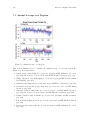
Annual Average over Regions . . . . . . . . . . . . . . . . . . . . . . . . . . . . . . . .
Monthly Cycle . . . . . . . . . . . . . . . . . . . . . . . . . . . . . . . . . . . . . . . . . . . . . . .
Regrid MODIS Data . . . . . . . . . . . . . . . . . . . . . . . . . . . . . . . . . . . . . . . . . .
Add Coordinates to MODIS Data . . . . . . . . . . . . . . . . . . . . . . . . . . . . .
Permute MODIS Coordinates . . . . . . . . . . . . . . . . . . . . . . . . . . . . . . . . .
247
253
256
263
266
269
270
8
Parallel . . . . . . . . . . . . . . . . . . . . . . . . . . . . . . . . . . . . . . . . 273
9
CCSM Example . . . . . . . . . . . . . . . . . . . . . . . . . . . . . . 275
10
References . . . . . . . . . . . . . . . . . . . . . . . . . . . . . . . . . . . 283
General Index . . . . . . . . . . . . . . . . . . . . . . . . . . . . . . . . . . . . 285
Foreword
1
Foreword
NCO is the result of software needs that arose while I worked on projects funded by NCAR,
NASA, and ARM. Thinking they might prove useful as tools or templates to others, it
is my pleasure to provide them freely to the scientific community. Many users (most of
whom I have never met) have encouraged the development of NCO. Thanks espcially to Jan
Polcher, Keith Lindsay, Arlindo da Silva, John Sheldon, and William Weibel for stimulating
suggestions and correspondence. Your encouragment motivated me to complete the NCO
User Guide. So if you like NCO, send me a note! I should mention that NCO is not connected
to or officially endorsed by Unidata, ACD, ASP, CGD, or Nike.
Charlie Zender
May 1997
Boulder, Colorado
Major feature improvements entitle me to write another Foreword. In the last five years
a lot of work has been done to refine NCO. NCO is now an open source project and appears
to be much healthier for it. The list of illustrious institutions that do not endorse NCO
continues to grow, and now includes UCI.
Charlie Zender
October 2000
Irvine, California
The most remarkable advances in NCO capabilities in the last few years are due to contributions from the Open Source community. Especially noteworthy are the contributions
of Henry Butowsky and Rorik Peterson.
Charlie Zender
January 2003
Irvine, California
NCO was generously supported from 2004–2008 by US National Science Foundation (NSF) grant IIS-0431203 (http: / / www . nsf . gov / awardsearch / showAward . do ?
AwardNumber=0431203). This support allowed me to maintain and extend core NCO code,
2
NCO 4.5.3-alpha03 User Guide
and others to advance NCO in new directions: Gayathri Venkitachalam helped implement
MPI; Harry Mangalam improved regression testing and benchmarking; Daniel Wang developed the server-side capability, SWAMP; and Henry Butowsky, a long-time contributor,
developed ncap2. This support also led NCO to debut in professional journals and meetings.
The personal and professional contacts made during this evolution have been immensely
rewarding.
Charlie Zender
March 2008
Grenoble, France
The end of the NSF SEI grant in August, 2008 curtailed NCO development. Fortunately
we could justify supporting Henry Butowsky on other research grants until May, 2010 while
he developed the key ncap2 features used in our climate research. And recently the NASA
ACCESS program commenced funding us to support netCDF4 group functionality. Thus
NCO will grow and evade bit-rot for the foreseeable future.
I continue to receive with gratitude the thanks of NCO users at nearly every scientific
meeting I attend. People introduce themselves, shake my hand and extol NCO, often effusively, while I grin in stupid embarassment. These exchanges lighten me like anti-gravity.
Sometimes I daydream how many hours NCO has turned from grunt work to productive
research for researchers world-wide, or from research into early happy-hours. It’s a cool
feeling.
Charlie Zender
April, 2012
Irvine, California
The NASA ACCESS 2011 program generously supported (Cooperative Agreement
NNX12AF48A) NCO from 2012–2015. This allowed us to produce the first iteration of
a Group-oriented Data Analysis and Distribution (GODAD) software ecosystem. Shifting
more geoscience data analysis to GODAD is a long-term plan. Then the NASA ACCESS 2013
program agreed to support (Cooperative Agreement NNX14AH55A) NCO from 2014–2016.
This support permits us to implement support for Swath-like Data (SLD). Most recently,
the DOE has funded me to implement NCO re-gridding and parallelization in support of
their ACME program. After many years of crafting NCO as an after-hours hobby, I finally
have the cushion necessary to give it some real attention. And I’m looking forward to this
next, and most intense yet, phase of NCO development.
Foreword
Charlie Zender
June, 2015
Irvine, California
3
Summary
5
Summary
This manual describes NCO, which stands for netCDF Operators. NCO is a suite of programs
known as operators. Each operator is a standalone, command line program executed at
the shell-level like, e.g., ls or mkdir. The operators take netCDF files (including HDF5
files constructed using the netCDF API) as input, perform an operation (e.g., averaging or
hyperslabbing), and produce a netCDF file as output. The operators are primarily designed
to aid manipulation and analysis of data. The examples in this documentation are typical
applications of the operators for processing climate model output. This stems from their
origin, though the operators are as general as netCDF itself.
Chapter 1: Introduction
7
1 Introduction
1.1 Availability
The complete NCO source distribution is currently distributed as a compressed tarfile from
http://sf.net/projects/nco and from http://dust.ess.uci.edu/nco/nco.tar.
gz. The compressed tarfile must be uncompressed and untarred before building NCO.
Uncompress the file with ‘gunzip nco.tar.gz’. Extract the source files from the resulting
tarfile with ‘tar -xvf nco.tar’. GNU tar lets you perform both operations in one step
with ‘tar -xvzf nco.tar.gz’.
The documentation for NCO is called the NCO User Guide. The User Guide is available
in PDF, Postscript, HTML, DVI, TEXinfo, and Info formats. These formats are included
in the source distribution in the files nco.pdf, nco.ps, nco.html, nco.dvi, nco.texi,
and nco.info*, respectively. All the documentation descends from a single source file,
nco.texi1 . Hence the documentation in every format is very similar. However, some of the
complex mathematical expressions needed to describe ncwa can only be displayed in DVI,
Postscript, and PDF formats.
A complete list of papers and publications on/about NCO is available on the NCO homepage. Most of these are freely available. The primary refereed publications are ZeM06 and
Zen08. These contain copyright restrictions which limit their redistribution, but they are
freely available in preprint form from the NCO.
If you want to quickly see what the latest improvements in NCO are (without downloading
the entire source distribution), visit the NCO homepage at http://nco.sf.net. The HTML
version of the User Guide is also available online through the World Wide Web at URL
http://nco.sf.net/nco.html. To build and use NCO, you must have netCDF installed.
The netCDF homepage is http://www.unidata.ucar.edu/packages/netcdf.
New NCO releases are announced on the netCDF list and on the nco-announce mailing
list http://lists.sf.net/mailman/listinfo/nco-announce.
1.2 How to Use This Guide
Detailed instructions about how to download the newest version (http://nco.sf.net/#
Source), and how to complie source code (http://nco.sf.net/#bld), as well as a FAQ
(http://nco.sf.net/#FAQ) and descriptions of Known Problems (http://nco.sf.net/#
bug) etc. are on our homepage (http://nco.sf.net/).
There are twelve operators in the current version (4.5.3-alpha03). The function of each
is explained in Chapter 4 [Reference Manual], page 129. Many of the tasks that NCO can
accomplish are described during the explanation of common NCO Features (see Chapter 3
[Shared features], page 27). More specific use examples for each operator can be seen
by visiting the operator-specific examples in the Chapter 4 [Reference Manual], page 129.
1
To produce these formats, nco.texi was simply run through the freely available programs texi2dvi,
dvips, texi2html, and makeinfo. Due to a bug in TEX, the resulting Postscript file, nco.ps, contains
the Table of Contents as the final pages. Thus if you print nco.ps, remember to insert the Table of
Contents after the cover sheet before you staple the manual.
8
NCO 4.5.3-alpha03 User Guide
These can be found directly by prepending the operator name with the xmp_ tag, e.g.,
http://nco.sf.net/nco.html#xmp_ncks. Also, users can type the operator name on the
shell command line to see all the available options, or type, e.g., ‘man ncks’ to see a help
man-page.
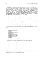
NCO is a command-line language. You may either use an operator after the prompt
(e.g., ‘$’ here), like,
$ operator [options] input [output]
or write all commands lines into a shell script, as in the CMIP5 Example (see Chapter 7
[CMIP5 Example], page 247).
If you are new to NCO, the Quick Start (see Chapter 6 [Quick Start], page 245) shows
simple examples about how to use NCO on different kinds of data files. More detailed “realworld” examples are in the Chapter 7 [CMIP5 Example], page 247. The [General Index],
page 285 is presents multiple keyword entries for the same subject. If these resources do
not help enough, please see Section 1.7 [Help Requests and Bug Reports], page 15.
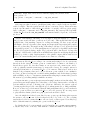
1.3 Operating systems compatible with NCO
In its time on Earth, NCO has been successfully ported and tested on so many 32- and 64-bit
platforms that if we did not write them down here we would forget their names: IBM AIX
4.x, 5.x, FreeBSD 4.x, GNU/Linux 2.x, LinuxPPC, LinuxAlpha, LinuxARM, LinuxSparc64,
LinuxAMD64, SGI IRIX 5.x and 6.x, MacOS X 10.x, DEC OSF, NEC Super-UX 10.x, Sun
SunOS 4.1.x, Solaris 2.x, Cray UNICOS 8.x–10.x, and Microsoft Windows (95, 98, NT, 2000,
XP, Vista, 7, 8, 10). If you port the code to a new operating system, please send me a note
and any patches you required.
The major prerequisite for installing NCO on a particular platform is the successful,
prior installation of the netCDF library (and, as of 2003, the UDUnits library). Unidata
has shown a commitment to maintaining netCDF and UDUnits on all popular UNIX platforms, and is moving towards full support for the Microsoft Windows operating system (OS).
Given this, the only difficulty in implementing NCO on a particular platform is standardization of various C-language API system calls. NCO code is tested for ANSI compliance
by compiling with C99 compilers including those from GNU (‘gcc -std=c99 -pedantic
-D_BSD_SOURCE -D_POSIX_SOURCE’ -Wall)2 , Comeau Computing (‘como --c99’), Cray
(‘cc’), HP/Compaq/DEC (‘cc’), IBM (‘xlc -c -qlanglvl=extc99’), Intel (‘icc -std=c99’),
LLVM (‘clang’), NEC (‘cc’), PathScale (QLogic) (‘pathcc -std=c99’), PGI (‘pgcc -c9x’),
SGI (‘cc -c99’), and Sun (‘cc’). NCO (all commands and the libnco library) and
the C++ interface to netCDF (called libnco_c++) comply with the ISO C++ standards as implemented by Comeau Computing (‘como’), Cray (‘CC’), GNU (‘g++ -Wall’),
HP/Compaq/DEC (‘cxx’), IBM (‘xlC’), Intel (‘icc’), Microsoft (‘MVS’), NEC (‘c++’), PathScale (Qlogic) (‘pathCC’), PGI (‘pgCC’), SGI (‘CC -LANG:std’), and Sun (‘CC -LANG:std’).
See nco/bld/Makefile and nco/src/nco_c++/Makefile.old for more details and exact
settings.
2
The ‘_BSD_SOURCE’ token is required on some Linux platforms where gcc dislikes the network header
files like netinet/in.h).
Chapter 1: Introduction
9
Until recently (and not even yet), ANSI-compliant has meant compliance with the 1989
ISO C-standard, usually called C89 (with minor revisions made in 1994 and 1995). C89 lacks
variable-size arrays, restricted pointers, some useful printf formats, and many mathematical special functions. These are valuable features of C99, the 1999 ISO C-standard. NCO
is C99-compliant where possible and C89-compliant where necessary. Certain branches in
the code are required to satisfy the native SGI and SunOS C compilers, which are strictly
ANSI C89 compliant, and cannot benefit from C99 features. However, C99 features are fully
supported by modern AIX, GNU, Intel, NEC, Solaris, and UNICOS compilers. NCO requires
a C99-compliant compiler as of NCO version 2.9.8, released in August, 2004.
The most time-intensive portion of NCO execution is spent in arithmetic operations,
e.g., multiplication, averaging, subtraction. These operations were performed in Fortran
by default until August, 1999. This was a design decision based on the relative speed of
Fortran-based object code vs. C-based object code in late 1994. C compiler vectorization capabilities have dramatically improved since 1994. We have accordingly replaced all Fortran
subroutines with C functions. This greatly simplifies the task of building NCO on nominally
unsupported platforms. As of August 1999, NCO built entirely in C by default. This allowed NCO to compile on any machine with an ANSI C compiler. In August 2004, the first
C99 feature, the restrict type qualifier, entered NCO in version 2.9.8. C compilers can
obtain better performance with C99 restricted pointers since they inform the compiler when
it may make Fortran-like assumptions regarding pointer contents alteration. Subsequently,
NCO requires a C99 compiler to build correctly3 .
In January 2009, NCO version 3.9.6 was the first to link to the GNU Scientific Library
(GSL). GSL must be version 1.4 or later. NCO, in particular ncap2, uses the GSL special function library to evaluate geoscience-relevant mathematics such as Bessel functions,
Legendre polynomials, and incomplete gamma functions (see Section 4.1.19 [GSL special
functions], page 161).
In June 2005, NCO version 3.0.1 began to take advantage of C99 mathematical special functions. These include the standarized gamma function (called tgamma() for “true
gamma”). NCO automagically takes advantage of some GNU Compiler Collection (GCC)
extensions to ANSI C.
As of July 2000 and NCO version 1.2, NCO no longer performs arithmetic operations
in Fortran. We decided to sacrifice executable speed for code maintainability. Since no
objective statistics were ever performed to quantify the difference in speed between the
Fortran and C code, the performance penalty incurred by this decision is unknown. Supporting Fortran involves maintaining two sets of routines for every arithmetic operation.
The USE_FORTRAN_ARITHMETIC flag is still retained in the Makefile. The file containing
the Fortran code, nco_fortran.F, has been deprecated but a volunteer (Dr. Frankenstein?)
could resurrect it. If you would like to volunteer to maintain nco_fortran.F please contact
me.
3
NCO may still build with an ANSI or ISO C89 or C94/95-compliant compiler if the C pre-processor
undefines the restrict type qualifier, e.g., by invoking the compiler with ‘-Drestrict=’’’.
10
NCO 4.5.3-alpha03 User Guide
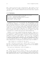
1.3.1 Compiling NCO for Microsoft Windows OS
NCO has been successfully ported and tested on most Microsoft Windows operating systems
including: XP SP2/Vista/7. Support is provided for compiling either native Windows
executables, using the Microsoft Visual Studio 2010 Compiler, or with Cygwin, the UNIXemulating compatibility layer with the GNU toolchain. The switches necessary to accomplish
both are included in the standard distribution of NCO.
Using Microsoft Visual Studio (MVS), one must build NCO with the C++ compiler since
MVS does not support C99. Qt, a convenient integrated development environment, was
used to convert the project files to MVS format. The Qt files themselves are distributed in
the nco/qt directory.
Using the freely available Cygwin (formerly gnu-win32) development environment4 , the
compilation process is very similar to installing NCO on a UNIX system. Set the PVM_ARCH
preprocessor token to WIN32. Note that defining WIN32 has the side effect of disabling
Internet features of NCO (see below). NCO should now build like it does on UNIX.
The least portable section of the code is the use of standard UNIX and Internet protocols
(e.g., ftp, rcp, scp, sftp, getuid, gethostname, and header files <arpa/nameser.h> and
<resolv.h>). Fortunately, these UNIX-y calls are only invoked by the single NCO subroutine
which is responsible for retrieving files stored on remote systems (see Section 3.7 [Remote
storage], page 33). In order to support NCO on the Microsoft Windows platforms, this
single feature was disabled (on Windows OS only). This was required by Cygwin 18.x—
newer versions of Cygwin may support these protocols (let me know if this is the case).
The NCO operators should behave identically on Windows and UNIX platforms in all other
respects.
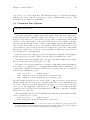
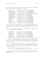
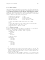
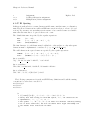
1.4 Symbolic Links
NCO relies on a common set of underlying algorithms. To minimize duplication of source
code, multiple operators sometimes share the same underlying source. This is accomplished
by symbolic links from a single underlying executable program to one or more invoked
executable names. For example, nces and ncrcat are symbolically linked to the ncra
executable. The ncra executable behaves slightly differently based on its invocation name
(i.e., ‘argv[0]’), which can be nces, ncra, or ncrcat. Logically, these are three different
operators that happen to share the same executable.
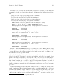
For historical reasons, and to be more user friendly, multiple synonyms (or pseudonyms)
may refer to the same operator invoked with different switches. For example, ncdiff is
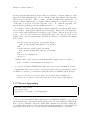
the same as ncbo and ncpack is the same as ncpdq. We implement the symbolic links and
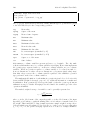
synonyms by the executing the following UNIX commands in the directory where the NCO
executables are installed.
ln -s -f ncbo ncdiff
ln -s -f ncra nces
4
# ncbo --op_typ=’-’
# ncra --pseudonym=’nces’
The Cygwin package is available from
http://sourceware.redhat.com/cygwin
Currently, Cygwin 20.x comes with the GNU C/C++ compilers (gcc, g++. These GNU compilers may be
used to build the netCDF distribution itself.
Chapter 1: Introduction
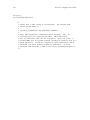
ln -s
ln -s
ln -s
ln -s
ln -s
ln -s
ln -s
# NB:
ln -s
...
11
-f ncra ncrcat
# ncra --pseudonym=’ncrcat’
-f ncbo ncadd
# ncbo --op_typ=’+’
-f ncbo ncsubtract # ncbo --op_typ=’-’
-f ncbo ncmultiply # ncbo --op_typ=’*’
-f ncbo ncdivide
# ncbo --op_typ=’/’
-f ncpdq ncpack
# ncpdq
-f ncpdq ncunpack # ncpdq --unpack
Windows/Cygwin executable/link names have ’.exe’ suffix, e.g.,
-f ncbo.exe ncdiff.exe
The imputed command called by the link is given after the comment. As can be seen,
some these links impute the passing of a command line argument to further modify the
behavior of the underlying executable. For example, ncdivide is a pseudonym for ncbo
--op_typ=’/’.
1.5 Libraries
Like all executables, the NCO operators can be built using dynamic linking. This reduces
the size of the executable and can result in significant performance enhancements on multiuser systems. Unfortunately, if your library search path (usually the LD_LIBRARY_PATH
environment variable) is not set correctly, or if the system libraries have been moved, renamed, or deleted since NCO was installed, it is possible NCO operators will fail with a
message that they cannot find a dynamically loaded (aka shared object or ‘.so’) library.
This will produce a distinctive error message, such as ‘ld.so.1: /usr/local/bin/nces:
fatal: libsunmath.so.1: can’t open file: errno=2’. If you received an error message
like this, ask your system administrator to diagnose whether the library is truly missing5 ,
or whether you simply need to alter your library search path. As a final remedy, you may
re-compile and install NCO with all operators statically linked.
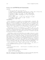
1.6 netCDF2/3/4 and HDF4/5 Support
netCDF version 2 was released in 1993. NCO (specifically ncks) began soon after this
in 1994. netCDF 3.0 was released in 1996, and we were not exactly eager to convert all
code to the newer, less tested netCDF implementation. One netCDF3 interface call (nc_
inq_libvers) was added to NCO in January, 1998, to aid in maintainance and debugging.
In March, 2001, the final NCO conversion to netCDF3 was completed (coincidentally on
the same day netCDF 3.5 was released). NCO versions 2.0 and higher are built with the
-DNO_NETCDF_2 flag to ensure no netCDF2 interface calls are used.
However, the ability to compile NCO with only netCDF2 calls is worth maintaining
because HDF version 4, aka HDF4 or simply HDF,6 (available from HDF (http://hdfgroup.
org)) supports only the netCDF2 library calls (see http://hdfgroup.org/UG41r3_html/
SDS_SD.fm12.html#47784). There are two versions of HDF. Currently HDF version 4.x
5
6
The ldd command, if it is available on your system, will tell you where the executable is looking for each
dynamically loaded library. Use, e.g., ldd ‘which nces‘.
The Hierarchical Data Format, or HDF, is another self-describing data format similar to, but more
elaborate than, netCDF. HDF comes in two flavors, HDF4 and HDF5. Often people use the shorthand
HDF to refer to the older format HDF4. People almost always use HDF5 to refer to HDF5.
12
NCO 4.5.3-alpha03 User Guide
supports the full netCDF2 API and thus NCO version 1.2.x. If NCO version 1.2.x (or earlier)
is built with only netCDF2 calls then all NCO operators should work with HDF4 files as
well as netCDF files7 . The preprocessor token NETCDF2_ONLY exists in NCO version 1.2.x
to eliminate all netCDF3 calls. Only versions of NCO numbered 1.2.x and earlier have this
capability.
HDF version 5 became available in 1999, but did not support netCDF (or, for that matter,
Fortran) as of December 1999. By early 2001, HDF5 did support Fortran90. Thanks to an
NSF-funded “harmonization” partnership, HDF began to fully support the netCDF3 read
interface (which is employed by NCO 2.x and later). In 2004, Unidata and THG began a
project to implement the HDF5 features necessary to support the netCDF API. NCO version
3.0.3 added support for reading/writing netCDF4-formatted HDF5 files in October, 2005.
See Section 3.9 [File Formats and Conversion], page 38 for more details.
HDF support for netCDF was completed with HDF5 version version 1.8 in 2007. The
netCDF front-end that uses this HDF5 back-end was completed and released soon after
as netCDF version 4. Download it from the netCDF4 (http://my.unidata.ucar.edu/
content/software/netcdf/netcdf-4) website.
NCO version 3.9.0, released in May, 2007, added support for all netCDF4 atomic data
types except NC_STRING. Support for NC_STRING, including ragged arrays of strings, was
finally added in version 3.9.9, released in June, 2009. Support for additional netCDF4
features has been incremental. We add one netCDF4 feature at a time. You must build
NCO with netCDF4 to obtain this support.
NCO supports many netCDF4 features including atomic data types, Lempel-Ziv com-
pression (deflation), chunking, and groups. The new atomic data types are NC_UBYTE,
NC_USHORT, NC_UINT, NC_INT64, and NC_UINT64. Eight-byte integer support is an especially useful improvement from netCDF3. All NCO operators support these types, e.g.,
ncks copies and prints them, ncra averages them, and ncap2 processes algebraic scripts
with them. ncks prints compression information, if any, to screen.
NCO version 3.9.1 (June, 2007) added support for netCDF4 Lempel-Ziv deflation.
Lempel-Ziv deflation is a lossless compression technique. See Section 3.30 [Deflation],
page 101 for more details.
NCO version 3.9.9 (June, 2009) added support for netCDF4 chunking in ncks and
ncecat. NCO version 4.0.4 (September, 2010) completed support for netCDF4 chunking in
the remaining operators. See Section 3.28 [Chunking], page 85 for more details.
NCO version 4.2.2 (October, 2012) added support for netCDF4 groups in ncks and
ncecat. Group support for these operators was complete (e.g., regular expressions to select
groups and Group Path Editing) as of NCO version 4.2.6 (March, 2013). See Section 3.13
[Group Path Editing], page 48 for more details. Group support for all other operators was
finished in the NCO version 4.3.x series completed in December, 2013.
7
One must link the NCO code to the HDF4 MFHDF library instead of the usual netCDF library. Apparently
‘MF’ stands for Multi-file not for Mike Folk. In any case, until about 2007 the MFHDF library only
supported netCDF2 calls. Most people will never again install NCO 1.2.x and so will never use NCO to
write HDF4 files. It is simply too much trouble.
Chapter 1: Introduction
13
Support for netCDF4 in the first arithmetic operator, ncbo, was introduced in NCO
version 4.3.0 (March, 2013). NCO version 4.3.1 (May, 2013) completed this support and
introduced the first example of automatic group broadcasting. See Section 4.3 [ncbo netCDF
Binary Operator], page 189 for more details.
netCDF4-enabled NCO handles netCDF3 files without change. In addition, it automagically handles netCDF4 (HDF5) files: If you feed NCO netCDF3 files, it produces netCDF3
output. If you feed NCO netCDF4 files, it produces netCDF4 output. Use the handy-dandy
‘-4’ switch to request netCDF4 output from netCDF3 input, i.e., to convert netCDF3 to
netCDF4. See Section 3.9 [File Formats and Conversion], page 38 for more details.
When linked to a netCDF library that was built with HDF4 support8 , NCO automatically
supports reading HDF4 files and writing them as netCDF3/netCDF4/HDF5 files. NCO can
only write through the netCDF API, which can only write netCDF3/netCDF4/HDF5 files.
So NCO can read HDF4 files, perform manipulations and calculations, and then it must
write the results in netCDF format.
NCO support for HDF4 has been quite functional since December, 2013. For best results
install NCO versions 4.4.0 or later on top of netCDF versions 4.3.1 or later. Getting to this
point has been an iterative effort where Unidata improved netCDF library capabilities in
response to our requests. NCO versions 4.3.6 and earlier do not explicitly support HDF4,
yet should work with HDF4 if compiled with a version of netCDF (4.3.2 or later?) that
does not unexpectedly die when probing HDF4 files with standard netCDF calls. NCO
versions 4.3.7–4.3.9 (October–December, 2013) use a special flag to workaround netCDF
HDF4 issues. The user must tell these versions of NCO that an input file is HDF4 format by
using the ‘--hdf4’ switch.
When compiled with netCDF version 4.3.1 (20140116) or later, NCO versions 4.4.0 (January, 2014) and later more gracefully handle HDF4 files. In particular, the ‘--hdf4’ switch is
obsolete. Current versions of NCO use netCDF to determine automatically whether the underlying file is HDF4, and then take appropriate precautions to avoid netCDF4 API calls that
fail when applied to HDF4 files (e.g., nc_inq_var_chunking(), nc_inq_var_deflate()).
When compiled with netCDF version 4.3.2 (20140423) or earlier, NCO will report that
chunking and deflation properties of HDF4 files as HDF4_UNKNOWN, because determining
those properties was impossible. When compiled with netCDF version 4.3.3-rc2 (20140925)
or later, NCO versions 4.4.6 (October, 2014) and later fully support chunking and deflation
features of HDF4 files. The ‘--hdf4’ switch is supported (for backwards compatibility) yet
redundant (i.e., does no harm) with current versions of NCO and netCDF.
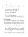
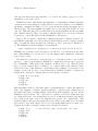
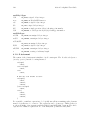
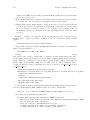
Converting HDF4 files to netCDF: Since NCO reads HDF4 files natively, it is now easy
to convert HDF4 files to netCDF files directly, e.g.,
ncks
fl.hdf fl.nc # Convert HDF4->netCDF4 (NCO 4.4.0+, netCDF 4.3.1+)
ncks --hdf4 fl.hdf fl.nc # Convert HDF4->netCDF4 (NCO 4.3.7-4.3.9)
The most efficient and accurate way to convert HDF4 data to netCDF format is to
convert to netCDF4 using NCO as above. Many HDF4 producers (NASA!) love to use
netCDF4 types, e.g., unsigned bytes, so this procedure is the most typical. Conversion of
8
The procedure for doing this is documented at http://www.unidata.ucar.edu/software/netcdf/docs/
build_hdf4.html.
14
NCO 4.5.3-alpha03 User Guide
HDF4 to netCDF4 as above suffices when the data will only be processed by NCO and other
netCDF4-aware tools.
However, many tools are not fully netCDF4-aware, and so conversion to netCDF3 may
be desirable. Obtaining any netCDF file from an HDF4 is easy:
ncks
ncks
ncks
ncks
ncks
ncks
ncks
ncks
-3 fl.hdf fl.nc
#
-4 fl.hdf fl.nc
#
-6 fl.hdf fl.nc
#
-7 -L 1 fl.hdf fl.nc #
--hdf4 -3 fl.hdf fl.nc
--hdf4 -4 fl.hdf fl.nc
--hdf4 -6 fl.hdf fl.nc
--hdf4 -7 fl.hdf fl.nc
HDF4->netCDF3 (NCO 4.4.0+, netCDF 4.3.1+)
HDF4->netCDF4 (NCO 4.4.0+, netCDF 4.3.1+)
HDF4->netCDF3 64-bit (NCO 4.4.0+, ...)
HDF4->netCDF4 classic (NCO 4.4.0+, ...)
# HDF4->netCDF3 (netCDF 4.3.0-)
# HDF4->netCDF4 (netCDF 4.3.0-)
# HDF4->netCDF3 64-bit (netCDF 4.3.0-)
# HDF4->netCDF4 classic (netCDF 4.3.0-)
As of NCO version 4.4.0 (January, 2014), these commands work even when the HDF4
file contains netCDF4 atomic types (e.g., unsigned bytes, 64-bit integers) because NCO can
autoconvert everything to atomic types supported by netCDF39 .
As of NCO version 4.4.4 (May, 2014) both ncl_convert2nc and NCO have built-in,
automatic workarounds to handle element names that contain characters that are legal in
HDF though are illegal in netCDF. For example, slashes and leading special characters
are are legal in HDF and illegal in netCDF element (i.e., group, variable, dimension, and
attribute) names. NCO converts these forbidden characters to underscores, and retains the
original names of variables in automatically produced attributes named hdf_name10 .
Finally, in February 2014, we learned that the HDF group has a project called H4CF
(described here (http://hdfeos.org/software/h4cflib.php)) whose goal is to make
HDF4 files accessible to CF tools and conventions. Their project includes a tool named
h4tonccf that converts HDF4 files to netCDF3 or netCDF4 files. We are not yet sure what
advantages or features h4tonccf has that are not in NCO, though we suspect both methods
have their own advantages. Corrections welcome.
As of 2012, netCDF4 is relatively stable software. Problems with netCDF4 and HDF
libraries have mainly been fixed. Binary NCO distributions shipped as RPMs and as debs
have used the netCDF4 library since 2010 and 2011, respectively.
9
10
Prior to NCO version 4.4.0 (January, 2014), we recommended the ncl_convert2nc tool to convert HDF
to netCDF3 when both these are true: 1. You must have netCDF3 and 2. the HDF file contains netCDF4
atomic types. More recent versions of NCO handle this problem fine, and include other advantages so we
no longer recommend ncl_convert2nc because ncks is faster and more space-efficient. Both automatically convert netCDF4 types to netCDF3 types, yet ncl_convert2nc cannot produce full netCDF4 files.
In contrast, ncks will happily convert HDF straight to netCDF4 files with netCDF4 types. Hence ncks
can and does preserve the variable types. Unsigned bytes stay unsigned bytes. 64-bit integers stay 64-bit
integers. Strings stay strings. Hence, ncks conversions often result in smaller files than ncl_convert2nc
conversions. A tool useful for converting netCDF3 to netCDF4 files is the Python script nc3tonc4 by
Jeff Whitaker.
Two real-world examples: NCO translates the NASA CERES dimension (FOV) Footprints to _FOV_
Footprints, and Cloud & Aerosol, Cloud Only, Clear Sky w/Aerosol, and Clear Sky (yes, the dimension name includes whitespace and special characters) to Cloud & Aerosol, Cloud Only, Clear Sky w_
Aerosol, and Clear Sky ncl_convert2nc makes the element name netCDF-safe in a slightly different
manner, and also stores the original name in the hdf_name attribute.
Chapter 1: Introduction
15
One must often build NCO from source to obtain netCDF4 support. Typically, one
specifies the root of the netCDF4 installation directory. Do this with the NETCDF4_ROOT
variable. Then use your preferred NCO build mechanism, e.g.,
export NETCDF4_ROOT=/usr/local/netcdf4 # Set netCDF4 location
cd ~/nco;./configure --enable-netcdf4 # Configure mechanism -orcd ~/nco/bld;./make NETCDF4=Y allinone # Old Makefile mechanism
We carefully track the netCDF4 releases, and keep the netCDF4 atomic type support
and other features working. Our long term goal is to utilize more of the extensive new
netCDF4 feature set. The next major netCDF4 feature we are likely to utilize is parallel
I/O. We will enable this in the MPI netCDF operators.
1.7 Help Requests and Bug Reports
We generally receive three categories of mail from users: help requests, bug reports, and
feature requests. Notes saying the equivalent of “Hey, NCO continues to work great and it
saves me more time everyday than it took to write this note” are a distant fourth.
There is a different protocol for each type of request. The preferred etiquette for all
communications is via NCO Project Forums. Do not contact project members via personal
e-mail unless your request comes with money or you have damaging information about our
personal lives. Please use the Forums—they preserve a record of the questions and answers
so that others can learn from our exchange. Also, since NCO is government-funded, this
record helps us provide program officers with information they need to evaluate our project.
Before posting to the NCO forums described below, you might first register (https://
sf.net/account/register.php) your name and email address with SourceForge.net or
else all of your postings will be attributed to nobody. Once registered you may choose to
monitor any forum and to receive (or not) email when there are any postings including
responses to your questions. We usually reply to the forum message, not to the original
poster.
If you want us to include a new feature in NCO, check first to see if that feature is
already on the TODO (file:./TODO) list. If it is, why not implement that feature yourself
and send us the patch? If the feature is not yet on the list, then send a note to the NCO
Discussion forum (http://sf.net/p/nco/discussion/9829).
Read the manual before reporting a bug or posting a help request. Sending questions
whose answers are not in the manual is the best way to motivate us to write more documentation. We would also like to accentuate the contrapositive of this statement. If you
think you have found a real bug the most helpful thing you can do is simplify the problem to
a manageable size and then report it. The first thing to do is to make sure you are running
the latest publicly released version of NCO.
Once you have read the manual, if you are still unable to get NCO to perform a documented function, submit a help request. Follow the same procedure as described below
for reporting bugs (after all, it might be a bug). That is, describe what you are trying to
do, and include the complete commands (run with ‘-D 5’), error messages, and version of
NCO (with ‘-r’). Post your help request to the NCO Help forum (http://sf.net/p/nco/
discussion/9830).
16
NCO 4.5.3-alpha03 User Guide
If you think you used the right command when NCO misbehaves, then you might have
found a bug. Incorrect numerical answers are the highest priority. We usually fix those
within one or two days. Core dumps and sementation violations receive lower priority.
They are always fixed, eventually.
How do you simplify a problem that reveal a bug? Cut out extraneous variables, dimensions, and metadata from the offending files and re-run the command until it no longer
breaks. Then back up one step and report the problem. Usually the file(s) will be very
small, i.e., one variable with one or two small dimensions ought to suffice. Run the operator
with ‘-r’ and then run the command with ‘-D 5’ to increase the verbosity of the debugging output. It is very important that your report contain the exact error messages and
compile-time environment. Include a copy of your sample input file, or place one on a publicly accessible location, of the file(s). If you are sure it is a bug, post the full report to the
NCO Project buglist (http://sf.net/p/nco/bugs). Otherwise post all the information to
NCO Help forum (http://sf.net/p/nco/discussion/9830).
Build failures count as bugs. Our limited machine access means we cannot fix all build
failures. The information we need to diagnose, and often fix, build failures are the three files
output by GNU build tools, nco.config.log.${GNU_TRP}.foo, nco.configure.${GNU_
TRP}.foo, and nco.make.${GNU_TRP}.foo. The file configure.eg shows how to produce
these files. Here ${GNU_TRP} is the “GNU architecture triplet”, the chip-vendor-OS string
returned by config.guess. Please send us your improvements to the examples supplied in
configure.eg. The regressions archive at http://dust.ess.uci.edu/nco/rgr contains
the build output from our standard test systems. You may find you can solve the build
problem yourself by examining the differences between these files and your own.
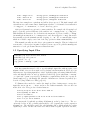
Chapter 2: Operator Strategies
17
2 Operator Strategies
2.1 Philosophy
The main design goal is command line operators which perform useful, scriptable operations
on netCDF files. Many scientists work with models and observations which produce too
much data to analyze in tabular format. Thus, it is often natural to reduce and massage
this raw or primary level data into summary, or second level data, e.g., temporal or spatial
averages. These second level data may become the inputs to graphical and statistical packages, and are often more suitable for archival and dissemination to the scientific community.
NCO performs a suite of operations useful in manipulating data from the primary to the
second level state. Higher level interpretive languages (e.g., IDL, Yorick, Matlab, NCL, Perl,
Python), and lower level compiled languages (e.g., C, Fortran) can always perform any task
performed by NCO, but often with more overhead. NCO, on the other hand, is limited to
a much smaller set of arithmetic and metadata operations than these full blown languages.
Another goal has been to implement enough command line switches so that frequently
used sequences of these operators can be executed from a shell script or batch file. Finally,
NCO was written to consume the absolute minimum amount of system memory required to
perform a given job. The arithmetic operators are extremely efficient; their exact memory
usage is detailed in Section 2.9 [Memory Requirements], page 24.
2.2 Climate Model Paradigm
NCO was developed at NCAR to aid analysis and manipulation of datasets produced by
General Circulation Models (GCMs). GCM datasets share many features with other gridded
scientific datasets and so provide a useful paradigm for the explication of the NCO operator
set. Examples in this manual use a GCM paradigm because latitude, longitude, time,
temperature and other fields related to our natural environment are as easy to visualize for
the layman as the expert.
2.3 Temporary Output Files
NCO operators are designed to be reasonably fault tolerant, so that a system failure or user-
abort of the operation (e.g., with C-c) does not cause loss of data. The user-specified outputfile is only created upon successful completion of the operation1 . This is accomplished by
performing all operations in a temporary copy of output-file. The name of the temporary
output file is constructed by appending .pid<process ID>.<operator name>.tmp to the
user-specified output-file name. When the operator completes its task with no fatal errors,
the temporary output file is moved to the user-specified output-file. This imbues the process with fault-tolerance since fatal error (e.g., disk space fills up) affect only the temporary
output file, leaving the final output file not created if it did not already exist. Note the construction of a temporary output file uses more disk space than just overwriting existing files
“in place” (because there may be two copies of the same file on disk until the NCO operation
successfully concludes and the temporary output file overwrites the existing output-file).
1
The ncrename and ncatted operators are exceptions to this rule. See Section 4.11 [ncrename netCDF
Renamer], page 230.
18
NCO 4.5.3-alpha03 User Guide
Also, note this feature increases the execution time of the operator by approximately the
time it takes to copy the output-file 2 . Finally, note this fault-tolerant feature allows the
output-file to be the same as the input-file without any danger of “overlap”.
Over time many “power users” have requested a way to turn-off the fault-tolerance safety
feature of automatically creating a temporary file. Often these users build and execute
production data analysis scripts that are repeated frequently on large datasets. Obviating
an extra file write can then conserve significant disk space and time. For this purpose NCO
has, since version 4.2.1 in August, 2012, made configurable the controls over temporary
file creation. The ‘--wrt_tmp_fl’ and equivalent ‘--write_tmp_fl’ switches ensure NCO
writes output to an intermediate temporary file. This is and has always been the default
behavior so there is currently no need to specify these switches. However, the default may
change some day, especially since writing to RAM disks (see Section 3.33 [RAM disks],
page 104) may some day become the default. The ‘--no_tmp_fl’ switch causes NCO to
write directly to the final output file instead of to an intermediate temporary file. “Power
users” may wish to invoke this switch to increase performance (i.e., reduce wallclock time)
when manipulating large files. When eschewing temporary files, users may forsake the
ability to have the same name for both output-file and input-file since, as described above,
the temporary file prevented overlap issues. However, if the user creates the output file in
RAM (see Section 3.33 [RAM disks], page 104) then it is still possible to have the same
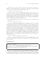
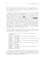
name for both output-file and input-file.
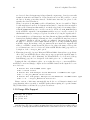
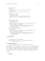
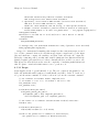
ncks
ncks
ncks
ncks
ncks
ncks
in.nc out.nc # Default: create out.pid.tmp.nc then move to out.nc
--wrt_tmp_fl in.nc out.nc # Same as default
--no_tmp_fl in.nc out.nc # Create out.nc directly on disk
--no_tmp_fl in.nc in.nc # ERROR-prone! Overwrite in.nc with itself
--create_ram --no_tmp_fl in.nc in.nc # Create in RAM, write to disk
--open_ram --no_tmp_fl in.nc in.nc # Read into RAM, write to disk
There is no reason to expect the fourth example to work. The behavior of overwriting a
file while reading from the same file is undefined, much as is the shell command ‘cat foo
> foo’. Although it may “work” in some cases, it is unreliable. One way around this is
to use ‘--create_ram’ so that the output file is not written to disk until the input file is
closed, See Section 3.33 [RAM disks], page 104. However, as of 20130328, the behavior of
the ‘--create_ram’ and ‘--open_ram’ examples has not been thoroughly tested.
The NCO authors have seen compelling use cases for utilizing the RAM switches, though
not (yet) for combining them with ‘--no_tmp_fl’. NCO implements both options because
they are largely independent of eachother. It is up to “power users” to discover which best
fit their needs. We welcome accounts of your experiences posted to the forums.
Other safeguards exist to protect the user from inadvertently overwriting data. If the
output-file specified for a command is a pre-existing file, then the operator will prompt
the user whether to overwrite (erase) the existing output-file, attempt to append to it, or
abort the operation. However, in processing large amounts of data, too many interactive
questions slows productivity. Therefore NCO also implements two ways to override its own
safety features, the ‘-O’ and ‘-A’ switches. Specifying ‘-O’ tells the operator to overwrite
any existing output-file without prompting the user interactively. Specifying ‘-A’ tells the
2
The OS-specific system move command is used. This is mv for UNIX, and move for Windows.
Chapter 2: Operator Strategies
19
operator to attempt to append to any existing output-file without prompting the user interactively. These switches are useful in batch environments because they suppress interactive
keyboard input.
2.4 Appending Variables
Adding variables from one file to another is often desirable. This is referred to as appending,
although some prefer the terminology merging 3 or pasting. Appending is often confused
with what NCO calls concatenation. In NCO, concatenation refers to splicing a variable
along the record dimension. The length along the record dimension of the output is the
sum of the lengths of the input files. Appending, on the other hand, refers to copying a
variable from one file to another file which may or may not already contain the variable4 .
NCO can append or concatenate just one variable, or all the variables in a file at the same
time.
In this sense, ncks can append variables from one file to another file. This capability is
invoked by naming two files on the command line, input-file and output-file. When outputfile already exists, the user is prompted whether to overwrite, append/replace, or exit from
the command. Selecting overwrite tells the operator to erase the existing output-file and
replace it with the results of the operation. Selecting exit causes the operator to exit—the
output-file will not be touched in this case. Selecting append/replace causes the operator
to attempt to place the results of the operation in the existing output-file, See Section 4.7
[ncks netCDF Kitchen Sink], page 203.
The simplest way to create the union of two files is
ncks -A fl_1.nc fl_2.nc
This puts the contents of fl_1.nc into fl_2.nc. The ‘-A’ is optional. On output,
fl_2.nc is the union of the input files, regardless of whether they share dimensions and
variables, or are completely disjoint. The append fails if the input files have differently
named record dimensions (since netCDF supports only one), or have dimensions of the
same name but different sizes.
2.5 Simple Arithmetic and Interpolation
Users comfortable with NCO semantics may find it easier to perform some simple mathematical operations in NCO rather than higher level languages. ncbo (see Section 4.3 [ncbo
netCDF Binary Operator], page 189) does file addition, subtraction, multiplication, division, and broadcasting. It even does group broadcasting. ncflint (see Section 4.6 [ncflint
netCDF File Interpolator], page 200) does file addition, subtraction, multiplication and interpolation. Sequences of these commands can accomplish simple yet powerful operations
from the command line.
3
4
The terminology merging is reserved for an (unwritten) operator which replaces hyperslabs of a variable
in one file with hyperslabs of the same variable from another file
Yes, the terminology is confusing. By all means mail me if you think of a better nomenclature. Should
NCO use paste instead of append?
20
NCO 4.5.3-alpha03 User Guide
2.6 Statistics vs. Concatenation
The most frequently used operators of NCO are probably the statisticians (i.e., tools that do
statistics) and concatenators. Because there are so many types of statistics like averaging
(e.g., across files, within a file, over the record dimension, over other dimensions, with or
without weights and masks) and of concatenating (across files, along the record dimension,
along other dimensions), there are currently no fewer than five operators which tackle these
two purposes: ncra, nces, ncwa, ncrcat, and ncecat. These operators do share many
capabilities5 , though each has its unique specialty. Two of these operators, ncrcat and
ncecat, concatenate hyperslabs across files. The other two operators, ncra and nces,
compute statistics across (and/or within) files6 . First, let’s describe the concatenators,
then the statistics tools.
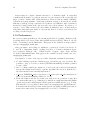
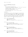
2.6.1 Concatenators ncrcat and ncecat
Joining together independent files along a common record dimension is called concatenation. ncrcat is designed for concatenating record variables, while ncecat is designed for
concatenating fixed length variables. Consider five files, 85.nc, 86.nc, . . . 89.nc each containing a year’s worth of data. Say you wish to create from them a single file, 8589.nc
containing all the data, i.e., spanning all five years. If the annual files make use of the
same record variable, then ncrcat will do the job nicely with, e.g., ncrcat 8?.nc 8589.nc.
The number of records in the input files is arbitrary and can vary from file to file. See
Section 4.10 [ncrcat netCDF Record Concatenator], page 228, for a complete description of
ncrcat.
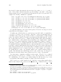
However, suppose the annual files have no record variable, and thus their data are all
fixed length. For example, the files may not be conceptually sequential, but rather members
of the same group, or ensemble. Members of an ensemble may have no reason to contain
a record dimension. ncecat will create a new record dimension (named record by default)
with which to glue together the individual files into the single ensemble file. If ncecat is
used on files which contain an existing record dimension, that record dimension is converted
to a fixed-length dimension of the same name and a new record dimension (named record)
is created. Consider five realizations, 85a.nc, 85b.nc, . . . 85e.nc of 1985 predictions from
the same climate model. Then ncecat 85?.nc 85_ens.nc glues together the individual
realizations into the single file, 85_ens.nc. If an input variable was dimensioned [lat,lon],
it will have dimensions [record,lat,lon] in the output file. A restriction of ncecat is that
the hyperslabs of the processed variables must be the same from file to file. Normally this
means all the input files are the same size, and contain data on different realizations of the
same variables. See Section 4.5 [ncecat netCDF Ensemble Concatenator], page 197, for a
complete description of ncecat.
ncpdq makes it possible to concatenate files along any dimension, not just the record
dimension. First, use ncpdq to convert the dimension to be concatenated (i.e., extended
5
6
Currently nces and ncrcat are symbolically linked to the ncra executable, which behaves slightly differently based on its invocation name (i.e., ‘argv[0]’). These three operators share the same source code,
and merely have different inner loops.
The third averaging operator, ncwa, is the most sophisticated averager in NCO. However, ncwa is in
a different class than ncra and nces because it operates on a single file per invocation (as opposed to
multiple files). On that single file, however, ncwa provides a richer set of averaging options—including
weighting, masking, and broadcasting.
Chapter 2: Operator Strategies
21
with data from other files) into the record dimension. Second, use ncrcat to concatenate
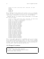
these files. Finally, if desirable, use ncpdq to revert to the original dimensionality. As
a concrete example, say that files x_01.nc, x_02.nc, . . . x_10.nc contain time-evolving
datasets from spatially adjacent regions. The time and spatial coordinates are time and x,
respectively. Initially the record dimension is time. Our goal is to create a single file that
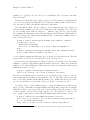
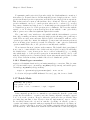
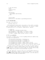
contains joins all the spatially adjacent regions into one single time-evolving dataset.
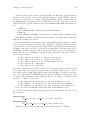
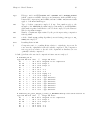
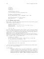
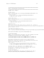
for idx in 01 02 03 04 05 06 07 08 09 10; do # Bourne Shell
ncpdq -a x,time x_${idx}.nc foo_${idx}.nc # Make x record dimension
done
ncrcat foo_??.nc out.nc
# Concatenate along x
ncpdq -a time,x out.nc out.nc # Revert to time as record dimension
Note that ncrcat will not concatenate fixed-length variables, whereas ncecat concatenates both fixed-length and record variables along a new record variable. To conserve system
memory, use ncrcat where possible.
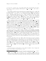
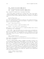
2.6.2 Averagers nces, ncra, and ncwa
The differences between the averagers ncra and nces are analogous to the differences between the concatenators. ncra is designed for averaging record variables from at least one
file, while nces is designed for averaging fixed length variables from multiple files. ncra performs a simple arithmetic average over the record dimension of all the input files, with each
record having an equal weight in the average. nces performs a simple arithmetic average
of all the input files, with each file having an equal weight in the average. Note that ncra
cannot average fixed-length variables, but nces can average both fixed-length and record
variables. To conserve system memory, use ncra rather than nces where possible (e.g., if
each input-file is one record long). The file output from nces will have the same dimensions
(meaning dimension names as well as sizes) as the input hyperslabs (see Section 4.4 [nces
netCDF Ensemble Statistics], page 194, for a complete description of nces). The file output from ncra will have the same dimensions as the input hyperslabs except for the record
dimension, which will have a size of 1 (see Section 4.9 [ncra netCDF Record Averager],
page 225, for a complete description of ncra).
2.6.3 Interpolator ncflint
ncflint can interpolate data between or two files. Since no other operators have this ability,
the description of interpolation is given fully on the ncflint reference page (see Section 4.6
[ncflint netCDF File Interpolator], page 200). Note that this capability also allows ncflint
to linearly rescale any data in a netCDF file, e.g., to convert between differing units.
2.7 Large Numbers of Files
Occasionally one desires to digest (i.e., concatenate or average) hundreds or thousands of
input files. Unfortunately, data archives (e.g., NASA EOSDIS) may not name netCDF files
in a format understood by the ‘-n loop’ switch (see Section 3.5 [Specifying Input Files],
page 30) that automagically generates arbitrary numbers of input filenames. The ‘-n loop’
switch has the virtue of being concise, and of minimizing the command line. This helps keeps
output file small since the command line is stored as metadata in the history attribute (see
Section 3.39 [History Attribute], page 122). However, the ‘-n loop’ switch is useless when
22
NCO 4.5.3-alpha03 User Guide
there is no simple, arithmetic pattern to the input filenames (e.g., h00001.nc, h00002.nc,
. . . h90210.nc). Moreover, filename globbing does not work when the input files are too
numerous or their names are too lengthy (when strung together as a single argument) to be
passed by the calling shell to the NCO operator7 . When this occurs, the ANSI C-standard
argc-argv method of passing arguments from the calling shell to a C-program (i.e., an
NCO operator) breaks down. There are (at least) three alternative methods of specifying
the input filenames to NCO in environment-limited situations.
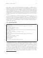
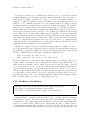
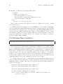
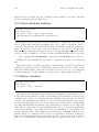
The recommended method for sending very large numbers (hundreds or more, typically)
of input filenames to the multi-file operators is to pass the filenames with the UNIX standard
input feature, aka stdin:
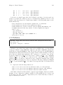
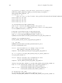
# Pipe large numbers of filenames to stdin
/bin/ls | grep ${CASEID}_’......’.nc | ncecat -o foo.nc
This method avoids all constraints on command line size imposed by the operating
system. A drawback to this method is that the history attribute (see Section 3.39 [History
Attribute], page 122) does not record the name of any input files since the names were not
passed on the command line. This makes determining the data provenance at a later date
difficult. To remedy this situation, multi-file operators store the number of input files in the
nco_input_file_number global attribute and the input file list itself in the nco_input_
file_list global attribute (see Section 3.40 [File List Attributes], page 123). Although
this does not preserve the exact command used to generate the file, it does retains all the
information required to reconstruct the command and determine the data provenance.
A second option is to use the UNIX xargs command. This simple example selects as
input to xargs all the filenames in the current directory that match a given pattern. For
illustration, consider a user trying to average millions of files which each have a six character
filename. If the shell buffer cannot hold the results of the corresponding globbing operator,
??????.nc, then the filename globbing technique will fail. Instead we express the filename
pattern as an extended regular expression, ......\.nc (see Section 3.11 [Subsetting Files],
page 43). We use grep to filter the directory listing for this pattern and to pipe the results
to xargs which, in turn, passes the matching filenames to an NCO multi-file operator, e.g.,
ncecat.
# Use xargs to transfer filenames on the command line
/bin/ls | grep ${CASEID}_’......’.nc | xargs -x ncecat -o foo.nc
The single quotes protect the only sensitive parts of the extended regular expression
(the grep argument), and allow shell interpolation (the ${CASEID} variable substitution)
to proceed unhindered on the rest of the command. xargs uses the UNIX pipe feature
to append the suitably filtered input file list to the end of the ncecat command options.
The -o foo.nc switch ensures that the input files supplied by xargs are not confused with
the output file name. xargs does, unfortunately, have its own limit (usually about 20,000
characters) on the size of command lines it can pass. Give xargs the ‘-x’ switch to ensure it
7
The exact length which exceeds the operating system internal limit for command line lengths varies
from OS to OS and from shell to shell. GNU bash may not have any arbitrary fixed limits to the size of
command line arguments. Many OSs cannot handle command line arguments (including results of file
globbing) exceeding 4096 characters.
Chapter 2: Operator Strategies
23
dies if it reaches this internal limit. When this occurs, use either the stdin method above,
or the symbolic link presented next.
Even when its internal limits have not been reached, the xargs technique may not
be sophisticated enough to handle all situations. A full scripting language like Perl can
handle any level of complexity of filtering input filenames, and any number of filenames.
The technique of last resort is to write a script that creates symbolic links between the
irregular input filenames and a set of regular, arithmetic filenames that the ‘-n loop’ switch
understands. For example, the following Perl script creates a monotonically enumerated
symbolic link to up to one million .nc files in a directory. If there are 999,999 netCDF files
present, the links are named 000001.nc to 999999.nc:
# Create enumerated symbolic links
/bin/ls | grep \.nc | perl -e \
’$idx=1;while(<STDIN>){chop;symlink $_,sprintf("%06d.nc",$idx++);}’
ncecat -n 999999,6,1 000001.nc foo.nc
# Remove symbolic links when finished
/bin/rm ??????.nc
The ‘-n loop’ option tells the NCO operator to automatically generate the filnames of
the symbolic links. This circumvents any OS and shell limits on command line size. The
symbolic links are easily removed once NCO is finished. One drawback to this method is that
the history attribute (see Section 3.39 [History Attribute], page 122) retains the filename
list of the symbolic links, rather than the data files themselves. This makes it difficult to
determine the data provenance at a later date.
2.8 Large Datasets
Large datasets are those files that are comparable in size to the amount of random access
memory (RAM) in your computer. Many users of NCO work with files larger than 100 MB.
Files this large not only push the current edge of storage technology, they present special
problems for programs which attempt to access the entire file at once, such as nces and
ncecat. If you work with a 300 MB files on a machine with only 32 MB of memory then you
will need large amounts of swap space (virtual memory on disk) and NCO will work slowly,
or even fail. There is no easy solution for this. The best strategy is to work on a machine
with sufficient amounts of memory and swap space. Since about 2004, many users have
begun to produce or analyze files exceeding 2 GB in size. These users should familiarize
themselves with NCO’s Large File Support (LFS) capabilities (see Section 3.10 [Large File
Support], page 42). The next section will increase your familiarity with NCO’s memory
requirements. With this knowledge you may re-design your data reduction approach to
divide the problem into pieces solvable in memory-limited situations.
If your local machine has problems working with large files, try running NCO from a
more powerful machine, such as a network server. If you get a memory-related core dump
(e.g., ‘Error exit (core dumped)’) on a GNU/Linux system, or the operation ends before
the entire output file is written, try increasing the process-available memory with ulimit:
ulimit -f unlimited
24
NCO 4.5.3-alpha03 User Guide
This may solve constraints on clusters where sufficient hardware resources exist yet where
system administrators felt it wise to prevent any individual user from consuming too much
of resource. Certain machine architectures, e.g., Cray UNICOS, have special commands
which allow one to increase the amount of interactive memory. On Cray systems, try to
increase the available memory with the ilimit command.
The speed of the NCO operators also depends on file size. When processing large files
the operators may appear to hang, or do nothing, for large periods of time. In order to see
what the operator is actually doing, it is useful to activate a more verbose output mode.
This is accomplished by supplying a number greater than 0 to the ‘-D debug-level’ (or
‘--debug-level’, or ‘--dbg_lvl’) switch. When the debug-level is nonzero, the operators
report their current status to the terminal through the stderr facility. Using ‘-D’ does
not slow the operators down. Choose a debug-level between 1 and 3 for most situations,
e.g., nces -D 2 85.nc 86.nc 8586.nc. A full description of how to estimate the actual
amount of memory the multi-file NCO operators consume is given in Section 2.9 [Memory
Requirements], page 24.
2.9 Memory Requirements
Many people use NCO on gargantuan files which dwarf the memory available (free RAM
plus swap space) even on today’s powerful machines. These users want NCO to consume
the least memory possible so that their scripts do not have to tediously cut files into smaller
pieces that fit into memory. We commend these greedy users for pushing NCO to its limits!
This section describes the memory NCO requires during operation. The required memory
is based on the underlying algorithms. The description below is the memory usage per
thread. Users with shared memory machines may use the threaded NCO operators (see
Section 3.3 [OpenMP Threading], page 27). The peak and sustained memory usage will
scale accordingly, i.e., by the number of threads. Memory consumption patterns of all
operators are similar, with the exception of ncap2.
2.9.1 Single and Multi-file Operators
The multi-file operators currently comprise the record operators, ncra and ncrcat, and
the ensemble operators, nces and ncecat. The record operators require much less memory
than the ensemble operators. This is because the record operators operate on one single
record (i.e., time-slice) at a time, whereas the ensemble operators retrieve the entire variable
into memory. Let M S be the peak sustained memory demand of an operator, F T be the
memory required to store the entire contents of all the variables to be processed in an
input file, F R be the memory required to store the entire contents of a single record of
each of the variables to be processed in an input file, V R be the memory required to store
a single record of the largest record variable to be processed in an input file, V T be the
memory required to store the largest variable to be processed in an input file, V I be the
memory required to store the largest variable which is not processed, but is copied from
the initial file to the output file. All operators require M I = V I during the initial copying
of variables from the first input file to the output file. This is the initial (and transient)
memory demand. The sustained memory demand is that memory required by the operators
during the processing (i.e., averaging, concatenation) phase which lasts until all the input
files have been processed. The operators have the following memory requirements: ncrcat
Chapter 2: Operator Strategies
25
requires M S <= V R. ncecat requires M S <= V T . ncra requires M S = 2F R + V R.
nces requires M S = 2F T + V T . ncbo requires M S <= 3V T (both input variables and
the output variable). ncflint requires M S <= 3V T (both input variables and the output
variable). ncpdq requires M S <= 2V T (one input variable and the output variable).
ncwa requires M S <= 8V T (see below). Note that only variables that are processed, e.g.,
averaged, concatenated, or differenced, contribute to M S. Variables which do not appear in
the output file (see Section 3.11 [Subsetting Files], page 43) are never read and contribute
nothing to the memory requirements.
Further note that some operators perform internal type-promotion on some variables
prior to arithmetic (see Section 3.36 [Type Conversion], page 113). For example, ncra
and nces both promote integer types to double-precision floating point prior to arithmetic,
then perform the arithmetic, then demote back to the original integer type after arithmetic.
This preserves the on-disk storage type while obtaining the accuracy advantages of floating
point arithmetic. Since version 4.3.6 (released in September, 2013), NCO also by default
converts single-precision floating point to double-precision prior to arithmetic, which incurs the same RAM penalty. Hence, the sustained memory required for integer variables
and single-precision floats are two or four-times their on-disk, uncompressed, unpacked
sizes if they meet the rules for automatic internal promotion. Put another way, disabling
auto-promotion of single-precision variables (with ‘--flt’) considerably reduces the RAM
footprint of arithmetic operators.
The ‘--open_ram’ switch (and switches that invoke it like ‘--ram_all’ and
‘--diskless_all’) incurs a RAM penalty. These switches cause each input file to be copied
to RAM upon opening. Hence any operator invoking these switches utilizes an additional
F T of RAM (i.e., M S+ = F T ). See Section 3.33 [RAM disks], page 104 for further details.
ncwa consumes between two and seven times the memory of a variable in order to process
it. Peak consumption occurs when storing simultaneously in memory one input variable,
one tally array, one input weight, one conformed/working weight, one weight tally, one
input mask, one conformed/working mask, and one output variable. When invoked, the
weighting and masking features contribute up to three-sevenths and two-sevenths of these
requirements apiece. If weights and masks are not specified (i.e., no ‘-w’ or ‘-a’ options)
then ncwa requirements drop to M S <= 3V T (one input variable, one tally array, and the
output variable).
The above memory requirements must be multiplied by the number of threads thr nbr
(see Section 3.3 [OpenMP Threading], page 27). If this causes problems then reduce (with
‘-t thr_nbr’) the number of threads.
2.9.2 Memory for ncap2
ncap2 has unique memory requirements due its ability to process arbitrarily long scripts
of any complexity. All scripts acceptable to ncap2 are ultimately processed as a sequence
of binary or unary operations. ncap2 requires M S <= 2V T under most conditions. An
exception to this is when left hand casting (see Section 4.1.4 [Left hand casting], page 136)
is used to stretch the size of derived variables beyond the size of any input variables. Let
V C be the memory required to store the largest variable defined by left hand casting. In
this case, M S <= 2V C.
26
NCO 4.5.3-alpha03 User Guide
ncap2 scripts are complete dynamic and may be of arbitrary length. A script that
contains many thousands of operations, may uncover a slow memory leak even though each
single operation consumes little additional memory. Memory leaks are usually identifiable
by their memory usage signature. Leaks cause peak memory usage to increase monotonically
with time regardless of script complexity. Slow leaks are very difficult to find. Sometimes a
malloc() (or new[]) failure is the only noticeable clue to their existance. If you have good
reasons to believe that a memory allocation failure is ultimately due to an NCO memory
leak (rather than inadequate RAM on your system), then we would be very interested in
receiving a detailed bug report.
2.10 Performance
An overview of NCO capabilities as of about 2006 is in Zender, C. S. (2008), “Analysis of Selfdescribing Gridded Geoscience Data with netCDF Operators (NCO)”, Environ. Modell.
Softw., doi:10.1016/j.envsoft.2008.03.004. This paper is also available at http://dust.
ess.uci.edu/ppr/ppr_Zen08.pdf.
NCO performance and scaling for arithmetic operations is described in Zender, C.
S., and H. J. Mangalam (2007), “Scaling Properties of Common Statistical Operators for Gridded Datasets”, Int. J. High Perform. Comput. Appl., 21(4), 485-498,
doi:10.1177/1094342007083802. This paper is also available at http://dust.ess.uci.
edu/ppr/ppr_ZeM07.pdf.
It is helpful to be aware of the aspects of NCO design that can limit its performance:
1. No data buffering is performed during nc_get_var and nc_put_var operations. Hyperslabs too large too hold in core memory will suffer substantial performance penalties
because of this.
2. Since coordinate variables are assumed to be monotonic, the search for bracketing the
user-specified limits should employ a quicker algorithm, like bisection, than the twosided incremental search currently implemented.
3. C format, FORTRAN format, signedness, scale format and add offset attributes are
ignored by ncks when printing variables to screen.
4. In the late 1990s it was discovered that some random access operations on large files
on certain architectures (e.g., UNICOS) were much slower with NCO than with similar
operations performed using languages that bypass the netCDF interface (e.g., Yorick).
This may have been a penalty of unnecessary byte-swapping in the netCDF interface.
It is unclear whether such problems exist in present day (2007) netCDF/NCO environments, where unnecessary byte-swapping has been reduced or eliminated.
Chapter 3: Shared Features
27
3 Shared Features
Many features have been implemented in more than one operator and are described here
for brevity. The description of each feature is preceded by a box listing the operators for
which the feature is implemented. Command line switches for a given feature are consistent
across all operators wherever possible. If no “key switches” are listed for a feature, then
that particular feature is automatic and cannot be controlled by the user.
3.1 Internationalization
Availability: All operators
NCO support for internationalization of textual input and output (e.g., Warning mes-
sages) is nascent. We introduced the first foreign language string catalogues (French and
Spanish) in 2004, yet did not activate these in distributions because the catalogues were
nearly empty. We seek volunteers to populate our templates with translations for their
favorite languages.
3.2 Metadata Optimization
Availability: All operators
Short options: None
Long options: ‘--hdr_pad’, ‘--header_pad’
NCO supports padding headers to improve the speed of future metadata operations. Use
the ‘--hdr_pad’ and ‘--header_pad’ switches to request that hdr pad bytes be inserted
into the metadata section of the output file. Future metadata expansions will not incur
the netCDF3 performance penalty of copying the entire output file unless the expansion
exceeds the amount of header padding exceeded. This can be beneficial when it is known
that some metadata will be added at a future date. The operators which benefit most from
judicious use of header padding are ncatted and ncrename, since they only alter metadata.
This optimization exploits the netCDF library nc__enddef() function, which behaves
differently with different versions of netCDF. It will improve speed of future metadata
expansion with CLASSIC and 64bit netCDF files, though not necessarily with NETCDF4
files, i.e., those created by the netCDF interface to the HDF5 library (see Section 3.9 [File
Formats and Conversion], page 38).
3.3 OpenMP Threading
28
NCO 4.5.3-alpha03 User Guide
Availability: ncap2, ncbo, nces, ncecat, ncflint, ncpdq, ncra, ncrcat, ncwa
Short options: ‘-t’
Long options: ‘--thr_nbr’, ‘--threads’, ‘--omp_num_threads’
NCO supports shared memory parallelism (SMP) when compiled with an OpenMPenabled compiler. Threads requests and allocations occur in two stages. First, users may
request a specific number of threads thr nbr with the ‘-t’ switch (or its long option equivalents, ‘--thr_nbr’, ‘--threads’, and ‘--omp_num_threads’). If not user-specified, OpenMP
obtains thr nbr from the OMP_NUM_THREADS environment variable, if present, or from the
OS, if not.
Caveat: Unfortunately, threading does not improve NCO throughput (i.e., wallclock
time) because nearly all NCO operations are I/O-bound. This means that NCO spends
negligible time doing anything compared to reading and writing. We have seen some and
can imagine other use cases where ncwa, ncpdq, and ncap2 (with long scripts) will complete
faster due to threading. The main benefits of threading so far have been to isolate the serial
from parallel portions of code. This parallelism is now exploited by OpenMP but then runs
into the I/O bottleneck during output. The bottleneck will be ameliorated for large files
by the use of MPI-enabled calls in the netCDF4 library when the underlying filesystem is
parallel (e.g., PVFS or JFS). Implementation of the parallel output calls in NCO is not a
goal of our current funding and would require new volunteers or funding.
NCO may modify thr nbr according to its own internal settings before it requests any
threads from the system. Certain operators contain hard-code limits to the number of
threads they request. We base these limits on our experience and common sense, and to
reduce potentially wasteful system usage by inexperienced users. For example, ncrcat is
extremely I/O-intensive so we restrict thr nbr <= 2 for ncrcat. This is based on the notion
that the best performance that can be expected from an operator which does no arithmetic
is to have one thread reading and one thread writing simultaneously. In the future (perhaps
with netCDF4), we hope to demonstrate significant threading improvements with operators
like ncrcat by performing multiple simultaneous writes.
Compute-intensive operators (ncap2, ncwa and ncpdq) benefit most from threading. The
greatest increases in throughput due to threading occur on large datasets where each thread
performs millions, at least, of floating point operations. Otherwise, the system overhead
of setting up threads probably outweighs the speed enhancements due to SMP parallelism.
However, we have not yet demonstrated that the SMP parallelism scales beyond four threads
for these operators. Hence we restrict thr nbr <= 4 for all operators. We encourage users
to play with these limits (edit file nco_omp.c) and send us their feedback.
Once the initial thr nbr has been modified for any operator-specific limits, NCO requests
the system to allocate a team of thr nbr threads for the body of the code. The operating
system then decides how many threads to allocate based on this request. Users may keep
track of this information by running the operator with dbg lvl > 0.
By default, threaded operators attach one global attribute, nco_openmp_thread_number,
to any file they create or modify. This attribute contains the number of threads the op-
Chapter 3: Shared Features
29
erator used to process the input files. This information helps to verify that the answers
with threaded and non-threaded operators are equal to within machine precision. This
information is also useful for benchmarking.
3.4 Command Line Options
Availability: All operators
NCO achieves flexibility by using command line options. These options are implemented
in all traditional UNIX commands as single letter switches, e.g., ‘ls -l’. For many years
NCO used only single letter option names. In late 2002, we implemented GNU/POSIX
extended or long option names for all options. This was done in a backward compatible
way such that the full functionality of NCO is still available through the familiar single
letter options. In the future, however, some features of NCO may require the use of long
options, simply because we have nearly run out of single letter options. More importantly,
mnemonics for single letter options are often non-intuitive so that long options provide a
more natural way of expressing intent.
Extended options, also called long options, are implemented using the system-supplied
getopt.h header file, if possible. This provides the getopt_long function to NCO1 .
The syntax of short options (single letter options) is -key value (dash-key-space-value).
Here, key is the single letter option name, e.g., ‘-D 2’.
The syntax of long options (multi-letter options) is --long_name value (dash-dash-keyspace-value), e.g., ‘--dbg_lvl 2’ or --long_name=value (dash-dash-key-equal-value), e.g.,
‘--dbg_lvl=2’. Thus the following are all valid for the ‘-D’ (short version) or ‘--dbg_lvl’
(long version) command line option.
ncks -D 3 in.nc
# Short option
ncks --dbg_lvl=3 in.nc # Long option, preferred form
ncks --dbg_lvl 3 in.nc # Long option, alternate form
The last example is preferred for two reasons. First, ‘--dbg_lvl’ is more specific and less
ambiguous than ‘-D’. The long option form makes scripts more self documenting and less
error prone. Often long options are named after the source code variable whose value they
carry. Second, the equals sign = joins the key (i.e., long name) to the value in an uninterruptible text block. Experience shows that users are less likely to mis-parse commands
when restricted to this form.
GNU implements a superset of the POSIX standard which allows any unambiguous truncation of a valid option to be used.
ncks -D 3 in.nc
# Short option
ncks --dbg_lvl=3 in.nc # Long option, full form
1
If a getopt_long function cannot be found on the system, NCO will use the getopt_long from the
my_getopt package by Benjamin Sittler [email protected]. This is BSD-licensed software available
from http://www.geocities.com/ResearchTriangle/Node/9405/#my_getopt.
30
NCO 4.5.3-alpha03 User Guide
ncks --dbg=3 in.nc
ncks --db=3 in.nc
ncks --d=3 in.nc
# Long option, unambiguous truncation
# Long option, unambiguous truncation
# Long option, ambiguous truncation
The first four examples are equivalent and will work as expected. The final example will
exit with an error since ncks cannot disambiguate whether ‘--d’ is intended as a truncation
of ‘--dbg_lvl’, of ‘--dimension’, or of some other long option.
NCO provides many long options for common switches. For example, the debugging level
may be set in all operators with any of the switches ‘-D’, ‘--debug-level’, or ‘--dbg_lvl’.
This flexibility allows users to choose their favorite mnemonic. For some, it will be ‘--debug’
(an unambiguous truncation of ‘--debug-level’, and other will prefer ‘--dbg’. Interactive
users usually prefer the minimal amount of typing, i.e., ‘-D’. We recommend that scripts
which are re-usable employ some form of the long options for future maintainability.
This manual generally uses the short option syntax in examples. This is for historical
reasons and to conserve space in printed output. Users are expected to pick the unambiguous
truncation of each option name that most suits their taste.
3.5 Specifying Input Files
Availability (-n): nces, ncecat, ncra, ncrcat
Availability (-p): All operators
Short options: ‘-n’, ‘-p’
Long options: ‘--nintap’, ‘--pth’, ‘--path’
It is important that users be able to specify multiple input files without typing every
filename in full, often a tedious task even by graduate student standards. There are four
different ways of specifying input files to NCO: explicitly typing each, using UNIX shell wildcards, and using the NCO ‘-n’ and ‘-p’ switches (or their long option equivalents, ‘--nintap’
or ‘--pth’ and ‘--path’, respectively). Techniques to augment these methods to specify arbitrary numbers (e.g., thousands) and patterns of filenames are discussed separately (see
Section 2.7 [Large Numbers of Files], page 21).
To illustrate these methods, consider the simple problem of using ncra to average five
input files, 85.nc, 86.nc, . . . 89.nc, and store the results in 8589.nc. Here are the four
methods in order. They produce identical answers.
ncra
ncra
ncra
ncra
ncra
85.nc 86.nc 87.nc 88.nc 89.nc 8589.nc
8[56789].nc 8589.nc
8?.nc 8589.nc
-p input-path 85.nc 86.nc 87.nc 88.nc 89.nc 8589.nc
-n 5,2,1 85.nc 8589.nc
The first method (explicitly specifying all filenames) works by brute force. The second method relies on the operating system shell to glob (expand) the regular expression
8[56789].nc. The shell then passes the valid filenames (those which match the regular
expansion) to ncra. In this case ncra never knows that a regular expression was used,
Chapter 3: Shared Features
31
because the shell intercepts and expands and matches the regular expression before ncra
is actually invoked. The third method is uses globbing with a different regular expression
that is less safe (it will also match unwanted files such as 81.nc and 8Z.nc if present). The
fourth method uses the ‘-p input-path’ argument to specify the directory where all the
input files reside. NCO prepends input-path (e.g., /data/username/model) to all input-files
(though not to output-file). Thus, using ‘-p’, the path to any number of input files need
only be specified once. Note input-path need not end with ‘/’; the ‘/’ is automatically
generated if necessary.
The last method passes (with ‘-n’) syntax concisely describing the entire set of filenames2 .
This option is only available with the multi-file operators: ncra, ncrcat, nces, and ncecat.
By definition, multi-file operators are able to process an arbitrary number of input-files.
This option is very useful for abbreviating lists of filenames representable as alphanumeric prefix+numeric suffix+.+filetype where alphanumeric prefix is a string of arbitrary
length and composition, numeric suffix is a fixed width field of digits, and filetype is a
standard filetype indicator. For example, in the file ccm3_h0001.nc, we have alphanumeric prefix = ccm3_h, numeric suffix = 0001, and filetype = nc.
NCO decodes lists of such filenames encoded using the ‘-n’ syntax. The simpler (threeargument) ‘-n’ usage takes the form -n file_number,digit_number,numeric_increment
where file number is the number of files, digit number is the fixed number of numeric digits comprising the numeric suffix, and numeric increment is the constant, integer-valued
difference between the numeric suffix of any two consecutive files. The value of alphanumeric prefix is taken from the input file, which serves as a template for decoding the filenames. In the example above, the encoding -n 5,2,1 along with the input file name 85.nc
tells NCO to construct five (5) filenames identical to the template 85.nc except that the
final two (2) digits are a numeric suffix to be incremented by one (1) for each successive file.
Currently filetype may be either be empty, nc, h5, cdf, hdf, hd5, or he5. If present, these
filetype suffixes (and the preceding .) are ignored by NCO as it uses the ‘-n’ arguments to
locate, evaluate, and compute the numeric suffix component of filenames.
Recently the ‘-n’ option has been extended to allow convenient specification of filenames with “circular” characteristics. This means it is now possible for NCO to automatically generate filenames which increment regularly until a specified maximum value,
and then wrap back to begin again at a specified minimum value. The corresponding
‘-n’ usage becomes more complex, taking one or two additional arguments for a total of
four or five, respectively: -n file_number,digit_number,numeric_increment[,numeric_
max[,numeric_min]] where numeric max, if present, is the maximum integer-value of numeric suffix and numeric min, if present, is the minimum integer-value of numeric suffix.
Consider, for example, the problem of specifying non-consecutive input files where the
filename suffixes end with the month index. In climate modeling it is common to create
summertime and wintertime averages which contain the averages of the months June–July–
August, and December–January–February, respectively:
ncra -n 3,2,1 85_06.nc 85_0608.nc
2
The ‘-n’ option is a backward-compatible superset of the NINTAP option from the NCAR CCM Processor.
The CCM Processor was custom-written Fortran code maintained for many years by Lawrence Buja at
NCAR, and phased-out in the late 1990s. NCO stole some ideas, like NINTAP-functionality, from CCM
Processor capabilities.
32
NCO 4.5.3-alpha03 User Guide
ncra -n 3,2,1,12 85_12.nc 85_1202.nc
ncra -n 3,2,1,12,1 85_12.nc 85_1202.nc
The first example shows that three arguments to the ‘-n’ option suffice to specify consecutive months (06, 07, 08) which do not “wrap” back to a minimum value. The second
example shows how to use the optional fourth and fifth elements of the ‘-n’ option to specify
a wrap value. The fourth argument to ‘-n’, when present, specifies the maximum integer
value of numeric suffix. In the example the maximum value is 12, and will be formatted as
12 in the filename string. The fifth argument to ‘-n’, when present, specifies the minimum
integer value of numeric suffix. The default minimum filename suffix is 1, which is formatted as 01 in this case. Thus the second and third examples have the same effect, that is,
they automatically generate, in order, the filenames 85_12.nc, 85_01.nc, and 85_02.nc as
input to NCO.
As of NCO version 4.5.2 (September, 2015), NCO supports an optional sixth argument to
‘-n’, the month-indicator. The month-indicator affirms to NCO that the right-most digits
being manipulated in the generated filenames correspond to month numbers (with January
formatted as 01 and December as 12). Moreover, it assumes digits to the left of the month
are the year. The full (six-argument) ‘-n’ usage takes the form -n file_number,digit_
number,month_increment,max_month,min_month,‘yyyymm’. The ‘yyyymm’ string is a
clunky way (can you think of a clearer way?) to tell NCO to enumerate files in yearmonth mode. When present, ‘yyyymm’ string causes NCO to automatically generate series
of filenames whose right-most two digits increment from min month by month increment
up to max month and then the leftmost digits (i.e., the year) increment by one, and the
whole process is reapeated until the file number filenames are generated.
ncrcat -n 3,6,1,12,1
198512.nc 198512_198502.nc
ncrcat -n 3,6,1,12,1,yyyymm 198512.nc 198512_198602.nc
ncrcat -n 3,6,1,12,12,yyyymm 198512.nc 198512_198712.nc
The first command concatenates three files (198512.nc, 198501.nc, 198502.nc) into
the output file. The second command concatenates three files (198512.nc, 198601.nc,
198602.nc). The ‘yyyymm’-indicator causes the left-most digits to increment each time
the right-most two digits reach their maximum and then wrap. The first command does
not have the indicator so it is always 1985. The third command concatenates three files
(198512.nc, 198612.nc, 198712.nc).
3.6 Specifying Output Files
Availability: All operators
Short options: ‘-o’
Long options: ‘--fl_out’, ‘--output’
NCO commands produce no more than one output file, fl out. Traditionally, users specify fl out as the final argument to the operator, following all input file names. This is the
positional argument method of specifying input and ouput file names. The positional ar-
Chapter 3: Shared Features
33
gument method works well in most applications. NCO also supports specifying fl out using
the command line switch argument method, ‘-o fl_out’.
Specifying fl out with a switch, rather than as a positional argument, allows fl out to
precede input files in the argument list. This is particularly useful with multi-file operators
for three reasons. Multi-file operators may be invoked with hundreds (or more) filenames.
Visual or automatic location of fl out in such a list is difficult when the only syntactic
distinction between input and output files is their position. Second, specification of a long
list of input files may be difficult (see Section 2.7 [Large Numbers of Files], page 21). Making
the input file list the final argument to an operator facilitates using xargs for this purpose.
Some alternatives to xargs are heinous and undesirable. Finally, many users are more
comfortable specifying output files with ‘-o fl_out’ near the beginning of an argument list.
Compilers and linkers are usually invoked this way.
Users should specify fl out using either (not both) method. If fl out is specified twice
(once with the switch and once as the last positional argument), then the positional argument takes precedence.
3.7 Accessing Remote Files
Availability: All operators
Short options: ‘-p’, ‘-l’
Long options: ‘--pth’, ‘--path’, ‘--lcl’, ‘--local’
All NCO operators can retrieve files from remote sites as well as from the local file system.
A remote site can be an anonymous FTP server, a machine on which the user has rcp, scp,
or sftp privileges, NCAR’s Mass Storage System (MSS), or an OPeNDAP server. Examples
of each are given below, following a brief description of the particular access protocol.
To access a file via an anonymous FTP server, simply supply the remote file’s URL.
Anonymous FTP usually requires no further credentials, e.g., no .netrc file is necessary.
FTP is an intrinsically insecure protocol because it transfers passwords in plain text format.
Users should access sites using anonymous FTP, or better yet, secure FTP (SFTP, see
below) when possible. Some FTP servers require a login/password combination for a valid
user account. NCO allows transactions that require additional credentials so long as the
required information is stored in the .netrc file. Usually this information is the remote
machine name, login, and password, in plain text, separated by those very keywords, e.g.,
machine dust.ess.uci.edu login zender password bushlied
Eschew using valuable passwords for FTP transactions, since .netrc passwords are potentially exposed to eavesdropping software3 .
3
NCO does not implement command line options to specify FTP logins and passwords because copying
those data into the history global attribute in the output file (done by default) poses an unacceptable
security risk.
34
NCO 4.5.3-alpha03 User Guide
SFTP, i.e., secure FTP, uses SSH-based security protocols that solve the security issues
associated with plain FTP. NCO supports SFTP protocol access to files specified with a
homebrew syntax of the form
sftp://machine.domain.tld:/path/to/filename
Note the second colon following the top-level-domain, tld. This syntax is a hybrid
between an FTP URL and standard remote file syntax.
To access a file using rcp or scp, specify the Internet address of the remote file. Of course
in this case you must have rcp or scp privileges which allow transparent (no password entry
required) access to the remote machine. This means that ~/.rhosts or ~/ssh/authorized_
keys must be set accordingly on both local and remote machines.
To access a file on a High Performance Storage System (HPSS) (such as that at NCAR,
ECMWF, LANL, DKRZ, LLNL) specify the full HPSS pathname of the remote file. NCO will
attempt to detect whether the local machine has direct (synchronous) HPSS access. In this
case, NCO attempts to use the Hierarchical Storage Interface (HSI) command hsi get4 .
The following examples show how one might analyze files stored on remote systems.
ncks
ncks
ncks
ncks
ncks
ncks
-l
-l
-l
-l
-l
-l
.
.
.
.
.
.
ftp://dust.ess.uci.edu/pub/zender/nco/in.nc
sftp://dust.ess.uci.edu:/home/ftp/pub/zender/nco/in.nc
dust.ess.uci.edu:/home/zender/nco/data/in.nc
/ZENDER/nco/in.nc
/home/zender/nco/in.nc
http://thredds-test.ucar.edu/thredds/dodsC/testdods/in.nc
The first example works verbatim if your system is connected to the Internet and is not
behind a firewall. The second example works if you have sftp access to the machine
dust.ess.uci.edu. The third example works if you have rcp or scp access to the machine
dust.ess.uci.edu. The fourth and fifth examples work on NCAR computers with local
access to the HPSS hsi get command5 . The sixth command works if your local version of
NCO is OPeNDAP-enabled (this is fully described in Section 3.7.1 [OPeNDAP], page 35), or
if the remote file is accessible via wget. The above commands can be rewritten using the
‘-p input-path’ option as follows:
ncks
ncks
ncks
ncks
ncks
ncks
4
5
-p
-p
-p
-p
-p
-p
ftp://dust.ess.uci.edu/pub/zender/nco -l . in.nc
sftp://dust.ess.uci.edu:/home/ftp/pub/zender/nco -l . in.nc
dust.ess.uci.edu:/home/zender/nco -l . in.nc
/ZENDER/nco -l . in.nc
/home/zender/nco -l . in.nc # HPSS
http://thredds-test.ucar.edu/thredds/dodsC/testdods \
The hsi command must be in the user’s path in one of the following directories: /usr/local/bin,
/opt/hpss/bin, or /ncar/opt/hpss/hsi. Tell us if the HPSS installation at your site places the hsi
command in a different location, and we will add that location to the list of acceptable paths to search
for hsi.
NCO supported the old NCAR Mass Storage System (MSS) until version 4.0.7 in April, 2011. NCO
supported MSS-retrievals via a variety of mechanisms including the msread, msrcp, and nrnet commands
invoked either automatically or with sentinels like ncks -p mss:/ZENDER/nco -l . in.nc. Once the MSS
was decommissioned in March, 2011, support for these retrieval mechanisms was replaced by support for
HPSS in NCO.
Chapter 3: Shared Features
35
-l . in.nc
Using ‘-p’ is recommended because it clearly separates the input-path from the filename
itself, sometimes called the stub. When input-path is not explicitly specified using ‘-p’,
NCO internally generates an input-path from the first input filename. The automatically
generated input-path is constructed by stripping the input filename of everything following
the final ‘/’ character (i.e., removing the stub). The ‘-l output-path’ option tells NCO
where to store the remotely retrieved file. It has no effect on locally-retrieved files, or on
the output file. Often the path to a remotely retrieved file is quite different than the path
on the local machine where you would like to store the file. If ‘-l’ is not specified then
NCO internally generates an output-path by simply setting output-path equal to input-path
stripped of any machine names. If ‘-l’ is not specified and the remote file resides on the
NCAR HPSS system, then the leading character of input-path, ‘/’, is also stripped from
output-path. Specifying output-path as ‘-l ./’ tells NCO to store the remotely retrieved
file and the output file in the current directory. Note that ‘-l .’ is equivalent to ‘-l ./’
though the latter is syntactically more clear.
3.7.1 OPeNDAP
The Distributed Oceanographic Data System (DODS) provides useful replacements for common data interface libraries like netCDF. The DODS versions of these libraries implement
network transparent access to data via a client-server data access protocol that uses the
HTTP protocol for communication. Although DODS-technology originated with oceanography data, it applyies to virtually all scientific data. In recognition of this, the data access
protocol underlying DODS (which is what NCO cares about) has been renamed the Opensource Project for a Network Data Access Protocol, OPeNDAP. We use the terms DODS
and OPeNDAP interchangeably, and often write OPeNDAP/DODS for now. In the future we
will deprecate DODS in favor of DAP or OPeNDAP, as appropriate6 .
NCO may be DAP-enabled by linking NCO to the OPeNDAP libraries. This is described in
the OPeNDAP documentation and automagically implemented in NCO build mechanisms7 .
The ./configure mechanism automatically enables NCO as OPeNDAP clients if it can find
the required OPeNDAP libraries8 . in the usual locations. The $DODS_ROOT environment
variable may be used to override the default OPeNDAP library location at NCO compile-time.
Building NCO with bld/Makefile and the command make DODS=Y adds the (non-intuitive)
commands to link to the OPeNDAP libraries installed in the $DODS_ROOT directory. The file
6
7
8
DODS is being deprecated because it is ambiguous, referring both to a protocol and to a collection of
(oceanography) data. It is superceded by two terms. DAP is the discipline-neutral Data Access Protocol
at the heart of DODS. The National Virtual Ocean Data System (NVODS) refers to the collection of
oceanography data and oceanographic extensions to DAP. In other words, NVODS is implemented with
OPeNDAP. OPeNDAP is also the open source project which maintains, develops, and promulgates the
DAP standard. OPeNDAP and DAP really are interchangeable. Got it yet?
Automagic support for DODS version 3.2.x was deprecated in December, 2003 after NCO version 2.8.4.
NCO support for OPeNDAP versions 3.4.x commenced in December, 2003, with NCO version 2.8.5. NCO
support for OPeNDAP versions 3.5.x commenced in June, 2005, with NCO version 3.0.1. NCO support for
OPeNDAP versions 3.6.x commenced in June, 2006, with NCO version 3.1.3. NCO support for OPeNDAP
versions 3.7.x commenced in January, 2007, with NCO version 3.1.9.
The minimal set of libraries required to build NCO as OPeNDAP clients, where OPeNDAP is supplied
as a separate library apart from libnetcdf.a, are, in link order, libnc-dap.a, libdap.a, and libxml2
and libcurl.a.
36
NCO 4.5.3-alpha03 User Guide
doc/opendap.sh contains a generic script intended to help users install OPeNDAP before
building NCO. The documentation at the OPeNDAP Homepage (http://www.opendap.
org) is voluminous. Check there and on the DODS mail lists (http://www.unidata.ucar.
edu/packages/dods/home/mailLists/). to learn more about the extensive capabilities of
OPeNDAP9 .
Once NCO is DAP-enabled the operators are OPeNDAP clients. All OPeNDAP clients have
network transparent access to any files controlled by a OPeNDAP server. Simply specify the
input file path(s) in URL notation and all NCO operations may be performed on remote
files made accessible by a OPeNDAP server. This command tests the basic functionality of
OPeNDAP-enabled NCO clients:
% ncks -O -o ~/foo.nc -C -H -v one -l /tmp \
-p http://thredds-test.ucar.edu/thredds/dodsC/testdods in.nc
% ncks -H -v one ~/foo.nc
one = 1
The one = 1 outputs confirm (first) that ncks correctly retrieved data via the OPeNDAP
protocol and (second) that ncks created a valid local copy of the subsetted remote file.
With minor changes to the above command, netCDF4 can be used as both the input and
output file format:
% ncks -4 -O -o ~/foo.nc -C -H -v one -l /tmp \
-p http://thredds-test.ucar.edu/thredds/dodsC/testdods in_4.nc
% ncks -H -v one ~/foo.nc
one = 1
And, of course, OPeNDAP-enabled NCO clients continue to support orthogonal features
such as UDUnits (see Section 3.24 [UDUnits Support], page 79):
% ncks -u -C -H -v wvl -d wvl,’0.4 micron’,’0.7 micron’ \
-p http://thredds-test.ucar.edu/thredds/dodsC/testdods in_4.nc
% wvl[0]=5e-07 meter
The next command is a more advanced example which demonstrates the real power
of OPeNDAP-enabled NCO clients. The ncwa client requests an equatorial hyperslab from
remotely stored NCEP reanalyses data of the year 1969. The NOAA OPeNDAP server (hopefully!) serves these data. The local ncwa client then computes and stores (locally) the
regional mean surface pressure (in Pa).
ncwa -C -a lat,lon,time -d lon,-10.,10. -d lat,-10.,10. -l /tmp -p \
http://www.esrl.noaa.gov/psd/thredds/dodsC/Datasets/ncep.reanalysis.dailyavgs/surface \
pres.sfc.1969.nc ~/foo.nc
All with one command! The data in this particular input file also happen to be packed (see
Section 4.1.11 [Methods and functions], page 145), although this complication is transparent
to the user since NCO automatically unpacks data before attempting arithmetic.
9
We are most familiar with the OPeNDAP ability to enable network-transparent data access. OPeNDAP
has many other features, including sophisticated hyperslabbing and server-side processing via constraint
expressions. If you know more about this, please consider writing a section on “OPeNDAP Capabilities
of Interest to NCO Users” for incorporation in the NCO User Guide.
Chapter 3: Shared Features
37
NCO obtains remote files from the OPeNDAP server (e.g., www.cdc.noaa.gov) rather
than the local machine. Input files are first copied to the local machine, then processed.
The OPeNDAP server performs data access, hyperslabbing, and transfer to the local machine.
This allows the I/O to appear to NCO as if the input files were local. The local machine
performs all arithmetic operations. Only the hyperslabbed output data are transferred over
the network (to the local machine) for the number-crunching to begin. The advantages of
this are obvious if you are examining small parts of large files stored at remote locations.
Natually there are many versions of OPeNDAP servers supplying data and bugs in the
server can appear to be bugs in NCO. However, with very few exceptions10 an NCO command
that works on a local file must work across an OPeNDAP connection or else there is a bug
in the server. This is because NCO does nothing special to handle files served by OPeNDAP,
the whole process is (supposed to be) completely transparent to the client NCO software.
Therefore it is often useful to try NCO commands on various OPeNDAP servers in order
to isolate whether a problem may be due to a bug in the OPeNDAP server on a particular
machine. For this purpose, one might try variations of the following commands that access
files on public OPeNDAP servers:
# Strided access to HDF5 file
ncks -v Time -d Time,0,10,2 http://eosdap.hdfgroup.uiuc.edu:8080/opendap/data/NASAFILES
# Strided access to netCDF3 file
ncks -O -D 1 -d time,1 -d lev,0 -d lat,0,100,10 -d lon,0,100,10 -v u_velocity http://no
These servers were operational at the time of writing, March 2014. Unfortunately, administrators often move or rename path directories. Recommendations for additional public
OPeNDAP servers on which to test NCO are welcome.
3.8 Retaining Retrieved Files
Availability: All operators
Short options: ‘-R’
Long options: ‘--rtn’, ‘--retain’
In order to conserve local file system space, files retrieved from remote locations are
automatically deleted from the local file system once they have been processed. Many NCO
operators were constructed to work with numerous large (e.g., 200 MB) files. Retrieval of
multiple files from remote locations is done serially. Each file is retrieved, processed, then
deleted before the cycle repeats. In cases where it is useful to keep the remotely-retrieved
files on the local file system after processing, the automatic removal feature may be disabled
by specifying ‘-R’ on the command line.
Invoking -R disables the default printing behavior of ncks. This allows ncks to retrieve
remote files without automatically trying to print them. See Section 4.7 [ncks netCDF
Kitchen Sink], page 203, for more details.
10
For example, DAP servers do not like variables with periods (“.”) in their names even though this is
perfectly legal with netCDF. Such names may cause the DAP service to fail because DAP interprets the
period as structure delimiter in an HTTP query string.
38
NCO 4.5.3-alpha03 User Guide
Note that the remote retrieval features of NCO can always be used to retrieve any file,
including non-netCDF files, via SSH, anonymous FTP, or msrcp. Often this method is
quicker than using a browser, or running an FTP session from a shell window yourself. For
example, say you want to obtain a JPEG file from a weather server.
ncks -R -p ftp://weather.edu/pub/pix/jpeg -l . storm.jpg
In this example, ncks automatically performs an anonymous FTP login to the remote
machine and retrieves the specified file. When ncks attempts to read the local copy of
storm.jpg as a netCDF file, it fails and exits, leaving storm.jpg in the current directory.
If your NCO is DAP-enabled (see Section 3.7.1 [OPeNDAP], page 35), then you may use
NCO to retrieve any files (including netCDF, HDF, etc.) served by an OPeNDAP server to
your local machine. For example,
ncks -R -l . -p \
http://www.esrl.noaa.gov/psd/thredds/dodsC/Datasets/ncep.reanalysis.dailyavgs/surface \
pres.sfc.1969.nc
It may occasionally be useful to use NCO to transfer files when your other preferred
methods are not available locally.
3.9 File Formats and Conversion
Availability: ncap2, nces, ncecat, ncflint, ncks, ncpdq, ncra, ncrcat, ncwa
Short options: ‘-3’, ‘-4’, ‘-6’, ‘-7’
Long options: ‘--3’, ‘--4’, ‘--6’, ‘--64bit’, ‘--7’, ‘--fl_fmt’, ‘--netcdf4’
All NCO operators support (read and write) all three (or four, depending on how one
counts) file formats supported by netCDF4. The default output file format for all operators
is the input file format. The operators listed under “Availability” above allow the user to
specify the output file format independent of the input file format. These operators allow
the user to convert between the various file formats. (The operators ncatted and ncrename
do not support these switches so they always write the output netCDF file in the same
format as the input netCDF file.)
3.9.1 File Formats
netCDF supports four types of files: CLASSIC, 64BIT, NETCDF4, and NETCDF4_CLASSIC, The
CLASSIC format is the traditional 32-bit offset written by netCDF2 and netCDF3. As of
2005, nearly all netCDF datasets were in CLASSIC format. The 64BIT format was added
in Fall, 2004. As of 2010, many netCDF datasets were in 64BIT format. As of 2013, an
increasing number of netCDF datasets were in NETCDF4_CLASSIC format.
The NETCDF4 format uses HDF5 as the file storage layer. The files are (usually) created,
accessed, and manipulated using the traditional netCDF3 API (with numerous extensions).
The NETCDF4_CLASSIC format refers to netCDF4 files created with the NC_CLASSIC_MODEL
mask. Such files use HDF5 as the back-end storage format (unlike netCDF3), though they
incorporate only netCDF3 features. Hence NETCDF4_CLASSIC files are entirely readable by
Chapter 3: Shared Features
39
applications that use only the netCDF3 API (though the applications must be linked with
the netCDF4 library). NCO must be built with netCDF4 to write files in the new NETCDF4
and NETCDF4_CLASSIC formats, and to read files in these formats. Datasets in the default
CLASSIC or the newer 64BIT formats have maximum backwards-compatibility with older
applications. NCO has deep support for NETCDF4 formats. If performance or disk-space
as important as backwards compatibility, then use NETCDF4_CLASSIC instead of CLASSIC
format files. As of 2014, NCO support for the NETCDF4 format is nearly complete and the
most powerful and disk/RAM efficient workflows will utilize this format.
As mentioned above, all operators write use the input file format for output files unless
told otherwise. Toggling the short option ‘-6’ or the long option ‘--6’ or ‘--64bit’ (or
their key-value equivalent ‘--fl_fmt=64bit’) produces the netCDF3 64-bit offset format
named 64BIT. NCO must be built with netCDF 3.6 or higher to produce a 64BIT file.
Using the ‘-4’ switch (or its long option equivalents ‘--4’ or ‘--netcdf4’), or setting its
key-value equivalent ‘--fl_fmt=netcdf4’ produces a NETCDF4 file (i.e., with all supported
HDF5 features). Using the ‘-7’ switch (or its long option equivalent ‘--7’11 , or setting its
key-value equivalent ‘--fl_fmt=netcdf4_classic’ produces a NETCDF4_CLASSIC file (i.e.,
with all supported HDF5 features like compression and chunking but without groups or new
atomic types). Operators given the ‘-3’ (or ‘--3’) switch without arguments will (attempt
to) produce netCDF3 CLASSIC output, even from netCDF4 input files.
Note that NETCDF4 and NETCDF4_CLASSIC are the same binary format. The latter simply
causes a writing application to fail if it attempts to write a NETCDF4 file that cannot be
completely read by the netCDF3 library. Conversely, NETCDF4_CLASSIC indicates to a
reading application that all of the file contents are readable with the netCDF3 library. NCO
has supported reading/writing basic NETCDF4 and NETCDF4_CLASSIC files since October,
2005.
3.9.2 Determining File Format
Input files often end with the generic .nc suffix that leaves (perhaps by intention) the
internal file format ambiguous. There are at least three ways to discover the internal format
of a netCDF-supported file. These methods determine whether it is a classic (32-bit offset)
or newer 64-bit offset netCDF3 format, or is a netCDF4 format. Each method returns
the information using slightly different terminology that becomes easier to understand with
practice.
First, examine the first line of global metadata output by ‘ncks -M’:
% ncks -M foo_3c.nc
Summary of foo_3c.nc: filetype = NC_FORMAT_CLASSIC, 0 groups ...
% ncks -M foo_364.nc
Summary of foo_364.nc: filetype = NC_FORMAT_64BIT, 0 groups ...
% ncks -M foo_4c.nc
Summary of foo_4c.nc: filetype = NC_FORMAT_NETCDF4_CLASSIC, 0 groups ...
% ncks -M foo_4.nc
Summary of foo_4.nc: filetype = NC_FORMAT_NETCDF4, 0 groups ...
11
The reason (and mnemonic) for ‘-7’ is that NETCDF4_CLASSIC files include great features of both netCDF3
(compatibility) and netCDF4 (compression, chunking) and, well, 3 + 4 = 7.
40
NCO 4.5.3-alpha03 User Guide
This method requires a netCDF4-enabled NCO version 3.9.0+ (i.e., from 2007 or later).
As of NCO version 4.4.0 (January, 2014), ncks will also print the extended or underlying
format of the input file. The extended filetype will be one of the six underlying formats
that are accessible through the netCDF API. These formats are NC_FORMAT_NC3 (classic and 64-bit versions of netCDF3 formats), NC_FORMAT_NC_HDF5 (classic and extended
versions of netCDF4, and “pure” HDF5 format), NC_FORMAT_NC_HDF4 (HDF4 format), NC_
FORMAT_PNETCDF (PnetCDF format), NC_FORMAT_DAP2 (accessed via DAP2 protocol), and
NC_FORMAT_DAP4 (accessed via DAP2 protocol). For example,
% ncks -D 2 -M hdf.hdf
Summary of hdf.hdf: filetype = NC_FORMAT_NETCDF4 (representation of \
extended/underlying filetype NC_FORMAT_HDF4), 0 groups ...
% ncks -D 2 -M http://thredds-test.ucar.edu/thredds/dodsC/testdods/in.nc
Summary of http://thredds-test.ucar.edu/thredds/dodsC/testdods/in.nc: \
filetype = NC_FORMAT_CLASSIC (representation of extended/underlying \
filetype NC_FORMAT_DAP2), 0 groups
% ncks -D 2 -M foo_4.nc
Summary of foo_4.nc: filetype = NC_FORMAT_NETCDF4 (representation of \
extended/underlying filetype NC_FORMAT_HDF5), 0 groups
The extended filetype determines some of the capabilities that netCDF has to alter the
file.
Second, query the file with ‘ncdump -k’:
% ncdump -k foo_3c.nc
classic
% ncdump -k foo_364.nc
64-bit-offset
% ncdump -k foo_4c.nc
netCDF-4 classic model
% ncdump -k foo_4.nc
netCDF-4
This method requires a netCDF4-enabled netCDF 3.6.2+ (i.e., from 2007 or later).
The third option uses the POSIX-standard od (octal dump) command:
% od
C
% od
C
% od
211
% od
211
-An
D
-An
D
-An
H
-An
H
-c -N4 foo_3c.nc
F 001
-c -N4 foo_364.nc
F 002
-c -N4 foo_4c.nc
D
F
-c -N4 foo_4.nc
D
F
This option works without NCO and ncdump. Values of ‘C D F 001’ and ‘C D F 002’
indicate 32-bit (classic) and 64-bit netCDF3 formats, respectively, while values of ‘211 H D
F’ indicate either of the newer netCDF4 file formats.
Chapter 3: Shared Features
41
3.9.3 File Conversion
Let us demonstrate converting a file from any netCDF-supported input format into any
netCDF output format (subject to limits of the output format). Here the input file in.nc
may be in any of these formats: netCDF3 (classic and 64bit), netCDF4 (classic and extended), HDF4, HDF5, HDF-EOS (version 2 or 5), and DAP. The switch determines the
output format written in the comment:12
ncks
ncks
ncks
ncks
ncks
ncks
ncks
ncks
ncks
ncks
ncks
ncks
--fl_fmt=classic in.nc foo_3c.nc # netCDF3 classic
--fl_fmt=64bit in.nc foo_364.nc # netCDF3 64bit
--fl_fmt=netcdf4_classic in.nc foo_4c.nc # netCDF4 classic
--fl_fmt=netcdf4 in.nc foo_4.nc # netCDF4
-3 in.nc foo_3c.nc # netCDF3 classic
--3 in.nc foo_3c.nc # netCDF3 classic
-6 in.nc foo_364.nc # netCDF3 64bit
--64 in.nc foo_364.nc # netCDF3 64bit
-4 in.nc foo_4.nc # netCDF4
--4 in.nc foo_4.nc # netCDF4
-7 in.nc foo_4c.nc # netCDF4 classic
--7 in.nc foo_4c.nc # netCDF4 classic
Of course since most operators support these switches, the “conversions” can be done
at the output stage of arithmetic or metadata processing rather than requiring a separate
step. Producing (netCDF3) CLASSIC or 64BIT files from NETCDF4_CLASSIC files will always
work.
3.9.4 Autoconversion
Because of the dearth of support for netCDF4 amongst tools and user communities (including the CF conventions), it is often useful to convert netCDF4 to netCDF3 for certain applications. Until NCO version 4.4.0 (January, 2014), producing netCDF3 files from netCDF4
files only worked if the input files contained no netCDF4-specific features (e.g., atomic types,
multiple record dimensions, or groups). As of NCO version 4.4.0, ncks supports autoconversion of many netCDF4 features to their closest netCDF3-compatible representations. Since
converting netCDF4 to netCDF3 results in loss of features, “automatic down-conversion”
may be a more precise description of what we term autoconversion.
NCO employs three algorithms to downconvert netCDF4 to netCDF3:
1. Autoconversion of atomic types: Autoconversion automatically promotes NC_UBYTE to
NC_SHORT, and NC_USHORT to NC_INT. It automatically demotes the three types NC_
UINT, NC_UINT64, and NC_INT64 to NC_INT. And it converts NC_STRING to NC_CHAR.
All numeric conversions work for attributes and variables of any rank. Two numeric
types (NC_UBYTE and NC_USHORT) are promoted to types with greater range (and greater
storage). This extra range is often not used so promotion perhaps conveys the wrong
impression. However, promotion never truncates values or loses data (this perhaps
justifies the extra storage). Three numeric types (NC_UINT, NC_UINT64 and NC_INT64)
12
The switches ‘-5’, ‘--5’, and ‘pnetcdf’ are reserved for PnetCDF files, i.e., NC_FORMAT_PNETCDF. Such
files are similar to netCDF3 classic files, yet also support 64-bit offsets and the additional netCDF4
atomic types.
42
NCO 4.5.3-alpha03 User Guide
are demoted. Since the input range is larger than the output range, demotion can result
in numeric truncation and thus loss of data. In such cases, it would possible to convert
the data to floating point values instead. If this feature interests you, please be the
squeaky wheel and let us know.
String conversions (to NC_CHAR) work for all attributes, but not for variables. This is
because attributes are at most one-dimensional and may be of any size whereas variables
require gridded dimensions that usually do not fit the ragged sizes of text strings. Hence
scalar NC_STRING attributes are correctly converted to and stored as NC_CHAR attributes
in the netCDF3 output file, but NC_STRING variables are not correctly converted. If
this limitation annoys or enrages you, please let us know by being the squeaky wheel.
2. Convert multiple record dimensions to fixed-size dimensions. Many netCDF4 and HDF5
datasets have multiple unlimited dimensions. Since a netCDF3 file may have at most
one unlimited dimension, all but possibly one unlimited dimension from the input
file must be converted to fixed-length dimensions prior to storing netCDF4 input as
netCDF3 output. By invoking --fix_rec_dmn all the user ensures the output file will
adhere to netCDF3 conventions and the user need not know the names of the specific
record dimensions to fix. See Section 4.7 [ncks netCDF Kitchen Sink], page 203 for a
description of the ‘--fix_rec_dmn’ option.
3. Flattening (removal) of groups. Many netCDF4 and HDF5 datasets have group hierarchies. Since a netCDF3 file may not have any groups, groups in the input file must be
removed. This is also called “flattening” the hierarchical file. See Section 3.13 [Group
Path Editing], page 48 for a description of the GPE option ‘-G :’ to flatten files.
Putting the three algorithms together, one sees that the recipe to convert netCDF4 to
netCDF4 becomes increasingly complex as the netCDF4 features in the input file become
more elaborate:
# Convert file with netCDF4 atomic types
ncks -3 in.nc4 out.nc3
# Convert file with multiple record dimensions + netCDF4 atomic types
ncks -3 --fix_rec_dmn=all in.nc4 out.nc3
# Convert file with groups, multiple record dimensions + netCDF4 atomic types
ncks -3 -G : --fix_rec_dmn=all in.nc4 out.nc3
Future versions of NCO may automatically invoke the record dimension fixation and
group flattening when converting to netCDF3 (rather than requiring it be specified manually). If this feature would interest you, please let us know.
3.10 Large File Support
Availability: All operators
Short options: none
Long options: none
NCO has Large File Support (LFS), meaning that NCO can write files larger than 2 GB on
some 32-bit operating systems with netCDF libraries earlier than version 3.6. If desired, LFS
Chapter 3: Shared Features
43
support must be configured when both netCDF and NCO are installed. netCDF versions 3.6
and higher support 64-bit file addresses as part of the netCDF standard. We recommend
that users ignore LFS support which is difficult to configure and is implemented in NCO only
to support netCDF versions prior to 3.6. This obviates the need for configuring explicit LFS
support in applications (such as NCO) that now support 64-bit files directly through the
netCDF interface. See Section 3.9 [File Formats and Conversion], page 38 for instructions on
accessing the different file formats, including 64-bit files, supported by the modern netCDF
interface.
If you are still interested in explicit LFS support for netCDF versions prior to 3.6,
know that LFS support depends on a complex, interlocking set of operating system13 and
netCDF support issues. The netCDF LFS FAQ (http://my.unidata.ucar.edu/content/
software/netcdf/faq-lfs.html) describes the various file size limitations imposed by
different versions of the netCDF standard. NCO and netCDF automatically attempt to
configure LFS at build time.
3.11 Subsetting Files
Options -g grp
Availability: ncbo, nces, ncecat, ncflint, ncks, ncpdq, ncra, ncrcat, ncwa
Short options: ‘-g’
Long options: ‘--grp’ and ‘--group’
Options -v var and -x
Availability: (ncap2), ncbo, nces, ncecat, ncflint, ncks, ncpdq, ncra, ncrcat, ncwa
Short options: ‘-v’, ‘-x’
Long options: ‘--variable’, ‘--exclude’ or ‘--xcl’
Options --unn
Availability: ncbo, nces, ncecat, ncflint, ncks, ncpdq, ncra, ncrcat, ncwa
Short options:
Long options: ‘--unn’ and ‘--union’
Options --grp_xtr_var_xcl
Availability: ncks
Short options:
Long options: ‘--gxvx’ and ‘--grp_xtr_var_xcl’
Subsetting variables refers to explicitly specifying variables and groups to be included
or excluded from operator actions. Subsetting is controlled by the ‘-v var[,...]’ and ‘-x’
options for directly specifying variables. Specifying groups, whether in addition to or instead
of variables, is quite similar and is controlled by the ‘-g grp[,...]’ and ‘-x’ options. A list
of variables or groups to extract is specified following the ‘-v’ and ‘-g’ options, e.g., ‘-v
time,lat,lon’ or ‘-g grp1,grp2’. Both options may be specified simultaneously and NCO
will extract the intersection of the lists, i.e., only variables of the specified names found in
groups of the specified names. The ‘--unn’ option causes NCO to extract the union, rather
than the intersection, of the specified groups and variables. Not using the ‘-v’ or ‘-g’ option
13
Linux and AIX do support LFS.
44
NCO 4.5.3-alpha03 User Guide
is equivalent to specifying all variables or groupp, respectively. The ‘-x’ option causes the
list of variables specified with ‘-v’ to be excluded rather than extracted. Thus ‘-x’ saves
typing when you only want to extract fewer than half of the variables in a file.
Variables or groups explicitly specified for extraction with ‘-v var[,...]’ or ‘-g
grp[,...]’ must be present in the input file or an error will result. Variables explicitly specified for exclusion with ‘-x -v var[,...]’ need not be present in the input file. To
accord with the sophistication of the underlying hierarchy, group subsetting is controlled by
a few powerful yet subtle syntactical distinctions. When learning this syntax it is helpful
to keep in mind the similarity between group hierarchies and directory structures.
As of NCO 4.4.4 (June, 2014), ncks (alone) supports an option to include specified
groups yet exclude specified variables. The ‘--grp_xtr_var_xcl’ switch (with long option
equivalent ‘--gxvx’) extracts all contents of groups given as arguments to ‘-g grp[,...]’,
except for variables given as arguments to ‘-v var[,...]’. Use this when one or a few
variables in hierarchical files are not to be extracted, and all other variables are. This is
useful when coercing netCDF4 files into netCDF3 files such as with converting, flattening,
or dismembering files (see Section 3.13.1 [Flattening Groups], page 49).
ncks --grp_xtr_var_xcl -g g1 -v v1 # Extract all of group g1 except v1
Two properties of subsetting, recursion and anchoring, are best illustrated by reminding
the user of their UNIX equivalents. The UNIX command mv src dst moves src and all its
subdirectories (and all their subdirectories etc.) to dst. In other words mv is, by default,
recursive. In contrast, the UNIX command cp src dst moves src, and only src, to dst, If
src is a directory, not a file, then that command fails. One must explicitly request to copy
directories recursively, i.e., with cp -r src dst. In NCO recursive extraction (and copying)
of groups is the default (like with mv, not with cp). Recursion is turned off by appending a
trailing slash to the path.
These UNIX commands also illustrate a property we call anchoring. The command mv
src dst moves (recursively) the source directory src to the destination directory dst. If
src begins with the slash character then the specified path is relative to the root directory,
otherwise the path is relative to the current working directory. In other words, an initial
slash character anchors the subsequent path to the root directory. In NCO an initial slash
anchors the path at the root group. Paths that begin and end with slash characters (e.g.,
//, /g1/, and /g1/g2/) are both anchored and non-recursive.
Consider the following commands, all of which may be assumed to end with ‘in.nc
out.nc’:
ncks
ncks
ncks
ncks
ncks
-g g1
-g g1/
-g /g1
-g /g1/
-g //
#
#
#
#
#
Extract,
Extract,
Extract,
Extract,
Extract,
recursively, all groups with a g1 component
non-recursively, all groups terminating in g1
recursively, root group g1
non-recursively root group g1
non-recursively the root group
The first command is probably the most useful and common. It would extract these
groups, if present, and all their direct ancestors and children: /g1, /g2/g1, and /g3/g1/g2.
In other words, the simplest form of ‘-g grp’ grabs all groups that (and their direct ancestors
and children, recursively) that have grp as a complete component of their path. A simple
Chapter 3: Shared Features
45
string match is insufficient, grp must be a complete component (i.e., group name) in the
path. The option ‘-g g1’ would not extract these groups because g1 is not a complete
component of the path: /g12, /fg1, and /g1g1. The second command above shows how
a terminating slash character / cancels the recursive copying of groups. An argument to
‘-g’ which terminates with a slash character extracts the group and its direct ancestors,
but none of its children. The third command above shows how an initial slash character /
anchors the argument to the root group. The third command would not extract the group
/g2/g1 because the g1 group is not at the root level, but it would extract, any group /g1
at the root level and all its children, recursively. The fourth command is the non-recursive
version of the third command. The fifth command is a special case of the fourth command.
As mentioned above, both ‘-v’ and ‘-g’ options may be specified simultaneously and
NCO will, by default, extract the intersection of the lists, i.e., the specified variables found
in the specified groups14 . The ‘--unn’ option causes NCO to extract the union, rather than
the intersection, of the specified groups and variables. Consider the following commands
(which may be assumed to end with ‘in.nc out.nc’):
# Intersection-mode subsetting (default)
ncks -g g1 -v v1 # Yes: /g1/v1, /g2/g1/v1. No:
ncks -g /g1 -v v1 # Yes: /g1/v1, /g1/g2/v1. No:
ncks -g g1/ -v v1 # Yes: /g1/v1, /g2/g1/v1. No:
ncks -v g1/v1
# Yes: /g1/v1, /g2/g1/v1. No:
ncks -g /g1/ -v v1 # Yes: /g1/v1. No: /g2/g1/v1,
ncks -v /g1/v1
# Yes: /g1/v1. No: /g2/g1/v1,
# Union-mode
ncks -g g1
ncks -g /g1
ncks -g g1/
ncks -g /g1/
/v1,
/v1,
/v1,
/v1,
/v1,
/v1,
/g2/v1
/g2/v1, /g2/g1/v1
/g2/v1, /g1/g2/v1
/g2/v1, /g1/g2/v1
/g2/v1 ...
/g2/v1 ...
subsetting (invoke with --unn or --union)
-v v1 --unn # All variables in g1 or progeny, or named v1
-v v1 --unn # All variables in /g1 or progeny, or named v1
-v v1 --unn # All variables in g1 or named v1
-v v1 --unn # All variables in /g1 or named v1
The first command (‘-g g1 -v v1’) extracts the variable v1 from any group named g1
or descendent g1. The second command extracts v1 from any root group named g1 and
any descendent groups as well. The third and fourth commands are equivalent ways of
extracting v1 only from the root group named g1 (not its descendents). The fifth and sixth
commands are equivalent ways of extracting the variable v1 only from the root group named
g1. Subsetting in union-mode (with ‘--unn’) causes all variables to be extracted which meet
either one or both of the specifications of the variable and group specifications. Union-mode
subsetting is simply the logical “OR” of intersection-mode subsetting. As discussed below,
the group and variable specifications may be comma separated lists of regular expressions
for added control over subsetting.
Remember, if averaging or concatenating large files stresses your systems memory or
disk resources, then the easiest solution is often to subset (with ‘-g’ and/or ‘-v’) to retain
only the most important variables (see Section 2.9 [Memory Requirements], page 24).
14
Intersection-mode can also be explicitly invoked with the ‘--nsx’ or ‘--intersection’ switches. These
switches are supplied for clarity and consistency and do absolutely nothing since intersection-mode is
the default.
46
NCO 4.5.3-alpha03 User Guide
ncks
ncks
ncks
ncks
ncks
-v
-g
-x
-g
in.nc out.nc # Extract all groups and variables
scl
# Extract variable scl from all groups
g1
# Extract group g1 and descendents
-g g1 # Extract all groups except g1 and descendents
g2,g3 -v scl # Extract scl from groups g2 and g3
Overwriting and appending work as expected:
# Replace scl in group g2 in out.nc with scl from group g2 from in.nc
ncks -A -g g2 -v scl in.nc out.nc
Due to its special capabilities, ncap2 interprets the ‘-v’ switch differently (see Section 4.1
[ncap2 netCDF Arithmetic Processor], page 130). For ncap2, the ‘-v’ switch takes no
arguments and indicates that only user-defined variables should be output. ncap2 neither
accepts nor understands the -x and -g switches.
Regular expressions the syntax that NCO use pattern-match object names in netCDF file
against user requests. The user can select all variables beginning with the string ‘DST’ from
an input file by supplying the regular expression ‘^DST’ to the ‘-v’ switch, i.e., ‘-v ’^DST’’.
The meta-characters used to express pattern matching operations are ‘^$+?.*[]{}|’. If
the regular expression pattern matches any part of a variable name then that variable is
selected. This capability is also called wildcarding, and is very useful for sub-setting large
data files.
Extended regular expressions are defined by the POSIX grep -E (aka egrep) command.
As of NCO 2.8.1 (August, 2003), variable name arguments to the ‘-v’ switch may contain
extended regular expressions. As of NCO 3.9.6 (January, 2009), variable names arguments
to ncatted may contain extended regular expressions. As of NCO 4.2.4 (November, 2012),
group name arguments to the ‘-g’ switch may contain extended regular expressions.
Because of its wide availability, NCO uses the POSIX regular expression library regex.
Regular expressions of arbitary complexity may be used. Since netCDF variable names are
relatively simple constructs, only a few varieties of variable wildcards are likely to be useful.
For convenience, we define the most useful pattern matching operators here:
‘^’
Matches the beginning of a string
‘$’
Matches the end of a string
‘.’
Matches any single character
The most useful repetition and combination operators are
‘?’
The preceding regular expression is optional and matched at most once
‘*’
The preceding regular expression will be matched zero or more times
‘+’
The preceding regular expression will be matched one or more times
‘|’
The preceding regular expression will be joined to the following regular expression. The resulting regular expression matches any string matching either
subexpression.
Chapter 3: Shared Features
47
To illustrate the use of these operators in extracting variables and groups, consider file
in_grp.nc with groups g0–g9, and subgroups s0–s9, in each of those groups, and file in.nc
with variables Q, Q01–Q99, Q100, QAA–QZZ, Q_H2O, X_H2O, Q_CO2, X_CO2.
ncks
ncks
ncks
ncks
ncks
ncks
ncks
ncks
ncks
ncks
ncks
ncks
ncks
ncks
ncks
ncks
-v
-v
-v
-v
-v
-v
-v
-v
-v
-v
-v
-v
-v
-g
-g
-g
’.+’ in.nc
# All variables (default)
’Q.?’ in.nc
# Variables that contain Q
’^Q.?’ in.nc
# Variables that start with Q
’^Q+.?.’ in.nc
# Q, Q0--Q9, Q01--Q99, QAA--QZZ, etc.
’^Q..’ in.nc
# Q01--Q99, QAA--QZZ, etc.
’^Q[0-9][0-9]’ in.nc
# Q01--Q99, Q100
’^Q[[:digit:]]{2}’ in.nc # Q01--Q99
’H2O$’ in.nc
# Q_H2O, X_H2O
’H2O$|CO2$’ in.nc
# Q_H2O, X_H2O, Q_CO2, X_CO2
’^Q[0-9][0-9]$’ in.nc
# Q01--Q99
’^Q[0-6][0-9]|7[0-3]’ in.nc # Q01--Q73, Q100
’(Q[0-6][0-9]|7[0-3])$’ in.nc # Q01--Q73
’^[a-z]_[a-z]{3}$’ in.nc # Q_H2O, X_H2O, Q_CO2, X_CO2
’g.’ in_grp.nc
# 10 Groups g0-g9
’s.’ in_grp.nc
# 100 sub-groups g0/s0, g0/s1, ... g9/s9
’g.’ -v ’v.’ in_grp.nc
# All variables ’v.’ in groups ’g.’
Beware—two of the most frequently used repetition pattern matching operators, ‘*’ and
‘?’, are also valid pattern matching operators for filename expansion (globbing) at the shelllevel. Confusingly, their meanings in extended regular expressions and in shell-level filename
expansion are significantly different. In an extended regular expression, ‘*’ matches zero
or more occurences of the preceding regular expression. Thus ‘Q*’ selects all variables,
and ‘Q+.*’ selects all variables containing ‘Q’ (the ‘+’ ensures the preceding item matches
at least once). To match zero or one occurence of the preceding regular expression, use
‘?’. Documentation for the UNIX egrep command details the extended regular expressions
which NCO supports.
One must be careful to protect any special characters in the regular expression specification from being interpreted (globbed) by the shell. This is accomplish by enclosing special
characters within single or double quotes
ncra -v Q?? in.nc out.nc
# Error: Shell attempts to glob wildcards
ncra -v ’^Q+..’ in.nc out.nc # Correct: NCO interprets wildcards
ncra -v ’^Q+..’ in*.nc out.nc # Correct: NCO interprets, Shell globs
The final example shows that commands may use a combination of variable wildcarding
and shell filename expansion (globbing). For globbing, ‘*’ and ‘?’ have nothing to do with
the preceding regular expression! In shell-level filename expansion, ‘*’ matches any string,
including the null string and ‘?’ matches any single character. Documentation for bash and
csh describe the rules of filename expansion (globbing).
3.12 Subsetting Coordinate Variables
48
NCO 4.5.3-alpha03 User Guide
Availability: ncap2, ncbo, nces, ncecat, ncflint, ncks, ncpdq, ncra, ncrcat, ncwa
Short options: ‘-C’, ‘-c’
Long options: ‘--no-coords’, ‘--no-crd’, ‘--crd’, ‘--coords’
By default, coordinates variables associated with any variable appearing in the input-file
will be placed in the output-file, even if they are not explicitly specified, e.g., with the ‘-v’
switch. Thus variables with a latitude coordinate lat always carry the values of lat with
them into the output-file. This feature can be disabled with ‘-C’, which causes NCO to not
automatically add coordinates to the variables appearing in the output-file. However, using
‘-C’ does not preclude the user from including some coordinates in the output files simply by
explicitly selecting the coordinates with the -v option. The ‘-c’ option, on the other hand,
is a shorthand way of automatically specifying that all coordinate variables in the inputfiles should appear in the output-file. Thus ‘-c’ allows the user to select all the coordinate
variables without having to know their names. As of NCO version 4.4.5 (July, 2014) both
‘-c’ and ‘-C’ honor the CF ancillary_variables convention described in Section 3.41 [CF
Conventions], page 124. As of NCO version 4.0.8 (April, 2011) both ‘-c’ and ‘-C’ honor
the CF bounds convention described in Section 3.41 [CF Conventions], page 124. As of
NCO version 4.4.9 (May, 2015) both ‘-c’ and ‘-C’ honor the CF climatology convention
described in Section 3.41 [CF Conventions], page 124. As of NCO version 3.9.6 (January,
2009) both ‘-c’ and ‘-C’ honor the CF coordinates convention described in Section 3.41
[CF Conventions], page 124.
3.13 Group Path Editing
Options -G gpe_dsc
Availability: ncbo, ncecat, nces, ncflint, ncks, ncpdq, ncra, ncrcat, ncwa
Short options: ‘-G’
Long options: ‘--gpe’
Group Path Editing, or GPE, allows the user to restructure (i.e., add, remove, and
rename groups) in the output file relative to the input file based on the instructions they
provide. As of NCO 4.2.3 (November, 2012), all operators that accept netCDF4 files with
groups accept the ‘-G’ switch, or its long-option equivalent ‘--gpe’. To master GPE one
must understand the meaning of the required gpe dsc structure/argument that specifies the
transformation of input-to-output group paths.
Each gpe dsc contains up to three elements (two are optional) in the following order:
gpe dsc = grp pth:lvl nbr or grp pth@lvl nbr
grp pth
Group Path. This (optional) component specifies the output group path that
should be appended after any editing (i.e., deletion or truncation) of the input
path is performed.
lvl nbr
The number of levels to delete (from the head) or truncate (from the tail) of
the input path.
Chapter 3: Shared Features
49
If both components of the argument are present, then a single character, either the colon
or at-sign (: or @), must separate them. If only grp pth is specifed, the separator character
may be omitted, e.g., ‘-G g1’. If only lvl nbr is specifed, the separator character is still
required to indicate it is a lvl nbr arugment and not a grp pth, e.g., ‘-G :-1’ or ‘-G @1’.
If the at-sign separator character @ is used instead of the colon separator character :,
then the following lvl nbr arugment must be positive and it will be assumed to refer to
Truncation-Mode. Hence, ‘-G :-1’ is the same as ‘-G @1’. This is simply a way of making
the lvl nbr argument positive-definite.
3.13.1 Deletion, Truncation, and Flattening of Groups
GPE has three editing modes: Delete, Truncate, and Flatten. Select one of GPE’s three
editing modes by supplying a lvl nbr that is positive, negative, or zero for Delete-, Truncateand Flatten-mode, respectively.
In Delete-mode, lvl nbr is a positive integer which specifies the maximum number of
group path components (i.e., groups) that GPE will try to delete from the head of grp pth.
For example lvl nbr = 3 changes the input path /g1/g2/g3/g4/g5 to the output path
/g4/g5. Input paths with lvl nbr or fewer components (groups) are completely erased and
the output path commences from the root level.
In other words, GPE is tolerant of specifying too many group components to delete. It
deletes as many as possible, without complaint, and then begins to flatten the file (which
fails if namespace conflicts arise).
In Truncate-mode, lvl nbr is a negative integer which specifies the maximum number of
group path components (i.e., groups) that GPE will try to truncate from the tail of grp pth.
For example lvl nbr = −3 changes the input path /g1/g2/g3/g4/g5 to the output path
/g1/g2. Input paths with lvl nbr or fewer components (groups) are completely erased and
the output path commences from the root level.
In Flatten-mode, indicated by the separator character alone or with lvl nbr = 0, GPE
removes the entire group path from the input file and constructs the output path beginning
at the root level. For example -G :0 and -G : are identical and change the input path
/g1/g2/g3/g4/g5 to the output path / whereas -G g1:0 and -G g1: are identical and
result in the output path /g1 for all variables.
Subsequent to the alteration of the input path by the specified editing mode, if any, GPE
prepends (in Delete Mode) or Appends (in Truncate-mode) any specifed grp pth to the output path. For example -G g2 changes the input paths / and /g1 to /g2 and /g1/g2, respectively. Likewise, -G g2/g3 changes the input paths / and /g1 to /g2/g3 and /g1/g2/g3,
respectively. When grp pth and lvl nbr are both specified, the editing actions are taken in
sequence so that, e.g., -G g1/g2:2 changes the input paths / and /h1/h2/h3/h4 to /g1/g2
and /g1/g2/h3/h4, respectively. Likewise, -G g1/g2:-2 changes the input paths / and
/h1/h2/h3/h4 to /g1/g2 and /h1/h2/g1/g2, respectively.
Combining GPE with subsetting (see Section 3.11 [Subsetting Files], page 43) yields
powerful control over the extracted (or excluded) variables and groups and their placement
in the output file as shown by the following commands. All commands below may be
assumed to end with ‘in.nc out.nc’.
50
NCO 4.5.3-alpha03 User Guide
# Prepending paths without editing:
ncks
# /g?/v? -> /g?/v?
ncks
-v v1 # /g?/v1 -> /g?/v1
ncks
-g g1
# /g1/v? -> /g1/v?
ncks -G o1
# /g?/v? -> /o1/g?/v?
ncks -G o1 -g g1
# /g1/v? -> /o1/g1/v?
ncks
-g g1 -v v1 # /g1/v1 -> /g1/v1
ncks -G o1
-v v1 # /g?/v1 -> /o1/g?/v1
ncks -G o1 -g g1 -v v1 # /g1/v1 -> /o1/g1/v1
ncks -G g1 -g / -v v1 # /v1
-> /g1/v1
ncks -G g1/g2
-v v1 # /g?/v1 -> /g1/g2/g?/v1
# Delete-mode: Delete from and Prepend to path head
# Syntax: -G [ppn]:lvl_nbr = # of levels to delete
ncks -G :1
-g g1
-v v1 # /g1/v1
-> /v1
ncks -G :1
-g g1/g1 -v v1 # /g1/g1/v1 -> /g1/v1
ncks -G :2
-g g1/g1 -v v1 # /g1/g1/v1 -> /v1
ncks -G :2
-g g1
-v v1 # /g1/v1
-> /v1
ncks -G g2:1 -g g1
-v v1 # /g1/v1
-> /g2/v1
ncks -G g2:2 -g g1/g1 -v v1 # /g1/g1/v1 -> /g2/v1
ncks -G g2:1 -g /
-v v1 # /v1
-> /g2/v1
ncks -G g2:1
-v v1 # /v1
-> /g2/v1
ncks -G g2:1 -g g1/g1 -v v1 # /g1/g1/v1 -> /g2/g1/v1
# Flatten-mode: Remove all input path components
# Syntax: -G [apn]: colon without numerical argument
ncks -G :
-v v1 # /g?/v1
-> /v1
ncks -G :
-g g1
-v v1 # /g1/v1
-> /v1
ncks -G :
-g g1/g1 -v v1 # /g1/g1/v1 -> /v1
ncks -G g2:
-v v1 # /g?/v1
-> /g2/v1
ncks -G g2:
# /g?/v?
-> /g2/v?
ncks -G g2: -g g1/g1 -v v1 # /g1/g1/v1 -> /g2/v1
# Truncate-mode: Truncate from and Append to path tail
# Syntax: -G [apn]:-lvl_nbr = # of levels to truncate
# NB: -G [apn]:-lvl_nbr is equivalent to -G [apn]@lvl_nbr
ncks -G :-1
-g g1
-v v1 # /g1/v1
-> /v1
ncks -G :-1
-g g1/g2 -v v1 # /g1/g2/v1 -> /g1/v1
ncks -G :-2
-g g1/g2 -v v1 # /g1/g2/v1 -> /v1
ncks -G :-2
-g g1
-v v1 # /g1/v1
-> /v1
ncks -G g2:-1
-v v1 # /g?/v1
-> /g2/v1
ncks -G g2:-1 -g g1
-v v1 # /g1/v1
-> /g2/v1
ncks -G g1:-1 -g g1/g2 -v v1 # /g1/g2/v1 -> /g1/g1/v1
3.13.2 Moving Groups
Until fall 2013 (netCDF version 4.3.1-pre1), netCDF contained no library function for renaming groups, and therefore ncrename cannot rename groups. However, NCO built on
earlier versions of netCDF than 4.3.1 can use a GPE-based workaround mechanism to “rename” groups. The GPE mechanism actually moves (i.e., copies to a new location) groups,
Chapter 3: Shared Features
51
a more arduous procedure than simply renaming them. GPE applies to all selected groups,
so, in the general case, one must move only the desired group to a new file, and then merge
that new file with the original to obtain a file where the desired group has been “renamed”
and all else is unchanged. Here is how to “rename” group /g4 to group /f4 with GPE
instead of ncrename
ncks -O -G f4:1 -g g4 ~/nco/data/in_grp.nc ~/tmp.nc # Move /g4 to /f4
ncks -O -x -g g4 ~/nco/data/in_grp.nc ~/out.nc # Excise /g4
ncks -A ~/tmp.nc ~/out.nc # Add /f4 to new file
If the original group g4 is not excised from out.nc (step two above), then the final
output file would contain both g4 and a copy named f4. Thus GPE can be used to both
“rename” and copy groups. The recommended way to rename groups when when netCDF
version 4.3.1 is availale is to use ncrename (see Section 4.11 [ncrename netCDF Renamer],
page 230).
One may wish to flatten hierarchical group files for many reasons. These include
1. Obtaining flat netCDF3 files for use with tools that do not work with netCDF4 files,
2. Splitting apart hierarchies to re-assemble into different hierarchies, and 3. Providing a
subset of a hierarchical file with the simplest possible storage structure.
ncks -O -G : -g cesm -3 ~/nco/data/cmip5.nc ~/cesm.nc # Extract /cesm to /
The -3 switch15 specifies the output dataset should be in netCDF3 format, the -G :
option flattens all extracted groups, and the -g cesm option extracts only the cesm group
and leaves all other groups (e.g., ecmwf, giss).
3.13.3 Dismembering Files
Let us show how to completely disaggregate (or, more memorably) dismember a hierarchical
dataset. For now we take this to mean: store each group as a standalone flat dataset in
netCDF3 format. This can be accomplished by looping the previous example over all groups.
This script ncdismember dismembers the input file fl in specified in the first argument and
places the resulting files in the directory drc out specified by the second argument:
cat > ~/ncdismember << ’EOF’
#!/bin/sh
15
#
#
#
#
#
Purpose: Dismember netCDF4/HDF5 hierarchical files. CF-check them.
Place each input file group in separate netCDF3 output file
Described in NCO User Guide at http://nco.sf.net/nco.html#dismember
Requirements: NCO 4.3.x+, UNIX shell utilities awk, grep, sed
Optional: Decker CFchecker https://bitbucket.org/mde_/cfchecker
#
#
#
#
Usage:
ncdismember <fl_in> <drc_out> [cf_chk] [cf_vrs] [opt]
where fl_in is input file/URL to dismember, drc_out is output directory
CF-compliance check is performed when optional third argument is not ’0’
Note that the -3 switch should appear after the -G and -g switches. This is due to an artifact of the
GPE implementation which we wish to remove in the future.
52
NCO 4.5.3-alpha03 User Guide
#
#
#
#
#
#
#
#
#
#
#
#
#
#
#
Default checker is Decker’s cfchecker installed locally
Specify cf_chk=nerc for smallified uploads to NERC checker
Optional fourth argument cf_vrs is CF version to check
Optional fifth argument opt passes straight-through to ncks
Arguments must not use shell expansion/globbing
NB: ncdismember does not clean-up output directory, so user must
chmod a+x ~/sh/ncdismember
Examples:
ncdismember ~/nco/data/mdl_1.nc /data/zender/tmp
ncdismember http://dust.ess.uci.edu/nco/mdl_1.nc /tmp
ncdismember http://thredds-test.ucar.edu/thredds/dodsC/testdods/foo.nc /tmp
ncdismember ~/nco/data/mdl_1.nc /data/zender/nco/tmp cf
ncdismember ~/nco/data/mdl_1.nc /data/zender/nco/tmp nerc
ncdismember ~/nco/data/mdl_1.nc /data/zender/nco/tmp cf 1.3
ncdismember ~/nco/data/mdl_1.nc /data/zender/nco/tmp cf 1.5 --fix_rec_dmn=all
# Command-line argument defaults
fl_in="${HOME}/nco/data/mdl_1.nc" # [sng] Input file to dismember/check
drc_out="${DATA}/nco/tmp" # [sng] Output directory
cf_chk=’0’ # [flg] Perform CF-compliance check? Which checker?
cf_vrs=’1.5’ # [sng] Compliance-check this CF version (e.g., ’1.5’)
opt=’’ # [flg] Additional ncks options (e.g., ’--fix_rec_dmn=all’)
# Use single quotes to pass multiple arguments to opt=${5}
# Otherwise arguments would be seen as ${5}, ${6}, ${7} ...
# Command-line
if [ -n "${1}"
if [ -n "${2}"
if [ -n "${3}"
if [ -n "${4}"
if [ -n "${5}"
argument option parsing
]; then fl_in=${1}; fi
]; then drc_out=${2}; fi
]; then cf_chk=${3}; fi
]; then cf_vrs=${4}; fi
]; then opt=${5}; fi
# Prepare output directory
echo "NCO dismembering file ${fl_in}"
fl_stb=$(basename ${fl_in})
drc_out=${drc_out}/${fl_stb}
mkdir -p ${drc_out}
cd ${drc_out}
chk_dck=’n’
chk_nrc=’n’
if [ ${cf_chk} = ’nerc’ ]; then
chk_nrc=’y’
fi # chk_nrc
if [ ${cf_chk} != ’0’ ] && [ ${cf_chk} != ’nerc’ ]; then
chk_dck=’y’
hash cfchecker 2>/dev/null || { echo >&2 "Local cfchecker command not found, will s
fi # !cf_chk
Chapter 3: Shared Features
53
# Obtain group list
grp_lst=‘ncks --cdl -m ${fl_in} | grep ’// group’ | awk ’{$1=$2=$3="";sub(/^ */,"",$0)
IFS=$’\n’ # Change Internal-Field-Separator from <Space><Tab><Newline> to <Newline>
for grp_in in ${grp_lst} ; do
# Replace slashes by dots for output group filenames
grp_out=‘echo ${grp_in} | sed ’s/\///’ | sed ’s/\//./g’‘
if [ "${grp_out}" = ’’ ]; then grp_out=’root’ ; fi
# Tell older NCO/netCDF if HDF4 with --hdf4 switch (signified by .hdf/.HDF suffix)
hdf4=‘echo ${fl_in} | awk ’{if(match(tolower($1),".hdf$")) hdf4="--hdf4"; print hdf
# Flatten to netCDF3, anchor, no history, no temporary file, padding, HDF4 flag, op
cmd="ncks -O -3 -G : -g ${grp_in}/ -h --no_tmp_fl --hdr_pad=40 ${hdf4} ${opt} ${fl_
# Use eval in case ${opt} contains multiple arguments separated by whitespace
eval ${cmd}
if [ ${chk_dck} = ’y’ ]; then
# Decker checker needs Conventions <= 1.6
no_bck_sls=‘echo ${drc_out}/${grp_out} | sed ’s/\\\ / /g’‘
ncatted -h -a Conventions,global,o,c,CF-${cf_vrs} ${no_bck_sls}.nc
else # !chk_dck
echo ${drc_out}/${grp_out}.nc
fi # !chk_dck
done
if [ ${chk_dck} = ’y’ ]; then
echo ’Decker CFchecker reports CF-compliance of each group in flat netCDF3 format’
cfchecker -c ${cf_vrs} *.nc
fi
if [ ${chk_nrc} = ’y’ ]; then
# Smallification and NERC upload from qdcf script by Phil Rasch (PJR)
echo ’Using remote CFchecker http://puma.nerc.ac.uk/cgi-bin/cf-checker.pl’
cf_lcn=’http://puma.nerc.ac.uk/cgi-bin/cf-checker.pl’
for fl in ${drc_out}/*.nc ; do
fl_sml=${fl}
cf_out=${fl%.nc}.html
dmns=‘ncdump -h ${fl_in} | sed -n -e ’/dimensions/,/variables/p’ | grep = | sed
hyp_sml=’’
for dmn in ${dmns}; do
dmn_lc=‘echo ${dmn} | tr "[:upper:]" "[:lower:]"‘
if [ ${dmn_lc} = ’lat’ ] || [ ${dmn_lc} = ’latitude’ ] || [ ${dmn_lc} = ’lo
hyp_sml=‘echo ${hyp_sml}" -d ${dmn},0"‘
fi # !dmn_lc
done
# Create small version of input file by sampling only first element of lat, lon
ncks -O ${hyp_sml} ${fl} ${fl_sml}
# Send small file to NERC checker
curl --form cfversion=1.6 --form upload=@${fl_sml} --form press="Check%20file"
# Strip most HTML to improve readability
cat ${cf_out} | sed -e "s/<[^>]*>//g" -e "/DOCTYPE/,/\]\]/d" -e "s/CF-Conventio
echo "Full NERC compliance-check log for ${fl} in ${cf_out}"
54
NCO 4.5.3-alpha03 User Guide
done
fi # !nerc
EOF
chmod 755 ~/ncdismember # Make command executable
/bin/mv -f ~/ncdismember ~/sh # Store in location on $PATH, e.g., /usr/local/bin
zender@roulee:~$ ncdismember ~/nco/data/mdl_1.nc ${DATA}/nco/tmp
NCO dismembering file /home/zender/nco/data/mdl_1.nc
/data/zender/nco/tmp/mdl_1.nc/cesm.cesm_01.nc
/data/zender/nco/tmp/mdl_1.nc/cesm.cesm_02.nc
/data/zender/nco/tmp/mdl_1.nc/cesm.nc
/data/zender/nco/tmp/mdl_1.nc/ecmwf.ecmwf_01.nc
/data/zender/nco/tmp/mdl_1.nc/ecmwf.ecmwf_02.nc
/data/zender/nco/tmp/mdl_1.nc/ecmwf.nc
/data/zender/nco/tmp/mdl_1.nc/root.nc
A (potentially more portable) binary executable could be written to dismember all groups
with a single invocation, yet dismembering without loss of information is possible now with
this simple script on all platforms with UNIXy utilities. Note that all dimensions inherited
by groups in the input file are correctly placed by ncdismember into the flat files. Moreover,
each output file preserves the group metadata of all ancestor groups, including the global
metadata from the input file. As written, the script could fail on groups that contain
advanced netCDF4 features because the user requests (with the ‘-3’ switch) that output be
netCDF3 classic format. However, ncks detects many format incompatibilities in advance
and works around them. For example, ncks autoconverts netCDF4-only atomic-types (such
as NC_STRING and NC_UBYTE) to corresponding netCDF3 atomic types (NC_CHAR and NC_
SHORT) when the output format is netCDF3.
3.13.4 Checking CF-compliance
One application of dismembering is to check the CF-compliance of each group in a file. When
invoked with the optional third argumnt ‘cf’, ncdismember passes each file it generates to
the freely available16 cfchecker command.
zender@roulee:~$ ncdismember ~/nco/data/mdl_1.nc /data/zender/nco/tmp cf
NCO dismembering file /home/zender/nco/data/mdl_1.nc
CFchecker reports CF-compliance of each group in flat netCDF3 format
WARNING: Using the default (non-CF) Udunits database
cesm.cesm_01.nc:
INFO: INIT:
running CFchecker version 1.5.15
INFO: INIT:
checking compliance with convention CF-1.5
INFO: INIT:
using standard name table version: 25, last modified: 2013-07-05T05:40:
INFO: INIT:
using area type table version: 2, date: 10 July 2013
INFO: 2.4:
no axis information found in dimension variables, not checking dimensio
WARNING: 3:
variable "tas1" contains neither long_name nor standard_name attribute
16
CFchecker is developed by Michael Decker and Martin Schultz at Forschungszentrum J¨
ulich and distributed at https://bitbucket.org/mde_/cfchecker.
Chapter 3: Shared Features
55
WARNING: 3:
variable "tas2" contains neither long_name nor standard_name attribute
INFO: 3.1:
variable "tas1" does not contain units attribute
INFO: 3.1:
variable "tas2" does not contain units attribute
-------------------------------------------------cesm.cesm_02.nc:
...
By default the CF version checked is determined automatically by cfchecker. The user
can override this default by supplying a supported CF version, e.g., ‘1.3’, as an optional
fourth argument to ncdismember. Current valid CF options are ‘1.0’, ‘1.1’, ‘1.2’, ‘1.3’,
‘1.4’, and ‘1.5’.
Our development and testing of ncdismember is funded by our involvement in NASA’s
Dataset Interoperability Working Group (DIWG (https://wiki.earthdata.nasa.gov/
display/ESDSWG/Dataset+Interoperability+Working+Group)), though our interest extends beyond NASA datasets. Taken together, NCO’s features (autoconversion to netCDF3
atomic types, fixing multiple record dimensions, autosensing HDF4 input, scoping rules for
CF conventions) make ncdismember reliable and friendly for both dismembering hierarchical files and for CF-compliance checks. Most HDF4 and HDF5 datasets can be checked for
CF-compliance with a one-line command. Example compliance checks of common NASA
datasets are at http://dust.ess.uci.edu/diwg. Our long-term goal is to enrich the
hierarchical data model with the expressivity and syntactic power of CF conventions.
NASA asked the DIWG to prepare a one-page summary of the procedure necessary to
check HDF files for CF-compliance:
cat > ~/ncdismember.txt << ’EOF’
Preparing an RPM-based OS to Test HDF & netCDF Files for CF-Compliance
By Charlie Zender, UCI & NASA Dataset Interoperability Working Group (DIWG)
Installation Summary:
1. HDF4 [with internal netCDF support _disabled_]
2. HDF5
3. netCDF [with external HDF4 support _enabled_]
4. NCO
5. numpy
6. netcdf4-python
7. python-lxml
8. CFunits-python
9. CFChecker
10. ncdismember
All 10 packages can use default installs _except_ HDF4 and netCDF.
Following instructions for Fedora Core 20 (FC20), an RPM-based Linux OS
Feedback and changes for other Linux-based OS’s welcome to zender at uci.edu
${H4DIR}, ${H5DIR}, ${NETCDFDIR}, ${NCODIR}, may all be different
For simplicity CZ sets them all to /usr/local
56
NCO 4.5.3-alpha03 User Guide
# 1. HDF4. Build in non-default manner. Turn-off its own netCDF support.
# Per http://www.unidata.ucar.edu/software/netcdf/docs/build_hdf4.html
# HDF4 support not necessary though it makes ncdismember more comprehensive
wget -c http://www.hdfgroup.org/ftp/HDF/HDF_Current/src/hdf-4.2.9.tar.gz
tar xvzf hdf-4.2.9.tar.gz
cd hdf-4.2.9
./configure --enable-shared --disable-netcdf --disable-fortran --prefix=${H4DIR}
make && make check && make install
# 2. HDF5. Build normally. RPM may work too. Please let me know if so.
# HDF5 is a necessary pre-requisite for netCDF4
wget -c ftp://ftp.unidata.ucar.edu/pub/netcdf/netcdf-4/hdf5-1.8.11.tar.gz
tar xvzf hdf5-1.8.11.tar.gz
cd hdf5-1.8.11
./configure --enable-shared --prefix=${H5DIR}
make && make check && make install
# 3. netCDF version 4.3.1 or later. Build in non-default manner with HDF4.
# Per http://www.unidata.ucar.edu/software/netcdf/docs/build_hdf4.html
# Earlier versions of netCDF may fail checking some HDF4 files
wget -c ftp://ftp.unidata.ucar.edu/pub/netcdf/netcdf-4.3.2.tar.gz
tar xvzf netcdf-4.3.2.tar.gz
cd netcdf-4.3.2
CPPFLAGS="-I${H5DIR}/include -I${H4DIR}/include" \
LDFLAGS="-L${H5DIR}/lib -L${H4DIR}/lib" \
./configure --enable-hdf4 --enable-hdf4-file-tests
make && make check && make install
# 4. NCO version 4.4.0 or later. Some RPMs available. Or install by hand.
# Later versions of NCO have much better support for ncdismember
wget http://nco.sourceforge.net/src/nco-4.4.4.tar.gz .
tar xvzf nco-4.4.4.tar.gz
cd nco-4.4.4
./configure --prefix=${NCODIR}
make && make install
# 5. numpy
sudo yum install numpy -y
# 6. netcdf4-python
sudo yum install netcdf4-python -y
# 7. python-lxml
sudo yum install python-lxml -y
# 8. CFunits-python. No RPM available. Must install by hand.
# http://code.google.com/p/cfunits-python/
Chapter 3: Shared Features
57
wget http://cfunits-python.googlecode.com/files/cfunits-0.9.6.tar.gz .
tar xvzf cfunits-0.9.6.tar.gz
cd cfunits-0.9.6
sudo python setup.py install
# 9. CFChecker. No RPM available. Must install by hand.
# https://bitbucket.org/mde_/cfchecker
wget https://bitbucket.org/mde_/cfchecker/downloads/CFchecker-1.5.15.tar.bz2 .
tar xvjf CFchecker-1.5.15.tar.bz2
cd CFchecker
sudo python setup.py install
# 10. ncdismember. Copy script from http://nco.sf.net/nco.html#ncdismember
# Store dismembered files somewhere, e.g., ${DATA}/nco/tmp/hdf
mkdir -p ${DATA}/nco/tmp/hdf
# Many datasets work with a simpler command...
ncdismember ~/nco/data/in.nc ${DATA}/nco/tmp/hdf cf 1.5
ncdismember ~/nco/data/mdl_1.nc ${DATA}/nco/tmp/hdf cf 1.5
ncdismember ${DATA}/hdf/AMSR_E_L2_Rain_V10_200905312326_A.hdf \
${DATA}/nco/tmp/hdf cf 1.5
ncdismember ${DATA}/hdf/BUV-Nimbus04_L3zm_v01-00-2012m0203t144121.h5 \
${DATA}/nco/tmp/hdf cf 1.5
ncdismember ${DATA}/hdf/HIRDLS-Aura_L3ZAD_v06-00-00-c02_2005d022-2008d077.he5 ${DATA}/n
# Some datasets, typically .h5, require the --fix_rec_dmn=all argument
ncdismember_${DATA}/hdf/GATMO_npp_d20100906_t1935191_e1935505_b00012_c20110707155932065
ncdismember ${DATA}/hdf/mabel_l2_20130927t201800_008_1.h5 \
${DATA}/nco/tmp/hdf cf 1.5 --fix_rec_dmn=all
EOF
A PDF version of these instructions is available here (http://dust.ess.uci.edu/diwg/
ncdismember.pdf).
3.14 C and Fortran Index conventions
Availability: ncbo, nces, ncecat, ncflint, ncks, ncpdq, ncra, ncrcat, ncwa
Short options: ‘-F’
Long options: ‘--fortran’
The ‘-F’ switch changes NCO to read and write with the Fortran index convention. By
default, NCO uses C-style (0-based) indices for all I/O. In C, indices count from 0 (rather
than 1), and dimensions are ordered from slowest (inner-most) to fastest (outer-most) varying. In Fortran, indices count from 1 (rather than 0), and dimensions are ordered from
fastest (inner-most) to slowest (outer-most) varying. Hence C and Fortran data storage
conventions represent mathematical transposes of eachother. Note that record variables
contain the record dimension as the most slowly varying dimension. See Section 4.8 [ncpdq
58
NCO 4.5.3-alpha03 User Guide
netCDF Permute Dimensions Quickly], page 217 for techniques to re-order (including transpose) dimensions and to reverse data storage order.
Consider a file 85.nc containing 12 months of data in the record dimension time. The
following hyperslab operations produce identical results, a June-July-August average of the
data:
ncra -d time,5,7 85.nc 85_JJA.nc
ncra -F -d time,6,8 85.nc 85_JJA.nc
Printing variable three dmn var in file in.nc first with the C indexing convention, then
with Fortran indexing convention results in the following output formats:
% ncks -v three_dmn_var in.nc
lat[0]=-90 lev[0]=1000 lon[0]=-180 three_dmn_var[0]=0
...
% ncks -F -v three_dmn_var in.nc
lon(1)=0 lev(1)=100 lat(1)=-90 three_dmn_var(1)=0
...
3.15 Hyperslabs
Availability: ncbo, nces, ncecat, ncflint, ncks, ncpdq, ncra, ncrcat, ncwa
Short options: ‘-d dim,[min][,[max][,[stride]]]’
Long options: ‘--dimension dim,[min][,[max][,[stride]]]’,
‘--dmn dim,[min][,[max][,[stride]]]’
A hyperslab is a subset of a variable’s data. The coordinates of a hyperslab are specified
with the -d dim,[min][,[max][,[stride]]] short option (or with the same arguments to
the ‘--dimension’ or ‘--dmn’ long options). At least one hyperslab argument (min, max,
or stride) must be present. The bounds of the hyperslab to be extracted are specified by
the associated min and max values. A half-open range is specified by omitting either the
min or max parameter. The separating comma must be present to indicate the omission of
one of these arguments. The unspecified limit is interpreted as the maximum or minimum
value in the unspecified direction. A cross-section at a specific coordinate is extracted by
specifying only the min limit and omitting a trailing comma. Dimensions not mentioned
are passed with no reduction in range. The dimensionality of variables is not reduced (in
the case of a cross-section, the size of the constant dimension will be one).
# First and second longitudes
ncks -F -d lon,1,2 in.nc out.nc
# Second and third longitudes
ncks -d lon,1,2 in.nc out.nc
As of version 4.2.1 (August, 2012), NCO allows one to extract the last N elements of a
hyperslab. Negative integers as min or max elements of a hyperslab specification indicate
offsets from the end (Python also uses this convention). Consistent with this convention,
the value ‘-1’ (negative one) indicates the last element of a dimension, and negative zero is
Chapter 3: Shared Features
59
algebraically equivalent to zero and so indicates the first element of a dimension. Previously,
for example, ‘-d time,-2,-1’ caused a domain error. Now it means select the penultimate
and last timesteps, independent of the size of the time dimension. Select only the first and
last timesteps, respectively, with ‘-d time,0’ and ‘-d time,-1’. Negative integers work for
min and max indices, though not for stride.
# Second through penultimate longitudes
ncks -d lon,1,-2 in.nc out.nc
# Second through last longitude
ncks -d lon,1,-1 in.nc out.nc
# Second-to-last to last longitude
ncks -d lon,-3,-1 in.nc out.nc
# Second-to-last to last longitude
ncks -d lon,-3, in.nc out.nc
The ‘-F’ argument, if any, applies the Fortran index convention only to indices specified as
positive integers:
# First through penultimate longitudes
ncks -F -d lon,1,-2 in.nc out.nc (-F affects only start index)
# First through last longitude
ncks -F -d lon,1,-1 in.nc out.nc
# Second-to-last to penultimate longitude (-F has no effect)
ncks -F -d lon,-3,-1 in.nc out.nc
# Second-to-last to last longitude (-F has no effect)
ncks -F -d lon,-3, in.nc out.nc
Coordinate values should be specified using real notation with a decimal point required in
the value, whereas dimension indices are specified using integer notation without a decimal
point. This convention serves only to differentiate coordinate values from dimension indices.
It is independent of the type of any netCDF coordinate variables. For a given dimension, the
specified limits must both be coordinate values (with decimal points) or dimension indices
(no decimal points).
If values of a coordinate-variable are used to specify a range or cross-section, then the
coordinate variable must be monotonic (values either increasing or decreasing). In this case,
command-line values need not exactly match coordinate values for the specified dimension.
Ranges are determined by seeking the first coordinate value to occur in the closed range
[min,max] and including all subsequent values until one falls outside the range. The coordinate value for a cross-section is the coordinate-variable value closest to the specified value
and must lie within the range or coordinate-variable values. The stride argument, if any,
must be a dimension index, not a coordinate value. See Section 3.16 [Stride], page 60, for
more information on the stride option.
# All longitude values between 1 and 2 degrees
ncks -d lon,1.0,2.0 in.nc out.nc
# All longitude values between 1 and 2 degrees
ncks -F -d lon,1.0,2.0 in.nc out.nc
# Every other longitude value between 0 and 90 degrees
ncks -F -d lon,0.0,90.0,2 in.nc out.nc
60
NCO 4.5.3-alpha03 User Guide
As shown, we recommend using a full floating point suffix of .0 instead of simply . in
order to make obvious the selection of hyperslab elements based on coordinate value rather
than index.
User-specified coordinate limits are promoted to double-precision values while searching
for the indices which bracket the range. Thus, hyperslabs on coordinates of type NC_CHAR
are computed numerically rather than lexically, so the results are unpredictable.
The relative magnitude of min and max indicate to the operator whether to expect a
wrapped coordinate (see Section 3.20 [Wrapped Coordinates], page 66), such as longitude.
If min > max, the NCO expects the coordinate to be wrapped, and a warning message will
be printed. When this occurs, NCO selects all values outside the domain [max < min], i.e.,
all the values exclusive of the values which would have been selected if min and max were
swapped. If this seems confusing, test your command on just the coordinate variables with
ncks, and then examine the output to ensure NCO selected the hyperslab you expected
(coordinate wrapping is currently only supported by ncks).
Because of the way wrapped coordinates are interpreted, it is very important to make
sure you always specify hyperslabs in the monotonically increasing sense, i.e., min < max
(even if the underlying coordinate variable is monotonically decreasing). The only exception
to this is when you are indeed specifying a wrapped coordinate. The distinction is crucial
to understand because the points selected by, e.g., -d longitude,50.,340., are exactly the
complement of the points selected by -d longitude,340.,50..
Not specifying any hyperslab option is equivalent to specifying full ranges of all dimensions. This option may be specified more than once in a single command (each hyperslabbed
dimension requires its own -d option).
3.16 Stride
Availability: ncbo, nces, ncecat, ncflint, ncks, ncpdq, ncra, ncrcat, ncwa
Short options: ‘-d dim,[min][,[max][,[stride]]]’
Long options: ‘--dimension dim,[min][,[max][,[stride]]]’,
‘--dmn dim,[min][,[max][,[stride]]]’
All data operators support specifying a stride for any and all dimensions at the same
time. The stride is the spacing between consecutive points in a hyperslab. A stride of 1
picks all the elements of the hyperslab, and a stride of 2 skips every other element, etc.. ncks
multislabs support strides, and are more powerful than the regular hyperslabs supported
by the other operators (see Section 3.19 [Multislabs], page 64). Using the stride option for
the record dimension with ncra and ncrcat makes it possible, for instance, to average or
concatenate regular intervals across multi-file input data sets.
The stride is specified as the optional fourth argument to the ‘-d’ hyperslab specification:
-d dim,[min][,[max][,[stride]]]. Specify stride as an integer (i.e., no decimal point)
following the third comma in the ‘-d’ argument. There is no default value for stride. Thus
using ‘-d time,,,2’ is valid but ‘-d time,,,2.0’ and ‘-d time,,,’ are not. When stride
is specified but min is not, there is an ambiguity as to whether the extracted hyperslab
Chapter 3: Shared Features
61
should begin with (using C-style, 0-based indexes) element 0 or element ‘stride-1’. NCO
must resolve this ambiguity and it chooses element 0 as the first element of the hyperslab
when min is not specified. Thus ‘-d time,,,stride’ is syntactically equivalent to ‘-d
time,0,,stride’. This means, for example, that specifying the operation ‘-d time,,,2’
on the array ‘1,2,3,4,5’ selects the hyperslab ‘1,3,5’. To obtain the hyperslab ‘2,4’
instead, simply explicitly specify the starting index as 1, i.e., ‘-d time,1,,2’.
For example, consider a file 8501_8912.nc which contains 60 consecutive months of data.
Say you wish to obtain just the March data from this file. Using 0-based subscripts (see
Section 3.14 [C and Fortran Index Conventions], page 57) these data are stored in records
2, 14, . . . 50 so the desired stride is 12. Without the stride option, the procedure is very
awkward. One could use ncks five times and then use ncrcat to concatenate the resulting
files together:
for idx in 02 14 26 38 50; do # Bourne Shell
ncks -d time,${idx} 8501_8912.nc foo.${idx}
done
foreach idx (02 14 26 38 50) # C Shell
ncks -d time,${idx} 8501_8912.nc foo.${idx}
end
ncrcat foo.?? 8589_03.nc
rm foo.??
With the stride option, ncks performs this hyperslab extraction in one operation:
ncks -d time,2,,12 8501_8912.nc 8589_03.nc
See Section 4.7 [ncks netCDF Kitchen Sink], page 203, for more information on ncks.
Applying the stride option to the record dimension in ncra and ncrcat makes it possible,
for instance, to average or concatenate regular intervals across multi-file input data sets.
ncra -F -d time,3,,12 85.nc 86.nc 87.nc 88.nc 89.nc 8589_03.nc
ncrcat -F -d time,3,,12 85.nc 86.nc 87.nc 88.nc 89.nc 8503_8903.nc
3.17 Record Appending
Availability: ncra, ncrcat
Short options: None
Long options: ‘--rec_apn’, ‘--record_append’
As of version 4.2.6 (March, 2013), NCO allows both Multi-File, Multi-Record operators
(ncra and ncrcat) to append their output directly to the end of an existing file. This feature
may be used to augment a target file, rather than construct it from scratch. This helps,
for example, when a timeseries is concatenated from input data that becomes available in
stages rather than all at once. In such cases this switch significantly speeds writing.
62
NCO 4.5.3-alpha03 User Guide
Consider the use case where one wishes to preserve the contents of fl_1.nc, and add to
them new records contained in fl_2.nc. Previously the output had to be placed in a third
file, fl_3.nc (which could also safely be named fl_2.nc), via
ncrcat -O fl_1.nc fl_2.nc fl_3.nc
Under the hood this operation copies all information in fl_1.nc and fl_2.nc not once
but twice. The first copy is performed through the netCDF interface, as all data from
fl_1.nc and fl_2.nc are extracted and placed in the output file. The second copy occurs
(usually much) more quickly as the (by default) temporary output file is copied (sometimes
a quick re-link suffices) to the final output file (see Section 2.3 [Temporary Output Files],
page 17). All this copying is expensive for large files.
The ‘--record_append’ switch appends all records in fl_2.nc to the end (after the last
record) of fl_1.nc:
ncrcat --rec_apn fl_2.nc fl_1.nc
The ordering of the filename arguments may seem non-intuitive. If the record variable
represents time in these files, then the values in fl_1.nc precede those in fl_2.nc, so why
do the files appear in the reverse order on the command line? fl_1.nc is the last file named
because it is the pre-existing output file to which we will append all the other input files listed
(in this case only fl_2.nc). The contents of fl_1.nc are completely preserved, and only
values in fl_2.nc (and any other input files) are copied. This switch avoids the necessity of
copying all of fl_1.nc through the netCDF interface to a new output file. The ‘--rec_apn’
switch automatically puts NCO into append mode (see Section 2.4 [Appending Variables],
page 19), so specifying ‘-A’ is redundant, and simultaneously specifying overwrite mode
with ‘-O’ causes an error. By default, NCO works in an intermediate temporary file. Power
users may combine ‘--rec_apn’ with the ‘--no_tmp_fl’ switch (see Section 2.3 [Temporary
Output Files], page 17):
ncrcat --rec_apn --no_tmp_fl fl_2.nc fl_1.nc
This avoids creating an intermediate file, and copies only the minimal amount of data
(i.e., all of fl_2.nc). Hence, it is fast. We recommend users try to understand the safety
trade-offs involved.
3.18 Subcycle
Availability: ncra, ncrcat
Short options: ‘-d dim,[min][,[max][,[stride][,[subcycle]]]]’
Long options: ‘--mro’ ‘--dimension dim,[min][,[max][,[stride][,[subcycle]]]]’
‘--dmn dim,[min][,[max][,[stride][,[subcycle]]]]’
As of version 4.2.1 (August, 2012), NCO allows both Multi-File, Multi-Record operators,
ncra and ncrcat, to extract and operate on multiple groups of records. These groups may
be connected to physical sub-cycles of a periodic nature, e.g., months of a year, or hours of
a day. Or they may be thought of as groups of a specifed duration. The feature and the
Chapter 3: Shared Features
63
terminology to describe it are new. For now, we call this the subcycle feature, sometimes
abbreviated SSC17 .
The subcycle feature allows processing of groups of records separated by regular intervals
of records. It is perhaps best illustrated by an extended example which describes how to
solve the same problem both with and without the SSC feature.
The first task in climate data processing is often creating seasonal cycles. Suppose a
150-year climate simulation produces 150 output files, each comprising 12 records, each
record a monthly mean: 1850.nc, 1851.nc, ... 1999.nc. Our goal is to create a single
file containing the summertime (June, July, and August, aka JJA) mean. Traditionally, we
would first compute the climatological monthly mean for each month of summer. Each of
these is a 150-year mean, i.e.,
# Step 1: Create climatological monthly files clm06.nc..clm08.nc
for mth in {6..8}; do
mm=‘printf "%02d" $mth‘
ncra -O -F -d time,${mm},,12 -n 150,4,1 1850.nc clm${mm}.nc
done
# Step 2: Average climatological monthly files into summertime mean
ncra -O clm06 clm07.nc clm08.nc clm_JJA.nc
So far, nothing is unusual and this task can be performed by any NCO version. The SSC
feature makes obsolete the need for the shell loop used in Step 1 above.
The new SSC option aggregates more than one input record at a time before performing
arithmetic operations, and, with an additional switch, allows us to archive those results in
multiple record output (MRO) files. This reduces the task of producing the climatological
summertime mean to one step:
# Step 1: Compute climatological summertime mean
ncra -O -F -d time,6,,12,3 -n 150,4,1 1850.nc clm_JJA.nc
The SSC option instructs ncra (or ncrcat) to process files in groups of three records. To
better understand the meaning of each argument to the ‘-d’ hyperslab option, read it this
way: “for the time dimension start with the sixth record, continue without end, repeat the
process every twelfth record, and define a sub-cycle as three consecutive records”.
A separate option, ‘--mro’, instructs ncra to output its results from each sub-group,
and to produce a Multi-Record Output (MRO) file rather than a Single-Record Output
(SRO) file. Unless ‘--mro’ is specified, ncra collects together all the sub-groups, operates
on their ensemble, and produces a single output record. The addition of ‘--mro’ to the
above example causes ncra to archive all (150) annual summertime means to one file:
# Step 1: Archive all 150 summertime means in one file
ncra --mro -O -F -d time,6,,12,3 -n 150,4,1 1850.nc 1850_2009_JJA.nc
# ...or all (150) annual means...
ncra --mro -O -d time,,,12,12 -n 150,4,1 1850.nc 1850_2009.nc
17
When originally released in 2012 this was called the duration feature, and was abbreviated DRN.
64
NCO 4.5.3-alpha03 User Guide
These operations generate and require no intermediate files. This contrasts to previous
NCO methods, which require generating, averaging, then catenating 150 files. The ‘--mro’
option has no effect on, or rather is redundant for, ncrcat since ncrcat always outputs all
selected records.
3.19 Multislabs
Availability: ncbo, nces, ncecat, ncflint, ncks, ncpdq, ncra, ncrcat
Short options: ‘-d dim,[min][,[max][,[stride]]]’
Long options: ‘--dimension dim,[min][,[max][,[stride]]]’,
‘--dmn dim,[min][,[max][,[stride]]]’
‘--msa_usr_rdr’, ‘--msa_user_order’
A multislab is a union of one or more hyperslabs. One defines multislabs by chaining
together hyperslab commands, i.e., -d options (see Section 3.15 [Hyperslabs], page 58).
Support for specifying a multi-hyperslab or multislab for any variable was first added to ncks
in late 2002. The other operators received these capabilities in April 2008. Multi-slabbing
is often referred to by the acronym MSA, which stands for “Multi-Slabbing Algorithm”. As
explained below, the user may additionally request that the multislabs be returned in the
user-specified order, rather than the on-disk storage order. Although MSA user-ordering
has been available in all operators since 2008, most users were unaware of it since the
documentation (below, and in the man pages) was not written until July 2013.
Multislabs overcome many restraints that limit simple hyperslabs. A single -d option can only specify a contiguous and/or a regularly spaced multi-dimensional data array. Multislabs are constructed from multiple -d options and may therefore have nonregularly spaced arrays. For example, suppose it is desired to operate on all longitudes
from 10.0 to 20.0 and from 80.0 to 90.0 degrees. The combined range of longitudes is
not selectable in a single hyperslab specfication of the form ‘-d dimension,min,max’ or
‘-d dimension,min,max,stride’ because its elements are irregularly spaced in coordinate
space (and presumably in index space too). The multislab specification for obtaining these
values is simply the union of the hyperslabs specifications that comprise the multislab, i.e.,
ncks -d lon,10.,20. -d lon,80.,90. in.nc out.nc
ncks -d lon,10.,15. -d lon,15.,20. -d lon,80.,90. in.nc out.nc
Any number of hyperslabs specifications may be chained together to specify the multislab.
MSA creates an output dimension equal in size to the sum of the sizes of the multislabs.
This can be used to extend and or pad coordinate grids.
Users may specify redundant ranges of indices in a multislab, e.g.,
ncks -d lon,0,4 -d lon,2,9,2 in.nc out.nc
This command retrieves the first five longitudes, and then every other longitude value
up to the tenth. Elements 0, 2, and 4 are specified by both hyperslab arguments (hence
this is redundant) but will count only once if an arithmetic operation is being performed.
This example uses index-based (not coordinate-based) multislabs because the stride option
Chapter 3: Shared Features
65
only supports index-based hyper-slabbing. See Section 3.16 [Stride], page 60, for more
information on the stride option.
Multislabs are more efficient than the alternative of sequentially performing hyperslab
operations and concatenating the results. This is because NCO employs a novel multislab
algorithm to minimize the number of I/O operations when retrieving irregularly spaced
data from disk. The NCO multislab algorithm retrieves each element from disk once and
only once. Thus users may take some shortcuts in specifying multislabs and the algorithm
will obtain the intended values. Specifying redundant ranges is not encouraged, but may
be useful on occasion and will not result in unintended consequences.
Suppose the Q variable contains three dimensional arrays of distinct chemical constituents in no particular order. We are interested in the NOy species in a certain geographic
range. Say that NO, NO2, and N2O5 are elements 0, 1, and 5 of the species dimension of
Q. The multislab specification might look something like
ncks -d species,0,1 -d species,5 -d lon,0,4 -d lon,2,9,2 in.nc out.nc
Multislabs are powerful because they may be specified for every dimension at the same
time. Thus multislabs obsolete the need to execute multiple ncks commands to gather the
desired range of data.
The MSA user-order switch ‘--msa_usr_rdr’ (or ‘--msa_user_order’, both of which
shorten to ‘--msa’) requests that the multislabs be output in the user-specified order from
the command-line, rather than in the input-file on-disk storage order. This allows the
user to perform complex data re-ordering in one operation that would otherwise require
cumbersome steps of hyperslabbing, concatenating, and permuting. Consider the recent
example of a user who needed to convert datasets stored with the longitude coordinate Lon
ranging from [−180,180) to datasets that follow the [0,360) convention.
% ncks -H -v Lon in.nc
Lon[0]=-180
Lon[1]=-90
Lon[2]=0
Lon[3]=90
Although simple in theory, this task requires both mathematics to change the numerical
value of the longitude coordinate, data hyperslabbing to split the input on-disk arrays at
Greenwich, and data re-ordering within to stitch the western hemisphere onto the eastern
hemisphere at the date-line. The ‘--msa’ user-order switch overrides the default that data
are output in the same order in which they are stored on-disk in the input file, and instead
stores them in the same order as the multi-slabs are given to the command line. This
default is intuitive and is not important in most uses. However, the MSA user-order switch
allows users to meet their output order needs by specifying multi-slabs in a certain order.
Compare the results of default ordering to user-ordering for longitude:
% ncks -O -H
Lon[0]=-180
Lon[1]=-90
Lon[2]=0
Lon[3]=90
-v Lon -d Lon,0.,180. -d Lon,-180.,-1.0 in.nc
66
NCO 4.5.3-alpha03 User Guide
% ncks -O -H --msa -v Lon -d Lon,0.,180. -d Lon,-180.,-1.0 in.nc
Lon[0]=0
Lon[1]=90
Lon[2]=-180
Lon[3]=-90
The two multi-slabs are the same but they can be presented to screen, or to an output file,
in either order. The second example shows how to place the western hemisphere after the
eastern hemisphere, although they are stored in the opposite order in the input file.
With this background, one sees that the following commands suffice to rotate the input
file by 180 degrees longitude:
% ncks -O -v LatLon --msa -d Lon,0.,180. -d Lon,-180.,-1.0 in.nc out.nc
% ncap2 -O -s ’where(Lon < 0) Lon=Lon+360’ out.nc out.nc
% ncks -C -H -v LatLon ~/nco/data/in.nc
Lat[0]=-45 Lon[0]=-180 LatLon[0]=0
Lat[0]=-45 Lon[1]=-90 LatLon[1]=1
Lat[0]=-45 Lon[2]=0 LatLon[2]=2
Lat[0]=-45 Lon[3]=90 LatLon[3]=3
Lat[1]=45 Lon[0]=-180 LatLon[4]=4
Lat[1]=45 Lon[1]=-90 LatLon[5]=5
Lat[1]=45 Lon[2]=0 LatLon[6]=6
Lat[1]=45 Lon[3]=90 LatLon[7]=7
% ncks -C -H -v LatLon ~/out.nc
Lat[0]=-45 Lon[0]=0 LatLon[0]=2
Lat[0]=-45 Lon[1]=90 LatLon[1]=3
Lat[0]=-45 Lon[2]=180 LatLon[2]=0
Lat[0]=-45 Lon[3]=270 LatLon[3]=1
Lat[1]=45 Lon[0]=0 LatLon[4]=6
Lat[1]=45 Lon[1]=90 LatLon[5]=7
Lat[1]=45 Lon[2]=180 LatLon[6]=4
Lat[1]=45 Lon[3]=270 LatLon[7]=5
There are other workable, valid methods to accomplish this rotation, yet none are simpler
nor more efficient than utilizing MSA user-ordering. Some final comments on applying
this algorithm: Be careful to specify hemispheres that do not overlap, e.g., by inadvertently
specifying coordinate ranges that both include Greenwich. Some users will find using indexbased rather than coordinate-based hyperslabs makes this clearer.
3.20 Wrapped Coordinates
Availability: ncks
Short options: ‘-d dim,[min][,[max][,[stride]]]’
Long options: ‘--dimension dim,[min][,[max][,[stride]]]’,
‘--dmn dim,[min][,[max][,[stride]]]’
Chapter 3: Shared Features
67
A wrapped coordinate is a coordinate whose values increase or decrease monotonically
(nothing unusual so far), but which represents a dimension that ends where it begins (i.e.,
wraps around on itself). Longitude (i.e., degrees on a circle) is a familiar example of a
wrapped coordinate. Longitude increases to the East of Greenwich, England, where it is
defined to be zero. Halfway around the globe, the longitude is 180 degrees East (or West).
Continuing eastward, longitude increases to 360 degrees East at Greenwich. The longitude
values of most geophysical data are either in the range [0,360), or [−180,180). In either case,
the Westernmost and Easternmost longitudes are numerically separated by 360 degrees,
but represent contiguous regions on the globe. For example, the Saharan desert stretches
from roughly 340 to 50 degrees East. Extracting the hyperslab of data representing the
Sahara from a global dataset presents special problems when the global dataset is stored
consecutively in longitude from 0 to 360 degrees. This is because the data for the Sahara
will not be contiguous in the input-file but is expected by the user to be contiguous in the
output-file. In this case, ncks must invoke special software routines to assemble the desired
output hyperslab from multiple reads of the input-file.
Assume the domain of the monotonically increasing longitude coordinate lon is 0 <
lon < 360. ncks will extract a hyperslab which crosses the Greenwich meridian simply by
specifying the westernmost longitude as min and the easternmost longitude as max. The
following commands extract a hyperslab containing the Saharan desert:
ncks -d lon,340.,50. in.nc out.nc
ncks -d lon,340.,50. -d lat,10.,35. in.nc out.nc
The first example selects data in the same longitude range as the Sahara. The second
example further constrains the data to having the same latitude as the Sahara. The coordinate lon in the output-file, out.nc, will no longer be monotonic! The values of lon will
be, e.g., ‘340, 350, 0, 10, 20, 30, 40, 50’. This can have serious implications should you
run out.nc through another operation which expects the lon coordinate to be monotonically increasing. Fortunately, the chances of this happening are slim, since lon has already
been hyperslabbed, there should be no reason to hyperslab lon again. Should you need to
hyperslab lon again, be sure to give dimensional indices as the hyperslab arguments, rather
than coordinate values (see Section 3.15 [Hyperslabs], page 58).
3.21 Auxiliary Coordinates
Availability: ncbo, nces, ncecat, ncflint, ncks, ncpdq, ncra, ncrcat
Short options: ‘-X lon_min,lon_max,lat_min,lat_max’
Long options: ‘--auxiliary lon_min,lon_max,lat_min,lat_max’
Utilize auxiliary coordinates specified in values of the coordinate variable’s standard_
name attributes, if any, when interpreting hyperslab and multi-slab options. Also
‘--auxiliary’. This switch supports hyperslabbing cell-based grids (aka unstructured
grids) over coordinate ranges. This works on datasets that associate coordinate variables
to grid-mappings using the CF-convention (see Section 3.41 [CF Conventions], page 124)
coordinates and standard_name attributes described here (http://cfconventions.org/
68
NCO 4.5.3-alpha03 User Guide
1.6.html#coordinate-system). Currently, NCO understands auxiliary coordinate variables pointed to by the standard_name attributes for latitude and longitude. Cells that
contain a value within the user-specified range [lon min,lon max,lat min,lat max] are included in the output hyperslab.
A cell-based or unstructured grid collapses the horizontal spatial information (latitude
and longitude) and stores it along a one-dimensional coordinate that has a one-to-one mapping to both latitude and longitude coordinates. Rectangular (in longitude and latitude)
horizontal hyperslabs cannot be selected using the typical procedure (see Section 3.15 [Hyperslabs], page 58) of separately specifying ‘-d’ arguments for longitude and latitude. Instead, when the ‘-X’ is used, NCO learns the names of the latitude and longitude coordinates
by searching the standard_name attribute of all variables until it finds the two variables
whose standard_name’s are “latitude” and “longitude”, respectively. This standard_name
attribute for latitude and longitude coordinates follows the CF-convention (see Section 3.41
[CF Conventions], page 124).
Putting it all together, consider a variable gds 3dvar output from simulations on a cellbased geodesic grid. Although the variable contains three dimensions of data (time, latitude,
and longitude), it is stored in the netCDF file with only two dimensions, time and gds_crd.
% ncks -m -C -v gds_3dvar ~/nco/data/in.nc
gds_3dvar: type NC_FLOAT, 2 dimensions, 4 attributes, chunked? no, \
compressed? no, packed? no, ID = 41
gds_3dvar RAM size is 10*8*sizeof(NC_FLOAT) = 80*4 = 320 bytes
gds_3dvar dimension 0: time, size = 10 NC_DOUBLE, dim. ID = 20 \
(CRD)(REC)
gds_3dvar dimension 1: gds_crd, size = 8 NC_FLOAT, dim. ID = 17 (CRD)
gds_3dvar attribute 0: long_name, size = 17 NC_CHAR, value = \
Geodesic variable
gds_3dvar attribute 1: units, size = 5 NC_CHAR, value = meter
gds_3dvar attribute 2: coordinates, size = 15 NC_CHAR, value = \
lat_gds lon_gds
gds_3dvar attribute 3: purpose, size = 64 NC_CHAR, value = \
Test auxiliary coordinates like those that define geodesic grids
The coordinates attribute lists the names of the latitude and longitude coordinates,
lat_gds and lon_gds, respectively. The coordinates attribute is recommended though
optional. With it, the user can immediately identify which variables contain the latitude
and longitude coordinates. Without a coordinates attribute it would be unclear at first
glance whether a variable resides on a cell-based grid. In this example, time is a normal
record dimension and gds_crd is the cell-based dimension.
The cell-based grid file must contain two variables whose standard_name attributes are
“latitude”, and “longitude”:
% ncks -m -C -v lat_gds,lon_gds ~/nco/data/in.nc
lat_gds: type NC_DOUBLE, 1 dimensions, 4 attributes, \
chunked? no, compressed? no, packed? no, ID = 37
lat_gds RAM size is 8*sizeof(NC_DOUBLE) = 8*8 = 64 bytes
lat_gds dimension 0: gds_crd, size = 8 NC_FLOAT, dim. ID = 17 (CRD)
Chapter 3: Shared Features
69
lat_gds attribute 0: long_name, size = 8 NC_CHAR, value = Latitude
lat_gds attribute 1: standard_name, size = 8 NC_CHAR, value = latitude
lat_gds attribute 2: units, size = 6 NC_CHAR, value = degree
lat_gds attribute 3: purpose, size = 62 NC_CHAR, value = \
1-D latitude coordinate referred to by geodesic grid variables
lon_gds: type NC_DOUBLE, 1 dimensions, 4 attributes, \
chunked? no, compressed? no, packed? no, ID = 38
lon_gds RAM size is 8*sizeof(NC_DOUBLE) = 8*8 = 64 bytes
lon_gds dimension 0: gds_crd, size = 8 NC_FLOAT, dim. ID = 17 (CRD)
lon_gds attribute 0: long_name, size = 9 NC_CHAR, value = Longitude
lon_gds attribute 1: standard_name, size = 9 NC_CHAR, value = longitude
lon_gds attribute 2: units, size = 6 NC_CHAR, value = degree
lon_gds attribute 3: purpose, size = 63 NC_CHAR, value = \
1-D longitude coordinate referred to by geodesic grid variables
In this example lat_gds and lon_gds represent the latitude or longitude, respectively,
of cell-based variables. These coordinates (must) have the same single dimension (gds_crd,
in this case) as the cell-based variables. And the coordinates must be one-dimensional—
multidimensional coordinates will not work.
This infrastructure allows NCO to identify, interpret, and process (e.g., hyperslab) the
variables on cell-based grids as easily as it works with regular grids. To time-average all
the values between zero and 180 degrees longitude and between plus and minus 30 degress
latitude, we use
ncra -O -X 0.,180.,-30.,30. -v gds_3dvar in.nc out.nc
NCO accepts multiple ‘-X’ arguments for cell-based grid multi-slabs, just as it accepts
multiple ‘-d’ arguments for multi-slabs of regular coordinates.
ncra -O -X 0.,180.,-30.,30. -X 270.,315.,45.,90. in.nc out.nc
The arguments to ‘-X’ are always interpreted as floating point numbers, i.e., as coordinate
values rather than dimension indices so that these two commands produce identical results
ncra -X 0.,180.,-30.,30. in.nc out.nc
ncra -X 0,180,-30,30 in.nc out.nc
In contrast, arguments to ‘-d’ require decimal places to be recognized as coordinates
not indices (see Section 3.15 [Hyperslabs], page 58). We recommend always using decimal
points with ‘-X’ arguments to avoid confusion.
3.22 Grid Generation
Availability: ncks
Short options: None
Long options: ‘--rgr key=val’ (multiple invocations allowed)
70
NCO 4.5.3-alpha03 User Guide
As of NCO version 4.5.2 (August, 2015), ncks generates accurate and complete SCRIPformat gridfiles for select grid types, including uniform, capped and Gaussian rectangular
latitude/longitude grids. The grids are stored in an external grid-file.
All options pertinent to the grid geometry and metadata are passed to NCO via keyvalue pairs prefixed by the ‘--rgr’ option. Perhaps the two most important key-value pair
arguments are The text strings that describe the grid and name the file are important aids
to convey the grid geometry to other users. These arguments, and their corresponding keys,
are the grid title (grd ttl), and grid filename (grid), respectively. The numbers of latitudes
(lat nbr) and longitudes (lon nbr) are independent, and together determine the grid storage
size. These four options should be considered mandatory, although NCO provides defaults
for any arguments omitted.
The remaining arguments depend on the whether the grid is global or regional. For global
grids, one should specify only two more arguments, the latitude (lat typ) and longitude
(lon typ) grid-types. These types are chosen as described below from a small selection of
options that together define the most common rectangular global grids. For regional grids,
one must specify the bounding box, i.e., the edges of the rectangular grid on the North
(lat nrt), South (lat sth), East (lat est), and West (lat nrt) sides. Specifying a bounding
box for global grids is redundant and will cause an error to ensure the user intends a global
grid. NCO assumes that regional grids are uniform, though it will attempt to produce
regional grids of other types if the user specifies other latitude (lat typ) and longitude
(lon typ) grid-types, e.g., Gaussian or Cap. Edges of a regional bounding box may be
specified individually, or in the single-argument forms.
The full description of grid-generation arguments, and their corresponding keys, is:
Grid Title: grd ttl
It is surprisingly difficult to discern the geometric configuration of a grid from
the coordinates of a SCRIP-format gridfile. A human-readable grid description
should be placed in grd ttl. Examples include “CAM-FV scalar grid 129x256”
and “T42 Gaussian grid”.
Grid File: grid
The grid-generation API was bolted-on to NCO and is somewhat primitive, e.g.,
having to repeat the ‘--rgr’ option. Another aspect of this is that the output
grid filename is distinct from the output filename of the host ncks command.
Specify the output gridfile name with grid, e.g., t42_SCRIP.20150901.nc. It
is conventional to include a datestamp in the gridfile name. This helps users
identify up-to-date and out-of-date grids. Any valid netCDF file may be named
as the source (e.g., in.nc). It will not be altered. The destination file (e.g.,
foo.nc) will be overwritten. Its contents are immaterial.
Grid Types: lat grd, lon grd
The keys that hold the longitude and latitude gridtypes (which are, by the
way, independent of eachother) are lon grd and lat grd. The lat typ options
for global grids are ‘uni’ for Uniform, ‘cap’ (or ‘fv’) for Capped (equivalent to
FV), and ‘gss’ for Gaussian. These values are all case-independent, so ‘Gss’
and ‘gss’ both work.
Chapter 3: Shared Features
71
As its name suggests, the latitudes in a Uniform-latitude grid are uniformly
spaced18 . The Uniform-latitude grid may have any number of latitudes. NCO
can only generate longitude grids (below) that are uniformly spaced, so the
Uniform-latitude grids we describe are also uniform in the 2D sense. Uniform grids are intuitive, easy to visualize, and simple to program. Hence their
popularity in data exchange, visualization, and archives. Moreover, regional
grids (unless they include the poles), are free of polar singularities, and thus
are well-suited to storage on Uniform grids. Theoretically, a Uniform-latitude
grid could have non-uniform longitudes, but NCO currently does not implement
non-uniform longitude grids.
Their mathematical properties (convergence and excessive resolution at the
poles, which can appear as singularities) make Uniform grids fraught for use
in global models. One purpose Uniform grids serve in modeling is as “offset”
or “staggered” grids, meaning grids whose centers are the interfaces of another
grid. The Finite-Volume (FV) method is often used to represent and solve
the equations of motion in climate-related fields. Many FV solutions (including the popular Lin-Rood method as used in the CESM CAM-FV atmospheric
model) evaluate scalar (i.e., non-vector) fields (e.g., temperature, water vapor)
at gridcell centers of what is therefore called the scalar grid. FV methods (like
Lin-Rood) that employ an Arakawa C-grid or D-grid formulation define velocities on the edges of the scalar grid. This CAM-FV velocity grid is therefore
“staggered” or “offset” from the CAM-FV scalar grid by one-half gridcell. The
CAM-FV scalar latitude grid has gridpoints (the “caps”) centered on each pole
to avoid singularities. The offset of a Cap-grid is a Uniform-grid, so the Uniform grid is often called an FV-”offset” or “staggered” grid. Hence an NCO
Uniform grid is equivalent to an NCL “Fixed Offset” grid. For example, a
128x256 Uniform grid is the offset or staggered version of a 129x256 Cap grid
(aka FV-grid).
Referring the saucer-like cap-points at the poles, NCO uses the term “Cap grid”
to describe the latitude portion of the FV-scalar grid as used by the CAM-FV
Lin-Rood dynamics formulation. NCO accepts the shorthand FV, and the more
descriptive “Yarmulke”, as synonyms for Cap. A Cap-latitude grid differs from
a Uniform-latitude grid in many ways:
Most importantly, Cap grids are 2D-representations of numerical grids with
cap-midpoints instead of zonal-teeth convergence at the poles. The rectangular
2D-representation of each cap contains gridcells shaped like sharp teeth that
converge at the poles similar to the Uniform grid, but the Cap gridcells are
meant to be aggregated into a single cell centered at the pole in a dynamical
transport algorithm. In other words, the polar teeth are a convenient way
to encode a non-rectangular grid in memory into a rectangular array on disk.
18
A Uniform grid in latitude could be called “equi-angular” in latitude, but NCO reserves the term Equiangular or “eqa” for grids that have the same uniform spacing in both latitude and longitude, e.g., 1◦ x1◦
or 2◦ x2◦ . NCO reserves the term Regular to refer to grids that are monotonic and rectangular grids.
Confusingly, the angular spacing in a Regular grid need not be uniform, it could be irregular, such as in a
Gaussian grid. The term Regular is not too useful in grid-generation, because so many other parameters
(spacing, centering) are necessary to disambiuate it.
72
NCO 4.5.3-alpha03 User Guide
Hence Cap grids have the unusual property that the poles are labeled as being
both the centers and the outer interfaces of all polar gridcells. Second, Cap
grids are uniform in angle except at the poles, where the latitudes span half the
meridional range of the rest of the gridcells. Even though in the host dynamical
model the Cap grid polar points are melded into caps uniform (in angle) with
the rest of the grid, the disk representation on disk is not uniform. Nevertheless,
some call the Cap grid a uniform-angle grid because the information contained
at the poles is aggregated in memory to span twice the range of a single polar
gridcell (which has half the normal width). The NCL uses the term “Fixed
grid” for a Cap grid. The “Fixed” terminology seems broken.
Finally, Gaussian grids are the Cartesian representation of global spectral transform models. Gaussian grids do not have points at the poles, and must have
an even number of latitudes. All three latitude grid-type supported by NCO
(Uniform, Cap, and Gaussian) are Regular grids in that they are monotonic.
The lon typ options for global grids are ‘grn_ctr’ and ‘180_ctr’ for the first
gridcell centered at Greenwich or 180 degrees, respecitvely. And ‘grn_wst’ and
‘180_wst’ for Greenwich or 180 degress lying on the western edge of the first
gridcell. Many global models use the ‘grn_ctr’ longitude grid as their “scalar
grid” (where, e.g., temperature, humidity, and other scalars are defined). The
“staggered” or “offset” grid (where often the dynamics variables are defined)
then must have the ‘grn_wst’ longitude convention. That way the centers of
the scalar grid are the vertices of the offset grid, and visa versa.
Grid Resolution: lat nbr, lon nbr
The number of gridcells in the horizontal spatial dimensions are lat nbr and
lon nbr, respectively. There are no restrictions on lon nbr for any gridtype.
Latitude grids do place some restrictions on lat nbr (see above).
Grid Edges: lon wst, lon est, lat sth, lat nrt
The outer edges of a regional rectangular grid are specified by the North
(lat nrt), South (lat sth), East (lat est), and West (lat nrt) sides. Latitudes
and longigudes must be specified in degrees (not radians). Latitude edges must
be between -90 and 90. Longitude edges may be positive or negative and separated by no more than 360 degrees. The edges may be specified individually
with four arguments, or together in one list to the options ‘wesn’ or ‘snwe’.
These two specifications are equivalent:
ncks ... --rgr lat_sth=30.0 --rgr lat_nrt=70.0 --rgr lon_wst=-120.0 --rgr lon
ncks ... --rgr snwe=30.0,70.0,-120.0,-90.0 ...
Generating common grids:
# 180x360 (1x1 degree) Equi-Angular grid, first longitude centered at Greenwich
ncks --rgr grd_ttl=’Equi-Angular grid 180x360’ --rgr grid=${DATA}/grids/180x360_SCRIP.2
--rgr lat_nbr=180 --rgr lon_nbr=360 --rgr lat_typ=uni --rgr lon_typ=grn_ctr \
~zender/nco/data/in.nc ~/foo.nc
# 129x256 CAM-FV grid, first longitude centered at Greenwich
ncks --rgr grd_ttl=’CAM-FV scalar grid 129x256’ --rgr grid=${DATA}/grids/129x256_SCRIP.
Chapter 3: Shared Features
73
--rgr lat_nbr=129 --rgr lon_nbr=256 --rgr lat_typ=fv --rgr lon_typ=grn_ctr \
~zender/nco/data/in.nc ~/foo.nc
# 128x256 Equi-Angular grid, Greenwich west edge of first longitude
# This is the CAM-FV offset grid for the 129x256 CAM-FV scalar grid above
ncks --rgr grd_ttl=’Equi-Angular grid 128x256’ --rgr grid=${DATA}/grids/128x256_SCRIP.2
--rgr lat_nbr=128 --rgr lon_nbr=256 --rgr lat_typ=uni --rgr lon_typ=grn_wst \
~zender/nco/data/in.nc ~/foo.nc
# T42 Gaussian grid, first longitude centered at Greenwich
ncks --rgr grd_ttl=’T42 Gaussian grid’ --rgr grid=${DATA}/grids/t42_SCRIP.20150901.nc \
--rgr lat_nbr=64 --rgr lon_nbr=128 --rgr lat_typ=gss --rgr lon_typ=Grn_ctr \
~zender/nco/data/in.nc ~/foo.nc
3.23 Regridding
Availability: ncks
Short options: None
Long options: ‘--map map-file’ or ‘--rgr_map map-file’
‘--rgr key=val’ (multiple invocations allowed)
‘--rnr=wgt_thr’ or ‘--rgr_rnr=wgt_thr’ or ‘--renormalize=wgt_thr’
As of NCO version 4.5.0 (June, 2015), ncks supports horizontal regridding of global
datasets where the grids and weights are all stored in an external map-file. Use the ‘--map’
or ‘--rgr_map’ options to specify the map-file, and NCO will regrid the input-file to a new
(or possibly the same, aka, an identity mapping) horizontal grid in the output-file, using
the input and output grids and mapping weights specified in the ESMF- or SCRIP-format
map-file. Currently NCO understands only the mapfile format pioneered by SCRIP (http://
oceans11.lanl.gov/svn/SCRIP/trunk/SCRIP) and later extended by ESMF (http://www.
earthsystemcog.org/projects/regridweightgen), and adopted by Tempest (https://
github.com/ClimateGlobalChange/tempestremap.git). See those references for documentation on map formats, grid specification, and weight generation.
The regridding currently supported by NCO could equally well be called weightapplication. NCO reads-in pre-stored weights from the map-file and applies them to (almost)
every variable, thereby creating a regridded output-file. Specify regridding with a standard
ncks command and options along with the additional specification of a map-file:
# Regrid entire file, same output format as input:
ncks --map=map.nc in.nc out.nc
# Entire file, netCDF4 output:
ncks -4 --map=map.nc in.nc out.nc
# Deflated netCDF4 output
ncks -4 -L 1 --map=map.nc in.nc out.nc
# Selected variables
ncks -v FS.?,T --map=map.nc in.nc out.nc
74
NCO 4.5.3-alpha03 User Guide
# Threading
ncks -t 8 --map=map.nc in.nc out.nc
# Deflated netCDF4 output, threading, selected variables:
ncks -4 -L 1 -t 8 -v FS.?,T --map=map.nc in.nc out.nc
OpenMP threading works well with regridding large datasets. Threading improves
throughput of regridding 1–10 GB files by factors of 2–5. Options specific to regridding
are described below.
NCO supports 1D⇒1D, 1D⇒2D, 2D⇒1D, and 2D⇒2D regridding for any unstructured
1D-grid and any rectangular 2D-grid. This has been tested by converting among and
between Gaussian, equiangular, FV, unstructured cubed-sphere grids, and regionally refined
grids. Support for irregular 2D- and regional grids (e.g., swath-like data) is planned.
First-order-accurate data regridding is a straightforward procedure of identifying gridcell
overlap and apportioning values correctly from source to destination. The presence of
missing values forces a decision on how to handle destination gridcells where some but not
all source cells are valid. NCO allows the user to choose between two distinct algorithms:
“conservative” and “renormalized”. The “conservative” algorithm uses all valid data from
the input grid on the output grid once and only once. Destination cells receive the weighted
valid values of the source cells. This is conservative because the global integrals of the source
and destination fields are equal. The “renormalized” algorithm divides the destination value
by the sum of the valid weights. This produces values equal to the mean of the valid input
values, but extended to the entire destination gridcell. Thus renormalization is equivalent
to extrapolating valid data to missing regions. Input and output integrals are unequal and
renormalized regridding is not conservative. Both algorithms produce identical answers
when no missing data maps to the destination gridcell.
By default, NCO implements the “conservative” algorithm because it has useful properties, is simpler to understand, and requires no additional parameters. To employ the
“renormalized” algorithm instead, use the ‘--rnr’, ‘--rgr_rnr’, or ‘--renormalize’ options to supply wgt thr, the threshold weight for valid destination values. Valid values
must cover at least the fraction wgt thr of the destination gridcell to meet the threshold for
a non-missing destination value. When wgt thr is exceeded, the mean valid value is renormalized by the valid area and placed in the destination gridcell. If the valid area covers
less than wgt thr, then the destination gridcell is assigned the missing value. Valid values
of wgt thr range from zero to one. Keep in mind though, that this threshold is potentially
a divisor, and values of zero or very near to zero can lead to floating-point underflow and
divide-by-zero errors. For convenience NCO permits users to specify a wgt thr = 0.0 threshold weight. This indicates that any valid data should be represented and renormalized on
the output grid.
ncks
--map=map.nc in.nc out.nc # Conservative regridding
ncks --rnr=0.1 --map=map.nc in.nc out.nc # Renormalized regridding
The first example uses the default conservative algorithm. The second example specifies
that valid values must cover at least 10% of the destination gridcell to meet the threshold for
a non-missing destination value. For a valid destination area of, say 25%, the renormalized
algorithm produces a destination value four-times greater than the conservative algorithm.
Chapter 3: Shared Features
75
NCO automatically annotates the output with relevant metadata such as coordinate
bounds, axes, and vertices (`
a la CF). These annotations include
Horizontal Dimension Names: lat, lon
The name of the horizontal spatial dimensions assumed to represent latitude and
longitude in 2D rectangular input files are lat nm and lon nm, which default
to lat and lon, respectively. Variables that contain a lat nm-dimension and a
lon nm-dimension on a 2D-rectangular input grid will be regridded, and variables regridded to a 2D-rectangular output grid will all contain the lat nm- and
lon nm-dimensions, and variables regridded to a 1D-unstructured output grid
will have lat nm and lon nm as auxiliary coordinate variables. To treat different dimensions and variables as latitude and longitude, use the options ‘--rgr
lat=lat_nm’ and ‘--rgr lon=lon_nm’. Note that, for now at least, lat nm and
lon nm indicate both the variable names associated and, where applicable (i.e.,
on 2D-grids), the dimensions of the horizontal coordinates.
Unstructured Dimension Name: col
The name of the horizontal spatial dimension assumed to delineate an unstructured grid is col nm, which defaults to ncol (number of columns). Variables
that contain the col nm-dimension on an unstructured input grid will be regridded, and regridded variables written to an unstructured output grid will all
contain the col nm-dimension. To treat a different dimension as unstructured,
use the option ‘--rgr col=col_nm’. Note: Often there is no coordinate variable
for the col nm-dimension, i.e., there is no variable named col nm, although such
a coordinate could contain useful information about the unstructured grid.
Structured Grid Standard Names and Units
Longitude and latitude coordinates (both regular and auxiliary, i.e., for unstructured grids) receive CF standard_name values of latitude and longitude, CF
axes attributes with values X and Y, and units attributes with values degrees_
east and degrees_north, respectively.
Unstructured Grid Auxiliary Coordinates
Unstructured grid auxiliary coordinates for longitude and latitude receive CF
coordinates attributes with values lon and lat, respectively.
Structured Grid Bounds Variables: bnd, lat bnd, lon bnd
Structured grids with 1D-coordinates use the dimension bnd nm (which defaults to nbnd) with the spatial bounds variables in lat bnd nm and lon bnd nm
which default to lon_bnds and lat_bnds, respectively. By default spatial
bounds for such structured grids parallel the oft-used temporal bounds dimension (nbnd=2) and variable (time_bnds). Bounds are attached to the horizontal spatial dimensions via their bounds attributes. Change the spatial
bounds dimension with the option ‘--rgr bnd=bnd_nm’. Rename the spatial
bounds variables with the options ‘--rgr lat_bnd=lat_bnd_nm’ and ‘--rgr
lon_bnd=lon_bnd_nm’.
Unstructured Grid Bounds Variables: bnd, lat bnd, lon bnd
Unstructured grids with 1D-coordinates use the dimension bnd nm (which defaults to nv, number of vertices) for the spatial bounds variables lat bnd nm and
76
NCO 4.5.3-alpha03 User Guide
lon bnd nm which default to lat_vertices and lon_vertices, respectively.
It may be impossible to re-use the temporal bounds dimension (often nbnd)
for unstructure grids, because the gridcells are not rectangles, and thus require
specification of all vertices for each gridpoint, rather than only two parallel
interfaces per dimension. These bounds are attached to the horizontal spatial
dimensions via their bounds attributes. Change the spatial bounds dimension
with the option ‘--rgr bnd=bnd_nm’. Rename the spatial bounds variables with
the options ‘--rgr lat_bnd=lat_bnd_nm’ and ‘--rgr lon_bnd=lon_bnd_nm’.
The temporal bounds dimension in unstructured grid output remains as in the
input-file, usually nbnd.
Gridcell Area: area
The variable area nm (which defaults to area) is always (re-)created in the
output file to hold the gridcell area in steradians. To store the area in a different
variable, use the option ‘--rgr area=area_nm’. The area nm variable receives
a standard_name attribute of cell_area, a units attribute of steradian (the
SI unit of solid angle), and a cell_methods attribute with value lat, lon:
sum, which indicates that area nm is extensive, meaning that its value depends
on the gridcell boundaries. Since area nm is a property of the grid, it is read
directly from the map-file rather than regridded itself.
Latitude weights: lat wgt
Rectangular 2D-grids use the variable lat wgt nm, which defaults to gw (originally for “Gaussian weight”), to store the 1D-weight appropriate for areaweighting the latitude grid. To store the latitude weight in a different variable,
use the option ‘--rgr lat_wgt=lat_wgt_nm’. The lat wgt nm variable will not
appear in 1D-grid output. Weighting statistics by latitude (i.e., by lat wgt nm
will produce the same answers (up-to round-off error) as weighting by area (i.e.,
by area nm) in grids that have both variables. The former requires less memory
because lat wgt nm is 1D), whereas the latter is more general because area nm
works on any grid.
Provenance Attributes
The map-file and input-file names are stored in the output-file global attributes
mapping_file and source_file, respectively.
One may supply muliple ‘--rgr key=value’ options to simultaneously customize multiple grid-field names. The following examples may all be assumed to end with the standard
options ‘--map=map.nc in.nc out.nc’.
ncks
ncks
ncks
ncks
--rgr
--rgr
--rgr
--rgr
lat=latitude --rgr lon=longitude
col=column --rgr lat_wgt=lat_wgt
bnd=bounds --rgr lat_bnd=lat_bounds --rgr lon_bnd=lon_bounds
bnd=vertices --rgr lat_bnd=lat_vrt --rgr lon_bnd=lon_vrt
The first command causes the regridder to associate the latitude and longitude dimensions with the dimension names latitude and longitude (instead of the defaults, lat and
lon). The second command causes the regridder to associate the independent columns in an
unstructured grid with the dimension name column (instead of the default, ncol) and the
variable containing latitude weights to be named lat_wgt (instead of the default, gw). The
Chapter 3: Shared Features
77
third command associates the latitude and longitude bounds with the dimension bounds
(instead of the default, nbnd) and the variables lat_bounds and lon_bounds (instead of the
defaults, lat_bnds and lon_bnds, respectively). The fourth command associates the latitude and longitude bounds with the dimension vertices (instead of the default, nv) and the
variables lat_vrt and lon_vrt (instead of the defaults, lat_vertices and lon_vertices,
respectively).
When used with an identity remapping files, regridding can signficantly enhance the
metadata and therefore the dataset usability. Consider these selected metadata (those
unchanged are not shown for brevity) associated with the variable FSNT from typical unstructured grid (CAM-SE cubed-sphere) output before and after an identity regridding:
# Raw model output before regridding
netcdf ne30_FSNT {
dimensions:
nbnd = 2 ;
ncol = 48602 ;
time = UNLIMITED ; // (1 currently)
variables:
float FSNT(time,ncol) ;
FSNT:long_name = "Net solar flux at top of model" ;
double time(time) ;
time:long_name = "time" ;
time:bounds = "time_bnds" ;
double time_bnds(time,nbnd) ;
time_bnds:long_name = "time interval endpoints" ;
} // group /
# Same model output after identity regridding
netcdf dogfood {
dimensions:
nbnd = 2 ;
ncol = 48602 ;
nv = 5 ;
time = 1 ;
variables:
float FSNT(time,ncol) ;
FSNT:long_name = "Net solar flux at top of model" ;
FSNT:coordinates = "lat lon" ;
double lat(ncol) ;
lat:long_name = "latitude" ;
lat:standard_name = "latitude" ;
lat:units = "degrees_north" ;
78
NCO 4.5.3-alpha03 User Guide
lat:axis = "Y" ;
lat:bounds = "lat_vertices" ;
lat:coordinates = "lat lon" ;
double lat_vertices(ncol,nv) ;
lat_vertices:long_name = "gridcell latitude vertices" ;
double lon(ncol) ;
lon:long_name = "longitude" ;
lon:standard_name = "longitude" ;
lon:units = "degrees_east" ;
lon:axis = "X" ;
lon:bounds = "lon_vertices" ;
lon:coordinates = "lat lon" ;
double lon_vertices(ncol,nv) ;
lon_vertices:long_name = "gridcell longitude vertices" ;
double time(time) ;
time:long_name = "time" ;
time:bounds = "time_bnds" ;
double time_bnds(time,nbnd) ;
time_bnds:long_name = "time interval endpoints" ;
} // group /
The raw model output lacks the CF coordinates and bounds attributes that the regridder adds. The metadata turns lat and lon into auxiliary coordinate variables (see
Section 3.21 [Auxiliary Coordinates], page 67) which can then be hyperslabbed (with ‘-X’)
using latitude/longitude coordinates bounding the region of interest:
% ncks -u -H -X 314.6,315.3,-35.6,-35.1 -v FSNT dogfood.nc
time[0]=31 ncol[0] FSNT[0]=344.575 W/m2
ncol[0] lat[0]=-35.2643896828 degrees_north
ncol[0]
ncol[0]
ncol[0]
ncol[0]
ncol[0]
nv[0]
nv[1]
nv[2]
nv[3]
nv[4]
lat_vertices[0]=-35.5977213708
lat_vertices[1]=-35.5977213708
lat_vertices[2]=-35.0972113817
lat_vertices[3]=-35.0972113817
lat_vertices[4]=-35.0972113817
ncol[0] lon[0]=315 degrees_east
ncol[0]
ncol[0]
ncol[0]
ncol[0]
nv[0]
nv[1]
nv[2]
nv[3]
lon_vertices[0]=315
lon_vertices[1]=315
lon_vertices[2]=315.352825437
lon_vertices[3]=314.647174563
Chapter 3: Shared Features
79
ncol[0] nv[4] lon_vertices[4]=314.647174563
time[0]=31 days since 1979-01-01 00:00:00
time[0]=31 nbnd[0] time_bnds[0]=0
time[0]=31 nbnd[1] time_bnds[1]=31
Thus auxiliary coordinate variables help to structure unstructured grids. The expanded
metadata annotations from an identity regridding may obviate the need to place unstructured data on a rectangular grid. For example, statistics for regions that can be expressed
as unions of rectangular regions can now be performed on the native (unstructured) grid.
Here are some quick examples of regridding from common models. All examples require
‘in.nc out.nc’ at the end.
# Identity re-map ACME CAM-SE Cubed-Sphere output (to improve metadata)
ncks --map=${DATA}/maps/map_ne30np4_to_ne30np4_aave.20150603.nc
# Convert ACME CAM-SE Cubed Sphere output to rectangular lat/lon
ncks --map=${DATA}/maps/map_ne30np4_to_fv129x256_aave.150418.nc
# Convert CAM3 T42 output to Cubed-Sphere grid
ncks --map=${DATA}/maps/map_ne30np4_to_t42_aave.20150601.nc
3.24 UDUnits Support
Availability: ncbo, nces, ncecat, ncflint, ncks, ncpdq, ncra, ncrcat, ncwa
Short options: ‘-d dim,[min][,[max][,[stride]]]’
Long options: ‘--dimension dim,[min][,[max][,[stride]]]’,
‘--dmn dim,[min][,[max][,[stride]]]’
There is more than one way to hyperskin a cat. The UDUnits (http://www.unidata.
ucar.edu/packages/udunits) package provides a library which, if present, NCO uses to
translate user-specified physical dimensions into the physical dimensions of data stored in
netCDF files. Unidata provides UDUnits under the same terms as netCDF, so sites should
install both. Compiling NCO with UDUnits support is currently optional but may become
required in a future version of NCO.
Two examples suffice to demonstrate the power and convenience of UDUnits support.
First, consider extraction of a variable containing non-record coordinates with physical
dimensions stored in MKS units. In the following example, the user extracts all wavelengths
in the visible portion of the spectrum in terms of the units very frequently used in visible
spectroscopy, microns:
% ncks -C -H -v wvl -d wvl,"0.4 micron","0.7 micron" in.nc
wvl[0]=5e-07 meter
The hyperslab returns the correct values because the wvl variable is stored on disk with
a length dimension that UDUnits recognizes in the units attribute. The automagical
algorithm that implements this functionality is worth describing since understanding it
80
NCO 4.5.3-alpha03 User Guide
helps one avoid some potential pitfalls. First, the user includes the physical units of the
hyperslab dimensions she supplies, separated by a simple space from the numerical values of
the hyperslab limits. She encloses each coordinate specifications in quotes so that the shell
does not break the value-space-unit string into separate arguments before passing them to
NCO. Double quotes ("foo") or single quotes (’foo’) are equally valid for this purpose.
Second, NCO recognizes that units translation is requested because each hyperslab argument
contains text characters and non-initial spaces. Third, NCO determines whether the wvl is
dimensioned with a coordinate variable that has a units attribute. In this case, wvl itself is
a coordinate variable. The value of its units attribute is meter. Thus wvl passes this test
so UDUnits conversion is attempted. If the coordinate associated with the variable does not
contain a units attribute, then NCO aborts. Fourth, NCO passes the specified and desired
dimension strings (microns are specified by the user, meters are required by NCO) to the
UDUnits library. Fifth, the UDUnits library that these dimension are commensurate and
it returns the appropriate linear scaling factors to convert from microns to meters to NCO.
If the units are incommensurate (i.e., not expressible in the same fundamental MKS units),
or are not listed in the UDUnits database, then NCO aborts since it cannot determine
the user’s intent. Finally, NCO uses the scaling information to convert the user-specified
hyperslab limits into the same physical dimensions as those of the corresponding cooridinate
variable on disk. At this point, NCO can perform a coordinate hyperslab using the same
algorithm as if the user had specified the hyperslab without requesting units conversion.
The translation and dimensional innterpretation of time coordinates shows a more powerful, and probably more common, UDUnits application. In this example, the user prints all
data between 4 PM and 7 PM on December 8, 1999, from a variable whose time dimension
is hours since the year 1900:
% ncks -u -H -C -v time_udunits -d time_udunits,"1999-12-08 \
16:00:0.0","1999-12-08 19:00:0.0" in.nc
time_udunits[1]=876018 hours since 1900-01-01 00:00:0.0
Here, the user invokes the stride (see Section 3.16 [Stride], page 60) capability to obtain every
other timeslice. This is possible because the UDUnits feature is additive, not exclusive—it
works in conjunction with all other hyperslabbing (see Section 3.15 [Hyperslabs], page 58)
options and in all operators which support hyperslabbing. The following example shows
how one might average data in a time period spread across multiple input files
ncra -d time,"1939-09-09 12:00:0.0","1945-05-08 00:00:0.0" \
in1.nc in2.nc in3.nc out.nc
Note that there is no excess whitespace before or after the individual elements of the ‘-d’
argument. This is important since, as far as the shell knows, ‘-d’ takes only one commandline argument. Parsing this argument into its component dim,[min][,[max][,[stride]]]
elements (see Section 3.15 [Hyperslabs], page 58) is the job of NCO. When unquoted
whitespace is present between these elements, the shell passes NCO arugment fragments
which will not parse as intended.
NCO implemented support for the UDUnits2 library with version 3.9.2 (August, 2007).
The UDUnits2 (http: / / www . unidata . ucar . edu / software / udunits / udunits-2 /
udunits2.html) package supports non-ASCII characters and logarithmic units. We are
interested in user-feedback on these features.
Chapter 3: Shared Features
81
One aspect that deserves mention is that UDUnits, and thus NCO, supports run-time
definition of the location of the relevant UDUnits databases. With UDUnits version 1,
users may specify the directory which contains the UDUnits database, udunits.dat, via
the UDUNITS_PATH environment variable. With UDUnits version 2, users may specify the
UDUnits database file itself, udunits2.xml, via the UDUNITS2_XML_PATH environment variable.
# UDUnits1
export UDUNITS_PATH=’/unusual/location/share/udunits’
# UDUnits2
export UDUNITS2_XML_PATH=’/unusual/location/share/udunits/udunits2.xml’
This run-time flexibility can enable the full functionality of pre-built binaries on machines
with libraries in different locations.
The UDUnits (http://www.unidata.ucar.edu/packages/udunits) package documentation describes the supported formats of time dimensions. Among the metadata conventions that adhere to these formats are the Climate and Forecast (CF) Conventions (http://
cf-pcmdi . llnl . gov) and the Cooperative Ocean/Atmosphere Research Data Service
(COARDS) Conventions (http://ferret.wrc.noaa.gov/noaa_coop/coop_cdf_profile.
html). The following ‘-d arguments’ extract the same data using commonly encountered
time dimension formats:
-d
-d
-d
-d
-d
time,’1918-11-11 00:00:0.0’,’1939-09-09 00:00:0.0’
time,’1918-11-11 00:00:0.0’,’1939-09-09 00:00:0.0’
time,’1918-11-11T00:00:0.0Z’,’1939-09-09T00:00:0.0Z’
time,’1918-11-11’,’1939-09-09’
time,’1918-11-11’,’1939-9-9’
All of these formats include at least one dash - in a non-leading character position (a dash
in a leading character position is a negative sign). NCO assumes that a space, colon, or
non-leading dash in a limit string indicates that a UDUnits units conversion is requested.
Some date formats like YYYYMMDD that are valid in UDUnits are ambiguous to NCO
because it cannot distinguish a purely numerical date (i.e., no dashes or text characters in
it) from a coordinate or index value:
-d time,1918-11-11 # Interpreted as the date November 11, 1918
-d time,19181111
# Interpreted as time-dimension index 19181111
-d time,19181111. # Interpreted as time-coordinate value 19181111.0
Hence, use the YYYY-MM-DD format rather than YYYYMMDD for dates.
As of version 4.0.0 (January, 2010), NCO supports some calendar attributes specified by the
CF conventions.
Supported types:
"365 day"/"noleap", "360 day", "gregorian", "standard"
Unsupported types:
"366 day"/"all leap","proleptic gregorian","julian","none"
Unsupported types default to mixed Gregorian/Julian as defined by UDUnits.
82
NCO 4.5.3-alpha03 User Guide
An Example: Consider the following netCDF variable
variables:
double lon_cal(lon_cal) ;
lon_cal:long_name = "lon_cal" ;
lon_cal:units = "days since 1964-2-28 0:0:0" ;
lon_cal:calendar = "365_day" ;
data:
lon_cal = 1,2,3,4,5,6,7,8,9,10;
‘ncks -v lon_cal -d lon_cal,’1964-3-1 0:00:0.0’,’1964-3-4 00:00:0.0’’ results
in lon_cal=1,2,3,4.
netCDF variables should always be stored with MKS (i.e., God’s) units, so that application programs may assume MKS dimensions apply to all input variables. The UDUnits
feature is intended to alleviate some of the NCO user’s pain when handling MKS units. It
connects users who think in human-friendly units (e.g., miles, millibars, days) to extract
data which are always stored in God’s units, MKS (e.g., meters, Pascals, seconds). The
feature is not intended to encourage writers to store data in esoteric units (e.g., furlongs,
pounds per square inch, fortnights).
3.25 Rebasing Time Coordinate
Availability: ncra, ncrcat Short options: None
Time rebasing is invoked when numerous files share a common record coordinate, and the
record coordinate units change among input files. The rebasing is performed automatically
if and only if UDUnits is installed. Usually rebasing occurs when the recoordinate is a timebased variable, and times are recorded in units of a time-since-basetime, and the basetime
changes from file to file. Since the output file can have only one unit (i.e., one basetime)
for the record coordinate, NCO, in such cases, chooses the units of the first input file to be
the units of the output file. It is necessary to “rebase” all the input record variables to this
output time unit in order for the output file to have the correct values.
For example suppose the time coordinate is in hours and each day in January is stored
in its own daily file. Each daily file records the temperature variable tpt(time) with an
(unadjusted) time coordinate value between 0–23 hours, and uses the units attribute to
advance the base time:
file01.nc time:units="hours since 1990-1-1"
file02.nc time:units="hours since 1990-1-2"
...
file31.nc time:units="hours since 1990-1-31"
// Mean noontime temperature in January
ncra -v tpt -d time,"1990-1-1 12:00:00","1990-1-31 23:59:59",24 \
file??.nc noon.nc
Chapter 3: Shared Features
83
// Concatenate day2 noon through day3 noon records
ncrcat -v tpt -d time,"1990-1-2 12:00:00","1990-1-3 11:59:59" \
file01.nc file02.nc file03.nc noon.nc
// Results: time is "re-based" to the time units in "file01.nc"
time=36, 37, 38, 39, 40, 41, 42, 43, 44, 45, 46, 47, 48, 49, 50, \
51, 52, 53, 54, 55, 56, 57, 58, 59 ;
// If we repeat the above command but with only two input files...
ncrcat -v tpt -d time,"1990-1-2 12:00:00","1990-1-3 11:59:59" \
file02.nc file03 noon.nc
// ...then output time coordinate is based on time units in "file02.nc"
time = 12, 13, 14, 15, 16, 17, 18, 19, 20, 21, 22, 23, 24, 25, \
26, 27, 28, 29, 30, 31, 32, 33, 34, 35 ;
As of NCO version 4.2.1 (August, 2012), NCO automatically rebases not only the record
coordinate (time, here) but also any cell boundaries associated with the record coordinate (e.g., time_bnds) (see Section 3.41 [CF Conventions], page 124). As of NCO version
4.4.9 (May, 2015), NCO also rebases any climatology boundaries associated with the record
coordinate (e.g., climatology_bounds) (see Section 3.41 [CF Conventions], page 124).
3.26 Multiple Record Dimensions
Availability: ncecat, ncpdq Short options: None
Long options: ‘--mrd’
The netCDF3 file format allows only one record dimension, and that dimension must
be the first dimension (i.e., the least rapidly varying dimension) of any variable in which it
appears. This imposes certain rules on how operators must perform operations that alter
the ordering of dimensions or the number of record variables. The netCDF4 file format
has no such restrictions. Files and variables may have any number of record dimensions
in any order. This additional flexibility of netCDF4 can only be realized by selectively
abandoning the constraints that would make operations behave completely consistently
between netCDF3 and netCDF4 files.
NCO chooses, by default, to impose netCDF3-based constraints on netCDF4 files. This
reduces the number of unanticipated consequences and keeps the operators functioning in
a familiar way. Put another way, NCO limits production of additional record dimensions so
processing netCDF4 files leads to the same results as processing netCDF4 files. Users can
override this default with the ‘--mrd’ (or ‘--multiple_record_dimension’) switch, which
enables netCDF4 variables to accumulate additional record dimensions.
How can additional record dimensions be produced? Most commonly ncecat (in recordaggregate mode) defines a new leading record dimension. In netCDF4 files this becomes
an additional record dimension unless the original record dimension is changed to a fixed
84
NCO 4.5.3-alpha03 User Guide
dimension (as must be done in netCDF3 files). Also when ncpdq reorders dimensions it
can preserve the “record” property of record variables. ncpdq tries to define as a record
dimension whichever dimension ends up first in a record variable, and, in netCDF4 files,
this becomes an additional record dimension unless the original record dimension is changed
to a fixed dimension (as must be done in netCDF3 files). It it easier if ncpdq and ncecat
do not increase the number of record dimensions in a variable so that is the default. Use
‘--mrd’ to override this.
3.27 Missing values
Availability: ncap2, ncbo, nces, ncflint, ncpdq, ncra, ncwa
Short options: None
The phrase missing data refers to data points that are missing, invalid, or for any reason
not intended to be arithmetically processed in the same fashion as valid data. The NCO
arithmetic operators attempt to handle missing data in an intelligent fashion. There are
four steps in the NCO treatment of missing data:
1. Identifying variables that may contain missing data.
NCO follows the convention that missing data should be stored with the FillValue
specified in the variable’s _FillValue attributes. The only way NCO recognizes that
a variable may contain missing data is if the variable has a _FillValue attribute. In
this case, any elements of the variable which are numerically equal to the FillValue
are treated as missing data.
NCO adopted the behavior that the default attribute name, if any, assumed to specify
the value of data to ignore is _FillValue with version 3.9.2 (August, 2007). Prior to
that, the missing_value attribute, if any, was assumed to specify the value of data
to ignore. Supporting both of these attributes simultaneously is not practical. Hence
the behavior NCO once applied to missing value it now applies to any FillValue. NCO
now treats any missing value as normal data19 .
It has been and remains most advisable to create both _FillValue and missing_
value attributes with identical values in datasets. Many legacy datasets contain only
missing_value attributes. NCO can help migrating datasets between these conventions. One may use ncrename (see Section 4.11 [ncrename netCDF Renamer], page 230)
to rename all missing_value attributes to _FillValue:
ncrename -a .missing_value,_FillValue inout.nc
Alternatively, one may use ncatted (see Section 4.2 [ncatted netCDF Attribute Editor],
page 183) to add a _FillValue attribute to all variables
ncatted -O -a _FillValue,,o,f,1.0e36 inout.nc
19
The old functionality, i.e., where the ignored values are indicated by missing_value not _FillValue,
may still be selected at NCO build time by compiling NCO with the token definition CPPFLAGS=’UNCO_USE_FILL_VALUE’.
Chapter 3: Shared Features
85
2. Converting the FillValue to the type of the variable, if neccessary.
Consider a variable var of type var type with a _FillValue attribute of type att type
containing the value FillValue. As a guideline, the type of the _FillValue attribute
should be the same as the type of the variable it is attached to. If var type equals
att type then NCO straightforwardly compares each value of var to FillValue to determine which elements of var are to be treated as missing data. If not, then NCO
converts FillValue from att type to var type by using the implicit conversion rules
of C, or, if att type is NC_CHAR20 , by typecasting the results of the C function strtod(_
FillValue). You may use the NCO operator ncatted to change the _FillValue attribute and all data whose data is FillValue to a new value (see Section 4.2 [ncatted
netCDF Attribute Editor], page 183).
3. Identifying missing data during arithmetic operations.
When an NCO arithmetic operator processes a variable var with a _FillValue attribute, it compares each value of var to FillValue before performing an operation.
Note the FillValue comparison imposes a performance penalty on the operator. Arithmetic processing of variables which contain the _FillValue attribute always incurs this
penalty, even when none of the data are missing. Conversely, arithmetic processing of
variables which do not contain the _FillValue attribute never incurs this penalty. In
other words, do not attach a _FillValue attribute to a variable which does not contain
missing data. This exhortation can usually be obeyed for model generated data, but it
may be harder to know in advance whether all observational data will be valid or not.
4. Treatment of any data identified as missing in arithmetic operators.
NCO averagers (ncra, nces, ncwa) do not count any element with the value FillValue
towards the average. ncbo and ncflint define a FillValue result when either of the
input values is a FillValue. Sometimes the FillValue may change from file to file in a
multi-file operator, e.g., ncra. NCO is written to account for this (it always compares
a variable to the FillValue assigned to that variable in the current file). Suffice it to
say that, in all known cases, NCO does “the right thing”.
It is impossible to determine and store the correct result of a binary operation in a single
variable. One such corner case occurs when both operands have differing FillValue
attributes, i.e., attributes with different numerical values. Since the output (result)
of the operation can only have one FillValue, some information may be lost. In this
case, NCO always defines the output variable to have the same FillValue as the first
input variable. Prior to performing the arithmetic operation, all values of the second
operand equal to the second FillValue are replaced with the first FillValue. Then
the arithmetic operation proceeds as normal, comparing each element of each operand
to a single FillValue. Comparing each element to two distinct FillValue’s would be
much slower and would be no likelier to yield a more satisfactory answer. In practice,
judicious choice of FillValue values prevents any important information from being
lost.
3.28 Chunking
20
For example, the DOE ARM program often uses att type = NC_CHAR and FillValue = ‘-99999.’.
86
NCO 4.5.3-alpha03 User Guide
Availability: ncap2, ncbo, nces, ncecat, ncflint, ncks, ncpdq, ncra, ncrcat, ncwa
Short options: none
Long options: ‘--cnk_byt cnk_sz’, ‘--chunk_byte cnk_sz’
‘--cnk_dmn dmn_nm,cnk_sz’, ‘--chunk_dimension dmn_nm,cnk_sz’
, ‘--cnk_map cnk_map’, ‘--chunk_map cnk_map’,
‘--cnk_min var_sz’, ‘--chunk_min var_sz’,
‘--cnk_plc cnk_plc’, ‘--chunk_policy cnk_plc’,
‘--cnk_scl cnk_sz’, ‘--chunk_scalar cnk_sz’
All netCDF4-enabled NCO operators that define variables support a plethora of chunksize options. Chunking can significantly accelerate or degrade read/write access to large
datasets. Dataset chunking issues are described by THG and Unidata here (http: / /
www . hdfgroup . org / HDF5 / doc / H5 . user / Chunking . html), here (http: / / www .
unidata . ucar . edu / blogs / developer / en / entry / chunking_data_why_it_matters),
and here (http: / / www . unidata . ucar . edu / blogs / developer / en / entry /
chunking_data_choosing_shapes). NCO authors are working on generalized algorithms
and applications of chunking strategies (stay tuned for more in 2015).
The NCO chunking implementation is designed to be flexible. Users control four aspects
of the chunking implementation. These are the chunking policy, chunking map, chunksize,
and minimum chunksize. The chunking policy determines which variables to chunk, and
the chunking map determines how (with what exact sizes) to chunk those variables. These
are high-level mechanisms that apply to an entire file and all variables and dimensions. The
chunksize option allows per-dimension specification of sizes that will override the selected
(or default) chunking map.
The var sz parameter is the minimum size in bytes (not elements) of variables to chunk.
This threshold is intended to restrict use of chunking to variables for which it is efficient.
By default this minimum variable size for chunking is twice the system blocksize (when
available) and is 8192 bytes otherwise. Users may set this to any value with the ‘--cnk_min’
switch.
The chunking implementation is similar to a hybrid of the ncpdq packing policies (see
Section 4.8 [ncpdq netCDF Permute Dimensions Quickly], page 217) and hyperslab specifications (see Section 3.15 [Hyperslabs], page 58). Each aspect is intended to have a sensible
default, so that many users only need to set one switch to obtain sensible chunking. Power
users can tune chunking with the three switches in tandem to obtain optimal performance.
By default, NCO preserves the chunking characteristics of the input file in the output
file21 . In other words, preserving chunking requires no switches or user intervention.
Users specify the desired chunking policy with the ‘-P’ switch (or its long option equivalents, ‘--cnk_plc’ and ‘--chunk_policy’) and its cnk plc argument. As of August, 2014,
six chunking policies are implemented:
21
This behavior became the default in November 2014 with NCO version 4.4.7. Prior versions would
always use netCDF default chunking in the output file when no NCO chunking switches were activated,
regardless of the chunking in the input file.
Chapter 3: Shared Features
87
Chunk All Variables
Definition: Chunk all variables possible. For obvious reasons, scalar variables
cannot be chunked.
Alternate invocation: ncchunk
cnk plc key values: ‘all’, ‘cnk_all’, ‘plc_all’
Mnemonic: All
Chunk Variables with at least Two Dimensions [default]
Definition: Chunk all variables possible with at least two dimensions
Alternate invocation: none
cnk plc key values: ‘g2d’, ‘cnk_g2d’, ‘plc_g2d’
Mnemonic: Greater than or equal to 2 Dimensions
Chunk Variables with at least Three Dimensions
Definition: Chunk all variables possible with at least three dimensions
Alternate invocation: none
cnk plc key values: ‘g3d’, ‘cnk_g3d’, ‘plc_g3d’
Mnemonic: Greater than or equal to 3 Dimensions
Chunk One-Dimensional Record Variables
Definition: Chunk all 1-D record variables
Alternate invocation: none
Any specified (with ‘--cnk_dmn’) record dimension chunksizes will be applied
only to 1-D record variables (and to no other variables). Other dimensions may
be chunked with their own ‘--cnk_dmn’ options that will apply to all variables.
cnk plc key values: ‘r1d’, ‘cnk_r1d’, ‘plc_r1d’
Mnemonic: Record 1-D variables
Chunk Variables Containing Explicitly Chunked Dimensions
Definition: Chunk all variables possible that contain at least one dimension
whose chunksize was explicitly set with the ‘--cnk_dmn’ option. Alternate
invocation: none
cnk plc key values: ‘xpl’, ‘cnk_xpl’, ‘plc_xpl’
Mnemonic: EXPLicitly specified dimensions
Chunk Variables that are already Chunked
Definition: Chunk only variables that are already chunked in the input file.
When used in conjunction with ‘cnk_map=xst’ this option preserves and copies
the chunking parameters from the input to the output file. Alternate invocation:
none
cnk plc key values: ‘xst’, ‘cnk_xst’, ‘plc_xst’
Mnemonic: EX iST ing chunked variables
88
NCO 4.5.3-alpha03 User Guide
Chunk Variables with NCO recommendations
Definition: Chunk all variables according to NCO best practices. This is a
virtual option that ensures the chunking policy is (in the subjective opinion
of the authors) the best policy for typical usage. As of NCO version 4.4.8
(February, 2015), this virtual policy implements ‘map_rew’ for 3-D variables
and ‘map_lfp’ for all other variables.
Alternate invocation: none
cnk plc key values: ‘nco’, ‘cnk_nco’, ‘plc_nco’
Mnemonic: N etC DFOperator
Unchunking
Definition: Unchunk all variables possible. The HDF5 storge layer requires
that record variables (i.e., variables that contain at least one record dimension)
must be chunked. Also variables that are compressed or use checksums must
be chunked. Such variables cannot be unchunked.
Alternate invocation: ncunchunk
cnk plc key values: ‘uck’, ‘cnk_uck’, ‘plc_uck’, ‘unchunk’
Mnemonic: U nC hunK
Equivalent key values are fully interchangeable. Multiple equivalent options are provided to
satisfy disparate needs and tastes of NCO users working with scripts and from the command
line.
The chunking algorithms must know the chunksizes of each dimension of each variable
to be chunked. The correspondence between the input variable shape and the chunksizes is
called the chunking map. The user specifies the desired chunking map with the ‘-M’ switch
(or its long option equivalents, ‘--cnk_map’ and ‘--chunk_map’) and its cnk map argument.
Eight chunking maps are currently implemented:
Chunksize Equals Dimension Size
Definition: Chunksize defaults to dimension size. Explicitly specify chunksizes
for particular dimensions with ‘--cnk_dmn’ option.
cnk map key values: ‘dmn’, ‘cnk_dmn’, ‘map_dmn’
Mnemonic: DiM eN sion
Chunksize Equals Dimension Size except Record Dimension
Definition: Chunksize equals dimension size except record dimension has size
one. Explicitly specify chunksizes for particular dimensions with ‘--cnk_dmn’
option.
cnk map key values: ‘rd1’, ‘cnk_rd1’, ‘map_rd1’
Mnemonic: Record Dimension size 1
Chunksize Equals Scalar Size Specified
Definition: Chunksize for all dimensions is set with the ‘--cnk_scl’ option.
cnk map key values: ‘xpl’, ‘cnk_xpl’, ‘map_xpl’
Chapter 3: Shared Features
89
Mnemonic: EXPLicitly specified dimensions
Chunksize Product Matches Scalar Size Specified
Definition: The product of the chunksizes for each variable matches (approximately equals) the size specified with the ‘--cnk_scl’ option. A dimension of
size one is said to be degenerate. For a variable of rank R (i.e., with R nondegenerate dimensions), the chunksize in each non-degenerate dimension is the
Rth root of cnk scl.
cnk map key values: ‘prd’, ‘cnk_prd’, ‘map_prd’
Mnemonic: PRoDuct
Chunksize Lefter Product Matches Scalar Size Specified
[default for netCDF3 input] Definition: The product of the chunksizes for each
variable (approximately) equals the size specified with the ‘--cnk_scl’ option.
This is accomplished by using dimension sizes as chunksizes for the rightmost
(most rapidly varying) dimensions, and then “flexing” the chunksize of the leftmost (least rapidly varying) dimensions such that the product of all chunksizes
matches the specified size. All dimensions to the left of and including the first
record dimension define the left-hand side. This map was first proposed by
Chris Barker.
cnk map key values: ‘lfp’, ‘cnk_lfp’, ‘map_lfp’
Mnemonic: LeF ter P roduct
Chunksize Equals Existing Chunksize
Definition: Chunksizes are copied from the input to the output file for every
variable that is chunked in the input file. Variables not chunked in the input
file will be chunked with default mappings.
cnk map key values: ‘xst’, ‘cnk_xst’, ‘map_xst’
Mnemonic: EX iST
Chunksize Balances 1D and (N-1)-D Access to N-D Variable [default for netCDF4 input]
Definition: Chunksizes are chosen so that 1-D and (N-1)-D hyperslabs of 3-D
variables (e.g., point-timeseries orn latitude/longitude surfaces of 3-D fields)
both require approximately the number of chunks. Hence their access time
should be balanced. Russ Rew explains the motivation and derivation for this
strategy here (http://www.unidata.ucar.edu/blogs/developer/en/entry/
chunking_data_choosing_shapes).
cnk map key values: ‘rew’, ‘cnk_rew’, ‘map_rew’
Mnemonic: Russ REW
Chunksizes use netCDF4 defaults
Definition: Chunksizes are determined by the underlying netCDF library. All
variables selected by the current chunking policy have their chunksizes determined by netCDF library defaults. The default algorithm netCDF uses to
determine chunksizes has changed through the years, and thus depends on the
90
NCO 4.5.3-alpha03 User Guide
netCDF library version. This map can be used to reset (portions of) previously
chunked files to default chunking values.
cnk map key values: ‘nc4’, ‘cnk_nc4’, ‘map_nc4’
Mnemonic: N etC DF4
Chunksizes use NCO recommendations [default for netCDF3 input]
Definition: Chunksizes are determined by the currently recommended NCO
map. This is a virtual option that ensures the chunking map is (in the subjective
opinion of the authors) the best map for typical usage. As of NCO version 4.4.9
(May, 2015), this virtual map calls ‘map_lfp’.
cnk map key values: ‘nco’, ‘cnk_nco’, ‘map_nco’
Mnemonic: N etC DFOperator
It is possible to combine the above chunking map algorithms with user-specified perdimension (though not per-variable) chunksizes that override specific chunksizes determined
by the maps above. The user specifies the per-dimension chunksizes with the (equivalent)
long options ‘--cnk_dmn’ or ‘--chunk_dimension’). The option takes two comma-separated
arguments, dmn nm,cnk sz, which are the dimension name and its chunksize, respectively.
The ‘--cnk_dmn’ option may be used as many times as necessary.
The default behavior of chunking depends on several factors. As mentioned above,
when no chunking options are explicitly specified by the user, then NCO preserves the
chunking characteristics of the input file in the output file. This is equivalent to specifying
both cnk plc and cnk map as “existing”, i.e., ‘--cnk_plc=xst --cnk_map=xst’. If output
netCDF4 files are chunked with the default behavior of the netCDF4 library.
When any chunking parameter except ‘cnk_plc’ or ‘cnk_map’ is specified (such as
‘cnk_dmn’ or ‘cnk_sz_scl’), then the “existing” policy and map are retained and the output
chunksizes are modified where necessary in accord with the user-specified parameter. When
‘cnk_map’ is specified and ‘cnk_plc’ is not, then NCO picks (what it thinks is) the optimal
chunking policy. This has always been policy ‘map_g2d’. When ‘cnk_plc’ is specified and
‘cnk_map’ is not, then NCO picks (what it thinks is) the optimal chunking map. This has
always been map ‘map_rd1’.
To start afresh and return to netCDF4 chunking defaults, select ‘cnk_map=nc4’.
# Simple chunking and unchunking
ncks -O -4 --cnk_plc=all
in.nc out.nc # Chunk in.nc
ncks -O -4 --cnk_plc=unchunk in.nc out.nc # Unchunk in.nc
# Chunk data then unchunk it, printing informative metadata
ncks -O -4 -D 4 --cnk_plc=all ~/nco/data/in.nc ~/foo.nc
ncks -O -4 -D 4 --cnk_plc=uck ~/foo.nc ~/foo.nc
# Set total chunksize to 8192 B
ncks -O -4 -D 4 --cnk_plc=all --cnk_byt=8192 ~/nco/data/in.nc ~/foo.nc
# More complex chunking procedures, with informative metadata
Chapter 3: Shared Features
ncks -O -4
ncks -O -4
ncks -O -4
~/foo.nc
ncks -O -4
ncks -O -4
--cnk_dmn
91
-D 4 --cnk_scl=8 ~/nco/data/in.nc ~/foo.nc
-D 4 --cnk_scl=8 dstmch90_clm.nc ~/foo.nc
-D 4 --cnk_dmn lat,64 --cnk_dmn lon,128 dstmch90_clm.nc \
-D 4 --cnk_plc=uck ~/foo.nc ~/foo.nc
-D 4 --cnk_plc=g2d --cnk_map=rd1 --cnk_dmn lat,32 \
lon,128 dstmch90_clm_0112.nc ~/foo.nc
# Chunking works with all operators...
ncap2 -O -4 -D 4 --cnk_scl=8 -S ~/nco/data/ncap2_tst.nco \
~/nco/data/in.nc ~/foo.nc
ncbo -O -4 -D 4 --cnk_scl=8 -p ~/nco/data in.nc in.nc ~/foo.nc
ncecat -O -4 -D 4 -n 12,2,1 --cnk_dmn lat,32 \
-p /data/zender/dstmch90 dstmch90_clm01.nc ~/foo.nc
ncflint -O -4 -D 4 --cnk_scl=8 ~/nco/data/in.nc ~/foo.nc
ncpdq -O -4 -D 4 -P all_new --cnk_scl=8 -L 5 ~/nco/data/in.nc ~/foo.nc
ncrcat -O -4 -D 4 -n 12,2,1 --cnk_dmn lat,32 \
-p /data/zender/dstmch90 dstmch90_clm01.nc ~/foo.nc
ncwa -O -4 -D 4 -a time --cnk_plc=g2d --cnk_map=rd1 --cnk_dmn lat,32 \
--cnk_dmn lon,128 dstmch90_clm_0112.nc ~/foo.nc
Chunking policy ‘r1d’ changes the chunksize of 1-D record variables (and no other variables) to that specified (with ‘--cnk_dmn’) chunksize. Any specified record dimension chunksizes will be applied to 1-D record variables only. Other dimensions may be chunked with
their own ‘--cnk_dmn’ options that will apply to all variables. For example,
ncks --cnk_plc=r1d --cnk_dmn=time,1000. in.nc out.nc
This sets time chunks to 1000 only in 1-D record variables. Without the ‘r1d’ policy,
time chunks would change in all variables.
It is appropriate to conclude by informing users about an aspect of chunking that may
not be expected. Three types of variables are always chunked: Record variables, Deflated
(compressed) variables, and Checksummed variables. Hence all variables that contain a
record dimension are also chunked (since data must be chunked in all dimensions, not just
one). Unless otherwise specified by the user, the other (fixed, non-record) dimensions of
record variables are assigned default chunk sizes. The HDF5 layer does all this automatically to optimize the on-disk variable/file storage geometry of record variables. Do not be
surprised to learn that files created without any explicit instructions to activate chunking
nevertheless contain chunked variables.
3.29 Compression
92
NCO 4.5.3-alpha03 User Guide
Availability: ncbo, ncecat, nces, ncflint, ncks, ncpdq, ncra, ncrcat, ncwa
Short options: None
Long options: ‘--ppc var1[,var2[,...]]=prc’,
‘--precision_preserving_compression var1[,var2[,...]]=prc’,
‘--quantize var1[,var2[,...]]=prc’
NCO implements or accesses four different compression algorithms, the standard lossless
DEFLATE algorithm and three lossy compression algorithms. All four algorithms reduce
the on-disk size of a dataset while sacrificing no (lossless) or a tolerable amount (lossy) of
precision. First, NCO can access the lossless DEFLATE algorithm, a combination of LempelZiv encoding and Huffman coding, algorithm on any netCDF4 dataset (see Section 3.30
[Deflation], page 101). Because it is lossless, this algorithm re-inflates deflated data to their
full original precision. This algorithm is accessed via the HDF5 library layer (which itself
calls the zlib library also used by gzip), and is unavailable with netCDF3.
The three lossy compression algorithms are Packing (see Section 3.34 [Packed data],
page 105), and two precision-preserving algorithms. Packing quantizes data of a higher
precision type into a lower precision type (often NC_SHORT) that thus stores a fewer (though
constant) number of bytes per value. Packed data almost unpacks into a (much) smaller
dynamic range than the floating-point data can represent. The type-conversion and reduced dynamic range of the data allows packing to eliminate bits typically used to store an
exponent, thus improving its packing efficiency. Packed data also can also be deflated for
additional space savings.
A limitation of packing is that unpacking data stored as integers into the linear range
defined by scale_factor and add_offset rapidly loses precision outside of a narrow range
of floating point values. Variables packed as NC_SHORT, for example, can represent only
about 64000 discrete values in the range −32768 ∗ scalef actor + addo f f set to 32767 ∗
scalef actor + addo f f set. The precision of packed data equals the value of scale_factor,
and scale_factor is usually chosen to span the range of valid data, not to represent the
intrinsic precision of the variable. In other words, the precision of packed data cannot be
specified in advance because it depends on the range of values to quantize.
NCO implemented the final two lossy compression algorithms in version 4.4.8 (February, 2015). These are both Precision-Preserving Compression (PPC) algorithms and since
standard terminology for precision is remarkably imprecise, so is our nomenclature. The
operational definition of “significant digit” in our precision preserving algorithms is that
the exact value, before rounding or quantization, is within one-half the value of the decimal
place occupied by the Least Significant Digit (LSD) of the rounded value. For example, the
value pi = 3.14 correctly represents the exact mathematical constant pi to three significant
digits because the LSD of the rounded value (i.e., 4) is in the one-hundredths digit place,
and the difference between the exact value and the rounded value is less than one-half of
one one-hundredth, i.e., (3.14159265358979323844 − 3.14 = 0.00159 < 0.005).
One PPC algorithm preserves the specified total Number of Signifcant Digits (NSD) of the
value. For example there is only one significant digit in the weight of most “eight-hundred
pound gorillas” that you will encounter, i.e., so nsd = 1. This is the most straightforward
measure of precision, and thus NSD is the default PPC algorithm.
Chapter 3: Shared Features
93
The other PPC algorithm preserves the number of Decimal Significant Digits (DSD), i.e.,
the number of significant digits following (positive, by convention) or preceding (negative)
the decimal point. For example, “0.008” and “800” have, respectively, three and negative
two digits digits following the decimal point, corresponding dsd = 3 and dsd = −2.
The only justifiable NSD for a given value depends on intrinsic accuracy and error characteristics of the model or measurements, and not on the units with which the value is
stored. The appropriate DSD for a given value depends on these intrinsic characteristics
and, in addition, the units of storage. This is the fundamental difference between the NSD
and DSD approaches. The eight-hundred pound gorilla always has nsd = 1 regardless of
whether the value is store in pounds or in some other unit. DSD corresponding to this
weight is dsd = −2 if the value is store in pounds, dsd = 4 if stored in megapounds.
Users may wish to express the precision to be preserved as either NSD or DSD. Invoke
PPC with the long option ‘--ppc var=prc’, or give the same arguments to the synonyms
‘--precision_preserving_compression’, or to ‘--quantize’. Here var is the variable
to quantize, and prc is the precision. The default algorithm assumes prc specifies NSD
precision, e.g., ‘T=2’ means nsd = 2. Prepend prc with a decimal point to specify DSD
precision, e.g., ‘T=.2’ means dsd = 2. NSD precision must be specified as a positive integer.
DSD precision may be a positive or negative integer; and is specified as the negative base 10
logarithm of the desired precision, in accord with common usage. For example, specifying
‘T=.3’ or ‘T=.-2’ tells the DSD algorithm to store only enough bits to preserve the value of
T rounded to the nearest thousandth or hundred, respectively.
Setting var to default has the special meaning of applying the associated NSD or DSD
algorithm to all floating point variables except coordinate variables. Variables not affected
by default include integer and non-numeric atomic types, coordinates, and variables mentioned in the bounds, climatology, or coordinates attribute of any variable. NCO applies
PPC to coordinate variables only if those variables are explicitly specified (i.e., not with the
‘default=prc’ mechanism. NCO applies PPC to integer-type variables only if those variables
are explicitly specified (i.e., not with the ‘default=prc’, and only if the DSD algorithm is
invoked with a negative prc. To prevent PPC from applying to certain non-coordinate variables (e.g., gridcell_area or gaussian_weight), explicitly specify a precision exceeding 7
(for NC_FLOAT) or 15 (for NC_DOUBLE) for those variables. Since these are the maximum
representable precisions in decimal digits, NCO turns-off PPC (i.e., does nothing) when
more precision is requested.
The time penalty for compressing and uncompressing data varies according to the algorithm. The Number of Significant Digit (NSD) algorithm quantizes by bitmasking, and
employs no floating point math. The Decimal Significant Digit (DSD) algorithm quantizes
by rounding, which does require floating point math. Hence NSD is likely faster than DSD,
though the difference has not been measured. NSD creates a bitmask to alter the significand
of IEEE 754 floating point data. The bitmask is one for all bits to be retained and zero
or one for all bits to be ignored. The algorithm assumes that the number of binary digits
(i.e., bits) necessary to represent a single base-10 digit is ln(10)/ln(2) = 3.32. The exact
numbers of bits Nbit retained for single and double precision values are ceil(3.32 ∗ nsd) + 1
and ceil(3.32 ∗ nsd) + 2, respectively. Once these reach 23 and 53, respectively, bitmasking
is completely ineffective. This occurs at nsd = 6.3 and 15.4, respectively.
94
NCO 4.5.3-alpha03 User Guide
The DSD algorithm, by contrast, uses rounding to remove undesired precision. The
rounding22 zeroes the greatest number of significand bits consistent with the desired precision.
To demonstrate the change in IEEE representation caused by PPC rounding algorithms,
consider again the case of pi, represented as an NC_FLOAT. The IEEE 754 single precision
representations of the exact value (3.141592...), the value with only three significant digits
treated as exact (3.140000...), and the value as stored (3.140625) after PPC-rounding with
either the NSD (prc = 3) or DSD (prc = 2) algorithm are, respectively,
S
0
0
0
0
Exponent
100000001
100000001
100000001
100000001
Fraction (Significand)
0010010000111111011011
0010001111010111000011
0010010000000000000000
0010010000000000000000
#
#
#
#
Decimal
3.14159265
3.14000000
3.14062500
3.14062500
Notes
Exact
NSD = 3
DSD = 2
The string of trailing zero-bits in the rounded values facilitates byte-stream compression.
Note that the NSD and DSD algorithms do not always produce results that are bit-for-bit
identical, although they do in this particular case.
Reducing the preserved precision of NSD-rounding produces increasingly long strings of
identical-bits amenable to compression:
S
0
0
0
0
0
0
0
0
0
Exponent
100000001
100000001
100000001
100000001
100000001
100000001
100000001
100000001
100000001
Fraction (Significand)
0010010000111111011011
0010010000111111011011
0010010000111111011010
0010010000111111011000
0010010000111111000000
0010010000111100000000
0010010000000000000000
0010010000000000000000
0010000000000000000000
#
#
#
#
#
#
#
#
#
Decimal
3.14159265
3.14159265
3.14159262
3.14159203
3.14158630
3.14154053
3.14062500
3.14062500
3.12500000
Notes
Exact
NSD =
NSD =
NSD =
NSD =
NSD =
NSD =
NSD =
NSD =
8
7
6
5
4
3
2
1
The consumption of about 3 bits per digit of base-10 precision is evident, as is the
coincidence of a quantized value that greatly exceeds the mandated precision for NSD = 2.
Although the NSD algorithm generally masks some bits for all nsd <= 7 (for NC_FLOAT),
compression algorithms like DEFLATE may need byte-size-or-greater (i.e., at least eightbit) bit patterns before their algorithms can take advantage of of encoding such patterns
for compression. Do not expect significantly enhanced compression from nsd > 5 (for NC_
FLOAT) or nsd > 14 (for NC_DOUBLE). Clearly values stored as NC_DOUBLE (i.e., eight-bytes)
are susceptible to much greater compression than NC_FLOAT for a given precision because
their significands explicitly contain 53 bits rather than 23 bits.
Maintaining non-biased statistical properties during lossy compression requires special
attention. The DSD algorithm uses rint(), which rounds toward the nearest even integer.
22
Rounding is performed by the internal math library rint() family of functions that were standardized
in C99. The exact alorithm employed is val := rint(scale ∗ val)/scale where scale is the nearest power
of 2 that exceeds 10 ∗ ∗prc, and the inverse of scale is used when prc < 0. For ppc = 3 or ppc = −2, for
example, we have scale = 1024 and scale = 1/128.
Chapter 3: Shared Features
95
Thus DSD has no systematic bias. However, the NSD algorithm uses a bitmask technique
susceptible to statistical bias. Zeroing all non-significant bits is guaranteed to produce
numbers quantized to the specified tolerance, i.e., half of the decimal value of the position
occupied by the LSD. However, always zeroing the non-significant bits results in quantized
numbers that never exceed the exact number. This would produce a negative bias in
statistical quantities (e.g., the average) subsequently derived from the quantized numbers.
To avoid this bias, NSD rounds non-significant bits down (to zero) or up (to one) in an
alternating fashion when processing array data. In general, the first element is rounded
down, the second up, and so on. This results in a mean bias quite close to zero. The only
exception is that the floating point value of zero is never quantized upwards. For simplicity,
NSD always rounds scalars downwards.
Although NSD or DSD are different algorithms under the hood, they both replace the
(unwanted) least siginificant bits of the IEEE significand with a string of consecutive zeroes.
Byte-stream compression techniques, such as the gzip DEFLATE algorithm compression
available in HDF5, always compress zero-strings more efficiently than random digits. The
net result is netCDF files that utilize compression can be significantly reduced in size.
This feature only works when the data are compressed, either internally (by netCDF) or
externally (by another user-supplied mechanism). It is most straightfoward to compress data
internally using the built-in compression and decompression supported by netCDF4. For
convenience, NCO automatically activates file-wide Lempel-Ziv deflation (see Section 3.30
[Deflation], page 101) level one (i.e., ‘-L 1’) when PPC is invoked on any variable in a
netCDF4 output file. This makes PPC easier to use effectively, since the user need not
explicitly specify deflation. Any explicitly specified deflation (including no deflation, ‘-L
0’) will override the PPC deflation default. If the output file is a netCDF3 format, NCO will
emit a message suggesting internal netCDF4 or external netCDF3 compression. netCDF3
files compressed by an external utility such as gzip accrue approximately the same benefits
(shrinkage) as netCDF4, although with netCDF3 the user or provider must uncompress
(e.g., gunzip) the file before accessing the data. There is no benefit to rounding numbers and
storing them in netCDF3 files unless such custom compression/decompression is employed.
Without that, one may as well maintain the undesired precision.
The user accesses PPC through a single switch, ‘--ppc’, repeated as many times as
necessary. To apply the NSD algorithm to variable u use, e.g.,
ncks -7 --ppc u=2 in.nc out.nc
The output file will preserve only two significant digits of u. The options ‘-4’ or ‘-7’
ensure a netCDF4-format output (regardless of the input file format) to support internal
compression. It is recommended though not required to write netCDF4 files after PPC. For
clarity the ‘-4/-7’ switches are omitted in subsequent examples. NCO attaches attributes
that indicate the algorithm used and degree of precision retained for each variable affected by
PPC. The NSD and DSD algorithms store the attributes number_of_significant_digits
and least_significant_digit23 , respectively.
23
A suggestion by Rich Signell and the nc3tonc4 tool by Jeff Whitaker inspired NCO to implement PPC.
NCO implements a different DSD algorithm than nc3tonc4, and produces slightly different (not bit-forbit) though self-consistent and equivalent results. nc3tonc4 records the precision of its DSD algorithm
in the attribute least_significant_digit and NCO does the same for consistency. The Unidata blog
here (http://www.unidata.ucar.edu/blogs/developer/en/entry/compression_by_bit_shaving) also
96
NCO 4.5.3-alpha03 User Guide
It is safe to attempt PPC on input that has already been rounded. Variables can be
made rounder, not sharper, i.e., variables cannot be “un-rounded”. Thus PPC attempted
on an input variable with an existing PPC attribute proceeds only if the new rounding level
exceeds the old, otherwise no new rounding occurs (i.e., a “no-op”), and the original PPC
attribute is retained rather than replaced with the newer value of prc.
To request, say, five significant digits (nsd = 5) for all fields, except, say, wind speeds
which are only known to integer values (dsd = 0) in the supplied units, requires ‘--ppc’
twice:
ncks -4 --ppc default=5 --ppc u,v=.0 in.nc out.nc
To preserve five digits in all variables except coordinate variables and u and v, use the
‘default’ option and separately specify the exceptions:
ncks --ppc default=5 --ppc u,v=20 in.nc out.nc
The ‘--ppc’ option may be specified any number of times to support varying precision
types and levels, and each option may aggregate all the variables with the same precision
ncks --ppc p,w,z=5 --ppc q,RH=4 --ppc T,u,v=3 in.nc out.nc
Any var argument may be a regular expression. This simplifies generating lists of related
variables:
ncks --ppc Q.?=5 --ppc FS.?,FL.?=4 --ppc RH=.3 in.nc out.nc
Although PPC-rounding instantly reduces data precision, on-disk storage reduction only
occurs once the data are compressed.
How can one be sure the lossy data are sufficiently precise? PPC preserves all significant
digits of every value. The DSD algorithm uses floating point math to round each value
optimally so that it has the maximum number of zeroed bits that preserve the specified
precision. The NSD algorithm uses a theoretical approach (3.2 bits per base-10 digit),
tuned and tested to ensure the worst case quantization error is less than half the value of
the minimum increment in the least significant digit.
We define several metrics to quantify the quantization error. The mean error ¯ and
mean absolute error ¯+ incurred in quantizing a variable from its true values xi to quantized
values qi are, respectively,
Pi=N
¯ =
µi mi wi (xi − qi )
Pi=N
i=1 µi mi wi
i=1
and
+
¯ =
Pi=N
i=1
µi mi wi |xi − qi |
i=1 µi mi wi
Pi=N
where µi is 1 unless xi equals the missing value, mi is 1 unless xi is masked, and wi is the
weight. The maximum and minimum errors max and min are both signed
max = max(xi − qi )
and
min = min(xi − qi )
while the maximum and minimum absolute errors +
mabs are positive-definite.
+
mabs = max|xi − qi | = max(|max |, |min |)
shows how to compress IEEE floating point data by zeroing insignificant bits. The author, John Caron,
writes that the technique has been called “bit-shaving”. When combined with our bias-elimination
procedure that rounds-up to one, a more suitable terminology might be “bit-grooming”.
Chapter 3: Shared Features
97
+
mibs = min|xi − qi | = min(|max |, |min |)
Typically +
mibs = 0 for quantization, since many exact values need no quantization. Bitshifting zeros into the least significant bits (LSBs) always underestimates true values so that
max = 0. Conversely, bit-shifting ones into the LSBs always overestimates true values so
that min = 0. Our NSD algorithm is balanced because it alternates bit-shifting zeroes and
+
ones. Balanced algorithms should yield max ≈ −min , +
≈ 0.
mabs ≈ mibs , and ¯
The three most important error metrics for quantization are +
+ , and ¯. The upper
mabs , ¯
+
+
bound (worst case) quantization performance is mabs . ¯ measures the absolute mean
accuracy of quantization, and does not allow positive and negative offsets to compensate
eachother and conceal poor performance. The difference bewtween +
+ indicates
mabs and ¯
how much of an outlier the worst case is. The mean accuracy ¯ indicates whether statistical
properties of quantized numbers will accurately reflect the true values.
All three metrics are expressed in terms of the fraction of the ten’s place occupied by the
LSD. If the LSD is the hundreds digit or the thousandths digit, then the metrics are fractions of 100, or of 1/100, respectively. PPC algorithms should produce maximum absolute
errors no greater than 0.5 in these units. If the LSD is the hundreds digit, then quantized
versions of true values will be within fifty of the true value. It is much easier to satisfy this
tolerance for a true value of 100 (only 50% accuracy required) than for 999 (5% accuracy
required). Thus the minimum accuracy guaranteed for nsd = 1 ranges from 5–50%. For
this reason, the best and worst cast performance usually occurs for true values whose LSD
value is close to one and nine, respectively. Of course most users prefer prc > 1 because
accuracies increase exponentially with prc. Continuing the previous example to prc = 2,
quantized versions of true values from 1000–9999 will also be within 50 of the true value,
i.e., have accuracies from 0.5–5%. In other words, only two significant digits are necessary to
guarantee better than 5% accuracy in quantization. We recommend that dataset producers
and users consider quantizing datasets with nsd = 3. This guarantees accuracy of 0.05–
0.5% for individual values. Statistics computed from ensembles of quantized values will,
assuming the mean error ¯ is small, have much better accuracy than 0.5%. This accuracy
is the most that can be justified for many applications.
To demonstrate these principles we conduct error analyses on an artificial, reproducible
dataset, and on an actual dataset of observational analysis values.24 The table summarizes
quantization accuracy based on the three metrics.
NSD
Number of Significant Digits.
Emabs
Maximum absolute error.
Emebs
Mean absolute error.
Emean
Mean error.
Artificial Data: N=1000000 values in [1.0,2.0) in steps of 1.0e-6
Single-Precision
Double-Precision
Single-Precision
NSD Emabs Emebs Emean
Emabs Emebs Emean DSD Emabs Emebs Emean
1 0.31 0.11 4.1e-4 0.31 0.11 4.0e-4 1 0.30 0.11 -8.1e-4
24
The artificial dataset employed is one million evenly spaced values from 1.0–2.0. The analysis data are
N = 13934592 values of the temperature field from the NASA MERRA analysis of 20130601.
98
NCO 4.5.3-alpha03 User Guide
2
3
4
5
6
7
0.39
0.49
0.30
0.37
0.36
0.00
0.14 6.8e-5
0.17 1.0e-6
0.11 3.2e-7
0.13 3.1e-7
0.12 -4.4e-7
0.00 0.0
0.39
0.49
0.30
0.38
0.48
0.30
0.14
0.17
0.11
0.13
0.17
0.10
5.5e-5
-5.5e-7
-6.1e-6
-5.6e-6
-4.1e-7
1.5e-7
2
3
4
5
6
7
0.39
0.49
0.30
0.38
0.48
0.00
0.14 -1.3e-4
0.17 -2.0e-5
0.11 5.1e-8
0.13 2.6e-6
0.17 7.2e-6
0.00 0.0
Observational Analysis: N=13934592 values MERRA Temperature 20130601
Single-Precision
NSD Emabs Emebs Emean
1 0.31 0.11 2.4e-3
2 0.39 0.14 3.8e-4
3 0.49 0.17 -9.6e-5
4 0.30 0.11 2.3e-3
5 0.37 0.13 2.2e-3
6 0.36 0.13 1.7e-2
7 0.00 0.00 0.0
All results show that PPC quantization performs as expected. Absolute maximum errors
Emabs < 0.5 for all prc. For 1 <= prc <= 6, quantization results in comparable maximum
absolute and mean absolute errors Emabs and Emebs, respectively. Mean errors Emean
are orders of magnitude smaller because quantization produces over- and under-estimated
values in balance. When prc = 7, quantization of single-precision values is ineffective,
because all available bits are used to represent the maximum precision of seven digits.
The maximum and mean absolute errors Emabs and Emebs are nearly identical across
algorithms, precisions, and dataset types. This is consistent with both the artificial data
and empirical data being random, and thus exercising equally strengths and weaknesses of
the algorithms over the course of millions of input values. We generated artificial arrays
with many different starting values and interval spacing and all gave qualitatively similar
results. The results presented are the worst obtained.
The artificial data has much smaller mean error Emean than the observational analysis.
The reason why is unclear. It may be because the temperature field is concentrated in
particular ranges of values (and associated quantization errors) prevalent on Earth, e.g.,
200 < T < 320. It is worth noting that the mean error Emean < 0.01 for 1 <= prc < 6,
and that Emean is typically at least two or more orders of magnitude less than Emabs. Thus
quantized values with precisions as low as prc = 1 still yield highly significant statistics by
contemporary scientific standards.
Testing shows that PPC quantization enhances compression of typical climate datasets.
The degree of enhancement depends, of course, on the required precision. Model results
are often computed as NC_DOUBLE then archived as NC_FLOAT to save space. This table
summarizes the performance of lossless and lossy compression on two typical, or at least
random, netCDF data files. The files were taken from representative model-simulated and
satellite-retrieved datasets. Only floating point data were compressed. No attempt was
made to compress integer-type variables as they occupy an insignificant fraction of every
dataset. The columns are
Chapter 3: Shared Features
99
Type
File-type: N3 for netCDF CLASSIC, N4 for NETCDF4, N7 for NETCDF4_CLASSIC
(which comprises netCDF3 data types and structures with netCDF4 storage
features like compression), H4 for HDF4, and H5 for HDF5. N4/7 means results
apply to both N4 and N7 filetypes.
LLC
Type of lossless compression employed, if any. Bare numbers refer to the
strength of the DEFLATE algorithm employed internally by netCDF4/HDF5,
while numbers prefixed with B refer to the block size employed by the BurrowsWheeler algorithm in bzip2.
PPC
Number of significant digits retained by the precision-preserving compression
NSD algorithm.
Pck
Y if the default ncpdq packing algorithm (convert floating point types to NC_
SHORT) was employed.
Size
Resulting filesize in MB.
%
Compression ratio, i.e., resulting filesize relative to original size, in percent. In
some cases the original files is already losslessly compressed. The compression
ratios reported are relative to the size of the original file as distributed, not as
optimally losslessly compressed.
A dash (-) indicates the associated compression feature was not employed.
# dstmch90_clm.nc
Type LLC PPC Pck
N3
- N3 B1
- N3 B9
- N7
- N7
1
- N7
9
- N7
- Y
N7
1
- Y
N7
1
7 N7
1
6 N7
1
5 N7
1
4 N7
1
3 N7
1
2 N7
1
1 -
Size
%
34.7 100.0
28.9 83.2
29.3 84.4
35.0 101.0
28.2 81.3
28.0 80.8
17.6 50.9
7.9 22.8
28.2 81.3
27.9 80.6
25.9 74.6
22.3 64.3
18.9 54.6
14.5 43.2
10.0 29.0
Flags and Notes
Original is not compressed
bzip2 -1
bzip2 -9
-L 1
-L 9
ncpdq
ncpdq
--ppc
--ppc
--ppc
--ppc
--ppc
--ppc
--ppc
-L 0
-L 1
default=7
default=6
default=5
default=4
default=3
default=2
default=1
# b1850c5cn_doe_polar_merged_0_cesm1_2_0_HD+MAM4+tun2b.hp.e003.cam.h0.0001-01.nc
Type LLC PPC Pck Size
%
Flags and Notes
N3
- - 119.8 100.0 Original is not compressed
N3 B1
- 84.2 70.3 bzip2 -1
N3 B9
- 84.8 70.9 bzip2 -9
N7
- - 120.5 100.7
N7
1
- 82.6 69.0 -L 1
N7
9
- 82.1 68.6 -L 9
100
NCO 4.5.3-alpha03 User Guide
N7
N7
N7
N7
N7
N7
N7
N7
N7
1
1
1
1
1
1
1
1
7
6
5
4
3
2
1
Y
Y
-
60.7
26.0
82.6
81.9
77.2
69.0
59.3
49.5
38.2
50.7
21.8
69.0
68.4
64.5
57.6
49.5
41.3
31.9
ncpdq
ncpdq
--ppc
--ppc
--ppc
--ppc
--ppc
--ppc
--ppc
-L 0
-L 1
default=7
default=6
default=5
default=4
default=3
default=2
default=1
# MERRA300.prod.assim.inst3_3d_asm_Cp.20130601.hdf
Type LLC PPC Pck Size
%
Flags and Notes
H4
5
- - 244.3 100.0 Original is compressed
H4 B1
- - 244.7 100.1 bzip2 -1
N4
5
- - 214.5 87.8
N7
5
- - 210.6 86.2
N4 B1
- - 215.4 88.2 bzip2 -1
N4 B9
- - 214.8 87.9 bzip2 -9
N3
- - 617.1 252.6
N4/7
- - 694.0 284.0 -L 0
N4/7
1
- - 223.2 91.3 -L 1
N4/7
9
- - 207.3 84.9 -L 9
N4/7
- Y 347.1 142.1 ncpdq -L 0
N4/7
1
- Y 133.6 54.7 ncpdq -L 1
N4/7
1
7 - 223.1 91.3 --ppc default=7
N4/7
1
6 - 225.1 92.1 --ppc default=6
N4/7
1
5 - 221.4 90.6 --ppc default=5
N4/7
1
4 - 201.4 82.4 --ppc default=4
N4/7
1
3 - 185.3 75.9 --ppc default=3
N4/7
1
2 - 150.0 61.4 --ppc default=2
N4/7
1
1 - 100.8 41.3 --ppc default=1
# OMI-Aura_L2-OMIAuraSO2_2012m1222-o44888_v01-00-2014m0107t114720.h5
Type LLC PPC Pck Size
%
Flags and Notes
H5
5
- 29.5 100.0 Original is compressed
H5 B1
- 29.3 99.6 bzip2 -1
N4
5
- 29.5 100.0
N4 B1
- 29.3 99.6 bzip2 -1
N4 B9
- 29.3 99.4 bzip2 -9
N4
- 50.7 172.3 -L 0
N4
1
- 29.8 101.3 -L 1
N4
9
- 29.4 99.8 -L 9
N4
- Y
27.7 94.0 ncpdq -L 0
N4
1
- Y
12.9 43.9 ncpdq -L 1
N4
1
7 29.7 100.7 --ppc default=7
N4
1
6 29.7 100.8 --ppc default=6
N4
1
5 27.3 92.8 --ppc default=5
Chapter 3: Shared Features
N4
N4
N4
N4
1
1
1
1
4
3
2
1
-
23.8
20.3
15.1
9.9
101
80.7
69.0
51.2
33.6
--ppc
--ppc
--ppc
--ppc
default=4
default=3
default=2
default=1
A selective, per-variable approach to PPC yields the best balance of precision and compression yet requires the dataset producer to understand the intrinsic precision of each
variable. Such a specification for a GCM dataset might look like this (using names for the
NCAR CAM model):
# Be conservative on non-explicit quantities, so default=5
# Some quantities deserve four significant digits
# Many quantities, such as aerosol optical depths and burdens, are
# highly uncertain and only useful to three significant digits.
ncks -7 -O \
--ppc default=5 \
--ppc AN.?,AQ.?=4 \
--ppc AER.?,AOD.?,ARE.?,AW.?,BURDEN.?=3 \
ncar_cam.nc ~/foo.nc
3.30 Deflation
Availability: ncap2, ncbo, nces, ncecat, ncflint, ncks, ncpdq, ncra, ncrcat, ncwa
Short options: ‘-L’
Long options: ‘--dfl_lvl’, ‘--deflate’
All NCO operators that define variables support the netCDF4 feature of storing variables
compressed with the lossless DEFLATE compression algorithm. DEFLATE combines the
Lempel-Ziv encoding with Huffman coding. The specific version used by netCDF4/HDF5 is
that implemented in the zlib library used by gzip. Activate deflation with the -L dfl_lvl
short option (or with the same argument to the ‘--dfl_lvl’ or ‘--deflate’ long options).
Specify the deflation level dfl lvl on a scale from no deflation (dfl lvl = 0) to maximum
deflation (dfl lvl = 9). Under the hood, this selects the compression blocksize. Minimal
deflation (dfl lvl = 1) achieves considerable storage compression with little time penalty.
Higher deflation levels require more time for compression. File sizes resulting from minimal
(dfl lvl = 1) and maximal (dfl lvl = 9) deflation levels typically differ by less than 10% in
size.
To compress an entire file using deflation, use
ncks -4 -L 0 in.nc out.nc # No deflation (fast, no time penalty)
ncks -4 -L 1 in.nc out.nc # Minimal deflation (little time penalty)
ncks -4 -L 9 in.nc out.nc # Maximal deflation (much slower)
Unscientific testing shows that deflation compresses typical climate datasets by 30-60%.
Packing, a lossy compression technique available for all netCDF files (see Section 3.34
[Packed data], page 105), can easily compress files by 50%. Packed data may be deflated to
squeeze datasets by about 80%:
102
NCO 4.5.3-alpha03 User Guide
ncks -4 -L 1
ncks -4 -L 9
ncpdq
ncpdq -4 -L 9
in.nc
in.nc
in.nc
in.nc
out.nc
out.nc
out.nc
out.nc
#
#
#
#
Minimal deflation
Maximal deflation
Standard packing
Deflated packing
(~30-60% compression)
(~31-63% compression)
(~50% compression)
(~80% compression)
ncks prints deflation parameters, if any, to screen (see Section 4.7 [ncks netCDF Kitchen
Sink], page 203).
3.31 MD5 digests
Availability: ncecat, ncks, ncrcat
Short options:
Long options: ‘--md5_dgs’, ‘--md5_digest’, ‘--md5_wrt_att’, ‘--md5_write_attribute’
As of NCO version 4.1.0 (April, 2012), NCO supports data integrity verification using the
MD5 digest algorithm. This support is currently implemented in ncks and in the multifile
concantenators ncecat and ncrcat. Activate it with the ‘--md5_dgs’ or ‘--md5_digest’
long options. As of NCO version 4.3.3 (July, 2013), NCO will write the MD5 digest of
each variable as an NC_CHAR attribute named MD5. This support is currently implemented
in ncks and in the multifile concantenators ncecat and ncrcat. Activate it with the
‘--md5_wrt_att’ or ‘--md5_write_attribute’ long options.
The behavior and verbosity of the MD5 digest is operator-dependent. When activating
MD5 digests with ncks it is assumed that the user simply wishes to see the digest of every
variable and this is done when the debugging level exceeds one. This incurs only the minor
overhead of performing the hash algorithm for each variable read. MD5 digests may be
activated in both the one- and two-filename argument forms of ncks, which are used for
printing and for sub-setting, respectively. The MD5 digests are shown as a 32-character
hexadecimal string in which each two characters represent one byte of the 16-byte digest:
> ncks -O -D 2 -C --md5 -v md5_a,md5_abc ~/nco/data/in.nc
...
ncks: INFO MD5(md5_a) = 0cc175b9c0f1b6a831c399e269772661
md5_a = ’a’
ncks: INFO MD5(md5_abc) = 900150983cd24fb0d6963f7d28e17f72
lev[0]=100 md5_abc[0--2]=’abc’
> ncks -O -D 2 -C -d lev,0 --md5 -v md5_a,md5_abc ~/nco/data/in.nc
...
ncks: INFO MD5(md5_a) = 0cc175b9c0f1b6a831c399e269772661
md5_a = ’a’
ncks: INFO MD5(md5_abc) = 0cc175b9c0f1b6a831c399e269772661
lev[0]=100 md5_abc[0--0]=’a’
In fact these examples demonstrate the validity of the hash algorithm since the MD5
hashes of the strings “a” and “abc” are widely known. The second example shows that
the hyperslab of variable md5_abc (= “abc”) consisting of only its first letter (= “a”) has
Chapter 3: Shared Features
103
the same hash as the variable md5_a (“a”). This illustrates that MD5 digests act only on
variable data, not on metadata.
When activating MD5 digests with ncecat or ncrcat it is assumed that the user wishes to
verify that every variable written to disk has the same MD5 digest as when it is subsequently
read from disk. This incurs the major additional overhead of reading in each variable after it
is written and performing the hash algorithm again on that to compare to the original hash.
Moreover, it is assumed that such operations are generally done “production mode” where
the user is not interested in actually examining the digests herself. The digests proceed
silently unless the debugging level exceeds three:
> ncecat -O -D 4 --md5 -p ~/nco/data in.nc in.nc ~/foo.nc | grep MD5
...
ncecat: INFO MD5(wnd_spd) = bec190dd944f2ce2794a7a4abf224b28
ncecat: INFO MD5 digests of RAM and disk contents for wnd_spd agree
> ncrcat -O -D 4 --md5 -p ~/nco/data in.nc in.nc ~/foo.nc | grep MD5
...
ncrcat: INFO MD5(wnd_spd) = 74699bb0a72b7f16456badb2c995f1a1
ncrcat: INFO MD5 digests of RAM and disk contents for wnd_spd agree
Regardless of the debugging level, an error is returned when the digests of the variable
read from the source file and from the output file disagree.
These rules are evolving and as NCO pays more attention to data integrity. We welcome
feedback and suggestions from users.
3.32 Buffer sizes
Availability: All operators
Short options:
Long options: ‘--bfr_sz_hnt’, ‘--buffer_size_hint’
As of NCO version 4.2.0 (May, 2012), NCO allows the user to request specific buffer sizes
to allocate for reading and writing files. This buffer size determines how many system calls
the netCDF layer must invoke to read and write files. By default, netCDF uses the preferred
I/O block size returned as the ‘st_blksize’ member of the ‘stat’ structure returned by the
stat() system call25 . Otherwise, netCDF uses twice the system pagesize. Larger sizes can
increase access speed by reducing the number of system calls netCDF makes to read/write
data from/to disk. Because netCDF cannot guarantee the buffer size request will be met,
the actual buffer size granted by the system is printed as an INFO statement.
# Request 2 MB file buffer instead of default 8 kB buffer
> ncks -O -D 3 --bfr_sz=2097152 ~/nco/data/in.nc ~/foo.nc
...
ncks: INFO nc__open() will request file buffer size = 2097152 bytes
25
On modern Linux systems the block size defaults to 8192 B. The GLADE filesystem at NCAR has a
block size of 512 kB.
104
NCO 4.5.3-alpha03 User Guide
ncks: INFO nc__open() opened file with buffer size = 2097152 bytes
...
3.33 RAM disks
Availability: All operators
Short options:
Long options: ‘--ram_all’, ‘--create_ram’, ‘--open_ram’, ‘--diskless_all’
As of NCO version 4.2.1 (August, 2012), NCO supports the use of diskless files, aka
RAM disks, for file access and creation. Two independent switches, ‘--open_ram’ and
‘--create_ram’, control this feature. Before describing the specifics of these switches, we
describe why many NCO operations will not benefit from them. Essentially, reading/writing
from/to RAM rather than disk only hastens the task when reads/writes to disk are avoided.
Most NCO operations are simple enough that they require a single read-from/write-to disk
for every block of input/output. Diskless access does not change this, but it does add an
extra read-from/write-to RAM. However this extra RAM write/read does avoid contention
for limited system resources like disk-head access. Operators which may benefit from RAM
disks include ncwa, which may need to read weighting variables multiple times, the multi-file
operators ncra, ncrcat, and ncecat, which may try to write output at least once per input
file, and ncap2 scripts which may be arbitrarily long and convoluted.
The ‘--open_ram’ switch causes input files to copied to RAM when opened. All further
metadata and data access occurs in RAM and thus avoids access time delays caused by diskhead movement. Usually input data is read at most once so it is unlikely that requesting
input files be stored in RAM will save much time. The likeliest exceptions are files that are
accessed numerous times, such as those analyzed extensively analyzed by ncap2.
Invoking ‘--open_ram’, ‘--ram_all’, or ‘--diskless_all’ uses much more system memory. To copy the input file to RAM increases the sustained memory use by exactly the
on-disk filesize of the input file, i.e., M S+ = F T . For large input files this can be a huge
memory burden that starves the rest of the NCO analysis of sufficient RAM. To be safe,
use ‘--open_ram’, ‘--ram_all’, or ‘--diskless_all’ only on files that are much (say at
least a factor of four) smaller than your available system RAM. See Section 2.9 [Memory
Requirements], page 24 for further details.
The ‘--create_ram’ switch causes output files to be created in RAM, rather than on disk.
These files are copied to disk only when closed, i.e., when the operator completes. Creating
files in RAM may save time, especially with ncap2 computations that are iterative, e.g.,
loops, and for multi-file operators that write output every record (timestep) or file. RAM
files provide many of the same benefits as RAM variables in such cases (see Section 4.1.12
[RAM variables], page 149).
Two switches, ‘--ram_all’ and ‘--diskless_all’, are convenient shortcuts for specifying both ‘--create_ram’ and ‘--diskless_ram’. Thus
ncks in.nc out.nc # Default: Open in.nc on disk, write out.nc to disk
ncks --open_ram in.nc out.nc # Open in.nc in RAM, write out.nc to disk
Chapter 3: Shared Features
105
ncks --create_ram in.nc out.nc # Create out.nc in RAM, write to disk
# Open in.nc in RAM, create out.nc in RAM, then write out.nc to disk
ncks --open_ram --create_ram in.nc out.nc
ncks --ram_all in.nc out.nc # Same as above
ncks --diskless_all in.nc out.nc # Same as above
It is straightforward to demonstrate the efficacy of RAM disks. For NASA we constructed
a test that employs ncecat an arbitrary number (set to one hundred thousand) of files are
all symbolically linked to the same file. Everything is on the local filesystem (not DAP).
# Create symbolic links for benchmark
cd ${DATA}/nco # Do all work here
for idx in {1..99999}; do
idx_fmt=‘printf "%05d" ${idx}‘
/bin/ln -s ${DATA}/nco/LPRM-AMSR_E_L3_D_SOILM3_V002-20120512T111931Z_20020619.nc \
${DATA}/nco/${idx_fmt}.nc
done
# Benchmark time to ncecat one hundred thousand files
time ncecat --create_ram -O -u time -v ts -d Latitude,40.0 \
-d Longitude,-105.0 -p ${DATA}/nco -n 99999,5,1 00001.nc ~/foo.nc
Run normally on a laptop in 201303, this completes in 21 seconds. The ‘--create_ram’
reduces the elapsed time to 9 seconds. Some of this speed may be due to using symlinks
and caching. However, the efficacy of ‘--create_ram’ is clear. Placing the output file in
RAM avoids thousands of disk writes. It is not unreasonable to for NCO to process a million
files like this in a few minutes. However, there is no substitute for benchmarking with real
files.
A completely independent way to reduce time spent writing files is to refrain from writing
temporary output files. This is accomplished with the ‘--no_tmp_fl’ switch (see Section 2.3
[Temporary Output Files], page 17).
3.34 Packed data
Availability: ncap2, ncbo, nces, ncflint, ncpdq, ncra, ncwa
Short options: None
Long options: ‘--hdf_upk’, ‘--hdf_unpack’
The phrase packed data refers to data which are stored in the standard netCDF3 packing
format which employs a lossy algorithm. See Section 4.7 [ncks netCDF Kitchen Sink],
page 203 for a description of deflation, a lossless compression technique available with
netCDF4 only. Packed data may be deflated to save additional space.
Packing Algorithm
Packing The standard netCDF packing algorithm (described here (http://www.unidata.
ucar . edu / software / netcdf / docs / netcdf / Attribute-Conventions . html)) produces
data with the same dynamic range as the original but which requires no more than half
106
NCO 4.5.3-alpha03 User Guide
the space to store. Like all packing algorithms, it is lossy. The packed variable is stored
(usually) as type NC_SHORT with the two attributes required to unpack the variable, scale_
factor and add_offset, stored at the original (unpacked) precision of the variable26 . Let
min and max be the minimum and maximum values of x.
scale factor = (max − min)/ndrv
add offset = (min + max)/2
pck = (upk − add offset)/scale factor
ndrv × [upk − (min + max)/2]
=
max − min
where ndrv is the number of discrete representable values for given type of packed variable.
The theoretical maximum value for ndrv is two raised to the number of bits used to store
the packed variable. Thus if the variable is packed into type NC_SHORT, a two-byte datatype,
then there are at most 216 = 65536 distinct values representable. In practice, the number of
discretely representible values is taken to be two less than the theoretical maximum. This
leaves space for a missing value and solves potential problems with rounding that may occur
during the unpacking of the variable. Thus for NC_SHORT, ndrv = 65536 − 2 = 65534. Less
often, the variable may be packed into type NC_CHAR, where ndrv = 28 − 2 = 256 − 2 = 254,
or type NC_INT where where ndrv = 232 − 2 = 4294967295 − 2 = 4294967293. One useful
feature of (lossy) netCDF packing algorithm is that additional, loss-less packing algorithms
perform well on top of it.
Unpacking Algorithm
Unpacking The unpacking algorithm depends on the presence of two attributes, scale_
factor and add_offset. If scale_factor is present for a variable, the data are multiplied
by the value scale factor after the data are read. If add_offset is present for a variable,
then the add offset value is added to the data after the data are read. If both scale_factor
and add_offset attributes are present, the data are first scaled by scale factor before the
offset add offset is added.
upk = scale factor × pck + add offset
pck × (max − min) min + max
+
=
ndrv
2
When scale_factor and add_offset are used for packing, the associated variable (containing the packed data) is typically of type byte or short, whereas the unpacked values
are intended to be of type int, float, or double. An attribute’s scale_factor and add_
offset and _FillValue, if any, should all be of the type intended for the unpacked data,
i.e., int, float or double.
Default Handling of Packed Data
Most files originally written in HDF format use the HDF packing/unpacking algorithm.
This algorithm is incompatible with the netCDF packing algorithm described above. The
26
Although not a part of the standard, NCO enforces the policy that the _FillValue attribute, if any, of
a packed variable is also stored at the original precision.
Chapter 3: Shared Features
107
unpacking component of the HDF algorithm (described here (http://www.hdfgroup.org/
HDF5/doc/UG/UG_frame10Datasets.html)) is
upk = scale factor × (pck − add offset)
Confusingly, the (incompatible) netCDF and HDF algorithms both store their parameters
in attributes with the same names (scale_factor and add_offset). Data packed with
one algorithm should never be unpacked with the other; doing so will result in incorrect
answers. Unfortunately, few users are aware that their datasets may be packed, and fewer
know the details of the packing algorithm employed. This is what we in the “bizness”
call an interoperability issue because it hampers data analysis performed on heterogeneous
systems.
As described below, NCO automatically unpacks data before performing arithmetic. This
automatic unpacking occurs silently since there is usually no reason to bother users with
these details. There is as yet no generic way for NCO to know which packing convention was
used, so NCO assumes the netCDF convention was used. NCO uses the same convention
for unpacking unless explicitly told otherwise with the ‘--hdf_upk’ (also ‘--hdf_unpack’)
switch. Until and unless a method of automatically detecting the packing method is devised,
it must remain the user’s responsibility to tell NCO when to use the HDF convention instead
of the netCDF convention to unpack.
If your data originally came from an HDF file (e.g., NASA EOS) then it was likely packed
with the HDF convention and must be unpacked with the same convention. Our recommendation is to only request HDF unpacking when you are certain. Most packed datasets
encountered by NCO will have used the netCDF convention. Those that were not will hopefully produce noticeably weird values when unpacked by the wrong algorithm. Before or
after panicking, treat this as a clue to re-try your commands with the ‘--hdf_upk’ switch.
See Section 4.8 [ncpdq netCDF Permute Dimensions Quickly], page 217 for an easy technique to unpack data packed with the HDF convention, and then re-pack it with the netCDF
convention.
Default Handling of Packed Data
All NCO arithmetic operators understand packed data. The operators automatically unpack
any packed variable in the input file which will be arithmetically processed. For example,
ncra unpacks all record variables, and ncwa unpacks all variable which contain a dimension
to be averaged. These variables are stored unpacked in the output file.
On the other hand, arithmetic operators do not unpack non-processed variables. For
example, ncra leaves all non-record variables packed, and ncwa leaves packed all variables
lacking an averaged dimension. These variables (called fixed variables) are passed unaltered
from the input to the output file. Hence fixed variables which are packed in input files remain
packed in output files. Completely packing and unpacking files is easily accomplished with
ncpdq (see Section 4.8 [ncpdq netCDF Permute Dimensions Quickly], page 217). Pack and
unpack individual variables with ncpdq and the ncap2 pack() and unpack() functions (see
Section 4.1.11 [Methods and functions], page 145).
3.35 Operation Types
108
NCO 4.5.3-alpha03 User Guide
Availability: ncap2, ncra, nces, ncwa
Short options: ‘-y’
Long options: ‘--operation’, ‘--op_typ’
The ‘-y op_typ’ switch allows specification of many different types of operations Set op typ
to the abbreviated key for the corresponding operation:
avg
Mean value
sqravg
Square of the mean
avgsqr
Mean of sum of squares
max
Maximum value
min
Minimum value
mabs
Maximum absolute value
mebs
Mean absolute value
mabs
Minimum absolute value
rms
Root-mean-square (normalized by N )
rmssdn
Root-mean square (normalized by N-1)
sqrt
Square root of the mean
ttl
Sum of values
NCO assumes coordinate variables represent grid axes, e.g., longitude. The only rankreduction which makes sense for coordinate variables is averaging. Hence NCO implements
the operation type requested with ‘-y’ on all non-coordinate variables, not on coordinate
variables. When an operation requires a coordinate variable to be reduced in rank, i.e.,
from one dimension to a scalar or from one dimension to a degenerate (single value) array,
then NCO always averages the coordinate variable regardless of the arithmetic operation
type performed on the non-coordinate variables.
The mathematical definition of each arithmetic operation is given below. See Section 4.12
[ncwa netCDF Weighted Averager], page 235, for additional information on masks and
normalization. If an operation type is not specified with ‘-y’ then the operator performs an
arithmetic average by default. Averaging is described first so the terminology for the other
operations is familiar.
The masked, weighted average of a variable x can be generally represented as
Pi=N
µi mi wi xi
x
¯ j = Pi=1
i=N
i=1 µi mi wi
where x
¯ j is the j’th element of the output hyperslab, xi is the i’th element of the input
hyperslab, µi is 1 unless xi equals the missing value, mi is 1 unless xi is masked, and wi is
the weight. This formiddable looking formula represents a simple weighted average whose
bells and whistles are all explained below. It is not too early to note, however, that when
µi = mi = wi = 1, the generic averaging expression above reduces to a simple arithmetic
Chapter 3: Shared Features
109
average. Furthermore, mi = wi = 1 for all operators except ncwa. These variables are
included in the discussion below for completeness, and for possible future use in other
operators.
The size J of the output hyperslab for a given variable is the product of all the dimensions
of the input variable which are not averaged over. The size N of the input hyperslab
contributing to each x
¯ j is simply the product of the sizes of all dimensions which are
averaged over (i.e., dimensions specified with ‘-a’). Thus N is the number of input elements
which potentially contribute to each output element. An input element xi contributes to
the output element xj except in two conditions:
1. xi equals the missing value (see Section 3.27 [Missing Values], page 84) for the variable.
2. xi is located at a point where the mask condition (see Section 4.12.1 [Mask condition],
page 236) is false.
Points xi in either of these two categories do not contribute to xj —they are ignored. We
now define these criteria more rigorously.
Each xi has an associated Boolean weight µi whose value is 0 or 1 (false or true).
The value of µi is 1 (true) unless xi equals the missing value (see Section 3.27 [Missing
Values], page 84) for the variable. Thus, for a variable with no _FillValue attribute, µi is
always 1. All NCO arithmetic operators (ncbo, ncra, nces, ncflint, ncwa) treat missing
values analogously.
Besides (weighted) averaging, ncwa, ncra, and nces also compute some common nonlinear operations which may be specified with the ‘-y’ switch (see Section 3.35 [Operation
Types], page 107). The other rank-reducing operations are simple variations of the generic
weighted mean described above. The total value of x (-y ttl) is
x
¯j =
i=N
X
µi mi wi xi
i=1
Note that the total is the same as the numerator of the mean of x, and may also be obtained
in ncwa by using the ‘-N’ switch (see Section 4.12 [ncwa netCDF Weighted Averager],
page 235).
The minimum value of x (-y min) is
x
¯ j = min[µ1 m1 w1 x1 , µ2 m2 w2 x2 , . . . , µN mN wN xN ]
Analogously, the maximum value of x (-y max) is
x
¯ j = max[µ1 m1 w1 x1 , µ2 m2 w2 x2 , . . . , µN mN wN xN ]
Thus the minima and maxima are determined after any weights are applied.
The minimum absolute value of x (-y mibs) is
x
¯ j = min[µ1 m1 w1 |x1 |, µ2 m2 w2 |x2 |, . . . , µN mN wN |xN |]
Analogously, the maximum absolute value of x (-y mabs) is
x
¯ j = max[µ1 m1 w1 |x1 |, µ2 m2 w2 |x2 |, . . . , µN mN wN |xN |]
110
NCO 4.5.3-alpha03 User Guide
Thus the minimum and maximum absolute values are determined after any weights are
applied. The mean absolute value of x (-y mebs) is
Pi=N
x
¯j =
i=1 µi mi wi |xi |
Pi=N
i=1 µi mi wi
!2
The square of the mean value of x (-y sqravg) is
Pi=N
x
¯j =
i=1 µi mi wi xi
Pi=N
i=1 µi mi wi
!2
The mean of the sum of squares of x (-y avgsqr) is
Pi=N
µi mi wi x2i
x
¯ j = Pi=1
i=N
i=1 µi mi wi
If x represents a deviation from the mean of another variable, xi = yi −¯
y (possibly created by
ncbo in a previous step), then applying avgsqr to x computes the approximate variance of
y. Computing the true variance of y requires subtracting 1 from the denominator, discussed
below. For a large sample size however, the two results will be nearly indistinguishable.
The root mean square of x (-y rms) is
v
u Pi=N
u
µi mi wi x2i
x
¯ j = t Pi=1
i=N
i=1
µi mi wi
Thus rms simply computes the squareroot of the quantity computed by avgsqr.
The root mean square of x with standard-deviation-like normalization (-y rmssdn) is
implemented as follows. When weights are not specified, this function is the same as the
root mean square of x except one is subtracted from the sum in the denominator
v
u Pi=N
2
u
i=1 µi mi xi
x
¯j = t
Pi=N
−1 +
i=1
µi mi
If x represents the deviation from the mean of another variable, xi = yi − y¯, then applying
rmssdn to x computes the standard deviation of y. In this case the −1 in the denominator
compensates for the degree of freedom already used in computing y¯ in the numerator.
Consult a statistics book for more details.
When weights are specified it is unclear how to compensate for this extra degree of
freedom. Weighting the numerator and denominator of the above by wi and subtracting
one from the denominator is only appropriate when all the weights are 1.0. When the weights
are arbitrary (e.g., Gaussian weights), subtracting one from the sum in the denominator
does not necessarily remove one degree of freedom. Therefore when -y rmssdn is requested
and weights are specified, ncwa actually implements the rms procedure. nces and ncra,
which do not allow weights to be specified, always implement the rmssdn procedure when
asked.
Chapter 3: Shared Features
111
2¸0130827: Fedora Core 19 (FC19) broke here with ”./nco.texi:6394: Missing dollarsign
inserted.” U
¸ buntu always built nco.texi fine A
¸ dding a dollarsign character right here breaks
Ubuntu builds too H
¸ ence I must carefully spell-out the word dollarsign instead 2¸0130829:
Making many smaller TeX environments does not solve problem 2¸0130910: Using latest
texinfo.tex from GNU does not solve problem 2¸0130910: Karl Berry solved problem by
fixing bug in texinfo.tex B
¸ ug was triggered in Fedora by apostrophe in ”User’s Guide”
(manual title) B
¸ ug not present in texinfo.tex version 2008-04-18.10 (used by Ubuntu 13.04)
B
¸ ug present in texinfo.tex version 2013-02-01.11 (used by FC19) B
¸ ug just fixed in texinfo.tex
version 2013-09-11 (committed by Karl) n¸ co/autobld/texinfo.tex now contains fixed version
B
¸ reakage always occurs near here The square root of the mean of x (-y sqrt) is
v
u Pi=N
u
µi mi wi xi
x
¯ j = t Pi=1
i=N
i=1
µi mi wi
The definitions of some of these operations are not universally useful. Mostly they were
chosen to facilitate standard statistical computations within the NCO framework. We are
open to redefining and or adding to the above. If you are interested in having other statistical
quantities defined in NCO please contact the NCO project (see Section 1.7 [Help Requests
and Bug Reports], page 15).
EXAMPLES
Suppose you wish to examine the variable prs_sfc(time,lat,lon) which contains a time
series of the surface pressure as a function of latitude and longitude. Find the minimum
value of prs_sfc over all dimensions:
ncwa -y min -v prs_sfc in.nc foo.nc
Find the maximum value of prs_sfc at each time interval for each latitude:
ncwa -y max -v prs_sfc -a lon in.nc foo.nc
Find the root-mean-square value of the time-series of prs_sfc at every gridpoint:
ncra -y rms -v prs_sfc in.nc foo.nc
ncwa -y rms -v prs_sfc -a time in.nc foo.nc
The previous two commands give the same answer but ncra is preferred because it has a
smaller memory footprint. A dimension of size one is said to be degenerate. By default,
ncra leaves the (degenerate) time dimension in the output file (which is usually useful)
whereas ncwa removes the time dimension (unless ‘-b’ is given).
These operations work as expected in multi-file operators. Suppose that prs_sfc is stored
in multiple timesteps per file across multiple files, say jan.nc, feb.nc, march.nc. We can
now find the three month maximum surface pressure at every point.
nces -y max -v prs_sfc jan.nc feb.nc march.nc out.nc
It is possible to use a combination of these operations to compute the variance and standard
deviation of a field stored in a single file or across multiple files. The procedure to compute
the temporal standard deviation of the surface pressure at all points in a single file in.nc
involves three steps.
112
NCO 4.5.3-alpha03 User Guide
ncwa -O -v prs_sfc -a time in.nc out.nc
ncbo -O -v prs_sfc in.nc out.nc out.nc
ncra -O -y rmssdn out.nc out.nc
First construct the temporal mean of prs_sfc in the file out.nc. Next overwrite out.nc
with the anomaly (deviation from the mean). Finally overwrite out.nc with the root-meansquare of itself. Note the use of ‘-y rmssdn’ (rather than ‘-y rms’) in the final step. This
ensures the standard deviation is correctly normalized by one fewer than the number of
time samples. The procedure to compute the variance is identical except for the use of ‘-y
var’ instead of ‘-y rmssdn’ in the final step.
ncap2 can also compute statistics like standard deviations. Brute-force implementation
of formulae is one option, e.g.,
ncap2 -s ’prs_sfc_sdn=sqrt((prs_sfc-prs_sfc.avg($time)^2).total($time)/($time.size-1))’
in.nc out.nc
The operation may, of course, be broken into multiple steps in order to archive intermediate quantities, such as the time-anomalies
ncap2 -s ’prs_sfc_anm=prs_sfc-prs_sfc.avg($time)’ \
-s ’prs_sfc_sdn=sqrt((prs_sfc_anm^2).total($time)/($time.size-1))’ \
in.nc out.nc
ncap2 supports intrinsic standard deviation functions (see Section 3.35 [Operation
Types], page 107) which simplify the above expression to
ncap2 -s ’prs_sfc_sdn=(prs_sfc-prs_sfc.avg($time)).rmssdn($time)’ in.nc out.nc
These instrinsic functions compute the answer quickly and concisely.
The procedure to compute the spatial standard deviation of a field in a single file in.nc
involves three steps.
ncwa -O -v prs_sfc,gw -a lat,lon -w gw in.nc out.nc
ncbo -O -v prs_sfc,gw in.nc out.nc out.nc
ncwa -O -y rmssdn -v prs_sfc -a lat,lon -w gw out.nc out.nc
First the appropriately weighted (with ‘-w gw’) spatial mean values are written to the
output file. This example includes the use of a weighted variable specified with ‘-w gw’.
When using weights to compute standard deviations one must remember to include the
weights in the initial output files so that they may be used again in the final step. The
initial output file is then overwritten with the gridpoint deviations from the spatial mean.
Finally the root-mean-square of the appropriately weighted spatial deviations is taken.
The ncap2 solution to the spatially-weighted standard deviation problem is
ncap2 -s ’prs_sfc_sdn=(prs_sfc*gw-prs_sfc*gw.avg($lat,$lon)).rmssdn($lat,$lon)’ \
in.nc out.nc
Be sure to multiply the variable by the weight prior to computing the the anomalies and
the standard deviation.
The procedure to compute the standard deviation of a time-series across multiple files
involves one extra step since all the input must first be collected into one file.
Chapter 3: Shared Features
113
ncrcat -O -v tpt in.nc in.nc foo1.nc
ncwa -O -a time foo1.nc foo2.nc
ncbo -O -v tpt foo1.nc foo2.nc foo3.nc
ncra -O -y rmssdn foo3.nc out.nc
The first step assembles all the data into a single file. Though this may consume a lot
of temporary disk space, it is more or less required by the ncbo operation in the third step.
3.36 Type Conversion
Availability (automatic type conversion): ncap2, ncbo, nces, ncflint, ncra, ncwa
Short options: None (it’s automatic)
Availability (manual type conversion): nces, ncra, ncwa
Short options: None
Long options: ‘--dbl’, ‘--flt’, ‘--rth_dbl’, ‘--rth_flt’
Type conversion refers to the casting or coercion of one fundamental or atomic data
type to another, e.g., converting NC_SHORT (two bytes) to NC_DOUBLE (eight bytes). Type
conversion always promotes or demotes the range and/or precision of the values a variable
can hold. Type conversion is automatic when the language carries out this promotion
according to an internal set of rules without explicit user intervention. In contrast, manual
type conversion refers to explicit user commands to change the type of a variable or attribute.
Most type conversion happens automatically, yet there are situations in which manual type
conversion is advantageous.
3.36.1 Automatic type conversion
There are at least two reasons to avoid type conversions. First, type conversions are expensive since they require creating (temporary) buffers and casting each element of a variable
from its storage type to some other type and then, often, converting it back. Second, a
dataset’s creator perhaps had a good reason for storing data as, say, NC_FLOAT rather than
NC_DOUBLE. In a scientific framework there is no reason to store data with more precision
than the observations merit. Normally this is single-precision, which guarantees 6–9 digits
of precision. Reasons to engage in type conversion include avoiding rounding errors and
out-of-range limitations of less-precise types. This is the case with most integers. Thus NCO
defaults to automatically promote integer types to floating point when performing lengthy
arithmetic, yet NCO defaults to not promoting single to double-precision floats.
Before discussing the more subtle floating point issues, we first examine integer promotion. We will show how following parsimonious conversion rules dogmatically can cause
problems, and what NCO does about that. That said, there are situations in which implicit
conversion of single- to double-precision is also warranted. Understanding the narrowness
of these situations takes time, and we hope the reader appreciates the following detailed
discussion.
Consider the average of the two NC_SHORTs 17000s and 17000s. A straightforward
average without promotion results in garbage since the intermediate value which holds their
114
NCO 4.5.3-alpha03 User Guide
sum is also of type NC_SHORT and thus overflows on (i.e., cannot represent) values greater
than 32,76727 . There are valid reasons for expecting this operation to succeed and the NCO
philosophy is to make operators do what you want, not what is purest. Thus, unlike C and
Fortran, but like many other higher level interpreted languages, NCO arithmetic operators
will perform automatic type conversion on integers when all the following conditions are
met28 :
1. The requested operation is arithmetic. This is why type conversion is limited to the
operators ncap2, ncbo, nces, ncflint, ncra, and ncwa.
2. The arithmetic operation could benefit from type conversion. Operations that could
benefit include averaging, summation, or any “hard” arithmetic that could overflow or
underflow. Larger representable sums help avoid overflow, and more precision helps to
avoid underflow. Type conversion does not benefit searching for minima and maxima
(‘-y min’, or ‘-y max’).
3. The variable on disk is of type NC_BYTE, NC_CHAR, NC_SHORT, or NC_INT. Type NC_
DOUBLE is not promoted because there is no type of higher precision. Conversion of type
NC_FLOAT is discussed in detail below. When it occurs, it follows the same procedure
(promotion then arithmetic then demotion) as conversion of integer types.
When these criteria are all met, the operator promotes the variable in question to type
NC_DOUBLE, performs all the arithmetic operations, casts the NC_DOUBLE type back to the
original type, and finally writes the result to disk. The result written to disk may not be
what you expect, because of incommensurate ranges represented by different types, and
because of (lack of) rounding. First, continuing the above example, the average (e.g., ‘-y
avg’) of 17000s and 17000s is written to disk as 17000s. The type conversion feature of NCO
makes this possible since the arithmetic and intermediate values are stored as NC_DOUBLEs,
i.e., 34000.0d and only the final result must be represented as an NC_SHORT. Without the
type conversion feature of NCO, the average would have been garbage (albeit predictable
garbage near -15768s). Similarly, the total (e.g., ‘-y ttl’) of 17000s and 17000s written to
disk is garbage (actually -31536s) since the final result (the true total) of 34000 is outside
the range of type NC_SHORT.
After arithmetic is computed in double-precision for promoted variables, the intermediate
double-precision values must be demoted to the variables’ original storage type (e.g., from
NC_DOUBLE to NC_SHORT). NCO has handled this demotion in three ways in its history.
Prior to October, 2011 (version 4.0.8), NCO employed the C library truncate function,
trunc()29 . Truncation rounds x to the nearest integer not larger in absolute value. For
example, truncation rounds 1.0d, 1.5d, and 1.8d to the same value, 1s. Clearly, truncation
does not round floating point numbers to the nearest integer! Yet truncation is how the
C language performs implicit conversion of real numbers to integers.
NCO stopped using truncation for demotion when an alert user (Neil Davis) informed
us that this caused a small bias in the packing algorithm employed by ncpdq. This led to
27
28
29
32767 = 215 − 1
Operators began performing automatic type conversions before arithmetic in NCO version 1.2, August,
2000. Previous versions never performed unnecessary type conversion for arithmetic.
The actual type conversions with trunction were handled by intrinsic type conversion, so the trunc()
function was never explicitly called, although the results would be the same if it were.
Chapter 3: Shared Features
115
NCO adopting rounding functions for demotion. Rounding functions eliminated the small
bias in the packing algorithm.
From February, 2012 through March, 2013 (versions 4.0.9–4.2.6), NCO employed the
C library family of rounding functions, lround(). These functions round x to the nearest
integer, halfway cases away from zero. The problem with lround() is that it always rounds
real values ending in .5 away from zero. This rounds, for example, 1.5d and 2.5d to 2s
and 3s, respectively.
Since April, 2013 (version 4.3.0), NCO has employed the other C library family of rounding functions, lrint(). This algorithm rounds x to the nearest integer, using the current
rounding direction. Halfway cases are rounded to the nearest even integer. This rounds,
for example, both 1.5d and 2.5d to the same value, 2s, as recommended by the IEEE.
This rounding is symmetric: up half the time, down half the time. This is the current and
hopefully final demotion algorithm employed by NCO.
Hence because of automatic conversion, NCO will compute the average of 2s and 3s in
double-precision arithmetic as (2.0d+3.0d)/2.0d) = 2.5d. It then demotes this intermediate
result back to NC_SHORT and stores it on disk as trunc(2.5d) = 2s (versions up to 4.0.8),
lround(2.5d) = 3s (versions 4.0.9–4.2.6), and lrint(2.5d) = 2s (versions 4.3.0 and later).
3.36.2 Promoting Single-precision to Double
Promotion of real numbers from single- to double-precision is fundamental to scientific
computing. When it should occur depends on the precision of the inputs and the number
of operations. Single-precision (four-byte) numbers contain about seven significant figures,
while double-precision contain about sixteen. More, err, precisely, the IEEE single-precision
representation gives from 6 to 9 significant decimal digits precision30 . And the IEEE doubleprecision representation gives from 15 to 17 significant decimal digits precision31 . Hence
double-precision numbers represent about nine digits more precision than single-precision
numbers.
Given these properties, there are at least two possible arithmetic conventions for the
treatment of real numbers:
1. Conservative, aka Fortran Convention Automatic type conversion during arithmetic in
the Fortran language is, by default, performed only when necessary. All operands in
an operation are converted to the most precise type involved the operation before
the arithmetic operation. Expressions which involve only single-precision numbers
are computed entirely in single-precision. Expressions involving mixed precision types
30
31
According to Wikipedia’s summary of IEEE standard 754, “If a decimal string with at most 6 significant
digits is converted to IEEE 754 single-precision and then converted back to the same number of significant
decimal, then the final string should match the original; and if an IEEE 754 single-precision is converted
to a decimal string with at leastn 9 significant decimal and then converted back to single, then the final
number must match the original”.
According to Wikipedia’s summary of IEEE standard 754, “If a decimal string with at most 15 significant
digits is converted to IEEE 754 double-precision representation and then converted back to a string with
the same number of significant digits, then the final string should match the original; and if an IEEE 754
double precision is converted to a decimal string with at least 17 significant digits and then converted
back to double, then the final number must match the original”.
116
NCO 4.5.3-alpha03 User Guide
are computed in the type of higher precision. NCO by default employs the Fortan
Convention for promotion.
2. Aggressive, aka C Convention The C language is by default much more aggressive
(and thus wasteful) than Fortran, and will always implicitly convert single- to doubleprecision numbers for no good reason. All real-number standard C library functions
are double-precision, and C programmers must take extra steps to only utilize single
precision arithmetic. The high level interpreted data analysis languages IDL, Matlab,
and NCL all adopt the C Convention.
NCO does not automatically promote NC_FLOAT because, in our judgement, the performance penalty of always doing so would outweigh the potential benefits. The now-classic
text “Numerical Recipes in C” discusses this point under the section “Implicit Conversion
of Float to Double”32 . That said, such promotion is warranted in some circumstances.
For example, rounding errors can accumulate to worrisome levels during arithmetic performed on large arrays of single-precision floats. This use-case occurs often in geoscientific
studies of climate where thousands-to-millions of gridpoints may contribute to a single average. If the inputs are all single-precision, then so should be the output. However the
intermediate results where running sums are accumulated may suffer from too much rounding or from underflow unless computed in double-precision.
The order of operations matters to floating point math even when the analytic expressions are equal. Cautious users feel disquieted when results from equally valid analyses
differ in the final bits instead of agreeing bit-for-bit. For example, averaging arrays in
multiple stages produces different answers than averaging them in one step. This is easily
seen in the computation of ensemble averages by two different methods. The NCO test
file in.nc contains single- and double-precision representations of the same temperature
timeseries as tpt_flt and tpt_dbl. Pretend each datapoint in this timeseries represents a
monthly-mean temperature. We will mimic the derivation of a fifteen-year ensemble-mean
January temperature by concatenating the input file five times, and then averaging the
datapoints representing January two different ways. In Method 1 we derive the 15-year
ensemble January average in two steps, as the average of three five-year averages. This
method is naturally used when each input file contains multiple years and multiple input
files are needed33 . In Method 2 we obtain 15-year ensemble January average in a single
step, by averaging all 15 Januaries at one time:
# tpt_flt and tpt_dbl are identical except for precision
ncks --cdl -C -v tpt_flt,tpt_dbl ~/nco/data/in.nc
# tpt_dbl = 273.1, 273.2, 273.3, 273.4, 273.5, 273.6, 273.7, 273.8, 273.9, 274
# tpt_flt = 273.1, 273.2, 273.3, 273.4, 273.5, 273.6, 273.7, 273.8, 273.9, 274
# Create file with five "ten-month years" (i.e., 50 timesteps) of temperature data
ncrcat -O -v tpt_flt,tpt_dbl -p ~/nco/data in.nc in.nc in.nc in.nc in.nc ~/foo.nc
32
See page 21 in Section 1.2 of the First edition for this gem:
One does not need much experience in scientific computing to recognize that the implicit
conversion rules are, in fact, sheer madness! In effect, they make it impossible to write
efficient numerical programs.
33
For example, the CMIP5 archive tends to distribute monthly average timeseries in 50-year chunks.
Chapter 3: Shared Features
117
# Average 1st five "Januaries" (elements 1, 11, 21, 31, 41)
ncra --flt -O -F -d time,1,,10 ~/foo.nc ~/foo_avg1.nc
# Average 2nd five "Januaries" (elements 2, 12, 22, 32, 42)
ncra --flt -O -F -d time,2,,10 ~/foo.nc ~/foo_avg2.nc
# Average 3rd five "Januaries" (elements 3, 13, 23, 33, 43)
ncra --flt -O -F -d time,3,,10 ~/foo.nc ~/foo_avg3.nc
# Method 1: Obtain ensemble January average by averaging the averages
ncra --flt -O ~/foo_avg1.nc ~/foo_avg2.nc ~/foo_avg3.nc ~/foo_avg_mth1.nc
# Method 2: Obtain ensemble January average by averaging the raw data
# Employ ncra’s "subcycle" feature (http://nco.sf.net/nco.html#ssc)
ncra --flt -O -F -d time,1,,10,3 ~/foo.nc ~/foo_avg_mth2.nc
# Difference the two methods
ncbo -O ~/foo_avg_mth1.nc ~/foo_avg_mth2.nc ~/foo_avg_dff.nc
ncks --cdl ~/foo_avg_dff.nc
# tpt_dbl = 5.6843418860808e-14 ;
# tpt_flt = -3.051758e-05 ;
Although the two methods are arithmetically equivalent, they produce slightly different
answers due to the different order of operations. Moreover, it appears at first glance that
the single-precision answers suffer from greater error than the double-precision answers. In
fact both precisions suffer from non-zero rounding errors. The answers differ negligibly to
machine precision, which is about seven significant figures for single precision floats (tpt_
flt), and sixteen significant figures for double precision (tpt_dbl). The input precision
determines the answer precision.
IEEE arithmetic guarantees that two methods will produce bit-for-bit identical answers
only if they compute the same operations in the same order. Bit-for-bit identical answers
may also occur by happenstance when rounding errors exactly compensate one another.
This is demonstrated by repeating the example above with the ‘--dbl’ (or ‘--rth_dbl’
for clarity) option which forces conversion of single-precision numbers to double-precision
prior to arithmetic. Now ncra will treat the first value of tpt_flt, 273.1000f, as
273.1000000000000d. Arithmetic on tpt_flt then proceeds in double-precision until the
final answer, which is converted back to single-precision for final storage.
# Average 1st five "Januaries" (elements 1, 11, 21, 31, 41)
ncra --dbl -O -F -d time,1,,10 ~/foo.nc ~/foo_avg1.nc
# Average 2nd five "Januaries" (elements 2, 12, 22, 32, 42)
ncra --dbl -O -F -d time,2,,10 ~/foo.nc ~/foo_avg2.nc
# Average 3rd five "Januaries" (elements 3, 13, 23, 33, 43)
ncra --dbl -O -F -d time,3,,10 ~/foo.nc ~/foo_avg3.nc
# Method 1: Obtain ensemble January average by averaging the averages
ncra --dbl -O ~/foo_avg1.nc ~/foo_avg2.nc ~/foo_avg3.nc ~/foo_avg_mth1.nc
# Method 2: Obtain ensemble January average by averaging the raw data
# Employ ncra’s "subcycle" feature (http://nco.sf.net/nco.html#ssc)
ncra --dbl -O -F -d time,1,,10,3 ~/foo.nc ~/foo_avg_mth2.nc
# Difference the two methods
ncbo -O ~/foo_avg_mth1.nc ~/foo_avg_mth2.nc ~/foo_avg_dff.nc
# Show differences
118
NCO 4.5.3-alpha03 User Guide
ncks --cdl ~/foo_avg_dff.nc
# tpt_dbl = 5.6843418860808e-14 ;
# tpt_flt = 0 ;
The ‘--dbl’ switch has no effect on the results computed from double-precision inputs.
But now the two methods produce bit-for-bit identical results from the single-precision
inputs! This is due to the happenstance of rounding along with the effects of the ‘--dbl’
switch. The ‘--flt’ and ‘--rth_flt’ switches are provided for symmetry. They enforce
the traditional NCO and Fortran convention of keeping single-precision arithmetic in singleprecision unless a double-precision number is explicitly involved.
We have shown that forced promotion of single- to double-precision prior to arithmetic has advantages and disadvantages. The primary disadvantages are speed and size.
Double-precision arithmetic is 10–60% slower than, and requires twice the memory of singleprecision arithmetic. The primary advantage is that rounding errors in double-precision are
much less likely to accumulate to values near the precision of the underlying geophysical
variable.
For example, if we know temperature to five significant digits, then a rounding error of
1-bit could affect the least precise digit of temperature after 1,000–10,000 consecutive onesided rounding errors under the worst possible scenario. Many geophysical grids have tensof-thousands to millions of points that must be summed prior to normalization to compute
an average. It is possible for single-precision rouding errors to accumulate and degrade
the precision in such situtations. Double-precision arithmetic mititgates this problem, so
‘--dbl’ would be warranted.
This can be seen with another example, averaging a global surface temperature field
with ncwa. The input contains a single-precision global temperature field (stored in TREFHT)
produced by the CAM3 general circulation model (GCM) run and stored at 1.9 by 2.5 degrees
resolution. This requires 94 latitudes and 144 longitudes, or 13, 824 total surface gridpoints,
a typical GCM resolution in 2008–2013. These input characteristics are provided only to
show the context to the interested reader, equivalent results would be found in statistics
of any dataset of comparable size. Models often represent Earth on a spherical grid where
global averages must be created by weighting each gridcell by its latitude-dependent weight
(e.g., a Gaussian weight stored in gw), or by the surface area of each contributing gridpoint
(stored in area).
Like many geophysical models and most GCMs, CAM3 runs completely in doubleprecision yet stores its archival output in single-precision to save space. In practice such models usually save multi-dimensional prognostic and diagnostic fields (like
TREFHT(lat,lon)) as single-precision, while saving all one-dimensional coordinates and
weights (here lat, lon, and gw(lon)) as double-precision. The gridcell area area(lat,lon)
is an extensive grid property that should be, but often is not, stored as double-precision.
To obtain pure double-precision arithmetic and storage of the globla mean temperature, we
first create and store double-precision versions of the single-precision fields:
ncap2 -O -s ’TREFHT_dbl=double(TREFHT);area_dbl=double(area)’ in.nc in.nc
Chapter 3: Shared Features
119
The single- and double-precision temperatures may each be averaged globally using four
permutations for the precision of the weight and of the intermediate arithmetic representation:
1. Single-precision weight (area), single-precision arithmetic
2. Double-precision weight (gw), single-precision arithmetic
3. Single-precision weight (area), double-precision arithmetic
4. Double-precision weight (gw), double-precision arithmetic
# NB: Values below are printed with C-format %5.6f using
# ncks -H -C -s ’%5.6f’ -v TREFHT,TREFHT_dbl out.nc
# Single-precision weight (area), single-precision arithmetic
ncwa --flt -O -a lat,lon -w area in.nc out.nc
# TREFHT
= 289.246735
# TREFHT_dbl = 289.239964
# Double-precision weight (gw),
single-precision arithmetic
ncwa --flt -O -a lat,lon -w gw
in.nc out.nc
# TREFHT
= 289.226135
# TREFHT_dbl = 289.239964
# Single-precision weight (area), double-precision arithmetic
ncwa --dbl -O -a lat,lon -w area in.nc out.nc
# TREFHT
= 289.239960
# TREFHT_dbl = 289.239964
# Double-precision weight (gw),
double-precision arithmetic
ncwa --dbl -O -a lat,lon -w gw
in.nc out.nc
# TREFHT
= 289.239960
# TREFHT_dbl = 289.239964
First note that the TREFHT_dbl average never changes because TREFHT_dbl(lat,lon)
is double-precision in the input file. As described above, NCO automatically converts all
operands involving to the highest precision involved in the operation. So specifying ‘--dbl’
is redundant for double-precision inputs.
Second, the single-precision arithmetic averages of the single-precision input TREFHT
differ by 289.246735 − 289.226135 = 0.0206 from eachother, and, more importantly, by as
much as 289.239964 − 289.226135 = 0.013829 from the correct (double-precision) answer.
These averages differ in the fifth digit, i.e., they agree only to four significant figures! Given
that climate scientists are concerned about global temperature variations of a tenth of
a degree or less, this difference is large. Global mean temperature changes significant to
climate scientists are comparable in size to the numerical artifacts produced by the averaging
procedure.
Why are the single-precision numerical artifacts so large? Each global average is the
result of multiplying almost 15,000 elements each by its weight, summing those, and then
dividing by the summed weights. Thus about 50,000 single-precision floating point operations caused the loss of two to three significant digits of precision. The net error of a series
of independent rounding errors is a random walk phenomena34 . Successive rounding errors
34
Thanks to Michael J. Prather for explaining this to me.
120
NCO 4.5.3-alpha03 User Guide
displace the answer further from the truth. An ensemble of such averages will, on average,
have no net bias. In other words, the expectation value of a series of IEEE rounding errors
is zero. And the error of any given sequence of rounding errors obeys, for large series, a
Gaussian distribution centered on zero.
Single-precision numbers use three of their four eight-bit bytes to represent the mantissa
so the smallest representable single-precision mantissa is ≡ 2−23 = 1.19209 × 10−7 . This is the smallest x such that 1.0 + x 6= 1.0. This is the rounding error for non-exact precisionnumbers. Applying random walk theory to p
rounding, it can be shown that the expected
rounding error after n inexact operations is 2n/π for large n. The expected
(i.e., mean
p
absolute) rounding error in our example with 13, 824 additions is about 2 × 13824/π =
91.96. Hence, addition alone of about fifteen thousand single-precision floats is expected to
consume about two significant digits of precision. This neglects the error due to the inner
product (weights times values) and normalization (division by tally) aspects of a weighted
average. The ratio of two numbers each containing a numerical bias can magnify the size of
the bias. In summary, a global mean number computed from about 15,000 gridpoints each
with weights can be expected to lose up to three significant digits. Since single-precision
starts with about seven significant digits, we should not expect to retain more than four
significant digits after computing weighted averages in single-precision. The above example
with TREFHT shows the expected four digits of agreement.
The NCO results have been independently validated to the extent possible in three other
languages: C, Matlab, and NCL. C and NCO are the only languages that permit singleprecision numbers to be treated with single precision arithmetic:
# Double-precision weight
ncwa_3528514.exe
# TREFHT
= 289.240112
# Double-precision weight
# TREFHT
= 289.239964
# Single-precision weight
# TREFHT
= 289.239964
# Double-precision weight
# TREFHT
= 289.239964
# Single-precision weight
ncl < ncwa_3528514.ncl
# TREFHT
= 289.239960
# TREFHT_dbl = 289.239964
# Double-precision weight
# TREFHT
= 289.239960
# TREFHT_dbl = 289.239964
(gw),
single-precision arithmetic (C)
(gw),
double-precision arithmetic (C)
(area), double-precision arithmetic (Matlab)
(gw),
double-precision arithmetic (Matlab)
(area), double-precision arithmetic (NCL)
(gw),
double-precision arithmetic (NCL)
All languages tested (C, Matlab, NCL, and NCO) agree to machine precision with doubleprecision arithmetic. Users are fortunate to have a variety of high quality software that
liberates them from the drudgery of coding their own. Many packages are free (as in beer)!
As shown above NCO permits one to shift to their float-promotion preferences as desired.
No other language allows this with a simple switch.
Chapter 3: Shared Features
121
To summarize, until version 4.3.6 (September, 2013), the default arithmetic convention of
NCO adhered to Fortran behavior, and automatically promoted single-precision to doubleprecision in all mixed-precision expressions, and left-alone pure single-precision expressions.
This is faster and more memory efficient than other conventions. However, pure singleprecision arithmetic can lose too much precision when used to condense (e.g., average)
large arrays. Statistics involving about n = 10, 000 single-precision inputs will lose about
2–3 digits if not promoted to double-precision prior to arithmetic. The loss scales with the
squareroot of n. For larger n, users should promote floats with the ‘--dbl’ option if they
want to preserve more than four significant digits in their results.
The ‘--dbl’ and ‘--flt’ switches are only available with the NCO arithmetic operators
that could potentially perform more than a few single-precision floating point operations per
result. These are nces, ncra, and ncwa. Each is capable of thousands to millions or more
operations per result. By contrast, the arithmetic operators ncbo and ncflint perform at
most one floating point operation per result. Providing the ‘--dbl’ option for such trivial
operations makes little sense, so the option is not currently made available.
We are interested in users’ opinions on these matters. The default behavior was changed
from ‘--flt’ to ‘--dbl’ with the release of NCO version 4.3.6 (October 2013). We will change
the default back to ‘--flt’ if users prefer. Or we could set a threshold (e.g., n ≥ 10000)
after which single- to double-precision promotion is automatically invoked. Or we could
make the default promotion convention settable via an environment variable (GSL does this
a lot). Please let us know what you think of the selected defaults and options.
3.36.3 Manual type conversion
ncap2 provides intrinsic functions for performing manual type conversions. This, for example, converts variable tpt to external type NC_SHORT (a C-type short), and variable prs to
external type NC_DOUBLE (a C-type double).
ncap2 -s ’tpt=short(tpt);prs=double(prs)’ in.nc out.nc
See Section 4.1 [ncap2 netCDF Arithmetic Processor], page 130, for more details.
3.37 Batch Mode
Availability: All operators
Short options: ‘-O’, ‘-A’
Long options: ‘--ovr’, ‘--overwrite’, ‘--apn’, ‘--append’
If the output-file specified for a command is a pre-existing file, then the operator will
prompt the user whether to overwrite (erase) the existing output-file, attempt to append
to it, or abort the operation. However, interactive questions reduce productivity when
processing large amounts of data. Therefore NCO also implements two ways to override
its own safety features, the ‘-O’ and ‘-A’ switches. Specifying ‘-O’ tells the operator to
overwrite any existing output-file without prompting the user interactively. Specifying ‘-A’
tells the operator to attempt to append to any existing output-file without prompting the
user interactively. These switches are useful in batch environments because they suppress
122
NCO 4.5.3-alpha03 User Guide
interactive keyboard input. NB: As of 20120515, ncap2 is unable to append to files that
already contain the appended dimensions.
3.38 Global Attribute Addition
Availability: All operators
Short options: None
Long options: ‘--glb’, ‘--gaa’, ‘--glb_att_add’
‘--glb att_nm=att_val’ (multiple invocations allowed)
All operators can add user-specified global attributes to output files. As of NCO version 4.5.2 (July, 2015), NCO supports multiple uses of the ‘--glb’ (or equivalent ‘--gaa’ or
‘--glb_att_add’) switch. The switch takes mandatory arguments ‘--glb att_nm=att_val’
where att nm is the desired name of the global attriute to add, and att val is its value.
Currently only text attributes are supported (recorded as type NC_CHAR), and regular expressions are not allowed (unlike see Section 4.2 [ncatted netCDF Attribute Editor], page 183).
ncra --glb machine=${HOSTNAME} --glb created_by=${USER} in*.nc out.nc
Multiple invocations simplify the annotation of output file at creation (or modification)
time.
This feature helps to avoid the performance penalty incurred by having to use ncatted
separately to annotate large files. Should users emit a loud hue and cry, we will consider
ading the the functionality of ncatted to the front-end of all operators, i.e., accepting valid
ncatted arguments to modify attributes of any type and to apply regular expressions.
3.39 History Attribute
Availability: All operators
Short options: ‘-h’
Long options: ‘--hst’, ‘--history’
All operators automatically append a history global attribute to any file they create or
modify. The history attribute consists of a timestamp and the full string of the invocation
command to the operator, e.g., ‘Mon May 26 20:10:24 1997: ncks in.nc out.nc’. The full
contents of an existing history attribute are copied from the first input-file to the outputfile. The timestamps appear in reverse chronological order, with the most recent timestamp
appearing first in the history attribute. Since NCO adheres to the history convention, the
entire data processing path of a given netCDF file may often be deduced from examination
of its history attribute. As of May, 2002, NCO is case-insensitive to the spelling of the
history attribute name. Thus attributes named History or HISTORY (which are nonstandard and not recommended) will be treated as valid history attributes. When more
than one global attribute fits the case-insensitive search for “history”, the first one found is
used. To avoid information overkill, all operators have an optional switch (‘-h’, ‘--hst’, or
Chapter 3: Shared Features
123
‘--history’) to override automatically appending the history attribute (see Section 4.2
[ncatted netCDF Attribute Editor], page 183). Note that the ‘-h’ switch also turns off
writing the nco_input_file_list-attribute for multi-file operators (see Section 3.40 [File
List Attributes], page 123).
As of NCO version 4.5.0 (June, 2015), NCO supports its own convention to retain the
history-attribute contents of all files that were appended to a file35 . This convention
stores those contents in the history_of_appended_files attribute, which complements
the history-attribute to provide a more complete provenance. These attributes may appear
something like this in output:
// global attributes:
:history = "Thu Jun 4 14:19:04 2015: ncks -A /home/zender/foo3.nc /home/zender/tmp.nc\
"Thu Jun 4 14:19:04 2015: ncks -A /home/zender/foo2.nc /home/zender/tmp.nc\n",
"Thu Jun 4 14:19:04 2015: ncatted -O -a att1,global,o,c,global metadata only in foo1
"original history from the ur-file serving as the basis for subsequent appends." ;
:history_of_appended_files = "Thu Jun 4 14:19:04 2015: Appended file \
/home/zender/foo3.nc had following \"history\" attribute:\n",
"Thu Jun 4 14:19:04 2015: ncatted -O -a att2,global,o,c,global metadata only in foo3
"history from foo3 from which data was appended to foo1 after data from foo2 was appe
"Thu Jun 4 14:19:04 2015: Appended file /home/zender/foo2.nc had following \"history
"Thu Jun 4 14:19:04 2015: ncatted -O -a att2,global,o,c,global metadata only in foo2
"history of some totally different file foo2 from which data was appended to foo1 bef
:att1 = "global metadata only in foo1" ;
Note that the history_of_appended_files-attribute is only created, and will only exist,
in a file that is, or descends from a file that was, appended to. The optional switch ‘-h’ (or
‘--hst’ or ‘--history’) also overrides automatically appending the history_of_appended_
files attribute.
3.40 File List Attributes
Availability: nces, ncecat, ncra, ncrcat
Short options: ‘-H’
Long options: ‘--fl_lst_in’, ‘--file_list’
Many methods of specifying large numbers of input file names pass these names via
pipes, encodings, or argument transfer programs (see Section 2.7 [Large Numbers of Files],
page 21). When these methods are used, the input file list is not explicitly passed on the
command line. This results in a loss of information since the history attribute no longer
contains the exact command by which the file was created.
NCO solves this dilemma by archiving input file list attributes. When the input file list
to a multi-file operator is specified via stdin, the operator, by default, attaches two global
35
Note that before version 4.5.0, NCO could, in append (‘-A’) mode only, inadvertently overwrite the global
metadata (including history) of the output file with that of the input file. This is opposite the behavior
most would want.
124
NCO 4.5.3-alpha03 User Guide
attributes to any file they create or modify. The nco_input_file_number global attribute
contains the number of input files, and nco_input_file_list contains the file names,
specified as standard input to the multi-file operator. This information helps to verify that
all input files the user thinks were piped through stdin actually arrived. Without the nco_
input_file_list attribute, the information is lost forever and the “chain of evidence”
would be broken.
The ‘-H’ switch overrides (turns off) the default behavior of writing the input file list
global attributes when input is from stdin. The ‘-h’ switch does this too, and turns off
the history attribute as well (see Section 3.39 [History Attribute], page 122). Hence both
switches allows space-conscious users to avoid storing what may amount to many thousands
of filenames in a metadata attribute.
3.41 CF Conventions
Availability: ncbo, nces, ncecat, ncflint, ncpdq, ncra, ncwa
Short options: None
NCO recognizes some Climate and Forecast (CF) metadata conventions, and applies
special rules to such data. NCO was contemporaneous with COARDS and still contains
some rules to handle older model datasets that pre-date CF, such as NCAR CCM and early
CCSM datasets. Such datasets may not contain an explicit Conventions attribute (e.g.,
‘CF-1.0’). Nevertheless, we refer to all such metadata collectively as CF metadata. Skip
this section if you never work with CF metadata.
The latest CF netCDF conventions are described here (http://cfconventions.org/
1.6.html). Most CF netCDF conventions are transparent to NCO. There are no known
pitfalls associated with using any NCO operator on files adhering to these conventions. To
increase user friendliness, NCO applies special rules to certain variables in CF files. Rules
not required by CF are because experience shows that they simplify data analysis.
Here is a general sense of NCO’s CF-support: Understanding and implementing NUG recommendations such as the history attribute, packing conventions, and attention to units.
Special handling of variables designated as coordinates, bounds, or ancillary variables, so
that users subsetting a certain variable automatically obtain all related variables. Special
handling and prevention of meaningless operations (e.g., the root-mean-square of latitude)
so that coordinates and bounds preserve meaningful information even as normal fields are
statistically transformed. Understanding units and certain calendars so that hyperslabs
may be specified in physical units, and so that user needs not manually decode per-file
time specifications. Understanding auxiliary coordinates so that irregular hyperslabs may
be specified on complex geometric grids. Checking for CF-compliance on netCDF3 and
netCDF4 and HDF files. Converting netCDF4 and HDF files to netCDF3 for strict CFcompliance. Finally, a main use of NCO is to “produce CF”, i.e., to improve CF-compliance
by annotating metadata, renaming objects (attributes, variables, and dimensions), permuting and inverting dimensions, recomputing values, and data compression.
Chapter 3: Shared Features
125
Currently, NCO determines whether a datafile is a CF output datafile simply by checking
(case-insensitively) whether the value of the global attribute Conventions (if any) equals
‘CF-1.0’ or ‘NCAR-CSM’ Should Conventions equal either of these in the (first) input-file,
NCO will apply special rules to certain variables because of their usual meaning in CF files.
NCO will not average the following variables often found in CF files: ntrm, ntrn, ntrk,
ndbase, nsbase, nbdate, nbsec, mdt, mhisf. These variables contain scalar metadata such
as the resolution of the host geophysical model and it makes no sense to change their values.
Furthermore, the size and rank-preserving arithmetic operators try not to operate on
certain grid properties. These operators are ncap2, ncbo, nces, ncflint, and ncpdq (when
used for packing, not for permutation). These operators do not operate, by default, on
(i.e., add, subtract, pack, etc.) the following variables: ORO, area, datesec, date, gw,
hyai, hyam, hybi. hybm, lat_bnds, lon_bnds, msk_*. These variables represent Gaussian
weights, land/sea masks, time fields, hybrid pressure coefficients, and latititude/longitude
boundaries. We call these fields non-coordinate grid properties. Coordinate grid properties
are easy to identify because they are coordinate variables such as latitude and longitude.
Users usually want all grid properties to remain unaltered in the output file. To be
treated as a grid property, the variable name must exactly match a name in the above list,
or be a coordinate variable. The handling of msk_* is exceptional in that any variable
name beginning with the string msk_ is considered to be a “mask” and is thus preserved
(not operated on arithmetically).
As of NCO version 4.5.0 (June, 2015), NCO began to support behavior required for the
DOE ACME program, and we refer to these rules collectively as the ACME convention.
The first ACME rule implemented is that the contents of input-file variables named date_
written and time_written, if any, will be updated to the current system-supplied (with
gmtime()) GMT-time as the variables are copied to the output-file.
You must spoof NCO if you would like any grid properties or other special CF fields
processed normally. For example rename the variables first with ncrename, or alter the
Conventions attribute.
As of NCO version 4.0.8 (April, 2011), NCO supports the CF bounds convention for cell
boundaries described here (http://cfconventions.org/1.6.html#cell-boundaries).
This convention allows coordinate variables (including multidimensional coordinates) to
describe the boundaries of their cells. This is done by naming the variable which contains
the bounds in in the bounds attribute. Note that coordinates of rank N have bounds of rank
N + 1. NCO-generated subsets of CF-compliant files with bounds attributes will include
the coordinates specified by the bounds attribute, if any. Hence the subsets will themselves
be CF-compliant. Bounds are subject to the user-specified override switches (including ‘-c’
and ‘-C’) described in Section 3.12 [Subsetting Coordinate Variables], page 47.
As of NCO version 4.4.9 (May, 2015), NCO supports the CF climatology convention for climatology statistics described here (http: / / cfconventions . org /
Data / cf-conventions / cf-conventions-1 . 7 / build / cf-conventions . html #
climatological-statistics). This convention allows coordinate variables (including multidimensional coordinates) to describe the (possibly nested) periods and statistical methods
of their associated statistics. This is done by naming the variable which contains the periods
and methods in the climatology attribute. Note that coordinates of rank N have climatol-
126
NCO 4.5.3-alpha03 User Guide
ogy bounds of rank N + 1. NCO-generated subsets of CF-compliant files with climatology
attributes will include the variables specified by the climatology attribute, if any. Hence
the subsets will themselves be CF-compliant. Climatology variables are subject to the userspecified override switches (including ‘-c’ and ‘-C’) described in Section 3.12 [Subsetting
Coordinate Variables], page 47.
As of NCO version 4.4.5 (July, 2014), NCO supports the CF ancillary_variables convention for described here (http://cfconventions.org/1.6.html#ancillary-data).
This convention allows ancillary variables to be associated with one or more primary variables. NCO attaches any such variables to the extraction list along with the primary variable
and its usual (one-dimensional) coordinates, if any. Ancillary variables are subject to the
user-specified override switches (including ‘-c’ and ‘-C’) described in Section 3.12 [Subsetting Coordinate Variables], page 47.
As of NCO version 3.9.6 (January, 2009), NCO supports the CF coordinates convention
described here (http://cfconventions.org/1.6.html#coordinate-system). This convention allows variables to specify additional coordinates (including mult-idimensional coordinates) in a space-separated string attribute named coordinates. NCO attaches any such
coordinates to the extraction list along with the variable and its usual (one-dimensional)
coordinates, if any. These auxiliary coordinates are subject to the user-specified override
switches (including ‘-c’ and ‘-C’) described in Section 3.12 [Subsetting Coordinate Variables], page 47.
Elimination of reduced dimensions from the coordinates attribute helps ensure that
rank-reduced variables become completely independent from their former dimensions. As
of NCO version 4.4.9 (May, 2015), NCO may modify the coordinates attribute to assist
this. In particular, ncwa eliminates from the coordinates attribute any dimension that it
collapses, e.g., by averaging. The former presence of this dimension will usually be indicated
by the CF cell_methods convention described here (http://cfconventions.org/1.6.
html#cell-methods). Hence the CF cell_methods and coordinates conventions can be
said to work in tandem to characterize the state and history of a variable’s analysis.
As of NCO version 4.4.2 (February, 2014), NCO supports some of the CF cell_methods
convention (http://cfconventions.org/1.6.html#cell-methods) to describe the analysis procedures that have been applied to data. The convention creates (or appends to an
existing) cell_methods attribute a space-separated list of couplets of the form dmn: op
where dmn is a comma-separated list of dimensions previously contained in the variable
that have been reduced by the arithmetic operation op. For example, the cell_methods
value time: mean says that the variable in question was averaged over the time dimension.
In such cases time will either be a scalar variable or a degenerate dimension or coordinate.
This simply means that it has been averaged-over. The value time, lon: mean lat: max
says that the variable in question is the maximum zonal mean of the time averaged original
variable. Which is to say that the variable was first averaged over time and longitude, and
then the residual latitudinal array was reduced by choosing the maximum value. Since the
cell methods convention may alter metadata in an undesirable (or possibly incorrect) fashion, we provide switches to ensure it is always or never used. Use long-options ‘--cll_mth’
or ‘--cell_methods’ to invoke the algorithm (true by default), and options ‘--no_cll_mth’
or ‘--no_cell_methods’ to turn it off. These options are only available in the operators
ncwa and ncra.
Chapter 3: Shared Features
127
3.42 ARM Conventions
Availability: ncrcat
Short options: None
ncrcat has been programmed to correctly handle data files which utilize the Atmospheric
Radiation Measurement (ARM) Program convention (http://www.arm.gov/data/time.
stm) for time and time offsets. If you do not work with ARM data then you may skip this
section. ARM data files store time information in two variables, a scalar, base_time, and
a record variable, time_offset. Subtle but serious problems can arise when these type
of files are blindly concatenated without CF or ARM support. NCO implements rebasing
(see Section 3.25 [Rebasing Time Coordinate], page 82) as necessary on both CF and ARM
files. Rebasing chains together consecutive input-files and produces an output-file which
contains the correct time information. For ARM files this is expecially complex because the
time coordinates are often stored as type NC_CHAR. Currently, ncrcat determines whether
a datafile is an ARM datafile simply by testing for the existence of the variables base_time,
time_offset, and the dimension time. If these are found in the input-file then ncrcat will
automatically perform two non-standard, but hopefully useful, procedures. First, ncrcat
will ensure that values of time_offset appearing in the output-file are relative to the
base_time appearing in the first input-file (and presumably, though not necessarily, also
appearing in the output-file). Second, if a coordinate variable named time is not found in the
input-files, then ncrcat automatically creates the time coordinate in the output-file. The
values of time are defined by the ARM conventions time = base time + time offset. Thus,
if output-file contains the time_offset variable, it will also contain the time coordinate.
A short message is added to the history global attribute whenever these ARM-specific
procedures are executed.
3.43 Operator Version
Availability: All operators
Short options: ‘-r’
Long options: ‘--revision’, ‘--version’, or ‘--vrs’
All operators can be told to print their version information, library version, copyright
notice, and compile-time configuration with the ‘-r’ switch, or its long-option equivalent
‘revision’. The ‘--version’ or ‘--vrs’ switches print the operator version information
only. The internal version number varies between operators, and indicates the most recent change to a particular operator’s source code. This is useful in making sure you are
working with the most recent operators. The version of NCO you are using might be, e.g.,
3.9.5. Using ‘-r’ on, say, ncks, produces something like ‘NCO netCDF Operators version
"3.9.5" last modified 2008/05/11 built May 12 2008 on neige by
zender Copyright (C) 1995--2008 Charlie Zender ncks version 20090918’. This tells
you that ncks contains all patches up to version 3.9.5, which dates from May 11, 2008.
Chapter 4: Reference Manual
129
4 Reference Manual
This chapter presents reference pages for each of the operators individually. The operators
are presented in alphabetical order. All valid command line switches are included in the
syntax statement. Recall that descriptions of many of these command line switches are
provided only in Chapter 3 [Shared features], page 27, to avoid redundancy. Only options
specific to, or most useful with, a particular operator are described in any detail in the
sections below.
130
NCO 4.5.3-alpha03 User Guide
4.1 ncap2 netCDF Arithmetic Processor
ncap2 understands a relatively full-featured language of operations, including loops, conditionals, arrays, and math functions. ncap2 is the most rapidly changing NCO operator
and its documentation is incomplete. The distribution file data/ncap2_tst.nco contains
an up-to-date overview of its syntax and capabilities. The data/*.nco distribution files
(especially bin_cnt.nco, psd_wrf.nco, and rgr.nco) contain in-depth examples of ncap2
solutions to complex problems.
SYNTAX
ncap2 [-3] [-4] [-6] [-7] [-A] [-C] [-c]
[-D dbg] [-F] [-f] [--glb ...] [-h] [--hdf] [--hdr_pad nbr] [-L dfl_lvl] [-l path]
[--no_tmp_fl] [-O] [-o output-file] [-p path] [-R] [-r] [--ram_all]
[-s algebra] [-S fl.nco] [-t thr_nbr] [-v]
input-file [output-file]
DESCRIPTION
ncap2 arithmetically processes netCDF files1 . The processing instructions are contained
either in the NCO script file fl.nco or in a sequence of command line arguments. The
options ‘-s’ (or long options ‘--spt’ or ‘--script’) are used for in-line scripts and ‘-S’
(or long options ‘--fl_spt’ or ‘--script-file’) are used to provide the filename where
(usually multiple) scripting commands are pre-stored. ncap2 was written to perform arbitrary algebraic transformations of data and archive the results as easily as possible. See
Section 3.27 [Missing Values], page 84, for treatment of missing values. The results of the
algebraic manipulations are called derived fields.
Unlike the other operators, ncap2 does not accept a list of variables to be operated on as
an argument to ‘-v’ (see Section 3.11 [Subsetting Files], page 43). Rather, the ‘-v’ switch
takes no arguments and indicates that ncap2 should output only user-defined variables.
ncap2 neither accepts nor understands the -x switch. NB: As of 20120515, ncap2 is unable
to append to files that already contain the appended dimensions.
Defining new variables in terms of existing variables is a powerful feature of ncap2. Derived fields inherit the metadata (i.e., attributes) of their ancestors, if any, in the script
or input file. When the derived field is completely new (no identically-named ancestors
exist), then it inherits the metadata (if any) of the left-most variable on the right hand side
of the defining expression. This metadata inheritance is called attribute propagation. Attribute propagation is intended to facilitate well-documented data analysis, and we welcome
suggestions to improve this feature.
The only exception to this rule of attribute propagation is in cases of left hand casting
(see Section 4.1.4 [Left hand casting], page 136). The user must manually define the proper
metadata for variables defined using left hand casting.
1
ncap2 is the successor to ncap which was put into maintenance mode in November, 2006. This documentation refers to ncap2, which has a superset of the ncap functionality. Eventually ncap will be deprecated
in favor ncap2. ncap2 may be renamed ncap in 2013.
Chapter 4: Reference Manual
131
4.1.1 Syntax of ncap2 statements
Mastering ncap2 is relatively simple. Each valid statement statement consists of standard
forward algebraic expression. The fl.nco, if present, is simply a list of such statements,
whitespace, and comments. The syntax of statements is most like the computer language C.
The following characteristics of C are preserved:
Array syntax
Arrays elements are placed within [] characters;
Array indexing
Arrays are 0-based;
Array storage
Last dimension is most rapidly varying;
Assignment statements
A semi-colon ‘;’ indicates the end of an assignment statement.
Comments
Multi-line comments are enclosed within /* */ characters. Single line comments
are preceded by // characters.
Nesting
Files may be nested in scripts using #include script. Note that the #include
command is not followed by a semi-colon because it is a pre-processor directive,
not an assignment statement. The filename script is interpreted relative to
the run directory.
Attribute syntax
The at-sign @ is used to delineate an attribute name from a variable name.
4.1.2 Expressions
Expressions are the fundamental building block of ncap2. Expressions are composed of
variables, numbers, literals, and attributes. The following C operators are “overloaded”
and work with scalars and multi-dimensional arrays:
Arithmetic Operators:
Binary Operators:
Unary Operators:
Conditional Operator:
Assign Operators:
* / % + - ^
> >= < <= == != == || && >> <<
+ - ++ -- !
exp1 ? exp2 : exp3
= += -= /= *=
In the following section a variable also refers to a number literal which is read in as a
scalar variable:
Arithmetic and Binary Operators
Consider var1 ’op’ var2
Precision
• When both operands are variables, the result has the precision of the higher precision
operand.
• When one operand is a variable and the other an attribute, the result has the precision
of the variable.
132
NCO 4.5.3-alpha03 User Guide
• When both operands are attributes, the result has the precision of the more precise
attribute.
• The exponentiation operator “^” is an exception to the above rules. When both
operands have type less than NC_FLOAT, the result is NC_FLOAT. When either type
is NC_DOUBLE, the result is also NC_DOUBLE.
Rank
• The Rank of the result is generally equal to Rank of the operand that has the greatest
number of dimensions.
• If the dimensions in var2 are a subset of the dimensions in var1 then its possible to
make var2 conform to var1 through broadcasting and or dimension reordering.
• Broadcasting a variable means creating data in non-existing dimensions by copying
data in existing dimensions.
• More specifically: If the numbers of dimensions in var1 is greater than or equal to the
number of dimensions in var2 then an attempt is made to make var2 conform to var1
,else var1 is made to conform to var2. If conformance is not possible then an error
message will be emitted and script execution will cease.
Even though the logical operators return True(1) or False(0) they are treated in the same
way as the arithmetic operators with regard to precision and rank.
Examples:
dimensions: time=10, lat=2, lon=4
Suppose we have the two variables:
double
float
P(time,lat,lon);
PZ0(lon,lat); // PZ0=1,2,3,4,5,6,7,8;
Consider now the expression:
PZ=P-PZ0
PZ0 is made to conform to P and the result is
PZ0 =
1,3,5,7,2,4,6,8,
1,3,5,7,2,4,6,8,
1,3,5,7,2,4,6,8,
1,3,5,7,2,4,6,8,
1,3,5,7,2,4,6,8,
1,3,5,7,2,4,6,8,
1,3,5,7,2,4,6,8,
1,3,5,7,2,4,6,8,
1,3,5,7,2,4,6,8,
1,3,5,7,2,4,6,8,
Once the expression is evaluated then PZ will be of type double;
Chapter 4: Reference Manual
133
Consider now
start=four-att_var@double_att; // start =-69 and is of type intger;
four_pow=four^3.0f
// four_pow=64 and is of type float
three_nw=three_dmn_var_sht*1.0f; // type is now float
start@n1=att_var@short_att*att_var@int_att;
// start@n1=5329 and is type int
Binary Operators
Unlike C the binary operators return an array of values. There is no such thing as short
circuiting with the AND/OR operators. Missing values are carried into the result in the
same way they are with the arithmetic operators. When an expression is evaluated in an
if() the missing values are treated as true.
The binary operators are, in order of precedence:
!
Logical Not
---------------------------<< Less Than Selection
>> Greater Than Selection
--------------------------->
Greater than
>= Greater than or equal to
<
Less than
<= Less than or equal to
---------------------------== Equal to
!= Not equal to
---------------------------&& Logical AND
---------------------------|| Logical OR
---------------------------To see all operators: see Section 4.1.26 [Operator precedence and associativity], page 180
Examples:
tm1=time>2 && time <7;
tm2=time==3 || time>=6;
tm3=int(!tm1);
tm4=tm1 && tm2;
tm5=!tm4;
//
//
//
//
//
tm1=0,
tm2=0,
tm3=1,
tm4=0,
tm5=1,
0,
0,
1,
0,
1,
1,
1,
0,
1,
0,
1,
0,
0,
0,
1,
1,
0,
0,
0,
1,
1,
1,
0,
1,
0,
0,
1,
1,
0,
1,
0,
1,
1,
0,
1,
0,
1,
1,
0,
1,
0
1
1
0
1
double
double
int
double
double
Regular Assign Operator
var1 ’=’ exp1
If var1 does not already exist in Output then var1 is written to Output with the values
and dimensions from expr1. If var1 already exists in Output, then the only requirement on
expr1 is that the number of elements must match the number already on disk. The type of
expr1 is converted if necessary to the disk type.
134
NCO 4.5.3-alpha03 User Guide
Other Assign Operators +=,-=,*=./=
var1 ’ass op’ exp1
if exp1 is a variable and it doesn’t conform to var1 then an attempt is made to make it
conform to var1. If exp1 is an attribute it must have unity size or else have the same number
of elements as var1. If expr1 has a different type to var1 the it is converted to the var1
type.
z1=four+=one*=10 // z1=14 four=14 one=10;
time-=2
// time= -1,0,1,2,3,4,5,6,7,8
Increment/Decrement Operators
These work in a similar fashion to their regular C counterparts. If say the variable four
is input only then the statement ++four effectively means read four from input increment
each element by one, then write the new values to Output;
Example:
n2=++four;
n2=5, four=5
n3=one--+20; n3=21 one=0;
n4=--time;
n4=time=0.,1.,2.,3.,4.,5.,6.,7.,8.,9.;
Conditional Operator ?:
exp1 ? exp2 : exp3
The conditional operator (or ternary Operator) is a succinct way of writing an if/then/else.
If exp1 evaluates to true then exp2 is returned else exp3 is returned.
Example:
weight_avg=weight.avg();
weight_avg@units= (weight_avg == 1 ? "kilo" : "kilos");
PS_nw=PS-(PS.min() > 100000 ? 100000 : 0);
Clipping Operators
<< Less-than Clipping
For arrays, the less-than selection operator selects all values in the left operand
that are less than the corresponding value in the right operand. If the value
of the left side is greater than or equal to the corresponding value of the right
side, then the right side value is placed in the result
>> Greater-than Clipping
For arrays, the greater-than selection operator selects all values in the left
operand that are greater than the corresponding value in the right operand.
If the value of the left side is less than or equal to the corresponding value of
the right side, then the right side value is placed in the result.
Example:
RDM2=RDM >> 100.0 // 100,100,100,100,126,126,100,100,100,100 double
RDM2=RDM << 90s // 1, 9, 36, 84, 90, 90, 84, 36, 9, 1 int
Chapter 4: Reference Manual
135
4.1.3 Dimensions
Dimensions are defined in Output using the defdim() function.
defdim("cnt",10); # Dimension size is fixed by default
defdim("cnt",10,NC_UNLIMITED); # Dimension is unlimited (record dimension)
defdim("cnt",10,0); # Dimension is unlimited (record dimension)
defdim("cnt",10,1); # Dimension size is fixed
defdim("cnt",10,737); # All non-zero values indicate dimension size is fixed
This dimension name must then be prefixed with a dollar-sign ‘$’ when referred to in
method arguments or left-hand-casting, e.g.,
new_var[$cnt]=time;
temperature[$time,$lat,$lon]=35.5;
temp_avg=temperature.avg($time);
The size method allows the dimension size to be used in an arithmetic expression:
time_avg=time.total() / $time.size;
Increase the size of a new variable by one and set new member to zero:
defdim("cnt_new",$cnt.size+1);
new_var[$cnt_new]=0.0;
new_var(0:($cnt_new.size-2))=old_var;
Dimension Abbreviations
It is possible to use dimension abbreviations as method arguments:
$0 is the first dimension of a variable
$1 is the second dimension of a variable
$n is the n+1 dimension of a variable
float four_dmn_rec_var(time,lat,lev,lon);
double three_dmn_var_dbl(time,lat,lon);
four_nw=four_dmn_rev_var.reverse($time,$lon)
four_nw=four_dmn_rec_var.reverse($0,$3);
four_avg=four_dmn_rec_var.avg($lat,$lev);
four_avg=four_dmn_rec_var.avg($1,$2);
three_mw=three_dmn_var_dbl.permute($time,$lon,$lat);
three_mw=three_dmn_var_dbl.permute($0,$2,$1);
ID Quoting
If the dimension name contains non-regular characters use ID quoting.
Section 4.1.27 [ID Quoting], page 181
defdim("a--list.A",10);
A1[’$a--list.A’]=30.0;
See see
136
NCO 4.5.3-alpha03 User Guide
GOTCHA
It is not possible to manually define in Output any dimensions that exist in Input. When
a variable from Input appears in an expression or statement its dimensions in Input are
automagically copied to Output (if they are not already present)
4.1.4 Left hand casting
The following examples demonstrate the utility of the left hand casting ability of ncap2.
Consider first this simple, artificial, example. If lat and lon are one dimensional coordinates
of dimensions lat and lon, respectively, then addition of these two one-dimensional arrays
is intrinsically ill-defined because whether lat lon should be dimensioned lat by lon or lon
by lat is ambiguous (assuming that addition is to remain a commutative procedure, i.e.,
one that does not depend on the order of its arguments). Differing dimensions are said to
be orthogonal to one another, and sets of dimensions which are mutually exclusive are orthogonal as a set and any arithmetic operation between variables in orthogonal dimensional
spaces is ambiguous without further information.
The ambiguity may be resolved by enumerating the desired dimension ordering of the
output expression inside square brackets on the left hand side (LHS) of the equals sign. This
is called left hand casting because the user resolves the dimensional ordering of the RHS of
the expression by specifying the desired ordering on the LHS.
ncap2 -s ’lat_lon[lat,lon]=lat+lon’ in.nc out.nc
ncap2 -s ’lon_lat[lon,lat]=lat+lon’ in.nc out.nc
The explicit list of dimensions on the LHS, [lat,lon] resolves the otherwise ambiguous
ordering of dimensions in lat lon. In effect, the LHS casts its rank properties onto the
RHS. Without LHS casting, the dimensional ordering of lat lon would be undefined and,
hopefully, ncap2 would print an error message.
Consider now a slightly more complex example. In geophysical models, a coordinate
system based on a blend of terrain-following and density-following surfaces is called a hybrid
coordinate system. In this coordinate system, four variables must be manipulated to obtain
the pressure of the vertical coordinate: PO is the domain-mean surface pressure offset
(a scalar), PS is the local (time-varying) surface pressure (usually two horizontal spatial
dimensions, i.e. latitude by longitude), hyam is the weight given to surfaces of constant
density (one spatial dimension, pressure, which is orthogonal to the horizontal dimensions),
and hybm is the weight given to surfaces of constant elevation (also one spatial dimension).
This command constructs a four-dimensional pressure prs_mdp from the four input variables
of mixed rank and orthogonality:
ncap2 -s ’prs_mdp[time,lat,lon,lev]=P0*hyam+PS*hybm’ in.nc out.nc
Manipulating the four fields which define the pressure in a hybrid coordinate system is
easy with left hand casting.
4.1.5 Arrays and hyperslabs
Generating a regularly spaced one-dimensional array with ncap2 is simple with the array()
function. The syntax is
var_out=array(val_srt,val_ncr,$dmn_nm); // One-dimensional output
Chapter 4: Reference Manual
137
var_out=array(val_srt,val_ncr,var_tpl); // Multi-dimensional output
where the arguments are the starting value val srt, incremental value val ncr, and, for
one-dimensional output, the single dimension $dmn_nm, or, for multi-dimensional output,
a template variable var_tpl, i.e., a variable with the same shape as the desired output.
The type of var_out will be the same as val_srt. Be sure to encode this type with
the appropriate decimal point and floating point suffix when val_srt is a “naked constant”
rather than a variable. For example, to produce an array of shorts (signed two-byte integers),
integers (signed four-byte integers), unsigned 64-bit integers, floats, or doubles use
var_out=array(1s,val_ncr,$dmn_nm); // NC_SHORT array
var_out=array(1,val_ncr,$dmn_nm); // NC_INT array
var_out=array(1ull,val_ncr,$dmn_nm); // NC_UINT64 array
var_out=array(1f,val_ncr,$dmn_nm); // NC_FLOAT array
var_out=array(1.,val_ncr,$dmn_nm); // NC_DOUBLE array
Once the associated dimensions have been defined, the start and increment arguments
may be supplied as values, mathmatical expressions, or variables:
var_out=array(1,1,$time); // 1,2,3,4,5,6,7,8,9,10
var_out=array(1+2-2,one,$time); // 1,2,3,4,5,6,7,8,9,10
var_out=array(1,2,three_dmn_rec_var); // 1,3,5,...155,157,159
Hyperslabs in ncap2 are more limited than hyperslabs with the other NCO operators.
ncap2 does not understand the shell command-line syntax used to specify multi-slabs,
wrapped co-ordinates, negative stride or coordinate value limits. However with a bit of
syntactic magic they are all are possible. ncap2 accepts (in fact, it requires) N-hyperslab
arguments for a variable of rank N :
var1(arg1,arg2 ... argN);
where each hyperslab argument is of the form
start:end:stride
and the arguments for different dimensions are separated by commas. If start is omitted,
it defaults to zero. If end is omitted, it defaults to dimension size minus one. If stride is
omitted, it defaults to one.
If a single value is present then it is assumed that that dimension collapses to a single value
(i.e., a cross-section). The number of hyperslab arguments MUST equal the variable’s rank.
Hyperslabs on the Right Hand Side of an assign
A simple 1D example:
($time.size=10)
od[$time]={20,22,24,26,28,30,32,34,36,38};
od(7);
od(7:);
// 34
// 34,36,38
138
NCO 4.5.3-alpha03 User Guide
od(:7);
od(::4);
od(1:6:2)
od(:)
//
//
//
//
20,22,24,26,28,30,32,34
20,28,36
22,26,30
20,22,24,26,28,30,32,34,36,38
A more complex three dimensional example:
($lat.size=2,$lon.size=4)
th[$time,$lat,$lon]=
{1, 2, 3, 4, 5, 6, 7, 8,
9,10,11,12,13,14,15,16,
17,18,19,20,21,22,23,24,
-99,-99,-99,-99,-99,-99,-99,-99,
33,34,35,36,37,38,39,40,
41,42,43,44,45,46,47,48,
49,50,51,52,53,54,55,56,
-99,58,59,60,61,62,63,64,
65,66,67,68,69,70,71,72,
-99,74,75,76,77,78,79,-99 };
th(1,1,3);
// 16
th(2,0,:);
// 17, 18, 19, 20
th(:,1,3);
// 8, 16, 24, -99, 40, 48, 56, 64, 72, -99
th(::5,:,0:3:2); // 1, 3, 5, 7, 41, 43, 45, 47
If hyperslab arguments collapse to a single value (a cross-section has been specified),
then that dimension is removed from the returned variable. If all the values collapse then
a scalar variable is returned. So, for example, the following is valid:
th_nw=th(0,:,:)+th(9,:,:);
// th_nw has dimensions $lon,$lat
// NB: the time dimension has become degenerate
The following is invalid:
th_nw=th(0,:,0:1)+th(9,:,0:1);
because the $lon dimension now only has two elements. The above can be calculated
by using a LHS cast with $lon_nw as replacement dim for $lon:
defdim("lon_nw",2);
th_nw[$lat,$lon_nw]=th(0,:,0:1) +th(9,:,0:1);
Hyperslabs on the Left Hand Side of an assign
When hyperslabing on the LHS, the expression on the RHS must evaluate to a scalar or a
variable/attribute with the same number of elements as the LHS hyperslab. Set all elements
of the last record to zero:
th(9,:,:)=0.0;
Set first element of each lon element to 1.0:
th(:,:,0)=1.0;
Chapter 4: Reference Manual
139
One may hyperslab on both sides of an assign. For example, this sets the last record to
the first record:
th(9,:,:)=th(0,:,:);
Say th0 represents pressure at height=0 and th1 represents pressure at height=1. Then
it is possible to insert these hyperslabs into the records
prs[$time,$height,$lat,$lon]=0.0;
prs(:,0,:,:)=th0;
prs(:,1,:,:)=th1
Reverse method
Use the reverse() method to reverse a dimension’s elements in a variable with at least one
dimension. This is equivalent to a negative stride, e.g.,
th_rv=th(1 ,:,:).reverse($lon); // {12,11,10,9 }, {16,15,14,13}
od_rv=od.reverse($time);
// {38,36,34,32,30,28,26,24,22,20}
Permute methodp
Use the permute() method to swap the dimensions of a variable. The number and names
of dimension arguments must match the dimensions in the variable. If the first dimension
in the variable is of record type then this must remain the first dimension. If you want to
change the record dimension then consider using ncpdq.
Consider the variable:
float three_dmn_var(lat,lev,lon);
three_dmn_var_prm=three_dmn_var.permute($lon,$lat,$lev);
// The permuted values are
three_dmn_var_prm=
0,4,8,
12,16,20,
1,5,9,
13,17,21,
2,6,10,
14,18,22,
3,7,11,
15,19,23;
4.1.6 Attributes
Attributes are referred to by var nm@att nm
All the following are valid statements:
global@text="Test Attributes"; /* Assign a global variable attribute */
a1[$time]=time*20;
a1@long_name="Kelvin";
a1@min=a1.min();
a1@max=a1.max();
a1@min++;
--a1@max; q
140
NCO 4.5.3-alpha03 User Guide
a1(0)=a1@min;
a1($time.size-1)=a1@max;
A value list can be used on the RHS of an assignment statement to instantiate a variable:
a1@trip1={1,2,3} ;
a1@triplet={a1@min,(a1@min+a1@max)/2,a1@max};
The netCDF specification allows all attribute types to have a size greater than one. The
maximum is defined by NC_MAX_ATTRS. The following is an ncdump of the metadata for
variable a1
double a1(time) ;
a1:long_name = "Kelvin" ;
a1:max = 199. ;
a1:min = 21. ;
a1:trip1 = 1, 2, 3 ;
a1:triplet = 21., 110., 199. ;
The size() method can be used with attributes. For example, to save an attribute text
string in a variable,
defdim("sng_len", a1@long_name.size());
sng_arr[$sng_len]=a1@long_name; // sng_arr now contains "Kelvin"
Attributes defined in a script are stored in memory and are written to Output after
script completion. To stop the attribute being written use the ram delete() method or use
a bogus variable name.
Attribute Propagation and Inheritance
• Attribute propagation occurs in a regular assign statement. The variable being defined
on the LHS gets copies of the attributes from the leftermost variable on the RHS.
• Attribute Inheritance: The LHS variable “inherits” attributes from an Input variable
with the same name
• It is possible to have a regular assign statement for which both propagation and inheritance occur.
// prs_mdp inherits attributes from P0:
prs_mdp[time,lat,lon,lev]=P0*hyam+hybm*PS;
// th_min inherits attributes from three_dmn_var_dbl:
th_min=1.0 + 2*three_dmn_var_dbl.min($time);
If the attribute name contains non-regular characters use ID quoting.
Section 4.1.27 [ID Quoting], page 181
See see
’b..m1@c--lost’=23;
4.1.7 Number literals
The table below lists the postfix character(s) to add to a number literal (aka, a naked
constant) for explicit type specification. The same type-specification rules are used for
Chapter 4: Reference Manual
141
variables and attributes. A floating point number without a postfix defaults to NC_DOUBLE,
while an integer without a postfix defaults to type NC_INT:
var[$rlev]=0.1;
var[$lon_grd]=2.0;
var[$gds_crd]=2e3;
var[$gds_crd]=2.0f;
var[$gds_crd]=2e3f;
var[$gds_crd]=2;
var[$gds_crd]=-3;
var[$gds_crd]=2s;
var[$gds_crd]=-3s;
var@att=41.;
var@att=41.f;
var@att=41;
var@att=-21s;
var@units="kelvin";
//
//
//
//
//
//
//
//
//
//
//
//
//
//
Variable will be type @code{NC_DOUBLE}
Variable will be type @code{NC_DOUBLE}
Variable will be type @code{NC_DOUBLE}
Variable will be type @code{NC_FLOAT} (note "f")
Variable will be type @code{NC_FLOAT} (note "f")
Variable will be type @code{NC_INT}
Variable will be type @code{NC_INT}
Variable will be type @code{NC_SHORT}
Variable will be type @code{NC_SHORT}
Attribute will be type @code{NC_DOUBLE}
Attribute will be type @code{NC_FLOAT}
Attribute will be type @code{NC_INT}
Attribute will be type @code{NC_SHORT}
Attribute will be type @code{NC_CHAR}
There is no postfix for characters, use a quoted string instead for NC_CHAR. ncap2
interprets a standard double-quoted string as a value of type NC_CHAR. In this case, any
receiving variable must be dimensioned as an array of NC_CHAR long enough to hold the
value.
To use the newer netCDF4 types NCO must be compiled/linked to the netCDF4 library
and the output file must be of type NETCDF4:
var[$time]=1UL;
// Variable will be type @code{NC_UINT}
var[$lon]=4b;
// Variable will be type @code{NC_BYTE}
var[$lat]=5ull;
// Variable will be type @code{NC_UINT64}
var[$lat]=5ll;
// Variable will be type @code{NC_INT64}
var@att=6.0d;
// Attribute will be type @code{NC_DOUBLE}
var@att=-666L;
// Attribute will be type @code{NC_INT}
var@att="kelvin"s; // Attribute will be type @code{NC_STRING} (note the "s")
Use a post-quote ‘s’ for NC_STRING. Place the letter ‘s’ immediately following the doublequoted string to indicate that the value is of type NC_STRING. In this case, the receiving
variable need not have any memory allocated to hold the string because netCDF4 handles
that memory allocation.
Suppose one creates a file containing an ensemble of model results, and wishes to label
the record coordinate with the name of each model. The NC_STRING type is well-suited to
this because it facilitates storing arrays of strings of arbitrary length. This is sophisticated,
though easy with ncap2:
% ncecat -O -u model cesm.nc ecmwf.nc giss.nc out.nc
% ncap2 -4 -O -s ’model[$model]={"cesm"s,"ecmwf"s,"giss"s}’ out.nc out.nc
The key here to place an ‘s’ character after each double-quoted string value to indicate
an NC_STRING type. The ‘-4’ ensures the output filetype is netCDF4 in case the input
filetype is not.
142
NCO 4.5.3-alpha03 User Guide
netCDF3/4 Types
b|B
NC_BYTE, a signed 1-byte integer
none
NC_CHAR, an ISO/ASCII character
s|S
NC_SHORT, a signed 2-byte integer
l|L
NC_INT, a signed 4-byte integer
f|F
NC_FLOAT, a single-precision (4-byte) floating point number
d|D
NC_DOUBLE, a double-precision (8-byte) floating point number
netCDF4 Types
ub|UB
NC_UBYTE, an unsigned 1-byte integer
us|US
NC_USHORT, an unsigned 2-byte integer
u|U|ul|UL
NC_UINT, an unsigned 4-byte integer
ll|LL
NC_INT64, a signed 8-byte integer
ull|ULL
NC_UINT64, an unsigned 8-byte integer
s
NC_STRING, a string of arbitrary length
4.1.8 if statement
The syntax of the if statement is similar to its C counterpart. The Conditional Operator
(ternary operator) has also been implemented.
if(exp1)
stmt1;
else if(exp2)
stmt2;
else
stmt3;
# Can use code blocks as well:
if(exp1){
stmt1;
stmt1a;
stmt1b;
}else if(exp2)
stmt2;
else{
stmt3;
stmt3a;
stmt3b;
}
For a variable or attribute expression to be logically true all its non-missing value elements
must be logically true, i.e., non-zero. The expression can be of any type. Unlike C there is
no short-circuiting of an expression with the OR (||) and AND (&&) operators. The whole
expression is evaluated regardless if one of the AND/OR operands are True/False.
Chapter 4: Reference Manual
143
# Simple example
if(time>0)
print("All values of time are greater than zero\n");
else if(time<0)
print("All values of time are less than zero\n");
else {
time_max=time.max();
time_min=time.min();
print("min value of time=");print(time_min,"%f");
print("max value of time=");print(time_max,"%f");
}
# Example from ddra.nco
if(fl_typ==fl_typ_gcm){
var_nbr_apx=32;
lmn_nbr=1.0*var_nbr_apx*varsz_gcm_4D; /* [nbr] Variable size */
if(nco_op_typ==nco_op_typ_avg){
lmn_nbr_avg=1.0*var_nbr_apx*varsz_gcm_4D; // Block size
lmn_nbr_wgt=dmnsz_gcm_lat; /* [nbr] Weight size */
} // !nco_op_typ_avg
}else if(fl_typ==fl_typ_stl){
var_nbr_apx=8;
lmn_nbr=1.0*var_nbr_apx*varsz_stl_2D; /* [nbr] Variable size */
if(nco_op_typ==nco_op_typ_avg){
lmn_nbr_avg=1.0*var_nbr_apx*varsz_stl_2D; // Block size
lmn_nbr_wgt=dmnsz_stl_lat; /* [nbr] Weight size */
} // !nco_op_typ_avg
} // !fl_typ
Conditional Operator
// netCDF4 needed for this example
th_nw=(three_dmn_var_sht >= 0 ? three_dmn_var_sht.uint() : \
three_dmn_var_sht.int());
4.1.9 print statement
print(variable_name/attribute name/string, format string);
The print function takes a variable name or attribute name or a quoted string and prints
the contents in a in a similar fashion to ncks -H. There is also an optional C-language
style format string argument. Currently the print function cannot print RAM variables or
expressions such as ’print(var_msk*3+4)’. To print an expression, first evaluate it as a
non-RAM variable (so it will be saved and can be printed), and then print the variable.
examples
print(lon);
lon[0]=0
144
NCO 4.5.3-alpha03 User Guide
lon[1]=90
lon[2]=180
lon[3]=270
print(lon_2D_rrg,"%3.2f,");
0.00,0.00,180.00,0.00,180.00,0.00,180.00,0.00,
print(mss_val_fst@_FillValue);
mss_val_fst@_FillValue, size = 1 NC_FLOAT, value = -999
print("This function \t is monotonic\n");
This function is
monotonic
4.1.10 Missing values ncap2
Missing values operate slightly differently in ncap2 Consider the expression where op is any
of the following operators (excluding ’=’)
Arithmetic operators ( * / % + - ^ )
Binary Operators
( >, >= <, <= ==, !=,==,||,&&, >>,<< )
Assign Operators
( +=,-=,/=, *= )
var1 ’op’ var2
If var1 has a missing value then this is the value used in the operation, otherwise the missing
value for var2 is used. If during the element-by-element operation an element from either
operand is equal to the missing value then the missing value is carried through. In this way
missing values ’percolate’ or propagate through an expression.
Missing values associated with Output variables are stored in memory and are written to
disk after the script finishes. During script execution its possible (and legal) for the missing
value of a variable to take on several different values.
# Consider the variable:
int rec_var_int_mss_val_int(time); =-999,2,3,4,5,6,7,8,-999,-999;
rec_var_int_mss_val_int:_FillValue = -999;
n2=rec_var_int_mss_val_int + rec_var_int_mss_val_int.reverse($time);
n2=-999,-999,11,11,11,11,11,11,999,-999;
The following methods manipulate missing value information associated with a variable.
They only work on variables in Output.
set_miss(expr)
The numeric argument expr becomes the new missing value, overwriting the
old missing value, if any. The argument given is converted if necessary to the
variable type. NB: This only changes the missing value attribute. Missing values in the original variable remain unchanged, and thus are no long considered
missing values. They are “orphaned”. Thus set_miss() is normally used only
Chapter 4: Reference Manual
145
when creating new variables. The intrinsic function change_miss() (see below)
is typically used to edit values of existing variables.
change_miss(expr)
Sets or changes (any pre-existing) missing value attribute and missing data
values to expr. NB: This is an expensive function since all values must be
examined. Use this function when changing missing values for pre-existing
variables.
get_miss()
Returns the missing value of a variable. If the variable exists in Input and
Output then the missing value of the variable in Output is returned. If the
variable has no missing value then an error is returned.
delete_miss()
Delete the missing value associated with a variable.
number_miss()
Count the number of missing values a variable contains.
th=three_dmn_var_dbl;
th.change_miss(-1e10d);
/* Set values less than 0 or greater than 50 to missing value */
where(th < 0.0 || th > 50.0) th=th.get_miss();
# Another example:
new[$time,$lat,$lon]=1.0;
new.set_miss(-997.0);
// Extract only elements divisible by 3
where (three_dmn_var_dbl%3 == 0)
new=three_dmn_var_dbl;
elsewhere
new=new.get_miss();
// Print missing value and variable summary
mss_val_nbr=three_dmn_var_dbl.number_miss();
print(three_dmn_var_dbl@_FillValue);
print("Number of missing values in three_dmn_var_dbl: ");
print(mss_val_nbr,"%d");
print(three_dmn_var_dbl);
4.1.11 Methods and functions
The convention within this document is that methods can be used as functions. However,
functions are not and cannot be used as methods. Methods can be daisy-chained d and
their syntax is cleaner than functions. Method names are reserved words and CANNOT
be used as variable names. The command ncap2 -f shows the complete list of methods
available on your build.
n2=sin(theta)
146
NCO 4.5.3-alpha03 User Guide
n2=theta.sin()
n2=sin(theta)^2 + cos(theta)^2
n2=theta.sin().pow(2) + theta.cos()^2
This statement chains together methods to convert three dmn var sht to type double,
average it, then convert this back to type short:
three_avg=three_dmn_var_sht.double().avg().short();
Aggregate Methods
These methods mirror the averaging types available in ncwa. The arguments to the methods
are the dimensions to average over. Specifying no dimensions is equivalent to specifying all
dimensions i.e., averaging over all dimensions. A masking variable and a weighting variable
can be manually created and applied as needed.
avg()
Mean value
sqravg()
Square of the mean
avgsqr()
Mean of sum of squares
max()
Maximum value
min()
Minimum value
mabs()
Maximum absolute value
mebs()
Mean absolute value
mibs()
Minimum absolute value
rms()
Root-mean-square (normalize by N )
rmssdn()
Root-mean square (normalize by N-1)
ttl() or total()
Sum of values
// Average a variable over time
four_time_avg=four_dmn_rec_var($time);
Packing Methods
For more information see see Section 3.34 [Packed data], page 105 and see Section 4.8
[ncpdq netCDF Permute Dimensions Quickly], page 217
pack() & pack_short()
The default packing algorithm is applied and variable is packed to NC_SHORT
pack_byte()
Variable is packed to NC_BYTE
pack_short()
Variable is packed to NC_SHORT
Chapter 4: Reference Manual
147
pack_int()
Variable is packed to NC_INT
unpack()
The standard unpacking algorithm is applied.
NCO automatically unpacks packed data before arithmetically modifying it. After modification NCO stores the unpacked data. To store it as packed data again, repack it with, e.g.,
the pack() function. To ensure that temperature is packed in the output file, regardless
of whether it is packed in the input file, one uses, e.g.,
ncap2 -s ’temperature=pack(temperature-273.15)’ in.nc out.nc
Basic Methods
These methods work with variables and attributes. They have no arguments
size()
Total number of elements
ndims()
Number of dimensions in variable
type()
Returns the netcdf type (see previous section)
Utility Methods
These functions are used to manipulate missing values and RAM variables.
Section 4.1.10 [Missing values ncap2], page 144
see
set_miss(expr)
Takes one argument the missing value. Sets or overwrites the existing missing
value. The argument given is converted if necessary to the variable type
change_miss(expr)
Changes the missing value elements of the variable to the new missing value
(n.b. an expensive function).
get_miss()
Returns the missing value of a variable in Input or Output
delete_miss()
Deletes the missing value associated with a variable.
ram_write()
Writes a RAM variable to disk i.e., converts it to a regular disk type variable
ram_delete()
Deletes a RAM variable or an attribute
PDQ Methods
See see Section 4.8 [ncpdq netCDF Permute Dimensions Quickly], page 217
reverse(dim args)
Reverses the dimension ordering of elements in a variable.
148
NCO 4.5.3-alpha03 User Guide
permute(dim args)
Re-shapes variables by re-ordering the dimensions. All the dims of the variable
must be specified in the arguments. A limitation of this permute (unlike ncpdq)
is that the record dimension cannot be re-assigned.
// Swap dimensions about and reorder along lon
lat_2D_rrg_new=lat_2D_rrg.permute($lon,$lat).reverse($lon);
lat_2D_rrg_new=0,90,-30,30,-30,30,-90,0
Type Conversion Methods
These methods allow ncap2 to convert variables and attributes to the different netcdf
types. For more details on automatic and manual type conversion see (see Section 3.36
[Type Conversion], page 113). You may only use the new netCDF4 types if you have
compiled/links NCO with the netCDF4 library and the Output file is HDF5.
netCDF3/4 Types
byte()
convert to NC_BYTE, a signed 1-byte integer
char()
convert to NC_CHAR, an ISO/ASCII character
short()
convert to NC_SHORT, a signed 2-byte integer
int()
convert to NC_INT, a signed 4-byte integer
float()
convert to NC_FLOAT, a single-precision (4-byte) floating point number
double()
convert to NC_DOUBLE, a double-precision (8-byte) floating point number
netCDF4 Types
ubyte()
convert to NC_UBYTE, an unsigned 1-byte integer
ushort()
convert to NC_USHORT, an unsigned 2-byte integer
uint()
convert to NC_UINT, an unsigned 4-byte integer
int64()
convert to NC_INT64, a signed 8-byte integer
uint64()
convert to NC_UINT64, an unsigned 8-byte integer
Intrinsic Mathematical Methods
The list of mathematical methods is system dependant. For the full list see Section 4.1.25
[Intrinsic mathematical methods], page 178
All the mathematical methods take a single argument except atan2() and pow() which
take two. If the operand type is less than float then the result will be of type float. Arguments of type double yield results of type double. Like the other methods, you are free to
use the mathematical methods as functions.
n1=pow(2,3.0f)
// n1 type float
n2=atan2(2,3.0)
// n2 type double
n3=1/(three_dmn_var_dbl.cos().pow(2))-tan(three_dmn_var_dbl)^2; // n3 type double
Chapter 4: Reference Manual
149
4.1.12 RAM variables
Unlike regular variables, RAM variables are never written to disk. Hence using RAM variables in place of regular variables (especially within loops) significantly increases execution
speed. Variables that are frequently accessed within for or where clauses provide the greatest opportunities for optimization. To declare and define a RAM variable simply prefix the
variable name with an asterisk (*) when the variable is declared/initialized. To delete a
RAM variables (and recover their memory) use the ram_delete() method. To write a RAM
variable to disk (like a regular variable) use ram_write().
*temp[$time,$lat,$lon]=10.0;
*temp_avg=temp.avg($time);
temp.ram_delete();
temp_avg.ram_write();
// Cast
// Regular assign
// Delete RAM variable
// Write Variable to output
// Create and increment a RAM variable from "one" in Input
*one++;
// Create RAM variables from the variables three and four in Input.
// Multiply three by 10 and add it to four.
*four+=*three*=10; // three=30, four=34
4.1.13 Where statement
A where() combines the definition and application of a mask all in one go and can lead to
succinct code. The full syntax of a where() statement is as follows:
// Single assign (the ’elsewhere’ block is optional)
where(mask)
var1=expr1;
elsewhere
var1=expr2;
// Multiple assigns
where(mask){
var1=expr1;
var2=expr2;
...
}elsewhere{
var1=expr3
var2=expr4
var3=expr5;
...
}
• The only expression allowed in the predicate of a where is assign, i.e., ’var=expr’. This
assign differs from a regular ncap2 assign. The LHS var must already exist in Input or
Output. The RHS expression must evaluate to a scalar or a variable/attribute of the
same size as the LHS variable.
• Consider when both the LHS and RHS are variables: For every element where mask
condition is True, the corresponding LHS variable element is re-assigned to its partner
150
NCO 4.5.3-alpha03 User Guide
element on the RHS. In the elsewhere part the mask is logically inverted and the assign
process proceeds as before.
• If the mask dimensions are a subset of the LHS variable’s dimensions, then it is made
to conform; if it cannot be made to conform then script execution halts.
• Missing values in the mask evaluate to False in the where code/block statement and
to True in the elsewhere block/statement. LHS variable elements set to missing value
are not re-assigned. For these reasons, do not explicitly reference missing values in
the masking condition, e.g., where(foo=foo.get_missing()) foo=1; will not work as
expected.
Example: Consider the variables float lon_2D_rct(lat,lon); and float var_
msk(lat,lon);. Suppose we wish to multiply by two the elements for which var_msk
equals 1:
where(var_msk==1) lon_2D_rct=2*lon_2D_rct;
Suppose that we have the variable int RDM(time) and that we want to set its values less
than 8 or greater than 80 to 0:
where(RDM < 8 || RDM > 80) RDM=0;
Consider
irregularly gridded data, described using rank 2 coordinates: double lat(south_north,east_
west), double lon(south_north,east_west), double temperature(south_north,east_
west). This type of structure is often found in regional weather/climate model (such as
WRF) output, and in satellite swath data. For this reason we call it “Swath-like Data”,
or SLD. To find the average temperature in a region bounded by [lat min,lat max] and
[lon min,lon max]:
temperature_msk[$south_north,$east_west]=0.0;
where((lat >= lat_min && lat <= lat_max) && (lon >= lon_min && lon <= lon_max))
temperature_msk=temperature;
elsewhere
temperature_msk=temperature@_FillValue;
temp_avg=temperature_msk.avg();
temp_max=temperature.max();
For North American Regional Reanalysis (NARR) data (example dataset (http://dust.
ess.uci.edu/diwg/narr_uwnd.199605.nc)) the procedure looks like this
ncap2 -O -v -S ~/narr.nco ${DATA}/hdf/narr_uwnd.199605.nc ~/foo.nc
where narr.nco is an ncap2 script like this:
/* North American Regional Reanalysis (NARR) Statistics
NARR stores grids with 2-D latitude and longitude, aka Swath-like Data (SLD)
Here we work with three variables:
lat(y,x), lon(y,x), and uwnd(time,level,y,x);
To study sub-regions of SLD, we use masking techniques:
1. Define mask as zero times variable to be masked
Chapter 4: Reference Manual
151
Then mask automatically inherits variable attributes
And average below will inherit mask attributes
2. Optionally, create mask as RAM variable (as below with asterisk *)
NCO does not write RAM variable to output
Masks are often unwanted, and can be big, so this speeds execution
3. Example could be extended to preserve mean lat and lon of sub-region
Follow uwnd example to do this: lat_msk=0.0*lat ... lat_avg=lat.avg($y,$x) */
*uwnd_msk=0.0*uwnd;
where((lat >= 35.6 && lat <= 37.0) && (lon >= -100.5 && lon <= -99.0))
uwnd_msk=uwnd;
elsewhere
uwnd_msk=uwnd@_FillValue;
// Average only over horizontal dimensions x and y (preserve level and time)
uwnd_avg=uwnd_msk.avg($y,$x);
Stripped of comments and formatting, this example is a three-statement script executed
by a one-line command. NCO needs only this meagre input to unpack and copy the input
data and attributes, compute the statistics, and then define and write the output file.
Unless the comments pointed out that wind variable (uwnd) was four-dimensional and the
latitude/longitude grid variables were both two-dimensional, there would be no way to tell.
This shows how NCO hides from the user the complexity of analyzing multi-dimensional
SLD. We plan to extend such SLD features to more operators soon.
4.1.14 Loops
ncap2 supplies for() loops and while() loops. They are completely unoptimized so use
them only with RAM variables unless you want thrash your disk to death. To break out of
a loop use the break command. To iterate to the next cycle use the continue command.
// Set elements in variable double temp(time,lat)
// If element < 0 set to 0, if element > 100 set to 100
*sz_idx=$time.size;
*sz_jdx=$lat.size;
for(*idx=0;idx<sz_idx;idx++)
for(*jdx=0;jdx<sz_jdx;jdx++)
if(temp(idx,jdx) > 100) temp(idx,jdx)=100.0;
else if(temp(idx,jdx) < 0) temp(idx,jdx)=0.0;
// Are values of co-ordinate variable double lat(lat) monotonic?
*sz=$lat.size;
for(*idx=1;idx<sz;idx++)
if(lat(idx)-lat(idx-1) < 0.0) break;
if(idx == sz) print("lat co-ordinate is monotonic\n");
else print("lat co-ordinate is NOT monotonic\n");
152
NCO 4.5.3-alpha03 User Guide
// Sum odd elements
*idx=0;
*sz=$lat_nw.size;
*sum=0.0;
while(idx<sz){
if(lat(idx)%2) sum+=lat(idx);
idx++;
}
ram_write(sum);
print("Total of odd elements ");print(sum);print("\n");
4.1.15 Include files
The syntax of an include-file is:
#include "script.nco"
The script filename is searched relative to the run directory. It is possible to nest include
files to an arbitrary depth. A handy use of inlcude files is to store often used constants.
Use RAM variables if you do not want these constants written to output-file.
// script.nco
// Sample file to #include in ncap2 script
*pi=3.1415926535; // RAM variable, not written to output
*h=6.62607095e-34; // RAM variable, not written to output
e=2.71828; // Regular (disk) variable, written to output
4.1.16 sort methods
In ncap2 there are multiple ways to sort data. Beginning with NCO 4.1.0 (March, 2012),
ncap2 support six sorting functions:
var_out=sort(var_in,&srt_map); // Ascending sort
var_out=asort(var_in,&srt_map); // Accending sort
var_out=dsort(var_in,&srt_map); // Desending sort
var_out=remap(var_in,srt_map); // Apply srt_map to var_in
var_out=unmap(var_in,srt_map); // Reverse what srt_map did to var_in
dsr_map=invert_map(srt_map); // Produce "de-sort" map that inverts srt_map
The first two functions, sort() and asort() sort, in ascending order, all the elements of
var in (which can be a variable or attribute) without regard to any dimensions. The third
function, dsort() does the same but sorts in descending order. Remember that ascending
and descending sorts are specified by asort() and dsort(), respectively.
These three functions are overloaded to take a second, optional argument called the sort
map srt map, which should be supplied as a call-by-reference variable, i.e., preceded with
an ampersand. If the sort map does not yet exist, then it will be created and returned as
an integer type the same shape as the input variable.
Chapter 4: Reference Manual
153
The output var out of each sort function is a sorted version of the input, var in. The
output var out of the two mapping functions the result of applying (with remap() or unapplying (with unmap()) the sort map srt map to the input var in. To apply the sort map
with remap() the size of the variable must be exactly divisible by the size of the sort map.
The final function invert_map() returns the so-called de-sorting map dsr map which is
inverse map of the input map srt map. This gives the user access to both the forward and
inverse sorting maps which can be useful in special situations.
a1[$time]={10,2,3,4,6,5,7,3,4,1};
a1_sort=sort(a1);
print(a1_sort);
// 1, 2, 3, 3, 4, 4, 5, 6, 7, 10;
a2[$lon]={2,1,4,3};
a2_sort=sort(a2,&a2_map);
print(a2);
// 1, 2, 3, 4
print(a2_map);
// 1, 0, 3, 2;
If the map variable does not exist prior to the sort() call, then it will be created with
the same shape as the input variable and be of type NC_INT. If the map variable already
exists, then the only restriction is that it be of at least the same size as the input variable.
To apply a map use remap(var_in,srt_map).
defdim("nlat",5);
a3[$lon]={2,5,3,7};
a4[$nlat,$lon]={
1, 2, 3, 4,
5, 6, 7, 8,
9,10,11,12,
13,14,15,16,
17,18,19,20};
a3_sort=sort(a3,&a3_map);
print(a3_map);
// 0, 2, 1, 3;
a4_sort=remap(a4,a3_map);
print(a4_sort);
// 1, 3, 2, 4,
// 5, 7, 6, 8,
// 9,11,10,12,
// 13,15,14,16,
// 17,19,18,20;
a3_map2[$nlat]={4,3,0,2,1};
154
NCO 4.5.3-alpha03 User Guide
a4_sort2=remap(a4,a3_map2);
print(a4_sort2);
// 3, 5, 4, 2, 1
// 8, 10, 9,7, 6,
// 13,15,14,12,11,
// 18,20,19,17,16
As in the above example you may create your own sort map. To sort in descending
order, apply the reverse() method after the sort().
Here is an extended example of how to use ncap2 features to hyperslab an irregular region
based on the values of a variable not a coordinate. The distinction is crucial: hyperslabbing
based on dimensional indices or coordinate values is straightforward. Using the values of
single or multi-dimensional variable to define a hyperslab is quite different.
cat > ~/ncap2_foo.nco << ’EOF’
// Purpose: Save irregular 1-D regions based on variable values
// Included in NCO User Guide at http://nco.sf.net/nco.html#sort
/* NB: Single quotes around EOF above turn off shell parameter
expansion in "here documents". This in turn prevents the
need for protecting dollarsign characters in NCO scripts with
backslashes when the script is cut-and-pasted (aka "moused")
from an editor or e-mail into a shell console window */
/* Copy coordinates and variable(s) of interest into RAM variable(s)
Benefits:
1. ncap2 defines writes all variables on LHS of expression to disk
Only exception is RAM variables, which are stored in RAM only
Repeated operations on regular variables takes more time,
because changes are written to disk copy after every change.
RAM variables are only changed in RAM so script works faster
RAM variables can be written to disk at end with ram_write()
2. Script permutes variables of interest during processing
Safer to work with copies that have different names
This discourages accidental, mistaken use of permuted versions
3. Makes this script a more generic template:
var_in instead of specific variable names everywhere */
*var_in=one_dmn_rec_var;
*crd_in=time;
*dmn_in_sz=$time.size; // [nbr] Size of input arrays
/* Create all other "intermediate" variables as RAM variables
to prevent them from cluttering the output file.
Mask flag and sort map are same size as variable of interest */
*msk_flg=var_in;
Chapter 4: Reference Manual
155
*srt_map=var_in;
/* In this example we mask for all values evenly divisible by 3
This is the key, problem-specific portion of the template
Replace this where() condition by that for your problem
Mask variable is Boolean: 1=Meets condition, 0=Fails condition */
where(var_in % 3 == 0) msk_flg=1; elsewhere msk_flg=0;
// print("msk_flg = ");print(msk_flg); // For debugging...
/* The sort() routine is overloaded, and takes one or two arguments
The second argument (optional) is the "sort map" (srt_map below)
Pass the sort map by reference, i.e., prefix with an ampersand
If the sort map does not yet exist, then it will be created and
returned as an integer type the same shape as the input variable.
The output of sort(), on the LHS, is a sorted version of the input
msk_flg is not needed in its original order after sort()
Hence we use msk_flg as both input to and output from sort()
Doing this prevents the need to define a new, unneeded variable */
msk_flg=sort(msk_flg,&srt_map);
// Count number of valid points in mask by summing the one’s
*msk_nbr=msk_flg.total();
// Define output dimension equal in size to number of valid points
defdim("crd_out",msk_nbr);
/* Now sort the variable of interest using the sort map and remap()
The output, on the LHS, is the input re-arranged so that all points
meeting the mask condition are contiguous at the end of the array
Use same srt_map to hyperslab multiple variables of the same shape
Remember to apply srt_map to the coordinate variables */
crd_in=remap(crd_in,srt_map);
var_in=remap(var_in,srt_map);
/* Hyperslab last msk_nbr values of variable(s) of interest */
crd_out[crd_out]=crd_in((dmn_in_sz-msk_nbr):(dmn_in_sz-1));
var_out[crd_out]=var_in((dmn_in_sz-msk_nbr):(dmn_in_sz-1));
/* NB: Even though we created all variables possible as RAM variables,
the original coordinate of interest, time, is written to the ouput.
I’m not exactly sure why. For now, delete it from the output with:
ncks -O -x -v time ~/foo.nc ~/foo.nc
*/
EOF
ncap2 -O -v -S ~/ncap2_foo.nco ~/nco/data/in.nc ~/foo.nc
ncks -O -x -v time ~/foo.nc ~/foo.nc
156
NCO 4.5.3-alpha03 User Guide
ncks ~/foo.nc
Here is an extended example of how to use ncap2 features to sort multi-dimensional
arrays based on the coordinate values along a single dimension.
cat > ~/ncap2_foo.nco << ’EOF’
/* Purpose: Sort multi-dimensional array based on coordinate values
This example sorts the variable three_dmn_rec_var(time,lat,lon)
based on the values of the time coordinate. */
// Included in NCO User Guide at http://nco.sf.net/nco.html#sort
// Randomize the time coordinate
time=10.0*gsl_rng_uniform(time);
//print("original randomized time =\n");print(time);
/* The sort() routine is overloaded, and takes one or two arguments
The first argument is a one dimensional array
The second argument (optional) is the "sort map" (srt_map below)
Pass the sort map by reference, i.e., prefix with an ampersand
If the sort map does not yet exist, then it will be created and
returned as an integer type the same shape as the input variable.
The output of sort(), on the LHS, is a sorted version of the input */
time=sort(time,&srt_map);
//print("sorted time (ascending order) and associated sort map =\n");print(time);print(
/* sort() always sorts in ascending order
The associated sort map therefore re-arranges the original,
randomized time array into ascending order.
There are two methods to obtain the descending order the user wants
1) We could solve the problem in ascending order (the default)
and then apply the reverse() method to re-arrange the results.
2) We could change the sort map to return things in descending
order of time and solve the problem directly in descending order. */
// Following shows how to do method one:
/* Expand the sort map to srt_map_3d, the size of the data array
1. Use data array to provide right shape for the expanded sort map
2. Coerce data array into an integer so srt_map_3d is an integer
3. Multiply data array by zero so 3-d map elements are all zero
4. Add the 1-d sort map to the 3-d sort map (NCO automatically resizes)
5. Add the spatial (lat,lon) offsets to each time index
6. de-sort using the srt_map_3d
7. Use reverse to obtain descending in time order
Loops could accomplish the same thing (exercise left for reader)
However, loops are slow for large datasets */
Chapter 4: Reference Manual
157
/* Following index manipulation requires understanding correspondence
between 1-d (unrolled, memory order of storage) and access into that
memory as a multidimensional (3-d, in this case) rectangular array.
Key idea to understand is how dimensionality affects offsets */
// Copy 1-d sort map into 3-d sort map
srt_map_3d=(0*int(three_dmn_rec_var))+srt_map;
// Multiply base offset by factorial of lesser dimensions
srt_map_3d*=$lat.size*$lon.size;
lon_idx=array(0,1,$lon);
lat_idx=array(0,1,$lat)*$lon.size;
lat_lon_idx[$lat,$lon]=lat_idx+lon_idx;
srt_map_3d+=lat_lon_idx;
print("sort map 3d =\n");print(srt_map_3d);
// Use remap() to re-map the data
three_dmn_rec_var=remap(three_dmn_rec_var,srt_map_3d);
// Finally, reverse data so time coordinate is descending
time=time.reverse($time);
//print("sorted time (descending order) =\n");print(time);
three_dmn_rec_var=three_dmn_rec_var.reverse($time);
// Method two: Key difference is srt_map=$time.size-srt_map-1;
EOF
ncap2 -O -v -S ~/ncap2_foo.nco ~/nco/data/in.nc ~/foo.nc
4.1.17 Irregular Grids
NCO is capable of analyzing datasets for many different underlying coordinate grid types.
netCDF was developed for and initially used with grids comprised of orthogonal dimensions
forming a rectangular coordinate system. We call such grids standard grids. It is increasingly common for datasets to use metadata to describe much more complex grids. Let us
first define three important coordinate grid properties: rectangularity, regularity, and fxm.
Grids are regular if the spacing between adjacent is constant. For example, a 4-by-5
degree latitude-longitude grid is regular because the spacings between adjacent latitudes
(4 degrees) are constant as are the (5 degrees) spacings between adjacent longitudes. Spacing in irregular grids depends on the location along the coordinate. Grids such as Gaussian
grids have uneven spacing in latitude (points cluster near the equator) and so are irregular.
Grids are rectangular if the number of elements in any dimension is not a function of
any other dimension. For example, a T42 Gaussian latitude-longitude grid is rectangular
because there are the same number of longitudes (128) for each of the (64) latitudes. Grids
are non-rectangular if the elements in any dimension depend on another dimension. Nonrectangular grids present many special challenges to analysis software like NCO.
158
NCO 4.5.3-alpha03 User Guide
Wrapped coordinates (see Section 3.20 [Wrapped Coordinates], page 66), such as longitude, are independent of these grid properties (regularity, rectangularity).
The preferred NCO technique to analyze data on non-standard coordinate grids is to
create a region mask with ncap2, and then to use the mask within ncap2 for variable-specific
processing, and/or with other operators (e.g., ncwa, ncdiff) for entire file processing.
Before describing the construction of masks, let us review how irregularly gridded geoscience data are described. Say that latitude and longitude are stored as R-dimensional
arrays and the product of the dimension sizes is the total number of elements N in the other
variables. Geoscience applications tend to use R = 1, R = 2, and R = 3.
If the grid is has no simple representation (e.g., discontinuous) then it makes sense to
store all coordinates as 1D arrays with the same size as the number of grid points. These
gridpoints can be completely independent of all the other (own weight, area, etc.).
R=1: lat(number of gridpoints) and lon(number of gridpoints)
If the horizontal grid is time-invariant then R=2 is common:
R=2: lat(south north,east west) and lon(south north,east west)
The Weather and Research Forecast (WRF) model uses R=3:
R=3: lat(time,south north,east west), lon(time,south north,east west)
and so supports grids that change with time.
Grids with R > 1 often use missing values to indicated empty points. For example,
so-called “staggered grids” will use fewer east west points near the poles and more near
the equator. netCDF only accepts rectangular arrays so space must be allocated for the
maximum number of east west points at all latitudes. Then the application writes missing
values into the unused points near the poles.
We demonstrate the ncap2 analysis technique for irregular regions by constructing a
mask for an R=2 grid. We wish to find, say, the mean temperature within [lat min,lat max]
and [lon min,lon max]:
ncap2 -s ’mask_var= (lat >= lat_min && lat <= lat_max) && \
(lon >= lon_min && lon <= lon_max);’ in.nc out.nc
Arbitrarily shaped regions can be defined by more complex conditional statements. Once
defined, masks can be applied to specific variables, and to entire files:
ncap2 -s ’temperature_avg=(temperature*mask_var).avg()’ in.nc out.nc
ncwa -a lat,lon -m mask_var -w area in.nc out.nc
Crafting such commands on the command line is possible though unwieldy. In such
cases, a script is often cleaner and allows you to document the procedure:
cat > ncap2.in << ’EOF’
mask_var = (lat >= lat_min && lat <= lat_max) && (lon >= lon_min && > lon <= lon_max);
if(mask_var.total() > 0){ // Check that mask contains some valid values
temperature_avg=(temperature*mask_var).avg(); // Average temperature
temperature_max=(temperature*mask_var).max(); // Maximum temperature
Chapter 4: Reference Manual
159
}
EOF
ncap2 -S ncap2.in in.nc out.nc
Grids like those produced by the WRF model are complex because one must use global
metadata to determine the grid staggering and offsets to translate XLAT and XLONG into real
latitudes, longitudes, and missing points. The WRF grid documentation should describe
this. For WRF files creating regional masks looks, in general, like
mask_var = (XLAT >= lat_min && XLAT <= lat_max) && (XLONG >= lon_min && XLONG <= lon_ma
A few notes: Irregular regions are the union of arrays lat/lon min/max’s. The mask
procedure is identical for all R.
4.1.18 Bilinear interpolation
As of version 4.0.0 NCO has internal routines to perform bilinear interpolation on gridded
data sets. In mathematics, bilinear interpolation is an extension of linear interpolation for
interpolating functions of two variables on a regular grid. The idea is to perform linear
interpolation first in one direction, and then again in the other direction.
Suppose we have an irregular grid of data temperature[lat,lon], with co-ordinate vars
lat[lat], lon[lon]. We wish to find the temperature at an arbitary point [X,Y ] within
the grid. If we can locate lat min,lat max and lon min,lon max such that lat_min <= X
<= lat_max and lon_min <= Y <= lon_max then we can interpolate in two dimensions the
temperature at [X,Y ].
The general form of the ncap2 interpolation function is
var_out=bilinear_interp(grid_in,grid_out,grid_out_x,grid_out_y,grid_in_x,grid_in_y)
where
grid_in
Input function data. Usually a two dimensional variable. It must be of size
grid_in_x.size()*grid_in_y.size()
grid_out
This variable is the shape of var_out. Usually a two dimensional variable. It
must be of size grid_out_x.size()*grid_out_y.size()
grid_out_x
X output values
grid_out_y
Y output values
grid_in_x
X input values values. Must be monotonic (increasing or decreasing).
grid_in_y
Y input values values. Must be monotonic (increasing or decreasing).
Prior to calculations all arguments are converted to type NC_DOUBLE. After calculations
var_out is converted to the input type of grid_in.
Suppose the first part of an ncap2 script is
160
NCO 4.5.3-alpha03 User Guide
defdim("X",4);
defdim("Y",5);
// Temperature
T_in[$X,$Y]=
{100, 200, 300,
101, 202, 303,
102, 204, 306,
103, 206, 309,
400,
404,
408,
412,
500,
505,
510,
515.0 };
// Coordinate variables
x_in[$X]={0.0,1.0,2.0,3.01};
y_in[$Y]={1.0,2.0,3.0,4.0,5};
Now we interpolate with the following variables:
defdim("Xn",3);
defdim("Yn",4);
T_out[$Xn,$Yn]=0.0;
x_out[$Xn]={0.0,0.02,3.01};
y_out[$Yn]={1.1,2.0,3,4};
var_out=bilinear_interp(T_in,T_out,x_out,y_out,x_in,y_in);
print(var_out);
// 110, 200, 300, 400,
// 110.022, 200.04, 300.06, 400.08,
// 113.3, 206, 309, 412 ;
It is possible to interpolate a single point:
var_out=bilinear_interp(T_in,0.0,3.0,4.99,x_in,y_in);
print(var_out);
// 513.920594059406
Wrapping and Extrapolation
The function bilinear_interp_wrap() takes the same arguments as bilinear_interp()
but performs wrapping (Y ) and extrapolation (X) for points off the edge of the grid. If
the given range of longitude is say (25-335) and we have a point at 20 degrees, then the
endpoints of the range are used for the interpolation. This is what wrapping means. For
wrapping to occur Y must be longitude and must be in the range (0,360) or (-180,180).
There are no restrictions on the longitude (X ) values, though typically these are in the range
(-90,90). This ncap2 script illustrates both wrapping and extrapolation of end points:
defdim("lat_in",6);
defdim("lon_in",5);
// Coordinate input vars
lat_in[$lat_in]={-80,-40,0,30,60.0,85.0};
lon_in[$lon_in]={30, 110, 190, 270, 350.0};
Chapter 4: Reference Manual
161
T_in[$lat_in,$lon_in]=
{10,40,50,30,15,
12,43,52,31,16,
14,46,54,32,17,
16,49,56,33,18,
18,52,58,34,19,
20,55,60,35,20.0 };
defdim("lat_out",4);
defdim("lon_out",3);
// Coordinate variables
lat_out[$lat_out]={-90,0,70,88.0};
lon_out[$lon_out]={0,190,355.0};
T_out[$lat_out,$lon_out]=0.0;
T_out=bilinear_interp_wrap(T_in,T_out,lat_out,lon_out,lat_in,lon_in);
print(T_out);
// 13.4375, 49.5, 14.09375,
// 16.25, 54, 16.625,
// 19.25, 58.8, 19.325,
// 20.15, 60.24, 20.135 ;
4.1.19 GSL special functions
As of version 3.9.6 (released January, 2009), NCO can link to the GNU Scientific Library (GSL). ncap2 can access most GSL special functions including Airy, Bessel, error,
gamma, beta, hypergeometric, and Legendre functions and elliptical integrals. GSL must
be version 1.4 or later. To list the GSL functions available with your NCO build, use ncap2
-f | grep ^gsl.
The function names used by ncap2 mirror their GSL names. The NCO wrappers for GSL
functions automatically call the error-handling version of the GSL function when available2 .
This allows NCO to return a missing value when the GSL library encounters a domain error
or a floating point exception. The slow-down due to calling the error-handling version of
the GSL numerical functions was found to be negligible (please let us know if you find
otherwise).
Consider the gamma function.
The GSL function prototype is
int gsl_sf_gamma_e(const double x, gsl_sf_result * result) The ncap2 script would
be:
lon_in[lon]={-1,0.1,0,2,0.3};
lon_out=gsl_sf_gamma(lon_in);
lon_out= _, 9.5135, 4.5908, 2.9915
2
These are the GSL standard function names postfixed with _e. NCO calls these functions automatically,
without the NCO command having to specifically indicate the _e function suffix.
162
NCO 4.5.3-alpha03 User Guide
The first value is set to _FillValue since the gamma function is undefined for negative
integers. If the input variable has a missing value then this value is used. Otherwise, the
default double fill value is used (defined in the netCDF header netcdf.h as NC_FILL_DOUBLE
= 9.969e+36).
Consider a call to a Bessel function with GSL prototype
int gsl_sf_bessel_Jn_e(int n, double x, gsl_sf_result * result)
An ncap2 script would be
lon_out=gsl_sf_bessel_Jn(2,lon_in);
lon_out=0.11490, 0.0012, 0.00498, 0.011165
This computes the Bessel function of order n=2 for every value in lon_in. The Bessel
order argument, an integer, can also be a non-scalar variable, i.e., an array.
n_in[lon]={0,1,2,3};
lon_out=gsl_sf_bessel_Jn(n_in,0.5);
lon_out= 0.93846, 0.24226, 0.03060, 0.00256
Arguments to GSL wrapper functions in ncap2 must conform to one another, i.e., they
must share the same sub-set of dimensions. For example: three_out=gsl_sf_bessel_
Jn(n_in,three_dmn_var_dbl) is valid because the variable three_dmn_var_dbl has a lon
dimension, so n_in in can be broadcast to conform to three_dmn_var_dbl. However time_
out=gsl_sf_bessel_Jn(n_in,time) is invalid.
Consider the elliptical integral with prototype int gsl_sf_ellint_RD_e(double x,
double y, double z, gsl_mode_t mode, gsl_sf_result * result)
three_out=gsl_sf_ellint_RD(0.5,time,three_dmn_var_dbl);
The three arguments are all conformable so the above ncap2 call is valid. The mode
argument in the function prototype controls the convergence of the algorithm. It also
appears in the Airy Function prototypes. It can be set by defining the environment variable
GSL_PREC_MODE. If unset it defaults to the value GSL_PREC_DOUBLE. See the GSL manual
for more details.
export GSL_PREC_MODE=0 // GSL_PREC_DOUBLE
export GSL_PREC_MODE=1 // GSL_PREC_SINGLE
export GSL_PREC_MODE=2 // GSL_PREC_APPROX
The ncap2 wrappers to the array functions are slightly different. Consider the following
GSL prototype
int gsl_sf_bessel_Jn_array(int nmin, int nmax, double x, double *result_array)
b1=lon.double();
x=0.5;
status=gsl_sf_bessel_Jn_array(1,4,x,&b1);
print(status);
b1=0.24226,0.0306,0.00256,0.00016;
This calculates the Bessel function of x=0.5 for n=1 to 4. The first three arguments are
scalar values. If a non-scalar variable is supplied as an argument then only the first value is
used. The final argument is the variable where the results are stored (NB: the & indicates
Chapter 4: Reference Manual
163
this is a call by reference). This final argument must be of type double and must be of least
size nmax-nmin+1. If either of these conditions is not met then then the function returns
an error message. The function/wrapper returns a status flag. Zero indicates success.
Consider another array function
int gsl_sf_legendre_Pl_array(int lmax, double x, double *result_array);
a1=time.double();
x=0.3;
status=gsl_sf_legendre_Pl_array(a1.size()-1, x,&a1);
print(status);
This call calculates P l(0.3) for l=0..9. Note that |x|<=1, otherwise there will be a domain
error. See the GSL documentation for more details.
The GSL functions implemented in NCO are listed in the table below. This table is correct
for GSL version 1.10. To see what functions are available on your build run the command
ncap2 -f |grep ^gsl . To see this table along with the GSL C-function prototypes look at
the spreadsheet doc/nco gsl.ods.
GSL NAME
gsl sf airy Ai e
gsl sf airy Bi e
gsl sf airy Ai scaled e
gsl sf airy Bi scaled e
gsl sf airy Ai deriv e
gsl sf airy Bi deriv e
gsl sf airy Ai deriv scaled e
gsl sf airy Bi deriv scaled e
gsl sf airy zero Ai e
gsl sf airy zero Bi e
gsl sf airy zero Ai deriv e
gsl sf airy zero Bi deriv e
gsl sf bessel J0 e
gsl sf bessel J1 e
gsl sf bessel Jn e
gsl sf bessel Jn array
gsl sf bessel Y0 e
gsl sf bessel Y1 e
gsl sf bessel Yn e
gsl sf bessel Yn array
gsl sf bessel I0 e
gsl sf bessel I1 e
gsl sf bessel In e
gsl sf bessel In array
gsl sf bessel I0 scaled e
gsl sf bessel I1 scaled e
I
Y
Y
Y
Y
Y
Y
Y
Y
Y
Y
Y
Y
Y
Y
Y
Y
Y
Y
Y
Y
Y
Y
Y
Y
Y
Y
NCAP FUNCTION CALL
gsl sf airy Ai(dbl expr)
gsl sf airy Bi(dbl expr)
gsl sf airy Ai scaled(dbl expr)
gsl sf airy Bi scaled(dbl expr)
gsl sf airy Ai deriv(dbl expr)
gsl sf airy Bi deriv(dbl expr)
gsl sf airy Ai deriv scaled(dbl expr)
gsl sf airy Bi deriv scaled(dbl expr)
gsl sf airy zero Ai(uint expr)
gsl sf airy zero Bi(uint expr)
gsl sf airy zero Ai deriv(uint expr)
gsl sf airy zero Bi deriv(uint expr)
gsl sf bessel J0(dbl expr)
gsl sf bessel J1(dbl expr)
gsl sf bessel Jn(int expr,dbl expr)
status=gsl sf bessel Jn array(int,int,double,&var out)
gsl sf bessel Y0(dbl expr)
gsl sf bessel Y1(dbl expr)
gsl sf bessel Yn(int expr,dbl expr)
gsl sf bessel Yn array
gsl sf bessel I0(dbl expr)
gsl sf bessel I1(dbl expr)
gsl sf bessel In(int expr,dbl expr)
status=gsl sf bessel In array(int,int,double,&var out)
gsl sf bessel I0 scaled(dbl expr)
gsl sf bessel I1 scaled(dbl expr)
164
gsl
gsl
gsl
gsl
gsl
gsl
gsl
gsl
gsl
gsl
gsl
gsl
gsl
gsl
gsl
gsl
gsl
gsl
gsl
gsl
gsl
gsl
gsl
gsl
gsl
gsl
gsl
gsl
gsl
gsl
gsl
gsl
gsl
gsl
gsl
gsl
gsl
gsl
gsl
gsl
gsl
gsl
gsl
gsl
gsl
gsl
gsl
NCO 4.5.3-alpha03 User Guide
sf
sf
sf
sf
sf
sf
sf
sf
sf
sf
sf
sf
sf
sf
sf
sf
sf
sf
sf
sf
sf
sf
sf
sf
sf
sf
sf
sf
sf
sf
sf
sf
sf
sf
sf
sf
sf
sf
sf
sf
sf
sf
sf
sf
sf
sf
sf
bessel In scaled e
bessel In scaled array
bessel K0 e
bessel K1 e
bessel Kn e
bessel Kn array
bessel K0 scaled e
bessel K1 scaled e
bessel Kn scaled e
bessel Kn scaled array
bessel j0 e
bessel j1 e
bessel j2 e
bessel jl e
bessel jl array
bessel jl steed array
bessel y0 e
bessel y1 e
bessel y2 e
bessel yl e
bessel yl array
bessel i0 scaled e
bessel i1 scaled e
bessel i2 scaled e
bessel il scaled e
bessel il scaled array
bessel k0 scaled e
bessel k1 scaled e
bessel k2 scaled e
bessel kl scaled e
bessel kl scaled array
bessel Jnu e
bessel Ynu e
bessel sequence Jnu e
bessel Inu scaled e
bessel Inu e
bessel Knu scaled e
bessel Knu e
bessel lnKnu e
bessel zero J0 e
bessel zero J1 e
bessel zero Jnu e
clausen e
hydrogenicR 1 e
hydrogenicR e
coulomb wave FG e
coulomb wave F array
Y
Y
Y
Y
Y
Y
Y
Y
Y
Y
Y
Y
Y
Y
Y
Y
Y
Y
Y
Y
Y
Y
Y
Y
Y
Y
Y
Y
Y
Y
Y
Y
Y
N
Y
Y
Y
Y
Y
Y
Y
N
Y
N
N
N
N
gsl sf bessel In scaled(int expr,dbl expr)
staus=gsl sf bessel In scaled array(int,int,double,&var out)
gsl sf bessel K0(dbl expr)
gsl sf bessel K1(dbl expr)
gsl sf bessel Kn(int expr,dbl expr)
status=gsl sf bessel Kn array(int,int,double,&var out)
gsl sf bessel K0 scaled(dbl expr)
gsl sf bessel K1 scaled(dbl expr)
gsl sf bessel Kn scaled(int expr,dbl expr)
status=gsl sf bessel Kn scaled array(int,int,double,&var out)
gsl sf bessel J0(dbl expr)
gsl sf bessel J1(dbl expr)
gsl sf bessel j2(dbl expr)
gsl sf bessel jl(int expr,dbl expr)
status=gsl sf bessel jl array(int,double,&var out)
gsl sf bessel jl steed array
gsl sf bessel Y0(dbl expr)
gsl sf bessel Y1(dbl expr)
gsl sf bessel y2(dbl expr)
gsl sf bessel yl(int expr,dbl expr)
status=gsl sf bessel yl array(int,double,&var out)
gsl sf bessel I0 scaled(dbl expr)
gsl sf bessel I1 scaled(dbl expr)
gsl sf bessel i2 scaled(dbl expr)
gsl sf bessel il scaled(int expr,dbl expr)
status=gsl sf bessel il scaled array(int,double,&var out)
gsl sf bessel K0 scaled(dbl expr)
gsl sf bessel K1 scaled(dbl expr)
gsl sf bessel k2 scaled(dbl expr)
gsl sf bessel kl scaled(int expr,dbl expr)
status=gsl sf bessel kl scaled array(int,double,&var out)
gsl sf bessel Jnu(dbl expr,dbl expr)
gsl sf bessel Ynu(dbl expr,dbl expr)
gsl sf bessel sequence Jnu
gsl sf bessel Inu scaled(dbl expr,dbl expr)
gsl sf bessel Inu(dbl expr,dbl expr)
gsl sf bessel Knu scaled(dbl expr,dbl expr)
gsl sf bessel Knu(dbl expr,dbl expr)
gsl sf bessel lnKnu(dbl expr,dbl expr)
gsl sf bessel zero J0(uint expr)
gsl sf bessel zero J1(uint expr)
gsl sf bessel zero Jnu
gsl sf clausen(dbl expr)
gsl sf hydrogenicR 1
gsl sf hydrogenicR
gsl sf coulomb wave FG
gsl sf coulomb wave F array
Chapter 4: Reference Manual
gsl
gsl
gsl
gsl
gsl
gsl
gsl
gsl
gsl
gsl
gsl
gsl
gsl
gsl
gsl
gsl
gsl
gsl
gsl
gsl
gsl
gsl
gsl
gsl
gsl
gsl
gsl
gsl
gsl
gsl
gsl
gsl
gsl
gsl
gsl
gsl
gsl
gsl
gsl
gsl
gsl
gsl
gsl
gsl
gsl
gsl
gsl
sf
sf
sf
sf
sf
sf
sf
sf
sf
sf
sf
sf
sf
sf
sf
sf
sf
sf
sf
sf
sf
sf
sf
sf
sf
sf
sf
sf
sf
sf
sf
sf
sf
sf
sf
sf
sf
sf
sf
sf
sf
sf
sf
sf
sf
sf
sf
coulomb wave FG array
coulomb wave FGp array
coulomb wave sphF array
coulomb CL e
coulomb CL array
coupling 3j e
coupling 6j e
coupling RacahW e
coupling 9j e
coupling 6j INCORRECT
dawson e
debye 1 e
debye 2 e
debye 3 e
debye 4 e
debye 5 e
debye 6 e
dilog e
complex dilog xy e
complex dilog e
complex spence xy e
multiply e
multiply err e
ellint Kcomp e
ellint Ecomp e
ellint Pcomp e
ellint Dcomp e
ellint F e
ellint E e
ellint P e
ellint D e
ellint RC e
ellint RD e
ellint RF e
ellint RJ e
elljac e
erfc e
log erfc e
erf e
erf Z e
erf Q e
hazard e
exp e
exp e10 e
exp mult e
exp mult e10 e
expm1 e
165
N
N
N
N
N
N
N
N
N
eN
Y
Y
Y
Y
Y
Y
Y
N
N
N
N
N
N
Y
Y
Y
Y
Y
Y
Y
Y
Y
Y
Y
Y
N
Y
Y
Y
Y
Y
Y
Y
N
Y
N
Y
gsl
gsl
gsl
gsl
gsl
gsl
gsl
gsl
gsl
gsl
gsl
gsl
gsl
gsl
gsl
gsl
gsl
gsl
gsl
gsl
gsl
gsl
gsl
gsl
gsl
gsl
gsl
gsl
gsl
gsl
gsl
gsl
gsl
gsl
gsl
gsl
gsl
gsl
gsl
gsl
gsl
gsl
gsl
gsl
gsl
gsl
gsl
sf
sf
sf
sf
sf
sf
sf
sf
sf
sf
sf
sf
sf
sf
sf
sf
sf
sf
sf
sf
sf
sf
sf
sf
sf
sf
sf
sf
sf
sf
sf
sf
sf
sf
sf
sf
sf
sf
sf
sf
sf
sf
sf
sf
sf
sf
sf
coulomb wave FG array
coulomb wave FGp array
coulomb wave sphF array
coulomb CL
coulomb CL array
coupling 3j
coupling 6j
coupling RacahW
coupling 9j
coupling 6j INCORRECT
dawson(dbl expr)
debye 1(dbl expr)
debye 2(dbl expr)
debye 3(dbl expr)
debye 4(dbl expr)
debye 5(dbl expr)
debye 6(dbl expr)
dilog
complex dilog xy e
complex dilog
complex spence xy e
multiply
multiply err
ellint Kcomp(dbl expr)
ellint Ecomp(dbl expr)
ellint Pcomp(dbl expr,dbl expr)
ellint Dcomp(dbl expr)
ellint F(dbl expr,dbl expr)
ellint E(dbl expr,dbl expr)
ellint P(dbl expr,dbl expr,dbl expr)
ellint D(dbl expr,dbl expr,dbl expr)
ellint RC(dbl expr,dbl expr)
ellint RD(dbl expr,dbl expr,dbl expr)
ellint RF(dbl expr,dbl expr,dbl expr)
ellint RJ(dbl expr,dbl expr,dbl expr,dbl expr)
elljac
erfc(dbl expr)
log erfc(dbl expr)
erf(dbl expr)
erf Z(dbl expr)
erf Q(dbl expr)
hazard(dbl expr)
exp(dbl expr)
exp e10
exp mult(dbl expr,dbl expr)
exp mult e10
expm1(dbl expr)
166
gsl
gsl
gsl
gsl
gsl
gsl
gsl
gsl
gsl
gsl
gsl
gsl
gsl
gsl
gsl
gsl
gsl
gsl
gsl
gsl
gsl
gsl
gsl
gsl
gsl
gsl
gsl
gsl
gsl
gsl
gsl
gsl
gsl
gsl
gsl
gsl
gsl
gsl
gsl
gsl
gsl
gsl
gsl
gsl
gsl
gsl
gsl
NCO 4.5.3-alpha03 User Guide
sf
sf
sf
sf
sf
sf
sf
sf
sf
sf
sf
sf
sf
sf
sf
sf
sf
sf
sf
sf
sf
sf
sf
sf
sf
sf
sf
sf
sf
sf
sf
sf
sf
sf
sf
sf
sf
sf
sf
sf
sf
sf
sf
sf
sf
sf
sf
exprel e
exprel 2 e
exprel n e
exp err e
exp err e10 e
exp mult err e
exp mult err e10 e
expint E1 e
expint E2 e
expint En e
expint E1 scaled e
expint E2 scaled e
expint En scaled e
expint Ei e
expint Ei scaled e
Shi e
Chi e
expint 3 e
Si e
Ci e
atanint e
fermi dirac m1 e
fermi dirac 0 e
fermi dirac 1 e
fermi dirac 2 e
fermi dirac int e
fermi dirac mhalf e
fermi dirac half e
fermi dirac 3half e
fermi dirac inc 0 e
lngamma e
lngamma sgn e
gamma e
gammastar e
gammainv e
lngamma complex e
taylorcoeff e
fact e
doublefact e
lnfact e
lndoublefact e
lnchoose e
choose e
lnpoch e
lnpoch sgn e
poch e
pochrel e
Y
Y
Y
Y
N
N
N
Y
Y
Y
Y
Y
Y
Y
Y
Y
Y
Y
Y
Y
Y
Y
Y
Y
Y
Y
Y
Y
Y
Y
Y
N
Y
Y
Y
N
Y
Y
Y
Y
Y
N
N
Y
N
Y
Y
gsl
gsl
gsl
gsl
gsl
gsl
gsl
gsl
gsl
gsl
gsl
gsl
gsl
gsl
gsl
gsl
gsl
gsl
gsl
gsl
gsl
gsl
gsl
gsl
gsl
gsl
gsl
gsl
gsl
gsl
gsl
gsl
gsl
gsl
gsl
gsl
gsl
gsl
gsl
gsl
gsl
gsl
gsl
gsl
gsl
gsl
gsl
sf
sf
sf
sf
sf
sf
sf
sf
sf
sf
sf
sf
sf
sf
sf
sf
sf
sf
sf
sf
sf
sf
sf
sf
sf
sf
sf
sf
sf
sf
sf
sf
sf
sf
sf
sf
sf
sf
sf
sf
sf
sf
sf
sf
sf
sf
sf
exprel(dbl expr)
exprel 2(dbl expr)
exprel n(int expr,dbl expr)
exp err(dbl expr,dbl expr)
exp err e10
exp mult err
exp mult err e10
expint E1(dbl expr)
expint E2(dbl expr)
expint En(int expr,dbl expr)
expint E1 scaled(dbl expr)
expint E2 scaled(dbl expr)
expint En scaled(int expr,dbl expr)
expint Ei(dbl expr)
expint Ei scaled(dbl expr)
Shi(dbl expr)
Chi(dbl expr)
expint 3(dbl expr)
Si(dbl expr)
Ci(dbl expr)
atanint(dbl expr)
fermi dirac m1(dbl expr)
fermi dirac 0(dbl expr)
fermi dirac 1(dbl expr)
fermi dirac 2(dbl expr)
fermi dirac int(int expr,dbl expr)
fermi dirac mhalf(dbl expr)
fermi dirac half(dbl expr)
fermi dirac 3half(dbl expr)
fermi dirac inc 0(dbl expr,dbl expr)
lngamma(dbl expr)
lngamma sgn
gamma(dbl expr)
gammastar(dbl expr)
gammainv(dbl expr)
lngamma complex
taylorcoeff(int expr,dbl expr)
fact(uint expr)
doublefact(uint expr)
lnfact(uint expr)
lndoublefact(uint expr)
lnchoose
choose
lnpoch(dbl expr,dbl expr)
lnpoch sgn
poch(dbl expr,dbl expr)
pochrel(dbl expr,dbl expr)
Chapter 4: Reference Manual
gsl
gsl
gsl
gsl
gsl
gsl
gsl
gsl
gsl
gsl
gsl
gsl
gsl
gsl
gsl
gsl
gsl
gsl
gsl
gsl
gsl
gsl
gsl
gsl
gsl
gsl
gsl
gsl
gsl
gsl
gsl
gsl
gsl
gsl
gsl
gsl
gsl
gsl
gsl
gsl
gsl
gsl
gsl
gsl
gsl
gsl
gsl
sf
sf
sf
sf
sf
sf
sf
sf
sf
sf
sf
sf
sf
sf
sf
sf
sf
sf
sf
sf
sf
sf
sf
sf
sf
sf
sf
sf
sf
sf
sf
sf
sf
sf
sf
sf
sf
sf
sf
sf
sf
sf
sf
sf
sf
sf
sf
gamma inc Q e
Y
gamma inc P e
Y
gamma inc e
Y
lnbeta e
Y
lnbeta sgn e
N
beta e
Y
beta inc e
N
gegenpoly 1 e
Y
gegenpoly 2 e
Y
gegenpoly 3 e
Y
gegenpoly n e
N
gegenpoly array
Y
hyperg 0F1 e
Y
hyperg 1F1 int e
Y
hyperg 1F1 e
Y
hyperg U int e
Y
hyperg U int e10 e
N
hyperg U e
Y
hyperg U e10 e
N
hyperg 2F1 e
Y
hyperg 2F1 conj e
Y
hyperg 2F1 renorm e
Y
hyperg 2F1 conj renorm e Y
hyperg 2F0 e
Y
laguerre 1 e
Y
laguerre 2 e
Y
laguerre 3 e
Y
laguerre n e
Y
lambert W0 e
Y
lambert Wm1 e
Y
legendre Pl e
Y
legendre Pl array
Y
legendre Pl deriv array
N
legendre P1 e
Y
legendre P2 e
Y
legendre P3 e
Y
legendre Q0 e
Y
legendre Q1 e
Y
legendre Ql e
Y
legendre Plm e
Y
legendre Plm array
Y
legendre Plm deriv array N
legendre sphPlm e
Y
legendre sphPlm array
Y
legendre sphPlm deriv array
N
legendre array size
N
conicalP half e
Y
167
gsl sf gamma inc Q(dbl expr,dbl expr)
gsl sf gamma inc P(dbl expr,dbl expr)
gsl sf gamma inc(dbl expr,dbl expr)
gsl sf lnbeta(dbl expr,dbl expr)
gsl sf lnbeta sgn
gsl sf beta(dbl expr,dbl expr)
gsl sf beta inc
gsl sf gegenpoly 1(dbl expr,dbl expr)
gsl sf gegenpoly 2(dbl expr,dbl expr)
gsl sf gegenpoly 3(dbl expr,dbl expr)
gsl sf gegenpoly n
gsl sf gegenpoly array
gsl sf hyperg 0F1(dbl expr,dbl expr)
gsl sf hyperg 1F1 int(int expr,int expr,dbl expr)
gsl sf hyperg 1F1(dbl expr,dbl expr,dbl expr)
gsl sf hyperg U int(int expr,int expr,dbl expr)
gsl sf hyperg U int e10
gsl sf hyperg U(dbl expr,dbl expr,dbl expr)
gsl sf hyperg U e10
gsl sf hyperg 2F1(dbl expr,dbl expr,dbl expr,dbl expr)
gsl sf hyperg 2F1 conj(dbl expr,dbl expr,dbl expr,dbl expr)
gsl sf hyperg 2F1 renorm(dbl expr,dbl expr,dbl expr,dbl expr)
gsl sf hyperg 2F1 conj renorm(dbl expr,dbl expr,dbl expr,dbl expr)
gsl sf hyperg 2F0(dbl expr,dbl expr,dbl expr)
gsl sf laguerre 1(dbl expr,dbl expr)
gsl sf laguerre 2(dbl expr,dbl expr)
gsl sf laguerre 3(dbl expr,dbl expr)
gsl sf laguerre n(int expr,dbl expr,dbl expr)
gsl sf lambert W0(dbl expr)
gsl sf lambert Wm1(dbl expr)
gsl sf legendre Pl(int expr,dbl expr)
status=gsl sf legendre Pl array(int,double,&var out)
gsl sf legendre Pl deriv array
gsl sf legendre P1(dbl expr)
gsl sf legendre P2(dbl expr)
gsl sf legendre P3(dbl expr)
gsl sf legendre Q0(dbl expr)
gsl sf legendre Q1(dbl expr)
gsl sf legendre Ql(int expr,dbl expr)
gsl sf legendre Plm(int expr,int expr,dbl expr)
status=gsl sf legendre Plm array(int,int,double,&var out)
gsl sf legendre Plm deriv array
gsl sf legendre sphPlm(int expr,int expr,dbl expr)
status=gsl sf legendre sphPlm array(int,int,double,&var out)
gsl sf legendre sphPlm deriv array
gsl sf legendre array size
gsl sf conicalP half(dbl expr,dbl expr)
168
gsl
gsl
gsl
gsl
gsl
gsl
gsl
gsl
gsl
gsl
gsl
gsl
gsl
gsl
gsl
gsl
gsl
gsl
gsl
gsl
gsl
gsl
gsl
gsl
gsl
gsl
gsl
gsl
gsl
gsl
gsl
gsl
gsl
gsl
gsl
gsl
gsl
gsl
gsl
gsl
gsl
gsl
gsl
gsl
gsl
gsl
gsl
NCO 4.5.3-alpha03 User Guide
sf
sf
sf
sf
sf
sf
sf
sf
sf
sf
sf
sf
sf
sf
sf
sf
sf
sf
sf
sf
sf
sf
sf
sf
sf
sf
sf
sf
sf
sf
sf
sf
sf
sf
sf
sf
sf
sf
sf
sf
sf
sf
sf
sf
sf
sf
sf
conicalP mhalf e
conicalP 0 e
conicalP 1 e
conicalP sph reg e
conicalP cyl reg e
legendre H3d 0 e
legendre H3d 1 e
legendre H3d e
legendre H3d array
legendre array size
log e
log abs e
complex log e
log 1plusx e
log 1plusx mx e
mathieu a array
mathieu b array
mathieu a
mathieu b
mathieu a coeff
mathieu b coeff
mathieu ce
mathieu se
mathieu ce array
mathieu se array
mathieu Mc
mathieu Ms
mathieu Mc array
mathieu Ms array
pow int e
psi int e
psi e
psi 1piy e
complex psi e
psi 1 int e
psi 1 e
psi n e
synchrotron 1 e
synchrotron 2 e
transport 2 e
transport 3 e
transport 4 e
transport 5 e
sin e
cos e
hypot e
complex sin e
Y
Y
Y
Y
Y
Y
Y
Y
N
N
Y
Y
N
Y
Y
N
N
N
N
N
N
N
N
N
N
N
N
N
N
N
Y
Y
Y
N
Y
Y
Y
Y
Y
Y
Y
Y
Y
N
N
N
N
gsl
gsl
gsl
gsl
gsl
gsl
gsl
gsl
gsl
gsl
gsl
gsl
gsl
gsl
gsl
gsl
gsl
gsl
gsl
gsl
gsl
gsl
gsl
gsl
gsl
gsl
gsl
gsl
gsl
gsl
gsl
gsl
gsl
gsl
gsl
gsl
gsl
gsl
gsl
gsl
gsl
gsl
gsl
gsl
gsl
gsl
gsl
sf
sf
sf
sf
sf
sf
sf
sf
sf
sf
sf
sf
sf
sf
sf
sf
sf
sf
sf
sf
sf
sf
sf
sf
sf
sf
sf
sf
sf
sf
sf
sf
sf
sf
sf
sf
sf
sf
sf
sf
sf
sf
sf
sf
sf
sf
sf
conicalP mhalf(dbl expr,dbl expr)
conicalP 0(dbl expr,dbl expr)
conicalP 1(dbl expr,dbl expr)
conicalP sph reg(int expr,dbl expr,dbl expr)
conicalP cyl reg(int expr,dbl expr,dbl expr)
legendre H3d 0(dbl expr,dbl expr)
legendre H3d 1(dbl expr,dbl expr)
legendre H3d(int expr,dbl expr,dbl expr)
legendre H3d array
legendre array size
log(dbl expr)
log abs(dbl expr)
complex log
log 1plusx(dbl expr)
log 1plusx mx(dbl expr)
mathieu a array
mathieu b array
mathieu a
mathieu b
mathieu a coeff
mathieu b coeff
mathieu ce
mathieu se
mathieu ce array
mathieu se array
mathieu Mc
mathieu Ms
mathieu Mc array
mathieu Ms array
pow int
psi int(int expr)
psi(dbl expr)
psi 1piy(dbl expr)
complex psi
psi 1 int(int expr)
psi 1(dbl expr)
psi n(int expr,dbl expr)
synchrotron 1(dbl expr)
synchrotron 2(dbl expr)
transport 2(dbl expr)
transport 3(dbl expr)
transport 4(dbl expr)
transport 5(dbl expr)
sin
cos
hypot
complex sin
Chapter 4: Reference Manual
gsl
gsl
gsl
gsl
gsl
gsl
gsl
gsl
gsl
gsl
gsl
gsl
gsl
gsl
gsl
gsl
gsl
gsl
gsl
gsl
sf
sf
sf
sf
sf
sf
sf
sf
sf
sf
sf
sf
sf
sf
sf
sf
sf
sf
sf
sf
complex cos e
N
complex logsin e
N
sinc e
N
lnsinh e
N
lncosh e
N
polar to rect
N
rect to polar
N
sin err e
N
cos err e
N
angle restrict symm e
N
angle restrict pos e
N
angle restrict symm err e N
angle restrict pos err e
N
zeta int e
Y
zeta e
Y
zetam1 e
Y
zetam1 int e
Y
hzeta e
Y
eta int e
Y
eta e
Y
169
gsl
gsl
gsl
gsl
gsl
gsl
gsl
gsl
gsl
gsl
gsl
gsl
gsl
gsl
gsl
gsl
gsl
gsl
gsl
gsl
sf
sf
sf
sf
sf
sf
sf
sf
sf
sf
sf
sf
sf
sf
sf
sf
sf
sf
sf
sf
complex cos
complex logsin
sinc
lnsinh
lncosh
polar to rect
rect to polar
sin err
cos err
angle restrict symm
angle restrict pos
angle restrict symm err
angle restrict pos err
zeta int(int expr)
zeta(dbl expr)
zetam1(dbl expr)
zetam1 int(int expr)
hzeta(dbl expr,dbl expr)
eta int(int expr)
eta(dbl expr)
4.1.20 GSL interpolation
As of version 3.9.9 (released July, 2009), NCO has wrappers to the GSL interpolation functions.
Given a set of data points (x1,y1)...(xn, yn) the GSL functions computes a continuous
interpolating function Y(x) such that Y(xi) = yi. The interpolation is piecewise smooth, and
its behavior at the end-points is determined by the type of interpolation used. For more
information consult the GSL manual.
Interpolation with ncap2 is a two stage process. In the first stage, a RAM variable is created
from the chosen interpolating function and the data set. This RAM variable holds in memory
a GSL interpolation object. In the second stage, points along the interpolating function are
calculated. If you have a very large data set or are interpolating many sets then consider
deleting the RAM variable when it is redundant. Use the command ram_delete(var_nm).
A simple example
x_in[$lon]={1.0,2.0,3.0,4.0};
y_in[$lon]={1.1,1.2,1.5,1.8};
// Ram variable is declared and defined here
gsl_interp_cspline(&ram_sp,x_in,y_in);
x_out[$lon_grd]={1.1,2.0,3.0,3.1,3.99};
y_out=gsl_spline_eval(ram_sp,x_out);
y2=gsl_spline_eval(ram_sp,1.3);
y3=gsl_spline_eval(ram_sp,0.0);
170
NCO 4.5.3-alpha03 User Guide
ram_delete(ram_sp);
print(y_out); // 1.10472, 1.2, 1.4, 1.42658, 1.69680002
print(y2);
// 1.12454
print(y3);
// ’_’
Note in the above example y3 is set to ’missing value’ because 0.0 isn’t within the input X
range.
GSL Interpolation Types
All
gsl
gsl
gsl
gsl
gsl
gsl
the interpolation functions have been implemented. These are:
interp linear()
interp polynomial()
interp cspline()
interp cspline periodic()
interp akima()
interp akima periodic()
Evaluation of Interpolating Types
Implemented
gsl spline eval()
Unimplemented
gsl spline deriv()
gsl spline deriv2()
gsl spline integ()
4.1.21 GSL least-squares fitting
Least Squares fitting is a method of calculating a straight line through a set of experimental
data points in the XY plane. The data maybe weighted or unweighted. For more information
please refer to the GSL manual.
These GSL functions fall into three categories:
A) Fitting data to Y=c0+c1*X
B) Fitting data (through the origin) Y=c1*X
C) Multi-parameter fitting (not yet implemented)
Section A
status=gsl fit linear
(data_x,stride_x,data_y,stride_y,n,&co,&c1,&cov00,&cov01,&cov11,&sumsq)
Input variables: data x, stride x, data y, stride y, n
From the above variables an X and Y vector both of length ’n’ are derived. If data x or
data y is less than type double then it is converted to type double. It is up to you to do
Chapter 4: Reference Manual
171
bounds checking on the input data. For example if stride x=3 and n=8 then the size of
data x must be at least 24
Output variables: c0, c1, cov00, cov01, cov11,sumsq
The ’&’ prefix indicates that these are call-by-reference variables. If any of the output
variables don’t exist prior to the call then they are created on the fly as scalar variables of
type double. If they already exist then their existing value is overwritten. If the function
call is successful then status=0.
status= gsl fit wlinear(data_x,stride_x,data_w,stride_w,data_y,stride_
y,n,&co,&c1,&cov00,&cov01,&cov11,&chisq)
Similar to the above call except it creates an additional weighting vector from the variables
data w, stride w, n
data_y_out=gsl fit linear est(data_x,c0,c1,cov00,cov01,cov11)
This function calculates y values along the line Y=c0+c1*X
Section B
status=gsl fit mul(data_x,stride_x,data_y,stride_y,n,&c1,&cov11,&sumsq)
Input variables: data x, stride x, data y, stride y, n
From the above variables an X and Y vector both of length ’n’ are derived. If data x or
data y is less than type double then it is converted to type double.
Output variables: c1,cov11,sumsq
status= gsl fit wmul(data_x,stride_x,data_w,stride_w,data_y,stride_
y,n,&c1,&cov11,&sumsq)
Similar to the above call except it creates an additional weighting vector from the variables
data w, stride w, n
data_y_out=gsl fit mul est(data_x,c0,c1,cov11)
This function calculates y values along the line Y=c1*X
The below example shows gsl fit linear() in action
defdim("d1",10);
xin[d1]={1,2,3,4,5,6,7,8,9,10.0};
yin[d1]={3.1,6.2,9.1,12.2,15.1,18.2,21.3,24.0,27.0,30.0};
gsl_fit_linear(xin,1,yin,1,$d1.size,&c0,&c1,&cov00,&cov01,&cov11,&sumsq);
print(c0); // 0.2
print(c1); // 2.98545454545
172
NCO 4.5.3-alpha03 User Guide
defdim("e1",4);
xout[e1]={1.0,3.0,4.0,11};
yout[e1]=0.0;
yout=gsl_fit_linear_est(xout, c0,c1, cov00,cov01, cov11, sumsq);
print(yout);
// 3.18545454545 ,9.15636363636, ,12.1418181818 ,33.04
4.1.22 GSL statistics
Wrappers for most of the GSL Statistical functions have been implemented. The GSL
function names include a type specifier (except for type double functions). To obtain the
equivalent NCO name simply remove the type specifier; then depending on the data type
the appropriate GSL function is called. The weighed statistical functions e.g., gsl_stats_
wvariance() are only defined in GSL for floating point types; so your data must of type
float or double otherwise ncap2 will emit an error message. To view the implemented
functions use the shell command ncap2 -f|grep _stats
GSL Functions
short gsl_stats_max (short data[], size_t stride, size_t n);
double gsl_stats_int_mean (int data[], size_t stride, size_t n);
double gsl_stats_short_sd_with_fixed_mean (short data[], size_t stride, size_t n, doubl
double gsl_stats_wmean (double w[], size_t wstride, double data[], size_t stride, size_
double gsl_stats_quantile_from_sorted_data (double sorted_data[], size_t stride, size_t
Equivalent ncap2 wrapper functions
short gsl_stats_max (var_data, data_stride, n);
double gsl_stats_mean (var_data, data_stride, n);
double gsl_stats_sd_with_fixed_mean (var_data, data_stride, n, var_mean);
double gsl_stats_wmean (var_weight, weight_stride, var_data, data_stride, n, var_mean);
double gsl_stats_quantile_from_sorted_data (var_sorted_data, data_stride, n, var_f) ;
GSL has no notion of missing values or dimensionality beyond one. If your data has missing
values which you want ignored in the calculations then use the ncap2 built in aggregate
functions( Section 4.1.11 [Methods and functions], page 145 ). The GSL functions operate
on a vector of values created from the var data/stride/n arguments. The ncap wrappers
check that there is no bounding error with regard to the size of the data and the final value
in the vector.
Some examples
a1[time]={1,2,3,4,5,6,7,8,9,10};
a1_avg=gsl_stats_mean(a1,1,10);
print(a1_avg); // 5.5
Chapter 4: Reference Manual
173
a1_var=gsl_stats_variance(a1,4,3);
print(a1_var); // 16.0
// bounding error, vector attempts to access element a1(10)
a1_sd=gsl_stats_sd(a1,5,3);
For functions with the signature func nm(var data,data stride,n), one may omit the second or third arguments. The default value for stride is 1. The default value for n is
1+(data.size()-1)/stride.
// Following statements are equvalent
n2=gsl_stats_max(a1,1,10)
n2=gsl_stats_max(a1,1);
n2=gsl_stats_max(a1);
// Following statements are equvalent
n3=gsl_stats_median_from_sorted_data(a1,2,5);
n3=gsl_stats_median_from_sorted_data(a1,2);
// Following statements are NOT equvalent
n4=gsl_stats_kurtosis(a1,3,2);
n4=gsl_stats_kurtosis(a1,3); //default n=4
The following example illustrates some of the weighted functions. The data are randomly
generated. In this case the value of the weight for each datum is either 0.0 or 1.0
defdim("r1",2000);
data[r1]=1.0;
// Fill with random numbers [0.0,10.0)
data=10.0*gsl_rng_uniform(data);
// Create a weighting variable
weight=(data>4.0);
wmean=gsl_stats_wmean(weight,1,data,1,$r1.size);
print(wmean);
wsd=gsl_stats_wsd(weight,1,data,1,$r1.size);
print(wsd);
// number of values in data that are greater than 4
weight_size=weight.total();
print(weight_size);
// print min/max of data
dmin=data.gsl_stats_min();
dmax=data.gsl_stats_max();
174
NCO 4.5.3-alpha03 User Guide
print(dmin);print(dmax);
4.1.23 GSL random number generation
The GSL library has a large number of random number generators. In addition there
are a large set of functions for turning uniform random numbers into discrete or continuous
probabilty distributions. The random number generator algorithms vary in terms of quality
numbers output, speed of execution and maximum number output. For more information
see the GSL documentation. The algorithm and seed are set via environment variables,
these are picked up by the ncap2 code.
Setup
The number algorithm is set by the environment variable GSL_RNG_TYPE. If this variable
isn’t set then the default rng algorithm is gsl rng 19937. The seed is set with the environment variable GSL_RNG_SEED. The following wrapper functions in ncap2 provide information
about the chosen algorithm.
gsl_rng_min()
the minimum value returned by the rng algorithm.
gsl_rng_max()
the maximum value returned by the rng algorithm.
Uniformly Distributed Random Numbers
gsl_rng_get(var_in)
This function returns var in with integers from the chosen rng algorithm. The
min and max values depend uoon the chosen rng algorthm.
gsl_rng_uniform_int(var_in)
This function returns var in with random integers from 0 to n-1. The value n
must be less than or equal to the maximum value of the chosen rng algorithm.
gsl_rng_uniform(var_in)
This function returns var in with double-precision numbers in the range [0.0,1).
The range includes 0.0 and excludes 1.0.
gsl_rng_uniform_pos(var_in)
This function returns var in with double-precision numbers in the range (0.0,1),
excluding both 0.0 and 1.0.
Below are examples of gsl_rng_get() and gsl_rng_uniform_int() in action.
export GSL_RNG_TYPE=ranlux
export GSL_RNG_SEED=10
ncap2 -v -O -s ’a1[time]=0;a2=gsl_rng_get(a1);’ in.nc foo.nc
// 10 random numbers from the range 0 - 16777215
// a2=9056646, 12776696, 1011656, 13354708, 5139066, 1388751, 11163902, 7730127, 155313
ncap2 -v -O -s ’a1[time]=21;a2=gsl_rng_uniform_int(a1).sort();’ in.nc foo.nc
// 10 random numbers from the range 0 - 20
Chapter 4: Reference Manual
175
a2 = 1, 1, 6, 9, 11, 13, 13, 15, 16, 19 ;
The following example produces an ncap2 runtime error. This is because the chose rng algorithm has a maximum value greater than NC_MAX_INT=2147483647 ; the wrapper functions
to gsl_rng_get() and gsl_rng_uniform_int() return variable of type NC_INT. Please be
aware of this when using random number distribution functions functions from the GSL
library which return unsigned int. Examples of these are gsl_ran_geometric() and
gsl_ran_pascal().
export GSL_RNG_TYPE=mt19937
ncap2 -v -O -s ’a1[time]=0;a2=gsl_rng_get(a1);’ in.nc foo.nc
To find the maximum value of the chosen rng algorithm use the following code snippet.
ncap2 -v -O -s ’rng_max=gsl_rng_max();print(rng_max)’ in.nc foo.nc
Random Number Distributions
The GSL library has a rich set of random number disribution functions. The library also
provides cumulative distribution functions and inverse cumulative distribution functions
sometimes referred to a quantile functions. To see whats available on your build use the
shell command ncap2 -f|grep -e _ran -e _cdf.
The following examples all return variables of type NC_INT
defdim("out",15);
a1[$out]=0.5;
a2=gsl_ran_binomial(a1,30).sort();
//a2 = 10, 11, 12, 12, 13, 14, 14, 15, 15, 16, 16, 16, 16, 17, 22 ;
a3=gsl_ran_geometric(a2).sort();
//a2 = 1, 1, 1, 1, 1, 1, 1, 1, 2, 2, 2, 2, 3, 4, 5 ;
a4=gsl_ran_pascal(a2,50);
//a5 = 37, 40, 40, 42, 43, 45, 46, 49, 52, 58, 60, 62, 62, 65, 67 ;
The following all return variables of type NC_DOUBLE;
defdim("b1",1000);
b1[$b1]=0.8;
b2=gsl_ran_exponential(b1);
b2_avg=b2.avg();
print(b2_avg);
// b2_avg = 0.756047976787
b3=gsl_ran_gaussian(b1);
b3_avg=b3.avg();
b3_rms=b3.rms();
print(b3_avg);
// b3_avg = -0.00903446534258;
print(b3_rms);
// b3_rms = 0.81162979889;
176
NCO 4.5.3-alpha03 User Guide
b4[$b1]=10.0;
b5[$b1]=20.0;
b6=gsl_ran_flat(b4,b5);
b6_avg=b6.avg();
print(b6_avg);
// b6_avg=15.0588129413
4.1.24 Examples ncap2
See the ncap.in and ncap2.in scripts released with NCO for more complete demonstrations
of ncap2 functionality (script available on-line at http://nco.sf.net/ncap2.in).
Define new attribute new for existing variable one as twice the existing attribute double att of variable att var:
ncap2 -s ’one@new=2*att_var@double_att’ in.nc out.nc
Average variables of mixed types (result is of type double):
ncap2 -s ’average=(var_float+var_double+var_int)/3’ in.nc out.nc
Multiple commands may be given to ncap2 in three ways. First, the commands may
be placed in a script which is executed, e.g., tst.nco. Second, the commands may be
individually specified with multiple ‘-s’ arguments to the same ncap2 invocation. Third,
the commands may be chained into a single ‘-s’ argument to ncap2. Assuming the file
tst.nco contains the commands a=3;b=4;c=sqrt(a^2+b^2);, then the following ncap2
invocations produce identical results:
ncap2 -v -S tst.nco in.nc out.nc
ncap2 -v -s ’a=3’ -s ’b=4’ -s ’c=sqrt(a^2+b^2)’ in.nc out.nc
ncap2 -v -s ’a=3;b=4;c=sqrt(a^2+b^2)’ in.nc out.nc
The second and third examples show that ncap2 does not require that a trailing semicolon ‘;’ be placed at the end of a ‘-s’ argument, although a trailing semi-colon ‘;’ is always
allowed. However, semi-colons are required to separate individual assignment statements
chained together as a single ‘-s’ argument.
ncap2 may be used to “grow” dimensions, i.e., to increase dimension sizes without altering existing data. Say in.nc has ORO(lat,lon) and the user wishes a new file with
new_ORO(new_lat,new_lon) that contains zeros in the undefined portions of the new grid.
defdim("new_lat",$lat.size+1); // Define new dimension sizes
defdim("new_lon",$lon.size+1);
new_ORO[$new_lat,$new_lon]=0.0f; // Initialize to zero
new_ORO(0:$lat.size-1,0:$lon.size-1)=ORO; // Fill valid data
The commands to define new coordinate variables new_lat and new_lon in the output
file follow a similar pattern. One would might store these commands in a script grow.nco
and then execute the script with
ncap2 -v -S grow.nco in.nc out.nc
Chapter 4: Reference Manual
177
Imagine you wish to create a binary flag based on the value of an array. The flag should
have value 1.0 where the array exceeds 1.0, and value 0.0 elsewhere. This example creates
the binary flag ORO_flg in out.nc from the continuous array named ORO in in.nc.
ncap2 -s ’ORO_flg=(ORO > 1.0)’ in.nc out.nc
Suppose your task is to change all values of ORO which equal 2.0 to the new value 3.0:
ncap2 -s ’ORO_msk=(ORO==2.0);ORO=ORO_msk*3.0+!ORO_msk*ORO’ in.nc out.nc
This creates and uses ORO_msk to mask the subsequent arithmetic operation. Values of
ORO are only changed where ORO_msk is true, i.e., where ORO equals 2.0
Using the where statement the above code simplifies to :
ncap2 -s ’where(ORO==2.0) ORO=3.0;’ in.nc foo.nc
This example uses ncap2 to compute the covariance of two variables. Let the variables
u and v be the horizontal wind components. The covariance of u and v is defined as
the time mean product of the deviations of u and v from their respective time means.
Symbolically,
the covariance [u0 v 0 ] = [uv] − [u][v] where [x] denotes the time-average of x,
R
1 t=τ
[x] ≡ τ t=0 x(t) dt and x0 denotes the deviation from the time-mean. The covariance tells
us how much of the correlation of two signals arises from the signal fluctuations versus the
mean signals. Sometimes this is called the eddy covariance. We will store the covariance in
the variable uprmvprm.
ncwa -O -a time -v u,v in.nc foo.nc # Compute time mean of u,v
ncrename -O -v u,uavg -v v,vavg foo.nc # Rename to avoid conflict
ncks -A -v uavg,vavg foo.nc in.nc # Place time means with originals
ncap2 -O -s ’uprmvprm=u*v-uavg*vavg’ in.nc in.nc # Covariance
ncra -O -v uprmvprm in.nc foo.nc # Time-mean covariance
The mathematically inclined will note that the same covariance would be obtained by
replacing the step involving ncap2 with
ncap2 -O -s ’uprmvprm=(u-uavg)*(v-vavg)’ foo.nc foo.nc # Covariance
As of NCO version 3.1.8 (December, 2006), ncap2 can compute averages, and thus covariances, by itself:
ncap2 -s ’uavg=u.avg($time);vavg=v.avg($time);uprmvprm=u*v-uavg*vavg’ \
-s ’uprmvrpmavg=uprmvprm.avg($time)’ in.nc foo.nc
We have not seen a simpler method to script and execute powerful arithmetic than
ncap2.
ncap2 utilizes many meta-characters (e.g., ‘$’, ‘?’, ‘;’, ‘()’, ‘[]’) that can confuse the
command-line shell if not quoted properly. The issues are the same as those which arise
in utilizing extended regular expressions to subset variables (see Section 3.11 [Subsetting
Files], page 43). The example above will fail with no quotes and with double quotes. This
is because shell globbing tries to interpolate the value of $time from the shell environment
unless it is quoted:
ncap2 -s ’uavg=u.avg($time)’ in.nc foo.nc # Correct (recommended)
ncap2 -s uavg=u.avg(’$time’) in.nc foo.nc # Correct (and dangerous)
178
NCO 4.5.3-alpha03 User Guide
ncap2 -s uavg=u.avg($time)
ncap2 -s "uavg=u.avg($time)"
in.nc foo.nc # Wrong ($time = ’’)
in.nc foo.nc # Wrong ($time = ’’)
Without the single quotes, the shell replaces $time with an empty string. The command
ncap2 receives from the shell is uavg=u.avg(). This causes ncap2 to average over all
dimensions rather than just the time dimension, and unintended consequence.
We recommend using single quotes to protect ncap2 command-line scripts from the
shell, even when such protection is not strictly necessary. Expert users may violate this rule
to exploit the ability to use shell variables in ncap2 command-line scripts (see Chapter 9
[CCSM Example], page 275). In such cases it may be necessary to use the shell backslash
character ‘\’ to protect the ncap2 meta-character.
A dimension of size one is said to be degenerate. Whether a degenerate record dimension
is desirable or not depends on the application. Often a degenerate time dimension is useful,
e.g., for concatentating, but it may cause problems with arithmetic. Such is the case in the
above example, where the first step employs ncwa rather than ncra for the time-averaging.
Of course the numerical results are the same with both operators. The difference is that,
unless ‘-b’ is specified, ncwa writes no time dimension to the output file, while ncra defaults
to keeping time as a degenerate (size 1) dimension. Appending u and v to the output file
would cause ncks to try to expand the degenerate time axis of uavg and vavg to the size of
the non-degenerate time dimension in the input file. Thus the append (ncks -A) command
would be undefined (and should fail) in this case. Equally important is the ‘-C’ argument
(see Section 3.12 [Subsetting Coordinate Variables], page 47) to ncwa to prevent any scalar
time variable from being written to the output file. Knowing when to use ncwa -a time
rather than the default ncra for time-averaging takes, well, time.
4.1.25 Intrinsic mathematical methods
ncap2 supports the standard mathematical functions supplied with most operating systems.
Standard calculator notation is used for addition +, subtraction -, multiplication *, division
/, exponentiation ^, and modulus %. The available elementary mathematical functions are:
abs(x)
Absolute value Absolute value of x, |x|. Example: abs(−1) = 1
acos(x)
Arc-cosine Arc-cosine of x where x is specified in radians. Example: acos(1.0) =
0.0
acosh(x)
Hyperbolic arc-cosine Hyperbolic arc-cosine of x where x is specified in radians.
Example: acosh(1.0) = 0.0
asin(x)
Arc-sine Arc-sine of x where x is specified in radians. Example: asin(1.0) =
1.57079632679489661922
asinh(x)
Hyperbolic arc-sine Hyperbolic arc-sine of x where x is specified in radians.
Example: asinh(1.0) = 0.88137358702
atan(x)
Arc-tangent Arc-tangent of x where x is specified in radians between −π/2 and
π/2. Example: atan(1.0) = 0.78539816339744830961
atan2(y,x)
Arc-tangent2 Arc-tangent of y/x
Chapter 4: Reference Manual
179
atanh(x)
Hyperbolic arc-tangent Hyperbolic arc-tangent of x where x is specified in radians between −π/2 and π/2. Example: atanh(3.14159265358979323844) = 1.0
ceil(x)
Ceil Ceiling of x. Smallest integral value not less than argument. Example:
ceil(0.1) = 1.0
cos(x)
Cosine Cosine of x where x is specified in radians. Example: cos(0.0) = 1.0
cosh(x)
Hyperbolic cosine Hyperbolic cosine of x where x is specified in radians. Example: cosh(0.0) = 1.0
erf(x)
Error function Error function of x where x is specified between −1 and 1.
Example: erf(1.0) = 0.842701
erfc(x)
Complementary error function Complementary error function of x where x is
specified between −1 and 1. Example: erfc(1.0) = 0.15729920705
exp(x)
Exponential
Exponential
of
exp(1.0) = 2.71828182845904523536
floor(x)
Floor Floor of x. Largest integral value not greater than argument. Example:
floor(1.9) = 1
gamma(x)
Gamma function Gamma function of x, Γ(x). The well-known
and loved con√
tinuous factorial function. Example: gamma(0.5) = π
ex .
x,
Example:
gamma_inc_P(x)
Incomplete Gamma function Incomplete Gamma function of parameter a and
variable x, P (a, x). One of the four incomplete gamma functions. Example:
gamma inc P(1, 1) = 1 − e−1
ln(x)
Natural Logarithm Natural logarithm
ln(2.71828182845904523536) = 1.0
of
x,
ln(x).
Example:
log(x)
Natural Logarithm Exact synonym for ln(x).
log10(x)
Base 10 Logarithm Base 10 logarithm of x, log10 (x). Example: log(10.0) = 1.0
nearbyint(x)
Round inexactly Nearest integer to x is returned in floating point format. No
exceptions are raised for inexact conversions. Example: nearbyint(0.1) = 0.0
pow(x,y)
Power Value of x is raised to the power of y. Exceptions are raised for domain errors. Due to type-limitations in the C language pow function, integer
arguments are promoted (see Section 3.36 [Type Conversion], page 113) to type
NC_FLOAT before evaluation. Example: pow(2, 3) = 8
rint(x)
Round exactly Nearest integer to x is returned in floating point format. Exceptions are raised for inexact conversions. Example: rint(0.1) = 0
round(x)
Round Nearest integer to x is returned in floating point format. Round halfway
cases away from zero, regardless of current IEEE rounding direction. Example:
round(0.5) = 1.0
sin(x)
Sine Sine of x where x is
sin(1.57079632679489661922) = 1.0
specified
in
radians.
Example:
180
sinh(x)
sqrt(x)
NCO 4.5.3-alpha03 User Guide
Hyperbolic sine Hyperbolic sine of x where x is specified in radians. Example:
sinh(1.0) = 1.1752
√
Square Root Square Root of x, x. Example: sqrt(4.0) = 2.0
tan(x)
Tangent Tangent of x where x is specified in radians.
tan(0.78539816339744830961) = 1.0
Example:
tanh(x)
Hyperbolic tangent Hyperbolic tangent of x where x is specified in radians.
Example: tanh(1.0) = 0.761594155956
trunc(x)
Truncate Nearest integer to x is returned in floating point format. Round halfway cases toward zero, regardless of current IEEE rounding direction. Example:
trunc(0.5) = 0.0
The complete list of mathematical functions supported is platform-specific. Functions mandated by ANSI C are guaranteed to be present and are indicated with an asterisk 3 . and
are indicated with an asterisk. Use the ‘-f’ (or ‘fnc_tbl’ or ‘prn_fnc_tbl’) switch to print
a complete list of functions supported on your platform. 4
4.1.26 Operator precedence and associativity
This page lists the ncap2 operators in order of precedence (highest to lowest). Their associativity indicates in what order operators of equal precedence in an expression are applied.
Operator
++ -()
.
++ -+!
^
*/%
+>> <<
< <=
> >=
== !=
&&
||
?:
3
4
Description
Postfix Increment/Decrement
Parentheses (function call)
Method call
Prefix Increment/Decrement
Unary Plus/Minus
Logical Not
Power of Operator
Multiply/Divide/Modulus
Addition/Subtraction
Fortran style array clipping
Less than/Less than or equal to
Greater than/Greater than or equal to
Equal to/Not equal to
Logical AND
Logical OR
Ternary Operator
Associativity
Right to Left
Right to Left
Right to Left
Left To Right
Left To Right
Left to Right
Left to Right
Left to Right
Left to Right
Left to Right
Right to Left
ANSI C compilers are guaranteed to support double-precision versions of these functions. These functions normally operate on netCDF variables of type NC_DOUBLE without having to perform intrinsic
conversions. For example, ANSI compilers provide sin for the sine of C-type double variables. The
ANSI standard does not require, but many compilers provide, an extended set of mathematical functions
that apply to single (float) and quadruple (long double) precision variables. Using these functions
(e.g., sinf for float, sinl for long double), when available, is (presumably) more efficient than casting
variables to type double, performing the operation, and then re-casting. NCO uses the faster intrinsic
functions when they are available, and uses the casting method when they are not.
Linux supports more of these intrinsic functions than other OSs.
Chapter 4: Reference Manual
Assignment
Addition/subtraction assignment
Multiplication/division assignment
=
+= -=
*= /=
181
Right to Left
4.1.27 ID Quoting
In this section when I refer to a name I mean a variable name, attribute name or a dimension
name The allowed characters in a valid netCDF name vary from release to release. (See end
section). If you want to use metacharacters in a name or use a method name as a variable
name then the name has to be quoted wherever it occurs.
The default NCO name is specified by the regular expressions:
DGT:
LPH:
name:
(’0’..’9’);
( ’a’..’z’ | ’A’..’Z’ | ’_’ );
(LPH)(LPH|DGT)+
The first character of a valid name must be alphabetic or the underscore. Any subsequent
characters must be alphanumeric or underscore. ( e.g., a1, 23, hell is 666 )
The valid characters in a quoted name are specified by the regular expressions:
LPHDGT:
name:
( ’a’..’z’ | ’A’..’Z’ | ’_’ | ’0’..’9’);
(LPHDGT|’-’|’+’|’.’|’(’|’)’|’:’ )+ ;
Quote a variable:
’avg’ , ’10 +10’,’set miss’ ’+-90field’ , ’–test’=10.0d
Quote a attribute:
’three@10’, ’set mss@+10’, ’666@hell’, ’t1@+units’="kelvin"
Quote a dimension:
’$10’, ’$t1–’, ’$–odd’, c1[’$10’,’$t1–’]=23.0d
The following comments are from the netCDF library definitions and detail the naming
conventions for each release. netcdf-3.5.1
netcdf-3.6.0-p1
netcdf-3.6.1
netcdf-3.6.2
/*
* ( [a-zA-Z]|[0-9]|’_’|’-’|’+’|’.’|’|’:’|’@’|’(’|’)’ )+
* Verify that name string is valid CDL syntax, i.e., all characters are
* alphanumeric, ’-’, ’_’, ’+’, or ’.’.
* Also permit ’:’, ’@’, ’(’, or ’)’ in names for chemists currently making
* use of these characters, but don’t document until ncgen and ncdump can
* also handle these characters in names.
*/
182
NCO 4.5.3-alpha03 User Guide
netcdf-3.6.3
netcdf-4.0 Final 2008/08/28
/*
* Verify that a name string is valid syntax. The allowed name
* syntax (in RE form) is:
*
* ([a-zA-Z_]|{UTF8})([^\x00-\x1F\x7F/]|{UTF8})*
*
* where UTF8 represents a multibyte UTF-8 encoding. Also, no
* trailing spaces are permitted in names. This definition
* must be consistent with the one in ncgen.l. We do not allow ’/’
* because HDF5 does not permit slashes in names as slash is used as a
* group separator. If UTF-8 is supported, then a multi-byte UTF-8
* character can occur anywhere within an identifier. We later
* normalize UTF-8 strings to NFC to facilitate matching and queries.
*/
Chapter 4: Reference Manual
183
4.2 ncatted netCDF Attribute Editor
SYNTAX
ncatted [-a att_dsc] [-a ...] [-D dbg] [-h] [--hdr_pad nbr]
[-l path] [-O] [-o output-file] [-p path] [-R] [-r] [--ram_all]
input-file [[output-file]]
DESCRIPTION
ncatted edits attributes in a netCDF file. If you are editing attributes then you are
spending too much time in the world of metadata, and ncatted was written to get you
back out as quickly and painlessly as possible. ncatted can append, create, delete, modify,
and overwrite attributes (all explained below). ncatted allows each editing operation to
be applied to every variable in a file. This saves time when changing attribute conventions
throughout a file. ncatted is for writing attributes. To read attribute values in plain text,
use ncks -m -M, or define something like ncattget as a shell command (see Section 4.7.2
[Filters for ncks], page 211).
Because repeated use of ncatted can considerably increase the size of the history
global attribute (see Section 3.39 [History Attribute], page 122), the ‘-h’ switch is provided
to override automatically appending the command to the history global attribute in the
output-file.
According to the netCDF User Guide, altering metadata in netCDF files does not incur
the penalty of recopying the entire file when the new metadata occupies less space than the
old metadata. Thus ncatted may run much faster (at least on netCDF3 files) if judicious
use of header padding (see Section 3.2 [Metadata Optimization], page 27) was made when
producing the input-file. Similarly, using the ‘--hdr_pad’ option with ncatted helps ensure
that future metadata changes to output-file occur as swiftly as possible.
When ncatted is used to change the _FillValue attribute, it changes the associated
missing data self-consistently. If the internal floating point representation of a missing value,
e.g., 1.0e36, differs between two machines then netCDF files produced on those machines
will have incompatible missing values. This allows ncatted to change the missing values in
files from different machines to a single value so that the files may then be concatenated,
e.g., by ncrcat, without losing information. See Section 3.27 [Missing Values], page 84, for
more information.
To master ncatted one must understand the meaning of the structure that describes
the attribute modification, att dsc specified by the required option ‘-a’ or ‘--attribute’.
This option is repeatable and may be used multiple time in a single ncatted invocation to
increase the efficiency of altering multiple attributes. Each att dsc contains five elements.
This makes using ncatted somewhat complicated, though powerful. The att dsc fields are
in the following order:
att dsc = att nm, var nm, mode, att type, att val
att nm
Attribute name. Example: units As of NCO 4.5.1 (July, 2015), ncatted accepts regular expressions (see Section 3.11 [Subsetting Files], page 43) for at-
184
NCO 4.5.3-alpha03 User Guide
tribute names (it has “always” accepted regular expressions for variable names).
Regular expressions will select all matching attribute names.
var nm
Variable name. Example: pressure, ’^H2O’. Regular expressions (see
Section 3.11 [Subsetting Files], page 43) are accepted and will select all matching variable (and/or group) names. The names global and group have special
meaning.
mode
Edit mode abbreviation. Example: a. See below for complete listing of valid
values of mode.
att type
Attribute type abbreviation. Example: c. See below for complete listing of
valid values of att type.
att val
Attribute value. Example: pascal.
There should be no empty space between these five consecutive arguments. The description
of these arguments follows in their order of appearance.
The value of att nm is the name of the attribute to edit. This meaning of this should be
clear to all ncatted users. Both att nm) and var nm may be specified as regular expressions. If att nm is omitted (i.e., left blank) and Delete mode is selected, then all attributes
associated with the specified variable will be deleted.
The value of var nm is the name of the variable containing the attribute (named att nm)
that you want to edit. There are three very important and useful exceptions to this rule.
The value of var nm can also be used to direct ncatted to edit global attributes, or to
repeat the editing operation for every group or variable in a file. A value of var nm of
global indicates that att nm refers to a global (i.e., root-level) attribute, rather than to
a particular variable’s attribute. This is the method ncatted supports for editing global
attributes. A value of var nm of group indicates that att nm refers to all groups, rather
than to a particular variable’s or group’s attribute. The operation will proceed to edit
group metadata for every group. Finally, if var nm is left blank, then ncatted attempts to
perform the editing operation on every variable in the file. This option may be convenient
to use if you decide to change the conventions you use for describing the data.
The value of mode is a single character abbreviation (a, c, d, m, or o) standing for one
of five editing modes:
a
Append. Append value att val to current var nm attribute att nm value
att val, if any. If var nm does not have an attribute att nm, there is no effect.
c
Create. Create variable var nm attribute att nm with att val if att nm does
not yet exist. If var nm already has an attribute att nm, there is no effect, so
the existing attribute is preserved without change.
d
Delete. Delete current var nm attribute att nm. If var nm does not have an
attribute att nm, there is no effect. If att nm is omitted (left blank), then all attributes associated with the specified variable are automatically deleted. When
Delete mode is selected, the att type and att val arguments are superfluous
and may be left blank.
Chapter 4: Reference Manual
185
m
Modify. Change value of current var nm attribute att nm to value att val. If
var nm does not have an attribute att nm, there is no effect.
o
Overwrite. Write attribute att nm with value att val to variable var nm, overwriting existing attribute att nm, if any. This is the default mode.
The value of att type is a single character abbreviation (f, d, l, i, s, c, b, u) or a short
string standing for one of the twelve primitive netCDF data types:
f
Float. Value(s) specified in att val will be stored as netCDF intrinsic type
NC_FLOAT.
d
Double. Value(s) specified in att val will be stored as netCDF intrinsic type
NC_DOUBLE.
i, l
Integer or Long. Value(s) specified in att val will be stored as netCDF intrinsic
type NC_INT.
s
Short. Value(s) specified in att val will be stored as netCDF intrinsic type
NC_SHORT.
c
Char. Value(s) specified in att val will be stored as netCDF intrinsic type
NC_CHAR.
b
Byte. Value(s) specified in att val will be stored as netCDF intrinsic type
NC_BYTE.
ub
Unsigned Byte. Value(s) specified in att val will be stored as netCDF intrinsic
type NC_UBYTE.
us
Unsigned Short. Value(s) specified in att val will be stored as netCDF intrinsic
type NC_USHORT.
u, ui, ul Unsigned Int. Value(s) specified in att val will be stored as netCDF intrinsic
type NC_UINT.
ll, int64 Int64. Value(s) specified in att val will be stored as netCDF intrinsic type
NC_INT64.
ull, uint64
Uint64. Value(s) specified in att val will be stored as netCDF intrinsic type
NC_UINT64.
sng, string
String. Value(s) specified in att val will be stored as netCDF intrinsic type
NC_STRING. Note that ncatted handles type NC_STRING attributes correctly
beginning with version 4.3.3 released in July, 2013. Earlier versions fail when
asked to handle NC_STRING attributes.
In Delete mode the specification of att type is optional (and is ignored if supplied).
The value of att val is what you want to change attribute att nm to contain. The
specification of att val is optional in Delete (and is ignored) mode. Attribute values for
all types besides NC_CHAR must have an attribute length of at least one. Thus att val may
186
NCO 4.5.3-alpha03 User Guide
be a single value or one-dimensional array of elements of type att_type. If the att val is
not set or is set to empty space, and the att type is NC_CHAR, e.g., -a units,T,o,c,""
or -a units,T,o,c,, then the corresponding attribute is set to have zero length. When
specifying an array of values, it is safest to enclose att val in single or double quotes,
e.g., -a levels,T,o,s,"1,2,3,4" or -a levels,T,o,s,’1,2,3,4’. The quotes are strictly
unnecessary around att val except when att val contains characters which would confuse
the calling shell, such as spaces, commas, and wildcard characters.
NCO processing of NC_CHAR attributes is a bit like Perl in that it attempts to do what
you want by default (but this sometimes causes unexpected results if you want unusual
data storage). If the att type is NC_CHAR then the argument is interpreted as a string and it
may contain C-language escape sequences, e.g., \n, which NCO will interpret before writing
anything to disk. NCO translates valid escape sequences and stores the appropriate ASCII
code instead. Since two byte escape sequences, e.g., \n, represent one-byte ASCII codes,
e.g., ASCII 10 (decimal), the stored string attribute is one byte shorter than the input string
length for each embedded escape sequence. The most frequently used C-language escape
sequences are \n (for linefeed) and \t (for horizontal tab). These sequences in particular
allow convenient editing of formatted text attributes. The other valid ASCII codes are \a,
\b, \f, \r, \v, and \\. See Section 4.7 [ncks netCDF Kitchen Sink], page 203, for more
examples of string formatting (with the ncks ‘-s’ option) with special characters.
Analogous to printf, other special characters are also allowed by ncatted if they are
“protected” by a backslash. The characters ", ’, ?, and \ may be input to the shell as \",
\’, \?, and \\. NCO simply strips away the leading backslash from these characters before
editing the attribute. No other characters require protection by a backslash. Backslashes
which precede any other character (e.g., 3, m, $, |, &, @, %, {, and }) will not be filtered and
will be included in the attribute.
Note that the NUL character \0 which terminates C language strings is assumed and
need not be explicitly specified. If \0 is input, it is translated to the NUL character.
However, this will make the subsequent portion of the string, if any, invisible to C standard
library string functions. And that may cause unintended consequences. Because of these
context-sensitive rules, one must use ncatted with care in order to store data, rather than
text strings, in an attribute of type NC_CHAR.
Note that ncatted interprets character attributes (i.e., attributes of type NC_CHAR) as
strings. EXAMPLES
Append the string Data version 2.0.\n to the global attribute history:
ncatted -a history,global,a,c,’Data version 2.0\n’ in.nc
Note the use of embedded C language printf()-style escape sequences.
Change the value of the long_name attribute for variable T from whatever it currently
is to “temperature”:
ncatted -a long_name,T,o,c,temperature in.nc
Chapter 4: Reference Manual
187
NCO arithmetic operators may not work as expected on IEEE NaN (short for Not-a-
Number) and NaN-like numbers such as positive infinity and negative infinity1 . One way
to work-around this problem is to change IEEE NaNs to normal missing values. As of NCO
4.1.0 (March, 2012), ncatted works with NaNs. First set the missing value (i.e., the value
of the _FillValue attribute) for the variable(s) in question to the IEEE NaN value.
ncatted -a _FillValue,,o,f,NaN in.nc
Then change the missing value from the IEEE NaN value to a normal IEEE number, like
1.0e36 (or to whatever the original missing value was).
ncatted -a _FillValue,,m,f,1.0e36 in.nc
Delete all existing units attributes:
ncatted -a units,,d,, in.nc
The value of var nm was left blank in order to select all variables in the file. The values of
att type and att val were left blank because they are superfluous in Delete mode.
Delete all attributes associated with the tpt variable, and delete all global attributes
ncatted -a ,tpt,d,, -a ,global,d,, in.nc
The value of att nm was left blank in order to select all attributes associated with the
variable. To delete all global attributes, simply replace tpt with global in the above.
Modify all existing units attributes to meter second-1:
ncatted -a units,,m,c,’meter second-1’ in.nc
Add a units attribute of kilogram kilogram-1 to all variables whose first three characters are ‘H2O’:
ncatted -a units,’^H2O’,c,c,’kilogram kilogram-1’ in.nc
Overwrite the quanta attribute of variable energy to an array of four integers.
ncatted -a quanta,energy,o,s,’010,101,111,121’ in.nc
As of NCO 3.9.6 (January, 2009), ncatted accepts extended regular expressions as arguments for variable names, and, since NCO 4.5.1 (July, 2015), for attribute names.
ncatted -a isotope,’^H2O*’,c,s,’18’ in.nc
ncatted -a ’.?_iso19115$’,’^H2O*’,d,, in.nc
The first example creates isotope attributes for all variables whose names contain ‘H2O’.
The second deletes all attributes whose names end in _iso19115 from all variables whose
names contain ‘H2O’. See Section 3.11 [Subsetting Files], page 43 for more details on using
regular expressions.
As of NCO 4.3.8 (November, 2013), ncatted accepts full and partial group paths in
names of attributes, variables, dimensions, and groups.
1
Arithmetic comparisons to NaN and NaN-like numbers always return False, contrary to the behavior of
all other numbers. This is difficult to inuit, yet is the behavior defined for NaN by IEEE 754. Using NaN
for the missing value in datasets is legal. We strongly discourage it.
188
NCO 4.5.3-alpha03 User Guide
# Overwrite units attribute of specific ’lon’ variable
ncatted -O -a units,/g1/lon,o,c,’degrees_west’ in_grp.nc
# Overwrite units attribute of all ’lon’ variables
ncatted -O -a units,lon,o,c,’degrees_west’ in_grp.nc
# Delete units attribute of all ’lon’ variables
ncatted -O -a units,lon,d,, in_grp.nc
# Overwrite units attribute with new type for specific ’lon’ variable
ncatted -O -a units,/g1/lon,o,sng,’degrees_west’ in_grp.nc
# Add new_att attribute to all variables
ncatted -O -a new_att,,c,sng,’new variable attribute’ in_grp.nc
# Add new_grp_att group attribute to all groups
ncatted -O -a new_grp_att,group,c,sng,’new group attribute’ in_grp.nc
# Add new_grp_att group attribute to single group
ncatted -O -a g1_grp_att,g1,c,sng,’new group attribute’ in_grp.nc
# Add new_glb_att global attribute to root group
ncatted -O -a new_glb_att,global,c,sng,’new global attribute’ in_grp.nc
Note that regular expressions work well in conjuction with group path support. In other
words, the variable name (including group path component) and the attribute names may
both be extended regular expressions.
Demonstrate input of C-language escape sequences (e.g., \n) and other special characters
(e.g., \")
ncatted -h -a special,global,o,c,
’\nDouble quote: \"\nTwo consecutive double quotes: \"\"\n
Single quote: Beyond my shell abilities!\nBackslash: \\\n
Two consecutive backslashes: \\\\\nQuestion mark: \?\n’ in.nc
Note that the entire attribute is protected from the shell by single quotes. These outer
single quotes are necessary for interactive use, but may be omitted in batch scripts.
Chapter 4: Reference Manual
189
4.3 ncbo netCDF Binary Operator
SYNTAX
ncbo [-3] [-4] [-6] [-7] [-A] [-C] [-c]
[--cnk_dmn nm,sz] [--cnk_map map] [--cnk_min sz] [--cnk_plc plc] [--cnk_scl sz]
[-D dbg] [-d dim,[min][,[max][,[stride]]] [-F]
[-G gpe_dsc] [-g grp[,...]] [--glb ...] [-h] [--hdr_pad nbr]
[-L dfl_lvl] [-l path] [--no_tmp_fl]
[-O] [-o file_3] [-p path] [-R] [-r] [--ram_all]
[-t thr_nbr] [--unn] [-v var[,...]] [-X ...] [-x] [-y op_typ]
file_1 file_2 [file_3]
DESCRIPTION
ncbo performs binary operations on variables in file 1 and the corresponding variables
(those with the same name) in file 2 and stores the results in file 3. The binary operation
operates on the entire files (modulo any excluded variables). See Section 3.27 [Missing
Values], page 84, for treatment of missing values. One of the four standard arithmetic
binary operations currently supported must be selected with the ‘-y op_typ’ switch (or
long options ‘--op_typ’ or ‘--operation’). The valid binary operations for ncbo, their
definitions, corresponding values of the op typ key, and alternate invocations are:
Addition
Definition: file 3 = file 1 + file 2
Alternate invocation: ncadd
op typ key values: ‘add’, ‘+’, ‘addition’
Examples: ‘ncbo --op_typ=add 1.nc 2.nc 3.nc’, ‘ncadd 1.nc 2.nc 3.nc’
Subtraction
Definition: file 3 = file 1 - file 2
Alternate invocations: ncdiff, ncsub, ncsubtract
op typ key values: ‘sbt’, ‘-’, ‘dff’, ‘diff’, ‘sub’, ‘subtract’, ‘subtraction’
Examples: ‘ncbo --op_typ=- 1.nc 2.nc 3.nc’, ‘ncdiff 1.nc 2.nc 3.nc’
Multiplication
Definition: file 3 = file 1 * file 2
Alternate invocations: ncmult, ncmultiply
op typ key values: ‘mlt’, ‘*’, ‘mult’, ‘multiply’, ‘multiplication’
Examples: ‘ncbo --op_typ=mlt 1.nc 2.nc 3.nc’, ‘ncmult 1.nc 2.nc 3.nc’
Division
Definition: file 3 = file 1 / file 2
Alternate invocation: ncdivide
op typ key values: ‘dvd’, ‘/’, ‘divide’, ‘division’
Examples: ‘ncbo --op_typ=/ 1.nc 2.nc 3.nc’, ‘ncdivide 1.nc 2.nc 3.nc’
190
NCO 4.5.3-alpha03 User Guide
Care should be taken when using the shortest form of key values, i.e., ‘+’, ‘-’, ‘*’, and ‘/’.
Some of these single characters may have special meanings to the shell 1 . Place these
characters inside quotes to keep them from being interpreted (globbed) by the shell2 . For
example, the following commands are equivalent
ncbo --op_typ=* 1.nc 2.nc 3.nc # Dangerous (shell may try to glob)
ncbo --op_typ=’*’ 1.nc 2.nc 3.nc # Safe (’*’ protected from shell)
ncbo --op_typ="*" 1.nc 2.nc 3.nc # Safe (’*’ protected from shell)
ncbo --op_typ=mlt 1.nc 2.nc 3.nc
ncbo --op_typ=mult 1.nc 2.nc 3.nc
ncbo --op_typ=multiply 1.nc 2.nc 3.nc
ncbo --op_typ=multiplication 1.nc 2.nc 3.nc
ncmult 1.nc 2.nc 3.nc # First do ’ln -s ncbo ncmult’
ncmultiply 1.nc 2.nc 3.nc # First do ’ln -s ncbo ncmultiply’
No particular argument or invocation form is preferred. Users are encouraged to use the
forms which are most intuitive to them.
Normally, ncbo will fail unless an operation type is specified with ‘-y’ (equivalent to
‘--op_typ’). You may create exceptions to this rule to suit your particular tastes, in
conformance with your site’s policy on symbolic links to executables (files of a different name
point to the actual executable). For many years, ncdiff was the main binary file operator.
As a result, many users prefer to continue invoking ncdiff rather than memorizing a
new command (‘ncbo -y sbt’) which behaves identically to the original ncdiff command.
However, from a software maintenance standpoint, maintaining a distinct executable for
each binary operation (e.g., ncadd) is untenable, and a single executable, ncbo, is desirable.
To maintain backward compatibility, therefore, NCO automatically creates a symbolic link
from ncbo to ncdiff. Thus ncdiff is called an alternate invocation of ncbo. ncbo supports
many additional alternate invocations which must be manually activated. Should users or
system adminitrators decide to activate them, the procedure is simple. For example, to
use ‘ncadd’ instead of ‘ncbo --op_typ=add’, simply create a symbolic link from ncbo to
ncadd3 . The alternatate invocations supported for each operation type are listed above.
Alternatively, users may always define ‘ncadd’ as an alias to ‘ncbo --op_typ=add’4 .
It is important to maintain portability in NCO scripts. Therefore we recommend
that site-specfic invocations (e.g., ‘ncadd’) be used only in interactive sessions from
the command-line. For scripts, we recommend using the full invocation (e.g., ‘ncbo
--op_typ=add’). This ensures portability of scripts between users and sites.
ncbo operates (e.g., adds) variables in file 2 with the corresponding variables (those
with the same name) in file 1 and stores the results in file 3. Variables in file 1 or file 2
1
2
3
4
A naked (i.e., unprotected or unquoted) ‘*’ is a wildcard character. A naked ‘-’ may confuse the command line parser. A naked ‘+’ and ‘/’ are relatively harmless.
The widely used shell Bash correctly interprets all these special characters even when they are not quoted.
That is, Bash does not prevent NCO from correctly interpreting the intended arithmetic operation when
the following arguments are given (without quotes) to ncbo: ‘--op_typ=+’, ‘--op_typ=-’, ‘--op_typ=*’,
and ‘--op_typ=/’
The command to do this is ‘ln -s -f ncbo ncadd’
The command to do this is ‘alias ncadd=’ncbo --op_typ=add’’
Chapter 4: Reference Manual
191
are broadcast to conform to the corresponding variable in the other input file if necessary5 .
Now ncbo is completely symmetric with respect to file 1 and file 2, i.e., file1 − file2 =
−(file2 − file1 ).
Broadcasting a variable means creating data in non-existing dimensions by copying data
in existing dimensions. For example, a two dimensional variable in file 2 can be subtracted
from a four, three, or two (not one or zero) dimensional variable (of the same name) in
file_1. This functionality allows the user to compute anomalies from the mean. In the
future, we will broadcast variables in file 1, if necessary to conform to their counterparts
in file 2. Thus, presently, the number of dimensions, or rank, of any processed variable in
file 1 must be greater than or equal to the rank of the same variable in file 2. Of course,
the size of all dimensions common to both file 1 and file 2 must be equal.
When computing anomalies from the mean it is often the case that file 2 was created by
applying an averaging operator to a file with initially the same dimensions as file 1 (often
file 1 itself). In these cases, creating file 2 with ncra rather than ncwa will cause the ncbo
operation to fail. For concreteness say the record dimension in file_1 is time. If file 2 was
created by averaging file 1 over the time dimension with the ncra operator (rather than
with the ncwa operator), then file 2 will have a time dimension of size 1 rather than having
no time dimension at all 6 . In this case the input files to ncbo, file 1 and file 2, will have
unequally sized time dimensions which causes ncbo to fail. To prevent this from occuring,
use ncwa to remove the time dimension from file 2. See the example below.
ncbo never operates on coordinate variables or variables of type NC_CHAR or NC_STRING.
This ensures that coordinates like (e.g., latitude and longitude) are physically meaningful
in the output file, file 3. This behavior is hardcoded. ncbo applies special rules to some
CF-defined (and/or NCAR CCSM or NCAR CCM fields) such as ORO. See Section 3.41
[CF Conventions], page 124 for a complete description. Finally, we note that ncflint (see
Section 4.6 [ncflint netCDF File Interpolator], page 200) is designed for file interpolation. As
such, it also performs file subtraction, addition, multiplication, albeit in a more convoluted
way than ncbo.
Beginning with NCO version 4.3.1 (May, 2013), ncbo supports group broadcasting.
Group broadcasting means processing data based on group patterns in the input file(s)
and automatically transferring or transforming groups to the output file. Consider the case
where file 1 contains multiple groups each with the variable v1, while file 2 contains v1
only in its top-level (i.e., root) group. Then ncbo will replicate the group structure of file 1
in the output file, file 3. Each group in file 3 contains the output of the corresponding
group in file 1 operating on the data in the single group in file 2. An example is provided
below.
EXAMPLES
Say files 85_0112.nc and 86_0112.nc each contain 12 months of data. Compute the
change in the monthly averages from 1985 to 1986:
5
6
Prior to NCO version 4.3.1 (May, 2013), ncbo would only broadcast variables in file 2 to conform to
file 1. Variables in file 1 were never broadcast to conform to the dimensions in file 2.
This is because ncra collapses the record dimension to a size of 1 (making it a degenerate dimension),
but does not remove it, while, unless ‘-b’ is given, ncwa removes all averaged dimensions. In other words,
by default ncra changes variable size though not rank, while, ncwa changes both variable size and rank.
192
NCO 4.5.3-alpha03 User Guide
ncbo
86_0112.nc
ncdiff 86_0112.nc
ncbo --op_typ=sub
ncbo --op_typ=’-’
85_0112.nc
85_0112.nc
86_0112.nc
86_0112.nc
86m85_0112.nc
86m85_0112.nc
85_0112.nc 86m85_0112.nc
85_0112.nc 86m85_0112.nc
These commands are all different ways of expressing the same thing.
The following examples demonstrate the broadcasting feature of ncbo. Say we wish to
compute the monthly anomalies of T from the yearly average of T for the year 1985. First we
create the 1985 average from the monthly data, which is stored with the record dimension
time.
ncra 85_0112.nc 85.nc
ncwa -O -a time 85.nc 85.nc
The second command, ncwa, gets rid of the time dimension of size 1 that ncra left in 85.nc.
Now none of the variables in 85.nc has a time dimension. A quicker way to accomplish
this is to use ncwa from the beginning:
ncwa -a time 85_0112.nc 85.nc
We are now ready to use ncbo to compute the anomalies for 1985:
ncdiff -v T 85_0112.nc 85.nc t_anm_85_0112.nc
Each of the 12 records in t_anm_85_0112.nc now contains the monthly deviation of T from
the annual mean of T for each gridpoint.
Say we wish to compute the monthly gridpoint anomalies from the zonal annual mean.
A zonal mean is a quantity that has been averaged over the longitudinal (or x) direction.
First we use ncwa to average over longitudinal direction lon, creating 85_x.nc, the zonal
mean of 85.nc. Then we use ncbo to subtract the zonal annual means from the monthly
gridpoint data:
ncwa -a lon 85.nc 85_x.nc
ncdiff 85_0112.nc 85_x.nc tx_anm_85_0112.nc
This examples works assuming 85_0112.nc has dimensions time and lon, and that 85_x.nc
has no time or lon dimension.
Group broadcasting simplifies evaluation of multiple models against observations. Consider the input file cmip5.nc which contains multiple top-level groups cesm, ecmwf, and
giss, each of which contains the surface air temperature field tas. We wish to compare
these models to observations stored in obs.nc which contains tas only in its top-level
(i.e., root) group. It is often the case that many models and/or model simulations exist,
whereas only one observational dataset does. We evaluate the models and obtain the bias
(difference) between models and observations by subtracting obs.nc from cmip5.nc. Then
ncbo “broadcasts” (i.e., replicates) the observational data to match the group structure of
cmip5.nc, subtracts, and then stores the results in the output file, bias.nc which has the
same group structure as cmip5.nc.
% ncbo -O cmip5.nc obs.nc bias.nc
% ncks -H -v tas -d time,3 bias.nc
/cesm/tas
Chapter 4: Reference Manual
193
time[3] tas[3]=-1
/ecmwf/tas
time[3] tas[3]=0
/giss/tas
time[3] tas[3]=1
As a final example, say we have five years of monthly data (i.e., 60 months) stored in
8501_8912.nc and we wish to create a file which contains the twelve month seasonal cycle
of the average monthly anomaly from the five-year mean of this data. The following method
is just one permutation of many which will accomplish the same result. First use ncwa to
create the five-year mean:
ncwa -a time 8501_8912.nc 8589.nc
Next use ncbo to create a file containing the difference of each month’s data from the
five-year mean:
ncbo 8501_8912.nc 8589.nc t_anm_8501_8912.nc
Now use ncks to group together the five January anomalies in one file, and use ncra to
create the average anomaly for all five Januarys. These commands are embedded in a shell
loop so they are repeated for all twelve months:
for idx in {1..12}; do # Bash Shell (version 3.0+)
idx=‘printf "%02d" ${idx}‘ # Zero-pad to preserve order
ncks -F -d time,${idx},,12 t_anm_8501_8912.nc foo.${idx}
ncra foo.${idx} t_anm_8589_${idx}.nc
done
for idx in 01 02 03 04 05 06 07 08 09 10 11 12; do # Bourne Shell
ncks -F -d time,${idx},,12 t_anm_8501_8912.nc foo.${idx}
ncra foo.${idx} t_anm_8589_${idx}.nc
done
foreach idx (01 02 03 04 05 06 07 08 09 10 11 12) # C Shell
ncks -F -d time,${idx},,12 t_anm_8501_8912.nc foo.${idx}
ncra foo.${idx} t_anm_8589_${idx}.nc
end
Note that ncra understands the stride argument so the two commands inside the loop
may be combined into the single command
ncra -F -d time,${idx},,12 t_anm_8501_8912.nc foo.${idx}
Finally, use ncrcat to concatenate the 12 average monthly anomaly files into one twelverecord file which contains the entire seasonal cycle of the monthly anomalies:
ncrcat t_anm_8589_??.nc t_anm_8589_0112.nc
194
NCO 4.5.3-alpha03 User Guide
4.4 nces netCDF Ensemble Statistics
SYNTAX
nces [-3] [-4] [-6] [-7] [-A] [-C] [-c]
[--cnk_dmn nm,sz] [--cnk_map map] [--cnk_min sz] [--cnk_plc plc] [--cnk_scl sz]
[-D dbg] [-d dim,[min][,[max][,[stride]]] [-F]
[-G gpe_dsc] [-g grp[,...]] [--glb ...] [-h] [--hdf] [--hdr_pad nbr]
[-L dfl_lvl] [-l path] [-n loop] [--no_tmp_fl] [--nsm_fl|grp] [--nsm_sfx sfx]
[-O] [-o outputfile] [-p path] [--ppc ...] [-R] [-r] [--ram_all] [--rth_dbl|flt]
[-t thr_nbr] [--unn] [-v var[,...]] [-X ...] [-x] [-y op_typ]
[input-files] [output-file]
DESCRIPTION
nces performs gridpoint statistics on variables across an arbitrary number (an ensemble)
of input-files and/or of input groups within each file. Each file (or group) receives an equal
weight. nces was formerly (until NCO version 4.3.9, released December, 2013) known as
ncea (netCDF Ensemble Averager)1 . For example, nces will average a set of files or groups,
weighting each file or group evenly. This is distinct from ncra, which performs statistics only
over the record dimension(s) (e.g., time), and weights each record in each record dimension
evenly.
The file or group is the logical unit of organization for the results of many scientific
studies. Often one wishes to generate a file or group which is the statistical product (e.g.,
average) of many separate files or groups. This may be to reduce statistical noise by
combining the results of a large number of experiments, or it may simply be a step in a
procedure whose goal is to compute anomalies from a mean state. In any case, when one
desires to generate a file whose statistical properties are equally influenced by all the inputs,
then nces is the operator to use.
Variables in the output-file are the same size as the variable hyperslab in each input
file or group, and each input file or group must be the same size after hyperslabbing2 nces
does allow files to differ in the record dimension size if the requested record hyperslab (see
Section 3.15 [Hyperslabs], page 58) resolves to the same size for all files. nces recomputes
the record dimension hyperslab limits for each input file so that coordinate limits may be
used to select equal length timeseries from unequal length files. This simplifies analysis of
unequal length timeseries from simulation ensembles (e.g., the CMIP3 IPCC AR4 archive).
nces works in one of two modes, file ensembles or group ensembles. File ensembles
are the default (equivalent to the old ncea) and may also be explicitly specified by the
‘--nsm_fl’ or ‘--ensemble_file’ switches. To perform statistics on ensembles of groups, a
1
2
The old ncea command was deprecated in NCO version 4.3.9, released December, 2013. NCO will
attempt to maintain back-compatibility and work as expected with invocations of ncea for as long as
possible. Please replace ncea by nces in all future work.
As of NCO version 4.4.2 (released February, 2014) nces allows hyperslabs in all dimensions so long as
the hyperslabs resolve to the same size. The fixed (i.e., non-record) dimensions should be the same size
in all ensemble members both before and after hyperslabbing, although the hyperslabs may (and usually
do) change the size of the dimensions from the input to the output files. Prior to this, nces was only
guaranteed to work on hyperslabs in the record dimension that resolved to the same size.
Chapter 4: Reference Manual
195
newer feature, use ‘--nsm_grp’ or ‘--ensemble_group’. Members of a group ensemble are
groups that share the same structure, parent group, and nesting level. Members must be
leaf groups, i.e., not contain any sub-groups. Their contents usually have different values
because they are realizations of replicated experiments. In group ensemble mode nces
computes the statistics across the ensemble, which may span multiple input files. Files may
contain members of multiple, distinct ensembles. However, all ensembles must have at least
one member in the first input file. Group ensembles behave as an unlimited dimension of
datasets: they may contain an arbitrary and extensible number of realizations in each file,
and may be composed from multiple files.
Output statistics in group ensemble mode are stored in the parent group by default. If the
ensemble members are /cesm/cesm_01 and /cesm/cesm_02, then the computed statistic will
be in /cesm in the output file. The ‘--nsm_sfx’ option instructs nces to instead store output
in a new child group of the parent created by attaching the suffix to the parent group’s name,
e.g., ‘--nsm_sfx=’_avg’’ would store results in the output group /cesm/cesm_avg:
nces --nsm_grp
mdl1.nc mdl2.nc mdl3.nc out.nc
nces --nsm_grp --nsm_sfx=’_avg’ mdl1.nc mdl2.nc mdl3.nc out.nc
See Section 2.6 [Statistics vs. Concatenation], page 20, for a description of the distinctions between the statistics tools and concatenators. As a multi-file operator, nces will
read the list of input-files from stdin if they are not specified as positional arguments on
the command line (see Section 2.7 [Large Numbers of Files], page 21).
Like ncra and ncwa, nces treats coordinate variables as a special case. Coordinate
variables are assumed to be the same in all ensemble members, so nces simply copies the
coordinate variables that appear in ensemble members directly to the output file. This
has the same effect as averaging the coordinate variable across the ensemble, yet does not
incur the time- or precision- penalties of actually averaging them. ncra and ncwa allow
coordinate variables to be processed only by the linear average operation, regardless of
the arithmetic operation type performed on the non-coordinate variables (see Section 3.35
[Operation Types], page 107). Thus it can be said that the three operators (ncra, ncwa, and
nces) all average coordinate variables (even though nces simply copies them). All other
requested arithmetic operations (e.g., maximization, square-root, RMS) are applied only to
non-coordinate variables. In these cases the linear average of the coordinate variable will
be returned.
EXAMPLES
Consider a model experiment which generated five realizations of one year of data, say
1985. Imagine that the experimenter slightly perturbs the initial conditions of the problem
before generating each new solution. Assume each file contains all twelve months (a seasonal
cycle) of data and we want to produce a single file containing the ensemble average (mean)
seasonal cycle. Here the numeric filename suffix denotes the realization number (not the
month):
nces 85_01.nc 85_02.nc 85_03.nc 85_04.nc 85_05.nc 85.nc
nces 85_0[1-5].nc 85.nc
nces -n 5,2,1 85_01.nc 85.nc
196
NCO 4.5.3-alpha03 User Guide
These three commands produce identical answers. See Section 3.5 [Specifying Input Files],
page 30, for an explanation of the distinctions between these methods. The output file,
85.nc, is the same size as the inputs files. It contains 12 months of data (which might or
might not be stored in the record dimension, depending on the input files), but each value
in the output file is the average of the five values in the input files.
In the previous example, the user could have obtained the ensemble average values in a
particular spatio-temporal region by adding a hyperslab argument to the command, e.g.,
nces -d time,0,2 -d lat,-23.5,23.5 85_??.nc 85.nc
In this case the output file would contain only three slices of data in the time dimension.
These three slices are the average of the first three slices from the input files. Additionally,
only data inside the tropics is included.
As of NCO version 4.3.9 (released December, 2013) nces also works with groups (rather
than files) as the fundamental unit of the ensemble. Consider two ensembles, /ecmwf and
/cesm stored across three input files mdl1.nc, mdl2.nc, and mdl3.nc. Ensemble members
would be leaf groups with names like /ecmwf/01, /ecmwf/02 etc. and /cesm/01, /cesm/02,
etc. These commands average both ensembles:
nces --nsm_grp mdl1.nc mdl2.nc mdl3.nc out.nc
nces --nsm_grp --nsm_sfx=’_min’ --op_typ=min -n 3,1,1 mdl1.nc out.nc
nces --nsm_grp -g cesm -v tas -d time,0,3 -n 3,1,1 mdl1.nc out.nc
The first command stores averages in the output groups /cesm and /ecmwf, while the
second stores minima in the output groups /cesm/cesm_min and /ecmwf/ecmwf_min: The
third command demonstrates that sub-setting and hyperslabbing work as expected. Note
that each input file may contain different numbers of members of each ensemble, as long as
all distinct ensembles contain at least one member in the first file.
Chapter 4: Reference Manual
197
4.5 ncecat netCDF Ensemble Concatenator
SYNTAX
ncecat [-3] [-4] [-6] [-7] [-A] [-C] [-c]
[--cnk_dmn nm,sz] [--cnk_map map] [--cnk_min sz] [--cnk_plc plc] [--cnk_scl sz]
[-D dbg] [-d dim,[min][,[max][,[stride]]] [-F]
[-G gpe_dsc] [-g grp[,...]] [--gag] [--glb ...] [-h] [--hdf] [--hdr_pad nbr]
[-L dfl_lvl] [-l path] [-M] [--md5_digest] [--mrd] [-n loop] [--no_tmp_fl]
[-O] [-o output-file] [-p path] [--ppc ...] [-R] [-r] [--ram_all]
[-t thr_nbr] [-u ulm_nm] [--unn] [-v var[,...]] [-X ...] [-x]
[input-files] [output-file]
DESCRIPTION
ncecat aggregates an arbitrary number of input files into a single output file using using
one of two methods. Record AGgregation (RAG), the traditional method employed on
(flat) netCDF3 files and still the default method, stores input-files as consecutive records
in the output-file. Group AGgregation (GAG) stores input-files as top-level groups in the
netCDF4 output-file. Record Aggregation (RAG) makes numerous assumptions about the
structure of input files whereas Group Aggregation (GAG) makes none. Both methods are
described in detail below. Since ncecat aggregates all the contents of the input files, it can
easily produce large output files so it is often helpful to invoke subsetting simultaneously
(see Section 3.11 [Subsetting Files], page 43).
RAG makes each variable (except coordinate variables) in each input file into a single
record of the same variable in the output file. Coordinate variables are not concatenated,
they are instead simply copied from the first input file to the output-file. All input-files
must contain all extracted variables (or else there would be “gaps” in the output file).
A new record dimension is the glue which binds together the input file data. The new
record dimension is defined in the root group of the output file so it is visible to all subgroups. Its name is, by default, “record”. This default name can be overridden with the
‘-u ulm_nm’ short option (or the ‘--ulm_nm’ or ‘rcd_nm’ long options).
Each extracted variable must be constant in size and rank across all input-files. The only
exception is that ncecat allows files to differ in the record dimension size if the requested
record hyperslab (see Section 3.15 [Hyperslabs], page 58) resolves to the same size for all files.
This allows easier gluing/averaging of unequal length timeseries from simulation ensembles
(e.g., the CMIP rchive).
Classic (i.e., all netCDF3 and NETCDF4_CLASSIC) output files can contain only one record
dimension. ncecat makes room for the new glue record dimension by changing the preexisting record dimension, if any, in the input files into a fixed dimension in the output file.
netCDF4 output files may contain any number of record dimensions, so ncecat need not
and does not alter the record dimensions, if any, of the input files as it copies them to the
output file.
Group AGgregation (GAG) stores input-files as top-level groups in the output-file. No
assumption is made about the size or shape or type of a given object (variable or dimension
or group) in the input file. The entire contents of the extracted portion of each input
198
NCO 4.5.3-alpha03 User Guide
file is placed in its own top-level group in output-file, which is automatically made as a
netCDF4-format file.
GAG has two methods to specify group names for the output-file. The ‘-G’ option, or its
long-option equivalent ‘--gpe’, takes as argument a group path editing description gpe dsc
of where to place the results. Each input file needs a distinct output group name to avoid
namespace conflicts in the output-file. Hence ncecat automatically creates unique output
group names based on either the input filenames or the gpe dsc arguments. When the
user provides gpe dsc (i.e., with ‘-G’), then the output groups are formed by enumerating
sequential two-digit numeric suffixes starting with zero, and appending them to the specified
group path (see Section 3.13 [Group Path Editing], page 48). When gpe dsc is not provided
(i.e., user requests GAG with ‘--gag’ instead of ‘-G’), then ncecat forms the output groups
by stripping the input file name of any type-suffix (e.g., .nc), and all but the final component
of the full filename.
ncecat --gag 85.nc 86.nc 87.nc 8587.nc # Output groups 85, 86, 87
ncecat -G 85_ a.nc b.nc c.nc 8589.nc # Output groups 85_00, 85_01, 85_02
ncecat -G 85/ a.nc b.nc c.nc 8589.nc # Output groups 85/00, 85/01, 85/02
With both RAG and GAG the output-file size is the sum of the sizes of the extracted
variables in the input files. See Section 2.6 [Statistics vs. Concatenation], page 20, for a
description of the distinctions between the various statistics tools and concatenators. As
a multi-file operator, ncecat will read the list of input-files from stdin if they are not
specified as positional arguments on the command line (see Section 2.7 [Large Numbers of
Files], page 21).
Suppress global metadata copying. By default NCO’s multi-file operators copy the global
metadata from the first input file into output-file. This helps to preserve the provenance
of the output data. However, the use of metadata is burgeoning and sometimes one encounters files with excessive amounts of extraneous metadata. Extracting small bits of
data from such files leads to output files which are much larger than necessary due to
the automatically copied metadata. ncecat supports turning off the default copying of
global metadata via the ‘-M’ switch (or its long option equivalents, ‘--no_glb_mtd’ and
‘--suppress_global_metadata’).
Consider five realizations, 85a.nc, 85b.nc, . . . 85e.nc of 1985 predictions from the same
climate model. Then ncecat 85?.nc 85_ens.nc glues together the individual realizations
into the single file, 85_ens.nc. If an input variable was dimensioned [lat,lon], it will by
default have dimensions [record,lat,lon] in the output file. A restriction of ncecat is that
the hyperslabs of the processed variables must be the same from file to file. Normally this
means all the input files are the same size, and contain data on different realizations of the
same variables.
Concatenating a variable packed with different scales across multiple datasets is beyond the capabilities of ncecat (and ncrcat, the other concatenator (Section 2.6.1 [Concatenation], page 20). ncecat does not unpack data, it simply copies the data from the
input-files, and the metadata from the first input-file, to the output-file. This means that
data compressed with a packing convention must use the identical packing parameters (e.g.,
scale_factor and add_offset) for a given variable across all input files. Otherwise the
concatenated dataset will not unpack correctly. The workaround for cases where the pack-
Chapter 4: Reference Manual
199
ing parameters differ across input-files requires three steps: First, unpack the data using
ncpdq. Second, concatenate the unpacked data using ncecat, Third, re-pack the result with
ncpdq.
EXAMPLES
Consider a model experiment which generated five realizations of one year of data, say
1985. You can imagine that the experimenter slightly perturbs the initial conditions of the
problem before generating each new solution. Assume each file contains all twelve months
(a seasonal cycle) of data and we want to produce a single file containing all the seasonal
cycles. Here the numeric filename suffix denotes the experiment number (not the month):
ncecat 85_01.nc 85_02.nc 85_03.nc 85_04.nc 85_05.nc 85.nc
ncecat 85_0[1-5].nc 85.nc
ncecat -n 5,2,1 85_01.nc 85.nc
These three commands produce identical answers. See Section 3.5 [Specifying Input Files],
page 30, for an explanation of the distinctions between these methods. The output file,
85.nc, is five times the size as a single input-file. It contains 60 months of data.
One often prefers that the (new) record dimension have a more descriptive, context-based
name than simply “record”. This is easily accomplished with the ‘-u ulm_nm’ switch:
ncecat -u realization 85_0[1-5].nc 85.nc
Users are more likely to understand the data processing history when such descriptive
coordinates are used.
Consider a file with an existing record dimension named time. and suppose the user
wishes to convert time from a record dimension to a non-record dimension. This may be
useful, for example, when the user has another use for the record variable. The simplest
method is to use ‘ncks --fix_rec_dmn’ but another possibility is to use ncecat followed
by ncwa:
ncecat in.nc out.nc # Convert time to non-record dimension
ncwa -a record in.nc out.nc # Remove new degenerate record dimension
The second step removes the degenerate record dimension. See Section 4.8 [ncpdq netCDF
Permute Dimensions Quickly], page 217 and Section 4.7 [ncks netCDF Kitchen Sink],
page 203 for other methods of of changing variable dimensionality, including the record
dimension.
200
NCO 4.5.3-alpha03 User Guide
4.6 ncflint netCDF File Interpolator
SYNTAX
ncflint [-3] [-4] [-6] [-7] [-A] [-C] [-c]
[--cnk_dmn nm,sz] [--cnk_map map] [--cnk_min sz] [--cnk_plc plc] [--cnk_scl sz]
[-D dbg] [-d dim,[min][,[max][,[stride]]]
[-F] [--fix_rec_crd] [-G gpe_dsc] [-g grp[,...]] [--glb ...] [-h] [--hdr_pad nbr]
[-i var,val3] [-L dfl_lvl] [-l path] [--no_tmp_fl]
[-O] [-o file_3] [-p path] [--ppc ...] [-R] [-r] [--ram_all]
[-t thr_nbr] [--unn] [-v var[,...]] [-w wgt1[,wgt2]] [-X ...] [-x]
file_1 file_2 [file_3]
DESCRIPTION
ncflint creates an output file that is a linear combination of the input files. This linear
combination is a weighted average, a normalized weighted average, or an interpolation of
the input files. Coordinate variables are not acted upon in any case, they are simply copied
from file 1.
There are two conceptually distinct methods of using ncflint. The first method is to
specify the weight each input file contributes to the output file. In this method, the value
val3 of a variable in the output file file 3 is determined from its values val1 and val2 in
the two input files according to val3 = wgt1 × val1 + wgt2 × val2 . Here at least wgt1,
and, optionally, wgt2, are specified on the command line with the ‘-w’ (or ‘--weight’ or
‘--wgt_var’) switch. If only wgt1 is specified then wgt2 is automatically computed as
wgt2 = 1 − wgt1. Note that weights larger than 1 are allowed. Thus it is possible to specify
wgt1 = 2 and wgt2 = −3. One can use this functionality to multiply all the values in a
given file by a constant.
The second method of using ncflint is to specify the interpolation option with ‘-i’ (or
with the ‘--ntp’ or ‘--interpolate’ long options). This is the inverse of the first method
in the following sense: When the user specifies the weights directly, ncflint has no work
to do besides multiplying the input values by their respective weights and adding together
the results to produce the output values. It makes sense to use this when the weights are
known a priori.
Another class of problems has the arrival value (i.e., val3) of a particular variable var
known a priori. In this case, the implied weights can always be inferred by examining the
values of var in the input files. This results in one equation in two unknowns, wgt1 and
wgt2: val3 = wgt1 × val1 + wgt2 × val2 . Unique determination of the weights requires
imposing the additional constraint of normalization on the weights: wgt1 + wgt2 = 1.
Thus, to use the interpolation option, the user specifies var and val3 with the ‘-i’ option.
ncflint then computes wgt1 and wgt2, and uses these weights on all variables to generate
the output file. Although var may have any number of dimensions in the input files, it
must represent a single, scalar value. Thus any dimensions associated with var must be
degenerate, i.e., of size one.
If neither ‘-i’ nor ‘-w’ is specified on the command line, ncflint defaults to weighting
each input file equally in the output file. This is equivalent to specifying ‘-w 0.5’ or ‘-w
Chapter 4: Reference Manual
201
0.5,0.5’. Attempting to specify both ‘-i’ and ‘-w’ methods in the same command is an
error.
ncflint does not interpolate variables of type NC_CHAR and NC_STRING. This behavior
is hardcoded.
By default ncflint interpolates or multiplies record coordinate variables (e.g., time is
often stored as a record coordinate) not other coordinate variables (e.g., latitude and longitude). This is because ncflint is often used to time-interpolate between existing files, but
is rarely used to spatially interpolate. Sometimes however, users wish to multiply entire
files by a constant that does not multiply any coordinate variables. The ‘--fix_rec_crd’
switch was implemented for this purpose in NCO version 4.2.6 (March, 2013). It prevents
ncflint from multiplying or interpolating any coordinate variables, including record coordinate variables.
Depending on your intuition, ncflint may treat missing values unexpectedly. Consider
a point where the value in one input file, say val1, equals the missing value mss val 1 and,
at the same point, the corresponding value in the other input file val2 is not misssing (i.e.,
does not equal mss val 2). There are three plausible answers, and this creates ambiguity.
Option one is to set val3 = mss val 1. The rationale is that ncflint is, at heart, an
interpolator and interpolation involving a missing value is intrinsically undefined. ncflint
currently implements this behavior since it is the most conservative and least likely to lead
to misinterpretation.
Option two is to output the weighted valid data point, i.e., val3 = wgt2 × val2 . The
rationale for this behavior is that interpolation is really a weighted average of known points,
so ncflint should weight the valid point.
Option three is to return the unweighted valid point, i.e., val3 = val2. This behavior
would appeal to those who use ncflint to estimate data using the closest available data.
When a point is not bracketed by valid data on both sides, it is better to return the known
datum than no datum at all.
The current implementation uses the first approach, Option one. If you have strong
opinions on this matter, let us know, since we are willing to implement the other approaches
as options if there is enough interest.
EXAMPLES
Although it has other uses, the interpolation feature was designed to interpolate file 3
to a time between existing files. Consider input files 85.nc and 87.nc containing variables
describing the state of a physical system at times time = 85 and time = 87. Assume each
file contains its timestamp in the scalar variable time. Then, to linearly interpolate to a
file 86.nc which describes the state of the system at time at time = 86, we would use
ncflint -i time,86 85.nc 87.nc 86.nc
Say you have observational data covering January and April 1985 in two files named
85_01.nc and 85_04.nc, respectively. Then you can estimate the values for February and
March by interpolating the existing data as follows. Combine 85_01.nc and 85_04.nc in a
2:1 ratio to make 85_02.nc:
202
NCO 4.5.3-alpha03 User Guide
ncflint -w 0.667 85_01.nc 85_04.nc 85_02.nc
ncflint -w 0.667,0.333 85_01.nc 85_04.nc 85_02.nc
Multiply 85.nc by 3 and by −2 and add them together to make tst.nc:
ncflint -w 3,-2 85.nc 85.nc tst.nc
This is an example of a null operation, so tst.nc should be identical (within machine
precision) to 85.nc.
Multiply all the variables except the coordinate variables in the file emissions.nc by
by 0.8:
ncflint --fix_rec_crd -w 0.8,0.0 emissions.nc emissions.nc scaled_emissions.nc
The use of ‘--fix_rec_crd’ ensures, e.g., that the time coordinate, if any, is not scaled
(i.e., multiplied).
Add 85.nc to 86.nc to obtain 85p86.nc, then subtract 86.nc from 85.nc to obtain
85m86.nc
ncflint -w 1,1 85.nc 86.nc 85p86.nc
ncflint -w 1,-1 85.nc 86.nc 85m86.nc
ncdiff 85.nc 86.nc 85m86.nc
Thus ncflint can be used to mimic some ncbo operations. However this is not a good
idea in practice because ncflint does not broadcast (see Section 4.3 [ncbo netCDF Binary
Operator], page 189) conforming variables during arithmetic. Thus the final two commands
would produce identical results except that ncflint would fail if any variables needed to
be broadcast.
Rescale the dimensional units of the surface pressure prs_sfc from Pascals to hectopascals (millibars)
ncflint -C -v prs_sfc -w 0.01,0.0 in.nc in.nc out.nc
ncatted -a units,prs_sfc,o,c,millibar out.nc
Chapter 4: Reference Manual
203
4.7 ncks netCDF Kitchen Sink
SYNTAX
ncks [-3] [-4] [-5] [-6] [-7] [-A] [-a] [-b binaryfile] [-C] [-c] [--cdl]
[--cnk_dmn nm,sz] [--cnk_map map] [--cnk_min sz] [--cnk_plc plc] [--cnk_scl sz]
[-D dbg] [-d dim,[min][,[max][,[stride]]] [-F] [--fix_rec_dmn dim]
[-G gpe_dsc] [-g grp[,...]] [--glb ...] [--grp_xtr_var_xcl]
[-H] [-h] [--hdn] [--hdr_pad nbr] [-L dfl_lvl] [-l path]
[-M] [-m] [--map map-file] [--md5] [--mk_rec_dmn dim]
[--no_blank] [--no_tmp_fl] [-O] [-o outputfile] [-P] [-p path] [--ppc ...]
[-Q] [-q] [-R] [-r] [--rad] [--ram_all] [--rgr ...] [--rnr=wgt] [-s format]
[-u] [--unn] [-V] [-v var[,...]] [-X ...] [-x] [--xml]
input-file [[output-file]]
DESCRIPTION
The nickname “kitchen sink” is a catch-all because ncks combines most features of
ncdump and nccopy with extra features to extract, hyperslab, multi-slab, sub-set, and
translate into one versatile utility. ncks extracts (a subset of the) data from input-file,
regrids it according to map-file if specified, then writes in netCDF format to output-file,
and optionally writes it in flat binary format to binary-file, and optionally prints it to
screen.
ncks prints netCDF input data in ASCII, CDL, or NcML text formats stdout, like (an
extended version of) ncdump. By default ncks prints data in a tabular format intended
to be easy to search for the data you want, one datum per screen line, with all dimension
subscripts and coordinate values (if any) preceding the datum. Option ‘-s’ (or long options
‘--sng_fmt’ and ‘--string’) permits the user to format data using C-style format strings,
while option ‘--cdl’ outputs CDL and option ‘--xml’ outputs NcML. ncks exposes many
flexible controls over printed output, including CDL and NcML.
Options ‘-5’, ‘-a’, ‘--cdl’, ‘-F’ , ‘-H’, ‘--hdn’, ‘-M’, ‘-m’, ‘-P’, ‘-Q’, ‘-q’, ‘-s’, ‘-u’, ‘-V’,
and ‘--xml’ (and their long option counterparts) control the formatted appearance of the
data.
ncks extracts (and optionally creates a new netCDF file comprised of) only selected
variables from the input file (similar to the old ncextr specification). Only variables and
coordinates may be specifically included or excluded—all global attributes and any attribute
associated with an extracted variable are copied to the screen and/or output netCDF file.
Options ‘-c’, ‘-C’, ‘-v’, and ‘-x’ (and their long option synonyms) control which variables
are extracted.
ncks extracts hyperslabs from the specified variables (ncks implements the original
nccut specification). Option ‘-d’ controls the hyperslab specification. Input dimensions
that are not associated with any output variable do not appear in the output netCDF. This
feature removes superfluous dimensions from netCDF files.
204
NCO 4.5.3-alpha03 User Guide
ncks will append variables and attributes from the input-file to output-file if outputfile is a pre-existing netCDF file whose relevant dimensions conform to dimension sizes of
input-file. The append features of ncks are intended to provide a rudimentary means of
adding data from one netCDF file to another, conforming, netCDF file. If naming conflicts
exist between the two files, data in output-file is usually overwritten by the corresponding
data from input-file. Thus, when appending, the user should backup output-file in case
valuable data are inadvertantly overwritten.
If output-file exists, the user will be queried whether to overwrite, append, or exit the
ncks call completely. Choosing overwrite destroys the existing output-file and create an
entirely new one from the output of the ncks call. Append has differing effects depending
on the uniqueness of the variables and attributes output by ncks: If a variable or attribute
extracted from input-file does not have a name conflict with the members of output-file then
it will be added to output-file without overwriting any of the existing contents of outputfile. In this case the relevant dimensions must agree (conform) between the two files; new
dimensions are created in output-file as required. When a name conflict occurs, a global
attribute from input-file will overwrite the corresponding global attribute from output-file.
If the name conflict occurs for a non-record variable, then the dimensions and type of the
variable (and of its coordinate dimensions, if any) must agree (conform) in both files. Then
the variable values (and any coordinate dimension values) from input-file will overwrite the
corresponding variable values (and coordinate dimension values, if any) in output-file 1 .
Since there can only be one record dimension in a file, the record dimension must have the
same name (though not necessarily the same size) in both files if a record dimension variable
is to be appended. If the record dimensions are of differing sizes, the record dimension of
output-file will become the greater of the two record dimension sizes, the record variable
from input-file will overwrite any counterpart in output-file and fill values will be written
to any gaps left in the rest of the record variables (I think). In all cases variable attributes
in output-file are superseded by attributes of the same name from input-file, and left alone
if there is no name conflict.
Some users may wish to avoid interactive ncks queries about whether to overwrite existing data. For example, batch scripts will fail if ncks does not receive responses to its
queries. Options ‘-O’ and ‘-A’ are available to force overwriting existing files and variables,
respectively.
Options specific to ncks
The following summarizes features unique to ncks. Features common to many operators
are described in Chapter 3 [Shared features], page 27.
‘-5’
1
Print data to screen alphabetically by group, and alphabetically by variable
within each group. This ordering here is used by default in CDL-mode printing,
and may be selected for traditional mode printing with ‘-5’ (The switch for
invocation may change to something more descriptive in the future).
Those familiar with netCDF mechanics might wish to know what is happening here: ncks does not
attempt to redefine the variable in output-file to match its definition in input-file, ncks merely copies
the values of the variable and its coordinate dimensions, if any, from input-file to output-file.
Chapter 4: Reference Manual
205
‘-a’
Do not alphabetize extracted fields. By default, the specified output variables
are extracted, printed, and written to disk in alphabetical order. This tends
to make long output lists easier to search for particular variables. Specifying
-a results in the variables being extracted, printed, and written to disk in the
order in which they were saved in the input file. Thus -a retains the original
ordering of the variables. Also ‘--abc’ and ‘--alphabetize’.
‘-b file’
Activate native machine binary output writing to binary file file. Also
‘--fl_bnr’ and ‘--binary-file’. Writing packed variables in binary format
is not supported. Metadata is never output to the binary file. Examine the
netCDF output file to see the variables in the binary file. Use the ‘-C’ switch,
if necessary, to avoid wanting unwanted coordinates to the binary file:
% ncks -O -v one_dmn_rec_var -b ~/bnr.dat -p ~/nco/data in.nc ~/out.nc
% ls -l ~/bnr.dat | cut -d ’ ’ -f 5 # 200 B contains time and one_dmn_rec_var
200
% ls -l ~/bnr.dat
% ncks -C -O -v one_dmn_rec_var -b ~/bnr.dat -p ~/nco/data in.nc ~/out.nc
% ls -l ~/bnr.dat | cut -d ’ ’ -f # 40 B contains one_dmn_rec_var only
40
‘--fix_rec_dmn’
Change record dimension dim in the input file into a fixed dimension in the
output file. Also ‘--no_rec_dmn’. Before NCO version 4.2.5 (January, 2013),
the syntax for --fix_rec_dmn did not permit or require the specification of
the dimension name dim. This is because the feature only worked on netCDF3
files, which support only one record dimension, so specifying its name was not
necessary. netCDF4 files allow an arbitrary number of record dimensions, so
the user must specify which record dimension to fix. The decision was made
that starting with NCO version 4.2.5 (January, 2013), it is always required to
specify the dimension name to fix regardless of the netCDF file type. This keeps
the code simple, and is symmetric with the syntax for --mk_rec_dmn, described
next.
As of NCO version 4.4.0 (January, 2014), the argument all may be given to
‘--fix_rec_dmn’ to convert all record dimensions to fixed dimensions in the
output file. Previously, ‘--fix_rec_dmn’ only allowed one option, the name of
a single record dimension to be fixed. Now it is simple to simultaneously fix
all record dimensions. This is useful (and nearly mandatory) when flattening
netCDF4 files that have multiple record dimensions per group into netCDF3
files (which are limited to at most one record dimension) (see Section 3.13
[Group Path Editing], page 48).
As of NCO version 4.4.0 (January, 2014), the ‘--hdn’ or ‘--hidden’ options
print hidden (aka special) attributes. This is equivalent to ‘ncdump -s’. Hidden attributes include: _Format, _DeflateLevel, _Shuffle, _Storage, _
ChunkSizes, _Endianness, _Fletcher32, and _NOFILL. Previously ncks ignored all these attributes in CDL/XML modes. Now it prints these attributes
as appropriate. As of NCO version 4.4.6 (September, 2014), ‘--hdn’ also prints
the extended file format (i.e., the format of the file or server supplying the
206
NCO 4.5.3-alpha03 User Guide
data) as _SOURCE_FORMAT. Users are referred to the Unidata netCDF Documentation (http://www.unidata.ucar.edu/software/netcdf/docs), or the
man pages for ncgen or ncdump, for detailed descriptions of the meanings of
these attributes.
‘--cdl’
As of NCO version 4.3.3 (July, 2013), ncks can print extracted data and metadata to screen (i.e., stdout) as valid CDL (network Common data form Description Language). CDL is the human-readable “lingua franca” of netCDF
ingested by ncgen and excreted by ncdump. Compare ncks “traditional” with
CDL printing:
zender@roulee:~$ ncks -v one ~/nco/data/in.nc
one: type NC_FLOAT, 0 dimensions, 1 attribute, chunked? no, compressed? no, p
one size (RAM) = 1*sizeof(NC_FLOAT) = 1*4 = 4 bytes
one attribute 0: long_name, size = 3 NC_CHAR, value = one
one = 1
zender@roulee:~$ ncks --cdl -v one ~/nco/data/in.nc
netcdf in {
variables:
float one ;
one:long_name = "one" ;
data:
one = 1 ;
} // group /
ncgen converts CDL-mode output into a netCDF file:
ncks --cdl -v one ~/nco/data/in.nc > ~/in.cdl
ncgen -k netCDF-4 -b -o ~/in.nc ~/in.cdl
ncks -v one ~/in.nc
The HDF version of ncgen, often named hncgen or ncgen-hdf, converts
netCDF3 CDL into an HDF file:
/usr/hdf4/bin/ncgen -b -o ~/in.hdf ~/in.cdl # HDF ncgen (local builds)
/usr/bin/hncgen
-b -o ~/in.hdf ~/in.cdl # Same as HDF ncgen (RPM packages
/usr/bin/ncgen-hdf -b -o ~/in.hdf ~/in.cdl # Same as HDF ncgen (Debian packa
hdp dumpsds ~/in.hdf
# ncdump/h5dump-equivalent for HD
Note that HDF4 does not support netCDF-style groups, so the above commands fail when the input file contains groups. Only netCDF4 and HDF5 support groups. In our experience the HDF ncgen command, by whatever name
installed, is not robust and can fail on valid netCDF3 CDL.
‘--mk_rec_dmn dim’
Change existing dimension dim to a record dimension in the output file. This is
the most straightforward way of changing a dimension to a/the record dimension, and works fine in most cases. See Section 4.5 [ncecat netCDF Ensemble
Chapter 4: Reference Manual
207
Concatenator], page 197 and Section 4.8 [ncpdq netCDF Permute Dimensions
Quickly], page 217 for other methods of changing variable dimensionality, including the record dimension.
‘-H’
Turn-on printing to screen or turn-off copying data (not metadata). Also activated using ‘--print’ or ‘--prn’. By default ncks prints all metadata and data
to screen if no netCDF output file is specified. Use ‘-H’ to print data to screen
if a netCDF output is specified, or to restrict printing to data (no metadata)
when no netCDF output is specified. Also use ‘-H’ to turn-off copying data
(not metadata) to an output file. Unless otherwise specified (with -s), each
element of the data hyperslab prints on a separate line containing the names,
indices, and, values, if any, of all of the variables dimensions. The dimension
and variable indices refer to the location of the corresponding data element with
respect to the variable as stored on disk (i.e., not the hyperslab).
% ncks -C -v three_dmn_var in.nc
lat[0]=-90 lev[0]=100 lon[0]=0 three_dmn_var[0]=0
lat[0]=-90 lev[0]=100 lon[1]=90 three_dmn_var[1]=1
lat[0]=-90 lev[0]=100 lon[2]=180 three_dmn_var[2]=2
...
lat[1]=90 lev[2]=1000 lon[1]=90 three_dmn_var[21]=21
lat[1]=90 lev[2]=1000 lon[2]=180 three_dmn_var[22]=22
lat[1]=90 lev[2]=1000 lon[3]=270 three_dmn_var[23]=23
Printing the same variable with the ‘-F’ option shows the same variable indexed
with Fortran conventions
% ncks -F -C -v three_dmn_var in.nc
lon(1)=0 lev(1)=100 lat(1)=-90 three_dmn_var(1)=0
lon(2)=90 lev(1)=100 lat(1)=-90 three_dmn_var(2)=1
lon(3)=180 lev(1)=100 lat(1)=-90 three_dmn_var(3)=2
...
Printing a hyperslab does not affect the variable or dimension indices since
these indices are relative to the full variable (as stored in the input file), and
the input file has not changed. However, if the hyperslab is saved to an output
file and those values are printed, the indices will change:
% ncks -H -d lat,90.0 -d lev,1000.0 -v three_dmn_var in.nc out.nc
...
lat[1]=90 lev[2]=1000 lon[0]=0 three_dmn_var[20]=20
lat[1]=90 lev[2]=1000 lon[1]=90 three_dmn_var[21]=21
lat[1]=90 lev[2]=1000 lon[2]=180 three_dmn_var[22]=22
lat[1]=90 lev[2]=1000 lon[3]=270 three_dmn_var[23]=23
% ncks -C -v three_dmn_var out.nc
lat[0]=90 lev[0]=1000 lon[0]=0 three_dmn_var[0]=20
lat[0]=90 lev[0]=1000 lon[1]=90 three_dmn_var[1]=21
lat[0]=90 lev[0]=1000 lon[2]=180 three_dmn_var[2]=22
lat[0]=90 lev[0]=1000 lon[3]=270 three_dmn_var[3]=23
‘-M’
Turn-on printing to screen or turn-off copying global and group metadata. This
includes file summary information and global and group attributes. Also ‘--Mtd’
208
NCO 4.5.3-alpha03 User Guide
and ‘--Metadata’. By default ncks prints global metadata to screen if no
netCDF output file and no variable extraction list is specified (with ‘-v’). Use
‘-M’ to print global metadata to screen if a netCDF output is specified, or if
a variable extraction list is specified (with ‘-v’). Use ‘-M’ to turn-off copying
of global and group metadata when copying, subsetting, or appending to an
output file.
The various combinations of printing switches can be confusing. In an attempt
to anticipate what most users want to do, ncks uses context-sensitive defaults
for printing. Our goal is to minimize the use of switches required to accomplish
the common operations. We assume that users creating a new file or overwriting
(e.g., with ‘-O’) an existing file usually wish to copy all global and variablespecific attributes to the new file. In contrast, we assume that users appending
(e.g., with ‘-A’ an explicit variable list from one file to another usually wish to
copy only the variable-specific attributes to the output file. The switches ‘-H’,
‘-M’, and ‘-m’ switches are implemented as toggles which reverse the default
behavior. The most confusing aspect of this is that ‘-M’ inhibits copying global
metadata in overwrite mode and causes copying of global metadata in append
mode.
ncks
ncks
ncks
ncks
ncks
ncks
ncks
ncks
ncks
ncks
ncks
ncks
ncks
ncks
ncks
-v
-M
-v
-m -v
-M -m -v
-O
-O
-O
-O
-O
-A
-A
-A
-A
-A
one
one
one
one
-v
-v
-m -v
-M -m -v
one
one
one
one
-v
-v
-m -v
-M -m -v
one
one
one
one
-M
-M
in.nc
in.nc
in.nc
in.nc
in.nc
in.nc
in.nc
in.nc
in.nc
in.nc
in.nc
in.nc
in.nc
in.nc
in.nc
out.nc
out.nc
out.nc
out.nc
out.nc
out.nc
out.nc
out.nc
out.nc
out.nc
#
#
#
#
#
#
#
#
#
#
#
#
#
#
#
Print
Print
Print
Print
Print
Copy
Copy
Copy
Copy
Copy
Append
Append
Append
Append
Append
VAs and GAs
VAs not GAs
GAs only
VAs only
VAs and GAs
VAs and GAs
VAs and GAs
VAs not GAs
GAs not VAs
only data (no atts)
VAs and GAs
VAs not GAs
VAs and GAs
only data (no atts)
GAs not VAs
where VAs and GAs denote variable and group/global attributes, respectively.
‘-m’
Turn-on printing to screen or turn-off copying variable metadata. Using ‘-m’
will print variable metadata to screen (similar to ncdump -h). This displays
all metadata pertaining to each variable, one variable at a time. This includes
information on the storage properties of the variable, such as whether it employs chunking, compression, or packing. Also activated using ‘--mtd’ and
‘--metadata’. The ncks default behavior is to print variable metadata to screen
if no netCDF output file is specified. Use ‘-m’ to print variable metadata to
screen if a netCDF output is specified. Also use ‘-m’ to turn-off copying of
variable metadata to an output file.
Chapter 4: Reference Manual
209
‘--no_blank’
Print numeric representation of missing values. As of NCO version 4.2.2 (October, 2012), NCO prints missing values as blanks (i.e., the underscore character
‘_’) by default. To enable the old behavior of printing the numeric representation of missing values (e.g., 1.0e36), use the ‘--no_blank’ switch. Also
activated using ‘--noblank’ or ‘--no-blank’.
‘-P’
Print data, metadata, and units to screen. The ‘-P’ switch is a convenience
abbreviation for ‘-C -H -M -m -u’. Also activated using ‘--print’ or ‘--prn’.
This set of switches is useful for exploring file contents.
‘-Q’
Print quietly, meaning omit dimension names, indices, and coordinate values
when printing arrays. Variable (not dimension) indices are printed. Variable
names appear flush left in the output:
zender@roulee:~$ ncks -Q -v three_dmn_rec_var -C -H ~/nco/data/in.nc
three_dmn_rec_var[0]=1
...
This helps locate specific variables in lists with many variables and different
dimensions. See also the ‘-V’ option, which omits all names and indices and
prints only variable values.
‘-q’
Quench (turn-off) all printing to screen. This overrides the setting of all printrelated switches, equivalent to -H -M -m when in single-file printing mode. When
invoked with -R (see Section 3.8 [Retaining Retrieved Files], page 37), ncks
automatically sets -q. This allows ncks to retrieve remote files without automatically trying to print them. Also ‘--quench’.
‘--rad’
Retain all dimensions. When invoked with --rad (Retain All Dimensions), ncks
copies each dimension in the input file to the output file, regardless of whether
the dimension is utilized by any variables. Normally ncks discards “orphan
dimensions”, i.e., dimensions not referenced by any variables. This switch allows
users to keep non-referenced dimensions in the workflow. When invoked in
printing mode, causes orphaned dimensions to be printed (they are not printed
by default). Also ‘--retain_all_dimensions’, ‘--orphan_dimensions’, and
‘--rph_dmn’.
‘-s format’
String format for text output. Accepts C language escape sequences and
printf() formats. Also ‘--string’ and ‘--sng_fmt’.
‘--secret’
Print summary of ncks hidden features. These hidden or secret features are
used mainly by developers. They are not supported for general use and may
change at any time. This demonstrates conclusively that I cannot keep a secret.
Also ‘--ssh’ and ‘--scr’.
‘-u’
Toggle the printing of a variable’s units attribute, if any, with its values. Also
‘--units’.
‘-V’
Print variable values only. Do not print variable and dimension names, indices,
and coordinate values when printing arrays.
210
NCO 4.5.3-alpha03 User Guide
zender@roulee:~$ ncks -V -v three_dmn_rec_var -C -H ~/nco/data/in.nc
1
...
See also the ‘-Q’ option, which prints variable names and indices, but not dimension names, indices, or coordinate values when printing arrays. Using ‘-V’
is the same as specifying ‘-Q --no_nm_prn’.
‘--xml, --ncml’
As of NCO version 4.3.3 (July, 2013), ncks can print extracted metadata to
screen (i.e., stdout) as XML in NcML, the netCDF Markup Language. ncks
supports for XML more completely than of ‘ncdump -x’. With ncks one can
translate entire netCDF3 and netCDF4 files into NcML, including metadata
and data, using all NCO’s subsetting and hyperslabbing capabilities. Compare
ncks “traditional” with XML printing:
zender@roulee:~$ ncks -v one ~/nco/data/in.nc
one: type NC_FLOAT, 0 dimensions, 1 attribute, chunked? no, compressed? no, p
one size (RAM) = 1*sizeof(NC_FLOAT) = 1*4 = 4 bytes
one attribute 0: long_name, size = 3 NC_CHAR, value = one
one = 1
zender@roulee:~$ ncks --xml -v one ~/nco/data/in.nc
<?xml version="1.0" encoding="UTF-8"?>
<netcdf xmlns="http://www.unidata.ucar.edu/namespaces/netcdf/ncml-2.2" locati
<variable name="one" type="float" shape="">
<attribute name="long_name" separator="*" value="one" />
<values>1.</values>
</variable>
</netcdf>
XML-mode prints variable metadata and, as of NCO version 4.3.7 (October,
2013), variable data and, as of NCO version 4.4.0 (January, 2014), hidden attributes. That ncks produces correct NcML translations of CDM files for all sup-
ported datatypes is verified by comparison to output from Unidata’s toolsUI
Java program. Please let us know how to improve XML/NcML features.
ncks provides additional options to configure NcML output:
‘--xml_no_location’, ‘--xml_spr_chr’, and ‘--xml_spr_nmr’. Every NcML
configuration option automatically triggers NcML printing, so that specifying
‘--xml’ in addition to a configuration option is redundant and unnecessary.
The ‘--xml_no_location’ switch prevents output of the NcML location element. By default the location element is printed with a value equal to the
location of the input dataset, e.g., location="/home/zender/in.nc". The
‘--xml_spr_chr’ and ‘--xml_spr_nmr’ options customize the strings used as
NcML separators for attributes and variables of character-type and numerictype, respectively. Their default separators are * and “ ” (a space):
zender@roulee:~$ ncks --xml -d time,0,3 -v two_dmn_rec_var_sng in.nc
...
Chapter 4: Reference Manual
211
<values separator="*">abc*bcd*cde*def</values>
...
zender@roulee:~$ ncks --xml_spr_chr=’, ’ -v two_dmn_rec_var_sng in.nc
...
<values separator=", ">abc, bcd, cde, def, efg, fgh, ghi, hij, jkl, klm</valu
...
zender@roulee:~$ ncks --xml -v one_dmn_rec_var in.nc
...
<values>1 2 3 4 5 6 7 8 9 10</values>
...
zender@roulee:~$ ncks --xml_spr_nmr=’, ’ -v one_dmn_rec_var in.nc
...
<values separator=", ">1, 2, 3, 4, 5, 6, 7, 8, 9, 10</values>
...
Separator elements for strings are a thorny issue. One must be sure that the
separator element is not mistaken as a portion of the string. NCO attempts to
produce valid NcML and supplies the ‘--xml_spr_chr’ option to work around
any difficulties. NCO performs precautionary checks with strstr(val,spr) to
identify presence of the separator string (spr) in data (val) and, when it detects
a match, automatically switches to a backup separator string (*|*). However
limitations of strstr() may lead to false negatives when the separator string
occurs in data beyond the first string in multi-dimensional NC_CHAR arrays.
Hence, results may be ambiguous to NcML parsers. If problems arise, use
‘--xml_spr_chr’ to specify a multi-character separator that does not appear
in the string array and that does not include an NcML formatting characters
(e.g., commas, angles, quotes).
4.7.2 Filters for ncks
We encourage the use of standard UNIX pipes and filters to narrow the verbose output of
ncks into more precise targets. For example, to obtain an uncluttered listing of the variables
in a file try
ncks -m in.nc | grep -E ’: type’ | cut -f 1 -d ’ ’ | sed ’s/://’ | sort
A Bash user could alias the previous filter to the shell command nclist as shown
below. More complex examples could involve command line arguments. For example, a
user may frequently be interested in obtaining the value of an attribute, e.g., for textual file
examination or for passing to another shell command. Say the attribute is purpose, the
variable is z, and the file is in.nc. In this example, ncks -m -v z is too verbose so a robust
grep and cut filter is desirable, such as
ncks -M -m in.nc | grep -E -i "^z attribute [0-9]+: purpose" | cut -f 11- -d ’ ’ | sort
The filters are clearly too complex to remember on-the-fly so the entire procedure could
be implemented as a shell command or function called, say, ncattget
function ncattget { ncks -M -m ${3} | grep -E -i "^${2} attribute [0-9]+: ${1}" | cut -
212
NCO 4.5.3-alpha03 User Guide
The shell ncattget is invoked with three arugments that are, in order, the names of the
attribute, variable, and file to examine. Global attributes are indicated by using a variable
name of global. This definition yields the following results
% ncattget purpose z in.nc
Height stored with a monotonically increasing coordinate
% ncattget Purpose Z in.nc
Height stored with a monotonically increasing coordinate
% ncattget history z in.nc
% ncattget history global in.nc
History global attribute.
Note that case sensitivity has been turned off for the variable and attribute names (and
could be turned on by removing the ‘-i’ switch to grep). Furthermore, extended regular
expressions may be used for both the variable and attribute names. The next two commands
illustrate this by searching for the values of attribute purpose in all variables, and then for
all attributes of the variable z:
% ncattget purpose .+ in.nc
1-D latitude coordinate referred to by geodesic grid variables
1-D longitude coordinate referred to by geodesic grid variables
...
% ncattget .+ Z in.nc
Height
Height stored with a monotonically increasing coordinate
meter
Extended filters are best stored as shell commands if they are used frequently. Shell
commands may be re-used when they are defined in shell configuration files. These files are
usually named .bashrc, .cshrc, and .profile for the Bash, Csh, and Sh shells, respectively.
# NB: Untested on Csh, Ksh, Sh, Zsh! Send us feedback!
# Bash shell (/bin/bash) users place these in .bashrc
# ncattget $att_nm $var_nm $fl_nm : What attributes does variable have?
function ncattget { ncks -M -m ${3} | grep -E -i "^${2} attribute [0-9]+: ${1}" | cut # ncunits $att_val $fl_nm : Which variables have given units?
function ncunits { ncks -M -m ${2} | grep -E -i " attribute [0-9]+: units.+ ${1}" | cut
# ncavg $var_nm $fl_nm : What is mean of variable?
function ncavg { ncwa -y avg -O -C -v ${1} ${2} ~/foo.nc ; ncks -H -C -v ${1} ~/foo.nc
# ncavg $var_nm $fl_nm : What is mean of variable?
function ncavg { ncap2 -O -C -v -s "foo=${1}.avg();print(foo)" ${2} ~/foo.nc | cut -f 3
# ncdmnlist $fl_nm : What dimensions are in file?
ncdmnlist { ncks --cdl -m ${1} | cut -d ’:’ -f 1 | cut -d ’=’ -s -f 1 ; }
# ncdmnsz $dmn_nm $fl_nm : What is dimension size?
function ncdmnsz { ncks -m -M ${2} | grep -E -i ": ${1}, size =" | cut -f 7 -d ’ ’ | un
# nclist $fl_nm : What variables are in file?
function nclist { ncks -m ${1} | grep -E ’: type’ | cut -f 1 -d ’ ’ | sed ’s/://’ | sor
# ncmax $var_nm $fl_nm : What is maximum of variable?
Chapter 4: Reference Manual
213
function ncmax { ncwa -y max -O -C -v ${1} ${2} ~/foo.nc ; ncks -H -C -v ${1} ~/foo.nc
# ncmax $var_nm $fl_nm : What is maximum of variable?
function ncmax { ncap2 -O -C -v -s "foo=${1}.max();print(foo)" ${2} ~/foo.nc | cut -f 3
# ncmdn $var_nm $fl_nm : What is median of variable?
function ncmdn { ncap2 -O -C -v -s "foo=gsl_stats_median_from_sorted_data(${1}.sort());
# ncrng $var_nm $fl_nm : What is range of variable?
function ncrng { ncap2 -O -C -v -s "foo_min=${1}.min();foo_max=${1}.max();print(foo_min
# ncmode $var_nm $fl_nm : What is mode of variable?
function ncmode { ncap2 -O -C -v -s "foo=gsl_stats_median_from_sorted_data(${1}.sort())
# ncrecsz $fl_nm : What is record dimension size?
function ncrecsz { ncks -M ${1} | grep -E -i "^Record dimension:" | cut -f 8- -d ’ ’ ;
# Csh shell (/bin/csh) users place these in .cshrc
ncattget() { ncks -M -m ${3} | grep -E -i "^${2} attribute [0-9]+: ${1}" | cut -f 11- ncdmnsz() { ncks -m -M ${2} | grep -E -i ": ${1}, size =" | cut -f 7 -d ’ ’ | uniq ; }
nclist() { ncks -m ${1} | grep -E ’: type’ | cut -f 1 -d ’ ’ | sed ’s/://’ | sort ; }
ncrecsz() { ncks -M ${1} | grep -E -i "^Record dimension:" | cut -f 8- -d ’ ’ ; }
# Sh shell (/bin/sh) users place these in .profile
ncattget() { ncks -M -m ${3} | grep -E -i "^${2} attribute [0-9]+: ${1}" | cut -f 11- ncdmnsz() { ncks -m -M ${2} | grep -E -i ": ${1}, size =" | cut -f 7 -d ’ ’ | uniq ; }
nclist() { ncks -m ${1} | grep -E ’: type’ | cut -f 1 -d ’ ’ | sed ’s/://’ | sort ; }
ncrecsz() { ncks -M ${1} | grep -E -i "^Record dimension:" | cut -f 8- -d ’ ’ ; }
EXAMPLES
View all data in netCDF in.nc, printed with Fortran indexing conventions:
ncks -F in.nc
Copy the netCDF file in.nc to file out.nc.
ncks in.nc out.nc
Now the file out.nc contains all the data from in.nc. There are, however, two differences
between in.nc and out.nc. First, the history global attribute (see Section 3.39 [History
Attribute], page 122) will contain the command used to create out.nc. Second, the variables
in out.nc will be defined in alphabetical order. Of course the internal storage of variable
in a netCDF file should be transparent to the user, but there are cases when alphabetizing
a file is useful (see description of -a switch).
Copy all global attributes (and no variables) from in.nc to out.nc:
ncks -A -x ~/nco/data/in.nc ~/out.nc
The ‘-x’ switch tells NCO to use the complement of the extraction list (see Section 3.11
[Subsetting Files], page 43). Since no extraction list is explicitly specified (with ‘-v’), the
default is to extract all variables. The complement of all variables is no variables. Without
any variables to extract, the append (‘-A’) command (see Section 2.4 [Appending Variables],
page 19) has only to extract and copy (i.e., append) global attributes to the output file.
Copy/append metadata (not data) from variables in one file to variables in a second file.
When copying/subsetting/appending files (as opposed to printing them), the copying of
data, variable metadata, and global/group metadata are now turned OFF by ‘-H’, ‘-m’, and
214
NCO 4.5.3-alpha03 User Guide
‘-M’, respectively. This is the opposite sense in which these switches work when printing a
file. One can use these switches to easily replace data or metadata in one file with data or
metadata from another:
# Extract naked (data-only) copies of two variables
ncks -h -M -m -O -C -v one,three_dmn_rec_var ~/nco/data/in.nc ~/out.nc
# Change values to be sure original values are not copied in following step
ncap2 -O -v -s ’one*=2;three_dmn_rec_var*=0’ ~/nco/data/in.nc ~/in2.nc
# Append in2.nc metadata (not data!) to out.nc
ncks -A -C -H -v one,three_dmn_rec_var ~/in2.nc ~/out.nc
Variables in out.nc now contain data (not metadata) from in.nc and metadata (not
data) from in2.nc.
Print variable three_dmn_var from file in.nc with default notations. Next print three_
dmn_var as an un-annotated text column. Then print three_dmn_var signed with very high
precision. Finally, print three_dmn_var as a comma-separated list.
% ncks -C -v three_dmn_var in.nc
lat[0]=-90 lev[0]=100 lon[0]=0 three_dmn_var[0]=0
lat[0]=-90 lev[0]=100 lon[1]=90 three_dmn_var[1]=1
...
lat[1]=90 lev[2]=1000 lon[3]=270 three_dmn_var[23]=23
% ncks -s ’%f\n’ -C -v three_dmn_var in.nc
0.000000
1.000000
...
23.000000
% ncks -s ’%+16.10f\n’ -C -v three_dmn_var in.nc
+0.0000000000
+1.0000000000
...
+23.0000000000
% ncks -s ’%f, ’ -C -v three_dmn_var in.nc
0.000000, 1.000000, ..., 23.000000,
Programmers will recognize these as the venerable C language printf() formatting strings.
The second and third options are useful when pasting data into text files like reports or
papers. See Section 4.2 [ncatted netCDF Attribute Editor], page 183, for more details on
string formatting and special characters.
As of NCO version 4.2.2 (October, 2012), NCO prints missing values as blanks (i.e., the
underscore character ‘_’) by default:
% ncks -C -H -v mss_val in.nc
lon[0]=0 mss_val[0]=73
lon[1]=90 mss_val[1]=_
lon[2]=180 mss_val[2]=73
lon[3]=270 mss_val[3]=_
% ncks -s ’%+5.1f, ’ -H -C -v mss_val in.nc
Chapter 4: Reference Manual
215
+73.0, _, +73.0, _,
To print the numeric value of the missing value instead of a blank, use the ‘--no_blank’
option.
ncks prints in a verbose fashion by default and supplies a number of switches to paredown (or even spruce-up) the output. The interplay of the ‘-Q’, ‘-V’, and (otherwise undocumented) ‘--no_nm_prn’ switches yields most desired verbosities:
% ncks -v three_dmn_rec_var -C -H ~/nco/data/in.nc
time[0]=1 lat[0]=-90 lon[0]=0 three_dmn_rec_var[0]=1
% ncks -Q -v three_dmn_rec_var -C -H ~/nco/data/in.nc
three_dmn_rec_var[0]=1
% ncks -V -v three_dmn_rec_var -C -H ~/nco/data/in.nc
1
% ncks -Q --no_nm_prn -v three_dmn_rec_var -C -H ~/nco/data/in.nc
1
% ncks --no_nm_prn -v three_dmn_rec_var -C -H ~/nco/data/in.nc
1 -90 0 1
One dimensional arrays of characters stored as netCDF variables are automatically
printed as strings, whether or not they are NUL-terminated, e.g.,
ncks -v fl_nm in.nc
The %c formatting code is useful for printing multidimensional arrays of characters representing fixed length strings
ncks -s ’%c’ -v fl_nm_arr in.nc
Using the %s format code on strings which are not NUL-terminated (and thus not technically
strings) is likely to result in a core dump.
Create netCDF out.nc containing all variables, and any associated coordinates, except
variable time, from netCDF in.nc:
ncks -x -v time in.nc out.nc
As a special case of this, consider how to remove a variable such as time_bounds that
is identified in a CF Convention (see Section 3.41 [CF Conventions], page 124) compliant
ancillary_variables, bounds, climatology, or coordinates attribute. NCO subsetting
assumes the user wants all ancillary variables, axes, bounds and coordinates associated with
all extracted variables (see Section 3.12 [Subsetting Coordinate Variables], page 47). Hence
to exclude a ancillary_variables, bounds, climatology, or coordinates variable while
retaining the “parent” variable (here time), one must use the ‘-C’ switch:
ncks -C -x -v time_bounds in.nc out.nc
The ‘-C’ switch tells the operator NOT to necessarily include all the CF ancillary variables, axes, bounds, and coordinates. Hence the output file will contain time and not
time_bounds.
216
NCO 4.5.3-alpha03 User Guide
Extract variables time and pressure from netCDF in.nc. If out.nc does not exist it
will be created. Otherwise the you will be prompted whether to append to or to overwrite
out.nc:
ncks -v time,pressure in.nc out.nc
ncks -C -v time,pressure in.nc out.nc
The first version of the command creates an out.nc which contains time, pressure, and
any coordinate variables associated with pressure. The out.nc from the second version is
guaranteed to contain only two variables time and pressure.
Create netCDF out.nc containing all variables from file in.nc. Restrict the dimensions
of these variables to a hyperslab. Print (with -H) the hyperslabs to the screen for good
measure. The specified hyperslab is: the fifth value in dimension time; the half-open
range lat > 0. in coordinate lat; the half-open range lon < 330. in coordinate lon; the
closed interval 0.3 < band < 0.5 in coordinate band; and cross-section closest to 1000. in
coordinate lev. Note that limits applied to coordinate values are specified with a decimal
point, and limits applied to dimension indices do not have a decimal point See Section 3.15
[Hyperslabs], page 58.
ncks -H -d time,5 -d lat,,0.0 -d lon,330.0, -d band,0.3,0.5
-d lev,1000.0 in.nc out.nc
Assume the domain of the monotonically increasing longitude coordinate lon is 0 <
lon < 360. Here, lon is an example of a wrapped coordinate. ncks will extract a hyperslab
which crosses the Greenwich meridian simply by specifying the westernmost longitude as
min and the easternmost longitude as max, as follows:
ncks -d lon,260.0,45.0 in.nc out.nc
For more details See Section 3.20 [Wrapped Coordinates], page 66.
Chapter 4: Reference Manual
217
4.8 ncpdq netCDF Permute Dimensions Quickly
SYNTAX
ncpdq [-3] [-4] [-6] [-7] [-A] [-a [-]dim[,...]] [-C] [-c]
[--cnk_dmn nm,sz] [--cnk_map map] [--cnk_min sz] [--cnk_plc plc] [--cnk_scl sz]
[-D dbg] [-d dim,[min][,[max][,[stride]]]
[-F] [-G gpe_dsc] [-g grp[,...]] [--glb ...] [-h] [--hdf] [--hdr_pad nbr]
[-L dfl_lvl] [-l path] [-M pck_map] [--mrd] [--no_tmp_fl]
[-O] [-o output-file] [-P pck_plc] [-p path] [--ppc ...]
[-R] [-r] [--ram_all] [-t thr_nbr] [-U] [--unn] [-v var[,...]] [-X ...] [-x]
input-file [output-file]
DESCRIPTION
ncpdq performs one (not both) of two distinct functions: packing or dimension permutation. ncpdq is optimized to perform these actions in a parallel fashion with a minimum
of time and memory. The pdq may stand for “Permute Dimensions Quickly”, “Pack Data
Quietly”, “Pillory Dan Quayle”, or other silly uses.
Packing and Unpacking Functions
The ncpdq packing (and unpacking) algorithms are described in Section 4.1.11 [Methods
and functions], page 145, and are also implemented in ncap2. ncpdq extends the functionality of these algorithms by providing high level control of the packing policy so that
users can consistently pack (and unpack) entire files with one command. The user specifies
the desired packing policy with the ‘-P’ switch (or its long option equivalents, ‘--pck_plc’
and ‘--pack_policy’) and its pck plc argument. Four packing policies are currently implemented:
Packing (and Re-Packing) Variables [default]
Definition: Pack unpacked variables, re-pack packed variables
Alternate invocation: ncpack
pck plc key values: ‘all_new’, ‘pck_all_new_att’
Packing (and not Re-Packing) Variables
Definition: Pack unpacked variables, copy packed variables
Alternate invocation: none
pck plc key values: ‘all_xst’, ‘pck_all_xst_att’
Re-Packing Variables
Definition: Re-pack packed variables, copy unpacked variables
Alternate invocation: none
pck plc key values: ‘xst_new’, ‘pck_xst_new_att’
Unpacking
Definition: Unpack packed variables, copy unpacked variables
Alternate invocation: ncunpack
218
NCO 4.5.3-alpha03 User Guide
pck plc key values: ‘upk’, ‘unpack’, ‘pck_upk’
Equivalent key values are fully interchangeable. Multiple equivalent options are provided to
satisfy disparate needs and tastes of NCO users working with scripts and from the command
line.
Regardless of the packing policy selected, ncpdq no longer (as of NCO version 4.0.4
in October, 2010) packs coordinate variables, or the special variables, weights, and other
grid properties described in Section 3.41 [CF Conventions], page 124. Prior ncpdq versions
treated coordinate variables and grid properties no differently from other variables. However, coordinate variables are one-dimensional, so packing saves little space on large files,
and the resulting files are difficult for humans to read. ncpdq will, of course, unpack coordinate variables and weights, for example, in case some other, non-NCO software packed
them in the first place.
Concurrently, Gaussian and area weights and other grid properties are often used to
derive fields in re-inflated (unpacked) files, so packing such grid properties causes a considerable loss of precision in downstream data processing. If users express strong wishes to
pack grid properties, we will implement new packing policies. An immediate workaround
for those needing to pack grid properties now, is to use the ncap2 packing functions or to
rename the grid properties prior to calling ncpdq. We welcome your feedback.
To reduce required memorization of these complex policy switches, ncpdq may also be
invoked via a synonym or with switches that imply a particular policy. ncpack is a synonym
for ncpdq and behaves the same in all respects. Both ncpdq and ncpack assume a default
packing policy request of ‘all_new’. Hence ncpack may be invoked without any ‘-P’ switch,
unlike ncpdq. Similarly, ncunpack is a synonym for ncpdq except that ncpack implicitly
assumes a request to unpack, i.e., ‘-P pck_upk’. Finally, the ncpdq ‘-U’ switch (or its
long option equivalents, ‘--upk’ and ‘--unpack’) requires no argument. It simply requests
unpacking.
Given the menagerie of synonyms, equivalent options, and implied options, a short list
of some equivalent commands is appropriate. The following commands are equivalent for
packing: ncpdq -P all_new, ncpdq --pck_plc=all_new, and ncpack. The following commands are equivalent for unpacking: ncpdq -P upk, ncpdq -U, ncpdq --pck_plc=unpack,
and ncunpack. Equivalent commands for other packing policies, e.g., ‘all_xst’, follow by
analogy. Note that ncpdq synonyms are subject to the same constraints and recommendations discussed in the secion on ncbo synonyms (see Section 4.3 [ncbo netCDF Binary
Operator], page 189). That is, symbolic links must exist from the synonym to ncpdq, or
else the user must define an alias.
The ncpdq packing algorithms must know to which type particular types of input variables are to be packed. The correspondence between the input variable type and the output,
packed type, is called the packing map. The user specifies the desired packing map with
the ‘-M’ switch (or its long option equivalents, ‘--pck_map’ and ‘--map’) and its pck map
argument. Five packing maps are currently implemented:
Chapter 4: Reference Manual
219
Pack Floating Precisions to NC_SHORT [default]
Definition: Pack floating precision types to NC_SHORT
Map: Pack [NC_DOUBLE,NC_FLOAT] to NC_SHORT
Types copied instead of packed: [NC_INT64,NC_UINT64,NC_INT,NC_UINT,NC_
SHORT,NC_USHORT,NC_CHAR,NC_BYTE,NC_UBYTE]
pck map key values: ‘flt_sht’, ‘pck_map_flt_sht’
Pack Floating Precisions to NC_BYTE
Definition: Pack floating precision types to NC_BYTE
Map: Pack [NC_DOUBLE,NC_FLOAT] to NC_BYTE
Types copied instead of packed: [NC_INT64,NC_UINT64,NC_INT,NC_UINT,NC_
SHORT,NC_USHORT,NC_CHAR,NC_BYTE,NC_UBYTE]
pck map key values: ‘flt_byt’, ‘pck_map_flt_byt’
Pack Higher Precisions to NC_SHORT
Definition: Pack higher precision types to NC_SHORT
Map: Pack [NC_DOUBLE,NC_FLOAT,NC_INT64,NC_UINT64,NC_INT,NC_UINT] to
NC_SHORT
Types copied instead of packed: [NC_SHORT,NC_USHORT,NC_CHAR,NC_BYTE,NC_
UBYTE]
pck map key values: ‘hgh_sht’, ‘pck_map_hgh_sht’
Pack Higher Precisions to NC_BYTE
Definition: Pack higher precision types to NC_BYTE
Map: Pack [NC_DOUBLE,NC_FLOAT,NC_INT64,NC_UINT64,NC_INT,NC_UINT,NC_
SHORT,NC_USHORT] to NC_BYTE
Types copied instead of packed: [NC_CHAR,NC_BYTE,NC_UBYTE]
pck map key values: ‘hgh_byt’, ‘pck_map_hgh_byt’
Pack to Next Lesser Precision
Definition: Pack each type to type of next lesser size
Map: Pack [NC_DOUBLE,NC_INT64,NC_UINT64], to NC_INT. Pack [NC_FLOAT,NC_
INT,NC_UINT] to NC_SHORT. Pack [NC_SHORT,NC_USHORT] to NC_BYTE.
Types copied instead of packed: [NC_CHAR,NC_BYTE,NC_UBYTE]
pck map key values: ‘nxt_lsr’, ‘pck_map_nxt_lsr’
The default ‘all_new’ packing policy with the default ‘flt_sht’ packing map reduces
the typical NC_FLOAT-dominated file size by about 50%. ‘flt_byt’ packing reduces an NC_
DOUBLE-dominated file by about 87%.
The netCDF packing algorithm (see Section 4.1.11 [Methods and functions], page 145)
is lossy—once packed, the exact original data cannot be recovered without a full backup.
Hence users should be aware of some packing caveats: First, the interaction of packing
and data equal to the FillValue is complex. Test the _FillValue behavior by performing
a pack/unpack cycle to ensure data that are missing stay missing and data that are not
220
NCO 4.5.3-alpha03 User Guide
misssing do not join the Air National Guard and go missing. This may lead you to elect a
new FillValue. Second, ncpdq actually allows packing into NC_CHAR (with, e.g., ‘flt_chr’).
However, the intrinsic conversion of signed char to higher precision types is tricky for values
equal to zero, i.e., for NUL. Hence packing to NC_CHAR is not documented or advertised. Pack
into NC_BYTE (with, e.g., ‘flt_byt’) instead.
Dimension Permutation
ncpdq re-shapes variables in input-file by re-ordering and/or reversing dimensions specified
in the dimension list. The dimension list is a whitespace-free, comma separated list of
dimension names, optionally prefixed by negative signs, that follows the ‘-a’ (or long options
‘--arrange’, ‘--permute’, ‘--re-order’, or ‘--rdr’) switch. To re-order variables by a
subset of their dimensions, specify these dimensions in a comma-separated list following
‘-a’, e.g., ‘-a lon,lat’. To reverse a dimension, prefix its name with a negative sign in the
dimension list, e.g., ‘-a -lat’. Re-ordering and reversal may be performed simultaneously,
e.g., ‘-a lon,-lat,time,-lev’.
Users may specify any permutation of dimensions, including permutations which change
the record dimension identity. The record dimension is re-ordered like any other dimension.
This unique ncpdq capability makes it possible to concatenate files along any dimension.
See Section 2.6.1 [Concatenation], page 20 for a detailed example. The record dimension
is always the most slowly varying dimension in a record variable (see Section 3.14 [C and
Fortran Index Conventions], page 57). The specified re-ordering fails if it requires creating
more than one record dimension amongst all the output variables1 .
Two special cases of dimension re-ordering and reversal deserve special mention. First,
it may be desirable to completely reverse the storage order of a variable. To do this,
include all the variable’s dimensions in the dimension re-order list in their original order,
and prefix each dimension name with the negative sign. Second, it may useful to transpose
a variable’s storage order, e.g., from C to Fortran data storage order (see Section 3.14 [C
and Fortran Index Conventions], page 57). To do this, include all the variable’s dimensions
in the dimension re-order list in reversed order. Explicit examples of these two techniques
appear below.
NB: fxm ncpdq documentation will evolve through Fall 2004. I will upload updates
to documentation linked to by the NCO homepage. ncpdq is a powerful operator, and I
am unfamiliar with the terminology needed to describe what ncpdq does. Sequences, sets,
sheesh! I just know that it does “The right thing” according to my gut feelings. Now do
you feel more comfortable using it?
Let D(x) represent the dimensionality of the variable x. Dimensionality describes the
order and sizes of dimensions. If x has rank N , then we may write D(x) as the N -element
vector
D(x) = [D1 , D2 , D3 , . . . , Dn−1 , Dn , Dn+1 , . . . , DN −2 , DN −1 , DN ]
where Dn is the size of the n’th dimension.
The dimension re-order list specified with ‘-a’ is the R-element vector
R = [R1 , R2 , R3 , . . . , Rr−1 , Rr , Rr+1 , . . . , RR−2 , RR−1 , RR ]
1
This limitation, imposed by the netCDF storage layer, may be relaxed in the future with netCDF4.
Chapter 4: Reference Manual
221
There need be no relation between N and R. Let the S-element vector S be the intersection
(i.e., the ordered set of unique shared dimensions) of D and R Then
S=R∩D
= [S1 , S2 , S3 , . . . , Ss−1 , Ss , Ss+1 , . . . , SS−2 , SS−1 , SS ]
S is empty if R ∈
/ D.
Re-ordering (or re-shaping) a variable means mapping the input state with dimensionality D(x) to the output state with dimensionality D0 (x0 ). In practice, mapping occurs in
three logically distinct steps. First, we tranlate the user input to a one-to-one mapping M
between input and output dimensions, D 7→ D0 . This tentative map is final unless external
constraints (typically netCDF restrictions) impose themselves. Second, we check and, if
necessary, refine the tentative mapping so that the re-shaped variables will co-exist in the
same file without violating netCDF-imposed storage restrictions. This refined map specifies the final (output) dimensionality. Third, we translate the output dimensionality into
one-dimensional memory offsets for each datum according to the C language convention for
multi-dimensional array storage. Dimension reversal changes the ordering of data, though
not the rank or dimensionality, and so is part of the third step.
Dimensions R disjoint from D play no role in re-ordering. The first step taken to re-order
a variable is to determine S. R is constant for all variables, whereas D, and hence S, is
variable-specific. S is empty if R ∈
/ D. This may be the case for some extracted variables.
The user may explicitly specify the one-to-one mapping of input to output dimension order
by supplying (with ‘-a’) a re-order list R such that S = N . In this case Dn0 = Sn . The
degenerate case occurs when D = S. This produces the identity mapping Dn0 = Dn .
The mapping of input to output dimension order is more complex when S 6= N . In this
case Dn0 = Dn for the N − S dimensions Dn0 ∈
/ S. For the S dimensions Dn0 ∈ S, Dn0 = Ss .
EXAMPLES
Pack and unpack all variables in file in.nc and store the results in out.nc:
ncpdq
ncpdq
ncpdq
ncpdq
ncpdq
in.nc out.nc # Same as ncpack in.nc out.nc
-P all_new -M flt_sht in.nc out.nc # Defaults
-P all_xst in.nc out.nc
-P upk in.nc out.nc # Same as ncunpack in.nc out.nc
-U in.nc out.nc # Same as ncunpack in.nc out.nc
The first two commands pack any unpacked variable in the input file. They also unpack
and then re-pack every packed variable. The third command only packs unpacked variables
in the input file. If a variable is already packed, the third command copies it unchanged to
the output file. The fourth and fifth commands unpack any packed variables. If a variable
is not packed, the third command copies it unchanged.
The previous examples all utilized the default packing map. Suppose you wish to archive
all data that are currently unpacked into a form which only preserves 256 distinct values.
Then you could specify the packing map pck map as ‘hgh_byt’ and the packing policy
pck plc as ‘all_xst’:
ncpdq -P all_xst -M hgh_byt in.nc out.nc
222
NCO 4.5.3-alpha03 User Guide
Many different packing maps may be used to construct a given file by performing the
packing on subsets of variables (e.g., with ‘-v’) and using the append feature with ‘-A’ (see
Section 2.4 [Appending Variables], page 19).
Users may wish to unpack data packed with the HDF convention, and then re-pack it
with the netCDF convention so that all their datasets use the same packing convention
prior to intercomparison.
# One-step procedure: For NCO 4.4.0+, netCDF 4.3.1+
# 1. Convert, unpack, and repack HDF file into netCDF file
ncpdq --hdf_upk -P xst_new modis.hdf modis.nc # HDF4 files
ncpdq --hdf_upk -P xst_new modis.h5 modis.nc # HDF5 files
# One-step procedure: For
# 1. Convert, unpack, and
ncpdq --hdf4 --hdf_upk -P
ncpdq
--hdf_upk -P
NCO 4.3.7--4.3.9
repack HDF file into netCDF file
xst_new modis.hdf modis.nc # HDF4
xst_new modis.h5 modis.nc # HDF5
# Two-step procedure: For NCO 4.3.6 and earlier
# 1. Convert HDF file to netCDF file
ncl_convert2nc modis.hdf
# 2. Unpack using HDF convention and repack using netCDF convention
ncpdq --hdf_upk -P xst_new modis.nc modis.nc
NCO now2 automatically detects HDF4 files. In this case it produces an output file
modis.nc which preserves the HDF packing used in the input file. The ncpdq command
first unpacks all packed variables using the HDF unpacking algorithm (as specified by
‘--hdf_upk’), and then repacks those same variables using the netCDF algorithm (because that is the only algorithm NCO packs with). As described above the ‘--P xst_new’
packing policy only repacks variables that are already packed. Not-packed variables are
copied directly without loss of precision3 .
Re-order file in.nc so that the dimension lon always precedes the dimension lat and
store the results in out.nc:
ncpdq -a lon,lat in.nc out.nc
ncpdq -v three_dmn_var -a lon,lat in.nc out.nc
The first command re-orders every variable in the input file. The second command
extracts and re-orders only the variable three_dmn_var.
2
3
Prior to NCO 4.4.0 and netCDF 4.3.1 (January, 2014), NCO requires the ‘--hdf4’ switch to correctly
read HDF4 input files. For example, ‘ncpdq --hdf4 --hdf_upk -P xst_new modis.hdf modis.nc’. That
switch is now obsolete, though harmless for backwards compatibility. Prior to version 4.3.7 (October,
2013), NCO lacked the software necessary to workaround netCDF library flaws handling HDF4 files, and
thus NCO failed to convert HDF4 files to netCDF files. In those cases, use the ncl_convert2nc command
distributed with NCL to convert HDF4 files to netCDF.
ncpdq does not support packing data using the HDF convention. Although it is now straightforward to
support this, we think it might sow more confusion than it reaps. Let us know if you disagree and would
like NCO to support packing data with HDF algorithm.
Chapter 4: Reference Manual
223
Suppose the dimension lat represents latitude and monotonically increases increases
from south to north. Reversing the lat dimension means re-ordering the data so that
latitude values decrease monotonically from north to south. Accomplish this with
% ncpdq -a -lat in.nc out.nc
% ncks -C -v lat in.nc
lat[0]=-90
lat[1]=90
% ncks -C -v lat out.nc
lat[0]=90
lat[1]=-90
This operation reversed the latitude dimension of all variables. Whitespace immediately
preceding the negative sign that specifies dimension reversal may be dangerous. Quotes and
long options can help protect negative signs that should indicate dimension reversal from
being interpreted by the shell as dashes that indicate new command line switches.
ncpdq
ncpdq
ncpdq
ncpdq
-a -lat in.nc out.nc # Dangerous? Whitespace before "-lat"
-a ’-lat’ in.nc out.nc # OK. Quotes protect "-" in "-lat"
-a lon,-lat in.nc out.nc # OK. No whitespace before "-"
--rdr=-lat in.nc out.nc # Preferred. Uses "=" not whitespace
To create the mathematical transpose of a variable, place all its dimensions in the dimension re-order list in reversed order. This example creates the transpose of three_dmn_var:
% ncpdq -a lon,lev,lat -v three_dmn_var in.nc out.nc
% ncks -C -v three_dmn_var in.nc
lat[0]=-90 lev[0]=100 lon[0]=0 three_dmn_var[0]=0
lat[0]=-90 lev[0]=100 lon[1]=90 three_dmn_var[1]=1
lat[0]=-90 lev[0]=100 lon[2]=180 three_dmn_var[2]=2
...
lat[1]=90 lev[2]=1000 lon[1]=90 three_dmn_var[21]=21
lat[1]=90 lev[2]=1000 lon[2]=180 three_dmn_var[22]=22
lat[1]=90 lev[2]=1000 lon[3]=270 three_dmn_var[23]=23
% ncks -C -v three_dmn_var out.nc
lon[0]=0 lev[0]=100 lat[0]=-90 three_dmn_var[0]=0
lon[0]=0 lev[0]=100 lat[1]=90 three_dmn_var[1]=12
lon[0]=0 lev[1]=500 lat[0]=-90 three_dmn_var[2]=4
...
lon[3]=270 lev[1]=500 lat[1]=90 three_dmn_var[21]=19
lon[3]=270 lev[2]=1000 lat[0]=-90 three_dmn_var[22]=11
lon[3]=270 lev[2]=1000 lat[1]=90 three_dmn_var[23]=23
To completely reverse the storage order of a variable, include all its dimensions in the
re-order list, each prefixed by a negative sign. This example reverses the storage order of
three_dmn_var:
% ncpdq -a -lat,-lev,-lon -v three_dmn_var in.nc out.nc
% ncks -C -v three_dmn_var in.nc
lat[0]=-90 lev[0]=100 lon[0]=0 three_dmn_var[0]=0
224
NCO 4.5.3-alpha03 User Guide
lat[0]=-90 lev[0]=100 lon[1]=90 three_dmn_var[1]=1
lat[0]=-90 lev[0]=100 lon[2]=180 three_dmn_var[2]=2
...
lat[1]=90 lev[2]=1000 lon[1]=90 three_dmn_var[21]=21
lat[1]=90 lev[2]=1000 lon[2]=180 three_dmn_var[22]=22
lat[1]=90 lev[2]=1000 lon[3]=270 three_dmn_var[23]=23
% ncks -C -v three_dmn_var out.nc
lat[0]=90 lev[0]=1000 lon[0]=270 three_dmn_var[0]=23
lat[0]=90 lev[0]=1000 lon[1]=180 three_dmn_var[1]=22
lat[0]=90 lev[0]=1000 lon[2]=90 three_dmn_var[2]=21
...
lat[1]=-90 lev[2]=100 lon[1]=180 three_dmn_var[21]=2
lat[1]=-90 lev[2]=100 lon[2]=90 three_dmn_var[22]=1
lat[1]=-90 lev[2]=100 lon[3]=0 three_dmn_var[23]=0
Creating a record dimension named, e.g., time, in a file which has no existing record
dimension is simple with ncecat:
ncecat -O -u time in.nc out.nc # Create degenerate record dimension named "time"
Now consider a file with all dimensions, including time, fixed (non-record). Suppose the
user wishes to convert time from a fixed dimension to a record dimension. This may be
useful, for example, when the user wishes to append additional time slices to the data. As
of NCO version 4.0.1 (April, 2010) the preferred method for doing this is with ncks:
ncks -O --mk_rec_dmn time in.nc out.nc # Change "time" to record dimension
Prior to 4.0.1, the procedure to change an existing fixed dimension into a record dimension required three separate commands, ncecat followed by ncpdq, and then ncwa.
The recommended method is now to use ‘ncks --fix_rec_dmn’, yet it is still instructive
to present the original procedure, as it shows how multiple operators can achieve the same
ends by different means:
ncecat -O in.nc out.nc # Add degenerate record dimension named "record"
ncpdq -O -a time,record out.nc out.nc # Switch "record" and "time"
ncwa -O -a record out.nc out.nc # Remove (degenerate) "record"
The first step creates a degenerate (size equals one) record dimension named (by default)
record. The second step swaps the ordering of the dimensions named time and record.
Since time now occupies the position of the first (least rapidly varying) dimension, it becomes the record dimension. The dimension named record is no longer a record dimension.
The third step averages over this degenerate record dimension. Averaging over a degenerate dimension does not alter the data. The ordering of other dimensions in the file (lat, lon,
etc.) is immaterial to this procedure. See Section 4.5 [ncecat netCDF Ensemble Concatenator], page 197 and Section 4.7 [ncks netCDF Kitchen Sink], page 203 for other methods
of changing variable dimensionality, including the record dimension.
Chapter 4: Reference Manual
225
4.9 ncra netCDF Record Averager
SYNTAX
ncra [-3] [-4] [-6] [-7] [-A] [-C] [-c]
[--cnk_dmn nm,sz] [--cnk_map map] [--cnk_min sz] [--cnk_plc plc] [--cnk_scl sz]
[-D dbg] [-d dim,[min][,[max][,[stride][,[subcycle]]]] [-F]
[-G gpe_dsc] [-g grp[,...]] [--glb ...] [-h] [--hdf] [--hdr_pad nbr]
[-L dfl_lvl] [-l path] [--mro] [-N] [-n loop] [--no_tmp_fl]
[-O] [-o outputfile] [-p path] [--ppc ...] [-R] [-r] [--ram_all] [--rec_apn] [--rth_dbl|flt]
[-t thr_nbr] [--unn] [-v var[,...]] [-w wgt] [-X ...] [-x] [-y op_typ]
[input-files] [output-file]
DESCRIPTION
ncra averages record variables across an arbitrary number of input-files. The record
dimension is, by default, retained as a degenerate (size 1) dimension in the output variables.
See Section 2.6 [Statistics vs. Concatenation], page 20, for a description of the distinctions
between the various statistics tools and concatenators. As a multi-file operator, ncra will
read the list of input-files from stdin if they are not specified as positional arguments on
the command line (see Section 2.7 [Large Numbers of Files], page 21).
Input files may vary in size, but each must have a record dimension. The record coordinate, if any, should be monotonic (or else non-fatal warnings may be generated). Hyperslabs
of the record dimension which include more than one file work correctly. ncra supports the
stride argument to the ‘-d’ hyperslab option (see Section 3.15 [Hyperslabs], page 58) for the
record dimension only, stride is not supported for non-record dimensions. ncra always averages coordinate variables (e.g., time) regardless of the arithmetic operation type performed
on non-coordinate variables (see Section 3.35 [Operation Types], page 107).
As of NCO version 4.4.9, released in May, 2015, ncra accepts user-specified weights with
the ‘-w’ (or long-option equivalent ‘--wgt’, ‘--wgt_var’, or ‘--weight’) switch. When no
weight is specified, ncra weights each record (e.g., time slice) in the input-files equally. ncra
does not attempt to see if, say, the time coordinate is irregularly spaced and thus would
require a weighted average in order to be a true time average.
Weights specified with ‘-w wgt’ may take one of two forms. In the first form, the ‘wgt’
argument is a comma-separated list of values by which to weight each file. Thus the number
of values must equal the number of files specified in the input file list, or else the program will
exit. In the second form, the ‘wgt’ argument is the name of a weighting variable present in
every input file. The variable may be a scalar or a one-dimensional record variable. Scalar
weights are applied uniformly to the entire file (i.e., a per-file weight). One-dimensional
weights apply to each corresponding record (i.e., per-record weights), and are suitable for
dynamically changing timesteps.
By default, any weights specified (whether by value or by variable name) are normalized to unity by dividing each specified weight by the sum of all the weights. This
means, for example, that, ‘-w 0.25,0.75’ is equivalent to ‘-w 2.0,6.0’ since both are
equal when normalized. This behavior simplifies specifying weights based on countable items. For example, time-weighting monthly averages for March, April, and May
226
NCO 4.5.3-alpha03 User Guide
to obtain a spring seasonal average can be done with ‘-w 31,30,31’ instead of ‘-w
0.33695652173913043478,0.32608695652173913043,0.33695652173913043478’.
However, sometimes one wishes to use weights in “dot-product mode”, i.e., multiply
by the (non-normalized) weights. As of NCO version 4.5.2, released in July, 2015, ncra
accepts the ‘-N’ (or long-option equivalent ‘--no_nrm_by_wgt’) switch that prevents automatic weight normalization. When this switch is used, the weights will not be normalized
(unless the user provides them as normalized), and the numerator of the weighted average
will not be divided by the sum of the weights (which is one for normalized weights).
Bear these two exceptions in mind when weighting input: First, ncra only applies weights
if the arithmetic operation type is averaging (see Section 3.35 [Operation Types], page 107),
i.e., for timeseries mean and for timeseries mean absolute value. Second, weights are never
applied for minimization, square-roots, etc. ncra never weights coordinate variables (e.g.,
time) regardless of the weighting performed on non-coordinate variables.
EXAMPLES
Average files 85.nc, 86.nc, . . . 89.nc along the record dimension, and store the results
in 8589.nc:
ncra 85.nc 86.nc 87.nc 88.nc 89.nc 8589.nc
ncra 8[56789].nc 8589.nc
ncra -n 5,2,1 85.nc 8589.nc
These three methods produce identical answers. See Section 3.5 [Specifying Input Files],
page 30, for an explanation of the distinctions between these methods.
Assume the files 85.nc, 86.nc, . . . 89.nc each contain a record coordinate time of
length 12 defined such that the third record in 86.nc contains data from March 1986, etc.
NCO knows how to hyperslab the record dimension across files. Thus, to average data from
December, 1985 through February, 1986:
ncra -d time,11,13 85.nc 86.nc 87.nc 8512_8602.nc
ncra -F -d time,12,14 85.nc 86.nc 87.nc 8512_8602.nc
The file 87.nc is superfluous, but does not cause an error. The ‘-F’ turns on the Fortran
(1-based) indexing convention. The following uses the stride option to average all the March
temperature data from multiple input files into a single output file
ncra -F -d time,3,,12 -v temperature 85.nc 86.nc 87.nc 858687_03.nc
See Section 3.16 [Stride], page 60, for a description of the stride argument.
Assume the time coordinate is incrementally numbered such that January, 1985 = 1 and
December, 1989 = 60. Assuming ‘??’ only expands to the five desired files, the following
averages June, 1985–June, 1989:
ncra -d time,6.,54. ??.nc 8506_8906.nc
The ‘-w wgt’ option weights input data per-file or per-timestep:
ncra -w 31,31,28 dec.nc jan.nc feb.nc out.nc
ncra -w delta_t in1.nc in2.nc in3.nc out.nc
Chapter 4: Reference Manual
227
The first example weights the input differently per-file to produce correctly weighted winter season mean statistics. The second example weights the input per-timestep to produce
correctly weighted mean statistics.
228
NCO 4.5.3-alpha03 User Guide
4.10 ncrcat netCDF Record Concatenator
SYNTAX
ncrcat [-3] [-4] [-6] [-7] [-A] [-C] [-c]
[--cnk_dmn nm,sz] [--cnk_map map] [--cnk_min sz] [--cnk_plc plc] [--cnk_scl sz]
[-D dbg] [-d dim,[min][,[max][,[stride][,[subcycle]]]] [-F]
[-G gpe_dsc] [-g grp[,...]] [--glb ...] [-h] [--hdr_pad nbr]
[-L dfl_lvl] [-l path] [--md5_digest] [-n loop] [--no_tmp_fl]
[-O] [-o outputfile] [-p path] [--ppc ...] [-R] [-r] [--ram_all] [--rec_apn]
[-t thr_nbr] [--unn] [-v var[,...]] [-X ...] [-x]
[input-files] [output-file]
DESCRIPTION
ncrcat concatenates record variables across an arbitrary number of input-files. The
final record dimension is by default the sum of the lengths of the record dimensions in the
input files. See Section 2.6 [Statistics vs. Concatenation], page 20, for a description of the
distinctions between the various statistics tools and concatenators. As a multi-file operator,
ncrcat will read the list of input-files from stdin if they are not specified as positional
arguments on the command line (see Section 2.7 [Large Numbers of Files], page 21).
Input files may vary in size, but each must have a record dimension. The record coordinate, if any, should be monotonic (or else non-fatal warnings may be generated). Hyperslabs
along the record dimension that span more than one file are handled correctly. ncra supports the stride argument to the ‘-d’ hyperslab option for the record dimension only, stride
is not supported for non-record dimensions.
Concatenating a variable packed with different scales multiple datasets is beyond the
capabilities of ncrcat (and ncecat, the other concatenator (Section 2.6.1 [Concatenation],
page 20). ncrcat does not unpack data, it simply copies the data from the input-files, and
the metadata from the first input-file, to the output-file. This means that data compressed
with a packing convention must use the identical packing parameters (e.g., scale_factor
and add_offset) for a given variable across all input files. Otherwise the concatenated
dataset will not unpack correctly. The workaround for cases where the packing parameters
differ across input-files requires three steps: First, unpack the data using ncpdq. Second,
concatenate the unpacked data using ncrcat, Third, re-pack the result with ncpdq.
ncrcat applies special rules to ARM convention time fields (e.g., time_offset). See
Section 3.42 [ARM Conventions], page 127 for a complete description.
EXAMPLES
Concatenate files 85.nc, 86.nc, . . . 89.nc along the record dimension, and store the
results in 8589.nc:
ncrcat 85.nc 86.nc 87.nc 88.nc 89.nc 8589.nc
ncrcat 8[56789].nc 8589.nc
ncrcat -n 5,2,1 85.nc 8589.nc
These three methods produce identical answers. See Section 3.5 [Specifying Input Files],
page 30, for an explanation of the distinctions between these methods.
Chapter 4: Reference Manual
229
Assume the files 85.nc, 86.nc, . . . 89.nc each contain a record coordinate time of
length 12 defined such that the third record in 86.nc contains data from March 1986, etc.
NCO knows how to hyperslab the record dimension across files. Thus, to concatenate data
from December, 1985–February, 1986:
ncrcat -d time,11,13 85.nc 86.nc 87.nc 8512_8602.nc
ncrcat -F -d time,12,14 85.nc 86.nc 87.nc 8512_8602.nc
The file 87.nc is superfluous, but does not cause an error. When ncra and ncrcat encounter a file which does contain any records that meet the specified hyperslab criteria,
they disregard the file and proceed to the next file without failing. The ‘-F’ turns on the
Fortran (1-based) indexing convention.
The following uses the stride option to concatenate all the March temperature data from
multiple input files into a single output file
ncrcat -F -d time,3,,12 -v temperature 85.nc 86.nc 87.nc 858687_03.nc
See Section 3.16 [Stride], page 60, for a description of the stride argument.
Assume the time coordinate is incrementally numbered such that January, 1985 = 1
and December, 1989 = 60. Assuming ?? only expands to the five desired files, the following
concatenates June, 1985–June, 1989:
ncrcat -d time,6.,54. ??.nc 8506_8906.nc
230
NCO 4.5.3-alpha03 User Guide
4.11 ncrename netCDF Renamer
SYNTAX
ncrename [-a old_name,new_name] [-a ...] [-D dbg]
[-d old_name,new_name] [-d ...] [-g old_name,new_name] [-g ...]
[--glb ...] [-h] [--hdf] [--hdr_pad nbr] [-l path] [-O] [-o outputfile] [-p path] [-R] [-r]
[-v old_name,new_name] [-v ...]
input-file [[output-file]]
DESCRIPTION
ncrename renames netCDF dimensions, variables, attributes, and groups. Each object
that has a name in the list of old names is renamed using the corresponding name in the list
of new names. All the new names must be unique. Every old name must exist in the input
file, unless the old name is preceded by the period (or “dot”) character ‘.’. The validity of
old name is not checked prior to the renaming. Thus, if old name is specified without the
‘.’ prefix that indicates the presence of old name is optional, and old name is not present
in input-file, then ncrename will abort. The new name should never be prefixed by a ‘.’
(or else the period will be included as part of the new name). As of NCO version 4.4.6
(released October, 2014), the old name and new name arguments may include (or be, for
groups) partial or full group paths. The OPTIONS and EXAMPLES show how to select
specific variables whose attributes are to be renamed.
Caveat lector: Unforunately from 2007–present (October, 2014) the netCDF library
(versions 4.0.0–4.3.2) contained bugs or limitations that sometimes prevent NCO from correctly renaming coordinate variables, dimensions, and groups in netCDF4 files. (To our
knowledge the netCDF library calls for renaming always work well on netCDF3 files so one
workaround to some netCDF4 issues is convert to netCDF3, rename, then convert back).
To understand the renaming limitations associated with particular netCDF versions, read
the ncrename documentation below in its entirety.
Although ncrename supports full pathnames for both old name and new name, this is
really “window dressing”. The full-path to new name must be identical to the full-path to
old name in all classes of objects (attributes, variables, dimensions, or groups). In other
words, ncrename can change only the local names of objects, it cannot change the location
of the object in the group hierarchy within the file. Hence using a full-path in new name is
redundant. The object name is the terminal path component of new name and this object
must already exist in the group specified by the old name path.
ncrename is an exception to the normal NCO rule that the user will be interactively
prompted before an existing file is changed, and that a temporary copy of an output file
is constructed during the operation. If only input-file is specified, then ncrename changes
object names in the input-file in place without prompting and without creating a temporary
copy of input-file. This is because the renaming operation is considered reversible if the
user makes a mistake. The new name can easily be changed back to old name by using
ncrename one more time.
Chapter 4: Reference Manual
231
Note that renaming a dimension to the name of a dependent variable can be used to invert
the relationship between an independent coordinate variable and a dependent variable.
In this case, the named dependent variable must be one-dimensional and should have no
missing values. Such a variable will become a coordinate variable.
According to the netCDF User Guide, renaming objects in netCDF files does not incur
the penalty of recopying the entire file when the new name is shorter than the old name.
Thus ncrename may run much faster (at least on netCDF3 files) if judicious use of header
padding (see Section 3.2 [Metadata Optimization], page 27) was made when producing the
input-file. Similarly, using the ‘--hdr_pad’ option with ncrename helps ensure that future
metadata changes to output-file occur as swifly as possible.
OPTIONS
‘-a old_name,new_name’
Attribute renaming. The old and new names of the attribute are specified
with ‘-a’ (or ‘--attribute’) by the associated old name and new name values.
Global attributes are treated no differently than variable attributes. This option
may be specified more than once. As mentioned above, all occurrences of the
attribute of a given name will be renamed unless the ‘.’ form is used, with one
exception. To change the attribute name for a particular variable, specify the
old name in the format old var name@old att name. The ‘@’ symbol delimits
the variable from the attribute name. If the attribute is uniquely named (no
other variables contain the attribute) then the old var name@old att name
syntax is redundant. The old var name variable names global and group have
special significance. They indicate that old att nm should only be renamed
where it occurs as a global (i.e., root group) metadata attribute (for global),
or (for group) as any group attribute, and not where it occurs as a variable
attribute. The var name@att name syntax is accepted, though not required,
for the new name.
‘-d old_name,new_name’
Dimension renaming. The old and new names of the dimension are specified with ‘-d’ (or ‘--dmn’, ‘--dimension’) by the associated old name and
new name values. This option may be specified more than once.
‘-g old_name,new_name’
Group renaming. The old and new names of the group are specified with ‘-g’
(or ‘--grp’, ‘--group’) by the associated old name and new name values. This
option may be specified more than once. This functionality is only available
in NCO version 4.3.7 (October, 2013) or later, and only when built on netCDF
library version 4.3.1-rc1 (August, 2013) or later.
‘-v old_name,new_name’
Variable renaming. The old and new names of the variable are specified with
‘-v’ (or ‘--variable’) by the associated old name and new name values. This
option may be specified more than once.
EXAMPLES
232
NCO 4.5.3-alpha03 User Guide
Rename the variable p to pressure and t to temperature in netCDF in.nc. In this
case p must exist in the input file (or ncrename will abort), but the presence of t is optional:
ncrename -v p,pressure -v .t,temperature in.nc
Rename the attribute long_name to largo_nombre in the variable u, and no other variables in netCDF in.nc.
ncrename -a u@long_name,largo_nombre in.nc
Rename the group g8 to g20 in netCDF4 file in_grp.nc:
ncrename -g g8,g20 in_grp.nc
Rename the variable /g1/lon to longitude in netCDF4 in_grp.nc:
ncrename -v /g1/lon,longitude in_grp.nc
ncrename -v /g1/lon,/g1/longitude in_grp.nc # Alternate
ncrename does not automatically attach dimensions to variables of the same name. This
is done to make renaming an easy way to change whether a variable is a coordinate. If you
want to rename a coordinate variable so that it remains a coordinate variable, you must
separately rename both the dimension and the variable:
ncrename -d lon,longitude -v lon,longitude in.nc
Unfortunately, the netCDF4 library had a longstanding bug (all versions until 4.3.1-rc5
released in December, 2013) that crashed NCO when performing this operation. Simultaneously renaming variables and dimensions in netCDF4 files with earlier versions of netCDF is
impossible; it must instead be done in two separate ncrename invocations (e.g., first rename
the variable, then rename the dimension) to avoid triggering the libary bug.
A related bug causes unintended side-effects with ncrename also built with all versions of
the netCDF4 library until 4.3.1-rc5 released in December, 2013): This bug caused renaming
either a dimension or its associated coordinate variable (not both, which would fail as above)
in a netCDF4 file to inadvertently rename both:
# Demonstate bug in netCDF4/HDF5 library prior to netCDF-4.3.1-rc5
ncks -O -h -m -M -4 -v lat_T42 ~/nco/data/in.nc ~/foo.nc
ncrename -O -v lat_T42,lat ~/foo.nc ~/foo2.nc # Also renames dimension
ncrename -O -d lat_T42,lat ~/foo.nc ~/foo2.nc # Also renames variable
To avoid this faulty behavior, either build NCO with netCDF version 4.3.1-rc5 or later, or
convert the file to netCDF3 first, then rename as intended, then convert back. Unforunately
while this bug and the related coordinate renaming bug were fixed in 4.3.1-rc5 (released in
December, 2013), a new and related bug was discovered in October 2014.
Another netCDF bug that causes unintended side-effects with ncrename affects (at least)
versions 4.3.1–4.3.2 and all snapshots of the netCDF4 library until January, 2015. This bug
(fixed in 4.3.3 in February, 2015) corrupts values or renamed netCDF4 coordinate variables
(i.e., variables with underlying dimensions of the same name) and other (non-coordinate)
variables that include an underlying dimension that was renamed. In other words, renaming
coordinate variables and dimensions succeeds yet it corrupts the values contained by the
Chapter 4: Reference Manual
233
affected array variables. This bug corrupts affected variables by replacing their values with
the default _FillValue for that variable’s type:
# Demonstate bug in netCDF4/HDF5 library prior to netCDF-4.3.3
ncks -O -4 -C -M -v lat ~/nco/data/in.nc ~/bug.nc
ncrename -O -v lat,tal ~/bug.nc ~/foo.nc # Broken until netCDF-4.3.3
ncrename -O -d lat,tal ~/bug.nc ~/foo.nc # Broken until netCDF-4.3.3
ncrename -O -d lat,tal -v lat,tal ~/bug.nc ~/foo.nc # Broken too
ncks --cdl ~/foo.nc
To avoid this faulty behavior, either build NCO with netCDF version 4.3.3 or later, or
convert the file to netCDF3 first, then rename as intended, then convert back. This bug
does not affect renaming of groups or of attributes.
The final netCDF bug that causes unintended side-effects with ncrename affects only
snapshots from January–February, 2015, and released version 4.3.3 (February, 2015). It
was fixed in netCDF version 4.3.3.1 (March, 2015). This bug causes renamed attributes of
coordinate variables in netCDF4 to files to disappear:
# Demonstate bug in netCDF4/HDF5 library netCDF-4.3.3
ncrename -O -h -a /g1/lon@units,new_units ~/nco/data/in_grp.nc ~/foo.nc
ncks -v /g1/lon ~/foo.nc # Shows units and new_units are both gone
As of netCDF version 4.3.3.1 (March, 2015) there are no known renaming bugs.
Create netCDF out.nc identical to in.nc except the attribute _FillValue is changed to
missing_value, the attribute units is changed to CGS_units (but only in those variables
which possess it), the attribute hieght is changed to height in the variable tpt, and in the
variable prs_sfc, if it exists.
ncrename -a _FillValue,missing_value -a .units,CGS_units \
-a tpt@hieght,height -a [email protected],height in.nc out.nc
The presence and absence of the ‘.’ and ‘@’ features cause this command to execute
successfully only if a number of conditions are met. All variables must have a _FillValue
attribute and _FillValue must also be a global attribute. The units attribute, on the
other hand, will be renamed to CGS_units wherever it is found but need not be present in
the file at all (either as a global or a variable attribute). The variable tpt must contain the
hieght attribute. The variable prs_sfc need not exist, and need not contain the hieght
attribute.
Rename the global or group attribute Convention to Conventions
ncrename
ncrename
ncrename
ncrename
ncrename
ncrename
ncrename
ncrename
-a
-a
-a
-a
-a
-a
-a
-a
Convention,Conventions in.nc # Variable and group atts.
.Convention,Conventions in.nc # Variable and group atts.
@Convention,Conventions in.nc # Group atts. only
@.Convention,Conventions in.nc # Group atts. only
global@Convention,Conventions
in.nc # Group atts. only
[email protected],Conventions in.nc # Group atts. only
global@Convention,Conventions
in.nc # Global atts. only
[email protected],Conventions in.nc # Global atts. only
234
NCO 4.5.3-alpha03 User Guide
The examples without the @ character attempt to change the attribute name in both
Global or Group and variable attributes. The examples with the @ character attempt to
change only global and group Convention attributes, and leave unchanged any Convention
attributes attached directly to variables. Attributes prefixed with a period (.Convention)
need not be present. Attributes not prefixed with a period (Convention) must be present.
Variables prefixed with a period (. or .global) need not be present. Variables not prefixed
with a period (global) must be present.
Chapter 4: Reference Manual
235
4.12 ncwa netCDF Weighted Averager
SYNTAX
ncwa [-3] [-4] [-6] [-7] [-A] [-a dim[,...]] [-B mask_cond] [-b] [-C] [-c]
[--cnk_dmn nm,sz] [--cnk_map map] [--cnk_min sz] [--cnk_plc plc] [--cnk_scl sz]
[-D dbg] [-d dim,[min][,[max][,[stride]]] [-F]
[-G gpe_dsc] [-g grp[,...]] [--glb ...] [-h] [--hdr_pad nbr] [-I]
[-L dfl_lvl] [-l path] [-M mask_val] [-m mask_var] [-N] [--no_tmp_fl]
[-O] [-o outputfile] [-p path] [--ppc ...] [-R] [-r] [--ram_all] [--rth_dbl|flt]
[-T mask_comp] [-t thr_nbr] [--unn] [-v var[,...]] [-w weight]
[-X ...] [-x] [-y op_typ]
input-file [output-file]
DESCRIPTION
ncwa averages variables in a single file over arbitrary dimensions, with options to specify
weights, masks, and normalization. See Section 2.6 [Statistics vs. Concatenation], page 20,
for a description of the distinctions between the various statistics tools and concatenators.
The default behavior of ncwa is to arithmetically average every numerical variable over all
dimensions and to produce a scalar result for each.
Averaged dimensions are, by default, eliminated as dimensions. Their corresponding
coordinates, if any, are output as scalar variables. The ‘-b’ switch (and its long option
equivalents ‘--rdd’ and ‘--retain-degenerate-dimensions’) causes ncwa to retain averaged dimensions as degenerate (size 1) dimensions. This maintains the association between
a dimension (or coordinate) and variables after averaging and simplifies, for instance, later
concatenation along the degenerate dimension.
To average variables over only a subset of their dimensions, specify these dimensions
in a comma-separated list following ‘-a’, e.g., ‘-a time,lat,lon’. As with all arithmetic
operators, the operation may be restricted to an arbitrary hyperslab by employing the ‘-d’
option (see Section 3.15 [Hyperslabs], page 58). ncwa also handles values matching the
variable’s _FillValue attribute correctly. Moreover, ncwa understands how to manipulate
user-specified weights, masks, and normalization options. With these options, ncwa can
compute sophisticated averages (and integrals) from the command line.
mask var and weight, if specified, are broadcast to conform to the variables being averaged. The rank of variables is reduced by the number of dimensions which they are averaged
over. Thus arrays which are one dimensional in the input-file and are averaged by ncwa
appear in the output-file as scalars. This allows the user to infer which dimensions may
have been averaged. Note that that it is impossible for ncwa to make make a weight or
mask var of rank W conform to a var of rank V if W > V. This situation often arises when
coordinate variables (which, by definition, are one dimensional) are weighted and averaged.
ncwa assumes you know this is impossible and so ncwa does not attempt to broadcast weight
or mask var to conform to var in this case, nor does ncwa print a warning message telling
you this, because it is so common. Specifying dbg > 2 does cause ncwa to emit warnings in
these situations, however.
236
NCO 4.5.3-alpha03 User Guide
Non-coordinate variables are always masked and weighted if specified. Coordinate variables, however, may be treated specially. By default, an averaged coordinate variable, e.g.,
latitude, appears in output-file averaged the same way as any other variable containing
an averaged dimension. In other words, by default ncwa weights and masks coordinate
variables like all other variables. This design decision was intended to be helpful but for
some applications it may be preferable not to weight or mask coordinate variables just like
all other variables. Consider the following arguments to ncwa: -a latitude -w lat_wgt -d
latitude,0.,90. where lat_wgt is a weight in the latitude dimension. Since, by default
ncwa weights coordinate variables, the value of latitude in the output-file depends on the
weights in lat wgt and is not likely to be 45.0, the midpoint latitude of the hyperslab. Option ‘-I’ overrides this default behavior and causes ncwa not to weight or mask coordinate
variables1 . In the above case, this causes the value of latitude in the output-file to be 45.0,
an appealing result. Thus, ‘-I’ specifies simple arithmetic averages for the coordinate variables. In the case of latitude, ‘-I’ specifies that you prefer to archive the arithmetic mean
latitude of the averaged hyperslabs rather than the area-weighted mean latitude.2 .
As explained in See Section 3.35 [Operation Types], page 107, ncwa always averages
coordinate variables regardless of the arithmetic operation type performed on the noncoordinate variables. This is independent of the setting of the ‘-I’ option. The mathematical
definition of operations involving rank reduction is given above (see Section 3.35 [Operation
Types], page 107).
4.12.1 Mask condition
Each xi also has an associated masking weight mi whose value is 0 or 1 (false or true). The
value of mi is always 1 unless a mask var is specified (with ‘-m’). As noted above, mask var
is broadcast, if possible, to conform to the variable being averaged. In this case, the value
of mi depends on the mask condition also known as the truth condition. As expected,
mi = 1 when the mask condition is true and mi = 0 otherwise.
The mask condition has the syntax mask var mask comp mask val. The preferred
method to specify the mask condition is in one string with the ‘-B’ or ‘--mask_condition’
switches. The older method is to use the three switches ‘-m’, ‘-T’, and ‘-M’ to specify the
mask var, mask comp, and mask val, respectively.3 . The mask condition string is automatically parsed into its three constituents mask var, mask comp, and mask val.
Here mask var is the name of the masking variable (specified with ‘-m’,
‘--mask-variable’, ‘--mask_variable’, ‘--msk_nm’, or ‘--msk_var’).
The truth
mask comp argument (specified with ‘-T’, ‘--mask_comparator’, ‘--msk_cmp_typ’, or
‘--op_rlt’ may be any one of the six arithmetic comparators: eq, ne, gt, lt, ge, le.
These are the Fortran-style character abbreviations for the logical comparisons =, 6=, >,
<, ≥, ≤. The mask comparator defaults to eq (equality). The mask val argument to ‘-M’
(or ‘--mask-value’, or ‘--msk_val’) is the right hand side of the mask condition. Thus for
1
2
3
The default behavior of (‘-I’) changed on 19981201—before this date the default was not to weight or
mask coordinate variables.
If lat_wgt contains Gaussian weights then the value of latitude in the output-file will be the areaweighted centroid of the hyperslab. For the example given, this is about 30 degrees.
The three switches ‘-m’, ‘-T’, and ‘-M’ are maintained for backward compatibility and may be deprecated
in the future. It is safest to write scripts using ‘--mask_condition’.
Chapter 4: Reference Manual
237
the i’th element of the hyperslab to be averaged, the mask condition is maski mask comp
mask val.
Each xi is also associated with an additional weight wi whose value may be user-specified.
The value of wi is identically 1 unless the user specifies a weighting variable weight (with
‘-w’, ‘--weight’, or ‘--wgt var’). In this case, the value of wi is determined by the weight
variable in the input-file. As noted above, weight is broadcast, if possible, to conform to
the variable being averaged.
M is the number of input elements xi which actually contribute to output element xj .
M is also known as the tally and is defined as
M=
i=N
X
µi mi
i=1
M is identical to the denominator of the generic averaging expression except for the omission
of the weight wi . Thus M = N whenever no input points are missing values or are masked.
Whether an element contributes to the output, and thus increments M by one, has more to
do with the above two criteria (missing value and masking) than with the numeric value of
the element per se. For example, xi = 0.0 does contribute to xj (assuming the _FillValue
attribute is not 0.0 and location i is not masked). The value xi = 0.0 will not change the
numerator of the generic averaging expression, but it will change the denominator (unless
its weight wi = 0.0 as well).
4.12.2 Normalization and Integration
ncwa has one switch which controls the normalization of the averages appearing in the
output-file. Short option ‘-N’ (or long options ‘--nmr’ or ‘--numerator’) prevents ncwa
from dividing the weighted sum of the variable (the numerator in the averaging expression)
by the weighted sum of the weights (the denominator in the averaging expression). Thus ‘-N’
tells ncwa to return just the numerator of the arithmetic expression defining the operation
(see Section 3.35 [Operation Types], page 107).
With this normalization option, ncwa can integrate variables. Averages are first computed as sums, and then normalized to obtain the average. The original sum (i.e., the
numerator of the expression in Section 3.35 [Operation Types], page 107) is output if default normalization is turned off (with ‘-N’). This sum is the integral (not the average) over
the specified (with ‘-a’, or all, if none are specified) dimensions. The weighting variable, if
specified (with ‘-w’), plays the role of the differential increment and thus permits more sophisticated integrals (i.e., weighted sums) to be output. For example, consider the variable
lev where lev = [100, 500, 1000] weighted by the weight lev_wgt where lev wgt = [10, 2, 1].
The vertical integral of lev, weighted by lev_wgt, is the dot product of lev and lev wgt.
That this is is 3000.0 can be seen by inspection and verified with the integration command
ncwa -N -a lev -v lev -w lev_wgt in.nc foo.nc;ncks foo.nc
EXAMPLES
Given file 85_0112.nc:
netcdf 85_0112 {
dimensions:
238
NCO 4.5.3-alpha03 User Guide
lat = 64 ;
lev = 18 ;
lon = 128 ;
time = UNLIMITED ; // (12 currently)
variables:
float lat(lat) ;
float lev(lev) ;
float lon(lon) ;
float time(time) ;
float scalar_var ;
float three_dmn_var(lat, lev, lon) ;
float two_dmn_var(lat, lev) ;
float mask(lat, lon) ;
float gw(lat) ;
}
Average all variables in in.nc over all dimensions and store results in out.nc:
ncwa in.nc out.nc
All variables in in.nc are reduced to scalars in out.nc since ncwa averages over all dimensions unless otherwise specified (with ‘-a’).
Store the zonal (longitudinal) mean of in.nc in out.nc:
ncwa -a lon in.nc out1.nc
ncwa -a lon -b in.nc out2.nc
The first command turns lon into a scalar and the second retains lon as a degenerate
dimension in all variables.
% ncks -C -H -v lon out1.nc
lon = 135
% ncks -C -H -v lon out2.nc
lon[0] = 135
In either case the tally is simply the size of lon, i.e., 180 for the 85_0112.nc file described
by the sample header above.
Compute the meridional (latitudinal) mean, with values weighted by the corresponding
element of gw 4 :
ncwa -w gw -a lat in.nc out.nc
Here the tally is simply the size of lat, or 64. The sum of the Gaussian weights is 2.0.
Compute the area mean over the tropical Pacific:
ncwa -w gw -a lat,lon -d lat,-20.,20. -d lon,120.,270. in.nc out.nc
Here the tally is 64 × 128 = 8192.
4
gw stands for Gaussian weight in many climate models.
Chapter 4: Reference Manual
239
Compute the area-mean over the globe using only points for which ORO < 0.55 :
ncwa -B ’ORO < 0.5’
-w gw -a lat,lon in.nc out.nc
ncwa -m ORO -M 0.5 -T lt -w gw -a lat,lon in.nc out.nc
It is considerably simpler to specify the complete mask cond with the single string argument
to ‘-B’ than with the three separate switches ‘-m’, ‘-T’, and ‘-M’6 . If in doubt, enclose the
mask cond within quotes since some of the comparators have special meanings to the shell.
Assuming 70% of the gridpoints are maritime, then here the tally is 0.70 × 8192 ≈ 5734.
Compute the global annual mean over the maritime tropical Pacific:
ncwa
-d
ncwa
-d
-B ’ORO < 0.5’
-w gw -a lat,lon,time \
lat,-20.0,20.0 -d lon,120.0,270.0 in.nc out.nc
-m ORO -M 0.5 -T lt -w gw -a lat,lon,time \
lat,-20.0,20.0 -d lon,120.0,270.0 in.nc out.nc
Further examples will use the one-switch specification of mask cond.
Determine the total area of the maritime tropical Pacific, assuming the variable area
contains the area of each gridcell
ncwa -N -v area -B ’ORO < 0.5’ -a lat,lon \
-d lat,-20.0,20.0 -d lon,120.0,270.0 in.nc out.nc
Weighting area (e.g., by gw) is not appropriate because area is already area-weighted
by definition. Thus the ‘-N’ switch, or, equivalently, the ‘-y ttl’ switch, correctly integrate
the cell areas into a total regional area.
Mask a file to contain FillValue everywhere except where thr min <= msk var <=
thr max:
# Set masking variable and its scalar thresholds
export msk_var=’three_dmn_var_dbl’ # Masking variable
export thr_max=’20’ # Maximum allowed value
export thr_min=’10’ # Minimum allowed value
ncecat -O in.nc out.nc # Wrap out.nc in degenerate "record" dimension
ncwa -O -a record -B "${msk_var} <= ${thr_max}" out.nc out.nc
ncecat -O out.nc out.nc # Wrap out.nc in degenerate "record" dimension
ncwa -O -a record -B "${msk_var} >= ${thr_min}" out.nc out.nc
After the first use of ncwa, out.nc contains FillValue where ${msk_var} >= ${thr_
max}. The process is then repeated on the remaining data to filter out points where ${msk_
var} <= ${thr_min}. The resulting out.nc contains valid data only where thr min <=
msk var <= thr max.
5
6
ORO stands for Orography in some climate models and in those models ORO < 0.5 selects ocean
gridpoints.
Unfortunately the ‘-B’ and ‘--mask_condition’ options are unsupported on Windows (with the MVS
compiler), which lacks a free, standard parser and lexer.
Chapter 5: Contributing
241
5 Contributing
We welcome contributions from anyone. The project homepage at https: / / sf . net /
projects/nco contains more information on how to contribute.
Financial contributions to NCO development may be made through PayPal (https://
www.paypal.com/xclick/business=zender%40uci.edu&item_name=NCO+development&
item_number=nco_dnt_dvl & no_note=1 & tax=0 & currency_code=USD). NCO has been
shared for over 10 years yet only two users have contributed any money to the developers1 .
So you could be the third!
5.1 Contributors
NCO would not exist without the dedicated efforts of the remarkable software engineers who
conceive, develop, and maintain netCDF, UDUnits, and OPeNDAP. Since 1995 NCO has
received support from, I believe, the entire staff of all these projects, including Russ Rew,
John Caron, Glenn Davis, Steve Emmerson, James Gallagher, Ed Hartnett, and Dennis
Heimbigner. In addition to their roles in maintaining the software stack on which NCO
perches, Yertl-like, some of these gentlemen have advised or contributed to NCO specifically.
That support is acknowledged separately below.
The primary contributors to NCO development have been:
Charlie Zender
All concept, design and implementation from 1995–2000. Since then autotools, bug-squashing, CDL, chunking, documentation, anchoring, recursion,
GPE, packing, NCO library redesign, ncap2 features, ncbo, ncpdq, SMP threading and MPI parallelization, netCDF4 integration, external funding, project
management, science research, releases.
Henry Butowsky
Non-linear operations and min(), max(), total() support in ncra and ncwa.
Type conversion for arithmetic. Migration to netCDF3 API. ncap2 parser,
lexer, GSL-support, and I/O. Multislabbing algorithm. Variable wildcarding.
Numerous hacks. ncap2 language.
Rorik Peterson
Original autotools build support. Long command-line options.
UDUnits support. Debianization. Numerous bug-fixes.
Original
Joe Hamman
Python bindings (NCOpy).
Daniel Wang
Script Workflow Analysis for MultiProcessing (SWAMP). RPM support.
Harry Mangalam
Benchmarking. OPeNDAP configuration.
1
Happy users have sent me a few gifts, though. This includes a box of imported chocolate. Mmm.
Appreciation and gifts are definitely better than money. Naturally, I’m too lazy to split and send gifts
to the other developers. However, unlike some NCO developers, I have a steady "real job". My intent is
to split monetary donations among the active developers and to send them their shares via PayPal.
242
NCO 4.5.3-alpha03 User Guide
Pedro Vicente
Windows Visual Studio support. netCDF4 groups.
Russ Rew Advice on NCO structural algorithms
Brian Mays
Original packaging for Debian GNU/Linux, nroff man pages.
George Shapovalov
Packaging for Gentoo GNU/Linux.
Bill Kocik Memory management.
Len Makin
NEC SX architecture support.
Jim Edwards
AIX architecture support.
Juliana Rew
Compatibility with large PIDs.
Karen Schuchardt
Auxiliary coordinate support.
Gayathri Venkitachalam
MPI implementation.
Scott Capps
Large work-load testing
Peter Campbell, Martin Dix, Mark Flanner, Markus Liebig, Keith Lindsay, Mike Page,
Martin Schmidt, Michael Schulz, Lori Sentman, Rich Signell, Gary Strand, George White
Andrew Wittenberg, Remik Ziemlinski
Excellent bug reports and feature requests.
Daniel Baumann, Nick Bower, Luk Claebs, Bas Couwenberg, Barry deFreese, Aleksandar
Jelenak, Francesco Lovergine, Matej Vela
Debian packaging
Patrice Dumas, Ed Hill, Orion Poplawski
RedHat packaging
George Shapavalov, Patrick Kursawe
Gentoo packaging
Filipe Fernandes
OpenSuse packaging
Takeshi Enomoto, Alexander Hansen, Ian Lancaster, Alejandro Soto
Mac OS packaging
Eric Blake Autoconf/M4 help
Gavin Burris, Kyle Wilcox
RHEL and CentOS build scripts and bug reports.
Chapter 5: Contributing
243
Andrea Cimatoribus
NCO Spiral Logo
Martin Otte, Etienne Tourigny
Single bug reports and fixes
Wenshan Wang
CMIP5 and MODIS processing documentation.
Please let me know if your name was omitted!
5.2 Citation
The recommended citations for NCO software are
Zender, C. S. (2008), Analysis of Self-describing Gridded Geoscience
Data with netCDF Operators (NCO), Environ. Modell. Softw., 23(10),
1338-1342, doi:10.1016/j.envsoft.2008.03.004.
Zender, C. S. (2014), netCDF Operator (NCO) User Guide, Version 4.4.3,
http://nco.sf.net/nco.pdf.
Use the former when referring to overall design, purpose, and optimization of NCO, and
use the latter when referring to specific features and/or the User Guide itself.
Additional information on citing NCO is in the User Guide at http://nco.sf.net#ctt.
A complete list of NCO publications and presentations is at http://nco.sf.net#pub. This
list links to the full papers and seminars themselves.
5.3 Proposals for Institutional Funding
NSF has funded a project (http://nco.sf.net#prp_sei) to improve Distributed Data
Reduction & Analysis (DDRA) by evolving NCO into a suite of Scientific Data Operators
called SDO. The two main components of this project are NCO parallelism (OpenMP,
MPI) and Server-Side DDRA (SSDDRA) implemented through extensions to OPeNDAP and
netCDF4. This project will dramatically reduce bandwidth usage for NCO DDRA.
With this first NCO proposal funded, the content of the next NCO proposal is clear. We
are interested in obtaining NASA support for HDF-specific enhancements to NCO. We plan
to submit a proposal to the next suitable NASA NRA or NSF opportunity.
We are considering other interesting ideas for still more proposals. Please contact us if
you wish to be involved with any future NCO-related proposals. Comments on the proposals
and letters of support are also very welcome.
Chapter 6: Quick Start
245
6 Quick Start
Simple examples in Bash shell scripts showing how to average data with different file structures. Here we include monthly, seasonal and annual average with daily or monthly data
in either one file or multiple files.
6.1 Daily data in one file
Suppose we have daily data from Jan 1st, 1990 to Dec. 31, 2005 in the file of in.nc with
the record dimension as time.
Monthly average:
for yyyy in {1990..2005}; do
for moy in {1..12}; do
mm=$( printf "%02d" ${moy} )
# Loop over years
# Loop over months
# Change to 2-digit format
# Average specific month yyyy-mm
ncra -O -d time,"${yyyy}-${mm}-01","${yyyy}-${mm}-31" \
in.nc in_${yyyy}${mm}.nc
done
done
# Concatenate monthly files together
ncrcat -O in_??????.nc out.nc
Annual average:
for yyyy in {1990..2005}; do
# Loop over years
ncra -O -d time,"${yyyy}-01-01","${yyyy}-12-31" in.nc in_${yyyy}.nc
done
# Concatenate annual files together
ncrcat -O in_????.nc out.nc
The -O switch means to overwrite the pre-existing files (see Section 3.37 [Batch Mode],
page 121). The -d option is to specify the range of hyperslabs (see Section 3.15 [Hyperslabs],
page 58). There are detailed instructions on ncra (see Section 4.9 [ncra netCDF Record
Averager], page 225 and ncrcat (see Section 4.10 [ncrcat netCDF Record Concatenator],
page 228). NCO supports UDUnits so that we can use readable dates as time dimension
(see Section 3.24 [UDUnits Support], page 79).
6.2 Monthly data in one file
Inside the input file in.nc, the record dimension time is from Jan 1990 to Dec 2005.
Seasonal average (e.g., DJF):
ncra -O --mro -d time,"1990-12-01",,12,3 in.nc out.nc
Annual average:
246
NCO 4.5.3-alpha03 User Guide
ncra -O --mro -d time,,,12,12 in.nc out.nc
Here we use the subcycle feature (i.e., the number after the fourth comma: ‘3’ in the
seasonal example and the second ‘12’ in the annual example) to retrieve groups of records
separated by regular intervals (see Section 3.18 [Subcycle], page 62). The option --mro
switches ncra to produce a Multi-Record Output instead of a single-record output. For
example, assume snd is a 3D array with dimensions time * latitude * longitude and
time includes every month from Jan. 1990 to Dec. 2005, 192 months as total, which are 16
years. Let’s look at the following two command lines.
ncra --mro -v snd -d time,"1990-12-01",,12,3 in.nc out_mro.nc
ncra -v snd -d time,"1990-12-01",,12,3 in.nc out_sro.nc
In the first output file, out_mro.nc, snd is still a 3D array with dimensions time *
latitude * longitude, but the length of time now is 16, meaning 16 winters. In the
second output file, out_sro.nc, the length of time is only 1. It is now the average of all
the 16 winters.
when using ‘-d dim,min[,max]’ to specify the hyperslabs, you can leave it blank if you
want to include the minimum or the maximum of the data, like we did above.
6.3 One time point one file
This means if you have daily data of 30 days, there will be 30 data files. Or if you have
monthly data of 12 months, there will be 12 data files. Dealing with this kind of files, you
need to specify the file names in shell scripts and pass them to NCO operators. For example,
your daily data files may look like snd_19900101.nc, snd_19900102.nc, snd_19900103.nc
... If you want to know the monthly average of Jan 1990, you can write like,
ncra -O snd_199001??.nc out.nc
You might want to use loop if you need the average of each month.
for moy in {1..12}; do
mm=$( printf "%02d" ${moy} )
# Loop over months
# Change to 2-digit format
ncra -O snd_????${mm}??.nc out_${mm}.nc
done
6.4 Multiple files with multiple time points
Similar as the last one, it’s more about shell scripts. Suppose you have daily data with one
month of them in one data file. The monthly average is simply to apply ncra on the specific
data file. And for seasonal averages, you can specify the three months by shell scripts.
Chapter 7: CMIP5 Example
247
7 CMIP5 Example
The fifth phase of the Coupled Model Intercomparison Project (CMIP5 (http: / /
cmip-pcmdi.llnl.gov/cmip5/index.html?submenuheader=0)) provides a multi-model
framework for comparing the mechanisms and responses of climate models from around
the world. However, it is a tremendous workload to retrieve a single climate statistic from
all these models, each of which includes several ensemble members. Not only that, it is
too often a tedious process that impedes new research and hypothesis testing. Our NASA
ACCESS 2011 project simplified and accelerated this process.
Traditional geoscience data analysis requires users to work with numerous flat (data in
one level or namespace) files. In that paradigm instruments or models produce, and then
repositories archive and distribute, and then researchers request and analyze, collections of
flat files. NCO works well with that paradigm, yet it also embodies the necessary algorithms
to transition geoscience data analysis from relying solely on traditional (or “flat”) datasets
to allowing newer hierarchical (or “nested”) datasets.
Hierarchical datasets support and enable combining all datastreams that meet userspecified criteria into a single or small number of files that hold all the science-relevant
data. NCO (and no other software to our knowledge) exploits this capability now. Data
and metadata may be aggregated into and analyzed in hierarchical structures. We call the
resulting data storage, distribution, and analysis paradigm Group-Oriented Data Analysis
and Distribution (GODAD). GODAD lets the scientific question organize the data, not the
ad hoc granularity of all relevant datasets. This chapter illustrates GODAD techniques
applied to analysis of the CMIP5 dataset.
To begin, we document below a prototypical example of CMIP5 analysis and evaluation
using traditional NCO commands on netCDF3-format model and HDF-EOS format observational (NASA MODIS satellite instrument) datasets. These examples complement the NCO
User Guide by detailing in-depth data analysis in a frequently encountered “real world”
context. Graphical representations of the results (NCL scripts available upon request) are
provided to illustrate physical meaning of the analysis. Since NCO can process hierarchical
datasets, i.e., datasets stored with netCDF4 groups, we present sample scripts illustrating
group-based processing as well.
7.1 Combine Files
Sometimes, the data of one ensemble member will be stored in several files to reduce single
file size. It is more convenient to concatenate these files into a single timeseries, and the
following script illustrates how. Key steps include:
1. Obtain number and names (or partial names) of files in a directory
2. Concatenate files along the record dimension (usually time) using ncrcat (see
Section 4.10 [ncrcat netCDF Record Concatenator], page 228).
#!/bin/bash
# shell type
shopt -s extglob # enable extended globbing
#===========================================================================
248
NCO 4.5.3-alpha03 User Guide
# Some of the models cut one ensemble member into several files,
# which include data of different time periods.
# We’d better concatenate them into one at the beginning so that
# we won’t have to think about which files we need if we want
# to retrieve a specific time period later.
#
# Method:
#
- Make sure ’time’ is the record dimension (i.e., left-most)
#
- ncrcat
#
# Input files like:
# /data/cmip5/snc_LImon_bcc-csm1-1_historical_r1i1p1_185001-190012.nc
# /data/cmip5/snc_LImon_bcc-csm1-1_historical_r1i1p1_190101-200512.nc
#
# Output files like:
# /data/cmip5/snc_LImon_bcc-csm1-1_historical_r1i1p1_185001-200512.nc
#
# Online: http://nco.sourceforge.net/nco.html#Combine-Files
#
# Execute this script: bash cmb_fl.sh
#===========================================================================
drc_in=’/home/wenshanw/data/cmip5/’ # Directory of input files
var=( ’snc’ ’snd’ )
rlm=’LImon’
xpt=( ’historical’ )
# Variables
# Realm
# Experiment ( could be more )
for var_id in {0..1}; do
# Loop over two variables
# Names of all the models (ls [get file names];
# cut [get model names];
# sort; uniq [remove duplicates]; awk [print])
mdl_set=$( ls ${drc_in}${var[var_id]}_${rlm}_*_${xpt[0]}_*.nc | \
cut -d ’_’ -f 3 | sort | uniq -c | awk ’{print $2}’ )
# Number of models (echo [print contents]; wc [count])
mdl_nbr=$( echo ${mdl_set} | wc -w )
echo "=============================="
echo "There are" ${mdl_nbr} "models for" ${var[var_id]}.
for mdl in ${mdl_set}; do
# Loop over models
# Names of all the ensemble members
nsm_set=$( ls ${drc_in}${var[var_id]}_${rlm}_${mdl}_${xpt[0]}_*.nc | \
cut -d ’_’ -f 5 | sort | uniq -c | awk ’{print $2}’ )
# Number of ensemble members in each model
nsm_nbr=$( echo ${nsm_set} | wc -w )
echo "------------------------------"
echo "Model" ${mdl} "includes" ${nsm_nbr} "ensemble member(s):"
Chapter 7: CMIP5 Example
249
echo ${nsm_set}"."
for nsm in ${nsm_set}; do
# Loop over ensemble members
# Number of files in this ensemble member
fl_nbr=$( ls ${drc_in}${var[var_id]}_${rlm}_${mdl}_${xpt[0]}_${nsm}_*.nc \
| wc -w )
# If there is only 1 file, continue to next loop
if [ ${fl_nbr} -le 1 ]
then
echo "There is only 1 file in" ${nsm}.
continue
fi
echo "There are" ${fl_nbr} "files in" ${nsm}.
# Starting date of data
#
(sed [the name of the first file includes the starting date])
yyyymm_str=$( ls ${drc_in}${var[var_id]}_${rlm}_${mdl}_${xpt[0]}_${nsm}_*.nc\
| sed -n ’1p’ | cut -d ’_’ -f 6 | cut -d ’-’ -f 1 )
# Ending date of data
#
(sed [the name of the last file includes the ending date])
yyyymm_end=$( ls ${drc_in}${var[var_id]}_${rlm}_${mdl}_${xpt[0]}_${nsm}_*.nc\
| sed -n "${fl_nbr}p" | cut -d ’_’ -f 6 | cut -d ’-’ -f 2 )
# Concatenate one ensemble member files
#
into one along the record dimension (now is time)
ncrcat -O ${drc_in}${var[var_id]}_${rlm}_${mdl}_${xpt[0]}_${nsm}_*.nc \
${drc_in}${var[var_id]}_${rlm}_${mdl}_${xpt[0]}_\
${nsm}_${yyyymm_str}-${yyyymm_end}
# Remove useless files
rm ${drc_in}${var[var_id]}_${rlm}_${mdl}_${xpt[0]}_${nsm}_\
!(${yyyymm_str}-${yyyymm_end})
done
done
done
CMIP5 model data downloaded from the Earth System Grid Federation (ESGF (http://
pcmdi9.llnl.gov/esgf-web-fe/)) does not contain group features yet. Therefore users
must aggregate flat files into hierarchical ones themselves. The following script shows how.
Each dataset becomes a group in the output file. There can be several levels of groups. In
this example, we employ two experiments (“scenarios”) as the top-level. The second-level
comprises different models (e.g., CCSM4, CESM1-BGC). Many models are run multiple
times with slight perturbed initial conditions to produce an ensemble of realizations. These
ensemble members comprise the third level of the hierarchy. The script selects two variables,
snc and snd (snow cover and snow depth).
250
NCO 4.5.3-alpha03 User Guide
#!/bin/bash
#
#============================================================
# Aggregate models to one group file
#
# Method:
# - Create files with groups by ncecat --gag
# - Append groups level by level using ncks
#
# Input files like:
# snc_LImon_CCSM4_historical_r1i1p1_199001-200512.nc
# snd_LImon_CESM1-BGC_esmHistorical_r1i1p1_199001-200512.nc
#
# Output files like:
# sn_LImon_199001-200512.nc
#
# Online: http://nco.sourceforge.net/nco.html#Combine-Files
#
# Execute this script: bash cmb_fl_grp.sh
#============================================================
# Directories
drc_in=’../data/’
drc_out=’../data/grp/’
# Constants
rlm=’LImon’
# Realm: LandIce; Time frequency:
tms=’200001-200512’ # Timeseries
flt=’nc’
# File Type
monthly
# Geographical weights
# Can be skipped when ncap2 works on group data
# Loop over all snc files
for fn in $( ls ${drc_in}snc_${rlm}_*_${tms}.${flt} ); do
ncap2 -O -s \
’gw = float(cos(lat*3.1416/180.)); gw@long_name="geographical weight";’\
${fn} ${fn}
done
var=( ’snc’ ’snd’ )
xpt=( ’esmHistorical’ ’historical’ )
mdl=( ’CCSM4’ ’CESM1-BGC’ ’CESM1-CAM5’ )
for i in {0..1}; do
# Loop over variables
for j in {0..1}; do
# Loop over experiments
for k in {0..2}; do # Loop over models
ncecat -O --glb_mtd_spp -G ${xpt[j]}/${mdl[k]}/${mdl[k]}_ \
Chapter 7: CMIP5 Example
251
${drc_in}${var[i]}_${rlm}_${mdl[k]}_${xpt[j]}_*_${tms}.${flt} \
${drc_out}${var[i]}_${rlm}_${mdl[k]}_${xpt[j]}_all-nsm_${tms}.${flt}
ncks -A \
${drc_out}${var[i]}_${rlm}_${mdl[k]}_${xpt[j]}_all-nsm_${tms}.${flt} \
${drc_out}${var[i]}_${rlm}_${mdl[0]}_${xpt[j]}_all-nsm_${tms}.${flt}
done
# Loop done: models
ncks -A \
${drc_out}${var[i]}_${rlm}_${mdl[0]}_${xpt[j]}_all-nsm_${tms}.${flt} \
${drc_out}${var[i]}_${rlm}_${mdl[0]}_${xpt[0]}_all-nsm_${tms}.${flt}
done
# Loop done: experiments
ncks -A \
${drc_out}${var[i]}_${rlm}_${mdl[0]}_${xpt[0]}_all-nsm_${tms}.${flt} \
${drc_out}${var[0]}_${rlm}_${mdl[0]}_${xpt[0]}_all-nsm_${tms}.${flt}
done
# Loop done: variables
# Rename output file
mv ${drc_out}${var[0]}_${rlm}_${mdl[0]}_${xpt[0]}_all-nsm_${tms}.${flt} \
${drc_out}sn_${rlm}_all-mdl_all-xpt_all-nsm_${tms}.${flt}
# Remove temporary files
rm ${drc_out}sn?_${rlm}*.nc
#- Rename Group:
#
E.g., file snc_LImon_CESM1-CAM5_historical_r1i1p1_199001-200512.nc
#
is now group /historical/CESM1-CAM5/CESM1-CAM5_00.
#
You can rename it to /historical/CESM1-CAM5/r1i1p1 to make more sense.
# Note: You don’t need to write the full path of the new name.
ncrename -g ${xpt}/${mdl}/${mdl}_00,r1i1p1 \
${drc_out}${var}_${rlm}_${mdl}_all-nsm_${tms}.${flt}
#-----------------------------------------------------------# Output file structure
#-----------------------------------------------------------# esmHistorical
# {
#
CESM1-BGC
#
{
#
CESM1-BGC_00
#
{
#
snc(time, lat, lon)
#
snd(time, lat, lon)
#
}
#
}
# }
# historical
# {
#
CCSM4
#
{
252
NCO 4.5.3-alpha03 User Guide
#
#
#
#
#
#
#
#
#
#
#
#
#
#
#
#
#
#
#
#
#
#
#
#
# }
CCSM4_00
{
snc(time,
snd(time,
}
CCSM4_01
{
snc(time,
snd(time,
}
CCSM4_02 {
CCSM4_03 {
CCSM4_04 {
lat, lon)
lat, lon)
lat, lon)
lat, lon)
...
...
...
}
}
}
}
CESM1-BGC
{
CESM1-BGC_00 { ... }
}
CESM1-CAM5
{
r1i1p1 { ... }
CESM1-CAM5_01 { ... }
CESM1-CAM5_02 { ... }
}
Chapter 7: CMIP5 Example
253
7.2 Global Distribution of Long-term Average
Figure 7.1: Global Distribution of Long-term Average.
This section illustrates how to calculate the global distribution of long-term average (see
Figure 7.1) with either flat files or group file (http://nco.sourceforge.net/nco.html#
index-groups). Key steps include:
1. Average ensemble members of each model using nces (see Section 4.4 [nces netCDF
Ensemble Statistics], page 194)
2. Average the record dimension using ncra (see Section 4.9 [ncra netCDF Record Averager], page 225)
3. Store results of each model as a distinct group in a single output file using ncecat (see
Section 4.10 [ncrcat netCDF Record Concatenator], page 228) with the --gag option
The first example shows how to process flat files.
#!/bin/bash
#===========================================================================
254
NCO 4.5.3-alpha03 User Guide
# After cmb_fl.sh
# Example: Long-term average of each model globally
#
# Input files like:
# /data/cmip5/snc_LImon_bcc-csm1-1_historical_r1i1p1_185001-200512.nc
#
# Output files like:
# /data/cmip5/output/snc/snc_LImon_all-mdl_historical_all-nsm_clm.nc
#
# Online:
# http://nco.sourceforge.net/nco.html#Global-Distribution-of-Long_002dterm-Average
#
# Execute this script: bash glb_avg.sh
#===========================================================================
#--------------------------------------------------------------------------# Parameters
drc_in=’/home/wenshanw/data/cmip5/’
# Directory of input files
drc_out=’/home/wenshanw/data/cmip5/output/’ # Directory of output files
var=( ’snc’ ’snd’ )
rlm=’LImon’
xpt=( ’historical’ )
# Variables
# Realm
# Experiment ( could be more )
fld_out=( ’snc/’ ’snd/’ )
# Folders of output files
#--------------------------------------------------------------------------for var_id in {0..1}; do
# Loop over two variables
# Names of all models
#
(ls [get file names]; cut [get the part for model names];
#
sort; uniq [remove duplicates]; awk [print])
mdl_set=$( ls ${drc_in}${var[var_id]}_${rlm}_*_${xpt[0]}_*.nc | \
cut -d ’_’ -f 3 | sort | uniq -c | awk ’{print $2}’ )
# Number of models (echo [print contents]; wc [count])
mdl_num=$( echo ${mdl_set} | wc -w )
for mdl in ${mdl_set}; do
# Loop over models
# Average all the ensemble members of each model
# Use nces file ensembles mode: --nsm_fl
nces --nsm_fl -O -4 -d time,"1956-01-01 00:00:0.0","2005-12-31 23:59:9.9" \
${drc_in}${var[var_id]}_${rlm}_${mdl}_${xpt[0]}_*.nc \
${drc_out}${fld_out[var_id]}${var[var_id]}_${rlm}_${mdl}_${xpt[0]}\
_all-nsm_195601-200512.nc
# Average along time
ncra -O ${drc_out}${fld_out[var_id]}${var[var_id]}_${rlm}_${mdl}_${xpt[0]}\
_all-nsm_195601-200512.nc \
Chapter 7: CMIP5 Example
255
${drc_out}${fld_out[var_id]}${var[var_id]}_${mdl}.nc
echo Model ${mdl} done!
done
# Remove temporary files
rm ${drc_out}${fld_out[var_id]}${var[var_id]}*historical*.nc
# Store models as groups in the output file
ncecat -O --gag ${drc_out}${fld_out[var_id]}${var[var_id]}_*.nc \
${drc_out}${fld_out[var_id]}${var[var_id]}_${rlm}_\
all-mdl_${xpt[0]}_all-nsm_clm.nc
echo Var ${var[var_id]} done!
done
With the use of group, the above script will be shortened to ONE LINE.
# Data from cmb_fl_grp.sh
# ensemble averaging
nces -O --nsm_grp --nsm_sfx=’_avg’ \
sn_LImon_all-mdl_all-xpt_all-nsm_200001-200512.nc \
sn_LImon_all-mdl_all-xpt_nsm-avg.nc
The input file, sn_LImon_all-mdl_all-xpt_all-nsm_200001-200512.nc, produced by
cmb_fl_grp.sh, includes all the ensemble members as groups. The option ‘--nsm_grp’ denotes that we are using group ensembles mode (http://nco.sf.net/nco.html#nsm_grp) of
nces, instead of file ensembles mode (http://nco.sf.net/nco.html#nsm_fl), ‘--nsm_fl’.
The option ‘--nsm_sfx=’_avg’’ instructs nces to store the output as a new child group
/[model]/[model name]_avg/var; otherwise, the output will be stored directly in the parent group /[model]/var. In the final output file, sn_LImon_all-mdl_all-xpt_nsm-avg_
tm-avg.nc, sub-groups with a suffix of ‘avg’ are the long-term averages of each model.
One thing to notice is that for now, ensembles with only one ensemble member will be left
untouched.
256
NCO 4.5.3-alpha03 User Guide
7.3 Annual Average over Regions
Figure 7.2: Annual Average over Regions.
This section illustrates how to calculate the annual average over specific regions (see
Figure 7.2). Key steps include:
1. Spatial average using ncap2 (see Section 4.1 [ncap2 netCDF Arithmetic Processor],
page 130) and ncwa (see Section 4.12 [ncwa netCDF Weighted Averager], page 235);
2. Change dimension order using ncpdq (see Section 4.8 [ncpdq netCDF Permute Dimensions Quickly], page 217);
3. Annual average using ncra (see Section 4.9 [ncra netCDF Record Averager], page 225);
4. Anomaly from long-term average using ncbo (see Section 4.3 [ncbo netCDF Binary
Operator], page 189);
5. Standard deviation using ncbo (see Section 4.3 [ncbo netCDF Binary Operator],
page 189) and nces (see Section 4.4 [nces netCDF Ensemble Statistics], page 194);
6. Rename variables using ncrename (see Section 4.11 [ncrename netCDF Renamer],
page 230);
7. Edit attributions using ncatted (see Section 4.2 [ncatted netCDF Attribute Editor],
page 183);
8. Linear regression using ncap2 (see Section 4.1 [ncap2 netCDF Arithmetic Processor],
page 130);
Chapter 7: CMIP5 Example
257
9. Use ncap2 (see Section 4.1 [ncap2 netCDF Arithmetic Processor], page 130) with nco
script file (i.e., .nco file);
10. Move variables around using ncks (see Section 4.7 [ncks netCDF Kitchen Sink],
page 203).
Flat files example
#!/bin/bash
# Includes gsl_rgr.nco
#===========================================================================
# After cmb_fl.sh
# Example: Annual trend of each model over Greenland and Tibet
#
( time- and spatial-average, standard deviation,
#
anomaly and linear regression)
#
# Input files:
# /data/cmip5/snc_LImon_bcc-csm1-1_historical_r1i1p1_185001-200512.nc
#
# Output files:
# /data/cmip5/outout/snc/snc_LImon_all-mdl_historical_all-nsm_annual.nc
#
# Online: http://nco.sourceforge.net/nco.html#Annual-Average-over-Regions
#
# Execute this script: bash ann_avg.sh
#===========================================================================
#--------------------------------------------------------------------------# Parameters
drc_in=’/home/wenshanw/data/cmip5/’
# Directory of input files
drc_out=’/home/wenshanw/data/cmip5/output/’ # Directory of output files
var=( ’snc’ ’snd’ )
rlm=’LImon’
xpt=( ’historical’ )
# Variables
# Realm
# Experiment ( could be more )
fld_out=( ’snc/’ ’snd/’ )
# Folders of output files
# -----------------------------------------------------------for var_id in {0..1}; do
# Loop over two variables
# Names of all models
#
(ls [get file names]; cut [get the part for model names];
#
sort; uniq [remove duplicates]; awk [print])
mdl_set=$( ls ${drc_in}${var[var_id]}_${rlm}_*_${xpt[0]}_*.nc | \
cut -d ’_’ -f 3 | sort | uniq -c | awk ’{print $2}’ )
for mdl in ${mdl_set}; do
# Loop over models
258
NCO 4.5.3-alpha03 User Guide
# Loop over ensemble members
for fn in $( ls ${drc_in}${var[var_id]}_${rlm}_${mdl}_${xpt[0]}_*.nc ); do
pfx=$( echo ${fn} | cut -d’/’ -f6 | cut -d’_’ -f1-5 )
# Two regions
# Geographical weight
ncap2 -O -s ’gw = cos(lat*3.1415926/180.); gw@long_name="geographical weight"\
;gw@units="ratio"’ ${fn} ${drc_out}${fld_out[var_id]}${pfx}_gw.nc
# Greenland
ncwa -O -w gw -d lat,60.0,75.0 -d lon,300.0,340.0 -a lat,lon \
${drc_out}${fld_out[var_id]}${pfx}_gw.nc \
${drc_out}${fld_out[var_id]}${pfx}_gw_1.nc
# Tibet
ncwa -O -w gw -d lat,30.0,40.0 -d lon,80.0,100.0 -a lat,lon \
${drc_out}${fld_out[var_id]}${pfx}_gw.nc \
${drc_out}${fld_out[var_id]}${pfx}_gw_2.nc
# Aggregate 2 regions together
ncecat -O -u rgn ${drc_out}${fld_out[var_id]}${pfx}_gw_?.nc \
${drc_out}${fld_out[var_id]}${pfx}_gw_rgn4.nc
# Change dimensions order
ncpdq -O -a time,rgn ${drc_out}${fld_out[var_id]}${pfx}_gw_rgn4.nc \
${drc_out}${fld_out[var_id]}${pfx}_gw_rgn4.nc
# Remove temporary files (optional)
rm ${drc_out}${fld_out[var_id]}${pfx}_gw_?.nc \
${drc_out}${fld_out[var_id]}${pfx}_gw.nc
# Annual average (use the feature of ’Duration’)
ncra -O --mro -d time,"1956-01-01 00:00:0.0","2005-12-31 23:59:9.9",12,12 \
${drc_out}${fld_out[var_id]}${pfx}_gw_rgn4.nc \
${drc_out}${fld_out[var_id]}${pfx}_yrly.nc
# Anomaly
# Long-term average
ncwa -O -a time ${drc_out}${fld_out[var_id]}${pfx}_yrly.nc \
${drc_out}${fld_out[var_id]}${pfx}_clm.nc
# Subtract long-term average
ncbo -O --op_typ=- ${drc_out}${fld_out[var_id]}${pfx}_yrly.nc \
${drc_out}${fld_out[var_id]}${pfx}_clm.nc \
${drc_out}${fld_out[var_id]}${pfx}_anm.nc
done
rm ${drc_out}${fld_out[var_id]}${var[var_id]}_${rlm}_${mdl}_${xpt[0]}_*_yrly.nc
# Average over all the ensemble members
Chapter 7: CMIP5 Example
259
ncea -O -4 ${drc_out}${fld_out[var_id]}${var[var_id]}_\
${rlm}_${mdl}_${xpt[0]}_*_anm.nc ${drc_out}${fld_out[var_id]}\
${var[var_id]}_${rlm}_${mdl}_${xpt[0]}_all-nsm_anm.nc
# Standard deviation -----------------------------for fn in $( ls ${drc_out}${fld_out[var_id]}${var[var_id]}_${rlm}_${mdl}_\
${xpt[0]}_*_anm.nc ); do
pfx=$( echo ${fn} | cut -d’/’ -f8 | cut -d’_’ -f1-5 )
# Difference between each ensemble member and the average of all members
ncbo -O --op_typ=- ${fn} \
${drc_out}${fld_out[var_id]}${var[var_id]}_\
${rlm}_${mdl}_${xpt[0]}_all-nsm_anm.nc \
${drc_out}${fld_out[var_id]}${pfx}_dlt.nc
done
# RMS
ncea -O -y rmssdn ${drc_out}${fld_out[var_id]}${var[var_id]}_${rlm}_\
${mdl}_${xpt[0]}_*_dlt.nc \
${drc_out}${fld_out[var_id]}${var[var_id]}_${rlm}_\
${mdl}_${xpt[0]}_all-nsm_sdv.nc
# Rename variables
ncrename -v ${var[var_id]},sdv \
${drc_out}${fld_out[var_id]}${var[var_id]}_${rlm}_\
${mdl}_${xpt[0]}_all-nsm_sdv.nc
# Edit attributions
ncatted -a standard_name,sdv,a,c,"_standard_deviation_over_ensemble" \
-a long_name,sdv,a,c," Standard Deviation over Ensemble" \
-a original_name,sdv,a,c," sdv" \
${drc_out}${fld_out[var_id]}${var[var_id]}_${rlm}_\
${mdl}_${xpt[0]}_all-nsm_sdv.nc
#-----------------------------------------------------------# Linear regression ----------------------------------------#!!!!!!!!!!!!!!!!!!!!!!!!!!!!!!!!!!!!!!!!!!!!!!!!!!!!!!!!!!!!!!!!!!!!!!!!!!!
# Have to change the name of variable in the commands file
#
of gsl_rgr.nco manually (gsl_rgr.nco is listed below)
ncap2 -O -S gsl_rgr.nco \
${drc_out}${fld_out[var_id]}${var[var_id]}_${rlm}_\
${mdl}_${xpt[0]}_all-nsm_anm.nc ${drc_out}${fld_out[var_id]}${var[var_id]}\
_${rlm}_${mdl}_${xpt[0]}_all-nsm_anm_rgr.nc
#!!!!!!!!!!!!!!!!!!!!!!!!!!!!!!!!!!!!!!!!!!!!!!!!!!!!!!!!!!!!!!!!!!!!!!!!!!!
# Get rid of temporary variables
ncks -O -v c0,c1,pval,${var[var_id]},gw \
${drc_out}${fld_out[var_id]}${var[var_id]}_${rlm}_${mdl}_\
${xpt[0]}_all-nsm_anm_rgr.nc \
260
NCO 4.5.3-alpha03 User Guide
${drc_out}${fld_out[var_id]}${var[var_id]}_${mdl}.nc
#-----------------------------------------------------------# Move the variable ’sdv’ into the anomaly files (i.e., *anm.nc files)
ncks -A -v sdv \
${drc_out}${fld_out[var_id]}${var[var_id]}_${rlm}_\
${mdl}_${xpt[0]}_all-nsm_sdv.nc \
${drc_out}${fld_out[var_id]}${var[var_id]}_${mdl}.nc
rm ${drc_out}${fld_out[var_id]}${var[var_id]}_*historical*
echo Model ${mdl} done!
done
# Store models as groups in the output file
ncecat -O --gag ${drc_out}${fld_out[var_id]}${var[var_id]}_*.nc
${drc_out}${fld_out[var_id]}${var[var_id]}_\
${rlm}_all-mdl_${xpt[0]}_all-nsm_annual.nc
echo Var ${var[var_id]} done!
done
gsl rgr.nco
//
//
//
//
//
Linear Regression
Called by ann_avg.sh
Caution: make sure the variable name is
in agreement with the main script (now is ’snd’)
Online: http://nco.sourceforge.net/nco.html#Annual-Average-over-Regions
// Declare variables
*c0[$rgn]=0.;
*c1[$rgn]=0.;
*sdv[$rgn]=0.;
*covxy[$rgn]=0.;
*x = double(time);
//
//
//
//
Intercept
Slope
Standard deviation
Covariance
for (*rgn_id=0;rgn_id<$rgn.size;rgn_id++)
// Loop over regions
{
gsl_fit_linear(time,1,snd(:,rgn_id),1,$time.size, \
&tc0, &tc1, &cov00, &cov01,&cov11,&sumsq); // Linear regression function
c0(rgn_id) = tc0;
// Output results
c1(rgn_id) = tc1;
covxy(rgn_id) = gsl_stats_covariance(time,1,\
$time.size,double(snd(:,rgn_id)),1,$time.size); // Covariance function
sdv(rgn_id) = gsl_stats_sd(snd(:,rgn_id), \
1, $time.size);
// Standard deviation function
}
Chapter 7: CMIP5 Example
261
// P value-----------------------------------------------------------*time_sdv = gsl_stats_sd(time, 1, $time.size);
*r_value = covxy/(time_sdv*sdv);
*t_value = r_value/sqrt((1-r_value^2)/($time.size-2));
pval = abs(gsl_cdf_tdist_P(t_value, $time.size-2) - \
gsl_cdf_tdist_P(-t_value, $time.size-2));
//---------------------------------------------------------------// Write RAM variables to disk
//-----------------------------------------------------------// Usually NCO writes the outputs directly to disk
// Using RAM variables, declared by *, will shorten running time
// Output the final results using ram_write()
//-----------------------------------------------------------ram_write(c0);
ram_write(c1);
With the group feature, all the loops over experiments, models and ensemble members
can be omitted. As we are working on implementing group feature in all NCO operators,
some functions (e.g., regression and standard deviation over ensemble members) may have
to wait until the new versions.
#!/bin/bash
#
#============================================================
# Group data output by cmb_fl_grp.sh
# Annual trend of each model over Greenland and Tibet
# Time- and spatial-average, standard deviation and anomaly
# No regression yet (needs ncap2)
#
# Input files:
# sn_LImon_all-mdl_all-xpt_all-nsm_200001-200512.nc
#
# Online: http://nco.sourceforge.net/nco.html#Annual-Average-over-Regions
#
# Execute this script: bash ann_avg_grp.sh
#===========================================================================
# Input and output directory
drc=’../data/grp/’
# Constants
pfx=’sn_LImon_all-mdl_all-xpt_all-nsm’
tms=’200001-200512’
# Time series
# Greenland
ncwa -O -w gw -d lat,60.0,75.0 -d lon,300.0,340.0 -a lat,lon \
${drc}${pfx}_${tms}.nc \
${drc}${pfx}_${tms}_grl.nc
262
NCO 4.5.3-alpha03 User Guide
# Tibet
ncwa -O -w gw -d lat,30.0,40.0 -d lon,80.0,100.0 -a lat,lon \
${drc}${pfx}_${tms}.nc \
${drc}${pfx}_${tms}_tbt.nc
# Aggregate 2 regions together
ncecat -O -u rgn ${drc}${pfx}_${tms}_???.nc \
${drc}${pfx}_${tms}_rgn2.nc
# Change dimensions order
ncpdq -O -a time,rgn ${drc}${pfx}_${tms}_rgn2.nc \
${drc}${pfx}_${tms}_rgn2.nc
# Remove temporary files (optional)
rm ${drc}${pfx}_${tms}_???.nc
#Annual average
ncra -O --mro -d time,,,12,12 ${drc}${pfx}_${tms}_rgn2.nc \
${drc}${pfx}_${tms}_rgn2_ann.nc
# Anomaly
#-----------------------------------------------------------# Long-term average
ncwa -O -a time ${drc}${pfx}_${tms}_rgn2_ann.nc \
${drc}${pfx}_${tms}_rgn2_clm.nc
# Subtract
ncbo -O --op_typ=- ${drc}${pfx}_${tms}_rgn2_ann.nc \
${drc}${pfx}_${tms}_rgn2_clm.nc \
${drc}${pfx}_${tms}_rgn2_anm.nc
#-----------------------------------------------------------# Standard Deviation: inter-annual variability
# RMS of the above anomaly
ncra -O -y rmssdn ${drc}${pfx}_${tms}_rgn2_anm.nc \
${drc}${pfx}_${tms}_rgn2_stddev.nc
Chapter 7: CMIP5 Example
263
7.4 Monthly Cycle
Figure 7.3: Monthly Cycle.
This script illustrates how to calculate the monthly anomaly from the annual average (see
Figure 7.3). In order to keep only the monthly cycle, we will subtract the annual average
of each year from the monthly data, instead of subtracting the long-term average. This is
a little more complicated in coding since we need to loop over years.
Flat files example
#!/bin/bash
#============================================================
# After cmb_fl.sh
# Example: Monthly cycle of each model in Greenland
#
# Input files:
# /data/cmip5/snc_LImon_bcc-csm1-1_historical_r1i1p1_185001-200512.nc
#
# Output files:
# /data/cmip5/snc/snc_LImon__all-mdl_historical_all-nsm_GN_mthly-anm.nc
#
# Online: http://nco.sourceforge.net/nco.html#Monthly-Cycle
#
# Execute this script: bash mcc.sh
#============================================================
#-----------------------------------------------------------# Parameters
drc_in=’/home/wenshanw/data/cmip5/’
# Directory of input files
drc_out=’/home/wenshanw/data/cmip5/output/’
# Directory of output files
var=( ’snc’ ’snd’ )
# Variables
264
NCO 4.5.3-alpha03 User Guide
rlm=’LImon’
xpt=( ’historical’ )
# Realm
# Experiment ( could be more )
fld_out=( ’snc/’ ’snd/’ )
# Folders of output files
#-----------------------------------------------------------for var_id in {0..1}; do
# Loop over two variables
# names of all models
# (ls [get file names]; cut [get the part for model names];
# sort; uniq [remove duplicates]; awk [print])
mdl_set=$( ls ${drc_in}${var[var_id]}_${rlm}_*_${xpt[0]}_*.nc | \
cut -d ’_’ -f 3 | sort | uniq -c | awk ’{print $2}’ )
for mdl in ${mdl_set}; do
## Loop over models
# Average all the ensemble members of each model
ncea -O -4 -d time,"1956-01-01 00:00:0.0","2005-12-31 23:59:9.9" \
${drc_in}${var[var_id]}_${rlm}_${mdl}_${xpt[0]}_*.nc \
${drc_out}${fld_out[var_id]}${var[var_id]}_${rlm}_${mdl}_${xpt[0]}_all-nsm.nc
# Greenland
# Geographical weight
ncap2 -O -s \
’gw = cos(lat*3.1415926/180.); \
gw@long_name="geographical weight";gw@units="ratio"’ \
${drc_out}${fld_out[var_id]}${var[var_id]}_${rlm}_${mdl}_${xpt[0]}_all-nsm.nc \
${drc_out}${fld_out[var_id]}${var[var_id]}_${rlm}_${mdl}_${xpt[0]}_all-nsm.nc
ncwa -O -w gw -d lat,60.0,75.0 -d lon,300.0,340.0 -a lat,lon \
${drc_out}${fld_out[var_id]}${var[var_id]}_${rlm}_${mdl}_${xpt[0]}_all-nsm.nc \
${drc_out}${fld_out[var_id]}${var[var_id]}_${rlm}_${mdl}_${xpt[0]}_all-nsm_GN.nc
# Anomaly---------------------------------------for moy in {1..12}; do
# Loop over months
mm=$( printf "%02d" ${moy} )
# Change to 2-digit format
for yr in {1956..2005}; do
# Loop over years
# If January, calculate the annual average
if [ ${moy} -eq 1 ]; then
ncra -O -d time,"${yr}-01-01 00:00:0.0","${yr}-12-31 23:59:9.9" \
${drc_out}${fld_out[var_id]}${var[var_id]}_${rlm}_${mdl}_\
${xpt[0]}_all-nsm_GN.nc ${drc_out}${fld_out[var_id]}${var[var_id]}_\
${rlm}_${mdl}_${xpt[0]}_all-nsm_GN_${yr}.nc
fi
# The specific month
ncks -O -d time,"${yr}-${mm}-01 00:00:0.0","${yr}-${mm}-31 23:59:9.9" \
${drc_out}${fld_out[var_id]}${var[var_id]}_\
${rlm}_${mdl}_${xpt[0]}_all-nsm_GN.nc \
Chapter 7: CMIP5 Example
265
${drc_out}${fld_out[var_id]}${var[var_id]}_${rlm}_${mdl}_${xpt[0]}_\
all-nsm_GN_${yr}${mm}.nc
# Subtract the annual average from the monthly data
ncbo -O --op_typ=- ${drc_out}${fld_out[var_id]}${var[var_id]}_\
${rlm}_${mdl}_${xpt[0]}_all-nsm_GN_${yr}${mm}.nc \
${drc_out}${fld_out[var_id]}${var[var_id]}_${rlm}_${mdl}_${xpt[0]}_\
all-nsm_GN_${yr}.nc ${drc_out}${fld_out[var_id]}${var[var_id]}_${rlm}_\
${mdl}_${xpt[0]}_all-nsm_GN_${yr}${mm}_anm.nc
done
# Average over years
ncra -O ${drc_out}${fld_out[var_id]}${var[var_id]}_${rlm}_${mdl}_\
${xpt[0]}_all-nsm_GN_????${mm}_anm.nc \
${drc_out}${fld_out[var_id]}${var[var_id]}_${rlm}_${mdl}_\
${xpt[0]}_all-nsm_GN_${mm}_anm.nc
done
#-------------------------------------------------# Concatenate months together
ncrcat -O ${drc_out}${fld_out[var_id]}${var[var_id]}_${rlm}_${mdl}_\
${xpt[0]}_all-nsm_GN_??_anm.nc \
${drc_out}${fld_out[var_id]}${var[var_id]}_${mdl}.nc
echo Model ${mdl} done!
done
rm -f ${drc_out}${fld_out[var_id]}${var[var_id]}*historical*
# Store models as groups in the output file
ncecat -O --gag -v ${var[var_id]} \
${drc_out}${fld_out[var_id]}${var[var_id]}_*.nc \
${drc_out}${fld_out[var_id]}${var[var_id]}_${rlm}_all-mdl_\
${xpt[0]}_all-nsm_GN_mthly-anm.nc
echo Var ${var[var_id]} done!
done
Using group feature and hyperslabs (http: / / nco . sourceforge . net / nco . html #
Hyperslabs) of ncbo, the script will be shortened.
#!/bin/bash
#============================================================
# Monthly cycle of each ensemble member in Greenland
#
# Input file from cmb_fl_grpsh
#
sn_LImon_all-mdl_all-xpt_all-nsm_199001-200512.nc
# Online: http://nco.sourceforge.net/nco.html#Monthly-Cycle
266
NCO 4.5.3-alpha03 User Guide
#
# Execute this script in command line: bash mcc_grp.sh
#============================================================
# Input and output directory
drc=’../data/grp/’
# Constants
pfx=’sn_LImon_all-mdl_all-xpt_all-nsm_200001-200512’
# Greenland
ncwa -O -w gw -d lat,60.0,75.0 -d lon,300.0,340.0 -a lat,lon \
${drc}${pfx}.nc ${drc}${pfx}_grl.nc
# Anomaly from annual average of each year
for yyyy in {2000..2005}; do
# Annual average
ncwa -O -d time,"${yyyy}-01-01","${yyyy}-12-31" \
${drc}${pfx}_grl.nc ${drc}${pfx}_grl_${yyyy}.nc
# Anomaly
ncbo -O --op_typ=- -d time,"${yyyy}-01-01","${yyyy}-12-31" \
${drc}${pfx}_grl.nc ${drc}${pfx}_grl_${yyyy}.nc \
${drc}${pfx}_grl_${yyyy}_anm.nc
done
# Monthly cycle
for moy in {1..12}; do
mm=$( printf "%02d" ${moy} )
# Change to 2-digit format
ncra -O -d time,"2000-${mm}-01",,12 \
${drc}${pfx}_grl_????_anm.nc ${drc}${pfx}_grl_${mm}_anm.nc
done
# Concatenate 12 months together
ncrcat -O ${drc}${pfx}_grl_??_anm.nc \
${drc}${pfx}_grl_mth_anm.nc
7.5 Regrid MODIS Data
In order to compare the results between MODIS and CMIP5 models, one usually regrids one
or both datasets so that the spatial resolutions match. Here, the script illustrates how to
regrid MODIS data. Key steps include:
1. Regrid using bilinear interpolation (see Section 4.1.18 [Bilinear interpolation], page 159)
2. Rename variables, dimensions and attributions using ncrename (see Section 4.11 [ncrename netCDF Renamer], page 230).
Main Script
#!/bin/bash
Chapter 7: CMIP5 Example
267
# include bi_interp.nco
#===========================================================================
# Example for
#
- regrid (using bi_interp.nco): the spatial resolution of MODIS data
#
is much finer than those of CMIP5 models. In order to compare
#
the two, we can regrid MODIS data to comform to CMIP5.
#
# Input files (Note: the .hdf files downloaded have to be converted to .nc at
# the present):
# /modis/mcd43c3/MCD43C3.A2000049.005.2006271205532.nc
#
# Output files:
# /modis/mcd43c3/cesm-grid/MCD43C3.2000049.regrid.nc
#
# Online: http://nco.sourceforge.net/nco.html#Regrid-MODIS-Data
#
# Execute this script: bash rgr.sh
#===========================================================================
var=( ’MCD43C3’ )
# Variable
fld_in=( ’monthly/’ )
# Folder of input files
fld_out=( ’cesm-grid/’ )
# Folder of output files
drc_in=’/media/grele_data/wenshan/modis/mcd43c3/’
# Directory of input files
for fn in $( ls ${drc_in}${fld_in}${var}.*.nc ); do
# Loop over files
sfx=$( echo $fn | cut -d ’/’ -f 8 | cut -d ’.’ -f 2 ) # Part of file names
# Regrid
ncap2 -O -S bi_interp.nco ${fn} ${drc_in}${fld_out}${var}.${sfx}.regrid.nc
# Keep only the new variables
ncks -O -v wsa_sw_less,bsa_sw_less ${drc_in}${fld_out}${var}.${sfx}.regrid.nc \
${drc_in}${fld_out}${var}.${sfx}.regrid.nc
# Rename the new variables, dimensions and attributions
ncrename -O -d latn,lat -d lonn,lon -v latn,lat -v lonn,lon \
-v wsa_sw_less,wsa_sw -v bsa_sw_less,bsa_sw -a missing_value,_FillValue \
${drc_in}${fld_out}${var}.${sfx}.regrid.nc
echo $sfx done.
done
bi interp.nco
// Bilinear interpolation
// Included by rgr.sh
// Online: http://nco.sourceforge.net/nco.html#Regrid-MODIS-Data
defdim("latn",192);
// Define new dimension:
latitude
268
NCO 4.5.3-alpha03 User Guide
defdim("lonn",288);
// Define new dimension: longitude
latn[$latn] = {90,89.0576 ,88.1152 ,87.1728 ,86.2304 ,85.288 ,\
84.3456 ,83.4031 ,82.4607 ,81.5183 ,80.5759 ,79.6335 ,78.6911 ,\
77.7487 ,76.8063 ,75.8639 ,74.9215 ,73.9791 ,73.0367 ,72.0942 ,\
71.1518 ,70.2094 ,69.267 ,68.3246 ,67.3822 ,66.4398 ,65.4974 ,\
64.555 ,63.6126 ,62.6702 ,61.7277 ,60.7853 ,59.8429 ,58.9005 ,\
57.9581 ,57.0157 ,56.0733 ,55.1309 ,54.1885 ,53.2461 ,52.3037 ,\
51.3613 ,50.4188 ,49.4764 ,48.534 ,47.5916 ,46.6492 ,45.7068 ,\
44.7644 ,43.822 ,42.8796 ,41.9372 ,40.9948 ,40.0524 ,39.11
,\
38.1675 ,37.2251 ,36.2827 ,35.3403 ,34.3979 ,33.4555 ,32.5131 ,\
31.5707 ,30.6283 ,29.6859 ,28.7435 ,27.8011 ,26.8586 ,25.9162 ,\
24.9738 ,24.0314 ,23.089 ,22.1466 ,21.2042 ,20.2618 ,19.3194 ,\
18.377 ,17.4346 ,16.4921 ,15.5497 ,14.6073 ,13.6649 ,12.7225 ,\
11.7801 ,10.8377 ,9.89529 ,8.95288 ,8.01047 ,7.06806 ,6.12565 ,\
5.18325 ,4.24084 ,3.29843 ,2.35602 ,1.41361 ,0.471204,-0.471204,\
-1.41361,-2.35602,-3.29843,-4.24084,-5.18325,-6.12565,-7.06806,\
-8.01047,-8.95288,-9.89529,-10.8377,-11.7801,-12.7225,-13.6649,\
-14.6073,-15.5497,-16.4921,-17.4346,-18.377 ,-19.3194,-20.2618,\
-21.2042,-22.1466,-23.089 ,-24.0314,-24.9738,-25.9162,-26.8586,\
-27.8011,-28.7435,-29.6859,-30.6283,-31.5707,-32.5131,-33.4555,\
-34.3979,-35.3403,-36.2827,-37.2251,-38.1675,-39.11 ,-40.0524,\
-40.9948,-41.9372,-42.8796,-43.822 ,-44.7644,-45.7068,-46.6492,\
-47.5916,-48.534 ,-49.4764,-50.4188,-51.3613,-52.3037,-53.2461,\
-54.1885,-55.1309,-56.0733,-57.0157,-57.9581,-58.9005,-59.8429,\
-60.7853,-61.7277,-62.6702,-63.6126,-64.555 ,-65.4974,-66.4398,\
-67.3822,-68.3246,-69.267 ,-70.2094,-71.1518,-72.0942,-73.0367,\
-73.9791,-74.9215,-75.8639,-76.8063,-77.7487,-78.6911,-79.6335,\
-80.5759,-81.5183,-82.4607,-83.4031,-84.3456,-85.288,-86.2304,\
-87.1728,-88.1152,-89.0576,-90};
// Copy of CCSM4 latitude
lonn[$lonn] = {-178.75,-177.5,-176.25,-175,-173.75,-172.5,-171.25,\
-170,-168.75,-167.5,-166.25,-165,-163.75,-162.5,-161.25,-160,\
-158.75,-157.5,-156.25,-155,-153.75,-152.5,-151.25,-150,-148.75,\
-147.5,-146.25,-145,-143.75,-142.5,-141.25,-140,-138.75,-137.5,\
-136.25,-135,-133.75,-132.5,-131.25,-130,-128.75,-127.5,-126.25,\
-125,-123.75,-122.5,-121.25,-120,-118.75,-117.5,-116.25,-115,\
-113.75,-112.5,-111.25,-110,-108.75,-107.5,-106.25,-105,-103.75,\
-102.5,-101.25,-100,-98.75,-97.5,-96.25,-95,-93.75,-92.5,-91.25,\
-90,-88.75,-87.5,-86.25,-85,-83.75,-82.5,-81.25,-80,-78.75,-77.5,\
-76.25,-75,-73.75,-72.5,-71.25,-70,-68.75,-67.5,-66.25,-65,-63.75,\
-62.5,-61.25,-60,-58.75,-57.5,-56.25,-55,-53.75,-52.5,-51.25,-50,\
-48.75,-47.5,-46.25,-45,-43.75,-42.5,-41.25,-40,-38.75,-37.5,\
-36.25,-35,-33.75,-32.5,-31.25,-30,-28.75,-27.5,-26.25,-25,-23.75,\
-22.5,-21.25,-20,-18.75,-17.5,-16.25,-15,-13.75,-12.5,-11.25,-10,\
-8.75,-7.5,-6.25,-5,-3.75,-2.5,-1.25,0,1.25,2.5,3.75,5,6.25,7.5,\
8.75,10,11.25,12.5,13.75,15,16.25,17.5,18.75,20,21.25,22.5,23.75,\
25,26.25,27.5,28.75,30,31.25,32.5,33.75,35,36.25,37.5,38.75,40,\
41.25,42.5,43.75,45,46.25,47.5,48.75,50,51.25,52.5,53.75,55,56.25,\
Chapter 7: CMIP5 Example
269
57.5,58.75,60,61.25,62.5,63.75,65,66.25,67.5,68.75,70,71.25,72.5,\
73.75,75,76.25,77.5,78.75,80,81.25,82.5,83.75,85,86.25,87.5,88.75,\
90,91.25,92.5,93.75,95,96.25,97.5,98.75,100,101.25,102.5,103.75,\
105,106.25,107.5,108.75,110,111.25,112.5,113.75,115,116.25,117.5,\
118.75,120,121.25,122.5,123.75,125,126.25,127.5,128.75,130,131.25,\
132.5,133.75,135,136.25,137.5,138.75,140,141.25,142.5,143.75,145,\
146.25,147.5,148.75,150,151.25,152.5,153.75,155,156.25,157.5,\
158.75,160,161.25,162.5,163.75,165,166.25,167.5,168.75,170,171.25,\
172.5,173.75,175,176.25,177.5,178.75,180};
// Copy of CCSM4 longitude
*out[$time,$latn,$lonn]=0.0;
// Output structure
// Bi-linear interpolation
bsa_sw_less=bilinear_interp_wrap(bsa_sw,out,latn,lonn,lat,lon);
wsa_sw_less=bilinear_interp_wrap(wsa_sw,out,latn,lonn,lat,lon);
// Add attributions
latn@units = "degree_north";
lonn@units = "degree_east";
latn@long_name = "latitude";
lonn@long_name = "longitude";
bsa_sw_less@hdf_name = "Albedo_BSA_shortwave";
bsa_sw_less@calibrated_nt = 5;
bsa_sw_less@missing_value = 32767.0;
bsa_sw_less@units = "albedo, no units";
bsa_sw_less@long_name = "Global_Albedo_BSA_shortwave";
wsa_sw_less@hdf_name = "Albedo_WSA_shortwave";
wsa_sw_less@calibrated_nt = 5;
wsa_sw_less@missing_value = 32767.0;
wsa_sw_less@units = "albedo, no units";
wsa_sw_less@long_name = "Global_Albedo_WSA_shortwave";
7.6 Add Coordinates to MODIS Data
Main Script
#!/bin/bash
#============================================================
# Example for
#
- regrid (using bi_interp.nco): the spatial resolution of MODIS data
#
is much finer than those of CMIP5 models. In order to compare
#
the two, we can regrid MODIS data to comform to CMIP5.
#
- add coordinates (using coor.nco): there is no coordinate information
#
in MODIS data. We have to add it manually now.
#
# Input files:
# /modis/mcd43c3/cesm-grid/MCD43C3.2000049.regrid.nc
270
NCO 4.5.3-alpha03 User Guide
#
# Output files:
# /modis/mcd43c3/cesm-grid/MCD43C3.2000049.regrid.nc
#
# Online: http://nco.sourceforge.net/nco.html#Add-Coordinates-to-MODIS-Data
#
# Execute this script: bash add_crd.sh
#============================================================
var=( ’MOD10CM’ )
# Variable
fld_in=( ’snc/nc/’ ) # Folder of input files
drc_in=’/media/grele_data/wenshan/modis/’ # directory of input files
for fn in $( ls ${drc_in}${fld_in}${var}*.nc ); do
sfx=$( echo ${fn} | cut -d ’/’ -f 8 | cut -d ’.’
echo ${sfx}
-f 2-4 )
# Loop over files
# Part of file names
# Rename dimension names
ncrename -d YDim_MOD_CMG_Snow_5km,lat -d XDim_MOD_CMG_Snow_5km,lon -O \
${drc_in}${fld_in}${var}.${sfx}.nc ${drc_in}${fld_in}${var}.${sfx}.nc
# Add coordinates
ncap2 -O -S crd.nco ${drc_in}${fld_in}${var}.${sfx}.nc \
${drc_in}${fld_in}${var}.${sfx}.nc
done
crd.nco
// Add coordinates to MODIS HDF data
// Included by add_crd.sh
// Online: http://nco.sourceforge.net/nco.html#Add-Coordinates-to-MODIS-Data
lon = array(0.f, 0.05, $lon) - 180;
lat = 90.f- array(0.f, 0.05, $lat);
7.7 Permute MODIS Coordinates
MODIS orders latitude data from 90◦ N to -90◦ N, and longitude from -180◦ E to 180◦ E.
However, CMIP5 orders latitude from -90◦ N to 90◦ N, and longitude from 0◦ E to 360◦ E.
This script changes the MODIS coordinates to follow the CMIP5 convention.
#!/bin/bash
##===========================================================================
## Example for
##
- permute coordinates: the grid of MODIS is
##
from (-180 degE, 90 degN), the left-up corner, to
##
(180 degE, -90 degN), the right-low corner. However, CMIP5 is
##
from (0 degE, -90 degN) to (360 degE, 90 degN). The script
##
here changes the MODIS grid to CMIP5 grid.
Chapter 7: CMIP5 Example
271
##
## Input files:
## /modis/mcd43c3/cesm-grid/MCD43C3.2000049.regrid.nc
##
## Output files:
## /modis/mcd43c3/cesm-grid/MCD43C3.2000049.regrid.nc
##
## Online: http://nco.sourceforge.net/nco.html#Permute-MODIS-Coordinates
##
## Execute this script: bash pmt_crd.sh
##===========================================================================
##--------------------------------------------------------------------------## Permute coordinates
##
- Inverse lat from (90,-90) to (-90,90)
##
- Permute lon from (-180,180) to (0,360)
for fn in $( ls MCD43C3.*.nc ); do
# Loop over files
sfx=$( echo ${fn} | cut -d ’.’ -f 1-3 )
# Part of file names
echo ${sfx}
## Lat
ncpdq -O -a -lat ${fn} ${fn}
# Inverse latitude (NB: there is ’-’ before ’lat’)
## Lon
ncks -O --msa -d lon,0.0,180.0 -d lon,-180.0,-1.25 ${fn} ${fn}
## Add new longitude coordinates
ncap2 -O -s ’lon=array(0.0,1.25,$lon)’ ${fn} ${fn}
done
Chapter 8: Parallel
273
8 Parallel
This section will describe NCO scripting strategies. Many techniques can be used to exploit
script-level parallelism, including GNU Parallel and Swift.
ls *historical*.nc | parallel ncks -O -d time,"1950-01-01","2000-01-01" {} 50y/{}
Chapter 9: CCSM Example
275
9 CCSM Example
This chapter illustrates how to use NCO to process and analyze the results of a CCSM
climate simulation.
************************************************************************
Task 0: Finding input files
x************************************************************************
The CCSM model outputs files to a local directory like:
/ptmp/zender/archive/T42x1_40
Each component model has its own subdirectory, e.g.,
/ptmp/zender/archive/T42x1_40/atm
/ptmp/zender/archive/T42x1_40/cpl
/ptmp/zender/archive/T42x1_40/ice
/ptmp/zender/archive/T42x1_40/lnd
/ptmp/zender/archive/T42x1_40/ocn
within which model output is tagged with the particular model name
/ptmp/zender/archive/T42x1_40/atm/T42x1_40.cam2.h0.0001-01.nc
/ptmp/zender/archive/T42x1_40/atm/T42x1_40.cam2.h0.0001-02.nc
/ptmp/zender/archive/T42x1_40/atm/T42x1_40.cam2.h0.0001-03.nc
...
/ptmp/zender/archive/T42x1_40/atm/T42x1_40.cam2.h0.0001-12.nc
/ptmp/zender/archive/T42x1_40/atm/T42x1_40.cam2.h0.0002-01.nc
/ptmp/zender/archive/T42x1_40/atm/T42x1_40.cam2.h0.0002-02.nc
...
or
/ptmp/zender/archive/T42x1_40/lnd/T42x1_40.clm2.h0.0001-01.nc
/ptmp/zender/archive/T42x1_40/lnd/T42x1_40.clm2.h0.0001-02.nc
/ptmp/zender/archive/T42x1_40/lnd/T42x1_40.clm2.h0.0001-03.nc
...
************************************************************************
Task 1: Regional processing
************************************************************************
The first task in data processing is often creating seasonal cycles.
Imagine a 100-year simulation with its 1200 monthly mean files.
Our goal is to create a single file containing 12 months of data.
Each month in the output file is the mean of 100 input files.
Normally, we store the "reduced" data in a smaller, local directory.
276
NCO 4.5.3-alpha03 User Guide
caseid=’T42x1_40’
#drc_in="${DATA}/archive/${caseid}/atm"
drc_in="${DATA}/${caseid}"
drc_out="${DATA}/${caseid}"
mkdir -p ${drc_out}
cd ${drc_out}
Method 1: Assume all data in directory applies
for mth in {1..12}; do
mm=‘printf "%02d" $mth‘
ncra -O -D 1 -o ${drc_out}/${caseid}_clm${mm}.nc \
${drc_in}/${caseid}.cam2.h0.*-${mm}.nc
done # end loop over mth
Method 2: Use shell ’globbing’ to construct input filenames
for mth in {1..12}; do
mm=‘printf "%02d" $mth‘
ncra -O -D 1 -o ${drc_out}/${caseid}_clm${mm}.nc \
${drc_in}/${caseid}.cam2.h0.00??-${mm}.nc \
${drc_in}/${caseid}.cam2.h0.0100-${mm}.nc
done # end loop over mth
Method 3: Construct input filename list explicitly
for mth in {1..12}; do
mm=‘printf "%02d" $mth‘
fl_lst_in=’’
for yr in {1..100}; do
yyyy=‘printf "%04d" $yr‘
fl_in=${caseid}.cam2.h0.${yyyy}-${mm}.nc
fl_lst_in="${fl_lst_in} ${caseid}.cam2.h0.${yyyy}-${mm}.nc"
done # end loop over yr
ncra -O -D 1 -o ${drc_out}/${caseid}_clm${mm}.nc -p ${drc_in} \
${fl_lst_in}
done # end loop over mth
Make sure the output file averages correct input files!
ncks -M prints global metadata:
ncks -M ${drc_out}/${caseid}_clm01.nc
The input files ncra used to create the climatological monthly mean
will appear in the global attribute named ’history’.
Use ncrcat to aggregate the climatological monthly means
ncrcat -O -D 1 \
Chapter 9: CCSM Example
277
${drc_out}/${caseid}_clm??.nc ${drc_out}/${caseid}_clm_0112.nc
Finally, create climatological means for reference.
The climatological time-mean:
ncra -O -D 1 \
${drc_out}/${caseid}_clm_0112.nc ${drc_out}/${caseid}_clm.nc
The climatological zonal-mean:
ncwa -O -D 1 -a lon \
${drc_out}/${caseid}_clm.nc ${drc_out}/${caseid}_clm_x.nc
The climatological time- and spatial-mean:
ncwa -O -D 1 -a lon,lat,time -w gw \
${drc_out}/${caseid}_clm.nc ${drc_out}/${caseid}_clm_xyt.nc
This file contains only scalars, e.g., "global mean temperature",
used for summarizing global results of a climate experiment.
Climatological monthly anomalies = Annual Cycle:
Subtract climatological mean from climatological monthly means.
Result is annual cycle, i.e., climate-mean has been removed.
ncbo -O -D 1 -o ${drc_out}/${caseid}_clm_0112_anm.nc \
${drc_out}/${caseid}_clm_0112.nc ${drc_out}/${caseid}_clm_xyt.nc
************************************************************************
Task 2: Correcting monthly averages
************************************************************************
The previous step appoximates all months as being equal, so, e.g.,
February weighs slightly too much in the climatological mean.
This approximation can be removed by weighting months appropriately.
We must add the number of days per month to the monthly mean files.
First, create a shell variable dpm:
unset dpm # Days per month
declare -a dpm
dpm=(0 31 28.25 31 30 31 30 31 31 30 31 30 31) # Allows 1-based indexing
Method 1: Create dpm directly in climatological monthly means
for mth in {1..12}; do
mm=‘printf "%02d" ${mth}‘
ncap2 -O -s "dpm=0.0*date+${dpm[${mth}]}" \
${drc_out}/${caseid}_clm${mm}.nc ${drc_out}/${caseid}_clm${mm}.nc
done # end loop over mth
278
NCO 4.5.3-alpha03 User Guide
Method 2: Create dpm by aggregating small files
for mth in {1..12}; do
mm=‘printf "%02d" ${mth}‘
ncap2 -O -v -s "dpm=${dpm[${mth}]}" ~/nco/data/in.nc \
${drc_out}/foo_${mm}.nc
done # end loop over mth
ncecat -O -D 1 -p ${drc_out} -n 12,2,2 foo_${mm}.nc foo.nc
ncrename -O -D 1 -d record,time ${drc_out}/foo.nc
ncatted -O -h \
-a long_name,dpm,o,c,"Days per month" \
-a units,dpm,o,c,"days" \
${drc_out}/${caseid}_clm_0112.nc
ncks -A -v dpm ${drc_out}/foo.nc ${drc_out}/${caseid}_clm_0112.nc
Method 3: Create small netCDF file using ncgen
cat > foo.cdl << ’EOF’
netcdf foo {
dimensions:
time=unlimited;
variables:
float dpm(time);
dpm:long_name="Days per month";
dpm:units="days";
data:
dpm=31,28.25,31,30,31,30,31,31,30,31,30,31;
}
EOF
ncgen -b -o foo.nc foo.cdl
ncks -A -v dpm ${drc_out}/foo.nc ${drc_out}/${caseid}_clm_0112.nc
Another way to get correct monthly weighting is to average daily
output files, if available.
************************************************************************
Task 3: Regional processing
************************************************************************
Let’s say you are interested in examining the California region.
Hyperslab your dataset to isolate the appropriate latitude/longitudes.
ncks -O -D 1 -d lat,30.0,37.0 -d lon,240.0,270.0 \
${drc_out}/${caseid}_clm_0112.nc \
${drc_out}/${caseid}_clm_0112_Cal.nc
The dataset is now much smaller!
To examine particular metrics.
Chapter 9: CCSM Example
279
************************************************************************
Task 4: Accessing data stored remotely
************************************************************************
OPeNDAP server examples:
UCI DAP servers:
ncks -M -p http://dust.ess.uci.edu/cgi-bin/dods/nph-dods/dodsdata in.nc
ncrcat -O -C -D 3 \
-p http://dust.ess.uci.edu/cgi-bin/dods/nph-dods/dodsdata \
-l /tmp in.nc in.nc ~/foo.nc
Unidata DAP servers:
ncks -M -p http://thredds-test.ucar.edu/thredds/dodsC/testdods in.nc
ncrcat -O -C -D 3 \
-p http://thredds-test.ucar.edu/thredds/dodsC/testdods \
-l /tmp in.nc in.nc ~/foo.nc
NOAA DAP servers:
ncwa -O -C -a lat,lon,time -d lon,-10.,10. -d lat,-10.,10. -l /tmp -p \
http://www.esrl.noaa.gov/psd/thredds/dodsC/Datasets/ncep.reanalysis.dailyavgs/surface \
pres.sfc.1969.nc ~/foo.nc
LLNL PCMDI IPCC OPeNDAP Data Portal:
ncks -M -p http://username:[email protected]/cgi-bin/dap-cgi.py/ipcc4/sresa1b/nc
Earth System Grid (ESG): http://www.earthsystemgrid.org
caseid=’b30.025.ES01’
CCSM3.0 1% increasing CO2 run, T42_gx1v3, 200 years starting in year 400
Atmospheric post-processed data, monthly averages, e.g.,
/data/zender/tmp/b30.025.ES01.cam2.h0.TREFHT.0400-01_cat_0449-12.nc
/data/zender/tmp/b30.025.ES01.cam2.h0.TREFHT.0400-01_cat_0599-12.nc
ESG supports password-protected FTP access by registered users
NCO uses the .netrc file, if present, for password-protected FTP access
Syntax for accessing single file is, e.g.,
ncks -O -D 3 \
-p ftp://climate.llnl.gov/sresa1b/atm/mo/tas/ncar_ccsm3_0/run1 \
-l /tmp tas_A1.SRESA1B_1.CCSM.atmm.2000-01_cat_2099-12.nc ~/foo.nc
# Average surface air temperature tas for SRESA1B scenario
# This loop is illustrative and will not work until NCO correctly
# translates ’*’ to FTP ’mget’ all remote files
for var in ’tas’; do
for scn in ’sresa1b’; do
for mdl in ’cccma_cgcm3_1 cccma_cgcm3_1_t63 cnrm_cm3 csiro_mk3_0 \
gfdl_cm2_0 gfdl_cm2_1 giss_aom giss_model_e_h giss_model_e_r \
280
NCO 4.5.3-alpha03 User Guide
iap_fgoals1_0_g inmcm3_0 ipsl_cm4 miroc3_2_hires miroc3_2_medres \
miub_echo_g mpi_echam5 mri_cgcm2_3_2a ncar_ccsm3_0 ncar_pcm1 \
ukmo_hadcm3 ukmo_hadgem1’; do
for run in ’1’; do
ncks -R -O -D 3 -p ftp://climate.llnl.gov/${scn}/atm/mo/${var}/${mdl}/run${run}
done # end loop over run
done # end loop over mdl
done # end loop over scn
done # end loop over var
cd sresa1b/atm/mo/tas/ukmo_hadcm3/run1/
ncks -H -m -v lat,lon,lat_bnds,lon_bnds -M tas_A1.nc | m
bds -x 096 -y 073 -m 33 -o ${DATA}/data/dst_3.75x2.5.nc # ukmo_hadcm3
ncview ${DATA}/data/dst_3.75x2.5.nc
# msk_rgn is California mask on ukmo_hadcm3 grid
# area is correct area weight on ukmo_hadcm3 grid
ncks -A -v area,msk_rgn ${DATA}/data/dst_3.75x2.5.nc \
${DATA}/sresa1b/atm/mo/tas/ukmo_hadcm3/run1/area_msk_ukmo_hadcm3.nc
Template for standardized data:
${scn}_${mdl}_${run}_${var}_${yyyymm}_${yyyymm}.nc
e.g., raw data
${DATA}/sresa1b/atm/mo/tas/ukmo_hadcm3/run1/tas_A1.nc
becomes standardized data
Level 0: raw from IPCC site--no changes except for name
Make symbolic link name match raw data
Template: ${scn}_${mdl}_${run}_${var}_${yyyymm}_${yyyymm}.nc
ln -s -f tas_A1.nc sresa1b_ukmo_hadcm3_run1_tas_200101_209911.nc
area_msk_ukmo_hadcm3.nc
Level I: Add all variables (not standardized in time)
to file containing msk_rgn and area
Template: ${scn}_${mdl}_${run}_${yyyymm}_${yyyymm}.nc
/bin/cp area_msk_ukmo_hadcm3.nc sresa1b_ukmo_hadcm3_run1_200101_209911.nc
ncks -A -v tas sresa1b_ukmo_hadcm3_run1_tas_200101_209911.nc \
sresa1b_ukmo_hadcm3_run1_200101_209911.nc
ncks -A -v pr sresa1b_ukmo_hadcm3_run1_pr_200101_209911.nc \
sresa1b_ukmo_hadcm3_run1_200101_209911.nc
If already have file then:
mv sresa1b_ukmo_hadcm3_run1_200101_209911.nc foo.nc
/bin/cp area_msk_ukmo_hadcm3.nc sresa1b_ukmo_hadcm3_run1_200101_209911.nc
Chapter 9: CCSM Example
ncks -A -v tas,pr foo.nc sresa1b_ukmo_hadcm3_run1_200101_209911.nc
Level II: Correct # years, months
Template: ${scn}_${mdl}_${run}_${var}_${yyyymm}_${yyyymm}.nc
ncks -d time,....... file1.nc file2.nc
ncrcat file2.nc file3.nc sresa1b_ukmo_hadcm3_run1_200001_209912.nc
Level III: Many derived products from level II, e.g.,
A. Global mean timeseries
ncwa -w area -a lat,lon \
sresa1b_ukmo_hadcm3_run1_200001_209912.nc \
sresa1b_ukmo_hadcm3_run1_200001_209912_xy.nc
B. Califoria average timeseries
ncwa -m msk_rgn -w area -a lat,lon \
sresa1b_ukmo_hadcm3_run1_200001_209912.nc \
sresa1b_ukmo_hadcm3_run1_200001_209912_xy_Cal.nc
281
Chapter 10: References
283
10 References
• [ZeM07] Zender, C. S., and H. J. Mangalam (2007), Scaling Properties of Common
Statistical Operators for Gridded Datasets, Int. J. High Perform. Comput. Appl.,
21(4), 485-498, doi:10.1177/1094342007083802.
• [Zen08] Zender, C. S. (2008), Analysis of Self-describing Gridded Geoscience Data
with netCDF Operators (NCO), Environ. Modell. Softw., 23(10), 1338-1342,
doi:10.1016/j.envsoft.2008.03.004.
• [WZJ07] Wang, D. L., C. S. Zender, and S. F. Jenks (2007), DAP-enabled Server-side
Data Reduction and Analysis, Proceedings of the 23rd AMS Conference on Interactive Information and Processing Systems (IIPS) for Meteorology, Oceanography, and
Hydrology, Paper 3B.2, January 14-18, San Antonio, TX. American Meteorological
Society, AMS Press, Boston, MA.
• [ZMW06] Zender, C. S., H. Mangalam, and D. L. Wang (2006), Improving Scaling
Properties of Common Statistical Operators for Gridded Geoscience Datasets, Eos
Trans. AGU, 87(52), Fall Meet. Suppl., Abstract IN53B-0827.
• [ZeW07] Zender, C. S., and D. L. Wang (2007), High performance distributed data
reduction and analysis with the netCDF Operators (NCO), Proceedings of the 23rd
AMS Conference on Interactive Information and Processing Systems (IIPS) for Meteorology, Oceanography, and Hydrology, Paper 3B.4, January 14-18, San Antonio, TX.
American Meteorological Society, AMS Press, Boston, MA.
• [WZJ06] Wang, D. L., C. S. Zender, and S. F. Jenks (2006), Server-side netCDF
Data Reduction and Analysis, Eos Trans. AGU, 87(52), Fall Meet. Suppl., Abstract
IN53B-0826.
• [WZJ073] Wang, D. L., C. S. Zender, and S. F. Jenks (2007), Server-side parallel
data reduction and analysis, in Advances in Grid and Pervasive Computing, Second
International Conference, GPC 2007, Paris, France, May 2-4, 2007, Proceedings. IEEE
Lecture Notes in Computer Science, vol. 4459, edited by C. Cerin and K.-C. Li, pp.
744-750, Springer-Verlag, Berlin/Heidelberg, doi:10.1007/978-3-540-72360-8 67.
• [WZJ074] Wang, D. L., C. S. Zender and S. F. Jenks (2007), A System for Scripted
Data Analysis at Remote Data Centers, Eos Trans. AGU, 88(52), Fall Meet. Suppl.,
Abstract IN11B-0469.
• [WZJ081] Wang, D. L., C. S. Zender and S. F. Jenks (2008), Cluster Workflow Execution of Retargeted Data Analysis Scripts, Proceedings of the 8th IEEE Int’l Symposium
on Cluster Computing and the Grid (IEEE CCGRID ’08), pp. 449-458, Lyon, France,
May 2008.
• [WZJ091] Wang, D. L., C. S. Zender, and S. F. Jenks (2009), Efficient Clustered
Server-side Data Analysis Workflows using SWAMP, Earth Sci. Inform., 2(3), 141-155,
doi:10.1007/s12145-009-0021-z.
• [PFT88] Press, Flannery, Teukolsky, and Vetterling (1988), Numerical Recipes in C,
Cambridge Univ. Press, New York, NY.
General Index
285
General Index
"
" (double quote) . . . . . . . . . . . . . . . . . . . . . . . . . . . . . . 186
#
#include . . . . . . . . . . . . . . . . . . . . . . . . . . . . . . . . . . . . . 131
$
$ (wildcard character) . . . . . . . . . . . . . . . . . . . . . . . . . 46
%
% (modulus) . . . . . . . . . . . . . . . . . . . . . . . . . . . . . . . . . . 178
’
’ (end quote) . . . . . . . . . . . . . . . . . . . . . . . . . . . . . . . . . 186
*
* . . . . . . . . . . . . . . . . . . . . . . . . . . . . . . . . . . . . . . . . . . . . . 189
* (filename expansion) . . . . . . . . . . . . . . . . . . . . . . . . . 46
* (multiplication) . . . . . . . . . . . . . . . . . . . . . . . . . . . . . 178
* (wildcard character) . . . . . . . . . . . . . . . . . . . . . . . . . 46
+
+ . . . . . . . . . . . . . . . . . . . . . . . . . . . . . . . . . . . . . . . . . . . . . 189
+ (addition) . . . . . . . . . . . . . . . . . . . . . . . . . . . . . . . . . . 178
+ (wildcard character) . . . . . . . . . . . . . . . . . . . . . . . . . 46
- . . . . . . . . . . . . . . . . . . . . . . . . . . . . . . . . . . . . . . . . . . . . . 189
- (subtraction) . . . . . . . . . . . . . . . . . . . . . . . . . . . . . . . 178
--3 . . . . . . . . . . . . . . . . . . . . . . . . . . . . . . . . . . . . . . . . . . . . 38
--4 . . . . . . . . . . . . . . . . . . . . . . . . . . . . . . . . . . . . . . . . . . . . 38
--5 . . . . . . . . . . . . . . . . . . . . . . . . . . . . . . . . . . . . . . . . . . . . 38
--6 . . . . . . . . . . . . . . . . . . . . . . . . . . . . . . . . . . . . . . . . . . . . 38
--64bit . . . . . . . . . . . . . . . . . . . . . . . . . . . . . . . . . . . . . . . 38
--7 . . . . . . . . . . . . . . . . . . . . . . . . . . . . . . . . . . . . . . . . . . . . 38
--abc . . . . . . . . . . . . . . . . . . . . . . . . . . . . . . . . . . . . . . . . 204
--alphabetize . . . . . . . . . . . . . . . . . . . . . . . . . . . . . . . 204
--apn . . . . . . . . . . . . . . . . . . . . . . . . . . . . . . . . 18, 121, 213
--append . . . . . . . . . . . . . . . . . . . . . . . . . . . . 18, 121, 213
--auxiliary . . . . . . . . . . . . . . . . . . . . . . . . . . . . . . . . . . 67
--auxiliary lon_min,lon_max,lat_min,lat_max
. . . . . . . . . . . . . . . . . . . . . . . . . . . . . . . . . . . . . . . . . . . 67
--bfr_sz_hnt . . . . . . . . . . . . . . . . . . . . . . . . . . . . . . . . 103
--binary . . . . . . . . . . . . . . . . . . . . . . . . . . . . . . . . . . . . . 205
--bnr . . . . . . . . . . . . . . . . . . . . . . . . . . . . . . . . . . . . . . . . 205
--cdl . . . . . . . . . . . . . . . . . . . . . . . . . . . . . . . . . . . . . . . . 206
--cell_methods . . . . . . . . . . . . . . . . . . . . . . . . . . . . . . 126
--chunk_byte . . . . . . . . . . . . . . . . . . . . . . . . . . . . . . . . . 85
--chunk_dimension. . . . . . . . . . . . . . . . . . . . . . . . . . . . 85
--chunk_map . . . . . . . . . . . . . . . . . . . . . . . . . . . . . . . . . . 85
--chunk_min . . . . . . . . . . . . . . . . . . . . . . . . . . . . . . . . . . 85
--chunk_policy . . . . . . . . . . . . . . . . . . . . . . . . . . . . . . . 85
--chunk_scalar . . . . . . . . . . . . . . . . . . . . . . . . . . . . . . . 85
--cll_mth . . . . . . . . . . . . . . . . . . . . . . . . . . . . . . . . . . . . 126
--cnk_byt . . . . . . . . . . . . . . . . . . . . . . . . . . . . . . . . . . . . . 85
--cnk_dmn . . . . . . . . . . . . . . . . . . . . . . . . . . . . . . . . . . . . . 85
--cnk_map . . . . . . . . . . . . . . . . . . . . . . . . . . . . . . . . . . . . . 85
--cnk_map cnk_map . . . . . . . . . . . . . . . . . . . . . . . . . . . . 88
--cnk_min . . . . . . . . . . . . . . . . . . . . . . . . . . . . . . . . . . . . . 85
--cnk_plc . . . . . . . . . . . . . . . . . . . . . . . . . . . . . . . . . . . . . 85
--cnk_scl . . . . . . . . . . . . . . . . . . . . . . . . . . . . . . . . . . . . . 85
--coords . . . . . . . . . . . . . . . . . . . . . . . . . . . . . . . . . 47, 126
--crd. . . . . . . . . . . . . . . . . . . . . . . . . . . . . . . . . . . . . 47, 126
--create_ram. . . . . . . . . . . . . . . . . . . . . . . . . . . . . 18, 104
--data . . . . . . . . . . . . . . . . . . . . . . . . . . . . . . . . . . . . . . . 207
--dbg_lvl debug-level . . . . . . . . . . . . . . . . 16, 24, 29
--dbl . . . . . . . . . . . . . . . . . . . . . . . . . . . . . . . . . . . . . . . . 115
--debug-level debug-level . . . . . . . . . . . . . . . 16, 24
--deflate . . . . . . . . . . . . . . . . . . . . . . . . . . . . . . . . . . . . 101
--dfl_lvl . . . . . . . . . . . . . . . . . . . . . . . . . . . . . . . . . . . . 101
--dimension
dim,[min],[max],[stride],[subcycle] . . 62
--dimension dim,[min],[max],stride . . . . . . . . 60
--dimension dim,[min][,[max][,[stride]]]
. . . . . . . . . . . . . . . . . . . . . . . . . . . . . . . . 58, 64, 66, 79
--diskless_all . . . . . . . . . . . . . . . . . . . . . . . . . . 24, 104
--dmn dim,[min],[max],[stride],subcycle]
. . . . . . . . . . . . . . . . . . . . . . . . . . . . . . . . . . . . . . . . . . . 62
--dmn dim,[min],[max],stride . . . . . . . . . . . . . . . 60
--dmn dim,[min][,[max][,[stride]]] . . . . 58, 64,
66, 79
--ensemble_file . . . . . . . . . . . . . . . . . . . . . . . . . . . . . 194
--ensemble_group. . . . . . . . . . . . . . . . . . . . . . . . . . . . 194
--ensemble_suffix . . . . . . . . . . . . . . . . . . . . . . . . . . 194
--exclude . . . . . . . . . . . . . . . . . . . . . . . . . . . . . . . . 43, 213
--file_format . . . . . . . . . . . . . . . . . . . . . . . . . . . . . . . . 38
--file_list . . . . . . . . . . . . . . . . . . . . . . . . . . . . . . . . . 123
--fix_rec_dmn all . . . . . . . . . . . . . . . . . . . . . . . . . . . . 42
--fix_rec_dmn dim . . . . . . . . . . . . . . . . . . . . . . . . . . . 205
--fl_bnr . . . . . . . . . . . . . . . . . . . . . . . . . . . . . . . . . . . . . 205
--fl_fmt . . . . . . . . . . . . . . . . . . . . . . . . . . . . . . . . . . . . . . 38
--fl_lst_in . . . . . . . . . . . . . . . . . . . . . . . . . . . . . . . . . 123
--fl_out fl_out . . . . . . . . . . . . . . . . . . . . . . . . . . . . . . 32
--fl_spt . . . . . . . . . . . . . . . . . . . . . . . . . . . . . . . . . . . . . 130
--flt . . . . . . . . . . . . . . . . . . . . . . . . . . . . . . . . . . . . . . . . 115
--fnc_tbl . . . . . . . . . . . . . . . . . . . . . . . . . . . . . . . . . . . . 180
--fortran . . . . . . . . . . . . . . . . . . . . . . . . . . . . . . . . . . . . . 57
--gaa . . . . . . . . . . . . . . . . . . . . . . . . . . . . . . . . . . . . . . . . 122
--gag . . . . . . . . . . . . . . . . . . . . . . . . . . . . . . . . . . . 198, 249
--glb . . . . . . . . . . . . . . . . . . . . . . . . . . . . . . . . . . . . . . . . 122
--glb att_nm=att_val . . . . . . . . . . . . . . . . . . . . . . . 122
286
--glb_att_add . . . . . . . . . . . . . . . . . . . . . . . . . . . . . . . 122
--gpe gpe_dsc. . . . . . . . . . . . . . . . . . . . . . . . . . . . . . . . . 48
--group grp . . . . . . . . . . . . . . . . . . . . . . . . . . . . . . . . . . . 43
--grp grp . . . . . . . . . . . . . . . . . . . . . . . . . . . . . . . . . . . . . 43
--grp_xtr_var_xcl. . . . . . . . . . . . . . . . . . . . . . . . . . . . 43
--gxvx . . . . . . . . . . . . . . . . . . . . . . . . . . . . . . . . . . . . . . . . 43
--hdf_unpack . . . . . . . . . . . . . . . . . . . . . . . . . . . . . . . . 105
--hdf_upk . . . . . . . . . . . . . . . . . . . . . . . . . . . . . . . . . . . . 105
‘--hdf4’ . . . . . . . . . . . . . . . . . . . . . . . . . . . . . . . . . . . . . . . 13
--hdn . . . . . . . . . . . . . . . . . . . . . . . . . . . . . . . . . . . . . . . . 205
--hdr_pad hdr_pad . . . . . . . . . . . . . . . . . . . . . . . . . . . . 27
--header_pad hdr_pad . . . . . . . . . . . . . . . . . . . . . . . . 27
--hidden . . . . . . . . . . . . . . . . . . . . . . . . . . . . . . . . . . . . . 205
--hieronymus . . . . . . . . . . . . . . . . . . . . . . . . . . . . . . . . 207
--history . . . . . . . . . . . . . . . . . . . . . . . . . . . . . . . . . . . . 122
--hst . . . . . . . . . . . . . . . . . . . . . . . . . . . . . . . . . . . . . . . . 122
--intersection . . . . . . . . . . . . . . . . . . . . . . . . . . . . . . . 45
--lcl output-path . . . . . . . . . . . . . . . . . . . . . . . . . . . . 33
--local output-path . . . . . . . . . . . . . . . . . . . . . . . . . . 33
--map . . . . . . . . . . . . . . . . . . . . . . . . . . . . . . . . . . . . . . 69, 73
--map cnk_map. . . . . . . . . . . . . . . . . . . . . . . . . . . . . . . . . 88
--map pck_map . . . . . . . . . . . . . . . . . . . . . . . . . . . . . . . 218
–map-file . . . . . . . . . . . . . . . . . . . . . . . . . . . . . . . . . . . . . . 73
--mask-value mask_val . . . . . . . . . . . . . . . . . . . . . . 236
--mask-variable mask_var . . . . . . . . . . . . . . . . . . . 235
--mask_comparator mask_comp . . . . . . . . . . . . . . . 236
--mask_condition mask_cond . . . . . . . . . . . . 235, 236
--mask_value mask_val . . . . . . . . . . . . . . . . . . . . . . 236
--mask_variable mask_var . . . . . . . . . . . . . . . . . . . 235
--md5_dgs . . . . . . . . . . . . . . . . . . . . . . . . . . . . . . . . . . . . 102
--md5_digest . . . . . . . . . . . . . . . . . . . . . . . . . . . . . . . . 102
--md5_write_attribute . . . . . . . . . . . . . . . . . . . . . . 102
--md5_wrt_att . . . . . . . . . . . . . . . . . . . . . . . . . . . . . . . 102
--Metadata . . . . . . . . . . . . . . . . . . . . . . . . . . . . . . . . . . 207
--metadata . . . . . . . . . . . . . . . . . . . . . . . . . . . . . . . . . . 208
--mk_rec_dmn dim . . . . . . . . . . . . . . . . . . . . . . . 199, 206
--mrd . . . . . . . . . . . . . . . . . . . . . . . . . . . . . . . . . . . . . . . . . 83
--mro . . . . . . . . . . . . . . . . . . . . . . . . . . . . . . . . . . . . . . . . . 62
--msa . . . . . . . . . . . . . . . . . . . . . . . . . . . . . . . . . . . . . . . . . 64
--msa_user_order . . . . . . . . . . . . . . . . . . . . . . . . . . . . . 64
--msa_usr_rdr . . . . . . . . . . . . . . . . . . . . . . . . . . . . . . . . 64
--msk_cmp_typ mask_comp . . . . . . . . . . . . . . . . . . . . 236
--msk_cnd mask_cond . . . . . . . . . . . . . . . . . . . . . . . . 235
--msk_cnd_sng mask_cond . . . . . . . . . . . . . . . . . . . . 236
--msk_nm mask_var . . . . . . . . . . . . . . . . . . . . . . . . . . . 235
--msk_val mask_val . . . . . . . . . . . . . . . . . . . . . . . . . . 236
--msk_var mask_var . . . . . . . . . . . . . . . . . . . . . . . . . . 235
--mtd . . . . . . . . . . . . . . . . . . . . . . . . . . . . . . . . . . . . . . . . 208
--Mtd . . . . . . . . . . . . . . . . . . . . . . . . . . . . . . . . . . . . . . . . 207
--multiple_record_dimensions . . . . . . . . . . . . . . . 83
--ncml . . . . . . . . . . . . . . . . . . . . . . . . . . . . . . . . . . . . . . . 210
--netcdf4 . . . . . . . . . . . . . . . . . . . . . . . . . . . . . . . . . . . . . 38
--nintap loop. . . . . . . . . . . . . . . . . . . . . . . . . . . . . . . . . 30
--no-blank . . . . . . . . . . . . . . . . . . . . . . . . . . . . . . . . . . 208
--no-coords . . . . . . . . . . . . . . . . . . . . . . . . . . . . . . 47, 126
--no-crd . . . . . . . . . . . . . . . . . . . . . . . . . . . . . . . . . 47, 126
--no_blank . . . . . . . . . . . . . . . . . . . . . . . . . . . . . . 208, 214
--no_cell_methods . . . . . . . . . . . . . . . . . . . . . . . . . . 126
NCO 4.5.3-alpha03 User Guide
--no_cll_mth . . . . . . . . . . . . . . . . . . . . . . . . . . . . . . . . 126
--no_dmn_var_nm . . . . . . . . . . . . . . . . . . . . . . . . 209, 215
--no_glb_mtd . . . . . . . . . . . . . . . . . . . . . . . . . . . . . . . . 198
--no_nm_prn. . . . . . . . . . . . . . . . . . . . . . . . . . . . . 209, 215
--no_rec_dmn dim . . . . . . . . . . . . . . . . . . . . . . . . . . . . 205
--no_tmp_fl . . . . . . . . . . . . . . . . . . . . . . . . . . . . . . 18, 105
--noblank . . . . . . . . . . . . . . . . . . . . . . . . . . . . . . . . . . . . 208
--nsm_fl . . . . . . . . . . . . . . . . . . . . . . . . . . . . . . . . . . . . . 194
--nsm_grp . . . . . . . . . . . . . . . . . . . . . . . . . . . . . . . . . . . . 194
--nsm_sfx . . . . . . . . . . . . . . . . . . . . . . . . . . . . . . . . . . . . 194
--nsx . . . . . . . . . . . . . . . . . . . . . . . . . . . . . . . . . . . . . . . . . 45
--omp_num_threads thr_nbr . . . . . . . . . . . . . . . . . . . 27
--op_rlt mask_comp . . . . . . . . . . . . . . . . . . . . . . . . . . 236
--op_typ op_typ . . . . . . . . . . . . . . . . . . . . . . . . 107, 189
--open_ram . . . . . . . . . . . . . . . . . . . . . . . . . . . 18, 24, 104
--operation op_typ . . . . . . . . . . . . . . . . . . . . . 107, 189
--orphan_dimensions . . . . . . . . . . . . . . . . . . . . . . . . 209
--output fl_out . . . . . . . . . . . . . . . . . . . . . . . . . . . . . . 32
--overwrite . . . . . . . . . . . . . . . . . . . . . . . . . . . . . . 18, 121
--ovr. . . . . . . . . . . . . . . . . . . . . . . . . . . . . . . . . . . . . 18, 121
--pack_policy pck_plc . . . . . . . . . . . . . . . . . . . . . . 217
--path input-path . . . . . . . . . . . . . . . . . . . . . . . . 30, 33
--pck_map pck_map . . . . . . . . . . . . . . . . . . . . . . . . . . . 218
--pck_plc pck_plc . . . . . . . . . . . . . . . . . . . . . . . . . . . 217
--ppc . . . . . . . . . . . . . . . . . . . . . . . . . . . . . . . . . . . . . . . . . 91
--precision_preserving_compression . . . . . . . . 91
--print . . . . . . . . . . . . . . . . . . . . . . . . . . . . . . . . . . . . . . 209
--prn . . . . . . . . . . . . . . . . . . . . . . . . . . . . . . . . . . . . . . . . 209
--prn_fnc_tbl . . . . . . . . . . . . . . . . . . . . . . . . . . . . . . . 180
--pseudonym . . . . . . . . . . . . . . . . . . . . . . . . . . . . . . . . . . 10
--pth input-path . . . . . . . . . . . . . . . . . . . . . . . . . 30, 33
--quantize. . . . . . . . . . . . . . . . . . . . . . . . . . . . . . . . . . . . 91
--quench . . . . . . . . . . . . . . . . . . . . . . . . . . . . . . . . . . . . . 209
--quiet . . . . . . . . . . . . . . . . . . . . . . . . . . . . . . . . . 209, 215
--rad . . . . . . . . . . . . . . . . . . . . . . . . . . . . . . . . . . . . . . . . 209
--ram_all . . . . . . . . . . . . . . . . . . . . . . . . . . . . . . . . 24, 104
‘--rcd_nm ulm_nm’ . . . . . . . . . . . . . . . . . . . . . . . . . . . . 197
--rec_apn . . . . . . . . . . . . . . . . . . . . . . . . . . . . . . . . . . . . . 61
--record_append . . . . . . . . . . . . . . . . . . . . . . . . . . . . . . 61
--renormalize . . . . . . . . . . . . . . . . . . . . . . . . . . . . . . . . 74
--retain . . . . . . . . . . . . . . . . . . . . . . . . . . . . . . . . . . . . . . 37
--retain_all_dimensions . . . . . . . . . . . . . . . . . . . 209
--revision . . . . . . . . . . . . . . . . . . . . . . . . . . . . . . . 16, 127
‘--rgr area=area_nm’. . . . . . . . . . . . . . . . . . . . . . . . . . 76
‘--rgr col=col_nm’ . . . . . . . . . . . . . . . . . . . . . . . . . . . . 75
‘--rgr grd_ttl=grd_ttl’ . . . . . . . . . . . . . . . . . . . . . . 70
‘--rgr grid=grid’ . . . . . . . . . . . . . . . . . . . . . . . . . . . . . 70
--rgr key=val . . . . . . . . . . . . . . . . . . . . . . . . . . . . . 69, 73
‘--rgr lat=lat_nm’ . . . . . . . . . . . . . . . . . . . . . . . . . . . . 75
‘--rgr lat_bnd=lat_bnd_nm’ . . . . . . . . . . . . . . . . . . . 75
‘--rgr lat_grd=lat_grd’ . . . . . . . . . . . . . . . . . . . . . . 70
‘--rgr lat_nbr=lat_nbr’ . . . . . . . . . . . . . . . . . . . . . . 72
‘--rgr lat_nrt=lat_nrt’ . . . . . . . . . . . . . . . . . . . . . . 72
‘--rgr lat_weight=lat_wgt_nm’ . . . . . . . . . . . . . . . 76
‘--rgr lon=lon_nm’ . . . . . . . . . . . . . . . . . . . . . . . . . . . . 75
‘--rgr lon_bnd=lon_bnd_nm’ . . . . . . . . . . . . . . . . . . . 75
‘--rgr lon_grd=lon_grd’ . . . . . . . . . . . . . . . . . . . . . . 70
‘--rgr lon_nbr=lon_nbr’ . . . . . . . . . . . . . . . . . . . . . . 72
General Index
‘--rgr snwe=lat_sth,lat_nrt,lon_wst,lon_est’
. . . . . . . . . . . . . . . . . . . . . . . . . . . . . . . . . . . . . . . . . . . 72
‘--rgr wesn=lon_wst,lon_est,lat_sth,lon_nrt’
. . . . . . . . . . . . . . . . . . . . . . . . . . . . . . . . . . . . . . . . . . . 72
--rgr_map . . . . . . . . . . . . . . . . . . . . . . . . . . . . . . . . . . . . . 73
--rgr_rnr . . . . . . . . . . . . . . . . . . . . . . . . . . . . . . . . . . . . . 74
--rnr . . . . . . . . . . . . . . . . . . . . . . . . . . . . . . . . . . . . . . . . . 74
--rph_dmn . . . . . . . . . . . . . . . . . . . . . . . . . . . . . . . . . . . . 209
--rth_dbl . . . . . . . . . . . . . . . . . . . . . . . . . . . . . . . . . . . . 115
--rth_flt . . . . . . . . . . . . . . . . . . . . . . . . . . . . . . . . . . . . 115
--rtn . . . . . . . . . . . . . . . . . . . . . . . . . . . . . . . . . . . . . . . . . 37
--scr . . . . . . . . . . . . . . . . . . . . . . . . . . . . . . . . . . . . . . . . 209
--script . . . . . . . . . . . . . . . . . . . . . . . . . . . . . . . . . . . . . 130
--script-file . . . . . . . . . . . . . . . . . . . . . . . . . . . . . . . 130
--secret . . . . . . . . . . . . . . . . . . . . . . . . . . . . . . . . . . . . . 209
--sng_fmt . . . . . . . . . . . . . . . . . . . . . . . . . . . . . . . 209, 214
--spt . . . . . . . . . . . . . . . . . . . . . . . . . . . . . . . . . . . . . . . . 130
--ssh . . . . . . . . . . . . . . . . . . . . . . . . . . . . . . . . . . . . . . . . 209
--string . . . . . . . . . . . . . . . . . . . . . . . . . . . . . . . . 209, 214
--suppress_global_metadata . . . . . . . . . . . . . . . . 198
--thr_nbr thr_nbr . . . . . . . . . . . . . . . . . . . . . . . . . . . . 27
--threads thr_nbr . . . . . . . . . . . . . . . . . . . . . . . . . . . . 27
‘--ulm_nm ulm_nm’ . . . . . . . . . . . . . . . . . . . . . . . . . . . . 197
--union . . . . . . . . . . . . . . . . . . . . . . . . . . . . . . . . . . . 43, 45
--units . . . . . . . . . . . . . . . . . . . . . . . . . . . . . . . . . . . . . . 209
--unn . . . . . . . . . . . . . . . . . . . . . . . . . . . . . . . . . . . . . . 43, 45
--unpack . . . . . . . . . . . . . . . . . . . . . . . . . . . . . . . . . . . . . 218
--upk . . . . . . . . . . . . . . . . . . . . . . . . . . . . . . . . . . . . . . . . 218
--var_val . . . . . . . . . . . . . . . . . . . . . . . . . . . . . . . 209, 215
--variable var . . . . . . . . . . . . . . . . . . . . . . . . . . . 43, 213
--version . . . . . . . . . . . . . . . . . . . . . . . . . . . . . . . . 16, 127
--vrs. . . . . . . . . . . . . . . . . . . . . . . . . . . . . . . . . . . . . 16, 127
--weight weight . . . . . . . . . . . . . . . . . . . . . . . . . . . . . 235
--weight wgt1[,wgt2] . . . . . . . . . . . . . . . . . . . . . . . 200
--wgt_var weight . . . . . . . . . . . . . . . . . . . . . . . . . . . . 235
--wgt_var wgt1[,wgt2] . . . . . . . . . . . . . . . . . . . . . . 200
--write_tmp_fl . . . . . . . . . . . . . . . . . . . . . . . . . . . . . . . 18
--wrt_tmp_fl . . . . . . . . . . . . . . . . . . . . . . . . . . . . . . . . . 18
--xcl. . . . . . . . . . . . . . . . . . . . . . . . . . . . . . . . . . . . . 43, 213
--xml . . . . . . . . . . . . . . . . . . . . . . . . . . . . . . . . . . . . . . . . 210
--xml_no_location . . . . . . . . . . . . . . . . . . . . . . . . . . 210
--xml_spr_chr . . . . . . . . . . . . . . . . . . . . . . . . . . . . . . . 210
--xml_spr_nmr . . . . . . . . . . . . . . . . . . . . . . . . . . . . . . . 210
-0 . . . . . . . . . . . . . . . . . . . . . . . . . . . . . . . . . . . . . . . . . . . . . 58
-3 . . . . . . . . . . . . . . . . . . . . . . . . . . . . . . . . . . . . . . . . . 13, 38
-4 . . . . . . . . . . . . . . . . . . . . . . . . . . . . . . . . . . . . . . . . . 13, 38
-5 . . . . . . . . . . . . . . . . . . . . . . . . . . . . . . . . . . . . . . . . 38, 204
-6 . . . . . . . . . . . . . . . . . . . . . . . . . . . . . . . . . . . . . . . . . . . . . 38
-7 . . . . . . . . . . . . . . . . . . . . . . . . . . . . . . . . . . . . . . . . . . . . . 38
-a . . . . . . . . . . . . . . . . . . . . . . . . . . . . . . . . . . . . . . . 204, 213
-A . . . . . . . . . . . . . . . . . . . . . . . . . . . . . . 18, 121, 213, 221
‘-b’ . . . . . . . . . . . . . . . . . . . . . . . . . . . . . . . . . 178, 191, 205
-B mask_cond . . . . . . . . . . . . . . . . . . . . . . . . . . . . 235, 236
-c . . . . . . . . . . . . . . . . . . . . . . . . . . . . . . . . . . . . . . . . 47, 126
-C . . . . . . . . . . . . . . . . . . . . . . . . . . . . . . . . . . . 47, 126, 178
-d dim,[min],[max],[stride],[subcycle] . . . . 62
-d dim,[min],[max],stride . . . . . . . . . . . . . . . . . . . 60
287
-d dim,[min][,[max][,[stride]]] . . . . 58, 64, 66,
79
-d dim,[min][,[max]] . . . . . . . . . . . . . . . . . . . . . . . 235
-D . . . . . . . . . . . . . . . . . . . . . . . . . . . . . . . . . . . . . . . . . . . . . 15
-D debug-level . . . . . . . . . . . . . . . . . . . . . . . . 16, 24, 29
-f . . . . . . . . . . . . . . . . . . . . . . . . . . . . . . . . . . . . . . . . . . . . 180
-F . . . . . . . . . . . . . . . . . . . . . . . . . . . . . . . . . . . . . . . . . . . . . 57
-g grp. . . . . . . . . . . . . . . . . . . . . . . . . . . . . . . . . . . . . . . . . 43
-G gpe_dsc . . . . . . . . . . . . . . . . . . . . . . . . . . . . . . . . . . . . 48
-h . . . . . . . . . . . . . . . . . . . . . . . . . . . . . . . . . . . . . . . 122, 183
-H . . . . . . . . . . . . . . . . . . . . . . . . . . . . . . . . . . . . . . . 123, 207
-I . . . . . . . . . . . . . . . . . . . . . . . . . . . . . . . . . . . . . . . . . . . . 236
-l output-path . . . . . . . . . . . . . . . . . . . . . . . . . . . . 33, 34
-L . . . . . . . . . . . . . . . . . . . . . . . . . . . . . . . . . . . . . . . . . . . . 101
-m . . . . . . . . . . . . . . . . . . . . . . . . . . . . . . . . . . . . . . . . . . . . 208
-m mask_var . . . . . . . . . . . . . . . . . . . . . . . . . . . . . . . . . . 235
-M . . . . . . . . . . . . . . . . . . . . . . . . . . . . . . . . . . . 39, 198, 207
-M cnk_map . . . . . . . . . . . . . . . . . . . . . . . . . . . . . . . . . . . . 88
-M pck_map . . . . . . . . . . . . . . . . . . . . . . . . . . . . . . . . . . . 218
-n loop . . . . . . . . . . . . . . . . . . . . . . . . . . . . . . . . 21, 23, 30
-N . . . . . . . . . . . . . . . . . . . . . . . . . . . . . . . . . . . . . . . 109, 237
-o fl_out . . . . . . . . . . . . . . . . . . . . . . . . . . . . . . . . . 22, 32
-O . . . . . . . . . . . . . . . . . . . . . . . . . . . . . . . . . . . . . . . . 18, 121
-p input-path . . . . . . . . . . . . . . . . . . . . . . . . . . . . . 30, 34
-P . . . . . . . . . . . . . . . . . . . . . . . . . . . . . . . . . . . . . . . . . . . . 209
-P pck_plc . . . . . . . . . . . . . . . . . . . . . . . . . . . . . . . . . . . 217
-q . . . . . . . . . . . . . . . . . . . . . . . . . . . . . . . . . . . . . . . . . . . . 209
-Q . . . . . . . . . . . . . . . . . . . . . . . . . . . . . . . . . . . . . . . 209, 215
-r . . . . . . . . . . . . . . . . . . . . . . . . . . . . . . . . . . . . 15, 16, 127
-R . . . . . . . . . . . . . . . . . . . . . . . . . . . . . . . . . . . . . . . . . . . . . 37
-s . . . . . . . . . . . . . . . . . . . . . . . . . . . . . . . . . . . . . . . 209, 214
-t thr_nbr . . . . . . . . . . . . . . . . . . . . . . . . . . . . . . . . 25, 27
-u . . . . . . . . . . . . . . . . . . . . . . . . . . . . . . . . . . . . . . . . . . . . 209
‘-u ulm_nm’ . . . . . . . . . . . . . . . . . . . . . . . . . . . . . . . . . . . 197
-U . . . . . . . . . . . . . . . . . . . . . . . . . . . . . . . . . . . . . . . . . . . . 218
‘-v’ . . . . . . . . . . . . . . . . . . . . . . . . . . . . . . . . . . . . . . . . . . 221
-v var . . . . . . . . . . . . . . . . . . . . . . . . . . . . . . . . . . . . 43, 213
-V . . . . . . . . . . . . . . . . . . . . . . . . . . . . . . . . . . . . . . . 209, 215
-w weight . . . . . . . . . . . . . . . . . . . . . . . . . . . . . . . . . . . . 235
-w wgt1[,wgt2] . . . . . . . . . . . . . . . . . . . . . . . . . . . . . . 200
-x . . . . . . . . . . . . . . . . . . . . . . . . . . . . . . . . . . . 43, 213, 215
-X . . . . . . . . . . . . . . . . . . . . . . . . . . . . . . . . . . . . . . . . . . . . . 67
-X lon_min,lon_max,lat_min,lat_max . . . . . . . . 67
-y op_typ . . . . . . . . . . . . . . . . . . . . . . . . . . . . . . . 107, 189
.
. . . . . . . . . . . . . . . . . . . . . . . . . . . . . . . . . . . . . . . . . . . . . . 230
. (wildcard character) . . . . . . . . . . . . . . . . . . . . . . . . . 46
.bashrc . . . . . . . . . . . . . . . . . . . . . . . . . . . . . . . . . . . . . . 211
.netrc . . . . . . . . . . . . . . . . . . . . . . . . . . . . . . . . . . . . . . . . 33
.rhosts . . . . . . . . . . . . . . . . . . . . . . . . . . . . . . . . . . . . . . . 33
/
/ . . . . . . . . . . . . . . . . . . . . . . . . . . . . . . . . . . . . . . . . . . . . . 189
/ (division) . . . . . . . . . . . . . . . . . . . . . . . . . . . . . . . . . . . 178
/*...*/ (comment) . . . . . . . . . . . . . . . . . . . . . . . . . . 131
288
NCO 4.5.3-alpha03 User Guide
// (comment) . . . . . . . . . . . . . . . . . . . . . . . . . . . . . . . . 131
:
: (separator character) . . . . . . . . . . . . . . . . . . . . . . . . 49
;
\b
\f
\n
\n
\r
\t
\t
\v
(ASCII BS, backspace) . . . . . . . . . . . . . . . . . . . . .
(ASCII FF, formfeed) . . . . . . . . . . . . . . . . . . . . . .
(ASCII LF, linefeed) . . . . . . . . . . . . . . . . . . . . . . .
(linefeed) . . . . . . . . . . . . . . . . . . . . . . . . . . . . . . . . . .
(ASCII CR, carriage return) . . . . . . . . . . . . . . .
(ASCII HT, horizontal tab) . . . . . . . . . . . . . . . .
(horizontal tab) . . . . . . . . . . . . . . . . . . . . . . . . . . .
(ASCII VT, vertical tab) . . . . . . . . . . . . . . . . . . .
186
186
186
214
186
186
214
186
; (end of statement) . . . . . . . . . . . . . . . . . . . . . . . . . . 131
|
<
| (wildcard character) . . . . . . . . . . . . . . . . . . . . . . . . . 46
<arpa/nameser.h> . . . . . . . . . . . . . . . . . . . . . . . . . . . . . 10
<resolv.h>. . . . . . . . . . . . . . . . . . . . . . . . . . . . . . . . . . . . 10
0
?
0 (NUL) . . . . . . . . . . . . . . . . . . . . . . . . . . . . . . . . . . . . . 186
? (filename expansion) . . . . . . . . . . . . . . . . . . . . . . . . . 46
? (question mark) . . . . . . . . . . . . . . . . . . . . . . . . . . . . 186
? (wildcard character) . . . . . . . . . . . . . . . . . . . . . . . . . 46
3
@
6
@ (attribute). . . . . . . . . . . . . . . . . . . . . . . . . . . . . . . . . . 131
@ (separator character) . . . . . . . . . . . . . . . . . . . . . . . . 49
64-bit offset file format . . . . . . . . . . . . . . . . . . . . . . . . 39
64BIT files . . . . . . . . . . . . . . . . . . . . . . . . . . . . . . . . . . . . . 38
[
A
[] (array delimiters) . . . . . . . . . . . . . . . . . . . . . . . . . . 131
abs . . . . . . . . . . . . . . . . . . . . . . . . . . . . . . . . . . . . . . . . . . . 178
absolute value . . . . . . . . . . . . . . . . . . . . . . . . . . . . . . . . 178
ACME conventions. . . . . . . . . . . . . . . . . . . . . . . . . . . . 124
acos . . . . . . . . . . . . . . . . . . . . . . . . . . . . . . . . . . . . . . . . . . 178
acosh. . . . . . . . . . . . . . . . . . . . . . . . . . . . . . . . . . . . . . . . . 178
add . . . . . . . . . . . . . . . . . . . . . . . . . . . . . . . . . . . . . . . . . . 189
add offset . . . . . . . . . . . . . . . . . . 26, 105, 198, 217, 228
adding data . . . . . . . . . . . . . . . . . . . . . . . . . . . . . 189, 200
addition . . . . . . . . . . . . . . . . . . . . . . . . . . . . 178, 189, 200
aggregation. . . . . . . . . . . . . . . . . . . . . . . . . . . . . . . . . . . 249
Alejandro Soto . . . . . . . . . . . . . . . . . . . . . . . . . . . . . . . 242
Aleksandar Jelenak . . . . . . . . . . . . . . . . . . . . . . . . . . . 242
Alexander Hansen . . . . . . . . . . . . . . . . . . . . . . . . . . . . 242
alias . . . . . . . . . . . . . . . . . . . . . . . . . . . . . . . 190, 211, 218
‘all’ . . . . . . . . . . . . . . . . . . . . . . . . . . . . . . . . . . . . . . . . . . 86
alphabetization . . . . . . . . . . . . . . . . . . . . . . . . . . . . . . . 204
alphabetize output . . . . . . . . . . . . . . . . . . . . . . . . . . . 213
alternate invocations . . . . . . . . . . . . . . . . . . . . . . . . . 189
anchor . . . . . . . . . . . . . . . . . . . . . . . . . . . . . . . . . . . . . . . . 44
anchoring . . . . . . . . . . . . . . . . . . . . . . . . . . . . . . . . . . . . . 44
ancillary variables convention . . . . . . . . . . . . . . . . . 126
ancillary_variables attribute . . . . . . . . . . 126, 215
Andrea Cimatoribus . . . . . . . . . . . . . . . . . . . . . . . . . . 242
Andrew Wittenberg . . . . . . . . . . . . . . . . . . . . . . . . . . 242
annual average . . . . . . . . . . . . . . . . . . . . . . . . . . . . . . . 256
annual average from daily data . . . . . . . . . . . . . . . 245
annual average from monthly data . . . . . . . . . . . . 245
anomalies . . . . . . . . . . . . . . . . . . . . . . . . . . . 191, 256, 263
ANSI . . . . . . . . . . . . . . . . . . . . . . . . . . . . . . . . . . . . . . . . . . . 8
ANSI C . . . . . . . . . . . . . . . . . . . . . . . . . . . . . . . . . . . . . . . 180
^
^ (power) . . . . . . . . . . . . . . . . . . . . . . . . . . . . . . . . . . . . 178
^ (wildcard character) . . . . . . . . . . . . . . . . . . . . . . . . . 46
_ChunkSizes . . . . . . . . . . . . . . . . . . . . . . . . . . . . . . . . .
_DeflateLevel . . . . . . . . . . . . . . . . . . . . . . . . . . . . . . .
_Endianness . . . . . . . . . . . . . . . . . . . . . . . . . . . . . . . . .
_FillValue . . . . . . . . 74, 84, 105, 183, 201, 219,
_Fletcher32 . . . . . . . . . . . . . . . . . . . . . . . . . . . . . . . . .
_Format . . . . . . . . . . . . . . . . . . . . . . . . . . . . . . . . . . . . . .
_NOFILL . . . . . . . . . . . . . . . . . . . . . . . . . . . . . . . . . . . . . .
_Shuffle . . . . . . . . . . . . . . . . . . . . . . . . . . . . . . . . . . . . .
_SOURCE_FORMAT . . . . . . . . . . . . . . . . . . . . . . . . . . . . . .
_Storage . . . . . . . . . . . . . . . . . . . . . . . . . . . . . . . . . . . . .
205
205
205
233
205
205
205
205
205
205
\
\ (backslash) . . . . . . . . . . . . . . . . . . . . . . . . . . . . . . . . .
\" (protected double quote) . . . . . . . . . . . . . . . . . .
\’ (protected end quote) . . . . . . . . . . . . . . . . . . . . .
\? (protected question mark) . . . . . . . . . . . . . . . . .
\\ (ASCII \, backslash) . . . . . . . . . . . . . . . . . . . . . . .
\\ (protected backslash) . . . . . . . . . . . . . . . . . . . . . .
\a (ASCII BEL, bell) . . . . . . . . . . . . . . . . . . . . . . . . .
186
186
186
186
186
186
186
32-bit offset file format . . . . . . . . . . . . . . . . . . . . . . . . 39
General Index
appending data . . . . . . . . . . . . . . . . . . . . . . . . . . 178, 203
appending to files . . . . . . . . . . . . . . . . . . . . 18, 121, 213
appending variables . . . . . . . . . . . . . . 18, 19, 130, 221
AR4 . . . . . . . . . . . . . . . . . . . . . . . . . . . . . . . . . . . . . . . . . . 194
arccosine function . . . . . . . . . . . . . . . . . . . . . . . . . . . . 178
arcsine function . . . . . . . . . . . . . . . . . . . . . . . . . . . . . . 178
arctangent function . . . . . . . . . . . . . . . . . . . . . . . . . . . 178
area . . . . . . . . . . . . . . . . . . . . . . . . . . . . . . . . . . . . . . 76, 124
area-averaging . . . . . . . . . . . . . . . . . . . . . . . . . . . . . . . . 256
area nm . . . . . . . . . . . . . . . . . . . . . . . . . . . . . . . . . . . . . . . 76
arithmetic operators . . . . . . . . . . . . . . . . . . . 84, 85, 235
arithmetic processor . . . . . . . . . . . . . . . . . . . . . . . . . . 130
ARM conventions . . . . . . . . . . . . . . . . . . . . . . . . 127, 228
array . . . . . . . . . . . . . . . . . . . . . . . . . . . . . . . . . . . . . . . . 136
array function . . . . . . . . . . . . . . . . . . . . . . . . . . . . . . . 136
array indexing . . . . . . . . . . . . . . . . . . . . . . . . . . . . . . . . 131
array storage . . . . . . . . . . . . . . . . . . . . . . . . . . . . . . . . . 131
array syntax . . . . . . . . . . . . . . . . . . . . . . . . . . . . . . . . . . 131
arrays . . . . . . . . . . . . . . . . . . . . . . . . . . . . . . . . . . . . . . . . 136
arrival value . . . . . . . . . . . . . . . . . . . . . . . . . . . . . . . . . . 200
ASCII . . . . . . . . . . . . . . . . . . . . . . . . . . . . . . . . . . . . . . . . 186
asin . . . . . . . . . . . . . . . . . . . . . . . . . . . . . . . . . . . . . . . . . . 178
asinh . . . . . . . . . . . . . . . . . . . . . . . . . . . . . . . . . . . . . . . . . 178
asort . . . . . . . . . . . . . . . . . . . . . . . . . . . . . . . . . . . . . . . . 152
assignment statement . . . . . . . . . . . . . . . . . . . . . . . . . 131
asynchronous file access . . . . . . . . . . . . . . . . . . . . . . . . 33
atan. . . . . . . . . . . . . . . . . . . . . . . . . . . . . . . . . . . . . . . . . . 178
atanh . . . . . . . . . . . . . . . . . . . . . . . . . . . . . . . . . . . . . . . . 178
attribute inheritance. . . . . . . . . . . . . . . . . . . . . . . . . . 140
attribute names. . . . . . . . . . . . . . . . . . . . . . . . . . 183, 230
attribute propagation . . . . . . . . . . . . . . . . . . . . . . . . . 140
attribute syntax . . . . . . . . . . . . . . . . . . . . . . . . . . . . . . 131
attribute, units . . . . . . . . . . . . . . . . . . . . . . . . . . . . . . . 79
attributes . . . . . . . . . . . . . . . . . . . . . . . . . . . . . . . . . . . . 183
attributes, appending . . . . . . . . . . . . . . . . . . . . . . . . . 184
attributes, creating . . . . . . . . . . . . . . . . . . . . . . . . . . . 184
attributes, deleting . . . . . . . . . . . . . . . . . . . . . . . . . . . 184
attributes, editing . . . . . . . . . . . . . . . . . . . 184, 256, 266
attributes, global . . . . . . 22, 122, 123, 127, 184, 187,
203, 204, 213, 231, 233
attributes, modifying . . . . . . . . . . . . . . . . 184, 256, 266
attributes, overwriting . . . . . . . . . . . . . . 184, 256, 266
attributesncap2. . . . . . . . . . . . . . . . . . . . . . . . . . . . . . . 139
autoconf . . . . . . . . . . . . . . . . . . . . . . . . . . . . . . . . . . . . . . 16
autoconversion . . . . . . . . . . . . . . . . . . . . . . . . . . . . . . . . 41
automagic . . . . . . . . . . . . . . . . . . . . . . . . . . . . . . . . . . 9, 21
automatic type conversion . . . . . . . . . . . . . . . 113, 179
auxiliary coordinates . . . . . . . . . . . . . . . . . . 67, 75, 126
average . . . . . . . . . . 107, 236, 245, 246, 253, 256, 263
averaging data . . . . . . . . . . . . . . . . . . 84, 194, 225, 235
avg . . . . . . . . . . . . . . . . . . . . . . . . . . . . . . . . . . . . . . . . . . 107
avg() . . . . . . . . . . . . . . . . . . . . . . . . . . . . . . . . . . . . . . . . . 146
avgsqr . . . . . . . . . . . . . . . . . . . . . . . . . . . . . . . . . . . . . . . 107
axes . . . . . . . . . . . . . . . . . . . . . . . . . . . . . . . . . . . . . . . . . . 75
B
Barry deFreese . . . . . . . . . . . . . . . . . . . . . . . . . . . . . . . 242
289
Bas Couwenberg. . . . . . . . . . . . . . . . . . . . . . . . . . . . . . 242
base_time . . . . . . . . . . . . . . . . . . . . . . . . . . . . . . . . . . . . 127
bash . . . . . . . . . . . . . . . . . . . . . . . . . . . . . . . . . . . . . . 47, 211
Bash Shell . . . . . . . . . . . . . . . . . . . . . . . . . . . . . . . . . . . . 193
Bash shell . . . . . . . . . . . . . . . . . . . . . . . . . . . . . . . 190, 211
batch mode . . . . . . . . . . . . . . . . . . . . . . . . . . . . . . . . . . 121
beer . . . . . . . . . . . . . . . . . . . . . . . . . . . . . . . . . . . . . . . . . . 120
benchmarks . . . . . . . . . . . . . . . . . . . . . . . . . . . . . . . . . . . 29
Bessel function . . . . . . . . . . . . . . . . . . . . . . . . . . . . . . . 162
bilinear interpolation . . . . . . . . . . . . . . . . . . . . . . . . . 266
Bill Kocik . . . . . . . . . . . . . . . . . . . . . . . . . . . . . . . . . . . . 242
binary format . . . . . . . . . . . . . . . . . . . . . . . . . . . . . . . . 205
binary operations . . . . . . . . . . . . . . . . . . . . . . . . . 25, 189
binary Operators . . . . . . . . . . . . . . . . . . . . . . . . . . . . . 133
bitmask . . . . . . . . . . . . . . . . . . . . . . . . . . . . . . . . . . . . . . . 93
blank . . . . . . . . . . . . . . . . . . . . . . . . . . . . . . . . . . . . . . . . 208
blocksize . . . . . . . . . . . . . . . . . . . . . . . . . . . . . . . . . . . . . . 86
bounds . . . . . . . . . . . . . . . . . . . . . . . . . . . . . . . . . . . . . . . . 75
bounds attribute . . . . . . . . . . . . . . . . . . . . . 93, 125, 215
bounds convention . . . . . . . . . . . . . . . . . . . . . . . . . . . . 125
Bourne Shell . . . . . . . . . . . . . . . . . . . . . . . . . . . . . . 61, 193
Brian Mays . . . . . . . . . . . . . . . . . . . . . . . . . . . . . . . . . . 242
broadcasting . . . . . . . . . . . . . . . . . . . . . . . . . . . . . . . . . 192
broadcasting groups . . . . . . . . . . . . . . . . . . 12, 191, 192
broadcasting variables . . . . . . . . . . 132, 190, 202, 235
BSD . . . . . . . . . . . . . . . . . . . . . . . . . . . . . . . . . . . . . . . . . . . . 29
Buffer sizes . . . . . . . . . . . . . . . . . . . . . . . . . . . . . . . . . . . 103
buffering . . . . . . . . . . . . . . . . . . . . . . . . . . . . . . . . . . . . . . 26
bugs, reporting . . . . . . . . . . . . . . . . . . . . . . . . . . . . . . . . 15
Burrows-Wheeler algorithm . . . . . . . . . . . . . . . . . . . . 98
byte() . . . . . . . . . . . . . . . . . . . . . . . . . . . . . . . . . . . . . . . . 148
bzip2 . . . . . . . . . . . . . . . . . . . . . . . . . . . . . . . . . . . . . . . . . 98
C
c++ . . . . . . . . . . . . . . . . . . . . . . . . . . . . . . . . . . . . . . . . . . . . . 8
C index convention . . . . . . . . . . . . . . . . . . . . . . . . . . . . 57
C language . . . . . . . . . . 9, 85, 114, 115, 131, 186, 209
C Shell . . . . . . . . . . . . . . . . . . . . . . . . . . . . . . . . . . . 61, 193
C++ . . . . . . . . . . . . . . . . . . . . . . . . . . . . . . . . . . . . . . . . . . . . 8
C format . . . . . . . . . . . . . . . . . . . . . . . . . . . . . . . . . . . . . . 26
C89 . . . . . . . . . . . . . . . . . . . . . . . . . . . . . . . . . . . . . . . . . . 8, 9
C99 . . . . . . . . . . . . . . . . . . . . . . . . . . . . . . . . . . . . . 9, 10, 94
CAM . . . . . . . . . . . . . . . . . . . . . . . . . . . . . . . . . . . . . . . . . 101
CAM-FV grid . . . . . . . . . . . . . . . . . . . . . . . . . . . . . . . . . 69
CAM3 . . . . . . . . . . . . . . . . . . . . . . . . . . . . . . . . . . . . . . . . 118
cc . . . . . . . . . . . . . . . . . . . . . . . . . . . . . . . . . . . . . . . . . . . . . . 8
CC . . . . . . . . . . . . . . . . . . . . . . . . . . . . . . . . . . . . . . . . . . . . . . 8
CCM Processor. . . . . . . . . . . . . . . . . . . . . . . 30, 226, 228
CCSM . . . . . . . . . . . . . . . . . . . . . . . . . . . . . . . . . . . 243, 275
CCSM conventions . . . . . . . . . . . . . . . . . . . . . . . . . . . . 124
CDL . . . . . . . . . . . . . . . . . . . . . . . . . . . . . . . . . . . . . . . . . . 206
ceil . . . . . . . . . . . . . . . . . . . . . . . . . . . . . . . . . . . . . . . . . . . 178
ceiling function . . . . . . . . . . . . . . . . . . . . . . . . . . . . . . . 178
cell methods convention . . . . . . . . . . . . . . . . . . . . . . 126
cell-based grid . . . . . . . . . . . . . . . . . . . . . . . . . . . . . . . . . 68
cell_area . . . . . . . . . . . . . . . . . . . . . . . . . . . . . . . . . . . . . 76
cell_methods. . . . . . . . . . . . . . . . . . . . . . . . . . . . . 76, 126
290
CF . . . . . . . . . . . . . . . . . . . . . . . . . . . . . . . . . . . . . . . . . . . . 75
CF compliance checker . . . . . . . . . . . . . . . . . . . . . . . . . 54
CF conventions . . . . . . . 48, 67, 81, 93, 124, 191, 215
cfchecker . . . . . . . . . . . . . . . . . . . . . . . . . . . . . . . . . . . . . 54
change_miss() . . . . . . . . . . . . . . . . . . . . . . . . . . . . . . . 145
char() . . . . . . . . . . . . . . . . . . . . . . . . . . . . . . . . . . . . . . . . 148
characters, special . . . . . . . . . . . . . . . . . . . . . . . . . . . . 186
Charlie Zender . . . . . . . . . . . . . . . . . . . . . . . . . . . . . 1, 241
chocolate . . . . . . . . . . . . . . . . . . . . . . . . . . . . . . . . . . . . . 241
Chris Barker . . . . . . . . . . . . . . . . . . . . . . . . . . . . . . . . . . 88
chunking . . . . . . . . . . . . . . . . . . . . . . . . . . . . . . 12, 85, 208
chunking map . . . . . . . . . . . . . . . . . . . . . . . . . . . . . . 86, 88
chunking policy . . . . . . . . . . . . . . . . . . . . . . . . . . . . . . . . 86
chunksize . . . . . . . . . . . . . . . . . . . . . . . . . . . . . . . . . . . . . . 86
citation . . . . . . . . . . . . . . . . . . . . . . . . . . . . . . . . . . . . . . 243
clang . . . . . . . . . . . . . . . . . . . . . . . . . . . . . . . . . . . . . . . . . . 8
CLASSIC files . . . . . . . . . . . . . . . . . . . . . . . . . . . . . . . . . . 38
client-server . . . . . . . . . . . . . . . . . . . . . . . . . . . . . . . . . . . 35
Climate and Forecast Metadata Convention . . . . 81
climate model . . . . . . . . . . . . . . . . 17, 20, 31, 198, 238
climatology attribute . . . . . . . . . . . . . . . 93, 125, 215
climatology convention . . . . . . . . . . . . . . . . . . . . . . . 125
clipping operators . . . . . . . . . . . . . . . . . . . . . . . . . . . . 134
CMIP . . . . . . . . . . . . . . . . . . . . . . . . . . . . . . . . . . . . 194, 197
CMIP5 . . . . . . . . . . . . . . . . . . . . . . . . . . . . . . . . . . . . . . . 247
‘cnk_all’ . . . . . . . . . . . . . . . . . . . . . . . . . . . . . . . . . . . . . . 86
‘cnk_dmn’ . . . . . . . . . . . . . . . . . . . . . . . . . . . . . . . . . . . . . . 88
‘cnk_g2d’ . . . . . . . . . . . . . . . . . . . . . . . . . . . . . . . . . . . . . . 86
‘cnk_g3d’ . . . . . . . . . . . . . . . . . . . . . . . . . . . . . . . . . . . . . . 86
‘cnk_lfp’ . . . . . . . . . . . . . . . . . . . . . . . . . . . . . . . . . . . . . . 88
cnk map . . . . . . . . . . . . . . . . . . . . . . . . . . . . . . . . . . . . . . 88
‘cnk_nc4’ . . . . . . . . . . . . . . . . . . . . . . . . . . . . . . . . . . . . . . 88
‘cnk_prd’ . . . . . . . . . . . . . . . . . . . . . . . . . . . . . . . . . . . . . . 88
‘cnk_r1d’ . . . . . . . . . . . . . . . . . . . . . . . . . . . . . . . . . . . . . . 86
‘cnk_rd1’ . . . . . . . . . . . . . . . . . . . . . . . . . . . . . . . . . . . . . . 88
‘cnk_rew’ . . . . . . . . . . . . . . . . . . . . . . . . . . . . . . . . . . . . . . 88
‘cnk_scl’ . . . . . . . . . . . . . . . . . . . . . . . . . . . . . . . . . . . . . . 88
‘cnk_xpl’ . . . . . . . . . . . . . . . . . . . . . . . . . . . . . . . . . . . . . . 86
‘cnk_xst’ . . . . . . . . . . . . . . . . . . . . . . . . . . . . . . . . . . 86, 88
col nm . . . . . . . . . . . . . . . . . . . . . . . . . . . . . . . . . . . . . . . . 75
Comeau . . . . . . . . . . . . . . . . . . . . . . . . . . . . . . . . . . . . . . . . 8
command line options . . . . . . . . . . . . . . . . . . . . . . . . . 29
command line switches . . . . . . . . . . . . 17, 27, 32, 129
comments . . . . . . . . . . . . . . . . . . . . . . . . . . . . . . . . . . . . 131
como . . . . . . . . . . . . . . . . . . . . . . . . . . . . . . . . . . . . . . . . . . . . 8
Compaq . . . . . . . . . . . . . . . . . . . . . . . . . . . . . . . . . . . . . . . . 8
comparator . . . . . . . . . . . . . . . . . . . . . . . . . . . . . . . . . . . 236
compatability . . . . . . . . . . . . . . . . . . . . . . . . . . . . . . . . . . . 8
compilers . . . . . . . . . . . . . . . . . . . . . . . . . . . . . . . . . . . . . . 33
complementary error function . . . . . . . . . . . . . . . . . 178
compliance checker . . . . . . . . . . . . . . . . . . . . . . . . . . . . 54
compression . . . . . . . . . . . . . . . . . . . . . . . . . . . . . 101, 208
concatenation . . . . . . . . . . . . . . . . . . . 19, 197, 220, 228
conditional Operator . . . . . . . . . . . . . . . . . . . . . . . . . 134
config.guess . . . . . . . . . . . . . . . . . . . . . . . . . . . . . . . . . 16
configure.eg . . . . . . . . . . . . . . . . . . . . . . . . . . . . . . . . . 16
conservative regridding . . . . . . . . . . . . . . . . . . . . . . . . 74
constraint expressions . . . . . . . . . . . . . . . . . . . . . . . . . 36
NCO 4.5.3-alpha03 User Guide
contents . . . . . . . . . . . . . . . . . . . . . . . . . . . . . . . . . . . . . . . . 7
contributing . . . . . . . . . . . . . . . . . . . . . . . . . . . . . . . . . . 241
contributors . . . . . . . . . . . . . . . . . . . . . . . . . . . . . . . . . . 241
coordinate limits . . . . . . . . . . . . . . . . . . . . . . . . . . . . . . 58
coordinate variable . . . . . . . . . 80, 108, 126, 191, 236
coordinate variables . . . . . . . . . . . . . . . . . . . . . . . . . . 232
coordinates . . . . . . . . . . . . . . . . . . . . . . . . . 67, 126, 269
coordinates attribute . . . . . . . . . . . . . . . . . . . . 93, 215
coordinates convention . . . . . . . . . . . . . . . . . . . . . . . 126
coordinates, modifying. . . . . . . . . . . . . . . . . . . . . . . . 270
core dump . . . . . . . . . . . . . . . . . . . . . . . . . . . . 15, 23, 215
cos . . . . . . . . . . . . . . . . . . . . . . . . . . . . . . . . . . . . . . . . . . . 178
cosh . . . . . . . . . . . . . . . . . . . . . . . . . . . . . . . . . . . . . . . . . . 178
cosine function . . . . . . . . . . . . . . . . . . . . . . . . . . . . . . . 178
covariance . . . . . . . . . . . . . . . . . . . . . . . . . . . . . . . . . . . . 177
cp . . . . . . . . . . . . . . . . . . . . . . . . . . . . . . . . . . . . . . . . . . . . . 44
Cray . . . . . . . . . . . . . . . . . . . . . . . . . . . . . . . . . . . . . . . . 8, 23
csh . . . . . . . . . . . . . . . . . . . . . . . . . . . . . . . . . . . . . . . . . . . . 47
Csh shell . . . . . . . . . . . . . . . . . . . . . . . . . . . . . . . . . . . . . 211
cubed-sphere grid . . . . . . . . . . . . . . . . . . . . . . . . . . . . . . 74
cxx . . . . . . . . . . . . . . . . . . . . . . . . . . . . . . . . . . . . . . . . . . . . . 8
Cygwin . . . . . . . . . . . . . . . . . . . . . . . . . . . . . . . . . . . . . . . . 10
D
daily data . . . . . . . . . . . . . . . . . . . . . . . . . . . . . . . 245, 246
Daniel Baumann . . . . . . . . . . . . . . . . . . . . . . . . . . . . . 242
Daniel Wang . . . . . . . . . . . . . . . . . . . . . . . . . . . . . . . . . 241
DAP . . . . . . . . . . . . . . . . . . . . . . . . . . . . . . . . . . . . . . . . . . . 35
data access protocol . . . . . . . . . . . . . . . . . . . . . . . . . . . 35
data safety . . . . . . . . . . . . . . . . . . . . . . . . . . . . . . . 17, 230
data, missing . . . . . . . . . . . . . . . . . . . . . . . . . . 74, 84, 183
date . . . . . . . . . . . . . . . . . . . . . . . . . . . . . . . . . . . . . . . . . 124
date_written . . . . . . . . . . . . . . . . . . . . . . . . . . . . . . . . 125
datesec . . . . . . . . . . . . . . . . . . . . . . . . . . . . . . . . . . . . . . 124
dbg lvl . . . . . . . . . . . . . . . . . . . . . . . . . . . . . . . . . 16, 24, 28
DDRA . . . . . . . . . . . . . . . . . . . . . . . . . . . . . . . . . . . . . . . . 243
Debian . . . . . . . . . . . . . . . . . . . . . . . . . . . . . . . . . . . . . . . . 14
debug-level . . . . . . . . . . . . . . . . . . . . . . . . . . . . . . . . 16, 24
debugging . . . . . . . . . . . . . . . . . . . . . . . . . . . . . . 15, 24, 28
Decimal Significant Digits . . . . . . . . . . . . . . . . . . . . . 92
DEC . . . . . . . . . . . . . . . . . . . . . . . . . . . . . . . . . . . . . . . . . . . . 8
defdim() . . . . . . . . . . . . . . . . . . . . . . . . . . . . . . . . . . . . . 135
defining dimensions in ncap2. . . . . . . . . . . . . . . . . . 135
DEFLATE . . . . . . . . . . . . . . . . . . . . . . . . . . . . . . . . . . . . . 95
deflation . . . . . . . . . . . . . . . . . . . . . . . . . . . . . 12, 101, 208
degenerate dimension . . 88, 111, 178, 191, 199, 200,
224, 225, 235, 238
degrees_east . . . . . . . . . . . . . . . . . . . . . . . . . . . . . . . . . 75
degrees_north . . . . . . . . . . . . . . . . . . . . . . . . . . . . . . . . 75
delete (groups) . . . . . . . . . . . . . . . . . . . . . . . . . . . . . . . . 49
delete_miss() . . . . . . . . . . . . . . . . . . . . . . . . . . . . . . . 145
demotion . . . . . . . . . . . . . . . . . . . . . . . . . . . . . . . . . . . . . 113
Dennis Heimbigner . . . . . . . . . . . . . . . . . . . . . . . . . . . 241
derived fields . . . . . . . . . . . . . . . . . . . . . . . . . . . . . . . . . 130
digest . . . . . . . . . . . . . . . . . . . . . . . . . . . . . . . . . . . . . . . . 102
Digital . . . . . . . . . . . . . . . . . . . . . . . . . . . . . . . . . . . . . . . . . 8
dimension limits . . . . . . . . . . . . . . . . . . . . . . . . . . . . . . . 58
General Index
dimension names . . . . . . . . . . . . . . . . . . . . . . . . . . . . . 230
dimension order . . . . . . . . . . . . . . . . . . . . . . . . . . . . . . 256
dimensions, growing . . . . . . . . . . . . . . . . . . . . . . . . . . 176
disaggregate . . . . . . . . . . . . . . . . . . . . . . . . . . . . . . . . . . . 51
disjoint files . . . . . . . . . . . . . . . . . . . . . . . . . . . . . . . . . . . 19
diskless files . . . . . . . . . . . . . . . . . . . . . . . . . . . . . . . . . . 104
dismember . . . . . . . . . . . . . . . . . . . . . . . . . . . . . . . . . . . . 51
Distributed Data Reduction & Analysis . . . . . . . 243
Distributed Oceanographic Data System . . . . . . . 35
divide . . . . . . . . . . . . . . . . . . . . . . . . . . . . . . . . . . . . . . . 189
dividing data . . . . . . . . . . . . . . . . . . . . . . . . . . . . . . . . . 189
division . . . . . . . . . . . . . . . . . . . . . . . . . . . . . . . . . . . . . . 178
‘dmn’ . . . . . . . . . . . . . . . . . . . . . . . . . . . . . . . . . . . . . . . . . . 88
documentation. . . . . . . . . . . . . . . . . . . . . . . . . . . . . . . . . . 7
DODS . . . . . . . . . . . . . . . . . . . . . . . . . . . . . . . . . . . . . . 35, 38
DODS_ROOT . . . . . . . . . . . . . . . . . . . . . . . . . . . . . . . . . . . . . 35
dot product . . . . . . . . . . . . . . . . . . . . . . . . . . . . . . . . . . 237
double() . . . . . . . . . . . . . . . . . . . . . . . . . . . . . . . . . . . . . . 148
double-precision . . . . . . . . . . . . . . . . . . . . . . . . . . . . . . 180
DSD . . . . . . . . . . . . . . . . . . . . . . . . . . . . . . . . . . . . . . . . . . . 92
dsort . . . . . . . . . . . . . . . . . . . . . . . . . . . . . . . . . . . . . . . . 152
duration . . . . . . . . . . . . . . . . . . . . . . . . . . . . . . . . . . . . . . . 62
dynamic linking . . . . . . . . . . . . . . . . . . . . . . . . . . . . . . . 11
E
Ed Hartnett . . . . . . . . . . . . . . . . . . . . . . . . . . . . . . . . . . 241
Ed Hill . . . . . . . . . . . . . . . . . . . . . . . . . . . . . . . . . . . . . . . 242
eddy covariance . . . . . . . . . . . . . . . . . . . . . . . . . . . . . . 177
editing attributes . . . . . . . . . . . . . . . . . . . . . . . . . . . . . 183
egrep . . . . . . . . . . . . . . . . . . . . . . . . . . . . . . . . . . . . . . . . . 46
Elliptic integrals . . . . . . . . . . . . . . . . . . . . . . . . . . . . . . 162
ensemble . . . . . . . . . . . . . . . . . . . . . . . . . . . . . . . . . 20, 194
ensemble average . . . . . . . . . . . . . . . . . . . . . . . . . . . . . 194
ensemble concatenation . . . . . . . . . . . . . . . . . . . . . . . 197
Equi-Angular grid . . . . . . . . . . . . . . . . . . . . . . . . . . . . . 69
equiangular grid . . . . . . . . . . . . . . . . . . . . . . . . . . . . . . . 74
erf . . . . . . . . . . . . . . . . . . . . . . . . . . . . . . . . . . . . . . . . . . . 178
erfc . . . . . . . . . . . . . . . . . . . . . . . . . . . . . . . . . . . . . . . . . . 178
Eric Blake . . . . . . . . . . . . . . . . . . . . . . . . . . . . . . . . . . . . 242
error function . . . . . . . . . . . . . . . . . . . . . . . . . . . . . . . . 178
error tolerance . . . . . . . . . . . . . . . . . . . . . . . . . . . . . . . . . 17
ESMF . . . . . . . . . . . . . . . . . . . . . . . . . . . . . . . . . . . . . . 69, 73
Etienne Tourigny . . . . . . . . . . . . . . . . . . . . . . . . . . . . . 243
exclusion . . . . . . . . . . . . . . . . . . . . . . . . . . . . . 43, 213, 215
execution time . . . . . . . . . 11, 18, 26, 27, 85, 183, 231
exp . . . . . . . . . . . . . . . . . . . . . . . . . . . . . . . . . . . . . . . . . . 178
exponent . . . . . . . . . . . . . . . . . . . . . . . . . . . . . . . . . . . . . 120
exponentiation . . . . . . . . . . . . . . . . . . . . . . . . . . . . . . . 178
exponentiation function. . . . . . . . . . . . . . . . . . . . . . . 178
expressions . . . . . . . . . . . . . . . . . . . . . . . . . . . . . . . . . . . 131
extended file format . . . . . . . . . . . . . . . . . . . . . . . . . . . 40
extended regular expressions . . . . . 22, 46, 177, 184,
187
extensive variable . . . . . . . . . . . . . . . . . . . . . . . . . . . . . . 76
extraction . . . . . . . . . . . . . . . . . . . . . . . . . . . . 43, 213, 215
291
F
f90 . . . . . . . . . . . . . . . . . . . . . . . . . . . . . . . . . . . . . . . . . . . . 10
features, requesting . . . . . . . . . . . . . . . . . . . . . . . . . . . . 15
File buffers . . . . . . . . . . . . . . . . . . . . . . . . . . . . . . . . . . . 103
file combination . . . . . . . . . . . . . . . . . . . . . . . . . . . . . . 247
file deletion . . . . . . . . . . . . . . . . . . . . . . . . . . . . . . . . . . . . 37
file multiplication . . . . . . . . . . . . . . . . . . . . . . . . . . . . . 202
file removal . . . . . . . . . . . . . . . . . . . . . . . . . . . . . . . . . . . . 37
file retention . . . . . . . . . . . . . . . . . . . . . . . . . . . . . . . . . . . 37
files, multiple . . . . . . . . . . . . . . . . . . . . . . . . . . . . . . . . . . 31
files, numerous input . . . . . . . . . . . . . . . . . . . . . . . . . . 21
Filipe Fernandes . . . . . . . . . . . . . . . . . . . . . . . . . . . . . . 242
filters . . . . . . . . . . . . . . . . . . . . . . . . . . . . . . . . . . . . . . . . 211
findgen-equivalent . . . . . . . . . . . . . . . . . . . . . . . . . . . . 136
fix record dimension . . . . . . . . . . . . . . . . 197, 199, 206
fixed dimension . . . . . . . . . . . . . . . . 197, 199, 205, 206
flags. . . . . . . . . . . . . . . . . . . . . . . . . . . . . . . . . . . . . . . . . . 176
flatten (groups) . . . . . . . . . . . . . . . . . . . . . . . . . . . . . . . . 49
flattening . . . . . . . . . . . . . . . . . . . . . . . . . . . . . . . . . . . . . . 42
float . . . . . . . . . . . . . . . . . . . . . . . . . . . . . . . . . . . . . . . . 180
float() . . . . . . . . . . . . . . . . . . . . . . . . . . . . . . . . . . . . . . . . 148
floor . . . . . . . . . . . . . . . . . . . . . . . . . . . . . . . . . . . . . . . . . 178
floor function . . . . . . . . . . . . . . . . . . . . . . . . . . . . . . . . . 178
‘flt_byt’ . . . . . . . . . . . . . . . . . . . . . . . . . . . . . . . . . . . . . 218
‘flt_sht’ . . . . . . . . . . . . . . . . . . . . . . . . . . . . . . . . . . . . . 218
for() . . . . . . . . . . . . . . . . . . . . . . . . . . . . . . . . . . . . . . . . . 151
force append . . . . . . . . . . . . . . . . . . . . . . . . . . . . . . . . . 121
force overwrite . . . . . . . . . . . . . . . . . . . . . . . . . . . . . . . 121
foreword . . . . . . . . . . . . . . . . . . . . . . . . . . . . . . . . . . . . . . . . 1
Fortran . . . . . . . . . . . . . . . . . . . . . . . . . . . . . 115, 226, 228
Fortran index convention . . . . . . . . . . . . . . . . . . . . . . 57
FORTRAN format . . . . . . . . . . . . . . . . . . . . . . . . . . . . 26
Francesco Lovergine . . . . . . . . . . . . . . . . . . . . . . . . . . 242
ftp . . . . . . . . . . . . . . . . . . . . . . . . . . . . . . . . . . . . . . . . 10, 33
FTP . . . . . . . . . . . . . . . . . . . . . . . . . . . . . . . . . . . . . . . . . . . 37
funding . . . . . . . . . . . . . . . . . . . . . . . . . . . . . . . . . . . . . . 243
FV grid . . . . . . . . . . . . . . . . . . . . . . . . . . . . . . . . . . . . 69, 74
G
g++ . . . . . . . . . . . . . . . . . . . . . . . . . . . . . . . . . . . . . . . . . 8, 10
‘g2d’ . . . . . . . . . . . . . . . . . . . . . . . . . . . . . . . . . . . . . . . . . . 86
‘g3d’ . . . . . . . . . . . . . . . . . . . . . . . . . . . . . . . . . . . . . . . . . . 86
GAG . . . . . . . . . . . . . . . . . . . . . . . . . . . . . . . . . . . . . . . . . 197
gamma . . . . . . . . . . . . . . . . . . . . . . . . . . . . . . . . . . . . 9, 178
gamma function . . . . . . . . . . . . . . . . . . . . . . . . . 161, 178
Gary Strand . . . . . . . . . . . . . . . . . . . . . . . . . . . . . . . . . . 242
Gaussian grid . . . . . . . . . . . . . . . . . . . . . . . . . . . . . . 69, 74
Gaussian weight . . . . . . . . . . . . . . . . . . . . . . . . . . . . . . . 76
Gaussian weights . . . . . . . . . . . . . . . . . . . . . . . . . . . . . 238
Gavin Burris . . . . . . . . . . . . . . . . . . . . . . . . . . . . . . . . . 242
Gayathri Venkitachalam . . . . . . . . . . . . . . . . . . . . . . 242
gcc . . . . . . . . . . . . . . . . . . . . . . . . . . . . . . . . . . . . . . . . . 8, 10
GCM . . . . . . . . . . . . . . . . . . . . . . . . . . . . . . . . . 17, 101, 118
geographical weight. . . . . . . . . . . . . . . . . . . . . . . . . . . 263
George Shapavalov . . . . . . . . . . . . . . . . . . . . . . . . . . . 242
George Shapovalov . . . . . . . . . . . . . . . . . . . . . . . . . . . 242
George White . . . . . . . . . . . . . . . . . . . . . . . . . . . . . . . . 242
292
get_miss() . . . . . . . . . . . . . . . . . . . . . . . . . . . . . . . . . . 145
gethostname . . . . . . . . . . . . . . . . . . . . . . . . . . . . . . . . . . 10
getopt . . . . . . . . . . . . . . . . . . . . . . . . . . . . . . . . . . . . . . . . 29
getopt.h . . . . . . . . . . . . . . . . . . . . . . . . . . . . . . . . . . . . . . 29
getopt_long . . . . . . . . . . . . . . . . . . . . . . . . . . . . . . . . . . 29
getuid . . . . . . . . . . . . . . . . . . . . . . . . . . . . . . . . . . . . . . . . 10
Glenn Davis . . . . . . . . . . . . . . . . . . . . . . . . . . . . . . . . . . 241
global attribute . . . . . . . . . . . . . . . . . . . . . . . . . 187, 231
global attributes . . 22, 122, 123, 127, 184, 187, 203,
204, 213, 231, 233
globbing . . . . . . . . . . . . 22, 30, 47, 177, 190, 226, 228
gmtime() . . . . . . . . . . . . . . . . . . . . . . . . . . . . . . . . . . . . . 125
GMT . . . . . . . . . . . . . . . . . . . . . . . . . . . . . . . . . . . . . . . . . 125
gnu-win32 . . . . . . . . . . . . . . . . . . . . . . . . . . . . . . . . . . . . . 10
GNU . . . . . . . . . . . . . . . . . . . . . . . . . . . . . . . . . . . . . . . 29, 46
GNU/Linux. . . . . . . . . . . . . . . . . . . . . . . . . . . . . . . . . . . . 23
GNUmakefile . . . . . . . . . . . . . . . . . . . . . . . . . . . . . . . . . . 10
God . . . . . . . . . . . . . . . . . . . . . . . . . . . . . . . . . . . . . . . . . . . 82
GODAD . . . . . . . . . . . . . . . . . . . . . . . . . . . . . . . . . . . . . . 247
grd ttl . . . . . . . . . . . . . . . . . . . . . . . . . . . . . . . . . . . . . . . . 70
grep -E . . . . . . . . . . . . . . . . . . . . . . . . . . . . . . . . . . . . . . . 46
grid . . . . . . . . . . . . . . . . . . . . . . . . . . . . . . . . . . . . . . . . . . . 70
grid, CAM-FV. . . . . . . . . . . . . . . . . . . . . . . . . . . . . . . . . 69
grid, Equi-Angular. . . . . . . . . . . . . . . . . . . . . . . . . . . . . 69
grid, Fixed . . . . . . . . . . . . . . . . . . . . . . . . . . . . . . . . . . . . 69
grid, FV . . . . . . . . . . . . . . . . . . . . . . . . . . . . . . . . . . . . . . . 69
grid, Gaussian . . . . . . . . . . . . . . . . . . . . . . . . . . . . . . . . . 69
grid, Offset . . . . . . . . . . . . . . . . . . . . . . . . . . . . . . . . . . . . 69
gridfile . . . . . . . . . . . . . . . . . . . . . . . . . . . . . . . . . . . . . . . . 69
group aggregation . . . . . . . . . . . . . . . . . . . . . . . 197, 249
group attributes . . . . . . . . . . . . . . . . . . . . . . . . . . . . . . 233
group names . . . . . . . . . . . . . . . . . . . . . . . . . . . . . . . . . 230
group path . . . . . . . . . . . . . . . . . . . . . . . . . . . . . . . . . . . . 48
group, aggregation. . . . . . . . . . . . . . . . . . . . . . . . . . . . 261
group, anomaly . . . . . . . . . . . . . . . . . . . . . . . . . . . . . . . 261
group, dimension permutation . . . . . . . . . . . . . . . . 261
group, spatial averaging . . . . . . . . . . . . . . . . . . . . . . 261
group, standard deviation . . . . . . . . . . . . . . . . . . . . 261
group, temporal averaging . . . . . . . . . . . . . . . . . . . . 261
groups . . . . . . . . . . . . . . . . . . . . . . . . . . . . . . . . . . . . 12, 187
groups, averaging . . . . . . . . . . . . . . . . . . . . . . . . . . . . . 255
groups, creating . . . . . . . . . . . . . . . . . . . . . . . . . . . . . . 249
groups, moving . . . . . . . . . . . . . . . . . . . . . . . . . . . . . . . . 50
groups, renaming . . . . . . . . . . . . . . . . . . . . . . . . . . . . . . 50
growing dimensions . . . . . . . . . . . . . . . . . . . . . . . . . . . 176
gsl sf bessel Jn . . . . . . . . . . . . . . . . . . . . . . . . . . . . . . . 162
gsl sf gamma . . . . . . . . . . . . . . . . . . . . . . . . . . . . . . . . . 161
gsl_sf_legendre_Pl . . . . . . . . . . . . . . . . . . . . . . . . . 163
GSL . . . . . . . . . . . . . . . . . . . . . . . . . . . . . . . . . . . 9, 161, 169
gunzip . . . . . . . . . . . . . . . . . . . . . . . . . . . . . . . . . . . . . . . . 95
gw . . . . . . . . . . . . . . . . . . . . . . . . . . . . . . . . . . . 76, 124, 238
gzip . . . . . . . . . . . . . . . . . . . . . . . . . . . . . . . . . . . . . . . 91, 95
H
h4tonccf . . . . . . . . . . . . . . . . . . . . . . . . . . . . . . . . . . . . . . 14
H4CF . . . . . . . . . . . . . . . . . . . . . . . . . . . . . . . . . . . . . . . . . . 14
Harry Mangalam . . . . . . . . . . . . . . . . . . . . . . . . . . . . . 241
NCO 4.5.3-alpha03 User Guide
hash . . . . . . . . . . . . . . . . . . . . . . . . . . . . . . . . . . . . . . . . . 102
hdf_name . . . . . . . . . . . . . . . . . . . . . . . . . . . . . . . . . . . . . . 14
HDF . . . . . . . . . . . . . . . . . . . . . . . . . . . . . 11, 38, 206, 243
HDF unpacking . . . . . . . . . . . . . . . . . . . . . . . . . . . . . . . 106
HDF4 . . . . . . . . . . . . . . . . . . . . . . . . . . . . . . . . . . . . . 13, 206
HDF4_UNKNOWN . . . . . . . . . . . . . . . . . . . . . . . . . . . . . . . . . 13
HDF5 . . . . . . . . . . . . . . . . . . . . . . . . . . . . . . . . . . 12, 13, 95
hdp . . . . . . . . . . . . . . . . . . . . . . . . . . . . . . . . . . . . . . . . . . 206
help . . . . . . . . . . . . . . . . . . . . . . . . . . . . . . . . . . . . . . . . . . . 15
Henry Butowsky . . . . . . . . . . . . . . . . . . . . . . . . . . . . . 241
‘hgh_byt’ . . . . . . . . . . . . . . . . . . . . . . . . . . . . . . . . . . . . . 218
‘hgh_sht’ . . . . . . . . . . . . . . . . . . . . . . . . . . . . . . . . . . . . . 218
hidden attributes . . . . . . . . . . . . . . . . . . . . . . . . . . . . . 205
hidden features . . . . . . . . . . . . . . . . . . . . . . . . . . . . . . . 209
Hierarchical Data Format . . . . . . . . . . . . . . . . . . . . . . 11
history . . . . . . . . . . . . 23, 33, 122, 127, 183, 198, 213
history_of_appended_files . . . . . . . . . . . . . . . . . 123
hncgen . . . . . . . . . . . . . . . . . . . . . . . . . . . . . . . . . . . . . . . 206
HP . . . . . . . . . . . . . . . . . . . . . . . . . . . . . . . . . . . . . . . . . . . . . 8
HPSS . . . . . . . . . . . . . . . . . . . . . . . . . . . . . . . . . . . . . . . . . . 34
hsi . . . . . . . . . . . . . . . . . . . . . . . . . . . . . . . . . . . . . . . . . . . . 34
HTML . . . . . . . . . . . . . . . . . . . . . . . . . . . . . . . . . . . . . . . . . . 7
HTTP protocol . . . . . . . . . . . . . . . . . . . . . . . . . . . . . . . . 35
Huffman coding . . . . . . . . . . . . . . . . . . . . . . . . . . . . . . . 91
hyai . . . . . . . . . . . . . . . . . . . . . . . . . . . . . . . . . . . . . . . . . 124
hyam . . . . . . . . . . . . . . . . . . . . . . . . . . . . . . . . . . . . . . . . . 124
hybi . . . . . . . . . . . . . . . . . . . . . . . . . . . . . . . . . . . . . . . . . 124
hybm . . . . . . . . . . . . . . . . . . . . . . . . . . . . . . . . . . . . . . . . . 124
hybrid coordinate system . . . . . . . . . . . . . . . . . . . . . 136
hyperbolic arccosine function . . . . . . . . . . . . . . . . . 178
hyperbolic arcsine function . . . . . . . . . . . . . . . . . . . 178
hyperbolic arctangent function . . . . . . . . . . . . . . . . 178
hyperbolic cosine function . . . . . . . . . . . . . . . . . . . . 178
hyperbolic sine function . . . . . . . . . . . . . . . . . . . . . . 178
hyperbolic tangent . . . . . . . . . . . . . . . . . . . . . . . . . . . 178
hyperslab . . . . . . . . . . 58, 86, 194, 197, 225, 228, 235
hyperslabs . . . . . . . . . . . . . . . . . . . . . . . . . . . . . . . . . . . . 137
I
I/O . . . . . . . . . . . . . . . . . . . . . . . . . . . . . . . . . . . . 37, 57, 65
I/O block size . . . . . . . . . . . . . . . . . . . . . . . . . . . . . . . . 103
I18N . . . . . . . . . . . . . . . . . . . . . . . . . . . . . . . . . . . . . . . . . . 27
Ian Lancaster . . . . . . . . . . . . . . . . . . . . . . . . . . . . . . . . 242
IBM . . . . . . . . . . . . . . . . . . . . . . . . . . . . . . . . . . . . . . . . . . . . 8
icc . . . . . . . . . . . . . . . . . . . . . . . . . . . . . . . . . . . . . . . . . . . . . 8
ID Quoting . . . . . . . . . . . . . . . . . . . . . . . . . . . . . . . . . . . 181
IDL . . . . . . . . . . . . . . . . . . . . . . . . . . . . . . . . . . . . . . . . . . . 17
IEEE . . . . . . . . . . . . . . . . . . . . . . . . . . . . . . . . . . . . . 94, 115
IEEE 754 . . . . . . . . . . . . . . . . . . . . . . . . . . . . . . . . . . . . . . 93
IEEE NaN . . . . . . . . . . . . . . . . . . . . . . . . . . . . . . . . . . . . 186
if() . . . . . . . . . . . . . . . . . . . . . . . . . . . . . . . . . . . . . . . . . . . 142
ilimit . . . . . . . . . . . . . . . . . . . . . . . . . . . . . . . . . . . . . . . . 24
illegal names . . . . . . . . . . . . . . . . . . . . . . . . . . . . . . . . . . 14
implicit conversion . . . . . . . . . . . . . . . . . . . . . . . . . . . 115
include . . . . . . . . . . . . . . . . . . . . . . . . . . . . . . . . . . . . . . 152
including files . . . . . . . . . . . . . . . . . . . . . . . . . . . . . . . . 131
index convention . . . . . . . . . . . . . . . . . . . . . . . . . . . . . . 57
General Index
293
indgen-equivalent . . . . . . . . . . . . . . . . . . . . . . . . . . . . . 136
inexact conversion . . . . . . . . . . . . . . . . . . . . . . . . . . . . 179
Info . . . . . . . . . . . . . . . . . . . . . . . . . . . . . . . . . . . . . . . . . . . . 7
input files . . . . . . . . . . . . . . . . . . . . . . . . . . 22, 30, 32, 33
input-path . . . . . . . . . . . . . . . . . . . . . . . . . . . . . . . . . 30, 34
installation. . . . . . . . . . . . . . . . . . . . . . . . . . . . . . . . . . 8, 16
instantiate . . . . . . . . . . . . . . . . . . . . . . . . . . . . . . . . . . . 140
instantiation . . . . . . . . . . . . . . . . . . . . . . . . . . . . . . . . . 140
int() . . . . . . . . . . . . . . . . . . . . . . . . . . . . . . . . . . . . . . . . . 148
int64() . . . . . . . . . . . . . . . . . . . . . . . . . . . . . . . . . . . . . . . 148
integration . . . . . . . . . . . . . . . . . . . . . . . . . . . . . . . . . . . 237
integrity . . . . . . . . . . . . . . . . . . . . . . . . . . . . . . . . . . . . . . 102
Intel . . . . . . . . . . . . . . . . . . . . . . . . . . . . . . . . . . . . . . . . . . . . 8
Internationalization . . . . . . . . . . . . . . . . . . . . . . . . . . . . 27
interoperability . . . . . . . . . . . . . . . . . . . . . . . . . . . . . . . 106
interpolation. . . . . . . . . . . . . . . . . . . . . . . . . . . . . 200, 266
intersection . . . . . . . . . . . . . . . . . . . . . . . . . . . . . . . . 43, 45
introduction . . . . . . . . . . . . . . . . . . . . . . . . . . . . . . . . . . . . 7
invert_map . . . . . . . . . . . . . . . . . . . . . . . . . . . . . . . . . . 152
IPCC . . . . . . . . . . . . . . . . . . . . . . . . . . . . . . . . . . . . 194, 243
irregular grids . . . . . . . . . . . . . . . . . . . . . . . . . . . . . . . . 157
ISO . . . . . . . . . . . . . . . . . . . . . . . . . . . . . . . . . . . . . . . . . . . . . 8
J
James Gallagher . . . . . . . . . . . . . . . . . . . . . . . . . . . . . . 241
Jeff Whitaker . . . . . . . . . . . . . . . . . . . . . . . . . . . . . . . . . . 95
Jim Edwards . . . . . . . . . . . . . . . . . . . . . . . . . . . . . . . . . 242
Joe Hamman . . . . . . . . . . . . . . . . . . . . . . . . . . . . . . . . . 241
John Caron . . . . . . . . . . . . . . . . . . . . . . . . . . . . . . . 95, 241
Juliana Rew . . . . . . . . . . . . . . . . . . . . . . . . . . . . . . . . . . 242
K
Karen Schuchardt . . . . . . . . . . . . . . . . . . . . . . . . . . . .
Keith Lindsay . . . . . . . . . . . . . . . . . . . . . . . . . . . . . . . .
kitchen sink . . . . . . . . . . . . . . . . . . . . . . . . . . . . . . . . . .
Kyle Wilcox . . . . . . . . . . . . . . . . . . . . . . . . . . . . . . . . . .
242
242
203
242
Least Significant Digit . . . . . . . . . . . . . . . . . . . . . . . . . 92
least_significant_digit . . . . . . . . . . . . . . . . . . . . . 95
left hand casting . . . . . . . . . . . . . . . . . . . . . . . . . . 25, 136
Legendre polynomial . . . . . . . . . . . . . . . . . . . . . . . . . 163
Lempel-Ziv deflation. . . . . . . . . . . . . . . . . . . . . . . . . . 101
Len Makin . . . . . . . . . . . . . . . . . . . . . . . . . . . . . . . . . . . 242
lexer . . . . . . . . . . . . . . . . . . . . . . . . . . . . . . . . . . . . . . . . . 130
‘lfp’ . . . . . . . . . . . . . . . . . . . . . . . . . . . . . . . . . . . . . . . . . . 88
LFS . . . . . . . . . . . . . . . . . . . . . . . . . . . . . . . . . . . . . . . . 23, 42
LHS . . . . . . . . . . . . . . . . . . . . . . . . . . . . . . . . . . . . . . . . . . 136
libnco . . . . . . . . . . . . . . . . . . . . . . . . . . . . . . . . . . . . . . . . . 8
libraries . . . . . . . . . . . . . . . . . . . . . . . . . . . . . . . . . . . . . . . 11
linkers . . . . . . . . . . . . . . . . . . . . . . . . . . . . . . . . . . . . . . . . . 33
Linux . . . . . . . . . . . . . . . . . . . . . . . . . . . . . . . . . . . . . . . . 180
LLVM . . . . . . . . . . . . . . . . . . . . . . . . . . . . . . . . . . . . . . . . . . 8
ln . . . . . . . . . . . . . . . . . . . . . . . . . . . . . . . . . . . . . . . . . . . . 178
ln -s . . . . . . . . . . . . . . . . . . . . . . . . . . . . . . . . . . . . 190, 218
log . . . . . . . . . . . . . . . . . . . . . . . . . . . . . . . . . . . . . . . . . . . 178
log10 . . . . . . . . . . . . . . . . . . . . . . . . . . . . . . . . . . . . . . . . . 178
logarithm, base 10 . . . . . . . . . . . . . . . . . . . . . . . . . . . . 178
logarithm, natural . . . . . . . . . . . . . . . . . . . . . . . . . . . . 178
lon . . . . . . . . . . . . . . . . . . . . . . . . . . . . . . . . . . . . . . . . . . . . 75
lon bnd nm . . . . . . . . . . . . . . . . . . . . . . . . . . . . . . . . . . . 75
lon_bnds . . . . . . . . . . . . . . . . . . . . . . . . . . . . . . . . . 75, 124
lon grd . . . . . . . . . . . . . . . . . . . . . . . . . . . . . . . . . . . . . . . . 70
lon nbr . . . . . . . . . . . . . . . . . . . . . . . . . . . . . . . . . . . . . . . . 72
lon nm . . . . . . . . . . . . . . . . . . . . . . . . . . . . . . . . . . . . . . . . 75
lon_vertices . . . . . . . . . . . . . . . . . . . . . . . . . . . . . . . . . 75
long double . . . . . . . . . . . . . . . . . . . . . . . . . . . . . . . . . . 180
long options . . . . . . . . . . . . . . . . . . . . . . . . . . . . . . 29, 223
long-term average . . . . . . . . . . . . . . . . . . . . . . . . . . . . 253
longitude . . . . . . . . . . . . . . . . . . . . . . . . . . . . . . . . . . 66, 75
Lori Sentman . . . . . . . . . . . . . . . . . . . . . . . . . . . . . . . . . 242
lossy compression . . . . . . . . . . . . . . . . . . . . . . . . . . . . . . 91
lrint(). . . . . . . . . . . . . . . . . . . . . . . . . . . . . . . . . . . . . . 115
lround(). . . . . . . . . . . . . . . . . . . . . . . . . . . . . . . . . . . . . 115
LSD . . . . . . . . . . . . . . . . . . . . . . . . . . . . . . . . . . . . . . . . . . . 92
Luk Claes . . . . . . . . . . . . . . . . . . . . . . . . . . . . . . . . . . . . 242
L
M
L10N . . . . . . . . . . . . . . . . . . . . . . . . . . . . . . . . . . . . . . . . . . 27
large datasets . . . . . . . . . . . . . . . . . . . . . . . . . . . . . . 23, 28
Large File Support . . . . . . . . . . . . . . . . . . . . . . . . . 23, 42
lat . . . . . . . . . . . . . . . . . . . . . . . . . . . . . . . . . . . . . . . . . . . . 75
lat bnd nm . . . . . . . . . . . . . . . . . . . . . . . . . . . . . . . . . . . . 75
lat_bnds . . . . . . . . . . . . . . . . . . . . . . . . . . . . . . . . . 75, 124
lat est . . . . . . . . . . . . . . . . . . . . . . . . . . . . . . . . . . . . . . . . . 72
lat grd . . . . . . . . . . . . . . . . . . . . . . . . . . . . . . . . . . . . . . . . 70
lat nbr . . . . . . . . . . . . . . . . . . . . . . . . . . . . . . . . . . . . . . . . 72
lat nm . . . . . . . . . . . . . . . . . . . . . . . . . . . . . . . . . . . . . . . . 75
lat nrt . . . . . . . . . . . . . . . . . . . . . . . . . . . . . . . . . . . . . . . . 72
lat sth . . . . . . . . . . . . . . . . . . . . . . . . . . . . . . . . . . . . . . . . 72
lat_vertices . . . . . . . . . . . . . . . . . . . . . . . . . . . . . . . . . 75
lat wgt nm . . . . . . . . . . . . . . . . . . . . . . . . . . . . . . . . . . . . 76
lat wst . . . . . . . . . . . . . . . . . . . . . . . . . . . . . . . . . . . . . . . . 72
latitude . . . . . . . . . . . . . . . . . . . . . . . . . . . . . . . . . . . . . . 75
LD_LIBRARY_PATH . . . . . . . . . . . . . . . . . . . . . . . . . . . . . . 11
mabs . . . . . . . . . . . . . . . . . . . . . . . . . . . . . . . . . . . . . . . . . 107
mabs() . . . . . . . . . . . . . . . . . . . . . . . . . . . . . . . . . . . . . . . 146
Macintosh . . . . . . . . . . . . . . . . . . . . . . . . . . . . . . . . . . . . . . 8
Makefile . . . . . . . . . . . . . . . . . . . . . . . . . . . . . . . . 8, 10, 35
malloc() . . . . . . . . . . . . . . . . . . . . . . . . . . . . . . . . . . . . . . 25
mantissa . . . . . . . . . . . . . . . . . . . . . . . . . . . . . . . . . . . . . 120
manual type conversion . . . . . . . . . . . . . . . . . . . . . . . 113
map . . . . . . . . . . . . . . . . . . . . . . . . . . . . . . . . . . . . . . . . . . . 73
‘map_dmn’ . . . . . . . . . . . . . . . . . . . . . . . . . . . . . . . . . . . . . . 88
‘map_lfp’ . . . . . . . . . . . . . . . . . . . . . . . . . . . . . . . . . . . . . . 88
‘map_nc4’ . . . . . . . . . . . . . . . . . . . . . . . . . . . . . . . . . . . . . . 88
‘map_prd’ . . . . . . . . . . . . . . . . . . . . . . . . . . . . . . . . . . . . . . 88
‘map_rd1’ . . . . . . . . . . . . . . . . . . . . . . . . . . . . . . . . . . . . . . 88
‘map_rew’ . . . . . . . . . . . . . . . . . . . . . . . . . . . . . . . . . . . . . . 88
‘map_scl’ . . . . . . . . . . . . . . . . . . . . . . . . . . . . . . . . . . . . . . 88
‘map_xst’ . . . . . . . . . . . . . . . . . . . . . . . . . . . . . . . . . . . . . . 88
mapping_file . . . . . . . . . . . . . . . . . . . . . . . . . . . . . . . . . 76
294
Mark Flanner . . . . . . . . . . . . . . . . . . . . . . . . . . . . . . . . 242
Markus Liebig . . . . . . . . . . . . . . . . . . . . . . . . . . . . . . . . 242
Martin Dix . . . . . . . . . . . . . . . . . . . . . . . . . . . . . . . . . . . 242
Martin Otte . . . . . . . . . . . . . . . . . . . . . . . . . . . . . . . . . . 243
Martin Schmidt . . . . . . . . . . . . . . . . . . . . . . . . . . . . . . 242
Martin Schultz . . . . . . . . . . . . . . . . . . . . . . . . . . . . . . . . 54
mask . . . . . . . . . . . . . . . . . . . . . . . . . . . . . . . . . . . . 157, 177
mask condition . . . . . . . . . . . . . . . . . . . . . . . . . . 236, 239
masked average . . . . . . . . . . . . . . . . . . . . . . . . . . . . . . . 235
Mass Store System . . . . . . . . . . . . . . . . . . . . . . . . . . . . 33
Matej Vela . . . . . . . . . . . . . . . . . . . . . . . . . . . . . . . . . . . 242
mathematical functions . . . . . . . . . . . . . . . . . . . . . . . 178
Matlab . . . . . . . . . . . . . . . . . . . . . . . . . . . . . . . . . . . . . . . . 17
max . . . . . . . . . . . . . . . . . . . . . . . . . . . . . . . . . . . . . . . . . . 107
max() . . . . . . . . . . . . . . . . . . . . . . . . . . . . . . . . . . . . . . . . 146
maximum . . . . . . . . . . . . . . . . . . . . . . . . . . . . . . . . . . . . 107
MD5 digest. . . . . . . . . . . . . . . . . . . . . . . . . . . . . . . . . . . 102
mean . . . . . . . . . . . . . . . . . . . . . . . . . . . . . . . . . . . . . . . . . 107
mebs . . . . . . . . . . . . . . . . . . . . . . . . . . . . . . . . . . . . . . . . . 107
mebs() . . . . . . . . . . . . . . . . . . . . . . . . . . . . . . . . . . . . . . . 146
memory available . . . . . . . . . . . . . . . . . . . . . . . . . 24, 104
memory leaks. . . . . . . . . . . . . . . . . . . . . . . . . . . . . . . . . . 25
memory requirements . . . . . . . . . . . . . . . . . 24, 45, 104
merging files . . . . . . . . . . . . . . . . . . . . . . . . . . . . . . 19, 203
metadata . . . . . . . . . . . . . . . . . . . . . . . . . . . . . . . . . . . . . 208
metadata optimization . . . . . . . . . . . . . . . . . . . . . . . . . 27
metadata, global . . . . . . . . . . . . . . . . . . . . . . . . . 198, 207
mibs . . . . . . . . . . . . . . . . . . . . . . . . . . . . . . . . . . . . . . . . . 107
mibs(). . . . . . . . . . . . . . . . . . . . . . . . . . . . . . . . . . . . . . . . 146
Michael Decker . . . . . . . . . . . . . . . . . . . . . . . . . . . . . . . . 54
Michael Prather . . . . . . . . . . . . . . . . . . . . . . . . . . . . . . 119
Michael Schulz . . . . . . . . . . . . . . . . . . . . . . . . . . . . . . . 242
Microsoft . . . . . . . . . . . . . . . . . . . . . . . . . . . . . . . . . . . 8, 10
Microsoft Visual Studio . . . . . . . . . . . . . . . . . . . . . . . . 10
Mike Folk . . . . . . . . . . . . . . . . . . . . . . . . . . . . . . . . . . . . . 11
Mike Page . . . . . . . . . . . . . . . . . . . . . . . . . . . . . . . . . . . . 242
min . . . . . . . . . . . . . . . . . . . . . . . . . . . . . . . . . . . . . . . . . . 107
min() . . . . . . . . . . . . . . . . . . . . . . . . . . . . . . . . . . . . . . . . 146
minimum . . . . . . . . . . . . . . . . . . . . . . . . . . . . . . . . . . . . . 107
missing values . . . . . . . . . . 74, 84, 109, 183, 201, 208
missing values ncap2 . . . . . . . . . . . . . . . . . . . . . . . . . 144
missing_value . . . . . . . . . . . . . . . . . . . 74, 84, 105, 233
MKS units . . . . . . . . . . . . . . . . . . . . . . . . . . . . . . . . . 79, 82
MODIS . . . . . . . . . . . . . . . . . . . . . . . . . . . . . . . . . . 266, 269
modulus . . . . . . . . . . . . . . . . . . . . . . . . . . . . . . . . . . . . . . 178
monotonic coordinates . . . . . . . . . . . . . . . . . . . . . . . . . 26
monthly average . . . . . . . . . . . . . . . . . . . . . . . . . 245, 263
monthly data . . . . . . . . . . . . . . . . . . . . . . . . . . . . 245, 246
move groups . . . . . . . . . . . . . . . . . . . . . . . . . . . . . . . . . . . 50
MRO . . . . . . . . . . . . . . . . . . . . . . . . . . . . . . . . . . . . . . . . . . 62
MSA . . . . . . . . . . . . . . . . . . . . . . . . . . . . . . . . . . . . . . . . . . 64
msk_* . . . . . . . . . . . . . . . . . . . . . . . . . . . . . . . . . . . . . . . . 124
msrcp . . . . . . . . . . . . . . . . . . . . . . . . . . . . . . . . . . . . . . 34, 37
msread . . . . . . . . . . . . . . . . . . . . . . . . . . . . . . . . . . . . . . . . 34
MSS . . . . . . . . . . . . . . . . . . . . . . . . . . . . . . . . . . . . . . . . . . . 33
multi-file operators . . 24, 31, 33, 195, 198, 225, 228
multi-hyperslab . . . . . . . . . . . . . . . . . . . . . . . . . . . . . . . . 64
Multi-Record Operator . . . . . . . . . . . . . . . . . . . . . . . . 62
NCO 4.5.3-alpha03 User Guide
multiplication . . . . . . . . . . . . . . . . . . . . . . . 178, 189, 202
multiply . . . . . . . . . . . . . . . . . . . . . . . . . . . . . . . . . . . . . 189
multiplying data . . . . . . . . . . . . . . . . . . . . . . . . . 189, 200
multislab . . . . . . . . . . . . . . . . . . . . . . . . . . . . . . . . . . . . . . 64
mv . . . . . . . . . . . . . . . . . . . . . . . . . . . . . . . . . . . . . . . . . . . . . 44
MVS . . . . . . . . . . . . . . . . . . . . . . . . . . . . . . . . . . . . . . . . . 8, 10
N
naked characters . . . . . . . . . . . . . . . . . . . . . . . . . . . . . 190
NaN . . . . . . . . . . . . . . . . . . . . . . . . . . . . . . . . . . . . . . . . . 186
NARR (North American Regional Reanalysis)a
. . . . . . . . . . . . . . . . . . . . . . . . . . . . . . . . . . . . . . . . . 150
NASA . . . . . . . . . . . . . . . . . . . . . . . . . . . . . . . . . . . . . . . . 243
NASA EOSDIS . . . . . . . . . . . . . . . . . . . . . . . . . . . . . . . . . 21
National Virtual Ocean Data System . . . . . . . . . . 35
nbnd . . . . . . . . . . . . . . . . . . . . . . . . . . . . . . . . . . . . . . . . . . 75
nc__enddef() . . . . . . . . . . . . . . . . . . . . . . . . . . . . . . . . . 27
nc3tonc4 . . . . . . . . . . . . . . . . . . . . . . . . . . . . . . . . . . . . . . 14
‘nc4’ . . . . . . . . . . . . . . . . . . . . . . . . . . . . . . . . . . . . . . . . . . 88
NC_BYTE . . . . . . . . . . . . . . . . . . . . . . . . . . . . . . . . . . . . . . 218
NC_CHAR . . . . . . . . . . . . . . . . . . . . . . . . . 60, 141, 191, 218
NC_DISKLESS . . . . . . . . . . . . . . . . . . . . . . . . . . . . . . . . . 104
NC_DOUBLE . . . . . . . . . . . . . . . . . . . . . . . . . . . . . . . 180, 218
NC_FLOAT . . . . . . . . . . . . . . . . . . . . . . . . . . . . . . . . . . . . . 218
NC_FORMAT_DAP2 . . . . . . . . . . . . . . . . . . . . . . . . . . . . . . . 40
NC_FORMAT_DAP4 . . . . . . . . . . . . . . . . . . . . . . . . . . . . . . . 40
NC_FORMAT_NC_HDF4. . . . . . . . . . . . . . . . . . . . . . . . . . . . 40
NC_FORMAT_NC_HDF5. . . . . . . . . . . . . . . . . . . . . . . . . . . . 40
NC_FORMAT_NC3 . . . . . . . . . . . . . . . . . . . . . . . . . . . . . . . . 40
NC_FORMAT_PNETCDF. . . . . . . . . . . . . . . . . . . . . . . . . . . . 40
NC_INT . . . . . . . . . . . . . . . . . . . . . . . . . . . . . . . . . . . . . . . 218
NC_INT64 . . . . . . . . . . . . . . . . . . . . . . . . . . . . . . . . . 12, 218
NC_SHORT . . . . . . . . . . . . . . . . . . . . . . . . . . . . . . . . . . . . . 218
NC_STRING . . . . . . . . . . . . . . . . . . . . . . . . . . . . . . . . . . . . 141
NC_UBYTE . . . . . . . . . . . . . . . . . . . . . . . . . . . . . . . . . 12, 218
NC_UINT . . . . . . . . . . . . . . . . . . . . . . . . . . . . . . . . . . 12, 218
NC_UINT64 . . . . . . . . . . . . . . . . . . . . . . . . . . . . . . . . 12, 218
NC_USHORT . . . . . . . . . . . . . . . . . . . . . . . . . . . . . . . . 12, 218
ncadd . . . . . . . . . . . . . . . . . . . . . . . . . . . . . . . . . . . . . . . . 189
ncap . . . . . . . . . . . . . . . . . . . . . . . . . . . . . . . . . . . . . . . . . 130
ncap2 . . . . . . . . . . . . . . . . . . . . . 9, 25, 28, 121, 130, 217
NCAR . . . . . . . . . . . . . . . . . . . . . . . . . . . . . . . . . . . . 17, 101
NCAR MSS . . . . . . . . . . . . . . . . . . . . . . . . . . . . . . . . . . . . 33
ncatted . . . . . . . . . . . . . . . . . . . . . . 46, 84, 85, 122, 183
ncattget . . . . . . . . . . . . . . . . . . . . . . . . . . . . . . . . 183, 211
ncavg . . . . . . . . . . . . . . . . . . . . . . . . . . . . . . . . . . . . . . . . 211
ncbo . . . . . . . . . . . . . . . . . . . . . . . . . . . . . . . . . . . . . . 85, 189
ncdiff . . . . . . . . . . . . . . . . . . . . . . . . . . . . . . . . . . . . . . . 189
ncdismember . . . . . . . . . . . . . . . . . . . . . . . . . . . . . . . 51, 54
ncdivide . . . . . . . . . . . . . . . . . . . . . . . . . . . . . . . . . . . . . 189
ncdmnlist . . . . . . . . . . . . . . . . . . . . . . . . . . . . . . . . . . . . 211
ncdmnsz . . . . . . . . . . . . . . . . . . . . . . . . . . . . . . . . . . . . . . 211
ncdump . . . . . . . . . . . . . . . . . . . . . . . . . . 40, 206, 208, 210
ncecat . . . . . . . . . . . . . . . . . . . . . . . . . . . . . . . . . . . 20, 197
nces . . . . . . . . . . . . . . . . . . . . . . . . . . . . . . . . . . 21, 85, 194
ncextr . . . . . . . . . . . . . . . . . . . . . . . . . . . . . . . . . . . . . . . 203
ncflint . . . . . . . . . . . . . . . . . . . . . . . . . . . . . . . 21, 85, 200
General Index
ncgen . . . . . . . . . . . . . . . . . . . . . . . . . . . . . . . . . . . . . . . . 206
ncgen-hdf . . . . . . . . . . . . . . . . . . . . . . . . . . . . . . . . . . . . 206
ncks . . . . . . . . . . . . . . . . . . . . . . . . . . . . 39, 102, 178, 203
ncl_convert2nc . . . . . . . . . . . . . . . . . . . . . . . . . . 14, 222
nclist . . . . . . . . . . . . . . . . . . . . . . . . . . . . . . . . . . . . . . . 211
NCL . . . . . . . . . . . . . . . . . . . . . . . . . . . . . . . . . . . . . . 17, 222
ncmax . . . . . . . . . . . . . . . . . . . . . . . . . . . . . . . . . . . . . . . . 211
ncmdn . . . . . . . . . . . . . . . . . . . . . . . . . . . . . . . . . . . . . . . . 211
ncmin . . . . . . . . . . . . . . . . . . . . . . . . . . . . . . . . . . . . . . . . 211
NcML . . . . . . . . . . . . . . . . . . . . . . . . . . . . . . . . . . . . . . . . 210
ncmult . . . . . . . . . . . . . . . . . . . . . . . . . . . . . . . . . . . . . . . 189
ncmultiply . . . . . . . . . . . . . . . . . . . . . . . . . . . . . . . . . . 189
nco script file . . . . . . . . . . . . . . . . . . . . . . . . . . . . . . . . . 256
nco.config.log.${GNU_TRP}.foo . . . . . . . . . . . . . . 16
nco.configure.${GNU_TRP}.foo . . . . . . . . . . . . . . . 16
nco.make.${GNU_TRP}.foo . . . . . . . . . . . . . . . . . . . . . 16
nco_input_file_list . . . . . . . . . . . . . . . . . . . . 22, 123
nco_input_file_number . . . . . . . . . . . . . . . . . . 22, 123
nco_openmp_thread_number . . . . . . . . . . . . . . . . . . . 27
NCO availability . . . . . . . . . . . . . . . . . . . . . . . . . . . . . . . . 7
NCO homepage . . . . . . . . . . . . . . . . . . . . . . . . . . . . . . . . . 7
NCO User Guide . . . . . . . . . . . . . . . . . . . . . . . . . . . . . . . 7
ncol . . . . . . . . . . . . . . . . . . . . . . . . . . . . . . . . . . . . . . . . . . 75
ncpack . . . . . . . . . . . . . . . . . . . . . . . . . . . . . . . . . . . . . . . 217
ncpdq . . . . . . . . . . . . . . . . . . . . 20, 28, 86, 198, 217, 228
ncra . . . . . . . . . . . . . . . . . . . . . . . . . . . . . 21, 85, 178, 225
ncrcat . . . . . . . . . . . . . . . . . . . . . . . . . . . . . . . . 20, 28, 228
ncrecsz . . . . . . . . . . . . . . . . . . . . . . . . . . . . . . . . . . . . . . 211
ncrename . . . . . . . . . . . . . . . . . . . . . . . . . . . . . . . . . 84, 230
ncrng . . . . . . . . . . . . . . . . . . . . . . . . . . . . . . . . . . . . . . . . 211
NCSA . . . . . . . . . . . . . . . . . . . . . . . . . . . . . . . . . . . . . . . . . 12
ncsub . . . . . . . . . . . . . . . . . . . . . . . . . . . . . . . . . . . . . . . . 189
ncsubtract . . . . . . . . . . . . . . . . . . . . . . . . . . . . . . . . . . 189
ncunits . . . . . . . . . . . . . . . . . . . . . . . . . . . . . . . . . . . . . . 211
ncunpack . . . . . . . . . . . . . . . . . . . . . . . . . . . . . . . . . . . . . 217
ncwa . . . . . . . . . . . . . . . . . . . . . . . . . . 21, 28, 85, 178, 235
ndims() . . . . . . . . . . . . . . . . . . . . . . . . . . . . . . . . . . . . . . 147
nearbyint . . . . . . . . . . . . . . . . . . . . . . . . . . . . . . . . . . . . . 178
nearest integer function (exact) . . . . . . . . . . . . . . . 178
nearest integer function (inexact) . . . . . . . . . . . . . 178
NEC . . . . . . . . . . . . . . . . . . . . . . . . . . . . . . . . . . . . . . . . . . . . 8
Neil Davis . . . . . . . . . . . . . . . . . . . . . . . . . . . . . . . . . . . . 114
nesting . . . . . . . . . . . . . . . . . . . . . . . . . . . . . . . . . . . . . . . 131
netCDF . . . . . . . . . . . . . . . . . . . . . . . . . . . . . . . . . . . . . . . . 7
netCDF2 . . . . . . . . . . . . . . . . . . . . . . . . . . . . . . . . . . 11, 38
NETCDF2_ONLY . . . . . . . . . . . . . . . . . . . . . . . . . . . . . . . . . 12
netCDF3 . . . . . . . . . . . . . . . . . . . . . . . . . . . . . . . . . . 11, 38
netCDF3 classic file format . . . . . . . . . . . . . . . . . . . . 39
netCDF4 . . . . . . . . . . . . . . . . . . . . . . . . . . . . . . . 12, 38, 83
netCDF4 classic file format . . . . . . . . . . . . . . . . . . . . 39
netCDF4 file format . . . . . . . . . . . . . . . . . . . . . . . . . . . 39
NETCDF4 files . . . . . . . . . . . . . . . . . . . . . . . . . . . . . . . . . . 38
NETCDF4_CLASSIC files . . . . . . . . . . . . . . . . . . . . . . . . . 38
NETCDF4_ROOT . . . . . . . . . . . . . . . . . . . . . . . . . . . . . . . . . 14
Nick Bower . . . . . . . . . . . . . . . . . . . . . . . . . . . . . . . . . . . 242
NINTAP . . . . . . . . . . . . . . . . . . . . . . . . . . . . . . . 30, 226, 228
NO_NETCDF_2 . . . . . . . . . . . . . . . . . . . . . . . . . . . . . . . . . . 11
non-coordinate grid properties . . . . . . . . . . . . . . . . 125
295
non-rectangular grids . . . . . . . . . . . . . . . . . . . . . . . . . 157
non-standard grids . . . . . . . . . . . . . . . . . . . . . . . . . . . 157
normalization . . . . . . . . . . . . . . . . . . . . . . . . . . . . . . . . 237
North American Regional Reanalysis (NARR)
. . . . . . . . . . . . . . . . . . . . . . . . . . . . . . . . . . . . . . . . . 150
Not-a-Number . . . . . . . . . . . . . . . . . . . . . . . . . . . . . . . . 186
NRA . . . . . . . . . . . . . . . . . . . . . . . . . . . . . . . . . . . . . . . . . 243
nrnet . . . . . . . . . . . . . . . . . . . . . . . . . . . . . . . . . . . . . . . . . 34
NSD . . . . . . . . . . . . . . . . . . . . . . . . . . . . . . . . . . . . . . . . . . . 92
NSF . . . . . . . . . . . . . . . . . . . . . . . . . . . . . . . . . . . . . . . . . . 243
NT (Microsoft operating system) . . . . . . . . . . . . . . . 10
NUL . . . . . . . . . . . . . . . . . . . . . . . . . . . . . . . . . . . . 186, 219
NUL-termination . . . . . . . . . . . . . . . . . . . . . . . . . . . . . 186
null operation . . . . . . . . . . . . . . . . . . . . . . . . . . . . . . . . 202
number literals ncap2 . . . . . . . . . . . . . . . . . . . . . . . . . 140
Number of Significant Digits . . . . . . . . . . . . . . . . . . . 92
number_miss() . . . . . . . . . . . . . . . . . . . . . . . . . . . . . . . 145
number_of_significant_digits . . . . . . . . . . . . . . . 95
numerator . . . . . . . . . . . . . . . . . . . . . . . . . . . . . . . 109, 237
nv . . . . . . . . . . . . . . . . . . . . . . . . . . . . . . . . . . . . . . . . . . . . . 75
NVODS . . . . . . . . . . . . . . . . . . . . . . . . . . . . . . . . . . . . . . . . 35
‘nxt_lsr’ . . . . . . . . . . . . . . . . . . . . . . . . . . . . . . . . . . . . . 218
O
oceanography . . . . . . . . . . . . . . . . . . . . . . . . . . . . . . . . . . 35
octal dump . . . . . . . . . . . . . . . . . . . . . . . . . . . . . . . . . . . . 40
od . . . . . . . . . . . . . . . . . . . . . . . . . . . . . . . . . . . . . . . . . . . . . 40
OMP_NUM_THREADS . . . . . . . . . . . . . . . . . . . . . . . . . . . . . . 28
on-line documentation . . . . . . . . . . . . . . . . . . . . . . . . . . 7
open source . . . . . . . . . . . . . . . . . . . . . . . . . . . . . . . . . 1, 35
Open-source Project for a Network Data Access
Protocol . . . . . . . . . . . . . . . . . . . . . . . . . . . . . . . . . . 35
OPeNDAP.. . . . . . . . . . . . . . . . . . . . . . . . . . . . . . . . . . . . . 35
OpenMP . . . . . . . . . . . . . . . . . . . . . . . . . . . 24, 25, 27, 73
operation types . . . . . . . . . . . . . . . . . . . . . 107, 225, 236
operator speed. . . . . . . . . 11, 18, 26, 27, 85, 183, 231
operators . . . . . . . . . . . . . . . . . . . . . . . . . . . . . . . . . . . . . . . 5
OptIPuter . . . . . . . . . . . . . . . . . . . . . . . . . . . . . . . . . . . . 243
Orion Powlawski . . . . . . . . . . . . . . . . . . . . . . . . . . . . . 242
ORO . . . . . . . . . . . . . . . . . . . . . . . . . . . . . . . . . . . . . . 124, 238
orphan dimensions. . . . . . . . . . . . . . . . . . . . . . . . . . . . 209
OS . . . . . . . . . . . . . . . . . . . . . . . . . . . . . . . . . . . . . . . . . . . . . 8
output file . . . . . . . . . . . . . . . . . . . . . . . . . . . . . . . . . 22, 32
output-path . . . . . . . . . . . . . . . . . . . . . . . . . . . . . . . . . . . 34
overview. . . . . . . . . . . . . . . . . . . . . . . . . . . . . . . . . . . . . . . 26
overwriting files . . . . . . . . . . . . . . . . . . . . . . . . . . . 18, 121
P
pack() . . . . . . . . . . . . . . . . . . . . . . . . . . . . . . . . . . . . . . . .
pack(x) . . . . . . . . . . . . . . . . . . . . . . . . . . . . . . . . . . . . . .
pack byte() . . . . . . . . . . . . . . . . . . . . . . . . . . . . . . . . . .
pack int() . . . . . . . . . . . . . . . . . . . . . . . . . . . . . . . . . . . .
pack short() . . . . . . . . . . . . . . . . . . . . . . . . . . . . . . . . . .
packing . . . . . . . . . . . . . . . . . 36, 86, 105, 198, 217,
packing map . . . . . . . . . . . . . . . . . . . . . . . . . . . . . . . . .
packing policy . . . . . . . . . . . . . . . . . . . . . . . . . . . . . . . .
146
105
146
147
146
228
218
217
296
papers . . . . . . . . . . . . . . . . . . . . . . . . . . . . . . . . . . . . . . . . . 26
Parallel . . . . . . . . . . . . . . . . . . . . . . . . . . . . . . . . . . . . . . 273
parallel . . . . . . . . . . . . . . . . . . . . . . . . . . . . . . . . . . . . . 273
parallelism . . . . . . . . . . . . . . . . . . . . . . . . . . . . . . . . 27, 243
parser . . . . . . . . . . . . . . . . . . . . . . . . . . . . . . . . . . . . . . . . 130
pasting variables . . . . . . . . . . . . . . . . . . . . . . . . . . . . . . . 19
pathcc . . . . . . . . . . . . . . . . . . . . . . . . . . . . . . . . . . . . . . . . . 8
pathCC . . . . . . . . . . . . . . . . . . . . . . . . . . . . . . . . . . . . . . . . . 8
PathScale . . . . . . . . . . . . . . . . . . . . . . . . . . . . . . . . . . . . . . 8
Patrice Dumas . . . . . . . . . . . . . . . . . . . . . . . . . . . . . . . 242
Patrick Kursawe . . . . . . . . . . . . . . . . . . . . . . . . . . . . . . 242
pattern matching . . . . . . . . . . . . . . . . . 22, 46, 184, 187
PayPal . . . . . . . . . . . . . . . . . . . . . . . . . . . . . . . . . . . . . . . 241
pck map . . . . . . . . . . . . . . . . . . . . . . . . . . . . . . . . . . . . . 218
pck plc . . . . . . . . . . . . . . . . . . . . . . . . . . . . . . . . . . . . . . 217
peak memory usage . . . . . . . . . . . . . . . . . . . . . . . 24, 104
Pedro Vicente . . . . . . . . . . . . . . . . . . . . . . . . . . . . . . . . 241
performance . . . . . . . . . . . 11, 18, 26, 27, 85, 183, 231
Perl . . . . . . . . . . . . . . . . . . . . . . . . . . . . . . . . . . . 17, 23, 186
permute dimensions . . . . . . . . . . . . . . . . . . . . . . . . . . 217
permute() . . . . . . . . . . . . . . . . . . . . . . . . . . . . . . . . . . . . 139
Peter Campbell. . . . . . . . . . . . . . . . . . . . . . . . . . . . . . . 242
pgcc . . . . . . . . . . . . . . . . . . . . . . . . . . . . . . . . . . . . . . . . . . . . 8
pgCC . . . . . . . . . . . . . . . . . . . . . . . . . . . . . . . . . . . . . . . . . . . . 8
PGI . . . . . . . . . . . . . . . . . . . . . . . . . . . . . . . . . . . . . . . . . . . . 8
philosophy. . . . . . . . . . . . . . . . . . . . . . . . . . . . . . . . . . . . . 17
pipes . . . . . . . . . . . . . . . . . . . . . . . . . . . . . . . . . . . . . . . . . . 22
‘plc_all’ . . . . . . . . . . . . . . . . . . . . . . . . . . . . . . . . . . . . . . 86
‘plc_g2d’ . . . . . . . . . . . . . . . . . . . . . . . . . . . . . . . . . . . . . . 86
‘plc_g3d’ . . . . . . . . . . . . . . . . . . . . . . . . . . . . . . . . . . . . . . 86
‘plc_r1d’ . . . . . . . . . . . . . . . . . . . . . . . . . . . . . . . . . . . . . . 86
‘plc_xpl’ . . . . . . . . . . . . . . . . . . . . . . . . . . . . . . . . . . . . . . 86
‘plc_xst’ . . . . . . . . . . . . . . . . . . . . . . . . . . . . . . . . . . . . . . 86
portability . . . . . . . . . . . . . . . . . . . . . . . . . . . . . . . . . . . . . . 8
positional arguments. . . . . . . . . . . . . . . . . . . . . . . . . . . 32
POSIX . . . . . . . . . . . . . . . . . . . . . . . . . . . . . . . . . . . . . 29, 46
pow . . . . . . . . . . . . . . . . . . . . . . . . . . . . . . . . . . . . . . . . . . 178
power . . . . . . . . . . . . . . . . . . . . . . . . . . . . . . . . . . . . . . . . 178
power function . . . . . . . . . . . . . . . . . . . . . . . . . . . . . . . 178
PPC . . . . . . . . . . . . . . . . . . . . . . . . . . . . . . . . . . . . . . . . . . . 92
‘prd’ . . . . . . . . . . . . . . . . . . . . . . . . . . . . . . . . . . . . . . . . . . 88
precision . . . . . . . . . . . . . . . . . . . . . . . . . . . . . . . . . . . . . 180
preprocessor tokens . . . . . . . . . . . . . . . . . . . . . . . . . . . . 10
presentations . . . . . . . . . . . . . . . . . . . . . . . . . . . . . . . . . . . 7
print() ncap2 . . . . . . . . . . . . . . . . . . . . . . . . . . . . . . . . . 143
printf . . . . . . . . . . . . . . . . . . . . . . . . . . . . . . . . . . . . . . . . . 8
printf() . . . . . . . . . . . . . . . . . . . . . . . . . . . 186, 209, 214
printing files contents . . . . . . . . . . . . . . . . . . . . . . . . . 203
printing variables . . . . . . . . . . . . . . . . . . . . . . . . . . . . . 203
Processor . . . . . . . . . . . . . . . . . . . . . . . . . . . . . . . . 226, 228
Processor, CCM . . . . . . . . . . . . . . . . . . . . . . . . . . . . . . . 30
promotion . . . . . . . . . . . . . . . . . . . . . . . . . . 113, 115, 179
proposals . . . . . . . . . . . . . . . . . . . . . . . . . . . . . . . . . . . . . 243
provenance . . . . . . . . . . . . . . . . . . . . . . . 22, 23, 123, 198
pseudonym . . . . . . . . . . . . . . . . . . . . . . . . . . . . . . . . . . . . 10
publications . . . . . . . . . . . . . . . . . . . . . . . . . . . . . . . . . . . . 7
NCO 4.5.3-alpha03 User Guide
Q
QLogic . . . . . . . . . . . . . . . . . . . . . . . . . . . . . . . . . . . . . . . . . 8
Qt . . . . . . . . . . . . . . . . . . . . . . . . . . . . . . . . . . . . . . . . . . . . 10
quadruple-precision . . . . . . . . . . . . . . . . . . . . . . . . . . . 180
quantization . . . . . . . . . . . . . . . . . . . . . . . . . . . . . . . 91, 92
quench . . . . . . . . . . . . . . . . . . . . . . . . . . . . . . . . . . . . . . . 209
Quick Start . . . . . . . . . . . . . . . . . . . . . . . . . . . . . . . . . . 245
quotes . . . . . . . . . . . . . . . . . . . . . . . . . . 47, 177, 190, 223
R
‘r1d’ . . . . . . . . . . . . . . . . . . . . . . . . . . . . . . . . . . . . . . . . . . 86
RAG . . . . . . . . . . . . . . . . . . . . . . . . . . . . . . . . . . . . . . . . . 197
ram delete(). . . . . . . . . . . . . . . . . . . . . . . . . . . . . . . . . . 149
ram write() . . . . . . . . . . . . . . . . . . . . . . . . . . . . . . . . . . 149
RAM . . . . . . . . . . . . . . . . . . . . . . . . . . . . . . . . . . . . . 24, 104
RAM disks . . . . . . . . . . . . . . . . . . . . . . . . . . . . . . . . 18, 104
RAM files . . . . . . . . . . . . . . . . . . . . . . . . . . . . . . . . . 18, 104
RAM variables . . . . . . . . . . . . . . . . . . . . . . . . . . . 104, 148
random walk . . . . . . . . . . . . . . . . . . . . . . . . . . . . . . . . . 119
rank . . . . . . . . . . . . . . . . . . . . . . 132, 190, 191, 192, 235
rcp . . . . . . . . . . . . . . . . . . . . . . . . . . . . . . . . . . . . . . . . 10, 33
RCS . . . . . . . . . . . . . . . . . . . . . . . . . . . . . . . . . . . . . . . . . . 127
‘rd1’ . . . . . . . . . . . . . . . . . . . . . . . . . . . . . . . . . . . . . . . . . . 88
re-dimension . . . . . . . . . . . . . . . . . . . . . . . . . . . . . . . . . 217
re-order dimensions . . . . . . . . . . . . . . . . . . . . . . . . . . . 217
record aggregation . . . . . . . . . . . . . . . . . . . . . . . . . . . . 197
record append . . . . . . . . . . . . . . . . . . . . . . . . . . . . . . . . . 61
record average . . . . . . . . . . . . . . . . . . . . . . . . . . . . . . . . 225
record concatenation . . . . . . . . . . . . . . . . . . . . . . . . . 228
record dimension . . . 19, 58, 91, 194, 197, 199, 205,
206, 220, 224, 225, 228
record variable . . . . . . . . . . . . . . . . . . . . . . . . . . . . 57, 220
rectangular grids . . . . . . . . . . . . . . . . . . . . . . . . . . . . . 157
recursion . . . . . . . . . . . . . . . . . . . . . . . . . . . . . . . . . . . . . . 44
recursive . . . . . . . . . . . . . . . . . . . . . . . . . . . . . . . . . . . . . . 44
regex . . . . . . . . . . . . . . . . . . . . . . . . . . . . . . . . . . . . . . . . . 46
regression . . . . . . . . . . . . . . . . . . . . . . . . . . . . . . . . . . . . 256
regressions archive . . . . . . . . . . . . . . . . . . . . . . . . . . . . . 16
regrid . . . . . . . . . . . . . . . . . . . . . . . . . . . . . . . . . . . . . . . . 266
regridding . . . . . . . . . . . . . . . . . . . . . . . . . . . . . . . . . . . . . 73
regular expressions . . . . . . . 22, 30, 46, 177, 184, 187
remap . . . . . . . . . . . . . . . . . . . . . . . . . . . . . . . . . . . . . . . . 152
Remik Ziemlinski . . . . . . . . . . . . . . . . . . . . . . . . . . . . . 242
remote files . . . . . . . . . . . . . . . . . . . . . . . . . . . . . . . . 10, 33
rename groups . . . . . . . . . . . . . . . . . . . . . . . . . . . . . . . . . 50
renaming attributes . . . . . . . . . . . . . . . . . . . . . . 230, 266
renaming dimensions. . . . . . . . . . . . . . . . . . . . . 230, 266
renaming groups. . . . . . . . . . . . . . . . . . . . . . . . . . . . . . 230
renaming variables . . . . . . . . . . . . . . . . . . 230, 256, 266
renormalized regridding . . . . . . . . . . . . . . . . . . . . . . . . 74
reporting bugs . . . . . . . . . . . . . . . . . . . . . . . . . . . . . . . . . 15
reshape variables . . . . . . . . . . . . . . . . . . . . . . . . . . . . . 217
restrict . . . . . . . . . . . . . . . . . . . . . . . . . . . . . . . . . . . . . . . 9
reverse data . . . . . . . . . . . . . . . . . . . . . . . . . . . . . . . . . . 223
reverse dimensions . . . . . . . . . . . . . . . . . . 217, 222, 223
reverse() . . . . . . . . . . . . . . . . . . . . . . . . . . . . . . . . . . . . . 139
‘rew’ . . . . . . . . . . . . . . . . . . . . . . . . . . . . . . . . . . . . . . . . . . 88
General Index
Rich Signell . . . . . . . . . . . . . . . . . . . . . . . . . . . . . . . 95, 242
rint . . . . . . . . . . . . . . . . . . . . . . . . . . . . . . . . . . . . . . . . . . 178
rint() . . . . . . . . . . . . . . . . . . . . . . . . . . . . . . . . . . . . . . . . 94
rms . . . . . . . . . . . . . . . . . . . . . . . . . . . . . . . . . . . . . . . . . . 107
rmssdn . . . . . . . . . . . . . . . . . . . . . . . . . . . . . . . . . . . . . . . 107
rmssdn() . . . . . . . . . . . . . . . . . . . . . . . . . . . . . . . . . . . . . 146
root-mean-square . . . . . . . . . . . . . . . . . . . . . . . . . . . . . 107
Rorik Peterson . . . . . . . . . . . . . . . . . . . . . . . . . . . . . . . 241
round . . . . . . . . . . . . . . . . . . . . . . . . . . . . . . . . . . . . . . . . 178
rounding. . . . . . . . . . . . . . . . . . . . . . . . . . . . . . . . . . 91, 119
rounding functions . . . . . . . . . . . . . . . . . . . . . . . . . . . 178
RPM . . . . . . . . . . . . . . . . . . . . . . . . . . . . . . . . . . . . . . . . . . 14
running average . . . . . . . . . . . . . . . . . . . . . . . . . . . . . . 225
Russ Rew . . . . . . . . . . . . . . . . . . . . . . . . . . . . . . . 241, 242
S
safeguards . . . . . . . . . . . . . . . . . . . . . . . . . . . . . . . . 17, 230
scale_factor . . . . . . . . . . . . . . . . . . 105, 198, 217, 228
scale format . . . . . . . . . . . . . . . . . . . . . . . . . . . . . . . . . . . 26
scaling . . . . . . . . . . . . . . . . . . . . . . . . . . . . . . . . . . . . 26, 202
Scientific Data Operators . . . . . . . . . . . . . . . . . . . . . 243
‘scl’ . . . . . . . . . . . . . . . . . . . . . . . . . . . . . . . . . . . . . . . . . . 88
Scott Capps . . . . . . . . . . . . . . . . . . . . . . . . . . . . . . . . . . 242
scp . . . . . . . . . . . . . . . . . . . . . . . . . . . . . . . . . . . . . . . . 10, 33
script file . . . . . . . . . . . . . . . . . . . . . . . . . . . . . . . . . . . . . 130
SCRIP . . . . . . . . . . . . . . . . . . . . . . . . . . . . . . . . . . . . . 69, 73
SDO . . . . . . . . . . . . . . . . . . . . . . . . . . . . . . . . . . . . . . . . . . 243
seasonal average . . . . . . . . . . . . . . . . . . . . . . . . . . . . . . 245
security . . . . . . . . . . . . . . . . . . . . . . . . . . . . . . . . . . . . . . 102
SEIII . . . . . . . . . . . . . . . . . . . . . . . . . . . . . . . . . . . . . . . . . 243
semi-colon . . . . . . . . . . . . . . . . . . . . . . . . . . . . . . . . . . . . 131
separator . . . . . . . . . . . . . . . . . . . . . . . . . . . . . . . . . . . . . 210
server . . . . . . . . . . . . . . . . . . . . . . . . . . . . . . . . . . 23, 35, 38
Server-Side Distributed Data Reduction &
Analysis . . . . . . . . . . . . . . . . . . . . . . . . . . . . . . . . . 243
server-side processing . . . . . . . . . . . . . . . . . . . . . 36, 243
set_miss() . . . . . . . . . . . . . . . . . . . . . . . . . . . . . . . . . . 144
sftp . . . . . . . . . . . . . . . . . . . . . . . . . . . . . . . . . . . . . . . 10, 33
SGI . . . . . . . . . . . . . . . . . . . . . . . . . . . . . . . . . . . . . . . . . . . . . 8
Sh shell . . . . . . . . . . . . . . . . . . . . . . . . . . . . . . . . . . . . . . 211
shared memory machines . . . . . . . . . . . . . . . . . . . . . . 24
shared memory parallelism . . . . . . . . . . . . . . . . . . . . . 27
shell . . . . . . . . . . . . . . . . . . . . . 22, 47, 80, 177, 190, 211
signedness . . . . . . . . . . . . . . . . . . . . . . . . . . . . . . . . . . . . . 26
significand . . . . . . . . . . . . . . . . . . . . . . . . . . . . . . . . . 93, 94
sin . . . . . . . . . . . . . . . . . . . . . . . . . . . . . . . . . . . . . . . . . . . 178
sine function . . . . . . . . . . . . . . . . . . . . . . . . . . . . . . . . . 178
single-precision . . . . . . . . . . . . . . . . . . . . . . . . . . . . . . . 180
sinh . . . . . . . . . . . . . . . . . . . . . . . . . . . . . . . . . . . . . . . . . . 178
size() . . . . . . . . . . . . . . . . . . . . . . . . . . . . . . . . . . . . . . . . . 147
SI . . . . . . . . . . . . . . . . . . . . . . . . . . . . . . . . . . . . . . . . . . . . . 76
SLD (Swath-like Data) . . . . . . . . . . . . . . . . . . . . . . . . 150
SMP . . . . . . . . . . . . . . . . . . . . . . . . . . . . . . . . . . . . . . . . . . . 27
snwe . . . . . . . . . . . . . . . . . . . . . . . . . . . . . . . . . . . . . . . . . . 72
solid angle . . . . . . . . . . . . . . . . . . . . . . . . . . . . . . . . . . . . . 76
sort . . . . . . . . . . . . . . . . . . . . . . . . . . . . . . . . . . . . . . . . . 152
sort alphabetically . . . . . . . . . . . . . . . . . . . . . . . 204, 213
297
source code . . . . . . . . . . . . . . . . . . . . . . . . . . . . . . . . . . . . . 7
source_file . . . . . . . . . . . . . . . . . . . . . . . . . . . . . . . . . . 76
spatial distribution . . . . . . . . . . . . . . . . . . . . . . . . . . . 253
special attributes . . . . . . . . . . . . . . . . . . . . . . . . . . . . . 205
special characters . . . . . . . . . . . . . . . . . . . . . . . . . . . . . 186
speed . . . . . . . . . . . . . . 11, 18, 24, 26, 27, 85, 183, 231
sqravg . . . . . . . . . . . . . . . . . . . . . . . . . . . . . . . . . . . . . . . 107
sqravg() . . . . . . . . . . . . . . . . . . . . . . . . . . . . . . . . . . . . . . 146
sqrt . . . . . . . . . . . . . . . . . . . . . . . . . . . . . . . . . . . . . 107, 178
square root function . . . . . . . . . . . . . . . . . . . . . . . . . . 178
SSDDRA . . . . . . . . . . . . . . . . . . . . . . . . . . . . . . . . . . . . . 243
sshort() . . . . . . . . . . . . . . . . . . . . . . . . . . . . . . . . . . . . . . 148
SSH . . . . . . . . . . . . . . . . . . . . . . . . . . . . . . . . . . . . . . . . 10, 37
standard deviation . . . . . . . . . . . . . . . . . . 107, 111, 256
standard input . . . . . . . . . . . . . 22, 195, 198, 225, 228
standard_name . . . . . . . . . . . . . . . . . . . . . . . . . . . . 67, 75
stat() system call . . . . . . . . . . . . . . . . . . . . . . . . . . 103
statement . . . . . . . . . . . . . . . . . . . . . . . . . . . . . . . . . . . . 131
static linking . . . . . . . . . . . . . . . . . . . . . . . . . . . . . . . . . . 11
stdin. . . . . . . . . . . . . . . . . . 22, 123, 195, 198, 225, 228
steradian . . . . . . . . . . . . . . . . . . . . . . . . . . . . . . . . . . . . . 76
Steve Emmerson . . . . . . . . . . . . . . . . . . . . . . . . . . . . . 241
stride . . . . . . . . . . . . 59, 60, 64, 80, 225, 226, 228, 229
strings . . . . . . . . . . . . . . . . . . . . . . . . . . . . . . . . . . . . . . . 186
Stu Muller . . . . . . . . . . . . . . . . . . . . . . . . . . . . . . . . . . . 242
stub . . . . . . . . . . . . . . . . . . . . . . . . . . . . . . . . . . . . . . . . . . . 35
sub-cycle . . . . . . . . . . . . . . . . . . . . . . . . . . . . . . . . . . . . . . 62
subcycle . . . . . . . . . . . . . . . . . . . . . . . . . . . . . . . . . . . . . . . 62
subsetting . . . . . . . . . . . . . . . . . . . 43, 47, 126, 213, 215
subtract . . . . . . . . . . . . . . . . . . . . . . . . . . . . . . . . . . . . . 189
subtracting data . . . . . . . . . . . . . . . . . . . . . . . . . . . . . . 189
subtraction . . . . . . . . . . . . . . . . . . . . . . . . . . . . . . 178, 189
summary . . . . . . . . . . . . . . . . . . . . . . . . . . . . . . . . . . . . . . . 5
Sun . . . . . . . . . . . . . . . . . . . . . . . . . . . . . . . . . . . . . . . . . . . . 8
swap space . . . . . . . . . . . . . . . . . . . . . . . . . . . . 23, 24, 104
Swath-like Data (SLD) . . . . . . . . . . . . . . . . . . . . . . . . 150
Swift . . . . . . . . . . . . . . . . . . . . . . . . . . . . . . . . . . . . . . . . . 273
switches . . . . . . . . . . . . . . . . . . . . . . . . . . . . . . . . . . . . . . . 29
symbolic links . . . . . . . . . . . . . . . . 10, 20, 23, 190, 218
synchronous file access . . . . . . . . . . . . . . . . . . . . . . . . . 33
synonym . . . . . . . . . . . . . . . . . . . . . . . . . . . . . . . . . . . . . . 10
syntax . . . . . . . . . . . . . . . . . . . . . . . . . . . . . . . . . . . . . . . 131
System calls . . . . . . . . . . . . . . . . . . . . . . . . . . . . . . . . . . 103
T
Takeshi Enomoto . . . . . . . . . . . . . . . . . . . . . . . . . . . . . 242
tan . . . . . . . . . . . . . . . . . . . . . . . . . . . . . . . . . . . . . . . . . . . 178
tanh . . . . . . . . . . . . . . . . . . . . . . . . . . . . . . . . . . . . . . . . . 178
temporary files. . . . . . . . . . . . . . . . . . . . . . . . . . . . 17, 105
temporary output files . . . . . . . . . . . . . . . 17, 105, 230
TEXinfo . . . . . . . . . . . . . . . . . . . . . . . . . . . . . . . . . . . . . . . . 7
thr nbr . . . . . . . . . . . . . . . . . . . . . . . . . . . . . . . . . . . . . . . . 28
threads. . . . . . . . . . . . . . . . . . . . . . . . . . . . . . . . . 24, 25, 27
time . . . . . . . . . . . . . . . . . . . . . . . . . . . . . . . . . . . . . . 80, 127
time-averaging . . . . . . . . 178, 245, 246, 253, 256, 263
time_bnds . . . . . . . . . . . . . . . . . . . . . . . . . . . . . . . . . . . . . 75
time_offset . . . . . . . . . . . . . . . . . . . . . . . . . . . . . . . . . 127
298
time_written . . . . . . . . . . . . . . . . . . . . . . . . . . . . . . . . 125
timestamp. . . . . . . . . . . . . . . . . . . . . . . . . . . . . . . . . . . . 122
total . . . . . . . . . . . . . . . . . . . . . . . . . . . . . . . . . . . . . . . . . 107
transpose . . . . . . . . . . . . . . . . . . . . . . . . . . . . . . . . . 57, 220
TREFHT . . . . . . . . . . . . . . . . . . . . . . . . . . . . . . . . . . . . . 118
trunc . . . . . . . . . . . . . . . . . . . . . . . . . . . . . . . . . . . . . . . . . 178
trunc() . . . . . . . . . . . . . . . . . . . . . . . . . . . . . . . . . . . . . . 114
truncate (groups) . . . . . . . . . . . . . . . . . . . . . . . . . . . . . . 49
truncation function . . . . . . . . . . . . . . . . . . . . . . . . . . . 178
truth condition . . . . . . . . . . . . . . . . . . . . . . . . . . 236, 239
ttl . . . . . . . . . . . . . . . . . . . . . . . . . . . . . . . . . . . . . . . . . . 107
ttl() . . . . . . . . . . . . . . . . . . . . . . . . . . . . . . . . . . . . . . . . . . 146
type conversion . . . . . . . . . . . . . . . . . . . . . . . . . . . . . . . 113
type() . . . . . . . . . . . . . . . . . . . . . . . . . . . . . . . . . . . . . . . . 147
U
ubyte() . . . . . . . . . . . . . . . . . . . . . . . . . . . . . . . . . . . . . . . 148
UDUnits . . . . . . . . . . . . . . . . . . . . . . . . . . . . . . . 8, 79, 124
uint() . . . . . . . . . . . . . . . . . . . . . . . . . . . . . . . . . . . . . . . . 148
ulimit . . . . . . . . . . . . . . . . . . . . . . . . . . . . . . . . . . . . . . . . 23
unary operations . . . . . . . . . . . . . . . . . . . . . . . . . . . . . . 25
underlying file format . . . . . . . . . . . . . . . . . . . . . . . . . . 40
UNICOS . . . . . . . . . . . . . . . . . . . . . . . . . . . . . . . . . . . . . . . 23
Unidata . . . . . . . . . . . . . . . . . . . . . . . . . . . . . . . . . 8, 12, 79
union . . . . . . . . . . . . . . . . . . . . . . . . . . . . . . . . . . . . . . 43, 45
union of files . . . . . . . . . . . . . . . . . . . . . . . . . . . . . . . . . . 19
unit64() . . . . . . . . . . . . . . . . . . . . . . . . . . . . . . . . . . . . . . 148
units. . . . . . . . . . . . . . . . . . . . . . . . . 75, 79, 80, 187, 202
UNIX . . . . . . . . . . . . . . . . . . . . . . . . 8, 10, 22, 29, 30, 211
unlimited dimension . . . . . . . . . . . . . . . . . . . . . . . . . . 197
unmap . . . . . . . . . . . . . . . . . . . . . . . . . . . . . . . . . . . . . . . . 152
unpack() . . . . . . . . . . . . . . . . . . . . . . . . . . . . . . . . . . . . . 147
unpack(x) . . . . . . . . . . . . . . . . . . . . . . . . . . . . . . . . . . . . 105
unpacking . . . . . . . . . . . . . . . . . . 36, 105, 198, 217, 228
unstructured grid . . . . . . . . . . . . . . . . . . . . . . . . . . . . . . 68
URL . . . . . . . . . . . . . . . . . . . . . . . . . . . . . . . . . . . . . . . . . . . 33
User Guide . . . . . . . . . . . . . . . . . . . . . . . . . . . . . . . . . . . . . 7
ushort() . . . . . . . . . . . . . . . . . . . . . . . . . . . . . . . . . . . . . . 148
V
value list . . . . . . . . . . . . . . . . . . . . . . . . . . . . . . . . . . . . . 140
variable names . . . . . . . . . . . . . . . . . . . . . . . . . . . . . . . 230
variables, appending . . . . . . . . . . . . . . . . . . . . . . . . . . 256
NCO 4.5.3-alpha03 User Guide
variance . . . . . . . . . . . . . . . . . . . . . . . . . . . . . . . . . . . . . . 107
version . . . . . . . . . . . . . . . . . . . . . . . . . . . . . . . . . . . . . . . 127
Vista (Microsoft operating system). . . . . . . . . . . . . 10
W
Weather and Research Forecast (WRF) Model
. . . . . . . . . . . . . . . . . . . . . . . . . . . . . . . . . . . . . . . . . 150
weighted average . . . . . . . . . . . . . . . . . . . . . . . . 235, 263
Wenshan Wang . . . . . . . . . . . . . . . . . . . . . . . . . . . . . . . 243
wesn . . . . . . . . . . . . . . . . . . . . . . . . . . . . . . . . . . . . . . . . . . 72
wget . . . . . . . . . . . . . . . . . . . . . . . . . . . . . . . . . . . . . . . . . . 33
wgt thr . . . . . . . . . . . . . . . . . . . . . . . . . . . . . . . . . . . . . . . 74
where() . . . . . . . . . . . . . . . . . . . . . . . . . . . . . . . . . . . . . . 149
while() . . . . . . . . . . . . . . . . . . . . . . . . . . . . . . . . . . . . . . . 151
whitespace . . . . . . . . . . . . . . . . . . . . . . . . . . . . . . . . . . . . 80
wildcards . . . . . . . . . . . . . . . . . . . . . . . . . 30, 46, 184, 187
WIN32 . . . . . . . . . . . . . . . . . . . . . . . . . . . . . . . . . . . . . . . . . 10
Windows. . . . . . . . . . . . . . . . . . . . . . . . . . . . . . . . . . . . 8, 10
wrapped coordinates. . . . . . . . . . . . . . 60, 66, 158, 216
wrapped filenames . . . . . . . . . . . . . . . . . . . . . . . . . . . . . 31
WRF . . . . . . . . . . . . . . . . . . . . . . . . . . . . . . . . . . . . . . . . . 159
WRF (Weather and Research Forecast Model)
. . . . . . . . . . . . . . . . . . . . . . . . . . . . . . . . . . . . . . . . . 150
WWW documentation . . . . . . . . . . . . . . . . . . . . . . . . . . 7
X
X axis . . . . . . . . . . . . . . . . . . . . . . . . . . . . . . . . . . . . . . . . . 75
xargs . . . . . . . . . . . . . . . . . . . . . . . . . . . . . . . . . . . . . . 22, 33
xlc . . . . . . . . . . . . . . . . . . . . . . . . . . . . . . . . . . . . . . . . . . . . . 8
xlC . . . . . . . . . . . . . . . . . . . . . . . . . . . . . . . . . . . . . . . . . . . . . 8
XML . . . . . . . . . . . . . . . . . . . . . . . . . . . . . . . . . . . . . . . . . 210
XP (Microsoft operating system) . . . . . . . . . . . . . . . 10
‘xpl’ . . . . . . . . . . . . . . . . . . . . . . . . . . . . . . . . . . . . . . . . . . 86
‘xst’ . . . . . . . . . . . . . . . . . . . . . . . . . . . . . . . . . . . . . . . 86, 88
Y
Y axis . . . . . . . . . . . . . . . . . . . . . . . . . . . . . . . . . . . . . . . . . 75
Yorick . . . . . . . . . . . . . . . . . . . . . . . . . . . . . . . . . . . . . 17, 26
Z
zlib . . . . . . . . . . . . . . . . . . . . . . . . . . . . . . . . . . . . . . . . . . 91