1
Gretl User’s Guide
Gnu Regression, Econometrics and Time-series
Allin Cottrell
Department of Economics
Wake Forest university
Riccardo “Jack” Lucchetti
Dipartimento di Economia
Università Politecnica delle Marche
May, 2007
Permission is granted to copy, distribute and/or modify this document under the terms of the
GNU Free Documentation License, Version 1.1 or any later version published by the Free Software
Foundation (see http://www.gnu.org/licenses/fdl.html).
Contents
1
I
2
3
4
5
Introduction
1
1.1
Features at a glance . . . . . . . . . . . . . . . . . . . . . . . . . . . . . . . . . . . . . . . . .
1
1.2
Acknowledgements
. . . . . . . . . . . . . . . . . . . . . . . . . . . . . . . . . . . . . . . . .
1
1.3
Installing the programs . . . . . . . . . . . . . . . . . . . . . . . . . . . . . . . . . . . . . . .
2
Running the program
4
Getting started
5
2.1
Let’s run a regression . . . . . . . . . . . . . . . . . . . . . . . . . . . . . . . . . . . . . . . .
5
2.2
Estimation output . . . . . . . . . . . . . . . . . . . . . . . . . . . . . . . . . . . . . . . . . .
7
2.3
The main window menus . . . . . . . . . . . . . . . . . . . . . . . . . . . . . . . . . . . . . .
8
2.4
Keyboard shortcuts . . . . . . . . . . . . . . . . . . . . . . . . . . . . . . . . . . . . . . . . .
11
2.5
The gretl toolbar . . . . . . . . . . . . . . . . . . . . . . . . . . . . . . . . . . . . . . . . . . .
11
Modes of working
13
3.1
Command scripts . . . . . . . . . . . . . . . . . . . . . . . . . . . . . . . . . . . . . . . . . . .
13
3.2
Saving script objects . . . . . . . . . . . . . . . . . . . . . . . . . . . . . . . . . . . . . . . . .
14
3.3
The gretl console . . . . . . . . . . . . . . . . . . . . . . . . . . . . . . . . . . . . . . . . . . .
15
3.4
The Session concept . . . . . . . . . . . . . . . . . . . . . . . . . . . . . . . . . . . . . . . . .
15
Data files
18
4.1
Native format . . . . . . . . . . . . . . . . . . . . . . . . . . . . . . . . . . . . . . . . . . . . .
18
4.2
Other data file formats . . . . . . . . . . . . . . . . . . . . . . . . . . . . . . . . . . . . . . .
18
4.3
Binary databases . . . . . . . . . . . . . . . . . . . . . . . . . . . . . . . . . . . . . . . . . . .
18
4.4
Creating a data file from scratch . . . . . . . . . . . . . . . . . . . . . . . . . . . . . . . . .
19
4.5
Structuring a dataset . . . . . . . . . . . . . . . . . . . . . . . . . . . . . . . . . . . . . . . . .
21
4.6
Missing data values
. . . . . . . . . . . . . . . . . . . . . . . . . . . . . . . . . . . . . . . . .
25
4.7
Maximum size of data sets . . . . . . . . . . . . . . . . . . . . . . . . . . . . . . . . . . . . .
26
4.8
Data file collections . . . . . . . . . . . . . . . . . . . . . . . . . . . . . . . . . . . . . . . . .
26
Special functions in genr
29
5.1
Introduction . . . . . . . . . . . . . . . . . . . . . . . . . . . . . . . . . . . . . . . . . . . . . .
29
5.2
Long-run variance . . . . . . . . . . . . . . . . . . . . . . . . . . . . . . . . . . . . . . . . . .
29
5.3
Time-series filters . . . . . . . . . . . . . . . . . . . . . . . . . . . . . . . . . . . . . . . . . .
29
5.4
Panel data specifics
31
. . . . . . . . . . . . . . . . . . . . . . . . . . . . . . . . . . . . . . . . .
i
Contents
6
7
8
9
ii
5.5
Resampling and bootstrapping . . . . . . . . . . . . . . . . . . . . . . . . . . . . . . . . . .
33
5.6
Cumulative densities and p-values . . . . . . . . . . . . . . . . . . . . . . . . . . . . . . . .
33
5.7
Handling missing values . . . . . . . . . . . . . . . . . . . . . . . . . . . . . . . . . . . . . .
34
5.8
Retrieving internal variables . . . . . . . . . . . . . . . . . . . . . . . . . . . . . . . . . . . .
35
5.9
Numerical maximization . . . . . . . . . . . . . . . . . . . . . . . . . . . . . . . . . . . . . .
36
5.10 The discrete Fourier transform . . . . . . . . . . . . . . . . . . . . . . . . . . . . . . . . . .
37
Sub-sampling a dataset
40
6.1
Introduction . . . . . . . . . . . . . . . . . . . . . . . . . . . . . . . . . . . . . . . . . . . . . .
40
6.2
Setting the sample . . . . . . . . . . . . . . . . . . . . . . . . . . . . . . . . . . . . . . . . . .
40
6.3
Restricting the sample . . . . . . . . . . . . . . . . . . . . . . . . . . . . . . . . . . . . . . . .
41
6.4
Random sampling . . . . . . . . . . . . . . . . . . . . . . . . . . . . . . . . . . . . . . . . . .
42
6.5
The Sample menu items . . . . . . . . . . . . . . . . . . . . . . . . . . . . . . . . . . . . . . .
42
Graphs and plots
43
7.1
Gnuplot graphs . . . . . . . . . . . . . . . . . . . . . . . . . . . . . . . . . . . . . . . . . . . .
43
7.2
Boxplots . . . . . . . . . . . . . . . . . . . . . . . . . . . . . . . . . . . . . . . . . . . . . . . .
44
Discrete variables
46
8.1
Declaring variables as discrete . . . . . . . . . . . . . . . . . . . . . . . . . . . . . . . . . . .
46
8.2
Commands for discrete variables . . . . . . . . . . . . . . . . . . . . . . . . . . . . . . . . .
47
Loop constructs
51
9.1
Introduction . . . . . . . . . . . . . . . . . . . . . . . . . . . . . . . . . . . . . . . . . . . . . .
51
9.2
Loop control variants . . . . . . . . . . . . . . . . . . . . . . . . . . . . . . . . . . . . . . . .
52
9.3
Progressive mode . . . . . . . . . . . . . . . . . . . . . . . . . . . . . . . . . . . . . . . . . . .
53
9.4
Loop examples . . . . . . . . . . . . . . . . . . . . . . . . . . . . . . . . . . . . . . . . . . . .
54
10 User-defined functions
58
10.1 Defining a function . . . . . . . . . . . . . . . . . . . . . . . . . . . . . . . . . . . . . . . . . .
58
10.2 Calling a function . . . . . . . . . . . . . . . . . . . . . . . . . . . . . . . . . . . . . . . . . . .
59
10.3 Function programming details . . . . . . . . . . . . . . . . . . . . . . . . . . . . . . . . . . .
60
10.4 Function packages . . . . . . . . . . . . . . . . . . . . . . . . . . . . . . . . . . . . . . . . . .
63
11 Named lists and strings
67
11.1 Named lists . . . . . . . . . . . . . . . . . . . . . . . . . . . . . . . . . . . . . . . . . . . . . .
67
11.2 Named strings . . . . . . . . . . . . . . . . . . . . . . . . . . . . . . . . . . . . . . . . . . . . .
69
12 Matrix manipulation
72
12.1 Introduction . . . . . . . . . . . . . . . . . . . . . . . . . . . . . . . . . . . . . . . . . . . . . .
72
12.2 Creating matrices . . . . . . . . . . . . . . . . . . . . . . . . . . . . . . . . . . . . . . . . . . .
72
12.3 Selecting sub-matrices . . . . . . . . . . . . . . . . . . . . . . . . . . . . . . . . . . . . . . . .
73
Contents
iii
12.4 Matrix operators . . . . . . . . . . . . . . . . . . . . . . . . . . . . . . . . . . . . . . . . . . .
74
12.5 Matrix–scalar operators . . . . . . . . . . . . . . . . . . . . . . . . . . . . . . . . . . . . . . .
75
12.6 Matrix functions . . . . . . . . . . . . . . . . . . . . . . . . . . . . . . . . . . . . . . . . . . .
76
12.7 Matrix accessors . . . . . . . . . . . . . . . . . . . . . . . . . . . . . . . . . . . . . . . . . . .
83
12.8 Namespace issues . . . . . . . . . . . . . . . . . . . . . . . . . . . . . . . . . . . . . . . . . .
84
12.9 Creating a data series from a matrix . . . . . . . . . . . . . . . . . . . . . . . . . . . . . . .
84
12.10 Matrices and lists . . . . . . . . . . . . . . . . . . . . . . . . . . . . . . . . . . . . . . . . . . .
84
12.11 Deleting a matrix . . . . . . . . . . . . . . . . . . . . . . . . . . . . . . . . . . . . . . . . . . .
85
12.12 Printing a matrix . . . . . . . . . . . . . . . . . . . . . . . . . . . . . . . . . . . . . . . . . . .
85
12.13 Example: OLS using matrices . . . . . . . . . . . . . . . . . . . . . . . . . . . . . . . . . . . .
85
13 Cheat sheet
II
88
13.1 Dataset handling . . . . . . . . . . . . . . . . . . . . . . . . . . . . . . . . . . . . . . . . . . .
88
13.2 Creating/modifying variables . . . . . . . . . . . . . . . . . . . . . . . . . . . . . . . . . . .
89
13.3 Neat tricks . . . . . . . . . . . . . . . . . . . . . . . . . . . . . . . . . . . . . . . . . . . . . . .
90
Econometric methods
91
14 Robust covariance matrix estimation
92
14.1 Introduction . . . . . . . . . . . . . . . . . . . . . . . . . . . . . . . . . . . . . . . . . . . . . .
92
14.2 Cross-sectional data and the HCCME . . . . . . . . . . . . . . . . . . . . . . . . . . . . . . .
93
14.3 Time series data and HAC covariance matrices . . . . . . . . . . . . . . . . . . . . . . . .
94
14.4 Special issues with panel data . . . . . . . . . . . . . . . . . . . . . . . . . . . . . . . . . . .
98
15 Panel data
15.1 Estimation of panel models
100
. . . . . . . . . . . . . . . . . . . . . . . . . . . . . . . . . . . . 100
15.2 Dynamic panel models . . . . . . . . . . . . . . . . . . . . . . . . . . . . . . . . . . . . . . . 104
15.3 Illustration: the Penn World Table . . . . . . . . . . . . . . . . . . . . . . . . . . . . . . . . 105
16 Nonlinear least squares
107
16.1 Introduction and examples . . . . . . . . . . . . . . . . . . . . . . . . . . . . . . . . . . . . . 107
16.2 Initializing the parameters . . . . . . . . . . . . . . . . . . . . . . . . . . . . . . . . . . . . . 107
16.3 NLS dialog window . . . . . . . . . . . . . . . . . . . . . . . . . . . . . . . . . . . . . . . . . . 108
16.4 Analytical and numerical derivatives . . . . . . . . . . . . . . . . . . . . . . . . . . . . . . . 108
16.5 Controlling termination . . . . . . . . . . . . . . . . . . . . . . . . . . . . . . . . . . . . . . . 109
16.6 Details on the code . . . . . . . . . . . . . . . . . . . . . . . . . . . . . . . . . . . . . . . . . . 109
16.7 Numerical accuracy . . . . . . . . . . . . . . . . . . . . . . . . . . . . . . . . . . . . . . . . . 109
17 Maximum likelihood estimation
112
17.1 Generic ML estimation with gretl . . . . . . . . . . . . . . . . . . . . . . . . . . . . . . . . . 112
17.2 Gamma estimation . . . . . . . . . . . . . . . . . . . . . . . . . . . . . . . . . . . . . . . . . . 114
Contents
iv
17.3 Stochastic frontier cost function . . . . . . . . . . . . . . . . . . . . . . . . . . . . . . . . . 115
17.4 GARCH models . . . . . . . . . . . . . . . . . . . . . . . . . . . . . . . . . . . . . . . . . . . . 116
17.5 Analytical derivatives . . . . . . . . . . . . . . . . . . . . . . . . . . . . . . . . . . . . . . . . 118
17.6 Debugging ML scripts . . . . . . . . . . . . . . . . . . . . . . . . . . . . . . . . . . . . . . . . 120
18 GMM estimation
121
18.1 Introduction and terminology . . . . . . . . . . . . . . . . . . . . . . . . . . . . . . . . . . . 121
18.2 OLS as GMM . . . . . . . . . . . . . . . . . . . . . . . . . . . . . . . . . . . . . . . . . . . . . . 122
18.3 TSLS as GMM
. . . . . . . . . . . . . . . . . . . . . . . . . . . . . . . . . . . . . . . . . . . . . 124
18.4 Covariance matrix options . . . . . . . . . . . . . . . . . . . . . . . . . . . . . . . . . . . . . 124
18.5 A real example: the Consumption Based Asset Pricing Model . . . . . . . . . . . . . . . . 126
18.6 Caveats . . . . . . . . . . . . . . . . . . . . . . . . . . . . . . . . . . . . . . . . . . . . . . . . . 127
19 Model selection criteria
131
19.1 Introduction . . . . . . . . . . . . . . . . . . . . . . . . . . . . . . . . . . . . . . . . . . . . . . 131
19.2 Information criteria . . . . . . . . . . . . . . . . . . . . . . . . . . . . . . . . . . . . . . . . . 131
20 Time series models
133
20.1 ARIMA models . . . . . . . . . . . . . . . . . . . . . . . . . . . . . . . . . . . . . . . . . . . . 133
20.2 Unit root tests . . . . . . . . . . . . . . . . . . . . . . . . . . . . . . . . . . . . . . . . . . . . . 139
20.3 ARCH and GARCH . . . . . . . . . . . . . . . . . . . . . . . . . . . . . . . . . . . . . . . . . . 140
20.4 Cointegration and Vector Error Correction Models . . . . . . . . . . . . . . . . . . . . . . 143
21 Discrete and censored dependent variables
148
21.1 Logit and probit models . . . . . . . . . . . . . . . . . . . . . . . . . . . . . . . . . . . . . . . 148
21.2 The Tobit model . . . . . . . . . . . . . . . . . . . . . . . . . . . . . . . . . . . . . . . . . . . 151
III
Technical details
22 Gretl and TEX
155
156
22.1 Introduction . . . . . . . . . . . . . . . . . . . . . . . . . . . . . . . . . . . . . . . . . . . . . . 156
22.2 TEX-related menu items . . . . . . . . . . . . . . . . . . . . . . . . . . . . . . . . . . . . . . . 156
22.3 Fine-tuning typeset output . . . . . . . . . . . . . . . . . . . . . . . . . . . . . . . . . . . . . 158
22.4 Character encodings . . . . . . . . . . . . . . . . . . . . . . . . . . . . . . . . . . . . . . . . . 161
22.5 Installing and learning TEX . . . . . . . . . . . . . . . . . . . . . . . . . . . . . . . . . . . . . 161
23 Troubleshooting gretl
162
23.1 Bug reports . . . . . . . . . . . . . . . . . . . . . . . . . . . . . . . . . . . . . . . . . . . . . . 162
23.2 Auxiliary programs . . . . . . . . . . . . . . . . . . . . . . . . . . . . . . . . . . . . . . . . . . 162
24 The command line interface
163
24.1 Gretl at the console . . . . . . . . . . . . . . . . . . . . . . . . . . . . . . . . . . . . . . . . . 163
Contents
v
24.2 CLI syntax . . . . . . . . . . . . . . . . . . . . . . . . . . . . . . . . . . . . . . . . . . . . . . . 163
IV
Appendices
164
A
Data file details
165
B
A.1
Basic native format . . . . . . . . . . . . . . . . . . . . . . . . . . . . . . . . . . . . . . . . . . 165
A.2
Traditional ESL format . . . . . . . . . . . . . . . . . . . . . . . . . . . . . . . . . . . . . . . . 165
A.3
Binary database details . . . . . . . . . . . . . . . . . . . . . . . . . . . . . . . . . . . . . . . 166
Building gretl
168
B.1
Requirements . . . . . . . . . . . . . . . . . . . . . . . . . . . . . . . . . . . . . . . . . . . . . 168
B.2
Build instructions: a step-by-step example . . . . . . . . . . . . . . . . . . . . . . . . . . . 168
C
Numerical accuracy
172
D
Related free software
173
E
Listing of URLs
174
Bibliography
175
Chapter 1
Introduction
1.1
Features at a glance
Gretl is an econometrics package, including a shared library, a command-line client program and a
graphical user interface.
User-friendly Gretl offers an intuitive user interface; it is very easy to get up and running with
econometric analysis. Thanks to its association with the econometrics textbooks by Ramu
Ramanathan, Jeffrey Wooldridge, and James Stock and Mark Watson, the package offers many
practice data files and command scripts. These are well annotated and accessible. Two other
useful resources for gretl users are the available documentation and the gretl-users mailing
list.
Flexible You can choose your preferred point on the spectrum from interactive point-and-click to
batch processing, and can easily combine these approaches.
Cross-platform Gretl’s “home” platform is Linux but it is also available for MS Windows and Mac
OS X, and should work on any unix-like system that has the appropriate basic libraries (see
Appendix B).
Open source The full source code for gretl is available to anyone who wants to critique it, patch it,
or extend it. See Appendix B.
Sophisticated Gretl offers a full range of least-squares based estimators, either for single equations
and for systems, including vector autoregressions and vector error correction models. Several specific maximum likelihood estimators (e.g. probit, ARIMA, GARCH) are also provided
natively; more advanced estimation methods can be implemented by the user via generic
maximum likelihood or nonlinear GMM.
Extendible Users can enhance gretl by writing their own functions and procedures in gretl’s scripting language, which includes a reasonably wide range of matrix functions.
Accurate Gretl has been thoroughly tested on several benchmarks, among which the NIST reference datasets. See Appendix C.
Internet ready Gretl can access and fetch databases from a server at Wake Forest University. The
MS Windows version comes with an updater program which will detect when a new version is
available and offer the option of auto-updating.
International Gretl will produce its output in English, French, Italian, Spanish, Polish or German,
depending on your computer’s native language setting.
1.2
Acknowledgements
The gretl code base originally derived from the program ESL (“Econometrics Software Library”),
written by Professor Ramu Ramanathan of the University of California, San Diego. We are much in
debt to Professor Ramanathan for making this code available under the GNU General Public Licence
and for helping to steer gretl’s early development.
1
Chapter 1. Introduction
2
We are also grateful to the authors of several econometrics textbooks for permission to package for
gretl various datasets associated with their texts. This list currently includes William Greene, author of Econometric Analysis; Jeffrey Wooldridge (Introductory Econometrics: A Modern Approach);
James Stock and Mark Watson (Introduction to Econometrics); Damodar Gujarati (Basic Econometrics); and Russell Davidson and James MacKinnon (Econometric Theory and Methods).
GARCH estimation in gretl is based on code deposited in the archive of the Journal of Applied
Econometrics by Professors Fiorentini, Calzolari and Panattoni, and the code to generate p-values
for Dickey–Fuller tests is due to James MacKinnon. In each case we are grateful to the authors for
permission to use their work.
With regard to the internationalization of gretl, thanks go to Ignacio Díaz-Emparanza (Spanish),
Michel Robitaille and Florent Bresson (French) , Cristian Rigamonti (Italian), Tadeusz Kufel and
Pawel Kufel (Polish), and Markus Hahn and Sven Schreiber (German).
Gretl has benefitted greatly from the work of numerous developers of free, open-source software:
for specifics please see Appendix B. Our thanks are due to Richard Stallman of the Free Software
Foundation, for his support of free software in general and for agreeing to “adopt” gretl as a GNU
program in particular.
Many users of gretl have submitted useful suggestions and bug reports. In this connection particular thanks are due to Ignacio Díaz-Emparanza, Tadeusz Kufel, Pawel Kufel, Alan Isaac, Cri
Rigamonti, Sven Schreiber, Talha Yalta, and Dirk Eddelbuettel, who maintains the gretl package for
Debian GNU/Linux.
1.3
Installing the programs
Linux
On the Linux1 platform you have the choice of compiling the gretl code yourself or making use of a
pre-built package. Building gretl from the source is necessary if you want to access the development
version or customize gretl to your needs, but this takes quite a few skills; most users will want to
go for a pre-built package.
Some Linux distributions feature gretl as part of their standard offering: Debian, for example, or
Ubuntu (in the universe repository). If this is the case, all you need to do is install gretl through
your package manager of choice (eg synaptic).
Ready-to-run packages are available in rpm format (suitable for Red Hat Linux and related systems)
on the gretl webpage http://gretl.sourceforge.net.
However, we’re hopeful that some users with coding skills may consider gretl sufficiently interesting to be worth improving and extending. The documentation of the libgretl API is by no means
complete, but you can find some details by following the link “Libgretl API docs” on the gretl homepage. People interested in the gretl development are welcome to subscribe to the gretl-devel mailing
list.
If you prefer to compile your own (or are using a unix system for which pre-built packages are not
available), instructions on building gretl can be found in Appendix B.
MS Windows
The MS Windows version comes as a self-extracting executable. Installation is just a matter of
downloading gretl_install.exe and running this program. You will be prompted for a location
to install the package (the default is c:\userdata\gretl).
1 In this manual we use “Linux” as shorthand to refer to the GNU/Linux operating system. What is said herein about
Linux mostly applies to other unix-type systems too, though some local modifications may be needed.
Chapter 1. Introduction
3
Updating
If your computer is connected to the Internet, then on start-up gretl can query its home website
at Wake Forest University to see if any program updates are available; if so, a window will open
up informing you of that fact. If you want to activate this feature, check the box marked “Tell me
about gretl updates” under gretl’s “Tools, Preferences, General” menu.
The MS Windows version of the program goes a step further: it tells you that you can update gretl
automatically if you wish. To do this, follow the instructions in the popup window: close gretl
then run the program titled “gretl updater” (you should find this along with the main gretl program
item, under the Programs heading in the Windows Start menu). Once the updater has completed
its work you may restart gretl.
Part I
Running the program
4
Chapter 2
Getting started
2.1
Let’s run a regression
This introduction is mostly angled towards the graphical client program; please see Chapter 24
below and the Gretl Command Reference for details on the command-line program, gretlcli.
You can supply the name of a data file to open as an argument to gretl, but for the moment let’s
not do that: just fire up the program.1 You should see a main window (which will hold information
on the data set but which is at first blank) and various menus, some of them disabled at first.
What can you do at this point? You can browse the supplied data files (or databases), open a data
file, create a new data file, read the help items, or open a command script. For now let’s browse the
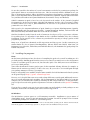
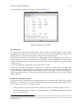
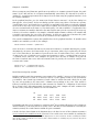
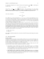
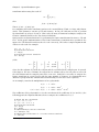
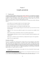
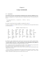
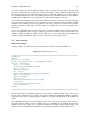
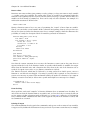
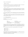
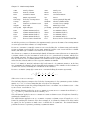
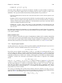
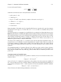
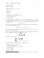
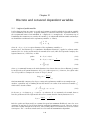
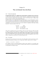
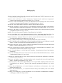
supplied data files. Under the File menu choose “Open data, Sample file”. A second notebook-type
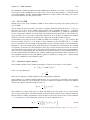
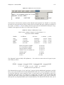
window will open, presenting the sets of data files supplied with the package (see Figure 2.1). Select
the first tab, “Ramanathan”. The numbering of the files in this section corresponds to the chapter
organization of Ramanathan (2002), which contains discussion of the analysis of these data. The
data will be useful for practice purposes even without the text.
Figure 2.1: Practice data files window
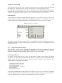
If you select a row in this window and click on “Info” this opens a window showing information on
the data set in question (for example, on the sources and definitions of the variables). If you find
a file that is of interest, you may open it by clicking on “Open”, or just double-clicking on the file
name. For the moment let’s open data3-6.
☞ In gretl windows containing lists, double-clicking on a line launches a default action for the associated list
entry: e.g. displaying the values of a data series, opening a file.
1 For convenience I will refer to the graphical client program simply as gretl in this manual. Note, however, that the
specific name of the program differs according to the computer platform. On Linux it is called gretl_x11 while on MS
Windows it is gretlw32.exe. On Linux systems a wrapper script named gretl is also installed — see also the Gretl
Command Reference.
5
Chapter 2. Getting started
6
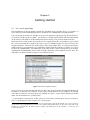
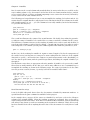
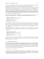
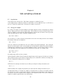
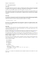
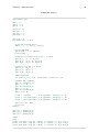
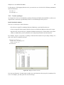
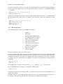
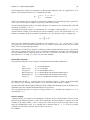
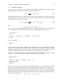
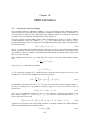
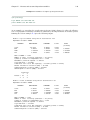
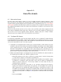
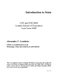
This file contains data pertaining to a classic econometric “chestnut”, the consumption function.
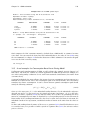
The data window should now display the name of the current data file, the overall data range and
sample range, and the names of the variables along with brief descriptive tags — see Figure 2.2.
Figure 2.2: Main window, with a practice data file open
OK, what can we do now? Hopefully the various menu options should be fairly self explanatory. For
now we’ll dip into the Model menu; a brief tour of all the main window menus is given in Section 2.3
below.
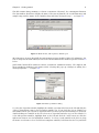
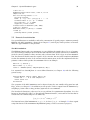
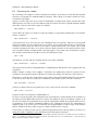
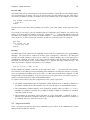
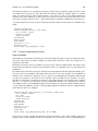
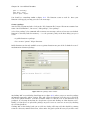
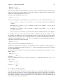
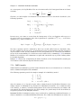
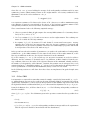
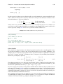
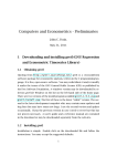
gretl’s Model menu offers numerous various econometric estimation routines. The simplest and
most standard is Ordinary Least Squares (OLS). Selecting OLS pops up a dialog box calling for a
model specification — see Figure 2.3.
Figure 2.3: Model specification dialog
To select the dependent variable, highlight the variable you want in the list on the left and click the
“Choose” button that points to the Dependent variable slot. If you check the “Set as default” box
this variable will be pre-selected as dependent when you next open the model dialog box. Shortcut:
double-clicking on a variable on the left selects it as dependent and also sets it as the default. To
select independent variables, highlight them on the left and click the “Add” button (or click the
right mouse button over the highlighted variable). To select several variable in the list box, drag
the mouse over them; to select several non-contiguous variables, hold down the Ctrl key and click
Chapter 2. Getting started
7
on the variables you want. To run a regression with consumption as the dependent variable and
income as independent, click Ct into the Dependent slot and add Yt to the Independent variables
list.
2.2
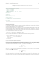
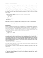
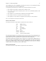
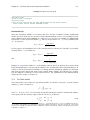
Estimation output
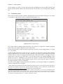
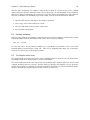
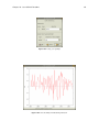
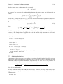
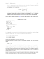
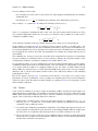
Once you’ve specified a model, a window displaying the regression output will appear. The output
is reasonably comprehensive and in a standard format (Figure 2.4).
Figure 2.4: Model output window
The output window contains menus that allow you to inspect or graph the residuals and fitted
values, and to run various diagnostic tests on the model.
For most models there is also an option to print the regression output in LATEX format. See Chapter 22 for details.
To import gretl output into a word processor, you may copy and paste from an output window,
using its Edit menu (or Copy button, in some contexts) to the target program. Many (not all) gretl
windows offer the option of copying in RTF (Microsoft’s “Rich Text Format”) or as LATEX. If you are
pasting into a word processor, RTF may be a good option because the tabular formatting of the
output is preserved.2 Alternatively, you can save the output to a (plain text) file then import the
file into the target program. When you finish a gretl session you are given the option of saving all
the output from the session to a single file.
Note that on the gnome desktop and under MS Windows, the File menu includes a command to
send the output directly to a printer.
☞ When pasting or importing plain text gretl output into a word processor, select a monospaced or typewriterstyle font (e.g. Courier) to preserve the output’s tabular formatting. Select a small font (10-point Courier
should do) to prevent the output lines from being broken in the wrong place.
2 Note that when you copy as RTF under MS Windows, Windows will only allow you to paste the material into applications that “understand” RTF. Thus you will be able to paste into MS Word, but not into notepad. Note also that there
appears to be a bug in some versions of Windows, whereby the paste will not work properly unless the “target” application
(e.g. MS Word) is already running prior to copying the material in question.
Chapter 2. Getting started
2.3
8
The main window menus
Reading left to right along the main window’s menu bar, we find the File, Tools, Data, View, Add,
Sample, Variable, Model and Help menus.
• File menu
– Open data: Open a native gretl data file or import from other formats. See Chapter 4.
– Append data: Add data to the current working data set, from a gretl data file, a commaseparated values file or a spreadsheet file.
– Save data: Save the currently open native gretl data file.
– Save data as: Write out the current data set in native format, with the option of using
gzip data compression. See Chapter 4.
– Export data: Write out the current data set in Comma Separated Values (CSV) format, or
the formats of GNU R or GNU Octave. See Chapter 4 and also Appendix D.
– Send to: Send the current data set as an e-mail attachment.
– New data set: Allows you to create a blank data set, ready for typing in values or for
importing series from a database. See below for more on databases.
– Clear data set: Clear the current data set out of memory. Generally you don’t have to do
this (since opening a new data file automatically clears the old one) but sometimes it’s
useful.
– Script files: A “script” is a file containing a sequence of gretl commands. This item
contains entries that let you open a script you have created previously (“User file”), open
a sample script, or open an editor window in which you can create a new script.
– Session files: A “session” file contains a snapshot of a previous gretl session, including
the data set used and any models or graphs that you saved. Under this item you can
open a saved session or save the current session.
– Databases: Allows you to browse various large databases, either on your own computer
or, if you are connected to the internet, on the gretl database server. See Section 4.3 for
details.
– Function files: Handles “function packages” (see Section 10.4), which allow you to access
functions written by other users and share the ones written by you.
– Exit: Quit the program. If expert mode is not selected you’ll be prompted to save any
unsaved work.
• Tools menu
– Statistical tables: Look up critical values for commonly used distributions (normal or
Gaussian, t, chi-square, F and Durbin–Watson).
– P-value finder: Open a window which enables you to look up p-values from the Gaussian,
t, chi-square, F, gamma or binomial distributions. See also the pvalue command in the
Gretl Command Reference.
– Test statistic calculator: Calculate test statistics and p-values for a range of common hypothesis tests (population mean, variance and proportion; difference of means, variances
and proportions). See also the item “Bivariate tests” under the Model menu.
– Command log: Open a window containing a record of the commands executed so far.
– Gretl console: Open a “console” window into which you can type commands as you would
using the command-line program, gretlcli (as opposed to using point-and-click).
Chapter 2. Getting started
9
– Start Gnu R: Start R (if it is installed on your system), and load a copy of the data set
currently open in gretl. See Appendix D.
– Sort variables: Rearrange the listing of variables in the main window, either by ID number
or alphabetically by name.
– NIST test suite: Check the numerical accuracy of gretl against the reference results for
linear regression made available by the (US) National Institute of Standards and Technology.
– Preferences: Set the paths to various files gretl needs to access. Choose the font in which
gretl displays text output. Select or unselect “expert mode”. (If this mode is selected
various warning messages are suppressed.) Activate or suppress gretl’s messaging about
the availability of program updates. Configure or turn on/off the main-window toolbar.
See the Gretl Command Reference for further details.
• Data menu
– Select all: Several menu items act upon those variables that are currently selected in the
main window. This item lets you select all the variables.
– Display values: Pops up a window with a simple (not editable) printout of the values of
the selected variable or variables.
– Edit values: Opens a spreadsheet window where you can edit the values of the selected
variables.
– Add observations: Gives a dialog box in which you can choose a number of observations
to add at the end of the current dataset; for use with forecasting.
– Remove extra observations: Active only if extra observations have been added automatically in the process of forecasting; deletes these extra observations.
– Read info, Edit info: “Read info” just displays the summary information for the current
data file; “Edit info” allows you to make changes to it (if you have permission to do so).
– Print description: Opens a window containing a full account of the current dataset, including the summary information and any specific information on each of the variables.
– Add case markers: Prompts for the name of a text file containing “case markers” (short
strings identifying the individual observations) and adds this information to the data set.
See Chapter 4.
– Remove case markers: Active only if the dataset has case markers identifying the observations; removes these case markers.
– Dataset structure: invokes a series of dialog boxes which allow you to change the structural interpretation of the current dataset. For example, if data were read in as a cross
section you can get the program to interpret them as time series or as a panel. See also
section 4.5.
– Compact data: For time-series data of higher than annual frequency, gives you the option
of compacting the data to a lower frequency, using one of four compaction methods
(average, sum, start of period or end of period).
– Expand data: For time-series data, gives you the option of expanding the data to a higher
frequency.
– Transpose data: Turn each observation into a variable and vice versa (or in other words,
each row of the data matrix becomes a column in the modified data matrix); can be useful
with imported data that have been read in “sideways”.
• View menu
– Icon view: Opens a window showing the content of the current session as a set of icons;
see section 3.4.
Chapter 2. Getting started
10
– Graph specified vars: Gives a choice between a time series plot, a regular X–Y scatter
plot, an X–Y plot using impulses (vertical bars), an X–Y plot “with factor separation” (i.e.
with the points colored differently depending to the value of a given dummy variable),
boxplots, and a 3-D graph. Serves up a dialog box where you specify the variables to
graph. See Chapter 7 for details.
– Multiple graphs: Allows you to compose a set of up to six small graphs, either pairwise
scatter-plots or time-series graphs. These are displayed together in a single window.
– Summary statistics: Shows a full set of descriptive statistics for the variables selected in
the main window.
– Correlation matrix: Active only if two or more variables are selected; shows the pairwise
correlation coefficients for the selected variables.
– Principal components: Active only if two or more variables are selected; produces a Principal Components Analysis of the selected variables.
– Mahalonobis distances: Active only if two or more variables are selected; computes the
Mahalonobis distance of each observation from the centroid of the selected set of variables.
• Add menu Offers various standard transformations of variables (logs, lags, squares, etc.) that
you may wish to add to the data set. Also gives the option of adding random variables, and
(for time-series data) adding seasonal dummy variables (e.g. quarterly dummy variables for
quarterly data).
• Sample menu
– Set range: Select a different starting and/or ending point for the current sample, within
the range of data available.
– Restore full range: self-explanatory.
– Define, based on dummy: Given a dummy (indicator) variable with values 0 or 1, this
drops from the current sample all observations for which the dummy variable has value
0.
– Restrict, based on criterion: Similar to the item above, except that you don’t need a predefined variable: you supply a Boolean expression (e.g. sqft > 1400) and the sample is
restricted to observations satisfying that condition. See the entry for genr in the Gretl
Command Reference for details on the Boolean operators that can be used.
– Random sub-sample: Draw a random sample from the full dataset.
– Drop all obs with missing values: Drop from the current sample all observations for
which at least one variable has a missing value (see Section 4.6).
– Count missing values: Give a report on observations where data values are missing. May
be useful in examining a panel data set, where it’s quite common to encounter missing
values.
– Set missing value code: Set a numerical value that will be interpreted as “missing” or “not
available”. This is intended for use with imported data, when gretl has not recognized
the missing-value code used.
• Variable menu Most items under here operate on a single variable at a time. The “active”
variable is set by highlighting it (clicking on its row) in the main data window. Most options
will be self-explanatory. Note that you can rename a variable and can edit its descriptive label
under “Edit attributes”. You can also “Define a new variable” via a formula (e.g. involving
some function of one or more existing variables). For the syntax of such formulae, look at the
online help for “Generate variable syntax” or see the genr command in the Gretl Command
Reference. One simple example:
foo = x1 * x2
Chapter 2. Getting started
11
will create a new variable foo as the product of the existing variables x1 and x2. In these
formulae, variables must be referenced by name, not number.
• Model menu For details on the various estimators offered under this menu please consult the
Gretl Command Reference. Also see Chapter 16 regarding the estimation of nonlinear models.
• Help menu Please use this as needed! It gives details on the syntax required in various dialog
entries.
2.4
Keyboard shortcuts
When working in the main gretl window, some common operations may be performed using the
keyboard, as shown in the table below.
2.5
Return
Opens a window displaying the values of the currently selected variables: it is
the same as selecting “Data, Display Values”.
Delete
Pressing this key has the effect of deleting the selected variables. A confirmation is required, to prevent accidental deletions.
e
Has the same effect as selecting “Edit attributes” from the “Variable” menu.
F2
Same as “e”. Included for compatibility with other programs.
g
Has the same effect as selecting “Define new variable” from the “Variable”
menu (which maps onto the genr command).
h
Opens a help window for gretl commands.
F1
Same as “h”. Included for compatibility with other programs.
r
Refreshes the variable list in the main window: has the same effect as selecting
“Refresh window” from the “Data” menu.
t
Graphs the selected variable; a line graph is used for time-series datasets,
whereas a distribution plot is used for cross-sectional data.
The gretl toolbar
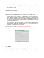
At the bottom left of the main window sits the toolbar.
The icons have the following functions, reading from left to right:
1. Launch a calculator program. A convenience function in case you want quick access to a
calculator when you’re working in gretl. The default program is calc.exe under MS Windows, or xcalc under the X window system. You can change the program under the “Tools,
Preferences, General” menu, “Programs” tab.
2. Start a new script. Opens an editor window in which you can type a series of commands to be
sent to the program as a batch.
3. Open the gretl console. A shortcut to the “Gretl console” menu item (Section 2.3 above).
4. Open the gretl session icon window.
5. Open the gretl website in your web browser. This will work only if you are connected to the
Internet and have a properly configured browser.
6. Open this manual in PDF format.
Chapter 2. Getting started
12
7. Open the help item for script commands syntax (i.e. a listing with details of all available
commands).
8. Open the dialog box for defining a graph.
9. Open the dialog box for estimating a model using ordinary least squares.
10. Open a window listing the sample datasets supplied with gretl, and any other data file collections that have been installed.
If you don’t care to have the toolbar displayed, you can turn it off under the “Tools, Preferences,
General” menu. Go o the Toolbar tab and uncheck the “show gretl toolbar” box.
Chapter 3
Modes of working
3.1
Command scripts
As you execute commands in gretl, using the GUI and filling in dialog entries, those commands are
recorded in the form of a “script” or batch file. Such scripts can be edited and re-run, using either
gretl or the command-line client, gretlcli.
To view the current state of the script at any point in a gretl session, choose “Command log” under
the Tools menu. This log file is called session.inp and it is overwritten whenever you start a new
session. To preserve it, save the script under a different name. Script files will be found most easily,
using the GUI file selector, if you name them with the extension “.inp”.
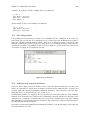
To open a script you have written independently, use the “File, Script files” menu item; to create a
script from scratch use the “File, Script files, New script” item or the “new script” toolbar button.
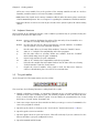
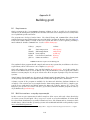
In either case a script window will open (see Figure 3.1).
Figure 3.1: Script window, editing a command file
The toolbar at the top of the script window offers the following functions (left to right): (1) Save the
file; (2) Save the file under a specified name; (3) Print the file (under Windows or the gnome desktop
only); (4) Execute the commands in the file; (5) Copy selected text; (6) Paste the selected text; (7)
Find and replace text; (8) Undo the last Paste or Replace action; (9) Help (if you place the cursor in
a command word and press the question mark you will get help on that command); (10) Close the
window.
When you click the Execute icon all output is directed to a single window, where it can be edited,
saved or copied to the clipboard. To learn more about the possibilities of scripting, take a look
at the gretl Help item “Command reference,” or start up the command-line program gretlcli and
consult its help, or consult the Gretl Command Reference.
If you click on the Execute icon when part of a script is highlighted, gretl will only run that portion.
13
Chapter 3. Modes of working
14
Moreover, if you want to run just the current line, you can do so by pressing Ctrl-Enter.1
In addition, the gretl package includes over 70 “practice” scripts. Most of these relate to Ramanathan (2002), but they may also be used as a free-standing introduction to scripting in gretl and
to various points of econometric theory. You can explore the practice files under “File, Script files,
Practice file” There you will find a listing of the files along with a brief description of the points
they illustrate and the data they employ. Open any file and run it to see the output. Note that
long commands in a script can be broken over two or more lines, using backslash as a continuation
character.
You can, if you wish, use the GUI controls and the scripting approach in tandem, exploiting each
method where it offers greater convenience. Here are two suggestions.
• Open a data file in the GUI. Explore the data — generate graphs, run regressions, perform
tests. Then open the Command log, edit out any redundant commands, and save it under
a specific name. Run the script to generate a single file containing a concise record of your
work.
• Start by establishing a new script file. Type in any commands that may be required to set
up transformations of the data (see the genr command in the Gretl Command Reference).
Typically this sort of thing can be accomplished more efficiently via commands assembled
with forethought rather than point-and-click. Then save and run the script: the GUI data
window will be updated accordingly. Now you can carry out further exploration of the data
via the GUI. To revisit the data at a later point, open and rerun the “preparatory” script first.
3.2
Saving script objects
When you estimate a model using point-and-click, the model results are displayed in a separate
window, offering menus which let you perform tests, draw graphs, save data from the model, and
so on. Ordinarily, when you estimate a model using a script you just get a non-interactive printout
of the results. You can, however, arrange for models estimated in a script to be “captured”, so that
you can examine them interactively when the script is finished. Here is an example of the syntax
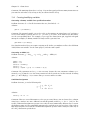
for achieving this effect:
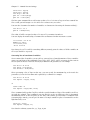
Model1 <- ols Ct 0 Yt
That is, you type a name for the model to be saved under, then a back-pointing “assignment arrow”,
then the model command. You may use names that have embedded spaces if you like, but such
names must be wrapped in double quotes:
"Model 1" <- ols Ct 0 Yt
Models saved in this way will appear as icons in the gretl icon view window (see Section 3.4) after
the script is executed. In addition, you can arrange to have a named model displayed (in its own
window) automatically as follows:
Model1.show
Again, if the name contains spaces it must be quoted:
"Model 1".show
1 This feature is not unique to gretl; other econometric packages offer the same facility. However, experience shows
that while this can be remarkably useful, it can also lead to writing dinosaur scripts that are never meant to be executed
all at once, but rather used as a chaotic repository to cherry-pick snippets from. Since gretl allows you to have several
script windows open at the same time, you may want to keep your scripts tidy and reasonably small.
Chapter 3. Modes of working
15
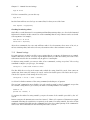
The same facility can be used for graphs. For example the following will create a plot of Ct against
Yt, save it under the name “CrossPlot” (it will appear under this name in the icon view window),
and have it displayed:
CrossPlot <- gnuplot Ct Yt
CrossPlot.show
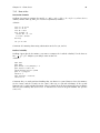
You can also save the output from selected commands as named pieces of text (again, these will
appear in the session icon window, from where you can open them later). For example this command sends the output from an augmented Dickey–Fuller test to a “text object” named ADF1 and
displays it in a window:
ADF1 <- adf 2 x1
ADF1.show
Objects saved in this way (whether models, graphs or pieces of text output) can be destroyed using
the command .free appended to the name of the object, as in ADF1.free.
3.3
The gretl console
A further option is available for your computing convenience. Under gretl’s “Tools” menu you will
find the item “Gretl console” (there is also an “open gretl console” button on the toolbar in the
main window). This opens up a window in which you can type commands and execute them one
by one (by pressing the Enter key) interactively. This is essentially the same as gretlcli’s mode of
operation, except that the GUI is updated based on commands executed from the console, enabling
you to work back and forth as you wish.
In the console, you have “command history”; that is, you can use the up and down arrow keys to
navigate the list of command you have entered to date. You can retrieve, edit and then re-enter a
previous command.
In console mode, you can create, display and free objects (models, graphs or text) aa described
above for script mode.
3.4
The Session concept
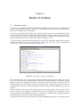
gretl offers the idea of a “session” as a way of keeping track of your work and revisiting it later.
The basic idea is to provide an iconic space containing various objects pertaining to your current
working session (see Figure 3.2). You can add objects (represented by icons) to this space as you
go along. If you save the session, these added objects should be available again if you re-open the
session later.
If you start gretl and open a data set, then select “Icon view” from the View menu, you should see
the basic default set of icons: these give you quick access to information on the data set (if any),
correlation matrix (“Correlations”) and descriptive summary statistics (“Summary”). All of these
are activated by double-clicking the relevant icon. The “Data set” icon is a little more complex:
double-clicking opens up the data in the built-in spreadsheet, but you can also right-click on the
icon for a menu of other actions.
To add a model to the Icon view, first estimate it using the Model menu. Then pull down the File
menu in the model window and select “Save to session as icon. . . ” or “Save as icon and close”.
Simply hitting the S key over the model window is a shortcut to the latter action.
To add a graph, first create it (under the View menu, “Graph specified vars”, or via one of gretl’s
other graph-generating commands). Click on the graph window to bring up the graph menu, and
select “Save to session as icon”.
Chapter 3. Modes of working
16
Figure 3.2: Icon view: one model and one graph have been added to the default icons
Once a model or graph is added its icon will appear in the Icon view window. Double-clicking on the
icon redisplays the object, while right-clicking brings up a menu which lets you display or delete
the object. This popup menu also gives you the option of editing graphs.
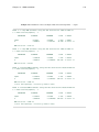
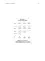
The model table
In econometric research it is common to estimate several models with a common dependent variable — the models differing in respect of which independent variables are included, or perhaps in
respect of the estimator used. In this situation it is convenient to present the regression results
in the form of a table, where each column contains the results (coefficient estimates and standard
errors) for a given model, and each row contains the estimates for a given variable across the
models.
In the Icon view window gretl provides a means of constructing such a table (and copying it in plain
text, LATEX or Rich Text Format). Here is how to do it:2
1. Estimate a model which you wish to include in the table, and in the model display window,
under the File menu, select “Save to session as icon” or “Save as icon and close”.
2. Repeat step 1 for the other models to be included in the table (up to a total of six models).
3. When you are done estimating the models, open the icon view of your gretl session, by selecting “Icon view” under the View menu in the main gretl window, or by clicking the “session
icon view” icon on the gretl toolbar.
4. In the Icon view, there is an icon labeled “Model table”. Decide which model you wish to
appear in the left-most column of the model table and add it to the table, either by dragging
its icon onto the Model table icon, or by right-clicking on the model icon and selecting “Add
to model table” from the pop-up menu.
5. Repeat step 4 for the other models you wish to include in the table. The second model selected
will appear in the second column from the left, and so on.
6. When you are finished composing the model table, display it by double-clicking on its icon.
Under the Edit menu in the window which appears, you have the option of copying the table
to the clipboard in various formats.
7. If the ordering of the models in the table is not what you wanted, right-click on the model
table icon and select “Clear table”. Then go back to step 4 above and try again.
2 The model table can also be built non-interactively, in script mode. For details on how to do this, see the entry for
modeltab in the Gretl Command Reference.
Chapter 3. Modes of working
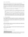
17
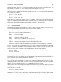
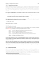
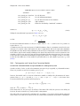
A simple instance of gretl’s model table is shown in Figure 3.3.
Figure 3.3: Example of model table
The graph page
The “graph page” icon in the session window offers a means of putting together several graphs
for printing on a single page. This facility will work only if you have the LATEX typesetting system
installed, and are able to generate and view either PDF or PostScript output.3
In the Icon view window, you can drag up to eight graphs onto the graph page icon. When you
double-click on the icon (or right-click and select “Display”), a page containing the selected graphs
(in PDF or EPS format) will be composed and opened in your viewer. From there you should be able
to print the page.
To clear the graph page, right-click on its icon and select “Clear”.
On systems other than MS Windows, you may have to adjust the setting for the program used
to view postscript. Find that under the “Programs” tab in the Preferences dialog box (under the
“Tools” menu in the main window). On Windows, you may need to adjust your file associations so
that the appropriate viewer is called for the “Open” action on files with the .ps extension. FIXME
discuss PDF here.
Saving and re-opening sessions
If you create models or graphs that you think you may wish to re-examine later, then before quitting
gretl select “Session files, Save session” from the File menu and give a name under which to save
the session. To re-open the session later, either
• Start gretl then re-open the session file by going to the “File, Session files, Open session”, or
• From the command line, type gretl -r sessionfile, where sessionfile is the name under which
the session was saved.
3 For PDF output you need pdflatex and either Adobe’s PDF reader or xpdf on X11. For PostScript, you must have dvips
and ghostscript installed, along with a viewer such as gv, ggv or kghostview. The default viewer for systems other than
MS Windows is gv.
Chapter 4
Data files
4.1
Native format
gretl has its own format for data files. Most users will probably not want to read or write such files
outside of gretl itself, but occasionally this may be useful and full details on the file formats are
given in Appendix A.
4.2
Other data file formats
gretl will read various other data formats.
• Plain text (ASCII) files. These can be brought in using gretl’s “File, Open Data, Import ASCII. . . ”
menu item, or the import script command. For details on what gretl expects of such files, see
Section 4.4.
• Comma-Separated Values (CSV) files. These can be imported using gretl’s “File, Open Data,
Import CSV. . . ” menu item, or the import script command. See also Section 4.4.
• Worksheets in the format of either MS Excel or Gnumeric. These are also brought in using
gretl’s “File, Open Data, Import” menu. The requirements for such files are given in Section 4.4.
• Stata data files (.dta).
• Eviews workfiles (.wf1).1
When you import data from the ASCII or CSV formats, gretl opens a “diagnostic” window, reporting on its progress in reading the data. If you encounter a problem with ill-formatted data, the
messages in this window should give you a handle on fixing the problem.
For the convenience of anyone wanting to carry out more complex data analysis, gretl has a facility
for writing out data in the native formats of GNU R and GNU Octave (see Appendix D). In the GUI
client this option is found under the “File, Export data” menu; in the command-line client use the
store command with the flag -r (R) or -m (Octave).
4.3
Binary databases
For working with large amounts of data gretl is supplied with a database-handling routine. A
database, as opposed to a data file, is not read directly into the program’s workspace. A database
can contain series of mixed frequencies and sample ranges. You open the database and select
series to import into the working dataset. You can then save those series in a native format data
file if you wish. Databases can be accessed via gretl’s menu item “File, Databases”.
For details on the format of gretl databases, see Appendix A.
1 This
is somewhat experimental. See http://www.ecn.wfu.edu/eviews_format/.
18
Chapter 4. Data files
19
Online access to databases
As of version 0.40, gretl is able to access databases via the internet. Several databases are available
from Wake Forest University. Your computer must be connected to the internet for this option to
work. Please see the description of the “data” command under gretl’s Help menu.
RATS 4 databases
Thanks to Thomas Doan of Estima, who made available the specification of the database format
used by RATS 4 (Regression Analysis of Time Series), gretl can also handle such databases. Well,
actually, a subset of same: I have only worked on time-series databases containing monthly and
quarterly series. My university has the RATS G7 database containing data for the seven largest
OECD economies and gretl will read that OK.
☞ Visit the gretl data page for details and updates on available data.
4.4
Creating a data file from scratch
There are several ways of doing this:
1. Find, or create using a text editor, a plain text data file and open it with gretl’s “Import ASCII”
option.
2. Use your favorite spreadsheet to establish the data file, save it in Comma Separated Values
format if necessary (this should not be necessary if the spreadsheet program is MS Excel or
Gnumeric), then use one of gretl’s “Import” options (CSV, Excel or Gnumeric, as the case may
be).
3. Use gretl’s built-in spreadsheet.
4. Select data series from a suitable database.
5. Use your favorite text editor or other software tools to a create data file in gretl format independently.
Here are a few comments and details on these methods.
Common points on imported data
Options (1) and (2) involve using gretl’s “import” mechanism. For gretl to read such data successfully, certain general conditions must be satisfied:
• The first row must contain valid variable names. A valid variable name is of 15 characters
maximum; starts with a letter; and contains nothing but letters, numbers and the underscore
character, _. (Longer variable names will be truncated to 15 characters.) Qualifications to the
above: First, in the case of an ASCII or CSV import, if the file contains no row with variable
names the program will automatically add names, v1, v2 and so on. Second, by “the first row”
is meant the first relevant row. In the case of ASCII and CSV imports, blank rows and rows
beginning with a hash mark, #, are ignored. In the case of Excel and Gnumeric imports, you
are presented with a dialog box where you can select an offset into the spreadsheet, so that
gretl will ignore a specified number of rows and/or columns.
• Data values: these should constitute a rectangular block, with one variable per column (and
one observation per row). The number of variables (data columns) must match the number
of variable names given. See also section 4.6. Numeric data are expected, but in the case of
importing from ASCII/CSV, the program offers limited handling of character (string) data: if
Chapter 4. Data files
20
a given column contains character data only, consecutive numeric codes are substituted for
the strings, and once the import is complete a table is printed showing the correspondence
between the strings and the codes.
• Dates (or observation labels): Optionally, the first column may contain strings such as dates,
or labels for cross-sectional observations. Such strings have a maximum of 8 characters (as
with variable names, longer strings will be truncated). A column of this sort should be headed
with the string obs or date, or the first row entry may be left blank.
For dates to be recognized as such, the date strings must adhere to one or other of a set of
specific formats, as follows. For annual data: 4-digit years. For quarterly data: a 4-digit year,
followed by a separator (either a period, a colon, or the letter Q), followed by a 1-digit quarter.
Examples: 1997.1, 2002:3, 1947Q1. For monthly data: a 4-digit year, followed by a period or
a colon, followed by a two-digit month. Examples: 1997.01, 2002:10.
CSV files can use comma, space or tab as the column separator. When you use the “Import CSV”
menu item you are prompted to specify the separator. In the case of “Import ASCII” the program
attempts to auto-detect the separator that was used.
If you use a spreadsheet to prepare your data you are able to carry out various transformations of
the “raw” data with ease (adding things up, taking percentages or whatever): note, however, that
you can also do this sort of thing easily — perhaps more easily — within gretl, by using the tools
under the “Add” menu.
Appending imported data
You may wish to establish a gretl dataset piece by piece, by incremental importation of data from
other sources. This is supported via the “File, Append data” menu items: gretl will check the new
data for conformability with the existing dataset and, if everything seems OK, will merge the data.
You can add new variables in this way, provided the data frequency matches that of the existing
dataset. Or you can append new observations for data series that are already present; in this case
the variable names must match up correctly. Note that by default (that is, if you choose “Open
data” rather than “Append data”), opening a new data file closes the current one.
Using the built-in spreadsheet
Under gretl’s “File, New data set” menu you can choose the sort of dataset you want to establish
(e.g. quarterly time series, cross-sectional). You will then be prompted for starting and ending dates
(or observation numbers) and the name of the first variable to add to the dataset. After supplying
this information you will be faced with a simple spreadsheet into which you can type data values. In
the spreadsheet window, clicking the right mouse button will invoke a popup menu which enables
you to add a new variable (column), to add an observation (append a row at the foot of the sheet),
or to insert an observation at the selected point (move the data down and insert a blank row.)
Once you have entered data into the spreadsheet you import these into gretl’s workspace using the
spreadsheet’s “Apply changes” button.
Please note that gretl’s spreadsheet is quite basic and has no support for functions or formulas.
Data transformations are done via the “Add” or “Variable” menus in the main gretl window.
Selecting from a database
Another alternative is to establish your dataset by selecting variables from a database. Gretl comes
with a database of US macroeconomic time series and, as mentioned above, the program will reads
RATS 4 databases.
Begin with gretl’s “File, Databases” menu item. This has three forks: “Gretl native”, “RATS 4” and
“On database server”. You should be able to find the file fedstl.bin in the file selector that
Chapter 4. Data files
21
opens if you choose the “Gretl native” option — this file, which contains a large collection of US
macroeconomic time series, is supplied with the distribution.
You won’t find anything under “RATS 4” unless you have purchased RATS data.2 If you do possess
RATS data you should go into gretl’s “Tools, Preferences, General” dialog, select the Databases tab,
and fill in the correct path to your RATS files.
If your computer is connected to the internet you should find several databases (at Wake Forest
University) under “On database server”. You can browse these remotely; you also have the option
of installing them onto your own computer. The initial remote databases window has an item
showing, for each file, whether it is already installed locally (and if so, if the local version is up to
date with the version at Wake Forest).
Assuming you have managed to open a database you can import selected series into gretl’s workspace
by using the “Series, Import” menu item in the database window, or via the popup menu that appears if you click the right mouse button, or by dragging the series into the program’s main window.
Creating a gretl data file independently
It is possible to create a data file in one or other of gretl’s own formats using a text editor or
software tools such as awk, sed or perl. This may be a good choice if you have large amounts of
data already in machine readable form. You will, of course, need to study the gretl data formats
(XML format or “traditional” format) as described in Appendix A.
4.5
Structuring a dataset
Once your data are read by gretl, it may be necessary to supply some information on the nature of
the data. We distinguish between three kinds of datasets:
1. Cross section
2. Time series
3. Panel data
The primary tool for doing this is the “Data, Dataset structure” menu entry in the graphical interface, or the setobs command for scripts and the command-line interface.
Cross sectional data
By a cross section we mean observations on a set of “units” (which may be firms, countries, individuals, or whatever) at a common point in time. This is the default interpretation for a data
file: if gretl does not have sufficient information to interpret data as time-series or panel data,
they are automatically interpreted as a cross section. In the unlikely event that cross-sectional data
are wrongly interpreted as time series, you can correct this by selecting the “Data, Dataset structure” menu item. Click the “cross-sectional” radio button in the dialog box that appears, then click
“Forward”. Click “OK” to confirm your selection.
Time series data
When you import data from a spreadsheet or plain text file, gretl will make fairly strenuous efforts
to glean time-series information from the first column of the data, if it looks at all plausible that
such information may be present. If time-series structure is present but not recognized, again you
can use the “Data, Dataset structure” menu item. Select “Time series” and click “Forward”; select the
appropriate data frequency and click “Forward” again; then select or enter the starting observation
2 See
www.estima.com
Chapter 4. Data files
22
and click “Forward” once more. Finally, click “OK” to confirm the time-series interpretation if it is
correct (or click “Back” to make adjustments if need be).
Besides the basic business of getting a data set interpreted as time series, further issues may arise
relating to the frequency of time-series data. In a gretl time-series data set, all the series must
have the same frequency. Suppose you wish to make a combined dataset using series that, in their
original state, are not all of the same frequency. For example, some series are monthly and some
are quarterly.
Your first step is to formulate a strategy: Do you want to end up with a quarterly or a monthly data
set? A basic point to note here is that “compacting” data from a higher frequency (e.g. monthly) to
a lower frequency (e.g. quarterly) is usually unproblematic. You lose information in doing so, but
in general it is perfectly legitimate to take (say) the average of three monthly observations to create
a quarterly observation. On the other hand, “expanding” data from a lower to a higher frequency is
not, in general, a valid operation.
In most cases, then, the best strategy is to start by creating a data set of the lower frequency, and
then to compact the higher frequency data to match. When you import higher-frequency data from
a database into the current data set, you are given a choice of compaction method (average, sum,
start of period, or end of period). In most instances “average” is likely to be appropriate.
You can also import lower-frequency data into a high-frequency data set, but this is generally not
recommended. What gretl does in this case is simply replicate the values of the lower-frequency
series as many times as required. For example, suppose we have a quarterly series with the value
35.5 in 1990:1, the first quarter of 1990. On expansion to monthly, the value 35.5 will be assigned
to the observations for January, February and March of 1990. The expanded variable is therefore
useless for fine-grained time-series analysis, outside of the special case where you know that the
variable in question does in fact remain constant over the sub-periods.
When the current data frequency is appropriate, gretl offers both “Compact data” and “Expand
data” options under the “Data” menu. These options operate on the whole data set, compacting or
exanding all series. They should be considered “expert” options and should be used with caution.
Panel data
Panel data are inherently three dimensional — the dimensions being variable, cross-sectional unit,
and time-period. For example, a particular number in a panel data set might be identified as the
observation on capital stock for General Motors in 1980. (A note on terminology: we use the
terms “cross-sectional unit”, “unit” and “group” interchangeably below to refer to the entities that
compose the cross-sectional dimension of the panel. These might, for instance, be firms, countries
or persons.)
For representation in a textual computer file (and also for gretl’s internal calculations) the three
dimensions must somehow be flattened into two. This “flattening” involves taking layers of the
data that would naturally stack in a third dimension, and stacking them in the vertical dimension.
Gretl always expects data to be arranged “by observation”, that is, such that each row represents
an observation (and each variable occupies one and only one column). In this context the flattening
of a panel data set can be done in either of two ways:
• Stacked time series: the successive vertical blocks each comprise a time series for a given
unit.
• Stacked cross sections: the successive vertical blocks each comprise a cross-section for a
given period.
You may input data in whichever arrangement is more convenient. Internally, however, gretl always
stores panel data in the form of stacked time series.
Chapter 4. Data files
23
When you import panel data into gretl from a spreadsheet or comma separated format, the panel
nature of the data will not be recognized automatically (most likely the data will be treated as
“undated”). A panel interpretation can be imposed on the data using the graphical interface or via
the setobs command.
In the graphical interface, use the menu item “Data, Dataset structure”. In the first dialog box
that appears, select “Panel”. In the next dialog you have a three-way choice. The first two options,
“Stacked time series” and “Stacked cross sections” are applicable if the data set is already organized
in one of these two ways. If you select either of these options, the next step is to specify the number
of cross-sectional units in the data set. The third option, “Use index variables”, is applicable if the
data set contains two variables that index the units and the time periods respectively; the next step
is then to select those variables. For example, a data file might contain a country code variable and
a variable representing the year of the observation. In that case gretl can reconstruct the panel
structure of the data regardless of how the observation rows are organized.
The setobs command has options that parallel those in the graphical interface. If suitable index
variables are available you can do, for example
setobs unitvar timevar --panel-vars
where unitvar is a variable that indexes the units and timevar is a variable indexing the periods.
Alternatively you can use the form setobs freq 1:1 structure, where freq is replaced by the “block
size” of the data (that is, the number of periods in the case of stacked time series, or the number
of units in the case of stacked cross-sections) and structure is either --stacked-time-series or
--stacked-cross-section. Two examples are given below: the first is suitable for a panel in
the form of stacked time series with observations from 20 periods; the second for stacked cross
sections with 5 units.
setobs 20 1:1 --stacked-time-series
setobs 5 1:1 --stacked-cross-section
Panel data arranged by variable
Publicly available panel data sometimes come arranged “by variable.” Suppose we have data on two
variables, x1 and x2, for each of 50 states in each of 5 years (giving a total of 250 observations
per variable). One textual representation of such a data set would start with a block for x1, with
50 rows corresponding to the states and 5 columns corresponding to the years. This would be
followed, vertically, by a block with the same structure for variable x2. A fragment of such a data
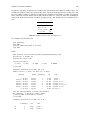
file is shown below, with quinquennial observations 1965–1985. Imagine the table continued for
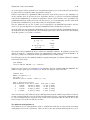
48 more states, followed by another 50 rows for variable x2.
x1
1965
1970
1975
1980
1985
AR
100.0
110.5
118.7
131.2
160.4
AZ
100.0
104.3
113.8
120.9
140.6
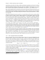
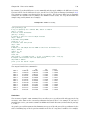
If a datafile with this sort of structure is read into gretl,3 the program will interpret the columns as
distinct variables, so the data will not be usable “as is.” But there is a mechanism for correcting the
situation, namely the stack function within the genr command.
Consider the first data column in the fragment above: the first 50 rows of this column constitute a
cross-section for the variable x1 in the year 1965. If we could create a new variable by stacking the
3 Note that you will have to modify such a datafile slightly before it can be read at all. The line containing the variable
name (in this example x1) will have to be removed, and so will the initial row containing the years, otherwise they will be
taken as numerical data.
Chapter 4. Data files
24
first 50 entries in the second column underneath the first 50 entries in the first, we would be on the
way to making a data set “by observation” (in the first of the two forms mentioned above, stacked
cross-sections). That is, we’d have a column comprising a cross-section for x1 in 1965, followed by
a cross-section for the same variable in 1970.
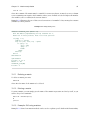
The following gretl script illustrates how we can accomplish the stacking, for both x1 and x2. We
assume that the original data file is called panel.txt, and that in this file the columns are headed
with “variable names” p1, p2, . . . , p5. (The columns are not really variables, but in the first instance
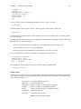
we “pretend” that they are.)
open panel.txt
genr x1 = stack(p1..p5) --length=50
genr x2 = stack(p1..p5) --offset=50 --length=50
setobs 50 1:1 --stacked-cross-section
store panel.gdt x1 x2
The second line illustrates the syntax of the stack function. The double dots within the parentheses indicate a range of variables to be stacked: here we want to stack all 5 columns (for all 5 years).
The full data set contains 100 rows; in the stacking of variable x1 we wish to read only the first 50
rows from each column: we achieve this by adding --length=50. Note that if you want to stack a
non-contiguous set of columns you can put a comma-separated list within the parentheses, as in
genr x = stack(p1,p3,p5)
On line 3 we do the stacking for variable x2. Again we want a length of 50 for the components of
the stacked series, but this time we want gretl to start reading from the 50th row of the original
data, and we specify --offset=50. Line 4 imposes a panel interpretation on the data; finally, we
save the data in gretl format, with the panel interpretation, discarding the original “variables” p1
through p5.
The illustrative script above is appropriate when the number of variable to be processed is small.
When then are many variables in the data set it will be more efficient to use a command loop to
accomplish the stacking, as shown in the following script. The setup is presumed to be the same
as in the previous section (50 units, 5 periods), but with 20 variables rather than 2.
open panel.txt
loop for i=1..20
genr k = ($i - 1) * 50
genr x$i = stack(p1..p5) --offset=k --length=50
endloop
setobs 50 1.01 --stacked-cross-section
store panel.gdt x1 x2 x3 x4 x5 x6 x7 x8 x9 x10 \
x11 x12 x13 x14 x15 x16 x17 x18 x19 x20
Panel data marker strings
It can be helpful with panel data to have the observations identified by mnemonic markers. A
special function in the genr command is available for this purpose.
In the example above, suppose all the states are identified by two-letter codes in the left-most
column of the original datafile. When the stacking operation is performed, these codes will be
stacked along with the data values. If the first row is marked AR for Arkansas, then the marker AR
will end up being shown on each row containing an observation for Arkansas. That’s all very well,
but these markers don’t tell us anything about the date of the observation. To rectify this we could
do:
Chapter 4. Data files
25
genr time
genr year = 1960 + (5 * time)
genr markers = "%s:%d", marker, year
The first line generates a 1-based index representing the period of each observation, and the second
line uses the time variable to generate a variable representing the year of the observation. The
third line contains this special feature: if (and only if) the name of the new “variable” to generate
is markers, the portion of the command following the equals sign is taken as C-style format string
(which must be wrapped in double quotes), followed by a comma-separated list of arguments.
The arguments will be printed according to the given format to create a new set of observation
markers. Valid arguments are either the names of variables in the dataset, or the string marker
which denotes the pre-existing observation marker. The format specifiers which are likely to be
useful in this context are %s for a string and %d for an integer. Strings can be truncated: for
example %.3s will use just the first three characters of the string. To chop initial characters off
an existing observation marker when constructing a new one, you can use the syntax marker + n,
where n is a positive integer: in the case the first n characters will be skipped.
After the commands above are processed, then, the observation markers will look like, for example,
AR:1965, where the two-letter state code and the year of the observation are spliced together with
a colon.
4.6
Missing data values
These are represented internally as DBL_MAX, the largest floating-point number that can be represented on the system (which is likely to be at least 10 to the power 300, and so should not be
confused with legitimate data values). In a native-format data file they should be represented as
NA. When importing CSV data gretl accepts several common representations of missing values including −999, the string NA (in upper or lower case), a single dot, or simply a blank cell. Blank cells
should, of course, be properly delimited, e.g. 120.6,,5.38, in which the middle value is presumed
missing.
As for handling of missing values in the course of statistical analysis, gretl does the following:
• In calculating descriptive statistics (mean, standard deviation, etc.) under the summary command, missing values are simply skipped and the sample size adjusted appropriately.
• In running regressions gretl first adjusts the beginning and end of the sample range, truncating the sample if need be. Missing values at the beginning of the sample are common in
time series work due to the inclusion of lags, first differences and so on; missing values at the
end of the range are not uncommon due to differential updating of series and possibly the
inclusion of leads.
If gretl detects any missing values “inside” the (possibly truncated) sample range for a regression,
the result depends on the character of the dataset and the estimator chosen. In many cases, the
program will automatically skip the missing observations when calculating the regression results.
In this situation a message is printed stating how many observations were dropped. On the other
hand, the skipping of missing observations is not supported for all procedures: exceptions include
all autoregressive estimators, system estimators such as SUR, and nonlinear least squares. In the
case of panel data, the skipping of missing observations is supported only if their omission leaves
a balanced panel. If missing observations are found in cases where they are not supported, gretl
gives an error message and refuses to produce estimates.
In case missing values in the middle of a dataset present a problem, the misszero function (use
with care!) is provided under the genr command. By doing genr foo = misszero(bar) you can
produce a series foo which is identical to bar except that any missing values become zeros. Then
Chapter 4. Data files
26
you can use carefully constructed dummy variables to, in effect, drop the missing observations
from the regression while retaining the surrounding sample range.4
4.7
Maximum size of data sets
Basically, the size of data sets (both the number of variables and the number of observations per
variable) is limited only by the characteristics of your computer. Gretl allocates memory dynamically, and will ask the operating system for as much memory as your data require. Obviously, then,
you are ultimately limited by the size of RAM.
Aside from the multiple-precision OLS option, gretl uses double-precision floating-point numbers
throughout. The size of such numbers in bytes depends on the computer platform, but is typically
eight. To give a rough notion of magnitudes, suppose we have a data set with 10,000 observations
on 500 variables. That’s 5 million floating-point numbers or 40 million bytes. If we define the
megabyte (MB) as 1024 × 1024 bytes, as is standard in talking about RAM, it’s slightly over 38 MB.
The program needs additional memory for workspace, but even so, handling a data set of this size
should be quite feasible on a current PC, which at the time of writing is likely to have at least 256
MB of RAM.
If RAM is not an issue, there is one further limitation on data size (though it’s very unlikely to
be a binding constraint). That is, variables and observations are indexed by signed integers, and
on a typical PC these will be 32-bit values, capable of representing a maximum positive value of
231 − 1 = 2, 147, 483, 647.
The limits mentioned above apply to gretl’s “native” functionality. There are tighter limits with
regard to two third-party programs that are available as add-ons to gretl for certain sorts of timeseries analysis including seasonal adjustment, namely TRAMO/SEATS and X-12-ARIMA. These programs employ a fixed-size memory allocation, and can’t handle series of more than 600 observations.
4.8
Data file collections
If you’re using gretl in a teaching context you may be interested in adding a collection of data files
and/or scripts that relate specifically to your course, in such a way that students can browse and
access them easily.
There are three ways to access such collections of files:
• For data files: select the menu item “File, Open data, Sample file”, or click on the folder icon
on the gretl toolbar.
• For script files: select the menu item “File, Script files, Practice file”.
When a user selects one of the items:
• The data or script files included in the gretl distribution are automatically shown (this includes
files relating to Ramanathan’s Introductory Econometrics and Greene’s Econometric Analysis).
• The program looks for certain known collections of data files available as optional extras,
for instance the datafiles from various econometrics textbooks (Davidson and MacKinnon,
Gujarati, Stock and Watson, Verbeek, Wooldridge) and the Penn World Table (PWT 5.6). (See
the data page at the gretl website for information on these collections.) If the additional files
are found, they are added to the selection windows.
4 genr also offers the inverse function to misszero, namely zeromiss, which replaces zeros in a given series with the
missing observation code.
Chapter 4. Data files
27
• The program then searches for valid file collections (not necessarily known in advance) in
these places: the “system” data directory, the system script directory, the user directory, and
all first-level subdirectories of these. (For reference, typical values for these directories are
shown in Table 4.1.)
Linux
MS Windows
system data dir
/usr/share/gretl/data
c:\userdata\gretl\data
system script dir
/usr/share/gretl/scripts
c:\userdata\gretl\scripts
user dir
/home/me/gretl
c:\userdata\gretl\user
Table 4.1: Typical locations for file collections
Any valid collections will be added to the selection windows. So what constitutes a valid file collection? This comprises either a set of data files in gretl XML format (with the .gdt suffix) or a set of
script files containing gretl commands (with .inp suffix), in each case accompanied by a “master
file” or catalog. The gretl distribution contains several example catalog files, for instance the file
descriptions in the misc sub-directory of the gretl data directory and ps_descriptions in the
misc sub-directory of the scripts directory.
If you are adding your own collection, data catalogs should be named descriptions and script catalogs should be be named ps_descriptions. In each case the catalog should be placed (along with
the associated data or script files) in its own specific sub-directory (e.g. /usr/share/gretl/data/mydata
or c:\userdata\gretl\data\mydata).
The syntax of the (plain text) description files is straightforward. Here, for example, are the first
few lines of gretl’s “misc” data catalog:
# Gretl: various illustrative datafiles
"arma","artificial data for ARMA script example"
"ects_nls","Nonlinear least squares example"
"hamilton","Prices and exchange rate, U.S. and Italy"
The first line, which must start with a hash mark, contains a short name, here “Gretl”, which
will appear as the label for this collection’s tab in the data browser window, followed by a colon,
followed by an optional short description of the collection.
Subsequent lines contain two elements, separated by a comma and wrapped in double quotation
marks. The first is a datafile name (leave off the .gdt suffix here) and the second is a short description of the content of that datafile. There should be one such line for each datafile in the
collection.
A script catalog file looks very similar, except that there are three fields in the file lines: a filename
(without its .inp suffix), a brief description of the econometric point illustrated in the script, and
a brief indication of the nature of the data used. Again, here are the first few lines of the supplied
“misc” script catalog:
# Gretl: various sample scripts
"arma","ARMA modeling","artificial data"
"ects_nls","Nonlinear least squares (Davidson)","artificial data"
"leverage","Influential observations","artificial data"
"longley","Multicollinearity","US employment"
If you want to make your own data collection available to users, these are the steps:
1. Assemble the data, in whatever format is convenient.
Chapter 4. Data files
28
2. Convert the data to gretl format and save as gdt files. It is probably easiest to convert the data
by importing them into the program from plain text, CSV, or a spreadsheet format (MS Excel
or Gnumeric) then saving them. You may wish to add descriptions of the individual variables
(the “Variable, Edit attributes” menu item), and add information on the source of the data (the
“Data, Edit info” menu item).
3. Write a descriptions file for the collection using a text editor.
4. Put the datafiles plus the descriptions file in a subdirectory of the gretl data directory (or user
directory).
5. If the collection is to be distributed to other people, package the data files and catalog in some
suitable manner, e.g. as a zipfile.
If you assemble such a collection, and the data are not proprietary, I would encourage you to submit
the collection for packaging as a gretl optional extra.
Chapter 5
Special functions in genr
5.1
Introduction
The genr command provides a flexible means of defining new variables. It is documented in the
Gretl Command Reference. This chapter offers a more expansive discussion of some of the special
functions available via genr and some of the finer points of the command.
5.2
Long-run variance
As is well known, the variance of the average of T random variables x1 , x2 , . . . , xT with equal variance σ 2 equals σ 2 /T if the data are uncorrelated. In this case, the sample variance of xt over the
sample size provides a consistent estimator.
PT
If, however, there is serial correlation among the xt s, the variance of X̄ = T −1 t=1 xt must be
estimated differently. One of the most widely used statistics for this purpose is a nonparametric
kernel estimator with the Bartlett kernel defined as
TX
−k
k
X
2
−1
ω̂ (k) = T
wi (xt − X̄)(xt−i − X̄) ,
(5.1)
t=k
i=−k
where the integer k is known as the window size and the wi terms are the so-called Bartlett weights,
|i|
defined as wi = 1 − k+1
. It can be shown that, for k large enough, ω̂2 (k)/T yields a consistent
estimator of the variance of X̄.
Gretl implements this estimator by means of the function lrvar(), which takes two arguments:
the series whose long-run variance must be estimated and the scalar k. If k is negative, the popular
choice T 1/3 is used.
5.3
Time-series filters
One sort of specialized function in genr is time-series filtering. In addition to the usual application
of lags and differences, gretl provides fractional differencing and two filters commonly used in
macroeconomics for trend-cycle decomposition: the Hodrick–Prescott filter and the Baxter–King
bandpass filter.
Fractional differencing
The concept of differencing a time series d times is pretty obvious when d is an integer; it may seem
odd when d is fractional. However, this idea has a well-defined mathematical content: consider the
function
f (z) = (1 − z)−d ,
where z and d are real numbers. By taking a Taylor series expansion around z = 0, we see that
f (z) = 1 + dz +
d(d + 1) 2
z + ···
2
29
Chapter 5. Special functions in genr
30
or, more compactly,
f (z) = 1 +
∞
X
ψi z i
i=1
with
Qk
ψk =
i=1 (d
+ i − 1)
d+k−1
= ψk−1
k!
k
The same expansion can be used with the lag operator, so that if we defined
Yt = (1 − L)0.5 Xt
this could be considered shorthand for
Yt = Xt − 0.5Xt−1 − 0.125Xt−2 − 0.0625Xt−3 − · · ·
In gretl this transformation can be accomplished by the syntax
genr Y = fracdiff(X,0.5)
The Hodrick–Prescott filter
This filter is accessed using the hpfilt() function, which takes one argument, the name of the
variable to be processed.
A time series yt may be decomposed into a trend or growth component gt and a cyclical component
ct .
yt = gt + ct , t = 1, 2, . . . , T
The Hodrick–Prescott filter effects such a decomposition by minimizing the following:
T
X
t=1
(yt − gt )2 + λ
TX
−1
(gt+1 − gt ) − (gt − gt−1 )
2
.
t=2
The first term above is the sum of squared cyclical components ct = yt − gt . The second term is a
multiple λ of the sum of squares of the trend component’s second differences. This second term
penalizes variations in the growth rate of the trend component: the larger the value of λ, the higher
is the penalty and hence the smoother the trend series.
Note that the hpfilt function in gretl produces the cyclical component, ct , of the original series.
If you want the smoothed trend you can subtract the cycle from the original:
genr ct = hpfilt(yt)
genr gt = yt - ct
Hodrick and Prescott (1997) suggest that a value of λ = 1600 is reasonable for quarterly data.
The default value in gretl is 100 times the square of the data frequency (which, of course, yields
1600 for quarterly data). The value can be adjusted using the set command, with a parameter of
hp_lambda. For example, set hp_lambda 1200.
The Baxter and King filter
This filter is accessed using the bkfilt() function, which again takes the name of the variable to
be processed as its single argument.
Consider the spectral representation of a time series yt :
Zπ
yt =
eiω dZ(ω)
−π
Chapter 5. Special functions in genr
31
To extract the component of yt that lies between the frequencies ω and ω one could apply a
bandpass filter:
Zπ
∗
F ∗ (ω)eiω dZ(ω)
ct =
−π
where F ∗ (ω) = 1 for ω < |ω| < ω and 0 elsewhere. This would imply, in the time domain,
applying to the series a filter with an infinite number of coefficients, which is undesirable. The
Baxter and King bandpass filter applies to yt a finite polynomial in the lag operator A(L):
ct = A(L)yt
where A(L) is defined as
A(L) =
k
X
ai Li
i=−k
The coefficients ai are chosen such that F (ω) = A(eiω )A(e−iω ) is the best approximation to F ∗ (ω)
for a given k. Clearly, the higher k the better the approximation is, but since 2k observations have
to be discarded, a compromise is usually sought. Moreover, the filter has also other appealing
theoretical properties, among which the property that A(1) = 0, so a series with a single unit root
is made stationary by application of the filter.
In practice, the filter is normally used with monthly or quarterly data to extract the “business
cycle” component, namely the component between 6 and 36 quarters. Usual choices for k are 8 or
12 (maybe higher for monthly series). The default values for the frequency bounds are 8 and 32,
and the default value for the approximation order, k, is 8. You can adjust these values using the
set command. The keyword for setting the frequency limits is bkbp_limits and the keyword for
k is bkbp_k. Thus for example if you were using monthly data and wanted to adjust the frequency
bounds to 18 and 96, and k to 24, you could do
set bkbp_limits 18 96
set bkbp_k 24
These values would then remain in force for calls to the bkfilt function until changed by a further
use of set.
5.4
Panel data specifics
Dummy variables
In a panel study you may wish to construct dummy variables of one or both of the following sorts:
(a) dummies as unique identifiers for the units or groups, and (b) dummies as unique identifiers for
the time periods. The former may be used to allow the intercept of the regression to differ across
the units, the latter to allow the intercept to differ across periods.
Two special functions are available to create such dummies. These are found under the “Add”
menu in the GUI, or under the genr command in script mode or gretlcli.
1. “unit dummies” (script command genr unitdum). This command creates a set of dummy
variables identifying the cross-sectional units. The variable du_1 will have value 1 in each
row corresponding to a unit 1 observation, 0 otherwise; du_2 will have value 1 in each row
corresponding to a unit 2 observation, 0 otherwise; and so on.
2. “time dummies” (script command genr timedum). This command creates a set of dummy
variables identifying the periods. The variable dt_1 will have value 1 in each row corresponding to a period 1 observation, 0 otherwise; dt_2 will have value 1 in each row corresponding
to a period 2 observation, 0 otherwise; and so on.
Chapter 5. Special functions in genr
32
If a panel data set has the YEAR of the observation entered as one of the variables you can create a
periodic dummy to pick out a particular year, e.g. genr dum = (YEAR=1960). You can also create
periodic dummy variables using the modulus operator, %. For instance, to create a dummy with
value 1 for the first observation and every thirtieth observation thereafter, 0 otherwise, do
genr index
genr dum = ((index-1) % 30) = 0
Lags, differences, trends
If the time periods are evenly spaced you may want to use lagged values of variables in a panel
regression (but see section 15.2 below); you may also wish to construct first differences of variables
of interest.
Once a dataset is identified as a panel, gretl will handle the generation of such variables correctly.
For example the command genr x1_1 = x1(-1) will create a variable that contains the first lag
of x1 where available, and the missing value code where the lag is not available (e.g. at the start of
the time series for each group). When you run a regression using such variables, the program will
automatically skip the missing observations.
When a panel data set has a fairly substantial time dimension, you may wish to include a trend in
the analysis. The command genr time creates a variable named time which runs from 1 to T for
each unit, where T is the length of the time-series dimension of the panel. If you want to create an
index that runs consecutively from 1 to m × T , where m is the number of units in the panel, use
genr index.
Basic statistics by unit
The functions pmean() and psd() can be used to generate basic descriptive statistics (mean and
standard deviation) for a given variable, on a per-group basis.
Suppose we have a panel data set comprising 8 time-series observations on each of N units or
groups. Then the command
genr pmx = pmean(x)
creates a series of this form: the first 8 values (corresponding to unit 1) contain the mean of x for
unit 1, the next 8 values contain the mean for unit 2, and so on. The psd() function works in a
similar manner. The sample standard deviation for group i is computed as
sP
(x − x̄i )2
si =
Ti − 1
where Ti denotes the number of valid observations on x for the given unit, x̄i denotes the group
mean, and the summation is across valid observations for the group. If Ti < 2, however, the
standard deviation is recorded as 0.
One particular use of psd() may be worth noting. If you want to form a sub-sample of a panel that
contains only those units for which the variable x is time-varying, you can do
smpl (psd(x) > 0) --restrict
Special functions for data manipulation
Besides the functions discussed above, there are some facilities in genr designed specifically for
manipulating panel data — in particular, for the case where the data have been read into the
program from a third-party source and they are not in the correct form for panel analysis. These
facilities are explained in Chapter 4.
Chapter 5. Special functions in genr
5.5
33
Resampling and bootstrapping
Another specialized function is the resampling, with replacement, of a series. Given an original
data series x, the command
genr xr = resample(x)
creates a new series each of whose elements is drawn at random from the elements of x. If the
original series has 100 observations, each element of x is selected with probability 1/100 at each
drawing. Thus the effect is to “shuffle” the elements of x, with the twist that each element of x may
appear more than once, or not at all, in xr.
The primary use of this function is in the construction of bootstrap confidence intervals or p-values.
Here is a simple example. Suppose we estimate a simple regression of y on x via OLS and find that
the slope coefficient has a reported t-ratio of 2.5 with 40 degrees of freedom. The two-tailed pvalue for the null hypothesis that the slope parameter equals zero is then 0.0166, using the t(40)
distribution. Depending on the context, however, we may doubt whether the ratio of coefficient to
standard error truly follows the t(40) distribution. In that case we could derive a bootstrap p-value
as shown in Example 5.1.
Under the null hypothesis that the slope with respect to x is zero, y is simply equal to its mean plus
an error term. We simulate y by resampling the residuals from the initial OLS and re-estimate the
model. We repeat this procedure a large number of times, and record the number of cases where
the absolute value of the t-ratio is greater than 2.5: the proportion of such cases is our bootstrap
p-value. For a good discussion of simulation-based tests and bootstrapping, see Davidson and
MacKinnon (2004, chapter 4).
Example 5.1: Calculation of bootstrap p-value
ols y 0 x
# save the residuals
genr ui = $uhat
scalar ybar = mean(y)
# number of replications for bootstrap
scalar replics = 10000
scalar tcount = 0
series ysim = 0
loop replics --quiet
# generate simulated y by resampling
ysim = ybar + resample(ui)
ols ysim 0 x
scalar tsim = abs($coeff(x) / $stderr(x))
tcount += (tsim > 2.5)
endloop
printf "proportion of cases with |t| > 2.5 = %g\n", tcount / replics
5.6
Cumulative densities and p-values
The two functions cdf and pvalue provide complementary means of examining values from several
probability distributions: the standard normal, Student’s t, χ 2 , F , gamma, and binomial. The syntax
of these functions is set out in the Gretl Command Reference; here we expand on some subtleties.
The cumulative density function or CDF for a random variable is the integral of the variable’s
density from its lower limit (typically either −∞ or 0) to any specified value x. The p-value (at
Chapter 5. Special functions in genr
34
least the one-tailed, right-hand p-value as returned by the pvalue function) is the complementary
probability, the integral from x to the upper limit of the distribution, typically +∞.
In principle, therefore, there is no need for two distinct functions: given a CDF value p0 you could
easily find the corresponding p-value as 1 − p0 (or vice versa). In practice, with finite-precision
computer arithmetic, the two functions are not redundant. This requires a little explanation. In
gretl, as in most statistical programs, floating point numbers are represented as “doubles” —
double-precision values that typically have a storage size of eight bytes or 64 bits. Since there are
only so many bits available, only so many floating-point numbers can be represented: doubles do
not model the real line. Typically doubles can represent numbers over the range (roughly) ±1.7977×
10308 , but only to about 15 digits of precision.
Suppose you’re interested in the left tail of the χ 2 distribution with 50 degrees of freedom: you’d
like to know the CDF value for x = 0.9. Take a look at the following interactive session:
? genr p1 = cdf(X, 50, 0.9)
Generated scalar p1 (ID 2) = 8.94977e-35
? genr p2 = pvalue(X, 50, 0.9)
Generated scalar p2 (ID 3) = 1
? genr test = 1 - p2
Generated scalar test (ID 4) = 0
The cdf function has produced an accurate value, but the pvalue function gives an answer of 1,
from which it is not possible to retrieve the answer to the CDF question. This may seem surprising
at first, but consider: if the value of p1 above is correct, then the correct value for p2 is 1−8.94977×
10−35 . But there’s no way that value can be represented as a double: that would require over 30
digits of precision.
Of course this is an extreme example. If the x in question is not too far off into one or other tail
of the distribution, the cdf and pvalue functions will in fact produce complementary answers, as
shown below:
? genr p1 = cdf(X, 50, 30)
Generated scalar p1 (ID 2) = 0.0111648
? genr p2 = pvalue(X, 50, 30)
Generated scalar p2 (ID 3) = 0.988835
? genr test = 1 - p2
Generated scalar test (ID 4) = 0.0111648
But the moral is that if you want to examine extreme values you should be careful in selecting the
function you need, in the knowledge that values very close to zero can be represented as doubles
while values very close to 1 cannot.
5.7
Handling missing values
Four special functions are available for the handling of missing values. The boolean function
missing() takes the name of a variable as its single argument; it returns a series with value 1
for each observation at which the given variable has a missing value, and value 0 otherwise (that is,
if the given variable has a valid value at that observation). The function ok() is complementary to
missing; it is just a shorthand for !missing (where ! is the boolean NOT operator). For example,
one can count the missing values for variable x using
genr nmiss_x = sum(missing(x))
The function zeromiss(), which again takes a single series as its argument, returns a series where
all zero values are set to the missing code. This should be used with caution — one does not want
to confuse missing values and zeros — but it can be useful in some contexts. For example, one can
determine the first valid observation for a variable x using
Chapter 5. Special functions in genr
35
genr time
genr x0 = min(zeromiss(time * ok(x)))
The function misszero() does the opposite of zeromiss, that is, it converts all missing values to
zero.
It may be worth commenting on the propagation of missing values within genr formulae. The
general rule is that in arithmetical operations involving two variables, if either of the variables has
a missing value at observation t then the resulting series will also have a missing value at t. The
one exception to this rule is multiplication by zero: zero times a missing value produces zero (since
this is mathematically valid regardless of the unknown value).
5.8
Retrieving internal variables
The genr command provides a means of retrieving various values calculated by the program in
the course of estimating models or testing hypotheses. The variables that can be retrieved in this
way are listed in the Gretl Command Reference; here we say a bit more about the special variables
$test and $pvalue.
These variables hold, respectively, the value of the last test statistic calculated using an explicit
testing command and the p-value for that test statistic. If no such test has been performed at the
time when these variables are referenced, they will produce the missing value code. The “explicit
testing commands” that work in this way are as follows: add (joint test for the significance of variables added to a model); adf (Augmented Dickey–Fuller test, see below); arch (test for ARCH); chow
(Chow test for a structural break); coeffsum (test for the sum of specified coefficients); cusum (the
Harvey–Collier t-statistic); kpss (KPSS stationarity test, no p-value available); lmtest (see below);
meantest (test for difference of means); omit (joint test for the significance of variables omitted
from a model); reset (Ramsey’s RESET); restrict (general linear restriction); runs (runs test for
randomness); testuhat (test for normality of residual); and vartest (test for difference of variances). In most cases both a $test and a $pvalue are stored; the exception is the KPSS test, for
which a p-value is not currently available.
An important point to notice about this mechanism is that the internal variables $test and $pvalue
are over-written each time one of the tests listed above is performed. If you want to reference these
values, you must do so at the correct point in the sequence of gretl commands.
A related point is that some of the test commands generate, by default, more than one test statistic
and p-value; in these cases only the last values are stored. To get proper control over the retrieval
of values via $test and $pvalue you should formulate the test command in such a way that the
result is unambiguous. This comment applies in particular to the adf and lmtest commands.
• By default, the adf command generates three variants of the Dickey–Fuller test: one based
on a regression including a constant, one using a constant and linear trend, and one using a
constant and a quadratic trend. When you wish to reference $test or $pvalue in connection
with this command, you can control the variant that is recorded by using one of the flags
--nc, --c, --ct or --ctt with adf.
• By default, the lmtest command (which must follow an OLS regression) performs several
diagnostic tests on the regression in question. To control what is recorded in $test and
$pvalue you should limit the test using one of the flags --logs, --autocorr, --squares or
--white.
As an aid in working with values retrieved using $test and $pvalue, the nature of the test to which
these values relate is written into the descriptive label for the generated variable. You can read the
label for the variable using the label command (with just one argument, the name of the variable),
to check that you have retrieved the right value. The following interactive session illustrates this
point.
Chapter 5. Special functions in genr
36
? adf 4 x1 --c
Augmented Dickey-Fuller tests, order 4, for x1
sample size 59
unit-root null hypothesis: a = 1
test with constant
model: (1 - L)y = b0 + (a-1)*y(-1) + ... + e
estimated value of (a - 1): -0.216889
test statistic: t = -1.83491
asymptotic p-value 0.3638
P-values based on MacKinnon (JAE, 1996)
? genr pv = $pvalue
Generated scalar pv (ID 13) = 0.363844
? label pv
pv=Dickey-Fuller pvalue (scalar)
5.9
Numerical maximization
Two special functions are available to aid in the construction of special-purpose estimators, namely
BFGSmax (the BFGS maximizer, discussed in Chapter 17) and fdjac, which produces a forwarddifference approximation to the Jacobian.
The BFGS maximizer
The BFGSmax function takes two arguments: a vector holding the initial values of a set of parameters, and a string specifying a call to a function that calculates the (scalar) criterion to be maximized,
given the current parameter values and any other relevant data. If the object is in fact minimization, this function should return the negative of the criterion. On successful completion, BFGSmax
returns the maximized value of the criterion and the matrix given via the first argument holds the
parameter values which produce the maximum. Here is an example:
matrix X = { dataset }
matrix theta = { 1, 100 }’
scalar J = BFGSmax(theta, "ObjFunc(&theta, &X)")
It is assumed here that ObjFunc is a user-defined function (see Chapter 10) with the following
general set-up:
function ObjFunc (matrix *theta, matrix *X)
scalar val = ... # do some computation
return scalar val
end function
The operation of the BFGS maximizer can be adjusted using the set variables bfgs_maxiter and
bfgs_toler (see Chapter 17). In addition you can provoke verbose output from the maximizer by
assigning a positive value to max_verbose, again via the set command.
The Rosenbrock function is often used as a test problem for optimization algorithms. It is also
known as “Rosenbrock’s Valley” or “Rosenbrock’s Banana Function”, on account of the fact that its
contour lines are banana-shaped. It is defined by:
f (x, y) = (1 − x)2 + 100(y − x 2 )2
The function has a global minimum at (x, y) = (1, 1) where f (x, y) = 0. Example 5.2 shows a gretl
script that discovers the minimum using BFGSmax (giving a verbose account of progress).
Chapter 5. Special functions in genr
37
Example 5.2: Finding the minimum of the Rosenbrock function
function Rosenbrock(matrix *param)
scalar x = param[1]
scalar y = param[2]
scalar f = -(1-x)^2 - 100 * (y - x^2)^2
return scalar f
end function
nulldata 10
matrix theta = { 0 , 0 }
set max_verbose 1
M = BFGSmax(theta, "Rosenbrock(&theta)")
print theta
Computing the Jacobian
To construct a covariance matrix for estimates produced via BFGS_max, you may wish to calculate
a numerical approximation to the relevant Jacobian.
The fdjac function again takes two arguments: an n×1 matrix holding initial parameter values and
a string specifying a call to a function that calculates and returns an m × 1 matrix (n ≤ m), given
the current parameter values and any other relevant data. On successful completion it returns an
m × n matrix holding the Jacobian. For example,
matrix Jac = fdjac(theta, "SumOC(&theta, &X)")
where we assume that SumOC is a user-defined function with the following structure:
function SumOC (matrix *theta, matrix *X)
matrix V = ... # do some computation
return matrix V
end function
5.10
The discrete Fourier transform
The discrete Fourier transform can be best thought of as a linear, invertible transform of a complex
vector. Hence, if x is an n-dimensional vector whose k-th element is xk = ak + ibk , then the output
of the discrete Fourier transform is a vector f = F (x) whose k-th element is
fk =
n−1
X
e−iωj,k xj
j=0
jk
where ωj,k = 2π i n . Since the transformation is invertible, the vector x can be recovered from f
via the so-called inverse transform
n−1
1 X iωj,k
xk =
e
fj .
n j=0
The Fourier transform is used in many diverse situations on account of this key property: the
convolution of two vectors can be performed efficiently by multiplying the elements of their Fourier
Chapter 5. Special functions in genr
38
transforms and inverting the result. If
n
X
zk =
xj yk−j ,
j=1
then
F (z) = F (x)
F (y).
That is, F (z)k = F (x)k F (y)k .
For computing the Fourier transform, gretl uses the external library fftw3: see Frigo and Johnson
(2003). This guarantees extreme speed and accuracy. In fact, the CPU time needed to perform
the transform is O(n log n) for any n. This is why the array of numerical techniques employed in
fftw3 is commonly known as the Fast Fourier Transform.
Gretl provides two matrix functions1 for performing the Fourier transform and its inverse: fft and
ffti. In fact, gretl’s implementation of the Fourier transform is somewhat more specialized: the
input to the fft function is understood to be real. Conversely, ffti takes a complex argument and
delivers a real result. For example:
x1 = { 1 ; 2 ; 3 }
# perform the transform
f = fft(a)
# perform the inverse transform
x2 = ffti(f)
yields
1
x1 =
2
3
6
f =
−1.5
−1.5
0
0.866
−0.866
1
x2 =
2
3
where the first column of f holds the real part and the second holds the complex part. In general,
if the input to fft has n columns, the output has 2n columns, where the real parts are stored in
the odd columns and the complex parts in the even ones. Should it be necessary to compute the
Fourier transform on several vectors with the same number of elements, it is numerically more
efficient to group them into a matrix rather than invoking fft for each vector separately.
As an example, consider the multiplication of two polynomals:
a(x)
=
1 + 0.5x
b(x)
=
1 + 0.3x − 0.8x 2
c(x) = a(x) · b(x)
=
1 + 0.8x − 0.65x 2 − 0.4x 3
The coefficients of the polynomial c(x) are the convolution of the coefficents of a(x) and b(x); the
following gretl code fragment illustrates how to compute the coefficients of c(x):
# define the two polynomials
a = { 1, 0.5, 0, 0 }’
b = { 1, 0.3, -0.8, 0 }’
# perform the transforms
fa = fft(a)
fb = fft(b)
# complex-multiply the two transforms
fc = cmult(fa, fb)
# compute the coefficients of c via the inverse transform
c = ffti(fc)
1 See
chapter 12.
Chapter 5. Special functions in genr
39
Maximum efficiency would have been achieved by grouping a and b into a matrix. The computational advantage is so little in this case that the exercise is a bit silly, but the following alternative
may be preferable for a large number of rows/columns:
# define the two polynomials
a = { 1 ; 0.5; 0 ; 0 }
b = { 1 ; 0.3 ; -0.8 ; 0 }
# perform the transforms jointly
f = fft(a ~ b)
# complex-multiply the two transforms
fc = cmult(f[,1:2], f[,3:4])
# compute the coefficients of c via the inverse transform
c = ffti(fc)
Traditionally, the Fourier tranform in econometrics has been mostly used in time-series analysis,
the periodogram being the best known example. Example script 5.3 shows how to compute the
periodogram of a time series via the fft function.
Example 5.3: Periodogram via the Fourier transform
nulldata 50
# generate an AR(1) process
series e = normal()
series x = 0
x = 0.9*x(-1) + e
# compute the periodogram
scale = 2*pi*$nobs
X = { x }
F = fft(X)
S = sumr(F.^2)
S = S[2:($nobs/2)+1]/scale
omega = seq(1,($nobs/2))’ .* (2*pi/$nobs)
omega = omega ~ S
# compare the built-in command
pergm x
print omega
Chapter 6
Sub-sampling a dataset
6.1
Introduction
Some subtle issues can arise here. This chapter attempts to explain the issues.
A sub-sample may be defined in relation to a full data set in two different ways: we will refer to
these as “setting” the sample and “restricting” the sample respectively.
6.2
Setting the sample
By “setting” the sample we mean defining a sub-sample simply by means of adjusting the starting
and/or ending point of the current sample range. This is likely to be most relevant for time-series
data. For example, one has quarterly data from 1960:1 to 2003:4, and one wants to run a regression
using only data from the 1970s. A suitable command is then
smpl 1970:1 1979:4
Or one wishes to set aside a block of observations at the end of the data period for out-of-sample
forecasting. In that case one might do
smpl ; 2000:4
where the semicolon is shorthand for “leave the starting observation unchanged”. (The semicolon
may also be used in place of the second parameter, to mean that the ending observation should be
unchanged.) By “unchanged” here, we mean unchanged relative to the last smpl setting, or relative
to the full dataset if no sub-sample has been defined up to this point. For example, after
smpl 1970:1 2003:4
smpl ; 2000:4
the sample range will be 1970:1 to 2000:4.
An incremental or relative form of setting the sample range is also supported. In this case a relative
offset should be given, in the form of a signed integer (or a semicolon to indicate no change), for
both the starting and ending point. For example
smpl +1 ;
will advance the starting observation by one while preserving the ending observation, and
smpl +2 -1
will both advance the starting observation by two and retard the ending observation by one.
An important feature of “setting” the sample as described above is that it necessarily results in
the selection of a subset of observations that are contiguous in the full dataset. The structure of
the dataset is therefore unaffected (for example, if it is a quarterly time series before setting the
sample, it remains a quarterly time series afterwards).
40
Chapter 6. Sub-sampling a dataset
6.3
41
Restricting the sample
By “restricting” the sample we mean selecting observations on the basis of some Boolean (logical)
criterion, or by means of a random number generator. This is likely to be most relevant for crosssectional or panel data.
Suppose we have data on a cross-section of individuals, recording their gender, income and other
characteristics. We wish to select for analysis only the women. If we have a gender dummy variable
with value 1 for men and 0 for women we could do
smpl gender=0 --restrict
to this effect. Or suppose we want to restrict the sample to respondents with incomes over $50,000.
Then we could use
smpl income>50000 --restrict
A question arises here. If we issue the two commands above in sequence, what do we end up with
in our sub-sample: all cases with income over 50000, or just women with income over 50000? By
default, in a gretl script, the answer is the latter: women with income over 50000. The second
restriction augments the first, or in other words the final restriction is the logical product of the
new restriction and any restriction that is already in place. If you want a new restriction to replace
any existing restrictions you can first recreate the full dataset using
smpl --full
Alternatively, you can add the replace option to the smpl command:
smpl income>50000 --restrict --replace
This option has the effect of automatically re-establishing the full dataset before applying the new
restriction.
Unlike a simple “setting” of the sample, “restricting” the sample may result in selection of noncontiguous observations from the full data set. It may also change the structure of the data set.
This can be seen in the case of panel data. Say we have a panel of five firms (indexed by the variable
firm) observed in each of several years (identified by the variable year). Then the restriction
smpl year=1995 --restrict
produces a dataset that is not a panel, but a cross-section for the year 1995. Similarly
smpl firm=3 --restrict
produces a time-series dataset for firm number 3.
For these reasons (possible non-contiguity in the observations, possible change in the structure of
the data), gretl acts differently when you “restrict” the sample as opposed to simply “setting” it. In
the case of setting, the program merely records the starting and ending observations and uses these
as parameters to the various commands calling for the estimation of models, the computation of
statistics, and so on. In the case of restriction, the program makes a reduced copy of the dataset
and by default treats this reduced copy as a simple, undated cross-section.1
If you wish to re-impose a time-series or panel interpretation of the reduced dataset you can do so
using the setobs command, or the GUI menu item “Data, Dataset structure”.
1 With one exception: if you start with a balanced panel dataset and the restriction is such that it preserves a balanced
panel — for example, it results in the deletion of all the observations for one cross-sectional unit — then the reduced
dataset is still, by default, treated as a panel.
Chapter 6. Sub-sampling a dataset
42
The fact that “restricting” the sample results in the creation of a reduced copy of the original
dataset may raise an issue when the dataset is very large (say, several thousands of observations).
With such a dataset in memory, the creation of a copy may lead to a situation where the computer
runs low on memory for calculating regression results. You can work around this as follows:
1. Open the full data set, and impose the sample restriction.
2. Save a copy of the reduced data set to disk.
3. Close the full dataset and open the reduced one.
4. Proceed with your analysis.
6.4
Random sampling
With very large datasets (or perhaps to study the properties of an estimator) you may wish to draw
a random sample from the full dataset. This can be done using, for example,
smpl 100 --random
to select 100 cases. If you want the sample to be reproducible, you should set the seed for the
random number generator first, using set. This sort of sampling falls under the “restriction”
category: a reduced copy of the dataset is made.
6.5
The Sample menu items
The discussion above has focused on the script command smpl. You can also use the items under
the Sample menu in the GUI program to select a sub-sample.
The menu items work in the same way as the corresponding smpl variants. When you use the item
“Sample, Restrict based on criterion”, and the dataset is already sub-sampled, you are given the
option of preserving or replacing the current restriction. Replacing the current restriction means,
in effect, invoking the replace option described above (Section 6.3).
Chapter 7
Graphs and plots
7.1
Gnuplot graphs
A separate program, gnuplot, is called to generate graphs. Gnuplot is a very full-featured graphing
program with myriad options. It is available from www.gnuplot.info (but note that a copy of gnuplot
is bundled with the MS Windows version of gretl). gretl gives you direct access, via a graphical
interface, to a subset of gnuplot’s options and it tries to choose sensible values for you; it also
allows you to take complete control over graph details if you wish.
With a graph displayed, you can click on the graph window for a pop-up menu with the following
options.
• Save as PNG: Save the graph in Portable Network Graphics format.
• Save as postscript: Save in encapsulated postscript (EPS) format.
• Save as Windows metafile: Save in Enhanced Metafile (EMF) format.
• Save to session as icon: The graph will appear in iconic form when you select “Icon view” from
the View menu.
• Zoom: Lets you select an area within the graph for closer inspection (not available for all
graphs).
• Print: (Gnome desktop or MS Windows only) lets you print the graph directly.
• Copy to clipboard: MS Windows only, lets you paste the graph into Windows applications such
as MS Word.1
• Edit: Opens a controller for the plot which lets you adjust various aspects of its appearance.
• Close: Closes the graph window.
Displaying data labels
In the case of a simple X-Y scatterplot (with or without a line of best fit displayed), some further
options are available if the dataset includes “case markers” (that is, labels identifying each observation).2 With a scatter plot displayed, when you move the mouse pointer over a data point its label
is shown on the graph. By default these labels are transient: they do not appear in the printed or
copied version of the graph. They can be removed by selecting “Clear data labels” from the graph
pop-up menu. If you want the labels to be affixed permanently (so they will show up when the
graph is printed or copied), you have two options.
• To affix the labels currently shown on the graph, select “Freeze data labels” from the graph
pop-up menu.
1 For best results when pasting graphs into MS Office applications, choose the application’s “Edit, Paste Special...” menu
item, and select the option “Picture (Enhanced Metafile)”.
2 For an example of such a dataset, see the Ramanathan file data4-10: this contains data on private school enrollment
for the 50 states of the USA plus Washington, DC; the case markers are the two-letter codes for the states.
43
Chapter 7. Graphs and plots
44
• To affix labels for all points in the graph, select “Edit” from the graph pop-up and check the
box titled “Show all data labels”. This option is available only if there are less than 55 data
points, and it is unlikely to produce good results if the points are tightly clustered since the
labels will tend to overlap.
To remove labels that have been affixed in either of these ways, select “Edit” from the graph pop-up
and uncheck “Show all data labels”.
Advanced options
If you know something about gnuplot and wish to get finer control over the appearance of a graph
than is available via the graphical controller (“Edit” option), you have two further options.
• Once the graph is saved as a session icon, you can right-click on its icon for a further pop-up
menu. One of the options here is “Edit plot commands”, which opens an editing window with
the actual gnuplot commands displayed. You can edit these commands and either save them
for future processing or send them to gnuplot (with the Execute icon on the toolbar in the
plot commands editing window).
• Another way to save the plot commands (or to save the displayed plot in formats other than
EPS or PNG) is to use “Edit” item on a graph’s pop-up menu to invoke the graphical controller,
then click on the “Output to file” tab in the controller. You are then presented with a dropdown menu of formats in which to save the graph.
To find out more about gnuplot see the online manual or www.gnuplot.info.
See also the entry for gnuplot in the Gretl Command Reference — and the graph and plot commands for “quick and dirty” ASCII graphs.
Figure 7.1: gretl’s gnuplot controller
7.2
Boxplots
Boxplots are not generated using gnuplot, but rather by gretl itself.
These plots (after Tukey and Chambers) display the distribution of a variable. The central box
encloses the middle 50 percent of the data, i.e. it is bounded by the first and third quartiles. The
“whiskers” extend to the minimum and maximum values. A line is drawn across the box at the
median.
Chapter 7. Graphs and plots
45
In the case of notched boxes, the notch shows the limits of an approximate 90 percent confidence
interval. This is obtained by the bootstrap method, which can take a while if the data series is very
long.
Clicking the mouse in the boxplots window brings up a menu which enables you to save the plots
as encapsulated postscript (EPS) or as a full-page postscript file. Under the X window system you
can also save the window as an XPM file; under MS Windows you can copy it to the clipboard as a
bitmap. The menu also gives you the option of opening a summary window which displays fivenumber summaries (minimum, first quartile, median, third quartile, maximum), plus a confidence
interval for the median if the “notched” option was chosen.
Some details of gretl’s boxplots can be controlled via a (plain text) file named .boxplotrc which
is looked for, in turn, in the current working directory, the user’s home directory (corresponding
to the environment variable HOME) and the gretl user directory (which is displayed and may be
changed under the “Tools, Preferences, General” menu). Options that can be set in this way are the
font to use when producing postscript output (must be a valid generic postscript font name; the
default is Helvetica), the size of the font in points (also for postscript output; default is 12), the
minimum and maximum for the y-axis range, the width and height of the plot in pixels (default,
560 x 448), whether numerical values should be printed for the quartiles and median (default, don’t
print them), and whether outliers (points lying beyond 1.5 times the interquartile range from the
central box) should be indicated separately (default, no). Here is an example:
font = Times-Roman
fontsize = 16
max = 4.0
min = 0
width = 400
height = 448
numbers = %3.2f
outliers = true
On the second to last line, the value associated with numbers is a “printf” format string as in the C
programming language; if specified, this controls the printing of the median and quartiles next to
the boxplot, if no numbers entry is given these values are not printed. In the example, the values
will be printed to a width of 3 digits, with 2 digits of precision following the decimal point.
Not all of the options need be specified, and the order doesn’t matter. Lines not matching the
pattern “key = value” are ignored, as are lines that begin with the hash mark, #.
After each variable specified in the boxplot command, a parenthesized boolean expression may
be added, to limit the sample for the variable in question. A space must be inserted between the
variable name or number and the expression. Suppose you have salary figures for men and women,
and you have a dummy variable GENDER with value 1 for men and 0 for women. In that case you
could draw comparative boxplots with the following line in the boxplots dialog:
salary (GENDER=1) salary (GENDER=0)
Chapter 8
Discrete variables
When a variable can take only a finite, typically small, number of values, then the variable is said to
be discrete. Some gretl commands act in a slightly different way when applied to discrete variables;
moreover, gretl provides a few commands that only apply to discrete variables. Specifically, the
dummify and xtab commands (see below) are available only for discrete variables, while the freq
(frequency distribution) command produces different output for discrete variables.
8.1
Declaring variables as discrete
Gretl uses a simple heuristic to judge whether a given variable should be treated as discrete, but
you also have the option of explicitly marking a variable as discrete, in which case the heuristic
check is bypassed.
The heuristic is as follows: First, are all the values of the variable “reasonably round”, where this
is taken to mean that they are all integer multiples of 0.25? If this criterion is met, we then ask
whether the variable takes on a “fairly small” set of distinct values, where “fairly small” is defined
as less than or equal to 8. If both conditions are satisfied, the variable is automatically considered
discrete.
To mark a variable as discrete you have two options.
1. From the graphical interface, select “Variable, Edit Attributes” from the menu. A dialog box
will appear and, if the variable seems suitable, you will see a tick box labeled “Treat this
variable as discrete”. This dialog box can also be invoked via the context menu (right-click on
a variable) or by pressing the F2 key.
2. From the command-line interface, via the discrete command. The command takes one or
more arguments, which can be either variables or list of variables. For example:
list xlist = x1 x2 x3
discrete z1 xlist z2
This syntax makes it possible to declare as discrete many variables at once, which cannot
presently be done via the graphical interface. The switch --reverse reverses the declaration
of a variable as discrete, or in other words marks it as continuous. For example:
discrete foo
# now foo is discrete
discrete foo --reverse
# now foo is continuous
The command-line variant is more powerful, in that you can mark a variable as discrete even if it
does not seem to be suitable for this treatment.
Note that marking a variable as discrete does not affect its content. It is the user’s responsibility
to make sure that marking a variable as discrete is a sensible thing to do. Note that if you want
to recode a continuous variable into classes, you can use the genr command and its arithmetic
functions, as in the following example:
46
Chapter 8. Discrete variables
47
nulldata 100
# generate a variable with mean 2 and variance 1
genr x = normal() + 2
# split into 4 classes
genr z = (x>0) + (x>2) + (x>4)
# now declare z as discrete
discrete z
Once a variable is marked as discrete, this setting is remembered when you save the file.
8.2
Commands for discrete variables
The dummify command
The dummify command takes as argument a series x and creates dummy variables for each distinct
value present in x, which must have already been declared as discrete. Example:
open greene22_2
discrete Z5 # mark Z5 as discrete
dummify Z5
The effect of the above command is to generate 5 new dummy variables, labeled DZ5_1 through
DZ5_5, which correspond to the different values in Z5. Hence, the variable DZ5_4 is 1 if Z5 equals
4 and 0 otherwise. This functionality is also available through the graphical interface by selecting
the menu item “Add, Dummies for selected discrete variables”.
The dummify command can also be used with the following syntax:
list dlist = dummify(x)
This not only creates the dummy variables, but also a named list (see section 11.1) that can be used
afterwards. The following example computes summary statistics for the variable Y for each value
of Z5:
open greene22_2
discrete Z5 # mark Z5 as discrete
list foo = dummify(Z5)
loop foreach i foo
smpl $i --restrict --replace
summary Y
end loop
smpl full
Since dummify generates a list, it can be used directly in commands that call for a list as input, such
as ols. For example:
open greene22_2
discrete Z5 # mark Z5 as discrete
ols Y 0 dummify(Z5)
The freq command
The freq command displays absolute and relative frequencies for a given variable. The way frequencies are counted depends on whether the variable is continuous or discrete. This command is
also available via the graphical interface by selecting the “Variable, Frequency distribution” menu
entry.
Chapter 8. Discrete variables
48
For discrete variables, frequencies are counted for each distinct value that the variable takes. For
continuous variables, values are grouped into “bins” and then the frequencies are counted for each
bin. The number of bins, by default, is computed as a function of the number of valid observations
in the currently selected sample via the rule shown in Table 8.1. However, when the command is
invoked through the menu item “Variable, Frequency Plot”, this default can be overridden by the
user.
Observations
Bins
8 ≤ n < 16
5
16 ≤ n < 50
50 ≤ n ≤ 850
7
√
d ne
n > 850
29
Table 8.1: Number of bins for various sample sizes
For example, the following code
open greene19_1
freq TUCE
discrete TUCE # mark TUCE as discrete
freq TUCE
yields
Read datafile /usr/local/share/gretl/data/greene/greene19_1.gdt
periodicity: 1, maxobs: 32,
observations range: 1-32
Listing 5 variables:
0) const
1) GPA
2) TUCE
3) PSI
4) GRADE
? freq TUCE
Frequency distribution for TUCE, obs 1-32
number of bins = 7, mean = 21.9375, sd = 3.90151
interval
<
13.417 16.250 19.083 21.917 24.750 >=
midpt
13.417
16.250
19.083
21.917
24.750
27.583
27.583
frequency
12.000
14.833
17.667
20.500
23.333
26.167
29.000
1
1
6
6
9
7
2
rel.
cum.
3.12%
3.12%
18.75%
18.75%
28.12%
21.88%
6.25%
3.12%
6.25%
25.00%
43.75%
71.88%
93.75%
100.00%
Test for null hypothesis of normal distribution:
Chi-square(2) = 1.872 with p-value 0.39211
? discrete TUCE # mark TUCE as discrete
? freq TUCE
Frequency distribution for TUCE, obs 1-32
frequency
12
14
1
1
rel.
3.12%
3.12%
cum.
3.12% *
6.25% *
*
*
******
******
**********
*******
**
Chapter 8. Discrete variables
17
19
20
21
22
23
24
25
26
27
28
29
3
3
2
4
2
4
3
4
2
1
1
1
9.38%
9.38%
6.25%
12.50%
6.25%
12.50%
9.38%
12.50%
6.25%
3.12%
3.12%
3.12%
49
15.62%
25.00%
31.25%
43.75%
50.00%
62.50%
71.88%
84.38%
90.62%
93.75%
96.88%
100.00%
***
***
**
****
**
****
***
****
**
*
*
*
Test for null hypothesis of normal distribution:
Chi-square(2) = 1.872 with p-value 0.39211
As can be seen from the sample output, a (Doornik–Hansen) test for normality is computed automatically. This test is suppressed for discrete variables where the number of distinct values is less
than 10.
This command accepts two options: --quiet, to avoid generation of the histogram when invoked
from the command line and --gamma, for replacing the normality test with Locke’s nonparametric
test, whose null hypothesis is that the data follow a Gamma distribution.
If the distinct values of a discrete variable need to be saved, the values() matrix construct can be
used (see chapter 12).
The xtab command
The xtab command cab be invoked in either of the following ways. First,
xtab ylist ; xlist
where ylist and xlist are lists of discrete variables. This produces cross-tabulations (two-way
frequencies) of each of the variables in ylist (by row) against each of the variables in xlist (by
column). Or second,
xtab xlist
In the second case a full set of cross-tabulations is generated; that is, each variable in xlist is tabulated against each other variable in the list. In the graphical interface, this command is represented
by the “Cross Tabulation” item under the View menu, which is active if at least two variables are
selected.
Here is an example of use:
open greene22_2
discrete Z* # mark Z1-Z8 as discrete
xtab Z1 Z4 ; Z5 Z6
which produces
Cross-tabulation of Z1 (rows) against Z5 (columns)
[
[
[
0]
1]
1][
20
28
2][
91
73
3][
75
54
4][
93
97
5]
36
34
TOT.
315
286
Chapter 8. Discrete variables
TOTAL
48
164
129
50
190
70
601
Pearson chi-square test = 5.48233 (4 df, p-value = 0.241287)
Cross-tabulation of Z1 (rows) against Z6 (columns)
[
[
[
0]
1]
TOTAL
9][
12][
4
3
36
8
7
44
14][
16][
17][
18][
20]
TOT.
106
48
70
45
52
37
45
67
2
78
315
286
154
115
89
112
80
601
Pearson chi-square test = 123.177 (6 df, p-value = 3.50375e-24)
Cross-tabulation of Z4 (rows) against Z5 (columns)
[
[
[
0]
1]
TOTAL
1][
2][
3][
4][
5]
TOT.
17
31
60
104
35
94
45
145
14
56
171
430
48
164
129
190
70
601
Pearson chi-square test = 11.1615 (4 df, p-value = 0.0248074)
Cross-tabulation of Z4 (rows) against Z6 (columns)
[
[
[
0]
1]
TOTAL
9][
12][
1
6
8
36
7
44
14][
16][
17][
18][
20]
TOT.
39
115
47
68
30
59
32
80
14
66
171
430
154
115
89
112
80
601
Pearson chi-square test = 18.3426 (6 df, p-value = 0.0054306)
Pearson’s χ 2 test for independence is automatically displayed, provided that all cells have expected
frequencies under independence greater than 10−7 . However, a common rule of thumb states that
this statistic is valid only if the expected frequency is 5 or greater for at least 80 percent of the
cells. If this condition is not met a warning is printed.
Additionally, the options --row or --column options can be given: in this case, the output displays
row or column percentages, respectively.
If you want to cut and paste the output of xtab to some other program, e.g. a spreadsheet, you
may want to use the --zeros option; this option causes cells with zero frequency to display the
number 0 instead of being empty.
Chapter 9
Loop constructs
9.1
Introduction
The command loop opens a special mode in which gretl accepts a block of commands to be repeated one or more times. This feature may be useful for, among other things, Monte Carlo simulations, bootstrapping of test statistics and iterative estimation procedures. The general form of a
loop is:
loop control-expression [ --progressive | --verbose | --quiet ]
loop body
endloop
Five forms of control-expression are available, as explained in section 9.2.
Not all gretl commands are available within loops. The commands that are accepted in this context
are shown in Table 9.1.
Table 9.1: Commands usable in loops
add
adf
append
arima
break
coint
coint2
corc
corr
criteria
diff
else
end
endif
endloop
freq
garch
genr
gmm
hccm
hilu
hsk
hurst
if
kpss
labels
lad
lags
ldiff
logs
loop
meantest
mle
mpols
multiply
nls
ols
omit
outfile
pca
pergm
print
printf
pvalue
pwe
rename
rhodiff
runs
set
setinfo
shell
smpl
spearman
square
store
string
summary
testuhat
tobit
tsls
var
varlist
vartest
vecm
wls
xtab
By default, the genr command operates quietly in the context of a loop (without printing information on the variable generated). To force the printing of feedback from genr you may specify the
--verbose option to loop. The --quiet option suppresses the usual printout of the number of
iterations performed, which may be desirable when loops are nested.
The --progressive option to loop modifies the behavior of the commands ols, print and store
in a manner that may be useful with Monte Carlo analyses (see Section 9.3).
The following sections explain the various forms of the loop control expression and provide some
examples of use of loops.
☞ If you are carrying out a substantial Monte Carlo analysis with many thousands of repetitions, memory
capacity and processing time may be an issue. To minimize the use of computer resources, run your script
using the command-line program, gretlcli, with output redirected to a file.
51
Chapter 9. Loop constructs
9.2
52
Loop control variants
Count loop
The simplest form of loop control is a direct specification of the number of times the loop should
be repeated. We refer to this as a “count loop”. The number of repetitions may be a numerical
constant, as in loop 1000, or may be read from a variable, as in loop replics.
In the case where the loop count is given by a variable, say replics, in concept replics is an
integer scalar. If it is in fact a series, its first value is read. If the value is not integral, it is converted
to an integer by truncation. Note that replics is evaluated only once, when the loop is initially
compiled.
While loop
A second sort of control expression takes the form of the keyword while followed by an inequality:
the left-hand term should be the name of a predefined variable; the right-hand side may be either a
numerical constant or the name of another predefined variable. For example,
loop while essdiff > .00001
Execution of the commands within the loop will continue so long as the specified condition evaluates as true. If the right-hand term of the inequality is a variable, it is evaluated at the top of the
loop at each iteration.
Index loop
A third form of loop control uses the special internal index variable i. In this case you specify
starting and ending values for i, which is incremented by one each time round the loop. The
syntax looks like this: loop i=1..20.
The index variable may be used within the loop body in one or both of two ways: you can access
the value of i (see Example 9.4) or you can use its string representation, $i (see Example 9.5).
The starting and ending values for the index can be given in numerical form, or by reference to
predefined variables. In the latter case the variables are evaluated once, when the loop is set up. In
addition, with time series data you can give the starting and ending values in the form of dates, as
in loop i=1950:1..1999:4.
This form of loop is particularly useful in conjunction with the values() matrix function when
some operation must be carried out for each value of some discrete variable (see chapter 8). Consider the following example:
open greene22_2
open greene22_2
discrete Z8
v8 = values(Z8)
n = rows(v8)
n = rows(v8)
loop for i=1..n
scalar xi = v8[$i]
smpl (Z8=xi) --restrict --replace
printf "mean(Y | Z8 = %g) = %8.5f, sd(Y | Z8 = %g) = %g\n", \
xi, mean(Y), xi, sd(Y)
end loop
In this case, we evaluate the conditional mean and standard deviation of the variable Y for each
value of Z8.
Chapter 9. Loop constructs
53
For each loop
The fourth form of loop control also uses the internal variable i, but in this case the variable ranges
over a specified list of strings. The loop is executed once for each string in the list. This can be
useful for performing repetitive operations on a list of variables. Here is an example of the syntax:
loop foreach i peach pear plum
print "$i"
endloop
This loop will execute three times, printing out “peach”, “pear” and “plum” on the respective iterations.
If you wish to loop across a list of variables that are contiguous in the dataset, you can give the
names of the first and last variables in the list, separated by “..”, rather than having to type all
the names. For example, say we have 50 variables AK, AL, . . . , WY, containing income levels for the
states of the US. To run a regression of income on time for each of the states we could do:
genr time
loop foreach i AL..WY
ols $i const time
endloop
For loop
The final form of loop control uses a simplified version of the for statement in the C programming
language. The expression is composed of three parts, separated by semicolons. The first part
specifies an initial condition, expressed in terms of a control variable; the second part gives a
continuation condition (in terms of the same control variable); and the third part specifies an
increment (or decrement) for the control variable, to be applied each time round the loop. The
entire expression is enclosed in parentheses. For example:
loop for (r=0.01; r<.991; r+=.01)
In this example the variable r will take on the values 0.01, 0.02, . . . , 0.99 across the 99 iterations.
Note that due to the finite precision of floating point arithmetic on computers it may be necessary
to use a continuation condition such as the above, r<.991, rather than the more “natural” r<=.99.
(Using double-precision numbers on an x86 processor, at the point where you would expect r to
equal 0.99 it may in fact have value 0.990000000000001.)
To expand on the rules for the three components of the control expression:
1. The initial condition must take the form LHS1 = RHS1. RHS1 must be a numeric constant or a
predefined variable. If the LHS1 variable does not exist already, it is automatically created.
2. The continuation condition must be of the form LHS1 op RHS2, where op can be <, >, <= or >=
and RHS2 is a numeric constant or a predefined variable. If RHS2 is a variable it is evaluated
each time round the loop.
3. The increment or decrement expression must be of the form LHS1 += DELTA or LHS1 -=
DELTA, where DELTA is a numeric constant or a predefined variable. If DELTA is a variable, it
is evaluated only once, when the loop is set up.
9.3
Progressive mode
If the --progressive option is given for a command loop, the effects of the commands ols, print
and store are modified as follows.
Chapter 9. Loop constructs
54
ols: The results from each individual iteration of the regression are not printed. Instead, after
the loop is completed you get a printout of (a) the mean value of each estimated coefficient across
all the repetitions, (b) the standard deviation of those coefficient estimates, (c) the mean value of
the estimated standard error for each coefficient, and (d) the standard deviation of the estimated
standard errors. This makes sense only if there is some random input at each step.
print: When this command is used to print the value of a variable, you do not get a print each time
round the loop. Instead, when the loop is terminated you get a printout of the mean and standard
deviation of the variable, across the repetitions of the loop. This mode is intended for use with
variables that have a single value at each iteration, for example the error sum of squares from a
regression.
store: This command writes out the values of the specified variables, from each time round the
loop, to a specified file. Thus it keeps a complete record of the variables across the iterations. For
example, coefficient estimates could be saved in this way so as to permit subsequent examination
of their frequency distribution. Only one such store can be used in a given loop.
9.4
Loop examples
Monte Carlo example
A simple example of a Monte Carlo loop in “progressive” mode is shown in Example 9.1.
Example 9.1: Simple Monte Carlo loop
nulldata 50
seed 547
genr x = 100 * uniform()
# open a "progressive" loop, to be repeated 100 times
loop 100 --progressive
genr u = 10 * normal()
# construct the dependent variable
genr y = 10*x + u
# run OLS regression
ols y const x
# grab the coefficient estimates and R-squared
genr a = $coeff(const)
genr b = $coeff(x)
genr r2 = $rsq
# arrange for printing of stats on these
print a b r2
# and save the coefficients to file
store coeffs.gdt a b
endloop
This loop will print out summary statistics for the ‘a’ and ‘b’ estimates and R 2 across the 100 repetitions. After running the loop, coeffs.gdt, which contains the individual coefficient estimates
from all the runs, can be opened in gretl to examine the frequency distribution of the estimates in
detail.
The command nulldata is useful for Monte Carlo work. Instead of opening a “real” data set,
nulldata 50 (for instance) opens a dummy data set, containing just a constant and an index
variable, with a series length of 50. Constructed variables can then be added using the genr command.See the set command for information on generating repeatable pseudo-random series.
Chapter 9. Loop constructs
55
Iterated least squares
Example 9.2 uses a “while” loop to replicate the estimation of a nonlinear consumption function of
the form
C = α + βY γ + as presented in Greene (2000, Example 11.3). This script is included in the gretl distribution under
the name greene11_3.inp; you can find it in gretl under the menu item “File, Script files, Practice
file, Greene...”.
The option --print-final for the ols command arranges matters so that the regression results
will not be printed each time round the loop, but the results from the regression on the last iteration
will be printed when the loop terminates.
Example 9.2: Nonlinear consumption function
open greene11_3.gdt
# run initial OLS
ols C 0 Y
genr essbak = $ess
genr essdiff = 1
genr beta = $coeff(Y)
genr gamma = 1
# iterate OLS till the error sum of squares converges
loop while essdiff > .00001
# form the linearized variables
genr C0 = C + gamma * beta * Y^gamma * log(Y)
genr x1 = Y^gamma
genr x2 = beta * Y^gamma * log(Y)
# run OLS
ols C0 0 x1 x2 --print-final --no-df-corr --vcv
genr beta = $coeff(x1)
genr gamma = $coeff(x2)
genr ess = $ess
genr essdiff = abs(ess - essbak)/essbak
genr essbak = ess
endloop
# print parameter estimates using their "proper names"
noecho
printf "alpha = %g\n", $coeff(0)
printf "beta = %g\n", beta
printf "gamma = %g\n", gamma
Example 9.3 shows how a loop can be used to estimate an ARMA model, exploiting the “outer
product of the gradient” (OPG) regression discussed by Davidson and MacKinnon in their Estimation
and Inference in Econometrics.
Indexed loop examples
Example 9.4 shows an indexed loop in which the smpl is keyed to the index variable i. Suppose we
have a panel dataset with observations on a number of hospitals for the years 1991 to 2000 (where
the year of the observation is indicated by a variable named year). We restrict the sample to each
of these years in turn and print cross-sectional summary statistics for variables 1 through 4.
Chapter 9. Loop constructs
56
Example 9.3: ARMA 1, 1
open armaloop.gdt
genr c = 0
genr a = 0.1
genr m = 0.1
series e = 1.0
genr de_c = e
genr de_a = e
genr de_m = e
genr crit = 1
loop while crit > 1.0e-9
# one-step forecast errors
genr e = y - c - a*y(-1) - m*e(-1)
# log-likelihood
genr loglik = -0.5 * sum(e^2)
print loglik
# partials of forecast errors wrt c, a, and m
genr de_c = -1 - m * de_c(-1)
genr de_a = -y(-1) -m * de_a(-1)
genr de_m = -e(-1) -m * de_m(-1)
# partials of l wrt
genr sc_c = -de_c *
genr sc_a = -de_a *
genr sc_m = -de_m *
c, a and m
e
e
e
# OPG regression
ols const sc_c sc_a sc_m --print-final --no-df-corr --vcv
# Update the parameters
genr dc = $coeff(sc_c)
genr c = c + dc
genr da = $coeff(sc_a)
genr a = a + da
genr dm = $coeff(sc_m)
genr m = m + dm
printf "
printf "
printf "
constant
= %.8g (gradient = %#.6g)\n", c, dc
ar1 coefficient = %.8g (gradient = %#.6g)\n", a, da
ma1 coefficient = %.8g (gradient = %#.6g)\n", m, dm
genr crit = $T - $ess
print crit
endloop
genr se_c = $stderr(sc_c)
genr se_a = $stderr(sc_a)
genr se_m = $stderr(sc_m)
noecho
print "
printf "constant = %.8g (se = %#.6g, t = %.4f)\n", c, se_c, c/se_c
printf "ar1 term = %.8g (se = %#.6g, t = %.4f)\n", a, se_a, a/se_a
printf "ma1 term = %.8g (se = %#.6g, t = %.4f)\n", m, se_m, m/se_m
Chapter 9. Loop constructs
57
Example 9.4: Panel statistics
open hospitals.gdt
loop i=1991..2000
smpl (year=i) --restrict --replace
summary 1 2 3 4
endloop
Example 9.5 illustrates string substitution in an indexed loop.
Example 9.5: String substitution
open bea.dat
loop i=1987..2001
genr V = COMP$i
genr TC = GOC$i - PBT$i
genr C = TC - V
ols PBT$i const TC V
endloop
The first time round this loop the variable V will be set to equal COMP1987 and the dependent
variable for the ols will be PBT1987. The next time round V will be redefined as equal to COMP1988
and the dependent variable in the regression will be PBT1988. And so on.
Chapter 10
User-defined functions
10.1
Defining a function
Since version 1.3.3, gretl has contained a mechanism for defining functions in the context of a
script. This functionality has been through some changes in search of a stable and extensible
framework. We believe that the version present in gretl 1.6.1 should provide a good basis for
future development.
Functions must be defined before they are called. The syntax for defining a function looks like this
function function-name(parameters)
function body
end function
function-name is the unique identifier for the function. Names must start with a letter. They have
a maximum length of 31 characters; if you type a longer name it will be truncated. Function names
cannot contain spaces. You will get an error if you try to define a function having the same name
as an existing gretl command.
The parameters for a function are given in the form of a comma-separated list. Parameters can be
of any of the types shown below.
Type
Description
bool
scalar variable acting as a Boolean switch
int
scalar variable acting as an integer
scalar
scalar variable
series
data series
list
named list of series
matrix
named matrix or vector
Each element in the listing of parameters must include two terms: a type specifier, and the name
by which the parameter shall be known within the function. An example follows:
function myfunc(series y, list xvars, bool verbose)
Each of the type-specifiers, with the exception of list, may be modified by prepending an asterisk
to the associated parameter name, as in
function myfunc(series *y, scalar *b)
The meaning of this modification is explained below (see section 10.3); it is related to the use of
pointer arguments in the C programming language. In addition, parameters may be modified by
the tag const (again, see 10.3).
Besides these required elements, the specification of a scalar parameter may include up to three
pieces of additional information: a minimum value, a maximum, and a default. These additional
58
Chapter 10. User-defined functions
59
values should directly follow the name of the parameter, enclosed in square brackets and with
the individual elements separated by colons. For example, suppose we have an integer parameter
order for which we wish to specify a minimum of 1, a maximum of 12, and a default of 4. We can
write
int order[1:12:4]
If you wish to omit any of the three specifiers, leave the corresponding field empty. For example
[1::4] would specify a minimum of 1 and a default of 4 while leaving the maximum unlimited.
For a parameter of type bool, you can specify a default of 1 (true) or 0 (false), as in
bool verbose[0]
You may define a function that has no parameters (these are called “routines” in some programming
languages). In this case, use the keyword void in place of the listing of parameters:
function myfunc2(void)
When a function is called, the parameters are instantiated by arguments given by the caller. There
are automatic checks in place to ensure that the number of arguments given in a function call
matches the number of parameters, and that the types of the given arguments match the types
specified in the definition of the function. An error is flagged if either of these conditions is violated.
One qualification: allowance is made for omitting arguments at the end of the list, provided that
default values are specified in the function definition. To be precise, the check is that the number
of arguments is at least equal to the number of required parameters, and is no greater than the
total number of parameters.
A scalar, series or matrix argument to a function may be given either as the name of a pre-existing
variable or as an expression which evaluates to a variable of the appropriate type. Scalar arguments
may also be given as numerical values. List arguments must be specified by name.
The function body is composed of gretl commands, or calls to user-defined functions (that is,
functions may be nested). A function may call itself (that is, functions may be recursive). While
the function body may contain function calls, it may not contain function definitions. That is, you
cannot define a function inside another function.
10.2
Calling a function
A user function is called or invoked by typing its name followed by zero or more arguments enclosed in parentheses. If there are two or more arguments these should be separated by commas.
The following trivial example illustrates a function call that correctly matches the function definition.
# function definition
function ols_ess(series y, list xvars)
ols y 0 xvars --quiet
scalar myess = $ess
printf "ESS = %g\n", myess
return scalar myess
end function
# main script
open data4-1
list xlist = 2 3 4
# function call (the return value is ignored here)
ols_ess(price, xlist)
Chapter 10. User-defined functions
60
The function call gives two arguments: the first is a data series specified by name and the second
is a named list of regressors. Note that while the function offers the variable myess as a return
value, it is ignored by the caller in this instance. (As a side note here, if you want a function to
calculate some value having to do with a regression, but are not interested in the full results of the
regression, you may wish to use the --quiet flag with the estimation command as shown above.)
A second example shows how to write a function call that assigns a return value to a variable in the
caller:
# function definition
function get_uhat(series y, list xvars)
ols y 0 xvars --quiet
series uh = $uhat
return series uh
end function
# main script
open data4-1
list xlist = 2 3 4
# function call
series resid = get_uhat(price, xlist)
10.3
Function programming details
Scope of variables
All variables created within a function are local to that function, and are destroyed when the function exits, unless they are made available as return values and these values are “picked up” or
assigned by the caller.
Functions do not have access to variables in “outer scope” (that is, variables that exist in the script
from which the function is called) except insofar as these are explicitly passed to the function as
arguments.
By default, when a variable is passed to a function as an argument, what the function actually “gets”
is a copy of the outer variable, which means that the value of the outer variable is not modified by
whatever goes on inside the function. There is, however, a mechanism for allowing a function and
its caller to “cooperate” such that an outer variable can be modified by the function. In effect,
this allows a function to “return” more than one value (although only one variable can be returned
directly — see below). The method is (at least superficially) similar to the passing of the address
of a variable in the C programming language. The parameter in question is marked with a prefix of
* in the function definition, and the corresponding argument is marked with the complementary
prefix & in the caller. For example,
function get_uhat_and_ess(series y, list xvars, scalar *ess)
ols y 0 xvars --quiet
ess = $ess
series uh = $uhat
return series uh
end function
# main script
open data4-1
list xlist = 2 3 4
# function call
scalar SSR
series resid = get_uhat_and_ess(price, xlist, &SSR)
In the above, we may say that the function is given the address of the scalar variable SSR, and it
assigns a value to that variable (under the local name ess). (For anyone used to programming in C:
Chapter 10. User-defined functions
61
note that it is not necessary, or even possible, to “dereference” the variable in question within the
function using the * operator. Unembellished use of the name of the variable is sufficient to access
the variable in outer scope.)
An “address” parameter of this sort can be used as a means of offering optional information to the
caller. (That is, the corresponding argument is not strictly needed, but will be used if present). In
that case the parameter should be given a default value of null and the the function should test to
see if the caller supplied a corresponding argument or not, using the built-in function isnull().
For example, here is the simple function shown above, modified to make the filling out of the ess
value optional.
function get_uhat_and_ess(series y, list xvars, scalar *ess[null])
ols y 0 xvars --quiet
if !isnull(ess)
ess = $ess
endif
series uh = $uhat
return series uh
end function
If the caller does not care to get the ess value, it should use null in place of a real argument:
series resid = get_uhat_and_ess(price, xlist, null)
List arguments
The use of a named list as an argument to a function gives a means of supplying a function with
a set of variables whose number is unknown when the function is written — for example, sets of
regressors or instruments. Within the function, the list can be passed on to commands such as
ols, or it can be “unpacked” using a foreach loop construct. For example, suppose you have a list
X and want to calculate the standard deviation of each variable in the list:
loop foreach i X
scalar sd_$i = sd($i)
end loop
When a named list of variables is passed to a function, the function is provided with a copy of
the list. The variables referenced in the list are, however, made directly accessible to the function,
in a similar manner to the case where a scalar or series argument is passed in “pointer” form, as
discussed above. Passing a list is therefore another means of allowing a function to do more in the
way of modifying data at the level of the caller than simply offering a return value. If the variables
will not be modified inside the function, it is a good idea to flag this fact using the const modifier
in the listing of parameters:
function myfunc (scalar y, const list X)
When a list is marked const, any attempt to rename, delete or overwrite the original values of the
variables in the list will generate an error.
If a list argument to a function is optional, this should be indicated by appending a default value
of null, as in
function myfunc (scalar y, list X[null])
In that case, if the caller gives null as the list argument then the named list X inside the function
will be empty. This possibility can be detected using the nelem() function, which returns 0 for
an empty list. (This mechanism can also be used to check whether a named, but empty, list was
supplied as an argument.)
Chapter 10. User-defined functions
62
Return values
Functions can return nothing (just printing a result, perhaps), or they can return a single variable
— a scalar, series, list or matrix. The return value, if any, is specified via a statement within the
function body beginning with the keyword return, followed by a type specifier and the name of a
variable (as in the listing of parameters). There can be only one such statement. An example of a
valid return statement is shown below:
return scalar SSR
Having a function return a list is one way of permitting the “return” of more than one variable.
That is, you can define several variable inside a function and package them as a list; in this case
they are not destroyed when the function exits. Here is a simple example, which also illustrates the
possibility of setting the descriptive labels for variables generated in a function.
function make_cubes (list xlist)
list cubes = null
loop foreach i xlist --quiet
series $i3 = $i^3
setinfo $i3 -d "cube of $i"
list cubes += $i3
end loop
return list cubes
end function
open data4-1
list xlist = price sqft
list cubelist = make_cubes(xlist)
print xlist cubelist --byobs
labels
Note that the return statement does not cause the function to return (exit) at the point where it
appears within the body of the function. Rather, it specifies which variable is available for assignment when the function exits, and a function exits only when (a) the end of the function code is
reached, (b) a gretl error occurs, or (c) a funcerr statement is reached.
The funcerr keyword, which may be followed by a string enclosed in double quotes, causes a
function to exit with an error flagged. If a string is provided, this is printed on exit, otherwise a
generic error message is printed. This mechanism enables the author of a function to pre-empt an
ordinary execution error and/or offer a more specific and helpful error message. For example,
if nelem(xlist) = 0
funcerr "xlist must not be empty"
end if
Error checking
When gretl first reads and “compiles” a function definition there is minimal error-checking: the
only checks are that the function name is acceptable, and, so far as the body is concerned, that you
are not trying to define a function inside a function (see Section 10.1). Otherwise, if the function
body contains invalid commands this will become apparent only when the function is called, and
its commands are executed.
Printing of output
The usual mechanism whereby gretl echos commands, and reports on the creation of new variables,
is suppressed by default when a function is being executed. If you want to turn this on (for example,
Chapter 10. User-defined functions
63
for the purpose of debugging function code), you can issue one or both of the following commands
inside the function:
set echo on
set messages on
10.4
Function packages
As of gretl 1.6.0, there is a mechanism to package functions and make them available to other users
of gretl. This is currently experimental, but here is a walk-through of the process.
Load a function in memory
There are several ways to load a function:
• If you have a script file containing function definitions, open that file and run it.
• Create a script file from scratch. Include at least one function definition, and run the script.
• Open the GUI console and type a function definition interactively. This method is not particularly recommended; you are probably better composing a function non-interactively.
For example, suppose you decide to package a function that returns the percentage change of a
time series. Open a script file and type
function pc(series y)
series foo = diff(y)/y(-1)
return series foo
end function
Figure 10.1: Output of function check
Now run your function. You may want to make sure your function works properly by running a few
tests. For example, you may open the console and type
Chapter 10. User-defined functions
64
genr x = uniform()
genr dpcx = pc(x)
print x dpcx --byobs
You should see something similar to figure 10.1. The function seems to work ok. Once your
function is debugged, you may proceed to the next stage.
Create a package
Start the GUI program and take a look at the “File, Function files” menu. This menu contains four
items: “On local machine”, “On server”, “Edit package”, “New package”.
Select “New package” (the command will return an error message, unless at least one user-defined
function is currently loaded in memory — see the previous point); in the first dialog you get to
select:
• A public function to package.
• Zero or more “private” helper functions.
Public functions are directly available to users; private functions are part of the “behind the scenes”
mechanism in a function package.
Figure 10.2: The package editor window
On clicking “OK” a second dialog should appear (see figure 10.2), where you get to enter the package
information (currently, author, version, date, and a short description). You also get to enter help
text for the public interface. You have a further chance to edit the code of the functions to be
packaged, by selecting them from the drop-down selector and clicking on “Edit function code”.
Finally, you can choose to upload the package on gretl’s server as soon as it is saved, by checking
the relevant checkbox.
Clicking “OK” in this dialog leads you to a File Save dialog. All being well, this should be pointing
towards a directory named functions, either under the gretl system directory (if you have write
Chapter 10. User-defined functions
65
permission on that) or the gretl user directory. This is the recommended place to save function
package files, since that is where the program will look in the special routine for opening such files
(see below).
Needless to say, the menu command “File, Function files, Edit package” allows you to edit again a
local function package.
A word on the file you just saved. By default, it will have a .gfn extension. This is a “function
package” file: unlike an ordinary gretl script file, it is an XML file containing both the function code
and the extra information entered in the packager. Hackers might wish to write such a file from
scratch rather than using the GUI packager, but most people are likely to find it awkward. Note
that XML-special characters in the function code have to be escaped, e.g. & must be represented as
&. Also, some elements of the function syntax differ from the standard script representation:
the parameters and return values (if any) are represented in XML. Basically, the function is preparsed, and ready for fast loading using libxml.
Load a package
Why package functions in this way? To see what’s on offer so far, try the next phase of the walkthrough.
Close gretl, then re-open it. Now go to “File, Function files, On local machine”. If the previous stage
above has gone OK, you should see the file you packaged and saved, with its short description. If
you click on “Info” you get a window with all the information gretl has gleaned from the function
package. If you click on the “View code” icon in the toolbar of this new window, you get a script
view window showing the actual function code. Now, back to the “Function packages” window, if
you click on the package’s name, the functions are loaded into gretl, ready to be called by clicking
on the “Call” button.
After loading the function(s) from the package, open the GUI console. Try typing help foo, replacing foo with the name of the public interface from the loaded function package: if any help text
was provided for the function, it should be presented.
In a similar way, you can browse and load the function packages available on the gretl server, by
selecting “File, Function files, On server”.
Once your package is installed on your local machine, you can use the function it contains via
the graphical interface as described above, or by using the CLI, namely in a script or through the
console. In the latter case, you load the function via the include command, specifying the package
file as the argument, complete with the .gfn extension.
To continue with our example, load the file np.gdt (supplied with gretl among the sample datasets).
Suppose you want to compute the rate of change for the variable iprod via your new function and
store the result in a series named foo.
Go to “File, Function files, On local machine”. You will be shown a list of the installed packages,
including the one you have just created. If you select it and click on “Execute” (or double-click on
the name of the function package), a window similar to the one shown in figure 10.3 will appear.
Click “Ok” and the series foo will be generated (see figure 10.4). You may have to go to “Data,
Refresh data” in order to have your new variable show up in the main window variable list (or just
press the “r” key).
Alternatively, the same could have been accomplished by the script
include pc.gfn
open np
foo = pc(iprod)
Chapter 10. User-defined functions
Figure 10.3: Using your package
Figure 10.4: Percent change in industrial production
66
Chapter 11
Named lists and strings
11.1
Named lists
Many gretl commands take one or more lists of variables as arguments. To make this easier to
handle in the context of command scripts, and in particular within user-defined functions, gretl
offers the possibility of named lists.
Creating and modifying named lists
A named list is created using the keyword list, followed by the name of the list, an equals sign,
and either null (to create an empty list) or one or more variables to be placed on the list. For
example,
list xlist = 1 2 3 4
list reglist = income price
list empty_list = null
The name of the list must start with a letter, and must be composed entirely of letters, numbers
or the underscore character. The maximum length of the name is 15 characters; list names cannot
contain spaces. When adding variables to a list, you can refer to them either by name or by their ID
numbers.
Once a named list has been created, it will be “remembered” for the duration of the gretl session,
and can be used in the context of any gretl command where a list of variables is expected. One
simple example is the specification of a list of regressors:
list xlist = x1 x2 x3 x4
ols y 0 xlist
Lists can be modified in two ways. To redefine an existing list altogether, use the same syntax as
for creating a list. For example
list xlist = 1 2 3
list xlist = 4 5 6
After the second assignment, xlist contains just variables 4, 5 and 6.
To append or prepend variables to an existing list, we simply make use of the fact that a named list
can stand in for a “longhand” list. For example, we can do
list xlist = xlist 5 6 7
list xlist = 9 10 xlist 11 12
Querying a list
You can determine whether an unknown variable actually represents a list using the function
islist().
67
Chapter 11. Named lists and strings
series xl1
series xl2
list xlogs
genr is1 =
genr is2 =
68
= log(x1)
= log(x2)
= xl1 xl2
islist(xlogs)
islist(xl1)
The first genr command above will assign a value of 1 to is1 since xlogs is in fact a named list.
The second genr will assign 0 to is2 since xl1 is a data series, not a list.
You can also determine the number of variables or elements in a list using the function nelem().
list xlist = 1 2 3
genr nl = nelem(xlist)
The scalar nl will be assigned a value of 3 since xlist contains 3 members.
You can display the membership of a named list as illustrated in this interactive session:
? list xlist = x1 x2 x3
Added list ’xlist’
? list xlist print
xlist: x1 x2 x3
Note that print xlist will do something different, namely print the values of all the variables in
xlist (as should be expected).
Generating lists of transformed variables
Given a named list of variables, you are able to generate lists of transformations of these variables
using a special form of the commands logs, lags, diff, ldiff, sdiff or square. In this context
these keywords must be followed directly by a named list in parentheses. For example
list xlist = x1 x2 x3
list lxlist = logs(xlist)
list difflist = diff(xlist)
When generating a list of lags in this way, you can specify the maximum lag order inside the
parentheses, before the list name and separated by a comma. For example
list xlist = x1 x2 x3
list laglist = lags(2, xlist)
or
scalar order = 4
list laglist = lags(order, xlist)
These command will populate laglist with the specified number of lags of the variables in xlist.
(As with the ordinary lags command, you can omit the order, in which case this is determined
automatically based on the frequency of the data.) One further special feature is available when
generating lags, namely, you can give the name of a single variable in place of a named list on the
right-hand side, as in
series lx = log(x)
list laglist = lags(4, lx)
Note that the ordinary syntax for, e.g., logs, is just
Chapter 11. Named lists and strings
69
logs x1 x2 x3
If xlist is a named list, you can also say
logs xlist
but this form will not save the logs as a named list; for that you need the form
list loglist = logs(xlist)
Checking for missing values
Gretl offers several functions for recognizing and handling missing values (see the Gretl Command
Reference for details). In this context it is worth remarking that the ok() function can be used with
a list argument. For example,
list xlist = x1 x2 x3
series xok = ok(xlist)
After these commands, the series xok will have value 1 for observations where none of x1, x2, or
x3 has a missing value, and value 0 for any observations where this condition is not met.
11.2
Named strings
For some purposes it may be useful to save a string (that is, a sequence of characters) as a named
variable that can be reused. Versions of gretl higher than 1.6.0 offer this facility, but some of the
refinements noted below are available only in gretl 1.6.3 and higher.
To define a string variable, you can use either of two commands, string or sprintf. The string
command is simpler: you just type, for example,
string foo = "some stuff I want to save"
The first field after string is the name under which the string should be saved, then comes an
equals sign, then comes the string to be saved, enclosed in double quotes. The latter can be represented as a sequence of sub-strings if need be, as in
string bits = "first " "and" " second"
See below for further variants of the string command, including use of getenv.
The sprintf command is more flexible. It works exactly as gretl’s printf command except that
the “format” string must be preceded by the name of a string variable. For example,
scalar x = 8
sprintf foo "var%d", x
To retrieve the value of a string variable, you give the name of the variable preceded by the “at”
sign, @.
In most contexts, the @ notation is treated as a “macro”. That is, if a sequence of characters in a gretl
command following the symbol @ is recognized as the name of a string variable, the value of that
variable is sustituted literally into the command line before the regular parsing of the command is
carried out. This is illustrated in the following interactive session:
Chapter 11. Named lists and strings
70
? scalar x = 8
scalar x = 8
Generated scalar x (ID 2) = 8
? sprintf foo "var%d", x
Saved string as ’foo’
? print "@foo"
var8
Note the effect of the quotation marks in the line print "@foo". The line
? print @foo
would not print a literal “var8” as above. After pre-processing the line would read
print var8
It would therefore print the value(s) of the variable var8, if such a variable exists, or would generate
an error otherwise.
In certain specific contexts, however, it is natural to treat @-variables as variables in their own right,
and gretl does so. These contexts are:
• When they appear among the arguments to the commands printf and sprintf.
• On the right-hand side of a string assignment.
• When they appear as an argument to the function isstring (see below).
Here is an illustration of the use of named string arguments with printf:
? string vstr = "variance"
Saved string as ’vstr’
? printf "vstr: %12s\n", @vstr
vstr:
variance
Note that @vstr should not be put in quotes in this context. Similarly with
? string copy = @vstr
Built-in strings
Apart from any strings that the user may define, some string variables are defined by gretl itself.
These may be useful for people writing functions that include shell commands. The built-in strings
are as shown in Table 11.1.
@gretldir
the gretl installation directory
@userdir
user’s gretl directory
@gnuplot
path to, or name of, the gnuplot executable
@tramo
path to, or name of, the tramo executable
@x12a
path to, or name of, the x-12-arima executable
@tramodir
tramo data directory
@x12adir
x-12-arima data directory
Table 11.1: Built-in string variables
Chapter 11. Named lists and strings
71
Reading strings from the environment
In addition, it is possible to read into gretl’s named strings, values that are defined in the external
environment. To do this you use the function getenv, which takes the name of an environment
variable as its argument. For example:
? string user = getenv("USER")
Saved string as ’user’
? string home = getenv("HOME")
Saved string as ’home’
? print "@user’s home directory is @home"
cottrell’s home directory is /home/cottrell
To check whether you got a non-empty value from a given call to getenv, you can use the function
isstring, as in
? string temp = getenv("TEMP")
Saved empty string as ’temp’
? scalar x = isstring(@temp)
Generated scalar x (ID 2) = 0
Note that isstring is really shorthand for “is a string that actually contains something”.
At present the getenv function can only be used on the right-hand side of a string assignment,
as in the above illustrations.
Chapter 12
Matrix manipulation
12.1
Introduction
Since version 1.5.1, gretl has offered the facility of creating and manipulating user-defined matrices.
There are a few changes in this respect in version 1.6.1.
12.2
Creating matrices
Matrices can be created using any of these methods:
1. By direct specification of the scalar values that compose the matrix, in numerical form, by
reference to pre-existing scalar variables, or using computed values.
2. By providing a list of data series.
3. By providing a named list of series.
4. Using a formula of the same general type that is used with the genr command, whereby a new
matrix is defined in terms of existing matrices and/or scalars, or via some special functions.
To specify a matrix directly in terms of scalars, the syntax is, for example:
matrix A = { 1, 2, 3 ; 4, 5, 6 }
The matrix is defined by rows; the elements on each row are separated by commas and the rows
are separated by semi-colons. The whole expression must be wrapped in braces. Spaces within the
braces are not significant. The above expression defines a 2 × 3 matrix. Each element should be a
numerical value, the name of a scalar variable, or an expression that evaluates to a scalar. Directly
after the closing brace you can append a single quote (’) to obtain the transpose.
To specify a matrix in terms of data series the syntax is, for example,
matrix A = { x1, x2, x3 }
where the names of the variables are separated by commas. Besides names of existing variables,
you can use expressions that evaluate to a series. For example, given a series x you could do
matrix A = { x, x^2 }
Each variable occupies a column (and there can only be one variable per column). You cannot use
the semi-colon as a row separator in this case: if you want the series arranged in rows, append the
transpose symbol. The range of data values included in the matrix depends on the current setting
of the sample range.
Please note: while gretl’s built-in statistical functions are capable of handling missing values, the
matrix arithmetic functions are not. When you build a matrix from series that include missing values,
observations for which at least one series has a missing value are skipped.
Instead of giving an explicit list of variables, you may instead provide the name of a saved list (see
Chapter 11), as in
72
Chapter 12. Matrix manipulation
73
list xlist = x1 x2 x3
matrix A = { xlist }
When you provide a named list, the data series are by default placed in columns, as is natural in an
econometric context: if you want them in rows, append the transpose symbol.
As a special case of constructing a matrix from a list of variables, you can say
matrix A = { dataset }
This builds a matrix using all the series in the current dataset, apart from the constant (variable 0).
When this dummy list is used, it must be the sole element in the matrix definition {...}. You can,
however, create a matrix that includes the constant along with all other variables using column-wise
concatenation (see below), as in
matrix A = {const}~{dataset}
You can create new matrices, or replace existing matrices, by means of various transformations
just as with scalars and data series. The relevant mechanisms are discussed in the next several
sections.
☞ Names of matrices must satisfy the same requirements as names of gretl variables in general: the name
can be no longer than 15 characters, must start with a letter, and must be composed of nothing but letters,
numbers and the underscore character.
12.3
Selecting sub-matrices
You can select sub-matrices of a given matrix using the syntax
A[rows,cols]
where rows can take any of these forms:
empty
selects all rows
a single integer
selects the single specified row
two integers separated by a colon
selects a range of rows
the name of a matrix
selects the specified rows
With regard to the second option, the integer value can be given numerically, as the name of an
existing scalar variable, or as an expression that evaluates to a scalar. With the last option, the
index matrix given in the rows field must be either p × 1 or 1 × p, and should contain integer values
in the range 1 to n, where n is the number of rows in the matrix from which the selection is to be
made.
The cols specification works in the same way, mutatis mutandis. Here are some examples.
matrix
matrix
matrix
matrix
matrix
B =
B =
B =
idx
B =
A[1,]
A[2:3,3:5]
A[2,2]
= { 1, 2, 6 }
A[idx,]
The first example selects row 1 from matrix A; the second selects a 2×3 submatrix; the third selects
a scalar; and the fourth selects rows 1, 2, and 6 from matrix A.
In addition there is a pre-defined index specification, diag, which selects the principal diagonal of
a square matrix, as in B[diag], where B is square.
Chapter 12. Matrix manipulation
74
You can use selections of this sort on either the right-hand side of a matrix-generating formula or
the left. Here is an example of use of a selection on the right, to extract a 2 × 2 submatrix B from a
3 × 3 matrix A:
matrix A = { 1, 2, 3; 4, 5, 6; 7, 8, 9 }
matrix B = A[1:2,2:3]
And here are examples of selection on the left. The second line below writes a 2 × 2 identity matrix
into the bottom right corner of the 3 × 3 matrix A. The fourth line replaces the diagonal of A with
1s.
matrix
matrix
matrix
matrix
12.4
A = { 1, 2, 3; 4, 5, 6; 7, 8, 9 }
A[2:3,2:3] = I(2)
d = { 1, 1, 1 }
A[diag] = d
Matrix operators
The following binary operators are available for matrices:
+
addition
-
subtraction
*
ordinary matrix multiplication
’
pre-multiplication by transpose
/
matrix “division” (see below)
.*
element-wise multiplication
./
element-wise division
.^
element-wise exponentiation
~
column-wise concatenation
|
row-wise concatenation
**
Kronecker product
=
test for equality
Here are explanations of the less obvious cases.
For matrix addition and subtraction, in general the two matrices have to be of the same dimensions
but an exception to this rule is granted if one of the operands is a 1 × 1 matrix or scalar. The scalar
is implicitly promoted to the status of a matrix of the correct dimensions, all of whose elements
are equal to the given scalar value. For example, if A is an m × n matrix and k a scalar, then the
commands
matrix C = A + k
matrix D = A - k
both produce m × n matrices, with elements cij = aij + k and dij = aij − k respectively.
By “pre-multiplication by transpose” we mean, for example, that
matrix C = X’Y
produces the product of X-transpose and Y . In effect, the expression X’Y is shorthand for X’*Y
(which is also valid).
In matrix “division”, A/B is algebraically equivalent to B −1 A (pre-multiplication by the inverse of
the “divisor”). Therefore the following two expressions are equivalent in principle:
Chapter 12. Matrix manipulation
75
matrix C = A / B
matrix C = inv(B) * A
where inv is the matrix inversion function (see below for more on matrix functions). The first form,
however, may be more accurate than the second; the solution is obtained via LU decomposition,
without the explicit calculation of the inverse.
In element-wise multiplication if we write
matrix C = A .* B
then the result depends on the dimensions of A and B. Let A be an m × n matrix and let B be p × q.
• If m = p and n = q then C is m × n with cij = aij × bij . This is known as the Hadamard
product.
• Otherwise, if m = 1 and n = q, or n = 1 and m = p, then C is p × q with cij = ak × bij , where
k = j if m = 1 else k = i.
• Otherwise, if p = 1 and n = q, or q = 1 and m = p, then C is m × n with cij = aij × bk , where
k = j if p = 1 else k = i.
• If none of the above conditions are satisfied the product is undefined and an error is flagged.
For example, if A is a row vector with the same number of columns of B, then the columns of C are
the columns of B multiplied by the corresponding element of A. Note that this convention makes
it unnecessary, in most cases, to use diagonal matrices to perform transformations by means of
ordinary matrix multiplication: if Y = XV , where V is diagonal, it is computationally much more
convenient to obtain Y via the instruction
matrix Y = X .* v
where v is a row vector containing the diagonal of V .
Element-wise division and element-wise exponentiation work in a manner exactly analogous to
element-wise multiplication: simply replace × by ÷, or the exponentation operation, in the account
given for multiplication.
In column-wise concatenation of an m×n matrix A and an m×p matrix B, the result is an m×(n+p)
matrix. That is,
matrix C = A ~ B
produces C =
h
A
B
i
.
Row-wise concatenation of an m × n matrix A and an p × n matrix B produces an (m + p) × n
matrix. That is,
matrix C = A | B
"
produces C =
12.5
A
B
#
.
Matrix–scalar operators
For matrix A and scalar k, the operators shown in Table 12.1 are available. (Addition and subtraction were discussed in section 12.4 but we include them in the table for completeness.) In addition,
for square A and integer k ≥ 0, B = A^k produces a matrix B which is A raised to the power k.
(Note that the operator ** cannot be used in place of ^ for this purpose because in a matrix context
it is reserved for the Kronecker product.)
Chapter 12. Matrix manipulation
76
Expression
Effect
matrix B = A * k
bij = kaij
matrix B = A / k
bij = aij /k
matrix B = k / A
bij = k/aij
matrix B = A + k
bij = aij + k
matrix B = A - k
bij = aij − k
matrix B = k - A
bij = k − aij
matrix B = A % k
bij = aij modulo k
Table 12.1: Matrix–scalar operators
12.6
Matrix functions
Creation
I
mnormal
muniform
ones
seq
zeros
cols
diag
dsort
mlag
mshape
rows
transp
unvech
vec
vech
atan
cnorm
cos
dnorm
exp
int
lngamma
log
qnorm
sin
det
eigengen
eigensym
fft
ffti
infnorm
inv
ldet
mexp
nullspace onenorm
qform
qrdecomp
rank
rcond
svd
tr
cdemean
imaxc
imaxr
iminc
iminr
mcorr
mcov
maxc
maxr
meanc
meanr
minc
minr
princomp
sumc
sumr
values
Shape/size
sort
Element by element
abs
gamma
sqrt
Matrix algebra
cholesky
tan
cmult
Statistical
Table 12.2: Table of matrix functions by category
Table 12.2 lists the matrix functions that gretl provides (an alphabetized version of the table is
provided at the end of this chapter as Table 12.3). The following functions are available for elementby-element transformations of matrices: log, exp, sin, cos, tan, atan, int, abs, sqrt, dnorm,
cnorm, qnorm, gamma and lngamma. These functions have the effects documented in relation to the
genr command. For example, if a matrix A is already defined, then
matrix B = sqrt(A)
√
generates a matrix such that bij = aij . All of these functions require a single matrix as argument,
or an expression which evaluates to a single matrix.
Note that to find the “matrix square root” you need the cholesky function (see below); moreover,
the exp function computes the exponential element by element, and therefore does not return the
matrix exponential unless the matrix is diagonal — to get the matrix exponential, use mexp.
The functions sort, dsort and values are available for matrices as well as data series. In the
matrix case the argument to these functions must be a vector (p × 1 or 1 × p). For sort and dsort
the return value is a vector containing the elements of the input vector sorted in ascending (sort)
Chapter 12. Matrix manipulation
77
or descending (dsort) order of magnitude. For values the return is a vector containing the distinct
values in the input vector, sorted in ascending order.
Several matrix-specific functions are available. These functions fall into five categories:
1. Those taking a single matrix as argument and returning a scalar.
2. Those taking a single matrix as argument (plus in some cases an additional parameter) and
returning a matrix.
3. Those taking one or two dimensions as arguments and returning a matrix.
4. Those taking two matrices as arguments and returning a matrix.
5. Those taking one or more matrices as arguments and returning one or more matrices.
These sets of functions are discussed in turn below.
Matrix to scalar functions
The functions which take a single matrix as argument and return a scalar are:
rows
number of rows
cols
number of columns
rank
rank
det
determinant
ldet
log-determinant
tr
trace
onenorm
1-norm
infnorm
infinity-norm
rcond
reciprocal condition number
The single matrix argument to these functions may be given as the name of an existing matrix or as
an expression that evaluates to a single matrix. Note that the functions det, ldet and tr require a
square matrix as input. The rank function is computed via the QR decomposition.
The functions onenorm and infnorm return, respectively, the 1-norm and the infinity-norm of a
matrix. The former is the maximum across the columns of the matrix of the sums of the absolute
values of the column elements, while the latter is the maximum across the rows of the matrix of
the sums of the absolute values of the row elements. The function rcond returns the reciprocal
condition number for a symmetric, positive definite matrix.
Matrix to matrix functions
The functions which take a single matrix as argument and return a matrix are:
Chapter 12. Matrix manipulation
78
sumc
sum by column
sumr
sum by row
meanc
mean by column
meanr
mean by row
mcov
covariance matrix
mcorr
correlation matrix
mexp
matrix exponential
inv
inverse
cholesky
Cholesky decomposition
diag
extract principal diagonal
transp
transpose
cdemean
subtract column means
vec
elements as column vector
vech
vectorize lower triangle
unvech
undo vech
mlag
matrix lag or lead
nullspace
right nullspace
princomp
principal components
maxc
column maxima (values)
maxr
row maxima (values)
imaxc
column maxima (indices)
imaxr
row maxima (indices)
minc
column minima (values)
minr
row minima (values)
iminc
column minima (indices)
iminr
row minima (indices)
fft
discrete Fourier transform
ffti
discrete inverse Fourier transform
As with the previous set of functions, the argument may be given as the name of an existing matrix
or as an expression that evaluates to a single matrix.
For an m × n matrix A, sumc(A) returns a row vector holding the n column sums, and sumr(A)
returns a column vector with the m row sums. meanc(A) returns a row vector with the n column
means, and meanr(A) a column vector with the m row means.
Also for an m × n matrix A, the max and min family of functions return either an m × 1 matrix (the
r variants, which select the extremum of each row) or a 1 × n matrix (the c variants, which select
the column extrema). The max vectors contain the values of the row or column maxima while the
min ones hold the row or column minima. The variants with an i prefix (e.g. imaxc) return not the
values but the (1-based) indices of the respective maxima or minima.
For a T × k matrix A, mcov(A) and mcorr(A) both return k × k symmetric matrices, in the first
case containing the variances (on the diagonal) and covariances of the variables in the columns of
A, and in the second, containing the correlations of the variables.
For an n × n matrix A, mexp(A) returns an n × n matrix holding the matrix exponential,
eA =
∞
X
Ak
I
A
A2
A3
=
+
+
+
+ ···
k!
0! 1!
2!
3!
k=0
(This series is sure to converge.)
The cholesky function computes the Cholesky decomposition L of a symmetric positive definite
matrix A: A = LL0 ; L is lower triangular (has zeros above the diagonal).
The diag function returns the principal diagonal of an n × n matrix A as a column vector — that
is, an n-vector v such that vi = aii .
The cdemean function applied to an m × n matrix A returns an m × n matrix B such that bij =
aij − Āj , where Āj denotes the mean of column j of A.
The vec function applied to an m × n matrix A returns a column vector of length mn formed by
stacking the columns of A.
The vech function applied to an n × n matrix A returns a column vector of length n(n + 1)/2
formed by stacking the elements of the lower triangle of A, column by column. Note that A must
be square; for the operation to make sense A should also be symmetric. The unvech function
performs the inverse operation, producing a symmetric matrix.
Chapter 12. Matrix manipulation
79
The mlag function requires two arguments, a matrix and a scalar lag order, m. Applied to an T × k
matrix A, this function returns a T × k matrix B such that
(
ai−m,j 1 ≤ i − m ≤ T
bij =
0
otherwise
That is, the columns of B are lagged versions of the columns of A, with missing values replaced by
zeros. The order m may be negative to generate leads instead of lags.
The nullspace function yields X, the right null space of a matrix A (it is assumed that A has full
row rank): X satisfies A · X = 0.
The function princomp requires two arguments, a T × k matrix X and a scalar p, 0 < p ≤ k. It is
assumed that X contains T observations on each of k variables (series). The return value is a T × p
matrix P containing the first p principal components of X. The elements of P are computed as
Ptj =
k
X
(j)
Zti vi
i=1
where Zti is the standardized value of variable i at observation t, Zti = (Xti − X̄i )/σ̂i , and v (j) is the
jth eigenvector of the correlation matrix of the Xi s, with the eigenvectors ordered by decreasing
value of the corresponding eigenvalues.
The functions fft and ffti return the real discrete Fourier transform and its inverse, respectively.
if X is an n × k matrix, then fft(X) is an n × 2k matrix containing the real part of the transform in
the odd columns and the complex part in the even ones. Conversely, ffti takes a n × 2k argument
and yields an n × k result. See section 5.10 for some examples.
Matrix filling functions
The functions taking one or two integers as arguments and returning a matrix are:
I(n)
n × n identity matrix
zeros(m,n)
m × n zero matrix
ones(m,n)
m × n matrix filled with 1s
muniform(m,n)
m × n matrix filled with uniform random values
mnormal(m,n)
m × n matrix filled with normal random values
seq(a,b)
row vector containing the numbers from a to b
The dimensions m and n — or in the case of seq, the limits a and b — may be given numerically,
by reference to pre-existing scalar variables, or as expressions that evaluate to scalars.
The muniform and mnormal matrix functions fill the matrix with drawings from the uniform (0–1)
distribution and the standard normal distribution respectively.
The seq function generates a sequence of integers from a to b inclusive, increasing if a < b or
decreasing if a > b.
Matrix reshaping
A matrix can also be created by re-arranging the elements of a pre-existing matrix. This is accomplished via the mshape function. It takes three arguments: the input matrix, A, and the rows and
columns of the target matrix, r and c respectively. Elements are read from A and written to the
target in column-major order. If A contains fewer elements than n = r × c, they are repeated
cyclically; if A has more elements, only the first n are used.
For example:
Chapter 12. Matrix manipulation
80
matrix a = mnormal(2,3)
a
matrix b = mshape(a,3,1)
b
matrix b = mshape(a,5,2)
b
produces
?
a
a
1.2323
0.54363
0.99714
0.43928
-0.39078
-0.48467
?
matrix b = mshape(a,3,1)
Generated matrix b
?
b
b
1.2323
0.54363
0.99714
?
matrix b = mshape(a,5,2)
Replaced matrix b
?
b
b
1.2323
0.54363
0.99714
0.43928
-0.39078
-0.48467
1.2323
0.54363
0.99714
0.43928
Single-return two-matrix functions
The function qform constructs a quadratic form in a matrix A and a conformable symmetric matrix
X. The command
B = qform(A, X)
calculates B = AXA0 . This is computed more efficiently than the alternative command B = A*X*A’.
In addition, the result is symmetric by construction.
The function cmult computes the complex product of two input matrices, A and B, representing
complex numbers. These matrices must have the same number of rows, n, and either one or two
columns. The first column contains the real part and the second (if present) the imaginary part.
The return value is an n × 2 matrix, or, if the product has no imaginary part, an n-vector.
Multiple-return matrix functions
The functions that take one or more matrices as arguments and compute one or more matrices are:
qrdecomp
QR decomposition
eigensym
Eigen-analysis of symmetric matrix
eigengen
Eigen-analysis of general matrix
svd
Singular value decomposition (SVD)
Chapter 12. Matrix manipulation
81
The syntax for all but the last of these functions is of the form
matrix B = func(A, &C)
while for svd it is
matrix B = func(A, &C, &D)
The first argument, A, represents the input data, that is, the matrix whose decomposition or analysis
is required.
The second argument (and in the case of svd, the third) must be either the name of an existing
matrix preceded by & (to indicate the “address” of the matrix in question), in which case an auxiliary
result is written to that matrix, or the keyword null, in which case the auxiliary result is not
produced, or is discarded.
In case a non-null second argument is given, the specified matrix will be over-written with the
auxiliary result. (It is not required that the existing matrix be of the right dimensions to receive the
result.)
The qrdecomp function computes the QR decomposition of an m × n matrix A: A = QR, where Q
is an m × n orthogonal matrix and R is an n × n upper triangular matrix. The matrix Q is returned
directly, while R can be retrieved via the second argument. Here are two examples:
matrix R
matrix Q = qrdecomp(M, &R)
matrix Q = qrdecomp(M, null)
In the first example, the triangular R is saved as R; in the second, R is discarded. The first line
above shows an example of a “simple declaration” of a matrix: R is declared to be a matrix variable
but is not given any explicit value. In this case the variable is initialized as a 1 × 1 matrix whose
single element equals zero.
The function eigensym computes the eigenvalues, and optionally the right eigenvectors, of a symmetric n × n matrix. The eigenvalues are returned directly in a column vector of length n; if the
eigenvectors are required, they are returned in an n × n matrix. For example:
matrix V
matrix E = eigensym(M, &V)
matrix E = eigensym(M, null)
In the first case E holds the eigenvalues of M and V holds the eigenvectors. In the second, E holds
the eigenvalues but the eigenvectors are not computed.
The function eigengen computes the eigenvalues, and optionally the eigenvectors, of a general
n × n matrix. The eigenvalues are returned directly in an n × 2 matrix, the first column holding the
real components and the second column the imaginary components.
If the eigenvectors are required (that is, if the second argument to eigengen is not null), they
are returned in an n × n matrix. The column arrangement of this matrix is somewhat non-trivial:
the eigenvectors are stored in the same order as the eigenvalues, but the real eigenvectors occupy
one column, whereas complex eigenvectors take two (the real part comes first); the total number of columns is still n, because the conjugate eigenvector is skipped. Example 12.1 provides a
(hopefully) clarifying example.
The function svd computes all or part of the singular value decomposition of the real m × n matrix
A. The decomposition is
A = U ΣV 0
where Σ is an m × n matrix which is zero except for its k = min(m, n) diagonal elements, U is an
m × m orthogonal matrix, and V is an n × n orthogonal matrix. The diagonal elements of Σ are
Chapter 12. Matrix manipulation
Example 12.1: Complex eigenvalues and eigenvectors
set seed 34756
matrix v
A = mnormal(3,3)
/* do the eigen-analysis */
l = eigengen(A,&v)
/* eigenvalue 1 is real, 2 and 3 are complex conjugates */
print l
print v
/*
column 1 contains the first eigenvector (real)
*/
B = A*v[,1]
c = l[1,1] * v[,1]
/* B should equal c */
print B
print c
/*
columns 2:3 contain the real and imaginary parts
of eigenvector 2
*/
B = A*v[,2:3]
c = cmult(ones(3,1)*(l[2,]),v[,2:3])
/* B should equal c */
print B
print c
82
Chapter 12. Matrix manipulation
83
the singular values of A; they are real and non-negative, and are returned in descending order. The
first min(m, n) columns of U and V are the left and right singular vectors of A.
The svd function returns the singular values, in a vector of length k. The left and/or right singular vectors may be obtained by supplying non-null values for the second and/or third arguments
respectively. For example:
matrix s = svd(A, &U, &V)
matrix s = svd(A, null, null)
matrix s = svd(A, null, &V)
In the first case both sets of singular vectors are obtained, in the second case only the singular
values are obtained; and in the third, the right singular vectors are obtained but U is not computed.
Please note: when the third argument is non-null, it is actually V 0 that is provided.
12.7
Matrix accessors
In addition to the matrix functions discussed above, various “accessor” strings allow you to create
copies of internal matrices associated with models previously estimated:
$coeff
vector of estimated coefficients
$stderr
vector of estimated standard errors
$uhat
vector of residuals
$yhat
vector of fitted values
$vcv
covariance matrix (see below)
$rho
autoregressive coefficients for error process
$jalpha
matrix α (loadings) from Johansen’s procedure
$jbeta
matrix β (cointegration vectors) from Johansen’s procedure
$jvbeta
covariance matrix for the unrestricted elements of β from Johansen’s procedure
If these accessors are given without any prefix, they retrieve results from the last model estimated,
if any. Alternatively, they may be prefixed with the name of a saved model plus a period (.), in
which case they retrieve results from the specified model. Here are some examples:
matrix u = $uhat
matrix b = m1.$coeff
matrix v2 = m1.$vcv[1:2,1:2]
The first command grabs the residuals from the last model; the second grabs the coefficient vector
from model m1; and the third (which uses the mechanism of sub-matrix selection described above)
grabs a portion of the covariance matrix from model m1.
If the “model” in question is actually a system (a VAR or VECM, or system of simultaneous equations), $uhat retrieves the matrix of residuals (one column per equation) and $vcv gets the crossequation covariance matrix; in the special case of a VAR or a VECM, $coeff returns the companion
matrix. At present the other accessors are not available for equation systems.
After a vector error correction model is estimated via Johansen’s procedure, the matrices $jalpha
and $jbeta are also available. These have a number of columns equal to the chosen cointegration
rank; therefore, the product
matrix Pi = $jalpha * $jbeta’
returns the reduced-rank estimate of A(1). Since β is automatically identified via the Phillips normalization (see section 20.4), its unrestricted elements do have a proper covariance matrix, which
can be retrieved through the $jvbeta accessor.
Chapter 12. Matrix manipulation
12.8
84
Namespace issues
Matrices share a common namespace with data series and scalar variables. In other words, no two
objects of any of these types can have the same name. It is an error to attempt to change the type
of an existing variable, for example:
scalar x = 3
matrix x = ones(2,2) # wrong!
It is possible, however, to delete or rename an existing variable then reuse the name for a variable
of a different type:
scalar x = 3
delete x
matrix x = ones(2,2) # OK
12.9
Creating a data series from a matrix
Section 12.2 above describes how to create a matrix from a data series or set of series. You may
sometimes wish to go in the opposite direction, that is, to copy values from a matrix into a regular
data series. The syntax for this operation is
series sname = mspec
where sname is the name of the series to create and mspec is the name of the matrix to copy from,
possibly followed by a matrix selection expression. Here are two examples.
series s = x
series u1 = U[,1]
It is assumed that x and U are pre-existing matrices. In the second example the series u1 is formed
from the first column of the matrix U.
For this operation to work, the matrix (or matrix selection) must be a vector with length equal to
either the full length of the current dataset, n, or the length of the current sample range, n0 . If
n0 < n then only n0 elements are drawn from the matrix; if the matrix or selection comprises n
elements, the n0 values starting at element t1 are used, where t1 represents the starting observation
of the sample range. Any values in the series that are not assigned from the matrix are set to the
missing code.
12.10
Matrices and lists
To facilitate the manipulation of named lists of variables (see Chapter 11), it is possible to convert
between matrices and lists. In section 12.2 above we mentioned the facility for creating a matrix
from a list of variables, as in
matrix M = { listname }
That formulation, with the name of the list enclosed in braces, builds a matrix whose columns hold
the variables referenced in the list. What we are now describing is a different matter: if we say
matrix M = listname
(without the braces), we get a row vector whose elements are the ID numbers of the variables in the
list. This special case of matrix generation cannot be embedded in a compound expression. The
syntax must be as shown above, namely simple assignment of a list to a matrix.
To go in the other direction, you can include a matrix on the right-hand side of an expression that
defines a list, as in
Chapter 12. Matrix manipulation
85
list Xl = M
where M is a matrix. The matrix must be suitable for conversion; that is, it must be a row or column
vector containing non-negative whole-number values, none of which exceeds the highest ID number
of a variable (series or scalar) in the current dataset.
Example 12.2 illustrates the use of this sort of conversion to “normalize” a list, moving the constant
(variable 0) to first position.
Example 12.2: Manipulating a list
function normalize_list (matrix *x)
# If the matrix (representing a list) contains var 0,
# but not in first position, move it to first position
if (x[1] != 0)
scalar k = cols(x)
loop for (i=2; i<=k; i++) --quiet
if (x[i] = 0)
x[i] = x[1]
x[1] = 0
break
endif
end loop
end if
end function
open data9-7
list Xl = 2 3 0 4
matrix x = Xl
normalize_list(&x)
list Xl = x
12.11
Deleting a matrix
To delete a matrix, just write
delete M
where M is the name of the matrix to be deleted.
12.12
Printing a matrix
To print a matrix, you can simply give the name of the matrix in question on a line by itself, or you
can use the print command:
matrix M = mnormal(100,2)
M
print M
12.13
Example: OLS using matrices
Example 12.3 shows how matrix methods can be used to replicate gretl’s built-in OLS functionality.
Chapter 12. Matrix manipulation
Example 12.3: OLS via matrix methods
open data4-1
matrix X = { const, sqft }
matrix y = { price }
matrix b = inv(X’X) * X’y
printf "estimated coefficient vector\n"
b
matrix u = y - X*b
scalar SSR = u’u
scalar s2 = SSR / (rows(X) - rows(b))
matrix V = s2 * inv(X’X)
V
matrix se = sqrt(diag(V))
printf "estimated standard errors\n"
se
# compare with built-in function
ols price const sqft --vcv
86
Chapter 12. Matrix manipulation
87
abs
atan
cdemean
cholesky
cmult
cnorm
cols
cos
det
diag
dnorm
dsort
eigengen
eigensym
exp
fft
ffti
gamma
I
imaxc
imaxr
iminc
iminr
infnorm
int
inv
ldet
lngamma
log
mcorr
mcov
maxc
maxr
meanc
meanr
mexp
minc
minr
mlag
mnormal
mshape
muniform
nullspace
onenorm
ones
princomp
qform
qnorm
qrdecomp
rank
rcond
rows
seq
sin
sort
sqrt
sumc
sumr
svd
tan
tr
transp
unvech
values
vec
vech
zeros
Table 12.3: Alphabetical listing of matrix functions
Chapter 13
Cheat sheet
This chapter explains how to perform some common — and some not so common — tasks in gretl’s
scripting language. Some but not all of the techniques listed here are also available through the
graphical interface. Although the graphical interface may be more intuitive and less intimidating
at first, we encourage users to take advantage of the power of gretl’s scripting language as soon as
they feel comfortable with the program.
13.1
Dataset handling
“Weird” periodicities
Problem: You have data sampled each 3 minutes from 9am onwards; you’ll probably want to specify
the hour as 20 periods.
Solution:
setobs 20 9:1 --special
Comment: Now functions like sdiff() (“seasonal” difference) or estimation methods like seasonal
ARIMA will work as expected.
Dropping missing observations selectively
Problem: You have a dataset with many variables and want to restrict the sample to those observations for which there are no missing observations for the variables x1, x2 and x3.
Solution:
list X = x1 x2 x3
genr sel = ok(X)
smpl sel --restrict
Comment: You can now save the file via a store command to preserve a subsampled version of
the dataset.
“By” operations
Problem: You have a discrete variable d and you want to run some commands (for example, estimate
a model) by splitting the sample according to the values of d.
Solution:
matrix vd = values(d)
m = rows(vd)
loop for i=1..m
scalar sel = vd[i]
smpl (d=sel) --restrict --replace
ols y const x
end loop
smpl full
88
Chapter 13. Cheat sheet
89
Comment: The main ingredient here is a loop. You can have gretl perform as many instructions as
you want for each value of d, as long as they are allowed inside a loop.
13.2
Creating/modifying variables
Generating a dummy variable for a specific observation
Problem: Generate dt = 0 for all observation but one, for which dt = 1.
Solution:
genr d = (t="1984:2")
Comment: The internal variable t is used to refer to observations in string form, so if you have a
cross-section sample you may just use d = (t="123"); of course, if the dataset has data labels,
use the corresponding label. For example, if you open the dataset mrw.gdt, supplied with gretl
among the examples, a dummy variable for Italy could be generated via
genr DIta = (t="Italy")
Note that this method does not require scripting at all. In fact, you might as well use the GUI Menu
“Add/Define new variable” for the same purpose, with the same syntax.
Generating an ARMA(1,1)
Problem: Generate yt = 0.9yt−1 + εt − 0.5εt−1 , with εt ∼ NIID(0, 1).
Solution:
alpha = 0.9
theta = -0.5
series e = normal()
series y = 0
series y = alpha * y(-1) + e + theta * e(-1)
Comment: The statement series y = 0 is necessary because the next statement evaluates y recursively, so y[1] must be set. Note that you must use the keyword series here instead of writing
genr y = 0 or simply y = 0, to ensure that y is a series and not a scalar.
Conditional assignment
Problem: Generate yt via the following rule:
(
yt =
xt
for
dt = 1
zt
for
dt = 0
Solution:
series y = d ? x : z
Comment: There are several alternatives to the one presented above. One is a brute force solution
using loops. Another one, more efficient but still suboptimal, would be y = d*x + (1-d)*z. The
ternary conditional assignment operator is not only the most numerically efficient way to accomplish what we want, it is also remarkably transparent to read when one gets used to it. Some readers
may find it helpful to note that the conditional assignment operator works exactly the same way as
the =IF() function in spreadsheets.
Chapter 13. Cheat sheet
13.3
90
Neat tricks
Interaction dummies
Problem: You want to estimate the model yi = xi β1 + zi β2 + di β3 + (di · zi )β4 + εt , where di is a
dummy variable while xi and zi are vectors of explanatory variables.
Solution:
list X = x1 x2
list Z = z1 z2
list dZ = null
loop foreach i
series d$i =
list dZ = dZ
end loop
x3
Z
d * $i
d$i
ols y X Z d dZ
Comment: It’s amazing what string substitution can do for you, isn’t it?
Realized volatility
Problem: P
Given data by the minute, you want to compute the “realized volatility” for the hour as
60
1
2
RVt = 60
τ=1 yt:τ . Imagine your sample starts at time 1:1.
Solution:
smpl full
genr time
genr minute = int(time/60) + 1
genr second = time % 60
setobs minute second --panel
genr rv = psd(y)^2
setobs 1 1
smpl second=1 --restrict
store foo rv
Comment: Here we trick gretl into thinking that our dataset is a panel dataset, where the minutes
are the “units” and the seconds are the “time”; this way, we can take advantage of the special
function psd(), panel standard deviation. Then we simply drop all observations but one per minute
and save the resulting data (store foo rv translates as “store in the gretl datafile foo.gdt the
series rv”).
Part II
Econometric methods
91
Chapter 14
Robust covariance matrix estimation
14.1
Introduction
Consider (once again) the linear regression model
y = Xβ + u
(14.1)
where y and u are T -vectors, X is a T × k matrix of regressors, and β is a k-vector of parameters.
As is well known, the estimator of β given by Ordinary Least Squares (OLS) is
β̂ = (X 0 X)−1 X 0 y
(14.2)
If the condition E(u|X) = 0 is satisfied, this is an unbiased estimator; under somewhat weaker
conditions the estimator is biased but consistent. It is straightforward to show that when the OLS
estimator is unbiased (that is, when E(β̂ − β) = 0), its variance is
(14.3)
Var(β̂) = E (β̂ − β)(β̂ − β)0 = (X 0 X)−1 X 0 ΩX(X 0 X)−1
where Ω = E(uu0 ) is the covariance matrix of the error terms.
Under the assumption that the error terms are independently and identically distributed (iid) we
can write Ω = σ 2 I, where σ 2 is the (common) variance of the errors (and the covariances are zero).
In that case (14.3) simplifies to the “classical” formula,
Var(β̂) = σ 2 (X 0 X)−1
(14.4)
If the iid assumption is not satisfied, two things follow. First, it is possible in principle to construct
a more efficient estimator than OLS — for instance some sort of Feasible Generalized Least Squares
(FGLS). Second, the simple “classical” formula for the variance of the least squares estimator is no
longer correct, and hence the conventional OLS standard errors — which are just the square roots
of the diagonal elements of the matrix defined by (14.4) — do not provide valid means of statistical
inference.
In the recent history of econometrics there are broadly two approaches to the problem of noniid errors. The “traditional” approach is to use an FGLS estimator. For example, if the departure
from the iid condition takes the form of time-series dependence, and if one believes that this
could be modeled as a case of first-order autocorrelation, one might employ an AR(1) estimation
method such as Cochrane–Orcutt, Hildreth–Lu, or Prais–Winsten. If the problem is that the error
variance is non-constant across observations, one might estimate the variance as a function of the
independent variables and then perform weighted least squares, using as weights the reciprocals
of the estimated variances.
While these methods are still in use, an alternative approach has found increasing favor: that
is, use OLS but compute standard errors (or more generally, covariance matrices) that are robust
with respect to deviations from the iid assumption. This is typically combined with an emphasis on
using large datasets — large enough that the researcher can place some reliance on the (asymptotic)
consistency property of OLS. This approach has been enabled by the availability of cheap computing
power. The computation of robust standard errors and the handling of very large datasets were
daunting tasks at one time, but now they are unproblematic. The other point favoring the newer
92
Chapter 14. Robust covariance matrix estimation
93
methodology is that while FGLS offers an efficiency advantage in principle, it often involves making
additional statistical assumptions which may or may not be justified, which may not be easy to test
rigorously, and which may threaten the consistency of the estimator — for example, the “common
factor restriction” that is implied by traditional FGLS “corrections” for autocorrelated errors.
James Stock and Mark Watson’s Introduction to Econometrics illustrates this approach at the level of
undergraduate instruction: many of the datasets they use comprise thousands or tens of thousands
of observations; FGLS is downplayed; and robust standard errors are reported as a matter of course.
In fact, the discussion of the classical standard errors (labeled “homoskedasticity-only”) is confined
to an Appendix.
Against this background it may be useful to set out and discuss all the various options offered
by gretl in respect of robust covariance matrix estimation. The first point to notice is that gretl
produces “classical” standard errors by default (in all cases apart from GMM estimation). In script
mode you can get robust standard errors by appending the --robust flag to estimation commands.
In the GUI program the model specification dialog usually contains a “Robust standard errors”
check box, along with a “configure” button that is activated when the box is checked. The configure
button takes you to a configuration dialog (which can also be reached from the main menu bar:
Tools → Preferences → General → HCCME). There you can select from a set of possible robust
estimation variants, and can also choose to make robust estimation the default.
The specifics of the available options depend on the nature of the data under consideration —
cross-sectional, time series or panel — and also to some extent the choice of estimator. (Although
we introduced robust standard errors in the context of OLS above, they may be used in conjunction
with other estimators too.) The following three sections of this chapter deal with matters that are
specific to the three sorts of data just mentioned. Note that additional details regarding covariance
matrix estimation in the context of GMM are given in chapter 18.
We close this introduction with a brief statement of what “robust standard errors” can and cannot
achieve. They can provide for asymptotically valid statistical inference in models that are basically
correctly specified, but in which the errors are not iid. The “asymptotic” part means that they
may be of little use in small samples. The “correct specification” part means that they are not a
magic bullet: if the error term is correlated with the regressors, so that the parameter estimates
themselves are biased and inconsistent, robust standard errors will not save the day.
14.2
Cross-sectional data and the HCCME
With cross-sectional data, the most likely departure from iid errors is heteroskedasticity (nonconstant variance).1 In some cases one may be able to arrive at a judgment regarding the likely
form of the heteroskedasticity, and hence to apply a specific correction. The more common case,
however, is where the heteroskedasticity is of unknown form. We seek an estimator of the covariance matrix of the parameter estimates that retains its validity, at least asymptotically, in face of
unspecified heteroskedasticity. It is not obvious, a priori, that this should be possible, but White
(1980) showed that
d h (β̂) = (X 0 X)−1 X 0 Ω̂X(X 0 X)−1
Var
(14.5)
does the trick. (As usual in statistics, we need to say “under certain conditions”, but the conditions
are not very restrictive.) Ω̂ is in this context a diagonal matrix, whose non-zero elements may be
estimated using squared OLS residuals. White referred to (14.5) as a heteroskedasticity-consistent
covariance matrix estimator (HCCME).
Davidson and MacKinnon (2004, chapter 5) offer a useful discussion of several variants on White’s
HCCME theme. They refer to the original variant of (14.5) — in which the diagonal elements of Ω̂
are estimated directly by the squared OLS residuals, û2t — as HC0 . (The associated standard errors
are often called “White’s standard errors”.) The various refinements of White’s proposal share a
1 In some specialized contexts spatial autocorrelation may be an issue. Gretl does not have any built-in methods to
handle this and we will not discuss it here.
Chapter 14. Robust covariance matrix estimation
94
common point of departure, namely the idea that the squared OLS residuals are likely to be “too
small” on average. This point is quite intuitive. The OLS parameter estimates, β̂, satisfy by design
the criterion that the sum of squared residuals,
X
û2t =
X
yt − Xt β̂
2
is minimized for given X and y. Suppose that β̂ ≠ β. This is almost certain to be the case: even is
OLS is not biased, it would be a miracle if the β̂ calculated from any finite sample
were
P exactly equal
P
to β. But in that case thePsum of squares of the true, unobserved errors, u2t = (yt − Xt β)2 is
bound to be greater than û2t . The elaborated variants on HC0 take this point on board as follows:
• HC1 : Applies a degrees-of-freedom correction, multiplying the HC0 matrix by T /(T − k).
• HC2 : Instead of using û2t for the diagonal elements of Ω̂, uses û2t /(1 − ht ), where ht =
Xt (X 0 X)−1 Xt0 , the t th diagonal element of the projection matrix, P , which has the property
that P · y = ŷ. The relevance of ht is that if the variance of all the ut is σ 2 , the expectation
of û2t is σ 2 (1 − ht ), or in other words, the ratio û2t /(1 − ht ) has expectation σ 2 . As Davidson
and MacKinnon show, 0 ≤ ht < 1 for all t, so this adjustment cannot reduce the the diagonal
elements of Ω̂ and in general revises them upward.
• HC3 : Uses û2t /(1 − ht )2 . The additional factor of (1 − ht ) in the denominator, relative to
HC2 , may be justified on the grounds that observations with large variances tend to exert a
lot of influence on the OLS estimates, so that the corresponding residuals tend to be underestimated. See Davidson and MacKinnon for a fuller explanation.
The relative merits of these variants have been explored by means of both simulations and theoretical analysis. Unfortunately there is not a clear consensus on which is “best”. Davidson and
MacKinnon argue that the original HC0 is likely to perform worse than the others; nonetheless,
“White’s standard errors” are reported more often than the more sophisticated variants and therefore, for reasons of comparability, HC0 is the default HCCME in gretl.
If you wish to use HC1 , HC2 or HC3 you can arrange for this in either of two ways. In script mode,
you can do, for example,
set hc_version 2
In the GUI program you can go to the HCCME configuration dialog, as noted above, and choose any
of these variants to be the default.
14.3
Time series data and HAC covariance matrices
Heteroskedasticity may be an issue with time series data too, but it is unlikely to be the only, or
even the primary, concern.
One form of heteroskedasticity is common in macroeconomic time series, but is fairly easily dealt
with. That is, in the case of strongly trending series such as Gross Domestic Product, aggregate
consumption, aggregate investment, and so on, higher levels of the variable in question are likely
to be associated with higher variability in absolute terms. The obvious “fix”, employed in many
macroeconometric studies, is to use the logs of such series rather than the raw levels. Provided the
proportional variability of such series remains roughly constant over time, the log transformation
is effective.
Other forms of heteroskedasticity may resist the log transformation, but may demand a special
treatment distinct from the calculation of robust standard errors. We have in mind here autoregressive conditional heteroskedasticity, for example in the behavior of asset prices, where large
disturbances to the market may usher in periods of increased volatility. Such phenomena call for
specific estimation strategies, such as GARCH (see chapter 20).
Chapter 14. Robust covariance matrix estimation
95
Despite the points made above, some residual degree of heteroskedasticity may be present in time
series data: the key point is that in most cases it is likely to be combined with serial correlation
(autocorrelation), hence demanding a special treatment. In White’s approach, Ω̂, the estimated
covariance matrix of the ut , remains conveniently diagonal: the variances, E(u2t ), may differ by
t but the covariances, E(ut us ), are all zero. Autocorrelation in time series data means that at
least some of the the off-diagonal elements of Ω̂ should be non-zero. This introduces a substantial
complication and requires another piece of terminology; estimates of the covariance matrix that
are asymptotically valid in face of both heteroskedasticity and autocorrelation of the error process
are termed HAC (heteroskedasticity and autocorrelation consistent).
The issue of HAC estimation is treated in more technical terms in chapter 18. Here we try to
convey some of the intuition at a more basic level. We begin with a general comment: residual
autocorrelation is not so much a property of the data, as a symptom of an inadequate model. Data
may be persistent though time, and if we fit a model that does not take this aspect into account
properly, we end up with a model with autocorrelated disturbances. Conversely, it is often possible
to mitigate or even eliminate the problem of autocorrelation by including relevant lagged variables
in a time series model, or in other words, by specifying the dynamics of the model more fully. HAC
estimation should not be seen as the first resort in dealing with an autocorrelated error process.
That said, the “obvious” extension of White’s HCCME to the case of autocorrelated errors would
seem to be this: estimate the off-diagonal elements of Ω̂ (that is, the autocovariances, E(ut us ))
using, once again, the appropriate OLS residuals: ω̂ts = ût ûs . This is basically right, but demands
an important amendment. We seek a consistent estimator, one that converges towards the true Ω
as the sample size tends towards infinity. This can’t work if we allow unbounded serial dependence. Bigger samples will enable us to estimate more of the true ωts elements (that is, for t and
s more widely separated in time) but will not contribute ever-increasing information regarding the
maximally separated ωts pairs, since the maximal separation itself grows with the sample size.
To ensure consistency, we have to confine our attention to processes exhibiting temporally limited
dependence, or in other words cut off the computation of the ω̂ts values at some maximum value
of p = t − s (where p is treated as an increasing function of the sample size, T , although it cannot
increase in proportion to T ).
The simplest variant of this idea is to truncate the computation at some finite lag order p, where
p grows as, say, T 1/4 . The trouble with this is that the resulting Ω̂ may not be a positive definite
matrix. In practical terms, we may end up with negative estimated variances. One solution to this
problem is offered by The Newey–West estimator (Newey and West, 1987), which assigns declining
weights to the sample autocovariances as the temporal separation increases.
To understand this point it is helpful to look more closely at the covariance matrix given in (14.5),
namely,
(X 0 X)−1 (X 0 Ω̂X)(X 0 X)−1
This is known as a “sandwich” estimator. The bread, which appears on both sides, is (X 0 X)−1 .
This is a k × k matrix, and is also the key ingredient in the computation of the classical covariance
matrix. The filling in the sandwich is
Σ̂
=
(k×k)
X0
Ω̂
X
(k×T )
(T ×T )
(T ×k)
Since Ω = E(uu0 ), the matrix being estimated here can also be written as
Σ = E(X 0 u u0 X)
which expresses Σ as the long-run covariance of the random k-vector X 0 u.
From a computational point of view, it is not necessary or desirable to store the (potentially very
large) T × T matrix Ω̂ as such. Rather, one computes the sandwich filling by summation as
Σ̂ = Γ̂ (0) +
p
X
j=1
wj Γ̂ (j) + Γ̂ 0 (j)
Chapter 14. Robust covariance matrix estimation
96
where the k × k sample autocovariance matrix Γ̂ (j), for j ≥ 0, is given by
Γ̂ (j) =
T
1 X
ût ût−j Xt0 Xt−j
T t=j+1
and wj is the weight given to the autocovariance at lag j > 0.
This leaves two questions. How exactly do we determine the maximum lag length or “bandwidth”,
p, of the HAC estimator? And how exactly are the weights wj to be determined? We will return to
the (difficult) question of the bandwidth shortly. As regards the weights, Gretl offers three variants.
The default is the Bartlett kernel, as used by Newey and West. This sets
1− j
j≤p
p+1
wj =
0
j>p
so the weights decline linearly as j increases. The other two options are the Parzen kernel and the
Quadratic Spectral (QS) kernel. For the Parzen kernel,
3
2
1 − 6aj + 6aj 0 ≤ aj ≤ 0.5
2(1 − aj )3
0.5 < aj ≤ 1
wj =
0
a >1
j
where aj = j/(p + 1), and for the QS kernel,
25
wj =
12π 2 d2j
sin mj
− cos mj
mj
!
where dj = j/p and mj = 6π di /5.
Figure 14.1 shows the weights generated by these kernels, for p = 4 and j = 1 to 9.
Figure 14.1: Three HAC kernels
Bartlett
Parzen
QS
In gretl you select the kernel using the set command with the hac_kernel parameter:
set hac_kernel parzen
set hac_kernel qs
set hac_kernel bartlett
Selecting the HAC bandwidth
The asymptotic theory developed by Newey, West and others tells us in general terms how the
HAC bandwidth, p, should grow with the sample size, T — that is, p should grow in proportion
to some fractional power of T . Unfortunately this is of little help to the applied econometrician,
working with a given dataset of fixed size. Various rules of thumb have been suggested, and gretl
implements two such. The default is p = 0.75T 1/3 , as recommended by Stock and Watson (2003).
An alternative is p = 4(T /100)2/9 , as in Wooldridge (2002b). In each case one takes the integer
part of the result. These variants are labeled nw1 and nw2 respectively, in the context of the set
command with the hac_lag parameter. That is, you can switch to the version given by Wooldridge
with
Chapter 14. Robust covariance matrix estimation
97
set hac_lag nw2
As shown in Table 14.1 the choice between nw1 and nw2 does not make a great deal of difference.
T
p (nw1)
p (nw2)
50
2
3
100
3
4
150
3
4
200
4
4
300
5
5
400
5
5
Table 14.1: HAC bandwidth: two rules of thumb
You also have the option of specifying a fixed numerical value for p, as in
set hac_lag 6
In addition you can set a distinct bandwidth for use with the Quadratic Spectral kernel (since this
need not be an integer). For example,
set qs_bandwidth 3.5
Prewhitening and data-based bandwidth selection
An alternative approach is to deal with residual autocorrelation by attacking the problem from two
sides. The intuition behind the technique known as VAR prewhitening (Andrews and Monahan,
1992) can be illustrated by a simple example. Let xt be a sequence of first-order autocorrelated
random variables
xt = ρxt−1 + ut
The long-run variance of xt can be shown to be
VLR (xt ) =
VLR (ut )
(1 − ρ)2
In most cases, ut is likely to be less autocorrelated than xt , so a smaller bandwidth should suffice.
Estimation of VLR (xt ) can therefore proceed in three steps: (1) estimate ρ; (2) obtain a HAC estimate
of ût = xt − ρ̂xt−1 ; and (3) divide the result by (1 − ρ)2 .
The application of the above concept to our problem implies estimating a finite-order Vector Autoregression (VAR) on the vector variables ξt = Xt ût . In general, the VAR can be of any order, but
in most cases 1 is sufficient; the aim is not to build a watertight model for ξt , but just to “mop up”
a substantial part of the autocorrelation. Hence, the following VAR is estimated
ξt = Aξt−1 + εt
Then an estimate of the matrix X 0 ΩX can be recovered via
(I − Â)−1 Σ̂ε (I − Â0 )−1
where Σ̂ε is any HAC estimator, applied to the VAR residuals.
You can ask for prewhitening in gretl using
set hac_prewhiten on
Chapter 14. Robust covariance matrix estimation
98
There is at present no mechanism for specifying an order other than 1 for the initial VAR.
A further refinement is available in this context, namely data-based bandwidth selection. It makes
intuitive sense that the HAC bandwidth should not simply be based on the size of the sample,
but should somehow take into account the time-series properties of the data (and also the kernel
chosen). A nonparametric method for doing this was proposed by Newey and West (1994); a good
concise account of the method is given in Hall (2005). This option can be invoked in gretl via
set hac_lag nw3
This option is the default when prewhitening is selected, but you can override it by giving a specific
numerical value for hac_lag.
Even the Newey–West data-based method does not fully pin down the bandwidth for any particular
sample. The first step involves calculating a series of residual covariances. The length of this series
is given as a function of the sample size, but only up to a scalar multiple — for example, it is given
as O(T 2/9 ) for the Bartlett kernel. Gretl uses an implied multiple of 1.
14.4
Special issues with panel data
Since panel data have both a time-series and a cross-sectional dimension one might expect that, in
general, robust estimation of the covariance matrix would require handling both heteroskedasticity
and autocorrelation (the HAC approach). In addition, some special features of panel data require
attention.
• The variance of the error term may differ across the cross-sectional units.
• The covariance of the errors across the units may be non-zero in each time period.
• If the “between” variation is not removed, the errors may exhibit autocorrelation, not in the
usual time-series sense but in the sense that the mean error for unit i may differ from that of
unit j. (This is particularly relevant when estimation is by pooled OLS.)
Gretl currently offers two robust covariance matrix estimators specifically for panel data. These are
available for models estimated via fixed effects, pooled OLS, and pooled two-stage least squares.
The default robust estimator is that suggested by Arellano (2003), which is HAC provided the panel
is of the “large n, small T ” variety (that is, many units are observed in relatively few periods). The
Arellano estimator is
n
−1 X
−1
0
0
0
Σ̂A = X X
Xi ûi ûi Xi X 0 X
i=1
where X is the matrix of regressors (with the group means subtracted, in the case of fixed effects)
ûi denotes the vector of residuals for unit i, and n is the number of cross-sectional units. Cameron
and Trivedi (2005) make a strong case for using this estimator; they note that the ordinary White
HCCME can produce misleadingly small standard errors in the panel context because it fails to take
autocorrelation into account.
In cases where autocorrelation is not an issue, however, the estimator proposed by Beck and Katz
(1995) and discussed by Greene (2003, chapter 13) may be appropriate. This estimator, which takes
into account contemporaneous correlation across the units and heteroskedasticity by unit, is
n X
n
−1 X
−1
0
0
Σ̂BK = X X
σ̂ij Xi Xj X 0 X
i=1 j=1
The covariances σ̂ij are estimated via
σ̂ij =
û0i ûj
T
Chapter 14. Robust covariance matrix estimation
99
where T is the length of the time series for each unit. Beck and Katz call the associated standard
errors “Panel-Corrected Standard Errors” (PCSE). This estimator can be invoked in gretl via the
command
set pcse on
The Arellano default can be re-established via
set pcse off
(Note that regardless of the pcse setting, the robust estimator is not used unless the --robust flag
is given, or the “Robust” box is checked in the GUI program.)
Chapter 15
Panel data
15.1
Estimation of panel models
Pooled Ordinary Least Squares
The simplest estimator for panel data is pooled OLS. In most cases this is unlikely to be adequate,
but it provides a baseline for comparison with more complex estimators.
If you estimate a model on panel data using OLS an additional test item becomes available. In the
GUI model window this is the item “panel diagnostics” under the Tests menu; the script counterpart
is the hausman command.
To take advantage of this test, you should specify a model without any dummy variables representing cross-sectional units. The test compares pooled OLS against the principal alternatives, the fixed
effects and random effects models. These alternatives are explained in the following section.
The fixed and random effects models
In gretl version 1.6.0 and higher, the fixed and random effects models for panel data can be estimated in their own right. In the graphical interface these options are found under the menu
item “Model/Panel/Fixed and random effects”. In the command-line interface one uses the panel
command, with or without the --random-effects option.
This section explains the nature of these models and comments on their estimation via gretl.
The pooled OLS specification may be written as
yit = Xit β + uit
(15.1)
where yit is the observation on the dependent variable for cross-sectional unit i in period t, Xit
is a 1 × k vector of independent variables observed for unit i in period t, β is a k × 1 vector of
parameters, and uit is an error or disturbance term specific to unit i in period t.
The fixed and random effects models have in common that they decompose the unitary pooled
error term, uit . For the fixed effects model we write uit = αi + εit , yielding
yit = Xit β + αi + εit
(15.2)
That is, we decompose uit into a unit-specific and time-invariant component, αi , and an observationspecific error, εit .1 The αi s are then treated as fixed parameters (in effect, unit-specific y-intercepts),
which are to be estimated. This can be done by including a dummy variable for each cross-sectional
unit (and suppressing the global constant). This is sometimes called the Least Squares Dummy Variables (LSDV) method. Alternatively, one can subtract the group mean from each of variables and
estimate a model without a constant. In the latter case the dependent variable may be written as
ỹit = yit − ȳi
The “group mean”, ȳi , is defined as
ȳi =
Ti
1 X
yit
Ti t=1
1 It is possible to break a third component out of u , namely w , a shock that is time-specific but common to all the
t
it
units in a given period. In the interest of simplicity we do not pursue that option here.
100
Chapter 15. Panel data
101
where Ti is the number of observations for unit i. An exactly analogous formulation applies to the
independent variables. Given parameter estimates, β̂, obtained using such de-meaned data we can
recover estimates of the αi s using
α̂i =
Ti
1 X
yit − Xit β̂
Ti t=1
These two methods (LSDV, and using de-meaned data) are numerically equivalent. Gretl takes the
approach of de-meaning the data. If you have a small number of cross-sectional units, a large number of time-series observations per unit, and a large number of regressors, it is more economical
in terms of computer memory to use LSDV. If need be you can easily implement this manually. For
example,
genr unitdum
ols y x du_*
(See Chapter 5 for details on unitdum).
The α̂i estimates are not printed as part of the standard model output in gretl (there may be a large
number of these, and typically they are not of much inherent interest). However you can retrieve
them after estimation of the fixed effects model if you wish. In the graphical interface, go to the
“Save” menu in the model window and select “per-unit constants”. In command-line mode, you can
do genr newname = $ahat, where newname is the name you want to give the series.
For the random effects model we write uit = vi + εit , so the model becomes
yit = Xit β + vi + εit
(15.3)
In contrast to the fixed effects model, the vi s are not treated as fixed parameters, but as random
drawings from a given probability distribution.
The celebrated Gauss–Markov theorem, according to which OLS is the best linear unbiased estimator (BLUE), depends on the assumption that the error term is independently and identically
distributed (IID). In the panel context, the IID assumption means that E(u2it ), in relation to equation 15.1, equals a constant, σu2 , for all i and t, while the covariance E(uis uit ) equals zero for all
s ≠ t and the covariance E(ujt uit ) equals zero for all j ≠ i.
If these assumptions are not met — and they are unlikely to be met in the context of panel data
— OLS is not the most efficient estimator. Greater efficiency may be gained using generalized least
squares (GLS), taking into account the covariance structure of the error term.
Consider observations on a given unit i at two different times s and t. From the hypotheses above
it can be worked out that Var(uis ) = Var(uit ) = σv2 + σε2 , while the covariance between uis and uit
is given by E(uis uit ) = σv2 .
In matrix notation, we may group all the Ti observations for unit i into the vector yi and write it as
y i = Xi β + u i
(15.4)
The vector ui , which includes all the disturbances for individual i, has a variance–covariance matrix
given by
Var(ui ) = Σi = σε2 I + σv2 J
(15.5)
where J is a square matrix with all elements equal to 1. It can be shown that the matrix
Ki = I −
r
where θ = 1 −
σε2
,
σε2 +Ti σv2
θ
J,
Ti
has the property
Ki ΣKi0 = σε2 I
Chapter 15. Panel data
102
It follows that the transformed system
Ki yi = Ki Xi β + Ki ui
(15.6)
satisfies the Gauss–Markov conditions, and OLS estimation of (15.6) provides efficient inference.
But since
Ki yi = yi − θȳi
GLS estimation is equivalent to OLS using “quasi-demeaned” variables; that is, variables from which
we subtract a fraction θ of their average. Notice that for σε2 → 0, θ → 1, while for σv2 → 0, θ → 0.
This means that if all the variance is attributable to the individual effects, then the fixed effects
estimator is optimal; if, on the other hand, individual effects are negligible, then pooled OLS turns
out, unsurprisingly, to be the optimal estimator.
To implement the GLS approach we need to calculate θ, which in turn requires estimates of the
variances σε2 and σv2 . (These are often referred to as the “within” and “between” variances respectively, since the former refers to variation within each cross-sectional unit and the latter to variation
between the units). Several means of estimating these magnitudes have been suggested in the literature (see Baltagi, 1995); gretl uses the method of Swamy and Arora (1972): σε2 is estimated by the
residual variance from the fixed effects model, and the sum σε2 + Ti σv2 is estimated as Ti times the
residual variance from the “between” estimator,
ȳi = X̄i β + ei
The latter regression is implemented by constructing a data set consisting of the group means of
all the relevant variables.
Choice of estimator
Which panel method should one use, fixed effects or random effects?
One way of answering this question is in relation to the nature of the data set. If the panel comprises
observations on a fixed and relatively small set of units of interest (say, the member states of the
European Union), there is a presumption in favor of fixed effects. If it comprises observations on a
large number of randomly selected individuals (as in many epidemiological and other longitudinal
studies), there is a presumption in favor of random effects.
Besides this general heuristic, however, various statistical issues must be taken into account.
1. Some panel data sets contain variables whose values are specific to the cross-sectional unit
but which do not vary over time. If you want to include such variables in the model, the fixed
effects option is simply not available. When the fixed effects approach is implemented using
dummy variables, the problem is that the time-invariant variables are perfectly collinear with
the per-unit dummies. When using the approach of subtracting the group means, the issue is
that after de-meaning these variables are nothing but zeros.
2. A somewhat analogous prohibition applies to the random effects estimator. This estimator is
in effect a matrix-weighted average of pooled OLS and the “between” estimator. Suppose we
have observations on n units or individuals and there are k independent variables of interest.
If k > n, the “between” estimator is undefined — since we have only n effective observations
— and hence so is the random effects estimator.
If one does not fall foul of one or other of the prohibitions mentioned above, the choice between
fixed effects and random effects may be expressed in terms of the two econometric desiderata,
efficiency and consistency.
From a purely statistical viewpoint, we could say that there is a tradeoff between robustness and
efficiency. In the fixed effects approach, we do not make any hypotheses on the “group effects”
(that is, the time-invariant differences in mean between the groups) beyond the fact that they exist
Chapter 15. Panel data
103
— and that can be tested; see below. As a consequence, once these effects are swept out by taking
deviations from the group means, the remaining parameters can be estimated.
On the other hand, the random effects approach attempts to model the group effects as drawings
from a probability distribution instead of removing them. This requires that individual effects are
representable as a legitimate part of the disturbance term, that is, zero-mean random variables,
uncorrelated with the regressors.
As a consequence, the fixed-effects estimator “always works”, but at the cost of not being able to
estimate the effect of time-invariant regressors. The richer hypothesis set of the random-effects
estimator ensures that parameters for time-invariant regressors can be estimated, and that estimation of the parameters for time-varying regressors is carried out more efficiently. These advantages, though, are tied to the validity of the additional hypotheses. If, for example, there is reason
to think that individual effects may be correlated with some of the explanatory variables, then the
random-effects estimator would be inconsistent, while fixed-effects estimates would still be valid.
It is precisely on this principle that the Hausman test is built (see below): if the fixed- and randomeffects estimates agree, to within the usual statistical margin of error, there is no reason to think
the additional hypotheses invalid, and as a consequence, no reason not to use the more efficient RE
estimator.
Testing panel models
If you estimate a fixed effects or random effects model in the graphical interface, you may notice
that the number of items available under the “Tests” menu in the model window is relatively limited.
Panel models carry certain complications that make it difficult to implement all of the tests one
expects to see for models estimated on straight time-series or cross-sectional data.
Nonetheless, various panel-specific tests are printed along with the parameter estimates as a matter
of course, as follows.
When you estimate a model using fixed effects, you automatically get an F -test for the null hypothesis that the cross-sectional units all have a common intercept. That is to say that all the αi s
are equal, in which case the pooled model (15.1), with a column of 1s included in the X matrix, is
adequate.
When you estimate using random effects, the Breusch–Pagan and Hausman tests are presented
automatically.
The Breusch–Pagan test is the counterpart to the F -test mentioned above. The null hypothesis is
that the variance of vi equals zero; if this hypothesis is not rejected, then again we conclude that
the simple pooled model is adequate.
The Hausman test probes the consistency of the GLS estimates. The null hypothesis is that these
estimates are consistent, that is, that the requirement of orthogonality of the vi and the Xi is
satisfied. The test is based on a measure, H, of the “distance” between the fixed-effects and randomeffects estimates, constructed such that under the null it follows the χ 2 distribution with degrees
of freedom equal to the number of time-varying regressors in the matrix X. If the value of H is
“large” this suggests that the random effects estimator is not consistent and the fixed-effects model
is preferable.
There are two ways of calculating H, the matrix-difference method and the regression method. The
procedure for the matrix-difference method is this:
• Collect the fixed-effects estimates in a vector β̃ and the corresponding random-effects estimates in β̂, then form the difference vector (β̃ − β̂).
• Form the covariance matrix of the difference vector as Var(β̃ − β̂) = Var(β̃) − Var(β̂) = Ψ ,
where Var(β̃) and Var(β̂) are estimated by the sample variance matrices of the fixed- and
random-effects models respectively.2
2 Hausman
(1978) showed that the covariance of the difference takes this simple form when β̂ is an efficient estimator
Chapter 15. Panel data
104
0
• Compute H = β̃ − β̂ Ψ −1 β̃ − β̂ .
Given the relative efficiencies of β̃ and β̂, the matrix Ψ “should be” positive definite, in which case
H is positive, but in finite samples this is not guaranteed and of course a negative χ 2 value is not
admissible. The regression method avoids this potential problem. The procedure is:
• Treat the random-effects model as the restricted model, and record its sum of squared residuals as SSRr .
• Estimate via OLS an unrestricted model in which the dependent variable is quasi-demeaned y
and the regressors include both quasi-demeaned X (as in the RE model) and the de-meaned
variants of all the time-varying variables (i.e. the fixed-effects regressors); record the sum of
squared residuals from this model as SSRu .
• Compute H = n (SSRr − SSRu ) /SSRu , where n is the total number of observations used. On
this variant H cannot be negative, since adding additional regressors to the RE model cannot
raise the SSR.
By default gretl computes the Hausman test via the matrix-difference method (largely for comparability with other software), but it uses the regression method if you pass the option --hausman-reg
to the panel command.
Robust standard errors
For most estimators, gretl offers the option of computing an estimate of the covariance matrix that
is robust with respect to heteroskedasticity and/or autocorrelation (and hence also robust standard
errors). In the case of panel data, robust covariance matrix estimators are available for the pooled
and fixed effects model but not currently for random effects. Please see section 14.4 for details.
15.2
Dynamic panel models
Special problems arise when a lag of the dependent variable is included among the regressors in a
panel model. Consider a dynamic variant of the pooled model (15.1):
yit = Xit β + ρyit−1 + uit
(15.7)
First, if the error uit includes a group effect, vi , then yit−1 is bound to be correlated with the error,
since the value of vi affects yi at all t. That means that OLS applied to (15.7) will be inconsistent
as well as inefficient. The fixed-effects model sweeps out the group effects and so overcomes this
particular problem, but a subtler issue remains, which applies to both fixed and random effects
estimation. Consider the de-meaned representation of fixed effects, as applied to the dynamic
model,
ỹit = X̃it β + ρ ỹi,t−1 + εit
where ỹit = yit − ȳi and εit = uit − ūi (or uit − αi , using the notation of equation 15.2). The trouble
is that ỹi,t−1 will be correlated with εit via the group mean, ȳi . The disturbance εit influences yit
directly, which influences ȳi , which, by construction, affects the value of ỹit for all t. The same
issue arises in relation to the quasi-demeaning used for random effects. Estimators which ignore
this correlation will be consistent only as T → ∞ (in which case the marginal effect of εit on the
group mean of y tends to vanish).
One strategy for handling this problem, and producing consistent estimates of β and ρ, was proposed by Anderson and Hsiao (1981). Instead of de-meaning the data, they suggest taking the first
difference of (15.7), an alternative tactic for sweeping out the group effects:
∆yit = ∆Xit β + ρ∆yi,t−1 + ηit
and β̃ is inefficient.
(15.8)
Chapter 15. Panel data
105
where ηit = ∆uit = ∆(vi + εit ) = εit − εi,t−1 . We’re not in the clear yet, given the structure of the
error ηit : the disturbance εi,t−1 is an influence on both ηit and ∆yi,t−1 = yit − yi,t−1 . The next step
is then to find an instrument for the “contaminated” ∆yi,t−1 . Anderson and Hsiao suggest using
either yi,t−2 or ∆yi,t−2 , both of which will be uncorrelated with ηit provided that the underlying
errors, εit , are not themselves serially correlated.
The Anderson–Hsiao estimator is not provided as a built-in function in gretl, since gretl’s sensible
handling of lags and differences for panel data makes it a simple application of regression with
instrumental variables — see Example 15.1, which is based on a study of country growth rates by
Nerlove (1999).3
Example 15.1: The Anderson–Hsiao estimator for a dynamic panel model
# Penn World Table data as used by Nerlove
open penngrow.gdt
# Fixed effects (for comparison)
panel Y 0 Y(-1) X
# Random effects (for comparison)
panel Y 0 Y(-1) X --random-effects
# take differences of all variables
diff Y X
# Anderson-Hsiao, using Y(-2) as instrument
tsls d_Y d_Y(-1) d_X ; 0 d_X Y(-2)
# Anderson-Hsiao, using d_Y(-2) as instrument
tsls d_Y d_Y(-1) d_X ; 0 d_X d_Y(-2)
Although the Anderson–Hsiao estimator is consistent, it is not most efficient: it does not make the
fullest use of the available instruments for ∆yi,t−1 , nor does it take into account the differenced
structure of the error ηit . It is improved upon by the methods of Arellano and Bond (1991) and
Blundell and Bond (1998). There is provisional support for the Arellano–Bond method in current
gretl — please see the documentation for the arbond command.
15.3
Illustration: the Penn World Table
The Penn World Table (homepage at pwt.econ.upenn.edu) is a rich macroeconomic panel dataset,
spanning 152 countries over the years 1950–1992. The data are available in gretl format; please see
the gretl data site (this is a free download, although it is not included in the main gretl package).
Example 15.2 opens pwt56_60_89.gdt, a subset of the PWT containing data on 120 countries,
1960–89, for 20 variables, with no missing observations (the full data set, which is also supplied
in the pwt package for gretl, has many missing observations). Total growth of real GDP, 1960–89,
is calculated for each country and regressed against the 1960 level of real GDP, to see if there is
evidence for “convergence” (i.e. faster growth on the part of countries starting from a low base).
3 Also
see Clint Cummins’ benchmarks page, http://www.stanford.edu/~clint/bench/.
Chapter 15. Panel data
106
Example 15.2: Use of the Penn World Table
open pwt56_60_89.gdt
# for 1989 (the last obs), lag 29 gives 1960, the first obs
genr gdp60 = RGDPL(-29)
# find total growth of real GDP over 30 years
genr gdpgro = (RGDPL - gdp60)/gdp60
# restrict the sample to a 1989 cross-section
smpl --restrict YEAR=1989
# convergence: did countries with a lower base grow faster?
ols gdpgro const gdp60
# result: No! Try an inverse relationship?
genr gdp60inv = 1/gdp60
ols gdpgro const gdp60inv
# no again. Try treating Africa as special?
genr afdum = (CCODE = 1)
genr afslope = afdum * gdp60
ols gdpgro const afdum gdp60 afslope
Chapter 16
Nonlinear least squares
16.1
Introduction and examples
Gretl supports nonlinear least squares (NLS) using a variant of the Levenberg–Marquandt algorithm.
The user must supply a specification of the regression function; prior to giving this specification
the parameters to be estimated must be “declared” and given initial values. Optionally, the user
may supply analytical derivatives of the regression function with respect to each of the parameters.
The tolerance (criterion for terminating the iterative estimation procedure) can be adjusted using
the set command.
The syntax for specifying the function to be estimated is the same as for the genr command. Here
are two examples, with accompanying derivatives.
Example 16.1: Consumption function from Greene
nls C = alpha + beta * Y^gamma
deriv alpha = 1
deriv beta = Y^gamma
deriv gamma = beta * Y^gamma * log(Y)
end nls
Example 16.2: Nonlinear function from Russell Davidson
nls y = alpha + beta * x1 + (1/beta) * x2
deriv alpha = 1
deriv beta = x1 - x2/(beta*beta)
end nls
Note the command words nls (which introduces the regression function), deriv (which introduces
the specification of a derivative), and end nls, which terminates the specification and calls for
estimation. If the --vcv flag is appended to the last line the covariance matrix of the parameter
estimates is printed.
16.2
Initializing the parameters
The parameters of the regression function must be given initial values prior to the nls command.
This can be done using the genr command (or, in the GUI program, via the menu item “Variable,
Define new variable”).
In some cases, where the nonlinear function is a generalization of (or a restricted form of) a linear
model, it may be convenient to run an ols and initialize the parameters from the OLS coefficient
107
Chapter 16. Nonlinear least squares
108
estimates. In relation to the first example above, one might do:
ols C 0 Y
genr alpha = $coeff(0)
genr beta = $coeff(Y)
genr gamma = 1
And in relation to the second example one might do:
ols y 0 x1 x2
genr alpha = $coeff(0)
genr beta = $coeff(x1)
16.3
NLS dialog window
It is probably most convenient to compose the commands for NLS estimation in the form of a
gretl script but you can also do so interactively, by selecting the item “Nonlinear Least Squares”
under the “Model, Nonlinear models” menu. This opens a dialog box where you can type the
function specification (possibly prefaced by genr lines to set the initial parameter values) and the
derivatives, if available. An example of this is shown in Figure 16.1. Note that in this context you
do not have to supply the nls and end nls tags.
Figure 16.1: NLS dialog box
16.4
Analytical and numerical derivatives
If you are able to figure out the derivatives of the regression function with respect to the parameters, it is advisable to supply those derivatives as shown in the examples above. If that is not
possible, gretl will compute approximate numerical derivatives. The properties of the NLS algorithm may not be so good in this case (see Section 16.7).
If analytical derivatives are supplied, they are checked for consistency with the given nonlinear
function. If the derivatives are clearly incorrect estimation is aborted with an error message. If the
derivatives are “suspicious” a warning message is issued but estimation proceeds. This warning
may sometimes be triggered by incorrect derivatives, but it may also be triggered by a high degree
of collinearity among the derivatives.
Note that you cannot mix analytical and numerical derivatives: you should supply expressions for
all of the derivatives or none.
Chapter 16. Nonlinear least squares
16.5
109
Controlling termination
The NLS estimation procedure is an iterative process. Iteration is terminated when the criterion for
convergence is met or when the maximum number of iterations is reached, whichever comes first.
Let k denote the number of parameters being estimated. The maximum number of iterations is
100 × (k + 1) when analytical derivatives are given, and 200 × (k + 1) when numerical derivatives
are used.
Let denote a small number. The iteration is deemed to have converged if at least one of the
following conditions is satisfied:
• Both the actual and predicted relative reductions in the error sum of squares are at most .
• The relative error between two consecutive iterates is at most .
This default value of is the machine precision to the power 3/4,1 but it can be adjusted using the
set command with the parameter nls_toler. For example
set nls_toler .0001
will relax the value of to 0.0001.
16.6
Details on the code
The underlying engine for NLS estimation is based on the minpack suite of functions, available
from netlib.org. Specifically, the following minpack functions are called:
lmder
Levenberg–Marquandt algorithm with analytical derivatives
chkder
Check the supplied analytical derivatives
lmdif
Levenberg–Marquandt algorithm with numerical derivatives
fdjac2
Compute final approximate Jacobian when using numerical derivatives
dpmpar
Determine the machine precision
On successful completion of the Levenberg–Marquandt iteration, a Gauss–Newton regression is
used to calculate the covariance matrix for the parameter estimates. If the --robust flag is given a
robust variant is computed. The documentation for the set command explains the specific options
available in this regard.
Since NLS results are asymptotic, there is room for debate over whether or not a correction for
degrees of freedom should be applied when calculating the standard error of the regression (and
the standard errors of the parameter estimates). For comparability with OLS, and in light of the
reasoning given in Davidson and MacKinnon (1993), the estimates shown in gretl do use a degrees
of freedom correction.
16.7
Numerical accuracy
Table 16.1 shows the results of running the gretl NLS procedure on the 27 Statistical Reference
Datasets made available by the U.S. National Institute of Standards and Technology (NIST) for testing nonlinear regression software.2 For each dataset, two sets of starting values for the parameters
are given in the test files, so the full test comprises 54 runs. Two full tests were performed, one
1 On
2 For
a 32-bit Intel Pentium machine a likely value for this parameter is 1.82 × 10⁻¹² .
a discussion of gretl’s accuracy in the estimation of linear models, see Appendix C.
Chapter 16. Nonlinear least squares
110
using all analytical derivatives and one using all numerical approximations. In each case the default
tolerance was used.3
Out of the 54 runs, gretl failed to produce a solution in 4 cases when using analytical derivatives,
and in 5 cases when using numeric approximation. Of the four failures in analytical derivatives
mode, two were due to non-convergence of the Levenberg–Marquandt algorithm after the maximum number of iterations (on MGH09 and Bennett5, both described by NIST as of “Higher difficulty”) and two were due to generation of range errors (out-of-bounds floating point values) when
computing the Jacobian (on BoxBOD and MGH17, described as of “Higher difficulty” and “Average
difficulty” respectively). The additional failure in numerical approximation mode was on MGH10
(“Higher difficulty”, maximum number of iterations reached).
The table gives information on several aspects of the tests: the number of outright failures, the
average number of iterations taken to produce a solution and two sorts of measure of the accuracy
of the estimates for both the parameters and the standard errors of the parameters.
For each of the 54 runs in each mode, if the run produced a solution the parameter estimates
obtained by gretl were compared with the NIST certified values. We define the “minimum correct
figures” for a given run as the number of significant figures to which the least accurate gretl estimate agreed with the certified value, for that run. The table shows both the average and the worst
case value of this variable across all the runs that produced a solution. The same information is
shown for the estimated standard errors.4
The second measure of accuracy shown is the percentage of cases, taking into account all parameters from all successful runs, in which the gretl estimate agreed with the certified value to at least
the 6 significant figures which are printed by default in the gretl regression output.
Table 16.1: Nonlinear regression: the NIST tests
Failures in 54 tests
Average iterations
Mean of min. correct figures,
Analytical derivatives
Numerical derivatives
4
5
32
127
8.120
6.980
4
3
8.000
5.673
5
2
96.5
91.9
97.7
77.3
parameters
Worst of min. correct figures,
parameters
Mean of min. correct figures,
standard errors
Worst of min. correct figures,
standard errors
Percent correct to at least 6 figures,
parameters
Percent correct to at least 6 figures,
standard errors
Using analytical derivatives, the worst case values for both parameters and standard errors were
improved to 6 correct figures on the test machine when the tolerance was tightened to 1.0e−14.
3 The data shown in the table were gathered from a pre-release build of gretl version 1.0.9, compiled with gcc 3.3,
linked against glibc 2.3.2, and run under Linux on an i686 PC (IBM ThinkPad A21m).
4 For the standard errors, I excluded one outlier from the statistics shown in the table, namely Lanczos1. This is an odd
case, using generated data with an almost-exact fit: the standard errors are 9 or 10 orders of magnitude smaller than the
coefficients. In this instance gretl could reproduce the certified standard errors to only 3 figures (analytical derivatives)
and 2 figures (numerical derivatives).
Chapter 16. Nonlinear least squares
111
Using numerical derivatives, the same tightening of the tolerance raised the worst values to 5
correct figures for the parameters and 3 figures for standard errors, at a cost of one additional
failure of convergence.
Note the overall superiority of analytical derivatives: on average solutions to the test problems
were obtained with substantially fewer iterations and the results were more accurate (most notably
for the estimated standard errors). Note also that the six-digit results printed by gretl are not 100
percent reliable for difficult nonlinear problems (in particular when using numerical derivatives).
Having registered this caveat, the percentage of cases where the results were good to six digits or
better seems high enough to justify their printing in this form.
Chapter 17
Maximum likelihood estimation
17.1
Generic ML estimation with gretl
Maximum likelihood estimation is a cornerstone of modern inferential procedures. Gretl provides
a way to implement this method for a wide range of estimation problems, by use of the mle command. We give here a few examples.
To give a foundation for the examples that follow, we start from a brief reminder on the basics
1
of ML estimation. Given a sample of size T , it is possible to define the density function
for the
whole sample, namely the joint distribution of all the observations f (Y; θ), where Y = y1 , . . . , yT .
Its shape is determined by a k-vector of unknown parameters θ, which we assume is contained in
a set Θ, and which can be used to evaluate the probability of observing a sample with any given
characteristics.
After observing the data, the values Y are given, and this function can be evaluated for any legitimate value of θ. In this case, we prefer to call it the likelihood function; the need for another name
stems from the fact that this function works as a density when we use the yt s as arguments and θ
as parameters, whereas in this context θ is taken as the function’s argument, and the data Y only
have the role of determining its shape.
In standard cases, this function has a unique maximum. The location of the maximum is unaffected
if we consider the logarithm of the likelihood (or log-likelihood for short): this function will be
denoted as
`(θ) = log f (Y; θ)
The log-likelihood functions that gretl can handle are those where `(θ) can be written as
`(θ) =
T
X
`t (θ)
t=1
which is true in most cases of interest. The functions `t (θ) are called the log-likelihood contributions.
Moreover, the location of the maximum is obviously determined by the data Y. This means that the
value
θ̂(Y) =Argmax `(θ)
(17.1)
θ∈Θ
is some function of the observed data (a statistic), which has the property, under mild conditions,
of being a consistent, asymptotically normal and asymptotically efficient estimator of θ.
Sometimes it is possible to write down explicitly the function θ̂(Y); in general, it need not be so. In
these circumstances, the maximum can be found by means of numerical techniques. These often
rely on the fact that the log-likelihood is a smooth function of θ, and therefore on the maximum
its partial derivatives should all be 0. The gradient vector, or score vector, is a function that enjoys
many interesting statistical properties in its own right; it will be denoted here as g(θ). It is a
1 We
are supposing here that our data are a realization of continuous random variables. For discrete random variables,
everything continues to apply by referring to the probability function instead of the density. In both cases, the distribution
may be conditional on some exogenous variables.
112
Chapter 17. Maximum likelihood estimation
113
k-vector with typical element
gi (θ) =
T
X
∂`t (θ)
∂`(θ)
=
∂θi
∂θi
t=1
Gradient-based methods can be shortly illustrated as follows:
1. pick a point θ0 ∈ Θ;
2. evaluate g(θ0 );
3. if g(θ0 ) is “small”, stop. Otherwise, compute a direction vector d(g(θ0 ));
4. evaluate θ1 = θ0 + d(g(θ0 ));
5. substitute θ0 with θ1 ;
6. restart from 2.
Many algorithms of this kind exist; they basically differ from one another in the way they compute
the direction vector d(g(θ0 )), to ensure that `(θ1 ) > `(θ0 ) (so that we eventually end up on the
maximum).
The method gretl uses to maximize the log-likelihood is a gradient-based algorithm known as the
BFGS (Broyden, Fletcher, Goldfarb and Shanno) method. This technique is used in most econometric
and statistical packages, as it is well-established and remarkably powerful. Clearly, in order to make
this technique operational, it must be possible to compute the vector g(θ) for any value of θ. In
some cases this vector can be written explicitly as a function of Y. If this is not possible or too
difficult the gradient may be evaluated numerically.
The choice of the starting value, θ0 , is crucial in some contexts and inconsequential in others. In
general, however, it is advisable to start the algorithm from “sensible” values whenever possible. If
a consistent estimator is available, this is usually a safe and efficient choice: this ensures that in
large samples the starting point will be likely close to θ̂ and convergence can be achieved in few
iterations.
The maxmimum number of iterations allowed for the BFGS procedure, and the relative tolerance
for assessing convergence, can be adjusted using the set command: the relevant variables are
bfgs_maxiter (default value 500) and bfgs_toler (default value, the machine precision to the
power 3/4).
Covariance matrix and standard errors
By default the covariance matrix of the parameter estimates is based on the Outer Product of the
Gradient. That is,
−1
d OPG (θ̂) = G0 (θ̂)G(θ̂)
Var
where G(θ̂) is the T × k matrix of contributions to the gradient. Two other options are available. If
the --hessian flag is given, the covariance matrix is computed from a numerical approximation to
the Hessian at convergence. If the --robust option is selected, the quasi-ML “sandwich” estimator
is used:
d QML (θ̂) = H(θ̂)−1 G0 (θ̂)G(θ̂)H(θ̂)−1
Var
where H denotes the numerical approximation to the Hessian.
Chapter 17. Maximum likelihood estimation
17.2
114
Gamma estimation
Suppose we have a sample of T independent and identically distributed observations from a
Gamma distribution. The density function for each observation xt is
f (xt ) =
αp p−1
x
exp (−αxt )
Γ (p) t
(17.2)
The log-likelihood for the entire sample can be written as the logarithm of the joint density of all
the observations. Since these are independent and identical, the joint density is the product of the
individual densities, and hence its log is
#
T
X
αp p−1
exp (−αxt ) =
`t
xt
`(α, p) =
log
Γ (p)
t=1
t=1
T
X
"
(17.3)
where
`t = p · log(αxt ) − γ(p) − log xt − αxt
and γ(·) is the log of the gamma function. In order to estimate the parameters α and p via ML, we
need to maximize (17.3) with respect to them. The corresponding gretl code snippet is
scalar alpha = 1
scalar p = 1
mle logl =
end mle
p*ln(alpha * x) - lngamma(p) - ln(x) - alpha * x
The two statements
alpha = 1
p = 1
are necessary to ensure that the variables p and alpha exist before the computation of logl is
attempted. The values of these variables will be changed by the execution of the mle command;
upon successful completion, they will be replaced by the ML estimates. The starting value is 1 for
both; this is arbitrary and does not matter much in this example (more on this later).
The above code can be made more readable, and marginally more efficient, by defining a variable
to hold α · xt . This command can be embedded into the mle block as follows:
scalar alpha = 1
scalar p = 1
mle logl = p*ln(ax) - lngamma(p) - ln(x) - ax
series ax = alpha*x
params alpha p
end mle
In this case, it is necessary to include the line params alpha p to set the symbols p and alpha
apart from ax, which is a temporarily generated variable and not a parameter to be estimated.
In a simple example like this, the choice of the starting values is almost inconsequential; the algorithm is likely to converge no matter what the starting values are. However, consistent method-ofmoments estimators of p and α can be simply recovered from the sample mean m and variance V :
since it can be shown that
E(xt ) = p/α
V (xt ) = p/α2
Chapter 17. Maximum likelihood estimation
115
it follows that the following estimators
ᾱ
=
m/V
p̄
=
m · ᾱ
are consistent, and therefore suitable to be used as starting point for the algorithm. The gretl script
code then becomes
scalar m = mean(x)
scalar alpha = m/var(x)
scalar p = m*alpha
mle logl = p*ln(ax) - lngamma(p) - ln(x) - ax
series ax = alpha*x
params alpha p
end mle
Another thing to note is that sometimes parameters are constrained within certain boundaries: in
this case, for example, both α and p must be positive numbers. Gretl does not check for this: it
is the user’s responsibility to ensure that the function is always evaluated at an admissible point
in the parameter space during the iterative search for the maximum. An effective technique is to
define a variable for checking that the parameters are admissible and setting the log-likelihood as
undefined if the check fails. An example, which uses the conditional assignment operator, follows:
scalar m = mean(x)
scalar alpha = m/var(x)
scalar p = m*alpha
mle logl = check ? p*ln(ax) - lngamma(p) - ln(x) - ax : NA
series ax = alpha*x
scalar check = (alpha>0) & (p>0)
params alpha p
end mle
17.3
Stochastic frontier cost function
When modeling a cost function, it is sometimes worthwhile to incorporate explicitly into the statistical model the notion that firms may be inefficient, so that the observed cost deviates from the
theoretical figure not only because of unobserved heterogeneity between firms, but also because
two firms could be operating at a different efficiency level, despite being identical under all other
respects. In this case we may write
Ci = Ci∗ + ui + vi
where Ci is some variable cost indicator, Ci∗ is its “theoretical” value, ui is a zero-mean disturbance
term and vi is the inefficiency term, which is supposed to be nonnegative by its very nature.
A linear specification for Ci∗ is often chosen. For example, the Cobb–Douglas cost function arises
when Ci∗ is a linear function of the logarithms of the input prices and the output quantities.
The stochastic frontier model is a linear model of the form yi = xi β + εi in which the error term
εi is the sum of ui and vi . A common postulate is that ui ∼ N(0, σu2 ) and vi ∼ N(0, σv2 ) . If
independence between ui and vi is also assumed, then it is possible to show that the density
function of εi has the form:
s
2
λεi 1
εi
f (εi ) =
Φ
φ
(17.4)
π
σ
σ
σ
where
q Φ(·) and φ(·) are, respectively, the distribution and density function of the standard normal,
σ
σ = σu2 + σv2 and λ = σuv .
Chapter 17. Maximum likelihood estimation
116
As a consequence, the log-likelihood for one observation takes the form (apart form an irrelevant
constant)
#
"
εi2
λεi
`t = log Φ
− log(σ ) +
σ
2σ 2
Therefore, a Cobb–Douglas cost function with stochastic frontier is the model described by the
following equations:
log Ci
=
log Ci∗ + εi
log Ci∗
=
c+
m
X
βj log yij +
j=1
εi
=
u i + vi
ui
∼
N(0, σu2 )
vi
∼
n
X
αj log pij
j=1
N(0, σv2 )
In most cases, one wants to ensure that the homogeneity of the cost function
with respect to
Pn
the prices holds by construction. Since this requirement is equivalent to j=1 αj = 1, the above
equation for Ci∗ can be rewritten as
log Ci − log pin = c +
m
X
βj log yij +
j=1
n
X
αj (log pij − log pin ) + εi
(17.5)
j=2
The above equation could be estimated by OLS, but it would suffer from two drawbacks: first,
the OLS estimator for the intercept c is inconsistent because the disturbance term has a non-zero
expected value; second, the OLS estimators for the other parameters are consistent, but inefficient
in view of the non-normality of εi . Both issues can be addressed by estimating (17.5) by maximum
likelihood. Nevertheless, OLS estimation is a quick and convenient way to provide starting values
for the MLE algorithm.
Example 17.1 shows how to implement the model described so far. The banks91 file contains part
of the data used in Lucchetti, Papi and Zazzaro (2001).
17.4
GARCH models
GARCH models are handled by gretl via a native function. However, it is instructive to see how they
can be estimated through the mle command.
The following equations provide the simplest example of a GARCH(1,1) model:
yt
=
µ + εt
εt
=
ut · σt
ut
∼
N(0, 1)
ht
=
2
ω + αεt−1
+ βht−1 .
Since the variance of yt depends on past values, writing down the log-likelihood function is not
simply a matter of summing the log densities for individual observations. As is common in time
series models, yt cannot be considered independent of the other observations in our sample, and
consequently the density function for the whole sample (the joint density for all observations) is
not just the product of the marginal densities.
Maximum likelihood estimation, in these cases, is achieved by considering conditional densities, so
what we maximize is a conditional likelihood function. If we define the information set at time t as
Ft = yt , yt−1 , . . . ,
Chapter 17. Maximum likelihood estimation
Example 17.1: Estimation of stochastic frontier cost function
open banks91
# Cobb-Douglas cost function
ols cost const y p1 p2 p3
# Cobb-Douglas cost function with homogeneity restrictions
genr rcost = cost - p3
genr rp1 = p1 - p3
genr rp2 = p2 - p3
ols rcost const y rp1 rp2
# Cobb-Douglas cost function with homogeneity restrictions
# and inefficiency
scalar
scalar
scalar
scalar
b0
b1
b2
b3
=
=
=
=
$coeff(const)
$coeff(y)
$coeff(rp1)
$coeff(rp2)
scalar su = 0.1
scalar sv = 0.1
mle logl
scalar
scalar
series
params
end mle
= ln(cnorm(e*lambda/ss)) - (ln(ss) + 0.5*(e/ss)^2)
ss = sqrt(su^2 + sv^2)
lambda = su/sv
e = rcost - b0*const - b1*y - b2*rp1 - b3*rp2
b0 b1 b2 b3 su sv
117
Chapter 17. Maximum likelihood estimation
118
then the density of yt conditional on Ft−1 is normal:
yt |Ft−1 ∼ N [µ, ht ] .
By means of the properties of conditional distributions, the joint density can be factorized as
follows
T
Y
f (yt , yt−1 , . . .) =
f (yt |Ft−1 ) · f (y0 )
t=1
If we treat y0 as fixed, then the term f (y0 ) does not depend on the unknown parameters, and therefore the conditional log-likelihood can then be written as the sum of the individual contributions
as
T
X
`(µ, ω, α, β) =
`t
(17.6)
t=1
where
"
1
`t = log p φ
ht
yt − µ
p
ht
!#
"
#
(yt − µ)2
1
log(ht ) +
=−
2
ht
The following script shows a simple application of this technique, which uses the data file djclose;
it is one of the example dataset supplied with gretl and contains daily data from the Dow Jones
stock index.
open djclose
series y = 100*ldiff(djclose)
scalar
scalar
scalar
scalar
mu = 0.0
omega = 1
alpha = 0.4
beta = 0.0
mle ll =
series
series
series
params
end mle
17.5
-0.5*(log(h) + (e^2)/h)
e = y - mu
h = var(y)
h = omega + alpha*(e(-1))^2 + beta*h(-1)
mu omega alpha beta
Analytical derivatives
Computation of the score vector is essential for the working of the BFGS method. In all the previous
examples, no explicit formula for the computation of the score was given, so the algorithm was fed
numerically evaluated gradients. Numerical computation of the score for the i-th parameter is
performed via a finite approximation of the derivative, namely
∂`(θ1 , . . . , θn )
`(θ1 , . . . , θi + h, . . . , θn ) − `(θ1 , . . . , θi − h, . . . , θn )
'
∂θi
2h
where h is a small number.
In many situations, this is rather efficient and accurate. However, one might want to avoid the
approximation and specify an exact function for the derivatives. As an example, consider the
following script:
nulldata 1000
Chapter 17. Maximum likelihood estimation
119
genr x1 = normal()
genr x2 = normal()
genr x3 = normal()
genr ystar = x1 + x2 + x3 + normal()
genr y = (ystar > 0)
scalar
scalar
scalar
scalar
b0
b1
b2
b3
=
=
=
=
0
0
0
0
mle logl = y*ln(P) + (1-y)*ln(1-P)
series ndx = b0 + b1*x1 + b2*x2 + b3*x3
series P = cnorm(ndx)
params b0 b1 b2 b3
end mle --verbose
Here, 1000 data points are artificially generated for an ordinary probit model2 : yt is a binary
variable, which takes the value 1 if yt∗ = β1 x1t + β2 x2t + β3 x3t + εt > 0 and 0 otherwise. Therefore,
yt = 1 with probability Φ(β1 x1t + β2 x2t + β3 x3t ) = πt . The probability function for one observation
can be written as
y
P (yt ) = πt t (1 − πt )1−yt
Since the observations are independent and identically distributed, the log-likelihood is simply the
sum of the individual contributions. Hence
`=
T
X
yt log(πt ) + (1 − yt ) log(1 − πt )
t=1
The --verbose switch at the end of the end mle statement produces a detailed account of the
iterations done by the BFGS algorithm.
In this case, numerical differentiation works rather well; nevertheless, computation of the analytical
∂`
score is straightforward, since the derivative ∂βi can be written as
∂` ∂πt
∂`
=
·
∂βi
∂πt ∂βi
via the chain rule, and it is easy to see that
∂`
∂πt
∂πt
∂βi
=
yt
1 − yt
−
πt
1 − πt
=
φ(β1 x1t + β2 x2t + β3 x3t ) · xit
The mle block in the above script can therefore be modified as follows:
mle logl = y*ln(P) + (1-y)*ln(1-P)
series ndx = b0 + b1*x1 + b2*x2 + b3*x3
series P = cnorm(ndx)
series tmp = dnorm(ndx)*(y/P - (1-y)/(1-P))
deriv b0 = tmp
deriv b1 = tmp*x1
deriv b2 = tmp*x2
deriv b3 = tmp*x3
end mle --verbose
2 Again, gretl does provide a native probit command (see section 21.1), but a probit model makes for a nice example
here.
Chapter 17. Maximum likelihood estimation
120
Note that the params statement has been replaced by a series of deriv statements; these have the
double function of identifying the parameters over which to optimize and providing an analytical
expression for their respective score elements.
17.6
Debugging ML scripts
We have discussed above the main sorts of statements that are permitted within an mle block,
namely
• auxiliary commands to generate helper variables;
• deriv statements to specify the gradient with respect to each of the parameters; and
• a params statement to identify the parameters in case analytical derivatives are not given.
For the purpose of debugging ML estimators one additional sort of statement is allowed: you can
print the value of a relevant variable at each step of the iteration. This facility is more restricted
then the regular print command. The command word print should be followed by the name of
just one variable (a scalar, series or matrix).
In the last example above a key variable named tmp was generated, forming the basis for the
analytical derivatives. To track the progress of this variable one could add a print statement within
the ML block, as in
series tmp = dnorm(ndx)*(y/P - (1-y)/(1-P))
print tmp
Chapter 18
GMM estimation
18.1
Introduction and terminology
The Generalized Method of Moments (GMM) is a very powerful and general estimation method,
which encompasses practically all the parametric estimation techniques used in econometrics. It
was introduced in Hansen (1982) and Hansen and Singleton (1982); an excellent and thorough
treatment is given in Davidson and MacKinnon (1993), chapter 17.
The basic principle on which GMM is built is rather straightforward. Suppose we wish to estimate
a scalar parameter θ based on a sample x1 , x2 , . . . , xT . Let θ0 indicate the “true” value of θ. Theoretical considerations (either of statistical or economic nature) may suggest that a relationship like
the following holds:
E xt − g(θ) = 0 a θ = θ0 ,
(18.1)
with g(·) a continuous and invertible function. That is to say, there exists a function of the data
and the parameter, with the property that it has expectation zero if and only if it is evaluated at the
true parameter value. For example, economic models with rational expectations lead to expressions
like (18.1) quite naturally.
If the sampling model for the xt s is such that some version of the Law of Large Numbers holds,
then
T
1 X
p
X̄ =
xt −→ g(θ0 );
T t=1
hence, since g(·) is invertible, the statistic
p
θ̂ = g −1 (X̄) −→ θ0 ,
so θ̂ is a consistent estimator of θ. A different way to obtain the same outcome is to choose, as an
estimator of θ, the value that minimizes the objective function
1
F (θ) =
T
T
X
2
2
(xt − g(θ)) = X̄ − g(θ) ;
(18.2)
t=1
the minimum is trivially reached at θ̂ = g −1 (X̄), since the expression in square brackets equals 0.
The above reasoning can be generalized as follows: suppose θ is an n-vector and we have m
relations like
E [fi (xt , θ)] = 0 for i = 1 . . . m,
(18.3)
where E[·] is a conditional expectation on a set of p variables zt , called the instruments. In the
above simple example, m = 1 and f (xt , θ) = xt − g(θ), and the only instrument used is zt = 1.
Then, it must also be true that
h
i
h
i
E fi (xt , θ) · zj,t = E fi,j,t (θ) = 0 for i = 1 . . . m and j = 1 . . . p;
(18.4)
equation (18.4) is known as an orthogonality condition, or moment condition. The GMM estimator is
defined as the minimum of the quadratic form
F (θ, W ) = f̄0 W f̄,
121
(18.5)
Chapter 18. GMM estimation
122
where f̄ is a (1 × m · p) vector holding the average of the orthogonality conditions and W is some
symmetric, positive definite matrix, known as the weights matrix. A necessary condition for the
minimum to exist is the order condition n ≤ m · p.
The statistic
θ̂ =Argmin F (θ, W )
(18.6)
θ
is a consistent estimator of θ whatever the choice of W . However, to achieve maximum asymptotic efficiency W must be proportional to the inverse of the long-run covariance matrix of the
orthogonality conditions; if W is not known, a consistent estimator will suffice.
These considerations lead to the following empirical strategy:
1. Choose a positive definite W and compute the one-step GMM estimator θ̂1 . Customary choices
for W are Im·p or Im ⊗ (Z 0 Z)−1 .
2. Use θ̂1 to estimate V (fi,j,t (θ)) and use its inverse as the weights matrix. The resulting estimator θ̂2 is called the two-step estimator.
3. Re-estimate V (fi,j,t (θ)) by means of θ̂2 and obtain θ̂3 ; iterate until convergence. Asymptotically, these extra steps are unnecessary, since the two-step estimator is consistent and
efficient; however, the iterated estimator often has better small-sample properties and should
be independent of the choice of W made at step 1.
In the special case when the number of parameters n is equal to the total number of orthogonality
conditions m · p, the GMM estimator θ̂ is the same for any choice of the weights matrix W , so the
first step is sufficient; in this case, the objective function is 0 at the minimum.
If, on the contrary, n < m · p, the second step (or successive iterations) is needed to achieve
efficiency, and the estimator so obtained can be very different, in finite samples, from the onestep estimator. Moreover, the value of the objective function at the minimum, suitably scaled by
the number of observations, yields Hansen’s J statistic; this statistic can be interpreted as a test
statistic that has a χ 2 distribution with m · p − n degrees of freedom under the null hypothesis of
correct specification. See Davidson and MacKinnon (1993), section 17.6 for details.
In the following sections we will show how these ideas are implemented in gretl through some
examples.
18.2
OLS as GMM
It is instructive to start with a somewhat contrived example: consider the linear model yt = xt β +
ut . Although most of us are used to read it as the sum of a hazily defined “systematic part” plus an
equally hazy “disturbance”, a more rigorous interpretation of this familiar expression comes from
the hypothesis that the conditional mean E(yt |xt ) is linear and the definition of ut as yt − E(yt |xt ).
From the definition of ut , it follows that E(ut |xt ) = 0. The following orthogonality condition is
therefore available:
E [f (β)] = 0,
(18.7)
where f (β) = (yt − xt β)xt . The definitions given in the previous section therefore specialize here
to:
• θ is β;
• the instrument is xt ;
• fi,j,t (θ) is (yt −xt β)xt = ut xt ; the orthogonality condition is interpretable as the requirement
that the regressors should be uncorrelated with the disturbances;
Chapter 18. GMM estimation
123
• W can be any symmetric positive definite matrix, since the number of parameters equals the
number of orthogonality conditions. Let’s say we choose I.
• The function F (θ, W ) is in this case
2
T
X
1
F (θ, W ) =
(ût xt )
T t=1
and it is easy to see why OLS and GMM coincide here: the GMM objective function has the
same minimizer as the objective function of OLS, the residual sum of squares. Note, however,
that the two functions are not equal to one another: at the minimum, F (θ, W ) = 0 while the
minimized sum of squared residuals is zero only in the special case of a perfect linear fit.
The code snippet contained in Example 18.1 uses gretl’s gmm command to make the above operational.
Example 18.1: OLS via GMM
/* initialize stuff */
series e = 0
scalar beta = 0
matrix V = I(1)
/* proceed with estimation */
gmm
series e = y - x*beta
orthog e ; x
weights V
params beta
end gmm
We feed gretl the necessary ingredients for GMM estimation in a command block, starting with gmm
and ending with end gmm. Three elements are compulsory within a gmm block:
1. one or more orthog statements
2. one weights statement
3. one params statement
The three elements should be given in the stated order.
The orthog statements are used to specify the orthogonality conditions. They must follow the
syntax
orthog x ; Z
where x may be a series, matrix or list of series and Z may also be a series, matrix or list. In
example 18.1, the series e holds the “residuals” and the series x holds the regressor. If x had been
a list (a matrix), the orthog statement would have generated one orthogonality condition for each
element (column) of x. Note the structure of the orthogonality condition: it is assumed that the
term to the left of the semicolon represents a quantity that depends on the estimated parameters
(and so must be updated in the process of iterative estimation), while the term on the right is a
constant function of the data.
The weights statement is used to specify the initial weighting matrix and its syntax is straightforward. The params statement specifies the parameters with respect to which the GMM criterion
should be minimized; it follows the same logic and rules as in the mle and nls commands.
Chapter 18. GMM estimation
124
The minimum is found through numerical minimization via BFGS (see section 5.9 and chapter 17).
The progress of the optimization procedure can be observed by appending the --verbose switch
to the end gmm line. (In this example GMM estimation is clearly a rather silly thing to do, since a
closed form solution is easily given by OLS.)
18.3
TSLS as GMM
Moving closer to the proper domain of GMM, we now consider two-stage least squares (TSLS) as a
case of GMM.
TSLS is employed in the case where one wishes to estimate a linear model of the form yt = Xt β+ut ,
but where one or more of the variables in the matrix X are potentially endogenous — correlated
with the error term, u. We proceed by identifying a set of instruments, Zt , which are explanatory
for the endogenous variables in X but which are plausibly uncorrelated with u. The classic twostage procedure is (1) regress the endogenous elements of X on Z; then (2) estimate the equation
of interest, with the endogenous elements of X replaced by their fitted values from (1).
An alternative perspective is given by GMM. We define the residual ût as yt − Xt β̂, as usual. But
instead of relying on E(u|X) = 0 as in OLS, we base estimation on the condition E(u|Z) = 0. In this
case it is natural to base the initial weighting matrix on the covariance matrix of the instruments.
Example 18.2 presents a model from Stock and Watson’s Introduction to Econometrics. The demand
for cigarettes is modeled as a linear function of the logs of price and income; income is treated as
exogenous while price is taken to be endogenous and two measures of tax are used as instruments.
Since we have two instruments and one endogenous variable the model is over-identified and therefore the weights matrix will influence the solution. Partial output from this script is shown in 18.3.
The estimated standard errors from GMM are robust by default; if we supply the --robust option
to the tsls command we get identical results.1
18.4
Covariance matrix options
The covariance matrix of the estimated parameters depends on the choice of W through
Σ̂ = (J 0 W J)−1 J 0 W ΩW J(J 0 W J)−1
where J is a Jacobian term
Jij =
(18.8)
∂ f¯i
∂θj
and Ω is the long-run covariance matrix of the orthogonality conditions.
Gretl computes J by numeric differentiation (there is no provision for specifying a user-supplied
analytical expression for J at the moment). As for Ω, a consistent estimate is needed. The simplest
choice is the sample covariance matrix of the ft s:
Ω̂0 (θ) =
T
1 X
ft (θ)ft (θ)0
T t=1
(18.9)
This estimator is robust with respect to heteroskedasticity, but not with respect to autocorrelation. A heteroskedasticity- and autocorrelation-consistent (HAC) variant can be obtained using the
Bartlett kernel or similar. A univariate version of this is used in the context of the lrvar() function
— see equation (5.1). The multivariate version is set out in equation (18.10).
T −k
k
1 XX
Ω̂k (θ) =
wi ft (θ)ft−i (θ)0 ,
T t=k i=−k
(18.10)
1 The data file used in this example is available in the Stock and Watson package for gretl. See http://gretl.
sourceforge.net/gretl_data.html.
Chapter 18. GMM estimation
125
Example 18.2: TSLS via GMM
open cig_ch10.gdt
# real avg price including sales tax
genr ravgprs = avgprs / cpi
# real avg cig-specific tax
genr rtax = tax / cpi
# real average total tax
genr rtaxs = taxs / cpi
# real average sales tax
genr rtaxso = rtaxs - rtax
# logs of consumption, price, income
genr lpackpc = log(packpc)
genr lravgprs = log(ravgprs)
genr perinc = income / (pop*cpi)
genr lperinc = log(perinc)
# restrict sample to 1995 observations
smpl --restrict year=1995
# Equation (10.16) by tsls
list xlist = const lravgprs lperinc
list zlist = const rtaxso rtax lperinc
tsls lpackpc xlist ; zlist --robust
# setup for gmm
matrix Z = { zlist }
matrix W = inv(Z’Z)
series e = 0
scalar b0 = 1
scalar b1 = 1
scalar b2 = 1
gmm e = lpackpc - b0 - b1*lravgprs - b2*lperinc
orthog e ; Z
weights W
params b0 b1 b2
end gmm
Chapter 18. GMM estimation
126
Example 18.3: TSLS via GMM: partial output
Model 1: TSLS estimates using the 48 observations 1-48
Dependent variable: lpackpc
Instruments: rtaxso rtax
Heteroskedasticity-robust standard errors, variant HC0
VARIABLE
const
lravgprs
lperinc
COEFFICIENT
9.89496
-1.27742
0.280405
STDERROR
0.928758
0.241684
0.245828
T STAT
10.654
-5.286
1.141
P-VALUE
<0.00001 ***
<0.00001 ***
0.25401
Model 2: 1-step GMM estimates using the 48 observations 1-48
e = lpackpc - b0 - b1*lravgprs - b2*lperinc
PARAMETER
b0
b1
b2
ESTIMATE
9.89496
-1.27742
0.280405
STDERROR
0.928758
0.241684
0.245828
T STAT
10.654
-5.286
1.141
P-VALUE
<0.00001 ***
<0.00001 ***
0.25401
GMM criterion = 0.0110046
Gretl computes the HAC covariance matrix by default when a GMM model is estimated on time
series data. You can control the kernel and the bandwidth (that is, the value of k in 18.10) using
the set command. See chapter 14 for further discussion of HAC estimation. You can also ask gretl
not to use the HAC version by saying
set force_hc on
18.5
A real example: the Consumption Based Asset Pricing Model
To illustrate gretl’s implementation of GMM, we will replicate the example given in chapter 3 of
Hall (2005). The model to estimate is a classic application of GMM, and provides an example of a
case when orthogonality conditions do not stem from statistical considerations, but rather from
economic theory.
A rational individual who must allocate his income between consumption and investment in a
financial asset must in fact choose the consumption path of his whole lifetime, since investment
translates into future consumption. It can be shown that an optimal consumption path should
satisfy the following condition:
pU 0 (ct ) = δk E rt+k U 0 (ct+k )|Ft ,
(18.11)
where p is the asset price, U (·) is the individual’s utility function, δ is the individual’s subjective
discount rate and rt+k is the asset’s rate of return between time t and time t + k. Ft is the information set at time t; equation (18.11) says that the utility “lost” at time t by purchasing the asset
instead of consumption goods must be matched by a corresponding increase in the (discounted)
future utility of the consumption financed by the asset’s return. Since the future is uncertain, the
individual considers his expectation, conditional on what is known at the time when the choice is
made.
We have said nothing about the nature of the asset, so equation (18.11) should hold whatever asset
we consider; hence, it is possible to build a system of equations like (18.11) for each asset whose
price we observe.
Chapter 18. GMM estimation
127
If we are willing to believe that
• the economy as a whole can be represented as a single gigantic and immortal representative
individual, and
• the function U (x) =
x α −1
α
is a faithful representation of the individual’s preferences,
then, setting k = 1, equation (18.11) implies the following for any asset j:
#
"
rj,t+1 Ct+1 α−1
Ft = 1,
E δ
pj,t
Ct
(18.12)
where Ct is aggregate consumption and α and δ are the risk aversion and discount rate of the
representative individual. In this case, it is easy to see that the “deep” parameters α and δ can be
estimated via GMM by using
rj,t+1 Ct+1 α−1
et = δ
−1
pj,t
Ct
as the moment condition, while any variable known at time t may serve as an instrument.
In the example code given in 18.4, we replicate selected portions of table 3.7 in Hall (2005). The
variable consrat is defined as the ratio of monthly consecutive real per capita consumption (services and nondurables) for the US, and ewr is the return–price ratio of a fictitious asset constructed
by averaging all the stocks in the NYSE. The instrument set contains the constant and two lags of
each variable.
The command set force_hc on on the second line of the script has the sole purpose of replicating
the given example: as mentioned above, it forces gretl to compute the long-run variance of the
orthogonality conditions according to equation (18.9) rather than (18.10).
We run gmm four times: one-step estimation for each of two initial weights matrices, then iterative
estimation starting from each set of initial weights. Since the number of orthogonality conditions
(5) is greater than the number of estimated parameters (2), the choice of intial weights should
make a difference, and indeed we see fairly substantial differences between the one-step estimates
(Models 1 and 2). On the other hand, iteration reduces these differences almost to the vanishing
point (Models 3 and 4).
Part of the output is given in 18.5. It should be noted that the J test leads to a rejection of the
hypothesis of correct specification. This is perhaps not surprising given the heroic assumptions
required to move from the microeconomic principle in equation (18.11) to the aggregate system
that is actually estimated.
18.6
Caveats
A few words of warning are in order: despite its ingenuity, GMM is possibly the most fragile estimation method in econometrics. The number of non-obvious choices one has to make when using
GMM is high, and in finite samples each of these can have dramatic consequences on the eventual
output. Some of the factors that may affect the results are:
1. Orthogonality conditions can be written in more than one way: for example, if E(xt − µ) = 0,
then E(xt /µ − 1) = 0 holds too. It is possible that a different specification of the moment
conditions leads to different results.
2. As with all other numerical optimization algorithms, weird things may happen when the objective function is nearly flat in some directions or has multiple minima. BFGS is usually quite
good, but there is no guarantee that it always delivers a sensible solution, if one at all.
3. The 1-step and, to a lesser extent, the 2-step estimators may be sensitive to apparently trivial
details, like the re-scaling of the instruments. Different choices for the initial weights matrix
can also have noticeable consequences.
Chapter 18. GMM estimation
Example 18.4: Estimation of the Consumption Based Asset Pricing Model
open hall.gdt
set force_hc on
scalar alpha = 0.5
scalar delta = 0.5
series e = 0
list inst = const consrat(-1) consrat(-2) ewr(-1) ewr(-2)
matrix V0 = 100000*I(nelem(inst))
matrix Z = { inst }
matrix V1 = $nobs*inv(Z’Z)
gmm e = delta*ewr*consrat^(alpha-1) - 1
orthog e ; inst
weights V0
params alpha delta
end gmm
gmm e = delta*ewr*consrat^(alpha-1) - 1
orthog e ; inst
weights V1
params alpha delta
end gmm
gmm e = delta*ewr*consrat^(alpha-1) - 1
orthog e ; inst
weights V0
params alpha delta
end gmm --iterate
gmm e = delta*ewr*consrat^(alpha-1) - 1
orthog e ; inst
weights V1
params alpha delta
end gmm --iterate
128
Chapter 18. GMM estimation
129
Example 18.5: Estimation of the Consumption Based Asset Pricing Model — output
Model 1: 1-step GMM estimates using the 465 observations 1959:04-1997:12
e = d*ewr*consrat^(alpha-1) - 1
PARAMETER
alpha
d
ESTIMATE
-3.14475
0.999215
STDERROR
6.84439
0.0121044
T STAT
-0.459
82.549
P-VALUE
0.64590
<0.00001 ***
GMM criterion = 2778.08
Model 2: 1-step GMM estimates using the 465 observations 1959:04-1997:12
e = d*ewr*consrat^(alpha-1) - 1
PARAMETER
alpha
d
ESTIMATE
0.398194
0.993180
STDERROR
2.26359
0.00439367
T STAT
0.176
226.048
P-VALUE
0.86036
<0.00001 ***
GMM criterion = 14.247
Model 3: Iterated GMM estimates using the 465 observations 1959:04-1997:12
e = d*ewr*consrat^(alpha-1) - 1
PARAMETER
alpha
d
ESTIMATE
-0.344325
0.991566
STDERROR
2.21458
0.00423620
T STAT
-0.155
234.070
P-VALUE
0.87644
<0.00001 ***
GMM criterion = 5491.78
J test: Chi-square(3) = 11.8103 (p-value 0.0081)
Model 4: Iterated GMM estimates using the 465 observations 1959:04-1997:12
e = d*ewr*consrat^(alpha-1) - 1
PARAMETER
alpha
d
ESTIMATE
-0.344315
0.991566
STDERROR
2.21359
0.00423469
GMM criterion = 5491.78
J test: Chi-square(3) = 11.8103 (p-value 0.0081)
T STAT
-0.156
234.153
P-VALUE
0.87639
<0.00001 ***
Chapter 18. GMM estimation
130
4. With time-series data, there is no hard rule on the appropriate number of lags to use when
computing the long-run covariance matrix (see section 18.4). Our advice is to go by trial and
error, since results may be greatly influenced by a poor choice. Future versions of gretl will
include more options on covariance matrix estimation.
One of the consequences of this state of things is that replicating various well-known published
studies may be extremely difficult. Any non-trivial result is virtually impossible to reproduce unless
all details of the estimation procedure are carefully recorded.
Chapter 19
Model selection criteria
19.1
Introduction
In some contexts the econometrician chooses between alternative models based on a formal hypothesis test. For example, one might choose a more general model over a more restricted one if
the restriction in question can be formulated as a testable null hypothesis, and the null is rejected
on an appropriate test.
In other contexts one sometimes seeks a criterion for model selection that somehow measures the
balance between goodness of fit or likelihood, on the one hand, and parsimony on the other. The
balancing is necessary because the addition of extra variables to a model cannot reduce the degree
of fit or likelihood, and is very likely to increase it somewhat even if the additional variables are
not truly relevant to the data-generating process.
The best known such criterion, for linear models estimated via least squares, is the adjusted R 2 ,
R̄ 2 = 1 −
SSR/(n − k)
TSS/(n − 1)
where n is the number of observations in the sample, k denotes the number of parameters estimated, and SSR and TSS denote the sum of squared residuals and the total sum of squares for
the dependent variable, respectively. Compared to the ordinary coefficient of determination or
unadjusted R 2 ,
SSR
R2 = 1 −
TSS
the “adjusted” calculation penalizes the inclusion of additional parameters, other things equal.
19.2
Information criteria
A more general criterion in a similar spirit is Akaike’s (1974) “Information Criterion” (AIC). The
original formulation of this measure is
AIC = −2`(θ̂) + 2k
(19.1)
where `(θ̂) represents the maximum loglikelihood as a function of the vector of parameter estimates, θ̂, and k (as above) denotes the number of “independently adjusted parameters within the
model.” In this formulation, with AIC negatively related to the likelihood and positively related to
the number of parameters, the researcher seeks the minimum AIC.
The AIC can be confusing, in that several variants of the calculation are “in circulation.” For example, Davidson and MacKinnon (2004) present a simplified version,
AIC = `(θ̂) − k
which is just −2 times the original: in this case, obviously, one wants to maximize AIC.
In the case of models estimated by least squares, the loglikelihood can be written as
`(θ̂) = −
n
n
(1 + log 2π − log n) − log SSR
2
2
131
(19.2)
Chapter 19. Model selection criteria
132
Substituting (19.2) into (19.1) we get
AIC = n(1 + log 2π − log n) + n log SSR + 2k
which can also be written as
SSR
AIC = n log
+ 2k + n(1 + log 2π )
n
(19.3)
Some authors simplify the formula for the case of models estimated via least squares. For instance,
William Greene writes
2k
SSR
+
(19.4)
AIC = log
n
n
This variant can be derived from (19.3) by dividing through by n and subtracting the constant
1 + log 2π . That is, writing AICG for the version given by Greene, we have
AICG =
1
AIC − (1 + log 2π )
n
Finally, Ramanathan gives a further variant:
AICR =
SSR 2k/n
e
n
which is the exponential of the one given by Greene.
Gretl began by using the Ramanathan variant, but since version 1.3.1 the program has used the
original Akaike formula (19.1), and more specifically (19.3) for models estimated via least squares.
Although the Akaike criterion is designed to favor parsimony, arguably it does not go far enough
in that direction. For instance, if we have two nested models with k − 1 and k parameters respectively, and if the null hypothesis that parameter k equals 0 is true, in large samples the AIC will
nonetheless tend to select the less parsimonious model about 16 percent of the time (see Davidson
and MacKinnon, 2004, chapter 15).
An alternative to the AIC which avoids this problem is the Schwarz (1978) “Bayesian information
criterion” (BIC). The BIC can be written (in line with Akaike’s formulation of the AIC) as
BIC = −2`(θ̂) + k log n
The multiplication of k by log n in the BIC means that the penalty for adding extra parameters
grows with the sample size. This ensures that, asymptotically, one will not select a larger model
over a correctly specified parsimonious model.
A further alternative to AIC, which again tends to select more parsimonious models than AIC,
is the Hannan–Quinn criterion or HQC (Hannan and Quinn, 1979). Written consistently with the
formulations above, this is
HQC = −2`(θ̂) + 2k log log n
The Hannan–Quinn calculation is based on the law of the iterated logarithm (note that the last term
is the log of the log of the sample size). The authors argue that their procedure provides a “strongly
consistent estimation procedure for the order of an autoregression”, and that “compared to other
strongly consistent procedures this procedure will underestimate the order to a lesser degree.”
Gretl reports the AIC, BIC and HQC (calculated as explained above) for most sorts of models. The
key point in interpreting these values is to know whether they are calculated such that smaller
values are better, or such that larger values are better. In gretl, smaller values are better: one wants
to minimize the chosen criterion.
Chapter 20
Time series models
20.1
ARIMA models
Representation and syntax
The arma command performs estimation of AutoRegressive, Integrated, Moving Average (ARIMA)
models. These are models that can be written in the form
φ(L)yt = θ(L)t
(20.1)
where φ(L), and θ(L) are polynomials in the lag operator, L, defined such that Ln xt = xt−n , and
t is a white noise process. The exact content of yt , of the AR polynomial φ(), and of the MA
polynomial θ(), will be explained in the following.
Mean terms
The process yt as written in equation (20.1) has, without further qualifications, mean zero. If the
model is to be applied to real data, it is necessary to include some term to handle the possibility
that yt has non-zero mean. There are two possible ways to represent processes with nonzero
mean: one is to define µt as the unconditional mean of yt , namely the central value of its marginal
distribution. Therefore, the series ỹt = yt − µt has mean 0, and the model (20.1) applies to ỹt . In
practice, assuming that µt is a linear function of some observable variables xt , the model becomes
φ(L)(yt − xt β) = θ(L)t
(20.2)
This is sometimes known as a “regression model with ARMA errors”; its structure may be more
apparent if we represent it using two equations:
yt
=
xt β + ut
φ(L)ut
=
θ(L)t
The model just presented is also sometimes known as “ARMAX” (ARMA + eXogenous variables). It
seems to us, however, that this label is more appropriately applied to a different model: another
way to include a mean term in (20.1) is to base the representation on the conditional mean of yt ,
that is the central value of the distribution of yt given its own past. Assuming, again, that this can
be represented as a linear combination of some observable variables zt , the model would expand
to
φ(L)yt = zt γ + θ(L)t
(20.3)
The formulation (20.3) has the advantage that γ can be immediately interpreted as the vector of
marginal effects of the zt variables on the conditional mean of yt . And by adding lags of zt to
this specification one can estimate Transfer Function models (which generalize ARMA by adding
the effects of exogenous variable distributed across time).
Gretl provides a way to estimate both forms. Models written as in (20.2) are estimated by maximum
likelihood; models written as in (20.3) are estimated by conditional maximum likelihood. (For more
on these options see the section on “Estimation” below.)
133
Chapter 20. Time series models
134
In the special case when xt = zt = 1 (that is, the models include a constant but no exogenous
variables) the two specifications discussed above reduce to
φ(L)(yt − µ) = θ(L)t
(20.4)
φ(L)yt = α + θ(L)t
(20.5)
and
respectively. These formulations are essentially equivalent, but if they represent one and the same
process µ and α are, fairly obviously, not numerically identical; rather
α = 1 − φ1 − . . . − φp µ
The gretl syntax for estimating (20.4) is simply
arma p q ; y
The AR and MA lag orders, p and q, can be given either as numbers or as pre-defined scalars.
The parameter µ can be dropped if necessary by appending the option --nc (“no constant”) to the
command. If estimation of (20.5) is needed, the switch --conditional must be appended to the
command, as in
arma p q ; y --conditional
Generalizing this principle to the estimation of (20.2) or (20.3), you get that
arma p q ; y const x1 x2
would estimate the following model:
yt − xt β = φ1 yt−1 − xt−1 β + . . . + φp yt−p − xt−p β + t + θ1 t−1 + . . . + θq t−q
where in this instance xt β = β0 + xt,1 β1 + xt,2 β2 . Appending the --conditional switch, as in
arma p q ; y const x1 x2 --conditional
would estimate the following model:
yt = xt γ + φ1 yt−1 + . . . + φp yt−p + t + θ1 t−1 + . . . + θq t−q
Ideally, the issue broached above could be made moot by writing a more general specification that
nests the alternatives; that is
φ(L) yt − xt β = zt γ + θ(L)t ;
(20.6)
we would like to generalize the arma command so that the user could specify, for any estimation
method, whether certain exogenous variables should be treated as xt s or zt s, but we’re not yet at
that point (and neither are most other software packages).
Seasonal models
A more flexible lag structure is desirable when analyzing time series that display strong seasonal
patterns. Model (20.1) can be expanded to
φ(L)Φ(Ls )yt = θ(L)Θ(Ls )t .
For such cases, a fuller form of the syntax is available, namely,
(20.7)
Chapter 20. Time series models
135
arma p q ; P Q ; y
where p and q represent the non-seasonal AR and MA orders, and P and Q the seasonal orders. For
example,
arma 1 1 ; 1 1 ; y
would be used to estimate the following model:
(1 − φL)(1 − ΦLs )(yt − µ) = (1 + θL)(1 + ΘLs )t
If yt is a quarterly series (and therefore s = 4), the above equation can be written more explicitly as
yt − µ = φ(yt−1 − µ) + Φ(yt−4 − µ) − (φ · Φ)(yt−5 − µ) + t + θt−1 + Θt−4 + (θ · Θ)t−5
Such a model is known as a “multiplicative seasonal ARMA model”.
Differencing and ARIMA
The above discussion presupposes that the time series yt has already been subjected to all the
transformations deemed necessary for ensuring stationarity (see also section 20.2). Differencing is
the most common of these transformations, and gretl provides a mechanism to include this step
into the arma command: the syntax
arma p d q ; y
would estimate an ARMA(p, q) model on ∆d yt . It is functionally equivalent to
series tmp = y
loop for i=1..d
tmp = diff(tmp)
end loop
arma p q ; tmp
except with regard to forecasting after estimation (see below).
When the series yt is differenced before performing the analysis the model is known as ARIMA (“I”
for Integrated); for this reason, gretl provides the arima command as an alias for arma.
Seasonal differencing is handled similarly, with the syntax
arma p d q ; P D Q ; y
where D is the order for seasonal differencing. Thus, the command
arma 1 0 0 ; 1 1 1 ; y
would produce the same parameter estimates as
genr dsy = sdiff(y)
arma 1 0 ; 1 1 ; dsy
where we use the sdiff function to create a seasonal difference (e.g. for quarterly data, yt − yt−4 ).
Chapter 20. Time series models
136
Estimation
The default estimation method for ARMA models is exact maximum likelihood estimation (under
the assumption that the error term is normally distributed), using the Kalman filter in conjunction with the BFGS maximization algorithm. The gradient of the log-likelihood with respect to the
parameter estimates is approximated numerically. This method produces results that are directly
comparable with many other software packages. The constant, and any exogenous variables, are
treated as in equation (20.2). The covariance matrix for the parameters is computed using a numerical approximation to the Hessian at convergence.
The alternative method, invoked with the --conditional switch, is conditional maximum likelihood (CML), also known as “conditional sum of squares” — see Hamilton (1994, p. 132). This
method was exemplified in the script 9.3, and only a brief description will be given here. Given a
sample of size T , the CML method minimizes the sum of squared one-step-ahead prediction errors
generated by the model for the observations t0 , . . . , T . The starting point t0 depends on the orders
of the AR polynomials in the model. The numerical maximization method used is BHHH, and the
covariance matrix is computed using a Gauss–Newton regression.
The CML method is nearly equivalent to maximum likelihood under the hypothesis of normality;
the difference is that the first (t0 − 1) observations are considered fixed and only enter the likelihood function as conditioning variables. As a consequence, the two methods are asymptotically
equivalent under standard conditions — except for the fact, discussed above, that our CML implementation treats the constant and exogenous variables as per equation (20.3).
The two methods can be compared as in the following example
open data10-1
arma 1 1 ; r
arma 1 1 ; r --conditional
which produces the estimates shown in Table 20.1. As you can see, the estimates of φ and θ are
quite similar. The reported constants differ widely, as expected — see the discussion following
equations (20.4) and (20.5). However, dividing the CML constant by 1 − φ we get 7.38, which is not
far from the ML estimate of 6.93.
Table 20.1: ML and CML estimates
Parameter
ML
CML
µ
6.93042
(0.673202)
1.07322
(0.488661)
φ
0.855360
(0.0512026)
0.852772
(0.0450252)
θ
0.588056
(0.0809769)
0.591838
(0.0456662)
Convergence and initialization
The numerical methods used to maximize the likelihood for ARMA models are not guaranteed
to converge. Whether or not convergence is achieved, and whether or not the true maximum of
the likelihood function is attained, may depend on the starting values for the parameters. Gretl
employs one of the following two initialization mechanisms, depending on the specification of the
model and the estimation method chosen.
1. Estimate a pure AR model by Least Squares (nonlinear least squares if the model requires
it, otherwise OLS). Set the AR parameter values based on this regression and set the MA
parameters to a small positive value (0.0001).
Chapter 20. Time series models
137
2. The Hannan–Rissanen method: First estimate an autoregressive model by OLS and save the
residuals. Then in a second OLS pass add appropriate lags of the first-round residuals to the
model, to obtain estimates of the MA parameters.
To see the details of the ARMA estimation procedure, add the --verbose option to the command.
This prints a notice of the initialization method used, as well as the parameter values and loglikelihood at each iteration.
Besides the build-in initialization mechanisms, the user has the option of specifying a set of starting
values manually. This is done via the set command: the first argument should be the keyword
initvals and the second should be the name of a pre-specified matrix containing starting values.
For example
matrix start = { 0, 0.85, 0.34 }
set initvals start
arma 1 1 ; y
The specified matrix should have just as many parameters as the model: in the example above
there are three parameters, since the model implicitly includes a constant. The constant, if present,
is always given first; otherwise the order in which the parameters are expected is the same as the
order of specification in the arma or arima command. In the example the constant is set to zero,
φ1 to 0.85, and θ1 to 0.34.
You can get gretl to revert to automatic initialization via the command set initvals auto.
Estimation via X-12-ARIMA
As an alternative to estimating ARMA models using “native” code, gretl offers the option of using
the external program X-12-ARIMA. This is the seasonal adjustment software produced and maintained by the U.S. Census Bureau; it is used for all official seasonal adjustments at the Bureau.
Gretl includes a module which interfaces with X-12-ARIMA: it translates arma commands using the
syntax outlined above into a form recognized by X-12-ARIMA, executes the program, and retrieves
the results for viewing and further analysis within gretl. To use this facility you have to install
X-12-ARIMA separately. Packages for both MS Windows and GNU/Linux are available from the gretl
website, http://gretl.sourceforge.net/.
To invoke X-12-ARIMA as the estimation engine, append the flag --x-12-arima, as in
arma p q ; y --x-12-arima
As with native estimation, the default is to use exact ML but there is the option of using conditional
ML with the --conditional flag. However, please note that when X-12-ARIMA is used in conditional
ML mode, the comments above regarding the variant treatments of the mean of the process yt do
not apply. That is, when you use X-12-ARIMA the model that is estimated is (20.2), regardless of
whether estimation is by exact ML or conditional ML.
Forecasting
ARMA models are often used for forecasting purposes. The autoregressive component, in particular, offers the possibility of forecasting a process “out of sample” over a substantial time horizon.
Gretl supports forecasting on the basis of ARMA models using the method set out by Box and
Jenkins (1976).1 The Box and Jenkins algorithm produces a set of integrated AR coefficients which
take into account any differencing of the dependent variable (seasonal and/or non-seasonal) in the
ARIMA context, thus making it possible to generate a forecast for the level of the original variable.
1 See
in particular their “Program 4” on p. 505ff.
Chapter 20. Time series models
138
By contrast, if you first difference a series manually and then apply ARMA to the differenced series,
forecasts will be for the differenced series, not the level. This point is illustrated in Example 20.1.
The parameter estimates are identical for the two models. The forecasts differ but are mutually
consistent: the variable fcdiff emulates the ARMA forecast (static, one step ahead within the
sample range, and dynamic out of sample).
Example 20.1: ARIMA forecasting
open greene18_2.gdt
# log of quarterly U.S. nominal GNP, 1950:1 to 1983:4
genr y = log(Y)
# and its first difference
genr dy = diff(y)
# reserve 2 years for out-of-sample forecast
smpl ; 1981:4
# Estimate using ARIMA
arima 1 1 1 ; y
# forecast over full period
smpl --full
fcast fc1
# Return to sub-sample and run ARMA on the first difference of y
smpl ; 1981:4
arma 1 1 ; dy
smpl --full
fcast fc2
genr fcdiff = (t<=1982:1)*(fc1 - y(-1)) + (t>1982:1)*(fc1 - fc1(-1))
# compare the forecasts over the later period
smpl 1981:1 1983:4
print y fc1 fc2 fcdiff --byobs
The output from the last command is:
1981:1
1981:2
1981:3
1981:4
1982:1
1982:2
1982:3
1982:4
1983:1
1983:2
1983:3
1983:4
y
7.964086
7.978654
8.009463
8.015625
8.014997
8.026562
8.032717
8.042249
8.062685
8.091627
8.115700
8.140811
fc1
7.940930
7.997576
7.997503
8.033695
8.029698
8.046037
8.063636
8.081935
8.100623
8.119528
8.138554
8.157646
fc2
0.02668
0.03349
0.01885
0.02423
0.01407
0.01634
0.01760
0.01830
0.01869
0.01891
0.01903
0.01909
fcdiff
0.02668
0.03349
0.01885
0.02423
0.01407
0.01634
0.01760
0.01830
0.01869
0.01891
0.01903
0.01909
Limitations
The structure of gretl’s arma command does not allow you to specify models with gaps in the lag
structure, other than via the seasonal specification discussed above. For example, if you have a
monthly time series, you cannot estimate an ARMA model with AR terms (or MA terms) at just lags
1, 3 and 5.
At a pinch, you could circumvent this limitation in respect of the AR part of the specification by the
trick of including lags of the dependent variable in the list of “exogenous” variables. For example,
Chapter 20. Time series models
139
the following command
arma 0 0 ; 0 1 ; y const y(-2)
on a quarterly series would estimate the parameters of the model
yt − µ = φ yt−2 − µ + t + Θt−4
However, this workaround is not really recommended: it should deliver correct estimates, but will
break the existing mechanism for forecasting.
20.2
Unit root tests
The ADF test
The ADF (Augmented Dickey-Fuller) test is, as implemented in gretl, the t-statistic on ϕ in the
following regression:
p
X
∆yt = µt + ϕyt−1 +
γi ∆yt−i + t .
(20.8)
i=1
This test statistic is probably the best-known and most widely used unit root test. It is a one-sided
test whose null hypothesis is ϕ = 0 versus the alternative ϕ < 0. Under the null, yt must be
differenced at least once to achieve stationarity; under the alternative, yt is already stationary and
no differencing is required. Hence, large negative values of the test statistic lead to the rejection of
the null.
One peculiar aspect of this test is that its limit distribution is non-standard under the null hypothesis: moreover, the shape of the distribution, and consequently the critical values for the test,
depends on the form of the µt term. A full analysis of the various cases is inappropriate here:
Hamilton (1994) contains an excellent discussion, but any recent time series textbook covers this
topic. Suffice it to say that gretl allows the user to choose the specification for µt among four
different alternatives:
µt
command option
0
--nc
µ0
--c
µ0 + µ1 t
--ct
µ0 + µ1 t + µ1 t 2
--ctt
These options are not mutually exclusive; when they are used together the statistic will be reported
separately for each case. By default, gretl uses by default the combination --c --ct --ctt. For
each case, approximate p-values are calculated by means of the algorithm developed in MacKinnon
(1996).
The gretl command used to perform the test is adf; for example
adf 4 x1 --c --ct
would compute the test statistic as the t-statistic for ϕ in equation 20.8 with p = 4 in the two cases
µt = µ0 and µt = µ0 + µ1 t.
The number of lags (p in equation 20.8) should be chosen as to ensure that (20.8) is a parametrization flexible enough to represent adequately the short-run persistence of ∆yt . Setting p too
low results in size distortions in the test, whereas setting p too high would lead to low power.
As a convenience to the user, the parameter p can be automatically determined. Setting p to a
negative number triggers a sequential procedure that starts with p lags and decrements p until the
t-statistic for the parameter γp exceeds 1.645 in absolute value.
Chapter 20. Time series models
140
The KPSS test
The KPSS test (Kwiatkowski, Phillips, Schmidt and Shin, 1992) is a unit root test in which the null
hypothesis is opposite to that in the ADF test: under the null, the series in question is stationary;
the alternative is that the series is I(1).
The basic intuition behind this test statistic is very simple: if yt can be written as yt = µ + ut ,
where ut is some zero-mean stationary process, then not only does the sample average of the yt ’s
provide a consistent estimator of µ, but the long-run variance of ut is a well-defined, finite number.
Neither of these properties hold under the alternative.
The test itself is based on the following statistic:
PT
η=
2
i=1 St
T 2 σ̄ 2
(20.9)
Pt
where St = s=1 es and σ̄ 2 is an estimate of the long-run variance of et = (yt − ȳ). Under the null,
this statistic has a well-defined (nonstandard) asymptotic distribution, which is free of nuisance
parameters and has been tabulated by simulation. Under the alternative, the statistic diverges.
As a consequence, it is possible to construct a one-sided test based on η, where H0 is rejected if η
is bigger than the appropriate critical value; gretl provides the 90%, 95%, 97.5% and 99% quantiles.
Usage example:
kpss m y
where m is an integer representing the bandwidth or window size used in the formula for estimating
the long run variance:
m X
|i|
σ̄ 2 =
1−
γ̂i
m+1
i=−m
The γ̂i terms denote the empirical autocovariances of et from order −m through m. For this
estimator to be consistent, m must be large enough to accommodate the short-run persistence of
et , but not too large compared to the sample size T . In the GUI interface of gretl, this value defaults
1/4
T
.
to the integer part of 4 100
The above concept can be generalized to the case where yt is thought to be stationary around a
deterministic trend. In this case, formula (20.9) remains unchanged, but the series et is defined as
the residuals from an OLS regression of yt on a constant and a linear trend. This second form of
the test is obtained by appending the --trend option to the kpss command:
kpss n y --trend
Note that in this case the asymptotic distribution of the test is different and the critical values
reported by gretl differ accordingly.
The Johansen tests
Strictly speaking, these are tests for cointegration. However, they can be used as multivariate unitroot tests since they are the multivariate generalization of the ADF test. See section 20.4 for more
details.
20.3
ARCH and GARCH
Heteroskedasticity means a non-constant variance of the error term in a regression model. Autoregressive Conditional Heteroskedasticity (ARCH) is a phenomenon specific to time series models,
Chapter 20. Time series models
141
whereby the variance of the error displays autoregressive behavior; for instance, the time series exhibits successive periods where the error variance is relatively large, and successive periods where
it is relatively small. This sort of behavior is reckoned to be quite common in asset markets: an
unsettling piece of news can lead to a period of increased volatility in the market.
An ARCH error process of order q can be represented as
ut = σt ε t ;
σt2 ≡ E(u2t |Ωt−1 ) = α0 +
q
X
αi u2t−i
i=1
where the εt s are independently and identically distributed (iid) with mean zero and variance 1,
and where σt is taken to be the positive square root of σt2 . Ωt−1 denotes the information set as of
time t − 1 and σt2 is the conditional variance: that is, the variance conditional on information dated
t − 1 and earlier.
It is important to notice the difference between ARCH and an ordinary autoregressive error process.
The simplest (first-order) case of the latter can be written as
ut = ρut−1 + εt ;
−1 < ρ < 1
where the εt s are independently and identically distributed with mean zero and variance σ 2 . With
an AR(1) error, if ρ is positive then a positive value of ut will tend to be followed, with probability
greater than 0.5, by a positive ut+1 . With an ARCH error process, a disturbance ut of large absolute
value will tend to be followed by further large absolute values, but with no presumption that the
successive values will be of the same sign. ARCH in asset prices is a “stylized fact” and is consistent
with market efficiency; on the other hand autoregressive behavior of asset prices would violate
market efficiency.
One can test for ARCH of order q in the following way:
1. Estimate the model of interest via OLS and save the squared residuals, û2t .
2. Perform an auxiliary regression in which the current squared residual is regressed on a constant and q lags of itself.
3. Find the T R 2 value (sample size times unadjusted R 2 ) for the auxiliary regression.
4. Refer the T R 2 value to the χ 2 distribution with q degrees of freedom, and if the p-value is
“small enough” reject the null hypothesis of homoskedasticity in favor of the alternative of
ARCH(q).
This test is implemented in gretl via the arch command. This command may be issued following
the estimation of a time-series model by OLS, or by selection from the “Tests” menu in the model
window (again, following OLS estimation). The result of the test is reported and if the T R 2 from the
auxiliary regression has a p-value less than 0.10, ARCH estimates are also reported. These estimates
take the form of Generalized Least Squares (GLS), specifically weighted least squares, using weights
that are inversely proportional to the predicted variances of the disturbances, σ̂t , derived from the
auxiliary regression.
In addition, the ARCH test is available after estimating a vector autoregression (VAR). In this case,
however, there is no provision to re-estimate the model via GLS.
GARCH
The simple ARCH(q) process is useful for introducing the general concept of conditional heteroskedasticity in time series, but it has been found to be insufficient in empirical work. The
dynamics of the error variance permitted by ARCH(q) are not rich enough to represent the patterns
found in financial data. The generalized ARCH or GARCH model is now more widely used.
Chapter 20. Time series models
142
The representation of the variance of a process in the GARCH model is somewhat (but not exactly)
analogous to the ARMA representation of the level of a time series. The variance at time t is allowed
to depend on both past values of the variance and past values of the realized squared disturbance,
as shown in the following system of equations:
yt
=
X t β + ut
ut
=
σt εt
σt2
=
α0 +
(20.10)
(20.11)
q
X
i=1
αi u2t−i +
p
X
2
δi σt−j
(20.12)
j=1
As above, εt is an iid sequence with unit variance. Xt is a matrix of regressors (or in the simplest
case, just a vector of 1s allowing for a non-zero mean of yt ). Note that if p = 0, GARCH collapses to
ARCH(q): the generalization is embodied in the δi terms that multiply previous values of the error
variance.
In principle the underlying innovation, εt , could follow any suitable probability distribution, and
besides the obvious candidate of the normal or Gaussian distribution the t distribution has been
used in this context. Currently gretl only handles the case where εt is assumed to be Gaussian.
However, when the --robust option to the garch command is given, the estimator gretl uses for
the covariance matrix can be considered Quasi-Maximum Likelihood even with non-normal disturbances. See below for more on the options regarding the GARCH covariance matrix.
Example:
garch p q ; y const x
where p ≥ 0 and q > 0 denote the respective lag orders as shown in equation (20.12). These values
can be supplied in numerical form or as the names of pre-defined scalar variables.
GARCH estimation
Estimation of the parameters of a GARCH model is by no means a straightforward task. (Consider equation 20.12: the conditional variance at any point in time, σt2 , depends on the conditional
variance in earlier periods, but σt2 is not observed, and must be inferred by some sort of Maximum Likelihood procedure.) Gretl uses the method proposed by Fiorentini, Calzolari and Panattoni
(1996),2 which was adopted as a benchmark in the study of GARCH results by McCullough and
Renfro (1998). It employs analytical first and second derivatives of the log-likelihood, and uses a
mixed-gradient algorithm, exploiting the information matrix in the early iterations and then switching to the Hessian in the neighborhood of the maximum likelihood. (This progress can be observed
if you append the --verbose option to gretl’s garch command.)
Several options are available for computing the covariance matrix of the parameter estimates in
connection with the garch command. At a first level, one can choose between a “standard” and a
“robust” estimator. By default, the Hessian is used unless the --robust option is given, in which
case the QML estimator is used. A finer choice is available via the set command, as shown in
Table 20.2.
It is not uncommon, when one estimates a GARCH model for an arbitrary time series, to find that
the iterative calculation of the estimates fails to converge. For the GARCH model to make sense,
there are strong restrictions on the admissible parameter values, and it is not always the case
that there exists a set of values inside the admissible parameter space for which the likelihood is
maximized.
The restrictions in question can be explained by reference to the simplest (and much the most
common) instance of the GARCH model, where p = q = 1. In the GARCH(1, 1) model the conditional
2 The algorithm is based on Fortran code deposited in the archive of the Journal of Applied Econometrics by the authors,
and is used by kind permission of Professor Fiorentini.
Chapter 20. Time series models
143
Table 20.2: Options for the GARCH covariance matrix
command
effect
set garch_vcv hessian
Use the Hessian
set garch_vcv im
Use the Information Matrix
set garch_vcv op
Use the Outer Product of the Gradient
set garch_vcv qml
QML estimator
set garch_vcv bw
Bollerslev–Wooldridge “sandwich” estimator
variance is
2
σt2 = α0 + α1 u2t−1 + δ1 σt−1
(20.13)
Taking the unconditional expectation of (20.13) we get
σ 2 = α0 + α1 σ 2 + δ1 σ 2
so that
σ2 =
α0
1 − α 1 − δ1
For this unconditional variance to exist, we require that α1 + δ1 < 1, and for it to be positive we
require that α0 > 0.
A common reason for non-convergence of GARCH estimates (that is, a common reason for the nonexistence of αi and δi values that satisfy the above requirements and at the same time maximize
the likelihood of the data) is misspecification of the model. It is important to realize that GARCH, in
itself, allows only for time-varying volatility in the data. If the mean of the series in question is not
constant, or if the error process is not only heteroskedastic but also autoregressive, it is necessary
to take this into account when formulating an appropriate model. For example, it may be necessary
to take the first difference of the variable in question and/or to add suitable regressors, Xt , as in
(20.10).
20.4
Cointegration and Vector Error Correction Models
Vector Error Correction Models as representation of a cointegrated system
Consider a VAR of order p with a deterministic part given by µt (typically, a polynomial in time).
Then, it is possible to write the n-variate process yt as
yt = µt + A1 yt−1 + A2 yt−2 + · · · + Ap yt−p + t ;
however, this model can be re-cast in a form more suitable to analyze the phenomenon of cointegration. Since yt = yt−1 − ∆yt and yt−i = yt−1 − (∆yt−1 + ∆yt−2 + · · · + ∆yt−i+1 , the Vector Error
Correction form of the previous model is given by
∆yt = µt + Πyt−1 +
p
X
Γi ∆yt−i + t ,
(20.14)
i=1
where Π =
Pp
i=1
Ai and Γk = −
Pp
i=k
Ai .
If the rank of Π is 0, the processes are all I(1); if the rank of Π is full, the processes are all I(0); in
between, Π can be written as αβ0 and you have cointegration.
The rank of Π is investigated by computing the eigenvalues of a closely related matrix (call it M)
whose rank is the same as Π: however, M is by construction symmetric and positive semidefinite.
Chapter 20. Time series models
144
As a consequence, all its eigenvalues are real and non-negative; tests on the rank of Π can therefore
be carried out by testing how many eigenvalues of M are 0.
If all the eigenvalues are significantly different from 0, then all the processes are stationary. If,
on the contrary, there is at least one zero eigenvalue, then the yt process is integrated, although
some linear combination β0 yt might be stationary. On the other extreme, if no eigenvalues are
significantly different from 0, then not only the process yt is non-stationary, but the same holds
for any linear combination β0 yt ; in other words, no cointegration occurs.
The two Johansen tests are the “λ-max” test, for hypotheses on individual eigenvalues, and the
“trace” test, for joint hypotheses. The gretl command coint2 performs these two tests.
As in the ADF test, the asymptotic distribution of the tests varies with the deterministic kernel µt
one includes in the VAR. gretl provides the following options (for a short discussion of the meaning
of the five options, see section 20.4 below):
µt
command option
0
--nc
0
µ0 , α⊥
µ0
=0
--rc
µ0
default
0
µ0 + µ1 t, α⊥
µ1 = 0
--crt
µ0 + µ1 t
--ct
Note that for this command the above options are mutually exclusive. In addition, you have the
option of using the --seasonal options, for augmenting µt with centered seasonal dummies. In
each case, p-values are computed via the approximations by Doornik (1998).
The following code uses the denmark database, supplied with gretl, to replicate Johansen’s example
found in his 1995 book.
open denmark
coint2 2 LRM LRY IBO IDE --rc --seasonal
In this case, the vector yt in equation (20.14) comprises the four variables LRM, LRY, IBO, IDE. The
number of lags equals p in (20.14) plus one. Part of the output is reported below:
Johansen test:
Number of equations = 4
Lag order = 2
Estimation period: 1974:3 - 1987:3 (T = 53)
Case 2: Restricted constant
Rank Eigenvalue Trace test p-value
0
0.43317
49.144 [0.1284]
1
0.17758
19.057 [0.7833]
2
0.11279
8.6950 [0.7645]
3
0.043411
2.3522 [0.7088]
Lmax test
30.087
10.362
6.3427
2.3522
p-value
[0.0286]
[0.8017]
[0.7483]
[0.7076]
Since both the trace and λ-max accept the null hypothesis that the smallest eigenvalue is in fact 0,
we may conclude that the series are in fact non-stationary. However, some linear combination may
be I(0), as indicated by the rejection of the λ-max of the hypothesis that the rank of Π is 0 (the
trace test gives less clear-cut evidence for this).
The Johansen cointegration test
The Johansen test for cointegration is used to establish the rank of β; in other words, how many
cointegration vectors the system has. This test has to take into account what hypotheses one is
Chapter 20. Time series models
145
willing to make on the deterministic terms, which leads to the famous “five cases.” A full and
general illustration of the five cases requires a fair amount of matrix algebra, but an intuitive
understanding of the issue can be gained by means of a simple example.
Consider a series xt which behaves as follows
xt = m + xt−1 + εt
where m is a real number and εt is a white noise process. As is easy to show, xt is a random
walk which fluctuates around a deterministic trend with slope m. In the special case m = 0, the
deterministic trend disappears and xt is a pure random walk.
Consider now another process yt , defined by
y t = k + x t + ut
where, again, k is a real number and ut is a white noise process. Since ut is stationary by definition,
xt and yt cointegrate: that is, their difference
zt = yt − xt = k + ut
is a stationary process. For k = 0, zt is simple zero-mean white noise, whereas for k 6= 0 the process
zt is white noise with a non-zero mean.
After some simple substitutions, the two equations above can be represented jointly as a VAR(1)
system
"
# "
# "
#"
# "
#
yt
k+m
0 1
yt−1
ut + εt
=
+
+
xt
m
0 1
xt−1
εt
or in VECM form
"
#
∆yt
"
=
#
"
k+m
#
+
m
"
=
µ0 + αβ
0
"
+
m
∆xt
=
k+m
−1
1
0
"
#
−1 h
yt−1
xt−1
#"
#
1
−1
i
"
+
xt−1
0
0
#
yt−1
"
yt−1
ut + ε t
εt
# "
xt−1
+
#
=
ut + εt
#
εt
=
+ ηt = µ0 + αzt−1 + ηt ,
where β is the cointegration vector and α is the “loadings” or “adjustments” vector.
We are now in a position to consider three possible cases:
1. m 6= 0: In this case xt is trended, as we just saw; it follows that yt also follows a linear trend
because on average it keeps at a distance k from xt . The vector µ0 is unrestricted. This case
is the default for gretl’s vecm command.
2. m = 0 and k 6= 0: In this case, xt is not trended and as a consequence neither is yt . However,
the mean distance between yt and xt is non-zero. The vector µ0 is given by
"
#
k
µ0 =
0
which is not null and therefore the VECM shown above does have a constant term. The
constant, however, is subject to the restriction that its second element must be 0. More
generally, µ0 is a multiple of the vector α. Note that the VECM could also be written as
"
# "
#
"
#
yt−1
h
i
∆yt
−1
u t + εt
1 −1 −k xt−1 +
=
∆xt
0
εt
1
Chapter 20. Time series models
146
which incorporates the intercept into the cointegration vector. This is known as the “restricted
constant” case; it may be specified in gretl’s vecm command using the option flag --rc.
3. m = 0 and k = 0: This case is the most restrictive: clearly, neither xt nor yt are trended, and
the mean distance between them is zero. The vector µ0 is also 0, which explains why this case
is referred to as “no constant.” This case is specified using the option flag --nc with vecm.
In most cases, the choice between the three possibilities is based on a mix of empirical observation
and economic reasoning. If the variables under consideration seem to follow a linear trend then
we should not place any restriction on the intercept. Otherwise, the question arises of whether
it makes sense to specify a cointegration relationship which includes a non-zero intercept. One
example where this is appropriate is the relationship between two interest rates: generally these
are not trended, but the VAR might still have an intercept because the difference between the two
(the “interest rate spread”) might be stationary around a non-zero mean (for example, because of a
risk or liquidity premium).
The previous example can be generalized in three directions:
1. If a VAR of order greater than 1 is considered, the algebra gets more convoluted but the
conclusions are identical.
2. If the VAR includes more than two endogenous variables the cointegration rank r can be
greater than 1. In this case, α is a matrix with r columns, and the case with restricted constant
entails the restriction that µ0 should be some linear combination of the columns of α.
3. If a linear trend is included in the model, the deterministic part of the VAR becomes µ0 + µ1 t.
The reasoning is practically the same as above except that the focus now centers on µ1 rather
than µ0 . The counterpart to the “restricted constant” case discussed above is a “restricted
trend” case, such that the cointegration relationships include a trend but the first differences
of the variables in question do not. In the case of an unrestricted trend, the trend appears
in both the cointegration relationships and the first differences, which corresponds to the
presence of a quadratic trend in the variables themselves (in levels). These two cases are
specified by the option flags --crt and --ct, respectively, with the vecm command.
Identification of the cointegration vectors
FIXME: this is but a stub
Maximum likelihood estimation of β can be shown to be equivalent to solving an eigenvector problem. In practice, if the cointegration rank is known to be r , the n × r matrix β is estimated as the
solution to the following matrix equation:
Mβ = βhλi
where hλi is a diagonal matrix containing the eigenvalues. Notice, however, that if all columns of β
are cointegration vectors, then any arbitrary linear combinations of those is a cointegration vector
too. This means that the matrix β is under-identified. As a consequence, its elements do not have
a proper covariance matrix, but this difficulty can be circumvented by imposing an appropriate
number of restrictions. The method gretl uses is known as the “Phillips normalization”. The
starting point is writing β in partitioned form as in
"
#
β1
β=
,
β2
where β1 is an r × r matrix and β2 is (n − r ) × r . Assuming that β1 has full rank, β can be
post-multiplied by β−1
1 , giving
#
"
# "
I
I
β̂ =
=
,
β2 β−1
βˆ2
1
Chapter 20. Time series models
147
The coefficients that gretl produces are β̂, with βˆ2 known as the matrix of unrestricted coefficients.
Chapter 21
Discrete and censored dependent variables
21.1
Logit and probit models
It often happens that one wants to specify and estimate a model in which the dependent variable
is not continuous, but discrete. A typical example is a model in which the dependent variable is
the occupational status of an individual (1 = employed, 0 = unemployed). A convenient way of
formalizing this situation is to consider the variable yi as a Bernoulli random variable and analyze
its distribution conditional on the explanatory variables xi . That is,
(
1 Pi
yi
(21.1)
0 1 − Pi
where Pi = P (yi = 1|xi ) is a given function of the explanatory variables xi .
In most cases, the function Pi is a cumulative distribution function F , applied to a linear combination of the xi s. In the probit model, the normal cdf is used, while the logit model employs the
logistic function Λ(). Therefore, we have
probit
logit
Pi = F (zi ) = Φ(zi )
1
Pi = F (zi ) = Λ(zi ) =
1 + e−zi
k
X
zi =
xij βj
(21.2)
(21.3)
(21.4)
j=1
where zi is commonly known as the index function. Note that in this case the coefficients βj cannot
be interpreted as the partial derivatives of E(yi |xi ) with respect to xij . However, for a given value
of xi it is possible to compute the vector of “slopes”, that is
slopej (x̄) =
∂F (z)
∂xj
z=z̄
Gretl automatically computes the slopes, setting each explanatory variable at its sample mean.
Another, equivalent way of thinking about this model is in terms of an unobserved variable yi∗
which can be described thus:
k
X
xij βj + εi = zi + εi
(21.5)
yi∗ =
j=1
yi∗
We observe yi = 1 whenever
> 0 and yi = 0 otherwise. If εi is assumed to be normal, then we
have the probit model. The logit model arises if we assume that the density function of εi is
λ(εi ) =
∂Λ(εi )
e−εi
=
∂εi
(1 + e−εi )2
Both the probit and logit model are estimated in gretl via maximum likelihood; since the score
equations do not have a closed form solution, numerical optimization is used. However, in most
cases this is totally transparent to the user, since usually only a few iterations are needed to ensure
convergence. The --verbose switch can be used to track the maximization algorithm.
148
Chapter 21. Discrete and censored dependent variables
149
Example 21.1: Estimation of simple logit and probit models
open greene19_1
logit GRADE const GPA TUCE PSI
probit GRADE const GPA TUCE PSI
As an example, we reproduce the results given in Greene (2000), chapter 21, where the effectiveness of a program for teaching economics is evaluated by the improvements of students’ grades.
Running the code in example 21.1 gives the following output:
Model 1: Logit estimates using the 32 observations 1-32
Dependent variable: GRADE
VARIABLE
const
GPA
TUCE
PSI
COEFFICIENT
-13.0213
2.82611
0.0951577
2.37869
STDERROR
4.93132
1.26294
0.141554
1.06456
T STAT
-2.641
2.238
0.672
2.234
SLOPE
(at mean)
0.533859
0.0179755
0.449339
Mean of GRADE = 0.344
Number of cases ’correctly predicted’ = 26 (81.2%)
f(beta’x) at mean of independent vars = 0.189
McFadden’s pseudo-R-squared = 0.374038
Log-likelihood = -12.8896
Likelihood ratio test: Chi-square(3) = 15.4042 (p-value 0.001502)
Akaike information criterion (AIC) = 33.7793
Schwarz Bayesian criterion (BIC) = 39.6422
Hannan-Quinn criterion (HQC) = 35.7227
Predicted
0
1
Actual 0 18
3
1
3
8
Model 2: Probit estimates using the 32 observations 1-32
Dependent variable: GRADE
VARIABLE
const
GPA
TUCE
PSI
COEFFICIENT
-7.45232
1.62581
0.0517288
1.42633
STDERROR
2.54247
0.693883
0.0838903
0.595038
T STAT
-2.931
2.343
0.617
2.397
SLOPE
(at mean)
0.533347
0.0169697
0.467908
Mean of GRADE = 0.344
Number of cases ’correctly predicted’ = 26 (81.2%)
f(beta’x) at mean of independent vars = 0.328
McFadden’s pseudo-R-squared = 0.377478
Log-likelihood = -12.8188
Likelihood ratio test: Chi-square(3) = 15.5459 (p-value 0.001405)
Akaike information criterion (AIC) = 33.6376
Schwarz Bayesian criterion (BIC) = 39.5006
Chapter 21. Discrete and censored dependent variables
150
Hannan-Quinn criterion (HQC) = 35.581
Predicted
0
1
Actual 0 18
3
1
3
8
In this context, the $uhat accessor function takes a special meaning: it returns generalized residuals as defined in Gourieroux et al (1987), which can be interpreted as unbiased estimators of the
latent disturbances εt . These are defined as
yi − P̂i
for the logit model
ui =
(21.6)
yi · φ(ẑi ) − (1 − yi ) · φ(ẑi )
for the probit model
Φ(ẑi )
1−Φ(ẑi )
Among other uses, generalized residuals are often used for diagnostic purposes. For example, it is
very easy to set up an omitted variables test equivalent to the familiar LM test in the context of a
linear regression; example 21.2 shows how to perform a variable addition test.
Example 21.2: Variable addition test in a probit model
open greene19_1
probit GRADE const GPA PSI
series u = $uhat
%$
ols u const GPA PSI TUCE -q
printf "Variable addition test for TUCE:\n"
printf "Rsq * T = %g (p. val. = %g)\n", $trsq, pvalue(X,1,$trsq)
Ordered models
These models are simple variations of ordinary logit/probit models, and are usually applied in case
the dependent variable is a discrete and ordered measurement, not necessarily quantitative. For
example, this sort of model can be applied when the dependent variable is a qualitative assessment
like “Good”, “Average” and “Bad”. Assuming we have p categories, the probability that individual i
falls in the j-th category is given by
for j = 0
F (zi + µ0 )
F (zi + µj ) − F (zi + µj−1 ) for 0 < j < p
P (yi = j|xi ) =
(21.7)
1 − F (z + µ
)
for j = p
i
p−1
The unknown parameters µj are called the “cutoff points” and are estimated together with the βs.
For identification purposes, µ0 is assumed to be 0. In terms of the unobserved variable yi∗ , the
model can be equivalently cast as P (yi = j|xi ) = P (µj−1 ≤ yi∗ < µj ).
In order to apply these models, the dependent variable must be marked as discrete and its lowest
value must be 0. Example 21.3 reproduces the estimation given in chap. 15 of Wooldridge (2002a).
Note that gretl does not provide a separate command for ordered models: the logit and probit
commands automatically estimate the ordered version if the dependent variable is not binary (provided it has already been marked as discrete).
After estimating ordered models, the $uhat accessor yields generalized residuals as in binary models; additionally, the $yhat accessor function returns ẑi , so it is possible to compute an unbiased
estimator of the latent variable yi∗ simply by adding the two together.
Chapter 21. Discrete and censored dependent variables
151
Example 21.3: Ordered probit model
open pension.gdt
series pctstck = pctstck/50
discrete pctstck
probit pctstck const choice age educ female black married finc25 finc35 \
finc50 finc75 finc100 finc101 wealth89 prftshr
Multinomial logit
When the dependent variable is not binary and does not have a natural ordering, multinomial
models are used. Gretl does not provide a native implementation of these yet, but simple models
can be handled via the mle command (see chapter 17). We give here an example of a multinomial
logit model. Let the dependent variable, yi , take on integer values 0, 1, . . . p. The probability that
yi = k is given by
exp(xi βk )
P (yi = k|xi ) = Pp
j=0 exp(xi βj )
For the purpose of identification one of the outcomes must be taken as the “baseline”; it is usually
assumed that β0 = 0, in which case
P (yi = k|xi ) =
1+
exp(xi βk )
Pp
j=1 exp(xi βj )
1+
Pp
and
P (yi = 0|xi ) =
1
j=1
exp(xi βj )
.
Example 21.4 reproduces Table 15.2 in Wooldridge (2002a), based on data on career choice from
Keane and Wolpin (1997). The dependent variable is the occupational status of an individual (0 = in
school; 1 = not in school and not working; 2 = working), and the explanatory variables are education
and work experience (linear and square) plus a “black” binary variable. The full data set is a panel;
here the analysis is confined to a cross-section for 1987. For explanations of the matrix methods
employed in the script, see chapter 12.
21.2
The Tobit model
The Tobit model is used when the dependent variable of a model is censored.1 Assume a latent
variable yi∗ can be described as
k
X
yi∗ =
xij βj + εi ,
j=1
where εi ∼ N(0, σ 2 ). If yi∗ were observable, the model’s parameters could be estimated via ordinary
least squares. On the contrary, suppose that we observe yi , defined as
(
yi
yi∗
for
yi∗ > 0
0
for
yi∗ ≤ 0
(21.8)
1 We assume here that censoring occurs from below at 0. Censoring from above, or at a point different from zero,
can be rather easily handled by re-defining the dependent variable appropriately. The more general case of two-sided
censoring is not handled by gretl via a native command yet, but it is possible to estimate such models using the mle
command (see chapter 17).
Chapter 21. Discrete and censored dependent variables
Example 21.4: Multinomial logit
function mlogitlogprobs(series y, matrix X, matrix theta)
scalar n = max(y)
scalar k = cols(X)
matrix b = mshape(theta,k,n)
matrix tmp = X*b
series ret = -ln(1 + sumr(exp(tmp)))
loop for i=1..n --quiet
series x = tmp[,i]
ret += (y=$i) ? x : 0
end loop
return series ret
end function
open Keane.gdt
status = status-1 # dep. var. must be 0-based
smpl (year=87 & ok(status)) --restrict
matrix X = { educ exper expersq black const }
scalar k = cols(X)
matrix theta = zeros(2*k, 1)
mle loglik = mlogitlogprobs(status,X,theta)
params theta
end mle --verbose --hessian
152
Chapter 21. Discrete and censored dependent variables
153
In this case, regressing yi on the xi s does not yield consistent estimates of the parameters β,
Pk
because the conditional mean E(yi |xi ) is not equal to j=1 xij βj . It can be shown that restricting
the sample to non-zero observations would not yield consistent estimates either. The solution is to
estimate the parameters via maximum likelihood. The syntax is simply
tobit depvar indvars
As usual, progress of the maximization algorithm can be tracked via the --verbose switch, while
$uhat returns the generalized residuals.
An important difference between the Tobit estimator and OLS is that the consequences of nonnormality of the disturbance term are much more severe: non-normality implies inconsistency for
the Tobit estimator. For this reason, the output for the tobit model includes the Chesher–Irish
(1987) test for normality by default.
Generalized Tobit model
In the so-called “Tobit II” model, there are two latent variables:
yi∗
=
k
X
xij βj + εi
(21.9)
zij γj + ηi
(21.10)
j=1
si∗
=
p
X
j=1
and the observation rule is given by
(
yi
yi∗
for
si∗ > 0
0
for
si∗ ≤ 0
(21.11)
One of the most popular applications of this model in econometrics is a wage equation coupled
with a labor force participation equation: we only observe the wage for the employed. If yi∗ and si∗
were (conditionally) independent, there would be no reason not to use OLS for estimating equation
(21.9); otherwise, OLS does not yield consistent estimates of the parameters βj .
A widely used estimator is the so-called Heckit estimator, named after Heckman (1979). The procedure can be briefly outlined as follows: first, a probit model is fit on equation (21.10); next, the
generalized residuals are inserted in equation (21.9) to correct for the effect of sample selection.
Example 21.5 shows two estimates from the dataset used in Mroz (1987): the first one replicates
Table 22.7 in Greene (2003), while the second one replicates table 17.1 in Wooldridge (2002a). Note
that the heckit.inp script (provided with gretl as an example script) is invoked.
Chapter 21. Discrete and censored dependent variables
Example 21.5: Heckit model
open mroz.gdt
include heckit.inp
genr EXP2 = AX^2
genr WA2 = WA^2
genr KIDS = (KL6+K618)>0
# Greene’s specification
list X = const AX EXP2 WE CIT
list Z = const WA WA2 FAMINC KIDS WE
heckit(WW,X,LFP,Z)
# Wooldridge’s specification
series
series
list X
list Z
NWINC = FAMINC - WW*WHRS
lww = log(WW)
= const WE AX EXP2
= X NWINC WA KL6 K618
heckit(lww,X,LFP,Z)
154
Part III
Technical details
155
Chapter 22
Gretl and TEX
22.1
Introduction
TEX — initially developed by Donald Knuth of Stanford University and since enhanced by hundreds
of contributors around the world — is the gold standard of scientific typesetting. Gretl provides
various hooks that enable you to preview and print econometric results using the TEX engine, and
to save output in a form suitable for further processing with TEX.
This chapter explains the finer points of gretl’s TEX-related functionality. The next section describes
the relevant menu items; section 22.3 discusses ways of fine-tuning TEX output; section 22.4 explains how to handle the encoding of characters not found in English; and section 22.5 gives some
pointers on installing (and learning) TEX if you do not already have it on your computer. (Just to
be clear: TEX is not included with the gretl distribution; it is a separate package, including several
programs and a large number of supporting files.)
Before proceeding, however, it may be useful to set out briefly the stages of production of a final
document using TEX. For the most part you don’t have to worry about these details, since, in regard
to previewing at any rate, gretl handles them for you. But having some grasp of what is going on
behind the scences will enable you to understand your options better.
The first step is the creation of a plain text “source” file, containing the text or mathematics to be
typset, interspersed with mark-up that defines how it should be formatted. The second step is to
run the source through a processing engine that does the actual formatting. Typically this is either:
• a program called latex that generates so-called DVI (device-independent) output, or
• a program called pdflatex that generates PDF output.1
For previewing, one uses either a DVI viewer (typically xdvi on GNU/Linux systems) or a PDF viewer
(for example, Adobe’s Acrobat Reader or xpdf), depending on how the source was processed. If
the DVI route is taken, there’s then a third step to produce printable output, typically using the
program dvips to generate a PostScript file. If the PDF route is taken, the output is ready for
printing without any further processing.
On the MS Windows and Mac OS X platforms, gretl calls pdflatex to process the source file, and
expects the operating system to be able to find the default viewer for PDF output; DVI is not
supported. On GNU/Linux the default is to take the DVI route, but if you prefer to use PDF you
can do the following: select the menu item “Tools, Preferences, General” then the “Programs” tab.
Find the item titled “Command to compile TeX files”, and set this to pdflatex. Make sure the
“Command to view PDF files” is set to something appropriate.
22.2
TEX-related menu items
The model window
The fullest TEX support in gretl is found in the GUI model window. This has a menu item titled
“LaTeX” with sub-items “View”, “Copy”, “Save” and “Equation options” (see Figure 22.1).
1 Experts will be aware of something called “plain T X”, which is processed using the program tex. The great majority
E
of TEX users, however, use the LATEX macros, initially developed by Leslie Lamport. Gretl does not support plain TEX.
156
Chapter 22. Gretl and TEX
157
Figure 22.1: LATEX menu in model window
The first three sub-items have branches titled “Tabular” and “Equation”. By “Tabular” we mean that
the model is represented in the form of a table; this is the fullest and most explicit presentation of
the results. See Table 22.1 for an example; this was pasted into the manual after using the “Copy,
Tabular” item in gretl (a few lines were edited out for brevity).
Table 22.1: Example of LATEX tabular output
Model 1: OLS estimates using the 51 observations 1–51
Dependent variable: ENROLL
Variable
Coefficient
t-statistic
Std. Error
p-value
const
0.241105
0.0660225
3.6519
0.0007
CATHOL
0.223530
0.0459701
4.8625
0.0000
PUPIL
−0.00338200
0.00271962
−1.2436
0.2198
WHITE
−0.152643
0.0407064
−3.7499
0.0005
Mean of dependent variable
0.0955686
S.D. of dependent variable
0.0522150
Sum of squared residuals
0.0709594
Standard error of residuals (σ̂ )
0.0388558
Unadjusted R 2
0.479466
Adjusted R̄ 2
0.446241
F (3, 47)
14.4306
The “Equation” option is fairly self-explanatory — the results are written across the page in equation format, as below:
Æ = 0.241105 + 0.223530 CATHOL − 0.00338200 PUPIL − 0.152643 WHITE
ENROLL
(0.066022)
T = 51
(0.04597)
2
R̄ = 0.4462
(0.0027196)
F (3, 47) = 14.431
(0.040706)
σ̂ = 0.038856
(standard errors in parentheses)
The distinction between the “Copy” and “Save” options (for both tabular and equation) is twofold.
First, “Copy” puts the TEX source on the clipboard while with “Save” you are prompted for the name
of a file into which the source should be saved. Second, with “Copy” the material is copied as a
“fragment” while with “Save” it is written as a complete file. The point is that a well-formed TEX
source file must have a header that defines the documentclass (article, report, book or whatever)
and tags that say \begin{document} and \end{document}. This material is included when you do
Chapter 22. Gretl and TEX
158
“Save” but not when you do “Copy”, since in the latter case the expectation is that you will paste
the data into an existing TEX source file that already has the relevant apparatus in place.
The items under “Equation options” should be self-explanatory: when printing the model in equation form, do you want standard errors or t-ratios displayed in parentheses under the parameter
estimates? The default is to show standard errors; if you want t-ratios, select that item.
Other windows
Several other sorts of output windows also have TEX preview, copy and save enabled. In the case of
windows having a graphical toolbar, look for the TEX button. Figure 22.2 shows this icon (second
from the right on the toolbar) along with the dialog that appears when you press the button.
Figure 22.2: TEX icon and dialog
One aspect of gretl’s TEX support that is likely to be particularly useful for publication purposes is
the ability to produce a typeset version of the “model table” (see section 3.4). An example of this is
shown in Table 22.2.
22.3
Fine-tuning typeset output
There are three aspects to this: adjusting the appearance of the output produced by gretl in
LATEX preview mode; adjusting the formatting of gretl’s tabular output for models when using the
tabprint command; and incorporating gretl’s output into your own TEX files.
Previewing in the GUI
As regards preview mode, you can control the appearance of gretl’s output using a file named
gretlpre.tex, which should be placed in your gretl user directory (see the Gretl Command Reference). If such a file is found, its contents will be used as the “preamble” to the TEX source. The
default value of the preamble is as follows:
\documentclass[11pt]{article}
\usepackage[latin1]{inputenc}
\usepackage{amsmath}
\usepackage{dcolumn,longtable}
\begin{document}
\thispagestyle{empty}
Note that the amsmath and dcolumn packages are required. (For some sorts of output the longtable
package is also needed.) Beyond that you can, for instance, change the type size or the font by altering the documentclass declaration or including an alternative font package.
Chapter 22. Gretl and TEX
159
Table 22.2: Example of model table output
OLS estimates
Dependent variable: ENROLL
const
CATHOL
PUPIL
WHITE
Model 1
Model 2
Model 3
0.2907∗∗
0.2411∗∗
0.08557
(0.07853)
(0.06602)
(0.05794)
0.2216∗∗
0.2235∗∗
0.2065∗∗
(0.04584)
(0.04597)
(0.05160)
−0.003035
−0.003382
−0.001697
(0.002727)
(0.002720)
(0.003025)
−0.1482
∗∗
(0.04074)
ADMEXP
−0.1526
∗∗
(0.04071)
−0.1551
(0.1342)
n
R̄
`
2
51
51
51
0.4502
0.4462
0.2956
96.09
95.36
88.69
Standard errors in parentheses
* indicates significance at the 10 percent level
** indicates significance at the 5 percent level
Chapter 22. Gretl and TEX
160
The line \usepackage[latin1]{inputenc} is automatically modified if gretl finds itself running
on a system where UTF-8 is the default character encoding — see section 22.4 below.
In addition, if you should wish to typeset gretl output in more than one language, you can set
up per-language preamble files. A “localized” preamble file is identified by a name of the form
gretlpre_xx.tex, where xx is replaced by the first two letters of the current setting of the LANG
environment variable. For example, if you are running the program in Polish, using LANG=pl_PL,
then gretl will do the following when writing the preamble for a TEX source file.
1. Look for a file named gretlpre_pl.tex in the gretl user directory. If this is not found, then
2. look for a file named gretlpre.tex in the gretl user directory. If this is not found, then
3. use the default preamble.
Conversely, suppose you usually run gretl in a language other than English, and have a suitable
gretlpre.tex file in place for your native language. If on some occasions you want to produce TEX
output in English, then you could create an additional file gretlpre_en.tex: this file will be used
for the preamble when gretl is run with a language setting of, say, en_US.
Command-line options
After estimating a model via a script — or interactively via the gretl console or using the commandline program gretlcli — you can use the commands tabprint or eqnprint to print the model to
file in tabular format or equation format respectively. These options are explained in the Gretl
Command Reference.
If you wish alter the appearance of gretl’s tabular output for models in the context of the tabprint
command, you can specify a custom row format using the --format flag. The format string must
be enclosed in double quotes and must be tied to the flag with an equals sign. The pattern for the
format string is as follows. There are four fields, representing the coefficient, standard error, tratio and p-value respectively. These fields should be separated by vertical bars; they may contain
a printf-type specification for the formatting of the numeric value in question, or may be left
blank to suppress the printing of that column (subject to the constraint that you can’t leave all the
columns blank). Here are a few examples:
--format="%.4f|%.4f|%.4f|%.4f"
--format="%.4f|%.4f|%.3f|"
--format="%.5f|%.4f||%.4f"
--format="%.8g|%.8g||%.4f"
The first of these specifications prints the values in all columns using 4 decimal places. The second
suppresses the p-value and prints the t-ratio to 3 places. The third omits the t-ratio. The last one
again omits the t, and prints both coefficient and standard error to 8 significant figures.
Once you set a custom format in this way, it is remembered and used for the duration of the gretl
session. To revert to the default formatting you can use the special variant --format=default.
Further editing
Once you have pasted gretl’s TEX output into your own document, or saved it to file and opened it
in an editor, you can of course modify the material in any wish you wish. In some cases, machinegenerated TEX is hard to understand, but gretl’s output is intended to be human-readable and
-editable. In addition, it does not use any non-standard style packages. Besides the standard LATEX
document classes, the only files needed are, as noted above, the amsmath, dcolumn and longtable
packages. These should be included in any reasonably full TEX implementation.
Chapter 22. Gretl and TEX
22.4
161
Character encodings
People using gretl in English-speaking locales are unlikely to have a problem with this, but if you’re
generating TEX output in a locale where accented characters (not in the ASCII character set) are
employed, you may want to pay attention here.
Gretl generates TEX output using whatever character encoding is standard on the local system. If
the system encoding is in the ISO-8859 family, this will probably be OK wihout any special effort
on the part of the user. Newer GNU/Linux systems, however, typically use Unicode (UTF-8). This
is also OK, so long as your TEX system can handle UTF-8 input, which requires use of the latexucs package. So: if you are using gretl to generate TEX in a non-English locale, where the system
encoding is UTF-8, you will need to ensure that the latex-ucs package is installed. This package
may or may not be installed by default when you install TEX.
For reference, if gretl detects a UTF-8 environment, the following lines are used in the TEX preamble:
\usepackage{ucs}
\usepackage[utf8x]{inputenc}
22.5
Installing and learning TEX
This is not the place for a detailed exposition of these matters, but here are a few pointers.
So far as we know, every GNU/Linux distribution has a package or set of packages for TEX, and in
fact these are likely to be installed by default. Check the documentation for your distribution. For
MS Windows, several packaged versions of TEX are available: one of the most popular is MiKTEX at
http://www.miktex.org/. For Mac OS X a nice implementation is iTEXMac, at http://itexmac.
sourceforge.net/. An essential starting point for online TEX resources is the Comprehensive TEX
Archive Network (CTAN) at http://www.ctan.org/.
As for learning TEX, many useful resources are available both online and in print. Among online
guides, Tony Roberts’ “LATEX: from quick and dirty to style and finesse” is very helpful, at
http://www.sci.usq.edu.au/staff/robertsa/LaTeX/latexintro.html
An excellent source for advanced material is The LATEX Companion (Goossens et al., 2004).
Chapter 23
Troubleshooting gretl
23.1
Bug reports
Bug reports are welcome. Hopefully, you are unlikely to find bugs in the actual calculations done
by gretl (although this statement does not constitute any sort of warranty). You may, however,
come across bugs or oddities in the behavior of the graphical interface. Please remember that the
usefulness of bug reports is greatly enhanced if you can be as specific as possible: what exactly
went wrong, under what conditions, and on what operating system? If you saw an error message,
what precisely did it say?
23.2
Auxiliary programs
As mentioned above, gretl calls some other programs to accomplish certain tasks (gnuplot for
graphing, LATEX for high-quality typesetting of regression output, GNU R). If something goes wrong
with such external links, it is not always easy for gretl to produce an informative error message.
If such a link fails when accessed from the gretl graphical interface, you may be able to get more
information by starting gretl from the command prompt rather than via a desktop menu entry or
icon. On the X window system, start gretl from the shell prompt in an xterm; on MS Windows, start
the program gretlw32.exe from a console window or “DOS box” using the -g or --debug option
flag. Additional error messages may be displayed on the terminal window.
Also please note that for most external calls, gretl assumes that the programs in question are
available in your “path” — that is, that they can be invoked simply via the name of the program,
without supplying the program’s full location.1 Thus if a given program fails, try the experiment of
typing the program name at the command prompt, as shown below.
Graphing
Typesetting
GNU R
X window system
gnuplot
latex, xdvi
R
MS Windows
wgnuplot.exe
pdflatex
RGui.exe
If the program fails to start from the prompt, it’s not a gretl issue but rather that the program’s
home directory is not in your path, or the program is not installed (properly). For details on
modifying your path please see the documentation or online help for your operating system or
shell.
1 The
exception to this rule is the invocation of gnuplot under MS Windows, where a full path to the program is given.
162
Chapter 24
The command line interface
24.1
Gretl at the console
The gretl package includes the command-line program gretlcli. On Linux it can be run from a
terminal window (xterm, rxvt, or similar), or at the text console. Under MS Windows it can be run in
a console window (sometimes inaccurately called a “DOS box”). gretlcli has its own help file, which
may be accessed by typing “help” at the prompt. It can be run in batch mode, sending output
directly to a file (see also the Gretl Command Reference).
If gretlcli is linked to the readline library (this is automatically the case in the MS Windows version;
also see Appendix B), the command line is recallable and editable, and offers command completion.
You can use the Up and Down arrow keys to cycle through previously typed commands. On a given
command line, you can use the arrow keys to move around, in conjunction with Emacs editing
keystokes.1 The most common of these are:
Keystroke
Effect
Ctrl-a
go to start of line
Ctrl-e
go to end of line
Ctrl-d
delete character to right
where “Ctrl-a” means press the “a” key while the “Ctrl” key is also depressed. Thus if you want
to change something at the beginning of a command, you don’t have to backspace over the whole
line, erasing as you go. Just hop to the start and add or delete characters. If you type the first
letters of a command name then press the Tab key, readline will attempt to complete the command
name for you. If there’s a unique completion it will be put in place automatically. If there’s more
than one completion, pressing Tab a second time brings up a list.
24.2
CLI syntax
Probably the most useful mode for heavy-duty work with gretlcli is batch (non-interactive) mode,
in which the program reads and processes a script, and sends the output to file. For example
gretlcli -b scriptfile > outputfile
The scriptfile is treated as a program argument; it should specify a data file to use internally, using
the syntax open datafile. Don’t forget the -b (batch) switch, otherwise the program will wait for
user input after executing the script.
1 Actually,
the key bindings shown below are only the defaults; they can be customized. See the readline manual.
163
Part IV
Appendices
164
Appendix A
Data file details
A.1
Basic native format
In gretl’s native data format, a data set is stored in XML (extensible mark-up language). Data
files correspond to the simple DTD (document type definition) given in gretldata.dtd, which is
supplied with the gretl distribution and is installed in the system data directory (e.g. /usr/share/
gretl/data on Linux.) Data files may be plain text or gzipped. They contain the actual data values
plus additional information such as the names and descriptions of variables, the frequency of the
data, and so on.
Most users will probably not have need to read or write such files other than via gretl itself, but
if you want to manipulate them using other software tools you should examine the DTD and also
take a look at a few of the supplied practice data files: data4-1.gdt gives a simple example;
data4-10.gdt is an example where observation labels are included.
A.2
Traditional ESL format
For backward compatibility, gretl can also handle data files in the “traditional” format inherited
from Ramanathan’s ESL program. In this format (which was the default in gretl prior to version
0.98) a data set is represented by two files. One contains the actual data and the other information
on how the data should be read. To be more specific:
1. Actual data: A rectangular matrix of white-space separated numbers. Each column represents
a variable, each row an observation on each of the variables (spreadsheet style). Data columns
can be separated by spaces or tabs. The filename should have the suffix .gdt. By default the
data file is ASCII (plain text). Optionally it can be gzip-compressed to save disk space. You
can insert comments into a data file: if a line begins with the hash mark (#) the entire line is
ignored. This is consistent with gnuplot and octave data files.
2. Header: The data file must be accompanied by a header file which has the same basename as
the data file plus the suffix .hdr. This file contains, in order:
• (Optional) comments on the data, set off by the opening string (* and the closing string
*), each of these strings to occur on lines by themselves.
• (Required) list of white-space separated names of the variables in the data file. Names
are limited to 8 characters, must start with a letter, and are limited to alphanumeric
characters plus the underscore. The list may continue over more than one line; it is
terminated with a semicolon, ;.
• (Required) observations line of the form 1 1 85. The first element gives the data frequency (1 for undated or annual data, 4 for quarterly, 12 for monthly). The second and
third elements give the starting and ending observations. Generally these will be 1 and
the number of observations respectively, for undated data. For time-series data one can
use dates of the form 1959.1 (quarterly, one digit after the point) or 1967.03 (monthly,
two digits after the point). See Chapter 15 for special use of this line in the case of panel
data.
• The keyword BYOBS.
165
Appendix A. Data file details
166
Here is an example of a well-formed data header file.
(*
DATA9-6:
Data on log(money), log(income) and interest rate from US.
Source: Stock and Watson (1993) Econometrica
(unsmoothed data) Period is 1900-1989 (annual data).
Data compiled by Graham Elliott.
*)
lmoney lincome intrate ;
1 1900 1989 BYOBS
The corresponding data file contains three columns of data, each having 90 entries. Three further
features of the “traditional” data format may be noted.
1. If the BYOBS keyword is replaced by BYVAR, and followed by the keyword BINARY, this indicates that the corresponding data file is in binary format. Such data files can be written from
gretlcli using the store command with the -s flag (single precision) or the -o flag (double
precision).
2. If BYOBS is followed by the keyword MARKERS, gretl expects a data file in which the first column
contains strings (8 characters maximum) used to identify the observations. This may be handy
in the case of cross-sectional data where the units of observation are identifiable: countries,
states, cities or whatever. It can also be useful for irregular time series data, such as daily
stock price data where some days are not trading days — in this case the observations can
be marked with a date string such as 10/01/98. (Remember the 8-character maximum.) Note
that BINARY and MARKERS are mutually exclusive flags. Also note that the “markers” are not
considered to be a variable: this column does not have a corresponding entry in the list of
variable names in the header file.
3. If a file with the same base name as the data file and header files, but with the suffix .lbl,
is found, it is read to fill out the descriptive labels for the data series. The format of the
label file is simple: each line contains the name of one variable (as found in the header
file), followed by one or more spaces, followed by the descriptive label. Here is an example:
price New car price index, 1982 base year
If you want to save data in traditional format, use the -t flag with the store command, either in
the command-line program or in the console window of the GUI program.
A.3
Binary database details
A gretl database consists of two parts: an ASCII index file (with filename suffix .idx) containing
information on the series, and a binary file (suffix .bin) containing the actual data. Two examples
of the format for an entry in the idx file are shown below:
G0M910 Composite index of 11 leading indicators (1987=100)
M 1948.01 - 1995.11 n = 575
currbal Balance of Payments: Balance on Current Account; SA
Q 1960.1 - 1999.4 n = 160
The first field is the series name. The second is a description of the series (maximum 128 characters). On the second line the first field is a frequency code: M for monthly, Q for quarterly, A for
annual, B for business-daily (daily with five days per week) and D for daily (seven days per week).
No other frequencies are accepted at present. Then comes the starting date (N.B. with two digits
following the point for monthly data, one for quarterly data, none for annual), a space, a hyphen,
Appendix A. Data file details
167
another space, the ending date, the string “n = ” and the integer number of observations. In the
case of daily data the starting and ending dates should be given in the form YYYY/MM/DD. This
format must be respected exactly.
Optionally, the first line of the index file may contain a short comment (up to 64 characters) on the
source and nature of the data, following a hash mark. For example:
# Federal Reserve Board (interest rates)
The corresponding binary database file holds the data values, represented as “floats”, that is, singleprecision floating-point numbers, typically taking four bytes apiece. The numbers are packed “by
variable”, so that the first n numbers are the observations of variable 1, the next m the observations
on variable 2, and so on.
Appendix B
Building gretl
B.1
Requirements
Gretl is written in the C programming language, abiding as far as possible by the ISO/ANSI C
Standard (C90) although the graphical user interface and some other components necessarily make
use of platform-specific extensions.
The program was developed under Linux. The shared library and command-line client should
compile and run on any platform that supports ISO/ANSI C and has the libraries listed in Table B.1.
If the GNU readline library is found on the host system this will be used for gretcli, providing a
much enhanced editable command line. See the readline homepage.
Library
purpose
website
zlib
data compression
info-zip.org
libxml2
XML manipulation
xmlsoft.org
LAPACK
linear algebra
netlib.org
FFTW3
Fast Fourier Transform
fftw.org
glib-2.0
Numerous utilities
gtk.org
Table B.1: Libraries required for building gretl
The graphical client program should compile and run on any system that, in addition to the above
requirements, offers GTK version 2.4.0 or higher (see gtk.org).1
Gretl calls gnuplot for graphing. You can find gnuplot at gnuplot.info. As of this writing the
most recent official release is 4.2 (of March, 2007). The MS Windows version of gretl comes with a
Windows version gnuplot 4.2; the gretl website also offers an rpm of gnuplot 3.8j0 for x86 Linux
systems.
Some features of gretl make use of portions of Adrian Feguin’s gtkextra library. The relevant parts
of this package are included (in slightly modified form) with the gretl source distribution.
A binary version of the program is available for the Microsoft Windows platform (Windows 98
or higher). This version was cross-compiled under Linux using mingw (the GNU C compiler, gcc,
ported for use with win32) and linked against the Microsoft C library, msvcrt.dll. It uses Tor
Lillqvist’s port of GTK 2.0 to win32. The (free, open-source) Windows installer program is courtesy
of Jordan Russell (jrsoftware.org).
B.2
Build instructions: a step-by-step example
In this section we give instructions detailed enough to allow a user with only a basic knowledge
of a Unix system to build gretl. These steps were tested on a fresh installation of Debian Etch.
For other Linux distributions (especially Debian-based ones, like Ubuntu and its derivatives) little
should change. Other Unix-like operating systems such as MacOSX and BSD would probably require
more substantial adjustments.
1 Up
till version 1.5.1, gretl could also be built using GTK 1.2. Support for this was dropped at version 1.6.0 of gretl.
168
Appendix B. Building gretl
169
In this guided example, we will build gretl complete with documentation. This introduces a few
more requirements, but gives you the ability to modify the documentation files as well, like the
help files or the manuals.
We assume that the basic GNU utilities are already installed on the system, together with these
other programs:
• some TEX/LATEXsystem (tetex or texlive will do beautifully)
• Gnuplot
• ImageMagick
We also assume that the user has administrative privileges and knows how to install packages. The
examples below are carried out using the apt-get shell command, but they can be performed with
menu-based utilities like aptitude, dselect or the GUI-based program synaptic. Users of Linux
distributions which employ rpm packages (e.g. Red Hat/Fedora, Mandriva, SuSE) may want to refer
to the dependencies page on the gretl website.
The first step is installing the C compiler and related utilities. On a Debian system, these are
contained in a bunch of packages that can be installed via the command
apt-get install gcc autoconf automake1.9 libtool flex bison gcc-doc \
libc6-dev libc-dev libgfortran1 libgfortran1-dev gettext pkgconfig
Then it is necessary to install the “development” (dev) packages for the libraries that gretl uses:
Library
command
GLIB
apt-get install libglib2.0-dev
GTK 2.0
apt-get install libgtk2.0-dev
PNG
apt-get install libpng12-dev
XSLT
apt-get install libxslt1-dev
LAPACK
apt-get install lapack3-dev
FFTW
apt-get install fftw3-dev
GMP
apt-get install libgmp3-dev
(GMP is optional, but recommended.) The dev packages for these libraries are necessary to compile
gretl — you’ll also need the plain, non-dev library packages to run gretl, but most of these should
already be part of a standard installation. In order to enable other optional features, like audio
support, you may need to install more libraries.
At this point, it is possible to build from the source.
1. Download the latest gretl source package from gretl.sourceforge.net. The released versions
are guaranteed to build correctly. However, if you like to live dangerously, you may download
the CVS version, which contains the work in progress towards the next release. For instructions on how to download the CVS version, please refer to the appropriate SourceForge page.
2. Unzip and untar the package. On a system with the GNU utilities available, the command
would be tar xvfz gretl-N.tar.gz (replace N with the specific version number of the file
you downloaded at step 1).
3. Change directory to the gretl source directory created at step 2 (e.g. gretl-1.6.2).
The next command you need is ./configure; this is a complex script that detects which tools you
have on your system and sets things up. The configure command accepts many options; you may
want to run
Appendix B. Building gretl
170
./configure --help
first to see what options are available. One option you way wish to tweak is --prefix. By default
the installation goes under /usr/local but you can change this. For example
./configure --prefix=/usr
will put everything under the /usr tree. Another useful option refers to the fact that, by default,
gretl offers support for the gnome desktop. If you want to suppress the gnome-specific features
you can pass the option --without-gnome to configure.
In order to have the documentation built, we need to pass the relevant option to configure, as in
./configure --enable-build-doc
You will see a number of checks being run, and if everything goes according to plan, you should
see a summary similar to that displayed in Example B.1.
Example B.1: Output from ./configure --enable-build-doc
Configuration:
Installation path:
Use readline library:
Use gnuplot for graphs:
Use PNG for gnuplot graphs:
Use LaTeX for typesetting output:
Gnu Multiple Precision support:
MPFR support:
LAPACK support:
FFTW3 support:
Build with GTK version:
Script syntax highlighting:
Use installed gtksourceview:
Build with gnome support:
Build gretl documentation:
Build message catalogs:
Gnome installation prefix:
X-12-ARIMA support:
TRAMO/SEATS support:
Experimental audio support:
/usr/local
yes
yes
yes
yes
yes
no
yes
yes
2.0
yes
yes
no
yes
yes
NA
yes
yes
no
Now type ’make’ to build gretl.
We are now ready to undertake the compilation proper: this is done by running the make command,
which takes care of compiling all the necessary source files in the correct order. All you need to do
is type
make
This step will likely take several minutes to complete; a lot of output will be produced on screen.
Once this is done, you can install your freshly baked copy of gretl on your system via
make install
Appendix B. Building gretl
171
On most systems, the make install command requires you to have administrative privileges.
Hence, either you log in as root before launching make install or you may want to use the sudo
utility:
sudo make install
Appendix C
Numerical accuracy
Gretl uses double-precision arithmetic throughout — except for the multiple-precision plugin invoked by the menu item “Model, Other linear models, High precision OLS” which represents floatingpoint values using a number of bits given by the environment variable GRETL_MP_BITS (default
value 256). The normal equations of Least Squares are by default solved via Cholesky decomposition, which is accurate enough for most purposes (with the option of using QR decomposition
instead). The program has been tested rather thoroughly on the statistical reference datasets provided by NIST (the U.S. National Institute of Standards and Technology) and a full account of the
results may be found on the gretl website (follow the link “Numerical accuracy”).
Giovanni Baiocchi and Walter Distaso published a review of gretl in the Journal of Applied Econometrics (2003). We are grateful to Baiocchi and Distaso for their careful examination of the program,
which prompted the following modifications.
1. The reviewers pointed out that there was a bug in gretl’s “p-value finder”, whereby the program printed the complement of the correct probability for negative values of z. This was
fixed in version 0.998 of the program (released July 9, 2002).
2. They also noted that the p-value finder produced inaccurate results for extreme values of x
(e.g. values of around 8 to 10 in the t distribution with 100 degrees of freedom). This too was
fixed in gretl version 0.998, with a switch to more accurate probability distribution code.
3. The reviewers noted a flaw in the presentation of regression coefficients in gretl, whereby
some coefficients could be printed to an unacceptably small number of significant figures.
This was fixed in version 0.999 (released August 25, 2002): now all the statistics associated
with a regression are printed to 6 significant figures.
4. It transpired from the reviewer’s tests that the numerical accuracy of gretl on MS Windows
was less than on Linux. For example, on the Longley data — a well-known “ill-conditioned”
dataset often used for testing econometrics programs — the Windows version of gretl was
getting some coefficients wrong at the 7th digit while the same coefficients were correct on
Linux. This anomaly was fixed in gretl version 1.0pre3 (released October 10, 2002).
The current version of gretl includes a “plugin” that runs the NIST linear regression test suite. You
can find this under the “Tools” menu in the main window. When you run this test, the introductory
text explains the expected result. If you run this test and see anything other than the expected
result, please send a bug report to [email protected].
As mentioned above, all regression statistics are printed to 6 significant figures in the current
version of gretl (except when the multiple-precision plugin is used, then results are given to 12
figures). If you want to examine a particular value more closely, first save it (for example, using the
genr command) then print it using print --long (see the Gretl Command Reference). This will
show the value to 10 digits (or more, if you set the internal variable longdigits to a higher value
via the set command).
172
Appendix D
Related free software
Gretl’s capabilities are substantial, and are expanding. Nonetheless you may find there are some
things you can’t do in gretl, or you may wish to compare results with other programs. If you are
looking for complementary functionality in the realm of free, open-source software we recommend
the following programs. The self-description of each program is taken from its website.
• GNU R r-project.org: “R is a system for statistical computation and graphics. It consists of
a language plus a run-time environment with graphics, a debugger, access to certain system
functions, and the ability to run programs stored in script files. . . It compiles and runs on a
wide variety of UNIX platforms, Windows and MacOS.” Comment: There are numerous add-on
packages for R covering most areas of statistical work.
• GNU Octave www.octave.org: “GNU Octave is a high-level language, primarily intended for
numerical computations. It provides a convenient command line interface for solving linear
and nonlinear problems numerically, and for performing other numerical experiments using
a language that is mostly compatible with Matlab. It may also be used as a batch-oriented
language.”
• JMulTi www.jmulti.de: “JMulTi was originally designed as a tool for certain econometric procedures in time series analysis that are especially difficult to use and that are not available
in other packages, like Impulse Response Analysis with bootstrapped confidence intervals for
VAR/VEC modelling. Now many other features have been integrated as well to make it possible to convey a comprehensive analysis.” Comment: JMulTi is a java GUI program: you need
a java run-time environment to make use of it.
As mentioned above, gretl offers the facility of exporting data in the formats of both Octave and
R. In the case of Octave, the gretl data set is saved as a single matrix, X. You can pull the X matrix
apart if you wish, once the data are loaded in Octave; see the Octave manual for details. As for R,
the exported data file preserves any time series structure that is apparent to gretl. The series are
saved as individual structures. The data should be brought into R using the source() command.
In addition, gretl has a convenience function for moving data quickly into R. Under gretl’s “Tools”
menu, you will find the entry “Start GNU R”. This writes out an R version of the current gretl
data set (in the user’s gretl directory), and sources it into a new R session. The particular way
R is invoked depends on the internal gretl variable Rcommand, whose value may be set under the
“Tools, Preferences” menu. The default command is RGui.exe under MS Windows. Under X it is
xterm -e R. Please note that at most three space-separated elements in this command string will
be processed; any extra elements are ignored.
173
Appendix E
Listing of URLs
Below is a listing of the full URLs of websites mentioned in the text.
Estima (RATS) http://www.estima.com/
FFTW3 http://www.fftw.org/
Gnome desktop homepage http://www.gnome.org/
GNU Multiple Precision (GMP) library http://swox.com/gmp/
GNU Octave homepage http://www.octave.org/
GNU R homepage http://www.r-project.org/
GNU R manual http://cran.r-project.org/doc/manuals/R-intro.pdf
Gnuplot homepage http://www.gnuplot.info/
Gnuplot manual http://ricardo.ecn.wfu.edu/gnuplot.html
Gretl data page http://gretl.sourceforge.net/gretl_data.html
Gretl homepage http://gretl.sourceforge.net/
GTK+ homepage http://www.gtk.org/
GTK+ port for win32 http://www.gimp.org/~tml/gimp/win32/
Gtkextra homepage http://gtkextra.sourceforge.net/
InfoZip homepage http://www.info-zip.org/pub/infozip/zlib/
JMulTi homepage http://www.jmulti.de/
JRSoftware http://www.jrsoftware.org/
Mingw (gcc for win32) homepage http://www.mingw.org/
Minpack http://www.netlib.org/minpack/
Penn World Table http://pwt.econ.upenn.edu/
Readline homepage http://cnswww.cns.cwru.edu/~chet/readline/rltop.html
Readline manual http://cnswww.cns.cwru.edu/~chet/readline/readline.html
Xmlsoft homepage http://xmlsoft.org/
174
Bibliography
Akaike, H. (1974) “A New Look at the Statistical Model Identification”, IEEE Transactions on Automatic Control, AC-19, pp. 716–23.
Anderson, T. W. and Hsiao, C. (1981) “Estimation of Dynamic Models with Error Components”,
Journal of the American Statistical Association, 76, pp. 598–606.
Andrews, D. W. K. and Monahan, J. C. (1992) “An Improved Heteroskedasticity and Autocorrelation
Consistent Covariance Matrix Estimator”, Econometrica, 60, pp. 953–66.
Arellano, M. (2003) Panel Data Econometrics, Oxford: Oxford University Press.
Arellano, M. and Bond, S. (1991) “Some Tests of Specification for Panel Data: Monte Carlo Evidence
and an Application to Employment Equations”, The Review of Economic Studies, 58, pp. 277–97.
Baiocchi, G. and Distaso, W. (2003) “GRETL: Econometric software for the GNU generation”, Journal
of Applied Econometrics, 18, pp. 105–10.
Baltagi, B. H. (1995) Econometric Analysis of Panel Data, New York: Wiley.
Baxter, M. and King, R. G. (1995) “Measuring Business Cycles: Approximate Band-Pass Filters for
Economic Time Series”, National Bureau of Economic Research, Working Paper No. 5022.
Beck, N. and Katz, J. N. (1995) “What to do (and not to do) with Time-Series Cross-Section Data”,
The American Political Science Review, 89, pp. 634–47.
Belsley, D., Kuh, E. and Welsch, R. (1980) Regression Diagnostics, New York: Wiley.
Berndt, E., Hall, B., Hall, R. and Hausman, J. (1974) “Estimation and Inference in Nonlinear Structural
Models”, Annals of Economic and Social Measurement, 3/4, pp. 653–65.
Blundell, R. and Bond S. (1998) “Initial Conditions and Moment Restrictions in Dynamic Panel Data
Models”, Journal of Econometrics, 87, pp. 115–43.
Bollerslev, T. and Ghysels, E. (1996) “Periodic Autoregressive Conditional Heteroscedasticity”, Journal of Business and Economic Statistics, 14, pp. 139–51.
Box, G. E. P. and Jenkins, G. (1976) Time Series Analysis: Forecasting and Control, San Franciso:
Holden-Day.
Box, G. E. P. and Muller, M. E. (1958) “A Note on the Generation of Random Normal Deviates”, Annals
of Mathematical Statistics, 29, pp. 610–11.
Cameron, A. C. and Trivedi, P. K. (2005) Microeconometrics, Methods and Applications, Cambridge:
Cambridge University Press.
Chesher, A. and Irish, M. (1987), “Residual Analysis in the Grouped and Censored Normal Linear
Model”, Journal of Econometrics, 34, pp. 33–61.
Cureton, E. (1967), “The Normal Approximation to the Signed-Rank Sampling Distribution when
Zero Differences are Present”, Journal of the American Statistical Association, 62, pp. 1068–
1069.
Davidson, R. and MacKinnon, J. G. (1993) Estimation and Inference in Econometrics, New York:
Oxford University Press.
Davidson, R. and MacKinnon, J. G. (2004) Econometric Theory and Methods, New York: Oxford
University Press.
Doornik, J. A. and Hansen, H. (1994) “An Omnibus Test for Univariate and Multivariate Normality”,
working paper, Nuffield College, Oxford.
175
Bibliography
176
Doornik, J. A. (1998) “Approximations to the Asymptotic Distribution of Cointegration Tests”, Journal of Economic Surveys, 12, pp. 573–93. Reprinted with corrections in M. McAleer and L. Oxley
Practical Issues in Cointegration Analysis, Oxford: Blackwell, 1999.
Edgerton, D. and Wells, C. (1994) “Critical Values for the Cusumsq Statistic in Medium and Large
Sized Samples”, Oxford Bulletin of Economics and Statistics, 56, pp. 355–65.
Fiorentini, G., Calzolari, G. and Panattoni, L. (1996) “Analytic Derivatives and the Computation of
GARCH Estimates”, Journal of Applied Econometrics, 11, pp. 399–417.
Frigo, M. and Johnson, S. G. (2005) “The Design and Implementation of FFTW3,” Proceedings of the
IEEE 93, 2, pp. 216–231 . Invited paper, Special Issue on Program Generation, Optimization, and
Platform Adaptation.
Goossens, M., Mittelbach, F., and Samarin, A. (2004) The LATEX Companion, 2nd edition, Boston:
Addison-Wesley.
Gourieroux, C., Monfort, A., Renault, E. and Trognon, A. (1987) “Generalized Residuals”, Journal of
Econometrics, 34, pp. 5–32.
Greene, William H. (2000) Econometric Analysis, 4th edition, Upper Saddle River, NJ: Prentice-Hall.
Greene, William H. (2003) Econometric Analysis, 5th edition, Upper Saddle River, NJ: Prentice-Hall.
Gujarati, Damodar N. (2003) Basic Econometrics, 4th edition, Boston, MA: McGraw-Hill.
Hall, Alastair D. (2005) Generalized Method of Moments, Oxford: Oxford University Press.
Hamilton, James D. (1994) Time Series Analysis, Princeton, NJ: Princeton University Press.
Hannan, E. J. and Quinn, B. G. (1979) “The Determination of the Order of an Autoregression”,
Journal of the Royal Statistical Society, B, 41, pp. 190–95.
Hansen, L. P. (1982) “Large Sample Properties of Generalized Method of Moments Estimation”,
Econometrica, 50, pp. 1029–1054.
Hansen, L. P. and Singleton, K. J. (1982) “Generalized Instrumental Variables Estimation of Nonlinear
Rational Expectations Models”, Econometrica 50, pp. 1269–86.
Hausman, J. A. (1978) “Specification Tests in Econometrics”, Econometrica, 46, pp. 1251–71.
Heckman, J. (1979) “Sample Selection Bias as a Specification Error”, Econometrica, 47, pp1̇53–161.
Hodrick, Robert and Prescott, Edward C. (1997) “Postwar U.S. Business Cycles: An Empirical Investigation”, Journal of Money, Credit and Banking, 29, pp. 1–16.
Johansen, Søren (1995) Likelihood-Based Inference in Cointegrated Vector Autoregressive Models,
Oxford: Oxford University Press.
Keane, Michael P. and Wolpin, Kenneth I. (1997) “The Career Decisions of Young Men”, Journal of
Political Economy, 105, pp. 473–522.
Kiviet, J. F. (1986) “On the Rigour of Some Misspecification Tests for Modelling Dynamic Relationships”, Review of Economic Studies, 53, pp. 241–61.
Kwiatkowski, D., Phillips, P. C. B., Schmidt, P. and Shin, Y. (1992) “Testing the Null of Stationarity
Against the Alternative of a Unit Root: How Sure Are We That Economic Time Series Have a
Unit Root?”, Journal of Econometrics, 54, pp. 159–78.
Locke, C. (1976) “A Test for the Composite Hypothesis that a Population has a Gamma Distribution”,
Communications in Statistics — Theory and Methods, A5(4), pp. 351–64.
Lucchetti, R., Papi, L., and Zazzaro, A. (2001) “Banks’ Inefficiency and Economic Growth: A Micro
Macro Approach”, Scottish Journal of Political Economy, 48, pp. 400–424.
McCullough, B. D. and Renfro, Charles G. (1998) “Benchmarks and software standards: A case study
of GARCH procedures”, Journal of Economic and Social Measurement, 25, pp. 59–71.
MacKinnon, J. G. (1996) “Numerical Distribution Functions for Unit Root and Cointegration Tests”,
Journal of Applied Econometrics, 11, pp. 601–18.
Bibliography
177
MacKinnon, J. G. and White, H. (1985) “Some Heteroskedasticity-Consistent Covariance Matrix Estimators with Improved Finite Sample Properties”, Journal of Econometrics, 29, pp. 305–25.
Maddala, G. S. (1992) Introduction to Econometrics, 2nd edition, Englewood Cliffs, NJ: Prentice-Hall.
Matsumoto, M. and Nishimura, T. (1998) “Mersenne twister: a 623-dimensionally equidistributed
uniform pseudo-random number generator”, ACM Transactions on Modeling and Computer
Simulation, 8, pp. 3–30.
Mroz, T. (1987) “The Sensitivity of an Empirical Model of Married Women’s Hours of Work to Economic and Statistical Assumptions” Econometrica 55, pp. 765–99.
Nerlove, M, (1999) “Properties of Alternative Estimators of Dynamic Panel Models: An Empirical
Analysis of Cross-Country Data for the Study of Economic Growth”, in Hsiao, C., Lahiri, K.,
Lee, L.-F. and Pesaran, M. H. (eds) Analysis of Panels and Limited Dependent Variable Models,
Cambridge: Cambridge University Press.
Neter, J. Wasserman, W. and Kutner, M. H. (1990) Applied Linear Statistical Models, 3rd edition,
Boston, MA: Irwin.
Newey, W. K. and West, K. D. (1987) “A Simple, Positive Semi-Definite, Heteroskedasticity and Autocorrelation Consistent Covariance Matrix”, Econometrica, 55, pp. 703–8.
Newey, W. K. and West, K. D. (1994) “Automatic Lag Selection in Covariance Matrix Estimation”,
Review of Economic Studies, 61, pp. 631–53.
R Core Development Team (2000) An Introduction to R, version 1.1.1.
Ramanathan, Ramu (2002) Introductory Econometrics with Applications, 5th edition, Fort Worth:
Harcourt.
Schwarz, G. (1978) “Estimating the dimension of a model”, Annals of Statistics, 6, pp. 461–64.
Shapiro, S. and Chen, L. (2001) “Composite Tests for the Gamma Distribution”, Journal of Quality
Technology, 33, pp. 47–59.
Silverman, B. W. (1986) Density Estimation for Statistics and Data Analysis, London: Chapman and
Hall.
Stock, James H. and Watson, Mark W. (2003) Introduction to Econometrics, Boston, MA: AddisonWesley.
Swamy, P. A. V. B. and Arora, S. S. (1972) “The Exact Finite Sample Properties of the Estimators of
Coefficients in the Error Components Regression Models”, Econometrica, 40, pp. 261–75.
White, H. (1980) “A Heteroskedasticity-Consistent Covariance Matrix Astimator and a Direct Test
for Heteroskedasticity”, Econometrica, 48, pp. 817–38.
Windmeijer, F. (2005) “A Finite Sample Correction for the Variance of Linear Efficient Two-step GMM
Estimators”, Journal of Econometrics, 126, pp. 25–51.
Wooldridge, Jeffrey M. (2002a) Econometric Analysis of Cross Section and Panel Data, Cambridge,
Mass.: MIT Press.
Wooldridge, Jeffrey M. (2002b) Introductory Econometrics, A Modern Approach, 2nd edition, Mason,
Ohio: South-Western.