Download Gaigen User Manual Version 0.99

Gaigen User Manual
Version 0.99
Dani¨el Fontijne
University of Amsterdam
November 24, 2003
2
Contents
1 Introduction
5
2 The User Interface
2.1 General . . . . . . . . . . . . . . . . . . . . . . . .
2.2 Signature . . . . . . . . . . . . . . . . . . . . . . .
2.3 Products . . . . . . . . . . . . . . . . . . . . . . .
2.3.1 Automatic optimizations using profiles,
tion options . . . . . . . . . . . . . . . . .
2.4 Order . . . . . . . . . . . . . . . . . . . . . . . . .
2.5 Functions . . . . . . . . . . . . . . . . . . . . . . .
2.6 Memory . . . . . . . . . . . . . . . . . . . . . . .
2.7 Generate . . . . . . . . . . . . . . . . . . . . . . .
. . . . . . . . .
. . . . . . . . .
. . . . . . . . .
and optimiza. . . . . . . . .
. . . . . . . . .
. . . . . . . . .
. . . . . . . . .
. . . . . . . . .
3 Layer 2: high level C++ interface
3.1 Construction . . . . . . . . . . . . . . . . . . . . . .
3.2 Assignment . . . . . . . . . . . . . . . . . . . . . .
3.3 Operators . . . . . . . . . . . . . . . . . . . . . . .
3.4 The basic products . . . . . . . . . . . . . . . . . .
3.4.1 Geometric Product . . . . . . . . . . . . . .
3.4.2 Outer Product . . . . . . . . . . . . . . . . .
3.4.3 The Scalar Product . . . . . . . . . . . . . .
3.4.4 The Inner Products . . . . . . . . . . . . . .
3.5 Inversion . . . . . . . . . . . . . . . . . . . . . . . .
3.6 Addition, subtraction, negation . . . . . . . . . . .
3.7 Reverse, Clifford Conjugate and Grade Involution
3.8 Grade Part Selection . . . . . . . . . . . . . . . . .
3.9 Meet and Join . . . . . . . . . . . . . . . . . . . . .
3.10 Factorization . . . . . . . . . . . . . . . . . . . . . .
3.11 Exponentiation . . . . . . . . . . . . . . . . . . . .
3.12 Outermorphism . . . . . . . . . . . . . . . . . . . .
3.13 Coordinate Output and Access . . . . . . . . . . .
3.14 Coordinate string parsing . . . . . . . . . . . . . .
3.15 Miscellaneous functions . . . . . . . . . . . . . . .
3.15.1 normal . . . . . . . . . . . . . . . . . . . . .
3.15.2 dual . . . . . . . . . . . . . . . . . . . . . .
3.15.3 mvType . . . . . . . . . . . . . . . . . . . .
3.15.4 layer 1 functions . . . . . . . . . . . . . . .
3.16 Profiling . . . . . . . . . . . . . . . . . . . . . . . .
3
.
.
.
.
.
.
.
.
.
.
.
.
.
.
.
.
.
.
.
.
.
.
.
.
.
.
.
.
.
.
.
.
.
.
.
.
.
.
.
.
.
.
.
.
.
.
.
.
.
.
.
.
.
.
.
.
.
.
.
.
.
.
.
.
.
.
.
.
.
.
.
.
.
.
.
.
.
.
.
.
.
.
.
.
.
.
.
.
.
.
.
.
.
.
.
.
.
.
.
.
.
.
.
.
.
.
.
.
.
.
.
.
.
.
.
.
.
.
.
.
.
.
.
.
.
.
.
.
.
.
.
.
.
.
.
.
.
.
.
.
.
.
.
.
.
.
.
.
.
.
.
.
.
.
.
.
.
.
.
.
.
.
.
.
.
.
.
.
.
.
.
.
.
.
.
.
.
.
.
.
.
.
.
.
.
.
.
.
.
.
.
.
7
7
9
9
11
11
12
15
17
19
21
23
25
26
26
26
26
26
27
28
29
29
30
30
31
31
33
36
37
37
37
37
38
38
CONTENTS
4
3.17
3.18
3.19
3.20
3.21
Basis Vectors and (Inverse) Pseudoscalar . . . . . . . . . . . . . .
Use of Internal Class and Floating Point Variables in Functions .
Temporary Variables . . . . . . . . . . . . . . . . . . . . . . . . .
Multitheading . . . . . . . . . . . . . . . . . . . . . . . . . . . . .
Drawing . . . . . . . . . . . . . . . . . . . . . . . . . . . . . . . .
4 Layer 1: Internal C++ class
4.1 C++ Class . . . . . . . . . . . . . . .
4.2 Constructors, Assignment Functions
4.3 The Products . . . . . . . . . . . . . .
4.3.1 Euclidean Metric Products . .
4.4 Other Functions . . . . . . . . . . . .
4.5 Internal Functions . . . . . . . . . . .
4.6 Global Internal Variables . . . . . . .
.
.
.
.
.
.
.
.
.
.
.
.
.
.
.
.
.
.
.
.
.
.
.
.
.
.
.
.
.
.
.
.
.
.
.
.
.
.
.
.
.
.
.
.
.
.
.
.
.
.
.
.
.
.
.
.
.
.
.
.
.
.
.
.
.
.
.
.
.
.
.
.
.
.
.
.
.
.
.
.
.
.
.
.
.
.
.
.
.
.
.
.
.
.
.
.
.
.
.
.
.
.
.
.
.
.
.
.
.
.
.
.
5 Layer 0: low level computational functions
6 File Formats
6.1 gaspectemplates.txt file
6.2 .opt files . . . . . . . .
6.3 .gas files . . . . . . . .
6.4 .gap files . . . . . . .
.
.
.
.
.
.
.
.
.
.
.
.
.
.
.
.
.
.
.
.
.
.
.
.
.
.
.
.
.
.
.
.
.
.
.
.
.
.
.
.
39
40
40
42
42
43
43
45
45
45
46
47
48
51
.
.
.
.
.
.
.
.
.
.
.
.
.
.
.
.
.
.
.
.
.
.
.
.
.
.
.
.
.
.
.
.
.
.
.
.
.
.
.
.
.
.
.
.
.
.
.
.
.
.
.
.
.
.
.
.
.
.
.
.
55
55
57
59
61
Chapter 1
Introduction
Gaigen is a program that can generate implementations of geometric algebras.
It generates C++, C and assembly source code that implements a geometric algebra requested by the user. This is an unconventional approach. The choice
to create such a program/package was made because we wanted performance
similar to optimized hand-written code, while maintaning full generality; for
(scientific) research and experimentation, many geometric algebras with different dimensionality, signatures and other properties may be required. Instead
of coding each algebra by hand, Gaigen provides the possibility to generate the
code for exactly the geometric algebra the user requires. This code may be less
efficient than fully optimized hand-written code, but is likely to be much more
efficient than one library that tries to support all possible algebras at once.
One such a library, CLU [6], uses C++ templates and style classes, which
specify the properties of the geometric algebra. While the CLU approach has
its advantages, (e.g. special code can easily be added to the style classes that
represent an algebra, and the size of the code implementation may be smaller,
especially when more than 1 algebra is used), initial experiments show that the
performance of code generated by Gaigen is about an order of magnitude more
efficient in terms of computation time. Another disadvantage of CLU is that
for each algebra you have to write a new style file (four style files are provided
in the package), you have to write your own style file. In Gaigen you simply
specify what you want in the user interface, hit the generate button and you
can use your new algebra.
The Gaigen package consists of
• this manual, which describes how to use Gaigen and what its internals
look like,
• an installation manual,
• a paper describing and discussing the design of Gaigen, and reporting
its performance relative to other packages and itself (using different settings),
• the Gaigen executable for win32 (most flavours of Windows), Sun Solaris
and Linux and its source code,
5
6
CHAPTER 1. INTRODUCTION
• pre-generated algebras for euclidean (e3ga), projective (p3ga) and conformal model for 3d geometry (c3ga),
• tutorials showing how to use the pre-generated algebras and how to generate and use your own algebras, and
• a quick reference page for the high level C++ interface.
This user manual is divided into six chapters, of which most users, not interested in modifying or changing Gaigen, will only have to read the first two
to get started. These chapters are chapter 2 that describes the Gaigen user interface, and chapter 3 which describes the high level C++ programming interface
of the source code Gaigen generates. The source code generated by Gaigen
is exposed to the user as a C++ class with member functions and overloaded
operators. No fancy C++ features (except for operator overloading) are used
to keep everything as basic and simple as possible. Gaigen does not depend
on other software packages, except for its user interface, which uses the FLTK
library [7].
Chapter 4 describes the intermediate C++ layer that lies between the low
level C or assembly code and the high level interface. The low level C or assembly code implements the actual computation of products of the geometric
algebra and is described in chapter 5. This chapter also describes how one
could implement his or her own version of this code, optimized for a specific
(processor) architecture. Finally chapter 6 describes the various file formats
used by Gaigen.
Chapter 2
The User Interface
It may seem a bit weird to download a programming package and the first
thing to do with it is start its user interface, but that is exactly how Gaigen
works (unless you use one of pre-generated sample implementions that come
with Gaigen). The user interface, that pops up after starting the gaigenui executable, is used to specify the properties (e.g. the dimension of the algebra, signature of the basis vectors, optimizations) of the geometric algebra you would
like to use. After selecting those properties you hit the generate button, and
source code for your algebra is generated. Then you can exit the Gaigen program and are ready to use your algebra. You don’t have to use the Gaigen user
interface again, unless you would want to change properties of your algebra
(or perhaps generate source code for an entirely new one), or if you would like
to change the performance optimizations of your algebra.
Changing the optimizations of the algebra can increase the performance of
your program drastically. Gaigen can include profiling code in your algebra
that tracks what products/multivector combinations you use and how often
you use them. With this code included, you can run your program and, at
any time, request a dump of that information, and use it to enable specific
optimizations, either by hand. (see section 2.3).
The user interface consists of a number of tabs at the top of the window, a
number of buttons at the bottom and a large field displaying the contents of
the currently active tab in the center.
Clicking on a tab will raise its contents. The contents of each tab allow you
to change a specific set of properties of the algebra that will be generated by
clicking on the generate button in the lower left of the window. The contents of
each tab and the properties they control is discussed in the following sections.
2.1 General
The contents of the general tab, shown in figure 2.1a, control the dimension, the
name of the class and source files, whether the high level C++ interface will be
included, in what directory the source files will be written, and the what type
of low level computational code will be generated.
The dimension is set to 0 by default and can be changed by using the dropdown box. Only dimensions 0 to 8 are allowed, because the approach used
7
CHAPTER 2. THE USER INTERFACE
8
a
b
Figure 2.1: The general and signature tabs with settings for the e3ga algebra.
by Gaigen to implement the products becomes infeasible for higher dimension
(see [1]). Generating a 0 dimensional algebra will basically give you a scalar
algebra.
If you want to use the high level C++ interface described in section 3, make
sure the checkbox high level C++ interface is ticked. Gaigen will include two
files (gaigenhl.h and gaigenhl.cpp) in the source code for your algebra.
The name of your algebra can be entered at the name textfield. This name
is used to generate the output filenames and as the name of the class which is
generated. Also, the name is used internally, with an i appended to it, as the
name of the class which sits between the low level code and the high level C++
interface. In the discussion and figures below, we assume that you call your
algebra e3ga 1 .
When you click the generate button at the lower right, the source code and
other files will be generated in your algebras directory (which you set in your
configuration file; see the installation manual). The files you have to include
into your programming project are e3ga.cpp, e3ga.h, and, depending which
checkboxes you activated in the generate tab, either e3ga optc.c, e3ga optc2.c
or e3ga optlapack.c. You need exactly one of these optimized files, or you’ll run
into link errors. If you use the e3ga optlapack.c file, be sure to include the LAPack library in your project.
Also, you can click the print tables button, which will cause e3ga.txt and
e3ga.tex to be generated. These text and TEX-files will contain the multiplication
tables for the products of your algebra. These may be useful for educational
purposes. To learn more about these tables, see [2] or [4].
To save the specification of your algebra to a file, such that you can reuse
it later, click the save algebra button. Gaigen will then ask you for a location
to store the specification. This stores every property of your algebra you can
control through the user interface in the file. The file format used is plain text
1 If you take a look inside gaigenhl.cpp and gaigenhl.h you will see that the classnames
GAIM CLASSNAME and CLASSNAME are used in these files. CLASSNAME is #defined as
the name of your class (e.g. e3ga) and GAIM CLASSNAME is #defined as the internal name of
your class (e.g. e3gai). GAIM stands for Geometric Algebra IMplementation and is used in Gaigen
source code as a prefix to macros that have to do with the intermediate C++ layer (section 4) and
the selections made in the gaigenui program.
2.2. SIGNATURE
9
and is described in section 6. To load the specification of an algebra, click the
load algebra button. A nice place to save your specifications is in the algebras
directory (which is the default location where the save algebra dialog starts).
2.2 Signature
Clicking the signature tab will raise its contents, which depend on the dimension of the algebra. Since the signature tab is used to modify the signature of
the basis vectors, its contents are empty if you selected ’0’ as the dimension of
your algebra in the general tab. In figure 2.1b you can see the signature tab for
a 3 dimension geometric algebra.
First of all, the signature tab can be used to change the names of the basis
vectors to something appropriate for your algebra using the textfields on the
left. E.g., if you want to generate an algebra to work with the conformal model
of euclidean space, you could give a special name to the basis vector representing the point at the origin and the point at infinity. Or you could call the basis
vectors of a 3d euclidean geometric algebra x, y and z, or red, green and blue, if
you like.
The main purpose of the signature tab is to set the signature of the basis
vectors. The signature of a basis vector is the value it squares to; e.g. we can
define e1 e1 = 1, e1 · e1 = −1 or even e1 · e1 = 0 (a null vector). The
signature of all basis vectors is 1 by default, but this can be changed to −1
and to 0 using the dropdown box provided for each basis vector. It is also
possible to create pairs of reciprocal null basis vectors. A pair of reciprocal null
vectors is a pair of vectors which square to 0 with itself, but to −1 or 1 with the
other. A pair of null vectors with these properties can be created by checking
the reciprocal checkbox between two basis vectors. An example of the use
of reciprocal null vectors are e0 and e∞ in the conformal model. Gaigen can
support these directly. The dropdown box to the right of the checkbox can then
be used to select the value the pair of vectors squares to. Because a reciprocal
checkbox is only provided between neighboring basis vectors, so only a limited
set of reciprocal null vectors can be created like this. This is not just a user
interface limitation, but a limitation in the way the code that Gaigen generates
works. It is not a limitation of geometric algebra in general, but we believe an
algebra specification can always be modified slightly to archive the same result
with ’neightboring’ reciprocal null vectors.
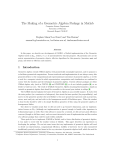
2.3 Products
Currently, Gaigen supports seven basic products between multivectors. Besides these basic products, some special products are available, such as the
outermorphism, meet and join, and the delta product. But only the seven basic
products are controlled from the products tab, which is shown in figure 2.2a.
The products tab itself contains another set of tabs, one for each product.
The names of these tabs are abbreviated versions of the products:
CHAPTER 2. THE USER INTERFACE
10
abbreviation
gp
hip
mhip
lcont
rcont
op
scp
full name
Geometric Product
Hestenes Inner Product
Modified Hestenes Inner Product
Left Contraction
Right Contraction
Outer Product
Scalar Product
The abbreviations are also used inside the generated source code as names of
the functions which compute the products.
The products tab is used to select which of these products you want to
include in your algebra. A common selection would be geometric, outer and
scalar product and either the left contraction or one of the Hestenes inner products. To include a product in your algebra, click on the tab of that product, and
check the checkbox left of the full name of the product. The color of the text in
the tab will change from black to red to reflect the inclusion of that product.
Below the checkbox is a large field that is used to control the optimizations
implemented for each product. You are not required to add any optimizations
to generate a basic algebra, but you can significantly increase the performance
of your application by doing so, sometimes by an order of magnitude. But,
by making the wrong optimizations you could in theory decrease the performance of your application. So it is important that you understand how the
optimizations work if you care about performance.
The optimizations are based on the assumption that it is likely that your
application will use certain products between certain multivectors much more
often than others. Suppose you use lots of rotations of 3D vectors in your
program, like:
(2.1)
w = (Rv)R−1 .
Then the performance of your program could be increased if Gaigen would
generate an optimized function for the geometric product between an even
multivector and a vector (Rv), and an optimized function for the geometric
product between an odd multivector and an even multivector ((Rv)R−1 ).
Because Gaigen tracks the grade usage (which grade parts of a multivector
are equal to 0 (empty) and which are not) of all multivectors you use in your application, it is in theory capable to generate and invoke an optimized function
for every combination of grade usages and products. Of course, generating an
optimized function for every possible combination is not feasible for high dimensional algebras, because the amount of code generated would get too large.
That’s why you can select a specific set of combinations from the products tab.
You turn on optimization for a specific combination of grade usage and
product by first swiching to that product (click its tab). Then you use the two
sets of little checkboxes (labeled [0...d] where d is the dimension you selected
for your algebra in the general tab) to specify the grade usage combination you
want to optimize for, and add it to the set of optimizations by clicking add.
So suppose you want to optimize for the example above (w = (Rv)R−1 ).
You would check 0 and 2 in the left set of check boxes (a general 3d rotor has a
non-empty grade 0 and 2), 1 in the right set (a 3d vector has a non-empty grade
1) , and then click add. This would optimize the product Rv. The combination
2.4. ORDER
11
will appear in the list below the two sets of checkboxes. Then you would check
1 and 3 in the left set (the product Rv will have and non-empty grade 1 and
3), and you check 0 and 2 in the right set (for the inverted rotor). Adding this
combination will optimize the product (Rv)R−1 . To remove any combination
already added, you simply click the remove button for that combination.
2.3.1 Automatic optimizations using profiles, and optimization
options
Of course, once your application gets more complicated, you won’t be able to
tell easily what combinations of products and grade usages you use most often. That’s why Gaigen can include profiling code in your application. You can
enable profiling by ticking the enable profiling checkbox in the optimizations
tab in the products tab. This tab is new in Gaigen version 0.95. The profiling
code (usage will be explained in the next section) will count how often you use
each combination and on request print or save a list of most used combinations. You can then use this list to manually optimize your algebra, but more
conveniently, you can let Gaigen handle the optimizations for you.
First of all, you can use the remove all optimizations button to remove all
product optimizations from the algebra specification. This is recommended
before adding automatic optimizations to make sure no old optimizations are
left behind.
Then, you can use the automatically add optimizations from profile button to add optimizations automatically. When you push the button, you are
prompted to select a .gap (Geometric Algebra Profile) file. These files are written by the saveProfile function (see section 3.16). Gaigen will then automatically add optimizations for all product/multivector combinations that are used
more than 2.0% of the time. You can use the optimize threshold in usage percentage slider to change this value of 2.0%. I.e., 0.0% would add optimizations
for every product/multivector combination that is used in your application.
If you tick the inline products checkbox, all generated products will be
prefixed with an inline statement. This might improve performance a few
percent.
You can use the Dispatch method radio buttons to select what dispatch
method to use. As shown in [1], the ifelse method is usually fastest, followed
by switch.
2.4 Order
Using the order tab (figure 2.2b) you can modify the order in which the coordinates referring to basis blades are stored, and you can change the orientation
of the basis blades. This part of the user interface is a bit primitive, though
functional.
You are concerned mostly with coordinates when you enter them into a
multivector object, e.g. by using the set function, when you retrieve them from
a multivector object, e.g. by using the coordinates function, or when you inspect them, e.g. by using the print function.
CHAPTER 2. THE USER INTERFACE
12
a
b
Figure 2.2: The products and order tabs with settings for the e3ga algebra.
In Gaigen all multivectors are stored as (compressed) arrays of coordinates.
A multivector
A = 1 + 2e1 + 3e1 + 4e1 + 5e1 ∧ e2 + 6e1 ∧ e3 + 7e2 ∧ e3 + 8e1 ∧ e2 ∧ e3 (2.2)
would, by default, be stored as an array {1, 2, 3, 4, 5, 6, 7, 8}. But suppose you
don’t like the orientation of the basis blade e1 ∧ e3 and prefer e3 ∧ e1 instead.
You could do this by clicking the g.2 tab (g.2 stands for grade 2), and clicking the toggle button for e1 ∧ e3 , which will then change into e3 ∧ e1 . The
multivector A with the same value as above would then have to be stored as
{1, 2, 3, 4, 5, −6, 7, 8}. Toggle buttons are active only for basis blades with a
grade higher than 1.
Now suppose you want to change the order in which the coordinates are
stored in the array, e.g. because the order in which you store your coordinate
data is different. You would use the up and down buttons to change the order of basis blades. Note that you can only modify the order of basis blades
within a grade. All coordinates for one grade are always packed together in
the coordinate array.
As an example, if you change the order and orientation of the grade 2 basis
blades of a 3d algebra to [e 2 ∧ e3 , e3 ∧ e1 , e1 ∧ e2 ], then the coordinates of the
multivector A would be stored as {1, 2, 3, 4, 7, −6, 5, 8}. This order and orientation is used by the pregenerated e3ga algebra and is the one shown in figure
2.2b.
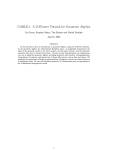
2.5 Functions
The functions tab (figure 2.3a) simply contains a lot of checkboxes which can
be used to include certain functions into the algebra code. Some functions
are interdependant on each other, some only work for specific dimensions and
most functions require that a product (usually the geometric product, outer
product, scalar product or left contraction) is included in the algebra. While
you are still unexperienced with Gaigen (and while Gaigen isn’t finished yet)
it might be best to always include these 4 products in your algebra, because
2.5. FUNCTIONS
a
13
b
Figure 2.3: The functions and memory tabs with settings for the e3ga algebra.
otherwise you might run into compilation errors2 . If you try to compile an
algebra and the compiler complains about a certain function or product which
does not exist, include it from the functions or products tabs.
Because the names of most functions speak for themselves, what follows is
a list of a functions with peculiarities or names that do not make 100 percent
clear what the function does. How to use the functions is explained in section
3.
• take grade. This function takes one grade part from a multivector and
copies it to a new multivector.
• highest grade. This function takes the highest grade part that is nonzero from a multivector and copies it to a new multivector. It is used to
compute the delta product.
• grade of a blade. When given a blade (or a homogenous multivector),
this function returns its grade. If a non-homogenous multivector which
is is passed, the function returns an error.
• norm. We have implemented several (currently two) functions to compute the norm of multivectors. However, every application seems to have
its own idea of what the of a multivector norm is, so these functions have
not entirely ’stabilized’ yet.
• normalize. Normalizes a multivector by dividing it by its magnitude
(norm). Uses the outer product and the norm.
• versor inverse. Computes the inverse of a multivector, assuming it is a
versor (a versor is a multivector that can be written as the geometric product of vectors). If the multivector is not a versor, something other than
the inverse is returned. The versor inverse is very efficient and should always be preferred over the general inverse function if possible. Requires
the reverse, scalar product and the outer product.
2 This should never happen, but we still have to build a good dependency system that checks
that all required products and functions are present.
CHAPTER 2. THE USER INTERFACE
14
• lounesto inverse. This function can compute the inverse of any invertible
multivector in a 3 dimensional algebra. Requires the clifford conjugate and
take grade functions and the geometric product. See [4] and [1] for more
information on how it works.
• general inverse. This function can compute the inverse of any invertible
multivector in an algebra of any dimension. It computes the inverse by
explicitly inverting the geometric product matrix expansion. It is slow
compared to the versor inverse or the lounesto inverse. See Gaigen tutorial 1 [3] for an example of relative efficiency and [1] for details. Does not
require any other functions or products.
• outermorphism. Use this function to create an outermorphism operator. If you have a linear function, you can construct an outermorphism
operator of it. Applying the outermorphism operator to multivector has
several advantages (efficiency, precision, floating point noise) over simply applying the original function to multivector. Requires take grade
and negate function and the outer product.
• spinor product. Including the spinor product function will add special
code for constructing outermorphism operators from spinors. This function will be removed from Gaigen in the future, since it was superceded
by the outer morphism. Requires take grade and negate function and the
geometric product and outer product.
• factor blade/versor. This function factors blades and versors into arbirary vector factors. It is used to compute the meet and join. Requires
norm, project, versor inverse, and take grade function, and the outer
product, geometric product and left contraction.
• meet and join. This function computes the meet and join of blades. Requires factor blade/versor.
• project and reject. These functions project and reject blades onto/from
blades and versors. Requires the versor inverse function, left contraction
and for projection onto versors the geometric product.
• random blade/versor. This function generates random blades and versors.
• fast temporary variables. This function is only of interest if you use the
high level C++ interface, which is what most people will do.When you
write an C++ expression such as
a = (b + c) * d;
temporary variables are used to store the intermediate results (i.e. (b + c)
and ((b + c) * d)). A method exists to allocate these variables very quickly
(compared to the default method used by the C++ compiler). The downside of this method is that it allocates the temporary variables from an
array with a fixed (e.g. 64 variables) size. When it comes to the end of
the array, it cycles back to first entry, whose contents will be overwritten
with the new intermediate results. If your program still had a reference to
2.6. MEMORY
15
this variable (as the (intermediate) result of a previous computation, this
refenence will be useles. Using the reference as if it still contained the
old value will cause your program to malfunction (but no crash). Checking the fast temporary variables checkbox will make your algebra about
twice as fast, but you will have to make sure you don’t run out of temporary variables. The main rule of thumb is never to pass references to
temporary variables to functions. Instead of writing something like
e3ga b, c, d;
someFunction((b + c) * d);
write something like
e3ga a, b, c, d;
a = (b + c) * d;
someFunction(a);
This will make sure you don’t pass references to temporary variables to
other functions and prevent most problems. The only other ways you
can get into trouble with fast temporary variables is by explicitly keeping
references to temporary variables like this:
e3ga &a = b + c;
or by writing expressiong which are so long that they use all (64) temporary variables at once. The number of temporary variable is controlled
by the line
#define MV_MAX_TEMP 64
in gaigenhl.h. In any case, if you suspect that a malfunction of your program is caused by using fast temporary variables, you can simply turn off
the fast temporary variables button, regenerate your algebra, recompile
your application and see if the malfunction disappears.
• fast dual. The fast dual function can compute the dual of a multivector
with respect to the pseudoscalar of the algebra very quickly (compared
to the default dual function) by simply shuffling and flipping the sign of
the coordinates.
• reciprocal frame. The reciprocal frame function can compute the reciprocal frame of a set of vectors.
• multivector type. This function can compute the type (blade, versor, or
general) of a multivector.
2.6 Memory
The memory tab, as shown in figure 2.3b, is used to control the memory allocation method and the floating point type used to store the coordinates. The
CHAPTER 2. THE USER INTERFACE
16
coordinates of multivectors are stored in arrays of floating variables. Gaigen
stores only coordinates of grade parts of which it knows that they are not equal
to 0. To save the amount of memory used to store the coordinates, it can allocate just enough memory for each multivector to store its coordinates. But
memory allocation costs computation time. If memory has to be reallocated
for each basic product or sum or other operation, performance might suffer.
That is why Gaigen allows you to make a compromise between minimal
memory usage and minimal memory allocation computation time. You can
choose from four memory allocation schemes, ranging from lowest memory
usage to lowest computational time:
• Tight: Exactly the right amount of memory is allocated to store the coordinates of the non-zero grades of a multivector. This implies frequent
memory reallocation, which is done via a simple and efficient memory
heap.
• Balanced: To prevent abundant memory reallocation, the balanced allocation scheme does not reallocate when less memory is required to store
the coordinates, up to a certain waste factor which the user can specify.
Suppose a variable holds a 3D rotor (4 coordinates), and is assigned a
vector (3 coordinates); the memory waste would be 33.3% if 4 coordinates memory locations would still be used to store 3 coordinates. The
balanced memory allocation algorithm then decides to either release the
4 old memory locations and allocate 3 new memory locations, or to just
waste 1 memory location. This depends on the the waste factor. If the
number of used memory location divided by the number of required memory locations will become larger than or equal to the waste factor, the algorithm will decide to reallocate. So the larger the waste factor, the more
memory may be wasted, but the less memory reallocations will occur.
However, this memory allocation scheme doesn’t work well in practice,
as shown in [1].
• Maximum: The maximum number of memory locations to store all 2d
coordinates is allocated when a multivector variable is created. Gaigen
never has to reallocate memory.
• Maximum parity pure: We call a multivector parity pure if it is either odd
or even. If the dimension of the algebra is larger than 0, only half of the 2d
coordinates have to be allocated to store the coordinates of a parity pure
multivector variable. The user must guarantee that he will never create
multivectors that are not parity pure, or weird things can happen (a crash
or incorrect results).
You can switch between the float (32 bit precision) and double (64 bit precision) types for coordinate storage by toggling the radio buttons on the right
side of the tab. If you always use the type GAIM FLOAT (defined as either
float or double) in your application, you can switch back and forth painlessly
between floats or doubles. So instead of writing
float c[1.0, 2.0, 3.0];
e3ga a;
a.set(GRADE1, c);
2.7. GENERATE
17
Figure 2.4: The generate tab with settings for the e3ga algebra.
write
GAIM_FLOAT c[1.0, 2.0, 3.0];
e3ga a;
a.set(GRADE1, c);
When you switch floating point type, the type of the array of coodinates c is
automatically switched too. If you use multiple algebras in one application,
make sure they use the same floating point type or you might run into trouble.
This might be improved in the future.
As shown with benchmarks in [1], the combination of maximum parity pure
memory allocation and the use of floats as floating point type leads to the highest performance. For high dimensional algebras (e.g. 5D) and doubles, the tight
memory allocation method might be more efficient however.
2.7 Generate
The generate tab, shown in figure 2.4, is used to control several aspects of the
code generation.
The output dir textfield has the same contents as the name field in the general tab by default; when you change the name field, the output dir field is
set to the same contents as the name field. However, you may find it useful to
have several algebras with the same name (e.g. e3ga), but with different properties (such as optimizations, products and functions). One instance where
this may be useful is when you use the same algebra in different applications.
Different applications may benefit from different product optimizations, but
instead of using two algebras with the different names (which would become
bothersome when you use code from one application in the other), you can use
two algebras with the same name, but with (slightly) different properties. You
would store the algebras in seperate directories (e.g. e3ga app1 and e3ga app2)
and compile and link each application with its own algebra which was tailored
to its own specific needs.
The checkboxes at the lower part of the general tab control what kind of
optimized code is generated to implement the computation of the products.
Only C, C2 and LAPack are available currently. Moreover LAPack is more like
18
CHAPTER 2. THE USER INTERFACE
a test implementation to compare the performance of the C implementation to
a brute force LAPack approach. In the future, SSE and 3DNow support may be
added.
The C code generator generates slightly more (a few percent) efficient code
than the C2 code generator. However, the code generated by the C2 generator
might be much smaller (especially when you add lots of optimizations in the
products tab, or when you generate a high dimensional algebra). When you
have finished an application, you may want to try the other generator to see
which one gives the best results.
Chapter 3
Layer 2: high level C++
interface
The most convenient way to use the source code generated by Gaigen is the
high level C++ interface. It consists of two classes (one for mulivectors, one
for outermorphism operators) which sit on top of the actual code generated
by Gaigen. The interface is contained in two files (gaigenhl.h and gaigenhl.cpp)
which you can easily change if you wanted to (for instance, if you don’t like
the operator definitions).
This chapter discusses not only the features provided by gaigenhl.h and
gaigenhl.cpp, but also some of the more convenient features provide by the
lower level C++ interface discussed in chapter 4, because those features are directly accessible. In short we could say that this chapter discusses everything
the casual user needs to know about programming geometric algebra using
source code generated by Gaigen.
One of the most important features introduced by the high level interface is
operator overloading. Operator overloading allows a programmer to give new
meaning to a symbol (e.g. =, *, +, - and —) to almost whatever he or she wants.
This allows us to write things like
a = R * b * !R;
to express a = RbR−1 . This example immediately shows a problem with operator overloading: picking the right operator symbol for the right operation.
The ∗ symbol is used for the scalar product in geometric algebra literature, but
is used for general multiplication in C++; thus one could reason it is a good
choice for the geometric product. The ! symbol is used in C++ arithmetic as
the ’not’ or ’binary complement’ operator for integers, which might make it a
good choice for the inverse (but also for the dual). As you can see, it is not easy
to pick the right symbol for each operation. Furthermore there are not enough
operator symbols available to give every operation its own symbol, so some
will have to do with regular function names. Functions are available for all
operations, and the code above could be written as
a.copy(gp(gp(R,b), R.inverse()));
which gives the same result, but isn’t half as readable. We have done our best
to make a reasonable operator selection for the operators and also provided the
19
20
CHAPTER 3. LAYER 2: HIGH LEVEL C++ INTERFACE
reasoning behind each operator, but there will always be people who disagree
with our choice. Already, our selection differs at some points from the selection
made in another package, CLU [6].
We now list the functions assigned to all overloaded operators, with a comment as to why we assigned that specific function to that specific operator. We
will discuss the use of operators later on, this is only a reference table:
operator
=
∗, ∗=
function
assignment
geometric
product
example
a = b;
c = a * b;
a ∗= b;
/, /=
division
inverse
geometric
product
outer
product
left
contraction
c = a / b;
a /= b;
>>,
>>=
%, %=
right
contraction
scalar
product
c = a >> b;
a >>= b;
c = a % b;
a %= b;
+, +=
addition
∧, ∧=
<<,
<<=
−, −=
c = a ∧ b;
a ∧= b;
c = a << b;
a <<= b;
c = a + b;
a += b;
subtraction, c = a − b;
negation
a −= b;
a = −b;
comment
The * symbol is used for multiplication
in C++. Thus it is the best for the most
fundamental product in geometric algebra.
Best visual match to wegde symbol.
<< is the binary shifting operator in
C++. The left contraction could be
thought of as ’shifting’ or removing
the lhs argument from the right hand
side argument. A trick to remember
the symbol: the < symbol is used to
express the ’smaller than’ relation in
mathematics. For the left contraction
to make sense, the grade of the object
on the lhs should be smaller than the
grade of the object on the right hand
side.
Same reasoning as with the left contraction.
The % symbol is used for modulo division in C++; the scalar product kind
of works like a modulo, returning only
the scalar part of a geometric product.
To remember the symbol, imagine the
two circles in the % symbol being two
zeros, indicating that only the grade 0
part will be returned.
3.1. CONSTRUCTION
21
!
inversion
a = !b;
∼
reversion
a = b∼;
a = ∼b;
−−
clifford
conjugate
a = b−−;
a = −−b;
++
a = ++b;
&, &=
grade
involution
meet
|, |=
join
()
grade part
selection
grade part
selection
[]
The ! symbol is used to denote the binary complement of integers in C++.
This suggests its use as the inversion
operator for multivector, since the inverse of a multivector could be considered its complement.
The superscript ∼ symbol is often used
in geometric algebra literature to denote the reverse.
This operator can be used both preand postfix. Both do the same, and
do not change the operand, unlike the
−− operator when applied to standard
C++ integers of floats.
Same comment as the −− operator.
c = a & b;
a &= b;
The & symbol is used for the binary
and operation for integers in C++. The
meet is like an and operation for subspaces.
c = a | b;
The | symbol is used for the binary or
a |= b;
operation for integers in C++. The join
is like an or operation for subspaces.
c
= The () operator selects the specified
a(GRADE1);
grade part of a multivector variable.
f0
= The [] operator returns a pointer to an
a[GRADE1][0]; array of floating point values repref1
= senting the coordinates for the specia[GRADE1][1]; fied grade part of a multivector varif2
= able.
a[GRADE1][2];
We now discuss how to use the C++ high level interface. Reading this section, and tutorial 1 which demonstrates the e3ga algebra (which stands for Euclidian 3 dimensional Geometric Algebra), will give you a good understanding
of how to write your own application using geometric algebra as implemented
by Gaigen. We will assume the classname is e3ga, but in your application it
might be any name, since you can set it in the Gaigen user interface (see section 2.1).
3.1 Construction
To create a new multivector variable a with the value 0 you would use:
e3ga a;
If you want a scalar valued multivector variable b use:
22
CHAPTER 3. LAYER 2: HIGH LEVEL C++ INTERFACE
e3ga b(1.0);
which creates a variable b with the value 1.0.
To explicitly set the coordinates of a homogenous multivector variable (a
multivector for which all grade parts are 0 except for one) or a blade, you can
use this constructor:
e3ga c(GRADE1, 1.0, 2.0, 3.0);
e3ga t(GRADE3, 8.0);
This creates a vector valued multivector c with the value 1e1 + 2e2 + 3e3 and a
multivector variable t with the value 8e1 ∧ e2 ∧ e3 . The GRADE1 macro tells
the constructor that the coordinates specified are for grade 1 of the multivector.
The GRADE3 macro tells the constructor that the coordinate specified is for
grade 3 of the multivector. Note that the order of coordinates matters here. It
depends on the order you specified in the order tab in the user interface when
you created the algebra. For instance, if you wanted to create a multivector
with the value of 1e1 ∧ e2 + 2e1 ∧ e3 + 3e2 ∧ e3 you would have to use
e3ga c(GRADE2, 3.0, -2.0, 1.0);
because the e3ga algebra stores its grade 2 coordinates in the following the
order and orientation: [e2 ∧ e3 , e3 ∧ e1 , e1 ∧ e2 ]. You can inspect and change this
order and orientation by loading the specification file e3ga.gas for the algebra
into the Gaigen UI (click on load algebra) and clicking on the order and g.2
tabs.
Of course, you can also construct such an object explicitly from basis vector
as follows
e3ga c = 1.0 * e3ga::e1 ˆ e3ga::e2 +
2.0 * e3ga::e1 ˆ e3ga::e3 +
3.0 * e3ga::e2 ˆ e3ga::e3;
This removes all doubt, but is less efficient In this code snippet we have used
some features we have not discussed yet (such as the =, + and ˆ operators, and
the use of e3ga::e1 to denote the ee1 basis vector). We will treat them later.
Now suppose you want explicitly set the coordinates of multiple grade
parts of a new multivector variable. You can do that like this:
float coordinates[4] = {1.0, 2.0, 3.0, 4.0};
e3ga d(GRADE0 | GRADE2, coordinates);
This creates a multivector variable d with the value 1.0 + 2e2 ∧ e3 + 3e3 ∧ e1 +
4e1 ∧ e2 . The macros GRADE0 and GRADE2 can be added together using
the standard binary ’or’ operator, telling the constructor that you will supply
coordinates for the grade 0 and grade 2 parts. The coordinates have to be supplied in an array, because supplying a separate constructor for almost every
grade combination would grow out of hand. If the supplied array is too short
to contain all coordinates, behaviour of the constructor will be unpredictable.
There is one more constructor; the copy constructor is used to create a new
multivector variable with the same value as another variable. The following
code creates a variable e with the same value as d:
e3ga e(d);
3.2. ASSIGNMENT
23
The definitions of all of these constuctors are:
// null constructor:
e3ga::e3ga();
// copy constructor:
e3ga::e3ga(e3ga &a);
// set to scalar value:
e3ga::e3ga(float scalar);
// construct & set single grade with N coordinates:
e3ga::e3ga(int gradeUsage, float c1, ..., float cN);
// construct & set multiple grades:
e3ga::e3ga(int gradeUsage, const float *coordinates);
3.2 Assignment
To set an existing multivector variable to the value 0 the function null can be
used:
a.null();
To set the coordinates of an existing multivector variable explicitly, you can
use one of the set functions. They are available in two flavours, just like the
constructors above. The first flavour can only be used to set a multivector
variable to a homogenous value:
a.set(GRADE1, 1.0, 2.0, 3.0);
This sets the existing multivector variables a to 1e1 + 2e2 + 3e3 .
To set the value to a non-homogenous value, the other flavour of the set
function can be used:
float coordinates[8] = {1.0, 2.0, 3.0, 4.0, 5.0, 6.0, 7.0, 8.0};
a.set(GRADE0 | GRADE1 | GRADE2 | GRADE3, coordinates);
This example would assign the value 1 + 2e1 + 3e2 + 4e3 + 5e2 ∧ e3 + 6e3 ∧ e1 +
7e1 ∧ e2 + 8e1 ∧ e2 ∧ e3 to a.
A variation of the set function are the named set functions:
a.setScalar(1.0);
b.setVector(2.0, 3.0, 4.0);
c.set3Vector(8.0);
float coordinates[3] = {4.0, 5.0, 6.0};
d.set2Vector(coordinates);
These can take both single coordinates and coordinates provided in arrays and
are available for all grades of the algebra.
A final variation of the set functions is the use of the = operator to assign a
scalar value to a multivector variable:
24
CHAPTER 3. LAYER 2: HIGH LEVEL C++ INTERFACE
a = 1.0f;
Note that the use of the = is made possible through operator overloading.
To copy the value of one multivector variable to another, use
a = b;
or
a.copy(b);
which would copy the value of b into a.
To set a multivector variable to a random value, the random blade / versor
function can be used. The following example sets the multivector variable a to
a random scalar:
a.randomBlade(GRADE0, 1.0f);
The distribution of the random value is linear from the range [−1.0, 1.0]. The
range is controlled by the second argument.
To set a multivector variable to a higher grade value the following would
be used:
b.randomBlade(GRADE2, 5.0f);
c.randomVersor(GRADE3, 0.5f);
This sets b to a grade 2 blade with a random value, and c to a versor with the
highest non-empty grade part 3. The blades and versors are created by generating the required number of random vectors within the range specified by the
second argument and respectively wedging and multiplying these together.
Higher grade random blades and versors are thus not taken from a linear distribution.
The definitions of all of these assignment functions are:
// set to 0:
void e3ga::null();
// set single grade with N coordinates:
int e3ga::set(int grade, float c1, ..., float cN);
// set multiple grades:
void e3ga::set(int gradeUsage, const float *coordinates);
// set single grade with N seperate coordinates:
int e3ga::setScalar(float c1);
int e3ga::setVector(float c1, ..., float cN1);
int e3ga::set2Vector(float c1, ..., float cN2);
.
.
.
int e3ga::setNVector(float c1);
// set single grade with an array of coordinates:
3.3. OPERATORS
int
int
int
.
.
.
int
25
e3ga::setScalar(const float coordinates[1]);
e3ga::setVector(const float coordinates[N1]);
e3ga::set2Vector(const float coordinates[N2]);
e3ga::setNVector(const float coordinates[1]);
// copy and assign multivector or float:
void e3ga::copy(const e3ga &a);
e3ga& e3ga::operator=(const e3ga &a);
e3ga& e3ga::operator=(float f);
// set to random blade or versor:
int e3ga::randomBlade(int grade, float scale);
int e3ga::randomVersor(int grade, float scale);
int e3ga::random(int grade, float scale, int versor);
3.3 Operators
As already discussed in at the start of this section, a number of often used operations such as addition, geometric product and outer product have special
symbols assigned to them (i.e. +, ∗ and ∧. This is done through a C++ feature called operator overloading, which allows the programmer to assign new
meaning to a symbol when it is used in combination with a class. It drastically
increases the readability of code, e.g. compare
a = R * b * R.inverse();
with
a.copy(gp(gp(R,b), R.inverse()));
The former, using operator overloading, is much easier understood, though
the C++ compiler will generate the same machine code for both cases.
One could classify the operators into thee types: binary and unary and ’in
place’. Binary operators (such as +) take two arguments, e.g.:
a = b + c;
which is equal to
a = add(b, c);
On the contrary, unary operators (e.g. ∼) take one argument, e.g.:
a = ˜b;
which is equal to
a = b.reverse();
And last of all, the ’in place’ operators take two arguments, one of which is also
used to store the result. e.g.:
26
CHAPTER 3. LAYER 2: HIGH LEVEL C++ INTERFACE
a += b;
which is equal to
a = a + b; // ...which in turn is equal to...
a.copy(add(a, b));
3.4 The basic products
We use the name basic products for all products which are included using the
products tab of gaigenui. Thus this definition excludes the delta product, the
meet and join, multiplying by the inverse and other derived products.
3.4.1 Geometric Product
The function gp computes the geometric product of two multivector variables.
The * symbol is used as the operator for the geometric product. The definitions
of the geometric product functions are:
e3ga& e3ga::operator*(const e3ga &a) const;
e3ga& e3ga::operator*=(const e3ga &a);
e3ga& gp(const e3ga &a, const e3ga &b);
3.4.2 Outer Product
The function op computes the outer product of two multivector variables. The
ˆ symbol is used as the operator for the outer product. The definitions of the
outer product functions are:
e3ga& e3ga::operatorˆ(const e3ga &a) const;
e3ga& e3ga::operatorˆ=(const e3ga &a);
e3ga& op(const e3ga &a, const e3ga &b);
3.4.3 The Scalar Product
The function scp computes the scalar product of two multivector variables.
The scalar product returns the grade 0 part of the geometric product. The %
symbol is used as the operator for the scalar product. The definitions of the
scalar product functions are:
e3ga& e3ga::operator%(const e3ga &a) const;
e3ga& e3ga::operator%=(const e3ga &a);
e3ga& scp(const e3ga &a, const e3ga &b);
3.4.4 The Inner Products
The are currently four inner products available in Gaigen, two of which have
no operator symbol. The number of inner products arises from the lack of consensus in the geometric algebra research community of which inner product
should be preferred. The definitions for the inner products are:
3.5. INVERSION
27
// left contraction:
e3ga &e3ga::operator<<(const e3ga &a) const;
e3ga &e3ga::operator<<=(const e3ga &a);
e3ga &lcont(const e3ga &a, const e3ga &b);
// right contraction:
e3ga &e3ga::operator>>(const e3ga &a) const;
e3ga &e3ga::operator>>=(const e3ga &a);
e3ga &rcont(const e3ga &a, const e3ga &b);
// Hestenes inner product:
e3ga &hip(const e3ga &a, const e3ga &b);
// Modified Hestenes inner product:
e3ga &mhip(const e3ga &a, const e3ga &b);
3.5 Inversion
If three inversion functions are available (versor, lounesto and general inverse),
then which one does Gaigen pick when you write one of the following equivalent line of code?
a = b / c;
a = b * !c;
a = b * c.inverse();
The answer is that Gaigen will prefer the versor inverse over the lounesto
inverse, and the lounesto inverse over the general inverse. So if you have
included all three inversion functions in your algebra, Gaigen will automatically use the fastest (versor) inverse. If the versor inverse is not available, the
lounesto inverse is used, and finally it resort to the general inverse. This is
handled by the following piece of code in gaigenhl.h:
#ifdef GAIM_FUNCTION_VERSORINVERSE
inline void inverse(const CLASSNAME &a) {versorInverse(a);};
#elif defined(GAIM_FUNCTION_LOUNESTOINVERSE)
inline void inverse(const CLASSNAME &a) {lounestoInverse(a);};
#elif defined(GAIM_FUNCTION_GENERALINVERSE)
inline void inverse(const CLASSNAME &a) {generalInverse(a);};
#endif
This automatic selection of the inverse function shouldn’t problem be a problem, unless you want to force the use of specific inversion function. One case
where this might occur is if you want to write
a = b * c.inverse();
where c is not a versor. If you have included the versor inverse, Gaigen will
apply it even though it will give the incorrect answer. To force Gaigen to use a
specific inversion function, you have to explictly name the inversion function
you want:
a = b * c.versorInverse();
a = b * c.lounestoInverse();
a = b * c.generalInverse();
28
CHAPTER 3. LAYER 2: HIGH LEVEL C++ INTERFACE
This of course rules out the use of the inverse() function and the / operator,
because they always resort to the default inversion function.
The definitions of the inversion functions are:
// compute the inverse using the default algorithm:
e3ga& e3ga::inverse() const;
e3ga& e3ga::operator!() const;
// the overloaded ’/’ operator in all its variations:
e3ga& e3ga::operator/(const e3ga &a) const;
e3ga& operator/(float a, const e3ga &b);
e3ga& e3ga::operator/(float a) const;
e3ga& e3ga::operator/=(const e3ga &a);
e3ga& e3ga::operator/=(float a);
// the three inverse functions:
e3ga& e3ga::versorInverse() const;
e3ga& e3ga::lounestoInverse() const;
e3ga& e3ga::generalInverse() const;
// the functions which do the same as the operators:
// igp stands for ’inverse geomtric product’
e3ga& igp(const e3ga &a, const e3ga &b);
e3ga& igp(const e3ga &a, float b);
e3ga& igp(float a, const e3ga &b);
Remember that every time you use the inverse geometric product, or the
/ operator, you are implictly inverting a multivector. So if you have to divide
by the same multivector value many times, it is more efficient to first invert
the multivector, store that inverse, and then multiply by the inverse instead of
dividing by the original multivector.
3.6 Addition, subtraction, negation
Multivector variable can be added and subtracted using the add, sub, + and
- functions and operators. The negate- operator is also used to compute the
negation of a multivector variable.
e3ga a, b, c;
a = -b; // this is equivalent to...
a = b.negate(); // ... this, which is equivalent to...
a = 0.0 - b; // ... this
The definitions of these the addition, subtraction and negation functions
are:
// addition:
e3ga& e3ga::operator+(const e3ga& a) const;
e3ga& e3ga::operator+=(const e3ga& a);
e3ga& add(const e3ga& a, const e3ga& b);
// subtraction:
3.7. REVERSE, CLIFFORD CONJUGATE AND GRADE INVOLUTION
29
e3ga& e3ga::operator-(const e3ga& a) const;
e3ga& e3ga::operator-=(const e3ga& a);
e3ga& sub(const e3ga& a, const e3ga& b);
// negation:
e3ga& e3ga::operator-() const;
e3ga& e3ga::negate() const;
Note that the – and ++ operators, which are used to decrement and increment integer and floating point variables by one in C++, have nothing to do
with addition of subtraction for multivector variables. They are used for the
Clifford conjugate and the grade involution in Gaigen (see section 3.7).
3.7 Reverse, Clifford Conjugate and Grade Involution
The reverse, Clifford conjugate and grade involution all toggle the sign of certain grade parts. They each have a unary operator. The ++ and – operators can
be applied both pre- and post-fix:
e3ga a, b;
a = ++b;
a = b++;
a = b.gradeInvolition();
all of which are equivalent. They do not alter the operand like the standard ++
and – operators for integer and floating point variables do. The definitions of
these functions and operators are:
// reverse:
e3ga& e3ga::operator˜() const;
e3ga& e3ga::reverse() const;
// clifford conjugate:
e3ga& e3ga::operator--() const;
e3ga& e3ga::operator--(int) const;
e3ga& e3ga::cliffordConjugate() const;
// grade involution:
e3ga& e3ga::operator++() const;
e3ga& e3ga::operator++(int) const;
e3ga& e3ga::gradeInvolution() const;
3.8 Grade Part Selection
The grade function and the () operator can be used to select a certain grade part
from a multivector variable. This may be useful when you are only interested
in a certain grade part and not in any others, such as in this example:
e3ga vector, rotor;
vector = rotor * vector * rotor.inverse();
vector = vector(GRADE1);
CHAPTER 3. LAYER 2: HIGH LEVEL C++ INTERFACE
30
Here some vector is rotated by some rotor. We know that the vector is a grade
1 blade, and should still be a grade 1 blade after the rotation. However, due to
floating point round off errors, a small grade 3 part may arise. This grade 3 part
is thrown away by the the third line in the example: the (GRADE1) operator
call selects only the grade 1 parts of vector. This example could have been one
line shorter like this:
e3ga vector, rotor;
vector = (rotor * vector * rotor.inverse())(GRADE1);
The definitions of the grade function and the () operator are:
e3ga& e3ga::grade(int g) const;
e3ga& e3ga::operator()(int g) const;
3.9 Meet and Join
The & and | symbols are used as operators for the meet and join of blades or
subspaces. These symbols are used as the binary and and or operations when
used on integers. The meet and join compute the and and or of subspaces, hence
the & and | are good operator symbols for them.
The join is on based the delta product [5] and algorithms described in [1].
The delta product is used to compute the grade of the join of the two input
blades. Then one blade is factored into a number of vectors, which are then
repeatedly wedged to the other blade until a blade best representing the join of
the input blades is found. The meet is compute using the join, as described in
[1].
The following shows how to use the meet and join:
// Assuming b and c are two blade valued multivector variables
// this code computes their meet and join
e3ga m = b | c;
e3ga j = b & c;
// which is equivalent to:
e3ga m = meet(b, c);
e3ga j = join(b, c);
The definitions of the meet and join functions are:
e3ga
e3ga
e3ga
e3ga
&meet(const e3ga &a, const e3ga
&join(const e3ga &a, const e3ga
&e3ga::operator&(const e3ga &a)
&e3ga::operator|(const e3ga &a)
&b);
&b);
const;
const;
3.10 Factorization
The function factor and factorVersor can be used to factor blade or versors into
vectors. When the vectors are wedged or multiplied together, they rebuild the
blade of versor. The factor function is used by the meet and join functions, and
a use of the factorVersor function might be to retrieve the vectors in the plane
of rotation of a rotor. The definitions of the factorization functions are:
3.11. EXPONENTIATION
31
// Factor a blade (’versor’ = 0) or a versor (’versor’ = 1)
// The function returns the number of factors and...
// stores them in ’f’.
int e3ga::factor(e3ga f[], int versor = 0) const;
// Factor a versor
// The function returns the number of factors and...
// stores them in ’f’.
int e3ga::factorVersor(e3ga f[]) const;
3.11 Exponentiation
The function exp, which computes the exponentiation of a multivector, is present
in the algebra whenver the geometric product is included. The function computes the taylor series expansion
exp(A) ≈
n
Ai
i=0
i!
(3.1)
n is specified by the optional integer argument which defaults to 9. This is
identical to the CLU exp function.
The definition of exp is:
e3ga& e3ga::exp(int order = 9) const;
3.12 Outermorphism
If you have a function f for which the following is true for any pair of input
blades a and b.
f (a ∧ b) = f (a) ∧ f (b)
(3.2)
then it is an outermorphism. Examples of outermorphisms are rotations. Another example are all operations that you traditionally can model using a 4 × 4
when you use homogeneous coordinates (translation, rotation, scaling, skewing and so on). If you have to apply such a function to multivectors many
times, you might consider constructing an outermorphism for it. It can be applied to blades of any grade. Once initialized, the outermorphism operator can
probably compute the result faster, and will assure that the result is the same
grade as the input.
The outermorphism operator is represented by its own class. The of this
class is the name of your algebra class (e.g. e3ga) with om concatenated to
it (e.g. e3ga om). You can initialize the outermorphism operator when you
construct it, or later on using one of the init functions. The outermorphism is
initialized by either passing it the images of all basis vectors under the linear
transformation, or by passing it a spinor. If you pass a spinor, the initialization
function will assume that the right way to apply the spinor is
e3ga spinor, vector, vectorImage;
vectorImage = spinor * vector / spinor;
32
CHAPTER 3. LAYER 2: HIGH LEVEL C++ INTERFACE
It will compute the vector images of all basis vectors and then pass these to the
vector images initilization function.
A typical use of the outermorphism operator would be something like this:
const int nb = 1000;
int i;
e3ga rotor, lotsOfVectors[nb], lotsOfVectorImages[nb];
e3ga_om om;
// initialize the outermorphism operator:
om.initSpinor(rotor);
// apply it to the vectors:
for (i = 0; i < nb; i++) {
lotsOfVectorImages[i] = om * lotsOfVectors[i];
/*
//this is the other way to compute the vector images:
lotsOfVectorImages[i] =
(rotor * lotsOfVectors[i] / rotor)(GRADE1);
*/
}
Of course the outermorphism operators doesn’t work on vectors only: you can
also use it to transform blades of any grade.
The outermorphism operator internally constructs a matrix representation
for the linear operator. The matrix representation for the grade 1 part is exactly
the traditional matrix that would be used when one would use linear algebra
to do geometry. The 1x1 ’matrix’ that transforms the pseudoscalar is the determinant of the transformation 1 .
The matrix representation leads to another advantage of the outermorphism;
because of the matrix form, it can easily be executed using Single Instruction Multiple Data (SIMD) instructions sets, such as supplied by the SSE(2),
3DNow! or AltiVec. This could be exploited by a future opt2X compiler.
The definitions of the outermorphism constructors are:
// construct but don’t initialize:
e3ga_om::e3ga_om();
// construct & initialize using array of vector images:
e3ga_om::e3ga_om(const e3ga vectorImages[3]);
// construct & initialize using array of pointer to vector images:
e3ga_om::e3ga_om(const e3ga *vectorImages[3]);
// construct & initialize using spinor/rotor/versor:
e3ga_om::e3ga_om(const e3ga &spinor);
The initialization functions are:
// init using a spinor/rotor/versor to create the vector images:
int e3ga_om::initSpinor(const CLASSNAME &spinor);
// init using images under the outermorphism of the basis vectors:
1 The other grade parts of the matrix represention are not widely know traditionally, but are also
very useful
3.13. COORDINATE OUTPUT AND ACCESS
33
int e3ga_om::initVectorImages(const CLASSNAME vectorImages[3]);
int e3ga_om::initVectorImages(const CLASSNAME *vectorImages[3]);
To apply the outermorphism to a multivector variable use either of these
functions:
// apply outermorphism L to multivector A, returns the result:
e3ga& om(const e3ga_om& L, const e3ga& A);
// the ’*’ operator does the same as the ’om’ function:
e3ga &operator*(const e3ga_om& L, const e3ga& A);
3.13 Coordinate Output and Access
You may want access to coordinate for several reasons. One reason is that
you may want to store your multivectors in files, to retrieve them later. This
can be done by storing their coordinates and later restoring them when your
application reads the file.
Another reason is inspection of the coordinates, either graphically or by
printing them as numbers. Although geometric algebra is coordinate free (and
Gaigen is as well, after you have entered the coordinates into multivectors),
most people find it useful (at least while still somewhat uncomfortable with
geometric algebra) to inspect the coordinates of multivectors.
We will first treat printing the coordinates via Gaigen, and then show how
your application can get get access the coordinates.
If you want to print the coordinates to the standard output, you can use the
print function like this:
e3ga a(GRADE1, 1.0, 2.0, 3.0);
a.print("a: ");
This example would print:
a: 1.00*e1
+ 2.00*e2 + 3.00*e3
The default way the floating point coordinates are printed is using the printf
¨
format %2.2f¨.
You can change this format by specifying it as the second argument of print, e.g.:
e3ga a(GRADE1, 1.0, 2.0, 3.0);
a.print("a: ", "%e");
This prints:
a: 1.000000e+000*e1
+ 2.000000e+000*e2 + 3.000000e+000*e3
You can also change it using the setFPPrecision() function described below.
If you want to print to something else than the standard output, you can use
the fprint function to print to any file. For total control of where your output
goes, you can print the coordinates to a string using the string function. You
can then do whatever you want with that string. The definitions of these three
functions are:
34
CHAPTER 3. LAYER 2: HIGH LEVEL C++ INTERFACE
// get a string representation of a multivector:
const char *e3ga::string(const char *prec = NULL) const;
// print a string representation of a multivector to...
// the standard output:
void e3ga::print(const char *text = NULL,
const char *prec = NULL) const;
// print a string representation of a multivector to...
// a file:
void e3ga::fprint(FILE *F, const char *text = NULL,
const char *prec = NULL) const;
Starting with Gaigen 0.99, two more function are available that control the
printing:
// set the default precision for all future prints/strings
static int e3ga::setFPPrecision(const char *prec);
//set the string delimiters for all future prints/strings
static int e3ga::setStringDelimiters(char start, char end);
The first function takes as argument an ASCIIZ string (e.g., ”%e”) that describes how to format floating point coordinates. The second function takes
as arguments to characters (e.g., ’[’ and ’]’) that will be used as start and end of
every string.
Two functions and one operator provide direct (read only) access to the
coordinates of a multivector: scalar, coordinates and []. The scalar function
returns the scalar coordinate of a multivector and is used like this:
e3ga a(1.0);
float sc = a.scalar();
The coordinates function and the [] operator can retrieve a pointer to the coordinates of any grade part of a multivector. You specify which grade part you’ll
get the the coordinates using the integer argument. This argument can be any
of the GRADE0 ... GRADEN macros, but you can not combine then to get the
coordinates of multiply grades in one call. This example demonstratres the use
of the coordinates function and the [] operator:
e3ga a(GRADE1, 1.0, 2.0, 3.0);
// get a pointer to the grade 1 coordinates of a:
float *g1c = a.coordinates(GRADE1);
// get the scalar coordnate of a:
float sc = a.coordinates(GRADE0)[0];
// get each of the grade 2 coordinates of a:
float *g2c = a.coordinates(GRADE2);
float g2c_e1_e2 = g2c[2];
float g2c_e2_e3 = g2c[0];
float g2c_e3_e1 = g2c[1];
3.13. COORDINATE OUTPUT AND ACCESS
35
In the last four lines of the example above, you can how the each of the three
coordinates of the grade 2 part of a is retrieved. This piece of code is very dependent on the orientation and order of the grade 2 basis blades. If you change
the orientation and order of these blades (using the order tab, see section 2.4),
this code would function incorrectly.
A better way to retrieve individual coordinates is using the E3GA X macros
defined in e3ga.h. For each coordinate, a macro is generated which specifies the
index of the coordinate in the coordinates array relative to the first coordinate
of that grade part. For the e3ga algebra, these macros look like this:
#define
#define
#define
#define
#define
#define
#define
#define
E3GA_S 0
E3GA_I 0
E3GA_E1 0
E3GA_E2 1
E3GA_E3 2
E3GA_E2_E3 0
E3GA_E3_E1 1
E3GA_E1_E2 2
If you change the order of the coordinates , these macros automaticly change
as well when you regenerate the code. It’s easy and readable to use the macros
like this to retrieve the individual coordinates:
// get each of the grade 2 coordinates of a:
float *g2c = a.coordinates(GRADE2);
float g2c_e1_e2 = g2c[E3GA_E1_E2];
float g2c_e2_e3 = g2c[E3GA_E2_E3];
float g2c_e3_e1 = g2c[E3GA_E3_E1];
The only instance where you could run into trouble with accessing coordinates like this is when you flip the orientation of the basis blades. For instance
this could change
#define E3GA_E3_E1 1
into
#define E3GA_E1_E3 1
and then your application won’t compile anymore if you still use E3GA E3 E1.
But this is better than compiling successfully and then failing at runtime because your application retrieve the wrong coordinates.
// get the scalar coordinate of a multivector:
float scalar() const;
// get the GRADEX coordinates of a multivector:
const float *e3ga::operator[](int grade) const;
const float *e3ga::coordinates(int grade) const;
You can retrieve the largest coordinate of a multivector using largestCoordinate():
CHAPTER 3. LAYER 2: HIGH LEVEL C++ INTERFACE
36
// Get the fabs() value of the (absolutely) largest coordinate
// of a multivector:
float e3ga::largestCoordinate() const;
For example:
e3ga a(GRADE1, 1.0, 2.0, -3.0);
GAIM_FLOAT lca = a.largestCoordinate(); // lca = 3
3.14 Coordinate string parsing
Gaigen can parse its own string output and a bit more. The function parseString() takes as input a string describing a multivector (as formatted for instance by the string() function), parses it, and sets the value of the multivector
accordingly:
int e3ga::parseString(const char *str, const c3ga_ben *ben = NULL);
Usage example:
e3ga a;
int nb;
nb = a.parseString("1.0*e1+2.0*e1ˆe2ˆe3");
The function returns the number of characters read from str, or -1 on failure.
The optional second argument of parseString() describes optional extra Basis Elements Names and the start and end delimited of the string. These are
contained in a small C++ class:
class e3ga_ben {
public:
e3ga_ben();
e3ga_ben(char startDelimiter, char endDelimiter);
˜e3ga_ben();
// add a basis element name and value to this ’ben’
int addName(const char *name, const e3gai &mv);
// remove a basis element name from this ’ben’
int removeName(const char *name);
// look up a basis element name and its value from this ’ben’
int lookupName(const char *name, e3gai &mv) const;
// remove all basis element names
int removeAll();
// set the start and end delimiters (e.g. ’[’ and ’]’)
// this can also be done using the
int setDelimiters(char startDelimiter, char endDelimiter);
// set ’this’ to defaults (no extra names, no delimiters)
int setDefaults();
};
3.15. MISCELLANEOUS FUNCTIONS
37
Usage example:
e3ga a;
e3ga_ben eb(’[’, ’]’);
int nb;
eb.addName("I", e3ga::e1 ˆ e3ga::e2 ˆ e3ga::e3);
nb = a.parseString("[1.0*I]", &eb);
A future version of Gaigen may contain a better multivector parser that
uses ANTLR, much like the parser that is already present in GAViewer.
3.15 Miscellaneous functions
3.15.1 normal
The normal function returns a normalized version of the multivector it is applied to, e.g.:
e3ga a, b;
//...
b = a.normal(); // set b to the normalized version of a
The normal function takes and optional integer argument, which specifies the
norm to be used. If the argument is 1, the ’Euclidean’ norm is take: the sum of
the square of all coordinates. If the argument is 2, the norm is computed as
GAIM_FLOAT norm = a % a.reverse();
3.15.2 dual
The dual function returns the dual with respect to the pseudoscalar I of the
algebra:
e3ga a, b;
//...
b = a.dual(); // set b to the dual of a
the dual is computed as b = a I−1 . If the fastDual function is included in
the algebra, then that function is used by default. It works by swapping and
negating the coordinates which is faster than explicitly computing the dual.
3.15.3 mvType
mvType() returns the type of a multivector: GA BLADE, GA VERSOR or
GA MULTIVECTOR. If the multivector is a blade, it also returns the grade
of the blade. It’s declaration is:
int mvType(int *grade, double epsilon) const;
The pointer to grade can be NULL if you don’t care about the grade. The value
in grade is one of the constants GRADE0, GRADE1 ... GRADEN. The value
of epsilon defaults to 1e-14 for doubles, 1e-7 for floats. A usage example:
e3ga a(GRADE1, 1.0, 2.0, -3.0);
int grade;
int type = a.mvType(&grade); //type = GA_BLADE, grade = GRADE1 (=2)
38
CHAPTER 3. LAYER 2: HIGH LEVEL C++ INTERFACE
3.15.4 layer 1 functions
There are also a number of functions from layer 1 that are useful and can be
accessed directly from the high level C++ interface:
• null. The null sets its argument to 0
• compress compresses its argument in place. This means to remove any
grade part that is equal to 0. You can supply an option floating point
argument to compress to tell it what is still considered to be 0:
e3ga a;
//...
a.compress(1e-10); // compress all grade parts < 1e-10
• reciprocalFrame. The static reciprocal frame function computes the reciprocal frame of a set of basis vectors. Its definition is
static int reciprocalFrame(c3gai f[], const c3gai e[],
int nbVectors);
This sets the set of ’nbVectors vectors f to the reciprocal frame of e.
3.16 Profiling
To use the profiler, the profile checkbox in the function must be ticked. Gaigen
will then include profiling code when the algebra is generated. Only two static
functions accessible by your application are added: resetProfile and printProfile. Static means that the functions are accessible without reference to an instantiation of the class. The following:
e3ga::printProfile();
will invoke the static printProfile function in the class e3ga. Thus, when you
use a static function of a class, you don’t have to have access to a variable of
that class.
Actually the three profiling functions are always present in the algebra
code, whether the checkbox is ticked or not. But when it is not ticked, the
generated function does nothing. If the functions would not be included at all
in the source code, you would have to remove or add your calls to the profiler
each time you turn the profiling option off or on. The profiling code slows
down the performance of your application, so its best to turn it off when you
don’t use it anyway.
resetProfile resets the count of all product/multivector combinations. You
should call this function at the start of your application.
printProfile prints out all product/multivector combinations to the standard output. It has an optional argument, which defaults to 2.0, which specifies up to what usage percentage the product/multivector combinations are
shown. printProfile computes how often each product/multivector combination is used relatively, and if a product/multivector combination falls below
the usage percentage threshold, it is not shown. So to print the usage of all
product/multivector combinations, use
3.17. BASIS VECTORS AND (INVERSE) PSEUDOSCALAR
39
e3ga::printProfile(0.0);
where the 0.0 tells the function to show all product/multivector combinations.
The default argument,
e3ga::printProfile();
which is equivalent to
e3ga::printProfile(2.0);
will print the product/multivector combinations with a usage above 2.0%.
saveProfile saves the profile to .gap file which can be read back by the
Gaigen user interface to automatically add optimizations (section 2.3). Use
the function as follows:
e3ga::saveProfile("profile_name.gap");
The definitions of resetProfile, printProfile and saveProfile are:
static int e3ga::resetProfile();
static int e3ga::printProfile(float threshold = 2.0);
static int e3ga::saveProfile(const char *filename = NULL);
3.17 Basis Vectors and (Inverse) Pseudoscalar
The internal class (see section 4) contains the multivector variables with the values of the basis vectors and (inverse) pseudoscalar as static 2 members. These
are also available from the high level C++ interface.
Using the basis vectors and (inverse) pseudoscalar you can write things
like:
e3ga a, b, one;
a = e3ga::e1 ˆ e3ga::e2;
b = a << e3ga::Ii;
one = e3ga::Ii * e3ga::I;
The definitions of the basis vectors and (inverse) pseudoscalar are:
static
static
static
static
static
static
e3gai::e3gai
e3gai::e3gai
e3gai::e3gai
e3gai::e3gai
e3gai::e3gai
e3gai::e3gai
e1;
e2;
e3;
I; // pseudoscalar
Ii; // inverse pseudoscalar
*bv[3]; // array of pointers to e1, e2, e3
bv is an array of pointers to the basis vectors. The basis vectors (e1, e2 and e3
in the example of the e3ga algebra) can have any name. In the 5d c3ga algebra
for instance, the basis vectors are called e1, e2, e3, e0, einf; a 3d ’color algebra’
could name the basis vectors red, green and blue. To change the name of the
basis vectors, use the signature tab (section 2.2).
2 Static in this context means that there is only one global copy of such a variable; it is not
included in every instantiation of a multivector variable.
40
CHAPTER 3. LAYER 2: HIGH LEVEL C++ INTERFACE
3.18 Use of Internal Class and Floating Point Variables in Functions
Besides writing statements like:
e3ga a, b, c;
c = a * b;
you of course also want to write
e3ga a, b, c;
c = 2.0 * a * b;
and
e3ga a, b, c;
c = e3ga::e1 ˆ e3ga::e2;
even though 2.0, e3ga::e1 and e3ga::e2 are not variables of type e3ga (2.0 is of
type float or double; e3ga::e1 and e3ga::e2 are of the internal class type (e3gai).
That’s why gaigenhl.h and gaigenhl.cpp contain a combination of automatic
type casting operator and extra inline defintions for some and operators functions such that you can write the statements given above.
The definition of the casting operator looks like this:
inline e3gai::operator e3ga &() const {return *((e3ga*)this);}
The operator casts variables of type e3gai to e3ga 3 .
Examples of extra functions for using floating point variables and internal
class variable in combination with multivectors are the following:
e3ga& gp(float a, const e3ga &b);
e3ga& gp(const e3gai &a, float b);
These function computes the geometric product of a float and an e3ga variable,
and of an e3gai and a float. Such extra definitions are present in gaigenhl.h and
gaigenhl.cpp for all functions where appropriate.
3.19 Temporary Variables
One may wonder where the temporary multivector variables come from in
code like
a = (b + c) + d; // both lines are equivalent
a = add(add(b, c), d); // both line do the same thing
since the program should first compute b + c, store the answer to that somewhere, and then compute (b + c) + d, possibly store that somewhere, and then
assign the result to a. Where the temporary variables come from, depends on
whether you selected the fast temporary variable.
If you turned the fast temporary variables off, the temporary variables are
handled in the default C++ way. All functions and operators like add and
operator+ return plain multivector variables like this:
3 Note that because of this casting operator, you can not add non-static member variables or
virtual functions to gaigenhl.h and gaigenhl.cpp. Doing so anyway might mess up the simple but
naive casting operator.
3.19. TEMPORARY VARIABLES
41
e3ga e3ga::operator+(const e3ga &a);
e3ga add(const e3ga &a, const e3ga &b);
Note the absence of the & symbol in the return type. This means that an actual
variable is returned, instead of just a reference. These variables are allocated
from the stack and then initialized using the standard constructor (the code to
do so is generated by the C++ compiler). One can imagine that allocating and
initializing a multivector variable for each intermediate result can lower the
performance of your application.
On the other hand, if you turned on the fast temporary variables, functions
and operators returning multivector variables will be defined like this:
e3ga& e3ga::operator+(const e3ga &a);
e3ga& add(const e3ga &a, const e3ga &b);
The functions and operators now return references to multivector variables (note
the & symbol in the return type). The actual temporary variables are allocated
by Gaigen source code from an array of multivectors variables with a fixed
size. This is more efficient than letting the C++ compiler allocate them from
the stack, but it has a drawback. Since the array of temporary variables has
a fixed size4 , at some point old temporary variables will have to be recycled.
If these old temporary variables are still in use somewhere in you program,
their value will be overwritten. This will lead to bugs in you program which
are very hard to find, especially of you don’t know what the symptoms of the
problem are. The section on temporary variables in tutorial 1 [3] demonstrates
the problem.
The rule of thumb is to never keep a reference to a temporary multivector
variable when you have enabled fast temporary variables in the functions tab.
The two main ways to keep a reference to a temporary variable are passing
them on to another function like this:
someFunction(a + b);
and explictly keeping a reference:
e3ga &c = a + b;
Explictly keeping a reference can be easily avoided, and pass a temporary variable to a function can be prevented like this:
c = a + b;
someFunction(c);
If you have a look at gaigenhl.h and gaigenhl.cpp, you will see that functions
and operators return the type GAIM RETURN TYPE. This is actually a macro
#defined as either e3ga or e3ga&, depending on whether the fast temporary
variables are enabled or not. The allocation of temporary variables is managed
by the GAIM RETURN VAR(variableName) macro. Both these macros are
defined in gaigenhl.h.
4 this
size is defined by MV MAX TEMP, in gaigenhl.h.
42
CHAPTER 3. LAYER 2: HIGH LEVEL C++ INTERFACE
3.20 Multitheading
Multitheading support has not yet been fully implemented in Gaigen. The
main functions which are not mt-safe are part of the tight and balanced memory allocation algorithms, the fast temporary variable allocation, and the string
function. Use of the string (and print and fprint functions can be avoided if
you really want to use multithreading, and the max or maxpp memory allocation algorithms can be used. Multitheading support might be more complete
in the future.
3.21 Drawing
There are no multivector drawing functions available in Gaigen. We have implemented GAViewer that allows you to view multivectors interactively with
minimal intrusion in your application. Your application only has to be able
to write multivectors and commands to a file, which can be conviniently done
using the print functions of Gaigen. This allows you to view results of computions and to debug your application without adding an (OpenGL) UI to it.
Chapter 4
Layer 1: Internal C++ class
This chapters describes the internal C++ class. The source code for this class is
generated by Gaigen. Much of this generated source code is copied and pasted
(with adjustments) from gaspectemplates.txt, a file which is described in section
6.1. Most people will not want to use the internal C++ class to actually program applications, since it’s a rather crude interface. This chapter is intended
for people who want to create their own high level C++ interface (to replace
gaigenhl.cpp), who want to squeeze the last bit of performance out of their application, or those who have to change or maintain the internal C++ class.
Many functions of the internal C++ class return void, unlike functions of
the high level C++ interface, which return the result. Instead, most internal
C++ class functions store the result in the calling class, e.g.:
c.add(a, b);
adds a and b and stores the result in c.
4.1 C++ Class
The storage parts of the C++ class declaration looks something like this:
class e3gai {
.
.
.
// Depending on the memory allocation algorithm...
// Either a pointer, or an array of floats
float *c; // pointer
float c[8]; // array of floats
// bitfield for grade part and memory usage administration
int usage;
// information about the class:
static const int dim;
static const int nbCoor;
43
CHAPTER 4. LAYER 1: INTERNAL C++ CLASS
44
memory usage
grade part usage
mem usage
3 2 1 0
msb
lsb
Figure 4.1: Storage of grade part and memory usage in the usage field.
// the basis vectors and (inverse) pseudoscalar
static e3gai e1;
static e3gai e2;
static e3gai e3;
static e3gai *bv[3];
static e3gai I;
static e3gai Ii;
.
.
.
}
First of all, the class contains either a pointer to an array of floating point variables, or an array of floating point variables. In either case, it is called c for coordintes. The type used depends on the memory allocation algorithm selected
in the storage tab. The difference is, that an array of floating point variables
inside the class always uses a certain amount of memory, while a pointer can
be used to point to any amount of memory. So with the array of floating point
variables inside the class, the e3gai class will still use 8 or 4 floating point variables to store a single coordinate (e.g. a scalar), while the pointer can point
to a much lower amount of memory (this is done by the tight and balanded
memory allocation algorithms). For coordinate access, there is no difference
between the pointer and the array.
The coordinates are always stored in ’compressed’ form in the c array. Even
if 8 floating point variable are allocated anyway, only 4 of them are used to store
(for example) a rotor.
The usage integer variable is to store the grade part usage (as a bitfield)
and the memory usage (as an integer). These two n-bit1 words are stored as
illustrated in figure 4.1. If a grade part is in use by the multivector, the bit in
the grade usage field will be set to 1, otherwise it will be set to 0. The memory
usage field stores the number of floating point variables allocated for this multivector. It is used by the balanced and tight memory allocation algorithms to
determine from which heap they allocated the coordinate array2 .
The other storage variables of the C++ class are static, which means that
only one copy of them is used in your application. They include dim. the
dimension of the algebra, nbCoor, the maximum number of coordinates used
by a multivector variable, and the basis vectors and (inverse)pseuodscalar. The
basis vectors are available individually, named as they in the signature tab, and
from an array of length ’d’ (the dimension of the algebra). The pseudoscalar
1 ’n’
is the dimension of the algebra plus 1.
heap is available for each array length, from 1 up to 2d .
2 One
4.2. CONSTRUCTORS, ASSIGNMENT FUNCTIONS
45
and inverse pseudoscalar are always called I and Ii. All these static multivector
variables are initialized to their proper values when your application starts.
4.2 Constructors, Assignment Functions
The constructors and assignment functions are identical to those used for the
high level C++ interface except that the operator symbol ’=’ is not available.
The random, randomBlade and randomVersor are available.
4.3 The Products
The product functions like gp, lcont and op all have the same syntax:
void
void
void
void
void
void
void
e3gai::gp(const e3gai &a, const e3gai &b);
e3gai::op(const e3gai &a, const e3gai &b);
e3gai::lcont(const e3gai &a, const e3gai &b);
e3gai::rcont(const e3gai &a, const e3gai &b);
e3gai::hip(const e3gai &a, const e3gai &b);
e3gai::mhip(const e3gai &a, const e3gai &b);
e3gai::scp(const e3gai &a, const e3gai &b);
They are used differently than those from the high level C++ interface; the
following line
c.gp(a, b);
computes the geometric product of a and b and stores it in c. No temporary
variables are used.
Versions of the outer product function are available in which one argument
can be a floating point value:
void e3gai::op(const e3gai &a, float scalar);
void e3gai::op(float scalar, const e3gai &a);
All product functions first check to see if an optimized function exists to
compute the product of the arguments. If so, they set the grade part and memory usage of the result, and call the optimized function. Otherwise they expand
the arguments to arrays of pointers to arrays of floating point variables (like the
one shown in figure 5.1), call the general implementation of the function, and
compress the result into the multivector variable.
4.3.1 Euclidean Metric Products
Only when the meet and join or factoring functions are included, in algebras
with a non-euclidean signature, special euclidean implementations of some
metric products (geometric product, left contraction and scalar product) are
available. They are used to implemented a LIFT (see [5]). Their definitions are
void e3gai::gp_em(const e3gai &a, const e3gai &b);
void e3gai::lcont_em(const e3gai &a, const e3gai &b);
void e3gai::scp_em(const e3gai &a, const e3gai &b);
CHAPTER 4. LAYER 1: INTERNAL C++ CLASS
46
4.4 Other Functions
To add or subtract two multivectors, use
void e3gai::add(const e3gai &a, const e3gai &b);
void e3gai::sub(const e3gai &a, const e3gai &b);
To add a multivector and a floating point variable, these functions are available:
void
void
void
void
e3gai::add(float
e3gai::add(const
e3gai::sub(float
e3gai::sub(const
scalar, const e3gai &b);
e3gai &b, float scalar);
scalar, const e3gai &b);
e3gai &b, float scalar);
These functions compute the reverse, clifford conjugate and grade involution of a multivector and store it in the calling multivector:
void e3gai::reverse(const e3gai &a);
void e3gai::cliffordConjugate(const e3gai &a);
void e3gai::gradeInvolution(const e3gai &a);
The three flavours of the inverse can be used with these functions:
// compute inverse, for versors only
int e3gai::versorInverse(const e3gai &a);
// compute inverse, for general 3d multivectors
int e3gai::lounestoInverse(const e3gai &a);
// compute inverse, for general multivectors;
// uses gaussian elimination
// (slower and less stable than versorInverse)
int e3gai::generalInverse(const e3gai &a);
These four functions can be used to extract grade parts, or to get information about the grade of a multivector:
void e3gai::takeGrade(const e3gai &a, int grade);
int e3gai::highestGrade(const e3gai &a);
int e3gai::grade() const;
int e3gai::maxGrade() const;
takeGrade extracts a single grade part from a multivector. highestGrade extracts the highest non-zero grade part from a multivector, and returns its grade
index. grade returns the grade of a homogenous multivector and -1 if the is not
homogenous. maxGrade returns the the index of the highest non-zero grade.
The norm of a multivector, according to one definition, can be computed
using the norm a function:
float e3gai::norm_a() const;
The function is called norm a (for now) because other norm definitions will
also be implemented. To normalize a multivector use:
4.5. INTERNAL FUNCTIONS
47
void e3gai::normalize(const e3gai &a, int norm);
The norm argument is used to specify which definition of the norm you want
to use; currently the only valid value is 1, which uses the norm a norm.
To project a multivector onto a blade or versor, or to reject a multivector
from a blade, one of the following functions can be used:
int e3gai::project(const e3gai &blade, const e3gai &a);
int e3gai::projectOntoVersor(const e3gai &versor, const e3gai &a);
int e3gai::reject(const e3gai &blade, const e3gai &a);
To compute the meet and join of two blades, use
int e3gai::join(const e3gai &a, const e3gai &b, int algorithm = 1);
int e3gai::meet(const e3gai &a, const e3gai &b, int algorithm = 1);
The algorithm argument (either 1 or 2) is used to specify which of the two
available join algorithms to use. The meet is computed with respect to the join.
These are three support functions used by the meet and join:
int e3gai::deltaProduct(const e3gai &a, const e3gai &b);
int e3gai::factor(e3gai factors[], int versor = 0) const;
int e3gai::factorVersor(e3gai factors[]) const;
The coordinates function returns a pointer to the coordinates of a certain
grade part. You should not try to modify the floating point variables this
pointer points to.
const float *e3gai::coordinates(int grade) const;
To compute the reciprocal frame of a set of nbVectors vectors e, use reciprocalFrame. The result goes into f.
static int e3gai::reciprocalFrame(e3gai f[], const e3gai e[], int nbVectors);
The outermorphism has the same construction and initialization functions
as the high level C++ interface outermorphism, except that there is no ’init with
spinor’ initializer.
The print and string functions are exactly those described in the high level
C++ interface.
The fastDual function can be used to compute the dual with respect to the
entire space.
int e3gai::fastDual(const e3gai &a);
4.5 Internal Functions
This section described several interesting internal functions.
The setUsage function sets the grade part and memory usage of a multivector variable. It makes sure enough memory has been allocated to store the
coordinates. It’s declaration is:
void e3gai::setUsage(int u);
48
CHAPTER 4. LAYER 1: INTERNAL C++ CLASS
These are several functions to expand the coordinates of a multivector.
// Expand a multivector into a matrix, according to table:
void e3gai::expand(float matrix[], const int table[]) const;
// Expand a multivector into an array of pointers
// to arrays of coordinates for each grade:
void e3gai::expand(const float *pa[4]) const;
// Expand 2 multivectors (’a’ and ’b’) into arrays of pointers
// to arrays of coordinates for each grade:
void e3gai::expand(const e3gai &b, float const *pa[4],
float const *pb[4]) const;
The profiling functionality is implemented by three functions (two of which
have already been described in chapter 3). The third, internal, function is incrementUsage. This function is called by the product functions when profiling is
enable. It counts (in the array usageCount) how many times each combination
of product and multivectors has been used. This information is printed when
you call printProfile. The productNames are used for printing purposes.
static int e3gai::resetProfile();
static int e3gai::printProfile(float threshold = 2.0);
int e3gai::incrementUsage(int product, int gua, int gub);
static int e3gai::usageCount[5][16][16];
static const char *e3gai::productNames[5];
Two algorithms are available to compute the join:
int e3gai::joinAlg1(const e3gai &a, const e3gai &b,
int ga, int gb, int gj);
int e3gai::joinAlg2(const e3gai &a, const e3gai &b,
int ga, int gb, int gj);
Algorithm 2 builds up candidates for the join by wedging vectors together,
algorithm 1 projects blades of the right grade onto on of the multivectors a or b,
to find a good candidate for the join. The best candidate (with the largest norm)
is returned as the join. Both algorithms take as arguments two multivectors (a
and b), the grade of each multivector (ga, gb) and the required grade of the
join (gj).
The inline functions gradeUsage and memUsage return the grade part and
memory usage of a multivector. This information is extracted from the usage
variable in the multivector.
inline int gradeUsage() const;
inline int memUsage() const;
4.6 Global Internal Variables
There are a number of interesting variables outside the C++ which are assumed
to be useful to the internal class only; that’s why they are not included in the
class itself. To name a few:
4.6. GLOBAL INTERNAL VARIABLES
49
const char *e3gai_basisElementNames[8];
int e3gai_gradeSize[4];
int e3gai_mvSize[16];
e3gai basisElementNames is an array of strings which holds the names of all
the basis vectors (e.g. e1, e2 and e3). These names are used for printing the
coordinates of a multivector variable. The integer array e3gai gradeSize contains the number of coordinates each grade part holds. e3gai mvSize is also
an integer array and holds, for each possible combination of grade usage, the
minimum number of coordinates required to store the coordinates. This is used
(among others) for the memory allocation algorithms. The grade part usage,
which serves as an index into the e3gai mvSize array, is specified in the same
binary format as in figure 4.1.
50
CHAPTER 4. LAYER 1: INTERNAL C++ CLASS
Chapter 5
Layer 0: low level
computational functions
Layer 0 is responsible for actually computing the (optimized) products and
computing other basic functions (such as addition and reversion). It is defined as an partially static and partially dynamic interface which must be implemented. An opt2X compiler is responsible for generating the layer 0 files
(although you can of course them by hand if you want). The compiler takes
an .opt file (see section 6.2), which contains specifications of the functions that
should be implemented, and generates a C++, C or assembly file which adhers
to the interface.
The static part of the interface currently consists of the following functions:
// copy ’src’ to ’dst’; length of arrays is ’length’
void e3gai_copy(float *dst, const float *src, int length);
// compute reverse multivector ’a’
void e3gai_reverse(float *a[]);
// compute clifford conjugate of multivector ’a’
void e3gai_cliffordConjugate(float *a[]);
// compute the grade involution of multivector ’a’
void e3gai_involution(float *a[]);
// negate ’src’ to ’dst’; length of array is ’length’
void e3gai_negate(float *dest, const float *src, int length);
// compute the norm (all coordinates squared) of ’a’
// length of array is ’length’
float e3gai_norm_a(float a[], int length);
// add two multivectors with the same grade part usage
// ’c’ = ’a’ + ’b’
// length of arrays is ’length’
void e3gai_addSameGradeUsage(float *c,
51
52
CHAPTER 5. LAYER 0: LOW LEVEL COMPUTATIONAL FUNCTIONS
a 0 scalar
b 0 scalar
1 e1
1 NULL
e2
e3
2 e2^e3
2 e2^e3
e3^e1
e3^e1
e1^e2
e1^e2
3 pseudoscalar
3 NULL
Figure 5.1: Array representation of multivector variables a and b.
const float *a, const float *b, int length);
// add two multivectors with the different grade part usage
// ’c’ = ’a’ + ’b’
void e3gai_add(const float *a[4], const float *b[4], float *c[4]);
// subtraction function, simular to addition functions
void e3gai_subSameGradeUsage(float *c,
const float *a, const float *b, int length);
void e3gai_sub(const float *a[4], const float *b[4], float *c[4]);
All these functions must always be implemented by the code generated by the
opt2X compiler. As you can see, all functions except e3gai copy, e3gai norm a,
e3gai negate, e3gai addSameGradeUsage and e3gai subSameGradeUsage take
arrays of pointers to arrays of floating point variables as arguments. These arrays contain the coordinates of each grade part. A pointer to a coordinate array
can also be NULL when a grade part is not in occupied by the multivector. This
is illustrated in figure 5.1. It shows the array representation of multivectors a
and b. a occupies all grade parts, so all 4 pointers actually point to coordinates. b on the other hand is a rotor and only occupies grade part 0 and 2. The
pointers for grade part 1 and 3 are NULL.
The .opt file contains the specifications of the dynamic part of the interface.
It specifies the name of the algebra (with an i appended to it, since this is an internal part of the algebra implementation), the dimension, the floating point
type and the (optimized) product functions which should be implemented.
The .opt file format is described in section 6.2.
The general product functions, which can compute the product of any type
of multivector with any other type of multivector, always look something like
this:
void e3gai_general_gp(const float *a[], const float *b[], float *c)
This function should compute a product of multivector a and b, and store it
in c. The coordinates of the multvectors are given in the format explain above
and illustrated in figure 5.1.
The optimized product functions, which can compute only a product of two
specific types of multivectors, always look something like this:
53
void e3gai_opt_0A_gp_05(const float *a, const float *b, float *c);
The functions receive the coordinates of their arguments a, b and c as arrays
of floating point variables. The opt2X compiler knows what it should do with
each coordinate because of the description of the function in the .opt file.
An opt2X compiler is free to implement all these function anyway it wants.
The opt2c compiler for instance, take the most straightforward approach and
almost directly converts the .opt file to C++. The opt2LAPack compiler, an
experimental compiler, uses LAPack to compute the general products. The
opt2c2 compiler splits up the products into many little functions and lets the
product functions call those as required.
54
CHAPTER 5. LAYER 0: LOW LEVEL COMPUTATIONAL FUNCTIONS
Chapter 6
File Formats
6.1 gaspectemplates.txt file
Gaigen reads and copies most piece of code that it generates from the gaspectemplates.txt file. The syntax of that file is discussed in this section. To read, parse
and output the code contained in the file, the codeTemplateContainer class in
codetemplate.cpp and codetemplate.h is used.
The gaspectemplates.txt file consists of codeblocks. Codeblocks are blocks of
code which Gaigen copies into the source code it generates. In early versions
of Gaigen, all code was simply printed to the sourcefiles using fprintf. This became very messy, since all of the code that now resides gaspectemplates.txt (over
a thousand lines) was contained in gaspec.cpp. Instead of that, we put almost
all of the code in templates (or codeblocks) in gaspectemplates.txt. That makes
them easy to read, create and maintain. Only the code which is very difficult
to ’copy and paste’ (e.g. which is extremely dependent on the dimension of the
algebra), is printed directly from gaspec.cpp.
Of course, Gaigen does not literally copy code from gaspectemplates.txt. Many
parts of the generated code depend on the dimension, name, floating point
type and many other properties of the required algebra. Thus special keywords
are used, which are replaced by the appropriate strings when the sourcefiles
are generated. These keyword are set by Gaigen and stored in a lookup table
(which also resides in the codeTemplateContainer class) 1 .
Each codeblock in gaspectemplates.txt has the following structure:
${CODEBLOCK codeBlockName}
.
.
.
${ENDCODEBLOCK}
Each code block starts with a CODEBLOCK statement, followed by the name
of the code block. That name is used to identify it the codeTemplateContainer
class. The statement starts with a dollar sign and is surrounded by curly braces.
1 If a keyword is used in gaspectemplates.txt which has not been entered into the lookup table,
the codeTemplate class prints out the name of the keyword in the generated source file, making it
easy to find such mistakes.
55
56
CHAPTER 6. FILE FORMATS
Each code block ends with a ENDCODEBLOCK statement. Between these two
statements, the code resides. Anything can be put between the two statements,
so not just (parts of) C++ code. Code or text outside a codeblock is ignored and
generates a warning when parsed by the codeTemplateContainer class.
In the code block, you can use keywords which will be replaced by strings
from the lookup table. An example of such a keyword is ${FLOAT}. When the
code is output by the codeTemplateContainer class, this keyword is changed
to either float or double, depending on the floating point type specified in the
storage tab.
These are often used keywords:
• {CLASSNAME}: the name of the class as it appears in the high level
C++ interface.
• {INTERNAL CLASSNAME}: the name of the class used in the low level
C++ glue.
• {FLOAT}: the floating point type (float or double).
• {FLOATSIZE}: the size of the floating point type in bytes (e.g. sizeof(float)).
• {FLOATCAST}: used to cast a type to a floating type (e.g. (double)).
• {FLOAT EPSILON}: the value that is consider ’small’ by default. 1e − 8
for float and 1e − 15 for double.
• {NUMBER OF COORDINATES}: the total number of coordinates (2d ).
• {DIMENSION}: the dimension of the algebra (e.g. 3).
• {DIMENSION+1}:the dimension of the algebra plus 1.
• {1<<(DIMENSION+1)}: 2 to the power of the dimension plus 1 (2d+1).
• {MAX NUMBER OF COORDINATES}: only used when the memory
allocation algorithm is max or maxpp. Is equal to the maximum number
of coordinates which can be stored in the coordinate array.
• {MEMFACTOR}: the balaned memory allocation algorithms ’waste factor’.
• {NUMBER OF PRODUCTS}: how many products are included in the
algebra (includes euclidean versions of the geometric and scalar product
and left contraction.
• {GP EM}: the name of the function which can compute the euclidean
metric geometric product (used for meet and join).
• {LCONT EM}: the name of the function which can compute the euclidean metric left contraction (used for meet and join).
• {SCP EM}: the name of the function which can compute the euclidean
metric scalar product (used for meet and join).
• {VERSORINVERSE EM}: the name of the function which can compute
the euclidean metric versor inverse (used for meet and join).
6.2. .OPT FILES
57
• {PROJECT EM}: the name of the function which can compute the euclidean metric projection (used for meet and join).
• {TMPVAR1}: temporary variable, set right before the code block is output. The value of these temporary variable varies from code block to code
block.
• {TMPVAR2}: temporary variable.
• {TMPVAR3}: temporary variable.
6.2 .opt files
.opt files are genereted by Gaigen and contain descriptions of the low level
computational functions which must be implemented to compute the products. There are two types of low level computational functions: general and
optimized. The general functions must always be implemented for every product that is included in the algebra; they must are able to compute the product
of any multivector with any other multivector (independent of grade usage).
Descriptions of optimized functions however, are generated for every optimization that was entered in the products tab. Optimized function can only
compute the product of two specific multivectors (e.g. the outer product of a
vector and a bivector).
The .opt files are read by special opt2X compilers, which compile them into
source code (e.g. C, C++ or assembly). The job of the compilers is to do this
as efficient as possible. The separation between the Gaigen program and the
opt2X compiles was made to make it easy for 3rd party developers to generate low level computational functions for specific platforms they use. The
standard opt2X which come with Gaigen (opt2c, opt2c2 and opt2LAPack) are
called directly by Gaigen when it generates the source code and the .opt file.
Which compiler is used can be controlled using the generate tab in the user
interface. opt.cpp and opt.h can be used to read and parse .opt files 2
Besides the function descriptions, the .opt files must contain three other keywords:
• dimension: the dimension of the algebra
• classname: the internal classname of the algebra (e.g. e3gai).
• floattype: the floating point type to be used (float or double).
A general function description starts with a line like this:
general e3gai_general_gp gp 0
2 opt.cpp and opt.h are also able to extract certain extra information from the products, called
product patterns. These are used by the opt2c2 compiler. Product patterns are the basic building
blocks of the products. Only a limited number of product patterns exist for each algebra, and all of
them are used by the geometric product. The other products are made of ’selections’ of the product
patterns of the geometric products. Thus, by implementing the product patterns of the geometric
product, all products can be implemented by calling the function which computes each required
product pattern. This is how the opt2c2 compiler works.
CHAPTER 6. FILE FORMATS
58
The general keyword is used to identify the start of a general function description. The next string is the name of the function to be generated (e3gai general gp
in this case). The next string is the abbreviated name of the product (gp). Finally the integer indicates that the products belongs to ’group’ 0 or ’group’ 1
(this information is used to build the product patterns). Multiple groups are
used when euclidean and non-euclidean versions of the metric products are
required.
The function which should be generated in response to the example above
is (in C syntax):
void e3gai_general_gp(const float *a[], const float *b[],
float *c) {
.
.
.
}
a and b are arrays of pointers to arrays of floating point values which contain
the coordinates of the input multivector variables. E.g. a[0] points to the scalar
coordinate of the first input multivector, and b[2] points to the 3 bivector coordinates of the second input multivector. When a grade part is not used in the
multivector variables, the pointer is set to NULL. c points to a single array of
floating point variables. This is where the results of the computition go.
The lines following the start of the general function description all look
something like this:
c[4] = + a[0][0] * b[2][0] - a[1][0] * b[3][0]
What this line says is that at c[4] the compiler should store a[0][0] * b[2][0] a[1][0] * b[3][0]. This could almost directly be copied and pasted to make up a
valid C function, except that one should check for NULL pointers in arrays a
and b.
The optimized function descriptions have a slightly different syntax than
the general functions. Here is an example of an optimized function description
which is to compute the geometric product of a rotor and a vector:
optimize
c[0] = +
c[1] = c[2] = +
c[3] = +
e3gai_opt_05_gp_02
a[0] * b[0] + a[3]
a[3] * b[0] + a[0]
a[2] * b[0] - a[1]
a[1] * b[0] + a[2]
gp 0 05 02
* b[1] - a[2]
* b[1] + a[1]
* b[1] + a[0]
* b[1] + a[3]
*
*
*
*
b[2]
b[2]
b[2]
b[2]
Again, the first keyword optimize is used to identify the start of the optimized
function description. This is followed by the name of the function, tha abbriviated name of the product, the group number (0), and the grade usage of the
input multivectors in hexadecimal format (05 and 02 in this case). opt2c generates this function is response to the functino description above:
void e3gai_opt_05_gp_02(const float *a, const float *b,
float *c) {
c[0] = + a[0] * b[0] + a[3] * b[1] - a[2] * b[2] ;
c[1] = - a[3] * b[0] + a[0] * b[1] + a[1] * b[2] ;
6.3. .GAS FILES
59
c[2] = + a[2] * b[0] - a[1] * b[1] + a[0] * b[2] ;
c[3] = + a[1] * b[0] + a[2] * b[1] + a[3] * b[2] ;
}
As you can see, compiling optimized functions is even simpler than compiling
general functions.
Besides the general and optimized functions, the opt2X compilers also generate a number of low level computational functions which can add, subtract,
negate, reverse, etc multivectors. These are to be described elsewhere.
6.3 .gas files
.gas files store Gaigen’s specifications of geometric algebras. .gas stands for
Geometric Algebra Specification. The .gas file format is very simple. Every line
consists of a keyword (e.g. dimension) and several arguments. Keywords can
appear in any order, with one exception: the dimension keyword is always the
first keyword of the file. Comments begin was the hash symbol ’#’ and end at
the end of a line. Keywords are case insensitive and if they are unknown to the
parser, the entire line is ignored.
If you look in the gaspec.cpp source code, functions that have to do with
.gas files have names like loadProfile and saveProfile. Initially the word profile
instead of specification was used to refer to the properties of an Gaigen algebra.
The word profile was not exposed to the user later on because it may cause
confusion in relation with the profile checkbutton and function.
This is a list of all keywords, arguments and descriptions in alphabetic order.
• basiselementname The basiselementname keyword has two arguments.
The first argument is a number followed by a colon (e.g. 0:), the second
a word which is a valid C++ variable name (e.g. e1). The basiselementname keyword is used to set the name of the basis elements (or vectors)
of the algebra. Basis elements are labeled from 0 to d − 1, where d is the
dimension of the algebra, as specified by the dimension keyword.
• dimension The single argument of the dimension keyword specifies the
dimension of the algebra. It should always be the first keyword in the
.gas file. Only lines with comment or blanks can preceed it.
• dirname The string argument to the dirname keyword specifies the directory (relative to the algebras directory) where the generated code will
be stored. This is equal to the name of the algebra by default, but this be
changed in the generate tab.
• floattype The floattype keyword is used to set the type of floating point
numbers (floats or doubles) which the generated source code uses. Gaigen
is not yet fully able to generate source code which uses doubles, so the
user interface does allow the user to set the the type of floating point
numbers yet.
• function The function keyword has a single argument which is an integer. The value of the integer specifies which functions are included in the
CHAPTER 6. FILE FORMATS
60
algebra. These functions correspond to the checkboxes in the function
tab, and the gaFunction enumeration in gaspec.h. The integer should be
interpreted as a binary word. Each bit which is on signals the inclusion
of specific function in the algebra. Which function corresponds to which
bit can be looked up in gaspec.h, in the gaFunction enumeration.
• generateoption Like the function keyword, the generateoption keyword
is followed by an integer which should be interpreted as a binary word.
Each bit which is on signals the (de)activation of a specific generate option.
Which options corresponds to chich bit can be looked up in gaspec.h, in
the gaGenerateOption enumeration.
• memfactor The single floating point argument of the memfactor keyword is the factor entered in the storage tab. It is only used when the
memory allocation algorithm is set to balanced. It must have a value of
1.0 or higher.
• memman The memory allocation (or management) algorithm is specified
by the string argument of the memman keyword. The string argument
can be one of tight, balanced, maxpp or max. These values correspond
to each of the four choices which can be made in the storage tab.
• name The name of the algebra follows the name keyword.
• optimize The optimize keyword specifies the optimization of a specific
multivector/product combination. The syntax is
optimize product (gradeUsage1, gradeUsage2) usage
where product can be any of the abbreviated product names (e.g. gp or
lcont), and gradeUsage1 and gradeUsage2 are grade usage of each of
the multivectors involved. The grade usage should be interpreted as a
binary word, just like they are in Gaigen internally. E.g. when bit 2 (4 in
decimal) is on, then grade 2 is in use. The optional floating point value
usage specifies how often this product was used according to a profile.
It is used by the ifelse and switch dispatching methods to ensure that the
most often used function are found most efficiently.
• order The order keyword specifies for each index in the uncompressed
coordinate array (from 0 to 2d − 1), what basis blade coordinate is stored
there. The basis blades are specified by which basis vectors are included
in them. The basis blades are again given as a binary word, where each
bit signals the in- or exclusion of a basis vector. So the line
order 7: 6
tells us that at uncompressed coordinate array location 7 the coordinate
relative to the basis blade e2 ∧ e3 is given. If an optimization is specified
for a product which is not included in the algebra, it is still read and
stored by gaigenui, but it won’t be visible in the products tab until the
product is included.
6.4. .GAP FILES
61
• product The product keyword is followed by any of the any of the abbreviated product names (e.g. gp or lcont) and specifies the inclusion of that
product in the algebra.
• sign The sign keyword is followed by a basis blade (specifed as a binary
word) and either 1 or -1. It specifies the orientation of the basisblade.
When you to toggle the orientation for a basis blade in the order tab, you
toggle
• reciprocal The reciprocal keyword is used to specify reciprocal null basis vectors. In the user interface, this is done by checking the reciprocal
checkbutton between two basis vectors (in the signature tab). The reciprocal keyword is used like this:
reciprocal 3 4 signature: 1
The 3 and 4 indicate which basis vectors are involved (they are indices in
the range [0 . . . d − 1]). The signature can be either -1 or 1. The signature
0 is forbidden, since then you could just as well create two ordinary null
vectors.
• signature The signature keyword specifies the signature of a basis vector.
The first argument is the index of the basis vector (range [0 . . . d − 1]) and
the second argument is either −1, 0 or 1.
6.4 .gap files
.gap files are written by the saveProfile function. There are four possible keywords in a .gap file:
• profiledate The profiledate keyword is followed by a string specifying
the date and time when the file was written.
• name. The argument to the name keyword specifies the name of the
algebra.
• dirname. The argument to the dirname keyword specifies the directory
name where the algebra was generated. Both name and dirname are
used to identify the algebra (i.e. to make sure you don’t use the wrong
argument
• productusage. The productusage specifies what product of what types
of multivectors is used how often. These lines form the bulk of a .gap
file. The format of the keyword arguments is identical to those of the
optimize keyword in a .gap file:
productusage product (gradeUsage1, gradeUsage2) usage
62
CHAPTER 6. FILE FORMATS
Bibliography
[0] To do: fix some of these references.
[1] D. Fontijne, T. Bouma, L. Dorst Gaigen: A Geometric Algebra Implementation
Generator. Available at http://carol.science.uva.nl/∼fontijne/gaigen
[2] D.
Fontijne.
Gaigen
user
manual.
http://carol.science.uva.nl/∼fontijne/gaigen
Available
at
[3] D.
Fontijne,
Gaigen
Tutorial
http://carol.science.uva.nl/∼fontijne/gaigen
Available
at
1
[4] S. Mann, L. Dorst, T Bouma, The Making of GABLE: A Geometric Algebra Learning Environment in Matlab, in Geometric Algebra with Applications in Science and Engineering, E Corrochano
and G Sobczyk (eds), Birkhauser, 2001, pg 491-511. Also available
at
ftp://cs-archive.uwaterloo.ca/cs-archive/CS-99-27/
and
http://carol.science.uva.nl/∼leo/clifford/gable.html, 1999
[5] T. Bouma About the delta product Where: ask Tim.... / online
[6] C. Perwass The CLU and CLUDraw
http://www.perwass.de/cbup/clu.html
Library
Available
at
[7] Bill Spitzak et al. FLTK: the Fast Light Tool Kit Available at
http://www.fltk.org/
63