Download CESM 1.0.5 near past initial conditions user guide

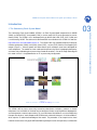
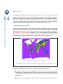
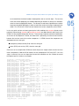
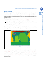
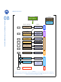
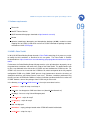
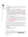
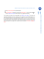
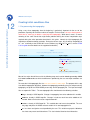
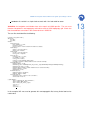
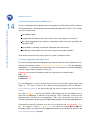
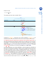
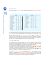
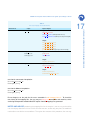
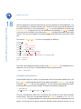
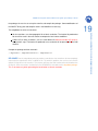
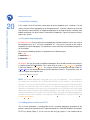
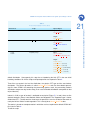
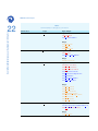
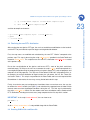
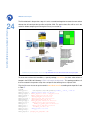
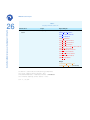
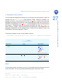
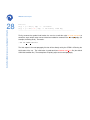
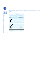
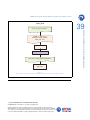
Research Papers
Issue RP0221
May 2014
Application and
Numerical Scenarios
By Florence Colleoni
Centro Euro-Mediterraneo sui i
Cambiamenti Climatici, Bologna
(Italy)
[email protected]
Nan Rosenbloom
National Center for
Atmospheric Research (USA)
[email protected]
We acknowledge Bette
Otto-Bliesner for its
scientific support on
CESM. We gratefully
acknowledge the support
of Italian Ministry of
Education, University and
Research and Ministry
for Environment, Land
and Sea through the
project GEMINA.
CESM 1.0.5 near past initial
conditions user guide: prescribing
ice sheets
SUMMARY The Community Earth System Model, developed and
maintained by NCAR, is the first completely open-source Earth System
Model. In this document, I will refer to CESM 1.0.5, which corresponds to
the last official release of CESM 1.0 (the more recent version is now CESM
1.2). CESM 1.0.5 includes atmosphere, land, ocean, sea-ice and a partially
coupled ice-sheet model. Several grid resolutions have been developed for
each component of CEMS and for present-day Earth’s
topography/bathymetry. One of the major advantage of this model is that
the procedure to run it is straightforward in its present-day configuration.
However, the CESM is not flexible when changes in the topography and
bathymetry have to be introduced in order to simulate near and deep past
climates. To implement a different land-sea mask, as well as different
surface conditions, such as vegetation cover, ice sheets etc..., each
component of CESM requires substantial changes in its initial conditions
files, which require an advanced knowledge of the model structure. In order
to make those kind of changes accessible to new users, the following
document aims at detailing a relatively simple procedure to modify the initial
conditions files for the coupled atmosphere-land-ocean-sea-ice
configuration of the CESM 1.0.5 (B compset). This procedure was
developed at NCAR and is based on the script released by the
Paleo-working Group. This procedure has been successfully tested on
CMCC IBM supercomputing facilities. In this user guide, the procedure is
applied to a glaciation case, i.e. when large ice sheets covered the
Northern Hemisphere repeatedly in the past and when sea level drop of
about 120 meters. This procedure is by far non automatic and requires
substantial manual work at each stage described in the document. Finally,
following this procedure does not provide any guarantees that the
simulations will be successful.
Table of Contents
Introduction . . . . . . . . . . . . . . . . . . . . . . . . . . . . . . . . . . . . . . . . . . . .
3
1 The Community Earth System Model . . . . . . . . . . . . . . . . . . . . . . . . . .
3
2 Modelling near past climates . . . . . . . . . . . . . . . . . . . . . . . . . . . . . .
4
Before Starting . . . . . . . . . . . . . . . . . . . . . . . . . . . . . . . . . . . . . . . . . .
7
1 Software requirements . . . . . . . . . . . . . . . . . . . . . . . . . . . . . . . . . .
9
2 NCAR’s Paleo Toolkit . . . . . . . . . . . . . . . . . . . . . . . . . . . . . . . . . .
9
3 Building a new CESM 1.0.5 B case . . . . . . . . . . . . . . . . . . . . . . . . . . .
10
Creating initial conditions files . . . . . . . . . . . . . . . . . . . . . . . . . . . . . . . . . .
12
1 Pre-processing the topography . . . . . . . . . . . . . . . . . . . . . . . . . . . . .
12
2 Ocean and coupler initial conditions files . . . . . . . . . . . . . . . . . . . . . . . .
14
3 Land initial conditions . . . . . . . . . . . . . . . . . . . . . . . . . . . . . . . . . .
20
4 Atmosphere initial conditions . . . . . . . . . . . . . . . . . . . . . . . . . . . . . .
27
Setting the namelists: B case . . . . . . . . . . . . . . . . . . . . . . . . . . . . . . . . . .
29
Generating the new initial CLM initial conditions restart file: the 5-days CESM 1.0.5 run .
32
Production run . . . . . . . . . . . . . . . . . . . . . . . . . . . . . . . . . . . . . . . . . .
32
Useful links related to CESM 1.0.5 paleoclimate modelling . . . . . . . . . . . . . . . . . .
33
Appendix 0: Execution time of the scripts used in this user guide . . . . . . . . . . . . . .
34
Appendix I: Flow charts summarizing the procedure described in this user guide . . . . .
35
2
CESM 1.0.5 near past initial conditions user guide: prescribing ice sheets
Introduction
The Community Earth System Model (CESM) is an Earth System Model composed of an AGCM
(CAM), an OGCM (POP), a land model (CLM), a sea-ice model (CICE) and a dynamical ice sheets
model (CISM). The CESM 1.0.5 is developed jointly by NCAR and LANL (POP, CICE, CISM) and
is maintained by NCAR. The code and its documentation are available on the CESM 1.0.5 website:
http://www.cesm.ucar.edu/models/cesm1.0/. The CESM 1.0.5 fully coupled compset (B compset)
includes atmosphere (CAM), land (CLM), ocean (POP), sea-ice (CICE) which are managed by the
coupler (Figure 1). Several spectral and finite-volume grids resolutions have been developed for
each component. The model has been calibrated for present-day Earth’s topography/bathymetry
and extensively validated against present-day climate observations. One of the major advantage of
this model is that it is straightforward to run in its present-day configuration.
Figure 1:
CESM 1.0.5 architecture. See CESM 1.0.5 webpage for more details.
The CESM 1.0.5 has been successfully tested for paleoclimate simulations, however its climate
components are not flexible to simulate near or deep past climates requiring different topographies
and or batymetries relative to present-day. To use a continental distribution or a sea level departing
from present-day ones, each component of CESM needs substantial changes in its initial conditions,
which requires an advanced knowledge of the model. The procedure is not simple but has been
however tested successfully by NCAR Paleo Working Group for various time periods (Last Glaciation
03
Centro Euro-Mediterraneo sui Cambiamenti Climatici
1 The Community Earth System Model
CMCC Research Papers
Centro Euro-Mediterraneo sui Cambiamenti Climatici
04
and deglaciation, Pliocene, Miocene, Permian, Cretaceous etc...). In order to make those kind of
changes more accessible to new users, the following document aims at describing this procedure to
introduce large changes in the land-sea mask and surface conditions in a the coupled atmosphereland-ocean-sea-ice configuration of the CESM 1.0.5 (B case). The user may note that this procedure
is by far non automatic and requires substantial manual work at each stages. Finally, following this
procedure does not provide any guarantees that the simulations will be successful.
2 Modelling near past climates
Simulating past climates implicates various changes in the Earth’s topography. Fifty million years ago
(Myrs), the continental distribution highly differed from present-day one and the modern configuration
emerged about 10 Myrs ago. “Near past climate” refers more or less to the last 10 Myrs, during which,
only sea-level and surface elevation changed as a result of the alternation of glacial/interglacial
cycles (Figure 2). On the contrary “Deep past climate” refers to periods older than 10 Myrs, more
specifically when the continental distribution was totally different than the modern one.
Figure 2:
Last Glacial Maximum topography from ICE-5G reconstruction (LGM, Peltier, 2004). White areas correspond to LGM distribution of
ice sheets and glaciers. Note that LGM sea level is lower by about 130 m relative to present-day one.
Creating initial conditions for “Near Past” or “Deep Past” has different implications:
Deep past: changes in the surface topography, land cover, but also of the ocean bathymetry
and ocean basins decomposition require a large amount of work both to create the initial files
and to modify some specific default files into the model itself, which are set-up with present-day
characteristics.
Near past: the ocean bathymetry is kept at its modern state, only some of the oceanic basins
CESM 1.0.5 near past initial conditions user guide: prescribing ice sheets
In this user guide, we focus on how to generate the initial conditions for near past climates and in
particular, how to change sea-level and prescribe ice sheets over North America and Eurasia in the
CESM 1.0.5 fully coupled configuration (B case). Those changes implicate substantial modifications
at all levels for all components. Beside, the model itself is particularly sensitive to inconsistencies
between the land-sea mask of the various component. In CESM, some of the components are
decomposed on the same grid:
atmosphere (CAM) and land (CLM) share the same grid
ocean (POP) and sea-ice (CICE) share the same grid.
Once the user has compiled the CESM and submit the job, the coupler checks that the land-sea
masks computed for CAM and CLM matches the one computed for POP and CICE. If this first
stage is successful, the user can hope that the new initial conditions are fine. Bellow, the end of
the coupler log file is shown as an example:
(seq_mct_drv) : Performing domain checking
(domain_check_mct) --- checking ocn/ice domains --(domain_check_grid_mct) the domain size is =
140
(domain_check_grid_mct) maximum
difference for mask
0.00000000000000
(domain_check_grid_mct) maximum allowable difference for mask 0.100000000000000E-01
(domain_check_grid_mct) the domain size is =
140
(domain_check_grid_mct) maximum
difference for lat 0.568434188608080E-13
(domain_check_grid_mct) maximum allowable difference for lat 0.100000000000000E-01
(domain_check_grid_mct) the domain size is =
140
(domain_check_grid_mct) maximum
difference for lon 0.568434188608080E-13
(domain_check_grid_mct) maximum allowable difference for lon 0.100000000000000E-01
(domain_check_grid_mct) the domain size is =
140
(domain_check_grid_mct) maximum
difference for area 0.130104260698261E-17
(domain_check_grid_mct) maximum allowable difference for area 0.100000000000000E+00
(domain_check_mct) --- checking atm/land domains --(domain_check_grid_mct) the domain size is =
48
(domain_check_grid_mct) maximum
difference for lat 0.142108547152020E-13
(domain_check_grid_mct) maximum allowable difference for lat 0.100000000000000E-11
(domain_check_grid_mct) the domain size is =
48
(domain_check_grid_mct) maximum
difference for lon 0.568434188608080E-13
(domain_check_grid_mct) maximum allowable difference for lon 0.100000000000000E-11
(domain_check_grid_mct) the domain size is =
48
(domain_check_grid_mct) maximum
difference for area 0.476528601300874E-09
(domain_check_grid_mct) maximum allowable difference for area 0.900000000000000E-06
(domain_check_mct) --- checking fractions in domains --(domain_check_mct) maximum
difference for ofrac sum
0.00000000000000
(domain_check_mct) maximum
difference for ifrac sum
0.00000000000000
(domain_check_mct) maximum allowable difference for frac sum
0.100000000000000E-01
(domain_check_mct) maximum allowable tolerance for valid frac
0.100000000000000E-01
(domain_check_mct) (domain_check_mct) : min/max ascale
0.00000000000000
1.00000000000004
(domain_check_mct) (domain_check_mct) : min/max ascale
0.999999999999841
1.00000000000004
(domain_areafactinit_mct) : min/max mdl2drv
0.999718744540964
1.00061729371141
areafact_a
(domain_areafactinit_mct) : min/max drv2mdl
0.999383087105043
1.00028133458592
areafact_a
(domain_areafactinit_mct) : min/max mdl2drv
0.979340530542676
1.01536195556158
areafact_i
(domain_areafactinit_mct) : min/max drv2mdl
0.984870463702687
1.02109528689257
areafact_i
(seq_mct_drv) : Initializing fractions
(map_atm2ocn_mct) :calling1 npfix
atmdom_a
lnddom_l
05
Centro Euro-Mediterraneo sui Cambiamenti Climatici
are removed from the default modern decomposition due to sea level drops. The land-sea
mask and surface topography are modified depending on whether or not the user introduces
some ice sheets or topographic features. The concept is to add some slight differences relative
to present-day global topography in order to reduce the number of changes introduced in the
model. This also limits the inconsistencies between the various components of the CESM.
CMCC Research Papers
Centro Euro-Mediterraneo sui Cambiamenti Climatici
06
(seq_frac_check) [lnd init] afrac min/max
=
1.000000000000000000
1.000000000000000000
(seq_frac_check) [lnd init] lfrac min/max
=
1.000000000000000000
1.000000000000000000
(seq_frac_check) [lnd init] lfrin min/max
=
1.000000000000000000
1.000000000000000000
(seq_frac_check) [ice init] afrac min/max
=
0.00000000000000000
1.00000000000000622
(seq_frac_check) [ice init] ofrac min/max
=
0.00000000000000000
1.000000000000000000
(seq_frac_check) [ice init] ifrac min/max
=
0.00000000000000000
0.00000000000000000
(seq_frac_check) [ocn init] afrac min/max
=
0.00000000000000000
1.00000000000000622
(seq_frac_check) [ocn init] ofrac min/max
=
0.00000000000000000
1.000000000000000000
(seq_frac_check) [ocn init] ifrac min/max
=
0.00000000000000000
0.00000000000000000
(seq_frac_check) [atm init] afrac min/max
=
1.000000000000000000
1.000000000000000000
(seq_frac_check) [atm init] lfrac min/max
=
1.000000000000000000
1.000000000000000000
(seq_frac_check) [atm init] ofrac min/max
=
0.00000000000000000
0.00000000000000000
(seq_frac_check) [atm init] ifrac min/max
=
0.00000000000000000
0.00000000000000000
(seq_frac_check) [atm init] lfrin min/max
=
1.000000000000000000
1.000000000000000000
(seq_frac_check) [atm init] sum min/max
=
1.000000000000000000
1.000000000000000000
(seq_frac_check) [atm init] sum ncnt/maxerr =
0
0.00000000000000000
(seq_mct_drv) : Setting fractions
(seq_mct_drv) : Initializing atm/ocn flux component
(seq_mct_drv) : Calling map_lnd2atm_mct
(seq_mct_drv) : Calling map_ocn2atm_mct for mapping o2x_ox to o2x_ax
(seq_mct_drv) : Calling map_ocn2atm_mct for mapping xao_ox to xao_ax
(seq_mct_drv) : Calling map_ice2atm_mct for mapping i2x_ix to i2x_ax
(seq_mct_drv) : Calling mrg_x2a_run_mct
(seq_mct_drv) : Calling atm_init_mct
(seq_mct_drv) : Model initialization complete
NOTA BENE: when everything get successful, the user is in total state of happiness and can
eventually enjoy and party!, most of the problems are solved... - Florence Colleoni
CESM 1.0.5 near past initial conditions user guide: prescribing ice sheets
Before Starting
The entire procedure begins with the computation of ocean new bathymetry and basins distribution.
In POP, the World Ocean is divided in 10 basins and 4 marginal seas (Figure 3):
Southern Ocean; Pacific Ocean; Indian Ocean; Atlantic Ocean; Arctic Ocean; Persian Gulf;
Mediterranean; Labrador Sea; Hudson Bay; GIN Sea
Red Sea; Baltic Sea; Black Sea; Caspian Sea
Changes in sea level sometimes imply a reorganization of the World Ocean basins and occasionally,
some marginal Seas or small peripheral basins may be removed by the procedure.
Figure 3:
Distribution of ocean basins and marginal seas within POP for present-day topography.
Once the ocean land-sea mask and basins have been created, it is then possible to compute the
coupler mapping files. The mapping files contain the interpolation weights needed to interpolate
from POP to CAM and vice versa. In this step, a mapping file to interpolate the runoff from land to
ocean is also computed. The next step is to compute the CLM surface conditions, which account
for the newly created land-sea mask and the new ice sheets and vegetation distribution. The final
step is to compute the initial conditions for CAM, which accounts for changes in surface topography
and land-sea mask.
07
Centro Euro-Mediterraneo sui Cambiamenti Climatici
First of all, to change the initial conditions, it is important to understand what are the steps of the
procedure and why the user must strictly follows the order of the various steps. It is important to
understand that the procedure starts with the computation of ocean and coupler initials conditions
on which most of the surface datasets are based. The user can have an overview of the whole
procedure in Figure 4.
CMCC Research Papers
Paleo tools
CESM1.0 tools
Scripts or packages
Step 1
change_kmt.ncl
Outputs
KMT_new,
region_basins
Ocean to atmosphere
mapping files
genrunoff
Runoff to ocean
mapping files
Step 3
gen_domain
ocn.domain & lnd.domain
Step 4
mkgriddata
Step 5
convert_mksrf.F90
or
paleo_mkraw.csh
Step 6
mksurfdata
Step 7
definesurf
topography
Step 8
5-day CESM run
clm.r.new-paleo-map
Step 9
interpinic
clm.r.CESM.standard
mapped to
clm.r.new-paleo-map
fractdata.10min
mksrf files
surface_dataset
ATMOS.
PRE-RUN - interp.
RUN
Production run CESM
fracdata.run_resolution
LAND
Step 10
COUPLER
mk_remap.csh
mk_runoff_remap
Step 2
Required if using CLM
restart files with
new landcover
OCEAN
Centro Euro-Mediterraneo sui Cambiamenti Climatici
08
Legend
USER INPUT:
land-ocn.mask.1deg.nc
topo-ice.10min.nc
Figure 4:
Flow chart of the steps described in this user guide, after Nan Rosembloom and Christina Shields’s flow chart (see Appendix II).
Orange boxes or blue boxes correspond to tools located in the main directory of the CESM, while brown boxes correspond to the
script developed and released in NCAR’s Paleo toolkit.
CESM 1.0.5 near past initial conditions user guide: prescribing ice sheets
1 Software requirements
NetCDF Fortran libraries
NCAR Command Language: download at http://www.ncl.ucar.edu/)
Ncview
Spherical Coordinates Remapping and Interpolation Package (SCRIP): needed to create
mapping files for CESM 1.0 and earlier versions of CCSM. Download the package and documentation on LANL SCRIP page.
2 NCAR’s Paleo Toolkit
In 2012, NCAR Paleo Working Group released a Paleo Toolkit containing all the necessary scripts
to modify the initial conditions as described in this user guide. The Paleo Toolkit is available
for download here: https://www2.cesm.ucar.edu/working-groups/pwg/documentation/cesm1-paleotoolkit.
Furthermore, the Paleo Working Group wiki page contains a lots of informations to properly set-up
the paleoclimate simulations and some of the scripts of the Paleo Toolkit. This toolkit contains two
tar files, one dedicated to the old version of CCSM3 and one dedicated to CCSM4 version. For
CESM 1.0.5, the user has to consider the CCSM4 tar file, which corresponds to the fully coupled
configuration B1850 using CAM4 (CAM5 presents large improvements about the chemistry of
atmosphere which are not of direct interest in our case). Therefore, simulations performed using
the early versions of CESM with CAM4 are similar to simulations performed with the last release of
CCSM4. However, some of the packages from CCSM3 may also be useful.
In the directory ccsm4 extra pub.2012mar16 nr/, the scripts are ordered such as:
atmlndfrac/ : scripts for steps 3 and steps 4
cam tools/ : for deep past or CAM stand alone run (docn/mk docn.domain.ncl)
cn nitdep/ : for cases using Carbon-Nitrogene pools
convert mksrf/ : scripts for step 5
cpl mapping/ : scripts for step 2
lnd/ : for deep past
mksurfdata/ : empty. package located under CESM1.0.5/models/lnd/clm/tools
modify kmt/ : scripts for step 1
09
Centro Euro-Mediterraneo sui Cambiamenti Climatici
Fortran 90
CMCC Research Papers
Centro Euro-Mediterraneo sui Cambiamenti Climatici
10
paleo ccsm4 aerosol/ : to prescribe a different aerosol distribution for paleo time period (not
used in this procedure, but could be included if the user needs to prescribe a new aerosol
distribution.)
paleo mkraw/ : for deep past (for near past, use convert mksrf/ scripts)
rtm/ : for deep past only. For near past use the tool gen runoff/, located in the Paleo Toolkit for
CCSM3. This tool aims at providing a new file of river flow directions used by the RTM model
coupled to CLM. However, for near past simulations using almost present-day topography, the
user may use the default CESM rdir05.nc already prescribed in the namelist. But, the user
will have to produce the runoff mapping file using the gen runoff tool to account for the new
land sea mask if needed. In alternative, a more recent version of this tool, runoff to ocn/ is
available in CESM 1.1 and more recent versions under CESM1.1/mapping/gen mapping files/.
The user may also find it in this CESM forum post.
In the directory ccsm3 setup tools 110319-NR-120316/, the user can find:
atm/ : scripts for step 7. The only tool that will be used form this directory is the definesurf
tool. There are two versions present in the directory: definesurf-svn100709/ is the most recent
version of this tool accounting for the changes between CCSM3 and CESM1.0. The other
version, definsurf-paleo-quaternary/ contains a directory landmcoslat/ in which the user can
find the script fix landm coslat.ncl used at step 7.
cpl/ : the user can find the gen runoff/ package which is used to compute the runoff mapping
files needed by the coupler.
For each step of this guide, the scripts, the input and output files are listed in the different Tables and
the settings and execution are extensively detailed. All the scripts ported on CMCC supercomputing
platforms were initially developed by Nan Rosembloom and Christina Shield (NCAR).
In all the tables of this document, the files generated from the scripts or provided by the user are
distinguished from the original raw grid files or others directly coming from CESM 1.0.5 by using the
following color code:
blue: default CESM 1.0.5 present-day raw data files
red: user provided files
orange: files computed during the procedure
3 Building a new CESM 1.0.5 B ca
Most of the scripts that will be used in this procedure introduce changes based on default presentday CESM 1.0 initial conditions files that the user can get building the CESM default case and for
which new boundary conditions will be created. In this manual, the procedure is described for:
B case (atm-lnd-ocn-sic)
CESM 1.0.5 near past initial conditions user guide: prescribing ice sheets
using pre-industrial period files (B1850 compset)
The instructions to build the case are provided in the CESM 1.0 User Guide. This process will
automatically download all the files required by all the components of the B1850 compset to run
with the default configurations already implemented in CESM 1.0. Once the user has built the case,
he can proceed with the steps described in the forthcoming sections. Do not clean-up the case
directory since it will be used to create the 5-days CLM restart file accouting for the new land sea
mask and needed to run a proper case using the new initial conditions (see section 7 and Figure 4,
step 7).
11
Centro Euro-Mediterraneo sui Cambiamenti Climatici
finite volume 0.9x1.25 atmospheric resolution and displaced pole 1◦ ocean resolution (f09 g16,
see the CESM 1.0 user guide for more details on the supported resolutions).
CMCC Research Papers
Creating initial conditions files
Centro Euro-Mediterraneo sui Cambiamenti Climatici
12
1 Pre-processing the topography
Using a very clean topography from the beginning is particularly important for the rest of the
procedure, especially for the ocean and for the coupler. For that reason, the user should spend as
much time as necessary to obtain a satisfying initial topography. What does it mean? It means
removing all the small islands that might create problems during the various interpolation steps
required during the entire procedure described in this guide. Indeed, the initial topography file
should be at 10 min horizontal resolution. During the various steps, this file will be interpolated at
0.5◦ , at 1◦ and finally at the CESM 1.0.5 case resolution (e.g. f09 g16, T31 gx3v7, see the CESM
1.0 user guide for more details on the supported resolutions).
Table 1
Pre-processing initial topography script and associated files
Numerical tool
Scripts
User based
User based
Inputs / Outputs
Input:
USGS gtopo30 10min.nc
Relief user 10min.nc (topography at 10min res.)
landice user.nc (ice mask)
Output:
topo user 10min.nc
(htopo, ice, landfract, landsmask,variance)
Most of the scripts that will be used in the following steps are based on default present-day CESM
1.0.5 initial conditions files to which the differences provided by the user new input conditions are
added.
To create the initial topography file, the user must create his own script. The purpose of this step
is to add the topographic difference, between the topography provided by the user and present-day
topography, on top of the CESM USGS present-day 10 min topography file. The input and output
files are reported in Table 1. The new topographic file should contain the following variables:
htopo: already in USGS topo file. Changes in topography have to be added on this variable
landfract: already in USGS topo file. Changes in land-sea mask have to be added on this
variable. Make sure that the values range between 0-1.
variance: already in USGS topo file. This variable does not have to be modified. The user
may copy and paste the USGS variance variable in his own topographic file
ice: ice-sheets and glaciers mask provided by the user. This variable may equals 100 where
ice sheets are present and 0 elsewhere. This also includes Greenland and Antarctica.
CESM 1.0.5 near past initial conditions user guide: prescribing ice sheets
landmask: this variable is a simple land-sea mask with 1 for land and 0 for ocean.
The user file should look like the following:
netcdf topo_mis6_10min.111021 {
dimensions:
lat = 1080 ;
lon = 2160 ;
variables:
float htopo(lat, lon) ;
htopo:_FillValue = -1.e+34f ;
htopo:units = "meter" ;
htopo:long_name = "10-min elevation from USGS 30-sec dataset" ;
double lat(lat) ;
lat:units = "cell center locations" ;
lat:long_name = "latitude" ;
double lon(lon) ;
lon:units = "cell center locations" ;
lon:long_name = "longitude" ;
float ice(lat, lon) ;
ice:missing_value = -1.e+34f ;
ice:_FillValue = -1.e+34f ;
ice:long_name = "landice" ;
ice:history = "From landlandice_MIS6_10min" ;
ice:lonFlip = "longitude coordinate variable has been reordered via lonFlip" ;
float landfract(lat, lon) ;
landfract:_FillVal = -1.e+34f ;
landfract:long_name = "RELIEF[D=Relief_140_aveclacs_casp0,GX=RELIEF[D=Relief],GY=RELIEF[D=Relief]]" ;
landfract:missing_value = -1.e+34f ;
landfract:lonFlip = "longitude coordinate variable has been reordered via lonFlip" ;
landfract:_FillValue = -1.e+34f ;
landfract:units = "meter" ;
int landmask(lat, lon) ;
landmask:longname = "landmask" ;
landmask:_FillValue = -9999 ;
float variance(lat, lon) ;
variance:long_name = "variance of 30-sec elevations" ;
variance:units = "meter**2" ;
// global attributes:
:infile3 = "USGS-gtopo30_10min_c050419.nc" ;
:infile2 = "landice_MIS6_10min" ;
:infile1 = "Relief_140_aveclacs_casp0" ;
:srcCode = " " ;
:author = " " ;
:create date = " " ;
In this example, NCL was used to generate this new topographic file, but any kind of tool can be
used to do it.
13
Centro Euro-Mediterraneo sui Cambiamenti Climatici
WARNING: the longitudes and latitudes have to be equals to USGS topo file. The user must
therefore interpolate his own topography and land-ice mask to USGS topography grid. Check also
that the coordinates are written in the same order than in USGS file.
CMCC Research Papers
2 Ocean and coupler initial conditions files
Centro Euro-Mediterraneo sui Cambiamenti Climatici
14
This part is dedicated to the computation of the initial conditions for POP (ocean) and CPL (coupler).
The whole procedure is described bellow and illustrated by the flow chart in Figure 4. In this section,
seven files are generated:
a new land-sea mask
a region mask: distribution of the various oceanic basins and marginal seas (Figure 3).
the coupler mapping files (x4): handle the interpolation from/to the oceanic grid to/from the
atmospheric grid.
a new runoff to ocean map: to handle the interpolation from land to ocean.
the land and oceanic domains: land-sea masks used to create surface conditions
The execution time of the all the scripts used in this section is detailed in Table 9.
2.1- Ocean topography and region mask
First of all, the initial pre-processed topography at 10 min resolution has to be interpolated at 1◦ x1◦ .
Similarly to the previous section, the script must be created by the user. The new topography
interpolated at 1◦ should contain the same variables than in the original user provided topography
at 10 min: htopo, landfract, landmask, variance, ice.
WARNING: be sure that the following variables are computed in the indicated ranges:
ICE: 0 - 100
LANDFRACT: 0 - 1
LANDMASK: 0 - 1
This new topography is used to generate the new land-sea mask and the ocean region mask
(Figure 3). This step is based on the CESM present-day bathymetry KMT file located in
csm/inputdata/ocn/pop2/grid/ (the present-day land-sea mask and region mask are binary files
.ieee4).
The script change kmt.ncl from the Paleo Toolkit is able to open those files and modify the areas
where the new topography is different from present-day. POP is particularly sensitive to new
continental points inserted in the new topography. That is why, for practical issue, when simulating near past climates, in the script, present-day bathymetry is preserved over the unchanged areas.
To generate the new KMT and region mask, the user has to point to the new topography 1x1.nc
file.
As reported in Table 2, change kmt.ncl also needs the original present-day POP
bathymetry, regions and horizontal grid files provided directly for the resolution of interest in the
csm/inputdata/ocn/pop2/grid directory.
CESM 1.0.5 near past initial conditions user guide: prescribing ice sheets
Execute the script:
The execution time of the scripts is detailed in Table 9.
Table 2
New ocean bathymetry and region mask files
Numerical tool
Scripts
User provided
User provided
Inputs / Outputs
Input:
topo user 10min.nc
Output:
new topo user 1x1.nc
NCL
change kmt.ncl
Input:
new topo user 1x1.nc (topography at 1◦ res.)
topography 20090204.ieeei4 (POP present-day topo)
region mask 20090205.ieeei4 (POP present-day ocean basins)
horiz grid 20010402.ieeer8 (POP present-day horizontal grid)
Output:
kmt gx1v6 user.ieeei4
region mask gx1v6 user.ieeei4
USER kmt.nc (file to check for disturbing pixels)
A NetCDF file, USER kmt.nc, containing the main variables modified by change kmt.ncl is also
created to help the user to check whether the new land-sea mask and region mask are correct.
It is important to check the number of basins contained in the new oceanic region mask. Indeed, when changing the ocean bathymetry, changes occur in the region mask since some basins
may disappear. In the present-day region mask file, each basin and marginal sea is assigned a
value between 1 to -14. You can find the present-day configuration in the main directory of the
CESM 1.0.5 model (CESM 1.0.5/models/ocn/pop2/input templates/gx1v6 region ids). The original
gx1v6 region ids file provided in the CESM 1.0.5 for present-day is shown in Table 3.
If the topo provided by the user induces modifications in the present-day basins distribution (no
Baltic Sea, no Hudson Bay for example), the previous values assigned to the basins have to be
re-assigned. An example is given in Table 3, illustrating our glaciation case. The Baltic Sea as
well as the Hudson Bay have been removed and filled with land. The basins no longer exist
in the new ocean bathymetry file and as a consequence, the user has to modify the list and
re-assign values to the Black Sea and the Caspian Sea. Note that a negative value is indicative
of a marginal sea. Those modifications are necessary because the POP ocean model checks
for the total number of ocean basins prescribed the gx1v6 region ids and takes the absolute
value of the maximum number written in this file. In our case, this number is abs(−12) = 12, for
15
Centro Euro-Mediterraneo sui Cambiamenti Climatici
> ncl change kmt.ncl
CMCC Research Papers
present-day it would be abs(−14) = 14. Those changes have to be done before building the compset.
Centro Euro-Mediterraneo sui Cambiamenti Climatici
16
Table 3
Present-day gx1v6 region ids file provided in CESM 1.0.5 (left) and an example of gx1v6 region ids file provided by users (right)
1 ’Southern Ocean ’
0.0
0.0
0.0
1
’Southern Ocean ’
0.0
0.0
0.0
2 ’Pacific Ocean ’
0.0
0.0
0.0
2
’Pacific Ocean ’
0.0
0.0
0.0
0.0
3 ’Indian Ocean ’
0.0
0.0
0.0
3
’Indian Ocean ’
0.0
0.0
4 ’Persian Gulf ’
22.0
60.0
0.0
4
’Persian Gulf ’
22.0
60.0
0.0
-5 ’Red Sea ’
14.0
47.0
3.0e15
-5
’Red Sea ’
14.0
47.0
3.0e15
6 ’Atlantic Ocean ’
0.0
0.0
0.0
6
’Atlantic Ocean ’
0.0
0.0
0.0
7 ’Mediterranean Sea ’
36.0
354.0
0.0
7
’Mediterranean Sea ’
36.0
354.0
0.0
8 ’Labrador Sea ’
0.0
0.0
0.0
8
’Labrador Sea ’
0.0
0.0
0.0
9 ’GIN Sea ’
0.0
0.0
0.0
9
’GIN Sea ’
0.0
0.0
0.0
10 ’Arctic Ocean ’
0.0
0.0
0.0
10
Arctic Ocean ’
0.0
0.0
0.0
11 ’Hudson Bay ’
61.0
295.0
0.0
-11
’ Black Sea ’
40.0
25.0
3.0e15
-12 ’Baltic Sea ’
56.0
8.0
3.0e15
-12
’Caspian Sea ’
82.0
72.0
3.0e15
-13 ’Black Sea ’
40.0
25.0
3.0e15
-14 ’Caspian Sea ’
70.0
65.0
3.0e15
The second feature that may change, due to the new land-sea mask, is the location of the overflows
areas. In POP, the location of the overflows for present-day bathymetry are prescribed in an initial
input file that the user may find in CESM 1.0.5/models/ocn/pop2/input templates/gx1v6 overflow).
In this file, there are several regions where overflows occur due to ocean bathymetry as for example:
the Denmark Strait, the Faroe Bank Channel, the Ross Sea and the Weddell Sea. Typically, for a
glaciation case, only the overflow located in the Denmark Strait is preserved.
2.2- Coupler mapping files
The mapping files contain informations (weights etc...) used by the coupler to interpolate the fields
from ocean grid onto the atmospheric grid and vice versa. The runoff to ocean map is also part of
this process since to be computed, it uses one of the ocean mapping file generated.
The script that computes the four mapping files is the shell script mk remap gx1v6.csh. This
script needs the SCRIP software, which handles the interpolation of the various grids (See Software
requirements). To perform the interpolation between ocean and atmosphere, mk remap gx1v6.csh
needs the original ocean and atmosphere grid files, and the new ocean KMT file generated at the
previous step. All the input and output files are reported in Table 4.
BE AWARE: mk remap gx1v6.csh has to be executed two times. This is because, two of the
mapping files are computed using a conservative interpolation method while the two others are
generated using a bilinear interpolation method. In the script, one of the two methods is commented
and the user has to comment them successively to get the four mapping files:
CESM 1.0.5 near past initial conditions user guide: prescribing ice sheets
Numerical tool
Scripts
shell + SCRIP
mk remap gx1v6.csh
Inputs / Outputs
Input:
kmt gx1v6 user.ieeei4
fv0.9x1.25 070727.nc (CAM grid at 0.9x1.25 res.)
horiz grid 20010402.ieeer8 (POP present-day horizontal grid)
Output:
map ocn to atm user aave.nc
map atm to ocn user aave.nc
map ocn to atm user bilin.nc
map atm to ocn user bilin.nc
gx1v6 user.nc (new ocean grid, only used for runoff map)
Fortran 90
gen runoff/
Input:
build.calypso.csh
gx1v6 user.nc
runoff.calypso.run
rdirc.05.061026
Output:
map r05 to gx1v6 user.nc
Fortran 90
gen domain/
Input:
map ocn to atm aave.nc
Output:
domain.ocn.gx1v6.user.nc
domain.lnd.fv09 1.25 gx1v6 user.nc
one time for conservative interpolation:
!mv scrip ina scrip in
!$scripdir/scrip
one time for bilinear interpolation:
!mv scrip inb scrip in
!$scripdir/scrip
Do not forget to set the path for the SCRIP executable in mk remap gx1v6.csh. To check the
consistency of the mapping files, the user may use scrip test executable and namelists, which
are designed to produce readable NetCDF outputs from the mapping files generated.
NOTES AND ADVICE: producing the mapping files for the coupler is not an easy task and the
user should pay attention to it since if it fails for some reasons, and for only one pixel, the model will
not be able to run with the new conditions. Then given the structure of this procedure, the user may
17
Centro Euro-Mediterraneo sui Cambiamenti Climatici
Table 4
New coupler mapping, runoff and domain files
CMCC Research Papers
have to start again from almost the beginning of the procedure (see all the flow charts in Figure 4.
Centro Euro-Mediterraneo sui Cambiamenti Climatici
18
Once the mapping files have been generated, the user may compute the runoff mapping file. This
file is generated at 0.5◦ horizontal resolution and is based on the new ocean grid file computed at
the previous step (Table 4). The runoff package gen runoff/ has to be compiled first using the script
build.machine.csh. In alternative, the user can download the new package runoff to ocn, available
in the latest version of CESM 1.2 and similar to the gen runoff package (See NCAR’s Paleo Toolkit
section). The user can thus follow the instructions below using the most recent version of this runoff
tool.
The namelist runoff map gx1.nml has to be set-up properly as following:
&input nml
gridtype = ”rtm”
file roff = ‘rdirc.05.061026‘
file ocn = ‘../gx1v6 user.nc‘
file nn = ‘map nn gx1v6.nc‘
file smooth = ‘map smoother gx1v6.nc‘
file new = ‘map r05 to gx1v6 user.nc‘
title = ‘runoffmap : r05− > gx1v6 full ice coverage in NH‘
eFold = 1000000.0
rMax = 300000.0
/
The runoff is then computed executing the batch script runoff.calypso.run. The computation time is
larger than 5 min, that is why it is recommended to avoid running interactively:
> bsub < runoff.run
2.3- Domain and fraction files
The penultimate step of this section is the computation of the land and oceanic domain files using
the gen domain package provided with the Paleo Toolkit and located in atmlndfrac/. First, edit the
namelist gen domain.nml with the new mapping files. The user may also edit the Makefile to specify
the NetCDF library and the Fortran compiler. To compile and execute the package do:
> ./make.AIX.csh
> gen domain.aix < gen domain.nml > gen domain.out
Finally, the land fraction file, both at the run resolution (here fv 0.9x1.25) and at 10 min resolution
can be created. Those files are generated through the mkgriddata package (CESM 1.0.5/models/lnd/clm/tools). The package produces three files containing land fraction, topography and a new
grid file. The two latter are not further used by the procedure neither during the run time. To use
CESM 1.0.5 near past initial conditions user guide: prescribing ice sheets
The mkgriddata has to be run two times:
10 min resolution: uses the topographic file at 10 min resolution. The fraction file produced at
10 min will be used in the next section to compute the land surface conditions.
fv 0.9x1.25 (or other) resolution: uses the land domain file domain.lnd.fv09 1.25 gx1v6.nc
from previous step. The fraction file produced at run resolution will be prescribed in the CLM
namelist.
Compile the package and then execute it:
> mkgriddata < mkgriddata.namelist > mkgriddata.out
BE AWARE that the mkgriddata package produces coordinates that sometimes do not completely
match with the coordinates of the surfdata.nc file. To avoid this problem, the user has to insert the
default CLM grid file in the namelist. The routines will force the land fraction to be calculated on the
CLM grid. Some instructions are detailed in the README file included into the mkgridata package.
This is not necessary when generating the land fraction at 10 min resolution.
19
Centro Euro-Mediterraneo sui Cambiamenti Climatici
the package, the user has to set-up the namelist and compile the package. Some modifications of
the NetCDF library path and compiler name in the Makefile are necessary.
CMCC Research Papers
3 Land initial conditions
Centro Euro-Mediterraneo sui Cambiamenti Climatici
20
In this section, the final CLM initial surface data file will be computed at 0.5◦ resolution. For that
reason, the initial 10 min topography will be interpolated at 0.5◦ resolution. However, to create the
final CLM initial surface data file, an additional topographic file at 10 min resolution, including some
bedrock informations has to be created. The flow chart in Appendix I, Figure 8 illustrates the various
steps of this section.
3.1 Pre-processing topography
For steps 4.2 to 4.3, the initial pre-processed topography at 10 min resolution used in step 2 has to
be interpolated at 0.5◦ x0.5◦ . As for the interpolation at 1◦ , the user has to create its own script to
interpolate the 10 min topography. The coordinates have to match those of the default mkglacier.nc
file, for example.
Be sure that the following variables are computed in the indicated ranges:
ICE: 0 - 100
LANDFRACT: 0 - 1
LANDMASK: 0 - 1
For step 3.4, the user also needs an additional topographic file at 10 min resolution which contains
a variable named TOPO BEDROCK. This is done using the script create mksrf topo.ncl provided
in the Paleo Toolkit in convert mksrf/. This script also needs the original present-day CESM mksrf topo 10min.nc file downloaded from the NCAR repositories (Table 5). To execute the script, the
user has to point to the topo files and:
> ncl create mksrf topo.ncl
NOTE: the bedrock topography corresponds to an ice free topography.
Those informations
are available for present-day (e.g. ETOPO2 and ETOPO1) but, for example, in the compset of
glaciations, if the user only knows about the surface elevation and the landice distribution but does
not have any information about the ice thickness, the bedrock topography cannot be retrieved.
However this information is only necessary in the compset of running a dynamical ice sheets model
which requires both ice thickness and bedrock topography as input fields. Since no ice sheet model
has been implemented yet in CESM 1.0.5 at the time of this user guide, the bedrock topography is
not necessary to run the simulations. Consequently, TOPO BEDROCK is set equal to TOPO ICE
in create mksrf topo.ncl.
3.2 Adding glaciers to the list of PFTs
The ice sheets distribution is extracted from the 0.5◦ resolution topography interpolated at the
previous step and transformed into a PFT type and landunit file. CLM initial conditions file considers
15 PFTs by default (Figure 5). As the user can note, the type “glaciers” is not included into this
CESM 1.0.5 near past initial conditions user guide: prescribing ice sheets
Numerical tool
Scripts
User based
User based
Inputs / Outputs
Input:
topo user 10min.nc
Output:
topo user 05deg.nc
NCL
create mksrf topo.ncl
Input:
topo user 10min.nc
mksrf topo.10min.c080912.nc
Output:
mksrf topo.10min.user.nc
Fortran
NetCDF
mkgriddata package
Input:
topo user 10min.nc
domain.lnd.fv09 1.25 gx1v6 user.nc
Output:
fracdata 10min.nc
griddata 10min.nc (not used)
topodata 10min.nc (not used)
fracdata fv09 1.25.nc (CLM namelist)
griddata fv09 1.25.nc (not used)
topodata fv09 1.25.nc (not used)
default distribution. Consequently, this step aims at introducing the 16th PFT in the new initial
boundary conditions file. All the scripts and input/output files are reported in Table 6.
Three files are created: the land ice distribution, the glaciers PFT type and the new landuse
distribution. The Fortran 90 routine is called convert mksrf.F90 and uses three default presentday files from CESM 1.0.5 containing the present-day glaciers mask, the present-day landunit
distribution and present-day landuse map (in our case the default distribution corresponds to that
of pre-industrial).
Indeed, in CLM, a type of landunit is attributed to each pixel (Figure 5). In total, there are five
declared landunits: Urban, Lake, Wetland, Glacier and Vegetated. The “Vegetated” type is further
divided into PFTs. To add some ice sheets over the ground, the user has to declare how much of
each pixel will be “Glacier” and/or vegetated. This is exactly what convert mksrf.F90 does.
The routine is based on a template routine in which the user has to point to the default CESM 1.0.5
files listed in Table 6:
To edit the script:
21
Centro Euro-Mediterraneo sui Cambiamenti Climatici
Table 5
Pre-processing topography for surface dataset
CMCC Research Papers
Centro Euro-Mediterraneo sui Cambiamenti Climatici
22
Table 6
New PFTs distribution - adding glaciers to the landcover
Numerical tool
Scripts
NCL
convert mksrf.F90
Inputs / Outputs
Input:
topo user 05deg.nc
mksrf topo.10min.c080912.nc
Output:
mksrf glacier user.nc
mksrf pft user.nc
mksrf landwat user.nc
NCL
add harvest.ncl
Input:
mksrf pft user.nc
mksrf landuse rc1850 c090630.nc
Output:
mksrf pft user harvest.nc
NCL
nn fill.ncl
Input:
mksrf glacier user.111021.nc
mksrf lanwat user.111021.nc
mksrf pft user.harvest.111021.nc
mksrf soitex.10level.c010119.nc
mksrf organic.10level.0.5deg.081112.nc
mksrf fmax.070406.nc
mksrf soilcol global c090324.nc
mksrf lai global c090506.nc
Output:
mksrf glacier user.nn.nc
mksrf lanwat user.nn.nc
mksrf pft user.harvest.nn.nc
mksrf soitex.10level user.nn.nc
mksrf organic.10level.0.5deg user.nn.nc
mksrf fmax user.nn.nc
mksrf soilcol user.nn.nc
mksrf lai global user.nn.nc
NCL
create urban.ncl
Input:
mksrf urban 3den 0.5x0.5 simyr2000.c090223 v1.nc
mksrf pft mis6.harvest.nn.111021.nc
Output:
mksrf urban user.nc
CESM 1.0.5 near past initial conditions user guide: prescribing ice sheets
cp convert mksrf.template convert mksrf.template.myrun
edit convert mksrf.template.myrun
and then to compile and execute:
> cp˜convert mksrf.template.myrun
> gmake
> ./convert mksrf
convert mksrf.F90
3.3 Finalising the new PFTs distribution
After creating the new glaciers PFT type, the user has to add those modifications to the landunits
and the PFTs of pre-industrial or present-day pre-existing default distribution.
First, the crop areas are modified and substituted by the new PFT “Glacier” computed at the
previous step. This step is done using the script add harvest.ncl provided in the Paleo Toolkit and
located in convert mksrf/. This script that uses the new PFTs distribution mksrf pft user.nc created
at the previous step.
Due to the new distribution of the glaciers and harvest PFTs, some of the pixels could have
remained empty. To fill them, the user has to execute the script nn fill.nc which corresponds to a
near-neighbor algorithm filling the empty pixels by using their nearest PFTs and soil properties and
computes all the soil properties. This step uses all the default CESM 1.0.5 soil properties files, as
for example, the vertical distribution of organic matter, the soil texture, the LAI, etc...Those files
are listed in Table 6. This script is not provided in the Paleo Toolkit and has to be required to Nan
Rosembloom. In alternative, the user may use any kind of tool to do this step
Finally, since for the near past and deep past simulations there are no urban areas, the user has
to remove the “urban” landunit (see Figure 5) and substitute it by vegetated areas to allow CLM to
recreate some consistent hydrological conditions during the run. This final step is performed by
the script create urban.ncl which uses the modern urban areas distribution and the combined new
PFTs distribution, including the harvest areas (crop) computed at the first step of this section.
IMPORTANT: in the script “create urban.ncl”, the user have to set:
pct urban = 0
As for nn fill.ncl, create urban.ncl is not provided along with the Paleo Toolkit.
3.4 Creating CLM initial conditions file
23
Centro Euro-Mediterraneo sui Cambiamenti Climatici
0)
1)
CMCC Research Papers
Centro Euro-Mediterraneo sui Cambiamenti Climatici
24
The files obtained in the previous steps 4.1 to 4.3 are combined together to create the new surface
dataset that will constitute the input file to initialize CLM. The path to those files will be set in the
namelists before compiling and running the B case (see section 6).
Figure 5:
CLM landcover pixel decomposition. Source from: http://www.CESM 1.0.2.ucar.edu/models/clm/surface.heterogeneity.html.
To create new surface initial conditions, a special package, mksurfdata, has been released and is
located in the CESM 1.0.5 directory CESM 1.0.5/models/land/clm/tools. This package combines all
the files created in the previous steps into a unique file that will be given as input to CLM.
First of all, the user has to set-up the namelist mksurfdata.namelist according to the input files listed
in Table 7:
&clmexp
mksrf_fgrid =
'csm/inputdata/lnd/clm2/griddata/griddata_0.9x1.25_070212.nc'
mksrf_fsoitex =
'mksrf_soitex.10level.c010119.nc'
mksrf_forganic = 'mksrf_organic.10level.0.5deg_mis6.nn.nc'
mksrf_flanwat =
'mksrf_lanwat_mis6.nn.111021.nc'
mksrf_fmax =
'mksrf_fmax_mis6.nn.111021.nc'
mksrf_fglacier =
'mksrf_glacier_mis6.nn.111021.nc'
mksrf_furban =
'mksrf_urban_mis6.111021.nc'
mksrf_fvegtyp =
'mksrf_pft_mis6.harvest.nn.111021.nc'
mksrf_fsoicol =
'mksrf_soilcol_mis6.nn.111021.nc'
mksrf_flai =
'mksrf_lai_global_mis6.nn.111021.nc'
mksrf_ftopo =
'mksrf_topo.10min.mis6.111021.nc'
mksrf_ffrac =
'fracdata_1080x2160.nc'
mksrf_fvocef =
'mksrf_vocef.c060502.nc'
mksrf_firrig =
' '
mksrf_fdynuse = 'pftdyn_hist_simyr1850.txt'
CESM 1.0.5 near past initial conditions user guide: prescribing ice sheets
.true.
In this package, one of the input files, pftdyn hist simyr1850.txt is particularly important and determines if the user will compute a surface dataset for dynamical vegetation use or for steady-state
conditions. The corresponding file to compute dynamic vegetation is called pftdyn hist simyr18502005.txt and contains the name of the raw vegetation files for each year from 1850 to 2005 included.
In this guide, we compute steady-state vegetation conditions.
A crucial aspect of this file is its format since the mksurfdata Fortran code reads it with a specific
format statement (A125, 1x, I4):
/users/home/ans021/BC/surface bc/surf ncl/mksrf pft mis6.harvest.nn.111021.nc
1850
BE SURE when modifying the absolute path of this file that the format is respected.
After some modifications in the Makefile, the user must compile the package following those options:
in the Makefile:
SMP = TRUE
then to compile:
> gmake SMP = TRUE -j 64
It is critical to follow those recommendations to run the executable in a reasonable time. Without
those optimisations, the run could last for hours and/or days. The executable is optimised
and can be submitted to a queue. On the CMCC supercomputing platform, the batch script is
mksurfdata.run:
# /bin/csh -f!
#===============================================================================
# SVN $Id$
# SVN $URL$
#===============================================================================
# This is an LSF batch job script for runoff computation
#===============================================================================
#BSUB -n 64
#BSUB -R "span[ptile=64]"
#BSUB -q poe_medium
#BSUB -N
#BSUB -a poe
#BSUB -o poe.stdout.%J
#BSUB -e poe.stderr.%J
#BSUB -J maprunoff
#BSUB -W 2:00
setenv LID "`date +%y%m%d-%H%M%S`"
setenv OMP_NUM_THREADS 64
# cd /fis01/cgd/cseg/csm/mapping/makemaps/r05_??? <- your working dir
25
Centro Euro-Mediterraneo sui Cambiamenti Climatici
outnc_double =
/
CMCC Research Papers
Centro Euro-Mediterraneo sui Cambiamenti Climatici
26
Table 7
Computing CLM initial conditions file
Numerical tool
Scripts
Fortran
mksurfdata package
NetCDF
Inputs / Outputs
Input:
griddata 0.9x1.25 070212.nc
mksrf soitex.10level.c010119.nc
mksrf vocef.c060502.nc
fracdata 1080x2160.nc
mksrf glacier user.nn.111021.nc
mksrf lanwat user.nn.111021.nc
mksrf urban mis6.111021.nc
mksrf organic.10level.0.5deg user.nn.111021.nc
mksrf fmax user.nn.111021.nc
mksrf pft user.harvest.nn.111021.nc
mksrf soilcol user.nn.111021.nc
mksrf lai global user.nn.111021.nc
mksrf topo.10min.use.111021.nc
pftdyn hist simyr1850.txt
Output:
surfdata.pftdyn 0192x0288 user.nc
surfdata 0192x0288 user.nc (CLM namelist)
set SRCDIR = /users/home/ans021/BC/surface_bc/mksurfdata
echo "start computing surface dataset" `date`
time $SRCDIR/mksurfdata < mksurfdata.namelist >& mksurfdat.out!
echo "finished computing surface dataset " `date`
tail -200 out.$LID
CESM 1.0.5 near past initial conditions user guide: prescribing ice sheets
4 Atmosphere initial conditions
To execute the package, first, the user may compile it and then:
> ./definesurf -t topo_mis6_10min.nc -g fv_0.9x1.25.nc -l landm_coslat.nc newtopo.nc
Table 8
Creating CAM initial conditions
Numerical tool
Scripts
Fortran
definesurf package
NetCDF
Inputs / Outputs
Input:
fv 0.9x1.25.nc
landm coslat.nc
topo user 10min.nc
Output:
topo user 0.9x1.25 remap.nc
NCL
fix landm coslat.ncl
Input:
topo user 0.9x1.25 remap.nc
Output:
topo user 0.9x1.25 remap.mod.nc
BUGS
A syntax bug was fixed in the routine map2f.f90. This bug might have been corrected in the latest
version of the code. The user may contact NCAR directly to get a more recent version:
----------------------------------------------------------------------Line 926:
sc(j) = jc + min(1., tmp) --> old version
sc(j) = jc + min(1.0d0 , tmp)
--> new version, fixed bug
27
Centro Euro-Mediterraneo sui Cambiamenti Climatici
The last CESM 1.0.5 component for which the user has to create new initial conditions is CAM. The
procedure uses the definesurf package (Paleo Toolkit for CCSM3 - definesurf-svn100709). This
package is based on, a pre-existing master T42 file landm coslat.nc containing the present-day
topography land fractions to the coastlines, on the atmospheric grid on which the user wants to interpolate his new topography, here fv 0.9x1.25.nc, and the topography at 10 min resolution obtained
from section 2. To keep consistent with the gradual land fraction, the script fix landm coslat.ncl
(Paleo Toolkit for CCSM3 in definsurf-paleo-quaternary/landmcoslat/) further modifies the new
topography interpolated on the final atmospheric grid. All those files are reported in Table 8 and
the procedure is described in Appendix I, Figure 9.
CMCC Research Papers
Centro Euro-Mediterraneo sui Cambiamenti Climatici
28
Line 951:
se(j) = jc + min(1., tmp) -->
old version
se(j) = jc + min(1.0d0 , tmp) --> new version, fixed bug
-----------------------------------------------------------------------
Finally, to correct the gradual land fraction, the user has to edit the script fix landm coslat.ncl to
correct the areas where some new land have been added or removed in the new topography (for
example, the Bering Strait). To execute:
> ncl fix landm coslat.ncl
The final output is the new topography file that will be directly red by the CESM 1.0.5 during the
initialisation of the run. The initialisation is performed from whatever cami ic.nc file (the default
CAM initial condition file). The atmosphere will quickly adjust to the new topography.
CESM 1.0.5 near past initial conditions user guide: prescribing ice sheets
Setting the namelists: B case
Once the B case directory is created, the first script to be modified is env conf.xml. Then the case
is configured and the user may edit the namelists located in $USER case/Buildconf (see CESM
1.0 user guide).
5.1 Coupler mapping files: env conf.xml
The user has to substitute the default mapping files by the ones computed in section 3.2:
<!--atm to ocn flux mapping file for fluxes (char) -->
<entry id="MAP_A2OF_FILE"
value="map_fv09_1.25_to_gx1v6_user_aave_da.nc"
<!--atm to ocn state mapping file for states (char) -->
<entry id="MAP_A2OS_FILE"
value="map_fv09_1.25_to_gx1v6_user_bilin_da.nc"
/>
/>
<!--ocn to atm mapping file for fluxes (char) -->
<entry id="MAP_O2AF_FILE"
value="map_gx1v6_to_fv09_1.25_user_aave_da.nc"
/>
<!--ocn to atm mapping file for states (char) -->
<entry id="MAP_O2AS_FILE"
value="map_gx1v6_to_fv09_1.25_user_aave_da.nc"
/>
.
.
<!--runoff (.5 degree) to ocn mapping file (char) -->
<entry id="MAP_R2O_FILE_R05"
value="map_r05_to_gx1v6_user.nc"
/>
Once the mapping files have been pointed by the user, configure the case:
> ./configure -case
5.2 Orbital parameters: env run.xml
To set-up the orbital forcing, the epoch of the simulation is specified in time A.D. (1950 + time). For
example, for the penultimate glaciation that occurred 140 kyrs BP, the time will be:
> vi env_rum.xml/
ORBITAL_MODE = fixed_year
ORBITAL_YEAR = -138050
29
Centro Euro-Mediterraneo sui Cambiamenti Climatici
In this final section are indicated the namelists fields where the user has to prescribed the new initial
conditions files computed along the entire procedure. First of all, the user has to indicate to the
CESM 1.0.5, where are located the new files. Since all the default input files for the CESM 1.0.5
runs are located in csm/inputdata, I used to put them there as well, because it limits the changes
introduced into the namelists.
CMCC Research Papers
For past time, the value is negative.
Centro Euro-Mediterraneo sui Cambiamenti Climatici
30
5.3 CAM namelist: cam.buildnml.csh
To initialise the atmospheric component, the user needs to set the new topography from section 5.
The user may also changes the values of the GHGs according to the epoch considered. Here the
values are taken from CO2 , CH4 and NO2 ice cores records retrieved from EPICA Dome C, East
Antarctica and corresponds to 140 kyrs BP.
&cam_inparm
= '$DIN_LOC_ROOT/atm/cam/topo/topo_mis6_0.9x1.25_remap_user.mod.nc'
bnd_topo
.
.
/
&chem_surfvals_nl
ch4vmr
= 791.6e-9
co2vmr
= 284.7e-6
f11vmr
= 12.48e-12
f12vmr
= 0.0
n2ovmr
= 275.68e-9
/
5.4 CLM namelist: clm.buildnml.csh
The user has to change the value of CO2 in agreement with that set-up in CAM namelist above.
Since in this example, we are modelling a past glaciation, the option “urban hac” is switched off (we
removed the urban landunits from the surface dataset in section 4.3).
&clm_inparm
co2_ppmv
fatmlndfrc
fsurdat
urban_hac
= 284.7
= '$DIN_LOC_ROOT/lnd/clm2/griddata/fracdata_0.9x1.25_gx1v6_user.nc'
= '$DIN_LOC_ROOT/lnd/clm2/surfdata/surfdata_192x288_user.nc'
= 'OFF'
5.5 POP namelist: pop2.buildnml.csh
As for CAM namelist, the user has to indicate the new bathymetry and ocean basins distribution
computed in section 3.1.
.
.
#----------------------------------------------------------------------------# identify all gx1v6 datasets residing in $DIN_LOC_ROOT/ocn/pop
CESM 1.0.5 near past initial conditions user guide: prescribing ice sheets
#-----------------------------------------------------------------------------
= $DIN_LOC_ROOT/ocn/pop/gx3v7/grid/region_mask_user.ieeei4
set topography_filename
= $DIN_LOC_ROOT/ocn/pop/gx3v7/grid/kmt_gx1v6_user.ieeei4
5.6 CICE namelist: cice.buildnml.csh
Since CICE shares the same grid with POP, the bathymetry has to be consistent:
&grid_nml
.
.
kmt_file
/
= '$DIN_LOC_ROOT/ocn/pop/gx3v7/grid/kmt_gx1v6_user.ieeei4'
31
Centro Euro-Mediterraneo sui Cambiamenti Climatici
set regionmask_filename
CMCC Research Papers
Centro Euro-Mediterraneo sui Cambiamenti Climatici
32
GENERATING THE NEW INITIAL CLM INITIAL CONDITIONS RESTART FILE: THE
5-DAYS CESM 1.0.5 RUN
When running on a new platform, outside of NCAR, it might be necessary to regenerate the initial
boundary conditions file for CLM. This is due to some differences in the allocation of the processors
and memory during the compilation of the model. This part corresponds step 8 and step 9 on
Figure 4 showing the whole procedure in Appendix I.
To do so, the user has to configure all the namelists, as shown in section 6, except for the CLM
namelist in which the original option pointing at the initial boundary conditions file is modified:
&clm_inparm
finidat
= '$USER_REPOSITORY/b40.1850.track1.1deg.006.clm2.r.0863-01-01-00000.nc'
into
&clm_inparm
finidat
= '
'
This will allow the model make a cold restart, i.e. create a new restart file containing the CLM initial
conditions adapted to the platform.
After this modification, the user can run the B case for 5 days only. The default configuration
of env run.xml is already set-up for a 5-day run. At the end of this run, the user gets a CLM
restart file clm.r.new-paleo which is used to interpolate the original CLM initial conditions file
b40.1850.track1.1deg.006.clm2.r.0863-01-01-00000.nc.
The interpolation is performed using the interpinic package located in the CESM 1.0.5 repository
CESM 1.0.5/models/lnd/clm/tools/interpinic. The user will have to edit the Makefile to change the
path of the NetCDF libraries and will have to compile the routines. To execute interpinic:
> ./interpinic -i b40.1850.track1.1deg.006.clm2.r.0863-01-01-00000.nc
-o
clm.r.new-paleo
The file clm.r.new-paleo will be then overwritten with the variables contained in
b40.1850.track1.1deg.006.clm2.r.0863-01-01-00000.nc, that is why, we recommend to rename it, for example: b40.1850.track1.1deg.006.clm2.r.0863-01-01-00000 interp-paleo.nc.
Production run
Finally, the user can run the final paleo experiment by:
CESM 1.0.5 near past initial conditions user guide: prescribing ice sheets
1. recreate or reuse the B case directory
3. point at the new interpolated CLM file in the finidat field of the CLM namelist.
4. compile and run the case
Useful links related to CESM 1.0.5 paleoclimate modelling
During the entire procedure and for the first paleo runs, I found the following Wiki pages very useful
for the various crashes of the components of CESM 1.0.5.
Paleo Documentation: the user can find some further documentation and advices when configuring
the run for paleo times. The Paleo working group, have created a wiki page which accessible to
anybody.
The following websites are dedicated to paleo datasets and ice sheet configurations used to create
paleo topographies:
PMIP3: Paleoclimate Models Intercomparison Phase 3
ICE-5G: W. R. Peltier Last glacial deglaciation (21k - 0k) ice sheets reconstructions (Peltier,
2004).
Ice Cores Gateway: to get the lastest GHGs records available for various parts of the world.
33
Centro Euro-Mediterraneo sui Cambiamenti Climatici
2. set the namelists and scripts XML as in Section ??
CMCC Research Papers
Centro Euro-Mediterraneo sui Cambiamenti Climatici
34
Appendix 0: Execution time of the scripts used in this user
guide
Table 9
Computational time estimates on CALYPSO IBM power 6
platform
Scripts
Execution time
change kmt.ncl
< 5 min
mk remap gx1v6.csh
< 5 min
gen domain.aix
< 5 min
runoff.run
< 20 min
mkgridata
< 5 min
create mksrf topo.nc
< 5 min
convert mksrf
< 5 min
add harvest.ncl
< 5 min
nn fill.ncl
< 5 min
create urban.ncl
< 5 min
mksurfdata
20 min - several hours
definesurf
< 5 min
fix landm coslat.ncl
< 5 min
CESM 1.0.5 near past initial conditions user guide: prescribing ice sheets
Flow chart showing the various steps of the procedure described in the user guide
Source: Nan Rosembloom
Various steps to compute the coupler mapping files described in section 3.2
Source: Nan Rosembloom
Various steps to compute the land surface dataset files described in section 4
Source: Nan Rosembloom
Various steps to compute the atmospheric topography described in section 5
Source: Nan Rosembloom
35
Centro Euro-Mediterraneo sui Cambiamenti Climatici
Appendix I: Flow charts summarizing the procedure described
in this user guide
CMCC Research Papers
Legend
Centro Euro-Mediterraneo sui Cambiamenti Climatici
36
USER INPUT:
land-ocn.mask.1deg.nc
topo-ice.10min.nc
Paleo tools
CESM1.0 tools
Required if using
CLM restart files
with new landcover
Step 1
change_kmt.ncl
or
kmtEd
KMT.myrun
Step 2
mk_remap.csh
mk_runoff_remap.csh
genrunoff
coupler mapping
Step 3
gen_domain
ocn.domain.myrun
lnd.domain.myrun
Step 4
mkgriddata
fracdata.myResolution
fracdata.10min.myrun
convert_mksrf.F90
or
paleo_mkraw.csh
Step 5
Step 6
mksurfdata
Step 7
definesurf
Step 10
Step 8
5-day CESM
Step 9
interpinic
mksrf.myrun files
surface_dataset.myrun
bnd_topo.myrun
clm.r.new-paleo-map
clm.r.spun-up-state mapped
to new-paleo-map
Production CESM
Figure 6:
Various steps of the procedure described in the user guide. Source: Nan Rosembloom
clm.buildnml.csh
[fatmlndfrc]
fracdata_0.9x1.5__myrun.DATE.nc
mkgriddata
Domain Files:
domain.lnd.fv0.9x1.25_gx1_myrun.DATE.nc
domain.ocn.gx1_myrun.DATE.nc
gen_domain
Coupler Mapping files
gx1_myrun_DATE.nc
mk_remap_gx1v6.csh
rdirc.05.061026
map_r05_to_gx1_myrun_e1000r300.DATE.nc
gen_runoffmap
r05_gx1.p21k_101005
map_gx1_myrun_to_fv09_1.25_aave_da_DATE.nc
Runoff Mapping
horiz_grid_20010402.ieeer8
fv0.9x1.25_070727.nc
37
Centro Euro-Mediterraneo sui Cambiamenti Climatici
env_conf.xml
cpl.buildnml.csh
set map_a2os_file =
$CASEROOT/SourceMods/
src.drv/$map_a2os_file$
(etc.)
map_gx1_myrun_to_fv09_1.25_aave_da.DATE.nc
map_gx1_myrun_to_fv09_1.25_bilin_da.DATE.nc
map_fv09_1.25_to_gx1_myrun_aave_da.DATE.nc
map_fv09_1.25_to_gx1_myrun_bilin_da.DATE.nc
[griddata_0192x0288.nc]
NOT USED
map_gx1_myrun_to_fv09_1.25_aave_da_DATE.nc
Land Domain
kmt_gx1v6_myrun.DATE.ieeei4
Coupler Mapping
CESM 1.0.5 near past initial conditions user guide: prescribing ice sheets
Figure 7:
Various steps to compute the coupler mapping files described in section 3.2. Source: Nan Rosembloom
topo_ice_myrun_10min.nc
create_mksrf_topo.ncl
mkgriddata
38
Figure 8:
Various steps to compute the land surface dataset files described in section 4. Source: Nan Rosembloom
mksurfdata
cllm.builnml.csh
(fsurdat)
surface_dataset_myrun.DATE.nc
mksrf_topo.10min.myrun.nc
fracdata_10min_myrun.DATE.nc
mksrf_lanwat_myrun.DATE.nc
mksrf_pft_myrun.DATE.nc
mksrf_glacier_myrun.DATE.nc
etc.
Add harvest variables for
CESM4 and set to 0.0
(add_pft_harvest.ncl)
mksrf_glacier_myrun.DATE.nc
mksrf_pft_myrun.DATE.nc
mksrf_lanwat_myrun.DATE.nc
convert_mksrf.F90
topo-ice.05deg_myrun.nc
Surface Dataset
Paleo tool
CESM1 tool
Fill new land points
with nearest neighbor
(nn_fill.ncl)
Set urban points to zero
(create_mksrf_urban.ncl)
mksrf_lanwat.050425.nc
mksrf_landuse_rc1850_c090630.nc
mksrf_glacier.060929.nc
Centro Euro-Mediterraneo sui Cambiamenti Climatici
CMCC Research Papers
CESM 1.0.5 near past initial conditions user guide: prescribing ice sheets
topo_ice_myrun_10min.nc
Gridfile: fv_0.9x1.25.nc
Landmask: landm_coslat.nc
Make_ross: true
definesurf
mod_landm_coslat.ncl
topo_myrun_remap_09x25.mod.DATE.nc
cam.buildnml.csh
(topo_bnd)
Figure 9:
Various steps to compute the atmospheric topography described in section 5. Source: Nan Rosembloom
© Centro Euro-Mediterraneo sui Cambiamenti Climatici 2014
Visit www.cmcc.it for information on our activities and publications.
The Euro-Mediteranean Centre on Climate Change is a Ltd Company with its registered office and
administration in Lecce and local units in Bologna, Venice, Capua, Sassari, Viterbo, Benevento and Milan.
The society doesn’t pursue profitable ends and aims to realize and manage the Centre, its promotion, and
research coordination and different scientific and applied activities in the field of climate change study.
39
Centro Euro-Mediterraneo sui Cambiamenti Climatici
topo_bnd