Download Community Ice CodE (CICE) User's Guide Version 4.0 Released

Community Earth System Model
National Center for Atmospheric Research, Boulder, CO
http://www.cesm.ucar.edu/models
Community Ice CodE (CICE) User’s Guide
Version 4.0
Released with CESM1.0
David Bailey
Marika Holland
Elizabeth Hunke
Bill Lipscomb
Bruce Briegleb
Cecilia Bitz
Julie Schramm
Contents
1 Introduction
1.1 What’s new in CICE4? . . . . . . . . . . . . . . . . . . . . . . . . . . . . . . . . . . . . . . . .
2
2
2 The CICE Scripts
2.1 Coupled Model Scripts . . . . . . . . . . . . . . . . . . . . . . . . . . . . . . . . . . . . . . . .
2.2 The Build Environment . . . . . . . . . . . . . . . . . . . . . . . . . . . . . . . . . . . . . . .
2.2.1 CICE Preprocessor Flags . . . . . . . . . . . . . . . . . . . . . . . . . . . . . . . . . .
3
4
4
5
3 Namelist Variables
3.1 Changing the timestep . . . . . . . . . . .
3.2 Writing Output . . . . . . . . . . . . . . .
3.3 Model Physics . . . . . . . . . . . . . . . .
3.4 Tracer Namelist . . . . . . . . . . . . . . .
3.5 Prescribed Ice Namelist . . . . . . . . . .
3.6 Grid Namelist . . . . . . . . . . . . . . . .
3.7 Domain Namelist . . . . . . . . . . . . . .
3.8 PIO Namelist . . . . . . . . . . . . . . . .
3.9 Example Namelists . . . . . . . . . . . . .
3.9.1 Example 1: CESM Fully Coupled .
3.9.2 Example 2: History File Namelist
.
.
.
.
.
.
.
.
.
.
.
.
.
.
.
.
.
.
.
.
.
.
.
.
.
.
.
.
.
.
.
.
.
.
.
.
.
.
.
.
.
.
.
.
.
.
.
.
.
.
.
.
.
.
.
.
.
.
.
.
.
.
.
.
.
.
.
.
.
.
.
.
.
.
.
.
.
.
.
.
.
.
.
.
.
.
.
.
.
.
.
.
.
.
.
.
.
.
.
.
.
.
.
.
.
.
.
.
.
.
.
.
.
.
.
.
.
.
.
.
.
.
.
.
.
.
.
.
.
.
.
.
.
.
.
.
.
.
.
.
.
.
.
.
.
.
.
.
.
.
.
.
.
.
.
.
.
.
.
.
.
.
.
.
.
.
.
.
.
.
.
.
.
.
.
.
.
.
.
.
.
.
.
.
.
.
.
.
.
.
.
.
.
.
.
.
.
.
.
.
.
.
.
.
.
.
.
.
.
.
.
.
.
.
.
.
.
.
.
.
.
.
.
.
.
.
.
.
.
.
.
.
.
.
.
.
.
.
.
.
.
.
.
.
.
.
.
.
.
.
.
.
.
.
.
.
.
.
.
.
.
.
.
.
.
.
.
.
.
.
.
.
.
.
.
.
.
.
.
.
.
.
.
.
.
.
.
.
.
.
.
.
.
.
.
.
.
.
.
.
.
.
.
.
.
.
.
.
.
.
.
.
.
.
.
.
.
.
.
5
5
7
7
9
9
9
10
10
10
11
12
4 Model Input Datasets
13
5 Run Types
14
6 Prescribed Ice Mode
14
7 Prescribed Aerosol Mode
14
8 Changing the Number of Ice Thickness Categories
14
9 Output Data
9.1 Stdout Output . . . . . . . . . . . . . . . .
9.2 Restart Files . . . . . . . . . . . . . . . . .
9.3 History Files . . . . . . . . . . . . . . . . .
9.3.1 Caveats Regarding Averaged Fields
9.3.2 Changing Frequency and Averaging
9.3.3 Changing Content . . . . . . . . . .
.
.
.
.
.
.
.
.
.
.
.
.
.
.
.
.
.
.
.
.
.
.
.
.
.
.
.
.
.
.
.
.
.
.
.
.
.
.
.
.
.
.
.
.
.
.
.
.
.
.
.
.
.
.
.
.
.
.
.
.
.
.
.
.
.
.
.
.
.
.
.
.
.
.
.
.
.
.
.
.
.
.
.
.
.
.
.
.
.
.
.
.
.
.
.
.
.
.
.
.
.
.
.
.
.
.
.
.
.
.
.
.
.
.
.
.
.
.
.
.
.
.
.
.
.
.
.
.
.
.
.
.
.
.
.
.
.
.
.
.
.
.
.
.
.
.
.
.
.
.
.
.
.
.
.
.
.
.
.
.
.
.
.
.
.
.
.
.
15
15
16
16
17
17
18
10 Troubleshooting
10.1 Code does not Compile or Run . . . . . . .
10.2 Negative Ice Area in Horizontal Remapping
10.3 Thermodynamic Iteration Error . . . . . . .
10.4 Conservation Error . . . . . . . . . . . . . .
10.5 NX does not divide evenly into grid . . . .
10.6 Enabling the Debugger . . . . . . . . . . . .
.
.
.
.
.
.
.
.
.
.
.
.
.
.
.
.
.
.
.
.
.
.
.
.
.
.
.
.
.
.
.
.
.
.
.
.
.
.
.
.
.
.
.
.
.
.
.
.
.
.
.
.
.
.
.
.
.
.
.
.
.
.
.
.
.
.
.
.
.
.
.
.
.
.
.
.
.
.
.
.
.
.
.
.
.
.
.
.
.
.
.
.
.
.
.
.
.
.
.
.
.
.
.
.
.
.
.
.
.
.
.
.
.
.
.
.
.
.
.
.
.
.
.
.
.
.
.
.
.
.
.
.
.
.
.
.
.
.
.
.
.
.
.
.
.
.
.
.
.
.
.
.
.
.
.
.
.
.
.
.
.
.
.
.
.
.
.
.
20
20
20
21
21
21
21
1
1
Introduction
This User’s Guide accompanies the CESM1 User’s Guide, and is intended for those who would like to run
CICE coupled, on a supported platform, and ”out of the box”. Users running CICE fully coupled should
first look at the CESM1 User’s Guide:
http://www.cesm.ucar.edu/models/cesm1.0/cesm doc/book1.html.
It includes a quick start guide for downloading the CESM1 source code and input datasets, and information on how to configure, build and run the model. The supported configurations and scripts for building
the fully coupled model are also described in the CESM1 User’s Guide. The CICE User’s Guide is intended
for users interested in making modifications to the ice model scripts or namelists or running the uncoupled
ice model. Users interested in modifying the source code should see the CICE Code Reference/ Developer’s
Guide.
CICE4 is the latest version of the Los Alamos Sea Ice Model, sometimes referred to as the Community
Ice CodE. It is the result of a community effort to develop a portable, efficient sea ice model that can be
run coupled in a global climate model or uncoupled as a stand-alone ice model. It has been released as the
sea ice component of the Community Earth System Model (CESM), a fully-coupled global climate model
that provides simulations of the earths past, present and future climate states. CICE4 is supported on highand low-resolution Greenland Pole and tripole grids, which are identical to those used by the Parallel Ocean
Program (POP) ocean model. The high resolution version is best suited for simulating present-day and
future climate scenarios while the low resolution option is used for paleoclimate simulations and debugging.
An uncoupled version of CICE is available separately from Los Alamos National Laboratory:
http://oceans11.lanl.gov/trac/CICE.
It provides a means of running the sea ice model independent of the other CESM components. It reads
in atmospheric and ocean forcing, which eliminates the need for the flux coupler, and the atmosphere, land
and ocean data models. It can be run on a reduced number of processors, or without MPI (Message Passing
Interface) for researchers without access to these computer resources.
The physics in the uncoupled ice model are identical to those in the ice model used in the fully coupled
system. CICE is a dynamic-thermodynamic model that includes a subgrid-scale ice thickness distribution
(Bitz et al. (2001); Lipscomb (2001)). It uses the energy conserving thermodynamics of Bitz and Lipscomb
(1999), has multiple layers in each thickness category, and accounts for the influences of brine pockets within
the ice cover. The ice dynamics utilizes the elastic-viscous-plastic (EVP) rheology of Hunke and Dukowicz
(1997). Sea ice ridging follows Rothrock (1975) and Thorndike et al. (1975). A slab ocean mixed layer
model is included. A Scientific Reference is available that contains more detailed information on the model
physics.
An attempt has been made throughout this document to provide the following text convention. Variable
names used in the code are typewritten. Subroutine names are given in italic, and file names are in
boldface.
1.1
What’s new in CICE4?
CICE4 is an upgraded version of the Community Sea Ice Model, CSIM5, which was based on CICE3, and
was released in June 2004. The model physics are similar to that of CSIM5, but it was decided to move to
CICE, the LANL sea ice model for practical reasons. The major changes are:
• The incremental remapping transport scheme is now the default and is available in the modules called
ice transport driver.F90 and ice transport remap.F90. The MPDATA transport scheme, is no
longer supported in CICE4. The upwind advection scheme is the only additional option and is contained
in ice transport driver.F90.
• The standalone ice model is now only available through Los Alamos National Laboratory.
2
• Several physics options have been shifted around into other or new modules. For example, most
of ice albedo.F90 is now in ice shortwave.F90. The new module contains all of the shortwave
radiative transfer plus the basic albedo calculations.
• The mechanical redistribution scheme has been changed significantly and is available in ice mechred.F90.
• A new drivers area has been created for modules that are specific to the CESM as opposed to the
standalone CICE model. The new CESM drivers are contained in the cpl mct and cpl share subdirectories. The ESMF driver (cpl esmf) is still under development. The source subdirectory now contains
driver independent source code for the most part.
• A new bld subdirectory has been introduced which contains CESM specific build and configure scripts.
These scripts handle the namelist generation, defaults, and configuration details.
The CICE source code is based on the Los Alamos sea ice model CICE model version 4. The main source
code is very similar in both versions, but the drivers are significantly different. If there are some topics
that are not covered in the CICE documentation, users are encouraged to look at the CICE documentation
Hunke and Lipscomb (2008). It is available at Los Alamos National Laboratory at:
http://oceans11.lanl.gov/trac/CICE.
2
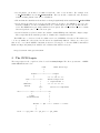
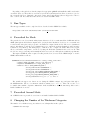
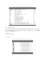
The CICE Scripts
The setup scripts for the coupled model are located in cesm1/scripts. The directory structure of CICE4
within CESM is shown below.
cesm1
(main directory)
|
|
models--------+--------- scripts
|
|
|
* * * * *|* * * * *
bld------+------ice
*build scripts for*
|
|
* coupled model *
(Makefile
|
* * * * * * * * * *
macros)
|
cice
(active ice component)
|
bld ---------- docs -------+------- src
|
|
(CICE
|
documentation)
|
|
|
drivers --- mpi ---+--- serial --- source
|
|
|
cice4 ---- cpl_esmf --+-- cpl_mct ---- cpl_share
3
2.1
Coupled Model Scripts
The CESM1 scripts have been significantly upgraded from CCSM3 and are based on a completely different
design philosophy. The new scripts will generate a set of ”resolved scripts” for a specific configuration determined by the user. The configuration includes components, resolution, run type, and machine. The run and
setup scripts that were previously in the /scripts directory for CCSM3 are now generated automatically.
See the CESM1 User’s Guide for information on how to use the new scripts:
http://www.cesm.ucar.edu/models/cesm1.0/cesm doc/book1.html.
The file that contains the ice model namelist is now located in $CASE/Buildconf. The script containing
the environment variables used for building the executable file for the ice model is also in $CASE/Buildconf.
The contents of the ice model namelist are described in section 3.
2.2
The Build Environment
The build and configure environment has changed significantly from previous versions of CESM. The build
namelist and configure utilities are based on the CAM scripts ().
The configure utility includes setting compile time parameters such as the horizontal grid, the sea ice
mode (prognostic or prescribed), tracers, etc. Additional options can be set using the configure utility such
as the decomposition, and the number of tasks, but these are typically set via CESM enviroment variables.
However, the CAM scripts set some of these explicitly through the configure command line. For example
one such configure line in the CESM scripts is:
#-------------------------------------------------------------------# Invoke cice configure
#--------------------------------------------------------------------
set hgrid = "-hgrid $ICE_GRID"
if ($ICE_GRID =~ *T*) set hgrid = "-hgrid ${ICE_NX}x${ICE_NY}"
set mode = "-cice_mode $CICE_MODE"
cd $CASEBUILD/ciceconf || exit -1
$CODEROOT/ice/cice/bld/configure $hgrid $mode -nodecomp $CICE_CONFIG_OPTS || exit -1
This example sets the horizontal grid and the mode (prognostic or prescribed). The build namelist
utility sets up the namelist which controls the run time options for the CICE model. This utility sets namelist
flags based on compile time settings from configure and some standard defaults based on horizontal grids
and other options. The typical execution during the CESM configure is:
$CODEROOT/ice/cice/bld/build-namelist -config config_cache.xml \
-csmdata \$DIN_LOC_ROOT -infile ccsm_namelist \
-inputdata $CASEBUILD/cice.input_data_list \
-namelist "&cice $CICE_NAMELIST_OPTS /" || exit -1
Again, the typical usage of the build namelist tool is through the CESM scripts, but can be called via
the command line interface.
4
2.2.1
CICE Preprocessor Flags
Preprocessor flags are activated in the form -Doption in the cice.buildexe.csh script. Only advanced users
should change these options. See the CESM User’s Guide or the CICE reference guide for more information
on these. The flags specific to the ice model are:
CPPDEFS := $(CPPDEFS) -DCESMCOUPLED -Dcoupled -Dncdf -DNCAT=5 -DNXGLOB=$()
-DNYGLOB=$() -DNTR_AERO=3 -DBLCKX=$() -DBLCKY=$() -DMXBLCKS=$()
The options -DCESMCOUPLED and -Dcoupled are set to activate the coupling interface. This will include
the source code in ice comp mct.F90, for example. In coupled runs, the CESM coupler multiplies the
fluxes by the ice area, so they are divided by the ice area in CICE to get the correct fluxes.
The options -DBLCKX=$(CICE BLCKX) and -DBLCKY=$(CICE BLCKY) set the block sizes used in each grid
direction. These values are set automatically in the scripts for the coupled model. Note that BLCKX and
BLCKY must divide evenly into the grid, and are used only for MPI grid decomposition. If BLCX or BLCKY do
not divide evenly into the grid, which determines the number of blocks in each direction, the model setup
will exit from the setup script and print an error message to the ice.bldlog* (build log) file.
The flag -DMXBLCKS is essentially the threading option. This controls the number of ”blocks” per processor. This can describe the number of OpenMP threads on an MPI task, or can simply be that a single MPI
task handles a number of blocks.
The flat -DNTR AERO=n flag turns on the aerosol deposition physics in the sea ice where n is the number
of tracer species and 0 turns off the tracers. More details on this are in the section on tracers.
The flag -D MPI sets up the message passing interface. This must be set for runs using a parallel
environment. To get a better idea of what code is included or excluded at compile time, grep for ifdef and
ifndef in the source code or look at the *.f90 files in the /obj directory.
3
Namelist Variables
CICE uses the same namelists for both the coupled and uncoupled models. This section describes the
namelist variables in the namelist ice nml, which determine time management, output frequency, model
physics, and filenames The ice namelists for the coupled model are now located in $CASE/Buildconf.
A script reads the input namelist at runtime, and writes the namelist information to the file ice in
in the directory where the model executable is located. Therefore, the namelist will be updated even if
the ice model is not recompiled. The default values of the ice setup, grid, tracer, and physics namelists
are set in ice init.F90. The prescribed ice option along with the history namelist variables are set in
ice prescribed.F90 and ice history.F90 respectively. If they are not set in the namelist in the script,
they will assume the default values listed in Tables 1-8, which list all available namelist parameters. The
default values shown here are for the coupled model, which is set up for a production run. Only a few of
these variables are required to be set in the namelist; these values are noted in the paragraphs below. An
example of the default namelist is shown in Section 3.9.1.
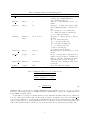
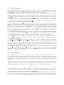
The main run management namelist options are shown in Table 1. While additional namelist variables
are available in the uncoupled version, they are set by the driver in CESM. Variables set by the driver
include: dt, runid, runtype, istep0, days per year, restart and dumpfreq. These should be changed in
the CESM configuration files:
CESM scripts (http://www.cesm.ucar.edu/models/cesm1.0/cesm doc/book1.html).
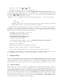
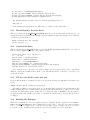
3.1
Changing the timestep
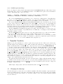
dt is the timestep in seconds for the ice model thermodynamics. The thermodynamics component is stable
but not necessarily accurate for any value of the timestep. The value chosen for dt depends on the stability
of the transport and the grid resolution. A conservative estimate of dt for the transport using the upwind
advection scheme is:
5
Table 1: Namelist Variables for Run Management
Default Value
Description
default
Filename for initial and branch runs
’default’ uses default initialization
’none’ initializes with no ice
xndt dyn
Integer
1
Times to loop through (sub-cycle) ice dynamics
diagfreq
Integer
24
Frequency of diagnostics written (min,
max, hemispheric sums) to standard output
24 => writes once every 24 timesteps
1 => diagnostics written each timestep
0 => no diagnostics written
histfreq
Character
’m’,’x’,’x’,’x’,’x’
Frequency of output written to history
Array
streams
’D’ or ’d’ writes daily data
’W’ or ’w’ writes weekly data
’M’ or ’m’ writes monthly data
’Y’ or ’y’ writes yearly data
’1’ writes every timestep
’x’ no history data is written
histfreq n
Integer
1,1,1,1,1
Frequency history data is written to each
stream
Logical
.true.
If true, averaged history information is
hist avg
written out at a frequency determined by
histfreq. If false, instantaneous values
rather than time-averages are written.
pointer file Character
’rpointer.ice’
Pointer file that contains the name of the
restart file.
lcdf64
Logical
.false.
Use 64-bit offset in netcdf files
Varible
ice ic
Type
character
Table 2: Maximum values for ice
Grid
min(∆x, ∆y)
gx3v5 28845.9 m
gx1v3 8558.2 m
∆t <
model timestep dt
max∆t
4.0 hr
1.2 hr
min(∆x, ∆y)
.
4max(u, v)
(1)
Maximum values for dt for the two standard CESM POP grids, assuming max(u, v) = 0.5m/s, are shown
in Table 2. The default timestep for CICE is 30 minutes, which must be equal to the coupling interval set
in the CESM configuration files.
Occasionally, ice velocities are calculated that are larger than what is assumed when the model timestep
is chosen. This causes a CFL violation in the transport scheme. A namelist option was added (xndt dyn)
to subcycle the dynamics to get through these instabilities that arise during long integrations. The default
value for this variable is one, and is typically increased to two when the ice model reaches an instability. The
value in the namelist should be returned to one by the user when the model integrates past that point.
6
3.2
Writing Output
The namelist variables that control the frequency of the model diagnostics, netCDF history, and restart
files are shown in Table 1. By default, diagnostics are written out once every 48 timesteps to the ascii file
ice.log.$LID (see section 9.1). $LID is a time stamp that is set in the main script.
The namelist variable histfreq controls the output frequency of the netCDF history files; writing
monthly averages is the default. The content of the history files is described in section 9.3. The value
of hist avg determines if instantaneous or averaged variables are written at the frequency set by histfreq.
If histfreq is set to ’1’ for instantaneous output, hist avg is set to .false. within the source code to
avoid conflicts. The latest version of CICE allows for multiple history streams, currently set to a maximum
of 5. The namelist variables, histfreq and histfreq n are now arrays which allow for different frequency
history file sets. More detail on this is available in 9.3.
The namelist variable pointer file is set to the name of the pointer file containing the restart file name
that will be read when model execution begins. The pointer file resides in the scripts directory and is created
initially by the ice setup script but is overwritten every time a new restart file is created. It will contain
the name of the latest restart file. The default filename ice.restart file shown in Table 1 will not work unless
some modifications are made to the ice setup script and a file is created with this name and contains the
name of a valid restart file; this variable must be set in the namelist. More information on restart pointer
files can be found in section 9.2.
The variables dumpfreq and dumpfreq n control the output frequency of the netCDF restart files; writing
one restart file per year is the default and is set by the CESM driver. The default format for restart files is
now netCDF, but this can be changed to binary through the namelist variable, restart format.
If print points is .true., diagnostic data is printed out for two grid points, one near the north pole
and one near the Weddell Sea. The points are set via namelist variables latpnt and lonpnt. This option
can be helpful for debugging.
incond dir, restart dir and history dir are the directories where the initial condition file, the restart
files and the history files will be written, respectively. These values are set at the top of the setup script and
have been modified from the default values to meet the requirements of the CESM filenaming convention.
This allows each type of output file to be written to a separate directory. If the default values are used, all
of the output files will be written to the executable directory.
incond file, dump file and history file are the root filenames for the initial condition file, the restart
files and the history files, respectively. These strings have been determined by the requirements of the CESM
filenaming convention, so the default values are set by the CESM driver. See 9.2 and 9.3 for an explanation
of how the rest of the filename is created.
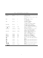
3.3
Model Physics
The namelist variables for the ice model physics are listed in Table 3. restart is almost always true since
most run types begin by reading in a binary restart file. See section 5 for a description of the run types and
about using restart files and internally generated model data as initial conditions. kcolumn is a flag that
will run the model as a single column if is set to 1. This option has not been thoroughly tested and is not
supported.
The calculation of the ice velocities is subcycled ndte times per timestep so that the elastic waves are
damped before the next timestep. The subcycling timestep is calculated as dte = dt/ndte and must be
sufficiently smaller than the damping timescale T, which needs to be sufficiently shorter than dt.
dte < T < dt
(2)
This relationship is discussed in Hunke (2001); also see Hunke and Lipscomb (2008), section 4.4. The
best ratio for [dte : T : dt] is [1 : 40 : 120]. Typical combinations of dt and ndte are (3600., 120), (7200.,
240) (10800., 120). The default ndte is 120 as set in ice init.F90.
kitd determines the scheme used to redistribute sea ice within the ice thickness distribution (ITD) as the
ice grows and melts. The linear remapping scheme is the default and approximates the thickness distribution
in each category as a linear function (Lipscomb (2001)). The delta function method represents g(h) in each
7
Varible Name
ndte
kcolumn
kitd
kdyn
kstrength
evp damping
advection
shortwave
albicev
albicei
albsnowv
albsnowi
R ice
R pnd
R snw
dT mlt in
rsnw mlt in
Table 3: Namelist Variables for Model Physics
Type
Default Value
Description
Integer
1
Number of sub-cycles in EVP dynamics.
Integer
0
Column model flag.
0 = off
1 = column model (not tested or supported)
Integer
1
Determines ITD conversion
0 = delta scheme
1 = linear remapping
Integer
1
Determines ice dynamics
0 = No ice dynamics
1 = Elastic viscous plastic dynamics
Integer
1
Determines pressure formulation
0 = Hibler (1979) parameterization
1 = Rothrock (1975) parameterization
Logical
.false.
If true, use damping procedure in evp dynamics (not supported).
Character
’remap’
Determines horizontal advection scheme.
’remap’ = incremental remapping
’upwind’ = first order advection
Character
’dEdd’
Shortwave Radiative Transfer Scheme
’default’ = CESM3 Shortwave
’dEdd’ = delta-Eddington Shortwave
Double
0.73
Visible ice albedo (CESM3)
Double
0.33
Near-infrared ice albedo (CESM3)
Double
0.96
Visible snow albedo (CESM3)
Double
0.68
Near-infrared snow albedo (CESM3)
Double
0.0
Base ice grain radius tuning parameter
(dEdd)
Double
1.5
Base snow grain radius tuning parameter
(dEdd)
Double
0.0
Base pond grain radius tuning parameter
(dEdd)
Double
1.5
Snow melt onset temperature parameter
(dEdd)
Double
1500.0
Snow melt maximum radius (dEdd)
8
Varible
tr iage
tr FY
tr lvl
tr pond
tr aero
Type
Logical
Logical
Logical
Logical
Logical
Table 4: Namelist Variables for Tracers
Default Value
Description
.true.
Ice age passive tracer
.true.
First-year ice area passive tracer
.false.
Level ice area passive tracer
.true.
Melt pond physics and tracer
.true.
Aerosol physics and tracer
category as a delta function (Bitz et al. (2001)). This method can leave some categories mostly empty at
any given time and cause jumps in the properties of g(h).
kdyn determines the ice dynamics used in the model. The default is the elastic-viscous-plastic (EVP)
dynamics Hunke and Dukowicz (1997). If kdyn is set to o 0, the ice dynamics is inactive. In this case, ice
velocities are not computed and ice is not transported. Since the initial ice velocities are read in from the
restart file, the maximum and minimum velocities written to the log file will be non-zero in this case, but
they are not used in any calculations.
The value of kstrength determines which formulation is used to calculate the strength of the pack ice.
The Hibler (1979) calculation depends on mean ice thickness and open water fraction. The calculation of
Rothrock (1975) is based on energetics and should not be used if the ice that participates in ridging is not
well resolved.
evp damping is used to control the damping of elastic waves in the ice dynamics. It is typically set to
.true. for high-resolution simulations where the elastic waves are not sufficiently damped out in a small
timestep without a significant amount of subcycling. This procedure works by reducing the effective ice
strength that’s used by the dynamics and is not a supported option.
advection determines the horizontal transport scheme used. The default scheme is the incremental
remapping method (Lipscomb and Hunke (2004)). This method is less diffusive and is computationally
efficient for large numbers of categories or tracers. The upwind scheme is also available. The upwind scheme
is only first order accurate.
The base values of the snow and ice albedos for the CESM3 shortwave option are set in the namelist.
The ice albedos are those for ice thicker than ahmax, which is currently set at 0.5 m. This thickness is a
parameter that can be changed in ice shortwave.F90. The snow albedos are for cold snow.
For the new delta-Eddington shortwave radiative transfer scheme Briegleb and Light (2007), the base
albedos are computed based on the inherent optical properties of snow, sea ice, and melt ponds. These
albedos are tunable through adjustments to the snow grain radius, R snw, temperature to transition to
melting snow, and maximum snow grain radius.
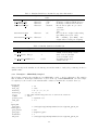
3.4
Tracer Namelist
The namelist parameters listed in Table 4 are for adding tracers. See section on tracers.
3.5
Prescribed Ice Namelist
The namelist parameters listed in Table 5 are for the prescribed ice option as used in AMIP and F compset
(standalone CAM) runs 6.
3.6
Grid Namelist
The namelist parameters listed in Table 6 are for grid and mask information. During execution, the ice model
reads grid and land mask information from the files grid file and kmt file that should be located in the
executable directory. There are commands in the scripts that copy these files from the input data directory,
rename them from global $ICE GRID.grid and global $ICE GRID.kmt to the default filenames shown
in Table 6.
9
Table 5: Namelist Variables for Prescribed Ice Option
Varible
prescribed ice
prescribed ice fill
stream year first
stream year last
model year align
Type
Logical
Logical
Integer
Integer
Integer
Default Value
.false.
.false.
1
1
1
stream domfilename
stream fldfilename
stream fldvarname
Character
Character
Character
ice cov
Varible
grid type
grid format
grid file
kmt file
kcatbound
Description
Flag to turn on prescribed ice
Flag to turn fill option
First year of prescribed ice data
Last year of prescribed ice data
Year in model run that aligns with
stream year first
Prescribed ice stream data file
Prescribed ice stream data file
Ice fraction field name
Table 6: Namelist Variables for Grid and Mask Information
Type
Default Value
Description
Character
’displaced pole’
Determines grid type.
’displaced pole’
’tripole’
’rectangular’
Character
binary
Grid file format (binary or netCDF)
Character
’data.domain.grid’
Input filename containing grid information.
Character
’data.domain.kmt’
Input filename containing land mask information.
Integer
0
How category boundaries are set (0 or
1)
For coupled runs, supported grids include the ’displaced pole’ grids (gx3v7 and gx1v6) and the
’tripole’ grids.
3.7
Domain Namelist
The namelist parameters listed in Table 7 are for computational domain decomposition information. These
are generally set in the build configure scripts based on the number of processors. See the CESM scripts
documentation.
3.8
PIO Namelist
The namelist parameters listed in Table 8 are for controlling parallel input/output. Only a brief overview
will be given here, but more on parallel input/output can be found at:
http://web.ncar.teragrid.org/~dennis/pio doc/html.
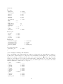
3.9
Example Namelists
This section shows several examples of namelists from the coupled ice model. These examples are taken
directly from cice.buildnml.csh for the coupled model. Most of the variables in the namelist are determined
from environment variables set elsewhere in the scripts. Since the namelists from the coupled model are
”resolved” by the scripts, meaning that the values of most of the shell script variables are put directly into
the namelist, examples are shown for the most commonly used configurations. Variables that are commonly
10
Table 7: Namelist Variables for Domain Decomposition Information
Type
Default
Description
Value
processor shape
Character
’square-pop’
Approximate block shapes
ew boundary type
Character
’cyclic’
Boundary conditions in E-W direction
ns boundary type
Character
’open’
Boundary conditions in N-S direction
Character
’cartesian’
How blocks are split onto processors
distribution type
’cartesian’
’spacecurve’
’rake’
distribution wght
Character
’erfc’
How blocks are weighted when using
space-filling curves (erfc or file)
distribution wght file Character
”
File containing space-filling curve
weights when not using erfc weighting
Varible
Table 8: Namelist Variables for Parallel I/O
Default Value
Description
-1
Number of I/O tasks.
default -1 selects all processors.
ice pio stride Integer
-1
Stride between I/O tasks.
-1 selects defaulto stride.
ice pio type nameCharacter
netcdf
Underlying library used.
default is netcdf.
Varible
Type
ice num iotasks Integer
changed directly in the namelist are the timestep dt and the number of subcycles per timestep in the ice
dynamics ndte.
3.9.1
Example 1: CESM Fully Coupled
The following example is the namelist used for CESM fully coupled, or the B configuration. The variables
that are still set to shell script variables have been set at the top of cice.buildnml.csh or in other scripts.
A completely resolved version of the namelist will be written to ice in in the executable directory.
&setup_nml
diagfreq
hist_avg
histfreq
histfreq_n
ice_ic
lcdf64
pointer_file
xndt_dyn
/
&grid_nml
grid_file
10402.grid’
grid_format
grid_type
kcatbound
kmt_file
= 24
= .true.
= ’m’,’x’,’x’,’x’,’x’
= 1,1,1,1,1
= ’b40.1850.track1.1deg.006.cice.r.0301-01-01-00000.nc’
= .false.
= ’rpointer.ice’
= 1.0
= ’/fis/cgd/cseg/csm/inputdata/ice/cice/global_gx1v6_200
= ’bin’
= ’displaced_pole’
= 0
= ’/fis/cgd/cseg/csm/inputdata/ice/cice/global_gx1v6_200
11
90204.kmt’
/
&ice_nml
advection
=
albedo_type
=
albicei
=
albicev
=
albsnowi
=
albsnowv
=
evp_damping
=
kdyn
= 1
kitd
= 1
krdg_partic
=
krdg_redist
=
kstrength
=
ndte
= 120
r_snw
= 1.5
shortwave
=
/
&tracer_nml
tr_aero
= .true.
tr_FY
= .true.
tr_iage
= .true.
tr_pond
= .true.
/
&domain_nml
distribution_type
ew_boundary_type
ns_boundary_type
processor_shape
/
&ice_prescribed_nml
prescribed_ice
=
/
3.9.2
’remap’
’default’
0.45
0.75
0.73
0.98
.false.
1
1
1
’dEdd’
=
=
=
=
’cartesian’
’cyclic’
’open’
’square-pop’
.false.
Example 2: History File Namelist
The second namelist controls what variables are written to the history file. By default, all files are written to
the history file. Variables that are not output are set in the namelist icefields nml. Some of the following
fields are not written to the history file since they can be retrieved from the ocean history files. The melt
and freeze onset fields are not used, since the information they contain may not be correct if the model is
restarted mid-year. The ice areas and volumes for categories six through ten are not used, since the default
thickness distribution consists of five ice categories.
f_aero
f_aicen
f_aisnap
f_apondn
f_congel
f_daidtd
f_daidtt
f_divu
f_dvidtd
f_dvidtt
f_faero_atm
= ’mxxxx’
=
=
=
=
=
=
= ’mxxxx’
=
=
=
’mxxxx’
’mdxxx’
’mxxxx’
’mxxxx’
’mxxxx’
’mxxxx’
’mxxxx’
’mxxxx’
’mxxxx’
12
f_faero_ocn
f_fhocn
f_fhocn_ai
f_frazil
f_fresh
f_fresh_ai
f_frz_onset
f_frzmlt
f_fsalt
f_fsalt_ai
f_fy
f_hisnap
f_icepresent
f_meltb
f_meltl
f_meltt
f_mlt_onset
f_opening
f_shear
f_sig1
f_sig2
f_snoice
f_sss
f_sst
f_strairx
f_strairy
f_strcorx
f_strcory
f_strength
f_strintx
f_strinty
f_strocnx
f_strocny
f_strtltx
f_strtlty
f_uocn
f_uvel
f_vicen
f_vocn
f_vvel
/
4
=
=
=
=
=
=
=
=
=
=
=
=
=
=
=
=
=
=
=
’mdxxx’
=
=
=
=
=
=
=
=
’mxxxx’
’mxxxx’
=
’xxxxx’
’xxxxx’
=
=
=
=
=
=
=
=
=
=
=
’xxxxx’
’mxxxx’
=
’xxxxx’
’mxxxx’
’mxxxx’
’mxxxx’
’mxxxx’
’mxxxx’
’mxxxx’
’mxxxx’
’xxxxx’
’xxxxx’
’mxxxx’
’mxxxx’
’mdxxx’
’mxxxx’
’mxxxx’
’mxxxx’
’mxxxx’
’xxxxx’
’mxxxx’
’mxxxx’
’mxxxx’
’mxxxx’
’mxxxx’
’mxxxx’
’mxxxx’
’mxxxx’
’mxxxx’
’mxxxx’
’mxxxx’
’mxxxx’
’xxxxx’
’xxxxx’
’mxxxx’
Model Input Datasets
The coupled CICE model requires a minimum of three files to run:
• global ${ICE GRID}.grid is a binary file containing grid information
• global ${ICE GRID}.kmt is a binary file containing land mask information
• iced.0001-01-01.${ICE GRID}.20lay are binary files containing initial condition information for
the gx1v6 and gx3v7 grids, respectively. The thickness distribution in this restart file contains 5
categories, each with 4 layers.
13
Depending on the grid selected in the scripts, the appropriate global* and iced* files will be used in the
executable directory. These files are read directory from the system input data directory and not copied to
the executable directory. Currently, only gx3v7, gx1v6, tx1v1, and tx0.1v2 grids are supported for the ice
and ocean models. Note that these files can now be used in netCDF format.
5
Run Types
The run types available for the coupled model are described in the CESM User’s Guide:
http://www.cesm.ucar.edu/models/cesm1.0/cesm doc/book1.html.
6
Prescribed Ice Mode
The prescribed ice mode is a functionality feature that is needed for certain standalone CAM runs such as
AMIP (Atmospheric Model Intercomparison Project) style runs. In this mode, the sea ice concentration is
read from a file and replaces the prognostic concentrations computed in the model. The sea ice dynamics is
turned off in this mode and the sea ice thickness is reset to 2 m in the northern hemisphere and 1 m in the
southern at every timestep. The main purpose of this mode is to compute the surface fluxes, snow depth,
albedos, and surface temperature over the ice by using the 1D thermodynamics in the sea ice model. This
mode is not energy conserving and is mainly intended as a testbed for atmospheric sensitivity experiments.
The input netCDF file name required for this prescribed mode is set in the CESM scripts or via the
CICE build-namelist as follows:
$CODEROOT/ice/cice/bld/build-namelist -config config_cache.xml \
-csmdata \$DIN_LOC_ROOT -infile ccsm_namelist \
-inputdata $CASEBUILD/cice.input_data_list \
-namelist "&cice $CICE_NAMELIST_OPTS \
stream_fldfilename=’$CESMSSTFN’ \
stream_domfilename=’$CESMSSTFN’ \
stream_year_first=$DOCN_SSTDATA_YEAR_START \
stream_year_last=$DOCN_SSTDATA_YEAR_END \
model_year_align=$DOCN_SSTDATA_YEAR_START \
stream_fldvarname=’ice_cov’ /" || exit -1
The variables in upper case letters are set during the CESM configure step and passed through to
the CICE namelist. The ice concentration variable is assumed to be ”ice cov”. There also needs to be a
reconizable time axis like ”days since 0001-01-01” in the netCDF file so that the time interpolation can be
handled within the ice model.
7
Prescribed Aerosol Mode
As of CESM version 1, prescribed aerosols are now handled within CAM or DATM.
8
Changing the Number of Ice Thickness Categories
The number of ice thickness categories affects ice model input files in three places:
• $NCAT in the run script
14
• The source code module ice model size.F90
• The initial condition (restart) file in the input file directory
The number of ice thickness categories is set in $CASE/Buildconf/cice.buildexe.csh using the variable called $NCAT. The default value is 5 categories. $NCAT is used to determine the CPP variable setting
(NCAT) in ice model size.F90. $RES is the resolution of the grid, 100x116 (gx3v7) and 320x384 (gx1v6)
for low and medium resolution grids, respectively.
NOTE: To use one ice thickness category, the following changes will need to be made in the namelist:
, kitd
, kstrength
= 0
= 0
With these settings, the model will use the delta scheme instead of linear remapping and a strength
parameterization based on open water area and mean ice thickness.
The information in the initial restart file is dependent on the number of ice thickness categories and the
total number of layers in the ice distribution. An initial condition file exists only for the default case of 5
ice thickness categories, with four layers in each category. To create an initial condition file for a different
number of categories or layers, these steps should be followed:
• Set $NCAT to the desired number of categories in
$CASE/Buildconf/cice.buildexe.csh.
• Set the namelist variable dumpfreq = ’m’ in
$CASE/Buildconf/cice.buildnml.csh
to print out restart files monthly.
• Set the namelist variable restart = .false. in $CASE/Buildconf/cice.buildnml.csh
to use the initial conditions within the ice model.
• Run the model to equilibrium.
• The last restart file can be used as an initial condition file.
• Change the name of the last restart file to iced.0001-01-01.$GRID.
• Copy the file into the input data directory or directly into the the executable directory.
Note that the date printed inside the binary restart file will not be the same as 0001-01-01. For coupled
runs, $BASEDATE will be the starting o date and the date inside the file will not be used.
9
Output Data
The ice model produces three types of output data. A file containing ASCII text, also known as a log file, is
created for each run that contains information about how the run was set up and how it progressed. A series
of binary restart files necessary to continue the run are created. A series of netCDF history files containing
gridded instantaneous or time-averaged output are also generated during a run. These are described below.
9.1
Stdout Output
Diagnostics from the ice model are written to an ASCII file that contains information from the compilation,
a record of the input parameters, and how hemispherically averaged, maximum and minimum values are
evolving with the integration. Certain error conditions detected within the ice setup script or the ice model
will also appear in this file. Upon the completion of the simulation, some timing information will appear at
the bottom of the file. The file name is of the form ice.log.$LID, where $LID is a timestamp for the file
ID. It resides in the executable directory. The frequency of the diagnostics is determined by the namelist
parameter diagfreq. Other diagnostic messages appear in the ccsm.log.$LID or cpl.log.$LID files in the
executable directory. See the CESM scripts documentation.
15
9.2
Restart Files
Restart files contain all of the initial condition information necessary to restart from a previous simulation.
These files are in a standard netCDF 64-bit binary format. A restart file is not necessary for an initial run,
but is highly recommended. The initial conditions that are internal to the ice model produce an unrealistic
ice cover that an uncoupled ice model will correct in several years. The initial conditions from a restart file
are created from an equilibrium solution, and provide more realistic information that is necessary if coupling
to an active ocean model. The frequency at which restart files are created is controlled by the namelist
parameter dumpfreq. The names of these files are proceeded by the namelist parameter dump file and,
by default are written out yearly to the executable directory. To change the directory where these files are
located, modify the variable $RSTDIR at the top of the setup script. The names of the restart files follow the
CESM Output Filename Requirements. The form of the restart file names are as follows:
$CASE.cice.r.yyyy-mm-dd-sssss.nc
For example, the file $CASE.cice.r.0002-01-01-00000.nc would be written out at the end of year 1,
month 12. A file containing the name of a restart file is called a restart pointer file. This filename information
allows the model simulation to continue from the correct point in time, and hence the correct restart file.
Restart Pointer Files
A pointer file is an ascii file named rpointer.ice that contains the path and filename of the latest restart
file. The model uses this information to find a restart file from which initialization data is read. The pointer
files are written to and then read from the executable directory. For startup runs, a pointer is created by
the ice setup script Whenever a restart file is written, the existing restart pointer file is overwritten. The
namelist variable pointer file contains the name of the pointer file. Pointer files seldom need editing. The
contents are usually maintained by the setup script and the component model.
9.3
History Files
History files contain gridded data values written at specified times during a model run. By default, the
history files will be written to the directory history dir defined in the namelist. The netCDF file names
are prepended by the character string given by history file in the ice nml namelist. This character string
has been set according to CESM Output Filename Requirements. If history file is not set in the namelist,
the default character string ’iceh’ is used. The user can specify the frequency at which the data are written.
Options are also available to record averaged or instantaneous data. The form of the history file names are
as follows:
Yearly averaged: $CASE.cice.h?.yyyy.nc
Monthly averaged: $CASE.cice.h?.yyyy-mm.nc
Daily averaged: $CASE.cice.h?.yyyy-mm-dd.nc
Instantaneous (histfreq = ’y’, ’m’, or ’d’): $CASE.cice.h?.yyyy-mm-dd-sssss.nc
Instantaneous (written every dt, histfreq = 1): $CASE.cice.h?.yyyy-mm-dd-sssss.nc
$CASE is set in the main setup script. Note that the ? denotes the multiple stream option where the first
stream is just .h. and subsequent streams are h1, h2, etc. All history files are written in the executable
directory. Changes to the frequency and averaging will affect all output fields. The best description of
the history data comes from the file itself using the netCDF command ncdump -h filename.nc. Variables
containing grid information are written to every file and are listed in Table 9. In addition to the history files,
a netCDF file containing a snapshot of the initial ice state can be created at the start of each run. The file
name is $CASE.cice.i.yyyy-mm-dd-sssss.nc and is written in the executable directory.
16
9.3.1
Caveats Regarding Averaged Fields
In computing the monthly averages for output to the history files, most arrays are zeroed out before being
filled with data. These zeros are included in the monthly averages where there is no ice. For some fileds,
this is not a problem, for example, ice thickness and ice area. For other fields, this will result in values that
are not representative of the field when ice is present. Some of the fields affected are:
• Flat, Fsens - latent and sensible heat fluxes
• evap - evaporative water flux
• Fhnet - ice/ocn net heat flux
• Fswabs - snow/ice/ocn absorbed solar flux
• strairx, strairy - zonal and meridional atm/ice stress
• strcorx, strcory - zonal and meridional coriolis stress
For some fields, a non-zero value is set where there is no ice. For example, Tsfc has the freezing point
averaged in, and Flwout has σTf4 averaged in. At lower latitudes, these values can be erroneous.
To aid in the interpretation of the fields, a field called ice present is written to the history file. It contains
information on the fraction of the time-averaging interval when any ice was present in the grid cell during
the time-averaging interval in the history file. This will give an idea of how many zeros were included in the
average.
The second caveat results from the coupler multiplying fluxes it receives from the ice model by the ice
area. Before sending fluxes to the coupler, they are divided by the ice area in the ice model. These are the
fluxes that are written to the history files, they are not what affects the ice, ocean or atmosphere, nor are
they useful for calculating budgets. The division by the ice area also creates large values of the fluxes at the
ice edge. The affected fields are:
• Flat, Fsens - latent and sensible heat fluxes
• Flwout - outgoing longwave
• evap - evaporative water flux
• Fresh - ice/ocn fresh water flux
• Fhnet - ice/ocn net heat flux
• Fswabs - snow/ice/ocn absorbed solar flux
When applicable, two of the above fields will be written to the history file: the value of the field that
is sent to the coupler (divided by ice area) and a value of the flux that has been multiplied by ice area
(what affects the ice). Fluxes multiplied by ice area will have the suffix aice appended to the variable
names in the history files. Fluxes sent to the coupler will have ”sent to coupler” appended to the long name.
Fields of rainfall and snowfall multiplied by ice area are written to the history file, since the values are valid
everywhere and represent the precipitation rate on the ice cover.
9.3.2
Changing Frequency and Averaging
The frequency at which data are written to a history file as well as the interval over which the time average is
to be performed is controlled by the namelist variable histfreq. Data averaging is invoked by the namelist
variable hist avg. The averages are constructed by accumulating the running sums of all variables in
memory at each timestep. The options for both of these variables are described in Table 1. If hist avg is
true, and histfreq is set to monthly, for example, monthly averaged data is written out on the last day of
the month.
17
Table 9: Time and Grid Information Written to History File
Field
Description
time
model time
time bounds boundaries for time-averaging interval
TLON
T grid center longitude
TLAT
T grid center latitude
ULON
U grid center longitude
ULAT
U grid center latitude
tmask
ocean grid mask (0=land, 1=ocean)
tarea
T grid cell area
uarea
U grid cell area
dxt
T cell width through middle
dyt
T cell height through middle
dxu
U cell width through middle
dyu
U cell height through middle
HTN
T cell width North side
HTE
T cell width East side
ANGLET
angle grid makes with latitude line on T grid
ANGLE
angle grid makes with latitude line on U grid
ice present fraction of time-averaging interval that any ice is present
9.3.3
Units
days
days
degrees
degrees
degrees
degrees
m2
m2
m
m
m
m
m
m
radians
radians
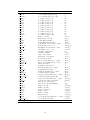
Changing Content
The second namelist in the setup script controls what variables are written to the history file. To remove a
field from this list, add the name of the character variable associated with that field to the &icefields nml
namelist in cice.buildnml.csh and assign it a value of ’xxxxx’. For example, to remove ice thickness and
snow cover from the history file, add
&icefields_nml
f_hi
= ’xxxxx’
, f_hs
= ’xxxxx’
/
to the namelist.
Table 10: Standard Fields Available for Output to History File
Logical Variable
f hi
f hs
f fs
f Tsfc
f aice
f aice1
f aice2
f aice3
f aice4
f aice5
f aice6
f aice7
Description
grid box mean ice thickness
grid box mean snow thickness
grid box mean snow fraction
snow/ice surface temperature
ice concentration (aggregate)
ice concentration (category 1)
ice concentration (category 2)
ice concentration (category 3)
ice concentration (category 4)
ice concentration (category 5)
ice concentration (category 6)
ice concentration (category 7)
continued on next page
18
Units
m
m
%
C
%
%
%
%
%
%
%
%
continued from previous page
f
f
f
f
f
f
f
f
f
f
f
f
f
f
f
f
f
f
f
f
f
f
f
f
f
f
f
f
f
f
f
f
f
f
f
f
f
f
f
f
f
f
f
f
f
f
f
f
aice8
aice9
aice10
vice1
vice2
vice3
vice4
vice5
vice6
vice7
vice8
vice9
vice10
uvel
vvel
fswdn
flwdn
snow
snow ai
rain
rain ai
sst
sss
uocn
vocn
frzmlt
fswabs
fswabs ai
aldvr
aldvi
flat
flat ai
fsens
fsens ai
flwout
flwout ai
evap
evap ai
Tref
Qref
congel
frazil
snoice
meltb
meltt
meltl
fresh
fresh ai
ice concentration (category 8)
ice concentration (category 9)
ice concentration (category 10)
ice volume (category 1)
ice volume (category 2)
ice volume (category 3)
ice volume (category 4)
ice volume (category 5)
ice volume (category 6)
ice volume (category 7)
ice volume (category 8)
ice volume (category 9)
ice volume (category 10)
zonal ice velocity
meridional ice velocity
downwelling solar flux
downwelling longwave flux
snow fall rate received from coupler
snow fall rate on ice cover
rain fall rate received from coupler
rain fall rate on ice cover
sea surface temperature
sea surface salinity
zonal ocean current
meridional ocean current
freeze/melt potential
absorbed solar flux sent to coupler
absorbed solar flux in snow/ocn/ice
visible direct albedo
near-infrared direct albedo
latent heat flux sent to coupler
ice/atm latent heat flux
sensible heat flux sent to coupler
ice/atm sensible heat flux
outgoing longwave flux sent to coupler
ice/atm outgoing longwave flux
evaporative water flux sent to coupler
ice/atm evaporative water flux
2 m reference temperature
2 m reference specific humidity
basal ice growth
frazil ice growth
snow-ice formation
basal ice melt
surface ice melt
lateral ice melt
ice/ocn fresh water flux sent to coupler
ice/ocn fresh water flux
continued on next page
19
%
%
%
m
m
m
m
m
m
m
m
m
m
cm s−1
cm s−1
W m−2
W m−2
cm day−1
cm day−1
cm day−1
cm day−1
C
g kg−1
cm s−1
cm s−1
W m−2
W m−2
W m−2
%
%
W m−2
W m−2
W m−2
W m−2
W m−2
W m−2
cm day−1
cm day−1
C
g/kg
cm day−1
cm day−1
cm day−1
cm day−1
cm day−1
cm day−1
cm day−1
cm day−1
continued from previous page
f
f
f
f
f
f
f
f
f
f
f
f
f
f
f
f
f
f
f
f
f
f
f
f
f
f
f
f
fsalt
fsalt ai
fhnet
fhnet ai
fswthru
fswthru ai
strairx
strairy
strtltx
strtlty
strcorx
strcory
strocnx
strocny
strintx
strinty
strength
divu
shear
opening
sig1
sig2
daidtt
daidtd
dvidtt
dvidtd
mlt onset
frz onset
10
10.1
ice to ocn salt flux sent to coupler
ice to ocn salt flux
ice/ocn net heat flux sent to coupler
ice/ocn net heat flux
SW transmitted through ice to ocean sent to coupler
SW transmitted through ice to ocean
zonal atm/ice stress
meridional atm/ice stress
zonal sea surface tilt
meridional sea surface tilt
zonal coriolis stress
meridional coriolis stress
zonal ocean/ice stress
meridional ocean/ice stress
zonal internal ice stress
meridional internal ice stress
compressive ice strength
velocity divergence
strain rate
lead opening rate
normalized principal stress component
normalized principal stress component
area tendency due to thermodynamics
area tendency due to dynamics
ice volume tendency due to thermo.
ice volume tendency due to dynamics
melt onset date
freeze onset date
kg m−2 day−1
kg m−2 day−1
W m−2
W m−2
W m−2
W m−2
N m−2
N m−2
m m−1
m m−1
N m−2
N m−2
N m−2
N m−2
N m−2
N m−2
N m−1
% day−1
% day−1
% day−1
% day−1
% day−1
cm day−1
cm day−1
Troubleshooting
Code does not Compile or Run
Check the ice.log.* or ice.bldlog.* files in the executable directory, or the standard output and error files
for information. Also, try the following:
• Delete the executable directory and rebuild the model.
• Make sure that there is a Macros.<OS> file for your platform. Modify the directory paths for the
libraries.
• Make sure all paths and file names are set correctly in the scripts.
• If changes were made to the ice model size.F90 file in the source code directory, they will be overwritten by the file in input templates.
10.2
Negative Ice Area in Horizontal Remapping
This error is written from ice transport remap.F90 when the ice model is checking for negative ice areas.
If it happens well into a model integration, it can be indicative of a CFL violation. The output looks like:
60:
60:
60:
60:
New area < 0, istep = 119588
(my_task,i,j,n) = 4 21 380 1
Old area = 0.960675000975677174E-05
New area = -0.161808948357841311E-06
20
60: Net flux = -0.976855895811461324E-05
60:(shr_sys_abort) ERROR: remap transport: negative area
60:(shr_sys_abort) WARNING: calling shr_mpi_abort() and stopping
60:(shr_mpi_abort):remap transport: negative area 0
The dynamics timestep should be reduced to integrate past this problem. Set
, xndt_dyn = 2
in the namelist and restart the model. When the job completes set the value back to 1.
10.3
Thermodynamic Iteration Error
This error is written from ice therm vertical.F90 when the ice model temperature iteration is not converging in the thermodynamics. This is usually a problem with the forcing, but sometimes can be indicative
of a timestep problem in the ice.
Thermo iteration does not converge
istep1, my_task, i, j:
10.4
Conservation Error
This error is written from ice itd.F when the ice model is checking that initial and final values of a conserved
field are equal to within a small value. The output looks like:
Conservation error: vice, add_new_ice
11 : 14 185
Initial value = 1362442.600400560
Final value = 1362442.600400561
Difference = 2.328306436538696D-10
(shr_sys_abort) ERROR: ice: Conservation error
(shr_sys_abort) WARNING: calling shr_mpi_abort() and stopping
(shr_mpi_abort):ice: Conservation error 0
Non-conservation can occur if the ice model is receiving very bad forcing, and is not able to deal with it.
This has occurred after a CFL violation in the ocean. The timestep in the ocean may be decreased to get
around the problem.
10.5
NX does not divide evenly into grid
If you modify the number of tasks used by the ice model, the model may stop with this error written to the
log file:
’ERROR: NX must divide evenly into grid,100,8’
The number of MPI processors used by the ice model must divide evenly into the grid dimensions. For
example, running the ice model with 8 tasks on the gx3v7 grid will result in an error, since 8 does not divide
evenly into the 100 longitude points. To fix this error, change the value of $NTASKS for the uncoupled ice
model in the main script. In this case, a value of 4 would work, and the task geometry would also have to
be changed.
10.6
Enabling the Debugger
This section explains how to set some compiler options for debugging. For the coupled model, set DEBUG to
TRUE in the env run.xml script. Before running the model, be sure to delete the object files so that the
source code will be recompiled. If a core file is created, it will be in the executable directory. Use dbx to
look at the core file. Useful information may also appear in the standard error and output files.
21
References
Bitz, C. M., M. Holland, M. Eby and A. J. Weaver, 2001: Simulating the ice-thickness distribution in a
coupled climate model. J. Geophys. Res., 106, 2441–2463.
Bitz, C. M. and W. H. Lipscomb, 1999: An energy-conserving thermodynamic model of sea ice. J. Geophys.
Res., 104, 15,669–15,677.
Briegleb, B. P. and B. Light, 2007: A Delta-Eddington Multiple Scattering Parameterization for Solar
Radiation in the Sea Ice Component of the Community Climate System Model. NCAR Technical Note
NCAR/TN-472+STR, National Center for Atmospheric Research, Boulder, Colorado.
Hibler, W. D., 1979: A dynamic thermodynamic sea ice model. J. Phys. Oceanogr., 9, 815–846.
Hunke, E. C., 2001: Viscous-plastic sea ice dynamics with the evp model: Linearization issues. J. Comp.
Phys., 170, 18–38.
Hunke, E. C. and J. K. Dukowicz, 1997: An elastic-viscous-plastic model for sea ice dynamics. J. Phys.
Oceanogr., 27, 1849–1867.
Hunke, E. C. and W. H. Lipscomb, 2008: CICE: The Los Alamos Sea Ice Model. Documentation and Software
User’s Manual. Version 4.0. T-3 Fluid Dynamics Group, Los Alamos National Laboratory, Tech. Rep.
LA-CC-06-012.
Lipscomb, W. H., 2001: Remapping the thickness distribution in sea ice models. J. Geophys. Res., 106,
13,989–14,000.
Lipscomb, W. H. and E. C. Hunke, 2004: Modeling sea ice transport using incremental remapping. Mon.
Wea. Rev., 132, 1341–1354.
Rothrock, D. A., 1975: The energetics of the plastic deformation of pack ice by ridging. J. Geophys. Res.,
80, 4514–4519.
Thorndike, A. S., D. S. Rothrock, G. A. Maykut and R. Colony, 1975: The thickness distribution of sea ice.
J. Geophys. Res., 80, 4501–4513.
22