Download TwoTowers 5.1 User Manual

TwoTowers 5.1
User Manual
Marco Bernardo
January 2006
c 2006
°
ii
Contents
1 Tool Description
1.1 What TwoTowers 5.1 Is . . . .
1.2 Architecture of TwoTowers 5.1
1.3 What TwoTowers 5.1 Offers . .
1.4 Case Studies . . . . . . . . . .
1.5 History of TwoTowers . . . . .
1.6 Acknowledgments . . . . . . . .
.
.
.
.
.
.
.
.
.
.
.
.
.
.
.
.
.
.
.
.
.
.
.
.
.
.
.
.
.
.
.
.
.
.
.
.
.
.
.
.
.
.
.
.
.
.
.
.
.
.
.
.
.
.
.
.
.
.
.
.
.
.
.
.
.
.
.
.
.
.
.
.
.
.
.
.
.
.
.
.
.
.
.
.
.
.
.
.
.
.
.
.
.
.
.
.
.
.
.
.
.
.
.
.
.
.
.
.
.
.
.
.
.
.
.
.
.
.
.
.
.
.
.
.
.
.
.
.
.
.
.
.
.
.
.
.
.
.
.
.
.
.
.
.
.
.
.
.
.
.
.
.
.
.
.
.
.
.
.
.
.
.
.
.
.
.
.
.
.
.
.
.
.
.
.
.
.
.
.
.
.
.
.
.
.
.
.
.
.
.
.
.
.
.
.
.
.
.
.
.
.
.
.
.
.
.
.
.
.
.
1
1
1
3
3
4
4
2 Tool Installation and Execution
2.1 Introduction . . . . . . . . . . .
2.2 Source Distribution . . . . . . .
2.3 Installation Procedure . . . . .
2.3.1 Linux . . . . . . . . . .
2.3.2 Windows . . . . . . . .
2.4 Running the Tool . . . . . . . .
2.4.1 Linux . . . . . . . . . .
2.4.2 Windows . . . . . . . .
.
.
.
.
.
.
.
.
.
.
.
.
.
.
.
.
.
.
.
.
.
.
.
.
.
.
.
.
.
.
.
.
.
.
.
.
.
.
.
.
.
.
.
.
.
.
.
.
.
.
.
.
.
.
.
.
.
.
.
.
.
.
.
.
.
.
.
.
.
.
.
.
.
.
.
.
.
.
.
.
.
.
.
.
.
.
.
.
.
.
.
.
.
.
.
.
.
.
.
.
.
.
.
.
.
.
.
.
.
.
.
.
.
.
.
.
.
.
.
.
.
.
.
.
.
.
.
.
.
.
.
.
.
.
.
.
.
.
.
.
.
.
.
.
.
.
.
.
.
.
.
.
.
.
.
.
.
.
.
.
.
.
.
.
.
.
.
.
.
.
.
.
.
.
.
.
.
.
.
.
.
.
.
.
.
.
.
.
.
.
.
.
.
.
.
.
.
.
.
.
.
.
.
.
.
.
.
.
.
.
.
.
.
.
.
.
.
.
.
.
.
.
.
.
.
.
.
.
.
.
.
.
.
.
.
.
.
.
.
.
.
.
.
.
.
.
.
.
.
.
.
.
.
.
.
.
.
.
.
.
.
.
.
.
.
.
.
.
.
.
.
.
.
.
.
.
.
.
.
.
5
5
5
7
7
7
8
8
8
Æmilia Compiler
Introduction . . . . . . . . . . . . . . . . . . . . . . . . .
Keywords and Comments . . . . . . . . . . . . . . . . .
Identifiers . . . . . . . . . . . . . . . . . . . . . . . . . .
Data Types, Operators, and Expressions . . . . . . . . .
3.4.1 Typed Identifier Declarations and Expressions .
3.4.2 Integers, Bounded Integers, and Reals . . . . . .
3.4.3 Booleans . . . . . . . . . . . . . . . . . . . . . .
3.4.4 Lists . . . . . . . . . . . . . . . . . . . . . . . . .
3.4.5 Arrays . . . . . . . . . . . . . . . . . . . . . . . .
3.4.6 Records . . . . . . . . . . . . . . . . . . . . . . .
3.4.7 Priorities, Rates, and Weights . . . . . . . . . . .
Architectural Type Header . . . . . . . . . . . . . . . .
Architectural Element Types . . . . . . . . . . . . . . .
3.6.1 AET Header . . . . . . . . . . . . . . . . . . . .
3.6.2 AET Behavior: EMPAgr Operators and Actions
3.6.3 AET Interactions . . . . . . . . . . . . . . . . . .
Architectural Topology . . . . . . . . . . . . . . . . . . .
3.7.1 Architectural Element Instances . . . . . . . . .
3.7.2 Architectural Interactions . . . . . . . . . . . . .
3.7.3 Architectural Attachments . . . . . . . . . . . .
Behavioral Variations . . . . . . . . . . . . . . . . . . .
3.8.1 Behavioral Hidings . . . . . . . . . . . . . . . . .
3.8.2 Behavioral Restrictions . . . . . . . . . . . . . .
.
.
.
.
.
.
.
.
.
.
.
.
.
.
.
.
.
.
.
.
.
.
.
.
.
.
.
.
.
.
.
.
.
.
.
.
.
.
.
.
.
.
.
.
.
.
.
.
.
.
.
.
.
.
.
.
.
.
.
.
.
.
.
.
.
.
.
.
.
.
.
.
.
.
.
.
.
.
.
.
.
.
.
.
.
.
.
.
.
.
.
.
.
.
.
.
.
.
.
.
.
.
.
.
.
.
.
.
.
.
.
.
.
.
.
.
.
.
.
.
.
.
.
.
.
.
.
.
.
.
.
.
.
.
.
.
.
.
.
.
.
.
.
.
.
.
.
.
.
.
.
.
.
.
.
.
.
.
.
.
.
.
.
.
.
.
.
.
.
.
.
.
.
.
.
.
.
.
.
.
.
.
.
.
.
.
.
.
.
.
.
.
.
.
.
.
.
.
.
.
.
.
.
.
.
.
.
.
.
.
.
.
.
.
.
.
.
.
.
.
.
.
.
.
.
.
.
.
.
.
.
.
.
.
.
.
.
.
.
.
.
.
.
.
.
.
.
.
.
.
.
.
.
.
.
.
.
.
.
.
.
.
.
.
.
.
.
.
.
.
.
.
.
.
.
.
.
.
.
.
.
.
.
.
.
.
.
.
.
.
.
.
.
.
.
.
.
.
.
.
.
.
.
.
.
.
.
.
.
.
.
.
.
.
.
.
.
.
.
.
.
.
.
.
.
.
.
.
.
.
.
.
.
.
.
.
.
.
.
.
.
.
.
.
.
.
.
.
.
.
.
.
.
.
.
.
.
.
.
.
.
.
.
.
.
.
.
.
.
.
.
.
.
.
.
.
.
.
.
.
.
.
.
.
.
.
.
.
.
.
.
.
.
.
.
.
.
.
.
.
.
.
.
.
.
.
.
.
.
.
.
.
.
.
.
.
.
.
.
.
.
.
.
.
.
.
.
.
.
.
.
.
.
.
.
.
.
.
.
.
.
.
.
.
.
.
.
.
.
.
.
.
.
.
.
.
.
.
.
.
.
.
.
.
.
.
.
.
.
.
.
.
.
.
.
.
.
.
.
.
.
.
.
9
9
10
11
11
11
12
15
16
16
17
17
17
18
18
18
20
21
21
22
22
23
23
24
3 The
3.1
3.2
3.3
3.4
3.5
3.6
3.7
3.8
iii
iv
CONTENTS
3.8.3 Behavioral Renamings . . . . . . . . . . . . . . . . . . . .
Compiling Æmilia Specifications . . . . . . . . . . . . . . . . . .
3.9.1 Parsing . . . . . . . . . . . . . . . . . . . . . . . . . . . .
3.9.2 Semantic Models . . . . . . . . . . . . . . . . . . . . . . .
3.9.3 Concrete and Symbolic Representation of Data Values . .
3.9.4 Compile-Time Crashes . . . . . . . . . . . . . . . . . . . .
3.10 Example A: The Alternating Bit Protocol . . . . . . . . . . . . .
3.10.1 Informal Description . . . . . . . . . . . . . . . . . . . . .
3.10.2 Pure Æmilia Description with Markovian Delays . . . . .
3.10.3 Value Passing Æmilia Description with Markovian Delays
3.10.4 Value Passing Æmilia Description with General Delays . .
3.11 Example B: The NRL Pump . . . . . . . . . . . . . . . . . . . .
3.11.1 Informal Description . . . . . . . . . . . . . . . . . . . . .
3.11.2 Æmilia Description . . . . . . . . . . . . . . . . . . . . . .
3.12 Example C: Dining Philosophers . . . . . . . . . . . . . . . . . .
3.12.1 Informal Description . . . . . . . . . . . . . . . . . . . . .
3.12.2 Æmilia Description . . . . . . . . . . . . . . . . . . . . . .
3.9
.
.
.
.
.
.
.
.
.
.
.
.
.
.
.
.
.
.
.
.
.
.
.
.
.
.
.
.
.
.
.
.
.
.
.
.
.
.
.
.
.
.
.
.
.
.
.
.
.
.
.
.
.
.
.
.
.
.
.
.
.
.
.
.
.
.
.
.
.
.
.
.
.
.
.
.
.
.
.
.
.
.
.
.
.
.
.
.
.
.
.
.
.
.
.
.
.
.
.
.
.
.
.
.
.
.
.
.
.
.
.
.
.
.
.
.
.
.
.
.
.
.
.
.
.
.
.
.
.
.
.
.
.
.
.
.
.
.
.
.
.
.
.
.
.
.
.
.
.
.
.
.
.
.
.
.
.
.
.
.
.
.
.
.
.
.
.
.
.
.
.
.
.
.
.
.
.
.
.
.
.
.
.
.
.
.
.
.
.
.
.
.
.
.
.
.
.
.
.
.
.
.
.
.
.
.
.
.
.
.
.
.
.
.
.
.
.
.
.
.
.
.
.
.
.
.
.
.
.
.
.
.
.
.
.
.
.
.
.
.
.
.
.
.
.
.
.
.
.
.
.
.
.
.
.
.
.
.
.
.
.
.
.
.
.
.
.
.
.
.
.
.
25
26
26
26
27
27
28
28
28
32
35
42
43
43
50
50
50
4 The
4.1
4.2
4.3
4.4
Equivalence Verifier
Introduction . . . . . . . . . . . . . . . . . .
Bisimulation-Based Behavioral Equivalences
Syntax of Distinguishing Formulas . . . . .
Example A: The Alternating Bit Protocol .
.
.
.
.
.
.
.
.
.
.
.
.
.
.
.
.
.
.
.
.
.
.
.
.
.
.
.
.
.
.
.
.
.
.
.
.
.
.
.
.
.
.
.
.
.
.
.
.
.
.
.
.
.
.
.
.
.
.
.
.
.
.
.
.
.
.
.
.
.
.
.
.
.
.
.
.
.
.
.
.
.
.
.
.
.
.
.
.
.
.
.
.
.
.
.
.
.
.
.
.
.
.
.
.
.
.
.
.
.
.
.
.
55
55
55
56
57
5 The
5.1
5.2
5.3
5.4
Model Checker
Introduction . . . . . . . . . . . . . . . . .
Syntax of .ltl Specifications . . . . . . .
Example A: The Alternating Bit Protocol
Example C: Dining Philosophers . . . . .
.
.
.
.
.
.
.
.
.
.
.
.
.
.
.
.
.
.
.
.
.
.
.
.
.
.
.
.
.
.
.
.
.
.
.
.
.
.
.
.
.
.
.
.
.
.
.
.
.
.
.
.
.
.
.
.
.
.
.
.
.
.
.
.
.
.
.
.
.
.
.
.
.
.
.
.
.
.
.
.
.
.
.
.
.
.
.
.
.
.
.
.
.
.
.
.
.
.
.
.
.
.
.
.
.
.
.
.
.
.
.
.
.
.
.
.
61
61
61
63
64
6 The
6.1
6.2
6.3
6.4
Security Analyzer
Introduction . . . . . . . . . .
Security Properties . . . . . .
Syntax of .sec Specifications
Example B: The NRL Pump
.
.
.
.
.
.
.
.
.
.
.
.
.
.
.
.
.
.
.
.
.
.
.
.
.
.
.
.
.
.
.
.
.
.
.
.
.
.
.
.
.
.
.
.
.
.
.
.
.
.
.
.
.
.
.
.
.
.
.
.
.
.
.
.
.
.
.
.
.
.
.
.
.
.
.
.
.
.
.
.
.
.
.
.
.
.
.
.
.
.
.
.
.
.
.
.
.
.
.
.
.
.
.
.
.
.
.
.
.
.
.
.
.
.
.
.
67
67
67
68
68
7 The
7.1
7.2
7.3
Performance Evaluator
Introduction . . . . . . . . . . . . . . . . . . . . .
Syntax of .rew Specifications . . . . . . . . . . .
Syntax of .sim Specifications . . . . . . . . . . .
7.3.1 Clock Action Type . . . . . . . . . . . . .
7.3.2 Simulation Run Length . . . . . . . . . .
7.3.3 Simulation Run Number . . . . . . . . . .
7.3.4 Measure Definition Sequence . . . . . . .
7.3.5 Trace Definition Sequence . . . . . . . . .
Syntax of .trc Specifications . . . . . . . . . . .
Example A: The Alternating Bit Protocol . . . .
7.5.1 Markovian Performance Evaluation . . . .
7.5.2 Simulation-Based Performance Evaluation
Example B: The NRL Pump . . . . . . . . . . .
Example C: Dining Philosophers . . . . . . . . .
.
.
.
.
.
.
.
.
.
.
.
.
.
.
.
.
.
.
.
.
.
.
.
.
.
.
.
.
.
.
.
.
.
.
.
.
.
.
.
.
.
.
.
.
.
.
.
.
.
.
.
.
.
.
.
.
.
.
.
.
.
.
.
.
.
.
.
.
.
.
.
.
.
.
.
.
.
.
.
.
.
.
.
.
.
.
.
.
.
.
.
.
.
.
.
.
.
.
.
.
.
.
.
.
.
.
.
.
.
.
.
.
.
.
.
.
.
.
.
.
.
.
.
.
.
.
.
.
.
.
.
.
.
.
.
.
.
.
.
.
.
.
.
.
.
.
.
.
.
.
.
.
.
.
.
.
.
.
.
.
.
.
.
.
.
.
.
.
.
.
.
.
.
.
.
.
.
.
.
.
.
.
.
.
.
.
.
.
.
.
.
.
.
.
.
.
.
.
.
.
.
.
.
.
.
.
.
.
.
.
.
.
.
.
.
.
.
.
.
.
.
.
.
.
.
.
.
.
.
.
.
.
.
.
.
.
.
.
.
.
.
.
.
.
.
.
.
.
.
.
.
.
.
.
.
.
.
.
.
.
.
.
.
.
.
.
.
.
.
.
.
.
.
.
.
.
.
.
.
.
.
.
.
.
.
.
.
.
.
.
.
.
.
.
.
.
.
.
.
.
.
.
.
.
.
.
.
.
.
.
.
.
.
.
.
.
.
.
.
.
.
.
.
.
.
.
.
.
.
.
.
.
.
.
.
.
.
.
.
.
.
.
.
.
.
.
.
.
.
.
71
71
71
73
73
73
73
74
75
76
76
76
77
80
80
7.4
7.5
7.6
7.7
.
.
.
.
.
.
.
.
.
.
.
.
.
.
.
.
.
.
.
.
.
.
.
.
.
.
.
.
Chapter 1
Tool Description
1.1
What TwoTowers 5.1 Is
TwoTowers 5.1 is an open-source software tool for the functional verification, security analysis, and performance evaluation of computer, communication and software systems modeled in the architectural description
language Æmilia [8, 1, 9, 2], which is based on the stochastic process algebra EMPAgr [4, 10, 7].
The study of the properties of the Æmilia specifications is conducted in TwoTowers 5.1 through equivalence verification with diagnostics [17], symbolic model checking with diagnostics [14] via NuSMV 2.2.5 [12],
information flow analysis with diagnostics [19], reward Markov chain solution [32, 22], and discrete event
simulation [34].
1.2
Architecture of TwoTowers 5.1
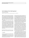
TwoTowers 5.1 is composed of about 45,000 lines of ANSI C [26] code organized as depicted in Fig. 1.1.
TwoTowers 5.1 is equipped with a simple graphical user interface written in Tcl/Tk [30] through which
the user can invoke the analysis routines by means of suitable menus. Each routine needs input files of
certain types and writes its results onto files of other types. The graphical user interface takes care of the
integrated management of the various file types needed by the different routines, which belong to the Æmilia
compiler, the equivalence verifier, the model checker, the security analyzer, and the performance evaluator.
The compiler is in charge of parsing Æmilia specifications stored in .aem files and signalling possible
lexical, syntax and static semantic errors through a .lis file. Based on the translation semantics for Æmilia
into EMPAgr and the operational semantics for EMPAgr , if an Æmilia specification is correct the compiler
can generate its integrated, functional or performance semantic model, which is written to a .ism, .fsm
or .psm file, respectively. As a faster option that does not require printing the state space onto a file, the
compiler can show only the size – in terms of number of states and transitions – of the semantic model, which
is written to a .siz file. The integrated semantic model of an Æmilia specification for a given system is a
state transition graph whose transitions are labeled with the name and the duration/priority/probability of
the corresponding system activities. The functional semantic model is a state transition graph in which only
the activity names label the transitions. The performance semantic model, which can be extracted only if
the Æmilia specification is performance closed, is a continuous- or discrete-time Markov chain [32].
The equivalence verifier checks through the application of the Kanellakis-Smolka algorithm [24] whether
two correct, finite-state Æmilia specifications are equivalent according to one of four different behavioral
equivalences: strong bisimulation equivalence, weak bisimulation equivalence, strong (extended) Markovian
bisimulation equivalence, and weak (extended) Markovian bisimulation equivalence [29, 10, 6]. The result of
the verification is written to a .evr file. In the case of non-equivalence a distinguishing modal logic formula
is reported as well, which is computed on the basis of the algorithm of [15] and is expressed in a verbose
variant of the Hennessy-Milner logic [20] or one of its probabilistic extensions [27, 13].
The equivalence verifier allows a comparative study of two Æmilia specifications to be conducted, aiming
at establishing whether they possess the same functional, security and performance properties in general.
1
2
Tool Description
Should the two Æmilia specifications be equivalent, in order to know whether they satisfy a particular
functional property, security requirement, or performance guarantee, it is necessary to apply to one of the
two Æmilia specifications the model checker, the security analyzer, or the performance evaluator, respectively.
GRAPHICAL USER INTERFACE
.lis
.siz
.aem
AEmilia COMPILER:
− Parser
− Semantic Model Size Calculator
− Semantic Model Generator
.ism
.fsm
.psm
.ltl
.sec
.rew
.sim
EQUIVALENCE VERIFIER:
− Strong Bisimulation Equivalence Verifier
− Weak Bisimulation Equivalence Verifier
− Strong Markovian Bisimulation Equivalence Verifier
− Weak Markovian Bisimulation Equivalence Verifier
.evr
MODEL CHECKER:
− Symbolic LTL Model Checker (via NuSMV)
.mcr
SECURITY ANALYZER:
− Non−Interference Analyzer
− Non−Deducibility on Composition Analyzer
.sar
PERFORMANCE EVALUATOR:
− Stationary/Transient Probability Distribution Calculator
− Stationary/Transient Reward−Based Measure Calculator
− Simulator
.dis
.val
.est
.trc
Figure 1.1: Tool architecture
The model checker verifies through the BDD-based routines of NuSMV 2.2.5 [12] whether a set of functional properties expressed through verbose LTL formulas [14], which are stored in a .ltl file, are satisfied
by a correct, finite-state Æmilia specification. The result of the check, together with a counterexample for
each property that is not met, is written to a .mcr file.
The security analyzer checks through the equivalence verifier whether a correct, finite-state Æmilia specification satisfies non-interference or non-deducibility on composition [19], both of which establish the absence
of illegal information flows from high security system components to low security system components. This
requires the classification in an additional .sec file of the system activities that are high and low with respect
to the security level. The result of the analysis is written to a .sar file, together with a modal logic formula
expressed in a verbose variant of the Hennessy-Milner logic to explain a possible security violation.
Finally, the performance evaluator assesses the quantitative characteristics of correct, finite-state and
performance closed Æmilia specifications. First, it can calculate the stationary/transient probability distribution for the state space of the performance semantic model of an Æmilia specification. The distribution
is written to a .dis file. Second, the performance evaluator can calculate for an Æmilia specification a
set of instant-of-time, stationary/transient performance measures specified through state and transition rewards [22] stored in a .rew file. The values of the measures are written to a .val file. The solution methods
implemented for the stationary case are Gaussian elimination and an adaptive variant of symmetric stochas-
1.3 What TwoTowers 5.1 Offers
3
tic over-relaxation, while for the transient case uniformization is available [32]. Third, the performance
evaluator can estimate via discrete event simulation the mean, variance or distribution of a set of performance measures specified through an extension of state and transition rewards, which are stored in a .sim
file together with the number and the length of the simulation runs. The simulation, which can be applied
also to Æmilia specifications with infinitely many states and general distributions, is based on the method
of independent replications with 90% confidence level [34] and can be trace driven, in which case the traces
are stored in .trc files. The result of the simulation is written to a .est file.
1.3
What TwoTowers 5.1 Offers
From the user viewpoint, TwoTowers 5.1 supplies the following capabilities:
• Component-oriented modeling with Æmilia:
– Separation of system component behavior specification from system topology specification.
– Support for the parameterization of system component behavior.
– Indexing mechanism for defining parameterized system topologies.
– Several data types: integer, bounded integer, real, boolean, list, array, and record.
– Representation of continuous- and discrete-time systems.
– Component activities with exponentially distributed, zero or unspecified durations.
– Random number generators for sampling durations/probabilities from other distributions [23].
– Prioritized and probabilistic choices among component activities.
– Generative-reactive synchronizations among component activities [10].
– Value passing across components (compiled concretely – if possible – or symbolically [5]).
• Companion languages for the parameterized specification of:
– Functional properties expressed in a verbose variant of LTL.
– Security levels.
– Performance measures based on state and transition rewards [7].
– Simulation experiments.
• Parsing of Æmilia and companion specifications with the generation of listings that pinpoint lexical,
syntactical and static semantical errors.
• Compilation of Æmilia specifications into state transition graphs that are shown in a readable format,
through the indication for each global state of the constituting local states of the components.
• Integrated framework for the study of functional, security and performance properties of Æmilia specifications and the provision of diagnostic information in the case of negative outcome.
1.4
Case Studies
A complete and updated list of the case studies conducted with TwoTowers 5.1 (or earlier versions) is maintained at http://www.sti.uniurb.it/bernardo/twotowers/, where their Æmilia and companion specifications as well as the related papers can be found.
4
1.5
Tool Description
History of TwoTowers
The development of TwoTowers started in 1996, then restarted from scratch in 1997. Its name stems from
the two medieval towers – Asinelli (97 mt.) and Garisenda (48 mt.) – that are the symbol of Bologna, the
city where the implementation of the tool started.
Version 1.0 was distributed in July 2001 for Linux and Unix operating systems only. Its input language
was EMPAgr , enriched with the symbolically treated data types integer, real, boolean, list, array, and record.
Its graphical user interface contained a menu for a parser and a compiler of EMPAgr specifications into state
transition graphs, an integrated analyzer for equivalence checking (strong Markovian bisimulation equivalence), a functional analyzer based on CWB-NC 1.2 [17] for model checking (µ-calculus and GCTL* [14])
and equivalence/preorder checking with diagnostics (strong/weak bisimulation equivalence, may/must testing equivalence and preorder [18]), and a performance analyzer in charge of reward-based Markovian analysis
through the solution methods of the commercial tool MarCA 3.0 [33] as well as discrete event simulation.
Version 2.0 was distributed in November 2002. As a faster compilation option not requiring any possibly
huge file to be written, it provided the capability to report only the size of the semantic models underlying an
EMPAgr specification. Unlike the previous version, it no longer relied on MarCA 3.0, as it had three built-in
analysis routines – Gaussian elimination, an adaptive variant of symmetric stochastic over-relaxation, and
uniformization – for the solution of reward Markov chains of arbitrary size. This allowed TwoTowers to be
distributed free of charge to educational and non-profit organizations.
Version 3.0 was completed in October 2003 but not distributed. In this version EMPAgr was replaced by
Æmilia, thus adopting a component-oriented modeling style leading to more confidence in the correctness
of the system specifications as well as a higher degree of parameterization and reuse. Also the companion
languages for the specification of functional properties and performance measures were modified according
to the adopted component-oriented style and became more verbose, thus increasing their ease of use. The
component-orientation reflected on a more readable state representation, as each global state could be
described through its constituting local states corresponding to the components. On the data type side,
bounded integers were introduced and the concrete treatment of data values of type different from integer,
real, and list was implemented in addition to the original symbolic treatment.
Version 4.0 was completed in January 2004 but not distributed. Its graphical user interface was reorganized in order to contain a menu for equivalence verification with diagnostics fully based on built-in routines
(strong/weak functional/Markovian bisimulation equivalence), a menu for model checking (based on CWBNC 1.2 as before), a novel menu for security analysis, and a menu for performance evaluation (as before).
The routines for security analysis required a companion language for the specification of the security levels
of the component activities, and employed weak bisimulation equivalence checking to assess non-interference
and non-deducibility on composition.
Version 5.0 was distributed in May 2004. In this version a symbolic model checker was adopted by
replacing the one of CWB-NC 1.2 with NuSMV 2.1.2. Consequently, the companion language for the
specification of functional properties was modified to express LTL formulas instead of µ-calculus and GCTL*
formulas.
Version 5.1 is being distributed since January 2006. Some minor modifications were done in order to
make the tool available for the Windows operating system as well. Moreover the use of NuSMV 2.1.2 was
replaced by the use of NuSMV 2.2.5.
1.6
Acknowledgments
The following people worked with Marco Bernardo for the definition of Æmilia and EMPAgr , the development
of the case studies, and the integration of TwoTowers with other tools: Pietro Abate, Andrea Acquaviva,
Alessandro Aldini, Simonetta Balsamo, Alessandro Bogliolo, Edoardo Bont`a, Mario Bravetti, Nadia Busi,
Paolo Ciancarini, Alessandro Cimatti, Rance Cleaveland, Marcello Colucci, Lorenzo Donatiello, Francesco
Franz`e, Roberto Gorrieri, Emanuele Lattanzi, Simone Mecozzi, Claudio Premici, Marina Ribaudo, Marco
Roccetti, Marta Simeoni, Steve Sims, and Billy Stewart.
Chapter 2
Tool Installation and Execution
2.1
Introduction
In this chapter we explain how to install and run TwoTowers 5.1 on a computer with the Linux or Windows
operating system.
2.2
Source Distribution
TwoTowers 5.1 is distributed through the compressed file TwoTowers.tar.gz. After moving this compressed
file into a new directory, the source files can be extracted together with the related documentation and
utilities through the following two commands (symbol > denotes the prompt of the operating system shell):
> gunzip TwoTowers.tar.gz
> tar -xvf TwoTowers.tar
which should result in the following directory structure:
. bin
|_. TTKernel.exe
. docs
|_. license.txt
. manual.pdf
. readme.txt
. gui
|_. TTGUI
. src
|_. Makefile
. compiler
|_. Makefile
. aemilia_compiler.c
. aemilia_parser.y
. aemilia_scanner.l
. listing_generator.c
. ltl_parser.y
. ltl_scanner.l
. rew_parser.y
. rew_scanner.l
. sec_parser.y
. sec_scanner.l
5
6
Tool Installation and Execution
. sim_parser.y
. sim_scanner.l
. symbol_handler.c
. driver
|_. Makefile
. driver.c
. equivalence_verifier
|_. Makefile
. equivalence_verifier.c
. headers
|_. Library.h
. aemilia_compiler.h
. aemilia_parser.h
. aemilia_scanner.h
. driver.h
. equivalence_verifier.h
. file_handler.h
. list_handler.h
. listing_generator.h
. ltl_parser.h
. ltl_scanner.h
. markov_solver.h
. memory_handler.h
. number_handler.h
. nusmv_connector.h
. rew_parser.h
. rew_scanner.h
. sec_parser.h
. sec_scanner.h
. security_analyzer.h
. sim_parser.h
. sim_scanner.h
. simulator.h
. string_handler.h
. symbol_handler.h
. table_handler.h
. model_checker
|_. Makefile
. nusmv_connector.c
. performance_evaluator
|_. Makefile
. markov_solver.c
. simulator.c
. security_analyzer
|_. Makefile
. security_analyzer.c
. utilities
|_. Makefile
. file_handler.c
. list_handler.c
. memory_handler.c
. number_handler.c
. string_handler.c
2.3 Installation Procedure
7
. table_handler.c
. win_utils
|_. cp.bat
. mv.bat
. rm.bat
. tt_compile.bat
. tt_exec.bat
2.3
Installation Procedure
The procedure for installing TwoTowers 5.1 comprises a couple of quick and easy steps.
2.3.1
Linux
On a Linux machine, make sure that the following packages are available:
flex
bison
make
gcc
(lexical analyzer generator,
http://www.gnu.org/software/flex/flex.html)
(parser generator,
http://www.gnu.org/software/bison/bison.html)
(program maintainance utility,
http://www.gnu.org/software/make/make.html)
(C compiler,
http://www.gnu.org/software/gcc/gcc.html)
The first step consists of compiling the ANSI C source files through the following commands:
> cd <TwoTowers 5.1 directory>/src/
> make
> make clean
which should result in the following executable file:
<TwoTowers 5.1 directory>/bin/TTKernel
The second step consists of creating a symbolic link to the above executable file through the following
command:
> ln -s <TwoTowers 5.1 directory>/bin/TTKernel TTKernel
given in a directory whose pathname occurs in the shell variable path.
2.3.2
Windows
The executable file for Windows is already available at:
<TwoTowers 5.1 directory>\bin\TTKernel.exe
Should you need to generate it again, make sure that the following packages are available in
\Program Files\GnuWin32:
flex
bison
(lexical analyzer generator,
http://gnuwin32.sourceforge.net/packages/flex.htm)
(parser generator,
http://gnuwin32.sourceforge.net/packages/bison.htm)
8
Tool Installation and Execution
and that the following packages are available as well:
make
gcc
(program maintainance utility,
http://www.mingw.org/)
(C compiler,
http://www.mingw.org/)
Then compile the C source files through the following commands:
<double click> <TwoTowers 5.1 directory>\win_utils\tt_compile
> make
> make clean
which should create the following executable file:
<TwoTowers 5.1 directory>\bin\TTKernel.exe
2.4
Running the Tool
Running the tool is very simple.
2.4.1
Linux
On a Linux machine, make sure that the following packages are available:
wish
NuSMV 2.2.5
(windowing shell for Tcl/Tk 8.0 or higher,
http://www.tcl.tk/software/tcltk/8.0.tml)
(symbolic model checker,
http://nusmv.irst.itc.it/)
Then type the following command to run the tool:
> wish <TwoTowers 5.1 directory>/gui/TTGUI &
To simplify this, we suggest to define an alias like the following:
alias tt ’wish <TwoTowers 5.1 directory>/gui/TTGUI &’
so that the command to run the tool simply becomes:
> tt
In order to be able to use to model checker, we also suggest to make sure that the following symbolic links:
> ln -s <NuSMV 2.2.5 directory>/NuSMV NuSMV
> ln -s <NuSMV 2.2.5 directory>/src/ltl/ltl2smv/ltl2smv ltl2smv
have been created in a directory whose pathname occurs in the shell variable path.
2.4.2
Windows
On a Windows machine, make sure that the following package is available in \Program Files\Tcl:
wish
(windowing shell for Tcl/Tk 8.0 or higher,
http://www.tcl.tk/software/tcltk/8.0.tml)
and that the following package is available in \Program Files\NuSMV-2.2.5:
NuSMV 2.2.5
(symbolic model checker,
http://nusmv.irst.itc.it/)
Then give the following command to run the tool:
<double click> <TwoTowers 5.1 directory>\win_utils\tt_exec
Chapter 3
The Æmilia Compiler
3.1
Introduction
TwoTowers 5.1 accepts only system models that are written in the architectural description language
Æmilia [9, 2] and are stored in .aem files.
An Æmilia description represents an architectural type [8, 1]. This is an intermediate abstraction between
a single system and an architectural style [31]. It consists of a family of systems sharing certain constraints on
the observable behavior of the system components as well as on the system topology. As shown in Table 3.1,
the description of an architectural type in Æmilia starts with the name and the formal parameters of the
architectural type and is composed of three sections.
ARCHI TYPE
/name and formal parameters.
ARCHI ELEM TYPES
ELEM TYPE
..
.
ELEM TYPE
/definition of the first architectural element type.
..
.
/definition of the last architectural element type.
ARCHI TOPOLOGY
ARCHI ELEM INSTANCES /declaration of the architectural element instances.
ARCHI INTERACTIONS
/declaration of the architectural interactions.
ARCHI ATTACHMENTS
/declaration of the architectural attachments.
[BEHAV VARIATIONS
[BEHAV HIDINGS
[BEHAV RESTRICTIONS
[BEHAV RENAMINGS
/declaration of the behavioral hidings.]
/declaration of the behavioral restrictions.]
/declaration of the behavioral renamings.]]
END
Table 3.1: Structure of an Æmilia description
The first section defines the types of components that characterize the system family. In order to include
both the computational components and the connectors among them, these types are called architectural
element types (AETs). The definition of an AET starts with its name and formal parameters and consists of
the specification of its behavior and its interactions. The behavior has to be provided in the form of a list of
sequential defining equations written in a verbose variant of the stochastic process algebra EMPAgr [4, 10, 7].
The interactions are those EMPAgr action types occurring in the behavior that act as interfaces for the
AET. Each of them has to be equipped with two qualifiers, which establish whether it is an input or output
9
10
The Æmilia Compiler
interaction and the multiplicity of the communications in which it can be involved, respectively. All the
other action types occurring in the behavior are assumed to represent internal activities.
The second section defines the architectural topology. This is specified in three steps. First we have the
declaration of the instances of the AETs (called AEIs) with their actual parameters, which represent the real
system components and connectors. Then we have the declaration of the architectural (as opposed to local)
interactions, which are those interactions of the AEIs that act as interfaces for the whole system family.
Finally we have the declaration of the directed architectural attachments among the local interactions of the
AEIs, which make the AEIs communicate with each other.
The third section, which is optional, defines some variations of the observable behavior of the system
family. This is accomplished by declaring some action types occurring in the behavior of certain AEIs to be
unobservable, prevented from occurring, or renamed into other action types.
3.2
Keywords and Comments
Here is the complete list of the keywords of Æmilia that can occur in .aem files:
ARCHI_TYPE
ARCHI_ELEM_TYPES
ELEM_TYPE
BEHAVIOR
INPUT_INTERACTIONS
OUTPUT_INTERACTIONS
UNI
AND
OR
ARCHI_TOPOLOGY
ARCHI_ELEM_INSTANCES
ARCHI_INTERACTIONS
ARCHI_ATTACHMENTS
FROM
TO
BEHAV_VARIATIONS
BEHAV_HIDINGS
HIDE
INTERNALS
INTERACTIONS
ALL
BEHAV_RESTRICTIONS
RESTRICT
OBS_INTERNALS
OBS_INTERACTIONS
ALL_OBSERVABLES
BEHAV_RENAMINGS
RENAME
AS
FOR_ALL
IN
END
const
local
stop
invisible
exp
inf
choice
cond
void
prio
rate
weight
integer
real
mod
min
max
abs
ceil
floor
power
epower
loge
log10
sqrt
sin
cos
c_uniform
erlang
gamma
exponential
weibull
beta
normal
pareto
b_pareto
d_uniform
bernoulli
binomial
poisson
neg_binomial
geometric
pascal
boolean
true
false
list
list_cons
first
tail
concat
insert
remove
length
array
array_cons
read
write
record
record_cons
get
put
where the upper-case keywords in the two leftmost columns refer in general to the three sections of an Æmilia
specification, while the lower-case keywords of the other four columns are used within specific parts of an
Æmilia specification like the architectural type formal parameters, the AET formal parameters, the AET
behavior, and the AEI actual parameters.
In addition to the keywords above, there are the following keywords that belong to the companion
languages and can occur in .evr, .ltl, .sec, .sar, .rew, and .sim files:
PROPERTY
IS
TRUE
FALSE
NOT
EXISTS_TRANS
EXISTS_WEAK_TRANS
FOR_ALL_TRANS
FOR_ALL_WEAK_TRANS
EXISTS_TRANS_SET
EXISTS_WEAK_TRANS_SET
FOR_ALL_TRANS_SETS
FOR_ALL_WEAK_TRANS_SETS
LABEL
DEADLOCK_FREE
FOR_ALL_PATHS
FOR_ALL_PATHS_ALL_STATES_SAT
FOR_ALL_PATHS_SOME_STATE_SAT
EXISTS_PATH
EXISTS_PATH_ALL_STATES_SAT
EXISTS_PATH_SOME_STATE_SAT
STRONG_UNTIL
WEAK_UNTIL
NEXT_STATE_SAT
ALL_FUTURE_STATES_SAT
SOME_FUTURE_STATE_SAT
UNTIL
RELEASES
OBS_NRESTR_INTERNALS
OBS_NRESTR_INTERACTIONS
ALL_OBS_NRESTR
MEASURE
ENABLED
STATE_REWARD
TRANS_REWARD
RUN_LENGTH_ON_EXEC
RUN_LENGTH
RUN_NUMBER
MEAN
VARIANCE
DISTRIBUTION
REWARD
3.3 Identifiers
11
MIN_AGGR_REA_PROB
MIN_AGGR_EXP_RATE
MIN_AGGR_GEN_PROB
REACHED_STATE_SAT
REACHED_STATES_SAT
MIN_FIXPOINT
MAX_FIXPOINT
PREV_STATE_SAT
ALL_PAST_STATES_SAT
SOME_PAST_STATE_SAT
SINCE
TRIGGERED
HIGH_SECURITY
LOW_SECURITY
EXECUTED
CUMULATIVE
NON_CUMULATIVE
DRAW
trc
FOR_ALL
IN
where the keywords in the two leftmost columns (except for the last two keywords) are used within modal and
temporal logic formulas, while the other keywords are used to express security levels as well as performance
measures and simulation experiments.
Comments can be inserted wherever in a .aem, .ltl, .sec, .rew or .sim file. A comment starts with
symbol % and terminates at the end of the line.
3.3
Identifiers
The user-defined identifiers denote architectural type names, AET names, AEI names, behavior names,
action type names, formal parameter names, local variable names, record field names, property names, and
measure names. Every user-defined identifier occurring in a .aem, .ltl, .sec, .rew or .sim file must be a
sequence of upper- and lower-case letters, decimal digits, and underscores, which starts with a letter and is
different from any of the keywords listed in Sect. 3.2. Every user-defined identifier occurring in a .ltl, .sec,
.rew or .sim file must have previously occurred in a .aem file, unless it denotes a property or a measure.
Except for architectural type names, AET names, and AEI names, every user-defined identifier is internally represented (and consequently written to output files) through the dot notation by prefixing it with
the name of the context in which it is defined/used, hence the user is free to give the same name to several
entities in different contexts. The internal representation of the type of an action stemming from the synchronization of several actions is given by the concatenation of the internal representation of the types of
the synchronizing actions, using symbol # as a separator.
3.4
Data Types, Operators, and Expressions
In this section we provide the syntax for typed identifier declaration and expressions, we define the value
domains for the data types available in Æmilia, and we introduce the related operators by specifying their
precedence and associativity whenever necessary. In order to describe the syntax, we adopt the BNF notation, with terminal symbols enclosed within double quotes, non-terminal symbols enclosed within angular
parentheses, and optional parts enclosed within square brackets.
3.4.1
Typed Identifier Declarations and Expressions
A typed identifier occurring in a .aem file represents a constant formal parameter of the architectural type
or one of its AETs, a variable formal parameter or a local variable of a behavior, or an action priority, rate,
or weight. A typed identifier can be declared within the header of an architectural type, AET, or behavior
in the following C-like way:
<data_type> <identifier>
with <data type> being defined by:
<data_type> ::=
|
<normal_type> ::=
|
|
<normal_type>
<special_type>
"integer"
"integer" "(" <expr> ".." <expr> ")"
"real"
12
The Æmilia Compiler
|
|
|
|
<special_type> ::=
|
|
"boolean"
"list" "(" <normal_type> ")"
"array" "(" <expr> "," <normal_type> ")"
"record" "(" <field_decl_sequence> ")"
"prio"
"rate"
"weight"
An expression – denoted by <expr> in the following – is composed of atomic elements, given by typed
identifiers, numeric constants, and truth values, possibly combined through the available operators. The
type of an expression is determined by the type of its atomic elements and the codomain of the operators
occurring in it, while the order in which the infix operators have to be applied to evaluate the expression is
given by their precedence and associativity. The order can be altered using parentheses ( ).
3.4.2
Integers, Bounded Integers, and Reals
The type integer denotes the set of integer numbers that can be represented in the used computer according
to the ANSI C standard. A special case is given by the bounded integer set defined as follows:
"integer" "(" <expr> ".." <expr> ")"
which denotes the set of integers between the value of the first expression and the value of the second
expression. Both expressions must be integer valued, free of undeclared identifiers, and free of invocations to
pseudo-random number generators. Moreover, the value of the first expression cannot be greater than the
value of the second expression.
The type real denotes the set of real numbers in fixed-point notation that can be represented in the
used computer according to the ANSI C standard.
Arithmetical Operators
The following four binary arithmetical operators are available in Æmilia:
<expr> ::=
|
|
|
<expr>
<expr>
<expr>
<expr>
"+"
"-"
"*"
"/"
<expr>
<expr>
<expr>
<expr>
with the division requiring the second operand to be different from zero and always returning a real number.
All the operators above are left associative, with the multiplicative ones taking precedence over the additive
ones. The unary - operator is not explicitly available as its effect can be achieved through a multiplication
by -1.
Relational Operators
The following six binary relational operators are available in Æmilia:
<expr> ::=
|
|
|
|
|
<expr>
<expr>
<expr>
<expr>
<expr>
<expr>
"=" <expr>
"!=" <expr>
"<" <expr>
"<=" <expr>
">" <expr>
">=" <expr>
All of them are non-associative. The arithmetical operators take precedence over them.
3.4 Data Types, Operators, and Expressions
13
Mathematical Functions
The following thirteen mathematical functions are available in Æmilia:
<expr> ::=
|
|
|
|
|
|
|
|
|
|
|
|
"mod" "(" <expr> "," <expr> ")"
"abs" "(" <expr> ")"
"ceil" "(" <expr> ")"
"floor" "(" <expr> ")"
"min" "(" <expr> "," <expr> ")"
"max" "(" <expr> "," <expr> ")"
"power" "(" <expr> "," <expr> ")"
"epower" "(" <expr> ")"
"loge" "(" <expr> ")"
"log10" "(" <expr> ")"
"sqrt" "(" <expr> ")"
"sin" "(" <expr> ")"
"cos" "(" <expr> ")"
where:
• mod computes the modulus of its first argument with respect to its second argument. Both arguments
must be integer, with the second one greater than zero.
• abs computes the absolute value of its argument.
• ceil (resp. floor) computes the smallest (resp. greatest) integer greater (resp. smaller) than or equal
to its argument.
• min (resp. max) computes the minimum (resp. maximum) of its two arguments.
• power computes the power of its first argument raised to its second argument. It cannot be applied to
a pair of arguments such that the first one is zero and the second one is not positive, or the first one
is negative and the second one is real.
• epower computes the power of e raised to its argument.
• loge (resp. log10) computes the natural (resp. base-10) logarithm of its argument, which must be
greater than zero.
• sqrt computes the square root of its argument, which cannot be negative.
• sin (resp. cos) computes the sine (resp. cosine) of its argument expressed in radians.
Pseudo-random Number Generators
The following sixteen pseudo-random number generators [23] are available in Æmilia:
<expr> ::=
|
|
|
|
|
|
|
|
|
|
"c_uniform" "(" <expr> "," <expr> ")"
"erlang" "(" <expr> "," <expr> ")"
"gamma" "(" <expr> "," <expr> ")"
"exponential" "(" <expr> ")"
"weibull" "(" <expr> "," <expr> ")"
"beta" "(" <expr> "," <expr> ")"
"normal" "(" <expr> "," <expr> ")"
"pareto" "(" <expr> ")"
"b_pareto" "(" <expr> "," <expr> "," <expr> ")"
"d_uniform" "(" <expr> "," <expr> ")"
"bernoulli" "(" <expr> "," <expr> "," <expr> ")"
14
The Æmilia Compiler
|
|
|
|
|
"binomial" "(" <expr> "," <expr> ")"
"poisson" "(" <expr> ")"
"neg_binomial" "(" <expr> "," <expr> ")"
"geometric" "(" <expr> ")"
"pascal" "(" <expr> "," <expr> ")"
where:
• c uniform generates a random number following a continuous uniform distribution between its two
arguments, with the second one greater than the first one:
1
pdf c uniform (x) =
for expr1 ≤ x ≤ expr2
expr2 − expr1
• erlang generates a random number following an Erlang distribution with rate parameter given by its
first argument, which must be greater than zero, and shape parameter given by its second argument,
which cannot be less than one:
xexpr2−1 · e−expr1·x
pdf erlang (x) =
for x ≥ 0
(expr2 − 1)! · (1/expr1)expr2
• gamma generates a random number following a gamma distribution with rate parameter given by its
first argument, which must be greater than zero, and shape parameter given by its second argument,
which must be greater than zero:
Z ∞
(expr1 · x)expr2−1 · e−expr1·x
pdf gamma (x) =
for x ≥ 0, where Γ(y) =
z y−1 · e−z dz
(1/expr1) · Γ(expr2)
0
• exponential generates a random number following an exponential distribution with rate parameter
given by its argument, which must be greater than zero:
pdf exponential (x) = expr · e−expr·x
for x ≥ 0
• weibull generates a random number following a Weibull distribution with rate parameter given by its
first argument, which must be greater than zero, and shape parameter given by its second argument,
which must be greater than zero:
expr2 · xexpr2−1 −(expr1·x)expr2
pdf weibull (x) =
·e
for x ≥ 0
(1/expr1)expr2
• beta generates a random number following a beta distribution with shape parameters given by its two
arguments, which must be greater than zero:
xexpr1−1 · (1 − x)expr2−1
Γ(y) · Γ(z)
pdf beta (x) =
for 0 ≤ x ≤ 1, where β(y, z) =
β(expr1, expr2)
Γ(y + z)
• normal generates a random number following a normal distribution with mean given by its first argument and standard deviation given by its second argument, which must be greater than zero:
(x−expr1)2
1
−
√
pdf normal (x) =
· e 2·expr22
expr2 · 2 · π
• pareto generates a random number following a Pareto distribution with shape parameter given by its
argument, which must be greater than zero:
pdf pareto (x) = expr · x−(expr+1)
for x ≥ 1
• b pareto generates a random number following a Pareto distribution with shape parameter given by
its first argument, which must be greater than zero, bounded between its other two arguments, with
the second argument not less than one but less than the third argument:
expr1 · expr2expr1
· x−(expr1+1)
for expr2 ≤ x ≤ expr3
pdf b pareto (x) =
1 − (expr2/expr3)expr1
3.4 Data Types, Operators, and Expressions
15
• d uniform generates a random number following a discrete uniform distribution between its two arguments, which must be integer with the second one greater than the first one:
1
pmf d uniform (x) =
for expr1 ≤ x ≤ expr2
expr2 − expr1 + 1
• bernoulli generates a random number following a Bernoulli distribution where the two possible values
are given by its first two arguments and the probability of choosing the first value is given by its third
argument, which must be in the open interval between zero and one:
pmf bernoulli (expr1) = expr3 and pmf bernoulli (expr2) = 1 − expr3
• binomial generates a random number following a binomial distribution with probability of success
given by its first argument, which must be in the open interval between zero and one, and number of
trials given by its second argument,
which
must be an integer not less than one:
µ
¶
expr2
pmf binomial (x) =
· expr1x · (1 − expr1)expr2−x
for 0 ≤ x ≤ expr2
x
• poisson generates a random number following a Poisson distribution with mean given by its argument,
which must be greater than zero:
exprx −expr
pmf poisson (x) =
·e
for x ≥ 0
x!
• neg binomial generates a random number following a negative binomial distribution with probability
of success given by its first argument, which must be in the open interval between zero and one, and
number of successes given by its
µ second argument,
¶ which must be an integer not less than one:
expr2 + x − 1
pmf neg binomial (x) =
· expr1expr2 · (1 − expr1)x
for x ≥ 0
expr2 − 1
• geometric generates a random number following a geometric distribution with probability of success
given by its argument, which must be in the open interval between zero and one:
pmf geometric (x) = expr · (1 − expr)x−1
for x ≥ 1
• pascal generates a random number following a Pascal distribution with probability of success given by
its first argument, which must be in the open interval between zero and one, and number of successes
given by its second argument,
which must
µ
¶ be an integer not less than one:
x−1
pmf pascal (x) =
· expr1expr2 · (1 − expr1)x−expr2
for x ≥ expr2
expr2 − 1
3.4.3
Booleans
The type boolean denotes the set composed of the two truth values true and false. The following three
logical operators are available in Æmilia:
<expr> ::= <expr> "&&" <expr>
| <expr> "||" <expr>
| "!" <expr>
with the logical negation (!) being right associative and taking precedence over the logical conjunction (&&)
and the logical disjunction (||), which are left associative and subject to short-circuitation. The relational
operators and the arithmetical operators take precedence over the logical ones.
16
The Æmilia Compiler
3.4.4
Lists
The type list, which denotes a possibly empty, variable-length sequence of elements of the same type, is
defined as follows:
"list" "(" <normal_type> ")"
where <normal type> is the type of its elements.
The following seven list-related functions are available in Æmilia:
<expr> ::=
|
|
|
|
|
|
"list_cons" "(" <pe_expr_sequence> ")"
"first" "(" <expr> ")"
"tail" "(" <expr> ")"
"concat" "(" <expr> "," <expr> ")"
"insert" "(" <expr> "," <expr> ")"
"remove" "(" <expr> "," <expr> ")"
"length" "(" <expr> ")"
where <pe expr sequence> is a possibly empty sequence of comma-separated expressions and:
• list cons constructs a possibly empty list composed of the values of the expressions in its argument,
which must be of the same type.
• first returns the first element of its argument, which must be a non-empty list.
• tail returns what follows the first element of its argument, which must be a list.
• concat concatenates its arguments, which must be two lists whose elements are of the same type.
• insert inserts the value of its first argument into its second argument, which must be a list whose
elements are of the same type as the first argument. The position at which the insertion takes place is
established according to the lexicographical order of the elements.
• remove removes the value of the element whose position is given by its first argument, which must be
an integer not less than one, from its second argument, which must be a list with sufficiently many
elements.
• length computes the number of elements of its argument, which must be a list.
3.4.5
Arrays
The type array, which denotes a non-empty, fixed-length sequence of elements of the same type, is defined
as follows:
"array" "(" <expr> "," <normal_type> ")"
where <expr> is its length and <normal type> is the type of its elements. The array length expression must
be integer valued, free of undeclared identifiers, free of invocations to pseudo-random number generators,
and not less than one.
The following three array-related functions are available in Æmilia:
<expr> ::= "array_cons" "(" <expr_sequence> ")"
| "read" "(" <expr> "," <expr> ")"
| "write" "(" <expr> "," <expr> "," <expr> ")"
where <expr sequence> is a non-empty sequence of comma-separated expressions and:
• array cons constructs an array composed of the values of the expressions in its argument, which must
be of the same type.
3.5 Architectural Type Header
17
• read reads from its second argument, which must be an array with sufficiently many elements, the
value of the element indexed by its first argument, which must be an integer between zero and the
length of the second argument decremented by one.
• write writes to its third argument, which must be an array with sufficiently many elements of the
same type as the second argument, the value of its second argument in the position indexed by its first
argument, which must be an integer between zero and the length of the third argument decremented
by one.
3.4.6
Records
The type record, which denotes a non-empty, fixed-length sequence of named elements of possibly different
types called fields, is defined as follows:
"record" "(" <field_decl_sequence> ")"
where <field decl sequence> is a non-empty sequence of comma-separated field declarations, each of the
form defined in Sect. 3.4.1.
The following three record-related functions are available in Æmilia:
<expr> ::= "record_cons" "(" <expr_sequence> ")"
| "get" "(" <identifier> "," <expr> ")"
| "put" "(" <identifier> "," <expr> "," <expr> ")"
where <expr sequence> is a non-empty sequence of comma-separated expressions and:
• record cons constructs a record composed of the values of the expressions in its argument.
• get gets from its second argument, which must be a record, the value of the field whose identifier is
given by its first argument, which must belong to the second argument.
• put puts into its third argument, which must be a record, the value of its second argument in the field
whose identifier is given by its first argument, which must belong to the third argument must and be
of the same type as the second argument.
3.4.7
Priorities, Rates, and Weights
The type prio denotes the set of immediate and passive action priorities, which coincides with the set of
positive integers.
The type rate denotes the set of exponentially timed action rates, which coincides with the set of positive
reals.
The type weight denotes the set of immediate and passive action weights, which coincides with the set
of positive reals.
3.5
Architectural Type Header
The architectural type header at the beginning of an Æmilia specification has the following syntax:
"ARCHI_TYPE" <identifier> "(" <init_const_formal_par_decl_sequence> ")"
where <identifier> is the name of the architectural type and <init const formal par decl sequence>
is either void or a non-empty sequence of comma-separated declarations of initialized constant formal parameters, each of the following form:
"const" <data_type> <identifier> ":=" <expr>
18
The Æmilia Compiler
A constant formal parameter represents a formal parameter whose value, which stems in this case from
the evaluation of the assigned expression, cannot change. The assigned expression must be of the same type
as the identifier, free of undeclared identifiers, and free of invocations to pseudo-random number generators.
As a consequence, the only identifiers that can occur in the assigned expression are those for the preceding
constant formal parameters declared in the architectural type header.
3.6
Architectural Element Types
The first section of an Æmilia specification starts with the keyword ARCHI ELEM TYPES and is composed of
a non-empty sequence of AET definitions, each of the following form:
<AET_header> <AET_behavior> <AET_interactions>
3.6.1
AET Header
Similarly to the architectural type header, the header of an AET has the following syntax:
"ELEM_TYPE" <identifier> "(" <const_formal_par_decl_sequence> ")"
where <identifier> is the name of the AET and <const formal par decl sequence> is either void or a
non-empty sequence of comma-separated declarations of constant formal parameters, each of the following
form:
"const" <data_type> <identifier>
The value of each such formal constant parameter is defined upon declaration of the instances of the AET
in the architectural topology section.
3.6.2
AET Behavior: EMPAgr Operators and Actions
The behavior of an AET has the following syntax:
"BEHAVIOR" <behav_equation_sequence>
where <behav equation sequence> is a non-empty sequence of semicolon-separated EMPAgr behavioral
equations, each of the following form:
<behav_equation_header> "=" <process_term>
The first behavioral equation in the sequence represents the initial behavior for the AET. Each of the other
possible behavioral equations in the sequence must describe a behavior that can be directly or indirectly
invoked by the initial one.
Behavioral Equation Header
The header of the first behavioral equation has the following syntax:
<identifier> "(" <init_var_formal_par_decl_sequence> ";" <local_var_decl_sequence> ")"
whereas the header of any subsequent behavioral equation has the following syntax:
<identifier> "(" <var_formal_par_decl_sequence> ";" <local_var_decl_sequence> ")"
In both headers, <identifier> is the name of the behavioral equation, while <local var decl sequence> is
either void or a non-empty sequence of comma-separated declarations of local variables, each of the following
form:
3.6 Architectural Element Types
19
"local" <normal_type> <identifier>
A local variable is typically used to store one of the values received when synchronizing an input action
of an instance of the AET with an output action of another AEI.
In the header of the first behavioral equation, <init var formal par decl sequence> is either void or
a non-empty sequence of comma-separated declarations of initialized variable formal parameters, each of the
following form:
<normal_type> <identifier> ":=" <expr>
In the header of the subsequent behavioral equations, <var formal par decl sequence> is either void or
a non-empty sequence of comma-separated declarations of variable formal parameters, each of the following
form:
<normal_type> <identifier>
A variable formal parameter represents a formal parameter whose value can change and, in the case of the
first behavioral equation, is initialized by evaluating the assigned expression. The assigned expression must
be of the same type as the identifier and free of undeclared identifiers. The only identifiers that can occur
in the assigned expression are those for the constant formal parameters declared in the AET header. No
initializing expression is needed for the variable formal parameters of each subsequent behavioral equation,
as they will be assigned the values of the actual parameters contained in the invocations of the related
behavioral equation.
Process Terms
The syntax for the process term following the behavioral equation header is a verbose variant of the syntax
for the EMPAgr dynamic operators – stop, action prefix, alternative composition, and behavioral equation
invocation:
<process_term> ::=
|
|
<process_term_1> ::=
|
<process_term_2> ::=
"stop"
<action> "." <process_term_1>
"choice" "{" <process_term_2_sequence> "}"
<process_term>
<identifier> "(" <actual_par_sequence> ")"
["cond" "(" <expr> ")" "->"] <process_term>
Constant stop represents the process term that cannot execute any action. The action prefix operator
(.) represents a process term that can execute an action given by its first operand and then behaves as
the process term given by its second operand. The alternative composition operator (choice) represents a
process term that behaves as one of the elements of <process term 2 sequence>, which is a sequence of
at least two comma-separated process terms, each possibly preceded by a boolean expression establishing
the condition under which it is available. The behavioral equation invocation represents a process term
that behaves as the behavioral equation whose name is given by <identifier>, when passing a possibly
empty sequence of expressions represented by <actual par sequence>. The actual parameters must match
by number, order and type with the variable formal parameters of the invoked behavioral equation. Note
that a behavioral equation invocation can occur only immediately after an action prefix operator.
Actions
The syntax for an action occurring in the process term of a behavioral equation is as follows:
<action> ::= "<" <action_type> "," <action_rate> ">"
<action_type> ::= <identifier>
| <identifier> "?" "(" <local_var_sequence> ")"
| <identifier> "!" "(" <expr_sequence> ")"
20
The Æmilia Compiler
<action_rate> ::=
|
|
|
|
"exp" "(" <expr> ")"
"inf" "(" <expr> "," <expr> ")"
"inf"
"_" "(" <expr> "," <expr> ")"
"_"
The action type is simply an identifier (unstructured action), an identifier followed by symbol ? and a
non-empty sequence of local variables (input action), or an identifier followed by symbol ! and a non-empty
sequence of expressions (output action). Whenever a local variable occurs in an expression within an output
action, a behavioral equation invocation, or a boolean guard without previously occurring in an input action,
it evaluates to zero, false, empty list, null array, or null record depending on its type.
The rate of an exponentially timed action (exp) is given by an expression, whose value must be a positive
real, that is interpreted as the rate of the exponentially distributed random variable describing the action
duration. The rate of an immediate action (inf) is expressed through a priority, given by an expression
whose value must be an integer not less than one, and a weight, given by an expression whose value must
be a positive real. The rate of a passive action ( ) is again expressed through two expressions denoting a
priority and a weight, respectively. If not specified, the values of the priority and the weight of an immediate
or passive action are assumed to be one.
There are three constraints to which the actions are subject. First, within the behavior of an AET,
the actions in which an action type identifier occur must all be unstructured, input with the same number,
order, and type of local variables, or output with the same number, order, and type of expressions. Second,
within the behavior of an AET, the actions in which an action type identifier occur must all be exponentially
timed, immediate with the same priority, or passive with the same priority. Third, every input action must
be passive.
If several actions are simultaneously enabled in the current AET behavior, as in the case of the alternative
composition, the one to be executed is selected as follows [10]. If all the considered actions are exponentially
timed, then the race policy applies: each considered action is selected with a probability proportional to
its rate. If some of the considered actions are immediate, then such immediate actions take precedence
over the exponentially timed ones and the generative preselection policy applies: each considered immediate
action with the highest priority is selected with a probability proportional to its weight. If some of the
considered actions are passive, then the reactive preselection policy applies to them: for every action type,
each considered passive action of that type with the highest priority level is selected with a probability
proportional to its weight (the choice among passive actions of different types is nondeterministic).
An action of an AEI can synchronize with an action of another AEI, possibly exchanging values. Besides
other constraints that we shall see in Sect. 3.7.3, in accordance with the generative-reactive paradigm [10] it
must be the case that at most one of the two actions is not passive, with both actions being unstructured,
or both being structured with at most one of them being an output action and their parameters matching
by number, order, and type. If both actions are passive, then the resulting synchronizing action is passive as
well, otherwise the rate of the resulting action is the (possibly normalized) rate of the involved non-passive
action. The identifier of the resulting action type is internally represented by concatenating the two original
identifiers, using symbol # as a separator. If one of the two involved actions is an output action, then the
resulting action is an output action with the same non-empty sequence of expressions as the original output
action. If instead both involved actions are input actions, then the resulting action is an input action with
the same non-empty sequence of local variables as one of the two original input actions.
3.6.3
AET Interactions
The identifiers of the types of the actions occurring in the behavior of an AET through which the instances
of that AET can communicate with other AEIs are declared to be interactions as follows:
"INPUT_INTERACTIONS" <input_interactions> "OUTPUT_INTERACTIONS" <output_interactions>
Every interaction has two qualifiers associated with it. First, an interaction is classified to be either
an input or an output interaction based on its communication direction, i.e. whether it tries to establish a
3.7 Architectural Topology
21
communication or is willing to be involved in a communication. In the particular case of an interaction given
by an action type identifier occurring in input (resp. output) actions, the action type must be declared to
be an input (resp. output) interaction.
Second, an input or output interaction is classified to be a uni-, and- or or-interaction depending
on the multiplicity of the communications in which it can be involved. Syntactically speaking, each of
<input interactions> and <output interactions> either is void or has the following format:
<uni_interactions> <and_interactions> <or_interactions>
with at least one of the three elements, which basically represent sequences of action type identifiers, being
non-empty.
A uni-interaction of an instance of an AET can communicate only with one interaction of another AEI
(point-to-point communication). If not empty, <uni interactions> has the following syntax:
"UNI" <identifier_sequence>
where <identifier sequence> is a non-empty sequence of semicolon-separated action type identifiers.
An and-interaction of an instance of an AET can simultaneously communicate with several interactions
of other AEIs (broadcast communication). If not empty, <and interactions> has the following syntax:
"AND" <identifier_sequence>
where <identifier sequence> is a non-empty sequence of semicolon-separated action type identifiers. Due
to the adoption of the generative-reactive paradigm, the identifier of an action type occurring in input actions
cannot be declared to be an (input) and-interaction.
An or-interaction of an instance of an AET can communicate with one of several interactions of other
AEIs (server-clients communication). If not empty, <or interactions> has the following syntax:
"OR" <identifier_sequence>
where <identifier sequence> is a non-empty sequence of semicolon-separated action type identifiers. Internally, every occurrence of an or-interaction is replaced within the AET behavior by a choice among as
many fresh uni-interactions as there are AEIs with which the original or-interaction can communicate. Each
such fresh uni-interaction is represented through the identifier of the original or-interaction augmented with
a dot followed by a unique index.
3.7
Architectural Topology
The second section of an Æmilia specification has the following syntax:
"ARCHI_TOPOLOGY" <AEIs> <architectural_interactions> <architectural_attachments>
3.7.1
Architectural Element Instances
The instances of the AETs defined in the first section of an Æmilia specification are declared as follows:
"ARCHI_ELEM_INSTANCES" <AEI_decl_sequence>
where <AEI decl sequence> is a non-empty sequence of semicolon-separated AEI declarations, each of the
following form:
<AEI_decl> ::= <identifier> ["[" <expr> "]"] ":" <identifier> "(" <pe_expr_sequence> ")"
| "FOR_ALL" <identifier> "IN" <expr> ".." <expr>
<identifier> "[" <expr> "]" ":" <identifier> "(" <pe_expr_sequence> ")"
22
The Æmilia Compiler
In its simpler form, an AEI declaration contains the identifier of the AEI, a possible integer-valued
expression enclosed in square brackets, which represents a selector and must be free of undeclared identifiers
and invocations to pseudo-random number generators, the identifier of the related AET, which must have
been defined in the first section of the Æmilia specification, and a possibly empty sequence of expressions
free of invocations to pseudo-random number generators, which provide the actual values for the constant
formal parameters of the AET and must match with them by number, order, and type. The only identifiers
that can occur in the possible selector expression and in the actual parameters are the ones of the constant
formal parameters declared in the architectural type header.
The second form is useful to concisely declare several instances of the same AET through an indexing
mechanism. This additionally requires the specification of the index identifier, which can then occur in the
selector expression and in the actual parameters, together with its range, which is given by two integer-valued
expressions. These two expressions must be free of undeclared identifiers and invocations to pseudo-random
number generators, with the value of the first expression being not greater than the value of the second
expression.
We observe that the identifier of an AEI can be augmented with a selector expression also in the simpler
form of AEI declaration. This is useful whenever it is desirable to declare a set of indexed instances of the
same AET, but only some of them have a common selector expression.
3.7.2
Architectural Interactions
The architectural interactions are declared through the following syntax:
"ARCHI_INTERACTIONS" <pe_architectural_interaction_decl>
where <pe architectural interaction decl> is either void or a non-empty sequence of semicolon-separated
architectural interaction declarations, each of the following form:
<architectural_interaction_decl> ::= <identifier> ["[" <expr> "]"] "." <identifier>
| "FOR_ALL" <identifier> "IN" <expr> ".." <expr>
<identifier> "[" <expr> "]" "." <identifier>
In its simpler form, an architectural interaction declaration contains the identifier of the AEI to which
the interaction belongs, a possible integer-valued expression enclosed in square brackets, which represents a
selector and must be free of undeclared identifiers and invocations to pseudo-random number generators, and
the identifier of the interaction. Both the AEI and the interaction for the type of the AEI, whose identifier
concatenation through the dot notation gives rise to the name of the architectural interaction, must have
been previously declared. The only identifiers that can occur in the possible selector expression are the ones
of the constant formal parameters declared in the architectural type header.
The second form is useful to concisely declare several architectural interactions through an indexing
mechanism. This additionally requires the specification of the index identifier, which can then occur in the
selector expression, together with its range, which is given by two integer-valued expressions. These two
expressions must be free of undeclared identifiers and invocations to pseudo-random number generators,
with the value of the first expression being not greater than the value of the second expression.
3.7.3
Architectural Attachments
The architectural attachments are declared through the following syntax:
"ARCHI_ATTACHMENTS" <pe_architectural_attachment_decl>
where <pe architectural attachment decl> is either void or a non-empty sequence of semicolon-separated
architectural attachment declarations, each of the following form:
<architectural_attachment_decl> ::= "FROM" <identifier> ["[" <expr> "]"] "." <identifier>
"TO" <identifier> ["[" <expr> "]"] "." <identifier>
3.8 Behavioral Variations
23
|
"FOR_ALL" <identifier> "IN" <expr> ".." <expr>
["AND" "FOR_ALL" <identifier> "IN" <expr> ".." <expr>]
"FROM" <identifier> ["[" <expr> "]"] "." <identifier>
"TO" <identifier> ["[" <expr> "]"] "." <identifier>
In its simpler form, an architectural attachment declaration contains the indication of an output interaction followed by the indication of an input interaction. Each of the two interactions is expressed in dot
notation through the identifier of the AEI to which the interaction belongs, a possible integer-valued expression enclosed in square brackets, which represents a selector and must be free of undeclared identifiers and
invocations to pseudo-random number generators, and the identifier of the interaction. Both the AEI and
the interaction for the type of the AEI must have been previously declared, with the interaction not being
architectural. The two AEIs must be different from each other. At least one of the two interactions must be
a uni-interaction, and at least one of them must occur in passive actions within the behavior of the AEI to
which it belongs. The actions in which the two interactions occur within the behavior of the two AEIs must
all be either unstructured or structured; in the latter case, the expressions of the output interaction must
match with the local variables of the input interaction by number, order, and type. The only identifiers that
can occur in the possible selector expression are the ones of the constant formal parameters declared in the
architectural type header.
The second form is useful to concisely declare several architectural attachments through an indexing
mechanism. This additionally requires the specification of up to two different index identifiers, which can
then occur in the selector expressions, together with their ranges, each of which is given by two integer-valued
expressions. These two expressions must be free of undeclared identifiers and invocations to pseudo-random
number generators, with the value of the first expression being not greater than the value of the second
expression.
All the non-architectural interactions should be involved at least in one architectural attachment, with
the non-architectural uni-interactions being involved at most in one architectural attachment. All the uniinteractions attached to the same and- or or-interaction must belong to different AEIs. Among all the
uni-interactions attached to the same passive and-interaction, at most one is admitted that occurs in nonpassive actions within the behavior of the AEI to which it belongs. No isolated groups of AEIs should be
present.
3.8
Behavioral Variations
The third section of an Æmilia specification has the following syntax:
["BEHAV_VARIATIONS" [<behav_hidings>] [<behav_restrictions>] [<behav_renamings>]]
This section is optional. If present, at least one of its three optional subsections must be there.
3.8.1
Behavioral Hidings
The behavioral hidings are declared through the following syntax:
"BEHAV_HIDINGS" <behav_hiding_decl_sequence>
where <behav hiding decl sequence> is a non-empty sequence of semicolon-separated behavioral hiding
declarations, each of the following form:
<behav_hiding_decl> ::=
|
|
|
|
"HIDE" "INTERNALS"
"HIDE" "INTERACTIONS"
"HIDE" "ALL"
"HIDE" <identifier> ["[" <expr> "]"] "." <action_type_set_h>
"FOR_ALL" <identifier> "IN" <expr> ".." <expr>
"HIDE" <identifier> "[" <expr> "]" "." <action_type_set_h>
24
The Æmilia Compiler
<action_type_set_h> ::=
|
|
|
<identifier>
"INTERNALS"
"INTERACTIONS"
"ALL"
In its simpler form, a behavioral hiding declaration consists of making unobservable all the action types
that are internal to the AEIs of the Æmilia specification, all the non-architectural interactions of the AEIs
of the Æmilia specification, or both of them. Alternatively, it is possible to hide a set of action types of a
specific AEI. In this case, the behavioral hiding declaration contains the identifier of the AEI to which the
action types to be hidden belong, a possible integer-valued expression enclosed in square brackets, which
represents a selector and must be free of undeclared identifiers and invocations to pseudo-random number
generators, and the identifier of the action type to be hidden or one of the three shorthands above for sets
of action types to be hidden. If specified, the AEI must have been previously declared. If specified, the
action type to be hidden must occur in the behavior of the AEI and cannot be an architectural interaction.
The only identifiers that can occur in the possible selector expression are the ones of the constant formal
parameters declared in the architectural type header.
The more complex form is useful to concisely hide some of the action types of several AEIs through an
indexing mechanism. This additionally requires the specification of the index identifier, which can then occur
in the selector expression, together with its range, which is given by two integer-valued expressions. These
two expressions must be free of undeclared identifiers and invocations to pseudo-random number generators,
with the value of the first expression being not greater than the value of the second expression.
If an internal action type is hidden, it is converted to the special action type invisible. If a nonarchitectural interaction is hidden, all the synchronizing action types in which it is involved are converted
to the special action type invisible. In both cases, all the possible action type parameters are dropped.
3.8.2
Behavioral Restrictions
The behavioral restrictions are declared through the following syntax:
"BEHAV_RESTRICTIONS" <behav_restriction_decl_sequence>
where <behav restriction decl sequence> is a non-empty sequence of semicolon-separated behavioral
restriction declarations, each of the following form:
<behav_restriction_decl> ::=
|
|
|
|
"RESTRICT" "OBS_INTERNALS"
"RESTRICT" "OBS_INTERACTIONS"
"RESTRICT" "ALL_OBSERVABLES"
"RESTRICT" <identifier> ["[" <expr> "]"] "." <action_type_set_r>
"FOR_ALL" <identifier> "IN" <expr> ".." <expr>
"RESTRICT" <identifier> "[" <expr> "]" "." <action_type_set_r>
<action_type_set_r> ::= <identifier>
| "OBS_INTERNALS"
| "OBS_INTERACTIONS"
| "ALL_OBSERVABLES"
In its simpler form, a behavioral restriction declaration consists of preventing the execution of all the
observable action types that are internal to the AEIs of the Æmilia specification, all the observable, nonarchitectural interactions of the AEIs of the Æmilia specification, or both of them. Alternatively, it is
possible to restrict a set of action types of a specific AEI. In this case, the behavioral restriction declaration
contains the identifier of the AEI to which the action types to be restricted belong, a possible integer-valued
expression enclosed in square brackets, which represents a selector and must be free of undeclared identifiers
and invocations to pseudo-random number generators, and the identifier of the action type to be restricted
or one of the three shorthands above for sets of action types to be restricted. If specified, the AEI must have
been previously declared. If specified, the action type to be hidden must occur in the behavior of the AEI
3.8 Behavioral Variations
25
and cannot be an architectural interaction or hidden. The only identifiers that can occur in the possible
selector expression are the ones of the constant formal parameters declared in the architectural type header.
The more complex form is useful to concisely restrict some of the action types of several AEIs through an
indexing mechanism. This additionally requires the specification of the index identifier, which can then occur
in the selector expression, together with its range, which is given by two integer-valued expressions. These
two expressions must be free of undeclared identifiers and invocations to pseudo-random number generators,
with the value of the first expression being not greater than the value of the second expression.
If an observable internal action type is restricted, it cannot be executed. If an observable, non-architectural
interaction is restricted, none of the synchronizing action types in which it is involved can be executed.
3.8.3
Behavioral Renamings
The behavioral renamings are declared through the following syntax:
"BEHAV_RENAMINGS" <behav_renaming_decl_sequence>
where <behav renaming decl sequence> is a non-empty sequence of semicolon-separated behavioral renaming declarations, each of the following form:
<behav_renaming_decl> ::= "RENAME" <identifier> ["[" <expr> "]"] "." <identifier>
"AS" <identifier> ["[" <expr> "]"]
| "FOR_ALL" <identifier> "IN" <expr> ".." <expr>
"RENAME" <identifier> "[" <expr> "]" "." <identifier>
"AS" <identifier> ["[" <expr> "]"]
In its simpler form, a behavioral renaming declaration contains the identifier of the AEI to which the
action type to be renamed belongs, a possible integer-valued expression enclosed in square brackets, which
represents a selector and must be free of undeclared identifiers and invocations to pseudo-random number
generators, and the identifier of the renaming action type possibly followed by another selector expression.
The AEI must have been previously declared. The action type to be renamed must occur in the behavior
of the AEI and cannot be hidden or restricted. The only identifiers that can occur in the possible selector
expressions are the ones of the constant formal parameters declared in the architectural type header.
The mroe complex form is useful to concisely rename some of the action types of several AEIs through an
indexing mechanism. This additionally requires the specification of the index identifier, which can then occur
in the selector expressions, together with its range, which is given by two integer-valued expressions. These
two expressions must be free of undeclared identifiers and invocations to pseudo-random number generators,
with the value of the first expression being not greater than the value of the second expression.
An observable, non-restricted action type can be renamed to a single action type. If an observable,
non-restricted, internal action type or an architectural interaction is renamed, it is converted to the specified
renaming action type. If an observable, non-restricted, non-architectural interaction is renamed, all the
synchronizing action types in which it is involved are converted to the specified renaming action type. Note
that the renaming action type is not expressed in dot notation, which may turn out to be useful when checking
for equivalence two Æmilia specifications whose AEIs have different identifiers. In the model checking case,
instead, any renaming action type must be different from the NuSMV 2.2.5 keywords, which are listed below:
A
ABF
ABG
AF
AG
ASSIGN
ASYNC
AX
BU
CTLWFF
EG
EVAL
EX
F
FAIRNESS
FALSE
FORMAT
G
GOTO
H
LTLSPEC
LTLWFF
MAX
MIN
MODULE
O
OUTPUT
RESET
S
SIMPWFF
Z
apropos
array
boolean
case
else
esac
if
in
init
26
The Æmilia Compiler
COMPASSION
COMPUTE
COMPWFF
CONSTANT
CONSTRAINT
DEFINE
E
EBF
EBG
EF
3.9
IMPLEMENTS
IN
INIT
INPUT
INVAR
INVARSPEC
ISA
IVAR
JUSTICE
LET
SPEC
STEP
T
TRANS
TRUE
U
V
VAR
X
Y
mod
next
of
process
self
sigma
then
union
xnor
xor
Compiling Æmilia Specifications
In this section we briefly describe how correct Æmilia specifications are compiled into finite semantic models
suited for analysis.
3.9.1
Parsing
While parsing an Æmilia (or companion) specification, a .lis file is generated in which each line of the
specification is reported by having it preceded by its line number. The parser is able to catch about 300 types
of lexical, syntax and static semantic error or warning, which are signalled through suitable messages in the
.lis file. The .lis file is terminated with the indication of the total number of errors and warnings that
have been detected. A specification with no errors is said to be correct.
3.9.2
Semantic Models
A correct Æmilia specification can be compiled into three semantic models: the integrated semantic model,
the functional semantic model, and the performance semantic model. All of them are state transition graphs,
whose states are in correspondence with the vectors of the current behaviors of the AEIs. More precisely, the
integrated semantic model is a state transition graph whose transitions are labeled with the type and the rate
of the corresponding actions, with the lower priority transitions being pruned. The functional semantic model
is a state transition graph in which only the action types label the transitions. The performance semantic
model can be extracted in the form of a Markov chain [32] only if the Æmilia specification is performance
closed, i.e. its integrated semantic model has no passive transitions and no non-determinism arises because
of some boolean condition – occurring in a behavioral choice – that cannot be statically evaluated. In
such a case, if the integrated semantic model has only exponentially timed transitions or both immediate
and exponentially timed transitions, the performance semantic model is a continuous-time Markov chain
obtained after removing the possible immediate transitions, with the transitions labeled with the rates of
the corresponding actions. If instead the integrated semantic model has only immediate transitions, they are
interpreted as taking one time unit and the performance semantic model is a discrete-time Markov chain,
with the transitions labeled with the probabilities of the corresponding actions.
Due to the process term syntax within the behavior of the AETs, which rules out static operators
(hence recursion over them) as well as behavioral equation invocations outside the scope of an action prefix,
the semantic model of an Æmilia specification with no variable formal parameters and local variables is
guaranteed to be finitely branching and finite state.
When printed to the related .ism, .fsm or .psm file, the semantic model is a sequence of numbered
global states with their outgoing transitions. Each global state is described through the vector of local
states representing the current behavior of the AEIs. In the case of the integrated and functional semantic
models, the global state numbered with one is the initial global state, which is composed of the local states
representing the initial behavior of the AEIs. In the case of the performance semantic model, the concept
of initial global state is replaced with an initial global state probability distribution – as the initial global
state may not be unique – whose values are reported in the .psm file for every global state. Each transition
is represented through its action-based label and the number of its target global state.
3.9 Compiling Æmilia Specifications
27
The .ism, .fsm or .psm file is terminated with the indication of the total number of global states and
transitions and their classification. The global states are divided into tangible (having exponentially timed
transitions), vanishing (having immediate transitions), open (having passive transitions), and deadlocked
(having no transitions). In the case of the performance semantic model, the global states with no outgoing
transitions are called absorbing rather than deadlocked as they might have self-looping transitions. Based
on their action types, the transitions are divided into observable and invisible. Based on their action rates,
the transitions are divided into exponentially timed, immediate, and passive.
The same global state and transition classification is reported, together with the related numbers, in a
.siz file whenever the user is interested only in the size of the semantic model.
3.9.3
Concrete and Symbolic Representation of Data Values
In the case in which variable formal parameters and local variables are present in the behavioral equations
of the AETs of an Æmilia specification, they must be compiled in a way that keeps the underlying semantic
models both finitely branching and finite state. This can be achieved in two different ways.
If each of the occurring variable formal parameters and local variables has a finite value domain, i.e. its
type is bounded integer, boolean, or array or record based on the two previous basic types, then a concrete
treatment is applied. This means that every expression – occurring in a behavioral equation invocation, a
boolean guard, or an output action – can be statically evaluated, after replacing every input action with a
choice among as many instances of it as needed to instantiate all of its local variables in every possible way
according to their finite value domains. In this case, the synchronization between an output action and an
input action is possible only if their parameters have pairwise the same value. In the .ism, .fsm or .psm
file, the current value of every variable formal parameter and local variable is represented through a concrete
assignment – an assignment whose right-hand side does not contain any variable – printed immediately after
the current behavior of the AEI to which the variable formal parameter or local variable belongs.
If instead there is at least one variable formal parameter or local variable with an infinite value domain, i.e.
whose type is integer, real, list, or array or record based on the three previous types, then a concrete treatment
is not possible. To keep the semantic models finite, a symbolic treatment is applied [5]. Every transition label
is augmented with an expression and a sequence of symbolic assignments. The expression, which arises from
the possible boolean guards of the alternative composition operator, represents the condition under which
the transition can be executed. The symbolic assignments establish how the values of the variable formal
parameters and of the local variables must be updated after executing the transition, due to behavioral
equation invocations in the target global state or value passing between the synchronized structured actions
involved in the transition. In the .ism, .fsm or .psm file, every transition is printed together with its boolean
guard and its sequence of symbolic assignments. Moreover, a list of initial symbolic assignments, based on
the initialization of the variable formal parameters in the header of the first behavioral equation of every
AEI, is printed at the beginning of the file. We remind that the performance semantic model cannot be
generated in the case of symbolic treatment if there is at least one boolean guard that cannot be statically
evaluated.
We conclude by recalling that equivalence verification, model checking, security analysis, and Markovchain-based performance evaluation can be applied only to correct Æmilia specifications in which all the
possible variable formal parameters and local variables can be treated concretely. Simulation, instead,
can be applied to any correct Æmilia specification (with no open and deadlock states), because the possible
expressions – including guards and symbolic assignments – are directly evaluated while generating the portion
of the integrated semantic model that is necessary to make the simulation advance.
3.9.4
Compile-Time Crashes
The compilation of an Æmilia specification can be interrupted because of lack of memory, inability to open a
file, illegal value of a symbolic action rate, or an error occurred during the evaluation of a concrete assignment,
like out-of-range bounded integer, symbolic array length mismatch, or invalid argument of an arithmetical
operator, a mathematical function, a pseudo-random number generator, or a list- or array-related function.
In each of these cases, which cannot be detected at parsing time, a suitable message is displayed.
28
The Æmilia Compiler
3.10
Example A: The Alternating Bit Protocol
In this section we introduce a simple communication protocol and we present three different Æmilia specifications for it, which exemplify the syntax of the language and illustrate its expressiveness.
3.10.1
Informal Description
The alternating bit protocol [3] is a data-link-level communication protocol that establishes a means whereby
two stations, one acting as a sender and the other acting as a receiver, connected by a full-duplex, FIFO
communication channel that may lose messages, can cope with message loss. The name of the protocol stems
from the fact that each message is augmented with an additional bit. Since consecutive messages that are
not lost are tagged with additional bits that are pairwise complementary, it is easy to distinguish between
an original message and its possible duplicates.
Initially, if the data link level of the sender obtains a message from the upper level in the protocol stack,
it augments the message with an additional bit set to 0, sends the tagged message to the receiver, and starts
a timer. If an acknowledgment tagged with 0 is received before the timeout expires, then the subsequent
message obtained from the upper level will be sent with an additional bit set to 1, otherwise the current
tagged message is sent again. On the other side, the data link level of the receiver waits for a message
tagged with 0. If it receives such a tagged message for the first time, then it passes the message to the
upper level in the protocol stack, sends an acknowledgment tagged with 0 back to the sender, and waits for
a message tagged with 1. On the contrary, if it receives a duplicate tagged message – due to message loss,
acknowledgment loss, or propagation taking an exceedingly long time – then it sends an acknowledgment
tagged with the same additional bit back to the sender and keeps waiting.
3.10.2
Pure Æmilia Description with Markovian Delays
We show below a pure Æmilia specification of the alternating bit protocol called abp.aem, where pure means
that no variable formal parameters and local variables are used:
ARCHI_TYPE ABP_Type(const
const
const
const
rate
rate
rate
weight
msg_gen_rate
timeout_rate
prop_rate
delivery_prob
:=
:=
:=
:=
5,
1,
9.375,
0.95)
ARCHI_ELEM_TYPES
ELEM_TYPE Sender_Type(const rate msg_gen_rate,
const rate timeout_rate)
BEHAVIOR
Sender_0(void; void) =
<generate_msg, exp(msg_gen_rate)> . <transmit_msg_0, inf> . Sender_0_Waiting();
Sender_0_Waiting(void; void) =
choice
{
<receive_ack_0, _> . Sender_1(),
<receive_ack_1, _> . Sender_0_Waiting(),
<timeout, exp(timeout_rate)> . Sender_0_Retransmitting()
};
Sender_0_Retransmitting(void; void) =
choice
3.10 Example A: The Alternating Bit Protocol
29
{
<transmit_msg_0, inf> . Sender_0_Waiting(),
<receive_ack_0, _> . Sender_1(),
<receive_ack_1, _> . Sender_0_Retransmitting()
};
Sender_1(void; void) =
<generate_msg, exp(msg_gen_rate)> . <transmit_msg_1, inf> . Sender_1_Waiting();
Sender_1_Waiting(void; void) =
choice
{
<receive_ack_1, _> . Sender_0(),
<receive_ack_0, _> . Sender_1_Waiting(),
<timeout, exp(timeout_rate)> . Sender_1_Retransmitting()
};
Sender_1_Retransmitting(void; void) =
choice
{
<transmit_msg_1, inf> . Sender_1_Waiting(),
<receive_ack_1, _> . Sender_0(),
<receive_ack_0, _> . Sender_1_Retransmitting()
}
INPUT_INTERACTIONS
UNI generate_msg;
receive_ack_0;
receive_ack_1
OUTPUT_INTERACTIONS
UNI transmit_msg_0;
transmit_msg_1
ELEM_TYPE Line_Type(const rate
prop_rate,
const weight delivery_prob)
BEHAVIOR
Line(void; void) =
choice
{
<receive_0, _> . <propagate_0, exp(prop_rate)> .
choice
{
<keep_0, inf(1, delivery_prob)> . <deliver_0, inf> . Line(),
<lose_0, inf(1, 1 - delivery_prob)> . Line()
},
<receive_1, _> . <propagate_1, exp(prop_rate)> .
choice
{
30
The Æmilia Compiler
<keep_1, inf(1, delivery_prob)> . <deliver_1, inf> . Line(),
<lose_1, inf(1, 1 - delivery_prob)> . Line()
}
}
INPUT_INTERACTIONS
UNI receive_0;
receive_1
OUTPUT_INTERACTIONS
UNI deliver_0;
deliver_1
ELEM_TYPE Receiver_Type(void)
BEHAVIOR
Receiver_0(void; void) =
choice
{
<receive_msg_0, _> . <consume_msg, inf> . <transmit_ack_0, inf> . Receiver_1(),
<receive_msg_1, _> . <transmit_ack_1, inf> . Receiver_0()
};
Receiver_1(void; void) =
choice
{
<receive_msg_1, _> . <consume_msg, inf> . <transmit_ack_1, inf> . Receiver_0(),
<receive_msg_0, _> . <transmit_ack_0, inf> . Receiver_1()
}
INPUT_INTERACTIONS
UNI receive_msg_0;
receive_msg_1
OUTPUT_INTERACTIONS
UNI consume_msg;
transmit_ack_0;
transmit_ack_1
ARCHI_TOPOLOGY
ARCHI_ELEM_INSTANCES
S
: Sender_Type(msg_gen_rate,
timeout_rate);
LM : Line_Type(prop_rate,
delivery_prob);
LA : Line_Type(prop_rate,
3.10 Example A: The Alternating Bit Protocol
R
31
delivery_prob);
: Receiver_Type()
ARCHI_INTERACTIONS
S.generate_msg;
R.consume_msg
ARCHI_ATTACHMENTS
FROM
FROM
FROM
FROM
FROM
FROM
FROM
FROM
S.transmit_msg_0
S.transmit_msg_1
LM.deliver_0
LM.deliver_1
R.transmit_ack_0
R.transmit_ack_1
LA.deliver_0
LA.deliver_1
TO
TO
TO
TO
TO
TO
TO
TO
LM.receive_0;
LM.receive_1;
R.receive_msg_0;
R.receive_msg_1;
LA.receive_0;
LA.receive_1;
S.receive_ack_0;
S.receive_ack_1
END
The Æmilia specification above is parameterized with respect to the message generation rate, the timeout
rate, the propagation rate of a single message, and the delivery probability of a single message. In order
to allow for a Markov-chain-based performance evaluation, the timeout delay and the message propagation
delay are assumed to be exponentially distributed. Supposed that the protocol uses two 9.6 Kbps lines and
that the average length of a message is 1024 bits, the propagation rate is 9.375 messages per second. We
also assume that the generation rate is 5 messages per second, the timeout delay is 1 second on average, and
the delivery probability is 0.95.
We have three AETs: one for the sender, one for a half-duplex communication line, and one for the
receiver. As far as Sender Type is concerned, initially a message is generated (i.e. arrives from the upper
level), which is then tagged with 0 and transmitted. Three cases arise. If an acknowledgment tagged with 0 is
received, then the same behavior is repeated for the next generated message, which will be tagged with 1. If
an acknowledgment tagged with 1 is received, the acknowledgment is simply ignored. If the timeout expires,
then the message is retransmitted unless an acknowledgment tagged with 0 is received in the meanwhile.
Line Type waits for the transmission of a message/acknowledgment tagged with 0 or 1, which is then
propagated along the line. With probability 0.95 the message/acknowledgment reaches its destination, while
with probability 0.05 the message/acknowledgment is lost. Afterwards, this behavior is repeated. Note that
the types of the actions representing the fact that a message/acknowledgment is kept or lost are not declared
to be interactions, as these events are not under the control of the protocol.
Receiver Type initially waits for a message tagged with 0. If it is received, then the message tagged
with 0 is passed to the upper level, an acknowledgment tagged with 0 is sent back, and this behavior is
repeated for the next expected message, which shall be tagged with 1. As long as a message tagged with 1
is received instead, the message is ignored and an acknowledgment tagged with 1 is sent back.
The architectural topology section contains the declaration of one instance of Sender Type, two instances
of Line Type – one for the messages and one for the acknowledgments – and one instance of Receiver Type.
The interactions S.generate msg and R.consume msg are declared to be architectural, as they are the access
points for the upper levels of the protocol stack both at the sender side and at the receiver side.
Here is the size of the semantic models of abp.aem:
Size of the integrated semantic model underlying ABP_Type:
- 302 states:
- 76 tangible,
- 226 vanishing,
32
The Æmilia Compiler
- 0 open,
- 0 deadlocked;
- 464 transitions:
- 464 observable,
- 0 invisible;
- 140 exponentially timed,
- 324 immediate,
- 0 passive.
Size of the functional semantic model underlying ABP_Type:
- 302 states:
- 302 nondeadlocked,
- 0 deadlocked;
- 464 transitions:
- 464 observable,
- 0 invisible.
Size of the homogeneous continuous-time Markov chain underlying ABP_Type:
- 76 states:
- 76 nonabsorbing,
- 0 absorbing;
- 204 transitions.
3.10.3
Value Passing Æmilia Description with Markovian Delays
A more concise Æmilia description can be obtained if the tagging bit is encoded through a boolean variable
that is passed across the components, as shown in the following abp vp.aem:
ARCHI_TYPE ABP_VP_Type(const
const
const
const
const
boolean
rate
rate
rate
weight
starting_bit
msg_gen_rate
timeout_rate
prop_rate
delivery_prob
:=
:=
:=
:=
:=
false,
5,
1,
9.375,
0.95)
ARCHI_ELEM_TYPES
ELEM_TYPE Sender_Type(const boolean starting_bit,
const rate
msg_gen_rate,
const rate
timeout_rate)
BEHAVIOR
Sender(boolean sent_bit := starting_bit;
void) =
<generate_msg, exp(msg_gen_rate)> . <transmit_msg!(sent_bit), inf> .
Sender_Waiting(sent_bit);
Sender_Waiting(boolean
sent_bit;
local boolean received_bit) =
3.10 Example A: The Alternating Bit Protocol
choice
{
<receive_ack?(received_bit), _> . Sender_Checking(sent_bit,
received_bit),
<timeout, exp(timeout_rate)> . Sender_Retransmitting(sent_bit)
};
Sender_Checking(boolean sent_bit,
boolean received_bit;
void) =
choice
{
cond(received_bit = sent_bit) ->
<check_bit, inf> . Sender(!sent_bit),
cond(received_bit != sent_bit) ->
<check_bit, inf> . Sender_Waiting(sent_bit)
};
Sender_Retransmitting(boolean
sent_bit;
local boolean received_bit) =
choice
{
<transmit_msg!(sent_bit), inf> . Sender_Waiting(sent_bit),
<receive_ack?(received_bit), _> . Sender_Checking(sent_bit,
received_bit)
}
INPUT_INTERACTIONS
UNI generate_msg;
receive_ack
OUTPUT_INTERACTIONS
UNI transmit_msg
ELEM_TYPE Line_Type(const rate
prop_rate,
const weight delivery_prob)
BEHAVIOR
Line(void;
local boolean tagging_bit) =
<receive?(tagging_bit), _> . <propagate, exp(prop_rate)> .
choice
{
<keep, inf(1, delivery_prob)> . <deliver!(tagging_bit), inf> . Line(),
<lose, inf(1, 1 - delivery_prob)> . Line()
}
INPUT_INTERACTIONS
UNI receive
33
34
The Æmilia Compiler
OUTPUT_INTERACTIONS
UNI deliver
ELEM_TYPE Receiver_Type(const boolean starting_bit)
BEHAVIOR
Receiver(boolean
expected_bit := starting_bit;
local boolean received_bit) =
<receive_msg?(received_bit), _> .
choice
{
cond(received_bit = expected_bit) ->
<consume_msg, inf> . <transmit_ack!(received_bit), inf> .
Receiver(!expected_bit),
cond(received_bit != expected_bit) ->
<transmit_ack!(received_bit), inf> . Receiver(expected_bit)
}
INPUT_INTERACTIONS
UNI receive_msg
OUTPUT_INTERACTIONS
UNI consume_msg;
transmit_ack
ARCHI_TOPOLOGY
ARCHI_ELEM_INSTANCES
S
: Sender_Type(starting_bit,
msg_gen_rate,
timeout_rate);
LM : Line_Type(prop_rate,
delivery_prob);
LA : Line_Type(prop_rate,
delivery_prob);
R : Receiver_Type(starting_bit)
ARCHI_INTERACTIONS
S.generate_msg;
R.consume_msg
ARCHI_ATTACHMENTS
FROM S.transmit_msg TO LM.receive;
FROM LM.deliver
TO R.receive_msg;
FROM R.transmit_ack TO LA.receive;
3.10 Example A: The Alternating Bit Protocol
FROM LA.deliver
35
TO S.receive_ack
END
Since all the occurring variable formal parameters and local variables are of type boolean, the concrete
treatment of data values applies. Here is the size of the semantic models of abp vp.aem:
Size of the integrated semantic model underlying ABP_VP_Type:
- 366 states:
- 76 tangible,
- 290 vanishing,
- 0 open,
- 0 deadlocked;
- 556 transitions:
- 556 observable,
- 0 invisible;
- 140 exponentially timed,
- 416 immediate,
- 0 passive.
Size of the functional semantic model underlying ABP_VP_Type:
- 366 states:
- 366 nondeadlocked,
- 0 deadlocked;
- 556 transitions:
- 556 observable,
- 0 invisible.
Size of the homogeneous continuous-time Markov chain underlying ABP_VP_Type:
- 76 states:
- 76 nonabsorbing,
- 0 absorbing;
- 214 transitions.
3.10.4
Value Passing Æmilia Description with General Delays
The value passing features are not only necessary to express data-driven computations and useful to obtain
more concise Æmilia specifications. They also allow for the representation of systems in which some activities
have generally distributed durations. As an example, in the case of the alternating bit protocol, it is
reasonable to assume that the message generation time is exponentially distributed, while it is more realistic
to describe the message propagation time through e.g. a normal distribution and the timeout period through
a fixed duration.
This is accomplished using a sub-language of Æmilia in which there are no exponentially timed actions. In
other words, a system with generally distributed delays is represented through a discrete-time model, in which
an explicit clock process marks the discrete-time steps for the whole system. The timed events are treated
by means of suitable list-typed variables that store the occurrence times of such events, where the related
occurrence times are expressed through suitable invocations to pseudo-random number generators. Timer
variables are then used in the specification of the various system components to detect when the occurrence
36
The Æmilia Compiler
time of a timed event has come, in order to enable the particular action representing the occurrence of the
event itself.
The guidelines above are followed in abp gd.aem shown below, in which the delays are expressed in
milliseconds, the propagation time is described through a normal distribution, and the timeout period is
described through a fixed duration:
ARCHI_TYPE ABP_GD_Type(const
const
const
const
const
const
boolean
real
integer
real
real
weight
starting_bit
msg_gen_rate
timeout_period
prop_delay_mean
prop_delay_st_dev
delivery_prob
:=
:=
:=
:=
:=
:=
false,
0.005,
1000,
107.0,
7.0,
0.95)
ARCHI_ELEM_TYPES
ELEM_TYPE Msg_Gen_Type(const real msg_gen_rate)
BEHAVIOR
Msg_Gen(integer time_to_gen_next := ceil(exponential(msg_gen_rate)),
integer msg_to_send
:= 0;
void) =
choice
{
cond(msg_to_send >= 1) ->
choice
{
<generate_msg, inf(3, 1)> . Msg_Gen_Updating(time_to_gen_next,
msg_to_send - 1),
<idle, inf> . Msg_Gen_Updating(time_to_gen_next,
msg_to_send)
},
cond(msg_to_send = 0) ->
<idle, inf> . Msg_Gen_Updating(time_to_gen_next,
msg_to_send)
};
Msg_Gen_Updating(integer time_to_gen_next,
integer msg_to_send;
void) =
choice
{
cond(time_to_gen_next = 0) ->
<elapse_tick, _> . Msg_Gen(ceil(exponential(msg_gen_rate)),
msg_to_send + 1),
cond(time_to_gen_next > 0) ->
<elapse_tick, _> . Msg_Gen(time_to_gen_next - 1,
msg_to_send)
}
INPUT_INTERACTIONS
UNI elapse_tick
3.10 Example A: The Alternating Bit Protocol
OUTPUT_INTERACTIONS
UNI generate_msg
ELEM_TYPE Sender_Type(const boolean starting_bit,
const integer timeout_period)
BEHAVIOR
Sender(boolean
sent_bit
:= starting_bit;
local boolean received_bit) =
choice
{
<get_msg, _> . Sender_Transmitting(sent_bit),
<receive_ack?(received_bit), _> . <elapse_tick, _> . Sender(sent_bit),
<elapse_tick, _> . Sender(sent_bit)
};
Sender_Transmitting(boolean
sent_bit;
local boolean received_bit) =
choice
{
<transmit_msg!(sent_bit), inf(2, 1)> . <elapse_tick, _> .
Sender_Waiting(sent_bit,
timeout_period),
<receive_ack?(received_bit), _> . <elapse_tick, _> .
Sender_Transmitting(sent_bit),
<elapse_tick, _> . Sender_Transmitting(sent_bit)
};
Sender_Waiting(boolean
sent_bit,
integer
time_to_timeout;
local boolean received_bit) =
choice
{
cond(time_to_timeout > 0) ->
choice
{
<receive_ack?(received_bit), _> . Sender_Checking_1(sent_bit,
time_to_timeout,
received_bit),
<elapse_tick, _> . Sender_Waiting(sent_bit,
time_to_timeout - 1)
},
cond(time_to_timeout = 0) ->
choice
{
<timeout, inf(2, 1)> . Sender_Retransmitting(sent_bit),
<receive_ack?(received_bit), _> . Sender_Checking_2(sent_bit,
received_bit)
}
37
38
The Æmilia Compiler
};
Sender_Checking_1(boolean sent_bit,
integer time_to_timeout,
boolean received_bit;
void) =
choice
{
cond(received_bit = sent_bit) ->
<elapse_tick, _> . Sender(!sent_bit),
cond(received_bit != sent_bit) ->
<elapse_tick, _> . Sender_Waiting(sent_bit,
time_to_timeout - 1)
};
Sender_Checking_2(boolean sent_bit,
boolean received_bit;
void) =
choice
{
cond(received_bit = sent_bit) ->
<elapse_tick, _> . Sender(!sent_bit),
cond(received_bit != sent_bit) ->
<idle, inf> . Sender_Retransmitting(sent_bit)
};
Sender_Retransmitting(boolean
sent_bit;
local boolean received_bit) =
choice
{
<transmit_msg!(sent_bit), inf(2, 1)> . <elapse_tick, _> .
Sender_Waiting(sent_bit,
timeout_period),
<receive_ack?(received_bit), _> . Sender_Checking_2(sent_bit,
received_bit),
<elapse_tick, _> . Sender_Retransmitting(sent_bit)
}
INPUT_INTERACTIONS
UNI get_msg;
receive_ack;
elapse_tick
OUTPUT_INTERACTIONS
UNI transmit_msg
ELEM_TYPE Line_Type(const real
prop_delay_mean,
const real
prop_delay_st_dev,
const weight delivery_prob)
BEHAVIOR
3.10 Example A: The Alternating Bit Protocol
39
Line(list(record(integer time_to_delivery,
boolean tag))
prop_queue := list_cons();
local boolean
tagging_bit) =
choice
{
<receive?(tagging_bit), _> .
choice
{
<keep, inf(2, delivery_prob)> .
Line_Delivering(concat(prop_queue,
list_cons(record_cons(ceil(normal(prop_delay_mean,
prop_delay_st_dev)),
tagging_bit)))),
<lose, inf(2, 1 - delivery_prob)> . Line_Delivering(prop_queue)
},
<idle, inf> . Line_Delivering(prop_queue)
};
Line_Delivering(list(record(integer time_to_delivery,
boolean tag))
prop_queue;
void) =
choice
{
cond((prop_queue != list_cons()) &&
get(time_to_delivery,
first(prop_queue)) <= 0) ->
<deliver!(get(tag,
first(prop_queue))), inf(3, 1)> .
Line_Propagating(tail(prop_queue)),
cond((prop_queue = list_cons()) ||
get(time_to_delivery,
first(prop_queue)) > 0) ->
<idle, inf> . Line_Propagating(prop_queue)
};
Line_Propagating(list(record(integer time_to_delivery,
boolean tag))
prop_queue;
void) =
choice
{
cond(prop_queue != list_cons()) ->
<propagate, inf(2, 1)> . Line_Updating(prop_queue,
list_cons()),
cond(prop_queue = list_cons()) ->
<elapse_tick, _> . Line(prop_queue)
};
Line_Updating(list(record(integer
boolean
list(record(integer
boolean
void) =
time_to_delivery,
tag))
prop_queue,
time_to_delivery,
tag))
new_prop_queue;
40
The Æmilia Compiler
choice
{
cond(prop_queue != list_cons()) ->
<compute_time_to_delivery, inf(2, 1)> .
Line_Updating(tail(prop_queue),
concat(new_prop_queue,
list_cons(record_cons(get(time_to_delivery,
first(prop_queue)) - 1,
get(tag,
first(prop_queue)))))),
cond(prop_queue = list_cons()) ->
<elapse_tick, _> . Line(new_prop_queue)
}
INPUT_INTERACTIONS
UNI receive;
elapse_tick
OUTPUT_INTERACTIONS
UNI deliver
ELEM_TYPE Receiver_Type(const boolean starting_bit)
BEHAVIOR
Receiver(boolean
expected_bit := starting_bit;
local boolean received_bit) =
choice
{
<receive_msg?(received_bit), _> . Receiver_Checking(expected_bit,
received_bit),
<elapse_tick, _> . Receiver(expected_bit)
};
Receiver_Checking(boolean expected_bit,
boolean received_bit;
void) =
choice
{
cond(received_bit = expected_bit) ->
<consume_msg, inf(2, 1)> . Receiver_Transmitting(!expected_bit,
received_bit),
cond(received_bit != expected_bit) ->
<idle, inf> . Receiver_Transmitting(expected_bit,
received_bit)
};
Receiver_Transmitting(boolean expected_bit,
boolean received_bit;
void) =
choice
3.10 Example A: The Alternating Bit Protocol
{
<transmit_ack!(received_bit), inf(2, 1)> . <elapse_tick, _> .
Receiver(expected_bit),
<elapse_tick, _> . Receiver_Transmitting(expected_bit,
received_bit)
}
INPUT_INTERACTIONS
UNI receive_msg;
elapse_tick
OUTPUT_INTERACTIONS
UNI consume_msg;
transmit_ack
ELEM_TYPE Clock_Type(void)
BEHAVIOR
Clock(void; void) =
<elapse_tick, inf> . Clock()
INPUT_INTERACTIONS
void
OUTPUT_INTERACTIONS
AND elapse_tick
ARCHI_TOPOLOGY
ARCHI_ELEM_INSTANCES
MG : Msg_Gen_Type(msg_gen_rate);
S : Sender_Type(starting_bit,
timeout_period);
LM : Line_Type(prop_delay_mean,
prop_delay_st_dev,
delivery_prob);
LA : Line_Type(prop_delay_mean,
prop_delay_st_dev,
delivery_prob);
R : Receiver_Type(starting_bit);
C : Clock_Type()
ARCHI_INTERACTIONS
R.consume_msg
ARCHI_ATTACHMENTS
41
42
The Æmilia Compiler
FROM
FROM
FROM
FROM
FROM
FROM
FROM
FROM
FROM
FROM
MG.generate_msg
S.transmit_msg
LM.deliver
R.transmit_ack
LA.deliver
C.elapse_tick
C.elapse_tick
C.elapse_tick
C.elapse_tick
C.elapse_tick
TO
TO
TO
TO
TO
TO
TO
TO
TO
TO
S.get_msg;
LM.receive;
R.receive_msg;
LA.receive;
S.receive_ack;
MG.elapse_tick;
S.elapse_tick;
LM.elapse_tick;
LA.elapse_tick;
R.elapse_tick
END
Note that C.elapse tick is an and-interaction, as it must simultaneously synchronize with the elapse tick
interactions of all the other AEIs in order to mark the discrete time steps for the whole system. Observe also
that such an and-interaction is given the lowest priority, so that all the system activities logically belonging
to the same time step can be completed before the clock ticks.
Because of the presence of integer-, integer-based-, and list-typed variable formal parameters and local
variables, only the symbolic treatment of data values applies. Moreover, the symbolic performance semantic model of abp gd.aem cannot be generated as the specification is not performance closed, due to nondeterminism arising from the boolean guards within the alternative compositions that cannot be statically
evaluated. Here is the size of the other two semantic models of abp gd.aem:
Size of the integrated semantic model underlying ABP_GD_Type:
- 701 states:
- 0 tangible,
- 701 vanishing,
- 0 open,
- 0 deadlocked;
- 2781 transitions:
- 2781 observable,
- 0 invisible;
- 0 exponentially timed,
- 2781 immediate,
- 0 passive.
Size of the functional semantic model underlying ABP_GD_Type:
- 701 states:
- 701 nondeadlocked,
- 0 deadlocked;
- 2781 transitions:
- 2781 observable,
- 0 invisible.
3.11
Example B: The NRL Pump
In this section we illustrate an extension of the alternating bit protocol used in a trusted device to guarantee
a suitable replication of information from low security users to high security users.
3.11 Example B: The NRL Pump
3.11.1
43
Informal Description
The NRL Pump [25] is a hardware device that interfaces a high security level LAN with a low security level
LAN. In essence, the pump places a buffer between the low LAN and the high LAN, pumps data from the
low LAN to the high LAN, and probabilistically modulates the timing of the acknowledgments from the
high LAN to the low LAN on the basis of the average transmission delay from the high LAN to the pump.
The low level and high level enclaves communicate with the pump through special interfacing software called
wrappers, which implement the pump protocol. Each wrapper is made of an application-dependent part,
which supports the set of functionalities that satisfy application-specific requirements, and a pump-dependent
part, which is a library of routines that implement the pump protocol. For security reasons, each process
that uses the pump must register its address with the pump administrator.
In order to establish a connection, the low LAN has to send a connection request message to the main
thread of the pump, which identifies the sending process and the address of the final destination. If both
addresses are valid (i.e., they have been previously registered), the main thread sends back a connection
valid message, otherwise it sends back a connection reject message. In the first case, the connection is
managed by a trusted low thread and a trusted high thread, which are created during the connection setup
phase to interact with the low LAN and the high LAN, respectively. Registered high processes are always
ready to accept a connection from the pump through the same handshake mechanism seen above. Once the
connection has been established, the pump sends a connection grant message to both LANs with initialization
parameters for the communication. During the connection, the trusted low thread receives data messages
from the low LAN, stores them in the connection buffer, and sends back the related acknowledgments by
introducing an additional stochastic delay computed on the basis of the average rate at which the trusted high
thread consumes messages. On the other hand, the trusted high thread delivers to the high LAN any data
message contained in the connection buffer, and the high LAN has to send back to the trusted high thread
the related acknowledgments before the expiration of a timeout. If the high LAN violates this protocol, the
trusted high thread aborts the connection. In such a case, as soon as the trusted low thread detects that the
trusted high thread is dead, it immediately sends to the low LAN all the remaining acknowledgments and a
connection exit message. Another special message is connection close, which is sent by the low LAN to the
pump at the end of a normal connection.
3.11.2
Æmilia Description
The following Æmilia specification called nrl pump.aem describes the scenario illustrated above, which comprises a low wrapper, a main thread, a trusted high thread, a trusted low thread, a connection buffer, a high
channel, and a high wrapper:
ARCHI_TYPE NRL_Pump_Type(const
const
const
const
const
const
const
const
integer
rate
rate
rate
rate
rate
rate
weight
buffer_size
conn_gen_rate
conn_init_rate
data_trans_rate
ack_trans_rate
ack_delay_rate
timeout_rate
valid_prob
ARCHI_ELEM_TYPES
ELEM_TYPE LW_Type(const rate conn_gen_rate,
const rate data_trans_rate)
BEHAVIOR
LW_Beh(void; void) =
<send_conn_request, exp(conn_gen_rate)>.
:=
:=
:=
:=
:=
:=
:=
:=
1,
10,
62.5,
125,
1306.12,
435.37,
57.04,
0.99)
44
The Æmilia Compiler
choice
{
<receive_conn_valid, _> . <receive_conn_grant, _> .
<send_msg, exp(data_trans_rate)> . <receive_low_ack, _> .
choice
{
<receive_conn_exit, _> . LW_Beh(),
<send_conn_close, exp(data_trans_rate)> . LW_Beh()
},
<receive_conn_reject, _> . LW_Beh()
}
INPUT_INTERACTIONS
UNI receive_conn_valid;
receive_conn_grant;
receive_conn_reject;
receive_low_ack;
receive_conn_exit
OUTPUT_INTERACTIONS
UNI send_conn_request;
send_msg;
send_conn_close
ELEM_TYPE MT_Type(const rate
data_trans_rate,
const weight valid_prob)
BEHAVIOR
MT_Beh(void; void) =
<receive_conn_request, _> .
choice
{
<conn_is_valid, inf(1, valid_prob)> . <wakeup_tht, inf> .
<send_conn_valid, exp(data_trans_rate)> . MT_Beh(),
<conn_not_valid, inf(1, 1 - valid_prob)> .
<send_conn_reject, exp(data_trans_rate)> . MT_Beh()
}
INPUT_INTERACTIONS
UNI receive_conn_request
OUTPUT_INTERACTIONS
UNI wakeup_tht;
send_conn_valid;
send_conn_reject
ELEM_TYPE THT_Type(const rate conn_init_rate,
const rate timeout_rate)
3.11 Example B: The NRL Pump
45
BEHAVIOR
THT_Beh(void; void) =
choice
{
<receive_high_wakeup, _> . <init_high_conn, exp(conn_init_rate)> .
<wakeup_tlt, inf> . THT_Beh(),
<read_msg, _> . <forward_msg, inf> .
choice
{
<receive_high_ack, _> . <delete_msg, inf> .
<send_ok_to_tlt, inf> . THT_Beh(),
<wait_for_timeout, exp(timeout_rate)> . <comm_timeout, inf> .
<delete_msg, inf> . <send_abort_to_tlt, inf> . THT_Beh()
}
}
INPUT_INTERACTIONS
UNI receive_high_wakeup;
read_msg;
receive_high_ack
OUTPUT_INTERACTIONS
UNI wakeup_tlt;
forward_msg;
delete_msg;
send_ok_to_tlt;
comm_timeout;
send_abort_to_tlt
ELEM_TYPE TLT_Type(const rate data_trans_rate,
const rate ack_trans_rate,
const rate ack_delay_rate)
BEHAVIOR
TLT_Beh(void; void) =
<receive_low_wakeup, _> . <send_conn_grant, exp(data_trans_rate)> .
<receive_msg, _> . <store_msg, inf> .
choice
{
<wait_delay, exp(ack_delay_rate)> . <send_low_ack, exp(ack_trans_rate)> .
choice
{
<receive_abort_from_tht, _> . <send_conn_exit, exp(data_trans_rate)> .
TLT_Beh(),
<receive_ok_from_tht, _> . <receive_conn_close, _> . TLT_Beh()
},
<receive_abort_from_tht, _> . <send_low_ack, exp(ack_trans_rate)> .
<send_conn_exit, exp(data_trans_rate)> . TLT_Beh(),
46
The Æmilia Compiler
<receive_ok_from_tht, _> . <wait_delay, exp(ack_delay_rate)> .
<send_low_ack, exp(ack_trans_rate)> . <receive_conn_close, _> . TLT_Beh()
}
INPUT_INTERACTIONS
UNI receive_low_wakeup;
receive_msg;
receive_abort_from_tht;
receive_ok_from_tht;
receive_conn_close
OUTPUT_INTERACTIONS
UNI send_conn_grant;
store_msg;
send_low_ack;
send_conn_exit
ELEM_TYPE Buffer_Type(const integer buffer_size)
BEHAVIOR
Buffer_Beh(integer(0..buffer_size) msg_num := 0;
void) =
choice
{
cond(msg_num < buffer_size) ->
<accept_msg, _> . Buffer_Beh(msg_num + 1),
cond(msg_num > 0) ->
choice
{
<read_msg, inf> . Buffer_Beh(msg_num),
<delete_msg, _> . Buffer_Beh(msg_num - 1)
}
}
INPUT_INTERACTIONS
UNI accept_msg;
delete_msg
OUTPUT_INTERACTIONS
UNI read_msg
ELEM_TYPE HC_Type(const rate data_trans_rate,
const rate ack_trans_rate)
BEHAVIOR
HC_Beh(void; void) =
<accept_msg, _> .
3.11 Example B: The NRL Pump
choice
{
<receive_timeout, _> . HC_Beh(),
<transmit_msg, exp(data_trans_rate)> . <accept_high_ack, _> .
choice
{
<receive_timeout, _> . HC_Beh(),
<transmit_high_ack, exp(ack_trans_rate)> . HC_Beh()
}
}
INPUT_INTERACTIONS
UNI accept_msg;
receive_timeout;
accept_high_ack
OUTPUT_INTERACTIONS
UNI transmit_msg;
transmit_high_ack
ELEM_TYPE HW_Type(void)
BEHAVIOR
HW_Beh(void; void) =
<receive_msg, _> . <send_high_ack, inf> . HW_Beh()
INPUT_INTERACTIONS
UNI receive_msg
OUTPUT_INTERACTIONS
UNI send_high_ack
ARCHI_TOPOLOGY
ARCHI_ELEM_INSTANCES
LW
: LW_Type(conn_gen_rate,
data_trans_rate);
MT : MT_Type(data_trans_rate,
valid_prob);
THT : THT_Type(conn_init_rate,
timeout_rate);
TLT : TLT_Type(data_trans_rate,
ack_trans_rate,
ack_delay_rate);
B
: Buffer_Type(buffer_size);
HC : HC_Type(data_trans_rate,
ack_trans_rate);
47
48
The Æmilia Compiler
HW
: HW_Type()
ARCHI_INTERACTIONS
void
ARCHI_ATTACHMENTS
FROM
FROM
FROM
FROM
FROM
FROM
FROM
FROM
FROM
FROM
FROM
FROM
FROM
FROM
FROM
FROM
FROM
FROM
FROM
FROM
LW.send_conn_request
MT.send_conn_valid
MT.send_conn_reject
MT.wakeup_tht
THT.wakeup_tlt
TLT.send_conn_grant
LW.send_msg
TLT.store_msg
TLT.send_low_ack
B.read_msg
THT.forward_msg
HC.transmit_msg
THT.comm_timeout
HW.send_high_ack
HC.transmit_high_ack
THT.delete_msg
THT.send_abort_to_tlt
THT.send_ok_to_tlt
TLT.send_conn_exit
LW.send_conn_close
TO
TO
TO
TO
TO
TO
TO
TO
TO
TO
TO
TO
TO
TO
TO
TO
TO
TO
TO
TO
MT.receive_conn_request;
LW.receive_conn_valid;
LW.receive_conn_reject;
THT.receive_high_wakeup;
TLT.receive_low_wakeup;
LW.receive_conn_grant;
TLT.receive_msg;
B.accept_msg;
LW.receive_low_ack;
THT.read_msg;
HC.accept_msg;
HW.receive_msg;
HC.receive_timeout;
HC.accept_high_ack;
THT.receive_high_ack;
B.delete_msg;
TLT.receive_abort_from_tht;
TLT.receive_ok_from_tht;
LW.receive_conn_exit;
TLT.receive_conn_close
END
The formal parameters of the Æmilia specification represent the connection buffer capacity, the connection
generation rate (one connection every 100 msec), the connection initialization rate (corresponds to the roundtrip delay), the data and acknowledgment transmission rates, the acknowledgment delay rate (corresponds
to the delay for transmitting 3 acknowledgments), the timeout rate (corresponds to twice the delay for
transmitting a data message and the related acknowledgment), and the probability that a connection request
is valid, respectively. The values of the rates are a consequence of the assumption that the channel capacity
is 64 Kbps, the data message length is 512 bits, and the acknowledgment length is 49 bits.
LW Type represents the wrapper at the sending site, which periodically generates a connection request.
After sending the request, LW Type is ready to accept either a connection reject message or a connection
valid message followed by a connection grant message. If a connection is established, LW Type sends a data
message to the trusted low thread and then waits for the related acknowledgment. Afterwards, LW Type can
either receive a connection exit message in the case that the connection is aborted by the high LAN, or send
a connection close message in the case that the connection is correctly terminated.
MT Type listens to the port of the NRL Pump to which the low LAN sends connection request messages.
We abstract away from the verification of the validity of an incoming request by assuming to know the
probability of receiving a valid request. If a valid connection must be established, the main thread awakens
the trusted high thread and sends a connection valid message to the low LAN, otherwise it sends a connection
reject message to the low LAN.
THT Type, which is spawned by the main thread during the setup phase, initializes the connection towards
the high LAN. For the sake of simplicity, we assume that the high wrapper cannot refuse the connection
request and we abstract away from the handshaking with the high wrapper through a single exponentially
timed action. Afterwards, THT Type awakens the trusted low thread. When the connection becomes active,
THT Type checks the buffer for new incoming data messages. Upon reading a message from the buffer,
3.11 Example B: The NRL Pump
49
THT Type outputs it to the high communication channel. An immediate action is used to express the
synchronization between THT Type and the high communication channel, which in turn explicitly models
the message transmission delay. Then, THT Type waits for the reception of the related acknowledgment
from the high LAN. The arrival of an acknowledgment competes with the timeout fixed by THT Type. In
particular, if the acknowledgment is received before the end of the timeout, THT Type removes the message
from the buffer and informs the trusted low thread about the successful transmission. On the other hand, if
the timeout expires before the reception of the acknowledgment, the trusted high thread notifies the timeout
expiration, removes the message from the buffer, and informs the trusted low thread about the aborted
connection.
TLT Type waits for the trusted high thread to awaken it, then establishes the connection from the low
LAN to the pump by sending a connection grant message to the low LAN. At that moment, TLT Type is
ready to receive a data message from the low LAN. Upon receiving a data message, TLT Type stores it
in the connection buffer, then delays the transmission of the acknowledgment to the low LAN through an
exponentially timed action. After the expiration of such a delay, TLT Type sends the acknowledgment to
the low LAN. At any moment, TLT Type may receive a message from the trusted high thread concerning
the status of the connection. In particular, in the case of trusted high thread failure, TLT Type must send
a connection exit message to the low LAN. On the contrary, if the trusted high thread is correctly working,
TLT Type can accept a connection close message from the low LAN. If TLT Type detects the trusted high
thread failure before sending the acknowledgment to the low LAN, then TLT Type immediately transmits
the acknowledgment and the connection exit message to the low LAN.
Buffer Type, which is initially empty, can be accessed by the trusted low thread and the trusted high
thread only. When Buffer Type is not full, a new data message can be accepted from the trusted low thread.
When Buffer Type is not empty, a data message can be read or deleted by the trusted high thread.
HC Type models the communications between the trusted high thread and the high LAN. We need an
explicit component to express the transmission delay of messages along that link, because the round-trip
delay of a communication between the trusted high thread and the high LAN must compete with the timeout
set by the trusted high thread. Initially, HC Type is ready to accept a data message from the trusted high
thread. An incoming message is transmitted to the high LAN according to an exponentially distributed
delay. After the delivery of the message, HC Type waits for the related acknowledgment to be transmitted
back to the trusted high thread. HC Type is always willing to accept a timeout notification from the trusted
high thread, in which case the connection will be aborted and all the pending messages will be dropped.
Finally, HW Type represents the wrapper at the receving site, which accepts data messages from the high
channel and sends back the related acknowledgments.
We conclude by reporting the size of the semantic models of nrl pump.aem:
Size of the integrated semantic model underlying NRL_Pump_Type:
- 46 states:
- 20 tangible,
- 26 vanishing,
- 0 open,
- 0 deadlocked;
- 58 transitions:
- 58 observable,
- 0 invisible;
- 31 exponentially timed,
- 27 immediate,
- 0 passive.
Size of the functional semantic model underlying NRL_Pump_Type:
- 46 states:
- 46 nondeadlocked,
50
The Æmilia Compiler
- 0 deadlocked;
- 58 transitions:
- 58 observable,
- 0 invisible.
Size of the homogeneous continuous-time Markov chain underlying NRL_Pump_Type:
- 20 states:
- 20 nonabsorbing,
- 0 absorbing;
- 32 transitions.
3.12
Example C: Dining Philosophers
In this section we present a simple randomized distributed algorithm for the solution of a classical mutual
exclusion problem, which illustrates the declaration of a parameterized architectural topology.
3.12.1
Informal Description
Suppose there are n philosophers sitting at a round table, each with a plate in front of him/her, and
n chopsticks on the table, each shared by two neighbor philosophers. Every philosopher alternately thinks
and eats. In order to get the rice at the center of the table, a philosopher needs both the chopstick on his/her
right and the chopstick on his/her left. The problem is that of defining a set of rules ensuring deadlock
freedom, which the philosophers should follow whenever they are hungry in order to get the chopsticks they
share with their neighbors.
The Lehmann-Rabin algorithm [28] provides a symmetric solution to the problem, in the sense that all
the philosophers behave according to the same protocol. Whenever a philosopher is hungry, he/she flips a
fair coin to decide which chopstick to pick up first, waits for that chopstick to become free, gets it, then
tries to get the other chopstick. It is free, then the philosopher picks it up and starts eating, otherwise the
philosopher puts down the first chopstick and restarts the whole process.
3.12.2
Æmilia Description
The following Æmilia specification called dining philosophers.aem describes the Lehmann-Rabin algorithm, assuming an exponential timing for the two activities carried out by every philosopher:
ARCHI_TYPE LR_Dining_Philosophers_Type(const integer philosopher_num := 3,
const rate
think_rate
:= 4.50,
const rate
eat_rate
:= 0.75)
ARCHI_ELEM_TYPES
ELEM_TYPE Philosopher_Type(const rate think_rate,
const rate eat_rate)
BEHAVIOR
Philosopher_Thinking(void; void) =
<think, exp(think_rate)> . Philosopher_Picking();
Philosopher_Picking(void; void) =
3.12 Example C: Dining Philosophers
choice
{
<flip_head, inf(1, 0.5)> . <pick_up_right_first, inf> .
choice
{
<pick_up_left_then, inf(2, 1)> . Philosopher_Eating(),
<put_down_right, inf> . Philosopher_Picking()
},
<flip_tail, inf(1, 0.5)> . <pick_up_left_first, inf> .
choice
{
<pick_up_right_then, inf(2, 1)> . Philosopher_Eating(),
<put_down_left, inf> . Philosopher_Picking()
}
};
Philosopher_Eating(void; void) =
<eat, exp(eat_rate)> . <put_down_right, inf> . <put_down_left, inf> .
Philosopher_Thinking()
INPUT_INTERACTIONS
void
OUTPUT_INTERACTIONS
UNI pick_up_right_first;
pick_up_right_then;
put_down_right;
pick_up_left_first;
pick_up_left_then;
put_down_left
ELEM_TYPE Chopstick_Type(void)
BEHAVIOR
Chopstick_Picking(void; void) =
choice
{
<pick_up_first, _> . Chopstick_Putting(),
<pick_up_then, _> . Chopstick_Putting()
};
Chopstick_Putting(void; void) =
<put_down, _> . Chopstick_Picking()
INPUT_INTERACTIONS
OR pick_up_first;
pick_up_then;
put_down
51
52
The Æmilia Compiler
OUTPUT_INTERACTIONS
void
ARCHI_TOPOLOGY
ARCHI_ELEM_INSTANCES
FOR_ALL i IN 0..philosopher_num - 1
P[i] : Philosopher_Type(think_rate,
eat_rate);
FOR_ALL i IN 0..philosopher_num - 1
C[i] : Chopstick_Type()
ARCHI_INTERACTIONS
void
ARCHI_ATTACHMENTS
FOR_ALL i IN 0..philosopher_num - 1
FROM P[i].pick_up_right_first TO C[i].pick_up_first;
FOR_ALL i IN 0..philosopher_num - 1
FROM P[i].pick_up_right_then TO C[i].pick_up_then;
FOR_ALL i IN 0..philosopher_num - 1
FROM P[i].put_down_right TO C[i].put_down;
FOR_ALL i IN 0..philosopher_num - 1
FROM P[i].pick_up_left_first TO C[mod(i + 1, philosopher_num)].pick_up_first;
FOR_ALL i IN 0..philosopher_num - 1
FROM P[i].pick_up_left_then TO C[mod(i + 1, philosopher_num)].pick_up_then;
FOR_ALL i IN 0..philosopher_num - 1
FROM P[i].put_down_left TO C[mod(i + 1, philosopher_num)].put_down
END
As far as the behavior is concerned, whenever both pick up left then (resp. pick up right then) and
put down right (resp. put down left) are enabled, then the first one is executed as it has higher priority.
We also observe that all the input interactions of the chopsticks are or-interactions, because each chopstick
is shared by two neighbor philosophers, but only one of them at a time can use the chopstick.
On the topology side, we note that the indexing mechanism for the declaration of AEIs and attachments
provides a concise and parameterized way to describe the application of the algorithm to an arbitrary number
of philosophers.
Here is the size of the semantic models of dining philosophers.aem for n = 3:
Size of the integrated semantic model underlying LR_Dining_Philosophers_Type:
- 109 states:
- 13 tangible,
- 96 vanishing,
- 0 open,
- 0 deadlocked;
- 147 transitions:
- 147 observable,
3.12 Example C: Dining Philosophers
-
53
0 invisible;
27 exponentially timed,
120 immediate,
0 passive.
Size of the functional semantic model underlying LR_Dining_Philosophers_Type:
- 109 states:
- 109 nondeadlocked,
- 0 deadlocked;
- 147 transitions:
- 147 observable,
- 0 invisible.
Size of the homogeneous continuous-time Markov chain underlying LR_Dining_Philosophers_Type:
- 13 states:
- 13 nonabsorbing,
- 0 absorbing;
- 30 transitions.
The size of the state space grows by a multiplicative factor between three and four with respect to the number
n of philosophers. As an example, for n = 10 the integrated semantic model of dining philosophers.aem
has 175887 states and 282530 transitions.
54
The Æmilia Compiler
Chapter 4
The Equivalence Verifier
4.1
Introduction
TwoTowers 5.1 is able to check whether two correct Æmilia specifications – in which all the possible variable
formal parameters and local variables are of type bounded integer, boolean, or array or record based on the
two previous basic types – are equivalent. The verification is carried out by applying the partition refinement
algorithm by Kanellakis and Smolka [24] and the result of the check is written to a .evr file, together with
a distinguishing modal logic formula [15] – in the case of non-equivalence – expressed in a verbose variant of
the Hennessy-Milner logic [20] or one of its probabilistic extensions [27, 13].
The equivalence verifier allows a comparative study of two Æmilia specifications to be conducted, aiming
at establishing whether they possess the same functional, security and performance properties in general.
Should the two Æmilia specifications be equivalent, in order to know whether they satisfy a particular
functional property, security requirement, or performance guarantee, it is necessary to apply to one of them
the model checker, the security analyzer, or the performance evaluator, respectively.
4.2
Bisimulation-Based Behavioral Equivalences
Four different bisimulation-based behavioral equivalences are available in TwoTowers 5.1: strong bisimulation
equivalence, weak bisimulation equivalence, strong (extended) Markovian bisimulation equivalence, and weak
(extended) Markovian bisimulation equivalence [29, 10, 6].
Strong bisimulation equivalence relates two Æmilia specifications if they are able to simulate each other’s
functional behavior. For each pair of strongly bisimilar states of the integrated semantic models of the two
Æmilia specifications, it must be the case that, whenever one of the two states is able to perform an action
of a certain type, then the other state is able to perform an action of the same type, with the two reached
states being again strongly bisimilar.
Weak bisimulation equivalence is a coarser variant of the previous equivalence, in which it is possible –
to some extent – to abstract from the execution of invisible actions, i.e. those actions whose type has been
hidden in the behavioral section of the Æmilia specifications to which equivalence checking is applied. In
essence, given a pair of weakly bisimilar states of the integrated semantic models of two Æmilia specifications,
it must be the case that, whenever one of the two states is able to perform an action of a certain type, then
the other state is able to perform an action of the same type possibly preceded and followed by the execution
of invisible actions, with the two reached states being again weakly bisimilar.
Strong Markovian bisimulation equivalence is a finer variant of the first equivalence, which takes into
account timing/probabilistic aspects as well. Given a pair of strongly Markovian bisimilar states of the
integrated semantic models of two Æmilia specifications, it must be the case that, whenever one of the two
states is able to perform a set of actions of a certain type and priority, then the other state is able to perform
a set of actions of the same type and priority, with both states reaching the same equivalence class of states
with the same aggregated rate.
55
56
The Equivalence Verifier
Weak Markovian bisimulation equivalence is a coarser variant of the previous equivalence, in which it is
possible – to some extent – to abstract from the execution of invisible immediate actions in the continuoustime case. Basically, given a pair of weakly Markovian bisimilar states of the integrated semantic models of
two Æmilia specifications, it must be the case that, whenever one of the two states is able to perform a set
of actions of a certain type and priority, then the other state is able to perform a set of actions of the same
type and priority, each possibly preceded and followed by the execution of invisible immediate actions, with
both states reaching the same equivalence class of states with the same aggregated rate.
Two Æmilia specifications are equivalent in accordance with one of the four equivalences above whenever so are the initial global states of their integrated semantic models. We recall that each of the four
bisimulation-based equivalences is deadlock sensitive, i.e. it never equates a deadlock-free Æmilia specification to an Æmilia specification that can deadlock, and that the two Markovian ones comply with the notion
of exact aggregation for Markov chains known as ordinary lumping [11, 21].
4.3
Syntax of Distinguishing Formulas
Whenever two Æmilia specifications are not found to be equivalent, a distinguishing modal logic formula is
produced, which has the following syntax:
<formula_expr> ::=
|
|
|
|
|
"TRUE"
"FALSE"
<formula_expr> "/\" <formula_expr>
<formula_expr> "\/" <formula_expr>
"NOT" "(" <formula_expr> ")"
"EXISTS_TRANS" "(" "LABEL" "(" <action_type_label> ")" ";"
"REACHED_STATE_SAT" "(" <formula_expr> ")" ")"
| "EXISTS_WEAK_TRANS" "(" "LABEL" "(" <action_type_label> ")" ";"
"REACHED_STATE_SAT" "(" <formula_expr> ")" ")"
| "FOR_ALL_TRANS" "(" "LABEL" "(" <action_type_label> ")" ";"
"REACHED_STATE_SAT" "(" <formula_expr> ")" ")"
| "FOR_ALL_WEAK_TRANS" "(" "LABEL" "(" <action_type_label> ")" ";"
"REACHED_STATE_SAT" "(" <formula_expr> ")" ")"
| "EXISTS_TRANS_SET" "(" "LABEL" "(" <action_type_label> ")" ";"
<min_value_type> "(" <pos_real_number> ")" ";"
"REACHED_STATES_SAT" "(" <formula_expr> ")" ")"
| "EXISTS_WEAK_TRANS_SET" "(" "LABEL" "(" <action_type_label> ")" ";"
<min_value_type> "(" <pos_real_number> ")" ";"
"REACHED_STATES_SAT" "(" <formula_expr> ")" ")"
| "FOR_ALL_TRANS_SETS" "(" "LABEL" "(" <action_type_label> ")" ";"
<min_value_type> "(" <pos_real_number> ")" ";"
"REACHED_STATES_SAT" "(" <formula_expr> ")" ")"
| "FOR_ALL_WEAK_TRANS_SETS" "(" "LABEL" "(" <action_type_label> ")" ";"
<min_value_type> "(" <pos_real_number> ")" ";"
"REACHED_STATES_SAT" "(" <formula_expr> ")" ")"
<min_value_type> ::= "MIN_AGGR_EXP_RATE"
| "MIN_AGGR_GEN_PROB"
| "MIN_AGGR_REA_PROB"
where the satisfaction relation with respect to a given state of the integrated semantic model of an Æmilia
specification is defined as follows:
• Constant TRUE is satisfied in every state, while constant FALSE is never satisfied.
• The logical conjunction (/\) of two properties is satisfied in a given state if so are both properties.
4.4 Example A: The Alternating Bit Protocol
57
• The logical disjunction (\/) of two properties is satisfied in a given state if so is at least one of the two
properties.
• The logical negation (NOT) of a property is satisfied in a given state if the property is not satisfied in
that state.
• Quantifier EXISTS TRANS expresses, with respect to a given state, the fact that from that state it is
possible to reach a state satisfying a certain property by traversing a transition that is labeled with a
certain action type.
• Quantifier EXISTS WEAK TRANS expresses, with respect to a given state, the fact that from that state it
is possible to reach a state satisfying a certain property by traversing a sequence of transitions, with
one of them being labeled with a certain action type and all the others being invisible.
• Quantifier FOR ALL TRANS expresses, with respect to a given state, the fact that whenever a transition
labeled with a certain action type can be traversed from that state, the reached state necessarily
satisfies a certain property.
• Quantifier FOR ALL WEAK TRANS expresses, with respect to a given state, the fact that whenever a sequence of transitions, with one of them being labeled with a certain action type and all the others being
invisible, can be traversed from that state, the reached state necessarily satisfies a certain property.
• Quantifier EXISTS TRANS SET expresses, with respect to a given state, the fact that from that state it
is possible to reach a set of states satisfying a certain property by traversing a set of transitions that
are labeled with a certain action type of a certain priority, whose aggregated rate is above a certain
threshold.
• Quantifier EXISTS WEAK TRANS SET expresses, with respect to a given state, the fact that from that
state it is possible to reach a set of states satisfying a certain property by traversing a set of sequences
of transitions whose aggregated rate is above a certain threshold, with every sequence having one
transition labeled with a certain action type of a certain priority and all the other transitions in the
sequence being invisible and immediate.
• Quantifier FOR ALL TRANS SETS expresses, with respect to a given state, the fact that whenever a set
of transitions, labeled with a certain action type of a certain priority and having an aggregated rate
above a certain threshold, can be traversed from that state, the reached states necessarily satisfy a
certain property.
• Quantifier FOR ALL WEAK TRANS SETS expresses, with respect to a given state, the fact that whenever a
set of sequences of transitions whose aggregated rate is above a certain threshold, with every sequence
having one transition labeled with a certain action type of a certain priority and all the other transitions
in the sequence being invisible and immediate, can be traversed from that state, the reached states
necessarily satisfy a certain property.
The last four formulas specify a lower bound for the aggregated rate of the considered set of transitions
or transition sequences, which is a positive real number interpreted as an aggregated exponential rate, a
generative probability, or a reactive probability depending on whether the considered action type refers to
an exponentially timed, immediate or passive action, respectively.
When concerned with an Æmilia specification, a modal logic formula expressed in the syntax above holds
if it is satisfied by the initial global state of the integrated semantic model of the Æmilia specification.
4.4
Example A: The Alternating Bit Protocol
From an abstract point of view, the system behavior enforced by the application of the alternating bit
protocol is the same as the behavior of a one-position buffer, in which messages are alternately generated
and consumed. This can be formalized through the following abp spec.aem:
58
The Equivalence Verifier
ARCHI_TYPE ABP_Spec_Type(const rate msg_gen_rate := 5)
ARCHI_ELEM_TYPES
ELEM_TYPE One_Pos_Buffer_Type(const rate msg_gen_rate)
BEHAVIOR
One_Pos_Buffer(void;
void) =
<generate_msg, exp(msg_gen_rate)> . <consume_msg, inf> . One_Pos_Buffer()
INPUT_INTERACTIONS
UNI generate_msg
OUTPUT_INTERACTIONS
UNI consume_msg
ARCHI_TOPOLOGY
ARCHI_ELEM_INSTANCES
OPB : One_Pos_Buffer_Type(msg_gen_rate)
ARCHI_INTERACTIONS
OPB.generate_msg;
OPB.consume_msg
ARCHI_ATTACHMENTS
void
END
Now the question is whether the Æmilia specification abp.aem of Sect. 3.10.2 is equivalent to the Æmilia
specification abp spec.aem, which would imply the correctness of abp.aem. Before applying equivalence
verification, we need to modify both specifications to get rid of the dot notation for the observable action
types, and in abp.aem we have to hide all the action types not related to message generation or consumption,
as these are the only ones occurring in abp spec.aem – hence the only ones that can be matched in the
bisimulation setting. Therefore, we rewrite abp.aem into abp impl.aem by defining a new architectural type
called ABP Impl Type with the same parameters, AETs, and architectural topology as before, and in addition
the following behavioral variations:
BEHAV_VARIATIONS
BEHAV_HIDINGS
HIDE LM.ALL;
HIDE LA.ALL;
HIDE S.timeout
4.4 Example A: The Alternating Bit Protocol
59
BEHAV_RENAMINGS
RENAME S.generate_msg AS generate_msg;
RENAME R.consume_msg AS consume_msg
Then we add the following behavioral variations to abp spec.aem:
BEHAV_VARIATIONS
BEHAV_RENAMINGS
RENAME OPB.generate_msg AS generate_msg;
RENAME OPB.consume_msg AS consume_msg
The result of the strong bisimulation equivalence verification is the following:
ABP_Impl_Type isn’t strongly bisimulation equivalent to ABP_Spec_Type
as demonstrated by the following modal logic formula
satisfied by ABP_Impl_Type but not by ABP_Spec_Type:
NOT(EXISTS_TRANS(
LABEL(generate_msg);
REACHED_STATE_SAT(
EXISTS_TRANS(
LABEL(consume_msg);
REACHED_STATE_SAT(TRUE)
)
)
)
)
which means that the second specification can consume a message right after its generation, while this is not
possible in the case of the first specification because of its actions explicitly modeling message transmission,
propagation, loss, and delivery. In other words, we cannot expect the two Æmilia specifications to be
strongly bisimulation equivalent, as the invisible actions – modeling details related to the message flow – of
abp impl.aem cannot be matched by any of the actions of abp spec.aem.
The result of the weak bisimulation equivalence verification is the following:
ABP_Impl_Type is weakly bisimulation equivalent to ABP_Spec_Type.
This ensures that the two specifications have the same functional behavior up to invisible actions. So, it is
now worth investigating whether the two specifications guarantees the same performance.
The following are the results of the strong and weak Markovian bisimulation equivalence verifications:
ABP_Impl_Type isn’t strongly Markovian bisimulation equivalent to ABP_Spec_Type
as demonstrated by the following modal logic formula
satisfied by ABP_Impl_Type but not by ABP_Spec_Type:
NOT(EXISTS_TRANS_SET(
LABEL(generate_msg);
MIN_AGGR_EXP_RATE(5.000000);
REACHED_STATES_SAT(
EXISTS_TRANS_SET(
LABEL(consume_msg);
MIN_AGGR_GEN_PROB(1.000000);
60
The Equivalence Verifier
REACHED_STATES_SAT(TRUE)
)
)
)
)
ABP_Impl_Type isn’t weakly Markovian bisimulation equivalent to ABP_Spec_Type
as demonstrated by the following modal logic formula
satisfied by ABP_Impl_Type but not by ABP_Spec_Type:
NOT(EXISTS_WEAK_TRANS_SET(
LABEL(generate_msg);
MIN_AGGR_EXP_RATE(5.000000);
REACHED_STATES_SAT(
EXISTS_WEAK_TRANS_SET(
LABEL(consume_msg);
MIN_AGGR_GEN_PROB(1.000000);
REACHED_STATES_SAT(TRUE)
)
)
)
)
As we should have expected, the two Æmilia specifications are not equivalent from the performance viewpoint.
The reason is that abp spec.aem completely abstracts from message losses as well as propagation delays.
The same results are obtained when considering the value passing Æmilia specification abp vp.aem of
Sect. 3.10.3 – enriched with suitable behavioral variations – in place of abp impl.aem.
Chapter 5
The Model Checker
5.1
Introduction
TwoTowers 5.1 is able to check whether certain functional properties, each expressed as a LTL formula [14] in
a .ltl file, are satisfied by a correct Æmilia specification, in which all the possible variable formal parameters
and local variables are of type bounded integer, boolean, or array or record based on the two previous basic
types. The verification is carried out by invoking the symbolic model checker NuSMV 2.2.5 [12] and the
result of the check is written to a .mcr file, together with a counterexample for each property that is not
satisfied.
5.2
Syntax of .ltl Specifications
A .ltl specification is a non-empty sequence of semicolon-separated property definitions, each of the following form:
<property_def> ::= "PROPERTY" <identifier> ["[" <expr> "]"] "IS" <property_expr>
| "FOR_ALL" <identifier> "IN" <expr> ".." <expr>
"PROPERTY" <identifier> "[" <expr> "]" "IS" <property_expr>
In its simpler form, a property definition contains the identifier of the property, a possible integer-valued
expression enclosed in square brackets, which represents a selector and must be free of undeclared identifiers
and invocations to pseudo-random number generators, and the property expression. The only identifiers
that can occur in the possible selector expression are the ones of the constant formal parameters declared in
the architectural type header of the Æmilia specification to which the model checking is applied.
The second form is useful to concisely define several variants of the same property through an indexing
mechanism. This additionally requires the specification of the index identifier, which can then occur in the
selector expression and in the property expression, together with its range, which is given by two integervalued expressions. These two expressions must be free of undeclared identifiers and invocations to pseudorandom number generators, with the value of the first expression being not greater than the value of the
second expression.
We observe that the identifier of a property can be augmented with a selector expression also in the
simpler form of property definition. This is useful whenever it is desirable to define a set of indexed variants
of the same property, but only some of them have a common selector expression.
The property expression is based on propositional and LTL operators and has the following verbose
syntax:
<property_expr> ::= "TRUE"
| "FALSE"
61
62
The Model Checker
|
|
|
|
|
|
|
|
|
|
|
|
|
|
|
|
|
|
<property_expr> "/\" <property_expr>
<property_expr> "\/" <property_expr>
"NOT" "(" <property_expr> ")"
<property_expr> "\_/" <property_expr>
<property_expr> "->" <property_expr>
<property_expr> "<->" <property_expr>
"DEADLOCK_FREE"
<identifier> ["[" <expr> "]"] "." <identifier>
"NEXT_STATE_SAT" "(" <property_expr> ")"
"ALL_FUTURE_STATES_SAT" "(" <property_expr> ")"
"SOME_FUTURE_STATE_SAT" "(" <property_expr> ")"
<property_expr> "UNTIL" <property_expr>
<property_expr> "RELEASES" <property_expr>
"PREV_STATE_SAT" "(" <property_expr> ")"
"ALL_PAST_STATES_SAT" "(" <property_expr> ")"
"SOME_PAST_STATE_SAT" "(" <property_expr> ")"
<property_expr> "SINCE" <property_expr>
<property_expr> "TRIGGERED" <property_expr>
where the satisfaction relation with respect to a given state of the functional semantic model of an Æmilia
specification is defined as follows:
• Constant TRUE is satisfied in every state, while constant FALSE is never satisfied.
• The logical conjunction (/\) of two properties is satisfied in a given state if so are both properties.
• The logical disjunction (\/) of two properties is satisfied in a given state if so is at least one of the two
properties.
• The logical negation (NOT) of a property is satisfied in a given state if the property is not satisfied in
that state.
• The logical exclusive disjunction (\_/) of two properties is satisfied in a given state if so is exactly one
of the two properties.
• The logical implication (->) between two properties is satisfied in a given state if it is not the case that
the first property is satisfied while the second one is not.
• The logical equivalence (<->) between two properties is satisfied in a given state if both properties are
satisfied or none of them is.
• Constant DEADLOCK FREE is satisfied in a given state if no computation path starting from that state
deadlocks.
• The property expression after DEADLOCK FREE in the syntax above represents an action type, which is
denoted through its identifier preceded by the identifier of the AEI possibly augmented with an integervalued selector expression enclosed in square brackets, which must be free of undeclared identifiers
and invocations to pseudo-random number generators. The AEI must be declared in the Æmilia
specification to which the model checking is applied, and the action type must occur in the behavior
of the type of the AEI. This property is satisfied in a given state if, along every computation path
starting from that state, the state executes an action with the specified type (or a synchronizing type
involving it, or a type renaming it).
• Operator NEXT STATE SAT expresses with respect to a given state the fact that, for every computation
path traversing that state, the next state along the path satisfies a certain property.
5.3 Example A: The Alternating Bit Protocol
63
• Operator ALL FUTURE STATES SAT expresses with respect to a given state the fact that, for every
computation path traversing that state, the traversed state and all the subsequent ones along the path
satisfy a certain property.
• Operator SOME FUTURE STATE SAT expresses with respect to a given state the fact that, for every
computation path traversing that state, there exists a state among the traversed one and all the
subsequent ones along the path that satisfies a certain property.
• Operator UNTIL expresses with respect to a given state the fact that, for every computation path
traversing that state, there exists a state among the traversed one and all the subsequent ones along
the path that satisfies the second property, with all the states between the traversed one and the one
that satisfies the second property satisfying the first property.
• Operator RELEASES expresses with respect to a given state the fact that, for every computation path
starting from that state, all the states among the traversed one and the subsequent ones along the path
satisfy the second property up to and including the first state (if any) that satisfies the first property.
• Operator PREV STATE SAT expresses with respect to a given state the fact that, for every computation
path traversing that state, the previous state along the path satisfied a certain property.
• Operator ALL PAST STATES SAT expresses with respect to a given state the fact that, for every computation path traversing that state, the traversed state and all the previous ones along the path satisfied
a certain property.
• Operator SOME PAST STATE SAT expresses with respect to a given state the fact that, for every computation path traversing that state, there exists a state among the traversed one and all the previous
ones along the path that satisfied a certain property.
• Operator SINCE expresses with respect to a given state the fact that, for every computation path
traversing that state, there exists a state among the traversed one and all the previous ones along the
path that satisfied the second property, with all the states between the traversed one and the one that
satisfied the second property satisfying the first property.
• Operator TRIGGERED expresses with respect to a given state the fact that, for every computation path
traversing that state, all the states among the traversed one and the previous ones along the path
satisfied the second property up to and including the first state (if any) that satisfied the first property.
The infix temporal operators UNTIL, RELEASES, SINCE, and TRIGGERED take precedence over the logical
conjunction operator, which takes precedence over the two logical disjunction operators, which takes precedende over the logical equivalence operator, which takes precedence over the logical implication operator.
All the mentioned infix operators are left associative, except for the logical implication one, which is right
associative. The precedence and associativity of such operators can be altered using parentheses ( ).
When checked against an Æmilia specification, a property expressed in a .ltl file holds if it is satisfied
by the initial global state of the functional semantic model of the Æmilia specification.
5.3
Example A: The Alternating Bit Protocol
The correctness of the Æmilia specification abp.aem of Sect. 3.10.2 can be checked against the following
abp.ltl:
PROPERTY deadlock_freedom IS
DEADLOCK_FREE;
PROPERTY always_consumes_after_generating IS
ALL_FUTURE_STATES_SAT(R.consume_msg -> SOME_PAST_STATE_SAT(S.generate_msg));
64
The Model Checker
PROPERTY correct_alternation IS
ALL_FUTURE_STATES_SAT(
(S.generate_msg -> (NEXT_STATE_SAT((NOT(S.generate_msg) UNTIL R.consume_msg) \_/
ALL_FUTURE_STATES_SAT(NOT(S.generate_msg) /\
NOT(R.consume_msg))))) /\
(R.consume_msg -> (NEXT_STATE_SAT((NOT(R.consume_msg) UNTIL S.generate_msg) \_/
ALL_FUTURE_STATES_SAT(NOT(R.consume_msg) /\
NOT(S.generate_msg))))))
The first property ensures that the protocol never causes a deadlock to occur. The second property guarantees
that, whenever a message is consumed at the receiver side, then it must have been previously generated at the
sender side. The third property establishes that message generations and consumptions correctly alternate.
Whenever a message is generated at the sender side, then along every computation path it must be the
case the either no new message is generated until the considered one is consumed at the receiver side, or no
further message generations and consumptions take place. Likewise, whenever a message is consumed at the
receiver side, then along every computation path it must be the case the either no message is consumed until
a new one is generated at the sender side, or no further message generations and consumptions take place.
The following is the result of the model checking:
Validity of the properties for ABP_Type:
- Property "deadlock_freedom" is satisfied.
- Property "always_consumes_after_generating" is satisfied.
- Property "correct_alternation" is satisfied.
5.4
Example C: Dining Philosophers
The correctness of the Æmilia specification dining philosophers.aem of Sect. 3.12.2 can be checked against
the following dining philosophers.ltl:
PROPERTY deadlock_freedom IS
DEADLOCK_FREE;
FOR_ALL i IN 0..philosopher_num - 1
PROPERTY starvation_freedom[i] IS
ALL_FUTURE_STATES_SAT(SOME_FUTURE_STATE_SAT(P[i].eat));
FOR_ALL i IN 0..philosopher_num - 1
PROPERTY no_adjacent_philosopher_simultaneously_eating[i] IS
ALL_FUTURE_STATES_SAT(
P[i].eat -> NEXT_STATE_SAT(
NOT(P[mod(i + 1, philosopher_num)].eat \/
P[mod((philosopher_num + i) - 1, philosopher_num)].eat)
UNTIL P[i].put_down_left))
The first property ensures that the algorithm avoids deadlock, in the sense that whenever several philosophers
are hungry, at least one of them manages to get the chopsticks and eat. The second set of properties
guarantees that no philosopher starves, i.e. whenever a philosopher is hungry, it eventually manages to eat.
The third set of properties establishes the mutual exclusive usage of the chopsticks, in the sense that whenever
a philosopher eats, then none of its two neighbors can eat until the philosopher releases both chopsticks.
What follows is the result of the model checking, where for each unsatisfied property a computation path
violating it is printed as the sequence of the types of the actions executed along the path, together with the
indication of possible loops in the path:
5.4 Example C: Dining Philosophers
Validity of the properties for LR_Dining_Philosophers_Type:
- Property "deadlock_freedom" is satisfied.
- Property "starvation_freedom[0]" isn’t satisfied
as demonstrated by the following execution sequence:
<<loop starts here>>
P[1].think
P[1].flip_tail
C[2].pick_up_first.2#P[1].pick_up_left_first
C[1].pick_up_then.1#P[1].pick_up_right_then
P[1].eat
C[1].put_down.1#P[1].put_down_right
C[2].put_down.2#P[1].put_down_left
P[1].think
- Property "starvation_freedom[1]" isn’t satisfied
as demonstrated by the following execution sequence:
P[1].think
P[1].flip_head
C[1].pick_up_first.1#P[1].pick_up_right_first
C[2].pick_up_then.2#P[1].pick_up_left_then
P[2].think
P[2].flip_head
P[0].think
<<loop starts here>>
P[0].flip_head
C[0].pick_up_first.1#P[0].pick_up_right_first
C[0].put_down.1#P[0].put_down_right
P[0].flip_head
- Property "starvation_freedom[2]" isn’t satisfied
as demonstrated by the following execution sequence:
<<loop starts here>>
P[1].think
P[1].flip_tail
C[2].pick_up_first.2#P[1].pick_up_left_first
C[1].pick_up_then.1#P[1].pick_up_right_then
P[1].eat
C[1].put_down.1#P[1].put_down_right
C[2].put_down.2#P[1].put_down_left
P[1].think
- Property "no_adjacent_philosopher_simultaneously_eating[0]" is satisfied.
- Property "no_adjacent_philosopher_simultaneously_eating[1]" is satisfied.
- Property "no_adjacent_philosopher_simultaneously_eating[2]" is satisfied.
65
66
The Model Checker
Chapter 6
The Security Analyzer
6.1
Introduction
TwoTowers 5.1 is able to check whether certain information flow properties, which are related to the security
levels of the system activities as expressed in a .sec file, are satisfied by a correct Æmilia specification, in
which all the possible variable formal parameters and local variables are of type bounded integer, boolean, or
array or record based on the two previous basic types. The analysis is carried out by means of the equivalence
verifier and the result of the check is written to a .sar file, together with a modal logic formula expressed
in a verbose variant of the Hennessy-Milner logic [20] (see Sect. 4.3) to explain a possible security violation.
6.2
Security Properties
Two different security properties can be analyzed with TwoTowers 5.1: non-interference and non-deducibility
on composition [19].
Supposing that low security users observe public operations only while high security users perform confidential operations only, an interference from high security users to low security users occurs if what the
high users can do is reflected in what the low users can observe. Formally, given an Æmilia specification and
classified each of its action types as being high, low or irrelevant from the security viewpoint, non-interference
is satisfied if the functional semantic model of the Æmilia specification with all the high action types being
hidden is weakly bisimulation equivalent to the functional semantic model of the Æmilia specification with
all the high action types being restricted (the irrelevant action types are hidden in both models). In this
case the low users cannot infer the behavior of the high users by observing the public view of the system,
because the low users are not able to distinguish between the situation in which the high users are carrying
out some confidential operation and the opposite situation in which the high users are not doing anything.
This means that the system does not leak any secret information from the high users to the low users.
Non-deducibility on composition is about the capability of altering or not the system view of the low
users when considering each of their potential interactions with the high users. Formally, given an Æmilia
specification and the usual security-based classification of its action types, non-deducibility on composition is
satisfied if, for each pair of states of the functional semantic model of the Æmilia specification such that the
first one has a transition that reaches the second one and is labeled with a high action type, the two states
are weakly bisimulation equivalent after restricting all the high action types (and hiding all the irrelevant
ones). This means that the low users are not able to note any difference in the system behavior before and
after each interaction with the high users.
The second property is more restrictive than the first one. Whenever an Æmilia specification satisfies
non-deducibility on composition, then it satisfies non-interference as well.
67
68
6.3
The Security Analyzer
Syntax of .sec Specifications
A .sec specification has the following syntax
"HIGH_SECURITY" <security_decl_sequence> "LOW_SECURITY" <security_decl_sequence>
where <security decl sequence> is a non-empty sequence of semicolon-separated security declarations,
each of the following form:
<security_decl> ::=
|
|
|
|
"OBS_NRESTR_INTERNALS"
"OBS_NRESTR_INTERACTIONS"
"ALL_OBS_NRESTR"
<identifier> ["[" <expr> "]"] "." <action_type_set_s>
"FOR_ALL" <identifier> "IN" <expr> ".." <expr>
<identifier> "[" <expr> "]" "." <action_type_set_s>
<action_type_set_s> ::= <identifier>
| "OBS_NRESTR_INTERNALS"
| "OBS_NRESTR_INTERACTIONS"
| "ALL_OBS_NRESTR"
In its simpler form, a security declaration consists of associating a high or low security level with all
the observable, non-restricted action types that are internal to the AEIs of the Æmilia specification, all the
observable, non-restricted interactions of the AEIs of the Æmilia specification, or both of them. Alternatively,
it is possible to associate a high or low security level with a set of action types of a specific AEI. In this
case, the security declaration contains the identifier of the AEI to which the high/low action types belong,
a possible integer-valued expression enclosed in square brackets, which represents a selector and must be
free of undeclared identifiers and invocations to pseudo-random number generators, and the identifier of the
high/low security action type or one of the three shorthands above for sets of high/low security action types.
If specified, the AEI must be declared in the Æmilia specification to which the security analysis is applied. If
specified, the high/low security action type must occur in the behavior of the type of the AEI and cannot be
hidden or restricted. Moreover, a high security action type cannot be redeclared to be low security. The only
identifiers that can occur in the possible selector expression are the ones of the constant formal parameters
declared in the architectural type header of the Æmilia specification.
The more complex form is useful to concisely declare several action types to be at the same security
level through an indexing mechanism. This additionally requires the specification of the index identifier,
which can then occur in the selector expression, together with its range, which is given by two integer-valued
expressions. These two expressions must be free of undeclared identifiers and invocations to pseudo-random
number generators, with the value of the first expression being not greater than the value of the second
expression.
6.4
Example B: The NRL Pump
In order to check for the absence of illegal information flows in the Æmilia specification nrl pump.aem of
Sect. 3.11.2, we classify its action types through the following nrl pump.sec:
HIGH_SECURITY HW.ALL_OBS_NRESTR
LOW_SECURITY
LW.ALL_OBS_NRESTR
where all the action types of the high (resp. low) wrapper are declared to be high (resp. low) security.
The following is the result of the non-interference analysis:
6.4 Example B: The NRL Pump
69
NRL_Pump_Type violates the non-interference property
as demonstrated by the following modal logic formula
satisfied when the high security actions are hidden
but not when the high security actions are restricted:
EXISTS_WEAK_TRANS(
LABEL(LW.send_conn_request#MT.receive_conn_request);
REACHED_STATE_SAT(
EXISTS_WEAK_TRANS(
LABEL(LW.receive_conn_valid#MT.send_conn_valid);
REACHED_STATE_SAT(TRUE)
) /\
NOT(EXISTS_WEAK_TRANS(
LABEL(LW.receive_conn_valid#MT.send_conn_valid);
REACHED_STATE_SAT(
EXISTS_WEAK_TRANS(
LABEL(LW.receive_conn_grant#TLT.send_conn_grant);
REACHED_STATE_SAT(
NOT(EXISTS_WEAK_TRANS(
LABEL(LW.send_msg#TLT.receive_msg);
REACHED_STATE_SAT(
EXISTS_WEAK_TRANS(
LABEL(LW.receive_low_ack#TLT.send_low_ack);
REACHED_STATE_SAT(
EXISTS_WEAK_TRANS(
LABEL(LW.send_conn_close#TLT.receive_conn_close);
REACHED_STATE_SAT(TRUE)
)
)
)
)
)
)
)
)
)
)
) /\
NOT(EXISTS_WEAK_TRANS(
LABEL(LW.receive_conn_reject#MT.send_conn_reject);
REACHED_STATE_SAT(TRUE)
)
)
)
)
The negative outcome above shows that, because of the acknowledgment mechanism, all the connections
are always aborted in the absence of high users, whereas some connections can successfully terminate in
the presence of high users. This reveals the existence of a covert channel related to a connect/disconnect
strategy, which a malicious high user may set up to pass confidential information to some low user.
Since nrl pump.aem does not satisfy non-interference, it cannot satisfy non-deducibility on composition,
either. In fact, the following is the result of the non-deducibility on composition analysis:
70
The Security Analyzer
NRL_Pump_Type violates the non-deducibility on composition property
as demonstrated by the following modal logic formula
satisfied by global state 45 with the high security actions restricted
but not by global state 27 with the high security actions restricted:
NOT(EXISTS_WEAK_TRANS(
LABEL(LW.send_conn_close#TLT.receive_conn_close);
REACHED_STATE_SAT(TRUE)
)
)
Chapter 7
The Performance Evaluator
7.1
Introduction
TwoTowers 5.1 is able to evaluate the performance of correct Æmilia specifications in two different ways.
In the first case instant-of-time, stationary/transient performance measures, which are defined through
state and transitions rewards [22] in a .rew file, are computed by solving the Markov chain underlying the
Æmilia specification. The value of each such performance measure, which is written to a .val file, is given by
the sum of the stationary/transient state probabilities and transition frequencies of the Markov chain, each
weighed by the corresponding state reward or transition reward, respectively. A state reward represents the
rate at which gain is cumulated while staying in a certain state, whereas a transition reward represents the
gain that is instantaneously earned when executing a certain transition. In TwoTowers 5.1 three methods are
available for solving Markov chains: Gaussian elimination, an adaptive variant of symmetric stochastic overrelaxation, and uniformization [32]. Gaussian elimination is an exact method for computing the stationary
solution of small Markov chains (up to a few thousands of states), while symmetric stochastic over-relaxation
is an iterative method for computing the stationary solution of larger Markov chains. On the contrary,
uniformization is an iterative method for computing the transient solution of Markov chains. The state
probability distribution representing the solution of a Markov chain is written to a .dis file. The Markovian
performance evaluation can be applied only to (correct and) performance closed Æmilia specifications in
which all the possible variable formal parameters and local variables are of type bounded integer, boolean,
or array or record based on the two previous basic types.
In the second case the method of independent replications [34], based on simulation experiments described in a .sim file, is applied to estimate with 90% confidence level the mean, variance or distribution of
performance measures, which are specified through an extension of state and transition rewards in the same
.sim file. The discrete event simulation can be trace driven, which means that certain values are taken from
a .trc file instead of being sampled from pseudo-random number generators. The result of the simulation is
written to a .est file. Unlike the Markovian performance evaluation, the simulation-based performance evaluation can be applied to any (correct) Æmilia specification with no open and deadlock states, thus making
it possible the estimation of the performance measures of systems with generally distributed delays. Besides
the compile-time crashes mentioned in Sect. 3.9.4, the discrete event simulation of an Æmilia specification
can be interrupted – during the construction of the portion of the integrated semantic model that is necessary
to make the simulation advance – because of the generation of a deadlock state, the generation of an open
state, or the absence of sufficiently many values to be read from a .trc file.
7.2
Syntax of .rew Specifications
A .rew specification is a non-empty sequence of semicolon-separated measure definitions, each of the following
form:
<measure_def> ::= "MEASURE" <identifier> ["[" <expr> "]"] "IS" <reward_structure>
71
72
The Performance Evaluator
|
"FOR_ALL" <identifier> "IN" <expr> ".." <expr>
"MEASURE" <identifier> "[" <expr> "]" "IS" <reward_structure>
In its simpler form, a measure definition contains the identifier of the measure, a possible integer-valued
expression enclosed in square brackets, which represents a selector and must be free of undeclared identifiers
and invocations to pseudo-random number generators, and the reward structure. The only identifiers that
can occur in the possible selector expression are the ones of the constant formal parameters declared in
the architectural type header of the Æmilia specification to which the Markovian performance evaluation is
applied.
The second form is useful to concisely define several variants of the same measure through an indexing
mechanism. This additionally requires the specification of the index identifier, which can then occur in the
selector expression and in the reward structure, together with its range, which is given by two integer-valued
expressions. These two expressions must be free of undeclared identifiers and invocations to pseudo-random
number generators, with the value of the first expression being not greater than the value of the second
expression.
We observe that the identifier of a measure can be augmented with a selector expression also in the
simpler form of measure definition. This is useful whenever it is desirable to define a set of indexed variants
of the same measure, but only some of them have a common selector expression.
The reward structure is a non-empty sequence of reward assignments, each of the following form:
<reward_assign> ::= "ENABLED" "(" <identifier> ["[" <expr> "]"] "." <identifier> ")"
"->" <reward_type> "(" <expr> ")"
| "FOR_ALL" <identifier> "IN" <expr> ".." <expr>
"ENABLED" "(" <identifier> "[" <expr> "]" "." <identifier> ")"
"->" <reward_type> "(" <expr> ")"
<reward_type> ::= "STATE_REWARD"
| "TRANS_REWARD"
In its simpler form, a reward assignment contains the identifier of an action type preceded by the identifier
of an AEI possibly augmented with an integer-valued selector expression enclosed in square brackets, which
must be free of undeclared identifiers and invocations to pseudo-random number generators. The AEI must
be declared in the Æmilia specification to which the Markovian performance evaluation is applied, and the
action type must occur in the behavior of the type of the AEI within non-passive actions. The only identifiers
that can occur in the possible selector expression are the ones of the constant formal parameters declared in
the architectural type header of the Æmilia specification.
The meaning is that, whenever an action with the specified type is enabled in a state, then that state
(resp. the transition that leaves that state and is originated from the considered action) is associated a state
(resp. transition) reward given by the value of the expression following symbol ->. The reward expression
must be real valued as well as free of undeclared identifiers and invocations to pseudo-random number
generators. The only identifiers that can occur in the reward expression are the ones of the constant formal
parameters declared in the architectural type header of the Æmilia specification, together with the index
possibly occurring at the beginning of the measure definition. An action type can occur at most once in the
reward structure specified within a measure definition.
The second form is useful to concisely define several variants of the same reward assignment through
an indexing mechanism. This additionally requires the specification of the index identifier, which can then
occur in the selector expression and in the reward expression, together with its range, which is given by two
integer-valued expressions. These two expressions must be free of undeclared identifiers and invocations to
pseudo-random number generators, with the value of the first expression being not greater than the value
of the second expression. The index for the reward assignment must be different from the index possibly
occurring at the beginning of the measure definition.
7.3 Syntax of .sim Specifications
7.3
73
Syntax of .sim Specifications
A .sim specification is composed of five sections:
<clock_act_type>
<sim_run_length>
<sim_run_number>
<measure_def_sequence>
[<trace_def_sequence>]
7.3.1
Clock Action Type
The clock action type represents the action type on the basis of which time is assumed to progress during
the simulation. Every execution of a transition labeled with the clock action type (or a type involving or
renaming it) corresponds to a clock tick.
The clock action type is defined through the following syntax:
"RUN_LENGTH_ON_EXEC" <identifier> ["[" <expr> "]"] "." <identifier>
which contains the identifier of an action type preceded by the identifier of an AEI possibly augmented
with an integer-valued selector expression enclosed in square brackets, which must be free of undeclared
identifiers and invocations to pseudo-random number generators. The AEI must be declared in the Æmilia
specification to which the simulation-based performance evaluation is applied, and the action type must occur
in the behavior of the type of the AEI within non-passive actions. The action type cannot be hidden or
restricted in the Æmilia specification. The only identifiers that can occur in the possible selector expression
are the ones of the constant formal parameters declared in the architectural type header of the Æmilia
specification.
7.3.2
Simulation Run Length
The simulation run length specifies the number of times that a transition labeled with the clock action
type (or a type involving or renaming it) must be executed in order for a simulation run to be considered
terminated.
The simulation run length is defined through the following syntax:
"RUN_LENGTH" <expr>
where the expression must be integer valued as well as free of undeclared identifiers and invocations to
pseudo-random number generators. The only identifiers that can occur in the expression are the ones of the
constant formal parameters declared in the architectural type header of the Æmilia specification to which
the simulation-based performance evaluation is applied. The value of the expression must be greater than
zero.
7.3.3
Simulation Run Number
The simulation run number specifies the number of independent simulation runs that have to be carried out
in order for the simulation to be considered terminated.
The simulation run number is defined through the following syntax:
"RUN_NUMBER" <expr>
74
The Performance Evaluator
where the expression must be integer valued as well as free of undeclared identifiers and invocations to
pseudo-random number generators. The only identifiers that can occur in the expression are the ones of the
constant formal parameters declared in the architectural type header of the Æmilia specification to which the
simulation-based performance evaluation is applied. The value of the expression must be between 1 and 30.
7.3.4
Measure Definition Sequence
The fourth section is a non-empty sequence of semicolon-separated measure definitions, each of the following
form:
<measure_def> ::= "MEASURE" <identifier> ["[" <expr> "]"] "IS" <measure_expr>
| "FOR_ALL" <identifier> "IN" <expr> ".." <expr>
"MEASURE" <identifier> "[" <expr> "]" "IS" <measure_expr>
In its simpler form, a measure definition contains the identifier of the measure, a possible integer-valued
expression enclosed in square brackets, which represents a selector and must be free of undeclared identifiers
and invocations to pseudo-random number generators, and the measure expression. The only identifiers that
can occur in the possible selector expression are the ones of the constant formal parameters declared in the
architectural type header of the Æmilia specification to which the simulation-based performance evaluation
is applied.
The second form is useful to concisely define several variants of the same measure through an indexing
mechanism. This additionally requires the specification of the index identifier, which can then occur in the
selector expression and in the measure expression, together with its range, which is given by two integervalued expressions. These two expressions must be free of undeclared identifiers and invocations to pseudorandom number generators, with the value of the first expression being not greater than the value of the
second expression.
We observe that the identifier of a measure can be augmented with a selector expression also in the
simpler form of measure definition. This is useful whenever it is desirable to define a set of indexed variants
of the same measure, but only some of them have a common selector expression.
The measure expression has the following syntax:
<measure_expr> ::= "MEAN" "(" <sim_expr> "," <expr> ".." <expr> ")"
| "VARIANCE" "(" <sim_expr> "," <expr> ".." <expr> ")"
| "DISTRIBUTION" "(" <sim_expr> "," <expr> ".." <expr> "," <expr> ")"
where <sim expr> is the expression whose mean, variance, or distribution has to be estimated during the
simulation, while the other expressions, which must be integer valued as well as free of undeclared identifiers
and invocations to pseudo-random number generators, delimit the observation interval within a simulation
run. The first expression represents the beginning of the observation interval, whose value must be between
zero and the simulation run length decremented by one. The second expression represents the end of the
observation interval, whose value must be between one and the simulation run length, and greater than the
value of the previous expression. The third expression, which is present only in the case of the distribution,
represents the width of the subintervals – within the observation interval – at the end of which the distribution
must be estimated. Its value must be greater than zero and a divisor of the length of the observation interval,
which is given by the difference between the values of the two previous expressions. The only identifiers that
can occur in these expressions are the ones of the constant formal parameters declared in the architectural
type header of the Æmilia specification to which the simulation-based performance evaluation is applied,
together with the index possibly occurring at the beginning of the measure definition.
The syntax for <sim expr> is the same as the syntax for <expr>, with in addition the following rewardbased production:
<sim_expr> ::= "REWARD" "(" "EXECUTED" "(" <identifier> ["[" <expr> "]"] "."
<identifier> ")" "->" <reward_expr> "," <cumulative> ")"
7.3 Syntax of .sim Specifications
75
<cumulative> ::= "CUMULATIVE"
| "NON_CUMULATIVE"
which contains the identifier of an action type preceded by the identifier of an AEI possibly augmented
with an integer-valued selector expression enclosed in square brackets, which must be free of undeclared
identifiers and invocations to pseudo-random number generators. The AEI must be declared in the Æmilia
specification to which the simulation-based performance evaluation is applied, and the action type must
occur in the behavior of the type of the AEI within non-passive actions. The only identifiers that can occur
in the possible selector expression are the ones of the constant formal parameters declared in the architectural
type header of the Æmilia specification, together with the index possibly occurring at the beginning of the
measure definition.
The meaning is that, whenever a transition labeled with the specified action type (or a type involving or
renaming it) is executed, then a reward is earned whose value is given by the expression following symbol
->. All the values of the reward expression collected during a run are summed up at the end of the run –
with this sum being divided by the number of collected values if the measure is not cumulative – then all
the sums are involved in a statistical inference process at the end of the simulation in order to derive the
measure estimate with 90% confidence level. The reward expression must be real valued as well as free of
undeclared identifiers and invocations to pseudo-random number generators. The only identifiers that can
occur in the reward expression are the ones of the constant formal parameters declared in the architectural
type header of the Æmilia specification, together with the index possibly occurring at the beginning of the
measure definition.
The syntax for <reward expr> is the same as the syntax for <expr>, with in addition the following
variable-based production:
<reward_expr> ::= <identifier> ["[" <expr> "]"] "." <identifier> "." <identifier>
which contains the identifier of a variable formal parameter or local variable preceded by the identifier of a
behavior, which is in turn preceded by the identifier of an AEI possibly augmented with an integer-valued
selector expression enclosed in square brackets, which must be free of undeclared identifiers and invocations
to pseudo-random number generators. The AEI must be declared in the Æmilia specification to which the
simulation-based performance evaluation is applied, the behavior must be defined within the type of the
AEI, and the variable formal parameter or local variable must be declared in the behavior header. Upon
evaluation, this denotes the value hold in the variable formal parameter or local variable at the time of the
evaluation. The only identifiers that can occur in the possible selector expression are the ones of the constant
formal parameters declared in the architectural type header of the Æmilia specification, together with the
index possibly occurring at the beginning of the measure definition.
7.3.5
Trace Definition Sequence
The fifth section, which is optional, is a possibly empty list of semicolon-separated trace definitions, each of
the following form:
<trace_def> ::= "DRAW" <trace_expr> "FROM" <trace_file_path> ["[" <expr> "]"] ".trc"
| "FOR_ALL" <identifier> "IN" <expr> ".." <expr>
"DRAW" <trace_expr> "FROM" <trace_file_path> "[" <expr> "]" ".trc"
In its simpler form, a trace definition contains the trace expression to be sampled, the trace file path
– without extension – from which the values for the trace expression are to be read during simulation, a
possible integer-valued expression enclosed in square brackets, which represents a selector and must be free
of undeclared identifiers and invocations to pseudo-random number generators, and the .trc extension.
The only identifiers that can occur in the possible selector expression are the ones of the constant formal
76
The Performance Evaluator
parameters declared in the architectural type header of the Æmilia specification to which the simulationbased performance evaluation is applied.
The second form is useful to concisely define several variants of the same trace through an indexing
mechanism. This additionally requires the specification of the index identifier, which can then occur in the
selector expression, together with its range, which is given by two integer-valued expressions. These two
expressions must be free of undeclared identifiers and invocations to pseudo-random number generators,
with the value of the first expression being not greater than the value of the second expression.
The path of a trace file is relative to the directory containing the .sim specification, must start with ./,
and must contain / (rather than \) as separator for directory names. The trace file path can be augmented
with a selector expression also in the simpler form of trace definition. This is useful whenever it is desirable
to associate different trace files with a set of indexed variants of the same trace expression belonging to
different AEIs, but only some of them have a common selector expression.
The syntax for <trace expr> is the same as the syntax for <expr>, except that it must start with an
invocation to a pseudo-random number generator and has the following constant-based production in place
of the production for a simple identifier:
<trace_expr> ::= <identifier> ["[" <expr> "]"] "." <identifier>
which contains the identifier of a constant formal parameter preceded by the identifier of an AEI possibly
augmented with an integer-valued selector expression enclosed in square brackets, which must be free of
undeclared identifiers and invocations to pseudo-random number generators. The AEI must be declared in
the Æmilia specification to which the simulation-based performance evaluation is applied, and the constant
formal parameter must be declared in the header of the type of the AEI. The overall trace expression must
occur in the behavior of the type of some AEI of the Æmilia specification, and at most one trace file can be
associated with it. Note that no variable formal parameter or local variable can occur in the trace expression.
The only identifiers that can occur in the possible selector expression are the ones of the constant formal
parameters declared in the architectural type header of the Æmilia specification, together with the index
possibly occurring at the beginning of the trace definition.
7.4
Syntax of .trc Specifications
A .trc file must contain sufficiently many real numbers in fixed point notation, each starting at the beginning
of a new line.
7.5
Example A: The Alternating Bit Protocol
In this section we evaluate the performance of the alternating bit protocol.
7.5.1
Markovian Performance Evaluation
The performance measures of interest for the Æmilia specification abp.aem of Sect. 3.10.2 can be defined
through the following abp.rew:
MEASURE throughput IS
ENABLED(S.generate_msg) -> TRANS_REWARD(1);
MEASURE utilization IS
ENABLED(LM.propagate_0) -> STATE_REWARD(1)
ENABLED(LM.propagate_1) -> STATE_REWARD(1)
7.5 Example A: The Alternating Bit Protocol
77
The throughput represents the number of messages that are delivered per unit of time. It is obtained by
associating an instantaneous unit reward with the transitions originated from S.generate msg. Equivalently,
it could have been obtained by associating a reward rate equal to the rate of S.generate msg with every
state in which S.generate msg is enabled. The utilization represents instead the percentage of time during
which the channel is busy because of message propagation. It is obtained by associating a unit reward rate
with every state in which LM.propagate 0 or LM.propagate 1 is enabled.
The following is the result of the Markovian performance evaluation at steady state:
Stationary value of the performance measures for ABP_Type:
- Value of measure "throughput":
1.88226
- Value of measure "utilization":
0.26291
As we can see, the throughput is much less than the maximum potential value (i.e. the rate of S.generate msg)
and the utilization is about 26%.
Similar results are obtained when considering the value passing Æmilia specification abp vp.aem of
Sect. 3.10.3 in place of abp.aem, provided that the following abp vp.rew is used:
MEASURE throughput IS
ENABLED(S.generate_msg) -> TRANS_REWARD(1);
MEASURE utilization IS
ENABLED(LM.propagate) -> STATE_REWARD(1)
7.5.2
Simulation-Based Performance Evaluation
The mean, variance, and distribution of the same performance measures as before can be defined for the
Æmilia specification abp gd.aem with general delays of Sect. 3.10.4 through the following abp gd.sim:
RUN_LENGTH_ON_EXEC
C.elapse_tick
RUN_LENGTH
10000
RUN_NUMBER
20
MEASURE throughput_avg IS
MEAN
{
REWARD(EXECUTED(MG.generate_msg) -> 1,
CUMULATIVE) / 10,
0..10000
};
MEASURE throughput_var IS
VARIANCE
{
78
The Performance Evaluator
REWARD(EXECUTED(MG.generate_msg) -> 1,
CUMULATIVE) / 10,
0..10000
};
MEASURE throughput_distr IS
DISTRIBUTION
{
REWARD(EXECUTED(MG.generate_msg) -> 1,
CUMULATIVE) / 1,
0..10000,
1000
};
MEASURE utilization_avg IS
MEAN
{
REWARD(EXECUTED(LM.propagate) -> 1,
CUMULATIVE) / 10000,
0..10000
};
MEASURE utilization_var IS
VARIANCE
{
REWARD(EXECUTED(LM.propagate) -> 1,
CUMULATIVE) / 10000,
0..10000
};
MEASURE utilization_distr IS
DISTRIBUTION
{
REWARD(EXECUTED(LM.propagate) -> 1,
CUMULATIVE) / 1000,
0..10000,
1000
}
Note that the duration of each run corresponds to 10000 msec of execution of the protocol and that the
throughput is expressed in number of messages delivered per second, hence the division by 10 instead of 10000.
The distributions of the throughput and of the utilization are estimated at the end of each of the 10 seconds.
The following is the result of the simulation-based performance evaluation, where the 90% confidence
intervals are shown in square brackets:
90% confidence estimate of the performance measures for ABP_GD_Type:
- Estimate of measure "throughput_avg":
3.005
[2.75757, 3.25243]
- Estimate of measure "throughput_var":
0.455237
7.5 Example A: The Alternating Bit Protocol
[0.258599, 0.651874]
- Estimate of measure
3.25
[2.80682,
2.5
[1.98826,
3.05
[2.46139,
2.8
[2.20989,
3.25
[2.64479,
3
[2.31652,
3.2
[2.65999,
2.6
[1.84376,
3.75
[3.24697,
2.65
[2.02863,
"throughput_distr":
3.69318]
3.01174]
3.63861]
3.39011]
3.85521]
3.68348]
3.74001]
3.35624]
4.25303]
3.27137]
- Estimate of measure "utilization_avg":
0.33745
[0.31401, 0.36089]
- Estimate of measure "utilization_var":
0.00408571
[0.00233904, 0.00583238]
- Estimate of measure "utilization_distr":
0.30735
[0.255711, 0.358989]
0.3047
[0.253016, 0.356384]
0.2883
[0.219288, 0.357312]
0.336
[0.277625, 0.394375]
0.36775
[0.30015, 0.43535]
0.3422
[0.283319, 0.401081]
0.373
[0.317583, 0.428417]
0.3199
[0.253941, 0.385859]
0.4162
[0.36628, 0.46612]
0.3191
[0.262867, 0.375333]
79
80
7.6
The Performance Evaluator
Example B: The NRL Pump
In order to measure the bandwidth of the covert channel of the Æmilia specification nrl pump.aem of
Sect. 3.11.2, we use the following nrl pump.rew:
MEASURE closed_connections_per_time_unit IS
ENABLED(LW.send_conn_close) -> TRANS_REWARD(1);
MEASURE aborted_connections_per_time_unit IS
ENABLED(TLT.send_conn_exit) -> TRANS_REWARD(1)
The two measures above are strictly related to the connect/disconnect strategy that a malicious high user
may exploit to pass confidential information to low users. The number of connections that can be closed
or aborted per unit of time represents an estimate of how many bits can be leaked in a certain period. We
recall that the low users can deduce the presence of the high users only if some connections are correctly
terminated, as in that case the high users must have sent acknowledgments.
The following is the result of the Markovian performance evaluation at steady state:
Stationary value of the performance measures for NRL_Pump_Type:
- Value of measure "closed_connections_per_time_unit":
4.37617
- Value of measure "aborted_connections_per_time_unit":
2.27526
This means that a malicious high user can set up a one-bit covert channel by means of which the high user
can leak about 6 bits per second.
7.7
Example C: Dining Philosophers
In the case of the Æmilia specification dining philosophers.aem of Sect. 3.12.2, it is interesting to assess
the degree of concurrency between non-adjacent philosophers, which can be expressed through the following
dining philosophers.rew:
MEASURE mean_number_eating_philosophers IS
FOR_ALL i IN 0..philosopher_num - 1
ENABLED(P[i].eat) -> STATE_REWARD(1)
The degree of concurrency is obtained by counting the number of philosophers that are eating in each state.
The following is the result of the Markovian performance evaluation conducted with the adaptive variant
of symmetric stochastic over-relaxation at steady state when there are 10 philosophers:
Stationary value of the performance measures for LR_Dining_Philosophers_Type:
- Value of measure "mean_number_eating_philosophers":
4.16684
This means that on average there are about 4 non-adjacent philosophers that are simultaneously eating at
each instant.
Bibliography
[1] A. Aldini and M. Bernardo, “On the Usability of Process Algebra: An Architectural View”, in Theoretical
Computer Science 335:281-329, 2005.
[2] S. Balsamo, M. Bernardo, and M. Simeoni, “Performance Evaluation at the Software Architecture Level”,
in Formal Methods for Software Architectures, LNCS 2804:207-258, 2003.
[3] K.A. Bartlett, R.A. Scantlebury, and P.T. Wilkinson, “A Note on Reliable Full-Duplex Transmission
over Half-Duplex Links”, in Comm. of the ACM 12:260-261, 1969.
[4] M. Bernardo, “Theory and Application of Extended Markovian Process Algebra”, Ph.D. Thesis, University of Bologna (Italy), 1999.
[5] M. Bernardo, “Symbolic Semantic Rules for Producing Compact STGLA from Value Passing Process
Descriptions”, in ACM Trans. on Computational Logic 5:436-469, 2004.
[6] M. Bernardo, “Weak Markovian Bisimilarity for GSPNs and EMPAgr ”, submitted for publication.
[7] M. Bernardo and M. Bravetti, “Performance Measure Sensitive Congruences for Markovian Process
Algebras”, in Theoretical Computer Science 290:117-160, 2003.
[8] M. Bernardo, P. Ciancarini, and L. Donatiello, “Architecting Families of Software Systems with Process
Algebras”, in ACM Trans. on Software Engineering and Methodology 11:386-426, 2002.
[9] M. Bernardo, L. Donatiello, and P. Ciancarini, “Stochastic Process Algebra: From an Algebraic Formalism to an Architectural Description Language”, in Performance Evaluation of Complex Systems:
Techniques and Tools, LNCS 2459:236-260, 2002.
[10] M. Bravetti and M. Bernardo, “Compositional Asymmetric Cooperations for Process Algebras with
Probabilities, Priorities, and Time”, in Proc. of the 1st Int. Workshop on Models for Time Critical
Systems (MTCS 2000), ENTCS 39(3), State College (PA), 2000.
[11] P. Buchholz, “Exact and Ordinary Lumpability in Finite Markov Chains”, in Journal of Applied Probability 31:59-75, 1994.
[12] R. Cavada, A. Cimatti, E. Olivetti, M. Pistore, and M. Roveri, “NuSMV 2.1 User Manual”, 2002.
[13] G. Clark, S. Gilmore, and J. Hillston, “Specifying Performance Measures for PEPA”, in Proc. of the
5th AMAST Int. Workshop on Formal Methods for Real Time and Probabilistic Systems (ARTS 1999),
LNCS 1601:211-227, 1999.
[14] E.M. Clarke, O. Grumberg, and D.A. Peled, “Model Checking”, MIT Press, 1999.
[15] W.R. Cleaveland, “On Automatically Explaining Bisimulation Inequivalence”, in Proc. of the 2nd Int.
Conf. on Computer Aided Verification (CAV 1990), LNCS 531:364-372, New Brunswick (NJ), 1990.
[16] W.R. Cleaveland, T. Li, and S. Sims, “The Concurrency Workbench of the New Century – Version 1.2”,
2000.
81
82
BIBLIOGRAPHY
[17] W.R. Cleaveland and O. Sokolsky, “Equivalence and Preorder Checking for Finite-State Systems”, in
Handbook of Process Algebra, Elsevier, pp. 391-424, 2001.
[18] R. De Nicola and M.C.B. Hennessy, “Testing Equivalences for Processes”, in Theoretical Computer
Science 34:83-133, 1983.
[19] R. Focardi and R. Gorrieri, “A Classification of Security Properties”, in Journal of Computer Security 3:5-33, 1995.
[20] M.C.B. Hennessy and R. Milner, “Algebraic Laws for Nondeterminism and Concurrency”, in Journal
of the ACM 32:137-161, 1985.
[21] J. Hillston, “A Compositional Approach to Performance Modelling”, Cambridge University Press, 1996.
[22] R.A. Howard, “Dynamic Probabilistic Systems”, John Wiley & Sons, 1971.
[23] R. Jain, “The Art of Computer Systems Performance Analysis”, John Wiley & Sons, 1991.
[24] P.C. Kanellakis and S.A. Smolka, “CCS Expressions, Finite State Processes, and Three Problems of
Equivalence”, in Information and Computation 86:43-68, 1990.
[25] M.H. Kang, A.P. Moore, and I.S. Moskowitz, “Design and Assurance Strategy for the NRL Pump”, in
IEEE Computer Magazine 31:56-64, 1998.
[26] B.W. Kernighan and D.M. Ritchie, “The C Programming Language”, Prentice Hall, 1988.
[27] K.G. Larsen and A. Skou, “Bisimulation through Probabilistic Testing”, in Information and Computation 94:1-28, 1991.
[28] D. Lehmann and M. Rabin, “On the Advantage of Free Choice: A Symmetric and Fully Distributed
Solution to the Dining Philosophers Problem”, in Proc. of the 8th Symp. on Principles of Programming
Languages (POPL 1981), ACM Press, pp. 133-138, New York (NY), 1981.
[29] R. Milner, “Communication and Concurrency”, Prentice Hall, 1989.
[30] J.K. Ousterhout, “Tcl and the Tk Toolkit”, Addison-Wesley, 1994.
[31] M. Shaw and D. Garlan, “Software Architecture: Perspectives on an Emerging Discipline”, Prentice
Hall, 1996.
[32] W.J. Stewart, “Introduction to the Numerical Solution of Markov Chains”, Princeton University Press,
1994.
[33] W.J. Stewart, “MarCA: Markov Chain Analyzer – Version 3.0”, 1996.
[34] P.D. Welch, “The Statistical Analysis of Simulation Results”, in “Computer Performance Modeling
Handbook”, Academic Press, pp. 267-329, 1983.