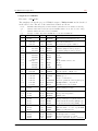
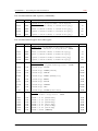
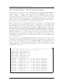
1
Consortium for Small-Scale Modelling A Description of the Nonhydrostatic Regional COSMO-Model Part VII : User’s Guide U. Sch¨ attler, G. Doms, and C. Schraff COSMO V4.29 October 2013 www.cosmo-model.org Printed at Deutscher Wetterdienst, P.O. Box 100465, 63004 Offenbach, Germany i Contents Contents 1 Overview on the Model System 1 1.1 General Remarks . . . . . . . . . . . . . . . . . . . . . . . . . . . . . . . . . . 1 1.2 Basic Model Design and Features . . . . . . . . . . . . . . . . . . . . . . . . . 3 1.3 Organization of the Documentation . . . . . . . . . . . . . . . . . . . . . . . . 6 2 Introduction 8 3 Model Formulation and Data Assimilation 10 3.1 Basic State and Coordinate-System . . . . . . . . . . . . . . . . . . . . . . . . 10 3.2 Differential Form of Thermodynamic Equations . . . . . . . . . . . . . . . . . 11 3.3 Horizontal and Vertical Grid Structure . . . . . . . . . . . . . . . . . . . . . . 12 3.4 Numerical Integration . . . . . . . . . . . . . . . . . . . . . . . . . . . . . . . 16 3.4.1 Runge-Kutta: 2-timelevel HE-VI Integration . . . . . . . . . . . . . . 17 3.4.2 Leapfrog: 3-timelevel HE-VI Integration . . . . . . . . . . . . . . . . . 17 3.4.3 Leapfrog: 3-timelevel Semi-Implicit Integration . . . . . . . . . . . . . 18 Physical Parameterizations . . . . . . . . . . . . . . . . . . . . . . . . . . . . 18 3.5.1 Radiation . . . . . . . . . . . . . . . . . . . . . . . . . . . . . . . . . . 19 3.5.2 Grid-scale Precipitation . . . . . . . . . . . . . . . . . . . . . . . . . . 19 3.5.3 Moist Convection . . . . . . . . . . . . . . . . . . . . . . . . . . . . . . 21 3.5.4 Vertical Turbulent Diffusion . . . . . . . . . . . . . . . . . . . . . . . . 23 3.5.5 Parameterization of Surface Fluxes . . . . . . . . . . . . . . . . . . . . 23 3.5.6 A subgrid-scale orography scheme . . . . . . . . . . . . . . . . . . . . 24 3.5.7 Soil Processes . . . . . . . . . . . . . . . . . . . . . . . . . . . . . . . . 24 Data Assimilation . . . . . . . . . . . . . . . . . . . . . . . . . . . . . . . . . 27 3.5 3.6 Part VII – User’s Guide 4.28 Contents ii Contents 4 Installation of the COSMO-Model 4.1 29 External Libraries for the COSMO-Model . . . . . . . . . . . . . . . . . . . . 29 4.1.1 libgrib1.a: . . . . . . . . . . . . . . . . . . . . . . . . . . . . . . . . 29 4.1.2 libnetcdf.a: . . . . . . . . . . . . . . . . . . . . . . . . . . . . . . . . 30 4.1.3 libmisc.a: . . . . . . . . . . . . . . . . . . . . . . . . . . . . . . . . . 30 4.1.4 libcsobank.a, libsupplement.a: . . . . . . . . . . . . . . . . . . . . 30 4.1.5 libRTTOV7.a: . . . . . . . . . . . . . . . . . . . . . . . . . . . . . . . . 31 4.2 Working with the VCS . . . . . . . . . . . . . . . . . . . . . . . . . . . . . . . 31 4.3 Preparing the Code . . . . . . . . . . . . . . . . . . . . . . . . . . . . . . . . . 31 4.4 Compiling and Linking . . . . . . . . . . . . . . . . . . . . . . . . . . . . . . . 33 4.5 Running the Code . . . . . . . . . . . . . . . . . . . . . . . . . . . . . . . . . 34 5 Data Formats for I/O 5.1 5.2 35 The GRIB Binary Data Format . . . . . . . . . . . . . . . . . . . . . . . . . . 35 5.1.1 Code Form . . . . . . . . . . . . . . . . . . . . . . . . . . . . . . . . . 35 5.1.2 Indicator and End Section . . . . . . . . . . . . . . . . . . . . . . . . . 36 5.1.3 Product Definition Section . . . . . . . . . . . . . . . . . . . . . . . . 38 5.1.4 Grid Description Section . . . . . . . . . . . . . . . . . . . . . . . . . . 40 5.1.5 Bit-map Section . . . . . . . . . . . . . . . . . . . . . . . . . . . . . . 40 5.1.6 Binary Data Section . . . . . . . . . . . . . . . . . . . . . . . . . . . . 40 The NetCDF Data Format . . . . . . . . . . . . . . . . . . . . . . . . . . . . 42 5.2.1 CF Conventions . . . . . . . . . . . . . . . . . . . . . . . . . . . . . . 42 5.2.2 Namelist Input . . . . . . . . . . . . . . . . . . . . . . . . . . . . . . . 43 5.2.3 netCDF Header Section . . . . . . . . . . . . . . . . . . . . . . . . . . 43 5.2.4 Useful Post-Processing Utilities . . . . . . . . . . . . . . . . . . . . . . 46 6 Input Files for the COSMO-Model 47 6.1 File for Namelist Input . . . . . . . . . . . . . . . . . . . . . . . . . . . . . . . 47 6.2 Conventions for File Names . . . . . . . . . . . . . . . . . . . . . . . . . . . . 49 6.3 Initial and Boundary Data . . . . . . . . . . . . . . . . . . . . . . . . . . . . . 51 6.4 Observation Input Files . . . . . . . . . . . . . . . . . . . . . . . . . . . . . . 53 Part VII – User’s Guide 4.28 Contents iii Contents 6.4.1 Templates for observation types for which Table-Driven Code Forms (TDCF) defined by WMO exist . . . . . . . . . . . . . . . . . . . . . . 55 6.4.2 Observation types with templates proposed or approved by WMO . . 64 6.4.3 Observation types without templates proposed by WMO . . . . . . . 69 6.4.4 The blacklist file . . . . . . . . . . . . . . . . . . . . . . . . . . . . . . 73 7 Namelist Input for COSMO-Modell 75 7.1 LMGRID — Specifying the Domain and the Model Grid . . . . . . . . . . . . . 77 7.2 RUNCTL — Parameters for the Model Run . . . . . . . . . . . . . . . . . . . . 78 7.3 DYNCTL — Parameters for the Adiabatic Model . . . . . . . . . . . . . . . . . 85 7.4 PHYCTL — Parameters for the Diabatic Model . . . . . . . . . . . . . . . . . . 94 7.5 TUNING — Parameters for tuning dynamics and physics . . . . . . . . . . . . 104 7.6 DIACTL — Parameters for Diagnostic Output . . . . . . . . . . . . . . . . . . 107 7.7 SATCTL — Controlling the Synthetic Satellite Images . . . . . . . . . . . . . . 110 7.8 INICTL — Parameters for the Model Initialization . . . . . . . . . . . . . . . 113 7.9 NUDGING — Controlling the Data Assimilation . . . . . . . . . . . . . . . . . . 114 7.10 EPSCTL — Controlling the Ensemble Prediction Mode . . . . . . . . . . . . . 136 7.11 IOCTL — Controlling the Grib I/O . . . . . . . . . . . . . . . . . . . . . . . . 137 7.12 DATABASE — Specification of Database Job . . . . . . . . . . . . . . . . . . . 140 7.13 GRIBIN — Controlling the Grib Input . . . . . . . . . . . . . . . . . . . . . . 141 7.14 GRIBOUT — Controlling the Grib Output . . . . . . . . . . . . . . . . . . . . . 144 8 Model Output 8.1 8.2 147 ASCII Output for the Forecast Model . . . . . . . . . . . . . . . . . . . . . . 147 8.1.1 M stationname — Grid point output . . . . . . . . . . . . . . . . . . . 148 8.1.2 YUSPECIF — NAMELIST-parameters . . . . . . . . . . . . . . . . . . . . 151 8.1.3 YUCHKDAT — Checking the Grib input/output data . . . . . . . . . . . 151 8.1.4 YUPRMASS — Protocolling the forecast with mass variables . . . . . . . 152 8.1.5 YUPRHUMI — Protocolling the forecast with humidity variables . . . . 152 ASCII Output Related to the Use of Observations . . . . . . . . . . . . . . . 156 8.2.1 YUAOFEX — Nudging: Observation Input AOF . . . . . . . . . . . . . . 156 8.2.2 YUOBSDR — Nudging: Active and Passive Reports . . . . . . . . . . . . 158 Part VII – User’s Guide 4.28 Contents iv Contents 8.2.3 YUREJCT — Nudging: Rejected Reports . . . . . . . . . . . . . . . . . 160 8.2.4 YUQUCTL — Nudging: Data Rejected by Quality Control . . . . . . . . 162 8.2.5 YUCAUTN — Nudging: Warning Messages on Insufficient Array Sizes . . 164 8.2.6 YUSTATS — Nudging: Statistics on Observation Processing . . . . . . . 166 8.2.7 YUVERIF — Nudging: Verification File VOF . . . . . . . . . . . . . . . 171 8.2.8 YUPRINT — Nudging: Other Aspects . . . . . . . . . . . . . . . . . . . 178 8.2.9 Standard Output — Basic Monitoring of Nudging . . . . . . . . . . . 182 8.2.10 YUSURF — 2-D Surface Analyses . . . . . . . . . . . . . . . . . . . . . 186 8.3 NetCDF Feedobs File . . . . . . . . . . . . . . . . . . . . . . . . . . . . . . . 188 8.4 Output of Forecast Fields . . . . . . . . . . . . . . . . . . . . . . . . . . . . . 189 References Part VII – User’s Guide 4.28 193 Contents 1 Section 1 Overview on the Model System 1.1 General Remarks The COSMO-Model is a nonhydrostatic limited-area atmospheric prediction model. It has been designed for both operational numerical weather prediction (NWP) and various scientific applications on the meso-β and meso-γ scale. The COSMO-Model is based on the primitive thermo-hydrodynamical equations describing compressible flow in a moist atmosphere. The model equations are formulated in rotated geographical coordinates and a generalized terrain following height coordinate. A variety of physical processes are taken into account by parameterization schemes. Besides the forecast model itself, a number of additional components such as data assimilation, interpolation of boundary conditions from a driving host model, and postprocessing utilities are required to run the model in NWP-mode, climate mode or for case studies. The purpose of the Description of the Nonhydrostatic Regional COSMO-Model is to provide a comprehensive documentation of all components of the system and to inform the user about code access and how to install, compile, configure and run the model. The basic version of the COSMO-Model (formerly known as Lokal Modell (LM)) has been developed at the Deutscher Wetterdienst (DWD). The COSMO-Model and the triangular mesh global gridpoint model GME form – together with the corresponding data assimilation schemes – the NWP-system at DWD, which is run operationally since end of 1999. The subsequent developments related to the model have been organized within COSMO, the Consortium for Small-Scale Modelling. COSMO aims at the improvement, maintenance and operational application of a non-hydrostatic limited-area modelling system, which is now consequently called the COSMO-Model. The meteorological services participating to COSMO at present are listed in Table 1.1. For more information about COSMO, we refer to the web-site at www.cosmo-model.org . The COSMO-Model is available free of charge for scientific and educational purposes, especially for cooperational projects with COSMO members. However, all users are required to sign an agreement with a COSMO national meteorological service and to respect certain conditions and restrictions on code usage. For questions concerning the request and the agreement, please contact the chairman of the COSMO Steering Committee. In the case of a planned operational or commercial use of the COSMO-Model package, special regulations Part VII – User’s Guide 4.28 Section 1: Overview on the Model System 2 1.1 General Remarks Table 1.1: COSMO: Participating Meteorological Services DWD MeteoSwiss USAM HNMS IMGW NMA RosHydroMet ARPA-SIMC ARPA-Piemonte CIRA AGeoBW Deutscher Wetterdienst, Offenbach, Germany Meteo-Schweiz, Zurich, Switzerland Ufficio Generale Spazio Aero e Meteorologia, Rome, Italy Hellenic National Meteorological Service, Athens, Greece Institute of Meteorology and Water Management, Warsaw, Poland National Meteorological Administration, Bucharest, Romania Hydrometeorological Centre of Russia, Moscow, Russia Agenzia Regionale per la Protezione Ambientale dell’ Emilia-Romagna, Servizio Idro Meteo Clima, Bologna, Italy Agenzia Regionale per la Protezione Ambientale, Piemonte, Turin, Italy Centro Italiano Ricerche Aerospaziali, Capua, Italy Amt f¨ ur Geoinformationswesen der Bundeswehr, Euskirchen, Germany will apply. The further development of the modelling system within COSMO is organized in Working Groups which cover the main research and development activities: data assimilation, numerical aspects, upper air physical aspects, soil and surface physics aspects, interpretation and applications, verification and case studies, reference version and implementation and predictability and ensemble methods. In 2005, the COSMO Steering Committee decided to define Priority Projects with the goal to focus the scientific activities of the COSMO community on some few key issues and support the permanent improvement of the model. For contacting the Working Group Coordinators or members of the Working Groups or Priority Projects, please refer to the COSMO web-site. The COSMO meteorological services are not equipped to provide extensive support to external users of the model. If technical problems occur with the installation of the model system or with basic questions how to run the model, questions could be directed via email to [email protected]. If further problems occur, please contact the members of an appropriate Working Group. We try to assist you as well as possible. The authors of this document recognize that typographical and other errors as well as discrepancies in the code and deficiencies regarding the completeness may be present, and your assistance in correcting them is appreciated. All comments and suggestions for improvement or corrections of the documentation and the model code are welcome and may be directed Part VII – User’s Guide 4.28 Section 1: Overview on the Model System 1.2 Basic Model Design and Features 3 to the authors. 1.2 Basic Model Design and Features The nonhydrostatic fully compressible COSMO-Model has been developed to meet highresolution regional forecast requirements of weather services and to provide a flexible tool for various scientific applications on a broad range of spatial scales. When starting with the development of the COSMO-Model, many NWP-models operated on hydrostatic scales of motion with grid spacings down to about 10 km and thus lacked the spatial resolution required to explicitly capture small-scale severe weather events. The COSMO-Model has been designed for meso-β and meso-γ scales where nonhydrostatic effects begin to play an essential role in the evolution of atmospheric flows. By employing 1 to 3 km grid spacing for operational forecasts over a large domain, it is expected that deep moist convection and the associated feedback mechanisms to the larger scales of motion can be explicitly resolved. Meso-γ scale NWP-models thus have the principle potential to overcome the shortcomings resulting from the application of parameterized convection in current coarse-grid hydrostatic models. In addition, the impact of topography on the organization of penetrative convection by, e.g. channeling effects, is represented much more realistically in high resolution nonhydrostatic forecast models. In the beginning, the operational application of the model within COSMO were mainly on the meso-β scale using a grid spacing of 7 km. The key issue was an accurate numerical prediction of near-surface weather conditions, focusing on clouds, fog, frontal precipitation, and orographically and thermally forced local wind systems. Since April 2007, a meso-γ scale version is running operationally at DWD by employing a grid spacing of 2.8 km. Applications with similar resolutions are now run by most COSMO partners. We expect that this will allow for a direct simulation of severe weather events triggered by deep moist convection, such as supercell thunderstorms, intense mesoscale convective complexes, prefrontal squallline storms and heavy snowfall from wintertime mesocyclones. The requirements for the data assimilation system for the operational COSMO-Model are mainly determined by the very high resolution of the model and by the task to employ it also for nowcasting purposes in the future. Hence, detailed high-resolution analyses have to be able to be produced frequently and quickly, and this requires a thorough use of asynoptic and high-frequency observations such as aircraft data and remote sensing data. Since both 3-dimensional and 4-dimensional variational methods tend to be less appropriate for this purpose, a scheme based on the observation nudging technique has been chosen for data assimilation. Besides the operational application, the COSMO-Model provides a nonhydrostatic modelling framework for various scientific and technical purposes. Examples are applications of the model to large-eddy simulations, cloud resolving simulations, studies on orographic flow systems and storm dynamics, development and validation of large-scale parameterization schemes by fine-scale modelling, and tests of computational strategies and numerical techniques. For these types of studies, the model should be applicable to both real data cases and artificial cases using idealized test data. Moreover, the model has been adapted by other communities for applications in climate mode (CCLM) and / or running an online coupled module for aerosols and reactive trace gases (ART). Part VII – User’s Guide 4.28 Section 1: Overview on the Model System 4 1.2 Basic Model Design and Features Such a wide range of applications imposes a number of requirements for the physical, numerical and technical design of the model. The main design requirements are: (i) use of nonhydrostatic, compressible dynamical equations to avoid restrictions on the spatial scales and the domain size, and application of an efficient numerical method of solution; (ii) provision of a comprehensive physics package to cover adequately the spatial scales of application, and provision of high-resolution data sets for all external parameters required by the parameterization schemes; (iii) flexible choice of initial and boundary conditions to accommodate both real data cases and idealized initial states, and use of a mesh-refinement technique to focus on regions of interest and to handle multi-scale phenomena; (iv) use of a high-resolution analysis method capable of assimilating high-frequency asynoptic data and remote sensing data; (v) use of pure Fortran constructs to render the code portable among a variety of computer systems, and application of the standard MPI-software for message passing on distributed memory machines to accommodate broad classes of parallel computers. The development of the COSMO-Model was organized along these basic guidelines. However, not all of the requirements are fully implemented, and development work and further improvement is an ongoing task. The main features and characteristics of the present release are summarized below. Dynamics - Model Equations – Nonhydrostatic, full compressible hydro-thermodynamical equations in advection form. Subtraction of a hydrostatic base state at rest. - Prognostic Variables – Horizontal and vertical Cartesian wind components, pressure perturbation, temperature, specific humidity, cloud water content. Optionally: cloud ice content, turbulent kinetic energy, specific water content of rain, snow and graupel. - Diagnostic Variables – Total air density, precipitation fluxes of rain and snow. - Coordinate System – Generalized terrain-following height coordinate with rotated geographical coordinates and user defined grid stretching in the vertical. Options for (i) base-state pressure based height coordinate, (ii) Gal-Chen height coordinate and (iii) exponential height coordinate (SLEVE) according to Sch¨ar et al. (2002). Numerics - Grid Structure – Arakawa C-grid, Lorenz vertical grid staggering. - Spatial Discretization – Second-order finite differences. For the two time-level scheme also 1st and 3rd to 6th order horizontal advection (default: 5th order). Option for explicit higher order vertical advection. - Time Integration – Two time-level 2nd and 3rd order Runge-Kutta split-explicit scheme after Wicker and Skamarock (2002) and a TVD-variant (Total Variation Diminishing) of a 3rd order Runge-Kutta split-explicit scheme. Option for a second-order leapfrog HE-VI (horizontally explicit, vertically implicit) time-split integration scheme, including extensions proposed by Skamarock and Klemp (1992). Option for a three time-level 3-d semi-implicit scheme (Thomas et al. (2000)) based on the leapfrog scheme. Part VII – User’s Guide 4.28 Section 1: Overview on the Model System 5 1.2 Basic Model Design and Features - Numerical Smoothing – 4th-order linear horizontal diffusion with option for a monotonic version including an orographic limiter. Rayleigh damping in upper layers. 2-d divergence damping and off-centering in the vertical in split time steps. Initial and Boundary Conditions - Initial Conditions – Interpolated initial data from various coarse-grid driving models (GME, ECMWF, COSMO-Model) or from the continuous data assimilation stream (see below). Option for user-specified idealized initial fields. - Lateral Boundary Conditions – 1-way nesting by Davies-type lateral boundary formulation. Data from several coarse-grid models can be processed (GME, IFS, COSMO-Model). Option for periodic boundary conditions. - Top Boundary Conditions – Options for rigid lid condition and Rayleigh damping layer. - Initialization – Digital-filter initialization of unbalanced initial states (Lynch et al. (1997)) with options for adiabatic and diabatic initialization. Physical Parameterizations - Subgrid-Scale Turbulence – Prognostic turbulent kinetic energy closure at level 2.5 including effects from subgrid-scale condensation and from thermal circulations. Option for a diagnostic second order K-closure of hierarchy level 2 for vertical turbulent fluxes. Preliminary option for calculation of horizontal turbulent diffusion in terrain following coordinates (3D Turbulence). - Surface Layer Parameterization – A Surface layer scheme (based on turbulent kinetic energy) including a laminar-turbulent roughness layer. Option for a stability-dependent draglaw formulation of momentum, heat and moisture fluxes according to similarity theory (Louis (1979)). - Grid-Scale Clouds and Precipitation – Cloud water condensation and evaporation by saturation adjustment. Precipitation formation by a bulk microphysics parameterization including water vapour, cloud water, cloud ice, rain and snow with 3D transport for the precipitating phases. Option for a new bulk scheme including graupel. Option for a simpler column equilibrium scheme. - Subgrid-Scale Clouds – Subgrid-scale cloudiness is interpreted by an empirical function depending on relative humidity and height. A corresponding cloud water content is also interpreted. Option for a statistical subgrid-scale cloud diagnostic for turbulence. - Moist Convection – Tiedtke (1989) mass-flux convection scheme with equilibrium closure based on moisture convergence. Option for the Kain-Fritsch (Kain and Fritsch (1993)) convection scheme with non-equilibrium CAPE-type closure. - Shallow Convection – Reduced Tiedtke scheme for shallow convection only. - Radiation – δ two-stream radiation scheme after Ritter and Geleyn (1992) short and longwave fluxes (employing eight spectral intervals); full cloud-radiation feedback. - Soil Model – Multi-layer version of the former two-layer soil model after Jacobsen and Heise (1982) based on the direct numerical solution of the heat conduction equation. Snow and interception storage are included. Option for the (old) two-layer soil model employing the extended force-restore method still included. - Fresh-Water Lake Parameterization – Two-layer bulk model after Mironov (2008) to predict the vertical temperature structure and mixing conditions in fresh-water lakes of various depths. - Sea-Ice Scheme – Parameterization of thermodynamic processes (without rheology) after Mironov and B. (2004). The scheme basically computes the energy balance at the ices surface, using one layer of sea ice. Part VII – User’s Guide 4.28 Section 1: Overview on the Model System 6 1.3 Organization of the Documentation - Terrain and Surface Data – All external parameters of the model are available at various resolutions for a pre-defined region covering Europe. For other regions or grid-spacings, the external parameter file can be generated by a preprocessor program using high-resolution global data sets. Data Assimilation - Basic Method – Continuous four-dimensional data assimilation based on observation nudging (Schraff (1996), Schraff (1997)), with lateral spreading of upper-air observation increments along horizontal surfaces. Explicit balancing by a hydrostatic temperature correction for surface pressure updates, a geostrophic wind correction, and a hydrostatic upper-air pressure correction. - Assimilated Atmospheric Observations – Radiosonde (wind, temperature, humidity), aircraft (wind, temperature), wind profiler (wind), and surface-level data (SYNOP, SHIP, BUOY: pressure, wind, humidity). Optionally RASS (temperature), radar VAD wind, and ground-based GPS (integrated water vapour) data. Surface-level temperature is used for the soil moisture analysis only. - Radar derived rain rates – Assimilation of near surface rain rates based on latent heat nudging (Stephan et al. (2008)). It locally adjusts the three-dimensional thermodynamical field of the model in such a way that the modelled precipitation rates should resemble the observed ones. - Surface and Soil Fields – Additional two-dimensional intermittent analysis: - Soil Moisture Analysis – Daily adjustment of soil moisture by a variational method (Hess (2001)) in order to improve 2-m temperature forecasts; use of a Kalman-Filter-like background weighting. - Sea Surface Temperature Analysis – Daily Cressman-type correction, and blending with global analysis. Use of external sea ice cover analysis. - Snow Depth Analysis – 6-hourly analysis by weighted averaging of snow depth observations, and use of snowfall data and predicted snow depth. Code and Parallelization - Code Structure – Modular code structure using standard Fortran constructs. - Parallelization – The parallelization is done by horizontal domain decomposition using a soft-coded gridline halo (2 lines for Leapfrog, 3 for the Runge-Kutta scheme). The Message Passing Interface software (MPI) is used for message passing on distributed memory machines. - Compilation of the Code – The compilation of all programs is performed by a Unix shell script invoking the Unix make command. All dependencies of the routines are automatically taken into account by the script. - Portability – The model can be easily ported to various platforms; current applications are on conventional scalar machines (UNIX workstations, LINUX and Windows-NT PCs), on vector computers (NEC SX series) and MPP machines (CRAY, IBM, SGI and others). - Model Geometry – 3-d, 2-d and 1-d model configurations. Metrical terms can be adjusted to represent tangential Cartesian geometry with constant or zero Coriolis parameter. 1.3 Organization of the Documentation For the documentation of the model we follow closely the European Standards for Writing and Documenting Exchangeable Fortran 90-Code. These standards provide a framework for the use of Fortran-90 in European meteorological organizations and weather services and thereby Part VII – User’s Guide 4.28 Section 1: Overview on the Model System 7 1.3 Organization of the Documentation Table 1.2: COSMO Documentation: A Description of the Nonhydrostatic Regional COSMOModel Part Part Part Part Part I: II: III: IV: V: Part VI: Part VII: Dynamics and Numerics Physical Parameterization Data Assimilation Implementation Documentation Preprocessing: Initial and Boundary Data for the COSMO-Model Postprocessing User’s Guide facilitate the exchange of code between these centres. According to these standards, the model documentation is split into two categories: external documentation (outside the code) and internal documentation (inside the code). The model provides extensive documentation within the codes of the subroutines. This is in form of procedure headers, section comments and other comments. The external documentation is split into seven parts, which are listed in Table 1.2. Parts I - III form the scientific documentation, which provides information about the theoretical and numerical formulation of the model, the parameterization of physical processes and the four-dimensional data assimilation. The scientific documentation is independent of (i.e. does not refer to) the code itself. Part IV will describe the particular implementation of the methods and algorithms as presented in Parts I - III, including information on the basic code design and on the strategy for parallelization using the MPI library for message passing on distributed memory machines (not available yet). The generation of initial and boundary conditions from coarse grid driving models is described in Part V. This part is a description of the interpolation procedures and algorithms used (not yet complete) as well as a User’s Guide for the interpolation program INT2LM. Available postprocessing utilities will be described (in the future) in Part VI. Finally, the User’s Guide of the COSMO-Model provides information on code access and how to install, compile, configure and run the model. The User’s Guide contains also a detailed description of various control parameters in the model input file (in NAMELIST format) which allow for a flexible model set-up for various applications. All parts of the documentation are available at the COSMO web-site (http://www.cosmo-model.org/content/model/documentation/core/default.htm). Part VII – User’s Guide 4.28 Section 1: Overview on the Model System 8 Section 2 Introduction The usage of the program package for the COSMO-Model is a rather complex task, both, for the experienced and even more for the non-experienced user. This User’s Guide serves in a first instance as a complete reference for all the different NAMELIST groups and variables, with which the execution of the model can be controlled. It also includes a description on how to install the package and gives additional necessary information, e.g. on the Grib format used for I/O. Knowing the meaning of all NAMELIST-variables normally is not enough to find the way through the possible configurations of the model. Therefore, a description would be desirable that explains how the variables can be put together to give a meaningful setup, or which variable settings contradict each other or simply are not possible. We apologize, that such a description is not yet available, but it will be developed in the future. It will explain, how the different components of the model (see Fig. 2.1) can be selected and which configurations are possible. Up to then, Part VII of the model documentation is organized as follows. First, an overview on the model formulation and the data assimilation is given. In Section 4, the installation of the package is explained. The necessary input files of the model are listed in Section 6 and Section 5.1 gives a short description of the GRIB code used for input and output of the meteorological fields. Section 7 then is the complete reference for all NAMELIST variables. Sections 8.1 and 8.2 finally describe the ASCII output of the COSMO-Model, and Section 8.4 provides information on the output model fields. Part VII – User’s Guide 4.28 Section 2: Introduction 9 Figure 2.1: Schematic view of the different COSMO-Model components Dynamics 3 time level split-explicit Leapfrog # 2 time level split-explicit Runge-Kutta (several variants) " 3 time level semi-implicit Leapfrog Relaxation Assimilation Physics $ Observation Grid Scale Clouds and processing Precipitation (with or without 3D transport of precipitating particles) - warm rain scheme - 1-category ice scheme Surface analysis - 2-category ice scheme - 3-category ice scheme & % ' Radiation ! ' Subgrid Scale Turbu lence Closure - 1-D diag. closure - 1-D TKE-based diagnostic closure - 3-D TKE-based prognostic closure & ' Parameterization of Surface Fluxes - Standard bulk transfer scheme - TKE-based surface scheme & Diagnostics Near surface weather parameters Mean values Nudging of atmo spheric variables Meteographs $ and surface pres sure Latent Heat Nudging % $ Synthetic Satellite Pictures Initialization % I/O Digital filtering Grib Subgrid sc. orography # Part VII – User’s Guide 4.28 Volume- and Area-Integrals Moist Convection - Tiedtke mass-flux - Kain-Fritsch scheme - Shallow convection Soil and Surface - 2-layer soil - multi-layer soil - lake model - sea-ice scheme " NetCDF Restart ! Section 2: Introduction 10 Section 3 Model Formulation and Data Assimilation 3.1 Basic State and Coordinate-System The COSMO-Model is based on the primitive hydro-thermodynamical equations describing compressible nonhydrostatic flow in a moist atmosphere without any scale approximations. A basic state is subtracted from the equations to reduce numerical errors associated with the calculation of the pressure gradient force in case of sloping coordinate surfaces. The basic state represents a time-independent dry atmosphere at rest which is prescribed to be horizontally homogeneous, vertically stratified and in hydrostatic balance. By introducing the basic state, the thermodynamic variables temperature (T ), pressure (p) and density (ρ) can be formally written as the sum of a height dependent reference value and a space and time dependent deviation: T = T0 (z) + T 0 , p = p0 (z) + p0 , ρ = ρ0 (z) + ρ0 , (3.1) where T0 (z), p0 (z) and ρ0 (z) are related by the hydrostatic equation ∂p0 gp0 = −gρ0 = − ∂z Rd T0 (3.2) and the equation of state, p0 = ρ0 Rd T0 . Rd is the gas constant of dry air. In principle, the vertical profile T0 (z) of temperature can be specified arbitrary since we do not linearize the model equations with respect to the reference state. For practical reasons, we prescribe a constant rate β for the temperature increase with the logarithm of pressure (as proposed by Dudhia (1993)), ∂T0 /∂ ln p0 = β. The integration of the hydrostatic equation (3.2) with the boundary values pSL = p0 (z = 0) and TSL = T0 (z = 0) for the pressure and temperature at mean sea level z = 0 then yields the vertical profiles of the reference state: p0 (z) = r pSL exp − TSL 1 − 1 − 2βgz2 β Rd TSL n o p exp − gz SL Rd TSL if β 6= 0 if β = 0 (3.3) Part VII – User’s Guide 4.28 Section 3: Model Formulation and Data Assimilation 11 3.2 Differential Form of Thermodynamic Equations s T0 (z) = TSL 1 − 2βgz 2 . Rd TSL For the three parameters pSL , TSL and β, which define the basic state, we use the default values pSL = 1000hPa, TSL = 288.15K and β = 42K. The variable names in the programs are p0sl (pSL ), t0sl (TSL ) and dt0lp (β), resp. The model equations are formulated with respect to a rotated lat/lon-grid with coordinates (λ, ϕ). The rotated coordinate system results from the geographical (λg , ϕg ) coordinates by tilting the north pole (see Part I of the Documentation, Dynamics and Numerics). In the vertical, we use a generalized terrain-following height coordinate ζ, where any unique function of geometrical height can be used for transformation. Since ζ doesn’t depend on time, the (λ, ϕ,ζ)-system represents a non-deformable coordinate system, where surfaces of constant ζ are fixed in space - in contrast to the pressure based coordinate system of most hydrostatic models, where the surfaces of constant vertical coordinate move in space with changing surface pressure. The transformation of the model equations from the orthogonal (λ, ϕ, z)-system to the nonorthogonal terrain-following (λ, ϕ, ζ)-system is given by the three elements of the inverse Jacobian matrix J z , z Jλ ≡ J13 = ∂z ∂λ , ζ z Jϕ ≡ J23 = ∂z ∂ϕ , z Jζ ≡ J33 = ζ √ ∂z = − G. ∂ζ (3.4) The terrain-following ζ-system of the COSMO-Model is defined to be left-handed, i.e. the value of the ζ-coordinate increases with decreasing height z from the top of the model √ to the surface. Thus, Jζ is always negative and equal to the negative absolute value ( G = | det (J z ) |) of the determinant of the inverse Jacobi matrix. 3.2 Differential Form of Thermodynamic Equations By transforming the primitive hydro-thermodynamical equations to the (λ, ϕ, ζ) coordinatesystem and subtracting the basic state, we achieve the following set of prognostic model equations for the three components u, v and w of the wind vector, the perturbation pressure p0 , the temperature T and the humidity variables q. ∂u uv + v · ∇u − tan ϕ − f v ∂t a ∂v u2 + v · ∇v + tan ϕ + f u ∂t a ∂w + v · ∇w ∂t ∂p0 + v · ∇p0 − gρ0 w ∂t ∂T + v · ∇T ∂t ∂q v + v · ∇q v ∂t Part VII – User’s Guide 4.28 1 ∂p0 Jλ ∂p0 = − +√ + Mu ρa cos ϕ ∂λ G ∂ζ 1 ∂p0 Jϕ ∂p0 = − +√ + Mv ρa ∂ϕ G ∂ζ 1 ∂p0 √ = + B + Mw ρ G ∂ζ (3.5) = −(cpd /cvd )pD = − p D + QT ρcvd = −(S l + S f ) + Mqv Section 3: Model Formulation and Data Assimilation 12 3.3 Horizontal and Vertical Grid Structure ∂q l,f 1 ∂Pl,f + v · ∇q l,f + √ ∂t ρ G ∂ζ = S l,f + Mql,f Here, the continuity equation has been replaced by an equation for p0 . In Eqs. (3.5) a is the radius of the earth, cpd and cvd are the specific heat of dry air at constant pressure and constant volume, g is the gravity acceleration, f is the Coriolis parameter, Rv and Rd are the gas constants for water vapour and dry air. ρ is the density of moist air which is calculated as a diagnostic variable from the equation of state: ρ = p{Rd (1 + (Rv /Rd − 1)q v − q l − q f )T }−1 . (3.6) q v is the specific humidity, q l represents the specific water content of a category of liquid water (cloud or rain water) and q f represents the specific water content of a category of frozen water (cloud ice, snow or graupel). The corresponding precipitation fluxes are denoted by Pl and Pf . The terms Mψ denote contributions from subgrid-scale processes as, e.g. turbulence and convection and QT summarizes the diabatic heating rate due to this processes. The various sources and sinks in the equations for the humidity variables due to microphysical processes of cloud and precipitation formation are denoted by S l and S f . The calculation of all these terms related to subgrid-scale processes is done by physical parameterization schemes. An overview of the schemes used in the COSMO-Model is given in Section 3.5. The term B in the equation for the vertical velocity is the buoyant acceleration given by ρ0 B=g ρ T − T0 p0 T0 − + T p0 T Rv − 1 qv − ql − qf . Rd (3.7) The advection operator in terrain-following coordinates is defined as 1 ∂ ∂ v·∇= u + v cos ϕ a cos ϕ ∂λ ∂ϕ ∂ + ζ˙ , ∂ζ where ζ˙ is the contra-variant vertical velocity in the ζ-system: 1 ζ˙ = √ G Jλ Jϕ u+ v−w . a cos ϕ a D is the three-dimensional wind divergence which is calculated from D= 1 a cos ϕ ∂u Jλ ∂u ∂ Jϕ ∂v +√ + (v cos ϕ) + cos ϕ √ ∂λ ∂ζ ∂ϕ G G ∂ζ 1 ∂w −√ . G ∂ζ In deriving the prognostic equation for the perturbation pressure from the continuity equation, a source term due to diabatic heating has been neglected. For most meteorological applications, this source term is much smaller than the forcing by divergence. This approximation is also used in many other nonhydrostatic simulation models. 3.3 Horizontal and Vertical Grid Structure The model equations (3.5) are solved numerically using the traditional finite difference method. In this technique, spatial differential operators are simply replaced by suitable finite Part VII – User’s Guide 4.28 Section 3: Model Formulation and Data Assimilation 13 3.3 Horizontal and Vertical Grid Structure difference operators. The time integration is also by discrete stepping using a fixed timestep ∆t. The terrain-following coordinate system with the generalized vertical coordinate ζ allows to map the irregular grid associated with the terrain-following system in physical space onto a rectangular and regular computational grid. Thus, constant increments ∆λ : grid-spacing in longitudinal direction, ∆ϕ : grid-spacing in latitudinal direction, ∆ζ : grid-spacing in ζ-direction (∆ζ = 1), of the independent variables are used to set up the computational grid. To simplify the notation, we set the vertical grid-spacing equal to one (see below). The discrete computational (λ, ϕ, ζ)-space is then represented by a finite number of grid points (i, j, k), where i corresponds to the λ-direction, j to the ϕ-direction and k to the ζ-direction. The position of the grid points in the computational space is defined by λi = λ0 + (i − 1) ∆λ , i = 1, · · · , Nλ = ϕ0 + (j − 1)∆ϕ, j = 1, · · · , Nϕ ϕj ζk = k , (3.8) k = 1, · · · , Nζ . Nλ denotes the number of grid points in λ-direction, Nϕ the number of points in the ϕdirection and Nζ the number of points in the ζ-direction. λ0 and ϕ0 define the south-western corner of the model domain with respect to the rotated geographical coordinates (λ, ϕ). Thus, i = 1 and i = Nλ correspond, respectively, to the western and the eastern boundaries of the domain. Accordingly, the southern and the northern borderlines are given by j = 1 and j = Nϕ . The corresponding variables in the programs are dlon (∆λ), dlat (∆ϕ), startlon tot (λ0 ), startlat tot (ϕ0 ), ie tot (Nλ ), je tot (Nϕ ) and ke tot (Nζ ). Every grid point (i, j, k) represents the centre of an elementary rectangular grid volume with side lengths ∆λ, ∆ϕ and ∆ζ. The grid-box faces are located halfway between the grid points in the corresponding directions, i.e. at λi±1/2 , ϕj±1/2 and ζk±1/2 . The model variables are staggered on an Arakawa-C/Lorenz grid with scalars (temperature, pressure and humidity variables) defined at the centre of a grid box and the normal velocity components defined on the corresponding box faces (see Figure 3.1). For a given grid spacing, this staggering allows for a more accurate representation of differential operators than in the A-grid, where all variables are defined at the same point. In general, we use second order centered finite difference operators, i.e. the numerical discretization error is reduced by a factor of four when we increase the resolution by a factor of two. For a detailed description of the numerical operators see Part I of the Documentation, Dynamics and Numerics. The grid-box faces in vertical direction are usually referred to as the half levels. These interfacial levels separate the model layers from each other. The model layers labeled by integers k are also denoted as main levels. Thus, for a model configuration with Nζ layers we have Nζ + 1 half levels. The top boundary of the model domain is defined to be the half level (ζ = 1/2) above the uppermost model layer (ζ = 1). At the lower boundary, the ζ-coordinate surface becomes conformal to the terrain height. The half level (ζ = Nζ + 1/2) below the first model layer above the ground (ζ = Nζ ) defines the lower boundary of the model. The discrete formulation of the model equations is independent on a specific choice for the vertical coordinate. This is achieved by a two-step transformation procedure: First we apply a Part VII – User’s Guide 4.28 Section 3: Model Formulation and Data Assimilation 14 3.3 Horizontal and Vertical Grid Structure k−1/2 w ϕ ● λ ζ ● k v u T ● ●u ● ● v j+1/2 w ● i−1/2 j i Figure 3.1: A grid box volume ∆V = ∆ζ ∆λ ∆ϕ showing the ArakawaC/Lorenz staggering of the dependent model variables. transformation to a specific terrain-following system, where in principle any unique function of geometrical height z can be used. As a default, either a generalized sigma-type coordinate η based on base-state pressure or a generalized Gal-Chen coordinate µ based on height can be chosen. In a second step this vertical coordinate is mapped onto the computational coordinate ζ with discrete coordinate values ζk = k and an equidistant grid spacing of ∆ζ = 1. The latter mapping is by a table which relates specific values of the terrain-following coordinate η or µ to the Nζ + 1 values of the half-level values ζk+1/2 . In this way a user-defined vertical grid-stretching can be easily applied. Details on the set-up of the vertical grid are provided in Part I of the Documentation, Dynamics and Numerics. To render the model code independent on η or µ, all metric terms involving the three components (3.4) of the Jacobi-matrix are evaluated numerically on the computational grid. These terms are rewritten in the form √ G= where have √ 1 √ γ, gρ0 J 1 ∂p0 √λ = − √ , γ ∂λ G J 1 ∂p0 √ϕ = − √ , γ ∂ϕ G (3.9) γ ≡ ∂p0 /∂ζ denotes the change of base-state pressure with ζ. In discretized form we √ γ k = (∆p0 )k = (p0 )k+1/2 − (p0 )k−1/2 , (3.10) (p0 )k = 1 {(p0 )k+1/2 + (p0 )k−1/2 } . 2 √ for γ and the base-state pressure p0 on model main levels. Additionally, the height of model half levels zk+1/2 resulting from the coordinate transformation is stored as a 3-D array. The Part VII – User’s Guide 4.28 Section 3: Model Formulation and Data Assimilation 15 3.3 Horizontal and Vertical Grid Structure w,z T , po , ρo , u 1/2 : model top γ u k=1 w,z w,z ζ T , po , ρo , u k − 1/2 γ u w,z k k + 1/2 w,z T , po , ρo , u γ u w,z i − 1/2 i k = Nζ N ζ + 1/2 : surface i + 1/2 Figure 3.2: Vertical staggering of variables and metric terms in a grid box column with Nζ layers. Dashed lines are the model half levels separating the main levels (full lines). base-state density on main levels then results from the discretized hydrostatic relation √ γk 1 (ρ0 )k = g zk−1/2 − zk+1/2 and the main level base-state temperature results from the equation of state. Fig. 3.2 illustrates the vertical staggering of model variables as well as base state variables and metric terms used in the discretization. In order to implement boundary conditions and to apply the domain decomposition strategy for code parallelization in a convenient way, the horizontal extent of the computational domain is chosen to be smaller than the total domain size. The lateral physical boundaries are positioned with a spatial offset from the outer boundaries to the interior. This offset is Noff ∆λ − ∆λ/4 Noff ∆ϕ − ∆ϕ/4 in λ-direction and in ϕ-direction, where Noff (nboundlines as program variable) denotes the number of grid intervals used to define the position of the physical boundaries. By default, Noff is set to 2 (larger but not smaller numbers for Noff may be specified by the user). Part VII – User’s Guide 4.28 Section 3: Model Formulation and Data Assimilation 16 3.4 Numerical Integration All grid points interior to the physical boundary constitute the computational (or model interior) domain, where the model equations are integrated numerically. These are points with subscripts (i, j) running from i = Noff +1, · · · , Nλ −Noff and j = Noff +1, · · · , Nϕ −Noff . The extra points outside the interior domain constitute the computational boundaries. At these points, all model variables are defined and set to specified boundary values, but no dynamical computations are done. For Noff = 2, we have two extra lines of grid points adjacent to each physical boundary (see Fig. 3.3). i T v T v T v T j TuTuTuT v uTu v Nϕ Nϕ−1 Nϕ−2 TuTuTuT T v T v T v T 1 2 3 i j 3 2 1 Nλ−2 Nλ−1 Nλ Figure 3.3: Horizontal model domain for Nλ × Nϕ grid points and an offset of Noff = 2 for the position of the physical boundaries (dotted). The computational boundaries are shaded; the integration is done for variables in the interior computational domain (i = 3, · · · , Nλ − 2 and j = 3, · · · , Nϕ − 2). 3.4 Numerical Integration Because the governing nonhydrostatic equations describe a compressible model atmosphere, meteorologically unimportant sound waves are also part of the solution. As acoustic waves are very fast, their presence severely limits the time step of explicit time integration schemes. In order to improve the numerical efficiency, the prognostic equations are separated into terms which are directly related to acoustic and gravity wave modes and into terms which refer to comparatively slowly varying modes of motion. This mode-splitting can formally be written in the symbolic form ∂ψ = sψ + fψ , (3.11) ∂t where ψ denotes a prognostic model variable, fψ the forcing terms due to the slow modes and sψ the source terms related to the acoustic and gravity wave modes. sψ is made up Part VII – User’s Guide 4.28 Section 3: Model Formulation and Data Assimilation 17 3.4 Numerical Integration of the pressure gradient terms in the momentum equations, the temperature and pressure contributions to the buoyancy term in the w-equation and the divergence term in the pressure and the temperature equation. The subset of equations containing the sψ -terms is then integrated with a special numerical scheme. The COSMO-Model provides four different integration methods. 3.4.1 Runge-Kutta: 2-timelevel HE-VI Integration Basic Namelist settings: l2tls=.TRUE.; lsemi imp=.FALSE.; irunge kutta=1/2 This scheme (with irunge kutta=1) is used for the COSMO-DE and COSMO-EU. This scheme has been implemented into the COSMO-Model as an alternative to the former default, the Leapfrog scheme, and can be combined with a forward-backward scheme for integrating the high-frequency modes of the elastic equations. The first (irunge kutta=1) variant is the normal 3rd-order Runge-Kutta scheme used by Wicker and Skamarock (2002) whereas the second one is a total variation diminishing (TVD) variant of 3rd-order (Liu et al. (1994)) (irunge kutta=2). Different horizontal advection upwind or centered-differences schemes of 3rd- to 6th-order can be used – the operators are formulated in advection form. The vertical advection is normally treated in an implicit way using a Crank-Nicolson scheme and centered-differences in space. Most slow tendencies such as vertical diffusion, thermal/solar heating, parameterized convection and coriolis force are computed only once using values of the prognostic variables at time step n. These tendencies are fixed during the individual Runge-Kutta steps and contribute to the total slow-mode tendencies which are integrated in several small time steps together with the fast-mode tendencies in a time-splitting sense. In contradiction to this, the whole 3D-advection is computed in each Runge-Kutta step. 3.4.2 Leapfrog: 3-timelevel HE-VI Integration Basic Namelist settings: l2tls=.FALSE.; lsemi imp=.FALSE. This method is a variant of the ? scheme which is based on a Leapfrog integration for the slow modes from time level n − 1 to time level n + 1 using an integration interval of 2∆t. The slow mode tendencies are evaluated at time level n for horizontal advection using standard second order centered differences and at time level n − 1 for most physical forcings. Vertical advection and vertical diffusion are calculated by a quasi-implicit scheme. The integration step is then subdivided into a number Ns of small time steps ∆τs according to 2∆t = Ns ∆τ and the prognostic equations (3.11) are stepped forward according to ψ ν+1 = ψ ν + sνψ ∆τ + fψn ∆τ . (3.12) Figure 3.4 illustrates the basic idea of the time-splitting scheme. In the integration of (3.12), sound waves are treated explicitly for horizontal directions using the forward-backward method while implicitly for the vertical direction (HE-VI). Thus, the small time step ∆τ is limited by the CFL stability criterion for horizontal but not for vertical sound wave propagation. This makes the HE-VI scheme numerically very efficient for large grid aspect ratios, i.e. ∆x/∆z 1, which are typically used in meso-β and meso-γ applications. Part VII – User’s Guide 4.28 Section 3: Model Formulation and Data Assimilation 18 3.5 Physical Parameterizations n−1 n n+1 n+2 tn ∆ts ∆t Figure 3.4: The time splitting algorithm An additional 3-D divergence damping as well as a slight time off-centering in the vertical implicit formulation is applied to damp acoustic modes. On the big time step, the Asselin time filter and a 4th order horizontal diffusion are used for numerical smoothing. While this 3-timelevel HE-VI integration was the default time scheme of the COSMO-Model in the beginning, it has now been replaced by the 2-timelevel Runge-Kutta schemes.. 3.4.3 Leapfrog: 3-timelevel Semi-Implicit Integration Basic Namelist settings: l2tls=.FALSE.; lsemi imp=.TRUE. Because the HE-VI scheme integrates the horizontal momentum equations explicitly, steep orography may provoke instabilities in small-scale applications. Full 3D semi-implicit schemes can avoid such stability problems by treating all pressure gradient and divergence terms implicitly both vertically and horizontally (HI-VI-scheme) - thus, a small time step is not used. Moreover, 3D semi-implicit schemes have the potential to become more cost-effective than split-explicit schemes at higher resolution where the grid aspect ratio is more isotropic and where the number of small time steps increases with the sound speed Courant number for low Mach number flows. The derivation of the scheme is based on the 3-timelevel Leapfrog integration and uses the time-tendency formulation to minimize cancellation errors. An elliptic equation for the pressure perturbation tendency L (δτ (p0 ) = qp is obtained by forming the divergence of the momentum equations and eliminating the buoyancy terms. However, the use of a nonorthogonal curvilinear coordinate system results in an elliptic operator L containing cross-derivative terms with variable coefficients. A minimal residual Krylov iterative solver (GMRES) was thus chosen to solve for the perturbation pressure tendency. We found the convergence criterion proposed by Skamarock et al. (1997) to be both sufficient and a robust predictor of when the RMS divergence of the flow has stabilized. An efficient line-Jacobi relaxation preconditioner was developed having the property that the number of Krylov solver iterations grows slowly as the convergence parameter εc decreases. Once the solution for the pressure tencendy is known, the other variables are updated by back-substitution. 3.5 Physical Parameterizations Some parts of the physics package of the COSMO-Model are adapted from the former operational hydrostatic model DM. Others have been widely rewritten or were replaced by new Part VII – User’s Guide 4.28 Section 3: Model Formulation and Data Assimilation 19 3.5 Physical Parameterizations developments. This section gives a short overview on the parameterization schemes used. A detailed description is given in Part II of the Documentation, Physical Parameterizations. 3.5.1 Radiation Basic Namelist settings: lphys=.TRUE.; lrad=.TRUE.; hincrad=1.0 To calculate the heating rate due to radiation we employ the parameterization scheme of Ritter and Geleyn (1992). This scheme is based on a δ-two-stream version of the general equation for radiative transfer and considers three shortwave (solar) and five longwave (thermal) spectral intervals. Clouds, aerosol, water vapour and other gaseous tracers are treated as optically active constituents of the atmosphere, which modify the radiative fluxes by absorption, emission and scattering. As an extension to the original scheme, a new treatment of the optical properties of ice particles has been introduced which allows a direct cloud-radiative feedback with the predicted ice water content when using the cloud ice scheme for the parameterization of cloud and precipitation. Numerically, the parameterization scheme is very cost-intensive. Thus, it is called only at hourly intervals during an operational forecast on the meso-β scale. The resulting shortand longwave heating rates are then stored and remain fixed for the following time interval. In case of high resolution simulations, the calling frequency of the radiation scheme can be increased to allow for a better representation of the interaction with the cloud field. The radiation can also be computed on a coarser grid to save computation time. 3.5.2 Grid-scale Precipitation Basic Namelist settings: lphys=.TRUE.; lgsp=.TRUE. The basic parameterization scheme for the formation of grid-scale clouds and precipitation is an adapted version of the DM-scheme. It is based on a Kessler-type bulk formulation and uses a specific grouping of various cloud and precipitation particles into broad categories of water substance. The particles in these categories interact by various microphysical processes which in turn have feedbacks with the overall thermodynamics. Microphysical processes are parameterized by corresponding mass transfer rates between the categories and are formulated in terms of the mixing ratios as the dependent model variables. Besides water vapour in the gaseous phase three categories of water are considered by the default scheme: - cloud water is in the form of small suspended liquid-phase drops. Cloud droplets are smaller than about 50 µm in radius and thus have no appreciable terminal fall speed relative to the airflow. - rain water is in the form of liquid-phase spherical drops which are large enough to have a non-negligible fall velocity. An exponential Marshall-Palmer size-distribution is assumed for the raindrops and a drop terminal velocity depending only on drop diameter is prescribed. Part VII – User’s Guide 4.28 Section 3: Model Formulation and Data Assimilation 20 3.5 Physical Parameterizations - Snow is made up of large rimed ice particles and rimed aggregates which are treated as thin plates with a specific size-mass relation. Particles in this category have a nonnegligible terminal velocity which is prescribed to depend only on particle size. An exponential Gunn-Marshall size-distribution is assumed. The budget equation for the specific water contents q of the various categories (water vapour q v , cloud water q c , cloud ice q i and graupel q g , depending on the scheme used) take advective and turbulent transport into account and contain source and sink terms due to the microphysical processes of cloud and precipitation formation. For rain water q r and snow q s , only advective transport is considered. The following mass-transfer rates are considered by the scheme: (a) condensation and evaporation of cloud water, (b) the initial formation of rainwater by autoconversion and of snow by nucleation from the cloud water phase, (c) the subsequent growth of the precipitation phases rain and snow by accretion, riming, deposition and shedding, (d) evaporation of rainwater and sublimation of snow in subcloud layers and (e) melting of snow to form rain and freezing of rain to form snow. The impact of the vertical motion of rain and snow relative to the airflow due to the sedimentation of particles with their terminal velocities is also taken into account by the vertical divergence of the corresponding precipitation fluxes Pr and Ps . Figure 3.5 illustrates the microphysical processes considered by this parameterization scheme. Smelt , Sfrz Sau Sac Sshed rain Snuc water Srim snow Sc Sev Pr cloud water vapour Fv Sdep Ps CCCCCCCCCCCCCCCCCCCCCCCCCCCCCCCC precipitation and evapotranspiration at ground level CCCCCCCCCCCCCCCCCCCCCCCCCCCCCCCC CCCCCCCCCCCCCCCCCCCCCCCCCCCCCCCC CCCCCCCCCCCCCCCCCCCCCCCCCCCCCCCC Figure 3.5: Hydrological cycle in the COSMO-Model cloud and precipitation scheme In contrast to the former diagnostic precipitation scheme with its assumption of column equilibrium for the precipitating particles, we now solve the complete prognostic equations Part VII – User’s Guide 4.28 Section 3: Model Formulation and Data Assimilation 21 3.5 Physical Parameterizations for rain q r and and snow q s (can be turned on/off by Namelist switches). This approach is therefore applicable to the meso-γ and smaller scales. For this purpose a semi-Lagrangeadvection scheme with a simple trilinear interpolation is implemented. This scheme is coupled by Marchuk-splitting with the cloud microphysical sources and sinks and the implicit sedimentation flux calculation. These options are available for the microphysics parameterization scheme: All options but the graupel scheme are available as diagnostic scheme (lprogprec=.FALSE.) or as prognostic scheme (lprogprec=.TRUE.): (a) itype gscp=1: A warm rain scheme which is similar to the original Kessler (1969) scheme; all ice-phase processes are ignored. (b) itype gscp=2: The basic scheme described above. (c) itype gscp=3: An extension of the basic scheme which includes cloud ice as an additional prognostic variable (cloud ice scheme). The scheme allows for an explicit representation of ice clouds and a more complete simulation of precipitation formation in mixed phase clouds. This scheme is used in the COSMO-EU. (d) itype gscp=4: A graupel-scheme (in addition to cloud-ice) has been implemented recently. It allows for an explicit simulation of deep convective clouds. This is available only as a prognostic scheme. This scheme is used in the COSMO-DE. The use of itype gscp=1/2 is not recommended for real cases. Also the diagnostic schemes (lprogprec=.FALSE.) are no longer used by DWD. Therefore, they are no longer tested and evaluated. 3.5.3 Moist Convection Basic Namelist settings: lphys=.TRUE.; lconv=.TRUE. For model applications on the meso-α and meso-β scales down to grid spacings of 5-10 km, cumulus convection is a subgrid-scale process which requires a parameterized representation. And even on the meso-γ scale it turned out, that a parameterization of shallow convection still is necessary. The COSMO-Model offers three options: (a) Mass flux Tiedtke scheme Basic Namelist settings: ltiedtke=.TRUE.; lkainfri=.FALSE., lshallow=.FALSE. The mass flux scheme of Tiedtke (1989), which is used in the COSMO-EU, has been implemented for the meso-α and meso-β scale. This parameterization discriminates three types of moist convection: shallow convection, penetrative convection and midlevel convection, which are treated by different closure conditions. Both shallow and penetrative convection have their roots in the atmospheric boundary layer but they differ in vertical extent. Midlevel convection, on the other hand, has its roots not in the boundary layer but originates at levels within the free atmosphere. As a closure condition, the Tiedtke scheme requires a formulation of the vertical mass flux at the convective cloud base in terms of the grid-scale variables. For shallow and penetrative convection, it is assumed that this mass flux is proportional to the vertically integrated moisture convergence between the surface and the cloud base. In case of Part VII – User’s Guide 4.28 Section 3: Model Formulation and Data Assimilation 3.5 Physical Parameterizations 22 midlevel convection, the mass flux is simply set proportional to the grid-scale vertical velocity. Given the mass flux at cloud base, the vertical redistribution of heat, moisture and momentum as well as the formation of precipitation is then calculated by integrating a simple stationary cloud model for both updrafts and downdrafts. This finally allows to compute the convective tendencies, i.e. the feedback of the subgrid vertical circulation onto the resolved flow. The downdrafts are assumed to originate at the level of free sinking. As an additional closure condition, the downdraft mass flux in this level is set proportional to the updraft mass flux at cloud base via a coefficient γd , which is a disposable parameter. In the present version of the scheme γd is set to a constant value of 0.3. In subsaturated regions below cloud base, the precipitation in the downdrafts may evaporate with a parameterized rate. Depending on the temperature of the lowest model layer, the precipitation is interpreted as convective snow or rain. The parameterization scheme is numerically very expensive. Thus, a timestep number increment can be specified for which the convection scheme is called. The convective tendencies are then stored and remain fixed for the following time steps. (b) Kain-Fritsch scheme Basic Namelist settings: ltiedtke=.FALSE.; lkainfri=.TRUE., lshallow=.FALSE. This scheme has lately been implemented for testing. Up to now there is no detailed evaluation available. (c) A scheme for shallow convection Basic Namelist settings: ltiedtke=.FALSE.; lkainfri=.FALSE., lshallow=.TRUE. This scheme has been extracted from the Tiedtke scheme and can be used for the convection permitting scales. It is applied for the COSMO-DE. Fractional Cloud Cover In the parameterization schemes for grid-scale clouds and precipitation the condensation rate for cloud water is based on saturation equilibrium with respect to water. Consequently, a grid element is either fully filled with clouds at water saturation where q c > 0 (relative humidity = 100%) or it is cloud free at water subsaturation where q c = 0 (relative humidity < 100%). The area fraction of a grid element covered with grid-scale clouds is thus a bivalued parameter which is either 1 or 0. However, with respect to the calculation of radiative transfer but also for weather interpretation in postprocessing routines, it is useful to define a fractional cloud cover also for those grid boxes where the relative humidity is less than 100% and no grid-scale cloud water exists. The calculation of the fractional cloud cover σc in each model layer is calculated based on a traditional scheme which has been used in the former operational hydrostatic models EM/DM. σc is determined by an empirical function depending on the relative humidity, the height of the model layer and the convective activity. In addition to the EM/DM scheme, the contribution of convection to σc is assumed to depend on the vertical extent of the convection cell by prescribing a heuristic function. Also, a check for temperature inversions at the convective cloud tops is done to take anvils by an increase of σc in case of inversions into account. Part VII – User’s Guide 4.28 Section 3: Model Formulation and Data Assimilation 23 3.5 Physical Parameterizations 3.5.4 Vertical Turbulent Diffusion Basic Namelist settings: lphys=.TRUE.; ltur=.TRUE. For vertical turbulent diffusion, several schemes are available: a) 1-D diagnostic closure: Basic Namelist settings: itype turb=1; l3dturb=.FALSE. In the original EM/DM scheme, the vertical diffusion due to turbulent transport in the atmosphere is parameterized by a second-order closure scheme at hierarchy level 2.0 (Mellor and Yamada (1974); M¨ uller (1981)). This results in a diagnostic closure where the turbulent diffusion coefficients are calculated in terms of the stability of the thermal stratification and the vertical wind shear. The impact of subgrid-scale effects on the heat and moisture fluxes due to condensation and evaporation of cloud water is not taken into account. b) 1-D TKE based diagnostic closure: Basic Namelist settings: itype turb=3; l3dturb=.FALSE. For the COSMO-Model, a new scheme has been developed, which is based on a prognostic equation for turbulent kinetic energy (TKE), that is a level 2.5 closure scheme. The new scheme includes the transition of turbulence which contributes mainly to the fluxes (diffusive turbulence) to very small scale (dissipative) turbulence by the action of small scale roughness elements, and the handling of non-local vertical diffusion due to the boundary layer scale turbulence. Most important seems to be the introduction of a parameterization of the pressure transport term in the TKE-equation, that accounts for TKE-production by subgrid thermal circulations. The whole scheme is formulated in conservative thermodynamic variables together with a statistical cloud scheme according to Sommeria and Deardorff (1977) in order to consider subgrid-scale condensation effects. c) 3-D closure: Basic Namelist settings: itype turb=5/7; l3dturb=.TRUE. The parameterization of subgrid-scale turbulent processes, also called a subgrid-scale (SGS) model, is of particular meaning for highly resolved LES-like model simulations. For resolutions reaching to the kilometer-scale, a more adequate turbulence parameterization scheme should be used. For both versions described above, there is the possibility to use a 3-D closure scheme. Up to now, this has been implemented into the COSMO-Model only for testing purposes. COSMO-EU and COSMO-DE use the 1-D TKE based closure scheme. 3.5.5 Parameterization of Surface Fluxes Basic Namelist settings: lphys=.TRUE.; ltur=.TRUE. Mesoscale numerical modelling is often very sensitive to surface fluxes of momentum, heat and moisture. These fluxes provide a coupling between the atmospheric part of the model and the soil model. For both closure schemes described in Sec. 3.5.4, a special surface layer scheme can be applied. Part VII – User’s Guide 4.28 Section 3: Model Formulation and Data Assimilation 24 3.5 Physical Parameterizations a) A bulk-transfer scheme: Basic Namelist settings: itype tran=1 For the 1-D diagnostic turbulence scheme, a stability and roughness-length dependent surface flux formulation based on Louis (1979) is implemented. b) A TKE-based surface transfer scheme: Basic Namelist settings: itype tran=2 In context with the TKE-scheme, a revised and consistent formulation for the transport through the surface layer should be used. This surface scheme extends the TKEequation to the constant flux layer and introduces an additional laminar layer just above the surface. This makes it possible to discriminate between the values of the model variables at the rigid surface (e.g. radiative surface temperatures) and values at the roughness height z0 (lower boundary of the turbulent atmosphere). The Charnock formula to estimate the surface fluxes over sea is also reformulated using TKE. COSMO-EU and COSMO-DE use the TKE based surface transfer scheme. 3.5.6 A subgrid-scale orography scheme Basic Namelist settings: lphys=.TRUE.; lsso=.TRUE. 3.5.7 Soil Processes Basic Namelist settings: lphys=.TRUE.; lsoil=.TRUE. The calculation of the surface fluxes requires the knowledge of the temperature and the specific humidity at the ground. The task of the soil model is to predict these quantities by the simultaneous solution of a separate set of equations which describes various thermal and hydrological processes within the soil. If vegetation is considered explicitly, additional exchange processes between plants, ground and air have to be taken into account. a) The soil model TERRA: Basic Namelist settings: lmulti layer=.FALSE. For land surfaces, the soil model TERRA provides the surface temperature and the specific humidity at the ground. The ground temperature is calculated by the equation of heat conduction which is solved in an optimized two-layer model using the extended force-restore method (Jacobsen and Heise (1982)). The soil water content is predicted for two or three layers by the Richards equation. Evaporation from bare land surfaces as well as transpiration by plants are derived as functions of the water content, and only for transpiration - of radiation and ambient temperature. Most parameters of the soil model (heat capacity, water storage capacity, etc.) strongly depend on soil texture. Five different types are distinguished: sand, sandy loam, loam, loamy clay and clay. Three special soil types are considered additionally: ice, rock and peat. Hydrological processes in the ground are not considered for ice and rock. Potential evaporation, however, is assumed to occur over ice, where the soil water content remains unchanged. Part VII – User’s Guide 4.28 Section 3: Model Formulation and Data Assimilation 25 3.5 Physical Parameterizations In the default configuration the thicknesses of the upper and lower thermal layers are taken to be 9 cm and 32 cm, respectively, and two layers of 10 cm and 90 cm depth are used for the hydrological calculations. Below these soil layers climatological values for temperature and soil moisture are prescribed. The soil model is run for all gridpoints with a land fraction larger or equal than 50%. All other gridpoints are treated as sea points with an initial surface temperature which remains constant throughout a model run. For operational applications, the sea surface temperature is provided by an external analysis scheme. b) The multi-layer soil model TERRA ML: Basic Namelist settings: lmulti layer=.TRUE. Recently, the multi-layer version (TERRA ML) of the soil model has been implemented in the COSMO-Model as an option. The main differences of this version in comparison to the older version (TERRA) are: - The EFR-method for the temperature prediction is replaced by a direct solution of the heat conduction equation. - The effect of freezing/melting of soil water/ice is included. - The process of snow melting is changed. - A time dependent snow albedo is introduced. The multi-layer concept avoids the dependence of layer thicknesses on the soil type. Additionally it avoids the use of different layer structures for the thermal and the hydrological sections of the model. c) The lake model FLake: Basic Namelist settings: lsoil=.TRUE.; llake=.TRUE. FLake (Fresh-water Lake), is a lake model (parameterisation scheme) capable of predicting the surface temperature in lakes of various depth on the time scales from a few hours to many years (see http://lakemodel.net for references and other information about FLake). It is based on a two-layer parametric representation (assumed shape) of the evolving temperature profile and on the integral budgets of heat and kinetic energy for the layers in question. The same concept is used to describe the temperature structure of the ice cover. An entrainment equation is used to compute the depth of a convectively-mixed layer, and a relaxation-type equation is used to compute the wind-mixed layer depth in stable and neutral stratification. Both mixing regimes are treated with due regard for the volumetric character of solar radiation heating. Simple thermodynamic arguments are invoked to develop the evolution equation for the ice thickness. The result is a computationally efficient bulk model that incorporates much of the essential physics. Importantly, FLake does not require re-tuning, i.e. empirical constants and parameters of FLake should not be re-evaluated when the model is applied to a particular lake. There are, of course, lake-specific external parameters, such as depth to the bottom and optical properties of water, but these are not part of the model physics. Using the integral approach, the problem of solving partial differential equations (in depth and time) for the temperature and turbulence quantities is reduced to solving ordinary differential equations for the time-dependent quantities that specify the temperature profile. FLake carries the equations for the mean temperature of the water column, for the mixed-layer temperature and its depth, for the temperature at the lake bottom, and for the shape factor with respect to the temperature profile in the lake Part VII – User’s Guide 4.28 Section 3: Model Formulation and Data Assimilation 3.5 Physical Parameterizations 26 thermocline (a stably stratified layer between the bottom of the mixed layer and the lake bottom). In case the lake is cover by ice, additional equations are carried for the ice depth and for the ice-surface temperature. The lake-surface temperature, i.e. the quantity that communicates information between the lake and the atmosphere, is equal to either the mixed-layer temperature or, in case the lake in question is covered by ice, to the ice-surface temperature. In the present configuration (a recommended choice), the heat flux through the lake water-bottom sediment interface is set to zero and a layer of snow over the lake ice is not considered explicitly. The effect of snow above the ice is accounted for parametrically through changes in the surface albedo with respect to solar radiation. Optionally, the bottom-sediment module and the snow module can be switched on. Then, additional equations are carried for the snow-surface temperature (temperature at the air-snow interface), for the snow depth, for the temperature at the bottom of the upper layer of bottom sediments penetrated by the thermal wave, and for the depth of that layer. Surface fluxes of momentum and of sensible and latent heat are computed with the operational COSMO-model surface-layer parameterization scheme. Optionally, a new surface-layer scheme can be used that accounts for specific features of the surface air layer over lakes. In order to be used within the COSMO model (or within any other NWP or climate model), FLake requires a number of two-dimensional external-parameter fields. These are, first of all, the fields of lake fraction (area fraction of a given numerical-model grid box covered by lake water that must be compatible with the land-sea mask used) and of lake depth. Other external parameters, e.g. optical characteristics of the lake water, are assigned their default values offered by FLake. Since no tile approach is used in the COSMO model, i.e. each COSMO-model grid box is characterised by a single land-cover type, only the grid boxes with the lake fraction in excess of 0.5 are treated as lakes. Each lake is characterised by its mean depth. Deep lakes are currently treated with the false bottom. That is, an artificial lake bottom is set at a depth of 50 m. The use of such expedient is justified since, strictly speaking, FLake is not suitable for deep lakes (because of the assumption that the thermocline extends down to the lake bottom). However, as the deep abyssal zones typically experience no appreciable temperature changes, using the false bottom produces satisfactory results. A Global Land Cover Characterization (GLCC) data set (http://edcdaac.usgs.gov/glcc) with 30 arc sec resolution, that is about 1 km at the equator, is used to generate the lake-fraction filed. The filed of lake depth is generated on the basis of a data set (developed at DWD) that contains mean depths of a number of European lakes and of major lakes of the other parts of the world. Notice that, unless tile approach is used to compute the surface fluxes, only the lake-depth external parameter filed is actually required to use FLake within the COSMO model. Setting the lake depth to its actual value for the COSO-model grid boxes with the lake fraction in excess of 0.5, and to a negative value, say −1m, otherwise, unambiguously specifies the grid-boxes for which the lake-surface temperature should be computed. d) A sea-ice scheme: Basic Namelist settings: lsoil=.TRUE., lseaice=.TRUE. The presence of sea ice on the oceans surface has a significant impact on the air-sea interactions. Compared to an open water surface the sea ice completely changes the surface characteristics in terms of albedo and roughness, and therefore substantially changes the surface radiative balance and the turbulent exchange of momentum, heat and moisture between air and sea. In order to deal with these processes the COSMO model includes a sea ice scheme (Mironov (2008)). Part VII – User’s Guide 4.28 Section 3: Model Formulation and Data Assimilation 27 3.6 Data Assimilation COSMO-EU and COSMO-DE use the multi-layer soil model and the FLake-Model. The sea-ice scheme is only used in COSMO-EU. 3.6 Data Assimilation Basic Namelist setting: luseobs=.TRUE. The requirements for the data assimilation system for the operational model are mainly determined by the very high resolution of the model and by the task to employ it also for very short-range forecasting. Hence, detailed high-resolution analyses of the atmosphere have to be able to be produced frequently, and this requires a thorough use of asynoptic and high-frequency observations such as aircraft data and remote sensing data. Note that the synoptic scales are largely determined by the lateral boundary conditions provided by the driving model, and the main purpose of the assimilation scheme is to analyze the meso scales. By design, 3-dimensional analysis methods tend to be less appropriate for this purpose. They do not allow to account for the exact observation time of asynoptic data, and they make it necessary to neglect most of the high-frequent data unless the analysis scheme is applied very frequently at significant computational costs. Moreover, the geostrophic approximation, a key ingredient of some of these schemes as used e.g. for the GME, is of limited validity on the meso scale. Therefore, 4-dimensional methods offer potential advantages since they include the model dynamics in the assimilation process directly. However, the 4-dimensional variational (4DVAR) method has been too expensive in the past for operational application considering the small amount of time available to produce the analyses and forecasts. a) Observation Nudging —— Basic Namelist setting: lnudge=.TRUE. Therefore, a scheme based on the observation nudging technique has been developed to define the atmospheric fields. It is based on an experimental nudging assimilation scheme which had been developed for the former hydrostatic model DM and its Swiss version SM (Schraff (1996); Schraff (1997)) and which compared favorably with the at that time operational Optimum Interpolation analysis of DM in a number of test cases. The scheme for COSMO has then been adapted to the nonhydrostatic modelling framework and runs on distributed memory machines using domain decomposition. Nudging or Newtonian relaxation consists of relaxing the prognostic model variables towards prescribed values within a predetermined time window (see e.g. Davies and Turner (1977); Stauffer and Seaman (1990)). In the present scheme, nudging is performed towards direct observations which is more appropriate for high-resolution applications than nudging towards 3-dimensional analyses (Stauffer and Seaman (1994)). A relaxation term is introduced into the model equations, and the tendency for a prognostic variable ψ(x, t) is given by X ∂ ψ(x, t) = F (ψ, ψ x, t) + Gψ · Wk · [ψk − ψ(xk , t)] ∂t k (3.13) (obs) F denotes the model dynamics and physical parameterizations, ψk the value of the k th observation influencing the grid point x at time t, xk the observation location, Gψ the constant so-called nudging coefficient, and Wk an observation-dependent weight which Part VII – User’s Guide 4.28 Section 3: Model Formulation and Data Assimilation 28 3.6 Data Assimilation usually varies between 0 and 1. Neglecting the dynamics and physics and assuming a single observation with a constant weight Wk equal 1, the model value at the observation location relaxes exponentially towards the observed value with an e-folding decay rate of 1/Gψ corresponding to about half an hour. The observational information is provided to the nudging scheme in the form of NetCDF observation input files which are described in Section 6.4. In practical applications, the nudging term usually remains smaller than the largest term of the dynamics so that the dynamic balance of the model is not strongly disturbed. The coupling between the mass and wind field innovations is primarily induced implicitly by the model dynamics. If the assimilation process is successful the model fields will be close to dynamic balance at the beginning of the forecast, and an initialization step is not required. b) Latent Heat Nudging —— Basic Namelist setting: llhn=.TRUE. Radar-derived precipitation rates can be assimilated by an extra Latent Heat Nudging scheme (Stephan et al. (2008)). It computes additional temperature and humidity increments at each model column independently from each other. It is tuned and should be used only for convection-permitting model configurations (with horizontal mesh widths of ≤ 3 km). The observation input is gridded precipitation rates read in the form of extra Grib files. Further Grib files can be read optionally, containing a blacklist, and radar beam height maps utilised for bright band detection. c) Analysis of surface and soil fields, outside COSMO code In addition to the nudging-type assimilation schemes for the atmosphere, a set of 2dimensional intermittent analysis schemes can be applied for some of the surface and soil fields in a full data assimilation cycle for the COSMO model. This comprises of a variational soil moisture analysis (Hess (2001)), a snow analysis, and a sea surface temperature (SST) analysis (including an analysis of sea ice cover). These analysis schemes are not integrated into the COSMO code, but are programs on their own. Therefore, they are not covered by this User’s Guide, even though a scientific description or outline of them is included in the COSMO Documentation Part III on data assimilation. d) Diagnostic surface analyses —— Basic Namelist setting: lsurfa=.TRUE. In contrast, the data assimilation code of the COSMO model includes a module with a Cressman-type successive correction analysis scheme, which can be used to compute a set of other 2-dimensional surface-level analyses. This set comprises of a 2-m temperature, 2-m relative humidity, 10-m wind speed, and surface precipitation analysis. While the precipitation analysis is purely based on rain gauge (surface synoptic) data, the other analyses use the corresponding model field as a first guess purely to help defining the small-scale details that are not resolved by the surface observations. All these analyses are used only for diagnostic purposes. As an exception, the daytime 2-m temperature and optionally 2-m humidity analyses are used in the variational soil moisture analysis. Part VII – User’s Guide 4.28 Section 3: Model Formulation and Data Assimilation 29 Section 4 Installation of the COSMO-Model This chapter explains the steps necessary to compile and run the model. Section 4.1 lists the external libraries that are necessary to run different components of the model and what can be done, if these libraries are not available. Section 4.2 describes how to use the VCS (Version Control System: a programming environment tool developed at DWD) for working with the model. If the VCS is not available, the source code together with a Makefile for compiling and linking and scripts for running the model are provided. The next sections give detailed informations on how to prepare, compile, link and run the COSMO-Model. 4.1 External Libraries for the COSMO-Model For some components, the COSMO-Model uses external libraries. Usage of most of these libraries can be controlled by conditional compilation. To handle this, the C preprocessor (cpp) must be called. Most Fortran compilers activate the C preprocessor for files ending with a capital F in the suffix: .F or .F90. INT2LM does not use capital letters in the suffix, therefore a special compiler option has to be set, to activate this preprocessor. Take a look to the manual of your compiler to find out about this option. At DWD, a data base system can be used for this, which needs special routines. If these are not available, dummy routines are provided to satisfy the external references. 4.1.1 libgrib1.a: This library has to be available and cannot be controlled by conditional compilation up to now. The standard WMO data format, the GRIB (Grided Binary), Version 1, can used for I/O of the COSMO-Model. With libgrib1.a, data can be packed in / unpacked from grib code. This library also contains C-routines to write data to and read it from disk. The Grib library is available from DWD and is provided together with the source code for the model package. A short guide for the installation is included in the tar-file of the Grib library. DWD still uses a Grib file format, where all records are starting and ending with additional bytes, the so-called controlwords. An implementation of the Grib library is prepared that also Part VII – User’s Guide 4.28 Section 4: Installation of the COSMO-Model 30 4.1 External Libraries for the COSMO-Model deals with pure Grib files, that do not have these controlwords. But still we guarantee correct execution only, if the controlwords are used. To ensure this you have to set the environment variable export LIBDWD FORCE CONTROLWORDS=1 4.1.2 libnetcdf.a: Since Version 3.18, input and output of data can also be done in the NetCDF format (Network Common Data Format). Using NetCDF requires an external library libnetcdf.a. The source code of this library can be downloaded from http://www.unidata.ucar.edu . Usage of the NetCDF library can be controlled by conditional compilation and setting the macro NETCDF. If this macro is not set during compilation, the parts of the source code that do use NetCDF calls are not compiled and the library will not be linked to the binary. NOTE: The usage of NetCDF can only be avoided, if also the Nudging is switched off. If Nudging (the data assimilation) shall be used, a NetCDF library has to be available, because the observation processing is done via NetCDF. 4.1.3 libmisc.a: For special applications in the data assimilation (the nudging), a library libmisc.a is used. For external users, these routines have been provided in the grib-library up to version DWD-libgrib1 061107 (from 6th November 2007). Newer versions of the grib-library do not contain these routines anymore and the misc-library has to be used instead. The use of libmisc.a can be controlled together with the assimilation component with the macro NUDGING, which turns on / off the whole assimilation component. If -DNUDGING is specified for compilation, the assimilation component is compiled and linked and the library libmisc.a has to be available. If it is not specified, the assimilation component is not compiled and linked and libmisc.a is not necessary then. 4.1.4 libcsobank.a, libsupplement.a: The COSMO-Model and INT2LM use a tool for parallel asynchronous I/O from or to files or a data base system (only for Grib). The routines for that tool are grouped together in a module mpe io.f90. In the VCS of DWD, mpe io.f90 is provided as an external module, hence it is not in the source code of the model library. mpe io.f90 uses the two libraries libcsobank.a and libsupplement.a. For users outside DWD, mpe io.f90 has been included in the source code of the COSMOModel and also in the INT2LM. To satisfy the calls from mpe io to the data base system, an additional file dummy db.f90 is provided. Part VII – User’s Guide 4.28 Section 4: Installation of the COSMO-Model 31 4.2 Working with the VCS 4.1.5 libRTTOV7.a: Since Version 3.7 the COSMO-Model contains an interface to the RTTOV7-library (Radiative Transfer Model). This interface has been developed at the DLR Institute for Atmospheric Physics in Oberpfaffenhofen. Together with the RTTOV7-library it is possible to compute synthetic satellite images (brightness temperatures and radiances) derived from model variables for Meteosat5-7 and Meteosat Second Generation. Since Version 4.18, also the use of newer RTTOV-libraries (namely RTTOV9) is possible. The RTTOV model has been developed by UKMO et.al. in the framework of the ESA NWPSAF. To use any version of the RTTOV model, a license is necessary. For getting this license, please contact [email protected]. Usage of the RTTOV libraries can be controlled by conditional compilation and setting the macros RTTOV7 and / or RTTOV9. Note that RTTOV7 has been modified at DWD to be used in parallel programs. For the usage or RTTOV9 (and also RTTOV10), a special interface mo rttov ifc.f90 is necessary, which can also be obtained from DWD. If the license (and hence the RTTOV libraries) is not available, the corresponding macros must not be set. The computation of the synthetic satellite images is not possible then. 4.2 Working with the VCS The Version Control System is a programming environment tool based on the Concurrent Version System (CVS). The programming environment consists of several shell scripts (or command procedures) that are accessible from an administrator directory (on DWD systems this directory is /e/rhome/for0adm/vcscmd; you can refer to this directory with the shell variable $ADM, if it is set properly). These command procedures serve to simplify tasks and contain safety features which may otherwise be easily forgotten. External users having a collaboration with DWD can access the code of the COSMO-Model (and also of other models), the necessary scripts for installing the programming environment tool, and a description of that tool via ftp. A list of all command procedures together with a short explanation can be obtained with $ADM/help. 4.3 Preparing the Code Source Code Administrator (for VCS) As a source code administrator you have to provide the external code and libraries. They have to be created on your system and put to a special directory. They also have to be specified as EXTOBJ in LinkLibs, in order to link them to the object files of the COSMO-Model. User (with VCS) If working with the VCS you have to create your own workbench within a special directory (e.g. $HOME/model) with the command $ADM/workbench lm f90. Part VII – User’s Guide 4.28 Section 4: Installation of the COSMO-Model 32 4.3 Preparing the Code The following files and subdirectories are created: ./CompilerFlags ./FileNames ./LinkLibs ./Makefile ./Options ./Parallel ./edid ./mk batch ./obj ./src ./work To specify, which module is compiled with which set of compiler options. To define the names of binaries and/or libraries. To define the libraries for the link step. Link to a makefile for compiling and linking. To set the compiler and linker options. To set the number of parallel tasks for compiling. Script to edit the SCCS-decks. Script to submit a batch job (optional). Directory containing object files of the files in src. Directory containing modified source files. Directory containing files you are working on. Normally, correct defaults are set by your administrator. You can change Options, Parallel and LinkLibs according to your needs (see also the part for the Source Code Administrator). User (without VCS) If the VCS is not available, you have got a tar-file cosmo yymmdd x.y, where yymmdd describes the date in the form ”Year-Month-Day” and x.y gives the version number as in the DWD Version Control System (VCS). By de-taring, a directory is created with the following contents: DOCS edid Fopts LOCAL Makefile runxxx2yy src obj ObjDependencies Objfiles work Contains a short documentation of the changes in version x. Script to edit files in src and store them in work. Definition of the compiler options and also directories of libraries. Contains several examples of Fopts-files for different computers. For compiling and linking the programs. Scripts to set the Namelist values for a configuration from model xxx to application yy and start the program. Subdirectory for the source code. Subdirectory where the object files are written. Definition of the dependencies between the different source files. Definition of the object files. Subdirectory for intermediate files. Here, also the source code for mpe io.f90 and the dummies for the external libraries are included in src: dummy db.f90. The directories ./obj and ./work are empty and can therefore get lost by the tar-process. If so, you have to create them again. In edid you have to adapt the pathnames if you want to work with it. Before compiling and linking the program you should check and, if necessary, adapt the KINDtype parameters listed below, which are used for selecting the precision of REAL-variables in the program and the precision of INTEGER-variables of the grib-library. Part VII – User’s Guide 4.28 Section 4: Installation of the COSMO-Model 33 4.4 Compiling and Linking 4.4 Compiling and Linking Before compiling, check and adapt the necessary parameters (see above). All other input variables for the program can be determined before running the program with the NAMELISTinput (see Chapter 7). You have to choose the options for compiling the code in the file Options (if working within the VCS) or in Fopts (otherwise). See the User Guide of your computer system for necessary and/or desired options. Before linking check that the Grib library, necessary for the I/O, the external object files mpe io.o (and dummy db.o) and the necessary external libraries (see 4.1) are available. The COSMO-Model is parallelized for distributed memory parallel computers using the domain decomposition technique and explicit message passing with the Message Passing Interface (MPI). Thus it can run on parallel platforms but also on sequential platforms where MPI is not available. For this purpose an additional module dummy mpi.f90 is provided, which has to be linked with the model then. sequential parallel On single processor systems you can create a binary for sequential execution without using MPI. To avoid warning messages by the linker, a file dummy mpi.f90 is provided to satisfy the MPI external references. On parallel computers with distributed memory you can create a binary for parallel execution, if MPI is available. You can also create a sequential binary, which can only run on one processor. In the VCS environment the creation of one or more certain binaries is fixed. Ask your administrator, if you want to change the default. Outside the VCS you can choose the binary by modifying Makefile. You can invoke a make-run by typing make entry. On batch-machines you can start a batch job for a make-run with mk batch entry. Within VCS type make help for a list of available entries. Outside the VCS, the following entries are available. Note that the special entry has to correspond to the settings of the macros purexe A pure binary without nudging and synthetic satellite images. -DNUDGING, -DRTTOVx and -DNETCDF must not be set. allexe A binary with nudging and synthetic satellite images, if -DNUDGING, -DRTTOVx and -DNETCDF are set. nudexe A binary with nudging but without synthetic satellite images. -DNUDGING and -DNETCDF must be set and -DRTTOVx must not be set. satexe A binary without nudging but with synthetic satellite images. -DNUDGING must not be set and -DRTTOVx must be set. More entries can be added on your own. Part VII – User’s Guide 4.28 Section 4: Installation of the COSMO-Model 34 4.5 Running the Code 4.5 Running the Code To run the code, several ASCII-files INPUT *** have to be provided that contain values for the NAMELIST variables. The form of these INPUT *** files is described in Chapters 6 and 7. They are created by the provided run-scripts. See the manual for your system on how to invoke the binary created in the last step. Part VII – User’s Guide 4.28 Section 4: Installation of the COSMO-Model 35 Section 5 Data Formats for I/O All input and output fields of the COSMO-Model and the preprocessor program providing interpolated initial and boundary conditions can be stored in GRIB or in NetCDF format. Restart files are always written in pure binary format. The basic namelist settings to control the format are yform read= string and yform write= string, where string can be either ’grb1’ or ’ncdf’. 5.1 The GRIB Binary Data Format GRIB means ”gridded binary” and is designed for the international exchange of processed data in the form of grid-point values expressed in binary form. The GRIB-code is part of the FM-system of binary codes of the World Meteorological Organization (WMO). Currently, we use Edition 1 of the GRIB-code with number FM 92-VIII. For coding details, see the Manual on Codes, International Codes, Volume 1.2 of WMO (WMO Publication No. 306, 1995). In this section, we describe only the basic features of the GRIB code which are relevant for the I/O of the COSMO-system. 5.1.1 Code Form Each GRIB-coded record (analysis or forecast field) consists of a continuous bit-stream which is made up of a sequence of octets (1 octet = 8 bits). The representation of data by means of series of bits is independent of any particular machine representation. The octets of a GRIB messsage are grouped in sections (see Table 5.1, where the length of the record and the length of the sections are expressed in octets. Section 0 has a fixed length of 8 octets and Section 5 has a fixed length of 4 octets. Sections 1, 2, 3 and 4 have a variable length which is included in the first three octets of each section. Octets are numbered 1, 2, 3, etc., starting at the beginning of each section. Bit positions within octets are referred to as bit 1 to 8, where bit 1 is the most significant bit and bit 8 is the least significant bit. Thus, an octet with only bit 8 set to 1 would have the integer value 1. Part VII – User’s Guide 4.28 Section 5: Data Formats for I/O 36 5.1 The GRIB Binary Data Format Table 5.1: Form of GRIB-code Section number 0 1 Product Definition Section 2 Grid Description Section (optional) Bit-map Section (optional) Binary Data Section End Section 3 4 5 5.1.2 Name Indicator Section Contents ”GRIB”; length of record; GRIB edition number Length of section; identification of the coded analysis/forecast field Length of section; grid geometry, as necessary Length of section; the bit per grid-point, placed in suitable sequence Length of section; data values 7777 Indicator and End Section The Indicator Section has a fixed length of 8 octets. The first four octets shall always be character coded as ”GRIB” (according to the CCITT International Alphabet No. 5). The remainder of the section shall contain the length of the entire GRIB-record (including the Indicator Section) expressed in binary form over the left-most 3 octets (i.e. 24 bits in octet 5-7), followed by the GRIB edition number (currently 1), in binary, in the remaining octet 8. The End Section has a fixed length of 4 octets. These octets are character coded as ”7777” according to the International Alphabet No. 5. Thus, the beginning and the end of a GRIB-record can be identified by the character coded words ”GRIB” and ”7777”. All other octets included in the code represent data in binary form. Each input or output array defined on the rotated lat/lon grid of the COSMO-model (e.g the surface pressure or the temperature at a specified model level) is coded as a GRIBrecord. Various records can be combined in a single GRIB-file. At DWD, still a modified Grib file format is used, because of historical reasons. In Grib 0, there was no information about the length of a record. Therefore, DWD added additional 4 bytes before the ”GRIB” and after the ”7777”, the so-called controlwords. Also, 4 bytes were added at the beginning and at the end of the file. DWD plans to remove these additional bytes in the future, but at the moment a correct processing of Grib files is possible only with these controlwords. To ensure this, an environment variable has to be set before running programs linked with the DWD Grib library: export LIBDWD FORCE CONTROLWORDS=1. Part VII – User’s Guide 4.28 Section 5: Data Formats for I/O 37 5.1 The GRIB Binary Data Format Table 5.2: C ontents of the Product Definition Section array ipds(i) 1 2 3 Octet number 1-3 4 5 Value 54 2 78 4 6 132 5 7 255 6 8 128 7 9 71 8 9-10 10 11-12 1 0 11 12 13 14 15 16 17 13 14 15 16 17 18 19 98 10 28 0 0 1 11 18 20 0 19 20 21 22-23 0 0 21 22 23 24 25-36 37 24 25 26 27-28 29-40 41 0 20 255 0 0 254 38 39 40 41 42 43 44 45 46 47 42 43-45 46 47 48 49 50 51 52 53-54 0 0 0 0 98 98 11 2 0 1 Part VII – User’s Guide 4.28 Contents of PDS Remarks Length of the PDS (in octets) Version number of the GRIB indicator table (see Table 5.3) Identification of originating/generating centre (DWD has WMO number 78) Generating process identification number (allocated by originating centre, see Table 5.4) Number of grid used - from catalogue defined by the originating centre. Octet 7 set to 255 indicates a non-cataloged grid, in which case the grid is defined in the grid description section. Block-flag; the value 128 indicates that the grid description section is included. Indicator of parameter (element number) from GRIB-table in ipds(2). Indicator of type of level, see Table 5.5 Value of level (height, pressure, etc.) for which the data are included (see Table 5.5) Year (start time of forecast; analysis time) Month (start time of forecast; analysis time) Day (start time of forecast; analysis time) Hour (start time of forecast; analysis time) Minute (start time of forecast; analysis time) Indicator of unit of time range (see Table 5.6) P1 - period of time (number of time units); time units given by octet 18 (ipds(16)) P2 - period of time (number of time units); time units given by octet 18 (ipds(16)) time range indicator (see Table 5.7) Number of forecasts included in average, when octet 21 (ipds(19)) indicates an average or accumulation of forecasts (or analyses); otherwise set to zero. Number of forecasts missing from averages or accumulations. Century of reference time of data given by octets 13- 17 Sub-centre identification, national use Units decimal scale factor (D) Reserved: need not to be present Octets 41-54 are reserved for the originating centre. The integer value 254 indicates that additional data follow. We use this part as follows: not used not used not used Additional indicator for a GRIB element number Year of production of GRIB-record Month of production of GRIB-record Day of production of GRIB-record Hour of production of GRIB-record Minute of production of GRIB-record Version number, currently 1 Section 5: Data Formats for I/O 38 5.1 The GRIB Binary Data Format 5.1.3 Product Definition Section The Product Definition Section (PDS) contains the necessary information to identify the binary coded field contained in the GRIB-record. The most important octet in this section is the indicator of the meteorological parameter. The indicator relates a specific meteorological element to an integer number. This indicator number is also referred to as GRIB-number or element-number and is defined in a separate code table. More than one indicator code tables may be used in GRIB-code. Thus, one can have the same element-number but different code table numbers for various fields. The element-numbers and code tables used by the COSMO-Model are described below. The program grbin1 of the supplementary GRIB-library griblib can be used to decode GRIB binary code. Besides the decoded data set, this program does also retrieve the contents of the octets of the PDS in an integer array ipds. To illustrate the structure of the PDS, Table 5.2 shows the contents of the product definition section of a binary coded output array, the total cloud cover (CLCT). The GRIB-record for this field is valid for 28.10.1998 00 UTC + 11 h and was created at 28.10.1998 7.04 UTC by a forecast of the COSMO-Model. Octet 4 (ipds(2)) assigns a table number to the parameter indicator number given in octet 9. Currently, we use three additional code tables besides the WMO-table (see Table 5.3). A full list of variables defined by these tables is available from DWD. Octet 6 (ipds(4)) indicates the process identification number which is allocated by the originating centre. Currently, we use only eight different process numbers for forecasts or analyses (see Table 5.4). At DWD this number is strongly connected to the data base system, because it also specifies the different application and whether it is a forecast or an analysis. The level or layer for which the data are included in the GRIB-record is coded in octets 10 - 12 (ipds(8) - ipds(9)), where octet 10 indicates the type of level and octets 11 and 12 indicate the value of this level. Table 5.5 shows the code figures used for the COSMO-Model. For reserved values, or if not defined, octets 11 and 12 shall contain zero. All 3-D variables except the vertical velocity are defined on terrain-following main levels. In GRIB, these main levels are coded as level-type 110: hybrid layers between two adjacent hybrid levels - which are the half levels in the COSMO-Model, i.e. the layer interfaces. In this case, octet 11 contains the level index of the upper half level and octet 12 contains the level index of the lower half level. The vertical velocity and the height of the half levels are coded as level type 109: hybrid levels, i.e. the model half levels. In this case, octet 11 contains zero and octet 12 contains the level index of the model half level. Pressure levels (ipds(8) = 100) and height levels (ipds(8) = 105) are used when the interpolation from model to specified por z-surfaces is switched on for model output. Table 5.3: GRIB-tables for parameter (element) indicator number Version number of GRIB-table; ipds(2) 2 201-205 Comment WMO-table of indicator parameters national tables of DWD for internal use Octets 13-17 contain the reference time of the data: the start of a forecast, the time for which an analysis is valid or the start of an averaging or accumulation period. The year of Part VII – User’s Guide 4.28 Section 5: Data Formats for I/O 39 5.1 The GRIB Binary Data Format Table 5.4: Process identification numbers process id-number; ipds(4) 131 132 134 135 137 138 Comment Analyses from data assimilation cycle for former model domain Forecasts and initialized analyses for former model domain Analyses from data assimilation cycle for COSMO EU Forecasts and initialized analyses for COSMO EU Analyses from data assimilation cycle for COSMO DE Forecasts and initialized analyses for COSMO DE Table 5.5: Types of fixed levels or layers used by the COSMO-Model level type ipds(8) 1 2 3 4 8 100 102 103 105 109 110 111 112 Meaning Ground or water surface Cloud base level Level of cloud tops Level of 0◦ C isotherm Top of atmosphere Pressure (isobaric) level Mean sea level Specified height above mean sea level Specified height level above ground Hybrid level (half levels) Hybrid layer (main level) between two hybrid levels Depth below land surface Layer between two depths below land surface ipds(9) ipds(10) 0 0 0 0 0 0 0 0 0 0 0 0 0 Pressure in hPa 0 Height in m 0 Height in m 0 Level number of top (k) 0 Depth of upper surface in cm Level number (k) Level number of bottom (k+1) Depth in cm Depth of lower surface in cm the century is coded in octet 13 and the century (100 years) in octet 25. For a reference time within the year 2000, octet 13 will contain the integer value 100 and octet 25 will contain the integer value 20. The time or time interval for which the data are valid with respect to the reference time is coded in octets 18-21 (ipds(16)-ipds(19)). Octets 19 and 20 contain two periods of time, P1 and P2. The units of the values of P1 and P2 are defined in octet 18. Currently, we use hours as the time unit, but other values may be more appropriate for special applications of the model as the maximum integer number in an octet is 256. Thus, for long-term climate runs or short-term cloud simulations, other time units must be chosen. The WMO code-table for the unit of time in P1 and P2 is given in Table 5.6. The meaning of the time period P1 in octet 19 (ipds(17)) and of the time period P2 in octet 20 (ipds(18)) - given in the units coded in octet 18 - depends on the time-range indicator, which is contained in octet 21 (ipds(19)). The WMO code-table allows for a large number of indicators including averages and accumulation over a number of forecasts and analyses. For the COSMO-system, we use only a few standard indicators as shown in Table 5.7. Part VII – User’s Guide 4.28 Section 5: Data Formats for I/O 40 5.1 The GRIB Binary Data Format Table 5.6: Code table for unit of time ipds(16) 0 1 2 3 4 Meaning Minute Hour Day Month Year ipds(16) 5 6 7 8-9 10 Meaning Decade Normal Century Reserved 3 hours ipds(16) 11 12 13-253 254 Meaning 6 hours 12 hours Reserved Second Table 5.7: Time range indicators used by the COSMO-Model ipds(19) 0 1 2 3 4 5.1.4 Meaning Forecast product valid for reference time + P1 (if P1 > 0) or uninitialized analysis product valid for reference time (P1 = 0) initialized analysis product valid for reference time (P1 = 0) Product with a valid time ranging between reference time + P1 and reference time + P2 Average from reference time + P1 to reference time + P2 Accumulation from reference time + P1 to reference time + P2; product valid for reference time + P2 Grid Description Section Section 2 of a GRIB-record, the grid description section GDS, contains all information about the geometry of the grid on which the data are defined. For all input and output files of the model, this section is coded completely for every field contained in the file. The program grbin1 of the supplementary GRIB-library griblib retrieves the contents of the GDS in an integer array igds. The contents of the grid description section of a model GRIB-record is illustrated in Table 5.8 for the model domain used operationally at DWD. The octets corresponding to the integer array igds are numbered relative to this section. 5.1.5 Bit-map Section This section is optional, and provides the possibility to include only some grid points of the grid defined in the Grid Description Section. The bit-map is a sequence of bits with a bit-to-grid point correspondence, ordered as defined in the grid definition. DWD uses bit-maps to send only those data from the global model GME to the national weather services running the COSMO-Model, that are needed for the corresponding domain. 5.1.6 Binary Data Section This section contains all values of the defined grid, usually in a packed format. At DWD typically 16 bits are used to store a packed value. Part VII – User’s Guide 4.28 Section 5: Data Formats for I/O 41 5.1 The GRIB Binary Data Format Table 5.8: C ontents of the Grid Description Section array igds(i) 1 Octet number 1-3 Value 202 2 4 40 3 5 43 4 6 10 5 6 7 7-8 9-10 11-13 325 325 -17000 8 14-16 -12500 9 17 0 10 18-20 3250 11 21-23 7750 12 24-25 0 13 26-27 0 14 28 64 15-19 20 29-32 33-35 0 -32500 21 36-38 10000 22 26-65 39-42 43-202 0 ..... Part VII – User’s Guide 4.28 Contents of GDS Meaning Length of GDS (in octets) including the vertical coordinate parameters. (here for ke = 35 layers, i.e. ke + 1 = 36 half levels) NV: Number of vertical coordinate parameters (four base state parameters + (ke + 1) values of the vertical coordinates of the half levels) PV: Location (octet number) of the list of vertical coordinate parameters Data representation type according to WMO code-table 6; ’10’ assigns a rotated latitude/longitude grid Number of gridpoints in ’zonal’ direction Number of gridpoints in ’meridional’ direction Rotated latitude of the first gridpoint in millidegrees Rotated longitude of the first gridpoint in millidegrees Resolution flag according to WMO code-table 7; ’0’ means that the grid spacing is not given Rotated latitude of the last gridpoint in millidegrees Rotated longitude of the last gridpoint in millidegrees Longitudinal direction increment (grid spacing in λ-direction, not given) Meridional direction increment (grid spacing in φ-direction, not given) Scanning mode flag according to WMO code-table 8 ’64’ means that points scan in +i and +j direction and adjacent points in i-direction are consecutive Reserved (set to zero) Geographical latitude of rotated southern pole in millidegrees Geographical longitude of rotated southern pole in millidegrees Angle of rotation List of vertical coordinate parameters, each packed on 4 octets (length = 4 x NV octets). first the three parameters defining the base state: igds(26)=p0sl, igds(27)=t0sl, igds(28)=dt0lp; then the parameter igds(29)=vcflat of the hybrid coordinate system; and finally the ke + 1 values of the vertical coordinate η(k) of the model half levels for k = 1, . . . , ke + 1 in igds(30),..., igds(65). Section 5: Data Formats for I/O 42 5.2 The NetCDF Data Format 5.2 The NetCDF Data Format netCDF (network Common Data Form) is an interface for array-oriented data access and a library that provides an implementation of the interface. The netCDF of the COSMO-Model is self explaining, i.e. no additional tables are needed. The contents of an output file can be listed with the program ncdump which installs automatically along with the netCDF library. The netCDF library also defines a machine-independent format for representing scientific data. Together, the interface, library, and format support the creation, access, and sharing of scientific data. The netCDF software was developed at the Unidata Program Center in Boulder, Colorado. The freely available source can be obtained as a compressed tar-file or a zip-file from Unidata or from other mirror sites. http://www.unidata.ucar.edu/packages/netcdf/index.html. Information on the F90 implementation can also be obtained from http://www.unidata.ucar.edu/packages/netcdf/f90/index.htm. In the current implementation of netCDF I/O data are in 32bit accuracy. For GRIB format, an additional packing can be done (usually using 16 bit accuracy). But this packing will lose information. NetCDF I/O can be turned on via the yform read and the yform write parameters in the namelist IOCTL. The parameters can be chosen independently, e.g. it is also possible to have GRIB as input and netCDF as output format and vice versa. Name yform read Type CHAR yform write CHAR 5.2.1 Definition / Purpose / Comments Format of input data ’grb1’ = GRIB formatted input ’ncdf’ = netCDF formatted input Format of output data ’grb1’ = GRIB formatted output ’ncdf’ = netCDF formatted output Default ’grb1’ ’grb1’ CF Conventions The basic conventions for netCDF Output in COSMO are the Climate and Forecast (CF) conventions. These define standards on the naming and structuring of the netCDF output. The latest description of the CF conventions can be found on the Lawrence Livermore WEB page http://cf-pcmdi.llnl.gov/. The values for units and standard name have fixed values and are defined by the CF conventions. Values for long name and the name of the parameter field can be freely chosen by the user. The long name is often used by graphic programs in creating the legend of figures. The FillValue attribute holds the value set for missing data. The name of the parameter is used to extract a certain field from the output file. Part VII – User’s Guide 4.28 Section 5: Data Formats for I/O 43 5.2 The NetCDF Data Format 5.2.2 Namelist Input The netCDF I/O can be controlled via the Namelist IOCTL. In addition to the parameters yform read and the yform write described above global attributes can be defined to describe the model simulation. yncglob institution yncglob title yncglob source yncglob contact yncglob project id yncglob experiment id yncglob references ncglob realization CHAR CHAR CHAR CHAR CHAR CHAR CHAR INT originating center name title string for the output program name and version identification of the project of the simulation identification of the experiment of the simulation contact e.g. email address URL, report etc. number of the realisation of the experiment ’-’ ’-’ ’-’ ’-’ ’-’ ’-’ ’-’ 1 The ”yncglob ...” parameters are written into the netCDF output as global attributes (see example header output below). 5.2.3 netCDF Header Section The following is a typical content of the header section of a netCDF formatted output file. Such a listing can be produced by using the ncdump command (ncdump -h lffd1979010200.nc in this example). The dimensions of the variables are written in the C language order, i.e. the last coordinate comes first (Example: float T(time, level, rlat, rlon) in C reads float T(rlon, rlat, level, time) in F90). netcdf lffd1979010200 { dimensions: rlon = 101 ; rlat = 107 ; srlon = 101 ; srlat = 107 ; level = 20 ; level1 = 21 ; height_2m = 1 ; height_10m = 1 ; soil = 9 ; soil1 = 10 ; time = UNLIMITED ; // (1 currently) bnds = 2 ; variables: char rotated_pole ; rotated_pole:long_name = "coordinates of the rotated North Pole" ; rotated_pole:grid_mapping_name = "rotated_latitude_longitude" ; rotated_pole:grid_north_pole_latitude = 32.5f ; rotated_pole:grid_north_pole_longitude = -170.f ; float rlon(rlon) ; rlon:standard_name = "grid_longitude" ; rlon:long_name = "rotated longitude" ; rlon:units = "degrees" ; float rlat(rlat) ; rlat:standard_name = "grid_latitude" ; rlat:long_name = "rotated latitude" ; rlat:units = "degrees" ; float srlon(srlon) ; srlon:standard_name = "grid_longitude" ; srlon:long_name = "staggered rotated longitude" ; srlon:units = "degrees" ; float srlat(srlat) ; srlat:standard_name = "grid_latitude" ; srlat:long_name = "staggered rotated latitude" ; srlat:units = "degrees" ; float lon(rlat, rlon) ; lon:standard_name = "longitude" ; lon:long_name = "longitude" ; lon:units = "degrees_east" ; float lat(rlat, rlon) ; lat:standard_name = "latitude" ; lat:long_name = "latitude" ; lat:units = "degrees_north" ; float slonu(rlat, srlon) ; Part VII – User’s Guide 4.28 Section 5: Data Formats for I/O 5.2 The NetCDF Data Format 44 slonu:standard_name = "longitude" ; slonu:long_name = "staggered U-wind longitude" ; slonu:units = "degrees_east" ; float slatu(rlat, srlon) ; slatu:standard_name = "latitude" ; slatu:long_name = "staggered U-wind latitude" ; slatu:units = "degrees_north" ; float slonv(srlat, rlon) ; slonv:standard_name = "longitude" ; slonv:long_name = "staggered V-wind longitude" ; slonv:units = "degrees_east" ; float slatv(srlat, rlon) ; slatv:standard_name = "latitude" ; slatv:long_name = "staggered V-wind latitude" ; slatv:units = "degrees_north" ; float vcoord(level1) ; vcoord:long_name = "terrain following coordinate" ; vcoord:units = "Pa" ; vcoord:p0sl = 100000. ; vcoord:t0sl = 288.15 ; vcoord:dt0lp = 42. ; vcoord:vcflat = 0.22 ; float height_2m(height_2m) ; height_2m:standard_name = "height" ; height_2m:long_name = "height above the surface" ; height_2m:units = "m" ; height_2m:positive = "up" ; float height_10m(height_10m) ; height_10m:standard_name = "height" ; height_10m:long_name = "height above the surface" ; height_10m:units = "m" ; height_10m:positive = "up" ; float soil1(soil1) ; soil1:standard_name = "depth" ; soil1:long_name = "depth of soil layers" ; soil1:units = "m" ; soil1:positive = "down" ; soil1:bounds = "soil1_bnds" ; float soil1_bnds(soil1, sbnds) ; soil1_bnds:long_name = "boundaries of soil layers" ; double time(time) ; time:standard_name = "time" ; time:long_name = "time" ; time:units = "seconds since 1979-01-01 00:00:00" ; time:calendar = "proleptic_gregorian" ; time:bounds = "time_bnds" ; double time_bnds(time, tbnds) ; time_bnds:long_name = "time bounds" ; time_bnds:units = "seconds since 1979-01-01 00:00:00" ; float P(time, level, rlat, rlon) ; P:standard_name = "air_pressure" ; P:long_name = "pressure" ; P:units = "Pa" ; P:grid_mapping = "rotated_pole" ; P:coordinates = "lon lat" ; float PS(time, rlat, rlon) ; PS:standard_name = "surface_air_pressure" ; PS:long_name = "surface pressure" ; PS:units = "Pa" ; PS:grid_mapping = "rotated_pole" ; PS:coordinates = "lon lat" ; float T(time, level, rlat, rlon) ; T:standard_name = "air_temperature" ; T:long_name = "temperature" ; T:units = "K" ; T:grid_mapping = "rotated_pole" ; T:coordinates = "lon lat" ; float U(time, level, rlat, srlon) ; U:standard_name = "grid_eastward_wind" ; U:long_name = "U-component of wind" ; U:units = "m s-1" ; U:grid_mapping = "rotated_pole" ; U:coordinates = "slonu slatu" ; float V(time, level, srlat, rlon) ; V:standard_name = "grid_northward_wind" ; V:long_name = "V-component of wind" ; V:units = "m s-1" ; V:grid_mapping = "rotated_pole" ; V:coordinates = "slonv slatv" ; float TOT_PREC(time, rlat, rlon) ; TOT_PREC:standard_name = "precipitation_amount" ; TOT_PREC:long_name = "total precipitation amount" ; TOT_PREC:units = "kg m-2" ; TOT_PREC:grid_mapping = "rotated_pole" ; TOT_PREC:coordinates = "lon lat" ; TOT_PREC:cell_methods = "time: sum" ; float ASOB_S(time, rlat, rlon) ; ASOB_S:standard_name = "surface_net_downward_shortwave_flux" ; ASOB_S:long_name = "surface net downward shortwave radiation" ; ASOB_S:units = "W m-2" ; ASOB_S:grid_mapping = "rotated_pole" ; ASOB_S:coordinates = "lon lat" ; ASOB_S:cell_methods = "time: mean" ; float VMAX_10M(time, height_10m, rlat, rlon) ; VMAX_10M:standard_name = "wind_speed" ; Part VII – User’s Guide 4.28 Section 5: Data Formats for I/O 45 5.2 The NetCDF Data Format VMAX_10M:long_name = "maximum 10m wind speed" ; VMAX_10M:units = "m s-1" ; VMAX_10M:grid_mapping = "rotated_pole" ; VMAX_10M:coordinates = "lon lat" ; VMAX_10M:cell_methods = "time: maximum" ; // global attributes: :title = "Simulation in the EU project ENSEMBLES" ; :institution = "GKSS" ; :source = "CCLM4" ; :project_id = "ENSEMBLES" ; :experiment_id = "ERA40@50km" ; :realization = 1 ; :Conventions = "CF-1.0" ; :conventionsURL = "http://www.unidata.ucar.edu/packages/netcdf/conventions.html" ; :contact = "[email protected]" ; :references = "http://www.ensembles-eu.org" ; :creation_date = "2005-09-16 20:50:38" ; } The header is divided in three parts : 1. Dimensions netCDF dimension rlon COSMO dimension ie rlat je srlon ie srlat je level level1 height 2m height 10m soil soil1 bnds ke ke1 – – ke soil ke soil1 – time – Description number of grid points in rotated longitudinal direction (mass points) number of grid points in rotated latitudinal direction (mass points) number of grid points in rotated longitudinal direction (flux points) number of grid points in rotated latitudinal direction (flux points) number of vertical full levels number of vertical half levels = 1 (single atmosphere level) = 1 (single atmosphere level) number of soil layers number of soil layers +1 =2 (bounds of variables soil bounds and time bounds) =1 (dimension for time series) The time dimension is different from the other dimensions since it is declared as ”unlimited”. This makes it possible to cat together several output files and construct time series and animations. 2. Variables Variables can be divided in two categories: coordinate variables and the meteorological quantities. Coordinate variables have the same name as their dimension. All variables are in 32bit (i.e. float) except of time which is in 64bit (i.e. double) and rotated pole which is defined as a character variable. 3. Global attributes The global attributes contain general information about the data. The attributes conventions, conventionsURL, and creation date are set within the model itself. The other global attributes can be set by the user via namelist IOCTL (see above). Part VII – User’s Guide 4.28 Section 5: Data Formats for I/O 46 5.2 The NetCDF Data Format 5.2.4 Useful Post-Processing Utilities • ncdump (Freeware) Shows information about the contents of a netCDF file. This program is part of the netCDF standard software package. • ncview (freeware) Visual browser for netCDF. http://meteora.ucsd.edu/ pierce/ncview home page.html • NCO (freeware) Software package including several programs to manipulate netCDF data. http://nco.sourceforge.net/ • CDO (freeware) Software package including several programs to manipulate grib and netCDF data. This is the successor of the PINGO package at the German Climate Research Centre (DKRZ). http://www.mpimet.mpg.de/∼cdo • Others An extensive listing of software that uses netCDF is available from http://www.unidata.ucar.edu/packages/netcdf/software.html Part VII – User’s Guide 4.28 Section 5: Data Formats for I/O 47 Section 6 Input Files for the COSMO-Model The COSMO-Model requires several input files. - ASCII-files, called INPUT *** (see below for the exact filenames), that contain the namelist variables. The form of these files is described in Section 6.1. The namelist groups, the variables, their meanings and possible values are described in Chapter 7. - GRIB-Code or NetCDF files for the initial and boundary values. These files are described in Section 6.2 and in Section 6.3, respectively. - NetCDF observation input files (or alternatively an AOF file) which contain the observational information for data assimilation (nudging) and for producing a NetCDF feedobs file. The purpose of the feedobs file (see first remarks in Section 8) is to serve as input to a LETKF analysis scheme or to verification tools. The NetCDF observation input files, including a blacklist file, are described in Section 6.4. 6.1 File for Namelist Input The COSMO-Model uses NAMELIST-input to specify runtime parameters. The parameters are splitted into several groups, which are distributed to the components. Table 6.1 lists the components, the groups and the corresponding INPUT *** files. The last group of component Input / Output (GRIBOUT) can occur several times. Every group can determine a different list of variables for output and also different output steps. The program provides default values for all parameters. To change a default value, an appropriate NAMELIST statement has to appear in the corresponding ASCII-file INPUT ***. The form of a NAMELIST statement depends on the specific platform you are using but is always similar to the following (refer to the Language Reference Manual of your system): 1. The ampersand (&) character, followed immediately by the name of the namelist group. 2. A sequence of zero or more parameter=value, statements. Part VII – User’s Guide 4.28 Section 6: Input Files for the COSMO-Model 48 6.1 File for Namelist Input Table 6.1: NAMELIST-groups and INPUT *** files Component Description Group INPUT file Setup specifying the domain and the size of the grid /LMGRID/ INPUT ORG parameters for the model run /RUNCTL/ parameters for tuning variables /TUNING/ Dynamics parameters for the adiabatic model /DYNCTL/ INPUT DYN Physics parameters for the diabatic model /PHYCTL/ INPUT PHY Diagnostics parameters for the diagnostic calculations /DIACTL/ INPUT DIA parameters for the satellite images /SATCTL/ Assimilation controlling the data assimilation /NUDGING/ INPUT ASS Additionals parameters for the initialization /INICTL/ INPUT INI parameters for controlling the EPS mode /EPSCTL/ INPUT EPS Input / controlling the I/O /IOCTL/ INPUT IO Output parameters for using DWD’s database system /DATABASE/ controlling the grib input /GRIBIN/ controlling the grib output /GRIBOUT/ 3. / to terminate the NAMELIST group. Example: In the following example new values are set for the parameters in the Namelist group lmgrid: &lmgrid startlon tot=-10.4, pollat=32.5, dlon=0.025, ie tot=72, / startlat tot=-3.025, pollon=-170.0, dlat=0.025, je tot=92, For a complete reference of all NAMELIST parameters see Chapter 7. Part VII – User’s Guide 4.28 Section 6: Input Files for the COSMO-Model 49 6.2 Conventions for File Names 6.2 Conventions for File Names The initial and boundary fields needed for the model are provided either in Grib or in NetCDF format. Also for the output files, one can choose between Grib or NetCDF. Restart files are written in binary format with full precision. There is one file for the initial fields and also for every set of boundary fields. The following conventions apply for the filenames. A file name for the COSMO-Model or the INT2LM has the general form yheader // ydate // yextension (for Grib files), yheader // ydate // yextension // ’.nc’ (for NetCDF files), or where yheader, ydate and yextension have the following meaning: yheader: File header (3 characters) - first character: specifies the model g: l: e: c: GME (global model) COSMO-Model ECMWF model IFS (Integrated Forecast System) A general (global) climate model - second character: a: i: b: f: r: analysis file (uninitialized) analysis file (initialized) boundary file forecast files restart files - third character: specifies the region covered by the data f: full model domain s: subdomain ydate: There are two forms of specifying the date, either with the full date or relative to the start date: - In the name of analysis files (second character in the header a or i) the full date is specified: ydate = ’yyyymmddhh’ with yyyy: year; mm: month; dd: day; hh: hour. Example: laf1992072100 COSMO-Model, uninitialized analysis for full model domain from July, 21st, 1992. - In forecast, boundary or restart files, ydate consists of a single character (the time unit of forecast range, ytunit), followed by a string. ydate = ytunit // ’string’ Part VII – User’s Guide 4.28 Section 6: Input Files for the COSMO-Model 50 6.2 Conventions for File Names Depending on ytunit, the string has the following meaning: t: timestep mode: forecast range given in timesteps f: forecast mode: the forecast range is given in the form ddhhmmss, where dd: day, hh: hour, mm: minute, ss: second c: climate mode: the forecast range is given in the form yyydddhh, where yyy: year, ddd: day of the year, hh: hour d: day mode: the full date is given in the form ’yyyymmddhh’, where yyyy: year; mm: month; dd: day; hh: hour yextension (1 character, optional): Extension, e.g. data interpolated from model to pressure levels. Examples: lbff00050000 lfff01233000 lrff01000000 Part VII – User’s Guide 4.28 COSMO-Model, file with boundary values for hour 5 COSMO-Model, forecast at day 1, 23 hours and 30 minutes. COSMO-Model, restart file for day 1. Section 6: Input Files for the COSMO-Model 51 6.3 Initial and Boundary Data 6.3 Initial and Boundary Data To start a forecast, the files containing the initial and boundary data have to provide all meteorological fields necessary for running the model. It is checked whether all fields are present, otherwise the run will be aborted. Which fields are needed, depends on the settings of special Namelist switches. All possible initial fields required are listed below. Initial fields required for the COSMO-Model in all cases: hsurf gz0 fr land soiltyp plcov lai rootdp u v w pp t t snow ts qv qc qv s wi w snow vio3 hmo3 geopotential of the earth’s surface roughness length part of land in the grid cell soil type of the land degree of plant covering leave area index root depth zonal wind speed meridional wind speed vertical wind speed deviation from reference pressure temperature temperature of snow surface temperature at the boundary soil-atmosphere specific water vapor content specific cloud water content specific water vapor content at the surface water content of interception water water content of snow vertical integrated ozone content ozone maximum Initial fields required for multi-layer soil model: t so w so rho snow freshsnw soil temperature on the different layers soil moisture of the different layers density of snow weighting function indicating ’freshness’ of snow Initial fields required for 2-layer soil model: t t w w w w m cl g1 g2 g3 cl temperature between upper and medium soil layer temperature between medium and lower soil layer water content of the upper soil layer water content of the medium soil layer water content of the lower soil layer climatological water content of the lowest soil layer Initial field required for cloud-ice, rain, snow and graupel if appropriate NAMELIST parameters are set): Part VII – User’s Guide 4.28 Section 6: Input Files for the COSMO-Model 52 6.3 Initial and Boundary Data qi qr qs qg specific specific specific specific cloud ice content rain content snow content graupel content Next, all possible fields necessary for the boundary files are listed. This again depends on Namelist switches. All boundary fields are provided for the full forecast domain. Boundary fields required for the COSMO-Model: u bd v bd pp bd t bd t snow bd qv bd qc bd qv s bd w snow bd zonal wind speed meridional wind speed deviation from reference pressure temperature temperature of snow surface specific water vapor content specific cloud water content specific water vapor content on the surface water content of snow Boundary fields required for 2-layer soil model: t t w w w s bd m bd g1 bd g2 bd g3 bd temperature at the boundary soil-atmosphere temperature between upper and medium soil layer water content of the upper soil layer water content of the medium soil layer water content of the lower soil layer For the multi-layer soil model, no boundary fields are necessary. If the model should run with cloud-ice, also the following field is needed. Boundary field required for cloud-ice, rain and snow if appropriate NAMELIST parameters are set): qi qr qs specific cloud ice content specific rain content specific snow content If the NAMELIST parameter LGEN is set to .TRUE. (see 7.2), the input of initial and boundary data is skipped and artificial data are generated instead in the routines gen ini data and gen bound data. Note that these routines have to be edited and modified by the user to generate appropriate conditions for the case under consideration. Part VII – User’s Guide 4.28 Section 6: Input Files for the COSMO-Model 53 6.4 Observation Input Files 6.4 Observation Input Files This section describes the format of the NetCDF file observation input to the COSMO model and what has to be done, if these files are used as input to the nudging-type assimilation scheme inside COSMO, or to writing (NetCDF or ASCII (i. e. YUVERIF)) feedobs files for verification purposes, or to perform surface analyses based on observations (e. g. of 2-m temperature). The observation input described here currently relates to conventional observations only, and it does not describe the (gribbed) input for the latent heat nudging. An alternative observation input for the conventional observations is given by the ’AOF’ file. Here, a single binary file has to be read, of which the format is described in a separate documentation (available from [email protected]). The AOF interface is not fully supported any more in the sense that it does not include new features introduced in the data assimilation part after COSMO V4 17 . In particular, writing NetCDF feedobs files is not working completely. The choice between the two formats of observation input is made by setting the value for the namelist parameter ’itype obfile’ of COSMO. A value of 1 indicates AOF file input and a value of 2 NetCDF files input. In the following items, general properties of the NetCDF file observation input are described: • Required files and file names : The NetCDF observation input files have fixed file names which are given in the following sub-sections and begin with ’cdfin ’. For the observation file type ’SYNOP’ for instance, the file name would be ’cdfin synop’. For each observation file type, it is possible to have several input files, with suffix ’.2’, ’.3’, etc. for the file names (the suffix ’.1’ is not used). An additional suffix ’.nc’ is optional. Thus, for a second file for SYNOP data, the file name ’cdfin synop.2.nc’ would be possible. The existence of any of the NetCDF observation input files is optional. If there are no observations available of a certain type then the corresponding NetCDF file should be missing in the input directory. Any file with a corresponding file name must have the correct format (as described further below), and files with zero length are not allowed. In addition, a blacklist file with fixed name ’blklsttmp’ containing a blacklist and a whitelist is read by COSMO. The existence of this file is mandatory (if itype obfile = 2 and any of the namelist parameters ’lnudge’, ’lverif’, or ’lsurfa’ is true). All these input files must reside in the directory given by the namelist parameter ’ycdfdir’. • Content of the NetCDF observation input files : The NetCDF observation input files ’cdfin ’* are usually created by direct conversion of BUFR files (using the ’bufrx2netcdf’ program). This means that they contain the same variables as the input BUFR files. Hence, if possible, all BUFR reports in a file should use exactly the same template in order to allow for a complete conversion into NetCDF. ’bufrx2netcdf’ will only convert those observation reports in a BUFR file which have exactly the same template as the first report converted, and it will neglect the other reports. Therefore, if the BUFR reports do not have an identical template, several calls of ’bufrx2netcdf’ (using the ’-x’ option to skip the previous reports with Part VII – User’s Guide 4.28 Section 6: Input Files for the COSMO-Model 54 6.4 Observation Input Files other templates) to a BUFR file are necessary to create several NetCDF files for the same observation file type. A BUFR file without any observations will result in a file ’cdfin ’* with zero length. Such a file must be deleted before starting running COSMO. COSMO expects the NetCDF files to contain specific variables. Some of the variables are mandatory while others are optional. This implies that the BUFR file prior to conversion into NetCDF must also contain these variables (at least the mandatory ones). Any BUFR files lacking these variables or containing the quantities in a different form with e.g. different variable names must first be converted into a BUFR file according to the specifications below prior to conversion into NetCDF. The descriptions of the templates below applies to the NetCDF input files. However, the templates, in particular of BUFR Section 3, are based upon those of the BUFR files. Therefore, reference is made to descriptions of BUFR templates where available by WMO, and additional common sequence BUFR descriptors are included in the description even though they are absent in the NetCDF file. The specified variable types (int / float / char) relate only to the NetCDF file after conversion from BUFR. • From BUFR Section 1, the following elements are mandatory for all observation types (i.e. COSMO will abort, if any of these are absent in the NetCDF file): descriptor C-11 C-12 C-13 C-13 type variable name (in NetCDF file) meaning int int int int int int int int edition number section1 centre section1 subcentre section1 update sequence nr section1 data category section1 int data sub category section1 date section1 time BUFR edition number (usually = 4) originating / generating data centre e.g. processing centre for GPS reports upd. seq. number (station correction) WMO data category internatl. (WMO) data sub category year-month-day [YYYYMMDD] hour-minute-second [HHMMSS] The identifiers C-* denote BUFR-CREX Common Code Tables which are detailed in: http://www.wmo.int/pages/prog/www/WMOCodes/TDCFtables.html#TDCFtables, link ’Common Code Tables to Binary and Alphanumeric Codes’. Observational reports which have missing values for ’section1 data category’ or for ’section1 int data sub category’ will be rejected. This also applies to GPS reports if ’section1 centre’ or ’section1 subcentre’ have missing values. • From BUFR Section 2, the following elements are optional. This means that they are read and stored internally for all observation types, but it is not mandatory that they exist or contain non-missing values (i. e. COSMO will not abort, if they do not exist): descriptor type variable name (in NetCDF file) meaning int int int section2 ikz section2 decoding date section2 decoding time DWD-internal data base ID year-month-day [YYYYMMDD] hour-minute-second [HHMMSS] • From BUFR Section 3, the variables read and used mandatorily or optionally are detailed in the following sub-sections for the different observation file types. The variable names in the NetCDF files equal the BUFR mnemonics for these variables. Part VII – User’s Guide 4.28 Section 6: Input Files for the COSMO-Model 55 6.4 Observation Input Files The ’ifxy’ attribute for any variable in the NetCDF file is equal to the BUFR descriptor for that variable. These BUFR descriptors are described in http://www.wmo.int/pages/prog/www/WMOCodes/TDCFtables.html#TDCFtables, link ’BUFR/CREX Table B - Classification of elements’ , and on the same page, the link ’Code and Flag Tables associated with BUFR/CREX Table B’ provides the details of the code tables. Observational reports are rejected unless they contain appropriate non-missing values for observation time (year, month, day, hour, minute), location (latitude, longitude), and for some observation types station altitude and some form of station identity. Note that for some observation file types, the (BUFR and the) NetCDF files produced at DWD contain an additional variable for each (or most) of the existing variables of section 3. This variable contains a quality flag related to the value of the original variable. The variable name of this quality flag variable is equal to the name of the original variable plus a suffix ’Q’. However, all the quality flag variables of this type are obsolete, i.e. they are never needed, never used or read by COSMO, they always contain missing values only, and therefore they are never described hereafter. In the following sub-sections of this section, the sequences of variables (templates) related to BUFR Section 3 are detailed for the different observation types. In the last sub-section, the blacklist file is described. 6.4.1 Templates for observation types for which Table-Driven Code Forms (TDCF) defined by WMO exist The BUFR templates, which the NetCDF files described in this sub-section are based on, are described at http://www.wmo.int/pages/prog/www/WMOCodes/TemplateExamples.html . • SYNOP, SYNOP MOBIL, and SHIP File names: for fixed land stations (SYNOP) : for mobile land stations (SYNOP MOBIL) : for sea stations (SHIP) : ’cdfin synop’ ’cdfin synop mob’ ’cdfin ship’. The templates for observation type SYNOP and for SYNOP MOBIL follow the WMO common sequence descriptors ’TM 3 07 080’ resp. ’TM 3 07 090’. These sequences, and also the use of the variables in COSMO, are identical to each other except for the report header (common sequences ’3 01 090’ esp. ’3 01 092’). The template for SHIP follows the WMO common sequence descriptor ’TM 3 08 009’. Caution: The use of observation file type ’SYNOP MOBIL’ in COSMO has not been tested yet due to a lack of testing opportunity because of a lack of data of this type. Its use is at the user’s own risk. However, as the template is almost the same as for fixed land SYNOP, errors are unlikely. If errors occur, they should be reported to the author. For all the 3 observation (file) types, the table below lists all the variables which are used by COSMO, plus some of the other variables, but it does not detail the variables for those common sequences which contain only variables that are not used by COSMO. For convenience, the table is split into a report header and three report body parts. Part VII – User’s Guide 4.28 Section 6: Input Files for the COSMO-Model 56 6.4 Observation Input Files The use of the variables (first column of table) is defined as follows: ’need’ : COSMO asks stringently for this variable and will abort if variable is absent (but will not abort if values are equal to ’missing value’) variable exists and is read/used (but COSMO will not abort if it does not exist); ’used’ means here that it is e. g. written to the feedobs file, but it does not imply active use in the data assimilation variable exists but is not read by COSMO descriptor (a BUFR common sequence, or a BUFR data description operator) exists only in the BUFR file, not in the NetCDF file descriptor itself exists only in the BUFR file, not in the NetCDF file; however the descriptor indicates a common sequence of variables, which are present in the NetCDF file, but which are not used by COSMO and hence are not detailed here ’opt’ : ’+’ : ’−’ : ’(−)’ : The existence (2nd column ’L’ for land stations, 3rd column ’S’ for SHIP sea stations) of the variables or descriptors for the different observation (file) types according to the above mentioned BUFR common sequence descriptors is defined as follows: ’+’ : ’f’ : ’m’ : ’ ’: exists (for both types of land stations resp. for sea stations) exists for fixed land stations, but not for mobile land stations exists for mobile land stations, but not for fixed land stations does not exist use − L f − m − − need + + + − need need opt need − need need need − need need − need need need need need need opt S m f f f f + + + + + + + + + + + + + m type mnemonics 3 01 092 + m WMO descriptor 3 01 090 3 01 093 + + + + + + + + + + + + + + Part VII – User’s Guide 4.28 3 01 036 0 01 011 0 01 012 0 01 013 0 01 003 3 01 004 0 01 001 0 01 002 0 01 015 0 02 001 3 01 011 0 04 001 0 04 002 0 04 003 3 01 012 0 04 004 0 04 005 3 01 021 0 05 001 0 06 001 0 05 002 0 06 002 0 07 030 0 07 031 0 33 024 char*9 int int int YDDDD MDS NVS MA int int char*20 int MII NIII YSOSN NIX int int int MJJJ MMM MYY int int MGG NGG float float float float float float int MLAH MLOH MLALA MLOLO MHOSNN MHOBNN MSEQM meaning Fixed surface station ID, time, horiz. + vertical coordinates Mobile surface station ID, time, horiz. + vertical coordinates Ship ID, movement, date / time, horiz. + vertical coordinates Ship ID, movement, time, lat/lon Ship or mobile land sta. identifier Platform motion direction Platform motion speed WMO region number Surface station identification WMO block number WMO station number Station or site name Type of station Year, month and day Year Month Day Hour, minute Hour Minute Latitude and Longitude Latitude (high accuracy) [degree] Longitude (high accuracy) [deg.] Latitude (coarse accuracy) [deg.] Longitude (coarse accur.) [deg.] Height of station above MSL (1) Height of barometer a. MSL (1) Station elevation quality mark Section 6: Input Files for the COSMO-Model 57 6.4 Observation Input Files use L − − need opt opt + + opt opt + + + + + + + + + − − − − opt + S + + + + + float float float int float float int mnemonics MPPP MPPPP NPPP NA NP24 MPN NHHHN Pressure data Pressure group Pressure Pressure reduced to MSL 3-hour pressure change Characteristic of press. tendency 24-hour pressure change Pressure (standard level) Geopotential height [gpm] of the standard level Basic synoptic ’instanteous’ data SHIP ’instanteous’ data float + 0 07 033 float + + + + + 0 12 101 0 02 039 0 12 102 0 12 103 0 13 003 3 02 033 3 02 053 0 07 032 0 07 033 float int float float int float float MHOSEN0 MHAWAS0 float MVV Height of sensor a. ground (vis.) Height of sensor above water surface (for visibility) Horizontal visibility MHOSEN1 MRR24 Precipitation past 24 hours Height of sensor a. gr. (precip.) Total precipitation past 24 hours Temperature + humidity data MHOSEN Height of sensor above local ground / marine deck platform (for temp. + humidity meas.) MHAWAS Height of sensor above water surface (temp. + hum. meas.) MTDBT Temperature / dry-bulb temperat. MMOWTM Method of wet-bulb temp. meas. MTFNH Wet-bulb temperature MTDNH Dew-point temperature MUUU Relative humidity [%] need + + need opt − − + opt + + + + + opt + + 0 20 001 − + opt + + + + + + 3 02 034 0 07 032 0 13 023 float float − opt opt opt + + + + + + + + 3 02 004 0 20 010 0 08 002 0 20 011 int int int MN MVTSU MNH opt opt opt opt opt − opt opt opt opt + + + + + + + + + + + + + + + + + + + + 0 20 013 0 20 012 0 20 012 0 20 012 0 31 001 3 02 005 0 08 002 0 20 011 0 20 012 0 20 013 float int int int int NH MCC MCC0 MCC1 MDREP int *n int *n int *n float*n MVTSU0 MNH0 MCC2 NH0 + + + meaning + + + opt 3 02 031 3 02 001 0 10 004 0 10 051 0 10 061 0 10 063 0 10 062 0 07 004 0 10 009 type 3 02 035 3 02 054 3 02 032 3 02 052 0 07 032 + + WMO descriptor Part VII – User’s Guide 4.28 Visibility data Cloud data Cloud cover (total) [%] Vertical significance Cloud amount (of low or middle clouds) Cloud base height above surface Cloud type (low clouds CL ) Cloud type (middle clouds CM ) Cloud type (high clouds CH ) Delayed descriptor replication Individual cloud layers of masses Vertical significance (2) Cloud amount (2) Cloud type (C) (2) Height of base of cloud (2) Section 6: Input Files for the COSMO-Model 58 6.4 Observation Input Files use L S (−) + 3 02 036 (−) (−) − + + + 3 02 047 3 02 048 3 02 037 opt opt + (−) (−) (−) (−) (−) (−) + + + 0 20 0 13 0 12 3 02 055 3 02 057 3 02 3 02 3 02 3 02 − − − opt opt opt opt (−) + − + + + + + + + WMO descriptor 062 013 113 type int float float mnemonics meaning ME NSSS MTGTGH Cloud with bases below station level Direction of cloud drift Direction and elevation of cloud State of ground, snow depth, ground minimum temperature State of ground (w. or w/o snow) Total snow depth Ground min. temperat. past 12 hrs Icing and ice SHIP marine data Sea surface temperature, depth Waves Wind waves Swell waves 056 021 024 023 + + + + + + 3 02 043 3 02 060 3 02 038 0 20 003 0 04 024 0 20 004 0 20 005 3 02 039 + + + + 3 02 040 0 07 032 − opt opt + + + + + + 1 02 002 0 04 024 0 13 011 − − + + + + 3 02 041 3 02 058 0 07 032 float MHOSEN4 + 0 07 033 float MHAWAS2 0 0 0 0 0 04 04 04 04 12 024 024 024 024 111 int int int int float MGGTP2 MGGTP1 MGGTP3 MGGTP2 MTXTXH 0 0 0 0 0 04 04 04 04 12 024 024 024 024 112 int int int int float MGGTP4 MGGTP3 MGGTP5 MGGTP4 MTNTNH + + + + + + + opt opt opt opt opt opt + opt opt opt opt opt + + + + + + + + + + + Part VII – User’s Guide 4.28 int int int int NWW MGGTP MW1 MW2 float MHOSEN3 int *2 float*2 MGGTP1 MRRR Basic synoptic ’period’ data SHIP ’period’ data Present and past weather Present weather Time period in hours Past weather 1 Past weather 2 Sunshine data Precipitation measurement Height of sensor above ground / marine deck platform (precip.) Replicate next 2 descript. twice Time period in hours Total precipitation / total water equivalent of snow Extreme temperature data Height of sensor above ground / marine deck platf. (temper.) Height of sensor above water surface (for temperature) Start of time period in hours End of time period in hours Maximum temperature over period specified Start of time period in hours End of time period in hours Minimum temperature over period specified Section 6: Input Files for the COSMO-Model 59 6.4 Observation Input Files use − − + opt + L + + + + + + WMO descriptor 3 02 042 3 02 059 0 07 032 0 07 033 0 02 002 opt + + 0 08 021 int MTISI opt + + 0 04 025 int NGGTP need need + − opt + opt (−) (−) (−) + + + + + + + + + + + + + + + + + 0 0 0 1 0 0 0 int float int NDNDN NFNFN MTISI0 int *2 int *2 float*2 NGGTP0 NMWGD NFXGU + S 11 11 08 03 04 11 11 001 002 021 002 025 043 041 type mnemonics meaning Wind data float float int MHOSEN5 MHAWAS2 NIW 3 02 044 3 02 045 3 02 046 Height of sensor a. ground/deck Height of sensor a. water surface Type of instrumentation for wind measurement Time significance (= 2 (time averaged)) Time period (-10 min, or since a significant wind change) Wind direction Wind speed Time significance (missing value) Replicate next 3 descript. twice Time period in minutes Maximum wind gust direction Maximum wind gust speed Evaporation data Radiation data Temperature change data Table notes: (1) Only one of the variables ’MHOBNN’ and ’MHOSNN’ is strictly needed to exist. ’MHOBNN’ is preferred to exist (and to be used if both variables exist and have non-missing values) because it should provide the precise height of the barometer for the pressure measurement, which is the observation with the most critical dependency on sensor (or ’station’) height. (2) The use of ’*n’ in the variable type definition means that this variable has an additional dimension, i. e. several values may be present in one report. If the corresponding replication factors ’MEDRE’ or ’MDREP’ are zero for all reports in the NetCDF file, then the corresponding multi-dimensional variables do not need to exist (and probably will not exist) in the NetCDF file. • TEMP, TEMP MOBIL, and TEMP SHIP File names: for fixed land stations (TEMP) for mobile land stations (TEMP MOBIL) for sea stations (TEMP SHIP) : ’cdfin temp’ : ’cdfin temp’ : ’cdfin tempship’. The template given by the common sequence descriptor ’TM 3 09 052’ is used for the observation types TEMP (fixed land stations), TEMP MOBIL (mobile land stations), as well as TEMP SHIP (sea stations). The table below lists all the variables of this template and their use in COSMO. Part VII – User’s Guide 4.28 Section 6: Input Files for the COSMO-Model 60 6.4 Observation Input Files The use of the variables (first column of table) is defined as follows: ’need’ : ’opt’ : ’+’ : ’−’ : COSMO asks stringently for this variable and will abort if variable is absent (but will not abort if values are equal to ’missing value’) variable exists and is read/used (but COSMO will not abort if it does not exist); ’used’ means here that it is e. g. written to the feedobs file, but it does not imply active use in the data assimilation variable exists but is not read by COSMO descriptor (a BUFR common sequence, or a BUFR data description operator) exists only in the BUFR file, not in the NetCDF file use WMO descriptor − − need need need need opt opt opt 3 01 111 3 01 001 0 01 001 0 01 002 0 01 011 0 02 011 0 02 013 0 02 014 0 02 003 − opt − need need need − need need + 3 01 113 0 08 021 3 01 011 0 04 001 0 04 002 0 04 003 3 01 013 0 04 004 0 04 005 0 04 006 − − need need need need opt opt 3 01 114 3 01 021 0 05 001 0 06 001 0 07 030 0 07 031 0 07 007 0 33 024 − opt opt opt opt opt opt + 3 02 049 0 08 0 20 0 20 0 20 0 20 0 20 0 22 002 011 013 012 012 012 043 Part VII – User’s Guide 4.28 type int int char*9 int int int int mnemonics meaning MII NIII YDDDD NRARA NSR NSASA NA4 Identific. of launch site + instumentation Station identification WMO block number (1) WMO station number (1) Ship or mobile land station identifier (1) Radiosonde type Solar and infrared radiation correction Tracking technique / status of system Type of measuring equipment int MTISI int int int MJJJ MMM MYY int int int MGG NGG MSEC Date / time of launch Time significance (= 18 (launch time)) Year, month and day Year Month Day Hour, minute, second Hour Minute Second MLAH MLOH MHOSNN MHOBNN MH MSEQM Horiz. + vert. coord. of launch site Latitude and Longitude Latitude (high accuracy) [degree] Longitude (high accuracy) [degree] Height of station above MSL (2) Height of barometer above MSL (2) Height of release of sonde above MSL Station elevation quality mark MVTSU MNH NH MCC MCC0 MCC1 MTN00 Cloud info reported with vert. soundings Vertical significance Cloud amount (of low or middle clouds) Cloud base height above surface Cloud type (low clouds CL ) Cloud type (middle clouds CM ) Cloud type (high clouds CH ) Sea / water temperature float float float float int int int int float int int int float Section 6: Input Files for the COSMO-Model 61 6.4 Observation Input Files use need − opt need need need opt opt need need need need + − + + + + + + + WMO descriptor 0 31 002 3 03 054 0 0 0 0 0 0 0 0 0 0 04 08 07 10 05 06 12 12 11 11 0 31 001 3 03 051 0 04 0 08 0 07 0 05 0 06 0 11 0 11 086 042 004 009 015 015 101 103 001 002 086 042 004 015 015 061 062 type mnemonics meaning int MEDRE int *n int *n float*n int *n float*n float*n float*n float*n int *n float*n NLTPD MEVSS MPN NHHHN MLADH MLODH MTDBT MTDNH NDNDN NFNFN Extended delayed descriptor replicat. fac. Temperature, dewpoint + wind data at a pressure level with sonde position Time displacement since launch time [s] Extended vertical sounding significance Pressure (vertical location) [Pa] Geopotential height [gpm] Latitude displacement since launch site Longitude displacement since launch site Temperature / dry-bulb temperature Dew-point temperature Wind direction [degree true] Wind speed [m/s] int MDREP int *n int *n float*n float*n float*n float*n float*n NLTPD0 MEVSS0 MPN0 MLADH0 MLODH0 NVBVB NVAVA Delayed descriptor replication factor Wind shear data at a pressure level Time displacement since launch time [s] Extended vertical sounding significance Pressure (vertical location) [Pa] Latitude displacement since launch site Longitude displacement since launch site Absolute wind shear in 1 km layer below Absolute wind shear in 1 km layer above [m/s] Table notes: (1) Only either the pair of variables ’MII’ and ’NIII’ or the single variable ’YDDDD’ is strictly needed to exist. If both exist and have non-missing values for a certain report, then the values of the pair ’MII’ and ’NIII’ are used. (2) Only one of the variables ’MHOBNN’ and ’MHOSNN’ is strictly needed to exist. For radiosondes, ’MHOBNN’ is found to be the pressure at the site where the ground check and calibration is done, whereas ’MHOSNN’ coincides with the ’surface level’ of the sounding. Therefore, for the three TEMP types and unlike for other observation types, ’MHOSNN’ is preferred to exist (and be used if both variables have non-missing values). (*n) ’*n’ in the variable type definition means that this variable has an additional dimension, used here for the vertical levels, and hence, several values may be present in one report. If the corresponding replication factors ’MEDRE’ or ’MDREP’ are zero for all reports in the NetCDF file, then the corresponding multi-dimensional variables do not need to exist (and probably will not exist) in the NetCDF file. • PILOT either with height or pressure as vertical coordinate File names: for PILOT with height as vertical coordinate for PILOT with pressure as vertical coordinate : ’cdfin pilot’ : ’cdfin pilot p’. Irrespective of the vertical coordinate used, the templates for PILOT (from fixed land stations), PILOT MOBIL (from mobile land stations), as well as PILOT SHIP (from sea stations) are identical. The common sequence descriptors ’TM 3 09 050’ and ’TM 3 09 051’ are used for PILOTs with pressure resp. height as vertical coordintate. These templates are identical to each other except for the vertical coordinate. ’TM 3 09 050’ contains pressure but lacks height as a variable, whereas for ’TM 3 09 051’, the variable pressure does not exist, and the vertical level is expressed as height. Part VII – User’s Guide 4.28 Section 6: Input Files for the COSMO-Model 62 6.4 Observation Input Files COSMO is coded such that from the file ’cdfin pilot p’, in addition to the mandatory pressure variable, the height variable can also be read as an optional variable, and from ’cdfin pilot’, in addtion to the mandatory height variable, the pressure variable is also read if present. This would allow for using PILOT reports which contain both pressure levels and height levels. However, since the current version of ’bufrx2netcdf ’ is not able to produce such ’mixed’ PILOT NetCDF files, this has never been tested. The table below, split into two parts, lists all the variables and their use in COSMO. The use of the variables (first column of the header table; columns ’Z’ and ’P’ of the body table for PILOT with height resp. pressure as vertical coordinate) is defined as follows: ’need’ : ’opt’ : ’(opt)’ : ’+’ : ’−’ : ’ ’: COSMO asks stringently for this variable and will abort if variable is absent (but will not abort if values are equal to ’missing value’) variable exists and is read/used (but COSMO will not abort if it does not exist); ’used’ means here that it is e. g. written to the feedobs file, but it does not imply active use in the data assimilation variable does not exist in the template; if it does exist nevertheless then it is read and used by COSMO variable exists but is not read by COSMO descriptor (for a BUFR common sequence) exists only in the BUFR file, not in the NetCDF file variable does not exist at all ’Z’, ’P’ WMO descriptor − − need need need need opt opt 3 01 110 3 01 001 0 01 001 0 01 002 0 01 011 0 02 011 0 02 014 0 02 003 − opt − need need need − need need + 3 01 113 0 08 021 3 01 011 0 04 001 0 04 002 0 04 003 3 01 013 0 04 004 0 04 005 0 04 006 − − need need need need opt opt 3 01 114 3 01 021 0 05 001 0 06 001 0 07 030 0 07 031 0 07 007 0 33 024 Part VII – User’s Guide 4.28 type int int char*9 int int int mnemonics meaning MII NIII YDDDD NRARA NSASA NA4 Identific. of launch site + instumentation Station identification WMO block number (1) WMO station number (1) Ship or mobile land station identifier (1) Radiosonde type Tracking technique / status of system Type of measuring equipment int MTISI int int int MJJJ MMM MYY int int int MGG NGG MSEC Date / time of launch Time significance (= 18 (launch time)) Year, month and day Year Month Day Hour, minute, second Hour Minute Second MLAH MLOH MHOSNN MHOBNN MH MSEQM Horiz. + vert. coord. of launch site Latitude and Longitude Latitude (high accuracy) [degree] Longitude (high accuracy) [degree] Height of station above MSL (2) Height of barometer above MSL (2) Height of release of sonde above MSL Station elevation quality mark float float float float int int Section 6: Input Files for the COSMO-Model 63 6.4 Observation Input Files ’Z’ ’P’ need need − − opt need (opt) need opt opt need need + − + + + + + + + opt need need (opt) opt opt need need + − + + + + + + + WMO descr. 0 31 002 3 03 050 3 03 052 0 04 0 08 0 07 0 07 0 05 0 06 0 11 0 11 0 31 001 3 03 051 3 03 053 0 04 0 08 0 07 0 07 0 05 0 06 0 11 0 11 086 042 004 009 015 015 001 002 086 042 004 009 015 015 061 062 type mnemonics meaning int MEDRE int *n int *n float*n int *n float*n float*n int *n float*n NLTPD MEVSS MPN NHHH MLADH MLODH NDNDN NFNFN Extended delayed descriptor replicat. Wind data at a pressure level Wind data at a height level Time displacem. since launch time [s] Extend. vertic. sounding significance Pressure (vertical location) [Pa] Geopotential height [gpm] Latitude displacem. since launch site Longitude displace. since launch site Wind direction [degree true] Wind speed [m/s] int MDREP int *n int *n float*n int *n float*n float*n float*n float*n NLTPD0 MEVSS0 MPN0 NHHH0 MLADH0 MLODH0 NVBVB NVAVA Delayed descriptor replication factor Wind shear data at a pressure level Wind shear data at a height level Time displacem. since launch time [s] Extend. vertic. sounding significance Pressure (vertical location) [Pa] Geopotential height [gpm] Latitude displacem. since launch site Longitude displace. since launch site Absolute shear in 1 km layer below Absolute shear in 1 km layer above [m/s] Table notes: (1) Only either the pair of variables ’MII’ and ’NIII’ or the single variable ’YDDDD’ is strictly needed to exist. If both exist and have non-missing values for a certain report, then the values of the pair ’MII’ and ’NIII’ are used. (2) Only one of the variables ’MHOBNN’ and ’MHOSNN’ is strictly needed to exist. If both exist and have non-missing values for a certain report, then the values of ’MHOBNN’ are used. (*n) ’*n’ in the variable type definition means that this variable has an additional dimension, used here for the vertical levels, and hence, several values may be present in one report. If the corresponding replication factors ’MEDRE’ or ’MDREP’ are zero for all reports in the NetCDF file, then the corresponding multi-dimensional variables do not need to exist (and probably will not exist) in the NetCDF file. Part VII – User’s Guide 4.28 Section 6: Input Files for the COSMO-Model 64 6.4 Observation Input Files 6.4.2 Observation types with templates proposed or approved by WMO The BUFR templates, which the NetCDF files described in this sub-section are based on, are described in (the lower part of) http://www.wmo.int/pages/prog/www/WMOCodes/TemplateExamples.html respectively for GPS zenith total delay and water vapour data at http://egvap.dmi.dk/support/formats/egvap bufr v10.pdf . • BUOY File name: ’cdfin buoy’. The template follows the proposed WMO descriptor ’TM 3 08 008’. The table below lists all the variables which are used by COSMO, plus only a subset of the variables that are not used by COSMO. For convenience, the table is split into a report header and a report body part. The use of the variables is defined as follows: ’need’ : COSMO asks stringently for this variable and will abort if variable is absent (but will not abort if values are equal to ’missing value’) variable exists and is read/used (but COSMO will not abort if it does not exist); ’used’ means here that it is e. g. written to the feedobs file, but it does not imply active use in the data assimilation variable exists but is not read by COSMO descriptor (for a BUFR common sequence) exists only in the BUFR file, not in the NetCDF file ’opt’ : ’+’ : ’−’ : use WMO descriptor need need + opt 0 0 0 0 01 02 02 02 − need need need − need need + 3 01 011 0 04 0 04 0 04 3 01 012 0 04 0 04 0 08 021 − − 3 01 011 3 01 012 mnemonics meaning int int int int MABNN NIX NBOTY MTODB Buoy / platform identifier Type of station Buoy type Type of data buoy 001 002 003 int int int MJJJ MMM MYY 004 005 int int int MGG NGG MTISI 005 001 036 149 type Year, month and day Year Month Day Hour, minute Hour Minute Time significance (= 26 (time of last known position)) Year, month and day Hour, minute − need need 3 01 021 0 05 001 0 06 001 float float MLAH MLOH Latitude and Longitude Latitude (high accuracy) [degree] Longitude (high accuracy) [degree] need + + opt 0 0 0 0 float int float int MHOSNN MDS MDSDS MQOBL Height of station above MSL (1) Platform drift direction Platform drift speed Quality of buoy location 07 01 01 33 030 012 014 023 Part VII – User’s Guide 4.28 Section 6: Input Files for the COSMO-Model 65 6.4 Observation Input Files use WMO descriptor − − + + + + − 3 02 021 3 06 004 0 31 0 07 0 22 0 22 3 06 005 − need need opt opt + 3 02 001 0 07 0 10 0 10 0 10 0 10 opt type mnemonics Waves Depths / salinities / temperatures Delayed descriptor replication factor Depth below sea / water surface (2) Sea / water temperature (2) Salinity (2) Depths / directions / speeds of currents 001 062 043 062 int float*n float*n float*n 031 004 051 061 063 float float float float int MHOBNN MPPP MPPPP NPPP NA 0 07 032 float MHOSEN + 0 07 033 float MHAWAS need need opt 0 12 101 0 12 103 0 13 003 float float int MTDBT MTDNH MUUU + 0 07 032 float MHOSEN0 + + 0 07 033 0 08 082 float int MHAWAS0 NACH2V + opt opt need need opt opt 0 0 0 0 0 0 0 033 021 025 001 002 025 041 float int int int float int float MHAWAS1 MTISI1 NGGTP NDNDN NFNFN NGGTP0 NFXGU Height of sensor above marine deck platform (for wind measurement) Height of sensor above w. surf. (wind) Artificial correction of sensor height to another value Height of sensor above w. surf. (wind) Time significance (= 2 (time averaged)) Time period in minutes Wind direction Wind speed Time period in minutes Maximum wind gust speed opt opt 0 04 024 0 13 011 int float MGGTP MRRR Time period in hours Total precipitation [kg/m2] 07 08 04 11 11 04 11 MDREP NZNZN MTN00 MSNSN meaning Pressure and pressure change Height of barometer above MSL (1) Pressure Pressure reduced to MSL 3-hour pressure change Characteristic of pressure tendency Height of sensor above marine deck platform (for temperature and humidity measurements) Height of sensor above water surface (for temperature and humidity) Temperature / dry-bulb temperature Dew-point temperature Relative humidity [%] Table notes: (1) Only one of the variables ’MHOBNN’ and ’MHOSNN’ are needed to exist. ’MHOBNN’ is preferred to exist (and to be used if both variables exist and have non-missing values) because it should provide the precise height of the barometer for the pressure measurement, which is the observation with the most critical dependency on sensor (or ’station’) height. (2) ’*n’ in the variable type definition means that this variable has an additional dimension, i. e. several values may be present in one report. If the corresponding replication factor ’MDREP’ is zero for all reports in the NetCDF file, then these multi-dimensional variables do not need to exist (and probably will not exist) in the NetCDF file. Part VII – User’s Guide 4.28 Section 6: Input Files for the COSMO-Model 66 6.4 Observation Input Files • GPS (GNSS) zenith total delay and water vapour File name: ’cdfin gps zenith’. GPS or GNSS (Global Navigation Satellite System: GPS, GLONASS, + GALILEI) reports on zenith total (path) delay (ZTD) are obtained via GTS from the UK Met Office as BUFR reports in a template which has been approved by WMO and has the (Table D) descriptor ’TM 3 07 022’. These reports can be directly converted into NetCDF. The following table describes this template, and a description can also be found at : http://egvap.dmi.dk/support/formats/egvap bufr v10.pdf . The formats consist of the descriptors in the following table where ’need’ : ’opt’ : ’+’ : COSMO asks stringently for this variable (and will abort if variable is absent) variable exists and is read/used (but COSMO will not abort if it does not exist) variable exists but is not read by COSMO GPS descript. need need need need need need need need need + need 0 0 0 0 0 0 0 0 0 0 0 01 04 04 04 04 04 05 06 07 08 04 015 001 002 003 004 005 001 001 001 021 025 need need need need + + + + need 0 0 0 0 0 0 0 0 0 10 12 13 33 08 02 01 05 07 need need + + + + + + 0 0 0 0 0 0 0 0 15 15 08 15 15 08 15 15 need 0 15 035 need + 0 13 016 0 15 011 Table note: type mnemonics meaning char*20 int int int int int float float int int int YSOSN MJJJ MMM MYY MGG NGG MLAH MLOH MHP MTISI NGGTP Station or site name Year Month Day Hour Minute Latitude (high accuracy) [degree] Longitude (high accuracy) [deg.] Height of station [m] Time significance Time period or displacement [min] 004 001 003 038 022 020 050 021 021 float float int int int int *n int *n float*n float*n MPPP MTN MUUU NQFGD MTOTN MSACL MPTID MDA MDE Pressure [Pa] Temperature / dry bulb temperature [K] Relative humidity [%] Quality flags for ground-based GNSS data Total number (accumulation / average) Satellite classification Platform transmitter ID number Bearing or azimuth [degree true] Elevation [degree] 031 032 060 033 034 060 033 034 float*n float*n int float float int float float NADES NEERR MSSMS NDPDL NEEPDD MSSMS0 NDPDL0 NEEPDD0 Atmospheric path delay in sat. signal [m] Estimated error in atmospheric path delay [m] Sample scanning mode significance Diff. in path delays for Limb views [m] Estimated error in path delay difference [m] Sample scanning mode significance Diff. in path delays for Limb views [m] Estimated error in path delay difference [m] float NCZWV float float NWLN MLIED Component of zenith path delay due to water vapour [m] Precipitable water [kg/m**2] LOG 10 of integrated electron density [log(1/m**2)] ’*n’ in the variable type definition means that this variable has an additional dimension. Currently, this is set to a fixed value of 25. Part VII – User’s Guide 4.28 Section 6: Input Files for the COSMO-Model 67 6.4 Observation Input Files • single-level AMDAR File name: ’cdfin amdar’. The template follows the proposed WMO descriptor ’TM 3 11 010’ and is described in the table below. The use of the variables is defined as follows: ’need’ : ’opt’ : ’+’ : ’(+)’ : COSMO asks stringently for this variable (and will abort if variable is absent) variable exists and is read/used (but COSMO will not abort if it does not exist) variable exists but is not read by COSMO descriptor exists only in the BUFR file, not in the NetCDF file use WMO descriptor + − need + − need need − need need need − need need + need opt 0 31 021 3 11 005 0 01 008 0 01 023 3 01 021 0 05 001 0 06 001 3 01 011 0 04 001 0 04 002 0 04 003 3 01 013 0 04 004 0 04 005 0 04 006 0 07 010 0 08 009 need need opt opt need + need need 0 11 0 11 0 11 0 11 0 12 0 33 0 08 004 0 02 064 opt need opt − + + + + + + + + + + 0 0 0 1 0 0 0 0 0 0 0 0 0 0 13 12 13 02 31 11 11 11 11 11 20 20 20 20 001 002 031 036 101 025 003 103 002 000 001 075 076 037 039 077 042 043 044 045 Part VII – User’s Guide 4.28 type mnemonics meaning MADDF char*8 int YAIRN NOSNO float float MLAH MLOH int int int MJJJ MMM MYY int int int int int MGG NGG MSEC NFLEV NDEPF Associated field significance (1) Standard AMDAR report Aircraft identification Observation sequence number Latitude and Longitude Latitude (high accuracy) [degree] Longitude (high accuracy) [degree] Year, month and day Year Month Day Hour, minute and second Hour Minute Second Flight level (2) Detailed phase of flight (3) int float int float float int int int NDNDN NFNFN MB NMDEWX MTDBT MAIV MPHAI MQARA Wind direction Wind speed Degree of turbulence Derived equivalent vertical gust speed Temperature / dry-bulb T ACARS interpolated values Phase of flight Wind quality/roll angle int float float MUUU MTDNH MMIXR int float*n float*n int int int int float float int MDREP MMPI MPTI MTUIN NTIED NRED NAICE NPLWC NALWC NSLD Relative humidity Dew-point temperature Mixing ratio Delayed replication of 2 descriptors Delayed descriptor replication factor Mean turbulent intensity (EDR) (4) Peak turbulent intensity (EDR) (4) Turbulence index (EDR) Extended time of occur. of peak EDR EDR reporting interval Ice/no ice Peak liquid water content Average liquid water content Supercooled water droplet conditions Section 6: Input Files for the COSMO-Model 68 6.4 Observation Input Files Table notes: (1) Variable ’MADDF’ does not exist in the WMO descriptor ’TM 3 11 010’, but is added at DWD by the decoding software. (2) Flight level is defined relative to the ICAO standard sea level pressure and is readily converted to static air pressure using standard formulae (i. e. using the ICAO standard atmosphere). Hence, flight level is not the geometrical height. (Once converted, the original resolution (either 100ft or 10ft) in the BUFR report is lost, hence it is desirable to disseminate the element in the received form.) (3) This phase of flight table is expanded to indicate wind quality from roll angle (or roll and pitch combined) and also to indicate the method of ascent and descent observation interval selection either by time or pressure increments. (4) The use of ’*n’ in the variable type definition means that this variable has an additional dimension, i. e. several values may be present in one report. If the corresponding replication factor ’MDREP’ is zero for all reports in the NetCDF file, then the variables ’MMPI’ and ’MPTI’ do not exist in the NetCDF file. • multi-level AMDAR File name: ’cdfin amdar ml’. Caution: The use of this observation file type in COSMO has not been tested thoroughly yet, mainly due to a lack of data of this type (at least over Europe). The use of it is at the user’s own risk. The template follows the proposed WMO descriptor ’TM 3 11 009’ and is described in the table below, which is split into two parts for convenience. There is also a proposed descriptor ’TM 3 11 008’ for aircraft profiles without latitude and longitude reported at each level. (Descriptor ’TM 3 11 008’ equals ’TM 3 11 009’ except that ’3 11 007’ is replaced by ’3 11 006’, which in turn is the same as ’3 11 007’ except that ’3 01 021’ is missing.) The use of the various variables is defined as follows: ’need’ : ’opt’ : ’+’ : ’(+)’ : use opt + + need − need need need − need need + − need need need COSMO asks stringently for this variable (and will abort if variable is absent) variable exists and is read/used (but COSMO will not abort if it does not exist) variable exists but is not read by COSMO descriptor exists only in the BUFR file, not in the NetCDF file WMO descriptor 0 01 033 0 01 034 0 01 023 0 01 008 3 01 011 0 04 001 0 04 002 0 04 003 3 01 013 0 04 004 0 04 005 0 04 006 3 01 021 0 05 001 0 06 001 0 08 004 Part VII – User’s Guide 4.28 type int int int char*8 mnemonics MMIOGC MMIOGS NOSNO YAIRN int int int MJJJ MMM MYY int int int MGG NGG MSEC float float int MLAH MLOH MPHAI meaning Identific. of orig./ generat. centre (1) Identific. of orig./ gen. sub-centre (1) Observation sequence number (1) Aircraft identification Year, month and day Year Month Day Hour, minute and second Hour Minute Second Latitude and Longitude Latitude (high accuracy) [degree] Longitude (high accuracy) [degree] Phase of flight Section 6: Input Files for the COSMO-Model 69 6.4 Observation Input Files use − need − WMO descriptor 1 01 000 0 31 001 3 11 007 need − opt opt 0 07 010 3 01 021 0 05 001 0 06 001 need need need need need + 0 0 0 0 0 0 11 11 02 12 12 13 001 002 064 101 103 002 type mnemonics int MDREP int *n NFLEV float*n float*n MLAH0 MLOH0 meaning Delayed replication of 1 descriptor Delayed descriptor replication factor Aircraft ascent / descent profile data for 1 level with lat. / lon. indicated Flight level (2, 3) Latitude and Longitude Latitude (high accuracy) [degree] (3) Longitude (high accuracy) [degree] (3) int *n float*n int *n float*n float*n float*n NDNDN NFNFN MQARA MTDBT MTDNH MMIXR Wind direction (3) Wind speed (3) Wind quality/roll angle (3) Temperature / dry-bulb temperature (3) Dew-point temperature (3) Mixing ratio (1, 3) Table notes: (1) The Variables ’MMIOGC’, ’MMIOGS’, ’NOSNO’, and ’MMIXR’ do not exist in the WMO BUFR descriptor ’TM 3 11 009’, but are added at DWD by the data base decoding software. (2) Flight level is defined relative to the ICAO standard sea level pressure and is readily converted to static air pressure using standard formulae (i. e. using the ICAO standard atmosphere). Hence, flight level is not the geometrical height. (Once converted, the original resolution (either 100ft or 10ft) in the BUFR report is lost, hence it is desirable to disseminate the element in the received form.) (3) The use of ’*n’ in the variable type definition means that this variable has an additional dimension, here for vertical levels. If the corresponding replication factor ’MDREP’ is zero for all reports in the NetCDF file, then these multi-dimensional variables do not need to exist (and probably will not exist) in the NetCDF file. 6.4.3 Observation types without templates proposed by WMO • ACARS File names: ’cdfin acars’, ’cdfin acars uk’, resp. ’cdfin acars us’. As a standard way implemented at DWD, ACARS can be read by COSMO in 2 different ways: 1. A file type (’cdfin acars us’) with BUFR obtained via GTS from ARINC Center 56 (USA, denoted as ’ us’ in the table below) plus another file type (’cdfin acars uk’) with BUFR obtained via GTS from UK Met Office and Canada (denoted as ’ uk’), or 2. A single file type (’cdfin acars’) in a unified format (defined by DWD) which contains the reports from the two other files (denoted as ’unif.’). The formats consist of the descriptors in the following table where ’need’ : ’opt’ : ’+’ : ’−’ : COSMO asks stringently for this variable (and will abort if variable is absent) variable exists and is read/used (but COSMO will not abort if it does not exist) variable exists but is not read by COSMO variable does not exist in this format Part VII – User’s Guide 4.28 Section 6: Input Files for the COSMO-Model 70 6.4 Observation Input Files unif. uk us type mnemonics meaning opt + need − + − − − need need need need need need need + − − need + − − − + need need need need need need need − − − need + − opt + − need need need need need need need + 0 0 0 0 0 0 0 0 0 0 0 0 0 0 0 0 01 01 01 01 01 02 02 02 05 06 04 04 04 04 04 04 033 034 008 006 023 001 002 061 001 001 001 002 003 004 005 006 int int char*8 char*8 int int int int float float int int int int int int MMIOGC MMIOGS YAIRN YXXNN NOSNO NIX NIW NS1 MLAH MLOH MJJJ MMM MYY MGG NGG MSEC Identific. of orig./ generat. centre Identific. of orig./ gen. sub-centre Aircraft identification Aircraft identification Observation sequence number Type of station Instrument type for wind measure. Aircraft navigational system Latitude (high accuracy) [degree] Longitude (high accuracy) [deg.] Year Month Day Hour Minute Second − need − need − opt need − + − − − − opt − − need − 0 0 0 0 0 0 07 07 07 07 10 08 002 004 007 010 070 009 float float int int int int MHHH MPN MH NFLEV MIAA NDEPF Height or altit. (vert. level) (1, 2) Pressure (vertical level) (1) Height Flight level (1, 2) Indicated aircraft altitude (1, 2) Detailed phase of flight (3) need need opt − − opt need need opt + + opt need need − − − − 0 0 0 0 0 0 11 11 11 11 11 11 001 002 031 032 033 036 int float int float float float NDNDN NFNFN MB MHBT MHTT NMDEWX Wind direction Wind speed Degree of turbulence Height of base of turbulence Height of top of turbulence Derived equiv. vertical gust speed − need + need − − need − + 0 12 001 0 12 101 0 33 025 float float int MTN MTDBT MAIV Temperature / dry-bulb T (4) Temperature / dry-bulb T (4) ACARS interpolated values need need need need need need 0 08 004 0 02 064 int int MPHAI MQARA Phase of flight Wind quality/roll angle opt opt opt − + opt + + + opt − − − − − opt + + opt + − − − − − − opt − opt − − opt + + + opt + + + 0 0 0 0 0 0 0 0 0 0 0 0 0 int float float float int float int int char*5 int int int int MUUU MTDNH MMIXR MPTI MAICI MPOTO NADRS NOSLL YAGRS MMRQ NGGTI NGGTM 011235 Relative humidity Dew-point temperature Mixing ratio Peak turbulent intensity (EDR) Airframe icing Precision of temperature observ. Type of aircraft data relay system Original specif. of latit. / longit. ACARS ground receiving system Mixing ratio quality Time increment Duration rel. to following value unknown descriptor Part VII – User’s Guide 4.28 descript. 13 12 13 11 20 02 02 02 02 33 04 04 11 003 103 002 076 041 005 062 070 065 026 015 032 235 Section 6: Input Files for the COSMO-Model 71 6.4 Observation Input Files Table notes: (1) For the definition of the vertical level, it is in fact only required that at least one of the variables ’NFLEV’, ’MIAA’, ’NHHH’, or ’MPN’ exists in (any of) the NetCDF file(s) but it does not really matter which one(s). (And in order to use a report, the corresponding vertical level must not be a missing value.) (2) Flight level is defined relative to the ICAO standard sea level pressure and is readily converted to static air pressure using standard formulae (i. e. using the ICAO standard atmosphere). Hence, flight level is not the geometrical height. In the above file types, the variables ’MIAA’ and ’NHHH’ also denote the same type of flight level as variable ’NFLEV’ and are therefore not geometrical height either. (Once converted, the original resolution (either 100ft or 10ft) in the BUFR report is lost, hence it is desirable to disseminate the element in the received form.) (3) This phase of flight table is expanded to indicate wind quality from roll angle (or roll and pitch combined) and also to indicate the method of ascent and descent observation interval selection either by time or pressure increments. (4) For temperature, it is in fact only required that at least one of the variables ’MTDBT’ or ’MTN’ exists in (any of) the NetCDF file(s), but it does not really matter which one. The unified ACARS format (’unif.’) produced at DWD (file type ’cdfin acars’) contains additionally the following variables which do not occur in either of the ACARS formats (’ uk’ and ’ us’) obtained via GTS (except for variable ’MPTI’), but which are part of the AMDAR template proposed by WMO: unif. − + + + + + + + + + + descript. 1 02 000 0 31 001 0 11 075 0 11 076 0 11 037 0 11 039 0 11 077 0 20 042 0 20 043 0 20 044 0 20 045 type int float*n float*n int int int int float float int mnemonics MDREP MMPI MPTI MTUIN NTIED NRED NAICE NPLWC NALWC NSLD meaning Delayed replication of 2 descriptors Delayed descriptor replication factor Mean turbulent intensity (EDR) (1) Peak turbulent intensity (EDR) (1) Turbulence index (EDR) Extended time of occurrence of peak EDR EDR reporting interval Ice/no ice Peak liquid water content Average liquid water content Supercooled water droplet conditions Table note: (1) The use of ’*n’ in the variable type definition means that this variable has an additional dimension, i. e. several values may be present in one report. If the corresponding replication factor ’MDREP’ is zero for all reports in the NetCDF file, then the variables ’MMPI’ and ’MPTI’ do not exist in the NetCDF file. • Wind Profiler, RASS temperature profiler, Radar VAD wind profiles File names: ’cdfin wprof’, ’cdfin rass’, resp. ’cdfin radar vad’. Wind Profiler reports (’WP’), Radio Acoustic Sounding System temperature profile reports (’RASS’), and Radar Velocity Azimuth Display wind profile reports (’VAD’) are usually obtained as BUFR reports with a variety of templates. At DWD, BUFR reports with a unified template for each of the 3 data types are produced from the original reports for subsequent conversion into NetCDF. These unified templates are described below. Part VII – User’s Guide 4.28 Section 6: Input Files for the COSMO-Model 72 6.4 Observation Input Files The formats consist of the descriptors in the following table where ’need’ : ’opt’ : ’+’ : ’−’ : COSMO asks stringently for this variable (and will abort if variable is absent) variable exists and is read/used (but COSMO will not abort if it does not exist) variable exists but is not read by COSMO variable does not exist in this format WP RASS VAD descript. type mnemonics meaning opt + need need + need need need need need need need need opt opt opt opt opt opt + need need + need need need need need need need need opt opt opt opt − opt + need need − need need need need need need need need − opt − − − 0 0 0 0 0 0 0 0 0 0 0 0 0 0 0 0 0 0 01 01 01 01 02 04 04 04 04 04 05 06 07 10 02 25 08 04 033 034 001 002 001 001 002 003 004 005 002 002 001 018 003 021 021 026 int int int int int int int int int int float float int char*5 int int int int MMIOGC MMIOGS MII NIII NIX MJJJ MMM MYY MGG NGG MLALA MLOLO MHP YSSOSN NA4 MWCE MTISI MSETP Identif. of orig./ generat. centre Identif. of orig./ gen. sub-centre WMO block number WMO station number Type of station Year Month Day Hour Minute Latitude (coarse accuracy) [deg.] Longitude (coarse accur.) [deg.] Height of station [m] Short station or site name Type of measur. equipment used Wind computation enhancement Time significance Time period or displacement [s] need opt need need need − opt opt opt opt + need − need − − need opt opt opt − − need opt need need need − opt − − opt − 0 0 0 0 0 0 0 0 0 0 0 31 33 07 11 11 12 11 21 25 11 11 001 002 007 001 002 007 006 030 034 050 051 int int *n int *n int *n float*n float*n float*n int *n int *n float*n float*n MDREP MQINZ MH NDNDN NFNFN MTVIR MWMPS NSINOR NWPQ NSTDFF NSTDVF Delayed descript. replic. factor Quality information Height [m] Wind direction [degree] Wind speed [m/s] Virtual temperature [K] W-component [m/s] Signal to noise ratio [db] NOAA WP quality ctrl. results Stand. deviat. wind speed [m/s] Std. vertical wind speed [m/s] Table notes: – If YSSOSN is present, then MII and NIII are not strictly mandatory. – ’*n’ in the variable type definition means that this variable has an additional dimension, here for vertical levels. If the corresponding replication factor ’MDREP’ is zero for all reports in the NetCDF file, then these multi-dimensional variables do not need to exist (and probably will not exist) in the NetCDF file. – Not all variables are listed here, that are present in some of the templates, but are not read and used by COSMO. – Some of the variables that are used (but not needed) e.g. in the wind profiler file but are not present e.g. in the VAD file, could be added to the VAD file in the future and used without changing the COSMO code. Part VII – User’s Guide 4.28 Section 6: Input Files for the COSMO-Model 73 6.4 Observation Input Files 6.4.4 The blacklist file The blacklist file contains both a blacklist and whitelist. The blacklist contains the stations with the variables and vertical ranges that are known to have a bad quality statistically. Observations of that variables and in that vertical ranges are then excluded permanently from active use in the assimilation. The whitelist contains all stations related to certain observation types, which are known to issue observations of good quality. The difference in concept between the blacklist and the whitelist becomes important when a new station sends observations of a certain type via GTS and these data have unknown quality. These observations will be excluded from active use only if a whitelist exists for that observation type. Whitelists are useful for types where there are not too many stations and the risk that a new station will deliver data of minor quality is considered rather high. This often applies to remote sensing observation types. A station (related to a certain observation type) can appear both on the whitelist and (several times) on the blacklist. The whitelist activates the station as a whole, and in the blacklist, certain vertical ranges for certain variables can be excluded then from active use. The blacklist file is a formatted ASCII file and has a format as follow: Format of Blacklist : 2IIIIIIII T 01295 1 0210 1 9Z4Y48JP 2 ABX. 2 ABX.. 2 ABX... 2 ABX.... 2 17912 4 21523 4 07137 5 10437 5 10828 5 10204 6 10266 6 10384 6 P.G.U P.G.O P.W.U P.W.O P.T.U P.T.O P.D.U P.D.O 1100 0 0 0 0 0 0 0 1100 0 0 0 0 0 0 0 0 0 0 0 1100 0 0 0 0 0 1100 0 0 0 0 0 0 0 1100 0 0 0 0 0 0 0 1100 0 0 0 0 0 0 0 1100 0 0 0 0 0 1100 0 0 0 0 0 0 0 0 0 1100 0 0 0 0 0 1100 0 1100 0 1100 0 0 0 300 0 1100 0 0 0 0 0 1100 0 1100 0 0 0 0 0 0 0 500 0 0 0 0 0 0 0 200 0 1100 0 0 0 0 0 1100 850 0 0 0 0 The first line is fixed, and the following lines are the entries in the blacklist, with following 10 columns: 1: 2: 3, 4: 5, 6: 7, 8: 9, 10: station identity (’.’ as wildcard allowed) observation type (1: surface-level, 2: aircraft, 4: buoy, 5: TEMP, 6: PILOT) lower / upper limit (pressure in [hPa]) of blacklisted vertical range for geopotential blacklisted vertical range for (horizontal) wind blacklisted vertical range for temperature blacklisted vertical range for humidity Part VII – User’s Guide 4.28 Section 6: Input Files for the COSMO-Model 74 6.4 Observation Input Files Immediately after the last line of the blacklist, the whitelist follows. Standard format of Whitelist WHITELIST 03019 6 10135 6 10266 6 10394 6 47912 6 47945 6 72246 6 74341 6 10169 6 10204 6 10384 6 132 132 132 132 134 134 136 136 137 137 137 Alternative format of Whitelist WHITELIST 6 132 03019 6 132 10135 6 132 10266 6 132 10394 6 132 WHITELIST 6 133 WHITELIST 6 134 47912 6 134 47945 6 134 WHITELIST 6 136 72246 6 136 74341 6 136 WHITELIST 6 137 10169 6 137 10204 6 137 10384 6 137 In the standard format, the first line is fixed, and the following lines are the entries in the whitelist, with the following 3 columns: 1: 2: 3: station identity observation type (currently only 6: PILOT , which includes profilers) observation code type (132: European wind profiler, 133: European RASS / SODAR, 134: Japan. wind profiler / RASS, 136: US wind profiler / RASS, 137: Radar VAD wind profiles) The standard format assumes a whitelist exactly for those observation code types for which there are entries on whitelist. In the blacklist file used at DWD currently, no RASS profiler station is on the whitelist, which implies that COSMO will assume that no whitelist exists for RASS. Hence, all RASS reports would be used actively unless they are on the blacklist. This is indeed the case, i. e. the temperature profiles from all the known RASS stations are put on the blacklist, see e. g. station 10266 in the example above. There is an alternative format for the whitelist which can be used (but is not yet as thoroughly tested). A line containing ’WHITELIST’ and observation type and code type precedes the whitelist for each code type, even if the whitelist for that code type is empty. Only this alternative format allows to use empty whitelists, and the above example in this alternative format is also shown above. Part VII – User’s Guide 4.28 Section 6: Input Files for the COSMO-Model 75 Section 7 Namelist Input for COSMO-Modell The execution of the COSMO-Model is controlled by 14 NAMELIST-groups: - LMGRID – specifying the domain and the size of the grid - RUNCTL – parameters for the model run - DYNCTL – parameters for the adiabatic model - PHYCTL – parameters for the diabatic model - TUNING – parameters for tuning dynamics and physics - DIACTL – parameters for the diagnostic calculations - SATCTL – parameters for the satellite images - NUDGING – controlling the data assimilation - INICTL – parameters for the initialization of model variables - EPSCTL – controlling the ensemble prediction mode - IOCTL – controlling the environment - DATABASE – specification of database job - GRIBIN – controlling the grib input - GRIBOUT – controlling the grib output These NAMELIST-groups have to appear in the corresponding INPUT * files. See Tab. 6.1 for the distribution of the NAMELIST-groups to the INPUT * files. The INPUT * files have to be in the directory, from where the model is started. Every group is read in a special subroutine called input groupname. This subroutine also sets default values for all parameters and checks most parameters that have been changed for correctness and consistency. The NAMELIST variables can be specified by the user in the run-script for the model, which then creates the INPUT * files. An excerpt of this run script is shown in Figure 7.1 for the forecast part and in Figure 7.2 for the nudging part. Part VII – User’s Guide 4.28 Section 7: Namelist Input for COSMO-Modell 76 ################################################# # cat together the INPUT*-files ################################################# cat > INPUT_ORG << end_input_org &LMGRID startlat_tot = -20.0, startlon_tot = -18.0, pollat=40.0, pollon=-170.0, dlat=0.0625, dlon=0.0625, ie_tot=665, je_tot=657, ke_tot=40, / &RUNCTL hstart = 0.0, hstop = 48.0, dt = 40.0, ydate_ini='2008021500', nprocx = 8, nprocy = 8, nprocio = 0, lphys = .TRUE., luse_rttov = .TRUE., luseobs = .FALSE., leps = .FALSE., idbg_level = 2, / &TUNING clc_diag = 0.75, pat_len = 500.0, rlam_heat = 1.0, rlam_mom = 0.0, rat_lam = 1.0, rat_can = 1.0, rat_sea = 20.0, c_lnd = 2.0, c_soil = 1.0, c_sea = 1.5, z0m_dia = 0.2, crsmin = 150.0, rat_sea = 20.0, wichfakt = 0.0, qc0 = 0.0, / end_input_org cat > INPUT_IO << end_input_io &IOCTL lgen=.FALSE., lasync_io=.FALSE., ngribout=1, yform_write='grb1', / &DATABASE / &GRIBIN hincbound=1.0, lchkini=.TRUE., lchkbd =.TRUE., lbdana=.FALSE., lana_qi=.TRUE., llb_qi=.TRUE., lana_rho_snow=.TRUE., lana_qr_qs=.FALSE., ydirini='/gtmp/routfor/dat/initial/', ydirbd='/gtmp/routfor/dat/boundaries/', / &GRIBOUT hcomb=0.0,48.0,1.0, lanalysis=.FALSE., lcheck=.TRUE., l_p_filter=.TRUE., l_z_filter=.TRUE., lwrite_const=.TRUE., yvarml='U ','V ','W ','T ','QV ','QC 'QI ','QR ','QS ', 'P ','PS ','T_SNOW ','T_SO ','W_SO ','W_SNOW 'QV_S ','W_I ','RAIN_GSP ','SNOW_GSP ','RAIN_CON ','SNOW_CON 'U_10M ','V_10M ','T_2M ','TD_2M ','TMIN_2M ','TMAX_2M 'VMAX_10M ','TCM ','TCH ','CLCT ','CLCL ','T_G 'TQC ','TQI ','TQV ','TKE ', W_CL ','T_CL 'FRESHSNW ','RHO_SNOW ','W_ICE ','H_SNOW ', yvarzl='default', yvarpl='default', yvarsl='default', ydir='/gtmp/routfor/dat/output/', / end_input_io ', ', ', ', ', ', cat > INPUT_DYN << end_input_dyn &DYNCTL betasw=0.4, epsass=0.15, hd_corr_q=0.5, hd_corr_t=0.75, hd_dhmax=250., itype_hdiff=2, lcond=.TRUE., lspubc=.TRUE., itype_lbcqx=1, / end_input_dyn cat > INPUT_PHY << &PHYCTL lgsp =.TRUE., lrad =.TRUE., ltur =.TRUE., lsoil=.TRUE., lconv=.TRUE., lsso =.TRUE., / end_input_phy end_input_phy lprogprec=.TRUE., ltrans_prec=.TRUE., itype_gscp=3, nradcoarse=1, lradf_avg=.FALSE. hincrad=1.0, lforest=.TRUE., lexpcor=.TRUE., ltmpcor=.FALSE., lprfcor=.FALSE., lnonloc=.FALSE., lcpfluc=.FALSE., ninctura=1, itype_turb=3, imode_turb=1, itype_tran=2, imode_tran=1, itype_wcld=2, icldm_rad =4, icldm_turb=2, icldm_tran=0, itype_synd=2, itype_evsl=2, itype_trvg=2, lmulti_layer=.TRUE., lmelt=.TRUE., lmelt_var=.TRUE., ke_soil = 7, czml_soil = 0.005, 0.02, 0.06, 0.18, 0.54, 1.62, 4.86, 14.58, itype_conv=0, lcape=.FALSE., cat > INPUT_DIA << end_input_dia &DIACTL n0meanval=0, nincmeanval=1, lgplong=.TRUE., lgpshort=.FALSE., lgpspec=.FALSE., n0gp=0, hincgp=1.0, stationlist_tot= 0, 0, 50.050, 8.600, 'Frankfurt-Flughafen', 0, 0, 52.220, 14.135, 'Lindenberg_Obs', 0, 0, 47.800, 10.900, 'Hohenpeissenberg', / end_input_dia Figure 7.1: Excerpt of run script from the COSMO-Model to create INPUT * files Part VII – User’s Guide 4.28 Section 7: Namelist Input for COSMO-Modell 77 7.1 LMGRID — Specifying the Domain and the Model Grid 7.1 LMGRID — Specifying the Domain and the Model Grid The namelist group LMGRID contains parameters that specify - the lat-lon coordinates of the pole of the rotated grid, - the position of the model domain within the rotated grid, - the size and resolution of the model grid. The specifications of the parameters for this group are included in the file INPUT ORG. Name Type Definition / Purpose / Comments Default pollat REAL Geographical latitude of the rotated north pole (in degrees, north > 0); for a non-rotated lat-lon grid set pollat = 90. 32.5 pollon REAL Geographical longitude of the rotated north pole (in degrees, east > 0); for a non-rotated lat-lon grid set pollon = -180. -170.0 polgam REAL Angle between the north poles of two rotated grids (in degrees, east > 0); necessary for transformation from one rotated grid to another rotated grid 0.0 dlat REAL ’Meridional’ (rotated lat-direction) grid spacing (in degrees). 0.008 dlon REAL ’Zonal’ (rotated lon-direction) grid spacing (in degrees). 0.008 startlat tot REAL Latitude of the lower left grid point of the total domain (in degrees, north > 0, rotated coordinates). -7.972 startlon tot REAL Longitude of the lower left grid point of the total domain (in degrees, east > 0, rotated coordinates). -1.252 ie tot INT Number of gridpoints of the total domain in ’west-east’ direction of the rotated coordinates. 51 je tot INT Number of gridpoints of the total domain in ’south-north’ direction of the rotated coordinates. 51 ke tot INT Number of gridpoints of the total domain in vertical direction (i.e. number of layers or main-levels; there are ke tot+1 halflevels). 20 The specifications for the model domain and the grid size are compared to the values from the headers of the data files (the Grid Description Section (GDS) of the Grib files or the headers of NetCDF files) for the initial and boundary fields. If they do not correspond, the program will print an error message and abort. Part VII – User’s Guide 4.28 Section 7: Namelist Input for COSMO-Modell 78 7.2 RUNCTL — Parameters for the Model Run 7.2 RUNCTL — Parameters for the Model Run The namelist group RUNCTL contains the parameters that control the basic configuration of a model run. The specifications for the parameters in RUNCTL are included in the file INPUT ORG. The namelist parameters of this group are described in the subsections - initial time, forecast range, time step and calendar used, - basic control parameters, - parameters related to artificial initial and boundary conditions, - parameters for parallel and sequential execution, - parameters for diagnostic min/max model output and - parameters for debug purposes Initial time, forecast range, time step and calendar used Name Type Definition / Purpose / Comments ydate ini CHAR Initial date and time of the forecast. Since Version 4.24 there are two different formats: Default ’ ’ • ydate ini = ’yyyymmddhh’, or • ydate ini = ’yyyymmddhhmise’. where yyyy = year, mm = month, dd = day, hh = hour, mi = minutes and se = seconds. If the date is specified in the old format (still the default), all file names are also treated as usual. If the date is given with minutes and seconds, then all relevant files are also written with minutes and seconds in the file names. This will be necessary, if a sub-hourly analysis cycle will be used. ydate bd CHAR Start date and time of the forecast from which the boundary fields are used, specified by year-month-day-hour. The format is ’yyyymmddhh’ as above. If omitted, ydate bd is set to ydate ini. ’ ’ ydate end CHAR End date for the whole forecast. This is needed for climate simulations, where the forecast is splitted into several runs on a computer and hstop only indicates the stop of a single run. The format is as above, i.e. either ’yyyymmddhh’ or ’yyyymmddhhmise’. If omitted, ydate end is not set and the end of the whole forecast is specified by hstop or nstop, resp. ’ ’ lyear 360 LOG To use a climatological year with 360 days. Eliminated: replaced by itype calendar in Version 4.4 Part VII – User’s Guide 4.28 Section 7: Namelist Input for COSMO-Modell 79 7.2 RUNCTL — Parameters for the Model Run Name itype calendar Type INT Definition / Purpose / Comments To specify, which calendar is used during the forecast (introduced in Version 4.4): Default 0 0: gregorian calendar 1: every year has 360 days 2: every year has 365 days hstart REAL Number of the first hour relative to the initial time given by ydate ini. For a regular forecast, hstart = 0.0. If hstart > 0.0, the model is in restart mode and it requires restart data (for Leapfrog from 2 consecutive time levels; for Runge-Kutta only from 1 time level) to resume a forecast run. 0.0 hstop REAL Duration of the forecast in hours. 0.0 nstop INT Number of time steps to be performed; determines the forecast range (nstop*dt) relative to the initial time. can be specified alternatively to hstop. 0 dt REAL Time step (in seconds); dt refers to the large time step size ∆t associated with the Leapfrog or Runge-Kutta time integration of the slow modes. Since vertical advection and diffusion is calculated implicitly, the large time step can be determined from the linear stability criterion for horizontal advection ∆s ∆t ≤ √ , 2 vmax 10.0 where ∆s is the minimum grid spacing in physical space and vmax is the maximum absolute horizontal velocity during the forecast. For operational purposes, vmax is estimated as a high jet-stream velocity of about 120 m/s. The number Ns of small time steps ∆τ per Leapfrog time intervall (2∆t = Ns ∆τ ) is calculated automatically inside the program using the CFL stability criterion for horizontal acoustic wave propagation to estimate ∆τ . With the above value for vmax , we get 7 small steps per Leapfrog intervall (or 4 steps per Eulerian forward time step in the Runge-Kutta scheme). Note: Both too small values (Ns < 3) and too large values (Ns > 20) for the number of small steps may have a detrimental impact to the solution. Part VII – User’s Guide 4.28 Section 7: Namelist Input for COSMO-Modell 80 7.2 RUNCTL — Parameters for the Model Run Basic control parameters The basic control parameters allow to switch on and of main features and/or packages of the model system. Name Type Definition / Purpose / Comments Default lphys LOG Main switch to include physical parameterizations. If .FALSE., the corresponding Namelist input from PHYCTL (see Section 7.4) is skipped and no physical parameterizations will be computed – except cloud condensation and evaporation by saturation adjustment. To supress this process, set lcond = .FALSE. in input group DYNCTL (see Section 7.3). .TRUE. ldiagnos LOG Main switch to include diagnostic calculations. .FALSE. ldfi LOG Main switch to run a model initialization by using the digital filtering scheme. .FALSE. luseobs LOG Main switch to use observations during the model run (for data assimilation purposes). To perform a free model forecast, luseobs is set to .FALSE. .FALSE. leps LOG Main Switch to run the model in ensemble mode. .FALSE. luse rttov LOG Main switch to compute synthetic satellite images. .FALSE. lroutine LOG To indicate an operational run (if .TRUE.. This variable is used to set GRIB2 meta data. .FALSE. l cosmo art LOG Main switch to compute the Aerosol and Reactive Tracer module. The COSMO-Model has to be compiled with -DCOSMOART to activate this module in the source code of the COSMOModel. The source code of the ART module itself can be obtained from the Karlsruhe Institute of Technology. .FALSE. l pollen LOG Main switch to compute the Pollen module. The COSMOModel has to be compiled with -DPOLLEN to activate this module in the source code of the COSMO-Model. The source code of the Pollen module itself can be obtained from the Karlsruhe Institute of Technology. .FALSE. llm LOG Running with zero vertical velocity as lower boundary condition in the fast waves solver. .FALSE. Part VII – User’s Guide 4.28 Section 7: Namelist Input for COSMO-Modell 81 7.2 RUNCTL — Parameters for the Model Run Parameters related to artificial initial and boundary conditions The following parameters are only in effect if the control parameter lartif data is set to .TRUE.. This parameter controls the basic type of the simulation: if it is set to .TRUE.,a run with artificial (or idealized) initial and boundary data is performed. If it is set to .FALSE., a real-case simulation with initial and boundary data coming from a coarse-grid driving model or from an assimilation run is done. If lartif data=.TRUE. is chosen, there are parameters to control the type of lateral boundary conditions (relaxation, periodic, open) and to include/exclude metrical terms. Also, in this case another namelist ARTIFCTL will be read from the file INPUT IDEAL and the namelist GRIBIN from file INPUT IO has no effect and will be skipped. ARTIFCTL offers parameters for a wide variety of choices to configure idealized runs, such as definition of orography (idealized hills or pre user-provided ASCII files), specification of atmospheric and soil profiles for intitial and boundary conditions, and artificial convection triggers (warm bubbles, soil hot spots). Name Type Definition / Purpose / Comments Default lartif data LOG If .TRUE., the model runs with user-defined initial and boundary data. All Namelist input from GRIBIN is skipped and the corresponding parameters are not in effect. A Namelist group /ARTIFCTL/ has to be defined instead. If .FALSE., the model expects initial and boundary data in Grib or NetCDF format. Control parameters for these files are contained in Namelist input group GRIBIN. (lartif data has been renamed (named lgen before) and moved from group GRIBIN to RUNCTL in Version 4.8.) .FALSE. l2dim LOG Run a 2-dimensional model version. To run the model in 2-d mode, the number of gridpoints in south-north direction must be set to je tot = 5. .FALSE. lperi LOG eliminated in Version 4.17 and replaced by lperi x and lperi y (see below). - lperi x LOG Use periodic lateral boundary conditions in x-direction. .FALSE. lperi y LOG Use periodic lateral boundary conditions in y-direction. .FALSE. lcori LOG moved to group /DYNCTL/ in Version 4.8 lmetr LOG moved to group /DYNCTL/ in Version 4.8 lradlbc LOG moved to group /DYNCTL/ in Version 4.8 Also, a 1-dimensional set-up can be realized by setting the number of gridpoints in west-east direction to ie tot = 5 and choosing periodic lateral boundary conditions. Depending on the problem at hand, however, some additional modification of the dynamics code might be neccessary (e.g. to include a constant pressure gradient in terms of a geostrophic wind). Part VII – User’s Guide 4.28 Section 7: Namelist Input for COSMO-Modell 82 7.2 RUNCTL — Parameters for the Model Run Note: To generate artificial initial and boundary conditions for idealized model runs, the routines gen ini data (to specify initial data) and gen bound data (to specify boundary data) contained in the source file src artifdata.f90 are used. The configuration of such idealized model runs can be done with the help of a large number of namelist parameters in the namelist ARTIFCTL in the file INPUT IDEAL, which offers a wide variety of choices for orography, atmosphere and soil profiles for initial and boundary conditions and convection triggers. However, there is no unique way for this specification as it depends on the problem to be considered, and therefore it is possible to extend src artifdata.f90 according to special needs. The documentation of the namelist group ARTIFCTL would go beyond the scope of this User Guide, therefore an extra document will be provided for running idealized cases. Parameters for parallel and sequential execution This section contains parameters for the decomposition (parallelization) of the model domain and for generating additional information about timings for the different parts of the model run. Furthermore, the type of communication can be specified (see parameters ldatatypes, ncomm type). How the different types of communications perform surely depends on the computer used. Therefore it would require some testing to find the optimal settings. Name Type Definition / Purpose / Comments Default nprocx INT Number of processors in the x-direction of the grid. 1 nprocy INT Number of processors in the y-direction of the grid. 1 nprocio INT Number of processors for GRIB I/O. 0 num asynio comm INT To choose the number of asynchronous I/O communicators for NetCDF. With several communicators it is possible to parallelize the output over the files to be written (the GRIBOUT namelists). 0 num iope percomm INT To choose the number of asynchronous I/O processes per communicator for NetCDF I/O. With several processes per communicator it is possible to do a parallel writing of single files. This is only possible, if the parallel NetCDF library is available and the code has been compiled with the preprocessor directive -DPNETCDF. 0 nboundlines INT Number of boundary lines at each side of a subdomain; specifies the size of the halo around each subdomain, where variables are updated by neighboring processors. Along nboundlines at the lateral boundaries of the total domain, the variables are set to boundary data from the driving host model. A minimum of 2 boundlines is required. 2 ltime proc LOG Eliminated; replaced by itype timing in Version 4.4 ltime mean LOG Eliminated; replaced by itype timing in Version 4.4 Part VII – User’s Guide 4.28 Section 7: Namelist Input for COSMO-Modell 83 7.2 RUNCTL — Parameters for the Model Run Name Type itype timing INT Definition / Purpose / Comments To specify, how a timing of the program should be done: Default 4 1: output hourly timings per task 2: output timings per task, summed up over all hours 3: output hourly mean values for all tasks 4: output mean values for all tasks, summed up over all hours lreproduce LOG Ensures the computation of reproducible results in parallel mode. .FALSE. lreorder LOG If .TRUE., the numbering of the MPI-processes can be reordered for the cartesian MPI-communicator. .TRUE. ldatatypes LOG Switch to choose between an explicit buffering (.FALSE.) or an implicit buffering (.TRUE.) using MPIdatatypes for the boundary exchange. .FALSE. ltime barrier LOG If .TRUE., some more barriers are called during the model run, to separate communications from computations in a very clean way. But without these barriers, the model will run faster. .TRUE. ncomm type INT To choose a certain type of communication: 1 1: immediate send, blocking receive and wait on the sender side 2: immediate receive, blocking send and wait on the receiver side 3: using MPI SENDRECV Parameters for diagnostic min/max model output Name Type Definition / Purpose / Comments hincmxt REAL Interval in hours for the period of validity of minimum and maximum values of the 2m-temperature (TMIN 2M and TMAX 2M), i.e. every hincmxt hours the corresponding arrays are reset to default values. 6.0 hincmxu REAL Interval in hours for the period of validity of minimum and maximum values of the 10-m wind gusts (VMAX 10M), i.e. every hincmxu hours the corresponding array is reset to default values. 1.0 Part VII – User’s Guide 4.28 Default Section 7: Namelist Input for COSMO-Modell 84 7.2 RUNCTL — Parameters for the Model Run Control parameters for debug purposes Additional informations on the status of the model run can be obtained by increasing the debug level. However, this reduces the efficiency of the model run and blow up the standard ascii output enormously. Therefore these options are recommended to be used by model developers and/or in case of problems with the execution of a model run. Name Type Definition / Purpose / Comments Default idbg level INT Selects the verbosity of ASCII output during a model run. The higher the value, the more debug output is written to standard output. To switch on/off debug output for special components, the additional flags ldebug xxx have to be set to .TRUE. / .FALSE. 2 ldump ascii LOG To save the ASCII-Files written during the model run to disk in every time step. This may cause a performance slow down on some machines and can be switched off. Then the files are only saved at the end of the run. .TRUE. lprintdeb all LOG In most cases, the debug output is only written from one processor (with ID=0). With lprintdeb all=.TRUE., all processors will print the debug output. .FALSE. ldebug dyn LOG To switch on/off the debug output for the dynamics. .FALSE. ldebug gsp LOG To switch on/off the debug output for the microphysics. .FALSE. ldebug rad LOG To switch on/off the debug output for the radiation. .FALSE. ldebug tur LOG To switch on/off the debug output for the turbulence. .FALSE. ldebug con LOG To switch on/off the debug output for the convection. .FALSE. ldebug soi LOG To switch on/off the debug output for the soil processes. .FALSE. ldebug io LOG To switch on/off the debug output for the input and output. .FALSE. ldebug mpe LOG To switch on/off the debug output for the asynchronous I/O module mpe io2.f90 (introduced in Version 4.27). .FALSE. ldebug dia LOG To switch on/off the debug output for the diagnostics. .FALSE. ldebug ass LOG To switch on/off the debug output for the assimilation. .FALSE. ldebug lhn LOG To switch on/off the debug output for the latent heat nudging. .FALSE. ldebug art LOG To switch on/off the debug output for the ART module (introduced in Version 4.9). .FALSE. linit fields LOG To switch on/off initialization of local variables (introduced in Version 4.9). .FALSE. Part VII – User’s Guide 4.28 Section 7: Namelist Input for COSMO-Modell 85 7.3 DYNCTL — Parameters for the Adiabatic Model 7.3 DYNCTL — Parameters for the Adiabatic Model The namelist group DYNCTL contains control parameters for the numerical methods used to solve the thermo-hydro-dynamic model equations (the adiabatic part of the COSMO-Model) and to specify the boundary conditions and the numerical filtering for the COSMO solution, in particular close to the boundaries. The specifications for the parameters in DYNCTL are included in the file INPUT DYN. The namelist parameters of this group are described in the subsections - main switches for the time integration, - parameters for the semi-implicit time-integration scheme, - parameters for the Runge-Kutta scheme, - parameters for the lateral boundary conditions, - horizontal diffusion, - lower and upper boundary condition, - additional numerical filters and - spectral Nudging Main switches for the time integration: The main switch for the dynamics in the COSMO-Model is l2tls. Several options for the choice of numerical schemes are available with one of the schemes only. The more recent developments are implemented for the Runge-Kutta scheme (l2tls=.TRUE.) only. In the first years of the COSMO-Model, the Leapfrog scheme was the only available dynamical core (l2tls = .FALSE.). But development for a 2 timelevel Runge-Kutta scheme started early. First, this scheme has been developed for very high resolutions below 4-5 km. But later it has been adapted also to the coarser resolutions. Now all applications can be run using the Runge-Kutta scheme and the Leapfrog scheme will no longer be supported. Part VII – User’s Guide 4.28 Section 7: Namelist Input for COSMO-Modell 86 7.3 DYNCTL — Parameters for the Adiabatic Model Name Type Definition / Purpose / Comments Default l2tls LOG The default time-integration scheme is a 2 time-level RungeKutta scheme with time-split treatment of acoustic and gravity waves (l2tls = .TRUE.). Alternatively, a 3 time-level Leapfrog time-split scheme may be used (l2tls = .FALSE.). .TRUE. lsemi imp LOG Instead of the standard Leapfrog time-split scheme, a Leapfrog scheme with semi-implicit treatment of acoustic and gravity waves may be used. This option works only with (l2tls = .FALSE.). Caution: the semi-implicit scheme is not yet fully evaluated. .FALSE. lcond LOG To include (.TRUE.) or exclude (.FALSE.) cloud water condensation and evaporation during the forecast. .TRUE. lcori LOG Run with Coriolis force (has been moved from group /RUNCTL/ to here in Version 4.8. .TRUE. lmetr LOG Run with metric terms. If .FALSE., the spherical geometry of the grid is neglected and the Coriolis force is assumed to be constant on the model domain (f-plane approximation). (has been moved from group /RUNCTL/ to here in Version 4.8. .TRUE. lcori deep LOG To take coriolis terms (cos(ϕ)) into account. .FALSE. ladv deep LOG To use all metric advective terms. .FALSE. Parameters for the semi-implicit time-integration scheme: Name Type Definition / Purpose / Comments Default ikrylow si INT Dimension of Krylow space for elliptic solver (GMRES). 20 iprint si INT Selects output of print statistics of the elliptical solver. > 1: Print statistics in file YUSOLVER. = 0: No statistics are printed. < 0: Print statistics on the screen. 0 maxit si INT Maximum number of iterations for elliptic solver. 200 eps si REAL Precision limit for the convergence of the solution from the elliptic solver. 10−8 Part VII – User’s Guide 4.28 Section 7: Namelist Input for COSMO-Modell 87 7.3 DYNCTL — Parameters for the Adiabatic Model Parameters for the Runge-Kutta scheme: Name irunge kutta Type INT Definition / Purpose / Comments Parameter to select a special Runge-Kutta scheme: Default 1 0: This option has been eliminated in Version 4.23 Associated with this option was the src 2timelevel dynamical core, which has been removed from the code. 1: Use new RK scheme from module src runge kutta 2: use new TVD-RK scheme irk order INT Order of the Runge-Kutta scheme. Can be in the range from 1-3. The value 3 is recommended. 3 iadv order INT Order of the horizontal advection scheme. 3 ieva order INT Order of the explicit vertical advection scheme. 3 itheta adv INT Option for using potential temperature as advected variable in the Runge-Kutta scheme: 0 0: Use T 0 (perturbation temperature) for advection 1: Use θ0 (perturbation potential temperature) 2: Use θ (full potential temperature) ltadv limiter LOG Switch to use a limiter for temperature advection (only for itheta adv = 2) .FALSE. intcr max INT Maximal integer courant number in courant-number independent advection 1 lva impl dyn LOG Switch to run with implicit vertical advection in the Runge-Kutta-scheme (.TRUE.) or not. itype fast waves INT Parameter to select the treatment of fast waves: .TRUE. 2 1: Old scheme (from module fast waves rk.f90). 2: New scheme (from module fast waves sc.f90) with – proper weightings for all vertical discretizations, – divergence operator in strong conservation form, – (optionally) isotropic (fully 3D) divergence damping, – (optionally) Mahrer (1984) discretization. This is the new default (from Version 4.27 on). Part VII – User’s Guide 4.28 Section 7: Namelist Input for COSMO-Modell 88 7.3 DYNCTL — Parameters for the Adiabatic Model Name itype bbc w Type INT Definition / Purpose / Comments Option for choosing bottom boundary condition for vertical wind: (before Version 4.12 this switch was named itype lbc w). For itype fast waves=1, allowed values are in the range 0-5: Default 114 0/1: Runge-Kutta like method following iadv order 2/3: Second-order centered differences 4/5: Fourth-order centered differences 0/2/4: Include linear extrapolation of horizontal wind to surface 1/3/5: No extrapolation of horizontal wind to surface For itype fast waves=2, the settings 102, 104, 112, 114, 122 and 124 are possible. The meaning of the three digits 1ed are: 1 To make the value bigger than 100, to indicate the settings for itype fast waves=2. e=0 No extrapolation of u and v to the bottom e=1 Linear extrapolation of u and v to the bottom e=2 Quadratic extrapolation of u and v to the bottom d=2 Centered differences of 2nd order to discretize dh/dx and dh/dy d=4 Centered differences of 4th order to discretize dh/dx and dh/dy ldiabf lh LOG Include diabatic forcing due to latent heat in the Runge-Kutta scheme. lsl adv qx LOG has been eliminated in Version 4.18. This is now set by the new parameter y scalar advect. (Switch to use semi-Lagrangian advection of the moisture variables in the Runge-Kutta-scheme (.TRUE.) or not.) --- yef adv qx CHAR has been eliminated in Version 4.18. This is now set by the new parameter y scalar advect. (type of Euler-forward advection of the moisture variables (= ’vanLeer’, ’PPM’, ’Bott 2’ ’Bott 4’) ) --- Part VII – User’s Guide 4.28 .TRUE. Section 7: Namelist Input for COSMO-Modell 89 7.3 DYNCTL — Parameters for the Adiabatic Model Name Type Definition / Purpose / Comments Default y scalar advect CHAR String to specify the special horizontal advection type (only) for the Runge-Kutta dynamical core. This parameter replaces the 2 former parameters yef adv qx and lsl adv qx. The following table shows the possible settings of y scalar advect and how the old settings can be replaced (only for options that were also available before): ’BOTT2 STRANG’ ’SL3 MF’ SL-Advection with tricubic interpolation, multiplicative filling-option (lsl adv qx=.TRUE., yef adv qx=’---’) ’SL3 SFD’ SL-Advection with tricubic interpolation, selective filling diffusion-option ’Bott2’, ’Bott4 Bott 2nd / 4th order finite-volume scheme (lsl adv qx=.FALSE., yef adv qx=’Bott x’) ’Bott2 XYZYX’, ’Bott4 XYZYX’ the same with modified sequence of Strang splitting. ’Bott2 Strang’, ’Bott4 Strang’ Bott 2nd / 4th order finite-volume scheme with Strang splitting (’z-y-2xy-z’) ’Bott2 Strang B’, ’Bott4 Strang B’ the same, but only works in the lowest k offset levels of the atmosphere. k offset is hardcoded with 5. ’vanLeer’ vanLeer type advection (lsl adv qx=.FALSE., yef adv qx=’vanLeer’) ’vanLeer Strang’ vanLeer type advection with Strang splitting ’PPM’ PPM type advection (lsl adv qx=.FALSE., yef adv qx=’PPM’) ’PPM Strang’ PPM type advection with Strang splitting ’MPDATA’ not yet available, work at MeteoCH NOTE: these strings are now case-insensitive (e.g. ’sl3 mF’ or ’SL3 Mf’ are both recognized). Part VII – User’s Guide 4.28 Section 7: Namelist Input for COSMO-Modell 90 7.3 DYNCTL — Parameters for the Adiabatic Model Parameters for the lateral boundary conditions: Name Type Definition / Purpose / Comments Default lw freeslip LOG Free-slip lateral boundary conditions are used for w by default in case of non-periodic Davies-type lateral boundaries. Otherwise, w must be specified along the boundaries. It is recommended to use free-slip lateral boundary conditions for real-data simulations. .TRUE. lexpl lbc LOG Chooses an explicit formulation of the lateral boundary relaxation. .TRUE. crltau REAL To set the time factor for the explicit formulation of lateral boundary relaxation: τr = crltau · ∆t. 1.0 rlwidth REAL If lexpl lbc = .TRUE., this parameter specifies the width of the relaxation layer in meters. It should be 10 to 15 times the grid mesh size in meters, but should not exceed 0.25 times the full domain size. 85000.0 itype outflow qrsg INT To choose the type of relaxation treatment for qr, qs, qg. (before Version 4.9 this switch was named itype lbcqx). 1 1: qr, qs, qg are treated with the same lateral boundary relaxation as the other variables 2: no relaxation of qr, qs, qg is done at outflow boundary points itype lbc qrsg INT To choose the type of lateral boundary treatment for qr, qs, qg, i.e., which values are used at the boundary zone. 1 1: A zero-gradient condition is used for qr, qs, qg 2: qr, qs, qg are set to 0.0 at the boundary zone 3: No presetting is done in the whole the boundary zone (must not be chosen for Leapfrog applications). lradlbc LOG To run with radiative lateral boundary conditions (if .TRUE.), or with Davies conditions (if .FALSE.). (In Version 4.5 this switch has been moved from the group RUNCTL to DYNCTL). .FALSE. relax fac REAL reduction factor for strength of lateral boundary relaxation (only if radiative lateral boundary conditions are used). (Switch has been introduced in Version 4.5). 0.01 Part VII – User’s Guide 4.28 Section 7: Namelist Input for COSMO-Modell 91 7.3 DYNCTL — Parameters for the Adiabatic Model Horizontal diffusion: Name Type Definition / Purpose / Comments Default .TRUE. lhordiff LOG Main switch to include horizontal diffusion. itype hdiff INT Parameter to select a scheme for horizontal diffusion. 1: Regular 4th-order linear scheme 2: Monotonic 4th-order linear scheme with orographic limiter 2 lhdiff mask LOG has been eliminated in Version 4.12 and has been replaced by reduction factors for the interior and the boundary zone (see below). - l diff Smag LOG to switch on/off the Smagorinsky diffusion. hd corr u REAL eliminated in 4.12; replaced by hd corr u [in,bd] hd corr u bd REAL Reduction factor for the horizontal diffusion flux for u, v and w in the boundary zone of the domain. 0.25 hd corr u in REAL Reduction factor for the horizontal diffusion flux for u, v and w in the interior zone of the domain. 0.25 hd corr t REAL eliminated in 4.12; replaced by hd corr t [in,bd] Also, there are separate factors now for t and pp. hd corr t bd REAL Reduction factor for the horizontal diffusion flux for t in the boundary zone of the domain. 0.0 hd corr t in REAL Reduction factor for the horizontal diffusion flux for t in the interior zone of the domain. 0.0 hd corr p bd REAL Reduction factor for the horizontal diffusion flux for pp in the boundary zone of the domain. 0.0 hd corr p in REAL Reduction factor for the horizontal diffusion flux for pp in the interior zone of the domain. 0.0 hd corr q REAL eliminated in 4.12; replaced by hd corr q [in,bd] .TRUE. hd corr q [in,bd] REAL Renamed in 4.26 to hd corr trcr [in,bd] hd corr trcr bd REAL Reduction factor for the horizontal diffusion flux for tracers in the boundary zone of the domain. 0.0 hd corr trcr in REAL Reduction factor for the horizontal diffusion flux for tracers in the interior zone of the domain. 0.0 hd dhmax REAL Threshold value for the maximum height difference (m) between adjacent gridpoints in the orographic flux limiter. With increasing height difference, the diffusive fluxes are gradually decreased to become zero at hd dhmax. Active only for itype hdiff = 2. Caution: The parameter hd dhmax should be adjusted when changing the grid spacing. 250.0 Part VII – User’s Guide 4.28 Section 7: Namelist Input for COSMO-Modell 92 7.3 DYNCTL — Parameters for the Adiabatic Model Lower and upper boundary condition: Name Type Definition / Purpose / Comments Default .TRUE. lspubc LOG Option to use a sponge layer with Rayleigh damping in the upper levels of the model domain. If lspubc =.FALSE., a rigid lid upper boundary condition is used. itype spubc INT To choose the type of Rayleigh damping in the upper levels. 1 1: chooses the damping against boundary fields; 2: chooses the damping against filtered forecast fields (can be chosen, if the boundary data is only available on frames. 3: New sponge layer near upper model boundary (according to Klemp et al.) nfi spubc2 INT Number of applications of smoother for the determination of the large scale field used in the Rayleigh damping with itype spubc=2 lrubc LOG Option to use a radiative upper boundary condition. Not yet implemented. .FALSE. rdheight REAL The bottom height (m) from which the Rayleigh sponge layer extends to the top of the model domain. A cosine damping profile with maximum damping at the top and zero damping at rdheight is assumed. 11000.0 nrdtau INT nrdtau*dt is the e-folding time for damping at the model top. Larger values of nrdtau result in weaker damping. 5 ldyn bbc LOG To choose a dynamical bottom boundary condition. Part VII – User’s Guide 4.28 10 .FALSE. Section 7: Namelist Input for COSMO-Modell 93 7.3 DYNCTL — Parameters for the Adiabatic Model Additional numerical filters: Name Type Definition / Purpose / Comments Default epsass REAL Value of the filter coefficient ε in the Asselin time-filter to damp the computational mode in the 3 time-level Leapfrog scheme (used only for l2tls=.FALSE.). Caution: both too small (ε < 0.01) and too large values (ε > 0.25) may cause instabilities. 0.15 alphaass REAL Weight for Williams 2009 modification to the Asselin time-filter (0.5 < alphaass ≤ 1). 1.0 betasw REAL Value of the β-parameter used for time-weighting of the future values in the vertically implicit treatment of acoustic (sound) waves. β = 0 gives a time-centred average with no damping, β = 1 results in a fully implicit vertical scheme with strong damping of acoustic and gravity wave modes. Slight positive off-centering is recommended to damp vertically propagating sound waves. 0.40 betagw REAL Same as betasw, but used for gravity waves. 0.40 beta2sw REAL Same as betasw, but used in the p∗ , T ∗ dynamics for sound waves. 0.40 beta2gw REAL Same as betagw, but used in the p∗ , T ∗ dynamics for gravity waves. 0.40 xkd REAL Coefficient for divergence damping 0.1 Type Definition / Purpose / Comments Default lspecnudge LOG to switch on/off spectral nudging .FALSE. yvarsn CHAR list of fields for spectral nudging (must be a subset of yvarbd U, V pp sn REAL lowest pressure level for spectral nudging 850.0 alpha sn REAL amplification factor for spectral nudging 0.05 isc sn INT spectral nudging in i-direction 2 jsc sn INT spectral nudging in j-direction 2 nincsn INT to define a time increment for calling the Spectral Nudging 1 Spectral Nudging Name Note: The spectral nudging has nothing to do with the Nudging, used as assimilation scheme in the COSMO-Model. Part VII – User’s Guide 4.28 Section 7: Namelist Input for COSMO-Modell 94 7.4 PHYCTL — Parameters for the Diabatic Model 7.4 PHYCTL — Parameters for the Diabatic Model The namelist group PHYCTL contains parameters controlling the physical parameterizations. All parameters are only active if the parameter lphys in Namelist RUNCTL is set to .TRUE. in order to enable physical parameterizations. There is one main switch for each physical process to turn on/off this process and to activate additional parameters and sub-options for the corresponding parameterisation. The specifications for the parameters in PHYCTL are included in the file INPUT PHY. The namelist parameters of this group are described in the subsections - Grid-Scale Precipitation, - Radiation, - Moist Convection, - Vertical turbulent diffusion, - Surface layer fluxes, - Soil Processes - Subgrid Scale Orography Part VII – User’s Guide 4.28 Section 7: Namelist Input for COSMO-Modell 95 7.4 PHYCTL — Parameters for the Diabatic Model Grid-Scale Precipitation These parameters control the parameterization of grid scale precipitation. Note that the sub-grid scale precipitation is controlled by the convection parameterization. Name Type Definition / Purpose / Comments Default lgsp LOG Main switch for including grid scale precipitation. If .TRUE., the model is run with a grid-scale precipitation scheme which computes the effects of precipitation formation on temperature and the prognostic moisture variables in the atmosphere (water vapour, cloud water, optionally cloud ice, rain, snow and graupel) as well as the precipitation fluxes of grid-scale rain and snow at the ground. .TRUE. itype gscp INT Control parameter to select a specific parameterization scheme. 3 1: Kessler-type warm rain parameterization scheme without ice-phase processes. 2: Kessler-type bulk formulation using cloud water, rain and snow. 3: Extension of the basic scheme with cloud water and cloud ice. 4: Graupel scheme with prognostic cloud water, cloud ice, and graupel. lprogprec LOG This switch has been eliminated in Version 4.23. All simulations are now done with prognostic precipitation. — ltrans prec LOG This switch has been eliminated in Version 4.23. All simulations are now done with prognostic precipitation. — ldiniprec LOG To switch on a diagnostic initialization of rain and snow, in case that no initial data are given. .FALSE. Up to COSMO-Model Version 3.6 the parameter itype gscp was used to switch on/off a prognostic treatment of rain and snow, but only for the 2-timelevel Runge-Kutta scheme (for irunge kutta = 0). Now only the specific kind of parameterization scheme can be chosen with itype gscp and there are two additional parameters to control the prognostic precipitation. Part VII – User’s Guide 4.28 Section 7: Namelist Input for COSMO-Modell 96 7.4 PHYCTL — Parameters for the Diabatic Model Radiation These parameters control the Ritter&Geleyn radiation parameterization scheme of the COSMOModel. Here, among others, the frequency of the calculation, the surface albedo, the background aerosols and the greenhouse gas concentration scenario can be specified. Name Type Definition / Purpose / Comments Default lrad LOG Main switch for including radiation. If .TRUE., the model is run with the radiation scheme which computes heating rates in the atmosphere (solar and thermal) and the energy balance (solar and thermal) at the ground. To save computing time, the radiation scheme will be called at certain time intervalls defined by nincrad or hincrad. Between two consecutive calls of the scheme, the radiative heating rates are kept constant. .TRUE. nincrad INT Interval (in time steps) between two calls of the radiation scheme. 360 hincrad REAL As nincrad, but time interval in hours. In general, an interval of 0.5 – 1 hour yields sufficient accuracy. Can be specified alternatively to nincrad. 0.0 icldm rad INT Parameter to select the mode of cloud representation (i.e. cloud cover, and cloud water and ice content) as input to the radiation parameterization. 4 0: No clouds are considered. 1: Only grid-scale clouds are considered. 2: Grid- and sub-grid scale water clouds are considered; cloud cover and water content are calculated according to a relative-humidity criterion (itype wcld = 1) or a statistical closure (itype wcld = 2). 3: Grid- and sub-grid scale (including convective) water and ice clouds are considered; cloud cover, water content and ice content are calculated by the default diagnostic scheme. 4: (at the moment) same as 3. forest LOG Switch to choose the external parameter fields describing evergreen and deciduous forest .FALSE. nradcoarse INT If nradcoarse > 1, the radiation is computed on a coarser grid to save computation time. nradcoarse grid points in every horizontal dimension are combined. Maximal possible value is nboundlines. 1 lradf avg LOG To average the radiative forcings when running on a coarser grid (nradcoarse > 1). .FALSE. lradtopo LOG To use topographic corrections for the radiation. .FALSE. nhori INT Number of sectors for the horizont used by the topographic corrections for the radiation. Part VII – User’s Guide 4.28 24 Section 7: Namelist Input for COSMO-Modell 97 7.4 PHYCTL — Parameters for the Diabatic Model Name ico2 rad Type INT Definition / Purpose / Comments Parameter to choose a special CO2 -concentration scenario: Default 0 0: constant CO2 -concentration of 360 ppm (default for weather prediction) 1: A1B scenario, only CO2 is considered 2: A1B scenario, effective CO2 is considered (i.e. CO2 + CH4 + N2 O 3: B1 scenario, only CO2 is considered 4: B1 scenario, effective CO2 is considered (i.e. CO2 + CH4 + N2 O 5: 6: 7: Scenario RCP2.6 8: Scenario RCP4.5 9: Scenario RCP6 10: Scenario RCP8.5 lco2 stab LOG Option, to perform simulations with stabilized GHG forcings. .FALSE. iy co2 stab LOG To define the year, when GHG stabilization begins (this is only in effect, if lco2 stab = .TRUE.) 2001 lemiss LOG Option, to use an external surface emissivity map (if set to .TRUE.). If lemiss is .FALSE. (default), a constant surface emissivity is assumed. .FALSE. itype aerosol INT Switch to choose the type of aerosol map. 1 1: Tanre. (As it was up to Version 4.10 in the model.) Constant aerosol distributions are given for rural, urban, desert areas and the sea. 2: Tegen. A monthly aerosol climatology is used for sulfate drops, total dust, organic, black carbon and sea salt itype albedo INT Switch to choose the type of solar surface albedo. This parameter has been introduced in Version 4.23. 1 1: surface albedo is a function of soiltype (method up to now and still default) 2: surface albedo is determined by two external fields for dry and for saturated soil. 3: A background albedo is prescribed by external fields, which give average values for every month. 4: The vegetation albedo is modified by forest fraction. Part VII – User’s Guide 4.28 Section 7: Namelist Input for COSMO-Modell 98 7.4 PHYCTL — Parameters for the Diabatic Model Moist Convection These parameters specify the convection parameterization used. In particular at resolutions below 3 km the deep convection parameterization should be switched off, since this process is mainly a grid scale process for such high horizontal resolutions. Name Type Definition / Purpose / Comments Default lconv LOG Main switch for including subgrid-scale convection. If .TRUE., the model is run with a moist convection parameterization, which computes the effect of moist convection on temperature, water vapour and horizontal wind in the atmosphere, and the precipitation rates of rain and snow at the ground. To save computing time, the convection scheme may not be called every time step, but at certain intervals defined by nincconv. Between two consecutive calls of the scheme, the convective tendencies and precipitation fluxes are kept constant. .FALSE. ltiedtke LOG Eliminated; replaced by itype conv in Version 4.4 lkainfri LOG Eliminated; replaced by itype conv in Version 4.4 lshallow LOG Eliminated; replaced by itype conv in Version 4.4 itype conv INT To specify the type of convection parameterization 0 0: Tiedtke scheme 1: This option has been eliminated 2: This option has been eliminated 3: Shallow convection based on Tiedtke scheme nincconv INT Interval (in time steps) between two calls of the convection scheme. 4 lconf avg LOG Switch to apply a horizontal smoothing of the convective forcings (moisture convergence, surface moisture flux and vertical velocity) prior to calling the convection scheme. .TRUE. lcape LOG Enables a CAPE-type closure within the Tiedtke convection scheme (not fully tested yet). .FALSE. lctke LOG Enables a turbulent kinetic energy closure within the Tiedtke scheme (not fully tested yet). .FALSE. lconv inst LOG Switch to write instantaneous (.TRUE.) or aggregate (.FALSE.) values of top con and bas con to model output. .FALSE. Part VII – User’s Guide 4.28 Section 7: Namelist Input for COSMO-Modell 99 7.4 PHYCTL — Parameters for the Diabatic Model Vertical turbulent diffusion There is one main switch to include turbulent diffusive fluxes, ltur, which activates both the parameterization of turbulent diffusion in the atmosphere and of surface-layer fluxes. A further selection of schemes can be done by the itype turb and itype tran parameters. Name Type Definition / Purpose / Comments Default ltur LOG Main switch for including turbulent diffusion. If .TRUE., the model is run with a turbulence parameterization which calculates the transport coefficients for momentum (Km ) and heat (Kh , also applied for water substance) in the atmosphere and the transfer coefficients at the ground (surface-layer). Over water, also the roughness length z0 is computed. To save computing time, the exchange coefficients in the atmosphere may not be computed every time step, but at certain time intervals defined by ninctura. .TRUE. ninctura INT Time step increment for recalculating the transport coefficients Km and Kh for vertical diffusion (itype turb = 1) or for recalculating the stability functions Sm and Sh (itype turb = 3) which are used to diagnose Km and Kh from the predicted TKE. When running with the Leapfrog time-integration, ninctura should be an odd number to avoid using the same time family all the time. 1 itype turb INT Parameter to select a specific vertical turbulent diffusion parameterization. 3 1: Default diagnostic scheme. 2: Not used. 3: Prognostic TKE-based scheme; includes effects from subgrid-scale condensation/evaporation. 4: Not used. 5/7: If a threedimensional turbulence scheme will be used. imode turb INT Mode of turbulent diffusion parametrization in case of itype turb = 3. 0 0: Standard implicit treatment of vertical diffusion in the solver for slow processes (slow tendencies.f90). 1: As option 0, but using Neumann boundary conditions for heat and moisture transport at the lower boundary (specified fluxes) instead of Dirichlet boundary conditions (specified values). 2: Explicit treatment of vertical diffusion by calculating a process-splitted (explicit) tendency. 3: Alternative implicit treatment of vertical diffusion by calculating a process-splitted (implicit) tendency. Part VII – User’s Guide 4.28 Section 7: Namelist Input for COSMO-Modell 100 7.4 PHYCTL — Parameters for the Diabatic Model Name icldm turb Type INT Definition / Purpose / Comments Default Mode of cloud representation to take into account subgrid-scale condensation within the turbulence parameterization in case of itype turb = 3. Options ’0’, ’1’ and ’2’ as for icldm rad, i.e. 1 0: No clouds are considered. 1: Only grid-scale clouds are considered. 2: Grid- and sub-grid scale water clouds are considered; cloud cover and water content are calculated according to a relative-humidity criterion (itype wcld = 1) or a statistical closure (itype wcld = 2). l3dturb LOG Switch to choose a 3D turbulence scheme (for (itype turb = 5/7). .FALSE. lprog tke LOG Switch to choose a prognostic treatment of TKE (for (itype turb = 5/7). .FALSE. l3dturb metr LOG To switch on/off the use of metric terms in the 3D turbulence .TRUE. lexpcor LOG Explicit corrections of implicitly calculated turbulent heat and moisture fluxes due to effects from subgrid-scale condensation (only if itype turb=3). Should be set to .TRUE. to allow for a consistent treatment of diffusion coefficients and fluxes. .FALSE. ltmpcor LOG Consideration of thermal TKE-source in enthalpy budget (only if itype turb=3). .FALSE. lnonloc LOG Nonlocal calculation of vertical gradients used for turbulent diffusion (only if itype turb=3). .FALSE. lcpfluc LOG Consideration of fluctuations of the heat capacity of air (only if itype turb=3). .FALSE. lturhor LOG Switch to include horizontal turbulent diffusion. It has been eliminated in Version 4.10 and replaced by limpltkediff. .FALSE. limpltkediff LOG Switch to include horizontal turbulent diffusion. Implemented in Version 4.10. .TRUE. ltkesso LOG Switch, to calculate SSO-wake turbulence production for TKE. Implemented in Version 4.10. .FALSE. ltkecon LOG Switch to consider convective buoyancy production for TKE. Implemented in Version 4.20. .FALSE. itype sher INT Type of shear production for TKE. Implemented in Version 4.10. 1 1: Only vertical shear. 2: Full isotropic 3D-shear. 3: Vertical shear and separted horizontal shear mode. Part VII – User’s Guide 4.28 Section 7: Namelist Input for COSMO-Modell 101 7.4 PHYCTL — Parameters for the Diabatic Model Surface layer fluxes These parameters control the calculation of the turbulent fluxes of latent and sensible heat. Name itype tran Type INT Definition / Purpose / Comments Main prameter to select a specific surface-layer parameterization. Default 1 1: Standard Louis-type scheme. 2: New TKE-based scheme including a laminar sub-layer. lfreeslip sfc LOG In Version 4.17 this functionality has been moved to the Namelist group ARTIFCTL, but with a new name lnosurffluxes {m,h}. (To switch on/off the surface momentum fluxes even if a turbulence scheme is used. ) --- The following parameters apply only for the new surface layer scheme, i.e. only in case of itype tran = 2. imode tran INT Type of surface-atmosphere transfer. 1 1: Based on diagnostic TKE in the surface layer. 2: Based on prognostic TKE in the surface layer. itype wcld INT Type of cloud water diagnosis. 1 1: Diagnosis based on a relative humidity scheme. 2: Diagnosis based on a statistical scheme. icldm tran INT Mode of cloud representation to take into account subgridscale condensation within the new surface layer parameterization itype tran = 2. Options ’0’, ’1’ and ’2’ as for icldm turb, i.e. 0 0: No clouds are considered. 1: Only grid-scale clouds are considered. 2: Grid- and sub-grid scale water clouds are considered; cloud cover and water content are calculated according to a relative-humidity criterion (itype wcld = 1) or a statistical closure (itype wcld = 2). itype synd INT Type of diagnosis of synoptic station values. 1 1: Interpolation of screen-level (2-m, 10-m) values using traditional similarity theory. 2: Interpolation of screen-level (2-m, 10-m) values based on profile relations used in the new surface-layer scheme. lprfcor LOG Part VII – User’s Guide 4.28 Using the profile values of the lowest main level instead of the mean value of the lowest layer for surface flux calculations. Not tested, should be set to .FALSE. .FALSE. Section 7: Namelist Input for COSMO-Modell 102 7.4 PHYCTL — Parameters for the Diabatic Model Soil Processes These parameters control the parameterization of soil and vegetation processes. Mainly the configurations of the soil and vegetation model TERRA, of the lake model FLake and of the snow model are specified. The optimal configuration depends on the region investigated. Note: Additional external parameter fields are required by some of the methods used as additional input fields (e.g. for FLake). They can be provided using an appropriate version of INT2LM. Name Type Definition / Purpose / Comments Default lsoil LOG Main switch to include soil processes by running a soil model. .TRUE. lseaice LOG Main switch to activate the sea ice scheme. Introduced in Version 4.10. .TRUE. llake LOG Main switch to include lake processes by running the lake model FLake. .FALSE. lmulti layer LOG Switch to run the new multi-layer soil model TERRA ML. If lmulti layer = .FALSE, the standard soil model TERRA based on the two-layer EFR-method is used. .TRUE. lmulti snow LOG Switch to run the multi-layer snow model. If lmulti snow = .FALSE, the standard snow model within TERRA ML is used. Introduced in Version 4.11. .FALSE. nlgw INT Number of prognostic soil water levels in the standard soil model TERRA, i.e. only for lmulti layer = .FALSE. At present only nlgw = 2 and nlgw = 3 are implemented. Caution: the number of soil water levels must be identical to the number of levels provided in the initial and boundary conditions. 2 lmelt LOG Switch to include melting processes within the soil when running the multi-layer soil model TERRA ML .FALSE. lmelt var LOG Sub-option for the lmelt parameter. IF lmelt var = .TRUE, the soil freezing temperature is treated to be dependent on the water content, otherwise a constant freezing temperature is used. .FALSE. ke soil INT Number of active soil layers in the new multi-layer soil model TERRA ML. The total number of layers is ke soil + 1, since a climatological layer with time-independent temperature and soil moisture values is added below the lowest active layer. 7 lstomata LOG Switch to use a minimum stomata resistance map for plants Introduced in Version 4.11. .FALSE. ke snow INT Number of layers in the multi-layer snow model Introduced in Version 4.11. czml soil(:) REAL Array to specify the main levels of the ke soil + 1 soil layers (in meters). The default specification is / 0.005, 0.02, 0.06, 0.18, 0.54, 1.62, 4.86, 14.58 / The maximum number of soil layers is limited to 20. Part VII – User’s Guide 4.28 2 see left Section 7: Namelist Input for COSMO-Modell 103 7.4 PHYCTL — Parameters for the Diabatic Model Name itype trvg Type INT Definition / Purpose / Comments Parameter to select the type of parameterization for transpiration by vegetation. Default 2 1: Bucket version. 2: BATS version. itype evsl INT Parameter to select the type of parameterization for evaporation of bare soil. 2 1: Bucket version. 2: BATS version. itype root INT Parameter to select the type of root distribution Introduced in Version 4.11. 1 1: Uniform (Default) 2: Exponential (following Arora & Boer, 2003) itype heatcond INT Parameter to select the type of soil heat conductivity Introduced in Version 4.11. 1 1: Use average soil moisture 2: Take into account soil moisture/soil ice itype hydbound INT Parameter to select the type of hydraulic lower boundary Introduced in Version 4.11. 1 1: Allow for drainage but not diffusion 2: Rigid lid: not yet implemented 3: Ground water with drainage and diffusion czbot w so REAL to specify depth of bottom of last hydrological active soil layer 2.5 Subgrid Scale Orography These parameters control the parameterization of the effect of unresolved orography on the resolved scales of motion. The main effect is an additional surface drag over mountains. Note: Additional external parameter fields describing the subgrid scale orography are needed as input fields. They can be provided using an appropriate version of INT2LM. Name Type Definition / Purpose / Comments Default lsso LOG Main switch to include subgrid scale orography processes .TRUE. nincsso INT Interval (in time steps) between two calls of the SSO scheme. Part VII – User’s Guide 4.28 5 Section 7: Namelist Input for COSMO-Modell 104 7.5 TUNING — Parameters for tuning dynamics and physics 7.5 TUNING — Parameters for tuning dynamics and physics The namelist group TUNING contains parameters that can be used to tune special components and packages of the parameterizations and dynamics. This namelist group is intended to be used mainly by the EXPERTS. The parameters can be used to adapt the behaviour of the model to special regions, applications and resolutions. The specifications for the parameters in TUNING are included in the file INPUT ORG. In the following table some limitations and ranges for meaningful values of the different parameters are given in the form: values ∈ [0, 1) where [, ] stands for including and (, ) for excluding a value. Name Type Definition / Purpose / Comments tkesmot REAL Time smoothing factor for TKE and diffusion coefficients. (tkesmot ∈ [0, 2]) 0.15 wichfakt REAL Vertical smoothing factor for explicit diffusion coefficients. (wichfakt ∈ (0, 0.5]) 0.0 securi REAL Security factor for maximal diffusion coefficients. (securi ∈ (0, 1]) 0.85 tkhmin REAL Minimal diffusion coefficients for heat. (tkhmin ∈ [0, 2]) 0.4 tkmmin REAL Minimal diffusion coefficients for momentum. (tkmmin ∈ [0, 2]) 0.4 z0m dia REAL Typical roughness length for a Synop station, which is used for the interpolation of screen-level values of the 10-m wind (instead of using the actual roughness length at the gridpoint). (z0m dia ∈ [0.001, 10]) 0.2 rat lam REAL Ratio of laminar boundary layer thickness for water wapour and sensible heat. (rat lam ∈ [0.1, 10]) 1.0 rat can REAL Scaling factor for the calculation of the canopy height. (rat can ∈ [0, 10]) 1.0 rat sea REAL Ratio of laminar scaling factors for heat over sea. (rat sea ∈ [1, 100]) 20.0 pat len REAL Length scale (m) of sub-scale surface patterns over land. (pat len ∈ [0, 10000]) 500.0 tur len REAL Maximal turbulent length scale (m). (tur len ∈ [0, 10000]) 500.0 c lnd REAL Surface-area index of gridpoints over land (excluding leafarea index). (c lnd ∈ [1, 10]) 2.0 c sea REAL Surface-area index of gridpoints over sea. (c sea ∈ [1, 10]) 1.5 c soil REAL Surface-area index of the evaporating fraction of gridpoints over land. (c soil ∈ [0, c lnd]) 1.0 Part VII – User’s Guide 4.28 Default Section 7: Namelist Input for COSMO-Modell 105 7.5 TUNING — Parameters for tuning dynamics and physics Name Type Definition / Purpose / Comments e surf REAL Exponent to get the effective surface area. (e surf ∈ [0.1, 10]) 1.5 rlam heat REAL Scaling factor for the thickness of the laminar boundary layer for heat. (rlam heat ∈ [0.1, 10]) 1.0 rlam mom REAL Scaling factor for the thickness of the laminar boundary layer for momentum. (rlam mom ∈ [0, 1]) 0.0 a heat REAL Factor for turbulent heat transport. (a heat ∈ [0.01, 100]) 0.74 a mom REAL Factor for turbulent momentum transport. (a mom ∈ [0.01, 100]) 0.92 a hshr REAL Length scale factor for separate horizontal shear production of TKE. Introduced in Version 4.10. 0.2 a stab REAL Length scale factor for the stability correction. Introduced in Version 4.10. 0.0 d heat REAL Factor for turbulent heat dissipation. (d heat ∈ [0.01, 100]) 10.1 d mom REAL Factor for turbulent momentum dissipation. (d mom ∈ [0.01, 100]) 16.6 c diff REAL Factor for turbulent diffusion of TKE. (c diff ∈ [0, 10]) 0.2 clc diag REAL Cloud cover at saturation in statistical cloud diagnostic. (clc diag ∈ (0, 1)) 0.5 q crit REAL Critical value for normalized over-saturation. (q crit ∈ [1, 10]) 4.0 crsmin REAL Minimum value of stomatal resistance (used by the BATS approach for vegetation transpiration, itype trvg=2). (crsmin ∈ [50, 200]) qc0 REAL Cloud water threshold for autoconversion. 0.0 qi0 REAL Cloud ice threshold for autoconversion. 0.0 entr sc REAL Mean entrainment rate for shallow convection. Introduced in Version 4.5. 0.0003 thick sc REAL limit for convective clouds to be ”shallow” (in Pa). Recommended values for thick sc: thick sc ∈ [10000.0, 45000.0] Introduced in Version 4.18. 25000.0 mu rain REAL Shape parameter of the rain drop size distribution. Reasonable values are: mu rain ∈ [0.0, 5.0]. Introduced in Version 4.5. ATTENTION: In Version 4.21 the default value has been changed from 0.5 to 0.0! 0.0 To reduce the evaporation of rain drops. Reasonable values are: rain n0 factor ∈ [0.0, 1.0]. Introduced in Version 4.14. 1.0 rain n0 factor REAL Part VII – User’s Guide 4.28 Default 150.0 Section 7: Namelist Input for COSMO-Modell 106 7.5 TUNING — Parameters for tuning dynamics and physics Name Type Definition / Purpose / Comments Default cloud num REAL Cloud droplet number concentration. v0snow REAL Factor in the terminal velocity for snow. This was a local variable in the subroutines hydci pp and hydci pp gr before, but had different values. To reproduce the results from the former version, the following values have to be set: 5.0 E+08 itype gscp = 3 and Leapfrog dynamics: 15.0 itype gscp = 3 and Runge-Kutta dynamics: 25.0 itype gscp = 4 and Runge-Kutta dynamics: 20.0 25.0 Introduced in Version 4.14. Part VII – User’s Guide 4.28 Section 7: Namelist Input for COSMO-Modell 107 7.6 DIACTL — Parameters for Diagnostic Output 7.6 DIACTL — Parameters for Diagnostic Output DIACTL contains parameters to generate gridpoint and control ASCII output. These parameters are only in effect if the main switch ldiagnos in RUNCTL is set to .TRUE.. In this case, some additional time integrated fields – TDIV HUM (vertically integrated divergence of specific humidity) and AEVAP S (surface moisture flux) – are also calculated to allow for a mass-budget calculation based on GRIB-output. Currently, the following ASCII output can be generated: - Grid point output (meteographs) in a specific form; results are written to files M stationname (see Section 8.1.1). - Control output for a quick-look monitoring of the model run; results are written to files YUPRMASS (for mass variables) and YUPRHUMI (for humidity variables), resp. (see Section 8.1.4 and 8.1.5). Note: Up to model version 3.4, two addtional forms of ASCII output could be generated: Diagnostics for various subdomains and differences between predicted and and boundary fields. Since these diagnostics can be easily calculated from GRIB-output, they will no longer be retained. Parameters for control ouput For control output, a number of variables are computed and written to the ASCII files YUPRMASS (for mass variables) and YUPRHUMI (for humidity variables). These variables are domain averages of quantities like surface pressure, surface pressure tendency, kinetic energy, dry static energy, moist static energy, cloud water content, absolute vertical velocity at certain levels, precipitation rates and accumulated precipitation, and domain maxima of absolute horizontal and vertical velocity. This allows for a quick-look control of the model run. Name Type Definition / Purpose / Comments Default n0meanval INT Number of time step for the first call of control output. If n0meanval > nstop, no control output will be computed. 0 nincmeanval INT Interval (in time steps) between two calls of the control calculations. 10 Ouput for COSMO Testsuite Name ltestsuite Type LOG Part VII – User’s Guide 4.28 Definition / Purpose / Comments Default To activate additional ASCII output, which is used and evaluated when running the COSMO Technical Testsuite. .FALSE. Section 7: Namelist Input for COSMO-Modell 108 7.6 DIACTL — Parameters for Diagnostic Output Control parameters for grid point output Only one type of grid point output can be chosen, either the short meteographs (lgpshort = .TRUE.), the long grid point output (lgplong = .TRUE.) or the special grid point output for the physics (lgspec = .TRUE.). The parameter nmaxgp (=100 per default) in the module src gridpoints.f90 gives the maximum number of gridpoints for which calculations can be done. For every grid point, the output is stored for all time steps to a file M stationname, where stationname is a name that can be specified by namelist input. If no name is specified, the geographical coordinates are used instead. Name Type Definition / Purpose / Comments Default n0gp INT Time step of the first grid point calculation. Alternatively: h0gp REAL Same as n0gp, but time in hours. nincgp INT Time interval (in time steps) between two calls for grid point output. Alternatively: hincgp REAL Same as nincgp, but time in hours. stationlist tot(:) TYPE The list of stations for grid point output can be specified with a derived type declaration. The components of the type are: 0 0.0 undefined 0.0 undefined - igp (INT): i-index - jgp (INT): j-index - rlatgp tot (REAL): geographical latitude - rlongp tot (REAL): geographical longitude - ystation name (CHAR): name of the station lgpshort LOG Calculate and print a short form of grid point output (1 line/step). .FALSE. lgplong LOG Calculate and print a long form of grid point output (about 1 page/step). .FALSE. lgspec LOG Calculate and print a special form of grid point output for physics diagnostics. .FALSE. Part VII – User’s Guide 4.28 Section 7: Namelist Input for COSMO-Modell 109 7.6 DIACTL — Parameters for Diagnostic Output Computation of special diagnostics Since Version 4.8 it is possible to choose different variants for special diagnostic computations: Name Type itype diag t2m INT Definition / Purpose / Comments Default To specify the method for computing the 2m temperature 1 1: Computation with an exponential canopy profile, but with a diagnostic Prandtl layer interpolation even for scalars, using an adopted canopy layer resistance. 2: Computation with exponential canopy profile itype diag gusts INT To specify the method for computing the maximal wind gusts 1 1: Dynamical gust derived from lowest model layer 2: Dynamical gust derived from 30 m 3: Dynamical gust derived after Brasseur 4: Similar to 1, but here the gust factor depends weakly on the mean wind speed at 10 meters. Computation of surface and volume integrals Since Version 3.23, the COSMO-Model offers the possibility to calculate volume integrals of arbitrary fields over an arbitrary cuboid defined in the numerical (i.e. terrain-following) grid. Also surface integrals of arbitrary vector fields (’fluxes’) over the surface of this cuboid can be computed. With the following set of namelist variables, the cuboid can be defined (in terms of grid point indices of the total domain) and these integrations can be switched on/off. Name Type Definition / Purpose / Comments Default imin integ INT Starting i-index of the cuboid. l integrals LOG To switch on/off the computation of integrals. imax integ INT Ending i-index of the cuboid. ie tot - nboundlines jmin integ INT Starting j-index of the cuboid. 1 + nboundlines jmax integ INT Ending j-index of the cuboid. je tot - nboundlines kmin integ INT Starting k-index of the cuboid 1 kmax integ INT Ending k-index of the cuboid ke tot Part VII – User’s Guide 4.28 1 + nboundlines .FALSE. Section 7: Namelist Input for COSMO-Modell 110 7.7 SATCTL — Controlling the Synthetic Satellite Images 7.7 SATCTL — Controlling the Synthetic Satellite Images In August 2003 a project was started between DWD and the DLR Institute for Atmospheric Physics which aimed at the generation of synthetic satellite images within the COSMOModel. The RTTOV (Radiative Transfer model for TIROS Operational Vertical sounder) model, Version 7, is used to compute radiances for satellite infrared or microwave nadir scanning radiometers from an atmospheric profile of temperature, variable gas concentrations, and cloud and surface properties. In Version 4.18, also the use of RTTOV, Version 9, has been implemented and since Version 4.26, also RTTOV, Version 10, can be used. The different RTTOV-libraries are included in the COSMO-Model by conditional compilation. Depending on which implementation is used, the corresponding macro has to be set when compiling the COSMO-Model (for example with -DRTTOV7): ’RTTOV7’ to use the RTTOV7 library. Note that the COSMO-Model does not use the official RTTOV7 library, but a modified one, which takes care of using this library within parallel programs. It also contains some optimizations for vector processors. ’RTTOV9’ to use the RTTOV9 library. ’RTTOV10’ to use the RTTOV10 library. To use RTTOV9 or RTTOV10, another module, developed at DWD, is necessary as interface to this library: mo rttov ifc.f90. This module is available from DWD. The RTTOV model can compute radiances and brightness temperatures of several instruments, which are located on diverse satellites. The implementation provided in the COSMOModel only can compute the values for the following two instruments and channels specified in Table 7.8. For every channel the following 4 products can be computed: • cloudy brightness temperature • clear-sky brightness temperature • cloudy radiance • clear-sky radiance Note that the values for METEOSAT satellites can be computed, but be aware of the location of these satellites. Only MSG 2 is located such that it is useful for Europe. Part VII – User’s Guide 4.28 Section 7: Namelist Input for COSMO-Modell 111 7.7 SATCTL — Controlling the Synthetic Satellite Images Table 7.8: Instruments and channels for use in the COSMO-Model Sensor Satellite Channel Central Wavelength MVIRI METEOSAT [7] 1 WV6.4 MVIRI METEOSAT [7] 2 IR11.5 SEVIRI MSG [1-2] 4 IR3.9 SEVIRI MSG [1-2] 5 WV6.2 SEVIRI MSG [1-2] 6 WV7.3 SEVIRI MSG [1-2] 7 IR8.7 SEVIRI MSG [1-2] 8 IR9.7 SEVIRI MSG [1-2] 9 IR10.8 SEVIRI MSG [1-2] 10 IR12.1 SEVIRI MSG [1-2] 11 IR13.4 Two fields have been implemented into the COSMO-Model to take care of the output of the synthetic satellite images. These fields can be specified by the shortnames ’SYNME7’ output of the products for MVIRI, METEOSAT7, ’SYNMSG’ output of the products for SEVIRI, MSG1 or MSG2. Although special channel and products can be chosen via Namelist, the implementation is such that all channels and all products of a special instrument are computed. Computation of the SynSat products can be controlled by the following namelist parameters: Name Type Definition / Purpose / Comments Default itype rttov INT To specify, which RTTOV Version shall be used. Possible values: 7,9. 7 num sensors INT Number of sensors used during the calculation. 0 lcon clw LOG To specify whether convective liquid water shall be used in the computations .FALSE. lsynsat LOG To activate computation of synthetic satellite images (default behaviour from former versions before 4.26). .FALSE. lobsrad LOG To activate satellite observation processing. This can only be done, if the model is compiled with -DRTTOV10! .FALSE. Part VII – User’s Guide 4.28 Section 7: Namelist Input for COSMO-Modell 112 7.7 SATCTL — Controlling the Synthetic Satellite Images Name Type Definition / Purpose / Comments Default sat input 01 TYPE Structure to specify characteristics for first instrument and to specify the products that shall be generated. CHAR Name of the satellite ’yyyyyyyy’ INT Satellite identification 0 CHAR Name of the sensor INT Number of channels used LOG To generate clear sky radiance .FALSE. LOG To generate cloudy sky radiance .FALSE. LOG To generate clear sky brightness temperature .FALSE. LOG To generate cloudy sky brightness temperature .FALSE. sat input 02 TYPE Structure to specify characteristics for second instrument and to specify the products that shall be generated (same as above). nchan input 01 INT input channel list for first sensor all 0 nchan input 02 INT input channel list for second sensor all 0 emiss input 01 REAL To read emissivities for all channels of first instrument all 0.0 emiss input 02 REAL To read emissivities for all channels of second instrument all 0.0 ’yyyyyyyyyyyy’ 0 The following parameters apply only for the RTTOV9 sat long 01 REAL Position of first satellite (longitude) -999.0 sat long 02 REAL Position of second satellite (longitude) -999.0 extrp type INT Type of extrapolation above highest model level 0 • 0: constant • 1: linear • 2: extrapolate towards a climatological value iceshape INT To specify, whether ice particles are 1 • 1: hexagonal • 2: or ice aggregates iwc2effdiam INT Type of conversion of ice water content to effective diameter of ice particles 4 • 1: Ou and Liou, 1995, Atmos. Res., 35, 127-138. • 2: Wyser et al. (see McFarquhar et al. (2003)) • 3: Boudala et al., 2002, Int. J. Climatol., 22, 12671284. • 4: McFarquhar et al. (2003) NOTE: Only scheme 4 has been tested extensively! Part VII – User’s Guide 4.28 Section 7: Namelist Input for COSMO-Modell 113 7.8 INICTL — Parameters for the Model Initialization 7.8 INICTL — Parameters for the Model Initialization When the COSMO-Model starts with interpolated data from a coarse grid driving model – GME, IFS or the COSMO-Model itself – the initial data will typically contain unbalanced information for the mass and wind field. This will give rise to spurious high-frequency oscillations of high amplitude during the first hours of integration (dynamical adaptation). Thus, the initial data should be modified by an initialization procedure in order to the unbalanced gravity and sound wave components to a realistic level. For this purpose, a digital filtering initialization scheme (DFI) has been implemented. By default, the initialization consists of a 1-hour adiabatic backward integration followed by a 1-hour diabatic forward integration of the model. INICTL contains control parameters for the DFI initialization. These parameters are only in effect if the main switch ldfi in RUNCTL is set to .TRUE. Name Type Definition / Purpose / Comments ndfi INT Indicator for kind of filtering. = 0: No filtering is done. = 1: Foreward-stage filtering (launching) using a diabatic foreward integration. = 2: Two-stage filtering using an adiabatic backward integration followed by a diabatic foreward integration. 0 nfilt INT Indicator for method of filtering. = 1: Dolph-Chebyshev filter is used. (no other filter is implemented) 1 tspan REAL Time-span (in seconds) for the adiabatic and diabatic stages of the initialization. Caution: The time-span has to be less or equal to the time, the first boundary data set is provided! dtbak REAL Time-step (s) for the backcast filtering stage. It is recommended to set dtbak = dt. 90.0 dtfwd REAL Time-step (s) for the forecast filtering stage. It is recommended to set dtfwd = dt. 90.0 taus REAL Cuttoff time period (in seconds) of the filter. High-frequency components with periods less than taus are filtered. It is recommended to set taus to a value smaller or equal to tspan. Part VII – User’s Guide 4.28 Default 3600.0 3600.0 Section 7: Namelist Input for COSMO-Modell 114 7.9 NUDGING — Controlling the Data Assimilation 7.9 NUDGING — Controlling the Data Assimilation The NAMELIST group ’NUDGING’ is required and read only if the compile option ’-DNUDGING’ is used for the production of the COSMO binary. ’NUDGING’ contains the variables that control all the processes which require meteorological observations, except for the use of satellite radiances in order to produce synthethic satellite images (see NAMELIST group ’SATCTL’). Figure 7.2 shows an example for it as an excerpt of the script that is used to run the COSMO-Model. Note that the whole of the namelist group ’NUDGING’ has no effect at all as long as the NAMELIST variable ’luseobs’ of NAMELIST group ’RUNCTL’ is set to .FALSE.. This means that if a free model forecast is to be performed solely, it is sufficient to set luseobs=.FALSE., and the group ’NUDGING’ does not have to be concerned with. At present, there a four main processes requiring observations: − data assimilation based on the nudging technique for atmospheric variables − verification, which means here simply the writing of a NetCDF feedobs file (see first comments in Section 8) and / or a verification observation file VOF (see Section 8.2.7) for the purpose of observation input for the LETKF analysis scheme or input for verification tools − latent heat nudging (LHN) for the assimilation of radar-derived surface precipitation rates − production of 2-dimensional (2D) surface-level analyses based on (synoptic) observations; these analyses can be used for validation purposes or as input for the variational soil moisture analysis (SMA). It is possible to perform any combination of these four processes, and the first group of NAMELIST variables in ’NUDGING’ decides which of them will be performed. Switches on the main processes: Name Type Definition / Purpose / Comments Default lnudge LOG On−off switch for nudging .FALSE. lverif LOG On−off switch for verification (i.e. for writing a VOF or NetCDF feedobs file, see mveripr) .FALSE. llhn LOG On−off switch for latent heat nudging (LHN) .FALSE. lsurfa LOG On−off switch for deriving 2D analyses from observations .FALSE. Part VII – User’s Guide 4.28 Section 7: Namelist Input for COSMO-Modell 115 7.9 NUDGING — Controlling the Data Assimilation cat > INPUT_ASS << end_input_ass &NUDGING lnudge =.TRUE., hnudgsta= 0.0, hnudgend = 7.0, tconbox = 180.0, lverif =.TRUE., lverpas = .TRUE., mveripr = 3, llhn =.TRUE., llhnverif=.TRUE., lhn_wweight=.TRUE., rqrsgmax= 0.4, radar_in='./', ycdfdir ='./', itype_obfile = 2, hversta = 0.001, hverend = 3.0, nwtyp = 7, niwtyp = 1,4,2,1,1,3,1, iwtyp = 0,-132,-133,-136,-137,1,4,2,9,-823,-830,-930,12, kwtyp = 1,1,1,1,2,2,2,2,1, khumbal = 100, mruntyp = 2, ntpscor = 1, ptpstop=400.0, luvgcor=.TRUE., mpsgcor = 1, ltipol =.TRUE., tipolmx = 3.0, wtukrsa = 3.0, wtukrse = 1.0, ltipsu =.TRUE., tipmxsu = 1.0, wtuksua = 1.5, wtuksue = 0.5, wtukara = 1.5, wtukare = 0.5, msprpar = 1, msprpsu = 0, gnudg = 0.0006, 0.0012, 0.0006, 0.0006, gnudgsu = 0.0006, 0.0012, 0.0000, 0.0006, gnudgar = 0.0006, 0.0000, 0.0006, 0.0000, gnudggp = 0.0003, vcorls = .333 , .333 , .04 , .04 , vcutof = 0.75, 0.75, 1.0 , 1.0 , vcorlsu = .013 , .013 , .002 ,.00001, vcutosu = 0.75, 0.75, 4.0 ,0.001, vcsnisu = 2500., 2500., 9. , 9. , rhvfac = 1.0 , 0.0 , 0.83, 0.83, rhinfl = 0., 70., 0., 0., rhtfac = 1.3 , 1.43, 1.3 , 1.3 , rhiflsu = 70., 70., 100., 70., rhtfsu = 1.0 , 1.43, 1.0 , 1.0 , fnondiv = 0.8 , cnondiv = 0.1 , cutofr = 3.5 , 3.5 , 3.5 , 3.5 , tnondiv = 1.1 , cutofsu = 2.0 , 3.5 , 2.0 , 2.0 , topobs = 849., 1099., 799., 699., botmod = 1099., 1099., 1099., 899., lscadj =.TRUE.,.TRUE.,.TRUE.,.FALSE., dtqc = 720., qcvf = 5.0 , 1.0 ,10.0 , 1.0 , qcc = 0., 500., 0., .0, qccsu = 12., 500., 12., .7, mqcorr92= 2, lsynop =.TRUE., laircf =.TRUE., ldribu =.TRUE., ltemp =.TRUE., lpilot =.TRUE., lsatem =.FALSE., lscatt =.TRUE., lcd122 =.TRUE., lcd123 =.TRUE., lgps =.TRUE., igpscen = 30,23,26,24,29,33,34,37,32,0,21,35,25, lcd132 =.TRUE., lcd133=.TRUE., lcd137=.TRUE., maxmlo = 800, maxsgo = 6000, maxuso = 5000, maxgpo = 7000 , nolbc = 5, altopsu = 100., 5000., 5000., 5000., thairh = 20., exnlat = 90., exslat =-90., exwlon = -180., exelon = 180., lsurfa =.TRUE., lt2m =.TRUE., ht2a = 0., ht2i = 1., lrh2m =.TRUE., hh2a = 0., hh2i = 1., lff10m =.TRUE., hffa = 0., hffi = 1., lprecp =.FALSE., hprc = 0., raintp = 12., lpraof =.FALSE., lprodr =.TRUE., ldiasa =.TRUE., ionl = 255, jonl = 271, ionl2 = 255, jonl2 = 271, / end_input_ass Figure 7.2: Excerpt of run script for COSMO-Model to create the INPUT ASS file related to the NAMELIST group ’NUDGING’. Part VII – User’s Guide 4.28 Section 7: Namelist Input for COSMO-Modell 116 7.9 NUDGING — Controlling the Data Assimilation General variables controlling the nudging: Name Type Definition / Purpose / Comments Default nudgsta INT start of nudging period in [timesteps] 0 nudgend INT end of nudging period in [timesteps] 0 hnudgsta REAL start of nudging period in [hours] 0.0 hnudgend REAL end of nudging period in [hours] (relative to initial time of model run) 0.0 tconbox REAL time box in [s] for which analysis increments are computed once and then held constant (dt : model timestep) 3*dt nwtyp INT if > 1 then compute net weighted observation increments (i.e. m preliminary analysis increments ∆ψ in Section 3.2 of Part III) for ’nwtyp’ different ’sets of observing systems’ separately 1 niwtyp(20) INT for each of the ’nwtyp’ ’sets of observing systems’: number of observation and/or code types which belong to and define that set of observing systems (for obs./code types, see below: ’use of observation and code types’) (nwtyp = number of non-zero elements in ’niwtyp’) 1, 0, 0, ... iwtyp (50) INT for each of the ’nwtyp’ ’sets of observing systems’: observation types (as positive values) and/or code types (as negative values by setting: ’minus code type’) which define successively one set after the other; ’0’ denotes: all the remaining observation and code types that are not specified to belong to another set of observing systems (number of non-zero elements in ’iwtyp’ = sum over values in array ’niwtyp’ minus 1) 0, 0, 0, ... kwtyp (22) INT mode of weighting W for multiple observations k , specified for each ’set of obseration systems’ m : w 2 + c wkm = 1 → cw(m) = 0 with Wkm = Pkm w w(m) + c 0 w(m) 0 km = 2 → cw(m) = 1 km 1, 1, 1, ... or: ( number of non-zero elements in ’kwtyp’ =1 if (nwtyp == 1) = nwtyp+2 if (nwtyp >= 2) → in this case, the - the first ’nwtyp’ entries are used for the ’nwtyp’ specified sets of observing systems - the ’nwtyp+1’th entry is used combine the net obs. increments from these sets for the final analysis increment, and - the ’nwtyp+2’th entry is for surface pressure ) Part VII – User’s Guide 4.28 Section 7: Namelist Input for COSMO-Modell 117 7.9 NUDGING — Controlling the Data Assimilation General variables controlling the verification without influence on the nudging: Name Type Definition / Purpose / Comments Default nversta INT start of verification period in [timesteps] 0 nverend INT end of verification period in [timesteps] 0 hversta REAL start of verification period in [hours] 0.0 hverend REAL end of verification period in [hours] 0.0 mveripr INT type of = 0: = 1: = 2: = 3: mruntyp INT type of current model run used for increments written to the (NetCDF feedobs and/or ASCII VOF) verification files = -1 : no increments written to VOF = 2 : increments from current assimilation run = 40 : increments from current forecast run -1 lverpas LOG on−off switch for writing also passive reports to the verification file(s) .TRUE. or: Part VII – User’s Guide 4.28 verification/observation file(s) written no file written, equivalent to ’lverif=.false.’ NetCDF (feedobs/feedback) file for EnKF or verif. ASCII file VOF (YUVERIF) both NetCDF feedobs and ASCII VOF files 3 Section 7: Namelist Input for COSMO-Modell 118 7.9 NUDGING — Controlling the Data Assimilation Corrections to balance the analysis increments: Name Type Definition / Purpose / Comments Default temperature correction : density − pressure balancing ntpscor INT switch for hydrostatic temperature correction (to balance the “surface” pressure analysis increments ∆pks such that the implied upper-level pressure increments ∆p decrease with increasing height according to the functions given below and become zero for p < ptop ) 1 = 0 : no hydrostatic temperature correction = 1: ∆p ∆pk 3 2 (1 − η )/8 =η e , η= p−ptop pks −ptop , p ≥ ptop η ·(1 + η)· pp , η= p−ptop pks −ptop , p ≥ ptop s = 2: ∆p ∆pk s ptpstop REAL = 1 2 ks upper boundary ptop of temperature correction in [hPa] 400.0 geostrophic wind correction : wind − mass field balancing luvgcor LOG on−off switch for geostrophic wind correction qgeo REAL fraction of the full geostrophic wind increments that is added to the model wind fields at 1000 hPa 0.3 qgeotop REAL fraction of the full geostrophic wind increments that is added to the model wind fields at level ’ptpstop’ (in between, this fraction is linearly interpolated) 0.5 .TRUE. geostrophic pressure correction : wind − mass field balancing mpsgcor INT switch for geostrophic pressure correction = 0 : no pressure correction = 1 : correction balacing wind increments from scatterometer = 2 : corr. balacing scatterometer + in-situ 10-m wind increm. 1 qgeops REAL fraction of the full geostrophic pressure increments that is added to the pressure field at the lowest model level 0.9 humidity − temperature balancing khumbal INT radius (in [number of mesh widths]) of the area around a convectively precipitating grid point, in which specific humidity instead of relative humidity is preserved when temperature is nudged. Special cases: = - 1 : relative humidity preserved everywhere ≥ 99 : specific humidity preserved everywhere ≥ 100 : specific humidity preserved additionally for increments from hydrostatic temperature correction Part VII – User’s Guide 4.28 100 Section 7: Namelist Input for COSMO-Modell 119 7.9 NUDGING — Controlling the Data Assimilation Several of the subsequent blocks of descriptions of NAMELIST parameters contain variables which are arrays of 4 elements. These always relate to the following physical quantities: 1: horizontal wind (u , v) 2: ’surface’ pressure ps ; this relates to station pressure observations and to pressure (observation and analysis) increments at the lowest model level 3: temperature T 4: humidity f Nudging coefficients: Name Type Definition / Purpose / Comments gnudg(4) REAL nudging coefficients in [1/s] for radiosonde data 6 ·10−4 , 1.2 ·10−3 , 6 ·10−4 , 6 ·10−4 gnudgar(4) REAL nudging coefficients in [1/s] for aircraft data 6 ·10−4 , gnudgsu(4) REAL nudging coefficients in [1/s] for surface-level data 6 ·10−4 , 1.2 ·10−3 , gnudggp REAL nudging coefficient in [1/s] for GPS-derived IWV Part VII – User’s Guide 4.28 Default 0. , 6 ·10−4 , 0. 0. , 6 ·10−4 0. Section 7: Namelist Input for COSMO-Modell 120 7.9 NUDGING — Controlling the Data Assimilation Temporal weights: Name Type Definition / Purpose / Comments Default linear temporal interpolation : ltipol LOG linear interpolation in time between pairs of collocated upper-air reports (one report in the past and one in the future) from the same station which are less than tipolmx hours apart from each other ==> at most 2 reports per station used at each timestep .TRUE. ltipsu LOG linear interpolation in time of pairs of surface-level reports less than tipmxsu hours apart from each other .TRUE. tipolmx REAL max. time span (in [hours]) between 2 upper-air reports to allow for temporal linear interpolation 1.0 tipmxsu REAL max. time span (in [hours]) between 2 surface-level reports to allow for temporal linear interpolation 1.0 temporal weights for single reports : temporal radii of influence relative to observation time tobs , if reports from the same saw−tooth shaped temporal 1 station are assimilated weights independently from each wt other using saw-tooth time shaped temporal weights: wtuk..a wtuk..e t obs wtukrsa REAL radius towards the past for radiosonde data 3.0 wtukrse REAL radius towards the future for radiosonde data 1.0 wtukara REAL radius towards the past for aircraft data 1.5 wtukare REAL radius towards the future for aircraft data 0.5 wtuksua REAL radius towards the past for surface-level data 1.5 wtuksue REAL radius towards the future for surface-level data 0.5 Part VII – User’s Guide 4.28 Section 7: Namelist Input for COSMO-Modell 121 7.9 NUDGING — Controlling the Data Assimilation Spatial weights, basic mode of spreading: Name Type Definition / Purpose / Comments Default msprpar INT switch specifying the surfaces along which upper-air observation increments are (primarily) spread = 0: spreading along model levels ==> vertical weights depend approximately on differences in log-pressure (exactly on differences in scaled height) between the point POI , for which the observation increment is valid, and the target level at the horizontal location of the observation = 1: spreading along horizontal surfaces ==> vertical weights depend approximately on log-pressure differences between point POI and the target grid point = 2: spreading along isentropic surfaces ==> vertical weights depend on potential temperature differences between point POI and the target grid point 1 msprpsu INT switch specifying the surface along which surface-level observation increments are (primarily) spread = 0: spreading along model levels = 1: spreading along horizontal surfaces = 2: spreading along isentropic surfaces (for msprpsu , point POI is always a grid point at the lowest full model level) 0 A “target grid point” is any model grid point for which the analysis increments and hence the influence (or weight) of any observation is to be computed. Part VII – User’s Guide 4.28 Section 7: Namelist Input for COSMO-Modell 122 7.9 NUDGING — Controlling the Data Assimilation Vertical weights: Name Type Definition / Purpose / Comments Default vertical weights for upper-air observations : vcorls(4) REAL square of the vertical correlation scale i.e. square of Gaussian vertical “radius” of influence - in log-pressure differences , if (msprpar ≤ 1) - in potential temperature Θ diff. , if (msprpar = 2) (reasonable values in latter case: 275., 275., 33., 33.) 0.333 , 0.333 , 0.04 , 0.04 vcutof(4) REAL cut-off for Gaussian vertical correlation function wz 2 cut /pobs ) − ln (pvcorls . −vcutof such that wz = e = e ( pcut : resulting cut-off pressure) (if (msprpar = 2) , ln(p) is replaced by Θ ) 0.75 , 0.75 , 1.0 , 1.0 lsvcorl LOG for aircraft observations only: decrease of the vertical correlation scales as given by vcorls such that the resulting correlation functions (dotted lines) are adjusted individually for each observation and take the value of 0.5 halfway between the present observation and nearest observation above resp. below if they are (nearly) colocated in the horizontal and are reported by the same aircraft ln p wz = e ∆ ln p (z) 2 ln p c −( ) .TRUE. −1/2 u : ln pc = (3) T : ln pc = 0.2 Obs Obs Obs 0 0.5 1 wz vertical weights for surface-level observations : vcorlsu(4) REAL square of the vertical correlation scale i.e. square of Gaussian vertical “radius” of influence - in log-pressure differences , if (msprpar ≤ 1) (i.e. default e-folding decay height for T, f ≈ 300 m) - in potential temperature Θ diff. , if (msprpar = 2) (reasonable values: 11.1, 11.1, 1.33, 1.33) 0.013 , 0.013 , 0.002 , 0.002 vcutosu(4) REAL cut-off for Gaussian vertical correlation function wz 2 cut /pobs ) − ln (p . −vcutosu vcorlsu such that wz = e = e ( pcut : resulting cut-off pressure) (if (msprpar = 2) , ln(p) is replaced by Θ ) 0.75 , 0.75 , 4.0 , 4.0 vpblsu(4) REAL Gaussian vertical “radius” of influence in potential temperature differences between the observation increment point POI and the target model level at the horizontal observation location (—> this defines an additional Gaussian weight that makes the total vertical weight depend on the near-surface stability even if (msprpar = 1)) 99.0 , 99.0 , 99.0 , 99.0 Part VII – User’s Guide 4.28 Section 7: Namelist Input for COSMO-Modell 123 7.9 NUDGING — Controlling the Data Assimilation Horizontal weights for upper-air observations: Name Type Definition / Purpose / Comments Default isotropic horizontal correlation function wxy : ( wxy = (1 + ∆r/s) · e −∆r/s for scalar model variables) rhinfl(4) REAL constant part sc of the correlation scale s s = (sc + fv · sv ) · st = (sc + fv · sv ) · (1 + (ft − 1)·(1 − wt )) rhvfac(4) REAL multiplication factor fv to the vertically varying part sv of the correlation scale s . sv is given in [km] as a function of pressure p ([hPa]) : p rhtfac(4) REAL 0.0 , 70.0 , 0.0 , 0.0 1000 850 700 500 400 300 250 200 150 50 sv (u,v) 70 80 90 100 100 110 115 120 125 125 sTv , sfv 70 80 90 100 100 100 100 110 120 120 temporal factor ft scaling the correlation scale s at the beginning st = 1 + (f t −1) (1−wt ) and the end of the nudging period for rhtfac, rhtfac, an individual obrhtfsu rhtfsu servation relative wt 1 to s valid at the observation time t obs 1.0 , 0.0 , 0.83 , 0.83 1.3 , 1.43 , 1.3 , 1.3 time rhfgps REAL additional scaling factor fGP S to the horizontal correlation scale s which is applied only for humidity profiles derived from GPS IWV ( sGP S = fGP S · s ) 0.45 cutofr(4) REAL cut-off (in [multiples of correlation scales s ]) of the horizontal correlation function wxy 3.5 , 3.5 , 3.5 , 3.5 non-isotropic correction wni to isotropic function wxy : vcsni(4) REAL square of Gaussian “radius” of influence - in potential temperature Θ diff. , if (msprpar ≤ 1) - in log-pressure differences , if (msprpar = 2) between the target grid point and the point at the horizontal observation location on the surface along which observation increments are spread laterally (see figure for vcsnisu below) Part VII – User’s Guide 4.28 2500. , 2500. , 2500. , 2500. Section 7: Namelist Input for COSMO-Modell 124 7.9 NUDGING — Controlling the Data Assimilation Horizontal weights for surface-level observations: Name Type Definition / Purpose / Comments Default isotropic horizontal correlation function wxy : ( wxy = (1 + ∆r/s) · e −∆r/s for scalar model variables) rhiflsu(4) REAL constant part sc of the correlation scale s (in [km]) s = sc · st = sc · (1 + (ft − 1)·(1 − wt )) (wt : temporal weight) 70.0 , 70.0 , 100.0 , 70.0 rhtfsu(4) REAL temporal factor ft scaling the correlation scale s at the beginning and the end of the nudging period for an individual observation relative to s valid at the observation time (see figure for rhtfac above) 1.0 , 1.43 , 1.0 , 1.0 cutofsu(4) REAL cut-off (in [multiples of correlation scales s ]) of the horizontal correlation function wxy 2.0 , 3.5 , 2.0 , 2.0 non-isotropic correction wni to isotropic function wxy : vcsnisu(4) REAL square of Gaussian ’radius’ of influence - in potential temperature differences (∆Θ)2 − vcsnisu ni if (msprpsu ≤ 1) i.e. w = e - in log-pressure differences , if (msprpsu = 2) between the target grid point and the point at the horizontal observation location on the surface along which observation increments are spread laterally 2500. , 2500. , 9. , 9. target grid point isentropes non−isotropic correction . ni mo un tai n −−> w 888888888888888888888888888 ∆Θ 888888888888888888888888888 isotropic 888888888888888888888888888 lateral inversion 888888888888888888888888888 888888888888888888888888888 spreading 888888888888888888888888888 −−> wxy 888888888888888888888888888 ∆r ∆Θ ∆r . . model levels vertical spreading ∆z , ∆Θ −−> wz . observation increment spreading of surface-level observation increments along model levels (msprpsu = 0) rhfpsdd REAL for scaling horizontal correlation scale for surface pressure data Part VII – User’s Guide 4.28 1.0 Section 7: Namelist Input for COSMO-Modell 125 7.9 NUDGING — Controlling the Data Assimilation Geometry for lateral spreading of horizontal wind: Name Type Definition / Purpose / Comments Default 2-dimensional wind correlation functions : correlation functions for longitudinal and transverse wind −∆r/s LL components wxy =e , LT TL wxy = wxy =0 , TT wxy =e −∆r/s − γn · (∆r/s) · e −∆r/s cnondiv REAL constant part γc of the non-divergence correction factor γn γn = (γc + fv · γv ) · γt = (γc + fv · γv ) · (1 + (ft − 1)·(1 − wt )) 0.1 fnondiv REAL multiplication factor fv to the vertically varying part γv of the non-divergence correction factor γn ; γv is given as a function of pressure p ([hPa]) : 0.8 p 1000 850 700 500 400 300 γv tnondiv REAL 0.4 0.5 0.5 0.5 0.5 250 200 0.6 0.65 150 50 0.7 0.75 0.75 temporal factor ft scaling the correction factor γn at the beginning and the end of the nudging period for an individual observation relative to γn valid at the observation time (analogous to rhtfac above) 1.1 Observation increments from multi-level reports: Name Type Definition / Purpose / Comments Default computation of observation increments at model levels : lscadj(4) LOG vertical scale adjustment (by vertical averaging the observed profile over each model layer) instead of vertical interpolation as a method to convey the observational information to the model levels .TRUE. , .TRUE. , .TRUE. , .FALSE. use of observation increments : topobs(4) REAL at pressure p < topobs (in [hPa]) , only observation increments at model levels are used, i.e. increments at observation levels are not used (topobs is fixed at 1099., if msprpar = 0) 849. , 1099. , 799. , 699. botmod(4) REAL at pressure p > botmod (in [hPa]) , only observation increments at observation levels are used, i.e. increments at model levels are not computed (botmod is fixed at 1099., if msprpar = 0) (botmod ≥ topobs must be satisfied) 1099. , 1099. , 1099. , 899. Part VII – User’s Guide 4.28 Section 7: Namelist Input for COSMO-Modell 126 7.9 NUDGING — Controlling the Data Assimilation Observation increments from surface-level reports: Name Type Definition / Purpose / Comments Default loiqv2m LOG TRUE: 2-m humidity observation increments as differences of specific humidity instead of relative humidity .FALSE. lqfqv2m LOG TRUE: quality weight factor for 2-m humidity observations dependent on 2-m temperature observation increments .FALSE. Threshold quality control: Name Type Definition / Purpose / Comments Default dtqc REAL timestep (in [s]) for the threshold quality control (QC) (in addition, QC is applied to an observation when it is used for the first time) 720.0 QC thresholds ψ thr for upper-air data qcc(4) REAL constant part ψcthr of the thresholds ψ thr at observation time ψ thr = (ψcthr + fv · ψvthr ) units for ψcthr : wind v: [m/s] , “surface” pressure: [hPa] , temperature T : [K] , relative humidity: [ ] qcvf(4) REAL multiplication factor fv to the vertically varying part ψvthr of the QC thresholds ψ thr ; the 2nd element relates to height / thickness checks for multi-level temperature rather than to “surf.” pressure; 0.0 , 500.0 , 0.0 , 0.7 5.0 , 1.0 , 10.0 , 0.0 ψvthr is given as a function of pressure p ([hPa]) for ) wind , Tvthr radiosonde (vvthr , Tvthr ) and aircraft (vvthr air air RS RS and temperature: p 1000 850 700 500 400 300 250 200 150 100 50 vvthr RS 2.3 2.3 2.5 3.0 3.5 3.7 3.5 3.5 3.4 3.3 3.2 vvthr air 2.5 2.5 3.0 3.5 4.0 4.0 4.0 4.0 4.0 4.0 Tvthr RS 1.2 1.0 .7 .4 .4 .5 .5 .6 .7 .8 Tvthr 1.2 air 1.0 .7 .5 .5 .6 .6 .7 .8 .9 .9 ψvthr for humidity (4th element) is given as a function of observation error, background error and stability. (for height / thickness thresholds, see Scientific Documentation Part III) qccsu(4) REAL QC thresholds ψ thr at observation time for surface-level data (units for as for qcc ) 12.0 , 500.0 , 12.0 , 0.7 QC thresholds ψ thr for GPS IWV data qcciq REAL constant part of the thresholds at observation time (in [mm]) 1.0 qcsiq REAL fraction of the IWV of the saturated model temperature profile, which is added to the QC threshold 0.15 Part VII – User’s Guide 4.28 Section 7: Namelist Input for COSMO-Modell 127 7.9 NUDGING — Controlling the Data Assimilation Quality weights for observations: Name Type Definition / Purpose / Comments Default doromx (4) REAL cut-off and Gaussian “radius” in [m] for reduction factor z which is part of quality weight for surface-level observations: fD ·∆z 2 − doromx (for ps only) |fD ∆z| ≤ doromx : z = e |fD ∆z| ≤ doromx : z = 1 (for the other variables) |fD ∆z| > doromx : z = 0 (applied to all variables) 100.0 , 150.0 , 150.0 , 150.0 where ∆z = zobs − zmod : difference (in [m]) between station height zobs and model orography zmod (for ps : zmod = height of lowest model level) and fD = 4 for ps if ∆z < 0 (i.e. if extrapolating) fD = 1 otherwise —> surface-level data are neglected if |fD ∆z| > doromx ! qcfpst REAL maximum enhancement factor of the (quality) weight for surface pressure observations due to observed 3-hourly surface pressure tendency ∂t ps (qcfpst is applied if |∂t ps | ≥ 25 hPa ; the enhancement decreases linearly with decreasing |∂t ps | to 1 for |∂t ps | ≤ 3 hPa) 1.5 Use of observations and reports: Name Type Definition / Purpose / Comments altopsu (4) REAL surface-level observations above height altopsu (in [m]) are neglected; if altopsu = 0. , all surface-level observations assigned to land grid points are neglected thairh REAL for contructing multi-level reports (’piecewise profiles’) from single-level aircraft reports : maximum horizontal distance in [km] between the resulting multi-level report and the original location of any single-level report included in this multi-level report 20. lgpsbias LOG seasonal daytime-dependent bias correction applied to GPSderived IWV (integrated water vapour) data .FALSE. mqcorr92 INT switch for bias correction for Vaisala RS92 radiosonde humidity = 0 : no correction for humidity = 1 : correction of solar radiation bias only = 2 : correction of total bias (incl. nighttime bias) 0 nolbc INT number of grid rows at the lateral boundaries of the COSMOModel domain where all reports are neglected 5 Part VII – User’s Guide 4.28 Default 100. , 5000. , 5000. , 5000. Section 7: Namelist Input for COSMO-Modell 128 7.9 NUDGING — Controlling the Data Assimilation Use of observations and reports (continued): Name Type Definition / Purpose / Comments Default observation area : all reports outside of it are neglected obnlat REAL latitude of northern boundary of observation area ([deg.]) 90. obslat REAL latitude of southern boundary of observation area ([deg.]) - 90. obwlon REAL longitude of western boundary of observation area ([deg.]) - 180. obelon REAL longitude of eastern boundary of observation area ([deg.]) 180. Use of observation types and code types: Name Type Definition / Purpose / Comments Default exclusion area : reports inside of it are neglected if their observation or code type is set to .FALSE. exnlat REAL latitude of northern boundary of exclusion area ([deg.]) 90. exslat REAL latitude of southern boundary of exclusion area ([deg.]) - 90. exwlon REAL longitude of western boundary of exclusion area ([deg.]) - 180. exelon REAL longitude of eastern boundary of exclusion area ([deg.]) 180. observation type : reports inside the exclusion area are set passive if their type is set to .FALSE. lsynop LOG observation type SYNOP .TRUE. laircf LOG observation type AIREP (aircraft) .TRUE. lsatob LOG observation type SATOB .FALSE. ldribu LOG observation type DRIBU (drifting buoy) .TRUE. ltemp LOG observation type TEMP .TRUE. lpilot LOG observation type PILOT .TRUE. lsatem LOG observation type SATEM .FALSE. lgps LOG observation type GPS .FALSE. lscatt LOG observation type SCATT (scatterometer) .TRUE. code type : reports inside the exclusion area are set passive if their code type is set to .FALSE. lcd011 lcd014 lcd021 lcd022 lcd023 lcd024 lcd140 LOG LOG LOG LOG LOG LOG LOG SYNOP SYNOP SYNOP SYNOP SYNOP SYNOP SYNOP Part VII – User’s Guide 4.28 code code code code code code code 11 14 21 22 23 24 140 (manual land) (autom. land) (manual ship) (abbrev. ship) (reduced ship) (autom. ship) (METAR) .TRUE. .TRUE. .TRUE. .TRUE. .TRUE. .TRUE. .TRUE. Section 7: Namelist Input for COSMO-Modell 129 7.9 NUDGING — Controlling the Data Assimilation Use of observation types and code types (continued): Name Type Definition / Purpose / Comments Default code type (continued): reports inside the exclusion area are set passive if their code type is set to .FALSE. lcd041 lcd141 lcd241 lcd144 lcd244 LOG LOG LOG LOG LOG AIREP AIREP AIREP AIREP AIREP lcd088 lcd188 LOG LOG SATOB code 88 (SATOB) SATOB code 188 (SST) .TRUE. .TRUE. lcd063 lcd064 lcd165 LOG LOG LOG DRIBU code 63 (bathy sphere) DRIBU code 64 (TESAC) DRIBU code 165 (drifting buoy) .TRUE. .TRUE. .TRUE. lcd035 lcd036 lcd037 lcd135 lcd039 lcd040 LOG LOG LOG LOG LOG LOG TEMP TEMP TEMP TEMP TEMP TEMP (land radiosonde) (ship radiosonde) (mobile radiosonde) (drop sonde) (land rocket) (ship rocket) .TRUE. .TRUE. .TRUE. .TRUE. .TRUE. .TRUE. lcd032 lcd033 lcd038 LOG LOG LOG PILOT code 32 PILOT code 33 PILOT code 38 (land PILOT) (ship PILOT) (mobile PILOT) .TRUE. .TRUE. .TRUE. lcd132 lcd133 lcd136 lcd137 LOG LOG LOG LOG PILOT PILOT PILOT PILOT (European wind profiler) (European SODAR / RASS) (US wind profiler / RASS) (radar VAD) .TRUE. .TRUE. .FALSE. .FALSE. lcd122 lcd123 LOG LOG SCATT code 122 SCATT code 123 (OSCAT) (ASCAT) .TRUE. .TRUE. lcd096 LOG GPS code 96 igpscen (20) INT array of processing centres of GPS reports used actively: − the order of centres determines the preference in the redundancy check; ’-1’ means no active centre − the numbers Np indicating the processing centres are given in the WMO Common Code Table C-12 for BUFR/CREX data (WMO descriptor ’0 01 034’) − the code types for GPS data (if read from NetCDF files) are set to ’X + Np ’ where X=800 or X=900 ; these code type have to be used e.g. for setting ’iwtyp’ Part VII – User’s Guide 4.28 code code code code code code code code code code code code code code code 41 (CODAR) 141 (AIREP) 241 (constant level balloon) 144 (AMDAR) 244 (ACAR) 35 36 37 135 39 40 132 133 136 137 (ground-based GPS) ; this code type is used only for GPS data read from a special ASCII file in COST-716 format .TRUE. .TRUE. .TRUE. .TRUE. .TRUE. .TRUE. -1,-1, ... Section 7: Namelist Input for COSMO-Modell 130 7.9 NUDGING — Controlling the Data Assimilation The previous blocks of NAMELIST variables (except for the verification block) determine the meteorologically relevant contents of the nudging scheme, i.e. they determine the direct (explicit) influence of the various observations on the model fields. Once the values for these variables have been set in a (quasi-)operational environment, they usually do not need to be adjusted according to the (day-to-day) variation of the observational supply except when the observation system changes so dramatically that it modifies the fundamental behaviour of the system. This is in some contrast to the following block of NAMELIST variables, and in particular to the first 4 variables. They determine the size of the run-time arrays which contain the observations and observation increments. They should be large enough to accommodate all these data, but at the same time, they must not be too large because these arrays contribute to the processor memory required. Thus, if the number of available observations (e.g. aircraft data) increases significantly, it may occur that the arrays are filled up completely, and some of the good data have to be neglected. In such a case, the program does not stop or crash, but it will issue messages with the label CAUTION both to standard output and additional ASCII output files. This is decribed in sections 8.2.6 and above all 8.2.5. The messages also provide information on which of the NAMELIST variables need to be increased in order to allow the use of all the good data. Observation dependent array sizes: Name Type Definition / Purpose / Comments Default size of internal arrays to store observations or increments maximum number of reports (or stations) which are actively used at the same timestep in the total model domain maxmlo INT maximum number of multi-level reports maxsgo INT maximum number of surface-level reports maxuso INT maximum number of upper-air single-level reports maxgpo INT maximum number of ground-based GPS reports 300 3000 900 3000 Note: - maxmlo + maxsgo = maximum number of surface pressure reports - maxmlo, maxsgo, and maxgpo also scale the size of the arrays which contain all the multi-level, single-level (upper-air and surface level) resp. GPS reports on the local sub-domain (on distributedmemory computers) which have to be stored at a certain timestep to be used then or later on maxmlv INT maximum number of observation levels in multi-level reports 100 mxfrep INT maximum number of reports in NetCDF feedobs file −1 mxfobs INT maximum number of observations in NetCDF feedobs file −1 Note: if mxfrep, mxfobs ≤ 0 then reasonable values are computed dynamically from maxmlo, hverend etc. Part VII – User’s Guide 4.28 Section 7: Namelist Input for COSMO-Modell 131 7.9 NUDGING — Controlling the Data Assimilation Directory and file names related to nudging: Name Type Definition / Purpose / Comments itype obfile INT Type of observation input file(s): = 1 : AOF = 2 : NetCDF yaofpath CHAR * 70 path (directory (unless working directory) and filename) of the input observation file ’AOF’ ycdfdir CHAR * 70 directory, where NetCDF observation input files and the blacklist file reside Default 1 ’aof’ ’./’ Diagnostic output: Name Type Definition / Purpose / Comments Default lprodr LOG diagnostic print about observation data record ODR on file YUOBSDR (see section 8.2.2) .TRUE. ionl jonl INT INT 167 103 ionl2 jonl2 INT INT point coordinates for control output } grid on file YUPRINT (see section 8.2.8) point coordinates for further control output } grid on file YUPRINT (see section 8.2.8) 167 103 diagnostic print of observational input from AOF files only lpraof LOG diagnostic print of analysis observation file AOF on file YUAOFEX (see section 8.2.1) dinlat REAL latitude of northern boundary of diagnostic print area ([deg.]) 0. dislat REAL latitude of southern boundary of diagnostic print area ([deg.]) 0. diwlon REAL longitude of western boundary of diagnostic print area ([deg.]) 0. dielon REAL longitude of eastern boundary of diagnostic print area ([deg.]) 0. noctrq INT observation or code type of reports to be printed; if (noctrq = 9) then print all report (types) 9 Part VII – User’s Guide 4.28 .FALSE. Section 7: Namelist Input for COSMO-Modell 132 7.9 NUDGING — Controlling the Data Assimilation The following variables and are relevant only if ’lsurfa = .TRUE.’ . 2-dimensional analyses derived from observations: Name Type Definition / Purpose / Comments Default 2-m temperature analyses lt2m LOG 2-m temperature field is analysed (if true) ht2a REAL time (in [hours]) of first 2-m temperature analysis relative to initial time of model run 999. ht2i REAL time increment (in [hours]) between successive 2-m temperature analyses 999. .FALSE. 2-m relative humidity analyses lrh2m LOG 2-m relative humidity field is analysed hh2a REAL time (in [hours]) of first 2-m relative humidity analysis relative to initial time of model run 999. hh2i REAL time increment (in [hours]) between successive 2-m relative humidity analyses 999. .FALSE. 10-m wind analyses lff10m LOG 10-m wind speed is analysed hffa REAL time (in [hours]) of first 10-m wind analysis relative to initial time of model run 999. hffi REAL time increment (in [hours]) between successive 10-m wind analyses 999. .FALSE. precipitation analyses lprecp LOG precipitation is analysed hprc REAL time (in [hours]) of analysis of precipitation sum relative to initial time of model run raintp REAL time period (in [hours]) over which precipitation is summed up ldiasa LOG diagnostics on 2-dimensional surface analyses on file YUSURF (see section 8.2.10) Part VII – User’s Guide 4.28 .FALSE. 999. 12. .FALSE. Section 7: Namelist Input for COSMO-Modell 133 7.9 NUDGING — Controlling the Data Assimilation The remaining variables in this section are related to the latent heat nudging and are relevant only if ’ llhn = .TRUE.’ . Some basic variables on the LHN and its diagnosis: Name Type Definition / Purpose / Comments Default Basic on−off switches llhnverif LOG switch for verification (skill scores against radar obs, written to file YULHN) .FALSE. lhn diag LOG switch for enhanced detailed diagnostic output (written to file YULHN) .TRUE. LHN period (relative to the initial time of the model run) nlhn start INT start of latent heat nudging (LHN) period in [timesteps] 0 nlhn end INT end of latent heat nudging (LHN) period in [timesteps] 0 hlhn start REAL start of latent heat nudging (LHN) period in [hours] 0.0 hlhn end REAL end of latent heat nudging (LHN) period in [hours] 0.0 or: verification period nlhnverif start INT start of period of verification of LHN in [timesteps] 0 nlhnverif end INT end of period of verification of LHN in [timesteps] 0 hlhnverif start REAL start of period of verification of LHN in [hours] 0.0 hlhnverif end REAL end of period of verification of LHN in [hours] 0.0 or: (relative to the initial time of the model run) Part VII – User’s Guide 4.28 Section 7: Namelist Input for COSMO-Modell 134 7.9 NUDGING — Controlling the Data Assimilation Variables controlling the LHN algorithm itself: Name Type Definition / Purpose / Comments Default ’reference precipitation’ lhn qrs LOG use of the vertically averaged precipitation flux as ’reference precipitation’ (i.e. this is used as the model quantity (instead of model surface precip) to compare with the observed precip rate) .TRUE. rqrsgmax REAL threshold in terms of fraction of the maximum of the precipitation flux in a model column which defines the uppermost model level used to compute the vertically averaged precip flux (which is then deployed as ’reference precipitation’) 0.0 ’grid point search’ lhn search LOG search for an appropriate nearby model heating profile (’grid point search’, applied to those grid points where the observed and modelled rain rates differ strongly) fac lhn search REAL threshold of the ratio of observed and simulated rain rate above which the ’grid point search’ is performed 5.0 rlhn search INT max. radius (in [number of grid pts.]) for ’grid point search’ 10 .TRUE. scaling factors of the latent heating profile } fac lhn up fac lhn down REAL REAL upper limit αmax of the factor α which scales lower limit αmin the model latent heating profile (the difference betw. the scaled and the original latent heating profile is the LHN temperature increment) lhn logscale LOG use of logarithmic scaling factors : α → (1 + log(α)) (so as to unbias the absolute size of positive and negative LHN increments ; this also scales αmax and αmin ) 2.0 0.5 .TRUE. limits, restrictions, reduced weighting of LHN increments lhn limit LOG absolute limits for LHN temperature increments abs lhn lim REAL upper limit (in [K/s]) for the absolute value of the LHN temperature increments (applied if lhn limit) lhn incloud LOG restriction of LHN increments to cloudy layers only kbot lhn ktop lhn INT INT index of lowest index of uppermost ktop temp REAL temperature of uppermost model level at which LHN increments are applied (as alternative to ktop lhn ) -999.9 lhn wweight LOG additional weighting of LHN increments; weight decreases with increasing mean horizontal wind speed (if > 20 m/s ) .FALSE. lhn coef REAL overall scaling factor ( ≤ 1 ) for the LHN temperature increments (i.e. a kind of nudging coefficient) 1.0 lhn hum adj LOG application of humidity adjustment (along with the temperature increments) Part VII – User’s Guide 4.28 } model level at which LHN increments are applied .TRUE. 50./3600. .TRUE. ke tot 1 .TRUE. Section 7: Namelist Input for COSMO-Modell 135 7.9 NUDGING — Controlling the Data Assimilation Observation and file input for LHN: Name Type Definition / Purpose / Comments Default spatial filtering lhn filt LOG vertical filtering of LHN temperature increments .TRUE. lhn relax LOG horizontal filtering, both of the − (observed and simulated) precipitation fields (input) − LHN temperature increments (output) .TRUE. nlhn relax INT number of iterations of (2-grid-point scale) horiz. filtering 2 thresholds and weighting of observation input thres lhn REAL threshold (in [mm/s]) below which the rain rate is considered to be zero in many aspects within the LHN scheme 0.1/3600. rad wobs lhn REAL maximum range from radar site with full observation weight (in [km]) 100. lhn spqual LOG use of a spatial quality function of the input rain rates .FALSE. observation and auxilliary file input nradar INT maximum number of radar stations in obs input data 33 lhn dt obs REAL time step of the observation input data (in [minutes]) 5.0 noobs date (36) CHAR * 12 dates without radar data (as [YYYYMMDDHHTT] , where YYYY = year , MM = month , DD = day , HH = hour , TT = minute ) ’ ’ lhn black LOG use of a blacklist for radar data (this requires an additional Grib file, see blacklist) .TRUE. lhn bright LOG bright band detection (and rejection of flagged data) (this requires radar beam height maps) .TRUE. lhn height LOG use of radar beam height maps (this requires an additional Grib file, see height file) .TRUE. Name Type Definition / Purpose / Comments Default directory and file names radar in CHAR * 100 directory in which the radar data files reside (incl. the blacklist & beam height map files) blacklist CHAR * 100 file name of blacklist for radar data ’blacklist dx.grib1’ height file CHAR * 100 file name of radar beam height maps ’height dx.grib1’ Part VII – User’s Guide 4.28 ’.’ Section 7: Namelist Input for COSMO-Modell 136 7.10 EPSCTL — Controlling the Ensemble Prediction Mode 7.10 EPSCTL — Controlling the Ensemble Prediction Mode labelepsmode Basic control parameters: Name Type Definition / Purpose / Comments Default iepsmem INT ID of the member in the ensemble (ID ≥ 0) As a local solution for Grib 1, iepsmem is coded in product definition section 52 (ipds(52)). -1 iepstot INT Total number of ensemble members (≥ 0) As a local solution for Grib 1, iepstot is coded in product definition section 51 (ipds(51)). -1 iepstyp INT ID of the ensemble generation type (ID ≥ 0) As a local solution for Grib 1, iepstyp is coded in product definition section 50 (ipds(50)). -1 Parameters for changing input fields: Name Type Definition / Purpose / Comments fac plcov REAL Modification factor for PLCOV 1.0 rmin plcov REAL Lower limit for values of PLCOV 0.0 rmax plcov REAL Upper limit for values of PLCOV 1.0 fac lai REAL Modification factor for LAI 1.0 rmin lai REAL Lower limit for values of LAI 0.0 rmax lai REAL Upper limit for values of LAI 8.0 fac rootdp REAL Modification factor for ROOTDP 1.0 rmin rootdp REAL Lower limit for values of ROOTDP 0.0 rmax rootdp REAL Upper limit for values of ROOTDP 2.0 Part VII – User’s Guide 4.28 Default Section 7: Namelist Input for COSMO-Modell 137 7.11 IOCTL — Controlling the Grib I/O 7.11 IOCTL — Controlling the Grib I/O IOCTL contains some general parameters to control the Grib or NetCDF IO of a model run. There is a main switch (lgen) to select a run with user-defined artificial initial and boundary data (you have to edit the module src artifdata.f90 for your purposes) or a real-case model run with initial and boundary data coming from a coarse-grid driving model (initial data can also be generated by a continuous data assimilation using the nudging technique). Extensive IO such as reading and writing full-domain files on a multi-processor machine can slow down the model performance significantly. For time-critical applications such as operational NWP, the COSMO-Model has the capability for doing IO operations asynchronous (with a certain pre- or postponement to the model execution) on dedicated extra processors. At the moment, the asynchronous IO is implemented only for Grib files. In an operational environment, the COSMO-Model can also be run in parallel with the interpolation program which generates lateral boundary conditions from the corresponding coarse-grid model run. In this case, the interpolation program writes so-called “ready-files” which simply indicate that a lateral boundary file for a certain forecast time has been successfully and completely written. During program execution, the model checks for the existence of these files in certain time intervals – and in this way waits until the required lateral boundary data-set is available for the next READ-operation on the corresponding input file. In a similar way, the COSMO-Model writes ready files for each output file that has been successfully written. This allows to run postprocessing utilities in parallel to the model execution. Basic control parameters: Name Type Definition / Purpose / Comments lgen LOG Moved to group lartif data lasync io LOG If .TRUE., the model runs with extra processors for asynchronous IO. .FALSE. lprefetch io LOG Enables reading of boundary files ahead of time, i.e. when the forthcoming I/O operation will be reading a GRIB file, then this can be done simultaneously with the preceding compute steps. Prefetching can only be enabled with true asynchronous I/O (lasync io=.TRUE.). .FALSE. itype gather INT To choose the type of gathering output fields: /RUNCTL/ Default and renamed with 1 1: (default) gather the fields by an extra communication per level 2: gather fields by one communication for nproc levels (with MPI ALLTOALLV) ngribout INT Part VII – User’s Guide 4.28 To specify how many NAMELIST-groups /GRIBOUT/ are contained for the model run. 1 Section 7: Namelist Input for COSMO-Modell 138 7.11 IOCTL — Controlling the Grib I/O Name Type Definition / Purpose / Comments Default nvers INT The version number of a model run for documenting purposes. nvers is coded in the PDS of GRIB output files and is the only parameter to distinguish GRIB output files for the same case but coming from different model versions. 1 ncenter INT To specify the WMO-identification of generating center. 78 nsubcenter INT To specify the WMO-identification of the originating subcenter (to set GRIB2 metadata). 255 nlocaldefnr INT To specify the local definition number for GRIB local sections. The default value of -1 means, that no local section is present. -1 yform read CHAR Specifies the format of input files. The following formats are implemented: ’grb1’ ’grb1’ (default) read GRIB1 data with DWD’s GRIB library. ’apix’ read GRIB (1 or 2) data with ECMWF’s grib api. ’ncdf’ read NetCDF data. yform write CHAR In Version 4.18 this parameter has been moved to /GRIBOUT/. This gives the possibility, that it can be specified for every output group. (Specifies the format of output files (can be ’grb1’ or ’ncdf’) ymode read CHAR Specifies the mode how files are opened for reading. ’r ’ ymode write CHAR Specifies the mode how files are opened for writing. ’w ’ num gribtabs INT Specifies the number of different GRIB tables used in COSMO-Model variable table. lst gribtabs(:) LOG Identifications of the different GRIB tables. Current table used are: 2, 201, 202, 203, 204, 205 lbdclim LOG If .TRUE., use additional boundary fields that are needed for long term simulations. .FALSE. lbdsst LOG If .TRUE., use an additional boundary field to update the Sea Surface Temperature during NWP simulations .FALSE. ldwd grib use LOG If .TRUE., special DWD Grib settings are used .TRUE. l ke in gds LOG If .TRUE., write number of vertical levels as a vertical coordinate parameter to the GDS grib section .TRUE. Part VII – User’s Guide 4.28 --- 6 see left Section 7: Namelist Input for COSMO-Modell 139 7.11 IOCTL — Controlling the Grib I/O Writing (and reading) Restart-Files: nhour restart INT Triplet to specify start, stop and increment for writing restart files. Specifications are in full forecast hours. ydir restart CHAR Directory, where to write the restart files ’’ ytunit restart CHAR Time unit to specify the file name for restart files. ’f’ 12, 0, 12 Additional specifications for NetCDF-IO: yncglob institution CHAR ’-’ yncglob title CHAR ’-’ yncglob source CHAR ’-’ yncglob contact CHAR ’-’ yncglob project id CHAR ’-’ yncglob experiment id CHAR ’-’ yncglob references CHAR ’-’ ncglob realization INT 1 Reading and writing “Ready-Files”: ytrans in CHAR Directory path for reading ready-files. ’ ’ ytrans out CHAR Directory path for writing ready-files. ’ ’ nincwait INT Seconds to wait until the next read attempt for a lateral boundary file if the corresponding ready file is not available. 0 nmaxwait INT Maximum seconds to wait until abort if the ready file for the next lateral boundary file is not available. 0 Controlling the Soil Moisture Analysis: nsma stat INT Status for soil moisture analysis. nsma stat is coded in the PDS of the grib-ed fields for soil moisture content (in the “local use area”). 0 0: this is a “normal” soil moisture field. 20: this is a field derived by soil moisture analysis. Part VII – User’s Guide 4.28 Section 7: Namelist Input for COSMO-Modell 140 7.12 DATABASE — Specification of Database Job 7.12 DATABASE — Specification of Database Job This Namelist group has been eliminated in Version 4.25, since the direct writing to the database system has never been used! Instead of using the file-based GRIB-IO, there is also a capability to read and write GRIBfiles directly from a database system. However, this option works only if you work within the DWD IT-environment, which provides a very special but not portable interface csodaban to a commercial database system. To use this option, you should be familiar with the DWD database interface and the structure of the database system. All users outside DWD have to work with file-based IO. Most Namelist input parameters from DATABASE are not relevant in this case – except nout sockets and nin sockets which both have to be set to 0 (default) in order to enable file-based IO. Name Type Definition / Purpose / Comments Default yinit order CHAR String to initialize the data-base interface program csodaban for GRIB-IO, including specifications to write GRIB output to the data base system. ’ak=nix’ yana tab CHAR Specifications to retrieve initial data from the data base system. ’*****’ ybd tab CHAR Specifications to retrieve boundary data from the data base system. ’*****’ nout sockets INT Number of sockets for database output per PE (0 means File-IO). 0 nin sockets INT Number of sockets for database input per PE (0 means File-IO; has to be ≤ 1). 0 iretry INT Number of seconds to retry on database failure. 0 ibackup size INT Size of incore backup space (in bytes) by a database failure. -1 ybackup dir CHAR Directory path for outcore backup. ’.’ idbg level INT Debug level for mpe io. 0 Part VII – User’s Guide 4.28 Section 7: Namelist Input for COSMO-Modell 141 7.13 GRIBIN — Controlling the Grib Input 7.13 GRIBIN — Controlling the Grib Input Control parameters for initial data Name Type Definition / Purpose / Comments ydirini CHAR Directory path of the initial data file – interpolated data from a driving model or analysis from a continuous COSMOModel data assimilation. lchkini LOG Checking the initial data for min/max values. yvarini(:) CHAR has been eliminated in Version 4.12. lana qi LOG If .TRUE., use the cloud-ice field contained in the initial data file as initial condition for cloud-ice; otherwise, initial conditions for cloud-ice are set in the model. .FALSE. lana qr qs LOG If .TRUE., values for rain and snow are read from the initial conditions. Otherwise, values are set in the model. .FALSE. lana qg LOG If .TRUE., values for the graupel scheme are provided in the initial data; .FALSE. lana rho snow LOG If .TRUE., values for the density of snow are provided in the initial data; .FALSE. nlgw ini INT Number of prognostic soil water levels in initial data. This parameter is only used for the “old” soil model. 2 ydirhhl CHAR directory that contains the HHL-file (which is necessary for reading / writing GRIB2 general vertical coordinate. ’ ’ ynamhhl CHAR name of the file that contains the HHL-file (which is necessary for reading / writing GRIB2 general vertical coordinate. ’ ’ Part VII – User’s Guide 4.28 Default ’ ’ .FALSE. Section 7: Namelist Input for COSMO-Modell 142 7.13 GRIBIN — Controlling the Grib Input Control parameters for boundary data Name Type Definition / Purpose / Comments hincbound REAL Interval in hours between two consecutive sets of boundary data (boundary update frequency). Within this time interval, boundary values are interpolated linearly in time. Only multiples of 0.25 are possible. 1.0 ydirbd CHAR Directory path of the boundary data files. ’ ’ lchkbd LOG Checking the boundary data for min/max values. yvarbd CHAR has been eliminated in Version 4.12. llb qi LOG If .TRUE., take cloud-ice values contained in the lateral boundary data as boundary condition for cloud ice; otherwise, cloud ice boundary conditions are set in the model. .FALSE. llb qr qs LOG If .TRUE., take rain and snow values contained in the lateral boundary data as boundary condition. .FALSE. llb qg LOG If .TRUE., take graupel values contained in the lateral boundary data as boundary condition. .FALSE. lbdana LOG If .TRUE., use analysis data as lateral boundary conditions. .FALSE. ytunitbd CHAR Time unit indicator in the boundary data file name (see Section 6.2). ’f’ nlgw bd INT Number of prognostic soil water levels in boundary data. This parameter is only used for the “old” soil model. 2 lbd frame LOG Normally, the boundary data are defined on the full 3-D model domain. IF lbd frame = .TRUE., it is assumed that the boundary data are only defined on a lateral frame (e.g. when using boundary data obtained from ECMWF/IFS). .FALSE. npstrframe INT Number of grid-point rows and colums where lateral boundary data are defined when using the lbd frame option. 8 ilevbotnoframe INT Number of vertical layer which separates frame and noframe boundary data. For layers extending from the top of the model domain to ilevbotnoframe, the boundary data are defined for the full horizontal domain (this enables the application of a Rayleigh damping layer near the model top), and for layers from ilevbotnoframe to the lowest layer, the boundary data are defined on a frame. 0 Part VII – User’s Guide 4.28 Default .FALSE. Section 7: Namelist Input for COSMO-Modell 143 7.13 GRIBIN — Controlling the Grib Input Additional parameters for continuous data assimilation Name Type Definition / Purpose / Comments Default newbc INT Number of times that boundary update is analysis after 1 hour. 360 newbcdt INT Time step increment of boundary update from analysis. ’ ’ hnewbcdt REAL Hour increment of boundary update from analysis. 0.0 nincboufac INT Factor to nincbound when new boundary update is analysis. lan t s LOG Selection of analysed (tri=0) sea surface temperature. .FALSE. lan t so0 LOG Selection of analysed (tri=0) sea surface temperature (for the multi-layer soil model. .FALSE. lan t snow LOG Selection of analysed snow temperature. .FALSE. lan t cl LOG Selection of analysed climatological soil temperature. .FALSE. lan w snow LOG Selection of analysed water content of snow. .FALSE. lan w i LOG Selection of analysed interception water. .FALSE. lan w so LOG Selection of analysed or external soil moisture. .FALSE. lan w cl LOG Selection of analysed climatological soil water content. .FALSE. lan vio3 LOG Selection of analysed vertical integrated ozone. .FALSE. lan hmo3 LOG Selection of analysed ozone maximum. .FALSE. lan plcov LOG Selection of analysed plant cover. .FALSE. lan lai LOG Selection of analysed leaf area index. .FALSE. lan rootdp LOG Selection of analysed root depth. .FALSE. lan rho snow LOG Selection of analysed density of snow. .FALSE. 2 The control of the parameters lan xxx is as follows: .TRUE.: Fields are used from external analyses or from an interpolated coarse grid field. .FALSE.: Fields are used from the continous data assimilation of the COSMO-Model. Part VII – User’s Guide 4.28 Section 7: Namelist Input for COSMO-Modell 144 7.14 GRIBOUT — Controlling the Grib Output 7.14 GRIBOUT — Controlling the Grib Output How to use the NAMELIST group gribout is explained in Section 8.4 in detail. Basic parameters for controlling the output: Name Type Definition / Purpose / Comments Default ydir CHAR Directory of the output file. yvarml(:) CHAR List of model variables for output yvarpl(:) CHAR List of variables for pressure levels plev(:) REAL Pressure levels yvarzl(:) CHAR List of variables for z-levels zlev(:) REAL Z-levels yvarsl(:) CHAR List of satellite channels for output ngrib(:) INT List of output steps given in time steps 99999 ncomb(:) INT Triplets for building ngrib 99999 hgrib(:) REAL List of output steps given in hours 0.0 hcomb(:) REAL Triplets for building ngrib 0.0 ’ ’ Controlling the output domain and time unit indicator: ytunit CHAR Time unit indicator in the output data file name (see Section 6.2). ’f’ ydomain CHAR Domain type (full or sub) indicator in the output data file name (see Section 6.2). ’f’ slon REAL Left longitude for a subdomain startlon tot slat REAL Bottom latitude for a subdomain startlat tot elon REAL Right longitude for a subdomain endlon tot elat REAL Upper latitude for a subdomain endlat tot Part VII – User’s Guide 4.28 Section 7: Namelist Input for COSMO-Modell 145 7.14 GRIBOUT — Controlling the Grib Output Additional parameters for controlling the output: Name Type Definition / Purpose / Comments ysystem CHAR This switch has been eliminated in Version 4.28 File, database or ecfs. ydbtype CHAR This switch has been eliminated in Version 4.28 Type of the database. yform write CHAR Specifies the format of output files Default ’grb1’ ’grb1’ (default) write GRIB1 data with DWD’s GRIB library. ’api1’ write GRIB 1 data with ECMWF’s grib api. ’api2’ write GRIB 2 data with ECMWF’s grib api. ’ncdf’ write NetCDF data. nprocess ini INT Generating process identification for initial data. -999999 nprocess bd INT Generating process identification for boundary data. -999999 n num INT This switch has been eliminated in Version 4.28 Counter for nests. nrbit INT Number of bits per value for grib packing. Usually, 16 bits give sufficient accuracy. 16 nunit of time INT Indicates the Unit of Time for Grib Code 1 lcheck LOG Checking the output data for min/max values. .TRUE. lanalysis LOG If .TRUE., analysis output files are written when the model runs in nudging mode. .FALSE. lwrite const LOG If .TRUE., constant fields are written as grib output at initial time. .TRUE. luvmasspoint LOG Enables interpolation of horizontal winds to mass grid points for output. .FALSE. l p filter LOG Logical switch, if .TRUE., the fields on pressure levels are digitaly filtered to remove small-scale noise .FALSE. l z filter LOG Logical switch, if .TRUE., the fields on height levels are digitaly filtered to remove small-scale noise. .FALSE. itype vertint INT To specify the type of the vertical interpolation used to interpolate values to p- and / or z-level. 1 1: Cubic tension splines (previous method) 2: Linear interpolation (new in Version 4.17) l fi ps smooth LOG This switch has been renamed (see below), because what really is smoothed here is the mean sea level pressure! --- l fi pmsl smooth LOG Logical switch, if .TRUE., additional smoothing is done for mean sea-level pressure and geopotential in mountainous areas. .FALSE. l fi filter LOG Logical switch to filter the geopotential FI independent of the settings of l p filter. .FALSE. Part VII – User’s Guide 4.28 Section 7: Namelist Input for COSMO-Modell 146 7.14 GRIBOUT — Controlling the Grib Output Name Type Definition / Purpose / Comments Default .TRUE. l pmsl filter LOG Logical switch to filter the mean sea level pressure PMSL independent of the settings of l p filter and / or l z filter ysuffix CHAR To add an optional suffix to the file names. Part VII – User’s Guide 4.28 ’’ Section 7: Namelist Input for COSMO-Modell 147 Section 8 Model Output The COSMO-Model provides three kinds of output: • The model fields resulting from the model integration can be written in GRIB or in NetCDF output; more information on this can be found in Section 8.4. • For a quick monitoring and diagnostic output, several ASCII files are written. These are described in Sections 8.1 and 8.2. • For data assimilation or verification purposes, a special NetCDF ’feedobs’ file (sometimes also (mis)called ’feedback’ file) can be written. Section 8.3 provides some information on it. A comprehensive description of the format of ’feedback’ files (which are extended ’feedobs’ files) is given in an extra documentation ’ Feedback File Definition ’ which can also be found on the COSMO web site (www.cosmo-model.org). 8.1 ASCII Output for the Forecast Model For a quick forecast monitoring the model writes various control output to ASCII files. These files are: • YUSPECIF: NAMELIST-parameters • YUCHKDAT: Checking the input/output data from GRIB / NetCDF • YUPRMASS: Protocolling the forecast with selected mean values for mass variables • YUPRHUMI: Protocolling the forecast with selected mean values for humidity variables • YUDEBUG: More detailed information for debugging purposes • YUTIMING: Timings for the different parts of the forecast In addition, output for meteographs (grid point output) can also be done. For every selected grid point a file M stationname is written. Part VII – User’s Guide 4.28 Section 8: Model Output 8.1 ASCII Output for the Forecast Model 8.1.1 148 M stationname — Grid point output The files M stationname provide a monitoring of model variables at single grid points. There is a short form (NAMELIST-variable lgpshort = .TRUE.) or a long form (lgplong = .TRUE.). Only one of these two forms can be chosen. If none of the two variables is set to .TRUE., the meteograph files are not printed. The number of grid points considered are limited because of memory reasons. Up to nmaxgp grid points can be chosen. The parameter nmaxgp is contained in data runcontrol.f90 (nmaxgp = 100). If more grid points should be considered, this parameter has to be changed and the program has to be recompiled. With n0gp and nincgp, the first output and the interval of outputs in time steps can be controlled (alternatively h0gp and hincgp for specifying these values in hours). Figure 8.1 shows an example of a file M stationname with the short form of the grid point output. This short form contains the following information for every grid point: A header specifying the initial date of the forecast and the i- and j-indices of the model domain, the model orography (m), the fraction of land (%) within the grid cell, the geographical latitude (ϕ) and the geographical longitude (λ). For every time step, the following quantities are listed in one line: HH PS DF10M DF500M DF850 DF700 DF500 TG T2M TD2M T30M T850 T700 T500 HML = HBAS HTOP RR RS WS date surface pressure reduced to sea-level wind direction (◦ ) and speed (kn, where 1 m/s ≈ 2 kn) at 10m above surface wind direction (◦ ) and speed (kn) at 500m above surface wind direction (◦ ) and speed (kn) at 850 hPa wind direction (◦ ) and speed (kn) at 700 hPa wind direction (◦ ) and speed (kn) at 500 hPa surface temperature (◦ C) temperature (◦ C) 2m above surface dew point (◦ C) 2m above surface temperature (◦ C) 30m above surface temperature (◦ C) at 850 hPa temperature (◦ C) at 700 hPa temperature (◦ C) at 500 hPa cloud cover (high, medium, low) (range 0 . . . 8) ground fog (range 0 . . . 8) base height of convective cloud above msl top height of convective cloud above msl rain (grid scale and convection) snow (grid scale and convection) water content of snow Figure 8.2 shows an example of a file M stationname with the long form of the grid point output. This long form contains the following information for every grid point: HSURF FR LAND LAT height of model orography (in m) land fraction (%) geographical latitude (in ◦ ) of the grid point Part VII – User’s Guide 4.28 Section 8: Model Output pressure and speed and speed and speed and speed and speed at at at at at 10m 950 850 700 500 hPa hPa hPa hPa 5 6 6 6 344/ 341/ 338/ 346/ 7 7 8 9 343/ 348/ 349/ 349/ 13 14 14 15 DF850 DF700 DF500 dgr m/s dgr m/s dgr m/s 342/ 332/ 332/ 327/ T2M TD2M T30M T850 T700 degree centrigrade 18 UTC TG -7.1 -7.0 -6.6 -6.5 -9.6 -8.9 -8.3 -7.6 0.3 0.3 0.1 0.1 1.2 -0.5 -1.1 -1.8 2.7 2.5 0.8 -0.5 -0.5 -1.0 -1.4 -2.0 70 (0..8) (0..8) (hpa) (hpa) (mm) (mm) (m) (C) (C) (C) (C) (C) (C) (C) (hours) (hpa) (degree/knots) (degree/knots) (degree/knots) (degree/knots) (degree/knots) *** Model: LM *** Start of the forecast: SUN 17.02.2008 Short meteograph of the LM at selected grid points Meaning of the parameters: HH: forecast hour PS: mean sea level DF10M: wind direction DF500M: wind direction DF850: wind direction DF700 wind direction DF500 wind direction ground temperature temperature at 2m dew point temperature at 2m temperature at ~ 30m (lowest level) temperature at 850 hpa temperature at 700 hpa temperature at 500 hpa 4 4 4 4 J: TG: T2M: TD2M: T30M: T850: T700: T500: 271/ 271/ 276/ 280/ 23 cloud cover (high, medium, low) ground fog base height of con. cloud above msl top height of con. cloud above msl rain amount (grid scale and convective) snow amount (grid scale and convective) water content of snow 1 1 2 2 DF10M DF500M dgr m/s dgr m/s 234/ 244/ 241/ 237/ I: HML: = : HBAS: HTOP RR: RS: WS: 1039.60 1039.67 1039.35 1039.12 PMSL hpa GRID POINT: Frankfurt-Flughafen Initial Date: SUN 17.02.2008 18 UTC HSURF ( m ): 111.208 FR_LAND ( % ): 100.000 LAT (dgr): 50.055 LON (dgr): 8.637 SOIL TYPE : sandy loam 4 HH h 18.0 19.0 20.0 21.0 000 100 100 100 0 0 0 0 T500 HML = octas -21.9 -22.0 -21.8 -22.0 0 0 0 0 HBAS HTOP 10*m 0 0 0 0 RR 0.00 0.00 0.00 0.00 mm 0.00 0.00 0.00 0.00 RS 0.000 0.000 0.000 0.000 WS m Section 8: Model Output Part VII – User’s Guide 4.28 149 8.1 ASCII Output for the Forecast Model Figure 8.1: Example file M stationname with short grid point output. 150 8.1 ASCII Output for the Forecast Model GRID POINT: Frankfurt-Flughafen Initial Date: SUN 17.02.2008 18 UTC HSURF ( m ): 111.208 FR_LAND ( % ): 100.000 LAT (dgr): 50.055 LON (dgr): 8.637 FC (1E4/s): 1.119 SOIL TYPE : sandy loam 4 Actual date: PS(hpa): 1025.3 K SUN 17.02.2008 DPSDT(hpa/h): -4.2 Pmain hPa T Grd C QV g/kg 1 34.19 2 51.27 3 69.20 4 88.30 .......... 37 1010.77 38 1016.66 39 1020.97 40 1024.03 -76.61 -78.10 -74.72 -73.62 0.004 0.004 0.004 0.004 0.000 0.000 0.000 0.000 0.000 0.000 0.000 0.000 3.46 3.24 2.95 2.71 1.696 1.722 1.740 1.759 0.000 0.000 0.000 0.000 0.000 0.000 0.000 0.000 K Phalf hPa 1 19.91 2 42.73 3 60.24 4 78.75 .......... 38 1013.71 39 1018.82 40 1022.50 41 1025.29 I: W cm/s 0.338 0.269 0.186 0.168 Surface variables: ( m/s ) ( m ) ( w/m2) ( g/kg) (kg/m2) Plants: Soil temperatures (dgr C) 18 UTC + QC QI REL_HUM mg/kg % TKVM TKVH m**2/s 0.000 -0.741 -1.355 -1.979 23 1.000 1.000 1.000 1.000 1.000 1.000 1.000 1.000 1.000 1.000 1.000 1.000 70 0.0 (time step: CLC % CLC_CON % 15.01 25.42 20.32 21.87 0.00 0.00 0.00 0.00 35.13 36.43 37.73 38.93 0.00 0.00 0.00 0.00 U V m/s SPEED HML m 0.00 0.00 0.00 0.00 42.73 30.44 22.42 13.30 -1.29 -13.05 -14.96 -14.65 42.75 33.12 26.95 19.79 22184.5 19807.4 18062.0 16634.0 0.00 0.00 0.00 0.00 1.73 1.33 1.06 0.85 1.37 0.99 0.76 0.60 2.21 1.66 1.30 1.04 226.7 179.6 145.4 121.2 : : 0.000 0.001 23588.5 20780.5 18834.3 17289.8 199.7 159.6 131.1 111.2 0.00000 0.00000 0.75001 0.007 -0.002 2.125 0.000 0.000 1.060 0.670 0.120 T_SNOW T_S T_G -0.460 -0.460 -0.460 ( N/m2) ( N/m2) 0): 1): 2): 3): 4): 5): 6): 7): 8): -0.460 -0.460 -0.181 0.545 0.678 2.592 5.600 8.717 9.795 Temperatures (dgr C) T2M TD2M TMIN2M TMAX2M : : : : 1.191 -9.592 1.191 1.191 Solar radiation (w/m**2) Photosynt. active Rad. SOBT SOBS PABS : : : 0.000 0.000 0.000 Precipitation RAIN_GSP: SNOW_GSP: RAIN_CON: SNOW_CON: TOTAL: rates (mm/d) 0.000 0.000 0.000 0.000 0.000 and amount (mm) 0.000 0.000 0.000 0.000 0.000 UMFL VMFL Ozone: VIO3 HMO3 : : 0.078 5477.051 Soil moistures/Snow (mm H2O) W_SNOW : W_I : FRESHSNW: RHO_SNOW: H_SNOW : 0.000 0.000 1.000 50.000 0.000 (kg/m3) (m) T_SO( T_SO( T_SO( T_SO( T_SO( T_SO( T_SO( T_SO( T_SO( 0) HHL m TCM : TCH : Z0 : SHFL : LHFL : QV_S : RUNOFF_S: RUNOFF_G: LAI : PLCOV : ROOTDP : : : : J: W_SO( W_SO( W_SO( W_SO( W_SO( W_SO( W_SO( W_SO( 1): 2): 3): 4): 5): 6): 7): 8): 1.338 2.710 8.211 25.668 26.953 353.938 1061.812 3185.500 Winds ( m/s ) Thermal radiation (w/m**2) Surface albedo (%) Cloud Cover (%) CLCH : CLCM : CLCL : CLCT : W_SO_ICE( W_SO_ICE( W_SO_ICE( W_SO_ICE( W_SO_ICE( W_SO_ICE( W_SO_ICE( W_SO_ICE( 1): 2): 3): 4): 5): 6): 7): 8): U10M : V10M : VBMAX10M: THBT THBS ALB : : : 0.234 0.000 0.000 0.000 0.000 0.000 0.000 0.000 0.832 0.584 1.206 -232.998 -104.491 17.108 4.701 0.000 0.000 4.701 Figure 8.2: Example file M stationname with long grid point output. Part VII – User’s Guide 4.28 Section 8: Model Output 151 8.1 ASCII Output for the Forecast Model LON FC SOIL TYPE PS DPSDT geographical longitude (in ◦ ) of the grid point Coriolisparameter (in 10−4 s−1 ) type of the soil (keys 0-9) unreduced surface pressure (in hP a) tendency of surface pressure (in hP a/h) For all main levels k=1,. . .,ke tot the following parameters are printed: Pmain T QV QC QI REL HUM CLC CLC CON U V SPEED HML pressure (in hP a) of the main levels temperature (in ◦ C) specific water vapor content (in g/kg) specific cloud water content (in g/kg) specific cloud ice content (in g/kg) relative humidity (in %) cover with grid scale clouds (in %) cover with convective clouds (in %) zonal wind component (in m/s) meridional wind component (in m/s) wind speed (in m/s) height of model main levels (in m) For the half levels the following parameters are printed: Phalf W TKVM TKVH HHL pressure (in hP a) of the half levels vertical velocity turbulent diffusion coefficients for momentum turbulent diffusion coefficients for heat and moisture height of model half levels (in m) In addition the values of several near surface and soil parameters are printed. 8.1.2 YUSPECIF — NAMELIST-parameters YUSPECIF contains all NAMELIST-variables, their default and their actual values. At the end of this file, the vertical coordinate parameters sigma(k) and the values of the reference atmosphere are printed. YUSPECIF is always written. 8.1.3 YUCHKDAT — Checking the Grib input/output data YUCHKDAT contains information about fields that are read from or written to GRIB files. For every field the maximum value, the minimum value (together with the corresponding indices) and the mean value are written. This output can be controlled with the NAMELIST-parameters • lchkini (in gribin): check the initial data • lchkbd (in gribin): check the boundary data • lcheck (in gribout): check the output data If none of these variables is set to .TRUE., YUCHKDAT is not written. Part VII – User’s Guide 4.28 Section 8: Model Output 152 8.1 ASCII Output for the Forecast Model 8.1.4 YUPRMASS — Protocolling the forecast with mass variables YUPRMASS contains meanvalues of model variables related to mass and deviations from initial mean values. First, the initial values of the following variables are written: • area mean value of the surface pressure (in hPa) for the total model domain without boundary zone. • volume mean values of dry static, moist static and kinetic energy (in J/kg). In the next lines, the following values are written: ntstep Real dpsdt ps dse mse ke vamx wamx waxxx actual time step. elapsed time since the last line was printed. area mean value of the tendency of the surface pressure. (This is a good measure for the noise in the model.) area mean value of the surface pressure. deviation of the volume mean value of dry static energy from the initial value. deviation of the volume mean value of moist static energy from the initial value. deviation of the volume mean value of kinetic energy from the initial value. maximum of the horizontal velocity. maximum of the absolute vertical velocity. area mean values of the absolute vertical velocity for three model layers in about 850, 500 and 300 hPa. The file YUPRMASS is always written. With the NAMELIST-parameters n0meanval and nincmeanval of /diactl/ the first output and the interval of the outputs in time steps can be controlled. With ldump ascii = .TRUE. / .FALSE., the flushing of YUPRMASS to disk in every time step can be switched on/off. An example of YUPRMASS is shown in Figure 8.3. 8.1.5 YUPRHUMI — Protocolling the forecast with humidity variables YUPRHUMI contains meanvalues of model variables related to humidity and rain rates. First, the initial values of the humidity variables are written. In the next lines, the following values are written: ntstep Real qc qi qr qs qg prrs prss prrk actual time step. elapsed time since the last line was printed. area mean value of cloud water. area mean value of cloud ice. area mean value of rain. area mean value of snow. area mean value of graupel. precipitation rate for grid scale rain. precipitation rate for grid scale snow. precipitation rate for convective rain Part VII – User’s Guide 4.28 Section 8: Model Output 967.195 967.324 967.265 967.289 967.284 967.289 967.299 967.294 967.303 967.297 967.301 967.297 967.298 967.295 967.294 967.291 967.288 967.284 967.281 967.277 967.272 967.267 967.262 967.257 967.252 967.246 967.240 967.233 967.226 967.220 967.214 967.208 967.200 967.190 967.180 1 -0.005 0.001 0.000 0.003 0.005 0.006 0.008 0.009 0.010 0.011 0.013 0.014 0.015 0.016 0.017 0.019 0.020 0.021 0.022 0.024 0.025 0.026 0.027 0.028 0.029 0.030 0.031 0.032 0.033 0.034 0.035 0.036 0.037 0.037 0.038 0.002 0.012 0.014 0.020 0.023 0.027 0.030 0.032 0.035 0.038 0.040 0.042 0.045 0.047 0.049 0.051 0.053 0.055 0.057 0.060 0.062 0.064 0.065 0.067 0.069 0.071 0.072 0.074 0.076 0.077 0.079 0.080 0.082 0.083 0.084 18 UTC + ke J/kg -0.621 -0.924 -1.220 -1.463 -1.679 -1.872 -2.044 -2.202 -2.338 -2.464 -2.573 -2.671 -2.755 -2.828 -2.889 -2.937 -2.975 -3.002 -3.020 -3.031 -3.035 -3.032 -3.025 -3.013 -2.997 -2.977 -2.953 -2.926 -2.894 -2.854 -2.807 -2.750 -2.686 -2.615 -2.539 47.647 47.693 47.724 47.749 47.769 47.784 47.797 47.807 47.817 47.826 47.834 47.842 47.850 47.859 47.868 47.879 47.894 47.910 47.917 47.921 47.926 47.933 47.941 47.948 47.955 47.963 47.971 47.980 47.990 47.997 48.001 48.005 48.017 48.033 48.045 0.800 0.801 0.810 0.828 0.845 0.860 0.869 0.874 0.877 0.880 0.883 0.883 0.883 0.881 0.885 0.917 0.946 0.975 1.002 1.029 1.056 1.084 1.111 1.138 1.164 1.189 1.212 1.233 1.249 1.264 1.275 1.285 1.291 1.296 1.300 18 UTC) 3.231 3.763 3.782 3.946 4.025 4.151 4.216 4.292 4.342 4.388 4.415 4.432 4.444 4.448 4.453 4.455 4.460 4.465 4.471 4.478 4.485 4.494 4.504 4.513 4.522 4.532 4.541 4.550 4.559 4.566 4.574 4.582 4.587 4.593 4.598 0 H (SUN 17.02.2008 18 UTC) vamx wamx wa850 m/s m/s cm/s 19.02.2008 3.940 5.798 4.657 4.945 4.739 4.887 4.806 4.855 4.819 4.814 4.815 4.814 4.823 4.822 4.836 4.844 4.859 4.877 4.898 4.918 4.935 4.957 4.981 5.003 5.027 5.054 5.080 5.104 5.125 5.144 5.159 5.169 5.177 5.185 5.191 5.151 7.087 5.440 5.979 5.595 5.730 5.588 5.617 5.595 5.567 5.583 5.563 5.581 5.574 5.592 5.586 5.597 5.600 5.617 5.641 5.661 5.680 5.696 5.708 5.716 5.728 5.744 5.768 5.792 5.809 5.811 5.804 5.803 5.813 5.828 15.21.47 19.02.2008 15.21.47 wa500 wa300 cm/s cm/s kinetic energy (J/kg) 207.08 Experiment: LM Number: 1 SUN 17.02.2008 18 UTC + 0 H (SUN 17.02.2008 Elapsed time for providing initial and boundary values: REAL (S): 1.12 22.809 25.425 17.142 14.223 11.841 12.827 11.485 11.888 10.977 11.277 10.802 10.548 10.328 10.335 9.545 8.093 8.277 8.472 8.484 8.104 7.968 8.029 7.658 7.442 7.288 7.210 6.887 6.880 6.796 6.489 5.797 5.203 4.570 4.018 3.653 SUN 17.02.2008 dse mse J/kg J/kg E+3 E+3 Initial mean values for nstart = 0 for several variables: surface pressure (hPa) dry static energy (J/kg) moist static energy (J/kg) 967.278 313977.93 314962.08 3.680 1.200 0.360 0.370 1.250 0.370 0.360 0.360 1.260 0.400 0.360 1.270 0.360 0.360 0.360 1.260 0.360 0.360 0.360 1.360 0.360 0.370 1.250 0.370 0.360 0.360 1.260 0.370 0.360 0.390 1.280 0.360 0.360 1.290 0.360 Experiment: LM Number: ntstep Real dpsdt ps s Pa/s hPa E-2 0 1 2 3 4 5 6 7 8 9 10 11 12 13 14 15 16 17 18 19 20 21 22 23 24 25 26 27 28 29 30 31 32 33 34 Section 8: Model Output Part VII – User’s Guide 4.28 153 8.1 ASCII Output for the Forecast Model Figure 8.3: Example file YUPRMASS 0.085 0.076 0.072 0.069 0.067 0.065 0.064 0.062 0.061 0.060 0.059 0.059 0.058 0.057 0.057 0.056 0.056 0.055 0.055 0.055 0.054 0.054 0.054 0.054 0.054 0.054 0.054 0.054 0.054 0.054 0.054 0.054 0.054 0.054 0.054 0.054 0.054 0.000 0.000 0.000 0.000 0.000 0.000 0.000 0.000 0.000 0.000 0.000 0.000 0.000 0.000 0.000 0.000 0.000 0.000 0.000 0.000 0.000 0.000 0.000 0.000 0.000 0.000 0.000 0.000 0.000 0.000 0.000 0.000 0.000 0.000 0.000 0.000 0.000 0.386 0.385 0.383 0.382 0.380 0.379 0.377 0.376 0.374 0.373 0.371 0.370 0.369 0.367 0.366 0.365 0.364 0.362 0.361 0.360 0.359 0.358 0.357 0.357 0.356 0.355 0.354 0.353 0.353 0.352 0.352 0.351 0.350 0.350 0.349 0.349 0.348 0.000 0.000 0.000 0.000 0.000 0.000 0.000 0.000 0.000 0.000 0.000 0.000 0.000 0.000 0.000 0.000 0.000 0.000 0.000 0.000 0.000 0.000 0.000 0.000 0.000 0.000 0.000 0.000 0.000 0.000 0.000 0.000 0.000 0.000 0.000 0.000 0.000 0.000 0.000 0.000 0.000 0.000 0.000 0.000 0.000 0.000 0.000 0.000 0.000 0.000 0.000 0.000 0.000 0.000 0.000 0.000 0.000 0.000 0.000 0.000 0.000 0.000 0.000 0.000 0.000 0.000 0.000 0.000 0.000 0.000 0.000 0.000 0.000 0.000 0.000 0.000 0.000 0.000 0.000 0.000 0.000 0.000 0.000 0.000 0.000 0.000 0.000 0.000 0.000 0.000 0.000 0.000 0.000 0.000 0.000 0.000 0.000 0.000 0.000 0.000 0.000 0.000 0.000 0.000 0.000 0.000 0.000 0.000 0.000 0.000 0.000 0.000 0.000 0.000 0.000 0.000 0.000 0.000 0.000 0.000 0.000 0.000 0.000 0.000 0.000 0.000 0.000 0.000 0.000 0.000 0.000 0.000 0.000 0.000 0.000 0.000 0.000 0.000 0.000 0.000 0.000 0.000 0.000 0.000 0.000 0.000 0.000 0.000 0 H (SUN 17.02.2008 prss prrk mm/D (all: g/kg) Experiment: LM Number: 1 SUN 17.02.2008 18 UTC + 0 H (SUN 17.02.2008 Elapsed time for providing initial and boundary values: REAL (S): 1.12 0.000 0.000 0.000 0.000 0.000 0.000 0.000 0.000 0.000 0.000 0.000 0.000 0.000 0.000 0.000 0.000 0.000 0.000 0.000 0.000 0.000 0.000 0.000 0.000 0.000 0.000 0.000 0.000 0.000 0.000 0.000 0.000 0.000 0.000 0.000 0.000 0.000 Initial mean values for nstart = cloud water cloud ice rain snow graupel 0.000 0.000 0.000 0.000 0.000 Experiment: LM Number: 1 SUN 17.02.2008 18 UTC + ntstep qc qi qr qs qg prrs kg/kg (1E-5) 0 1 2 3 4 5 6 7 8 9 10 11 12 13 14 15 16 17 18 19 20 21 22 23 24 25 26 27 28 29 30 31 32 33 34 35 36 18 UTC) 19.02.2008 15.21.47 15.21.47 0.000 0.000 0.000 0.000 0.000 0.000 0.000 0.000 0.000 0.000 0.000 0.000 0.000 0.000 0.000 0.000 0.000 0.000 0.000 0.000 0.000 0.000 0.000 0.000 0.000 0.000 0.000 0.000 0.000 0.000 0.000 0.000 0.000 0.000 0.000 0.000 0.000 19.02.2008 rrn rsn mm 0.000 0.000 0.000 0.000 0.000 0.000 0.000 0.000 0.000 0.000 0.000 0.000 0.000 0.000 0.000 0.000 0.000 0.000 0.000 0.000 0.000 0.000 0.000 0.000 0.000 0.000 0.000 0.000 0.000 0.000 0.000 0.000 0.000 0.000 0.000 0.000 0.000 18 UTC) prsk 0.000 0.000 0.000 0.000 0.000 0.000 0.000 0.000 0.000 0.000 0.000 0.000 0.000 0.000 0.000 0.000 0.000 0.000 0.000 0.000 0.000 0.000 0.000 0.000 0.000 0.000 0.000 0.000 0.000 0.000 0.000 0.000 0.000 0.000 0.000 0.000 0.000 Section 8: Model Output Part VII – User’s Guide 4.28 154 8.1 ASCII Output for the Forecast Model Figure 8.4: Example file YUPRHUMI 8.1 ASCII Output for the Forecast Model prsk rrn rsn 155 precipitation rate for convective snow. sum of precipitation (rain) since start of the forecast. sum of precipitation (snow) since start of the forecast. The file YUPRHUMI is always written. With the NAMELIST-parameters n0meanval and nincmeanval of /diactl/ the first output and the interval of the outputs in time steps can be controlled. With ldump ascii = .TRUE. / .FALSE., the flushing of YUPRHUMI to disk in every time step can be switched on/off. An example of YUPRHUMI is shown in Figure 8.4. Part VII – User’s Guide 4.28 Section 8: Model Output 156 8.2 ASCII Output Related to the Use of Observations 8.2 ASCII Output Related to the Use of Observations The ASCII output described in this section is produced only if the compile option ’-DNUDGING’ is used for the production of the COSMO binary, and the NAMELIST variable ’luseobs’ is set to .TRUE.. For some of the files, additional prerequisites exist. The ASCII files provide a helpful tool for a quick monitoring and diagnosis of the tasks related to the use of observations, such as data assimilation, input for verification, and production of 2-dimensional analyses based on observations. These files are: • YUAOFEX : Nudging, observation input AOF • YUOBSDR : Nudging, list of active and passive reports • YUREJCT : Nudging, list of rejected reports • YUQUCTL : Nudging, list of data rejected by quality control • YUSTATS : Nudging, statistics on observation processing • YUCAUTN : Nudging, warning messages indicating insufficient array sizes • YUVERIF : Nudging, verification file VOF • YUPRINT : Nudging, other, various aspects • YUSURF : 2-D surface analyses • YULHN : Latent Heat Nudging (description not yet available) Note that the NAMELIST-parameters related to the tasks which use observations are also written to file YUSPECIF. This has already been described in Section 8.1. Furthermore, the file YUTIMING is also extended with parts that consider the nudging (or production of the YUVERIF and / or NetCDF feedobs files) and the latent heat nudging. 8.2.1 YUAOFEX — Nudging: Observation Input AOF File YUAOFEX is written only if the observations for the nudging scheme are read from an ’AOF’ file (see variable ’itype obfile’ in NAMELIST ’NUDGING’) and if NAMELIST variable ’lpraof’ is set to ’.TRUE.’ . YUAOFEX then prints the complete observations that are read from the AOF file. In this case, the AOF file contains all the observations (except for the GPS data) that made available to the COSMO Model either for the purpose of nudging, verification, or production of two-dimensional surface analyses. Figure 8.5 shows an example of a file YUAOFEX which includes an aircraft report, a SYNOP report, and the beginning of a TEMP report. For each report, the first four lines contain the 19 items of the report header: 1 2 3-5 6/7 8 9 length of record for whole report length of preliminary array missing (length of next record; record number; analysis box number) observation type / code type (see Figure 8.12) station latitude, in [degree * 100 + 9000] station longitude, in [degree * 100 + 18000] Part VII – User’s Guide 4.28 Section 8: Model Output 157 8.2 ASCII Output Related to the Use of Observations 10 11 / 12 13 , 14 15 16 17 / 18 19 date of observation, in [yyyymmdd] (yyyy=year; mm=month; dd=day) synoptic / exact time of observation, in [hh ’ ’ ] (hh=hour; ’ ’ = minutes) station identity (for characters 1 - 4 resp. 5 - 8, ASCII allocating sequence) data base key station altitude, in [m + 1000] station characteristics / instrument specifications flags on latitude/longitude/date/time/altitude Further details related to these elements are given in the AOF documentation in appendix A of Documentation Part IV (Implementation Guide). In file YUAOFEX, the header is repeated in octal numbers. Then each observation level of the report body is also given first in digital numbers and then in octal numbers. For each observation type used currently, the first elements are pressure (in [0.1 hPa], or geopotential [m]), wind direction ([◦ ]), wind speed ([m/s]), and temperature ([0.1 K]). For TEMP radiosonde reports, this is followed by dew point ([0.1 K]), height ([m+1000]), and two flag words. For PILOT and aircraft reports, the same applies except that there is no value for dew point. For SYNOP reports, dew point is followed by pressure tendency ([0.1 hPa / 3 h]), sea surface temperature ([0.1 K]), the weather group word and general cloud group word, a pressure level code flag and two further flag words, and optional groups. ****************************************************** A O F 0 27 4 2147483647 2147483647 2147483647 2 144 14425 18863 20020109 1100 1158 88773930 88773930 2147483647 2147483647 1032192 22 0 33 4 17777777777 17777777777 17777777777 2 220 34131 44657 114275615 2114 2206 522512452 522512452 17777777777 17777777777 3740000 26 0 0 2381 212 40 2140 2147483647 0 0 4515 324 50 4134 17777777777 0 0 ****************************************************** A O F 0 35 4 2147483647 2147483647 2147483647 1 11 13552 18867 20020109 1200 1200 103651382 109580320 16166 1169 65 32 0 43 4 17777777777 17777777777 17777777777 1 13 32360 44663 114275615 2260 2260 613314066 642010040 37446 2221 101 40 0 0 10160 999 0 2692 2678 502 2147483647 131073280 133757695 64 0 0 256 127 0 23660 1747 766 17777777777 0 0 0 764002400 400 5204 776175377 177 R E P O R T ***** R E P O R T ***** 5166 100 0 ****************************************************** A O F R E P O R T ***** 0 332 4 2147483647 2147483647 2147483647 5 35 14057 19038 20020109 1200 1200 103553716 117968928 56 1450 768 127 0 514 4 17777777777 17777777777 17777777777 5 43 33351 45136 114275615 2260 2260 613015264 702010040 70 2652 1400 177 0 0 9830 150 1 2679 2676 1453 507904 0 23146 226 1 5167 5164 2655 1740000 0 ................................................................................ Figure 8.5: Example file YUAOFEX. Part VII – User’s Guide 4.28 Section 8: Model Output 8.2 ASCII Output Related to the Use of Observations 8.2.2 158 YUOBSDR — Nudging: Active and Passive Reports File YUOBSDR lists the active reports. It is written only if the NAMELIST parameter ’lprodr’ is set to ’.TRUE.’ . The passive reports are also listed if ’lverif=.TRUE.’ and ’lverpas=.TRUE.’. The criteria to distinguish between passive and fully rejected (i.e. omitted) reports are given in Figure 8.13. In addition, a message is also written if a report or a single observation level within a multi-level report is redundant. The first three lines in Figure 8.6 relate to redundant surface-level reports. At first, the station identity and code type (see Figure 8.12) of the redundant report are given. This is followed by a list of properties of the (resulting) active report, consisting of the (rotated) wind components, temperature, relative humidity, pressure, station identity, code type, longitude, latitude, order index, station correction flag, replacement indicator, and report time (relative to the initial time of the model run). The replacement indicator is organized in the same --> REDUNDANT: 60571 35 / ACTIVE: -1.3 -1.6 290.2 0.39******** 60571 35 -2.3 31.5 1 F 0 2.0 --> REDUNDANT: 11520 14 / ACTIVE: 2.1 -2.2 273.4 0.91 98300. 11520 11 14.5 50.0 2 T 0 0.0 --> REDUNDANT: 11520 35 / ACTIVE: 1.0 -2.9 274.0 0.91******** 11520 35 14.5 50.0 1 F 32 2.3 11520 Z: ACT/REJ: P/ZERR/Z: 39900. 40000.****** 9.8******* 6970. 11520 T: ACT/REJ: P/T/FLAG: 39900. 40000.****** 0.4 0 0 11520 Q: ACT/REJ: P/Q/FLAG: 39900. 40000.****** 0.2 0 0 TEMP 11520 0.9 -2.8 274.0 0.90*************** 302***** 1.2 0.40***** 0(335,322) 14.44 50.02 35 5 2.25 TEMP 11520 P 0.9 -2.8 274.0 0.90*************** 302***** 1.2 0.40***** 0(335,322) 14.44 50.02 35 5 2.25 SYNOP 11520 P 2.1 -2.2 273.4 0.91 983.00 303. 303***** 1.0 0.10 7.5 1(335,322) 14.44 50.02 11 1 0.00 SYNOP 11520 2.1 -2.2 273.4 0.91 983.00 303. 303***** 1.0 0.10 7.5 1(335,322) 14.44 50.02 11 1 0.00 SYNOP 11520 2.1 -2.2 273.6 0.92 983.70 303. 303***** 1.0 0.10 7.5 1(335,322) 14.44 50.02 11 1 1.00 SYNOP 11520 1.2 -2.8 274.0 0.90 984.40 303. 303***** 1.0 0.10 7.5 1(335,322) 14.44 50.02 11 1 2.00 TEMP 11520 OBS/CODE TYPE: 5 35 STA/MOD HEIGHT: 302 301 LON= 14.44 LAT= 50.02 G.P.=(335,322) HOUR= 2.3 u v t rh p z v-err t-er rh-er z-er lev 0.9 -2.8 274.0 0.90 985.0 302.*************** 4.3 64 2.8 -6.4************ 958.0******* 2.1*************** 128 ************** 271.0 1.00 945.0************ 1.1 0.10***** 256 1.2 -7.9 269.9 1.00 925.0 803. 2.2 1.1 0.10 4.3 32 -2.0 -9.8 266.3 0.93 850.0 1468. 2.4 1.0 0.10 4.4 32 -3.3 -8.4************ 800.0******* 2.4*************** 32 -4.7 -7.7************ 765.0******* 2.5*************** 128 ************** 258.5 0.90 738.0************ 0.8 0.10***** 256 ************** 259.9 0.89 732.0************ 0.8 0.10***** 256 -5.4 -10.7 257.3 0.59 700.0 2956. 2.5 0.7 0.10 5.2 32 -10.0 -11.2************ 600.0******* 2.9*************** 32 ************** 247.3 0.25 568.0************ 0.5 0.10***** 256 -14.3 -19.3 241.4 0.14 500.0 5410. 3.4 0.4 0.15 8.4 32 ************** 240.9 0.09 473.0************ 0.4 0.15***** 256 ************** 241.1 0.11 469.0************ 0.4 0.15***** 256 -17.8 -29.0 233.4 0.12 400.0 6970. 3.5 0.4 0.15 9.8 33 ************** 226.3 0.20 344.0************ 0.5 0.20***** 256 -13.6 -22.1 222.9 0.09 300.0 8880. 3.7 0.5 0.20 10.7 32 -14.7 -23.9 218.3 0.06 259.0******* 3.5 0.5********** 2 -13.6 -22.1 218.3 0.05 250.0 10060. 3.5 0.5***** 11.8 32 -12.1 -24.1************ 206.0******* 3.5*************** 128 -12.1 -24.1 217.9 0.02 200.0 11480. 3.5 0.6***** 13.2 32 ************** 219.6 0.01 155.0************ 0.7********** 256 -7.3 -11.9 218.6 0.01 150.0 13320. 3.4 0.7***** 15.2 32 -0.3 -11.0 215.6 0.01 100.0******* 3.3 0.8********** 384 -2.4 -11.8 214.3 0.01 70.0 18140. 3.2 0.8***** 19.5 8 -3.6 -3.4 214.1 0.01 50.0 20250. 3.2 0.9***** 22.5 8 -0.6 -1.9 212.4 0.01 30.0 23430. 3.3 0.9***** 25.0 8 2.9 0.7 212.1 0.01 20.0 25940. 3.6 1.0***** 32.0 8 11.0 -0.3 220.6 0.01 10.0******* 4.5 1.2********** 128 PILOT 10266 OBS/CODE TYPE: 6 132 STA/MOD HEIGHT: 57 56 LON= 11.84 LAT= 53.31 G.P.=(306,374) HOUR= 0.5 u v t rh p z v-err t-er rh-er z-er lev -1.1 -2.5************ 958.9 525. 2.1*************** 0 -0.8 -2.3************ 941.6 669. 2.1*************** 0 -1.0 -2.1************ 924.5 814. 2.2*************** 0 -0.6 -2.5************ 907.9 958. 2.2*************** 0 0.8 -3.4************ 891.4 1103. 2.3*************** 0 PILOT 10266 P OBS/CODE TYPE: 6 133 STA/MOD HEIGHT: 57 56 LON= 11.84 LAT= 53.31 G.P.=(306,374) HOUR= 0.5 u v t rh p z v-err t-er rh-er z-er lev ************** 270.4***** 956.9 542.******************** 0 ************** 269.7***** 940.4 679.******************** 0 ************** 269.0***** 924.3 816.******************** 0 ************** 269.1***** 908.3 954.******************** 0 ************** 270.3***** 892.8 1091.******************** 0 SYNOP Q671 0.7 -1.9 272.6 1.00******** 750. 750***** 1.0 0.10***** 1(284,295) 9.48 48.38 14 1 2.00 SYNOP 07497 P -1.0 0.2 278.5 0.52 917.90 868. 868******************* -781(253,252) 6.76 45.61 11 1 2.00 SYNOP 02868 P 5.1 7.4 262.0 0.92 1002.60 0. 488******************* 156(417,596) 29.14 66.16 14 1 2.00 SYNOP 02876 4.3 5.5 271.1 0.80 1003.40 5. 5 3.6 1.0 0.10 7.4 2(396,571) 25.39 65.00 14 1 2.00 SYNOP 63108 6.0 -3.0 280.0 0.94 1017.50 0. 0 3.6 1.0 0.10 14.5 0(223,497) 1.70 60.79 24 1 2.00 SYNOP DBFC 2.0 -2.2 273.9 0.73 1024.30 0. 0 3.6 1.0 0.10 14.5 0(320,402) 13.39 55.00 21 1 2.00 DRIBU 63551 ********************** 1014.50 0. 0************** 14.5 0(230,605) 0.84 67.53 165 4 0.00 DRIBU 64071 -0.5 -5.0 265.3 1.00******** 0. 0 5.4 1.0********** 0(171,632) -9.25 68.46 165 4 2.00 Scatt 004 4.7 0.5******************* 0. 0 7.0************** 0(227,395) 3.36 54.46 123 9 1.63 Scatt 004 4.3 -0.1******************* 0. 0 7.0************** 0(235,395) 4.23 54.48 123 9 1.63 Figure 8.6: Example file YUOBSDR , first part. Part VII – User’s Guide 4.28 Section 8: Model Output 8.2 ASCII Output Related to the Use of Observations 159 way as the finite observation error indicator of the VOF (see section 8.2.7). It reveals which observations of the active report have been missing and were replaced by data from the rejected report. Rejected multi-level reports are written to file YUOBSDR in a format very similar to that for the active reports (see below). The next three lines inform about an observation level being redundant within a multi-level report. Pressure level, observation error, and observed value for height resp. quality flags for other variables are provided both from the active and the redundant level. The following information is given for each (active or passive) single-level report (stars ’ *** ’ always indicate missing values): - observation type , and station identity - status indicator: ’ ’: active, ’P’: passive, ’M’: used as part of a multi-level report - zonal and meridional wind components u , v [m/s] - temperature T [K] , and relative humidity rh [ ] - pressure level p [hPa] - height z at observation level [m] , and station height [m] - observation errors assigned to wind, temperature, humidity, and height data - station altitude minus height of model orography - coordinates of the grid point to which the report is assigned - longitude and latitude [◦ ] - code type , and observation type (see Figure 8.12) - reported observation time [h] relative to the initial model time AIREP AIREP AIREP AIREP AIREP AIREP AIREP AIREP AIREP AIREP AIREP AIREP AIREP AIREP AIREP AIREP AIREP AIREP AIREP AIREP AIREP EU5331 EU5331 EU5331 EU5331 EU5331 EU5331 EU5331 EU5331 EU5331 EU5331 EU5331 EU5331 EU5331 EU5331 EU5331 EU5331 EU5331 EU5331 EU5331 EU5331 EU5331 u v 0.3 -0.4 0.2 -1.5 -0.1 -2.6 -0.3 -2.6 -0.4 -2.6 -0.5 -2.5 -0.3 -2.1 -0.6 -2.5 -0.4 -2.6 -0.1 -3.1 AIREP EU5331 u v 0.6 -3.5 0.3 -2.6 0.7 -3.5 -0.1 -3.1 0.2 -4.1 0.4 -5.1 GPS COMO-METO GPS COMO-METO GPS COMO-ROB_ GPS COMO-ROB_ GPS COMO-ASI_ GPS COMO-ASI_ GPS COMO-SGN_ GPS COMO-SGN_ GPS COMO-SGN1 GPS COMO-SGN1 GPS COMO-BKG_ M 0.4 -5.1 265.5 0.66 840.38 1550.***** 2.5 1.0 0.10**********(313,297) 12.27 48.50 244 2 2.51 M 0.2 -4.1 266.5 0.62 848.67 1470.***** 2.5 1.0 0.10**********(313,297) 12.25 48.47 244 2 2.51 M -0.1 -3.1 267.0 0.63 858.08 1380.***** 2.5 1.0 0.10**********(313,297) 12.23 48.45 244 2 2.51 M 0.7 -3.5 268.0 0.56 869.69 1270.***** 2.5 1.0 0.10**********(313,296) 12.21 48.43 244 2 2.53 0.1 -2.6 268.5 0.65 882.51 1150.***** 2.5 1.0 0.10**********(312,296) 12.15 48.41 244 2 2.53 P 1.1 -4.5 268.8 0.50 879.29 1180.***** 2.5 1.0 0.10**********(312,296) 12.18 48.42 244 2 2.53 P 0.2 -2.1 268.8 0.63 882.51 1150.***** 2.5 1.0 0.10**********(312,296) 12.12 48.40 244 2 2.54 M 0.3 -2.6 269.0 0.62 881.43 1160.***** 2.5 1.0 0.10**********(311,296) 12.10 48.40 244 2 2.54 M 0.6 -3.5 269.3 0.58 882.51 1150.***** 2.5 1.0 0.10**********(311,295) 12.06 48.38 244 2 2.54 P 0.2 -3.1 269.3 0.55 882.51 1150.***** 2.5 1.0 0.10**********(311,295) 12.03 48.38 244 2 2.56 M -0.1 -3.1 269.5 0.54 882.51 1150.***** 2.5 1.0 0.10**********(310,295) 12.01 48.37 244 2 2.56 M -0.4 -2.6 270.0 0.52 890.05 1080.***** 2.5 1.1 0.10**********(310,295) 11.98 48.37 244 2 2.56 M -0.6 -2.5 270.8 0.53 902.01 970.***** 2.5 1.1 0.10**********(310,295) 11.95 48.37 244 2 2.58 M -0.3 -2.1 270.8 0.62 913.00 870.***** 2.5 1.1 0.10**********(310,295) 11.93 48.37 244 2 2.58 M -0.5 -2.5 272.5 0.58 922.98 780.***** 2.5 1.1 0.10**********(309,295) 11.91 48.37 244 2 2.58 M -0.4 -2.6 272.8 0.60 930.81 710.***** 2.5 1.1 0.10**********(309,295) 11.89 48.37 244 2 2.60 M -0.3 -2.6 273.2 0.56 938.69 640.***** 2.5 1.1 0.10**********(309,295) 11.87 48.37 244 2 2.60 M -0.1 -2.6 273.3 0.58 946.62 570.***** 2.5 1.1 0.10**********(309,295) 11.86 48.37 244 2 2.60 M 0.2 -1.5 273.8 0.59 955.75 490.***** 2.5 1.1 0.10**********(309,295) 11.85 48.37 244 2 2.61 M 0.3 -0.4 274.3 0.60 963.80 420.***** 2.5 1.2 0.10**********(308,295) 11.82 48.36 244 2 2.61 OBS/CODE TYPE: 2 244 STA/MOD HEIGHT:**** 443 LON= 11.82 LAT= 48.36 G.P.=(308,295) HOUR= 2.6 t rh p z v-err t-er rh-er z-er lev 274.3 0.60 963.8 420. 2.5 1.2 0.10***** 384 273.8 0.59 955.8 490. 2.5 1.1 0.10***** 384 273.3 0.58 946.6 570. 2.5 1.1 0.10***** 384 273.2 0.56 938.7 640. 2.5 1.1 0.10***** 384 272.8 0.60 930.8 710. 2.5 1.1 0.10***** 384 272.5 0.58 923.0 780. 2.5 1.1 0.10***** 384 270.8 0.62 913.0 870. 2.5 1.1 0.10***** 384 270.8 0.53 902.0 970. 2.5 1.1 0.10***** 384 270.0 0.52 890.1 1080. 2.5 1.1 0.10***** 384 269.5 0.54 882.5 1150. 2.5 1.0 0.10***** 384 OBS/CODE TYPE: 2 244 STA/MOD HEIGHT:**** 481 LON= 12.06 LAT= 48.38 G.P.=(311,295) HOUR= 2.5 t rh p z v-err t-er rh-er z-er lev 269.3 0.58 882.5 1150. 2.5 1.0 0.10***** 384 269.0 0.62 881.4 1160. 2.5 1.0 0.10***** 384 268.0 0.56 869.7 1270. 2.5 1.0 0.10***** 384 267.0 0.63 858.1 1380. 2.5 1.0 0.10***** 384 266.5 0.62 848.7 1470. 2.5 1.0 0.10***** 384 265.5 0.66 840.4 1550. 2.5 1.0 0.10***** 384 P 6.5 42.1******************* 2286.0 247 1.4 0.00 -46(279,253) 9.09 45.80 80012 0.50 P 6.4 41.2******************* 2285.1 247 1.7 0.00 -46(279,253) 9.09 45.80 80012 0.75 P****************************** 2279.8 247 1.7 ***** -46(279,253) 9.09 45.80 83712 0.50 P****************************** 2278.1 247 1.8 ***** -46(279,253) 9.09 45.80 83712 0.75 P****************************** 2272.6 247 2.4 ***** -46(279,253) 9.09 45.80 82112 0.50 P****************************** 2261.2 247 2.6 ***** -46(279,253) 9.09 45.80 82112 0.75 P****************************** 2275.0 247 2.2 ***** -46(279,253) 9.09 45.80 82912 0.50 ****************************** 2273.4 247 2.5 ***** -46(279,253) 9.09 45.80 82912 0.75 P****************************** 2274.3 247 2.3 ***** -46(279,253) 9.09 45.80 92912 0.50 P****************************** 2272.6 247 2.6 ***** -46(279,253) 9.09 45.80 92912 0.75 ****************************** 2273.6 247 1.0 ***** -46(279,253) 9.09 45.80 83012 0.50 Figure 8.7: Example file YUOBSDR , second part. Part VII – User’s Guide 4.28 Section 8: Model Output 8.2 ASCII Output Related to the Use of Observations 160 Figure 8.6 provides examples of a TEMP radiosonde, a wind profiler, and a RASS multilevel report. For multi-level reports, a self-explanatory header line is followed by lines each providing the following information for one observation level: horizontal wind components, temperature, relative humidity, pressure, height, observation errors for wind, temperature, humidity, and height, and level identity. The latter is a bit pattern as specified for the VOF (see section 8.2.7). Figure 8.6 also includes examples for drifting buoy, scatterometer wind, Synop ship, and Synop surface land reports. Two of the latter reports are set passive since all their observations are passive due to large differences between observation level and model orography. Figure 8.7 shows an example of an descending aircraft before landing. The process of deriving a multi-level report from the original single-level reports is interrupted at a level where the aircraft had to stay on hold before it was allowed for the final landing. As a result, two instead of one multi-level reports are created, and at the holding altitude (of 882 hPa), several singlelevel reports remain, all of which except for one are set passive due to redundancy. Figure 8.7 is completed by examples of ground-based GPS reports. Compared to other singlelevel reports, the values for wind are replaced here by integrated water vapour and zenith wet delay values (in [mm]), height by zenith total delay (ZTD, in [mm]), and the observation errors by the ZTD error and the bias correction (in [mm]). All reports shown here are from one station (COMO), but the raw data have been processed by different processing centres in order to obtain ZTD. In such cases, all except for one report have to be set to passive due to redundancy according to the preference given by NAMELIST parameter ’igpscen’. In the example, the reports processed by ’BKG’ for observation time 0.5 and by ’SGN’ for time 0.75 are active. 8.2.3 YUREJCT — Nudging: Rejected Reports YUREJCT (see Figure 8.8) lists the station identities of the rejected (or passive) reports and indicates the reasons for their rejection. For instance, the station height and its difference to the model orography is provided if this difference is so large that every observed quantity from that report is excluded from use. Most of the messages are self-explanatory. The ’ FLIGHT TRACK ’ messages all deliver station identity, observation time (relative to the model initial time), and pressure of observation level. They are complemented by position confidences (in [%]) with original resp. reversed sign for longitude (if the line includes ”LON SIGN”) or position confidences for the foreward resp. backward trajectory of the report sequence. The ’ BLACKLISTED ’ messages indicate in general rejection of certain parts rather than complete reports. Observation types ’ OBTYP ’ are as specified in Figure 8.12, and the 4 pairs of numbers at the end of the lines indicate the lower and upper limit in [hPa] of the blacklisted vertical range for height (geopotential) or pressure, wind, temperature, resp. humidity. The last 12 lines in Figure 8.8 relate to single observed quantities or to single observation levels of multi-level reports. The lapse rate and wind shear messages deliver station identity, observation time, threshold value, actual value (in [K] resp. [m/s]), and the pressure range of the rejected levels. By default (see NAMELIST parameter ’ maxmlv ’), a maximum of 100 observation levels are allowed in a multi-level report (see second but last message). Part VII – User’s Guide 4.28 Section 8: Model Output 161 8.2 ASCII Output Related to the Use of Observations STATION 04339 : OBS. LOCATION OUT OF DOMAIN -22.0 70.5 , 2.0 HRS STATION 004 : OBS. LOCATION OUT OF DOMAIN 10.5 70.8 , -0.1 HRS STATION EU0324 : OBSERVATION TOO OLD: −0.6 [FORECAST HRS] STATION 11142 : HEIGHT 647. DIFF. TO MODEL 937. TOO LARGE, 0.0 HRS STATION 11916 : HEIGHT 2007. DIFF. TO MODEL 1294. TOO LARGE, 0.0 HRS STATION 01455 : HEIGHT 255. DIFF. TO MODEL 410. TOO LARGE, 0.0 HRS STATION LCAR-METO : HEIGHT 16. DIFF. TO MODEL 172. TOO LARGE, 1.0 HRS STATION ARDE-LPT_ : HEIGHT 1497. DIFF. TO MODEL 2033. TOO LARGE, 1.0 HRS STATION ASDE09 : SEA OBS. IS LOCATED OVER (MODEL) LAND AT 10.0 53.0 , 1.6 HRS STATION ASDE09 : NO SURFACE-LEVEL REPORT DERIVED FROM TEMP / PILOT STATION DBBI : SEA OBS. IS LOCATED OVER (MODEL) LAND AT 8.5 53.5 , 0.0 HRS STATION 61933 : STA HEIGHT FLAGGED, -0.5 HRS STATION 62934 : STA HEIGHT FLAGGED, 1.3 HRS STATION 11164 : NO SURFACE-LEVEL REPORT DERIVED FROM TEMP / PILOT STATION 06620 CODE TYPE 132 NOT ON WHITELIST, 0.0 HRS STATION 07145 CODE TYPE 137 NOT ON WHITELIST, 0.5 HRS FLIGHT TRACK THINNING EU4611 , 3.73, 393.: (TOO) CLOSE TO OBS. TIME 3.72 FLIGHT TRACK THINNING EU4611 , 3.80, 330.: (TOO) CLOSE TO OBS. TIME 3.77 FLIGHT TRACK THINNING EU4611 , 3.83, 330.: (TOO) CLOSE TO OBS. TIME 3.77 FLIGHT TRACK CHECK EU6363 , 0.80 216.: HORIZONTAL CONFIDENCES: 83.9 57.9 FLIGHT TRACK CHECK EU3311 ,-0.07 344.: HORIZONTAL CONFIDENCES: 101.0 58.5 FLIGHT TRACK CHECK EU1234 , 3.52 238.: HORIZONTAL CONFIDENCES: 59.2 101.0 EXAGGERATED HORIZONTAL COLOCATION EU0350 : 28 REPORTS FROM 1.68 TO 3.70 FLIGHT TRACK CHECK LHEU0456 , 4.80 780.: HORIZONTAL CONFIDENCES: 19.0 0.0 FLIGHT TRACK CHECK EU3268 , 2.70 376.: VERTICAL CONFIDENCES: 59.0 81.2 FLIGHT TRACK CHECK EU9145 , 3.88 290.: LON SIGN, FOREWARD CONFIDENCE: 54 89 FLIGHT TRACK CHECK EU8969 , 1.61 376.: LON SIGN, FOREWARD CONFIDENCE: 29 89 STA STA STA STA STA STA STA STA STA STA STA 62023 16115 EU8742 KLM791 RCH7440 62337 34247 22522 08007 08007 10678 OBTYP OBTYP OBTYP OBTYP OBTYP OBTYP OBTYP OBTYP OBTYP OBTYP OBTYP 1 1 2 2 2 5 5 5 6 6 6 BLACKLISTED BLACKLISTED BLACKLISTED BLACKLISTED BLACKLISTED BLACKLISTED BLACKLISTED BLACKLISTED BLACKLISTED BLACKLISTED BLACKLISTED (Z,V,T,Q): 0 (Z,V,T,Q): 1100 (Z,V,T,Q): 0 (Z,V,T,Q): 0 (Z,V,T,Q): 0 (Z,V,T,Q): 30 (Z,V,T,Q): 150 (Z,V,T,Q): 1100 (Z,V,T,Q): 0 (Z,V,T,Q): 0 (Z,V,T,Q): 0 0 0 0 0 0 0 0 0 0 0 0 1100 0 0 0 0 0 0 0 1100 1100 0 0 1100 0 1100 1100 0 30 0 0 150 0 0 1100 1100 900 0 600 0 0 200 0 1100 0 0 0 0 0 0 0 0 0 0 0 0 0 0 0 0 0 0 0 0 0 0 0 0 0 0 0 0 0 0 0 0 0 PRECIPITATION AMOUNT EXCEEDS LIMIT − DATUM REJECTED. STID=08226 RR=914.0 TR=12. PRECIPITATION AMOUNT EXCEEDS LIMIT − DATUM REJECTED. STID=07649 RR= 18.0 TR= 1. 03507 : Fog with precip.: weather:127 ,vis.: 300 ,flags: 0 0 10488 : Fog with precip.: weather: 51 ,vis.: 200 ,flags: 0 0 10544 : Fog with precip.: weather: 77 ,vis.: 300 ,flags: 0 0 LAPSE RATE EU8943 , 0.8: THRESHOLD , VALUE: -0.5 -0.69 , P: 332. - 331. LAPSE RATE 22550 , 2.5: THRESHOLD , VALUE: -1.5 -2.10 , P: 565. - 549. WIND SPEED SHEAR 03920 , 3.0: THRESH, VALUE: 42.6 44.0 , P: 250. − 200. WIND SPEED SHEAR 03496 , 3.0: THRESH, VALUE: 39.9 50.0 , P: 400. − 300. SINGLE LEV REP 06458 : PRESSURE TENDENCY: 4506 , FLAG: 0 SINGLE LEV REP 07600 : NO ACCEPTED DATA IN REPORT MULTI LEV REP 03501 : 130th LEVEL, BUT ODR SIZE IS 100 Figure 8.8: Example file YUREJCT. Part VII – User’s Guide 4.28 Section 8: Model Output 162 8.2 ASCII Output Related to the Use of Observations 8.2.4 YUQUCTL — Nudging: Data Rejected by Quality Control YUQUCTL (see Figure 8.9) lists the data which are rejected by the quality control at the observation time. Note that as the quality control procedures are applied to each observation several times during the individual assimilation time window, the messages do not imply automatically that all of these observations are never used. It only means that these data are rejected at least at the individual observation time itself, when the checks give the best estimation about the data quality, and when the nudging weights would be largest. List of Observations Rejected by the Threshold Quality Control at the Observation Time ====================================================================================== Station ID Code Time Pressure Lat. Lon. Thresh. Var: Obs /Model uv : V-mult: T -2m : uv-10m: RH : RH : RH : RH : RH : q-mult: T-mult: T-mult: T-mult: T-mult: uv : T : uv : T : dz : uv : T : uv : T : ps-scc: z-mult: RH : RH : RH : IWV-sc: uv : T : z-mult: z-mult: ps : ps-scc: IWV : IWV : IWV : IWV-sc: IWV-sc: RH-2m : RH : q-mult: q-mult: z-mult: z : RH : IWV-sc: p-TEMP: ps : ps : z-mult: T : T : T-mult: dz : ps-scc: ps-scc: 08019 08019 62144 06012 EU6564 EU6564 EU6564 EU6564 EU6564 EU6564 EU9734 EU9734 EU9734 EU9734 RCH7440 RCH7440 EU5261 EU5261 EU5261 EU0350 EU0350 RCH8125 RCH8125 SKEC 40179 60571 60571 60571 60571 16080 16080 17609 17600 16080 16080 TRYN-NGAA NYKO-NGAA OSV2-NGAA NYKO-NGAA TRYN-NGAA 01415 01415 EU5331 EU5331 17220 17220 60571 60571 02527 02527 02527 02527 26038 26038 26038 26038 14427 16584 137 137 24 14 244 244 244 244 244 244 144 144 144 144 141 141 244 244 244 244 244 141 141 24 35 35 35 35 35 35 35 32 32 35 35 834 834 834 834 834 35 35 244 244 35 35 35 35 35 11 35 35 35 35 35 35 11 14 0.0 0.0 0.0 0.0 0.0 0.1 0.1 0.1 0.1 0.1 0.1 0.2 0.2 0.3 0.3 0.3 0.7 0.7 0.6 0.7 0.7 0.8 0.8 1.0 1.5 1.8 1.8 1.8 1.8 1.9 1.9 2.0 2.0 2.0 2.0 2.2 2.2 2.2 2.2 2.2 2.4 2.4 2.4 2.5 2.5 2.5 3.0 3.0 3.0 3.0 3.0 3.0 3.0 3.0 3.0 3.0 3.0 3.0 893.9 915.8 1000.1 995.7 815.9 857.0 883.6 846.6 838.3 846.6 959.5 694.2 555.9 465.6 206.5 206.5 507.1 507.1 984.7 197.0 197.0 196.8 196.8 994.6 1000.0 604.0 500.0 485.0 371.0 10.0 10.0 977.6 977.7 985.0 985.0 ****** ****** ****** ****** ****** 1012.0 560.0 618.0 707.3 1000.0 10.0 500.0 400.0 948.4 953.0 953.0 953.0 250.0 245.0 250.0 250.0 1011.8 1011.9 43.5 43.5 53.4 62.3 48.2 48.3 48.3 48.3 48.3 48.3 50.2 50.3 50.3 50.2 60.0 60.0 51.2 51.2 51.4 50.1 50.1 57.5 57.5 56.1 32.0 31.5 31.5 31.5 31.5 45.4 45.4 34.9 34.7 45.4 45.4 61.4 55.9 60.2 55.9 61.4 58.9 58.9 48.9 48.7 38.4 38.4 31.5 31.5 57.7 57.7 57.7 57.7 59.4 59.4 59.4 59.4 43.8 41.1 -6.3 -6.3 1.7 -6.3 12.2 12.1 12.0 12.1 12.1 12.1 14.3 14.1 13.8 13.5 -20.3 -20.3 11.6 11.6 12.2 8.6 8.6 -17.6 -17.6 16.6 34.8 -2.2 -2.2 -2.2 -2.2 9.3 9.3 33.6 32.5 9.3 9.3 12.4 11.7 17.2 11.7 12.4 5.7 5.7 12.5 12.4 27.2 27.2 -2.2 -2.2 12.5 12.5 12.5 12.5 24.6 24.6 24.6 24.6 15.2 16.8 Var: Obs /Model Obs. Diff Op. 10.4 : u 5.5 -7.1 , v -2.3 2.3 13.5 p-top: 367.6 12.0 : T 250.7 287.4 -36.6 12.0 : u 2.9 -11.3 , v -1.2 -10.0 16.7 0.45: RH 0.46 0.96 0.44: RH 0.48 0.95 0.44: RH 0.46 0.94 0.44: RH 0.48 0.96 0.47: RH 0.50 0.97 p-top: 815.9 p-top: 729.9 p-top: 578.7 p-top: 483.4 p-top: 406.5 16.1 : u 21.8 18.0 , v 7.8 13.8 7.1 6.9 : T 233.1 223.4 14.0 : u 19.8 18.7 , v 15.6 14.3 1.7 5.1 : T 267.0 260.8 26.1 p-top: 750.6 : dz 45.9, dT-mean 5.8 16.1 : u -15.9 -12.7 , v -18.2 -37.0 19.1 7.1 : T 221.7 213.6 16.1 : u 21.7 23.5 , v 15.7 12.8 3.4 7.1 : T 229.1 218.8 3.3 : ps 994.6 998.5 , bias|w2: -0.1 8.5 p-top: 50.0 0.58: RH 0.02 0.66 0.56: RH 0.11 0.86 0.56: RH 0.10 0.82 5.2 :IWV 5.6 11.7 , bias|w2: 0.0 0.0 22.7 : u 19.4 -3.9 , v 1.5 3.6 23.5 12.1 : T 226.9 211.1 p-top: 783.1 p-top: 844.1 5.0 : ps 985.0 990.0 5.5 : ps 985.0 987.0 , bias|w2: -3.0 17.5 2.82:IWV 6.87 9.73 3.47:IWV 4.98 8.60 3.05:IWV 5.24 9.08 3.9 :IWV 5.0 8.6 , bias|w2: -1.6 2.7 3.0 :IWV 6.9 9.8 , bias|w2: -0.7 1.2 0.70: RH 0.05 0.80 -0.76 0.51: RH 0.22 0.76 p-top: 538.0 p-top: 639.2 p-top: 50.0 312.1 (p-top: 10.0) : z 324.2 0.56: RH 0.11 0.88 5.2 :IWV 5.1 12.0 , bias|w2: 0.0 0.0 5.0 : ps 948.4 955.0 5.0 : ps 953.0 959.5 5.0 : ps 953.0 959.6 p-top: 500.0 5.0 : T 207.1 212.4 5.1 : T 206.7 212.5 p-top: 150.0 96.9 p-top: 100.0 : dz -119.9, dT-mean -4.5 3.4 : ps 1011.8 1015.3 , bias|w2: 0.1 12.0 3.6 : ps 1011.9 1008.3 , bias|w2: -0.3 9.3 Figure 8.9: Example file YUQUCTL. Part VII – User’s Guide 4.28 Section 8: Model Output 8.2 ASCII Output Related to the Use of Observations 163 The entries for each line denote the type of rejection. The entries ’ uv ’, ’ uv-10m ’, ’ T ’, ’ T -2m ’, ’ RH ’, and ’ RH-2m ’ indicate that an upper-air resp. surface-level wind, temperature, resp. humidity observation is rejected by the individual threshold quality control. The same applies to the entries ’ p-TEMP ’ and ’ ps ’ for pressure, except that ’ p-TEMP ’ refers to a single pressure datum at the lowest model level as derived from radiosonde geopotential data. The entry ’ IWV ’ relates to an integrated water vapour value (in [mm]), which is derived from a ground-based GPS report (and possibly bias-corrected), and which is either rejected by the threshold quality control or is smaller than an absolute minimum threshold value (2 mm). For each entry, the following properties are given: station identity, code type (see Figure 8.12), observation time (relative to the model initial time, in [h]), pressure (in [hPa]) at the observation level, latitude and longitude (in [◦ ]), threshold value for the difference, observed value, model value, and in some cases the difference between observed and model value. For wind, both the zonal and meridional value components are given, complemented by the absolute value of the difference vector (in [m/s]). For relative humidity (in [ ]), the temperature values (in [K]) are also provided if the humidity observation is rejected only due to the rejection of the corresponding temperature observation. The same applies to aircraft temperature, if it is rejected due to the rejection of the wind observations, and vice versa. The entry ’ ps-scc ’ usually denotes a (surface) pressure report which after passing the individual threshold quality control is rejected by the spatial consistency check. However, if the entry follows immediately the entry ’ ps ’ for the same report (e.g. report ’ 16080 ’ in Figure 8.9), it implies that the spatial consistency check accepts the observation by cancelling the rejection suggested by the individual threshold quality control. The ’ ps-scc ’ lines are always complemented with the value for the bias correction applied to the model value used in the check, and with the total weight of the observations used to determine this bias. The same as for ’ ps-scc ’ applies to entry ’ IWV-sc ’, if it is related to a ground-based GPS observation. ’ IWV-sc ’ can also occur for a radiosonde report − in this case, this means that the whole humidity profile report is rejected. In the case of the entry ’ z ’, the height observation increment as derived hydrostatically from multi-level temperature increments (and possibly a surface pressure increment) exceeds the threshold at the given pressure level. This implies that all temperature, humidity, and geopotential data from that level up to the top level ’ p-top ’ of the multi-level profile are set passive. Similarly, the entry ’ dz ’ means that these types of data are rejected due to the hydrostatic thickness check between the given pressure level and the pressure level ’ p-top ’ which in this case does not coincide with the top level of the report in general. The specification of the threshold and the thickness increment is complemented here by the mean temperature increment ’ dT-mean ’ corresponding to the thickness increment within the given vertical range. Finally, the entries ’ V-mult ’, ’ T-mult ’, ’ q-mult ’, and ’ z-mult ’ indicate that the corresponding observations are set passive in the given pressure range due to the multi-level check. While rejection of temperature implies rejection of humidity, rejection of height does not imply rejection of temperature here. Part VII – User’s Guide 4.28 Section 8: Model Output 8.2 ASCII Output Related to the Use of Observations 8.2.5 164 YUCAUTN — Nudging: Warning Messages on Insufficient Array Sizes The size of arrays which are used to store non-gridded observational information are a function of several NAMELIST parameters. This means that the values of these NAMELIST parameters determine the size of these arrays. If the values are too small, there are various places in the program, where such arrays may fail to accommodate all the available data. In such a case, the program will not crash or stop, but it will simply omit the surplus data and issue warning messages which always contain the label ’ CAUTION ’ . This allows to ’grep’ for it (yet there may be also other types of messages containing the word ’ CAUTION ’). Messages on short array sizes related to individual observational reports are written to the files YUREJCT (see section 8.2.3), YUPRINT (section 8.2.8), and / or to the standard output. The messages on YUPRINT are written by one processing unit and often take into account only one sub-domain on distributed-memory machines. In contrast, the whole model domain is considered by the messages on YUREJCT and the standard output. In addition, there are summary ’ CAUTION ’ messages related to insufficient array size occurring in any of the sub-domains written to the files YUSTATS (section 8.2.6) and YUCAUTN. In an operational setting, it is important that the model does not crash due to insufficient array size. Otherwise, any simple increase from one day to the next of the number of observations that are input to the data assimilation scheme could potentially cause a crash of the operational suite. Omitting the (presumably rather small number of) surplus observations will usually lead only to a minor degradation of the analysis, if at all. On the other hand, it should be made sure that the data assimilation does not run for weeks or months with too small array sizes. The file ’ YUCAUTN ’ serves this purpose. It is not created at all, except if one of the following two events occurs. Either there is an insufficient array size related to observational information, or an observation with unknown observation type has been read. Thus, if the file YUCAUTN is produced by the COSMO model, this implies that action needs to be taken to ensure an optimal use of the data in subsequent data assimilation cylces. (At DWD, e-mails are sent automatically to responsible persons if the file YUCAUTN is created in the operational suite or even in an experiment by the experimentation system NUMEX.) If an unknown observation type is found, the reason has to be investigated. The event may indicate that there is a problem with the observation data base or with a pre-processing step before the data are read by the COSMO model. If an array size is too small, the value(s) of some NAMELIST parameter(s) have to be increased appropriately (this requires testing that there is enough memory available on the processors of the computer). File YUCAUTN also provides recommendations on how much to increase the value of which NAMELIST parameter. Even though the recommended increase is often sufficient to obtain appropriate array sizes everywhere, this is not always the case, particularly in situations where several arrays are too small for several reasons and the surplus data add to each other. Note that similar types of messages and recommendations are also given in file YUSTATS (see Section 8.2.6). Figure 8.10 shows excerpts of an example file. Each message contains the model timestep (after ’ t = ’ ), at which the message was issued. While in a real YUCAUTN file, the messages are ordered according to the timestep, they have been ordered thematically in the example shown here for convenience. Part VII – User’s Guide 4.28 Section 8: Model Output 165 8.2 ASCII Output Related to the Use of Observations CAUTION ==> CAUTION CAUTION ==> CAUTION ==> ... CAUTION ==> CAUTION ==> CAUTION ==> ... CAUTION ==> ... CAUTION ==> !!!!! t= 0: 1923 LOCAL SINGLE-LEVEL OBS. BEYOND maxsgl 5573 INCREASE NAMELIST VARIABLE maxsgo BY AT LEAST 1381 !!!!! t= 0: 88 LOC MULTI-LEV. AIRCRAFT REPORTS BEYOND ARRAY SIZE !!!!! t= 0: 203 LOCAL MULTI-LEVEL OBS. BEYOND maxmll 244 INCREASE NAMELIST VARIABLE maxmlo BY AT LEAST 292 !!!!! t= 0: 980 LOCAL GPS (IWV) OBS. BEYOND maxgpl 3344 INCREASE NAMELIST VARIABLE maxgpo BY AT LEAST 587 !!!!! t= 90: 2617 UPPER-AIR SINGLE-LEVEL OBS. INCR., ARRAY SIZE 2500 INCREASE NAMELIST VARIABLE maxuso BY AT LEAST 117 !!!!! t= 162: 4372 SURFACE PRESSURE OBS. INCREMENTS, ARRAY SIZE 4350 INCREASE NAMELIST VARIABLE maxsgo BY AT LEAST 22 !!!!! t= 270: 1374 MULTI-LEVEL STATIONS OF OBS. INCR., ARRAY SIZE 1351 INCREASE NAMELIST VARIABLE maxmlo, maxgpo OR maxtvo BY AT LEAST 23 !!!!! t= 252: 2452 IWV INCREMENTS FOR HUMIDITY CHECK, ARRAY SIZE INCREASE NAMELIST VARIABLE maxmlo OR maxgpo BY AT LEAST 102 2350 !!!!! total number of reports 35088 > FOF size max_rep = 25056 INCREASE SUM OF NAMELIST VARIABLES maxmlo + maxsgo + 2*maxgpo + 2*maxtvo BY AT LEAST 3344 FOR NetCDF FEEDOBS FILE fof_* ... Figure 8.10: Example file YUCAUTN. The first group of 4 messages relates to the observation reports themselves. After reading, the observations to be used at a certain timestep or later on are stored in arrays called ’observation data record’ (ODR). The ODR is a local array, i.e. at each local node on a distributed-memory computing platform, only the data related to the respective model sub-domain are stored. The size of the ODR arrays depends on the NAMELIST parameters ’ maxsgo ’ for single-level reports, ’ maxmlo ’ for multi-level reports, and ’ maxgpo ’ for GPS ZTD (or IWV) reports. The second message in Figure 8.10 simply means that the ODR size for multi-level reports is too small in order to accommodate all multi-level aircraft reports which could have been created from the input single-level reports. In this case, the aircraft reports do not have to be omitted (unless ’ maxsgo ’ is also too small), but they are assimilated as single-level reports rather than multi-level reports as preferred. The second group of 3 messages relates to the arrays containing the observation increments from the total model domain used at a certain timestep. There are four types of sets of increments in the scheme and hence four types of families of arrays in the code: multi-level, upper-air single-level, surface-level, and surface pressure increments. The length of the respective arrays correspond to the number of stations (in case of temporal linear interpolation) or reports (otherwise) with active observation increments (or reports to be written to the YUVERIF or NetCDF feedobs files). These lengths are given by the NAMELIST parameters ’ maxmlo + maxgpo/2 + 1 ’ for multi-level, ’ maxuso ’ for upper-air single-level, ’ maxsgo ’ for surface level, and ’ maxsgo + maxmlo ’ for surface pressure increment arrays. Note that e.g. from the GPS ZTD observations, profiles of humidity increments are derived. Therefore, the size of the multi-level increment arrays also depends on ’ maxgpo ’ . The next message relates to an array that is used purely for the spatial consistency quality check for integrated water vapour (IWV) derived from GPS ZTD and from radiosonde humidity profile data. The final message in Figure 8.10 indicates that there is insufficient space in the NetCDF feedobs file to write all the observations onto that file. Part VII – User’s Guide 4.28 Section 8: Model Output 166 8.2 ASCII Output Related to the Use of Observations 8.2.6 YUSTATS — Nudging: Statistics on Observation Processing YUSTATS provides statistics on the processed observations and on the analysis increments accumulated over time. It consists of several parts. In the first part (Figure 8.11), the domain-averged analysis increments integrated over time since the beginning of the model integration are provided once every hour (the last hour is written almost at the end of the file). For the 3-dimensional variables wind speed ’|v|’, wind direction, temperature ’ T ’, pressure ’ p ’, geopotential ’ FI ’, specific water vapour content ’ qv ’, and specific cloud water content ’ qc ’, this information is given for each vertical model level separately, and this results in vertical profiles of the domain averaged analysis increments. Note that the time integrated values are obtained by updating them with the analysis increments from the nudging (without the latent heat nudging) at each model timestep, i.e. it is the sum over the nudging increments from every timestep. This can be very different from the difference ’analysis minus first guess’, if ’first guess’ is e.g. a 3-hour free forecast. The reason is that the model dynamics and physics can react to the changes of the model state from the nudging by producing modfied dynamics and physics tendencies in the subsequent timestep(s). The second part of YUSTATS (Figure 8.12) shows the number of processed, active, passive, and rejected reports for each observation type and code type. The meaning of the type numbers is also specified. The third part (Figure 8.13) first mentions the conditions for a report to be set passive rather than rejected. In contrast to rejected reports, passive reports are processed further for being written to the VOF file YUVERIF and / or the NetCDF feedobs file for verification purposes (if NAMELIST variable ’lverpas’ is set to ’.TRUE.’). The subsequent ’ REPORT EVENTS ’ table declares the reasons in a statistical sense (rather than 1 Diagnostics on time-integrated analysis increments 2009022409 + 2 h: horizontal mean of 2-hourly sums of analysis increments TQV [g/m2] TQC [mg/m2] Dry Static Energy [J/kg] -389.070 7539.854 0.003 (volumn mean) level p0(k) |v| wind dir T p FI qv qc hPa m/s deg K hPa m2/s2 g/kg mg/kg 1 30.00 -0.174 -14.29 0.728 0.13 211.7 0.000 0.000 2 50.18 -0.074 -73.22 1.228 0.08 88.7 0.000 0.000 3 70.87 -0.025 -124.75 -0.064 0.04 32.7 0.000 0.000 4 92.35 0.241 -46.38 -0.176 0.06 41.5 0.000 0.000 5 114.84 0.150 -5.74 0.186 0.07 41.1 0.000 0.000 6 138.49 0.096 8.00 0.267 0.06 28.1 0.000 0.000 7 163.43 0.247 -5.58 0.695 0.01 3.9 0.000 0.000 8 189.73 0.377 -23.58 0.051 -0.04 -13.5 0.000 0.000 9 217.42 0.302 7.52 -0.379 -0.02 -6.9 0.000 0.000 10 246.48 0.227 -10.69 -0.273 0.02 4.5 0.000 0.000 11 276.87 0.144 -8.65 -0.221 0.06 12.4 -0.001 0.000 12 308.52 0.109 -6.54 -0.232 0.10 19.8 -0.002 0.002 ... 29 30 31 32 33 34 35 36 37 38 39 40 867.95 890.50 910.85 928.96 944.79 958.36 969.73 979.00 986.31 991.87 995.93 998.82 -0.017 -0.021 -0.021 -0.031 -0.092 -0.207 -0.301 -0.339 -0.353 -0.366 -0.375 -0.377 37.67 44.06 38.69 69.08 76.08 50.72 20.85 -1.08 -19.18 -37.67 -51.05 -63.93 0.046 0.045 0.109 0.146 0.138 0.138 0.175 0.216 0.249 0.255 0.251 0.251 0.18 0.18 0.18 0.18 0.17 0.17 0.16 0.16 0.15 0.15 0.15 0.10 16.2 15.9 15.5 14.9 14.3 13.9 13.5 13.0 12.6 12.2 12.0 8.0 -0.067 -0.084 -0.122 -0.109 -0.101 -0.083 -0.075 -0.069 -0.070 -0.088 -0.092 0.095 4.879 7.029 3.819 1.592 0.094 -0.338 -0.007 0.544 0.494 0.447 0.369 -0.121 Figure 8.11: Example file YUSTATS, first part (incomplete). Part VII – User’s Guide 4.28 Section 8: Model Output 8.2 ASCII Output Related to the Use of Observations 167 1 0 ---DISTRIBUTION OF PROCESSED/ACTIVE/PASSIVE/REJECTED REPORTS FOR ASSIMILATION 0 processed active passive rejected 0 0 --- total number of reports 59556 38808 14041 11437 reports with unknown obs/code type 0 0 0 0 0 --- observation type 1 SYNOP 16011 11860 1025 4959 code type 11 SYNOP Manual Land 5955 4951 457 1025 code type 14 SYNOP Automatic Land 9430 6418 537 3830 code type 21 SHIP 126 90 6 30 code type 22 SHIP Abbreviated 0 0 0 0 code type 23 SHIP Reduced SHRED 0 0 0 0 code type 24 SHIP Automatic 500 401 25 74 code type 140 METAR 0 0 0 0 0 --- observation type 2 AIREP 11716 10214 926 576 code type 41 CODAR 0 0 0 0 code type 141 AIREP Aircraft 386 178 9 199 code type 144 AMDAR 4721 4167 321 233 code type 244 ACARS 6609 5869 596 144 code type 241 COLBA Const Lev Ball 0 0 0 0 0 --- observation type 3 SATOB 0 0 0 0 0 --- observation type 4 DRIBU 778 138 0 640 code type 63 BATHY 0 0 0 0 code type 165 DRIBU Drifting Buoy 778 138 0 640 0 --- observation type 5 TEMP 549 114 1 434 code type 35 TEMP Land 531 111 0 420 code type 36 TEMP SHIP 18 3 1 14 code type 37 TEMP Mobile 0 0 0 0 code type 39 ROCOB Land 0 0 0 0 code type 40 ROCOB SHIP 0 0 0 0 code type 135 TEMP DROP 0 0 0 0 0 --- observation type 6 PILOT 1389 601 740 262 code type 32 PILOT Land 25 2 3 20 code type 33 PILOT SHIP 0 0 0 0 code type 38 PILOT Mobile 0 0 0 0 code type 132 Wind Profiler (Eur) 235 107 128 0 code type 133 RASS / SODAR (Eur) 40 4 36 0 code type 136 Wind Prof/RASS (US) 0 0 0 0 code type 137 RADAR VAD Wind Prof. 1089 488 573 242 0 --- observation type 7 SATEM 0 0 0 0 0 --- observation type 9 Scatterometer 1322 1145 0 177 code type 123 ASCAT scatterometer 1322 1145 0 177 code type 122 QuickScat scatterom. 0 0 0 0 0 --- observation type12 GPS 27791 14736 11349 4389 code type 800 GPS by METO 4270 2127 2097 347 code type 900 GPS by MET_ 0 0 0 0 code type 821 GPS by ASI_ 939 152 727 162 code type 823 GPS by GFZ_ 0 0 0 0 code type 824 GPS by GOP_ 352 153 199 46 code type 924 GPS by GOPE 0 0 0 0 code type 825 GPS by IEEC 0 0 0 0 code type 826 GPS by LPT_ 802 406 188 308 code type 926 GPS by LPTR 1800 722 607 833 code type 829 GPS by SGN_ 3581 2483 906 519 code type 929 GPS by SGN1 3335 600 2567 377 code type 830 GPS by BKG_ 564 548 4 143 code type 930 GPS by BKGH 0 0 0 0 code type 832 GPS by ROB_ 0 0 0 0 code type 833 GPS by KNMI 1122 683 439 228 code type 933 GPS by KNM1 621 376 245 106 code type 834 GPS by NGAA 4602 4094 400 184 code type 934 GPS by NGA_ 0 0 0 0 code type 835 GPS by IGE_ 2424 1228 917 579 code type 837 GPS by ROB_ 3379 1164 2053 557 code type 899 GPS by XXX_ 0 0 0 0 0 --- Notes on the table above: "Rejected"/"passive" means that the whole report is rejected /set passive. Partly rejected and partly passive reports are labeled "active". A report can be labeled "active" even if part of its data is black listed. Figure 8.12: Example file YUSTATS, second part. Part VII – User’s Guide 4.28 Section 8: Model Output 168 8.2 ASCII Output Related to the Use of Observations Reports may only be rejected or set passive for reasons given by report events 1 - 13 , except for events 3 and 5 (on station altitude) for TEMPs and PILOTs. Hence, the number of these events must equal the number of rejected and passive reports. In the verification mode (i.e if data are written to the VOF), reports are rejected in case of report events 1 - 3, 8 - 13, and event 4 if the report is outside the model domain. Otherwise the reports are set passive, except that already passive reports are also rejected if they do not contain any data or if they are redundant and a subset of an active report. Without verification, reports are always rejected for events 1 to 13. 0 1 *** REPORT EVENTS DEFINITIONS (THEIR ORDER MATCHES THE ORDER OF THE CHECKS): 1 = DATA BASE FLAG ON LOCATION / TIME / ALTITUDE HIGH 2 = OBSERVATION TIME OUT OF RANGE (TOO OLD) (OR TIME MISSING) 3 = STATION ALTITUDE MISSING 4 = STATION LOCATION OUT OF DOMAIN OR OUT OF USER-SPECIFIED AREA 5 = DISTANCE "MODEL OROGRAPHY - STATION ALTITUDE" TOO LARGE 6 = BLACKLISTED SHIP 7 = OBSERVATION OR CODE TYPE EXCLUDED IN AREA AROUND STATION LOCATION 8 = REPORT NUMBER EXCEEDING SIZE OF ODR (==> ADJUST NAMELIST !!!) 9 = NO ACCEPTED DATA IN REPORT 10 = PRESSURE TOO SMALL ( < 9 HPA), OR MISSING WITH AIRCRAFT REPORT 11 = REDUNDANCY BETWEEN 2 MULTI-LEVEL, OR 2 SINGLE-LEVEL REPORTS 12 = FLIGHT TRACK SUSPICIOUS, OR EXAGGERATED COLOCATION 13 = THINNING OF DENSE AIRCRAFT FLIGHT TRACK 14 = SURFACE LEVEL FROM MULTI-LEVEL REP. REDUNDANT AGAINST OTHER REPORT 15 = ONE MULTI-LEVEL REPORT MADE FROM SINGLE-LEVEL REPORTS 16 = SINGLE-LEVEL REPORT PUT IN MULTI-LEVEL REPORT AND SET PASSIVE 17 = MULTI-LEVEL REPORT NOT BUILT DUE TO ODR SIZE LIMIT: ADJUST NAMELIST 0 events 1 2 3 4 5 6 7 8 9 10 11 12 13 14 15 16 17 -----0 *SYNOP SYNOP Manual Land 0 0 0 496 329 0 0508 54 0 125 0 0 0 0 0 0 SYNOP Automatic L 0 0 0 81 415 0 0*** 2439 0 77 0 0 0 0 0 0 SHIP 0 0 0 30 6 0 0 0 0 0 0 0 0 0 0 0 0 ... SHIP Automatic 0 0 0 15 7 0 0 0 59 0 18 0 0 0 0 0 0 0 *AIREP CODAR 0 0 0 0 0 0 0 0 0 0 0 0 0 0 0 0 0 AIREP Aircraft 0 0 0 199 0 0 0 0 4 0 3 0 2 0 0 0 0 AMDAR 0 0 0 233 67 0 0 0 0 0 185 0 69 0 342 2359 38 ACARS 0 0 0 144 50 0 0 0 3 0 109 40 394 0 148 1632 87 COLBA Const Lev B 0 0 0 0 0 0 0 0 0 0 0 0 0 0 0 0 0 0 *SATOB SATOB 0 0 0 0 0 0 0 0 0 0 0 0 0 0 0 0 0 High-res VIS Wind 0 0 0 0 0 0 0 0 0 0 0 0 0 0 0 0 0 AMV 0 0 0 0 0 0 0 0 0 0 0 0 0 0 0 0 0 SST as DRIBU 0 0 0 0 0 0 0 0 0 0 0 0 0 0 0 0 0 0 *DRIBU BATHY 0 0 0 0 0 0 0 0 0 0 0 0 0 0 0 0 0 DRIBU Drifting Bu 18 0 0 399 0 0 0 0 223 0 0 0 0 0 0 0 0 0 *TEMP TEMP Land 0 0 0 116 0 0 0 0 71 0 7 0 0139 0 226 0 TEMP SHIP 0 0 18 4 2 0 0 0 3 0 0 0 0 0 0 6 0 ... 0 *PILOT PILOT Land 0 0 0 12 0 0 0 0 5 0 4 0 0 0 0 2 0 PILOT SHIP 0 0 0 0 0 0 0 0 0 0 0 0 0 0 0 0 0 PILOT Mobile 0 0 0 0 0 0 0 0 0 0 0 0 0 0 0 0 0 Wind Profiler (Eu 0 0 0 0 7 0 0 0 87 0 41 0 0 0 0 0 0 RASS / SODAR (Eu 0 0 0 0 0 0 0 0 36 0 0 0 0 0 0 0 0 Wind Prof/RASS (U 0 0 0 0 0 0 0 0 0 0 0 0 0 0 0 0 0 RADAR VAD Wind Pr 0 0 0 0 96 0 0214 584 0 17 0 0 0 0 0 0 0 *SATEM ... 0 *Scatterometer ASCAT scatteromet 0 0 0 177 0 0 0 0 0 0 0 0 0 0 0 0 0 QuickScat scatter 0 0 0 0 0 0 0 0 0 0 0 0 0 0 0 0 0 0 *GPS GPS by METO 0 0 0 46 92 0 0301 0 0 2005 0 0 0 0 0 0 ... GPS by LPT_ 0 0 0 36 144 0 0116 28 0 188 0 0 0 0 0 0 GPS by LPTR 0 0 0 0 400 0 0425 71 0 607 0 0 0 0 0 0 GPS by BKG_ 0 0 0 0 12 0 0133 0 0 4 0 0 0 0 0 0 ... Figure 8.13: Example file YUSTATS, third part (incomplete). Part VII – User’s Guide 4.28 Section 8: Model Output 169 8.2 ASCII Output Related to the Use of Observations for each individual report), why a certain number of the reports of a certain code type is set passive or rejected. Further report events relate mainly to the processing of aircraft reports. The ’ DATA EVENTS ’ tables in the forth part (Figure 8.14) provide similar statistical information on the reasons for rejecting parts of reports, i.e. either complete observation levels or single observations. 1 *** DATA EVENTS DEFINITIONS (LEVEL EVENTS APPLY TO MULTI-LEVEL DATA ONLY, THE ORDER OF ALL EVENTS MATCHES THE ORDER OF THE CHECKS EXCEPT FOR EVENT 8 1 = LEVEL REJECTED: NUMBER OF LEVELS EXCEEDING ODR SIZE 2 = LEVEL REJECTED: PRESSURE (PILOT: PRESSURE AND HEIGHT) MISSING 3 = LEVEL REJECTED: PRESSURE (PILOT: HEIGHT) FLAGGED 4 = LEVEL REJECTED: TOO MANY SURFACE LEVELS 5 = LEVEL REJECTED: PILOT HEIGHT LEVEL OUTSIDE RANGE OF MODEL LEVELS 6 = LEVEL REJECTED: PRESSURE < 9 HPA, OR LEVEL BELOW STATION HEIGHT 7 = LEVEL REJECTED: SIGNIFICANT LEVEL ABOVE A SPECIFIED LIMIT 8 = LEVEL REJECTED: REDUNDANT LEVEL IN REPORT (NOT ACTIVE YET) 9 = PRESSURE (TEMP: HEIGHT): MISSING 10 = PRESSURE (TEMP: HEIGHT): FLAGGED 11 = PRESSURE: BAD REPORTING PRACTICE 12 = PRESSURE: HEIGHT DISTANCE TO OROGRAPHY OR STATION HEIGHT TOO LARGE 13 = PRESSURE TENDENCY: FLAGGED, OR ABSOLUTE VALUE > 40 HPA/3H 14 = TEMPERATURE: MISSING (TEMP: AT SIGNIFICANT TEMPERATURE LEVELS ONLY) 15 = TEMPERATURE: FLAGGED 16 = TEMPERATURE: < -90 C, OR > +60 C (P < 700HPA: > +20 C , ETC) 17 = TEMPERATURE AT 2M: HEIGHT OR HEIGHT DISTANCE TO OROGRAPHY TOO LARGE 18 = TEMPERATURE (TEMP ONLY): LAPSE RATE TOO LARGE 0 events 1 2 3 4 5 6 7 8 9 10 11 12 13 14 15 16 17 18 -----0 *SYNOP SYNOP Manual Lan 0 0 0 0 0 0 0 0 129 20 2 257 0 36 0 0 200 0 SYNOP Automatic 0 0 0 0 0 0 0 0 4303 13 0 111 0 2569 0 0 119 0 SHIP 0 0 0 0 0 0 0 0 1 4 0 0 0 0 0 0 0 0 ... TEMP Land 38 1 0 0 0 216 3402 0 4212 77 0 0 0 519 93 0 0 18 ... GPS by LPTR 0 0 0 0 0 0 0 0 1038 0 0 0 0 1038 0 0 0 0 ... ... 1 *** DATA EVENTS DEFINITIONS (CONTINUED): 19 = HUMIDITY: MISSING (TEMP: AT SIGNIFICANT LEVELS BELOW 300 HPA LEVEL) 20 = HUMIDITY: FLAGGED 21 = HUMIDITY: DEWPOINT < -150 C (SURFACE-LEV OBS: < -90 C), OR > +40 C 22 = HUMIDITY: ABOVE 300 HPA LEVEL 23 = HUMIDITY: EXCEEDING ALLOWED VALUE (120%) 24 = HUMIDITY: FORCED TO BE SATURATED (T>O) 25 = HUMIDITY: FORCED TO BE SATURATED (T<O) 26 = HUMIDITY: FORCED TO BE <= 100% (T>0) 27 = HUMIDITY: FORCED TO BE <= 100% (T<0) 28 = HUMIDITY AT 2M: HEIGHT OR HEIGHT DISTANCE TO OROGRAPHY TOO LARGE 29 = WIND DIRECTION: MISSING 30 = WIND SPEED: MISSING 31 = WIND DIRECTION: FLAGGED , OR ABSOLUTE VALUE > 360 DEGREES 32 = WIND SPEED: FLAGGED 33 = WIND SPEED: < 0 (DRIBU: <= 0) , OR > 150 M/S (P > 700HPA: > 90 M/S) 34 = WIND AT 10M: HEIGHT OR HEIGHT DISTANCE TO OROGRAPHY TOO LARGE 35 = WIND SPEED: SHEAR TOO LARGE 36 = WIND DIRECTION: SHEAR TOO LARGE 37 = PRECIPITATION: AMOUNT EXCEEDING THRESHOLD LIMIT 38 = ZENITH PATH DELAY MISSING OR TOO SMALL 0 events 19 2021 22 23 24 2526 27 28 29 30 31 32 33 3435 36 37 -----0 *SYNOP SYNOP Manual La 67 1 0 0 16 178 49 0 0 200 47 58 0 0 0 2739 0 0 0 SYNOP Automatic2623 1 0 0 0 190 102 1 1 11435573559 0 0 0 1851 0 0 0 SHIP 13 0 0 0 0 3 0 0 0 0 0 0 0 0 0 3 0 0 0 ... TEMP Land 0 43 0 1214 0 23 69 0 0 0 95 95 24 24 0 99 1 0 0 ... GPS by LPTR 0 0 0 0 0 0 0 0 0 0 0 0 0 0 0 0 0 0 0 ... 38 0 0 0 0 71 Figure 8.14: Example file YUSTATS, forth part (incomplete). Part VII – User’s Guide 4.28 Section 8: Model Output 170 8.2 ASCII Output Related to the Use of Observations 1 0 ---HOURLY MAX. TOTAL NUMBER OF STATIONS WITH ACTIVE OBSERVATION INCREMENTS + (only for MPP applications) + --multi| upper-air | surface- | surface + level | single-level | level | pressure + 1. hour : 1224 2608 3589 3960 + 2. hour : 1331 2617 3995 4372 + 3. hour : 1293 2550 3995 4439 + 4. hour : 1374 2531 3428 4115 + total max. : 1374 2617 3995 4439 + array bounds: 1351 2500 4000 4350 Figure 8.15: Example file YUSTATS, fifth part. The fifth part (Figure 8.15) finally delivers the hourly maximum total number of stations (in case of temporal linear interpolation) or reports (otherwise) with active observation increments. There are four types of sets of increments in the scheme and hence four types of families of arrays in the code: multi-level, upper-air single-level, surface-level, and surface pressure increments. The length of the corresponding arrays, listed in the table as ’ array bounds ’ , are a function of NAMELIST parameters: ’ maxmlo + maxgpo/2 + 1 ’ for multi-level, ’ maxuso ’ for upper-air single-level, ’ maxsgo ’ for surface level, and ’ maxsgo + maxmlo ’ for surface pressure increment reports. If the array lengths which depend on the selected values of these NAMELIST parameters are not sufficiently large, there are various places in the program, where arrays may fail to accommodate all the available data. The program will not crash or stop in such a case, but it will simply omit the surplus data and issue warning messages which always contain the label ’ CAUTION ’ . For more information on this concept, see Section 8.2.5. As already mentioned there, summary messages are also written to YUSTATS . As shown in Figure 8.16, there are two + + 0 ... 0 ... 1 0 + + + + !!! CAUTION !!!!! CAUTION !!!!! CAUTION !!!!! CAUTION !!!!! CAUTION !!!!! ~~~~~~~~~~~~~~~~~~~~~~~~~~~~~~~~~~~~~~~~~~~~~~~~~~~~~~~~~~~~~~~~~~~~~~~~~ WARNING: array size for multi-level observations is too small ======= to accommodate all observations --> Increase "MAXMLO" (namelist) by 312: usually ok for local obs. array ================= (possibly still insufficient for the global obs increment array!) WARNING: array size for GPS observations is too small ======= to accommodate all observations --> Increase "MAXGPO" (namelist) by 1190: usually ok for local obs. array ================= (possibly still insufficient for the global obs increment array!) !!! CAUTION !!!!! CAUTION !!!!! CAUTION !!!!! CAUTION !!!!! CAUTION !!!!! ~~~~~~~~~~~~~~~~~~~~~~~~~~~~~~~~~~~~~~~~~~~~~~~~~~~~~~~~~~~~~~~~~~~~~~~~~ WARNING: array size for multi-level obs. increments is ======= too small to accommodate all obs. increments --> Increase "MAXMLO" (namelist) from 350 to at least 373 or increase "MAXGPO" (namelist) from2000 to at least2046 or increase "MAXTVO" (namelist) from 1 to at least 24 ================= WARNING: array size for upper-air single-level obs. increments is ======= too small to accommodate all obs. increments --> Increase "MAXUSO" (namelist) from 2500 to at least 2617 ================= WARNING: array size for surface-level obs. increments is ======= too small to accommodate all obs. increments --> Increase "MAXSGO" (namelist) from 4000 to at least 4089 ================= Figure 8.16: Example file YUSTATS, warning messages related to specified array sizes. Part VII – User’s Guide 4.28 Section 8: Model Output 8.2 ASCII Output Related to the Use of Observations 171 types of messages. The first one relates to the arrays which store internally the observation reports themselves from the local sub-domain, and the second one to arrays containing the observation increments from the total model domain that are used at a certain timestep. Both types of events, the relation to certain NAMELIST parameters, and considerations on the recommendations on how much to increase the values of these parameters are already decribed in detail in Section 8.2.5. 8.2.7 YUVERIF — Nudging: Verification File VOF YUVERIF is called ’Verification Observation File’ VOF and lists all the active observations, of which the observation time lies within a selected period between the beginning and the end of the model integration time. It is important to note that under normal circumstances it never lists all the observations which are used actively in the nudging (and which e.g. enter the statistics shown in file YUSTATS). This is due to the use of a finite temporal weight function for the relaxation, so that the nudging also uses data that are older than the beginning of the model integration time. In a data assimilation cycle, moreover, it normally also uses data with observation time later than the end of the model run. These data outside the model integration time are never written to YUVERIF. YUVERIF is written only if the NAMELIST variables ’lverif = .TRUE.’ and ’mveripr ≥ 2’ . Passive reports and the deviations of the observed values from the model values, i.e. the observation increments, are optionally included. Furthermore, YUVERIF can be post-processed by means of additional programs to include also the deviations e.g. from different forecast runs and to derive statistical quantities. Thus, it can be used for monitoring, validation, and verification purposes. Figure 8.17 shows a short example for YUVERIF. The file begins with a header part which is mostly self-explanatory. Note that the ’ initial date and hour of the run ’ entry in the table at the end of the file header relates to the formal initial time of the forecast, which is set to the final model integration time for an assimilating run. Then, the file body with the list of reports follows. In the current example, it consists of a subset of the reports already shown in Figures 8.6 and 8.7 for YUOBSDR, namely 3 GPS ZTD (IWV), 1 scatterometer, 1 buoy, 2 Synop, 6 aircraft single-level, and 1 aircraft multi-level report. The last line of the file has always the same form in order to indicate the end of file. Each report consists of a report header, a regular report body, and an optional report body extension which contains the devations of the observed values from the model values. In the report header und regular body, there are entries consisting of long bit patterns. These entries are written to YUVERIF as octal numbers, so that each digit consists of 3 bits. This makes it easy to directly make out in the formatted ASCII file, which bits are set. The following description details the VOF file body for the case that the observations are read from NetCDF observation input files. If the observations are read from an AOF file, not all the details are exactly as described here, particularly the flags. Report Header For each type of report, the header has the same format and consists of 15 entries in one line: Part VII – User’s Guide 4.28 Section 8: Model Output 172 8.2 ASCII Output Related to the Use of Observations VOF: Verification Observation File: Version 3 Verification period: initial date and hour 2009022409 start: 0.0000 , end: 3.0000 Set-up of the reference model run, used for threshold quality control (QC): - LM-grid: pole: 40.00 -170.00 , lower left corner: -20.000 -18.000 resolution: 0.06250 0.06250 , upper right: 21.000 23.500 domain size: 665 657 40 - Initial date and time: 2009022409 - QC time step : 720. [s] - QC thresholds: upper-air, vertical table: 5.00 1.00 10.00 1.00 upper-air, constant part : 0.00 500.00 0.00 0.00 upper-air, time factor : 0.10 0.20 0.10 0.03 surface , constant part : 12.00 500.00 12.00 0.70 surface , time factor : 0.10 0.20 0.10 0.03 Number of model runs to compare with observations: 1 Domain used for verification (rotated pole: see above): lower left corner: -20.000 -18.000 , upper right: 21.000 23.500 domain size: 665 657 Types assigned to "model runs" in table below: = 0: the "model run" is one straightforward model integration > 0: the "model run" comprises of x-hourly periods from a series of cycled integrations starting at x-hour intervals (x = 6, 12 or 24), and the initial date and time relates to the latest of these integrations = 2: the "model run" is a series of analyses | |forecast time | horiz. | number | model | initial |at the end of | mesh | of | run |date and hour| verification | width |vertical| description of no.|type| of the run | period [hrs] |[1/deg.]| levels | the model run 1 02 2009022412 0.0000 16.00 40 analysis -4 COMO-METO 910 4580 30 603 650 -9 -9 -9 2286 78 -4 COMO-SGN_ 910 4580 30 433 9999 -9 -9 -9 2275 -92 -4 COMO-BKG_ 910 4580 30 411 9999 -9 -9 -9 2274 -114 -1 004 337 5446 98 47 5 -9 -9 -9 0 -30 117 9999 9999 9999 -9 -1 63551 84 6746 120 9999 9999 -9 -9 101510 0 9999 9999 9999 9999 -58 -9 0 07497 677 4562 120 -10 2 2785 522 91790 868 -9 -9 -9 2 -9 -9 -90 9 692 -27 48 13 -1 Q671 948 4839 120 7 -19 2726 1000 -9 750 -174 211 -40 15 9999 -9 -3 EU5331 1215 4842 152 1 -26 2685 655 88251 1150 156 91 -18 -118 -3 EU5331 1207 4839 153 6 -35 2693 585 88251 1150 158 -18 69 -240 6 EU5331 1207 4839 153 6 -35 2693 585 88251 1150 3 -26 2690 629 88144 1160 7 -35 2680 570 86970 1270 -1 -31 2670 639 85808 1380 2 -41 2665 624 84868 1470 4 -51 2655 667 84038 1550 158 -18 69 -240 9999 129 75 45 -199 9999 191 -20 22 -291 9999 135 63 6 -257 9999 140 -6 18 -295 9999 120 -78 -29 -270 9999 9999 -3 EU5331 1210 4840 153 3 -26 2690 629 88144 1160 151 75 47 -178 -3 EU5331 1212 4840 153 2 -21 2688 640 88251 1150 173 142 12 -133 -3 EU5331 1202 4837 154 -1 -31 2695 543 88251 1150 56 16 95 -317 -3 EU5331 1204 4839 154 2 -31 2693 552 88251 1150 122 28 69 -274 -9 xxxxx 0 0 0 247 32 293 12 800 0 0 102 42 2000 2 0 279 253 64 247 32 293 12 829 0 0 102 -9 2000 2 0 279 253 64 247 32 293 12 830 0 0 0 0 0 0 279 253 64 -9 0 64 200 -9 -9 0 0 0 227 395 -9 17777777777 17777777777 -9 0 200 64 510 -9 0 0 0 230 604 -9 17777777777 1777777777 -9 412 40 2 2 253 252 1 501 3 2500 17714653400 1766252774 -9 0 0 1 9 123 0 -9 -9 -9 0 8 0 4 165 0 -9 -9 -9 868 1649 1 11 0 0 203004020 0 -9 -9 9999 9999 9999 9999 9999 750 749 1 14 0 0 0 0 284 295 6 0 20 1 -9 -9 -9 17777777777 1762277775 -9 -9 -9 -999 495 2 244 140000000 0 0 0 312 296 7 0 400140600 384 -9 -999 7 481 2 244 140000001 0 400140600 384 -9 10000 1 0 311 295 -999 7 7 7 7 7 7 481 2 244 140000000 0 400140600 384 0 400140600 384 4 400140600 384 4 400140600 384 4 400140600 384 4 400140600 384 0 0 4 311 295 -999 7 477 2 244 140000001 0 400140600 384 -9 10000 1 0 311 296 -999 7 495 2 244 140000102 0 400140600 384 -9 2000 2 0 312 296 -999 7 458 2 244 140000001 0 400140600 384 -9 10000 1 0 310 295 -999 7 481 2 244 140000102 0 400140600 384 -9 2000 2 0 311 295 0 0 0 0 0 0 0 0 0 0 -9 Figure 8.17: Example file YUVERIF. Part VII – User’s Guide 4.28 Section 8: Model Output 8.2 ASCII Output Related to the Use of Observations 173 report header 1. basic report type: > 0 : multi-level report : number of vertical levels = 0 : complete synoptic surface-level report (SYNOP) = −1 : short surface-level report (with cloud and precipitation) = −2 : very short surface-level report (without cloud and precip) = −3 : upper-air single-level report = −4 : GPS report on integrated water vapour (IWV) 2. station identity 3. longitude of observing station [1/100 deg] 4. latitude of observing station [1/100 deg] 5. observation time, relative to initial verification hour (see VOF header) [min] 6. station altitude [m] 7. height of model orography at station location [m] 8. observation type (see Figure 8.12) 9. code type (see Figure 8.12) 10. station characteristics (bit pattern as octal number, see below) 11. report flag word (reasons for status ≥ 1) (bit pattern as octal number, see below) 12. report status = 0 : active report, i.e. used by nudging (or LETKF) = 1 : single-level aircraft set passive because used as part of a multi-level rep. = 2 : passive report, i.e. not used by nudging (or LETKF) 13. threshold quality control (QC) flag for extrapolated surface pressure from multi-level radiosonde report = 0 : active data used, value ok = 1 : active data used, value not ok = 2 : only passive data used, value ok = 3 : only passive data used, value not ok = 4 : no data at all usable 14. , 15. x- resp. y- coordinate of model grid point to which report is assigned The station characteristics is given by the following bit pattern (the description related to a bit number is true only if that bit takes the value of 1): bit numbers of : station characteristics 0: single-level report set passive because it is used as part of a multi-level report 1: report set passive because at least 1 flag at positions 2−6 or 20−21 is set 2: flag: station location outside of user-specified area 3: flag: distance between model orography and station altitude too large 4: flag: suspicious aircraft identity 5: flag: observation or code type excluded at station location (user-specified) 6: flag: redundant report 7: report located at sea grid point 8: station correction indicator 9 / 10 : station suspicion indicator / important station indicator 13−19 : instrument specification word (only for obs reports read from AOF file) 20 : flight track error flag 21 : flight thinning flag 22−25 : indicator for phase of flight (aircraft), code table WMO descriptor ’0 08 004’: = 2 : unsteady = 3 , 4 : level flight = 5 : ascending = 6 : descending = 7 : missing value 26−27 : aircraft roll angle (WMO descriptor ’0 02 064’, not used for report status) Part VII – User’s Guide 4.28 Section 8: Model Output 8.2 ASCII Output Related to the Use of Observations 174 The report flag word indicates all reasons why a whole report is not used actively in the assimilation (nudging or LETKF). This flag word is given by the following bit pattern (a flag is true if the bit is set to 1; the report flag is equal to the quality check flags for reports in the NetCDF feedobs file, see ’Feedback File Description’): bit numbers of : report flag word 0 : passive report type (at observation location) 1 : blacklisted (or not on whitelist) 2 : suspicious location or date/time 4 : location not in valid area 5 : location not in valid height range 6 : incorrect surface (land, ice, etc.) 10 : redundant report 11 : flight track error flag 12 : report merged into another report (e.g. aircraft single-level into multi-level report) 13 : thinning 19 : no active observations in report Note that the report flag word is written only if the observations are read from NetCDF observation input files. If the observations are read from an AOF file, a different flag word (not described here) is used. Report Body The regular report body contains all the observed values and the quality flags for the individual data. It has 22 entries for complete synoptic surface-level reports, the last 6 of which are written to the VOF in a second line. For the other basic types of reports, the last few entries are omitted in such a way that the body length is as follows: body length = = = = = 22 16 11 10 11 : : : : : for for for for for complete synoptic surface-level reports short surface-level reports (see also report header) upper-air single-level or very short surface-level reports (each observation level of) multi-level reports ground-based GPS reports on ZTD / IWV (integ. water vapour) For multi-level reports, the regular report body consists of as many lines with 10 entries each as there are observation levels. The following list declares the complete set of 22 entries: regular report body 1. zonal wind component [1/10 m/s] (for GPS reports : derived IWV (ice-to-water saturat. + bias adjusted) [1/100 mm]) 2. meridional wind component (GPS: reported IWV [1/100 mm]) [1/10 m/s] 3. temperature [1/10 K] 4. relative humidity (ice-to-water saturation adjusted) [1/10 %] 5. pressure [Pa] 6. height (GPS: zenith total delay (ZTD) [mm]) [m] 7. observation status flag (bit pattern as decimal number, see below) (if bit is set to 1 then the obs is active unless − the QC flag is set, or − status 6= 0 in report header) 8. QC flag (bit pattern as decimal number, see below) (if bit is set to 1 then the obs is rejected by the threshold quality control; bit 3 for height is also set if upper-air obs is below model orography) Part VII – User’s Guide 4.28 Section 8: Model Output 8.2 ASCII Output Related to the Use of Observations 9. 10. 11. 12. 13. 14. 15. 16. 17. 18. 19. 20. 21. 22. 175 main flag word for wind, temperat., humidity, pressure (as octal number, see below) level identity (bit pattern) or pressure code (SYNOP) (as decimal number, see below) (3-hourly) pressure tendency (GPS: zenith wet delay [mm]) [10 Pa/3h + 500] low cloud cover [octas] (horizontal) visibility [10 m] combined cloud and weather group (code tables as octal number, see below) SYNOP: combined weather & ground group (code tables as octal number, see below) single-level aircraft: degree of turbulence (WMO decriptor ’0 11 031’ as octal number) precipitation amount rr over 12 hrs (’-1’ denotes: 0 < rr < 0.1 mm) [1/10 mm] minimum temperature (at 2 m during past 12 hrs) [1/10 K] maximum temperature (at 2 m during past 12 hrs) [1/10 K] (only for AOF read :) min. ground temperature (at 5 cm in past 12 hrs) [1/10 K] maximum wind speed of gusts over 1 hour [m/s] maximum wind speed of gusts over 6 hrs [m/s] (only for AOF read :) global radiation, sum over 1 hour [10 kJ/m2] Missing values are denoted by 0 − 9 0 for quantities which do not take negative values, by 0 − 999 0 for height, and by 0 9999 0 otherwise. Entries 7, 8, 9, 10, 14, and 15 are detailed by the following lists: main flag word (entry 9) main flag groups on : horiz. wind / temperature / humidity / pressure or geopot. bit position for flag groups: 0 , 7 , 14 , 21 bit position within flag groups of 7 bits each (a 1-bit flag is set if the bit set to 1): 0 : − aircraft wind : roll angle (code table, WMO descriptor ’0 02 064’) − otherwise : 2-bit dataset quality flag (WMO descriptor ’0 33 002’ : 0 : data ok , 1 : data suspect , 3 : missing info , set for aircraft, wind profiler, RASS data) 2 : blacklisted 3 : gross error 4 : not in valid height range : − surface-level data : height or height distance to orography too large − upper-air humidity: above 300 hPa level 5 : bad reporting practice : − SYNOP pressure : bad reporting practice − aircraft height : not measured, derived from p using std. atmosphere − upper-air height : without temperature obs − buoy wind : zero wind speed − radar VAD wind : small wind speed − aircraft wind : bad roll angle quality − dew point : temperature not active − mixing ratio : temperature or pressure not active − relative humidity : temperature not active (if needed) − generally : sensor not at appropriate height, or : measurement duration not appropriate 6 : − gross error for multi-level temperature or wind found in special check : - temperature : lapse rate check - horiz. wind : wind speed shear or directional shear check − (rel.) humidity : > 96 % and bias-corrected to saturation − upper-air pressure : derived from reported height using model atmosphere bit 28 (of main flag word): flag indicating observation level is below surface Part VII – User’s Guide 4.28 Section 8: Model Output 176 8.2 ASCII Output Related to the Use of Observations bit numbers for : observation status flag (entry 7) and QC flag (entry 8) 0 : horizontal wind 1 : temperature 2 : humidity 3 : pressure (surface-level obs) / height (upper-air obs) 5 : IWV (vertically integrated water vapour) 6 : ZTD (zenith total delay of GPS signal) level identity / pressure code (entry 10) level identity (for non-SYNOP observations) | pressure code (for SYNOP observations) bit : meaning | code : meaning 0 : maximum wind level | 0 : sea level 1 : tropopause | 1 : station level pressure 2 : TEMP D part | 2 : 850 hPa level geopotential 3 : TEMP C part | 3 : 700 hPa level geopotential 4 : TEMP B part | 4 : 500 gpm level pressure 5 : TEMP A part | 5 : 1000 gpm level pressure 6 : surface level | 6 : 2000 gpm level pressure 7 : significant wind level | 7 : 3000 gpm level pressure 8 : significant temperature level | 8 : 8000 gpm level pressure (several bits can be set at the same time) | 9 : 900 hPa level geopotential | 10 : 1000 hPa level geopotential | 11 : 500 hPa level geopotential combined cloud and weather group (entry 14) bits : meaning 0 − 3 : type of high cloud 4 − 7 : type of middle cloud 8 − 11 : cloud base height 12 − 15 : type of low cloud 16 − 19 : cover of low cloud if > 0, else of middle cloud 20 − 23 : total cloud cover 24 − 30 : present weather [VUB [VUB [VUB [VUB [VUB [VUB [VUB WMO WMO WMO WMO WMO WMO WMO Code Code Code Code Code Code Code table table table table table table table 0509] 0515] 1600] 0513] 2700] 2700] 4677] combined weather and ground group (entry 15, for SYNOP obs) bits : meaning 0 − 8 : present weather [WMO descriptor ’0 02 003’] 9 − 13 : past weather [WMO descriptor ’0 02 004’] 14 − 19 : time period of past weather [VUB WMO Code table 4019, keys 0 − 7] (1 : 6 h , 2 : 12 h , 3 : 18 h , 4 : 24 h , 5 : 1 h , 6 : 2 h , 7 : 3 h ) 20 − 21 : accuracy flag for low cloud cover ( 0 : high accuracy , 1 : low accuracy ) 22 − 27 : state of ground [WMO descriptor ’0 02 062’] 28 − 30 : ( precip obs duration ( 2 : 12 hrs , 0 : otherwise ) ) Some VUB WMO Code tables relate to WMO descriptors in the following way: VUB VUB VUB VUB WMO WMO WMO WMO table table table table 0509 0513 0515 4677 Part VII – User’s Guide 4.28 ≈ (code figures 10 − 19 of WMO decriptor ’0 20 012’) − 10 ≈ (code figures 20 − 29 of WMO decriptor ’0 20 012’) − 20 ≈ (code figures 30 − 39 of WMO decriptor ’0 20 012’) − 30 ≈ code figures 00 − 99 of WMO decriptor ’0 20 003’ Section 8: Model Output 177 8.2 ASCII Output Related to the Use of Observations In VUB WMO Code table 2700, code figures 0−8 indicate the cloud cover in octas, and code figure 9 indicates sky or clouds invisible. VUB WMO Code table 1600 is defined as follows: 0 : < 50 m , 1 : < 100 m , 2 : < 200 m , 3 : < 300 m , 4 : < 600 m , 5 : < 1000 m , 6 : < 1500 m , 7 : < 2000 m , 8 : < 2500 m , 9 : ≥ 2500 m or cloud-free , 15 : undefined. Report Body Extension for Increments The regular report body is followed by an optional report body extension if the NAMELIST variable ’ mruntyp ≥ 0 ’. It consists of observation increments or full model values of the (assimilating) model run which writes YUVERIF. This part can be extended by analogous increments from several other model runs, e.g. forecasts, by use of a post-processing program lmstats which can read and write extended YUVERIF files. Here, the extended format of YUVERIF is described which can contain the increments from one or several runs. Similarly to the regular report body, the number of entries (increments) per model run depends on the basic type of reports. Moreover, the number of runs, for which the increments of an observation level are written to the same line, also depends on that type. Both the number of entries and the number of runs on the same line are given in the following list: increment body length basic type of report complete synoptic surface-level report short surface-level report very short surface-level report upper-air single-level report multi-level report (each obs. level) ground-based GPS report | # entries | 14 | 9 | 5 | 4 | 5 | 1 | # runs per line | 1 | 2 | 3 | 4 | 3 | 12 For multi-level reports, this means that the five increments from the first run followed by twice five increments from the next two runs are written to one line for the first observation level. Analogously, the increments from these three runs are then written for the other observation levels line by line. Finally, an extra line is added for multi-level reports only with the three surface pressure increments (in [Pa]) from the three runs, before the process is repeated for the next (one, two, or) three runs, and so on. The following list declares the complete set of 14 increment entries: report body extension on increments 1. zonal wind component (for GPS reports: IWV [1/100 mm]) [1/100 m/s] 2. meridional wind component [1/100 m/s] 3. temperature [1/100 K] 4. relative humidity [1/10 %] 5. pressure (surface-level reports) | geopotential (upper-air) [Pa] | [m2/s2] 6. total cloud cover (full model value instead of increment) [octas] 7. low cloud cover (full model value instead of increment) [octas] 8. (horizontal) visibility (full model value instead of increment) [10 m] 9. precipitation amount (full model value instead of increment) [1/10 mm] 10. minimum temperature (at 2 m during past 12 hrs) [1/10 K] 11. maximum temperature (at 2 m during past 12 hrs) [1/10 K] 12. minimum ground temperature (at 5 cm during past 12 hrs) [1/10 K] 13. max. wind speed of gusts (time range as in regular body) [m/s] 14. global radiation, sum over 1 hour [10 kJ/m2] Part VII – User’s Guide 4.28 Section 8: Model Output 8.2 ASCII Output Related to the Use of Observations 8.2.8 178 YUPRINT — Nudging: Other Aspects YUPRINT provides a large variety of information. Much of it has been used mainly at the stage of developing and testing new pieces of code. Instead of inflating this documentation by explaining all types of statements in detail, only the most important ones are described here, including those which are most likely to be of some value for monitoring the model run. A small part of the information written to YUPRINT is also written to the standard output or to file YUCAUTN. These parts are described in the respective sections 8.2.9 and 8.2.5. Much of the information is ’local’, i.e. it relates only to a certain sub-domain which accommodates the grid point with coordinates given by the NAMELIST variables ’ ionl ’, ’ jonl ’ and which coincides with the area processed by one node on an MPP (massively parallel platform, i.e. with distributed memory) computing environment. Also, most types of information are given only at the first timestep, or once per hour. After some self-explanatory header information about the run, some details about the processing of aircraft data and cloud observations, the numbers of single-level reports ’ NSGOB ’, of multi-level reports ’ NMLOB ’, and of GPS reports ’ NGPOB ’ currently stored on each subdomain (related to nodes ’ CART ID ’) are provided (Figure 8.18). ’ NTOTSGO ’, ’ NTOTMLO ’, and ’ NTOTGPO ’ denote the number of reports which have been read at previous timesteps. ’ GLOBAL NUMBER ’ relates to the number of reports on the total model domain. The lines (starting with) ’ airep ’ provide the following information for an aircraft report: number of active reports, internal report index, passive report flag, end of nudging period in [timesteps], timestep in [h], station identity, observation time, beginning and end of individual nudging time window relative to observation time in [h], time in [h] for which analysis increments are to be computed currently, end of period for which these analysis increments are valid, temperature observation error in [K], temperature nudging coefficient for aircrafts in [s−1 ], observation level pressure in [Pa]. Time is always specified relative to the initial model time except where indicated differently. NUMBER OF SINGLE- AND MULTI-LEVEL AND GPS DATA TO BE PRINTED: NODE: CART_ID | NTOTSGO | NTOTSG | NTOTMLO | NTOTML | NTOTGPO | NTOTGP 0 0 128 0 38 0 152 1 0 864 0 163 0 3023 ... 14 0 78 0 6 0 11 MAX. LOCAL NUMBER: 0 5810 0 430 0 4046 LOCAL ARRAY SIZE : 8360 557 11704 GLOBAL NUMBER : 0 14748 0 1150 0 15611 ......... airep 0 13 0 630 0.011 EU3080 -0.5 0.5 1.5 0.0 0.03 0.8 0.0006 72990. ......... mladm: 45 multi-level reports mladm 1 0 1 141 55 02591 -999.00 2.67 0.00 3.00 3.00 0.00 0.12 0.00 0.12 ... mladm 45 0 128 135 87 EU7654 -999.00 0.33 0.00 1.50 1.50 0.00 0.80 0.00 0.80 sgadm: 429 surface-level and 354 upper-air single-level reports sgadm 1 843 0 217 119 22892 0.00-999.00 0.50 0.00 0.00 0.94 0.00 0.94 0.00 ... sgadm 429 0 1750 19 101 LF4B -999.00 1.17 0.00 1.50 1.17 0.00 0.24 0.00 0.24 sgadm 430 13 0 131 84 EU3080 -0.47-999.00 0.50 0.00 0.00 0.01 0.00 0.01 0.00 ... sgadm 783 0 785 171 70 EU0301 -999.00 1.52 0.00 1.50 1.50 0.00 0.01 0.00 0.01 gpadm: 181 GPS reports gpadm 1 1 701 91 22 BUDP-BKG_ -0.50 0.50 1.00 1.00 1.00 0.47 0.53 0.00 0.69 ... gpadm 181 0 1327 114 13 VEST-NGAA-999.00 1.08 0.00 1.50 1.50 0.00 0.30 0.00 0.30 ......... ps -QC: 60195 11 Obs/Mod/Thresh 853.60 849.22 4.30, Time Obs/Mod 0.0 0.0 uv -QC: 08495 0 Obs/Mod/Thr 24.7 -5.2 -16.0 -4.3 27.9, Time O/M 2.4 0.0, P 10. IWV-sc-QC: 60571 0 Obs/Mod/Thr 5.56 10.79 5.13, T O/M 1.8 0.0, bias|w 0.0 0.0 V-mult-QC: 08019 137 , Time Obs/Mod 0.0 0.0, P 916.- 368. Figure 8.18: Example file YUPRINT, first part related to observation statistics and quality control. Part VII – User’s Guide 4.28 Section 8: Model Output 8.2 ASCII Output Related to the Use of Observations 179 The lines ’ mladm ’ , ’ sgadm ’ , and ’ gpadm ’ provide the local number of currently active multilevel, single-level, resp. GPS reports or stations and list the following items of them: station indices for 2 reports (i.e. 1 report in the past and 1 report in the future), grid point coordinates, station identity, 2 observation times in [h] (i.e. for the 2 reports; ’-999’ denotes missing report), lengths of the decreasing part, selected increasing part, and minimum possible increasing part of the temporal weight function, the 2 temporal weights according to the temporal function selected, the 2 temporal weights assuming that temporal linear interpolation cannot be applied. A statement containing ’ -QC: ’ is made whenever the quality status of an observation changes due to the threshold quality control (QC), i.e. when an observation does not pass the QC for the first time, or when it is accepted after it has failed the QC in the past. After some information e.g. on extrapolating surface pressure and on processing of aircraft data and multi-level data, YUPRINT provides the following self-explanatory lists (Figure 8.19): surface-level observations interpolated to the lowest model level, multi-level observation increments from TEMP, PILOT, or AIRCRAFT reports or (in a different format) as derived from GPS-ZTD reports. The lines ’ ps spread ’ (Figure 8.20) relate to the spreading of pressure observation increments at the lowest model level. They consist of the station identity, the local part of the nudging weights (i.e. temporal and quality weight) of the 2 reports from the station, the total weight at grid point (ionl2, jonl2) from all the reports processed previously (including the present report), the 2 observation increments (in [Pa]), the total sum of weighted increments at that grid point, the distance (in [km]) of the station to that point, the indication whether that point is within the area of influence, and the orography-dependent correction of the lateral weights at that point. The line ’ ps-ana.incr.’ provides the local coordinates of point (ionl2, jonl2) and the final surface pressure analysis increment at that point. Interpolation of surface-level observations to the lowest model level ke ======================================================================== (upper-air single-level reports are also listed here) (station height differences with the flag "s" are scaled as for the extrapolation of pressure) | obs: observed values / ke: obs. interpolated to level ke / inc: obs. increments at ke | Sta. | height | surf. pressure | 10m - horizontal wind | 2m-temperature | 2m-rel humid.|t id | diff. * | obs / ke / inc | 10m-obs / at ke / inc | obs / ke / inc | obs/ ke /inc | EU1312 0. 227.3************ 28.2 13.7********** -3.2 -4.1 221.4****** 2.4********** 0.00 2 10946 s 53. 937.6 931.4 0.4 1.9 -0.7 3.2 -1.8 0.0 0.0 273.9 272.6 0.0 0.89 0.94-0.07 1 ...... Vertical profiles of observation increments from TEMP, PILOT, AIRCRAFT ====================================================================== station 06610 , (255,271), 56 levels ; mbotlv, mtoplv 6 2 8 4 1 12 u-incr v-incr T-incr Qd-incr RH-incr pressure height pot. T. 06610 **************** 1.578 -0.00099 -0.219 95800. 535. 278.36 **************** 1.553****************** 95659. 547. 278.36 **************** 1.455****************** 95113. 593. 278.41 **************** 1.324****************** 94394. 654. 278.69 **************** 1.156****************** 93483. 732. 279.08 **************** 1.009 -0.00075 -0.180 92700. 799. 279.32 1.055 -0.039 0.916 -0.00074 -0.178 92500. 817. 279.39 1.027 -0.045 0.955****************** 92367. 828. 279.43 ... station ZIMM-BKG_, (260,271), 24 levels ; mbotlv, mtoplv 0 0 5 0 0 11 quality weight Qd-incr RH-incr pressure height pot. T. ZIMM-BKG_ 0.48531 -0.00050 -0.128 90514. 990. 279.89 0.57270 -0.00048 -0.127 89441. 1085. 280.17 ..... Integrated water vapour IWV values from processing of ground-based GPS ====================================================================== timestep: 0 obs # satu- obs IWV: adjusted: IWV model w. satu- extratime it- rated repor- reice, from model cloud rated polat. STA hr erat. lev ted trieved bias qv-obs IWV ice model quot p-int p-rep ZIMM- 0.5 1 0 ******* 5.72 5.72 5.72 6.24 6.24 10.61 0.6 914.6******* Figure 8.19: Example file YUPRINT, second part related to observations and observation increments. Part VII – User’s Guide 4.28 Section 8: Model Output 8.2 ASCII Output Related to the Use of Observations 180 ps_spread 63112 , weights 0.97 0.03 0.58, (wght.) incr -52.83 -2.9 -5.9, dist 171. T 0.99 ps_spread 63101 , weights 0.97 0.03 0.91, (wght.) incr -47.35 12.6 -10.8, dist 163. T 0.99 ... End of ps_ana_i: weight sqr 3.55, net weight 0.000409, ana incr -0.3988 1.0000 ps-ana.incr. 18 126 -0.399 ......... mul-kl: 01400 3, p,z: obs/v-cut: 0. 8253. -400. 9165.100000. -400. -1597. 10474.: no k air-kl: EU1337 1 23720., height at obs/cutoff: 10949. 7722. 14176., k-range 13 6 thresh RH k 40 40 285 385 10142 34.,mx omy:k+1,k: 1.000 0.735,RH incr 0.045-0.092 ... airmy: EU3080 131 84 1,omyk1/2 0.011 0.000 vCS-fac 1.000 0.935 dz 2571. omym 0.716381 ... sfc-kl: 06610 2 94994., height at obs/cutoff: 563.9 -400.0, k-range 41 sfc-kl: 06610 3 94994., height at obs/cutoff: 563.9 572.4, k-range 40 sfc-cor 06610 4 35 167 103 140.,spr-par: ob,cutof 564.*******,at k 564. 480 402 omyk: 06610 4 3 0.972 0.028 1.000 0.972 0.028 269.27 T 0.00 563.9 563.9 1.0 ......... zuwi,om?u: 06610 -0.0419 0.7773 0.1840 ztwi,om?t: 06610 -0.0086 0.9657 0.3401 zqwi,om?q: 06610 -0.00344256 0.5075 0.1302 ......... mul-infl(km) 277. EU4591 352 477, z: obs,v-cut: 2082. 3508. 1391. 4567., k-range: 34 20 air-infl(km) 492. SAS903 234 517 20647., zu/vwi,omyu 0.025 -0.042 0.7700 sfc-infl(km) 140. 06610 167 103 94994., zqwi,omyq,2 0.198833 6.1970 3.8493 ... thresh uv k 31 31 260 452 01427 24.,mx omy:k+1,k: 0.642 0.490,uv incr 1.9 0.1 thrair T k 27 31 27 358 478 EU7654 1607. 1721.,max omy: 0.792,T incr 0.0 -1.9 air-cor EU1337 1 13 167 103 408.,spr-par: ob,cutof 10949. 7722. 14176.,at k 7368. 640 43 thrair uv k 13 13 6 167 103 EU1337 10949. 7368.,max omy: 0.240,uv incr 1.0 -2.1 Figure 8.20: Example file YUPRINT, third part related to spreading of observation increments. The lines ’ sfc-kl ’ , ’ sfc-cor ’ , ’ sfc-infl ’ , and ’ omyk:’ for surfac-level data resp. ’ mul-kl ’ , ’ air-kl ’ , ’ ras-cor ’ , ’ air-cor ’ , ’ mul-infl ’ and ’ air-infl ’ for upperair data provide a variety of information on the spreading of observation increments (Figure 8.20). The lines ’ thresh ’ and ’ thrair ’ also relate to the spreading of surface-level resp. upper-air single-level data and consist of the observation type (’uv ’ for wind, ’ T ’ for temperature, ’ RH ’ for humidity), the current vertical model level, the lowest (for upper-air data only) and uppermost model level influenced by the observation, the grid point coordinates of the station, the station identity, the height at the observation point, the value of the spreading parameter (usually height) at the current model level, the maximum spatial weight at any grid point on the previous (for surface-level data only) and current model level within the local sub-domain, and the 2 observation increments. The entry ’ vCS-fac ’ in the lines ’ airmy ’ denote the reduction factor of the scale of the vertical weight function below and above a single-level aircraft observation. The lines ’ zuwi ’ (or ’ ztwi ’ , ’ zqwi ’) provide the station identity, the sum of weighted zonal wind (resp. temperature or humidity) increments, the sum of weights, and the sum of squared weights from the previously processed and the present observations at the lowest but fifth model level at grid point (ionl, jonl). The same applies to lines ’ omu ’ (see Figure 8.21, resp. ’ omt ’ , ’ omq ’) and lines ’ ntstep= .... ztwi ’ (without squared weights) except that the sum is over all observations. The lines ’ nudge horiz wind ’ or ’ Tqnudge ’ deliver the local coordinates of grid point (ionl2, jonl2), the model level, and the analysis increments of the wind components resp. of temperature, of specific humidity from nudging temperature data, and of humidity from nudging humidity data at that point. The lines ’ itera q11 ’ indicate the iteration in solving the Poisson equation to derive geostophic surface pressure increments from wind increments based on 10-m wind data. From these pressure increments, geostrophic wind field can be derived again, from which the maximum relative change in [0.1 %] in the iteration and the maximum magnitude of the wind increments are also given for the subdomain with point (ionl2, jonl2). Furthermore, ’ zdfi max ’ and ’ max(psaigeo 1) ’ provide the largest positive and negative geopotential resp. pressure increment on that subdomain. The arrays of lines ’ nudging, ’ list the analysis increments as a result of different processes as indicated, at the given six pres- Part VII – User’s Guide 4.28 Section 8: Model Output 181 8.2 ASCII Output Related to the Use of Observations ntstep= 0, k=35, T / qv / qc : 276.84 0.004943 0.000000 18 126, ztwi / omyt: Tqnudge: T,q-ana.incr. 18 126 35 0.0008 0.000000 0.000000 omu: weight/ sqr/ weighted incr 35 0.0000 0.0000 0.0000 0.0000 omu: weight / weighted incr 35 0.0001153 1.3699 -0.4132 ......... geostroph_ps_corr: uv-ana.incr. 18 126 0.0000 0.0000 itera q11 umax = 1 120.014440 0.164226 itera q11 umax = 2 64.963402 0.164223 ... itera q11 umax = 50 2.570915 0.175688 zdfi_max = 8 0.2562859401204606 -2.629577730880562E-002 max(psaigeo_1): 8 0.2927315768875584 -3.061252112578843E-002 max(psaigeo_2): 8 0.2634584191988025 -2.755126901320959E-002 ......... nudge_horiz_wind: uv-ana.incr. 18 126 35 0.0138 -0.0056 0 34 651 3: max. unreduced geost. incr. on total domain, v-gr.pt: 2.75 0 34 185 106: max. unreduced geost. incr. on inner domain, u-gr.pt: 0.59 0 34 224 134 0.83: reduced geost. incr. at i/jonl: -0.001 -0.002 ......... nudging, pressure 3767. 23293. 55121. 85067.100053. 101361. nudging, p-incr, no T-change -0.005 -0.031 -0.072 -0.112 -0.131 -0.133 nudging, p-incr, T-corr, no T-nudge 0.007 0.042 0.080 -0.030 -0.124 -0.133 nudging, p-incr, T-nudge, no evapo. -1.694 -7.566 -1.024 -0.020 -0.113 -0.133 nudging, p-incr, T-nudge complete -0.025 -0.112 -0.030 -0.085 -0.128 -0.133 nudging, T-incr, T-corr, no T-nudge 0.000 0.000 0.001 0.002 0.002 0.002 nudging, T-incr, T-nudge, no evapo. 0.023 0.006 -0.166 0.002 0.002 0.002 nudging, T-incr, T-nudge complete 0.000 0.000 -0.002 0.001 0.001 0.001 nudging, q-incr, RH-nudge, no evapo. 0.000 0.000 1.327 0.000 0.000 6.580 nudging, q-incr, T+RH-nudge complete 0.000 0.000 0.019 0.000 0.000 0.206 nudging, u-incr, geostrophic 0.000 0.000 0.000 -0.002 -0.001 0.000 nudging, v-incr, geostrophic 0.000 0.000 0.000 0.000 0.000 0.000 0.00 0.00000 Figure 8.21: Example file YUPRINT, forth part related to weighted increments and balancing. sure levels at grid point (ionl, jonl). Mostly self-explantory information on the geostrophic wind correction is given by the lines containing ’ geost. incr.’ (not shown). Last but perhaps most essentially, nearly self-explanatory lists of the coordinates of the grid points, at which the maximum absolute values for the analysis increments occur on each model level, are provided together with the values of the increments themselves (Figure 8.22). This is done at each timestep that new analysis increments are computed, and it allows to monitor which variables at which levels are explicitly influenced by the nudging. Analysis increments at timestep 12 max. (ABS of) analysis increments of mass field (prior to condensation / evaporation except for pressure increments) le- T-corr global T-incr global qv-incr due gl. qv-incr global RH-incr global p-incr global vel [K] coord. [K] coord. to T-incr coord. [g/kg] coord. [%] coord. [Pa] coord. 1 0.000 0 0 0.04 634 91 0.0000 0 0 0.0000 0 0 0.00 0 0 0.689 635 92 2 0.000 0 0 0.08 640 87 0.0000 0 0 0.0000 0 0 0.00 0 0 0.740 273 189 ... 9 0.000 0 0 -0.04 326 582 0.0000 0 0 0.0000 0 0 0.00 0 0 1.600 268 196 10 0.000 0 0 0.05 325 185 0.0000 0 0 0.0001 113 320 0.11 113 320 1.743 533 518 ... 38 -0.067 195 648 0.07 114 40 0.0000 0 0 -0.0326 300 225 -0.62 300 226 13.929 195 648 39 -0.067 195 648 0.07 114 40 0.0000 0 0 -0.0329 300 225 -0.62 301 225 14.097 195 648 40 -0.067 195 648 0.07 114 40 0.0000 0 0 0.1434 520 84 -1.47 649 645 14.215 195 648 ... max. (ABS of) increments of horizontal wind field components in [m/s] (ana incr: analysis increments net incr: net observation increments geo corr: geostrophic wind correction) le- u-ana global v-ana global u-net global v-net global u-geo global v-geo global vel incr coord. incr coord. incr coord. incr coord. corr coord. corr coord. 1 0.06 258 343 0.05 599 131 -13.3 540 82 7.1 483 345 0.00 0 0 0.00 0 0 2 0.09 280 248 0.10 60 594 -11.2 540 82 -9.0 42 319 0.00 0 0 0.00 0 0 ... 13 0.11 292 111 0.15 105 508 8.3 292 111 -9.0 337 64 0.00 0 0 0.00 0 0 14 0.16 113 40 -0.14 114 40 9.4 175 25 9.4 55 16 0.00 193 109 0.00 649 26 ... 33 0.17 420 64 -0.22 23 249 -9.6 641 218 10.1 621 200 -0.13 16 238 -0.22 23 249 ... 39 0.20 410 55 0.23 344 648 -9.1 642 220 7.3 255 88 -0.01 16 238 -0.02 23 249 40 0.20 410 55 0.23 344 648 -9.2 642 220 7.4 258 84 0.00 16 238 -0.01 23 249 Figure 8.22: Example file YUPRINT, fifth part related to analysis increments. Part VII – User’s Guide 4.28 Section 8: Model Output 182 8.2 ASCII Output Related to the Use of Observations 8.2.9 Standard Output — Basic Monitoring of Nudging As already mentioned e.g. in Section 8.2.5, warning messages containing the label ’ CAUTION ’ are also issued to the standard output, if the values of the NAMELIST variables ’ maxmlo ’, ’ maxuso ’, ’ maxsgo ’, or ’ maxgpo ’ are not large enough to hold in memory and process all observations. In such a case, the program will not crash or stop (see Section 8.2.5). In the standard output, such a message is written for each individual multi-level observation report, which cannot be used due to insufficient array size. Furthermore, summary messages indicate how many reports of which type had to be discarded for that reason. Figure 8.23 lists the types of regular messages that are also written to the standard output by the nudging. The first line specifies the length of regular time boxes (in [h]) in which analysis increments are computed once and then used to update the model variables at all timesteps within the time box (this length corresponds to ’ NAMELIST ’ variable ’ tconbox ’ (in [s])). ’ AI-box ’ denotes the time box interval (in [h]), and ’ mean ’ the middle of the interval, i.e. ’ mean ’ declares the time (in [h]) for which the temporal weights used to compute the analysis increments are exactly valid. ’ next: AI ’ denotes the time (in [h]) at which new analysis increments are to be computed for the next time, and ’ obs process ’ the next time at which new observations must be read again from the AOF. If the observations are read from NetCDF observation input files, the ’ obs process ’ entry does not have any meaning and is simply equal to zero. Next, the path name of the BLACKLIST / WHITELIST file is given. This is followed by a list of NetCDF observation input files which do not exist due to missing data, but which would be read if they existed. Then for each of the existing NetCDF observation input files, the number of reports are indicated and the time interval from which all reports have to be read currently. This last type of lines is written again whenever new observations are read, which is typically once every hour. !! Analysis Increments ("AI") held constant during time boxes of ca 0.067 hours hour: AI-box: [0.000,0.056], mean: 0.028, next: AI: 0.07, obs process.: 0.00 open and read BLACKLIST / WHITELIST from NOTE: NO FILE ./cdfin_tempdrop (.nc) NOTE: NO FILE ./cdfin_amdar_ml (.nc) NOTE: NO FILE ./cdfin_amdar_vp (.nc) NOTE: NO FILE ./cdfin_acars_uk (.nc) NOTE: NO FILE ./cdfin_acars_us (.nc) NOTE: NO FILE ./cdfin_synop_mob (.nc) NOTE: NO FILE ./cdfin_metar (.nc) NOTE: NO FILE ./cdfin_satob (.nc) processing 415 reports from -58 - 241 processing 14 reports from -58 - 241 processing 7 reports from -58 - 241 processing 5 reports from -58 - 241 processing 2829 reports from -28 - 151 processing 3709 reports from -28 - 151 processing 118 reports from -28 91 processing 20 reports from -28 91 processing 556 reports from -28 91 processing 8662 reports from -58 - 151 processing 335 reports from -58 - 151 processing 246 reports from -58 - 151 processing 16369 reports from -58 - 151 processing 705 reports from -58 - 151 processing 0 reports from -58 - 151 ./blklsttmp [min] [min] [min] [min] [min] [min] [min] [min] [min] [min] [min] [min] [min] [min] [min] from from from from from from from from from from from from from from from file file file file file file file file file file file file file file file cdfin_temp cdfin_tempship cdfin_pilot cdfin_pilot_p cdfin_amdar cdfin_acars cdfin_wprof cdfin_rass cdfin_radar_vad cdfin_synop cdfin_ship cdfin_buoy cdfin_gps_zenith cdfin_ascat cdfin_qscat Figure 8.23: First part of example messages on nudging written to standard output. Part VII – User’s Guide 4.28 Section 8: Model Output 183 8.2 ASCII Output Related to the Use of Observations Next (see Figure 8.24), the path name of the NetCDF feedobs (or feedback) file is given. At timestep zero and after each time box defined by ’ tconbox ’, the number of reports and number of individual observations that are currently written to the feedobs file are also indicated, as well as the numbers of reports and obserations already having been written at previous timesteps. It follows a line with ’ NUMBER OF (SINGLE OR PAIRS OF) REPORTS WITH OBS INCREMENTS’. This provides the total number of increment reports (resp. stations in case of temporal linear interpolation of observations), which have been used to compute the observation increments (for the purpose of nudging or of writing a NetCDF feedobs or VOF file) at the timestep given at the beginning of the line. In the subsequent lines, it is specified how many of these increment reports are multi-level, upper-air single-level, surface-level, surface pressure, and scatterometer increment reports. The multi-level reports are further distinguished between radiosonde TEMP, PILOT balloon, wind profiler, radar VAD wind, aircraft, RASS temperature, and GPS humidity (from ZTD resp. IWV observations) increment reports. (An additional entry is added for preparing the use of retrievals from satellite radiance data; this number is always zero here.) This whole block of lines is also written at ’ tconbox ’ intervals and is quite helpful for monitoring the assimilation. Creation of NetCDF feedobs file fof_* OPENED: /e/uwork/fe12sra/test/09022409/lme/sx9/zlm4m/zwtyp/fof_20090224090000.nc feedobs file: # newrep 4734, oldrep 0, newobs 38392, oldobs 0 STEP 0: NUMBER OF (SINGLE OR PAIRS OF) REPORTS WITH OBS INCREMENTS: 8744 1259 multi-level: 106 TEMP, 2 PILOT, 16 WINDPROF, 20 RADAR-VAD 225 AIRCRAFT, 1 RASS, 889 GPS, 0 RETRIEVALS 1999 sing-lev aircraft, 2878 in-situ surface, 2444 surf. pressure 164 scatterometer Temperature correction for (surface) pressure nudging: top at 400hPa in layer 14 ================================================================================ (*): relative to the surface pressure increment height T-corr pressure z-z dp level |height T-corr pressure z-z dp level K/hPa full hydro correl (*) | K/hPa full hydro correl (*) 7746. -0.000 374. 374. 0.000 0.000 14 | 9030. -0.000 312. 312. 0.000 0.000 14 7110. -0.016 410. 410. 0.001 0.001 15 | 8587. 0.000 332. 332. 0.000 0.000 15 6506. -0.069 446. 446. 0.013 0.008 16 | 8157. 0.000 354. 354. 0.000 0.000 16 5933. -0.121 482. 482. 0.038 0.022 17 | 7742. 0.000 375. 375. 0.000 0.000 17 5391. -0.172 519. 519. 0.076 0.045 18 | 7344. -0.010 397. 397. 0.000 0.000 18 4878. -0.220 555. 556. 0.122 0.076 19 | 6962. -0.129 419. 419. 0.007 0.007 19 4395. -0.267 592. 592. 0.177 0.115 20 | 6598. -0.272 441. 441. 0.033 0.025 20 3941. -0.310 628. 628. 0.237 0.161 21 | 6252. -0.408 462. 462. 0.073 0.055 21 3516. -0.351 663. 663. 0.301 0.214 22 | 5924. -0.538 483. 483. 0.127 0.097 22 3119. -0.386 697. 697. 0.366 0.272 23 | 5616. -0.659 504. 504. 0.190 0.149 23 2749. -0.419 730. 730. 0.433 0.334 24 | 5327. -0.767 524. 524. 0.259 0.209 24 2408. -0.448 762. 762. 0.501 0.399 25 | 5058. -0.867 543. 543. 0.335 0.276 25 2093. -0.473 792. 792. 0.568 0.465 26 | 4809. -0.951 561. 561. 0.411 0.348 26 1806. -0.492 820. 820. 0.631 0.530 27 | 4580. -1.021 578. 578. 0.487 0.423 27 1544. -0.507 847. 847. 0.690 0.594 28 | 4371. -1.077 594. 594. 0.560 0.498 28 1308. -0.518 871. 871. 0.745 0.656 29 | 4181. -1.120 609. 609. 0.631 0.571 29 1097. -0.525 893. 893. 0.795 0.713 30 | 4011. -1.150 622. 622. 0.694 0.641 30 911. -0.529 913. 913. 0.839 0.766 31 | 3860. -1.169 635. 634. 0.753 0.706 31 748. -0.530 931. 931. 0.878 0.813 32 | 3728. -1.182 645. 645. 0.805 0.765 32 608. -0.528 946. 946. 0.911 0.855 33 | 3614. -1.187 655. 655. 0.850 0.818 33 489. -0.526 959. 959. 0.938 0.891 34 | 3517. -1.188 663. 663. 0.890 0.863 34 391. -0.522 970. 970. 0.958 0.922 35 | 3437. -1.185 670. 670. 0.921 0.902 35 311. -0.517 979. 979. 0.973 0.947 36 | 3372. -1.181 675. 675. 0.948 0.933 36 249. -0.512 986. 987. 0.984 0.966 37 | 3321. -1.176 680. 680. 0.967 0.958 37 202. -0.508 992. 992. 0.991 0.981 38 | 3283. -1.171 683. 683. 0.982 0.976 38 168. -0.504 996. 996. 0.996 0.992 39 | 3255. -1.167 685. 685. 0.993 0.990 39 144. -0.502 999. 999. 1.000 1.000 40 | 3235. -1.164 687. 687. 1.000 1.000 40 Figure 8.24: Second part of example messages on nudging written to standard output. Part VII – User’s Guide 4.28 Section 8: Model Output 184 8.2 ASCII Output Related to the Use of Observations Next, two examples for the temperature correction balancing the surface pressure nudging are given, one for a grid point with surface pressure close to 1000 hPa , and one for an elevated grid point. The information provided at each model level consists of the height (in [m]), the temperature correction (in [K/hPa]), the full pressure and the hydrostatic pressure (in [hPa]), the quotient between the (hypothetic) height increment at upper levels and at the surface, the quotient between the resulting upper-air pressure increment and surface pressure increment, and the model level index. The lines containing ’ dt,dt2,dtdeh ’ describe that at timestep 0, the length of the timestep is halved outside the nudging, but set to the original length temporarily within the nudging. Before that, the size of the coarse grid used to speed up the Poisson solver is indicated. Messages are also written whenever two-dimensional surface analysis based on Synop observations are written to Grib files. ’ t2m ’ relates to 2-m temperature, ’ r2m ’ to 2-m relative humidity, ’ fff ’ to 10-m wind speed, and ’ prc ’ to precipitation. The lines with ’ maybe not written to YUVERIF ’ indicate reports, that are flagged not to have been written to the VOF or NetCDF feedobs files at the time when they are deleted internally for the reason of being too old to be used any more. Most often, this relates to multi-level aircraft reports which may have been created only after the observation time. This can happen, when new observations with the same aircraft identifier (station ID) are read. Then, all multi-level reports are deleted first, and multi-level reports are derived again based on all the single-level reports from the same aircraft, even if some of those reports are older than the current model time. Normally, the aircraft observations missing on the feedobs file(s) should already have been written as a single-level report report or as part of another multi-level report. Lines of the type considered can also relate to other observation types. Typically, this occurs for redundant reports from stations which issue very frequent reports of observation types where temporal linear interpolation is applied between active reports. The lines starting with ’ nudge: ’ render the last timestep of the model run, the index of (the lowest, middle, or top) model level, and temperature and specific humidity (’ Tq ’) resp. pressure and zonal wind (’ pu ’) at grid point (ionl, jonl) in unformatted form. This often allows to diagnose tiny differences between runs done with slightly different model versions coarse grid size for Poisson solver = 63 63 STEP 0: dt,dt2,dtdeh: within the nudging 40. 80. 0.0111 STEP 0: dt,dt2,dtdeh: outside the nudging 20. 40. 0.0056 Surface analysis GRIB output file <lansfc> opened t2m- GRIB field written on file r2m- GRIB field written on file fff- GRIB field written on file fff- GRIB field written on file ... NOTE: m-l report EU5185 , 2.05 [hrs], 99892. [Pa] maybe not written to YUVERIF NOTE: GPS report ZIM2-LPTR , 2.53 [hrs],******* [Pa] maybe not written to YUVERIF NOTE: m-l report EU3421 , 1.95 [hrs], 65764. [Pa] maybe not written to YUVERIF ... nudge: Tq 270 40 276.9854634975543 4.096394061700189E-003 nudge: pu 270 40 1775.909540306221 -2.396582502917388 nudge: Tq 270 20 256.6670491482951 1.044913113842654E-003 nudge: pu 270 20 -96.66768992558980 19.39489036339958 nudge: Tq 270 1 211.5194561088256 3.947515866446530E-006 nudge: pu 270 1 766.6450024472723 -1.518195750920522 Figure 8.25: Third part of example messages on nudging written to standard output. Part VII – User’s Guide 4.28 Section 8: Model Output 185 8.2 ASCII Output Related to the Use of Observations or configurations and helps to identify the existence of errors which lead to violations of bit-identical reproducibility. Note that once such a difference or error is present at a grid point to which observations are assigned, then the nudging process will usually spread it very quickly to the whole model domain including point (ionl, jonl). It is further mentioned, again, that ’ CAUTION ’ messages related to insufficient array sizes are also written to the standard output (see also Section 8.2.5). This includes messages on individual multi-level reports, on multi-level aircraft reports (e.g. ’ CAUTION for maxmlo: nexceair 0 11 ’), as well as summary messages. Finally, there are messages (Figure 8.26), which are not written by the nudging itself, but which are related to the set-up of the data assimilation as a whole. It lists the originating process for a number of 2-dimensional grib fields which are used as part of the initial condition of the model integration. Time range indicator 13 means that the corresponding field has been produced by an COSMO-Model assimilation integration, whereas a value of 0 indicates that the field originates from a snow analysis (for ’ T SNOW ’ , ’ W SNOW ’, and ’ W I ’), a sea surface temperature analysis, or another external data collection and interpolation process. Additional element number 20 for ’ W SO ’ implies finally that the initial soil moisture fields are produced by the variational soil moisture analysis instead of the nudging-based COSMOModel assimilation run. Note: Note: Note: Note: Note: Note: Note: Note: Note: Note: Note: Note: Note: Note: Note: Note: Note: Note: Note: Note: Note: Note: Note: Note: Note: Note: Note: Note: Note: Note: Note: Note: Note: ... Note: Note: ... Note: analysis analysis analysis analysis analysis analysis analysis analysis analysis analysis analysis analysis analysis analysis analysis analysis analysis analysis analysis analysis analysis analysis analysis analysis analysis analysis analysis analysis analysis analysis analysis analysis analysis field field field field field field field field field field field field field field field field field field field field field field field field field field field field field field field field field LAI VIO3 HMO3 PLCOV ROOTDP LAI ROOTDP PLCOV HMO3 VIO3 RHO_SNOW T_ICE H_ICE H_ICE T_ICE RHO_SNOW W_SNOW T_SNOW W_I T_SNOW W_SNOW W_I T_SO T_SO T_SO T_SO T_SO T_SO T_SO T_SO T_SO T_SO W_SO with time range indicator with time range indicator with time range indicator with time range indicator with time range indicator with time range indicator with time range indicator with time range indicator with time range indicator with time range indicator with time range indicator with time range indicator with time range indicator with time range indicator with time range indicator with time range indicator with time range indicator with time range indicator with time range indicator with time range indicator with time range indicator with time range indicator with time range indicator with time range indicator with time range indicator with time range indicator with time range indicator with time range indicator with time range indicator with time range indicator with time range indicator with time range indicator with add. element number 0 is used 0 is used 0 is used 0 is used 0 is used 13 is discarded 13 is discarded 13 is discarded 13 is discarded 13 is discarded 13 is discarded 13 is discarded 13 is discarded 0 is used 0 is used 0 is used 0 is used 0 is used 0 is used 13 is discarded 13 is discarded 13 is discarded 13 is discarded 13 is used 13 is used 13 is used 13 is used 13 is used 13 is used 13 is used 13 is used 0 is used 20 is used analysis field W_SO analysis field W_SO with add. element number with add. element number 20 0 is used is discarded analysis field W_SO with add. element number 0 is discarded Figure 8.26: Example messages on the originating processes for 2-dimensional grib fields which are part of the initial condition. Part VII – User’s Guide 4.28 Section 8: Model Output 186 8.2 ASCII Output Related to the Use of Observations 8.2.10 YUSURF — 2-D Surface Analyses YUSURF relates to the determination of two-dimensional analyses which are based mainly on observations and can be used for verification purposes and as input for separate analysis schemes such as the variational soil moisture analysis. There are four types of analyses, namely the 2-m temperature analysis, the 2-m relative humidity analysis, the 10-m wind speed analysis, and the precipitation analysis. While the latter is based purely on observations, the first three include the corresponding fields of the model run as first guess fields. The basic functions and parameters of the successive correction schemes are first outlined in YUSURF (Figure 8.27). Then, some basic information is provided for the analysis at grid point (ionl, jonl) for each analysis variable, analysis date, and correction scan (Figure 8.28). The squared distance ’ zdistm ’ (in [km2 ]) to that point, the distance scaled by the scan radius (’ zrormx ’), and the horizontal weight ’ wwa ’ are written up for each observation influencing that point. SURFACE (ANY 2-D) ANALYSIS RUN ------------------------------2M TEMPERATURE ANALYSIS -2M RELATIVE HUMIDITY ANALYSIS -PRECIPITATION ANALYSIS -10M WIND SPEED ANALYSIS ANALYSIS DATE: MON 16.04.2012 06 UTC Total precipitation amount in the last 12. hours -----------------------------------------------Precipitation analysis parameters: Weights function: W = H(R) * V(H) where : H(R)= (RMAX**2-R**2)/(RMAX**2+R**2) V(H)= 0.5*(COS(H/HMAX*PI)+0.5 HMAX= MAX(MOD_ORO , 400.) m Analysis function: A = SUM(W*D)/SUM(W) Number of scans: 3 Scan 1, radius: 40000. m Scan 2, radius: 70000. m Scan 3, radius: 110000. m No smoothing 2m temperature analysis sucessive correction parameters: -------------------------------------------------------Weights function: W = H(R) * V(H) where : H(R)= (RMAX**2-R**2)/(RMAX**2+R**2) V(H)= (HMAX**2-H**2)/(HMAX**2+H**2) HMAX= MAX(MOD_ORO/2.7 , 300.) m Increment function: I = SUM(W*D)/SUM(W) Number of scans: 3 Scan 1, radius: 200000. m Scan 2, radius: 100000. m Scan 3, radius: 50000. m 2m Rel. Humid. Analysis Sucessive Correction parameters: ............................................................................... 10m wind speed analysis sucessive correction parameters: -------------------------------------------------------Weights function: W = H(R) * V(H) where : H(R)= (RMAX**2-R**2)/(RMAX**2+R**2) V(H)= (HMAX**2-H**2)/(HMAX**2+H**2) HMAX= MAX(MOD_ORO/3.0 , 300.) m Increment function: I = SUM(W*D)/SUM(W) Number of scans: 3 Scan 1, radius: 200000. m Scan 2, radius: 100000. m Scan 3, radius: 50000. m Figure 8.27: Example file YUSURF, first part on description of methods. Part VII – User’s Guide 4.28 Section 8: Model Output 187 8.2 ASCII Output Related to the Use of Observations After a description of the grid point itself, station identity, latitude, longitude, height, observation increment, and total weight of the increment at the grid point are also provided for these observations. For precipitation observations assigned to the grid point itself, this is complemented by the vertical distance ’ zvdis ’ and vertical weight ’ zwi ’ in the lines starting with ’ zmodor ’ . Finally, the resulting analysis increment of the scan and some statistics on the analysis are provided. Total number of surface observations extracted from ODR: zdistm=189364. zrormx=0.947 wwa=0.055 ... zdistm=192541. zrormx=0.963 wwa=0.038 Diagnostic 2M TEMPERATURE analysis scan 1 grid point ix=167 iy=103 lat= 47.54 lon= Observations influencing this grid point: 8.74 nobtot= 1049 height= 462. stat_id lat lon height increment weight 06771 45.84 8.93 352. -1.21 0.08 06770 46.00 8.96 301. 0.02 0.16 ... 10733 49.30 8.91 240. -0.33 0.02 Resulting t2m analysis increment: -0.15 ..................................................................... Diagnostic 2M TEMPERATURE analysis scan 2 ..................................................................... Resulting t2m analysis increment: -0.25 ..................................................................... Diagnostic 2M TEMPERATURE analysis scan 3 ..................................................................... Resulting t2m analysis increment: -0.04 *** STATISTICS ON ANALYSIS OF 2M TEMPERATURE; UNIT=DEGREES SUM OF CHANGES = 60422.7556 NO. OF ANAL. POINTS = 194081 AVERAGRE CHANGE = 0.3113 STANDARD DEVIATION = 0.8121 MAX. CHANGE = 3.9370 MAX. POSITIVE CHANGE = 3.9370 AT MODEL LAT./LON. = -3.3500 0.4500 MAX. NEGATIVE CHANGE = -1.9850 AT MODEL LAT./LON. = -4.7750 3.8250 ............................................................................... Diagnostic 2M REL. HUMIDI analysis scan 3 ............................................................................... Diagnostic 10M WIND SPEED analysis scan 3 ............................................................................... zdistm= 14959. zrormx=0.374 wwa=0.623 zdistm= 26371. zrormx=0.659 wwa=0.217 ......... zmodor= 462. rpaght= 540. zvdis= 78. zvdmax= 462. zwi=0.931 wwa=0.511 zmodor= 462. rpaght= 445. zvdis= -17. zvdmax= 462. zwi=0.997 wwa=0.210 Diagnostic PRECIPITATION analysis scan 1 grid point ix=167 iy=103 lat= 47.54 lon= Observations influencing this grid point: stat_id lat lon height increment 06679 47.48 8.90 540. 11.00 ... Q942 47.77 8.82 445. 2.00 Resulting prc analysis increment: 7.61 8.74 height= 462. weight 0.51 0.21 *** STATISTICS ON ANALYSIS OF PRECIPITATION AMOUNT; UNIT=mm SUM OF CHANGES = 497251.8071 NO. OF ANAL. POINTS = 194081 AVERAGRE CHANGE = 2.5621 STANDARD DEVIATION = 8.7602 MAX. CHANGE = 137.0000 MAX. POSITIVE CHANGE = 137.0000 AT MODEL LAT./LON. = 5.3250 -0.7250 MAX. NEGATIVE CHANGE = 0.0000 AT MODEL LAT./LON. = -5.0000 -2.8000 Figure 8.28: Example file YUSURF, second part on current analyses. Part VII – User’s Guide 4.28 Section 8: Model Output 188 8.3 NetCDF Feedobs File 8.3 NetCDF Feedobs File For data assimilation or verification purposes, a special NetCDF ’feedobs’ file (sometimes also (mis)called ’feedback’ file) can be written. This file contains the observations themselves from a specifiable period within the model integration period (see Namelist parameter ’ hversta ’, etc.). Moreover, it also accommodates estimated observation errors and other pieces of information which depend on the model state of the COSMO run itself. This includes the quality control flags, bias corretions, as well as the simulated observations derived from the model state exactly at the respective observation times. The purpose of the feedobs file is to serve as input for a Local Ensemble Transform Kalman Filter (LETKF) analysis, or for a utility, which computes the simulated observations from various model runs and writes them into an extended NetCDF feedback file. This feedback file then contains all the input information required for grid point verification. Its format (and in principle its contents) are identical to that of the feedobs file, except that such feedback files can contain the simulated observations from more than just one model run. The format is described in a separate documentation ’ Feedback File Definition ’ which can also be found on the COSMO web site (www.cosmo-model.org). The file name of the feedobs file has the following form: ’fof ’ // yyyymmddhhttss // ’.nc’ with : yyyy: year , mm: month , dd: day , hh: hour , tt: minute , ss: second . (yyyy means ’year’ in 4 digits, while the other quantities are expressed in 2 digits each.) The date and time refers to ’ verification ref date ’ and ’ verification ref time ’ as described in the ’ Feedback File Definition . As the file name starts with ’fof’, the feedobs file is also sometimes called ’ fof ’ file. Considering the purpose of the NetCDF feedobs file, it should contain all the observations that are potentially used for grid-point verification. This means that it contains many more observation types than actively used in data assimilation, i.e. e.g. in a LETKF analysis. However, it does not include all types of ’exotic’ observations present e.g. in an original surface synoptic report, and it also fails to contain all the header and complementary information (e.g. on the instrumentation) from the originial observation reports. Thus, the feedobs file cannot be considered a complete surrogate or extension of the original BUFR observation files resp. NetCDF observation input files. Part VII – User’s Guide 4.28 Section 8: Model Output 189 8.4 Output of Forecast Fields 8.4 Output of Forecast Fields The results of the model forecast can be written to Grib (Edition 1) or NetCDF files. The Grib Code is explained in Section 5.1 in more detail. The files, to which the forecast fields are written, obey to the File Name Conventions explained in Section 6.2. Depending on the type of data, the filenames get a certain extension: ’p’ Forecast fields on pressure levels. ’z’ Forecast fields on geometric z-levels. ’s’ Synthetic satellite images. All fields on model levels, soil and surface fields are written to a file without extension. All fields can be written for the full domain or a subdomain, if the NAMELIST parameters ydomain = ’s’ and slon, slat, elon, elat in the group /gribout/ are specified. To distinguish NetCDF from Grib files, the NetCDF files contain the suffix .nc. The output of the forecast fields is controlled by the NAMELIST-group gribout (the name of this group comes from the time, when only Grib was implemented, but it it also valid for NetCDF output). It is possible to specify several instances of this group. The NAMELIST parameter ngribout in the group IOCTL has to be set accordingly. For every instance you have to define a list of variables for output and a description of the special kind of output. For that purpose you have to set the NAMELIST variables contained in gribout (see Section 7.14) properly: • Specifying the list of variables for output: – yvarml(:): Variables on model levels. e.g. yvarml = ’U’, ’V’, ’HSURF’. – yvarpl(:): Variables on pressure levels. – plev(:): A list of pressure levels to which the model variables are interpolated. – yvarzl(:): Variables on z-levels. – zlev(:): A list of z-levels to which the model variables are interpolated. – yvarsl(:): Variables that contain images for channels of selected satellites. By specifying yvarxl = ’default’ (x ∈ {m, p, z, s}), a predefined list of variables is written. Table 8.1 gives a list of basic model variables that can be specified for output. The second column indicates whether a variable is in a special default list for output. • Specifying the time steps, when these variables shall be written: There are two ways of specifying the output steps: – With a list of time steps (ngrib(:)) or alternatively a list of hours (hgrib(:)), e.g. ngrib = 0, 2, 4, 24, 138, 400 hgrib = 0.0, 0.5, 1.0, 1.75, 4.3 Up to 100 different output steps can be specified. Part VII – User’s Guide 4.28 Section 8: Model Output 190 8.4 Output of Forecast Fields – With a list of begin-, end- and increment steps given in time steps (ncomb(:)) or in hours (hcomb(:)). The values have to be given in triples, e.g. hcomb = 0.0, 12.0, 1.0, 12.0, 24.0, 0.5, 24.0, 48.0, 2.0 With this specification, the following output is performed: ∗ From forecast hour 0.0 to 12.0 results are written every hour. ∗ From forecast hour 12.0 to 24.0 results are written every 30 Minutes. ∗ From forecast hour 24.0 to 48.0 results are written every 2 hours. If nothing is specified for these variables, results will be written every hour starting with the beginning of the forecast. • Specifying the domain for which these variables shall be written: With the variable ydomain you can specify whether the variables are written for the full domain (ydomain = ’f’: default) or for a subdomain (ydomain = ’s’). In case of a subdomain you also have to define the start- and endpoints of this subdomain (slon, slat, elon and elat) in rotated geographical coordinates. • Specifying the time unit of the forecast range: With the variable ytunit the time unit of the forecast range (form of the output file name) can be specified. • Specifying the system where the variables are written to: There are two possibilities: – ysystem = ’FILE’: The results are written to grib files in the directory ydir. – ysystem = ’BASE’: This possibility is not implemented yet. • Specifying the packing rate for the Grib code: nrbit gives the number of bits that will be used for storing one real variable of the model. Possible values are 4, 8, 16, 24, 32 and 48. • Specifying control output: If lcheck = .TRUE., minimum, maximum and mean values of the fields are calculated and written to file YUCHKDAT. Table 8.1: Basic output fields for the COSMO-Model Field U V W T QV QC QI QR QS QG defaults mpz mpz m z mpz m m m m m Meaning zonal wind speed meridional wind speed vertical wind speed temperature specific water vapor content specific cloud water content specific cloud ice content specific rain content specific snow content specific snow content Part VII – User’s Guide 4.28 Section 8: Model Output 8.4 Output of Forecast Fields PP P PS PMSL HHL HSURF TS T SNOW TG TM T SO QV S WG 1 WG 2 WG 3 W SO TKVM TKVH WI W SNOW T CL W CL TCM TCH CLCT CLCH CLCM CLCL DPSDT BAS CON TOP CON HBAS CON HTOP CON ASOB S ATHB S APAB S m z m m m m m m m m m m m m m m m m m m m m m m m m m m m m m m ASOB T ATHB T m m VIO3 HMO3 Z0 FR LAND m m 191 deviation from reference pressure pressure surface pressure surface pressure on mean sealevel geometrical height of half levels height of surface topography temperature of surface temperature of snow surface temperature at the boundary soil-atmosphere temperature between upper and medium soil layer temperature of (multi-layer) soil levels specific water vapor content at the surface water content of the upper soil layer water content of the medium soil layer water content of the lower soil layer water content of (multi-layer) soil levels turbulent diffusion coefficients for momentum in the atmosphere turbulent diffusion coefficients for heat and moisture in the atmosphere water content of interception water water content of snow temperature between medium and lower soil layer climatological water content of the lowest soil layer turbulent diffusion coefficients for momentum at the surface turbulent diffusion coefficients for heat and moisture at the surface total cloud cover cloud cover with high clouds cloud cover with medium clouds cloud cover with low clouds tendency of the surface pressure index of lower boundary of convective clouds index of upper boundary of convective clouds height of lower boundary of convective clouds height of upper boundary of convective clouds average solar radiation budget (surface) (mean value over forecast) average thermal radiation budget (surface) (mean value over forecast) average photosynthetic active radiation (surface) (mean value over fcast.) average solar radiation budget (model top) (mean value over forecast) average thermal radiation budget (model top) (mean value over forecast) vertical integrated ozone content ozone maximum roughness length * g part of land in the grid cell Part VII – User’s Guide 4.28 Section 8: Model Output 192 8.4 Output of Forecast Fields SOILTYP PLCOV LAI ROOTDP ALB RAD RLAT RLON FC RAIN GSP SNOW GSP RAIN CON SNOW CON U 10M V 10M T 2M TD 2M TMIN 2M TMAX 2M PRR CON PRS CON PRR GSP PRS GSP AUMFL S AVMFL S ASHFL S ALHFL S RUNOFF S RUNOFF G VMAX 10M FI OMEGA RELHUM TOT PREC m m m m m m m m m m m m m m m m m m m m m p p pz m soil type of the land degree of plant covering leaf area index root depth albedo of the ground geographical latitude geographical longitude Coriolisparameter rain, precipitation (sum over forecast) snow, precipitation (sum over forecast) rain, convective (sum over forecast) snow, convective (sum over forecast) zonal wind in 10m meridional wind in 10m temperature in 2m dew-point in 2m minimum temperature in 2m maximum temperature in 2m rate of precipitation, convective rain rate of precipitation, convective snow rate of precipitation, scale rain rate of precipitation, scale snow average u-momentum flux (surface) average v-momentum flux (surface) average sensible heat flux (surface) average latent heat flux (surface) surface water drainage; (sum over forecast) soil water drainage; (sum over forecast) maximal windspeed in 10m geopotential height vertical velocity p-dot in pressure coordinate system relative humidity total precipitation Part VII – User’s Guide 4.28 Section 8: Model Output REFERENCES 193 References Davies, H. and R. Turner, 1977. Updating prediction models by dynamical relaxation: An examination of the technique. Quart. J. R. Met. Soc., 103, 225–245. Dudhia, J., 1993. A nonhydrostatic version of the Penn State / NCAR mesoscale model: Validation tests and simulation of an Atlantic cyclone and cold front. Mon. Wea. Rev., 121, 1493–1513. Hess, R., 2001. Assimilation of screen-level observations by variational soil moisture analysis. Meteorol. Atmos. Phys., 77, 155 – 166. Jacobsen, I. and E. Heise, 1982. A new economic method for the computation of the surface temperature in numerical models. Contr. Atmos. Phys., 55, 128–141. Kain, J. S. and J. M. Fritsch, 1993. Convective Parameterization for Mesoscale Models: The Kain-Fritsch Scheme. In: The Representation of Cumulus Convection in Numerical Models. Meteorological Monographs, No. 46, American Meteorol. Soc., 165–170. Kessler, E., 1969. On the distribution and continuity of water substance in atmospheric circulation. Meteorological Monographs, No. 32 American Meteorol. Soc., 84 pp. Klemp, J. B. and R. B. Wilhelmson, 1978. The simulation of three-dimensional convective storm dynamics. J. Atmos. Sci., 35, 1070–1096. Liu, X.-D., S. Osher and T. Chan, 1994. Weighted essentially non-oscillatory schemes. J. Comput. Phys., 115, 200–212. Louis, J.-F., 1979. A parametric model of vertical eddy fluxes in the atmosphere. Bound. Layer Meteor., 17, 187–202. Lynch, P., D. Girard, and V. Ivanovici, 1997. Improving the efficiency of a digital filtering scheme. Mon. Wea. Rev., 125, 1976–1982. Mellor, G. and T. Yamada, 1974. A hierarchy of turbulence closure models for planetary boundary layers. J. Atm. Sc., 31, 1791–1806. Mironov, D., 2008. Parameterization of lakes in numerical weather prediction. Description of a lake model. COSMO Technical Report No. 11, Deutscher Wetterdienst, Deutscher Wetterdienst, D-63004 Offenbach, Germany. Mironov, D. and R. B., 2004. Testing the new ice model for the global NWP system GME of the German Weather Service. Technical documentation, 1220, WMO, WMO, Geneve, Switzerland. M¨ uller, E., 1981. Turbulent flux parameterization in a regional-scale model. In ECMWF Workshop on planetary boundary layer parameterization, pp. 193–220. 25-27 November, 1981. Part VII – User’s Guide 4.28 REFERENCES REFERENCES 194 Ritter, B. and J.-F. Geleyn, 1992. A comprehensive radiation scheme for numerical weather prediction models with potential applications in climate simulations. Mon. Wea. Rev., 120, 303–325. Sch¨ ar, C., D. Leuenberger, O. Fuhrer, D. L¨ uthi and C. Girard, 2002. A new terrain-following vertical coordinate formulation for atmospheric prediction models. Mon. Wea. Rev., 130, 2459–2480. Schraff, C., 1996. Data assimilation and mesoscale weather prediction: A study with a forecast model for the Alpine region. Publication 56, Swiss Meteorological Institute, Z¨ urich. Schraff, C., 1997. Mesoscale data assimilation and prediction of low stratus in the Alpine region. Meteorol. Atmos. Phys., 64, 21–50. Skamarock, W. C. and J. B. Klemp, 1992. The stability of time-split numerical methods for the hydrostatic and the nonhydrostatic elastic equations. Mon. Wea. Rev., 120, 2109–2127. Skamarock, W. C., P. K. Smolarkiewicz and J. B. Klemp, 1997. Preconditioned conjugate-residual solvers for Helmholtz equations in nonhydrostatic models. Mon. Wea. Rev., 125, 587–599. Sommeria, G. and J. W. Deardorff, 1977. Subgrid-scale condensation in models of non-precipitating clouds. J. Atmos. Sci., 34, 344–355. Stauffer, D. and N. Seaman, 1990. Use of four-dimensional data assimilation in a limited-area mesoscale model. Part I: Experiments with synoptic-scale data. Mon. Wea. Rev., 118, 1250–1277. Stauffer, D. and N. Seaman, 1994. Multiscale four-dimensional data assimilation. J. Appl. Meteor., 33, 416–434. Stephan, K., S. Klink and C. Schraff, 2008. Assimilation of radar-derived rain rates into the convective-scale model COSMO-DE at DWD. Quart. J. R. Meteor. Soc., 134, 1315–1326. Thomas, S., C. Girard, G. Doms and U. Sch¨ attler, 2000. Semi-implicit scheme for the DWD Lokal-Modell. Meteor. Atmos. Phys., 75, 105–125. Tiedtke, M., 1989. A comprehensive mass flux scheme for cumulus parameterization in large-scale models. Mon. Wea. Rev., 117, 1779–1799. Wicker, L. and W. Skamarock, 1998. A time-splitting scheme for the elastic equations incorporating second-order Runge-Kutta time differencing. Mon. Wea. Rev., 126, 1992–1999. Wicker, L. and W. Skamarock, 2002. Time-splitting methods for elastic models using forward time schemes. Mon. Wea. Rev., 130, 2088–2097. Part VII – User’s Guide 4.28 REFERENCES