1
cgFLOAT
©
USER’S Manual
http://www.runet-software.com
© 2000-2006 RUNET Norway as
cgFLOAT
RUNET software
Contents
1. About cgFLOAT ........................................................................ 3
2. How to get started ................................................................... 3
Short introduction .........................................................................3
Files ............................................................................................4
Tools ...........................................................................................4
3. Running an example ................................................................ 5
General data.................................................................................5
Load Correlation............................................................................5
Pontoon Properties ........................................................................6
Connectors properties ....................................................................6
Hydrodynamic coefficients ..............................................................7
Wave data....................................................................................7
Computations ...............................................................................8
Graphic results..............................................................................8
4. Structural Model ...................................................................... 9
5. Hydrodynamic Coefficients .................................................... 10
Hydrodynamic Mass ..................................................................... 12
Hydrodynamic Damping ............................................................... 13
Hydrodynamic Exiting Force 4 ....................................................... 14
Hydrodynamic Exiting Force 6 ....................................................... 15
Hydrodynamic Exiting Force 8 ....................................................... 16
Hydrodynamic Force .................................................................... 17
Table 3.1 ................................................................................... 18
Table 3.2 ................................................................................... 18
6. Spatial Correlation of Nodal Loads ......................................... 19
7. Monte Carlo Simulation of Random Sea States....................... 20
8. Frequency Domain Analysis ................................................... 20
9. Time Domain Analysis ............................................................ 23
10.
Boat Wake Response........................................................... 24
11.
Wave Coherence ................................................................. 25
12.
Examples............................................................................. 26
Example 1 of Breakwater.............................................................. 26
Example 2 of Breakwater.............................................................. 29
User’s Manual
1
cgFLOAT
RUNET software
13.
List of Figures ..................................................................... 31
14.
List of Symbols.................................................................... 32
15.
List of Tables....................................................................... 33
16.
References .......................................................................... 34
17.
Documents .......................................................................... 35
User’s Manual
2
cgFLOAT
1.
RUNET software
About cgFLOAT
Although the structural modeling of a floating bridge or breakwater poses no particular difficulty, the
implementation of the short crested waves in the nodal loads needs to be done carefully.
The response calculation can be done with existing computer programs (SAPIV, STRUDL, NASTRAN,
...) with additional help from other programs, to simulate the sea state and process the results. This
procedure can prove to be time and money consuming, risking the opportunity of errors in the handling
and transformation of the data.
The program cgFLOAT, combines fluid structure and stochastic process theories in one program. In
this way the response computation of floating structures is reduced to a routine problem.
The following aspects have been implemented in the program:
1. Flexibility and ease of modeling with reduction of input data for floating bridges and breakwaters.
2. Continuous structures as well as structures with flexible connectors.
3. Frequency and time domain analysis.
4. Boat wake analysis.
5. Frequency dependent hydrodynamic coefficients.
6. Short-crested waves.
7. Wave Time series simulation from wave spectra.
8. Monte Carlo simulation of random sea state.
9. Programming optimisation for reduced cost and central memory requirements.
10.
Graphical output of results in convenient format.
Following is a brief theoretical background of the program (more in this can be found in ref. 6)
Additional publications, references 25 to 34.
Verification of the accuracy of the program has been done with the response of the original HoodCanal bridge for which there exist actual field measurements under various wave loadings, Ref. [9, 10,
18].
2.
How to get started
Short introduction
You run cgFLOAT. Open a file in a folder you choose.
In cgFLOAT you complete all the data in the corresponding pages. (General, Load correlation,
pontoons, connectors, Hydr. Coefficients, Wave data ).
In the page Computations, by pressing Run Float, the FLOAT computational modulus is running and
the output is created and text shows on the screen. You can preview the output file with Note-Pad or
Word with the corresponding buttons.
In the page Graphics you can see the graphical output (mode shapes, frequency domain, and time
domain analysis), by pressing the button Show Graphs.
It will be helpful to follow the examples in the \DOC\Examples\ pdf or word files.
With the menu [Tools/Unit Conversion], and [Tools/Cross Section Areas] extra tools to help you
converting units or to compute cross-section areas are included.
User’s Manual
3
cgFLOAT
RUNET software
Files
The program is installed in a folder \cgFLOAT. Inside this folder a subfolder \Examples is created,
where some examples are included and a folder \Projects, where you may create your project files.
The files in the folder \cgFLOAT are :
FLOAT, [Dos application (32 bit)]. The main solution modulus of program FLOAT.
This program runs with Input a text file FL_IN.TXT and produces an output text file FL_OUT.TXT. Both
these files are in the same directory with FLOAT.
The Input file structure is described in the program users manual. In this user manual, the word Card
means a Line in the text input file. The data in this file must be input in strict format as it is described in
the program users manual.
cgFLOAT, [Windows application (32 bit)].
By running this program you create the input text file. The Float program runs automatically from
inside cgFLOAT and consequently you obtain the output text file. cgFLOAT creates its own data file in
a folder the user specifies. The main file with the data has the form FileName.FDT.
cgFLOAT also creates in the same folder with the FileName.FDT, the files FileName_INP.TXT and
FileName_OUT.TXT files that are the input and output file of the program FLOAT. So to work with the
results you simply open with a text editor the file File_Name_OUT.TXT.
\Examples
Example01: floating breakwater with rigid connectors. Loading, standard spectrum.
Example02: floating breakwater with rigid connectors. Loading, standard spectrum.
Example03: floating breakwater with flexible. Loading, standard spectrum.
Example04: floating breakwater rigid connectors. Unequal pontoons
Example05: floating breakwater with flexible connectors. Unequal pontoons
In the folder \Doc for each example a doc or a pdf file is included with step-by-step directions of how to
run the program with the particular example.
Tools
From the menu Tools:
User’s Manual
4
cgFLOAT
3.
RUNET software
Running an example
General data
After you open the file, the data are saved at various moments automatically.
Chapters Frequency Domain Analysis, Time Domain Analysis,Boat Wake Response explain the
methods of analysis.
Load Correlation
The Load Correlation is explained in Spatial Correlation of Nodal Loads
User’s Manual
5
cgFLOAT
RUNET software
Pontoon Properties
The structural model is explained in Structural Model
Pontoons Properties
Connectors properties
User’s Manual
6
cgFLOAT
RUNET software
Hydrodynamic coefficients
The values for the hydrodynamic coefficients are created automatically by pressing the button
Generate Values. Chapter 3 of the users manual has the corresponding tables of hydrodynamic
coefficients. The values for the added mass are (1+β ) where b the values of the tables, (structural
mass + added mass)/structural mass.
More about hydrodynamic coefficients
Wave data
Boat Wake Response
Wave Coherence
cgWindwaves A program for Forecasting of wind generated waves
User’s Manual
7
cgFLOAT
RUNET software
Computations
Press Run FLOAT to run the main computation modulus.
The output file is created in the directory of the data file and has the ending FileName_OUT.TXT.
With the buttons [Output to NotPad] and [Output to Word] you can preview the output file from the
NotPad or the Word.
Graphic results
These graphic results can be preview or printed:
Mode shapes - Frequency response - Time domain Response - Response to harmonic wave
Responce time series - Wave data
User’s Manual
8
cgFLOAT
4.
RUNET software
Structural Model
The program computes the response of straight floating bridges and breakwaters. In such cases
neglecting the small coupling between sway and roll due to hydrodynamic mass and damping, the
response can be considered uncoupled for the three directions of motion; sway, heave, roll. A future
extension of the program will be for the case of curved bridges, where the response is threedimensional.
Finite beam elements of half pontoon length, and linear elastic springs for the lateral anchoring are
used in the structural modeling. A consistent mass and bouyancy matrix is used, based on a third
degree polynomial element displacement field Ref. [5], [24]. The structural idealization as well as the
stiffness and mass matrices are shown in Figures 2.1 a, b.
In the same figures are shown the stiffness matrices for flexible connectors (if any exist between the
pontoons), based on a constant curvature displacement field due to their smaller length.
Elastic springs for the lateral anchoring can be specified at the ends and middle of each pontoon. The
nodal point spacing can be chosen closer than half pontoon length by specifying pontoons shorter
than the actual ones. In the later case and in case of a structure with connectors, very stiff connectors
should be specified to simulate the rigid connections between the shorter pontoons (see Fig 2.2).
Assembling the structure stiffness and mass matrices and condensing the rotational degrees of
freedom, the equations of motion are:
User’s Manual
9
cgFLOAT
RUNET software
Bending stiffness
for pontoons
Torsional stiffness
for pontoons
Buoyancy stiffness
s = wb Heave
s = wb 3 /12 Roll
w : water specific weight
b : cross - section width
Torsional stiffness connectors
Mass matrix
hydr. + struct.mass
β =
struck.mass
m = ∫∫ ρ g dA (Heave, Sway); m = ∫∫ ρ gr 2 dA (Roll)
Ac
Ac
Bending stiffness connectors
Stiffness and Mass Matrices
where : [m], [c] virtual mass and damping matrices (structure + Hydrodynamic).
[k]
structure stiffness + buoyancy matrix
{R(t)}
exciting wave forces
{r(t)}
nodal displacements
The above equation is solved in frequency and time domain as discussed in paragraphs 6 and 7
below.
5.
Hydrodynamic Coefficients
User’s Manual
10
cgFLOAT
RUNET software
The hydrodynamic forces in the oscillating structure are: added mass (proportional to the structure
acceleration), added damping (proportional to the structure velocity), and exciting force (proportional to
the incident wave). The way these forces are computed is described in Ref. 6, and Ref.33. Here are
presented in summary some results in tables and graphs for practical use obtained using program
HYDRO. Detailed description of the theory behind this program and its use can be found in the above
references.
In the graphs and tables following are presented the coefficients:
(where subscripts 1, 2, 3 are used for the three directions of motion: sway, heave, roll).
Using the above coefficients we can get (per unit length of structure):
Added Mass:
Added Damping:
The above coefficient represent percent of critical damping in respect to the virtual mass.
Exciting Forces:
To take into account the directional wave spectrum the coefficients (delta) have been modified, (Table
3.2)
All, the above coefficients are frequency dependent and in the graphs the normalized frequency has
been used
Hydrodynamic Mass (rectangular section B/T = 4, 6, 8)
Hydrodynamic Damp (rectangular cross section B/T = 4, 6, 8)
Hydrodynamic Force for Wave Direction (rectangular cross section B/T = 4, 6, 8)
Hydrodynamic Exiting Force for Different Wave directions (rectangular cross section B/T = 4)
Hydrodynamic Exiting Force for Different Wave directions (rectangular cross section B/T = 6)
Hydrodynamic Exiting Force for Different Wave directions (rectangular cross section B/T = 8)
Table 3.1 Hydrodynamic Coefficients, Tabulated Results of Figures 3.1, 3.2, 3.3
User’s Manual
11
cgFLOAT
RUNET software
Hydrodynamic Mass
User’s Manual
12
cgFLOAT
RUNET software
Hydrodynamic Damping
User’s Manual
13
cgFLOAT
RUNET software
Hydrodynamic Exiting Force 4
User’s Manual
14
cgFLOAT
RUNET software
Hydrodynamic Exiting Force 6
User’s Manual
15
cgFLOAT
RUNET software
Hydrodynamic Exiting Force 8
User’s Manual
16
cgFLOAT
RUNET software
Hydrodynamic Force
User’s Manual
17
cgFLOAT
RUNET software
Table 3.1
Table 3.2
User’s Manual
18
cgFLOAT
6.
RUNET software
Spatial Correlation of Nodal Loads
To deal with the short-crested waves, two methods have been implemented in the program to take into
account the spatial correlation of the wave loading.
The first is the S.C.F. method which consists of weighting the nodal loads by a factor to take into
account the fact that the wave pressure is not fully correlated between nodal points. The nodes are
assumed to be far enough so that the nodal loads are uncorrelated. (Measurements in Hood Canal
and Evergreen floating bridges show that after a distance 0.6λ the wave forces can be considered
uncorrelated, Ref. 9, 18, 20.)
The S.C.F. factor was developed empirically from measurements on the Hood Canal floating bridge
and more about it can be found in Ref. 13.
In fig. 4.1 is shown the variation of S.C.F. with the ratio of nodal distance to wave length. The two
curves shown on this figure correspond to linear, curve 1, or quadratic, curve 2, decrease of in-phase
loadings from 0 to 0.6λ(lamda).
Figure 4.1
Spatial Correlation Factor vs. ratio of nodal distance to wave length
The second method is described in Ref. 6 and consists in a theoretically developed wave correlation.
Briefly it is as follows:
The wave coherence along the bridge is assumed to vary exponentially and for two points at distance
∆z assumed to be of the form:
The values of α and β (beta) depend on the wave directional spectrum. In Fig. 4.2 are shown curves of
the form y=exp(-axβ), and in Fig. 4.3 are shown curves for the wave coherence between two points at
distance z on the bridge obtained for a directional spectrum of the form:
Using least square fitting the values of α and β can be obtained by fitting curves of fig. 4.2 to those of
fig. 4.3. (All these have been done using a small program COHER). Results for α and β values are
shown in Table 4.1.
The nodal load cross-spectral densities can be written in the form:
where ρij (ω) depends on α, β and the nodal distances and can be easily computed using numerical
integration (eight point Gauss quadrature method proved to be adequate).
Then the nodal loads are constructed from Ν series of uncorrelated loads,
Xi (t), i = 1,....N, as:
In order for the nodal loads to satisfy (4.5) the computation of aij is reduced to an eigenvalue problem
and aij are obtained as:
User’s Manual
19
cgFLOAT
RUNET software
where [Λ] is the eigenvalue matrix of [pij] in respect to a unit matrix and [Q] are the corresponding
eigenvectors.
Table 4.1 results of Program COHER for α and β Coefficients Fitting Eq. 4.3 to Curves of Figure 4.3
7.
Monte Carlo Simulation of Random Sea States
In a wave spectrum there are an infinite number of sea states, each one resulting in different loading in
the structure.
To estimate the expected response values a Monte Carlo simulation is followed in this program.
For this the structure response is calculated for N sets of different nodal loads resulting from the same
wave spectrum.
The mean and standard deviation between these sample response values are calculated and they
approximate the expected response value and its standard deviation provided the sample number N is
large enough.
To figure out an appropriate value for N, runs should be made with different N values and from the
variation of the results the value of N can be judged. From experience a value for N between 8 and 16
seems adequate. As an example Fig. 5.1, 5.2, and 5.3 show results for N = 8, 16, 24. The small
difference between the results for Ν = 16 and 24, shows that a value for N = 16 is adequate.
Ref.5 and Ref.29
8.
Frequency Domain Analysis
First the response to short-crested harmonic waves of single frequency ω (omega) is calculated
assuming the structure oscillates in a steady state with frequencyω. Again two methods are
implemented corresponding to the two approaches of [4], above. To take into account the wave spatial
correlation (para. 4), the nodal loads are computed as follows (Fig. 6.1.):
a)
This angle can be chosen with a uniform probability between 0 and Φ (phi). A value of Φ(phi) equal to
π/2 produces less correlated loads than equal to 2π (pi) [6].
b)
User’s Manual
20
cgFLOAT
RUNET software
Here the nodal loads are constructed from N uncorrelated time series, as described in para. 4 and aij
are obtained from Eq. (4.7) for the wave coherence function assumed to be of the form of Eq. (4.3).
The structure loaded as shown in Figure 6.2, and oscillating in a steady state will have displacements:
Figure 6.2 Nodal Harmonic Loads
and
or
in case of (6.2).
Writing the damping in the form :
relation (2.1) becomes:
User’s Manual
21
cgFLOAT
RUNET software
Solving (6.9) the sin and cos terms, {a} and {b} for the displacements are obtained and consequently
the bending moments and shearing forces. The corresponding maximum values are computed as:
Figure 6.3.a Response to unit
amplitude waves
Figure 6.3.b. Wave Spectrum
The frequency response H(ω) (H/omega) to unit wave amplitude [η(ω) = 1] is evaluated for different
wave periods and different sets of random phase angles. Maximum average values and standard
deviations between the sets of random shifts are computed and the maximum values along the bridge
are plotted for each wave period.
For the response due to a wave spectrum (Fig. 6.3.b), the wave field is constructed by the
superposition of certain number of harmonics with amplitude the square root of the corresponding
spectral area, and the structural response amplitude is computed as:
Again the response to a wave spectrum is computed for different sets of random phase angles for the
wave harmonics, and maximum, average and standard deviations values are computed and plotted
along the bridge length. The above procedure is as if we superimpose Figure (6.2) for different wave
periods and amplitudes η(ω), with a result shown in Figure (6.4) in which the structure is loaded with
different time series having the same energy spectrum and being either the uncorrelated case (6.1) or
the appropriate correlated case (6.2).
Figure 6.4 Nodal wave loading
User’s Manual
22
cgFLOAT
9.
RUNET software
Time Domain Analysis
The mode superposition method has been adopted for the time domain analysis, being a more
economic solution as the higher mode shapes do not participate in the response. Constant
hydrodynamic coefficients S.C.F. and load correlation matrix, are assumed as computed for the peak
spectrum frequency. The generalized Jacobi's method [1] is used in the eigenvalue solution. The
above method seems more appropriate due to the small number of eigenvalues and to the fact that
the condensed stiffness and mass matrices, although not banded, are strongly diagonal which helps in
the fast convergence of Jacobi's method.
The wave time series are inputted or constructed from the wave spectrum as described in [4], by
superposition of harmonics:
where : ψi are random angles from 0 to 2π and ωi , i = 1, 2 . . . . Μ are frequencies in which the wave
energy spectrum is split, chosen either at equal spacing or at equal spectra areas between them
.
To construct different samples of time series the above time series ω(t) are shifted at random intervals.
If the time series are constructed from the wave spectrum, for each set of random shifts the time
series are reconstructed from (7.1) with different phase angles, ψ. For the corresponding cases of
(6.1) and (6.2) the nodal loading is constructed
as:
where Tj is the shifting interval range between 0 and TSH, where TSH should be inputted and should
be about two to four times the peak wave period.(delta) and Ci are described in para. 6 and
correspond to the peak wave frequency. In the third case the time series wj(t) are constructed using
linear filtering methods as is discussed in para. 4.
The decoupled equations of motion are integrated using Wilson's theta method [1], which is
unconditionally stable for theta >=1.4.
To be able to manipulate the large amount of data in a small central memory, the time integration and
all further manipulations are done by writing the time series in blocked form, the optimum size of which
is computed by the program to minimize execution time and meet memory limits. Again maximum,
average and standard deviations are computed between the sets of randomly shifted time series and
plotted along the bridge length. Also, representative time series of the response from each set of
randomly shifted series can be plotted for three bridge locations, left bridge end, left quarter span and
middle of the bridge.
User’s Manual
23
cgFLOAT
RUNET software
10. Boat Wake Response
For the response to boat wakes [Ref 32] the wave forces have been modeled as shown in Figure 8.1.
Figure 8.1 Boat wake (Tm/T =9)
From observed data it seems that a ratio Tm/T of 3 to 15 is appropriate.
The loading of the bridge at a time t (t = 0 when the wake is at the left end) is shown in Figure 8.2 and
can be represented by the following relations:
Figure 8.2. Boat wake loading
V is the boat speed parallel to the bridge. Assuming linear displacement field for the bridge (Fig. 8.3)
we have for node i:
User’s Manual
24
cgFLOAT
RUNET software
Figure 8.3. Linear displacement field for - node i .
Applying virtual work, the nodal loads are computed as:
Relation ( 8.4 ) can be integrated explicitly for the nodal loads. Another way of computing the boat
wake response is by loading the nodal points with a time delay (∆t) (deltat) between them, where:
The forces would be determined by multiplying ( 8.1 ) by δ(ω,θ) and by an appropriate "contribution
length", which may or may not be the same as the nodal spacing.
The latter case of computing the nodal loads, can give erroneous results if the nodes are not closely
spaced and the "contribution length" properly chosen. Results of boat wake response are shown in
Figure 8.4 for a breakwater with flexible connectors.
11. Wave Coherence
The wave coherence along the bridge is assumed to vary exponentially and for two points at distance
∆z assumed to be of the form:
The values of α and β depend on the wave directional spectrum. In Fig. 4.2 are shown curves of the
form y=exp(-axβ), and in Fig. 4.3 are shown curves for the wave coherence between two points at
distance z on the bridge obtained for a directional spectrum of the form:
Using least square fitting the values of Table 4.1 for of a and β are obtained.
Table 4.1 results of Program COHER for α and β Coefficients Fitting Eq. 4.3 to Curves of Figure 4.3
User’s Manual
25
cgFLOAT
RUNET software
12. Examples
Example 1 of Breakwater
The response of a breakwater of length (8x 75’ = 600’) with rigid or flexible connectors will be modeled
as an example.
Figure 9.1
Figure 9.2
PONTOON PROPERTIES
Cross section area :
Moments of inertia:
Mass:
User’s Manual
26
cgFLOAT
RUNET software
(mt is the mass inertia per unit length)
Hydrodynamic Coefficients for Example Breakwater
B/t = Width/draft = 16/3.55 =4.5
From Table 3.1 the mass and damping coefficients are found to be:
The Hydrodynamic Force Coefficients are:
If the directional and short crested effects are to be included in the Hydrodynamic Force Coefficients
and an exponentially decayed load correlation instead of in an SCF equation the following values from
Table 4.5 would be used*
* this case was not run here but makes a good comparison run.
Flexible Connectors Modeling
User’s Manual
27
cgFLOAT
RUNET software
Figure 9.3
Shearing areas:
Moments of inertia:
User’s Manual
28
cgFLOAT
RUNET software
Example 2 of Breakwater
Consider breakwater of Fig.
Width/draft ratio B/T = 4.00/1.00 =4
Normalize frequency factor
Converting wave period T in sec :
to σ normalized frequency
Cross section under water area : A=4.00 x1.00 = 4.00 m²
Distance of cross section centroid
rom free surface :
C=-0.25m
Water specific mass :
ρw=1000kg/m³
Acceleration of gravity :
g = 9.81 m/sec²
From Fig. 6, 7, 8 or Table 2 we get for added mass and damping coefficients and existing force, in
nondimensional form:
And in dimensional form:
ADDED MASS : see Eq. (6.1, b, c)
ADDED DAMPING FORCES : see Eq. (7.1, b, c)
User’s Manual
29
cgFLOAT
RUNET software
HYDRODYNAMIC EXCITING FORCES : Eq. (8.1, b, c)
Wave direction θ=0°
For the case of directional waves depending on the choice of spreading function the coefficients are
evaluated from Tables 4, 5 and 6.
User’s Manual
30
cgFLOAT
RUNET software
13. List of Figures
2.1.a
2.1.b
2.2
3.1.a
3.1.b
3.1.c
3.2.a
3.2.b
3.2.c
3.3.a
3.3.b
3.3.c
3.4.a
3.4.b
3.4.c
4.1
4.2
4.3
5.1
5.2
5.3
6.3.a
6.3.b
6.4
8.1
8.2
8.3
8.4
8.4.b
8.4.c
8.4.d
9.2
9.3
Structure Idealization
Stiffness and Mass Matrices
Connector Idealizations
Hydrodynamic Mass Coefficients (rectangular
cross section B/T=4)
Hydrodynamic Damping (rectangular cross section B/T=4)
Hydrodynamic Exciting Force(rectangular cross
section B/T=4)
Hydrodynamic Mass (rectangular cross section B/T=6)
Hydrodynamic Damping (rectangular cross section B/T=6)
Hydrodynamic Exciting Force (rectangular cross section B/T=6
Hydrodynamic Mass(rectangular cross section B/T=8
Hydrodynamic Damping(rectangular cross section B/T=8
Hydrodynamic Exciting Force (rectangular cross
section B/T=8
Hydrodynamic Exciting Force for Different Wave
Directions (rectangular cross section B/T=4
Hydrodynamic Exciting Force for Different Wave
Directions (rectangular cross section B/T=6)
Hydrodynamic Exciting Force for Different Wave
Directions (rectangular cross section B/T=8)
"Spatial Correlation Factor vs. Ration of Nodal
Distance to Wave
Wave Coherence Functions
Wave Coherence for Directional Spectrum
S(f,θ) = S(f)cosn(θ-θo) Wind Direction on Curves
Number of Random Load Samples: 8
Number of Random Load Samples: 16
Number of Random Load Samples: 24
Response to Unit Amplitude Waves
Wave Spectrum
Nodal Wave Loading
Boat Wake (Tm/T=9)
Boat Wake Loading
Linear Displacement Field for Node
Floating Breakwater Boat Wake 15 mph
Computer Run Structure and Wave Characteristics
Floating Breakwater Boat Wake 15 mph Sway
Mode Shapes and Natural Periods
Floating Breakwater Boat Wake 15 mph Sway
Response to Boat Wake
Floating Breakwater Boat Wake 15 mph Sway
Response to Wave Time Series
Pontoon Cross Section
Flexible Connectors Modeling
User’s Manual
31
cgFLOAT
RUNET software
14. List of Symbols
The following is a list of symbols which are most commonly used in the text. Other symbols used are
defined in the text when they first appear.
User’s Manual
32
cgFLOAT
RUNET software
15. List of Tables
3.1 Hydrodynamic Coefficients,Tabulated Results of Figures 3.1, 3.2, 3.3
3.2 Hydrodynamic Exciting Forces for Different Wave Angles, Tabulated Results of Fig. 3.4
4.5.a Hydrodynamic Force Coefficients, including directional effect B/T=4
4.5.b Hydrodynamic Force Coefficients, including directional effect B/T=6
4.5.c Hydrodynamic Force Coefficients, including directional effect B/T=8
4.1 Results of Program COHER for and Coefficients Fitting Eq . 4.3 to Curves of Fig. 4.3
User’s Manual
33
cgFLOAT
RUNET software
16. References
1. Bathe, K.J and E.L. Wilson. Numerical Methods in Finite Element Analysis. Prentice-Hall, Inc.
Englewood Cliffs, N.Y., 1976.
2. Beauchamp, C.H. and D.N. Brocard. "Dynamic Response of Floating Bridge to Wave Forces,"
Second ASCE/EMD Specialty Conference on Dynamic Response of Structures, Atlanta, GA, Jan.
15-16, 1981.
3. Bendat, F. and A.G. Piersol. Random Data Analysis and Measurement Procedures. WileyInterscience, New York, N.Y., 1971.
4. Borgman, L.E. "Ocean Wave Simulation for Engineering Design, "J. ASCE WW4, Nov. 1960, pp
557-583.
5. Clough, R.W. and J. Penzie , Dynamic of Structures. McGraw-Hill, New York, 1975.
6. Georgiadis, C. "Wave Induced Vibration of Continuous Floating Structures," Ph.D. dissertation,
Univ. of Washington, 1981.
7. Gould, P.L. and S.H. Abu-Sitta. Dynamic Response of Structures to Wind and Earthquake Loading,
Halsted Press, John Wiley, New York, 1980.
8. Handbook of Wave Analysis and Forecasting, World Meterological Organization, Geneva,
Switzerland, 1976.
9. Hartz, B.J. "Summary Report on Structural Behavior of Floating Bridges," June 1972, Dept. of Civil
Engineering, University of Washington, Report to Washington State Department of Highways,
Contract Y-909, 2 volumes.
10. Hartz, B.J., and Β. Mukherji, "Dynamic Response of a Floating Bridge to Wave Forces," Proc.
International Conference on Bridging Rion-Antirion. Patras, Greece, Sept. 1977.
11. Hartz, B.J. "Dynamic Response of the Hood Canal Floating Bridge" Proceedings Second
ASCE/EMD Specialty Conference on Dynamic Response of Structures,Atlanta, GA, Jan. 15-16,
1981
12. Hartz, B.J. "The Hood Canal Bridge Failure, A Report of an Independent Investigation," Sept. 1979
and Nov.1979, to the Washington State Transportation Commission.
13. Hartz, B.J. "Notes on the Spatial Correlation Factor; " University of Washington, Seattle, WA, June
1980, unpublished.
14. Holand, Ι., Ι. Langen, and R. Sigbjornsson, "Dynamic Analysis of Curved Floating Bridge,"
IABSE Proceedings Ρ-5/77, 1977.
15. Ippen, A.Ι. Estuary and Coastline Hydrodynamics, McGraw-Hill, New York, 1966.
16. Langen, I. and R. Sigbjornsson. "On the Stochastic Dynamics of Floating Bridges," J. Eng.
Structures. Oct. 1980, Vol. 12, pp 209 216.
17. Langen, I. "Frequency Domain Analysis of a Floating Bridge Expose to Irregular Short-Crested
Waves," SINTEF Report, Trondheim, 1980.
18. Mukherji, B. "Dynamic Behavior of a Continuous Floating Bridge," Ph.D. Dissertation, University of
Washington, 1972.
19. Newman, J.N. Marine Hydrodynamics. MIT Press, Cambridge Massachusets, 1980.
20. Seltzer, G."Wave Crests--How Long?" Dept of Civil Engineering, University of Washington,
Seattle, Oct. 1979.
21. Seymour, R.J. "Estimating Wave Generation on Restricted Fetches," J. ASCE WW2 May 1977, pp
251-263.
22. Shinozuka, M. "Monte Carlo Simulation of Structural Dynamics" International Journal of Computers
and Structures, Vol. 2, 1972, pp 855-874.
23. Vugts, J.H. The Hydrodynamic Forces and Ship Motions, Vitgererij Waltman Delf, 1970.
24. Zienkiewicz, D.C. The Finite Element Method in Engineering Science, McGraw-Hill, London, 1971.
25. Georgiadis, C. and Hartz, B.J., " A Computer Program for the Dynamic Analysis of Continuous
Floating Structures in Short Crested Waves ", Proceedings of Second Conference on Floating
Breakwaters, October 19-20, Seattle Washington, 1981
26. Georgiadis, C. and Hartz, B.J., " A Boundary Element Program for the Computation of ThreeDimensional Hydrodynamic Coefficients ", Proceedings of the International Conference on Finite
Element Methods, Shanghai, China, August 2-6, 1982, Gordon and Beach Science Publishers, Inc.
New York, pp. 487-492
User’s Manual
34
cgFLOAT
RUNET software
27. Hartz, B.J. and Georgiadis, C., " A Finite Element Program for Dynamic Analysis of Continuous
Floating Structures in Short Crested Waves ", Proceedings of the International Conference on
Finite Element Methods, Shanghai, China, August 2-6, 1982, Gordon and Beach Science
Publishers, Inc. New York, pp. 493-498.
28. Georgiadis, C. and Hartz, B.J., " Theory and Experiment for the Response of Long Floating
Structures ", Proceedings of the International Symposium on Offshore Engineering, Rio de Janeiro
Brazil, September 12-16, 1983, Pentech Press London, pp. 439-459.
29. Georgiadis, C. " CGFLOAT A Computer Program for the Dynamic Analysis of Floating Bridges
and Breakwaters ", journal of Advances in Engineering Software, Vol. 5, No. 4, October 1983,
CML Publication Southampton, England, pp. 215-220.
30. Georgiadis, C. " Finite Element Modelling of the Response of Long Floating Structures Under
Harmonic Excitation ", Offshore Mechanics and Arctic Engineering, proceedings of American
Society of Mechanical Engineers ASME book I00171, Vol.1, 1984, New York, pp. 246-252.
31. Georgiadis, C., " Time and Frequency Domain Analysis of Marine Structures in Short-Crested sea
by Simulating Appropriate Nodal Loads ", Offshore Mechanics and Arctic Engineering, proceedings
of American Society of Mechanical Engineers ASME book I00171,Vol.1, 1984, New York, pp. 177183.
32. Georgiadis, C., " Modelling Boat Wake Loading on Long Floating Structures ",Journal of computers
and structures, Vol.18,No. 4,1984, Pergamon Press, London, pp. 575-581.
33. Georgiadis, C., " CGHYDRO a Boundary Element Program for the Computation of Hydrodynamic
Forces on Long Floating Structures ", Journal of Advances in Engineering Software, Vol.6, No.3,
July1984, CML publication, Southampton, England, pp. 164-167.
34. Georgiadis, C., " Finite Element Modeling of the Response of Long Floating Structures Under
Harmonic Excitation ", Transactions of ASME, Journal of Energy Resources Technology, Vol.
107, March 1985, pp. 48-53.
17. Documents
Unfortunately Html help does not allow links to external files, but you can find folowing publications in
pdf format here: C:\Program Files\RUNET\cgFLOAT\DOC
CGFLOAT.pdf
29) Georgiadis, C. " CGFLOAT A Computer Program for the Dynamic Analysis of Floating
Bridges and Breakwaters ", journal of Advances in Engineering Software, Vol. 5, No. 4, October
1983, CML Publication Southampton, England, pp. 215-220.
Finite element modelling.pdf
30) Georgiadis, C. " Finite Element Modelling of the Response of Long Floating Structures
Under Harmonic Excitation ", Offshore Mechanics and Arctic Engineering, proceedings of American
Society of Mechanical Engineers ASME book I00171, Vol.1, 1984, New York, pp. 246-252.
Time and frequency domain analysis.pdf
31) Georgiadis, C., " Time and Frequency Domain Analysis of Marine Structures in ShortCrested sea by Simulating Appropriate Nodal Loads ", Offshore Mechanics and Arctic
Engineering, proceedings of American Society of Mechanical Engineers ASME book I00171,Vol.1,
1984, New York, pp. 177-183.
Modelling boat wake loading.pdf
32) Georgiadis, C., " Modelling Boat Wake Loading on Long Floating Structures ",Journal of
computers and structures, Vol.18,No. 4,1984, Pergamon Press, London, pp. 575-581.
cghydro.pdf
33) Georgiadis, C., " CGHYDRO a Boundary Element Program for the Computation of
Hydrodynamic Forces on Long Floating Structures ", Journal of Advances in Engineering
Software, Vol.6, No.3, July1984, CML publication, Southampton, England, pp. 164-167.
User’s Manual
35