Download QUICK USER GUIDE Contents 1. Introduction 1 2. Overview of

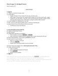
QUICK USER GUIDE
DAGMARA OSZKIEWICZ
Contents
1. Introduction
2. Overview of phase functions
2.1. H,G phase function
2.2. H,G1 ,G2 phase function
2.3. H,G12 phase function
3. Numerical methods
3.1. Least Squares
3.2. Error estimation
3.3. Fitting data for individual asteroids
3.4. Fitting data for asteroid families
4. Software description, requirements and dependences
5. Testing the code
6. Running instructions
6.1. Processing single asteroid phase curve data
6.2. Processing multiple asteroids at the same time
7. Processing big amount of data
8. Example input file
9. Example results
10. Comments
11. Acknowledgments
References
1
1
2
3
4
4
4
5
6
6
6
7
8
8
8
10
11
13
13
13
14
1. Introduction
2. Overview of phase functions
Absolute magnitude computation relies on magnitude phase-curve fitting. A
number of different mathematical formulations for magnitude phase curves have
been developed. Here we make use of the H,G phase function, the H,G1 ,G2 phase
function, and the H,G12 phase function.
Date: February 17, 2011.
1
2
DAGMARA OSZKIEWICZ
The H,G phase function was developed to predict the magnitude of an asteroid as a function of solar phase angle [Bowell et al. (1989)]. This function was
adopted by the International Astronomical Union in 1985 to redefine the absolute
magnitudes of asteroids. The H,G phase function is not valid for phase angles
greater than 120◦ .
The H,G1 ,G2 and H,G12 phase functions [K. Muinonen et al. (2010)] are based
on cubic splines. The H,G1 ,G2 phase function is designed to fit asteroid phase
curves containing substantial numbers of observations, whereas the H,G12 phase
function is applicable to asteroids that have sparse or low-accurancy photometric
data.
2.1. H,G phase function. In the H,G magnitude phase function, the reduced
apparent magnitudes can be obtained from:
10−0.4V (α) = a1 Φ1 (α) + a2 Φ2 (α)
= 10−0.4H [(1 − G)Φ1 (α) + GΦ2 (α)] ,
(1)
where α is the phase angle, V (α) is the reduced magnitude. The basis functions
Φ1 , Φ2 are defined as:
(2)
0.986 sin α
Φ1 (α) = w 1 −
0.119 + 1.341 sin α − 0.754 sin2 α
!
1
+ (1 − w) exp(−3.332 tan0.631 α) ,
2
!
0.238 sin α
Φ2 (α) = w 1 −
0.119 + 1.341 sin α − 0.754 sin2 α
!
1
+ (1 − w) exp − 1.862 tan1.218 α ,
2
!
1
w = exp − 90.56 tan2 α .
2
!
The coefficients a1 and a2 are estimated from observations using linear least
squares. The absolute magnitude H and slope parameter G, can then be obtained
from:
(3)
(4)
H = −2.5 log10 (a1 + a2 ),
G=
a2
.
a1 + a2
QUICK USER GUIDE
3
2.2. H,G1 ,G2 phase function. The reduced magnitudes V (α) can be obtained
from [K. Muinonen et al. (2010)]:
10−0.4V (α) = a1 Φ1 (α) + a2 Φ2 (α) + a3 Φ3 (α)
= 10−0.4H [G1 Φ1 (α) + G2 Φ2 (α) + (1 − G1 − G2 )Φ3 (α)] ,
(5)
where the absolute magnitude H and slope parameters G1 , and G2 are:
(6)
H = −2.5 log10 (a1 + a2 + a3 ),
(7)
G1 =
a1
,
a1 + a2 + a3
a2
.
a1 + a2 + a3
The coefficients a1 , a2 , a3 are estimated from the observations using linear least
squares. The basis functions Φ1 (α), Φ2 (α), Φ3 (α) are defined as:
• For 0◦ < α ≤ 7.5◦ :
– Φ1 (α) = 1 − π6 α;
9
– Φ2 (α) = 1 − 5π
α;
– Φ3 (α) is defined using a cubic spline as defined in Table 2.
• For 7.5◦ < α ≤ 30◦ :
– Φ1 (α) is defined using a cubic spline as defined in Table 1;
– Φ2 (α) is defined using a cubic spline as defined in Table 1;
– Φ3 (α) is defined using a cubic spline as defined in Table 2.
• For 30◦ < α ≤ 150◦ :
– Φ1 (α) is defined using a cubic spline as defined in Table 1;
– Φ2 (α) is defined using a cubic spline as defined in Table 1;
– Φ3 (α) = 0.
(8)
G2 =
α (deg)
7.5
30.0
60.0
90.0
120.0
150.0
Table 1.
Φ1
7.5 ×10−1
3.3486016 ×10−1
1.3410560 ×10−1
5.1104756 ×10−2
2.1465687 ×10−2
3.6396989 ×10−3
Knots for splines
Φ2
9.25 ×10−1
6.2884169 ×10−1
3.1755495 ×10−1
1.2716367 ×10−1
2.2373903 ×10−2
1.6505689 ×10−4
used in Φ1 and Φ2 .
π
The first derivatives (per radian) at the ends of splines are: Φ01 ( 24
) = − π6 ,
9
−2
0 π
0 5π
−8
= −9.1328612×10 , Φ2 ( 24 ) = − 5π , Φ2 ( 6 ) = −8.6573138×10 , Φ03 (0) =
−0.10630097, Φ03 ( π6 ) = 0.
Φ01 ( 5π
)
6
4
DAGMARA OSZKIEWICZ
α (deg) Φ3
0.0
1
0.3
8.3381185 ×10−1
1.0
5.7735424 ×10−1
2.0
4.2144772 ×10−1
4.0
2.3174230 ×10−1
8.0
1.0348178 ×10−1
12.0
6.1733473 ×10−2
20.0
1.6107006 ×10−2
30.0
0
Table 2. Knots for spline used in Φ3 .
2.3. H,G12 phase function. G1 and G2 from the three-parameter phase function
are replaced by a single slope parameter G12 which relates to the G slope parameter
in the H,G system (though there is not an exact correspondence). The reduced
flux densities can be obtained from [K. Muinonen et al. (2010)]:
(9)
10−0.4V (α) = L0 (G1 Φ1 (α) + G2 Φ2 (α) + (1 − G1 − G2 )Φ3 (α))
where:
0.7527G12 + 0.06164,
G1 =
0.9529G12 + 0.02162,
−0.9612G12 + 0.6270,
G2 =
−0.6125G12 + 0.5572,
if G12 < 0.2;
otherwise;
if G12 < 0.2;
otherwise;
(10)
H = −2.5 log10 L0 ;
(11)
and L0 is the disk-integrated brightness at zero phase angle. The basis functions
are as in the H,G1 ,G2 magnitude phase function. Coefficients L0 and G12 are
estimated from observations using non-linear least squares.
3. Numerical methods
3.1. Least Squares. Least-squares fitting is carried out in the flux-density domain, because it reduces the problem to a linear problem for the H,G1 ,G2 and
H,G phase functions, and the errors are symmetric about the fit. The flux for the
ith observation is computed using:
Li = 10−0.4Vi ,
(12)
(L)
σi
(V )
= Li (100.4σi
− 1),
QUICK USER GUIDE
5
(V )
where σi are standard deviations of the magnitude measurements. The χ2 -value
to be minimized here with respect to the parameters a is
(13)
2
χ (a) =
N
X
[Li − Li (αi , a)]2
(L)
[σi ]2
i=1
.
The computed disk-integrated brightnesses are expressed via Na basis functions
Φ1 (α), Φ2 (α), . . . , ΦNa (α):
(14)
Li (αi , a) =
Na
X
al Φl (αi ).
l=1
For the H,G and H,G1 ,G2 phase functions, the a coefficients are fitted using linear
least squares and for the H,G12 phase function the L0 , and G12 parameters are
fitted using simplex non-linear regression [J. A. Nelder and R. Mead (1965)].
3.2. Error estimation. The absolute magnitude computation requires MonteCarlo error estimation because of its nonlinearity. Gaussian errors in parameters
a1 , and a2 (in the H, G, phase function) or a1 , a2 , and a3 (in the H,G1 ,G2 phase
function) result in non-Gaussian errors in the H,G or H,G1 ,G2 parameters. To
estimate those errors, we make use of the least-squares solution for a1 , and a2 or a1 ,
a2 , and a3 and its error covariance matrix. We set the error covariance matrix and
the least-squares solution as a covariance and mean of a multi-normal distribution
to produce a sample a1 , a2 or a1 , a2 , a3 using a multi-normal random number
generator. The ai samples are then converted to H,G or H,G1 ,G2 samples using
either Eqs. 3 and 4 or 6, 7 and 8. Next, the samples are ordered in descending
goodness of fit and then 68.27% (equivalent to 1-σ) and 99.73 % (equivalent to
3-σ) error cut-offs are computed, resulting in a list of subsamples. The limiting
(maximum and minimum) H,G or H,G1 ,G2 parameters are selected from that list
and the two-sided errors are computed.
Error estimation for the H,G12 parameters derives from the Markov chain MonteCarlo (MCMC) technique. From non-linear least-squares fitting we obtain the
least-squares values of L0 and G12 . The errors in L0 , G12 are non-Gaussian, so
the error estimation used for the H,G and H,G1 ,G2 phase functions cannot be
used. To proceed, we create one long Markov chain by sampling possible L0 , G12
solutions. The chain is started at the least-squares point for L0 , G12 , and makes
use of a multivariate Gaussian proposal distribution, where a covariance matrix for
L0 , G12 is taken from the least-squares solution. After obtaining 10, 000 different
solutions, the two-sided errors are computed based on the equivalents of the 1-σ
and 3-σ cut-offs as in the H,G and H,G1 ,G2 phase functions. Error envelopes are
based on the 1-σ and 3-σ Monte Carlo samples. We compute reduced magnitude
for all the sampled values of H,G and/or H,G1 ,G2 and/or L0 , G12 for a set of
phase angles, and choose the maximum and minimum of reduced magnitude at
each phase angle.
6
DAGMARA OSZKIEWICZ
3.3. Fitting data for individual asteroids. We start our computation by performing least-squares fits with all three phase functions, assuming 0.3 mag standard deviation for all of the observations (see section ??). We extract magnitude
residual rms value from that computation and repeat least-square fitting assuming
magnitude uncertainties equal to the rms value for each phase function. Next,
we perform the Monte-Carlo error computation to obtain two-sided errors in the
photometric parameters, together with the error envelopes for the phase functions.
3.4. Fitting data for asteroid families. We fit family data sets using the
H,G1 ,G2 phase function. Family membership was established by agglomerating
asteroids in relative velocity phase space [M.-T. Enga et al. (2011, in prep.)]. Velocity cutoffs for each family are related to the background population velocity. We
devise a 20 × 20(400 nodes) grid in G1 , G2 phase space (G1 ∈ (0, 1), G2 ∈ (0, 1)),
and step through that grid. In each step, G1 , G2 parameters are fixed to the node
G1 , G2 values, and for a number of asteroids in a given family (i = 1, 2, ..., N ) a
linear least-squares fit of L0i is performed. Global family χ2 is computed assuming
no correlation in the noise among different asteroids. From the 400 nodes we select
the one with the best χ2 , and create a new, denser grid in the vicinity of that node
(stretching 1-node distance on each side from the best χ2 solution). We repeat the
least squares analysis in the nodes of the new grid. This operation is repeated a
number of times to obtain improved precision of the G1 , G2 parameters. Once the
family G1,f , G2,f have been obtained, we perform Monte-Carlo error analysis in the
N + 2 parameters phase space to obtain the two-sided 1-σ and 3-σ uncertainties.
4. Software description, requirements and dependences
The Asteroid Phase Function Analyzer is an online, free, interactive applet
written in Java. It is cross platform and it runs in a Web browser using a Java
Virtual Machine (JVM). It requirers 1.6 Java Runtime Environment (JRE).
The core of the applet constitutes a multi-threaded Java program composed of
a number of packages, the contents of which are summarized in Table 3. The
program uses the Java Scientific Library written by Flanagan []. The program is
multi-threaded, and uses a thread pool pattern, in which a number of threads are
created (one per computer core) to perform absolute-magnitude computations (one
per asteroid) in parallel. Tasks are organized in a queue. As soon as the thread
has completed a task, the next task from the queue is requested until all the tasks
are completed. The programming details need not be known to applet users. The
applet is straightforward and very easy to use. A user guide is also provided. It
is, however, expected that the user be familiar with the methods behind state-ofthe-art empirical phase-functions as well as non-Gaussian error estimation. The
applet primarily produces absolute magnitudes and slope parameters, together
with two-sided uncertainties for all three phase functions at the same time for a
QUICK USER GUIDE
7
Package
Classes included
Content
absoluteMagnitude AsteroidData.java
Main package, with Thread Pool
AsteroidPhotometricSolution.java creating jobs (for different asteroids)
AbsoluteMagnitudeand distributing them among cores.
CalculatorThreaded.java
Contains data object and object
ThreadPool.java
with collected results.
phaseCurves
Function1D.java
Contains the phase functions
HGfunction.java
and methods for evaluating
HG1G2function.java
them for different sets of parameters.
HG12function.java
regression
LinearRegressor.java
Contains tools for performing
FittedFunctionHG12.java
linear and nonlinear least-squares
FitterHG.java
phase-curve fitting and least-squares
FitterHG1G2.java
error analysis.
FitterHG12.java
errorAnalysis
NonGaussianErrorEstimator.java Contains methods for
MCMCSampler.java
two-sided error estimation,
RandomNumberGenerator.java
a multinormal random number
PdfComparator.java
generator, a Markov-chain MonteParameterComparator.java
Carlo sampler, comparators.
PhaseCurveSolution.java
inputOutput
DataFileReader.java
Contains methods dealing
OutputWriter.java
with input/output.
Utils.java
ui
PhaseCurveAnalyserApplet.java
Contains the applet and graphical
DataEntry.java
user interface.
FileInputPane.java
InputTableModel.java
Task.java
ResultPane.java
Logger.java
TextInputPane.java
Table 3. Description of main packages
given data file. Other photometric parameters and plots are also produced. The
tool is available at http://asteroid.astro.helsinki.fi/AstPhase/.
5. Testing the code
We compared the results obtained from this software and those from Fortran
software [K. Muinonen et al. (2010)]. We have repeated calculations for all the
asteroids listed in Table 4 using the same data and error estimates (that is, ±0.03
8
DAGMARA OSZKIEWICZ
mag uncertainty for all the objects except for the Moon, where we assume ±0.023
mag uncertainty for phase angles α < 100◦ , and ±0.2 mag uncertainty for phase
angles α ≥ 100◦ ). Tables 5 and 6 contain the results obtained using Java software
(I) and Fortran software (II). The results from [K. Muinonen et al. (2010)] and
the Asteroid Phase Function Analyzer agree very well. There exist some small
differences in the error analysis which can be explained by the limited number of
samples in the Monte Carlo simulations.
Asteroid
Class pV
Nobs αmin αmax References
(24) Themis C, B 0.08 22
0.34 20.8 [Harris et al. (1989a)]
(44) Nysa
E
0.54 23
0.17 21.5 [Harris et al. (1989b)]
(69) Hesperia M
0.14 21
0.13 16.0 [Poutanen et al. (1985)]
(82) Alkmene S
0.21 11
2.29 27.2 [Harris et al. (1984b)]
(133) Cyrene SR
0.26 11
0.20 13.2 [Harris et al. (1984a)]
(419) Aurelia F
0.05 7
0.62 15.4 [Harris and Young (1988)]
(1862) Apollo Q
0.26 18
0.2 89.0 [Harris et al. (1987)]
0.17 17
0.5 140.0 [Bowell et al. (1989)]
The Moon
Table 4. Objects used to illustrate the Asteroid Phase Function
Analyzer capabilities. We show the V -band geometric albedo pv
[Tedesco, E.F. at al. (2002a)], the number of observations Nobs , the
minimum and maximum phase angles of the observations αmin and
αmax , and references to the observations.
6. Running instructions
6.1. Processing single asteroid phase curve data. Go to ”File Input” tab,
click ”Load file”, import data file from your file system (data file has to be in
format specified below). Once the file is imported click Compute. Go to ”Log”
tab to trace the progress of computation. New tab with figures will appear. Go
to that tab and switch between different phase function plots. To save the figures
right click on the figure and pick ”save as...” to save numerical results right click
on the figure and pick ”save numerical results as ...”.
6.2. Processing multiple asteroids at the same time. Everything the same
as for processing single asteroid phase curve, except that the data file contains
many asteroids. File should be in the following format:
A s t e r o i d D e s i g n a t i o n NrOfDataPoints
PhaseAngle1 ReducedMagnitude1
PhaseAngle2 ReducedMagnitude2
PhaseAngle3 ReducedMagnitude3
.
QUICK USER GUIDE
9
Asteroid
(24) Themis
H (II) H (I)
G1 (II) G1 (I) G2 (II) G2 (I)
7.088
7.088
0.62
0.62
0.14
0.14
−0.073 −0.069 −0.24 −0.25 −0.16 −0.16
+0.079 +0.084 +0.28 +0.26 +0.16 +0.15
(44) Nysa
6.904
6.904
0.050
0.050
0.67
0.67
−0.070 −0.068 −0.259 −0.275 −0.15 −0.17
+0.079 +0.079 +0.269 +0.299 +0.14 +0.14
(69) Hesperia 6.927
6.927
0.36
0.36
0.29
0.29
−0.069 −0.067 −0.25 −0.23 −0.18 −0.17
+0.069 +0.072 +0.28 +0.28 +0.16 +0.15
(82) Alkmene 8.06
8.06
0.17
0.17
0.39
0.39
−0.25 −0.25
−0.28 −0.27 −0.13 −0.12
0.33
+0.33
+0.46 +0.43 +0.11 +0.103
(133) Cyrene 7.831
7.831
0.21
0.21
0.39
0.39
−0.088 −0.088 −0.45 −0.43 −0.33 −0.39
+0.098 +0.098 +0.52 +0.52 +0.30 +0.32
(419) Aurelia 8.49
8.49
0.95
0.95
−0.057 -0.057
−0.14 −0.13
−0.54 −0.52 −0.399 −0.367
+0.16 +0.16
+0.69 +0.66 +0.318 +0.326
(1862) Apollo 16.249 16.249 0.38
0.38
0.354
0.354
−0.097 −0.097 −0.12 −0.12 −0.051 −0.051
+0.100 +0.105 +0.15 +0.15 +0.052 +0.053
Moon
−0.126 −0.126 0.36
0.36
0.338
0.338
−0.084 − 0.085 −0.12 −0.12 −0.052 −0.048
+0.091 +0.090 +0.14 +0.14 +0.049 +0.049
Table 5. Absolute magnitudes, and slope parameters with
two-sided 99.73% errors.
Comparison with Muinonen et al.
[K. Muinonen et al. (2010)] for the H,G1 ,G2 phase function. (I) results obtained using the Java software, (II) results obtained using
the Fortran software.
.
.
.
PhaseAngleN ReducedMagnitudeN
First line contains asteroid designation and N - number of data points to follow.
Next N lines contain phase angles and corresponding reduced magnitudes. File
can contain more then one object, the above record style would be then repeated
and next asteroid record could be added following the first record. For example
input files see ”Example.txt” (below).
10
DAGMARA OSZKIEWICZ
Asteroid
(24) Themis
H (II) H (I)
G12 (II) G12 (I)
7.121
7.121
0.68
0.68
−0.042 −0.043 −0.23
−0.24
+0.044 +0.044 +0.25
+0.26
(44) Nysa
6.896
6.896
−0.066 −0.066
−0.041 −0.038 −0.077 −0.075
+0.044 +0.043 +0.072 +0.074
(69) Hesperia 6.987
6.987
0.41
0.41
−0.036 −0.041 −0.21
−0.22
+0.040 +0.043 +0.26
+0.28
(82) Alkmene 8.187
8.187
0.30
0.30
−0.032 −0.032 −0.14
−0.14
+0.034 +0.033 +0.19
+0.19
(133) Cyrene 7.882
7.882
0.20
0.20
−0.026 −0.027 −0.51
−0.016
+0.070 +0.03
+0.49
+0.015
(419) Aurelia 8.514
8.514
1.04
1.04
−0.074 −0.077 −0.46
−0.50
+0.052 + 0.084 +0.16
+0.55
(1862) Apollo 16.209 16.209 0.334
0.334
−0.022 −0.024 −0.077 −0.081
+0.023 +0.025 +0.077 +0.078
Moon
−0.124 −0.124 0.358
0.358
−0.020 −0.020 −0.073 −0.075
+0.022 +0.021 +0.073 +0.074
Table 6. Absolute magnitudes, and slope parameters with
two-sided 99.73% errors.
Comparison with Muinonen et al.
[K. Muinonen et al. (2010)] for the H,G12 phase function. (I) results obtained using Java software, (II) results obtained using Fortran software.
7. Processing big amount of data
Download PhaseCurveAnalyzer.jar file and run it using:
j a v a −j a r PhaseCurveAnalyzer . j a r Example . t x t nrOfCores
ie.:
j a v a −j a r PhaseCurveAnalyzer . j a r d a t a F i l e . dat 2
Output will be written to files on your disk. Output files will include:
• Plots:
– *HGPhaseCurve.png
QUICK USER GUIDE
11
– *HG1G2PhaseCurve.png
– *HG12PhaseCurve.png
• Text files:
– *.resultsSummary - summary of all the objects processed.
– *.results - detailed output for each asteroid processed.
The files will be located in the input file directory.
8. Example input file
See the below example input file. Notice that asteroid name together with
asteroid number is a single String!
”Example . t x t ”
( 2 4 ) Themis 22
13.55 7.825
13.28 7.853
7.26 7.600
6.89 7.586
4.95 7.478
4.75 7.452
4.36 7.439
3.95 7.417
2.94 7.366
2.80 7.351
2.40 7.317
1.98 7.295
1.71 7.278
1.57 7.279
1.39 7.250
1.17 7.239
0.74 7.207
0.57 7.197
0.44 7.172
0.34 7.146
7.79 7.626
20.79 8.110
( 4 4 ) Nysa 23
19.00 7.551
18.52 7.524
17.16 7.511
12
13.81 7.437
13.20 7.426
8.27 7.304
0.98 7.052
0.63 7.014
0.17 6.911
0.36 6.972
0.75 7.033
1.23 7.080
1.62 7.105
2.02 7.126
4.95 7.235
9.78 7.341
11.59 7.385
12.94 7.425
13.27 7.427
13.58 7.433
13.89 7.434
19.40 7.545
21.47 7.599
( 6 9 ) H e s p e r i a 21
16.00 7.82
12.19 7.71
11.90 7.68
11.62 7.67
9.89 7.64
5.10 7.48
4.04 7.42
3.26 7.28
2.46 7.25
1.67 7.13
1.28 7.12
0.92 7.08
0.13 7.00
0.29 6.99
1.04 7.10
2.23 7.23
5.69 7.43
6.03 7.43
DAGMARA OSZKIEWICZ
QUICK USER GUIDE
13
8.59 7.53
12.72 7.64
13.00 7.69
9. Example results
For each asteroid three plots are produced: H, G phase function, H, G1 , G2
phase function and H, G12 phase function. Example result plots are show in Fig.
1, 2, 3. File *.result which is a text file containing detailed numerical output is
produced, and also a summary file *resultsSummary is produced.
Figure 1. H, G phase function for asteroid (2) Pallas
10. Comments
Comments, bugs etc. can be reported to [email protected].
11. Acknowledgments
Research supported by the Magnus Ehrnrooth Foundation, Academy of Finland, Lowell Observatory, and the Spitzer Science Center. We would like to thank
Michael Thomas Flanagan for developing and maintaining the Java Scientific Library, which we have used in the Asteroid Phase Function Analyzer. DO thanks
Berry Holl for help with Java plotters and Saeid Zoonemat Kermani for valuable
advice on Java applets. We thank the Department of Physics of Northern Arizona
University for CPU time on its Javelina open cluster allocated for our computing.
14
DAGMARA OSZKIEWICZ
Figure 2. H, G1 , G2 phase function for asteroid (2) Pallas
Figure 3. H, G12 phase function for asteroid (2) Pallas
References
[Bowell et al. (1989)] Bowell E., Hapke B., Domingue D., Lumme K., Peltoniemi J., and Harris
A. W. Application of photometric models to asteroids. In: T. Gehrels, M. T. Matthews, R.
P. Binzel, editors. Asteroids II, University of Arizona Press; 1989, p. 524-555.
[K. Muinonen et al. (2010)] K. Muinonen, I. N. Belskaya, A. Cellino, M. Delbo, A.-C. LevasseurRegourd, A. Penttil¨
a, E. F. Tedesco. A three-parameter magnitude phase function for asteroids. Icarus 2010; 209: 542-555.
[J. A. Nelder and R. Mead (1965)] J. A. Nelder and R. Mead. A simplex method for function
minimization Computer Journal 1965; 7: 308-313.
QUICK USER GUIDE
15
[Tedesco, E.F. at al. (2002a)] Tedesco, E.F., Noah, P.V., Noah, M., Price, S.D. The supplemental
IRAS minor planet survey. Astron. J. 2002a; 123: 10561085.
[M.-T. Enga et al. (2011, in prep.)] M.-T. Enga et al. Asteroid family albedos from the Spritzer
asteroid catalog in preparation.
http://www.ee.ucl.ac.uk/ mflanaga/java/ Michael Thomas Flanagan’s Java Scientific Library.
ftp://ftp.lowell.edu/pub/elgb/astorb.html The Asteroid Orbital Elements Database.
[Zeljko Ivezic et al. (2001)] Z. Ivezic, S. Tabachnik, R. Rafikov, R. H. Lupton, T. Quinn, M.
Hammergren, L. Eyer, J. Chu, J. C. Armstrong, X. Fan, K. Finlator, T. R. Geballe, J. E.
Gunn, G. S. Hennessy, G. R. Knapp, S. K. Leggett, J. A. Munn, J. R. Pier, C. M. Rockosi,
D. P. Schneider, M. A. Strauss, B. Yanny, J. Brinkmann, I. Csabai, R. B. Hindsley, S.
Kent, D. Q. Lamb, B. Margon, T. A. McKay, J. A. Smith, P. Waddel and D. G. York Solar
System objects observed in the Sloan Digita Sky Survey Commissioning data. Astron. J.
2001; 122:2749-2784
[C. T. Rogers et al. (2006)] C. T. Rodgers, R. Canterna, J. A. Smith, M. J. Pierce and D. L.
Tucker Improved u’g’r’i’z’ to UBVRC IC transformation equations for main-sequence stars.
Astron. J. 2006; 132:989-993.
[Harris et al. (1989a)] Harris A. W., Young J. W., Bowell E., Martin L. J., Millis R. L., Poutanen M., Scaltriti F., Zappal`
a V., Schober H. J., Debehogne H., and Zeigler K. W 1989a.
Photoelectric observation of asteroids 3, 24, 60, 261, 863. Icarus 1989a; 77: 171-186.
[Harris et al. (1989b)] Harris A. W., Young J. W., Contreiras L., Dockweiler T., Belkora L., Salo
H., Harris W. D., Bowell E., Poutanen M., Binzel R. P., Tholen D. J., and Wang S. Phase
relations of high albedo asteroids: the unusual opposition brightening of 44 Nysa and 64
Angelina. Icarus 1989b; 81: 365-374.
[Harris et al. (1987)] Harris, A.W., Young, J.W., Goguen, J., Hammel, H.B., Hahn, G., Tedesco,
E.F., Tholen, D.J. Photoelectric lightcurves of the Asteroid 1862 Apollo. Icarus 1987; 70:
246-256.
[Poutanen et al. (1985)] Poutanen M., Bowell E., Martin L. J., and Thompson D. T., Photoelectric photometry of asteroid 69 Hesperia. Astron. Astroph. Suppl. Ser. 1985; 61: 291-297.
[Harris et al. (1984b)] Harris A. W., Young J. W., Scaltriti F. and Zappal`a V., The lightcurve
and phase relation of the asteroids 82 Alkmene and 444 Gyptis. Icarus 1984b; 57: 251-258.
[Harris et al. (1984a)] Harris A. W., Carlsson M., Young J. W., and Lagerkvist C.-I., The
lightcurve and phase relation of the asteroid 133 Cyrene. Icarus 1984a; 58: 246-256.
[Harris and Young (1988)] Harris, A. W., and Young J. W., Two dark asteroids with very small
opposition effects. Lunar Planet Sci. 1988; XIX 2: 447-448
http://ssd.jpl.nasa.gov/sbdb.cgi JPL Small-Body Database Browser.
[NASA (2003)] NASA, Study to determine the feasibility of extending the search for near-Earth
objects to smaller limiting diameters. NASA Office of Space Science, Solar System Exploration Division, Washington DC. 2003.