1
©2012 Fodor Lab UNCC Contents Chapter 1 Using PeakStudio Introduction Installation System Requirements Running from Command Line Terms used with PeakStudio An overview of the workflow Chapter 2 Dropdown menus in PeakStudio File Edit View Axis Analysis Help Chapter 3 PCA in PeakStudio Appendix A Peak Diagram and Peak Calling Appendix B QC Number Appendix C Automated Peak Adjusting Acknowledgements Chapter 1 Introduction Welcome to Peak Studio, a program for viewing and analyzing fragment analysis files generated by ABI capillary electrophoresis instruments. PeakStudio is an open source program developed at UNCC in the department of Bioinformatics and Genomics by Jon McCafferty. PeakStudio was developed in order to help make more objective decisions about fragment analysis files. It allows users to view any file with a .fsa file extension, assign sizing to peaks, manually edit sizing calls and generate PCA plots to analyze the grouping of data. (PeakStudio screen shot) Installation To install Peak Studio, consult the requirements listed below, then download the .jar file. To use the program, you can double click on the icon or run from a command line (details below). (Windows icon) (Mac icon) System Requirements Max OS X Mac OS X 10.5 (Leopard) or higher Intel processor 1 GB Ram 4 MB available disk space Java version 6 Peak Studio was built and tested on Mac OS X 10.6.4 (Snow Leopard) with 2.8GHz Intel Core 2 Duo processor and 2 GB of RAM. Windows Windows XP Intel processor 1 GB RAM 4 MB available disk space Java version 6 Peak Studio was tested on Windows XP with a 3.0GHz Intel Pentium processor and 2GB of RAM. Running from command Line Mac OS X Open a terminal window, found in the Applications/Utilities folder. From here, change to the directory where PeakStudio.jar is located using “cd yourpath/” (without the quotation marks) and run using this command: user$ “java –Xms128m -Xmx1024m –jar PeakStudio.jar” (without the quotation marks). Windows The Command Prompt application can be found in All Programs \ Accessories, or accessed by clicking Start then Run and typing “cmd” and clicking OK. From here, change to the directory where PeakStudio.jar is located using “cd yourpath\” (without the quotation marks) and run using this command: C:\path>” java -Xms128m -Xmx1024m -jar PeakStudio. Jar” (without the quotation marks). Before using PeakStudio, we recommend reading through the user manual and/or watching our tutorial videos at (http://www.fodorlab.uncc.edu/PeakStudioPage.html) . In the next section, we will discuss some terms used with PeakStudio that may be unfamiliar. Terms used with PeakStudio This manual contains some terms that are specific to PeakStudio and some which have a particular meaning for our purposes in regard to PeakStudio. A list follows with several of these terms, which will help as you read through the rest of the manual: Bin – Bins are used to group peaks for analysis. Smaller bin sizes are more exclusive while larger bin sizes cause peaks of similar size to be grouped with each other. Spectra – In the context of PeakStudio, the word “spectra” is used to refer to one of the 5 possible colors captured by the CCD camera in the genetic analyzer. Every .fsa file contains the data from the different colors (channels), but a spectra is one color separated from the others. Table View – This is the bottom portion of the PeakStudio window. Table View is essentially a customizable table that lists details regarding samples that have been imported for analysis. Two spectra from the same .fsa file which have been overlayed for viewing in the Viewing Window. TableView An overview of the workflow PeakStudio has been designed to provide a straightforward method of data viewing and analysis. Below is a walkthrough of a typical project. To begin You should have the PeakStudio.jar file downloaded on your computer (or the source code). You will need .fsa files to analyze and a size standard file. The size standard file indicates which size standard fragments were used and should be in a .txt file format that contains a list of each size separated by a return (each size on its own line). Import samples At the upper left of the window go to File, Open Spectra and select the file(s) to be analyzed. You must select the color of the dye labeled products (in ARISA, this is typically Blue for FAM) and the color of the size standard dye (by default this is Orange for LIZ). If you are using other dyes for your products or size standards, you can specify that now. Click the Open button to open them into the Peak Studio window. Files are displayed in the Table View (bottom portion of the PeakStudio window). Each .fsa file that you import will generate a separate spectra for each dye previously specified. With ARISA for example, there should be two spectra; one for the blue, FAM labeled products and one for the orange, LIZ labeled size standard fragments. Add a standards file Go to Edit, Standards, click the Import Standards button, then find your standards file and apply. You can opt to apply the standards to all the files, or you can select certain files in TableView. Once you have applied a size standard file to the spectra, you will want to determine whether the peak calling algorithm has identified the size standard peaks correctly. Begin by checking the NumPeaks column. If you are using LIZ-1200 from ABI, you should have 68 size standard peaks. Notice that sample 4 only contains 67 identified size standard peaks. We will correct this shortly. Right click anywhere in the Table View and select Show columns, then click on QC number. Generally, the lower the number, the more confidence that peaks have been called correctly. As a general guideline, a QC between 0.18 and 0.30 is good (see Appendix B). Any column in Table View can be used to sort the data by clicking on the header. Click the check box for Show Graph to display the spectra. If you prefer, you can go to Axis, and check Basepair to display the spectra in basepair, rather than raw data format. Also in the Axis dropdown, you can choose to Display the X and Y axes. To see which peaks have been assigned with each size, go to View, Show Peak Numbers. If you find that you are missing peaks, or that they have been incorrectly identified, you can manually correct this problem. Double click on the misidentified peak and then right click; this will bring up the option to Toggle Peak, which allows a peak to be reassigned from accepted to rejected or vice versa. Before toggling the algorithm has missed this peak After toggling the peak is now correctly assigned You can also choose to edit peak calling parameters by going to Edit then Parameter Set and then allow the software to automatically call peaks again. The modified peak calling parameters can be applied to a particular spectra, or applied to all selected spectra. Analyze your data Once the standards spectra are acceptable you can choose to remove them from Table View by right clicking in Table View and selecting Spectra, then uncheck the box for your standards color. The sizing will remain in effect, but you will only see sample data now. As was the case for standards spectra, the Show Graph check box brings up each data spectra in the window. You can show one or many spectra at a time. Sometimes when viewing multiple spectra it can be helpful to change the display color. This is easily achieved by clicking on the Peak Color box for the spectra, then selecting a new color in the pop up window. Now you can determine how closely related your samples are to each other using PCA. To do this, go to Analysis and click on PCA. This will bring up a window where you can specify which range of bases you would like to compare, how large your bin size should be, and what threshold to use for cutting off peaks. In capillary electrophoresis, very small and very large fragments are often not as reliably sized as those in the middle, so we often limit our analysis to what we consider to be the best fragments for those samples. Note the Start BasePair of 25 and End BasePair of 900. Depending on the range of fragments of interest, you may want to make that range narrower or wider. Using the current setting, bins would be 25 – 28, 28 – 31, etc. Peak Height Threshold indicates the minimum y-axis value (Relative Fluorescence Unit) required for a peak to be considered. Once you click Run a new window will pop up with a graph of your PCA. This allows you to visually examine the grouping of samples. You can mouse over data points to reveal which sample is represented or go to View, then click the Name radio button and all the names will be displayed on the graph. (Hint: you may find it useful to color code your samples to make them easier to visually inspect on the PCA graph. To do this, go back to Table View and click on the color of the sample you want to change. You can assign any color to any sample.) It is possible to export the data used to generate the PCA for further analysis by going to Export, then Matrix, then select Data. Chapter 2 Dropdown menu options File Dropdown Menu Open Spectra (Ctrl + O) – Use this function to open one or many .fsa files Open Project (Ctrl + P) – Use this function to open a .svaz project generated by PeakStudio Save (Ctrl + S) – Saves the current project as a .svaz file Save As – Save the current project to another location or with another name Import – Allows the user to import metadata to associate with samples. When importing metadata into PeakStudio, the file must be formatted as a tab delimited text file and it must be formatted using the following template: The first column must be titled “sample name” and the remaining metadata columns can contain any title you choose. The sample names included in the metadata file must match the sample names loaded in PeakStudio. Once metadata have been assigned to the spectra, right clicking in a header column in Table View allows the spectra to be colored based on the data in that column. Spectra which have been colored by header2, then sorted by header2 Export PNG – Export a .png screenshot picture of the spectra currently displayed Encapsulated PostScript – Export a .eps screenshot picture of the spectra currently displayed Table View – Export a spreadsheet of the samples’ details in Table View Binned Peak Matrix – Export the matrix of peaks and bins for any stats All Peaks – Export peak information for a selected file QC Files – Export a list of scan numbers and associated peak algorithm assignments Sizing Table – Export a table that conforms to the format output of GeneMapper software Sizing Table: 6 columns Dye Color,Peak# ; File Name; BP location; Peak Height; Peak Area; Data Point Remove Sample(s) (Ctrl + C) – Highlight one or multiple files in the Table view and remove Close Project (Ctrl + A) – Closes the current project, but keeps PeakStudio open Exit (Ctrl + Enter) – Closes PeakStudio Edit Dropdown Menu Parameter Set (Ctrl + Q) – Allows the user to adjust peak calling parameters Standards (Ctrl + W) – Use this to import a standards file Data Smoothing (Ctrl + -) – Use this to smooth data View Dropdown Menu Show Peak Numbers (Ctrl + B) – Inserts numbers above peaks which have been called by the peak calling algorithm Mouse Over Peaks (Ctrl + V) – Displays information box when the mouse cursor is placed on a peak Shade Peaks (Ctrl + D) – Shades the area under a peak when the mouse cursor is placed on a peak Peak X Coordinates (Ctrl + J) – Inserts peak numbers based on base pair or scan number, depending on the current view Line Thickness (Ctrl + U) – Adjusts the thickness of the displayed spectra Set X zoom (Ctrl + X) – Sets the x axis zoom level Set Y zoom (Ctrl + Y) – Sets the y axis zoom level Zoom Out (Ctrl + Z) – Zooms spectra out to the original image size Raw (Ctrl + R) – View data in raw form Smooth (Alt + R) – View data in smoothed baseline corrected form Axis Dropdown Menu Display – Displays the y axis with relative fluorescence units (RFUs) and the x axis with either scan numbers (raw data) or base pair numbers (based on peak calling algorithm) BasePair (Ctrl + K) – Converts the spectral display from scan numbers (raw data) to base pair numbers (based on peak calling algorithm) Analysis Dropdown Menu PCA (Ctrl + 4) – Opens a new window displaying principle component analysis (PCA) on the spectra open in the Table View. Select the range of basepair values, the size of the bin to use and a value for the peak height threshold, then select Run. The PCA output opens in a new window. Hovering over data points reveals the identity of each point. Colors are associated with the Peak Color from the PeakStudio viewer window. See Chapter 3 for description of PCA in PeakStudio. Help Dropdown Menu About (Ctrl + I) – Contains version information Table View Table view is the bottom panel of the PeakStudio window. Columns can be sorted by clicking on the column headers. Default columns in Table view are: File Name – Displays the file name associated with each sample Data channel – Displays the data channel associated with the dye used Show Graph – Check the box to display the electropherogram in PeakStudio. One or many graphs can be displayed at a time and peak colors can be adjusted to tell them apart. Peak Color – Peak colors are associated with dye colors, but can be modified by clicking on the color swatch in Table view. Rejected Peak Color – Peaks which are identified by the peak calling algorithm, but are rejected as non-real display as blue on the spectra. Spectra Type – This indicates whether the file represents data from a sample, or the size standard associated with that sample. NumPeaks – The number of real peaks identified by the peak calling algorithm Additional columns available under Show Columns (right click the mouse when cursor is within Table View) include: Graph Color – The color of the spectra which is not identified by the peak calling algorithm as a peak or rejected peak Selected Peak Color – The color a peak displays when it has been selected by double clicking on it QC Status – Displays “Good Data” or “Bad Data” depending on whether the peak identification algorithm was able to correlate the size standard peaks to their correct sizes Standards File – The file name which was used to assign sizes to spectra is displayed Num Size Standard Peaks – Displays the number of peaks in the assigned standards file QC Number – A numerical representation of the quality of peaks based on the interpretation between expected peaks and observed peaks (See appendix B for further detail on QC number) Base Pairs Called – Displays whether basepairs have been called for each sample Smoothed – Lets user know if smoothing algorithm has been applied to the spectra Additional right click options: Spectra: 1 – blue dye (FAM, HEX) 2 – green dye (VIC) 3 – yellow dye (NED) 4 – red dye(PET, ROX) 105 – orange dye (LIZ) Show: Select all – marks all the checkboxes to show all spectra on the screen at one time Unselect all – unmarks all the checkboxes to clear the screen of all spectra Add A Column – Adds a blank column in which you can add your own text Delete – Deletes a column that was added using the Add A Column function Rename – Allows you to rename the column that was added Color by – Changes the color of the spectra associated with the label in the column created. Chapter 3 PCA in PeakStudio PCA, or Principal Component Analysis, is an algorithm that identifies patterns by revealing similarities in a dataset. This is accomplished by transforming a high dimensional multivariate dataset into a set of principal components, allowing you to project the data onto a new coordinate system such that the greatest variance by any projection of the data comes to lie on the first principal component, the second greatest variance on the second component, and so on. Data can now be visualized in a lower dimensional space creating a more informative view of the dataset. The Data Matrix used as input to the PCA algorithm is generated with user-defined parameters. Using a start and stop location, bin width, and peak height threshold; the spectra is divided up into bins and the peaks which meet the height threshold are grouped into the bins. A binned matrix with columns representing bins and rows representing spectra is created with the cells containing the sum of peak heights, for each peak over the defined threshold. The PCA algorithm uses this binned data matrix as input. Menus in PCA Window Export PNG – Export a .png screenshot picture of the PCA currently displayed Matrix Data – Export the matrix of peaks and bins for any stats Components – Export the matrix of the transformed data View Shape Size – This enables the size of data points to be adjusted between 3 levels Zoom Out (Ctrl + Z) - Zooms PCA window out to the original image size Name – Displays the name of the spectra associated with each data point Edit Axis – Displays dialog that allows components to be changed along the x and y axes Appendix A Peak Calling Heuristics Below is a diagram of a peak, as it is determined by the peak calling algorithm. Initial Peak Calling Accurate identification of peaks is a critical step in ensuring that data is prepared for further analysis. Our peak-calling algorithm applies linear interpolation to separate signals of peaks from that of baseline in raw data from fragment analysis files. The algorithm works by using a configurable parameter set that contains thresholds for values such as slope, and peak heights assigning each data point to one of five possible phases non-peak, peak, up-slope, down-slope or inter-peak. After assigning all the data points to one of the four phases, the peaks can be identified. A peak is recognized as a collection of points that meet the requirement of beginning at an up slope phase and ending at a down slope phase. Taking the difference between the highest and lowest data points in the region containing the peak determines peak heights. If the peak height does not meet the threshold from the parameter set, the region is relabeled as a nonpeak region. Adjusting the parameters allows the user to redefine what constitutes a peak with the resulting peak calls seen in real time. Since any peak-calling algorithm has the potential of missing peaks or miscalling peaks Peak Studio combines automated peak detection with the ability for the user to visually inspect and manually select peaks that need to be adjusted. Through the use of the program, samples that have misidentified peaks can be salvaged by manual user selection of peaks. Appendix B QC Number: A quality control method was developed to allow the user to rapidly identify any spectra where the peak-calling algorithm mislabeled peaks. Quality control scores are calculated through a linear interpolation process. We start with a standard spectra and walk through all of the peaks that have been called. Taking a set of 3 peaks at time we use the location of the left and right peak to predict the location of the middle peak. The QC Score is then the sum of the absolute value of the difference between the predicted location and the observed location of the middle peak divided by the number of total peaks called (Equation 1). When the user toggles a peak on or off the QC Score is updated in real time, with lower scores being better. The score represents the overall accuracy of the peak-calling algorithm therefore a smaller score, especially less than 0.5, indicates that the predicted peak was very close to the actual peak that was called. Higher scores are a signal that something is wrong, and the user may have to manually adjust peaks. QC Number = Σ | predicted –observed | number of peaks (Equation 1) Appendix C Automated Peak Adjusting: To increase the user friendliness and the speed at which data can be processed, we implemented a feature that allows the user to automatically adjust peaks in the standard spectra correcting any potentially misclassified data regions. We try to separate background noise from what should be actual peaks by applying filters to the spectral data. Our first filter assumes that because peaks will have larger areas and higher heights than non-peaks they will contribute more to the variation in the distribution of areas under the curve for the spectra. Setting a default threshold of 3 standard deviations (user preference in the parameter set) we can filter out larger peaks from background noise. The second filter is applied if the number of called peaks differs from the number of actual peaks according to the user provided weights. We walk through the current set of peaks and make adjustments by turning peaks on or off trying to minimize the QC score. Our third and final filter is applied if the previous two filters were not successful in correctly adjusting the peaks. This filter uses the current set of features (peaks & nonpeaks) and gathers potential peaks by incorporating features that are a default 2 standard deviations away and also requiring that a peak meets a default height threshold of 33% (user preference in the parameter set) the height of the nearest called peak. Post automated adjustment of the standard spectra; the weights should be applied correctly to the called peaks. Understanding that this is a heuristic and will provide the optimal solution but not always the correct solution, the user has the ability to manually adjust any standard spectra that passed the filter steps yet has miscalled peaks. This adjustment procedure is intended to reduce the amount of time a user needs to process data from raw .fsa files to usable data for downstream analysis. 1. Identify features with SD greater than 3, label them as peaks. 2. Toggle features on and off, trying to minimize the QC score. Gather features with SD greater than 2 and whose height meets a 3. threshold of 33% the height of the nearest called peak. Table 1. Automated Peak Adjusting Filtering Algorithm. SD = standard deviation Acknowledgements Dr. Michael Thomas Flanagan for making his code publicly available (www.ee.ucl.ac.uk/~mflanaga), which we used for smoothing and area calculations in Peak Studio.