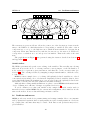
Download MONA Version 1.4 User Manual

BRICS
Basic Research in Computer Science
BRICS NS-01-1
Klarlund & Møller: MONA Version 1.4 — User Manual
MONA Version 1.4
User Manual
Nils Klarlund
Anders Møller
BRICS Notes Series
ISSN 0909-3206
NS-01-1
January 2001
c 2001,
Copyright Nils Klarlund & Anders Møller.
BRICS, Department of Computer Science
University of Aarhus. All rights reserved.
Reproduction of all or part of this document
is permitted on condition that it is
unmodified, includes this copyright notice,
and distributed for free.
See back inner page for a list of recent BRICS Notes Series publications.
Copies may be obtained by contacting:
BRICS
Department of Computer Science
University of Aarhus
Ny Munkegade, building 540
DK–8000 Aarhus C
Denmark
Telephone: +45 8942 3360
Telefax: +45 8942 3255
Internet: [email protected]
BRICS publications are in general accessible through the World Wide
Web and anonymous FTP through these URLs:
http://www.brics.dk
ftp://ftp.brics.dk
This document in subdirectory NS/01/1/
MONA Version 1.4
User Manual
Nils Klarlund, [email protected]
Anders Møller, [email protected]
January 2001
c 1997-2001 Nils Klarlund & Anders Møller
Copyright BRICS, Department of Computer Science, University of Aarhus
All rights reserved.
Reproduction of all or part of this document is permitted
on condition that it is unmodified, includes this copyright
notice, and is distributed for free.
The MONA tool is available under the GNU General Public License.
Contents
1 Introduction
1.1 Introductory example .
1.2 MONA applications . . .
1.3 Concepts and algorithms
1.4 How to use this manual
1.5 Acknowledgments . . . .
.
.
.
.
.
.
.
.
.
.
.
.
.
.
.
.
.
.
.
.
.
.
.
.
.
.
.
.
.
.
.
.
.
.
.
.
.
.
.
.
.
.
.
.
.
.
.
.
.
.
.
.
.
.
.
.
.
.
.
.
.
.
.
.
.
.
.
.
.
.
.
.
.
.
.
.
.
.
.
.
.
.
.
.
.
.
.
.
.
.
.
.
.
.
.
.
.
.
.
.
.
.
.
.
.
.
.
.
.
.
.
.
.
.
.
.
.
.
.
.
3
3
4
7
8
8
2 Basic features
2.1 The essential syntax . . . . . . . . .
2.2 The essential semantics . . . . . . .
2.3 Analyzing formulas . . . . . . . . . .
2.4 Outputting the program automaton
2.5 What are MONA automata really? .
2.6 Predicates and macros . . . . . . . .
2.7 Example: Reasoning about queues .
.
.
.
.
.
.
.
.
.
.
.
.
.
.
.
.
.
.
.
.
.
.
.
.
.
.
.
.
.
.
.
.
.
.
.
.
.
.
.
.
.
.
.
.
.
.
.
.
.
.
.
.
.
.
.
.
.
.
.
.
.
.
.
.
.
.
.
.
.
.
.
.
.
.
.
.
.
.
.
.
.
.
.
.
.
.
.
.
.
.
.
.
.
.
.
.
.
.
.
.
.
.
.
.
.
.
.
.
.
.
.
.
.
.
.
.
.
.
.
.
.
.
.
.
.
.
.
.
.
.
.
.
.
.
.
.
.
.
.
.
.
.
.
.
.
.
.
.
.
.
.
.
.
.
.
.
.
.
.
.
.
9
9
10
11
12
13
14
15
3 The automaton–logic connection
3.1 The classical approach . . . . . . . . . . . . . . . . . . . . . . . . . . . . . . .
3.2 The MONA approach . . . . . . . . . . . . . . . . . . . . . . . . . . . . . . . .
18
18
22
4 Translation optimizations
4.1 DAG representation of formulas . . . . . . . . . . . . . . . . . . . . . . . . . .
4.2 Formula reductions . . . . . . . . . . . . . . . . . . . . . . . . . . . . . . . . .
4.3 Separate compilation . . . . . . . . . . . . . . . . . . . . . . . . . . . . . . . .
27
27
28
29
5 Translation information
5.1 Verbose processing . . . . . . . . . . . . . . . . . . . . . . . . . . . . . . . . .
5.2 Visualization of automata . . . . . . . . . . . . . . . . . . . . . . . . . . . . .
30
30
32
6 Advanced constructs
6.1 Exporting and importing automata . . . . . . . . . . . .
6.2 Prefix-closing . . . . . . . . . . . . . . . . . . . . . . . .
6.3 Presburger arithmetic . . . . . . . . . . . . . . . . . . .
6.4 Restriction . . . . . . . . . . . . . . . . . . . . . . . . .
6.5 Emulating Monadic Second-order Logic on Strings . . .
6.6 Example: Regular expressions over the ASCII alphabet
.
.
.
.
.
.
.
.
.
.
.
.
.
.
.
.
.
.
.
.
.
.
.
.
.
.
.
.
.
.
.
.
.
.
.
.
.
.
.
.
.
.
.
.
.
.
.
.
.
.
.
.
.
.
.
.
.
.
.
.
.
.
.
.
.
.
.
.
.
.
.
.
33
33
34
34
34
36
36
7 Tree logic and tree automata
7.1 The WS2S logic . . . . . . . . . . . . . . .
7.2 Guided Tree Automata . . . . . . . . . . .
7.3 Specifying the guide . . . . . . . . . . . .
7.4 Other tree-mode specific constructs . . . .
7.5 Example: Exponential savings with guides
7.6 Tree mode output format . . . . . . . . .
7.7 Inherited-acceptance analysis . . . . . . .
7.8 Emulating Monadic Second-order Logic on
.
.
.
.
.
.
.
.
.
.
.
.
.
.
.
.
.
.
.
.
.
.
.
.
.
.
.
.
.
.
.
.
.
.
.
.
.
.
.
.
.
.
.
.
.
.
.
.
.
.
.
.
.
.
.
.
.
.
.
.
.
.
.
.
.
.
.
.
.
.
.
.
.
.
.
.
.
.
.
.
.
.
.
.
.
.
.
.
.
.
.
.
.
.
.
.
39
39
39
41
43
43
44
46
47
.
.
.
.
.
.
.
.
.
.
.
.
.
.
.
.
.
.
.
.
.
.
.
.
.
.
.
.
.
.
. . . .
. . . .
. . . .
. . . .
. . . .
. . . .
. . . .
Trees
.
.
.
.
.
.
.
.
.
.
.
.
.
.
.
.
.
.
.
.
.
.
.
.
.
.
.
.
.
.
.
.
7.9
Recursive types and WSRT . . . . . . . . . . . . . . . . . . . . . . . . . . . .
8 Plans for future versions
8.1 BDD variable orderings . . . . . . . . . . . . . . .
8.2 Heuristic reductions . . . . . . . . . . . . . . . . .
8.3 Encoding of boolean variables in tree mode . . . .
8.4 Support for user-definable predicates and functions
8.5 Higher-level notation . . . . . . . . . . . . . . . . .
47
.
.
.
.
.
51
51
51
52
52
52
A Syntax
A.1 MONA grammar . . . . . . . . . . . . . . . . . . . . . . . . . . . . . . . . . .
A.2 Precedence and associativity . . . . . . . . . . . . . . . . . . . . . . . . . . . .
53
53
56
B Usage
57
C Using automaton files in other applications
C.1 Using DFA files . . . . . . . . . . . . . . . . . . . . . . . . . . . . . . . . . . .
C.2 Using GTA files . . . . . . . . . . . . . . . . . . . . . . . . . . . . . . . . . . .
58
58
59
D The MONA DFA package
D.1 Examples: Presburger arithmetic and transduction . . . . . . . . . . . . . . .
62
66
E The MONA GTA package
68
F The MONA BDD package
73
References
76
Index
80
.
.
.
.
.
.
.
.
.
.
.
.
.
.
.
.
.
.
.
.
.
.
.
.
.
.
.
.
.
.
.
.
.
.
.
.
.
.
.
.
.
.
.
.
.
.
.
.
.
.
.
.
.
.
.
.
.
.
.
.
.
.
.
.
.
.
.
.
.
.
MONA 1.4
1 Introduction
It has been known since 1960 that the class of regular languages 1 is linked to decidability
questions in formal logics. In particular, WS1S (Weak monadic Second-order theory of 1
Successor ) is decidable2 through the automaton-logic connection, which can be simply stated:
the set of satisfying interpretations of a subformula is represented by a finite-state automaton [B¨
uc60b, Elg61]. WS1S thus acts as a notation for regular languages, just as regular
expressions do.
The automaton for a formula can be calculated by a simple induction scheme, where logical
connectives correspond to classic automata-theoretic operations such as product and subset
constructions. Validity and unsatisfiability of the formula can be determined and satisfying
examples and counter-examples can be constructed by analyzing the associated automaton.
Despite its name, WS1S is a simple and natural notation. Being a variation of firstorder logic, WS1S is a formalism with quantifiers and boolean connectives. Its interpretation,
however, is tied to arithmetic—somewhat weakened to keep the formalism decidable. In
WS1S, first-order variables denote natural numbers, which can be compared and subjected to
addition with constants. WS1S also allows second-order variables while remaining decidable;
each such variable is interpreted as a finite set of numbers.
WS1S and its generalization WS2S [TW68, Don70], which is interpreted over the infinite
binary tree, can be used to express problems ranging from hardware verification to formal linguistics. Unfortunately, the space and time requirements for translating formulas to automata
have been shown to be non-elementary (i.e., bounded from below by a stack of exponentials
whose height is proportional to the length of the formula) [Mey75]. Thus, the decidability
property has for many years been considered intractable for practical use. Nevertheless, the
MONA tool shows that an efficient implementation of the decision procedures for WS1S and
WS2S is possible. “Efficient” here means that the tool is fast enough to have been used in
a variety of non-trivial settings. MONA translates WS1S and WS2S formulas into minimum
DFAs (Deterministic Finite Automata) and GTAs (Guided Tree Automata [BKR97]), respectively. The automata are represented by shared, multi-terminal BDDs (Binary Decision
Diagrams) [Bry92, HJJ+ 96].
Version 1.4 of the MONA tool is several orders of magitude more efficient than the first
experimental versions due to techniques such as BDD representation, DAGification, and formula reductions. In addition, MONA provides many features, such as three-valued logics
and automata, automaton visualization, importing and exporting of automata, and recursive
types.
1.1 Introductory example
We introduce MONA through a tiny example showing its basic functionality. MONA is run
on a file that defines a WS1S or WS2S formula. The result of the compilation is an automaton, which can be used in any way the MONA programmer might desire. Often, however,
the interest in the compilation is the analysis that MONA can carry out on the calculated
1
A regular language is a set of finite strings recognized by a finite-state automaton. We assume that the reader
is familiar with automata theory as taught in undergraduate computer science courses.
2
A logic is decidable if an algorithm exists that determines for any formula its truth status: valid (formula
is always true) or not valid (sometimes formula is false); alternatively—and equivalently—the algorithm can
classify formulas according to whether they are satisfiable (sometimes true) or unsatisfiable (always false).
3
MONA 1.4
1.2
MONA applications
automaton.
A MONA program consists of a number of declarations and formulas. The two-line WS1S
program below, contained in a file simple.mona, declares two free second-order variables, P
and Q, and postulates that the set difference of P and Q is the union of the sets {0,4} and
{1,2}:
var2 P,Q;
P\Q = {0,4} union {1,2};
Clearly, this formula is not always true, but there is an interpretation that makes it hold,
for example the one which assigns {0, 1, 2, 4} to P and {5} to Q. This interpretation, usually
written as [P 7→ {0, 1, 2, 4}, Q 7→ {5}], can also be represented by 0s and 1s in a string
P
1
1
1
0
1
0
0
0
0
0
0
1
Q
0
1
2
3
4
5
where letters are bit-vectors. Each variable is described by a track along the string. Here, the
P-track is 111010 and the Q-track is 000001. The positions in the string correspond to natural
numbers: a “1” in a position means that the number is in the set, a “0” that it is not.
We can define the language associated to simple.mona as the set of such finite strings
that define satisfying interpretations. It is a fact (see Section 3) that for WS1S, this language
is regular, i.e. it can be recognized by a finite-state automaton.
MONA is able to analyze simple.mona automatically by translating it into the minimum
automaton recognizing the set of satisfying interpretations. The command
mona simple.mona
produces the automaton, analyzes it, and generates the following output:
A counter-example of least length (0) is:
P
X
Q
X
P = {}
Q = {}
A satisfying example of least length (5) is:
P
X 11101
Q
X 000X0
P = {0,1,2,4}
Q = {}
This analysis tells us that a counter-example to the formula is obtained by interpreting both
P and Q as the empty set. MONA has also calculated a satisfying interpretation, namely P
= {0, 1, 2, 4}, Q = {}. An X in a string means “either 0 or 1”. The columns with the two Xs
are used for boolean variables, of which there are none in this example.
1.2 MONA applications
A substantial number of applications of MONA have been published. Also, MONA has successfully been integrated into or used as foundation of a number of other tools. MONA has
4
MONA 1.4
1.2
MONA applications
gained lots of attention recently; thus more than 10 of the publications referenced in the
following small survey have been published during the last year.
In an application perspective, arithmetic and logic is useful because interesting systems
and properties can be encoded. A common observation is that WS1S and the related logic
M2L-Str (see Section 6.5) can be viewed as generalizations of quantified propositional logic,
adding a single “unbounded dimension” orthogonal to the dimension bounded by the number
of variables. This unboundedness can be used in two ways:
• to model parameterized systems and verify a whole family of finite systems at once; or
• to model discrete time and verify safety properties or synthesize controllers.
Similarly, the tree logics WS2S and M2L-Tree can be used to model tree-shaped systems or
branching time instead of linear time. These ideas have led to a whole branch of research.
Another kind of application is to reduce other logics to the MONA logics.
Hardware verification One of the first MONA applications was hardware verification. In
[BK98], the ideas of modeling parameterized systems or discrete time were introduced. In
[ABF99] this verification technique is further described and generalized to trees. Many of the
applications mentioned below also build on these ideas.
Controller synthesis As mentioned, M2L-Str can be viewed as a temporal logic, that is, as a
logic modeling the occurrence of events over time. In [Tho90], it is shown how PLTL (Propositional Linear Time Logic) can be encoded in M2L-Str. To synthesize run time controllers,
MONA turns requirements of Web services [SS98] or Lego robots [HS00] into automata, which
may act as programs. Whenever a process (a Web session or a Lego robot) wishes to pass
certain “checkpoints”, it is ensured that doing so is allowed by the automata (in the sense
that reject states are not entered).
FIDO FIDO [KS99] is a high-level language built on top of MONA. It helps the programmer
overcome the low-level bit-encoding usually required whenever something is encoded directly
in MONA logic. The FIDO language is based on recursive data types over finite domains,
but it also adds other programming language concepts, such as subtyping, unification, and
coercion. Not exploiting the Guided Tree Automata concept of MONA, FIDO has to some
extent been obsoleted by the WSRT logic (described in Section 7.9).
LISA The LISA language [ABP98] was developed in parallel with FIDO. It contains many
of the same features as FIDO, but instead of recursive data types, it is based on the more
general feature logics.
Trace abstractions In [KNS96b, KNS96a], FIDO is used to perform behavioral reasoning
about distributed reactive systems based on trace abstractions. M2L-Str is used as a temporal
logic to address the “Broy-Lamport challenge” of modeling and verification a memory server
specification. This work provided the motivation for the development of FIDO.
Computational linguistics An application of MONA for linguistic processing and theory
verification using WS2S is described in [MC97].
5
MONA 1.4
1.2
MONA applications
Protocol verification MONA has been used for various kinds of protocol verification. In
[HJJ+ 96], a variant of the Dining Philosophers protocol is verified, and in [SK99], the Sliding
Window communication protocol is modeled using I/O automata and then translated to
WS1S and verified.
DCVALID DCVALID [Pan99, Pan00] is a tool for checking validity of Quantified Discretetime Duration Calculus formulas based on MONA. It has been used to verify properties of
SMV, Verilog, ESTEREL, and SPIN systems.
YakYak YakYak [DKS99] is an extension of the Yacc parser generator. Side constraints
expressed in a first-order parse tree logic are translated into Guided Tree Automata using
MONA. During the bottom-up Yacc parsing, the parse tree is run on these automata yielding
evaluation of the side constraints.
Software engineering In [KKS96], it is shown that many software design architecture descriptions are expressible in M2L-Tree. Using FIDO, parse-tree constraints are expressed
and compiled to automata. This project was a precursor of YakYak and did not combine
constraint checking with parsing or use Guided Tree Automata.
FMona FMona [BF00b, BF97] is a high-level extension of MONA adding e.g. enumeration
types, record types, and higher-order macros to the MONA syntax. It has been used to express
parameterized transition systems, abstraction relations, synthesis of finite abstractions, and
validation of safety properties.
STTools MONA has been used for M2L-Str-based model checking of programs in the Synchronized Transitions language [Ras99].
PEN PEN [Nil99] is a tool for verifying distributed programs parameterized by the number of
processes. The systems are modeled by transducer automata, and properties of configurations
are represented by normal automata. By performing transitive closure of the transducer
(see [JN00]) and using an acceleration technique, reachability properties can be verified. The
implementation is based on the DFA part of MONA.
PAX PAX [BSBL00] is yet another tool for verifying parameterized systems using MONA.
The contribution of PAX is a heuristic-based technique for abstracting parameterized systems
in WS1S into finite-state systems for model checking.
PVS MONA has been integrated into the PVS theorem prover [OR00]. Properties expressible within WS1S can then be verified without user interaction.
ISABELLE The combination of WS1S and higher-order logic has been investigated using
MONA as a WS1S oracle in the ISABELLE system [BF00a].
6
MONA 1.4
1.3
Concepts and algorithms
Program verification In [JJKS97], the MONA logic is used to encode the effect of executing
loop-free code with pointer operations on list shaped structures. The approach is based on
[KS94], which employs transductions (a form of predicate transformation expressible by an
automaton), and is extended to code containing loops using classical Hoare logic.
This technique is generalized to recursive data types in [EMS00, Elg99]. To overcome
the increased complexity, a new logic WSRT, Weak monadic Second-order logic with Recursive Types (see Section 7.9), is introduced. This logic is reminiscent of FIDO and LISA.
WSRT permits a more efficient decision procedure: based on a technique called shape encoding [DKS99], an efficient guide can automatically be deduced. The newest version of the
YakYak tool also uses the WSRT part of MONA.
In [MS00], the technique is further generalized to cover the whole class of data structures
that can be described as graph types [KS93]. As an example, the technique is used to verify
that an implementation of the insert procedure for red-black search trees preserves the nonarithmetical part of the red-black invariant.
This manual describes two additional example applications. In Section 2.7, it is shown how
the MONA representation of certain queue structures specializes to those suggested elsewhere
in the literature, and in Section 6.6, it is explained how regular expressions over the ASCII
alphabet can be effectively encoded in MONA, making WS1S a much more versatile notation
for patterns than regular expressions.
1.3 Concepts and algorithms
For more information about the development of MONA, we suggest the following papers which
describe the concepts and algorithms applied in the tool:
“Mona: Monadic Second-Order Logic in Practice” [HJJ+ 96] The first paper on the implementation of monadic-second order logic on finite strings. Data structures, algorithms,
and an application to verification of safety and liveness properties of a parameterized
distributed system are discussed.
“BDD Algorithms and Cache Misses” [KR96] A description of techniques for speeding up
BDD operations. By rethinking data structures for BDD algorithms, random memory
access can be reduced.
“Algorithms for Guided Tree Automata” [BKR97] Introduction of Guided Tree Automata
as a technique for combatting state-space explosions in tree automata.
“Mona & Fido: The Logic-Automaton Connection in Practice” [Kla98] A survey paper on
BDDs, BDD-represented automata, WS1S and WS2S, practical techniques for decision
procedures, and applications of automaton-based symbolic reasoning.
“A theory of restrictions for logics and automata” [Kla99] Description of the mathematical
framework MONA uses for handling first-order variables and emulation of e.g. M2L-Str
in WS1S. This framework is also described in Section 3.2.
“MONA Implementation Secrets” [KMS00] Overview of the techniques used in the MONA
tool. The respective effects of the techniques are quantified by experiments on a number
of benchmarks.
These papers are available from the MONA Web site.
7
MONA 1.4
1.4
How to use this manual
1.4 How to use this manual
Read Section 2 to get started. It introduces the basic MONA features for using the WS1S logic,
and it will be sufficient for many applications. To understand the semantic details of the logic
and the translation procedure, turn to Section 3. It summarizes the classical automaton-logic
connection for WS1S and explains the three-valued automaton concept used in the MONA
implementation. Section 4 describes the DAG representation, formula reduction, and separate
compilation features, which all exist to speed up the processing. In Section 5, you will learn
various ways of making MONA produce detailed information about the processing and the
resulting automata. Section 6 contains a description of more advanced constructs, which
allow you to control variable restrictions, import and export automata, emulate Presburger
arithmetic, and more. To learn about the WS2S part of MONA, turn to Section 7. Our
future plans for the MONA project are described in Section 8. If you want to extend MONA,
you may consult the appendices to find a detailed description of the MONA DFA, GTA,
and BDD packages. Also look in the appendices for detailed accounts of MONA syntax and
command-line usage.
What’s new in version 1.4?
This manual describes MONA version 1.4 as released September 2000. It is a revised edition
of the version 1.3 manual updating the survey of related work and adding documentation
of the newly implemented features: recursive types for the tree-logic part (see Section 7.9),
and formula reductions (Section 4.2). Furthermore, a number of minor modifications and
improvements have been made. A detailed list of changes to the tool can be found on the
project Web site.
Availability
The complete UNIX (Linux/Solaris/SGI) C/C++ source code for MONA version 1.4 is available under the GNU General Public Licence. Please visit the MONA Web site at
http://www.brics.dk/mona
for further information.
All bug reports, ideas for future versions, and other comments are appreciated. We are
always interested in hearing about applications and extensions of the MONA tool. Our email
address is [email protected].
1.5 Acknowledgments
The following people have contributed to the MONA project either by helping making it or by
providing us with useful feedback: Abdelwaheb Ayari, David Basin, Nikolaj Bjørner, Morten
Biehl Christiansen, Rowan Davies, Jacob Elgaard, Mamoun Filali, Jesper Gulmann Henriksen, Jakob Jensen, Michael Jørgensen, Doug McIllroy, Frank Morawietz, Mogens Nielsen, the
late Robert Paige, Paritosh Pandya, Andreas Potthoff, Theis Rauhe, Harald Ruess, Anders
Sandholm, Michael I. Schwartzbach, Tom Shiple, Kim Sunesen, and Ralf Treinen.
8
MONA 1.4
2 Basic features
MONA syntax is essentially that of WS1S or WS2S augmented with lots of syntactic sugar
and miscellaneous ways of defining the parameters of the compilation. The MONA tool runs
in either linear mode, using the WS1S logic and DFAs, or in tree mode, using the WS2S
logic and GTAs. In this section, the basic syntax and features concerning linear mode are
introduced. Tree mode is described in Section 7.
A MONA program consists of a number of declarations and formulas, which are all terminated by semicolons. The MONA program itself is valid if the conjunction of all formulas
is valid. In Figure 1 below, an extension of the program simple.mona from the introduction is shown. This program imposes additional constraints on P and Q; it also introduces
a first-order variable x, which denotes some natural number, and a boolean variable A. We
write var0 A to declare A, since boolean variables in MONA are regarded as “zero’th-order”.
Variables introduced by var declarations are the free variables of the program. They are also
called global variables. The existentially quantified formula ex2 Q:... is satisfied if and only
if x is an even number, since the formula reads: there is a finite set Q of numbers such that
(a) for all numbers q, where 0 < q ≤ x, the membership status of q in Q is the opposite of
that of q − 1 and (b) 0 is in Q. The variable Q declared by the existential quantifier is a local
variable whose scope is the formula that follows the colon character.
The formula A & x notin P states that A is true and that x is not in P. The whole
program is thus satisfied if P\Q = {0, 1, 2, 4}, A is true, and x is even and not in P.
2.1 The essential syntax
The even.mona example illustrates the main points about MONA syntax. Note how comments are inserted using the # character. A comment spanning several lines can be made by
delimiting it with /* and */. One important restriction is not obvious from the example: on
the right hand side of a + or a - sign only a term denoting a constant may occur. Thus the
term x + y is not allowed if y is declared as a variable. Without this restriction, the logic
var2 P,Q;
P\Q = {0,4} union {1,2}; # the formula from Section 1
var1 x;
var0 A;
ex2 Q: x in Q
& (all1 q:
(0 < q & q <= x) =>
(q in Q => q - 1 notin Q)
& (q notin Q => q - 1 in Q))
& 0 in Q;
A & x notin P;
Figure 1: even.mona
9
MONA 1.4
2.2
The essential semantics
Numbers
Formulas
Formulas
(1st order terms)
(0th order terms)
(0th order terms)
0
+
−
0
+
Sets
(2nd order terms)
∅
∪
∩
\
{. . . }
empty
union
inter
\
{. . . }
0th order arguments
¬
∧
∨
⇒
⇔
∃
∀
~
&
|
=>
<=>
ex0 ex1 ex2
all0 all1 all2
1st order arguments
<
>
≤
≥
=
6
=
<
>
<=
>=
=
~=
2nd order arguments
⊆
=
6
=
sub
=
~=
1st/2nd order arguments
∈
6
∈
in
notin
Figure 2: Essential MONA syntax
would be undecidable. Other conventional mathematical syntax is rendered in MONA according to Figure 2. Precedence and associativity rules are the standard ones, see Appendix A.2.
Other simple constructs
Integer constants can be introduced by const declarations; for example,
const c = 1+2*3;
declares a constant c with value 7. Local variables can also be declared without quantification
by means of a let expression. For example,
let1 y = x+c in y notin Q;
declares a first-order variable y with value x+c. The scope of y is the formula following
in. Local boolean and second-order variables can similarly be declared with let0 and let2
constructs.
There are min and max terms as well; for example, the value of min {5,3,8} is 3. Certain
modulo calculations, but not all, can be expressed, e.g. 3 + 5 % 6, which is 2.
2.2 The essential semantics
Since WS1S is a logic closely related to arithmetic, most constructs have a straightforward
mathematical semantics, see Section 3.1. One important property of the semantics is that
only finite sets can be expressed. For instance, one could not have specified the set of even
numbers as EVEN in:
var2 EVEN;
0 in EVEN & all1 p: p in EVEN <=> p+1 notin EVEN;
10
MONA 1.4
2.3
Analyzing formulas
A few constructs need further explanation:
• The value of t-I, where t is a first-order term and I is a constant integer expression, is
0 if the value of t is less than that of I.
• The value of t1 + I % t2 (and t1 - I % t2 ), where t1 and t2 are first-order terms and I
is a constant integer expression, is not defined if t1 > t2 . So in that case, the MONA
programmer should not assume anything about the value of the term; otherwise, the
result is the expected one. (Allowing arbitrary modulo calculation would make the logic
undecidable.)
• The value of min T and max T , where T is a second-order term, is 0 if T denotes the
empty set.
2.3 Analyzing formulas
When MONA is run on even.mona, the following analysis is printed:
A counter-example of least length (1) is:
P
X X
Q
X X
x
X 1
A
0 X
P
Q
x
A
=
=
=
=
{}
{}
0
false
A satisfying example of least length (7) is:
P
X 1110100
Q
X 000X0XX
x
X 0000001
A
1 XXXXXXX
P
Q
x
A
=
=
=
=
{0,1,2,4}
{}
6
true
Let us look deeper into the issue of example generation. MONA calculates a program automaton, which is the minimum, deterministic automaton whose language is the set of strings
that interpret the global variables such that the conjunction of all formulas in the program
holds. These strings are like the ones in the introductory example, except that they begin
with a bit-vector that interprets the boolean variables. We might regard this initial letter to
be in position −1. Therefore, the language associated with a formula consists of non-empty
strings, even if there are no global boolean variables in the program. Additionally, if there is
a global first-order variable like x above, then a string must have length at least 2 (including
the boolean vector). For example, when x is 0, the first letter interprets the boolean variables,
and the second letter, in position 0, is a vector with a “1” in the x-track.
MONA analyzes the automaton to find a smallest counter-example by calculating a shortest path from the initial state to a rejecting state, and it prints out a string that puts the
11
MONA 1.4
2.4
Outputting the program automaton
automaton in that rejecting state. In the case above, a shortest such string has length 2
(including the letter at position −1). Finding a satisfying example is done similarly, simply
by searching for an accepting state instead of a rejecting state.
2.4 Outputting the program automaton
If MONA is executed with option -w, then the program automaton is printed. For example,
mona -w -u even.mona
generates the following output (somewhat abbreviated here):
DFA for formula with free variables: P Q x A
Initial state: 0
Accepting states: 9
Rejecting states: 0 1 2 3 4 5 6 7 8
Automaton has
Transitions:
State 0: XXX0
State 0: XXX1
State 1: XXXX
State 2: 0XXX
State 2: 100X
State 2: 101X
State 2: 11XX
State 3: 0XXX
State 3: 100X
State 3: 101X
State 3: 11XX
...
State 9: 0XXX
State 9: 10XX
State 9: 11XX
10 states and 33 BDD-nodes
->
->
->
->
->
->
->
->
->
->
->
state
state
state
state
state
state
state
state
state
state
state
1
2
1
1
3
1
1
1
4
1
1
-> state 9
-> state 1
-> state 9
(The -u option is described in Section 6.4.) The output is read as follows. First the free
variables are printed in order of declaration. Next, the initial state, the types of the various
states, and the size of the automaton is shown. Finally, a list of transitions is printed. The list
of transitions is specified using a bit-vector notation (this time horizontally). This notation
is often exponential in the number of BDD nodes (see Section 2.5).
In Figure 3, the automaton is visualized as a drawing in the traditional DFA style. Note
that from the initial state 0, the first three components of the letter do not matter; only
the last component, corresponding to the A-track, has any importance. If A is false, the
initial transition brings the automaton to the universally rejecting state 1. Otherwise, the
automaton attempts to proceed from state 2 to 7, while checking that the set difference of P
and Q is {0, 1, 2, 4}. Then, it counts modulo 2 in the cycle of length 2, while checking the set
difference, until x occurs. Depending on the parity of x, the latter event brings the automaton
either into an accepting state or into the universally rejecting state.
Related issues Section 5.2 explains how to generate drawings of automata as graphs. In
Section 6.1, it is shown how to export automata to be used in other applications.
12
MONA 1.4
2.5
What are MONA automata really?
X
X
X
0
X
X
X
1
0
0 1 1
X 0 1
X 1 X
X,X,X
2
1
0
0
X
0 1 1
X 0 1
X 1 X
X,X,X
3
1
0
0
X
0 1 1
X 0 1
X 1 X
X,X,X
4
X
X
X
X
0 1 1
X 0 1
1 X 1
X,X,X
1
0
0
X
5
1
0 1 1
X 0 1
X 1 X
X,X,X
0 1
X 1
0 0
X,X
6
1
0
0
X
7
0 1
X 1
0 0
X,X
0 1
X 1
0 0
X,X
0 1 1
X 0 1
1 X 1
X,X,X
0
X
1
X
8
0 1
X 1
X X
X,X
1
0
X
X
9
1 1
0 1
X 1
X,X
Figure 3: The even.mona automaton
2.5 What are MONA automata really?
The automaton above has 16 (24 ) letters and 10 states. Therefore, its transition table has
160 entries. The MONA representation is a lot more concise than this number would indicate.
In fact, the actual data structure for this automaton, depicted in Figure 4, is an acyclic,
directed graph with only 35 nodes. The graph shown is essentially a multi-terminal, shared
BDD [Bry92, HJJ+ 96], where the leaves are the boxes at the bottom. Every MONA variable is
associated a unique variable index used for the BDD representation, as explained below. The
internal BDD nodes are round and contain variable indices. Each node has a low successor
denoted by a dashed arrow and a high successor denoted by a solid arrow. In the internal
representation, automata have three kinds of states: accepting (denoted with 1), rejecting
(here denoted with -1), and don’t-care (here denoted with 0), see Section 3.2. All states are
described with their accept status in the array shown at the top.
In this case, the only states that are not don’t-care states are those that are reached by
strings containing at least one occurrence of a “1” in the x track. Variables are indexed from
0 (P in the first track) to 3 (A in the fourth track).
To see how the transition table is represented, consider state 2 and the letter

1

 
0
 
 .
0
 
1
13
MONA 1.4
2.6
0
0
3
2
0
1
-1 0 0
3 4 5
0
0
1
2
4
0 0
1 2
0 0
8 9
5
2
6
1
10
0
1
2
1
0 0
6 7
0
1
2
1
2
3
Predicates and macros
0
0
1
1
2
7
2
9
0
2
1
10
8
Figure 4: The BDD-based representation of even.mona
The next state is gotten as follows: follow the pointer out of the description of state 2 in the
array to the BDD node, which has index 0 corresponding to variable P. The value of the P
component is 1, so we go to the high successor, which in turn is marked 1, denoting the Q
component. Then, since this bit is 0, we take the low successor to the next node. That node
corresponds to x, which is 0, so we end up at a leaf mark 4. That is the value of the next
state.
The graph shown in Figure 4 was generated using the features described in Section 6.1
and Appendix C.1.
Variable indices
The BDD representation depends on an ordering of the variables. Theoretically, any ordering
will work, however the choice of ordering can have a strong impact on the the number of
nodes required to represent a given automaton, and thus also on the execution time (see
Section 8.1). The ordering is defined by assigning a unique natural number, called the index ,
to each variable.
MONA 1.4 uses a simple choice of ordering: All explicitly declared variables are ordered
consecutively in ascending order of declaration. Implicitly declared variables, that is, those
created internally during the translation process, are placed after the explicitly declared variables in the order they are allocated (which is somewhat arbitrary).
Although this ordering usually is sufficient, we plan to extend MONA with heuristic methods for obtaining more efficient orderings, as explained in Section 8.
To avoid confusion, note that each variable is also assigned a variable number used for
internal references within MONA. In the current index assignment, these numbers are the
same as the indices, however, this will change in future versions.
2.6 Predicates and macros
MONA provides two methods for parameterizing and reusing formulas. Macros are instantiated by syntactical expansion where actual parameters replace formal parameters. Predicates
are compiled into automata that may be reused. Both macros and predicates may refer to
global variables.
14
MONA 1.4
2.7
Example: Reasoning about queues
var2 P,Q;
P\Q = {0,4} union {1,2};
pred even(var1 p) =
ex2 Q: p in Q
& (all1 q:
(0 < q & q <= p) =>
(q in Q => q - 1 notin Q)
& (q notin Q => q - 1 in Q))
& 0 in Q;
var1 x;
var0 A;
A & even(x) & x notin P;
Figure 5: even with pred.mona
In Figure 5, even.mona has been rewritten such that the “even” property is expressed
as a predicate. MONA is sometimes able to reuse the automaton for a predicate. During
compilation, MONA simplifies predicate invocations so that each actual parameter always
is represented by a single variable. For example, even(x+1) is internally rewritten to ex1
t: t = x+1 & even(t), where t is a fresh variable. If a predicate is used twice, where the
variable indices of the actual parameters and free variables are ordered similarly, then MONA
is able to reuse the automaton. In even with pred.mona, we could add more uses of the even
predicate, while no recompilation of it would be necessary, since the predicate has only one
free variable, so the variable ordering is trivially unchanged.
Semantically, there is no difference between macros and predicates, but the automatatheoretic calculations performed during their compilation may be very different. As a rule of
thumb: Use a macro if the formula to be parameterized is small and a predicate otherwise.
Related issues Section 4.1 describes the general technique for automatic reuse of intermediate results. Section 4.3 shows how predicates can be used for managing automaton libraries.
2.7 Example: Reasoning about queues
In this example, we show how MONA can be used to carry out parameterized verification. The
example is inspired by [GL96], where a data structure that is a hybrid between an automaton
and a BDD was proposed. Essentially the same data structure arises in the MONA description
we now formulate.
We are modeling queues of arbitrary length that contain elements in {0, 1, 2, 3}. To do
so, we describe a queue Q with second-order variables Qe, and Q1, Q2:
• Qe denotes the used positions, so we assume it is an initial subset of the natural numbers.
• The four possible membership status combinations that a position p has relative to Q1
and Q2 encode the value stored at position p.
15
MONA 1.4
2.7
Example: Reasoning about queues
In Figure 6, we have described the encoding. The predicate Queue stipulates that the queue
has length l and that it is ordered. Another predicate, LooseOne, expresses the removal of
some element from a queue. The formulas of the program hold if there is a queue Q of length
4 and a queue Q’ such that Q’ contains the value 3 and is the same as Q with one element
removed. We can indeed recognize such a situation from the MONA output below, where the
bit-pattern notation comes in handy:
A satisfying example of least length (4) is:
Qe
X 1111
Q1
X 0011
Q2
X 0101
Qe’
X 1110
Q1’
X 001X
Q2’
X 011X
Qe = {0,1,2,3}
Q1 = {2,3}
Q2 = {1,3}
Qe’ = {0,1,2}
Q1’ = {2}
Q2’ = {1,2}
For other practical examples, visit our Web site or see the references in Section 1.2.
16
MONA 1.4
2.7
Example: Reasoning about queues
# Qe describes the valid indices of a queue
pred isWfQueue(var2 Qe) =
all1 p: (p in Qe & p > 0 => p - 1 in Qe);
# isx holds if p
pred is0(var1 p,
pred is1(var1 p,
pred is2(var1 p,
pred is3(var1 p,
contains
var2 Qe,
var2 Qe,
var2 Qe,
var2 Qe,
an x
Q1, Q2)
Q1, Q2)
Q1, Q2)
Q1, Q2)
=
=
=
=
p
p
p
p
in
in
in
in
Qe
Qe
Qe
Qe
# lt compares the elements at positions p
pred lt(var1 p, q, var2 Qe, Q1, Q2) =
(is0(p, Qe, Q1, Q2) & ~is0(q, Qe, Q1,
| (is1(p, Qe, Q1, Q2) & (is2(q, Qe, Q1,
| (is2(p, Qe, Q1, Q2) & (is3(q, Qe, Q1,
&
&
&
&
p
p
p
p
notin
notin
in Q1
in Q1
Q1 & p notin Q2;
Q1 & p in Q2;
& p notin Q2;
& p in Q2;
and q of a queue
Q2))
Q2) | is3(q, Qe, Q1, Q2)))
Q2)));
# isLast holds if p is the last element in the queue
pred isLast(var1 p, var2 Qe) =
p in Qe & (all1 q’: q’ in Qe => q’ <= p);
# an ordered queue of length l
pred Queue(var2 Qe, Q1, Q2, var1 l) =
isLast(l - 1, Qe)
& (all1 p, q: p < q & p in Qe & q in Qe => lt(p, q, Qe, Q1, Q2));
# eqQueue2 compares elements in two queues
pred eqQueue2(var1 p, q, var2 Q1, Q2, Q1’, Q2’) =
(p in Q1 <=> q in Q1’) & (p in Q2 <=> q in Q2’);
# LooseOne holds about a queue Q and a queue Q’ if
# queue Q’ is the same as Q except that one
# element (denoted by p below) is removed
pred LooseOne(var2 Qe, Q1, Q2, Qe’, Q1’, Q2’) =
ex1 p: p in Qe
& (all1 q: (~isLast(q, Qe) => (q in Qe <=> q in Qe’))
& (isLast(q, Qe) => (q notin Qe’)))
& (all1 q: q < p & q in Qe => eqQueue2(q, q, Q1, Q2, Q1’, Q2’))
& (all1 q: q > p & q in Qe => eqQueue2(q, q - 1, Q1, Q2, Q1’, Q2’));
var2 Qe, Q1, Q2;
var2 Qe’, Q1’, Q2’;
# the queue Q
# the queue Q’
assert isWfQueue(Qe);
# the primed variables denote a queue of length 3 containing
# three of the elements 0, 1, 2, 3 in that order and the element 3
Queue(Qe, Q1, Q2, 4);
# the queue Q is a queue of length 3
# containing the elements 0, 1, 2, 3
LooseOne(Qe, Q1, Q2, Qe’, Q1’, Q2’); # Q’ is Q except for one element
ex1 p: is3(p, Qe’, Q1’, Q2’); # Q’ does contain the element 3
Figure 6: lossy queue.mona
17
MONA 1.4
3 The automaton–logic connection
(The beginning MONA programmer may skip this section, but it is necessary for a thorough
understanding of the tool.)
Since the MONA notation is a logic interpreted over natural numbers, it is not difficult to
define its formal semantics. But a programming notation also has a compilation semantics,
which details how the source code is transformed. Usually, an exact description of the compilation, such as the source code for a compiler, is neither available nor useful to a programmer.
With MONA, however, we need to carefully explain the compilation, since the process may
involve heavy or even infeasible symbolic calculations. Our explanation is in two parts: first,
we explain the classical WS1S approach (B¨
uchi [B¨
uc60b] and Elgot [Elg61]); next, we introduce a version of WS1S where restrictions are syntactically manifest, and we explain the
semantic and automata-theoretic consequences.
3.1 The classical approach
The central idea in the classical approach is to recursively translate each subformula of a main
formula φ0 into a deterministic, finite-state automaton that represents the set of satisfying
interpretations. The approach can be presented as follows.
Simplifying the language
Before the actual translation takes place, some syntactic transformations of φ0 are performed:
• First-order terms are encoded as second-order terms, since a first-order value can be
seen as a singleton second-order value. Also, we may encode booleans in a variety of
ways, but for simplicity, we assume here that strings start with position 0 (as opposed
to the actual encoding explained previously).
• All second-order terms are “flattened” by introducing variables that contain the values
of all subterms. Example: A = (B union C) inter D is reduced to ex2 V: A = V
inter D & V = B union C, where V is a fresh variable.
• The subformulas are rewritten to involve fewer kinds of operations. Example: all2 A: φ
is reduced to ~(ex2 A: ~φ).
Consequently, it can be shown that φ0 can be massaged into a form where atomic subformulas
(those without boolean connectives or quantifiers) express either a subset, a set difference, or a
successor relation, and where each logical operator expresses either a negation, a conjunction,
or an existential quantification. The abstract syntax for simplified WS1S formulas can be
defined by the following grammar (where Pi ranges over a set of variables):
φ
::=
|
~φ0
Pi sub Pj
|
|
φ0 & φ00
Pi =Pj \ Pk
|
|
ex2 Pi : φ0
Pi =Pj +1
Semantics of the simplified language
Given a fixed main formula φ0 , we define its semantics inductively relative to a string w
over the alphabet Bk , where B = {0, 1} and k is the number of variables in φ0 . Assume
18
MONA 1.4
3.1
The classical approach
every variable of φ0 is assigned a unique number in the range 1, 2, .., k called the variable
number (as in Section 2.5). Let Pi denote the variable with number i. As indicated in
Section 1.1, the string w now determines an interpretation w(Pi ) of Pi defined as the finite
set {j | the jth bit in the Pi -track is 1}. For example, the formula φ0 ≡ ∃C : A = B\C has
variables A, B, and C, which we can assign the numbers 1, 2, and 3, respectively. A typical
string w over B3 looks like:
    
A
1
0
1
0
 0  0  1  0 
B
C
1
1
0
0
0
1
2
3
This string interprets all three variables although C is not free in φ0 . Thus, the language
associated with φ0 is independent of the C-track in the sense that changing the bits on the
track for a string w does not affect the membership status of w. Also note that suffixing w
with any string of the form






∗
0
.. 

.
0

defines the same interpretation as w. Therefore, we will say that w is minimum if there is no
such non-empty suffix.
The semantics of a formula φ can now be defined inductively relative to an interpretation
w. We use the notation w φ (which is read: w satisfies φ) if the interpretation defined by
w makes φ true:
w
w
w
w
w
w
~φ0
φ0 & φ00
ex2 Pi : φ0
Pi sub Pj
Pi = Pj \Pk
Pi = Pj +1
iff
iff
iff
iff
iff
iff
w 2 φ0
w φ0 and w φ00
∃ finite M ⊆ N : w[Pi 7→ M ] φ0
w(Pi ) ⊆ w(Pj )
w(Pi ) = w(Pj )\w(Pk )
w(Pi ) = {j + 1 | j ∈ w(Pj )}
where we use the notation w[Pi 7→ M ] for the shortest string w0 that interprets all variables
Pj , j 6= i, as w does, but interprets Pi as M . Note that if we assume that w is minimum,
then w0 decomposes into w0 = w · w00 , where w00 is a string of letters of the form

0

 .
 .
 .

 0


X


 0


 .
 .
 .


















(1)
0
where the ith component is the only one that may be different from 0.
It has been shown that the complexity of the decision problem for WS1S is non-elementary
[Mey75]. Our decision procedure described next exhibits this worst case behavior. However,
in practice [KMS00], the situation is often not that unfavorable.
19
MONA 1.4
3.1
The classical approach
The semantics allows quantification over only finite sets of naturals. Without this restriction, the logic is simply S1S (monadic Second-order theory of 1 Successor), which is
also non-elementary decidable [B¨
uc60a], although no practically useful decision procedure is
known.
Automaton construction
For a formula φ, define its language L(φ) as the set of satisfying strings:
L(φ) = {w | w φ}
We now formulate the automata-theoretic calculations that allow us to conclude that any
L(φ) is a regular language. Thus, we will show by induction on the formula how to construct
a deterministic automaton A such that L(A) = L(φ), where L(A) is the language recognized
by A. The atomic formulas are hand-translated into what we call basic automata. Composite
formulas correspond to well-known automaton operations.
Translating atomic formulas
For simplicity, we only show basic automata for the case where i = 1, j = 2, k = 3. We also
only show the first two or three components of a letter.
φ = P1 sub P2 : The automaton must recognize the language
L(P1 sub P2 ) = {w ∈ (Bk )∗ | for all letters in w: if the first component is 1, then so is the second }
Such an automaton is:
X 0
1 , 0
X
X
1
0
The other atomic formulas are treated similarly.
φ = P1 =P2 \P3 :
0 1 0
0 1 X
0 ,0 ,1
X
X
X
1 0 1
0 1 X
0 ,0 ,1
φ = P1 =P2 +1:
1
1
0
0
0
1
1
0
1
X
X
X
20
0
X
MONA 1.4
3.1
The classical approach
Translating composite formulas
φ = ~φ0 : Negation of a formula corresponds to automaton complementation, so if we have
already calculated A0 such that L(φ0 ) = L(A0 ), then
L(~φ0 ) = {L(φ0 ) = {L(A0 ) = L({A0 ),
where { denotes both the language-theoretic operation of complementation and automatatheoretic operation of complementation. Thus, A = {A0 is the desired automaton for φ.
Naturally, the automaton operation { in MONA is implemented as the linear-time complementation algorithm that simply consists of flipping accepting and rejecting states.
φ = φ0 & φ00 : Conjunction corresponds to language intersection:
L(φ0 & φ00 ) = L(φ0 ) ∩ L(φ00 ).
So the desired automaton A is the automaton product A0 × A00 of the automata for the
subformulas. In MONA, only the reachable product states—pairs of the form (s0 , s00 ),
where s0 and s00 are states of A0 and A00 —are calculated. Usually, this set is much
smaller than the product state space.
φ = ex2 Pi : φ0 : Intuitively, the desired automaton A acts as the automaton A0 for φ0 except
that it is allowed to guess the bits on the Pi -track. Let A00 be the result of such an
automaton-theoretic projection operation on A0 , that is, A00 is just a non-deterministic
version of A0 , where there are up to two transitions possible out of each state on each
letter. In order to acquire a deterministic automaton A, we must further subject A00
to a subset construction to get A. Unfortunately, already the A00 automaton does not
quite do the job. The problem is that the witness w[Pi 7→ M ] may be longer than w.
However, if this is the case, then it can be seen that there is a state s in A00 reachable
on w from the initial state such that a final state can be reached from s on a string
consisting of letters of the form (1). Thus, it suffices to characterize such states s as
accepting before the projection and subset construction are carried out. This step can
be carried out in linear time by a breadth-first, backwards exploration of the automaton
from final states. The subset construction is carried out so that only reachable subset
states are calculated. In practice, this construction is often linear, not exponential as it
may be feared [BK98].
In language-theoretic terms, the operations above can be characterized as follows. Let
the right-quotient of a language L with a language L0 be defined as
L/L0 = {w | ∃u ∈ L0 : w·u ∈ L}.
Also, let the projection operation E i be defined by
E i (L) = {w | ∃w0 : w is identical to w0 except for the Pi -track}.
Choose the language Li to be
Li = {w ∈ (Bk )∗ | the Pj -track w is of the form 0∗ for j 6= i}
It can then be proven that
L(ex2 Pi : φ0 ) = E i (L(φ0 )/Li ),
which is a language-theoretic explanation of the automata calculations outlined above.
21
MONA 1.4
3.2
The MONA approach
Notice that a conjunction (or some other binary boolean operator) in worst case causes a
quadratic increase in automaton size, while a quantification may cause an exponential increase
due to the determinization. As a consequence, the number of states in the minimal automaton
corresponding to a formula with n nested quantifiers (or more precicely: alternation depth
n, since theoretically, a sequence of quantifiers of the same type could be implemented as a
single, combined projection) is in the worst case
.
22
..
2c·n
o
c·n
for some constant c. In other words, the complexity of this decision procedure is nonelementary.
Issues in the classical approach
The elimination of first-order variables poses conceptual and practical problems. The conceptual problem is that viewing a first-order term t as a second-order term T relies on restricting
T s values to be singleton sets where the sole element denotes the value of t; therefore, the
semantics is not closed under complementation. For example, the formula φ = p=0, where p
is first-order is handled as φ0 = P={0}, where P is second-order. But the complement of φ0 is
~(P = {0}), something that is different from the representation of ~(p = 0), namely ~(P =
{0}) & singleton(P), where singleton(P) is a predicate denoting that P is a singleton set.
So the problem boils down to a simple fact: regarding formulas under conjunctive restrictions
is not robust under negation.
The practical problem is that if we try to keep automata in a normal form, where the
singleton restriction for all first-order variables is obeyed, then additional product and minimization calculations would be necessary: for each automaton A representing a subformula
φ and each free variable Pi , the automaton representing the singleton property for Pi must
be conjoined to A.
The singleton restriction is not the only one we need. For example, to emulate the semantics of the Monadic Second-order Logic on Strings in WS1S (see Section 6.5), we must
restrict all first and second-order terms to numbers that correspond to positions $ in the
given finite string. A naive approach, where each occurrence of a first-order variable p in an
atomic formula is accompanied by conjoining the restriction p in $ to the atomic formula,
may easily lead to doubly-exponential blow-ups [Kla99]. Instead, we would like a general
semantic mechanism, and a simple syntactic means, of safely compiling formulas under such
constraints.
3.2 The MONA approach
MONA uses automata that extend the classical translation in three ways.
• To address the issues in the classical approach, MONA uses the notion of formula restrictions and the ternary partitioning of strings suggested in [Kla99]. Thus, the states of
MONA automata are partitioned into three kinds: accepting, rejecting, and don’t-care,
as described below.
• To handle boolean variables efficiently, MONA automata read an initial letter that
encodes only boolean variables before reading the letters that define first and second22
MONA 1.4
3.2
The MONA approach
order variables. This was explained in Section 2. First-order values are not encoded
as singleton sets as suggested, but as non-empty sets. The value denoted by such a
set is interpreted as its smallest number. (This encoding turns out to be slightly more
efficient than the singleton method.)
• A larger number of basic automata and boolean connectives are used in order to reduce
the overhead of simplifying the formulas.
WS1S with restrictions
We introduce WS1S-R, a version of the simplified WS1S above where restrictions are now
made explicit by the syntax. The basic notion is that a variable P can be associated with a
restriction ρ, which is a formula restraining the values of P . For example,
0
φ = ex2 X where X
| sub
{z $} : φ
ρ
restricts X so that the formula φ is compiled under the restriction ρ = X ⊆ $. Of course, the
automaton for φ is equivalent to the one calculated as
ex2 X : X sub $ & φ0
However, our intention with a restriction is that it should be implicitly conjoined to any
subformula mentioning P . To do this, we assume again that all formulas are subformulas of
a main formula φ0 . We focus on the simplified syntax, but we change the rule for existential
quantification to:
φ
::=
ex2 Pi where ρ : φ0
Let ρ(Pi ) = ρ be the restriction of variable Pi . We assume that each Pi is restricted, possibly
to the formula Pi =Pi , which is a way of writing true in the simplified logic.
The ternary semantics
Under the binary semantics, a formula φ is either true (+) or false (−) for a given interpretation. MONA semantics defines a third possibility: that the formula φ is don’t-care (⊥) if
the restriction of some free variable in φ is not fulfilled.
As an example, consider the following MONA program:
var2 $ where $={0,...,5};
var1 p where p in $;
p > 5;
The status of φ0 = p > 5 under the interpretation [p 7→ i] is ⊥ if i > 5 and 0 for i ≤ 5. In
particular, p > 5 is not satisfiable under the conjunction of the restrictions for p and $.
It is shown in [Kla99] how this notion yields a robust semantics: variables can be constrained where they occur, and the meaning of constraints is preserved under the connectives
and quantifiers. Here, we briefly explain the semantics along with its automata-theoretic
implications.
23
MONA 1.4
3.2
The MONA approach
Let X be an expression, that is X is either a formula or a variable. We define ρ∗ (X) to
be the formula that is the conjunction of all ρ(Pi ), where Pi is free in X, or free in ρ(Pj ) for
some Pj free in X, etc.; that is,
ρ∗ (X) = P &
∈P
i
ρ(Pi ),
where P is the least set such that FV (X) ⊆ P and ∪P ∈P FV (ρ(P )) ⊆ P. In particular,
ρ(Pi ) is the natural closure of ρ(Pi ): ρ(Pi ) implies the direct restriction ρ(Pi ) and all indirect
restrictions ρ(Pj ), where Pj appears in the transitive closure of free variables in restrictions.
(We assume that this closure is finite.)
The semantics of the boolean connectives in the three-valued interpretation is the usual
one augmented with the rule that any boolean formula is ⊥ if and only if a subformula is ⊥.
In particular, we have the following truth tables:
~
⊥
−
+
&
⊥
−
+
⊥
+
−
⊥
⊥
⊥
⊥
−
⊥
−
−
+
⊥
−
+
Now the three-valued semantics is defined as:
[[~φ0 ]]w = ~[[φ0 ]]w
[[φ0 & φ00 ]]w = [[φ0 ]]w &


+ if
0
[[ex2 Pi where ρ : φ ]]w =
− if


⊥ if


+ if
[[Pi sub Pj ]]w =
− if


⊥ if
[[φ00 ]]w
7 M] = +
∃M : [[φ0 ]]w[Pi →
0
∀M : [[φ ]]w[Pi →
7 M ] 6= + and ∃M : [[φ0 ]]w[Pi 7→ M ] = −
∀M : [[φ0 ]]w[Pi →
7 M] = ⊥
w Pi sub Pj and [[ρ∗ (Pi ) & ρ∗ (Pj )]]w = +
w 2 Pi sub Pj and [[ρ∗ (Pi ) & ρ∗ (Pj )]]w = +
[[ρ∗ (Pi ) & ρ∗ (Pj )]]w 6= +
where we have only shown one kind of atomic formula, since the other ones are treated
similarly: the meaning of an atomic formula is ⊥ if the meaning of the conjunction of all
restrictions of variables in the formula is not +; otherwise the semantics is the standard one.
The automata-theoretic approach
As in the case of WS1S, we can show that the semantics can be represented by finite-state
automata. So, we need to demonstrate automata Aφ that calculate [[φ]]w. Naturally, the
states of these automata are characterized according to the three-valued domain, that is, as
accepting (+), rejecting (−), or don’t-care (⊥). We write A(w) to denote the value calculated
by A on word w; this value is the acceptance status of the state that A reaches when reading
w. A basic observation is that any automaton A, by a simple relabeling of acceptance status,
can be transformed into an automaton RA such that
(
+ if A(w) = +
RA(w) =
⊥ if A(w) 6= +
24
MONA 1.4
3.2
The MONA approach
Then, it is not hard to see that an atomic formula like φ = Pi sub Pj can be represented by
the automaton
RAρ∗ (Pi ) × RAρ∗ (Pj ) × A,
where A is the classical automaton for Pi sub Pj as already presented and × is the automata
product with product states characterized according to the three-value truth table for &. Note
the use of the recursion in arguments ρ∗ (Pi ) and ρ∗ (Pj ).
It can be shown that the automata-theoretic calculations of the three inductive cases in
the classical approach can be generalized to the three-valued semantics. In fact, only the case
of existential quantification requires careful consideration.
The transformation from A to RA is explicitly available in the MONA syntax in the form
of the restriction operator:
φ
::=
restrict(φ0)
If A is the automaton generated for φ0 , then RA is the automaton generated for restrict(φ0).
An example
Consider the atomic formula p in P in the full MONA syntax. If there are no restrictions
introduced by where or defaultwhere clauses, then the automaton for p in P is formed as
the product of
• an automaton that calculates a value that is either + or ⊥ according to whether the
singleton property holds for the p-track, and
• the basic automaton for p sub P, where p is regarded as a second-order variable.
This automaton looks like:
0
X
X
X
1
0
1
1
X
X
where we assume that the variable number of p is 1 and that of P is 2. A complete description
of the restriction constructs in MONA is given in Section 6.4.
Requirements on restrictions
The ternary semantics will not provide meaningful results unless the following requirement
holds for all formulas φ of the form ex2 Pi where ρ : φ0 :
ex2 Pi : ρ∗ (Pi )
25
MONA 1.4
3.2
The MONA approach
That is: for any interpretation that defines the values of all free variables, except for Pi , in
the closure ρ∗ (Pi ) of Pi , there exists an interpretation of Pi that makes the closure hold. For
example, φ = ex2 P where ~P=P: P=P does not satisfy this requirement, since the restriction
is always false. Indeed, there is a problem here: the formula evaluates to ⊥ under the semantics
just given, not to − as one would expect of a false formula that contains no restricted free
variables.
Equivalence of the binary and ternary semantics
It can be proven [Kla99], that the classical semantics is equivalent to the ternary semantics
for WS1S-R in the following sense:
w 2 ρ∗ (φ)
⇔ [[φ]]w = ⊥
∗
w φ & ρ (φ) ⇔ [[φ]]w = 1
w ~φ & ρ∗ (φ) ⇔ [[φ]]w = 0
Section 6.4 describes how to make MONA generate ordinary two-valued automata.
26
MONA 1.4
4 Translation optimizations
Although the decision procedure does have a very high worst case complexity, in practice, it
does pay off to simplify and reuse computations whenever possible, as shown in [KMS00]. This
section describes the internal representation of formulas and related techniques for improving
performance as employed by MONA.
4.1 DAG representation of formulas
Internally MONA is divided into a front-end and a back-end. The front-end parses the input
and reduces it to an internal code describing the automata-theoretic operations that will
calculate the resulting program automata. The back-end then carries out the automaton
operations in a way similar to the simplified decision procedure explained in Section 3.
For efficiency reasons, the internal code is stored in a DAG (Directed Acyclic Graph)
rather than a more conventional tree structure. The atomic formulas are located in the leaves
and the composite constructs are in the internal nodes. The DAG can be thought of as being
constructed from the tree using a bottom-up collapsing process. This process is based on a
formula equivalence relation:
signature equivalence Two formulas φ and φ0 are signature-equivalent if there is an orderpreserving renaming of the variables in φ (with respect to the indices of the variables)
such that the code trees of φ and φ0 become identical.
A property of the BDD representation is that the automata corresponding to signatureequivalent trees are isomorphic in the sense that only the node indices differ. This property
is used by MONA for automatic reuse of intermediate results.
For example, consider the formula
ex1 q: p<q & q<r
where the variables p, q, r have the indices 1, 2, 3 respectively. The automata for the subformulas p<q and q<r are isomorphic, so their tree nodes are collapsed. The edges of the
resulting DAG are labelled with the renaming information.
&
&
DAGification
p<q
[]
[q/p, r/q]
p<q
q<r
Experiments show that significant time improvements using “DAGification” are possible,
typically a factor 2 to 4.
The contents of the DAG can be shown as a graph as above using the -gd option and the
graphviz dot tool. (See Section 5.2 for more information about visualization using graphviz.)
27
MONA 1.4
4.2
Formula reductions
4.2 Formula reductions
Formula reduction is a means of “optimizing” the formulas in the DAG before translating
them into automata. The reductions are based on a syntactic analysis that attempts to
identify valid subformulas and equivalences among subformulas.
Formula reductions are by default enabled; option -o0 causes this translation phase to be
skipped. MONA performs three kinds of formula reductions: 1) simple equality and boolean
reductions, 2) special quantifier reductions, and 3) special conjunction reductions. The first
kind can be described by simple rewrite rules (only some typical ones are shown):
Xi = Xi
true & φ
false & φ
true
φ
false
φ&φ
φ
~~φ
φ
~false
true
These rewrite steps are guaranteed to reduce complexity, but will not cause significant improvements in running time, since they all either deal with constant size automata or rarely
apply in realistic situations. Nevertheless, they are extremely cheap, and they may yield small
improvements, in particular on machine generated MONA code.
The second kind of reductions can potentially cause tremendous improvements. As mentioned, the non-elementary complexity of the decision procedure is caused by the automaton
projection operations, which stem from quantifiers. The accompanying determinization construction may cause an exponential blow-up in automaton size. The basic idea is to apply a
rewrite step resembling let-reduction, which removes quantifiers:
ex2 Xi : φ
φ[T /Xi ] provided that φ => Xi = T is valid, and T is
some term satisfying FV (T ) ⊆ FV (φ)
where FV (·) denotes the set of free variables. For several reasons, this is not the way to
proceed in practice. First of all, finding terms T satisfying the side condition can be an
expensive task, in worst case non-elementary. Secondly, the translation into automata requires
the formulas to be “flattened” by introduction of quantifiers such that there are no nested
terms. So, if the substitution φ[T /X] generates nested terms, then the removed quantifier
is recreated by the translation. Thirdly, when the rewrite rule applies in practice, φ usually
has a particular structure as reflected in the following more restrictive rewrite rule chosen in
MONA:
φ[Xj /Xi ] provided that φ ≡ · · · & Xi = Xj & · · ·
and Xj is some variable other than Xi
ex2 Xi : φ
In contrast to equality and boolean reductions, this rule is not guaranteed to improve performance, since substitutions may cause the DAG reuse degree to decrease.
The third kind of reductions applies to conjunctions, of which there are two special sources.
One is the formula flattening just mentioned; the other is the formula restriction technique
mentioned in Section 3.2. Both typically introduce many new conjunctions. Studies of a
graphical representation of the formula DAGs (as explained in Section 4.1) have shown that
many of these new conjunctions are redundant. A typical rewrite rule addressing such redundant conjunctions is the following:
φ1 & φ2
φ1
provided that nonrestr (φ2 ) ⊆ nonrestr (φ1 ) ∪ restr (φ1 ) and
restr (φ2 ) ⊆ restr (φ1 )
28
MONA 1.4
4.3
Separate compilation
# example predicate library
# example application
pred foo(...) = ...;
include "library.mona";
pred bar(...) = ...;
...application...
(a) library.mona
(b) application.mona
Figure 7: Template for separate compilation
Here, restr (φ) is the set of restrict(·) conjuncts in φ (see Sections 3.2 and 6.4), and
nonrestr (φ) is the set of non-restrict(·) conjuncts in φ. This reduction states that it
is sufficient to assert φ1 when φ1 & φ2 was originally asserted in situations where the nonrestricted conjuncts of φ2 are already conjuncts of φ1 —whether restricted or not—and the
restricted conjuncts of φ2 are non-restricted conjuncts of φ1 . It is not sufficient that they be
restricted conjuncts of φ1 , since the restrictions may not be the same in φ1 .
All rewrite rules mentioned here have the property that they cannot “do any harm”, that
is, have a negative impact on the automaton sizes. (They can however damage the reuse
factor obtained by the DAGification, but this is rarely a problem in practice.) A different
kind of rewrite rules could be obtained using heuristic—this will be investigated in the future
(see Section 8.2). The effect of performing the formula reductions mentioned in this section
is investigated in [KMS00].
A general benefit from formula reductions is that tools generating MONA formulas from
other formalisms may generate naive and voluminous output while leaving optimizations to
MONA. In particular, tools may use existential quantifiers or let constructs to bind terms to
fresh variables, knowing that MONA will take care of the required optimization.
4.3 Separate compilation
MONA supports efficient use of libraries of predicate definitions through the separate compilation feature. The user can divide the input file into a number of smaller files and then
use the include construct to combine them. If MONA is executed with the option -e, all
automata corresponding to predicate applications are stored in an automaton library, and
automatically reused in subsequent executions of MONA. The user can decide where to store
the automaton library by setting the environment variable MONALIB. When MONA finds out
that a source file has changed (using the file time-stamp), the part of the automaton library
containing automata for that specific source file is recomputed.
The automaton library is a directory containing a sub-directory for each source file.
Each sub-directory contains a number of automaton files (in the format also used by the
import/export mechanism, see Section 6.1) and a special contents file.
In Figure 7, a template for separate compilation is shown. Executing
mona -e application.mona
causes MONA to store the automata generated by applications of the predicates in the directory $MONALIB/library/. In subsequent compilations of the application file (application
.mona), MONA will attempt to reuse the stored automata unless the library source file
(library.mona) has been altered.
29
MONA 1.4
5 Translation information
This section describes features that provide detailed information about the translation process
from formula to automaton.
5.1 Verbose processing
To monitor the translation process, MONA provides a number of facilities, which can be used
for “debugging” MONA code. For instance, the -s and -t options can reveal the source of
state space explosions – something that likely happens if complicated properties are expressed.
The user can then attempt to rewrite that particular part of the source code (or modify the
tool generating the MONA code, if not manually written) and rerun MONA.
Progress information
By default, MONA prints some progress information. It prints the name of the current translation phase, the time spent in each phase, and the completion percentage in the automatonconstruction phase. Also, information about the DAG representing the code (see Section 4.1)
and the results of the formula reductions (see Section 4.2) is shown.
As an example,
mona lossy_queue.mona
yields the following output (where the counter-example and the satisfying example are omitted
for clarity):
MONA v1.4 for WS1S/WS2S
Copyright (C) 1997-2000 BRICS
PARSING
Time: 00:00:00.01
CODE GENERATION
DAG hits: 297, nodes: 116
Time: 00:00:00.01
REDUCTION
Projections removed: 1 (of 15)
Products removed: 10 (of 63)
Other nodes removed: 1 (of 37)
DAG nodes after reduction: 103
Time: 00:00:00.01
AUTOMATON CONSTRUCTION
100% completed
Time: 00:00:00.05
Automaton has 11 states and 43 BDD-nodes
ANALYSIS
A counter-example of least length (0) is:
...
30
MONA 1.4
5.1
Verbose processing
A satisfying example of least length (4) is:
...
Total time: 00:00:00.08
The completion percentage shows how many of the automaton operations that are completed
along with the number of automata currently in memory and the amount om memory being
used.
All progress information can be disabled using the -q option.
Dumps
The -d option causes the following information to be printed:
• the main formula and assertion (see Section 3.2), the variable restrictions, and all macros
and predicates;
• the contents of the symbol table (mainly used for internal debugging purposes);
• the contents of the code DAG (see Section 4.1) shown expanded as a tree; and
• in WS2S mode (see Section 7), the guide is also printed.
Statistics
The -s option makes MONA print some statistics about each automaton operation. It prints
• the type of the current operation;
• the location in the source code where the operation originates; and
• the sizes of the input and the resulting automata, if either a product, a project, or a
minimization operation.
The output looks like:
...
Product & ’even.mona’ line 12 column 3
& 0 in Q;
^
(4,4)x(7,14) -> (12,26)
Minimizing (12,26) -> (6,11)
Right-quotient
Projecting #20 ’even.mona’ line 7 column 1
ex2 Q: x in Q
^
(6,11) -> (6,7)
Minimizing (6,7) -> (5,6)
...
This can be read as follows: the conjunction in line 12 results in a product operation of two
automata, one with 4 states and 4 BDD nodes, the other with 7 states and 14 BDD nodes.
The product automaton with 12 states, 26 BDD nodes and its minimized version are also
31
MONA 1.4
5.2
Visualization of automata
reported on, and so forth. The ^ character points to the column in the source line where the
operation originates.
When the compilation is completed, a summary of the use of the various automata operations is printed. Also, the largest number of states and the largest number of BDD nodes of
any intermediate, minimized automata is shown.
Timing
Using the option -t causes MONA to print a summary of the total time (CPU time, not
physical time) spent in the main automaton operations. If -t is used together with -s
(statistics), the time spent in each operation is also printed.
Intermediate automata
The -i option is intended for use together with -s (see above). It extends the information being printed at each automaton operation with a verbose description of the resulting
automaton.
The following example illustrates the output:
...
Resulting DFA:
Initial state: 0
Accepting states: 1
Rejecting states: 2
Don’t-care states: 0
Transitions:
State 0: -> state 1
State 1: #8=0, #10=0, #11=0 -> state
State 1: #8=0, #10=0, #11=1 -> state
State 1: #8=0, #10=1, #11=0 -> state
State 1: #8=0, #10=1, #11=1 -> state
State 1: #8=1, #11=0 -> state 2
State 1: #8=1, #11=1 -> state 1
State 2: -> state 2
...
1
2
2
1
The format resembles the one from Section 2.4. The only difference is that the transitions
are written more explicitly. For example, #8=1 means that the variable with index 8 has the
value 1.
5.2 Visualization of automata
In WS1S mode, a graph representation of the program automaton can be generated with
the -gw option. The format of the output is readable by the graphviz tool dot (property of
AT&T). Example:
mona -gw even.mona > even.dot
dot -Tps even.dot -o even.ps
generates the graph shown on page 13 to the file even.ps. (The graphviz tools can be found
at http://www.research.att.com/sw/tools/graphviz/.) Appendix C.1 describes another
kind of automaton visualization which shows the full BDD structure.
32
MONA 1.4
6 Advanced constructs
This section describes features for exporting and importing of automata, performing prefix
closing of automata, controlling formula restrictions, and emulating monadic second-order
logic on strings (M2L-Str) and Presburger arithmetic.
6.1 Exporting and importing automata
If MONA is used as an automaton-generation tool, two features are available for exporting
automata. The first is using the -w option as described in Section 2.4. The other is the
formula-level construct
export("f ilename", φ)
which evaluates to the same (minimal) automaton as φ but has the side-effect of writing the
automaton to the designated file. If allpos p (see Section 6.5) has been specified, for instance
using the m2l-str declaration, the variable p will be projected away from the automaton being
exported.
It is often the case that export is used for the side-effect only and that a MONA file
contains several exports. The top-level construct
execute φ;
can then be useful (with φ being an export formula). It translates φ for side-effects only and
evaluates to “true”. In other words, the automaton is “thrown away” after being exported.
The automaton is stored in external format, also called “.dfa” format. Appendix C
describes this format and shows how automaton files in this format can be used in other
applications.
Automata in external format can be imported using the construct
import("f ilename", n1 ->n01 , n2 ->n02 , ... , nk ->n0k )
which evaluates to the automaton stored in the designated file where the free variables
n1 , n2 , ..., nk (from the variables list in the dfa file, see Appendix C) have been substituted by n01 , n02 , ..., n0k respectivly.
It is checked that the type of each ni is the same as that of n0i . Also, the substitution
must be order preserving in terms of variable indices. If one wants to import an automaton
in one variable order into a MONA program with another variable order, the variables need
to be reordered “manually” using quantifications. As an example, importing an automaton
mapping automaton variables A1, A2 (where the numbers define the ordering) into a MONA
variables B2, B1, respectively, can be done as follows:
var2 B1,B2;
ex2 C1,C2: import("file.dfa",A1->C1,A2->C2) & B1=C2 & B2=C1;
We here use the property that MONA chooses the variable order as the order of declaration
of the variables.
As an alternative to the -w option, the option -xw is provided. It causes the main formula
to be output in external format rather than the format shown in Section 2.4.
33
MONA 1.4
6.2
Prefix-closing
6.2 Prefix-closing
The predicate notation prefix(φ) stands for an operation that calculates the prefix-closure
of the automaton associated to φ. In other words, a string w satisfies a formula prefix(φ) if
and only if there is some string v so that w·v satisfies φ.
The prefix operation has no logical meaning, but it is useful for instance in the synthesis
of controllers for reactive systems [SS98, HS00].
6.3 Presburger arithmetic
Presburger arithmetic consists of formulas built from natural number constants and variables,
equality, first-order logical connectives, and addition. In contrast to WS1S, there are no
second-order constructs, but addition of arbitrary terms is allowed—not just addition with
constants. Presburger arithmetic can be expressed in WS1S by encoding naturals as bit
strings using base 2 encoding [BC96, B¨
uc60a, SKR98]. In this way, a Presburger-arithmetic
first-order value corresponds to a WS1S second-order value.
The MONA second-order term construct
pconst(I)
encodes the natural number I into a second-order value using least-significant-bit-first encoding. (This encoding has the property that is is closed by concatenation with 0s which is
required by the WS1S decision procedure—see Section 3.1.)
All other Presburger constructs can be expressed using predicates. Appendix D.1 contains
some examples of using Presburger arithmetic.
6.4 Restriction
As described in Section 3.2, MONA allows restrictions to be associated with the use of variables. Where quantifications and global declarations of first-order and second-order variables
(var1, all2, etc.) occur, it is possible to specify where ρ, which makes ρ the user-defined
restriction of the variable.
See Section 3.2 for a discussion of the semantics of restrictions. (Note that restrictions must
always be satisfiable for MONA to calculate correctly; MONA does not check this requirement.)
As an example, in the program
var2 R;
var2 W where W sub R;
φ;
the variable W is associated the restriction W sub R. This program will evaluate to don’t-care
if W is not a subset of R, no matter what φ is. As another example, the formula
ex1 p where p in Q: φ
evaluates to true if there exists a position p in Q such that φ is satisfied, to don’t-care if p in
Q cannot be satisfied, i.e. if Q is empty, and to false otherwise.
Note that restrictions are only associated to variables—not to terms in general. However, if
a subformula evaluates to don’t-care, that value propagates to enclosing formulas as explained
in Section 3.2.
34
MONA 1.4
6.4
Restriction
Default restrictions
It is possible to specify default user-definable restrictions using the constructs
defaultwhere1(p) = φ
and
defaultwhere2(P ) = φ
For instance,
defaultwhere1(x) = x <= 7;
is equivalent to specifying where p <= 7 for each first-order variable p that does not already
have an explicit where restriction. (First-order variables are always implicitly associated an
extra restriction of being non-empty as mentioned in Section 3.2.) The default restrictions
do not apply to variables declared within the default declarations.
Explicit restriction and global assertions
To better take advantage of the ternary semantics, programmers may use the formula-level
construct
restrict(φ)
to turn false into don’t-care. (More precisely, if φ evaluates to false, restrict(φ) evaluates
to don’t-care; otherwise, it evaluates to the same as φ.) Internally in MONA, all uses of restrictions are reduced to such primitive restrict operations. The operation is implemented
by converting reject states into don’t-care states in the automaton corresponding to φ and
minimizing the result.
Often, the MONA programmer wants to analyze a whole program under certain assumptions.
For instance, if a program consists of two formulas, φ and φ0 , one might want to assert that
φ holds, so that any counter-example that is printed satisfies φ but not φ0 . MONA provides
a method for specifying such assertions. The declaration
assert φ;
is equivalent to
restrict(φ);
and has the desired effect.
Unrestriction
It is often the case that the user does not want to distinguish between don’t-care states
(see Section 3.2) and reject states. The option -u makes MONA “unrestrict” the automaton
printed with -w and all automata generated using export (see Section 6.1). Unrestricting
an automaton means transforming don’t-care states into reject states and minimizing the
resulting automaton. In this way, the unrestricted automaton is the minimal automaton
accepting the same language as the original.
35
MONA 1.4
6.5
Emulating Monadic Second-order Logic on Strings
6.5 Emulating Monadic Second-order Logic on Strings
Any automaton produced by the MONA in its pure linear mode recognizes a language that
is closed under certain string operations, as described in Section 3. A slight variation on
WS1S is called Monadic Second-order Logic on Strings (M2L-Str). In WS1S, formulas are
interpreted over infinite string models (but quantification is restricted to finite sets only). In
M2L-Str, formulas are instead interpreted over finite string models. That is, the universe is
not the whole set of naturals N, but a bounded subset {0, . . . , n − 1}, where n is defined by
the length of the given string. This restriction is not a WS1S concept, because of the closure
properties just mentioned. From the language point of view, M2L-Str corresponds exactly to
the regular languages (all formulas correspond to automata and vice versa). This properties
make M2L-Str preferable for some applications (e.g. [BK98, SS98]). However, the fact that
not all positions have a successor often makes M2L-Str rather unnatural to use. Being closer
tied to arithmetic, the WS1S semantics is easier to understand. Also, for instance Presburger
Arithmetic can easily be encoded in WS1S (see Section 6.3) whereas there is no obvious
encoding in M2L-Str.
The standard decision procedure for M2L-Str is almost the same as for WS1S (see Section 3), only slightly simpler: the quotient operation (before projection) is just omitted.
However, with restrictions (Section 3.2), M2L-Str can be emulated efficiently in WS1S, provided that a single extra basic operation, allpos, is added to the logic for breaking the closure
properties mentioned above.
We turn MONA into M2L-Str mode if we write
m2l-str;
in the top of a MONA program. This declaration is just an abbreviation for:
ws1s;
var2 $ where ~ex1 p where true: p notin $ & p+1 in $;
allpos $;
defaultwhere1(p) = p in $;
defaultwhere2(P) = P sub $;
The restriction associated to $ ensures that $ always has the value {0, . . . , n − 1} for some
n. The defaultwhere declarations restrict all variables to $. The non-WS1S concept of a
bounded universe is enforced by the allpos declaration. It works by conjoining a special
basic automaton to the main formula, ensuring that $ is interpreted as the whole set of
positions in the universe. It also causes the $ variable to be projected away as a very last operation (and at every export), so it will not occur in the program automata or in the analysis.
Previous versions of MONA used a slightly different emulation technique where $ instead was a
first-order variable representing the last position in the universe. For backwards compatibility,
an option -m is provided.
6.6 Example: Regular expressions over the ASCII alphabet
Regular expressions can be easily translated into MONA. Consider the problem of constructing
an automaton over the ASCII alphabet that recognizes the language a*(ab)*. This can
be done in a straightforward manner: we introduce a second-order variable $ restricted to
36
MONA 1.4
6.6
Example: Regular expressions over the ASCII alphabet
{0, . . . , n − 1} for some n to denote the string. We declare second-order variables bit0,. . . ,
bit7—restricted to be subsets of $—for the representation of a string of ASCII characters.
We make the default restriction on first and second-order variables that they involve numbers
at most 1 higher than the largest element in $. Then, we recursively construct for each
subexpression E of a*(ab)* a predicate is E(p, q) such that is E(p, q) holds if and only
if the substring from position p to position q (including the p’th letter but not the q’th) belongs
to the language defined by E. Finally, we remember to declare $ as an allpos variable such
that it is removed from the final automaton. The details can be found in Figure 9. It can
been seen to be essential that the default restrictions allow values higher than the largest
element in the string; otherwise, the induction would be much more cumbersome to express.
0 1 1 1 1 1 1 1
X 0 0 0 0 0 0 1
X 0 0 0 0 0 1 X
X 0 0 0 0 1 X X
X 0 0 0 1 X X X
X 0 1 1 X X X X
X X 0 1 X X X X
X,X,X,1,X,X,X,X
1
0
0
0
0
1
1
0
0
1
0
0
0
1
1
0
4
0
X
X
X
X
X
X
X
X
1
0
0
0
0
1
1
0
1
1
0
0
0
0
1
1
0
0
1
0
0
0
1
1
0
5
0 0 0 0 0 0 0 1 1 1 1 1 1 1
0 1 1 1 1 1 1 0 0 0 0 0 0 1
X 0 0 0 0 0 1 0 0 0 0 0 1 X
X 0 0 0 0 1 X 0 0 0 0 1 X X
X 0 0 0 1 X X 0 0 0 1 X X X
X 0 1 1 X X X 0 1 1 X X X X
X X 0 1 X X X X 0 1 X X X X
X,X,X,1,X,X,X,X,X,1,X,X,X,X
0 0 0 0 0 0 0 1
0 1 1 1 1 1 1 X
X 0 0 0 0 0 1 X
X 0 0 0 0 1 X X
X 0 0 0 1 X X X
X 0 1 1 X X X X
X X 0 1 X X X X
X,X,X,1,X,X,X,X
X
X
X
X
X
X
X
X
2
3
0 1 1 1 1 1 1 1
X 0 0 0 0 0 0 1
X 0 0 0 0 0 1 X
X 0 0 0 0 1 X X
X 0 0 0 1 X X X
X 0 1 1 X X X X
X X 0 1 X X X X
X,X,X,1,X,X,X,X
Figure 8: Regular expression over ASCII alphabet
The resulting automaton is shown in Figure 8. It can be seen that the representation of
intervals, like a-z would be very efficient, by the approach just sketched. Thanks to the
BDD representation, any interval on which the transition relation remains constant for a
given state introduces at most sixteen nodes, but on average only eight nodes. Also, the
regular expressions can easily be extended with complementation and conjunction. Thus
MONA should be a useful tool for the construction of automata for pattern matching via
more concise formalisms than regular expressions.
37
MONA 1.4
6.6
Example: Regular expressions over the ASCII alphabet
var2 $ where ~ex1 p where true: p notin $ & p+1 in $;
allpos $;
defaultwhere1(p) = all1 r: r<p => r in $;
defaultwhere2(P) = all1 p: p in P => all1 r: r<p => r in $;
# we declare a string of
var2 bit0 where bit0 sub
bit2 where bit2 sub
bit4 where bit4 sub
bit6 where bit6 sub
8-bit vectors
$, bit1 where
$, bit3 where
$, bit5 where
$, bit7 where
bit1
bit3
bit5
bit7
sub
sub
sub
sub
$,
$,
$,
$;
macro consecutive_in_set(var1 p, var1 q, var2 P) =
p < q & p in P & q in P & all1 r: p < r & r < q => r notin P;
# ASCII ’a’ is 97, which is 01100001
macro is_a(var1 p, var1 q) =
q = p + 1 &
p in bit0 & p notin bit1 & p notin bit2 & p notin bit3 &
p notin bit4 & p in bit5 & p in bit6 & p notin bit7;
# ASCII ’b’ is 98, which is 01100010
macro is_b(var1 p, var1 q) =
q = p + 1 &
p notin bit0 & p in bit1 & p notin bit2 & p notin bit3 &
p notin bit4 & p in bit5 & p in bit6 & p notin bit7;
# we concatenate by guessing the intermediate position where
# the string parsed according to the first regular expression
# (in this case "a") ends and the string parsed according to
# the second (in this case "b") starts
pred is_ab(var1 p, var1 q) =
ex1 r: is_a(p, r) & is_b(r, q);
# a star expression is handled by guessing the set of
# intermediate positions
pred is_ab_star(var1 p, var1 q) =
ex2 P: p in P & q in P &
all1 r, r’: consecutive_in_set(r, r’, P) => is_ab(r, r’);
pred is_a_star(var1 p, var1 q) =
ex2 P: p in P & q in P &
all1 r, r’: consecutive_in_set(r, r’, P) => is_a(r, r’);
pred is_a_star_ab_star(var1 p, var1 q) =
ex1 r: is_a_star(p, r) & is_ab_star(r, q);
is_a_star_ab_star(0, max($)+1);
Figure 9: Regular expression over ASCII alphabet
38
MONA 1.4
7 Tree logic and tree automata
(Those readers only interested in MONA applied to linear structures may skip this section.)
The MONA tool can also be used to decide logical theories based on trees. This section
describes the WS2S logic, the Guided Tree Automata used in the decision procedure, and
the various MONA-specific tree mode constructs. Also, an extension of WS2S, called WSRT,
adding explicit support for recursive types is described.
7.1 The WS2S logic
WS2S, the Weak monadic Second-order theory of 2 Successors, is the logic obtained by generalizing WS1S to the domain of elements generated by two successors (left and right) instead
of one (+1). In WS1S, interpretations correspond to strings, and in WS2S, to finite, labeled
trees. In WS1S, a first-order variable is interpreted as a natural number, and in WS2S, as a
position in the infinite binary tree.
MONA runs in either linear mode or tree mode corresponding to the logics WS1S or WS2S.
The mode is chosen with the keywords ws1s (the default) or ws2s in the header.
Also in tree mode, MONA uses three-valued logic (see Section 3.2). Restrictions can be
defined using where and defaultwhere just as in linear mode, and an evaluation can lead to
either true, false, or don’t-care.
Operator
root
t.0
t.1
t.^
Meaning
the root of the binary tree
left successor of t
right successor of t
predecessor of t
Figure 10: Essential tree mode operators
In WS2S, the +1 successor notation is replaced with .0 and .1 representing the left and
right successor, respectively. A string of 0s and 1s can be used as abbreviation for multiple
applications of the successor operators, e.g. p.011 means ((p.0).1).1. The predecessor
operator -1 in WS1S has an WS2S counterpart named ^ (“up”). Finite sets of positions can
be expressed with the same set operators as in WS1S. For a formal definition of WS2S, we
refer to [Tho90].
7.2 Guided Tree Automata
Just as WS1S, WS2S is decidable using automata. This section formally describes the automata used in the MONA decision procedure for WS2S. The technical definitions are provided
here for completeness; they are not crucial for the understanding of WS2S and can safely be
skipped at first reading.
Theoretically, normal bottom-up tree automata are sufficient for deciding validity and
generating counter-examples for WS2S. However, tree automata impose an extra level of complexity compared to string automata, since the transition tables have an additional dimension.
This makes state-space explosions a significant practical problem. The MONA solution is to
use a special kind of tree automata, called Guided Tree Automata (GTA) [BKR97], which are
39
MONA 1.4
7.2
Guided Tree Automata
defined in the following.
A tree t over the alphabet Σ, written t ∈ TΣ , can be defined by the grammar
t ::= | α<t1 , t2 >
where denotes the empty tree, α ∈ Σ and t1 and t2 are the left and right subtrees of t
respectively.
A guide G = (D, µ, d0 ) is a top-down, deterministic tree automaton that does not look at
the labeling. Its states will be used to designate state space names of bottom-up automata.
More formally, G consists of
– D, a finite set of state space names,
– µ : D → D × D, the guide function, and
– d0 ∈ D, the initial state space name.
A Guided Tree Automaton (GTA) MG with guide G is a set of bottom-up tree automata:
MG = ({Qd }d∈D , Σ, {δd }d∈D , {q d }d∈D , F ) where
– {Qd }d∈D is a family of disjoint finite sets, one set for each state space name,
– Σ is the alphabet,
– {δd }d∈D is a family of transition functions, one for each state space name, such that
if µ(d) = (d1 , d2 ), then δd is of the form δd : (Qd1 × Qd2 ) → (Σ → Qd ),
– {q d }d∈D is the family of initial states, one for each state space name, such that
q d ∈ Qd for each d, and
– F ⊆ Qd0 is the set of final states.
Given a tree t and a GTA MG , we define whether MG accepts t by a two-step process:
1. First, a state space is assigned to each node in t. Let T(Σ,D) denote the set of trees
defined by the grammar
t˜ ::= d | (α, d)<t˜1 , t˜2 >
where α ∈ Σ and d ∈ D. The bottom-up tree automaton distinguishes between different
empty subtrees—thus the need for the leaf of the form d above. The tree t can now be
labeled with state spaces in a top-down style by applying the function µ
ˆ : TΣ × D →
T(Σ,D) to (t, d0 ), where µ
ˆ is defined by:
µ
ˆ(, d) = d
µ
ˆ(α<t1 , t2 >, d) = (α, d) <ˆ
µ(t1 , d1 ), µ
ˆ(t2 , d2 )>, where µ(d) = (d1 , d2 )
Notice that the state spaces are assigned independently of the labels in t.
2. Next, each subtree of the resulting
tree µ
ˆ(t, d0 ) is assigned a state in a bottom-up style
S
by the function δˆ : T(Σ,D) → d∈D Qd defined by:
ˆ
δ(d)
= qd
ˆ
ˆ t˜1 ), δ(
ˆ t˜2 ))(α)
δ((α, d)<t˜1 , t˜2 >) = δd (δ(
The language recognized by MG is the set of trees t ∈ TΣ such that δˆ ◦ µ
ˆ(t, d0 ) ∈ F .
A GTA can be seen as an ordinary tree automaton, where the state space has been factorized
according to the guide. A GTA with only one state space is thus just an ordinary tree
automaton.
The above definition of Guided Tree Automata follows [BKR97] and does not take the
ternary semantics into account. This means that states in the root state space, which in the
40
MONA 1.4
7.3
Specifying the guide
definition above are partitioned into final and not-final, are actually partitioned into the three
kinds: accepting (also called “final”), rejecting, and don’t-care. All definitions, results, and
operations generalize accordingly.
Factorizations using a guide may avoid state-space explosions. If one has certain knowledge
or heuristics about locations of independent information in the binary tree, then a guide may
sometimes be constructed that express these features as positional knowledge. Examples are
shown in Sections 7.5 and 7.9.
7.3 Specifying the guide
In addition to the essential tree mode operators, MONA also contains syntax for specifying
the guide and for restricting variables to specific state spaces. The guide is defined in the
header with the guide construct. As an example
guide a->(b,c), b->(d,e), c->(c,c), d->(d,d), e->(e,f), f->(f,f);
defines a guide with state space names a, . . . , f, the guide function which maps a to (b, c)
etc., and with a (the first name in the list) as name of the initial state space. The initial
state space is also called the boolean state space, since it is reserved for the interpretation of
the boolean variables, just as the very first position in the strings in linear mode is reserved
for boolean variables.
Universes
A universe u is a subtree of the infinite binary tree satisfying the property that if the position
p is in u then both the left and the right successors of p are also in u. A universe can thus
be identified by a string of 0s and 1s representing the sequence of left and right successors
leading from the root of the infinite binary tree to the root of the universe. A universe u has
associated to it the set of state spaces Du reachable from the root of u: a state space d is in
Du if and only if there is some tree containing a node in u that is assigned state space d.
We assume that the infinite binary tree is covered with disjoint universes in the following
sense: Along every infinite path defined by the guide, starting from the root, exactly one
universe is eventually reached. Furthermore, we require that Du and Dv are disjoint whenever
u and v are distinct universes. And as a final requirement, all state spaces must be reachable
from the root of the infinite binary tree by the guide.
This scenario can be depicted by the following example illustrating a division of the infinite binary tree into three universes, u1, u2 and u3 (identified by the strings 00, 01 and 1
respectively) and some nodes in the top that are not part of any universe.
0
0
1
1
u3
u1
u2
The state spaces associated to the universes are as follows, assuming the guide defined above:
41
MONA 1.4
7.3
Specifying the guide
Du1 = {d}, Du2 = {e, f}, Du3 = {c}. MONA allows the user to define these universes by the
declaration:
universe u1:00, u2:01, u3:1;
Since the boolean state space must be separate from the state spaces belonging to universes,
there must be at least two universes.
Using state spaces and universes
The user can declare variables to range over values in only certain universes. For instance,
var1 [u1] x;
. . . ex2 [u2,u3] Y,Z: . . .
declares that x is interpreted as a node in u1 and that Y and Z are interpreted as subsets
of the union of the universes u2 and u3. The semantics of assigning a set of universes to a
variable is—seen from an automaton point of view—that positions outside these universes
are ignored at the track corresponding to that variable. If [u1 ,. . . ,uk ] is omitted from such
a declaration, the set of all explicitly declared universes is assumed by default.
As an alternative to restricting variables to certain universes, individual state spaces names
may be used in place of universe names. This provides a more fine-grained control of the use
of guides.
Guides and universes can be specified by one of four methods:
1. Neither a guide nor any universes are specified. MONA then generates two universes
(of which one is a “dummy”) and a trivial guide. (Two universes are needed because of
the encoding of boolean variables mentioned above.) The automata being constructed
are then essentially traditional tree automata.
2. A number of universes without positions are specified but no guide. MONA then generates a guide as a balanced tree and places the universes at the leaves of this tree, such
that each universe has a single state space. If only one universe is explicitly declared, a
“dummy” universe is implicitly added.
3. A guide and a number of universes with positions are specified completely by the user,
as described above.
4. One or more recursive types are declared as described in Section 7.9.
Anywhere a universe name is required, a variable name can be used instead. The variable
name then denotes the set of universes over which the variable ranges according to its declaration.
The use of guides and universes has changed considerably since the first MONA applications of WS2S. We plan to simplify the use of tree mode in the future, perhaps by removing
the concept of universes in favor of a more direct access to the state spaces.
42
MONA 1.4
7.4
Other tree-mode specific constructs
ws2s;
var2 A,B;
ex1 p1,p2,p3,p4,p5:
p1<p2 & p2<p3 & p3<p4 & p4<p5 &
A = {p1,p2,p3,p4,p5};
ex1 p1,p2,p3,p4,p5,p6,p7:
p1<p2 & p2<p3 & p3<p4 & p4<p5 & p5<p6 & p6<p7 &
B = {p1,p2,p3,p4,p5,p6,p7};
Figure 11: ab1.mona
7.4 Other tree-mode specific constructs
The root of a universe u can be expressed using the first-order construct
root(u)
If the guide and universes are specified according to method 1, then the expression root can
be used to denote the root of the implicitly constructed (non-dummy) universe.
The root(u) term can be used to express first-order constants (i.e. position constants),
e.g. root(u2).01101. Another way of accessing the roots of universes is using the formula
root(t, [u1 , u2 , . . . , un ])
where t is a first-order term and each ui is a universe name. It is true if and only if t is the
root of one of the universes u1 , u2 , . . . , un .
The formula
in state space(t,s1,. . . ,sk )
where t is a first-order term and s1 , . . . , sk are state space names (declared in the guide) is
true if and only if the position designated by t in the binary tree belongs to one of the state
spaces s1 , . . . , sk according to the guide.
7.5 Example: Exponential savings with guides
Assume we want a GTA to accept the set of trees which have a branch with exactly 5 a labels
and a branch with exactly 7 b labels. With ordinary tree automata (e.g. using method 1
for describing universes), the automaton could be encoded as shown in Figure 11. Since the
resulting automaton has to keep track of both how many as (0 to 5) and how many bs (0 to
7) it encounters, it has approximately 6 · 8 states.
Now assume that we happen to know that as occur only in the left part of the binary
tree, that is, any node labeled a is below root.0. Similarly, any node labeled b is below
root.1. Utilizing this location independence, we can construct a guide (with three state
spaces) and two universes and restrict the various variables to the appropriate universes as
shown in Figure 12.
43
MONA 1.4
7.6
Tree mode output format
ws2s;
guide d0->(a,b), a->(a,a), b->(b,b);
universe ua:0, ub:1;
var2 [ua] A;
var2 [ub] B;
ex1 [ua] p1,p2,p3,p4,p5:
p1<p2 & p2<p3 & p3<p4 & p4<p5 &
A = {p1,p2,p3,p4,p5};
ex1 [ub] p1,p2,p3,p4,p5,p6,p7:
p1<p2 & p2<p3 & p3<p4 & p4<p5 & p5<p6 & p6<p7 &
B = {p1,p2,p3,p4,p5,p6,p7};
Figure 12: ab2.mona
In effect, we now get one automaton counting as and one counting b’s, so the total
number of states is now around 6 + 8. In general, exploiting positional knowledge using
the guide/universe technique can give an exponential decrease in state space size. Experience
shows that positional knowledge often arises naturally [KS99, MS00].
7.6 Tree mode output format
In the following, the format of output of automata, satisfying examples and counter-examples,
etc. for tree mode is described.
WS2S formula analysis
Executing
mona ab2.mona
generates (amongst other output) the following satisfying example, which illustrates the WS2S
output format:
A satisfying example is:
Booleans:
XX
Universe ua:
(1X,(1X,(),(1X,(),(1X,(),(1X,(),())))),())
Universe ub:
(X1,(X1,(X1,(X1,(),(X1,(),(X1,(),(X1,(),())))),()),()),())
First, the values from the boolean state space is written in a string. None of the free variables
in this example are boolean, so the string just contains Xs. Next, for each universe, a tree is
printed. An empty subtree is written as (), and a node of the form α<t1 , t2 > (see p. 40) ) is
written as (α, t1 , t2 ). As one can see, A is assigned a set with 5 elements and B is assigned a
set with 7 elements as requested by the MONA program.
44
MONA 1.4
7.6
Tree mode output format
The satisfying examples and counter-examples can be shown graphically using the graphviz
tool dot (see Section 5.2). For instance, executing
mona -gs ab2.mona > ab2-sat_ex.dot
dot -Tps ab2-sat_ex.dot -o ab2-sat_ex.ps
generates the following output in the file ab2-sat ex.ps, which shows the satisfying example
from before:
SATISFYING EXAMPLE
Free variables are: A, B
Booleans: XX
a: 1X
a: -
ua
ub
a: 1X
b: X1
a: -
b: X1
a: 1X
b: -
b: X1
b: -
a: -
a: 1X
b: X1
b: -
a: -
a: 1X
b: -
b: X1
a: -
a: -
b: -
b: X1
b: -
b: X1
b: -
b: -
Again we see 5 occurences of 1 in the A track and 7 occurences of 1 in the B track.
Outputting minimal GTAs
Executing
mona -w ab2.mona
first prints
Guide:
d0: 0 -> (1,2)
a: 1 -> (1,1)
b: 2 -> (2,2)
45
MONA 1.4
7.7
Inherited-acceptance analysis
which shows how numbers are assigned to the state spaces. The number 0 is always the
number of the boolean state space, i.e. the state space in the root of the binary tree. It then
prints:
GTA for formula with free variables: A B
Accepting states: 1
Rejecting states: 0
State space 0 ’d0’ (size 2):
Initial state: 0
Transitions:
(0,0,XX) -> 1
...
(6,7,XX) -> 0
(6,8,XX) -> 0
State space 1 ’a’ (size 7):
Initial state: 2
Transitions:
(0,0,XX) -> 3
(0,1,XX) -> 3
(0,2,0X) -> 0
(0,2,1X) -> 3
...
(6,6,XX) -> 3
State space 2 ’b’ (size 9):
Initial state: 2
Transitions:
(0,0,XX) -> 5
(0,1,XX) -> 5
(0,2,X0) -> 0
(0,2,X1) -> 5
...
(8,8,XX) -> 5
The format resembles the one described in Section 2.4. As an example: the very last transition
shown here defines that δ2 (8, 8)(XX) = 5 in the notation used on p. 40. For a method for
visualizing GTAs, see Appendix C.2.
7.7 Inherited-acceptance analysis
For GTAs, the notion of acceptance-status of states is only defined in the root state space, as
described in Section 7.2. For some applications however, it is useful to be able to characterize
the states in the other state spaces as well. An inherited-acceptance analysis infers this
information. It characterizes a state q in a state space d as “can lead to accept” if there exists
a tree, which at some position belonging to d is in state q, and that tree gets accepted by the
automaton. Similarly for “can lead to don’t-care” and “can lead to reject”.
MONA is able to perform this analysis using the -h option. It writes the results of the
analysis combined with the output from the -w option (see Section 7.6). As an example,
mona -h ab2.mona
46
MONA 1.4
7.8
Emulating Monadic Second-order Logic on Trees
produces the following results for the states in state space a:
Inherited-acceptance:
States leading to reject: 3 4
States leading to accept or reject: 0 1 2 5 6
This shows for instance that if the automaton at some point is in state 3 in state space a at
some position, it can only lead to reject—no matter what the automaton reads further up
the tree.
For an application of inherited-acceptance information, see [DKS99].
7.8 Emulating Monadic Second-order Logic on Trees
Just as WS2S is a generalization of WS1S, Monadic Second-order Logic on Trees (M2L-Tree)
is a generalisation of M2L-Str, which was briefly described in Section 6.5. M2L-Tree can be
emulated by writing
m2l-tree;
which is the same as writing
ws2s;
var2 $ where all1 p where true: (p in $) => ((p^ in $) | (p^=p));
allpos $;
defaultwhere1(p) = p in $;
defaultwhere2(P) = P sub $;
The idea is the same as for M2L-Str: A special variable $ is used as a “skeleton” to which all
other explicitly declared variables are restricted.
7.9 Recursive types and WSRT
In order for the GTA-based decision procedure for WS2S to be efficient, a proper guide must
be constructed – a task that requires knowledge about the application domain. However,
for applications that are based on recursive types, an efficient guide can often be constructed
automatically from the recursive types being used. Note that this MONA feature is just one
example of extending WS2S. We plan to add more high-level support of this kind in future
versions. This section is not essential for the understanding of tree mode in MONA.
The logic WSRT, Weak monadic Second-order logic with Recursive Types, is a variant of
WS2S where recursive types are made explicit. WS2S was introduced in [EMS00], based on
an encoding technique from [DKS99]. When applicable, WSRT has some benefits compared
to pure WS2S:
• it allows structures for which the number of successors to a given tree position is not
fixed to two;
• it provides more high-level structural primitives; and
• generated examples and counter-examples are provideed in a more high-level format.
Current applications of WSRT include the tools described in [EMS00] and [DKS99].
47
MONA 1.4
7.9
Recursive types and WSRT
Recursive types
A recursive type is defined by a set of recursive equations of the form:
type Ei = V1 (C1,1 :Ej1,1 ,. . . ,C1,m1 :Ej1,m1 ),
...,
Vn (Cn,1 :Ejn,1 ,. . . ,Cn,mn :Ejn,mn );
Each E is the name of a type, each V is called a variant, and each C is called a component.
A type contains a number of variants, each containing a number of components, and each
component is associated a type. An instance of a recursive type E is a finite labeled tree: its
root is labeled with a variant V from E and it has a successor for each component C in V
such that the successor recursively constitutes an instance of the type of C.
The WSRT logic
Formulas in WSRT are interpreted over a set of tree structures: each universe declaration of
the form
universe u:E;
corresponds to a tree. Each node in such a tree is associated a type. The type of the root is
given by the universe declaration. Each outgoing edge corresponds to a component of a variant
of the type of the node. The type of a non-root node is the one associated to the component
corresponding to its incoming edge. In other words, the tree is given by “unfolding” the
recursive type. Such a tree is infinite if the type contains recursion.
As in WS1S and WS2S, a WSRT first-order variable denotes a single node, and a secondorder variable denotes a finite set of nodes. A tree variable, declared by
tree [u1 ,. . . ,uk ] P ;
(optionally with a where formula) denotes a non-empty subset of nodes in the universes
u1 ,. . . ,uk and a labeling of these nodes with the following properties:
1. the subset forms a connected set of nodes;
2. each node in the subset is associated a label, which is a variant of the type of that node;
and
3. for each node in the subset, a given child node is also in the subset iff it is associated a
component of the variant that the node is labeled with.
In this way, a tree variable denotes an instance of one of the declared recursive types. Notice
that a node can be labeled with a number of variant labels – one for each tree variable.
The reason for this perhaps non-obvious interpretation is that it allows a simple and efficient
encoding into WS2S with guides. However, typically, there is only one tree variable per
universe, and often, the root of the tree is restricted to be at the root of the universe.
As an example showing the concrete MONA syntax for WSRT declarations, the following
program declares two recursive types, Tree and List, a universe u of type Tree, and a tree
variable x whose value is a tree located somewhere in the u universe:
48
MONA 1.4
7.9
Recursive types and WSRT
ws2s;
type Tree = RED(left: Tree, middle: List, right: Tree), BLUE(next: List);
type List = NULL(), GREEN(next: List);
universe u:Tree;
tree [u] x;
A formula is built from the usual boolean connectives, first-order and weak monadic secondorder quantifiers, and the special WSRT basic formulas:
type(t,E) which is true iff the the first-order term t denotes a node which is associated the
type E; and
variant(t,x,E,V ) which is true iff the tree denoted by the tree variable x at the position
denoted by t has type E and is labeled with the E variant V .
Second-order terms are built from second-order variables and the set operations union, intersection and difference, as in WS1S and WS2S. First-order terms are built from first-order
variables and the special WSRT functions:
tree root(x) which evaluates to the root of the tree denoted by x; and
succ(t,E,V ,C) which, provided that the first-order term t denotes a node of the E variant
V , evaluates to its C component (and is undefined otherwise).
Tree constants can be expressed using the second-order term construct
const tree(t,E,consttree)
where a consttree has the form V (consttree1 ,. . . ,consttree m ), V is a variant of E, and, recursively, there is a consttreei for each component of V .
Continuing the example above, consider the following extension:
tree_root(x)~=root(u);
var2 r;
all1 p:
p in r <=>
(variant(p,x,Tree,BLUE) &
variant(succ(p,Tree,BLUE,next),x,List,GREEN));
~empty(r);
First, it is stated that the root of x is not located at the root of u. Then, a second-order
variable r is declared. A position p is in the set denoted by r if and only if its x label is BLUE
and the next successor is GREEN for x. Finally, r is required to be non-empty.
For the full WSRT syntax, see Appendix A. This logic corresponds to the core of the
FIDO language [KS99] and is also reminiscent of the LISA language [ABP98]. It can be
reduced to WS2S and thus provides no more expressive power, but utilizing the guide, a more
efficient decision procedure is often possible.
Example output
When one or more recursive types have been declared, the output format of satisfying examples and counter-examples is essentially the same as the format of constant tree expressions.
For instance, MONA generates the following satisfying example for the program shown above:
49
MONA 1.4
7.9
Recursive types and WSRT
A satisfying example is:
x = u:RED.right.BLUE(GREEN(NULL))
r = {u:RED.right}
This is read as follows: The root of the x tree is at the RED.right successor of the root of the
u universe. The root of x is labeled BLUE, its x successor is labeled GREEN (if BLUE had more
than one component we would also get a successor for the other components here), and its
successor is labeled NULL. The set denoted by r is a singleton set containing the RED.right
successor of u, that is, the same position as the root of x.
Implementation
WSRT is reduced to WS2S extended with a few extra constructs using a technique called
shape encoding introduced in [DKS99]. We omit the details here but describe the basic ideas.
A central aspect is that extra nodes are added to the trees such that they become binary
trees. This allows a guide to be constructed from the recursive types. The resulting state
spaces can be divided into five groups:
• universe branches, located in the top of the infinite binary tree with a leaf for each
universe;
• variant branches, for each type, these state spaces form a subtree with a leaf for each
variant;
• variant leaves, which are the leaves of the variant subtrees;
• component branches, for each variant, these form a subtree with a leaf for each component; and
• dummies, which act as dummy universes, variants, and components to ensure a binary
fanout.
In the terminology of [DKS99], the variant branches and leaves form the OR trees and the
component branches form the AND trees.
To enable an efficienct encoding of WSRT, two special constructs are used:
tree(P ) which is true iff the second-order variable P denotes an instance of a recursive type;
and
sometype(T ) which is true iff all positions in the set denoted by T correspond to variant
leaves.
These constructs are also explicitly available in the MONA syntax.
The -d option (see Section 5.1) shows the desugared code corresponding to the actual
automata operations performed by MONA. Furthermore, the normal WS2S output style for
counter-examples and satisfying examples can be forced with option -f.
50
MONA 1.4
8 Plans for future versions
This section describes the major ideas and plans for future work on the MONA project.
Users of the MONA tool are encouraged to participate in the further development, both by
contributing with implementation and by suggesting useful features.
8.1 BDD variable orderings
The indices assigned to the variables in a formula (see Section 2.5) are used in the internal
BDD representation to define the ordering of BDD nodes. It is a well-known fact (see [Bry86])
that the ordering has a significant influence on the number of BDD nodes required. When the
number of nodes increases, the time spent on automaton operations increases correspondingly.
In the current version of MONA, indices are assigned to variables in order of occurrence.
Consider the following MONA program:
var2 P1,Q1,P2,Q2,P3,Q3,P4,Q4,P5,Q5;
P1=Q1 & P2=Q2 & P3=Q3 & P4=Q4 & P5=Q5;
The corresponding automaton generated by MONA has 3 states and 17 BDD nodes are used
to represent the transition function. If we simply change the order of the declarations of
the variables as shown below, 95 BDD nodes are required to represent essentially the same
automaton.
var2 P1,P2,P3,P4,P5,Q1,Q2,Q3,Q4,Q5;
P1=Q1 & P2=Q2 & P3=Q3 & P4=Q4 & P5=Q5;
By adding more Pi-Qi pairs, the number of BDD nodes grows linearly in the first program,
and exponentially in the second. This is thus an example of an exponential difference caused
by the ordering of the indices.
Another well-known fact about BDDs is that deciding the optimal ordering is NP-complete,
so searching for optimal orderings is not feasible. One solution is to shift the burden to the
MONA programmer, such that the variable ordering can be specified manually in the MONA
programs. Preliminary experiments have shown that useful ordering rules often are of the
form “P should have a higher index than Q” or “the indices of P and Q should be close to
each other”.
A perhaps more reasonable approach is to attempt to find a good variable ordering automatically using heuristics. Many such techniques are known for other applications of BDDs
(see e.g. [BRKM91]). We plan to investigate whether these or similar techniques could be
useful for MONA.
8.2 Heuristic reductions
The formula reductions carried out by the current version of MONA are chosen such that
they cannot have a negative impact on the automaton sizes (see Section 4.2). This technique
gives a predictable behavior, but it also precludes a number of interesting optimizations. For
instance, in the formula
φ1 & φ2 & φ3
51
MONA 1.4
8.3
Encoding of boolean variables in tree mode
the sizes of the intermediate automata vary significantly according to whether the first or the
second product operation is performed first. In general, the best choice cannot be determined
without trying both of them, however, a heuristic approach might be usable. We will examine
this in a future version.
8.3 Encoding of boolean variables in tree mode
The boolean variable encoding in trees often leads to exponential explosions, since the tree
automata can work under no assumptions about what the boolean values are in the top. This
phenonomen does not occur for strings, where the first thing that the automaton encounters
is the assignment of values to the booleans. We would like tree mode to use the same idea in
a future version of MONA.
8.4 Support for user-definable predicates and functions
Many applications of MONA would benefit from the possibility of defining automata and
automata operations and incorporate these in the syntax. To some extent, this is currently
possible using the interfaces to the DFA, GTA and BDD packages (see Appendices D, E, F).
What needs to be done is a rewrite of the front-end, so that user-defined automata and
automaton operations easily can be plugged into it in a modular way. Also, the current
syntax only allows predicates (and macros) as syntactic abbreviations. It is often convenient
to also allow functions evaluating to first or second-order values to be defined.
8.5 Higher-level notation
Although based on mathematical logic, the current MONA notation has many similarities with
machine code. To manually encode systems and properties as booleans, natural numbers, sets
of numbers, and binary trees can be a tedious process. To alleviate this burden, we plan to
integrate a higher-level symbolic language as syntactic sugar on top of the basic language.
The recursive types described in Section 7.9 is one step in this direction. Other useful features
include enumeration types and composite types, arbitrary fanout in the tree mode guide, and
more features found in FMona [BF00b] and FIDO [KS99].
52
MONA 1.4
A
Syntax
The grammar below describes the full MONA syntax in a BNF-like notation with the following meta-syntax:
[X |Y ]
[ X ]?
[ X ]∗
[ X ]
[ X ]+
[ X ]⊕
either X or Y ,
an optional X,
zero or more occurrences of X,
zero or more occurrences of X separated by commas,
one or more occurrences of X, and
one or more occurrences of X separated by commas.
A.1 MONA grammar
MONA program
program
header
::=
::=
|
|
|
[ header ; ]? [ declaration ; ]+
ws1s
ws2s
m2l-str
m2l-tree
Declarations
declaration
::=
|
|
|
|
|
|
|
|
|
|
|
|
|
|
|
|
φ
guide [ guidearg ]⊕
universe [ univarg ]⊕
include "f ilename"
assert φ
execute φ
const c = I
defaultwhere1 ( p ) = φ
defaultwhere2 ( P ) = φ
var0 [ b ]⊕
var1 [ univs ]? [ varwhere1 ]⊕
var2 [ univs ]? [ varwhere2 ]⊕
tree [ univs ]? [ varwhere2 ]⊕
macro name [ params ]? = φ
pred name [ params ]? = φ
allpos P
type E = [ V [ ( [ C : E ] ) ]? ]⊕
53
MONA 1.4
A.1
MONA grammar
Formulas
φ
::=
|
|
|
|
|
|
|
|
|
|
|
|
|
|
|
|
|
|
true
| false
b
| ~φ
φ1 | φ2
| φ1 => φ2
name ( [ exp ] ) | name
t1 ~= t2
| t1 < t2
t1 <= t2
| t1 >= t2
T1 ~= T2
| T1 sub T2
t notin T
| empty ( T )
export ( "f ilename" φ )
import ( "f ilename" [ , v -> var ]∗ )
ex0 [ b ]⊕ : φ
all0 [ b ]⊕ : φ
ex1 [ univs ]? [ varwhere1 ]⊕ : φ
all1 [ univs ]? [ varwhere1 ]⊕ : φ
ex2 [ univs ]? [ varwhere2 ]⊕ : φ
all2 [ univs ]? [ varwhere2 ]⊕ : φ
let0 [ b = φ ]⊕ in φ
let1 [ p = t ]⊕ in φ
let2 [ P = T ]⊕ in φ
|
|
|
|
|
|
|
|
(φ)
φ1 & φ2
φ1 <=> φ2
t1 = t2
t1 > t2
T1 = T2
t in T
restrict ( φ )
The following formula is additionally allowed in linear mode:
φ ::= prefix ( φ )
The following formulas are additionally
φ ::= root ( t , univs )
|
variant ( t , P , E , V )
|
type ( t , E )
allowed in tree mode:
| in state space ( t , [ s ]⊕ )
| tree ( P )
| sometype ( [ t | T ] )
First-order terms in linear mode
t
::=
|
p
max T
|
|
|
(t)
min T
I
|
|
t+I
t-I
|
|
t1 + I % t2
t1 - I % t2
Second-order terms in linear mode
T
::=
|
P
T1 union T2
|
|
(T )
T1 inter T2
|
|
{ [ elems ] }
T1 \ T2
|
|
|
|
empty
T +I
pconst ( I )
T -I
First-order terms in tree mode
t
::=
|
p | (t)
tree root ( T )
|
|
t.succ | tˆ | root [ ( u ) ]?
succ ( t , E , V , C )
Second-order terms in tree mode
T
::=
|
|
{ [ elems ]⊕ } | ( T )
T1 union T2
| T1 inter T2
const tree ( t , E , consttree )
|
|
54
P
T1 \ T2
|
T .succ
|
Tˆ
MONA 1.4
A.1
MONA grammar
Other
|
elems
::=
t
univs
::=
[ [ u ]⊕ ]
succ
exp
t1 , ... , t2
[ 0 | 1 ]+
::=
::=
|
t
T
|
φ
params ::= ( [ par ] )
par ::= var0 [ b ]⊕
|
var1 [ varwhere1 ]⊕
|
var2 [ varwhere2 ]⊕
|
universe u
var
::=
guidearg
univarg
p
::=
::=
varwhere1
varwhere2
consttree
|
b
P
s1 -> ( s2 , s3 )
u [ : [ succ | E ] ]?
::=
::=
::=
|
p [ where φ ]?
P [ where φ ]?
V [ ( [ consttree ] ) ]?
Restrictions and comments
• b is a name of a boolean variable, which we also regard as a zeroth-order variable; p, P
are names of first and second-order variables, respectively. A name can be any string
of letters, digits, underscores, dollar symbols, and single quotes.
I is an constant integer expression, e.g. (2 + 4 ∗ k/(7 − c)), where k and c are constants
declared by the const declaration.
i denotes an integer.
c, name, s and u denote the names of a constant, a predicate or macro, a state space, or
a name of universe, respectively. In general, a variable can be used in place of universe
or state space name, denoting the universes or state spaces associated to the variable.
E, V , and C denote the names of a recursive type, a type variant, and a variant
component, respectively.
v denotes the name of a variable in an external file.
• Variables, macros, and predicates must be defined before they are used. If defaultwhere
declarations are used, they must be placed before all predicate and macro declarations.
• For macro and predicate invocations, the argument types must match. In tree mode,
the formal arguments inherit the universe declarations from the actual arguments, but
the associated restrictions are given by the predicate declaration.
55
MONA 1.4
A.2 Precedence and associativity
• Anything related to guides, universes, and recursive types only makes sense in tree
mode. There can be at most one guide header and one universe header. The guide
must be declared before the universes. Universe positions must be specified if and only
if an explicit guide is declared. An explicit guide cannot be made if recursive types are
used. Recursive types require tree mode.
• The root term requires an argument if universes are explicitly declared. The argument
must denote a single universe.
• The recursive-type constructs succ, tree, type, sometype, variant, const tree, tree root are only allowed if recursive types are declared.
• A most one allpos declaration is allowed.
A # in a line causes MONA to treat the rest of the line as a comment. Alternatively, a whole
block can be treated as a comment by delimiting it with /* and */.
A.2 Precedence and associativity
The table below shows the precedence and associativity of the MONA operators. If for instance
the operator op1 has higher precedence (lower precedence number) than the operator op2 , then
the expression E1 op1 E2 op2 E3 is interpreted as (E1 op1 E2 ) op2 E3 . If the precedences
are equal, then the interpretation is decided by the associativity, e.g. if op is right-associative
then E1 op E2 op E3 is interpreted as E1 op (E2 op E3 ). The default rules can be overridden
with parentheses.
Precedence
1
2
3
4
5
6
7
8
9
10
11
12
13
14
15
Operator
. ^
* / %
+ \
inter
union
max min
= ~= > >= < <=
in notin sub
~
&
|
=>
<=>
:
56
Associativity
non-associative
left-associative
left-associative
left-associative
left-associative
left-associative
non-associative
non-associative
non-associative
non-associative
left-associative
left-associative
right-associative
right-associative
non-associative
MONA 1.4
B Usage
The usage of the MONA-tool is:
mona [options] <filename>
The options are:
-w Output a description of the resulting automaton. See Section 2.4.
-n Disable analysis of resulting automaton. If analysis is enabled (default), MONA prints
“valid”, “unsatisfiable” or a satisfying example and a counter-example. See Section 2.3.
-t Print the time spent computing. See Section 5.1.
-s Print statistics for each automaton operation. See Section 5.1.
-i After each automaton operation, the resulting automaton is printed. See Section 5.1.
-d Dump the abstract-syntax tree, symbol-table contents, the guide (in tree mode), and
the code DAG. See Section 5.1.
-q Disable progress information. (Default is to enable.) See Section 5.1.
-e Enable separate compilation. The directory designated by the environment variable
MONALIB is used as base for the automaton library. If MONALIB is not set, the current
working directory will be used instead. See Section 4.3.
-oN Set code optimization level. Currently only 0 and 1 are allowed. 0 means “disable
optimization”, 1 means enable all optimization described in Section 4.2. (Default level
is 1.) See Section 4.2.
-f Force normal tree-mode output style of satisfying examples and counter-examples (instead of linear-mode or WSRT output style).
-m Use alternative M2L-Str emulation (v1.3 style). See Section 6.5.
-h Analyze inherited acceptance status on resulting automaton. See Section 7.7.
-u Unrestrict output automata. See Section 6.4.
-gw Output resulting automaton in graphviz format if in linear mode. See Section 5.2.
-gs Output satisfying example tree in graphviz format if in tree mode. See Section 7.6.
-gc Output counter-example tree in graphviz format if in tree mode. See Section 7.6.
-gd Output DAG in graphviz format. See Section 4.1.
-xw Output resulting automaton in external format. See Section 6.1.
The MONA package includes a man page that also describes these command-line options.
57
MONA 1.4
C
Using automaton files in other applications
Appendices D, E, and F show the interfaces to the DFA, GTA, and BDD packages used inside
MONA. These packages allow advanced operations on the very efficient but also complex
internal representation of automata.
This appendix describes the format of DFA and GTA files used by import and export (see
Section 6.1), and some simple libraries for reading and writing such files in other programs.
If MONA is used as an automaton-construction tool, these libraries can provide a very simple
way of using the automata in other applications. The libraries do not require linking any
of the MONA code into the applications, and they use less memory than the representation
MONA uses internally.
C.1 Using DFA files
Format of DFA files
The external file format used by import and export in linear mode (see Section 6.1) is
BDD-representation plus some auxiliary information written in ASCII. For instance, running
MONA on
var2 P,Q;
export("test.dfa", P sub Q);
yields the following contents of test.dfa:
MONA DFA
number of variables: 2
variables: P Q
orders: 2 2
states: 3
initial: 0
bdd nodes: 4
final: 0 1 -1
behaviour: 0 1 3
bdd:
-1 1 0
0 0 2
1 3 0
-1 2 0
end
The behaviour array assigns a BDD node to each state. Each line following bdd corresponds
to a BDD node. If the i’th line contains “-1 val 0”, BDD node i is a leaf with value val. If it
contains “x l r”, where x 6= −1, node i is an internal node with index x, left (low) successor
l, and right (high) successor r.
The DFA-file library
A simple C application programming interface for DFA files is available in the MONA package
(as Lib/dfalib.[ch]). It allows the user to load, manipulate, and store DFAs in the external
file format and to “run” a given string on the DFAs completely independent of MONA.
The interface file dfalib.h contains the following functions:
58
MONA 1.4
C.2
Using GTA files
mdDfa *mdLoad(char *filename ) - loads a DFA file into memory.
int mdStore(mdDfa *dfa, char *filename ) - stores a DFA in a file. If the stored automaton is modified and used in MONA (using import), the user must ensure that the
content is consistent and that the BDD is properly reduced and ordered.
void mdFree(mdDfa *dfa ) - deallocates the memory used by the DFA.
mdState mdDelta(mdDfa *dfa, mdState s, mA a ) - represents the transition function
δ : Q × Σ → Q of the automaton. The parameter a refers to an array of 0/1 chars,
which denotes an alphabet symbol. The array has one entry per variable, in declaration
order.
An example application
A simple application of dfalib is located in the Lib directory as dfa2dot.c. It takes two
command-line arguments: the name of a source dfa file, and the name of a destination dot
file. It simply reads the dfa file using mdLoad and dumps it in dot format to the dot file.
This dot file can then later be processed with the dot tool. The following graph is generated
for the P sub Q example above:
0
0
1
1
-1
2
0
1
1
2
The complete structure of the BDD representation is shown. A larger example is shown in
Figure 4. See [Kla98] for a description of the use of BDDs in MONA. The graphviz tool is also
used in Section 5.2.
C.2 Using GTA files
Format of GTA files
Running MONA on the following program
ws2s;
var2 P,Q;
export("test.gta", P sub Q);
generates the file test.gta which illustrates the format of a “.gta” file:
MONA GTA
number of variables: 2
state spaces: 3
59
MONA 1.4
C.2
Using GTA files
universes: 2
state space sizes: 2 2 1
final: 1 -1
guide:
<hat> 1 2
<univ> 1 1
<dummy> 2 2
universes:
<univ> 0
<dummy> 1
variable orders and state spaces:
P 2: 1
Q 2: 1
state space 0:
initial state: 0
bdd nodes: 2
behaviour:
0
1
bdd:
-1 0 0
-1 1 0
...
end
The GTA-file library
Similar to the DFA-file library described in the previous section, a small GTA-file library is
available in the MONA package (as Lib/gtalib.[ch]) so that the GTAs generated by MONA
can be used in other applications. The following functions are in the library:
mgGta *mgLoad(char *filename ) - loads a GTA from a file.
int mgStore(mgGta *gta, char *filename ) - stores a GTA in a file.
void mgFree(mgGta *gta ) - deallocates the memory used by a GTA.
mgState mgDelta(mgGta *gta, mgId ss, mgState left, mgState right, mA a )
represents the transition function of a GTA (see Section 7.2). The arguments are a
GTA, a state space identifier, a state from the left state space, a state from the right
state space, and an alphabet symbol.
void mgAssign(mgGta *gta, mgTreeNode *t, mgId id ) - assigns state space identifiers
and states to the nodes of a labeled binary tree.
int mgCheck(mgGta *gta, mgTreeNode *t ) - takes a GTA and a labeled binary tree as
arguments and checks whether the tree is accepted by the GTA or not.
See gtalib.h for further descriptions.
60
MONA 1.4
C.2
Using GTA files
An example application
Similar to the dfa2dot application of the DFA library, there is an example application of
the GTA library called gta2dot. It shows the structure of a GTA in BDD representation
graphically. The following graph generated by gta2dot and the dot tool shows the BDD
representation of the GTA test.gta from before:
state space: <hat> (root)
state space: <univ>
state space: <dummy>
left state space: <univ>
right state space: <dummy>
initial state: 0
left state space: <univ>
right state space: <univ>
initial state: 0
left state space: <dummy>
right state space: <dummy>
initial state: 0
(0,0)
0 (1)
(1,0)
(0,0)
1 (-1)
(0,1)
0
(1,0)
(1,1)
(0,0)
0
1
0
1
It shows the three state spaces (there are three because the example uses the first method
for specifying guides and universes described in Section 7.3, that is, no explicit guide or
universes). For each state space, there is an array of state pairs, each with a pointer to a
BDD node. The numbers in parentheses in the leaves in the root state space (named <hat>)
are the state kinds (-1: reject, 0: don’t-care, 1: accept).
It can be seen that a tree gets accepted if every position belonging to the <univ> state
space is in state 0. This occurs if and only if whenever the variable with number 0 (P) has a 1
at one of these positions, so has the variable with number 1 (Q). In other words, the automaton
does accept the language belonging to the formula P sub Q as stated in the MONA file.
61
MONA 1.4
D The MONA DFA package
This appendix shows how to use the full finite-state automaton package of MONA without
going through the front-end. The package is located in the DFA subdirectory of the source
package. The interface allows the user to directly construct basic automata, perform all
automaton operations, and to import, export, analyze, and draw automata.
The whole interface to the package is contained in the file dfa.h. Note that the package
depends on the BDD package (see Appendix F).
Section D.1 describes some examples where the DFA package has been used to construct
operations for Presburger arithmetic. One of the examples also illustrates how to make
automaton transductions.
Structure of a DFA
The following struct defines a MONA DFA:
typedef struct {
bdd_manager *bddm;
int ns;
bdd_ptr *q;
int s;
int *f;
} DFA;
/*
/*
/*
/*
/*
manager of BDD nodes */
number of states */
transition array */
start state */
state statuses; -1:reject, 0:don’t care, +1:accept */
This representation of automata is described in detail in [Kla98]. The whole DFA structure
can be illustrated as in Figure 4. The array q corresponds to the thick pointers from the
boxes labeled 0 to 10 in that figure. The bdd manager is described in Appendix F. For
most operations the functions described below, which do not expose the BDD level, should
be sufficient.
Predefined basic automata
The functions in Figure 13 construct basic automata. P, p and b denote second-order, firstorder and boolean variables, respectively, and n denotes an integer constant.
In functions with a “2” in the name, the variables denote second-order variables. A “1”
means first-order variables. As described in Section 3, first-order variables are encoded as
second-order variables in the following way: the value of a first-order variable is the smallest
element in the set belonging to the variable interpreted as a second-order variable. First-order
variables are implicitly restricted to being non-empty, i.e. a string which assigns an empty
set to a first-order variable is categorized as “don’t-care”. This is enforced by the automaton
constructed by the function dfaFirstOrder(i ) and by the function dfaRestrict described
below. The initial state in any basic automaton is a don’t-care state, which reflects the
property that at least the first string symbol (representing boolean variables) must be read
to determine acceptance.
The function dfaAllPos(i ) constructs an automaton which is in an accept state, unless
a “0” has been met on the track belonging to Pi in which case it is in a don’t-care state.
(This automaton is used for the allpos construct, see Section 6.5).
The function dfaLastPos(i ) constructs an automaton which, while reading a string
encoding the value of Pi , is in a don’t-care state if a “1” on the track belonging to Pi has not
62
MONA 1.4
DFA function
DFA
DFA
DFA
DFA
DFA
DFA
DFA
DFA
DFA
DFA
DFA
DFA
DFA
DFA
DFA
DFA
DFA
DFA
DFA
DFA
DFA
DFA
DFA
DFA
DFA
DFA
DFA
*dfaTrue();
*dfaFalse();
*dfaConst(int n, int i );
*dfaLess(int i, int j );
*dfaLesseq(int i, int j );
*dfaPlus1(int i, int j, int n );
*dfaMinus1(int i, int j, int n );
*dfaEq1(int i, int j );
*dfaEq2(int i, int j );
*dfaPlus2(int i, int j );
*dfaMinus2(int i, int j );
*dfaPlusModulo1(int i, int j, int k );
*dfaMinusModulo1(int i, int j, int k );
*dfaEmpty(int i );
*dfaIn(int i, int j );
*dfaSubset(int i, int j );
*dfaUnion(int i, int j, int k );
*dfaInter(int i, int j, int k );
*dfaSetminus(int i, int j, int k );
*dfaMax(int i, int j );
*dfaMin(int i, int j );
*dfaBoolvar(int i );
*dfaPresbConst(int i, int n );
*dfaSingleton(int i );
*dfaLastPos(int i );
*dfaAllPos(int i );
*dfaFirstOrder(int i );
MONA formula
true
false
pi = n
pi < pj
pi <= pj
pi = pj + n
pi = pj + n
pi = pj
Pi = Pj
Pi = Pj + 1
Pi = Pj - 1
pi = pj + 1 % pk
pi = pj - 1 % pk
Pi = empty
pi in Pj
Pi sub Pj
Pi = Pj union Pk
Pi = Pj inter Pk
Pi = Pj \ Pk
pi = max(Pj )
pi = min(Pj )
bi
Pi = pconst(n )
singleton(Pi )
see p. 62
see p. 62
see p. 62
Figure 13: Basic DFAs
been met, in an accept state if the first “1” was met on the previous transition, and in a reject
state otherwise. (This automaton is used for the -m compatibility option, see Section 6.5).
Constructing automata explicitly
Constructing automata like those listed in Figure 13 is done using the following functions:
void dfaSetup(int n, int len, int indices []) - prepares construction of a DFA with
n states and variable indices given by the array indices of length len .
void dfaAllocExceptions(int n ) - prepares construction of the next state allocating room
for n exceptions, i.e. n calls to dfaStoreException.
void dfaStoreException(int s, char *path ) - stores an exception: on the transitions
63
MONA 1.4
given by path (array of ’0’s, ’1’s, and ’X’s of length len given by dfaSetup), go to state
s instead of the default destination.
void dfaStoreState(int s ) - sets the default destination state to s for the state currently
being constructed.
DFA *dfaBuild(char statuses []) - constructs the DFA prepared by the previous functions
using statuses (array of ’+’s, ’-’s, and ’0’s representing accept, reject, and don’t-care
respectively) as state statuses.
These functions are used as the following pseudo-code indicates:
dfaSetup(number of states, number of variables, array of variable indices);
for each state starting with number 0 (the initial state) do
dfaAllocExceptions(number of exceptions for going to the default state);
for each exception do
dfaStoreException(some state, some path);
end
dfaStoreState(default destination state);
end
dfaBuild(array of state statuses);
An example is described in Section D.1.
Automaton operations
The following automaton operations are available. All operations returning a DFA leave the
input automata unchanged; operations returning void change the input automata.
void dfaFree(DFA *a ) - deallocates the memory used to store a including the memory
handled by the BDD manager.
void dfaNegation(DFA *a ) - performs language complementation by changing accept states
to reject states and vice versa.
void dfaRestrict(DFA *a ) - changes reject states to don’t-care states.
void dfaUnrestrict(DFA *a ) - changes don’t-care states to reject states.
DFA *dfaCopy(DFA *a ) - creates a copy of a .
void dfaReplaceIndices(DFA *a, int map []) - replaces the variable indices in a according to map . For each internal BDD node, the variable index i is replaced by map [i ].
The replacing must be order-preserving (see definition of signature-equivalence in Section 4.1).
void dfaPrefixClose(DFA *a ) - performs the prefix-close operation on a (see Section 6.2).
DFA *dfaProduct(DFA *a1 , DFA *a2 , dfaProductType mode ) - performs product construction on a1 and a2 . The value of mode defines which boolean operation is performed
according to the table in Figure 14.
64
MONA 1.4
Boolean function
a1 ∧ a2
a1 ∨ a2
a1 ⇒ a2
a1 ⇔ a2
mode
dfaAND
dfaOR
dfaIMPL
dfaBIMPL
Figure 14: Product operation modes
DFA *dfaProject(DFA *a, unsigned index ) - projects away track index from a and determinizes the resulting automaton.
void dfaRightQuotient(DFA *a, unsigned index ) - performs the right-quotient operation described in Section 3.1.
DFA *dfaMinimize(DFA *a ) - minimizes a , that is, constructs an automaton with the minimal number of states and BDD nodes accepting and rejecting the same languages as
the original automaton.
Analysis and printing
The following functions generate information about automata:
char *dfaMakeExample(DFA *a, int kind, int num, unsigned indices [])
generates a shortest satisfying example (if kind = +1) or a counter-example (if kind =
−1) to the formula represented by a using the technique described in Section 2.3. The
array indices of length num contains the free variables. The resulting char array is
the concatenation of the rows of ’0’s, ’1’s, and ’X’s of the example string.
void dfaAnalyze(DFA *a, int num, char *names [],
unsigned indices [], char orders [], int treestyle )
analyzes the automaton a and prints the results as shown in Section 2.3. The arrays
names , indices , and orders are for the free variables. These arrays have length num .
The array orders contains 0s, 1s, and 2s representing boolean, first-order, and secondorder respectively. If treestyle is non-zero, examples are written in GTA style.
void dfaPrintVitals(DFA *a ) - prints the number of states and BDD nodes in a .
void dfaPrint(DFA *a, int num, char *names [], unsigned indices []) - prints a textual description of a as shown in Section 2.4. The arguments num , names , and indices
are the number of free variables, their names, and their indices, respectively.
void dfaPrintGraphviz(DFA *a, int num, unsigned indices []) - prints a in dot format as illustrated in Figure 3.
void dfaPrintVerbose(DFA *a ) - prints a verbose textual description of a as illustrated
in Section 5.1.
65
MONA 1.4
D.1
Examples: Presburger arithmetic and transduction
Exporting and importing
Importing and exporting as described in Section 6.1 is done using the following functions:
void dfaExport(DFA *a, char* filename, char *names [], int orders [])
exports a to the file named filename in the format described in Appendix C.1. The
null-terminated array names contains the names of the variables of a , and orders
contains the orders (’0’: boolean, ’1’: first-order, ’2’: second-order).
DFA *dfaImport(char* filename, char ***names, int **orders )
imports an automaton from the file named filename and makes *names and *orders
point to newly allocated arrays as those described at dfaExport.
D.1 Examples: Presburger arithmetic and transduction
In general there are two methods for creating new automata:
1. The first is to write a MONA WS1S formula which expresses the desired property, then
make MONA export the corresponding automaton using the export construct, and
finally use dfaImport to import the automaton in your application.
2. The other is to use the functions for explicit construction of automata as it has been
done for the basic automata in MONA.
The first method allows you to use the succinct logic of WS1S instead of describing the
automaton explicitly. The second method allows you to parameterize the construction and
has the advantage that you do not have to consider variable ordering.
The construction of the automaton for Presburger constants (see the function dfaPresbConst in DFA/basic.c) illustrates the second method. The construction is parameterized in
the sense that it depends on the choice of the constant.
The example program Examples/presburger analysis.c illustrates the use of the functions dfaImport and dfaMakeExample and shows how to use the DFA package without including the MONA front-end. It takes two command-line arguments: the name of a“.dfa”
file, and the name of a variable. It reads the file, searches for the variable of the given name,
and then analyses the automaton to find a satisfying example. It then extracts the part of
the example belonging to the chosen variable, decodes the base 2 encoded value, and prints
it. As an example, running MONA on the following program
var2 X;
export("test.dfa", X = pconst(42));
and then executing
presburger_analysis test.dfa X
gives the following reply:
satisfying example:
X = 42
66
MONA 1.4
D.1
Examples: Presburger arithmetic and transduction
The example program Examples/presburger transduction.c illustrates the use of the
functions dfaImport, dfaProduct, dfaMinimize, dfaRightQuotient, dfaProject, dfaReplaceIndices, and dfaPrintGraphviz. It also illustrates the first method mentioned above
for constructing automata and shows how to perform automaton transductions iteratively.
The program constructs the automaton for a Presburger-encoded constant by starting
with an automaton for the relation P = 1 and then iteratively performing a transduction
which adds one to the constant a given number of times. (The resulting automaton is the
same as the one explicitly constructed by dfaPresbConst—the purpose of this program is
merely to illustrate the techniques.)
The Presburger-addition automaton used in the transduction is made using the MONA
program Examples/presburger.mona. See the source of the program for further description.
67
MONA 1.4
E
The MONA GTA package
This appendix describes the GTA package of the MONA source. The interface is contained in
the file gta.h. The package depends on the BDD package described in Appendix F.
Structure of a GTA and a guide
A GTA is defined by the following:
typedef struct {
State initial;
unsigned size;
unsigned ls, rs;
bdd_handle *behaviour;
bdd_manager *bddm;
} StateSpace;
/*
/*
/*
/*
/*
initial state */
number of states */
dimensions of behaviour matrix incl. unused */
behaviour[i*rs+j]: BDD ptr for state pair (i,j) */
BDD manager */
typedef struct {
int *final;
/* final-status vector, -1:reject, 0:don’t care, +1:accept */
StateSpace *ss; /* array of state spaces */
} GTA;
It is assumed that a GTA guide (named guide of type Guide) has been declared globally.
This guide is shared for all automata. The following functions are associated the guide:
void makeGuide(unsigned numSs, SsId muLeft [], SsId muRight [],
char *ssName [], unsigned numUnivs, char *univPos [],
char *univName [], int ssType [], SsKind *ssKind )
creates a guide with numSs state spaces. The arrays muLeft and muRight define the
mappings from state space identifiers to left and right state space identifiers respectively.
numUnivs is the number of universes, univPos defines their positions (as ’0’/’1’ strings
representing paths), and univName defines their names. The array ssType contains,
for each state space, the type number associated to that state space or −1 if the state
space is not associated any type. The array ssKind contains, for each state space, the
“kind” of the state space, which is one of the SsKind constants in gta.h. If recursive
types are not being used, ssType and ssKind may be set to 0.
void makeDefaultGuide(unsigned numUnivs, char *univName [])
creates a default guide as described in Section 7.3 as “method 2”.
void freeGuide() - deallocates the memory used in the guide.
void printGuide() - prints a textual description of the guide.
int checkAllCovered() - checks that the guide is covered with universes, as described in
Section 7.3.
int checkDisjoint() - checks that the universes cover disjoint state space sets.
int checkAllUsed() - check that all state spaces are reachable from the root.
68
MONA 1.4
GTA function
GTA
GTA
GTA
GTA
GTA
GTA
GTA
GTA
GTA
GTA
GTA
GTA
GTA
GTA
GTA
GTA
GTA
GTA
GTA
GTA
GTA
GTA
GTA
*gtaTrue();
*gtaFalse();
*gtaLess(int i, int j, SSSet si , SSSet sj );
*gtaLesseq(int i, int j, SSSet si , SSSet sj );
*gtaEq1(int i, int j, SSSet si , SSSet sj );
*gtaEq2(int i, int j, SSSet si , SSSet sj );
*gtaEmpty(int i, SSSet si );
*gtaIn(int i, int j, SSSet si , SSSet sj );
*gtaSub(int i, int j, SSSet si , SSSet sj );
*gtaUnion(int i, int j, int k,
SSSet si , SSSet sj , SSSet sk );
*gtaInter(int i, int j, int k,
SSSet si , SSSet sj , SSSet sk );
*gtaSetminus(int i, int j, int k,
SSSet si , SSSet sj , SSSet sk );
*gtaDot0(int i, int j, SSSet si , SSSet sj );
*gtaDot1(int i, int j, SSSet si , SSSet sj );
*gtaUp(int i, int j, SSSet si , SSSet sj );
*gtaRoot(int i, SSSet si , SSSet u);
*gtaBoolvar(int i );
*gtaSingleton(int i, SSSet si );
*gtaInStateSpace(int i, SSSet ss, SSSet si );
*gtaFirstOrder(int i, SSSet si );
*gtaAllPos(int i, SSSet si );
*gtaWellFormedTree(int i, SSSet si );
*gtaSomeType(int i, SSSet si );
MONA formula
true
false
pi < pj
pi <= pj
pi = pj
Pi = Pj
Pi = empty
pi in Pj
Pi sub Pj
Pi = Pj union Pk
Pi = Pj inter Pk
Pi = Pj \ Pk
Pi = Pj .0
Pi = Pj .1
Pi = Pj ^
Pi = root(u)
bi
singleton(Pi )
in state space(Pi, ss)
see below
see below
tree(Pi )
type(Pi )
Figure 15: Basic GTAs
Predefined basic automata
Figure 15 shows the functions that construct basic automata. The notation used is the same
as for the basic automata in the DFA package (see p. 62). The SSSet arguments contain sets
of state space identifiers. Each variable Pi has an associated a state space set si .
The automaton constructed by gtaFirstOrder(i,si ) accepts the trees which have a “1”
at index i at a position belonging to a state spaces in si and that there are not two such
positions that are incomparable. (This automaton is used as the implicit restriction associated
to all first-order variables.)
The automaton constructed by gtaAllPos(i,si ) accepts the trees which have a “1” at
index i at every position belonging to a state spaces in si . (This automaton is used for the
allpos construct.)
Constructing automata explicitly
GTAs can be constructed explicitly using the following functions:
69
MONA 1.4
void gtaSetup(unsigned rootsize ) - prepares construction of GTA with rootsize states
in the root state space.
void gtaSetupDelta(SsId d, unsigned lsize, unsigned rsize,
unsigned *indices, unsigned num )
prepares construction of transitions in state space d where the left state space of d has
lsize states and the right state space of d has rsize states. The array indices of
length num contains the indices of the free variables.
void gtaAllocExceptions(SsId l, SsId r, unsigned n ) - allocates n exceptions for state
pair (l,r) in current state space.
void gtaStoreException(unsigned s, char *path ) - stores next exception: go to state
s on BDD path path instead of going to the default destination.
void gtaStoreDefault(unsigned s ) - sets the default destination to state s .
void gtaBuildDelta(State initial ) - constructs transitions for current state space with
initial state initial .
GTA *gtaBuild(char statuses []) - constructs automaton prepared by the previous functions using the statuses array as state statuses.
The following pseudo-code shows how these functions are used:
gtaSetup(number of states in root state space);
for each state space s do
gtaSetupDelta(s, size of left s.s., size of right s.s., index-array, number of indices);
for each state pair (l,r) do
gtaAllocExceptions(l, r, number of exceptions);
gtaStoreException(some state, some path);
...repeat gtaStoreException for each exception...
gtaStoreDefault(default destination state);
end
gtaBuildDelta(initial state);
end
gtaBuild(state status array);
Automaton operations
The following GTA operations are available:
void gtaFree(GTA *a ) - deallocates the memory used to store a including the BDD manager.
void gtaNegation(GTA *a ) - changes accept states to reject states and vice versa.
void gtaRestrict(GTA *a ) - changes reject states to don’t-care states.
void gtaUnrestrict(GTA *a ) - changes don’t-care states to reject states.
70
MONA 1.4
Boolean function
a1 ∧ a2
a1 ∨ a2
a1 ⇒ a2
a1 ⇔ a2
mode
gtaAND
gtaOR
gtaIMPL
gtaBIMPL
Figure 16: Product operation modes
GTA *gtaCopy(GTA *a ) - creates a copy of a .
void gtaReplaceIndices(GTA *a, unsigned map []) - replaces the indices in a according
to map . (See dfaReplaceIndices p. 64.)
GTA *gtaProduct(GTA *a 1 , GTA *a 2 , gtaProductType mode ) - performs product construction according to mode (see Figure 16).
GTA *gtaQuotientAndProject(GTA *a, unsigned index, int quotient ) - performs projection operation of index index on a . If quotient is non-zero, the right-quotient
operation is performed before the projection.
GTA *gtaMinimize(GTA *a ) - returns a minimal automaton accepting and rejecting the
same languages as a .
Analysis and printing
Tree *gtaMakeExample(GTA *a, int kind ) - generates a satisfying example (if kind =
+1) or a counter-example (if kind = −1) to the formula represented by a . The resulting Tree structure is defined in gta.h.
void gtaAnalyze(GTA *a, unsigned num, char *names [],
unsigned indices [], int optgs , int optgc )
analyses the automaton a and prints the results. The arrays names and indices of
length num contain the names and indices of the free variables. If the flags optgs and
optgc are non-zero, the results are written in dot format instead of the usual textual
format.
boolean ***gtaCalcInheritedAcceptance(GTA *a )
performs the inherited-acceptance analyses described in Section 7.7. If the result is
stored the variable r, then r[d][p][s] (where d is a state space number, p is a state
and s is either -1, 0 or +1) is non-zero if and only if there is a labelled tree that makes
the GTA enter a state at the root node that has status s and enter the state p in a node
assigned to state space d.
void gtaFreeInheritedAcceptance(boolean ***ia ) - deallocates the memory allocated
by gtaCalcInheritedAcceptance.
void gtaPrintVitals(GTA *a ) - prints the number of states and BDD nodes for each state
space and the total number of states and BDD nodes.
71
MONA 1.4
void gtaPrint(GTA *a, unsigned indices [], unsigned num, char *names [],
int inherited acceptance )
prints a textual description of a as shown in Section 7.6. If inherited acceptance is
non-zero, the results of a inherited-acceptance analysis are also printed.
void gtaPrintVerbose(GTA *a ) - prints a verbose textual description of a .
Exporting and importing
int gtaExport(GTA *a, char *filename, char *names [],
int orders [], SSSet ss [])
exports a to the file named filename in the format described in Appendix C.2. The
null-terminated array names contains the names of the free variable, orders contains
the orders (’0’: boolean, ’1’: first-order, ’2’: second-order), and ss is the state space
sets associated to the free variables.
GTA *gtaImport(char *filename, char ***names, int **orders,
SSSet **ss, int set guide )
imports an automaton from the file named filename and makes *names , *orders ,
and *ss point to newly allocated arrays as those described at gtaExport. If set guide
is non-zero, the global guide is set to the guide defined in the file. If zero, it it checked
that the global guide and the guide in the file are the same.
An example application
A small example dummy application is located in Examples/gta example.c. It uses the
functions gtaImport, gtaCalcInheritedAcceptance, and various BDD functions.
72
MONA 1.4
The MONA BDD package
F
The MONA BDD package has been written for maximum speed of the BDD operations needed
for the BDD-represented automata in the MONA tool. The package achieves a factor 6
speed-up [KR96] over David Long’s original BDD package3 for the specialized task of MONA
calculations, but at the expense of a storage model that may make it hard to use correctly.
In the MONA tool, an automaton with n states is represented by a shared BDD with n
roots and n leaves. It is assumed that when an automaton is calculated, there is not a large
proportion of it that can be retrieved as part of an already calculated automaton. This is
in contrast to usual BDD packages, which use facts such as 1 ∧ φ = φ to calculate certain,
specialized products in unit time by pointing to an already calculated subresult. This strategy
hinges on using a global, hashed node space. In the world of automata, it is computationally
expensive to identify isomorphic subgraphs, in contrast to the case of BDDs, where a node
can be hashed relative to its successors in a well-founded manner.
Thus in the MONA BDD package, the shared BDD of an automaton is represented in
a node space unique to the automaton. Such a node space is administered through a BDD
manager of type bdd_manager.
The bdd_manager
A BDD manager keeps the BDD nodes in an array node_table. Thus nodes are not individually allocated, in contrast to conventional BDD packages. A bdd_ptr is an offset into this
table. The first used offset is BDD_NUMBER_OF_BINS (2). The table consists of a hashed part,
whose size table_size is 2table log size , where table_log_size is a natural number. In addition, there is an overflow area following the hashed part. The overflow area is enlarged in increments of table_overflow_increment. The field table_total_size is the number of BDD
nodes in the allocated table. Initially, this number is BDD_NUMBER_OF_BINS + table_size
+ table_overflow_increment. The maximum allowed value of table_total_size is 224 ,
roughly 16 million.
The BDD manager also keeps a result cache, which is a table of previously computed
results used for binary apply and project operations. It is pointed to by cache. This pointer
is null if the cache has not been allocated. The cache is hashed with an overflow area
incremented in steps of cache_overflow_increment.
Various statistics about the number of lookups, insertions, and collisions in the node table
and the result cache are maintained by the BDD manager.
BDD nodes
A BDD node is described in a structure data type name bdd_record. The left and right
successors are each described as a bdd_ptr packed into three bytes. The node index (name of
variable) is a two byte unsigned integer. Thus the maximum allowed index is 216 − 2 = 65534,
since the value 216 − 1 encodes a leaf. The successors and the index are packed into two
words (each word is four bytes) named lri[2]. The bdd_record also contains a next field,
which holds a bdd_ptr to an overflow list, and a mark field used by the unary apply routine
and by other routines. A BDD node occupies four words or 16 bytes. This small size should
enable two consecutive nodes to be loaded into a CPU cache line at a time. Consequently,
3
A more recent version of Long’s package is described in [Lon98].
73
MONA 1.4
the hashing scheme uses two bins per bucket, that is, BDD_NUMBER_OF_BINS = 2. Note that
a BDD table consists of at most 228 bytes or 256Mb.
Since BDD nodes sit in the hashed node table, BDD pointers are volatile data: when the
node table is doubled, all BDD pointers in existence become invalid.
For this reason, a BDD manager provides an alternative way of describing the results of
BDD operations. The manager maintains a dynamic array of BDD pointers bdd_roots, which
are automatically updated when the node table is doubled. An offset into this array is called
a bdd_handle. The BDD package guarantees that the pointer described by a handle always
denotes the same BDD node. The apply operations augment automatically the bdd_roots
array to contain the result of the operation. Some of the basic operations do not use the
bdd_roots list, but can be given a user defined list whose pointers are updated in the case that
the table is doubled. Such lists are declared and manipulated using the SEQUENTIAL_LIST
macros, which enable lists with pop and push operations to be efficiently implemented as
dynamically allocated arrays.
Basic operations that allow updating of lists also can be given a pointer of type void
(*update_fn) (unsigned (*new_place) (unsigned node)). The denoted function takes
as argument a function new_place. The basic operation calls update_fn when the table is
doubled and it supplies the function new_place, which specifies the new pointer value of a
BDD node given the old value.
Manipulation of bdd_roots
The macro BDD_ADD_ROOT(bddm, p ) adds a BDD pointer p to the bdd_roots list of the BDD
manager bddm . The macro BDD_LAST_HANDLE(bddm ) can be used after a BDD_ADD_ROOT(bddm,
p ) application to get the handle of the bdd_roots list where the BDD pointer to the node
currently designated as p is stored. For convenience, BDD_ADD_ROOT_SET_HANDLE(bddm, p,
h ) combines the two preceding operations and assigns the variable h of type bdd_handle the
value of the last handle. The macro BDD_ROOT(bddm, handle ) looks at the BDD pointer
corresponding to handle .
Sequential mode
It is possible to use the BDD manager in a sequential mode, where nodes are not hashed.
This is useful when it is known that any node inserted is a new one. Such a situation may
occur when a BDD is read from a file or when the apply (product) of two BDDs is performed
with a leaf function that form pairs. In these cases, BDD nodes can be inserted sequentially.
When table is doubled, nodes do not change position; thus for sequential insertions, bdd_ptr
is not volatile. Sequential and hashed modes cannot be combined.
Basic operations
The find node operation locates a BDD node if it already is known to exist (hashed mode only)
or creates a new node. In hashed mode, there are two variations of the find node operation:
both add the current value of the BDD pointer to the bdd_roots list, and they differ only in
whether this pointer is returned as a result or the handle is returned. There is also a more
primitive version that as parameters take a list of bdd_ptrs and an update_fn as discussed
above.
74
MONA 1.4
The apply operations
The unary apply operation has the following declaration:
bdd_ptr bdd_apply1(bdd_manager *bddm , bdd_ptr p ,
bdd_manager *bbdm_r ,
unsigned (*apply1_leaf_function )(unsigned value ));
Here, *bddm is the manager that holds the BDD on which the apply operation is carried
out. We call this manager the source manager. The operation is initiated in the node p of
the source table. The result is written into the shared BDD administered by *bbdm_r , the
result manager, and a BDD pointer, denoting the resulting BDD, in *bbdm_r is returned; as
a side-effect, this node is added to bdd_roots of the result manager. Thus a handle to the
result can be obtained by using BDD_LAST_HANDLE(bddm_r) right after the apply operation.
A unary apply operation does not use a result cache. Instead, the value of the apply
operation on a node is stored in the node itself. The mark field holds this information.
Therefore all such fields must be initialized before the apply operation can be performed.
This initialization is carried out by a call of
void bdd_prepare_apply1(bdd_manager *bddm );
In a sequence of unary apply operations with the same leaf function, it is not necessary to
reinitialize the manager between operations.
The case that bddm ==bbdm_r is allowed. If, on the other hand, the managers are different,
then a doubling of the result table does not invalidate BDD pointers in the source table.
The binary apply operation, apply2, and the project operation, bdd_project, are similar
to apply1 with one important difference: a result cache is used to store the results of earlier
apply (or project) operations, and this cache is administered by the result manager. Therefore,
before any such operation is initiated, a cache must have been allocated for the result manager.
Also, it is important to kill and recreate the cache whenever a new apply or project operation
is carried out. Only if the new operation is identical (same leaf function or same index that
is projected on) may the cache be reused. When the node table is doubled, the result cache
is also doubled. The BDD package allows two cache doubling policies: either the new cache
can be erased, or the BDD pointers in the cache may be rehashed. Experiments indicate that
the former policy is the faster one.
Examples
The program Examples/bdd example.c in the MONA source package shows an application
of the BDD package, including the gathering of very detailed statistics. The file Examples/
bdd_volatility shows how to use the hashed version of find-node in a setting where the
program stores BDD pointers in global and local variables.
75
References
[ABF99]
Abdelwaheb Ayari, David Basin, and Stefan Friedrich. Structural and behavioral
modeling with monadic logics. In IEEE International Symposium on MultipleValued Logic. IEEE Computer Society, 1999.
[ABP98]
Abdelwaheb Ayari, David Basin, and Andreas Podelski. LISA: A specification
language based on WS2S. In Computer Science Logic, CSL’97, LNCS, 1998.
[BC96]
Alexandre Boudet and Hubert Comon. Diophantine equations, presburger arithmetic and finite automata. In Trees and algebra in programming, CAAP’96,
volume 1059 of LNCS, 1996.
[BF97]
Jean-Paul Bodeveix and Mamoun Filali. Quantifier elimination technics for program validation. Technical report, IRIT 97-44-R, 1997.
[BF00a]
David Basin and Stefan Friedrich. Combining WS1S and HOL. In Frontiers of
Combining Systems 2, volume 7 of Studies in Logic and Computation. Research
Studies Press/Wiley, 2000.
[BF00b]
Jean-Paul Bodeveix and Mamoun Filali. FMona: a tool for expressing validation
techniques over infinite state systems. In Tools and Algorithms for the Construction and Analysis of Systems, TACAS’00, volume 1785 of LNCS, 2000.
[BK98]
David Basin and Nils Klarlund. Automata based symbolic reasoning in hardware
verification. Formal Methods In System Design, 13:255–288, 1998. Extended
version of: “Hardware verification using monadic second-order logic,” CAV’95,
LNCS 939.
[BKR97]
Morten Biehl, Nils Klarlund, and Theis Rauhe. Algorithms for guided tree automata. In First International Workshop on Implementing Automata, WIA’96,
volume 1260 of LNCS, 1997.
[BRKM91] Kenneth M. Butler, Don E. Ross, Rohit Kapur, and M. Ray Mercer. Heuristics to
compute variable orderings for efficient manipulation of ordered binary decision
diagrams. In ACM/IEEE Design Automation Conference, DAC’91, 1991.
[Bry86]
Randal E. Bryant. Graph-based algorithms for boolean function manipulation.
IEEE Transactions on Computers, C-35(8):677–691, Aug 1986.
[Bry92]
Randal E. Bryant. Symbolic boolean manipulation with ordered binary-decision
diagrams. ACM Computing surveys, 24(3):293–318, September 1992.
[BSBL00]
Kai Baukus, Karsten Stahl, Saddek Bensalem, and Yassine Lakhnech. Abstracting
WS1S systems to verify parameterized networks. In Tools and Algorithms for the
Construction and Analysis of Systems, TACAS’00, volume 1785 of LNCS, 2000.
[B¨
uc60a]
Julius Richard B¨
uchi. On a decision method in restricted second-order arithmetic. In Proc. Internat. Cong. on Logic, Methodol., and Philos. of Sci. Stanford
University Press, 1960.
76
[B¨
uc60b]
Julius Richard B¨
uchi. Weak second-order arithmetic and finite automata. Z.
Math. Logik Grundl. Math., 6:66–92, 1960.
[DKS99]
Niels Damgaard, Nils Klarlund, and Michael I. Schwartzbach. YakYak: Parsing
with logical side constraints. In Developments in Language Theory, DLT’99, 1999.
[Don70]
John Doner. Tree acceptors and some of their applications. J. Comput. System
Sci., 4:406–451, 1970.
[Elg61]
Calvin C. Elgot. Decision problems of finite automata design and related arithmetics. Transactions of the American Mathematical Society, 98:21–52, 1961.
[Elg99]
Jacob Elgaard. Verifying C pointer programs using monadic second-order logic.
Master’s thesis, Department of Computer Science, University of Aarhus, 1999.
[EMS00]
Jacob Elgaard, Anders Møller, and Michael I. Schwartzbach. Compile-time debugging of C programs working on trees. In European Symposium on Programming
Languages and Systems, ESOP’00, volume 1782 of LNCS, 2000.
[GL96]
Patrice Godefroid and David E. Long. Symbolic protocol verification with Queue
BDDs. In IEEE Symposium on Logic in Computer Science, LICS’96, 1996.
[HJJ+ 96]
Jesper G. Henriksen, Jakob L. Jensen, Michael E. Jørgensen, Nils Klarlund,
Robert Paige, Theis Rauhe, and Anders Sandholm. Mona: Monadic second-order
logic in practice. In Tools and Algorithms for the Construction and Analysis of
Systems, TACAS’95, volume 1019 of LNCS, 1996.
[HS00]
Thomas Hune and Anders Sandholm. A case study on using automata in control
synthesis. In Fundamental Approaches to Software Engineering, FASE’00, volume
1783 of LNCS, 2000.
[JJKS97]
Jakob L. Jensen, Michael E. Jørgensen, Nils Klarlund, and Michael I.
Schwartzbach. Automatic verification of pointer programs using monadic secondorder logic. In ACM SIGPLAN Conference on Programming Language Design
and Implementation, PLDI’97, 1997.
[JN00]
Bengt Jonsson and Marcus Nilsson. Transitive closures of regular relations for
verifying infinite-state systems. In Tools and Algorithms for the Construction and
Analysis of Systems, TACAS’00, volume 1785 of LNCS, 2000.
[KKS96]
Nils Klarlund, Jari Koistinen, and Michael I. Schwartzbach. Formal design constraints. In ACM SIGPLAN Conference on Object-Oriented Programming Systems, Languages & Applications, OOPSLA’96, 1996.
[Kla98]
Nils Klarlund. Mona & Fido: The logic-automaton connection in practice. In
Computer Science Logic, CSL’97, volume 1414 of LNCS, 1998.
[Kla99]
Nils Klarlund. A theory of restrictions for logics and automata. In Computer
Aided Verification, CAV’99, volume 1633 of LNCS, 1999.
[KMS00]
Nils Klarlund, Anders Møller, and Michael I. Schwartzbach. MONA implementation secrets. In Fifth International Conference on Implementation and Application
of Automata, CIAA’00, LNCS, 2000.
77
[KNS96a]
Nils Klarlund, Mogens Nielsen, and Kim Sunesen. Automated logical verification
based on trace abstraction. In ACM Symposium on Principles of Distributed
Computing, PODC ’96, 1996.
[KNS96b] Nils Klarlund, Mogens Nielsen, and Kim Sunesen. A case study in automated
verification based on trace abstractions. In M. Broy, S. Merz, and K. Spies, editors,
Formal System Specification, The RPC-Memory Specification Case Study, volume
1169 of LNCS, pages 341–374. Springer Verlag, 1996.
[KR96]
Nils Klarlund and Theis Rauhe. BDD algorithms and cache misses. Technical report, BRICS Report Series RS-96-5, Department of Computer Science, University
of Aarhus, 1996.
[KS93]
Nils Klarlund and Michael I. Schwartzbach. Graph types. In 20th Symposium on
Principles of Programming Languages, POPL’93. ACM, 1993.
[KS94]
Nils Klarlund and Michael I. Schwartzbach. Graphs and decidable transductions
based on edge constraints. In Trees in Algebra and Programming, CAAP’94,
volume 787 of LNCS, 1994.
[KS99]
Nils Klarlund and Michael I. Schwartzbach. A domain-specific language for regular sets of strings and trees. IEEE Transactions On Software Engineering,
25(3):378–386, 1999.
[Lon98]
David E. Long. The design of a cache-friendly BDD library. In International
Conference on Computer Aided Design, ICCAD’98, ACM, 1998.
[MC97]
Frank Morawietz and Tom Cornell. The logic-automaton connection in linguistics.
In Logical Aspects of Computational Linguistics, LACL’97, number 1582 in LNAI,
1997.
[Mey75]
Albert R. Meyer. Weak monadic second-order theory of successor is not elementary recursive. In R. Parikh, editor, Logic Colloquium, (Proc. Symposium on
Logic, Boston, 1972), volume 453 of LNCS, pages 132–154, 1975.
[MS00]
Anders Møller and Michael I. Schwartzbach. The Pointer Assertion Logic Engine,
November 2000. Submitted for publication.
[Nil99]
Marcus Nilsson. Analyzing parameterized distributed algorithms. Master’s thesis,
Department of Computer Systems at Uppsala University, Sweden, 1999.
[OR00]
Sam Owre and Harald Ruess. Integrating WS1S with PVS. In Computer-Aided
Verification, CAV’00, LNCS, 2000.
[Pan99]
Paritosh K. Pandya. DCVALID 1.3: The user manual. Technical report, Tata
Institute of Fundamental Research, STCS-99/1, 1999.
[Pan00]
Paritosh K. Pandya. Specifying and deciding quantified discrete-time duration
calculus formulae using DCVALID. Technical report, Tata Institute of Fundamental Research, TCS00-PKP-1, 2000.
78
[Ras99]
Anders Steen Rasmussen. Symbolic model checking using monadic second order
logic as requirement language. Master’s thesis, Technical University of Denmark
(DTU), 1999. IT-E 821.
[SK99]
Mark A. Smith and Nils Klarlund. Verification of a sliding window protocol using
IOA and Mona, 1999. Submitted for publication.
[SKR98]
Thomas R. Shiple, James H. Kukula, and Rajeev K. Ranjan. A comparison
of Presburger engines for EFSM reachability. In Computer Aided Verification,
CAV’98, volume 1427 of LNCS, 1998.
[SS98]
Anders Sandholm and Michael I. Schwartzbach. Distributed safety controllers for
Web services. In Fundamental Approaches to Software Engineering, FASE’98,
volume 1382 of LNCS, 1998.
[Tho90]
Wolfgang Thomas. Automata on infinite objects. In J. van Leeuwen, editor, Handbook of Theoretical Computer Science, volume B, pages 133–191. MIT
Press/Elsevier, 1990.
[TW68]
James W. Thatcher and Jesse B. Wright. Generalized finite automata with an
application to a decision problem of second-order logic. Math. Systems Theory,
2:57–82, 1968.
Several of the articles are available from http://www.brics.dk/mona/papers.html.
79
Index
-d, 30
-e, 28
-f, 49
-gd, 26
-gw, 31
-h, 46
-i, 31
-o, 27
-q, 30
-s, 30
-t, 31
-u, 34
-w, 11, 32
-xw, 32
FIDO, 4
first-order variable, 8, 17, 21
flattening, 17
formula, 8
graph representation, 26, 31, 44, 58
graphviz, 26, 31, 44, 58
GTA, Guided Tree Automaton, 38, 57, 67
gtalib, 59
guide, 39–42
import, 32, 57
in state space, 42
index, 12, 13, 26
inherited acceptance, 45
integer constants, 9
allpos, 35, 61
analysis, 10, 43
assert, 34
associativity, 55
automaton, 10, 19, 38, 57
language, 3
let, 9
linear mode, 8, 38
local variable, 8
BDD, binary decision diagram, 12, 72
boolean variable, 8, 22
M2L-Str, 35
m2l-str, 35
M2L-Tree, 46
m2l-tree, 46
macro, 13
max, 9, 10
min, 9, 10
minus, 10
modulo, 9, 10
cache, 6
command-line usage, 56
comments, 8
complement operation, 20
conjunction, 20
const tree, 48
counter-example, 3, 10
negation, 20
DAG, 26, 29
debugging, 29
decidable logic, 2
declaration, 8
defaultwhere, 34
DFA, 11, 61
dfalib, 57
discrete time, 4
don’t-care, 21, 33
operators, 9, 55
parameterized systems, 4
parameterized verification, 4, 14
precedence, 55
predecessor, 38
predicate, 13
prefix, 33
Presburger arithmetic, 33, 65
product operation, 20
program, 8
program automaton, 10, 11
execute, 32
export, 32, 57
external format, 32, 57, 58
80
project operation, 20
quantification, 20
Queue BDD, 14
quotient operation, 20
recursive types, 46
reduction, 27
regular expression, 35
regular language, 2, 35
restrict, 24, 34
restriction, 22, 24, 33, 38
root, 42
S1S, 19
satisfying example, 11
second-order variable, 8
semantics, 9, 17
separate compilation, 28
signature equivalence, 26
sometype, 49
source code, 7
succ, 48
successor, 38
temporal logics, 4
terms, 9
timing, 31
translation, 17
tree, 47, 49
tree logic, 38
tree mode, 8, 38
tree root, 48
type, 47, 48
universe, 40, 41, 47
unrestriction, 34
variable index, 12, 13, 26
variable number, 18
variant, 48
visualization, 31
Web site, 7
WS1S, 2, 17
WS2S, 2, 38
WSRT, 46
zero’th-order variable, 8
81
Recent BRICS Notes Series Publications
NS-01-1 Nils Klarlund and Anders Møller. MONA Version 1.4 — User
Manual. January 2001. 83 pp.
NS-00-8 Anders Møller and Michael I. Schwartzbach. The XML Revolution. December 2000. 149 pp.
NS-00-7 Nils Klarlund, Anders Møller, and Michael I. Schwartzbach.
Document Structure Description 1.0. December 2000. 40 pp.
NS-00-6 Peter D. Mosses and Hermano Perrelli de Moura, editors. Proceedings of the Third International Workshop on Action Semantics, AS 2000, (Recife, Brazil, May 15–16, 2000), August 2000.
viii+148 pp.
NS-00-5 Claus Brabrand. <bigwig> Version 1.3 — Tutorial. September 2000. ii+92 pp.
NS-00-4 Claus Brabrand. <bigwig> Version 1.3 — Reference Manual.
September 2000. ii+56 pp.
NS-00-3 Patrick Cousot, Eric Goubault, Jeremy Gunawardena, Maurice Herlihy, Martin Raussen, and Vladimiro Sassone, editors. Preliminary Proceedings of the Workshop on Geometry
and Topology in Concurrency Theory, GETCO ’00, (State College, USA, August 21, 2000), August 2000. vi+116 pp.
NS-00-2 Luca Aceto and Bj¨orn Victor, editors. Preliminary Proceedings
of the 7th International Workshop on Expressiveness in Concurrency, EXPRESS ’00, (State College, USA, August 21, 2000),
August 2000. vi+130 pp.
NS-00-1 Bernd G¨artner. Randomization and Abstraction — Useful Tools
for Optimization. February 2000. 106 pp.
NS-99-3 Peter D. Mosses and David A. Watt, editors. Proceedings of the
Second International Workshop on Action Semantics, AS ’99,
(Amsterdam, The Netherlands, March 21, 1999), May 1999.
iv+172 pp.
¨
NS-99-2 Hans Huttel,
Josva Kleist, Uwe Nestmann, and Ant´onio
Ravara, editors. Proceedings of the Workshop on Semantics of
Objects As Processes, SOAP ’99, (Lisbon, Portugal, June 15,
1999), May 1999. iv+64 pp.