Download Excess emissions planning tool (EXEMPT) user guide - UK-Air

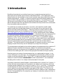
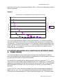
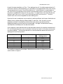
AEAT/ENV/R/0639 Issue 1
UG219 TRAMAQ.
Excess emissions planning
tool (EXEMPT) user guide
AP Smith
May 2001
AEAT/ENV/R/0639 Issue 1
UG219 TRAMAQ.
Excess emissions planning
tool (EXEMPT) user guide
AP Smith
May 2001
AEAT/ENV/R/0639 Issue 1
Title
UG219 TRAMAQ. Excess emissions planning tool (EXEMPT)
user guide
Customer
DETR
Customer reference
PPAD 9/99/6
Confidentiality,
copyright and
reproduction
Copyright AEA Technology plc
All rights reserved.
Enquiries about copyright and reproduction should be addressed to
the Commercial Manager, AEA Technology plc.
The views expressed in this report are not necessarily those of the
DETR.
File reference
DD89927
Report number
AEAT/ENV/R/0639
Report status
Issue 1
AEA Technology plc
Engines and Emissions
401.8, Harwell Laboratory
Harwell
Didcot
Oxfordshire
OX11 0QJ
Telephone 01235 434422
Facsimile 01235 436322
AEA Technology is the trading name of AEA Technology plc
AEA Technology is certificated to BS EN ISO9001:(1994)
Name
Author
AP Smith
Reviewed by
EA Feest
Approved by
DCW Blaikley
Signature
Date
AEA Technology ii
AEAT/ENV/R/0639 Issue 1
Contents
1
Introduction
1
2
Loading the model
2
3
Using the model
3
3.1
MAIN MENU
3
3.2
INFORMATION
3
3.3
DATA ENTRY AND RESULTS
3
3.4
ADVANCED MENU
3.4.1 Vehicle parc definition
3.4.2 Detailed results
3.4.3 Graphs menu
3.4.4 HELP
5
5
6
7
9
3.5
QUIT
9
4
Scenarios
9
4.1
EXCESS EMISSIONS AS A FUNCTION OF DISTANCE FROM A CAR PARK
4.2
EXCESS EMISSIONS AS A FUNCTION OF DISTANCE FROM A TOWN
CENTRE
10
4.3
EFFECT OF CHANGING THE NUMBER OF TRAFFIC LANES
12
Acknowledgements
9
13
Appendices
APPENDIX 1
MODEL PARAMETERS
AEA Technology iii
AEAT/ENV/R/0639 Issue 1
1 Introduction
Modelling the emissions from vehicles is becoming an increasingly important activity in
planning the environmental impact of future urban developments. This is largely done using
emissions factors for vehicles based on their level of emission when being driven at their normal
operating temperatures. However, in urban environments vehicles are usually started under
engine conditions that are different to the hot operating conditions. The emissions from these
vehicles can be very different to those calculated using the basic emission factors. This model
seeks to address this issue and calculates the extra emissions that are produced when vehicles start
from more realistic starting conditions.
The results from this model may be used in conjunction with results from a traffic-based
emissions model that calculates mass emissions on a road network from vehicles with their
engines at normal operating temperature. These may come from models combining trafficbased emission factors in g/km, (available from the National Atmospheric Emissions Inventory,
http://www.aeat.co.uk/netcen/airqual/index.html, and the national emission factor database)
with vehicle kilometres travelled on the road network. Alternatively they may come from other
air quality and emission estimation procedures, for example the Highways Agency DMRB
procedure “Design Manual Roads and Bridges, Volume 11, Section 3, Environmental Assessment
Techniques: Part 1 Air Quality, March 2000”, where the user inputs traffic flows on specified road
links to calculate emissions and air concentrations near the road side. The user can then add the
impact of excess emissions from starting vehicles in an area to the hot exhaust emissions
calculated. This might be useful for a scheme appraisal, for example a car-park or out-of-town
shopping complex where many cars will starting their journeys with cold engines.
The excess emissions calculated by the model are based on the measurements from a sample of 2
diesel and 13 petrol cars fitted with three-way catalysts. The results from the model are
weighted according to the proportions of the sampled car types in the national fleet in 1999, not
in terms of the model types, but in terms of fuel type (petrol and diesel) and engine capacity.
Note that no account is taken of excess emissions from non-catalyst gasoline engines. In the
current (1999) petrol car vehicle parc, non-catalyst gasoline vehicles make up 44% of the total
number of vehicles, predicted to fall to ~6% by 2005. By assuming all gasoline vehicles have
catalysts, the model somewhat overestimates the total excess emissions - the overestimate
decreasing as the number of non-catalyst vehicles decreases in future years.
It should be noted that the model is based on excess emissions from cars with Euro 2 engines. It
is likely that these excess emissions will decrease for new catalyst cars in the future, as the new
European emission standards (Euro 3 and Euro 4) start to “kick in” from 2000. This is because
car manufacturers will need to reduce emissions during the engine start-up phase of the drive
cycle to satisfy the more stringent regulatory type-approval limit values. This is likely to be
achieved by reducing catalyst light-off time (the time it takes the catalyst to reach a temperature
at which it becomes effective), for example by pre-heating or locating the catalyst unit closer to
the exhaust manifold.
AEA Technology Page 1
AEAT/ENV/R/0639 Issue 1
Estimating how much such new technologies will reduce the excess emissions is not trivial and
is beyond the scope of the current model design requirements. The model could, however, be
updated to include the impact of the evolution of the technologies should the necessary
experimental input data become available. By excluding the impact of new technologies on
excess emissions from the fleet in future years, as well as the excess emissions from non-catalyst
cars, the model will always tend to be overestimating the contribution of excess emissions to the
overall emissions calculated for a particular scheme. However, the ranking of comparative
schemes analysed is likely to remain valid.
The equations used to model the excess emissions were determined from experimental data as
part of a UK DETR funded project. The summary report of the project has the following
reference: DCW Blaikley, AP smith, EA Feest and AH Reading, UG219 TRAMAQ- Cold start
emissions. Summary report. AEA Technology report no. AEAT/ENV/R/0638 (May 2001),
which can be obtained electronically from http://www.aeat.co.uk/netcen/airqual/research
reports.
2 Loading the model
The model has been incorporated into a Microsoft Excel spreadsheet. The user uses a mouse to
click on menu buttons which run macros to enable access to the different areas of the model.
The model calculations are based on the equations outlined in Appendix 1. The calculations are
hidden from the user and occur instantly when any user input parameter has been changed.
The user should either double click on the file name EXEMPT.XLS within Windows explorer,
or open the file from within Excel. The file is a Microsoft Excel 97 workbook.
The user will be prompted by Excel to enable the macros. Click on the “Enable Macros”
button.
A password prompt will then appear. The workbook is protected from being accidentally
corrupted by a set of passwords. The user should click on the “Read Only” button.
On opening the spreadsheet the appearance of Excel will be changed by macros within the
spreadsheet, removing scroll bars, formula bars, etc.
AEA Technology Page 2
AEAT/ENV/R/0639 Issue 1
3 Using the model
This section will describe the user operation of the model and the results given.
3.1 MAIN MENU
The opening sheet of the model (the main menu) has four options, as per the picture below.
Clicking on any of the buttons will either take the user to a new sheet, or quit from the model.
Figure 1. Main menu sheet.
Excess emissions planning tool
(Version 2.4)
INFORMATION
DATA ENTRY
AND RESULTS
ADVANCED MENU
QUIT
3.2 INFORMATION
Clicking on <INFORMATION> loads a screen which gives a brief description of the model
and its purpose. The user returns to the main screen by clicking on the only button on this
sheet.
3.3 DATA ENTRY AND RESULTS
Clicking on the <DATA ENTRY AND RESULTS> button accesses the sheet (see picture
below) in which the user enters the information relevant for the simulation to be performed, and
AEA Technology Page 3
AEAT/ENV/R/0639 Issue 1
the total excess emissions of each pollutant integrated over all vehicles and all three stages is
displayed. The simulation is split into three stages:
1.
2.
3.
Driving
Parking
Driving
Figure 2. DATA ENTRY AND RESULTS sheet.
Total number of vehicles
1000
TOTAL EXCESS EMISSION
STAGE 1 - DRIVING
Ambient temperature (°C)
Vehicle start oil temperature (°C)
Driving distance (km)
Drive cycle type
0
0
4
1
Carbon dioxide, CO2 (kg)
448.3
Carbon monoxide, CO (kg)
57.10
STAGE 2 - PARKING
Ambient temperature (°C)
Parking start oil temperature (°C)
Parking time (minutes)
0
999
180
Total unburned hydrocarbons (kg)
4.67
Oxides of nitrogen, NOx (kg)
0.93
STAGE 3 - DRIVING
Ambient temperature (°C)
Vehicle start oil temperature (°C)
Driving distance (km)
Drive cycle type
0
999
4
1
Particulates (g)
63.84
MAIN MENU
PRINT
The user enters the total number of vehicles in the simulation, followed by the information for
stage 1 driving – ambient temperature, start engine temperature, driving distance and drive cycle
type. The drive cycle type must be a number between 1 and 9 inclusive. A list of options will
appear when entering data in this cell. In the present model only one drive cycle is incorporated
– the multiple ECE urban cycle tested in this work. The other options have been incorporated
for possible future upgrades of the model
After the initial driving, a parking stage is incorporated which models the cool down of the
vehicle. The start vehicle temperatures can be set manually, or the model will calculate them
automatically from the heating profile of the first driving stage if the user enters “999”.
The final driving stage is similar to the first, except that the start engine temperature can either
be set manually or calculated by the model from the parking (i.e. cooling) stage.
The screen above is obtained using the default vehicle parc (see Section 3.4.1 below).
AEA Technology Page 4
AEAT/ENV/R/0639 Issue 1
By clicking on <PRINT>, the sheet will be printed. Clicking on <MAIN MENU> will
return to the main menu.
Note that the model can be used to calculate the emissions from a single stage by setting the
time of stage 2 to zero and the distance of stage 3 to zero.
3.4 ADVANCED MENU
Clicking on <ADVANCED MENU> gives the user access to more detailed analysis facilities.
There are five options available in this menu, including returning to the main menu.
Figure 3. Advanced menu screen
Excess emissions planning tool
Advanced Menu
VEHICLE PARC
GRAPHS MENU
DETAILED RESULTS
RETURN TO
MAIN MENU
HELP
3.4.1 Vehicle parc definition
Clicking on <VEHICLE PARC> accesses the sheet where the distribution of vehicle types is
defined. There are currently 10 different vehicle classifications in the population, and the
percentages of each should be set to represent the overall vehicle population distribution. The
total percentage should be 100% exactly, otherwise error warnings will be printed in other areas
of the model.
Figure 4 shows the vehicle parc definition screen, together with the default settings. These are
based on the national fleet in 1999 figures, not in terms of the model types, but in terms of fuel
type (petrol and diesel) and engine capacity.
Note that the model predicts excess emission given by diesel and catalyst gasoline vehicles. No
account is taken of non-catalyst gasoline engines. In the current (1999) vehicle parc, noncatalyst gasoline vehicles comprise 44% of the total number of vehicles, predicted to fall to 6%
by 2005. By assuming all gasoline vehicles have catalysts, we will be overestimating the total
excess emissions - the overestimate decreasing as the number of non-catalyst vehicles decreases.
AEA Technology Page 5
AEAT/ENV/R/0639 Issue 1
The reason for this overestimate is the fact that excess emission is relative to hot emission.
Consider an engine that is fitted into two vehicles, one with (vehicle A) and the other without
(vehicle B) a catalyst. Assuming both engines produce very nearly the same levels of pollutants
when hot, vehicle B will emit less due to the effect of the catalyst. When both vehicles are cold,
the engines will produce extra emissions above their hot start emissions. The catalyst will not be
at operating temperature during most of this period and so both vehicles will give similar
emissions. Thus, relative to the hot start emissions, vehicle B will produce a higher excess
emission.
Clicking on <RETURN> takes the user back to the ADVANCED MENU.
Figure 4. Vehicle parc definition.
Vehicle type
1
2
3
4
5
6
7
8
9
10
Vehicle description
Percentage of vehicle parc
Diesel vehicles
1.2l gasoline engines with catalyst
1.25l gasoline engines with catalyst
1.4l gasoline engines with catalyst
1.6l gasoline engines with catalyst
1.8l gasoline engines with catalyst
1.8l GDI gasoline engines with catalyst
2.0l gasoline engines with catalyst
2.5l gasoline engines with catalyst
3.0l gasoline engines with catalyst
12.2
16.38
8.08
16.16
26.05
10.5
3.5
3.23
2.14
1.76
Total percentage
RETURN
PRINT
100
3.4.2 Detailed results
Clicking on <DETAILED RESULTS> gives access to the sheet where all of the results are
displayed in detail. The results are presented on a stage by stage basis for each individual vehicle
type.
For the two driving cycles, the excess emission per vehicle for each vehicle type is listed,
together with the total when integrated over all vehicles. The final vehicle temperature is also
given after driving and parking.
The results in Figure 5 are obtained using the data listed under DATA ENTRY and VEHICLE
PARC AND DRIVE CYCLE listed earlier.
AEA Technology Page 6
AEAT/ENV/R/0639 Issue 1
Figure 5. Detailed results screen.
TOTAL EXCESS EMISSION, all vehicles (g)
CO2
CO
THC
NO x
VEHICLE
STAGE 1 - DRIVING
Diesel vehicles
1.2l gasoline engines with catalyst
1.25l gasoline engines with catalyst
1.4l gasoline engines with catalyst
1.6l gasoline engines with catalyst
1.8l gasoline engines with catalyst
1.8l GDI gasoline engines with catalyst
2.0l gasoline engines with catalyst
2.5l gasoline engines with catalyst
3.0l gasoline engines with catalyst
TOTALS
STAGE 3 - DRIVING
Diesel vehicles
1.2l gasoline engines with catalyst
1.25l gasoline engines with catalyst
1.4l gasoline engines with catalyst
1.6l gasoline engines with catalyst
1.8l gasoline engines with catalyst
1.8l GDI gasoline engines with catalyst
2.0l gasoline engines with catalyst
2.5l gasoline engines with catalyst
3.0l gasoline engines with catalyst
TOTALS
Particulate
38680.2
25553.6
17900.0
38169.1
79174.2
32757.2
9689.8
5148.8
14786.5
6150.9
452.5
4235.9
3975.4
7899.0
19277.0
4712.1
1339.3
1154.7
1436.6
643.3
63.1
380.2
219.4
519.9
1277.7
485.3
246.5
66.4
236.6
65.3
60.4
73.3
-24.8
36.9
-2.8
166.8
56.7
-30.5
22.8
23.0
10.9
4.0
0.5
14.1
5.5
1.9
2.7
2.2
2.4
0.5
268010.3
45125.8
3560.3
381.9
44.6
21885.6
18328.2
12277.6
26444.9
56769.9
22624.9
7359.2
3781.0
7470.1
3373.2
255.1
1395.1
176.3
2255.5
5156.2
1209.1
695.9
420.0
163.0
247.3
35.5
134.5
29.1
114.5
422.7
112.6
161.8
32.2
45.2
20.7
-13.7
101.1
0.4
75.7
173.3
57.0
73.5
-13.6
78.3
17.0
3.5
2.4
0.2
7.2
2.4
0.8
1.1
1.0
0.6
0.1
180314.7
11973.4
1108.7
549.1
19.3
60.6
43.9
30.2
64.6
135.9
55.4
17.0
8.9
22.3
9.5
0.71
5.63
4.15
10.15
24.43
5.92
2.04
1.57
1.60
0.89
0.10
0.51
0.25
0.63
1.70
0.60
0.41
0.10
0.28
0.09
0.05
0.17
-0.02
0.11
0.17
0.22
0.13
-0.04
0.10
0.04
0.014
0.006
0.001
0.021
0.008
0.003
0.004
0.003
0.003
0.001
GRAND TOTALS (in kg)
Diesel vehicles
1.2l gasoline engines with catalyst
1.25l gasoline engines with catalyst
1.4l gasoline engines with catalyst
1.6l gasoline engines with catalyst
1.8l gasoline engines with catalyst
1.8l GDI gasoline engines with catalyst
2.0l gasoline engines with catalyst
2.5l gasoline engines with catalyst
3.0l gasoline engines with catalyst
RETURN
PRINT
3.4.3 Graphs menu
Clicking on <GRAPHS MENU> accesses another menu screen to choose which pollutant to
plot the histogram of total excess emission, integrated over all stages and for every vehicle within
a given type, as a function of vehicle for the conditions under study. An example of one such
plot, for CO2 excess emission, is given in Figure 7 for the data listed above. Clicking on the
<RETURN> on the graph takes the user back to the GRAPHS MENU.
AEA Technology Page 7
AEAT/ENV/R/0639 Issue 1
Figure 6. Graphs menu screen.
Excess emissions planning tool
Graphs Menu
CARBON DIOXIDE
CHART
HYDROCARBON
CHART
CARBON MONOXIDE
CHART
PARTICULATES
CHART
NITROGEN OXIDES
CHART
Figure 7. Graph of CO2 excess emission.
RETURN
PRINT
Total excess carbon dioxide emissions by vehicle type
1.60E+02
1.40E+02
Excess emission (kg)
1.20E+02
1.00E+02
8.00E+01
6.00E+01
4.00E+01
2.00E+01
0.00E+00
Diesel vehicles
1.2l gasoline
engines with
catalyst
1.25l gasoline
engines with
catalyst
1.4l gasoline
engines with
catalyst
1.6l gasoline
engines with
catalyst
1.8l gasoline
engines with
catalyst
1.8l GDI
gasoline
engines with
catalyst
2.0l gasoline
engines with
catalyst
2.5l gasoline
engines with
catalyst
3.0l gasoline
engines with
catalyst
Vehicle type
AEA Technology Page 8
AEAT/ENV/R/0639 Issue 1
3.4.4 HELP
Clicking on <HELP> accesses the sheet shown below which gives a simple summary of
instructions on how to use the model.
3.5 QUIT
Clicking on <QUIT> from the main menu will close down the model and restore Excel
settings to include the formula bar, scroll bars, etc. The user will be prompted to ensure they
want to quit.
4 Scenarios
4.1 EXCESS EMISSIONS AS A FUNCTION OF DISTANCE FROM
A CAR PARK
The model can be used to calculate the distribution of excess emissions as a function of distance
from a car park. There will be excess emission due to the fact that the vehicle engine
temperatures will have cooled during the parking time.
For example, let us assume that all vehicles arrive in the car park with their engines hot,
producing no excess emission in the surrounding area on the way to the car park. If the car park
was attached to a sports complex, we might assign a parking time of 100 minutes. This time
would vary depending on the car park application. We will also assume a total of 1000 parked
vehicles during a cold winter’s day with an ambient temperature of 0°C.
In order to ensure that the vehicles arrive hot, we set the stage 1 distance to a high value,
say400km, with a start temperature of 50°C and ambient temperature of 0°C. However, this
initial stage will produce some excess emission that we do not wish to include in the calculation.
Therefore, the distance for stage 3 should initially be set to zero so that the model calculates the
excess emission from stage 1. These values should then be subtracted from all subsequent
calculated values.
We set the time for parking in stage 2 as 100 minutes and the start of parking temperature as 999
so that the model uses the calculated hot engine temperature from stage 1. The ambient
temperature is set to 0°C for all three stages. In stage 3 we set the start engine temperature to
999 so that it is calculated from the rate of cooling in the car park. We then allow the model to
calculate the excess emission as a function of distance, for example at 0.5km intervals up to 5km.
The excess emission produced in stage 1 has to be subtracted from all of the data calculated as a
function of distance from the car park. The excess emission produced at each distance from the
car park is then calculated by subtracting the sum of all the excess produced up to that point.
For example, the total excess emission produced at a distance of 3km would be the total excess
AEA Technology Page 9
AEAT/ENV/R/0639 Issue 1
produced by driving 3km minus that from driving 2.5km. In this way, the distribution shown in
Figure 8 is obtained.
Figure 8.
Excess emission of CO and particulate as a function of distance from a car park
7
2.5
6
2
1.5
4
3
1
2
Excess particulate emission (g)
Excess CO emission (kg)
5
CO
Particulate
0.5
1
0
0
0
1
2
3
4
5
6
Distance from car park (km)
The model can simulate many different car parking arrangements. For example, the parking
time might be different if the car park is for a shopping centre (a distribution of parking times
could be used). The vehicles may not arrive in a hot condition so that the excess leading to the
car park has to be included in the calculation. The vehicles may not all drive beyond 5km from
the car park, etc. The change with time of day could be simulated with changes in vehicle
number and ambient temperature.
4.2 EXCESS EMISSIONS AS A FUNCTION OF DISTANCE FROM
A TOWN CENTRE
The model calculates the total excess emissions produced from a specified set of conditions –
there is no information given about the spatial or time distribution of these emissions. However,
by careful use of the model, this data can be extracted.
For example, let us consider arbitrary radial zones surrounding a city centre at 0, 1, 2, 3….up to
7km from the city centre as an example, labelled as zones A to H respectively. For simplicity of
explanation we will assume that vehicles only drive into the city centre itself. We can calculate
the excess emissions produced in each zone on driving into the city by using the following
procedure.
In DATA ENTRY sheet, we will use just stage 1, so set the time and distance parameters of
stages 2 and 3 to zero. Then, with the appropriate temperatures, set the distance travelled to
1km and note the excess emissions for 1 vehicle (total vehicles set to one). Calculate the same
AEA Technology Page 10
AEAT/ENV/R/0639 Issue 1
for each kilometre travelled up to 7km. Then starting at zone H, the total excess produced in G
is the total number of vehicles starting in H multiplied by the excess emission from 1km driving.
The excess produced in zone F by vehicles starting in H, is the difference in excess between 1
and 2km of driving multiplied by the number of vehicles starting from H and driving 2km. This
procedure is repeated all the way into the city centre. The same is then done with the vehicles
starting in each zone in turn, until in zone B all vehicles travel 1km into zone A. The total
excess in each zone is then integrated from each starting point.
Note that this can be made even more complex by defining different vehicle parc distributions at
different zones, perhaps reflecting different wealth in each area. Also, the return journey
parameters can also be calculated by initially following the above procedure and then
subsequently adding a cooling and driving home stage – the stage 3 excess emissions being
calculated from the difference to the above calculation.
As an example we have assumed a vehicle start temperature equal to the ambient temperature of
0°C and that vehicles drive in only one direction into the city centre (i.e. the return journey has
not been modelled). The following distribution of vehicles has been assumed as a function of
starting point from the city centre.
Zone
Distance from centre (km)
B
C
D
E
F
G
H
1
2
3
4
5
6
7
Number of vehicles
starting in zone
500
1200
1500
2000
1000
500
300
The resulting excess particulate emission distribution as a function of distance from the town
centre is shown in figure 9.
AEA Technology Page 11
AEAT/ENV/R/0639 Issue 1
Figure 9.
Simulated excess particulate emission as a function of distance from town centre
80
70
Excess emission (g)
60
50
40
30
20
10
0
0
1
2
3
4
5
6
Distance from centre (km)
4.3 EFFECT OF CHANGING THE NUMBER OF TRAFFIC LANES
If the number of traffic lanes is changed, the flow of traffic may be affected which will change the
time taken to drive a set distance. As the excess emissions are produced as a function of time, for
relatively short distances there could be a significant impact on the excess emissions produced.
This effect can be estimated using the model.
The model calculates emissions as a function of driving time and not distance. The driving time
is calculated from the distance and assuming a constant average speed of the ECE cycle used to
measure excess emissions. No real-life situation is going to exactly reflect this drive cycle so the
calculated excess emissions are representative of urban-style driving. However, relative changes
may be predicted, so that if a lane change produces a 20% increase in average speed, for example,
then the journey time decreases by 20%. As the average speed used by the model cannot be
changed, the user can simulate this circumstance by reducing the travelled distance by 20% and
calculating excess emissions.
For example, consider 1000 vehicles driving 4km along a road at an average speed x kph. The
journey time for case 1 is then 4 x hours. If the number of traffic lanes is reduced we may get a
25% reduction in average speed, which is now 3x 4 , implying a journey time of 16 3x for case
2. But for the purposes of the model the speed is unchanged (it actually assumes a constant
average speed of 18.4kph) at x kph. Therefore, we must adjust the distance travelled in the
model to give the correct journey time – i.e. the effective distance travelled is now 16 3 km. If
we assume an ambient temperature of 0°C, a start temperature for stage 1 equal to the ambient
AEA Technology Page 12
AEAT/ENV/R/0639 Issue 1
temperature, parking for 3 hours and equal drive distances in stages 1 and 3 of the model, we get
the following results.
Case 1
Case 2
(reduced
traffic lanes)
Excess CO2
(kg)
448
475
Excess CO
(kg)
57.1
55.9
Excess
THC (kg)
4.67
4.74
Excess NOx
(kg)
0.93
0.98
Excess PM
(g)
63.8
63.6
There is clearly a substantial increase in excess CO2 emissions produced by this simulated
reduction in traffic lanes, but the other emissions are largely unaffected, with particulate excess
actually reducing slightly. This is because although greater excess of particulate will be
produced on the stage 1 journey for case 2, as the journey time is longer the engine will get
hotter and therefore will be warmer at the start of stage 3 which will produce less excess than for
case 1. The overall excess change will therefore be very dependent on parking time and
ambient conditions.
5 Acknowledgements
The author is grateful to:
- Eric Wyatt of the DETR for his support and encouragement during the project,
- The AEA Technology’s Engines & Emissions team for the provision of experimental data.
- Tim Murrells, John Watterson, John Abbott and Beth Conlan of AEA Technology’s
Environment NETCEN Division for their advice on the application of the model to air
quality modelling.
- The Local Authorities who gave of their time to discuss this work and its relevance to them,
and to suggest improvements to the model.
AEA Technology Page 13
AEAT/ENV/R/0639 Issue 1
Appendix 1
Model parameters
CONTENTS
1
2
3
Parameters for calculating excess emissions
Parameters for the time evolution of excess emissions
Heating and cooling parameters
AEA Technology Appendix 1 Page 1
AEAT/ENV/R/0639 Issue 1
6 Parameters for calculating excess
emissions
When ∆T0<Ttest,
a3
Xs = a1 ∆T0a1 + a 2 ∆T0 ,
'
otherwise
Xs = a4 + a5 ∆T0 ,
where
∆T0 = Thot − T0
T0
Start engine oil temperature
Thot
Hot engine oil temperature ( Thot = a + bTambient )
All temperatures are in °C.
Pollutant
Ttest
a1
a1’
a2
a3
a4
a5
VW Golf 1.9l, Tdi (diesel)
CO2
CO
THC
NOx
PM
95
-
0
0
0
0
0
1
1
1
1
1
2.5×10-3
4.3×10-5
7.4×10-6
-0.02
1.2×10-11
2.5
2.5
2.5
0.5
5
-6.84
-
0.07
-
0
0.42
0.09
0.065
-
1
1
1
1
-
3.5×10-3
-5.00×10-5
-1.3×10-5
-1.1×10-9
-
2.5
3
3
5
-
-181.73
-28.5
-25.9
-
2.3
0.35
0.3
-
0
1.4×10-4
5.0×10-5
1.2×10-3
0
1
3
3
2
1
0.4
-4.0×10-12
-8.0×10-9
-1.1×10-5
1.2×10-11
1.5
7
5
3
5
-71.5
-7.5
-
1.2
0.16
-
0
0
0
0
0
1
1
1
1
1
0.006
4.3×10-5
5×10-6
-0.01
1.2×10-11
2.5
2.5
2.5
0.5
5
-5.34
-
0.07
-
0
0.3
0.07
0.1
0
1
1
1
1
1
0.0085
-4.0×10-5
-7×10-6
-9×10-6
1.2×10-11
2.5
3
3
3
5
-181.87
-37.98
0
-
2.5
0.5
0
-
Vauxhall Vectra estate, 1.8l
CO2
CO
THC
NOx
PM
82
82
87
-
Mitsubishi Carisma, 1.8l GDi
CO2
CO
THC
NOx
PM
71
70
-
Peugeot 306 estate 1.9l, Hdi (diesel)
CO2
CO
THC
NOx
PM
75
-
Vauxhall Omega auto, 2.5l
CO2
CO
THC
NOx
PM
75
80
105
-
AEA Technology Appendix 1 Page 2
AEAT/ENV/R/0639 Issue 1
Pollutant
a1
a1’
a2
a3
a4
a5
80
80
106
-
0
0.1
0.03
0.025
0
1
1
1
1
1
0.04
0
-2.5×10-6
-2.1×10-6
2.5×10-12
2
0
3
3
5
-128.0
-8.48
0
-
1.7
0.12
0
-
80
80
100
-
0
0.03
0.005
8×10-3
0
1
1
1
1
1
0.035
0
0
-1.5×10-6
1.2×10-12
2
0
0
3
5
-477.6
-23.6
-0.7
-
6
0.3
0
-
0
0.07
0.007
0
0
1
1
1
1
1
0.027
0
0
3.5×10-5
1×10-12
2
0
0
2
5
-218.7
-26.37
-
2.5
0.3
-
0
0.25
0.07
7×10-4
0
1
1
1
2
1
0.04
0
-6.2×10-4
-7.5×10-6
3×10-12
2
0
2
3
5
-300
-18.37
-0.5
-
4
0.25
0
-
85
85
100
-
0
0.25
0.02
0.035
0
1
1
1
1
1
0.035
-2.5×10-5
-2.0×10-6
-4.0×10-4
5.0×10-12
2
3
3
2
5
-308.6
-33.53
-0.5
-
3.7
0.4
0
-
80
90
-
0
0.1
0.015
3.5×10-2
0
1
1
1
1
1
0.035
0
0
-3.2×10-4
1.2×10-7
2
1
1
2
3
-232
-25.65
-
3
0.3
-
80
85
-
0
0.04
0.01
0.017
0
1
1
1
1
1
0.02
0
-1.4×10-8
-1.53×10-3
5.0×10-12
2
1
4
1.5
5
-88.8
-10.1
-
1.15
0.12
-
85
85
-
0
0.05
0.007
0.01
0
1
1
1
1
1
0.017
0
0
-2×10-6
5×10-12
2
1
1
3
5
-123.25
-5.36
-
1.5
0.07
-
Ttest
Renault Laguna, 1.8l
CO2
CO
THC
NOx
PM
Ford Fiesta, 1.25l
CO2
CO
THC
NOx
PM
Vauxhall Corsa, 1.2l
CO2
CO
THC
NOx
PM
90
90
-
Mitsubishi Carisma, 1.6l
CO2
CO
THC
NOx
PM
80
80
100
-
Toyota Avensis 1.8l
CO2
CO
THC
NOx
PM
Honda Civic 1.4l
CO2
CO
THC
NOx
PM
Skoda Fabia 1.4l
CO2
CO
THC
NOx
PM
Ford Mondeo 2.0l
CO2
CO
THC
NOx
PM
AEA Technology Appendix 1 Page 3
AEAT/ENV/R/0639 Issue 1
Pollutant
Ttest
a1
a1’
a2
a3
a4
a5
85
80
-
0
0.15
0.052
0.055
0
1
1
1
1
1
0.018
0
-6.1×10-6
-5.3×10-4
6×10-8
2
1
3
2
3
-412.25
-18.96
-
5
0.25
-
85
95
-
0
0.3
0.016
0.013
0
1
1
1
1
1
0.05
-2×10-5
0
0
3×10-12
2
3
1
1
5
-114.28
-36.48
-
1.5
0.4
-
Peugeot 206 1.2l
CO2
CO
THC
NOx
PM
Jaguar S-type 3.0l
CO2
CO
THC
NOx
PM
Parameters to calculate Thot = a + bTambient
Vehicle
VW Golf 1.9l, Tdi (diesel)
Vauxhall Vectra estate, 1.8l
Mitsubishi Carisma, 1.8l GDi
Peugeot 306 estate, 1.9l, Hdi (diesel)
Vauxhall Omega auto, 2.5l
Renault Laguna, 1.8l, gasoline
Ford Fiesta, 1.25l
Vauxhall Corsa, 1.2l
Mitsubishi Carisma, 1.6l
Toyota Avensis 1.8l
Honda Civic 1.4l
Skoda Fabia 1.4l
Ford Mondeo 2.0l
Peugeot 206 1.2l
Jaguar S-type 3.0l
a
100
102
91.5
91.1
99.6
97.6
87.8
91.7
93.5
95.8
99.5
104.4
106
90.7
100.6
b
0
0
0.32
0.48
0.23
0.28
0.51
0.52
0.50
0.33
0.31
0.236
0.37
0.28
0.24
AEA Technology Appendix 1 Page 4
AEAT/ENV/R/0639 Issue 1
7 Parameters for the time evolution
of excess emissions
F = 1 − exp (− bt )
where F is the fraction of total excess emissions produced after time t.
Vehicle
VW Golf 1.9l, Tdi (diesel)
Vauxhall Vectra estate, 1.8l
Mitsubishi Carisma, 1.8l, GDi
Peugeot 306 estate, 1.9l, Hdi (diesel)
Vauxhall Omega auto, 2.5l
Renault Laguna, 1.8l
Ford Fiesta, 1.25l
Vauxhall Corsa, 1.2l
Mitsubishi Carisma, 1.6l
Toyota Avensis 1.8l
Honda Civic 1.4l
Skoda Fabia 1.4l
Ford Mondeo 2.0l
Peugeot 206 1.2l
Jaguar S-type 3.0l
CO2
0.003
0.0025
0.002
0.0025
0.0022
0.0027
0.0022
0.0025
0.0026
0.0028
0.0028
0.0018
0.0023
0.002
0.0015
CO
0.0035
0.011 − 1.3 × 10−4 T0
0.009
0.0075
0.017
0.013
0.020
0.013
0.020
0.004
0.017
0.015
0.015
0.008
0.008
THC
0.0026
0.0045
0.0055
0.0055
0.0035
0.004
0.006
0.004
0.005
0.002
0.004
0.007
0.008
0.004
0.0055
NOx
0.0026
0.0048
0.015
0.0022
0.017
0.008
0.005
0.015
0.01
0.005
0.015
0.007
0.0016
0.004
0.01
Particulate
0.0026
0.0055
0.0055
0.0035
0.004
0.006
0.004
0.005
0.002
0.004
0.007
0.008
0.004
0.0055
AEA Technology Appendix 1 Page 5
AEAT/ENV/R/0639 Issue 1
8 Heating and cooling parameters
For the vehicle heating profile:
Tt − Ta = c1 (t + t ') + c2 (t + t ') until t + t ' ≥ t max or Tt − Ta > Tmax when Tt − Ta = Tmax .
2
The value of t’ is dependent on the vehicle start temperature and is calculated by solving the
equation
Tt − Ta = c1 t '+c 2 t ' 2
so that
t' =
− c 1 + c12 − 4c 2 (Ta − T0 )
2c 2
.
For vehicle cooling:
(Tt − Ta ) =
256


4


 (T − T )14 + kt 
 0 a

4
where T0 is the temperature at time zero (i.e. at the start of cooling).
Vehicle
VW Golf 1.9l, Tdi (diesel)
Vauxhall Vectra estate, 1.8l
Mitsubishi Carisma, 1.8l GDi
Peugeot 306 1.9l estate, Hdi (diesel)
Vauxhall Omega auto, 2.5l
Renault Laguna, 1.8l
Ford Fiesta, 1.25l
Vauxhall Corsa, 1.2l
Mitsubishi Carisma, 1.6l
Toyota Avensis 1.8l
Honda Civic 1.4l
Skoda Fabia 1.4l
Ford Mondeo 2.0l
Peugeot 206 1.2l
Jaguar S-type 3.0l
Heating parameters
c1
0.125
0.115
0.119 – 0.0008Ta
0.116 - 0.0013Ta
0.112 - 0.0011Ta
0.105 - 0.0010Ta
0.115 - 0.0007Ta
0.105 - 0.00064Ta
0.126 - 0.0006Ta
0.116 - 0.0006Ta
0.13
0.112 - 0.0005Ta
0.163 - 0.0006Ta
0.10
0.145 - 0.0007Ta
c2
-4.07×10-5 – 4.4×10-7Ta
-3.44×10-5 – 4.0×10-7Ta
-4.05×10-5 + 2.5×10-7Ta
-3.71×10-5 + 4.07×10-7Ta
-3.33×10-5 + 4.63×10-7Ta
-3.00×10-5 + 3.00×10-7Ta
-3.80×10-5 + 2.60×10-7Ta
-3.00×10-5 + 1.70×10-7Ta
-4.30×10-5 + 1.29×10-7Ta
-3.76×10-5 + 6.06×10-8Ta
-4.48×10-5 - 4.51×10-7Ta
-3.18×10-5 – 5.93×10-8Ta
-6.50×10-5 - 1.20×10-7Ta
-2.60×10-5
-5.47×10-5 + 3.70×10-8Ta
Cooling
k
Tmax
97 - Ta
95.5 – 0.88Ta
87 – 0.83Ta
88 - Ta
93.6 – 0.48Ta
91.5 – 0.86Ta
86.1 – 0.56Ta
87.3 – 0.67Ta
90.5 – 0.65Ta
88.5 – 0.79Ta
95.1 – 0.80Ta
98.2 – 0.92Ta
103 – 0.84Ta
87.1 – 0.84Ta
95.9 – 0.89Ta
AEA Technology Appendix 1 Page 6
0.0028
0.0033
0.0035
0.003
0.0023
0.0035
0.0035
0.0035
0.0038
0.0035
0.0035
0.003
0.004
0.0038
0.0024