Download GASTAR 3.2 USER MANUAL

GASTAR 3.2
USER MANUAL
8 April 2009
Cambridge Environmental Research Consultants Ltd
3 King's Parade, Cambridge, CB2 1SJ, UK
www.cerc.co.uk
Contents
Preface ............................................................................................................................ iv
1. Getting Started ............................................................................................................... 1
1.1
System requirements ................................................................................................ 1
1.2
Installing and starting GASTAR .............................................................................. 1
1.2.1
Use of GASTAR 3.2 with earlier versions of GASTAR ................................. 1
1.2.2
Installing GASTAR 3.2.................................................................................... 2
1.2.3
Starting GASTAR ............................................................................................ 3
2. Using GASTAR .............................................................................................................. 4
2.1
Windows terminology .............................................................................................. 4
2.1.1
Menus ............................................................................................................... 4
2.1.2
Folders.............................................................................................................. 4
2.1.3
Information....................................................................................................... 7
2.1.4
Navigating using a keyboard............................................................................ 7
2.2
Main features of the GASTAR interface.................................................................. 8
2.2.1
Menus ............................................................................................................... 8
2.2.2
Folders.............................................................................................................. 9
2.3
Setting up a problem ................................................................................................ 9
2.3.1
Starting ........................................................................................................... 10
2.3.2
Editing ............................................................................................................ 10
2.3.3
Saving............................................................................................................. 11
2.3.4
Template files................................................................................................. 11
2.4
Running a problem ................................................................................................. 12
2.4.1
Running GASTAR from Windows ................................................................ 12
2.4.2
Running GASTAR from DOS ....................................................................... 12
2.4.3
List files for batch mode................................................................................. 14
2.4.4
Warning and error messages .......................................................................... 14
2.5
Examining output from a run ................................................................................. 15
2.6
User preferences..................................................................................................... 15
2.7
GASTAR command line ........................................................................................ 18
2.7.1
Switches and arguments ................................................................................. 18
2.7.2
Example command lines ................................................................................ 19
3. Entering input............................................................................................................... 21
3.1
Meteorology details................................................................................................ 21
3.1.1
Wind speed..................................................................................................... 22
3.1.2
Wind height .................................................................................................... 22
3.1.3
Wind direction................................................................................................ 23
3.1.4
Roughness length ........................................................................................... 23
3.1.5
Air temperature .............................................................................................. 23
3.1.6
Surface temperature........................................................................................ 23
3.1.7
Atmospheric pressure..................................................................................... 24
3.1.8
Relative humidity ........................................................................................... 24
3.1.9
Atmospheric stability ..................................................................................... 24
3.2
Source details ......................................................................................................... 25
3.2.1
Source material............................................................................................... 25
3.2.2
Release type.................................................................................................... 25
3.2.3
Source details ................................................................................................. 28
3.2.4
Flash calculation............................................................................................. 32
i
GASTAR
Contents
3.3
Complex effects: obstacles..................................................................................... 34
3.3.1
Obstacle summary .......................................................................................... 34
3.3.2
Defining obstacles .......................................................................................... 35
3.4
Complex effects: slopes ......................................................................................... 39
3.4.1
Slopes summary ............................................................................................. 40
3.5
Output details ......................................................................................................... 46
3.5.1
Title ................................................................................................................ 46
3.5.2
Modelled time ................................................................................................ 46
3.5.3
Averaging time............................................................................................... 47
3.5.4
Specified Output Points.................................................................................. 47
3.5.5
Specified Output Times.................................................................................. 48
3.5.6
Additional output ........................................................................................... 48
4. Viewing and Plotting Output ...................................................................................... 52
4.1
Selecting data to plot .............................................................................................. 53
4.1.1
Selecting data files for plotting ...................................................................... 53
4.1.2
Selecting the graph type ................................................................................. 53
4.1.3
X-Y plotting ................................................................................................... 53
4.1.4
Flammables plotting....................................................................................... 54
4.2
Plotting and viewing data....................................................................................... 55
4.3
Graph display features............................................................................................ 55
4.3.1
Viewing the data values on a graph ............................................................... 55
4.3.2
Zooming in on a graph ................................................................................... 55
4.3.3
Configuring the graph .................................................................................... 56
4.4
Output parameters .................................................................................................. 57
4.5
Other data appearing in the output file................................................................... 57
4.6
Output for plotting contours................................................................................... 57
5. Pool uptake model ........................................................................................................ 62
5.1
Accessing the pool uptake model........................................................................... 62
5.2
Input ....................................................................................................................... 63
5.2.1
Meteorological input for the pool uptake model............................................ 63
5.2.2
Source input for the pool uptake model ......................................................... 63
5.3
Running the model and using the results ............................................................... 66
5.3.1
Modelling time ............................................................................................... 66
5.3.2
Calculate uptake ............................................................................................. 67
5.3.3
Pool uptake results ......................................................................................... 67
6. Materials Database....................................................................................................... 68
6.1
The materials database ........................................................................................... 68
6.1.1
Viewing the materials database...................................................................... 68
6.1.2
Using a user-defined material ........................................................................ 68
6.1.3
Changing the materials database .................................................................... 70
6.2
Material properties ................................................................................................. 71
7. GASTAR Files .............................................................................................................. 72
7.1
Licence file............................................................................................................. 72
7.2
User-generated files ............................................................................................... 72
8. Theory ........................................................................................................................... 73
8.1
Dense gas dispersion .............................................................................................. 73
8.1.1
Formation of dense gas clouds ....................................................................... 74
8.1.2
Physical processes in dense gas clouds.......................................................... 75
8.1.3
Dispersion models .......................................................................................... 76
8.1.4
Instantaneous releases .................................................................................... 76
ii
GASTAR
Contents
8.1.5
Continuous releases........................................................................................ 78
8.1.6
Time-varying releases .................................................................................... 79
8.2
GASTAR dense gas dispersion model ................................................................... 81
8.2.1
Dispersion model............................................................................................ 81
8.2.2
Meteorology ................................................................................................... 83
8.2.3
Thermal effects............................................................................................... 84
8.2.4
Thermodynamics ............................................................................................ 85
8.2.5
Passive dispersion .......................................................................................... 85
8.2.6
Longitudinal shear dispersion ........................................................................ 86
8.2.7
Concentration profiles .................................................................................... 87
8.2.8
Averaging time............................................................................................... 88
8.2.9
Current model limitations and uncertainties .................................................. 88
8.3
Extended GASTAR................................................................................................ 89
8.3.1
Source input algorithms ................................................................................. 89
8.3.2
Uptake model ................................................................................................. 91
8.3.3
Jet model ........................................................................................................ 93
8.3.4
Topography .................................................................................................... 99
8.3.5
Buildings and obstacles................................................................................ 106
9. References ................................................................................................................... 117
iii
Preface
This document is the User Manual for Version 3.2 of the GASTAR dense gas dispersion model.
It is a self-contained description of both the installation and use of the computer model and the
theoretical basis for the underlying mathematical model, and is intended as the main point of
reference for beginner and experienced user alike.
GASTAR is an integral or box model, describing the evolution of a dense gas cloud in terms of
properties integrated or averaged over the entire cloud or over sections through it. The model
comprises a main dispersion calculation, determining the concentration and thermodynamic
properties of the gas cloud, augmented by a variety of sub-models representing different features
of the source giving rise to the cloud or the environment through which the gas cloud travels.
Thus the capabilities of the model include:
• continuous, instantaneous and time-varying source types
• three-dimensional jet model and pool uptake model available as additional source types
• flash calculation and aerosol releases
• complex effects - sloping terrain and obstacles (separately or in combination)
GASTAR runs on a PC under Microsoft Windows (XP or Vista). It should be installed and run
on a standalone PC. The number of standalone PCs on which GASTAR may be installed and run
is controlled by the user’s licence agreement. GASTAR’s Windows interface provides a userfriendly environment in which to set up and run the model and view the output. Output suitable
for generating contour plots using other plotting software are generated for certain model options.
The model is quick to run, with typical simulations taking at most a few minutes and often only a
few seconds.
Overview of User Manual
The User Manual contains the following main sections:
1
Getting Started
Installation of GASTAR and use of the model for the first time.
2
Using GASTAR
Overview of the operation of the model.
3
Entering Input
Detailed description of input data items and how to enter them.
4
Viewing and Plotting Graphical display of model results.
Output
5
Pool Uptake Model
Additional model that calculates source conditions due to a
vaporising liquid pool.
6
Materials Database
Database of material properties and utility for editing database
7
GASTAR Files
List of files associated with GASTAR.
iv
8
Theory
Theoretical background and description of the mathematical
model.
9
References
Complete reference list.
Typographical conventions
The following conventions have been adopted in the layout of this User Manual:
Style
Usage
Example
Italic
UPPER CASE
File names
Directory names
Text entered by the user, including
the contents of files
Text appearing on the interface
screens
gastar.exe
C:\GASTAR
Fixed width
sans serif
dir /B *.gpl > allruns.lst
Complex Effects folder, Run! menu
Note that “pathname” refers to the location of a file or directory, including the full hierarchy of
directories leading to it starting with the drive letter, e.g. C:\GASTAR\CASES\test1.gpl.
Note
Sections of text marked with a vertical bar in the margin are relevant principally to use of
GASTAR as part of RISKAT, the risk assessment package used by the UK Health and Safety
Executive. They are therefore not relevant to general users of GASTAR.
v
1
Getting Started
1.1 System requirements
GASTAR is supported for use on systems running Microsoft Windows XP and Vista. The
following is the recommended minimum configuration although GASTAR will run successfully
on lower specification PCs:
• PC with a Pentium 1.5 GHz or compatible processor
• 0.5 Gbytes of RAM
• 100 Mbytes of disk space available
1.2 Installing and starting GASTAR
You have been supplied with a CD-ROM containing the latest version of all the files necessary to
install GASTAR. You will also have been sent, probably by email, a GASTAR licence file. The
licence file must be named (and if necessary renamed) to gastar3.lic and copied to the application
directory i.e. the directory in which GASTAR is installed. Users should ensure they keep a
backup of the licence file on a suitable media.
GASTAR should be installed to and run on a standalone PC. Use of a single installation of
GASTAR by multiple users at once is not supported.
1.2.1 Use of GASTAR 3.2 with earlier versions of GASTAR
GASTAR 3.2 can be installed and used on a PC that has earlier versions of the model i.e. version
3.1 and earlier, installed.
If you choose to install the earlier version of GASTAR follow the following steps:
• For version 3.05c to version 3.1 uninstall the program by means of the Windows
Add/Remove Programs feature. Click on the Windows Start button, then click on Settings,
and then Control Panel. Double-click on Add/Remove Programs and then highlight
GASTAR in the list of programs and click on the Add/Remove… button on the
Install/Uninstall tab.
• For versions earlier than 3.05c for which the GASTAR installation simply involved copying
1
GASTAR
Section 1: Getting Started
files from the supplied diskettes, you should find the relevant files and delete them. (See
Section 7 of your earlier GASTAR manual for a list of all files associated with GASTAR).
You may wish to archive any user files (.gpl, .gof, etc.) generated by that version in a
dedicated directory.
1.2.2 Installing GASTAR 3.2
Please check first with your own IT personnel for company procedures for installing software.
The installation of GASTAR is straightforward. It uses an Installation Wizard, which guides the
user through a short series of screens, collecting information on the user and installation
parameters, before installing the software. The following steps lead you through the GASTAR
installation process.
• Log on as Local Administrator for the PC.
•
Insert the GASTAR install CD, whereupon it should automatically run. If it does not, click on
the Windows Start button, select Settings and then Control Panel. Double-click on the
Add/Remove Programs icon and press the Install… button. Browse for the CD-ROM drive
and select setup.exe in the root directory on the drive.
•
Click Next > through the Welcome screen and then select I accept the terms of the licence
agreement, and click Next > in the Licence Agreement screen if you do accept the licence
terms to get to the Customer Information screen. If you do not accept the licence terms select
I do not accept the terms of the licence agreement and click Next > to finish the install.
•
Enter your user name and organisation in the designated places. You also have the option of
installing GASTAR for all users or just for you. Click Next > to go through to the Destination
Folder screen.
•
You should select a drive with at least 1GB of available disk space. The default installation
directory is C:\Program Files\CERC\GASTAR but we suggest you install it in
<Drive>\CERC\GASTAR, where <Drive> can be C: or another drive of your choice. Use the
Change… button to select your own installation directory. Click OK to return to the
Destination Folder screen.
•
The abbreviation <install_path> will be used in the rest of the User Guide to denote the
installation directory you have chosen, for example C\CERC\GASTAR 3.2.
•
Click Next > to view the options you have specified.
•
If the settings shown are correct, press the Install button to complete the install procedure.
However, if you first wish to amend any details, press the < Back and Next > buttons as
appropriate. Once the Install button has been pressed, and the GASTAR files have been
successfully installed, the final screen will appear.
•
Click Finish to complete the installation. The installation procedure automatically puts a
shortcut to GASTAR on your Windows desktop. If the Show the readme file box is checked
the document What's New in GASTAR 3.2? will be opened automatically once you click on
2
GASTAR
Section 1: Getting Started
Finish.
The installation is now complete.
You have been provided with a unique licence file, either by email or on a separate floppy disk,
which is required in order to run the model. It is important that you install this new licence file as
instructed.
•
To install the GASTAR licence, copy the file gastar3.lic to the <install_path> directory.
1.2.3 Starting GASTAR
The GASTAR files are now installed on your computer. The installation process automatically
provides shortcuts for starting up the GASTAR interface:
• it puts a shortcut to the GASTAR interface executable gaswin.exe on the desktop of all users
for which the program was installed. Double-click on this shortcut to start the interface
• it puts an entry in the Windows Start menu for GASTAR, i.e. click on Start and then
Programs and find the entry GASTAR 3 with the GASTAR icon next to it. Clicking on this
starts the interface
• When you have launched GASTAR checking the licence details (through Help, Licence Details)
will give the location of the licence currently being used. Although the model will run when
the licence file is in the Windows WINNT directory, it is recommended that the location be
the <install_path> directory.
• Restart your computer: you are now ready to use the model.
3
2
Using GASTAR
Having described in Section 1 the procedure for installing and starting GASTAR, we turn now in
Section 2 to the operation of the model. Since GASTAR has a Windows interface, we begin in
Section 2.1 with an overview of the Windows terminology that will be used in other parts of this
document, notably in Sections 3 and 4 that describe entering input and viewing output. Next we
give an initial overview of the main features of the GASTAR Windows interface in Section 2.2.
Then in Section 2.3 we describe the stages in setting up a problem for GASTAR to run, while
Section 2.4 deals with the running of such a problem. Section 2.5 gives a preview of examining
output from a run (which is described in more detail in Section 4). Finally, Section 2.6 describes
the various preferences that a user can set and which control a number of ways in which the
interface behaves, while Section 2.7 details the GASTAR command line.
2.1 Windows terminology
In this section, we list the main Windows features that make up the GASTAR interface, defining
the terminology that will be used elsewhere in the description of the computer model. The user
should refer to Figure 2.1 to see examples of (most of) the features described.
2.1.1 Menus
A menu is a heading offering a list of menu options. The menus are located on the menu bar,
which is located near the top of the screen underneath the title bar (see below). By clicking on a
menu title a list of options will appear from which a single selection is made. A menu option may
itself be a menu heading, and selecting it will give rise to a further list of options. For example
the File menu has a list of options, one of which, Preferences, will give a further menu of options
if selected. A menu option may also have an ellipsis at the end of its name, for example Open… this denotes that a dialogue box (see below) will be launched if this option is selected.
2.1.2 Folders
Much of the rest of the interface screen is occupied by a set of folders. Each folder is a group of
controls that deal with a particular aspect of the model. In GASTAR, folders are used to divide up
the input to the model, and allow the user to specify the input data in a structured way. Another
separate folder is used to display the graphical output. The folders appear to lie on top of one
another, and a particular folder is accessed by clicking on the tab that appears along its top edge,
whereupon the folder moves to the top of the "stack".
Within the various GASTAR folders there are different types of control, and in the rest of this
4
GASTAR
Section 2: Using GASTAR
section we outline what these are. Please refer to Figure 2.1 where appropriate.
Figure 2.1 – Example view of interface.
2.1.2.1
Enabled and disabled item
Items in the interface can either be enabled, in which case they are available for use, or disabled,
in which case they cannot be used. Disabled items appear grey rather than black.
2.1.2.2
Text box
Text boxes allow you to enter text data. When you move to an empty text box, an insertion
point (a blinking vertical cursor) appears. The text you type appears at the insertion point.
Each text box is accompanied by a caption which explains the significance of the text in the
box, for example Temperature (K) in Figure 2.1. Text boxes which cannot be edited appear
dimmed.
2.1.2.3
Check box
Check boxes allow you to set or clear an option. When a check box is set it contains an ‘X’, for
example Momentum Initially Well Mixed in Figure 2.1. You can set or clear a check box by
clicking it with the mouse, or by pressing the SPACEBAR, provided the check box is selected. If it
is selected, it will have a dashed box around it.
2.1.2.4
Radio button
Radio buttons represent a group of mutually exclusive options, i.e. you can select only one option
5
GASTAR
Section 2: Using GASTAR
at a time, and if you select a new option, the previous one becomes unselected. The selected
option contains a black dot, for example Instantaneous in the group of four radio buttons under
Release Type in Figure 2.1. Names of options which cannot be selected appear dimmed.
2.1.2.5
Spin button
You move forwards (down) through the list by clicking the down arrow with the mouse. Spin
buttons are used to cycle through an ordered list. You move forwards (back) through the list by
clicking the up arrow with the mouse. Correspondingly, you move backwards (up) through the
list by clicking the up arrow with the mouse. See Figure 4.5 for an example: spin buttons are used
to cycle through data points displayed on a graph.
2.1.2.6
Dialogue box
Dialogue boxes are floating screens which appear when you need to supply additional
information to complete a task. An ellipsis (…) after a menu command indicates that a dialogue
box will appear when you choose that command. For example, if you choose the Open command
on the File menu, the dialogue box shown in Figure 2.2 will appear. In this dialogue box, you
specify the name of the file you want to open. You choose the OK button to open the file you
have chosen. You choose the Cancel button to close the dialogue box without opening a file.
Several other dialogue boxes have OK and Cancel buttons. Cancel will always close the dialogue
box and discard any actions or input made in it, whereas OK will accept any input from the
dialogue box and carry out any appropriate action. Note that double-clicking on a list box item
(see 2.1.2.7) may also be used to select that item and thereby circumvent the need to select the
item and then click on OK.
Figure 2.2 – The Open GASTAR Data File dialogue box.
6
GASTAR
Section 2: Using GASTAR
2.1.2.7
List box
List boxes allow you to choose one item from a list of choices. If it is a drop-down list box, it
normally appears as a rectangular box containing the current selection; however, when you select
the box, the list of available choices appears. If there are more items than can fit in the box, scroll
bars are provided. For example, the Source Material is selected through a drop down list box in
Figure 2.1.
2.1.3 Information
Besides menus and folders, which allow the user to carry out actions, there are other parts of the
interface which provide the user with information.
2.1.3.1
Title bar
This is located at the very top of the screen, and gives the version number of the model together
with the name of the current .gpl file (see Section 2.3), e.g. GASTAR (3.1) : C:\DATA\TEST.GPL.
2.1.3.2
Help bar
The main GASTAR window has a help bar at the bottom. This gives you information about the
part of the interface you are currently using in the form of a short description of the item. If you
are entering a numeric value, the maximum and minimum permissible values will be displayed,
and you will be prevented from entering values outside this range.
2.1.3.3
Message box
Message boxes are a particular type of dialogue box. They may give you a brief message, or they
may ask you to make a simple choice, such as yes or no. For example, a message box appears
when you select Plot Graph on the Graphics folder if an output file has not been selected.
2.1.4 Navigating using a keyboard
Microsoft Windows environments have been developed with a mouse in mind. If you do not have
a mouse, or prefer not to use it, your Windows user guide and help files will explain how to
reproduce all mouse actions using a keyboard. Here is a brief guide to some useful actions:
Moving the cursor between input items.
TAB
SHIFT+TAB
RETURN
Allows you to move the cursor forwards through text boxes and buttons
allows you to move the cursor backwards through text boxes and buttons
"enters" or accepts the current data page or executes the action of a
highlighted button
Entering data into a text box
DELETE
BACKSPACE
← CURSOR
→ CURSOR
HOME
END
SHIFT+CURSOR
will delete the character immediately to the right of the cursor
will delete the character immediately to the left of the cursor
will move the cursor to the left in the current box
will move the cursor to the right in the current box
will move the cursor to the start of the text in the current box
will move the cursor to the end of the text in the current box
selects text in the direction of the arrow
7
GASTAR
Section 2: Using GASTAR
Radio buttons
↑ CURSOR /
← CURSOR
↓ CURSOR /
→ CURSOR
will move the cursor up through the radio buttons for the current item
will move the cursor down through the radio buttons for the current item
In general if a letter in the name of an interface item is underlined, then pressing the ALT key with
the key for that letter will trigger that interface item. For example the File menu has the letter “F”
underlined on the screen. Pressing the ALT and “F” together will open the menu. Additionally, the
SPACE bar can be used in a similar way to the mouse click; the control with the focus (i.e. where
the cursor is) will be “clicked”.
2.2 Main features of the GASTAR interface
As noted in Section 2.1, the main screen of the GASTAR interface is made up of menus and
folders, together with some areas providing information. In this section we list the options
available.
Figure 2.3 – The File menu items.
2.2.1 Menus
There are three main menu options, namely File, Run! and Help (see Figure 2.3). These have the
options shown in the table below.
8
GASTAR
File
Section 2: Using GASTAR
New
Resets the input parameters to their default values
Allows the user to open a previously saved data file
(see Figure 2.2)
Saves the current parameters under the current file
name
Saves the current parameters under a user-specified
file name
Open…
Save
Save As…
File
Open Template…
Save As Template…
Preferences
View Output…
Exit…
1, …, 5
Opens a previously saved template file (see
Section 2.3.4)
Saves a set of data as a template file (see
Section 2.3.4)
GASTAR user preferences (see Section 2.6)
Opens a GASTAR output file in Notepad, Write or
other user-specified viewer
Quits GASTAR
The five most recently-opened or saved input (.gpl)
files – click on one to open the file
Run!
Runs the dispersion model using the current data
file
Help Obtaining Technical Support…
Address and contact information
Version information
Details of licence being used to run model
Current working directory (e.g. for file operations)
About Gastar…
Licence Details
Current Directory
2.2.2 Folders
There are five folders altogether: four are used to specify the input to the model and the fifth
controls the viewing of output from a run:
Meteorology
Source
Complex Effects
Output
Graphics
Input parameters describing meteorological conditions
Input parameters describing the release, i.e. its type, size, etc.
Input parameters describing the buildings, fences and slopes
Parameters affecting the current run of the model
Used for displaying graphically output from a GASTAR run
2.3 Setting up a problem
Having described the features of the interface, we now turn to how these are used in the stages of
setting up a problem. Each problem can be thought of in three different ways:
9
GASTAR
Section 2: Using GASTAR
(a) as a physical problem which the user wishes to simulate with GASTAR
(b) as a set of GASTAR input data, i.e. a set of values for each parameter in the complete list
of GASTAR input parameters
(c) as a file containing these data items
and these definitions tend to be used interchangeably. However, it is important to realise that
typically there may be several alternative sets of input data (b) for a given physical problem (a),
as the user finds possibly different ways to express the physical problem in terms of the input
which the model can accept, whereas there is only one file (c) corresponding to a given set of
input data (b). Such input files for GASTAR are distinguished by a constant extension .gpl e.g.
datafile.gpl.
This User Manual does not give detailed guidance on how to go from (a) to (b) other than to
describe the input data items and to provide some notes on the selection of values. In the rest of
this section we are concerned with the general points concerning how to go from (b) to (c), i.e.
how to set up a .gpl file: the details of specifying the input parameters are covered in Section 3.
2.3.1 Starting
There are several ways to begin setting up a GASTAR problem.
(a) when the interface is started up, the text boxes are blank1 and the controls which require a
choice are at their default settings (a fixed choice accompanying the interface). The user
can then enter all values and make choices from scratch
(b) by selecting the New option on the File menu the text boxes are blank and control settings
take their default values exactly as in (a). This is the recommended way in which to start a
new problem from scratch
(c) by selecting the Open… option on the File menu the user can browse the current directory
(or other directories) to find a .gpl file which has been defined previously. By default the
interface will only display files with the .gpl extension. This is the recommended way in
which to start a new problem based on a pre-existing one.
(d) by selecting the Open Template… option on the File menu the user can open a template
file, which can be used as the basis for a new input file (see Section 2.3.4).
2.3.2 Editing
Whichever method is used to start setting up a problem, the user will then need to edit some or all
of the input data. This is achieved by selecting a folder and then typing in values in text boxes
and selecting options for controls such as check boxes, radio buttons and so on. The mouse is the
usual way in which the folders are navigated; however an alternative is to use the TAB key to
move systematically through the controls, i.e. each control in turn receives the focus. If the
control is a text box, the current text becomes highlighted when it receives the focus.
To change a parameter value in a text box, select the folder containing that parameter by clicking
on the folder’s tab, move the pointer until it is over the appropriate text box and click the left
mouse button. The cursor will now appear in the box. Use DELETE and/or BACKSPACE to remove
unwanted characters before typing in the new value. If you double click the parameter, it will
become highlighted. If you now type the new value it automatically replaces what was
highlighted.
1
In fact, there are two exceptions, namely the wind height (see 3.1.2) and the hazardous fraction (see 3.2.3.4),
which are set to default values of 10.0m and 1, respectively.
10
GASTAR
Section 2: Using GASTAR
Changes to the option selected for radio buttons, list boxes, etc. can be made by clicking on the
required control or via the keyboard using a combination of the SPACE bar and the UP/DOWN and
LEFT/RIGHT keys.
When the focus is given to a control, the help bar at the bottom of the interface screen is
activated. It displays a brief description of the data corresponding to the control. If the control is a
text box the help bar contains a maximum and a minimum value for the parameter. If the user
enters a value outside the permitted range, GASTAR will display a warning dialogue box. This
tells the user whether the value is too large or too small, and what the appropriate bound is. The
user must click OK to clear the warning box before re-entering a value within the given range for
that parameter.
2.3.3 Saving
Once all the desired changes to the input data have been made the user needs to save the values.
This is achieved in one of two ways:
(a) select Save on the File menu to save the input data in a .gpl file with the same name as that
currently loaded. If either of options 2.3.1(a) or 2.3.1(b) had been used then there is no
current name, and the Save As dialogue box will appear (see below)
(b) select Save As on the File menu to save the input data in a .gpl file with a new name. A
dialogue box will appear allowing the user to specify the name (and directory) of the file.
The extension “.gpl” is added unless the file name entered contains a “.”.
The user can also save a set of input data as a template file using the Save As Template… option
of the File menu (see Section 2.3.4).
2.3.4 Template files
When setting up a new problem, it is most convenient to edit an existing set of data rather than
start from scratch each time. One way to do this is to use an existing .gpl file, edit this and then
use File, Save As… to create a new .gpl file. An alternative is to use the GASTAR templates
feature, which is accessed via the File menu.
A GASTAR template is a complete input data file but with the .gpt extension. The interface
provides the means both to open existing templates, and thereby provide the starting point for a
new GASTAR input file, and to create new templates for later use.
To start a new input data set based on a template file, use the File, Open Template… menu
option: the GASTAR interface loads the data in the template file but sets the data set name to
2
(untitled) in the banner at the top of the interface window . You can then edit these data and save
as a new data file with File, Save As…
To create a new template file, simply edit an existing data set in the interface – which may have
been loaded as a .gpl or .gpt file or entered from scratch – and then use File, Save As Template…
to save the template with the desired path name and the .gpt extension.
2
Note that you could also open a template (.gpt) file with File, Open… (provided you select Template Files
(*.GPT) from the List Files of Type: drop-down list box), or using the recently-opened files, but this would simply
open the file “as is”, and is not the recommended way of using template files. Similarly, File, Save and File,
Save As… could be used to save template files, but again this is not recommended.
11
GASTAR
Section 2: Using GASTAR
2.4 Running a problem
The next stage in the process of using GASTAR is to run the problem whose setting-up has been
described in Section 2.3. The obvious conclusion to entering data in the way described above is
to go to the main menu and click on Run! to run the program. There is an alternative to this,
which is to run GASTAR from the DOS prompt. These are both described in more detail below.
Note that in the majority of cases, GASTAR is run from Windows, and so the complications of
command line arguments (see below) are avoided. One circumstance in which they are required
is in carrying out RISKAT runs of GASTAR.
2.4.1 Running GASTAR from Windows
Running a problem directly from Windows is achieved by selecting the Run! main menu option.
The result of this action is that the interface calls the Fortran executable gastar.exe with the
current file name as an argument (see Section 2.7 for more on command line arguments). The
model will then run as a QuickWin application completely separate from the interface.
The output files produced by a GASTAR run depend on whether or not the model is carrying out
a RISKAT run: see Section 2.7 or Section 7 for a list of output files produced by the model in
each case.
Note that if the current input data have not already been saved (as in Section 2.3.3), then selecting
Run! will cause the interface to prompt for saving. The user is presented with a message box
asking them whether they wish to save the data with the current name and run the model. The
user clicks Yes to continue, No to interrupt the Run! command and allow the file to be saved
under an alternative name and Cancel to halt the Run! command completely. (If the data had not
been saved before selecting the Run! command, for example if New had been selected prior to
inputting the data, then the user will be prompted for a file name under which to save the data.)
2.4.2 Running GASTAR from DOS
GASTAR may also be run from the DOS prompt or from a DOS batch (.bat) file. In the latter
case, this is known as running GASTAR in “batch” mode. The essential difference between this
case and that in Section 2.4.1 is that the user starts and finishes in DOS rather than in Windows.
It is important to note that the syntax for running applications from DOS has varied from one
version of Windows to another, so you should consult the online DOS Help for more information.
However, note that the recommended way to run GASTAR from the command line is by using
“list” files – see Section 2.4.3 for full details – which reduces the potential complications of
running from DOS.
The rest of this section can be omitted on first reading.
At the heart of running GASTAR from DOS is the use of GASTAR command lines, with
command line switches and arguments, such as
\GPATH\gastar.exe /I1 \IPATH\datafile.gpl
(see below and Section 2.7 for more details, including examples). There are two main parts.
12
GASTAR
Section 2: Using GASTAR
•
The first part, namely \GPATH\gastar.exe, is the full path name of the gastar.exe
file, i.e. \GPATH is the complete path of the directory containing the GASTAR simulation
engine executable.
•
The second part, namely the rest of the line, /I1 \IPATH\datafile.gpl, are
command line arguments to gastar.exe. It states that the input file expected is a GASTAR
input file (/I1), as opposed to a RISKAT input file (which would have used /I2); the
accompanying path name is the name of the GASTAR input file. Typically this would
have been created using the GASTAR interface. The executable has several possible
command line arguments, and these are explained in full in Section 2.7.
The net result of running GASTAR in this way is that a main output file \IPATH\datafile.gof is
produced, which may then be examined in the usual way by means of the GASTAR interface:
files \IPATH\datafile.log and \IPATH\datafile.gph are also produced.
There may be more than one (input) file name supplied as an argument in the command line. For
example, the above case could be extended to
\GPATH\gastar.exe /I1 \IPATH1\data.gpl \IPATH2\data.gpl
This would cause two (sequential) runs of GASTAR to take place using the input data files
\IPATH1\data.gpl and \IPATH2\data.gpl in turn; two distinct sets of output files would be
produced, one for each run.
An alternative to typing the command line at the DOS prompt is to use a batch file instead. Thus
the same command lines may be typed into a file such as rungas.bat and run more simply from
the DOS prompt by typing rungas (again provided rungas.bat is either in your current directory
or in a directory on your current path, otherwise the full path name for rungas.bat would need to
be given).
A DOS session running under Windows NT4, etc. can also accept the start command. Using
this command you can start other applications at either the DOS prompt or from a DOS batch file.
For more information on the start command, type start /? at the DOS prompt.
Using the start command, you may write a multiple line batch file to run many cases. The lines
in the batch file will be run consecutively provided the /w switch is included after the start
command, so the second line will run after the first is completed and so on. This ensures that the
GASTAR run is completed before the next line of the batch file executes. Also, for the batch file
to regain control after executing the first line, the FORTRAN executable must be told to shut
down on completion by using the /E2 command line switch. See Section 2.7 for more details on
the GASTAR command line options.
If you have a network, you may make use of the Universal Naming Convention for the computers
on your network. For example, if the Network recognises a computer named THOR which has a
shared directory called DATA, and another computer called APOLLO with a shared directory
called MODELS (which has a sub-directory for GASTAR), then we can have the following
examples in a batch file
13
GASTAR
Section 2: Using GASTAR
: Batch files can have comment lines starting with a colon
REM Lines starting with 'REM' will be printed to the DOS screen
: Multiple command lines can be used in Windows batch files
start /w \\APOLLO\MODELS\GASTAR\gastar.exe /I1 /E2 \\THOR\DATA\test1.gpl
start /w \\APOLLO\MODELS\GASTAR\gastar.exe /I1 /E2 \\THOR\DATA\test2.gpl
start /w \\APOLLO\MODELS\GASTAR\gastar.exe /I1 /E2 \\THOR\DATA\test3.gpl
In these examples, note that the batch file is run from a DOS session running under Windows
anywhere on the network. Which ever networked machine runs the batch file, the correct data file
and model will be used.
2.4.3 List files for batch mode
As well as input file names, GASTAR can also accept a list file as an argument to the input file
switch on the command line. Any file having the extension .lst will be assumed by GASTAR to
contain a list of data files, one file per line. The model will run each line in the list file in turn
until completion of all entries in the list file. This is the recommended way to run GASTAR from
the command line.
You can build a suitable file from the DOS prompt using the DIR command (the /B option is
needed to produce brief listing data). For example
dir /B *.gpl > allruns.lst
would produce a list file called allruns.lst containing all .gpl files in the current directory. You
may then edit this file to include additional files, or comment out entries by placing a semi-colon
on the line (the model will ignore anything appearing after the semi-colon on the given line).
You may wish to build a list file with full path names so that it can be used from any directory.
You can do this again with the DIR command but this time using the /S option, which includes all
sub-directories of the current directory as well:
dir /B /S *.gpl > allruns.lst
For more information on the version of DIR available on your operating system, type dir /? or
consult your Microsoft DOS manual.
2.4.4 Warning and error messages
While the model is running, GASTAR will display a minimal amount of information in a window
opened to allow the user to monitor progress of the simulation. When the calculation has
successfully completed, this window will be redundant and the user may click Yes when the
following dialogue box appears on screen:
Program terminated with exit code 0
Exit Window?
The exit code 0 confirms that the Fortran code has terminated, but does not guarantee that the
simulation has run to completion: there is the possibility that the code has encountered an internal
problem in the calculation that might cause a run time error if allowed to continue. In these cases
the code notifies both the screen and the log file of the error it has found before terminating the
current run. The error message should help to discover the cause of the problem.
14
GASTAR
Section 2: Using GASTAR
If the program terminates with error code 1, then there has been some other error, not accounted
for by the Fortran code. In such cases, it is advisable to take note of any error messages that
appear on screen, before exiting GASTAR and Windows and re-booting your PC. Having done
this, attempt to run the same inputs that previously caused the program to fail to see if the
problem is repeatable. Sometimes, testing the code on an alternative machine will also highlight
possible faults and/or differences between two PCs. In this case, check the configuration of both
machines to see what differences there are: look in the config.sys and autoexec.bat files to see if
there might be conflicts with other software that is being loaded when the computer boots up.
When the Fortran code notices a possible problem with data and/or results, it will issue a warning
to the screen or the log file or the data output file, whichever is the more appropriate place. For
example, if the interpolation code calculates values beyond that to which it has integrated, a
warning is included in the output file. This will not cause a terminal error to occur, so the code
continues with the dispersion calculation. However, the validity of the output beyond the distance
actually integrated will be questionable, so this is flagged to the user by issuing the warning.
2.5 Examining output from a run
Once the run has completed, the user may examine the results of the run by means of graphical
display facilities provided by the interface. These are located in the Graphics folder, and provide
extensive line plotting of all quantities calculated by the model. This facility is described in detail
in Section 4.
2.6 User preferences
Next in this Section on using GASTAR, we describe the preferences controlling certain aspects
of use of the interface. These are accessed by selecting Preferences from the File menu, which, in
turn, provides three options as follows. Note that for the options with a dialogue box (Figures 2.4,
2.5 and 2.6), any changes to preferences made by clicking on OK hold for the current session
only. They do not become permanent preferences unless you click on Save Defaults, in which
case they supplant the entry in your .ini file; similarly, you can restore settings from the .ini file
by clicking on Restore Defaults.
Concentrations in ppm
Run Time…
This user preference sets the concentration units to be either
mol/mol or parts per million (ppm). The choice of units is used in
the filed output in the .gof file, in the input data (concentration
for maximum range option) and in the graphical display. To set
ppm as the concentration units, click on the Concentrations in
ppm option from the File, Preferences drop-down list – if you
revisit this list you will see a tick against the Concentrations in
ppm option. Repeating the above process will remove the tick
and toggle back to mol/mol concentration units.
The calculations are performed by a FORTRAN executable that
is launched from the interface but runs as a separate application.
These options allow the user to determine how this application is
launched and how it terminates. For example, because many
GASTAR runs take about a second to execute, you may choose
15
GASTAR
Section 2: Using GASTAR
to run the model minimised, without focus and automatic shut
down at completion. In this way, the GASTAR interface will
remain the current application, allowing you to continue working
without interruption (see Figure 2.4).
Figure 2.4 – The Run Time preferences dialogue box.
Graph Printing…
Allows the user to set some of the commonly used printing
options for graphics output, including the printer, the size and
position of the graph on the page and the overall Page title (this
is not the graph title, which must be set for each individual
graph) – see Figure 2.5.
Figure 2.5 – The Graph Output preferences dialogue box.
Viewing Output…
Allows the user to specify the viewer of their choice to use with
output files. The Other option allows a full command line to be
16
GASTAR
Section 2: Using GASTAR
entered, including any switches for macros, etc. (see Figure 2.6).
Figure 2.6 – The Viewing preferences dialogue box.
GASTAR Output…
Allows the user to select the type of output that a GASTAR run
produces and is primarily of interest to RISKAT users. It is an
alternative way to set the GASTAR output mode command line
switch “/O” (see Section 2.7.1 for more on command line
switches and arguments). A dialogue box for selecting options is
displayed (see Figure 2.7).
By clicking on one of the radio button options, you can select
which of the following types of output file are generated.
Figure 2.7 – The GASTAR Output preferences dialogue box.
•
•
•
GASTAR Output – produce GASTAR output files (.log,
.gof, .gph), equivalent to /O1
RISKAT Toxics Output – produce RISKAT Toxic file
(.bc), equivalent to /O2
RISKAT Flammables Output – produce RISKAT
Flammable file (.flm), equivalent to /O3
17
GASTAR
Section 2: Using GASTAR
2.7 GASTAR command line
As noted in Section 2.4, the gastar.exe executable takes command line switches and arguments.
The general form of the command line is
gastar.exe /Em /In /Op {File name(s)}
where /E, /I and /O are the switches and the integers m, n and p and the name(s) {File name(s)}
are the arguments. There should not be a space between a switch and its integer argument.
Unless you are running GASTAR from a DOS prompt or you need to carry out a RISKAT run of
GASTAR, you can omit the rest of this section on first reading.
2.7.1 Switches and arguments
2.7.1.1
GASTAR exit mode
This flag is optional.
/Em
1
Flag to set the Exit Mode for QuickWin applications. The value of m can be:
Default Exit, with termination box to prompt for Application closure if desired
2 No Termination box, Application is automatically closed at end of run
3 No Termination box, Application is retained at end of run
Note that Exit mode 2 is needed for setting up multiple runs using BATch files in DOS. See
Section 2.4.2 for more details.
2.7.1.2
GASTAR input mode
This flag is compulsory.
/In
Flag to set the Input Mode for GASTAR. The value of n can be:
1 Look for GASTAR input file (.gpl)
2 Look for RISKAT input files (.mat, .bmi, .bsi, .slp, bsys.dat, bconc.in)
2.7.1.3
GASTAR output mode
This switch is optional.
/Op
Flag to set the Output Mode for GASTAR. The value of p can be:
1 Produce GASTAR output files (.log, .gof, .gph)
2 Produce RISKAT Toxic file (.bc)
3 Produce RISKAT Flammable file (.flm)
This flag is optional, but the following defaults apply:
GPL Input Mode will default to GASTAR output (.log, .gof, .gph)
RISKAT Input Mode will default to Toxic output (.bc)
18
GASTAR
Section 2: Using GASTAR
2.7.1.4
Command line file names
This argument is compulsory.
{File name(s)}
The file name(s), which must include the full path, i.e. drive and
directory. The interpretation of this argument depends on the input mode
(/In):
GPL
GASTAR will read all non-flag items given on the
command line as file names. These are executed in the order they appear
on the command line. If these are list (.lst) files, the contents are read and
each line interpreted as a GASTAR input data (.gpl) file name and
executed in the order given in the .lst file. If these are not .lst files, they
are interpreted as GASTAR input data (.gpl) file names and executed in
the order given. The command line can consist of a mixture of .gpl and
.lst files. GASTAR opens all .gpl files as they are given and without
alteration.
RISKAT
GASTAR will expect and read the first and only the first file name from
the command line arguments. This must be fully qualified with drive,
directory and file name or file stem. RISKAT Input mode ignores any
file name extension that may be present and builds the required Input
File names from the path and stem only.
2.7.2 Example command lines
2.7.2.1
Example command lines for GASTAR standalone runs
Example 1
GASTAR.EXE /I1 C:\PROJECT\SET1.LST
Runs all files listed in set1.lst. Output will consist of .gof, .gph and .log files for each entry in the
.lst file that exists. The location of the .gof, .gph and .log files will correspond to the .gpl file used
for the run. A standard termination box will prompt the user whether to close the window.
Example 2
GASTAR.EXE /I1 /E2 C:\TEST1.GPL C:\DAT\SET2.LST C:\TEST2.GPL
Runs the file test1.gpl, which will create test1.gof, test1.gph and test1.log in the root directory of
the C: drive. Then runs all files listed in set2.lst. Output from this will consist of .gof, .gph and
.log files for each entry in the .lst file that exists. The location of these .gof, .gph and .log files
will correspond to the GPL file used for the run. Finally, the command line runs test2.gpl, which
will create test2.gof, test2.gph and test2.log in the root directory of the C: drive. A standard
termination box will prompt the user whether to close the window.
Example 3
GASTAR.EXE Y:\MODELS\SET3.LST /O1 /I1 /E3
19
GASTAR
Section 2: Using GASTAR
Runs all files listed in set3.lst. Output will consist of .gof, .gph and .log files for each entry in the
.lst file that exists. The location of the .gof, .gph and .log files will correspond to the .gpl file used
for the run. No termination box, but the window is retained.
2.7.2.2
Example command lines for a RISKAT run of GASTAR
Example 1
GASTAR.EXE /I2 C:\PROJECT\RISK1
Runs the files risk1.mat, risk1.bmi, risk1.bsi from the C:\PROJECT directory, bsys.dat from the
home directory of gastar.exe and will also look for the file C:\PROJECT\risk1.slp. It will also use
the file bconc.in from the gastar.exe home directory to produce the output file
C:\PROJECT\risk1.bc. A standard termination box will prompt the user whether to close the
window.
Example 2
GASTAR.EXE /I2 /O2 C:\PROJECT\RISK1.MAT
This will have the same effect as the example above.
Example 3
GASTAR.EXE Y:\MODELS\RISK2 /O3 /I2 /E2
Runs the files risk2.mat, risk2.bmi, risk2.bsi from the Y:\MODELS directory, bsys.dat from the
home directory of gastar.exe and will also look for the file Y:\MODELS\risk2.slp. It will also use
the file bconc.in from the gastar.exe home directory to produce the output file
Y:\MODELS\risk2.flm. The run time window will close automatically at the end of the run.
20
3
Entering input
As noted in Section 2, there are four folders or screens used to define the input data to a problem,
namely Meteorology, Source, Complex Effects and Output. In this section we describe each input
folder in detail, one at a time. Note that although the folders are described in the same order that
their tabs appear, the folders may be accessed in any order and controls/data items set in any
order. Any inter-dependence of folders is highlighted in the text.
3.1 Meteorology details
The Meteorological input folder is shown in Figure 3.1. There follows a complete list of the input
parameters needed to define the meteorological conditions.
Figure 3.1 – The Meteorology input folder.
21
GASTAR
Section 3: Entering Input
3.1.1 Wind speed
A real number defining the wind speed in metres per second at a known height above the ground.
If you have defined slopes with their own meteorological data, this is disabled and the caption
(Slopes On) appears in the textbox. In such circumstances, the cloud development is based on the
conditions prevailing on the current slope. For more details see Section 3.4.1.10 under Slopes.
Minimum 0.1
m/s
Maximum 20.0
m/s
3.1.2 Wind height
A real number defining the height in metres above the ground at which the wind speed
measurement (above) was taken. If you have defined slopes with their own meteorological data,
this is disabled and the caption (Slopes On) appears in the textbox. In such circumstances, the
cloud development is based on the conditions prevailing on the current slope. For more details
see Section 3.4.1.11 under Slopes.
It has been common practice to measure the wind height at 10m, and consequently a default value
of 10 appears in this textbox.
Minimum 0.1
m
Maximum 15.0
m
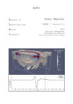
Figure 3.2 – Definition of wind bearing and x-axis.
22
GASTAR
Section 3: Entering Input
3.1.3 Wind direction
A real number defining the wind bearing measured clockwise from North in degrees. Note that
this uses the meteorological definition of wind bearing, namely the direction from which the wind
is coming (see Figure 3.2). The slope bearing and the jet release (azimuthal) angle are defined in
a similar way.
Minimum
0.0
deg.
Maximum
360.0
deg.
3.1.4 Roughness length
A real number giving the roughness length in metres. The roughness length is a length scale that
categorises the surface roughness by representing the eddy size at the surface. Some approximate
values for a variety of land types are given in Table 3.1. If you have defined slopes with their
own meteorological data, this is disabled and the caption (Slopes On) appears in the textbox. In
such circumstances, the cloud development is based on the conditions prevailing on the current
slope. For more details see Section 3.4.1.9 under Slopes.
Minimum
0.0001
m
Maximum
2.0
m
Land Type
Roughness Length (m)
Cities, Woodland
1.0
Parkland, Open Suburbia
0.5
Agricultural Areas (max)
0.3
Agricultural Areas (min)
0.2
Root Crops
0.1
Open Grassland
0.02
Short Grass
0.005
Sandy Desert
0.001
Table 3.1 – Typical roughness length values for a range of surfaces.
3.1.5 Air temperature
A real number giving the ambient air temperature in kelvin. Note that 0oC is approximately
273K. The air temperature also defines zero enthalpy.
Minimum
220.0
K
Maximum
330.0
K
3.1.6 Surface temperature
A real number giving the surface temperature in kelvin. If the Source Release Type is Isothermal,
this parameter is not required and the text box contains the caption (Isothermal) and cannot be
edited. In such cases the surface temperature is assumed to be the same as the air temperature.
23
GASTAR
Minimum
Maximum
Section 3: Entering Input
220.0
330.0
K
K
3.1.7 Atmospheric pressure
A real number giving the ambient air pressure in millibars. Note that 1 Atmosphere is
approximately 1013.24 mb.
Minimum
800.0
mb
Maximum
1200.0
mb
3.1.8 Relative humidity
A real number giving the relative humidity of the air as a percentage.
Minimum
0.0
%
Maximum
100.0
%
3.1.9 Atmospheric stability
Radio buttons that allow a mutually exclusive choice between entering the stability conditions in
terms of the Monin-Obukhov length (Lmo) or the Pasquill-Gifford stability category (PSC) (see
Section 8.2.2 for more on the relationship between the Monin-Obukhov length and PasquillGifford stability categories).
3.1.9.1
Monin-Obukhov length
This is a real number relating turbulence to the heat flux and friction velocity. It is measured in
metres and can be thought of as giving the relative importance of heat convection over
mechanical turbulence. Theoretically, it can take all values between "4, but in reality its modulus
is unlikely to fall below about 2.
Minimum modulus
2.0
metres
Maximum modulus
1000000.0
metres
3.1.9.2
Pasquill-Gifford stability category (PSC)
This is defined by a mutually exclusive choice of 7 buttons each representing a letter between A
and G inclusive. This is another method of indicating the relative importance of heat convection
and mechanical turbulence by dividing the meteorological conditions into fairly simple bands.
For instance, A means extremely unstable conditions and therefore strong convection with large
vertical dispersion. D represents neutral conditions, turbulence is purely mechanical, and G is
stable conditions where the mechanical turbulence is strongly damped by the stratification.
24
GASTAR
Section 3: Entering Input
3.2 Source details
The Source definition folder is shown in Figure 3.3. Below is a complete list of the input
parameters needed to define the source.
Figure 3.3 – The Source definition folder.
3.2.1 Source material
If the From Database radio button is selected, material is selected from the drop-down list box.
Click on this with the mouse (or type ALT-8 or ALT-9 at the keyboard) to make the list drop
down. All materials available in the database can then be scanned and selected. Notice that the
list will always be alphabetically sorted no matter what order the materials might appear in the
database. Typing a letter will automatically change the current entry to one whose first letter
matches the letter typed. The command button will allow you to View Data in table form. This
interface will not allow the addition, deletion or modification of materials in the database - the
database editor (see Section 6) is required in order to do this.
If the material is User Defined, the material name appears on a non-editable panel. In order to
create and/or change any of the properties of this substance from the values given in the database,
click on the button (now marked Edit User Data) to bring up the database and editable text boxes.
This option is not recommended.
3.2.2 Release type
There are two main choices for the release type, each represented by a mutually exclusive array
of choice buttons; the radio buttons to the left distinguish between Instantaneous, Continuous,
25
GASTAR
Section 3: Entering Input
Time-Varying and Jet releases described in the rest of this section, while the group buttons to the
right define whether the release is Isothermal (no temperature or phase changes), Thermal
(temperature changes allowed but single phase) or Aerosol (two-phase with temperature/phase
changes).
3.2.2.1
Instantaneous release
For instantaneous releases the initial volume, V0, is calculated using the mass released and
prevailing Meteorological and Source conditions. The initial puff diameter, D0, is specified. The
initial puff is assumed to be a right circular cylinder. The initial height of this cylinder is then
given by H0=V0/(¼ π D02).
The initial temperature T0 (for Thermal and Aerosol cases), initial aerosol fraction (for Aerosol
cases), initial concentration C0 and initial density ρ 0 are assumed to be uniform over the initial
volume.
For Instantaneous releases, check Momentum Initially Well Mixed to select whether the initial
conditions of the puff momentum are well mixed or not well mixed. The default is for the
momentum to be initially well mixed. This option is used to determine the initial conditions for
puff momentum mixing. Typically, instantaneous releases are a result of some catastrophic event
such as a tank rupture or explosion. In these cases it is easy to see that internally the puff will
have a well mixed momentum. For some situations this is not true, for example the Thorney
Island instantaneous heavy gas dispersion trials. Here the cloud was created inside a large tentlike construction that dropped to the ground to release the puff. The material effectively appeared
as a large stationary puff which slowly picked up speed as the wind advected it away. It would be
more appropriate to model this case assuming the momentum was not well mixed initially. The
effect of this is to make the cloud advection velocity start from zero and gradually grow. When
the Momentum Initially Well Mixed option is chosen, this reduction factor is not used and the
cloud advection velocity is non-zero from the start of the modelling process.
3.2.2.2
Continuous release
For continuous releases, either the physical source width or the actual plume width can be
specified (see below). The initial mass flux, M0, at the source is also specified. The initial plume
cross section is assumed to be rectangular. The model will calculate the source density, ρ 0, in the
same manner used by the Instantaneous release. The source height, H0, is found such that the
correct mass flux is obtained using M0 = H.W.Ua.ρ 0, where Ua is the (calculated) effective speed
for the cloud based on the current wind speed profile (see Section 8.2.1.3).
The initial temperature T0 (for Thermal and Aerosol cases), initial aerosol fraction (for Aerosol
cases), initial concentration C0 and initial density ρ 0 are assumed to be uniform over the initial
section.
For Continuous releases, you can check Internally Calculate Initial Plume Width if you wish
GASTAR to determine the initial conditions for continuous release calculations, ie the source
width and height are calculated internally. You must supply the source release rate and the
physical source width. The effective (ie the actual plume) width, height and density are calculated
from the source mass flux, temperature and prevailing Meteorological conditions. This option
produces a physically realistic plume aspect ratio.
If you do not choose to allow the model to calculate the initial plume dimensions, the value you
26
GASTAR
Section 3: Entering Input
enter for the Width is assumed to be the initial plume width and will be retained by the model for
the starting conditions, ie the user specified width is ALWAYS the effective source width. This
option is useful if you know the actual plume width (eg modelling experimental results) or you
wish to fix a certain width (eg you are using the results from another source model). It may also
be required if the geometry of the release prevents lateral spreading of the plume beyond the
physical source width.
3.2.2.3
Time-varying release
For time-varying releases the initial conditions are specified as a sequence of piece-wise constant
segments. The segments are specified by the time duration of each segment. The other details of
the source specification are similar to the continuous case.
For each segment of the time-varying release the physical source width, D0, and initial mass flux,
M0, are specified. The initial condition is assumed to be a rectangular section with an effective
source width W0, effective source height H0 and source density ρ 0.
The initial temperature T0 (for Thermal and Aerosol cases), initial aerosol fraction (for Aerosol
cases), initial concentration C0 and initial density ρ 0 are assumed to be uniform over the initial
section.
Figure 3.4 – Source parameters for three-dimensional Jet release.
The time-varying segments can also be calculated by the Pool Uptake Model. This considers the
evaporation from a (developing) pool and calculates the dimensions of the developing cloud
above the pool. For more details see Section 5 on the Pool Uptake Model.
27
GASTAR
Section 3: Entering Input
3.2.2.4
Gas and liquid jet release
For jet releases, either the physical source diameter or the pseudo jet diameter can be specified.
The initial mass flux, M0, at the source is also specified. The jet cross section is assumed to be
circular if airborne and semi-circular if the jet is grounded. The model will calculate the source
density, ρ 0. There is no height dimension for jets, but the jet does have a height, z, to the centre
of the circular cross-section.
The initial temperature T0 (for Thermal and Aerosol cases), initial aerosol fraction (for Aerosol
cases), initial concentration C0 and initial density ρ 0 are assumed to be uniform over the initial
section.
For Jet releases, there are options for the source to be elevated, and to be orientated in any (3-D)
direction (see Figure 3.4).
3.2.3 Source details
The exact requirements are dependent on the Release Type. Where there is a choice of release
types including Instantaneous releases, items in parentheses generally refer to the noninstantaneous case. There follows a brief explanation of all inputs.
3.2.3.1
Source location
The source location can be entered in one six formats that can be chosen by clicking Change…
on the Source folder and selecting a format from the drop down box labelled Source Location
Type, Figure 3.5. The formats are:
•
•
•
•
•
•
Latitude-longitude
UK grid 6 digits
UK grid 2x5 digits
UK grid 2x6 digits
Irish grid 2x3 digits
Irish grid 2x5 digits
The Source Location must be entered by the user in the correct format for the Source Location
Type selected. Advice on the format is given on the screen as shown in Figure 3.5.
Figure 3.5 – Parameters for defining the source location.
28
GASTAR
Section 3: Entering Input
The Source Location is not used by the GASTAR model code but is written to the .ggd file to
assist plotting and overlaying contours on a map.
3.2.3.2
Release start (UTC)
The Release Start time must be entered in UTC (hours and minutes) plus day of the month,
month and year. The Release Start is not used by the GASTAR model code but is written to the
.ggd file to assist plotting output as a time series.
3.2.3.3
Initial air entrainment (rate)
For Instantaneous and Continuous Releases only. Because of the nature of some releases,
particularly explosive instantaneous, it is desirable to allow an initial mixing with air for the
source term. It is unlikely in a real incident that the exact amount of air entrainment at the start
would be known, however you are required to give the mass (flux) of air entrained at the start.
The model assumes this to be at the air temperature and will use this together with the mass (flux)
and temperature of released material to recalculate an overall cloud temperature and density.
This is a real number giving the mass of the air entrained initially.
Minimum
Maximum
0.0
kg (/s)
10000000.0 kg (/s)
3.2.3.4
Source width
The real number giving the width of the source in metres.
• For Instantaneous releases: this is the initial diameter of the puff.
• For Continuous releases: this is the physical source width giving rise to the plume if the
Internally calculate initial plume width option is chosen, otherwise it is the initial width of
the plume.
• For Time-Varying releases: this is the actual width of the cloud.
• For Jet releases: this is the initial diameter of the jet for ambient pressure releases, or the
pseudo diameter if the release is under pressure, i.e. the diameter after expansion to
ambient pressure.
For Time-Varying Releases, this entry will refer to the current segment given in the Current
Segment Number box.
Minimum
Maximum
0.01 m
1000.0 m
3.2.3.5
Source mass (flux)
The real number giving the mass (flux) of material released. For Instantaneous releases, this is a
single total amount measured in kilograms. For Continuous, Time-Varying and Jet releases, this
is a mass flux for the source measured in kilograms per second. For instantaneous and
continuous releases this does not include entrained air (see 3.2.3.1).
For Time-Varying Releases, this entry will refer to the current segment given in the Current
Segment Number box.
29
GASTAR
Minimum
Maximum
Section 3: Entering Input
0.01
kg (/s)
1000000.0 kg (/s)
3.2.3.6
Hazardous fraction
This parameter gives the fraction of the release that is considered hazardous. For general use this
is the whole release: consequently this has a default value of 1. By changing this value you may
model the release of a dense gas (say CO2) in which a small amount of a contaminant (say H2S)
was present. In this case, the dynamics of the cloud will depend on the main dense gas (CO2), but
the important concentration levels will be those of the contaminant in the release. The
concentration of the contaminant will therefore be given directly in the model output.
For Time-Varying Releases, this entry will refer to the current segment given in the Current
Segment Number box.
Minimum
Maximum
0.000001
1.0
3.2.3.7
Source temperature
For Thermal and Aerosol Releases only. This is a real number giving the temperature of the
initial cloud of released gas and/or aerosol (after flashing but before any air entrainment). Some
care is needed to ensure all Source Details are consistent. For example, if there is a spill of
volatile material that is stored as a liquid under pressure at ambient temperature, you will need to
perform a "flashing" calculation (see Section 3.2.4) to determine the final temperature and
aerosol fraction. In such a case, the storage temperature might not be the initial cloud
temperature. It is the initial temperature of the released material that is required by the code.
For Time-Varying Releases, this entry will refer to the current segment given in the Current
Segment Number box.
Minimum
Maximum
10.0 K
2000.0 K
3.2.3.8
Source aerosol fraction
For Aerosol Releases only. This is a real number giving the fraction of the source material that is
in liquid state initially. This fraction can be found by using the Flash calculation (see Section
3.2.4).
For Time-Varying Releases, this entry will refer to the current segment given in the Current
Segment Number box.
Minimum
Maximum
0.0
99
3.2.3.9
Number of segments
For Time-Varying Releases only. This is an integer giving the number of distinct segments the
source term has been broken into in order to simulate the time-varying source. The details of each
segment may be displayed by changing the Current Segment Number in the panel below this one.
30
GASTAR
Minimum
Maximum
Section 3: Entering Input
1
20
3.2.3.10 Segment duration
For Time-Varying Releases only. This is a real number giving the time duration in seconds for
the currently selected segment of a Time-Varying release.
Minimum
Maximum
1.0
s
2000.0 s
Figure 3.6 – Definition of jet height and elevation (vertical section through the jet).
3.2.3.11 Height of jet source
For Jet Releases only. This is the height of the jet source above ground level (see hJ in Figure 3.4
and Figure 3.6).
Minimum
Maximum
0.0
m
100.0 m
3.2.3.12 Azimuthal angle for jet source
For Jet Releases only. This is the horizontal bearing of the jet at the source. This is measured in
the same manner as the wind bearing, clockwise from North in degrees and represents the
direction from which the jet is coming (see θJ in Figure 3.7).
Minimum
Maximum
0.0
deg.
360.0 deg.
31
GASTAR
Section 3: Entering Input
Figure 3.7 – Definition of jet bearing.
3.2.3.13 Elevation angle for jet source
For Jet Releases only. This is the elevation angle of the jet at the source. This is measured from
the horizontal and is positive if the jet is pointing upwards (see φJ Figure 3.4 and Figure 3.6).
Minimum
Maximum
-90.0 deg.
90.0 deg.
3.2.4 Flash calculation
When choosing an Aerosol release type on the Source folder, you will enable the Flash
calculation button to the right of the Aerosol Fraction textbox. This utility is useful when you
need to model the release of a material with a boiling point below ambient temperature stored in a
pressurised container at ambient temperature. When suddenly released these materials 'flash',
producing a cold, dense cloud containing some material in liquid phase.
The Flash calculation screen (see Figure 3.8) will use the material properties for the material
currently chosen in the main GASTAR interface. You will then need to supply the storage
temperature of the material, which is typically the ambient temperature, and the ambient pressure.
If the main interface has the Air Temperature and Pressure defined, these values are
automatically copied to the Flash calculation screen. You may then choose to use these values or
enter different ones before calculating the aerosol fraction and temperature of the released
material.
32
GASTAR
Section 3: Entering Input
The model uses two slightly different algorithms to do this, and both sets of results are given. The
reason for this is to give the most flexible approach for the modeller. The commonly used method
is labelled 'Normal method', and these are the results returned to the main GASTAR interface
from the Flash screen. The formula used for the normal method is
⎛
T storage − T BP ⎞
Aerosol Fraction = 1 − ⎜⎜ C pl
⎟⎟
H LG
⎝
⎠
(1)
and that for the exponential method is
⎛
T storage − T BP ⎞
Aerosol Fraction = exp ⎜⎜ − C pl
⎟⎟
H LG
⎝
⎠
(2)
where
Tstorage
TBP
HLG
Cpl
is the storage temperature of the liquid
is the boiling point of the released material
is the specific heat of vaporisation of the released material
is the specific heat capacity of the released liquid
Please note that if you change the Storage Conditions from the values copied from the main
interface, the changed values will not be copied back. You must update the Air Temperature and
Pressure on the Meteorology folder yourself. The reason for this is to allow you to operate the
Flash model as a tool or utility separately from the work you might be doing in the main
GASTAR interface.
Figure 3.8 – The Flash Calculation screen.
33
GASTAR
Section 3: Entering Input
3.3 Complex effects: obstacles
The Complex Effects folder (Figure 3.9) displays a summary of the current obstacle data in table
form. You cannot manipulate the obstacle data directly in the table, other than turn individual
obstacles on and off in the Obstacle table.
Complex effects are not available for Jet releases.
Figure 3.9 – The Complex Effects folder.
3.3.1 Obstacle summary
The frame for the Obstacles on the Complex Effects folder has a check box, the summary of
obstacles in table form and four buttons that control the editing of the obstacle data. A more
detailed description follows.
3.3.1.1
Consider obstacles check box
The check box for the obstacles allows you to disable all the current obstacle data without having
to delete it. This is useful when you wish to run comparisons with and without the obstacle data,
or because you have changed the wind direction and know that the obstacles are no longer
important. Switching off their effect for a run allows you to keep the data rather than deleting it
from the data file.
If the check box is not selected, the rest of the Obstacles frame will be disabled. You must check
this box before you can edit, add or delete any obstacle data.
34
GASTAR
Section 3: Entering Input
3.3.1.2
Table Summary
The table summarises the current obstacle data. There are three columns in the table.
The first column will respond to the mouse click. Try double clicking on an entry in the table and
you will see the word OFF appear and disappear. This allows you to turn off the effects of
obstacles on an individual basis.
The second and third columns give the name and the data summary for each obstacle you have
entered. The order in which they appear in the table is the order in which you entered the data.
There is no importance, inferred or otherwise, to their order in the table.
3.3.1.3
New, edit, copy and delete buttons
The four buttons to the side of the table allow you to edit the obstacle data.
New will bring up the Obstacle Definition form with the default values, as shown in Figure 3.10.
This is the form that allows you to define the obstacle data. The parameters are defined in more
detail below. If you cancel the form from this point, no new obstacle will be created.
Edit will bring up the Obstacle Definition form with the details of the obstacle currently selected
in the table. You can change any part of the data and save it again if you wish. If you cancel the
form from this point, none of the changes will be saved and the obstacle definition will be left
unchanged.
Copy will bring up the Obstacle Definition form with a copy of the details of the obstacle
currently selected in the table. The only change to the data will be the obstacle name, which will
say "copy of…". You can change any part of the data and save it again if you wish. If you
cancel the form from this point, no new copy of the obstacle will be created.
Delete will delete (ie completely remove) the definition data of the currently selected obstacle in
the table. There is no warning before the obstacle is removed. In general it is preferable to turn an
obstacle off (see Section 3.3.1.2) rather than delete it.
Figure 3.10 – The Obstacle Definition dialogue box.
3.3.2 Defining obstacles
The Obstacle definition form, shown in Figure 3.10, is where you define and edit the obstacle
35
GASTAR
Section 3: Entering Input
data. A more detailed description of each parameter follows. In Figures 3.11 – 3.13 the source is
located at the origin.
3.3.2.1
Obstacle types
Choose which type of obstacle you want to add from those in the drop-down list box. GASTAR
can model fences and circular or rectangular buildings. The definition parameters will change
according to the type of obstacle being added, so it is recommended that you select the obstacle
type first, before entering other data.
Figure 3.11 – Definition of a circular building.
Circular Buildings are defined by a height, the location of the centre point of the building and a
width (see Figure 3.11).
Rectangular Buildings are defined by a height, the location of the centre point of the building, a
width and depth and the orientation of the building (see Figure 3.12).
Fences are defined by a height, the location of a point along the fence and the orientation of the
fence (see Figure 3.13).
3.3.2.2
Obstacle name
Give the obstacle a name to help you identify it in the table and later on in the output files. The
model will tell you if the cloud passed over and interacted with the obstacle or not, so a
descriptive name is recommended.
36
GASTAR
Section 3: Entering Input
3.3.2.3
Obstacle width
This obstacle dimension is only required for buildings. With a circular building, it is the diameter
in metres. For rectangular buildings it can be either of the horizontal dimensions of the obstacles see the definition of the obstacle orientation (Section 3.3.2.6), which is linked to this parameter.
Minimum
Maximum
1.0
1000.0
m
m
Figure 3.12 – Definition of a rectangular building.
3.3.2.4
Obstacle depth
This obstacle dimension is only required for rectangular buildings (see Figure 3.12). It represents
the other horizontal dimension of the building to that given above as the obstacle width. Please
read the definition of the obstacle width and orientation for more explanation.
Minimum
Maximum
1.0
1000.0
m
m
3.3.2.5
Obstacle height
This is the obstacle height. All types of obstacle require their height in metres to be entered.
Minimum
Maximum
1
50.0
m
m
3.3.2.6
Obstacle orientation
Fences and rectangular buildings must have their orientation with respect to North defined so that
the model can calculate the interaction effects. Circular buildings, by definition, cannot have an
37
GASTAR
Section 3: Entering Input
orientation.
For rectangular buildings (Figure 3.12), the relevant angle is the bearing of the side defined as the
building width above measured in degrees clockwise from North. The angle chosen is the
smallest positive value and consequently will be less than 180 degrees.
For fences (Figure 3.13), the orientation is the bearing of the fence measured clockwise from
North. As with rectangular buildings, this orientation takes the general form (θ + n.180), where n
is an integer. The angle used is the smallest positive angle. It is also important to remember that
the model considers fences to be infinitely long, so any error on your definition of the fence
orientation will become magnified as you move away from the point on the fence defining its
position (see obstacle distance and bearing).
Minimum
Maximum
0.0
180.0
deg.
deg.
Figure 3.13 – Definition of a fence.
3.3.2.7
Obstacle distance
This parameter, together with the obstacle bearing, will position the obstacle relative to the
source.
For buildings, this is the distance, measured along the ground in metres, from the source to the
centre of the building.
For fences, this is the distance to any point along the fence. However, this parameter is linked
with the obstacle bearing, so you will need to know the bearing of this line defining the distance.
Depending where you are obtaining the obstacle data, you may consider a number of strategies to
38
GASTAR
Section 3: Entering Input
reduce the effect of any errors in your measurement data.
One way would be to measure the distance to the fence along a well defined direction, such as
North, South, East or West, thereby removing the error in the obstacle bearing. Another might be
to find the nearest point along the fence to the source, so that the fence orientation and bearing
are 90 degrees different.
For cases where the orientation of the fence is quite oblique to the cloud trajectory, you may wish
to define the point along the fence that lies in the path of the trajectory. In this case you may have
to run the model without considering the fence, ie turn if off by double clicking in the first
column of the summary table or unchecking the Consider this obstacle box on the obstacle
definition form. Having discovered the trajectory of the cloud, you will know approximately
where it will interact with the fence and can define a point near to that in the obstacle distance
and bearing parameters.
Minimum
Maximum
1.0
5000.0
m
m
3.3.2.8
Obstacle bearing
The obstacle bearing, together with the obstacle distance, will position the obstacle relative to the
source.
For buildings, this is the bearing, measured clockwise from North in degrees, of the imaginary
line drawn from the source to the centre of the building.
For fences, this is the bearing, measured clockwise from North in degrees, of the imaginary line
drawn from the source to a point along the fence whose length is the obstacle distance defined
above.
Note that this parameter is linked with the obstacle distance defined above. Please read the
definition of obstacle distance and obstacle orientation for more details.
Minimum
Maximum
0.0
360.0
deg.
deg.
3.3.2.9
Obstacle solidity
The solidity allows the effect of the obstacle to be faded in or out. It represents the ratio of the
surface area blocked to the complete surface area for the obstacle projected into the wind. As a
general rule, buildings are not porous and have a solidity of 1. The parameter is usually only
applied to fences which are often not solid. For example, if the fence is a picket type where the
slats are the same width as the gaps between them, an appropriate solidity factor would be 0.5.
Minimum 0
Maximum 1
3.4 Complex effects: slopes
The Complex Effects folder (Figure 3.9) displays a summary of the current slope data in table
39
GASTAR
Section 3: Entering Input
form. You cannot manipulate the slope data directly in the table.
Complex effects are not available for Jet releases.
3.4.1 Slopes summary
The frame for the Slopes on the Complex Effects folder is similar to that for the Obstacles in that
it has a check box, the summary in table form and four buttons that control the editing of the
slope data. It also has a further check box for Meteorological data and a textbox for the bearing of
the slope vector. A more detailed description follows.
3.4.1.1
Consider slopes check box
The check box for the Slopes allows you to disable all the current slope data without having to
delete it. This is useful when you wish to run comparisons with and without the slope data.
Switching off the effect of slopes for a run allows you to keep the data rather than deleting it from
the data file.
If the check box is not selected, the rest of the Slopes frame will be disabled. You must check this
box before you can edit, add or delete any slope data.
3.4.1.2
Table Summary
The table summarises the current slope data. There are two columns in the table.
The first column gives the range of each of the slope segments measured in metres relative to the
source location. The second column gives the data summary for each slope segment you have
entered.
The slope segments are assumed to abut one another without gaps. Unlike the obstacle summary,
the segments in the slope summary are logically ordered. If you modify a slope distance, the
summary table is rebuilt to account for changes in the order.
3.4.1.3
Use Met Screen data for all slopes check box
Each slope segment has an associated set of data not just for the slope parameters, but also for the
ground roughness length, wind speed and height of the wind speed measurement for the segment.
These data parameters are duplicated on the Meteorological Folder. This check box will tell the
model which set of Meteorological data is to be used.
If you have slopes turned on and choose not to use the Meteorological Screen data, you will need
to enter Met data for each slope segment and these data will be displayed in the table summary.
Also, on the Meteorology Folder, the textboxes for roughness length, wind speed and height will
display the text (Slopes On) and will not be editable.
If you wish to use the Meteorology Screen data for all slope segments, you should check this box.
You will notice that when you check the box, the summary table automatically updates to reflect
the change by no longer displaying any meteorology data.
Turning the Use Met Screen data for all slopes check box on and off will return the table to its
original appearance. This is because no data is lost when you check the box. Any meteorological
40
GASTAR
Section 3: Entering Input
data you enter with the slope segments is retained, but will appear greyed out in the Slope
Definition form, meaning that it is not going to be used by the model. Unchecking the box again
will reinstate the data, allowing you to edit it.
3.4.1.4
Bearing of slope vector
This defines the bearing, measured clockwise from North in degrees, of the line of maximum
slope for the slope segments (see θS in Figure 3.14).
The slope module allows simple slopes to be modelled. Such slopes can be visualised as
resembling an infinite sheet of card, folded along parallel lines. The folds are the boundaries
between the rectilinear plane slope segments. With the exception of the first and last segment, the
segments have a finite length, and all segments extend laterally to infinity.
The slope segments are simple flat planes like a concertinaed sheet of card. The lines of
maximum slope for each slope segment are parallel and this direction defines the slope vector.
However, the bearing of the slope vector need not be aligned with the wind direction. The model
allows the orientation of the slopes and wind to differ, giving rise to cross wind slopes.
The bearing is measured in the same manner as the wind. This means it is the angle, measured
clockwise from North, of the direction from which the first slope is defined (theoretically at -4).
For example, if you have the same value for the slope and wind bearing, they will be aligned such
that moving along the slope vector in the negative direction is upwind, and in the positive
direction is downwind.
This form of definition allows you to separate the slope angle and the wind direction, because the
slope angle is measured relative to the slope vector and is the incline seen by someone moving in
the positive direction along the slope vector. You can reverse the wind direction simply by
adding 180o to the wind bearing and the ground will not be altered, ie the effective reversal of the
slopes seen by the cloud will be accounted for by the slope vector.
Minimum
Maximum
0.0
360.0
deg.
deg.
3.4.1.5
New, edit, split and delete buttons
The four buttons to the side of the table allow you to edit the slope data. Note that under certain
circumstances, part or parts of this data will be greyed out and not be editable. See under the
individual parameter entries below for more details. The Slope Definition form is shown in
Figure 3.16.
New will bring up the Slope Definition form with the default values, as shown in Figure 3.16.
This is the form that allows you to define the slope data. The parameters are defined in more
detail below. If you cancel the form from this point, no new slope will be created.
41
GASTAR
Section 3: Entering Input
Figure 3.14 – Definition of slope bearing.
Edit will bring up the Slope Definition form with the details of the slope currently selected in the
table. You can change any part of the data and save it again if you wish. If you cancel the form
from this point, none of the changes will be saved and the slope definition will be left unchanged.
Figure 3.15 – The Split Slope dialogue box.
Split will firstly bring up the Split Slope dialogue (Figure 3.15), asking you to choose the point at
which you wish to split the current slope. The current slope range is provided, and you will have
to choose a number within this limit. If you cancel this form, the slope will not be split.
Having entered a valid number and clicked OK, the Slope Definition form will be displayed with
your new split distance value already entered but greyed out. This is because it cannot be changed
again when splitting a slope into two slopes, although it can be re-edited once the second slope
42
GASTAR
Section 3: Entering Input
has been accepted. The other data on the Slope Definition form will be copied from the original
single slope, any of which you may edit. If you cancel this form, the slope will not be split.
Delete will delete (ie completely remove) the definition data of the currently selected slope in the
table. The region of the deleted slope is absorbed into the slope definition of the preceding slope.
This is because there can be no gaps in the definition of slopes. There is no warning before the
slope is removed.
Figure 3.16 – The Slope Definition dialogue box.
3.4.1.6
Defining slopes
The Slope Definition form, shown in Figure 3.16, is where you define and edit the slope data. A
more detailed description of each parameter follows.
Figure 3.17 – Vertical section through the sloping ground parallel to the slope vector.
43
GASTAR
Section 3: Entering Input
3.4.1.7
Slope distance
This is the distance, measured in metres from the source, along the slope vector to the start of the
slope segment in question (see Figure 3.17). Remember that the slope vector is directional and
therefore these distances can be positive or negative.
The first slope will start at -4 (the model actually uses a large negative number) and this value
cannot be changed. If you edit the first slope, the Distance on the Slope Definition form will be
greyed out and will not be editable.
The only other time you will not be able to edit the distance will be when splitting a slope into
two. Having chosen the distance in the Split Slope dialogue, you will not be able to edit it again
until the slope has been accepted into the summary table.
The slope finish will be the start of the next slope. If this is the last slope, the slope will extend to
+4 (the model actually uses a large positive number).
Minimum
Maximum
-1.0E99
+1.0E99
m
m
3.4.1.8
Slope angle
This is the angle of dip or elevation of the current slope segment measured in degrees from the
horizontal as you move along the positive direction of the slope vector (see Figure 3.17). An
upward slope will have a positive slope angle, and a downward slope will have a negative slope
angle.
Minimum
Maximum
-45.0
+45.0
deg.
deg.
3.4.1.9
Slope ground roughness length
This is the roughness length for the current slope section and has the same definition as the
roughness length defined in Section 3.1.4. The ground roughness length used in the model will
depend on the Use Meteorology Screen Data check box. If this box is checked, then the model
will use the information given on the Meteorology Screen and this parameter will appear greyed
out when you edit the data on the Slope Definition form. If the box is unchecked, the model will
use the data for the appropriate slope segment and this data will be editable in the Slope
Definition form.
Minimum
Maximum
0.0001
2.0
m
m
3.4.1.10 Slope wind speed
This is the wind speed over the current slope section and has the same definition as the wind
speed defined in Section 3.1.1. The wind speed used in the model will depend on the Use
Meteorology Screen Data check box. If this box is checked, then the model will use the
information given on the Meteorology Screen and this parameter will appear greyed out when
you edit the data on the Slope Definition form. If the box is unchecked, the model will use the
data for the appropriate slope segment and this data will be editable in the Slope Definition form.
44
GASTAR
Minimum
Maximum
Section 3: Entering Input
0.1
20.0
m
m
3.4.1.11 Slope wind speed height
This is the height of the wind speed measurement for the current slope section and has the same
definition as the wind speed height defined in Section 3.1.2. The wind speed height used in the
model will depend on the Use Meteorology Screen Data check box. If this box is checked, then
the model will use the information given on the Meteorology Screen and this parameter will
appear greyed out when you edit the data on the Slope Definition form. If the box is unchecked,
the model will use the data for the appropriate slope segment and this data will be editable in the
Slope Definition form.
Minimum
Maximum
0.1
15.0
m
m
45
GASTAR
Section 3: Entering Input
3.5 Output details
The Output folder, shown in Figure 3.18, is where you specify options for the output produced by
the model run. As discussed in Sections 4.4 and 4.5, the main numerical output from the model is
written to an output (.gof) file, containing a core of output giving the solution calculated by the
model at a set of times distributed through the simulated period, but it may also contain various
auxiliary information derived from these basic solution data. The Output folder is where the user
specifies which (if any) of these auxiliary data are included in the output, as well as overall
parameters for the simulation, such as its title and the length of time modelled in the run.
Figure 3.18 – The Output folder.
3.5.1 Title
This is a string up to 80 characters in length. You might use this to name the run and give some
descriptive details to help identify the run. It will be used as a title in the tabulated output file
(.gof).
3.5.2 Modelled time
This is a real number giving the time in seconds to which the code will model the cloud
dispersion. It is important to consider an appropriate time interval, particularly if special output,
such as Dose or Range information, is also being requested. Having an unnecessarily large value
will make output points more sparse and reduce the accuracy of interpolated data values used.
Minimum
Maximum
1.0
100000.0
s
s
46
GASTAR
Section 3: Entering Input
3.5.3 Averaging time
For Continuous and Time-Varying Releases only. The averaging time is used to calculate
diffusion and dispersion of the cloud.
For Instantaneous Releases, this is disabled and the caption (puff) appears in the text box. The
model sets the averaging time internally to 20 seconds (the puff dispersion averaging time).
NOTE: The averaging time cannot be set to less than the value for puff dispersion (Tavg = 20s) in
this version of the code. This reflects the observation that when Tavg ≈ 20s plume width
correlations revert to puff width correlations: the plume can never be narrower than the puff. If a
value less than 20s is entered at the interface, the program will set the averaging time to the puff
dispersion averaging time.
Minimum
Maximum
1.0
3600.0
s
s
3.5.4 Specified Output Points
For Instantaneous, Continuous and Time-Varying releases only. The Specified Output Points are
specified as a list of up to 1024 points in (x, y, z) for which additional output can be requested:
the current version provides the Dose, Toxic Load and Concentration Time History at each point,
if requested.
On clicking the Edit button on the Output folder, the Define Specified Output Points dialogue box
shown in Figure 3.19 is displayed. Enter values for the x-, y- and z-coordinates of a point in the
horizontal set of three text boxes and then click on Add or press the Space bar to add the point to
the list, which is displayed in the large text box underneath. To remove a point from the list,
highlight it and click on Delete. The list of points is sorted numerically by x then y then z as they
are added. No points may be repeated.
Minimum (x, y)
(z)
Maximum (x, y, z)
-10000.0
0
10000.0
m
m
m
47
GASTAR
Section 3: Entering Input
Figure 3.19 – The Define Specified Output Points dialogue box.
The three Fix… check boxes can be used to fix temporarily the value in one of the three entry
boxes. It is then much quicker to enter a large number of points that only vary in, say, one
dimension by first fixing the dimensions that do not vary and then entering the value in the
dimension that changes, using the space bar to enter the data into the list. The entry will be added
and a new value can immediately be typed into the textbox. It is therefore very quick to
repeatedly type a new number followed by a space to enter a long list of points.
Note that the numerical method that integrates the model equations in time adjusts the timestep so
that the x-coordinate of the cloud hits that of each specified point, which means that both the core
output, for the cloud as a whole, as well as the additional output appears in the .gof file at these
points (provided the modelled time is large enough to permit the cloud to have travelled that far).
3.5.5 Specified Output Times
For Instantaneous, Continuous and Time-Varying releases only. The Specified Output Times are
quite similar to the Specified Output Points described above, in that they are input as a list of
times at which the model produces output: both the core output for the cloud as a whole and the
Flammables output is calculated at these times. Up to 50 different times may be specified, which
is achieved by entering the time in the text box and either clicking on the Add button or pressing
the Space bar; any specified time may be deleted by highlighting it in the list and clicking on
Delete.
Minimum
Maximum
0.1
100000.0
s
s
3.5.6 Additional output
After the GASTAR run has time-stepped from t = 0 to the modelled time, the model carries out
48
GASTAR
Section 3: Entering Input
post-processing of the resulting data to give additional information on the cloud. You must
request such additional output before the run, and the Additional Output part of the Output folder
is where you do this. The different types of additional output are separated onto three tabbed
folders, each of which is described below. In each case the output produced is added to the end of
the .gof file after the main tabulated output. Further information on the output produced is given
in Section 4.5.
3.5.6.1
Dose folder
This output is available for Instantaneous, Continuous and Time-Varying releases only. It
consists of the dose D(x) and/or the concentration as a function of time, c(t; x), at each of the
Specified Output Points x, where D is defined by
D ( x ) = ∫ c(t; x ) dt .
T
For Instantaneous and Time-varying releases, the period of integration T corresponds to the entire
modelling time. The concept of dose is extended to include Continuous releases, even though by
definition the concentration is constant in time and so the dose is simply proportional to the
integration time; hence T is user-specified for Continuous releases (see below).
Whenever the dose is calculated so is the toxic load, Γ(x), where
Γ( x ) = ∫ {c(t; x )} dt ,
n
T
and n ≥ 1 is the toxic exponent for the release substance.
This folder contains the following controls and input parameters.
•
•
•
Check the Calculate Dose check box if you want to calculate the dose and toxic load at
each of the Specified Output Points.
If the release is Continuous, you must also specify a value for the Dose Integration Period
(minimum value 1s, maximum value 105s).
Check the Calculate concentration-time history check box to obtain the concentration at
the set of output times at each of the Specified Output Points.
3.5.6.2
Flammables folder
This output is available for Instantaneous, Continuous and Time-Varying releases only. It
consists of information on the flammable part of the cloud for releases of flammable materials,
specifically the following properties of the cloud for both the LFL and half-LFL contours:
∗ downwind and crosswind radius and range (cloud downwind distance plus downwind
radius) of the contour
∗ volume enclosed within the contour
∗ mass of flammable material enclosed within the contour
This information is recorded at each of the specified output times for Instantaneous releases and
once only for Continuous releases.
•
Check the Calculate flammable output parameters check box to obtain the above output
49
GASTAR
Section 3: Entering Input
for releases of flammable materials.
3.5.6.3
Range folder
This output is available for Instantaneous releases only. It calculates the maximum range over all
modelled time to a given concentration level. The output consists of the maximum range found,
together with the time and the point(s) at which the maximum occurred.
•
•
Check the Calculate maximum range output check box to obtain the above output.
Enter the value for the concentration whose maximum range is to be found in the
Concentration text box expressed in the current concentration units (mol/mol or ppm).
Minimum
Maximum
0.00000001
0.99999
mol/mol
mol/mol
3.5.6.4
Gridded folder
This output is available for Instantaneous and Continuous releases only. If the user checks
the Calculate Gridded Output tick box a .ggd output file is created containing output that can
be used by other software for plotting contours. A more detailed description of the .ggd file
can be found in Section 4.6.
Figure 3.20 – Calculate Gridded Output in the Gridded folder.
In the Gridded folder the user enters the minimum and maximum X and Y co-ordinates for
the gridded output, the height above ground level at which the output will be calculated and
the number of grid lines in the X and Y directions i.e. the fineness of the results grid.
50
GASTAR
Section 3: Entering Input
Note that X is the alongwind distance from the source, and Y is the crosswind distance.
Minimum (x, y)
(z)
(Number of lines)
Maximum (x, y, z)
(Number of lines)
-10000.0
0
1
10000.0
101
m
m
m
IMPORTANT NOTE
The calculation of many of the additional output items utilises some function of either space or
time: for example, the dose is found by integrating the concentration at a point with respect to
time; or the flammable mass in a plume is found by integrating the concentration field over the
(fixed) region within the LFL contour; or the maximum range is found by looking at the cloud
concentration as a whole as a function of time. These calculations therefore rely on the cloud
properties being adequately resolved in space or time.
The integration scheme used in GASTAR has been optimised for short run times, so that the time
step tends to be significantly larger at the end of the simulation than at the beginning. The output
is stored at the end of each timestep used, which means that the resolution of cloud properties is
typically relatively coarse at the end of the simulation compared with the start.
There are facilities to increase the resolution, in the form of the Specified Output Points (SOP’s)
and Specified Output Times (SOT’s), which, if specified, augment the times at which the output
is stored because they force the time steps to be adjusted so that the cloud position coincides with
the given x-coordinate(s) and/or time(s).
Thus if your simulation calculates any additional output, it is helpful to bear the above points in
mind and, if necessary, add some Specified Output Points and/or Times on the Output folder in
order to improve the accuracy of the post-processing. In general
•
dose/toxic load/concentration time history – add further SOP’s near the points of interest or
SOT’s around the time that the cloud arrives at the given point
•
flammables output – for continuous releases, add more SOP’s over the flammable region (or
SOT’s corresponding to passage over this region)
•
range output – add SOT’s in general around the time that the cloud maximum concentration
falls below the concentration of interest
51
4
Viewing and Plotting Output
The Graphical Display folder is shown in Figure 4.1.
Figure 4.1 – The Graphics folder (showing the X-Y Line Plotting option).
The Graphics folder allows you to select the variable(s) you wish to plot, which output file(s) to
take the data from and the type of plot.
52
GASTAR
Section 4: Viewing Output
4.1 Selecting data to plot
4.1.1 Selecting data files for plotting
This involves selecting one or more graphical data (.gph) files using the File Details controls. Use
the Drive list box at the top to select the drive from which you wish to plot data. This conforms to
the Windows standard and will show any drive that is currently mapped by your system – make
sure that the drive you want to use has actually been mapped (e.g. using "Map Network Drive"
under Tools in Explorer) so that it will appear in this list box. You then use the Directory list box
in the middle to navigate to the correct directory on the drive. Once there, all the available output
data files in that directory will appear in the File list box at the bottom.
Click on the data file you wish to plot in the File list box. If you wish to plot from multiple files
do so in the normal Windows way by holding down the SHIFT key and clicking on the final data
file you want to plot. To select multiple isolated files from the list, hold down the CONTROL key
and click on those files you want to plot. When you have selected one or more GASTAR data
files the Plot Graph button will become enabled, signifying that data are available to plot.
If you have just run the model in the directory currently displayed but the new data file has not
appeared, try clicking with the right mouse button in the file list box. This will request it to
update and display the current contents of the directory.
4.1.2 Selecting the graph type
There are two types of graph available, namely x-y line plotting and flammables graphical output,
and which one you choose determines the form of the rest of the display on this folder.
(a) X-Y Line Plotting – in the majority of cases, you will want to use the x-y line plotting facility,
as this allows you to plot any of the core output data, so ensure the X-Y Line Plotting radio
button is “on”. This causes the central panel of the folder to display the variables that may be
plotted against each other (see Figure 4.1 and also Section 4.1.3).
(b) Flammables – it is not in general possible to view graphically the optional output, such as
dose, concentration time history, etc., but one exception is the flammable release output (see
Table 4.2). If you wish to plot this output, click on the Flammables radio button (see
Figure 4.2 and also Section 4.1.4).
4.1.3 X-Y plotting
The x-y Plotting Details part of the Graphics folder allows you to select which combination of
output variables are plotted.
4.1.3.1
Selecting the variable for plotting
Once you have selected one or more graphical data files, you should choose which variable(s)
you want to plot, i.e. the dependent variables. To select which variables to plot, click on the
appropriate check boxes. A checked box means plot the variable, an unchecked box means ignore
the variable, and you may choose to plot more than one variable at the same time.
The output available for plotting will vary depending on the type of run made. Therefore the
number of option buttons and check boxes in the list will change depending on the run type of the
53
GASTAR
Section 4: Viewing Output
graphical data file selected. If you have chosen to plot an output variable for a selection of files,
you will be warned if any files chosen do not contain the variable.
4.1.3.2
Selecting the independent axis
As well as the dependent variable(s), you must specify the independent variable, e.g. time,
distance, etc. The default choice for the independent variable is Arc Length, but to change this
simply click on the radio button corresponding to the variable you wish to use for the
independent axis. Note that changes do not occur immediately: it is necessary for you to click on
the Plot Graph button, which then updates the graphical display.
4.1.4 Flammables plotting
This option is only available for releases of flammable materials, i.e. for which there is a nonzero value for the LFL (lower flammability limit) concentration in the material properties. When
the Flammables radio button is “on”, the Graphics screen is as shown in Figure 4.2.
A series of check boxes is displayed, one for each variable that may be plotted. Check the box for
each variable you wish to plot. Above the check boxes is a list box containing the concentrations
that may be plotted, i.e. the LFL and half-LFL concentrations: highlight one or both of these to
select them for plotting.
Figure 4.2 – The Graphics folder showing the Flammables plotting option.
54
GASTAR
Section 4: Viewing Output
4.2 Plotting and viewing data
Whichever type of plotting you have selected, once you have chosen the variables and data sets
you wish to plot, click on the Plot Graph button to update the graphical display. If you have not
chosen any variables to plot, there appears a warning message box (Figure 4.3). For X-Y plotting,
this means checking at least one of the output variable check boxes, while for Flammables
plotting this means in addition selecting at least one concentration.
Figure 4.3 – Warning message when no variables selected for plotting.
Note that the graphical display does not update immediately, it is necessary for you to click on
the Plot Graph button, which then updates the plot. If you just want to bring the graphical display
to the foreground without re-plotting any data, use the Show Graph button. This will restore the
graphical display window without the update.
4.3 Graph display features
A typical example of a graph produced by the procedure in Sections 4.1 and 4.2 is shown in
Figure 4.4. In the rest of this section we describe other aspects of the display.
4.3.1 Viewing the data values on a graph
When you plot a graph in the graphical display, the actual data values are available in a number
of ways. The panels on the left below the graph give the actual values plotted on the independent
(x) and dependent (y) axes. The set and point being displayed can be changed using the spin
buttons.
The graph control can also respond to clicks from the mouse. If you position your cursor over a
point and click the left mouse button, the corresponding data value will be displayed in these
panels. Alternatively, if the graph is displaying a linear-linear plot (i.e. not using logarithmic
axes) then as you move the cursor over the graph, the panels below the graph to the right will
display the current cursor location. To obtain an indication of the value of any plotted point, hold
the cursor over the point and read the values given in these Current X and Current Y panels.
Finally, the complete data sets are available for viewing from the Data folder in the Graph
Design dialogue box, which is accessed via the Graph Setup button.
4.3.2 Zooming in on a graph
When displaying a linear-linear plot, you may use the mouse to select and zoom into a region of
the graph. To do this, move the cursor to one corner of the desired region, use the right mouse
55
GASTAR
Section 4: Viewing Output
button to click and drag a region in the graph. Releasing the right mouse button at some other
point over the graph will allow the region selected to fill the display.
If the region you select is too small, the graph will ignore the selection, assuming you have
accidentally clicked the right mouse button over the graph.
To reset the axes, click the Reset Axes button which appears to the right of the Current X panel
once you have made a zoom on the current graph.
Figure 4.4 – Example graph.
4.3.3 Configuring the graph
The graph is configurable in many ways. There is the ability to change much of a graph’s
appearance, including options that are not necessarily applicable to GASTAR output, by clicking
on the Graph Setup button (also see Preferences in Section 2.6).
The graphical display comes with its own on-line help file, which can be accessed via the Graph
Design form which itself is accessed via the Graph Setup button.
There is no attempt here to describe the configuration options available for the graphing display:
please refer to the online help, accessed using the Help button on the Graph Design form.
56
GASTAR
Section 4: Viewing Output
4.4 Output parameters
As noted in Section 7, the main formatted output file is the .gof file produced for each problem.
This contains the model set up parameters entered in the GASTAR interface and saved in the .gpl
file, followed by the values of the main integration variables at each integration step, together
with some other derived variables. The meaning of each output parameter is given in Table 4.1.
Notes on Table 4.1
(a) most of the parameters in the .gof file are obtained directly from the integration routines,
i.e. they are the values of the box model variables (see Section 8), or they are derived
directly from these variables. Those which are not are marked with an asterisk*
(b) in general, a parameter refers to the flux at a given cross-section when the release is
continuous or time-varying (or a jet), but refers to the whole cloud for puff releases
(c) for puff releases, the time corresponding to a given parameter value is the actual elapsed
time since the release was made; for all other types of release it refers to the time taken
for material to be advected to the given point along the plume/cloud/jet
4.5 Other data appearing in the output file
Besides the core tabulated output discussed in the previous section, the .gof file may contain the
results of the post-processing carried out according to the specification given in the Additional
Output part of the Output folder (see Section 3.5.6). The output for each additional output option
is summarised in Table 4.2. Note that the output appears in the file in the same order as its order
of appearance in the table. Note also that no additional output is available for jet releases.
4.6 Output for plotting contours
The .ggd file contains data that can be used by other software to plot contours. It is only
available for ‘Continuous’ and ‘Instantaneous’ release types and if the user has ticked Calculate
Gridded Output in the Gridded folder of the Output screen.
Figure 4.5 shows the file format. A full description is given following Figure 4.5. Figure 4.6
shows an example of a .ggd file. Note that in the GASTAR output X is the alongwind distance
from the source, and Y is the crosswind distance.
57
GASTAR
Section 4: Viewing Output
Parameter Units
S
m
X
m
Y
m
Z
m
C
Cmax*
mol/mol
mol/mol
MF
W
H
V (flux)
U
M (flux)
E (flux)
m
m
m3 or m3/s
m/s
kg or kg/s
kJ or kJ/s
T
Rho
AF
Ri
K
kg/m3
-
Xle
m
Xte
m
Wtot*
m
Wdisp*
m
Area
m2
Description
arc length, i.e. distance along cloud centreline trajectory. Usually
the same as downwind position X (see below)
downwind position of point on cloud centreline (plume/jet);
downwind position of cloud centre (puff) at given time
crosswind position of point on cloud centreline (plume/jet);
crosswind position of cloud centre (puff) at given time
vertical position of jet centreline at (X,Y); zero for grounded jets
and all other release types
concentration
maximum concentration value in a cross-section when
concentration profiles have been applied
mass fraction, i.e. as concentration C but based on mass
cloud diameter for puff releases, otherwise cloud width
cloud height
volume for puffs, volume flux for all other release types
cloud advection speed
total mass for puffs, mass flux for all other release types
total enthalpy for puffs, enthalpy flux for all other release types.
Ambient conditions define zero level.
cloud temperature
cloud density
aerosol fraction – mass of liquid as a fraction of total cloud mass
Richardson number based on friction velocity, cloud density and
height
puff releases only – leading edge position relative to source
based on diameter W
puff releases only – trailing edge position relative to source
based on diameter W
lateral width of cloud taking into account turbulent spreading
(σy). Mainly important for passive clouds.
puff releases only - width in downwind direction taking into
account turbulent spreading (σx) and shear dispersion (σs).
Mainly important for passive clouds.
puff releases only - area of cloud based on diameter W
Table 4.1 – Output parameters found in .gof files.
58
GASTAR
Dose
calculation
Section 4: Viewing Output
Release
types
C, I, T
Frequency
of output
For each
Specified
Output Point
Information output
•
•
•
•
•
Concentration
time history
C, I, T
For each
Specified
Output Point
•
•
Flammable
release output
C, I
Once per
simulation
(C) or for
each
Specified
Output Time
(I)
•
•
•
Once per
simulation
•
Maximum
range
calculation
I
•
•
•
•
Point number
x-, y- and z-coordinates of point
Dose in (mol/mol).min or ppm.min
Toxic load in (mol/mol)n.min or (ppm)n.min,
where n is the toxic exponent
Information on status of point relative to cloud
that might affect the value calculated, e.g. point
still within cloud at end of simulation.
x-, y- and z-coordinates of point
Tabulated output in three columns giving time
and the concentration (in current concentration
units) and (for I) cloud centre coordinates at that
time
Time (I)
x-, y- and z-coordinates of cloud center (I)
for both the LFL and half-LFL concentrations
∗ range in m, i.e. downwind distance of cloud
centre plus downwind radius of contour
∗ crosswind radius of contour in m
∗ downwind radius of contour in m
∗ maximum height at which concentration
occurs in m
∗ volume within the contour in m3
∗ mass of flammable release material contained
within the contour in kg
maximum range, i.e. the maximum distance over
all simulated time between the origin and any
point on the contour of the given concentration
time at which maximum range occurs
x- and y-coordinates of the point(s) at which the
maximum range occurs
flag indicating that the maximum range found
may be an underestimate since the concentration
contour of interest still existed (maximum
concentration ≥ concentration of interest) at the
end of the simulation
flag indicating that there was an obstacle
interaction around the same time that the given
concentration contour disappeared
Table 4.2 – Summary of additional output information. Each set of data may be requested
separately in the GASTAR interface (Additional Output folders on the main Output folder),
and appears at the end of the .gof file in the order indicated above. The abbreviations used in
the Release Types column are C = continuous, I = instantaneous, T = time-varying.
59
GASTAR
Section 4: Viewing Output
GASTAR gridded data output file
FILE_VERSION=(real)
FILE_STEM=(string)
PATH=(string)
WIND_DIRECTION=(real)
COORD_SYSTEM=(string)
SOURCE_LOCATION=(string)
RELEASE_DATE_AND_TIME=(string)
TIME_ZONE=(string)
POLLUTANT_NAME=(string)
CONCENTRATION_UNITS=(string)
AVERAGING_TIME_SECONDS=(real)
END_OF_HEADER_SECTION
integer NX
integer NY
integer NZ
integer NT
real T_1
real T_2
.
.
.
real T_NT
“Year”,”Day”,”Hour”,”Time(s)”,”X(m)”,”Y(m)”,”Z(m)”,
“Conc|(units)|(pollutant name)|(blank)|(blank)|(averaging time)”
integer Year, integer Day, integer Hour, real T, real X, real Y, real Z,
real Concentration
(etc)
Figure 4.5 - .ggd file template
The file begins with a header section, containing the following data:
Line 1
Line 2
Line 3
Line 4
Line 5
Line 6
Line 7
Line 8
Line 9
Line 10
A header line
File version – current version number of output file, included for reference in case
the format of the output file changes in the future.
Input file stem, i.e. name of input .gpl file
Full pathname of directory in which .gpl file is located
Direction from which wind is blowing, in degrees clockwise from North, included
so that the output (x,y) co-ordinates (which are always aligned so that the positive
x-axis is downwind) can be translated to a fixed co-ordinate system for plotting, if
required.
Identifier for co-ordinate system in which the source location is given.
COORD_SYSTEM=1 latitude-longitude
COORD_SYSTEM=2 UK 2 letters 6 digits
COORD_SYSTEM=3 UK 2 letters 2 x 5 digits
COORD_SYSTEM=4 UK 2 letters 2 x 6 digits
COORD_SYSTEM=5 Irish 1 letter 2 x 3 digits
COORD_SYSTEM=6 Irish 1 letter 2 x 5 digits
Source location, in the above co-ordinate system. This may contain a comma.
Release date and time, in the format YYYY/MM/DD HH:MM, with a space
between the date and time.
Time zone in which release date and time is specified.
Pollutant name
60
GASTAR
Line 11
Line 12
Line 13
Line 14
Line 15
Line 16
Line 17
Section 4: Viewing Output
Units of concentration output. Currently this will always be mol/mol, but
including it in the header section gives us the option to allow more flexibility in
the future.
Averaging time in seconds
A line indicating that the end of the header section has been reached. Extra lines
of information may subsequently be added to the header section, but this line will
always indicate the end of the section.
Number of x-values in the output grid
Number of y-values in the output grid
Number of z-values in the output grid. Initially this will always be 1, but
including it gives us the option to allow more flexibility in the future.
Number of timesteps for which output is given. This is only really relevant for
instantaneous releases (puffs); for continuous releases (plumes) the value will
always be 1.
The times at which output is given (in seconds) are then listed on consecutive lines.
There is then a header row for the columns of output. Note that the header for the concentration
column includes the units, pollutant name and averaging time, as well as a couple of dummy
values – these are included so that the file format matches similar output from other CERC
models.
Finally the data is given, in 8 columns (year, day, hour, time, x, y, z, concentration), in commaseparated format. The year, day and hour values are taken from the release start time entered by
the user. The time column is only relevant for puffs – for plumes this column will contain a
dummy value of –999. The x, y, and z co-ordinates are in metres. A “.” is used for the decimal
separator. Note that there may also be spaces between the columns. The first part of an example
.ggd file is shown in Figure 4.6.
GASTAR gridded data output file
FILE_VERSION=1.0
FILE_STEM=A_3_2
PATH=G:\VB6\Gastar\JunkGPLs\modelCR1000\
WIND_DIRECTION=225.00
COORD_SYSTEM=2
SOURCE_LOCATION=TQ301799
RELEASE_DATE_AND_TIME=2009/02/14 10:45
TIME_ZONE=UTC
POLLUTANT_NAME=Chlorine
CONCENTRATION_UNITS=mol/mol
AVERAGING_TIME_SECONDS=60.0
END_OF_HEADER_SECTION
51
51
1
1
-999.0
"Year","Day","Hour","Time(s)","X(m)","Y(m)","Z(m)","Conc|mol/mol|Chlorine| | |60.0s"
2009, 45, 10, -999.00, 0.00, -250.00, 0.00,
0.000000E+00
2009, 45, 10, -999.00, 20.00, -250.00, 0.00,
0.000000E+00
2009, 45, 10, -999.00, 40.00, -250.00, 0.00,
0.000000E+00
2009, 45, 10, -999.00, 60.00, -250.00, 0.00,
0.000000E+00
2009, 45, 10, -999.00, 80.00, -250.00, 0.00,
0.000000E+00
2009, 45, 10, -999.00, 100.00, -250.00, 0.00,
0.000000E+00
2009, 45, 10, -999.00, 120.00, -250.00, 0.00,
0.000000E+00
2009, 45, 10, -999.00, 140.00, -250.00, 0.00,
0.000000E+00
Figure 4.6 - Extract from an example .ggd file
61
5
Pool uptake model
The Pool Uptake model provides a simple way for you to create a time-varying source term based
on the evaporation of material from a pool. The model uses the supplied evaporation rates to
calculate the subsequent cloud development above the pool which can then be used as a source
term inside GASTAR.
The Uptake model does not calculate the vaporisation rates from the pool. In order to do this a
pool spill model will be required. One example is the LSMS3 (Liquid Spill Modelling System)
model which can calculate the spreading of liquids and supply the vaporisation rate from the
developing pool for use in GASTAR. This model has the added advantage of an automated direct
link with GASTAR to facilitate the transfer of information between the two models: when LSMS
has run it is possible to use the output from the run to generate a GPL file for GASTAR;
furthermore, the GASTAR interface is started up and the GPL file loaded.
IMPORTANT
If you use the results of the Uptake Calculation, all the data common to the main GASTAR
interface will be copied back, overwriting any data that is already there. If you do not wish to lose
the data in the main interface, you should save it before entering the uptake model. In particular,
changing the source material on the pool uptake source folder changes the material on the source
folder of the main dispersion model (see Section 5.2.2.1).
5.1 Accessing the pool uptake model
The pool uptake model is a separate utility which may be launched from the Source folder when
the release is time-varying. This results in a separate screen appearing comprising three folders:
two for input to the model (Meteorology and Source) and one for the results from the model
(Time-Varying Results).
In order to ensure consistency, data items which are common between the main dispersion model
and the Pool Uptake Model are copied from the former to the latter when the Pool Uptake Model
is launched. It is therefore recommended that the meteorology and source data are entered on the
respective folders of the main interface first before accessing the Pool Uptake Model and
completing its own folders.
3
LSMS User Manual, CERC 1997.
62
GASTAR
Section 5: Pool Uptake Model
5.2 Input
The inputs to the pool uptake model are similar to those for GASTAR itself and are described in
more detail below.
5.2.1 Meteorological input for the pool uptake model
The Meteorological input (Figure 5.1) is a subset of the GASTAR input and the items have the
same meaning. Please refer to the equivalent sub-section of Section 3.1 for a fuller explanation of
these input parameters.
If you have data already entered into the Meteorological folder of GASTAR, this will be copied
automatically into the Pool Uptake Meteorological folder. You may edit and change these data if
you wish. However, it is very important to remember that if at the end of the Pool Uptake
calculation you choose to use the results, then all changed Meteorological data will be transferred
back to the GASTAR interface, overwriting any existing data.
Figure 5.1 – The Meteorology folder for the pool uptake model.
5.2.2 Source input for the pool uptake model
The Source input (Figure 5.2) defines the details of the release itself. Because this relates to the
pool, the Source folder has little in common with the equivalent GASTAR Source folder apart
from the choice of source material.
63
GASTAR
Section 5: Pool Uptake Model
Figure 5.2 – The Source folder for the pool uptake model.
A brief description of the Source input parameters is given below.
5.2.2.1
Source material
The Source Material section here is a simplified version of that on the GASTAR Source folder. It
is linked directly to the controls on the Source folder so if you change the Source material
here, it will be immediately changed in the GASTAR interface as well.
The initial Source Material will be that given on the main Source folder. You may choose to use
the User Defined substance on this folder if you wish, but it can only be defined using the main
GASTAR folder. Similarly, you can change the chosen material from the database, but you may
only view the data and link to an alternative data source using the main GASTAR folder.
5.2.2.2
Pool type
As material evaporates or boils off from the pool of spilled liquid, a cloud will form above the
pool. The Pool Uptake model will provide information on the development of this cloud as it
changes with time. However, it is also possible for the pool itself to be changing in time.
Therefore, there is the option to have a Continuous or Time-Varying pool.
A continuous pool will have a fixed dimension and therefore a fixed rate at which material is
leaving the pool and contributing to the cloud above it.
A time-varying pool is one that changes in time. It is defined in a similar way to a Time-Varying
GASTAR release, in that the pool development is broken down into a number of "segments"
which last for a given time duration. Each parameter required for the pool definition must be
supplied for each segment of the release.
64
GASTAR
Section 5: Pool Uptake Model
5.2.2.3
Pool width
A real number giving the physical width of the pool in metres.
For Time-Varying pools, this entry will refer to the current segment given in the Current Segment
Number box.
Minimum
Maximum
0.01
1000.0
m
m
5.2.2.4
Mass flux from pool
A real number giving the mass flux of material leaving the pool in kg/s. This information will
frequently be derived from a pool spill model (such as LSMS – see Introduction to this section).
For Time-Varying pools, this entry will refer to the current segment given in the Current
Segment Number box.
Minimum
Maximum
0.01
10000000.0
m
m
5.2.2.5
Initial cloud volume
A real number giving the initial cloud volume in cubic metres. It is likely that you will have no
information regarding the starting condition of the cloud, or you want the model to assume there
is not any cloud initially. In these cases, you should give the initial cloud volume as a very small
number.
Minimum
Maximum
m3
m3
0.01
100000.0
5.2.2.6
Initial cloud diameter
A real number giving the initial cloud diameter in metres. Although this parameter has fixed
minimum and maximum values, the cloud width should not be less than the pool width defined
above. This is because the Pool Uptake model assumes that the mass flux of material leaving the
pool is uniform over the whole area of the pool. Consequently, if a cloud forms it must form at
least over the whole width of the spill and never less. If you have no information regarding the
starting condition of the cloud, or you want the model to assume there is no cloud initially, you
should use the pool width value defined above.
Minimum
Maximum
0.01
1000.0
m
m
5.2.2.7
Hazardous fraction
This is the same as the parameter given on the main Source folder. This parameter gives the
fraction of the released material that is considered hazardous. For general use this is the whole
release, consequently this has a default value of 1. For more details, see the main entry in Section
3.2.3.4.
Minimum
0.0000001
65
GASTAR
Maximum
Section 5: Pool Uptake Model
1.0
5.2.2.8
Cloud temperature
A real number giving the initial cloud temperature over the pool in kelvin. This matches the
Source Temperature parameter on the Source folder of the main interface. This information will
frequently be derived from a pool spill model (such as LSMS). This will also give the starting
temperature for the cloud. As a guideline, if the material is classed as a cryogen then it will boil
off and produce a cloud at the boiling point of the material. However, if it is considered to be
volatile, then the cloud will be at the pool temperature.
Minimum
Maximum
20
1000
K
K
5.3 Running the model and using the results
The Results folder (Figure 5.3) allows the user to run the pool uptake model, view the timevarying source term that GASTAR would use to model the evaporating pool spill, and use these
results in a GASTAR run.
Figure 5.3 – The Time Varying Results folder for the pool uptake model.
A brief description of the controls on the Results folder is given below.
5.3.1 Modelling time
This is a real number giving the time in seconds to which the code will model the cloud
development. This is equivalent to, and should therefore be the same as, the Modelling Time
given on the Output folder of the main interface.
66
GASTAR
Minimum
Maximum
Section 5: Pool Uptake Model
1.0
s
100000.0 s
5.3.2 Calculate uptake
When all the required data has been entered into the uptake folders, you may click on the
Calculate Uptake button to run the Pool Uptake model. The results will appear in the table below
the button.
5.3.3 Pool uptake results
Once the results have been displayed in the table on the Results folder, you may choose to ignore
them by clicking on Close or to use them by clicking on Use Results.
67
6
Materials Database
When modelling the dispersion of a cloud, GASTAR uses a set of physical properties of the
released material, such as the molecular weight, boiling point, etc. These properties are stored in
a materials database, Materials.gdb, that is read by the interface. GASTAR is supplied with a
database containing certain key materials, but you may wish either to edit existing entries or add
completely new materials. Alternatively, you can store the properties for a user-defined material
for use in a particular model run.
6.1 The materials database
6.1.1 Viewing the materials database
The materials and their properties stored in the materials database can be viewed by selecting
From Database on the Source screen and the clicking View Data. Figure 6.1 shows how the
materials and their properties are displayed. The complete properties for each material can be
viewed by scrolling horizontally in the top table, or, when the material is selected in the upper
table the complete properties for that material are shown in the lower part of the window, under
Current Database Record.
6.1.2 Using a user-defined material
To enter material properties for a material not currently in the materials database, so that the
properties will be stored with the gpl file, select User Defined on the Source screen and the click
Edit User Data. The screen shown in Figure 6.2 will appear and it is here under User Supplied
Data that you can enter a name and properties for a new material. Note that these material
properties will be stored with the gpl file but not in the materials database and therefore this userdefined material is available for this gpl file only. To create a new material that can be selected
and used in any gpl file see Section 6.1.3.
68
GASTAR
Section 6: Database Editor
Figure 6.1 – The material properties database editor.
Figure 6.2 – Editing a material properties database.
69
GASTAR
Section 6: Database Editor
6.1.3 Changing the materials database
The materials database, Materials.gdb is supplied as a read only, file that has a simple comma
separated format. It is up to each licence holder to decide who should have the ability to edit
Materials.mdb in order to add a new material that then can be used in any gpl file, delete an
existing material or edit the properties of an existing material.
To make changes to Materials.mdb, firstly change the properties of the file from read-only so that
it can be edited. You can do this by right clicking on Materials.mdb in Explorer, selecting
Properties and then under Attributes uncheck the box labelled Read-only. Then open the file in
Notepad, Figure 6.3, or Excel. The first line contains the names of the variables. Each following
line contains the properties for each material. Materials can be added or deleted or properties
edited. After the change has been made and Materials.gdb saved it is advisable to change the
properties of Materials.gdb to be read-only again to prevent accidental changes.
Figure 6.3 – Materials.gdb opened in Notepad.
70
GASTAR
Section 6: Database Editor
6.2 Material properties
For each material in the database, the following information is stored:
Material Name
Molecular Weight
Density (liquid)
Boiling Point
Heat of Vaporisation
Specific Heat Capacity (vapour)
Specific Heat Capacity (liquid)
Heat Transfer Group*
Lower Flammability Limit
Upper Flammability Limit
Prandtl Number
Toxic Exponent
Probit Number (A)
Probit Number (B)
Antoine Coefficient (A)
Antoine Coefficient (B)
Antoine Coefficient (C)
g/mole
kg/m3 (at STP)
K (at SP)
kJ/kg
kJ/Kkg
kJ/Kkg
%
%
K
K
*The Heat Transfer Group is a composite property that takes the value: MW.cpg.[ ν/(T Pr)2 ]1/3,
where MW is the molecular weight and T is a representative temperature in K, taken to be
273.17K
71
7
GASTAR Files
This section describes some of the files associated with GASTAR of which users will need to be
aware. These are, the licence file, which is needed to run GASTAR and the user-generated files,
which are created by runs of GASTAR.
7.1 Licence file
To install GASTAR users must firstly run the install CD as described in Section 1.2. The
GASTAR licence file is sent by email to the licence holder and the licence file must be named
(and if necessary renamed) to gastar3.lic and copied to the application directory i.e. the directory
in which GASTAR is installed. Users should ensure they keep a backup of the licence file on a
suitable media.
7.2 User-generated files
There are a number of user-generated files. These have a common stem (path name) indicated by
“<prob>” in the list below. The generated files are stored in the same directory to which the gpl
is saved. It is good practice to keep your model runs together in a dedicated directory, with subdirectories as appropriate to contain different sets of runs.
<prob>.gpl
<prob>.gof
<prob>.gph
<prob>.log
<prob>.ggd
Main input file
Formatted output file
Unformatted output file
Output log file
Formatted, gridded output for plotting contours
For RISKAT runs only:
<prob>.mat
Material properties input file
<prob>.bmi
Meteorological input file
<prob>.bsi
Source term input file
<prob>.slp
Slopes input file
bsys.dat
System control input file
bconc.in
Output control input file
bflam.in
Output control (flammables) input file
<prob>.bc
Concentration history output file
<prob>.flm
Flammables output file
72
8
Theory
8.1 Dense gas dispersion
Public concern over the risks posed by the use of hazardous materials has grown markedly over
the past few decades. The dioxin release in Seveso (Italy) in 1976, that of methyl isocynanate in
Bhopal (India) in 1984, and the liquefied petroleum gas explosions in Mexico City in the same
year emphasised the possible scale of the tragedies that may accompany activities involving
hazardous materials.
The development of appropriate regulatory measures to achieve an acceptable balance between
economic benefit and potential harm accompanying such activities requires quantitative
assessment of the consequences of the accidental release of material into the environment.
It is commonly the case that both flammable and toxic hazardous industrial materials produce a
cloud that is denser than the environment upon release into the atmosphere.
The current state of knowledge of dense gas dispersion has been outlined in the reviews by
Britter and McQuaid (1988), Britter (1989a), Britter (1995a) and Hanna and Drivas (1987, 1997).
The information on dense gas dispersion that is of interest to the hazards analyst is contained in
the distribution of concentration as a function of the spatial coordinates and time. Very often, this
information is required only in summary form, such as
1. the distance to a given concentration (for example, the lower flammability limit);
2. the size, composition, and shape of the cloud. These are needed for thermal radiation estimates
in the event of burning or as input to methods of estimating explosion propagation;
3. the mass of gas in the cloud between the upper and lower flammability limits. This is often
regarded as the appropriate mass to be used in estimating the TNT-equivalence of a flammable
cloud; and
4. the concentration and its time history at a given distance, needed to define toxic effects on
human and non-human biota.
73
GASTAR
Section 8: Theory
8.1.1 Formation of dense gas clouds
The density of the cloud4 results not only from the properties of the material released, but also
from the methods of storage and of release. Most cases of interest are covered by the following
broad categories:
1. material with a high molecular weight compared with that of air (e.g. chlorine);
2. materials with low molecular weight that may be at a low temperature (e.g. cold methane
evolving from the boiling of refrigerated liquefied natural gas (LNG) following a spill onto a
warmer surface);
3. materials with low molecular weight and whose vapour at the boiling temperature is less dense
than the environment, but which, as a result of the release type, produce a cloud including
liquid droplets. The cloud-borne droplets increase the cloud density, as does the cooling
resulting from their subsequent evaporation, e.g. ammonia (see Griffiths & Kaiser 1982); and
4. materials in which a chemical transformation takes place as a result of reaction with water
vapour in the ambient atmosphere, e.g. nitrogen tetroxide, N2O4, hydrogen fluoride, HF (see
Clough et al. 1987).
Storage and release conditions have been discussed by Fryer & Kaiser (1979). The releases may
be broadly classified as instantaneous (e.g. catastrophic release), continuous (e.g. pipe break) or
time varying. The release may also be classified as either pressurised or non-pressurised
depending on the type of containment. Source term models have been reviewed by Hanna &
Drivas (1987).
The quantitative assessment of the dispersion of dense gases is quite different to conventional
dispersion problems for the following reasons:
1. unlike covenanted chimney emissions, the modes of release are very diverse in terms of
geometry and source specification;
2. because the released material is typically stored in a liquid phase, the volumes of gas released
may be very large;
3. the release may be a gas/liquid mixture;
4. the release is usually transient;
5. the formation of the gas cloud typically involves phase changes; and there may be heat and/or
mass transfer with the underlying surface.
In addition, the dispersing gas forms a low-level cloud that is sensitive to the effects of both manmade and natural obstructions and topography.
4
"Cloud" is used here as a general descriptive term: "plume" refers to a continuous release,
whereas "puff" refers to an instantaneous release.
74
GASTAR
Section 8: Theory
These complications indicate that the task of predicting the consequences of an accident will not
be simple. Further, the rapid development of the field has restricted specific study of the various,
relevant fluid-mechanical phenomena.
8.1.2 Physical processes in dense gas clouds
The density difference between the released material and its environment introduces four major
effects with regard to dispersion problems.
The velocity field produced by the horizontal density difference, in a gravitational field, is an
additional transport mechanism to that provided by the ambient flow. This self-generated flow
produces a cloud with an increased horizontal, and reduced vertical, extent when compared with a
similar release having no density difference. In addition, the self-generated component of the
motion is predominantly deterministic, not random; as a result, profiles of concentration in the
lateral direction are frequently quite uniform.
The velocity shear introduced by this velocity field may lead to a gross intermingling of the two
fluids and eventually to turbulence generation and consequential turbulent mixing and cloud
dilution. This mechanism of dilution is of primary importance when the self-generated velocities
are large compared with the mean ambient velocity. In addition, turbulence generated from this
flow near rigid boundaries provides a mechanism for cloud dilution.
Frequently it is the ambient turbulence that is responsible for cloud dilution, be it locally
generated or advected from upstream. The variation of density in the vertical direction will, in a
gravitational field, be stably stratified, and turbulence and turbulent mixing can be significantly
reduced or entirely inhibited (Turner 1973). This effect can extend to the atmospheric turbulence
in the wind flow over the cloud, as well as to the cloud itself.
The inertia of the released material is directly dependent upon the density of the material.
However, when the density difference is small compared with either density, the influence of the
density difference on the inertia is small and may be neglected. This may not be valid close to the
source, but cloud dilution will eventually allow this assumption. Under these conditions, the
density difference frequently appears as gN = g[(ρ-ρa)/ρa], where g is the acceleration due to
gravity and ρ and ρa are the density of the cloud and of the ambient fluid, respectively.
These effects emphasise the difference between the dense gas dispersion and the dispersion of
non-dense, or "passive", pollutants. It is obvious that the density difference is not the sole
variable determining whether the release behaves as a dense gas. A very small release or release
rate into a strong wind, or alternatively a release over a large source area, may be considered
effectively passive. A continuous source of volume flow rate q0, with source density difference
characterised by g 0′ , may be considered effectively passive when
(g 0′ q0 / D )1 / 3 / U ≤ 0.15,
(5)
where D is the source dimension and U is the ambient velocity (Britter & McQuaid 1988).
For an instantaneous source of release volume Q0 and implied source dimension Q01/3, the
criterion becomes
75
GASTAR
Section 8: Theory
(g ′ Q )
0
1/ 3 1/ 2
0
/ U ≤ 0.2.
(6)
The form of these criteria emphasises the importance of the ambient velocity in describing the
flow. In the latter criterion, a halving of the wind speed is equivalent to a 64-fold increase in Q0.
In addition, there may be thermodynamic or chemical processes depending on the nature of the
material and the release conditions. Eventually the dispersion of the cloud becomes passive due
to dilution.
8.1.3 Dispersion models
There are probably in excess of 100 analytical or numerical models currently available that
purport to describe the dispersion of dense gases. Reviews by Blackmore et al. (1980), Wheatley
& Webber (1985) and Hanna & Drivas (1987, 1997) describe some of these models.
Modifications of the conventional Gaussian dispersion models have been shown to be inadequate,
leading to errors of as much as two orders of magnitude (Havens 1980).
There have been two distinct approaches in dense gas dispersion models:
• The first approach, three-dimensional models, uses Reynolds-averaged, three-dimensional,
time-dependent conservation equations. The most common of these use K-theory for
turbulent closure. Havens et al. (1987) compared four models. There are still considerable
difficulties in applying this type of model.
• The second approach, an integral formulation, integrates out vertical and horizontal variations
in the cloud or plume, and later reincorporates these through empirically determined profiles.
These models, referred to as box models, have a small number of adjustable constants whose
effect may be easily interpreted physically. These models are effective and computationally
inexpensive. Hanna & Drivas (1987) list over 40 models.
Integral models incorporate three specific effects:
• the cloud spreads horizontally under its own negative buoyancy
• there is a dilution of the cloud by mixing with the ambient flow
• the cloud is advected by the ambient flow.
8.1.4 Instantaneous releases
The near-instantaneous release of material giving rise to a dense cloud may result from the
catastrophic failure of a storage vessel. This produces a rapidly expanding, entraining cloud
whose description and quantification are still unclear.
Shortly after release, this self-generated motion weakens and the cloud collapses toward the
surface and spreads horizontally while being advected and diluted by the ambient flow. This
latter collapse and subsequent motion has been extensively studied. The initial geometrical
configuration is typically an aspect ratio (height to diameter) of about 1.
76
GASTAR
Figure 8.1 Box model representation of a puff release
Section 8: Theory
Observations (Spicer & Havens
1985) show that after the cloud
collapse, much of the cloud material
is contained within a toroidal vortex
formed from the roll-up of the
vorticity
generated
by
the
nonvertical density gradient at the
cloud edge. This horizontally
propagating vortex ring is stabilized
by vortex stretching and produces
intense mixing of the cloud with the
environment. Some of the mixed
fluid is left behind the advancing
vortex to provide a substantially
diluted cloud. Eventually the
leading edge vortex weakens and
adopts the classical gravity head
form. It is only at this stage that
similarity theory can be valid.
A very substantial dilution of
the cloud is observed in the
laboratory (Spicer & Havens
1985) and field experiments
(Brighton & Prince 1987). The
cloud dilution is a direct
consequence of the strong
leading-edge vortex and is
nearly an order of magnitude
larger than the mixing
associated with the gravity
current head (Puttock 1988).
Releases in ambient flows, both
in the laboratory and in the
field, show a cloud spreading
under its own buoyancy and
being advected downwind.
Multipoint data from large-scale
field experiments (Brighton et
al. 1985) confirm that the
growth rates of cloud area are
similar to those in calm
conditions. The clouds are
slightly longer than they are
wide as a result of longitudinal
dispersion. The movement Figure 8.2 Model and experimental puff development
downwind results from mixing between the cloud and the ambient flow (Rottman et al. 1985)
rather than from any form drag.
Britter and McQuaid (1988) summarised available data from laboratory and field experiments.
77
GASTAR
Section 8: Theory
8.1.5 Continuous releases
Figure 8.3 Box model representation of a plume release
Continuous
releases
from
ground-level sources or nearground-level sources have been
the subject of many studies.
Britter & McQuaid (1988)
summarized available data from
laboratory experiments using
idealized area sources with low
momentum. More complicated
source configurations will
eventually lead to a dense plume
at ground level to which these
idealized source experiments
may be relevant (Meroney 1982).
Field experiments have also
considered more realistic, less
idealized sources.
Britter (1979) considered a release
in calm conditions. An imposed
ambient flow will limit the upwind
spreading and ensure that all the
source material is eventually
carried downwind. The mechanism
by which this flow reversal is
attained is uncertain. For a uniform
flow, the flow reversal may occur
solely through an inertial,
nonmixing process. The flow
interaction is less clear when the
ambient flow is a turbulent
boundary layer.
For a gravity current spreading
under a turbulent flow, the near
source region may involve both an
inertial interaction and a scouring
or detrainment of the fluid near the
source by the ambient flow.
Observation
of
laboratory
experiments would favour the
latter of these mechanisms.
One or both of these mechanisms Figure 8.4 Model and experimental plume development
allow the plume to travel upwind and laterally at the source prior to being advected downwind.
78
GASTAR
Section 8: Theory
If the plume is considered downwind from the source, the plume width increases as a result of the
lateral buoyancy driven motion and atmospheric diffusion, whereas the cloud depth decreases as
a result of lateral spreading and increases as a result of diffusion by atmospheric and
self-generated turbulence.
In contradiction to the often made assumption, there is no evidence in laboratory or field
experiments that dense gas plumes appear as a well-mixed layer surmounted by a sharp density
interface. In fact, quite the opposite is observed, with the vertical profiles of mean concentration
having a near-exponential variation. The height of the plume centroid is substantially reduced
when the plume is dense, which is a result of the buoyancy-driven flow and reduced vertical
mixing.
Density differences reduce the mixing between the plume and the environment, but the large
surface area of the plume across which mixing takes place will enhance dilution. Observations
from Britter & Snyder (1988) show that these two effects can often produce a decay of the
maximum, ground level concentration very similar to that for neutrally buoyant passive plumes.
Other laboratory studies Meroney (1982) have also found that the ground-level concentration is
not as strongly influenced by the density difference as is the plume shape.
8.1.6 Time-varying releases
In many situations the release
is neither instantaneous nor
continuous, but varies with
time. For example, consider a
pool of a boiling liquid
cryogen, or a rupture of a
pressurised line or vessel. In
the former case, the pool can
spread over the ground
providing an increasing area
for the transfer of heat from the
underlying surface; and in the
latter, as the stored material
slowly depressurises, the mass
flow rate through the rupture
will reduce.
Figure 8.5 Time-varying release
These are typically treated by replacing the time varying release as a finite number of discrete
release rates. Segments of the solution for each of these release rates are combined to form a
segmented plume solution. Longitudinal diffusion/ dispersion may be added to smooth between
the segments or to treat the leading and trailing segments.
79
GASTAR
Figure 8.6 Box model representation of a time-varying release
Section 8: Theory
It might be noted here,
and will be considered
further in Section
8.3.2, that not all the
released
airborne
material need be taken
up by the ambient
flow passing over the
source position. If this
is the case, the cloud
over
the
source
position will expand
with time to produce a
secondary source or
'vapour blanket'. This
will continue to
expand until the
material taken up by
the ambient flow
matches the material emanating from the primary source.
80
GASTAR
Section 8: Theory
8.2 GASTAR dense gas dispersion model
8.2.1 Dispersion model
A specific description of the overall GASTAR model is best addressed by considering the
dispersion module first.
The model is a similarity model in that similar shapes are assumed for various parts of the model,
thus reducing the basic equations of motion to simpler ordinary differential equations. These
equations are written in bulk (or box model) form; then modified to re-introduce the assumed
profile. This technique is common in the study of buoyancy or density influenced flows (Turner
1973). The dynamics of the flow influence the motion of the "similar shape".
The bulk characteristic dimensions of the puff or plume, the radius or width and the height are
then the mean radius (R) or width (w) and the height of the puff or plume (h).
The rate at which a puff or plume spreads horizontally under its own negative buoyancy is given
by a gravity current head formula.
8.2.1.1
Horizontal spreading
Horizontal spreading of a plume is modelled with a gravity current head formula
u f = C ( g ′h )
1/ 2
(7)
where
⎛ ρ − ρa
g ′ = g ⎜⎜
⎝ ρa
⎞
⎟⎟
⎠
(8)
and C is a constant near unity, ρ is the (uniform) density within the modelled puff or plume and
ρa is the ambient density. The velocity uf is the horizontal velocity of the edge of the plume.
Thus
dR dw / 2
1/ 2
or
= CF ( g ′h )
dt
dt
(9)
In the case of an instantaneous (puff) release a more complicated algorithm is used in the model
to account for the initial radial acceleration although this rapidly asymptotes to the above form.
Atmospheric turbulence acts to reduce CF (see Linden & Simpson 1988) and this effect is
modelled by the empirical form
81
GASTAR
Section 8: Theory
⎛
1 ⎞
⎟⎟
CF = CF0 ⎜⎜1 −
⎝ Ri* ⎠
(10)
where the Richardson number Ri* is a measure of the puff or plume stability
⎛ ρ − ρ a ⎞ h g ′h
⎟⎟ 2 = 2
Ri* = g ⎜⎜
u*
⎝ ρ a ⎠ u*
(11)
in which u* is the friction velocity of the undisturbed flow, and is a measure of the atmospheric
turbulence.
8.2.1.2
Dilution of the cloud
The dilution of the cloud is modelled using an entrainment velocity approach, ie the cloud mass
m evolves according to
dm
= ρ a (ue Ae + ut At )
dt
(12)
where ue and ut are edge and top entrainment velocities and are determined by appeal to
correlations based on experiments. Ae and At are edge and top entraining areas respectively.
The puff or plume is diluted by mechanisms associated with the advancing leading edge (edge
entrainment) and the downwind advection by the ambient wind field (top entrainment). These are
modelled using entrainment velocities. The edge entrainment velocity ue is modelled by
u e = 0.6u f
(13)
where uf is the leading edge velocity. For instantaneous releases a further factor h0/R accounts for
the initial aspect ratio of the release.
The top entrainment velocity ut is modelled by
ut =
0.4u*
(1 + 0.125Ri* )
(14)
after an appeal to the results of McQuaid (1976) as analyzed by Britter (1980) and further
experimental results by Stretch (1986) and others.
Top entrainment due to thermal convection in the cloud is incorporated using a model based on
penetrative convection. This reduces essentially to the incorporation of the conventional
convection velocity w* in addition to u* .
8.2.1.3
Advection by the wind
The modelling of the cloud movement downwind is based on either entrained momentum or,
82
GASTAR
Section 8: Theory
more simply (and valid away from the source), on the ambient wind speed at a height
representative of the cloud height. Referred to as the advection velocity, it is given by
U a = U (z eff
)
(15)
where U(z) is the wind speed profile and zeff = 0.56h. The coefficient is taken after appeal to
passive puff results e.g. Lagrangian similarity results of Batchelor (1952) or Chatwin (1968).
This result is obtained from a consideration of a neutrally stratified boundary layer. It is not
considered worthwhile to modify this for any explicit influence of atmospheric stability.
However, a dense puff or plume does not travel with the ambient wind velocity: the puff or plume
perturbs the ambient flow. This effect has been accounted for by using a multiplicative factor to
adjust the advection velocity, given by
0.8 +
0.2
.
(1 + Ri* )
(16)
The puff is assumed to adopt an advection velocity determined by the ambient velocity profile.
However, for an unmixed release, e.g. the field tests at Thorney Island, the puff advection is
solely by momentum added to the puff by subsequent mixing with ambient fluid (as a result of
atmospheric turbulence and the flow generated by the negative buoyancy).
8.2.2 Meteorology
The required meteorological information for the model is that of
• wind speed profile
• atmospheric stability, and
• the dependent friction velocity, u*
The atmospheric stability may be characterised by the Pasquill-Gifford stability category (PSC),
or more objectively, the Monin-Obukhov length, denoted here and elsewhere in Section 8 by L.
The user may input either the Pasquill-Gifford stability category or the Monin-Obukhov length,
and the surface roughness length, z0. When required, the non-specified descriptor is calculated
from the relationships given in Table 3.2.
The mean wind velocity profiles are given by
⎤
⎞
Uw 1 ⎡ ⎛ h
= ⎢ln⎜⎜ + 1⎟⎟ − ψ ⎥
u*
k ⎣ ⎝ z0
⎠
⎦
(17)
where
u*
is the friction velocity (m/s),
k
is the von Karman constant,
h
is the height (m) at which the wind speed is to be calculated,
z0
is the Roughness Length (m),
and ψ is dependent on the atmospheric stability, eg the Monin-Obukhov length L.
83
GASTAR
Section 8: Theory
Pasquill-Gifford Stability Category
Monin-Obukhov Length
A
-8.81z00.1025
B
-26.0z00.1710
C
-123.5z00.3045
D
4
E
123.5z00.3045
F
26.0z00.1710
G
8.81z00.1025
Table 8.1 Relation between Pasquill-Gifford Categories and Monin-Obukhov Lengths
For stable atmospheric conditions
ψ = − 4 .7
hw
L
L>0
(18)
L<0
(19)
and for unstable atmospheric conditions
⎛1+ ζ
⎝ 2
ψ = 2 ln⎜
⎛1+ ζ 2
⎞
⎜⎜
+
ln
⎟
⎠
⎝ 2
⎞
π
⎟⎟ − 2 arctan(ζ ) +
2
⎠
where
hw
is the height at which the wind speed is measured
and with
⎛
ζ = ⎜1 −
⎝
15hw ⎞
⎟
L ⎠
1/ 4
(20)
The friction velocity is obtained by inverting the mean velocity equation.
8.2.3 Thermal effects
Heat transfer to or from the ground is based on conventional forced and free convection heat
transfer correlations. Phase changes of the released material or water vapour in the atmosphere
are based on an assumption of homogeneous thermodynamic equilibrium.
The thermal codes use an enthalpy balance with surface heat transfer inputs given by the
maximum of the forced and free convection heat transfer coefficients multiplied by the relevant
surface area.
The heat transfer coefficients used are
84
GASTAR
Section 8: Theory
h free
⎛ gk 3 ⎞
⎟⎟
= 0.19⎜⎜
⎝ vαT ⎠
1/ 2
ΔT 1 / 3
(21)
and
h forced
⎛Cf
= ρ C pU r ⎜⎜
⎝ 2
⎞⎛ v ⎞
⎟⎟⎜ ⎟
⎠⎝ α ⎠
−2 / 3
,
(22)
where k is the thermal conductivity, ν the kinematic viscosity, α the thermal diffusivity, Cp the
specific heat at constant pressure, Cf the surface skin friction coefficient, T the cloud
temperature, ΔT the surface-cloud temperature difference and Ur the reference velocity given by
(
U r = U a2 + aU 2f
)
1/ 2
,
(23)
where Ua is the advection velocity of the cloud and Uf is the front velocity due to the negative
buoyancy of the cloud. The constant a is 2/3 for puff releases and 1/2 for plume releases.
8.2.4 Thermodynamics
The aerosol model is an homogeneous equilibrium model which assumes that the liquid droplets
are in thermodynamic equilibrium with the (uniform) concentration puff or plume cross section.
That is, the cloud with a given enthalpy flux (based on source conditions and any subsequent
ground heating) adopts a temperature, T, and an aerosol mass fraction such that the partial
pressure of the released vapour, pv, satisfies the equation
log10 p v = A −
B
T +C
(24)
where A, B, C are constants, namely the Antoine coefficients.
The model allows for atmospheric water vapour to condense to liquid.
8.2.5 Passive dispersion
The dispersion of the release in the atmosphere may be passive from the source if the release has
a density the same as the atmospheric density, or may become effectively passive when the
density difference (characterised through the Richardson number, Ri* ) becomes small.
Under these conditions, the dispersion should be similar to that from conventional dispersion
formulae. The lateral growth of the plume is automatically accounted for by the use of σy in the
lateral concentration profile. The σy's used are taken from Briggs (1973) as outlined below for
open country conditions. The form of σy remains unchanged,
σy =
C1 x
1 + 0.0001x
(25)
85
GASTAR
Section 8: Theory
where C1 is a coefficient taken from the Table 8.2 below and x is the downwind distance (the
modulus is used to allow for negative x with slopes).
PSC
A
B
C
D
E
F
G
C1
0.22
0.16
0.11
0.08
0.06
0.04
0.04
Table 8.2 Coefficients used in expression for the lateral diffusion term σy.
The vertical growth of the release when effectively passive is based on the extended Lagrangian
similarity theory and uses a modification to the vertical entrainment velocities, e.g. see Hanna,
Briggs and Hosker (1982); Wheatley (1988). Specifically,
ue
h⎞
⎛
= k ⎜1 − 9 ⎟
u*
L⎠
⎝
1/ 2
(26)
for unstable conditions and
ue
h⎞
⎛
= k ⎜ 1 + 6 .3 ⎟
L⎠
u*
⎝
(27)
for stable conditions, which have the limit of
ue
=k
u*
(28)
for neutral conditions; k is the von Karman constant.
These formulations are used when the cloud Richardson number, Ri* , falls below 1.1. For puff
releases, where necessary, the along-wind turbulent diffusion, characterised by σx, is equated
with σy.
8.2.6 Longitudinal shear dispersion
For ground based puff releases in particular, the variation of the mean velocity with height leads
to the cloud being stretched longitudinally, i.e. the upper parts move faster than the lower parts,
while there is also vertical mixing. This process is known as shear dispersion. This will produce a
characteristic longitudinal σs.
Many empirical formulae are available for σs, but those are traditionally based on passive
releases and written in terms of the downwind distance. Instead, we have reinterpreted such
formulae (e.g. Wheatley 1988) in terms of development with the cloud height, h, this being the
region which is undergoing shear dispersion. We have then argued that this approach, based on
86
GASTAR
Section 8: Theory
cloud height, will not be influenced by whether the cloud is passive or dense.
The algorithms used are
• for neutral stratification (category D),
σ s = 4.5h
•
(29)
for stable ambient stratification (categories E-G),
σ s = 4.5h p
(30)
where
8⎞
⎛
p = ⎜1 − ⎟
L⎠
⎝
•
−1
(31)
for unstable ambient stratification (categories A-C),
σ s = 2.0h p
(32)
There is a small interpolation region such that
⎛
⎝
σ s = ⎜ 4.5 +
250 ⎞ p
⎟h
L ⎠
(33)
if 0 $ 1/L $ −0.01. In equations (31) and (33), L is the Monin-Obukhov length.
The overall characteristic longitudinal scale of the puff is
(σ
2
x
+ σ s2
)
1/ 2
(34)
8.2.7 Concentration profiles
The 'uniform' puff or plume concentration is determined from a mass balance.
The assumed profiles in the horizontal are a uniform concentration with error function edges in
order to represent a puff or plume with a central uniform concentration being eroded at the edges
by ambient turbulence. When the two eroding edges eventually overlap substantially, the merged
error functions produce the conventional Gaussian distribution.
The edge erosion is modelled by appeal to conventional passive dispersion results. Currently the
formulation proposed by Hanna, Briggs & Hosker (1982) is used.
The vertical concentration profile for ground level sources in passive plumes is typically of the
form exp(−z1.5) (not exp(−z2), though this is commonly employed as a useful approximation in
Gaussian plume theory). There is no evidence that the concentration profile is exp(−z1+α) where α
is the power law exponent in the mean velocity profile.
87
GASTAR
Section 8: Theory
The model uses observations from the field and laboratory to justify the vertical concentration
profile of the form exp(−z) when the puff or plume is exhibiting dense gas effects.
8.2.8 Averaging time
An averaging time option is available for plumes and this accounts for meander. This has a
minimum default value, to be consistent with puff dispersion parameters.
The use of smaller averaging times is not justified for determining 'peak' puff or plume
concentrations. A specific concentration fluctuation module is required.
8.2.9 Current model limitations and uncertainties
The general philosophy behind the modelling has been to ensure that the model is physically
correct and as simple (transparent) as possible. Several physical effects have not been included
initially because it is commonly the case that their inclusion produces a vastly more complicated
model with no commensurate improvement in model performance. Thus while we have no
qualms about minor changes in some model constants, or incorporation of other, better, physical
descriptions, this will only be done when it is apparent that the model is severely lacking in
performance in some particular area. We believe that it is essential for there to be strong
experimental evidence that demands a change to the model before any alteration is considered.
Listed below are some points of concern to the developers of this model which are currently
under consideration:
• Along-wind shear dispersion has been included for instantaneous releases but not for the timevarying releases.
• The vertical concentration profiles will change with cloud stability, being nearly top-hat when
Ri* is large and the buoyancy driven flows are larger than the ambient flows, with a negative
experimental coefficient of 1.5 when Ri* is of order unity or less and with a negative
experimental coefficient of 1.0 over the extensive range of Ri* . The current dispersion model
only allows for a value of unity. This may be changed if enough evidence is available that this
is necessary.
• The near-source description in this model for very negatively buoyant release is thought to be
more correctly based than in other models, however, this complicated region may require
more attention. There is, in fact, very limited experimental data available on which to base a
more sophisticated model of this region.
• The influence of surface roughness and atmospheric stability on the dispersion code enters,
essentially, through the effect on u* . There is little evidence available to confirm or negate
this
approach.
88
GASTAR
Section 8: Theory
8.3 Extended GASTAR
8.3.1 Source input algorithms
8.3.1.1
Instantaneous release
The instantaneous source is modelled as a right-cylinder with user-specified dimensions. Two
options are available:(a) in which the cloud and ambient momentum are well-mixed, such as might result from a
catastrophic release and subsequent cloud expansion and mixing. This cloud adopts the ambient
velocity from the initiation time.
(b) in which the cloud and ambient momentum are not well-mixed, such as might result from
idealised laboratory or field tests e.g. Thorney Island. In this case cloud acceleration results
solely from subsequent mixing between the cloud and the ambient fluid.
8.3.1.2
Continuous release with no significant momentum
It is observed in experiments in the laboratory and field that a continuous plume may travel
upwind from the source and can be far wider at the source position than the physical dimension
of the source. This has been interpreted as the formation of a vapour blanket over the physical
source.
The continuous release source module provides plume widths and heights at the source position
in terms of ambient conditions, the plume density and release rate and the physical size of the
source region. If the release rate is small and the source dimension large there will be dilution of
the plume at the source position. If this is the case the effective source density and concentration
will be less than that from the source.
The algorithms used here address the detrainment of the source material by the ambient flow, a
balance being met when the effective source is large enough to allow complete detrainment of
source volume flux, q0. Note that this is not an entrainment problem and thus the use of the
entrainment relationships is not valid. Some conventional codes use such entrainment
relationships and then utilise the experiments of Britter (1980) on near-source dimensions of
dense gas clouds to calibrate an uptake model. A simplified version of such a calibrated model,
appeal to the original experiments, appeal to the correlation provided by Britter (1980) and
analysis based on detrainment due to a buoyancy limited Kelvin-Helmholtz instability all suggest
that the plume depth above any gas blanket and just downstream of the source will scale on
u*2 / g 0′ with a coefficient of about 100.
From experience we use a plume depth of 200 u*2 / g 0′ but apply a minimum restriction of 0.20m
based on pragmatic, physical grounds. We had considered setting this minimum as some multiple
of the surface roughness length z0 but found no evidence that this would be preferable.
89
GASTAR
Section 8: Theory
The width of the source, w, is determined from
q 0 = whoutU ( z = 0.56hout )
(35)
where q0 is the continuous volume release rate.
The concentration of the plume is taken to be concentration of the source material. The model is
isothermal and thus the volume flow rates used might just as well be mass flow rates. A nonisothermal model may be introduced in the future though the effect of heat transfer from the
underlying surface is unlikely to be of great significance.
If the source width so calculated is smaller than the physical source width, obviously the more
appropriate physical source width is selected.
There must be an upper limit on the plume height at the source input to the dispersion model as
the density difference becomes small ie. u*2 / g 0′ increases without limit. The passive limit will be
an upper limit and will, approximately, have a linear plume growth over the downstream distance
of the physical source size or, possibly, over the vapour blanket. We use, as an upper limit of the
plume thickness to input to the dispersion model, 0.05D where D is the along-wind dimension of
either the physical source or the vapour blanket if one exists, the along-wind dimension being
equated to the cross-wind dimension in the current version.
Under these circumstances, such as the dispersion from a large pool of evaporating petrol, the
initial concentration of the plume will be less than the concentration from the source.
Finally we note that a difficulty can arise when the release is near passive (thus not allowing any
significant vapour blanket formation) but with a large vapour flux. Under these circumstances the
plume depth H is determined solely by the kinematic mass conservation requirements that
m& src = DHU ( z = 0.56 H )
(36)
where D is the width of the physical source.
8.3.1.3
Continuous release alternative
This source allows completely user specified initial width for input to the continuous release
code. This option is applicable if, for example, the releases scenario imposes externally a specific
dimension on the plume at the source position.
90
GASTAR
Section 8: Theory
8.3.2 Uptake model
A continuous release, starting from time t = 0 will take some time to establish steady-state near
source conditions. Initially, due to the small source width, only a fraction of released material is
taken up by the ambient flow and carried downstream to form a plume. The remaining fraction
will spread radially as a “vapour blanket”; eventually the blanket width is adequate to allow all
the released material to be taken up by the ambient flow and advected downstream,
corresponding to steady state conditions.
Figure 8.7 Uptake of material and cloud development over a liquid pool
The vapour blanket is modelled as a radially growing cloud following the general approach of
Britter (1979). The height H, and radius R of the vapour blanket are determined by the
conservation expression
d
πR 2 H = Qin − Qout
(37)
dt
(
)
where Qin and Qout are the volume fluxes of the released material from the source and advected
downstream by the ambient wind, respectively, and an equation for the leading edge motion
dR
1/ 2
(38)
= C E ( g ′H )
dt
which is consistent with the formulation of the instantaneous release algorithms. The calculation
91
GASTAR
Section 8: Theory
is normally commenced with an initial radius reflecting the area of the physical source, although
GASTAR users can choose any initial radius. The radial growth is stopped whenever Qin equals
or falls below Qout.
The volume flux out of the vapour blanket follows the argument in Section 8.3.1.2 where
hout =
200u*2
g 0′
(39)
and
Qout = 2 RhoutU ( z = 0.56hout ).
(40)
The width of the source is taken to be W = 2R.
As outlined in Section 8.3.1.2 a vapour blanket need not exist if the physical source size is large
or the mass release rate at the source is small e.g. the evaporation from a large pool of petrol.
Thus, at time t = 0 the calculated Qout is larger than Qin. Under these conditions the source flow
rate must be Qin and the source width must be the physical source width. Also the plume depth is
the smaller of 200 u*2 / g 0′ and 0.05D. It will be apparent that the initial plume concentration will
then be smaller than the source concentration as expected. These calculations are performed by
GASTAR.
In general, output of the model provides the source width, source flow rate, density and
concentration as a function of time. This output is segmented and automatically placed into the
main GASTAR interface for subsequent running of the time-varying release code.
For a release of constant mass flux starting at time t = 0 and stopping at a much later time, the
mass flux in the plume and the width of the plume at the source will grow to their steady state
values and, after the release stops, these values are maintained as the vapour blanket is removed
and H decreases to zero.
For a release in which the mass flux increases with time the plume mass flux and source width
will increase monotonically with time to a maximum when Qout becomes equal to Qin. Thereafter
the width is maintained until the vapour blanket is removed. After that, Qout is set equal to Qin and
the steady state relationships are used to determine the plume width at the source.
92
GASTAR
Section 8: Theory
8.3.3 Jet model
The jet model is a conventional integral jet model which broadly follows the approach used in
Cleaver and Edwards (1990) with extensions e.g. from a single phase two-dimensional model to a
single or two-phase three-dimensional model. The model assumes that the jet is at atmospheric
pressure and, consequently, high pressure releases require a release model to reduce underexpanded jets down to atmospheric pressure.
The model is applicable to single and two-phase (aerosol) jets released at any direction to the
ambient wind. The equations are written in terms of the mass, momentum and enthalpy fluxes of
the jet.
The jet centreline trajectory is written in natural co-ordinates (s, θ, φ) where s is the distance
along the trajectory. The ambient wind is along the x axis with (x, y, z) forming a right-handed
system. Thus θ = 90o , φ = 0o is the y axis and φ = 90o is the z axis.
The jet is given a similarity shape which is circular while not in contact with the underlying
surface. Thus the jet has radius Rj, velocity (actually speed along the s co-ordinate) u and density
ρ which is different to the ambient density of ρa. The ambient density and ambient temperature,
Ta, in the model are assumed constant and independent of height.
8.3.3.1
Fundamental equations
The scalar mass flux in the jet is
m& = πR 2j uρ
(41)
the vector momentum flux is
M = m& u = (M x , M y , M z ),
(42)
and the scalar enthalpy flux is
H = m& h ,
(43)
where h is the specific enthalpy of the jet material.
The fundamental differential equations are
dm&
=E,
ds
(44)
where E is referred to as the mass entrainment rate.
dM x
= E .U (z) ,
ds
dM y
ds
= 0,
(45)
(46)
93
GASTAR
Section 8: Theory
dM z
= g ( ρ − ρ a )πR 2j
ds
(47)
dx
= cos φ cos θ ,
ds
(48)
dy
= cos φ sin θ ,
ds
(49)
dz
= sin φ .
ds
(50)
and
Similarly, if M denotes the magnitude of the momentum flux then the momentum components are
and
M x = M cos φ cos θ ,
(51)
M y = M cos φ sin θ
(53)
M z = M sin φ .
(53)
Two further equations are those for enthalpy flux
d
m& h = E h∞
ds
(54)
and species concentration, C
d
m& C = EC ∞
ds
(55)
where h∞ , C ∞ refer to ambient enthalpy flux and species concentration respectively.
To simplify the calculations the enthalpy is referenced to the ambient enthalpy, and so h∞ = 0.
Similarly, the species concentration in the ambient air is taken as zero. Thus the equations
simplify to
d
m& h = 0
(56)
ds
and
d
m& C = 0
ds
(57)
94
GASTAR
Section 8: Theory
The mass flux consists of released material and air, with mass fractions of mf and (1 − mf)
respectively. The released material may be in gaseous or liquid (aerosol) forms with mass
fractions (mf − af) and af respectively.
The specific enthalpy of the cloud at temperature T (K) is then
h = C pa (T − Ta ) (1 − m f )
+ C pg (T − Ta ) (m f )
(58)
if there is complete evaporation, or
h = C pa (T − Ta ) (1 − m f )
+ C pg (T − Ta ) (m f − a f )
+ C pl (T − TBP ) (a f )
(59)
+ C pg (TBP − Ta ) (a f )
− H lg (a f )
otherwise. Here, TBP is the boiling point (K) of the released material, Ta is the air temperature
(K), Cpg is the specific heat capacity (kJ/Kkg) of the material vapour, Cpa is the specific heat
capacity (kJ/Kkg) of the air, Cpl is the specific heat capacity (kJ/Kkg) of the material liquid and
Hlg is the heat of vaporisation (kJ/kg) of the released material. In particular, at release there is no
ambient air and the specific enthalpy at the source is given by
h = C pg (T0 − Ta ) (1 − a f )
+ C pl (T0 − TBP ) (a f )
+ C pg (TBP − Ta ) (a f )
(60)
− H lg (a f )
The crucial empirical input to integral jet models is the parameterisation of the entrainment. This
is typically represented in terms of a product of an entraining area/unit jet length (i.e. 2πRj), the
ambient air density and an entrainment velocity. There are three different contributions to the
entrainment velocity. The first relates to an entrainment due to the differing velocities in the
along-jet (s) direction between the jet and the environment, ie
α 1 u 2 − (U a cos φ cos θ )2
1/ 2
(61)
The value of the coefficient α1 is taken to be 0.07 (Cleaver & Edwards, 1990).
The second term relates to the velocity of the ambient wind normal to the jet trajectory
(
a 2U a sin 2 θ + sin 2 φ cos 2 θ
)
1/ 2
(62)
The value of the coefficient α2 is taken to be 0.7 (Cleaver & Edwards, 1990).
95
GASTAR
Section 8: Theory
Two factors are introduced to reduce the entrainment close to the source. A factor f1 given by
⎛ U ⎞
(63)
f1 = min⎜1, 0 ⎟
⎝ 3.7U ⎠
is incorporated into the first entrainment velocity term (equation (61)) to account, in part, for a
region of flow establishment. The second entrainment velocity term (equation (62)) will not be
significant when the jet momentum is dominant, and so a factor
⎛
⎛ s / L − 0.4 ⎞ ⎞
f 2 = min⎜⎜1, max⎜ 0,
⎟ ⎟⎟
0.6
⎠⎠
⎝
⎝
(64)
is introduced. In the equation, L is a length scale over which momentum is dominant, i.e.
⎛ρ U2
L = D⎜⎜ 0 02
⎝ ρ aU a
⎞
⎟,
⎟
⎠
(65)
where D is the source diameter and the subscript ‘0’ refers to source conditions. Finally both
entrainment velocity terms are multiplied by a factor (ρ/ρa)1/2 to reflect increased entrainment due
to dynamic rather than solely kinematic effects.
The third entrainment term accounts for the effect of ambient turbulence and this will be more
significant as the influences of momentum and buoyancy decline away from the source. The
intent is to smoothly link the model into the conventional ambient turbulence dispersion curves
by Briggs (1973). Rather than switch from an active to a passive description with the attendant
difficulties of the selection of a transition criterion, we have differentiated the Briggs curves and
introduced the differential curves into the entrainment formulation. This requires a third
entrainment term of the form
4πρ a
d (σ yσ z )
dx
U a ( z = 10).
(66)
8.3.3.2
Interaction with the ground
When the jet reaches the ground the z momentum is turned off, and the cross sectional shape is
changed from circular to semi-circular but maintaining the jet area. The jet 'touchdown' occurs
when the centroid height reaches Rj/2. The code also calculates when both the jet edge (i.e. the
radial edge) and the centroid intersect the ground.
After the jet reaches the ground it may still develop in the horizontal plane subject to the ambient
wind. However, as the jet axis (but not the centroid) is now on the ground, the velocity of the
entrained ambient fluid is taken to be at a fraction of the jet radius, namely
z e = 0.56 R j
(67)
8.3.3.3
Transition to the dense gas model
The jet model calculation is halted when the jet velocity reduces to some predetermined level and
96
GASTAR
Section 8: Theory
the jet has attained the touchdown criterion.
The jet velocity must asymptote towards the ambient velocity, so the criterion for transition must
be in terms of (u − Ua) and this should be referenced to buoyancy-generated velocities, which
1/ 2
will scale on (g ′R j ) . We use, as an indicator of transition, the criterion
⎡ ⎛ πR 2
(u − U a ) = 1 ⎢ g ′⎜⎜ j
2⎢ ⎝ 4
⎣
⎞
⎟
⎟
⎠
1/ 2
⎤
⎥
⎥
⎦
1/ 2
.
(68)
At this point, transition to the dense gas model occurs with an initial width of
⎛ πR 2j
2⎜
⎜ 4
⎝
⎞
⎟
⎟
⎠
1/ 2
(69)
and a height determined by a mass balance calculation in the usual manner for plumes.
8.3.3.4
Positively buoyant jets
The model can address the problem of a positively buoyant jet although the development is based
solely on the vertical buoyancy force giving rise to an increasing vertical momentum and
consequent jet rise.
8.3.3.5
Underexpanded jets
High pressure gaseous releases can lead to underexpanded jets in which the pressure at the
release exit is in excess of the ambient pressure. For perfect gases this is the case when the
upstream (stagnation) pressure, P0, is greater than
γ
⎛ γ + 1 ⎞ γ −1
⎜
⎟ Pa ,
⎝ 2 ⎠
(70)
where γ is the ratio of specific heat at constant volume to the specific heat at constant pressure,
Cv/Cp. Under these conditions the exit pressure will be
γ
⎛ 2 ⎞ γ −1
⎟⎟ P0 .
Pe = ⎜⎜
⎝ γ +1⎠
(71)
However the jet model, like most integral jet models, is based on ambient pressure throughout.
The underexpanded jet undergoes various shocks and expansions close to the release to drop the
jet pressure to ambient pressure. During this process the momentum flux of the jet increases. The
momentum flux of the jet is the dominant parameter describing the development and dilution of a
jet. Thus the correct momentum flux must be determined (Britter 1994, 1995b).
Although the complex processes close to the source will also involve entrainment of ambient air
it is convenient to keep these processes distinct.
97
GASTAR
Section 8: Theory
For a release with pressure Pe, density ρe, velocity Ue, and area Ae the appropriate input condition
to a jet model is one with a velocity of
U = Ue +
Ae
(Pe − Pa )
m&
(72)
where m& = ρe Ae Ue and Pa is the atmospheric pressure, i.e.
U=
m&
+ Ae (Pe − P a )
ρ e Ae m&
(73)
The appropriate input area is determined from m& , U and the appropriate density. The density
may be obtained from the jet temperature, which in turn may be determined by application of the
enthalpy equation.
8.3.3.6
Flashing releases
Pressurised liquids which flash upon release to the atmosphere require calculation of the flash
fraction i.e. the proportion of the release changing to gas; the remaining material is assumed to be
suspended aerosol. No allowance for rainout is made.
The correlation used for the aerosol (or “flash”) fraction is
Tstorage − TBP
⎛
Aerosol Fraction = 1 − ⎜⎜ C pl
H LG
⎝
where
Tstorage
TBP
HLG
Cpl
⎞
⎟⎟
⎠
(74)
is the storage temperature of the liquid
is the boiling point of the released material
is the specific heat of vaporisation of the released material
is the specific heat capacity of the released liquid
Obviously a rainout allowance may be introduced manually following the flash fraction
calculation and prior to running the jet model. The previous comments on determination of the
correct momentum flux to input into the jet model also apply here. Frequently the exit pressure
for flashing releases is the saturation pressure of the material at the storage (stagnation)
temperature. The excess above ambient pressure will also lead to an increase in the jet
momentum.
98
GASTAR
Section 8: Theory
8.3.4 Topography
Variations in the elevation of the underlying surface will influence the buoyancy driven motion of
the dense gas. Topography, whether in the form of a general slope, isolated hills or more complex
terrain, will alter or divert the cloud or plume. The topography may enhance plume dilution and
divert the plume away from regions of elevated terrain. Alternatively, the dense plume may be
channelled into valleys or low-lying areas and then be protected from the diluting influence of the
ambient flow. There is extensive treatment of the interaction of topography with buoyancy
influenced flows in the geophysical literature, but little use has been made of this information
source.
Topographic features that are small compared with the size of the release may be considered in
much the same way as buildings or structures but without any substantial flow separation unless
the topography is very abrupt.
When the topographic feature is large compared with the scale of the release, the topography
reduces to the local slope. Somewhat surprisingly, the downslope velocity of a dense fluid
released on a slope under calm conditions is not a strong function of the slope. Hopfinger (1983)
summarises results of instantaneous, continuous and starting two dimensional flows and finds
1/ 2
that the flow has velocities such that U / ( g ′h ) is typically between 1 and 2 for slopes between
0o and 90o. Larger slopes lead to increased entrainment and dilution, with the entrained fluid
acting as an effective drag on the downslope flow.
Little information is available concerning three dimensional flows under calm conditions. Unlike
two dimensional flows, the release is able to spread across the slope, and the Reynolds number of
the flow, based on the flow depth, may increase with distance from the source (Fietz & Wood
1967). As a consequence, these flows in the laboratory are frequently influenced by viscosity,
which reduces the downslope velocity, the width and the dilution. Picknett (1981) found that
instantaneous releases under non-calm conditions on a slope of 1/13 were influenced by the slope
for very low wind speed conditions. Hall et al. (1974) observed that slopes of 1/12 and 1/50,
respectively, altered their continuous plume results.
Broadly, three characteristic velocities are relevant:
• the ambient wind velocity
• the buoyancy generated velocity found on flat terrain
• the buoyancy generated velocity found on slopes (downslope)
The latter two velocities both scale on ( g ′h ) . As the coefficient in the expression for the slope
flow is only a weak function of slope, the slope will have an effect on the clouds for which
buoyancy generated velocities are relevant. However, the flow development times may differ. For
example, the instantaneous release might initially spread radially, then develop a bulk downslope
flow, before finally being diluted and swept upslope by an ambient flow.
1/ 2
When the wind is upslope, the cloud widens and its dilution is enhanced. When the wind is
downslope, the cloud is narrower and the dilution is decreased. The variation of the lateral growth
of the plume results from the effective summation of the wind and the buoyancy induced motion
down the slope. The entrainment is influenced by the velocity shear and will therefore be
enhanced by an upslope wind and reduced by a downslope wind. The ambient velocity required
99
GASTAR
Section 8: Theory
to reverse a downslope flow of a plume or cloud is a weak function of a slope and is typically
twice the downslope flow under calm conditions (Turner 1973). In the case of cross winds, Hall
et al. (1982) found that the dilution is not greatly affected, although their conclusion is based on a
single wind tunnel experiment. Further discussion of these points is available in Britter (1982).
A distinctly different topographic influence occurs when the topography alters the velocity field
within which the cloud is dispersing. Britter & Snyder (1988) found this to be more important
than the direct effect of the slope on the cloud.
Koopman et al. (1982) provide results of field experiments showing the effect of more
complicated topography, with the plume moving to low lying areas.
The scouring of gases from low lying areas by the ambient flow has been addressed by Bell and
Thompson (1980), and Briggs et al. (1990).
8.3.4.1
Uniform slopes
Here we consider the influence of slopes on the dispersion of denser-than-air gas clouds ie. where
the cloud size is small compared to the scale over which the topography is changing. This work
follows that of Britter (1982), Britter (1989a), Britter (1989b) and Britter, Cleaver and Cooper
(1991). We will later allow the slope to change in the advection direction of the clouds.
Many authors have considered the effects of slopes and, in particular, Ellison and Turner (1959),
Britter and Linden (1980) and Beghin et al. (1981) have studied two-dimensional buoyancydriven flows on slopes using entrainment theory. In cases of releases into still air, observations
support the predictions that entrainment into the plume and subsequent plume dilution increases
with slope in a manner so as to ensure that the plume velocity is independent of distance down
the slope and very nearly independent of the gradient of the slope. Similar results also hold for
1/ 2
the ‘starting plume’, and the downslope velocities U are generally about U ~ ( g ′h ) . Point or
area source releases on slopes have received less attention, but unpublished work by Britter
suggests that a similar analysis may be appropriate.
In its simplest form, for the two-dimensional problem, the cloud growth rate on a slope of angle θ
is given by an entrainment function.
E=
dh
≈ Ri n tan θ
dx
(75)
g ′h
cosθ
U d2
(76)
where
Rin ≈
and Ud is the downslope cloud velocity.
Further progress requires the use of experimental information linking two of E, Rin and θ.
Although correlations between E and Rin are more fundamental, a correlation between E and θ is
often used, e.g. E = 0.0012 θ (see Petersen, 1980). Note that this produces a downslope cloud
velocity with a weak dependence on the slope angle θ in the form of sinθ/θ. More complicated
expressions provide more rigour and allow the introduction of the surface drag coefficient which
is important at small slopes.
100
GASTAR
Section 8: Theory
An ambient flow can be incorporated in the two-dimensional case. This can be achieved through
the inclusion of a momentum equation. However, following Ellison and Turner (1959), a
satisfactory approximation to this results from summing the velocities produced by the slope and
the ambient flow. The entrainment due to surface-generated turbulence is based on the resulting
absolute velocity, whilst that due to interfacial shear-generated turbulence is based on the
velocity difference.
This general approach can be extended to point or area sources and to cases where the wind and
slope are not aligned, and to puff or time-varying releases.
Figure 8.8 Effect of Slope on Cloud Radius. The x coordinate is in the direction of the wind
The predictions obtained using such algorithms are generally consistent with the field data from
Picknett (1981) and the relevant laboratory experiments of Hall et al. (1974), Britter and Snyder
(1988), Knudsen and Krogstad (1986) and Jindal (1989). Figure 8.8 and Figure 8.9 show a
prediction for the radius and concentration of an instantaneous release dispersing over level
terrain compared with predictions for dispersion up and down a small slope. The level terrain
case corresponds with conditions experienced during Trial 15 of the Thorney Island Phase 1 tests,
and the predictions of the model are in agreement with the experimental data for that trial. The
effect of the slope is seen in that a narrow faster moving cloud is produced when the wind is
blowing down the slope. In contrast, the centroid of the cloud initially moves in an upwind
direction in the case when the wind is blowing up the slope. Having experienced some dilution
there, the cloud then moves off in a downwind direction (up the slope), giving the lower
concentrations seen in Figure 8.9.
101
GASTAR
Section 8: Theory
Figure 8.9 Effect of Slope on Centreline concentration. The x coordinate is in the direction
of the wind.
The above development for modelling the release of dense gas on slopes assumes that the
ambient velocity field is known. Thus we must consider the influence of the slope on the wind
field. Extensive on site field measurements could provide this separately; alternatively, three
other approaches could be considered:
(a)
Estimation of maximum and minimum changes from analysis and experiment, for example
Britter (1982), Britter, Hunt and Richards (1984) and others.
(b)
Use of specific codes for wind fields in complex terrain.
(c)
Specific codes might be used for a number of standard cases, e.g. plateau to slope, plateau
to slope to plateau etc., and a simple library formulated.
As an interim measure the use of case (a) has been found to provide output consistent with
available data.
8.3.4.2
Basis for code development
Previous simple analyses which are of an integral type provide support for the possibility of
incorporating slope effects into integral models for dense gas dispersion. Of course the analyses
have only been developed for somewhat idealised situations. Nevertheless the limited field and
laboratory data available are quite consistent with the simple analyses. Thus such analyses or a
simplified interpretation of their outcome are used.
We assume that the ambient velocity field has been separately specified in terms of a friction
102
GASTAR
Section 8: Theory
velocity and a velocity profile which may vary in space. Initially we consider only a unidirectional flow.
8.3.4.3
Advection velocity
Analysis and experimental observation indicate that the advection velocity (for the cloud) Uad be
modelled as
U ad = U am + U d = U am + C ( g ′m z )
1/ 2
(77)
where Uam is the ambient wind speed, C is a function of slope and the last term is the downslope
velocity. The coefficient C is near unity and is a weak function of slope. It may be obtained from
experimental results in the absence of any ambient wind. In these cases the flows adopt a constant
value of C due to a local balance between a downslope force and a retardation due to skin friction
and/or entrainment.
In the current version of the code the coefficient C has been set to 1 reflecting the approximations
pervading the approach. More refinement may be appropriate following extensive model usage.
8.3.4.4
Lateral plume spreading
No modification is made to the radial or lateral plume spreading to account for slopes. This
implies that the velocity, in particular the downslope component, for both the uphill and
downhill edges remains unchanged by the presence of the slope and there is symmetric spreading
1/ 2
about the cloud centreline. Any modification would have involved a velocity scaling on ( g ′h ) the same scaling used for the downslope flow and, typically, for the cloud edge velocity.
8.3.4.5
Entrainment
In dealing with the entrainment we note two effects:
(i)
entrainment due to the difference in velocity between the 'buoyant' downslope motion and
the ambient motion which is considered as an interfacial mixing flow; and
(ii)
entrainment due to surface generated turbulence - this might be expected to depend on the
advection velocity over the ground.
For the first effect we note that the difference in velocity is just C ( g ′h ) . We appeal here to the
basic entrainment relation from Ellison and Turner and others that an additional entrainment
velocity
1/ 2
ut = 1.2 × 10 −3θ (U ad − U am )
(78)
where θ is the slope in degrees, i.e.
u t = 1.2 × 10 −3 θ C ( g ′h )
1/ 2
(79)
should be included for plumes. A similar result is applied for instantaneous releases but with a
coefficient of 4×10-3 θ, the coefficient reflecting the growth rate of the leading edge of gravity
103
GASTAR
Section 8: Theory
currents (Britter and Linden 1980) which is similar to the flow resulting from instantaneous
releases, Beghin et al. (1981).
The approach used here is to model the second effect (surface generated turbulence) by using the
standard entrainment correlation for flow over flat terrain but with the friction velocity adjusted
from u* to
u*
U ad
U am
(80)
The correlation based directly on slope has, effectively, included this second effect, albeit in an
approximate way. Consequently we select the larger of the two entrainment estimates5.
8.3.4.6
Reversing flows
(i) Instantaneous releases
These could move downslope (under gravity) and then upslope (due to the ambient wind). This is
directly handled by the previous algorithms.
(ii) Continuous/time-varying releases
These are also directly handled to allow the reversing of the plume; however we note that after
the plume has been reversed it will be riding over the downslope plume.
8.3.4.7
Ambient wind not parallel to the slope
The model breaks the downslope velocity into “along-wind” and a “cross-wind” components.
The along-wind component is added to the usual advection velocity while the cross-wind
component provides a normal velocity, the relative magnitudes providing the cloud trajectory
direction. Entrainment is treated in two parts as previously: an increased surface-generated
turbulence and an explicit slope dependent part (but see also footnote, Section 8.3.4.5 regarding
the former).
8.3.4.8
Change of slope
The current version of the model allows changes of slope up to a predefined maximum (see the
relevant section on slopes). The line of maximum slope for all slope sections lies along a single
vector, which itself can be oriented in any direction. The only restriction is that we must consider
the puff or a representative plume cross section to always be on only one slope. This is not a very
severe constraint.
8.3.4.9
Experiences and developments
• A difficulty was found in the implementation of the code when a plume, after initially flowing
downslope, attempts to reverse. As the plume advection velocity decreases towards zero, the
calculated plume depth increases to satisfy mass conservation. The increased depth produces a
larger downslope velocity and, consequently, the plume does not reverse.
5
Incorporation of the second entrainment term introduced some complications with no significant change in model
performance. This was subsequently omitted but will be reinstated if model performance indicates that its lack is of
consequence.
104
GASTAR
Section 8: Theory
The difficulty has been overcome by forcing Uad = 0.3 Uam if |Uad| # 0.3 Uam. Such a
modification is probably a better reflection of the physics of plume turning than the simple
velocity addition anyway (see Turner, 1973).
Note that in his analyses and experiments, Turner paid little attention to the velocity profile of
the ambient flow; the ambient velocity would be substantially larger than the ambient velocity
used in our model.
Attempts to reduce the above coefficient from 0.3 to 0.1 dramatically increased the execution
time and output was not always obtained.
• For reversing flows of plumes on a slope it had been intended to determine the point of
maximum downslope extent and commence a new calculation from there. Upon further
consideration this seemed unwise.
Currently the code calculates the plume development as it descends the slope and as it is
blown back up the slope. This is obviously appropriate for all cases except when the ambient
wind is directly up the slope. However we shall apply the result to all cases, including the
directly upslope wind, until experimental results show this to be unsatisfactory.
• The code allows for plume or puff development over a series of slopes with no limit on the
number of changes. Relevant ambient velocities and surface roughness must be entered by the
user for each slope change.
A case often encountered is when a cloud on horizontal ground is advected on to an uphill
slope. Depending upon the magnitude of this slope the cloud may then have an advection
velocity back down the slope towards the horizontal ground. In practice it is expected that a
cloud (puff or plume segment) would linger there broadening and diluting until the cloud was
able to travel up the slope. The code mimics this behaviour by allowing the cloud to make
very small time steps on and off the upward slope until the density is such that the ambient
wind will take the cloud up the slope. Thus, there may be two cloud conditions at the base of
the slope, one corresponding to the cloud's arrival there and one corresponding to its departure
from there up the slope.
The downslope velocity will asymptote towards zero with time.
The slope entrainment term for the instantaneous release has been taken from still air
experiments on slopes. It is apparent that this will include (to some extent) the edge
entrainment velocity of conventional box models. There is then the possibility of double
counting. Consequently the direct slope entrainment term is only used when it exceeds the
sum of all other entrainment terms.
A possible defect of the model for instantaneous releases is the assumed similarity shape,
essentially based on a flat circular cylinder, which may be less appropriate for situations with
significant slopes. Of course this does not mean that the predictions may not be very useful,
only that there exists an avenue for model improvement if this was found necessary.
105
GASTAR
Section 8: Theory
8.3.5 Buildings and obstacles
The arguments and algorithms below are based on work in Britter (1982), Britter and McQuaid
(1988), Britter (1989a), Britter (1989b), Britter, Cleaver and Cooper (1991) and Brighton et al.
(1993). Some of the original algorithms developed by Britter were implemented in GASTAR
V2.24. They have been extended (particularly with appropriate interpolation formulae),
implemented within a dense gas model and compared favourably with experiments by Cleaver et
al. (1995). The interpolated algorithms have been incorporated into GASTAR V3.00.
8.3.5.1
Releases near individual obstacles
Denser-than-air clouds may be significantly affected by the interaction of the cloud with solid (or
porous) obstacles such as buildings, tanks or pipe arrays or the source structure itself.
Our approach is to consider a small number of relevant and commonly occurring situations and to
seek to provide models for those cases. Within the spirit of integral models we look for
algorithms that will reflect the influence of obstacles on advection (speed and direction), dilution
and, for time-varying or instantaneous releases, the fluid 'hold-up' near the obstacle.
Studies by Britter (1982c), König (1987) and Britter (1989b) provide a basis for algorithm
development. In addition there are many studies, both field and laboratory, which can be used for
model assessment. Most of the available experiments have been reviewed by Brighton et al.
(1993)
The model algorithms are not intended to describe complex flow processes near an obstacle but
to quantify the net change in cloud features as the cloud interacts with the obstacle, thereby
providing a step adjustment to the cloud variables at the obstacle position. This may be used to
estimate the concentrations of the cloud approaching the front face or leaving the rear face of the
obstacle, although care would be required in assessing the concentrations in the immediate
neighbourhood of the obstacle.
The scenarios for which algorithms6 have been developed include:
(i)
a two-dimensional fence, solid or porous, at right angles to the ambient flow. The algorithm
has been extended to fences at an angle to the flow although there is less experimental
evidence available for such cases;
(ii)
a confining (e.g. three-sided or enclosing) fence;
(iii) single fences near-parallel to the flow inhibiting the lateral spread of the cloud;
(iv) two fences or building rows nearly parallel to the flow
(v)
single or many isolated arbitrarily-shaped and oriented three-dimensional obstacles
upstream or downstream of the source position, such as the porous process areas to be
6
All five scenarios were installed in GASTAR Version 2.24 but only scenarios (i) and (v) are included in GASTAR
Version 3.00. These current omissions result from Version 2.24 only allowing selection of slopes or obstacles codes while
Version 3.00 allows selection of slopes and obstacles simultaneously. In future versions the other three scenarios may be
re-instated.
106
GASTAR
Section 8: Theory
found on many industrial sites.
As an example of our general approach consider cases (i) and (v). For the case of a twodimensional fence normal to the flow, the relevant dimensionless parameters are
U2
g ′h
(81)
in the absence of the fence, and
h
H
(82)
otherwise, where
H
U
h
g′
is the fence height
is the cloud advection speed
is the height of the cloud centroid
is the reduced gravity
The reduced gravity is defined as
⎛ρ
⎞
g ′ = g ⎜⎜ m − 1⎟⎟
⎝ ρa
⎠
(83)
where ρm is the maximum ground-level density within the cloud and ρa is the density of the
ambient air. Observations from Britter (1989b), based on continuous plume experiments, indicate
that the effect of the fence is to widen the plume upstream of the fence and to dilute the plume in
the lee. Britter argued that the ratio of plume width with a fence, wf , to that without the fence, wnf
, was such that
⎛U 2 h ⎞
, ⎟⎟ .
= f ⎜⎜
wnf
⎝ g ′h H ⎠
wf
(84)
An empirical fit7 to the data which is currently used is
wf
wnf
⎡H ⎤
− 1 = (1) ⎢ ⎥
⎣h⎦
⎡ g ′h ⎤
⎢⎣ U 2 ⎥⎦
1/ 3
.
(85)
The dilution in the lee of the fence is such that the bulk plume concentration can be expressed as
7
The curve fit given here is a corrected version of that appearing in Britter (1989b).
107
GASTAR
Section 8: Theory
C = (1)
C 0 q0
U (z = βH) H w f
(86)
where C0q0 is mass flux of pollutant at the source and U(z = βH) is the plume advection velocity,
i.e. the ambient velocity at a specified fraction β of the plume height.
The change in variables from Britter (1989b) to those used here produces coefficients whose
values are near unity. Given further data, it is possible that more precise values could be assigned
to these coefficients and improved algorithms could be developed. In the absence of this
definitive data coefficients of unity have been used.
In addition, the following constraints are imposed on the solution:
(i)
(ii)
the cloud depth cannot be decreased by the fence;
the cloud concentration cannot be increased by the fence.
The same approach can be applied to instantaneous releases (puffs), with the same correlation for
increased puff width and the puff depth being determined in a consistent manner.
8.3.5.2
Hold up
Hold up of material in the front and in the lee of the fence will occur due to altered advection
velocities and the recirculating flow in the regions of flow separation. The regions of flow
separation will appear as an effective longitudinal diffusion. The work of Vincent (1979) suggests
that the retention of material in wakes can be modelled as an effective longitudinal diffusion σx of
about 10H.
The altered advection velocity will appear as a net time delay as the cloud is slowed ahead of the
fence and accelerated over it. There has been the “drift” function introduced by Lighthill (1956).
The time delay must be proportional to H/U and depend upon h/H in the absence of buoyancy
effects. Currently, our model includes an empirical description of this time delay function that is
independent of buoyancy effects.
Thus the model includes algorithms for:
• cloud widening
• cloud dilution
• cloud hold-up, i.e. longitudinal diffusion, and
• cloud time delay
These algorithms are based on an appropriate description of the physical phenomena involved
and semi-empirical or empirical quantification.
Extension of the approach to a confining fence, for example a three-sided fence downwind of the
source, is straightforward and involves a constraint of the lateral width of the cloud equal to the
distance between the two side fences. If the cloud grows laterally to this width then the cloudfence interaction becomes two-dimensional (Britter, 1989b). The only complication is that an
assessment must be made as to whether or not the cloud is blocked by the fence (Britter, 1989b).
This has no effect on any steady solution for a continuous release, but will influence the time
development to that solution. It will be of more interest for an instantaneous release which may
be trapped for a considerable time.
108
GASTAR
Section 8: Theory
Turning now to the second case of an individual building, the same type of arguments can be
applied when seeking to model the cloud widening, cloud dilution etc.
The plume width downstream of an obstacle of width8 W is taken to be the larger of
(a) the obstacle width and
(b) the plume width in the absence of the obstacle plus half the obstacle width.
These rules have the pragmatically correct limits i.e.
(i) if the plume is much wider than the obstacle there is relatively little effect on the plume
width.
(ii) if the plume is much narrower than the obstacle then the plume width becomes equal to the
obstacle width.
(iii) If the plume width is equal to the obstacle width then the plume width is increased by some
fraction of the obstacle width (here taken as half). This uncomplicated algorithm should
cover situations when the plume and obstacle are co-linear and when their overlap is only
slight; alternatively, the algorithm has spread any error across the possible scenarios.
Britter (1982) argued that the turbulent kinetic energy created in the lee of an obstacle was able to
raise the potential energy of the dense gas plume by an amount that could be characterised by a
height increase Δh, proportional to
2
CD
U
H
g ′h
(87)
The coefficient of proportionality CD is typically of order 0.1 and this value has been used in the
model.
Of course, the increased height should not lead to a cloud height greatly in excess of the obstacle
height H; the limit chosen in the model is H.
The increased depth only occurs over the region in which the plume interacts with the obstacle;
however consistent with the use of an integral model, the increased height is spread (averaged)
over the complete plume width.
8.3.5.3
Model implementation
Cleaver et al. (1995) have combined the algorithms for fences and buildings into a common
algorithm.
A fence (normal to the flow direction) has unlimited width and a height H while a building has a
width W and height H.
Three cases are considered:
8
The width W is actually the effective width in a direction normal to plume trajectory.
109
GASTAR
Section 8: Theory
h#H
H < h < 3H
h $ 3H
a strong interaction regime,
an intermediate regime,
a no-interaction regime
where h is the cloud depth prior to obstacle.
The model requires a conversion of the cloud dimensions w, h prior to the obstacle to w′, h′
following the obstacle. These, together with the standard advection velocity formulation9, will
determine the cloud concentration.
Strong interaction regime
In the first of these three cases the cloud width is given by:
w ′ = min ( w f ′, wb ′,W c ) ,
(88)
where
wf'
wb'
Wc
is the width after implementing the fence algorithm
is the width after implementing the building algorithm
is a 'confining width' around the source.
The new width due to a fence is found from
H
wf ′
− 1= Ri 1 / 3
h
w
(89)
where w is the width of the cloud before the interaction and Ri, the Richardson number, is defined
by
g′ h
(90)
Ri = 2
U
where U is the advection velocity prior to the interaction (c.f. Ri * based on the friction velocity
u * ).
The new width due to a building is found from
wb′ = max(W , w + 0.5W ).
(91)
(The third parameter, the 'confining width' refers to the scenario (ii), a confining or three sided
fence.)
These results are applied to instantaneous, continuous and time-varying releases. For the
instantaneous release, W is replaced by D, the puff diameter.
9
That is, the advection velocities determined from the ambient velocity at a fixed fraction of the cloud depth (together with
any slope induced velocity).
110
GASTAR
Section 8: Theory
The height conversion is given by
hb = max(h0′ , h )
(92)
where
n
⎛w⎞
h0′ = ⎜ ⎟ h + Roverlap dh
⎝ w′ ⎠
The ‘overlap’ parameter, Roverlap, is given by
w1 ′
w′
(93)
(94)
for the continuous and time varying cases where w1′ , is the length of the overlap region and by
A1 ′
π / 4 w′ 2
(95)
for instantaneous releases, where A1' is the overlap area.
The first term just spreads the upstream cloud depth over the new cloud width. The exponent n is
unity for continuous and time-varying releases and two for instantaneous releases. The height rise
dh is given by a mixture of expressions for fences and buildings: the expression for a fence is
⎛w⎞
dh f = H − h⎜ ⎟
⎝ w′ ⎠
n
(96)
and that for a building is
n
⎞
⎛ 0.1H
⎛w⎞
⎜
, H − h⎜ ⎟ , 5h ⎟ ,
dhb = min
⎟
⎜ Ri
⎝ w′ ⎠
⎠
⎝
(97)
dh = F dh f + (1 − F ) dhb
(98)
so that
where F is a factor used to combine the two results:
When wf' > 2wb', the interaction will be that for a building, in that the cloud can go around
as well as over the building. Thus F = 0.
When wf' < wb'/2, the building will look more like a fence and the cloud must go over the
building. Thus F = 1.
Between the cases an interpolation is used, namely
1 3
F= +
2 2
⎛ wb′ − w′f
⎜
⎜ w ′ + w′
f
⎝ b
⎞
⎟.
⎟
⎠
(99)
111
GASTAR
Section 8: Theory
Intermediate regime
For the intermediate region an interpolation is provided between the interaction when h = H and
the no-interaction case when h = 3H using an interpolation parameter
G=
3H − h
2H
(100)
which runs from unity to zero as the cloud depth increases from H to 3H.
The cloud width conversion is
w′ = G w′H + (1 − G ) w
(101)
where w′H is calculated as before in equation (88), but with h = H.
The cloud height conversion is
dh′ = G dh H
(102)
where dhH is calculated as before in equation (92), but with h = H.
The previous calculation in cloud height increase has not taken into account that in some
scenarios the cloud after the obstacle can extend beyond the obstacle; however only the cloud in
the lee of the obstacle can be diluted by the lee turbulence. Again, consistent with the integral
model formulation being developed, this increase is spread (averaged) over the complete cloud.
This is handled by the parameter Roverlap.
8.3.5.4
Releases near individual obstacles
Another scenario for which current models are not directly applicable is an accidental release into
a complex array of obstacles occurring on site.
Brighton et al. (1993) in his review notes “Although some other data exists on dispersion on
models of industrial sites it seems clear that arrays of roughness elements are the type of obstacle
most in need of investigation both into passive flow and dispersion characteristics and into
heavy-gas effects”.
Our objective is to develop and validate a set of algorithms within the context of integral
modelling that allow for dispersion through such an obstacle array. It is our intention to treat any
site in a broad statistical manner in the first instance, rather than with a detailed description of its
individual component elements on the site.
As before we address the effects of the obstacle arrays on
112
GASTAR
(i)
(ii)
(iii)
(iv)
Section 8: Theory
advection
horizontal spreading due to buoyancy
dilution of the plume, and
plume hold-up, which is particularly important for transient releases.
We have examined the available experimental data summarised in Brighton et al. (1993) and the
further data given in Petersen and Ratcliff (1989). We conclude that
1.
There is support for the view that an industrial site may be modelled as an equivalent
uniform roughness. Care must be taken to ensure that no isolated large structures require
separate treatment. It should be noted that within this approach the accuracy of the
predictions of the model are limited to scales which are larger than those of the isolated
structures.
2.
For homogeneous arrays there is evidence that the advection velocity should be treated in
the same manner as for smooth or small roughness surfaces i.e. dependent upon the plume
depth. The most appropriate velocity profile within the roughness array is, however, still
uncertain.
3.
The presence of many distributed obstacles has two effects on the cloud. The obstacles
lead to an increase in the turbulence levels in the flow and this by itself will tend to
increase horizontal diffusion of the cloud. This can be parameterised by an increased
value of the ground friction velocity, u* . However, as Linden and Simpson (1988) have
shown, increased turbulence levels may also break down the organised frontal motions
associated with the gravitational spreading and hence lead to reduced cloud widths.
4.
The influence of the surface roughness on vertical entrainment is still uncertain. However,
it appears that conventional entrainment correlations may be used without serious loss of
accuracy.
5.
The evidence in Melia and Britter (1990) suggests that the retention time of dense gas
plumes in the wakes of individual roughness elements might best be modelled by the
incorporation of a longitudinal diffusion, with σ x ∝ u*t , where t is the travel time within
the array.
A model based on these arguments has been developed and does reproduce the existing data base
satisfactorily. For example it accommodates the effect of turbulence on gravity spreading by
reducing the buoyancy-spreading velocity asymptotically to zero as g ′h / u*2 approaches a critical
value. We have extended this approach, with the same consistent critical value, from cases where
the plume is larger than the obstacles to cases where the plume may be smaller than the obstacles.
More definitive data is required to confirm the correctness of this extension. The model is unable
to predict the detail of the concentration distribution within the congested region. That is, the
lower limit on the spatial resolution is of the same order as the largest obstacles within the
obstructed area.
8.3.5.5
Further effects
1. Fence at angle to the ambient wind.
For a fence at an angle to the ambient wind we note that, as far as turbulence generation by the
113
GASTAR
Section 8: Theory
fence is concerned, the length of the fence interacting with the cloud increases but the ambient
velocity normal to the fence decreases. These two opposing (though not exactly equal) effects
suggest that in the case of an oblique fence the model should just consider the fence as being
effectively normal to the wind. Arguments can also be presented for mechanisms to increase or
decrease the cloud width caused by the fence as the angle changes. In the absence of definitive
information it is assumed that the “effectively normal” fence is adequate, this also being
consistent with the treatment of buildings.
2. Fence or building solidity
There is obviously an interest in modelling porous structures e.g. pipe racks, forests etc. This is
initially approached by noting that some of the correlations for cloud depth increase are implicitly
based on an assumed drag coefficient of unity. Consequently we consider solidity in terms of the
drag coefficient. We expect that decreased solidity will inhibit both the width and height
increases.
The simple approach we have adopted is to include the solidity S in the following algorithms (cf
equations (89), (91), (96) and (97)):
w′f
w
− 1= S
H 1/ 3
Ri
h
(103)
wb′ = max (WS, w + 0.5 WS )
(104)
n
⎡
⎛w⎞ ⎤
dh f = ⎢ H − h⎜ ⎟ ⎥ S
⎝ w′ ⎠ ⎥⎦
⎢⎣
(105)
n
⎛ 0.1H ⎡
⎞
⎛w⎞ ⎤
⎜
dhb = min
S , ⎢ H − h ⎜ ⎟ ⎥ S , 5h ⎟
⎜ Ri
⎟
⎝ w′ ⎠ ⎦⎥
⎢⎣
⎝
⎠
(106)
3. Multiple Fences and Buildings
The code allows for multiple fences and rectangular buildings of arbitrary orientation. If the
buildings and fences are in close proximity their diluting effects will not be additive.
Consequently buildings within 2H of a given building will be completely or partially discounted
depending upon the extent of overlap in the direction of the cloud trajectory. The proximity
distance 2H was selected as representative of the extent of the recirculation region for threedimensional, surface mounted obstacles.
4. Buildings upwind of the source
Sources that are within the recirculating region downstream of an obstacle will be influenced
significantly by the obstacle. Initially quite complex algorithms were considered in order to allow
for this scenario. However, after some experience a simpler alternative has been adopted, namely
114
GASTAR
Section 8: Theory
for any building within 2H upwind of the source the standard obstacle interaction calculation is
performed.
5. Time and Position Steps
For computational reasons the new solution downstream of the obstacle is started at a position
H/10 downstream.
There will be a hold up of the cloud as it encounters the obstacle. This time delay is modelled
with
H
⎛ w ⎞
min ⎜1, 1 ⎟
(107)
Δt=S
Ua
⎝ w′ ⎠
6. Passive or Near-Passive Releases
There will obviously be a temptation to use this modelling approach for passive or near-passive
releases and it would be attractive if this were possible. The only significant difficulty is that for
passive releases the box model plume or puff will not grow in the non-vertical directions, the
influence of the ambient turbulence being incorporated later through σ, a measure of cloud
spread. Thus the occurrence of any interactions may be underestimated with the present
approach. The least disruptive way to deal with such cases is to check for any interaction using
the effective or total cloud extent. For a puff, this would mean replacing the diameter, D, by 2Rtot
where
(
Rtot = R 1 + 3σ 2 / R 2
)
(108)
For a plume, the width, w, would be replaced by wtot, where
wtot
w⎡
3σ 2 ⎤
= ⎢1 +
⎥.
2 ⎣ (w / 2 ) 2 ⎦
(109)
In order to conserve mass, the reduced gravity term must also be replaced. Thus for puffs we use
(
′ = g ′ 1 + 3σ 2 / R 2
g tot
)
−1
(110)
and for plumes
⎛
3σ 2
′ = g ′⎜1 +
g tot
⎜
(W / 2)2
⎝
−1
⎞
⎟ .
⎟
⎠
(111)
If an interaction does occur the previous algorithms are used.
7. Blocking
A difficulty may arise with the combined slopes and obstacles code with scenarios in which the
ambient wind is zero or much smaller than slope driven velocities. The kinetic energy in the
cloud itself may be considerably less than that in the atmospheric wind. This is obvious when
considering a solely slope driven flow encountering a fence: whereas an ambient wind driven
115
GASTAR
Section 8: Theory
flow will eventually surmount the fence a slope driven flow may just pool in front of the fence. A
satisfactory treatment of this scenario is still under development.
116
9
References
In the following list of references a letter in square brackets at the end of the reference denotes
that it appears in a particular section, namely [J] = jet model (Section 8.3.3), [S] = slopes (Section
8.3.4) and [O] = obstacles (Section 8.3.5).
Batchelor, G.K.B. (1952) Application of the similarity theory of turbulence to atmospheric
diffusion. Q. J. Roy. Met. Soc. 76, 133-146.
Beghin, P., Hopfinger, E.J. & Britter, R.E. (1981) Gravitational convection from instantaneous
sources or inclined boundaries. J. Fluid Mech. 107, 407-422. [S]
Bell, R.C. & Thompson, R. (1980) Valley ventilation by cross wind. J. Fluid Mech. 96, 757-767.
Blackmore, D.R., Herman, M.N. & Woodward, J.L. (1980) Heavy gas dispersion models. J.
Hazardous Materials 6, 107-128.
Briggs, G.A. (1973) Diffusion estimates for small emissions. ATDL. contribution file No.79.
Atmospheric Turbulence and Diffusion Laboratory, Oak Ridge, TN, U.S.A.
Briggs, G.A., Thompson, R.S. & Snyder, W.H. (1990) Dense gas removal from a valley by crosswinds. J. Hazardous Materials 24, 1-38. [S]
Brighton, P.W.M. (1988) The effects of natural and man-made obstacles on heavy gas dispersion.
U.K.S.R.D. report to C.E.C. under contract EV4T.0013.UK(H).
Brighton, P.W.M. & Prince, A.J. (1987) Overall properties of the heavy gas clouds in the
Thorney Island Phase II trials. J. Hazardous Materials 16, 103-38.
Brighton, P.W.M., Jones, S.J. & Wren, T. (1993) The effects of natural and man-made obstacles
on heavy gas dispersion. Part 1: Review of earlier data. AEA Technology Report SRD/HSE
R581. [O]
Brighton, P.W.M., Prince, A.J. & Webber, D.M. (1985) Determination of cloud area and path
from visual and concentration records. J. Hazardous Materials 11, 155-178.
Britter, R.E. (1979) The spread of a negatively buoyant plume in a calm environment. Atmos.
117
GASTAR
Section 9: References
Environ. 13, 1241-47.
Britter, R.E. (1980) The ground level extent of a negatively buoyant plume in a turbulent
boundary layer. Atmos. Environ. 14, 779-85.
Britter, R.E. (1982) Special topics on dense gas dispersion. Health Saf. Exec. Rep. 12001/01.01,
Sheffield, UK. [O]
Britter, R.E. (1986) Experiments on some effects of obstacles on dense gas dispersion. Saf
Reliab. Dir. Rep. SRD R407, U.K.A.E.A., Culcheth, UK. [O]
Britter, R.E. (1989a) Atmospheric dispersion of dense gases. Ann. Rev. Fluid Mech. 21, 317-344.
Britter, R.E. (1989b) Experiments on some effects of obstacles on dense-gas dispersion. U.K.
Atomic Energy Authority, Safety & Reliability Directorate Rep. No. SRD R 407.
Britter, R.E. (1994) The modelling of a pseudo-source for complex releases. CERC report
FM89/2. [J]
Britter, R.E. (1995a) A Researchers/Consultants view on advances in source and dispersion
modelling. C.C.P.S. International Conference and Workshop on Modelling and Mitigating the
Consequences of Accidental Released of Hazardous Materials – September 26-29, New Orleans
– Contained in Conference Proceedings published by A.I.Ch.E./C.C.P.S.
Britter, R.E. (1995b) A further note on modelling flashing releases. CERC report FM89/3. [J]
Britter, R. E. and Linden P.F. (1980) The motion of the front of a gravity current travelling down
an incline. J. Fluid Mech. 99, 531-543. [S]
Britter, R.E. & McQuaid, J. (1988) Workbook on the dispersion of dense gases. Health & Safety
Executive Report No. 17/1988.
Britter, R.E. & Snyder, W.H. (1988) Fluid modelling of dense gas dispersion over a ramp. J.
Hazardous Materials 18, 37-67.
Britter, R.E., Cleaver, R.P. & Cooper, M.G. (1991) Development of a simple model for the
dispersion of denser-than-air vapour clouds over real terrain. British Gas Report MRS E622,
Midlands Research Station, Solihull. [O]
Britter, R.E, Hunt, J.C.R. and Richards, K.J. (1984) Air flow over a two-dimensional hill, studies
of velocity speed up, roughness effects and turbulence. Q. J. Roy. Met Soc. 107, 91-110. [S]
CERC (1997) LSMS (version 1.0) User Manual.
Chatwin, P. C. (1968) The dispersion of a puff of passive contaminant in the constant stress
region. Q. J. Roy. Met. Soc. 94, 350-360.
Cleaver, R.P. & Edwards, P. F (1990) Comparison of an integral model for predicting the
dispersion of a turbulent jet in a crossflow with experimental data. J. Loss Prev. Proc. Ind. 3, 91-
118
GASTAR
Section 9: References
96. [J]
Cleaver, R.P., Cooper, M.G. & Halford, A.R. (1995) Further development of a model for dense
gas dispersion over real terrain. J. Hazardous Materials 40, 85-108.
Clough, P.N., Grist, D.R. & Wheatley, C.J. (1987) The mixing of anhydrous hydrogen fluoride
with moist air. International Conference on Vapor Cloud Modeling, Boston, A .I.Ch.E./C.C.P.S.,
pp 39-55.
Davies, M.E. & Inman, P.M. (1987) A statistical examination of wind tunnel modelling of the
Thorney Island trials. J. Hazardous Materials 16, 149-172.
Deaves, D.M. (1985) Three-dimensional model predictions for the upwind building trial of
Thorney Island. Phase II. J. Hazardous Materials 11, 341-346.
Ellison, T and Turner, J. S. (1959) Turbulent entrainment in stratified flows. J Fluid Mech. 6,
432-448. [S]
Ermak, D.L. & Chan, S.T. (1988) Recent developments on the FEM3 and SLAB atmospheric
dispersion models. Stably stratified flow and dense gas dispersion. Ed. J.S. Puttock, Clarendon
Press, Oxford.
Ermak, D.L., Chan, S.T., Morgan, D.L. & Morris, L.K. (1982) A comparison of dense gas model
simulations with Burro series LNG spill tests. J. Hazardous Materials 6, 129-160.
Fietz, T.R. & Wood, I.R. (1967) Three-dimensional density current. J. Hydraul. Div. Proc.
ASCE 93(HU6): 1-23.
Fryer, L.S. & Kaiser, G.D. (1979) DENZ – a computer program for the calculation of the
dispersion of dense toxic or explosive gases in the atmosphere. Saf. Reliab. Dir. Rep. SRD R152,
U.K.A.E.A., Culcheth, UK.
Griffiths, R.F. & Kaiser, G.D. (1982) Production of dense gas mixtures from ammonia releases.
J. Hazardous Materials 6, 197-212.
Hall, D. J., Barrett, C. F. and Ralph, M. O. (1974) Experiments on a model of an escape of heavy
gas. Report No. CR882(AP), Warren Spring Laboratory, Stevenage, Herts. [S]
Hall, D.J., Hollis, E.J. & Ishaq, H. (1982) A wind tunnel model of the Porton dense gas spill field
trials. Rep. No. LR394 (AP), Dept. Trade Ind., Stevenage, UK. [S]
Hanna, S.R., Briggs, C.A. & Hosker, R.P. (1982) Handbook on Atmospheric Diffusion,
Technical Information Centre, US Dept. of Energy DOE/TIC-11223.
Hanna, S.R. & Drivas, P.J. (1987/1997) Vapor cloud dispersion models. First edition, second
edition. Center for Chemical Process Safety, A.I.Ch.E. New York.
Havens, J.A. (1980) An assessment of predictability of LNG vapour dispersion from catastrophic
spills onto water. J. Hazardous Materials 3, 267-78.
119
GASTAR
Section 9: References
Havens, J.A. & Spicer, T.O (1985) Development of an atmospheric dispersion model for heavierthan-air gases. US Coast Guard Report CG-D-23-85.
Havens, J.A., Spicer, T.O. & Schreurs, P.J. (1987) Evaluation of three dimensional models for
atmospheric dispersion of LNG vapor. International Conference on Vapor Cloud Modeling,
Boston A .I.Ch.E./C.C.P.S., pp. 495-538.
Hopfinger E.J. (1983) Snow avalanche motion and related phenomena. Ann. Rev. Fluid Mech. 15,
47-76. [S]
Jindal, M. (1989) A wind tunnel study of dispersion of dense gas released on sloping terrain.
M.Sc thesis. N. Carolina State Univ. [S]
Knudsen, S. L. and Krogtsad, D.A. (1986) Dispersion of a heavy gas cloud driven up a slope.
SINTEF Report STF 15 F86068. [S]
Koopman, R.P. et al. (1982) Analysis of Burro Series 40m3 LNG spill experiments. J. Hazardous
Materials 6, 43-83.
König, G (1987) Windkanalmodellierung der Aubrietung strfallartig fregestzter Gase shwere als
Luft. Hamburger Geophysikalische Einzelschriften Nr. 85, Verlag Wittenborn & Sohne,
Hamburg. [S]
Lighthill, M.J. (1956) Drift. J. Fluid Mech. 1, 31-53. [O]
Linden P. F. and Simpson J. E. (1988) Development of density discontinuities in turbulent fluid.
Stably stratified flow and dense gas dispersion. Ed. J. S. Puttock, Clarendon Press, Oxford. [O]
McQuaid, J. (1976) Some experiments on the structure of stably-stratified shear flows. SMRE
Technical paper P21, Safety in Mines Research Establishment, UK.
McQuaid, J. (1987) Design of the Thorney Island continuous release trials. J. Hazardous
Materials 16, 1-8.
Melia, J. & Britter, R.E. (1990) The dispersion of dense gases through an obstacle array. In
Waves and Turbulence in Stratified Flow. Proc. IMA Conference, Leeds, 1989. Oxford
University Press. [O]
Meroney, R.N. (1982) Wind tunnel experiments on dense gas dispersion. J. Hazardous Materials
6, 85-106.
Meroney, R.N. & Lohmeyer, A. (1983) Statistical characteristics of instantaneous gas cloud
releases in an atmospheric boundary layer wind tunnel. Boundary Layer Met. 28, 1-22.
Petersen, F. B. (1980). A monograph on turbulent entrainment and friction in two-layer stratified
flow. Tech. Univ of Denmark. [S]
Petersen, R.L. & Ratcliff, M.A. (1989) Effects of homogeneous and heterogeneous surface
roughness on HTAG dispersion. American Petroleum Institute Publication No. 4491. [O]
120
GASTAR
Section 9: References
Picknett, R.G. (1981) Dispersion of dense gas puffs released in the atmosphere at ground level.
Atmos. Env. 15, 509-523. [S]
Puttock, J.S. (1988) A model for gravity dominated dispersion of dense-gas clouds, Flow and
Dense Gas Dispersion. Oxford: Clarendon.
Rottman, J.W., Hunt, J.C.R. & Mercer, A. (1985) The initial gravity spreading phases of heavy
gas dispersion: comparison of models with Phase I data. J. Hazardous Materials 11, 261-280.
Spicer, T.O. & Havens, J.A. (1985) Modelling Phase I Thorney Island experiments. J. Hazardous
Materials 11, 237-260.
Stretch, D. (1986) The dispersion of slightly dense contaminants. PhD thesis. Univ. Cambridge,
England.
Turner, J.S. (1973) Buoyancy Effects in Fluids. Cambridge. Cambridge Univ. Press. 367pp. [S]
van Ulden, A.P. (1988) The spreading and mixing of a dense gas cloud in still air. Stably
Stratified Flow and Dense Gas Dispersion. Clarendon Press, Oxford.
Vincent, J.H. (1978) Scalar transport in the near aerodynamic wakes of surface mounted cubes.
Atmos. Env. 12, 1319-1322. [O]
Webber, D.M. & Wheatley, C.J. (1987) The effect of initial potential energy on the dilution of a
heavy gas cloud. J. Hazardous Materials 16, 357-380.
Wheatley, C.J. (1988) Dispersion of a puff release at the ground into the diabatic atmospheric
boundary layer. UK Atomic Energy Authority Report SRD R445.
Wheatley, C.J. & Prince, A.J. (1987) Translational cloud speeds in the Thorney Island trials. J.
Hazardous Materials 16, 185-200.
Wheatley, C.J. & Webber, D.M. (1985) Aspects of the dispersion of heavier than air vapours that
are of relevance to gas cloud explosions. Rep. EUR592en, Comm. Eur. Communities, Brussels.
121