Download CXSFIT --- User Manual

ADAS-R(07)01
ADAS
Atomic Data and Analysis Structure
A D Whiteford, M G von Hellermann, L D Horton and K-D Zastrow
CXSFIT — User Manual
08 November 2007
This communication has been prepared for discussion within the ADAS and OPENADAS community. It is subject to change without notice. Please contact the authors
c
before referencing it in peer-reviewed literature. 1995–2009,
The ADAS Project.
CXSFIT
User Manual
8th November 2007
A D Whiteford1, M G von Hellermann2,
L D Horton3 and K-D Zastrow4
1 ADAS
Department of Physics
University of Strathclyde
107 Rottenrow
Glasgow, G4 0NG
UK
2 FOM-Institute for Plasma Physics Rijnhuizen
Association EURATOM-FOM
Member of Trilateral Euregio Cluster
PO Box 1207
3430 BE Nieuwegein
The Netherlands
3 Max-Planck-Institut f¨ur Plasmaphysik
EURATOM-IPP Association
D-85748 Garching
Germany
4 Euratom/UKAEA Fusion Association
Culham Science Centre
Abingdon, OX14 3DB
UK
Contents
1
Introduction and Background
1.1 Fitting charge exchange spectra . . . . . . . . . . . . . . . . . . . . . .
1.2 Historical information . . . . . . . . . . . . . . . . . . . . . . . . . . .
2
General use of CXSFIT
2.1 Screen layout and dropdown menus
2.1.1 File menu . . . . . . . . . .
2.1.2 View menu . . . . . . . . .
2.1.3 Spectra menu . . . . . . . .
2.1.4 Fit menu . . . . . . . . . .
2.1.5 Results menu . . . . . . . .
2.1.6 External menu . . . . . . .
2.2 Displaying spectra . . . . . . . . .
2.2.1 Display options . . . . . . .
2.3 Fit modes . . . . . . . . . . . . . .
2.3.1 Single frame fit . . . . . . .
2.3.2 Multiple frame fit . . . . . .
2.3.3 Refit failed frames . . . . .
2.4 Initial estimates and bounds . . . . .
2.5 Pixel range and blind areas . . . . .
2.6 Parameter coupling . . . . . . . . .
2.7 Examining results . . . . . . . . . .
2.8 Global Switches . . . . . . . . . . .
3
.
.
.
.
.
.
.
.
.
.
.
.
.
.
.
.
.
.
.
.
.
.
.
.
.
.
.
.
.
.
.
.
.
.
.
.
.
.
.
.
.
.
.
.
.
.
.
.
.
.
.
.
.
.
.
.
.
.
.
.
.
.
.
.
.
.
.
.
.
.
.
.
.
.
.
.
.
.
.
.
.
.
.
.
.
.
.
.
.
.
.
.
.
.
.
.
.
.
.
.
.
.
.
.
.
.
.
.
.
.
.
.
.
.
.
.
.
.
.
.
.
.
.
.
.
.
.
.
.
.
.
.
.
.
.
.
.
.
.
.
.
.
.
.
Advanced use of CXSFIT
3.1 Track Specific Options . . . . . . . . . . . . . . .
3.2 Other track estimates . . . . . . . . . . . . . . . .
3.3 In place wavelength calibration . . . . . . . . . . .
3.4 Wavelength shifts . . . . . . . . . . . . . . . . . .
3.5 Automatic determination of reference line position
3.6 External estimates . . . . . . . . . . . . . . . . . .
3.7 Poor fits . . . . . . . . . . . . . . . . . . . . . . .
3.7.1 Poorly fitted data . . . . . . . . . . . . . .
3.7.2 Marking fits as poor . . . . . . . . . . . .
3.8 GUI mouse and keyboard shortcuts . . . . . . . . .
3.9 NAG options . . . . . . . . . . . . . . . . . . . .
i
.
.
.
.
.
.
.
.
.
.
.
.
.
.
.
.
.
.
.
.
.
.
.
.
.
.
.
.
.
.
.
.
.
.
.
.
.
.
.
.
.
.
.
.
.
.
.
.
.
.
.
.
.
.
.
.
.
.
.
.
.
.
.
.
.
.
.
.
.
.
.
.
.
.
.
.
.
.
.
.
.
.
.
.
.
.
.
.
.
.
.
.
.
.
.
.
.
.
.
.
.
.
.
.
.
.
.
.
.
.
.
.
.
.
.
.
.
.
.
.
.
.
.
.
.
.
.
.
.
.
.
.
.
.
.
.
.
.
.
.
.
.
.
.
.
.
.
.
.
.
.
.
.
.
.
.
.
.
.
.
.
.
.
.
.
.
.
.
.
.
.
.
.
.
.
.
.
.
.
.
.
.
.
.
.
.
.
.
.
.
.
.
.
.
.
.
.
.
.
.
.
.
.
.
.
.
.
.
.
.
.
.
.
.
.
.
.
.
.
.
.
.
.
.
.
.
.
.
.
.
.
.
.
.
.
.
.
.
.
.
.
.
.
.
.
.
.
.
.
.
.
.
.
.
.
.
.
.
.
.
.
.
.
.
.
.
.
.
.
.
.
.
.
.
.
.
.
.
.
.
.
.
.
.
.
.
.
.
.
.
1
2
6
.
.
.
.
.
.
.
.
.
.
.
.
.
.
.
.
.
.
7
7
7
8
9
9
11
11
11
12
13
14
16
17
18
19
22
23
24
.
.
.
.
.
.
.
.
.
.
.
26
26
27
28
28
28
32
33
33
33
36
38
4
5
6
Histories, recipes and automated processing
4.1 Viewing history information . . . . . . . . . . . .
4.2 Recipes . . . . . . . . . . . . . . . . . . . . . . .
4.3 Strategy for cleaning up data . . . . . . . . . . . .
4.4 Strategy for automatic reference line determination
.
.
.
.
40
40
42
42
43
.
.
.
.
.
.
.
.
.
.
.
45
45
45
47
48
49
50
50
50
50
50
52
Command line usage
6.1 Basic usage . . . . . . . . . . . . . . . . . . . . . . . . . . . . . . . .
6.2 Practical examples . . . . . . . . . . . . . . . . . . . . . . . . . . . .
54
54
55
Machine Specific Information
5.1 JET . . . . . . . . . . . . . . . . . . . . . . . .
5.1.1 Reading data . . . . . . . . . . . . . . .
5.1.2 Writing data . . . . . . . . . . . . . . .
5.1.3 Running headless from the command line
5.1.4 Automatic processing in loadleveller . . .
5.2 AUG . . . . . . . . . . . . . . . . . . . . . . . .
5.2.1 Reading data . . . . . . . . . . . . . . .
5.2.2 Writing data . . . . . . . . . . . . . . .
5.3 TEXTOR . . . . . . . . . . . . . . . . . . . . .
5.3.1 Reading data . . . . . . . . . . . . . . .
5.3.2 Writing data . . . . . . . . . . . . . . .
.
.
.
.
.
.
.
.
.
.
.
.
.
.
.
.
.
.
.
.
.
.
.
.
.
.
.
.
.
.
.
.
.
.
.
.
.
.
.
.
.
.
.
.
.
.
.
.
.
.
.
.
.
.
.
.
.
.
.
.
.
.
.
.
.
.
.
.
.
.
.
.
.
.
.
.
.
.
.
.
.
.
.
.
.
.
.
.
.
.
.
.
.
.
.
.
.
.
.
.
.
.
.
.
.
.
.
.
.
.
.
.
.
.
.
.
.
.
.
.
.
.
.
.
.
.
.
.
.
.
.
.
.
.
.
.
.
.
.
.
.
.
.
.
.
.
.
.
.
.
.
.
.
.
.
.
.
.
.
.
.
References
A Internal data structures
A.1 Spectrum data structure .
A.2 Fit settings data structure
A.3 History Data Structure .
A.4 Output data structure . .
56
.
.
.
.
.
.
.
.
.
.
.
.
.
.
.
.
.
.
.
.
.
.
.
.
.
.
.
.
.
.
.
.
.
.
.
.
.
.
.
.
.
.
.
.
.
.
.
.
.
.
.
.
.
.
.
.
.
.
.
.
.
.
.
.
.
.
.
.
.
.
.
.
57
57
58
59
60
B External file formats
B.1 Spectra — .spc file . . . . . . . . . .
B.2 Fit settings — .fit file . . . . . . . .
B.3 Fit output — .otp file . . . . . . . . .
B.4 External estimates — .ext file . . . .
B.5 Complete dataset — .cxf file . . . . .
B.6 Extra read options — .opt file file
.
.
.
.
.
.
.
.
.
.
.
.
.
.
.
.
.
.
.
.
.
.
.
.
.
.
.
.
.
.
.
.
.
.
.
.
.
.
.
.
.
.
.
.
.
.
.
.
.
.
.
.
.
.
.
.
.
.
.
.
.
.
.
.
.
.
.
.
.
.
.
.
.
.
.
.
.
.
.
.
.
.
.
.
.
.
.
.
.
.
.
.
.
.
.
.
.
.
.
.
.
.
61
61
61
61
61
61
62
.
.
.
.
.
.
.
.
.
.
.
.
.
.
.
.
.
.
.
.
ii
.
.
.
.
.
.
.
.
1
Introduction and Background
Charge Exchange Spectroscopy (Isler 1977; Afrosimov et al 1978; Fonck et al 1983;
Boileau et al 1989; Summers and von Hellermann 1993) is a very advanced diagnostic
tool which can routinely deliver local temperature and rotation information from a fusion plasma. With further work, impurity concentrations and associated quantities (e.g.
Zeff ) may also be determined.
We note specifically that for the next generation fusion experiment, ITER, active
charge exchange recombination spectroscopy has been identified as the sole diagnostic
for the measurement of the density of the fusion ‘ash’ He2+ (von Hellermann et al 1996).
The strength of charge exchange spectroscopy is based on a comprehensive background of supporting atomic data giving effective emission rates, neutral beam stopping
calculations, calculations of effective beam emission rates and populations of excited
states (Summers 2004). Just as important is the experience gained on many of today’s
fusion devices which apply CXRS as a routine tool. One part of this experience is an
intimate knowledge of accompanying background spectra and use of this knowledge to
provide routine analysis. CXSFIT is the current practical implementation dealing with
the full subtlety and complexity of the spectra.
Our complex spectra are superpositions of passive and active spectra. The former
consists of broad-band continuum radiation along with emission from a narrow layer of
low ionisation stages emitted close to the plasma boundary. Atomic and plasma modelling may deliver a non-local simulation of the line-of-sight integrated passive spectrum making use of external plasma data as input for collisional radiative processes.
The active charge exchange recombination contribution is essentially locally emitted at
the beam/plasma/viewing-line intersection and allows the key diagnosis of local plasma
data. In hot fusion plasma with temperatures of several keV, the passive spectrum is
generally not as strong as the active one. In principle, the passive and active spectra
may be separated by, for example, beam modulation. It is the contention of the current
work and all the work it builds on that we must still seek the ability to evaluate the
complete superposed complex spectral structure, comprising the simultaneous active
(hot-core) and passive (primarily edge) parts. The reason for accepting the evaluation
of a complex spectral structure requiring comprehensive modelling, rather than the apparent ‘simplicity’ offered by a subtraction method, is that in many cases the seemingly
stable background emission is affected by the injection of a neutral beam. It is noted that
in most of the present fusion devices, where CXRS is applied, a typical neutral power in
excess of 1MW is needed for routine diagnostics and that this is not a first order (linear)
perturbation.
The dual existence of passive emission spectroscopy representing the plasma edge
and the so called active core CXRS spectroscopy is a complex but very intriguing challenge, describing in its entirety the whole plasma environment.
1
1.1
Fitting charge exchange spectra
˚ and serves as an
The most frequently exploited CX spectrum is that of CVI at 5290.6A,
introductory illustration of the main strengths but also potential pit-falls of CX analysis.
As in most CX spectra observed in the visible wavelength range, the observed CVI
spectrum is a composition of several emission features representing the same impurity
ion-stage involved in different collisional processes within the plasma volume. Each
of those features is emitted at about the same wavelength, and the spectral separation is
due to local differences in ion temperature and rotation speeds. The composite spectrum
(figure 1) is described by the superposition of a dominant broad high temperature core
feature (> 2 keV), which is denoted as the active component (active charge exchange —
ACX). Then a medium broad, and also lower rotation speed, passive CX feature (200eV
to 1 keV) usually denoted as PCX. Finally there is often a narrow low temperature (50eV
to 150 eV) electron impact component (not fitted in the example here). The indicated
temperature values can vary from machine to machine and also obviously depend on
the operation and plasma heating scenario. Subject to sufficient neutral beam power, the
active component should be the dominant feature. This applies for example for the case
of JET, TEXTOR and ASDEX-Upgrade where the power levels are around 1MW, and
beam energies are between 50 and 70 keV/amu. For ITER, a negative ion diagnostic
neutral beam with energy of 100 keV/amu and a power of about 2 MW is proposed (von
Hellermann 2005; Gormezano et al 2007).
A key strategy for a robust and unique spectral interpretation is the modelling of the
passive components, in particular the PCX feature. For details of thee passive emission processes see Tunklev et al (1999). In the example shown, the PCX width and its
Doppler shift are no longer free parameters but are fixed to the temperature and velocity
of the ACX component close to the plasma boundary. Empirically it was proven that,
although the PCX component being a line-of-sight integrated spectrum has not necessarily a Gaussian line-shape, it can be approximated by a combination of a Doppler
shifted Gaussian feature located at approximately a minor radius of (r/a = 0.95) and an
unshifted edge-component (CVI-ice). Note that modelling (as opposed to just fitting) of
the PCX amplitude requires as input a modelling of the neutral density as donor for the
passive CX process. The neutral density, in most cases, is not known better than within
a factor of 2 (see Tunklev 1999).
A longstanding experience in CX analysis also exists for the NeX CX spectrum,
which is comparable to the main CX spectrum for CVI (n = 8 → n = 7). The main reason
˚ and 5290.59A
˚ respectively,
is the close vicinity in the same spectral range at 5248.97A
allowing simultaneous measurement with the same instrument. A number of impurity
transport studies were also facilitated by the fact that the behaviour of an intrinsic impurity (C6+ ) could be compared directly with that of a seeded impurity (Ne10+ ). More
recently, in radiation cooling experiments neon is added as intermediary gas mitigating
the power load on plasma walls by enhanced radiation processes.
2
Figure 1: Example of composite CVI spectrum observed for JET shot 70312. The
CVI temperatures of the active (ACX) and passive (PCX) components are 2811eV and
823eV respectively.
The twin presence of two CX spectra (see figure 2) suggests coupling the two
Doppler widths and also their respective Doppler-shifts assuming equal ion temperatures and plasma rotation. This method enables the monitoring of very low levels of
neon since the only free parameter in the least-square minimisation is the NeX spectral
amplitude. Together with a constraint parameter option permitting only positive amplitude values, a twin solution of CX-CVI and CX-NeX exists for almost any plasma
condition. A slight modification for the ‘standard’ CVI-setup is required by the superposition of additional NeVI lines (see table 1).
See von Hellermann (2005)1 for a further discussion of spectra including He and N
composite spectra.
1
The text in this section is based largely on this publication.
3
Figure 2: Example of composite CVI and NeX spectrum observed for JET shot 68822.
The dominant features from left to right are the NeX CX feature, the BeII reference
line, the CVI CX feature and the CIII edge line. The individual components show that a
large number of sub-dominant lines must also be fitted in order to correctly understand
the data.
4
˚
Description Wavelength (A)
Transition
Relative height
CVI CX
5290.59
8→7
—
NeX CX
5248.97
11 → 10
—
4
4
CII
5257.24
D7/2 → F9/2
1.0
CII
5259.06 4 D5/2 →4 F7/2
0.686
CII
5259.71 4 D3/2 →4 F5/2
0.728
CIII
5249.11 5p 1 P → 4d 1 D
—
CIII
5304.62
7g → 5f
—
NeVI
5287.27
8k → 7i
1.0
NeVI
5280.72
8i → 7h
0.59
NeVI
5239.45
8h → 7g
0.23
Nea
5294.43
—
—
a
Ne
5291.50
—
—
a
Ne
5284.50
—
—
Nea
5278.18
—
—
a
Ne
5275.03
—
—
a
Ne
5267.79
—
—
(a)These lines appear in the outer parts of low temperature plasma and are simply
classified as Ne-lines of intermediate charge states (Ne3+ → Ne5+ ).
Table 1: C and Ne lines in the spectral range of the 8 → 7 CVI CX line and the 11 → 10
NeX CX line.
5
1.2
Historical information
The present implementation (CXSFIT) is built upon almost two decades of experience
gained by von Hellermann and co-workers at JET. Until CXSFIT, the practical implementation at JET as a TSO-based program called KS4FIT written primarily by von
Hellermann. While the graphical interface and various routine are no longer in use it
should be recognised that CXSFIT is largely a re-implementation of these ideas. In fact,
the code which does the actually fitting is a variant of this KS4FIT (also called KS4FIT)
which was extracted from JET by von Hellermann and which also appears as the main
fitting engine inside the code InSPECtor
As well as a modern graphical user interface, significant advances have been made
with regards to automation of fitting procedure and reproducibility of fits but all of
this building on the same core routines and algorithms as were produced at JET and
subsequently refined at JET, TEXTOR and ASDEX-Upgrade.
6
2
General use of CXSFIT
2.1
Screen layout and dropdown menus
Figure 3: Overview of CXSFIT graphical layout.
The general screen layout of CXSFIT is shown in figure 3. Spectra appear to the
left of the main window and fitting parameters to the right. The track and frame being
displayed can be adjusted with slider widgets below the spectrum, for more information
on this area see section 2.2. To the right of this are nine panels with the various fit
options, these are discussed at length throughout sections 2 and 3. Other tabs are present
allowing for the inspection of the various measured quantities — these are discussed in
section 2.7. Options exist in the view menu to have these other windows be free floating
at the users preference. The details of each of the dropdown menus are given below.
2.1.1
File menu
The file menu of CXSFIT is show in figure 4. From this menu
it is possible to:
• Load: Load a previous entire analysis (data, options and
results) in from an external file (default extension .cxf
— see appendix B)
• Save: Save the entire session to the current .cxf file.
• Save as: As above but prompt for a new filename.
7
Figure 4: File menu.
• Print Spectrum: Print the currently displayed spectrum
as either an EPS figure or a PNG image.
• Quit: Exit CXSFIT
It should be noted that each of the drop-down menus (with the exception of the view
menu — see below) in CXSFIT contain options to ‘Load’, ‘Save’ and ‘Save as’. These
options tend to save whatever else is controlled by that menu. The options in the file
menu are global and can be thought of as being equivalent to doing individual loading
or saving using each menu in turn.
2.1.2
View menu
The view menu controls how the data are visualised inside
CXSFIT. Unlike the other menus, the view menu does not
affect the analysis itself and the way the data are being viewed
is not saved with the data. The view menu can be seen in
figure 5.
• Display: Various sub-options for what should appear in
the spectrum plot, see section 2.2.1 for more details.
• Floating: Allows the various panels (e.g. spectrum, parameters, temperature, rotation etc.) to float in their own
windows.
• Wavelength: Option as to whether to use the wavelength scale from the read data or from the on-the-fly
calibration (see section 3.3 for more details on this).
Figure 5: View menu.
• Rotation: Option to show rotations in rad/s or m/s.
• Colour Scheme: Colour scheme for the spectrum plot, either white on black or
black on white.
• Contour Scheme: Colour scheme for the contours, either a red gradient or a hue
gradient. Also allows for inversion of the colour scheme (useful for finding low
value outliers).
• Zoom: Options controlling the zoom display on the spectrum plot only:
– Retain X zoom: Keep zoomed x range when a frame/track is changed.
– Retain Y zoom: Keep zoomed y range when a frame/track is changed.
8
– Zoom Y to fitted pixel range: use the pixel fitting range (see section 2.5) to
autoscale the plots.
– Clear spectrum zoom: Unzoom and go back to default view
– Note: see section 3.8 for details on how to zoom using the mouse and section
2.2 for details on viewing the spectra.
• Lock: Options controlling how the results panels are locked together:
– Zooming: When one contour (e.g. temperature) is zoomed into then all of
the other contours follow (e.g. intensity, rotation etc.).
– Lines: When the line being viewed on one contour (e.g. temperature) is
changed into then all of the other contours follow (e.g. intensity, rotation
etc.).
– Note: see section 3.8 for details on how to zoom using the mouse and section
2.7 for details on viewing the results.
• View Fit Log: Displays detailed output from the underlying fitting routine (i.e.
KS4FIT).
• View Pixel References: Displays automatically determined position of the reference line (see section 3.3 for more details on this).
• Save defaults: Saves all the options set in the view menu to a file ∼/.cxsfit.dat
so that they are used in all subsequent sessions.
2.1.3
Spectra menu
The spectra menu (see figure 6) controls the reading of
spectra from data sources. See section 5 for details of machine specific reading options and appendix A.1 for details
of the internal data structure for spectra. This menu also
allows spectra to be saved/loaded to local files (see also appendix B). The ‘spectra information’ option allows textual
information to be shown about a spectrum as illustrated in
figure 7. The shortcut key (ctrl-R) is automatically set depending on what computer system CXSFIT is running on.
2.1.4
Figure 6: Spectra menu.
Fit menu
The fit menu (see figure 8) controls the process of fitting
data and saving the parameter sets. The parameters themselves are set in various panels
9
Figure 7: Textual information about the spectra inside CXSFIT. Option available from
the ‘spectra’ menu.
discussed in this section. It should be noted that the ‘Load’, ‘Save’ and ‘Save as’ buttons
here do not store the results of the fit but rather the parameter settings and the complete
history of parameter settings used in the current analysis — the rationale behind this is
discussed in detail in section 4. The fit menu also has a ‘Library’ option which works
like the ‘Load’ button but goes to a centrally located repository of pre-prepared parameter settings. The parameter settings are stored as .fit files2 the format is detailed in
appendix B.
The fit menu also contains the options to actually do fitting. The most frequently used is ‘Fit
now’ (ctrl-F) which takes the parameters set in the
various panels and does a fit. The exact action carried out depends on the panel settings, in particular to the selected fit mode (see section 2.3). An
override is also present allowing a ‘single frame
fit’ to be done (ctrl-G). This is simply a time saving feature and is formally equivalent to setting
the fit mode to single frame mode, doing a fit and
then setting the fit mode back to whatever it was
before. The fit menu also allows the history to be
replayed, viewed and cleared. See section 4 for
Figure 8: Fit menu.
more information on this.
2
Unrelated to the Flexible Image Transport (FIT) file format.
10
As well as loading settings (i.e. histories) from a file, they can also be recalled from
fit results in the machine-specific database, see section 5 for more information on this.
2.1.5
Results menu
The results menu (shown in figure 9) contains options
to save the results of the fitting (i.e. Ti etc) to a number of places. The entire set of results can be saved in
a .res file (see appendix B) which CXSFIT can re-read
at a later time or the results can be written to a number
of machine specific locations (see section 5 for details).
Individual quantities can also be written to ASCII files
or UFILES. IDL savefiles can also be written suitable for
inspection/plotting inside an interactive IDL session.
2.1.6
External menu
Figure 9: Results menu.
The external menu (see figure 10) allows the user to read in
external Ti or angular frequency estimates from previously
written results. These reading routines are machine specific
(see section 5) for details.
There are also options to view the currently stored external estimates, these will pop up panels similar to the results
display panels which are discussed in section 2.7. As for
each of the menus, the user can Load or Save external estimates to local files.
For a discussion as to how external estimates are used
within CXSFIT see section 3.6.
2.2
Figure 10:
menu.
Displaying spectra
External
Spectra and individual fits are displayed in the spectrum window which can either be docked into the main CXSFIT window or free-floating (see
section 2.1.2 for information on how to make panels float). An example of the spectrum
contained in the main window was shown in figure 3 (section 2.1) and an example of it
free floating is shown in figure 11. This shows the original data (in black), the spectral
fit (in blue) and the individual fit components (in magenta). Also shown are the pixel
bounds (green) and line-centres (magenta). The various data can be turned on and off
— for a full list of the different options see below (section 2.2.1).
Below the spectrum the current track and frame can be changed using the sliders
which also displays the nominal radius of the spectrum and the recorded time. An
11
asterisk is put next to the word ‘Frame’ if the beam is considered to be on (see section
5 for machine specific implementations). Also shown are the current position of the
mouse cursor and the line closest to the mouse courser along with its parameters. The
initial estimates, pixel ranges etc. can also be manipulated with the mouse and zooming
features are available; for a more detailed description of mouse usage see section 3.8.
Figure 11: Example of a free-floating spectrum window.
2.2.1
Display options
Various display options are available in CXSFIT controlling how the spectra are displayed. The total fit and the original data are always turned on but others can be turned
on and off. Figure 12 shows the options to turn these features on and off. The various
options are:
12
• fitted components (magenta): displays each fitted component resolved rather than
summed,
• initial components (red): displays the initial estimates of each line as individual
components,
• initial spectrum (red): displays the initial estimates on top of the fitted (not initial)
background,
• pixel Fit Range (green): displays the pixel fit range as solid bars,
• highlight Reduced Areas (green area): shades the reduced areas with a different
background,
• fitted Line Centres (magenta): displays positions of the line centres across the top
of the plot,
• residuals from Fit: displays additional plot in bottom 30% of window,
• error bars on spectrum: displays error bars in original data.
Figure 12: Options for what to display on spectrum plot.
Note that the colour scheme can be changed (from the ‘Colour Scheme’ option in
the ‘View’ menu). The colours given above are the default colour scheme for CXSFIT
(‘Black on White’) and is the colour scheme used throughout this document.
2.3
Fit modes
The fit mode of CXSFIT is set inside the fit parameters panel (see figures 13–15) and
can take one of five values:
13
• Single Frame Fit,
• Multiple Frame Fit,
• Refit Failed Frames,
• Extract Pixel Reference,
• Mark Fits as Poor.
Extracting the pixel reference and marking fits as poor are more advanced uses of
CXSFIT and are discussed in sections 3.5 and 3.7.2 respectively. The other three options
are discussed below (sections 2.3.1–2.3.3). Options also exist to use previous fits as
initial estimates, the options are:
• no estimates: use estimates from the other panels as normal,
• previous frame estimates: for each fit, use the results from the previous frame on
the same track for the initial estimates,
• neighbouring track estimates: use an average of the tracks on each side or simply
the one neighbouring track if a track is at the edge,
• self mapping estimates: use the same parameters as the current fit found (typically
used after a good fit has been found — more parameters are made free than would
have converged allowing fine tuning),
• self mapping (with baseline): as above but with a baseline.
See section 4.3 for more details on the practical uses of the latter four options. Also
note in particular that these options are usually used to repair sets of data with poor or
failed frames rather than as an initial estimate at the analysis. In particular, doing an
initial fit with previous frame estimates can lead to results which are incorrect but look
plausible at first glance, especially if there are a lot of ELMs.
2.3.1
Single frame fit
The single frame fit mode setting is shown in figure 13. As can be see, there are no
specific options related to this fitting mode but most of the other panels (‘Data Params’,
‘Line Details’ etc.) still affect the fitting. The currently displayed spectrum (with the
track and frame selected by the sliders — see section 2.2) will be the one which is fitted.
When doing a single frame fit, the option to clear the results buffer is present. If
this option is selected then previous results will be cleared before the fit is done. If this
option is not selected then it’s possible (in principle) to go through each spectrum in turn
doing a fit. Doing a single frame fit on a specific frame will also override any other fit
which was previously done on this frame, allowing the user to manually select outliers
or poor fits after a multiple frame fit (see below) and fix them by hand.
14
Figure 13: Single frame fit mode.
15
2.3.2
Multiple frame fit
Options available for doing a multiple frame fit are shown in figure 14. The main options
are to select the time window to do the fit between, this can be specified by selecting a
frame or by typing in a time (which will automatically change the selected frame). An
option also exists to use the beam times for the first and last frames, this will take the
first frame the beams are on to the last frames the beams are on, intermediate frames
with no beams can be ignored by selecting the ‘Fit only frames when beam is on’ option.
One can also select whether to fit all tracks or only the currently selected track. Note
however that in ‘Fit all tracks’ mode of operation the ‘Track Options’ panel (see section
3.1) can exclude particular tracks.
As with the single frame fit mode, one can choose to clear the buffer or not. Allowing
different temporal regions to be manually selected (e.g. you could fit from frame 100–
150 and then from frame 200–250).
Figure 14: Multiple frame fit mode.
16
2.3.3
Refit failed frames
The options available for refitting failed frames are shown in figure 15. These are similar
to the options for doing a multiple frame fit in terms of the way spectra are selected for
processing.
Figure 15: Refit failed frames mode.
When in this mode, the program will go through any fits which failed in previous fits
and attempt to refit them. It doesn’t make sense to do this without modifying the initial
estimates etc. or the fit will just fail again. The strategies behind this procedure are
discussed in detail in section 4.3. A typical procedure might be to do a multiple frame
fit and then switch to refit mode with previous frame estimates selected. Since this
procedure is working on previous results the clear results buffer option is not available
CXSFIT has the concept of failed frames and poor fits. When refitting failed frames
it’s also possible to refit ones which CXSFIT considers to be poor by selecting the option
in the panel. The distinction between a failed fit and a poor fit is of course somewhat
arbitrary. See section 3.7 for more details on this concept and how to mark a fit as poor.
17
2.4
Initial estimates and bounds
Figure 16 shows the main panel where the initial estimates and parameter bounds of
each line can be adjusted.
Figure 16: Line details panel (initial estimates and bounds).
At the top of this panel, the number of lines can be selected along with whether to
use a flat or linear baseline. Below this is a droplist which allows one to select which
line to view/edit. In this case the line called ‘CVI 8-7’ has been selected. The line names
are arbitrary but are limited to eight characters for display purposes. Beside the droplist
is a text box allowing the name of the line to be changed. By default, lines start off being
called ‘Line 1’, ‘Line 2’ etc. Below the line name is an option allowing preset values
to be selected. Inside this box are known charge exchange and passive lines, selecting
one of these will set the current line’s name, mass and theoretical wavelength values to
accepted values. It will also put the line position at the theoretical wavelength, set its
height to whatever the currently viewed spectra is at this value and set the temperature
to 150eV.
18
Beside the line selection box is an option to remove the line. This will remove the
line from the list and adjust all of the other panels accordingly, there is no undo function.
Below these options is a framed area which contains the initial estimates of each
parameter (height, centre and temperature). Note that the fit parameter is height and not
area but that the fit output (see section 2.7) is intensity (i.e. area). Also note that the
position of lines can be set in either nm or pixels. To the right of the initial estimates
are parameter bounds — in the example given they are insensitive, this is because the
global switch to use parameter bounds is turned off (see section 2.8 for information
about global switches). The string ‘inf’ should be entered to indicate no upper bound.
To the right of the parameter bounds are options to set the parameter to be fixed (as
oppose to free). Note also there is a global switch controlling these which must be
turned on to use them. Below these are the mass of the emitter ion in AMU, a value can
be entered or an accepted value can be from the dropdown box which will be entered
automatically.
Below the free parameters are options to use an automatic height detection algorithm
or to suppress the line. Line suppression is also turned on and off on a track by track
basis — see section 3.1 for details.
Below this is information as to whether the line is active or passive. If it is selected as active then a nuclear charge, ionic charge and upper/lower n can be entered.
A theoretical wavelength can also be input, this wavelength is necessary to convert a
wavelength shift into a rotation in the case of an active line. It also plays an important
role if on-the-fly wavelength calibration is going to be performed with a reference line
— see section 3.3 for details on this procedure.
Note again that the ‘Select Line’ droplist box should be used to specify which initial
estimates are to be viewed/edited. Also note that the initial estimates can be adjusted
(and lines inserted) graphically, see section 3.8 for more information.
2.5
Pixel range and blind areas
There are two ways to deselect data in CXSFIT, one using pixel ranges and the other
using reduced areas. The reasons for these two methods existing are partly historic.
Figure 17 shows the panel where pixel ranges can be adjusted. These are the solid green
bars which can be displayed on the spectrum (see section 2.2.1). These can either be
set by entering data in the text boxes or moved about on the screen with the mouse
(see section 3.8). The other important use this range has is to allow the spectrum plot
to be scaled according to only the data being used (see section 2.1.2) — meaning that
noisy data towards the end of a spectrum will not dominate the Y-scaling of the plotted
spectrum.
Figure 18 shows the panel which allows reduced areas to be set. These regions
do not need to be specified at the edges of the spectra and can be used to remove
noisy/unfittable data. The can be set as either a function of pixel or of wavelength
19
Figure 17: Data parameters panel.
20
— being able to set by wavelength is useful when on-the-fly wavelength calibration will
be done (see section 3.3) and/or when the wavelength range changes from track to track.
Individual reduced regions can be turned on and off individually and there is a global
switch (see section 2.8) which can turn them all on or off simultaneously.
Figure 18: Reduced areas panel.
21
2.6
Parameter coupling
CXSFIT allows the coupling of parameters together in a single fit — see figure 19.
This allows the width, temperature, height or centre to be related to each via either a
multiplicative factor or additive constant. This allows, for example, the position of nonrotating lines to be coupled together to reduced the number of free parameters. It also
allows the fitting of a group of lines where the intensity ratios and relative positions are
known from atomic physics.
Figure 19: Coupled parameters panel.
Note the parameter which is coupled is truly height and not area/intensity (and important distinction if coupling lines of different masses and/or temperatures). Note also
that it is possible to do limited quasi-coupling across tracks, see section 3.2 for details.
22
2.7
Examining results
The results of fitting are displayed in six panels showing:
• temperature: the temperature of any given line,
• intensity: the intensity of any given line,
• rotation: the rotation (in m/s or rad/s — see section 2.1.2) of any given line,
• wavelength: the fitted wavelength of any given line,
• background: the fitted background,
• reference: the pixel position of the reference line — see section 3.3 for details.
The various results either appear as tabs in the main window or can be made to float
freely, see section 2.1.2 for details.
Figure 20 shows an example of the temperature of a fit being displayed.
Figure 20: Output display of ion temperature.
The main part of the display is a filled contour plot showing all of the data for the
selected line (the line to be viewed is selected at the top of the screen). Each individual
spectrum is a single point on this plot3 , the cursor can be moved over this contour plot
and the text at the top of the screen indicates the selected track (with its radius) and
frame (with its time). The exact value of the temperature is also displayed along with
3
In the present document (and on conventional monitors) these points can appear as horizontal lines
because at high time resolution they are very close together.
23
its error. Simultaneously the two smaller plots at the left of the screen will change. The
upper plot displays a profile for the selected time and the lower plot displays a time
trace for the selected track. Note that zooming in on the contour plot can be achieved
by drawing a box with the mouse. Also, the upper and lower scale can be changed by
dragging in the box at the right of the plot which indicates this scale — this feature is
useful if the scale is being dominated by a small number of outliers. Note that poor fits
on this contour plot show up as a cross (+) and failed fits show up as an asterisk (?). The
currently selected point is outlined by a box. An individual spectrum can be viewed by
simply clicking on the point which corresponds to it, this will switch the spectrum view
menu to the selected point and also bring it to the front if the current window is tabbed
in the same frame as the spectrum window. The selected point can also be moved using
the arrow keys and selected using the spacebar — see section 3.8 for more information
on GUI shortcuts.
An option in the view menu (see section 2.1.2) exists to lock panels together. This
allows a line selection on one panel to modify the line selection on another or zooming
on one panel to also zoom all the others. Whether these things are locked can be toggled
on and off individually.
2.8
Global Switches
Figure 21 shows the global switches panel where features of the program can be turned
on and off. This will cause relevant boxes to be sensitised or de-sensitised as appropriate. Most of this can also be achieved by turning individually options on and off (e.g.
you can turn parameter bounds off in global switches or simply go through every bound
setting them to -inf/inf and have the same effect).
A number of the global switches are also duplicated on other panels, e.g. in the
reduced areas panel (figure 18 in section 2.5) its possible to turn on and off the global
switch directly. This is simply a further convenience to the user and the two buttons do
the same thing.
24
Figure 21: Global switches panel.
25
3
Advanced use of CXSFIT
3.1
Track Specific Options
Figure 22 shows track specific options for CXSFIT. Namely, whether to fit a track or
whether to suppress lines or not. The shift fields are deactivated in the figure shown
but are discussed in section 3.4. The fit track option requests whether or not when in
multiple frame fit (section 2.3.2) or refit failed frame mode (section 2.3.3) particular
tracks should be fitted when the ‘Fit all tracks’ option is selected. The suppress line
options only work in multiple or refit mode4 — this specifies on a track by track basis
whether or not the ‘Suppress line’ button for each line has any effect or not.
Figure 22: Track options panel.
This latter option is typically used to suppress a passive line near the edge (due to
not being able to distinguish it from the active line). The line is set as suppressed in the
4
In single frame fit mode these boxes are ignored.
26
‘Line details’ panel and then only the suppress lines boxes on the outer tracks are set to
actually suppress the line.
3.2
Other track estimates
The other tracks estimate panel is shown in figure 23. This panel allows the results from
one track to be imposed on other tracks.
The type of parameter to be linked (temperature, angular frequency or intensity) can
be selected as well as the line to which to apply the estimate. The track and line to which
to apply the estimate is also required. Note that if in the initial estimates the specified
parameter is set to fixed then the result from the other track is used as a fixed parameter.
Figure 23: Track options panel.
This option is typically used when a passive temperature is measured on one track
and then the results of this measurement can be applied to every other track. In the
figure shown the active line is measured on track 12 and then the passive line receives
27
the rotation and temperature from the track 12 measurement. See also the previous
section where the passive line was turned off on the outer tracks.
3.3
In place wavelength calibration
For spectrometers where the absolute wavelength calibration is not well known (e.g.
most spectrometers at JET) CXSFIT can do an on-the-fly wavelength calibration. This
works by taking a non-rotating line with a known wavelength and fitting this line. If
the dispersion is known then the entire wavelength calibration can be based on this line
position. Figure 24 shows this being done via the selection of a ‘Reference line’. If
a reference line is selected then its initial estimate must be given in pixels. CXSFIT
will then fit this line as normal and then re-calculate the wavelength grid based on this
line being at its specified theoretical wavelength as set in the line details panel — see
section 2.4. Rotations of the other lines are adjusted accordingly. The position of the
line can also be fixed in which case its not treated as a free parameter but the wavelength
re-calibration is still done.
When this feature is used, it’s possible to ask CXSFIT to either view the initial
wavelength grid (as read) or the automatically generated one. This option is present in
the view menu (see section 2.1.2).
3.4
Wavelength shifts
If the reference line position is set to fixed (see discussion above) then it is useful to be
able to supply relative shifts between tracks. Figure 25 shows the input panel for this
feature. This allows specification of the shift from one track to another. In the example
case track 11 has been specified to have a zero shift in terms of the pixel position of
the reference line (we refer to this as the zero shifted track) and all of the others are
specified according. So, if we set the reference line pixel to be 192.03 then on track 11
it would stay as 192.03 and on track 10 it would be 192.03-2.11 = 189.92.
3.5
Automatic determination of reference line position
CXSFIT can automatically determine average reference line positions (and hence wavelength shifts). This is a fit mode which looks at previous results as shown in figure 26.
This fit mode can only be used after doing an initial fit. A track to be zero shifted has to
be designated. CXSFIT will then take the fitted pixel positions of the reference line and
find a mean for each track. This mean is then used to determine relative shifts between
tracks (see section 3.4 above) and a suggested pixel position for the zero shifted track.
If the automatically determined pixel shifts are to be used then the ‘use automatic
estimates from cache’ button on the track shift panel (see figure 25 above) should be
pressed. This will grey out the manually entered shift boxes. To view the pixel position
28
Figure 24: Data parameters panel.
29
Figure 25: Track options panel with shifts activated.
30
Figure 26: Extract reference fit mode.
31
which will be used a popup with numbers can be displayed from the view menu (see
section 2.1.2) as shown in figure 27. The determined pixel position will also be shown
on the reference output tab as a solid line running through the time traces.
Figure 27: Viewing automatically determined pixels.
To use the automatically determined pixel position for the zero shifted track, the
‘Automatically set reference line to pre-determined position’ button must be pressed on
the ‘Data parameters’ panel — see figure 24. This then overrides the initial estimate
setting for the reference line position. Note that using the pre-determined position for
the position of the reference line is distinct from using it for the track to track pixel shifts
but it is common to use both options together. The position which will be used is also
shown in figure 27 (269.202) and is also shown on the reference time traces.
3.6
External estimates
CXSFIT can read data from other analyses in order to given initial estimates to parameters. This is limited to the main charge exchange line temperature and rotation. External
estimates can be read via the external menu (see section 2.1.6). These options are also
quite machine specific (see section 5) since they are reading in external data. After the
data has been read it can be displayed in a standard contour plot (also from the ‘external’ menu). In order to have CXSFIT use the data during a fit, the global switch must be
turned on for either/both of ‘external Ti’ and ‘external AF’. If the temperature/rotation
32
is set to fixed then CXSFIT will force the parameters to be the external ones otherwise
they will only be used as initial estimates.
Interpolation in time and space is done inside CXSFIT, however this is limited in
that CXSFIT has no knowledge of the plasma centre so will typically extrapolate temperature upwards through it (as opposed to letting it turn over). In addition, and perhaps
more importantly, CXSFIT has no knowledge of the vertical extent of the plasma and
thus can not interpolate in flux coordinates. Furthermore, it is interpolating in R only
something which can lead to more subtle errors if two lines of sight have different
heights or inclination angles.
3.7
3.7.1
Poor fits
Poorly fitted data
Whilst doing a fit, CXSFIT will identify fits as poor if various convergence criteria are
not found with regards to the data being fitted. On the contour plots (see section 2.7)
these fits are marked with a cross rather than a dot. When in refit mode (see section
2.3.3) an option exists to either refit only frames with failed fits or also frames with poor
fits. Selecting this option allows for the cleaning up of data. It is also possible to mark
other data points as being poor based on different criteria, these are discussed below.
3.7.2
Marking fits as poor
Several options exist for marking fits as poor. The most commonly used one is to find
poor fits based on outliers in time. Figure 28 shows the options available for this. It allows the selection of a specific quantity (temperature, intensity, velocity or background)
and the selection of a specific line (an option exists for ‘all’ lines and no line can be
selected when the background is the quantity of interest). Criteria are then set for how
high a point has to be above both points on either side of it or how far below. A further
option exists to specify whether data values are used for these criteria or the error bar
limits. Care should be taken when using error bar limits since bad data often have very
large error bars and so will not be found if limits of error bars are investigated.
Figure 29 shows the option to find poor fits based on the reference pixel (see section
3.3 for details on the reference pixel). This will find any points which have a reference
pixel which is more than X pixels from the mean reference position for each track.
Note that the mean reference position is calculated by only using good fits. This gives
the feature that once data have been excluded the mean can change then other data
can be outside of the range. An option exists to recursively apply the algorithm until
convergence is achieved with respect to this feature. As with finding outliers, data values
or error bar ranges can be used when checking the data.
33
Figure 28: Finding poor fits based on outliers.
34
Figure 29: Finding poor fits based on the reference pixel.
35
Figure 30 shows the options for finding outliers based on monotonic temperature
values. This is the only option which works on all the tracks of a given frame to find
poor data. Besides specifying error bars or data values no further options exist. The
algorithm simply checks for an increase in temperature with radius and marks that fit
as poor. This has the limitation that it may be the other data point which is too low as
such this option is less safe for automatic processing and is more useful when looking
at data.
Figure 30: Finding poor fits based on monotonic temperature values.
3.8
GUI mouse and keyboard shortcuts
A number of shortcuts exist within the CXSFIT graphical user interface which are discussed in other parts of this manual but which are collected here for convenience.
On the contour plots (e.g. figure 20) it is possible to zoom in on the contour by
36
simply dragging5 the mouse over the display. A box will be drawn indicating the zoom
area and when the mouse button is released the selected area will be zoomed in to. Both
the time traces and the profiles will also change. Note that it is possible to select from
the view menu (see section 2.1.2) whether zooming in on one contour will cause the
others to also zoom in or whether each contour can be controlled separately. To zoom
back out to the default view simply right click on the contour plot.
Clicking on the contour plot will jump the spectrum window to the selected track /
frame under the mouse cursor (and highlighted with a box). If the spectrum window or
the contour window are free floating then the selected spectrum will simply be changed
but if they are tabbed in the same panel then the spectrum tab will also come to the top.
Whilst on the contour window, it’s possible to change the selected point (with a box
around it) with the cursor keys and to select a point by pressing the spacebar. This
serves as a more precise way to select individual points than the mouse (particularly
when the time resolution is very high and the points are close together on screen). It is
not possible to zoom using the cursor keys6 .
The scale bar at the right of the contour window can also be adjusted. The minimum
or maximum value can be dragged up and down with the mouse to compress the colour
range into a smaller region. This is useful if one or two outliers are skewing the whole
plotting range. Note also that the contours can be inverted from the view menu (section
2.1.2) or by pressing ctrl-I. This feature is useful when looking for low lying outliers.
Depending on the machine specific options (see section 5) it is possible to click on
either the profile or time trace and read in arbitrary data to be plotted in the window. This
allows, e.g., a Dα signal to be plotted below the ion temperature to look for correlations
with ELMs or similar.
On the spectrum plots (e.g. figure 11) the mouse has a number of functions. It is
possible to drag any initial estimate around. Dragging near the top of the line will allow
the adjustment of the position and height, dragging near the side of the line will allow
the adjustment of the width/temperature. Pixel ranges can also be moved as well as
reduced areas boundaries (see section 2.5). While an element is being dragged the fit
parameters panel will switch tabs (and line selection if necessary) to show the details of
the element being changed in real time. Whilst dragging a line, it is possible to remove
it by pressing the delete key, this is equivalent to pressing the ‘Remove this line’ button
on the initial estimates panel (see section 2.4).
Whilst the mouse is moving around the spectrum display, the program will select
the closest fitted line (note: not initial estimate) and show its name and calculated parameters below the spectrum. If the fitted line centres option is activated (see section
2.2.1) then a box will also be put around the centre mark of the line. If it also possible
to select a line by moving across the line centres at the top of the plot, in this case the
5
6
In this context, dragging means to move the mouse with the button held down.
Unless specialist software has been installed to allow the mouse to be controlled from the keyboard.
37
program only pays attention to x-coordinates when selecting the closest line which can
often make things simpler.
Right clicking on the spectrum plot at any point will insert a new line at that position. By default the line will be given a position and height of where the mouse was
clicked. Its temperature will be arbitrarily set to 150eV. If CXSFIT has a line within
its wavelength database at the wavelength which was clicked the line will be issued
an appropriate name, mass and theoretical wavelength. If not then it will be set to an
unknown carbon line.
It is possible to zoom in on the spectrum by holding a modifier key (typically shift
or ctrl) while dragging over the spectrum window. Holding a modifier and right clicking
will unzoom back to the default view.
3.9
NAG options
The options passed to the underlying NAG routine (E04UPF7 ) can be changed from
the ‘NAG Options Panel’ — shown in figure 31. Normally these should be left at their
default values. The values which can be changed are:
• Major Print Level: The amount of output produced on screen for each major
iteration (the default of 0 implies no output).
• Minor Print Level: The amount of output produced on screen for each minor
iteration (the default of 0 implies no output).
• Verify Level: Verification that gradients will be checked on each iteration (the
default of -1 implies no checking which makes the code run faster).
• Function Precision: Control over what NAG sees as the inherent error in the calculation of the spectra.
• Major Iteration Limit: The number of major iterations which will be tested before
the fitting algorithm gives up.
• Step Limit: How far the algorithm will move on each step. Smaller values work
best on rapidly varying functions but need a better initial solution. NAG recommends a number typically between 0.01 and 2.
• Line Search Tolerance: A specification of how accurate a search should be performed along the search direction.
7
http://www.nag.com/numeric/FL/manual19/pdf/E04/E04UNF fl19.pdf
38
• Optimality Tolerance: How good a solution is required. Can be thought of as how
many significant figures are required in the result (the default value of 1 actually
makes NAG use its default which is related to machine precision).
Figure 31: Nag options panel.
39
4
Histories, recipes and automated processing
CXSFIT records the status of the fit settings panels each time ‘Fit Now’ is selected. Each
of these settings are stored in order and the result can be thought of as a history of the
steps taken to go from a raw spectroscopic data through to final results (temperatures,
intensities etc.). This history of steps, if made generic enough, can be applied to many
shots and can then be considered a recipe. This section discusses the practical usage of
the history both to reprocess data and as fixed recipes.
Given a saved history and initial data (i.e. a .fit and .spc respectively — see
section B) CXSFIT can reproduce the same results. The spectra should be loaded along
with the history file. The ‘Replay History’ (ctrl-H) option should then be used and
CXSFIT will replay all the steps as before to get the same results. The same history
file can be used with different initial data if it is re-read and calibration has changed.
However it should be noted that in this case ad-hoc corrections to single fits may be
slightly different since the initial data have changed but this is not usually the case.
Typically, the fit history is written along with the outputs to the final database. This
option is machine specific: see section 5 for more details on the implementation at each
site. Options appear in the ‘Fit menu’ (see section 2.1.4) to reload histories from PPFs
or Level-1 shotfiles.
The entire history can be cleared from the fit menu and more advanced history options appear when explicitly viewing the history information (discussed below).
4.1
Viewing history information
This history information can be viewed by selecting the option in the ‘Fit menu’ (see
section 2.1.4). This pops up a window as shown in figure 32.
The main content of the window is identical to the parameter settings as displayed
in the main CXSFIT window. These panels allow inspection of each history entry. The
entry to be viewed is chosen from the droplist at the top of the window — in this case the
seventh step is being viewed. For more advanced usage it is sometimes convenient to
edit the history: this can be done in a number of ways. Any history entry can simply be
modified, this will alter the history and when a replay is subsequently done the modified
history will be played. This is useful if, e.g., the user wanted to modify some small
detail in the middle of the steps but didn’t want to go through the trouble of repeating
all the steps. Note however, that each entry has to be modified manually so if the fitted
pixel range had to be changed then it would need to be changed for each item in the
history.
It is also possible to delete history entries, the current entry can be deleted, all of the
entries previous to (but not including) the current entry or all of the entries subsequent
to (but not including) the current entry. This allows, e.g., the user to go back to some
step and then start again from that point. There is also a button to remove all the entries
40
Figure 32: Example of displaying the fit history.
41
before the last clear. If the buffer is cleared then history entries previous to this are not
required to reproduce the results. These entries are automatically discarded when a fit
history is saved but are still present for convenience when running CXSFIT.
Finally, at the bottom it is possible to copy the currently selected entry to the main
buffer or perform a fit up to the selected entry. Note also that there is no cancel option
when editing history entries.
There is an important distinction between the last history entry and the currently
displayed parameters. Often they will be the same but they don’t need to be. It’s possible
to do a fit, change the parameter settings and then save the settings. In this case the final
history entry will be different from the one viewed in the normal CXSFIT window (but,
the history viewing option will still display the actual options used to fit the data).
4.2
Recipes
Clearly, a set of history steps need not be replayed on the same shot they were produced
on. Using the history from one shot on another is termed applying it as a ‘Recipe’.
These recipes are typically unique to a particular instrument, wavelength setting and
observed species and may also be based on the type of shot being analysed. Some of the
options present in CXSFIT do not lend themself to being part of a recipe. For instance,
repairing a particular track and frame in one shot can’t be applied to a different shot
since the chances of the exact same track/frame failing is very small.
A discussion of the recipes for each machine is given in section 5 and information
on automatically applying recipes via the command line is provided in section 6.
The requirement for histories to be turned into generic recipes is the primary reason for some of the features of CXSFIT such as automatically determining poor fits,
automatic determination of the reference line position etc. A short discussion of some
specific strategies follows in the next sections.
4.3
Strategy for cleaning up data
The strategy given here is typical of one which is used to do an automated fit with
little user interaction. The first ten steps were typically the actions manually used at
JET in KS4FIT and the final step is an automated approach to identifying outliers and
correcting them.
1. Set up initial estimates.
2. Switch to ‘Multiple Frame Fit’ in the ‘Fit Mode’ panel.
3. Do a fit.
4. Switch to ‘Refit Failed Frames’ in the ‘Fit Mode’ panel.
42
5. Turn on ‘Previous frame estimates’ in the ‘Fit Mode’ panel.
6. Do a fit.
7. Do another fit.
8. Turn on ‘Neighbouring estimates’ in the ‘Fit Mode’ panel.
9. Do a fit.
10. Do another fit.
11. Check for poor data:
(a) Switch to ‘Mark fits as poor’ in the ‘Fit Mode’ panel.
(b) Set up criteria to mark the fits as poor.
(c) Do a fit (really just marks fits as poor).
(d) Switch to ‘Refit Failed Frames’ in the ‘Fit Mode’ panel.
(e) Ensure the ‘Include poor fits’ option is selected.
(f) Turn on ‘Previous frame estimates’ in the ‘Fit Mode’ panel.
(g) Do a fit.
(h) Repeat as necessary.
4.4
Strategy for automatic reference line determination
The strategy given here is typical of one which would be used to automatically determine the position of the reference line and then do a wavelength recalibration based
on it. This strategy is also suitable for automation and can be replayed from one history/recipe file.
1. Set up initial estimates which includes a reference line with a position specified
in pixels.
2. Make sure the reference line is selected in the ‘Data Params’ panel.
3. Make sure the position of the reference line is free.
4. Switch to ‘Multiple Frame Fit’ in the ‘Fit Mode’ panel.
5. Do a fit.
6. Switch to ‘Extract Pixel Reference’ mode in the ‘Fit Mode’ panel.
43
7. Do a fit (actually just extract the results from the previous fit).
8. Inspect the reference position which has been determined in the ‘Reference’ output panel.
9. Go back to multiple frame fit in the ‘Fit Mode’ panel.
10. Turn on ‘Automatically set reference line to pre-determined position’ in the ‘Data
Params’ panel.
11. Turn on ‘Use relative pixel shifts for reference line’ and ‘Use automatic estimates
from cache’ in the ‘Track Options’ panel.
12. Do a fit again and cleanup etc. as necessary.
44
5
Machine Specific Information
5.1
JET
At JET, CXSFIT is installed in the cxs account but is available for anyone with access to the JACs to use without any special privileges. It can be run by simply typing
/u/cxs/bin/cxsfit but it is recommended that an alias or similar should be setup.
For people who produce vast quantities of charge exchange data, the intermediate files produced can become quite large. For this reason an area is available in
/common/cxsfit for such files. This area is only available to specified people and
should be considered a scratch area — not for long term storage and the disk does not
benefit from snapshot etc.
In addition to the interactive CXSFIT program, two batch processing programs exist
at JET, these are:
• /u/cxs/bin/cxsfit batch.pl: Command to run CXSFIT from the command line (or from within a script) such that no display is required (see section
5.1.3).
• /u/cxs/bin/cxsfit process.pl: Command to automatically build and
submit a loadleveller job to process a series of shots (see section 5.1.4).
5.1.1
Reading data
Data can be read from the JET JPF system from the option in the spectra menu (see
section 2.1.3) as shown in figure 33. At the top of the window there is a dropdown
to pick the diagnostic name and an entry box to enter the shot number. Under normal
operation this is all that is required and is the recommended way to read data although
further options exist. Note that this reading stage does reading of the JPF, calibration of
the data, determination of instrument functions and association with geometry. There
is an option to preview the data in the SHOW display program. This will read the
uncalibrated data and feed it into show.
CXSFIT will automatically determine the first frame to be used as a background
by analysing the change in standard deviation by taking subsequent background frames
(working back in time). The default value for this change is 1.5% but this can be overridden. The procedure used can also be viewed graphically by pressing ‘Manual Background Analysis’, this allows the user to specify different percentages and see where the
cutoff would be. Finally, a manual frame can be specified (counting from 1) to be used
as the first background frame (the background frames end at t = 40s by definition).
Towards the bottom of the window, a number of boxes appear to manually specify a
wavelength/pixel pair for each track. This is not normally used since CXSFIT can do an
45
Figure 33: Reading JET data.
46
internal wavelength recalibration based on the position of the reference line but if necessary one can specify these at the reading stage. There is also an option to downsample
data, this will take successive N frames and add them together to form a longer frame.
This feature simulates running the diagnostic on a slower time resolution to collect more
data per frame but isn’t perfect with regards to the increase in readout noise etc. Note
that entering a value of 1 is equivalent to having the option turned off.
Finally, due to a problem with XCAM CCDs, there is an option to input a number
which will unscramble the data. Determination of this number must be done manually
but it is noted that the preview in show option is useful for this.
If required, all of the extra options input can be saved in a .opt file (see appendix
B). This will save all of the options with the exception of the shot number and diagnostic.
The options used to read data which eventually produced an output PPF can also be read
via the PPF button.
5.1.2
Writing data
The window to write JET data is shown in figure 34.
Figure 34: Writing JET data.
A PPFUID must be specified along with a DDA. Note that if writing public PPFs
then the DDA must conform with the standards shown in table 2 and the correct DDA
will be filled in automatically, it is not possible to override this for a public PPF. If
47
Element KS5A
C, He, N CXSM
Be
CXS4
Ne
CXS6
Ar
CXS8
KS7A
CXPM
CXP4
CXP6
CXP8
Instrument
KS5B KS5C
CXDM CXFM
CXD4 CXF4
CXD6 CXF6
CXD8 CXF8
KS5D
CXGM
CXG4
CXG6
CXG8
KS5E
CXHM
CXH4
CXH6
CXH8
Table 2: DDA naming conventions.
writing a private PPF then the DDA can be anything. Note also that special permission
is required to write public PPFs.
First and last frames can also be specified, these are filled in by default based on
where data exist but can be overridden. Also, the radial chords to write can also be
overridden. Like the start and end time, these are by default based on where data are
present but tracks with poor data can be turned off if necessary. The PPF written is
compatible with the JET version of CHEAP (written in Fortran).
5.1.3
Running headless from the command line
The program /u/cxs/bin/cxsfit batch.pl is a wrapper to CXSFIT so that a
non-graphical instance8 of CXSFIT can be run in batch mode. This program should be
used if incorporating CXSFIT into other processing schemes or used by itself from the
command line. Its core function is to allow CXSFIT to run without the requirement for
it to display anything on screen.
It takes, as its arguments a recipe file, an instrument name, a ppfname and a list of
shots. The shotlist is specified as either individual numbers separated by spaces or a
range with a ‘-’ between them. Multiple ranges or individual shots and ranges can be
specified simultaneously. A typical usage might be:
cxsfit batch.pl /u/cxs/cxsfit/recipes/my recipe.fit \
ks5c cxfm 69007 69011-69015 69017
this will read data from ks5c for the shots 69007, 69011, 69012, 69013, 69014, 69015
and 69017, use the specified recipe and then write the results to a CXFM PPF. The
parameters can be given in any order. If no PPF is specified then the program will
simply save a .cxf file (for each shot) to the current directory after it has finished.
Note that before running cxsfit batch.pl for the first time it is suggested you first run:
/u/cxs/bin/cxsfit process.pl --setup
8
Internally, the routine works by redirecting the CXSFIT GUI to a VNC session.
48
5.1.4
Automatic processing in loadleveller
The program /u/cxs/bin/cxsfit process.pl is a wrapper for the (see above)
cxsfit batch.pl program which works via loadleveller. Its arguments are similar
to cxsfit batch.pl but it is slightly more focused on producing data in a standard
way.
Before running the program for the first time it is necessary to type:
/u/cxs/bin/cxsfit process.pl --setup
which will setup some directories etc. Instructions and information will be given onscreen during the setup process. cxsfit process.pl also comes with its own built
in help which can be viewed by typing:
cxsfit process.pl --help
The program takes a recipe file and a list of shots as its minimal arguments, an
example might be:
cxsfit process.pl \
/home/cxs/cxsfit/recipes/my ks5c Recipe.fit \
69007 69011-69015 69017
note the calling sequence is similar to cxsfit bath.pl but the instrument name is
not specified, rather this is inferred from the recipe filename. For a discussion as to how
the shot ranges work either see the in-built help or section 5.1.3 above.
The program will then construct and submit a loadleveller job which will process
each shot in turn and then deposit the results in /common/cxsfit/username/ as
a series of .cxf files and .log files (the .log files correspond to what would have
appeared on the terminal during an interactive session of CXSFIT and can be useful in
tracking down errors). These files can then be opened by hand, inspected and a PPF
written.
By default, cxsfit process.pl will submit one job to the loadleveller system
which will do each shot in turn. However, if the word ‘parallel’ appears on the command
line then one job per shot will be submitted. e.g.:
cxsfit process.pl \
/home/cxs/cxsfit/recipes/my ks5c Recipe.fit \
69007 69011-69015 69017 parallel
This decreases the waiting time immensely but if overused could cause other users of
the JAC system to complain9 .
9
Note that it is the function of the loadleveller system to distribute jobs fairly and, in theory, one
should feel free to submit as many jobs as one likes but in practice this may be considered impolite.
49
5.2
5.2.1
AUG
Reading data
Data can be read from the AUG Level-0 shotfiles from the option in the spectra menu
(see section 2.1.3) as shown in figure 35. The only inputs are a diagnostic name and a
pulse number. Everything else is determined automatically (such as dark noise subtraction etc). Note that this reading stage does reading of the Level-0 shotfile, calibration of
the data, determination of instrument functions and association with geometry.
Figure 35: Reading AUG data.
For the special case of the AUG Li-beam diagnostic an extra panel will pop up to
do preliminary data analysis and preparation of data. This panel is based directly on
Li-beam analysis software and its description is outwith the scope of this document.
5.2.2
Writing data
A Level-1 shotfile can be written from the option in the results menu (see section 2.1.5)
as shown in figure 36. The main input is an experiment which will either be the user’s
username or ‘AUGD’ to write a public shotfile. Sufficient permissions are required
to write a Level-1 ‘AUGD’ shotfile but no permissions are necessary to write a user
shotfile, necessary directories etc. will be created if they don’t already exist in the user’s
home directory.
A comment can also be supplied, some information is filled in by default but other
information can be added. The shotfile diagnostic designation is automatically determined from the original instrument and corresponds to the information in table 3. The
shotfile written is compatible with the AUG version of CHEAP (written in IDL).
5.3
5.3.1
TEXTOR
Reading data
Data can be read from the TEXTOR Web Umbrella (TWU) system from the option
in the spectra menu (see section 2.1.3) as shown in figure 37. The only inputs are
50
Figure 36: Writing AUG data.
System type
Level-0 Diagnostic
Core charge exchange
CER
Core charge exchange
CHR
Edge charge exchange
CMR
Lithium beam
LIA
Level-1 Diagnostic
CEZ
CHZ
CMZ
LIT
Table 3: AUG naming conventions.
51
a diagnostic (i.e. Kamera) and a pulse number. The TWU system is completely web
based so unlike JET and AUG data, the TEXTOR data can be read equally well from
any machine with an internet connection. Note that this reading stage does reading of
the various TWU signals to handle calibration of the data, determination of instrument
functions and association with geometry.
Figure 37: Reading TEXTOR data.
5.3.2
Writing data
The results can be written to a TEXTOR compatible UFILE set from the option in the
results menu (see section 2.1.5) as shown in figure 38. As can be seen it’s possible to
override the first and last frame which should be written as well as the radial chords (the
interface is very similar to the JET panel — see section 5.1.2).
Figure 38: Writing TEXTOR data.
52
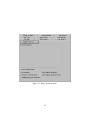
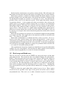
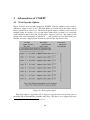
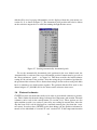
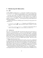
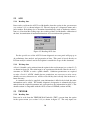
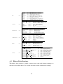
A directory name must be given for all of the UFILEs to be output to, this defaults to
a standard TEXTOR naming convention by default but can be overridden. A directory
is (and any directories above it are) created if necessary. This directory is compatible
with the TEXTOR version of CHEAP (implemented in Matlab).
In addition, there is a button to ‘Write main CX line output to TPD’. This will take
the line indicated as the CX line (set via the data parameters panel — see, e.g., figure
17) and send its various parameters to the TEXTOR Physics Database (TPD). This is
also done remotely via the web but permissions are only granted if physically using a
computer at TEXTOR. This system, in reality, simply copies several of the UFILES to
a web server.
53
6
Command line usage
When CXSFIT is called from the command line of a UNIX terminal a number of different arguments can be passed to it, these are discussed here. The individual commands
are processed in order and essentially simulate the user haven driven the graphical interface. Because of this, the order of arguments is important.
Throughout this documentation, it is assumed that the CXSFIT command from a
UNIX terminal is simply cxsfit where appropriate aliasing or PATH environment
variables have been set up. Note that some of the examples given here are machine
specific.
6.1
Basic usage
The simplest command is to load data immediately on startup. This can be from a JPF,
TWU or a Level-0 shotfile, examples are:
cxsfit ks5c:66869
cxsfit cer:17818
cxsfit k5:103357
The above uses defaults for reading options, to use a saved .otp file (only relevant for
JET; AUG doesn’t have any extra reading options) specify it before the data, e.g.:
cxsfit /path/to/myfile.otp ks5c:66869
In addition, to use the settings as used to read data which eventually produced a PPF
one can do:
cxsfit readoptions cxfm:69744:awhitef ks5c:69744
(the :awhitef is optional)
To load in any valid CXSFIT file (see appendix B) just give it at the command line,
multiple files can be used e.g.:
cxsfit my session.cxf
cxsfit my spectra.spc
cxsfit my spectra.spc my settings.fit
For this feature to work, the default CXSFIT file extensions must be used (see appendix
B). To save any CXSFIT file, specify it at the command line with the word save before
it. e.g. to load in a whole session and just save the fit history:
cxsfit my session.cxf save my settings.fit
or, to load data and then save it:
cxsfit ks5c:66869 save my spectra.spc
Again, any number of files can be saved.
To replay a history issue the command ”replay”, e.g.:
cxsfit ks5c:66869 /path/to/recipe.fit replay
or
cxsfit my session.cxf replay
54
to load a history from the PPF:
cxsfit settings cxfm:66869
(defaults to sequence 0 and JETPPF) or:
cxsfit settings cxfm:66869:awhitef
To re-do a fit as it was done from the PPF one could then:
cxsfit ks5c:66869 settings cxfm:66869 replay
To write a ppf, e.g.:
cxsfit my session.cxf write awhitef:cxfm
cxsfit my session.cxf write jetppf:cxfm
note that any PPF written from the command line will have a status flag of zero.
To quit the program after all of the commands issue the command ”quit”, e.g.
cxsfit my session.cxf write jetppf:cxfm quit.
6.2
Practical examples
To do a range of shots using a particular recipe file and save them for later inspection
it’s possible to type something like:
cxsfit ks5c:66869 /path/to/recipe.fit replay \
save ks5c 66869.cxf quit
cxsfit ks5c:66870 /path/to/recipe.fit replay \
save ks5c 66870.cxf quit
cxsfit ks5c:66871 /path/to/recipe.fit replay \
save ks5c 66871.cxf quit
It’s also possible to do a range of shots and just write a PPF at the end:
cxsfit ks5c:66869 /path/to/recipe.fit replay \
write jetppf:cxfm quit
cxsfit ks5c:66870 /path/to/recipe.fit replay \
write jetppf:cxfm quit
cxsfit ks5c:66871 /path/to/recipe.fit replay \
write jetppf:cxfm quit
For inspection of data which has been queried, it’s possible to bring it up inside CXSFIT
for manual inspection:
cxsfit readoptions cxfm:66869 ks5c:66869 \
settings cxfm:66869 replay
It’s possible to quickly reprocess a list of shots because, e.g., calibration has changed:
cxsfit readoptions cxfm:66869 ks5c:66869 \
settings cxfm:66869 replay write jetppf:cxfm quit
cxsfit readoptions cxfm:66870 ks5c:66870 \
settings cxfm:66870 replay write jetppf:cxfm quit
cxsfit readoptions cxfm:66871 ks5c:66871 \
settings cxfm:66871 replay write jetppf:cxfm quit
55
References
Afrosimov V V, Gordeev Yu S, Zinovev A N and Korotkov A (1978) JETP Lett. 28 500
Boileau A, von Hellermann M G, Horton L D, Spence J and Summers H P (1989)
Plasma Phys. Contr. Fusion 31 779
Fonck R J, Darrow D S and Jaehnig K P (1983) Phys. Rev. A 29 3288
Gormezano C, Sips A C C, Luce T C, Ide S, Becoulet A, Litaudon X, Isayama A, Hobirk
J, Wade M R, Oikawa T, Prater R, Zvonkov A, Lloyd B, Suzuki T, Barbato E, Bonoli P,
Phillips C K, Vdovin V, Joffrin E, Casper T, Ferron J, Mazon D, Moreau D, Bundy R,
Kessel C, Fukuyama A, Hayashi N, Imbeaux F, Murakami M, Polevoi A R and St John
H E Nuclear Fusion 47 S285
Isler R C (1977) Phys. Rev. Lett. 38 1359
Summers H P and von Hellermann M (1993) ‘Atomic and Plasma Material Interaction Processes in Controlled Thermonuclear Fusion’, Edited by Janev, (Elsevier Science
Publishers) 87–117.
Summers H P (2004) The ADAS User Manual, version 2.6
http://adas.phys.strath.ac.uk
Tunklev M, Breger P, G¨unther K, von Hellermann M, K¨onig R, O’Mullane M and Zastrow K-D (1999) Plasma Phys. Contr. Fusion 41 985
von Hellermann M, Core W G F, Howman A, Juper C, Konig R W T, Stamp M F,
Summers H P, Thomas P R and Zastrow K D (1996) ‘Diagnostics for Experimental
Fusion Reactors I’ Edited by Stott et al (Plenum Press N.Y.) 321
von Hellermann M G, Bertschinger G, Biel W, Giroud C, Jaspers R, Jupen C, Marchuk
O, O’Mullane M, Summers H P, Whiteford A and Zastrow K-D (2005) Physica Scripta
T120 19
von Hellermann M (2005) ‘ITER Active Charge Exchange Spectroscopy (CXRS) and
Beam Emission Spectroscopy (BES+MSE) with Diagnostic Neutral Beam (DNB)’ (under EFDA contract; not publicly available, contact: [email protected])
56
A
Internal data structures
A.1
Spectrum data structure
machine name [AUG, JET, TEXTOR, ...]
path to machine info [ /cxrsfit/<mach>]
[’AUGSF’, ’PPF’, ...]
MACHINE
STR
NAME
PATH
DATAFORMAT
STG
STG
STG
SPECTROMETER
STR
NAME
INFO
[’CER’] for identifying data source
descriptive string
INPUT FILE
SHOT NR
NPIXEL
NTRACK
NFRAME
NINST
STG
LNG
LNG
LNG
LNG
LNG
STG
STG
full path name for local file input
shot number
number of pixels
number of tracks
number of frames
number of instrument functions
Elements above are used to initialise structure, elements below are added automatically.
WLENGTH
SLIT
LOS NAME
R POS
z POS
PHI POS
R ORIG
z ORIG
PHI ORIG
TIME
EXPOSURE
BEAM
INTENSITY
FLT
FLT
STG[NTRACK]
FLT[NTRACK]
FLT[NTRACK]
FLT[NTRACK]
FLT[NTRACK]
FLT[NTRACK]
FLT[NTRACK]
FLT[NFRAME]
FLT[NFRAME]
BYT[NFRAME]
STR
spectrometer nominal central wavelength in Angstroms
spectrometer slit width in microns
Names of each track
crossing point of LOS with beam - used as a zero-order position of fitted parameters
see R pos
see R pos
position of the origin of the LOS - with [R pos,z pos,ph pos] to define the LOS
see R orig
see R orig
central time of exposure in seconds
duration of exposure of each frame
switch for beam on (=1) or off (=0)
DATA
ERROR
FLT[NPIXEL,NTRACK,NFRAME]
FLT[NPIXEL,NTRACK,NFRAME]
VALIDITY
BYT[NPIXEL,NTRACK,NFRAME]
REFERENCE
STG
(ph/(m2 srnm))
Error in above
Bit
Meaning
1
Dead pixel
2
Saturation
4
Undefined
6
Undefined
8
Undefined
16
Undefined
32
Undefined
64
Undefined
text specifying source
WAVELENGTH
STR
DATA
ERROR
REFERENCE
FLT[npixel,ntrack]
FLT[npixel,ntrack]
STG
wavelength (nm)
Error in above
text specifying source
DISPERSION
STR
DATA
ERROR
REFERENCE
FLT[NPIXEL,NTRACK]
FLT[NPIXEL,NTRACK]
STG
inverse linear dispersion in nm/pixel
Error in above
text specifying source
Y0
FLT[NINST,NTRACK]
XW
FLT[NINST,NTRACK]
XS
FLT[NINST,NTRACK]
REFERENCE
STG
relative intensity of individual Gaussians
1/e half width in Angstroms of individual
Gaussians in instrument function
relative shift in Angstroms of individual
Gaussians in instrument function
text specifying source
INSTFU
STR
57
A.2
Fit settings data structure
FRAME
TRACK
FITMODE
INT
INT
PTR
Selected frame
Selected track
MODE
FIRST FRAME
LAST FRAME
ALLTRACKS
IGNORE NOBEAM
CLEARBUFFER
PREVIOUS FRAME
NEIGHBOUR TRACK
SELF MAPPING
SELF MAPPING BACK
USEBEAMS
INCLUDE POOR
FRAMEADD
PIXELADD
NLINES
BASE
INITIAL
FPARAM
PTR
PTR
LINE
WLENGTH
PIXMIN
PIXMAX
CXLINE
REFLINE
COSMIC
LNG
INT
STR[8]
STG
INT
INT
LNG
LNG
LNG
STG
LNG
LNG
INT
INT
LNG
INT
INT
INT
INT
INT
LNG
INT
INT
‘single’, ‘mulitple’, ‘refit’, ‘reference’ or ‘markpoor’
First frame to fit
Last frame to fit
Fit all tracks
Ignore times when beam is off
Clear buffer before fit
Use previous frame estimaes
Use neighbouring track estimates
Use self mapping estimates
Use self mapping estimates with background
Use beam times for fit
Treat poor fits as failed
Unused
Unused
number of lines
baseline setting 0=flat; 1=linear
DESCRIPTION
STG
HEIGHT
FLT
CENTRE
FLT
TEMP
FLT
MASS
FLT
CENTRE UNIT
LNG
HEIGHT MAX
FLT
HEIGHT MIN
FLT
CENTRE MAX
FLT
CENTRE MIN
FLT
TEMP MAX
FLT
TEMP MIN
FLT
AMP FIXED
INT
WID FIXED
INT
POS FIXED
INT
AUTO AMPLITUDE
INT
SUPPRESS
INT
WAVELENGTH
FLT
UPPER
INT
LOWER
INT
Z0
INT
Z
INT
ACTIVE
INT
Unused
Minimum pixel range to fit
Maximum pixel range to fit
Main CX line (1 indexed ; 0=None)
Reference line (1 indexed ; 0=None)
Suppress cosmic bursts
58
8 character line description
Initial height estimate
Initial position estimate
Initial temperature estimate
Mass
1=nm ; 0=px
Maximum height value
Minimum height value
Maximum centre value
Minimum centre value
Maximum temperature value
Minimum temperature value
1=Fixed amplitude
1=Fixed width
1=Fixed position
1=Auto amplitude
1=Suppress line
Theoretical wavelength
Upper n level
Lower n level
Nuclear charge of receiver
Ionic charge of receiver
1=Active Line ; 0=Passive Line
NAG
COUPLED
SAVETRACKS
OTHERTRACKS
AREAS
GLOBSW
A.3
LNG
LNG
LNG
FLT
LNG
FLT
FLT
FLT
Major Print Level (see section 3.9)
Minor Print Level (see section 3.9)
Verify Level (see section 3.9)
Function Precision (see section 3.9)
Major Iteration Limit(see section 3.9)
Step Limit (see section 3.9)
Line Search Tolerance (see section 3.9)
Optimality Tolerance (see section 3.9)
PTR
MAJPRN
MINPRN
VERIF
FUNPRES
MAJIT
STPLIM
LINTOL
OPTTOL
PTR
COUPLED ON
ONOFF
PTYPE
LINE1
LINE2
OPERATOR
NUMBER
PTR
SAVETRACK
SUPPRESSLINE
OFFSET
USEOFFSET
AUTOOFFSET
PTR
ONOFF
PTYPE
TO LINE
FROM LINE
FROM TRACK
TI FACTOR
AF FACTOR
INT[20]
INT[20]
INT[20]
INT[20]
INT[20]
FLT
FLT
Track link is on
0=Ti ; 1=Intensity ; 2=AF
Line to go to (0 indexed)
Line to come from (0 indexed)
Track to come from (0 indexed)
Ti factor
AF factor
PTR
REDUCED ON
ONOFF
MIN VALUES
MAX VALUES
PTYPE
INT
INT[10]
FLT[10]
FLT[10]
INT[10]
Linked to global switch
Reduced area is on
Min range of reduced area
Max range of reduced area
0=pixels ; 1=nm
PTR
FIXED ESTIMATES
COUPLED PARAMETERS
AUTOMATIC AMPLITUDE ESTIMATES
EXTERNAL TRACK ESTIMATES
EXTERNAL TI ESTIMATES
EXTERNAL AF ESTIMATES
REDUCED AREA ACTIVATION
SUPPRESS GAUSSIAN ACTIVATION
PARAMETER BOUNDS ACTIVATION
PEDESTAL FUNCTION ACTIVATION
PIXEL CORRECTIONS ACTIVATION
INT
INT[50]
INT[50]
INT[50]
INT[50]
INT[50]
FLT[50]
INT[20]
INT[20]
FLT[20]
LNG
LNG
Linked to global switch
Particular coupling is turned on
0=Centre ; 1=Width ; 2=Height ; 3=Ti
Line to link to (0 indexed)
Line to link from (0 indexed)
0=x ; 1=+
Factor or costant (operator dependent)
Perform fit on this track
Suppress lines on this track
Pixel offset value
Use pixel offsets
Use pixel offsets from cache
INT
INT
INT
INT
INT
INT
INT
INT
INT
INT
INT
Allow parameters to be fixed
Activate coupled parameters
Turn on automatic amp. estimates
Turn on external track estimates
Turn on external Ti estimates
Turn on external AF estimates
Turn on reduced areas feature
Turn on suppressed guassians
Turn on paramater bounds
Unused
Turn on pixel correction options
History Data Structure
This history data structure is simply a pointer array with each element pointing to a
structure as described above. See section 4 for more details on the history settings.
59
A.4
Output data structure
CODE
MACHINE
SPECTROMETER
SHOT NR
NTRACK
NFRAME
NLINES
STG
STG
STG
LNG
LNG
LNG
LNG
Code use to do the fit (e.g. ’ks4fit’)
Machine (e.g. ’AUG’)
Spectrometer (e.g. ’CER’)
Shot number
Number of tracks
Number of frames
Number of lines
Elements above are used to initialise structure, elements below are added automatically.
Mass of each line
MASS
FLT[NLINES]
TEMP
STR
DATA
ERROR
FLT[NFRAME,NLINES,NTRACK]
FLT[NFRAME,NLINES,NTRACK]
Temperature
Error in above
INTENSITY
STR
DATA
ERROR
FLT[NFRAME,NLINES,NTRACK]
FLT[NFRAME,NLINES,NTRACK]
Intensity
Error in above
WAVELENGTH
STR
DATA
ERROR
FLT[NFRAME,NLINES,NTRACK]
FLT[NFRAME,NLINES,NTRACK]
Wavelength
Error in above
VROT
STR
DATA
ERROR
FLT[NFRAME,NLINES,NTRACK]
FLT[NFRAME,NLINES,NTRACK]
Rotation
Error in above
BASELINE
STR
DATA
ERROR
FLT[NFRAME,NTRACK]
FLT[NFRAME,NTRACK]
FIT STATUS
INT[NFRAME,NTRACK]
WSHIFT
WLFP
FLT[NFRAME,NTRACK]
FLT[NFRAME,NTRACK]
Baseline
Error in above
<0
Failed
=0
Not attempted
=1
Good fit
>1
Poor fit
Wavelength shift (on the fly calibration only)
Wavelength of first fitted pixel (on the fly calibration only)
60
B
B.1
External file formats
Spectra — .spc file
An .spc file contains calibrated spectra, instrument functions, geometry information
etc. It is an IDL Savefile format and contains a data structure as detailed in appendix
A.1. The files can be loaded/saved from the ‘Spectra’ menu (see section 2.1.3) or from
the command line (see section 6).
B.2
Fit settings — .fit file
The fit settings file can be saved and loaded from the ‘Fit’ menu and contain both the
history information and the currently displayed option. Unlike the other files generated
by CXSFIT, these files are ASCII in a markup language and can be inspected with a
conventional text editor. Note that it’s also possible to read in fit settings from a PPF or
Level-1 shotfile, also from the ‘Fit’ menu (see section 2.1.4).
B.3
Fit output — .otp file
An .otp file contains the output data from a fit (temperature, intensity etc.). It is an
IDL Savefile format and contains a data structure as detailed in appendix A.4. The files
can be loaded/saved from the ‘Results’ menu (see section 2.1.5) or from the command
line (see section 6).
B.4
External estimates — .ext file
An external estimates file (.ext) contains the external Ti and AF estimates in an IDL
Savefile format. The files can be loaded/saved from the ‘External’ menu (see section
2.1.6) or from the command line (see section 6).
B.5
Complete dataset — .cxf file
A .cxf file contains everything stored inside CXSFIT at a given point in time (with
the exception of the display options) in an IDL Savefile format. It consists of the data
structures specified in appendix A. The files can be loaded/saved from the ‘File’ menu
(see section 2.1.1) or from the command line (see section 6). These files are the most
convenient way to save a shot for either work in the future or for passing to someone
else.
61
B.6
Extra read options — .opt file file
An extra read options file (.opt) contains read options used to obtain spectra in an IDL
Savefile format and suitable to be passed directly to the underlying reading routine. The
files can be loaded and saved from the machine specific reading panels (see section 5)
and can also be specified at the command line (see section 6) just before data are read
at the command line.
62