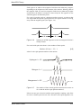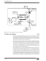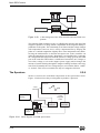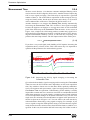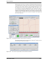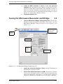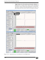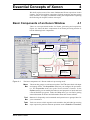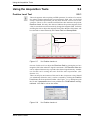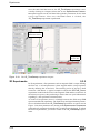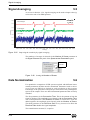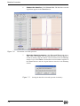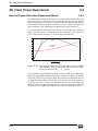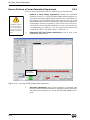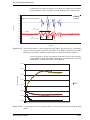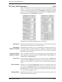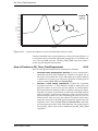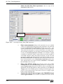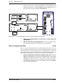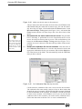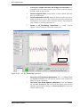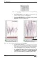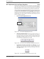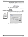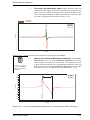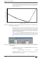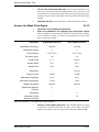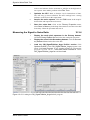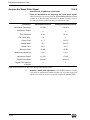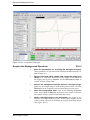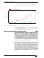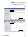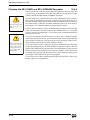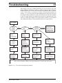
1
Xenon User’s Guide EMX EMX plus premiumX . XENON USER’S GUIDE Author: Ralph T. Weber Ph.D. Illustrations: Ralph T. Weber Ph.D. EPR Division Bruker BioSpin Corporation Billerica, MA USA Manual Version 1.3 Part Number 4757925 Software Version 1.1b50 February, 2011 Xenon User’s Guide: Manual Version 1.3 Software Version 1.1b50 Copyright © 2011 Bruker BioSpin Corporation The text, figures, and programs have been worked out with the utmost care. However, we cannot accept either legal responsibility or any liability for any incorrect statements which may remain, and their consequences. The following publication is protected by copyright. All rights reserved. No part of this publication may be reproduced in any form by photocopy, microfilm or other procedures or transmitted in a usable language for machines, in particular data processing systems without our written authorization. The rights of reproduction through lectures, radio and television are also reserved. The software and hardware descriptions referred in this manual are in many cases registered trademarks and as such are subject to legal requirements. This manual is part of the original documentation for the Bruker Xenon software. Preface 0 Bruker strives to supply you with instructional and accurate documentation. We encourage you to tell us how we are doing. Please send us your suggestions for improvements, corrections, or bug reports. If there is anything you particularly liked, tell us as well. With your input and assistance, Bruker can continually improve its products and documentation. You can send your messages and correspondence via e-mail, FAX, telephone, or mail. It is important to include the document name, product name, version number, and page number in your response. Here are the addresses and numbers to which you can send your messages. North America International epr_applications@ bruker-biospin.com [email protected] FAX: 978-670-8851 (0721) 5161-6237 Tel. 978-663-7406 (0721) 5161-6141 e-mail: mailing address EPR Division EPR Division Bruker BioSpin Corporation Bruker BioSpin GmbH 44 Manning Road Silberstreifen Manning Park D-76287 Rheinstetten/ Karlsruhe Billerica, MA 01821 USA Germany Thank you for your help. Electrical Safety 0.1 Do not remove any of the protective covers or panels of the instrument. They are fitted to protect you and should be opened by qualified service personnel only. Power off the instrument and disconnect the line cord before starting any cleaning work in the spectrometer. Never operate the instrument with the grounding cord disconnected or bypassed. Facility wiring must include a properly grounded power receptacle. Chemical Safety 0.2 Individuals working with hazardous chemicals, toxic substances, or enclosed liquid samples must take every precaution possible to avoid exposure to these agents. As a general rule, THINK OF THE CHEMICAL LABORATORY AS A HAZARDOUS ENVIRONMENT IN WHICH YOU MUST CONTINUALLY MAINTAIN A HIGH STANDARD OF VIGILANCE. Do not assume a cavalier attitude -- the substances with which you work present very real, and very serious threats to your health and safety. Xenon User’s Guide Microwave Safety Adhere to all currently recommended guidelines for standard laboratory safety as promulgated by governmental codes and contemporary laboratory practice. Inform yourself about the specific risks that are present when you handle actual or potential carcinogens (cancer-causing agents), explosive materials, strong acids, or any liquids that are sealed in glass containers. Specifically: • Be extremely careful when you handle sealed glass samples that are rapidly heated or cooled. The rapid cooling of some samples may result in the formation of a solid bolus in the sample tube that may make the tube prone to explosive rupture. • Educate yourself about the temperature at which chemicals evaporate. When a sample gets close to the temperature at which it evaporates, it may quickly become volatile. • In general, the safety threat posed by flying glass and violently escaping gases and liquids should not be underestimated. • Wear safety glasses, face masks, and other protective clothing whenever there is any risk of spillage, breakage, or explosion. Protective shields should also be employed when there is any risk of explosion. • Be sure that both storage and working areas are properly ventilated. They should be equipped with powerful blowers and fume heads. • Store chemicals safely. Avoid integrating containers of chemicals that may result in dangerous combinations. • Practice good housekeeping in work and storage areas. Clean up spills and refuse promptly. Do not leave volatile, combustible, or acidic liquids exposed on counters, benches, or other work areas. • Make certain all chemical containers are properly labeled and classified, and that especially hazardous materials are appropriately designated with clearly understood decals or warnings. • Never taste or inhale unmarked chemicals. • All laboratories should be equipped with fire doors, fire extinguishers, fire smothering materials, and sprinkler systems or showers, as well as a detailed fire safety plan. Microwave Safety 0.3 As long as the microwaves are contained in metal structures, microwaves can be very safe. Here are some precautions which, if followed, will eliminate the possibility of injury due to the microwaves. • Do not have an open waveguide when the microwave power is on. • Switch the bridge to standby when you remove or change EPR cavities. • Never look down an open waveguide when there is microwave power. The eyes are very susceptible to damage from microwaves. iv Table of Contents Table of Contents 0.1 0 Preface ............................................................................................... iii 0.1 0.2 0.3 0.1 Electrical Safety.............................................................................................................iii Chemical Safety.............................................................................................................iii Microwave Safety .......................................................................................................... iv Table of Contents............................................................................................................ v 1 Introduction .......................................................................................1-1 1.1 EPR Applications.........................................................................................................1-1 1.1.1 1.1.2 1.1.3 1.1.4 1.1.5 Chemistry.......................................................................................................................... 1-1 Physics .............................................................................................................................. 1-1 Materials Research ........................................................................................................... 1-2 Ionizing Radiation ............................................................................................................ 1-2 Biology and Medicine ...................................................................................................... 1-2 1.2 Using this Manual........................................................................................................1-3 1.2.1 How to Find Things.......................................................................................................... 1-3 1.2.2 Fonts ................................................................................................................................. 1-4 1.2.3 Special notes ..................................................................................................................... 1-4 2 An EPR Primer .................................................................................2-1 2.1 Basic EPR Theory........................................................................................................2-1 2.1.1 2.1.2 2.1.3 2.1.4 Introduction to Spectroscopy............................................................................................ 2-1 The Zeeman Effect ........................................................................................................... 2-2 Hyperfine Interactions ...................................................................................................... 2-4 Signal Intensity ................................................................................................................. 2-8 2.2 Basic EPR Practice ......................................................................................................2-8 2.2.1 2.2.2 2.2.3 2.2.4 2.2.5 2.2.6 Introduction to Spectrometers .......................................................................................... 2-8 The Microwave Bridge................................................................................................... 2-10 The EPR Cavity .............................................................................................................. 2-11 The Signal Channel ........................................................................................................ 2-13 The Magnetic Field Controller ....................................................................................... 2-15 The Spectrum.................................................................................................................. 2-16 2.3 Automated Parameter Adjustments ...........................................................................2-17 2.3.1 2.3.2 2.3.3 2.3.4 2.3.5 2.3.6 Effect of Mod. Amp. on the Number of Points .............................................................. 2-17 Effect of Sweep Width on Sweep Time ......................................................................... 2-19 Effect of Mod. Amp. on Conversion Time and Number of Points ................................ 2-19 Summary of Automated Parameter Setting Rules.......................................................... 2-19 Some Fine Points Regarding Modulation Amplitude..................................................... 2-20 Time Constants and Digital Filtering ............................................................................. 2-21 2.4 Default Xenon Parameters .........................................................................................2-23 2.4.1 2.4.2 2.4.3 2.4.4 Initial Default Parameters............................................................................................... 2-23 Organic Radicals Default Parameters............................................................................. 2-24 Transition Metals............................................................................................................ 2-25 Parameters That Are Not Changed................................................................................. 2-25 2.5 Parameter Optimization .............................................................................................2-26 Xenon User’s Guide v Table of Contents 2.5.1 2.5.2 2.5.3 2.5.4 2.5.5 Microwave Power ...........................................................................................................2-26 Field Modulation.............................................................................................................2-27 Second Harmonic Detection ...........................................................................................2-30 Measurement Time .........................................................................................................2-32 Receiver Gain..................................................................................................................2-33 2.6 Magnetic Field Parameters Optimization.................................................................. 2-34 2.6.1 Field Offsets....................................................................................................................2-34 2.6.2 Field Sweep Rates...........................................................................................................2-34 2.6.3 Field Settling after Flyback.............................................................................................2-36 2.7 Spin Quantitation....................................................................................................... 2-38 2.7.1 Signal Integration............................................................................................................2-38 2.7.2 Relative Measurements...................................................................................................2-40 2.7.3 Absolute Measurement ...................................................................................................2-45 2.8 Suggested Reading .................................................................................................... 2-48 3 Getting Started ................................................................................. 3-1 3.1 Turning the Spectrometer On...................................................................................... 3-2 3.2 Tuning the Microwave Resonator and Bridge ............................................................ 3-7 3.3 Acquiring Spectra...................................................................................................... 3-10 3.4 3.5 3.6 3.7 Storing and Saving the Spectrum .............................................................................. 3-14 Printing the Spectrum................................................................................................ 3-16 Acquiring a Second Harmonic Spectrum.................................................................. 3-17 Turning the Spectrometer Off ................................................................................... 3-19 4 Essential Concepts of Xenon ........................................................... 4-1 4.1 Basic Components of an Xenon Window ................................................................... 4-1 4.2 Viewports .................................................................................................................... 4-2 4.2.1 4.2.2 4.2.3 4.2.4 Display Area .....................................................................................................................4-3 Dataset Display Line.........................................................................................................4-3 The Result Section ............................................................................................................4-5 Individual Scale Buttons ...................................................................................................4-5 4.3 Tools............................................................................................................................ 4-6 4.3.1 4.3.2 4.3.3 4.3.4 4.3.5 4.3.6 4.3.7 4.3.8 Management.....................................................................................................................4-6 Selection...........................................................................................................................4-7 Display Toggling ..............................................................................................................4-7 Zooming............................................................................................................................4-7 Printing..............................................................................................................................4-7 Graphics and Measurement Tools ....................................................................................4-7 Qualifiers...........................................................................................................................4-8 Terminate Operation .........................................................................................................4-9 4.4 Mouse Functions ......................................................................................................... 4-9 4.4.1 4.4.2 4.4.3 4.4.4 4.4.5 vi The Cursors.......................................................................................................................4-9 Reading Out Coordinates................................................................................................4-10 Measuring Distances.......................................................................................................4-10 Zooming Spectra.............................................................................................................4-11 Moving a Spectrum Around............................................................................................4-13 Table of Contents 4.4.6 Changing Parameters Coarsely............................................................................. 4-14 4.5 Help............................................................................................................................4-14 5 Data Acquisition ................................................................................5-1 5.1 Spectrometer Monitoring Panel ...................................................................................5-1 5.1.1 5.1.2 5.1.3 5.1.4 5.1.5 5.1.6 Acquisition Control .......................................................................................................... 5-1 Experiment Definition ...................................................................................................... 5-2 Acquisition Toolbar.......................................................................................................... 5-2 Bridge Status..................................................................................................................... 5-3 Hardware Information ...................................................................................................... 5-3 The Meters........................................................................................................................ 5-4 5.2 Using the Acquisition Tools ........................................................................................5-5 5.2.1 Position Level Tool ......................................................................................................... 5-5 5.2.2 Sweep Tool ...................................................................................................................... 5-6 5.2.3 Sweep and Gain Tool ...................................................................................................... 5-8 5.3 Experiments ...............................................................................................................5-11 5.3.1 1D Experiments .............................................................................................................. 5-11 5.3.2 2D Experiments .............................................................................................................. 5-12 5.4 The Bridge Tuning Panel...........................................................................................5-13 5.4.1 Auto Tuning vs. Fine Tune............................................................................................. 5-13 5.4.2 Q Value Measurement .................................................................................................... 5-15 5.5 Signal Averaging .......................................................................................................5-16 5.6 Data Normalization....................................................................................................5-16 5.7 The 1D_FieldSweep Parameters and Options ...........................................................5-17 5.7.1 5.7.2 5.7.3 5.7.4 5.7.5 5.7.6 5.7.7 Magnetic Field................................................................................................................ 5-18 Signal Channel................................................................................................................ 5-18 Microwave ...................................................................................................................... 5-19 Digital Filter ................................................................................................................... 5-19 Magnetic Field (Options)................................................................................................ 5-19 Signal Channel (Options) ............................................................................................... 5-20 Scan ................................................................................................................................ 5-21 6 Data Input and Output ......................................................................6-1 6.1 Data Input ....................................................................................................................6-1 6.1.1 Loading in a BES3T® File ............................................................................................... 6-1 6.1.2 Importing an ESP File ..................................................................................................... 6-3 6.2 Data Output..................................................................................................................6-3 6.2.1 Saving a BES3T® File ..................................................................................................... 6-3 6.2.2 Exporting an ESP or ASCII File....................................................................................... 6-5 6.3 The Dataset Table ........................................................................................................6-5 6.3.1 6.3.2 6.3.3 6.3.4 6.3.5 Open Dataset Table .......................................................................................................... 6-6 File Menu of the Dataset Table ........................................................................................ 6-6 Edit Dataset Table ............................................................................................................ 6-8 Properties of the Dataset Table......................................................................................... 6-9 Options............................................................................................................................ 6-11 Xenon User’s Guide vii Table of Contents 7 Data Processing Tutorial .................................................................. 7-1 7.1 Baseline Correction ..................................................................................................... 7-2 7.2 Peak Picking................................................................................................................ 7-5 7.3 Integration and Quantitative EPR ............................................................................. 7-11 7.3.1 Approaches to Integration...............................................................................................7-11 7.3.2 How to Integrate .............................................................................................................7-12 7.3.3 Quantitative EPR ............................................................................................................7-19 7.4 Curve Fitting ............................................................................................................. 7-24 7.5 Subtracting Spectra and Spectral Titration................................................................ 7-28 7.5.1 Spectral Titration ............................................................................................................7-28 7.5.2 Subtracting Spectra .........................................................................................................7-30 7.6 SpinFit ....................................................................................................................... 7-32 7.6.1 SpinFit Using a Spectral Library ....................................................................................7-32 7.6.2 SpinFit Using Spectra in Memory ..................................................................................7-36 7.6.3 Creating Library Spectra.................................................................................................7-36 7.7 Interpolation .............................................................................................................. 7-42 8 Further Experiments ........................................................................ 8-1 8.1 1D _TimeSweep Experiment ...................................................................................... 8-1 8.1.1 8.1.2 8.1.3 8.1.4 8.1.5 8.1.6 8.1.7 How the 1D_TimeSweep Experiment Works...................................................................8-1 1D_TimeSweep Parameters..............................................................................................8-3 1D_TimeSweep vs. 2D_Field_Delay Experiments ..........................................................8-4 An Example for a 1D_TimeSweep Experiment ...............................................................8-4 How to Perform a 1D_TimeSweep Experiment ...............................................................8-5 How to Analyze the Kinetics Data....................................................................................8-7 Troubleshooting 1D_TimeSweep Experiments................................................................8-9 8.2 2D_Field_Power Experiment.................................................................................... 8-10 8.2.1 8.2.2 8.2.3 8.2.4 8.2.5 8.2.6 How the Power Saturation Experiment Works...............................................................8-10 2D_Field Power Parameters ...........................................................................................8-12 An Example for a Power Saturation Experiment............................................................8-12 How to Perform a Power Saturation Experiment ...........................................................8-14 Analyzing the Power Saturation Data.............................................................................8-15 Troubleshooting 2D_Field_Power Experiments.............................................................8-19 8.3 2D_Field_Delay Experiment..................................................................................... 8-19 8.3.1 8.3.2 8.3.3 8.3.4 8.3.5 How the 2D_Field_Delay Experiment Works................................................................8-19 2D_Field_Delay Parameters ...........................................................................................8-21 An Example for a 2D_Field_Delay Experiment.............................................................8-21 How to Perform a 2D_Field_Delay Experiment ............................................................8-26 Analyzing the 2D_Field_Delay Data..............................................................................8-27 8.4 2D_Time_Field Experiment...................................................................................... 8-38 8.4.1 8.4.2 8.4.3 8.4.4 8.4.5 8.4.6 8.4.7 viii How a 2D_Time_Field Experiment Works ....................................................................8-38 2D_Time_Field Parameters ............................................................................................8-39 2D_Time_Field vs. 2D_Field_Delay Experiments.........................................................8-40 An Example of a 2D_Time_Field Experiment ...............................................................8-40 How to Perform a 2D_Time_Field Experiment..............................................................8-41 How to Analyze the Data................................................................................................8-43 Troubleshooting 2D_Time_Field Experiments ..............................................................8-48 Table of Contents 8.5 2D_Field_Temp Experiment .....................................................................................8-49 8.5.1 8.5.2 8.5.3 8.5.4 8.5.5 How the Variable Temperature Experiment Works ....................................................... 8-49 2D_Field_Temp Parameters ........................................................................................... 8-50 An Example of a Variable Temperature Experiment ..................................................... 8-51 How to Perform a Variable Temperature Experiment.................................................... 8-54 Troubleshooting 2D_Field_Temp Experiments ............................................................. 8-58 8.6 References..................................................................................................................8-59 9 Additional Techniques & Helpful Hints .............................................9-1 9.1 Manually Tuning a Microwave Bridge........................................................................9-1 9.1.1 Visual Aids for Manually Tuning a Bridge ...................................................................... 9-1 9.1.2 Manual Tuning Method .................................................................................................... 9-2 9.2 Acquiring a Phase Quadrature Spectrum.....................................................................9-9 9.3 Changing EPR Resonators.........................................................................................9-11 9.4 AFC Adjustments ......................................................................................................9-17 9.4.1 9.4.2 9.4.3 9.4.4 9.4.5 The AFC and its Parameters........................................................................................... 9-17 Suggested Values for AFC Parameters .......................................................................... 9-18 AFC Adjustment for Optimal Sensitivity....................................................................... 9-18 AFC Adjustments for Low Power Operation ................................................................. 9-21 AFC Time Constant Adjustment .................................................................................... 9-22 9.5 Hints for Finding EPR Signals...................................................................................9-23 9.6 Optimizing Sensitivity ...............................................................................................9-26 9.6.1 Instrumental Factors ....................................................................................................... 9-26 9.6.2 Optimize the Sample ...................................................................................................... 9-27 9.6.3 Parameter Selection ........................................................................................................ 9-27 10 Calibration and Performance Tests ..............................................10-1 10.1 Signal Channel Calibration......................................................................................10-1 10.1.1 10.1.2 10.1.3 10.1.4 BDPA(Bis Diphenyl Allyl)-Benzene Complex............................................................ 10-1 Theory of Signal Channel Calibration.......................................................................... 10-1 When Should You Recalibrate? ................................................................................... 10-4 Calibrating the Signal Channel..................................................................................... 10-6 10.2 Magnetic Field Calibration ....................................................................................10-13 10.2.1 10.2.2 10.2.3 10.2.4 10.2.5 10.2.6 Field Offsets ............................................................................................................... 10-13 Field Calibration Standards ........................................................................................ 10-15 Calibrating a Constant Field Offset ............................................................................ 10-16 Calibrating a Linear Field Offset................................................................................ 10-19 Tips for Measuring the Field Offset ........................................................................... 10-22 g-Value Measurements ............................................................................................... 10-23 10.3 Signal to Noise Ratio Test .....................................................................................10-24 10.3.1 10.3.2 10.3.3 10.3.4 Preparing for the S/N Test .......................................................................................... 10-24 Acquire the Weak Pitch Signal................................................................................... 10-25 Acquire the Noise Spectrum....................................................................................... 10-26 Measuring the Signal to Noise Ratio.......................................................................... 10-27 10.4 Resonator Background Test...................................................................................10-29 10.4.1 Preparing for the Background Signal Test ................................................................. 10-29 Xenon User’s Guide ix Table of Contents 10.4.2 10.4.3 10.4.4 10.4.5 Acquire the Weak Pitch Signal ...................................................................................10-30 Acquire the Background Spectrum.............................................................................10-31 Measure the Weak Pitch to Background Ratio ...........................................................10-32 Cleaning the ER 4119HS and ER 4122SHQE Resonator ..........................................10-34 11 Troubleshooting ........................................................................... 11-1 11.1 No Cavity Dip. ........................................................................................................ 11-2 11.2 Tuning Error............................................................................................................ 11-2 11.3 No Tuning Picture ................................................................................................... 11-3 11.4 Unable to Critically Couple Cavity......................................................................... 11-3 11.5 Magnet Power Supply Shuts Down ........................................................................ 11-3 11.6 Baseline Distortion.................................................................................................. 11-4 11.7 Excessive Noise Output .......................................................................................... 11-4 11.8 Poor Sensitivity ....................................................................................................... 11-5 11.9 Poor Resolution ....................................................................................................... 11-6 11.10 Lineshape Distortion ............................................................................................. 11-6 11.11 No Signal When Everything Works...................................................................... 11-8 11.12 Warning Noises ..................................................................................................... 11-8 12 Bibliography ................................................................................. 12-1 A Brief Tips on Linux ........................................................................... A-1 A.1 Login ......................................................................................................................... A-1 A.2 The Desktop .............................................................................................................. A-2 A.2.1 A.2.2 A.2.3 A.2.4 A.2.5 A.2.6 Elements of the Desktop ................................................................................................. A-2 Starting Help ................................................................................................................... A-3 Folders............................................................................................................................. A-4 Removable Media ........................................................................................................... A-7 The Terminal................................................................................................................... A-9 Logout or Shutdown......................................................................................................A-10 A.3 Basic Mouse Functions ........................................................................................... A-11 A.4 An Application Window ......................................................................................... A-12 A.4.1 Dialog Boxes................................................................................................................. A-14 x Introduction 1 This document describes the basic operation of a Bruker EPR (Electron Paramagnetic Resonance) spectrometer running the Xenon software. This software is capable of running on an EMXmicro, EMXplus, and Elexsys-II spectrometer. No assumptions have been made about the background of the readers except that they have a general scientific or technical background. Many of the elementary principles necessary for following the chapters are presented in a concise form. We start with a list of EPR applications. A brief description of the spectrometer and its capabilities follows. The chapter concludes with an explanation of how to use this manual. EPR Applications 1.1 EPR has matured into a powerful, versatile, nondestructive, and nonintrusive analytical method. Unlike many other techniques, EPR yields meaningful structural and dynamical information, even from ongoing chemical or physical processes without influencing the process itself. Therefore, it is an ideal complementary technique for other methods in a wide range of studies and application areas. Here is a list of some of the EPR applications which are commonly used. Chemistry 1.1.1 • Kinetics of radical reactions • Polymerization reactions • Spin trapping • Organo-metallic compounds • Catalysis • Petroleum research • Oxidation and reduction processes • Biradicals and triplet states of molecules Physics 1.1.2 • Measurement of magnetic susceptibility • Transition metal, lanthanide, and actinide ions • Conduction electrons in conductors and semiconductors • Defects in crystals (e.g. color centers in alkali-halides) • Optical detection of magnetic resonance, excited states of molecules • Crystal fields in single crystals • Recombination at low temperatures Xenon User’s Guide EPR Applications Materials Research 1.1.3 • Degradation of paints and polymers by light • Polymer properties • Defects in diamond • Defects in optical fibers • Laser materials • Organic conductors • Influence of impurities and defects in semiconductors • Properties of novel magnetic materials • High TC superconductors • C60 compounds • Behavior of free radicals in corrosion Ionizing Radiation 1.1.4 • Alanine radiation dosimetry • Control of irradiated foods • Archaeological dating • Short-time behavior of organic free radicals produced by radiation • Radiation effects and damage • Radiation effects on biological compounds Biology and Medicine • Spin label and spin probe techniques • Spin trapping • Dynamics of biomolecules using saturation transfer techniques • Free radicals in living tissues and fluids • Antioxidants, radical scavengers • Contrast agents • Oximetry • Drug detection, metabolism, and toxicity • Enzyme reactions • Photosynthesis • Structure and identification of metal-binding sites • Photochemical and radiolytic generation of radicals • Oxygen based radicals • NO in biological systems • Carcinogenic reactions 1-2 1.1.5 Using this Manual Using this Manual 1.2 This manual describes basic and advanced operation of the Xenon application. How to Find Things 1.2.1 Preface First, you should read the safety guide in the preface of the manual. Microwaves can be dangerous, particularly to your eyes. With normal precautions, the risk for injury can be minimized. Chapter 2 Users who are not familiar with EPR should start by reading Chapter 2, which is a concise introduction to the theory and practice of EPR spectroscopy. It is by no means exhaustive; it gives the necessary information to follow the other chapters of the manual. A short list of references is given at the end of the chapter for more information. Chapter 3 This chapter is a simple “how to” section describing how to acquire the spectrum of a sample. It covers turning the spectrometer on, tuning the microwave cavity and bridge, and acquiring spectra. The step by step instructions lead you through the acquisition of a strong pitch (a standard sample) EPR signal. Chapter 4 This chapter introduces you to the essential concepts of Xenon. It describes the basic features and how to use those Xenon features. Chapter 5 This tutorial guides you through many common data acquisition tasks. It gives you detailed examples of how to use many of the convenient and commonly used features of the spectrometer. The chapter covers both 1D and 2D spectra. Chapter 6 Deatils regarding data input and output is described here including how to export data for other applications. Chapter 7 This chapter gives you a tutorial on the basic operations of data processing such as data handling, baseline correction, peak picking, integration, and curve fitting. Chapter 8 Chapter 3 describes the standard field swept EPR experiment. There are many more experiments offered by Xenon. An additional 1D experiment is a time sweep experiment. In addition introduction of a second axis allows you to combine the field sweeps with other parameters such as time, microwave power, and sample temperature. These techniques are described here with concrete examples demonstrating the techniques. Chapter 9 The most basic operations of the Bruker EPR spectrometer are covered in Chapter 3. This chapter introduces you to additional techniques such as manually tuning the bridge, changing cavities, and adjusting the AFC. Also general helpful hints for acquiring EPR spectra are presented in this chapter. Before consulting this chapter, you should be familiar with the material in Chapters 2 and 3. It gives tips on where to find EPR signals as well as how to optimize the sensitivity of the spectrometer for your particular sample. Chapter 10 Calibration of the spectrometer is important to maintain the performance of the spectrometer. It is also important to test if the spectrometer still meets its specifications. Both topics are presnted in detail in this chapter. Xenon User’s Guide 1-3 Using this Manual Chapter 11 Sometimes, things go wrong. Chapter 11 gives some possible solutions to problems you may be having. Many times, problems appear to be the fault of the instrument; however, with the proper choice of operating conditions, these problems often disappear. Chapter 12 An extensive bibliography of EPR references is given in this chapter. It includes many different EPR applications as well as educational texts. This is a good place to start a literature search. Fonts 1.2.2 Special fonts are used in the text to differentiate between normal manual text and the text displayed in the program. Times Helvetica Special notes This is the font used for the normal text in the manual. This is the font used for text that is displayed by the program or must be entered into the program by you. 1.2.3 Some special notation is employed in this manual to simplify the descriptions. Warning box. < ... > The content between the brackets needs to be substituted with proper entries by the user. > The right bracket indicates sequential selection of the menu entries. For example, Processing > Filtering > Smoothing means clicking the Processing button in the menu bar, followed by clicking Filtering in the sub-menu, and then clicking Smoothing. You will see a warning box sometimes in the lefthand margin. These are meant to point out critical information. In particular, it warns you about any procedures or operations that may be dangerous to the spectrometer or you. Always read and follow this advice. In addition, there are also hint boxes in the lefthand margin These are meant to be helpful hints and point out important information. Hint box. In between the special notes previously mentioned are important issues of which you should make note. These are presented in take note boxes. Take note box. 1-4 An EPR Primer 2 This chapter is an introduction to the basic theory and practice of EPR spectroscopy. It gives you sufficient background to understand the following chapters. In addition, we strongly encourage the new user to explore some of the texts and articles at the end of this chapter. You can then fully benefit from your particular EPR application or think of new ones. Basic EPR Theory 2.1 Introduction to Spectroscopy 2.1.1 During the early part of the 20th century, when scientists began to apply the principles of quantum mechanics to describe atoms or molecules, they found that a molecule or atom has discrete (or separate) states, each with a corresponding energy. Spectroscopy is the measurement and interpretation of the energy differences between the atomic or molecular states. With knowledge of these energy differences, you gain insight into the identity, structure, and dynamics of the sample under study. We can measure these energy differences, E, because of an important relationship between E and the absorption of electromagnetic radiation. According to Planck's law, electromagnetic radiation will be absorbed if: E = h [2-1] where h is Planck's constant and is the frequency of the radiation. DE Figure 2-1 hn Transition associated with the absorption of electromagnetic energy. The absorption of energy causes a transition from the lower energy state to the higher energy state. (See Figure 2-1.) In conventional spectroscopy, is varied or swept and the frequencies at which absorption occurs correspond to the energy differences of the states. (We shall see later that EPR differs slightly.) This record is called a spectrum. (See Figure 2-2.) Typically, the frequencies vary from the megahertz range for NMR (Nuclear Magnetic Resonance) (AM, FM, and TV transmissions use electromagnetic radiation at these frequencies), through visible light, to ultraviolet light. Radiation in the gigahertz range (the same as in your microwave oven) is used for EPR experiments. Xenon User’s Guide Basic EPR Theory h2 h1 Absorption 1 Figure 2-2 2 A spectrum. The Zeeman Effect 2.1.2 The energy differences we study in EPR spectroscopy are predominately due to the interaction of unpaired electrons in the sample with a magnetic field produced by a magnet in the laboratory. This effect is called the Zeeman effect. Because the electron has a magnetic moment, it acts like a compass or a bar magnet when you place it in a magnetic field, B0. It will have a state of lowest energy when the moment of the electron, µ, is aligned with the magnetic field and a state of highest energy when µ is aligned against the magnetic field. (See Figure 2-3.) The two states are labelled by the projection of the electron spin, Ms, on the direction of the magnetic field. Because the electron is a spin 1/2 particle, the parallel state is designated as Ms = - 1/2 and the antiparallel state is Ms = + 1/2. B0 Figure 2-3 B0 Minimum and maximum energy orientations of µ with respect to the magnetic field B0. From quantum mechanics, we obtain the most basic equations of EPR: E = g B B0 Ms = ± 1--- g B B0 [2-2] E = h = g BB0. [2-3] 2 and 2-2 Basic EPR Theory g is the g-factor, which is a proportionality constant approximately equal to 2 for most samples, but varies depending on the electronic configuration of the radical or ion. µB is the Bohr magneton, which is the natural unit of electronic magnetic moment. Two facts are apparent from equations Equation [2-2] and Equation [2-3] and its graph in Figure 2-4. • The two spin states have the same energy in the absence of a magnetic field. • The energies of the spin states diverge linearly as the magnetic field increases. For g = 2, the slope is 2.8 MHz/G. These two facts have important consequences for spectroscopy. • Without a magnetic field, there is no energy difference to measure. • The measured energy difference depends linearly on the magnetic field. Because we can change the energy differences between the two spin states by varying the magnetic field strength, we have an alternative means to obtain spectra. We could apply a constant magnetic field and scan the frequency of the electromagnetic radiation as in conventional spectroscopy. Alternatively, we could keep the electromagnetic radiation frequency constant and scan the magnetic field. (See Figure 2-4.) A peak in the absorption will occur when the magnetic field “tunes” the two spin states so that their energy difference matches the energy of the radiation. This field is called the “field for resonance”. Owing to the limitations of microwave electronics, the latter method offers superior performance. This technique is used in all Bruker EPR spectrometers. E Absorption B0 Figure 2-4 Variation of the spin state energies as a function of the applied magnetic field. The field for resonance is not a unique “fingerprint” for identification of a compound because spectra can be acquired at several different frequencies. The g-factor, h g = -----------B B0 Xenon User’s Guide [2-4] 2-3 Basic EPR Theory being independent of the microwave frequency, is much better for that purpose. Notice that high values of g occur at low magnetic fields and vice versa. A list of fields for resonance for a g = 2 signal at microwave frequencies commonly available in EPR spectrometers is presented in Table 2-1. Microwave Band Frequency (GHz) Bres (G) L 1.1 390 S 4.0 1430 X 9.75 3480 Q 34.0 12100 W 94.0 33500 Table 2-1 Field for resonance, Bres, for a g = 2 signal at selected microwave frequencies. Hyperfine Interactions 2.1.3 Measurement of g-factors can give us some useful information; however, it does not tell us much about the molecular structure of our sample. Fortunately, the unpaired electron, which gives us the EPR spectrum, is very sensitive to its local surroundings. The nuclei of the atoms in a molecule or complex often have a magnetic moment, which produces a local magnetic field at the electron. The interaction between the electron and the nuclei is called the hyperfine interaction. It gives us a wealth of information about our sample such as the identity and number of atoms which make up a radical or complex as well as their distances from the unpaired electron. B0 BI Electron Nucleus B0 Electron Figure 2-5 BI Nucleus Local magnetic field at the electron, BI, due to a nearby nucleus. Figure 2-5 depicts the origin of the hyperfine interaction. The magnetic moment of the nucleus acts like a bar magnet (albeit a weaker magnet than the electron) and produces a magnetic field at the electron, BI. This magnetic 2-4 Basic EPR Theory field opposes or adds to the magnetic field from the laboratory magnet, depending on the alignment of the moment of the nucleus. When BI adds to the magnetic field, we need less magnetic field from our laboratory magnet and therefore the field for resonance is lowered by BI. The opposite is true when BI opposes the laboratory field. For a spin 1/2 nucleus such as a hydrogen nucleus (proton), we observe that our single EPR absorption signal splits into two signals which are each BI away from the original signal. (See Figure 2-6.) BI Figure 2-6 BI Splitting in an EPR signal due to the local magnetic field of a nearby nucleus. For nuclei with spins other than 1/2, the number of lines equals: Number of Lines = 2I + 1 [2-5] where I is the spin quantum number of the nucleus. Hydrogen I = 1/2 Nitrogen I = 1 Manganese I = 5/2 Figure 2-7 The number of lines from hyperfine interactions increases as 2I+1 with the nuclear spin quantum number, I. If there are two spin 1/2 nuclei with the same hyperfine coupling, each of the two lines is further split into two lines. Because of the equal hyperfine cou- Xenon User’s Guide 2-5 Basic EPR Theory pling two of the EPR signals will overlap, giving a triplet with an intensity distribution of 1:2:1. 2 1 1 BI BI BI Figure 2-8 A 1:2:1 triplet resulting from the hyperfine interactions of two equivalent spin 1/2 nuclei. For n spin 1/2 nuclei with equal hyperfine couplings, the number of lines is given by: Number of Lines = 2n + 1 [2-6] with each of the lines separated by the hyperfine coupling. The relative intensities are given by: n n! = ----------------------- k k! n – k ! 0kn [2-7] which are related to Pascal’s triangle and polynomial coefficients. 6 4 a) 4 1 792 495 b) 1 1 12 66 O 220 792 495 220 66 12 1 O H H Me Me H H Me Me O Figure 2-9 2-6 924 O Relative intensities for benzosemiquinone (a) and durosemiquinone (b) radical anions in alkaline DMSO. The number of lines is given by Equation [2-6] and the relative intensities by Equation [2-7]. Basic EPR Theory The situation for nuclei with different hyperfine couplings is similar to equal hyperfine couplings, except that there is no overlap between the lines leading to the Pascal triangle intensity distribution. Each of the lines is split by the additional hyperfine couplings. As an example, it is possible to make the durosemiquinone radical cation. This is similar to the anion shown in Figure 2-9 except that the oxygens are protonated, thus producing further hyperfine splittings. We start off on the left side of Figure 2-10 with the 13 line pattern to be expected from the 12 equivalent methyl protons. Then there is the additional splittings from the hydrogens bound to the oxygens. Since the two protons are equivalent, we have a 1:2:1 triplet from them. If we split each of the 13 lines from the methyl proton splittings with this 1:2:1 triplet, we see that we can nicely reproduce the complicated experimental EPR spectrum of the durosemiquinone radical cation in sulfuric acid. H O Me Me Me Me O H 12 Methyl Protons Figure 2-10 Two Hydroxyl Protons Estimating the EPR spectrum of the durosemiquinone radical cation in sulfuric acid and reduced with sodium dithionite by splitting each of the EPR lines due to the 12 methyl protons by a 1:2:1 triplet from the hydroxyl protons. For N spin 1/2 nuclei, we will generally observe 2N EPR signals. As the number of nuclei gets larger, the number of signals increases exponentially. Sometimes there are so many signals that they overlap and we only observe one broad signal, resulting in what is called a gaussian lineshape. Figure 2-11 Xenon User’s Guide A large number of nuclei produces a gaussian lineshape. 2-7 Basic EPR Practice Signal Intensity 2.1.4 So far, we have concerned ourselves with the field for resonance of the EPR signal, but the size of the EPR signal is also important if we want to measure the concentration of the EPR active species in our sample. In the language of spectroscopy, the size of a signal is defined as the integrated intensity, i.e., the area beneath the absorption curve. (See Figure 2-12.) The integrated intensity of an EPR signal is proportional to the concentration. Figure 2-12 Integrated intensity of absorption signals. Both signals have the same intensity. Signal intensities do not depend solely on concentrations. They also depend on the microwave power. If you do not use too much microwave power, the signal intensity grows as the square root of the power. At higher power levels, the signal diminishes as well as broadens with increasing microwave power levels. This effect is called saturation. If you want to measure accurate linewidths, lineshapes, and closely spaced hyperfine splittings, you should avoid saturation by using low microwave power. A quick means of checking for the absence of saturation is to decrease the microwave power and verify that the signal intensity also decreases by the square root of the microwave power. Some of these topics are covered in greater detail in Section 2.7. Basic EPR Practice Introduction to Spectrometers 2.2 2.2.1 In the first half of this chapter, we discussed the theory of EPR spectroscopy. Now we need to consider the practical aspects of EPR spectroscopy. Theory and practice have always been strongly interdependent in the development and growth of EPR. A good example of this point is the first detection of an EPR signal by Zavoisky in 1945. The Zeeman effect had been known in optical spectroscopy for many years, but the first direct detection of EPR had to wait until the development of radar during World War II. Only then, did scientists have the necessary components to build sufficiently sensitive spectrometers (scientific instruments designed to acquire spectra). The same is true today with the development of advanced techniques in EPR such as Fourier Transform and high frequency EPR. The simplest possible spectrometer has three essential components: a source of electromagnetic radiation, a sample, and a detector. (See Figure 2-13.) To acquire a spectrum, we change the frequency of the electromagnetic radiation and measure the amount of radiation which passes through the sample with a detector to observe the spectroscopic absorptions. Despite the apparent complexities of any spectrometer you may encounter, it can always be simplified to the block diagram shown in Figure 2-13. 2-8 Basic EPR Practice Source Figure 2-13 Sample Detector The simplest spectrometer. Figure 2-14 shows the general layout of a Bruker EPR spectrometer. The electromagnetic radiation source and the detector are in a box called the “microwave bridge”. The sample is in a microwave resonator (or cavity), which is a metal box that helps to amplify weak signals from the sample. As mentioned in Section 2.1.2, there is a magnet to “tune” the electronic energy levels. In addition, we have a console, which contains signal processing and control electronics. There is a computer used for analyzing data as well as coordinating all the units for acquiring a spectrum. In the following sections you will become acquainted with how these different parts of the spectrometer function and interact. Microwave Bridge EMX Console EMX premiumX Magnet plus Magnet Power Supply Figure 2-14 Resonator Linux Workstation The modules and components of the EMXplus spectrometer. Xenon User’s Guide 2-9 Basic EPR Practice Signal Out G Reference Arm Detector Diode E F Source A C Attenuator B Circulator D Cavity Figure 2-15 Block diagram of a microwave bridge. The Microwave Bridge 2.2.2 The microwave bridge houses the microwave source and the detector. There are more parts in a bridge than shown in Figure 2-15, but most of them are control, power supply, and security electronics and are not necessary for understanding the basic operation of the bridge. We shall now follow the path of the microwaves from the source to the detector. We start our tour of the microwave bridge at point A, the microwave source. The output power of the microwave source cannot be varied easily, however in our discussion of signal intensity, we stressed the importance of changing the power level. Therefore, the next component, at point B, after the microwave source is a variable attenuator, a device which blocks the flow of microwave radiation. With the attenuator, we can precisely and accurately control the microwave power which the sample sees. Bruker EPR spectrometers operate slightly differently than the simple spectrometer shown in the block diagram, Figure 2-13. The diagram depicts a transmission spectrometer (It measures the amount of radiation transmitted through the sample.) and most EPR spectrometers are reflection spectrometers. They measure the changes (due to spectroscopic transitions) in the amount of radiation reflected back from the microwave cavity containing the sample (point D in the Figure 2-15). We therefore want our detector to see only the microwave radiation coming back from the cavity. The circulator at 2-10 Basic EPR Practice point C is a microwave device which allows us to do this. Microwaves coming in port 1 of the circulator only go to the cavity through port 2 and not directly to the detector through port 3. Reflected microwaves are directed only to the detector and not back to the microwave source. We use a detector diode to detect the reflected microwaves (point E in Figure 2-15). It converts the microwave power to an electrical current. At low power levels, (less than 1 microwatt) the diode current is proportional to the microwave power and the detector is called a square law detector. (Remember that electrical power is proportional to the square of the voltage or current.) At higher power levels, (greater than 1 milliwatt) the diode current is proportional to the square root of the microwave power and the detector is called a linear detector. The transition between the two regions is very gradual. For quantitative signal intensity measurements as well as optimal sensitivity, the diode should operate in the linear region. The best results are attained with a detector current of approximately 200 microamperes. To insure that the detector operates at that level, there is a reference arm (point F in the Figure 2-15) which supplies the detector with some extra microwave power or “bias”. Some of the source power is tapped off into the reference arm, where a second attenuator controls the power level (and consequently the diode current) for optimal performance. There is also a phase shifter to insure that the reference arm microwaves are in phase with the reflected signal microwaves when the two signals combine at the detector diode. The detector diodes are very sensitive to damage from excessive microwave power and will slowly lose their sensitivity. To prevent this from happening, there is protection circuitry in the bridge which monitors the current from the diode. When the current exceeds 400 microamperes, the bridge automatically protects the diode by lowering the microwave power level. This reduces the risk of damage due to accidents or improper operating procedures. However, it is good lab practice to follow correct procedures and not rely on the protection circuitry. The EPR Cavity 2.2.3 In this section, we shall discuss the properties of microwave (EPR) cavities and how changes in these properties due to absorption result in an EPR signal. We use microwave cavities to amplify weak signals from the sample. A microwave cavity is simply a metal box with a rectangular or cylindrical shape which resonates with microwaves much as an organ pipe resonates with sound waves. Resonance means that the cavity stores the microwave energy; therefore, at the resonance frequency of the cavity, no microwaves will be reflected back, but will remain inside the cavity. (See Figure 2-16.) Reflected Microwave Power Figure 2-16 Xenon User’s Guide res Reflected microwave power from a resonant cavity. 2-11 Basic EPR Practice Cavities are characterized by their Q or quality factor, which indicates how efficiently the cavity stores microwave energy. As Q increases, the sensitivity of the spectrometer increases. The Q factor is defined as 2 (energy stored) Q = ---------------------------------------------------------------energy dissipated per cycle [2-8] where the energy dissipated per cycle is the amount of energy lost during one microwave period. Energy can be lost to the side walls of the cavity because the microwaves generate electrical currents in the side walls of the cavity which in turn generates heat. We can measure Q factors easily because there is another way of expressing Q: res Q = -------- , [2-9] where res is the resonant frequency of the cavity and is the width at half height of the resonance. Sample Stack Microwave Magnetic Field Figure 2-17 Sample Stack Microwave Electric Field Magnetic and electric field patterns in a standard EPR cavity. A consequence of resonance is that there will be a standing wave inside the cavity. Standing electromagnetic waves have their electric and magnetic field components exactly out of phase, i.e. where the magnetic field is maximum, the electric field is minimum and vice versa. The spatial distribution of the amplitudes of the electric and magnetic fields in a commonly used EPR cavity is shown in Figure 2-17. We can use the spatial separation of the electric and magnetic fields in a cavity to great advantage. Most samples have non-resonant absorption of the microwaves via the electric field (this is how a microwave oven works) and the Q will be degraded by an increase in the dissipated energy. It is the microwave magnetic field that drives the absorption in EPR. Therefore, if we place our sample in the electric field minimum and the magnetic field maximum, we obtain the biggest signals and the highest sensitivity. The cavities are designed for optimal placement of the sample. We couple the microwaves into the cavity via a hole called an iris. The size of the iris controls the amount of microwaves which will be reflected back from the cavity and how much will enter the cavity. The iris accomplishes this by carefully matching or transforming the impedances (the resistance to the waves) of the cavity and the waveguide (a rectangular pipe used to carry microwaves). There is an iris screw in front of the iris which allows us to adjust the “matching”. This adjustment can be visualized by noting that as the screw moves up and down, it effectively changes the size of the iris. (See 2-12 Basic EPR Practice Figure 2-18.) When the iris screw properly matches the cavity impedance (also called critical coupling), no microwaves are reflected back from the cavity. Iris Screw Waveguide Iris Cavity Figure 2-18 The matching of a microwave cavity to waveguide. How do all of these properties of a cavity give rise to an EPR signal? When the sample absorbs the microwave energy, the Q is lowered because of the increased losses and the coupling changes because the absorbing sample changes the impedance of the cavity. The cavity is therefore no longer critically coupled and microwave will be reflected back to the bridge, resulting in an EPR signal. The Signal Channel 2.2.4 EPR spectroscopists use a technique known as phase sensitive detection to enhance the sensitivity of the spectrometer. The advantages include less noise from the detection diode and the elimination of baseline instabilities due to the drift in DC electronics. A further advantage is that it encodes the EPR signals to make it distinguishable from sources of noise or interference which are almost always present in a laboratory. The signal channel, a unit which fits in the spectrometer console, contains the required electronics for the phase sensitive detection. The detection scheme works as follows. The magnetic field strength which the sample sees is modulated (varied) sinusoidally at the modulation frequency. If there is an EPR signal, the field modulation quickly sweeps through part of the signal and the microwaves reflected from the cavity are amplitude modulated at the same frequency. For an EPR signal which is approximately linear over an interval as wide as the modulation amplitude, the EPR signal is transformed into a sine wave with an amplitude proportional to the slope of the signal (See Figure 2-19.) First Derivative Figure 2-19 Xenon User’s Guide Field modulation and phase sensitive detection. 2-13 Basic EPR Practice The signal channel (more commonly known as a lock-in amplifier or phase sensitive detector) produces a DC signal proportional to the amplitude of the modulated EPR signal. It compares the modulated signal with a reference signal having the same frequency as the field modulation and it is only sensitive to signals which have the same frequency and phase as the field modulation. Any signals which do not fulfill these requirements (i.e., noise and electrical interference) are suppressed. To further improve the sensitivity, a time constant is used to filter out more of the noise. Modulation Amplitude Phase sensitive detection with magnetic field modulation can increase our sensitivity by several orders of magnitude; however, we must be careful in choosing the appropriate modulation amplitude, frequency, and time constant. All three variables can distort our EPR signals and make interpretation of our results difficult. B0 Figure 2-20 Signal distortions due to excessive field modulation. As we apply more magnetic field modulation, the intensity of the detected EPR signals increases; however, if the modulation amplitude is too large (larger than the linewidths of the EPR signal), the detected EPR signal broadens and becomes distorted. (See Figure 2-20.) A good compromise between signal intensity and signal distortion occurs when the amplitude of the magnetic field modulation is equal to the width of the EPR signal. Also, if we use a modulation amplitude greater than the splitting between two EPR signals, we can no longer resolve the two signals. Time constants filter out noise by slowing down the response time of the spectrometer. As the time constant is increased, the noise levels will drop. If we choose a time constant which is too long for the rate at which we scan the magnetic field, we can distort or even filter out the very signal which we are trying to extract from the noise. Also, the apparent field for resonance will shift. Figure 2-21 shows the distortion and disappearance of a signal as the time constant is increased. If you need to use a long time constant to see a weak signal, you must use a slower scan rate. A safe rule of thumb is to make sure that the time needed to scan through a single EPR signal should be ten times greater than the length of the time constant. 2-14 Time Constant Basic EPR Practice B0 Figure 2-21 Signal distortion and shift due to excessive time constants. For samples with very narrow or closely spaced EPR signals, (~ 50 milligauss. This usually only happens for organic radicals in dilute solutions.) we can get a broadening of the signals if our modulation frequency is too high (See Figure 2-22.) 12.5 kHz 100 kHz B0 Figure 2-22 Loss of resolution due to high modulation frequency. The Magnetic Field Controller 2.2.5 The magnetic field controller allows us to sweep the magnetic field in a controlled and precise manner for our EPR experiment. It consists of two parts; a part which sets the field values and the timing of the field sweep and a part which regulates the current in the windings of the magnet to attain the requested magnetic field value. The magnetic field values and the timing of the magnetic field sweep are controlled by a microprocessor in the controller. A field sweep is divided into a maximum of 256,000 discrete steps (128,000 for the EMXmicro) called sweep addresses. At each step, a reference voltage corresponding to the magnetic field value is sent to the part of the controller that regulates the magnetic field. The sweep rate is controlled by varying the conversion time (waiting time at each step of the individual steps during which the signal channel digitizes the EPR signal). Xenon User’s Guide 2-15 Basic EPR Practice Power Supply Magnet Hall Probe Magnet 3475 3476 3477 Microprocessor Figure 2-23 Regulator Reference Voltage A block diagram of the field controller and associated components. The magnetic field regulation occurs via a Hall probe placed in the gap of the magnet. It produces a voltage which is dependent on the magnetic field perpendicular to the probe. The relationship is not linear and the voltage changes with temperature; however, this is easily compensated for by keeping the probe at a constant temperature slightly above room temperature and characterizing the nonlinearities so that the microprocessor in the controller can make the appropriate corrections. Regulation is accomplished by comparing the voltage from the Hall probe with the reference voltage given by the other part of the controller. When there is a difference between the two voltages, a correction voltage is sent to the magnet power supply which changes the amount of current flowing through the magnet windings and hence the magnetic field. Eventually the error voltage drops to zero and the field is “stable” or “locked”. This occurs at each discrete step of a magnetic field scan. The Spectrum 2.2.6 We have seen how the individual components of the spectrometer work. Figure 2-24 shows how they work together to produce a spectrum. Spectrum Y-axis Intensity Microwave Bridge X-axis Magnetic Field Signal Channel Cavity and Magnet Sample Figure 2-24 2-16 Block diagram of an EPR spectrometer. Field Controller Automated Parameter Adjustments Automated Parameter Adjustments 2.3 Traditionally, acquisition parameters such as number of points, conversion time and time constant were adjusted separately and it was assumed that the user knew how to optimize all the parameters. It turns out that many of the parameters are inter-related and some linking of parameters can be used to ease and simplify the optimization process. This section explains how some parameters are set automatically and which ones have priority in Xenon. Effect of Mod. Amp. on the Number of Points 2.3.1 The parameter that most influences the choice of other parameters is the modulation amplitude. As can be seen in Figure 2-25, the apparent linewidth that is observed is dependent on the modulation amplitude. It is difficult to resolve features narrower than the modulation amplitude owing to the modulation broadening or smearing out of the EPR lines. Also one typically sets the modulation amplitude to a value approximately less than or equal to the EPR linewidth. 20 mG Mod Amp (Current) 320 mG Mod Amp 0.2 BRUKER 0.1 Intensity [] 0 -0.1 -0.2 -0.3 -0.4 3504.6 Figure 2-25 3504.7 3504.8 3504.9 3504.99 3505.1 Field [G] 3505.2 3505.3 3505.4 3505.5 Reduction in resolution owing to excessive modulation amplitude. EPR spectra are recorded by stepping the magnetic field in discrete steps and digitizing the EPR signal at each of these field steps. The size of these discrete steps must be sufficiently small that the EPR lineshape is characterized well. (See Figure 2-26.) Because the resolution cannot greatly exceed the modulation amplitude, this sets a limit on the number of points required to characterize an EPR signal. This is expressed by the parameter Pts / Mod. Amp. The Pts / Mod. Amp. parameter has an influence on how well the EPR lineshape is characterized. A value of 1 produces a very poor representation of the EPR lineshape. Increasing the value yields an increasingly faithful representation of the EPR lineshape. Xenon User’s Guide 2-17 Automated Parameter Adjustments 70 70 BRUKER 60 50 40 40 30 30 20 10 5 Pts./MA 0 -10 Intensity [] Intensity [] 20 1 Pts./MA 0 -20 -30 -30 -40 -40 -50 -50 -60 -70 -70 3514 3515 3516 3517 Field [G] 3518 3519 3520 3514 70 3515 3516 3517 Field [G] 3518 3519 3520 70 BRUKER 60 BRUKER 60 50 50 40 40 30 30 20 20 10 10 Pts./MA 0 -10 Intensity [] Intensity [] 10 -10 -20 -60 2 Pts./MA BRUKER 60 50 10 0 -10 -20 -20 -30 -30 -40 -40 -50 -50 -60 -60 -70 -70 3514 Figure 2-26 3515 3516 3517 Field [G] 3518 3519 3520 3514 3515 3516 3517 Field [G] 3518 3519 3520 Increasing the Pts / Mod. Amp. gives a more faithful representation of the EPR lineshape. The Pts / Mod. Amp. parameter always takes priority in setting other acquisition parameters. Its value remains constant unless you intentionally change its value. The other linked (or automatically adjusted) parameters are adjusted according to its value. The resultant Number of Points in the EPR spectrum is set to: The Number of Points is automatically calculated and cannot be directly changed by the user. To change its value, change the value of Pts / Mod. Amp. Sweep Width Number of Points = Pts / Mod. Amp. -------------------------------Mod. Amp. This relation is the first automatic parameter linkage in Xenon. As can be seen in Figure 2-27, 1 G Mod. Amp. and 10 Pts / Mod. Amp. and a Sweep Width of 100 G yield 1000 for Number of Points. Figure 2-27 2-18 [2-10] Number of Points for a given Mod. Amp. and Sweep Width. Automated Parameter Adjustments Effect of Sweep Width on Sweep Time 2.3.2 The next thing to consider is the time it takes to sweep the field. The Conversion Time is the amount of time the magnetic field remains at the individual discrete field steps and the EPR intensity is digitized. The Sweep Time then equals: The Conversion Time is automatically calculated and cannot be directly changed by the user. To change its value, change the value of Sweep Time. Sweep Time = Number of Points Conversion Time [2-11] From Equation [2-10] we see that if we increase the Sweep Width by a factor of two, the Number of Points is increased by a factor of two. Xenon keeps the Conversion Time constant when automatically adjusting parameters for different Sweep Widths, therefore, the Sweep Time is increased by a factor of two. This is the second automatic parameter linkage in Xenon. You can of course change the value of the Sweep Time manually should you wish to do so. Effect of Mod. Amp. on Conversion Time and Number of Points 2.3.3 The third automatic parameter linkage in Xenon is the effect of changing the Modulation Amplitude. The Pts / Mod. Amp. remains constant and therefore the Number of Points changes. The Sweep Time remains constant and Xenon adjusts the Conversion Time to maintain the original Sweep Time. Therefore if the Modulation Amplitude is increased by a factor of two, the Number of Points is halved and the Conversion Time is doubled. Summary of Automated Parameter Setting Rules 2.3.4 Initial Values The Number of Points is determined by Pts/Mod. Amp., Mod. Amp., and Sweep Width. (See Equation [2-10].) Pts/Mod. Amp. This parameter always has priority and remains constant unless you intentionally change its value. Change Sweep Width The Conversion Time and Pts/Mod. Amp. parameters have priority and remain constant. The Sweep Time is automatically adjusted to accommodate the new Number of Points. (See Equation [2-11].) Change Mod. Amp. The Sweep Time and Pts/Mod. Amp. parameters have priority and remain constant. The Conversion Time is automatically adjusted to accommodate the new Number of Points. (See Equation [2-11].) Changing Parameters With the exceptions of Number of Points and Conversion Time, if the automatically adjusted parameters are not appropriate for your sample, you can always change their values to the desired values. Xenon User’s Guide 2-19 Automated Parameter Adjustments Some Fine Points Regarding Modulation Amplitude 2.3.5 There are a few fine points that you should be aware of regarding the modulation amplitude. If you undermodulate (Mod. Amp. << linewidth), then the Number of Points tends to be much larger than needed. If you overmodulate (Mod. Amp. >> linewidth), then the Number of Points tends to be much smaller than needed. Figure 2-28 Over and under modulation can result in too many or too few points in the spectrum. Another thing you may notice is that not all values of Mod. Amp. are allowed because: Sweep Width Number of Points = Integer Value = Pts / Mod. Amp. -------------------------------Mod. Amp. [2-12] You cannot have fractional number of data points in your dataset. You may ensure that you have the exact Mod. Amp. you want by setting the Sweep Width such that Equation [2-12] has an integer value. 2-20 Automated Parameter Adjustments Time Constants and Digital Filtering 2.3.6 As we saw in Section 2.2.4, the time constant of the signal channel is used to filter out noise and thereby attain a higher S/N (Signal to Noise ratio). The assumption is that the signal has mostly low frequency components and the noise will have components at all frequencies. By filtering out the high frequencies components in the signal channel output with the time constant, we are suppressing the noise in the spectrum. If we sweep too quickly for a given time constant, we can start to filter out the EPR signal as well. Figure 2-21 showed that increasing the time constant too far leads to a significant distortion of the lineshape and also of the line position. Another approach to improving the S/N ratio is to suppress noise by using digital filtering techniques after the data has been acquired instead of using long time constants. In Xenon a binomial smoothing technique is used. This technique replaces the intensity value for a particular point in the EPR spectrum by a weighted average of the surrounding data points. The important parameter for the filtering is n, the Number of Points of the Digital Filter. Figure 2-29 The Digital Filter parameters. For a given n, the intensities of the n points before and the n points after the data point as well as the intensity of the data point itself are used in the weighted average comprised of 2n+1 points. (These data points are the green points labeled I-2 to I2 in Figure 2-30.) The weighting coefficients are given by the binomial coefficients that are the polynomial coefficients when (1+x)n is expanded. For n = 2, this is 1:4:6:4:1. After filtering, the filtered intensity at the center (the blue point in Figure 2-30) is given by: filtered I0 = 1 I – 2 + 4 I – 1 + 6 I 0 + 4 I 1 + 1 I 2 16 , [2-13] where the factor of 16 is required for normalization. This filtering procedure is then repeated for each individual data point of the spectrum. (1 * I + 4 * I + 6 * I + 4 * I + 1 * I ) / 16 -2 -1 0 1 2 1.35 I0 1.3 BRUKER 1.25 I1 I2 1.2 1.15 Intensity [] 1.1 1.05 1.0 0.95 I-2 0.9 0.85 I -1 0.8 0.75 0.7 0.65 3519.0 Figure 2-30 Xenon User’s Guide 3519.5 3520.0 3520.5 Field [G] 3521.0 3521.5 3522.0 Binomial smoothing of the EPR data. 2-21 Automated Parameter Adjustments Figure 2-31 shows a comparison of the two noise reduction techniques. The unfiltered spectrum acquired with the minimum time constant is noisy. Increasingly longer time constants filter out more noise in the data. Increasingly larger Number of Points in the Digital Filter also filter out more noise in the data. Both techniques introduce distortions in the EPR lineshape for excessive parameter values, most notably a broadening of the peak-to-peak width and a diminishing of the peak-to-peak amplitude. The advantage of the digital filtering technique is that the EPR signal remains symmetric and does not exhibit a field shift as an excessively long analog time constant does. No Filtering Minimum Time Constant 2.56 ms Time Constant 2 Point Smoothing 10.24 ms Time Constant 10 Point Smoothing 40.96 ms Time Constant 190 Points Smoothing Figure 2-31 Comparison of spectra acquired using different time constants with spectra acquired using the minimum constant and digital filtering with different numbers of points. By default, Xenon sets the Time Constant to the minimum value. The Digital Filter Mode is set to Auto mode. In this mode the Number of Points for the Digital Filter is set to the Pts/Mod. Amp. parameter value. 2-22 Default Xenon Parameters Default Xenon Parameters 2.4 In order to aid in finding EPR signals and optimizing them there are three sets of default parameters available in the Xenon software for different types of samples. It should be emphasized that these default parameter sets are only starting points. The first step for parameter optimization is to have an observable EPR spectrum (even though it may not be pretty) that you can optimize and the default parameter sets should give you an EPR spectra with which to start in most cases. Section 2.5 describes methods to further optimize the acquisition parameters. Initial Default Parameters 2.4.1 When the software is first started there is a general default parameter set that is an appropriate starting point for finding EPR signals from almost any organic radical sample with a strong EPR signal such as calibration samples. Figure 2-32 Initial default parameters. Xenon User’s Guide 2-23 Default Xenon Parameters Organic Radicals Default Parameters 2.4.2 The Organic Radicals default parameter set is a good starting point to find EPR signals from organic radicals. Organic radicals tend to be g=2 and exhibit transitions over a fairly narrow field range. Therefore the Center Field is set to the g=2 value for the present Microwave Frequency and the Sweep Width is set to 200 G. Linewidths or spectral features tend to vary typically from 0.1 G to 15 G which makes the Mod. Amp. of 1 G appropriate for signal detection. For most samples, 2 mW of microwave power will not saturate the EPR signal too much. These parameters are not optimum for all of your samples, but it is a good starting point to optimize the acquisition parameters. Figure 2-33 2-24 Default spectrometer parameters for organic radical samples. Default Xenon Parameters Transition Metals 2.4.3 The Transition Metals default parameter set is a good starting point to find EPR signals from paramagnetic metals. Transition metals tend to exhibit transitions over a fairly broad field range. Therefore the Center Field is set to 3200 G and the Sweep Width is set to 6000 G in order not to miss any EPR signals. Linewidths or spectral features tend to be broader than for organic radicals thereby requiring a higher Mod. Amp. of 4 G. For most samples, 2 mW of microwave power will not saturate the EPR signal too much. These parameters are not optimum for all of your samples, but it is a good starting point to optimize the acquisition parameters. Figure 2-34 Default spectrometer parameters for transition metal samples. Parameters That Are Not Changed 2.4.4 The following parameters are not changed or reset when either the Organic Radicals or Transition Metals default parameters are chosen. Receiver Gain All Magnetic Field Parameters in Options Time Constant Modulation Phase Dual Detection All Scan Parameters Digital Filter Mode Digital Filter Number of Points Table 2-2 Unchanged parameters. Xenon User’s Guide 2-25 Parameter Optimization Parameter Optimization 2.5 Once an EPR signal has been found, the acquisition parameters must be optimized for the sample under study. This section offers advice on how to optimize these parameters. Microwave Power 2.5.1 The intensity of an EPR signal increases with the square root of the microwave power (dashed line in Figure 2-35) in the absence of saturation effects. When saturation sets in, the signals broaden and peak-peak amplitude decreases. The first thing that is obvious is that more microwave power helps to increase the signal strength until its starts decreasing. Also, if you are measuring spin concentrations, you want to work in the linear region. 55 Peak-Peak Amplitude 50 1.8 45 Peak-Peak Amplitude 40 1.4 35 Peak-Peak Linewidth 30 1.2 1.0 25 0.8 20 0.6 15 10 0.4 5 0.2 0 Peak-Peak Linewidth (G) 1.6 0 0 1 2 4 3 5 6 8 7 9 10 11 12 13 14 √Microwave Power (mW) Figure 2-35 Experimental microwave power dependence data for a BDPA (Bis Diphenyl Allyl) point sample. The system is homogeneously broadened with T1 ~ T2 ~ 100 ns. Though, the peak-peak intensity may decrease at higher microwave power, the integrated intensity of the EPR signal continues to grow. The increase in linewidth offsets the decrease in peak-peak intensity. 120 Integrated Intensity 110 100 90 Intensity 80 70 Peak-Peak Intensity 60 50 40 30 20 10 0 0 1 2 3 4 5 6 7 8 9 10 11 12 13 14 √Microwave Power (mW) Figure 2-36 2-26 Comparison of the peak-peak intensity and integrated intensity for a BDPA (Bis Diphenyl Allyl) point sample as a function of the square root of the microwave power. Parameter Optimization Even though the signal intensity may not change greatly with microwave power, EPR signals with very narrow lines (linewidth < 100 mG) are particular susceptible to distortion because of excessive microwave power broadening. 25 dB 31 dB 37 dB 43 dB 3509.4 Figure 2-37 3509.59 3509.8 3510.0 Field [G] 3510.2 3510.4 3510.59 Galvinoxyl in heptane at different microwave attenuations. You should try several microwave power levels to find the optimal microwave power for your sample. A convenient way to find the optimum power is to use the 2D_Field_Power experiment routine described in Section 8.2. A general “rule of thumb” is that samples saturate more readily as the temperature decreases. Systems with greater orbital angular momentum tend to saturate less readily. Therefore organic radicals that usually have their orbital angular momentum quenched saturate readily. Transition metals and rare earth ions in particular have a great deal of orbital angular momentum and therefore do not saturate readily. The exceptions to this rule are S state ions such as Mn+2 and Gd+3 that do not have orbital angular momentum and these ions will saturate more readily than other ions in the series. Field Modulation 2.5.2 Excessive field modulation broadens the EPR lines and does not contribute to a more intense signal. Figure 2-38 shows the dependence of the peak-peak linewidth and amplitude on the modulation amplitude. 15 180 Peak-Peak Amplitude 160 14 13 Peak-Peak Amplitude 11 10 120 9 100 8 7 80 6 Peak-Peak Linewidth 60 [Peak-Peak Width (G) 12 140 5 4 40 3 2 20 1 0 0 0 1 Figure 2-38 Xenon User’s Guide 2 3 4 5 6 7 8 9 Modulation Amplitude (G) 10 11 12 13 14 15 Experimental Modulation Amplitude data for a BDPA (Bis Diphenyl Allyl) point sample. 2-27 Parameter Optimization In contrast to the peak-peak intensity, the integrated intensity (or double integral) of the EPR signal maintains a linear dependence with respect to the Modulation Amplitude owing to the modulation broadening. Integrated Intensity Peak-Peak Amplitude 0 0.2 0.4 0.6 0.8 1.0 1.2 1.4 1.6 1.8 2.0 2.2 2.4 2.6 2.8 3.0 3.2 3.4 3.6 3.8 4.0 4.2 4.4 4.6 4.8 5.0 Modulation Amplitude (G) Figure 2-39 Experimental Modulation Amplitude integrated intensity data for a BDPA (Bis Diphenyl Allyl) point sample. A good “rule of thumb” is to use a field modulation amplitude that is approximately one quarter the width of the narrowest EPR line you are trying to resolve. Keep in mind that there is always a compromise that must be made between resolving narrow lines and increasing your signal to noise ratio. If you have a very weak signal, you may need to sacrifice resolution (i.e., by using a higher field modulation) in order to even detect the signal. However, if you have a high signal to noise ratio, you may choose to use a much lower field modulation amplitude in order to maximize resolution. For small splittings in EPR spectra, excessive Modulation Amplitude can mask small splittings as shown below. 160 mG 140 mG 120 mG 100 mG 10 mG 3516.5 Figure 2-40 2-28 3517.0 3517.5 3518.0 Field [G] 3518.5 3519.0 3519.5 Experimental data for perylene radical cations in H2SO4 at different modulation amplitudes. Parameter Optimization The best sensitivity is usually attained with 100 kHz field modulation, but the Modulation Frequency can also affect the resolution or linewidth of the EPR signal if the signals are very narrow (< 50 mG). The 100 kHz field modulation produces 35 mG sidebands that can broaden the linewidth. Figure 2-41 shows the effect of the Modulation Frequency on the linewidth of a very narrow EPR line from nitrogen in C60. 10 kHz 20 kHz 50 kHz 100 kHz 3516.2 Figure 2-41 3516.25 3516.3 Field [G] 3516.35 3516.4 Experimental Modulation Frequency data for a N-C60 sample in CS2 sample. J.S Hyde found a nice example of how a higher modulation frequency can cause problems sometimes in the interpretation of EPR spectra with very narrow lines and small hyperfine splittings. The galvinoxyl radical has very small hyperfine splittings (~ 50 mG) from the two adjacent t-butyl groups producing a multiplet of 37 lines from the 18 equivalent protons. Figure 2-43 shows the results with 100 kHz and 10 kHz modulation. The 10 kHz spectrum appears to be much better resolved than the 100 kHz spectrum. Owing to the closeness of the hyperfine splittings and the 100 kHz sidebands, the integral of the 100 kHz first harmonic spectrum shows immediately and incorrectly an even number of EPR lines in the multiplet The 10 kHz integrated signal shows correctly an odd number of lines in the multiplet. t-Bu t-Bu O O t-Bu Figure 2-42 Xenon User’s Guide t-Bu The structure of the galvinoxyl radical. 2-29 Parameter Optimization 0.35 First Derivative 0.3 BRUKER 0.25 10 kHz 0.2 Intensity [] 0.15 0.1 0.05 100 kHz 0 -0.05 -0.1 -0.15 3509.4 3509.6 3509.8 3510.0 Field [G] 3510.2 3510.4 3510.6 Odd Number of Peaks 0.04 Intensity [] BRUKER Absorption 0.035 0.03 Even Number of Peaks 0.025 10 kHz 0.02 0.015 0.01 0.005 100 kHz 0 -0.005 3509.4 Figure 2-43 3509.6 3509.8 3510.0 Field [G] 3510.2 3510.4 3510.6 Galvinoxyl radical in heptane spectra acquired at 100 and 10 kHz Modulation Frequency. Second Harmonic Detection 2.5.3 There is an option in the software for detecting the second harmonic of the field modulated EPR signal. The second harmonic signal represent the second derivative of the EPR absorption signal. It is usually smaller (and therefore less sensitive) than the first harmonic (derivative) signal, but it has one big advantage; it can give better resolution for overlapping lines. BRUKER 1st Harmonic 2nd Harmonic 3440 3460 Figure 2-44 2-30 3480 3500 3520 Field [G] 3540 3560 First and second harmonic EPR signals. 3580 3600 3620 Parameter Optimization Below is an example of the superior resolution of the second harmonic signal compared to the first harmonic signal. The nitroxide TEMPOL exhibits a nitrogen hyperfine splitting (the three line triplet) and each of the lines is further split by hyperfine splittings from the twelve methyl group protons. The first harmonic exhibits some wiggles that may hint at splittings. The second harmonic nicely shows further expected EPR lines with their predicted intensities. Six of the expected thirteen are too weak to observe. BRUKER 3485 3490 3495 3500 3505 3510 Field [G] 3515 3520 3525 3530 BRUKER 924 792 495 220 O N Me2 H 3483 3484 3485 3486 3487 3488 3489 3490 3491 3492 3493 3494 3495 3496 3497 3498 3499 3500 Field [G] Me2 H O H Figure 2-45 Superior resolution from the use of the second harmonic when looking at the small methyl group proton hyperfine splittings in the nitroxide TEMPOL. Xenon User’s Guide 2-31 Parameter Optimization Measurement Time 2.5.4 We have seen in Section 2.3.6 that time constants and digital filtering can be used to increase the S/N (Signal to Noise ratio). Another means of improving S/N is to use signal averaging. The field sweep is repeated for a specified number of times, n. The result of the n acquisitions is then averaged. The signal grows linearly with n, but the noise increases more slowly, as n, because of the random nature of the noise. Therefore the S/N increases as n. Another alternative is to increase the Sweep Time, thereby automatically increasing the Conversion Time. This in effect is also signal averaging because the digitizer can digitize or average more times at each individual point of the field sweep as the Conversion Time increases. As we can see in Figure 2-46, a single 2.62 s field sweep produces a rather noisy signal. Averaging the field sweep 100 times produces a 10 fold increase in S/N. Increasing the Conversion Time by a factor of 100 and only acquiring once produces the same improvement. The S/N improvement comes with a price: S/N Total Acquisition Time [2-14] If you have a very weak signal, each doubling of S/N requires increasing the acquisition time by a factor of four. This is the reason why it is important to optimize all the parameters for weak and noisy spectra. BRUKER 0 2.62 s Scan -0.5 Intensity [] -1.0 100 x 2.62 s Scan -1.5 262 s Scan -2.0 -2.5 -3.0 3470 Figure 2-46 3480 3490 3500 3510 3520 Field [G] 3530 3540 3550 3560 Improving the S/N by signal averaging or increasing the Conversion Time. Given that both methods, signal averaging and increasing the Conversion Time, increase the S/N with the same dependence on the total acquisition time, why would we choose one over the other? With a perfectly stable laboratory environment and spectrometer, signal averaging and increasing the Conversion Time are equivalent. Unfortunately, perfect stability is usually impossible to attain and slow variations can result in considerable baseline drifts when measuring very weak signals. A common cause of such variations are room temperature changes or air drafts around the cavity. For the slow single scan, the variations cause broad features to appear in the spectrum as is shown in spectrum b of Figure 2-47. You can achieve the same sensitivity without baseline distortion by using signal averaging. For example, if you were to signal average the EPR spectrum using a scan time that was significantly shorter than the variation time, these baseline features could be averaged out. In this case, the baseline drift will cause only a DC offset in each of 2-32 Parameter Optimization the scanned spectra. Spectrum a shows the improvement in baseline stability through the use of short time scans with signal averaging when the laboratory environment is not stable. a b Figure 2-47 a) Signal with signal averaging with a short Sweep Time. b) Signal with a long Sweep Time. Receiver Gain 2.5.5 Improvements in the dynamic range of the ADC (Analog to Digital Converter) in the signal channel make the optimization of the Receiver Gain much less critical than with previous generations of spectrometers. The remaining problem is to keep the Receiver Gain sufficiently low to prevent the signals from clipping. In Figure 2-48 we can see an example of clipping: the lines are suddenly cut off at a certain amplitude. This can sometimes result in all of the lines appearing to have the same amplitude. a b Figure 2-48 The effect of using gain settings that are either (a) optimal or (b) too high on an EPR spectrum. Adjust the Receiver Gain to prevent clipping. You may also monitor the Receiver Level while acquiring the spectrum to verify that the absolute value of the Receiver Level stays less than 100%. Figure 2-49 Xenon User’s Guide Monitoring clipping using the Receiver Level indicator. 2-33 Magnetic Field Parameters Optimization Magnetic Field Parameters Optimization 2.6 The g-values and hyperfine splittings of samples give you valuable insight into the electronic structure of the species you are studying with EPR. In order to measure these parameters accurately, you need to be careful in your measurements. In this section we discuss some of the possible pitfalls that can cause problems with accurate field measurement. Field Offsets 2.6.1 The Hall probe used to control and measure the magnetic field and the EPR sample are not in the same place in the magnet airgap. A great deal of effort is used to manufacture a magnet with the highest magnetic field homogeneity (a measure of how constant the magnetic field is at all places in the magnet airgap). However, there are difference in the magnetic fields at the two previously mentioned positions. The difference is typically 3-4 G at g=2 for X-band. Hall Probe Sample Figure 2-50 Differences in positions of the Hall probe and the EPR sample leads to offsets in the measured field for resonance of an EPR line. Section 10.2 describes some strategies for measuring and correcting for these field offsets. Field Sweep Rates 2.6.2 The signal averaging with fast field sweeping has some advantages in terms of baseline, but you need to be a bit careful to not sweep more quickly than the magnet and field controller can follow. Ideally the magnetic field sweep should be linear and the indicated magnetic field values in the spectrum correspond to the actual magnetic field values. There are a few situations in which this may not be possible. The first case is when you have a very rapid field sweep. The inductance of the magnet combined with the rapidly changing current will lead to a nonlinear sweep with magnetic field offset at sweep rates greater than 30 G/s. Note the difference between the magnetic field for the EPR signals of the two traces in Figure 2-51 is not constant over the sweep width. Initially the field lags and then catches up towards the end of the sweep. 2-34 Magnetic Field Parameters Optimization Intensity [] 250 G/ s 1 G/s 220 200 180 160 140 120 100 80 60 40 20 0 -20 -40 -60 -80 -100 -120 -140 -160 -180 3300 Figure 2-51 3350 3400 3450 3500 Field [G] 3550 3600 3650 3700 3750 Field offsets from sweeping too rapidly. The green trace was swept at 1 G/s and accurately reflects the correct magnetic field values. The red trace was swept at an excessive rate (250 G/s) to exaggerate the offset effects. For slower sweep rates than 30 G/s, the field sweep may be linear, but there still may be a constant magnetic field offset. If you need very precise magnetic field measurements, it is best to use a sweep rate of 1-2 G/s. Another situation in which you may encounter these offset effects is setting the static field for time sweep experiments from the EPR spectrum using the Position Level tool. (See Section 8.1.) Because of the field offset, the level indicator will indicate the EPR maximum at a lower field than the peak in the spectrum trace when sweeping too quickly. It is best to acquire your EPR spectrum for setting the static field at a sufficiently slow rate. Figure 2-52 Field offsets from sweeping too rapidly. The left figure shows the Position Level tool maximum agrees with the EPR spectrum acquired at 1 G/s. The right figure shows the Position Level tool maximum happens at a lower magnetic field with the EPR spectrum acquired at 10 G/s. Xenon User’s Guide 2-35 Magnetic Field Parameters Optimization Field Settling after Flyback 2.6.3 A magnetic field sweep is comprised of three parts. The first is the magnetic field sweep in which the field is swept slowly and then followed by the flyback consisting of rapid return to the initial magnetic field value. The third part is a period of time in which the field needs to be stabilized or settled to the desired initial magnetic field value of the field sweep. Flyback Field Sweep B0 Field Settling Time Time Figure 2-53 The three parts of a magnetic field sweep when signal averaging. Typically problems with field settling appear at the left edge of averaged spectra. There are four options for controlling the field settling time: Do Not Wait There may be cases where you need to average the EPR spectra quickly because of unstable species in the sample. By selecting this option, you eliminate the overhead associated with the field settling time. You need to be careful though as the field linearity of the field sweep may suffer, thereby preventing you from obtaining precise field for resonance value from your EPR spectrum. This option should never be used for precise magnetic field measurements when measuring g-values and hyperfine splitting constants. Figure 2-54 shows what can happen when averaging. The first scan is correct because the magnetic field starts in a stable or settled condition. The second scan is different because the starting magnetic field is unstable because of the lack of settling time after the flyback. There is an extra line from the flyback. The first non-flyback line is also shifted to the right. When we sum the two scans and divide by two, we see that some extra peaks in the averaged spectrum have appeared. Also we can see that the magnetic field has finally caught up by the middle line of the nitroxide spectrum. First Scan Second Scan Average of Two Scans Figure 2-54 2-36 Extra lines caused by not waiting for the field to settle with the Do Not Wait option. Magnetic Field Parameters Optimization Wait LED Off This is the default option. The magnetic field value is measured at regular time intervals and once the measured field value is equal (within a certain tolerance) of the desired initial magnetic field value, the field sweep starts. It usually works well for most spectra. For fast averaging and with an EPR line at the left edge of the sweep, this option may still not be sufficient. Early peaks in the spectrum may be distorted as shown in Figure 2-55. First Scan Second Scan Average of Two Scans Figure 2-55 Distorted peaks caused by the magnetic field not being completely settled with the Wait LED Off option. Wait Stable For wide field sweeps and field sweeps going close to zero magnetic field, the default option may not work as well as desired. After the flyback, the magnetic field may oscillate a bit resulting in a false start of the field sweep. With the Wait stable option, the field sweep starts after three consecutive readings of the magnetic field match the desired initial magnetic field value. This more stringent criterion helps minimize the effect of the oscillations and results in better sweep linearity and reproducibility. For signal averaging, it will also add a bit of overhead to the measurement time. Figure 2-56 shows that this option works fairly well, even for this problematic case. The first line is very slightly distorted by a slight field shift. First Scan Second Scan Average of Two Scans Figure 2-56 Almost undistorted averaged EPR spectrum using the Wait Stable option. Xenon User’s Guide 2-37 Spin Quantitation Given Delay For particularly wide field sweeps or if you need to go all the way to zero field, the best option is Given delay. The field sweep only starts after the time interval specified in the Settling Delay parameter. First Scan Second Scan Average of Two Scans Figure 2-57 Undistorted averaged EPR spectrum by using a three second delay for field settling. Which option you should use depends on what experiment you are doing. If you need to average quickly, Do Not Wait is the required option. If you need very precise field measurement or you have very wide sweeps, the Wait Stable and Given delay options are the best. The default Wait LED Off option is a good compromise; it gives reasonable precision and does not greatly increase acquisition time. Spin Quantitation 2.7 Often you need to answer the question, “How many radicals or spins are in my sample?”. There are two approaches to answering this question: relative measurements in which the unknown sample is compared to a sample of known concentration or absolute measurements in which the absolute EPR signal intensity is directly converted to a concentration without the need of a reference sample. Signal Integration 2.7.1 Both approaches require the integrated intensity of the EPR absorption signal., i.e. the area under the absorption curve. Because we are using field modulation and demodulation, we obtain a first derivative of the EPR absorption signal. Therefore, in order to obtain the integrated intensity, we need to integrate the EPR signal twice. Figure 2-58 shows the expected shapes of the first and second integral of an EPR signal. The first integral rises and then falls back to zero at the end of the spectrum. The second integral starts flat, rises, and then maintains a steady level after the rise.The value of the last point of the double integral is equal to the area of the EPR absorption. 2-38 Spin Quantitation 1st Derivative 1st Integral 2nd Integral Figure 2-58 Integrated EPR signals with no offsets or backgrounds. Things get a little complicated if there are any background signals or offsets. Figure 2-59 shows the integrals of an EPR signal that has a tiny DC offset in the signal level. In such a case, the first integral exhibits a linear sloping baseline. This is to be expected because the integral of a constant term is a sloped line. The second integral shows even more dramatic effects because the integral of a sloped line is a quadratic or parabola. We can see that the second integral not only has information regarding the EPR integrated intensity but also a large contribution from the DC offset. The value of the last point of the double integral is no longer equal to the area of the EPR absorption. The situation is even worse if there is a linear background, as the double integral of a sloped line is a cubic polynomial. Often there may be a broad almost unseen underlying signal such as a signal from metal ions in the sample that can contribute to the double integral. 1st Derivative 1st Integral 2nd Integral Figure 2-59 Integrated EPR signals with a DC offset or backgrounds. Xenon User’s Guide 2-39 Spin Quantitation Because the double integral is so sensitive to offsets and backgrounds, it is very important to perform a careful background subtraction in order to perform a successful double integration. There are a few tricks that can be used to overcome some of these difficulties or to obtain a quick estimate of the integrated intensity. One means of estimating the relative integrated intensity if the different EPR signals have the same linewidth and lineshape is to compare the peak to peak amplitude of the first derivative signals. Background effects are suppressed when subtracting the peak and trough values. Note that the EPR signals must have the same linewidth for such a comparison to be made. 0.5 BRUKER 0.4 0.3 Amplitude 0.2 0.1 0 -0.1 -0.2 Width -0.3 -0.4 -0.5 3356 3358 3360 3362 3364 3366 3368 3370 3372 3374 3376 3378 3380 3382 3384 3386 3388 3390 3392 3394 Field [G] Figure 2-60 Peak to peak amplitude and linewidth of an EPR line. A better estimate can be made by including the linewidth as well as the amplitude. The double integral of an EPR signal can be approximated by Double Integral Amplitude Width 2 [2-15] The best means of integration is to simulate the EPR spectrum with a program such as SpinFit as described in Section 7.6 and Section 8.3.5 followed by integrating the simulated spectrum. Relative Measurements 2.7.2 Traditionally, spin quantitation has been accomplished by comparing the integrated intensity of an unknown sample with the integrated intensity of a sample of know concentration, commonly called the standard sample. This technique is known as a relative measurement. The double integral (DI) of an EPR spectrum can be expressed as: c DI = --------------------- G R C t n P B m Q n B S S + 1 n S f (B 1,B m) where 2-40 [2-16] Spin Quantitation c point sample calibration factor B1 microwave magnetic field Bm modulation amplitude f(B1,Bm) spatial distribution of B1 and Bm GR receiver gain Ct conversion time n number of averages P square root of the microwave power Q quality factor of the resonator nB Boltzmann factor to correct for temperature S electronic spin nS number of spins Table 2-3 Parameter definitions for Equation [2-16]. The number of spins can be expressed as: DI n S = --------------------------------------------------------------------------------------------------------------------------------------------------------c ------------------- GR Ct n P Bm Q nB S S + 1 f (B 1,B m) [2-17] So if we had values for all these parameters, we could directly calculate the number of spins. (See Section 2.7.3.) In the past, these values have not been easily accessible. If we keep all these parameters identical for the standard and unknown sample, these terms cancel out if we take the ratio of the double integrals: n S unknown DI unknown ----------------------- = ---------------------n S standard DI standard [2-18] Alas keeping all parameters and conditions identical for the standard and unknown sample is not always possible or desirable. We still can make corrections for the parameters that are different and have known values by entering their values into Equation [2-17] when we calculate the ratio. Easy corrections for some of the experimental parameters may be made. The Xenon software accounts for these easy corrections by normalizing (or dividing) the EPR amplitude by the normalization constant, N: N = Conversion Time(ms) Number of Scans 20 10 Receiver Gain(dB)/20 [2-19] Note that this corresponds to the second term in Equation [2-16]. Xenon User’s Guide 2-41 Spin Quantitation The third term can often be accounted for in a relatively straightforward manner. As we saw in Section 2.5.1, the EPR signal grows with the square root of the applied microwave power in the absence of saturation. Therefore in order to make a proper comparison of two EPR spectra, it is important that the two spectra have been acquired in a non-saturating microwave power. Another factor is the quality factor of the resonator, Q. Strictly speaking, the EPR intensity is proportional to the microwave magnetic field, B1, in the resonator and the efficiency of the resonator in converting the EPR absorption into a measurable signal. By recording the microwave power and the Q value, these two factors can be accounted for. As was shown in Figure 2-39, the integrated intensity of an EPR spectrum is proportional to the modulation amplitude. By recording this parameter, this factor can also be accounted for. The Boltzmann factor can be accounted for by recording the sample temperature at which the EPR spectrum was acquired. In the high temperature limit (satisfied under most EPR experimental conditions) this factor is: h n B ------------2k B T [2-20] where h is Planck’s constant, the microwave frequency, kB the Boltzmann constant, and T the sample temperature in Kelvin. For the last term in the third term of Equation [2-16], we need information regarding the spin state of the paramagnetic species in the samples. Once all this information is known, the integrated intensities can be normalized (or divided) by the third term of Equation [2-16]. The first term of Equation [2-16] is perhaps the most difficult term required to compare unknown and standard samples. The point sample correction factor accounts for response of the EPR detector, electronic gains, and resonator properties. This should not be a problem if the same spectrometer is used to measure the unknown and standard sample but must be accounted for if measured on different spectrometers. f(B1,Bm), the spatial distribution of the microwave magnetic field and modulation amplitude corrects for the fact that not all parts of a sample give the same signal amplitude owing to its position in the resonator. Figure 2-61 shows the dependence of the signal intensity as a function of the vertical distance from the center of the resonator. The maximum intensity is at the center and this defines the point sample correction factor that has been previously mentioned. The signal then drops off and finally disappears as the distance from the center increases. 2-42 Spin Quantitation 15 10 5 0 -5 -10 -15 0 0.1 0.05 0.2 0.15 0.3 0.25 0.4 0.35 -30 -25 -20 Distance from Center (mm) 20 25 BRUKER 30 62.5 mm Intensity [] Figure 2-61 The signal intensity distribution in an ER 4119HS resonator. The signal intensity is proportional to the intensity distribution curve integrated over the length of the sample. Therefore to compare samples of different lengths, the signal intensity needs to be normalized by the integrated intensity distribution shown in Figure 2-62. Because of the signal variation, it is important to center samples shorter than the length of resonator for maximum signal. As can be seen from Figure 2-62a and b, a sample that is not centered will produce less signal than the sample centered in the resonator. Also a longer centered sample as shown in Figure 2-62c will have a greater signal intensity than a shorter sample shown in Figure 2-62b. A convenient way to eliminate this dependency on sample length and positioning is to prepare samples that are longer than the resonator length. In the case of the ER 4119HS resonator, this is 40 mm. Provided the spin concentration is homogeneous throughout the sample volume, there should be no large change in signal intensity as the sample is moved up or down. Xenon User’s Guide 2-43 Spin Quantitation 0.4 BRUKER 0.35 0.3 a) Intensity [] 0.25 0.2 0.15 0.1 0.05 0 -30 -25 -20 -15 -10 -5 0 5 10 15 20 25 30 Distance from Center (mm) 0.4 BRUKER 0.35 0.3 b) Intensity [] 0.25 0.2 0.15 0.1 0.05 0 -30 -25 -20 -15 -10 -5 0 5 10 15 20 25 30 Distance from Center (mm) 0.4 BRUKER 0.35 0.3 Intensity [] 0.25 c) 0.2 0.15 0.1 0.05 0 -30 -25 -20 -15 -10 -5 0 5 10 15 20 25 30 Distance from Center (mm) Figure 2-62 Integrated intensity distribution for different sample lengths and positions. a) shows a short sample that has been inserted too low into the resonator. b) shows the same sample but centered in the resonator. c) shows a longer centered sample. The accuracy of the spin quantitation depends strongly on the number of known parameter values, how accurate those values are, and how identical the unknown parameters are. With care and attention to carefully controlling these parameters, the relative measurement or comparison with a standard sample can yield accurate spin counts. It is also very important to do all the bookkeeping and record all the relevant parameters for the spectra. 2-44 Spin Quantitation Absolute Measurement 2.7.3 It would be wonderful to quantitate the number of spins without the need for a reference standard. In principle, Equation [2-17] can be used directly if we have values for all the parameters. As can be seen however, there is quite a bit of record keeping and calculations required to accomplish this goal. Xenon can perform the calculations for you automatically and give you accurate results provided you are careful in setting up the experiment. As in any quantitative work, the microwave power must be kept below saturation. As can be seen in Figure 2-62, centering of the sample in the resonator is important. The Q can be measured from the tuning mode curve. Owing to the nonlinear response of the microwave detector, it is important to measure the Q only after the resonator and bridge are properly tuned and at a specific microwave attenuation (33 dB). Q-Value Figure 2-63 Measuring the Q-value in tune mode at 33 dB. The spatial distribution f(B1,Bm) (See Figure 2-64.) and c (point sample calibration factor) have been characterized at the factory. An eighth order polynomial is fitted to the spatial distribution along the axis of the resonator. All of the other factors in Equation [2-16] are recorded by the software except for the electronic spin state of the sample, S. Xenon User’s Guide 2-45 Intensity [] Spin Quantitation 0.36 0.34 0.32 0.3 0.28 0.26 0.24 0.22 0.20 0.18 0.16 0.14 0.12 0.1 0.08 0.06 0.04 0.02 0 BRUKER -22 Figure 2-64 2-46 -20 -18 -16 -14 -12 -10 -8 -6 -4 -2 0 2 Y [mm] 4 6 8 10 12 14 16 18 20 22 Fitting a ninth order polynomial to the intensity distribution along the axis of a resonator. Spin Quantitation What remains to be done is to acquire an EPR signal with good sensitivity and enough baseline on either side of the signal to ensure a good background subtraction for the double integration. Poor background subtraction is often the limiting factor in the success of quantitative EPR. (See Figure 2-59.) Once integrated, clicking the Calculate button opens a dialog box asking for more information regarding the sample and resonator. The first is the sample diameter (not including the sample tube), the distance to the center of the sample from the top sample collet (62.5 mm for the ER 4119HS resonator when the sample is centered in the resonator), the length of the sample, and the electronic spin state. Figure 2-65 Calculating the number of spins and spin concentration. Xenon then calculates the spin concentration in spins/mm3 and M as well as the total number of spins in the sample. Figure 2-66 The results of a spin number and concentration calculation. Xenon User’s Guide 2-47 Suggested Reading Suggested Reading 2.8 This chapter is a brief overview of the basic theory and practice of EPR spectroscopy. If you would like to learn more, there are many good books and articles that have been written on these subjects. We recommend the following: Instrumentation: Poole, C. Electron Spin Resonance a Comprehensive Treatise on Experimental Techniques, Editions 1,2: Interscience Publishers, New York, (1967), (1983). Feher, G. Sensitivity Considerations in Microwave Paramagnetic Resonance Absorption Techniques: Bell System Tech. J. 36, 449 (1957). Theory: Knowles, P.F., D. Marsh and H.W.E. Rattle. Magnetic Resonance of Biomolecules: J. Wiley, New York, (1976). Weil, John A., J.R. Bolton, and Wertz, J.E., Electron Paramagnetic Resonance, Elementary Theory and Practical Applications: Wiley-Interscience, New York, (1994). A more extensive bibliography is found in last chapter of this manual. 2-48 Getting Started 3 This chapter contains basic operating instructions for first time users of a Bruker EMXplus, EMXmicro or Elexsys spectrometer running the Xenon software. It describes basic spectrometer operation with an X-band bridge (9.2-9.9 GHz). This chapter guides you from a completely shut down spectrometer to a hardcopy of your spectrum on a printer. You will learn to acquire an EPR spectrum of a standard sample with the Xenon software. There are also recommended precautions to prevent damage to the instrument. All the components have self-protecting features; however, it is good lab practice to follow correct operating procedures and not rely on the protection circuitry. No in-depth knowledge of EPR is required; however we recommend that you familiarize yourself with some of the material in Chapter 2. To help you in the following sections, Figure 3-1 assists you in identifying the various units which comprise the EPR spectrometer. Microwave Bridge EMX Console EMX Magnet plus Magnet Power Supply Figure 3-1 premiumX Resonator Linux Workstation The modules and components of the EMXplus spectrometer. Xenon User’s Guide Turning the Spectrometer On Turning the Spectrometer On If you are not sure how the electric power or water is connected, consult your local instrument or facilities manager. EMX 3.1 1. Turn on the power for the system. How you do this depends on how the electric power was hooked up when the spectrometer was installed. Most likely you need to activate the switch on the breaker box for the spectrometer. Breaker boxes are usually mounted on the wall. Consult the local instrument or facilities manager if you are not sure where the breaker box is. 2. Turn on the tap water for cooling. There are usually two valves, one for the supply and one for the return (or drain). Consult the local instrument or facilities manager if you are not sure where the valves are. 3. Turn on the power for the console. First identify which console you have. (See Figure 3-2.) If the standby button is flashing blue for EMXplus and EMXmicro consoles, you can start the console by simply pressing the button. If the standby button is not flashing, you need to turn the console power on. The power switch for the console is located in the rear right side of the console. After the standby button starts flashing, press the button. For E500 consoles, press the green power on switch. plus Power Switch E500 Standby Button EMXplus TRIG E R CAN IN MODE CAN OUT FREQUENCY COUNTER ETHERNET CAN RESET Power Switch EMXplus SLD BUS MW CONTROL MICROWAVE BRIDGE CONTROLLER EXT. MOD. IN Signal Channel RS IN SIG OUT 1 RESONATOR 1 SIG OUT 2 ETHERNET RESONATOR 2 RS OUT 50 G SIG IN 1 EXT TRIG SIG IN 2 LOCK MOD IN REF SWA P R T Modulation Amplifier A RS OUT 200 G O E MODULATION AMPLIFIER POWER TEMP RESET Field Controller ETHERNET T O E SWA P R A AC ON READY READY READY READY READY + 5V INT1 - 12V + 15V PLS1 D D S MOD OUT - 15V PLS2 VMEF PLS3 TRG RS 1 ANAF 10 MHz in AUX SLD RS 1 DC ON C O N T R O L RS 2 EMX micro Power Switch EMXmicro .... 010110 CHEAPER NET T C E OUT 2 S T M CLK OUT IN ACPU TVI AI I/O ADF RSC EIF TEMP RESET THERMOCOUPLE TEMP CONTROL -12 V N2 EVAPORATOR +12 V +5 V +24 V HALL SENSOR TRIGGER IN SIGNAL CHANNEL ESR SIGNAL Standby Button EMXmicro Figure 3-2 3-2 PSD T A EARTH P1 P2 POWER MODULATION KB C L T E OUT 1 ETHERNET ETHERNET N2 HEATER 8 FIELD CONTROL MAGNET POWER SUPPLY The locations of the standby button and console power switch. IEC 625 GSI AUX CENT PM SIP GND PSU T-No.: E4001309 Ser-No.: INT2 ZPH MOD IN BRUKER + 12v RSC 10 MHz RESET Turning the Spectrometer On Turn on the power for the bridge. First identify which bridge you have. (See Figure 3-3.) The power switch is found on the rear left side of the bridge. Turn the switch on. The status indicator starts flashing after a few seconds indicating that the bridge is initializing. Then it remains lit after a few more seconds. Do not proceed to the next step until this has happened. 4. premiumX EMX microX EMX Status Indicator Status Indicator Bridge Power Switch Bridge Power Switch Line Line Preamplifier Standard Output Preamplifier Standard Output Goniometer Goniometer Aux Out Aux Out Remote Control Remote Control Filtered Output Filtered Output Bridge Power Switch Line SUPER X Status Indicator CW EPR Bridge Figure 3-3 Preamplifier Standard Output Goniometer Aux Out Remote Control Filtered Output The locations of the power switch and status indicator. 5. Xenon User’s Guide Start the Xenon Program. If the computer workstation is off, turn on the power for the computer. Log onto the Linux workstation. If you are unfamiliar with Linux, please refer to Appendix A for Linux tips. We recommend using the xuser user account which is set up by the Bruker service engineer when the spectrometer is installed. The initial password for this account is user@xepr. Click the Xenon icon on the desktop to launch the program. The application window appears. 3-3 Turning the Spectrometer On Spectrometer Control Panel Figure 3-4 The Xenon application window. 6. Figure 3-5 3-4 Connect to the spectrometer. Normally the software auto-connects to the spectrometer. If the spectrometer control panel does not appear there are two ways to connect to the spectrometer. The easiest is to click Switch to Acquisition Mode. A new window appears. Alternatively you could select Acquistion>Connect to Spectrometer in the menu. Click OK to connect to the spectrometer. After several seconds the spectrometer control panel should appear. Connecting to the spectrometer. Turning the Spectrometer On 7. Identify your magnet power supply. There are several different magnet power supplies offered and each has slightly different procedures for turning them on. EMX plus ON OFF I CURRENT CONTROL Reg. R.S.T. Ext. Temp. Limit. DC SET CUR 0 1 0 20 30 4 0 5 0 60 POWER 0 80 0 70 9 ELECT.ON V ER 083CS Magnet Power Supply Behind Door EMX 081 EMX 080 & EMX 081 EMX 080 & EMX 081 EMX Plus Figure 3-6 ER 083 B-EC1 Different magnet power supplies offered with the spectrometer. 8. Identify your heat exchanger. There are several different heat exchangers offered and each has slightly different positions for the power switch. Power Switch Power Switch ER 091 Figure 3-7 9. Xenon User’s Guide ER 091H Power Switch ER 09H Different heat exchangers offered and location of the power switch. Turn on the heat exchanger and magnet power supply. (Instructions for EMX 080 and 081 Supplies.) You must first turn the heat exchanger on by activating the power switch. The location of the power switch may vary depending on your heat exchanger. To turn the power supply on; push its POWER ON/OFF button. For the EMXplus, you need to open the door by pushing it inwards to access the button. Go to Step 12. 3-5 Turning the Spectrometer On EMX 080/081 Power On/OFF Switch EMX 081 Figure 3-8 10. The power switch for EMX 080/081 magnet power supplies. Turn on the heat exchanger and magnet power supply. (Instructions for ER 083 Supplies.) You must first turn the heat exchanger on by activating the power switch. The location of the power switch may vary depending on your heat exchanger. With these magnet power supplies, you need to first press the ELECT. ON button. and then the POWER ON button. Go to Step 12. Elect. On Button Figure 3-9 11. Power On Button The power buttons for ER 083 magnet power supplies. Turn on the heat exchanger and magnet power supply. (Instructions for B-EC1 Supplies.) You must first engage the LINE circuit breaker (by flipping it up) on the rear of the magnet power supply in order to supply voltage to the heat exchanger. Then turn the heat exchanger on by activating the power switch. The location of the power switch may vary depending on your heat exchanger. Supply power to the control unit by en gaging the BEC SW MOD circuit breaker. Activate the magnet current by turning on the DC On/Off switch on the front of the magnet power supply. Go to Step 12. DC SET CUR DC On/Off Switch PRT EXT BEC SW MOD Circuit Breaker Line Circuit Breaker LINE BEC POWER SUPPLY SW MOD. ELECTR. + ENDOR COMPUT P. A. HEAT EXCH. 3x 380 / 400 V 50 / 60 Hz Figure 3-10 3-6 The switches and circuit breakers for B-EC1 magnet power supplies. Tuning the Microwave Resonator and Bridge 12. Install an EPR resonator if there is not one presently installed. The instructions in this chapter assume you are using a properly installed Bruker ER 4119HS or ER 4122SHQE resonator. If there is no resonator installed or the installed resonator is not one of them, seek the assistance of a knowledgeable EPR colleague or refer to Section 9.3 to learn how to install a resonator. 13. Proceed to Section 3.2. Tuning the Microwave Resonator and Bridge 1. 3.2 Open the Microwave Bridge Tuning dialog box. Click the Tuning button in the spectrometer control panel. (See Figure 3-4.) The Microwave Bridge Tuning dialog box then appears. (See Figure 3-11.) Microwave Bridge Tuning Dialog Box Tuning Button Tune Button Auto Tuning Button Figure 3-11 Attenuation Display The Microwave Bridge Tuning dialog box. Xenon User’s Guide 2. Switch the microwave bridge to Tune. Click the Tune button in the dialog box to change to Tune. 3. Set the microwave attenuator to 30 dB. The microwave attenuation is set by clicking the arrows on either side of the attenuation display in the dialog box. (See Figure 3-11.) The arrows on the left change the attenuator in 10 dB steps; those on the right in 1 dB steps. 3-7 Tuning the Microwave Resonator and Bridge 4. Take care if you are wearing an analog (mechanical) watch. The magnetic field in the air gap of the magnet is sufficiently strong to magnetize your watch! Therefore, t o a v o i d d a m ag e t o your watch, remove your watch before putting your hands in the magnet air gap. Remove the sample. If there already is a sample in the resonator, remove it. Loosen the top collet nut (You do not need to remove the collet nut.) and carefully remove the sample from the resonator. Pulling the sample tube out as straight as possible prevents you from breaking the sample tube thereby destroying your valuable samples. (See Figure 3-12 and Figure 3-13 for details.) The ER 4119HS resonator is shown in the figures; however, the procedure of removing and inserting a sample is the same for other resonators. Sample Tube Collet Nut Resonator Pedestal 3-8 Figure 3-12 A Bruker ER 4119HS resonator. Figure 3-13 The right and wrong technique for removing a sample. Tuning the Microwave Resonator and Bridge If this is your first time operating the spectrometer, we recommend that you use the strong pitch sample supplied with your instrument. Our instructions in this chapter are based on using this sample. 5. Clean the sample tube to be inserted into the resonator. It is vital to avoid contaminating the microwave resonator with paramagnetic contaminants that produce spurious EPR signals or distorted base lines. Wiping the outside of the sample tube with tissue paper is usually adequate. 6. Insert the sample tube carefully into the resonator. (See Figure 3-12 and Figure 3-13.) Make sure you have the appropriate collet size for your sample tube size. The tube should be slightly loose before you tighten the collet nut. The bottom of your sample should rest in the indentation on the pedestal. This ensures that your sample is centered horizontally. The height can be adjusted by loosening the bottom collet nut and moving the pedestal up and down. Tighten the top collet nut to firmly hold the sample tube in place and the bottom collet to firmly hold the pedestal. 7. Tune the bridge and resonator. Pressing either the Up button or Down button of Auto Tune starts the automatic tuning procedure. (See Figure 3-11.) The Up button starts by scanning the microwave frequency up in search of the resonator dip (or frequency where the resonator resonates). The Down button starts by scanning the microwave frequency down in search of the resonator dip. If you are not sure if the search should start up or down, do not worry. The frequency is scanned until its limit is reached and then scan in the other direction until the resonator dip is found. The Auto-Tune routine adjusts the frequency, phase, and bias of the bridge and the coupling (matching) of the resonator. If there is an error message, try manual tuning described in Section 9.1. If you still have difficulty in tuning, it usually means that you have a lossy or conductive sample. Refer to Chapter 11 for trouble shooting. 8. Measure the resonator Q-value. If you need to perform quantitative concentration measurements, you need to measure the Q-Value. First switch to Tune mode. Set the Attenuation to 33 dB. The Xenon software then measures the Q from the cavity dip and microwave frequency and displays it in the Q-Value display. Switch back to Operate mode. Make sure that the pedestal is not in the resonator, as it can give an EPR signal and also degrades the sensitivity. You must be at 33 dB attenuation for the Q-value to be read. Figure 3-14 Xenon User’s Guide The microwave bridge status section with the Q-value display. 9. Close the Microwave Bridge Tuning dialog box. Click the Close button. The Microwave Bridge Tuning dialog box then disappears. (See Figure 3-11.) 10. Proceed to the next section to learn how to acquire spectra. 3-9 Acquiring Spectra Acquiring Spectra 3.3 1. Follow the instructions of Section 3.1 through Section 3.2. You should have the spectrometer turned on, a Bruker ER 4119HS or ER 4122SHQE resonator installed, a strong pitch sample inserted in it, and the microwave bridge and resonator tuned. 2. Select the 1D_FieldSweep experiment. This is a simple EPR field sweep experiment. Make sure 1D_FieldSweep is highlighted in the Acquisition Type selector. If not, click its entry. Sample Info Acquisition Type Selector Figure 3-15 The Control Panel for Spectrometer. 3. Set Sample Information. Click the Sample Info button in the control panel. A sample information dialog box opens in which you can type information regarding your sample. Enter your sample information and then click OK to close the window. It is very important to enter the sample information so that you maintain a record of the sample used to acquire the spectrum. Comments are very useful because you can keep track of such things as sample preparation details. Figure 3-16 4. Set the Organic Radical default parameters. Click the Organic Radicals Default Values button towards the bottom of the Field Sweep panel. Figure 3-17 3-10 The sample information dialog box. Default spectrometer parameters for organic radical samples. Acquiring Spectra 5. Acquire a spectrum. Click the RUN button in the control panel to start an acquisition. (See Figure 3-18.) If you have a spectrum similar to the one in Figure 3-19, congratulations! You have successfully acquired an EPR spectrum. Run Button Figure 3-18 The Run button. Figure 3-19 An EPR signal of strong pitch. 6. Xenon User’s Guide Center the spectrum and adjust the Sweep Width. You may notice that the EPR spectrum is not nicely centered and the Sweep Width is not correct. The next step helps you center your spectrum and adjust the Sweep Width. To interactively set the center field, click the Sweep Tool button and then click and drag the Center Field marker to the center of the EPR spectrum. (See Figure 3-20.) To adjust the Sweep Width, click and drag the ends of the Sweep Tool for the desired Sweep Width. Either end of the tool works. 3-11 Acquiring Spectra Sweep Tool End Center Field Marker Sweep Tool Button Figure 3-20 The Sweep Tool. The result should look similar to Figure 3-21. This action replaces the Center Field and Sweep Width parameter values with the marker positions. Figure 3-21 3-12 Properly adjusted Center Field and Sweep Width. Acquiring Spectra In order to acquire the spectrum with the new Center Field and Sweep Width, click the RUN button in the control panel. The newly acquired spectrum is then centered nicely. (See Figure 3-22.) Remove Tool Button Run Button Figure 3-22 The centered spectrum. 7. Remove the center marker. You may remove the center marker by clicking the Remove Tool button in the tool bar. (See Figure 3-22.) The Remove Tool function removes the current active tool. If the tool cannot be removed in an active viewport it may be because the tool is inactive. Click the tool to activate it and then click the Remove Tool button to remove it. Xenon User’s Guide 3-13 Storing and Saving the Spectrum Storing and Saving the Spectrum 3.4 After you have acquired your spectrum, you may wish to save or store it. What is the difference between these two operations? The Store in Memory operation stores the spectrum temporarily in memory which means it is lost when you exit Xenon. The Save to Disk operation saves a permanent data file on your hard disk for future reference. Typically, Store in Memory is used to store intermediate results and Save to Disk is used to permanently save the results of your data acquisition or processing. 1. Store your spectrum. Click the Store in Memory button. (See Figure 3-23.) The Store dialog box allows you to enter a descriptive title for the dataset. The presently active spectrum is stored in memory when you click Store. You may also notice that Xenon switches to Processing Mode. To return to Acquisition Mode, click the Switch Mode button. Save and Store Buttons Switch Mode Button Figure 3-23 3-14 The Save, Store buttons and Store in Memory dialog box. Storing and Saving the Spectrum 2. Do not save data in the . . / x e n o n F i l es / D a t a / sharedData directory. This is a protected directory and your data are not be saved. You will receive an error message. Save your spectrum. Click the Save to Disk button. (See Figure 3-23.) Enter a descriptive title for the dataset in the Title box. The Save dialog box lets you enter a filename and destination directory. (See Figure 3-24.) Clicking on the Up One Level button twice brings you to the parent directory. Enter a new directory name in the Present Directory display (StrongPitch) and click the Create New Directory button. Enter the file name in the Filename box. Clicking OK saves the presently active spectrum on the hard disk. Note that the spectrum is also stored in memory when saved. Create New Directory Button Up One Level Button Present Directory Display Some characters such as space, *, ?, / are not valid for file or directory names. Filename Box Figure 3-24 The Save to Disk dialog box. If the chosen filename is already used for another file in the same directory, a warning box gives you the opportunity to decide whether to overwrite the existing file with the present spectrum. (See Figure 3-25.) Clicking No cancels the save process and allows you to select another name or directory. Figure 3-25 Xenon User’s Guide The warning dialog box for overwriting files. 3-15 Printing the Spectrum Printing the Spectrum Is your printer on line? 3.5 1. Prepare to print the spectrum. Turn the printer on. Make sure that the paper is loaded. Refer to your printer documentation for details. 2. Print the spectrum. Click Print button in the toolbar near the top of the display. Print Button Figure 3-26 The Print button in the toolbar. A dialog box then appears in which you select desired options and print your spectrum. (See Figure 3-27.) Figure 3-27 The Print dialog box. Select the options shown in the above figure. Clicking Print starts the document printing and closes the dialog box. The output from the printer should look similar to Figure 3-28. 3-16 Acquiring a Second Harmonic Spectrum Strong Pitch Practice Acquisition TITLE Strong Pitch Practice Acquisition FILE NAME StrongPitch01 FILE PATH /home/xuser/xenonFiles/Data/StrongPitch/ DATASET TYPE Experimental 1D Real, Intensity(Field) AXIS STRUCTURE Field: indexed BRUKER 35 30 25 20 AXIS DATA FORMAT Intensity: double Field: double AXIS RANGE Field [G]: 3461.75 to 3564.95, 1033 pts width 103.2, center 3513.35 ---------------------------------------------------------------------- 15 AVAILABLE PARAMETERS Operator Date Time Sample Sample Formula Comment State of Aggregation Averaged Scans Resonator Sampling Time [s] Field Mod. Amplitude Field Mod. Frequency [Hz] Microwave Frequency [Hz] Microwave Power [W] Receiver Gain Receiver Time Constant [s] Receiver Phase [deg] Receiver Harmonic Receiver Offset [%FS] 10 Intensity [] 5 0 -5 -10 -15 xuser 11/06/08 10:51:18 Strong Pitch No. 1204D171 Practice with ER 4119HS Resonator P 1 HS0805 0.015 0.0001 100000 9.862466e+09 0.002 30 1e-05 0.0 1 0.0 ---------------------------------------------------------------------- -20 -25 -30 -35 -40 3460 3470 Figure 3-28 3480 3490 3500 3510 3520 Field [G] 3530 3540 3550 3560 Typical output from the printer. Acquiring a Second Harmonic Spectrum 1. Follow the instructions in Section 3.3. Before Step 5. of that section, change Dual Detection from Off to 1./2. Harm. in the Options panel. Figure 3-29 Xenon User’s Guide 3.6 Selecting 1./2. Harm. for Dual Detection. 3-17 Acquiring a Second Harmonic Spectrum 2. Toggle between the first and second harmonic display. The EPR spectrum is a complex dataset with the real part containing the first harmonic and the imaginary part containing the second harmonic. The display is toggled by clicking the Re/Im button in the toolbar. The (Re) and (Im) at the end of the title indicates the displayed component. Re/Im Button Figure 3-30 3-18 Displaying the first or second harmonic via the Re/Im button. Turning the Spectrometer Off Turning the Spectrometer Off 1. 3.7 Open the Microwave Bridge Tuning dialog box. If this window is not already open, click the Tuning button in the control panel. The Microwave Bridge Tuning dialog box then appears. (See Figure 3-31.) Microwave Bridge Tuning Dialog Box Tuning Button Stand By Button Auto Tuning Button Figure 3-31 Attenuation Display The Microwave Bridge Tuning dialog box. Xenon User’s Guide 2. Switch the microwave bridge to Stand By. Click the Stand By button in the dialog box to change to Stand By. (See Figure 3-31.) The microwave attenuator is set to 60 dB automatically. 3. Close the Microwave Bridge Control dialog box. Click the Close button in the dialog box. The Microwave Bridge Tuning dialog box then disappears. 4. Remove the sample from the resonator. See Section 3.2 for details on how to do this. 5. Cover the upper collet or insert a solid collet plug. 3-19 Turning the Spectrometer Off 6. It is important to exit the software in an orderly manner (i.e. don’t just turn the computer off before disconnecting the instrument and exiting the software) because many instrument parameters are set to specific values for a safe shut-down of the spectrometer. Exit the Xenon application. Click the File menu bar and then click Exit. You are asked if you wish to save any unsaved datasets. Select yes or no and then OK. If you selected yes, then you are prompted to save the data as described in Section 3.4. Figure 3-32 7. Exiting the Xenon application. Turn off the magnet power supply and heat exchanger. (Instructions for EMX 080 and 081 Supplies.) You must first turn the power supply off; push its POWER ON/OFF button. For the EMXplus, you need to open the door by pushing it inwards to access the button. Then turn the heat exchanger off by deactivating the power switch. The location of the power switch may vary depending on your heat exchanger. Go to Step 10. EMX 081 Figure 3-33 8. Figure 3-34 3-20 The power switch for EMX 080/081 magnet power supplies. Turn off the heat exchanger and magnet power supply. (Instructions for ER 083 Supplies.) You must first press the Power Off button and then the ELECT. ON button to turn the magnet power supply off. Then turn the heat exchanger off by deactivating the power switch. The location of the power switch may vary depending on your heat exchanger. Go to Step 10. Elect. On Button 9. EMX 080/081 Power On/OFF Switch Power Off Button The power buttons for ER 083 magnet power supplies. Turn off the heat exchanger and magnet power supply. (Instructions for B-EC1 Supplies.) First turn the magnet current off by deactivating the DC On/Off switch on the front of the magnet power supply. Turn the BEC SW MOD circuit breaker off to power down the control unit. Then turn the heat exchanger off by deactivating the power switch. The location of the power switch may vary depend- Turning the Spectrometer Off ing on your heat exchanger. Finally turn off the line circuit breaker on the rear of the magnet power supply. Go to Step 10. DC SET CUR DC On/Off Switch PRT EXT BEC SW MOD Circuit Breaker Line Circuit Breaker LINE BEC POWER SUPPLY SW MOD. ELECTR. + ENDOR COMPUT P. A. HEAT EXCH. 3x 380 / 400 V 50 / 60 Hz Figure 3-35 If you have many power outages or electrical storms, it is a very good idea to shut off the power to the spectrometer. The switches and circuit breakers for B-EC1 magnet power supplies. 10. Turn off the tap water for cooling. There are usually two valves, one for the supply and one for the return (or drain). Consult the local instrument or facilities manager if you are not sure where the valves are. 11. Turn the console to standby mode or off. First identify which console you have. (See Figure 3-36.) For EMXplus and EMXmicro consoles, press the standby button and it starts flashing blue, You may want to turn the console power off as well. The power switch for the console is located in the rear right side of the console. Turn the switch off. For E500 console, press the red power off button. 12. Turn off the power for the bridge. First identify which bridge you have. (See Figure 3-3.) The power switch is found on the rear left side of the bridge. Turn the switch off. 13. Turn off the power for the system. (Optional) How you do this depends on how the electric power was hooked up when the spectrometer was installed. Most likely you need to deactivate the switch on the breaker box for the spectrometer. Breaker boxes are usually mounted on the wall. Consult the local instrument or facilities manager if you are not sure where the breaker box is. 14. Log Out. Exit the software first before logging out. Xenon User’s Guide 3-21 Turning the Spectrometer Off EMX plus Power Switch E500 Standby Button EMXplus TRIG E R CAN IN MODE CAN OUT FREQUENCY COUNTER ETHERNET CAN RESET Power Switch EMXplus SLD BUS MW CONTROL MICROWAVE BRIDGE CONTROLLER EXT. MOD. IN Signal Channel RS IN SIG OUT 1 RESONATOR 1 SIG OUT 2 ETHERNET RESONATOR 2 RS OUT 50 G SIG IN 1 EXT TRIG SIG IN 2 LOCK MOD IN REF SWA P R T Modulation Amplifier A RS OUT 200 G O E MODULATION AMPLIFIER POWER TEMP RESET Field Controller ETHERNET T O E SWA P R A AC ON READY READY READY READY READY + 5V INT1 - 12V + 15V PLS1 D D S MOD OUT - 15V PLS2 VMEF PLS3 TRG RS 1 ANAF 10 MHz in AUX SLD RS 1 DC ON C O N T R O L RS 2 EMX micro Power Switch EMXmicro .... 010110 CHEAPER NET T C E OUT 2 S T M CLK OUT IN ACPU TVI AI I/O ADF RSC EIF TEMP RESET THERMOCOUPLE TEMP CONTROL -12 V N2 EVAPORATOR +12 V +5 V +24 V HALL SENSOR TRIGGER IN SIGNAL CHANNEL ESR SIGNAL Standby Button EMXmicro Figure 3-36 3-22 PSD T A EARTH P1 P2 POWER MODULATION KB C L T E OUT 1 ETHERNET ETHERNET N2 HEATER 8 FIELD CONTROL MAGNET POWER SUPPLY The locations of the standby button and console power switch. IEC 625 GSI AUX CENT PM SIP GND PSU T-No.: E4001309 Ser-No.: INT2 ZPH MOD IN BRUKER + 12v RSC 10 MHz RESET Essential Concepts of Xenon 4 We shall explore some of the most fundamental Xenon operations in this chapter. You will need these operations for both acquiring and processing data. Therefore, we highly recommend reading this chapter before exploring the following two chapters on these two topics. Basic Components of an Xenon Window 4.1 There are two operational modes for Xenon, processing and acquisition. Figure 4-1 shows the basic components of an Xenon processing window. It has the following basic components: Menu Bar Tool Bar Dataset Display Line Viewport Result Dataset Qualifier Secondary Dataset Primary Dataset Task Bar Figure 4-1 Viewport Selector Bar The basic components of a Xenon window in processing mode. Menu Bar The menu bar groups several menus together. The File menu deals with input and output of files. The Acquisition menu lets you configure the spectrometer. The Properties menu sets up the Xenon window’s features. In the Options menu you can modify the behavior and properties of tools and load external ProDEL programs. Under the Help menu you can find a getting started document for Xenon and information about the Xenon software. Tool Bar Buttons for frequently used commands and operations are grouped here for your convenience. Task Bar Tasks are macros which organize and streamline the individual processing steps required to perform common operations such as Baseline Correction, Xenon User’s Guide Viewports Integration, and Peak Picking. These routines are grouped together in the Task Bar. Viewports The window in the center is called the Viewport. It displays your data. We will discuss viewports in the next section. Acquisition Mode There are two modes for Xenon. We have already seen the processing mode. The second mode is acquisition mode. In this mode, the left side of the application window displays the acquisition parameters. The switch button switches between the two modes. It shares many of the same features as the processing mode window but also has a spectrometer parameters panel for setting parameters and a spectrometer control panel for monitoring spectrometer conditions, selecting experiments, and starting, stopping, and pausing experiments. Switch Button Spectrometer Parameters Panel Spectrometer Control Panel Figure 4-2 The basic components of a Xenon window in acquisition mode. Viewports 4.2 The viewport is the central feature of the Xenon software. All datasets are presented and processed in a viewport. When you start the Xenon software, a single viewport appears by default. A viewport can show 1D or 2D datasets in the display area with a multitude of options. (See Section 4.2.1.) You can control which datasets are displayed and their options with the dataset display line. (See Section 4.2.2.) When you have more than one spectrum in the viewport, they can be individual scaled by using the individual scale buttons. (See Section 4.2.4.) 4-2 Viewports Display Area 4.2.1 The center part of a viewport is the display area. By default, the background is white. Viewport Selector Bar There may be some instances when there are more than one viewport. A red or highlighted bar indicates the active viewport. You can switch active viewports by clicking this bar. It is also used sometimes to display readout information. There are four types of datasets that can be displayed: Primary If you only have one dataset, it is normally in the Primary dataset. This is the spectrum which you process or analyze. Its default display color is red. Result After you process the dataset in Primary, the results of your operation are temporarily stored in the Result dataset. The Result and Primary datasets appear simultaneously in the Viewport. Its default display color is blue. Secondary Some operations require two datasets, such as subtracting two spectra from one another. In this case, the second spectrum should be loaded into the Secondary dataset. Its default display color is green. Qualifier The qualifier allows you to define or qualify the region of a dataset which is affected when you perform an operation. By default, the whole dataset is qualified. Its default display color is orange. Dataset Display Line 4.2.2 Below the tool bar is the Dataset Display Line. It is separated into four sections corresponding to the dataset which it controls. Most of the sections consist of four elements which are described below. Primary Secondary Result Qualifier Properties Menu Full Scale Button Figure 4-3 Dataset Selector Dataset Label The Display Line and its elements. Dataset Label The Dataset Label indicates which spectrum is selected, for example Cu_VOSO4 in H2O in Figure 4-3 is selected as the Primary dataset. The inverse video highlighting indicates that the Primary dataset is active, i.e. that it is the input for any data processing. For example, if we wish to multiply the Secondary dataset by three, we would first click the Secondary Dataset Label to make it active and then perform a multiplication. By default, the Primary dataset is active. Each type of dataset (Primary, Secondary ...) has its own Dataset Label. Xenon User’s Guide 4-3 Viewports Dataset Selector In order to select a dataset, click the small triangle next to the Dataset Label. A menu drops down listing all of the datasets that are currently loaded in Xenon. (See Figure 4-4.) To select the dataset to display in the viewport, click the desired dataset. You can also choose not to show any dataset by clicking <no Primary> (or <no Secondary>...). A particularly useful feature is <Result>. When you click it, it loads the latest Result dataset. Selector Figure 4-4 Selecting a dataset to display. Full Scale Button To the left of the Dataset Selector is a button labeled FS. (See Figure 4-4.) When clicked, it resizes the spectrum so that it completely fills the viewport. Properties Menu The Properties menu allows you to choose the Display Type. (See Figure 4-5.) 1D datasets can be presented as points, line, histogram, numeric, or distance. For 2D datasets you can choose from density, contour, dot plot, stackplot, transparent, and hidden lines. Properties Menu Figure 4-5 Choices for the display type of a dataset. Under Color you can choose the color of the display to distinguish Primary, Secondary, and Result datasets. (See Figure 4-6.) Figure 4-6 Choosing the dataset color. Show Description allows you to view the parameters of the dataset you select. 4-4 Viewports You can store or save the currently displayed dataset. Store in Memory temporally saves the data in the memory. When you quit Xenon the data is lost. The Save on Disk function writes the data onto the hard disk and makes the data permanent. The Result Section 4.2.3 The Result section is similar in structure to the Primary section. In the property menu most of the submenus are the same except that there is Show History to allow you to view the data processing history. (See Figure 4-7.) The FS button is the same. The select menu is a little different The menu lists the results of each dataset processing operation. It has a <no Result> button to clear the Result from the viewport. Figure 4-7 The properties menu of the Result section. Sometimes when much data is processed the huge amount of data could overload the memory and slow down the computer. The Clear List button removes all the temporary result data. (See Figure 4-8.) Store or Save the useful results and use Clear List frequently when you process data intensively. Figure 4-8 Individual Scale Buttons The selection menu of the Result section. 4.2.4 You can set different scales for the Primary, Secondary, and Result datasets by clicking these buttons. (See Figure 4-1.) Clicking S adjusts the scale for the Secondary dataset only. Clicking R allows you to independently adjust the Result dataset scale. A * appears next to S or R when the Secondary or Result dataset scales are different. Clicking N brings them back to the same scale as the Primary. Xenon User’s Guide 4-5 Tools Tools 4.3 The tool bar lies underneath the menu bar. (See Figure 4-1.) It contains 31 commonly used tools arranged in eight groups. In order from left to right, we list the name and the function of each tool button. Management 4.3.1 Load Dataset Clicking this button opens a dialog box for choosing the dataset (and its path) you want to load into Xenon. (See Figure 4-9.) Clicking the two dots (..) in Group brings you up one directory level. Figure 4-9 Loading s. Save Dataset Clicking this button opens the save file dialog box so that you can save the dataset onto the hard drive. On top, you can select the source (e.g. Primary, Secondary, ...) as well as enter a title for the dataset. Below, you can choose the path and filename for the saved dataset. (See Figure 4-10.) Figure 4-10 Saving a dataset. Dataset Table This dataset table lists all the datasets loaded or currently stored in memory. 4-6 Tools Selection 4.3.2 Previous/Next Dataset Clicking this button displays the dataset listed before/after the current dataset in the dataset table. Display Toggling 4.3.3 Toggle Dimension Clicking this button toggles the current active viewport between 1D and 2D views. Toggle Complex Part Clicking this button toggles the current display between the real and imaginary part of the dataset if the dataset is a complex datset. Zooming 4.3.4 X-Range * 2 This button expands the X-axis by a factor of 2. X-Range / 2 This button shrinks the X-axis by a factor of 2. Y-Range * 2 This button expands the Y-axis by a factor of 2. Y-Range / 2 This button shrinks the Y-axis by a factor of 2. Previous Range Clicking this button brings you back to the previous range. Printing 4.3.5 Print Viewport Click this button to print the spectra in the currently active viewport. Graphics and Measurement Tools 4.3.6 Expand With this button selected you can select regions to zoom or expand with the mouse. Dot Marker A point marker appears in the current viewport when you click this button. You can use the mouse to move it to where you want. The x and y coordinates are displayed next to the marker. Free Line This marker provides you with a straight line of arbitrary angle and length. Both ends can be moved by dragging with the mouse. While active, the height and width of the line are displayed in the viewport selector bar. Vertical Line This tool provides you with a vertical line. You can move it to any place and stretch it to any length with the mouse. While active, the height of the line is displayed in the viewport selector bar. Xenon User’s Guide 4-7 Tools Horizontal Line This tool is similar to the vertical line except that it is horizontal. While active, the width of the line is displayed in the viewport selector bar. Gaussian This tool provides you with a gaussian lineshape. You can change its height and width by dragging its handles. While active, the amplitude and full width at half height are displayed in the viewport selector bar. Lorentzian This tool is similar to the gaussian lineshape except that it is a lorentzian lineshape. While active, the amplitude and full width at half height are displayed in the viewport selector bar. Derivative Gaussian This tool provides you with a first derivative gaussian lineshape. You can change the height and width with the mouse. While active, the peak-peak amplitude and width are displayed in the viewport selector bar. Derivative Lorentzian This tool is similar to the derivative gaussian tool except that it is a first derivative lorentzian lineshape. While active, the peak-peak amplitude and width are displayed in the viewport selector bar. Remove Tool If you use the mouse to select the marker and then click this remove tool button the marker disappears. Qualifiers 4.3.7 The last group consists of six qualifier buttons. The various types of qualifiers allow you to select certain parts of the spectrum for processing. When the qualifier is active, one or several handles appear for changing the size of the qualifier. Clicking on the qualifier activates that qualifier. Position Qualifier This qualifier provides you with a vertical line and allows you to select an x-axis position for processing. You can drag the qualifier to the exact position you want to select. Once selected, the position qualifier cannot be moved. It can be removed by left-clicking it. Point Qualifier You can select a point for processing with this tool. Using the mouse, you can precisely move the qualifier to the desired point. Once selected, the point qualifier cannot be moved. It can be removed by left-clicking it. Region Qualifier Using this qualifier you can select a region of the x-axis for processing. Grabbing the handles on each side, you can move the region to cover the part of the dataset you want to process. Background Qualifier Using this qualifier you can select a region of the x-axis for background or baseline fitting. Grabbing the handles on each side, you can move the region to cover the part of the dataset you want to fit. Area Qualifier This tool provides you with a rectangle to cover the area you wish to process. Dragging each corner can change the size of the square. Integral Qualifier This tool consists of two vertical lines and a free line. The vertical lines indicate the starting and ending points respectively. The free line indicates the offset and the slope. It is designed for integration. 4-8 Mouse Functions No Qualifier This tool removes the qualifier. Terminate Operation 4.3.8 Some operations or calculations may take a long time such as SpinFit simulations. The terminate operation button allows you to stop an operation. Terminate operation This button stops a process or operation that is running. Normally the button is grayed out. When a process is running, it turns red. Clicking the red button brings up a dialog box. Click Yes to stop the process. Once the process is terminated, a new window appears confirming the process has been terminated. Figure 4-11 Stopping a running operation or process. Mouse Functions 4.4 Depending on which buttons you pressed, the mouse performs many different functions such as resizing, moving, and measuring. By default, the mouse is in auto select mode and changes its function and mouse cursor according to the buttons pressed and location of the cursor. The following examples illustrate the various mouse functions. The Cursors 4.4.1 The mouse cursor indicates the current mouse function in Xenon. Expand When this cursor is present you can click the left mouse button on the position you want to expand and drag the mouse to the place you want to end. A rectangle shows up indicating the area you want to expand. The area covered by the square expands to fill the screen of the viewport. Zoom This symbol indicates that the zooming function is activated. Clicking with the right mouse button in the display area of the viewport displays this symbol. Dragging the cursor upwards or downwards vertically zooms in or out the area you point to. Dragging towards the right or left horizontally zooms in or out the area you point to. Dragging at an arbitrary angle zooms both horizontally and vertically at the same time. If you click the right mouse button in the x- or y-axis area, you zoom either horizontally or vertically. Moving Clicking on the middle mouse button changes the cursor to this symbol. The spectrum moves in the direction you drag the mouse. When you click the middle mouse button in the axis area you only move the spectrum either up and down or to the left and right. Read Out With this mouse function you can read out the X-, Y-, and other values of the point where the mouse is in the spectrum. See the next section for details. Xenon User’s Guide 4-9 Mouse Functions Reading Out Coordinates 4.4.2 Move the mouse cursor close to the spectrum curve. The mouse cursor changes from the Expand to the Read Out cursor. Left click on a point of the spectrum: the coordinates of the cursor are displayed next to the cursor. The field value, intensity, and the g factor value are also displayed inside the Viewport Selector Bar if the spectrum is an EPR field sweep spectrum. (See Figure 4-12.) Viewport Selector Bar Figure 4-12 Using the Read Out mouse function. Measuring Distances 4.4.3 Move the mouse cursor to the starting point. Press the left button and the right button simultaneously. Hold the mouse buttons and drag the cursor to the point where you want to end the measurement. The distance between the starting point and the ending points along the x and y axes are displayed in the Viewport Selector Bar. (See Figure 4-13.) Figure 4-13 4-10 Measuring distances. Mouse Functions Zooming Spectra 4.4.4 You can zoom in on a specific area of a spectrum by using the rectangular scaling option. Move the mouse pointer to the display area of the viewport. The mouse pointer changes to the expand cursor. Click the left mouse button and drag the rectangle until it encompasses the region of interest. Release the mouse button and the region of interest then expands to fill the viewport. (See Figure 4-14.) Figure 4-14 Xenon User’s Guide Zooming in with the rectangle scaling option. 4-11 Mouse Functions A second means of zooming not only allows you to zoom in but also to zoom out. Place the mouse pointer in the spectrum area or in the axes area where you want to zoom. Click the right mouse button. The mouse pointer changes into a zoom cursor. Dragging up or right zooms in the spectrum or axis. Dragging down or left zooms out the spectrum or axis. (See Figure 4-15.) Zoom In Zoom In Zoom Out Zoom Out Zoom In Zoom Out Zoom Out Figure 4-15 Zoom In Zooming the spectrum. You can also use the X-Range*2, Y-Range*2, or X-Range/2, Y-Range/2 buttons in the Tool bar to zoom in or out by a factor of 2. The previous range button brings you back to the previous scale. The FS button brings the spectrum back to full scale in case you zoom in too much and get lost. To display a precisely defined area you can click Properties from the menu bar and then Display Range. (See Figure 4-16.) Figure 4-16 4-12 Activating the display range function. Mouse Functions A dialog box appears in which you can then select precisely the X- and the Y- range for display. Click the Set button in the dialog box to execute the selected range. (See Figure 4-17.) Figure 4-17 The set display range dialog box. Moving a Spectrum Around 4.4.5 You can move the spectrum around by clicking the middle mouse button while the cursor is in the viewport display area and dragging the spectrum. The cursor changes to a move cursor. You can also place the cursor on either axis area to constrain the movement along one axis. (See Figure 4-18.) Move Up Move Up Move Left Move Right Move Down Move Down Move Left Figure 4-18 Xenon User’s Guide Move Right Moving the spectrum. 4-13 Help 4.4.6 Changing Parameters Coarsely You can change parameters in coarse steps by pressing the Ctrl key and clicking the arrow button. Pressing Shift and clicking the arrow button at the same time gives an even bigger stepsize. Figure 4-19 Parameters can be adjusted in bigger steps by pressing the Ctrl and Shift keys while clicking the arrows. Help 4.5 Help Menu Clicking on Help in the menu bar brings up the options you can access for assistance. (See Figure 4-20.) Figure 4-20 The Help menu. Manual Clicking Manual launches a PDF viewer with this document, Xenon User’s Guide. Getting Started Clicking Getting Started launches a PDF viewer with the Getting Started with Xenon document. Figure 4-21 Panel 4-14 The Getting Started with Xenon document. If you click on Panel in the Help menu a window containing information about the VIEWING & PROCESSING PANEL appears. (See Figure 4-20.) Help Clicking on More in this window turns to the next page of the topic. You can click Back to turn back to the previous page. Figure 4-22 A help panel. If you select a phrase by highlighting it with the mouse and then click on the Help On Selection button, a window displays the help information on that topic. (See Figure 4-23 for details.) Clicking on Close exits Help. Figure 4-23 Help On Selection. Display Clicking on Dataset Display in the Help menu brings up a window containing information on changing dataset display parameters. About Xenon Clicking on About Xenon in the Help menu brings up a window containing version number information. Figure 4-24 Xenon User’s Guide The viewport commands. 4-15 Notes 4-16 Data Acquisition 5 This chapter contains useful and helpful hints to get the most out of the Xenon Acquisition software. In Chapter 3, we blindly followed many instructions to acquire a spectrum. Here is the opportunity to explore some of the features in a bit more depth. The tutorial is not meant to be an exhaustive treatise on all details of the spectrometer. Instead, it is a starting point from which you can explore the capabilities of the instrument. Spectrometer Monitoring Panel 5.1 The spectrometer monitoring panel appears in the Xenon window after connecting to the spectrometer. It displays the spectrometer status, hardware information, meters, acquisition tool buttons, and other controlling functions in several sections. The spectrometer monitoring panel can be divided into Experiment Definition, Tools, Acquisition Control, Bridge Status, Hardware Information, and Meters sections. (See Figure 5-1.) The following is a brief description of each section. Experiment Definition Bridge Status Acquisition Control Figure 5-1 Acquisition Toolbar Hardware Information Meters The spectrometer monitoring panel. Acquisition Control 5.1.1 There are three handy buttons in this section for controlling the acquisitions such as starting, and stopping acquisitions. If there is no experiment defined, all four buttons are greyed out. Clicking the buttons toggles their functions from an engaged to disengaged state. Run/Abort Clicking the RUN button starts an acquisition. Clicking this button while an acquisition is in progress stops the data acquisition immediately. Stop Clicking this button stops the acquisition at the earliest possibility. In CW EPR experiments it usually stops the acquisition after the current scan finishes. This button is particularly useful for signal averaging and 2D experiments. It stops the signal averaging or increment of the second variable after the current scan and then stops the acquisition. Pause This button pauses the data acquisition. It functions similarly to Stop except that it allows you to resume the acquisition by clicking this button again. Xenon User’s Guide Spectrometer Monitoring Panel Experiment Definition 5.1.2 Acquisition Type Selector The list of available experiments are displayed here. The experiment is selected by clicking or highlighting the experiment name in the list. Selecting one of the experiments activates that experiment. Each experiment has its own data buffer that contains the most recently acquired spectrum associated with this experiment. This dataset is also displayed in the viewport when the experiment is selected. Acquisition Toolbar 5.1.3 The acquisition tools provide you convenient ways to interactively adjust the center field, sweep width, receiver gain, and other parameters. You need an unstored and unsaved spectrum or the experiment’s buffer spectrum active in the current viewport to activate the Acquisition Tools. If you have stored or saved the spectrum you just acquired, click the Experiment List button and select the experiment again. Bridge Tuning Clicking this button opens the microwave bridge tuning dialog box. This window is described in Section 5.4. Copy Parameters to Hardware If you have a previously acquired dataset in the viewport, clicking this buttons sets the spectrometer parameters in the presently active experiment to those of the previously acquired dataset. Teslameter and FFLock Control Clicking this button opens a dialog box where you can control and set parameters for the Teslameter and field frequency lock device if these optional accessories are installed. VTU Control If you have an optional VTU (Variable Temperature Unit), clicking this button opens a control panel for the unit. Goniometer Control If you have an optional goniometer for rotating samples, clicking this button opens a control panel for the unit. Sample Information Clicking this button opens a dialog box for entering information about your sample. Position Level Tool Clicking this button brings up a dialog box. The Xand Y-parameters have been predefined as FieldPosition and SignalLevel. Click OK to activate the marker. This tool is described in Section 5.2.1. Sweep Tool Clicking this button will create a tool in the viewport with which you can change both the center field and the sweep width for a field sweep experiment. This tool is described in Section 5.2.2. Sweep and Gain Tool This tool is a rectangular shaped box. The width of the box defines the sweep width and the height of the box defines the receiver gain for the next acquisition. This tool is described in Section 5.2.3. 5-2 Spectrometer Monitoring Panel Bridge Status 5.1.4 This section indicates the status of the microwave bridge. It has three small displays. The top display indicates the present mode of the microwave bridge. It can be Stand By, Tune, or Operate. If Operate is indicated but the display is red, the AFC has been turned off. The middle and the bottom windows indicate whether the microwave power of the bridge is Levelled and Calibrated in Operate mode. (See Figure 5-2.) If the microwave power is not leveled (i.e. the power at 0 dB is not 200 mW) the display turns red and indicate Unlevelled. If the bridge is not calibrated (i.e. the Diode Current exceeds 400 A.) the display turns red and indicates Uncalibrated. Figure 5-2 The microwave bridge status section. Hardware Information Figure 5-3 5.1.5 The microwave bridge status section. Freq. [GHz]: Power [mW]: This displays the microwave frequency when you switch the bridge to Operate mode. If you have a frequency counter and it is configured properly, the reading will be read from the frequency counter. This shows the current microwave power in milliwatts. Atten. [dB]: This shows the current microwave attenuation in dB. The leveled microwave power for an X-band bridge is ~200 mW at 0 db. Q: This displays the Q factor value of the cavity. You need to switch to tune mode and set the Attenuation to 33 dB to read the Q value. More details are given in Section 5.4.2. T: This is the temperature reading from the temperature controller. The temperature controller needs to be connected and configured correctly to display the temperature. Green indicates the temperature has reached the set temperature whereas red indicates the set temperature has not yet been reached. A: This displays the current sample angle if you are using an automated goniometer. Field [G]: This shows the current magnetic field regulated by the Hall probe. When it is red, the actual magnetic field has not reached the set value yet. Green indicates that the actual magnetic field value matches the set value. If it is red or switches back and forth from green to red during the field sweep, you proba- Xenon User’s Guide 5-3 Spectrometer Monitoring Panel bly are sweeping the field too fast. Increase the sweep time to allow the magnetic field to follow the sweep better. TM-Field [G]: This is the magnetic field value detected by the optional ER 036TM NMR teslameter if one is installed on the spectrometer. FF-Lock [G]: This is the indicator of the optional ER 033S FF (Field Frequency) lock if one is installed on the spectrometer. When the magnetic field is locked, it turns to green and indicates the offset. The Meters 5.1.6 There are three meters indicating the status of the spectrometer. Watch these meters closely when you tune the microwave bridge or select the parameters interactively. Diode Current The Diode Current meter is on the left side of the meter section. It indicates the diode current in a scale from 0 to 400 A while a digital display underneath gives a numerical value of the diode current. (See Figure 5-4.) When everything is properly tuned, the diode current should be approximately 200 A (indicator in the center). Figure 5-4 Lock Offset The Lock Offset meter indicates the AFC error signal. (See Figure 5-5.) Keep the indicator in the middle by adjusting the microwave frequency. If it is difficult to keep the indicator in the middle, check the AFC Gain of the microwave bridge. Further details are given in Section 9.4. Figure 5-5 Receiver Level The Lock Offset meter. This meter reflects the level of the receiver. (See Figure 5-6.) Adjust the Receiver Gain to keep the indicator within three quarters of the meter scale during the sweep. You may also need to adjust the Offset so that the indicator is centered when the magnetic field is set on the baseline. Figure 5-6 5-4 The Diode Current meter. The Receiver Level meter. Using the Acquisition Tools Using the Acquisition Tools 5.2 Position Level Tool 5.2.1 This tools appears after acquiring an EPR spectrum. It consists of a vertical line whose position indicates the present magnetic field value. As the field sweeps in an EPR experiment you may have noticed it moves across the viewport. There is also a small horizontal line that indicates the present Receiver Level. Not only does this tool indicate the present magnetic field value, it can also be used to interactively change the magnetic field. Left click and drag the tool to adjust the magnetic field. Note that the field values will be restricted to values limited by the Center Field and Sweep Width. Position Level Tool Figure 5-7 The Position Level tool. One use for this tool is to adjust the Receiver Gain by placing the tool at a magnetic field value where the signal is maximum. The Receiver Gain then can be adjusted interactively to produce the desired signal intensity. Another use for this tool is setting the static field for other experiments. (See Section 8.1.) There can only be one instance of this tool in the viewport at a time. Should you mistakenly delete the tool, it can be recreated by clicking the Position Level button in the Acquisition Toolbar. (See Figure 5-1.) A dialog box with the X- and Y-parameters have been predefined as FieldPosition and SignalLevel. Click OK to activate the marker. Figure 5-8 Xenon User’s Guide The Position Level tool. 5-5 Using the Acquisition Tools Sweep Tool 5.2.2 This tool allows you to adjust both the Center Field and Sweep Width of an EPR acquisition interactively. Clicking its button in the Acquisition Toolbar will create a tool in the viewport. It consists of a horizontal line whose length indicates the present Sweep Width and a vertical line at the center that indicates the present Center Field. Sweep Tool Figure 5-9 The Sweep Tool. As with the Position Level tool, the tool not only indicates but also allows you to change the parameters values interactively. In the spectrum displayed in Figure 5-9, we see that the EPR spectrum is not centered in the sweep. If we left click the center vertical marker and drag the tool so the marker is in the center of the EPR spectrum, the Center Field will then be set to the center of the EPR spectrum upon releasing the mouse button. Figure 5-10 5-6 Setting the Center Field. Using the Acquisition Tools The Sweep Width can be likewise adjusted interactively. If we left click and drag the left or right end of the tool, we can change the width of the tool and thereby change the Sweep Width. Figure 5-11 Setting the Sweep Width. What we have done so far has only changed the spectrometer parameter values. We now need to reacquire the EPR spectrum in order to obtain the desired result. Figure 5-12 Xenon User’s Guide The desired result: a centered spectrum with an appropriate Sweep Width. 5-7 Using the Acquisition Tools Sweep and Gain Tool 5.2.3 The Sweep and Gain tool combines feature from both of the previously mentioned tools. Clicking its button in the Acquisition Toolbar will create a box-shaped tool in the viewport. The width of the box indicates the present Sweep Width and the horizontal center indicates the present Center Field. The box height indicates the present Receiver Gain and the vertical center indicates the present Receiver Offset. If you have acquired an EPR spectrum with a very low Receiver Gain, you may only see the vertical edges of the box. You need then to increase the scale of the viewport vertical display to view the horizontal edges. Figure 5-13 5-8 The Sweep and Gain tool. Using the Acquisition Tools Left clicking the perimeter of the rectangle (Not the small squares.) and dragging the rectangle horizontally changes the Center Field of the sweep interactively. Moving the rectangle vertically changes the Signal Channel Offset. Figure 5-14 Changing the Center Field and Signal Channel Offset interactively by moving the Sweep and Gain rectangle. Left clicking the small squares at the centers of the rectangle edges (Not the rectangle perimeter.) and dragging horizontally changes the Sweep Width of the sweep interactively. Dragging vertically changes the Receiver Gain. Figure 5-15 Xenon User’s Guide Changing the Sweep Width and Receiver Gain interactively by dragging the edges of the Sweep and Gain rectangle. 5-9 Using the Acquisition Tools The figure below shows a set of proper parameters for the EPR spectrum. Figure 5-16 Properly set parameters using the Sweep and Gain tool. What we have done so far has only changed the spectrometer parameter values. We now need to reacquire the EPR spectrum in order to obtain the desired result. Figure 5-17 5-10 The desired result: a centered spectrum with an appropriate Sweep Width, Receiver Gain, and Signal Channel Offset. Experiments Experiments 5.3 There are both 1D and 2D (one and two dimensional) experiments available in Xenon. Here is a general introduction to these classes of experiments. 1D Experiments 5.3.1 In 1D experiments, the signal intensity is measured as a function of one external variable or parameter. In Xenon, these two parameters are magnetic field (the 1D_FieldSweep experiment) and time (the 1D_TimeSweep experiment). If you have the optional ENDOR hardware installed in your console, RF (Radio Frequency, the ENDOR experiment) is an additional parameter that can be swept in a 1D experiment. We have already seen the 1D_FieldSweep already in Chapter 3. This experiment can then be used to set up the 1D_TimeSweep experiment. After the EPR spectrum is acquired, the 1D_TimeSweep experiment is selected by clicking its entry in the Acquisition Type selector. Another viewport appears for the time sweep experiment. Position Level Tool Acquisition Type Selector Figure 5-18 The 1D_FieldSweep experiment viewport. From the acquired EPR spectrum, we can decide at which magnetic field value we wish to monitor the EPR intensity as a function of time. The static magnetic field for the time sweep experiment is adjusted by positioning the Position Level Tool at the desired magnetic field in the EPR spectrum. Xenon User’s Guide 5-11 Experiments Once the static field has been set, the 1D_TimeSweep experiment is activated by clicking its viewport selector bar. A new Spectrometer Parameters panel appears on the left hand side with the parameters for the time sweep experiment. Now once the Run button is clicked, the 1D_TimeSweep experiment is performed. Spectrometer Parameters Panel Viewport Selector Bar Figure 5-19 The 1D_TimeSweep experiment viewport. 2D Experiments 5.3.2 In 2D experiments, a first parameter such as magnetic field is swept defining the first axis. A second parameter is then stepped and the sweep repeated, thereby defining the second axis. The resulting series of sweeps is then treated as a 2D dataset. A typical example would be the 2D-Field_Power experiment in which the first axis is the magnetic Field and the second axis is the microwave power, thus producing a dataset that can yield information regarding T1 (the spin-lattice relaxation time). As in the 1D acquisitions, there is a linkage between the field swept EPR spectrum and the 2D experiment. The field sweep and signal channel parameters are all inherited from the 1D_FieldSweep experiment. As can be seen in Figure 5-20, these parameters are missing in the Spectrometer Parameters panel and only parameters that define the second axis are displayed. To adjust the first axis parameters, you need to return to the 1D_FieldSweep experiment. 5-12 The Bridge Tuning Panel Spectrometer Parameters Panel Figure 5-20 The 2D_FieldPower experiment viewport. The Bridge Tuning Panel Auto Tuning vs. Fine Tune The time saved by u s i n g F i n e Tu n e instead of the full Auto Tune procedure can be particularly important when you are working with unstable and decaying samples. Xenon User’s Guide 5.4 5.4.1 In Chapter 3, we used the Auto Tune commands to tune the microwave bridge and cavity. This routine tunes everything, including the Bias, Signal Phase, Frequency, and the cavity matching. Quite often after an initial full tuning of the resonator and bridge, you do not need to adjust all these parameters. For example, unless you have a large change in microwave frequency after changing a sample, the Bias and Signal Phase do not need to be readjusted. The parameters that change more frequently are the Frequency and the matching of the cavity. The Fine Tune routine optimizes only the Frequency and the matching (iris position) and therefore is considerably faster than the complete Auto Tune procedure. A good approach to take is to initially use the Auto Tune routine to make sure that the Bias and Signal Phase are set properly. Then as you change samples (providing they have similar properties) or rotate your sample, etc., you can use the Fine Tune routine to tune the spectrometer. To initiate fine tuning, open the Microwave Bridge Tuning dialog box and press the Fine button under Auto Tuning. (See Figure 5-21.) 5-13 The Bridge Tuning Panel Fine Tune Button Figure 5-21 The Fine tune button. When signal averaging it may be advantageous to fine tune before each sweep. Click the Fine Tuning per Scan On button in the Options subpanel of the Spectrometer Parameters panel to enable this option. Figure 5-22 Enabling Fine Tuning for signal averaging. In 2D experiments in which a second parameter is scanned, it is advisable to perform a fine tuning for each second parameter value. This is particularly important for changes in sample temperature or microwave power in which the samples physical properties may be changing. Click the Fine Tuning per Slice On button in the Spectrometer Parameters panel to enable this option. 5-14 The Bridge Tuning Panel Figure 5-23 Enabling Fine Tuning for 2D experiments. Q Value Measurement 5.4.2 Q (Quality Factor) values for the EPR resonator are required for quantitative EPR measurements. In order for the Q value to be read, you first must have the resonator correctly tuned. Then go to tune mode. Adjust the Attenuation to 33 dB. The Q value will be displayed in the hardware information section. 33 dB Attenuation Q Value Display Figure 5-24 Measuring Q values. Xenon User’s Guide 5-15 Signal Averaging Signal Averaging 5.5 As we saw in Section 2.5.4, signal averaging can be used to improve the signal to noise ratio of an EPR spectrum. -0.2 BRUKER 100 Averages -0.3 -0.4 Intensity [] 10 Averages -0.5 -0.6 1 Average -0.7 -0.8 -0.9 3460 3465 3470 3475 3480 3485 3490 3495 3500 3505 3510 3515 3520 3525 3530 3535 3540 3545 Field [G] Figure 5-25 Improving the sensitivity by signal averaging. The numbers of averages is selected via the Number of Scans parameter in the Signal Channel sub panel of the Spectrometer Parameters panel. Number of Scans Figure 5-26 Setting the Number of Scans. Data Normalization 5.6 For quantitative comparison of EPR spectra acquired with different instrumental parameters the data must be normalized. Parameters such as microwave power are difficult to include in such calculation as this requires knowledge of the spin-lattice and spin-spin relaxation of the paramagnetic species in the sample. There are other instrumental parameters that are easily included. The first parameter is the Conversion Time. This is the amount of time the signal is digitized. The amplitude grows linearly with the Conversion Time. The second parameter is the Number of Scans. If consecutive scans are added together, the amplitude grows linearly with the Number of Scans. The third parameter is the Receiver Gain. Every increase of 6 dB in the Receiver Gain doubles the signal amplitudes The normalization constant, N, is equal to 5-16 The 1D_FieldSweep Parameters and Options N = Conversion Time(ms) Number of Scans 20 10 Receiver Gain(dB)/20 [5-1] By default the data displayed in the Xenon viewport is automatically normalized by dividing the raw data from the hardware by the normalization constant. The normalization can be toggled on and off by selecting Spectrometer Configuration>SignalChannel and clicking the Normalize Acquisition button. Green corresponds to normalized. Figure 5-27 Selected normalized or non-normalized data. The 1D_FieldSweep Parameters and Options 5.7 The parameters for most experiments are separated into two panels. The first panel is labeled with the name of the experiment, in this case Field Sweep. It contains the parameters that are most likely to be modified by the user. The second panel is labeled Options and contains parameters that will be modified infrequently by the user. Figure 5-28 Xenon User’s Guide 1D_FieldSweep Parameters and Options. 5-17 The 1D_FieldSweep Parameters and Options Magnetic Field Center Field 5.7.1 The Center Field of the magnetic field sweep. Sweep Width The Sweep Width of the magnetic field sweep. The magnetic sweep range is Center Field - Sweep Width/2 to Center Field + Sweep Width/2. Sweep Time The time used to sweep from the beginning to the end of the magnetic field sweep. Set Field to g-Factor The g-factor and the microwave frequency determine the magnetic field at which the EPR signal will appear and is given by h Field for Resonance = -----------g B [5-2] where h is Planck’s constant, is the microwave frequency, g is the Spectrum Center g-factor, and |B| is the absolute value of the Bohr magneton. If the microwave frequency is given in GHz and the magnetic field in Gauss, the Center Field is set to the field for resonance given by: 714.4775 Center Field = -----------------------------g [5-3] Signal Channel 5.7.2 Receiver Gain The gain used in the signal channel. Note that the units are in dB. The formula for the Receiver Gain is given by: 2 V output - Receiver Gain = log10 -------------- V 2input [5-4] where Voutput is the output voltage and Vinput is the input voltage. The change in signal size will have the following dependence on the Receiver Gain. Receiver Gain Change Increase/Decrease in Signal +6 2 -6 1/2 +20 10 -20 1/10 Table 5-1 Note that this does not influence the data values because by default the values are normalized by the Receiver Gain. (See Section 5.6.) Mod. Amp. The field modulation amplitude for acquiring the signal. The optimization of this parameter is discussed in Section 2.5.2. Number of Scans This is the number of averages when one is signal averaging. The advantages of signal averaging are discussed in Section 2.5.4. 5-18 The 1D_FieldSweep Parameters and Options Offset Sometimes the EPR signal may have a large offset owing to a linear baseline or a broad signal underlying a narrower signal. The Offset parameter introduces a DC offset to ensure the signal channel does not clip the EPR signal. Microwave Attenuation 5.7.3 This parameter is the microwave attenuation. The microwave source produces 200 mW and this power is then attenuated by the microwave attenuator. The microwave power is given by: Microwave Power (mW) = 200 10 Power – Microwave Attenuation (dB) 10 [5-5] The microwave power can be adjusted either by editing the Attenuation (described above) or directly entering a microwave Power. The effect of varying the microwave power is discussed in Section 2.5.1. Digital Filter 5.7.4 Digital filtering is discussed in Section 2.3.6. Mode Number of Points There are two modes for digital filtering. By default it is set to Auto. In this mode, the number of points is linked and set to the value of Pts. / Mod. Amp. This is probable the best option to use as the resolution of the spectrum is limited by the modulation amplitude. The Manual mode allows you to independently adjust the Number of Points used for digital filtering. Increasing the Number of Points can be useful when measuring very broad EPR lines. The Number of Points used in digital filtering. Magnetic Field (Options) 5.7.5 Number of Points The Number of Points in the magnetic field sweep. This value is automatically calculated from the Sweep Width and the Pts. / Mod. Amp. Refer to Section 2.3.1 for more details. Field Settling Typically a field sweep starts at the initial magnetic field value and the magnetic field is already stable. If you are signal averaging, the magnetic field field needs to stabilize after the Field Flyback before starting the next magnetic field sweep. The default is Wait LED off and this typically works the best for most sweeps. In cases of very wide sweeps (> 1000 G) or initial magnetic field values that are very low (< 100 G), the field controller may need the more stringent field settling criterion, Wait stable. When this criterion is not sufficient for accurate field control, you can also select a Given delay before the field sweep is started. In some cases, speedy acquisition takes priority over precise field measurements. For these situations, the waiting prior to sweeping can be disabled by selecting the Do not wait option. For more details consult Section 2.6.3. Settling Delay When the Given delay option is selected, this parameter defines the Settling Delay in seconds. Sweep Direction The magnetic field can be either swept Up (by default) or Down. Situations in which the Sweep Direction could make a difference are samples with Xenon User’s Guide 5-19 The 1D_FieldSweep Parameters and Options magnetic hysteresis in which there will be changes in the spectrum between the two different Sweep Directions. Field Flyback With the default On option, the field controller returns the magnetic field to the initial value after a field sweep. In some cases you may wish to choose the Off option in which the magnetic field remains at the final value after a field sweep. Signal Channel (Options) 5.7.6 Calibrated When this button is green, it indicates that there is a valid calibration (See Section 10.1.) for the selected modulation frequency. Also, when green, only Modul. Freq. values for which there is a calibration can be selected. Clicking the button toggles the signal channel between calibrated and uncalibrated modes. In uncalibrated mode, the calibration is not used and any frequency between 6 and 100 kHz can be selected. Modul. Freq. The field modulation frequency used for acquiring the EPR spectrum. In Calibrated mode, only modulation frequencies for which there is a calibration can be selected. When the Calibrated button is not green, any value between 6 and 100 kHz can be selected. Usually the default frequency of 100 kHz should be used for optimal sensitivity. There may be a few cases where other modulation frequencies may be needed. (See Section 2.5.2.) Modulation Phase The reference phase for demodulating the field modulated EPR signal. (See Section 10.1.2.) It can be set to any value between 0.0 and 359.9. It should normally be set to 0.0. Conv. Time The Conv. (Conversion) Time is the amount of time the magnetic field remains at the individual discrete field steps and the EPR intensity is digitized. This value is not editable but is calculated by the Xenon software to fulfill different needs for the EPR acquisition. (See Section 2.3.2 and Section 2.3.3.) Time Constant The Time Constant for filtering noise in the signal channel. This is set to 0.01 ms (minimum value) by default and digital filtering is performed at the end of the field sweep to suppress noise. (See Section 2.3.6.) Dual Detection Selector for the detection mode. The default value Off selects a normal EPR acquisition with only one detection channel. 0/90 Degrees selects a dual acquisition of the EPR signal with a Modulation Phase of both 0 and 90. The 0 trace is in the real channel of the dataset and the 90 in the imaginary channel. 1./2. Harm. selects a dual acquisition of the EPR signal with both first and second harmonics (derivatives) of the EPR signals. The first harmonic trace is in the real channel of the dataset and the second harmonic in the imaginary channel. Pts / Mod. Amp. This parameter controls the Number of Points based upon the modulation amplitude. (See Section 2.3.1.) 5-20 The 1D_FieldSweep Parameters and Options Scan 5.7.7 Fine Tune Each Scan This parameter specifies whether a Fine Tune is performed before each field sweep. (See Section 5.4.1.) Auto Scaling When On, the dataset is automatically scaled to fill the display after the acquisition has ended. Note that this does not change the actual data; it only changes the appearance. Replace Mode The default of Off means the data is averaged when multiple scans have been selected in Number of Scans. When On is selected, the results of the previous scan are overwritten by the next scan. Auto Offset The default of Off selects no offset correction. When On is selected, the average intensity value of the complete dataset is subtracted from the dataset. External Trigger Field sweeps can be triggered by external devices such as lasers by the rising edge of TTL trigger pulses. When External Trigger is selected (green), the spectrometer will wait until it receives the pulse before sweeping. When off, the sweeps are automatically initiated by the spectrometer. The pulses should be applied to the SMB connector labeled EXT TRG on the signal channel of the EMXplus, TRIG IN on the E500 console, or the BNC connector labeled TRIGGER IN on the rear of the EMXmicro console. Xenon User’s Guide 5-21 The 1D_FieldSweep Parameters and Options EXT. MOD. IN SIGNAL CHANNEL RS IN SIG OUT 1 RESONATOR 1 SIG OUT 2 External Trigger Input SIG IN 1 ETHERNET RESONATOR 2 RS OUT 50 G EXT TRIG SIG IN 2 LOCK MOD IN REF SWA P R T SIG OUT 1 SIG OUT 2 TRIG IN MOD MOD SWA IN REF P R T A 80 Hz - 4 kHz RESONATOR 1 RESONATOR 2 O E RS OUT 50 G ETHERNET TRIG OUT SIG IN 1 EXT. MOD. IN RS IN ETHERNET TRIG OUT SIG OUT 1 MODULATION AMPLIFIER SIGNAL CHANNEL SIG OUT 2 SIG IN 2 RS OUT 200 G O E External Trigger Input SIG IN 1 MODULATION AMPLIFIER A TRIG IN MOD MOD SWA IN REF P R A 4 kHz - 100 kHz MODULATION AMPLIFIER RS OUT 200 G SIG IN 2 T O E MODULATION AMPLIFIER ETHERNET THERMOCOUPLE N2 HEATER TEMP CONTROL -12 V External Trigger Input N2 EVAPORATOR +12 V +5 V +24 V MODULATION HALL SENSOR TRIGGER IN SIGNAL CHANNEL ESR SIGNAL Figure 5-29 5-22 FIELD CONTROL MAGNET POWER SUPPLY Locations of the external trigger inputs for the EMXplus, E500, and EMXmicro consoles. Data Input and Output 6 This chapter describes and demonstrates data input and output in Xenon in addition to exporting data in other formats. The first topic covers basic data input and output. This is followed by descriptions of the Dataset Table. Data Input 6.1 Xenon can read two types of EPR spectra, the BES3T® data files and ESP format data files. The BES3T® data files include two files for each spectrum; the .DSC file and .DTA files. The .DSC file is an ASCII file containing all the parameters for the spectrum. The .DTA is a binary file containing the spectrum data. The ESP data files include two files for each spectrum, the .par file and the .spc file. The .par file is an ASCII file and contains all the parameters of the spectrum. The .spc file is a binary file containing the spectrum data. Loading in a BES3T® File 6.1.1 Click File in the menu bar and select Load or click the Load button in the tool bar. (See Figure 6-1.) Load BES3T File Load BES3T File Figure 6-1 The File menu. Xenon User’s Guide Data Input A dialog box appears. (See Figure 6-2.) Up One Folder Level Back to Previous Folder Create New Folder Button Current Folder Double-click to Enter this Folder Click to Select Dataset Name of the File to be Loaded Brief Description of the Selected Dataset Load File Button Figure 6-2 The load dataset dialog box. Select the folder where the spectrum is stored. Double click the folder name to enter that folder. Clicking the Up One Folder button brings you to the next higher level folder. The left arrow (Back to Previous Folder button) returns you back to the previously selected folder. You can also enter the folder name in the current folder display followed by <Enter>. The filename is actually used by the file system of the operating system. The title is part of the descriptor file and can be much more descriptive than the filename. It makes finding and identifying spectra easier. You have the option to show either the spectrum title or the file name. By default the title of the dataset is displayed. If you click on the FileNames button, all the spectrum files with extension .DSC in the selected folder are displayed. (See Figure 6-3.) Files listed as Filenames Figure 6-3 Click to Show Filenames Showing file names. Click the spectrum file title or file name and then click Load to read the spectrum into Xenon. Alternatively you can double click the file to load it. After loading all the spectra click Close to exit the dialog box. Clicking the OK button loads the highlighted dataset and then automatically closes the dialog box. 6-2 Data Output Importing an ESP File 6.1.2 This option is for importing datasets from older ESP and ECS 106 spectrometers. Click File in the menu bar and then Import ESP. A dialog box appears listing available ESP data files. Select the correct folder to find ESP data files. (See Figure 6-4.) Click to select the file and then click Load to import the spectrum into Xenon. After importing all the spectra click Close to exit the dialog box. Clicking the OK button imports the highlighted dataset and then automatically closes the dialog box. Figure 6-4 Importing an ESP file. Data Output 6.2 Saving a BES3T® File 6.2.1 3 ® To save data in BES T format, click File in the menu bar and then Save on Disk or the Save button in the tool bar. (See Figure 6-5.) Save BES3T® File Button Save Data to BES3T® File Figure 6-5 Do not use spaces or special characters such as *, ?, / in file or folder names. Xenon User’s Guide Export Data to ESP File Export Data to ASCII File Saving a spectrum data file. A dialog box appears in which you can choose to save the dataset from Primary, Secondary, Qualifier, or Result by clicking the corresponding button. Enter a new title in New Title. Select the desired folder to save your data. The folder you select to save the data files appears in the folder box. You can create a new folder in this dialog box. Enter the new folder name and click the create new folder button. Make sure you have permission to write to the folder. Enter a file name without extension in the File box. The software automatically adds the proper extension for you. Click Save to save and exit the Save dialog box. (See Figure 6-6.) 6-3 Data Output Up One Folder Level Back to Previous Folder Current Folder Save the Data from Create New Folder Button Double-click to Enter this Folder Enter Filename Enter New Title Save Button Figure 6-6 The Save dialog. You can always save files from the dataset display line. Figure 6-7 6-4 Saving a dataset from the dataset display line. The Dataset Table Exporting an ESP or ASCII File ESP format files are long integers and the native Xenon format is double and the normalized intensities tend to be small numbers. Multiply your dataset by a large value in order to use it in Win-EPR. 6.2.2 If you want to process the data using Win-EPR or other software you need to export the spectra in either ESP or ASCII format. Click File in the menu bar and then Export ESP or Export ASCII. The dialog box that appears has the same format as that for saving BES3T® files except the title of the window is either vpSaveEsp or vpSaveAsc. (See Figure 6-8.) Follow the above instructions regarding entering the title, folder, and file name, and then click Save to export the file and exit the dialog box. For ASCII files, you should type the file extension, e.g. txt or asc. Figure 6-8 Exporting a dataset as an ESP file. The Dataset Table 6.3 All the spectra datasets read into Xenon or acquired and stored/saved in Xenon are listed in the Dataset Table. The Dataset Table is where you can organize datasets and obtain information regarding the datasets. These datasets can also be found in the dataset selector of the viewport. To display the data in the list, click the dataset selector of either Primary or Secondary dataset of the viewport and select the spectrum you want to display. Dataset Selector Figure 6-9 Xenon User’s Guide Selecting a dataset to display. 6-5 The Dataset Table Open Dataset Table 6.3.1 Click the Dataset Table button in the tool bar or click File in the menu bar and click Dataset Table. (See Figure 6-10.) Open Dataset Table Open Dataset Table Figure 6-10 Opening the Dataset Table. The Dataset Table opens. The first column of the Dataset Table is a list of numbers called the Dataset Handles. Each dataset is assigned a sequential unique Dataset Handle when it is input into Xenon memory. Some Xenon functions refer to the dataset by its Dataset Handle. By default there are four other columns listed as Class, Filename, Title, and Size. The Class indicates whether the dataset is a 1D spectrum or 2D spectrum. The icon of a regular EPR signal indicates that the dataset is a 1D spectrum as the datasets #1 to #4 shown in the Dataset Table of Figure 6-11. The contour plot icon in Class indicates that a dataset is a 2D spectrum as in dataset #5. Filenames are also listed. Those which have been stored but not saved yet are listed as <unsaved>. All the titles of the datasets are listed in the next column. The size of the dataset is listed in the last column. Handle Number of the Dataset Figure 6-11 The Dataset Table. File Menu of the Dataset Table 6.3.2 In the Dataset Table you can input and output datasets in a similar manner as for basic input and output of data described in Section 6.1 and Section 6.2. Click File in the Dataset Table menu bar and select the command you want to execute. (See Figure 6-12.) To save or export, you need to click the dataset you want to save in order to highlight it. 6-6 The Dataset Table Figure 6-12 Show Description You can also display the description of the highlighted dataset. The description includes all the parameters used during the acquisition. Clicking the Show BEST3T.DSC entry displays the raw information of the DSC. Clicking the Show Description menu entry displays shows the information in a human readable form. Figure 6-13 Show Data The dataset description. You can take a look at the numerical data by clicking Show Data. Clicking Save saves the data to the hard drive. This is another method to save ASCII text files. Figure 6-14 Xenon User’s Guide The File menu in the Dataset Table. Viewing the numerical data. 6-7 The Dataset Table Delete Dataset Clicking this entry allows you to delete datasets from the hard drive. Highlight the file and click Delete. Figure 6-15 Deleting datasets from the hard drive. Edit Dataset Table 6.3.3 To edit the Dataset Table, click Edit in the Dataset Table menu bar. Figure 6-16 Copy & Paste The Edit menu in the Dataset Table. You can duplicate a dataset by using Copy and Paste. Removing Data You can remove a dataset by clicking to highlight it and then clicking Remove. You are prompted for a confirmation. Remove All removes all the datasets in the Dataset Table. Dataset Attributes You can check the dataset attributes such as Title, Byte Sequence, and other descriptions. However, if you want to modify the attributes of an acquired dataset, you can only do so with a copy of the original dataset. Use Cut and Paste for this operation. 6-8 The Dataset Table Sort Datasets Datasets can be sorted according to dataset handle (#), Filename, Title, or Size. There are two options for sorting order, String and Number. The dataset handle and Size are both numbers, so they automatically are sorted by the Number option, i.e. in ascending order according to their numerical value. The Filename and Title can contain both numbers and letters. If Number is selected and the initial characters are numbers, these entries are sorted in ascending order. If the first character is a letter, the numeric value is considered zero and those entries appear at the beginning of the table and are further sorted with the String option. The String option sorts the datasets in ascending alphabetical order and entries starting with numbers appear at the beginning of the table in ascending order. Note that the sorting changes the value of the dataset handles. Figure 6-17 Sorting entries in the dataset table. Properties of the Dataset Table View You can customize the Dataset Table by clicking Properties in the Dataset Table menu bar. (See Figure 6-18.) You can choose which dataset properties you want to display in the table by selecting the View items. Figure 6-18 Data Path The Properties menu in the Dataset Table. This entry controls the default folder that is displayed upon opening the Dataset Table. By default, the previously accessed directory is displayed. If the Auto-Set-Path (See Security settings.) option is set to no, the Dataset Table always opens in this folder. Figure 6-19 Xenon User’s Guide 6.3.4 Setting a default Data Path. 6-9 The Dataset Table Security Many operations in the Dataset Table require confirmation in order to avoid accidental changes or deletions. These security options can be changed here. Figure 6-20 Changing Security settings. When the Remove option is set to just_do, you are not prompted before the dataset is removed. If all is selected, you are only prompted once to remove all datasets in the table. Single prompts you for each dataset removal. For the Replace option, just_do, suppresses any prompts when replacing or changing datasets. The dataset option causes a prompt when you attempt to replace a file. The attribute option causes a prompt to appear when you attempt to change a dataset attribute such as the Title. The Overwrite option controls the prompt for overwriting files on the hard disk. just_do suppresses the prompt. confirm causes you to be prompted for each overwriting operation. If there are any <unsaved> files in the table, you are prompted upon exiting the software to save them. If Save on Exit is yes, the default is yes in the confirmation dialog box. Figure 6-21 Prompting for saving <unsaved> datasets. The Auto-Set-Path option was described in the previous section. 6-10 The Dataset Table Options 6.3.5 In addition to the listed features, you can define what to show in the Dataset Table by using UsrDef. For example, click Options in the menu bar and click User Defined Column 1. Figure 6-22 Sorting entries in the dataset table. A dialog box appears in which you can select an item from the list, CMNT, for example, as the feature you wish. Click Properties, View, and UsrDef1 and the comments are listed in the Dataset Table. Figure 6-23 Xenon User’s Guide Sorting entries in the dataset table. 6-11 Notes 6-12 Data Processing Tutorial 7 This chapter describes and demonstrates the processing capabilities of the Xenon software. In Chapter 5, we focused on acquiring spectra. Here is the opportunity to explore some of the data processing features. The tutorial is not meant to be an exhaustive treatise on all details of data processing. Instead, it is a starting point from which you can explore the capabilities of the software. For more details, consult the Data Processing Reference in Appendix B. Data processing tasks are accessed via the Processing taskbar. This task bar is displayed when you click Switch to Processing Mode. The different classes of processing tasks are accessed by clicking its button. Some tasks may also have sub-task bars splitting the task into further sub-tasks. Task Bar Figure 7-1 The Processing taskbar. Xenon User’s Guide Baseline Correction Baseline Correction 7.1 Sometimes EPR spectra may have offsets, sloping baselines, or background signals from other species. This can be particularly problematic for integrations. (See Section 7.3.1.) Often these problems can be remedied by performing a baseline correction. Portions of the EPR spectrum are selected as “baseline”, i.e. not part of the EPR signal we are interested in. A polynomial is fitted to the selected portion and then subtracted from the EPR spectrum to yield the baseline corrected spectrum. 1. Load the spectrum. Load the first derivative EPR spectrum into the Primary dataset. 2. Start the Baseline Correction task. Click Baseline Correction in the TASKS menu. (See Figure 7-1.) A new task bar then appears. Figure 7-2 3. Figure 7-3 Click the Polynomial button. We are using a polynomial to fit the baseline. A new task bar then appears. The Polynomial task bar. 4. 7-2 The two choices for baseline correction. Define the baseline region. Click Define Region. Click and drag the cursor to select the region or regions that you wish to define as Baseline Correction baseline. By default, the Qualifier is a Region Qualifier. Resize the qualifiers if necessary. 5. Fit a polynomial. Click one of the Nth Order buttons to fit a polynomial of order N to the baseline signal. (In this case, 1st Order works very well.) The fitted polynomial then appears in the Result dataset and is the blue trace in the viewport. If your first choice is not satisfactory, you can try again by choosing another order polynomial. You can also modify the region qualifiers. The Define Region button switches to Modify Region after you have defined the region. Click Modify Region and click and drag the rectangles on the qualifier edges to resize. Rectangle for Resizing Qualifier Figure 7-4 Two Region Qualifiers and a fitted line. If you have a 2D dataset, a new window pops up. If you wish to fit and subtract the baseline from each slice, it is important that you select all. Otherwise when you perform the subtraction in the next step, the result is a 1D baseline corrected spectrum of the current active slice. Figure 7-5 Selecting all for 2D datasets. Clicking Close closes the window and the fitted baseline appears in the Result dataset. Xenon User’s Guide 7-3 Baseline Correction 6. Figure 7-6 Subtract the baseline. Click Subtract Line. The baseline corrected signal then appears in the Result dataset. The baseline corrected spectrum. 7. Store the dataset in memory. Click Store and Return and enter a Title. Then click Store. The resultant baseline corrected dataset is stored in memory and this dataset is then transferred to the Primary dataset. If you click Return, the baseline corrected dataset remains in the Result dataset and the original dataset remains in the Primary dataset. Figure 7-7 7-4 Storing the baseline corrected spectrum in memory. Peak Picking Peak Picking 7.2 Determination of peak positions is critical in EPR spectral analysis. The Peak Picking task offers you a convenient and powerful means of finding your peaks. 1. Load the spectrum. Load the first derivative EPR spectrum into the Primary dataset. 2. Start the Peak Picking task. Click Peak Picking in the TASKS menu. (See Figure 7-1.) A new task bar then appears. Figure 7-8 3. The available operations for peak picking. Click Pick. Click Pick in the Peak Picking task bar. (See Figure 7-8.) A peak picking dialog box appears. If you have a 2D spectrum you have an option to pick peaks on the current slice or apply the operation to all the slices. Select Derivative for the Type. Then click Pick. Figure 7-9 The Peak Picking menu. The Peak Picking results are then displayed in the viewport. Xenon User’s Guide 7-5 Peak Picking Figure 7-10 Peak Picking results. 4. Figure 7-11 7-6 Change the resolution. The X- and Y-resolutions set the threshold for picking the peaks. In Figure 7-10, the small peaks are still not picked. Reduce the Y-Resolution by turning the knob counter-clockwise in the dialog box. The small peaks are now picked by the Peak Picking function. Changing the resolution. Peak Picking 5. Figure 7-12 Define the Peak Picking area. If you are only interested in the peaks of only a specific area of the spectrum, you can define the area for the peak picking function. Click the Define Area button. Click and drag with the mouse cursor to enclose the area for peak picking and then click the Pick button. The peaks within the area you defined are now picked. If you are picking the Derivative Type, you need to add an additional qualifier so that both the peaks and troughs are picked. The Define Region button switches to Modify Region after you have defined the region. Click Modify Region and click and drag the corners of the qualifiers to resize them if needed. Defining the Peak Picking area. 6. Xenon User’s Guide Add and Remove Peaks. When dealing with multiple species or noisy spectra, it is difficult to pick only the peaks you want by adjusting the resolutions or qualifier area. Add and Remove Peak allow you to add the peaks that the program missed or remove the unwanted peaks. Click Add Peak (or Remove Peak) in the Peak Picking menu. Move the mouse pointer to where the peak is or would like one to be and click the left mouse button. The peak is added (or removed). 7-7 Peak Picking Peak Added Figure 7-13 Adding a peak. 7. Figure 7-14 7-8 Show a Histogram. You can select to display the peaks picked in numerical (default) or histogram format. Click Show Histogram in the Peak Picking menu. The numbers are change to vertical bars. A Histogram display of the Peak Picking results. Peak Picking 8. Figure 7-15 Show Distance. You can also display the distances or splittings between the peaks. Click Show Distance and the splittings are then displayed. A Distance display of the Peak Picking results. 9. View the peaks report. Click Report Peaks and a window with a list of all the picked peaks appears. You can save the results in an ASCII file by simply clicking Save. Figure 7-16 Xenon User’s Guide Report of the peak picking result. 7-9 Peak Picking A new dialog box appears to prompt you for a filename and folder where results are to be saved. Click Save to continue. Figure 7-17 10. View the distances report. Click Report Distances. The distance results are then displayed. This window works in a similar fashion as the Report Peaks window. Figure 7-18 11. Viewing the distance results. Store the peak picking results in memory. Click Store and Return and enter a Title. Then click Store. The picked peaks are stored in memory and this dataset is then transferred to the Primary dataset. If you click Return, the pick picking results remain in the Result dataset and the original dataset remains in the Primary dataset. Figure 7-19 7-10 Saving the peak picking results. Storing the results in memory. Integration and Quantitative EPR Integration and Quantitative EPR 7.3 Double integration of the first derivative EPR spectrum is commonly used to quantitate EPR samples. Because most spectrometers record the EPR signal as a first derivative of the absorption signal, we have to integrate the spectrum once to recover the absorption spectrum and then integrate a second time to obtain the area under the absorption curve. The data are normalized with respect to Receiver Gain, Conversion Time, and number of averages. (See Section 5.6.) They are not normalized with respect to Microwave Power and Modulation Amplitude. The double integral is proportional to the Modulation Amplitude. With the improved characterization of the microwave resonator and bridge, the double integral can now be used to count spin or measure concentration via the Quantitative EPR task described in Section 7.3.3. Approaches to Integration 7.3.1 It is important to realize that even slight baseline drifts, background signals, or a very low signal to noise ratio can be detrimental to the accuracy of your double integrations. Fortunately, there are many ways to avoid these problems. One means is to use signal averaging with a lower time constant as opposed to a signal sweep with a long time constant as shown in Figure 2-47 to suppress baseline variations. The Integration task includes techniques to correct for offsets and slopes in the backgrounds, however you may have a more complicated background. For such cases, you need to use the Baseline Correction routines described in Section 7.1. Why is the integral so sensitive to backgrounds? If we look at a slight offset in the level of a spectrum, when we integrate this constant offset along with the spectrum, it introduces a linear baseline. If we integrate twice, it results in a quadratic baseline which can become large quickly. The upper part Figure 7-20 shows what to expect with no offset or baseline. The first integral returns to zero at the end. The double integral becomes a straight line leveling off at the value of the integral. If there is a slight constant offset, then the first integral has a slight negative linear baseline. The double integral is very distorted and cannot be use for proper quantitation. Xenon User’s Guide 7-11 Integration and Quantitative EPR No Offset 1st Derivative 1st Integral 2nd Integral 3320 3330 3340 3350 3360 3370 3380 Field [G] 3390 3400 3410 3420 3430 Small Negative Offset 1st Derivative 1st Integral 2nd Integral 3320 Figure 7-20 3330 3340 3360 3370 3380 Field [G] 3390 3400 3410 3420 3430 The effect of a small negative offset on the integrated EPR spectrum. How to Integrate 7-12 3350 7.3.2 1. Load the spectrum. Load the first derivative EPR spectrum into the Primary dataset. 2. Start the Integration task. Click Integration in the TASKS menu. (See Figure 7-1.) A new task bar then appears. Integration and Quantitative EPR Figure 7-21 3. The available operations for integration and differentiation. Define the baseline and integration region. Clicking on the Define Region button activates the Baseline qualifier definition mode. The mouse cursor changes into an x shape. Clicking and dragging the mouse cursor creates a Baseline qualifier consisting of four lines and a shaded area. The center region is the region to be integrated. The outer two regions are selected as baseline. A straight line is fitted to the baseline regions and this fitted line is then subtracted from the EPR data Integration Region Baseline Region Figure 7-22 Baseline Region Defining the integration region. Xenon User’s Guide 7-13 Integration and Quantitative EPR Don’t be worried if the region selection was not perfect. We now edit the regions. Click the Change Region button; now we can click and drag the lines to change their positions and thereby change the regions. The second and third lines control start and end points of the integration region. You may notice that the widths of the baseline regions do not change. The first line follows the second line and the fourth line follows the third line. The baseline region widths are changed by clicking and dragging the first or fourth line. You may notice that both widths are linked. Changing the position of the first line changes the position of the fourth line and vice versa. Figure 7-23 Defining the baseline regions. It may take a few iterations to get what you want. Once you are satisfied, proceed to integration. 7-14 Integration and Quantitative EPR Figure 7-24 Well chosen integration and baseline regions. 4. Figure 7-25 Integrate the spectrum. Click Single Integration. The region of the spectrum you selected is integrated once and displayed in the Result dataset. The first integral of the selected region. Xenon User’s Guide 7-15 Integration and Quantitative EPR 5. Figure 7-26 The double integral of the selected region. 6. Figure 7-27 7-16 Double integrate the spectrum. Click Double Integration. The region of the spectrum you selected is integrated twice and displayed in the Result dataset. Select individual peaks for integration. You can integrate each EPR peak separately with Xenon. Click Define Region and move the qualifier to cover the EPR peak you want to integrate. Repeat this procedure until all the peaks you want to integrate have been covered by individual qualifiers. Click Change Region and fine adjust each qualifier. Selecting regions with individual qualifiers. Integration and Quantitative EPR 7. Figure 7-28 Double integrate the individual peaks. Click Double Integration. The double integrals of all the regions you selected is displayed in the viewport. Double integration of individual peaks. 8. Normalization to one of the integrals. Quite often, the relative ratios of the integrals is important in the data analysis. (E.g. hyperfine patterns and quality of a spectrum.) You can normalize the integrals with respect to one of the integrals to obtain these relative ratios. There are three ways to do this. If you simply click Normalize Result, the highest value integral is selected as the normalization constant to normalize the rest of the integrals. Integral Value 100%Normalized Integral = -------------------------------------------------------Normalization Constant [7-1] Should you wish another integral for normalization, first click Select Norm Integral and then Normalize Result. A dialog box appears allowing you to select the integral for normalization. Click the up or down arrow to select the integral. Click the Normalize button in the dialog box. All the integrals is normalized with respect to the integral you select. Xenon User’s Guide 7-17 Integration and Quantitative EPR Figure 7-29 Normalizing with respect to the first integral. Alternatively, you could click Select Norm Integral and use the Region qualifier to select the desired integral. Then click Normalize and the integrals are normalized without the dialog box appearing. 9. Inspect and save the integral values. Click Show Report. You now have a list of the integral values displayed. Figure 7-30 7-18 Viewing the integration list. Integration and Quantitative EPR If you wish to save these values in a text file, click Save. A dialog box appears prompting you where to save the file. Figure 7-31 10. Store the integration result. Click Store and Return and enter a Title. Then click Store. You are then returned to the main Processing taskbar. The integral is stored in memory and this dataset is then transferred to the Primary dataset. If you click Return, the integral dataset remains in the Result dataset and the original dataset remains in the Primary dataset. Figure 7-32 Quantitative EPR Saving the integration list. Storing the integral result in memory. 7.3.3 One requirement for measuring the Absolute Number of Spins is that you have measured the Q of the resonator as described in Section 5.4.2. It is important that the EPR spectrum is acquired with the microwave power set sufficiently low that the EPR signal is not saturated. Finally, the sample must be centered in the resonator. For the ER 4119HS or ER 4122SHQE resonator, this is 62.5 mm from the top collet. 1. Xenon User’s Guide Load the spectrum. Load the first derivative EPR spectrum into the Primary dataset. 7-19 Integration and Quantitative EPR 2. Start the Quantitative EPR task. Click Quantitative EPR in the TASKS menu. (See Figure 7-1.) A new task bar then appears. Figure 7-33 3. Start the Absolute Number of Spins task. A new task bar appears. Figure 7-34 4. The Quantitative EPR task. The Absolute Number of Spins task. Define the baseline and integration region. Clicking on the Define Region button activates the Baseline qualifier definition mode. The mouse cursor changes into an x shape. Clicking and dragging the mouse cursor creates a Baseline qualifier consisting of four lines and a shaded area. The center region is the region to be integrated. The outer two regions are selected as baseline. A straight line is fitted to the baseline regions and this fitted line is then subtracted from the EPR data. Integration Region Baseline Region Figure 7-35 7-20 Defining the integration region. Baseline Region Integration and Quantitative EPR Don’t be worried if the region selection was not perfect. We now edit the regions. Click the Change Region button; now we can click and drag the lines to change their positions and thereby change the regions. The second and third lines control start and end points of the integration region. You may notice that the widths of the baseline regions do not change. The first line follows the second line and the fourth line follows the third line. The baseline region widths are changed by clicking and dragging the first or fourth line. You may notice that both widths are linked. Changing the position of the first line changes the position of the fourth line and vice versa. Figure 7-36 Defining the baseline regions. It may take a few iterations to get what you want. Once you are satisfied, proceed to integration. Figure 7-37 Well chosen integration and baseline regions. Xenon User’s Guide 7-21 Integration and Quantitative EPR 5. Figure 7-38 Double integrate the spectrum. Click Double Integration. The region of the spectrum you selected is integrated twice and displayed in the Result dataset. The double integral of the selected region. 6. Calculate the number of spins. Click Calculate. A new window appears with some parameters to enter. Enter the appropriate parameter values. Figure 7-39 The Absolute Spins window. Parameter Definition Diameter[mm] Diameter of the sample (Note that this is not the outer diameter of the sample tube.) Center[mm] Distance from the center of the sample to the top collet. For the ER 4119HS resonator and a properly centered sample, this is 62.5 mm Length[mm] Sample length (Not the sample tube length) Electron Spin/2 Spin of the species. I.e. 1 corresponds to S = 1/2 Table 7-1 Absolute Spins parameter definitions. 7-22 Integration and Quantitative EPR 7. Click OK. A new window appears with the results of the calculation. The results are displayed in three different units, spins/mm3, molarity, and absolute number of spins. When the window first appears, not all entries are visible; you need to use the slider bar or stretch the window wider in order to view the last two values. Slider Bar Figure 7-40 The results of the Absolute Spins calculation. If you wish to save these values in a text file, click Save. A dialog box appears prompting you where to save the file. Figure 7-41 Xenon User’s Guide Saving the concentration list. 7-23 Curve Fitting Curve Fitting 7.4 You can fit experimental curves with polynomials, lineshapes, and exponential functions. Here we present an example of fitting a Lorentzian first derivative function to a 2D microwave power saturation dataset. 1. Load the spectrum. Load the first derivative EPR spectrum into the Primary dataset. 2. Perform a Baseline Correction. Refer to Section 7.1 for details. In order for the lineshape fitting to succeed, we must eliminate slopes and offsets first. 3. Start the Fitting routine. Click Fitting in the TASKS menu. (See Figure 7-1.) The TASKS menu changes to a menu with a list of the fitting functions. Figure 7-42 4. Select Lineshape fitting. Click Lineshapes. A new set of commands appear in the task bar. Figure 7-43 7-24 The Fitting menu. The Lineshape menu. Curve Fitting 5. Define the fitting region. The first thing you need to do is to define the spectrum region to fit. Click the Define Region button in the LINESHAPE FIT menu. (See Figure 7-44.) Figure 7-44 The LINESHAPE FIT task. It activates the qualifier so you can click on the spectrum where you want to start and then drag to the place where you want to stop. 6. Select the fitting function. There are four lineshape functions to choose from. In this example we use Lorentzian Deriv. Click the Lorentzian Deriv. button and a dialog box appears for the fitting parameters. Because we have a 2D dataset for this example, we need to make sure that all is checked for Slice. All Slices Setup Figure 7-45 7. Xenon User’s Guide Setting fitting for all slices of a 2D dataset. Set up for fitting. You can set up the fitting options by clicking the Setup button. Click the GuessEach Slice yes option. When each slice is fitted, initial guesses is calculated for each individual slice to 7-25 Curve Fitting insure good and efficient fitting. Click Set after you have chosen your options. Figure 7-46 7-26 Setup of the fitting options. 8. Fit the function. Click Fit in the Lorentzian Deriv. window. The function is fitted to each slice of the 2D dataset and the result is displayed in the Result dataset. If you wish, you can store the result in memory. 9. Convert the fitted parameters to a dataset. Click Close in the Lorentzian Deriv. window. Click Return in the Lineshape Fit task bar. This returns you back to the Processing task bar. Click Fitting and then Coeffs to DSet in the Fitting task bar. The fitted coefficients are then converted into a 2D dataset and are displayed in the Result dataset. The first slice is the first parameter (Amplitude) as a function of Microwave Power, the second slice is the second parameter (EPR line center) as a function of Microwave Power and the third slice is the third parameter (Linewidth) as a function of the Microwave Power. Store the Result in memory. Transfer the Result to the Primary dataset. 10. Extract the slices. Because the data has different size values in the individual slice, it makes it difficult to view the slices easily. Click Return and then Structure in the Processing task bar. Use the side slider bar on the right to select the desired slice; in this case we want the first slice. Click Extract Slice. The current slice of the 2D dataset is converted to a 1D dataset and appears in the Primary. Store the Primary in memory. We are primarily interested in the first (amplitude) and third slice (linewidth). Reload the 2D dataset into the Primary and scroll to the third slice. Once more click Extract Slice and store the Primary in memory. Curve Fitting Figure 7-47 Extracting slices from a 2D dataset. We now have a plot of the linewidth and amplitude as a function of Microwave Power. We can now see that at higher power, the size of the EPR signal decreases. Also, the higher power broadens the linewidth we measure. 75 1.4 Amplitude 70 1.3 Line Width 65 1.2 60 1.1 55 1.0 0.9 45 0.8 40 35 0.7 30 0.6 25 0.5 20 0.4 15 0.3 10 0.2 5 Linewidth [G] Amplitude 50 0.1 0 0 0 10 Figure 7-48 20 30 40 50 60 70 80 90 100 110 120 Microwave Power [mW] 130 140 150 160 170 180 190 200 The amplitude and linewidth of BDPA as a function of Microwave Power. Xenon User’s Guide 7-27 Subtracting Spectra and Spectral Titration Subtracting Spectra and Spectral Titration 7.5 You may have to disentangle overlapping spectra at times to identify and quantitate the different species in a sample. Spectral titration and subtraction offer these possibilities to you. Spectral Titration 7.5.1 This task moves and stretches the Secondary dataset in order to fit or match the qualified region of the Primary dataset. This can be used to quantify the contribution of the Secondary dataset to the Primary dataset or to resolve overlapping EPR spectra. For example if we had a spectrum of a mixture of CuSO4 and VOSO4 in H20 and a spectrum of pure VOSO4 in H2O, we could quantify the amount of vanadyl signal in the mixture. The resultant fitted vanadyl spectrum could then be used to subtract the vanadyl contribution from the mixture to yield the pure CuSO4 in H2O spectrum. Given that the vanadyl signal dominates, we could qualify the complete spectrum. The fit could be improved by qualifying the region of the vanadyl signal where there is no overlap between it and the copper signal. 6 4 BRUKER 2 VOSO4 in H2O 0 -2 Intensity [] -4 Non-overlapping Area CuSO4 in H2O -6 -8 -10 -12 Mixture -14 -16 -18 -20 2000 Figure 7-49 7-28 2200 2400 2600 2800 3000 3200 3400 3600 Field [G] 3800 4000 4200 4400 4600 4800 The EPR spectrum of a mixture of two species. 1. Load the mixture spectrum in the Primary dataset. 2. Load the pure spectrum in the Secondary dataset. 5000 Subtracting Spectra and Spectral Titration 3. Start the Fitting routine. Click Fitting in the Processing menu. (See Figure 7-1.) The TASKS menu changes to a menu with a list of the fitting functions. Figure 7-50 4. Figure 7-51 The Fitting menu. Qualify the non-overlapping region of the two species. Select the non-overlapping region with a Region Qualifier. Qualifying the non-overlapping region of the two species. 5. Xenon User’s Guide Click Spectral Titration in the Processing task bar. The Spectral Titration window appears. Click Fit. The Secondary is stretched and shifted to match its component in the mixture spectrum and the resultant fitted spectrum is displayed in the Result dataset. Note that the x shift is close to zero and the x factor is close to one because the microwave frequency does not differ much between the two EPR spectra. The y factor value of 21.361315 indicates that the component of the Secondary dataset in the Primary (mixture) dataset is 21.361315% of the Secondary dataset. 7-29 Subtracting Spectra and Spectral Titration Figure 7-52 The EPR spectrum of a mixture of two species. The vanadyl spectrum contribution has been fitted and appears in the Result dataset. The Result has been offset for better visibility. 6. Store the Result. Click Close and then store the Result dataset in memory. Proceed to Section 7.5.2 for instructions on subtracting two datasets. Subtracting Spectra 7.5.2 We shall now subtract the fitted vanadyl spectrum from the mixture spectrum to obtain a pure copper spectrum. 1. Load the mixture spectrum in the Primary dataset. 2. Load the pure spectrum in the Secondary dataset. In this example, this is the result of our Spectral Titration in the previous section. 3. Start the Algebra routine. Click Algebra in the Processing menu. (See Figure 7-1.) Figure 7-53 7-30 The Algebra menu. Subtracting Spectra and Spectral Titration 4. Figure 7-54 Click Prim-Sec in the Algebra task bar. A new window appears. Click Subtract. The Secondary is then subtracted from the Primary. The EPR spectrum of a mixture of two species. The successful subtraction of the vanadyl spectrum from the mixture results in a pure copper spectrum. Xenon User’s Guide 5. Adjust Gain, x-Shift and x-Stretch. Adjust these parameters until the desired result is achieved. The Gain controls how much of the Secondary is subtracted from the Primary. The x-Shift moves the Secondary left and right with respect to the Primary. x-Stretch stretches the Secondary with respect to the Primary. Because we are using the Spectral Titration results from the previous section, these adjustments are not necessary in this case. 6. Store the Result. Click Close and then store the Result dataset in memory. Proceed to Section 7.3.3 for instructions on how to quantitate the pure vanadyl and copper spectra to determine their individual concentrations. 7-31 SpinFit SpinFit 7.6 Spectral titration often can yield good results when disentangling spectra. Another approach is to simulate the two or more species and using least-squares analysis and optimization. SpinFit offers you this capability. SpinFit Using a Spectral Library 7.6.1 SpinFit can use previously simulated spectra for a single species that are stored on the disk of the computer as a starting point for fitting simulations of spectra with multiple species. A collection of previously simulated spectra stored in a folder is called a spectral library. Section 7.6.3 show how to create spectra for your own personal spectral library. 1. Load the spectrum. Load the EPR spectrum into the Primary dataset. In this example we are using one slice from the example given in Section 8.3. There are two species, a superoxide anion and acyl adduct. 2. Start the SpinFit task. Click SpinFit in the TASKS menu. (See Figure 7-1.) A new window then appears. Figure 7-55 3. 7-32 The SpinFit window. Load spectra from the a spectral library on the disk. Click Load>From Disk. A new window appears for loading the reference datasets for simulating the spectrum with multiple species. We wish to simulate at least two species here, so the append option needs to be selected by clicking its radio button. Otherwise the previous spectra is replaced. Navigate to the folder with the previously simulated spectra (spectral library). Click the desired spectrum followed by Load. Continue until all the needed spectra are loaded. In this case it is spectra of superoxide and acyl adducts of DMPO. When finished, click Cancel. The g-Factor and HFS (HyperFine Splittings) as well as the lineshape/linewidth parameters are loaded for the species. (See Figure 7-57.) SpinFit Figure 7-56 Loading previously simulated spectra from a spectral library on the disk. 4. Figure 7-57 Fit the species parameters to the spectrum. There are several different parameters that are fit. When Fit Line Positions is selected the g-Factor and HFS are fitted. When Fit /Shape is selected, the linewidth and the Gaussian/Lorentzian contribution is fitted. In this example, both are fitted simultaneously. The Area (integrated intensity of the species) of each species is also fitted. This value reflects the concentration of the species. The simulated spectrum appears in the Result dataset. Fitting the parameters of the individual species. The result simulation is shown in blue. Xenon User’s Guide 7-33 SpinFit Instead of viewing the simulated spectrum, clicking the Show Residual button displays the difference between the experimental and simulated spectra. Figure 7-58 Fitting the parameters of the individual species. The residual is shown in blue. The increasing values of the residual at higher fields is caused by the decay of the species. 5. Figure 7-59 7-34 Store or save the result. Make sure that the Show Residual option is not selected. Click on the properties menu of the Result dataset. Select either Store in Memory or Save on Disk from the drop-down menu. Refer to Section 3.4 for more information. All the simulation parameters for both species and the simulated spectra are stored or saved with the dataset. Saving or storing the simulation result. SpinFit 6. Figure 7-60 The display of the results of the fit. 7. Figure 7-61 View the results. Click Report>Parameters. A new window appears displaying the results of the fit. Perform Spin Counting. Click Report>Spin Count. A new window appears requesting sample information. This procedure works similarly to what is described in Section 7.3.3 except the integral of the simulated spectrum is used for the quantitation. Therefore no baseline correction is required. Click OK and a new window appears displaying the concentrations and number of spins of the individual species. The display of concentration and number of spins calculated from the simulation. 8. Xenon User’s Guide Fitting 2D datasets. SpinFit also works with 2D datasets in which the second axis can be time or some other parameter. Simply click Fit All Slices and the fit is performed on each of the slices. Refer to the example in Section 8.3 for further details. 7-35 SpinFit SpinFit Using Spectra in Memory 7.6.2 In the previous section, we loaded simulated spectra from a spectral library on the disk. We may also use simulated spectra that are in memory as well. Select Load>From Dataset. and a new window appears. This works similarly to Load>From Disk. A new window appears with which you can add species for the simulation. Dataset specifies which dataset is to be added. Clicking Load adds the specified dataset (Primary, Secondary, or Result) to the simulation. Continue until all the needed spectra are loaded. If you need more than three species, load the additional datasets into the Primary, Secondary, or Result datasets and continue. When finished, click Cancel. Figure 7-62 Loading previously simulated spectra from memory. Creating Library Spectra 7.6.3 In Section 7.6.1 we saw how having a spectral library of known radicals greatly helped in trying to simulate a mixture of different paramagnetic species. This section describes how to create entries to build your own spectral library. The best approach is to acquire experimental spectra of single species samples in which the identity of the radical has been established. The simulation of these spectra can then form a basis set for analyzing complicated mixture. The steps in this section can be followed to learn how to estimate simulation parameters. There are further explanations and hints in Section 8.3.5. 7-36 1. Load the spectrum. Load the EPR spectrum into the Primary dataset. In this example we are using a single species nitroxide spectrum. 2. Start the SpinFit task. Click SpinFit in the TASKS menu. (See Figure 7-1.) A new window then appears. 3. Add a species. Click the Radical Add button. A new species is created with default parameters. The simulated spectrum which is a single line appears in the result dataset as the blue trace. The field to the right of button is for entering a comment for the species. Click the area to the right of Name and enter a name for the species. SpinFit Figure 7-63 Adding a new species. 4. Enter a g-Factor. The g-Factor can be estimated by clicking the center of the spectrum (not necessarily corresponding to the center of the field sweep) and reading the g-Factor displayed in the viewport selector bar. (See Section 4.4.2.) Click the area next to g-Factor and enter this value. G-Factor Value Figure 7-64 Estimating the g-Factor using the cursor readout. Xenon User’s Guide 7-37 SpinFit The simulated spectrum is now a line approximately at the center of the experimental EPR spectrum. Figure 7-65 The simulated spectrum should consist of a single line centered approximately in the experimental spectrum if the g-Factor is approximately correct. 5. Enter the HFS. First use the distance tool to measure the splittings of the hyperfine lines due to one of the nuclei. (See Section 4.4.3.) Its value is displayed in the viewport selector bar. Look for lines with constant splittings and regular patterns and measure the splittings to obtain the hyperfine splitting in Gauss. Refer to Section 2.1.3 for hints. HFS Value Figure 7-66 Estimating the HFS using the distance tool. Once the approximate HFS values have been measured the data needs to be entered for the nuclei. Click Add under the Nucleus heading. A new entry for the nucleus is then created with default parameters. First enter the spin of the nucleus. Click the spin entry. Up and down arrows appear to the right of the entry. The entry is the spin divided by two. Therefore it is 1 for I=1/2, 2 for I=1, etc., where I is the nuclear spin. 7-38 SpinFit Click the up or down arrows in order to select the desired nuclear spin. In this case it is I=1 for 14N. Next enter the Mult. (multiplicity) which is the number of identical spins. Click the Mult. entry and enter the desired value. In this case we have a single nitrogen and its value is 1. Finally enter the HFS that we measured earlier in this step. Click its entry and enter the HFS value. In this case it is 17.1 G. Continue adding nuclei until all the nuclei for the species have been entered. Figure 7-67 Entering the hyperfine parameters for a species. As the nuclei are added, the result simulation appears in the Result dataset as a blue trace. Figure 7-68 A simulated spectrum reflecting both the approximate g-Factor and HFS. The line positions in the experimental and simulated spectra should line approximately up. Xenon User’s Guide 7-39 SpinFit 6. Measure the Line Width. Use the distance tool to measure the peak-to-peak linewidth of the EPR lines. (See Section 4.4.3.) Its value is displayed in the viewport selector bar. Click the Line Width entry and enter the measured value. In this case its value is 1.4 G. Value Figure 7-69 Estimating the peak-to-peak linewidth with the distance tool. 7. Figure 7-70 7-40 Fit the spectrum. Enable Fit Line Positions and Fit /Shape. Click Fit and all the parameters are optimized via least-squares analysis to minimize the difference between the simulated and experimental spectrum. The optimized simulated spectrum appears in the Result dataset as a blue trace. Optimizing the simulation parameters. SpinFit 8. Figure 7-71 Save the result. Make sure that the Show Residual option is not selected. Click on the properties menu of the Result dataset. Select Save on Disk from the drop-down menu. Refer to Section 3.4 for more information. All the simulation parameters for the species and the simulated spectrum are saved with the dataset. This saved spectrum can be used for simulating and Spin Counting as shown in Section 7.6.1. By organizing and saving the simulated spectra in folders you can create your own libraries for collections of different paramagnetic species. Saving the simulation result. Xenon User’s Guide 7-41 Notes Interpolation 7.7 Automated parameter adjustments described in Section 2.3 can sometimes result in odd or strange numbers of points. This does not affect the information content of the data, but it may cause problems for software written for a specific number of points. The data can be interpolated (either increasing or decreasing the number of points) by using the interpolation task. Figure 7-72 1. Load the spectrum. Load the dataset into the Primary dataset. 2. Start the Structure routine. Click Structure in the TASKS menu. (See Figure 7-1.) The TASKS menu changes to a menu with a list of the structure functions. 3. Select Interpolation. Click Interpolation. A new window appears to enter and execute an interpolation. By default, New Length starts at the original length of the dataset. Enter a new value and click Interpolate. The interpolated data appears in the Result dataset as a blue trace. Caption Text. 4. 7-42 Store the Result. Click Close and then store the Result dataset in memory. Further Experiments 8 Chapter 3 described the standard 1D field sweep EPR experiment. This chapter expands the description to time sweep experiments and more advanced 2D experiments. Each of the experiments described in this chapter require that you first acquire a 1D field sweep experiment. The more advanced experiments then inherit the EPR parameters from the initial 1D field sweep experiment. 1D _TimeSweep Experiment 8.1 How the 1D_TimeSweep Experiment Works 8.1.1 In this experiment, the magnetic field is set to a value where there is an EPR signal and the EPR intensity is measured as a function of time at that constant field value (the static field). Because only one magnetic field value is used, we need to know beforehand what the EPR signal looks like in order to set the magnetic field properly, thereby requiring a magnetic field sweep experiment first as well as some means of generating the paramagnetic species. If you are looking at the decay of a species due to light irradiation, heat, or addition of a reagent, this is accomplished by acquiring a field swept EPR signal without, the light, heat, or reagent. For experiments in which the EPR signal increases, you may need to perform an initial field sweep experiment on a sample that has been treated followed by a time sweep experiment on a sample that has not been treated. For transient species, you must be able to produce a steady population that can be measured via a magnetic field sweep. Once the EPR spectrum has been acquired, it can be used to select the static field for the time sweep experiment. 4 BRUKER 3 2 Intensity [] 1 0 -1 -2 -3 -4 -5 3460 3470 3480 3490 3500 3510 Field [G] 3520 3530 3540 8 3550 BRUKER 7 Intensity [] 6 5 4 3 2 1 0 0 Figure 8-1 Xenon User’s Guide 50 100 150 200 250 300 Time [s] 350 400 450 500 550 600 Setting the static field for a time sweep experiment. 1D _TimeSweep Experiment The static field is set by placing the Position Level tool at the desired magnetic field in the field swept EPR spectrum. If you sweep the field too fast, you may notice that the tool position for maximum signal may be at a lower field value than the EPR signal. It is best to rely upon the signal level of the tool when setting the static field. Since a low time constant is used and digital smoothing performed afterwards, the signal level can be very noisy. It is usually a good idea to increase the time constant when choosing the static field to eliminate noise. Figure 8-2 Choosing the static field and the effect of magnetic field offsets when setting the static field. The magnetic field sweep can be used to adjust the Receiver Gain as well as the static field; the time sweep experiment inherits these parameters from the field sweep experiment. Remember that you may need to decrease the Receiver Gain if your EPR signal will be increasing. In most cases you should not use smoothing to increase the sensitivity in the time sweep experiment. The smoothing may distort the time sweep. Instead of smoothing, a time constant that is 1/5 of the time resolution value is a better approach to avoid distortion. Another issue may arise if you are interested in the final EPR intensity (how much of the paramagnetic species remains) in the time sweep. Therefore the automatic baseline must be disabled. You can run into problems with electronic offsets. In order to avoid this problem, it is best to acquire a time sweep at a magnetic field where there is no EPR signal. A straight line can be then fitted and subtracted from the time sweep to eliminate the offset. 8-2 1D _TimeSweep Experiment 1D_TimeSweep Parameters 8.1.2 Most of the parameters for this experiments have been already described in Section 5.7. There is one new parameter and some of the default values have been changed from those of the 1D_FieldSweep experiment. Figure 8-3 1D_TimeSweep parameters and options. Resolution This parameter represents the time resolution in ms of the acquired time data. This is equivalent to the Conv. (conversion) Time. Smoothing Number of Points By default, this parameter is set to 1. Smoothing of the data would result in a lowering of the time resolution, therefore it is highly recommended to change the value to zero to avoid smoothing of the data. You can always smooth the data further after acquisition. Conv. Time As has already been mentioned, this is the same parameter as Resolution. Unlike the 1D_FieldSweep experiment, this experiment allows you to directly enter the parameter as opposed to Xenon automatically calculating its value. Time Constant Because we are not using Smoothing to remove noise from the time trace, we need to use a Time Constant to filter out noise. A good value to use is 1/5 the value of the Resolution in order not to distort the data. If you are using a Resolution that is much finer that what is needed to characterize the kinetics, you can also use higher values. Replace Mode By default, this parameter is set to On. In this mode no signal averaging is performed. Xenon User’s Guide 8-3 1D _TimeSweep Experiment 1D_TimeSweep vs. 2D_Field_Delay Experiments 8.1.3 Because only one magnetic field value is used, we need to know beforehand what the EPR signal looks like in order to set the magnetic field properly. Also you cannot monitor two different species simultaneously. In such cases, it is better to perform the 2D experiments described in Section 8.3 or Section 8.4 in which the addition of a second abscissa (the magnetic field value) enables you to overcome these two problems. An additional problem may occur if you have a very narrow line; these measurements are susceptible to drifts in line position owing to changing conditions. For such cases it is usually advisable to perform the 2D field time experiment described in Section 8.3. There are some cases in which the 2D experiment is not possible. The 1D experiment is more successful than the 2D experiment if you need to follow kinetics that are too fast for field scans or if you have weak signals. Some of the problems such as following the kinetics of multiple species can be solved by performing multiple 1D time sweeps at different static fields. An Example for a 1D_TimeSweep Experiment 8.1.4 The example given in this sections is the reaction of ascorbate (vitamin C) with the nitroxide TEMPOL. Ascorbate reduces the TEMPOL to a diamagnetic hydroxylamine. [1] H O OH O Me2 O HO N O OH Me2 O + -O H H -O H OH H O O H H Figure 8-4 Me2 + OH AscH- N Me2 O HO TEMPOL Reduced TEMPOL AscH - Reduction of TEMPOL by ascorbate. With a large excess of ascorbate, the decay of the TEMPOL concentration (and the decay of the EPR signal) exhibits pseudo-first order kinetics: d [TEMPOL] = k [TEMPOL] obs dt [TEMPOL] = [TEMPOL] 0 e [8-1] – k obs t where kobs is the pseudo-first order rate constant and [TEMPOL]0 is the initial TEMPOL concentration. The experiment was performed by using a syringe pump (Bruker Part No. ER 4117D-HA22) with ascorbate solution in one syringe and TEMPOL in the other syringe and mixing the two solutions in a 19 bore AquaX mixing cell (Bruker Part No. 8635120) to obtain a steady state EPR signal with which to set the static field for the time sweep experiment. Then the time sweep exper- 8-4 1D _TimeSweep Experiment iment was started and the flow was stopped after a few seconds. The TEMPOL signal decreases as it is reduced to a diamagnetic hydroxylamine. How to Perform a 1D_TimeSweep Experiment 8.1.5 Here are some general instructions for acquiring time sweep data. 1. Generate some paramagnetic species. If you are starting with a signal that will decay after irradiation or addition of a reagent, you do not need to worry about this. If your EPR signal grows after irradiation or addition of a reagent, you will need to generate an EPR signal in order to set the static field. (See Section 8.1.1.) 2. Perform a field sweep experiment. Perform the experiment described in Section 3.3. The parameters should be adjusted for your particular sample. If you need to generate radicals, you should probably keep that process running in order to establish a steady state signal. 3. Set the Static Field. Place the Position Level tool at the desired magnetic field in the EPR spectrum. Usually this is the maximum of the EPR signal. You may need to change the Time Constant to a longer value in order to filter out noise. If you swept the field quickly, you may also notice that the maximum signal intensity occurs at a magnetic field slightly less than expected from the EPR signal. You should adjust the position of the tool for the maximum level. Figure 8-5 Xenon User’s Guide Choosing the static field and the effect of magnetic field offsets when setting the static field. 8-5 1D _TimeSweep Experiment 4. Select the 1D_TimeSweep experiment. Click its entry in the Acquisition Type selector. Click the viewport selector bar for the time sweep experiment viewport to activate it. Viewport Selector Bar Acquisition Type Selector Figure 8-6 8-6 Activating the 1D_TimeSweep experiment. 5. Enter some parameters. Many of the parameters are set to default values or are inherited from the field sweep experiment. You will need to enter the Sweep Time and Resolution. You will also need to enter a Time Constant that is ~ 1/5 of the Resolution. The example experiment given here uses a Sweep Time of 600 s with a Resolution of 100 ms and a Time Constant of 20.48 ms. Set Smoothing Number of Points to 0 to disable smoothing. 6. Run the 1D_TimeSweep experiment. Click the play button. Store the time trace in memory after completion of the acquisition. 7. Acquire an off resonance trace. Activate the field sweep experiment by clicking its viewport selector bar. Set the static field as described in Step 3. of this section to a field where there is no EPR signal. We need to measure the offsets in the time sweep. Click the viewport selector bar of the 1D_TimeSweep experiment and click the play button. Store the off resonance time sweep in memory after completion of the acquisition. 1D _TimeSweep Experiment How to Analyze the Kinetics Data 8.1.6 Here are some general guidelines for analyzing the kinetics data. First you need to subtract any offset from the time trace to determine if there is any EPR signal at the end of the time sweep by subtracting the off resonance time sweep data. Because we have pseudo-first order kinetics, we will try to fit a single decaying exponential to the corrected data. 1. Figure 8-7 Fit a 0th order polynomial to the off resonance trace. If we were to use the off resonance data directly, we would introduce noise when subtracting the offset. Make sure the off resonance trace is in the Primary dataset. Select the Baseline Correction task and then the Polynomial task. Then choose 0th Order. Click Store and Return. The resultant noiseless fit is stored and moved to the Primary dataset. Fitting a 0th order polynomial to the off resonance time trace. 2. Xenon User’s Guide Subtract the fitted line. Select the Algebra task. Move the on resonance time sweep acquired in Step 6. of the previous section to the Primary dataset and the fitted offset from Step 1. of this section to the Secondary dataset. Click Prim - Sec to subtract the two datasets. 8-7 1D _TimeSweep Experiment Figure 8-8 Subtracting the fitted offset from the time sweep. Click Store and Return. The resultant offset corrected time sweep is stored and moved to the Primary dataset. 3. Figure 8-9 8-8 Fit a decaying exponential to the offset corrected time sweep data. Select the Fitting task and click the Exponentials sub-task. The resultant time sweep data corrected for the offset. 1D _TimeSweep Experiment Click Define Region and qualify the decay curve in the dataset. Do not include the initial steady state data as this is not a decaying exponential. Click Exp. Decay to fit the exponential decay. The prFitExpDec window appears. Click Fit and the fitted parameters appear in the window. The fitted function is y = amplitude e – t Tau + y offset [8-2] From the results shown in Figure 8-9, we see that Tau ~ 20 s, which yields a kobs of 1 - = 0.05 s –1 k obs = -------Tau [8-3] We also see that y Offset is very small compared to the Amplitude. This means that the reaction has gone to completion and reduced all the TEMPOL. Troubleshooting 1D_TimeSweep Experiments 8.1.7 • Flat time trace. Make sure you are sitting at the correct static field value. • Drifting time trace. Make sure you have the spectrometer turned on for at least 1 hour to ensure everything is warmed up. • Drifting time trace. Make sure that you wait for the sample to thermally equilibrate at the microwave power you are using. Sample warming effects can cause resonant frequency drifts and thus resonant field drifts. Use of the optional ER 033S FF (Field Frequency) lock accessory greatly helps with this problem. Xenon User’s Guide 8-9 2D_Field_Power Experiment 2D_Field_Power Experiment 8.2 How the Power Saturation Experiment Works 8.2.1 The EPR signal intensity should increase linearly with the square root of the microwave power. At high microwave power the signal grows less quickly than the linear behavior or may even decrease because the EPR transition is driven faster than the spin-lattice relaxation rate 1/T1, resulting in microwave power saturation. This experiment can therefore be used to measure T1. For homogeneously broadened EPR signals, the linewidth can increase at higher microwave power. Extrapolation of the linewidth to zero microwave power can be used to measure T2, the spin-spin relaxation time. 55 Peak-Peak Amplitude 50 1.8 45 Peak-Peak Amplitude 40 1.4 35 Peak-Peak Linewidth 30 1.2 1.0 25 0.8 20 15 0.6 10 0.4 5 0.2 0 Peak-Peak Linewidth (G) 1.6 0 0 1 2 3 4 5 6 7 8 9 10 11 12 13 14 √Microwave Power (mW) Figure 8-10 Experimental microwave power dependence data for a BDPA (Bis Diphenyl Allyl) point sample. The system is homogeneously broadened with T1 ~ T2 ~ 100 ns. The experiment is performed by acquiring a series of field swept EPR experiments and sequentially changing the microwave power to build a 2D dataset. In general you need to perform an initial 1D experiment to determine the center field and sweep width as well as the receiver gain. Because the signal varies greatly from slice to slice in the 2D dataset, the receiver gain needs to be adjusted so that the signal channel does not clip at the highest intensity and the parameters are adjusted for sufficient sensitivity for the weakest slices. 8-10 2D_Field_Power Experiment 1 5 9 13 17 Microwave Attenuation [dB] 21 25 29 33 37 41 45 49 53 57 3510 Figure 8-11 3512 3514 3516 3518 3520 Field [G] 3522 3524 3526 3528 A 2D magnetic field vs. microwave attenuation dataset. Xenon User’s Guide 8-11 2D_Field_Power Experiment 2D_Field Power Parameters 8.2.2 Most of the parameters for this experiments have been already described in Section 5.7. All other parameters such as Receiver Gain, Center Field, and Sweep Width are inherited from the 1D_FieldSweep experiment. Figure 8-12 Start Atten. 2D_Field_Power parameters. This parameter is the initial microwave attenuation for the 2D acquisition. Increment This is the stepsize with which the microwave attenuation is incremented between each slice of the 2D acquisition. Number of Points The 2D acquisition consists of this number of steps in microwave attenuation or slices. Settling Time There may be issues with sample heating when operating at high microwave power levels. The Settling Time defines the amount of time that the spectrometer waits between slices of the 2D acquisition in order that the sample is in thermal equilibrium before the fine tuning and slice acquisition. Flyback If Flyback is activated (green), the microwave attenuator will be set to the initial microwave attenuator setting after the 2D acquisition is finished. If it is deactivated (grey), the microwave attenuator setting remains at the final value after the 2D acquisition. The Flyback is toggled On and Off by clicking the button. Fine Tuning per Slice When On is selected, a fine tuning is performed for each slice of the 2D acquisition. This is the recommended option as conditions may change as a function microwave power. When Off is selected, no further fine tuning is performed. Curr. Atten. The current microwave attenuator setting. An Example for a Power Saturation Experiment 8.2.3 The Bruker EPR calibration standard BDPA is a very good sample to demonstrate this 2D experiment. It is homogeneously broadened line and has a T1 that is sufficiently long to observe a decrease in peak to peak intensity at higher power. By integrating the Bloch equations the following solution for the peak to peak intensity can be derived: 8-12 2D_Field_Power Experiment P I pp P = I 0 -----------------------------------------–b 2 1 + P P1 2 [8-4] where Ipp is the peak to peak amplitude, I0 is a proportionality constant, P is the microwave power, P1/2 is the half power point and b indicates the degree of inhomogeneous broadening.[2] P1/2 is the power at which the saturation factor s 2 2 s = 1 + B1 T1 T2 –1 [8-5] equals 1/2 where (-1.7609x10⁻² ns-1G-1 for g = 2) is the gyromagnetic ratio, and B1 is the microwave magnetic field. A value of 3 for b corresponds to a pure homogeneously broadened line while a value of 1 corresponds to a purely inhomogeneously broadened line. If we set s = 1/2 in Equation [8-5] we can now solve for T1: 1 T 1 = ------------------. 2 2 B1 T2 [8-6] In order to measure T1 we need to know B1 and T2. Integration of Bloch equations yields the following relation for the peak to peak first derivative width, Wpp of a homogeneously broadened as a function of B1: 2 . W pp = -------------------------12 3T 2 s [8-7] A measurement at low microwave power then gives us a value for T2. The last remaining quantity needed to calculate T1 from the P1/2 parameter is the B1 value. This can be calculated from B1 = P [8-8] where is the conversion factor for the resonator. For an ER 4119HS resonator equals = 2.2G W [8-9] for a Q value of 8300. Note that the conversion factor is proportional to Q. If we substitute B12 with P1/2 in Equation [8-6] we obtain: 1 - = ---------------------------1 T 1 = -------------------. 2 2 2 2 B1 T2 P1 2 T2 [8-10] Note if a sample with known T1 and T2 values is used, the P1/2 value can also be used to calculate the conversion factor. = Xenon User’s Guide 1 ----------------------------. 2 P1 2 T1 T2 [8-11] 8-13 2D_Field_Power Experiment How to Perform a Power Saturation Experiment 8.2.4 Here are some general instructions for acquiring power saturation data. The BDPA sample is a small point sample, so it is important to center the sample vertically in the resonator. 1. Perform a field sweep experiment. Perform the experiment described in Section 3.3 using the Bruker BDPA standard sample. It is advisable to determine approximately what microwave attenuation setting produces the largest EPR signal and set the receiver gain so the signal channel does not clip. You should also optimized the experimental parameters for the best sensitivity at the lowest microwave power. You will also need linewidth information to ensure that you are not overmodulating your EPR line. It is also important to measure and record the Q value as described in Step 8. of Section 3.2. 2. Select the 2D_Field_Power experiment. Click its entry in the Acquisition Type selector. Acquisition Type Selector Figure 8-13 Selecting the 2D_Field_Power experiment. 3. 8-14 Set some parameters. Most of the parameters are inherited from the field sweep experiment and must be adjusted from that experiment. The microwave parameters are set from the 2D_Field_Power experiment. 2D_Field_Power Experiment Figure 8-14 2D_Field_Power parameters. The following parameters are recommended for the BDPA standard sample. Start Atten. 0.0 dB Increment 1.0 dB Number of Points 61 Settling Time 3000 ms Fine Tuning per Slice On Table 8-1 Recommended microwave parameters for the BDPA standard sample. 4. Set the Curr. Atten. to the Start Atten. value. The sample may start to warm up, causing the Diode Current and Lock Offset to drift. You may need to click the Fine Tune button in the tuning window several times to keep things tuned. Wait until the Diode Current and Lock Offset are stable. Click the Fine Tune button once more. 5. Run the 2D_Field_Power experiment. Click the play button. Store the dataset in memory after completion of the acquisition. Analyzing the Power Saturation Data 8.2.5 Here are some general guidelines for analyzing the microwave power saturation data. First you need to subtract any offset from the slices. A lorentzian first derivative lineshape is fitted for each slice. The resultant linewidth is used to calculate T2. The P1/2 value obtained from a fit of the intensity vs. microwave power is used to calculate the T1. Xenon User’s Guide 1. Switch to Processing Mode. After storing or saving the data Xenon automatically switches to processing mode. If you have not stored or saved the most recent acquired data, click the Switch to Processing Mode button. 2. Perform a Baseline Correction. Follow the instructions in Section 7.1 of this manual. A linear correction is probably enough. 8-15 2D_Field_Power Experiment Figure 8-15 3. Perform a Curve Fitting. Follow the instructions in Section 7.4 of this manual. We are fitting a Lorentzian derivative to the data and creating a dataset with the amplitude and linewidth as a function of microwave power. 4. Load the linewidth vs. microwave power dataset into the Primary dataset. 5. Set up some fitting parameters. We would like to get values and estimated errors for T2 and P1/2. Click Fitting in the Processing taskbar and then Fitting Setup. Click In_Box to enable it (green) under Result Param. Click Set. Then click Return in the Fitting taskbar to return to the Processing taskbar. Note that you may want to set the Result Param. option back to the default value of in_Dialog after finishing the analysis described in this section. Setting up some fitting parameters. 6. 8-16 Extrapolate the linewidth to zero microwave power. Click Baseline Correction in the Processing taskbar followed by Polynomial in Baseline taskbar. Click Define Region and mark the low power points in the data where there is approximately linear dependency. Click 1st Order. Click Fit and a new window appears with the fitted parameters. The parameter b corresponds to the y intercept and indicates the linewidth extrapolated to zero power. 2D_Field_Power Experiment Figure 8-16 Extrapolating the linewidth data to zero microwave power. Here we see that it equals 0.7954 0.006 G. Click Close in both windows and then Return. Remove the Region Qualifier. Figure 8-17 7. Xenon User’s Guide The results of the extrapolation. Load the amplitude vs. microwave power dataset into the Primary dataset. 8-17 2D_Field_Power Experiment 8. Figure 8-18 Fit P1/2. Click Fitting and P-half Analysis. Click Fit to fit the parameters. Fitting P1/2 and b. Here we see the term b is 2.84 0.03 is close to three, indicating the EPR line is homogeneously broadened. The P1/2 term is 92 1 mW. Figure 8-19 9. The linewidth of BDPA varies somewhat from sample to sample. You may not obtain the same value as in this example. 8-18 The results of fitting P1/2. Calculate T2. In order to obtain a value for T1 we need to first have a value for T2. We can use Equation [8-7] for calculation. The term s becomes one in the limit of zero microwave power. Equation [8-7] can be rewritten as 2 T 2 = -------------------- . 3W pp using the value of and Wpp, we obtain [8-12] 2D_Field_Delay Experiment 2 T 2 = -------------------------------------------------------------- = 82.4 ns . –2 3 1.7609 10 0.7954 10. The B 1 calculation here is valid only for E R 4 11 9 H S a n d ER 4122SHQE resonators. Calculate B1. We need to have a value now for B1 in order to calculate T1. Using Equation [8-8], the value for , the Q value, and P1/2, we obtain –2 Q- P 8400 B 1 = 2.2 ----------= 0.67G . 1 2 = 2.2 ------------ 9.2 10 8300 8300 11. [8-13] [8-14] Calculate T1. Using Equation [8-7] we obtain 1 - = --------------------------------------------------------------------1 T 1 = ------------------- = 87.2 ns . [8-15] 2 2 –2 2 2 B1 T2 1.7609 10 0.67 82.4 As for T2, the T1 value can vary in BDPA from sample to sample. Troubleshooting 2D_Field_Power Experiments 8.2.6 • Too much frequency or diode current drift. Make sure that you wait for the sample to thermally equilibrate at the initial microwave power you are using. Sample warming effects can cause resonant frequency and diode current drifts. • Too much frequency or diode current drift. Make sure that the Settling Time is sufficiently long. This is the same problem discussed in the previous hint except it occurs at each of the individual microwave power steps. • Too much frequency or diode current drift. Make sure the Fine Tuning per Slice is enabled. • The spectra at high microwave power are unexpectedly small and noisy. The AFC may be oscillating at high power. (See Section 9.4.) The smaller signal is also accompanied by a background offset shift as well. Lower the AFC modulation depth. 2D_Field_Delay Experiment How the 2D_Field_Delay Experiment Works 8.3 8.3.1 In this experiment, the magnetic field is swept. Then there is a time delay followed by another magnetic field sweep. This process is repeated in order to build a 2D dataset in which each slice along the time axis (second abscissa) is a snapshot of the EPR spectra at a given moment in time. As discussed in Section 8.1.3, this type of experiment is better than the 1D_TimeSweep experiment when you need to follow the kinetics of multiple species. It also has the added advantage that if the Sweep Width is set sufficiently large and the Center Field is set to an approximately correct g-value, you don’t necessarily have to perform a preliminary 1D_FieldSweep experiment. If you have some means of generating a steady-state radical population, it would be best to run this 1D experiment to optimize spectrometer parameters. Xenon User’s Guide 8-19 2D_Field_Delay Experiment 220 200 180 160 Time [s] 140 120 100 80 60 40 20 0 3420 3440 3460 3480 3500 3520 3540 3560 Magnetic Field [G] Figure 8-20 8-20 A 2D magnetic field vs. time dataset showing the appearance and disappearance of multiple species. 2D_Field_Delay Experiment 2D_Field_Delay Parameters 8.3.2 Most of the parameters for this experiments have been already described in Section 5.7. All other parameters such as Receiver Gain, Center Field, and Sweep Width are inherited from the 1D_FieldSweep experiment. Figure 8-21 Delay Number of Pts Count Down 2D_Field_Delay parameters. The delay between individual field sweeps in units of ms. The number of field sweeps (slices) to be acquired for the 2D experiment. This display counts down the remaining time left for the given Delay. Elapsed Time This displays the present Elapsed Time since the start of the experiment. This depends on the Delay, the Sweep Time, the slice number, the position in the field sweep as well as any overhead from field stabilization or fine tuning. Fine Tuning per Slice When On is selected, a fine tuning is performed for each slice of the 2D acquisition. When Off is selected, no further fine tuning is performed. This is the recommended option as fine tuning adds some overhead and variability in the time between slices. An Example for a 2D_Field_Delay Experiment 8.3.3 As an example for this experiment we use a spintrapping experiment. Often radicals are very unstable and may be difficult to detect in chemical reactions. Spintraps are diamagnetic molecules that react with these short-lived radicals to form a stable adduct. Beta-hydrogen H N-O CH3 R CH3 (spin trap) “EPR silent” Figure 8-22 + . CH3 (short lived radical) R . N– O CH3 (stable radical adduct) “EPR active” General scheme for a spintrapping reaction. Xenon User’s Guide 8-21 2D_Field_Delay Experiment This example uses DMPO (5,5-Dimethyl-1-Pyrroline N-Oxide). The hydroxyl adduct of this spin trap exhibits hyperfine splittings from a single nitrogen and a single proton. We saw in Section 2.1.3 how to construct the hyperfine pattern for given nuclear spins and hyperfine couplings. Each nucleus will split the other hyperfine splittings. The resultant EPR spectrum consists of the sum of the lines. 1H I = ½ a = 14.7 G 14 N I = 1 a = 14.5 G S 3465 Figure 8-23 3470 3475 3480 3485 3490 3495 Field [G] 3500 3505 3510 3515 3520 Construction of the hyperfine pattern of the DMPO-OH adduct. The doublet of the proton is further split into two triplets by the nitroxide nitrogen. Here we have an unusual case in that the hyperfine coupling constants for both nuclei are almost identical. When we sum the two triplets, we obtain an approximate intensity ratio of 1:2:2:1 as shown in the lowest trace of Figure 8-23. The g-values, hyperfine couplings, and number of splittings provide a convenient way to identify and quantitate the short-lived radicals in a chemical reaction. With the addition of the time axis, we have the opportunity to study the kinetics of the reaction. The chemical system used in this example is one of the components of hops, a plant and ingredient used in the brewing of beer.[3] Hops contain a mixture of active components including humulones, cohumulones, adhumulones, beta acids, iso-alpha acids and essential oils such as humulenes. These components contribute to the bitter taste, stability and foaming properties of the beer. 8-22 2D_Field_Delay Experiment The hop product investigated here is described as an aqueous alkaline solution of the potassium salts of tetrahydroiso-alpha-acids (9%). It is used as additive when brewing beer without a dry hopping process. Upon exposure to UV (ultraviolet) or visible light, multiple short lived radical species are produced. O O R O HO Figure 8-24 OH Tetrahydroiso-alpha-acids. In this experiment, the hop sample was mixed with the spintrap DMPO to yield a DMPO concentration of 200mM. The sample was contained in a quartz flat cell and irradiated in situ in an ER 4119HS resonator using the Bruker ER 203UV lamp accessory. The EPR spectra were recorded under continuous irradiation using a Bruker EMXmicro EPR spectrometer. Figure 8-25 The Bruker ER203UV lamp accessory. Free radicals production as well as phosphorescence were evident immediately after the lamp shutter was opened. The irradiation produces at least three major radicals that were trapped by the DMPO, therefore making this system a nice example for sorting out complicated mixtures of EPR active species using SpinFit. Xenon User’s Guide 8-23 2D_Field_Delay Experiment One of the radicals trapped is superoxide anion radical. It could be identified by its EPR spectrum in the slice of the 2D dataset after the lamp shutter was opened. Spin hamiltonian parameters are given in the STDB (SpinTrap DataBase) available at http://www.niehs.nih.gov/research/resources/software/tools/index.cfm. This adduct exhibits a small splitting from a hydrogen. Its identity was confirmed chemically by addition of SOD (superoxide dismutase) which completely eliminates the DMPO superoxide radical adduct spectrum. 4.0 BRUKER 3.5 DMPO-OOH Simulation 3.0 2.5 2.0 Intensity [] 1.5 1.0 0.5 t = 13.5 s 0 -0.5 -1.0 -1.5 -2.0 -2.5 3410 Figure 8-26 3420 3430 3440 3450 3460 3470 3480 3490 Field [G] 3500 3510 3520 3530 3540 3550 3560 Simulation of the DMPO-OOH adduct EPR spectrum as well as the experimental EPR spectrum 13.5 seconds after opening the lamp shutter. Once the DMPO-OOH adduct has been identified, the other adduct’s spin hamiltonian parameters can be estimated. Checking the STDB, it is likely that the second species is an acyl adduct. 5.5 5.0 BRUKER 4.5 DMPO-Acyl Simulation 4.0 3.5 3.0 Intensity [] 2.5 1 a H = 18.3 G 2.0 1.5 1.0 t = 13.5 s 0.5 0 -0.5 -1.0 -1.5 a -2.0 14N = 15.0 G -2.5 3410 Figure 8-27 8-24 3420 3430 3440 3450 3460 3470 3480 3490 Field [G] 3500 3510 3520 3530 3540 3550 3560 Simulation of the DMPO-acyl adduct EPR spectrum as well as the experimental EPR spectrum 13.5 s after opening the lamp shutter. 2D_Field_Delay Experiment At later times a third species appears. As with the acyl adduct, the spin hamiltonian parameters can be estimated. from the EPR spectrum of the mixture. 3.5 BRUKER 3.0 DMPO-Acyl & OOH Simulation 2.5 Intensity [] 2.0 1.5 1 a H = 25 G 1.0 t = 80 s 0.5 0 -0.5 a -1.0 14N = 15.3 G -1.5 3410 Figure 8-28 3420 3430 3440 3450 3460 3470 3480 3490 Field [G] 3500 3510 3520 3530 3540 3550 3560 The EPR spectrum 80 s after opening the lamp shutter. The third species is probably a carbon centered trapped radical.The simulation of the DMPO-OOH and acyl adduct EPR spectra is shown to identify the peaks that are coming from the third species. As seen in Figure 8-20, the concentration of the three species vary with time. Using SpinFit together with Spin Counting the concentrations of the individual species as a function of time can be obtained. 7.00E-004 6.00E-004 Concentration [M] 5.00E-004 4.00E-004 DMPO-OOH DMPO-CO2 Unknown 3.00E-004 2.00E-004 1.00E-004 0.00E+000 0.00E+000 Figure 8-29 2.00E+002 4.00E+002 6.00E+002 8.00E+002 1.00E+003 1.20E+003 1.40E+003 1.60E+003 Concentration of the three spintrap adducts as a function of time after opening the lamp shutter. Xenon User’s Guide 8-25 2D_Field_Delay Experiment The hyperfine coupling values (in Gauss) and proposed identities of the radicals trapped are shown in Table 8-2. Radical Adduct aN aH DMPO-OOH 13.9G 11.4 G ( = 1.3G) DMPO-Acyl 14.9G 18.2G DMPO-Carbon 15.3G 25.2G Table 8-2 Parameters and identities for the three radical adducts identified from simulating the experimental spectrum. A possible explanation for superoxide production (and phosphorescence) in the hop sample could involve tetrahydroiso-alpha-acid (THAA) radical formation via a “triplet” state pathway similar to that described by the Forbes group in 2001. [4] Inter System Crossing THAA + h *THAA Polymerized THAA aggregates Figure 8-30 THAA· + O2 phosphorescence THAA·, R· THAA + O2·- DMPO DMPO trapped carbon centered radicals Proposed mechanism for spintrapping THAA. Simulation using SpinFit indicates that the other two DMPO radical adducts were likely from carbon centered radicals. These could have arisen from trapping at two different positions in the THAA radical or from radicals produced as scission products. The first carbon centered radical adduct has hyperfine couplings very similar to that for a DMPO-Acyl radical adduct. Such a radical could arise from cleavage of the acyl side chain of the 5-membered ring. The second carbon centered radical adduct has a broader linewidth and a hydrogen coupling of ~25 gauss. This is similar to that reported for the DMPO-phenyl radical adduct. It is possible that a radical site is being trapped somewhere on the five-membered ring portion of the THAA molecule, but further experiments are needed to confirm this possibility. However, such light induced reactivity could provide one pathway for a pro-oxidant effect of hop components in beer. How to Perform a 2D_Field_Delay Experiment 8.3.4 Here are some general instructions for acquiring 2D field time data. 1. 8-26 Generate some paramagnetic species. If you are starting with a signal that will decay after irradiation or addition of a reagent, you do not need to worry about this. If your EPR signal grows after irradiation or addition of a reagent, you will need to generate an EPR signal in order to set the Center Field and Sweep Width. 2D_Field_Delay Experiment 2. Perform a field sweep experiment. Perform the experiment described in Section 3.3. The parameters should be adjusted for your particular sample. If you need to generate radicals, you should probably keep that process running in order to establish a steady state signal. If you are interested in measuring concentrations, remember to measure the resonator Q as described in Step 8. of Section 3.2. 3. Select the 2D_Field_Delay experiment. Click its entry in the Acquisition Type selector. Acquisition Type Selector Figure 8-31 Selecting the 2D_Field_Delay experiment. 4. Enter some parameters. Many of the parameters are set to default values or are inherited from the field sweep experiment. You will need to enter the Delay in ms and Number of Pts. It is probably best to set the Fine Tuning per Slice to Off. 5. Run the 2D_Field_Delay experiment. Click the play button. Store the time trace in memory after completion of the acquisition. Analyzing the 2D_Field_Delay Data 8.3.5 Here are some general guidelines for analyzing 2D_Field_Delay data using SpinFit and Spin Counting. We shall first extract the spin hamiltonian parameters for the individual species produced in the chemical reactions. Then using this information, the concentration of the individual species as a function of time is plotted. Xenon User’s Guide 8-27 2D_Field_Delay Experiment Figure 8-32 1. Find a good slice. We need to find a slice with the least number of paramagnetic species. In this example it is slice 2 which is the slice directly after the lamp shutter is opened. There are two species present in the EPR spectrum. 2. Click SpinFit. The SpinFit window. 3. 8-28 Add some spin hamiltonian parameters. Consult Section 7.6 for more details. If possible, we wish to simulate the species sequentially starting with a single species. Previous knowledge helps greatly. We suspect in this case that superoxide radicals are produced and trapped. This adduct exhibits an easily recognizable spectrum owing to the proton hyperfine splitting. The parameters are available in the spintrapping database. First click the Radical Add button. All the fields are editable by clicking in the field. There are two fields for identifying the radical; enter a name in the Radical and Name fields. Enter a value for the g-Factor, the linewidth, and the lineshape parameters. Click the Add button under Nucleus to add hyperfine parameters. For the spin, there are up and down arrows for setting the nuclear spin. For a spin 1/2 nucleus, enter 1, 2 for a spin 1 nucleus, etc. Click in the fields to enter the number of nuclei (Multi) and the hyperfine coupling in Gauss (HFS). 2D_Field_Delay Experiment Figure 8-33 Adding a species and its parameters in SpinFit. 4. Figure 8-34 Click Fit. Click Fit Line Positions and Fit /Shape to highlight them in order to enable fitting the values. Make sure the Fit All Slices is not enabled. The fitted spectrum of the superoxide adduct is displayed in the Result dataset. Fitting the superoxide adduct parameters from the experimental spectrum. Xenon User’s Guide 8-29 2D_Field_Delay Experiment 5. Figure 8-35 Estimating the acyl parameters. 6. 8-30 Identify the g-value, linewidth, splittings of the second species. The first species is displayed in blue. Identify the lines that are not from the first species. The g-value can be estimated by clicking the center of the spectrum and reading the g-value displayed in the viewport selector bar. (See Section 4.4.2.) Measure the peak to peak linewidth using the distance tool. (See Section 4.4.3.) Look for lines with constant splittings and regular patterns and measure the splittings to obtain the hyperfine splitting in Gauss. Refer to Section 2.1.3 for hints. Add a new species and the parameters as described in Step 3. Fit the parameters as described in Step 4. Search for more species. Species may appear and disappear with time. Find a slice with another species appearing. Simulate the spectra of the already identified species by clicking Fit as described in Step 4. This allows us to look for extra peaks that are not from the already identified species. Estimate the parameters as described in Step 5. Repeat until all the species have been identified and have values for the simulation. 2D_Field_Delay Experiment 3.5 BRUKER 3.0 DMPO-Acyl & OOH Simulation 2.5 Intensity [] 2.0 1.5 1 a H = 25 G 1.0 t = 80 s 0.5 0 -0.5 a -1.0 14N = 15.3 G -1.5 3410 Figure 8-36 3420 3430 3440 3450 3460 3470 3480 3490 Field [G] 3500 3510 3520 3530 3540 3550 3560 Estimating the unknown spin adduct parameters. 7. Fit the intensities in all slices. Click Fit Line Positions and Fit Line Width/Shape to unhighlight them in order to disable fitting these parameter. If we have good values for these parameters the calculation of the Area of the individual species is quicker and more stable. Click Fit All Slices to fit all the slices of the 2D dataset. The Area of the individual species in all of the slices is fitted. Figure 8-37 Xenon User’s Guide Fitting the areas of the species. 8-31 2D_Field_Delay Experiment 8. Perform Spin Counting. Select Report>Spin Count. Figure 8-38 Invoking Spin Counting. Enter the relevant parameters for quantitation. Refer to Section 7.3.3 for further details. Figure 8-39 Entering the parameters for quantitation. Click OK and a new window appears with the concentrations as a function of time for each of the species. The first column is the slice number. The second is time. The third is the species name. The fifth is the concentration in M. In order to save the quantitation results, click Save. Go to the folder in which you wish to save the data. Type in the filename in Selection. For this example we shall use a spreadsheet to plot the data. Type .csv (comma separated values) after the filename to ensure the proper file extension. 8-32 2D_Field_Delay Experiment Figure 8-40 Saving the report as a csv file. 9. Open the report file with OpenOffice.org Calc. Navigate to the folder containing the report file using konqueror. Calc is a spreadsheet. Right click the file and select Open With>OpenOffice.org Calc. Figure 8-41 Xenon User’s Guide Opening the report file with Calc. 8-33 2D_Field_Delay Experiment 10. Import the report file. Calc will prompt you on how to parse and filter the data. The data can be parsed by selecting the Separated by, Space, and Merge delimiters options. The other delimiters do not need to be specified. The row and column markers will then appear. The first two rows do not contain useful information so selecting 3 for the From row parameter leaves the first two rows out of the imported data. Click OK to import the data. Figure 8-42 11. Parsing the imported data. Select the data to be plotted. Click the C column heading to select it. Press <Ctrl> and click the F column heading. Both columns are now highlighted in blue. Chart Icon Figure 8-43 Selecting the data to be plotted. 12. 8-34 Start the Chart wizard. Click the Chart icon in the toolbar. 2D_Field_Delay Experiment 13. Choose the Chart Type. Click XY (Scatter). Choose the line/point style as well. Then click Next >>. Figure 8-44 14. Select the Data Range. We already picked which columns we wanted to plot in Step 11. Calc now picks the range automatically. Then click Next >>. Figure 8-45 15. Xenon User’s Guide Choosing the chart type. Choosing the Data Range. Assign the Data Series. The example given here consists of 100 time slices of three species. The first species data is in rows 1-100. The second species data is in rows 101-200, etc. We wish to create three separate data series for the three species. First click Remove to delete the default single data series. (See Figure 8-46.) 8-35 2D_Field_Delay Experiment Figure 8-46 Deleting the default Data Series. We need to give a name to the data series. Column D contains the names of the species. Click Name to highlight it and then enter D1 for Range for Name. The data series is now named DMPO-OOH which was the entry in cell D1. Figure 8-47 Choosing the Data Series name. Next we need to define the Range for X-Values. Click X-values to highlight it. Enter C1:C100. Repeat for the Y-Values, except the range is now F1:F100. Repeat for the second species except Range for Name is now D101, Range for X-Values is C101:C200, and Range for Y-Values is 101:200. Repeat until all the species are defined a data series. Then click Next >>. 8-36 2D_Field_Delay Experiment Figure 8-48 16. Setting the Data Series values. Add Chart Elements. Finally we need to add a Title, X axis and Y axis labels and other options. When finished, click Finish. Figure 8-49 Setting Chart Elements. A chart or plot of the data appears in the worksheet. You can change the size of the plot by clicking and dragging the corners. Figure 8-50 A plot of the concentration of three species as a function of time. Xenon User’s Guide 8-37 2D_Time_Field Experiment 2D_Time_Field Experiment 8.4 How a 2D_Time_Field Experiment Works 8.4.1 This experiment is a two dimensional version of the 1D_TimeSweep experiment described in Section 8.1. The experiment is performed by acquiring a series of time sweep experiments and sequentially changing the static field to build a 2D dataset. The big advantage over the 1D_TimeSweep experiment is the ability to monitor the kinetics of multiple species. It is also advantageous if you do not know exactly where your EPR signal is. It is the customers responsibility to supply the necessary external equipment to generate the radicals. Some of the components may be available from your local Bruker representaive. One important requirement for this experiment is to have some means of repeating the experiment. The time sweep experiment must be repeated for each individual static field value. Examples for initiating a time dependent phenomenon could be light flashes to initiate photochemistry or photophysics or adding reagents with a syringe pump to repeat a chemical reaction. Another requirement is to have a synchronization signal to trigger the spectrometer consistently after the initiation events to ensure that each slice has identical timing. The device used to initiate events often has a TTL output for this purpose. Below is the setup for the example used for this experiment. A Hg arc lamp is used to illuminate the sample. There is a light shutter that allows us to create light pulses for illuminating the sample repeatedly for short periods of time. The shutter is controlled by a pulse generator. This control signal is then also sent to the external trigger of the spectrometer for synchronization. SIGNAL CHANNEL EXT. MOD. IN RS IN SIG OUT 1 RESONATOR 1 SIG OUT 2 ETHERNET RESONATOR 2 RS OUT 50 G SIG IN 1 SIG IN 2 TRIG OUT TRIG IN MOD MOD IN REF SWA MODULATION AMPLIFIER P R A T O E RS OUT 200 G MODULATION AMPLIFIER Signal Channel Resonator Pulse Generator hn Shutter Figure 8-51 8-38 Lamp A simple setup for creating light pulses and a synchronization signal for one type of 2D_Time_Field experiment. 2D_Time_Field Experiment 2D_Time_Field Parameters 8.4.2 Most of the parameters for this experiments have been already described in Section 5.7. There are two new parameter and some of the default values have been changed from those of the 1D_FieldSweep experiment. All other parameters such as Receiver Gain, Center Field, and Sweep Width are inherited from the 1D_FieldSweep experiment. Figure 8-52 2D_Time_Field parameters and options. Resolution This parameter represents the time resolution in ms of the acquired time data. This is equivalent to the Conv. (conversion) Time. Smoothing Number of Points By default, this parameter is set to 1. Smoothing of the data would result in a lowering of the time resolution, therefore it is highly recommended to change the value to zero to avoid smoothing of the data. You can always smooth the data further after acquisition. Abscissa 2:Field Number of Points This is the number of field values at which time sweeps are performed. The field is stepped in equal sized steps from Center Field - Sweep Width/2 to Center Field + Sweep Width/2. Conv. Time As has already been mentioned, this is the same parameter as Resolution. Unlike the 1D_FieldSweep experiment, this experiment allows you to directly enter the parameter as opposed to Xenon automatically calculating its value. Time Constant Because we are not using Smoothing to remove noise from the time trace, we need to use a Time Constant to filter out noise. A good value to use is 1/5 the value of the Resolution in order not to distort the data. If you are using a Resolution that is much finer than what is needed to characterize the kinetics, you can also use higher values. Replace Mode By default, this parameter is set to On. If you need to signal average, this definitely needs to be set back to Off. Xenon User’s Guide 8-39 2D_Time_Field Experiment External Trigger Clicking the button toggles the External Trigger on (green) and off (Grey). 2D_Time_Field vs. 2D_Field_Delay Experiments 8.4.3 Both experiments offer the ability to monitor the kinetics of multiple species. For cases in which the kinetics is too fast to sweep the field sufficiently quickly, the 2D_Time_Field experiment offers better time resolution. The important requirement, as already mentioned in Section 8.4.1, is that you need a means of triggering the experiment for synchronization. If you have a trigger, you can then also perform signal averaging with the 2D_Time_Field experiment in order to increase the sensitivity. In contrast, the 2D_Field_Time experiment would be difficult to implement to perform signal averaging. An Example of a 2D_Time_Field Experiment 8.4.4 Many organic compounds have excited triplet states. The triplet state, T cannot be directly populated by driving the singlet S0 ground state to T transition because this transition is spin forbidden. The triplet can be populated by driving the S0 to S1 transition however. Then through a process called intersystem crossing, the triplet state is populated. The triplet state then decays back to the ground state via phosphorescence. Because the transition from the excited triplet to the singlet ground state is spin forbidden, the lifetime of the triplets can be long. Early EPR experiments demonstrated the triplet nature of the phosphorescence from these samples. S1 Intersystem Crossing T hn Phosphorescence S0 Figure 8-53 A Jablonsky diagram showing the energy levels involved in phosphorescence. 4-Amino-benzophenone in isopropanol glass at 77 K has a particularly long lifetime for its 3(CT) excited triplet state.[5] Upon radiation with UV, the steady state triplet is easily detected. The half-field transition corresponding to the M = 2 transition is particularly easy to detect. 8-40 2D_Time_Field Experiment 0.22 0.2 BRUKER 0.18 O 0.16 0.14 0.12 Intensity [] 0.1 0.08 0.06 0.04 NH2 0.02 0 -0.02 -0.04 -0.06 -0.08 -0.1 -0.12 1550 Figure 8-54 1560 1570 1580 1590 1600 1610 Field [G] 1620 1630 1640 1650 1660 4-Amino-benzophenone and its half-field EPR transition at 80 K. The three manifolds of the excited triplet may not have the same lifetimes. As a consequence decay of the EPR signal after stopping the UV irradiation may vary across the EPR spectrum. The 2D_Time_Field experiment offers a means of performing this measurement. How to Perform a 2D_Time_Field Experiment 8.4.5 Here are some general instructions for acquiring time field data. Xenon User’s Guide 1. Generate some paramagnetic species. If you are starting with a signal that will decay after irradiation or addition of a reagent, you do not need to worry about this. If your EPR signal grows after irradiation or addition of a reagent, you will need to generate an EPR signal in order to set the Center Field and Sweep Width. 2. Perform a field sweep experiment. Perform the experiment described in Section 3.3. The parameters should be adjusted for your particular sample. If you need to generate radicals, you should probably keep that process running in order to establish a steady state signal. Typically you acquire some baseline on either side of the EPR signal in order to perform a good baseline subtraction. Offset corrections can be applied along the time axis, thus eliminating the need to record so much baseline. This decreases the number of magnetic field values required to characterize the EPR signal and thereby shortens the total acquisition time. Choose Center Field and Sweep Width values that just encompass the portion of the EPR signal that you are interested in investigating. These values will be inherited by the 2D_Time_Field experiment. 8-41 2D_Time_Field Experiment 3. Select the 2D_Time_Field experiment. Click its entry in the Acquisition Type selector. Acquisition Type Selector Figure 8-55 8-42 Activating the 2D_Time_Field experiment. 4. Enter some parameters. Many of the parameters are set to default values or are inherited from the field sweep experiment. You will need to enter the Sweep Time and Resolution. In this case we want ~ 5 ms for the resolution and we need to follow the signal for about 3 seconds. This yields 600 data points. For time domain data, it is usually advisable to disable smoothing. You can always smooth the data in post-processing. Set Smoothing Number of Points to 0 to disable it. Signal averaging is required to achieve good sensitivity. Set the number of scans high enough to obtain the needed sensitivity. In this case 200 averages is enough. The triplet state does not saturate readily, so a low Microwave Attenuation of 6 dB works well. There are no narrow features in the spectrum, so 10 G Modulation Amplitude can be used. Also, because there are no narrow features, Abscissa 2 : Field Number of Points can be set to 40. 5. Enter some Options values. You will also need to enter a Time Constant that is ~ 1/5 of the Resolution. Because we are signal averaging, Replace Mode should be set Off. In order to synchronize the acquisition with the light shutter or other external device, the External Trigger needs to be enabled (green). Clicking its button toggles it on and off. The acquisition then waits until it receives a trigger signal before it starts acquiring data. 6. Connect the external device trigger to the TRIGGER IN input of the signal channel. The connector is in different locations for the 2D_Time_Field Experiment different spectrometers and labeled differently. On the EMXplus and E500 spectrometers it is labeled TRIG IN. On the EMXmicro it is in the back of the console and labeled TRIGGER IN. SIGNAL CHANNEL SIG OUT 1 SIG OUT 2 SIG IN 1 SIG IN 2 TRIG OUT TRIG IN MOD MOD SWA IN REF P R SIG OUT 2 SIG IN 1 SIG IN 2 80 Hz - 4 kHz A RESONATOR 1 ETHERNET T SIG OUT 1 EXT. MOD. IN RS IN ETHERNET RESONATOR 2 O E ETHERNET TRIG OUT TRIG IN MOD MOD SWA IN REF P R 4 kHz - 100 kHz A RS OUT 50 G MODULATION AMPLIFIER RS OUT 200 G T O E MODULATION AMPLIFIER THERMOCOUPLE TRIG IN SIGNAL CHANNEL EXT. MOD. IN N2 HEATER TEMP CONTROL RS IN -12 V SIG OUT 1 RESONATOR 1 SIG OUT 2 ETHERNET N2 EVAPORATOR TRIGGER IN RESONATOR 2 RS OUT 50 G SIG IN 1 SIG IN 2 TRIG OUT TRIG IN MOD MOD IN REF SWA +12 V +5 V +24 V MODULATION HALL SENSOR MODULATION AMPLIFIER P R A T O E RS OUT 200 G TRIGGER IN MODULATION AMPLIFIER SIGNAL CHANNEL ESR SIGNAL FIELD CONTROL MAGNET POWER SUPPLY TRIG IN Figure 8-56 The external trigger connections for the different spectrometers. 7. Start your external device. In this case it is the lamp and light shutter. 8. Run the 2D_Time_Field experiment. Click the play button. Store the time trace in memory after completion of the acquisition. How to Analyze the Data 8.4.6 Here are some general guidelines for analyzing the kinetics data. First you need to subtract any offset from the slices. The EPR spectrum is integrated along the field axis. A decaying exponential is fitted along the time axis for each magnetic field value. A dataset is then created in which the time constant of the exponential decay as a function of magnetic field is plotted. 1. Xenon User’s Guide Perform a Baseline Correction along the time axis. Select the Baseline Correction task and then the Polynomial task. Click Define Region and qualify the last part of trace where it is flat. Then choose 0th Order fit. Make sure that you select all in the window that appears to ensure all the slices are fitted. Click Close. Then click Subtract Line and Store and Return. 8-43 2D_Time_Field Experiment Change slice direction Button Figure 8-57 8-44 Subtracting the offset from the time traces. 2. Transfer the newly stored dataset to the Primary. 3. Change the axis to the field axis. Click the Change slice direction located in the lower right hand corner of the application window. (See Figure 8-57.) 4. Integrate the dataset along the field axis. Consult Section 7.3.2 for further details. Qualify the integrated range only where there is signal and not far out in the wings. Click Single Integration. Then click Store and Return. 2D_Time_Field Experiment Change slice direction Button Figure 8-58 Integrating the EPR spectrum along the field axis. Xenon User’s Guide 5. Transfer the newly stored dataset to the Primary. 6. Change the axis to the time axis. Click the Change slice direction located in the lower right hand corner of the application window. (See Figure 8-57.) 7. Select Fitting>Exponentials. Click these PROCESSING task buttons. 8-45 2D_Time_Field Experiment 8. Figure 8-59 Define the fitting region. Click the Define Region button in the EXPONENTIAL FIT menu. (See Figure 8-59.) Qualify from the start of the exponential decay to the end of the decay. Qualifying the area to be fitted with a decaying exponential. 9. Select the fitting function. There are four functions to choose from. Click the Exp. Decay. and a dialog box appears for the fitting parameters. Because we have a 2D dataset for this example, we need to make sure that all is checked for Slice. All Slices Setup Figure 8-60 8-46 Setting fitting for all slices of a 2D dataset. 2D_Time_Field Experiment 10. Set up for fitting. You can set up the fitting options by clicking the Setup button. Click the Guess Each Slice yes option. When each slice is fitted, initial guesses will be calculated for each individual slice to insure good and efficient fitting. Click Set after you have chosen your options. Figure 8-61 Xenon User’s Guide Setup of the fitting options. 11. Fit the function. Click Fit in the Exp. Decay window. The function will be fitted to each slice of the 2D dataset and the result is displayed in the Result dataset. 12. Convert the fitted parameters to a dataset. Click Close in the Exp. Decay window. Click Return in the EXPONENTIAL FIT task bar. This returns you back to the PROCESSING task bar. Click Fitting and then Coeffs to DSet in the FITTING task bar. The fitted coefficients are then converted into a 2D dataset and are displayed in the Result dataset. The first slice is the first parameter (amplitude) as a function of time, the second slice is the second parameter (Tau or the time constant of the exponential decay or lifetime) as a function of time and the third slice is the third parameter (y offset) as a function of the time. Store the Result in memory. Transfer the Result to the Primary dataset. 13. Extract the slices. Because the data has different size values in the individual slice, it makes it difficult to view the slices easily. Click Return and then Structure in the Processing task bar. Use the side slider bar on the left to select the desired slice; in this case we want the second slice. Click Extract Slice. The current slice of the 2D dataset is converted to a 1D dataset and appears in the Primary. Store the Primary in memory. You may need to click FS (Full Scale) to zoom in on the data. As can be seen in Figure 8-62, the triplet lifetime varies across the EPR spectrum. 8-47 2D_Time_Field Experiment Figure 8-62 Anisotropy of the lifetime of 4-amino-benzophenone. Troubleshooting 2D_Time_Field Experiments 8.4.7 • Spectrometer does not trigger. The trigger input is not a high impedance input. It may drop the voltage on your trigger signal sufficiently so that it does not trigger the spectrometer. • Signal jumps around in time. Make sure that External Trigger is enabled. Remove the trigger cable and verify nothing triggers if you start an experiment. 8-48 2D_Field_Temp Experiment 2D_Field_Temp Experiment How the Variable Temperature Experiment Works 8.5 8.5.1 The sample temperature can often have a great influence on the sample’s EPR spectrum. There can be large changes in the motional dynamics of the species in the sample as you vary sample temperature, potentially giving you information regarding activation energies. Observing intensity changes as a function of temperature as the temperature is dropped can give the signs of the ZFS (Zero Field Splitting) parameters in high spin systems. Such experiments can also yield information regarding chemical reactions that can provide information about activation energies. Variable temperature studies can also provide you with information regarding phase transitions. The experiment is performed by acquiring a series of field swept EPR experiments and sequentially changing the sample temperature to build a 2D dataset. In general you need to perform an initial 1D experiment to determine the center field and sweep width as well as the receiver gain. Because the signal varies greatly from slice to slice in the 2D dataset, the receiver gain needs to be adjusted so that the signal channel does not clip at the highest intensity and the parameters are adjusted for sufficient sensitivity for the weakest slices. The equipment is often referred to as the VTU (Variable Temperature Unit). The user specifies the desired sample temperature, often referred as the set temperature. Cold (or hot) gas is flowed past the sample and a heater is used to control the temperature of the flowing gas. For low temperature experiments, either liquid nitrogen can be used with the ER 4141VT accessory down to 100 K or liquid helium with the ER 4112VT accessory down to 3.9 K. The temperature is actively controlled by a temperature controller. This is essentially a feedback loop with P (Proportional), I (Integral), and D (Derivative) parameters for fine tuning the feedback loop so that the set temperature is achieved quickly and then remains stable. The temperature controllers have internal tables for these parameters for different set temperature ranges. The set temperature is not instantaneously reached. It take some time for temperatures to stabilize and also for the sample to thermally equilibrate with the cold or hot gas flow. For these reasons, you can specify a tolerance and settling time for the temperature steps. The tolerance parameter specifies that if the temperature is within the specified tolerance that a field sweep will be acquired and the temperature stepped to the next value. This is helpful if you are performing wide temperature sweeps with a large step size. In this case you may not need data at precisely specified temperatures and a larger tolerance value would make the measurement faster. The settling time is useful for ensuring that the sample is thermally stabilized with the cold or hot flowing gas. Xenon User’s Guide 8-49 2D_Field_Temp Experiment 2D_Field_Temp Parameters 8.5.2 Most of the parameters for this experiments have been already described in Section 5.7. All other parameters such as Receiver Gain, Center Field, and Sweep Width are inherited from the 1D_FieldSweep experiment. Figure 8-63 Start Value 2D_Field_Temp parameters. This parameter is the initial sample temperature for the 2D acquisition. Increment This is the stepsize with which the sample temperature is incremented (or decremented) between each slice of the 2D acquisition. Number of Points The 2D acquisition consists of this number of steps in sample temperature or slices. Sweep Type The sample temperature can be increased or decreased in the temperature sweep. Ramp up increases the sample temperature whereas Ramp down decreases the sample temperature. Fine Tuning per Slice When On is selected, a fine tuning is performed for each slice of the 2D acquisition. This is the recommended option as large changes in the dielectric properties of the sample may occur during a phase transition, thus requiring a retuning of the resonator. When Off is selected, no fine tuning is performed. Set Temperature 8-50 The current set temperature for the VTU. Tolerance The VTU actively regulates the sample temperature. The tolerance specifies how close the set and actual temperatures need to be in order to start the acquisition of a slice. It may take a while for the temperature to stabilize within 0.1 K. In order to make the acquisition faster when you do not need exact or specific sample temperature values, the Tolerance value can be set to a larger value. The actual temperature is measured before the field sweep occurs in order to reflect the correct temperatures along the temperature axis. Temp. Settling Time The sample temperature may vary from the gas temperature owing to heat conduction issues. In order for the two to achieve thermal equilibrium, you can specify a settling time during which the sample can equilibrate. 2D_Field_Temp Experiment An Example of a Variable Temperature Experiment 8.5.3 We have already used the durosemiquinone radical cation as an example of hyperfine splittings in Figure 2-10. Bolton and Carrington in 1962 observed unusual linewdth behavior in this sample as a function of temperature.[6] This behavior was even more pronounced when the hydroxyl groups were deuterated by dissolving the duroquinone in concentrated D2SO4 and reduction with sodium dithionite. This is known as the alternating linewidth effect and this is one of the early examples of this effect. The spectrum consists of the expected 13 lines due to the methyl group protons and each of these is further split into four lines by the weak deuterium hyperfine couplings. At lower temperature, every other deuterium quartet is broadened. 338 328 Temperature [K] 318 308 298 287 278 3315 Figure 8-64 3320 3325 3330 Field [G] 3335 3340 The alternating linewidth effect in deuterated durosemiquinone radical cation as a function of sample temperature. Xenon User’s Guide 8-51 2D_Field_Temp Experiment Maki had previously developed an explanation for such a phenomenon in another radical.[7] The radical can exist in a cis or trans isomer with respect to the hydroxyl groups. The orientation of the hydroxyl group has a strong influence on the hyperfine interactions of the methyl group protons. Closer proximity to the hydroxyl group increases the methyl proton hyperfine coupling whereas further distance decreases the hyperfine coupling. The hyperfine couplings can be described by x-y, x+y, x-z, and x+z where x is the average hyperfine coupling constant. For durosemiquinone, x ~ 2.0 G, y ~ 0.1 G, and z ~ 0.4 G. D D O O x-y Me Me x+y x-z Me Me x+z x+y Me Me x-y x-z Me Me x+z O D D Trans Figure 8-65 O Cis Hyperfine coupling constants for the cis and trans isomers of the durosemiquinone radical cation. It can be a bit difficult to envision how the alternating linewidth arises from the mixture of the two isomers if we include the coupling of the deuterium. Below are simulations of the cis and trans species and their sum ignoring the deuterium couplings. We can see from the simulation using a narrow linewidth that the broader features of the durosemiquinone radical cation spectrum originate in the splitting of these lines. The narrower lines do not get split into as many lines as the broader lines. When simulated with a broader linewidth, the broad features in the simulated spectrum qualitatively resemble the broad features of the experimental results at 278 K shown in Figure 8-64. This mixture of isomers still does not explain the experimental spectrum completely. It was hypothesized that there is a hindered rotation of the hydroxyl groups. There is a lifetime associated with how long a radical remains as a particular isomer. At lower temperatures the rotation that converts a radical between the two isomers is slow and > 1/ where is equal to the energy differences between the lines of the different isomers. In this situation we then see predominantly a simple sum of the two isomers. This situation is often referred to as the slow or rigid limit. Alas we cannot cool the sample sufficiently to attain this condition completely for this sample because the sulfuric acid freezes. If we heat the sample up to 338 K, the rotation becomes rapid and < 1/. Under these conditions, the change in the hyperfine coupling is so fast that only the average hyperfine coupling of the methyl protons, x ~ 2.0 G, is 8-52 2D_Field_Temp Experiment observed and all the linewidths are the same and are narrow. This situation is often referred to as the fast limit. At room temperature, ~ 1/ and the hydroxyl groups are not rotating sufficiently quickly to completely average out the four hyperfine coupling constants of the isomers. This is referred to as the intermediate regime. This situation is characterized by a broadening of linewidths. Because the broader features correspond to more closer spaced lines in magnetic field and therefore smaller , these lines will have a broader linewidth than the narrower features. This gives rise to the alternative linewidths observed at room temperature. Narrow Lines BRUKER Cis Trans Cis + Trans 3368 3370 3372 3374 3376 3378 3380 3382 3384 Field [G] 3386 3388 3390 3392 3394 3396 3398 Wide Lines BRUKER Cis Trans Cis + Trans 3368 3370 Figure 8-66 3372 3374 3376 3378 3380 3382 3384 Field [G] 3386 3388 3390 3392 3394 3396 3398 Simulations for the cis and trans isomers of the durosemiquinone radical cation and there sums using narrow and wide linewidths. Xenon User’s Guide 8-53 2D_Field_Temp Experiment How to Perform a Variable Temperature Experiment 8.5.4 Here are some general instructions for acquiring time field data. 1. Figure 8-67 Selecting the temperature controller for use with the EPR experiment. 2. 8-54 Select the temperature controller. Usually the correct controller is already selected and configured during the installation of the spectrometer. If you have more than one variable temperature system you may have to change the controller used by the spectrometer. Select Acquisition>Spectrometer Configuration in the menu. Click the Misc. tab and under Temperature Controller Type select your temperature controller. For the controller in the console for liquid nitrogen work, choose VTU. For the helium VT system, choose ITC503 RS-232. Click Apply. If you wish this to be your default temperature controller, click Save. Then click Close. Assemble the VT system. Consult the VT system documentation for further information. 2D_Field_Temp Experiment 3. Enable the VT system. Click the temperature controller panel button. (It looks like a thermometer.) A new window appears. Click the Use VTU button to enable the temperature controller. VTU Button Figure 8-68 Selecting the temperature controller for use with the EPR experiment. 4. Xenon User’s Guide Heat or cool the sample to the desired temperature. Enter the initial desired set temperature in the Temperature window. (See Figure 8-68.) Click the VTU Control tab. First turn the LN2 Evaporator Heater On button for experiments below room temperature or VTU Air Supply On for experiments above room temperature. (See Figure 8-69.) Then click Heater On. The temperature controller now attempts to reach and stabilize the temperature to the set temperature. 8-55 2D_Field_Temp Experiment Figure 8-69 5. 8-56 VTU Control parameters. Perform a field sweep experiment. Once the sample has reached the desired initial temperature, perform the experiment described in Section 3.3. It is advisable to set the Receiver Gain sufficiently low so the signal channel does not clip. You should also optimized the experimental parameters for the best sensitivity at the temperature giving you the least signal intensity. Typically lower temperatures give the biggest amplitudes owing to the Boltzmann distribution of the spin states and will decrease as 1/kT in the high temperature limit. If there is power saturation or lineshape changes, this may no longer be true. 2D_Field_Temp Experiment 6. Select the 2D_Field_Temp experiment. Click its entry in the Acquisition Type selector. Acquisition Type Selector Figure 8-70 Activating the 2D_Field_Temp experiment. Note that you may receive a warning message. The reason is that you have specified a set temperature in the temperature controller panel and this probably is not the same as the temperature specified in the 2D_Field_Temp experiment. Since the sample is at our intended Start Value, click Main Panel to set the Set Temperature to that temperature. Figure 8-71 Xenon User’s Guide Specifying which Set Temperature to be used. 8-57 2D_Field_Temp Experiment 7. Set some parameters. Most of the parameters are inherited from the field sweep experiment and must be adjusted from that experiment. The temperature parameters are set from the 2D_Field_Temp experiment. Figure 8-72 2D_Field_Temp parameters. The following parameters are recommended for the durosemiquinone radical cation. Start Value 278 K Increment 5K Number of Points 13 Sweep Type Ramp up Fine Tuning per Slice On Set Temperature 278 K Tolerance 1.00 K Temp Settling Time 120 s Table 8-3 Recommended parameters for the durosemiquinone radical cation sample. 8. Run the 2D_Field_Power experiment. Click the play button. Store the dataset in memory after completion of the acquisition. Troubleshooting 2D_Field_Temp Experiments 8.5.5 • Resonator cannot be matched any more. Use a nitrogen purge to prevent condensation. • Temperature instability. Make sure you are using the correct PID settings. 8-58 References References Xenon User’s Guide 8.6 [1] Paleos, C.M., P. Dais. J. Chem. Soc. Chem. Comm.: 10, 346, 1977. [2] Mailer, C., T. Sarna, H.M. Swartz, J.S. Hyde. J. Magn. Res.: 25, 205, 1977. [3] Barr, D.P. EPR-detected free-radical formation following photoactivation of a commercial hop oil product: 73rd Annual Meeting of the American Society of Brewing Chemists, 2010 [4] Burns, C.S., A. Heyrick, D. deKeukeleire, M.D.E. Forbes. Chem: A European J.: 7, 4553, 2001. [5] Scharf, G., J.D. Winefordner. Talanta: 33, 17, 1986. [6] Bolton, J. R. and A. Carrington. Mol. Phys.: 5, 161, 1962. [7] Maki, A.H. J. Chem. Phys.: 35, 761, 1961. 8-59 Notes 8-60 Additional Techniques & Helpful Hints 9 This chapter provides instructions for procedures that are routine for some users, but may be infrequently encountered by others. Specifically, the chapter describes manually tuning the Xenon spectrometer, changing resonators, optimizing the AFC settings, and helpful hints. We assume that you are already familiar with the material in Chapters 3-8 before performing these additional techniques. Manually Tuning a Microwave Bridge 9.1 The Auto Tune routine of the Xenon software is effective at tuning the resonator and bridge under most circumstances. However, there are some circumstances in which automatic tuning may have difficulties. Lossy samples such as water can be problematic, particularly when you work at high microwave power levels. Some cavities and resonators are not able to auto tune. These instructions help you to tune the spectrometer when using these difficult samples or resonators without the auto tuning feature. Visual Aids for Manually Tuning a Bridge 9.1.1 Xenon has a few visual aids that can help you to tune the bridge. 1. Logarithm Scale display of the resonator dip. When the Q is relatively low or there are severe microwave reflections it is difficult to identify the resonator dip. This function can differentiate the resonator dip from other reflections. It employs a logarithmic display to make the resonator dip easier to identify. Press the Log. Scale button in the Microwave Bridge Tuning dialog box. The tuning mode picture is displayed in logarithmic scale. This feature can also be used as an aid to maximize the depth of the resonator depth as it is more sensitive to small changes compared to the linear display. (See Figure 9-1.) Log. Scale Figure 9-1 2. Xenon User’s Guide Monitoring Button Helpful visual tools for tuning. Monitoring tool. Sometimes the operator needs to stand far away from the computer screen to change the coupling and the normally sized meters for AFC, diode current, and receiver level are too small to be seen. Click the Monitoring button. (See Figure 9-1.) A floating frame containing three meters appears. You can enlarge the size of the meters till you can see them clearly from a distance. Manually Tuning a Microwave Bridge Manual Tuning Method 9.1.2 The method described in this section works well for most types of samples and resonators. It is optimized for lossy samples that lower the resonator Q. If the Q drops too much, even this procedure cannot properly tune the resonator. If this happens you should consider making the samples smaller or positioning them differently. 1. Open the Microwave Bridge Tuning dialog box. If this window is not already open, click its button in the monitoring panel. The microwave bridge tuning dialog box then appears. Frequency Slider Tune Button Bias Slider Auto Tune Buttons Tuning Button The LEVELLED indicator underneath the bridge status indicator turns on when you switch from STANDBY to the TUNE or OPERATE modes. UNCALIThe BRATED indicator activates when you are in TUNE and refers to the detection diode. However, this is not a problem as the diode does not need to maintain its 200 microamp setting in the TUNE mode. Figure 9-2 2. Bridge Status Indicator Figure 9-3 9-2 Attenuation Display Signal Phase Slider Iris Buttons The Microwave Bridge Tuning dialog box. Switch the microwave bridge to Tune mode. The bridge status indicator shows the three states or modes for the microwave bridge, Stand By, Tune, and Operate. In Stand By the power to the microwave source is shut off. When you switch to Tune, the source turns on and you produce a frequency sweep that allows you to see the tuning dip for your resonator. Switching to Operate causes power only at the source microwave frequency (the center of the frequency sweep) to be transmitted to the resonator. When you turn on your spectrometer and connect to the spectrometer, it should be in Stand By mode, which is indicated by Stand By appearing in the Bridge Status Indicator and the Microwave Bridge Tuning dialog box. If you have been acquiring spectra already, your bridge is probably in Operate mode. Click the Tune button in the dialog box to change to the Tune mode. Diode Current Meter The indicators for the microwave bridge. Lock Offset Meter Receiver Level Manually Tuning a Microwave Bridge The resonant frequency of most resonators is usually approximately 9.86 GHz. A cryostat drops the frequency to approximately 9.4 GHz. 3. Set the microwave attenuator to 25 dB. The microwave attenuation is set by clicking the arrows on either side of the attenuation display. (See Figure 9-2.) The buttons to the left change the attenuation in steps of 10 dB and the buttons to the right change the attenuation in steps of 1 dB. 4. Turn the Reference Arm off. Click the Reference Arm Off button. Having the reference arm turned off makes finding the resonator dip easier, particularly when the Q is low. 5. Tune the microwave source. Adjust the Frequency slider bar to locate and center the resonator dip in the display monitor. The dip corresponds to the microwave power absorbed by the resonator, and thus is not reflected back to the detector diode. By centering the dip on the center line of the display monitor, the microwave source is set to oscillate at the same frequency as the resonator resonant frequency. a) Figure 9-4 b) c) Resonator dip a) too high, b) correct, and c) too low a frequency. Moving the Frequency slider to the right moves the dip to the right and moving it to the left moves the dip to the left. There are three ways to move the slider with varying degrees of fineness. Grabbing and dragging the slider moves the Frequency quickly but very coarsely. Clicking in the white area changes the Frequency in coarse steps. Clicking the arrows on the sides moves the Frequency in the finest steps. White Area Side Arrow Figure 9-5 6. Xenon User’s Guide Slider Different ways to change the Frequency. Adjust the microwave power. If the mode pattern amplitude is too small, increase the microwave power in 1 dB steps by decreasing the attenuation. It is best if the tune dip fills much of the display. More microwave power can help if you were not able to locate the dip in the previous step. If the mode pattern amplitude is too large and clips on top, decrease the microwave power in 1 dB steps by increasing the attenuation. (See Figure 9-6.) 9-3 Manually Tuning a Microwave Bridge Figure 9-6 7. The resonator dip at a) correct, and b) too high a microwave power. Insert the sample tube carefully into the resonator. First clean the sample tube to be inserted into the resonator. Wiping the outside of the sample tube with tissue paper is usually adequate. It is vital to avoid contaminating the microwave resonator as paramagnetic contaminants may result in spurious EPR signals or distorted base lines in your EPR spectra. Make sure you have the appropriate collet size for your sample tube size. The tube should be slightly loose before you tighten the collet nut. The bottom of your sample should rest in the indentation on the pedestal. This ensures that your sample is centered horizontally. If you have a small sample (less than 4 cm in length), you should visually judge how far the tube should go into the resonator in order to vertically center the sample in the resonator. You can adjust the sample position by loosening the bottom collet nut and moving the pedestal up and down. Tighten the top collet nut to firmly hold the sample tube in place and the bottom collet to firmly hold the pedestal. Make sure that the pedestal is not in the resonator, as it can give an EPR signal or prevent proper tuning. Sample Tube Collet Nut Resonator Pedestal Figure 9-7 9-4 A Bruker ER 4119HS resonator. The distance from the top of the collet nut and the resonator center is 62.5 mm. Manually Tuning a Microwave Bridge 8. Retune the microwave source. Repeat the procedure of Step 5. You may notice a shift in frequency or change in width and depth of the resonator dip when the sample is inserted. This is an indication that the microwave field patterns in the resonator are perturbed by the sample and tube. High dielectric constant or conductive samples greatly perturb the field patterns, resulting in large shifts in the resonant frequency. High dielectric constant samples shift the frequency downwards. Highly conductive samples tend to increase the resonant frequency by decreasing the effective resonator volume. Lossy samples cause the dip to become wider and shallower (lower Q). 9. Match or couple the resonator. (Coarse) Click and hold either the up or down iris button. We wish to maximize the depth of the resonator dip in this step; a condition in which microwave power is not reflected back from the resonator. This condition is often called matched or critically coupled. There are two other conditions as well. The undercoupled condition occurs when the iris screw is too high. As you lower the iris screw, critical coupling occurs when the dip is deepest. If you continue to lower the screw, the overcoupled condition occurs and the dip starts to go up again and to broaden. a) Figure 9-8 b) c) Three coupling regimes: a) undercoupled, b) critically coupled, c) overcoupled. Xenon User’s Guide 10. Retune the microwave source. The dip also may no longer be centered in the display after adjusting the iris. Use the Frequency slider to once more center the dip in the display. 11. Match or couple the resonator. (Intermediate) In this step we perform a more careful adjustment of the iris than in Step 9. Set the Attenuation to 30 dB. Switch to Operate mode. The Lock Offset indicator should be near the center of the meter. If not, use the Frequency slider to move it towards the middle. Moving the slider to the left moves the indicator to the left and vice versa. Click and hold either the up or down iris button. We wish to minimize the Diode Current in this step. You probably cannot reach zero, but you probably are able to attain 2-10 A that corresponds to the indicator being on the left edge of the Diode Current display. Decrease the Attenuation in 1 dB steps. Monitor the Diode Current. If the Diode Current starts to rise, click either the up or down iris button to maintain minimum Diode Current. Continue until you reach 10 dB Attenuation. 9-5 Manually Tuning a Microwave Bridge 12. Adjust the Bias. Adjust the Attenuation to 60 dB. Do not worry if the Lock Offset indicator rushes off to either side. We need not be locked for this step. Click the Reference Arm On. Adjust the Bias slider until the Diode Current is 200 A. (See Figure 9-2.) Note that there may be hysteresis in the Bias control. Click the Reference Arm On button Off and On twice. Readjust the Bias slider once more for 200 A. 13. Tune the Signal Phase. (Coarse) Decrease the Attenuation to 30 dB. Switch to Tune mode. While the dip is in the center of the display, adjust the Signal Phase slider until the dip is negative going and the dip shoulders look somewhat symmetric. We wish to make the dip look like the 0 figure shown in Figure 9-9. 0? 90? 180? 270? Figure 9-9 The resonator dip display for different Signal Phase settings. We shall fine-tune this phase later, but this procedure gets us close to the correct phase. There are two Signal Phase settings that work. If the slider bar is near the left or right edge of the display, choose the setting closest to the center of the Signal Phase slider bar as shown in Figure 9-10 b). 9-6 Manually Tuning a Microwave Bridge a) Figure 9-10 b) Two equivalent settings for the Signal Phase slider for 0. The setting shown in b) is the preferred setting. Note that it is important to perform this step at 30 dB Attenuation. As can be seen in Figure 9-11, the Signal Phase response does not work properly at higher microwave power. There is not sufficient Bias in Tune mode to bias the detector diode properly at higher microwave power. 30 dB Figure 9-11 20 dB 180 Signal Phase tuning pictures at two different Attenuation settings. The dip also may no longer be centered in the display after adjusting the Signal Phase. Use the Frequency slider to once more center the dip in the display. 14. Xenon User’s Guide Phase tuning for low Q conditions. Usually the Signal Phase is easily adjusted using the instructions in the previous step. If the dip is very broad it can be difficult to adjust the Signal Phase using that procedure and an alternate method is required for coarse phase adjustment. This may happen with lossy samples or resonators such as split-ring and loopgap resonators. Toggle the Reference Arm Off and On. If the Signal Phase is adjusted properly, the bottom of the dip remains in the same place with respect to left and right in the tuning display. (See Figure 9-12.) If it is not adjusted properly the dip moves to the left or right as the Reference Arm is toggled off and on. Adjust the Signal Phase until the dip does not move when toggling. In some cases you may need to decrease the Attenuation to see the dip better. Remember to set it back to 30 dB when finished. 9-7 Manually Tuning a Microwave Bridge a) Figure 9-12 b) Adjusting the Signal Phase under low Q conditions. a) The resonator dip with the Reference Arm Off. b) The resonator dip with the Reference Arm On and the Signal Phase not set correctly. c) The resonator dip with the Reference Arm On and the Signal Phase set correctly. Critical coupling results in a maximum power transfer between the waveguide and the r e s o n a t or. I t a l s o means that no incident microwaves are reflected back from the resonator. If the resonator and waveguide are truly matched, the reflected microwave power seen by the detector should remain constant (i.e. 0) when we vary the attenuation. This is the criterion we use for critical coupling. 9-8 c) 15. Fine-tune the microwave source frequency. Click the Operate button in the dialog box to change to the Operate mode. Adjust the Frequency slider until the needle of the Lock Offset meter is centered. 16. Match the resonator. (Fine) Decrease the Attenuation by 1 dB steps. Click the Upor Down iris buttons for the iris screw motor or adjust the iris screw on the resonator until the diode current again returns to 200 microamperes. (i.e. The indicator is centered. This is different from what we did in Step 11. in which we try to maintain the indicator at the left edge of the display.) Repeat the procedure (-1 dB steps in the attenuator setting and adjust the current to 200 microamperes with the iris screw) until you have reached an attenuator setting of 10 dB. You should notice that as the microwave power is increased, the diode current becomes more sensitive to the position of the iris screw. Another thing you may notice is that the Lock Offset meter also changes with the iris screw position. Simply adjust the Frequency slider until the needle is centered again. 17. Tune the Signal Phase. (Fine) When you have reached 10 dB microwave attenuation, adjust the Signal Phase slider until you achieve a local maximum in the diode current. You should not have to adjust it very much. 18. Check the tuning. Verify that you have achieved critical coupling by changing the microwave attenuation from 10 dB to 50 dB with little change in the Diode Current. Repeat Step 12. and Step 15. through Step 17. if you were not able to achieve this condition. If you need to operate at power levels greater than 20 mW (10 dB), set the attenuation for the desired microwave power and once again adjust the diode current to 200 microamperes with the iris screw. The current can sometimes drift because the high microwave power starts to heat the sample. If this happens, wait a minute or two and readjust the coupling. Acquiring a Phase Quadrature Spectrum 19. You must be at 33 dB attenuation for the Q-value to be read. Measure the resonator Q-value. If you need to perform quantitative concentration measurements, you need to measure the Q-value. First switch to Tune mode. Set the Attenuation to 33 dB. The Xenon software then measures the Q from the resonator dip and microwave frequency and displays it in the Q-Value display. Switch back to Operate mode and close the Microwave Tuning window. Figure 9-13 The microwave bridge status section with the Q-value display. Acquiring a Phase Quadrature Spectrum 9.2 The phase for detecting the field modulated signal affects the intensity and sometimes the lineshape of EPR spectra. (See Section 10.1.2.) This section describes how to acquire data simultaneously with a reference phase of 0° and 90°. 1. Follow the instructions in Section 3.3. Before Step 5. of that section, change Dual Detection from Off to 0/90 Degrees in the Options panel. Figure 9-14 2. Xenon User’s Guide Selecting 0/90 Degrees for Dual Detection. Toggle between the 0° and 90° display. The EPR spectrum is recorded as a complex dataset with the real part containing the 0° reference phase and the imaginary part containing the 90°reference phase. The display is toggled by clicking the Re/Im button in the toolbar. The (Re) and (Im) at the end of the title indicates the displayed component. 9-9 Acquiring a Phase Quadrature Spectrum Re/Im Button Figure 9-15 9-10 Displaying the 0° and 90° reference phase spectra via the Re/Im button. Changing EPR Resonators Changing EPR Resonators 9.3 We assume that the spectrometer is turned on, connected, and the 1D_FieldSweep experiment selected before performing the following operations. 1. Setting the magnetic field to the minimum value avoids the risk of magnetizing your watch when changing resonators. Xenon User’s Guide Set the modulation amplitude to a minimum value. Enter a value of 0.00 in the Mod. Amp. box. Figure 9-16 Set the Modulation Amplitude to zero. 2. Set the magnetic field to the minimal value. Click the Absc. 1:Field tab. Enter in a value of 0.00 in the Sweep Width box and then a value of 0.00 in the Center Field box. 3. Open the Microwave Bridge Tuning panel. If this window is not already open, click its button in the monitoring panel. The button toggles the panel open and closed. The Microwave Bridge Tuning panel then appears. 9-11 Changing EPR Resonators Microwave Bridge Tuning Panel Tuning Button Stand By Button Attenuation Display Up Iris Button Figure 9-17 9-12 Down Iris Button The Microwave Bridge Tuning dialog box. 4. Switch the microwave bridge to Stand By mode. Click the Stand By button in the dialog box to change to the Stand By mode. 5. Disconnect any accessories. If a variable temperature dewar assembly is installed, disconnect the coolant transfer line and the thermocouple connections from the cryostat. 6. Disconnect the modulation cable from the resonator. This is the twin-ax cable labeled with a white connector and attached to the front of the standard resonator. To remove it, push the connector in, turn counter-clockwise and gently pull the cable away. (See Figure 9-18.) 7. Disconnect the nitrogen purge line from the port on the waveguide. The port is half way down the waveguide attached to the resonator. (See Figure 9-18.) Changing EPR Resonators Waveguide Screws Iris Motor Waveguide Gasket Nitrogen Purge Port Iris Motor Shaft Iris Screw Modulation Cable Figure 9-18 8. Connections on the ER 4119HS resonator. Disconnect the iris motor shaft from the iris screw. First unscrew the lock nut from the iris screw. Lift the shaft upwards to disconnect. Move the iris motor to the side where it is out of the way. You can keep the lock nut on the shaft. Iris Motor Shaft Lock Nut Iris Screw Figure 9-19 Xenon User’s Guide Disconnecting the iris motor shaft from the iris screw. 9-13 Changing EPR Resonators 9. Disconnect the resonator. While grasping the waveguide attached to the resonator with one hand, unscrew the four waveguide screws joining the two sections of waveguide. (See Figure 9-18.) These are captive screws, so do not remove them from the upper waveguide flange. Loosen the waveguide stabilizers by rotating the screws and carefully remove the resonator from the air gap of the magnet. Remove the waveguide stabilizers. Seal the resonator with the solid collets and put the resonator in a safe clean place. Figure 9-20 10. Steps 12. and 16. are used to set the limit switches in the iris m o t o r. T h e l i m i t switches prevent you from screwing the iris in too far and thereby breaking the iris screw. Make sure you connect the modulation cable to the MOD (modulation) connector and not the R.S. (Rapid Scan) connector. Not all resonators have rapid scan coils and this connector. 9-14 Loosening the waveguide stabilizers. Install the waveguide stabilizers on the new resonator. Visually position them just above the magnet pole caps. Figure 9-21 Removing/Installing the waveguide stabilizers. 11. Attach the appropriate size collet and pedestal on the resonator. 12. Screw in the iris on the new resonator. Manually (By hand!) turn the iris screw almost all the way in. The iris screw should stop rotating. Back the screw out at least a half a turn after it hits the bottom. This further decreases your chances of accidentally breaking the iris screw during the tune procedure. 13. Connect the modulation cable to the resonator. (See Figure 9-18.) 14. Reconnect the waveguide sections and tighten the stabilizers. Position the resonator in the center of the magnet air gap by moving the bridge on the table. Carefully tighten the stabilizers. Be careful not to stress the waveguide when expanding the stabilizers. Reconnect the nitrogen purge line and adjust the flow rate for a light flow. 15. Reposition the iris motor. Move the iris motor into a position such that the iris motor shaft hangs freely in the magnet. It should not be in contact with other objects. Changing EPR Resonators 16. Lower the iris motor. Open the Microwave Bridge Tuning panel. Click the Options button. Options Iris Up Button Figure 9-22 Iris Down Button Iris controls in the Microwave Bridge Tuning panel. A dialog box for lowering the iris screw appears. Click the button next to Iris Run Down. Figure 9-23 The Options panel. A message reminding you to disconnect the iris motor pops up. Heed the message and then click the Yes button to close the dialog box. (See Figure 9-24.) Xenon User’s Guide 9-15 Changing EPR Resonators Figure 9-24 Make sure the iris motor is disconnected. The iris motor turns until it reaches the lower limit. Click Close on the Iris Control dialog box when the iris motor stops. You can also manually lower the iris motor. Click and hold the Iris Down button. In the Microwave Bridge Tuning panel (See Figure 9-22.), activate the Iris Down button until the iris motor stops; this is the lower limit of the motor. The end of the iris motor shaft should fit easily in the top of the iris screw. If it does not, rotate the iris screw counterclockwise until it fits easily. 17. Reconnect the iris motor shaft to the iris screw. The procedure here is like Step 8. performed in reverse. Reposition the iris screw motor. Screw the lock nut on the iris screw. Click and hold the up iris button in the Microwave Bridge Tuning panel (See Figure 9-17.) until the iris screw is about a 5 mm above the top surface of the resonator body. 18. Read in the calibration file for the resonator. Click the arrow of the Calibration Data Set box to view the drop-down list. Select the appropriate calibration file for your resonator and click the Apply button at the bottom of the folder. This automatically loads the calibration data you have selected. Spectrometer Configuration Button Figure 9-25 The Calibration Data Set drop-downlist. Confirm that the calibration file is the correct one for the resonator. The calibration file name usually consists of two or three letters that identify the type of resonator (HS for ER 4119HS resonator) followed by the serial number of the resonator. This number is found on the back or front of the resonator. Click Close to exit. If you can not find the calibration file for the resonator you need to do the calibration first. Follow the instruction in Section 10.1 to create a calibration file. 9-16 AFC Adjustments AFC Adjustments 9.4 The AFC (Automatic Frequency Control) locks the frequency of the microwave source to the resonant frequency of the resonator. The improper adjustment of the AFC parameters can have a dramatic effect on the sensitivity of the spectrometer. The optimal parameter values depend on the Q-value of the resonator and the Q-value also is influenced by the dielectric properties of the sample. This section describes procedures for parameter optimization. The AFC and its Parameters 9.4.1 Figure 9-26 shows a block diagram of the AFC and how the parameters relate to elements of the block diagram. You do not need to full understand the block diagram in order to follow the optimization procedure. AFC Clock 78.125kHz AFC Modulation Correction Table (Depending on Attenuation) DAC To Source’s Varicap DAC Fine AFC AFC On/Off DAC 1 From Preamplifier 1 AFC Gain (x1 - x1/10) DAC -1 AFC AC Gain 1/10 AFC Clock 78.125kHz AFC On/Off ? High Voltage Amplifier . To Source’s Piezo DC Gain & Offset (Factory Adjusted) AFC Display ADC AFC Time Constant Figure 9-26 Block diagram of the AFC and parameter definitions. Xenon User’s Guide 9-17 AFC Adjustments Suggested Values for AFC Parameters 9.4.2 The follow table lists suggested parameter values for common resonators. They should work well in most cases. Resonator AFC Modulation AFC AC Gain AFC DC Gain ER 4119HS 50% 30% 1/10 ER 4102ST 60% 30% 1 Q-band 60% 30% 1 Table 9-1 Suggested values for AFC parameters. AFC Adjustment for Optimal Sensitivity 9.4.3 Other AFC parameter values may be required for some situations. Here is a set of instructions for optimizing the parameters. The adjustment procedure is for X-band only. Q-band is much less sensitive to the settings and does not require adjustment. 1. Set starting AFC parameter values. Open the Microwave Bridge Tuning panel. Open the Options panel by clicking the Options button. Enter the recommended parameters listed in Table 9-1. Options Button Figure 9-27 9-18 The Options panel. AFC Adjustments 2. Insert your sample and tune the bridge and resonator. It is important to have the same resonator Q as you have with your particular EPR sample in the resonator. 3. Set the magnetic field. Set the field to a value at which you know there is no EPR signal. 4. Set the Attenuator to 0 dB. Adjust the diode current to 200 microamperes with the iris screw. The current can sometimes drift because the high microwave power starts to heat the sample. If this happens, wait a minute or two and readjust the iris. 5. Select a 1D_TimeSweep experiment. A second viewport appears. Click its viewport selector bar to activate it. Viewport Selector Bar Figure 9-28 The 1D_TimeSweep experiment. Xenon User’s Guide 6. Set some 1D_TimeSweep parameters. Set a 1 s Sweep Time. Set Number of Scans to 0; the software repeats scans continuously until you stop the experiment. 7. Set some Time Scan Options parameters. Click the Options tab. Set Auto Scaling Off. We do not want the display to be rescaled when the signal intensity changes. Set Replace Mode On. We do not want to signal average. 9-19 AFC Adjustments Figure 9-29 Selecting some Options parameters for the 1D_TimeSweep experiment. 8. Click the Play button. Click the FS button to make the display full scale. The software repeatedly scans the EPR signal. 9. Increase the AFC Modulation. At some point the AFC starts oscillating and the Receiver Level oscillates wildly. Decrease the AFC Modulation 5% below the oscillation value. Non-Oscillating Oscillating Receiver Level Figure 9-30 9-20 AFC oscillations caused by excessive AFC Modulation. 10. Increase the AFC AC Gain. If you cannot get the AFC to oscillate in the previous step, increase the AFC AC Gain by 5% and repeat Step 9. Repeat this procedure until the AFC oscillates. Remember to set the AFC Modulation 5% below the oscillation value afterwards. 11. Increase the AFC DC Gain. If you still cannot get the AFC to oscillate, set the AFC DC Gain to 1. Repeat the previous two steps. The general advice for low Q operation is to set the AFC Modulation to 100%, set the AFC DC Gain to 1, and the AFC AC Gain to 100%. AFC Adjustments AFC Adjustments for Low Power Operation 9.4.4 In most cases, particularly if the microwave attenuation is less than 50 dB, the AFC works very well without any need for adjusting the AFC Fine Adjustment. Experiments at low microwave power require that you follow the instructions in this section to optimize this AFC parameter to maintain lock. This procedure is not necessary for Attenuation less than 50 dB and it is best to keep the AFC Fine Adjustment at zero even though this parameter does not influence the AFC performance at lower Attenuation. This procedure is appropriate for both X-band and Q-band bridges. The difference is that for X-band bridges, the value is negative whereas the Q-band bridge may need positive or negative corrections. 1. Set the Fine AFC Adjustment to zero. AFC Fine Adjustment Figure 9-31 2. Tune the microwave bridge. Follow the procedures in Section 3.2 for automatic tuning or Section 9.1 for manual tuning. The frequency, bias, phase, and iris screw should be adjusted so that the needles of the Lock Offset and Diode Current meters remain centered as the microwave attenuation is changed from 10 to 50 dB. Figure 9-32 3. The Fine AFC Adjustment slider bar. The location of the Lock Offset and Diode Current meters. Increase the microwave attenuation in 1 dB steps. The Lock Offset meter may start to drift to the right. Continue until the indica- tor nearly reaches the right (or left for Q-band) edge of the meter. (See Figure 9-33.) Figure 9-33 Xenon User’s Guide The Lock Offset needle drifting towards the right. 9-21 AFC Adjustments 4. Adjust the Fine AFC Adjustment. Drag the slider bar until the Lock Offset needle is once again centered in the Lock Offset meter. (See Figure 9-34.) Figure 9-34 5. Centering the Lock Offset meter. Continue Step 3. and Step 4. until you reach the desired Attenuation. AFC Time Constant Adjustment 9.4.5 For maximum stability, the AFC Time Constant should be set to High or Medium High. For cases in which a faster response may be necessary such as bubbling liquid nitrogen in a finger dewar, it is better to select Low or Medium Low. For finger dewars with bubbling liquid nitrogen, it is best to use a Low AFC Time Constant and set the DC AFC Gain to 1. Figure 9-35 9-22 The AFC Time Constant selector. Hints for Finding EPR Signals Hints for Finding EPR Signals 9.5 • Make sure that the spectrometer is functioning properly. If you followed the directions of Chapter 3, this should not be a problem. There are many common mistakes. Is the modulation cable connected properly to the resonator and console? Is everything turned on? Advice on troubleshooting is presented in Chapter 11. Cryostats shift the resonant frequency of the resonator and hence the frequency of the spectrometer to a lower value. The field for resonance of the signals therefore occurs at lower field values than you would expect for a resonator without a cryostat. • Scan over the correct magnetic field range. If you do not sweep over the correct magnetic field range, you may miss your signals. This mistake occurs quite often when using a cryostat in the EPR resonator. Consult literature references to determine approximate g-values for the species in your sample. You can then estimate and choose the appropriate magnetic field for your sample by using the following formula: 714.48 B 0 = ---------------- g [9-1] where is the microwave frequency in GHz, g is the g factor, B0 is the magnetic field in Gauss. Most organic radicals have a g-value of approximately 2. This corresponds to a field for resonance of approximately 3515 Gauss at a microwave frequency of 9.85 GHz. Metal ions can have large departures from g = 2 as well as large zero-field splittings, making it difficult to guess where the resonance(s) might occur. Performing a wide scan in your initial experiment maximizes your probability of finding the EPR signal. • Finding an EPR signal. Sometimes you may have difficulty finding the EPR signal from an unknown sample or a sample you are not familiar with. Here we provide two examples of parameter sets that are useful for finding EPR signals from unknown samples that you suspect may consist of either an organic radical or a transition metal ion, respectively. (See Table 9-2.) These parameters can be easily loaded by clicking the Organic Radical or Transition Metal buttons. (See Section 2.4.) The suggested parameters are by no means optimized, but they serve to help you find the signal. After you find the EPR signal you need to reset the field center and scan range. (See Section 3.3 or Section 5.2.) You also need to optimize your EPR signal using the method described later in this chapter. If you still cannot find the signal you may have to adjust parameters such as the microwave power, modulation amplitude, scan time, etc. Xenon User’s Guide 9-23 Hints for Finding EPR Signals Parameter Organic Radicals Metal Ions Microwave Power (mW) 2 2 Center Field (G) g=2 3200 Sweep Width (G) 200 6000 Receiver Gain (dB) 30 30 Modulation Frequency (kHz) 100 100 Modulation Amplitude (G) 1 4 Sweep Time (s) 30 60 Table 9-2 Recommended parameter sets for unknown samples. • Make sure your sample is positioned correctly in the resonator. Only the central region of the resonator contributes significantly to the EPR signal. (See Figure 2-62.) If you place the sample sufficiently out of this region you may not detect a signal. The center of ER 4119HS and ER 4122SHQE resonators is 62.5 mm below the upper collet. • Use an appropriate microwave power level. Using more microwave power does not necessarily result in a more intense EPR signal. Saturation can occur. (See Section 2.1.4 and Section 9.6.) Organic radicals or many samples at cryogenic temperatures are susceptible to saturation effects. Try running the EPR experiment at several different power levels. I f you do not know what type of signals to expect, try a variety of parameter value combinations. • Use appropriate signal channel parameters. The parameters should be optimized for the type of signal to be expected. (See Section 9.6.) If you get a straight noiseless line for a spectrum, the signal channel may be overloaded. The needle of the Receiver Level meter may be pegged on either side of the meter. If this occurs, change the offset to bring the needle of the Receiver Level meter back to the center. If changing of the offset does not help, turn down the receiver gain, microwave power or the modulation amplitude. • Optimize the sensitivity. You may have a very weak signal in which case you need to optimize your parameter settings for sensitivity. The chart on the next page summarizes common factors that are important for getting the optimum sensitivity from your EPR measurements. The pages that follow the chart provide a more in-depth discussion of these factors. 9-24 Hints for Finding EPR Signals Secure waveguide with stabilizer Tighten sample collets Minimize microphonics Avoid vibrating objects on bridge Avoid excessive air drafts Make sure iris screw is not loose Instrument related factors Maintain a stable environment Minimize electrical interference Minimize temperature fluctuations Flow dry nitrogen gas through cavity Shield the system Isolate or turn off the noise source Make sure the cavity is critically coupled Allow the spectrometer to warm up Optimize AFC modulation depth Choose proper sample cell Sample related factors Optimize the sample volume Optimize the sample position Choose proper receiver gain Optimize time constant Parameter related factors Optimize field modulation Optimize microwave power Select number of data points Figure 9-36 Flowchart for optimizing sensitivity. Xenon User’s Guide 9-25 Optimizing Sensitivity Optimizing Sensitivity Instrumental Factors 9.6 9.6.1 • Minimize microphonics. Microphonics are unwanted mechanical vibrations in the spectrometer. Depending on the nature and frequency of the microphonics, these vibrations may generate noise in your EPR spectrum. The most common microphonic sources include the resonator, the sample and the bridge. Prevent microphonic noise by securing the waveguide with the waveguide stabilizers. Rigidly secure the sample in the resonator by tightening the collets on the resonator sample stack. If you are performing variable temperature experiments, make sure the flow rate is not too high. Do not place objects on the microwave bridge that may vibrate or are free to move. • Periodically check the iris coupling screw for tightness of fit. A worn iris screw thread may make the iris susceptible to microphonics which can modulate the resonator coupling. For better spectrometer stability, keep the spectrometer away from windows and ventilation ducts. • Maintain a controlled environment for the best spectrometer performance. Air drafts past the spectrometer, especially the resonator, may induce temperature fluctuations or microphonics from sample vibration. Large fluctuations in the ambient temperature may degrade performance by reducing the frequency stability of the resonator. Very humid environments may cause water condensation. You can reduce condensation inside the resonator by maintaining a constant purging stream of dry nitrogen gas. Note that excessive gas flow rates can generate microphonic noise through sample vibration. • Minimize electrical interference. Noise pick-up from electromagnetic interference (EMI noise) may be encountered in some environments. You may be able to minimize EMI noise by shielding or perhaps by turning the noise source off if generated by equipment near the spectrometer. There is often less EMI at night. • Allow the spectrometer to warm up. One hour is usually adequate to achieve a stable operating temperature. For maximum stability under extreme operating conditions such as any combination of high microwave power, high magnetic field modulation amplitudes, and variable temperature work, allow the system to equilibrate under the same conditions as the experiment will be performed. • Critically couple the resonator. Best performance is obtained with a critically coupled resonator. Maximum transfer of power between the resonator and the waveguide occurs under this condition. • Optimize the AFC. See Section 9.4. Cryostats can protect your resonator from contamination due to sample tube breakage. 9-26 • Insert a cryostat in the resonator. Quartz has a dielectric constant of 3.8 but a low dielectric loss. Insertion of a variable temperature quartz dewar, actually concentrates the microwave magnetic field intensity at the sample. The increased field intensity produces an EPR spectrum with a larger signal to noise ratio than is achieved in the absence of the dewar insert. If your experiments approach the sensitivity limit and your samples are nonlossy you may benefit from the use of the variable temperature quartz dewar insert, even if the experiment is run at room temperature. Optimizing Sensitivity Optimize the Sample 9.6.2 • Select the proper sample cell. For nonlossy and nonconductive samples you can use large diameter quartz tubing (e.g. 3 mm or larger i.d. for X-band) to increase the filling factor by increasing the sample volume and therefore increasing the signal intensity. For conductive or lossy samples, you need to reduce the sample diameter (e.g. less than 1 mm for aqueous sample in X-band) to critically couple the system. Specially designed sample cells, such as flat cells or tissue cells, allow you to use more sample and still be able to critically couple the system. • Optimize the sample volume. In general, large sample volume corresponds to high filling factor, more spins, and therefore high signal intensity. For lossy material, large sample volume usually results in low Q and consequently low signal intensity. Balance the Q factor and the sample volume to maximize the signal intensity. • Optimize the sample position. Properly positioning the sample requires two adjustments. First, make sure the sample is vertically centered in the resonator. This is particularly important for point samples. Second, rotate and center the sample to maximize the Q factor. This is particularly important for samples exhibiting a large dielectric loss and using flat cells. Improper sample positioning may perturb the microwave field mode patterns in the resonator, resulting in reduced sensitivity. Parameter Selection 9.6.3 Parameter optimization has already been presented in Section 2.3 and Section 2.5. Refer to those sections for further details. If you choose to use a time constant instead of the digital filtering, you need to optimize the time constant as follows: • Optimize the time constant for the selected conversion time. The time constant filters out noise; however, if you choose a time constant that is excessively high relative to your sweep time, you may actually filter out your signal! You should adjust your time constant to “fit” the conversion time you have selected. These two parameters are actually very related because the conversion time determines the total sweep time. You need to use a time constant that is sufficiently long to filter out undesirable noise yet short enough that you do not distort your signal. Therefore, if you want to use a longer time constant you need to increase the scan time as well. Figure 9-37 shows the effect of progressively increasing the time constant while maintaining the same sweep time. All the spectra are at the same scale. A safe rule of thumb is to make sure that the time needed to scan through an EPR signal (i.e. one EPR line) is ten times greater than the length of the time constant. A time constant that is 1/4 that of the conversion time should guarantee that your spectrum is not distorted. However, for samples limited by a low signal to noise ratio, you may want to make the time constant equal to the conversion time or greater. Xenon User’s Guide 9-27 Optimizing Sensitivity a b c d Figure 9-37 9-28 The effect of using a progressively longer time constant (a-d) on an EPR spectrum. Calibration and Performance Tests Signal Channel Calibration 10 10.1 For many experiments, it is vital that your spectrometer is carefully calibrated. For example, it is essential to know the precise values of the magnetic field modulation amplitude in order to obtain quantitative EPR spectra. The calibration procedures in this chapter enable you to measure the experimental conditions produced by the spectrometer with considerable accuracy. This section is not meant to be a general overview of spectrometer calibration. Therefore, we highly recommend the following references which discuss the topic in much greater detail: • Poole, C.P. Electron Spin Resonance, a Comprehensive Treatise on Experimental Techniques: First Ed., Interscience, New York, 1967. • Poole, C.P. Electron Spin Resonance, a Comprehensive Treatise on Experimental Techniques: Second Ed., Wiley, New York, 1983. • Alger, R.S. Electron Paramagnetic Resonance: Interscience, New York, 1968. BDPA(Bis Diphenyl Allyl)-Benzene Complex 10.1.1 BDPA-benzene complex is an excellent reference sample for signal channel calibration. It is a stable solid exhibiting a signal narrow EPR line. Parameter Value peak to peak linewidth 0.45-0.8 G g-value 2.00254 3.2x10⁻⁵ Table 10-1 Parameter values for the BDPA-benzene complex. Theory of Signal Channel Calibration 10.1.2 You need to carefully calibrate your spectrometer’s signal channel reference phase and modulation amplitude in order to obtain maximum sensitivity, minimum distortion, and quantitatively reproducible measurements. The signal channel in conjunction with the Xenon software make this calibration easy to perform. The results of the calibration are saved on disk for future use. We recommend checking the calibration at least once a year to ensure quantitative and reproducible results. If the calibration is not within specification, then a recalibration is necessary. Each cavity or resonator has its own individual calibration file, therefore, this procedure must be followed for each cavity. Introduction Xenon User’s Guide Calibration of the signal channel involves two separate yet interdependent procedures. The first procedure is to calibrate the peak to peak modulation amplitude. For the sake of brevity, modulation amplitude will be used in place of peak to peak modulation amplitude. The second procedure is to calibrate the phase difference between the reference signal and the modulated EPR signal. Because the calibration and adjustment of the modulation amplitude can affect the phase difference, the first procedure is performed first. Signal Channel Calibration Amplitude Calibration You calibrate the modulation amplitude by overmodulating (modulation amplitude > EPR linewidth) a narrow EPR signal. A crystal of BDPA-benzene complex, with a linewidth of approximately 0.7 G, is a very good sample to use. When the modulation amplitude is large compared to the linewidth, the magnetic field modulation brings the sample into resonance before and after the magnet has reached the field for resonance. This results in a broadening and distortion of the EPR signal. (See Figure 10-1.) For an overmodulated EPR signal, the peak to peak width of the first derivative EPR signal will be approximately equal to the peak to peak modulation amplitude minus the non-overmodulated EPR linewidth. 32 G 16 G Mo Am dulati plit on ude 8G 4G 2G 1G Figure 10-1 The signal shape of the BDPA EPR signal as a function of the field modulation amplitude. The first step of calibrating the modulation amplitude involves choosing the correct tuning capacitors. The modulation amplifier needs a bit of help to obtain large modulation amplitudes at modulation frequencies greater than 50 kHz. This is a consequence of the decreasing skin depth with increasing frequency. The modulation coils on the cavity are tuned, or made resonant, by adding a tuning capacitor in series with the modulation coil. Modulation Coil Tuning Capacitor Figure 10-2 The LC resonant circuit for high modulation frequencies. The calibration routine switches various tuning capacitors in and out of the circuit until the modulation amplitude is maximized. Those familiar with older EPR spectrometers will remember the tuning boxes for tuning the modulation coils. The above mentioned software and hardware make these tuning boxes unnecessary as well as adding greater flexibility in the choice of modulation frequencies. 10-2 Signal Channel Calibration The second step is to determine the gain required to attain the desired maximum modulation amplitude for the resonator. These values are listed in Table 10-2. The gain is increased until the desired modulation amplitude is reached. The output voltage is also measured to avoid overdriving the modulation coils and the software may limit the output. In this case, the desired maximum modulation amplitude is not reached. Phase Calibration Once the modulation amplitude has been calibrated, the reference phase is easily calibrated by studying the phase angle dependence of the signal intensity. The intensity of the output signal is proportional to the cosine of the phase difference between the reference signal and the modulated EPR signal. (See Figure 10-3.) It is most convenient to determine where the 90 phase difference occurs because first, the absence of a signal (cos(90) = 0) is easy to detect and second, the cosine function (and hence the intensity) changes rapidly with respect to the phase angle at 90. In the calibration routine, spectra are acquired at several different values of the reference phase and the 90 phase difference is extrapolated from the signal intensities. The phase angle resulting in maximum signal intensity for that particular frequency is recorded and saved with the calibration file. Figure 10-3 Pha 180 o o 165 o 150 o 135 120 o o 105 o 90 o 75 o 60 o 45 o 30 o 15 o 0 se The phase difference between the modulated EPR signal and the reference signal depends on several experimental conditions. The length of the cable leading to the modulation coils, the inductance of the coils in the particular cavity, the gain setting of the modulation amplifier, the tuning capacitors, and the signal channel used can all change the phase difference. However, the reference phase calibration is performed automatically during the routine described in this section. The signal intensity as a function of the reference phase angle. Xenon User’s Guide 10-3 Signal Channel Calibration Intensity Distribution There is yet a third part of the calibration but you do not need to measure the parameters. The intensity of the EPR signal is dependent on the position in the resonator. The intensity distribution can be measured for the different types of resonators by an EPR imaging experiments and their behavior represented as a polynomial expansion. (See Section 2.7.3.) Values for the polynomial expansion coefficients for different resonators are found in the /var/opt/Bruker/eprcalib/FUSETUP/FUSct/Resonator folder. Calibration Files Location The calibration results are stored in a calibration file (with file extension *.cal) in the /var/opt/Bruker/eprcalib/FUSETUP/FUSct/CalibData folder. When Should You Recalibrate? 10.1.3 Upon installation of the instrument, the Bruker EPR service engineers calibrates the signal channel for each of the individual resonators delivered with the system. In general, the spectrometer does not need to be recalibrated unless there are problems such as a decreased sensitivity. Recalibration should be used as a last resort. The calibration should be checked at least once a year. This verification is easy to perform with the following instructions. 1. Insert the BDPA sample into the resonator. Make sure the sample is centered vertically in the resonator. (Refer to Section 2. of Section 10.1.4) There is often a mark on the sample tube indicating the position of the point BDPA sample. 2. Acquire an EPR spectrum. Select a 1D_FieldSweep experiment. Store the spectrum in memory. This spectrum serves as a reference for comparison with the 90 spectrum acquired in the next step. 3. Set the Modulation Phase to 90. In the Options tab, set the Modulation Phase to 90 (See Figure 10-4.) and acquire an EPR spectrum. The signal should be much less than the 0 spectrum of the previous step. 0 Degrees 90 Degrees 140 BRUKER 120 100 80 60 Intensity [] 40 20 0 -20 -40 -60 -80 -100 -120 Modulation Phase -140 3340 Figure 10-4 10-4 3350 3360 3370 3380 3390 Field [G] 3400 3410 The Options tab and the 0 and 90 EPR spectra of BDPA. 3420 3430 Signal Channel Calibration 4. Fine adjust the Modulation Phase. Adjust the phase until you minimize the EPR signal. Note that the signal may not completely disappear, but may resemble a third derivative signal at the phase minimum. If the phase minimum is differs more than ±10 from 90, then you need to recalibrate as described in Section 10.1.4. 90 Degrees 94 Degrees 8 7 BRUKER 6 5 4 3 Intensity [] 2 1 0 -1 -2 -3 -4 -5 -6 -7 -8 3340 Figure 10-5 3350 3360 3370 3380 3390 Field [G] 3400 3410 3420 3430 Searching for the phase minimum of the EPR spectra of BDPA. 5. Yo u m a y n e e d t o increase Pts/Mod. Amp. for sufficient resolution. Measure the maximum Modulation Amplitude. Set the Modulation Phase back to 0. Set the Modulation Amplitude to the maximum value for the resonator. (Consult Table 10-2.) Measure the peak to peak width and add the non-overmodulated linewidth. If this sum differs more than 1 G from the Modulation Amplitude you set in this step, then you need to recalibrate as described in Section 10.1.4. 140 BRUKER 120 100 80 60 Intensity [] 40 20 0 -20 -40 -60 -80 -100 -120 -140 3340 Figure 10-6 3350 3360 3370 3380 3390 Field [G] 3400 3410 3420 3430 Measuring the Modulation Amplitude by overmodulating the BDPA EPR signal. Xenon User’s Guide 10-5 Signal Channel Calibration Calibrating the Signal Channel 1. Enabling Signal Channel Calibration Mode. Select Acquisition>Signal Channel Calibration Mode from the menu. Click the On radio button. A new window appears with the default parameter values Signal Channel Calibration On and Store Spectra On. These default values should work fine. Figure 10-7 2. Enabling Signal Channel Calibration Mode. Get ready for the calibration routine. Follow the instructions of Section 3.1 and 3.2 of this manual. Select the 1D_FieldSweep experiment for setting and optimizing the parameters for the calibration. Figure 10-8 Do not attempt to calibrate a cavity with an E R 4 11 2 H V o r E R 4113HV helium cryostat installed in the cavity. The cryostat sample holder prevents the B D PA s a m p l e f r o m being centered properly. 10.1.4 Selecting the 1D_FieldSweep experiment. Insert the BDPA calibration sample in the resonator. The sample is a point sample (The position is marked by a line on the sample tube.) so it is important to have it roughly centered in the cavity. The distance from the collet to the center of the ER 4119HS and ER 4122SHQE resonators is 62.5 mm. The distance is different for other resonators. 62.5 mm Figure 10-9 10-6 The distance from the collet to the center of the cavity. Signal Channel Calibration 3. Set some 1D_FieldSweep parameters. Set Number of Scans to 0; the software will repeat scans continuously until you stop it. 4. Set some Options parameters. Click the Options tab. Set Auto Scaling Off. We do not want the display to be rescaled when the signal intensity changes. Set Replace Mode On. We do not want to signal average. Figure 10-10 Selecting some Options parameters for centering the BDPA sample. 5. Click the Play button. The software repeatedly scans the EPR signal. Click the FS button to make the display full scale. You may receive the following warning message. Just click OK and ignore it. Figure 10-11 A warning message regarding lack of a valid signal channel calibration file. Xenon User’s Guide 6. Optimize the BDPA sample position. Move the sample tube up and down until the maximum signal intensity is attained. (See Figure 10-12.) Avoid moving the sample from side to side. Perhaps the best technique is to loosen the collet nuts for the pedestal and sample tube and move the sample too low. Then use the pedestal to slowly push the sample up. Sometimes the process of moving the sample tube in the cavity can cause the AFC to lose lock. Re-tune the frequency if this happens. If the signal is clipped, decrease the Receiver Gain. Rotate the sample tube until the maximum signal intensity is attained. When you have maximized the signal intensity, secure the sample tube by tightening the collet nuts. Check the matching if needed. Click the Run button when finished to stop the acquisition. You may need to re-center the signal by adjusting the Center Field. with the sweep tool. 7. Set some 1D_FieldSweep parameters. Set Number of Scans to 0; the software will repeat scans continuously until you stop it. 10-7 Signal Channel Calibration BDPA Sample Figure 10-12 Fine adjustment of the BDPA sample height in the cavity. 8. Select the calibration experiment. Select the SigChannelCalib experiment for calibrating the signal channel. Figure 10-13 Selecting the SigChannelCalib experiment. 9. The EN 801 ENDOR resonator should not be used or calibrated above 25 kHz. Note that the EMXmicro only operates at 100 and 10 kHz. 10-8 Set the Frequency Range. A calibration is required for each modulation frequency that you intend to use. The signal channel, has a range of 100 kHz to 6 kHz in 0.01 kHz steps. Most people will normally run all their spectra using 100 kHz modulation, but under some special circumstances other frequencies may be desirable. (See Section 2.5.2.) A good approach to take is to calibrate the signal channel at 100, 50, 30, and 10 kHz. A sufficiently large range of frequencies is then covered for most EPR experiments. The increment is not constant, so we shall do 100 and 50 kHz at this stage and return to calibrate the other lower frequencies. Enter the Mod. Frequency Start [kHz] (usually 100 kHz), Mod. Frequency End [kHz] (usually 50 kHz) as well as the Mod. Frequency Increment [kHz] (usually 50 kHz) values. The start value must be greater than the end value. (See Figure 10-14.) Signal Channel Calibration Figure 10-14 The Calibration parameters. 10. Set parameter values for the Tuning Caps Search. The parameters in this section set the starting values for the tuning capacitor search. The Initial Modulation Amplitude defines the modulation amplitude used when optimizing the tuning capacitors. The default value, 10%, is appropriate for most cavities and resonators. The default Initial Sweep Width of 20 G works well for a BDPA sample. If you know an approximate optimal value for the tuning capacitors at 100 kHz, you can enter that value in Tuning C Start Value. This will save you time because otherwise the searching routine will start from 0 nF. Mod Frequency Limit defines the lower modulation frequency limit for using tuning capacitors and should be set at 49 kHz because skin depth poses less of a problem at lower modulation frequencies. The Tuning Caps Step parameter defines the step size for the coarse optimization of the tuning capacitors and the default value of 8 works fine for some cases. For modulation coils requiring larger capacitance values, larger step sizes may be required for proper optimization. (See Figure 10-14.) 11. Set parameter values for the Modulation Amplitude Search. The Mod. Amplitude Limit parameter specifies the desired maximum modulation amplitude. Table 10-2 list the values for many Bruker EPR resonators at 100 kHz. Use the appropriate maximum value for your resonator. A 100 G Sweep Width is sufficient for most resonators. (See Figure 10-14.) When in doubt, always consult the resonator product description that was delivered with the resonator for the appropriate maximum value. Note that the EMXmicro uses a fixed capacitor at 100 kHz and no tuning capacitor search is performed. Note that some resonators such as the ER 4119HS and ER 4122 SHQE have a 5 G maximum modulation specification below 30 kHz. Note that the EMXmicro has a maximum modulation amplitude of 10 G at 100 kHz Xenon User’s Guide 10-9 Signal Channel Calibration Cavity Maximum Mod. / Gauss at 100 kHz ER 4102ST 32 ER 4105DR 32 ER 4104OR 32 ER 4116DM 10 ER 4103TM 16 ER 4108TMH 32 ER 4106ZRC 10 ER 4106ZRAC 10 ER 4107WZC 10 ER 4107WZAC 10 ER 4115ODC 10 ER 4115ODAC 10 ER 4119HS 20 ER 4122SHQ 15 ER 4122SHQE 20 ER 4114HT 7 ER 4117MX (or D-MVT) 10 ER 4117D-R 32 ER 4109EF 10 Table 10-2 Maximum modulation amplitude for EPR resonators at 100 kHz. Better safe than sorry. It is a good idea to calibrate the phase of the second harmonic when running the calibration routine. 10-10 12. Enter values for the Modulation Phase Search. The parameters in this step depend on your calibration sample. The Sample Linewidth for the Bruker BDPA sample at the higher microwave power used in the calibration routine is ~ 0.8 G. The 20 G Sweep Width works well with the Bruker BDPA standard. The signal channel can produce either a first harmonic (first derivative) or a second harmonic (second derivative) spectrum. If you have no need for second harmonic spectra and wish to save a bit of time in the calibration routine, you may deselect this option by clicking the Calibrate 2nd Harmonic button. (See Figure 10-14.) 13. Enter the filename for the calibration file. Click the Results tab. (See Figure 10-15.) The calibration file name usually consists of two to four letters that identify the type of cavity (HS for ER 4119HS or SHQE for ER 4122SHQE) followed by the serial number of the cavity. This number is found on the back or front of the cavity. For FlexLine series resonators the serial number is found at the top part of the module block. Enter the calibration file name into the Calibration Data Signal Channel Calibration Set box. Do not use spaces or special characters. If you are re-calibrating, you can click the file name in the drop down list of the Calibration Data Set. The new values will be appended to the calibration file or replace previous values in the file. If you want to start fresh, click the Delete Data Set button to delete the old calibration data. Calibration File Name Select Resonator Delete Resonator Type Button Figure 10-15 The Results folder of the Calibration Parameters dialog box. The ER 4105DR dual cavity is different from the E R 4 11 6 D M d u a l m o d e c a v i t y. T h e E R 4 11 6 D M h a s only one set of modulation coils. 14. Select the resonator. In almost all cases, the 1st Resonator should be selected. (See Figure 10-15.) The ER 4105DR dual cavity has two sets of modulation coils. By selecting 1st Resonator or 2nd Resonator, you are selecting the set of modulation coils that are to be calibrated. 15. Select the Resonator Type. As was seen in Section 2.7, the intensity distribution of the resonator is important for spin quantitation. The Resonator Type selects the file with the fitted polynomial coefficients of that specific Resonator Type. 16. Start the calibration routine. Click the Result tab. Move the Calibration Parameters window to the corner so that you can see the acquisition and the calibration result at the same time. Click the Run button in the monitoring panel to start the calibration routine. Run Button Pause Button Stop Button Figure 10-16 The Acquisition control buttons. Xenon User’s Guide 10-11 Signal Channel Calibration 17. It i s im por ta nt to k e e p t h e r e ce i v er gain sufficiently low. If the EPR signal is too big and clips the signal channel, the modulation amplitude calibration will not be correct. Adjust the Receiver Gain. Monitor the Receiver Level while the scan is running. (See Figure 10-17.) If the needle deflects more than 1/2 of the display, stop the calibration routine by clicking the Run/Abort button. Lower the Receiver Gain and restart the calibration by clicking the Run button again. A warning message will appear asking if you want to overwrite the existing value. Click the Yes button to continue. Repeat until the needle does not deflect more than 1/2 of the display. You may have to repeat this last step a few times. Receiver Figure 10-17 Monitoring the Receiver Gain. 18. Observe the calibration results. The Results panel consists of a table of parameter values and settings for each modulation frequency. The first column is the modulation frequency. For modulation frequencies greater than 49 kHz, the optimal tuning capacitor value is listed in the second column. The third column contains the value of Mod Amp [% max]. Mod Amp [G] in the fourth column is the measured maximum modulation amplitude when the corresponding Mod Amp [% max] is used. Phase #1 and Phase #2, in columns five and six respectively, are the phases at which the first and second harmonic signals are nulled. Intermediate results as the calibration is performed are displayed below the table of parameter values. (See Figure 10-18.) Final Results Intermediate Results Figure 10-18 The calibration results. 10-12 Magnetic Field Calibration 19. Note that some resonators such as the ER 4119HS and ER 4122SHQE have a 5 G maximum modulation specification below 30 kHz. Adding additional frequencies. If you wish to add more frequencies to the calibration file, simply follow the instructions from Step 9. of this section onwards. Typically you would add 30 and 10 kHz. Enter the Mod. Frequency Start value followed by the Mod. Frequency End value. It is advisable to perform the 10 and 30 kHz experiments in two separate acquisitions because some resonators have a different Mod. Amplitude Limit specification at lower modulation frequencies. Magnetic Field Calibration 10.2 The g-values and hyperfine splittings of samples give you valuable insight into the electronic structure of the species you are studying with EPR. In order to obtain accurate values for these spin hamiltonian parameters, accurate magnetic field values for the EPR transitions are required. This section discusses some of the techniques that can be used to obtain these accurate magnetic field measurements. Field Offsets 10.2.1 The Hall probe used to control and measure the magnetic field and the EPR sample are not in the same place in the magnet airgap. A great deal of effort is used to manufacture a magnet with the highest magnetic field homogeneity (a measure of how constant the magnetic field is at all places in the magnet airgap). However, there are differences in the magnetic fields at the two previously mentioned positions. This field difference is often called the field offset. The offset is typically 3-4 G at g=2 for X-band. For the study of organic radicals in which narrow magnetic field sweeps (Sweep Width < 200 G) are performed, a constant offset correction is enough to obtain accurate g-values. Hall Probe Sample Figure 10-19 Differences in positions of the Hall probe and the EPR sample leads to offsets in the measured field for resonance of an EPR line. For wider magnetic field sweeps, the constant offset correction is no longer good enough. The field offset is linearly dependent on the magnetic field Xenon User’s Guide 10-13 Magnetic Field Calibration measured at the Hall probe up to a field of about 10 kG. Above this field, the iron in the magnet saturates and the offset departs from linear behavior as shown in Figure 10-20. 3 2 Hall - Sample Magnetic Field [G] 1 0 -1 -2 -3 -4 -5 -6 -7 -8 -9 2000 3000 4000 5000 6000 7000 8000 9000 Hall Magnetic Field [G] 10000 11000 12000 13000 14000 Figure 10-20 Field offset as a function of the Hall magnetic field measured via a Teslameter positioned at the sample location. By applying a linear correction to the Hall magnetic field, we can remove the field offset for fields less than 10 kG. In order to determine the slope and y-intercept for the linear correction function, the offset must be measured as a function of the Hall magnetic field and then these parameters are obtained by least-squares analysis of the data. There is an entry in the Spectrometer Configuration that enables the software to automatically apply the correction in order that the magnetic field values along the abscissa correspond to the magnetic field values of the sample. Figure 10-21 The field calibration parameters under Spectrometer Configuration>Field>ER032T Field Controller. Two things need to be noted here. The Calibration Slope is in units of G/kG, therefore its value is equal to: Calibration Slope = slope 1000 [10-1] Calibration Offset does not correspond to the y-intercept but refers to the offset at 3480 G. Its value is equal to: 10-14 Magnetic Field Calibration Calibration Offset = y-intercept + slope 3.48 [10-2] As seen in the figure below, use of the linear correction greatly diminishes the magnetic field offsets at magnetic fields less than 10 kG. 6 Hall - Sample Magnetic Field [G] 4 Linear Correction 2 0 -2 -4 No Correction -6 -8 -10 2000 Figure 3 3000 4000 5000 6000 7000 Hall Magnetic Field [G] 8000 9000 10000 Field offset as a function of the Hall magnetic field measured via a Teslameter positioned at the sample location. The lower trace is acquired with no correction and the upper trace with the linear correction enabled. How often do you need to calibrate the field offset? It depends on how precisely you need to know the actual field values. You may need to calibrate the field offset every time you change the cavity or move the bridge if you need to measure your g-values more precisely than 4 figures after the decimal point. Field Calibration Standards 10.2.2 A standard sample with an accurately measured g-value, which is used to mark the field value, is called a field calibration standard. It is also called a g-marker. The criteria for selecting such a standard sample are: • The g-factor has been accurately measured. • The EPR signal is isotropic and symmetric with good reproducibility. • The EPR signal has a relatively narrow linewidth. The narrower the linewidth, the more accurately the magnetic field or g-value can be determined. • The EPR signal is strong enough to avoid noise induced errors. • The sample is relatively stable. The Bruker BDPA sample works well for field calibration if you only need a constant offset correction for narrow magnetic field sweeps. Its g-value is given in Table 10-1. A dilute perylene solution in degassed concentrated H2SO4 can also serve as an excellent field standard when only a constant offset correction is needed. Xenon User’s Guide 10-15 Magnetic Field Calibration The g-factor has been reported to be 2.002569 ± 0.000006. (B. G. Segal, M. Kaplan, and G. K. Fraenkel, J. Chem. Phys., 43, 4191 (1965); R. D. Allendoerfer, J. Chem. Phys., 55, 3615 (1971)) For wide magnetic field scans (Sweep Width > 200 G), linear offset corrections are required and a sample with an EPR spectra with large splittings are required for a calibration sample. One calibration standard that has been used previously for calibrating W-band magnets is Mn+2 in CaO. Calibrating a Constant Field Offset 10.2.3 The BDPA sample offers a good standard for field calibration when only an offset correction is required. 1. Insert the BDPA sample and tune the system. 2. Set the Field Offset to zero. Click Acquisition>Spectrometer Configuration in the menu and then click the Field tab. Enter 0 in the Field Offset and Calibration Slope box. Click Apply and Close. Figure 10-22 The Field tab of the Spectrometer Configuration window. 3. 10-16 Select the 1D_FieldSweep experiment. Magnetic Field Calibration 4. Set appropriate parameters for your sample. The default parameters for organic radicals should work fine at this stage. 5. Acquire a spectrum. Run the experiment. 6. Center the EPR signal. Select a center field that centers the EPR signal in the sweep or use the sweep tool. 7. Adjust the sweep width. The following rule of thumb usually works well: sweep width---------------------------- 10 peak-peak linewidth # of points [10-4] 20 gauss works well for the BDPA sample. 8. Adjust the Modulation Amplitude. Set the amplitude to 0.5 G in order to not broaden the EPR spectrum. 9. Adjust the Sweep Time. In order to measure the field precisely, the field should be swept at a rate of 1 G/s. This corresponds to 20 s for the 20 G sweep. 10. Acquire the spectrum again. 11. Measure the magnetic field for the center line. Move the cursor to the zero cross over point of the center EPR line. Read the field value, B0, from the Viewport Selection bar. Field Value Figure 10-23 Measuring the zero crossover of the EPR signal. 12. Xenon User’s Guide Determine the field value for the known g factor. Move the cursor until the g-factor reading from the Viewport Selection bar matches the known sample g-factor. Read the magnetic field value, B0, of that point. 10-17 Magnetic Field Calibration Field Value Figure 10-24 Measuring the field value for the known g-value. 13. Calculate the Field Offset. The value equals: Field Offset =B0 - B0 10-18 [10-5] 14. Set the Field Offset value. Click Acquisition > Spectrometer Configuration > Field. Enter the value calculated above in the Calibration Offset box. Click Apply and then Save and then Close. 15. Re-acquire the spectrum to check the field offset. Zoom in on the center line and read the g-factor at the zero cross over point. If it matches the given g-factor, the Field Offset has been calibrated successfully. If it does not match the given g-factor, repeat Step 11. through Step 14. Add the result to the Field Offset in the Spectrometer Configuration dialog box. Click Apply, Save, and Close. You may need to repeat this procedure several times to get the Field Offset correct. Magnetic Field Calibration g-Value Figure 10-25 Checking the field offset. Calibrating a Linear Field Offset 10.2.4 As was mentioned in Section 10.2.1, a linear offset correction is required for the broader magnetic field sweeps often required for transition metal ion samples. A Mn+2 in CaO sample may be used for this calibration. 1. Insert the Mn+2 sample in the resonator and tune the system. 2. Set the Field Offset to zero. Click Acquisition>Spectrometer Configuration in the menu and then click the Field tab. Enter 0 in the Field Offset and Calibration Slope box. Click Apply and Close. Figure 10-26 The Field tab of the Spectrometer Configuration window. 3. Xenon User’s Guide Select the 1D_FieldSweep experiment. 10-19 Magnetic Field Calibration 4. Set the following parameters: Parameter Value Center Field g=2 Sweep Width 700 G Sweep Time 700 s Modulation Amplitude 0.3 G Microwave Attenuation 25 dB Table 10-3 Spectrometer parameters for calibrating the linear field offset using Mn+2 in CaO. The large number of points are required to have sufficient resolution to characterize the lineshapes. The field sweep rate of 1 G/s is required to avoid offsets from sweeping too quickly. 10-20 5. Acquire a spectrum. It should look similar to that shown in Figure 10-27. 6. Store the spectrum. Click on the Primary Properties menu, select Store in Memory in the drop down menu to store the spectrum in memory. Name the spectrum and store it. 7. Load the FieldCalibrate ProDeL routine. Click Options>ProDeL. If the FieldCalibrate program is not listed, click Load Program. A new window appears for selecting the program to load. Go to ../sharedProDeL/Standard. Click FieldCalibrate.fsu and then Load. Magnetic Field Calibration Figure 10-27 Loading the FieldCalibrate ProDel program. A new window appears. Click Close. Then click Close in the program loading window. Figure 10-28 Window containing information regarding the FieldCalibrate ProDeL program. Xenon User’s Guide 10-21 Magnetic Field Calibration 8. Run the FieldCalibrate ProDeL routine. Click Options>ProDeL>FieldCalibrate. A new window pops up with the offset and slope values. Record these values and then click OK to close the window. Figure 10-29 Running the FieldCalibrate ProDeL program. 9. Set the Field Offset and Calibration Slope values. Click Acquisition > Spectrometer Configuration > Field. Enter the value calculated above in the Calibration Offset and Calibration Slope boxes. Click Apply and then Save and then Close. Tips for Measuring the Field Offset 10.2.5 • Thermal equilibrium. The Hall voltage used for field regulation has a temperature coefficient. This effect is compensated by use of a thermostat to control the Hall probe temperature. Very good performance is achieved after about one hour after turning the spectrometer on. Wait until the spectrometer is warmed up Saturating the magnet only applies to 8” or larger magnet with a 7 kW or greater power su pply. Fo r pr ecise measurements of g-values and calibration of the field offset, an 8” or larger magnet and corresponding power supply is recommended. • Magnet hysteresis. Magnet hysteresis affects the accuracy of the field values. You may need to saturate the magnets by setting the magnetic field to ~ 12,000 gauss for about one minute before you start measurements. Saturating the magnet first will reduce the hysteresis. • Select the proper number of data points. You may need to select more data points to read the field value precisely. Depending on the sweep width and the linewidth, more data points usually give you more accuracy. (See Section 2.3.1.) When you are close to the correct field you may need to use narrower sweep width. If the signal is strong you may acquire the second harmonic spectrum to more precisely locate the field of the center EPR line. • Scan slowly. If you sweep the field too fast the magnet may not be able to follow. Set the sweep time long enough to avoid any distortion. (See Section 2.6.2 and Section 2.6.3.) • Avoid saturating the sample. Too much microwave power not only saturates the sample and causes distortion and broadening of the EPR signal, but also may heat up the sample. (See Section 2.5.1.) The g-value of the sample may be temperature dependent, resulting in an inaccurate calibration. Frequently the EPR absorption signal becomes more dispersive under power saturation, which makes determination of the zero cross over point more difficult and less accurate. • Do not over-modulate the signal. Over-modulation causes signal distortion which can also affect the accuracy of the field offset measurement. (See Section 2.5.2.) 10-22 Magnetic Field Calibration • Excessive time constant. This can cause line position shifts. (See Figure 2-21.) • How often do I need to calibrate the field offset? It depends on how precisely you need to know the actual field values. You may need to calibrate the field offset every time you change the cavity or move the bridge if you need to measure your g-values more precisely than 4 figures after the decimal point. g-Value Measurements 10.2.6 To precisely determine the g-factor you need to know two values: the magnetic field and the microwave frequency. Then you can calculate the g-value based on the formula: h g = -----------, B B0 [10-6] where h is Planck’s constant, is the Bohr magneton, is the microwave frequency in GHz and B0 is the magnetic field in gauss. Alternatively: g = 714.4775 ------ . B0 A microwave frequency counter is essential to measure the g-value to a precision any greater than two digits after the decimal point. [10-7] The precision of the g-factor measurement depends on how precisely you can determine the microwave frequency and the magnetic field. If you are using a microwave frequency counter, the magnetic field uncertainty determines the precision. Precise g-value measurement requires some care. The tips listed in Section 10.2.5 also hold true for g-value measurements. Contributions to field measurement uncertainties are not necessarily due to instrumental factors. Such factors as lineshape, linewidth, solvent effects, isotropic or anisotropic interactions, sensitivity to concentration, etc. must be considered. If you are using the Hall field controller for field measurement, you can measure g-values to 100 ppm if you have carefully determined the field offset, followed the hints (as described in the previous section), and you have a sufficiently narrow EPR line (< 0.1 G). For more precise g-value determinations, you must use a teslameter. If you have followed the advice of the previous section, have carefully calibrated the teslameter offset, and have a sufficiently narrower line (<0.1 G) you can measure g-values sometimes down to 100 ppb precision. Xenon can automatically provide the g-factor based on the frequency and field value it has measured. You only need to place the mouse pointer to where you want to know the g-factor and the g-value will be displayed in the selection bar of the viewport. (See Figure 10-25.) Xenon even has a function that can convert the field domain to the g-domain (Transformation > g-factor). Xenon User’s Guide 10-23 Signal to Noise Ratio Test Signal to Noise Ratio Test 10.3 The S/N (Signal to Noise ratio) test measures the spectrometer's sensitivity. The procedure described here is especially designed to test as many of the components of the spectrometer as possible with one simple test. It therefore gives you a good indication of the overall health of your spectrometer. It is also an excellent criterion for comparing the sensitivity of different spectrometers. The signal to noise ratio test uses the ER 4119HS or ER 4122SHQE cavity. The test measures the EPR signal intensity (peak-to-peak height) of the Bruker weak pitch sample at low microwave power (23 dB) and then measures the noise level under the same conditions except higher microwave power (0 dB) and higher receiver gain to characterize the noise better. The formula for calculation of the signal to noise ratio is: PN 2.5 S A ---- = ------S ----- ----------------N AN PS TC [10-8] where AS and AN are the peak to peak height of the weak pitch and amplitude of the noise respectively. PS and PN are the powers used in two measurements and we use the square root of the ratio of powers to correct for the power difference. The factor of 2.5 translates the peak-to-peak noise level to a RMS (Root Mean Square) noise level. T is the time constant (in seconds) and we use the square root of the time constant to normalize the S/N to a one second time constant. C is the weak pitch correction factor that is printed on the label of the weak pitch sample. The receiver gain is not required in the calculation because the data is normalized according to Equation [2-19]. The standard instrument settings for signal and noise measurements are listed in Table 10-4. Preparing for the S/N Test 1. Install an ER 4119HS or ER 4122SHQE cavity. (See Section 9.3 for instructions.) The specification for the signal to noise ratio is based on an ER 4119HS or ER 4122SHQE cavity using the weak pitch sample. We strongly suggest using this cavity for the standard test and keep a record and verify the specification periodically. If you use other types of cavities to do the signal to noise ratio test the results and the settings will be different due to different Q values and the microwave field distributions of the cavities. This test is performed without a cryostat in the resonator. 2. Insert the weak pitch sample. Copy down the calibration factor posted on the label of the weak pitch sample before you insert it. We will need this value later. The weak pitch sample should be inserted in the cavity until the bottom of the label and tape on the sample tube is flush with the collet. You also should use the pedestal to hold the weak pitch sample rigidly. The sample should be rotated so that Bruker logo on the sample label points towards the front of the magnet. The calibration factor is found on the weak pitch sample’s label. It is listed as: C = C0 x calibration factor It is usually approximately equal to one and corrects for variations in the sample concentration. 10-24 10.3.1 Signal to Noise Ratio Test 3. Turn on the instrument and tune. Turn on the instrument if it is not on yet. Tune the microwave bridge and the cavity. It is best to wait several hours to let the spectrometer fully warm up because the spectrometer is most sensitive and stable after it has achieved thermal equilibrium. 4. Optimize the AFC. Refer to Section 9.4 for instructions or hints. Acquire the Weak Pitch Signal 10.3.2 1. Select the 1D_FieldSweep experiment. 2. Enter the parameters for acquiring the weak pitch signal. These parameters are presented in Table 10-4. Because many parameters are linked in Xenon, it is best to set the parameters in the order they are listed in the table. Parameter Signal Measurement Noise Measurement 100 kHz 100 kHz 0 0 1310.72 ms 1310.72 ms 120 120 Center Field g=2 3400 G Sweep Width 50 G 0.1 G Sweep Time 160 s 160 s -- 160 ms Receiver Gain 60 dB 80 dB Modulation Amplitude 6.0 G 6.0 G Microwave Attenuation 23 dB 0 dB Manual Manual Digital Filter Number of Points 0 -- Smoothing -- 0 Abscissa 2: Field Number of Points -- 10 Modulation Frequency Modulation Phase Time Constant Pts / Mod. Amp. Resolution Digital Filter Mode Table 10-4 Parameters for Signal/Noise Measurements. 3. Xenon User’s Guide Acquire a weak pitch spectrum. Click the Run button to acquire a spectrum. It should look similar to Figure 10-30. If the weak pitch signal is not centered, use the sweep tool to adjust the Center Field. 10-25 Signal to Noise Ratio Test Figure 10-30 A weak pitch EPR signal. 4. Store the signal spectrum. Click on the Primary Properties menu, select Store in Memory in the drop down menu to store the spectrum in memory. Name the spectrum and store it. Acquire the Noise Spectrum 10.3.3 Because the noise amplitude is in the denominator of Equation [10-8] and is considerably less in amplitude compared to the signal, the noise measurement can cause scatter in the measured S/N. In order to characterize the noise better, ten noise measurements are performed to gather better statistics on the S/N value. In order to automate the data collection, we use a 2D experiments in which abscissa 1 is time and abscissa 2 is field with a very narrow Sweep Width. 10-26 1. Set the Center Field and Sweep Width. Set these to 1500 G and 0.1 G respectively as listed in Table 10-4. 2. Select the 2D_Time_Field experiment. 3. Enter the parameters for acquiring the noise signal. These parameters are presented in Table 10-4. Note that you may need to set the Time Constant to the longer value before the Xenon software will allow you to set the Receiver Gain to 80 dB. 4. Tune the resonator. At 0 dB Microwave Attenuation, the resonator may no longer be matched. Perform a Fine Tune. You may need to Signal to Noise Ratio Test wait several minutes for the resonator to stabilize at the high microwave power. Once stable, perform a final Fine Tune. 5. Optimize the AFC. Refer to Section 9.4 for instructions or hints. The AFC may go into oscillation. The AFC settings have a strong influence on the noise in this experiment. 6. Acquire the noise spectra. Click the RUN button in the acquisition tool bar and acquire the noise traces. 7. Store the noise data. Click on the Primary Properties menu, select Store in Memory in the drop down menu to store the noise data in memory. Name the spectrum and store it. Measuring the Signal to Noise Ratio 10.3.4 1. Display the weak pitch spectrum in the Primary dataset. Click the Primary Dataset List and select the weak pitch spectrum. 2. Display the noise in the Secondary dataset. Click the Secondary Dataset List and select the noise data. 3. Load the CW_SignalToNoise_Avgs ProDeL routine. Click Options>ProDeL. If the CW_SignalToNoise_Avgs program is not listed, click Load Program. A new window appears for selecting the program to load. Go to ../sharedProDeL/Standard. Click CW_SignalToNoise_Avgs.fsu and then Load. Figure 10-31 Loading the CW_SignalToNoise_Avgs ProDeL program. Xenon User’s Guide 10-27 Signal to Noise Ratio Test A new window appears. Click Close. Then click Close in the program loading window. Figure 10-32 Window containing information regarding CW_SignalToNoise_Avgs ProDeL program. 4. the Run the CW_SignalToNoise_Avgs ProDeL routine. Click Options>ProDeL>CW_SignalToNoise_Avgs. A new window pops up requesting information. Enter the Weak Pitch Factor printed on the weak pitch label and then click OK. A new window pops up displaying the S/N values for each noise measurement as well as the average value. Record the S/N average value. Click OK to close the window. Figure 10-33 Loading the CW_SignalToNoise_Avgs ProDel program. 5. 10-28 Compare the S/N with the specification. The specifications for different spectrometers is given in Table 10-5. Should your spectrometer or cavity not meet specifications, first consult Chapter 9 and Chapter 11. If none of the hints result in meeting the sensitivity specification, contact your Bruker EPR service representative. Resonator Background Test Spectrometer S/N Spec. EMX with Standard Bridge 1200:1 EMX with PremiumX Package 2000:1 E500 with SuperX Package 3000:1 E580 2500:1 Table 10-5 S/N specifications for different spectrometers/bridges. Resonator Background Test 10.4 Cavity background signals can sometimes be a problem, particularly when they overlap with your EPR signals or with the area you need to integrate. They can distort the EPR signals of your sample and make quantification difficult. The best way to avoid these problems is to keep your cavity clean. Here we provide a standard procedure to test your cavity background signal. The standard cavity background signal test compares the weak pitch signal with the spectrum acquired with an empty cavity over a wide scan range. The parameter setting for a standard test is shown in Table 10-6. The ratio of the cavity background signal over the peak-to-peak height of the weak pitch signal should be less than 1/2 to meet the specifications. We strongly suggest keeping a record and verify the specification periodically. If you use other types of cavities to do the resonator background test the results and the settings will be different due to different specifications, Q values and the microwave field distributions of the resonators. Preparing for the Background Signal Test 1. Install an ER 4119HS or ER 4122SHQE cavity. (See Section 9.3 for instructions.) The specification for the resonator background test is based on an ER 4119HS or ER 4122SHQE cavity using the weak pitch sample. 2. Insert the weak pitch sample. Copy down the calibration factor posted on the label of the weak pitch sample before you insert it. The weak pitch sample should be inserted in the cavity until the bottom of the label and tape on the sample tube is flush with the collet. You also should use the pedestal to hold the weak pitch sample rigidly. The sample should be rotated so that Bruker logo on the sample label points towards the front of the magnet. 3. Turn on the instrument and tune. Turn on the instrument if it is not on yet. Tune the microwave bridge and the cavity. It is best to wait several hours to let the spectrometer fully warm up because the spectrometer is most sensitive and stable after it has achieved thermal equilibrium. 4. Optimize the AFC. Refer to Section 9.4 for instructions or hints. The calibration factor is found on the weak pitch sample’s label. It is listed as: C=C0xcalibration factor It is usually approximately equal to one and corrects for variations in the sample concentration. Xenon User’s Guide 10.4.1 10-29 Resonator Background Test Acquire the Weak Pitch Signal 10.4.2 1. Select the 1D_FieldSweep experiment. 2. Enter the parameters for acquiring the weak pitch signal. These parameters are presented in the Signal Measurement column of Table 10-6. Because many parameters are linked in Xenon, it is best to set the parameters in the order they are listed in the table. Parameter Signal Measurement Background Measurement 100 kHz 100 kHz 0 0 80 ms 80 ms 120 2 Center Field g=2 3500 G Sweep Width 50 G 5000 G Sweep Time 160 s 160 s Receiver Gain 60 dB 60 dB Modulation Amplitude 6.0 G 6.0 G Microwave Power 12 mW 12 mW Digital Filter Mode Manual Manual 0 0 Modulation Frequency Modulation Phase Time Constant Pts / Mod. Amp. Digital Filter Number of Points Table 10-6 Parameters for Resonator Background Measurements. 3. 10-30 Acquire a weak pitch spectrum. Click the Run button to acquire a spectrum. It should look similar to Figure 10-34. If the weak pitch signal is not centered, use the sweep tool to adjust the Center Field. Resonator Background Test Figure 10-34 A weak Pitch EPR signal. Acquire the Background Spectrum Xenon User’s Guide 10.4.3 1. Enter the parameters for acquiring the background signal. These parameters are presented in the Background Measurement column of Table 10-6. 2. Remove the weak pitch sample and retune the bridge and cavity. Go to Tune at 25 dB and remove the sample. Center the dip in the display and switch to Operate. Set the Microwave Power to 12 mW. Perform a Fine Tune. 3. Acquire the background spectra without a nitrogen purge. Make sure the nitrogen purge is NOT flushing the resonator. Click the RUN button in the acquisition tool bar and acquire the noise traces. 4. Store the background data. Click on the Primary Properties menu, select Store in Memory in the drop down menu to store the noise data in memory. Name the spectrum and store it. 5. Apply a nitrogen purge to the waveguide. (See Figure 9-18.) You don’t need much flow or pressure. Just enough to displace the air in the resonator. We need to eliminate the oxygen signal from the air. (See Figure 10-35.) 10-31 Resonator Background Test 6. Acquire the background spectra with a nitrogen purge. Make sure the nitrogen purge is now flushing the resonator. It may take a minute or two to completely displace the air in the resonator. Click the RUN button in the acquisition tool bar and acquire the noise traces. Baseline with no nitrogen purge Background with nitrogen purge 2.5 2.0 Intensity [] 1.5 1.0 0.5 0 -0.5 1000 1500 2000 2500 3000 3500 Field [G] 4000 4500 5000 5500 6000 Figure 10-35 Background signals with and without using a nitrogen purge. 7. Store the background data. Click on the Primary Properties menu, select Store in Memory in the drop down menu to store the noise data in memory. Name the spectrum and store it. Measure the Weak Pitch to Background Ratio 10-32 10.4.4 1. Measure the peak to peak amplitude of the background signal. Load the background signal acquired with the nitrogen purge (from Step 6. of the previous section) into the Primary dataset. Click the horizontal line tool button twice to create two horizontal line markers. Position the horizontal line markers so they coincide with the maximum and minimum intensity values of the background signal. Click the vertical line tool button. Move and stretch it between the two horizontal line markers. The vertical length is displayed in Viewport Selection bar. Record the length. Alternatively, you could print the background spectrum and measure it with a ruler. 2. Measure the peak to peak amplitude of the weak pitch signal. You probably should decrease the width of the horizontal line tools. Click their ends and drag the ends to make them narrower and center them near g = 2. Load the weak pitch signal into the Primary dataset. Position the horizontal line markers so they coincide with the maximum and minimum intensity values of the weak pitch signal. Click the vertical line tool. Move and stretch it between the two horizontal line markers. The vertical length is displayed in Viewport Selection bar. Record the length. Alternatively, you could print the background spectrum and measure it with a ruler. Note if you use a ruler you must correct for the y axis scale. Resonator Background Test 3. Calculate the ratio. The ratio of the cavity background signal with the weak pitch signal (normalized by the calibration factor printed on the label of the weak pitch sample) is the test result. The ratio must be less than 1/2 to meet the specifications. If the ratio is greater than 1/2, consult the next section for advice on cleaning the resonator. background amplitude 1 ------------------------------------------------------------------------------------------------- --weak pitch amplitude calibration factor 2 [10-9] Line Marker Tools Length Display Line Marker Tools Length Display Figure 10-36 Measuring the peak to peak amplitude of the background and weak pitch signals. Xenon User’s Guide 10-33 Resonator Background Test Cleaning the ER 4119HS and ER 4122SHQE Resonator 10.4.5 If the resonator does not pass the background signal specification, there are several means of cleaning the resonator. Note that these instructions are only valid for the ER 4119HS and ER 4122SHQE resonators. Do not disassemble the resonator to clean it. Never immerse the resonator in solvent. Only use a wash bottle to squirt the solvent on the inside of the resonator. The first thing to try is to physically remove the contaminant in the resonator. This can be accomplished by directing a stream of dry nitrogen into the resonator through the sample collet stacks and the irradiation grid. First remove the sample collets, collet nuts, and black irradiation grid cover on the front of the resonator. Use a Pasteur pipette to increase the gas velocity. If the resonator still does not pass the background specification after blowing it out, solvents need to be used to remove the contamination. It is very useful to know what the contamination is. The nature of the contaminant influences the choice of solvent. For most contaminants, deionized water is a good choice. With the sample collets and collet nuts removed, spray deionized water from a wash bottle into the resonator. Follow this with spraying the inside sparingly with acetone. Then flush the inside of the resonator with dry nitrogen. If you know that you have a transition metal ion contaminant, you may want to start off with spraying 0.1 M disodium EDTA inside the resonator. This can chelate and solubilize the transition metal ion contamination. Do not keep the EDTA solution in the resonator longer than five minutes. Follow this initial treatment with spraying with deionized water and acetone and drying with dry nitrogen as described in the previous paragraph. If you still can not achieve the background signal specification, contact your Bruker EPR service representative. 10-34 Troubleshooting 11 This chapter lists some common problems you may encounter with your Bruker EMXplus, EMXmicro or Elexsys EPR spectrometer. Major hardware malfunctions are not covered. We concentrate on problems due to operator errors, set up errors, or protective circuitry. The material presented in Chapter 2, 3, 4, and 5 is useful in understanding much of what is discussed in this chapter. Many problems are easily solved by the user. The flow diagram on the next page will help you diagnose the majority of problems that occur when you cannot find a signal. If you fail to find a solution to your problem after reading this chapter, call your Bruker EPR service representative. No Signal Able to couple cavity No Yes Cavity dip No Yes Tuning picture Yes Abnormal No Check correct microwave band selected in spectrometer configuration Check cable connections Too much lossy sample Check magnet power Check sample alignment Incorrect frequency Too much lossy sample Check Hall probe Iris motor limits not set correctly Cavity far from match Bridge switches to standby automatically Check parameter settings Iris tip too small Check waveguide gasket Cooling water or security circuit Microwave power too low Call your local Bruker EPR service representatives if you are not successful Figure 11-1 Flow chart for diagnosing problems. Xenon User’s Guide No Cavity Dip. No Cavity Dip. 11.1 • Cavity undercoupled or overcoupled. First, look at the microwave frequency where you normally expect the cavity to resonate and then adjust the iris screw for better coupling. This can occur when working with lossy samples such as aqueous solutions in flat cells or capillaries. • You need more microwave power. If you are using insufficient microwave power, it can be difficult to see the cavity dip. We recommend setting the microwave attenuator at 30 dB for the best visibility. • You are not at the correct frequency. By putting the sample in, you may cause the cavity to resonate at a lower frequency. Thus, you will usually need to lower the frequency after you have placed the sample in the cavity in order to see the dip. A cryostat will also cause a drop in the cavity resonant frequency. (I.e. from 9.8 to 9.4 GHz.) Tuning Error 11.2 Both the auto-tune and fine-tune procedures of the microwave bridge controller will terminate with an appropriate error message if a particular parameter cannot be set or optimized. Here are the possible error messages. • Tuning Frequency. Both the upper and lower limits of the frequency range (i.e., 9.2-9.9 GHz) have been reached and no defined dip has been detected. Check manually if a dip can be found. A very small or wide dip (e.g. very lossy sample) may not be detected by the auto-tune routine. • Adjusting Ref. Arm Phase. The full 400 range of the signal phase has not resulted in an optimal phase setting. • Adjusting Ref. Arm Bias. The system is unable to set the diode current to 200 microamperes at 50 dB attenuation. • Adjusting AFC Lock Offset. The system is unable to set the AFC lock offset to zero. Check that the AFC is on in Microwave Bridge Tuning>Options. (See Figure 9-27.) If this error occurs during fine-tune, try auto-tune or manual-tune. • Critically coupling cavity. The iris motor has reached both of its limit switches and has been unable to obtain a diode current of 200 microamperes. Check if the iris motor is still connected to the screw and that the limit switches have been set properly. (See Section 9.3.) If you are using a flat cell when this happens, it is likely that you need to adjust the position of the flat cell. It is easier to optimize the cavity dip if you adjust the flat cell while you are looking at the tuning picture. If this error occurs during fine-tune, try auto-tune or manual-tune. 11-2 Magnet Power Supply Shuts Down No Tuning Picture 11.3 • Microwave bridge controller automatically switches from Tune to Stand By. There is insufficient cooling for the microwave source. The protection circuitry will shut the microwave source off if the temperature rises too high. Make sure that the valves for the coolant lines leading to the bridge are open. Make sure that the heat exchanger is on and has sufficient cold raw water flow. • Reference microwave power too low. Carefully adjust the Bias slider bar of the Microwave Bridge Tuning dialog box until you observe a tuning mode pattern on the display. Unable to Critically Couple Cavity 11.4 • Lossy samples. If too much of a lossy sample is in the microwave electric field in the cavity, you will not be able to critically couple the cavity. Reduce the diameter of the sample tube until you are able to critically couple. If the lossy sample is not positioned properly, you may also experience difficulties coupling the cavity. The sample position is particularly critical for flat cells and capillaries. Move the sample until the coupling improves. • Microwave reference phase. If the microwave reference phase is not set properly, you will not be able to critically couple the cavity. Carefully follow the instructions in Section 3.2 and Section 9.1 when tuning the spectrometer. • Iris motor limits improperly set. If the iris motor limits were improperly set, the iris can not be screwed in sufficiently. Follow the procedure in Section 9.3 to properly adjust the iris motor limits. Magnet Power Supply Shuts Down 11.5 • Insufficient cooling capacity. Make sure that the heat exchanger is on and that there is sufficient cold water flowing through it. Either the Ext. or Temp. warning LED's on the magnet power supply will light up with this fault. • Hall probe inserted with the wrong polarity. The magnetic field will go to the maximum field. • Hall probe fallen out of the magnetic air gap. If the Hall probe has fallen from the pole piece of the magnet, the power supply may go to the maximum current value, which will cause it to shut down. Xenon User’s Guide 11-3 Baseline Distortion Baseline Distortion 11.6 • Linear baseline drifts. The use of very large modulation fields can produce large eddy currents in the cavity side walls. These currents can interact with the magnetic field to produce a linear field dependent baseline when using high microwave power. Perform a background test as described in Section 10.4. Contact your Bruker EPR service representative if the resonator does not pass this performance test. • Slowly and randomly varying baseline. The use of high microwave power or large modulation fields can heat the cavity and the sample. The ensuing thermal drifts in the coupling of the cavity, as well as the frequency of the cavity, can result in a fluctuating offset in the signal. Allow the tuned cavity and sample to come to thermal equilibrium before performing the final tuning of the cavity. Once the cavity is equilibrated and properly tuned under the equilibrated condition, you can start acquiring a spectrum. Avoid air drafts around the cavity, as they can randomly change the temperature of the cavity and sample and hence, the baseline of the s p e c t r u m . Yo u m a y w a n t t o c o n s i d e r s i g n a l a v e r a g i n g . ( S e e Section 2.5.4.) • Variable temperature operation. Cavity frequency and coupling instability may be induced during variable temperature operation, especially at very low or very high temperatures. Increase the flow rate of the cavity and waveguide purging gas as the operating temperature departs further from room temperature. Wait for the cavity to stabilize at each new operating temperature before recording the spectrum. Retune the cavity to compensate for any frequency shift and re-establish critical coupling at each temperature. • Background signal. Your cavity, cryostat, sample tube, or sample may be contaminated. First, determine if the signal is from your sample tube or cryostat and not a contaminated cavity. Perform a background test as described in Section 10.4. Contact your Bruker EPR service representative if the resonator does not pass this performance test. Never take the cavity apart to clean it. • Oxygen Signals. Did you remember to use a nitrogen purge? (See Figure 10-35.) Excessive Noise Output 11.7 • Electromagnetic interference. Verify that laboratory equipment is not a source of electromagnetic interference (EMI). If possible, turn off all other equipment in the laboratory and observe spectrometer noise output. Determine if radio, microwave, or TV broadcasting stations are operating in proximity to the spectrometer. Record the noise level while operating at various times of the day and night. EMI related noise will often be reduced at night. • Power line noise. Check the noise content of the AC power lines feeding the spectrometer. Line transients or momentary blackouts will drastically degrade the performance of high gain detection systems such as EPR spectrometers. 11-4 Poor Sensitivity • Ground loops. Ground loops are very common and often difficult to avoid. Disconnect accessory equipment, especially if it is plugged into remote AC outlets and observe the noise level. Turn off the magnet power supply and observe the noise level. If the noise level changes during either of these tests, consult your Bruker EPR service representative for alternate installation planning. • Microphonic generated noise. Secure the waveguide and cavity assembly by using the plastic waveguide stabilizers. Secure the sample firmly in the collet. If you use a cryostat, make sure that the cryostat sits firmly in the cavity. Make sure that an excessive nitrogen gas flow rate through the cryostat does not vibrate the sample. • Worn iris screw. Check for a worn iris coupling screw. An iris screw that does not fit snugly in the waveguide may generate noise by modulating the cavity coupling. Replace the worn iris screw with a new one. • Boiling liquids. If you are using a dewar with a boiling refrigerant such as liquid nitrogen, you will need to optimize the AFC parameters. (See Section 9.4.) Poor Sensitivity 11.8 • Excessive microwave power. The microwave power may be set too high which will cause your sample to saturate. Optimize the power for your sample by recording spectra at a variety of power levels. • Wrong resonator type for sample. The type of resonator you use for a particular sample can make a large difference in sensitivity. Consult the Bruker literature on the full line of EPR resonators to determine which one is best for your samples. • Low cavity Q. The cavity Q can be degraded because of improper sample positioning. Having your sample positioned in the microwave electric field will reduce the sensitivity by degrading the cavity Q, especially for samples with high dielectric loss. This can happen if you are using flat cells or capillaries. Observe the dip or Q value read-out in the hardware information section of the monitoring panel when you are adjusting the sample position. • Cavity not critically coupled. Maximum power is transferred between the cavity and waveguide when the cavity properly matches the impedance of the waveguide. (I.e., is critically coupled.) A drastically undercoupled iris will not transmit power to the cavity and so will not excite EPR transitions. A drastically overcoupled cavity will have a lower Q, resulting in lower sensitivity. These effects can occur when using lossy samples such as aqueous solutions or conducting samples. • Water condensation. During low temperature operation, water can condense inside the cavity. Water, being a high dielectric loss material, will absorb the microwave power in the cavity and destroy the cavity Q. Avoid condensation by using a purging nitrogen gas flow through the cavity. • Signal channel not calibrated. The modulation amplitude and phase of the signal channel may not be properly calibrated. Make sure that you load the proper calibration file into Xenon. Also, make sure that the Cali- Xenon User’s Guide 11-5 Poor Resolution brated check box is activated. The software will also warn you if it is not activated. • Receiver gain or modulation not optimized. See Section 9.6. • Sample not positioned properly. Center your sample in the cavity. Poor Resolution 11.9 • Microwave power set too high. Saturating microwave power levels will broaden your resonance line. Verify that the linewidth is independent of the microwave power level by recording the spectrum at various power levels. (See Section 2.5.1.) • Modulation amplitude set too high. Large field modulation amplitudes will broaden your resonance line, particularly as the modulation amplitude approaches the linewidth. Reduce the modulation amplitude to ensure that the spectrum is independent of the modulation amplitude. (See Section 2.5.2.) • Modulation frequency set too high. The spectral resolution is limited by the field equivalence of the modulation frequency used. Reduce the modulation frequency to verify that the linewidth is independent of the frequency. (See Section 2.5.2.) • Time constant too long for sweep time. A larger time constant will begin to filter out the high frequency components of your signal. Consequently, if the sweep rate is too fast relative to the time constant, the spectrum will appear distorted and broadened. To avoid this problem make sure that the time required to sweep through one of your EPR lines is at least ten times the length of the time constant. (See Section 9.6.3.) • Too much smoothing. (See Section 2.3.6.) • Magnetic field inhomogeneities or gradients. Extremely narrow lines, less than 20 milliGauss, may be limited by magnetic field irregularities. Vary the position of the cavity in the magnet air gap. If the linewidth changes, check for magnetic objects in or around the magnet. If possible, suspend these objects by a string and watch for a deflection in the same field strength as used in the experiment. Do not attempt this with the cavity in the magnet. The force of a ferromagnetic object being pulled into the magnet air gap can cause serious damage to accessories in the air gap. • Spectrometer not thermally stabilized. Be sure that the spectrometer has been turned on for several hours. Verify that the laboratory conditions are within specified limitations, i.e., temperature fluctuations, etc. Lineshape Distortion 11.10 • Microwave power set too high. The effect of saturating microwave fields is to broaden the resonance. This is easily apparent for single structureless lines; however, small splittings may become unresolvable if strongly saturating levels of microwave power are used. Lower the microwave power until you obtain a power independent lineshape. (See Section 2.5.1.) 11-6 Lineshape Distortion • Modulation amplitude set too high. Large field modulation will broaden the resonance line. Lower the modulation amplitude to a region where the lineshape is independent of the modulation amplitude. (See Section 2.5.2.) • Time constant too long for sweep time used. A safe rule of thumb is that the time required to sweep through an EPR line should be ten times the length of the time constant. (See Section 9.6.3.) • Modulation frequency set too high. The modulation frequency can determine the resolution of the experiment. The spectral profile may also change, due to the effect of molecular dynamics, if saturating microwave fields are applied. These effects are especially pronounced if the motional frequency for the spin dynamics is similar to the applied modulation frequency. The technique of saturation transfer is based on this mechanism. The spectral profile may change markedly if the modulation frequency is varied while applying strong microwave fields. (See Section 2.5.2.) • Magnetic field gradients. These may produce highly asymmetric lineshapes. Reposition the cavity within the magnet air gap to check the magnet for homogeneity. Check for magnetic objects in or around the air gap. Magnetic field inhomogeneity could also obscure small splittings due to overlapping spectral components. If possible, suspend these objects by a string and watch for a deflection in the same field strength as used in the experiment. Do not attempt this with the cavity in the magnet. The force of a ferromagnetic object being pulled into the magnet air gap can cause serious damage to accessories in the air gap. • Anisotropic g matrix. It is natural for a sample with a highly anisotropic g-matrix to produce asymmetric lines. • Background signal. A strong background signal from contamination of the EPR cavity or the sample can distort your EPR spectrum. First, determine if the signal is from your sample tube or cryostat and not a contaminated cavity. Perform a background test as described in Section 10.4. Contact your Bruker EPR service representative if the resonator does not pass this performance test. Never take the cavity apart to clean it. • High conductivity. High conductivity exhibited by samples with mobile electrons will result in asymmetric lines known as Dysonian lineshapes. This results from a mixing of absorption and dispersion components induced in the sample itself. • Lossy samples. If you put large lossy samples in a cavity, you can also obtain Dysonian lineshapes. Use progressively smaller capillaries until you obtain a symmetric lineshape. • Microwave reference phase. The dispersion signal from easily saturated samples can be very large compared to the absorption signal. To minimize the contribution of the dispersion signal, carefully adjust the microwave reference phase. In addition, make sure that the AFC offset is close to zero. • Magnetic field drifts. Magnetic field drift may produce an asymmetric or distorted line for samples exhibiting very narrow resonance linewidths. This problem may arise for linewidths less than 20 mG. Use a field-frequency lock system to eliminate field drift problems. Xenon User’s Guide 11-7 No Signal When Everything Works No Signal When Everything Works 11.11 • Check cables. Make sure that all the cables are connected. Check the modulation cable and the preamplifier cable. • Sample position. If you have a small sample, make sure that the sample is centered in the cavity. • Magnetic field values. Are you using the correct field values to see your EPR signal? If you are using a cryostat, remember that the microwave frequency drops and hence the field for resonance will also be lower. Is the Hall probe positioned properly in the magnet? Warning Noises 11.12 • High pitched noise from the heat exchanger. The heat exchanger will emit a high pitched noise when it requires more distilled and deionized water. • Warning sound from the console. The ventilator units in an Elexsys spectrometer console emit a warning noise when they are not functioning properly. There are two ventilators (three for a double console). Check the Temp LEDs. Frequently it is because the filters are dirty. Turn off the spectrometer and take out the filters. Reinstall them after cleaning. The filters should be cleaned every month. TEMP LED Figure 11-2 Caption Text. • Funny noises from the iris motor. Stop turning the iris motor immediately. You may be breaking the iris screw. 11-8 Bibliography 12 Abragam, A. The Principles of Nuclear Magnetism: Clarendon Press, Oxford, International Monographs of Physics, 1961. Abragam, A., B. Bleaney. Electron Paramagnetic Resonance of Transition Ions: Clarendon Press, Oxford, 1970. Abragam, A., M. Goldman. Nuclear Magnetism: Order and Disorder: Clarendon Press, Oxford, 1982. Aleksandrov, I.G. The Theory of Nuclear Magnetic Resonance: Academic Press, New York, 1966. Alekseev, B.F., Yu. V. Bogachev, V.Z. Drapkin, A.S. Serdjuk, N.B. Strakhov, S.G. Fedin. Radiospectroscopy of Natural Substances (by EPR and NMR): Norell, Mays Landing, New Jersey, 1991. Alger, R.S. Electron Paramagnetic Resonance Techniques and Applications: Interscience (Wiley), New York, 1968. Allen, P.S., E.R. Andrew, C.A. Bates, Editors. Magnetic Resonance and Related Phenomena, Proceedings of 18th Ampere Congress: North-Holland and American Elsevier Publishing Co., New York, 1975. Allendoerfer, R.D. Magnetic Resonance: M.T.P. Inter. Rev. Sci. Phys. Chem. Sec 2, Vol 4, McDowell, C. A., Editor Butterworth Publications, London 1972, pp 29-53. Al'tshuler, S.A., B.M. Kozyrev. Electron Paramagnetic Resonance: New York, 1964, C. P. Poole, Editor. Al'tshuler, S.A., B.M. Kozyrev. Electron Paramagnetic Resonance in Compounds of Transition Elements: 2nd Ed., Halsted, New York, 1974. Andrew, E.R. Nuclear Magnetic Resonance: Cambridge University Press, 1954. Assenheim, H.M. Introduction to Electron Spin Resonance: Hilger and Watts, London, Hilger Monographs on ESR, 1960. Atherton, N.M. Electron Spin Resonance, Theory and Application: Halsted, New York, 1973. Atherton, N.M. Principles of Electron Spin Resonance: Ellis Horwood Ltd., Chichester, England, 1993. Atkins, P.W., M.C.R. Symons. The Structure of Inorganic Radicals (An Application of Electron Spin Resonance to the Study of Molecular Structure): Elsevier, Amsterdam, New York, 1967. Averbuch, P., Editor. Magnetic Resonance and Radio-frequency Spectroscopy, Proceedings of the 15th Colloque Ampere: North Holland, Amsterdam, 1969. Axel, F.S. Biophys. Struct. Mechanism: 2, 181-218, 1976. Ayscough, P.B. Electron Spin Resonance in Chemistry: Methuen, London, Barnes and Nobel, New York, 1967. Ayscough, P.B. Electron Spin Resonance, Volumes 1-5. American Chemical Society. Xenon User’s Guide Bibliography Bagguley, D.M.S., Editor. Pulsed Magnetic Resonance: NMR, ESR, and Optics: Clarendon Press, Oxford, 1992. Bass, A.M., H.P. Broida, Editors. Formation and Trapping of Free Radicals: Academic Press, New York, 1960. Bencini, A., D. Gatteschi. Electron Paramagnetic Resonance of Exchange-coupled Systems: Springer Verlag, Berlin, 1990. Benedek, G.B. Magnetic Resonance at High Pressure: Interscience, New York, 1963. Berliner, L.J., Editor. Spin Labeling: Theory and Applications: Academic Press, New York, 1976. Berliner, L.J., Editor. Spin Labeling II: Theory and Applications: Academic Press, New York, 1979. Berliner, L.J., J. Reuben. Biological Magnetic Resonance, Volumes 1-: Plenum New York, 1978 and subsequent years. Bernheim, R. An Introduction to Optical Pumping: W.A. Benjamin, New York, 1965. Bersohn, M., J.C. Baird. An Introduction to Electron Paramagnetic Resonance: W. A. Benjamin, New York, Frontiers in Chemistry, 1966. Bertini, I., R. Drago. ESR & NMR of Paramagnetic Species in Biological and Relates Systems: NATO Advanced Studies Institute, Kluwer, Boston 1980. Bielski, B.H., J.M. Gebicki. Atlas of Electron Resonance Spectra: Academic Press, New York, 1967. Bleaney, B., K.W.H. Stevens. Reports Prog. Phys: 16, 108, 1953. Blinc, R. Magnetic Resonance and Relaxation: North Holland Publishing Co., Amsterdam, 1967. Bloch, F., Editor. Spectroscopic and Group Theoretical Methods in Physics: North Holland Publishing Co., Amsterdam and Interscience (Wiley), New York, 1968. Bloembergen, N. Nuclear Magnetic Relaxation: Drukkery fa. Schotanus and Jens, Utrecht, 1948. Blois, M.S. et. al., Free Radicals in Biological Systems: Academic Press, New York, 1961. Blumenfel'd, L.A, V.V. Voevodskii, A.G. Semenov. Applications of ESR in Chemistry: Academic Nauk. SSSR, Sibirsk, Old. 1962. Blumenfel'd, L.A, W.W. Wojewolski, A.G. Semenov. Die Anwendug der Paramagnetischen Elektronen Resonanz in der Chemie: Akademische Verlagsgesellschaft, Leipzig, 1966. Bowers, K.D, J. Owen. Reports Progr. Physics: 18, 304, 1950. Boyer, R.F., S.E. Keinath, Editors. Molecular Motion in Polymers by ESR: Harwood Academic Publishers, New York, 1980. Box, H.C. Radiation Effects: ESR and ENDOR Analysis: Academic Press, New York, 1977. 12-2 Bibliography Buchachenko, A.L. ESR of Stable Radicals: Consultants Bureau, New York, 1965. Carrington, A., H.C. Longuet-Higgins. Quarterly Reviews: London, 14, 427, 1960. Carrington, A., A.D. McLachlan. Introduction to Magnetic Resonance with Applications to Chemistry and Chemical Physics: Harper and Row, Chemistry Series, 1967. Caspers, W.J. Theory of Spin Relaxation: Interscience, New York, 1964. Catoire, B., Editor, Electron Spin Resonance (ESR) Applications in Organic and Bioorganic Materials: (1990 Conference Proceedings), Springer Verlag, Berlin, 1992. Clarke, R.H., Editor, Triplet State ODMR Spectroscopy: Wiley, New York, 1982. Cohen, G., B. Giovannini. EPR of Magnetic Ions in Metals: (Conf. Proc., Haute-Nendez, Switz., 3-5 Sept. 1973), Universite de Geneve, Geneve, 1974. Coogan, C.K., Editor. International Symposium on Electron and Nuclear Magnetic Resonance: Melbourne, 1963. Coogan, C.K., N.S. Ham, S.N. Stuart, J.R. Pilbrow, G.V.H. Wilson. Editors. International Symposium on Electron and Nuclear Magnetic Resonance: Melbourne, 1969, Plenum Press, New York, 1970. Cross, R.C., Editor. Molecular Relaxation Processes: Academic Press, New York, 1966. Czoch, R., A. Francik, Instrumental Effects in Homodyne EPR Spectrometers: Horwood, Chichester, UK, 1989. Dalal, D.P., S.S. Eaton, G.R. Eaton. The Effects of Lossy Solvents on Quantitative EPR Studies: J. Magn. Res., 44, 415, 1981. Dalton, L.R., Editor, EPR and Advanced EPR Studies of Biological Systems: CRC Press, Boca Raton, 1985. DeWitt, C., B. Dreyfus, P.G. de Gennes, Editors. Low Temperature Physics: Les Houches Lecturers, University Grenoble, 1961, Gordon and Breach, New York, 1962. Dikanov S.A., Y.D. Tsvetkov. Electron Spin Echo Envelope Modulation (ESSEM) Spectroscopy: CRC Press, Boca Raton, 1992. Dixon, W.T. Theory and Interpretation of Magnetic Resonance Spectra: Plenum Press, New York Dorio, M.M., J.H. Freed, Editors. Multiple Electron Resonance Spectroscopy: Plenum, New York, 1979. Drago, R.S. Physical Methods in Chemistry: W.B. Saunders Co., Philadelphia, 1977. Eaton G.R., S.S. Eaton. Electron Paramagnetic Resonance: in Ewing G.W., Editor. Analytical Instrumentation Handbook: Marcel Dekker, New York, 1990. Xenon User’s Guide 12-3 Bibliography Feher, G. Sensitivity Considerations in Microwave Paramagnetic Resonance Absorption Techniques: Bell System Tech. J. 36, 449 (1957). Eaton G.R., S.S. Eaton, D.P. Barr, R.T. Weber Quantitative EPR: Springer Verlag, Vienna, 2010. Eaton G.R., S.S. Eaton, K. Ohno. EPR Imaging and In Vivo EPR: CRC Press, Boca Raton, 1991. Ehrenberg, A., B.G. Malmstroem, T. Vaenngard, Editors. International Conference on Magnetic Resonance in Biological Systems: Stockholm, 1966, Pergamon Press, London and New York, 1967. Erbeia, A., Editor. Resonance Magnetique: Centre d'actualisation scientifique et technique Monographies, no. 4, Recueil de travaux des sessions de perfectionement, Institut National des sciences appliquees, Lyon, September 1967; Masson Paris, 1969. Faraday Society. Microwave and Radio Frequency Spectroscopy - General Discussions of the Faraday Society: Aberdeen University Press, Aberdeen, 1955. Fischer, H., H. Heimgartner, Editors., Organic Free Radicals, Proceedings of the Fifth International Symposium: Springer Verlag, Berlin, 1988. Feher, G. Electron Paramagnetic Resonance with Applications to Selected Problems in Biology: Les Houches Lectures, 1969, Gordon and Breach, New York, 1970. Forester, A.R., J.M. Hay, R.H. Thomson. Organic Chemistry of Stable Free Radicals: Academic Press, New York, 1968. Foster, M.A., Magnetic Resonance in Medicine and Biology: Pergamon Press, Oxford, 1984. Fraenkel, G.K. Ann. New York Acad: Science 67, 546, 1957. Fraissard, J.P., H.A. Resing, Editors, Magnetic Resonance in Colloid and Interface Science: Reidel, Hingham, MA, 1980. Franconi, C. Magnetic Resonance of Biological Systems: Gordon and Breach, New York, 1971. Freed, J.H. Electron Spin Resonance in Annual Review of Physical Chemistry: H. Eyring, C.J. Christensen, H.S. Johnston, Editors, Annual Reviews Inc., Palo Alto, CA, 1972, Vol. 23, pp 265-310. Freeman, A.J., R.B. Frankel. Hyperfine Interactions: Academic Press, New York, 1967. Fujiwara, S., Editor. Recent Developments of Magnetic Resonance in Biological Systems: Hirokawa, Tokyo, 1968. Gaffney, B.J., C.M. McNamee. Spin Label Measurements in Membranes: Methods Enzymol. 32, 161-198, 1974. Gerson, F. High Resolution E.S.R. Spectroscopy: J. Wiley and Sons, London, Chemical Topics for Students, 1, 1970. Geschwind, S., Editor. Electron Paramagnetic Resonance: Plenum Press, New York, 1972. 12-4 Bibliography Goldberg, I.B., A.J. Bard. Electron Spin Resonance Spectroscopy; in Treatise on Analytical Chemistry: 10, 225: P.J. Elving - Editor (2nd Ed.); John Wiley & Sons, New York, 1983. Gould, R., Editor. Advances in Chemistry Series 36:Free Radicals in Inorganic Chemistry: American Chemical Society, Washington, 1962. Gordy, W. Techniques of Chemistry, Vol. 15, Theory and Applications of Electron Spin Resonance: John Wiley and Sons, New York, 1979. Gorter, C.J. Paramagnetic Relaxation: Elsevier Publishing Co., New York, Amsterdam, London, and Brussels, 1947. Gorter, C.J., Editor. Progress in Low Temperature Physics: Annual Series, Interscience, New York, began in 1957. Griffith, O.H., A.S. Waggoner. Nitroxide Free Radicals: Spin Labels for Probing Biomolecular Structure: Accounts Chem. Res. 2, 17-24, 1969. Haar ter, D. Fluctuation, Relaxation and Resonance in Magnetic Systems: Oliver and Boyd, London, Edinburgh, 1961. Hagen, W.R. Biomolecular EPR Spectroscopy: CRC Press, Boca Raton, 2009. Harriman, J.E. Theoretical Foundations of Electron Spin Resonance: Academic Press, New York, 1978. Hecht, H.G. Magnetic Resonance Spectroscopy: Wiley, New York, 1967. Hellwege, K., A. Hellwege, Editors. Magnetic Properties of Free Radicals: Springer, Berlin, 1967. Herak, J.N., K.J. Adamic, Editors. Magnetic Resonance in Chemistry and Biology: (Lectures at the Ampere Int. Summer School, Basko Polje, Yugoslavia, June 1971), Marcel Dekker, New York, 1975. Hershenson, H.M. Nuclear Magnetic Resonance and Electron Spin Resonance Spectra Index: 1958-63, Academic Press, New York, 1965. Hill, H.A.O., P. Day, Editors. Physical Methods in Advanced Inorganic Chemistry (ESR, NMR, Moessbauer): Wiley, New York, 1968. Hoff, A.J. Advanced EPR, Applications in Biology and Biochemistry: Elsevier Science Publishers B.V., 1989. Holtzman, J.L., Spin Labeling in Pharmacology: New York, 1984. Hovi, V., Editor. Magnetic Resonance and Related Phenomena, Proceedings of the XVII the Congress Ampere: North-Holland Publishing Company Amsterdam, 1973. Hudson, R.P. Principles and Applications of Magnetic Cooling: North-Holland Publishing Company, Amsterdam, and American Elsevier Publishing Company, New York, 1972. Hutchison Jr., C.A. Determination of Organic Structures by Physical Methods: Chapter 7, E.A. Braude and F.C.Nachod, Editors, Academic Press, New York, 1955. Xenon User’s Guide 12-5 Bibliography Hyde, J.S. Paramagnetic Relaxation, in Annual Review of Physical Chemistry: Eyring, H., C.J. Christensen, H.S. Johnston, Editors, Annual Reviews, Inc., Palo Alto, CA, 1974. Hyde, J.S. Saturation Transfer Spectroscopy in Methods in Enzymology: Enzyme Structure. Part F.: C.H.W. Hiss, S.N. Timasheff, Editors, Academic Press, New York, 1978, Vol. 49G, No. 19, pp. 480-511. Ikeya, M. New Applications of Electron Spin Resonance, Dating, Dosimetry, and Microscopy: World Scientific, Singapore, 1993. Ingram, D.J.E. Free Radicals as Studied by Electron Spin Resonance: Butterworths, London, 1958. Ingram, D.J.E. Biological and Biochemical Application of Electron Spin Resonance: Butterworths, London, 1958. Ingram, D.J.E. Spectroscopy at Radio and Microwave Frequencies: Butterworths, London, 1967. Ingram, D.J.E. Radio and Microwave Spectroscopy: Butterworths, 1975. Jeffries, C.D. Dynamic Nuclear Orientation: No. 23, Interscience Publishers, John Wiley and Sons, New York, 1963. Jones, R.A.Y., et. al. Techniques of NMR and ESR: United Travel Press Ltd., London. 1965. Jost, P.C., O.H. Griffith. in Methods in Pharmacology: Vol. II, Physical Methods, F. Chignell, Editor, Appleton-Century-Crafts, New York, 1972, pp 223-276. Jost, P.C., A.S. Waggoner, O.H. Griffith. Spin Labeling and Membrane Structure, in Structure and Function of Biological Membranes: Rothfeld, Editor, Academic Press, New York, 1971. Kaiser, E.T., L. Kevan, Editors. Radical Ions: Interscience, New York, 1968. Kalmanson, A.E., G.L. Grigoryan. Spin Labels in EPR Investigation of Biological Systems, in Experimental Methods in Biophysical Chemistry: Nicolau, E., Editor Wiley, New York, 1973, pp 589-612. Keijzers, C.P., E.J. Reijerse, J. Schmidt. Pulsed EPR: A New Field of Applications: Koninklijke Nederlandse Akademie van Wetenschappen, 1989. Kevan, L., R.N. Schwartz, Editors. Time Domain Electron Spin Resonance: Wiley-Interscience, New York, 1979. Kevan, L., M.K. Bowman. Modern Pulsed and Continuous- wave Electron Spin Resonance: John Wiley and Sons, New York, 1990. Kevan, L., L.D. Kispert. Electron Spin Double Resonance Spectroscopy: John Wiley and Sons, New York, 1979. Kinell, P-O, B. Rånby, V. Runnström-Reio, Editors. ESR Applications to Polymer Research: Halsted Press, New York, 1973. Kliava, J. EPR Spectroscopy of Disordered Solids: Zinatne Publ., Moscow, 1988 (in Russia). Knowles, P.F., D. Marsh, H.W.E. Rattle. Magnetic Resonance of Biomolecules: Wiley-Interscience, New York, 1976. 12-6 Bibliography Kocherginsky, N, H.M. Swartz. Nitroxide Spin Labels:Reactions in Biology and Chemistry: CRC Press, Boca Raton, 1995. Kundla, E., E. Lipmaa, T. Saluvere, Editors, Magnetic Resonance and Related Phenomena: Springer Verlag, Berlin, 1979. Kwiram, A.L. Electron Nuclear Double Resonance in Annual Review of Physical Chemistry: Annual Review Inc., Palo Alto, CA 1971, Vol. 22, pp 133-170. Kwiram, A.L. in Magnetic Resonance, M.T.P. Int. Rev. Sci. Phys. Chem. Ser. 2: C.A. McDowell, Editor, Butterworths Publication, London, 1972, Vol. 4, pp 271-316. Kurreck, Harry., Burkhard Kirste, Wolfgang Lubitz. Electron Nuclear Double Resonance Spectroscopy of Radicals in Solution: VCH Publishers, Inc., 1988. Lancaster, G. Electron Spin Resonance in Semiconductors: Hilger and Watts, London, 1966. Lebedev, Ya. S. Atlas of Electron Spin Resonance Spectra: Consultant Bureau, New York, 1963-1964. Lichtenstein, G.I. Spin Labeling Methods in Molecular Biology: Wiley Interscience, New York, 1976. Low, W. Solid State Physics, Vol 2: Supplement, Academic Press, New York, London, 1960. Low, W. Paramagnetic Resonance in Solids: Academic Press, New York, 1960. Low, W. Paramagnetic Resonance, Vol. 2: (Proceedings of the First International Conference held in Jerusalem), Academic Press, New York, London, 1963. Mabbs, F.E., D. Collison, Electron Paramagnetic Resonance of d-transition Metal Compounds, in Studies in Inorganic Chemistry: Vol 16, Elsevier Science, Amsterdam, 1992. McConnell, H.M., B.G. McFarland. Quart. Rev. Biophys., Vol. 3: 91-136, 1970. McDowell, C.A., Editor. Magnetic Resonance: MTP International Review of Science, Vol. 4, Butterworths, London, University Park Press, Baltimore, Physical Chemistry Series, 1972. McGlynn, S.P., Ti, Azumi, M. Kinoshita. Molecular Spectroscopy of the Triplet State: Prentice-Hall, New York, 1969. McLachlan, A.D. Electron Spin Resonance: Harper and Row, New York, 1969. McLauchlan, K.A. Magnetic Resonance: Oxford University Press, Don Mills, Ontario, Oxford Chemistry Series, 1974. McMillan, J. Electron Paramagnetism: Reinhold, New York, 1960. McWeeny, R. Spins in Chemistry: Academic Press, New York, 1970. Manenkov, A.A., R. Orbach. Spin Lattice Relaxation in Ions Solids: Harper and Row, New York, Evanston, London, 1966. Xenon User’s Guide 12-7 Bibliography Memory, J.D. Quantum Theory of Magnetic Resonance Parameters: McGraw-Hill, New York 1968. Microwave and Radio-Frequency Spectroscopy - General Discussion of the Faraday Society: Aberdeen University Press, Aberdeen, 1950. Mims, W.B. The Linear Electric Field Effect in Paramagnetic Resonance: Oxford Press, Oxford, 1976. Minkoff, G.J. Frozen Free Radicals: Interscience, New York, 1960. Minkoff, G.J. Frozen Free Radicals: Electron Spin Relaxation in Liquids: Plenum Press, New York, 1972. Möbius, K., A. Savitsky, Editors. High-Field EPR Spectroscopy on Proteins and their Model Systems: Characterizations of Transient Paramagnetic States: RSC Publishing, Cambridge, 2009. Molin, Yu N., K.M. Salikhov and K.I. Zamaraev. Spin Exchange - Principles and Applications in Chemistry and Biology: Springer Verlag, Berlin, New York, 1980. Morello, M.J., F. Shahidi, C-T. Ho, Editors. Free Radicals in Food: Chemistry, Nutrition, and Health Effects: American Chemical Society, Washington, 2002. Muus, L.T., P.W. Atkins. Electron Spin Relaxation in Liquids: Plenum Press, New York, London, 1972. Myers, R.J. Molecular Magnetism and Magnetic Resonance Spectroscopy: Prentice-Hall, Englewood Cliffs, New Jersey, 1973. NMR and EPR, Selected Reprints: American Institute of Physics, New York. Nelson, S.F. in Free Radicals: J.K. Kochi, Editor, Wiley, New York, 1973, Vol. II, Chapter 21, pp 527-594. Norman, R.O.C., Editor. Specialist Periodical Reports. Electron Spin Resonance: The Chemical Society, Burlington House, London WIV OBN 1973 and following years. Ohnishi, S. The Spin Label Technique: Seibutsu Butsuri, Vol. 8, 118-129, 1968. Orton, J.W. Electron Paramagnetic Resonance, An Introduction to Transition Group Ions in Crystals: Iliffe, London, 1968. Orton, J.W. Reports Progr. Phys., 22, 204, 1959. O'Reilly, D.E., J.H. Anderson. Magnetic Properties: Reprinted from Physics and Chemistry of the Organic Solid State, Vol. II: Edited by D. Fox, M. Labes, and A. Weisberger. Owens, F.J., C.P. Poole, Jr., and H.A. Farach, Editors. Magnetic Resonance of Phase Transitions: Academic Press, New York, 1979. Pake, G.E. Paramagnetic Resonance: W.A. Benjamin, Inc., New York, 1962. Pake, G.E., T.L. Estle. The Physical Principles of Electron Paramagnetic Resonance: Addison Wesley, Reading, Mass., 1974. Peisach, J., W.E. Blumberg. Electron Spin Resonance of Metal Complexes: Plenum Press, New York, 1969. 12-8 Bibliography Petrakis, L., J.P. Fraissaird, Editors, Magnetic Resonance: Introduction, Advanced Topics and Applications to Fossil Energy: NATO ASI Series C124, Reidel, Dordrecht, 1984. Pilbrow J.R., Transition Ion Electron Paramagnetic Resonance: Clarendon Press, Oxford, 1990. Poole, C.P. Electron Spin Resonance, A Comprehensive Treatise on Experimental Techniques: First Ed., Interscience Publishers, New York, 1967. Poole, C.P. Electron Spin Resonance, A Comprehensive Treatise on Experimental Techniques: Second Ed., J. Wiley, New York, 1983. Poole, C.P., H.A. Farach, Editors. Handbook of Electron Spin Resonance, Data Sources, Computer Technology, Relaxation, and ENDOR: AIP Press, New York, 1994. Poole, C.P., Editor. Magnetic Resonance Reviews, Vol. I: Gordon and Breach, New York, 1971. Poole, C.P., and H.A. Farach. Relaxation in Magnetic Resonance: Dielectric and Moessbauer Applications: Academic Press, New York, 1971. Poole, C.P., and H.A. Farach. The Theory of Magnetic Resonance: Wiley Interscience, New York, 1972. Rado, G.T., H. Suhl. Magnetism, Vol. II, Part A: Academic Press, New York, London, 1965. Ramsey, N.F. Nuclear Moments: John Wiley and Sons, New York, Chapman and Hall, Ltd., London, 1953. Rånby, B., J.F. Rabek. ESR Spectroscopy in Polymer Research: Springer, New York, 1977. Rieger, P.H. Electron Spin Resonance: Analysis and Interpretation: RSC Publishing, Cambridge, 2007. Rosen, G.M., B.E. Britigan, H.J. Halpern, S. Pou. Free Radicals: Biology and Detection by Spin Trapping: Oxford University Press, Oxford,1999. Royal Society of Chemistry. Electron Spin Resonance - Specialist Periodical Reports, Vol. 1: Roy. Soc. Chem., London, 1971. Rozantsev, E.G. Free Nitroxyl Radicals: Plenum Press, New York, 1970. Rozantsev, E.G., V.D. Scholle. Synthesis and Reactions of Stable Nitroxyl Radicals: Synthesis, 1971, pp 190-202. Salikhov, K.M., A.G. Semenov, D. Yu. Tsvetkov. Electron Spin Echo and its Applications: Novosibirsk, Nauka, 1976. Salikhov, K.A., Yu. N. Molin, R.Z. Sagdeev and A.L. Buchachenko. Spin Polarization and Magnetic Effects in Radical Reactions, Elsevier, Amsterdam, 1984. Schoffa, G. Electronensprinresonanz in der Biologie: G. Braun, Karlsruhe, 1964. Schumacher, R.T. Introduction to Magnetic Resonance: Benjamin, New York, 1970. Xenon User’s Guide 12-9 Bibliography Schweiger, A. Pulsed Electron Spin Resonance Spectroscopy: Basic Principles, Techniques, and Examples of Applications: Angew. Chem. Int. Ed. Engl., 30, 265, 1991. Schweiger, A., G. Jeschke. Principles of Pulse Electron Paramagnetic Resonance: Oxford University Press, Oxford, 2001. Seitz, F., D. Turnbull, Editors. Solid State Physics, Advances in Research and Applications, Vol. 5: Academic Press, New York, 1957. Servant, R., A. Charru, Editors. Electronic Magnetic Resonance and Solid Dielectrics, Proceeding of the 12th Colloque Ampere: North Holland Publishing Co., Amsterdam, 1964. Sixl, H., Festkoerperspektroskopie II - Resonanzspektroskopie: Hochschulverlag, Stuttgart, 1979. Sigel, H., A. Sigel. Metal Ions In Biological Systems: ENDOR, EPR, and Electron Spin Echo for Probing Coordination Spheres, Vol. 22: Marcel Dekker, Inc., New York and Basel, 1987. Skobel'tsyn, D.V., Editor. Quantum Electronics and Paramagnetic Resonance: Plenum Press, New York. Slichter, C.P. Principles of Magnetic Resonance: Harper and Row, New York, Evanston, London, 1963. 2nd Edition, Springer Verlag, Berlin and New York, 1978. 3rd Edition 1989. Smidt, J., Editor. Magnetic and Electric Resonance and Relaxation, Proceedings of the 11th Colloque Ampere: Amsterdam, North Holland Publishing Co., 1963. Snipes, W., Editor. Conference on Electron Spin Resonance and the Effects of Radiation on Biological Systems: Gatlinburg, Tennessee, 1965, National Academy of Science, National Research council, 1965. Sorin, L., M.V. Vlasova. Electron Spin Resonance of Paramagnetic Crystals: Plenum Press, New York. Spaeth, J.-M., J.R. Niklas and R.H. Bartram. Structural Analysis of Point Defects in Solids, An Introduction to Multiple Magnetic Resonance Spectroscopy: Springer Verlag, Berlin, 1982. Specialist Periodical Reports: Electron Spin Resonance: R.O.C. Norman (Ed. Vol. 1-3), The Chemical Society, London, P.B. Ayscough (Ed. Vol. 4). Speight J.G. The Application of Spectroscopic Techniques to the Structural Analysis of Coal and Petroleum: Applied Spectroscopy Reviews, 5, 211, 1971. Squires, T.L. An Introduction to Electron Spin Resonance: Academic Press, New York, 1964. Squires, T.L. Introduction to Microwave Spectroscopy: G. Newnev, London, 1963. Standley, K.J., R.A. Vaughan. Electron Spin Relaxation Phenomena in Solids: Adam Hilger Ltd., London, 1969. Stepin, L.D. Quantum Radio-Frequency Physics: Translated by Scripta Technica, Inc., Edited by H.H. Stroke, MIT Press, Cambridge, 1965. 12-10 Bibliography Stoneham, A.M., Theory of Defects in Solids: Clarendon Press, Oxford 1975, Chapter 13. Strandberg, M.W.P. Microwave Spectroscopy: Wiley, New York, 1954. Sugano, S., Y. Tanabe, H. Kamimura, Multiplets of Transition- metal Ions in Crystals: Academic Press, New York, 1970. Swartz, H.M., J.R. Bolton and D.C. Borg, Editors. Biological Applications of Electron Spin Resonance: Wiley-Interscience, New York, 1972. Symons, M.C.R. Chemical and Biochemical Aspects of Electron Spin Resonance Spectroscopy: J. Wiley, New York, 1978. Symons, M.C.R. Electron Spin Resonance. Specialist Periodical Reports, Volumes 10 A,B: Royal Society of Chemistry, London, 1987. Talpe, J. Theory of Experiments in Paramagnetic Resonance: Pergamon Press, Oxford and New York, International Series of Monographs in Natural Philosophy, Vol. 33, 1971. Teh, F.Y., Editor. Symposium on Electron Spin Resonance of Metal Chelates: Cleveland, 1968, Electron Spin Resonance of Metal Complexes: Plenum Press, New York 1958. Townes, C.H., and A.L. Schawlow. Microwave Spectroscopy: McGraw-Hill, New York, 1955. Ursu, I. La Resonance Electronique: Dunod, Paris, 1968. Ursu, I. Resonata Electronic de Spin: (Bucuresti) Editura Academiee, Republicii Socialiste Romania,1965. Ursu, I., Editor. Magnetic Resonance and Related Phenomena, Proceedings of the 16th Colloque Ampere: Acad. Socialist Repub. Romania, Bucharest, 1971. Van Gerven, L., Editor. Koninklijke Vlaamse Academie voor Wetenschappen, Proceedings of the 13th Colloque Ampere: North Holland, Amsterdam, 1965. Van Reijen, L.L. Electron Spin Resonance Studies of Pentavalent and Trivalent Chromium: Amsterdam, 1964. Varian Associates. Workshop on Nuclear Magnetic Resonance and Electron Paramagnetic Resonance: Pergamon Press, New York, 1959. Vonsovskii, S.V., Editor. Ferromagnetic Resonance: U.S. Dept. of Commerce, Washington, 1965. Waugh, J.S., Editor. Advances in Magnetic Resonance, Vol. 1: Academic Press, New York, 1965. Weil, John A., Editor, Electronic Magnetic Resonance of the Solid State: The Canadian Society for Chemistry, Ottawa, Ontario, Canada, 1987. Weil, John A., J.R. Bolton, and Wertz, J.E. Electron Paramagnetic Resonance, Elementary Theory and Practical Applications: Wiley-Interscience, New York, 1994. Weissbluth, M. The Triplet State in Molecular Biophysics: B. Pullman and M. Weissbluth, Editors, Academic Press, New York, 1965, p 205. Xenon User’s Guide 12-11 Bibliography Weissbluth, M., Phonon-Atom Interactions: Academic Press, New York, 1989, Chapter 3. Weltner, W.W. Jr. Magnetic Atoms and Molecules: Scientific and Academic Editions - Van Nostrand Reinhold, New York, 1983. Wertheim, G.K., A. Hausmann, W. Sander. The Electronic Structure of Point Defect as Determined by Moessbauer Spectroscopy and by Spin-Spin Resonance: American Elsevier, New York, 1971. Wertz, J.E. Nuclear and Electronic Spin Magnetic Resonance: Chemical Reviews, Vol. 55, No. 5, October 1955. Wertz, J.E., J.R. Bolton. Electron Spin Resonance, Elementary Theory and Practical Applications: McGraw-Hill, New York, McGraw-Hill Series in Advanced Chemistry, 1972. Whiffen, D.H. Quarterly Reviews: London, Vol. 12, 250, 1958. Wilmhurst, T.H. Electron Spin Resonance Spectrometers: Adam Hilger Ltd., London, monograph, 1967. Winter, J. Magnetic Resonance in Metals: Oxford University Press, 1971. Wyard, S.J. Solid State Biophysics: McGraw-Hill, New York, 1969. Yariv, A., Quantum Electronics: Wiley, New York, 1967, Chapter 8. Yen, T.F., Editor. Electron Spin Resonance of Metal Complexes: Plenum Press, New York, 1969. Yordanov, N.D., Electron Magnetic Resonance of Disordered Systems: World Scientific, Singapore, 1989. Yordanov, N.D., Electron Magnetic Resonance of Disordered Systems: World Scientific, Singapore, 1991. Zahlan, A.B., Editor. Excitons, Magnons and Phonons in Molecular Crystals: Beirut Symposium, 1968. Zahlan, A.B and others, Editors: The Triplet State, International Symposium on the Triplet State: Cambridge University Press, Cambridge, 1967. 12-12 Brief Tips on Linux A Not everyone may be familiar with the Linux operating system. It is not meant to be an in-depth treatise: the Linux documentation should be consulted for more details. If you are already familiar with Linux, you can easily skip this section. If you have not used Linux before, we highly recommend Linux’s on-line help. Login A.1 UNIX is case sensitive. Make sure you use the correct case for every character of your user name, password, as well as any commands. One of the advantages of the UNIX system is security. Security is accomplished by assigning each user an account with a user name and a password. There are two types of accounts: root or super user, and user. You will typically use the user accounts for all operations. The root or super user account is solely for administration and maintenance only. Before you start you need to login into your own account. If you don’t have an account yet ask the system administrator to create one for you. By default, Bruker creates a user account with the username xuser and the password user@xepr. The login window looks like that in Figure A-1. Click the user icon on the left of the screen or type your user name in the Username box. Type the password and press ENTER or click the Enter button. You are brought to the desktop of your user account. User Icons Figure A-1 The login screen. Xenon User’s Guide Enter Button The Desktop The Desktop A.2 Spectrometers are delivered with a computer running the KDE desktop. There are several elements that allow you to accomplish various tasks. Desktop Icon Desktop Previewer Quick Launcher Taskbar System Tray Main Menu Figure A-2 A KDE desktop. Elements of the Desktop A.2.1 Main Menu In the lower left corner is the main menu also known as the K Menu. (See Figure A-3.) Clicking it makes the menu appear containing the various applications. Left-clicking the application entry launches it. Quick Launcher Often used programs are displayed here as icons. Left-clicking the icon launches the application. Desktop Previewer There can be multiple independent desktops. By clicking the icon for a desktop, it appears as the active desktop. System Tray In the lower right-hand corner are icons for commonly used system applications such as the clock. Desktop Icon A-2 Clicking the desktop icon launches the application. The Desktop Taskbar When a window or application is launched an entry appears here. If you click a window title in the taskbar, the window is brought to the front. If it is already in the foreground, the window is minimized. Figure A-3 The main menu. Starting Help A.2.2 This appendix is meant to be a brief introduction. For detailed information select Favorites>Help from the main menu. Figure A-4 Xenon User’s Guide Launching Help. A-3 The Desktop Folders A.2.3 Files are organized on the hard disk in folders. Users have their own home directory (/home/<username>) that contains their files and data. You can open your home directory folder in the file manager by clicking the Home Folder icon in the quick launcher. A window will open showing the contents of your home directory. (See Figure A-6.) Home Folder Figure A-5 Launching the home folder display in the file manager. You can view the contents of sub-folders by clicking (ONCE, not twice) its icon. Figure A-6 Contents of xuser’s home folder. In order to go back or forward one step when browsing folders, click the back or forward arrow. To go up one level in the folder hierarchy, click the up arrow. To return to the home folder, click the home icon. Figure A-7 A-4 Buttons for navigating between folders. The Desktop The contents of the folders can be viewed in several different ways. Choosing View>View Mode allows you to select the desired view mode. Figure A-8 Switching from Tree View to Icon View. New folders are easily created by right clicking in the display. A window appears in which you enter the name of the new sub-folder. Click OK to create the new folder. Figure A-9 Creating a new sub-folder. Xenon User’s Guide A-5 The Desktop Click Tools>Find File to search for files. In the example below we are searching for files with a .DTA extension. Figure A-10 Searching for files with a .DTA extension. Files and folders can be moved or copied by dragging and dropping the file into another folder. When dropping the file or folder, you are prompted whether you wish to copy or move the file. Figure A-11 A-6 Copying or moving folders and files. The Desktop Files and folders can be deleted by right-clicking them and then selecting Move to Trash. Figure A-12 Deleting folders or files. Removable Media A.2.4 Data can be transferred to other computers or backed up via USB drives. Insert the drive into a USB port and after the drive is recognized a new window appears. Select Open in New Window. The contents of the USB drive are then displayed in a new window. Files and folders can be copied/moved to and from the USB drive. Figure A-13 Opening a USB drive for viewing. Xenon User’s Guide A-7 The Desktop In order to safely remove the USB drive click the My Computer icon on the desktop. Figure A-14 Opening up My Computer. A new window appears. Right-click the Removable Media icon and select Safely Remove. When the icon disappears the USB drive can be removed from the USB port. Figure A-15 Safely removing the USB drive. Note that most USB drives are formatted as vfat. This format does not pay good attention as to whether characters are upper or lower case. Linux does care very much about the case. If you transfer spectra from one Linux computer to another with a USB drive, the .DTA and .DSC extensions may have been changed to lower case. In order to change them back we need to open a terminal window. (See Section A.2.5.) First go to the folder on the Linux computer where the transferred data is. Then type: rename .dsc .DSC *.dsc <Enter> rename .dta .DTA *.dta <Enter> A-8 The Desktop The Terminal A.2.5 In a few rare cases, such as the automatic renaming of files described on the previous page, Linux functions may need to be executed by shell commands. A shell is a command line interpreter in which you can enter Linux commands. Figure A-16 A shell or terminal window. To open a shell window, you can simply click the Terminal Program icon in the main menu or in quick launcher. Terminal Program Terminal Program Figure A-17 Launching the terminal program. Commonly used Linux shell commands are listed below: Xenon User’s Guide ls <directory> list the contents of a directory passwd change the password pwd display the working directory cd <directory> change the directory A-9 The Desktop mkdir <directory> make a new directory cp <file1> <file2> copy file1 to file2 rm <file or directory>remove or delete a file or directory mv <file1> <file2> move or rename a file cat <file> display the contents of a file less <file> display file contents using paging man <command> launch the on-line technical reference whatis <command> display a short description of a command Logout or Shutdown A.2.6 It is always a good practice to log out after you finish your work. Click Leave>Logout in the main menu. Figure A-18 Starting the logout process. A new window appears allowing you to cancel the procedure. If nothing is done the timeout is reached and you are automatically logged out. Click Confirm to log out immediately. Figure A-19 The logout window. A-10 Basic Mouse Functions You should not simply press the power button of the computer to shut it down. Instead Click Leave>Shutdown in the main menu. Figure A-20 Starting the shutdown process. A new window appears allowing you to cancel the procedure. If nothing is done the timeout is reached and the computer automatically shuts down. Click Confirm to shut down immediately. Figure A-21 The shutdown window. Basic Mouse Functions A.3 The basic mouse functions by default are: Xenon User’s Guide Left mouse button: operation Middle mouse button: paste Right mouse button: menu A-11 An Application Window An Application Window A.4 Title Bar Menu Bar Tool Bar Viewport Viewport Bar Window Border Figure A-22 The parts of an application window. Application Window Most Linux programs operate in an application window. Xenon displays all its commands and spectra in the application window. Viewport Each application window has a working area. The working area for Xenon is called a viewport. Acquired spectra are displayed in a viewport. You may have multiple viewports open at the same time, however, only one is active at a time. The active viewport is the one upon which operations will be performed. Viewport Bar The viewport bar displays the number of the viewport. The active viewport has a red viewport bar at the bottom and the inactive viewports have grey bars. You activate a viewport by clicking the viewport bar. Title Bar The bar on the top of a window is the title bar. It shows the name of the application. The color of the title bar indicates whether a window is active or not. Clicking within the application window activates that window. You can type in the window only when it is active. By clicking and dragging the title bar, the window may be moved. Other elements in the title bar are: A-12 Maximize Button The maximize button of the application window expands it to fill the entire screen. Restore Button After a window has been maximized, you may restore the window to its original size by clicking the restore button. An Application Window Minimize Button Close Button The minimize button of the application window shrinks the window and places it in the taskbar. A click on the minimized window icon opens it up to its original size. Clicking the Close button closes the application window. The appearances of these buttons may be different depending on which window manager you use and how it is set up. Menu Bar The horizontal bar under the title bar of the application window is the menu bar. It displays the names of the available drop-down menus. Choose the desired menu by clicking on it with the left mouse button. The menu consists of a collection of commands. You choose a command by clicking on it with the left mouse button. Tool Bar The horizontal bar below the menu bar is the tool bar. It displays buttons to activate the most commonly used commands. Clicking on a button activates the commands. Window Border The perimeter of the window is the window border. When the cursor is placed anywhere on the straight edge of a window border, an arrow with a short line replaces the regular cursor. If you click and drag, the window can be resized to the desired size. When the cursor is placed on a corner of a window, a right angle with an arrow replaces the regular cursor. If you click and drag a corner, the two sides that form the corner are resized simultaneously. Xenon User’s Guide A-13 An Application Window Dialog Boxes A.4.1 Many commands open a dialog box. The dialog box allows you to enter required input for acquisition or processing. What follows is a description of the basic elements of a dialog box and how to use them. Folder Tab Drop-down List Scroll Bar Slider Bar Radio Button Editable Box Turning Knob Check Box Arrow Buttons Push Button Figure A-23 Caption Text. Editable Box A-14 The editable box is a plain box with a white background. As the name suggests, you may edit the value in the box. It is used for the input and display of quantities that are not restricted to specific values but may have a continuum of values such as the center field. After a click with the left mouse button in the text of the box, an insertion marker appears (a vertical line). Any text (or numbers) you type are inserted after the insertion marker. Several characters may be selected or highlighted simultaneously by clicking and dragging over the desired text. Any typed text replaces the highlighted text. The selected text may also be deleted by pressing the Del key. The left and right arrow keys of the keyboard move the insertion marker left and right. Keeping the keys pressed repeats the action automatically. An Application Window Drop-down List This input method is used for parameters that have a limited number of options or choices. After clicking on the downward pointing arrow next to the box, the allowed values appear in a drop-down list and the arrow points upward. The presently active option is highlighted. The highlighted choice is changed by pressing the up and down arrow keys of the keyboard. You may also select the desired choice by clicking the value with the left mouse button. Click the upward pointing arrow. The drop-down list then disappears with the newly selected value or option displayed in the box. Check Box The check box acts like a toggle. When clicked, the action turns the option on or off. The color of the box turns green, indicating an on (or active) state. Gray indicates an off (or inactive) state. Radio Button Radio buttons are a group of buttons. There is always one that is activated and all others in the group are off. Clicking one of the inactivated buttons activates it and deactivates the previously active button. Green indicates an active state and gray an inactive state. Push Button A push button will execute a command when you click it with the left mouse button. The command, such as OK, Cancel, Close, or Help is displayed in the center of the button. Arrow Buttons The arrow buttons are used to change a variable in a discrete step-wise fashion. If the box has a white background, the values may be edited as in an editable box. Clicking the up or down arrow button increases or decreases the parameter with a fixed step size. For example, the step size for modulation amplitude is 0.1 Gauss. Sometimes there are two sets of arrow boxes. The left arrow buttons allow you change the value in coarse steps while the right arrow buttons change the value in fine steps. Also pressing the <Ctrl> key while clicking changes the parameter in coarser steps. Pressing the <Shift> key changes the parameter in even coarser steps. If the background of the box were gray, you are then not able to edit the values, but must change them with the arrows. Slider Bar The slider bar is used to vary a parameter continuously between its allowed limits. For example, it is used to vary the microwave source frequency from 9.2 to 9.9 GHz. Clicking to the left or right of the rectangular bar acts as a coarse adjustment while clicking the left or right arrows allows fine adjustments. Keeping the mouse button pressed repeats the action automatically. The value of the parameter is indicated graphically by the rectangle to supply you with visual feedback. The parameter may be varied as well by clicking and dragging the rectangular bar. Scroll Bar The scroll bar looks like a slider bar but functions differently. It is used to view entries in a list. For example, it is used in the Save As dialog box to choose subdirectories. Clicking the up or down arrows scrolls the list up and down. Keeping the mouse button pressed repeats the action automatically. The position of the viewed entry in the list is indicated graphically by the square. The list may be scrolled as well by clicking and dragging the square. Folder Some dialog boxes have several folders in a dialog box. Clicking on the tab of the folder brings that folder to the front. Turning Knob A turning knob is used to change the parameter continuously. Click and hold the left mouse button on the knob and turn it clockwise (increasing the value) or counter-clockwise (decreasing the value). Xenon User’s Guide A-15 Notes A-16