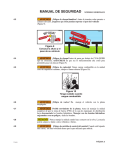
1
Version 10.6 Ensure before Welding™ User Manual SWANTEC Software and Engineering ApS March 2011 SORPAS® User Manual Version 10.6 SORPAS® is the professional welding software for Simulation and Optimization of Resistance Projection And Spot welding processes SORPAS® is professional welding software specialized in resistance welding. It has been designed for and used by engineers in industry including automotive, steel making, welding equipment, electronics and other metal processing industries. It has been used to support design and evaluation of the weldability of materials, design and selection of electrodes, as well as to directly support the optimization and planning of weld schedules with optimal welding process parameters. With the functions for estimating the properties of welds after welding, SORPAS® has also been applied for quality assurance. SORPAS® is developed for engineers by engineers. The user-friendly graphic user interface with engineering language familiar to engineers has made it a very unique and powerful tool for applications in industry. According to the practice of users, a 1-2 days training has been sufficient for welding or design engineers to learn and start using SORPAS®. The special features of SORPAS® can be summarized as follows: Professional Straightforward Easy-to-use - specialized and verified in resistance welding - designed and applied for industrial applications - developed for engineers directly to use in industry ©2011 SWANTEC Software and Engineering ApS - www.swantec.com -1- SORPAS® User Manual Version 10.6 What’s new in SORPAS® 10? With this new version, all models and functions in the entire system of SORPAS® have been thoroughly tested and improved based on many valuable feedbacks and requirements from users as well as our own tests and verifications. All known issues have been corrected. Many new functions have been developed and implemented. For example, the new landmark Weld Planning function can automatically predict the fully optimized weld schedule specifications (WSS) including optimized weld current, weld force, weld time and hold time, simply according to user defined Weld Task Description (WTD) defining only the sheets, electrodes, type of weld machine and the desired weld quality. The key new updates comparing to previously released SORPAS® 9.0 are described below: Weld Planning to predict the optimized weld force, time and current with the process window (see figure above). a. WTD – Weld Task Description is the new input window for specifying a weld task. As the purpose of the Weld Planning is to find the optimal welding process parameters, the WTD will only need information about the sheets, electrodes, type of welding machine, and the desired weld quality. b. User preferences is for user preferred planning strategy. The welding process window will be predicted by SORPAS®. The user can choose the weld current at a preferred percentage to the splash (expulsion) limit. Users have also freedom to give preferred input values to other parameters, for example to specify weld force, weld time, or number of pulse, or simply let SORPAS® to fully optimize by leaving the parameters at 0. c. WSS – Weld Schedule Specifications is the result of the Weld Planning with the optimized welding process parameters and the welding process window as well as the weld quality results simulated with the optimal welding process parameters. Multiple welds can be simulated now with continuous simulation of repetitive welding with the same electrodes but renewed sheets for every weld. The Idle time is introduced after Off-time (with possibility for using a larger time step) to speed up simulation of cooling between welds. The heating and cooling history in electrodes is continuously accumulated through all welds. Many other updates for improved accuracy and graphic user interfaces. ©2011 SWANTEC Software and Engineering ApS - www.swantec.com -2- SORPAS® User Manual Version 10.6 Contents WHAT’S NEW IN SORPAS® 10? ........................................................................................................................ 2 BEFORE YOU START ............................................................................................................................................ 5 SYSTEM REQUIREMENTS ......................................................................................................................................... 5 INSTALLATION OF SORPAS® ................................................................................................................................ 5 EDITIONS OF SORPAS® ....................................................................................................................................... 6 ADD-ON MODULES .............................................................................................................................................. 8 STARTING SORPAS®............................................................................................................................................ 9 CHAPTER 1 INTRODUCTION ........................................................................................................................ 11 1.1 WHAT IS FEM ............................................................................................................................................. 11 1.1.1 Mesh density ............................................................................................................................. 11 1.1.2 Time step .................................................................................................................................... 12 1.2 HOW TO MAKE SIMULATIONS WITH SORPAS® .............................................................................................. 13 1.3 APPLICATIONS OF SORPAS® ...................................................................................................................... 14 1.3.1 Evaluation of weldability of new materials and designs ............................................... 14 1.3.2 Optimization of process parameter settings .................................................................... 15 1.3.3 Prediction of the weld quality and properties after welding........................................ 15 1.3.4 Production maintenance ....................................................................................................... 16 1.3.5 Education and training ........................................................................................................... 16 CHAPTER 2 EXAMPLES .................................................................................................................................. 17 2.1 S1-S1.DAT .................................................................................................................................................. 20 2.2 S1-S1_COATING.DAT ................................................................................................................................. 21 2.3 3-SHEETS.DAT .............................................................................................................................................. 22 2.4 S1-S1_GAP-1FORCE.DAT ........................................................................................................................... 23 2.5 S1-S1_GAP-2FORCE.DAT ........................................................................................................................... 24 2.6 DP-TRIP_WATERCOOL.DAT ......................................................................................................................... 25 2.7 CROSS-WIRE.DAT ....................................................................................................................................... 26 2.8 S1-S1_GROWTH-CURVE.FIL – WELD GROWTH CURVE ..................................................................................... 27 2.9 S1-S1_LOBE-TIME.FIL – WELDABILITY LOBE (CURRENT-TIME) ............................................................................ 28 2.10 S1-S1_LOBE-FORCE.FIL – WELDABILITY LOBE (CURRENT-FORCE) ................................................................... 29 CHAPTER 3 USING SORPAS® ....................................................................................................................... 30 3.1 INPUT WIZARD ............................................................................................................................................. 30 3.2 WELD PLANNING AND WTD ........................................................................................................................ 37 3.3 EDIT DATA FILE ............................................................................................................................................. 38 3.3.1 Define geometry and materials ........................................................................................... 39 3.3.2 Define 3D geometries with the Block Model .................................................................... 49 3.3.3 Specify machine settings ...................................................................................................... 52 3.3.4 Define simulation control parameters ................................................................................ 57 3.3.5 Define process simulation for single weld or multiple welds ....................................... 60 3.3.6 Define optimization procedures .......................................................................................... 62 ©2011 SWANTEC Software and Engineering ApS - www.swantec.com -3- SORPAS® User Manual Version 10.6 3.4 PREFERENCES .............................................................................................................................................. 66 3.5 RUNNING SIMULATIONS ............................................................................................................................... 67 3.5.1 Run process simulation for single weld or multiple welds ............................................. 67 3.5.2 Run batch simulations ............................................................................................................ 68 3.5.3 Run optimization procedures................................................................................................ 70 3.5.4 Run Weld Planning ................................................................................................................... 72 3.5.5 Simulation watcher .................................................................................................................. 73 3.6 DISPLAY RESULTS AND ANIMATIONS ............................................................................................................. 74 3.6.1 Process parameter curves .................................................................................................... 75 3.6.2 Nodal value curves ................................................................................................................. 77 3.6.3 WGC - Weld Growth Curve ................................................................................................... 79 3.6.4 WBL - Weldability Lobes ......................................................................................................... 80 3.6.5 WSS – Weld Schedule Specifications .................................................................................. 81 3.6.6 Report of simulation ................................................................................................................ 82 3.6.7 Final Temperature Distribution and Weld Results ............................................................. 82 3.6.8 Animations ................................................................................................................................. 84 3.7 DISPLAY METALLURGY RESULTS ..................................................................................................................... 89 3.7.1 Distribution of Peak Temperature ........................................................................................ 90 3.7.2 Distribution of Cooling Rate at 700°C ................................................................................. 91 3.7.3 Distribution of Cooling Time from 800°C to 500°C ........................................................... 92 3.7.4 Distribution of Volume Fraction of Austenization ............................................................. 93 3.7.5 Distribution of Volume Fraction of Martensite Formation .............................................. 94 3.7.6 Distribution of Hardness .......................................................................................................... 95 3.8 DISPLAY THE RESULTS OF RESIDUALS .............................................................................................................. 95 3.8.1 Distribution of Residual Stresses ........................................................................................... 96 3.8.2 Distribution of Cracking Risks................................................................................................ 96 3.9 DATABASES ................................................................................................................................................. 98 3.9.1 Material database ................................................................................................................... 98 3.9.2 Electrode database .............................................................................................................. 101 3.9.3 Workpiece database ............................................................................................................ 105 3.9.4 Machine database................................................................................................................ 107 3.10 OTHER FUNCTIONS .................................................................................................................................. 109 3.10.1 View ........................................................................................................................................ 109 3.10.2 Help ......................................................................................................................................... 110 CHAPTER 4 ERROR MESSAGES .................................................................................................................. 111 4.1 4.2 4.3 4.4 ERRORS RELATED TO DATA FILES................................................................................................................... 111 ERRORS RELATED TO INPUT DATA AND MESH GENERATION ............................................................................. 111 RUN TIME ERRORS ...................................................................................................................................... 113 REMARKS .................................................................................................................................................. 114 APPENDIX END-FACE IN Z FOR BLOCK MODEL .................................................................................... 115 ©2011 SWANTEC Software and Engineering ApS - www.swantec.com -4- SORPAS® User Manual Version 10.6 Before You Start System Requirements SORPAS® is professional welding software for simulation and optimization of resistance welding processes directly for industrial applications. The following system specifications are recommended: Operating system: Processor: RAM: Hard disk free space: Graphic mode resolution: Windows XP / Vista / Windows 7 2.0 GHz or higher 1 GB or higher 10 GB or higher 1024x768 or higher It is always beneficial to use the fastest computer available. For an efficient computation speed especially for optimization procedures, the processor speed shall be preferably faster than 2.5 GHz. Installation of SORPAS® Depending on the method of delivery, the procedure for installation is as follows: Delivery by CD: Insert the CD of SORPAS® into the CD drive of the licensed computer. The installation program will start automatically. In case the installation procedure is not started automatically, click the “Start” menu of Windows and click “Run…”, then type the following and click OK: D:\Install (if the CD drive is other than “D”, type the correct letter instead) Follow the instructions to go through the installation procedures. Delivery by Web-downloading: All licensed users have obtained a special link to their user account at the website of SWANTEC, on which the user information and links to downloading are stated. ©2011 SWANTEC Software and Engineering ApS - www.swantec.com -5- SORPAS® User Manual Version 10.6 1) Download the installation program (usually in zipped format). 2) Start the downloaded program “Install.exe”. All program components of SORPAS including standard databases will be installed. 3) Typical case studies are presented in the “Gallery” at the SWANTEC website. After installing SORPAS® on the hard disk, three shortcuts will be automatically created in the menu list of Programs in the Start menu and also on the desktop: o o o “SORPAS 10.6 Enterprise” for starting the simulation software. “Watcher 10.6” for watching the simulation progress while it is running. “SORPAS 10.6 User Manual” for the PDF version of this user manual. Editions of SORPAS® Three editions of SORPAS® have been released including the Standard Edition, the Professional Edition and the Enterprise Edition. The automated procedures for optimization of the weld current, prediction of the weldability lobes and verification of the contact resistance are available only in the Enterprise Edition which gives users the ultimate benefits to ensure developments and optimizations before welding. The following table shows the different functions included in each Edition. Explanations of the main functions: • • Graphic user interface for data input: including the Input Wizard and the Data file editor for design of geometries and selection of materials (from integrated databases) for electrodes, weld parts and coatings, and settings of welding process parameters. Automatic mesh generation: to automatically generate FEM mesh for spot welding according to user defined number of elements and density distributions. ©2011 SWANTEC Software and Engineering ApS - www.swantec.com -6- SORPAS® User Manual • • • • • • • • • • • Version 10.6 Electrical model: calculates the current distribution and heat generation depending on types of weld current and weld material combinations. Thermal model (including metallurgical model): calculates the heat transfer, temperature development, materials properties changing with temperature, and weld nugget formation. Mechanical model: calculates the mechanical reactions including deformation of materials, evolution of contact areas at interfaces, stress and strain status depending on welding machine characteristics and dynamics. Graphic display of results: display of simulation results including curves of process parameters and animations of the evolution of variable distribution (temperature, current etc.) and development of the weld nugget shape and size in each material. Editor for databases: the user interface for editing (adding, removing and modifying) data in the four integrated databases for material properties, electrode forms, designs of workpieces and properties of welding machines. Build-in databases: four databases are integrated in the software system including the material database with properties of most commonly used materials, the electrode database with most standard electrode forms (ISO 5821), the workpiece database for retrievable design of weld parts, and the machine database for properties of welding machines. Single simulation: simulation of one specific welding process with specified electrode and material combinations, and given process parameter settings (weld current, force and time etc.). Batch simulation: to run a batch of simulations following a list of predefined data files of different welding conditions or procedures for process optimization. Automated verification of contact resistance: automatically verify the contact resistance factors against a tested weld nugget size for verifying data of new materials. Automated optimization of weld current: two optimization functions are implemented for optimization of the weld current. One is for automatically running a series of simulations according to user-defined range of weld current from a lower limit to a higher limit with a given increment, whereby the weld growth curve will be generated. The other one is for automatically running simulations to seek for the optimal weld current according to a targeted objective weld nugget size. Automated generation of weldability lobe: two types of the weldability lobes can be generated automatically following the procedures recommended in ISO 14327:2004, where two process parameters are varied. One type is to vary the weld current and time while keep weld force ©2011 SWANTEC Software and Engineering ApS - www.swantec.com -7- SORPAS® User Manual • Version 10.6 constant. The other type is to vary the weld current and force while keep the weld time constant. The splash limits are predicted and the weld ranges are indicated according to three reference weld nugget sizes (minimum nugget diameter, maximum nugget diameter and minimum nugget height penetration in the thinnest outer sheet) which are given by the users. Automated weld planning: This new function can automatically predict the optimal weld schedule specifications (WSS) including optimal weld current, weld force, weld time and hold time, simply according to user defined Weld Task Description (WTD) defining only the sheets, electrodes, type of weld machine and the desired weld quality. Add-on Modules Two add-on modules including the Metallurgical module for prediction of martensite and hardness and the Residual module for prediction of residual stresses and cracking risks in the welds have been developed and released with SORPAS®. These include the following functions: • • • • • • Output of simulation results useful for metallurgical analysis: including distribution of the peak temperature, distribution of the cooling rate at 700°C and distribution of the cooling time from 800°C to 500°C. Prediction of austenization resulted from the heating process depending on the austenization temperatures of the steels. Prediction of martensite formation resulted from the cooling process depending on the martensite start and finish temperatures and the critical cooling rates. Prediction of the hardness distribution depending on the carbon equivalent of the steel and the cooling rate. Residual stress distribution including residual stresses in radial, axial and ring directions resulted from elastic unloading and thermal shrinkage. Cracking risk factor indicating the cracking risks due to residual stresses after welding. ©2011 SWANTEC Software and Engineering ApS - www.swantec.com -8- SORPAS® User Manual Version 10.6 Starting SORPAS® To start SORPAS®, double click the SORPAS icon on the desktop or click the “Start” menu, point to “Programs”, and then click “SORPAS 10.6 Enterprise”. After SORPAS® started, a new window will be displayed with the main menu system as shown in Fig. 1. The functions of the main menu items are explained below. Fig. 1 Main menu system. File: Input: Mesh: Simulation: Batch Run: Optimization: Weld Planning: Results: Animations: Metallurgy: Residuals: View: File management for opening and saving data files and batch files. Prepare or Edit data file with input data for simulation, edit the batch file and set up the Preferences. Generate and view mesh. Run single simulation starting new simulation or continuing from interrupted simulation. Run series of simulations in a queue controlled by a batch file that contains a list of data files to be simulated. Start automated optimization procedures for optimization of weld current, generation of weld growth curve and weldability lobe, as well as verification of contact resistance. Prepare or edit the Weld Task Description (WTD), run fully automated weld planning and show the resulted optimal Weld Schedule Specifications (WSS). Show results of simulation including curves of process parameters, evolution of nodal values and report of simulation. Show animations of the evolution of parameters including temperature distribution, current distribution, stress and strain distribution etc. throughout the entire welding process. Show simulation results of metallurgical properties including distribution of hardness and martensite formation etc. Show results of Residual stresses, residual strains and cracking risks. Options and operations of graphic display. ©2011 SWANTEC Software and Engineering ApS - www.swantec.com -9- SORPAS® User Manual Database: Help: Version 10.6 Edit and modify databases of materials, electrodes, workpieces, and machines. Information about the user and SORPAS®. It is recommended that all new users of SORPAS® shall take the training course (1-2 days) on the fundamental knowledge and the practical procedures for using the software with hands-on exercises before starting to work with SORPAS®. In this User Manual, brief background knowledge and general introduction of SORPAS® are given in Chapter 1. The examples for applications of SORPAS® are presented in Chapter 2. The instructions on operations of SORPAS® are described in Chapter 3. ©2011 SWANTEC Software and Engineering ApS - www.swantec.com - 10 - SORPAS® User Manual Version 10.6 Chapter 1 Introduction SORPAS® is professional welding software for Simulation and Optimization of Resistance Projection And Spot welding processes. It is developed with an integration of the FEM and the engineering welding expertise. It is commercially applied in industry for supporting evaluation of the weldability of weld combinations and the design of parts and electrodes, as well as optimization of the process parameter settings in resistance welding. 1.1 What is FEM The finite element method (FEM) is used in SORPAS® for the numerical simulations. The FEM is a numerical method widely applied for engineering analysis. The main idea of FEM is that a complex engineering problem can be solved by dividing into a number of simple pieces or elements. When the problem is solved in each piece or element, the solution of the entire problem can be obtained by an assemblage of all pieces or elements. Due to this universal procedure, FEM can be used to solve nearly all kinds of engineering problems with very complex geometry and material combinations. After many years research and development according to industrial applications, all numerical procedures have been developed and fully automated in the system of SORPAS®. The user interface of SORPAS® is designed with professional language and engineering expertise in resistance welding. Due to this, many users have started using SORPAS® without prior knowledge of the FEM. Most of users are welding engineers working in industry. It is always helpful to get some basic knowledge of the FEM in order to better understand the software and to make more reliable simulations. More detailed fundamental knowledge of the FEM will be introduced at the training course, we hereby emphasize two basic concepts that have essential influence on simulations. 1.1.1 Mesh density The mesh density or the size of elements has essential influence on the accuracy of FEM calculations regarding to distribution of variables in geometry or in the materials. ©2011 SWANTEC Software and Engineering ApS - www.swantec.com - 11 - SORPAS® User Manual Version 10.6 As the basic concept of FEM, the problem domain (geometry and materials) is divided into a number of elements (or mesh). The procedure to divide the domain into elements is called mesh generation. In SORPAS® the four-sided (or quadrilateral) shape elements are used. The FEM calculations are mainly based on the values of variables on nodal points and the interpolation between the nodal points inside the elements. The more nodal points or elements are divided, the more accurate results can be obtained for the geometrical distribution of variables. Increasing the total number of elements will increase the elements in local areas, but also increase the number of calculations or the time of computation. It will be efficient to get only more elements in the areas with large changes (or gradients) of variables but fewer elements in the areas with small changes while still keeping the total elements in a reasonable number. This is the reason that the mesh density control is introduced to allow users to define where to get more elements (or high mesh density) at a specified total number of elements. In SORPAS® seven density control points are generated automatically as default. They are located around the weld combination with two high mesh density points in the center area between the electrodes. Users may relocate or modify the high density points to the area with most changes or add more density control points to get better mesh distribution. For more details, please read Section 3.3.1. 1.1.2 Time step In order to calculate the highly non-linear and dynamic changes of variables through the welding process, the process time is divided into small steps during simulations. The FEM calculations will be carried out incrementally through the entire welding process to simulate the dynamic changes or the gradients of variables in time, such as the temperature development in resistance welding process. The time step has essential influence on the accuracy of FEM simulations regarding to the dynamics of variables changing in time. The smaller the time step is divided, the more accurate results can be obtained regarding to the dynamic changes of variables. But it will also increase the number of calculations thus the computation time. In SORPAS® it is possible to use individual time steps for simulations in different stages of the resistance welding process, namely the squeeze, weld, hold, off and idle stages. Users can also decide how often to save the simulation results for showing animated display of the results by skipping some steps especially when using smaller time steps. For more details, please read Section 3.3.4. ©2011 SWANTEC Software and Engineering ApS - www.swantec.com - 12 - SORPAS® User Manual Version 10.6 1.2 How to make simulations with SORPAS® Simulation with SORPAS® is a virtual resistance welding process on a computer. The only difference from the actual welding process is that the whole process, from design to welding, is done on the computer without using actual materials and welding equipment. Users will see the welding results virtually on the computer. In this way, the welding engineers can evaluate the weldability of materials, design parts and electrodes and optimize process parameter settings before performing actual welding tests. The procedure of making simulation with SORPAS® is similar to the procedure of doing practical welding process, which can be divided into the following three steps: • • • Data preparation - the materials and geometries of the workpieces and electrodes are defined, the type of welding machine is selected and the process parameters are specified. Running simulation of welding - the parts are welded in the selected welding machine with the specified process parameter settings. The simulations can be carried out in four ways: single simulations, batch simulations, automated optimizations and weld planning. Evaluation of results - the results of welding and quality of weld are evaluated thus the design and parameter settings are verified. With the optimization procedures the weld growth curve and the weldability lobes can be obtained. With the newly implemented metallurgical and residual modules, the microstructures and the hardness as well as residual stresses and cracking risks in the welds can be predicted. The input data for preparation of simulation with SORPAS® can be summarized as below: 1) Geometry and materials: o Define geometry and select materials of workpieces o Define thickness and select materials of coatings o Define forms and select materials of electrodes o Define contact interfaces between materials (for spot welding this is automatically done with Input Wizard) 2) Machine settings: o Define mounting of electrodes (or connection of electrode to machine) o Select welding machine ©2011 SWANTEC Software and Engineering ApS - www.swantec.com - 13 - SORPAS® User Manual o o Version 10.6 Define water cooling parameters Set welding process parameters 3) Simulation control: o Define time step and interval for saving result files o Select numerical models and define accuracy of each model o Set optimization procedures (weld growth curves, weldability lobes etc.) After all the input data are prepared, the simulation can be started simply by clicking a button. The simulation will then run automatically. The results will be saved along with the progress of simulation, which will be used later for analysis and graphical display including the process parameter curves, animations for the dynamic development of weld nugget and temperature distribution in the materials etc. In order to facilitate industrial applications of SORPAS®, four databases have been established and integrated in the system of SORPAS®. The material database includes mechanical and metallurgical properties of most commonly used materials. The electrode database includes standard and user defined forms of electrodes. The workpiece database is for frequently used product designs defined by users. The machine database is for properties and capabilities of different welding machines. With the Input Wizard and support of the databases, SORPAS® becomes much easier to use directly by engineers and more adequate for industrial applications. 1.3 Applications of SORPAS® SORPAS® has been widely applied for evaluation of the weldability of materials and supporting design of products and electrodes, as well as optimization of process parameter settings in various industrial sectors. Before doing real welding tests, the joint design and the welding process parameter settings can be tested and optimized already on a computer. With this innovative method, the development time and cost, and the lead time to production can be significantly reduced. The applications and benefits of SORPAS® are summarized below: 1.3.1 Evaluation of weldability of new materials and designs With the user-friendly graphic user interface in SORPAS®, it is easy to draw geometries of workpieces and electrodes as well as to select materials for each ©2011 SWANTEC Software and Engineering ApS - www.swantec.com - 14 - SORPAS® User Manual Version 10.6 part of the weld combination from the integrated material database. This makes the evaluations of different designs and weldability of new materials much easier. For example, spot welding of multiple sheets with different materials and complex thickness combinations can be easily simulated where the optimal weld current can also be predicted. The design of joints in projection welding can be evaluated and tested with simulations before real welding tests. By making simulations with different forms of electrodes, the optimal electrode form can be determined according to the results of welding simulations. By making simulations with different materials of the electrodes, the optimal material of electrode can be determined. The same evaluations and optimizations can be made for surface coatings. 1.3.2 Optimization of process parameter settings A tedious job of welding engineers doing everyday is to optimize the process parameter settings for every specific weld combination. In many cases the design and materials of the joints have been decided by preceding production stages, for example stamping. This leaves the welding engineers only the possibilities for selecting the form and material of the electrodes and optimizing the welding process parameters. With support of SORPAS®, the process parameter settings can be optimized by running simulations with the automated procedures. In SORPAS®, there types of the parameter optimizations can be automatically carried out. One for weld current optimization by automatically generating the weld growth curve at given weld force and time. The weld current range can be predicted with indication of splashes. The other is for prediction of the complete weldability lobes. Two types of weldability lobes can be generated: 1) with varying weld current and time but constant weld force and 2) with varying weld current and force but constant weld time. The weldability lobes can be predicted with reference to the user specified reference nugget sizes (minimum nugget diameter, maximum nugget diameter and minimum nugget height penetration in the thinnest outer sheet). The splash limits are predicted automatically. The third option is to use the weld planning features where SORPAS® automatically finds the most optimal welding parameters (force, time, pulses and current) based on an iterative simulation process. 1.3.3 Prediction of the weld quality and properties after welding With the newly added functions for simulations of the metallurgical properties and residuals, it is possible to predict the distribution of austenization and martensite formation, distribution of hardness as well as residual stresses and cracking risks in ©2011 SWANTEC Software and Engineering ApS - www.swantec.com - 15 - SORPAS® User Manual Version 10.6 the welds after welding. The weld strengths are also calculated referring to the test methods described by the ISO standards including Cross Tension Strength (ISO 14272:2000), Shear Strength (ISO 14273:2000) and Peel Strength (ISO 14270:2000). So it is possible to optimize the welding process window and parameters according to the resulted weld strengths. 1.3.4 Production maintenance SORPAS® can also be applied for troubleshooting welding problems in existing production lines. By applying the same design of the workpieces and the electrodes with the actual process parameter settings, the welding process can be simulated and evaluated on the computer. The development of temperature and the formation of the weld nugget can be illustrated graphically on the computer throughout the entire welding process. In this way, it is possible to identify the reasons for the problems and to understand why and when the problem occurs in the process thus to find out solutions for the problems. This can help the welding engineers near production lines to diagnose and solve the welding problems in a very efficient way. 1.3.5 Education and training SORPAS® has been designed with engineering expertise in resistance welding and equipped with graphical illustrations of the welding process. It has been frequently applied for supporting education and training for new engineers to get into the welding job much more quickly. ©2011 SWANTEC Software and Engineering ApS - www.swantec.com - 16 - SORPAS® User Manual Version 10.6 Chapter 2 Examples In order to demonstrate how SORPAS® can be used for actual applications, seven examples for single simulation, one example for weld growth curve and two examples for weldability lobes are included in the software package. The descriptions and purposes of the examples are presented in Table 1. Table 1 The examples and their purposes. Filename How to open Description s1-s1.dat File -> Spot welding of two 1 Open Data File mm mild steel sheets S1-s1_Coating.dat File -> Open Data File 3-sheets.dat File -> Open Data File s1-s1_Gap-1force.dat File -> Open Data File s1-s1_Gap-2force.dat File -> Open Data File Spot welding of two 1 mm mild steel sheets with galvanized coating Spot welding of 3 sheets with 0.8 mm low carbon steel, 1.5 mm HSLA and 1.5 mm DP600. Spot welding of two 1 mm mild steel sheets with a gap between the sheets before welding. Only upper electrode is moving by force. Spot welding of two 1 mm mild steel sheets with a gap between the sheets before welding. Both electrodes are moving by force ©2011 SWANTEC Software and Engineering ApS - www.swantec.com Purposes of the example To show the basic procedures for data preparation and results of simulation To show how to simulate spot welding of materials with coating To show how to simulate spot welding of 3-sheets with dissimilar metals and different thickness, and the difficulty of welding the thin low carbon steel To show how to simulate spot welding with gap between the sheets before welding To show how to simulate spot welding with gap between the sheets before welding - 17 - SORPAS® User Manual Version 10.6 DP-TRIP_ watercool.dat File -> Open Data File Spot welding of 1.5 mm DP600 to 1.2 mm TRIP700 steel sheets with water cooling in the electrodes Cross-Wire.dat File -> Open Data File s1-s1_growthcurve.fil File -> Open Batch File File -> Open Batch File Cross wire welding with diameters of ø2 mm applying the 2.5D block model Weld growth curve for spot welding of two 1 mm mild steel sheets Weldability lobe with varying weld current and time and constant force for spot welding of two 1 mm mild steel sheets. Weldability lobe with varying weld current and force and constant time for spot welding of two 1 mm mild steel sheets. s1-s1_lobe-time.fil s1-s1_lobe-force.fil File -> Open Batch File To show how to simulate with water cooling in electrodes and to demonstrate the metallurgical and residuals results To show how to simulate 3D geometries with the 2.5D treatment in SORPAS® To show the predicted weld growth curve To show the predicted weldability lobe To show the predicted weldability lobe In order to understand how SORPAS® works, it is recommended that new users shall first view the examples to get familiar with the main functions of the software system. After knowing the basic procedures for making simulations, it will be helpful to try a couple of simulations by just redoing the examples with the same conditions or with simple modifications (remember first to duplicate the data file to a new file name with the “Save As” function before making modifications). Opening single simulation examples: The single simulation examples can be opened by clicking on the menu item File and then clicking Open Data File, and then browse for the data file (*.dat) to be opened. Opening batch simulation examples: The batch simulation examples including the weld growth curve and the wedability lobes can be opened by clicking on the menu item File and then clicking Open Batch File, and then browse for the batch file (*.fil) to be opened. When a batch file is opened a series of the data files will be loaded, while one data file is opened at a time whose name is shown at the top title bar. ©2011 SWANTEC Software and Engineering ApS - www.swantec.com - 18 - SORPAS® User Manual Version 10.6 Editing Data Files: The detailed data of each data file can be seen and edited in the Input menu by clicking Edit Data File, which include geometry / materials, machine and process parameters etc. Viewing Simulation Results: The results of simulation can be seen in the Results menu, including the process parameter curves, nodal value curves, weld growth curves, weldability lobes. The final size of the weld nugget with width and height of the weld nugget in each workpiece is shown together with the Final Temperature Distribution and Weld Results. Animated display of variable distributions can be displayed by the Animations menu and then find which variable to show. The metallurgical results can be seen in the Metallurgy menu. The residual results can be seen in the Residuals menu. The weld strengths are presented with the Final Temperature Distribution and Weld Results, the Weld Growth Curves and the Weldability Lobe Curves. The examples are presented as follows. For more details about how to make simulations with SORPAS®, please refer to Chapter 3. ©2011 SWANTEC Software and Engineering ApS - www.swantec.com - 19 - SORPAS® User Manual Version 10.6 2.1 s1-s1.dat The example “s1-s1” is for simulation of spot welding of two 1 mm mild steel sheets using type B electrode with a conical tip face diameter of 6mm. This example has also been used in Chapter 3 for describing the main functions of the software. The process parameters used for the simulation are shown in Table 2. The report of simulation generated by SORPAS® is shown in Fig. 2. Table 2 Welding parameters for spot welding example s1-s1. Filename Squeeze time Weld time Hold time Current (RMS) s1-s1 [ms] 40 [ms] 160 [ms] 100 [kA] 8.3 Current type AC Force [kN] 2.2 Fig. 2 The report of simulation generated by SORPAS® for example “s1-s1”. The upper part is the welding conditions and the lower part is the main simulation results. ©2011 SWANTEC Software and Engineering ApS - www.swantec.com - 20 - SORPAS® User Manual Version 10.6 2.2 s1-s1_Coating.dat The example “s1-s1_Coating” is to show how surface coating can be introduced and simulated. The electrode geometry and the sheets are the same as in example “s1-s1”. The process parameters used for the simulation are shown in Table 3, and the report of simulation generated by SORPAS® is shown in Fig. 3. Table 3 Weld parameters for example s1-s1_Coating. Filename Squeeze time Weld time Hold time s1-s1_Coating [ms] 40 [ms] 240 Current (RMS) [ms] 80 [kA] 8.4 Current type AC Force [kN] 2.2 Fig. 3 The report of simulation generated by SORPAS® for example “s1-s1_Coating”, the upper part is the welding conditions and the lower part is the main simulation results. ©2011 SWANTEC Software and Engineering ApS - www.swantec.com - 21 - SORPAS® User Manual Version 10.6 2.3 3-sheets.dat The example “3-sheets” is a simulation of three-sheet spot welding with one 0.8 mm mild steel sheet, one 1.5 mm HSLA steel sheet and one 1.5 mm DP600 steel sheet. The electrode is type B with a tip face diameter of 6 mm. This example also shows the use of multi pulses during welding. The welding process parameters used for the simulation are shown in Table 4, and the report of simulation generated by SORPAS® is shown in Fig. 4. Table 4 Weld parameters for example 3-sheets. Filename Squeeze time Weld time Hold time [ms] 3-sheets 40 [ms] 3 pulses of 180 ms Current (RMS) [ms] [kA] Current type (3 pulses) 300 11.0 AC Force 4.3 [kN] Fig. 4 The report of simulation generated by SORPAS® for example “3-sheets”, the upper part is the welding conditions and the lower part is the main simulation results. ©2011 SWANTEC Software and Engineering ApS - www.swantec.com - 22 - SORPAS® User Manual Version 10.6 2.4 s1-s1_Gap-1force.dat The example “s1-s1_Gap-1force” is to illustrate how spot welding with a gap of 0.2 mm between the sheets before welding can be simulated. The electrode is type B with conical shape and a tip face diameter of 6 mm. In this example, only the upper electrode is moving with controlled force. The process parameters used for the simulation are shown in Table 5, and the report of simulation generated by SORPAS® is shown in Fig. 5. Table 5 Weld parameters for example s1-s1_Gap-1force. Filename Squeeze time Weld time Hold time Current (RMS) s1-s1_Gap1force [ms] [ms] [ms] [kA] 40 160 120 8.6 Current type Force AC 2.4 [kN] Fig. 5 The report of simulation generated by SORPAS® for example “s1-s1_Gap-1force”, the upper part is the welding conditions and the lower part is the main simulation results. ©2011 SWANTEC Software and Engineering ApS - www.swantec.com - 23 - SORPAS® User Manual Version 10.6 2.5 s1-s1_Gap-2force.dat The example “s1-s1_Gap-2force” is to illustrate how spot welding with a gap of 0.2 mm between the sheets before welding can be simulated. The electrode is type B with conical shape and a tip face diameter of 6 mm. In this example, both electrodes are moving with equally controlled force. The process parameters used for the simulation are shown in Table 6, and the report of simulation generated by SORPAS® is shown in Fig. 6. Table 6 Weld parameters for example s1-s1_Gap. Filename Squeeze time Weld time Hold time s1-s1_Gap2force Current (RMS) [ms] [ms] [ms] [kA] 40 160 120 8.4 Current type Force AC 2.4 [kN] Fig. 6 The report of simulation generated by SORPAS® for example “s1-s1_Gap-2force”, the upper part is the welding conditions and the lower part is the main simulation results. ©2011 SWANTEC Software and Engineering ApS - www.swantec.com - 24 - SORPAS® User Manual Version 10.6 2.6 DP-TRIP_watercool.dat The example “DP-TRIP_watercool” describes a spot welding of 1.2 mm TRIP700 steel to a 1.5 mm DP600 steel with water cooling in electrodes. The cooling process is fully completed, therefore all metallurgical and residual results can be shown with this example. The electrode is type B with conical tip face of diameter of 8 mm. The process parameters used for the simulation are shown in Table 7, and the report of simulation generated by SORPAS® is shown in Fig. 7. Table 7 Weld parameters for example s1-s1_watercool. Filename Squeeze Weld Hold Off time time time time [ms] [ms] [ms] [ms] DP-TRIP_ 40 200 1000 500 watercool.dat Current (RMS) [kA] Current type Force 8.5 AC 4.0 [kN] Fig. 7 The report of simulation generated by SORPAS® for example “s1-s1_watercool”, the upper part is the welding conditions and the lower part is the main simulation results. ©2011 SWANTEC Software and Engineering ApS - www.swantec.com - 25 - SORPAS® User Manual Version 10.6 2.7 Cross-Wire.dat The example “Cross-Wire” is a simulation of the cross-wire welding of steel wires with diameter of ø2 mm. One wire is perpendicular (going in) to the screen and the other wire is parallel to the screen. This example shows how to define 3D geometries using the Block model with the 2.5D treatment. The process parameters used for the simulation are shown in Table 8, and the report of simulation generated by SORPAS® is shown in Fig. 8. Table 8 Weld parameters for example Cross-Wire. Filename Squeeze time Weld time Hold time Cross-Wire [ms] 20 [ms] 40 Current (RMS) [ms] 40 [kA] 1.50 Current type DC Force [kN] 0.6 Fig. 8 The report of simulation generated by SORPAS® for example “Cross-Wire”, the upper part is the welding conditions and the lower part is the main simulation results. ©2011 SWANTEC Software and Engineering ApS - www.swantec.com - 26 - SORPAS® User Manual Version 10.6 2.8 s1-s1_growth-curve.fil – weld growth curve The weld growth curve can be simulated with a series of data files automatically created with increasing weld currents from a lower limit (2 kA) to a higher limit (15 kA) with an increment (1 kA). The series of data files are automatically generated in a sub-folder and included in the batch file “s1-s1_growth-curve.fil”. It can be opened by “Open Batch File”. After opening this batch file, the simulated weld growth curve is displayed as shown in Fig. 9. Fig. 9a is the weld growth curve with weld nugget diameters. Fig. 9b is the weld growth curve with weld Cross Tension Strengths. The red points indicate splashes (expulsions) at the interfaces between the sheets or over sized weld nuggets, the purple points indicate electrode melting (simulation can be set to automatically stop when the electrode melts which will result in slightly smaller nugget due to unfinished simulation). The black points with open markers indicate no weld and that with solid markers indicate undersized welds. The green points indicate the welds within the welding process window. In Fig. 9b, the open markers show interface failure and solid markers show plug failure together with the resulting weld strengths by cross tension tests. Similarly, it is also possible to show the weld growth curves with the Weld Shear Strength and the Weld Peel Strength. More details on how to prepare data for making the weld growth curve are described in Section 3.3.6. (a) (b) Fig. 9 Weld growth curve for spot welding of two 1 mm mild steel sheets with weld time of 10 cycles and weld force of 3 kN. ©2011 SWANTEC Software and Engineering ApS - www.swantec.com - 27 - SORPAS® User Manual Version 10.6 2.9 s1-s1_lobe-time.fil – weldability lobe (current-time) The weldability lobe can be simulated with a series of data files automatically created by varying two process parameters namely the weld current and weld time. It is organized with increasing weld time from a lower limit (e.g. 4 cycles) to a higher limit (16 cycles) with an increment (2 cycles), and for each weld time increasing weld current from a lower limit (4 kA) to a higher limit (16 kA) with an increment (1 kA). The limits can be from the welding machine limits or with a wider range so that the software will find the actual welding process window. The series of data files are automatically generated in a sub-folder and included in the batch file “s1-s1_lobe-time.fil”. It can be opened by “Open Batch File”. After opening this batch file, the weldability lobe is displayed first with weld nugget diameters, see Fig. 10a. The red color points indicate oversized weld nugget or splashes at interfaces between sheets. The orange color indicates a profound likely hood of splash occurring. The purple color points indicate electrode melting. The gray color points with open markers indicate no weld and solid markers indicate undersized welds. The green points indicate welds with a weld nugget in between the maximum and minimum weld nugget diameters as seen in Fig. 10a. The weldability lobe can also be shown with Cross Tension Strength, Shear Strength and Peel Strength, see Fig. 11b, where the open markers indicate Interface Failure and solid markers indicate Plug Failure. More details on how to prepare data for making the weldability lobes are described in Section 3.3.6. (a) (b) Fig. 10 Weldability lobe with varying weld current and time but constant weld force for spot welding of two 1 mm mild steel sheets. ©2011 SWANTEC Software and Engineering ApS - www.swantec.com - 28 - SORPAS® User Manual Version 10.6 2.10 s1-s1_lobe-force.fil – weldability lobe (current-force) The weldability lobe can be simulated with a series of data files automatically created with two varying process parameters, in this case the weld current and the weld time. It is organized by increasing weld force from a lower limit (2.5 kN) to a higher limit (5 kN) and an increment (0.5 kN), and for each weld force with increasing weld current from a lower limit (4 kA) to a higher limit (14 kA) with an increment (1 kA). The limits can be from the welding machine limits or with a wider range so that the software will find the actual welding process window. The series of data files are automatically generated in a sub-folder and included in the batch file “s1-s1_lobe-force.fil”. It can be opened by “Open Batch File”. After opening this batch file, the weldability lobe is displayed first with the weld nugget diameters, see Fig. 11a. The red points indicate oversized weld nugget or splashes at the interfaces between sheets. The orange color indicates a profound likely hood of splash occurring. The purple points indicate electrode melting. The gray points with open markers indicate no weld and with solid markers indicate undersized welds. The green points indicate welds with a nugget in between the maximum and minimum weld nugget diameters as seen in Fig. 11a. The weldability lobe can be shown further with Cross Tension Strength, Shear Strength and Peel Strength, see Fig. 11b, where the open markers indicate Interface Failure and solid markers indicate Plug Failure. More details on how to prepare data for making the weldability lobes are described in Section 3.3.6. (a) (b) Fig. 11 Weldability lobe with varying weld current and force but constant weld time for spot welding of two 1 mm mild steel sheets. ©2011 SWANTEC Software and Engineering ApS - www.swantec.com - 29 - SORPAS® User Manual Version 10.6 Chapter 3 Using SORPAS® In this chapter, we will explain how to use SORPAS® including: • preparing input data, • running simulations and optimizations, • displaying and analyzing the results, and • preparing and editing data in the databases. The Input Wizard is a step by step procedure for preparing the input data which is described in Section 3.1. The data preparation for Weld Planning is explained in Section 3.2. More details for preparing and editing the input data are described in Section 3.3. The use and preparation of the Preferences are described in Section 3.4. The procedures for running simulations, optimizations and Weld Planning are described in Section 3.5. The analysis and display of results are described in Section 3.6. The display of metallurgy results is described in Section 3.7. The display of results for residuals is described in Section 3.8. The databases are described in Section 3.9 and some other functions described in Section 3.10. 3.1 Input Wizard The input data for simulations and optimizations of spot welding can be quickly and easily prepared with the Input Wizard in just 7 steps. The input wizard can be activated for making new data file by clicking the menu item “File” and then clicking “New Input Wizard…”, or for editing existing data file by clicking “Input” and then clicking “Edit Input Wizard…”. Step 1: Define the file name and Problem ID Each case of simulation and optimization shall have a unique file name for the data files to store all input data and to save simulation results. The “Problem ID Name” and the “Note” can be defined to identify the case, see Fig.12. ©2011 SWANTEC Software and Engineering ApS - www.swantec.com - 30 - SORPAS® User Manual Version 10.6 Fig. 12 The Input Wizard step 1: to define the data file name, the problem ID name and note. Step 2: Select welding process The data input and preparation procedures in the Input Wizard are mainly designed for spot welding. The “Go to >> Welding Planning” button will directly get to the window for defining Weld Task Description (WTD) for planning optimal welding parameters (more details in Section 3.2). If projection welding or other resistance welding processes are to be simulated, the Edit Data File window will be used which is more flexible with more detailed data for preparing complex problems, please refer to Section 3.3 for further details. (a) (b) Fig. 13 The Input Wizard step 2: to select the process to be simulated. (a) Spot welding to continue with the Wizard for further data preparation or go to weld planning. (b) Projection welding to switch to the general data editor (more details described in Section 3.3). ©2011 SWANTEC Software and Engineering ApS - www.swantec.com - 31 - SORPAS® User Manual Version 10.6 Step 3: Define sheet combination As shown in Fig. 14, the combination of sheets can be easily built up by giving the number of sheets and then the thickness and material of each sheet. If the sheet is coated, the thickness and material of the coating can be defined similarly. The thickness of coating is given in microns or g/m2 per side. A coating layer is added automatically on both surfaces of the sheet. A Gap between sheets can be added with a given size in mm, either equally at all interfaces or with different sizes separately at individual interfaces. Clamping in Y adds small tools at the edges of the sheets acting as static clamping in Y-direction. Fixing in X makes static clamping at the edges of the sheets in X-direction. Unchecking one will allow free movement in respective direction. The weld stack / combination of materials are built up automatically with interface layers inserted between the sheets, which represent the contact properties. Fig. 14 The Input Wizard step 3: to define the weld combination of sheets. ©2011 SWANTEC Software and Engineering ApS - www.swantec.com - 32 - SORPAS® User Manual Version 10.6 Step 4: Define electrodes As shown in Fig. 15, the electrode design can be selected from the database of electrodes and its material can be selected from the database of materials. More details about the databases are described in Section 3.9. It is recommended to create all new or special electrode designs in the database before preparing the simulations and optimizations. Fig. 15 The Input Wizard step 4: to select the electrodes and their materials from databases. ©2011 SWANTEC Software and Engineering ApS - www.swantec.com - 33 - SORPAS® User Manual Version 10.6 Step 5: Welding machine and current settings The welding machine/gun can be selected from the machine database. The type of electrical power source such as AC, DC and CD is shown at the beginning of the machine name (more details are described in Section 3.9.4). It is possible to limit the process parameters to the machine capabilities by checking the check box “Limit to Machine”. The frequency (e.g. 50 Hz or 60 Hz) for the weld current is defined in the Preferences (more details are described in Section 3.4). It is possible to define multiple pulses with individual RMS value of current for each pulse. Up-slope and down-slope can be defined for each pulse. It is also possible to define a stepped current if the cooling between the pulses is set as 0. Fig. 16 The Input Wizard step 5: to select welding machine and define weld current settings. ©2011 SWANTEC Software and Engineering ApS - www.swantec.com - 34 - SORPAS® User Manual Version 10.6 Step 6: Welding process time and force settings The welding process time can be defined in each stage including squeeze time, weld time, hold time, off-time and idle time. The weld time has been set in connection with the weld current. The squeeze time is the time used to build up and stabilize the weld force. The hold time is for cooling with electrodes sitting on the workpieces. The off-time is for cooling after electrode ejects from the sheets so electrodes and workpieces can continue cooling down separately. The idle time is used mainly for further cooling of electrodes between welds in simulations of multiple welds. The weld force can be given in kN or pounds. It can also be defined how the weld force is applied, from the upper, lower or both electrodes. A weld force profile (or programmable weld force) can be set by specifying multiple force steps. The force level, the force buildup slope and the step time with the same force can be defined to build any force profile. Details of the weld force as function of time can also be defined in the general input data editor as described in Section 3.3.3. Fig. 17 The Input Wizard step 6: to set the welding process time and the weld force. ©2011 SWANTEC Software and Engineering ApS - www.swantec.com - 35 - SORPAS® User Manual Version 10.6 Step 7: Define simulation and optimization procedures. For a single simulation with the given welding parameter settings, it is just a simple click on the Start button to run the simulation. It is also possible to simulate multiple welds by giving the number of welds. Further details on multiple welds are described in Section 3.3.5. The mesh has been automatically generated with high mesh density located in the weld zone. It is possible to define automated optimization procedures for: 1) optimization of the weld current such as prediction of the weld growth curve or optimizing the weld current to achieve a targeted weld nugget size; 2) prediction of the weldability lobes to find the ranges of two welding parameters such as weld current and time or weld current and force. 3) Weld planning for prediction of the optimal weld parameters. More details for the automated optimization procedures are described in Sections 3.3.6. The weld nugget size in diameter or in height can be targeted with options at the overall maximum, overall minimum or at any specified sheet / object. Fig. 18 The Input Wizard step 7 – to select procedure for simulation and optimizations. ©2011 SWANTEC Software and Engineering ApS - www.swantec.com - 36 - SORPAS® User Manual Version 10.6 3.2 Weld Planning and WTD The Weld Planning is a brand new function developed and released with SORPAS® Version 10. It can automatically predict the Weld Schedule Specifications (WSS) with optimal weld current, weld force, weld time and hold time, according to the user defined Weld Task Description (WTD) with information of the sheets, electrodes, type of weld machine and the desired weld quality, see Fig. 19. A Weld Task Number is assigned or manually defined by the user for identification of the weld task. The procedures for defining the sheets and selecting electrodes and welding machine are similar to the Input Wizard as described in Section 3.1 for steps 3-5. When the check box Limit to Max Force of Machine is checked, the maximum force capable to be delivered by the welding machine (given in the Machine Database) will be used as the limit of the weld force during the optimizations. The optimal welding parameters together with the welding process window will be predicted by SORPAS®. The optimal weld current is then chosen at a preferred percentage to the splash (expulsion) limit specified by the user. Fig. 19 The graphic user interface for preparing the Weld Task Description for Weld Planning. ©2011 SWANTEC Software and Engineering ApS - www.swantec.com - 37 - SORPAS® User Manual Version 10.6 It is also possible to set User Preferred Parameters with given values for weld force, weld time, or number of pulse, see Fig. 20. Setting a parameter at 0 will allow SORPAS® to fully optimize that parameter. In case of welding with multiple pulses, it is possible to optimize selected number of pulses by giving the range of the pulse numbers (from … to …). If the levels of weld current are different in different pulses, SORPAS® will keep the ratio of the weld current levels unchanged during the optimizations. The weld current of the pulse number given by Ref. will be used as reference during the optimizations. Fig. 20 User Preferred Parameters for WSS. 3.3 Edit data file The data file can be opened as follows: Click the menu item File, then click Open Data File…; the Open Data File dialog box appears (similar to all standard Windows programs); browse to the folder “…\Work” in the main folder of SORPAS®, then choose for example the “s1s1.dat” file and then press Open. When the data file is correctly opened, the input data editor window will be displayed for new data file, or the final temperature distribution will be displayed if the simulation results had been generated before, or otherwise the mesh will be displayed if mesh was already generated. The input data editor for preparing and editing simulation data can be opened by clicking the menu item “Input” and then clicking “Edit Data File…”. A dialog window for input data of geometry and materials will appear as seen in Fig. 21. ©2011 SWANTEC Software and Engineering ApS - www.swantec.com - 38 - SORPAS® User Manual Version 10.6 Three groups of input data need to be prepared: 1) geometry and materials, 2) machine settings and 3) simulation control parameters. The example “s1-s1.dat” is going to be used to explain the details. Information related to the example is written in Italic. 3.3.1 Define geometry and materials The geometry and materials to be defined include the workpieces, the electrodes, the coatings and the contact interface layers between the workpieces and between the workpiece and the electrode. The geometries of the workpieces and electrodes are defined according to the design of weld parts and electrodes. Fig. 21 Input window for geometry and materials. The interface layers are introduced to represent the contact properties at the interfaces. The geometry of the interface layers is defined according to the geometry of the contact interfaces. The thickness of the interface layer is determined by the roughness of the contacting surfaces and the thickness of the contaminant films, which is usually in an order of 0.005 - 0.05 mm. For large scale applications, e.g. spot welding, the ©2011 SWANTEC Software and Engineering ApS - www.swantec.com - 39 - SORPAS® User Manual Version 10.6 contact layer thickness is usually set as 0.05 mm, while for micro-welding and projection welding the contact layer may be set as 0.01 mm. The procedure for geometry design and material selection will be described below with the example “s1-s1.dat”. In the tab Geometry and Materials the following data should be defined. 1) In the Problem ID Name box, the name of the problem “Spot welding” is written. In the Note box, the condition or note for the problem “steel 1 mm – steel 1 mm” is written. 2) The Type of Geometric Model can be axisymmetric or block model. The axisymmetric model is for cylindrical geometry. The block model is for geometries of 3D shape with a specified thickness or shape of end face in the third dimension. Each object may be defined in different thickness or different shape of end face in Z (this is referred to as 2.5D for treating the 3D problems). Please refer to Section 3.3.2 for more details. The example of spot welding is defined with axisymmetric model. 3) The Symmetry Lines should be selected according to the geometry defined for simulations. For axisymmetric problem, only half of the geometry is needed for simulation thus a vertical symmetry line is used. The vertical symmetry line is only allowed at x=0 and horizontal symmetry line at y=0. The geometry should be placed on the positive side of the symmetry line. 4) Insert and define the geometry of all objects including electrodes, workpieces, coatings and contact interfaces. The contact interface layer should be inserted as an object to represent the contact properties at the interface. The procedure for defining the geometry and materials of each object is as follows: I. Click the Insert button to open the Inserting window, see Fig. 22. The highlighted object can be duplicated. New objects can be inserted as a Duplicate the Current Object (highlighted in yellow color), as a Sheet / Rectangle (defined by a width and a height), as a Thin Layer (defined by a width and a height), as loading from the Workpiece Database, as an object loading from the Electrode Database, as a New object, or load an object From Text File. ©2011 SWANTEC Software and Engineering ApS - www.swantec.com - 40 - SORPAS® User Manual Version 10.6 The Electrode Database and the Workpiece Database are connected respectively to the integrated databases of workpieces and electrodes to select pre-defined designs. More details are described in Sections 3.9.2 and 3.9.3. The New inserts an object with only a starting point that can be extended into any shape. For inserting a new object From Text File, the text file shall be written in text format with a list of corner points at each line with the values of x, y, and the round corner radius “r”. After choosing the shape of the object, the Position to insert must be selected. The object can be inserted On Top or Under Bottom of the existing objects or At Position defined by x and y coordinates in mm (the position refers always to the lower-left corner of the new object). Fig. 22 Input window for inserting new objects. The two steel sheets in the example are inserted as Sheets with a width (W) of 12 mm and thickness (H) of 1 mm. The electrodes are inserted as ISO 5821 Type B0 with a conical tip diameter of 6 mm selected from the Electrode Database. The interface layers are inserted as Thin Layers with a width of 12 mm and thickness of 0.05 mm. II. The geometry of the object can be defined or modified in the box for Definition of the current object with the x and y coordinates of the contour points and the radius of curvature, r, for each contour line. The points must ©2011 SWANTEC Software and Engineering ApS - www.swantec.com - 41 - SORPAS® User Manual Version 10.6 be defined successively in the counter-clockwise direction, if the direction is wrong, “ERR” will be displayed in the centre of the object instead of the object number. The active object is highlighted in yellow color with red lines on the border in the graphics window. The coordinates for the corner points, shown in the list box at the right side, can after selection be modified in the edit box at the left side. The selected point is shown as a red dot in the graphics window. The round corners or curved lines can be defined by giving the radius of the curve. The curved line is always drawn from the current point (the one with value of the radius) to the next point connecting the two points. A positive radius defines a convex round corner while a negative radius defines a concave round corner. In order to avoid confusion in the orientation, an exact half circle should be defined by two pieces of arcs by inserting a middle point. Button “>>” is to insert point co-ordinates below the selected point or otherwise to the end of the list, “<<” is to remove the selected point and “==” is to modify the selected point. The contacting lines between objects should coincide or overlap each other precisely in order to ensure reasonable mesh generation and electric current conduction through the connection of objects. III. The type of each object must be selected among Electrode, Workpiece, Coating (solid materials) or Interface (artificial layer to represent the contact properties). When Electrode, Workpiece or Coating is selected, the material database will automatically be activated with the default material defined in Preferences, after that different categories and name of materials can be selected from the integrated material database. The Interface is introduced as an artificial layer between the loosely contacting surfaces to represent the contact properties. The contact resistance is calculated by the following model: σ ρ contact = 3 s _ soft σn ρ1 + ρ 2 + γρ contaminants 2 where σs_soft is the flow stress of the softer metal of the two in contact, σn is the contact normal pressure at the interface, ρ is the resistivity with subscripts 1 and 2 indicating the two base metals in contact. ρcontaminants is the surface contaminants resistivity due to oxides, oil, water vapor and dirt etc. This value is included in the material database as described in Section 3.9.1. γ is a factor introduced for adjustment and verification of the contact resistance. ©2011 SWANTEC Software and Engineering ApS - www.swantec.com - 42 - SORPAS® User Manual Version 10.6 When Interface is selected, the scaling slider for adjusting the contact resistance (dirty-clean) factor is activated with a default value of 1.0 implying directly taking the values of the surface contaminants resistivity from the material database. It can be changed between 0.1 and 10.0 according to the surface conditions of the materials in contact. When calculating the contact resistance, this factor will be multiplied to the surface contaminants resistivity from the materials database. If the two contacting materials are the same, the surface contaminants resistivity of the material is used for calculating the contact resistance. If the two contacting materials are not the same, the lower surface contaminants resistivity of the two materials is used to calculate the contact resistance. In the example, “ISO 5182 A2-2 Electrode CuCrZr” is chosen for the electrodes (Object 1 and 7) and the steel material “AISI 1005” is chosen for the sheets (Object 3 and 5). For the interface layers a scaling factor of 1.0 is used for all interfaces. IV. Click Move to change the location of one or more objects. The Moving window is shown in Fig. 23. The selected objects can be moved by displacement in both X- and Y-direction or to a specified point referring to the lower-left corner of the objects, or fit the selected objects to on top or to under bottom of other objects. They can also be flipped around the X- or the Y-axis and rotated with any angle. Fig. 23 Window for moving selected objects. ©2011 SWANTEC Software and Engineering ApS - www.swantec.com - 43 - SORPAS® User Manual V. Version 10.6 Click Size to change the width or the height of the selected objects. The Sizing window is shown in Fig. 24. The selected objects can be resized by directly modifying the dimensions, or by a user specified percentage of sizes in one or both dimensions. Fig. 24 Window for sizing selected objects. VI. Click Delete to remove the highlighted object. VII. Click Merge to combine selected objects into one or fewer number of objects. The Merging window is shown in Fig. 25. Fig. 25 Window for merging selected objects. VIII. IX. The Object Scroll Bar is used to search the objects. Return to step I. for new object and perform the same procedure for all materials and contact interface layers. ©2011 SWANTEC Software and Engineering ApS - www.swantec.com - 44 - SORPAS® User Manual Version 10.6 5) Input the initial temperature of the object in the Initial T. box. It is possible to specify initial temperature for every object individually, for example a higher initial temperature for the electrodes etc. The default value of the initial temperature of object is set to 20°C. 6) Define the squeezing out behavior of coating. Click the button Coating, a window is displayed for specifying whether to use the Automatic or Manual option. As default, the automatic option is chosen where the coating materials are assumed to be squeezed out starting at 80% of the melting temperature of the coating material and completing at 5% over the melting point. Users may change the starting and completing temperatures for the squeezing out by selecting the manual option and giving new temperatures as seen in Fig. 26. The melting temperature of the coating material is shown above the input boxes as reference. Fig. 26 Window for defining the squeezing out of Coating. 7) Define the two ends of a thin layer by clicking Thin layer ends if the mesh of the thin layer (coating or interface) is not made properly with regular shape. They are normally automatically identified by the program, thus not necessary to do anything about this until the mesh in the thin layer is seen not made in regular shapes (a regular shape should have corners in nearly right-angle). Users can then manually define the two ends of the thin layer by giving the corner point numbers at the starting of each end line, which will help to make the mesh in the thin layer regular, see Fig. 27. Fig. 27 Window for defining the corner points at the ends of thin layer. ©2011 SWANTEC Software and Engineering ApS - www.swantec.com - 45 - SORPAS® User Manual Version 10.6 8) The total number of Elements needs to be specified by users. The default number is defined in the Preferences for example 500 of each sheet. In general, the accuracy of simulation can be increased with increasing number of elements, but the computation time will also increase. The optimal number of elements can be found by trying several simulations of the same example with increasing number of elements, for example 500, 1000 and 2000 with 5000 as maximal. If the results of simulation will not change much with an increased number of elements, then the smaller number can be chosen as the optimal number of elements. The mesh in the spot welding example is specified to 1000 elements. 9) The density distribution of the mesh is specified by the density control points (DCP) defined by the co-ordinates, x and y, and the density scale (from 1 to 9). Higher density scale means higher density or smaller size of elements. Pressing Default button, the default density control points will be generated automatically where several low density points locate at the top and bottom and some high density points near the weld zone. Users may move a density control point by changing its coordinates or delete any density control point if necessary. It is also possible to add more density control points into the list. Clicking on Add DCP, the mouse enhanced function for adding density control points is activated. First set the density scale, and then Left Clicking at the positions to add density control points. Right clicking will finish the operation. Fig. 28 shows the activities for adding density control points. It can be seen that the high density points are located in the middle of the weld zone (density scale 9), while the low density points are located at the end of the steel sheets (density scale 2) and other places in the geometry (density scale 1). ©2011 SWANTEC Software and Engineering ApS - www.swantec.com - 46 - SORPAS® User Manual Version 10.6 Fig. 28 Location of density control points with indication of density scale. 10) Click Generate Mesh, the mesh will be automatically generated for all the materials in the combination. Before mesh generation, the connection (or mounting) of electrode to the machine has to be defined first as described in the Section 3.3.3 on machine settings. The Mesh menu includes three items. Generate Mesh is to generate mesh automatically according to the input geometry data and mesh density control. View Mesh is to display the existing mesh data. Fig. 29 shows the spot welding geometry with generated mesh. Advanced is a function for refining a specific object with user defined number of elements, see Fig. 30. This function is only necessary when a local area or small part needs more elements, for example in some micro welding applications. ©2011 SWANTEC Software and Engineering ApS - www.swantec.com - 47 - SORPAS® User Manual Version 10.6 Fig. 29 Spot welding geometry with mesh generated. Fig. 30 Advanced mesh generation for refining the mesh in an object with user specified number of elements. Common functions: At the top of Fig. 21, seven common function buttons are included: Reset Zoom Image Save As Save is to set the graphics to normal scale fitting the window. is to zoom in or out and to move the displayed graph. is to save the displayed graph in bitmap picture. is to save the data file to another name. is to save the data file. ©2011 SWANTEC Software and Engineering ApS - www.swantec.com - 48 - SORPAS® User Manual Undo Cancel OK Version 10.6 is to discard any changes after the last save of the data file. is to close the input windows without saving modified data. is to close the input windows and save the data file. Button Zoom is to zoom in or out the display area and move the graph by using the control tool shown in Fig. 31. Button Reset is to resume the graphical display fitting the window. Button In is to enlarge the graph and Out is to shrink the graph. Buttons Up, Down, Left and Right are to move the graph. Button “>>” is for fast zooming and moving and “>” is for slow zooming. The vertical scroll bar on the left is for zooming in by going down or zooming out by going up. The horizontal scroll bar is for moving the object horizontally and the vertical scroll bar on the right is for moving the object vertically. The button Click 2 Points in the Zoom window is to activate the mouse enhanced zoom function. The zoom area can be defined by clicking 2 points crossing the desired area (with whichever order). The two corner points of the zoom area (after correction to the aspect ratio) are displayed in the edit window bar. The two points can be modified, and then with the Set Zoom function the zoom area can be set manually. This makes it possible to define exactly the same zoom by copying the coordinates of the zoom area corner points from one example to another. The width and height of the display area are given by dx and dy. Fig. 31 Control tool for zooming and moving of graphics. 3.3.2 Define 3D geometries with the Block Model Many of 3-dimensional geometries with mixed cylindrical or sphere shapes and cubic blocks can be modeled by the 2.5D treatment developed in SORPAS®. ©2011 SWANTEC Software and Engineering ApS - www.swantec.com - 49 - SORPAS® User Manual Version 10.6 To define 3D geometries, the Block Model has to be used. The geometries of the objects are first defined on the x-y plane as displayed on the screen. The thickness of the object in Z (the 3rd dimension) can be given individually for each object in the edit box Bulk thickness in Z. The end face of the selected object in the 3rd dimension can be defined by the function: End face in Z. Fig. 32 shows the geometry of the included example of “Cross-Wire.dat”, where the object no.3 is defined as a cylinder in Z. Fig. 33 shows the required variables for defining the different types of end faces in Z. Fig. 32 The Block model for defining 3D geometries with the “Cross-Wire” example. ©2011 SWANTEC Software and Engineering ApS - www.swantec.com - 50 - SORPAS® User Manual Version 10.6 Fig. 33 Data input window for defining the shape with end face in Z. For modeling 3D geometries, the shape of the selected object in the 3rd dimension can be defined with the bulk thickness in Z and the end face in Z as follows: 1) Flat end face, which is defined by a. The bulk thickness in Z only. 2) Ball end face, which is defined by a. The bulk thickness in Z, equals 0 for standard ball or has a bulk thickness (cylindrical piece) combined with the ball end face. b. The radius of the ball. c. The coordinates of the central point of the ball. 3) Cylinder end face, which is defined by a. The bulk thickness in Z, equals 0 for standard cylinder or has a bulk block of the given thickness combined with the cylindrical end face. b. The radius of the cylinder. c. The coordinates of a point on the central axis of the cylinder. d. The angle of the central axis of the cylinder with respect to x-axis. ©2011 SWANTEC Software and Engineering ApS - www.swantec.com - 51 - SORPAS® User Manual 4) 5) Version 10.6 Cone end face, which is defined by a. The bulk thickness in Z, equals 0 for standard cone or has a bulk thickness combined with the cone end face. b. The radii of the bottom (R1) and the top (R2) of the cone. c. The coordinates of a point on the central axis of the cone. d. The angle of the central axis of the cone (from bottom to top) with respect to x-axis. Wedge end face, which is defined by a. The bulk thickness in Z, equals 0 for standard wedge or has a bulk block of the given thickness combined with the wedge end face. b. The angle of the central axis of the wedge (from bottom to top) with respect to x-axis. c. The bottom length of the wedge end face as illustrated in Fig. 33. The ending shape of the object in Z is defined with the end face in Z which is added in two halves equally to each end of the flat Bulk thickness in Z. When “Half in Z” is checked, only one half of the ending shape defined by the End Face in Z will be added to the Bulk thickness in Z. The bulk thickness in Z is not influenced by the activation of Half in Z. Some examples are provided in the Appendix for illustrations of how to define the Block Models with End Face in Z. 3.3.3 Specify machine settings After defining the geometry and materials, the welding process parameters or the Machine Settings need to be specified. The welding parameters for the spot welding example are defined in Table 2. 1) In Fig. 21, choose the tab Machine Settings. The dialog window for input of machine settings and process parameters appears as shown in Fig. 34. 2) Select the welding machine to be used from the integrated Machine Database. It is an option whether to limit the process parameters with the machine capabilities. ©2011 SWANTEC Software and Engineering ApS - www.swantec.com - 52 - SORPAS® User Manual Version 10.6 Fig. 34 Input window for machine settings. 3) Define the welding process time in five stages: Squeeze time, Weld time, Hold time, Off time and Idle time. Similar to programming a welding machine, the squeeze time, the weld time, the hold time and the off time can be specified. The welding process time can be specified either by milliseconds or by the number of cycles. The squeeze time should be set longer than the time needed to build up the electrode force to allow the weld force and deformation of materials to stabilize. It should be mentioned here that the actual squeeze time in the real welding process is a parameter depending on individual welding machines. In many cases, the necessary squeeze time of a specific welding machine at a specific welding force can be found by simple loading test. This squeeze time should be used in the actual welding process. In the numerical simulation, the building up of electrode force can be much faster than in the actual welding process. In order to save computation time, usually a rather short squeeze time is used in simulations, but the users should remember that the actual squeeze time might be much longer than the squeeze time used in the simulations. ©2011 SWANTEC Software and Engineering ApS - www.swantec.com - 53 - SORPAS® User Manual Version 10.6 The weld time is the time with current flow and heat generation. It is corresponding to the actual weld time specified on the welding machine. The hold time is the time needed for cooling the weld zone and solidification of the melted materials while electrodes still sitting on the workpieces. The hold time can be determined by seeing all materials solidified or reached a state of solidification that has no more risk of separating the welded parts. The off time is the time after electrode eject where cooling of the workpieces and electrodes continues separately. It is usually the operation time of robots between welds in the production line. The idle time is used when doing multiple welds simulation to help speed up simulation of cooling between the welds. In the spot welding example, the welding process time was defined by cycles, where a squeeze time of 2 cycles, a weld time of 10 cycles and a hold time of 8 cycles (50Hz) are specified as described in Table 2. 4) Insert the tools (here tool implying the mounting of the electrode to the welding machine) that conduct current from the machine to the electrodes and apply the electrode force. The total number of tools may be up to 10 but minimum 2 for application of the force and the electric current. The scroll bar is used to search the tools. Note: Tool No.1 is always assumed to be the tool to conduct current from machine to electrode. Tool No.2 is always assumed to be the opposing tool to complete the electric circuit. More tools can be added for mechanical support but any tool from no.3 will not work with electrical system. I. Click the Insert-button to open the Inserting window, see Fig. 35. A new tool can be inserted as a Duplicate the Current Object (highlighted in yellow color), as a Rectangle, defined by a width and a height, or as a New to be defined by user. After choosing the shape of the tool, the Position to insert must be selected. The tool can be inserted On Top or Under Bottom of the existing geometries or it can be located At Position defined by x and y in mm. Tool 1 and Tool 2 in the spot welding example are inserted as Rectangle respectively on top and under bottom of the existing electrodes. ©2011 SWANTEC Software and Engineering ApS - www.swantec.com - 54 - SORPAS® User Manual Version 10.6 Fig. 35 Window for inserting new tools. II. The geometry of each tool is defined by a list of corner points defined with x and y coordinates, see Fig. 34. This list can be modified or extended. Button “==” is to modify the co-ordinates of the selected point, “>>” is to insert a new point of co-ordinates below the selected point or otherwise to the end of the list and “<<” is to remove the selected point. Note: The geometry of tools is defined with segments of straight lines, which defines how the electrodes are mounted into the welding machine. The co-ordinates of each corner point should be input sequentially in the counter-clockwise direction. III. Click Move to change the location of one or more tools. The Moving window is the same as shown in Fig. 23. The selected tools can be displaced in both x- and y-direction, they can be flipped around x- or y-axis or they can be rotated with any angle. IV. Click Size to change the width or the height of the selected tools. The Sizing window is the same as shown in Fig. 24. 5) Select the way of mechanical loading control. Any tool can be defined to move. The movement can be controlled by force or by velocity, however only maximum two tools are allowed to be controlled by force. When two tools are controlled by force, the user shall make sure the forces are to be balanced. When two tools have been selected for force control, no other tools are allowed to be controlled by ©2011 SWANTEC Software and Engineering ApS - www.swantec.com - 55 - SORPAS® User Manual Version 10.6 force, but they can then be controlled by velocity. Stationary tools should be controlled by velocity and setting velocity to zero (default for all tools). If a different tool should be controlled by force, then change one of the force controlled tools to velocity control and then select another tool to be controlled by force. Note: The force or velocity (with two components in x and y) is defined as a function of time. Positive value in y direction means upward and in x means to the right whereas negative values mean the opposite directions. Normally the tools are chosen as rectangles which ensure contact with the electrodes. Tool no.1 in the spot welding example is chosen to be the moving tool, while Tool no.2 is stationary. The movement of Tool no.1 is determined by the specified welding force. Similar to the real procedure on a welding machine the electrode force needs time to build up to the required level, however the building up time in SORPAS® can be shorter comparing to actual welding machines. In the example, the electrode force is 3 kN and the building up time is set to 20 ms, therefore the mechanical loading for Tool no.1 is as follows (t, Fx, Fy): 0, 0, 0 20, 0, -3.0 Tool 2 is stationary, therefore the mechanical loading is set to velocity control and the velocity input is set to (t, vx, vy): 0, 0, 0 6) Define electric power supply. The type of machine has been determined by the selected machine from the machine database, which includes alternating current (AC) machine, direct current (DC) machine and Inverter machine (assumed as DC), capacitor discharge (CD) machine. The power input can be defined either By voltage, By current, or By power. The Frequency is defined in the Preferences. The Conduction angle is defined in the machine database only for AC machines representing the phase shifting effects of the power control and means the percentage (or degree) of the working part of the truncated sine curve of the current (or voltage or power). ©2011 SWANTEC Software and Engineering ApS - www.swantec.com - 56 - SORPAS® User Manual Version 10.6 In the example, the conduction angle is 75%, which gives a curve of current starting at zero with the first 25% and then 75% with truncated sine curve for each half cycle. The pulsed current, voltage or power curves can be set by specifying the number of pulses, and the number of heating cycles and cooling cycles of each pulse. Please refer to example “3-sheets_hss1-s2-s2” to see how the pulsed current is defined. The up-slope, weld time, down-slope and the RMS current value can be specified for each pulse individually. If the cooling time between the pulses is set to 0.0, a stepped current can be obtained. In the example “s1-s1”, a single pulse AC current with a RMS-value of 8 kA and a weld time of 10 cycles is used without up-slope and down-slope. 7) Water cooling. A new function for water cooling has been developed to simulate water cooling in electrodes as function of water temperature and flow rate (liter/minute). The water cooling is added by inserting a special Tool block fitting exactly the water cooling cavity in the electrodes. The water cooling can be added in the electrode database, so it will be automatically loaded into the system when preparing simulations with the Input Wizard. Tools no.1 and no.2 are reserved for electrical connections, so the Tools used for water cooling can only start from no. 3. When the check box “Water cooling” is checked, the Tool block for water cooling will change its color to light blue indicating it is now set as water cooling. 8) Gap tools are introduced for defining gap between sheets, which can be inserted in the gap at the edges of the sheets. When X-fix is checked the gap tool and the contacting nodal points of objects are fixed in X-direction. When Y-fix is checked the gap tool and the contacting nodal points of objects are fixed in Y-direction. Otherwise, the gap tool is allowed to float freely in space. 3.3.4 Define simulation control parameters The last part of input data needed before starting simulation is to define the simulation control parameters. 1) In Fig. 21, choose the tab Simulation Control. The dialog window for input of simulation control parameters appears as shown in Fig. 36. ©2011 SWANTEC Software and Engineering ApS - www.swantec.com - 57 - SORPAS® User Manual Version 10.6 Fig. 36 Input window for simulation control parameters. 2) Enter the time step increment for the squeeze time, the weld time and the hold time. The numerical simulation is carried out incrementally with time steps. The Time step increment is the length of the time step used during simulation. Reducing the time step may improve accuracy of simulations regarding to dynamics (especially for problems with strong dynamics of temperature development and deformation of materials etc.) but will consume more computation time since the number of steps for calculation is increased. In the example a time step increment of 0.5 ms is used for the squeeze and 0.2 ms for the weld time, while a time step increment of 1.0 ms is used for the hold time. 3) Define the frequency for saving the results during simulation. The Save data per: … steps implies that with an interval of how many steps the results will be saved to the hard disk. The saved results will be used to generate animations after simulation. In order to save disk space, it is not ©2011 SWANTEC Software and Engineering ApS - www.swantec.com - 58 - SORPAS® User Manual Version 10.6 necessary to save data every step, especially when running simulations with a small time step increment. In the example, the results are saved with an interval of every 10 steps for all welding stages (or every 5 ms with the time step of 0.5 ms in the squeeze and every 2 ms with the time step of 0.2 ms in the weld time and every 10 ms with the time step of 1.0 ms in the hold time). 4) Include numerical models and define accuracy for convergence. Depending on the interest of users or the nature of problems, it is free to select which model(s) will be included in the simulation by simply clicking on the necessary model(s). Selection of thermal model will automatically include metallurgical model. The example of spot welding includes all four models therefore all models have been selected. Accuracy for convergence of the numerical procedures must be specified with respect to the electrical, thermal and mechanical models. Smaller value indicates higher accuracy of simulation but also increases the computation time since more calculations will be needed to achieve convergence. A typical value is 10-5. Note: Simulations are carried out with coupled interdisciplinary analysis including electrical, thermal, metallurgical and mechanical models. The electrical model is for electric conduction and heat generation due to Joule heating. The thermal model is for temperature development and heat transfer. The metallurgical model (integrated with the thermal model) is for material properties and microstructures varying with temperature. The mechanical model will calculate the deformation of materials and the stress and strain status. 5) Options to include special modules for Elastic Loading, Thermal Stresses and Unloading/Residuals. The elastic loading (as shown with the blue line in Fig. 37) has been implemented as an option to combine with the plastic deformation that has been modeled with the flow stress (stress-strain) curve. As illustrated in Fig. 37, the elastic loading presents only at very low strain, thus gives minimal effect on large scale welding. It may be more important for examples with less overall deformation especially in micro welding applications. The module Unloading/Residuals is implemented for calculating resulted residual stresses, which works only in the Off Time after the electrodes have been separated from the sheets /objects. ©2011 SWANTEC Software and Engineering ApS - www.swantec.com - 59 - SORPAS® User Manual Version 10.6 Fig. 37 Illustration of the elastic loading and non-linear stress-strain curve. Thermal stresses have been implemented with calculations on the thermal expansions during heating and thermal contractions during cooling. 6) Input temperature and heat transfer rate of the surrounding media (normally air) for calculation of the heat loss to surroundings. Due to the fact that resistance welding is a very fast process, heat transfer to the surroundings is not significant. Only the convective heat transfer to air is considered in the simulations thereby the room temperature and the heat transfer rate of air is required as shown at the bottom in Fig. 36. 3.3.5 Define process simulation for single weld or multiple welds As shown in Fig. 36, with the selection for Process simulation, one can simulate the entire welding process of a single weld by setting the number of welds at “1”. Increasing the number of welds beyond “1” will automatically set the simulation to run with multiple welds. The simulation of multiple welds allows the user to make continuous simulation of repetitive welding for a number of welds with the same electrodes. Clicking the button “Option” activates the window as seen in Fig. 38. There are currently two options available. The first option uses the same materials and sheets but unwelded new sheets each time starting a new weld, this is similar to an industrial welding line. The second option uses the same sheet, repeating the weld at the same spot, which acts as a “re-weld”. Other options are still under development and may be available in future versions. ©2011 SWANTEC Software and Engineering ApS - www.swantec.com - 60 - SORPAS® User Manual Version 10.6 Fig. 38 Window for multiple welds options. Fig. 39 shows an example of the simulation result for the temperature development at the electrode tip with multiple welds. Fig. 39 Temperature development at the electrode tip with multiple welds. ©2011 SWANTEC Software and Engineering ApS - www.swantec.com - 61 - SORPAS® User Manual Version 10.6 3.3.6 Define optimization procedures In order to further increase the efficiency of simulations, several automated procedures have been implemented in SORPAS® including generation of the weld growth curve, weldability lobes and verification of the contact resistance factor. After setting up the parameters as described below, the optimization procedures can be started as described in Section 3.5.3. Automated procedures for optimization of weld current As shown in Fig. 36, clicking on Optimization of weld current will activate the window for specifying the automated procedures for optimization of weld current, see Fig. 40. It is requested first to specify which pulses will be optimized. If there are more than one pulse, the average value of the RMS values of current of all selected pulses will be used for optimizations and the relative ratio of the initially specified RMS values of current between pulses will be preserved during the optimization. Two optimization procedures can then be defined as following. The first procedure is to automatically generate the Weld Growth Curve (WGC). The weld growth curve shows the weld nugget sizes growing with increasing weld current. A series of simulations will be prepared and run automatically according to the given range of the weld current from a lower current limit to a higher current limit with an increment (that defines how many points to be simulated), as shown in Fig. 40. After all simulations are finished, the weld growth curve will be obtained as for example shown in Fig. 9 as described in Section 2.8. On the simulated weld growth curve, the splash points are predicted and indicated with red color, the points with no weld are shown in black color, whereby the weld current range can be obtained with points shown in green color. Sometimes when the green points are close to the red splash points (within 5% difference), they will appear as orange color. The weld nugget size obtained at each weld current can also be shown on the curve. ©2011 SWANTEC Software and Engineering ApS - www.swantec.com - 62 - SORPAS® User Manual Version 10.6 Fig. 40 Control parameters for simulation of weld growth curve. The second procedure is for fully automated simulations to find the optimal weld current for achieving the targeted weld nugget size. The targeted weld nugget size can be given as shown in Fig. 41. After the simulation and optimization finished, the weld current in the data file will be changed to the optimal weld current for reaching the requested weld nugget size. Fig. 41 Control parameters for automated optimization of weld current according to a requested weld nugget size. ©2011 SWANTEC Software and Engineering ApS - www.swantec.com - 63 - SORPAS® User Manual Version 10.6 Prediction of the Weldability Lobe with varying weld current and time The weldability lobes show the range of two welding process parameters with reference to the required weld nugget sizes. Two types of the weldability lobes as defined in ISO 14327:2004 can be predicted automatically with SORPAS®. The first type is the weldability lobe with varying weld current and time but constant force. The parameters can be defined in the data input window as shown in Fig. 42. The maximum and minimum weld current with an increment and similarly the limits of the weld time can be defined for generating the weldability lobes. Three weld nugget sizes can be given as references: minimum nugget diameter, maximum nugget diameter and minimum nugget height penetration in the thinnest outer sheet. A matrix of simulations will be prepared and run automatically with varying weld current and weld time as specified. After all simulations are finished, the weldability lobes will be obtained as shown in Fig.10 in Section 2.9. Fig. 42 Control parameters for generation of the weldability lobe with varying weld current and time but constant weld force. Each of the reference weld nugget size will show a line that will define the welding range. The reference weld nugget sizes and the corresponding lines can be given with different values even after the simulations have been finished. In the simulated weldability lobe, the splash points and over-sized weld nuggets are shown in red color, the under-sized weld nuggets are shown in black color, whereas the points in ©2011 SWANTEC Software and Engineering ApS - www.swantec.com - 64 - SORPAS® User Manual Version 10.6 between are shown in green color, the likelihood of splash points are shown in yellow to orange color depending on the probability. It is possible to read the weld nugget size at each point by moving the scroll bar on the control tool when display the weldability lobes. Prediction of the Weldability Lobe with varying weld current and force The second type is the weldability lobe with varying weld current and force but constant time. This can be defined in the data input window as shown in Fig. 43. The maximum and minimum weld current with an increment, and similarly the limits of the weld force can be defined for generating the weldability lobes. Fig. 43 Control parameters for generation of the weldability lobe with varying weld current and force but constant weld time. After all simulations are finished, the weldability lobe will be obtained as shown in Fig.11 in Section 2.10. In the predicted weldability lobe, the splash points and oversized weld nuggets are shown in red color, the under-sized weld nuggets are shown in black color, whereas the points in between are shown in green color. Automated verifications of contact resistance factor An automated procedure is implemented in SORPAS® to automatically verify the value of the surface contamination multiplier (dirty-clean factor) according to a given weld nugget size obtained from an actual welding test. An iterative ©2011 SWANTEC Software and Engineering ApS - www.swantec.com - 65 - SORPAS® User Manual Version 10.6 algorithm has been implemented for searching the relevant surface contamination multiplier. As seen in Fig. 36, clicking on the Verification of contact resistance to get nugget size, the input box for a specified weld nugget size is activated. Giving a tested weld nugget size for the specified materials, the relevant contact resistance factor can be found / verified by running the automated procedure as described in section 3.5.3. 3.4 Preferences When making new simulation with the Input Wizard or the data file Editor, default values will be taken from the Preferences including the choices of materials, electrodes, welding machine and some other parameters as shown in Fig. 44. It will still be possible to change the values of all data in the Input Wizard and in the data file Editor after the default values taken from the Preferences. The simulation will run only according to the data finally defined and saved in the data file. Fig. 44 Preferences. ©2011 SWANTEC Software and Engineering ApS - www.swantec.com - 66 - SORPAS® User Manual Version 10.6 3.5 Running Simulations Before starting the simulation, the finite element meshes must be properly generated. A correctly generated mesh is shown in Fig. 45. There must be red boundary lines in connection to the tools in order to ensure the weld current and force correctly applied to the electrodes, and light blue lines along the free boundaries. Fig. 45 Correctly generated mesh. 3.5.1 Run process simulation for single weld or multiple welds After all the necessary data are prepared and mesh generated correctly, the process simulation for single weld and multiple welds can be started by clicking the menu item Simulation in Fig. 1, then selecting New Simulation as shown in Fig. 46. New simulation is to start simulation with the currently opened data file from the initial state of the welding process (time 0). Continue is to continue an interrupted simulation from where it was stopped. ©2011 SWANTEC Software and Engineering ApS - www.swantec.com - 67 - SORPAS® User Manual Version 10.6 Fig. 46 Menu items of “Simulation”. The grayed functions are not yet implemented in the current version. Continue from Other Data File… is to continue from another data file with finished simulation, whereas the new simulation will first copy results from the other simulation until a point of user-defined process time and then continue simulation with the new data file (this function is not yet implemented). 3.5.2 Run batch simulations A special feature of SORPAS® is to run a series of simulations automatically by using a batch file containing a list of existing data files. The main menu item Batch Run in Fig. 1 is used for running batch simulations, which include the menu items as shown in Fig. 47. Fig. 47 Menu items of “Batch Run”. Batch Run All is to run new simulations through the list of all data files in the batch file. Batch Run from Current Data File is to run new simulations from the currently opened data file through the rest of all data files in the batch file. Continue from Current Data File is to run batch simulations continuing from the interrupted simulation of the currently opened data file and then new simulations through the rest of all data files in the batch file. Continue from the Latest Simulated Data File is to automatically find and continue simulations from the latest simulated data file. Backward is for scrolling the active data file backward through the data file list, whereas Forward is for scrolling forward through the data file list. ©2011 SWANTEC Software and Engineering ApS - www.swantec.com - 68 - SORPAS® User Manual Version 10.6 A list of data files must be put into the batch file before starting batch simulations. In the main menu as shown In Fig. 1, click File and then choose either New Batch File… or Open Batch File… as shown in Fig. 48, the batch file will be opened. Fig. 48 Menu items of “File”. After opening the batch file, data files can be added into the batch file with the batch file editor opened by clicking the main menu item Input and then clicking the menu item Edit Batch File. A dialog window for editing the batch file will appear as shown in Fig. 49. Fig. 49 Editor for the batch file. Button “Browse >> Add a data file…” is to add a data file to the file list by browsing the data files in the computer. Button “Browse >> Add a batch…” is to add a batch of data files from another batch file to the new batch file by browsing the batch ©2011 SWANTEC Software and Engineering ApS - www.swantec.com - 69 - SORPAS® User Manual Version 10.6 files in the computer. Button “>>” is to insert a data file manually from the edit box into the file list below a selected filename or otherwise to the end of the list. Button “<<” is to remove the selected data file from the list. The data file has to be created before adding into the data file list. The selected data file will be the active data file after closing the batch file editor. The batch file will be automatically saved when closing the editor by pressing OK. All data files belonging to the same batch file have to be located in the same folder together with the batch file itself. Running batch of batch simulations can be done by creating a new batch file (with a new name such as “All-Batches.fil”) and then add the existing batch files (with lists of data files) into the new batch file. The new batch file having now batch of batch files (or all data files from the other batch files) can run with the functions for Batch Run. When the simulations of all data files in the new batch file are finished, each batch file can be opened individually to view the results. Running multiple optimization procedures can be done similarly as running batch of batch simulations. A batch file will be automatically created for each optimization procedure (weld growth curve and weldability lobes) after it is started. This may take up to several minutes as all data files will be created and mesh generated before simulations. When the “Elapsed time” on the simulation Watcher starts to run, stop the simulation as the batch file for the optimization has been created. For weldability lobe only the one “.fil” file without any number attached to the end has the complete list of all data files. Adding the batch files of different optimizations to a new batch file (with a new name such as “All-Batches.fil”) similar to running batch of batch simulations, multiple optimizations can be carried out by running this new batch file with the batch run functions. When the simulations of all data files in the new batch file are finished, the optimization results (weld growth curve or weldability lobes) can be displayed by opening each corresponding batch file individually. 3.5.3 Run optimization procedures With the Input Wizard, the optimization procedures can be started by simply clicking on the Start button at step 7 after defining the optimization control parameters as explained in Section 3.3.6. The main menu item Optimization in Fig. 1 is used for starting the optimization procedures. It includes the menu items as shown in Fig. 50. ©2011 SWANTEC Software and Engineering ApS - www.swantec.com - 70 - SORPAS® User Manual Version 10.6 Fig. 50 Menu items of “Optimization” with active items for weld current optimizations. Depending on the selected optimization procedure, only one item on the Optimization menu will be activated. Optimization of Weld Current will run simulations automatically to find the optimal weld current for the specified weld combination by estimating the simulated weld nugget size against the targeted weld nugget size. Only the weld current in the data file will be modified with iterations, while keeping all other data unchanged. When the simulation is completed, the optimal weld current is the one saved in the data file. Generation of Weld Growth Curve will automatically prepare and run special batch simulations for generating the weld growth curve with the parameters as described in Section 3.3.6. When the parameters defining the weldability lobe is defined as described in Section 3.3.6, the corresponding menu item will be activated as shown in Fig. 51. Clicking Generation of Weldability Lobe will automatically prepare and run special batch simulations for generating the weldability lobe. Fig. 51 Menu items of “Optimization” with active item for weldability lobe. After the optimizations are finished, the results can be viewed by “Open Batch File” under main menu File and then select the batch file with the same name as the initial data file which was used to start the optimization procedure. When the procedure for verification of contact resistance is selected and defined as described in Section 3.3.6, the menu item Verification of contact resistance is ©2011 SWANTEC Software and Engineering ApS - www.swantec.com - 71 - SORPAS® User Manual Version 10.6 activated as shown in Fig. 52. Clicking on it, the automated procedure for verification of the contact resistance factor will start and the data file will be modified iteratively. When the simulated weld nugget size reaching the given tested weld nugget size, the simulation will be finished and new values of the contact resistance multiplier will be obtained as read in Fig. 21 with the data file editor. Fig. 52 Menu items of “Optimization” with active item for verification of contact resistance. Continue from Current Data File is to continue the optimization procedure from the currently opened data file. If the optimization procedure was stopped and the active data file had been changed, it should return to the same data file where it was stopped before continuing. Continue from Latest Simulated Data File is to automatically find and continue simulations from the latest simulated data file. 3.5.4 Run Weld Planning Clicking the main menu item Weld Planning in Fig. 1 the menu items for weld planning will be displayed as shown in Fig. 53. Fig. 53 Menu items of “Weld Planning”. The Weld Planning always starts with the Weld Task Description (WTD) with information of the sheets, electrodes and type of welding machine as explained in Section 3.2. After all information and user preferred parameters have been prepared, clicking on the “Start” button on the WTD window, see fig. 19, the Weld Planning will be started to run fully automated. When it is completed, the “WSS – Weld Schedule Specifications” will be obtained with the optimal welding process parameters as described in Section 3.6.5. ©2011 SWANTEC Software and Engineering ApS - www.swantec.com - 72 - SORPAS® User Manual Version 10.6 3.5.5 Simulation watcher After invoking the simulation, the window of SORPAS® will be automatically closed and calculations will then run behind the screen. At the same time a status window for watching the progress of simulations will be displayed as shown in Fig. 54. If it didn’t start automatically, it can be started manually by clicking the Start menu, then Programs, then SORPAS and clicking Watcher, or double clicking the Watcher icon on the desktop. (a) (b) Fig. 54 Status window of the watcher for simulation progress. (a)single weld simulation, (b) multiple welds simulation and batch simulations. The information displaying dynamically during the simulation includes: name of data file, process time, weld current, weld force, peak temperature in all materials, nugget volume, nugget size, and electrode displacement. Two simulation progress bars are displayed showing how far the simulation is running. The upper bar shows the progress of the actual simulation running while the lower bar shows the overall progress for a batch run or multiple welds. Below each progress bar are the elapsed computation time and estimated remaining time for the simulation. To the right the estimated total computation time for the simulation is indicated. Button Close Watcher is to close the simulation watcher, which has no influence to the running simulation. Button Stop Simulation is to stop the running simulation. ©2011 SWANTEC Software and Engineering ApS - www.swantec.com - 73 - SORPAS® User Manual Version 10.6 The simulation progress percentage (including the current number of simulation or number of weld for batch simulation or multiple welds) is also displayed with the Watcher on the Windows taskbar at the bottom of the desktop. 3.6 Display Results and Animations After calculation finished, users can see the simulation results. Click the main menu item Results in Fig. 1, a list of parameters obtained in the simulation appears as shown in Fig. 55. Fig. 55 Menu items of “Results”. The first three items are for displaying the process related parameter curves. Peak Temperature in Materials is to display the peak temperature in each material as function of time. Contact Resistance of Interfaces is to display the contact resistance at each interface as function of time. The second group of five items are for displaying the nodal value curves. The three items in the middle are for displaying the Weld Growth Curve and Weldability Lobes and the Weld Schedule Specifications when available. Report of Simulation is for generating and showing the report of simulation with both input conditions and the selected main simulations results. Final Temperature Distribution and Weld Results is for displaying the final temperature distribution together with the final weld nugget sizes and weld strengths at each weld interface or in each sheet / workpiece. ©2011 SWANTEC Software and Engineering ApS - www.swantec.com - 74 - SORPAS® User Manual Version 10.6 Click the main menu item Animations in Fig. 1, a list of eight items for displaying animations of variable distribution as shown in Fig. 56. Fig. 56 Menu items of “Results”. 3.6.1 Process parameter curves Process Parameter Curves are to display the simulated results of process related parameters with evolutions through the entire welding process including: • • • • • • • • the voltage the current, showing also the RMS value in the whole weld time the power, showing also the total energy consumption the total resistance of the weld combination the volume of melted materials The weld nugget size the welding force on the moving tool the total displacement of the moving tool An example of the process parameter curve as function of welding time is shown in Fig. 57. ©2011 SWANTEC Software and Engineering ApS - www.swantec.com - 75 - SORPAS® User Manual Version 10.6 Fig. 57 Process parameter curve showing the development of the weld nugget size as function of process time. Fig. 58 shows the control buttons “|<” and “>|” for searching through the process parameter curves or which can also be selected from the drop down list. The scroll bar below the buttons is for locating the cursor and reading the values of the point on the displayed curve. Fig. 58 Control tool for parameter curves. The button “Scale” is for changing the scale limits of the axis. Fig. 59 shows the dialog window for setting the scale limits of axis for displaying the parameter curves. The same function can be used similarly for displaying all curves so long as the button “Scale” is activated. ©2011 SWANTEC Software and Engineering ApS - www.swantec.com - 76 - SORPAS® User Manual Version 10.6 Fig. 59 Setting scale limits of axis for displaying parameter curves. All result data of the process parameter curves are saved in a text file with the same filename as the data file but extension name “.tot”, as seen in Fig. 60. Fig. 60 Data sheet for simulation results of all process parameter curves. 3.6.2 Nodal value curves Click on the menu item Nodal Temperature Curves, a new window is displayed for specifying the nodal numbers to display nodal temperature curves, see Fig. 61. The nodal numbers can be obtained by displaying the mesh and then clicking twice on the menu item Mesh / Nodal Number under the main menu item View or by displaying the Animation of Deformation and then clicking on the button Node. If the check box “Save nodal data in file” is checked, the nodal temperature data making the curves will be saved in a text file with a name consisting of the data file name attached with the nodal numbers and an extension name “.tem”. Press OK ©2011 SWANTEC Software and Engineering ApS - www.swantec.com - 77 - SORPAS® User Manual Version 10.6 the temperature curves of the two nodal points through the whole welding process will be displayed as shown in Fig. 62. Fig. 61 Window for input nodal points to display nodal temperature curves. Fig. 62 Nodal temperature curves. Other nodal values can be displayed similarly except for that the nodal temperature and nodal current density will show as individual nodal value curves, whereas the nodal voltage, nodal resistance and nodal displacement will show the relative values between the two nodes (the value of second nodal point shows at 0). An example of the nodal resistance curve is shown in Fig. 63. ©2011 SWANTEC Software and Engineering ApS - www.swantec.com - 78 - SORPAS® User Manual Version 10.6 Similarly all nodal values used for making the curves can be saved in text files if the check box Save nodal data in file is checked when defining the nodal numbers, see Fig. 61. The file names will be made with the name of the data file attaching the nodal numbers with different extension names: nodal current density with “.cud”, nodal voltage with “.vol”, nodal resistance with “.res” and nodal displacement with “.dis”. Fig. 63 Nodal resistance curve. 3.6.3 WGC - Weld Growth Curve When the optimization of weld current is completed for generation of the weld growth curve, a batch file has been made of data files with increasing weld current. The batch file has the same name as the initial data file but with an extension name “.fil”. It can be opened by clicking on the main menu item “File” and then “Open Batch File”. When the batch file is opened, the weld growth curve will be displayed automatically or by clicking on the main menu item “Results” and then clicking on the menu item “WGC - Weld Growth Curves”. The control tools as shown in Fig. 64 will be available including 1) the list of types of the weld growth curves referring to weld nugget sizes and weld strengths, 2) the ©2011 SWANTEC Software and Engineering ApS - www.swantec.com - 79 - SORPAS® User Manual Version 10.6 reference values for defining the Weld Quality Range, 3) the manual correction factor for splash/expulsion limit, 4) the list of positions of the weld nugget sizes or strengths, 5) the scroll bar to switch between each point on the curve, and 6) the Scale. The weld nugget sizes can be viewed by moving the scroll bar. The scale limits of the axis can be changed by clicking on the Scale button and then with the dialog window as shown in Fig. 59. (a) (b) (c) (d) Fig. 64 a) Control box with functions for weld growth curves, b) list of 4 kinds of weld quality measures, c) and d) list of positions where the weld quality values are measured. An example of the weld growth curve is shown in Fig. 9 in Section 2.8 with detailed description of the colors and indications on curves. Please note that the simulation will be automatically stopped if any electrode is melted, thus it may be seen that the nugget size may be getting smaller and the welding time is not completed for some splash points due to this hard stopping. 3.6.4 WBL - Weldability Lobes The weldability lobe shows the welding range of two process parameters with reference to the specified weld nugget sizes. Two types of the weldability lobe as defined in ISO 14327:2004 can be predicted automatically. ©2011 SWANTEC Software and Engineering ApS - www.swantec.com - 80 - SORPAS® User Manual Version 10.6 The first type is with varying weld current and time but constant force. The control parameters can be defined as described in Section 3.3.6 and the simulations can be started as described in Section 3.5.3. When the simulations for generation of the weldability lobe are completed, several batch files have been made containing the data files with varying weld time and current. The main batch file has the same name as the initial data file but with an extension name “.fil”, which contains all the data files for the complete weldability lobe. Several other batch files were also created for weld growth curves at each weld time. The weldability lobe can be opened by clicking on the main menu item File and then Open Batch File. When the batch file is opened, the weldability lobe will be displayed automatically or by clicking on the main menu item Results and then clicking on the menu item “WBL Weldability Lobe Curves”. Fig. 10 shows an example of the first type of weldability lobe as described in Section 2.9. In order to get the welding range, three weld nugget sizes can be given as references: minimum nugget diameter, maximum nugget diameter and minimum nugget height penetration in the thinnest outer sheet. The black line shows the lower border of the welding process window satisfying both the minimum nugget diameter and the minimum nugget height penetration. The red line shows the upper border of the welding process window defined with the maximum nugget sizes and/or splash (expulsion). Accordingly, the splash/expulsion points and oversized weld nuggets are shown in red color, the under-sized weld nuggets are shown in black color, whereas the points within the welding process window are shown in green color. It is also possible to read the weld nugget size at each point by moving the scroll bar on the control tool. The second type is with varying weld current and force but constant time. The control parameters can be defined, simulations started and results viewed similarly as the first type of weldability lobe. Fig. 11 shows an example of the second type of weldability lobe as described in Section 2.10. 3.6.5 WSS – Weld Schedule Specifications The results of the Weld Planning are shown in the Weld Planning Report with the optimal Weld Schedule Specifications (WSS). Fig. 65 shows an example of the Weld Planning Report, which includes four parts: 1) The upper-left quarter is the weld task description (WTD) with information of the sheets, electrodes and type of welding machine; 2) The upper-right quarter is the graphical display of the optimal welding process parameters; 3) the lower-left quarter is the Weld Schedule Specifications (WSS) with the optimal weld current, ©2011 SWANTEC Software and Engineering ApS - www.swantec.com - 81 - SORPAS® User Manual Version 10.6 foce, weld time and hold time together with the welding process window with predicted splash limits; 4) the lower-right quarter with the welding results obtained with the optimal welding process parameters. Based on the proposed optimal welding process parameters, users can quickly pick up the starting welding parameters. Fig. 65 Weld Planning Report. 3.6.6 Report of simulation In the Report of Simulation, the initial conditions and the weld process parameter settings are shown together with the results of simulation including a selected parameter curve and the final temperature distribution with weld nugget formation. The maximum power requirement and total energy consumption of the welding process are also shown in the report, which are useful for selection of welding equipment. Examples of the report of simulation are shown in Fig. 2 - Fig. 8 as described in Sections 2.1-2.7. 3.6.7 Final Temperature Distribution and Weld Results ©2011 SWANTEC Software and Engineering ApS - www.swantec.com - 82 - SORPAS® User Manual Version 10.6 The final temperature distribution with the weld nugget formation and weld strengths is shown as the final result of welding simulations. The weld nugget diameter and height in each sheet are obtained and shown on the graph. If splash occurred, it is also shown with a graphical indication at the splash point. Fig. 66 shows an example of the final temperature distribution. Fig. 66 Final temperature distribution with weld nugget sizes and weld strengths. It is optional to show the Weld nugget sizes at weld interface or in sheet. The option is set in the “Preferences”, see Fig. 44. When “Nugget Size at Interface” is checked, the weld nugget sizes will be calculated at each interface. Otherwise they are calculated in each sheet. There are three choices for calculating the weld nugget size at the weld interface according to the nugget sizes of the two contacting sheets, i) smaller, ii) average, or iii) larger, up to the user preference. When showing the final weld results, the sheets are re-ordered from top to bottom and listed in alphabetic A, B, C ... The position of the weld interface is indicated by connection bars “--”. For example, (A--BC) indicates interface between A and B, while the weld strengths are obtained by pulling A from the fastened B and C. ©2011 SWANTEC Software and Engineering ApS - www.swantec.com - 83 - SORPAS® User Manual Version 10.6 3.6.8 Animations Animation of the parameter distribution is activated from the menu list as shown in Fig. 56 for the following variables: • Temperature distribution • Temperature rate distribution • Current distribution • Voltage distribution • Deformation (showing changes of geometry during welding process) • Strain distribution • Strain rate distribution • Stress distribution All animations of the parameter distributions are controlled with the control tool as shown in Fig. 67. An example of the animation of temperature distribution (example s1-s1.dat) is shown in Fig. 68. The welding time and the maximum values of the parameters in each material are displayed at the bottom of the window. Fig. 67 Control tool for animated display of parameter distributions. ©2011 SWANTEC Software and Engineering ApS - www.swantec.com - 84 - SORPAS® User Manual Version 10.6 Fig. 68 Animation of temperature distribution for spot welding example. In Fig. 67, button Isotherm is for options to display the heat affected zone or an isotherm line defined by the user, or to show the temperatures of two nodal points as shown in Fig. 69. Fig. 69 Options for display of HAZ, isotherm line with user defined temperature, or temperatures of two nodal points. Button Nugget is to show the maximum nugget with solid filling or only a contour line. Button Mesh is for displaying the mesh and nodal numbers. Button Scale is for users to define the scale for the colour spectrum used for distribution of parameters. ©2011 SWANTEC Software and Engineering ApS - www.swantec.com - 85 - SORPAS® User Manual Version 10.6 Button Image is to save the graph in bitmap file either as a single picture or as a series of pictures for making animation videos, as shown in Fig. 70. Fig. 70 Select type of images to save as single image or series of images. Button “|<<” is to fast rewind the animation to the beginning. Button “||<” is to backward the animation step by step. Button “>” is to play the animation automatically. Button “>||” is to forward the animation step by step or stop the automatic play. Button “--“ and “+” are to control the speed of animation with 1 for normal speed or 2, 5, 10, 20 and 50 times of the normal speed, and also -1, -2 and -3 for slower animation. Button Go to is to go to a specified welding time. Button “>>|” is to fast forward to the end. Button OK is to close the animation. The animation of deformation is managed by the control tool shown in Fig. 71 that is similar to the control tool for animation of parameter distributions shown in Fig. 67. But there are two special buttons for checking the co-ordinates of nodal points. Button Node is to display the nodal numbers and Coord for displaying the coordinates of two nodal points. An example of the animation of deformation is shown in Fig. 72. Fig. 71 Control tool for animated display of deformation. ©2011 SWANTEC Software and Engineering ApS - www.swantec.com - 86 - SORPAS® User Manual Version 10.6 Fig. 72 Animation of deformation in the spot welding geometry. When displaying animations of strain, strain rate and stress, options of the components will be asked among effective value, component in X, component in Y and component in XY, see Fig. 73. Fig. 74 is an example of the distribution of the stress component in Y (vertical). Fig. 73 Selection of component of variable to display. ©2011 SWANTEC Software and Engineering ApS - www.swantec.com - 87 - SORPAS® User Manual Version 10.6 Fig. 74 Animation of normal pressure (or vertical component of stress in Y). ©2011 SWANTEC Software and Engineering ApS - www.swantec.com - 88 - SORPAS® User Manual Version 10.6 3.7 Display Metallurgy Results In order to obtain the correct metallurgy results, the simulation shall finish with sufficient cooling time to make sure all phase transformations have completed for example all sheets have cooled down to below the martensite finish temperature. The metallurgy results can be seen by clicking the main menu item Metallurgy in Fig. 1 and then clicking on the desired metallurgy result as shown in Fig. 75. Fig. 75 Menu items of “Metallurgy”. Examples of the metallurgy results are described in the following sections. ©2011 SWANTEC Software and Engineering ApS - www.swantec.com - 89 - SORPAS® User Manual Version 10.6 3.7.1 Distribution of Peak Temperature The peak temperatures at all nodal points through the entire welding process have been recorded. Fig. 76 shows an example of the peak temperature distribution. Fig. 76 Distribution of peak temperature. ©2011 SWANTEC Software and Engineering ApS - www.swantec.com - 90 - SORPAS® User Manual Version 10.6 3.7.2 Distribution of Cooling Rate at 700°C The cooling rate at 700°C has been recorded during the cooling process. It is obvious that the peak temperature at the node shall have reached above 700°C and the actual temperature shall have cooled down below 700°C in order to get any value at the node. Fig. 77 is an example of the distribution of the cooling rate at 700°C. Fig. 77 Distribution of cooling rate at 700°C. ©2011 SWANTEC Software and Engineering ApS - www.swantec.com - 91 - SORPAS® User Manual Version 10.6 3.7.3 Distribution of Cooling Time from 800°C to 500°C The cooling time from 800°C to 500°C has been recorded during the cooling process. The peak temperature at the node shall have reached above 800°C and the actual temperature shall have cooled down below 500°C in order to get any value at the node. Fig. 78 is an example of the distribution of the cooling time from 800°C to 500°C. Fig. 78 Distribution of cooling time from 800°C to 500°C. ©2011 SWANTEC Software and Engineering ApS - www.swantec.com - 92 - SORPAS® User Manual Version 10.6 3.7.4 Distribution of Volume Fraction of Austenization The austenization is calculated during the heating process according to the austenization temperatures namely the austenization start temperature TAc1 and full austenization temperature TAc3. Fig. 79 shows an example of the volume fraction of the austenization. Fig. 79 Distribution of volume fraction of austenization. ©2011 SWANTEC Software and Engineering ApS - www.swantec.com - 93 - SORPAS® User Manual Version 10.6 3.7.5 Distribution of Volume Fraction of Martensite Formation The martensite formation has been modeled according to the austenization, the martensite start and finish temperatures and the critical cooling rate for martensite start and full formation. The martensite start and finish temperatures are dependent on the chemical composition of the steel. There are numerous formulas can be used to calculate these characteristic temperatures. The critical cooling rates can be obtained from the CCT diagram of the steel. Fig. 80 shows an example of the volume fraction of the martensite formation. Fig. 80 Distribution of volume fraction of martensite formation. ©2011 SWANTEC Software and Engineering ApS - www.swantec.com - 94 - SORPAS® User Manual Version 10.6 3.7.6 Distribution of Hardness The distribution of hardness is dependent on the chemical composition such as the Carbon Equivalent of the steel as well as the cooling rate usually measured at 700°C. Fig. 81 shows an example of the hardness distribution. Fig. 81 Distribution of hardness. 3.8 Display the Results of Residuals Because the calculations of the Residuals are based on the metallurgy results, the simulation shall complete with sufficient cooling time to make sure the sheets have cooled down to below all phase transformation temperatures. The functions for Residuals are available by clicking the main menu item Residuals in Fig. 1. If the results of residuals were not generated automatically, it is possible to get again by clicking on Run Calculation of Residuals. Then the results of Residual stresses, Residual strains and Cracking risks can be displayed by clicking on the menu list as shown in Fig. 82. ©2011 SWANTEC Software and Engineering ApS - www.swantec.com - 95 - SORPAS® User Manual Version 10.6 Fig. 82 Menu items of “Residuals”. 3.8.1 Distribution of Residual Stresses Fig. 83 shows an example of the distribution the residual stresses in radial direction. The residual stresses have been calculated based on elastic unloading, cooling shrinkage and phase transformations. Fig. 83 Distribution of residual stresses in radial direction. 3.8.2 Distribution of Cracking Risks Fig. 84 shows an example of the distribution of the cracking risk. The cracking risks have been estimated with the residual stresses, the hardness and the critical cracking strain of the materials. ©2011 SWANTEC Software and Engineering ApS - www.swantec.com - 96 - SORPAS® User Manual Version 10.6 Fig. 84 Distribution of cracking risk factor. ©2011 SWANTEC Software and Engineering ApS - www.swantec.com - 97 - SORPAS® User Manual Version 10.6 3.9 Databases Click main menu item Database in Fig. 1, there are four active databases in the menu as shown in Fig. 85. Fig. 85 The menu items of “Database”. The users can edit, modify and add new items in the databases for material data, geometries of electrodes and workpieces, and machine properties. 3.9.1 Material database Material properties are indispensable data for simulation. There is a build-in material database in SORPAS®. It is convenient for users to edit the material database, modify it, add new materials, and load material data from other material database files. Selecting the menu item Material Database under the Database menu as shown in Fig. 85, the editor for material database is opened, as shown in Fig. 86. The materials are listed in different categories, this makes it easier to search the materials. It is possible to add new, duplicate existing or remove categories, and in each category to add new, duplicate existing or remove materials. The function Load Material from Database File is for transferring material data from other existing material database files. Press on the button, another material database file can be opened and the category and material lists are displayed as shown in Fig. 87. Users can decide to load the selected category or only the selected material into the active material database of the system. ©2011 SWANTEC Software and Engineering ApS - www.swantec.com - 98 - SORPAS® User Manual Version 10.6 Fig. 86 Editor of the material database. Fig. 87 Loading materials data from other material database file. Other functions for editing the category and the material data are described below. 1) Category list • Duplicate button is to add a new category at the end of the category list including the same material list as in the selected category. ©2011 SWANTEC Software and Engineering ApS - www.swantec.com - 99 - SORPAS® User Manual • • Version 10.6 Add New button is to add a new category at the end of the category list with no material listed. Remove button is to delete the selected category including all materials in it from the database. 2) Material list • Duplicate button is to add a new material in the selected category with the same material data as the selected material. • Add New button is to add a new material in the selected category with no material data listed. • Remove button is to delete the selected material from the category and the database. Three general operational buttons are located in the upper right corner of the material database editor: • Save button is to save the material data into database. • Cancel button is to close the editor of database without saving newly entered data. • OK button is to close the editor and save the database. Each material in the database is given a material ID, which is used to identify the materials during simulations. The material ID is universal and permanent. This means that removing materials from the list will not affect the ID number of the other materials in the database. The material ID is shown at the upper-right corner of the window. The number beside the material ID is the total number of materials in the database. User added materials will start at ID number 1000 and then increase as they add more material data. The Category List is a dropdown list of all the material categories in the database. The Material List, also a dropdown list, is related to each category in the Category List. Users may select any material to display the material data. The name of the current category or material can be entered with the edit box below the category list or the material list. An edit box and a list window are designed for inputting the data of each material property. The button “>>” is to add the data in the edit box into the list, the button “==” is to replace the selected data in the list with the data in the edit box whereas the button “<<” is to remove the selected data from the list. Thermal conductivity, heat capacity, mass density and resistivity are defined as functions of temperature. The temperature and the corresponding value of the property are typed in the same time separated by a comma or a space. ©2011 SWANTEC Software and Engineering ApS - www.swantec.com - 100 - SORPAS® User Manual Version 10.6 The surface contaminants resistivity of the material is used for calculating the contact resistance between materials during simulations, which is now associated with each material. As a general rule, when two different materials come into contact during welding simulation, the lower value of the surface resistivity of the two materials will be used as the contact resistivity at the interface. The flow stress is defined as a function of temperature, strain and strain rate with the following expression at each temperature: σ s = C ⋅ ( B + ε ) n ⋅ ε m Where σs is the flow stress, C is the material constant, B is the pre strain for work-hardened material ε is the true strain n is the strain hardening exponent ε is the strain rate m is the strain rate exponent The parameters for the flow stress are input at each temperature with the four constants: C, B, n and m, see Fig. 86. For every material, a SORPAS Classification Code has been introduced with 6 numbers to define the following: [Category] – [Class] – [Grade] – [Heat treatment] – [Surface condition] – [Batch number]. A new section has been added in the material database for the metallurgy data which is associated with every material. They are needed for simulation of the metallurgical results such as distribution of harness and microstructures. The Mechanical Properties at Room Temperature are data useful for verifying the flow stress curves at room temperature, but not directly used in simulations. However, the Elongation at Break is used when calculating the Cracking Risks. The Weld Strength Factors are used for correcting the predicted weld strengths when the user has made verifications with real weld tests and found the correlation factors between the simulated and tested weld strengths respectively. 3.9.2 Electrode database ©2011 SWANTEC Software and Engineering ApS - www.swantec.com - 101 - SORPAS® User Manual Version 10.6 Spot welding are characterized by a great number of standardized electrodes which are recommended for specific workpieces and weld situations, but also in projection welding many electrode design can be used for different weld situations. These electrodes will be used again and again in many different simulations, therefore an electrode database is included in the program. The electrode database includes all the spot welding electrodes recommended in ISO 5821. It is also open for the user to add new electrode design or modify electrode design already included. Click Database menu in Fig. 1 and then select Electrode Database. The editor for the electrode database is shown in Fig. 88. The Electrode List is a dropdown list for all the electrode design in the database. Users may select any one to display the electrode design data. The name of the current electrode can be entered with the edit box below the electrode list. Selection of the electrode can also be done with the Scroll Bar. The number on the left side of the scroll bar is the ID-number of the current electrode displayed. The number on the right side is the total number of electrodes in the database. It is possible to add new, duplicate existing and remove electrodes. The buttons for editing the electrode list are described below. • Duplicate button is to add a new electrode at the end of the electrode list with the same design as the selected electrode. • Add New button is to add a new electrode at the end of the electrode list with no design listed. • Remove button is to delete the selected electrode from the database. Load Electrode from Database is for loading electrode design from another electrode database into the current one. It is for transferring data between database files. An edit box and a list window are designed for input the geometry of electrodes. The geometry of the electrode is defined in the edit box with the x and y coordinates of the contour points and the radius of curvature, r. The points must be defined in the counter-clockwise direction. If the direction is wrong, “ERR” will be displayed in the graph. The electrode is highlighted in yellow color with red lines on the border in the graphics window. The coordinates for the contour points, shown in the list window, can after selection be modified in the edit box. The selected point is shown as a red dot in the graph. ©2011 SWANTEC Software and Engineering ApS - www.swantec.com - 102 - SORPAS® User Manual Version 10.6 Button “>>” is to insert point co-ordinates below the selected point or otherwise to the end of the list, “<<” is to remove the selected point and “==” is to modify the selected point. A round corner may be defined by giving the radius of the corner to the starting point connecting to the next point. It is obvious that the radius should be larger than a half of the distance between the two points. A positive radius defines a convex round corner while a negative radius defines a concave round corner. In order to avoid confusion in the orientation, an exact half circle should be defined by two pieces of arcs by inserting a middle point. There are four buttons in the middle for building up the electrode. The Delete and Insert buttons are for removing object and adding new object, the Zoom and Reset buttons are for zooming and moving the objects and resetting to full view of the whole electrode, similarly as described in Section 3.3.1, see Fig. 31. Five general function buttons are located in the upper right corner of the electrode database editor: • • • • • Image button is to save the picture of the selected electrode as a bitmap picture. Save button is to save the electrode data into database. Undo button is to discard changes after the last save of the database file. Cancel button is to close the editor of database without saving newly entered data. OK button is to close the editor and save the database. ©2011 SWANTEC Software and Engineering ApS - www.swantec.com - 103 - SORPAS® User Manual Version 10.6 Fig. 88 Editor for electrode database. The elevated height of the corner of the dome shaped electrode tip face can be calculated with a formula derived according to the geometric relations: h = R − R 2 − r 2 , where R is the radius of the tip face curvature (big circle), r is the tip face radius and h is the tip face height as illustrated in Fig. 88. Giving the values of R and r, the value of h will be automatically calculated as shown in Fig. 89. R r Fig. 89 Illustration of the dimensions at electrode tip face. h ©2011 SWANTEC Software and Engineering ApS - www.swantec.com - 104 - SORPAS® User Manual Version 10.6 3.9.3 Workpiece database A great number of different workpiece designs are often used in resistance welding, for example plates in spot welding and plates with embossed projection in projection welding, implying that many workpiece designs can be used again and again in many different simulations. A workpiece database with pre-defined workpieces is therefore included in the program to ease the definition of geometries in new simulation files. The workpiece database is open for users to input workpiece designs. Click Database menu in Fig. 1 and select Workpiece Database. The editor for the workpiece database is shown in Fig. 90. The Workpiece List is a dropdown list for all the workpiece design in the database. Users may select any one to display the workpiece design data. The name of the current workpiece can be entered with the edit box below the workpiece list. Selection of the workpiece can also be done with the Scroll Bar. The number on the left side of the scroll bar is the ID-number of the current workpiece displayed. The number on the right side is the total number of workpieces in the database. It is possible to add new, duplicate existing and remove workpieces. The buttons for editing the workpiece list are described below. • Duplicate button is to add a new workpiece at the end of the workpiece list with the same design as the selected workpiece. • Add New button is to add a new workpiece at the end of the workpiece list with no data listed. • Remove button is to delete the selected workpiece from the database. Load Workpiece from Database is for loading workpiece design from another workpiece database into the current one. It is for transferring data between database files. An edit box and a list window are designed for the coordinates of the workpieces. The geometry of the workpiece is defined in the edit box with the x and y coordinates of the contour points and the radius of curvature, r. The points are defined in the counter-clockwise direction. If the direction is wrong, “ERR” will be displayed in the graph. The workpiece is highlighted in yellow color with red lines on the border in the graphics window. The coordinates for the contour points, shown in the list window, can after selection be modified in the edit box. The selected point is shown as a red dot in the graphics window. ©2011 SWANTEC Software and Engineering ApS - www.swantec.com - 105 - SORPAS® User Manual Version 10.6 Button “>>” is to insert point co-ordinates below the selected point or otherwise to the end of the list, “<<” is to remove the selected point and “==” is to modify the selected point. A round corner may be defined by giving the radius of the corner to the starting point connecting to the next point. It is obvious that the radius should be larger than a half of the distance between the two points. A positive radius defines a convex round corner while a negative radius defines a concave round corner. In order to avoid confusion in the orientation, an exact half circle should be defined by two pieces of arcs with a middle point. Similar to electrode database, functions are added for supporting storage of multiple objects in the workpiece database, see Fig. 90. Five general operational buttons are located in the upper right corner of the workpiece database editor: • • • • • Image button is to save the picture of the selected workpiece as a bitmap picture. Save button is to save the workpiece data into database. Undo button is to discard changes after the last save of the database file. Cancel button is to close the editor of database without saving newly entered data. OK button is to close the editor and save the database. ©2011 SWANTEC Software and Engineering ApS - www.swantec.com - 106 - SORPAS® User Manual Version 10.6 Fig. 90 Editor for workpiece database. 3.9.4 Machine database The machine database has been implemented to take into account the different conditions and properties of individual welding machines in order to make more realistic simulations for practical welding processes. The machine database includes capabilities of the welding machine or gun such as the maximum limits of weld current, power and force; the type of power source; and the electrical and mechanical characteristics of the machine system. Some data are not yet used in the current version. The types of power source including AC, DC and Capacitor Discharge (CD) have been moved to the machine database as they are associated with each individual machine. The power source type appears in the name of the machine as a prefix. ©2011 SWANTEC Software and Engineering ApS - www.swantec.com - 107 - SORPAS® User Manual Version 10.6 The conduction angle with AC machine is defined as a function of r.m.s. current in the database in a similar way as it works in the actual machine. It can be set either in Percentage or in Degree. When preparing data for simulations, the conduction angle will be automatically calculated from the functions in the Machine Database corresponding to the given r.m.s. current. The maximum capabilities have been introduced to make sure that the welding process runs within the limits of the actual welding machine. Users can choose as an option during preparation of simulation data whether to use the machine limits or not. Fig. 91 Editor for machine database. For the mechanical dynamic properties of the machine, two parameters are currently functioning namely the Vel.max and Acc.max. The Vel.max parameter is the maximum follow-up velocity and the Acc.max parameter is the maximum acceleration of the moving electrode depending on the mechanical ©2011 SWANTEC Software and Engineering ApS - www.swantec.com - 108 - SORPAS® User Manual Version 10.6 characteristics of the welding machine. They are introduced to consider the followup behavior of the electrode in case of collapse of materials (especially in projection welding). According to testing of some welding machines, the max velocity is usually between 10-100 mm/s during welding and the default value of Vel.max is set to 30 mm/s. The max acceleration is usually between 1000-100000 mm/s2 and the default value of Acc.max is set to 2000 mm/s2. 3.10 Other Functions There are two more menu items in Fig. 1 for other functions. 3.10.1 View The menu item View in Fig. 1 includes eight items as shown in Fig. 92. Clear Screen is to clear the display window. Save Image As is to save the displayed graph in bitmap picture. Zoom is for zooming and moving the graph. Mesh / Nodal Number is for display the mesh and clicking twice for nodal numbers. Isotherm line is for displaying the isotherm line, heat affected zone, or the temperatures at two nodal points. Fill in Nugget / Outline is for display the weld nugget in solid filling, with only contour line, or no nugget outline. Show Weld Nugget Sizes is to write the final weld nugget sizes on the graph. Show Splash is for showing the graphical indication of splashes/expulsions. Set Scale is for user-defined scale limits for the color spectrum used for distribution of parameters or for current and force in Report of Simulation. Click on Show Full in Symmetry will switch between full and half display of the symmetric geometry. Hide Electrodes will only display the distribution of results in workpieces. Hide Workpieces will only display the distribution of results in electrodes. ©2011 SWANTEC Software and Engineering ApS - www.swantec.com - 109 - SORPAS® User Manual Version 10.6 Fig. 92 Menu items of “View”. 3.10.2 Help The Help menu in Fig. 1 includes two items as shown in Fig. 93. The Valid Period is to check how many days the program will be functioning. The About SORPAS is the information about the program and the authorized user and the product ID number. Fig. 93 Menu items of “Help”. ©2011 SWANTEC Software and Engineering ApS - www.swantec.com - 110 - SORPAS® User Manual Version 10.6 Chapter 4 Error Messages 4.1 Errors related to data files ERR0001: “Invalid version of the data file.” This error occurs when an invalid version ID number in the data file is found not belonging to any of the released versions. This may only occur when the data file was modified manually or generated with a newer version. Proposed way to solve the problem: Send the data file to the developers for checking and correcting the errors. ERR0002: “Invalid data encountered! The data file was damaged.” This error occurs when a wrong type of data found in the data file usually due to manual modification of the data file. Proposed way to solve the problem: Send the data file to the developers for checking and correcting the errors. ERR0003: “Cannot write to file!” This error usually occurs when trying to write to a file which is “read only” or being opened by another program. Proposed way to solve the problem: Check the file attributes and close the file if it is opened. 4.2 Errors related to input data and mesh generation ERR1001: “Null thickness detected in block model.” The thickness of objects in block model is the 3rd dimension perpendicular to the screen. It must not be zero. Proposed way to solve the problem: Input the correct thickness. ERR1002: “Too few density control points! Check if any object with zero area.” This error occurs when any object was un-defined or had zero area. Proposed way to solve the problem: Check the co-ordinates of the object and correct the errors. ©2011 SWANTEC Software and Engineering ApS - www.swantec.com - 111 - SORPAS® User Manual Version 10.6 ERR1003: “Coordinates error detected in object no. xx” This error occurs when the corner point co-ordinates of the object were defined in a wrong sequential order (the correct order is counter-clockwise) or the area of the object was zero. Proposed way to solve the problem: Check the co-ordinates of the object and correct the errors. ERR1004: “Coordinates error detected in tool no. xx. ” This error occurs when the corner point co-ordinates of the tool were defined in a wrong sequential order (the correct order is counter-clockwise), or the tools were un-defined. Proposed way to solve the problem: Check the co-ordinates of the tool and correct the errors. ERR1005: “The given radius does not fit!” This error occurs usually due to incorrect definition of the radius at a round corner. Proposed way to solve the problem: Check the co-ordinates and radius at the round corners and correct the errors. ERR1101: “Solution failed due to null resistivity data!” This error occurs when at least one of the materials had zero resistivity. Proposed way to solve the problem: Check the entire list of resistivity data for every material and remove the zero values. ERR1102: “Solution failed due to null thermal conductivity data!” This error occurs when at least one of the materials had zero thermal conductivity. Proposed way to solve the problem: Check the entire list of thermal conductivity data for every material and remove the zero values. ERR1103: “Solution failed due to null heat capacity data!” This error occurs when at least one of the materials had zero heat capacity. Proposed way to solve the problem: Check the entire list of heat capacity data for every material and remove the zero values. ERR1104: “Solution failed due to null density data!” This error occurs when at least one of the materials had zero density. ©2011 SWANTEC Software and Engineering ApS - www.swantec.com - 112 - SORPAS® User Manual Version 10.6 Proposed way to solve the problem: Check the entire list of density data for every material and remove the zero values. ERR1105: “Solution failed due to null flow stress data!” This error occurs when at least one of the materials had zero flow stress. Proposed way to solve the problem: Check the entire lists of flow stress data for every material and remove the zero values. ERR1106: “Solution failed due to null machine electric capacitance data!” This error occurs only when applying capacitor discharge (CD) machine and the machine capacitance was set zero. Proposed way to solve the problem: Correct the machine capacitance data. 4.3 Run time errors ERR2001: “There was no model selected for simulation!” All models were unchecked or not included for simulation. Proposed way to solve the problem: Go to <Edit Data File> and then <Process Control> to select the necessary models for simulation. ERR2002: “Velocity control is applicable only for deformation!” Velocity of tool is only meaningful for deformation of materials. It is unrealistic to run a simulation with velocity control but no deformation. Proposed way to solve the problem: Either change to with deformation or to force control without deformation. ERR2003: “Cannot continue with deformation from a non-deformation calculation!” It is not allowed to mix the history of simulations with and without deformation. Proposed way to solve the problem: Choosing the same condition of deformation as the previous part of the simulation. ERR2004: “Cannot continue without deformation from a deformation calculation!” It is not allowed to mix the history of simulations with and without deformation. ©2011 SWANTEC Software and Engineering ApS - www.swantec.com - 113 - SORPAS® User Manual Version 10.6 Proposed way to solve the problem: Choosing the same condition of deformation as the previous part of the simulation. ERR2101: “Solution failed due to negative Jacobian!” This error occurs due to large distortion of one or more elements during deformation. Proposed way to solve the problem: It is difficult to overcome this problem without regenerating the mesh. One of the ways to improve the situation is to make a finer initial mesh around the place where the largest mesh distortion occurred. Reducing the time step increment may also help a little. ERR2102: “Solution failed due to deformation does not converge!” This error occurs when the calculation of deformation is not converged. Proposed way to solve the problem: Reduce the time step increment and re-do the simulation. ERR2104: “Solution failed due to temperature becomes unrealistic!” This error occurs when the simulated temperature is unrealistically too high. Proposed way to solve the problem: Check the process settings and materials data, correct the errors and re-do the simulation. 4.4 Remarks If users encountered any error or abnormal phenomenon that was not mentioned above, please note down the problem and inform the developers ([email protected]) together with the original data file (filename.dat) and the associated material database (Material.dbs). ©2011 SWANTEC Software and Engineering ApS - www.swantec.com - 114 - SORPAS® User Manual Version 10.6 Appendix End-Face in Z for Block Model Cylinder definition: 5 y x 2 Cross-section on x-y plane (on the screen): Geometry on 3rd dimension – end face in Z: 1) Angle to x-axis = 0°, radius = 1 mm 2) Angle to x-axis = 90°, radius = 2.5 mm r = 2.5 xc, yc r=1 xc, yc ©2011 SWANTEC Software and Engineering ApS - www.swantec.com - 115 - SORPAS® User Manual Version 10.6 Cylinder definition – Half in Z: 5 y x 2 Cross-section on x-y plane (on the screen): Geometry on 3rd dimension – end face in Z: 1) Angle to x-axis = 0°, radius = 1 mm 2) Angle to x-axis = 90°, radius = 2.5 mm r = 2.5 xc, yc r=1 xc, yc ©2011 SWANTEC Software and Engineering ApS - www.swantec.com - 116 - SORPAS® User Manual Version 10.6 How to make a ball with cylinder definition: Cross-section on x-y plane (on the screen): y 2.5 x Geometry on 3rd dimension – end face in Z: 1) Radius = 2.5 Half in Z Bulk thickness in Z xc, yc Bulk thickness in Z xc, yc ©2011 SWANTEC Software and Engineering ApS - www.swantec.com - 117 - SORPAS® User Manual Version 10.6 Wedge definition: 5 Rectangle on x-y plane (on the screen) y Bulk thickness in Z = 2 mm 2 x 1 z Wedge geometry on y-z plane (look from right to the left) 1) Angle to x-axis = 90°, and Bottom length = 0.5 mm 2) Angle to x-axis = 270°, and Bottom length = 0.5 mm 0.5 y 0.5 2 2 0.5 z 0.5 Wedge geometry on x-z plane (look from top downward) 3) Angle to x-axis = 0°, and Bottom length = 0.5 mm 4) Angle to x-axis = 180°, and Bottom length = 0.5 mm 0.5 0.5 z 2 x 0.5 ©2011 SWANTEC Software and Engineering ApS - www.swantec.com 2 0.5 - 118 - SORPAS® User Manual Version 10.6 Wedge definition – Half in Z: 5 Rectangle on x-y plane (on the screen) y Bulk thickness in Z = 2 mm 2 x z 1 Wedge geometry on y-z plane (look from right to the left) 1) Angle to x-axis = 90°, and Bottom length = 0.5 mm 2) Angle to x-axis = 270°, and Bottom length = 0.5 mm 2 y 2 0.5 z 0.5 Wedge geometry on x-z plane (look from top downward) 3) Angle to x-axis = 0°, and Bottom length = 0.5 mm 4) Angle to x-axis = 180°, and Bottom length = 0.5 mm 0.5 0.5 2 z x ©2011 SWANTEC Software and Engineering ApS - www.swantec.com 2 - 119 -