Download PLUMED User's Guide

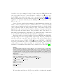
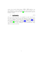
PLUMED User’s Guide
Complement for the dAFED and UFED methods
Michel A. Cuendet
PLUMED 1.3 – dAFED 0.7 - July 2012
Chapter 1
Running free-energy
simulations
1.1
Driven Adiabatic Free Energy Dynamics
(dAFED)
The driven adiabatic free energy (dAFED) algorithm [1] is also called temperature accelerated molecular dnamics (TAMD) by other authors [2]. In
fact, dAFED/TAMD is an improvement over the earlier AFED method [3, 4],
which required cumbersome coordinates transformations. In the dAFED/TAMD
method, an extra dynamical variable S is coupled to a collective variable s(r),
where r represents the coordinates of a number N of atoms in the system.
The coupling is mediated by a potential energy function with harmonic constant κ,
1
V (S, s(r)) = κ (S − s(r))2 .
2
(1.1)
The dynamics of the S meta-variable is adiabatically decoupled from
the dynamics of the underlying physical system by choosing a large mass
mS m,
¯ where m
¯ is a typical mass of the physical system. Thanks to the
adiabatic separation, a temperature TS > T can be assigned to the S metavariable. With this choice of mS and Ts , the physical system will evolve fast
at room temperature T around the instantaneous value of s(r) = S . On
the other hand, S will evolve slowly, but have a temperature large enough to
drive the system over high free energy barriers.
1
In the limit of κ → ∞, it can be shown that the free energy surface
at temperature T can be recovered from the density ρadb (S) sampled at
temperature TS during the adiabatic dAFED simulation using
G(S) = −kB TS log ρadb (S) .
(1.2)
This result generalizes well to the case where more than one collective variable
is used and G(S) is a multi-dimensional free energy surface.
The dAFED method requires very efficient thermostatting of the metavariable S. In the present implementation, S is coupled to a Generalized
Gaussian Moment Thermostat (GGMT) [5] or to a Langevin thermostat [6].
If multiple reaction coordinates are used, one separate GGMT or Langevin
thermostat is associated to each of them.
In the case of GGMT, the meta-variable is coupled to two thermostatting
variables pη and pζ , with associated masses Qη and Qζ , respectively. Given
a typical time scale τ of the thermostated system, optimal masses are Qη =
kB TS τ 2 and Qζ = 38 (kB TS )3 τ 2 . The order-2 GGMT dynamics for one degree
of freedom is
pζ
1 p2S
pη
pS −
kB TS +
pS ,
V (S, s(r)) −
Qη
Qζ
3 mS
p2S
− kB TS ,
mS
"
#2
1 p2S
− (kB TS )2 ,
3 mS
pS
pη
pζ
, η˙ =
, ζ˙ =
.
mS
Qη
Qζ
"
p˙S =
p˙η =
p˙ζ =
S˙ =
#
(1.3)
(1.4)
(1.5)
(1.6)
The implemented integrator for the dynamics above is based on a Trotter
decomposition of the corresponding Liouville operator [1]. The quality of
the integration can be monitored using the quantity HS , which would be
conserved if the dynamics of S was decoupled from the physical system,
HS (S, pS , η, pη , ζ, pζ ) =
p2
p2
p2S
+ V (S) + η + ζ + kB TS (η + ζ)(1.7)
2mS
2Qη 2Qζ
The heat transfer WS from the meta-variable to the physical system can
be calculated,
WS =
Z t
0
dt0 κ (S − s(r))
pS
mS
(1.8)
2
The effective adiabaticity of the coupling can thus be asserted. In addition, for each extended variable S, the quantity HS + WS should be strictly
conserved, which provides a quality check for the simulation. In addition,
Let H be the pseudo-energy of the physical system including the associated thermostats and barostats. Then the total energy of the simulation,
P
H + dj=1 HSj , should be conserved as well. As a corollary, considering the
P
physical system only, the quantity H − dj=1 WSj should be conserved.
A different way to assess the adiabaticity of the simulation is through the
configurational temperature of the collective variable s,
Tconfig
E
1 h|∇U (s)|2 i
κ D
2
=
=
(s
−
S)
.
kB h∇2 U (s)i
kB
(1.9)
For a system at equilibrium the configurational temperature should be equivalent to the kinetic temperature and the heat bath temperature. A higher
configurational temperature is a signature of nonequilibrium dynamics, in
which a significant heat flow would take place between extended and physical system.
In practice, the choice of mS is subject to some pragmatic considerations.
The value of mS should be as high as possible to ensure good adiabatic separation. However, given the limited planned simulation time, the evolution
of S has to be fast enough to correctly sample the CV range of interest.
By running a short dAFED simulation and plotting the evolution of S, one
can estimate an average diffusion speed. From that, a maximum admissible
value for mS can be deduced, such that S can cross many time the CV range
during the simulation.
The choice of the coupling constant κ determines the resolution of the
observed free energy surface G(S). Ideally, κ should be very large, but its
value is limited by the requirement of integrating accurately the coupling
term, Eq.
q 1.1. The typical period of that harmonic oscillator is given by
τ = 2π µ/κ, where µ = mS meff /(mS + meff ) is the reduced mass, with meff
the effective mass of the CV s(r). For a one-dimensional CV, meff can be
expressed as

meff = 
3N
X
j=1
ds
drj
!2
−1
1 
mj
.
(1.10)
Note that if the CV is multidimensional the situation is slightly more
complicated and meff is in fact a tensor, whose diagonal elements are given
3
by Eq. 1.10. Nevertheless, meff can be used to estimate an order of magnitude
for the period τ for each CV, and thus estimate which time step is appropriate
for a given mS (or vice versa). It is recommended to check that the time step
is appropriate for the chosen κ by plotting the evolution of s(r) and S from
a short simulation in which the dAFED variables are saved very frequently.
1.1.1
Input for dAFED
For each CV, a DAFED directive is used to define the parameters of the corresponding dynamics. On the same line, the number of the CV to which the
directive applies is specified after the keyword CV. The temperature TS in
K is given after keyword TEMPERATURE. The thermostat time constant τ is
given in ps after keyword TAUTHERMO. The mass mS and harmonic constant
κ, are given after the keywords MASS and KAPPA, respectively. The units of κ
and mS depend on the nature of the CV. They should always be such that
κS 2 and mS˙ 2 are both in units of energy (kJ/mol= amu nm2 / ps2 ), see the
example below.
In addition, tow optional keywords can be used with the DAFED directive.
First, for periodic CVs such as torsion angles, the S variable should also
evolve on a periodic interval. This is specified by the keyword PERIODIC,
followed by two numbers for the lower and upper bounds. The numbers can
be replaced by MINUS PI, PLUS PI, or PLUS 2PI to specify −π, +π, or +2π,
respectively.
The optional keyword JACOBIAN FORCE causes a bias force F = −2kB T /S
to be applied to the dynamics of S. This is useful with distance CVs in order
to counterbalance the effect of the Jacobian factor and sample a more uniform
distribution along the CV.
4
Example.
The following lines couple CV 1 (a distance in nm) to a meta-variable of mass 105 amu with a harmonic
constant of 106 kJ/mol/nm2 and CV 2 (a unitless number) to a meta-variable with mass 103 amu*nm2
with a harmonic constant of 104 kJ/mol. For both CV, the dAFED temperature is 600 K and the GGMT
thermostat time constant is 0.2 ps. See text for the optional keywords JACOBIAN FORCE and PERIODIC.
DISTANCE LIST 1 34
TORSION LIST 5 15 29 36
DAFED CV 1 TEMPERATURE 600 MASS 1e5 KAPPA 1e6 TAUTHERMO 0.2 JACOBIAN FORCE
DAFED CV 2 TEMPERATURE 600 MASS 1e3 KAPPA 1e4 TAUTHERMO 0.2 PERIODIC MINUS PI PLUS PI
DAFED CONTROL RESTART checkpoint file WRITE STATE -1 N RESPA 1
PRINT W STRIDE 100
ENDMETA
A separate DAFED CONTROL directive contains general controls for the
dAFED simulation. The dAFED dynamics, including all variables described
in Eqs. 1.3 - 1.6 can be restarted exactly from a previous run using a checkpoint file. Following the WRITE STATE keyword appears the number of steps
after which a checkpoint file is saved. A value of −1 implies that a checkpoint file is written only when GROMACS saves its own checkpoint file, i.e.
at regular wall clock time intervals. The checkpoint file is saved in the current
directory with default name DAFED STATE. The optional keyword RESTART is
used to specify the path to the checkpoint file from which to restart.
The integrator for S can be selected on the DAFED CONTROL line with the
keyword INTEGRATOR, followed by either GGMT (default) or LANGEVIN EM for
Langevin evolution with the simple Euler-Maruyama integrator, or LANGEVIN CV
for Langevin evolution with the integrator of Ciccotti-Vanden Eijnden [6].
Specifying LANGEVIN defaults to LANGEVIN EM.
With a high value of κ (as required by the dAFED method), oscillations
of s(r) can become faster than the fastest mode in the physical system. This
would in principle require choosing a smaller time step, at the expense of
sampling efficiency. Instead, following a multiple time step approach, the
dAFED force can be integrated more often than the forces in the physical
system. This feature is implemented only with GROMACS and the GGMT
thermostat. The user has to divide the general MD time step by a number
NRESPA (typically between 2 and 10). The optional keyword N RESPA followed
by the number NRESPA in the DAFED CONTROL directive instructs GROMACS
to evaluate the physical forces only every NRESPA steps. Together with the
md-vv integrator of GROMACS, this should produce a correct RESPA [7]
5
scheme in the NVT ensemble. With this, nstcalcenergy = 1 has to be set
in the GROMACS input file. Note that this feature is still experimental and
energy conservation should be checked.
1.1.2
Typical output for dAFED
With the dAFED method, the COLVAR file will contain the following data, if
d collective variables are used:
• time step
• value of the collective variable s1 (r)...sd (r)
Then for each of the Sj , j = 1...d, appears a set of 5 columns with :
• the meta-variable S
• the instantaneous temperature of S in K
• the conserved quantity HS , see Eq. 1.7, in kJ/mol
• the work WS from S to the physical system, see Eq. 1.8, in kJ/mol
• the effective mass meff according to Eq. 1.10, in a.m.u.
These fields are labeled sj, T sj, E sj, W sj, and M effj respectively,
in the COLVAR header line, j = 1...d. Additional collective variables can be
monitored during a dAFED run, in which case more columns will appear
before the first set of dAFED fields. For long production runs, the user
can choose a more compact form of output in which only the CV sj (r) and
the position Sj of each corresponding extended variable are printed. This is
achieved by adding the keyword PRINT NO DETAILS on the DAFED CONTROL
input line.
1.1.3
Unified Free Energy Dynamics (UFED)
UFED is a recent extension [8] of the dAFED/TAMD method which combines high temperature extended variables with adaptive bias potentials similar to those used in metadynamics. The UFED method rests on the fact that
the free energy surface can be reconstructed from the thermodynamic force
6
F(S) instead of the histogram ρadb (S). Note that the use of the force is also
found in some other methods, such as the umbrella integration method [9]
or the single sweep method [10]. Essentially, in the spirit of the well-known
thermodynamic integration technique, we can write
F(S) = −∇S Gβ (S)
κ
1 Z
2
dr κ(s(r) − S) e−β [U (r)+ 2 (s(r)−S) ]
=
Z(S)
= hfr→S iS
(1.11)
(1.12)
(1.13)
The last line represents the force exerted by the physical system on the
extended variable, averaged at a fixed position of S. This average can easily
be obtained in a post processing phase from the values of S and s(r) stored
in the COLVAR file using a grid in the S space. Note that due to the fast oscillations of s(r), samples should be collected at high frequency. Finally, F(S)
is integrated numerically to get the free energy profile. In dimensions greater
than one, F(S) will not exactly be a consistent multidimensional gradient,
due to statistical noise. The PMF can however easily be reconstructed as the
surface Gβ (S) whose discrete derivative best fits F(S) in the least-squares
sense. This postprocessing step provides the additional benefit of producing
a smooth PMF.
The second fundamental ingredient for the UFED method is that, if the
adiabatic separation is effective, F(S) does not depend on the actual distribution of s [8]. If this holds, we can introduce a bias potential of any kind
acting on S. We introduce a Gaussian-based adaptive potential

Vbias (S, t) = h
X
kτ <t
exp −

d
X
i=1
2 
S − S (0) (kτ ) 
,
2σ 2
(1.14)
which is similar to the metadynamics bias potential, except that it acts on the
extended variables S instead of the CV s(r). UFED has several advantages
over its parent methods. First, the adaptive bias allows using a lower temperature than dAFED, which facilitates obtaining effective adiabatic separation.
Second, the use of the force to construct the free energy surface (instead of
the sum of hills in metadynamics) makes the final accuracy of UFED independent of the hill size, and does not require that all basins are filled up with
hills.
In order to activate UFED, the user only needs to add a line with the
directive UFED HILLS in addition to the DAFED and DAFED CONTROL directives
7
described above (see example below). For most aspects, UFED HILLS works
just as the HILLS directive of metadynamics. It must be followed by a keyword HEIGHT after which the value of h is specified, see Eq. (1.14). The
hill deposition stride is specified after the keyword W STRIDE. The Gaussian
widths σi are taken from the keywords SIGMA specified on the line of each
CV, i = 1, ..., d.
Some collective variables have intrinsic domain limitations (such as the
number of H-bonds that cannot be smaller than zero), or the user might
want to impose limitations (such as the maximum distance to which a ligand
can be separated from it’s host). In these cases, it is useful to impose the
limitations to the domain of the S variables, which are otherwise unbounded.
This is especially necessary when a bias potential is used. One way to do
this without perturbing the distribution of S within the range of interest is
to use reflective walls at which the momentum PS is inverted.
Reflective walls are activated with the directives LREFLECT and UREFLECT,
corresponding to a lower or upper limit, respectively. The CV on which the
reflective wall acts is specified after the keyword CV and the limit value is
given after the keyword LIMIT. If UFED HILLS and LREFLECT or UREFLECT
are active, extra hills are added at a symmetrical position on the other side
of the wall as soon as Si is closer than 3σi to the wall. This prevents the
formation of an artificial ditch in the bias potential close to the wall [11].
Example.
The following example shows how to setup a UFED run. CV 1 (a distance in nm) is coupled with a
harmonic constant of 105 kJ/mol/nm2 to a meta-variable of mass 106 a.m.u. at temperature 400 K. In this
case we have specified a Langevin integrator for this meta-variable and we print a compact COLVAR file.
For UFED, we deposit every 1000 steps a hill of height 0.5 kJ/mol and width 0.1 nm. In addition, we have
restricted the space of the meta-variable with a lower reflection wall at 0.1 nm and an upper reflection
wall at 1.5 nm.
DISTANCE LIST 1 2 SIGMA 0.1
DAFED CV 1 TEMPERATURE 400 MASS 1e6 KAPPA 1e5 TAUTHERMO 0.5
DAFED CONTROL WRITE STATE -1 INTEGRATOR LANGEVIN PRINT NO DETAILS
UFED HILLS HEIGHT 0.5 W STRIDE 1000
LREFLECT CV 1 LIMIT 0.1
UREFLECT CV 1 LIMIT 1.5
PRINT W STRIDE 100
ENDMETA
We note that, in addition to G(S), it is possible to calculate the ensemble
8
average of any observable A(r) in during a dAFED or UFED simulation, even
if the distribution of states is different form the canonical ensemble at low
(physical) temperature. It can be shown [12] that if the adiabatic separation
is effective, we have
R
hAi =
ds hAiS e−βG(S)
R
,
ds e−βG(S)
(1.15)
where hAiS is the average value of A accumulated on a grid of fixed S positions. Here, G(S) is obtained from the same simulation by integrating values
of hfr→s iS accumulated on the same grid. The integral in Eq. 1.15 is performed numerically a posteriori. Using Eq. 1.15, dAFED can for example
be combined [12] with thermodynamic integration (A = dH/dλ) or free energy perturbation (A = exp[−β ∆H(λ)]) to calculate alchemical free energy
differences in flexible molecules.
9
Bibliography
[1] J. B. Abrams, M. E. Tuckerman, Efficient and direct generation of multidimensional free energy surfaces via adiabatic dynamics without coordinate transformations, J. Phys. Chem. B 112 (2008) 15742–15757.
[2] L. Maragliano, E. Vanden-Eijnden, A temperature accelerated method
for sampling free energy and determining reaction pathways in rare
events simulations, Chem. Phys. Lett. 426 (2006) 168–175.
[3] L. Rosso, M. E. Tuckerman, An adiabatic molecular dynamics method
for the calculation of free energy profiles, Mol. Simul. 28 (1) (2002) 91–
112.
[4] L. Rosso, P. Minary, Z. Zhu, M. E. Tuckerman, On the use of adiabatic
molecular dynamics to calculate free energy profiles, J. Chem. Phys. 116
(2002) 4389–4402.
[5] Y. Liu, M. E. Tuckerman, Generalized Gaussian moment thermostatting: A new continuous dynamical approach to the canonical ensemble,
J. Chem. Phys. 112 (4) (2000) 1685–1700.
[6] E. Vanden-Eijnden, G. Ciccotti, Second-order integrators for langevin
equations with holonomic constraints, Chem. Phys. Lett. 429 (1-3)
(2006) 310–316.
[7] G. J. Martyna, M. E. Tuckerman, D. J. Tobias, M. L. Klein, Explicit
reversible integrators for extended systems dynamics, Mol. Phys. 87 (5)
(1996) 1117.
[8] M. Chen, M. A. Cuendet, M. E. Tuckerman, Heating and flooding: A
unified approach for rapid generation of free energy surfaces, J. Chem.
Phys. 137 (2012) 024102.
10
[9] J. K¨astner, W. Thiel, Bridging the gap between thermodynamic integration and umbrella sampling provides a novel analysis method: ”umbrella
integration”, J. Chem. Phys. 123 (2005) 144104.
[10] L. Maragliano, E. Vanden-Eijnden, Single-sweep methods for free energy
calculations, J. Chem. Phys. 128 (2008) 184110.
[11] Y. Crespo, F. Marinelli, F. Pietrucci, A. Laio, Metadynamics convergence law in a multidimensional system, Physical Review E 81 (5) (2010)
55701.
[12] M. A. Cuendet, M. E. Tuckerman, Alchemical free energy differences in
flexible molecules from thermodynamic integration or free energy perturbation combined with driven adiabatic dynamics, J. Chem. Theory
Comput. (2012) in press,doi:10.1021/ct300090z.
11