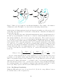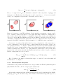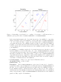
Download 1.1M PDF - Theoretical Biophysics Group

NAMD User’s Guide
Version CVS-2015-12-17
M. Bhandarkar, A. Bhatele, E. Bohm, R. Brunner, F. Buelens, C. Chipot,
A. Dalke, S. Dixit, G. Fiorin, P. Freddolino, P. Grayson, J. Gullingsrud,
A. Gursoy, D. Hardy, C. Harrison, J. Hénin, W. Humphrey, D. Hurwitz,
A. Hynninen, N. Jain, N. Krawetz, S. Kumar, D. Kunzman, J. Lai, C. Lee,
R. McGreevy, C. Mei, M. Nelson, J. Phillips, B. Radak, O. Sarood,
A. Shinozaki, D. Tanner, D. Wells, G. Zheng, F. Zhu
December 17, 2015
Theoretical Biophysics Group
University of Illinois and Beckman Institute
405 N. Mathews
Urbana, IL 61801
Description
The NAMD User’s Guide describes how to run and use the various features of the molecular
dynamics program NAMD. This guide includes the capabilities of the program, how to use these
capabilities, the necessary input files and formats, and how to run the program both on uniprocessor
machines and in parallel.
NAMD Version CVS-2015-12-17
Authors: M. Bhandarkar, A. Bhatele, E. Bohm, R. Brunner, F. Buelens, C. Chipot,
A. Dalke, S. Dixit, G. Fiorin, P. Freddolino, P. Grayson, J. Gullingsrud, A. Gursoy,
D. Hardy, C. Harrison, J. Hénin, W. Humphrey, D. Hurwitz, A. Hynninen, N. Jain,
N. Krawetz, S. Kumar, D. Kunzman, J. Lai, C. Lee, R. McGreevy, C. Mei, M. Nelson,
J. Phillips, B. Radak, O. Sarood, A. Shinozaki, D. Tanner, D. Wells, G. Zheng, F. Zhu
Theoretical and Computational Biophysics Group, Beckman Institute, University of Illinois.
c
1995-2011
The Board of Trustees of the University of Illinois. All Rights Reserved
NAMD Molecular Dynamics Software
Non-Exclusive, Non-Commercial Use License
Introduction
The University of Illinois at Urbana-Champaign has created its molecular dynamics software,
NAMD, developed by the Theoretical and Computational Biophysics Group (“TCBG”) at Illinois’ Beckman Institute available free of charge for non-commercial use by individuals, academic
or research institutions and corporations for in-house business purposes only, upon completion and
submission of the online registration form presented when attempting to download NAMD at the
web site http://www.ks.uiuc.edu/Research/namd/.
Commercial use of the NAMD software, or derivative works based thereon, REQUIRES A
COMMERCIAL LICENSE. Commercial use includes: (1) integration of all or part of the Software
into a product for sale, lease or license by or on behalf of Licensee to third parties, or (2) distribution
of the Software to third parties that need it to commercialize product sold or licensed by or on
behalf of Licensee. The University of Illinois will negotiate commercial-use licenses for NAMD upon
request. These requests can be directed to [email protected]
Online Download Registration Requirements
In completing the online registration form presented before downloading individuals may register
in their own name or with their institutional or corporate affiliations. Registration information
must include name, title, and e-mail of a person with signature authority to authorize and commit
the individuals, academic or research institution, or corporation as necessary to the terms and
conditions of the license agreement.
All parts of the information must be understood and agreed to as part of completing the form.
Completion of the form is required before software access is granted. Pay particular attention to
the authorized requester requirements above, and be sure that the form submission is authorized
by the duly responsible person.
UNIVERSITY OF ILLINOIS
NAMD MOLECULAR DYNAMICS SOFTWARE LICENSE AGREEMENT
Upon execution of this Agreement by the party identified below (“Licensee”), The Board of Trustees
of the University of Illinois (“Illinois”), on behalf of The Theoretical and Computational Biophysics
Group (“TCBG”) in the Beckman Institute, will provide the molecular dynamics software NAMD
in Executable Code and/or Source Code form (“Software”) to Licensee, subject to the following
terms and conditions. For purposes of this Agreement, Executable Code is the compiled code,
which is ready to run on Licensee’s computer. Source code consists of a set of files which contain
the actual program commands that are compiled to form the Executable Code.
1. The Software is intellectual property owned by Illinois, and all right, title and interest, including copyright, remain with Illinois. Illinois grants, and Licensee hereby accepts, a restricted,
non-exclusive, non-transferable license to use the Software for academic, research and internal business purposes only e.g. not for commercial use (see Paragraph 7 below), without a fee. Licensee
agrees to reproduce the copyright notice and other proprietary markings on all copies of the Software. Licensee has no right to transfer or sublicense the Software to any unauthorized person or
entity. However, Licensee does have the right to make complimentary works that interoperate with
NAMD, to freely distribute such complimentary works, and to direct others to the TCBG server
to obtain copies of NAMD itself.
2. Licensee may, at its own expense, modify the Software to make derivative works, for its own
academic, research, and internal business purposes. Licensee’s distribution of any derivative work
is also subject to the same restrictions on distribution and use limitations that are specified herein
for Illinois’ Software. Prior to any such distribution the Licensee shall require the recipient of the
Licensee’s derivative work to first execute a license for NAMD with Illinois in accordance with
the terms and conditions of this Agreement. Any derivative work should be clearly marked and
renamed to notify users that it is a modified version and not the original NAMD code distributed
by Illinois.
3. Except as expressly set forth in this Agreement, THIS SOFTWARE IS PROVIDED “AS
IS” AND ILLINOIS MAKES NO REPRESENTATIONS AND EXTENDS NO WARRANTIES
OF ANY KIND, EITHER EXPRESS OR IMPLIED, INCLUDING BUT NOT LIMITED TO
WARRANTIES OR MERCHANTABILITY OR FITNESS FOR A PARTICULAR PURPOSE,
OR THAT THE USE OF THE SOFTWARE WILL NOT INFRINGE ANY PATENT, TRADEMARK, OR OTHER RIGHTS. LICENSEE ASSUMES THE ENTIRE RISK AS TO THE RESULTS AND PERFORMANCE OF THE SOFTWARE AND/OR ASSOCIATED MATERIALS.
LICENSEE AGREES THAT UNIVERSITY SHALL NOT BE HELD LIABLE FOR ANY DIRECT, INDIRECT, CONSEQUENTIAL, OR INCIDENTAL DAMAGES WITH RESPECT TO
ANY CLAIM BY LICENSEE OR ANY THIRD PARTY ON ACCOUNT OF OR ARISING FROM
THIS AGREEMENT OR USE OF THE SOFTWARE AND/OR ASSOCIATED MATERIALS.
4. Licensee understands the Software is proprietary to Illinois. Licensee agrees to take all
reasonable steps to insure that the Software is protected and secured from unauthorized disclosure,
use, or release and will treat it with at least the same level of care as Licensee would use to protect
and secure its own proprietary computer programs and/or information, but using no less than a
reasonable standard of care. Licensee agrees to provide the Software only to any other person or
entity who has registered with Illinois. If licensee is not registering as an individual but as an
institution or corporation each member of the institution or corporation who has access to or uses
Software must understand and agree to the terms of this license. If Licensee becomes aware of any
unauthorized licensing, copying or use of the Software, Licensee shall promptly notify Illinois in
3
writing. Licensee expressly agrees to use the Software only in the manner and for the specific uses
authorized in this Agreement.
5. By using or copying this Software, Licensee agrees to abide by the copyright law and all
other applicable laws of the U.S. including, but not limited to, export control laws and the terms
of this license. Illinois shall have the right to terminate this license immediately by written notice
upon Licensee’s breach of, or non-compliance with, any of its terms. Licensee may be held legally
responsible for any copyright infringement that is caused or encouraged by its failure to abide by
the terms of this license. Upon termination, Licensee agrees to destroy all copies of the Software
in its possession and to verify such destruction in writing.
6. The user agrees that any reports or published results obtained with the Software will acknowledge its use by the appropriate citation as follows:
NAMD was developed by the Theoretical and Computational Biophysics Group in the
Beckman Institute for Advanced Science and Technology at the University of Illinois at
Urbana-Champaign.
Any published work which utilizes NAMD shall include the following reference:
James C. Phillips, Rosemary Braun, Wei Wang, James Gumbart, Emad Tajkhorshid,
Elizabeth Villa, Christophe Chipot, Robert D. Skeel, Laxmikant Kale, and Klaus Schulten. Scalable molecular dynamics with NAMD. Journal of Computational Chemistry,
26:1781-1802, 2005.
Electronic documents will include a direct link to the official NAMD page:
http://www.ks.uiuc.edu/Research/namd/
One copy of each publication or report will be supplied to Illinois at the addresses listed below
in Contact Information.
7. Should Licensee wish to make commercial use of the Software, Licensee will contact Illinois
([email protected]) to negotiate an appropriate license for such use. Commercial use includes: (1)
integration of all or part of the Software into a product for sale, lease or license by or on behalf
of Licensee to third parties, or (2) distribution of the Software to third parties that need it to
commercialize product sold or licensed by or on behalf of Licensee.
8. Government Rights. Because substantial governmental funds have been used in the development of NAMD, any possession, use or sublicense of the Software by or to the United States
government shall be subject to such required restrictions.
9. NAMD is being distributed as a research and teaching tool and as such, TCBG encourages
contributions from users of the code that might, at Illinois’ sole discretion, be used or incorporated to
make the basic operating framework of the Software a more stable, flexible, and/or useful product.
Licensees that wish to contribute their code to become an internal portion of the Software may be
required to sign an “Agreement Regarding Contributory Code for NAMD Software” before Illinois
can accept it (contact [email protected] for a copy).
4
Contact Information
The best contact path for licensing issues is by e-mail to [email protected] or send correspondence
to:
NAMD Team
Theoretical and Computational Biophysics Group
Beckman Institute
University of Illinois
405 North Mathews MC-251
Urbana, Illinois 61801 USA
5
Contents
1 Introduction
12
1.1 NAMD and molecular dynamics simulations . . . . . . . . . . . . . . . . . . . . . . . 12
1.2 Acknowledgments . . . . . . . . . . . . . . . . . . . . . . . . . . . . . . . . . . . . . . 14
2 Getting Started
2.1 What is needed . . . . . . . . . . . . . . . . . . . . . . . .
2.2 NAMD configuration file . . . . . . . . . . . . . . . . . . .
2.2.1 Configuration parameter syntax . . . . . . . . . . .
2.2.2 Tcl scripting interface and features . . . . . . . . .
2.2.3 Multiple-copy/replica-exchange scripting interface
2.2.4 Required NAMD configuration parameters . . . .
.
.
.
.
.
.
.
.
.
.
.
.
.
.
.
.
.
.
.
.
.
.
.
.
.
.
.
.
.
.
.
.
.
.
.
.
.
.
.
.
.
.
3 Input and Output Files
3.1 File formats . . . . . . . . . . . . . . . . . . . . . . . . . . . . . . . . .
3.1.1 PDB files . . . . . . . . . . . . . . . . . . . . . . . . . . . . . .
3.1.2 X-PLOR format PSF files . . . . . . . . . . . . . . . . . . . . .
3.1.3 CHARMM19, CHARMM22, and CHARMM27 parameter files
3.1.4 DCD trajectory files . . . . . . . . . . . . . . . . . . . . . . . .
3.1.5 NAMD binary files . . . . . . . . . . . . . . . . . . . . . . . . .
3.2 NAMD configuration parameters . . . . . . . . . . . . . . . . . . . . .
3.2.1 Input files . . . . . . . . . . . . . . . . . . . . . . . . . . . . . .
3.2.2 Output files . . . . . . . . . . . . . . . . . . . . . . . . . . . . .
3.2.3 Standard output . . . . . . . . . . . . . . . . . . . . . . . . . .
3.3 AMBER force field parameters . . . . . . . . . . . . . . . . . . . . . .
3.4 GROMACS force field parameters . . . . . . . . . . . . . . . . . . . .
4 Creating PSF Structure Files
4.1 Ordinary Usage . . . . . . . . . . . .
4.1.1 Preparing separate PDB files
4.1.2 Deleting unwanted atoms . .
4.2 BPTI Example . . . . . . . . . . . .
4.3 Building solvent around a protein . .
4.4 List of Commands . . . . . . . . . .
4.5 Example of a Session Log . . . . . .
.
.
.
.
.
.
.
.
.
.
.
.
.
.
.
.
.
.
.
.
.
.
.
.
.
.
.
.
.
.
.
.
.
.
.
.
.
.
.
.
.
.
.
.
.
.
.
.
.
.
.
.
.
.
.
.
.
.
.
.
.
.
.
.
.
.
.
.
.
.
.
.
.
.
.
.
.
.
.
.
.
.
.
.
.
.
.
.
.
.
.
.
.
.
.
.
.
.
.
.
.
.
.
.
.
.
.
.
.
.
.
.
.
.
.
.
.
.
.
.
.
.
.
.
.
.
.
.
.
.
.
.
15
15
15
15
16
19
20
.
.
.
.
.
.
.
.
.
.
.
.
22
22
22
22
22
22
23
23
23
24
26
28
30
.
.
.
.
.
.
.
.
.
.
.
.
.
.
.
.
.
.
.
.
.
.
.
.
.
.
.
.
.
.
.
.
.
.
.
.
.
.
.
.
.
.
.
.
.
.
.
.
.
.
.
.
.
.
.
.
.
.
.
.
.
.
.
.
.
.
.
.
.
.
.
.
.
.
.
.
.
.
.
.
.
.
.
.
.
.
.
.
.
.
.
.
.
.
.
.
.
.
.
.
.
.
.
.
.
.
.
.
.
.
.
.
.
.
.
.
.
.
.
.
.
.
.
.
.
.
.
.
.
.
.
.
.
.
.
.
.
.
.
.
.
.
.
.
.
.
.
.
.
.
.
.
.
.
.
.
.
.
.
.
.
.
.
.
.
.
.
.
.
.
.
.
.
.
.
32
32
33
33
34
38
39
45
5 Force Field Parameters
5.1 Potential energy functions . . . . . . . . .
5.1.1 Bonded potential energy terms . .
5.1.2 Nonbonded potential energy terms
5.2 Non-bonded interactions . . . . . . . . . .
5.2.1 Van der Waals interactions . . . .
5.2.2 Electrostatic interactions . . . . .
5.2.3 Non-bonded force field parameters
5.2.4 PME parameters . . . . . . . . . .
5.2.5 MSM parameters . . . . . . . . . .
.
.
.
.
.
.
.
.
.
.
.
.
.
.
.
.
.
.
.
.
.
.
.
.
.
.
.
.
.
.
.
.
.
.
.
.
.
.
.
.
.
.
.
.
.
.
.
.
.
.
.
.
.
.
.
.
.
.
.
.
.
.
.
.
.
.
.
.
.
.
.
.
.
.
.
.
.
.
.
.
.
.
.
.
.
.
.
.
.
.
.
.
.
.
.
.
.
.
.
.
.
.
.
.
.
.
.
.
.
.
.
.
.
.
.
.
.
.
.
.
.
.
.
.
.
.
.
.
.
.
.
.
.
.
.
.
.
.
.
.
.
.
.
.
.
.
.
.
.
.
.
.
.
.
.
.
.
.
.
.
.
.
.
.
.
.
.
.
.
.
.
.
.
.
.
.
.
.
.
.
.
.
.
.
.
.
.
.
.
.
.
.
.
.
.
.
.
.
.
.
.
.
.
.
.
.
.
.
.
.
.
.
.
.
.
.
46
46
46
47
47
47
48
48
51
53
.
.
.
.
.
.
.
.
.
.
.
.
.
.
6
5.3
5.4
5.5
5.6
5.2.6 Full direct parameters . . . . . . . . . . . . .
5.2.7 Tabulated nonbonded interaction parameters
Water Models . . . . . . . . . . . . . . . . . . . . . .
Drude polarizable force field . . . . . . . . . . . . . .
5.4.1 Required input files . . . . . . . . . . . . . .
5.4.2 Standard output . . . . . . . . . . . . . . . .
5.4.3 Drude force field parameters . . . . . . . . .
MARTINI Residue-Based Coarse-Grain Forcefield . .
Constraints and Restraints . . . . . . . . . . . . . .
5.6.1 Bond constraint parameters . . . . . . . . . .
5.6.2 Harmonic restraint parameters . . . . . . . .
5.6.3 Fixed atoms parameters . . . . . . . . . . . .
5.6.4 Extra bond, angle, and dihedral restraints . .
6 Generalized Born Implicit Solvent
6.1 Theoretical Background . . . . . . .
6.1.1 Poisson Boltzmann Equation
6.1.2 Generalized Born . . . . . . .
6.1.3 Generalized Born Equations .
6.2 3-Phase Calculation . . . . . . . . .
6.3 Configuration Parameters . . . . . .
.
.
.
.
.
.
.
.
.
.
.
.
.
.
.
.
.
.
.
.
.
.
.
.
.
.
.
.
.
.
.
.
.
.
.
.
.
.
.
.
.
.
.
.
.
.
.
.
.
.
.
.
.
.
7 Standard Minimization and Dynamics Parameters
7.1 Boundary Conditions . . . . . . . . . . . . . . . . . .
7.1.1 Periodic boundary conditions . . . . . . . . .
7.1.2 Spherical harmonic boundary conditions . . .
7.1.3 Cylindrical harmonic boundary conditions . .
7.2 Energy Minimization . . . . . . . . . . . . . . . . . .
7.2.1 Conjugate gradient parameters . . . . . . . .
7.2.2 Velocity quenching parameters . . . . . . . .
7.3 Dynamics . . . . . . . . . . . . . . . . . . . . . . . .
7.3.1 Timestep parameters . . . . . . . . . . . . . .
7.3.2 Initialization . . . . . . . . . . . . . . . . . .
7.3.3 Conserving momentum . . . . . . . . . . . .
7.3.4 Multiple timestep parameters . . . . . . . . .
7.4 Temperature Control and Equilibration . . . . . . .
7.4.1 Langevin dynamics parameters . . . . . . . .
7.4.2 Temperature coupling parameters . . . . . .
7.4.3 Temperature rescaling parameters . . . . . .
7.4.4 Temperature reassignment parameters . . . .
7.4.5 Lowe-Andersen dynamics parameters . . . . .
7.5 Pressure Control . . . . . . . . . . . . . . . . . . . .
7.5.1 Berendsen pressure bath coupling . . . . . . .
7.5.2 Nosé-Hoover Langevin piston pressure control
.
.
.
.
.
.
.
.
.
.
.
.
.
.
.
.
.
.
.
.
.
.
.
.
.
.
.
.
.
.
.
.
.
.
.
.
.
.
.
.
.
.
.
.
.
.
.
.
.
.
.
.
.
.
.
.
.
.
.
.
.
.
.
.
.
.
.
.
.
.
.
.
.
.
.
.
.
.
.
.
.
.
.
.
.
.
.
.
.
.
.
.
.
.
.
.
.
.
.
.
.
.
.
.
.
.
.
.
.
.
.
.
.
.
.
.
.
.
.
.
.
.
.
.
.
.
.
.
.
.
.
.
.
.
.
.
.
.
.
.
.
.
.
.
.
.
.
.
.
.
.
.
.
.
.
.
.
.
.
.
.
.
.
.
.
.
.
.
.
.
.
.
.
.
.
.
.
.
.
.
.
.
.
.
.
.
.
.
.
.
.
.
.
.
.
.
.
.
.
.
.
.
.
.
.
.
.
.
.
.
.
.
.
.
.
.
.
.
.
.
.
.
.
.
.
.
.
.
.
.
.
.
.
.
56
56
58
58
59
59
59
60
61
61
62
63
64
.
.
.
.
.
.
.
.
.
.
.
.
.
.
.
.
.
.
.
.
.
.
.
.
.
.
.
.
.
.
.
.
.
.
.
.
.
.
.
.
.
.
.
.
.
.
.
.
.
.
.
.
.
.
.
.
.
.
.
.
.
.
.
.
.
.
.
.
.
.
.
.
.
.
.
.
.
.
.
.
.
.
.
.
.
.
.
.
.
.
.
.
.
.
.
.
.
.
.
.
.
.
.
.
.
.
.
.
66
66
66
66
66
69
70
.
.
.
.
.
.
.
.
.
.
.
.
.
.
.
.
.
.
.
.
.
72
72
72
73
74
75
75
76
76
76
77
78
78
80
80
81
81
82
82
83
84
85
.
.
.
.
.
.
.
.
.
.
.
.
.
.
.
.
.
.
.
.
.
.
.
.
.
.
.
.
.
.
.
.
.
.
.
.
.
.
.
.
.
.
.
.
.
.
.
.
.
.
.
.
.
.
.
.
.
.
.
.
.
.
.
.
.
.
.
.
.
.
.
.
.
.
.
.
.
.
.
.
.
.
.
.
.
.
.
.
.
.
.
.
.
.
.
.
.
.
.
.
.
.
.
.
.
.
.
.
.
.
.
.
.
.
.
.
.
.
.
.
.
.
.
.
.
.
.
.
.
.
.
.
.
.
.
.
.
.
.
.
.
.
.
.
.
.
.
.
.
.
.
.
.
.
.
.
.
.
.
.
.
.
.
.
.
.
.
.
.
.
.
.
.
.
.
.
.
.
.
.
.
.
.
.
.
.
.
.
.
.
.
.
.
.
.
.
.
.
.
.
.
.
.
.
.
.
.
.
.
.
.
.
.
.
.
.
.
.
.
.
.
.
.
.
.
.
.
.
.
.
.
.
.
.
.
.
.
.
.
.
.
.
.
.
.
.
.
.
.
.
.
.
.
.
.
.
.
.
.
.
.
.
.
.
.
.
.
.
.
.
.
.
.
.
.
.
.
.
.
.
.
.
.
.
.
.
.
.
.
.
.
.
.
.
.
.
.
.
.
.
.
.
.
.
.
.
.
.
.
.
.
.
.
.
.
.
.
.
.
.
.
.
.
.
.
.
.
.
.
.
.
.
.
.
.
.
.
.
.
.
.
.
.
.
.
.
.
.
.
.
.
.
.
.
.
.
.
8 Performance Tuning
88
8.1 Non-bonded interaction distance-testing . . . . . . . . . . . . . . . . . . . . . . . . . 88
7
9 User Defined Forces
9.1 Constant Forces . . . . . . . . . . . . .
9.2 External Electric Field . . . . . . . . .
9.3 Grid Forces . . . . . . . . . . . . . . .
9.4 Moving Constraints . . . . . . . . . . .
9.5 Rotating Constraints . . . . . . . . . .
9.6 Symmetry Restraints . . . . . . . . . .
9.7 Targeted Molecular Dynamics (TMD)
9.8 Steered Molecular Dynamics (SMD) .
9.9 Interactive Molecular Dynamics (IMD)
9.10 Tcl Forces and Analysis . . . . . . . .
9.11 Tcl Boundary Forces . . . . . . . . . .
9.12 External Program Forces . . . . . . . .
.
.
.
.
.
.
.
.
.
.
.
.
.
.
.
.
.
.
.
.
.
.
.
.
.
.
.
.
.
.
.
.
.
.
.
.
.
.
.
.
.
.
.
.
.
.
.
.
.
.
.
.
.
.
.
.
.
.
.
.
.
.
.
.
.
.
.
.
.
.
.
.
.
.
.
.
.
.
.
.
.
.
.
.
.
.
.
.
.
.
.
.
.
.
.
.
.
.
.
.
.
.
.
.
.
.
.
.
.
.
.
.
.
.
.
.
.
.
.
.
.
.
.
.
.
.
.
.
.
.
.
.
.
.
.
.
.
.
.
.
.
.
.
.
.
.
.
.
.
.
.
.
.
.
.
.
92
92
92
93
96
98
99
101
103
104
105
109
112
10 Collective Variable-based Calculations
10.1 General parameters and input/output files . . . . . . . . . . . .
10.1.1 NAMD parameters . . . . . . . . . . . . . . . . . . . . .
10.1.2 Configuration syntax for the collective variables module
10.1.3 Input state file (optional) . . . . . . . . . . . . . . . . .
10.1.4 Output files . . . . . . . . . . . . . . . . . . . . . . . . .
10.2 Defining collective variables and their properties . . . . . . . .
10.2.1 General options for a collective variable . . . . . . . . .
10.2.2 Artificial boundary potentials (walls) . . . . . . . . . . .
10.2.3 Trajectory output . . . . . . . . . . . . . . . . . . . . .
10.2.4 Extended Lagrangian. . . . . . . . . . . . . . . . . . . .
10.2.5 Statistical analysis of collective variables . . . . . . . . .
10.3 Selecting atoms for colvars: defining atom groups . . . . . . . .
10.3.1 Selection keywords . . . . . . . . . . . . . . . . . . . . .
10.3.2 Moving frame of reference. . . . . . . . . . . . . . . . .
10.3.3 Treatment of periodic boundary conditions. . . . . . . .
10.3.4 Computational cost of colvars based on group size. . . .
10.4 Collective variable components (basis functions) . . . . . . . . .
10.4.1 List of available colvar components . . . . . . . . . . . .
10.4.2 Advanced usage and special considerations . . . . . . .
10.4.3 Linear and polynomial combinations of components . .
10.4.4 Colvars as scripted functions of components . . . . . . .
10.5 Biasing and analysis methods . . . . . . . . . . . . . . . . . . .
10.5.1 Adaptive Biasing Force . . . . . . . . . . . . . . . . . .
10.5.2 Metadynamics . . . . . . . . . . . . . . . . . . . . . . .
10.5.3 Harmonic restraints . . . . . . . . . . . . . . . . . . . .
10.5.4 Linear restraints . . . . . . . . . . . . . . . . . . . . . .
10.5.5 Adaptive Linear Bias/Experiment Directed Simulation .
10.5.6 Multidimensional histograms . . . . . . . . . . . . . . .
10.5.7 Scripted biases . . . . . . . . . . . . . . . . . . . . . . .
10.6 Colvars scripting . . . . . . . . . . . . . . . . . . . . . . . . . .
10.6.1 Managing the colvars module . . . . . . . . . . . . . . .
10.6.2 Input and output . . . . . . . . . . . . . . . . . . . . . .
.
.
.
.
.
.
.
.
.
.
.
.
.
.
.
.
.
.
.
.
.
.
.
.
.
.
.
.
.
.
.
.
.
.
.
.
.
.
.
.
.
.
.
.
.
.
.
.
.
.
.
.
.
.
.
.
.
.
.
.
.
.
.
.
.
.
.
.
.
.
.
.
.
.
.
.
.
.
.
.
.
.
.
.
.
.
.
.
.
.
.
.
.
.
.
.
.
.
.
.
.
.
.
.
.
.
.
.
.
.
.
.
.
.
.
.
.
.
.
.
.
.
.
.
.
.
.
.
.
.
.
.
.
.
.
.
.
.
.
.
.
.
.
.
.
.
.
.
.
.
.
.
.
.
.
.
.
.
.
.
.
.
.
.
.
.
.
.
.
.
.
.
.
.
.
.
.
.
.
.
.
.
.
.
.
.
.
.
.
.
.
.
.
.
.
.
.
.
.
.
.
.
.
.
.
.
.
.
.
.
.
.
.
.
.
.
.
.
.
.
.
.
.
.
.
.
.
.
.
.
.
.
.
.
.
.
.
.
.
.
.
.
.
.
.
.
.
.
.
.
.
.
.
.
.
.
.
.
.
.
.
.
.
.
.
.
.
.
.
.
.
.
.
.
.
.
.
.
.
.
.
.
.
.
.
.
.
.
.
.
.
.
.
.
.
.
.
.
.
.
.
.
.
.
.
.
.
.
.
.
.
.
.
.
.
.
.
.
.
.
.
.
.
.
.
.
.
.
.
.
.
.
.
.
.
.
.
.
.
.
.
.
.
.
.
.
.
.
.
.
.
.
.
.
.
.
.
.
.
.
.
.
.
.
.
.
.
.
.
.
.
.
.
.
.
.
.
.
.
.
.
.
.
.
113
113
113
115
118
118
118
119
120
121
122
123
125
125
127
129
130
130
131
143
145
145
146
147
152
157
161
161
162
163
163
163
163
.
.
.
.
.
.
.
.
.
.
.
.
8
.
.
.
.
.
.
.
.
.
.
.
.
.
.
.
.
.
.
.
.
.
.
.
.
.
.
.
.
.
.
.
.
.
.
.
.
.
.
.
.
.
.
.
.
.
.
.
.
.
.
.
.
.
.
.
.
.
.
.
.
.
.
.
.
.
.
.
.
.
.
.
.
.
.
.
.
.
.
.
.
.
.
.
.
.
.
.
.
.
.
.
.
.
.
.
.
.
.
.
.
.
.
.
.
.
.
.
.
.
.
.
.
.
.
.
.
.
.
.
.
.
.
.
.
.
.
.
.
.
.
.
.
.
.
.
.
.
.
.
.
.
.
.
.
10.6.3 Accessing collective variables . . . . . . . . . . . . . . . . . . . . . . . . . . . 164
10.6.4 Accessing biases . . . . . . . . . . . . . . . . . . . . . . . . . . . . . . . . . . 164
11 Alchemical Free Energy Methods
11.1 Theoretical Background . . . . . . . . . . . . . . . . . . . . . . . . . .
11.1.1 The dual–topology paradigm . . . . . . . . . . . . . . . . . . .
11.1.2 Free Energy Perturbation . . . . . . . . . . . . . . . . . . . . .
11.1.3 Thermodynamic Integration . . . . . . . . . . . . . . . . . . .
11.2 Implementation of the free energy methods in NAMD . . . . . . . . .
11.3 Examples of input files for running alchemical free energy calculations
11.4 Description of a free energy calculation output . . . . . . . . . . . . .
11.4.1 Free Energy Perturbation . . . . . . . . . . . . . . . . . . . . .
11.4.2 Thermodynamic Integration . . . . . . . . . . . . . . . . . . .
12 Accelerated Sampling Methods
12.1 Accelerated Molecular Dynamics . . . . . . . . . . . .
12.1.1 Theoretical background . . . . . . . . . . . . .
12.1.2 NAMD parameters . . . . . . . . . . . . . . . .
12.2 Adaptive Tempering . . . . . . . . . . . . . . . . . . .
12.2.1 NAMD parameters . . . . . . . . . . . . . . . .
12.3 Locally enhanced sampling . . . . . . . . . . . . . . .
12.3.1 Structure generation . . . . . . . . . . . . . . .
12.3.2 Simulation . . . . . . . . . . . . . . . . . . . .
12.4 Replica exchange simulations . . . . . . . . . . . . . .
12.5 Random acceleration molecular dynamics simulations
13 Structure based simulations
13.1 Hybrid MD-Go Simulation . . . . . . .
13.1.1 Hybrid MD-Go model . . . . .
13.1.2 Hybrid MD-Go considerations .
13.1.3 Configuration file modifications
13.1.4 GoParameter format . . . . . .
13.2 Running SMOG simulations . . . . . .
13.2.1 SMOG model considerations .
13.2.2 Configuration file modifications
.
.
.
.
.
.
.
.
.
.
.
.
.
.
.
.
.
.
.
.
.
.
.
.
.
.
.
.
.
.
.
.
.
.
.
.
.
.
.
.
.
.
.
.
.
.
.
.
.
.
.
.
.
.
.
.
.
.
.
.
.
.
.
.
.
.
.
.
.
.
.
.
.
.
.
.
.
.
.
.
.
.
.
.
.
.
.
.
.
.
.
.
.
.
.
.
.
.
.
.
.
.
.
.
.
.
.
.
.
.
.
.
.
.
.
.
.
.
.
.
.
.
.
.
.
.
.
.
.
.
.
.
.
.
.
.
.
.
.
.
.
.
.
.
.
.
.
.
.
.
.
.
.
.
.
.
.
.
.
.
.
.
.
.
.
.
.
.
.
.
.
.
.
.
.
.
.
.
.
.
.
.
.
.
.
.
.
.
.
.
.
.
.
.
.
.
.
.
.
.
.
.
.
.
.
.
.
.
.
.
.
.
.
.
.
.
.
.
.
.
.
.
.
.
.
.
.
.
.
.
.
.
.
.
.
.
.
.
.
.
.
.
.
.
.
.
.
.
.
.
.
.
.
.
.
.
.
.
.
.
.
.
.
.
.
.
.
.
.
.
.
.
.
.
.
.
.
.
.
.
.
.
.
.
.
.
.
.
.
.
.
.
.
.
.
.
.
.
.
.
.
.
.
.
.
.
.
.
.
.
.
.
.
.
.
.
.
.
.
.
.
.
.
.
.
.
.
.
.
.
.
.
.
.
.
.
.
.
.
.
.
.
.
.
.
.
.
.
.
.
.
.
.
.
.
.
.
.
.
.
.
.
.
.
.
.
.
.
.
.
.
.
.
.
.
.
.
.
.
.
.
.
.
.
.
.
.
.
.
.
.
.
.
.
.
.
165
165
165
166
167
168
171
173
173
173
.
.
.
.
.
.
.
.
.
.
.
.
.
.
.
.
.
.
.
.
.
.
.
.
.
.
.
.
175
. 175
. 175
. 176
. 177
. 178
. 180
. 180
. 180
. 181
. 183
.
.
.
.
.
.
.
.
187
. 187
. 187
. 187
. 187
. 188
. 189
. 189
. 189
14 Runtime Analysis
191
14.1 Pair interaction calculations . . . . . . . . . . . . . . . . . . . . . . . . . . . . . . . . 191
14.2 Pressure profile calculations . . . . . . . . . . . . . . . . . . . . . . . . . . . . . . . . 192
15 Translation between NAMD and X-PLOR configuration parameters
196
16 Sample configuration files
198
17 Running NAMD
203
17.1 Individual Windows, Linux, Mac OS X, or Other Unix Workstations . . . . . . . . . 203
17.2 Windows Clusters and Workstation Networks . . . . . . . . . . . . . . . . . . . . . . 203
17.3 Linux Clusters with InfiniBand or Other High-Performance Networks . . . . . . . . . 203
9
17.4 Linux or Other Unix Workstation Networks . .
17.5 Shared-Memory and Network-Based Parallelism
17.6 Cray XE/XK/XC . . . . . . . . . . . . . . . . .
17.7 SGI Altix UV . . . . . . . . . . . . . . . . . . .
17.8 IBM POWER Clusters . . . . . . . . . . . . . .
17.9 CPU Affinity . . . . . . . . . . . . . . . . . . .
17.10CUDA GPU Acceleration . . . . . . . . . . . .
17.11Xeon Phi Acceleration . . . . . . . . . . . . . .
17.12Memory Usage . . . . . . . . . . . . . . . . . .
17.13Improving Parallel Scaling . . . . . . . . . . . .
18 NAMD Availability and Installation
18.1 How to obtain NAMD . . . . . . . . . . . . .
18.2 Platforms on which NAMD will currently run
18.3 Installing NAMD . . . . . . . . . . . . . . . .
18.4 Compiling NAMD . . . . . . . . . . . . . . .
18.5 Documentation . . . . . . . . . . . . . . . . .
.
.
.
.
.
. . . . . . . . .
(SMP Builds)
. . . . . . . . .
. . . . . . . . .
. . . . . . . . .
. . . . . . . . .
. . . . . . . . .
. . . . . . . . .
. . . . . . . . .
. . . . . . . . .
.
.
.
.
.
.
.
.
.
.
.
.
.
.
.
.
.
.
.
.
.
.
.
.
.
.
.
.
.
.
.
.
.
.
.
.
.
.
.
.
.
.
.
.
.
.
.
.
.
.
.
.
.
.
.
.
.
.
.
.
.
.
.
.
.
.
.
.
.
.
.
.
.
.
.
.
.
.
.
.
.
.
.
.
.
.
.
.
.
.
.
.
.
.
.
.
.
.
.
.
.
.
.
.
.
.
.
.
.
.
.
.
.
.
.
.
.
.
.
.
204
205
206
207
207
207
208
209
209
210
.
.
.
.
.
.
.
.
.
.
.
.
.
.
.
.
.
.
.
.
.
.
.
.
.
.
.
.
.
.
.
.
.
.
.
.
.
.
.
.
.
.
.
.
.
.
.
.
.
.
.
.
.
.
.
.
.
.
.
.
.
.
.
.
.
211
211
211
211
212
212
.
.
.
.
.
.
.
.
.
.
.
.
.
.
.
.
.
.
.
.
.
.
.
.
.
.
.
.
.
.
.
.
.
.
.
.
.
.
.
.
References
213
Index
219
10
List of Figures
1
2
3
4
5
6
7
8
9
10
11
Graph of van der Waals potential with and without switching . . . . . . . . . . . .
Graph of electrostatic potential with and without shifting function . . . . . . . . .
Graph of electrostatic split between short and long range forces . . . . . . . . . . .
Example of cutoff and pairlist distance uses . . . . . . . . . . . . . . . . . . . . . .
Graph showing a slice of a ramp potential, showing the effect of mgridforcevoff .
Graphical representation of a collective variables configuration. . . . . . . . . . . .
Dual topology description for an alchemical simulation. Case example of the mutation of alanine into serine. The lighter color denotes the non–interacting, alternate
state. . . . . . . . . . . . . . . . . . . . . . . . . . . . . . . . . . . . . . . . . . . .
Convergence of an FEP calculation. If the ensembles representative of states a and
b are too disparate, equation (59) will not converge (a). If, in sharp contrast, the
configurations of state b form a subset of the ensemble of configurations characteristic
of state a, the simulation is expected to converge (b). The difficulties reflected in
case (a) may be alleviated by the introduction of mutually overlapping intermediate
states that connect a to b (c). It should be mentioned that in practice, the kinetic
contribution, T (px ), is assumed to be identical for state a and state b. . . . . . .
Relationship of user-defined λ to coupling of electrostatic or vdW interactions to a
simulation, given specific
values of alchElecLambdaStart or alchVdwLambdaEnd. .
Sample TI data (log( ∂U
∂λ ) against λ). The blue shaded area shows the integral with
fine sampling close to the end point. The red area shows the difference when λ values
are more sparse. In this example, insufficient sampling before λ '0.1 can result in
a large overestimation of the integral. Beyond '0.2, sparser sampling is justified as
dE/dλ is not changing quickly. . . . . . . . . . . . . . . . . . . . . . . . . . . . . .
Schematics of the aMD method. When the original potential (thick line) falls below
a threshold energy E (dashed line), a boost potential is added. The modified energy
profiles (thin lines) have smaller barriers separating adjacent energy basins. . . . .
11
.
.
.
.
.
.
48
49
49
89
97
114
. 166
. 167
. 170
. 174
. 176
1
Introduction
NAMD is a parallel molecular dynamics program for UNIX platforms designed for high-performance
simulations in structural biology. This document describes how to use NAMD, its features, and
the platforms on which it runs. The document is divided into several sections:
Section 1 gives an overview of NAMD.
Section 2 lists the basics for getting started.
Section 3 describes NAMD file formats.
Section 4 explains PSF file generation with psfgen.
Section 5 presents the potential functions, non-bonded interactions, and full electrostatics.
Section 6 explains Generalized Born implicit solvent simulations.
Section 7 lists standard minimization and dynamics parameters.
Section 8 lists performance tuning parameters.
Section 9 explains user defined forces. conformation change calculations.
Section 10 describes collective variable-based calculations.
Section 11 explains alchemical free energy calculations.
Section 12 presents accelerated sampling methods.
Section 14 lists runtime analysis options.
Section 15 provides hints for X-PLOR users.
Section 16 provides sample configuration files.
Section 17 gives details on running NAMD.
Section 18 gives details on installing NAMD.
1.1
NAMD and molecular dynamics simulations
Molecular dynamics (MD) simulations compute atomic trajectories by solving equations of motion
numerically using empirical force fields, such as the CHARMM force field, that approximate the
actual atomic force in biopolymer systems. Detailed information about MD simulations can be
found in several books such as [1, 51]. In order to conduct MD simulations, various computer
programs have been developed including X-PLOR [13] and CHARMM [12]. These programs were
originally developed for serial machines. Simulation of large molecules, however, require enormous
computing power. One way to achieve such simulations is to utilize parallel computers. In recent
years, distributed memory parallel computers have been offering cost-effective computational power.
NAMD was designed to run efficiently on such parallel machines for simulating large molecules.
NAMD is particularly well suited to the increasingly popular Beowulf-class PC clusters, which are
quite similar to the workstation clusters for which is was originally designed. Future versions of
NAMD will also make efficient use of clusters of multi-processor workstations or PCs.
NAMD has several important features:
12
• Force Field Compatibility
The force field used by NAMD is the same as that used by the programs CHARMM [12]
and X-PLOR [13]. This force field includes local interaction terms consisting of bonded
interactions between 2, 3, and 4 atoms and pairwise interactions including electrostatic and
van der Waals forces. This commonality allows simulations to migrate between these three
programs.
• Efficient Full Electrostatics Algorithms
NAMD incorporates the Particle Mesh Ewald (PME) algorithm, which takes the full electrostatic interactions into account. This algorithm reduces the computational complexity of
electrostatic force evaluation from O(N 2 ) to O(N log N ).
• Multiple Time Stepping
The velocity Verlet integration method [1] is used to advance the positions and velocities of
the atoms in time. To further reduce the cost of the evaluation of long-range electrostatic
forces, a multiple time step scheme is employed. The local interactions (bonded, van der
Waals and electrostatic interactions within a specified distance) are calculated at each time
step. The longer range interactions (electrostatic interactions beyond the specified distance)
are only computed less often. This amortizes the cost of computing the electrostatic forces
over several timesteps. A smooth splitting function is used to separate a quickly varying
short-range portion of the electrostatic interaction from a more slowly varying long-range
component. It is also possible to employ an intermediate timestep for the short-range nonbonded interactions, performing only bonded interactions every timestep.
• Input and Output Compatibility
The input and output file formats used by NAMD are identical to those used by CHARMM
and X-PLOR. Input formats include coordinate files in PDB format [6], structure files in
X-PLOR PSF format, and energy parameter files in either CHARMM or X-PLOR formats.
Output formats include PDB coordinate files and binary DCD trajectory files. These similarities assure that the molecular dynamics trajectories from NAMD can be read by CHARMM
or X-PLOR and that the user can exploit the many analysis algorithms of the latter packages.
• Dynamics Simulation Options
MD simulations may be carried out using several options, including
– Constant energy dynamics,
– Constant temperature dynamics via
∗ Velocity rescaling,
∗ Velocity reassignment,
∗ Langevin dynamics,
– Periodic boundary conditions,
– Constant pressure dynamics via
∗ Berendsen pressure coupling,
∗ Nosé-Hoover Langevin piston,
– Energy minimization,
– Fixed atoms,
13
– Rigid waters,
– Rigid bonds to hydrogen,
– Harmonic restraints,
– Spherical or cylindrical boundary restraints.
• Easy to Modify and Extend
Another primary design objective for NAMD is extensibility and maintainability. In order to
achieve this, it is designed in an object-oriented style with C++. Since molecular dynamics is a
new field, new algorithms and techniques are continually being developed. NAMD’s modular
design allows one to integrate and test new algorithms easily. If you are contemplating a
particular modification to NAMD you are encouraged to contact the developers for guidance.
• Interactive MD simulations
A system undergoing simulation in NAMD may be viewed and altered with VMD; for instance,
forces can be applied to a set of atoms to alter or rearrange part of the molecular structure.
For more information on VMD, see http://www.ks.uiuc.edu/Research/vmd/.
• Load Balancing
An important factor in parallel applications is the equal distribution of computational load
among the processors. In parallel molecular simulation, a spatial decomposition that evenly
distributes the computational load causes the region of space mapped to each processor to
become very irregular, hard to compute and difficult to generalize to the evaluation of many
different types of forces. NAMD addresses this problem by using a simple uniform spatial
decomposition where the entire model is split into uniform cubes of space called patches.
An initial load balancer assigns patches and the calculation of interactions among the atoms
within them to processors such that the computational load is balanced as much as possible.
During the simulation, an incremental load balancer monitors the load and performs necessary
adjustments.
1.2
Acknowledgments
NAMD development is supported by the National Institutes of Health (NIH 9P41GM104601) and
relies on computational resources funded by the National Science Foundation and the Department
of Energy.
The authors would particularly like to thank the members of the Theoretical and Computational
Biophysics Group, past and present, who have helped tremendously in making suggestions, pushing
for new features, and testing bug-ridden code.
14
2
Getting Started
2.1
What is needed
Before running NAMD, explained in section 17, the following are be needed:
• A CHARMM force field in either CHARMM or X-PLOR format.
• An X-PLOR format PSF file describing the molecular structure.
• The initial coordinates of the molecular system in the form of a PDB file.
• A NAMD configuration file.
NAMD provides the psfgen utility, documented in Section 4, which is capable of generating the
required PSF and PDB files by merging PDB files and guessing coordinates for missing atoms. If
psfgen is insufficient for your system, we recommend that you obtain access to either CHARMM
or X-PLOR, both of which are capable of generating the required files.
2.2
NAMD configuration file
Besides these input and output files, NAMD also uses a file referred to as the configuration file.
This file specifies what dynamics options and values that NAMD should use, such as the number
of timesteps to perform, initial temperature, etc. The options and values in this file control how
the system will be simulated. The NAMD configuration file is specified on the NAMD command
line, either before or after the various parallel execution options described in section 17.
A NAMD configuration file contains a set of options and values. The options and values
specified determine the exact behavior of NAMD, what features are active or inactive, how long the
simulation should continue, etc. Section 2.2.1 describes how options are specified within a NAMD
configuration file. Section 2.2.4 lists the parameters which are required to run a basic simulation.
Section 15 describes the relation between specific NAMD and X-PLOR dynamics options. Several
sample NAMD configuration files are shown in section 16.
During execution NAMD will change to the directory containing the configuration file so that
all file paths in the configuration file are relative to the configuration file directory. Multiple
configuration files may be specified on the command line and the will be read in order, but all file
paths will be relative to the first configuration file to call a “run” (or “minimize” or “startup”)
command, or to the last configuration file if “run” is not called.
Commands or parameters may also be specified directly on the command line
via --keyword value argument pairs, for example --outputenergies 100 --run 100
-- checkpoint. This may be used to include multiple configuration files without altering the
working directory via --source /path/to/second.conf. Note that escaping or quoting of command line parameter values containing spaces may be difficult or impossible on some systems due to
multiple levels of scripts called during the NAMD parallel launch process and because the keyword
and value are simply merged into a single string that is passed to the Tcl interpreter.
2.2.1
Configuration parameter syntax
Each line in the configuration files consists of a keyword identifying the option being specified, and
a value which is a parameter to be used for this option. The keyword and value can be separated
by only white space:
15
keyword
value
or the keyword and value can be separated by an equal sign and white space:
keyword
=
value
Blank lines in the configuration file are ignored. Comments are prefaced by a # and may appear
on the end of a line with actual values:
keyword
value
#
This is a comment
or may be at the beginning of a line:
#
This entire line is a comment . . .
Some keywords require several lines of data. These are generally implemented to either allow the
data to be read from a file:
keyword
filename
or to be included inline using Tcl-style braces:
keyword {
lots of data
}
The specification of the keywords is case insensitive so that any combination of upper and
lower case letters will have the same meaning. Hence, DCDfile and dcdfile are equivalent. The
capitalization in the values, however, may be important. Some values indicate file names, in which
capitalization is critical. Other values such as on or off are case insensitive.
2.2.2
Tcl scripting interface and features
When compiled with Tcl (all released binaries) the config file is parsed by Tcl in a fully backwards
compatible manner with the added bonus that any Tcl command may also be used. This alone
allows:
• the “source” command to include other files (works w/o Tcl too!),
• the “print” command to display messages (“puts” to stdout fails on some platforms),
• environment variables through the env array (“$env(USER)”), and
• user-defined variables (“set base sim23”, “dcdfile $base.dcd”).
Additional features include:
• The “callback” command takes a 2-parameter Tcl procedure which is then called with a list
of labels and a list of values during every timestep, allowing analysis, formatting, whatever.
• The “run” command takes a number of steps to run (overriding the now optional numsteps
parameter, which defaults to 0) and can be called repeatedly. You can “run 0” just to get
energies. Normally the preceeding timestep is repeated to account for any modifications to
the energy function; this can be avoided with “run norepeat”.
16
• The “minimize” command is similar to “run” and performs minimization for the specified
number of force evaluations.
• The “startup” command will trigger simulation startup as would the first “run” or “minimize”
command, but without any force/energy evaluation.
• Configuration file parameter introspection is supported by invoking a (case-insensitive) parameter keyword with no argument (e.g., “numsteps”) and by the helper commands “isset”
and “istrue”. Note that keywords are not parsed until the first “run” command, and before
this values are treated as unformatted strings, so for example “eFieldOn” and “eField” may
return “yes” and “1 2 3” before the first “run” command, but “1” and “1.0 2.0 3.0” after
parsing (“istrue eFieldOn” would return “1” in both cases). Similarly, “isset badparam” will
return “0” before parsing but raise an “unknown parameter” error after.
• Between “run” commands the reassignTemp, rescaleTemp, and langevinTemp parameters can be changed to allow simulated annealing protocols within a single config file.
The useGroupPressure, useFlexibleCell, useConstantArea, useConstantRatio, LangevinPiston, LangevinPistonTarget, LangevinPistonPeriod, LangevinPistonDecay, LangevinPistonTemp, SurfaceTensionTarget, BerendsenPressure, BerendsenPressureTarget, BerendsenPressureCompressibility, and BerendsenPressureRelaxationTime parameters may be changed to
allow pressure equilibration. The fixedAtoms, constraintScaling, and nonbondedScaling parameters may be changed to preserve macromolecular conformation during minimization and
equilibration (fixedAtoms may only be disabled, and requires that fixedAtomsForces is enabled to do this). The consForceScaling parameter may be changed to vary steering forces or
to implement a time-varying electric field that affects specific atoms. The eField, eFieldFreq,
and eFieldPhase parameters may be changed to implement at time-varying electric field that
affects all atoms. The alchLambda and alchLambda2 parameters may be changed during
alchemical free energy runs. The DCDfile may be changed to write binary coordinate trajectory output to separate files. The restartname may be changed to write restart output to
separate files.
• The “checkpoint” and “revert” commands (no arguments) allow a scripted simulation to save
and restore (in memory) to a single prior state. The “output” and “reinitatoms” commands
support multiple saved states using files. Multiple saved states in memory are supported by
the commands “checkpointStore”, “checkpointLoad”, “checkpointSwap”, and “checkpointFree”, all of which take a string key as an argument, plus an optional second argument that
is either replica index (the checkpoint is stored asynchronously on the target replica) or the
keyword “global” (the target replica is computed as a hash of the key).
• The “output” command takes an output file basename and causes .coor, .vel, and .xsc files to
be written with that name. Alternatively, “output withforces” and “output onlyforces” will
write a .force file either in addition to or instead of the regular files.
• The “reinitatoms” command reinitializes coordinates, velocities, and periodic cell dimensions
to those initially read in (random velocities are generated if they were not read from a file).
An optional file basename argument (matching that passed to the output command) causes
.coor, .vel, and .xsc files to be read, assuming the format indicated by the binaryoutput
parameter.
17
• The “exit” command writes output files and exits cleanly.
• The “abort” command concatenates its arguments into an error message and exits immediately without writing output files.
• The “numPes”, “numNodes”, and “numPhysicalNodes” commands allow performance-tuning
parameters to be set based on the parallel execution environment.
• The “reinitvels” command reinitializes velocities to a random distribution based on the given
temperature.
• The “rescalevels” command rescales velocities by the given factor.
• The “reloadCharges” command reads new atomic charges from the given file, which should
contain one number for each atom, separated by spaces and/or line breaks.
• The “consForceConfig” command takes a list of 0-based atom indices and a list of forces
which replace the existing set of constant forces (constantForce must be on).
• The “measure” command allows user-programmed calculations to be executed in order to
facilitate automated methods. (For example, to revert or change a parameter.) A number
of measure commands are included in the NAMD binary; the module has been designed to
make it easy for users to add additional measure commands.
• The “coorfile” command allows NAMD to perform force and energy analysis on trajectory
files. “coorfile open dcd filename” opens the specified DCD file for reading. “coorfile read”
reads the next frame in the opened DCD file, replacing NAMD’s atom coordinates with
the coordinates in the frame, and returns 0 if successful or -1 if end-of-file was reached.
“coorfile skip” skips past one frame in the DCD file; this is significantly faster than reading
coordinates and throwing them away. “coorfile close” closes the file. The “coorfile” command
is not available on the Cray T3E.
Force and energy analysis are especially useful in the context of pair interaction calculations;
see Sec. 14.1 for details, as well as the example scripts in Sec. 16.
Please note that while NAMD has traditionally allowed comments to be started by a # appearing anywhere on a line, Tcl only allows comments to appear where a new statement could begin.
With Tcl config file parsing enabled (all shipped binaries) both NAMD and Tcl comments are
allowed before the first “run” command. At this point only pure Tcl syntax is allowed. In addition,
the “;#” idiom for Tcl comments will only work with Tcl enabled. NAMD has also traditionally
allowed parameters to be specified as “param=value”. This is supported, but only before the first
“run” command. Some examples:
# this is my
reassignFreq
reassignTemp
run 1000
reassignTemp
config file
100 ; # how often to reset velocities
20 # temp to reset velocities to
40 ; # temp to reset velocities to
<<<<<-
OK
only w/ Tcl
OK before "run"
now Tcl only
";" is required
NAMD has also traditionally allowed parameters to be specified as “param=value” as well as
“param value”. This is supported, but only before the first “run” command. For an easy life, use
“param value”.
18
2.2.3
Multiple-copy/replica-exchange scripting interface
Multiple-copy (or replica-based) algorithms are supported by the following commands, which utilize
two-sided semantics modeled on MPI:
• myReplica
• numReplicas
• replicaBarrier
• replicaSend data dest
• replicaRecv source
• replicaSendrecv data dest source
• replicaAtomSend dest
• replicaAtomRecv source
• replicaAtomSendrecv dest source
The replicaSend/Sendrecv data argument may be any string, and hence any Tcl object (e.g.,
a list) that can be represented as a string. Data received from the source replica is returned by
replicaRecv/Sendrecv. In order to ensure message ordering, replicaSend/Sendrecv will block until
the corresponding remote receive call (except when replicaSend is called from inside replicaEval,
as discussed below).
The parameter replicaUniformPatchGrids must be true for atom exchange (replicaAtom...) or
remote checkpointing (checkpoint... with a second argument, see below).
The following additional commands utilize one-sided semantics, and should provide a complete
feature set for running a simulation with fewer NAMD replica partitions than logical replicas:
• checkpointStore key ?replica or global?
• checkpointLoad key ?replica or global?
• checkpointSwap key ?replica or global?
• checkpointFree key ?replica or global?
• replicaEval replica script
• replicaYield ?seconds?
• replicaDcdFile index—off ?filename?
The key can be any string. By default the checkpoint is stored in the memory of the replica
the command is called on. If you specify a replica index the checkpoint is stored asynchronously
in that replica’s memory. If you specify “global” a hash is computed based on the key to select the
replica on which to store the checkpoint. You can have checkpoints with the same key stored on
multiple replicas at once if you really want to. The checkpoint... commands will not return until
the checkpoint operation has completed.
19
Storing checkpoints is not atomic. If two replicas try to store a checkpoint with the same
key on the same replica at the same time you may end up with a mix of the two (and probably
duplicate/missing atoms). If one replica tries to load a checkpoint while another replica is storing
it the same may happen. You cannot store a checkpoint on a replica until that replica has created
its own patch data structures. This can be guaranteed by calling “startup” and “replicaBarrier”
before any remote checkpoint calls.
The replicaEval command asynchronously executes its script in the top-level context of the
target replica’s Tcl interpreter and returns the result or error. This should be general enough to
build any kind of work scheduler or shared data structure you need. If you want to call replicaEval repeatedly, e.g., to check if some value has been set, you should call “replicaYield seconds” in
between, as this will introduce a delay but still enable processing of asynchronous calls from other
replicas. Potentially blocking functions such as replicaRecv should not be called from within replicaEval, nor should functions such as run, checkpointLoad/Store, and replicaAtomSend/Recv that
would require the simulation of the remote replica to be halted. It is allowed to call replicaSend
(but not replicaSendrecv) from within replicaEval, since replicaSend is non-blocking and one-sided
(but potentially overtaking) in this context. Rather than polling a remote replica (e.g., for work)
via replicaEval, it is more efficient to register a request via replicaEval and then call replicaRecv
to wait for notification.
The replicaDcdFile command is similar to the dcdFile command in that it changes the trajectory
output file, but the file is actually opened by a different replica partition and may be written to
by any other partition that calls replicaDcdFile with the same index but no filename argument. If
a filename argument is given, any file currently associated with the index is closed and a new file
created, even if the new and old filenames are the same. The new file is created only when the next
trajectory frame is written, not during the replicaDcdFile command itself. The caller must ensure
that an index is not used before it is associated with a filename, and that each index is in use by
only one replica at a time. The keyword “off” will return to writing the local trajectory file set by
the dcdFile command.
2.2.4
Required NAMD configuration parameters
The following parameters are required for every NAMD simulation:
• numsteps (page 77),
• coordinates (page 23),
• structure (page 23),
• parameters (page 23),
• exclude (page 50),
• outputname (page 24),
• one of the following three:
– temperature (page 77),
– velocities (page 24),
– binvelocities (page 24).
20
These required parameters specify the most basic properties of the simulation. In addition, it is
highly recommended that pairlistdist be specified with a value at least one greater than cutoff.
21
3
Input and Output Files
NAMD was developed to be compatible with existing molecular dynamics packages, especially the
packages X-PLOR [13] and CHARMM [12]. To achieve this compatibility, the set of input files
which NAMD uses to define a molecular system are identical to the input files used by X-PLOR
and CHARMM. Thus it is trivial to move an existing simulation from X-PLOR or CHARMM to
NAMD. A description of these molecular system definition files is given in Section 3.1.
In addition, the output file formats used by NAMD were chosen to be compatible with XPLOR and CHARMM. In this way the output from NAMD can be analyzed using X-PLOR,
CHARMM, or a variety of the other tools that have been developed for the existing output file
formats. Descriptions of the output files formats are also given in Section 3.1.
3.1
3.1.1
File formats
PDB files
The PDB (Protein Data Bank) format is used for coordinate, velocity, force, or other data being
read or written by NAMD. This is the standard format for coordinate data for most other molecular
dynamics programs as well, including X-PLOR and CHARMM. A full description of this file format
can be obtained from the PDB web site at http://www.rcsb.org/pdb/. Positions in PDB files
are stored in Å. Velocities in PDB files are stored in Å/ps and may be divided by PDBVELFACTOR=20.45482706 to convert to the NAMD internal units used in DCD and NAMD binary files.
Forces in PDB files are stored in kcal/mol/Å. NAMD binary files (below) should be preferred to
PDB files in most cases due to their higher precision.
3.1.2
X-PLOR format PSF files
NAMD uses the same protein structure files that X-PLOR does. These files may be generated with
psfgen, VMD, X-PLOR, or CHARMM. CHARMM can generate an X-PLOR format PSF file with
the command “write psf card xplor”.
3.1.3
CHARMM19, CHARMM22, and CHARMM27 parameter files
NAMD supports CHARMM19, CHARMM22, and CHARMM27 parameter files in both X-PLOR
and CHARMM formats. (X-PLOR format is the default, CHARMM format parameter files may be
used given the parameter “paraTypeCharmm on”.) For a full description of the format of commands
used in these files, see the X-PLOR and CHARMM User’s Manual [13].
3.1.4
DCD trajectory files
NAMD produces DCD trajectory files in the same format as X-PLOR and CHARMM. The DCD
files are single precision binary FORTRAN files, so are transportable between computer architectures. The file readers in NAMD and VMD can detect and adapt to the endianness of the machine
on which the DCD file was written, and the utility program flipdcd is also provided to reformat
these files if needed. The exact format of these files is very ugly but supported by a wide range
of analysis and display programs. The timestep is stored in the DCD file in NAMD internal units
and must be multiplied by TIMEFACTOR=48.88821 to convert to fs. Positions in DCD files are
stored in Å. Velocities in DCD files are stored in NAMD internal units and must be multiplied by
PDBVELFACTOR=20.45482706 to convert to Å/ps. Forces in DCD files are stored in kcal/mol/Å.
22
3.1.5
NAMD binary files
NAMD uses a trivial double-precision binary file format for coordinates, velocities, and forces.
Due to its high precision this is the default output and restart format. VMD refers to these files
as the “namdbin” format. The file consists of the atom count as a 32-bit integer followed by all
three position or velocity components for each atom as 64-bit double-precision floating point, i.e.,
NXYZXYZXYZXYZ... where N is a 4-byte int and X, Y, and Z are 8-byte doubles. If the number
of atoms the file contains is known then the atom count can be used to determine endianness. The
file readers in NAMD and VMD can detect and adapt to the endianness of the machine on which
the binary file was written, and the utility program flipbinpdb is also provided to reformat these
files if needed. Positions in NAMD binary files are stored in Å. Velocities in NAMD binary files
are stored in NAMD internal units and must be multiplied by PDBVELFACTOR=20.45482706 to
convert to Å/ps. Forces in NAMD binary files are stored in kcal/mol/Å.
3.2
3.2.1
NAMD configuration parameters
Input files
• coordinates < coordinate PDB file >
Acceptable Values: UNIX filename
Description: The PDB file containing initial position coordinate data. Note that path
names can be either absolute or relative. Only one value may be specified.
• structure < PSF file >
Acceptable Values: UNIX filename
Description: The X-PLOR format PSF file describing the molecular system to be simulated. Only one value may be specified.
• parameters < parameter file >
Acceptable Values: UNIX filename
Description: A CHARMM19, CHARMM22, or CHARMM27 parameter file that defines
all or part of the parameters necessary for the molecular system to be simulated. At least one
parameter file must be specified for each simulation. Multiple definitions (but only one file
per definition) are allowed for systems that require more than one parameter file. The files
will be read in the order that they appear in the configuration file. If duplicate parameters
are read, a warning message is printed and the last parameter value read is used. Thus, the
order that files are read can be important in cases where duplicate values appear in separate
files.
• paraTypeXplor < Is the parameter file in X-PLOR format? >
Acceptable Values: on or off
Default Value: on
Description: Specifies whether or not the parameter file(s) are in X-PLOR format. XPLOR format is the default for parameter files! Caveat: The PSF file should be also constructed with X-PLOR in case of an X-PLOR parameter file because X-PLOR stores information about the multiplicity of dihedrals in the PSF file. See the X-PLOR manual for
details.
• paraTypeCharmm < Is the parameter file in CHARMM format? >
Acceptable Values: on or off
23
Default Value: off
Description: Specifies whether or not the parameter file(s) are in CHARMM format. XPLOR format is the default for parameter files! Caveat: The information about multiplicity
of dihedrals will be obtained directly from the parameter file, and the full multiplicity will be
used (same behavior as in CHARMM). If the PSF file originates from X-PLOR, consecutive
multiple entries for the same dihedral (indicating the dihedral multiplicity for X-PLOR) will
be ignored.
• velocities < velocity PDB file >
Acceptable Values: UNIX filename
Description: The PDB file containing the initial velocities for all atoms in the simulation.
This is typically a restart file or final velocity file written by NAMD during a previous simulation. Either the temperature or the velocities/binvelocities option must be defined
to determine an initial set of velocities. Both options cannot be used together.
• binvelocities < binary velocity file >
Acceptable Values: UNIX filename
Description: The binary file containing initial velocities for all atoms in the simulation.
A binary velocity file is created as output from NAMD by activating the binaryrestart
or binaryoutput options. The binvelocities option should be used as an alternative to
velocities. Either the temperature or the velocities/binvelocities option must be
defined to determine an initial set of velocities. Both options cannot be used together.
• bincoordinates < binary coordinate restart file >
Acceptable Values: UNIX filename
Description:
The binary restart file containing initial position coordinate data.
A binary coordinate restart file is created as output from NAMD by activating the
binaryrestart or binaryoutput options. Note that, in the current implementation at least,
the bincoordinates option must be used in addition to the coordinates option, but the
positions specified by coordinates will then be ignored.
• cwd < default directory >
Acceptable Values: UNIX directory name
Description:
The default directory for input and output files. If a value is given, all
filenames that do not begin with a / are assumed to be in this directory. For example, if
cwd is set to /scr, then a filename of outfile would be modified to /scr/outfile while a
filename of /tmp/outfile would remain unchanged. If no value for cwd is specified, than all
filenames are left unchanged but are assumed to be relative to the directory which contains
the configuration file given on the command line.
3.2.2
Output files
• outputname < output file prefix >
Acceptable Values: UNIX filename prefix
Description: At the end of every simulation, NAMD writes two files, one containing the
final coordinates and another containing the final velocities of all atoms in the simulation. This
option specifies the file prefix for these two files as well as the default prefix for trajectory and
restart files. The position coordinates will be saved to a file named as this prefix with .coor
24
appended. The velocities will be saved to a file named as this prefix with .vel appended. For
example, if the prefix specified using this option was /tmp/output, then the two files would
be /tmp/output.coor and /tmp/output.vel.
• binaryoutput < use binary output files? >
Acceptable Values: yes or no
Default Value: yes
Description:
Enables the use of binary output files. If this option is not set to no, then
the final output files will be written in binary rather than PDB format. Binary files preserve
more accuracy between NAMD restarts than ASCII PDB files, but the binary files are not
guaranteed to be transportable between computer architectures. (The atom count record is
used to detect wrong-endian files, which works for most atom counts. The utility program
flipbinpdb is provided to reformat these files if necessary.)
• restartname < restart files prefix >
Acceptable Values: UNIX filename prefix
Default Value: outputname.restart
Description:
The prefix to use for restart filenames. NAMD produces restart files that
store the current positions and velocities of all atoms at some step of the simulation. This
option specifies the prefix to use for restart files in the same way that outputname specifies
a filename prefix for the final positions and velocities. If restartname is defined then the
parameter restartfreq must also be defined.
• restartfreq < frequency of restart file generation >
Acceptable Values: positive integer
Description: The number of timesteps between the generation of restart files.
• restartsave < use timestep in restart filenames? >
Acceptable Values: yes or no
Default Value: no
Description:
Appends the current timestep to the restart filename prefix, producing a
sequence of restart files rather than only the last version written.
• binaryrestart < use binary restart files? >
Acceptable Values: yes or no
Default Value: yes
Description:
Enables the use of binary restart files. If this option is not set to no,
then the restart files will be written in binary rather than PDB format. Binary files preserve
more accuracy between NAMD restarts than ASCII PDB files, but the binary files are not
guaranteed to be transportable between computer architectures. (The atom count record is
used to detect wrong-endian files, which works for most atom counts. The utility program
flipbinpdb is provided to reformat these files if necessary.)
• DCDfile < coordinate trajectory output file >
Acceptable Values: UNIX filename
Default Value: outputname.dcd
Description: The binary DCD position coordinate trajectory filename. This file stores the
trajectory of all atom position coordinates using the same format (binary DCD) as X-PLOR.
If DCDfile is defined, then DCDfreq must also be defined.
25
• DCDfreq < timesteps between writing coordinates to trajectory file >
Acceptable Values: positive integer
Description: The number of timesteps between the writing of position coordinates to the
trajectory file. The initial positions will not be included in the trajectory file. Positions in
DCD files are stored in Å.
• DCDUnitCell < write unit cell data to dcd file? >
Acceptable Values: yes or no
Default Value: yes if periodic cell
Description: If this option is set to yes, then DCD files will contain unit cell information
in the style of Charmm DCD files. By default this option is enabled if the simulation cell is
periodic in all three dimensions and disabled otherwise.
• velDCDfile < velocity trajectory output file >
Acceptable Values: UNIX filename
Default Value: outputname.veldcd
Description: The binary DCD velocity trajectory filename. This file stores the trajectory
of all atom velocities using the same format (binary DCD) as X-PLOR. If velDCDfile is
defined, then velDCDfreq must also be defined.
• velDCDfreq < timesteps between writing velocities to trajectory file >
Acceptable Values: positive integer
Description: The number of timesteps between the writing of velocities to the trajectory
file. The initial velocities will not be included in the trajectory file. Velocities in DCD files are
stored in NAMD internal units and must be multiplied by PDBVELFACTOR=20.45482706
to convert to Å/ps.
• forceDCDfile < force trajectory output file >
Acceptable Values: UNIX filename
Default Value: outputname.forcedcd
Description: The binary DCD force trajectory filename. This file stores the trajectory of
all atom forces using the same format (binary DCD) as X-PLOR. If forceDCDfile is defined,
then forceDCDfreq must also be defined.
• forceDCDfreq < timesteps between writing force to trajectory file >
Acceptable Values: positive integer
Description: The number of timesteps between the writing of forces to the trajectory file.
The initial forces will not be included in the trajectory file. Forces in DCD files are stored
in kcal/mol/Å. In the current implementation only those forces that are evaluated during
the timestep that a frame is written are included in that frame. This is different from the
behavior of TclForces and is likely to change based on user feedback. For this reason it is
strongly recommended that forceDCDfreq be a multiple of fullElectFrequency.
3.2.3
Standard output
NAMD logs a variety of summary information to standard output. The standard units used by
NAMD are Angstroms for length, kcal/mol for energy, Kelvin for temperature, and bar for pressure.
Wallclock or CPU times are given in seconds unless otherwise noted.
26
BOUNDARY energy is from spherical boundary conditions and harmonic restraints, while MISC
energy is from external electric fields and various steering forces. TOTAL is the sum of the various
potential energies, and the KINETIC energy. TOTAL2 uses a slightly different kinetic energy
that is better conserved during equilibration in a constant energy ensemble. TOTAL3 is another
variation with much smaller short-time fluctuations that is also adjusted to have the same running
average as TOTAL2. Defects in constant energy simulations are much easier to spot in TOTAL3
than in TOTAL or TOTAL2.
PRESSURE is the pressure calculated based on individual atoms, while GPRESSURE incorporates hydrogen atoms into the heavier atoms to which they are bonded, producing smaller fluctuations. The TEMPAVG, PRESSAVG, and GPRESSAVG are the average of temperature and
pressure values since the previous ENERGY output; for the first step in the simulation they will
be identical to TEMP, PRESSURE, and GPRESSURE.
• outputEnergies < timesteps between energy output >
Acceptable Values: positive integer
Default Value: 1
Description:
The number of timesteps between each energy output of NAMD. This
value specifies how often NAMD should output the current energy values to stdout (which
can be redirected to a file). By default, this is done every step. For long simulations, the
amount of output generated by NAMD can be greatly reduced by outputting the energies
only occasionally.
• mergeCrossterms < add crossterm energy to dihedral? >
Acceptable Values: yes or no
Default Value: yes
Description:
If crossterm (or CMAP) terms are present in the potential, the energy is
added to the dihedral energy to avoid altering the energy output format. Disable this feature
to add a separate “CROSS” field to the output.
• outputMomenta < timesteps between momentum output >
Acceptable Values: nonnegative integer
Default Value: 0
Description:
The number of timesteps between each momentum output of NAMD. If
specified and nonzero, linear and angular momenta will be output to stdout.
• outputPressure < timesteps between pressure output >
Acceptable Values: nonnegative integer
Default Value: 0
Description: The number of timesteps between each pressure output of NAMD. If specified
and nonzero, atomic and group pressure tensors will be output to stdout.
• outputTiming < timesteps between timing output >
Acceptable Values: nonnegative integer
Default Value: the greater of firstLdbStep or 10× outputEnergies
Description: The number of timesteps between each timing output of NAMD. If nonzero,
CPU and wallclock times and memory usage will be output to stdout. These data are from
node 0 only; CPU times and memory usage for other nodes may vary.
27
3.3
AMBER force field parameters
AMBER format PARM file and coordinate file can be read by NAMD, which allows one to use
AMBER force field to carry out all types of simulations that NAMD has supported. NAMD can
read PARM files in either the format used in AMBER 6 or the new format defined in AMBER 7.
The output of the simulation (restart file, DCD file, etc.) will still be in traditional format that
has been used in NAMD.
• amber < use AMBER format force field? >
Acceptable Values: yes or no
Default Value: no
Description:
If amber is set to on, then parmfile must be defined, and structure and
parameters should not be defined.
• parmfile < AMBER format PARM file >
Acceptable Values: UNIX filename
Description:
This file contains complete topology and parameter information of the
system.
• ambercoor < AMBER format coordinate file >
Acceptable Values: UNIX filename
Description: This file contains the coordinates of all the atoms. Note that coordinates
can also be used for PDB format coordinate file. When amber is set to on, either ambercoor
or coordinates must be defined, but not both.
• readexclusions < Read exclusions from PARM file? >
Acceptable Values: yes or no
Default Value: yes
Description:
PARM file explicitly gives complete exclusion (including 1-4 exclusions)
information. When readexclusions is set to on, NAMD will read all exclusions from PARM
file and will not add any more; alternatively, if readexclusions is set to off, NAMD will
ignore the exclusions in PARM file and will automatically generate them according to the
exclusion policy specified by exclude.
• scnb < VDW 1-4 scaling factor >
Acceptable Values: decimal ≥ 1.0
Default Value: 2.0
Description:
Same meaning as SCNB in AMBER. Note that in NAMD, 1-4 vdw interactions are DIVIDED by scnb, whereas 1-4 electrostatic interactions are MULTIPLIED by
1-4scaling. So 1-4scaling should be set to the inverse of SCEE value used in AMBER.
Caveat:
1. Polarizable parameters in AMBER are not supported.
2. NAMD does not support the 10-12 potential terms in some old AMBER versions. When non-zero
10-12 parameter is encountered in PARM file, NAMD will terminate.
3. NAMD has several exclusion policy options, defined by exclude. The way AMBER dealing with
exclusions corresponds to the “scaled1-4” in NAMD. So for simulations using AMBER force field,
one would specify “exclude scaled1-4” in the configuration file, and set 1-4scaling to the inverse
value of SCEE as would be used in AMBER.
28
4. NAMD does not read periodic box lengths in PARM or coordinate file. They must be explicitly
specified in NAMD configuration file.
5. By default, NAMD applies switching functions to the non-bond interactions within the cutoff distance, which helps to improve energy conservation, while AMBER does not use switching
functions so it simply truncates the interactions at cutoff. However, if “authentic” AMBER cutoff
simulations are desired, the switching functions could be turned off by specifying “switching off”
in NAMD configuration file.
6. NAMD and AMBER may have different default values for some parameters (e.g., the tolerance
of SHAKE). One should check other sections of this manual for accurate descriptions of the NAMD
options.
Following are two examples of the NAMD configuration file to read AMBER force field and
carry out simulation. They may help users to select proper NAMD options for AMBER force field.
For the convenience of AMBER users, the AMBER 6 sander input files are given in the left for
comparison, which would accomplish similar tasks in AMBER.
Example 1: Non-periodic boundary system, cutoff simulation
---AMBER---TITLE
&cntrl
ntb=0, igb=2,
nstlim=1000,
ntpr=50,
ntwr=50,
ntwx=100,
dt=0.001,
tempi=0.,
cut=10.,
scee=1.2,
scnb=2.0
&end
---NAMD---
# non-periodic, use cutoff for non-bond
numsteps
1000 # Num of total steps
outputEnergies 50 # Energy output frequency
restartfreq
50 # Restart file frequency
DCDfreq
100 # Trajectory file frequency
timestep
1 # in unit of fs (This is default)
temperature
0 # Initial temp for velocity assignment
cutoff
10
switching
off # Turn off the switching functions
exclude
scaled1-4
1-4scaling
0.833333 # =1/1.2, default is 1.0
scnb
2 # This is default
amber
parmfile
ambercoor
outputname
on # Specify this is AMBER force field
prmtop # Input PARM file
inpcrd # Input coordinate file
md # Prefix of output files
Example 2: Periodic boundary system, PME, NVE ensemble, using SHAKE algorithm
---AMBER---TITLE
&cntrl
ntc=2, ntf=2,
---NAMD---
# SHAKE to the bond between each hydrogen and it mother atom
29
tol=0.0005,
nstlim=500,
ntpr=50,
ntwr=100,
ntwx=100,
dt=0.001,
tempi=300.,
cut=9.,
&end
&ewald
a=62.23,
b=62.23,
c=62.23,
nfft1=64,
nfft2=64,
nfft3=64,
ischrgd=1,
&end
rigidBonds
rigidTolerance
numsteps
outputEnergies
restartfreq
DCDfreq
timestep
temperature
cutoff
switching
PME
on # Use PME for electrostatic calculation
# Orthogonal periodic box size
cellBasisVector1
62.23 0 0
cellBasisVector2
0 62.23 0
cellBasisVector3
0 0 62.23
PMEGridSizeX
64
PMEGridSizeY
64
PMEGridSizeZ
64
# NAMD doesn’t force neutralization of charge
amber
parmfile
ambercoor
outputname
exclude
1-4scaling
3.4
all
0.0005 # Default is 0.00001
500 # Num of total steps
50 # Energy output frequency
100 # Restart file frequency
100 # Trajectory file frequency
1 # in unit of fs (This is default)
300 # Initial temp for velocity assignment
9
off # Turn off the switching functions
on # Specify this is AMBER force field
FILENAME # Input PARM file
FILENAME # Input coordinate file
PREFIX # Prefix of output files
scaled1-4
0.833333 # =1/1.2, default is 1.0
GROMACS force field parameters
NAMD has the ability to load GROMACS ASCII topology (.top) and coordinate (.gro) files, which
allows you to run most GROMACS simulations in NAMD. All simulation output will still be in
the traditional NAMD formats.
• gromacs < use GROMACS format force field? >
Acceptable Values: on or off
Default Value: off
Description:
If gromacs is set to on, then grotopfile must be defined, and structure
and parameters should not be defined.
• grotopfile < GROMACS format topology/parameter file >
Acceptable Values: UNIX filename
Description:
This file contains complete topology and parameter information of the
system.
• grocoorfile < GROMACS format coordinate file >
Acceptable Values: UNIX filename
Description: This file contains the coordinates of all the atoms. Note that coordinates
30
can also be used for PDB format coordinate file. When gromacs is set to on, either
grocoorfile or coordinates must be defined, but not both.
However, NAMD does not have support for many GROMACS-specific options:
• Dummies (fake atoms with positions generated from the positions of real atoms) are not
supported.
• The GROMACS pairs section, where explicit 1–4 parameters are given between pairs of
atoms, is not supported, since NAMD calculates its 1–4 interactions exclusively by type.
• Similarly, exclusions are not supported. The biggest problem here is that GROMACS RB
dihedrals are supposed to imply exclusions, but NAMD does not support this.
• Constraints, restraints, and settles are not implemented in NAMD.
• In some cases, it may not work to override some but not all of the parameters for a bond,
atom, etc. In this case, NAMD will generate an error and stop. The parser will sometimes
not tolerate correct GROMACS files or fail to detect errors in badly formatted files.
• NAMD does not support all the types of bond potentials that exist in GROMACS, but
approximates them with harmonic or sinusoidal potentials.
• NAMD does not read periodic box lengths in the coordinate file. They must be explicitly
specified in the NAMD configuration file.
31
4
Creating PSF Structure Files
The psfgen structure building tool consists of a portable library of structure and file manipulation
routines with a Tcl interface. Current capabilities include
• reading CHARMM topology files
• reading psf files in X-PLOR/NAMD format
• extracting sequence data from single segment PDB files
• generating a full molecular structure from sequence data
• applying patches to modify or link different segments
• writing NAMD and VMD compatible PSF structure files
• extracting coordinate data from PDB files
• constructing (guessing) missing atomic coordinates
• deleting selected atoms from the structure
• writing NAMD and VMD compatible PDB coordinate files
We are currently refining the interface of psfgen and adding features to create a complete
molecular building solution. We welcome your feedback on this new tool.
4.1
Ordinary Usage
psfgen is currently distributed in two forms. One form is as a standalone program implemented as
a Tcl interpreter which reads commands from standard output. You may use loops, variables, etc.
as you would in a VMD or NAMD script. You may use psfgen interactively, but we expect it to be
run most often with a script file redirected to standard input. The second form is as a Tcl package
which can be imported into any Tcl application, including VMD. All the commands available to
the standalone version of psfgen are available to the Tcl package; using psfgen within VMD lets
you harness VMD’s powerful atom selection capability, as well as instantly view the result of your
structure building scripts. Examples of using psfgen both with and without VMD are provided in
this document.
Generating PSF and PDB files for use with NAMD will typically consist of the following steps:
1. Preparing separate PDB files containing individual segments of protein, solvent, etc. before
running psfgen.
2. Reading in the appropriate topology definition files and aliasing residue and atom names found
in the PDB file to those found in the topology files. This will generally include selecting a
default protonation state for histidine residues.
3. Generating the default structure using segment and pdb commands.
4. Applying additional patches to the structure.
5. Reading coordinates from the PDB files.
32
6. Deleting unwanted atoms, such as overlapping water molecules.
7. Guessing missing coordinates of hydrogens and other atoms.
8. Writing PSF and PDB files for use in NAMD.
4.1.1
Preparing separate PDB files
Many PDB files in the PDB databank contain multiple chains, corresponding to protein subunits,
water, and other miscellaneous groups. Protein subunits are often identified by their chain ID in
the PDB file. In psfgen, each of these groups must be assigned to their own segment. This applies
most strictly in the case of protein chains, each of which must be assigned to its own segment so
that N-terminal and C-terminal patches can be applied. You are free to group water molecules into
whatever segments you choose.
Chains can be split up into their own PDB files using your favorite text editor and/or Unix
shell commands, as illustrated in the BPTI example below. If you are using VMD you can also use
atom selections to write pieces of the structure to separate files:
# Split a file containing protein and water into separate segments.
# Creates files named myfile_water.pdb, myfile_frag0.pdb, myfile_frag1.pdb,...
# Requires VMD.
mol load pdb myfile.pdb
set water [atomselect top water]
$water writepdb myfile_water.pdb
set protein [atomselect top protein]
set chains [lsort -unique [$protein get pfrag]]
foreach chain $chains {
set sel [atomselect top "pfrag $chain"]
$sel writepdb myfile_frag${chain}.pdb
}
4.1.2
Deleting unwanted atoms
The delatom command described below allows you to delete selected atoms from the structure.
It’s fine to remove atoms from your structure before building the PSF and PDB files, but you
should never edit the PSF and PDB files created by psfgen by hand as it will probably mess up
the internal numbering in the PSF file.
Very often the atoms you want to delete are water molecules that are either too far from the
solute, or else outside of the periodic box you are trying to prepare. In either case VMD atom
selections can be used to select the waters you want to delete. For example:
# Load a pdb and psf file into both psfgen and VMD.
resetpsf
readpsf myfile.psf
coordpdb myfile.pdb
mol load psf myfile.psf pdb myfile.pdb
# Select waters that are more than 10 Angstroms from the protein.
set badwater1 [atomselect top "name OH2 and not within 10 of protein"]
33
# Alternatively, select waters that are outside our periodic cell.
set badwater2 [atomselect top "name OH2 and (x<-30 or x>30 or y<-30 or>30
or z<-30 or z>30)"]
# Delete the residues corresponding to the atoms we selected.
foreach segid [$badwater1 get segid] resid [$badwater1 get resid] {
delatom $segid $resid
}
# Have psfgen write out the new psf and pdb file (VMD’s structure and
# coordinates are unmodified!).
writepsf myfile_chopwater.psf
writepdb myfile_chopwater.pdb
4.2
BPTI Example
To actually run this demo requires
• the program psfgen from any NAMD distribution,
• the CHARMM topology and parameter files top_all22_prot.inp and par_all22_prot.inp
from http://www.pharmacy.umaryland.edu/faculty/amackere/force fields.htm, and
• the BPTI PDB file 6PTI.pdb available from the Protein Data Bank at http://www.pdb.org/
by searching for 6PTI and downloading the complete structure file in PDB format.
Building the BPTI structure
In this demo, we create the files bpti.psf and bpti.pdb in the output directory which can then
be used for a simple NAMD simulation.
# File: bpti_example.tcl
# Requirements: topology file top_all22_prot.inp in directory toppar
#
PDB file 6PTI.pdb in current directory
# Create working directory; remove old output files
mkdir -p output
rm -f output/6PTI_protein.pdb output/6PTI_water.pdb
# (1) Split input PDB file into segments}
grep -v ’^HETATM’ 6PTI.pdb > output/6PTI_protein.pdb
grep ’HOH’ 6PTI.pdb > output/6PTI_water.pdb
# (2) Embed the psfgen commands in this script
psfgen << ENDMOL
# (3) Read topology file
topology toppar/top_all22_prot.inp
# (4) Build protein segment
segment BPTI {
34
pdb output/6PTI_protein.pdb
}
# (5)
patch
patch
patch
Patch protein segment
DISU BPTI:5 BPTI:55
DISU BPTI:14 BPTI:38
DISU BPTI:30 BPTI:51
# (6) Read protein coordinates from PDB file
pdbalias atom ILE CD1 CD
; # formerly "alias atom ..."
coordpdb output/6PTI_protein.pdb BPTI
# (7) Build water segment
pdbalias residue HOH TIP3
segment SOLV {
auto none
pdb output/6PTI_water.pdb
}
; # formerly "alias residue ..."
# (8) Read water coordinaes from PDB file
pdbalias atom HOH O OH2
; # formerly "alias atom ..."
coordpdb output/6PTI_water.pdb SOLV
# (9) Guess missing coordinates
guesscoord
# (10) Write structure and coordinate files
writepsf output/bpti.psf
writepdb output/bpti.pdb
# End of psfgen commands
ENDMOL
Step-by-step explanation of the script:
(1) Split input PDB file into segments. 6PTI.pdb is the original file from the Protein Data
Bank. It contains a single chain of protein and some PO4 and H2O HETATM records. Since each
segment must have a separate input file, we remove all non-protein atom records using grep. If
there were multiple chains we would have to split the file by hand. Create a second file containing
only waters.
(2) Embed the psfgen commands in this script. Run the psfgen program, taking everything
until “ENDMOL” as input. You may run psfgen interactively as well. Since psfgen is built on a
Tcl interpreter, you may use loops, variables, etc., but you must use $$ for variables when inside a
shell script. If you want, run psfgen and enter the following commands manually.
35
(3) Read topology file. Read in the topology definitions for the residues we will create. This
must match the parameter file used for the simulation as well. Multiple topology files may be read
in since psfgen and NAMD use atom type names rather than numbers in psf files.
(4) Build protein segment. Actually build a segment, calling it BPTI and reading the sequence
of residues from the stripped pdb file created above. In addition to the pdb command, we could
specify residues explicitly. Both angles and dihedrals are generated automatically unless “auto
none” is added (which is required to build residues of water). The commands “first” and “last”
may be used to change the default patches for the ends of the chain. The structure is built when
the closing } is encountered, and some errors regarding the first and last residue are normal.
(5) Patch protein segment. Some patch residues (those not used to begin or end a chain) are
applied after the segment is built. These contain all angle and dihedral terms explicitly since they
were already generated. In this case we apply the patch for a disulfide link three separate times.
(6) Read protein coordinates from PDB file. The same file used to generate the sequence
is now read to extract coordinates. In the residue ILE, the atom CD is called CD1 in the pdb file,
so we use “pdbalias atom” to define the correct name. If the segment names in the pdb file match
the name we gave in the segment statement, then we don’t need to specify it again; in this case we
do specify the segment, so that all atoms in the pdb file must belong to the segment.
(7) Build water segment. Build a segment for the crystal waters. The residue type for water
depends on the model, so here we alias HOH to TIP3. Because CHARMM uses an additional H-H
bond we must disable generation of angles and dihedrals for segments containing water. Then read
the pdb file.
(8) Read water coordinates from PDB file. Alias the atom type for water oxygen as well
and read coordinates from the file to the segment SOLV. Hydrogen doesn’t show up in crystal
structures so it is missing from this pdb file.
(9) Guessing missing coordinates. The tolopogy file contains default internal coordinates
which can be used to guess the locations of many atoms, hydrogens in particular. In the output
pdb file, the occupancy field of guessed atoms will be set to 0, atoms which are known are set
to 1, and atoms which could not be guessed are set to -1. Some atoms are “poorly guessed” if
needed bond lengths and angles were missing from the topology file. Similarly, waters with missing
hydrogen coordinates are given a default orientation.
Write structure and coordinate files. Now that all of the atoms and bonds have been created,
we can write out the psf structure file for the system. We also create the matching coordinate pdb
file. The psf and pdb files are a matched set with identical atom ordering as needed by NAMD.
Using generated files in NAMD.
The files bpti.pdb and bpti.psf can now be used with NAMD, but the initial coordinates require
minimization first. The following is an example NAMD configuration file for the BPTI example.
36
# NAMD configuration file for BPTI
# molecular system
structure output/bpti.psf
# force field
paratypecharmm on
parameters toppar/par_all22_prot.inp
exclude scaled1-4
1-4scaling 1.0
# approximations
switching on
switchdist 8
cutoff 12
pairlistdist 13.5
margin 0
stepspercycle 20
#integrator
timestep 1.0
#output
outputenergies 10
outputtiming 100
binaryoutput no
# molecular system
coordinates output/bpti.pdb
#output
outputname output/bpti
dcdfreq 1000
#protocol
temperature 0
reassignFreq 1000
reassignTemp 25
reassignIncr 25
reassignHold 300
#script
minimize 1000
run 20000
37
4.3
Building solvent around a protein
The following script illustrates how psfgen and VMD can be used together to add water around a
protein structure. It assumes you already have a psf and pdb file for your protein, as well as a box
of water which is large enough to contain the protein. For more information on how atomselections
can be used within VMD scripts, see the VMD User’s Guide.
proc addwater { psffile pdbfile watpsf watpdb } {
# Create psf/pdb files that contain both our protein as well as
# a box of equilibrated water. The water box should be large enough
# to easily contain our protein.
resetpsf
readpsf $psffile pdb $pdbfile
readpsf $watpsf pdb $watpdb
# Load the combined structure into VMD
writepsf combine.psf
writepdb combine.pdb
mol load psf combine.psf pdb combine.pdb
# Assume that the segid of the water in watpsf is QQQ
# We want to delete waters outside of a box ten Angstroms
# bigger than the extent of the protein.
set protein [atomselect top "not segid QQQ"]
set minmax [measure minmax $protein]
foreach {min max} $minmax { break }
foreach {xmin ymin zmin} $min { break }
foreach {xmax ymax zmax} $max { break }
set xmin [expr $xmin - 10]
set ymin [expr $ymin - 10]
set zmin [expr $zmin - 10]
set xmax [expr $xmax + 10]
set ymax [expr $ymax + 10]
set zmax [expr $zmax + 10]
# Center the water on the protein. Also update the coordinates held
# by psfgen.
set wat [atomselect top "segid QQQ"]
$wat moveby [vecsub [measure center $protein] [measure center $wat]]
foreach atom [$wat get {segid resid name x y z}] {
foreach {segid resid name x y z} $atom { break }
coord $segid $resid $name [list $x $y $z]
}
# Select waters that we don’t want in the final structure.
set outsidebox [atomselect top "segid QQQ and (x <= $xmin or y <= $ymin \
or z <= $zmin or x >= $xmax or y >= $ymax or z >= $xmax)"]
38
set overlap [atomselect top "segid QQQ and within 2.4 of (not segid QQQ)"]
# Get a list of all the residues that are in the two selections, and delete
# those residues from the structure.
set reslist [concat [$outsidebox get resid] [$overlap get resid]]
set reslist [lsort -unique -integer $reslist]
foreach resid $reslist {
delatom QQQ $resid
}
# That should do it - write out the new psf and pdb file.
writepsf solvate.psf
writepdb solvate.pdb
# Delete the combined water/protein molecule and load the system that
# has excess water removed.
mol delete top
mol load psf solvate.psf pdb solvate.pdb
# Return the size of the water box
return [list [list $xmin $ymin $zmin] [list $xmax $ymax $zmax]]
}
4.4
List of Commands
• topology [list] <file name>
Purpose: Read in molecular topology definitions from file.
Arguments: <file name>: CHARMM format topology file.
list: Lists all currently specified topology files.
residues: Return a list of the known residue topologies.
patches: Return a list of the known residue patches.
Context: Beginning of script, before segment. May call multiple times.
• topology alias <alternate residue name> <existing residue name>
Purpose: Provide alternate names for residues found in topology file. An alternate name
used to generate a residue will be used on output. Compare to “pdbalias residue” below, in
which the real name is used on output.
Arguments: <alternate residue name>: Desired residue name.
<existing residue name>: Residue name found in topology file.
Context: Before reading sequence with pdb. May call multiple times.
• pdbalias residue <alternate name> <real name>
Purpose: Provide translations from residues found in PDB files to proper residue names read
in from topology definition files. Proper names from topology files will be used in generated
PSF and PDB files. Compare to “topology alias” above, in which the alias is is used as the
residue name in generated files. This command also exists under the deprecated name alias.
Arguments: <alternate name>: Residue name found in PDB file.
39
<real name>: Residue name found in topology file or aliases.
Context: Before reading sequence with pdb. May call multiple times.
• segment [segids] [resids] [residue] [first] [last] <segment ID> [resid] [atom name] {
<commands> }
Purpose: Build a segment of the molecule. A segment is typically a single chain of protein
or DNA, with default patches applied to the termini. Segments may also contain pure solvent
or lipid. Options [segids] [resids] [residue] [first] [last] are used to query information
about the specified segment.
Arguments: segids: Return a list of segids for the molecule in the current context.
resids: Return a list of resids for the molecule in the current context.
residue: Return the residue name of the residue in the given segment with the given resid.
atoms: Return a list of atoms for the given segment with the given resid.
coordinates: Return x, y, z coordinates for the given atom.
first: Returns the name of the patch that was applied to the beginning of the specified
segment.
last: Returns the name of the patch that was applied to the end of the specified segment.
<segment ID>: Unique name for segment, 1–4 characters.
<commands>: Sequence of commands in Tcl syntax to build the primary structure of the
segment, including auto, first, last, residue, pdb, etc.
Context: After topology definitions and residue aliases. May call multiple times. Structure
information is generated at the end of every segment command.
• auto [angles] [dihedrals] [none]
Purpose: Override default settings from topology file for automatic generation of angles and
dihedrals for the current segment.
Arguments: angles: Enable generation of angles from bonds.
dihedrals: Enable generation of dihedrals from angles.
none: Disable generation of angles and dihedrals.
Context: Anywhere within segment, does not affect later segments.
• first <patch name>
Purpose: Override default patch applied to first residue in segment. Default is read from
topology file and may be residue-specific.
Arguments: <patch name>: Single-target patch residue name or none.
Context: Anywhere within segment, does not affect later segments.
• last <patch name>
Purpose: Override default patch applied to last residue in segment. Default is read from
topology file and may be residue-specific.
Arguments: <patch name>: Single-target patch residue name or none.
Context: Anywhere within segment, does not affect later segments.
• residue <resid> <resname> [chain]
Purpose: Add a single residue to the end of the current segment.
Arguments: <resid>: Unique name for residue, 1–5 characters, usually numeric.
<resname>: Residue type name from topology file. <chain>: Single-character chain identifier.
Context: Anywhere within segment.
40
• pdb <file name>
Purpose: Extract sequence information from PDB file when building segment. Residue IDs
will be preserved, residue names must match entries in the topology file or should be aliased
before pdb is called.
Arguments: <file name>: PDB file containing known or aliased residues.
Context: Anywhere within segment.
• mutate <resid> <resname>
Purpose: Change the type of a single residue in the current segment.
Arguments: <resid>: Unique name for residue, 1–5 characters, usually numeric.
<resname>: New residue type name from topology file.
Context: Within segment, after target residue has been created.
• patch [list] <patch residue name> <segid:resid> [...]
Purpose: Apply a patch to one or more residues. Patches make small modifications to the
structure of residues such as converting one to a terminus, changing the protonation state, or
creating disulphide bonds between a pair of residues.
Arguments: list: Lists all patches applied explicitey using the command ’patch’.
listall: Lists all currently applied patches including default patches.
<patch residue name>: Name of patch residue from topology definition file.
<segid:resid>: List of segment and residue pairs to which patch should be applied.
Context: After one or more segments have been built.
• regenerate [angles] [dihedrals]
Purpose: Remove all angles and/or dihedrals and completely regenerate them using the
segment automatic generation algorithms. This is only needed if patches were applied that
do not correct angles and bonds. Segment and file defaults are ignored, and angles/dihedrals
for the entire molecule are regenerated from scratch.
Arguments: angles: Enable generation of angles from bonds.
dihedrals: Enable generation of dihedrals from angles.
Context: After one or more segments have been built.
• regenerate [resids]
Purpose: Remove insertion codes and minimally modify resids to retain uniqueness. No
modifications will be made in segments that have monotonically increasing resids and do
not contain insertion codes. Within a segment, no modifications will be made to residues
preceeding the first non-increasing resid or residue with an insertion code.
Arguments: resids: Enable regeneration of resids to remove insertion codes.
Context: After one or more segments have been built.
• multiply <factor> <segid[:resid[:atomname]]> [...]
Purpose: Create multiple images of a set of atoms for use in locally enhanced sampling. The
beta column of the output pdb file is set to 1...<factor> for each image. Multiple copies of
bonds, angles, etc. are created. Atom, residue or segment names are not altered; images are
distinguished only by beta value. This is not a normal molecular structure and may confuse
other tools.
Arguments: <factor>:
<segid:resid:atomname>: segment, residue, or atom to be multiplied. If :resid is omitted the
41
entire segment is multiplied; if :atomname is omitted the entire residue is multiplied. May be
repeated as many times as necessary to include all atoms.
Context: After one or more segments have been built, all patches applied, and coordinates
guessed. The effects of this command may confuse other commands.
• delatom <segid> [resid] [atom name]
Purpose: Delete one or more atoms. If only segid is specified, all atoms from that segment
will be removed from the structure. If both segid and resid are specified, all atoms from
just that residue will be removed. If segid, resid, and atom name are all specified, just a
single atom will be removed.
Arguments: <segid>: Name of segment.
<resid>: Name of residue (optional).
<atom name>: Name of atom (optional).
Context: After all segments have been built and patched.
• resetpsf
Purpose: Delete all segments in the structure. The topology definitions and aliases are left
intact. If you want to clear the topology and aliases as well, use psfcontext reset instead.
Arguments:
Context: After one or more segments have been built.
• psfcontext [context] [new] [delete]
Purpose: Switches between complete contexts, including structure, topology definitions, and
aliases. If no arguments are provided, the current context is returned. If <context> or new is
specified, a new context is entered and the old context is returned. If delete is also specified,
the old context is destroyed and “deleted <old context>” is returned. An error is returned if
the specified context does not exist or if delete was specified and the current context would
still be in use. It may be possible to write robust, error-tolerant code with this interface, but
it would not be easy. Please employ the following revised psfcontext usage instead.
Arguments: <context>: Context ID returned by psfcontext.
Context: At any time.
• psfcontext mixedcase
Purpose: Make context case sensitive by preserving case of all segment, residue, atom, and
patch names on input.
Arguments:
Context: Before reading files requiring case sensitive behavior, normally as the first command.
• psfcontext allcaps
Purpose: Make context case insensitive by converting all segment, residue, atom, and patch
names to upper case characters on input. This is the default behavior and should match the
behavior of versions prior to 1.5.0.
Arguments:
Context: Before reading files requiring case insensitive behavior, not needed in normal use.
• psfcontext reset
Purpose: Clears the structure, topology definitions, and aliases, creating clean environment
just like a new context.
42
Arguments:
Context: At any time.
• psfcontext create
Purpose: Creates a new context and returns its ID, but does not switch to it. This is different
from psfcontext new above, which switches to the newly created context and returns the
current context’s ID.
Arguments:
Context: At any time.
• psfcontext delete <context>
Purpose: Deletes the specified context. An error is returned if the specified context does not
exist or would still be in use. This is different from psfcontext <context> delete above,
which switches to the specified context and deletes the current one.
Arguments: <context>: Context ID returned by psfcontext.
Context: At any time.
• psfcontext eval <context> { <commands> }
Purpose: Evaluates <commands> in the specified context, returning to the current context
on exit. This should be totally robust, returning to the orignal context in case of errors and
preventing its deletion when nested.
Arguments: <context>: Context ID returned by psfcontext create.
<commands>: Script to be executed in the specified context.
Context: At any time.
• psfcontext stats
Purpose: Returns the total numbers of contexts that have been created and destroyed. This
is useful for checking if a script is leaking contexts.
Arguments:
Context: At any time.
• writepsf [charmm] [x-plor] [cmap] [nocmap] <file name>
Purpose: Write out structure information as PSF file. A simplified session log is listed in
the REMARKS section of the PSF file.
Arguments: charmm: Use CHARMM format (numbers for atom types).
x-plor: Use X-PLOR format (names for atom types), the default format required by NAMD.
cmap: Write cross-term entries to PSF file if present, the default.
nocmap: Do not write cross-term entries to PSF file, even if present.
<file name>: PSF file to be generated.
Context: After all segments have been built and patched.
• readpsf <file name> [pdb] [pdb file name] [namdbin] [namdbin file name] [velnamdbin]
[velocity file name]
Purpose: Read in structure information from PSF file and add it to the structure. Optionally also read coordinates and insertion codes from a PDB file, assuming that the atom order
is the same in both files. Optionally also read coordinates a NAMD binary file, assuming
that the atom order is the same as the psf file. It is an error if any segments in the PSF file
already exist.
Arguments: <file name>: PSF file in X-PLOR format (names for atom types).
43
pdb: Read coordinates and insertion codes from PDB file.
<pdb file name>: PDB file with atoms in same order as PSF file.
namdbin: Read coordinates from NAMD binary file.
<namdbin file name>: NAMD binary file with atoms in same order as PSF file.
velnamdbin: Read velocities from NAMD binary file.
<velocity file name>: NAMD binary velocity file with atoms in same order as PSF file.
Context: Anywhere but within segment.
• pdbalias atom <residue name> <alternate name> <real name>
Purpose: Provide translations from atom names found in PDB files to proper atom names
read in from topology definition files. Proper names from topology files will be used in
generated PSF and PDB files. This command also exists under the deprecated name alias.
Arguments: <residue name>: Proper or aliased residue name.
<alternate name>: Atom name found in PDB file.
<real name>: Atom name found in topology file.
Context: Before reading coordinates with coordpdb. May call multiple times.
• coord <segid> <resid> <atomname> <{ x y z }>
Purpose: Set coordinates for a single atom.
Arguments: <segid>: Segment ID of target atom.
<resid>: Residue ID of target atom.
<atomname>: Name of target atom.
<{ x y z }>: Coordinates to be assigned.
Context: After structure has been generated.
• coordpdb <file name> [segid] [namdbin] [namdbin file name]
Purpose: Read coordinates from PDB file, matching segment, residue and atom names.
Arguments: <file name>: PDB file containing known or aliased residues and atoms.
<segid>: If specified override segment IDs in PDB file.
namdbin: Read coordinates from NAMD binary file.
<namdbin file name>: NAMD binary file with atoms in same order as PDB file.
Context: After segment has been generated and atom aliases defined.
• guesscoord
Purpose: Guesses coordinates of atoms for which they were not explicitly set. Calculation
is based on internal coordinate hints contained in toplogy definition files. When these are
insufficient, wild guesses are attempted based on bond lengths of 1 Å and angles of 109◦ .
Arguments: None.
Context: After stucture has been generated and known coordinates read in.
• writepdb <file name>
Purpose: Writes PDB file containing coordinates. Atom order is identical to PSF file generated by writepsf (unless structure has been changed). The O field is set to 1 for atoms with
known coordinates, 0 for atoms with guessed coordinates, and -1 for atoms with no coordinate
data available (coordinates are set to 0 for these atoms).
Arguments: <file name>: PDB file to be written.
Context: After structure and coordinates are complete.
44
• writenamdbin <file name> [velnamdbin] [velocity file name]
Purpose: Writes NAMD binary file containing coordinates. Atom order is identical to PSF
file generated by writepsf (unless structure has been changed). Coordinates are set to 0 for
atoms with no coordinate data.
Arguments: <file name>: NAMD binary file to be written.
velnamdbin: Also write velocities to NAMD binary file.
<velocity file name>: NAMD binary velocity file to be written.
Context: After structure and coordinates are complete.
4.5
Example of a Session Log
The command “writepsf” prints a simple session log as “REMARKS” at the beginning of the PSF
file. The log contains information about applied patches and used topology files which not stored
in the standard records of PSF files. These informations are also available after a PSF file was read
by command “readpsf”. Here’a a simple axample:
PSF
1
REMARKS
REMARKS
REMARKS
REMARKS
REMARKS
REMARKS
REMARKS
REMARKS
REMARKS
REMARKS
!NTITLE
original generated structure x-plor psf file
4 patches were applied to the molecule.
topology 1LOV_autopsf-temp.top
segment P1 { first NTER; last CTER; auto angles dihedrals }
segment O1 { first NONE; last NONE; auto none }
segment W1 { first NONE; last NONE; auto none }
defaultpatch NTER P1:1
defaultpatch CTER P1:104
patch DISU P1:10 P1:2
patch DISU P1:103 P1:6
1704 !NATOM
1 P1
1
ALA
N
NH3
-0.300000
14.0070
0
...
All patches that were applied explicitely using the “patch” command are listed following the
keyword “patch”, but the patches that result from default patching like the first and last patches
of a segment are marked as “defaultpatch”. Further the segment based patching rules are listed
along with the angle/dihedral autogeneration rules.
45
5
Force Field Parameters
5.1
Potential energy functions
Evaluating the force is the most computationally demanding part of molecular dynamics. The force
is the negative gradient of a scalar potential energy function,
F~ (~r) = −∇U (~r),
and, for systems of biomolecules, this potential function involves the summing,
X
X
U (~r) =
Ubonded (~r) +
Unonbonded (~r),
(1)
(2)
over a large number of bonded and nonbonded terms. The bonded potential terms involve 2–
, 3–, and 4–body interactions of covalently bonded atoms, with O(N ) terms in the summation.
The nonbonded potential terms involve interactions between all pairs of atoms (usually excluding
pairs of atoms already involved in a bonded term), with O(N 2 ) terms in the summation, although
fast evaluation techniques are used to compute good approximations to their contribution to the
potential with O(N ) or O(N log N ) computational cost.
5.1.1
Bonded potential energy terms
The bonded potential terms involve 2–, 3–, and 4–body interactions of covalently bonded atoms.
The 2–body spring bond potential describes the harmonic vibrational motion between an (i, j)–
pair of covalently bonded atoms,
Ubond = k(rij − r0 )2 ,
(3)
where rij = k~rj − ~ri k gives the distance between the atoms, r0 is the equilibrium distance, and k is
the spring constant.
The 3–body angular bond potential describes the angular vibrational motion occurring between
an (i, j, k)–triple of covalently bonded atoms,
Uangle = kθ (θ − θ0 )2 + kub (rik − rub )2 ,
(4)
where, in the first term, θ is the angle in radians between vectors ~rij = ~rj − ~ri and ~rkj = ~rj − ~rk , θ0
is the equilibrium angle, and kθ is the angle constant. The second term is the Urey–Bradley term
used to describe a (noncovalent) spring between the outer i and k atoms, active when constant
kub 6= 0, where, like the spring bond, rik = k~rk − ~ri k gives the distance between the pair of atoms
and rub is the equilibrium distance.
The 4–body torsion angle (also known as dihedral angle) potential describes the angular spring
between the planes formed by the first three and last three atoms of a consecutively bonded
(i, j, k, l)–quadruple of atoms,
(
k(1 + cos(nψ + φ)) if n > 0,
Utors =
(5)
k(ψ − φ)2
if n = 0,
where ψ is the angle in radians between the (i, j, k)–plane and the (j, k, l)–plane. The integer
constant n is nonnegative and indicates the periodicity. For n > 0, φ is the phase shift angle and k
is the multiplicative constant. For n = 0, φ acts as an equilibrium angle and the units of k change
to potential/rad2 . A given (i, j, k, l)–quadruple of atoms might contribute multiple terms to the
potential, each with its own parameterization. The use of multiple terms for a torsion angle allows
for complex angular variation of the potential, effectively a truncated Fourier series.
46
5.1.2
Nonbonded potential energy terms
The nonbonded potential terms involve interactions between all (i, j)–pairs of atoms, usually excluding pairs of atoms already involved in a bonded term. Even using a fast evaluation methods
the cost of computing the nonbonded potentials dominates the work required for each time step of
an MD simulation.
The Lennard–Jones potential accounts for the weak dipole attraction between distant atoms
and the hard core repulsion as atoms become close,
"
#
Rmin 12
Rmin 6
ULJ = (−Emin )
−2
,
(6)
rij
rij
where rij = k~rj −~ri k gives the distance between the pair of atoms. The parameter Emin = ULJ (Rmin )
is the minimum of the potential term (Emin < 0, which means that −Emin is the well-depth). The
Lennard–Jones potential approaches 0 rapidly as rij increases, so it is usually truncated (smoothly
shifted) to 0 past a cutoff radius, requiring O(N ) computational cost.
The electrostatic potential is repulsive for atomic charges with the same sign and attractive for
atomic charges with opposite signs,
Cqi qj
Uelec = 14
,
(7)
0 rij
where rij = k~rj − ~ri k gives the distance between the pair of atoms, and qi and qj are the charges
on the respective atoms. Coulomb’s constant C and the dielectric constant 0 are fixed for all
electrostatic interactions. The parameter 14 is a unitless scaling factor whose value is 1, except
for a modified 1–4 interaction, where the pair of atoms is separated by a sequence of three covalent
bonds (so that the atoms might also be involved in a torsion angle interaction), in which case
14 = ε, for a fixed constant 0 ≤ ε ≤ 1. Although the electrostatic potential may be computed with
a cutoff like the Lennard–Jones potential, the 1/r potential approaches 0 much more slowly than
the 1/r6 potential, so neglecting the long range electrostatic terms can degrade qualitative results,
especially for highly charged systems. There are other fast evaluation methods that approximate the
contribution to the long range electrostatic terms that require O(N ) or O(N log N ) computational
cost, depending on the method.
5.2
Non-bonded interactions
NAMD has a number of options that control the way that non-bonded interactions are calculated.
These options are interrelated and can be quite confusing, so this section attempts to explain the
behavior of the non-bonded interactions and how to use these parameters.
5.2.1
Van der Waals interactions
The simplest non-bonded interaction is the van der Waals interaction. In NAMD, van der Waals
interactions are always truncated at the cutoff distance, specified by cutoff. The main option
that effects van der Waals interactions is the switching parameter. With this option set to on, a
smooth switching function will be used to truncate the van der Waals potential energy smoothly at
the cutoff distance. A graph of the van der Waals potential with this switching function is shown
in Figure 1. If switching is set to off, the van der Waals energy is just abruptly truncated at the
cutoff distance, so that energy may not be conserved.
47
energy
switchdist
cutoff
0
distance
Figure 1: Graph of van der Waals potential with and without the application of the switching function.
With the switching function active, the potential is smoothly reduced to 0 at the cutoff distance. Without
the switching function, there is a discontinuity where the potential is truncated.
The switching function used is based on the X-PLOR switching function. The parameter
switchdist specifies the distance at which the switching function should start taking effect to bring
the van der Waals potential to 0 smoothly at the cutoff distance. Thus, the value of switchdist
must always be less than that of cutoff.
5.2.2
Electrostatic interactions
The handling of electrostatics is slightly more complicated due to the incorporation of multiple
timestepping for full electrostatic interactions. There are two cases to consider, one where full
electrostatics is employed and the other where electrostatics are truncated at a given distance.
First let us consider the latter case, where electrostatics are truncated at the cutoff distance.
Using this scheme, all electrostatic interactions beyond a specified distance are ignored, or assumed
to be zero. If switching is set to on, rather than having a discontinuity in the potential at the
cutoff distance, a shifting function is applied to the electrostatic potential as shown in Figure 2. As
this figure shows, the shifting function shifts the entire potential curve so that the curve intersects
the x-axis at the cutoff distance. This shifting function is based on the shifting function used by
X-PLOR.
Next, consider the case where full electrostatics are calculated. In this case, the electrostatic
interactions are not truncated at any distance. In this scheme, the cutoff parameter has a slightly
different meaning for the electrostatic interactions — it represents the local interaction distance,
or distance within which electrostatic pairs will be directly calculated every timestep. Outside of
this distance, interactions will be calculated only periodically. These forces will be applied using a
multiple timestep integration scheme as described in Section 7.3.4.
5.2.3
Non-bonded force field parameters
• cutoff < local interaction distance common to both electrostatic and van der Waals calculations (Å) >
Acceptable Values: positive decimal
Description: See Section 5.2 for more information.
48
energy
0
cutoff
distance
energy
Figure 2: Graph showing an electrostatic potential with and without the application of the shifting function.
direct at
every step
fma
cutoff
0
distance
Figure 3: Graph showing an electrostatic potential when full electrostatics are used within NAMD, with
one curve portion calculated directly and the other calculated using PME.
• switching < use switching function? >
Acceptable Values: on or off
Default Value: on
Description: If switching is specified to be off, then a truncated cutoff is performed.
If switching is turned on, then smoothing functions are applied to both the electrostatics
and van der Waals forces. For a complete description of the non-bonded force parameters see
Section 5.2. If switching is set to on, then switchdist must also be defined.
• vdwForceSwitching < use force switching for VDW? >
Acceptable Values: on or off
Default Value: off
Description: If both switching and vdwForceSwitching are set to on, then CHARMM
force switching is used for van der Waals forces. LJcorrection as implemented is inconsistent with vdwForceSwitching.
• switchdist < distance at which to activate switching/splitting function for electrostatic
49
and van der Waals calculations (Å) >
Acceptable Values: positive decimal ≤ cutoff
Description: Distance at which the switching function should begin to take effect. This
parameter only has meaning if switching is set to on. The value of switchdist must be less
than or equal to the value of cutoff, since the switching function is only applied on the range
from switchdist to cutoff. For a complete description of the non-bonded force parameters
see Section 5.2.
• exclude < non-bonded exclusion policy to use >
Acceptable Values: none, 1-2, 1-3, 1-4, or scaled1-4
Description: This parameter specifies which pairs of bonded atoms should be excluded
from non-bonded interactions. With the value of none, no bonded pairs of atoms will be
excluded. With the value of 1-2, all atom pairs that are directly connected via a linear bond
will be excluded. With the value of 1-3, all 1-2 pairs will be excluded along with all pairs of
atoms that are bonded to a common third atom (i.e., if atom A is bonded to atom B and atom
B is bonded to atom C, then the atom pair A-C would be excluded). With the value of 1-4,
all 1-3 pairs will be excluded along with all pairs connected by a set of two bonds (i.e., if atom
A is bonded to atom B, and atom B is bonded to atom C, and atom C is bonded to atom D,
then the atom pair A-D would be excluded). With the value of scaled1-4, all 1-3 pairs are
excluded and all pairs that match the 1-4 criteria are modified. The electrostatic interactions
for such pairs are modified by the constant factor defined by 1-4scaling. The van der Waals
interactions are modified by using the special 1-4 parameters defined in the parameter files.
The value of scaled1-4 is necessary to enable the modified 1-4 VDW parameters present in
the CHARMM parameter files.
• 1-4scaling < scaling factor for 1-4 electrostatic interactions >
Acceptable Values: 0 ≤ decimal ≤ 1
Default Value: 1.0
Description: Scaling factor for 1-4 electrostatic interactions. This factor is only used when
the exclude parameter is set to scaled1-4. In this case, this factor is used to modify the
electrostatic interactions between 1-4 atom pairs. If the exclude parameter is set to anything
but scaled1-4, this parameter has no effect regardless of its value.
• dielectric < dielectric constant for system >
Acceptable Values: decimal ≥ 1.0
Default Value: 1.0
Description: Dielectric constant for the system. A value of 1.0 implies no modification of
the electrostatic interactions. Any larger value will lessen the electrostatic forces acting in
the system.
• nonbondedScaling < scaling factor for nonbonded forces >
Acceptable Values: decimal ≥ 0.0
Default Value: 1.0
Description: Scaling factor for electrostatic and van der Waals forces. A value of 1.0
implies no modification of the interactions. Any smaller value will lessen the nonbonded
forces acting in the system.
• vdwGeometricSigma < use geometric mean to combine L-J sigmas >
Acceptable Values: yes or no
50
Default Value: no
Description: Use geometric mean, as required by OPLS, rather than traditional arithmetic
mean when combining Lennard-Jones sigma parameters for different atom types.
• limitdist < maximum distance between pairs for limiting interaction strength(Å) >
Acceptable Values: non-negative decimal
Default Value: 0.
Description:
The electrostatic and van der Waals potential functions diverge as the
distance between two atoms approaches zero. The potential for atoms closer than limitdist
is instead treated as ar2 + c with parameters chosen to match the force and potential at
limitdist. This option should primarily be useful for alchemical free energy perturbation
calculations, since it makes the process of creating and destroying atoms far less drastic
energetically. The larger the value of limitdist the more the maximum force between atoms
will be reduced. In order to not alter the other interactions in the simulation, limitdist
should be less than the closest approach of any non-bonded pair of atoms; 1.3 Å appears to
satisfy this for typical simulations but the user is encouraged to experiment. There should
be no performance impact from enabling this feature.
• LJcorrection < Apply long-range corrections to the system energy and virial to account
for neglected vdW forces? >
Acceptable Values: yes or no
Default Value: no
Description: Apply an analytical correction to the reported vdW energy and virial that
is equal to the amount lost due to switching and cutoff of the LJ potential. The correction
will use the average of vdW parameters for all particles in the system and assume a constant,
homogeneous distribution of particles beyond the switching distance. See [63] for details
(the equations used in the NAMD implementation are slightly different due to the use of a
different switching function). Periodic boundary conditions are required to make use of tail
corrections. LJcorrection as implemented is inconsistent with vdwForceSwitching.
5.2.4
PME parameters
PME stands for Particle Mesh Ewald and is an efficient full electrostatics method for use with
periodic boundary conditions. None of the parameters should affect energy conservation, although
they may affect the accuracy of the results and momentum conservation.
• PME < Use particle mesh Ewald for electrostatics? >
Acceptable Values: yes or no
Default Value: no
Description: Turns on particle mesh Ewald.
• PMETolerance < PME direct space tolerance >
Acceptable Values: positive decimal
Default Value: 10−6
Description: Affects the value of the Ewald coefficient and the overall accuracy of the
results.
• PMEInterpOrder < PME interpolation order >
Acceptable Values: positive integer
51
Default Value: 4 (cubic)
Description: Charges are interpolated onto the grid and forces are interpolated off using
this many points, equal to the order of the interpolation function plus one.
• PMEGridSpacing < maximum space between grid points >
Acceptable Values: positive real
Description: The grid spacing partially determines the accuracy and efficiency of PME.
If any of the grid sizes below are not set, then PMEGridSpacing must be set (recommended
value is 1.0 Å) and will be used to calculate them. If a grid size is set, then the grid spacing
must be at least PMEGridSpacing (if set, or a very large default of 1.5).
• PMEGridSizeX < number of grid points in x dimension >
Acceptable Values: positive integer
Description: The grid size partially determines the accuracy and efficiency of PME. For
speed, PMEGridSizeX should have only small integer factors (2, 3 and 5).
• PMEGridSizeY < number of grid points in y dimension >
Acceptable Values: positive integer
Description: The grid size partially determines the accuracy and efficiency of PME. For
speed, PMEGridSizeY should have only small integer factors (2, 3 and 5).
• PMEGridSizeZ < number of grid points in z dimension >
Acceptable Values: positive integer
Description: The grid size partially determines the accuracy and efficiency of PME. For
speed, PMEGridSizeZ should have only small integer factors (2, 3 and 5).
• PMEProcessors < processors for FFT and reciprocal sum >
Acceptable Values: positive integer
Default Value: larger of x and y grid sizes up to all available processors
Description: For best performance on some systems and machines, it may be necessary
to restrict the amount of parallelism used. Experiment with this parameter if your parallel
performance is poor when PME is used.
• FFTWEstimate < Use estimates to optimize FFT? >
Acceptable Values: yes or no
Default Value: no
Description: Do not optimize FFT based on measurements, but on FFTW rules of thumb.
This reduces startup time, but may affect performance.
• FFTWUseWisdom < Use FFTW wisdom archive file? >
Acceptable Values: yes or no
Default Value: yes
Description: Try to reduce startup time when possible by reading FFTW “wisdom” from
a file, and saving wisdom generated by performance measurements to the same file for future
use. This will reduce startup time when running the same size PME grid on the same number
of processors as a previous run using the same file.
• FFTWWisdomFile < name of file for FFTW wisdom archive >
Acceptable Values: file name
Default Value: FFTW NAMD version platform.txt
52
Description: File where FFTW wisdom is read and saved. If you only run on one platform
this may be useful to reduce startup times for all runs. The default is likely sufficient, as it
is version and platform specific.
5.2.5
MSM parameters
The multilevel summation method (MSM) [32] is an alternative to PME for calculating full electrostatic interactions. The use of the FFT in PME has two drawbacks: (1) it generally requires the
use of periodic boundary conditions, in which the simulation describes an infinite three-dimensional
lattice, with each lattice cell containing a copy of the simulated system, and (2) calculation of the
FFT becomes a considerable performance bottleneck to the parallel scalability of MD simulations,
due to the many-to-many communication pattern employed. MSM avoids the use of the FFT in
its calculation, instead employing the nested interpolation in real space of softened pair potentials,
which permits in addition to periodic boundary conditions the use of semi-periodic boundaries, in
which there is periodicity along just one or two basis vectors, or non-periodic boundaries, in which
the simulation is performed in a vacuum. Also, better parallel scaling has been observed with MSM
when scaling a sufficiently large system to a large number of processors. See the MSM research
web page (http://www.ks.uiuc.edu/Research/msm/) for more information.
In order to use the MSM, one need only specify “MSM on” in the configuration file. For
production use, we presently recommend using the default “MSMQuality 0” (C 1 cubic interpolation
with C 2 Taylor splitting), which has been validated to correctly reproduce the PME results [32].
At this time, we discourage use of the higher order interpolation schemes (Hermite, quintic, etc.),
as they are still under development. With cubic interpolation, MSM now gets roughly half the
performance of PME. Comparable performance and better scaling for MSM have been observed
with the optimizations described in Ref. [32], which will be available shortly.
For now, NAMD’s implementation of the MSM does not calculate the long-range electrostatic
contribution to the virial, so use with a barostat for constant pressure simulation is inappropriate.
(Note that the experiments in Ref. [32] involving constant pressure simulation with MSM made use
of a custom version that is incompatible with some other NAMD features, so is not yet available.)
The performance of PME is generally still better for smaller systems with smaller processor counts.
MSM is the only efficient method in NAMD for calculating full electrostatics for simulations with
semi-periodic or non-periodic boundaries.
The periodicity is defined through setting the cell basis vectors appropriately, as discussed in
Sec. 7. The cutoff distance, discussed earlier in this section, also determines the splitting distance
between the MSM short-range part, calculated exactly, and long-range part, interpolated from the
grid hierarchy; this splitting distance is the primary control for accuracy for a given interpolation
and splitting, although most simulations will likely want to keep the cutoff set to the CHARMMprescribed value of 12 Å.
The configuration options specific to MSM are listed below. A simulation employing nonperiodic boundaries in one or more dimensions might have atoms that attempt to drift beyond the
predetermined extent of the grid. In the case that an atom does drift beyond the grid, the simulation
will be halted prematurely with an error message. Several options listed below deal with defining
the extent of the grid along non-periodic dimensions beyond what can be automatically determined
by the initial coordinates. It is also recommended for non-periodic simulation to configure boundary
restraints to contain the atoms, for instance, through Tcl boundary forces in Sec. 9.11.
• MSM < Use multilevel summation method for electrostatics? >
53
Acceptable Values: yes or no
Default Value: no
Description: Turns on multilevel summation method.
• MSMGridSpacing < spacing between finest level grid points (Å) >
Acceptable Values: positive real
Default Value: 2.5
Description: The grid spacing determines in part the accuracy and efficiency of MSM. An
error versus cost analysis shows that the best tradeoff is setting the grid spacing to a value
close to the inter-particle spacing. The default value works well in practice for atomic scale
simulation. This value will be exact along non-periodic dimensions. For periodic dimensions,
the grid spacing must evenly divide the basis vector length;
4 6 the
actual spacing for a desired
grid spacing h is guaranteed to be within the interval 5 h, 5 h .
• MSMQuality < select the approximation quality >
Acceptable Values: 0, 1, 2, 3, 4
Default Value: 0
Description: This parameter offers a simplified way to select higher order interpolation
and splitting for MSM. The available choices are:
– 0 sets C 1 cubic (p = 3) interpolation with C 2 Taylor splitting,
– 1 sets C 1 Hermite (p = 4) interpolation with C 3 Taylor splitting,
– 2 sets C 1 quintic (p = 5) interpolation with C 3 Taylor splitting,
– 3 sets C 1 septic (p = 7) interpolation with C 4 Taylor splitting,
– 4 sets C 1 nonic (p = 9) interpolation with C 5 Taylor splitting.
We presently recommend using the default selection, which has been validated to correctly
reproduce the PME results [32], and discourage use of the higher order interpolation schemes,
as they are still under development. With cubic interpolation, MSM now gets roughly half
the performance of PME. Comparable performance and better scaling for MSM have been
observed with the optimizations described in Ref. [32], which will be available shortly.
There is generally a tradeoff between quality and performance. Empirical results show that
the C 1 interpolation schemes offer a little better accuracy than the alternative interpolation
schemes that have greater continuity. Also, better accuracy has been observed by using a
splitting function with C d(p+1)/2e continuity where p is the order of the interpolant.
• MSMApprox < select the interpolant >
Acceptable Values: 0, 1, . . . , 7
Default Value: 0
Description: Select the interpolation scheme:
– 0 sets C 1 cubic (p = 3) interpolation,
– 1 sets C 1 quintic (p = 5) interpolation,
– 2 sets C 2 quintic (p = 5) interpolation,
– 3 sets C 1 septic (p = 7) interpolation,
– 4 sets C 3 septic (p = 7) interpolation,
54
– 5 sets C 1 nonic (p = 9) interpolation,
– 6 sets C 4 nonic (p = 9) interpolation,
– 7 sets C 1 Hermite (p = 4) interpolation.
• MSMSplit < select the splitting >
Acceptable Values: 0, 1, . . . , 6
Default Value: 0
Description: Select the splitting function:
– 0 sets C 2 Taylor splitting,
– 1 sets C 3 Taylor splitting,
– 2 sets C 4 Taylor splitting,
– 3 sets C 5 Taylor splitting,
– 4 sets C 6 Taylor splitting,
– 5 sets C 7 Taylor splitting,
– 6 sets C 8 Taylor splitting.
• MSMLevels < maximum number of levels >
Acceptable Values: non-negative integer
Default Value: 0
Description: Set the maximum number of levels to use in the grid hierarchy. Although
setting slightly lower than the default might (or might not) improve performance and/or
accuracy for non-periodic simulation, it is generally best to leave this at the default value ”0”
which will then automatically adjust the levels to the size of the given system.
• MSMPadding < grid padding (Å) >
Acceptable Values: non-negative real
Default Value: 2.5
Description: The grid padding applies only to non-periodic dimensions, for which the
extent of the grid is automatically determined by the maximum and minimum of the initial
coordinates plus the padding value.
• MSMxmin, MSMymin, MSMzmin < minimum x-, y-, z-coordinate (Å) >
Acceptable Values: real
Description: Set independently the minimum x-, y-, or z-coordinates of the simulation.
This parameter is applicable only to non-periodic dimensions. It is useful in conjunction with
setting a boundary restraining force with Tcl boundary forces in Sec. 9.11.
• MSMxmax, MSMymax, MSMzmax < maximum x-, y-, z-coordinate (Å) >
Acceptable Values: real
Description: Set independently the maximum x-, y-, or z-coordinates of the simulation.
This parameter is applicable only to non-periodic dimensions. It is useful in conjunction with
setting a boundary restraining force with Tcl boundary forces in Sec. 9.11.
• MSMBlockSizeX, MSMBlockSizeY, MSMBlockSizeZ < block size for grid decomposition >
Acceptable Values: positive integer
Default Value: 8
55
Description: Tune parallel performance by adjusting the block size used for parallel domain
decomposition of the grid. Recommended to keep the default.
• MSMSerial < Use serial long-range solver? >
Acceptable Values: yes or no
Default Value: no
Description: Enable instead the slow serial long-range solver. Intended to be used only
for testing and diagnostic purposes.
5.2.6
Full direct parameters
The direct computation of electrostatics is not intended to be used during real calculations, but
rather as a testing or comparison measure. Because of the O(N 2 ) computational complexity for
performing direct calculations, this is much slower than using PME or MSM to compute full electrostatics for large systems. In the case of periodic boundary conditions, the nearest image convention
is used rather than a full Ewald sum.
• FullDirect < calculate full electrostatics directly? >
Acceptable Values: yes or no
Default Value: no
Description: Specifies whether or not direct computation of full electrostatics should be
performed.
5.2.7
Tabulated nonbonded interaction parameters
In order to support coarse grained models and semiconductor force fields, the tabulated energies
feature replaces the normal van der Waals potential for specified pairs of atom types with one
interpolated from user-supplied energy tables. The electrostatic potential is not altered.
Pairs of atom types to which the modified interactions apply are specified in a CHARMM
parameter file by an NBTABLE section consisting of lines with two atom types and a corresponding
interaction type name. For example, tabulated interactions for SI-O, O-O, and SI-SI pairs would
be specified in a parameter file as:
NBTABLE
SI O SIO
O O OO
SI SI SISI
Each interaction type must correspond to an entry in the energy table file. The table file consists
of a header formatted as:
# multiple comment lines
<number_of_tables> <table_spacing (A)> <maximum_distance (A)>
followed by number of tables energy tables formatted as:
TYPE <interaction type name>
0 <energy (kcal/mol)> <force (kcal/mol/A)>
<table_spacing> <energy (kcal/mol)> <force (kcal/mol/A)>
<2*table_spacing> <energy (kcal/mol)> <force (kcal/mol/A)>
56
<3*table_spacing>
...
<maximum_distance
<maximum_distance
<maximum_distance
<energy (kcal/mol)> <force (kcal/mol/A)>
- 3*table_spacing> <energy (kcal/mol)> <force (kcal/mol/A)>
- 2*table_spacing> <energy (kcal/mol)> <force (kcal/mol/A)>
- table_spacing> <energy (kcal/mol)> <force (kcal/mol/A)>
The table entry at maximum distance will match the energy of the previous entry but have a
force of zero. The maximum distance must be at least equal to the nonbonded cutoff distance and
entries beyond the cutoff distance will be ignored. For the above example with a cutoff of 12 Å the
table file could look like:
# parameters for silicon dioxide
3 0.01 14.0
TYPE SIO
0 5.092449e+26 3.055469e+31
0.01 5.092449e+14 3.055469e+17
0.02 7.956951e+12 2.387085e+15
0.03 6.985526e+11 1.397105e+14
...
13.98 0.000000e+00 -0.000000e+00
13.99 0.000000e+00 -0.000000e+00
TYPE OO
0 1.832907e+27 1.099744e+32
0.01 1.832907e+15 1.099744e+18
0.02 2.863917e+13 8.591751e+15
0.03 2.514276e+12 5.028551e+14
...
13.98 0.000000e+00 -0.000000e+00
13.99 0.000000e+00 -0.000000e+00
TYPE SISI
0 0.000000e+00 -0.000000e+00
0.01 0.000000e+00 -0.000000e+00
...
13.98 0.000000e+00 -0.000000e+00
13.99 0.000000e+00 -0.000000e+00
The following three parameters are required for tabulated energies.
• tabulatedEnergies < use tabulated energies >
Acceptable Values: yes or no
Default Value: no
Description: Specifies whether or not tabulated energies will be used for van der Waals
interactions between specified pairs of atom types.
• tabulatedEnergiesFile < file containing energy table >
Acceptable Values: file name
Description: Provides one energy table for each interaction type in parameter file. See
format above.
57
• tableInterpType < cubic or linear interpolation >
Acceptable Values: cubic or linear
Description: Specifies the order for interpolating between energy table entries.
5.3
Water Models
NAMD currently supports the 3-site TIP3P water model, the 4-site TIP4P water model, and the
5-site SWM4-NDP water model (from the Drude force field) [44]. TIP3P is the current default
water model. Usage of alternative water models is described below.
• waterModel < using which water model? >
Acceptable Values: tip3, tip4, swm4
Default Value: tip3
Description: Specifies the water model to be used. When using the TIP3P water model,
the ordering of atoms within each TIP3P water molecule must be oxygen, hydrogen, hydrogen. When using the TIP4P water model, the ordering of atoms within each TIP4P water
molecule must be oxygen, hydrogen, hydrogen, lone pair. When using the SWM4-NDP water
model, the ordering of atoms within each SWM4-NDP water molecule must be oxygen, Drude
particle, lone pair, hydrogen, hydrogen. Alternative orderings will fail.
5.4
Drude polarizable force field
The Drude oscillator model represents induced electronic polarization by introducing an auxiliary
particle attached to each polarizable atom via a harmonic spring. The advantage with the Drude
model is that it preserves the simple particle-particle Coulomb electrostatic interaction employed in
nonpolarizable force fields, thus its implementation in NAMD is more straightforward than alternative models for polarization. NAMD performs the integration of Drude oscillators by employing
a novel dual Langevin thermostat to freeze the Drude oscillators while maintaining the warm degrees of freedom at the desired temperature [38]. Use of the Langevin thermostat enables better
parallel scalability than the earlier reported implementation which made use of a dual Nosé-Hoover
thermostat acting on, and within, each nucleus-Drude pair [45]. Performance results show that the
NAMD implementation of the Drude model maintains good parallel scalability, with an increase in
computational cost by not more than twice that of using a nonpolarizable force field [38].
The Drude polarizable force field requires some extensions to the CHARMM force field. The
Drude oscillators differ from typical spring bonds only in that they have an equilibrium length of
zero. The Drude oscillators are optionally supplemented by a maximal bond length parameter,
beyond which a quartic restraining potential is also applied. The force field is also extended by
an anisotropic spring term that accounts for out-of-plane forces from a polarized atom and its
covalently bonded neighbor with two more covalently bonded neighbors (similar in structure to
an improper bond). The screened Coulomb correction of Thole is calculated between pairs of
Drude oscillators that would otherwise be excluded from nonbonded interaction and optionally
between non-excluded, nonbonded pairs of Drude oscillators that are within a prescribed cutoff
distance [71, 72].
Also included in the Drude force field are the use of off-centered massless interaction sites,
so called “lone pairs” (LPs), to avoid the limitations of centrosymmetric-based Coulomb interactions [31]. The coordinate of each LP site is constructed based on three “guide” atoms.
The calculated forces on the massless LP must be transferred to the guide atoms, preserving
58
total force and torque. After an integration
the LP is updated based on the three guide
ters that give displacement and in-plane and
(http://www.ks.uiuc.edu/Research/Drude/)
sults.
5.4.1
step of velocities and positions, the position of
atoms, along with additional geometry parameout-of-plane angles. See our research web page
for additional details and parallel performance re-
Required input files
No additional files are required by NAMD to use the Drude polarizable force field. However, it is
presently beyond the capability of the Psfgen tool to generate the PSF file needed to perform a
simulation using the Drude model. For now, CHARMM is needed to generate correct input files.
The CHARMM force field parameter files specific to the Drude model are required. The PDB
file must also include the Drude particles (mass between 0.1 and 1.0) and the LPs (mass 0). The
Drude particles always immediately follow their parent atom. The PSF file augments the “atom”
section with additional columns that include the “Thole” and “alpha” parameters for the screened
Coulomb interactions of Thole. The PSF file also requires additional sections that list the LPs,
including their guide atoms and geometry parameters, and list the anisotropic interaction terms,
including their parameters. A Drude-compatible PSF file is denoted by the keyword “DRUDE”
given along the top line.
5.4.2
Standard output
The NAMD logging to standard output is extended to provide additional temperature data on the
cold and warm degrees of freedom. Four additional quantities are listed on the ETITLE and ENERGY
lines:
DRUDECOM gives the temperature for the warm center-of-mass degrees of freedom,
DRUDEBOND gives the temperature for the cold Drude oscillator degrees of freedom,
DRCOMAVG gives the average temperature (averaged since the previously reported temperature) for
the warm center-of-mass degrees of freedom,
DRBONDAVG gives the average temperature (averaged since the previously reported temperature) for
the cold Drude oscillator degrees of freedom.
The energies resulting from the Drude oscillators and the anisotropic interactions are summed into
the BOND energy. The energies resulting from the LPs and the screened Coulomb interactions of
Thole are summed into the ELECT energy.
5.4.3
Drude force field parameters
The Drude model should be used with the Langevin thermostat enabled (Langevin=on). Doing
so permits the use of normal sized time steps (e.g., 1 fs). The Drude model is also compatible
with constant pressure simulation using the Langevin piston. Long-range electrostatics may be
calculated using PME. The nonbonded exclusions should generally be set to use either the 1-3
exclusion policy (exclude=1-3) or the scaled 1-4 exclusion policy (exclude=scaled1-4).
The Drude water model (SWM4-NDP) is a 5-site model with four charge sites and a negatively charged Drude particle [44], with the particles ordered in the input files as oxygen, Drude
particle, LP, hydrogen, hydrogen. The atoms in the water molecules should be constrained
59
(rigidBonds=water), with use of the SETTLE algorithm recommended (useSettle=on). Explicitly setting the water model (waterModel=swm4) is optional.
• drude < Perform integration of Drude oscillators? >
Acceptable Values: on or off
Default Value: off
Description: The integration uses a dual Langevin thermostat to freeze the Drude oscillators while maintaining the warm degrees of freedom at the desired temperature. Must also
enable the Langevin thermostat. If drude is set to on, then drudeTemp must also be defined.
• drudeTemp < temperature for freezing the Drude oscillators (K) >
Acceptable Values: non-negative decimal
Description: For stability, the Drude oscillators must be kept at a very cold termpature.
Using a Langevin thermostat, it is possible to set this temperature to 0 K.
• drudeDamping < damping coefficient for Drude oscillators (1/ps) >
Acceptable Values: positive decimal
Description: The Langevin coupling coefficient to be applied to the Drude oscillators. If
not given, drudeDamping is set to the value of langevinDamping.
• drudeBondLen < Drude oscillator bond length, beyond which to apply restraint (Å) >
Acceptable Values: positive decimal
Description: An additional quartic restraining potential is applied to a Drude oscillator if its length exceeds drudeBondLen. The recommended value is 0.2 Å, fitted from QM
calculations.
• drudeBondConst < Drude oscillator restraining force constant >
Acceptable Values: positive decimal
Description: If drudeBondConst is defined, an additional quartic restraining potential is
applied to a Drude oscillator if its length exceeds drudeBondLen. The recommended value is
40000, fitted from QM calculations.
• drudeNbTholeCut < nonbonded Thole interaction radius (Å) >
Acceptable Values: positive decimal
Description: If drudeNbTholeCut is defined, the screened Coulomb correction of Thole is
also calculated for non-excluded, nonbonded pairs of Drude oscillators that are within this
radius of interaction. The recommended value is 5.0 Å.
5.5
MARTINI Residue-Based Coarse-Grain Forcefield
The MARTINI forcefield for residue-based coarse-grain models allows simulation of several tens
of atoms as only several large coarse-grained particles [49, 50, 52]. In the MARTINI model, each
protein residue is represented by a backbone bead and usually one or more sidechain beads.
When preparing MARTINI simulations it is important to include only those dihedrals specified
by the forcefield. Using the “auto dihedrals” or “regenerate dihedrals” feature of psfgen will create
dihedrals for all possible sets of four bonded atoms. This is incorrect for MARTINI and will result
in energy jumps because the dihedral potential function is degenerate for the angles of 180 degrees
allowed by cosine-based angles.
When using MARTINI the following configuration parameters should be set as indicated:
60
cosAngles on
martiniSwitching on
dielectric 15.0
PME off
• cosAngles < enable the MARTINI cosine-based angle potential function >
Acceptable Values: on or off
Default Value: off
Description: Specifies whether or not the MARTINI forcefield is being used, specifically
cosine-based angle potential function. The cosine-based potential will only be used for angles
in CHARMM parameter files that specify the cos keyword.
• martiniSwitching < enable the MARTINI Lennard-Jones switching function? >
Acceptable Values: on or off
Default Value: off
Description: Specifies whether or not the MARTINI forcefield is being used, specifically
the Lennard-Jones switching function.
• martiniDielAllow < Allow dielectrics != 15.0 for use with MARTINI >
Acceptable Values: on or off
Description: off Allows user to specify a dielectric not equal to 15.0, ie a non-standard
dielectric for MARTINI.
5.6
5.6.1
Constraints and Restraints
Bond constraint parameters
• rigidBonds < controls if and how ShakeH is used >
Acceptable Values: none, water, all
Default Value: none
Description: When water is selected, the hydrogen-oxygen and hydrogen-hydrogen distances in waters are constrained to the nominal length or angle given in the parameter file,
making the molecules completely rigid. When rigidBonds is all, waters are made rigid
as described above and the bond between each hydrogen and the (one) atom to which it is
bonded is similarly constrained. For the default case none, no lengths are constrained.
• rigidTolerance < allowable bond-length error for ShakeH (Å) >
Acceptable Values: positive decimal
Default Value: 1.0e-8
Description:
The ShakeH algorithm is assumed to have converged when all constrained
bonds differ from the nominal bond length by less than this amount.
• rigidIterations < maximum ShakeH iterations >
Acceptable Values: positive integer
Default Value: 100
Description:
The maximum number of iterations ShakeH will perform before giving up
on constraining the bond lengths. If the bond lengths do not converge, a warning message is
printed, and the atoms are left at the final value achieved by ShakeH. Although the default
value is 100, convergence is usually reached after fewer than 10 iterations.
61
• rigidDieOnError < maximum ShakeH iterations >
Acceptable Values: on or off
Default Value: on
Description:
Exit and report an error if rigidTolerance is not achieved after rigidIterations.
• useSettle < Use SETTLE for waters. >
Acceptable Values: on or off
Default Value: on
Description: If rigidBonds are enabled then use the non-iterative SETTLE algorithm to
keep waters rigid rather than the slower SHAKE algorithm.
5.6.2
Harmonic restraint parameters
The following describes the parameters for the harmonic restraints feature of NAMD. For historical
reasons the terminology of “harmonic constraints” has been carried over from X-PLOR. This feature
allows a harmonic restraining force to be applied to any set of atoms in the simulation.
• constraints < are constraints active? >
Acceptable Values: on or off
Default Value: off
Description: Specifies whether or not harmonic constraints are active. If it is set to off,
then no harmonic constraints are computed. If it is set to on, then harmonic constraints are
calculated using the values specified by the parameters consref, conskfile, conskcol, and
consexp.
• consexp < exponent for harmonic constraint energy function >
Acceptable Values: positive, even integer
Default Value: 2
Description: Exponent to be use in the harmonic constraint energy function. This value
must be a positive integer, and only even values really make sense. This parameter is used
only if constraints is set to on.
• consref < PDB file containing constraint reference positions >
Acceptable Values: UNIX file name
Description: PDB file to use for reference positions for harmonic constraints. Each atom
that has an active constraint will be constrained about the position specified in this file.
• conskfile < PDB file containing force constant values >
Acceptable Values: UNIX filename
Description: PDB file to use for force constants for harmonic constraints.
• conskcol < column of PDB file containing force constant >
Acceptable Values: X, Y, Z, O, or B
Description: Column of the PDB file to use for the harmonic constraint force constant.
This parameter may specify any of the floating point fields of the PDB file, either X, Y, Z,
occupancy, or beta-coupling (temperature-coupling). Regardless of which column is used, a
value of 0 indicates that the atom should not be constrained. Otherwise, the value specified
is used as the force constant for that atom’s restraining potential.
62
• constraintScaling < scaling factor for harmonic constraint energy function >
Acceptable Values: positive
Default Value: 1.0
Description: The harmonic constraint energy function is multiplied by this parameter,
making it possible to gradually turn off constraints during equilibration. This parameter is
used only if constraints is set to on.
• selectConstraints < Restrain only selected Cartesian components of the coordinates? >
Acceptable Values: on or off
Default Value: off
Description: This option is useful to restrain the positions of atoms to a plane or a line
in space. If active, this option will ensure that only selected Cartesian components of the
coordinates are restrained. E.g.: Restraining the positions of atoms to their current z values
with no restraints in x and y will allow the atoms to move in the x-y plane while retaining
their original z-coordinate. Restraining the x and y values will lead to free motion only along
the z coordinate.
• selectConstrX < Restrain X components of coordinates >
Acceptable Values: on or off
Default Value: off
Description: Restrain the Cartesian x components of the positions.
• selectConstrY < Restrain Y components of coordinates >
Acceptable Values: on or off
Default Value: off
Description: Restrain the Cartesian y components of the positions.
• selectConstrZ < Restrain Z components of coordinates >
Acceptable Values: on or off
Default Value: off
Description: Restrain the Cartesian z components of the positions.
5.6.3
Fixed atoms parameters
Atoms may be held fixed during a simulation. NAMD avoids calculating most interactions in which
all affected atoms are fixed unless fixedAtomsForces is specified.
• fixedAtoms < are there fixed atoms? >
Acceptable Values: on or off
Default Value: off
Description: Specifies whether or not fixed atoms are present.
• fixedAtomsForces < are forces between fixed atoms calculated? >
Acceptable Values: on or off
Default Value: off
Description: Specifies whether or not forces between fixed atoms are calculated. This
option is required to turn fixed atoms off in the middle of a simulation. These forces will
affect the pressure calculation, and you should leave this option off when using constant
pressure if the coordinates of the fixed atoms have not been minimized. The use of constant
pressure with significant numbers of fixed atoms is not recommended.
63
• fixedAtomsFile < PDB file containing fixed atom parameters >
Acceptable Values: UNIX filename
Default Value: coordinates
Description: PDB file to use for the fixed atom flags for each atom. If this parameter is
not specified, then the PDB file specified by coordinates is used.
• fixedAtomsCol < column of PDB containing fixed atom parameters >
Acceptable Values: X, Y, Z, O, or B
Default Value: O
Description: Column of the PDB file to use for the containing fixed atom parameters for
each atom. The coefficients can be read from any floating point column of the PDB file. A
value of 0 indicates that the atom is not fixed.
5.6.4
Extra bond, angle, and dihedral restraints
Additional bond, angle, and dihedral energy terms may be applied to system, allowing secondary
or tertiary structure to be restrained, for example. Extra bonded terms are not considered part
of the molecular structure and hence do not alter nonbonded exclusions. The energies from extra
bonded terms are included with the normal bond, angle, and dihedral energies in NAMD output.
All extra bonded terms are harmonic potentials of the form U (x) = k(x−xref )2 except dihedrals
and impropers with a non-zero periodicity specified, which use U (x) = k(1 + cos(nx − xref )). The
only difference between dihedrals and impropers is the output field that their potential energy is
added to.
The extra bonded term implementation shares the parallel implementation of regular bonded
terms in NAMD, allowing large numbers of extra terms to be specified with minimal impact on
parallel scalability. Extra bonded terms do not have to duplicate normal bonds/angles/dihedrals,
but each extra bond/angle/dihedral should only involve nearby atoms. If the atoms involved are
too far apart a bad global bond count will be reported in parallel runs.
Extra bonded terms are enabled via the following options:
• extraBonds < enable extra bonded terms? >
Acceptable Values: on or off
Default Value: off
Description: Specifies whether or not extra bonded terms are present.
• extraBondsFile < file containing extra bonded terms >
Acceptable Values: file
Description: File containing extra bonded terms. May be repeated for multiple files.
The extra bonds file(s) should contain lines of the following formats:
• bond <atom> <atom> <k> <ref>
• angle <atom> <atom> <atom> <k> <ref>
• dihedral <atom> <atom> <atom> <atom> <k> <ref>
• dihedral <atom> <atom> <atom> <atom> <k> <n> <ref>
• improper <atom> <atom> <atom> <atom> <k> <ref>
64
• improper <atom> <atom> <atom> <atom> <k> <n> <ref>
• # <comment ...>
In all cases <atom> is a zero-based atom index (the first atom has index 0), <ref> is a reference
distance in Å (bond) or angle in degrees (others), and <k> is a spring constant in the potential
energy function U (x) = k(x − xref )2 or, for dihedrals and impropers with periodicity <n> specified
and not 0, U (x) = k(1 + cos(nx − xref )). Note that xref is only a minimum for the harmonic
potential; the sinusoidal potential has minima at (xref + 180)/n + i × 360/n.
65
6
Generalized Born Implicit Solvent
Generalized Born implicit solvent (GBIS) is a fast but approximate method for calculating molecular
electrostatics in solvent as described by the Poisson Boltzmann equation which models water as a
dielectric continuum. GBIS enables the simulation of atomic structures without including explicit
solvent water. The elimination of explicit solvent greatly accelerates simulations; this speedup is
lessed by the increased computational complexity of the implicit solvent electrostatic calculation
and a longer interaction cutoff. These are discussed in greater detail below.
6.1
Theoretical Background
Water has many biologically necessary properties, one of which is as a dielectric. As a dielectric,
water screens (lessens) electrostatic interactions between charged particles. Water can therefore be
crudely modeled as a dielectric continuum. In this manner, the electrostatic forces of a biological
system can be expressed as a system of differential equations which can be solved for the electric
field caused by a collection of charges.
6.1.1
Poisson Boltzmann Equation
The Poisson Boltzmann equation (PBE),
h
i
X
−qi Ψ(~r)
f
∞
~
~
∇ · (~r)∇Ψ(~r) = −4πρ (~r) − 4π
ci qi λ(~r) · exp
kB T
i
is a nonlinear equation which solves for the electrostatic field, Ψ(~r), based on the position dependent
dielectric, (~r), the position-dependent accessibility of position ~r to the ions in solution, λ(~r), the
solute charge distribution, ρf (~r), and the bulk charge density, c∞
i , of ion qi . While this equation
does exactly solve for the electrostic field of a charge distribution in a dielectric, it is very expensive
to solve, and therefore not suitable for molecular dynamics.
6.1.2
Generalized Born
The Generalized Born (GB) equation is an approximation of the PBE. It models atoms as charged
spheres whose internal dielectric is lower than that of the environment. The screening which each
atom, i, experiences is determined by the local environment; the more atom i is surrounded by other
atoms, the less it’s electrostatics will be screened since it is more surrounded by low dielectric; this
property is called one atom descreening another. Different GB models calculate atomic descreening
differently. Descreening is used to calculate the Born radius, αi , of each atom. The Born radius of
an atom measures the degree of descreening. A large Born radius represents small screening (strong
electric field) as if the atom were in vacuum. A small Born radius represents large screening (weak
electric field) as if the atom were in bulk water. The next section describes how the Born radius is
calculated and how it is used to calculate electrostatics.
6.1.3
Generalized Born Equations
In a GB simulation, the total electrostatic force on an atom, i, is the net Coulomb force on atom i
(from nearby atoms) minus the GB force on atom i (also caused by nearby atoms):
F~i = F~iCoulomb − F~iGB .
66
Forces are contributed by other nearby atoms within a cutoff. The GB force on atom i is the
derivative of the total GB energy with respect to relative atom distances rij ,
X dE GB GB
T
~
Fi
= −
r̂ji
(8)
drij
j
"
#
GB
X X ∂E GB dαk
∂E
ij
T
= −
+
r̂ji
(9)
∂αk drij
∂rij
j
k
#
"
GB
GB
X ∂E GB dαi
∂E
∂E
dα
j
ij
T
T
+
+
r̂ji .
(10)
= −
∂αi drij
∂αj drij
∂rij
j
where the partial derivatives are included since the Born radius, α, is a function of all relative atom
distances. The total GB energy of the system is
XX
X
GB
ETGB =
Eij
+
EiiGB ,
(11)
i
j>i
i
where EiiGB is the Born radius dependent self energy of atom i, and the GB energy between atoms
i and j is given by
qi qj
GB
Eij
= −ke Dij
.
(12)
fij
The dielectric term [67] is
Dij =
exp (−κfij )
1
−
p
s
,
(13)
and the GB function [68] is
v
u
u
2 + α α exp
fij = trij
i j
2
−rij
4αi αj
!
.
(14)
As the Born radii of atoms i and j decrease (increasing screening), the effective distance between
the atoms (fij ) increases. The implicit solvent implemented in NAMD is the model of Onufriev,
Bashford and Case [55, 56] which calculates the Born radius as
−1
1
1
2
3
αk =
− tanh δψk − βψk + γψk
(15)
ρk0 ρk
where
ψk = ρk0
X
Hkl .
(16)
l
Hij is the piecewise descreening

0



 I




 II
III
Regimes =


IV




 V


VI
function [56, 33, 62]; the seven piecewise regimes are
rij > rc + ρjs
rij > rc − ρjs
rij > 4ρjs
rij > ρi0 + ρjs
rij > |ρi0 − ρjs |
ρi0 < ρjs
otherwise
67
(sphere j beyond cutoff)
(sphere j partially within cutoff)
(artificial regime for smoothing)
(spheres not overlapping)
(spheres overlapping)
(sphere i inside sphere j)
(sphere j inside sphere j)
(17)
and the values of Hij are

0 0 h


i


2rij
rij −ρjs
1
1
2 − 4r r − ρ2

1
+
+
r
+
2
ln
I

c ij
2
8rij


rij −ρ2 js rc 2 ij
js 2 rc

2
2

ρ
ρ
ρ
ρ
ρ

ρjs

a + rjs
b + rjs
c + rjs
d + rjs
II rjs

2 r2
2
2
2
2 e


ij ij
ij
ij
ij
ij


ρjs
rij −ρjs
1
III 12 r2 −ρ
Hij =
ln rij
2 + 2r
+ρjs
ij

ij
js

h i


ρi0
1
1
1
1
1
2
2 − ρ2

IV
2
−
r
+
ρ
+
ln
−

ij
i0
4 ρi0
2rij ρi0
rij +ρjs
rij
rij +ρjs


js



ρjs
ρ −rij
2

+ 2r1ij ln rijjs+ρjs
V 12 r2 −ρ

2 + ρ

i0

ij
js


VI 0
(18)
Below are defined the derivatives of the above functions which are required for force calculations.
#
"
∂Eij
qi qj ∂Dij
qi qj Dij ∂fij
= −ke
−
(19)
∂rij
fij ∂rij
fij2 ∂rij
∂Dij
∂fij
κ
= exp (−κfij )
∂rij
s
∂rij
"
!#
2
−rij
∂fij
rij
1
=
1 − exp
∂rij
fij
4
4αi αj
(20)
(21)
dψk
α2
dαk
δ − 2βψk + 3βψk2
= k 1 − tanh2 δψk − βψk2 + γψk3
drij
ρk
drij
dψk
drij
= ρk0
X dHkl
l
= ρk0
l
dαk
=
drij
+
(23)
drij
X ∂Hkl drkl
= ρk0
(22)
(24)
∂rkl drij
∂Hkj
∂Hki
δki +
δkj
∂rkj
∂rki
(25)
α2i ρi0
ρi
α2j ρj0
ρj
∂H
1 − tanh2 δψi − βψi2 + γψi3
δ − 2βψi + 3βψi2 ∂rijij δki
∂H
1 − tanh2 δψj − βψj2 + γψj3
δ − 2βψj + 3βψj2 ∂rijji δkj
∂Eij
1 ke qi qj
=−
∂αi
αi 2fij2
∂Eij
1 ke qi qj
=−
∂αj
αj 2fij2
Dij
κ
exp (−κfij ) −
s
fij
Dij
κ
exp (−κfij ) −
s
fij
68
2
rij
αi αj +
4
!
2
rij
αi αj +
4
!
!
exp
2
−rij
4αi αj
!
exp
2
−rij
4αi αj
(26)
(27)
(28)
∂Hij
∂rij

0






I








II





III
=






IV








V





VI
0
2
(rc +ρjs −rij )(rc −ρjs +rij )(ρ2js +rij
)
rij −ρjs
1
− 4r2 ln rc
−
2 (ρ −r )2
8rc2 rij
js
ij
ij
ρ3js
ρ5js
ρ7js
ρ9js
ρ11
js
−4a r5 − 6b r7 − 8c r9 − 10d r11 − 12e r13
ij
ij
ij
ij
ij
2 +ρ2
ρ
r
(
)
js
r
−ρ
ij
js
ij
js
1
1
2 ln r +ρ
2 − r (r 2 −ρ2 )2 − 2rij
ij
js
ij ij 2js 2 2
3
rij (ρi0 −ρjs )−2rij ρjs +ρ2js (ρ2i0 −ρ2js )
ρi0
1
1
1
− r2 ln rij +ρjs
2 ρ2 (r +ρ )2
4 − 2ρ2i0 +
2rij
js
ij
i0 ij
2 +ρ2
ρ
r
(
)
js
ρ
−r
ij
js
js
ij
1
1
2 ln r +ρ
2 − r (r 2 −ρ2 )2 − 2rij
ij
js
ij ij
js
0
(29)
Other variables referenced in the above GB equations are
rij - distance between atoms i and j; calculated from atom coordinates.
q
0 p kT
−1 = 10 Å for
κ - debye screening length; calculated from ion concentration, κ−1 = 2N
2 ; κ
Ae I
0.1 M monovalent salt.
s - dielectric constant of solvent.
p - dielectric constant of protein.
αi - Born radius of atom i.
ρi - intrinsic radius of atom i taken from Bondi [9].
ρ0 - intrinsic radius offset; ρ0 = 0.09 Å by default [56].
ρi0 = ρi − ρ0
ρis = ρi0 Sij
Sij - atom radius scaling factor [33, 67].
ke - Coulomb’s constant,
1
4π0 ,
332.063711 kcal Å / e2 .
{δ, β, γ} = {0.8, 0, 2.91} or {1.0, 0.8, 4.85} [56]
6.2
3-Phase Calculation
The GBIS algorithm requires three phases of calculation, with each phase containing an iteration
over all atom pairs with the cutoff. In phase 1, the screening of atom pairs is summed; at the
∂E GB
conclusion of phase 1, the Born radii are calculated. In phase 2, the ∂rijij force contribution
(hereafter called the dEdr force) is calculated as well as the partial derivative of the Born radii with
respect to the atom positions,
the dEda force) is calculated.
dαi
drij .
In phase 3, the
69
∂ETGB dαi
∂αi drij
force contribution (hereafter called
6.3
Configuration Parameters
When using GBIS, user’s should not use PME (because it is not compatible with GBIS). Periodic
boundary conditions are supported but are optional. User’s will need to increase cutoff; 16-18 Å is
a good place to start but user’s will have to check their system’s behavior and increase cutoff
accordingly. GBIS interactions are never excluded regardless of the type of force field used, thus
user’s can choose any value for exclude without affecting GBIS; user’s should still choose exclude
based on the force field as if using explicit solvent. When using GBIS, multiple timestepping behaves
as follows: the dEdr force is calculated every nonbondedFreq steps (as with explicit solvent, 2 is a
reasonable frequency) and the dEda force is calculated every fullElectFrequency steps (because
dEda varies more slowly than dEdr, 4 is a reasonable frequency).
• GBIS < Use Generalized Born Implicit Solvent? >
Acceptable Values: on or off
Default Value: off
Description: Turns on GBIS method in NAMD.
• solventDielectric < dielectric of water >
Acceptable Values: positive decimal
Default Value: 78.5
Description: Defines the dielectric of the solvent, usually 78.5 or 80.
• intrinsicRadiusOffset < shrink the intrinsic radius of atoms (Å) >
Acceptable Values: positive decimal
Default Value: 0.09
Description: This offset shrinks the intrinsic radius of atoms (used only for calculating
Born radius) to give better agreement with Poisson Boltzmann calculations. Most users
should not change this parameter.
• ionConcentration < concentration of ions in solvent (Molar) >
Acceptable Values: positive decimal
Default Value: 0.2
Description: An ion concentration of 0 M represents distilled water. Increasing the ion
concentration increases the electrostatic screening.
• GBISDelta < GBOBC parameter for calculating Born radii >
Acceptable Values: decimal
Default Value: 1.0
Description: Use {GBISDelta, GBISBeta, GBISGamma} = {1.0, 0.8, 4.85} for GBOBC II and
{0.8, 0.0, 2.90912} for GBOBC I. See {α, β, γ} in [56] for more information.
• GBISBeta < GBOBC parameter for calculating Born radii >
Acceptable Values: decimal
Default Value: 0.8
Description: See GBISDelta.
• GBISGamma < GBOBC parameter for calculating Born radii >
Acceptable Values: decimal
Default Value: 4.85
Description: See GBISDelta.
70
• alphaCutoff < cutoff used in calculating Born radius and derivatives (phases 1 and 3) (Å)
>
Acceptable Values: positive decimal
Default Value: 15
Description: Cutoff used for calculating Born radius. Only atoms within this cutoff descreen an atom. Though alphaCutoff can bet set to be larger or shorter than cutoff, since
atom forces are more sensitive to changes in position than changes in Born radius, user’s
should generally set alphaCutoff to be shorter than cutoff.
• SASA < whether or not to calculate SASA >
Acceptable Values: on or off
Default Value: off
Description: The nonpolar / hydrophobic energy contribution from implicit solvent is
calculated; it is proportional to the solvent-accessible surface area (SASA) which is calculated
by the Linear Combination of Pairwise Overlap (LCPO) method [75]. It evaluated every
nonbondedFreq steps and its energy is added into the reported ELECT energy.
• surfaceTension < surface tension of SASA energy >
Acceptable Values: positive decimal
Default Value: 0.005 kcal/mol/Å2
Description: Surface tension used when calculating hydrophobic SASA energy; Enonpolar =
surfaceTension × surfaceArea.
Below is a sample excerpt from a NAMD config file for nonbonded and multistep parameters
when using GBIS and SASA:
#GBIS parameters
GBIS on
ionConcentration 0.3
alphaCutoff 14
#nonbonded parameters
switching on
switchdist 15
cutoff 16
pairlistdist 18
#hydrophobic energy
sasa on
surfaceTension 0.006
#multistep parameters
timestep 1
nonbondedFreq 2
fullElectFrequency 4
71
7
Standard Minimization and Dynamics Parameters
7.1
Boundary Conditions
In addition to periodic boundary conditions, NAMD provides spherical and cylindrical boundary
potentials to contain atoms in a given volume. To apply more general boundary potentials written
in Tcl, use tclBC as described in Sec. 9.11.
7.1.1
Periodic boundary conditions
NAMD provides periodic boundary conditions in 1, 2 or 3 dimensions. The following parameters
are used to define these boundary conditions.
• cellBasisVector1 < basis vector for periodic boundaries (Å) >
Acceptable Values: vector
Default Value: 0 0 0
Description: Specifies a basis vector for periodic boundary conditions.
• cellBasisVector2 < basis vector for periodic boundaries (Å) >
Acceptable Values: vector
Default Value: 0 0 0
Description: Specifies a basis vector for periodic boundary conditions.
• cellBasisVector3 < basis vector for periodic boundaries (Å) >
Acceptable Values: vector
Default Value: 0 0 0
Description: Specifies a basis vector for periodic boundary conditions.
• cellOrigin < center of periodic cell (Å) >
Acceptable Values: position
Default Value: 0 0 0
Description: When position rescaling is used to control pressure, this location will remain
constant. Also used as the center of the cell for wrapped output coordinates.
• extendedSystem < XSC file to read cell parameters from >
Acceptable Values: file name
Description: In addition to .coor and .vel output files, NAMD generates a .xsc (eXtended
System Configuration) file which contains the periodic cell parameters and extended system
variables, such as the strain rate in constant pressure simulations. Periodic cell parameters
will be read from this file if this option is present, ignoring the above parameters.
• XSTfile < XST file to write cell trajectory to >
Acceptable Values: file name
Default Value: outputname.xst
Description: NAMD can also generate a .xst (eXtended System Trajectory) file which
contains a record of the periodic cell parameters and extended system variables during the
simulation. If XSTfile is defined, then XSTfreq must also be defined.
• XSTfreq < how often to append state to XST file >
Acceptable Values: positive integer
72
Description: Like the DCDfreq option, controls how often the extended system configuration will be appended to the XST file.
• wrapWater < wrap water coordinates around periodic boundaries? >
Acceptable Values: on or off
Default Value: off
Description:
Coordinates are normally output relative to the way they were read in.
Hence, if part of a molecule crosses a periodic boundary it is not translated to the other side
of the cell on output. This option alters this behavior for water molecules only.
• wrapAll < wrap all coordinates around periodic boundaries? >
Acceptable Values: on or off
Default Value: off
Description:
Coordinates are normally output relative to the way they were read in.
Hence, if part of a molecule crosses a periodic boundary it is not translated to the other side
of the cell on output. This option alters this behavior for all contiguous clusters of bonded
atoms.
• wrapNearest < use nearest image to cell origin when wrapping coordinates? >
Acceptable Values: on or off
Default Value: off
Description: Coordinates are normally wrapped to the diagonal unit cell centered on the
origin. This option, combined with wrapWater or wrapAll, wraps coordinates to the nearest
image to the origin, providing hexagonal or other cell shapes.
7.1.2
Spherical harmonic boundary conditions
NAMD provides spherical harmonic boundary conditions. These boundary conditions can consist
of a single potential or a combination of two potentials. The following parameters are used to define
these boundary conditions.
• sphericalBC < use spherical boundary conditions? >
Acceptable Values: on or off
Default Value: off
Description: Specifies whether or not spherical boundary conditions are to be applied to
the system. If set to on, then sphericalBCCenter, sphericalBCr1 and sphericalBCk1 must
be defined, and sphericalBCexp1, sphericalBCr2, sphericalBCk2, and sphericalBCexp2
can optionally be defined.
• sphericalBCCenter < center of sphere (Å) >
Acceptable Values: position
Description: Location around which sphere is centered.
• sphericalBCr1 < radius for first boundary condition (Å) >
Acceptable Values: positive decimal
Description: Distance at which the first potential of the boundary conditions takes effect.
This distance is a radius from the center.
• sphericalBCk1 < force constant for first potential >
Acceptable Values: non-zero decimal
73
Description: Force constant for the first harmonic potential. A positive value will push
atoms toward the center, and a negative value will pull atoms away from the center.
• sphericalBCexp1 < exponent for first potential >
Acceptable Values: positive, even integer
Default Value: 2
Description: Exponent for first boundary potential. The only likely values to use are 2
and 4.
• sphericalBCr2 < radius for second boundary condition (Å) >
Acceptable Values: positive decimal
Description: Distance at which the second potential of the boundary conditions takes effect.
This distance is a radius from the center. If this parameter is defined, then spericalBCk2
must also be defined.
• sphericalBCk2 < force constant for second potential >
Acceptable Values: non-zero decimal
Description: Force constant for the second harmonic potential. A positive value will push
atoms toward the center, and a negative value will pull atoms away from the center.
• sphericalBCexp2 < exponent for second potential >
Acceptable Values: positive, even integer
Default Value: 2
Description: Exponent for second boundary potential. The only likely values to use are 2
and 4.
7.1.3
Cylindrical harmonic boundary conditions
NAMD provides cylindrical harmonic boundary conditions. These boundary conditions can consist
of a single potential or a combination of two potentials. The following parameters are used to define
these boundary conditions.
• cylindricalBC < use cylindrical boundary conditions? >
Acceptable Values: on or off
Default Value: off
Description: Specifies whether or not cylindrical boundary conditions are to be applied to
the system. If set to on, then cylindricalBCCenter, cylindricalBCr1, cylindricalBCl1
and cylindricalBCk1 must be defined, and cylindricalBCAxis, cylindricalBCexp1,
cylindricalBCr2, cylindricalBCl2, cylindricalBCk2, and cylindricalBCexp2 can optionally be defined.
• cylindricalBCCenter < center of cylinder (Å) >
Acceptable Values: position
Description: Location around which cylinder is centered.
• cylindricalBCAxis < axis of cylinder (Å) >
Acceptable Values: x, y, or z
Description: Axis along which cylinder is aligned.
74
• cylindricalBCr1 < radius for first boundary condition (Å) >
Acceptable Values: positive decimal
Description: Distance at which the first potential of the boundary conditions takes effect
along the non-axis plane of the cylinder.
• cylindricalBCl1 < distance along cylinder axis for first boundary condition (Å) >
Acceptable Values: positive decimal
Description: Distance at which the first potential of the boundary conditions takes effect
along the cylinder axis.
• cylindricalBCk1 < force constant for first potential >
Acceptable Values: non-zero decimal
Description: Force constant for the first harmonic potential. A positive value will push
atoms toward the center, and a negative value will pull atoms away from the center.
• cylindricalBCexp1 < exponent for first potential >
Acceptable Values: positive, even integer
Default Value: 2
Description: Exponent for first boundary potential. The only likely values to use are 2
and 4.
• cylindricalBCr2 < radius for second boundary condition (Å) >
Acceptable Values: positive decimal
Description: Distance at which the second potential of the boundary conditions takes effect
along the non-axis plane of the cylinder. If this parameter is defined, then cylindricalBCl2
and spericalBCk2 must also be defined.
• cylindricalBCl2 < radius for second boundary condition (Å) >
Acceptable Values: positive decimal
Description: Distance at which the second potential of the boundary conditions takes
effect along the cylinder axis. If this parameter is defined, then cylindricalBCr2 and
spericalBCk2 must also be defined.
• cylindricalBCk2 < force constant for second potential >
Acceptable Values: non-zero decimal
Description: Force constant for the second harmonic potential. A positive value will push
atoms toward the center, and a negative value will pull atoms away from the center.
• cylindricalBCexp2 < exponent for second potential >
Acceptable Values: positive, even integer
Default Value: 2
Description: Exponent for second boundary potential. The only likely values to use are 2
and 4.
7.2
7.2.1
Energy Minimization
Conjugate gradient parameters
The default minimizer uses a sophisticated conjugate gradient and line search algorithm with much
better performance than the older velocity quenching method. The method of conjugate gradients
75
is used to select successive search directions (starting with the initial gradient) which eliminate
repeated minimization along the same directions. Along each direction, a minimum is first bracketed
(rigorously bounded) and then converged upon by either a golden section search, or, when possible,
a quadratically convergent method using gradient information.
For most systems, it just works.
• minimization < Perform conjugate gradient energy minimization? >
Acceptable Values: on or off
Default Value: off
Description: Turns efficient energy minimization on or off.
• minTinyStep < first initial step for line minimizer >
Acceptable Values: positive decimal
Default Value: 1.0e-6
Description: If your minimization is immediately unstable, make this smaller.
• minBabyStep < max initial step for line minimizer >
Acceptable Values: positive decimal
Default Value: 1.0e-2
Description: If your minimization becomes unstable later, make this smaller.
• minLineGoal < gradient reduction factor for line minimizer >
Acceptable Values: positive decimal
Default Value: 1.0e-4
Description: Varying this might improve conjugate gradient performance.
7.2.2
Velocity quenching parameters
You can perform energy minimization using a simple quenching scheme. While this algorithm is not
the most rapidly convergent, it is sufficient for most applications. There are only two parameters
for minimization: one to activate minimization and another to specify the maximum movement of
any atom.
• velocityQuenching < Perform old-style energy minimization? >
Acceptable Values: on or off
Default Value: off
Description: Turns slow energy minimization on or off.
• maximumMove < maximum distance an atom can move during each step (Å) >
Acceptable Values: positive decimal
Default Value: 0.75 × cutoff/stepsPerCycle
Description: Maximum distance that an atom can move during any single timestep of
minimization. This is to insure that atoms do not go flying off into space during the first few
timesteps when the largest energy conflicts are resolved.
7.3
7.3.1
Dynamics
Timestep parameters
• numsteps < number of timesteps >
Acceptable Values: positive integer
76
Description: The number of simulation timesteps to be performed. An integer greater
than 0 is acceptable. The total amount of simulation time is numsteps × timestep.
• timestep < timestep size (fs) >
Acceptable Values: non-negative decimal
Default Value: 1.0
Description: The timestep size to use when integrating each step of the simulation. The
value is specified in femtoseconds.
• firsttimestep < starting timestep value >
Acceptable Values: non-negative integer
Default Value: 0
Description: The number of the first timestep. This value is typically used only when a
simulation is a continuation of a previous simulation. In this case, rather than having the
timestep restart at 0, a specific timestep number can be specified.
7.3.2
Initialization
• temperature < initial temperature (K) >
Acceptable Values: positive decimal
Description: Initial temperature value for the system. Using this option will generate a
random velocity distribution for the initial velocities for all the atoms such that the system
is at the desired temperature. Either the temperature or the velocities/binvelocities
option must be defined to determine an initial set of velocities. Both options cannot be used
together.
• COMmotion < allow initial center of mass motion? >
Acceptable Values: yes or no
Default Value: no
Description:
Specifies whether or not motion of the center of mass of the entire system
is allowed. If this option is set to no, the initial velocities of the system will be adjusted to
remove center of mass motion of the system. Note that this does not preclude later centerof-mass motion due to external forces such as random noise in Langevin dynamics, boundary
potentials, and harmonic restraints.
• seed < random number seed >
Acceptable Values: positive integer
Default Value: pseudo-random value based on current UNIX clock time
Description:
Number used to seed the random number generator if temperature or
langevin is selected. This can be used so that consecutive simulations produce the same
results. If no value is specified, NAMD will choose a pseudo-random value based on the
current UNIX clock time. The random number seed will be output during the simulation
startup so that its value is known and can be reused for subsequent simulations. Note that if
Langevin dynamics are used in a parallel simulation (i.e., a simulation using more than one
processor) even using the same seed will not guarantee reproducible results.
77
7.3.3
Conserving momentum
• zeroMomentum < remove center of mass drift due to PME >
Acceptable Values: yes or no
Default Value: no
Description:
If enabled, the net momentum of the simulation and any resultant drift
is removed before every full electrostatics step. This correction should conserve energy and
have minimal impact on parallel scaling. This feature should only be used for simulations that
would conserve momentum except for the slight errors in PME. (Features such as fixed atoms,
harmonic restraints, steering forces, and Langevin dynamics do not conserve momentum; use
in combination with these features should be considered experimental.) Since the momentum
correction is delayed, enabling outputMomenta will show a slight nonzero linear momentum
but there should be no center of mass drift.
7.3.4
Multiple timestep parameters
To further reduce the cost of computing full electrostatics, NAMD uses a multiple timestepping
integration scheme. In this scheme, the total force acting on each atom is broken into two pieces, a
quickly varying local component and a slower long range component. The local force component is
defined in terms of a splitting function. The local force component consists of all bonded and van der
Waals interactions as well as that portion of electrostatic interactions for pairs that are separated
by less than the local interaction distance determined by the splitting function. The long range
component consists only of electrostatic interactions outside of the local interaction distance. Since
the long range forces are slowly varying, they are not evaluated every timestep. Instead, they are
evaluated every k timesteps, specified by the NAMD parameter fullElectFrequency. An impulse
of k times the long range force is applied to the system every k timesteps (i.e., the r-RESPA
integrator is used). For appropriate values of k, it is believed that the error introduced by this
infrequent evaluation is modest compared to the error already incurred by the use of the numerical
(Verlet) integrator. Improved methods for incorporating these long range forces are currently being
investigated, with the intention of improving accuracy as well as reducing the frequency of long
range force evaluations.
In the scheme described above, the van der Waals forces are still truncated at the local interaction distance. Thus, the van der Waals cutoff distance forms a lower limit to the local interaction
distance. While this is believed to be sufficient, there are investigations underway to remove this
limitation and provide full van der Waals calculations in O(N ) time as well.
One of the areas of current research being studied using NAMD is the exploration of better
methods for performing multiple timestep integration. Currently the only available method is the
impulse-based Verlet-I or r-RESPA method which is stable for timesteps up to 4 fs for long-range
electrostatic forces, 2 fs for short-range nonbonded forces, and 1 fs for bonded forces Setting rigid
all (i.e., using SHAKE) increases these timesteps to 6 fs, 2 fs, and 2 fs respectively but eliminates
bond motion for hydrogen. The mollified impulse method (MOLLY) reduces the resonance which
limits the timesteps and thus increases these timesteps to 6 fs, 2 fs, and 1 fs while retaining all
bond motion.
• fullElectFrequency < number of timesteps between full electrostatic evaluations >
Acceptable Values: positive integer factor of stepspercycle
Default Value: nonbondedFreq
78
Description: This parameter specifies the number of timesteps between each full electrostatics evaluation. It is recommended that fullElectFrequency be chosen so that the
product of fullElectFrequency and timestep does not exceed 4.0 unless rigidBonds all
or molly on is specified, in which case the upper limit is perhaps doubled.
• nonbondedFreq < timesteps between nonbonded evaluation >
Acceptable Values: positive integer factor of fullElectFrequency
Default Value: 1
Description: This parameter specifies how often short-range nonbonded interactions should
be calculated. Setting nonbondedFreq between 1 and fullElectFrequency allows triple
timestepping where, for example, one could evaluate bonded forces every 1 fs, short-range
nonbonded forces every 2 fs, and long-range electrostatics every 4 fs.
• MTSAlgorithm < MTS algorithm to be used >
Acceptable Values: impulse/verletI or constant/naive
Default Value: impulse
Description: Specifies the multiple timestep algorithm used to integrate the long and short
range forces. impulse/verletI is the same as r-RESPA. constant/naive is the stale force
extrapolation method.
• longSplitting < how should long and short range forces be split? >
Acceptable Values: c1, c2
Default Value: c1
Description: Specifies the method used to split electrostatic forces between long and short
range potentials. The c1 option uses a cubic polynomial splitting function,
3
S3 (r) = 1 −
2
r
rcut
1
+
2
r
3
rcut
,
to affect C 1 continuity in the splitting of the electrostatic potential [66]. The c2 option uses
a quintic polynomial splitting function,
S5 (r) = 1 − 10
r
3
+ 15
rcut
r
rcut
4
−6
r
rcut
5
,
to affect C 2 continuity in the splitting of the electrostatic potential. The S5 splitting function, contributed by Bruce Berne, Ruhong Zhou, and Joe Morrone, produces demonstrably
better long time stability than S3 without requiring any additional computational cost during
simulation, since the nonbonded forces are calculated via a lookup table. Note that earlier
options xplor and sharp are no longer supported.
• molly < use mollified impulse method (MOLLY)? >
Acceptable Values: on or off
Default Value: off
Description: This method eliminates the components of the long range electrostatic forces
which contribute to resonance along bonds to hydrogen atoms, allowing a fullElectFrequency
of 6 (vs. 4) with a 1 fs timestep without using rigidBonds all. You may use rigidBonds
water but using rigidBonds all with MOLLY makes no sense since the degrees of freedom
which MOLLY protects from resonance are already frozen.
79
• mollyTolerance < allowable error for MOLLY >
Acceptable Values: positive decimal
Default Value: 0.00001
Description: Convergence criterion for MOLLY algorithm.
• mollyIterations < maximum MOLLY iterations >
Acceptable Values: positive integer
Default Value: 100
Description: Maximum number of iterations for MOLLY algorithm.
7.4
7.4.1
Temperature Control and Equilibration
Langevin dynamics parameters
NAMD is capable of performing Langevin dynamics, where additional damping and random forces
are introduced to the system. This capability is based on that implemented in X-PLOR which is
detailed in the X-PLOR User’s Manual [13], although a different integrator is used.
• langevin < use Langevin dynamics? >
Acceptable Values: on or off
Default Value: off
Description: Specifies whether or not Langevin dynamics active. If set to on, then the
parameter langevinTemp must be set and the parameters langevinFile and langevinCol
can optionally be set to control the behavior of this feature.
• langevinTemp < temperature for Langevin calculations (K) >
Acceptable Values: positive decimal
Description: Temperature to which atoms affected by Langevin dynamics will be adjusted.
This temperature will be roughly maintained across the affected atoms through the addition
of friction and random forces.
• langevinDamping < damping coefficient for Langevin dynamics (1/ps) >
Acceptable Values: positive decimal
Default Value: per-atom values from PDB file
Description:
Langevin coupling coefficient to be applied to all atoms (unless
langevinHydrogen is off, in which case only non-hydrogen atoms are affected). If not given,
a PDB file is used to obtain coefficients for each atom (see langevinFile and langevinCol
below).
• langevinHydrogen < Apply Langevin dynamics to hydrogen atoms? >
Acceptable Values: on or off
Default Value: on
Description: If langevinDamping is set then setting langevinHydrogen to off will turn
off Langevin dynamics for hydrogen atoms. This parameter has no effect if Langevin coupling
coefficients are read from a PDB file.
• langevinFile < PDB file containing Langevin parameters >
Acceptable Values: UNIX filename
Default Value: coordinates
80
Description: PDB file to use for the Langevin coupling coefficients for each atom. If this
parameter is not specified, then the PDB file specified by coordinates is used.
• langevinCol < column of PDB from which to read coefficients >
Acceptable Values: X, Y, Z, O, or B
Default Value: O
Description: Column of the PDB file to use for the Langevin coupling coefficients for each
atom. The coefficients can be read from any floating point column of the PDB file. A value
of 0 indicates that the atom will remain unaffected.
7.4.2
Temperature coupling parameters
NAMD is capable of performing temperature coupling, in which forces are added or reduced to
simulate the coupling of the system to a heat bath of a specified temperature. This capability is
based on that implemented in X-PLOR which is detailed in the X-PLOR User’s Manual [13].
• tCouple < perform temperature coupling? >
Acceptable Values: on or off
Default Value: off
Description: Specifies whether or not temperature coupling is active. If set to on, then
the parameter tCoupleTemp must be set and the parameters tCoupleFile and tCoupleCol
can optionally be set to control the behavior of this feature.
• tCoupleTemp < temperature for heat bath (K) >
Acceptable Values: positive decimal
Description: Temperature to which atoms affected by temperature coupling will be adjusted. This temperature will be roughly maintained across the affected atoms through the
addition of forces.
• tCoupleFile < PDB file with tCouple parameters >
Acceptable Values: UNIX filename
Default Value: coordinates
Description: PDB file to use for the temperature coupling coefficient for each atom. If
this parameter is not specified, then the PDB file specified by coordinates is used.
• tCoupleCol < column of PDB from which to read coefficients >
Acceptable Values: X, Y, Z, O, or B
Default Value: O
Description: Column of the PDB file to use for the temperature coupling coefficient for
each atom. This value can be read from any floating point column of the PDB file. A value
of 0 indicates that the atom will remain unaffected.
7.4.3
Temperature rescaling parameters
NAMD allows equilibration of a system by means of temperature rescaling. Using this method,
all of the velocities in the system are periodically rescaled so that the entire system is set to the
desired temperature. The following parameters specify how often and to what temperature this
rescaling is performed.
81
• rescaleFreq < number of timesteps between temperature rescaling >
Acceptable Values: positive integer
Description: The equilibration feature of NAMD is activated by specifying the number of
timesteps between each temperature rescaling. If this value is given, then the rescaleTemp
parameter must also be given to specify the target temperature.
• rescaleTemp < temperature for equilibration (K) >
Acceptable Values: positive decimal
Description: The temperature to which all velocities will be rescaled every rescaleFreq
timesteps. This parameter is valid only if rescaleFreq has been set.
7.4.4
Temperature reassignment parameters
NAMD allows equilibration of a system by means of temperature reassignment. Using this method,
all of the velocities in the system are periodically reassigned so that the entire system is set to the
desired temperature. The following parameters specify how often and to what temperature this
reassignment is performed.
• reassignFreq < number of timesteps between temperature reassignment >
Acceptable Values: positive integer
Description:
The equilibration feature of NAMD is activated by specifying the number of timesteps between each temperature reassignment. If this value is given, then the
reassignTemp parameter must also be given to specify the target temperature.
• reassignTemp < temperature for equilibration (K) >
Acceptable Values: positive decimal
Default Value: temperature if set, otherwise none
Description: The temperature to which all velocities will be reassigned every reassignFreq
timesteps. This parameter is valid only if reassignFreq has been set.
• reassignIncr < temperature increment for equilibration (K) >
Acceptable Values: decimal
Default Value: 0
Description: In order to allow simulated annealing or other slow heating/cooling protocols,
reassignIncr will be added to reassignTemp after each reassignment. (Reassignment is
carried out at the first timestep.) The reassignHold parameter may be set to limit the final
temperature. This parameter is valid only if reassignFreq has been set.
• reassignHold < holding temperature for equilibration (K) >
Acceptable Values: positive decimal
Description:
The final temperature for reassignment when reassignIncr is set;
reassignTemp will be held at this value once it has been reached. This parameter is valid
only if reassignIncr has been set.
7.4.5
Lowe-Andersen dynamics parameters
NAMD can perform Lowe-Andersen dynamics, a variation of Andersen dynamics whereby the
radial relative velocities of atom pairs are randomly modified based on a thermal distribution.
The Lowe-Andersen thermostat is Galilean invariant, therefore conserving momentum, and is thus
82
independent of absolute atom velocities. Forces are applied only between non-bonded, non-hydrogen
pairs of atoms. When using rigid bonds, forces are applied to the center of mass of hydrogen groups.
The implementation is based on Koopman and Lowe [42].
• loweAndersen < use Lowe-Andersen dynamics? >
Acceptable Values: on or off
Default Value: off
Description: Specifies whether or not Lowe-Andersen dynamics are active. If set to on,
then the parameter loweAndersenTemp must be set and the parameters loweAndersenCutoff
and loweAndersenRate can optionally be set.
• loweAndersenTemp < temperature for Lowe-Andersen calculations (K) >
Acceptable Values: positive decimal
Description: Temperature of the distribution used to set radial relative velocities. This
determines the target temperature of the system.
• loweAndersenCutoff < cutoff radius for Lowe-Andersen collisions (Å) >
Acceptable Values: positive decimal
Default Value: 2.7
Description: Forces are only applied to atoms within this distance of one another.
• loweAndersenRate < rate for Lowe-Andersen collisions (1/ps) >
Acceptable Values: positive decimal
Default Value: 50
Description: Determines the probability of a collision between atoms within the cutoff
radius. The probability is the rate specified by this keyword times the non-bonded timestep.
7.5
Pressure Control
Constant pressure simulation (and pressure calculation) require periodic boundary conditions. Pressure is controlled by dynamically adjusting the size of the unit cell and rescaling all atomic coordinates (other than those of fixed atoms) during the simulation.
Pressure values in NAMD output are in bar. PRESSURE is the pressure calculated based on
individual atoms, while GPRESSURE incorporates hydrogen atoms into the heavier atoms to which
they are bonded, producing smaller fluctuations. The TEMPAVG, PRESSAVG, and GPRESSAVG
are the average of temperature and pressure values since the previous ENERGY output; for the
first step in the simulation they will be identical to TEMP, PRESSURE, and GPRESSURE.
The phenomenological pressure of bulk matter reflects averaging in both space and time of the
sum of a large positive term (the kinetic pressure, nRT /V ), and a large cancelling negative term
(the static pressure). The instantaneous pressure of a simulation cell as simulated by NAMD will
have mean square fluctuations (according to David Case quoting Section 114 of Statistical Physics
by Landau and Lifshitz) of kT /(V β), where β is the compressibility, which is RMS of roughly 100
bar for a 10,000 atom biomolecular system. Much larger fluctuations are regularly observed in
practice.
The instantaneous pressure for a biomolecular system is well defined for “internal” forces that
are based on particular periodic images of the interacting atoms, conserve momentum, and are
translationally invariant. When dealing with externally applied forces such as harmonic constraints,
fixed atoms, and various steering forces, NAMD bases its pressure calculation on the relative
83
positions of the affected atoms in the input coordinates and assumes that the net force will average
to zero over time. For time periods during with the net force is non-zero, the calculated pressure
fluctuations will include a term proportional to the distance to the affected from the user-defined
cell origin. A good way to observe these effects and to confirm that pressure for external forces
is handled reasonably is to run a constant volume cutoff simulation in a cell that is larger than
the molecular system by at least the cutoff distance; the pressure for this isolated system should
average to zero over time.
Because NAMD’s impluse-basd multiple timestepping system alters the balance between bonded
and non-bonded forces from every timestep to an average balance over two steps, the calculated
pressure on even and odd steps will be different. The PRESSAVG and GPRESSAVG fields provide
the average over the non-printed intermediate steps. If you print energies on every timestep you
will see the effect clearly in the PRESSURE field.
The following options affect all pressure control methods.
• useGroupPressure < group or atomic quantities >
Acceptable Values: yes or no
Default Value: no
Description: Pressure can be calculated using either the atomic virial and kinetic energy
(the default) or a hydrogen-group based pseudo-molecular virial and kinetic energy. The
latter fluctuates less and is required in conjunction with rigidBonds (SHAKE).
• useFlexibleCell < anisotropic cell fluctuations >
Acceptable Values: yes or no
Default Value: no
Description: NAMD allows the three orthogonal dimensions of the periodic cell to fluctuate
independently when this option is enabled.
• useConstantRatio < constant shape in first two cell dimensions >
Acceptable Values: yes or no
Default Value: no
Description:
When enabled, NAMD keeps the ratio of the unit cell in the x-y plane
constant while allowing fluctuations along all axes. The useFlexibleCell option is required
for this option.
• useConstantArea < constant area and normal pressure conditions >
Acceptable Values: yes or no
Default Value: no
Description: When enabled, NAMD keeps the dimension of the unit cell in the x-y plane
constant while allowing fluctuations along the z axis. This is not currently implemented in
Berendsen’s method.
7.5.1
Berendsen pressure bath coupling
NAMD provides constant pressure simulation using Berendsen’s method. The following parameters
are used to define the algorithm.
• BerendsenPressure < use Berendsen pressure bath coupling? >
Acceptable Values: on or off
84
Default Value: off
Description:
Specifies whether or not Berendsen pressure bath coupling
is active.
If set to on, then the parameters BerendsenPressureTarget,
BerendsenPressureCompressibility and BerendsenPressureRelaxationTime must
be set and the parameter BerendsenPressureFreq can optionally be set to control the
behavior of this feature.
• BerendsenPressureTarget < target pressure (bar) >
Acceptable Values: positive decimal
Description: Specifies target pressure for Berendsen’s method. A typical value would be
1.01325 bar, atmospheric pressure at sea level.
• BerendsenPressureCompressibility < compressibility (bar−1 ) >
Acceptable Values: positive decimal
Description:
Specifies compressibility for Berendsen’s method. A typical value would
−1
be 4.57E-5 bar , corresponding to liquid water. The higher the compressibility, the more
volume will be adjusted for a given pressure difference. The compressibility and the relaxation
time appear only as a ratio in the dynamics, so a larger compressibility is equivalent to a
smaller relaxation time.
• BerendsenPressureRelaxationTime < relaxation time (fs) >
Acceptable Values: positive decimal
Description: Specifies relaxation time for Berendsen’s method. If the instantaneous pressure did not fluctuate randomly during a simulation and the compressibility estimate was
exact then the inital pressure would decay exponentially to the target pressure with this time
constant. Having a longer relaxation time results in more averaging over pressure measurements and hence smaller fluctuations in the cell volume. A reasonable choice for relaxation
time would be 100 fs. The compressibility and the relaxation time appear only as a ratio in
the dynamics, so a larger compressibility is equivalent to a smaller relaxation time.
• BerendsenPressureFreq < how often to rescale positions >
Acceptable Values: positive multiple of nonbondedFrequency and fullElectFrequency
Default Value: nonbondedFrequency or fullElectFrequency if used
Description: Specifies number of timesteps between position rescalings for Berendsen’s
method. Primarily to deal with multiple timestepping integrators, but also to reduce cell
volume fluctuations, cell rescalings can occur on a longer interval. This could reasonably be
between 1 and 20 timesteps, but the relaxation time should be at least ten times larger.
7.5.2
Nosé-Hoover Langevin piston pressure control
NAMD provides constant pressure simulation using a modified Nosé-Hoover method in which
Langevin dynamics is used to control fluctuations in the barostat. This method should be combined
with a method of temperature control, such as Langevin dynamics, in order to simulate the NPT
ensemble.
The Langevin piston Nose-Hoover method in NAMD is a combination of the Nose-Hoover
constant pressure method as described in GJ Martyna, DJ Tobias and ML Klein, ”Constant pressure
molecular dynamics algorithms”, J. Chem. Phys 101(5), 1994, with piston fluctuation control
implemented using Langevin dynamics as in SE Feller, Y Zhang, RW Pastor and BR Brooks,
85
”Constant pressure molecular dynamics simulation: The Langevin piston method”, J. Chem. Phys.
103(11), 1995.
The equations of motion are:
r0 = p/m + e0 r
p0 = F − e0 p − gp + R
V 0 = 3V e0
e00 = 3V /W (P − P0 ) − ge e0 + Re /W
W
= 3N τ 2 kT
< R2 > = 2mgkT /h
τ
<
Re2
= oscillationperiod
> = 2W ge kT /h
Here, W is the mass of piston, R is noise on atoms, and Re is the noise on the piston.
The user specifies the desired pressure, oscillation and decay times of the piston, and temperature of the piston. The compressibility of the system is not required. In addition, the user specifies
the damping coefficients and temperature of the atoms for Langevin dynamics.
The following parameters are used to define the algorithm.
• LangevinPiston < use Langevin piston pressure control? >
Acceptable Values: on or off
Default Value: off
Description:
Specifies whether or not Langevin piston pressure control is active. If set to on, then the parameters LangevinPistonTarget, LangevinPistonPeriod,
LangevinPistonDecay and LangevinPistonTemp must be set.
• LangevinPistonTarget < target pressure (bar) >
Acceptable Values: positive decimal
Description: Specifies target pressure for Langevin piston method. A typical value would
be 1.01325 bar, atmospheric pressure at sea level.
• LangevinPistonPeriod < oscillation period (fs) >
Acceptable Values: positive decimal
Description:
Specifies barostat oscillation time scale for Langevin piston method. If
the instantaneous pressure did not fluctuate randomly during a simulation and the decay
time was infinite (no friction) then the cell volume would oscillate with this angular period.
Having a longer period results in more averaging over pressure measurements and hence slower
fluctuations in the cell volume. A reasonable choice for the piston period would be 200 fs.
• LangevinPistonDecay < damping time scale (fs) >
Acceptable Values: positive decimal
Description: Specifies barostat damping time scale for Langevin piston method. A value
larger than the piston period would result in underdamped dynamics (decaying ringing in the
cell volume) while a smaller value approaches exponential decay as in Berendsen’s method
above. A smaller value also corresponds to larger random forces with increased coupling to
the Langevin temperature bath. Typically this would be chosen equal to or smaller than the
piston period, such as 100 fs.
86
• LangevinPistonTemp < noise temperature (K) >
Acceptable Values: positive decimal
Description: Specifies barostat noise temperature for Langevin piston method. This should
be set equal to the target temperature for the chosen method of temperature control.
• SurfaceTensionTarget < Surface tension target (dyn/cm) >
Acceptable Values: decimal
Default Value: 0.0
Description: Specifies surface tension target. Must be used with useFlexibleCell and
periodic boundary conditions. The pressure specified in LangevinPistonTarget becomes the
pressure along the z axis, and surface tension is applied in the x-y plane.
• StrainRate < initial strain rate >
Acceptable Values: decimal triple (x y z)
Default Value: 0. 0. 0.
Description: Optionally specifies the initial strain rate for pressure control. Is overridden
by value read from file specified with extendedSystem. There is typically no reason to set
this parameter.
• ExcludeFromPressure < Should some atoms be excluded from pressure rescaling? >
Acceptable Values: on or off
Default Value: off
Description: Specifies whether or not to exclude some atoms from pressure rescaling. The
coordinates and velocites of such atoms are not rescaled during constant pressure simulations,
though they do contribute to the virial calculation. May be useful for membrane protein
simulation. EXPERIMENTAL.
• ExcludeFromPressureFile < File specifying excluded atoms >
Acceptable Values: PDB file
Default Value: coordinates file
Description: PDB file with one column specifying which atoms to exclude from pressure
rescaling. Specify 1 for excluded and 0 for not excluded.
• ExcludeFromPressureCol < Column in PDB file for specifying excluded atoms >
Acceptable Values: O, B, X, Y, or Z
Default Value: O
Description: Specifies which column of the pdb file to check for excluded atoms.
87
8
8.1
Performance Tuning
Non-bonded interaction distance-testing
The last critical parameter for non-bonded interaction calculations is the parameter pairlistdist.
To reduce the cost of performing the non-bonded interactions, NAMD uses a non-bonded pair list
which contained all pairs of atoms for which non-bonded interactions should be calculated. Performing the search for pairs of atoms that should have their interactions calculated is an expensive
operation. Thus, the pair list is only calculated periodically, at least once per cycle. Unfortunately,
pairs of atoms move relative to each other during the steps between preparation of the pair list.
Because of this, if the pair list were built to include only those pairs of atoms that are within
the cutoff distance when the list is generated, it would be possible for atoms to drift closer together than the cutoff distance during subsequent timesteps and yet not have their non-bonded
interactions calculated.
Let us consider a concrete example to better understand this. Assume that the pairlist is built
once every ten timesteps and that the cutoff distance is 8.0 Å. Consider a pair of atoms A and B
that are 8.1 Å apart when the pairlist is built. If the pair list includes only those atoms within the
cutoff distance, this pair would not be included in the list. Now assume that after five timesteps,
atoms A and B have moved to only 7.9 Å apart. A and B are now within the cutoff distance of each
other, and should have their non-bonded interactions calculated. However, because the non-bonded
interactions are based solely on the pair list and the pair list will not be rebuilt for another five
timesteps, this pair will be ignored for five timesteps causing energy not to be conserved within the
system.
To avoid this problem, the parameter pairlistdist allows the user to specify a distance greater
than the cutoff distance for pairs to be included in the pair list, as shown in Figure 4. Pairs that
are included in the pair list but are outside the cutoff distance are simply ignored. So in the above
example, if the pairlistdist were set to 10.0 Å, then the atom pair A and B would be included
in the pair list, even though the pair would initially be ignored because they are further apart than
the cutoff distance. As the pair moved closer and entered the cutoff distance, because the pair was
already in the pair list, the non-bonded interactions would immediately be calculated and energy
conservation would be preserved. The value of pairlistdist should be chosen such that no atom
pair moves more than pairlistdist − cutoff in one cycle. This will insure energy conservation
and efficiency.
The pairlistdist parameter is also used to determine the minimum patch size. Unless the
splitPatch parameter is explicitly set to position, hydrogen atoms will be placed on the same
patch as the “mother atom” to which they are bonded. These hydrogen groups are then distance
tested against each other using only a cutoff increased by the the value of the hgroupCutoff
parameter. The size of the patches is also increased by this amount. NAMD functions correctly
even if a hydrogen atom and its mother atom are separated by more than half of hgroupCutoff
by breaking that group into its individual atoms for distance testing. Margin violation warning
messages are printed if an atom moves outside of a safe zone surrounding the patch to which it
is assigned, indicating that pairlistdist should be increased in order for forces to be calculated
correctly and energy to be conserved.
Margin violations mean that atoms that are in non-neighboring patches may be closer than the
cutoff distance apart. This may sometimes happen in constant pressure simulations when the cell
shrinks (since the patch grid remains the same size). The workaround is to increase the margin
parameter so that the simulation starts with fewer, larger patches. Restarting the simulation will
88
pairlist distance
cutoff
Figure 4: Depiction of the difference between the cutoff distance and the pair list distance. The pair list
distance specifies a sphere that is slightly larger than that of the cutoff so that pairs are allowed to move in
and out of the cutoff distance without causing energy conservation to be disturbed.
also regenerate the patch grid.
In rare special circumstances atoms that are involved in bonded terms (bonds, angles, dihedrals,
or impropers) or nonbonded exclusions (especially implicit exclusions due to bonds) will be placed
on non-neighboring patches because they are more than the cutoff distance apart. This can result
in the simulation dying with a message of “bad global exclusion count”. If an “atoms moving too
fast; simulation has become unstable”, “bad global exclusion count”, or similar error happens on
the first timestep then there is likely something very wrong with the input coordinates, such as the
atoms with uninitialized coordinates or different atom orders in the PSF and PDB file. Looking
at the system in VMD will often reveal an abnormal structure. Be aware that the atom IDs in the
“Atoms moving too fast” error message are 1-based, while VMD’s atom indices are 0-based. If an
“atoms moving too fast; simulation has become unstable”, “bad global exclusion count”, or similar
error happens later in the simulation then the dynamics have probably become unstable, resulting
in the system “exploding” apart. Energies printed at every timestep should show an exponential
increase. This may be due to a timestep that is too long, or some other strange feature. Saving
a trajectory of every step and working backwards in can also sometimes reveal the origin of the
instability.
• pairlistdist < distance between pairs for inclusion in pair lists (Å) >
Acceptable Values: positive decimal ≥ cutoff
Default Value: cutoff
Description:
A pair list is generated pairlistsPerCycle times each cycle, containing
pairs of atoms for which electrostatics and van der Waals interactions will be calculated.
This parameter is used when switching is set to on to specify the allowable distance between
atoms for inclusion in the pair list. This parameter is equivalent to the X-PLOR parameter
89
CUTNb. If no atom moves more than pairlistdist−cutoff during one cycle, then there will
be no jump in electrostatic or van der Waals energies when the next pair list is built. Since
such a jump is unavoidable when truncation is used, this parameter may only be specified
when switching is set to on. If this parameter is not specified and switching is set to on,
the value of cutoff is used. A value of at least one greater than cutoff is recommended.
• stepspercycle < timesteps per cycle >
Acceptable Values: positive integer
Default Value: 20
Description: Number of timesteps in each cycle. Each cycle represents the number of
timesteps between atom reassignments. For more details on non-bonded force evaluation, see
Section 5.2.
• splitPatch < how to assign atoms to patches >
Acceptable Values: position or hydrogen
Default Value: hydrogen
Description: When set to hydrogen, hydrogen atoms are kept on the same patch as their
parents, allowing faster distance checking and rigid bonds.
• hgroupCutoff (Å) < used for group-based distance testing >
Acceptable Values: positive decimal
Default Value: 2.5
Description: This should be set to twice the largest distance which will ever occur between
a hydrogen atom and its mother. Warnings will be printed if this is not the case. This value
is also added to the margin.
• margin < extra length in patch dimension (Å) >
Acceptable Values: positive decimal
Default Value: 0.0
Description: An internal tuning parameter used in determining the size of the cubes of
space with which NAMD uses to partition the system. The value of this parameter will not
change the physical results of the simulation. Unless you are very motivated to get the very
best possible performance, just leave this value at the default.
• pairlistMinProcs < min procs for pairlists >
Acceptable Values: positive integer
Default Value: 1
Description: Pairlists may consume a large amount of memory as atom counts, densities,
and cutoff distances increase. Since this data is distributed across processors it is normally
only problematic for small processor counts. Set pairlistMinProcs to the smallest number of
processors on which the simulation can fit into memory when pairlists are used.
• pairlistsPerCycle < regenerate x times per cycle >
Acceptable Values: positive integer
Default Value: 2
Description:
Rather than only regenerating the pairlist at the beginning of a cycle,
regenerate multiple times in order to better balance the costs of atom migration, pairlist
generation, and larger pairlists.
90
• outputPairlists < how often to print warnings >
Acceptable Values: non-negative integer
Default Value: 0
Description:
If an atom moves further than the pairlist tolerance during a simulation
(initially (pairlistdist - cutoff)/2 but refined during the run) any pairlists covering that atom
are invalidated and temporary pairlists are used until the next full pairlist regeneration. All
interactions are calculated correctly, but efficiency may be degraded. Enabling outputPairlists
will summarize these pairlist violation warnings periodically during the run.
• pairlistShrink < tol *= (1 - x) on regeneration >
Acceptable Values: non-negative decimal
Default Value: 0.01
Description: In order to maintain validity for the pairlist for an entire cycle, the pairlist
tolerance (the distance an atom can move without causing the pairlist to be invalidated) is
adjusted during the simulation. Every time pairlists are regenerated the tolerance is reduced
by this fraction.
• pairlistGrow < tol *= (1 + x) on trigger >
Acceptable Values: non-negative decimal
Default Value: 0.01
Description: In order to maintain validity for the pairlist for an entire cycle, the pairlist
tolerance (the distance an atom can move without causing the pairlist to be invalidated) is
adjusted during the simulation. Every time an atom exceeds a trigger criterion that is some
fraction of the tolerance distance, the tolerance is increased by this fraction.
• pairlistTrigger < trigger is atom beyond (1 - x) * tol >
Acceptable Values: non-negative decimal
Default Value: 0.3
Description:
The goal of pairlist tolerance adjustment is to make pairlist invalidations
rare while keeping the tolerance as small as possible for best performance. Rather than
monitoring the (very rare) case where atoms actually move more than the tolerance distance,
we reduce the trigger tolerance by this fraction. The tolerance is increased whenever the
trigger tolerance is exceeded, as specified by pairlistGrow.
91
9
User Defined Forces
There are several ways to apply external forces to simulations with NAMD. These are described
below.
9.1
Constant Forces
NAMD provides the ability to apply constant forces to some atoms. There are three parameters
that control this feature.
• constantForce < Apply constant forces? >
Acceptable Values: yes or no
Default Value: no
Description: Specifies whether or not constant forces are applied.
• consForceFile < PDB file containing forces to be applied >
Acceptable Values: UNIX filename
Description:
The X, Y, Z and occupancy (O) fields of this file are read to determine
the constant force vector of each atom, which is (X,Y,Z)*O, in unit of kcal/(mol*Å). The
occupancy (O) serves as a scaling factor, which could expand the range of the force applied.
(One may be unable to record very large or very small numbers in the data fields of a PDB
file due to limited space). Zero forces are ignored.
Specifying consforcefile is optional; constant forces may be specified or updated between
runs by using the consForceConfig command.
• consForceScaling < Scaling factor for constant forces >
Acceptable Values: decimal
Default Value: 1.0
Description: Scaling factor by which constant forces are multiplied. May be changed
between run commands.
9.2
External Electric Field
NAMD provides the ability to apply a constant electric field to the molecular system being simulated. Energy due to the external field will be reported in the MISC column and will be continuous
even in simulations using periodic boundary conditions as unwrapped coordinates are used to calculate energy and pressure, resulting in linearly increasing pressure over time for systems with free
ions. To avoid this effect, for periodic simulations the new eFieldNormalized option should be
used with the electric field vector multiplied by the cell dimension. There are three parameters
that control this feature.
• eFieldOn < apply electric field? >
Acceptable Values: yes or no
Default Value: no
Description: Specifies whether or not an electric field is applied.
• eField < electric field vector >
Acceptable Values: vector of decimals (x y z)
Description:
Vector which describes the electric field to be applied.
92
Units are
kcal/(mol Å e), which is natural for simulations. This parameter may be changed between
run commands, allowing a square wave or other approximate wave form to be applied.
• eFieldNormalized < electric field vector scaled by cell basis vectors? >
Acceptable Values: yes or no
Default Value: no
Description: Specifies whether or not that eField vector has been scaled by the cell basis
vectors, thus indicating the voltage drop across the cell in units of kcal/(mol e). The eField
vector is then scaled by the reciprocal lattice vectors at each timestep. When eFieldNormalized is true the eField forces do not contribute to the pressure calculation.
9.3
Grid Forces
NAMD provides the ability to specify grids describing a potential in the simulation space. Each
atom is affected by the potential based on its charge and its position, using the potential function
interpolated from the specified grid(s). Energy due to the grid-defined field will be reported in the
MISC column of the output, unless a scaling factor not proportional to (1,1,1) is used.
NAMD allows the definition of multiple grids, each with a separate set of defining parameters. This is specified using a tag field in each of the mgridforceXXX commands. The tag is an
alphanumeric string without spaces which identifies to which grid the specified field applies.
The grid file format is a subset of the DataExplorer DX file format, as shown below:
# Lines at the beginning of the file starting with a # symbol
# are ignored as comments
# Variables (replaced by numbers in an actual file):
#
xn, yn, and zn are the number of data points along each dimension;
#
xorg, yorg, and zorg is the origin of the grid, in angstroms;
#
x[1-3]del, y[1-3]del, and z[1-3]del are the basis vectors which transform
#
grid indices to coordinates in angstroms:
#
x(i,j,k) = xorg + i * x1del + j * y1del + k * z1del
#
y(i,j,k) = yorg + i * x2del + j * y2del + k * z2del
#
z(i,j,k) = zorg + i * x3del + j * y3del + k * z3del
#
#
Grid data follows, with three values per line, ordered z fast, y medium,
#
and x slow. Exactly xn*yn*zn values should be given. Grid data is then
#
terminated with a field object.
#
# Note: Other features of the DX file format are not handled by this code
#
object 1 class gridpositions counts xn yn zn
origin xorg yorg zorg
delta x1del y1del z1del
delta x2del y2del z2del
delta x3del y3del z3del
object 2 class gridconnections counts xn yn zn
object 3 class array type double rank 0 items [ xn*yn*zn ] data follows
f1 f2 f3
f4 f5 f6
93
.
.
.
object 4 class field
component "positions" value 1
component "connections" value 2
component "data" value 3
Each dimension of the grid may be specified as continuous or not. If the grid is not continuous in
a particular dimension, the potential grid is padded with one border slices on each non-continuous
face of the grid, and border grid values are computed so that the force felt by an atom outside the
grid goes to zero. If the grid is continuous along a particular dimension, atoms outside the grid
are affected by a potential that is interpolated from the grid and its corresponding periodic image
along that dimension.
To calculate the force on an atom due to the grid, the atom’s coordinates are transformed
according to the current basis vectors of the simulation box to a coordinate frame that is centered
at the center of the specified grid. Note that the size and spatial coordinates of the grid remain
fixed, and are not scaled as the size of the simulation box fluctuates. For atoms within the grid,
the force is computed by analytically determining the gradient of the tricubic polynomial used to
interpolate the potential from surrounding grid values. For atoms outside the grid, the state of the
mgridforcecont[1,2,3] determine whether the force is zero, or computed from the images of the
grid as described above. Note that if the grid is ever larger than the periodic box, it is truncated
at the edge of that box. The consequence of this is that the computed potential will not vary
smoothly at the edges, introducing numerical instability.
NAMD also supports non-uniform grids, allowing regions of a grid to be defined at higher
resolution. Non-uniform grids are structured hierarchically, with a single maingrid which has one
or more subgrid s. Each subgrid spans a number of maingrid cells in each of the three dimensions, and
effectively redefines the data in that region. The subgrids are usually defined at higher resolution,
with the restriction that the number of cells along each dimension is an integral number of the
original number in the maingrid. Note that the maingrid still has data points in regions where
subgrids are defined, and that, on the boundary of a subgrid, they must agree with the values in
the subgrid. Subgrids, in turn, may have subgrids of their own, which may have subgrids of their
own, etc.
A non-uniform grid file takes the form of a special comment block followed by multiple normal
grid definitions. The special comment block defines the grid hierarchy, and consists of comments
beginning with # namdnugrid. An example follows:
#
#
#
#
#
#
namdnugrid
namdnugrid
namdnugrid
namdnugrid
namdnugrid
namdnugrid
version 1.0
maingrid subgrids count 2
subgrid 1 generation 1 min
subgrid 2 generation 2 min
subgrid 3 generation 2 min
subgrid 4 generation 1 min
x1
x3
x5
x7
y1
y3
y5
y7
z1
z3
z5
z7
max
max
max
max
x2
x4
x6
x8
y2
y4
y6
y8
z2
z4
z6
z8
subgrids
subgrids
subgrids
subgrids
count
count
count
count
2
0
0
0
The maingrid is described by the number of subgrids. Subgrids are additionally described by a
subgrid number; a generation number, which should be one higher than the generation of its supergrid; and min and max attributes, which describe the location of the subgrid within its supergrid.
In this example, the maingrid has two subgrids, subgrid 1 and subgrid 4, labeled generation 1.
94
The first of these subgrids has two subgrids of its own (generation 2). Notice that subgrids are
described immediately after their supergrid. The min and max attributes are given in units of grid
cells of the supergrid. For example, a subgrid with min 0 0 0 max 1 1 1 would redefine 8 cells
of its supergrid, the space between gridpoints (0, 0, 0) and (2, 2, 2) in grid coordinates. Following
the comment block, the maingrid and subgrids are defined in the format described above, in the
same order as the comment block.
The following parameters describe the grid-based potentials.
• mgridforce < apply grid forces? >
Acceptable Values: yes or no
Default Value: no
Description: Specifies whether or not any grid forces are being applied.
• mgridforcefile < tag > < PDB file specifying force multipliers and charges for each atomd
>
Acceptable Values: UNIX file name
Description: The force on each atom is scaled by the corresponding value in this PDB file.
By setting the force multiplier to zero for an atom, it will not be affected by the grid force.
• mgridforcecol < tag > < column of PDB from which to read force multipliers >
Acceptable Values: X, Y, Z, O, or B
Default Value: B
Description: Which column in the PDB file specified by mgridforcefile contains the
scaling factor
• mgridforcechargecol < tag > < column of PDB from which to read atom charges >
Acceptable Values: X, Y, Z, O, or B
Default Value: Atom charge used for electrostatics.
Description: Which column in the PDB file specified by mgridforcefile contains the
atom charge. By default, the charge value specified for the short-range Columb interactions
are also used for the grid force. Both mgridforcecol and mgridforceqcol can be specified,
in which case the apparent charge of the atom will be the product of the two values.
• mgridforcepotfile < tag > < grid potential file name >
Acceptable Values: UNIX file name
Description: File specifying the grid size, coordinates, and potential values.
• mgridforcevolts < tag > < grid potential units in eV/charge >
Acceptable Values: yes or no
Default Value: no
Description: If set, the grid potential values are expressed in eV. Otherwise, values are in
kcal/(mol charge)
• mgridforcescale < tag > < scale factor for grid potential >
Acceptable Values: Vector of decimals scalex scaley scalez
Default Value: 1 1 1
Description: Scale factor applied to the grid potential values
• mgridforcecont1 < tag > < Is grid continuous in the direction of the first basis vector >
Acceptable Values: yes or no
95
Default Value: no
Description: By specifying that the grid is continuous in a direction, atoms outside of the
grid will be affected by a force determined by interpolating based on the values at the edge
of the grid with the values of the corresponding edge of the periodic image of the grid. The
current size of the simulation box is taken into account, so that as the simulation box size
fluctuates, the force on an atom outside of the grid varies continuously until it re-enters the
opposite edge of the grid. If the grid is not continuous in this direction, the interpolated force
on atoms near the edge of the grid is calculated so that it continuously approaches zero as an
atom approaches the edge of the grid.
• mgridforcecont2 < tag > < Is grid continuous in the direction of the second basis vector
>
Acceptable Values: yes or no
Default Value: no
Description: Operates the same as mgridforcecont1 except applies in the direction of
the second basis vector
• mgridforcecont3 < tag > < Is grid continuous in the direction of the third basis vector >
Acceptable Values: yes or no
Default Value: no
Description: Operates the same as mgridforcecont1 except applies in the direction of
the third basis vector
• mgridforcevoff < tag > < Offset periodic images of the grid by specified amounts >
Acceptable Values: vector of decimals (x y z)
Default Value: (0 0 0)
Description: If a continuous grid is used along a particular basis vector, it may be desirable
to shift the potentials in the image to manipulate the potential outside the grid. For example,
consider the case where the potential is a ramp in the x direction and the grid is defined for
points [0, N ), with a potential f (i, j, k) given by f (i, j, k) = f0 + i(f1 − f0 )/N . By shifting
the images of the grid, the potential can be transformed as illustrated in Fig. 5.
• mgridforcelite < tag > < Is grid to use Gridforce Lite interpolation? >
Acceptable Values: yes or no
Default Value: no
Description:
When Gridforce Lite is enabled, a faster but less accurate interpolation
method is used to compute forces. Specifically, rather than computing a tri-cubic interpolation
of the potential, from which the force is then computed analytically, Gridforce Lite computes
force as a linear interpolation. This method also increases the memory required by Gridforce.
Note that Gridforce Lite is incompatible with use of the mgridforcecont[123] keywords and
with non-uniform grids.
9.4
Moving Constraints
Moving constraints feature works in conjunction with the Harmonic Constraints (see an appropriate
section of the User’s guide). The reference positions of all constraints will move according to
~r(t) = ~r0 + ~v t .
96
(30)
22
20
18
Potential
16
14
12
10
8
Unshifted
Shifted
6
4
5
6
7
0
1
2
3
4
5
6
7
0
1
2
3
Grid index
Figure 5: Graph showing a slice of a ramp potential, with eight grid points along the axis, and a periodic
cell size which just contains the grid. The Unshifted case shows how the pontential is not smooth when
mgridforcevoff is not specified, or set to zero. The Shifted potential shows the grid that results when
mgridfocevoff is set so that the wrapped potential is offset so that the potential has constant slope at the
periodic boundaries.
A velocity vector ~v (movingConsVel) needs to be specified.
The way the moving constraints work is that the moving reference position is calculated every integration time step using Eq. 30, where ~v is in Å/timestep, and t is the current timestep
(i.e., firstTimestep plus however many timesteps have passed since the beginning of NAMD
run). Therefore, one should be careful when restarting simulations to appropriately update the
firstTimestep parameter in the NAMD configuration file or the reference position specified in the
reference PDB file.
NOTE: NAMD actually calculates the constraints potential with U = k(x − x0 )d and the force
with F = dk(x − x0 ), where d is the exponent consexp. The result is that if one specifies some
value for the force constant k in the PDB file, effectively, the force constant is 2k in calculations.
This caveat was removed in SMD feature.
The following parameters describe the parameters for the moving harmonic constraint feature
of NAMD.
• movingConstraints < Are moving constraints active >
Acceptable Values: on or off
Default Value: off
Description:
Should moving restraints be applied to the system. If set to on, then
movingConsVel must be defined. May not be used with rotConstraints.
97
• movingConsVel < Velocity of the reference position movement >
Acceptable Values: vector in Å/timestep
Description: The velocity of the reference position movement. Gives both absolute value
and direction
9.5
Rotating Constraints
The constraints parameters are specified in the same manner as for usual (static) harmonic constraints. The reference positions of all constrained atoms are then rotated with a given angular
velocity about a given axis. If the force constant of the constraints is sufficiently large, the constrained atoms will follow their reference positions.
A rotation matrix M about the axis unit vector v is calculated every timestep for the angle
of rotation corresponding to the current timestep. angle = Ωt, where Ω is the angular velocity of
rotation.
From now on, all quantities are 3D vectors, except the matrix M and the force constant K.
The current reference position R is calculated from the initial reference position R0 (at t = 0),
R = M (R0 − P ) + P , where P is the pivot point.
Coordinates of point N can be found as N = P + ((R − P ) · v)v. Normal from the atom pos to
the axis is, similarly, normal = (P + ((X − P ) · v)v) − X The force is, as usual, F = K(R − X);
This is the force applied to the atom in NAMD (see below). NAMD does not know anything
about the torque applied. However, the torque applied to the atom can be calculated as a vector
product torque = F × normal Finally, the torque applied to the atom with respect to the axis is
the projection of the torque on the axis, i.e., torqueproj = torque · v
If there are atoms that have to be constrained, but not moved, this implementation is not
suitable, because it will move all reference positions.
Only one of the moving and rotating constraints can be used at a time.
Using very soft springs for rotating constraints leads to the system lagging behind the reference
positions, and then the force is applied along a direction different from the ”ideal” direction along
the circular path.
Pulling on N atoms at the same time with a spring of stiffness K amounts to pulling on the
whole system by a spring of stiffness NK, so the overall behavior of the system is as if you are
pulling with a very stiff spring if N is large.
In both moving and rotating constraints the force constant that you specify in the constraints
2
pdb file is multiplied by 2 for the force calculation, i.e., if you specified K = 0.5 kcal/mol/Å in the
2
pdb file, the force actually calculated is F = 2K(R − X) = 1 kcal/mol/Å (R − X). SMD feature
of namd2 does the calculation without multiplication of the force constant specified in the config
file by 2.
• rotConstraints < Are rotating constraints active >
Acceptable Values: on or off
Default Value: off
Description:
Should rotating restraints be applied to the system. If set to on, then
rotConsAxis, rotConsPivot and rotConsVel must be defined. May not be used with
movingConstraints.
• rotConsAxis < Axis of rotation >
Acceptable Values: vector (may be unnormalized)
98
Description: Axis of rotation. Can be any vector. It gets normalized before use. If the
vector is 0, no rotation will be performed, but the calculations will still be done.
• rotConsPivot < Pivot point of rotation >
Acceptable Values: position in Å
Description: Pivot point of rotation. The rotation axis vector only gives the direction of
the axis. Pivot point places the axis in space, so that the axis goes through the pivot point.
• rotConsVel < Angular velocity of rotation >
Acceptable Values: rate in degrees per timestep
Description: Angular velocity of rotation, degrees/timestep.
9.6
Symmetry Restraints
Symmetry restraints are based on symmetrical relationships between monomers. Defined monomers
are transformed to overlap and an average position for each atom is calculated. After the average
structure is transformed back, a harmonic force is calculated which drives each monomer to the
average.
• symmetryRestraints < Are symmetry restraints active? >
Acceptable Values: on or off
Default Value: off
Description: Should Symmetry constraining forces be applied to the system. If symmetry
restraints are enabled, symmetryk* and symmetryFile must be defined in the input file as
well. *See symmetryk entry for details.
• symmetryFirstFullStep < First step to apply full harmonic force >
Acceptable Values: Non-negative integer
Default Value: symmetryFirstStep
Description: Force constant symmetryk linearly increased from symmetryFirstStep to
symmetryFirstFullStep
• symmetryLastFullStep < Last step to apply full harmonic force >
Acceptable Values: Non-negative integer
Default Value: symmetryLastStep
Description: Force constant symmetryk linearly decreased from symmetryLastFullStep
to symmetryLastStep
• symmetryk < Constant for harmonic restraining forces >
Acceptable Values: Positive value
Description: Harmonic force constant. Scaled down by number of atoms in the monomer.
If this setting is omitted, the value in the occupancy column of the pdb file specified by
symmetrykFile will be used as the constant for that atom. This allows the user to specify
the constant on a per-atom basis.
• symmetrykFile < pdb containing per atom force constants >
Acceptable Values: Path to pdb file
Description: pdb where the occupancy column specifies the per atom force constants.
If using overlapping symmetry groups, you must include one additional symmetrykfile per
symmetryFile
99
• symmetryScaleForces < Scale symmetry restraints over time >
Acceptable Values: on or off
Default Value: off
Description:
If turned on, the harmonic force applied by the symmetry restraints will linearly evolve with each time step based on symmetryFirstFullStep and
symmetryLastFullStep.
• symmetryFile < File for symmetry information >
Acceptable Values: Path to PDB file
Description: Restrained atoms are those whose occupancy (O) is nonzero in the symmetry
pdb file. The file must contain no more atoms than the structure file and those atoms present
must have the exact same index as the structure file (i.e., the file may contain a truncated atom
selection “index < N ” but not an arbitrary selection). The value in the occupancy column
represent the ”symmetry group” the atom belongs to. These symmetry groups are used for
denoting monomers of the same type. These groups will be transformed by the matrices in
their own symmetryMatrixFile and averaged separetely from other groups. The designation
in the occupancy column should be an integer value starting at 1 and proceeding in ascending
order, mirroring the order of the corresponding matrix file within the configuration file (e.g.
the first symmetryMatrixFile contains the matrices for symmetry group 1). The value in the
atom’s beta column represents its monomer designation. This should be an integer value
starting at 1 and proceeding in ascending order, relative to the order of the corresponding
transformation matrix found in the symmetry group’s symmetryMatrixFile. If an atom is
contained in more than one symmetry group, additional pdb files can be listed. These pdb
files should follow the same rules as the first one (unique group and monomer identifiers in
increasing order).
• symmetryMatrixFile < File for transformation matrices >
Acceptable Values: Path to matrix file
Description:
The symmetryMatrixFile is a path to a file that contains a list of transformation matrices to make the monomers overlap. The file should contain one (and only
one) matrix for each monomer in the order of monomer ID designated in the symmetryFile.
Each symmetry group should have its own symmetryMatrixFile file containing only the matrices used by the monomers in that group. These should be formatted with spaces between
columns and NO spaces between rows as follows:
1
0
0
0
0
1
0
0
0
0
1
0
0
0
0
1
with different matrices separated by a single blank line (and no line before the first or after
the last matrix). This file is OPTIONAL. Leave this line out to have namd generate the
transformations for you.
• symmetryFirstStep < first symmetry restraint timestep >
Acceptable Values: Non-negative integer
Default Value: 0
Description:
100
• symmetryLastStep < last symmetry restraint timestep >
Acceptable Values: Positive integer
Default Value: infinity
Description:
Symmetry restraints are applied only between symmetryFirstStep and
symmetryLastStep. Use these settings with caution and ensure restraints are only being
applied when necessary (e.g. not during equilibration).
9.7
Targeted Molecular Dynamics (TMD)
In TMD, subset of atoms in the simulation is guided towards a final ’target’ structure by means
of steering forces. At each timestep, the RMS distance between the current coordinates and the
target structure is computed (after first aligning the target structure to the current coordinates).
The force on each atom is given by the gradient of the potential
UT M D =
1k
[RM S(t) − RM S ∗ (t)]2
2N
(31)
where RM S(t) is the instantaneous best-fit RMS distance of the current coordinates from the
target coordinates, and RM S ∗ (t) evolves linearly from the initial RMSD at the first TMD step to
the final RMSD at the last TMD step. The spring constant k is scaled down by the number N of
targeted atoms.
Atoms can be separated into non-overlapping constraint domains by assigning integer values
in the beta column of the TMDFile. Forces on the atoms will be calculated for each domain
independently of the other domains.
Within each domain, the set of atoms used to fit the target structure can be different from the
set of atoms that are biased towards the target structure. If the altloc field in the TMDFile is not
‘ ’ or ‘0’ then the atom is fitted. If the occupancy is non-zero then the atom is biased. If none of
the atoms in a domain have altloc set then all biased atoms are fitted.
Note that using different atoms for fitting and biasing or not using the same spring constant for
all target atoms within a domain will result in forces conserving neither energy nor momentum. In
this case harmonic restraints and Langevin dynamics are likely needed.
• TMD < Is TMD active >
Acceptable Values: on or off
Default Value: off
Description: Should TMD steering forces be applied to the system. If TMD is enabled,
TMDk, TMDFile, and TMDLastStep must be defined in the input file as well.
• TMDk < Elastic constant for TMD forces >
Acceptable Values: Positive value in kcal/mol/Å2 .
Description: The value of k in Eq. 31. A value of 200 seems to work well in many cases. If
this setting is omitted, the value in the occupancy column of the pdb file specified by TMDFile
will be used as the constant for that atom. This allows the user to specify the constant on a
per-atom basis.
• TMDOutputFreq < How often to print TMD output >
Acceptable Values: Positive integer
Default Value: 1
Description:
TMD output consists of lines of the form TMD ts targetRMS currentRMS
101
where ts is the timestep, targetRMS is the target RMSD at that timestep, and currentRMS
is the actual RMSD.
• TMDFile < File for TMD information >
Acceptable Values: Path to PDB file
Description: Biased atoms are those whose occupancy (O) is nonzero in the TMD PDB
file. Fitted atoms are those whose altloc field is not ‘ ’ or ‘0’, if present, otherwise all biased
atoms are fitted. The file must contain no more atoms than the structure file and those
atoms present must have the exact same index as the structure file (i.e., the file may contain
a truncated atom selection “index < N ” but not an arbitrary selection). The coordinates
for the target structure are also taken from the targeted atoms in this file. Non-targeted
atoms are ignored. The beta column of targetted atoms is used to designate non-overlapping
constraint domains. Forces will be calculated for atoms within a domain separately from
atoms of other domains.
• TMDFirstStep < first TMD timestep >
Acceptable Values: Positive integer
Default Value: 0
Description:
• TMDLastStep < last TMD timestep >
Acceptable Values: Positive integer
Description: TMD forces are applied only between TMDFirstStep and TMDLastStep. The
target RMSD evolves linearly in time from the initial to the final target value.
• TMDInitialRMSD < target RMSD at first TMD step >
Acceptable Values: Non-negative value in Å
Default Value: from coordinates
Description:
In order to perform TMD calculations that involve restarting a previous
NAMD run, be sure to specify TMDInitialRMSD with the same value in each NAMD input
file, and use the NAMD parameter firstTimestep in the continuation runs so that the target
RMSD continues from where the last run left off.
• TMDFinalRMSD < target RMSD at last TMD step >
Acceptable Values: Non-negative value in Å
Default Value: 0
Description: If no TMDInitialRMSD is given, the initial RMSD will be calculated at the
first TMD step. TMDFinalRMSD may be less than or greater than TMDInitialRMSD, depending
on whether the system is to be steered towards or away from a target structure, respectively.
Forces are applied only if RM S(t) is betwween TMDInitialRMSD and RM S ∗ (t); in other
words, only if the current RMSD fails to keep pace with the target value.
• TMDDiffRMSD < Is double-sided TMD active? >
Acceptable Values: on or off
Default Value: off
Description: Turns on the double-sided TMD feature which targets the transition between
two structures. This is accomplished by modifying the TMD force such that the potential is
based on the difference of RMSD’s from the two structures:
1k
UT M D =
[DRM S(t) − DRM S ∗ (t)]2
(32)
2N
102
where DRM S(t) is RMS1(t) - RMS2(2) (RMS1 being the RMSD from structure 1 and RMS2
the RMSD from structure 2). The first structure is specified as normal in TMDFile and the
second structure should be specified in TMDFile2, preserving any domain designations found
in TMDFile.
• TMDFile2 < Second structure file for double-sided TMD >
Acceptable Values: Path to PDB file
Description: PDB file defining the second structure of a double sided TMD. This file should
contain the same number of atoms as TMDFile along with the same domain designations if
any are specified.
9.8
Steered Molecular Dynamics (SMD)
The SMD feature is independent from the harmonic constraints, although it follows the same ideas.
In both SMD and harmonic constraints, one specifies a PDB file which indicates which atoms are
’tagged’ as constrained. The PDB file also gives initial coordinates for the constraint positions.
One also specifies such parameters as the force constant(s) for the constraints, and the velocity
with which the constraints move.
There are two major differences between SMD and harmonic constraints:
• In harmonic constraints, each tagged atom is harmonically constrained to a reference point
which moves with constant velocity. In SMD, it is the center of mass of the tagged atoms
which is constrained to move with constant velocity.
• In harmonic constraints, each tagged atom is constrained in all three spatial dimensions. In
SMD, tagged atoms are constrained only along the constraint direction (unless the optional
SMDk2 keyword is used.)
The center of mass of the SMD atoms will be harmonically constrained with force constant k
(SMDk) to move with velocity v (SMDVel) in the direction ~n (SMDDir). SMD thus results in the
following potential being applied to the system:
i2
1 h
~ −R
~ 0 ) · ~n .
U (~r1 , ~r2 , ..., t) = k vt − (R(t)
(33)
2
Here, t ≡ Nts dt where Nts is the number of elapsed timesteps in the simulation and dt is the size
~
of the timestep in femtoseconds. Also, R(t)
is the current center of mass of the SMD atoms and
R0 is the initial center of mass as defined by the coordinates in SMDFile. Vector ~n is normalized
by NAMD before being used.
Optionally, one may also specify a transverse force constant k2 (SMDk2). The potential then
becomes
i2 1 2 2 1 h
~
~
~
~
~
~
U (~r1 , ~r2 , ..., t) = k vt − (R(t) − R0 ) · ~n + k2 R(t) − R0 − (R(t) − R0 ) · ~n
. (34)
2
2
In this case, the force constant k controls the potential parallel to the pulling direction ~n, while the
transverse force constant k2 controls the potential perpendicular to ~n.
Output NAMD provides output of the current SMD data. The frequency of output is specified
by the SMDOutputFreq parameter in the configuration file. Every SMDOutputFreq timesteps NAMD
will print the current timestep, current position of the center of mass of the restrained atoms, and
the current force applied to the center of mass (in piconewtons, pN). The output line starts with
word SMD
103
Parameters The following parameters describe the parameters for the SMD feature of NAMD.
• SMD < Are SMD features active >
Acceptable Values: on or off
Default Value: off
Description: Should SMD harmonic constraint be applied to the system. If set to on, then
SMDk, SMDFile, SMDVel, and SMDDir must be defined. Specifying SMDOutputFreq is optional.
• SMDFile < SMD constraint reference position >
Acceptable Values: UNIX filename
Description: File to use for the initial reference position for the SMD harmonic constraints.
All atoms in this PDB file with a nonzero value in the occupancy column will be tagged as
SMD atoms. The coordinates of the tagged SMD atoms will be used to calculate the initial
center of mass. During the simulation, this center of mass will move with velocity SMDVel
in the direction SMDDir. The actual atom order in this PDB file must match that in the
structure or coordinate file, since the atom number field in this PDB file will be ignored.
• SMDk < force constant to use in SMD simulation >
Acceptable Values: positive real
Description: SMD harmonic constraint force constant. Must be specified in kcal/mol/Å2 .
The conversion factor is 1 kcal/mol = 69.479 pN Å.
• SMDk2 < force constant for transverse direction to use in SMD simulation >
Acceptable Values: positive real
Default Value: 0
Description: SMD transverse harmonic constraint force constant. Must be specified in
kcal/mol/Å2 . The conversion factor is 1 kcal/mol = 69.479 pN Å.
• SMDVel < Velocity of the SMD reference position movement >
Acceptable Values: nonzero real, Å/timestep
Description: The velocity of the SMD center of mass movement. Gives the absolute value.
• SMDDir < Direction of the SMD center of mass movement >
Acceptable Values: non-zero vector
Description: The direction of the SMD reference position movement. The vector does not
have to be normalized, it is normalized by NAMD before being used.
• SMDOutputFreq < frequency of SMD output >
Acceptable Values: positive integer
Default Value: 1
Description: The frequency in timesteps with which the current SMD data values are
printed out.
9.9
Interactive Molecular Dynamics (IMD)
NAMD now works directly with VMD to allow you to view and interactively steer your simulation.
With IMD enabled, you can connect to NAMD at any time during the simulation to view the
current state of the system or perform interactive steering.
104
• IMDon < is IMD active? >
Acceptable Values: on or off
Default Value: off
Description: Specifies whether or not to listen for an IMD connection.
• IMDport < port number to expect a connection on >
Acceptable Values: positive integer
Description: This is a free port number on the machine that node 0 is running on. This
number will have to be entered into VMD.
• IMDfreq < timesteps between sending coordinates >
Acceptable Values: positive integer
Description: This allows coordinates to be sent less often, which may increase NAMD
performance or be necessary due to a slow network.
• IMDwait < wait for an IMD connection? >
Acceptable Values: yes or no
Default Value: no
Description: If no, NAMD will proceed with calculations whether a connection is present
or not. If yes, NAMD will pause at startup until a connection is made, and pause when the
connection is lost.
• IMDignore < ignore interactive steering forces >
Acceptable Values: yes or no
Default Value: no
Description: If yes, NAMD will ignore any steering forces generated by VMD to allow a
simulation to be monitored without the possibility of perturbing it.
9.10
Tcl Forces and Analysis
NAMD provides a limited Tcl scripting interface designed for applying forces and performing onthe-fly analysis. This interface is efficient if only a few coordinates, either of individual atoms or
centers of mass of groups of atoms, are needed. In addition, information must be requested one
timestep in advance. To apply forces individually to a potentially large number of atoms, use tclBC
instead as described in Sec. 9.11. The following configuration parameters are used to enable the
Tcl interface:
• tclForces < is Tcl interface active? >
Acceptable Values: on or off
Default Value: off
Description: Specifies whether or not Tcl interface is active. If it is set to off, then no Tcl
code is executed. If it is set to on, then Tcl code specified in tclForcesScript parameters
is executed.
• tclForcesScript < input for Tcl interface >
Acceptable Values: file or {script}
Description: Must contain either the name of a Tcl script file or the script itself between {
and } (may include multiple lines). This parameter may occur multiple times and scripts will
be executed in order of appearance. The script(s) should perform any required initialization
105
on the Tcl interpreter, including requesting data needed during the first timestep, and define
a procedure calcforces { } to be called every timestep.
At this point only low-level commands are defined. In the future this list will be expanded.
Current commands are:
• print <anything>
This command should be used instead of puts to display output.
“print Hello World”.
For example,
• atomid <segname> <resid> <atomname>
Determines atomid of an atom from its segment, residue, and name. For example, “atomid
br 2 N”.
• addatom <atomid>
Request coordinates of this atom for next force evaluation, and the calculated total force on
this atom for current force evaluation. Request remains in effect until clearconfig is called.
For example, “addatom 4” or “addatom [atomid br 2 N]”.
• addgroup <atomid list>
Request center of mass coordinates of this group for next force evaluation. Returns a group
ID which is of the form gN where N is a small integer. This group ID may then be used to
find coordinates and apply forces just like a regular atom ID. Aggregate forces may then be
applied to the group as whole. Request remains in effect until clearconfig is called. For
example, “set groupid [addgroup { 14 10 12 }]”.
• clearconfig
Clears the current list of requested atoms. After clearconfig, calls to addatom and addgroup
can be used to build a new configuration.
• getstep
Returns the current step number.
• loadcoords <varname>
Loads requested atom and group coordinates (in Å) into a local array. loadcoords should
only be called from within the calcforces procedure. For example, “loadcoords p” and
“print $p(4)”.
• loadforces <varname>
Loads the forces applied in the previous timestep (in kcal mol−1 Å−1 ) into a local array.
loadforces should only be called from within the calcforces procedure. For example,
“loadforces f” and “print $f(4)”.
• enabletotalforces/disabletotalforces
Enables/disables the “loadtotalforces” command, described below, which is disabled by
default to avoid unneeded work and communication.
• loadtotalforces <varname>
Loads the total forces on each requested atom and group in the previous time step (in kcal
mol−1 Å−1 ) into a local array. The total force also includes external forces. Note that the
106
“loadforces” command returns external forces applied by the user. Therefore, one can
subtract the external force on an atom from the total force on this atom to get the pure force
arising from the simulation system. Note that “enabletotalforces” must be called first.
• loadmasses <varname>
Loads requested atom and group masses (in amu) into a local array. loadmasses should only
be called from within the calcforces procedure. For example, “loadcoords m” and “print
$m(4)”.
• addforce <atomid|groupid> <force vector>
Applies force (in kcal mol−1 Å−1 ) to atom or group. addforce should only be called from
within the calcforces procedure. For example, “addforce $groupid { 1. 0. 2. }”.
• addenergy <energy (kcal/mol)>
This command adds the specified energy to the MISC column (and hence the total energy) in
the energy output. For normal runs, the command does not affect the simulation trajectory
at all, and only has an artificial effect on its energy output. However, it can indeed affect
minimizations.
With the commands above and the functionality of the Tcl language, one should be able to
perform any on-the-fly analysis and manipulation. To make it easier to perform certain tasks, some
Tcl routines are provided below.
Several vector routines (vecadd, vecsub, vecscale) from the VMD Tcl interface are defined.
Please refer to VMD manual for their usage.
The following routines take atom coordinates as input, and return some geometry parameters
(bond, angle, dihedral).
• getbond <coor1> <coor2>
Returns the length of the bond between the two atoms. Actually the return value is simply
the distance between the two coordinates. “coor1” and “coor2” are coordinates of the atoms.
• getangle <coor1> <coor2> <coor3>
Returns the angle (from 0 to 180) defined by the three atoms. “coor1”, “coor2” and “coor3”
are coordinates of the atoms.
• getdihedral <coor1> <coor2> <coor3> <coor4>
Returns the dihedral (from -180 to 180) defined by the four atoms. “coor1”, “coor2”, “coor3”
and “coor4” are coordinates of the atoms.
The following routines calculate the derivatives (gradients) of some geometry parameters (angle,
dihedral).
• anglegrad <coor1> <coor2> <coor3>
An angle defined by three atoms is a function of their coordinates: θ (r~1 , r~2 , r~3 ) (in radian).
This command takes the coordinates of the three atoms as input, and returns a list of { ∂∂θ
r~1
∂θ ∂θ
}.
Each
element
of
the
list
is
a
3-D
vector
in
the
form
of
a
Tcl
list.
∂ r~2 ∂ r~3
• dihedralgrad <coor1> <coor2> <coor3> <coor4>
A dihedral defined by four atoms is a function of their coordinates: φ (r~1 , r~2 , r~3 , r~4 ) (in radian).
This command takes the coordinates of the four atoms as input, and returns a list of { ∂∂φ
r~1
∂φ ∂φ ∂φ
}.
Each
element
of
the
list
is
a
3-D
vector
in
the
form
of
a
Tcl
list.
∂ r~2 ∂ r~3 ∂ r~4
107
As an example, here’s a script which applies a harmonic constraint (reference position being 0)
to a dihedral. Note that the “addenergy” line is not really necessary – it simply adds the calculated
constraining energy to the MISC column, which is displayed in the energy output.
tclForcesScript {
# The IDs of the four atoms defining the dihedral
set aid1 112
set aid2 123
set aid3 117
set aid4 115
# The "spring constant" for the harmonic constraint
set k 3.0
addatom
addatom
addatom
addatom
$aid1
$aid2
$aid3
$aid4
set PI 3.1416
proc calcforces {} {
global aid1 aid2 aid3 aid4 k PI
loadcoords p
# Calculate the current dihedral
set phi [getdihedral $p($aid1) $p($aid2) $p($aid3) $p($aid4)]
# Change to radian
set phi [expr $phi*$PI/180]
# (optional) Add this constraining energy to "MISC" in the energy output
addenergy [expr $k*$phi*$phi/2.0]
# Calculate the "force" along the dihedral according to the harmonic constraint
set force [expr -$k*$phi]
# Calculate the gradients
foreach {g1 g2 g3 g4} [dihedralgrad $p($aid1) $p($aid2) $p($aid3) $p($aid4)] {}
# The force to be applied on
# corresponding gradient
addforce $aid1 [vecscale $g1
addforce $aid2 [vecscale $g2
addforce $aid3 [vecscale $g3
addforce $aid4 [vecscale $g4
each atom is proportional to its
$force]
$force]
$force]
$force]
108
}
}
9.11
Tcl Boundary Forces
While the tclForces interface described above is very flexible, it is only efficient for applying
forces to a small number of pre-selected atoms. Applying forces individually to a potentially large
number of atoms, such as applying boundary conditions, is much more efficient with the tclBC
facility described below.
• tclBC < are Tcl boundary forces active? >
Acceptable Values: on or off
Default Value: off
Description: Specifies whether or not Tcl interface is active. If it is set to off, then no
Tcl code is executed. If it is set to on, then Tcl code specified in the tclBCScript parameter
is executed.
• tclBCScript < input for Tcl interface >
Acceptable Values: {script}
Description: Must contain the script itself between { and } (may include multiple lines).
This parameter may occur only once. The script(s) should perform any required initialization
on the Tcl interpreter and define a procedure calcforces <step> <unique> [args...] to
be called every timestep.
• tclBCArgs < extra args for tclBC calcforces command >
Acceptable Values: {args...}
Description: The string (or Tcl list) provided by this option is appended to the tclBC
calcforces command arguments. This parameter may appear multiple times during a run in
order to alter the parameters of the boundary potential function.
The script provided in tclBCScript and the calcforces procedure it defines are executed in
multiple Tcl interpreters, one for every processor that owns patches. These tclBC interpreters do
not share state with the Tcl interpreter used for tclForces or config file parsing. The calcforces
procedure is passed as arguments the current timestep, a “unique” flag which is non-zero for exactly
one Tcl interpreter in the simulation (that on the processor of patch zero), and any arguments
provided to the most recent tclBCArgs option. The “unique” flag is useful to limit printing of
messages, since the command is invoked on multiple processors.
The print, vecadd, vecsub, vecscale, getbond, getangle, getdihedral, anglegrad, and
dihedralgrad commands described under tclForces are available at all times.
The wrapmode <mode> command, available in the tclBCScript or the calcforces procedure,
determines how coordinates obtained in the calcforces procedure are wrapped around periodic
boundaries. The options are:
• patch, (default) the position in NAMD’s internal patch data structure, requires no extra
calculation and is almost the same as cell
• input, the position corresponding to the input files of the simulation
• cell, the equivalent position in the unit cell centered on the cellOrigin
109
• nearest, the equivalent position nearest to the cellOrigin
The following commands are available from within the calcforces procedure:
• nextatom
Sets the internal counter to a new atom and return 1, or return 0 if all atoms have been
processed (this may even happen the first call). This should be called as the condition of a
while loop, i.e., while {[nextatom]} { ... } to iterate over all atoms. One one atom may
be accessed at a time.
• dropatom
Excludes the current atom from future iterations on this processor until cleardrops is called.
Use this to eliminate extra work when an atom will not be needed for future force calculations.
If the atom migrates to another processor it may reappear, so this call should be used only
as an optimization.
• cleardrops
All available atoms will be iterated over by nextatom as if dropatom had never been called.
• getcoord
Returns a list {x y z} of the position of the current atom wrapped in the periodic cell (if
there is one) in the current wrapping mode as specified by wrapmode.
• getcell
Returns a list of 1–4 vectors containing the cell origin (center) and as many basis vectors
as exist, i.e., {{ox oy oz} {ax ay az} {bx by bz} {cx cy cz}}. It is more efficient to set
the wrapping mode than to do periodic image calculations in Tcl.
• getmass
Returns the mass of the current atom.
• getcharge
Returns the charge of the current atom.
• getid
Returns the 1-based ID of the current atom.
• addforce {<fx> <fy> <fz>}
Adds the specified force to the current atom for this step.
• addenergy <energy>
Adds potential energy to the BOUNDARY column of NAMD output.
As an example, these spherical boundary condition forces:
sphericalBC
sphericalBCcenter
sphericalBCr1
sphericalBCk1
sphericalBCexp1
on
0.0,0.0,0.0
48
10
2
110
Are replicated in the following script:
tclBC on
tclBCScript {
proc veclen2 {v1} {
foreach {x1 y1 z1} $v1 { break }
return [expr $x1*$x1 + $y1*$y1 + $z1*$z1]
}
#
#
#
#
wrapmode
wrapmode
wrapmode
wrapmode
input
cell
nearest
patch ;# the default
proc calcforces {step unique R K} {
if { $step % 20 == 0 } {
cleardrops
# if $unique { print "clearing dropped atom list at step $step" }
}
set R [expr 1.*$R]
set R2 [expr $R*$R]
set tol 2.0
set cut2 [expr ($R-$tol)*($R-$tol)]
while {[nextatom]} {
# addenergy 1 ; # monitor how many atoms are checked
set rvec [getcoord]
set r2 [veclen2 $rvec]
if { $r2 < $cut2 } {
dropatom
continue
}
if { $r2 > $R2 } {
# addenergy 1 ; # monitor how many atoms are affected
set r [expr sqrt($r2)]
addenergy [expr $K*($r - $R)*($r - $R)]
addforce [vecscale $rvec [expr -2.*$K*($r-$R)/$r]]
}
}
}
}
tclBCArgs {48.0 10.0}
111
9.12
External Program Forces
This feature allows an external program to be called to calculate forces at every force evaluation,
taking all atom coordinates as input.
• extForces < Apply external program forces? >
Acceptable Values: yes or no
Default Value: no
Description: Specifies whether or not external program forces are applied.
• extForcesCommand < Force calculation command >
Acceptable Values: UNIX shell command
Description: This string is the argument to the system() function at every forces evaluation
and should read coordinates from the file specified by extCoordFilename and write forces to
the file specified by extForceFilename.
• extCoordFilename < Temporary coordinate file >
Acceptable Values: UNIX filename
Description:
Atom coordinates are written to this file, which should be read by the
extForcesCommand. The format is one line of “atomid charge x y z” for every atom followed
by three lines with the periodic cell basis vectors “a.x a.y a.z”, “b.x b.y b.z”, and “c.x c.y
c.z”. The atomid starts at 1 (not 0). For best performance the file should be in /tmp and
not on a network-mounted filesystem.
• extForceFilename < Temporary force file >
Acceptable Values: UNIX filename
Description:
Atom forces are read from this file after extForcesCommand in run. The
format is one line of “atomid replace fx fy fz” for every atom followed by the energy on a line
by itself and then, optionally, three lines of the virial “v.xx v.xy v.xz”, “v.yx v.yy v.yz”, “v.zx
v.zy v.zz” where, e.g., v.xy = - fx * y for a non-periodic force. The atomid starts at 1 (not 0)
and all atoms must be present and in order. The energy is added to the MISC output field.
The replace flag should be 1 if the external program force should replace the forces calculated
by NAMD for that atom and 0 if the forces should be added. For best performance the file
should be in /tmp and not on a network-mounted filesystem.
112
Collective Variable-based Calculations1
10
In today’s molecular dynamics simulations, it is often useful to reduce the large number of degrees
of freedom of a physical system into few parameters whose statistical distributions can be analyzed
individually, or used to define biasing potentials to alter the dynamics of the system in a controlled
manner. These have been called ‘order parameters’, ‘collective variables’, ‘(surrogate) reaction
coordinates’, and many other terms. Here we use primarily the term ‘collective variable’ (shortened
to colvar ), which indicates any differentiable function of atomic Cartesian coordinates, xi , with i
between 1 and N , the total number of atoms:
ξ(t) = ξ (xi (t), xj (t), xk (t), . . .) , 1 ≤ i, j, k . . . ≤ N
(35)
The colvars module in NAMD may be used in both MD simulations and energy minimization runs.
The module is designed to perform multiple tasks concurrently during or after a simulation, the
most common of which are:
• apply restraints or biasing potentials to multiple colvars, tailored on the system by choosing
from a wide set of basis functions, without limitations on their number or on the number
of atoms involved; while this can in principle be done through a TclForces script, using the
colvars module is both easier and computationally more efficient;
• calculate potentials of mean force (PMFs) along any set of colvars, using different enhanced
sampling methods, such as Adaptive Biasing Force (ABF), metadynamics, steered MD and
umbrella sampling; variants of these methods that make use of an ensemble of replicas are
supported as well;
• calculate statistical properties of the colvars, such as running averages and standard deviations, correlation functions of pairs of colvars, and multidimensional histograms: this can be
done either at run-time without the need to save very large trajectory files, or after a simulation has been completed using VMD and the cv command or NAMD and the coorfile
read command as illustrated in 16.
To briefly illustrate the flexibility of the colvars module, Figure 6 shows an example of a nontrivial configuration (the corresponding input can be found in 10.1.2).
Detailed explanations of the design of the colvars module are provided in reference [23]. Please
cite this reference whenever publishing work that makes use of this module.
10.1
General parameters and input/output files
Here, we document the syntax of the commands and parameters used to set up and use the collective
variables module in NAMD. One of these parameters is the configuration file or the configuration
text for the module itself, whose syntax is described in 10.1.2 and in the following sections.
10.1.1
NAMD parameters
To enable a collective variables-based calculation, two parameters must be added to the NAMD
configuration file, colvars and colvarsConfig. An optional third parameter, colvarsInput, can
be used to continue a previous simulation.
1
The features described in this section were contributed by Giacomo Fiorin (ICMS, Temple University, Philadelphia, PA, USA) and Jérôme Hénin (IBPC, CNRS, Paris, France). Please send feedback and suggestions to the NAMD
mailing list.
113
Figure 6: Graphical representation of a collective variables configuration. The colvar called “d” is
defined as the difference between two distances: the first distance (d1 ) is taken between the center
of mass of atoms 1 and 2 and that of atoms 3 to 5, the second (d2 ) between atom 7 and the center
of mass of atoms 8 to 10. The difference d = d1 − d2 is obtained by multiplying the two by a
coefficient C = +1 or C = −1, respectively. The colvar called “c” is the coordination number
calculated between atoms 1 to 10 and atoms 11 to 20. A harmonic restraint is applied to both
d and c: to allow using the same force constant K, both d and c are scaled by their respective
fluctuation widths wd and wc . A third colvar “alpha” is defined as the α-helical content of residues
1 to 10. The values of “c” and “alpha” are also recorded throughout the simulation as a joint
2-dimensional histogram.
• colvars < Enable the collective variables module >
Context: NAMD configuration file
Acceptable Values: boolean
Default Value: off
Description: If this flag is on, the collective variables module within NAMD is enabled;
the module requires a separate configuration file, to be provided with colvarsConfig.
• colvarsConfig < Configuration file for the collective variables >
Context: NAMD configuration file
Acceptable Values: UNIX filename
Description: This file contains the definition of all collective variables and their biasing or
analysis methods. Parameters within the configuration file can be controlled from a NAMD
config file using Tcl variables in the following way:
colvars on
colvarsConfig colvars subst.tmp
set myParameter someValue
114
# Parse template and create specific config file on the fly
set infile [open colvars template.in r]
set outfile [open colvars subst.tmp w+]
puts $outfile [subst [read $infile]]
close $infile
close $outfile
In this example, the string $myParameter will be replaced with the value someValue wherever
it appears in the file colvars template.in. This value will then be read in by the colvars
module when it parses its input.
• colvarsInput < Input state file for the collective variables >
Context: NAMD configuration file
Acceptable Values: UNIX filename
Description: When continuing a previous simulation run, this file contains the current
state of all collective variables and of their associated algorithms. It is written automatically
at the end of any simulation with collective variables.
10.1.2
Configuration syntax for the collective variables module
All the parameters defining the colvars and their biasing or analysis algorithms are read from the
file specified by colvarsConfig. Hence, none of the keywords described in this section and the
following ones are available as keywords for the NAMD configuration file.
The syntax of the
colvars configuration is “keyword value”, where the keyword and its value are separated by any
white space. The following rules apply:
• keywords are case-insensitive (upperBoundary is the same as upperboundary and
UPPERBOUNDARY): their string values are however case-sensitive (e.g. file names);
• a long value or a list of multiple values can be distributed across multiple lines by using curly
braces, “{” and “}”: the opening brace “{” must occur on the same line as the keyword,
following a space character or other white space; the closing brace “}” can be at any position
after that;
• many keywords are nested, and are only meaningful within a specific context: for every
keyword documented in the following, the “parent” keyword that defines such context is also
indicated in parentheses;
• unlike in the NAMD main configuration file, the deprecated ‘=’ sign between a keyword and
its value is not allowed;
• unlike in the NAMD main configuration file, Tcl commands and variables are not available,
but it is possible to use Tcl to generate a new configuration file with different parameters (see
10.1.1);
• if a keyword requiring a boolean value (yes|on|true or no|off|false) is provided without
an explicit value, it defaults to ‘yes|on|true’; for example, ‘outputAppliedForce’ may be
used as shorthand for ‘outputAppliedForce on’;
• the hash character # indicates a comment: all text in the same line following this character
will be ignored.
115
The following keywords are available in the global context of the colvars configuration, i.e. they
are not nested inside other keywords:
• colvarsTrajFrequency < Colvar value trajectory frequency >
Context: global
Acceptable Values: positive integer
Default Value: 100
Description:
The values of each colvar (and of other related quantities, if requested)
are written to the file outputName.colvars.traj every these many steps throughout the
simulation. If the value is 0, such trajectory file is not written. For optimization the output
is buffered, and synchronized with the disk only when the restart file is being written.
• colvarsTrajAppend < Append to trajectory file? >
Context: global
Acceptable Values: boolean
Default Value: off
Description:
If this flag is enabled, and a file with the same name as the trajectory
file is already present, new data is appended to that file. Otherwise, a new file is created
with the same name that overwrites the previous file. Note: when running consecutive
simulations with the same outputName (e.g. in FEP calculations), you should enable this
option to preserve the previous contents of the trajectory file.
• colvarsRestartFrequency < Colvar module restart frequency >
Context: global
Acceptable Values: positive integer
Default Value: restartFreq
Description: Allows to choose a different restart frequency for the collective variables
module. Redefining it may be useful to trace the time evolution of those few properties which
are not written to the trajectory file for reasons of disk space.
• indexFile < Index file for atom selection (GROMACS “ndx” format) >
Context: global
Acceptable Values: UNIX filename
Description: This option reads an index file (usually with a .ndx extension) as produced
by the make ndx tool of GROMACS. This keyword may be repeated to load multiple index
files: the same group name cannot appear in multiple index files. The names of index groups
contained in this file can then be used to define atom groups with the indexGroup keyword.
Other supported methods to select atoms are described in 10.3.
• analysis < Turn on run-time statistical analysis >
Context: global
Acceptable Values: boolean
Default Value: off
Description: If this flag is enabled, each colvar is instructed to perform whatever run-time
statistical analysis it is configured to, such as correlation functions, or running averages and
standard deviations. See section 10.2.5 for details.
The example below defines the same configuration shown in Fig. 6. The options within the
colvar blocks are described in 10.2 and 10.4, the ones within the harmonic and histogram blocks
116
in 10.5. Note: except colvar, none of the keywords shown is mandatory.
colvar {
# difference of two distances
name d
width 0.2 # 0.2 Å of estimated fluctuation width
distance {
componentCoeff 1.0
group1 { atomNumbers 1 2 }
group2 { atomNumbers 3 4 5 }
}
distance {
componentCoeff -1.0
group1 { atomNumbers 7 }
group2 { atomNumbers 8 9 10 }
}
}
colvar {
name c
coordNum
cutoff
group1
group2
}
}
{
6.0
{ atomNumbersRange 1-10 }
{ atomNumbersRange 11-20 }
colvar {
name alpha
alpha {
psfSegID PROT
residueRange 1-10
}
}
harmonic {
colvars d c
centers 3.0 4.0
forceConstant 5.0
}
histogram {
colvars c alpha
}
117
Section 10.2 explains how to define a colvar and its behavior, regardless of its specific functional
form. To define colvars that are appropriate to a specific physical system, Section 10.3 documents
how to select atoms, and section 10.4 lists all of the available functional forms, which we call “colvar
components”. Finally, section 10.5 lists the available methods and algorithms to perform biased
simulations and multidimensional analysis of colvars.
10.1.3
Input state file (optional)
Aside from the colvars configuration, an optional input state file may be provided to load the
relevant data from a previous simulation. The name of this file is provided as a value to the
keyword colvarsInput.
10.1.4
Output files
During a simulation with collective variables defined, the following three output files are written:
• a state file, named outputName.colvars.state; this file is in ASCII format , regardless of
the value of binaryOutput in the NAMD configuration; to continue the simulation, the name
of this file must be included in the configuration of the next run using colvarsInput, together
with the other NAMD output files;
• if the NAMD parameter restartFreq or the parameter colvarsRestartFrequency is larger
than zero, a restart file named restartName.colvars.state is written every that many steps:
this file is equivalent to the final state file;
• if the parameter colvarsTrajFrequency is greater than 0 (default: 100), a trajectory file is
written during the simulation: its name is outputName.colvars.traj; unlike the state file,
it is not needed to restart a simulation, but can be used later for post-processing and analysis.
Other output files may be written by specific methods applied to the colvars (e.g. by the ABF
method, see 10.5.1, or the metadynamics method, see 10.5.2). Like the colvar trajectory file, they
are needed only for analyzing, not continuing a simulation. All such files’ names also begin with
the prefix outputName.
Finally, the total energy of all biases or restraints applied to the colvars appears under the
NAMD standard output, under the MISC column.
10.2
Defining collective variables and their properties
In the configuration file each colvar is defined by the keyword colvar, followed by its configuration options within curly braces: colvar { ... }. One of these options is the name of a colvar
component: for example, including rmsd { ... } defines the colvar as a RMSD function. In most
applications, only one component is used, and the component is equal to the colvar.
The full list of colvar components can be found in Section 10.4, with the syntax to select atoms
in Section 10.3. The following section lists several options to control the behavior of a single colvar,
regardless of its type.
118
10.2.1
General options for a collective variable
The following options are not required by default; however, the first four are very frequently used:
• name < Name of this colvar >
Context: colvar
Acceptable Values: string
Default Value: “colvar” + numeric id
Description: The name is an unique case-sensitive string which allows the colvar module
to identify this colvar unambiguously; it is also used in the trajectory file to label to the
columns corresponding to this colvar.
• width < Colvar fluctuation scale, or resolution for grid-based methods >
Context: colvar
Acceptable Values: positive decimal
Default Value: 1.0
Description: This number has the same physical unit as the colvar value and defines an
effective colvar unit. Biasing algorithms use it for different purposes. Harmonic restraints
(10.5.3) use it to set the physical unit of the force constant, which is useful for multidimensional restraints involving colvars with different units or scale which may then be defined by
a single, scaled force constant. Histogram (10.5.6) and ABF biases (10.5.1) interpret it as the
grid spacing in the direction of this variable. Metadynamics (10.5.2) uses it to set the width
of newly added hills. In other cases, it is simplest to keep the default value of 1, so that
harmonic force constants are provided in their usual physical unit. When a non-unity width
is required by the application, the optimal value is application-dependent, but can often be
thought of as a user-provided estimate of the fluctuation amplitude for the colvar. In those
cases, it should generally be set smaller than or equal to the standard deviation of the colvar
during a very short simulation run.
• lowerBoundary < Lower boundary of the colvar >
Context: colvar
Acceptable Values: decimal
Description: Defines the lowest end of the interval of “relevant” values for the colvar. This
number can be either a true physical boundary, or a user-defined number. Together with
upperBoundary and width, it is used to define a grid of values along the colvar (not available
for colvars based on distanceDir, distanceVec, and orientation). This option does not
affect dynamics: to confine a colvar within a certain interval, the options lowerWall and
lowerWallConstant should be used.
• upperBoundary < Upper boundary of the colvar >
Context: colvar
Acceptable Values: decimal
Description: Similarly to lowerBoundary, defines the highest possible or allowed value.
• hardLowerBoundary < Whether the lower boundary is the physical lower limit >
Context: colvar
Acceptable Values: boolean
Default Value: off
119
Description: This option does not affect simulation results, but enables some internal optimizations. Depending on its mathematical definition, a colvar may have “natural” boundaries:
for example, a distance colvar has a “natural” lower boundary at 0. Setting this option instructs the colvars module that the user-defined lower boundary is “natural”. See Section 10.4
for the physical ranges of values of each component.
• hardUpperBoundary < Whether the upper boundary is the physical upper limit of the
colvar’s values >
Context: colvar
Acceptable Values: boolean
Default Value: off
Description: Analogous to hardLowerBoundary.
• expandBoundaries < Allow to expand the two boundaries if needed >
Context: colvar
Acceptable Values: boolean
Default Value: off
Description:
If defined, biasing and analysis methods may keep their own copies of
lowerBoundary and upperBoundary, and expand them to accommodate values that do not fit
in the initial range. Currently, this option is used by the metadynamics bias (10.5.2) to keep
all of its hills fully within the grid. This option cannot be used when the initial boundaries
already span the full period of a periodic colvar.
10.2.2
Artificial boundary potentials (walls)
The following options are useful to define restraints (confining potentials) for this colvar. To apply
moving restraints, or restraints to more than one colvar simultaneously, a more convenient option
is to use the harmonic bias (10.5.3). When using an extended Lagrangian, the boundary potential
is applied to the “actual” colvar, in contrast with forces for all types of biases, which are applied
to the extended coordinate.
• lowerWallConstant < Lower wall force constant (kcal/mol/U2 ) >
Context: colvar
Acceptable Values: positive decimal
Description:
Defines the force constant for a confining restraint on the colvar, in the
form of a “half-harmonic” potential. The potential starts at lowerWall if it is defined, or
lowerBoundary otherwise. The energy unit of the constant is kcal/mol, while the spatial unit
U is that of the colvar.
• lowerWall < Position of the lower wall >
Context: colvar
Acceptable Values: decimal
Default Value: lowerBoundary
Description: Defines the value below which a confining restraint on the colvar is applied,
in the form of a “half-harmonic” potential. Allows to use a different position of the wall than
lowerBoundary.
• upperWallConstant < Upper wall force constant (kcal/mol/U2 ) >
Context: colvar
120
Acceptable Values: positive decimal
Description: Analogous to lowerWallConstant.
• upperWall < Position of the upper wall >
Context: colvar
Acceptable Values: decimal
Default Value: upperBoundary
Description: Analogous to lowerWall.
10.2.3
Trajectory output
• outputValue < Output a trajectory for this colvar >
Context: colvar
Acceptable Values: boolean
Default Value: on
Description: If colvarsTrajFrequency is non-zero, the value of this colvar is written to
the trajectory file every colvarsTrajFrequency steps in the column labeled “<name>”.
• outputVelocity < Output a velocity trajectory for this colvar >
Context: colvar
Acceptable Values: boolean
Default Value: off
Description: If colvarsTrajFrequency is defined, the finite-difference calculated velocity
of this colvar are written to the trajectory file under the label “v <name>”.
• outputEnergy < Output an energy trajectory for this colvar >
Context: colvar
Acceptable Values: boolean
Default Value: off
Description:
This option applies only to extended Lagrangian colvars.
If
colvarsTrajFrequency is defined, the kinetic energy of the extended degree and freedom
and the potential energy of the restraining spring are are written to the trajectory file under
the labels “Ek <name>” and “Ep <name>”.
• outputSystemForce < Output a system force trajectory for this colvar >
Context: colvar
Acceptable Values: boolean
Default Value: off
Description: If colvarsTrajFrequency is defined, the total system force on this colvar
(i.e. the projection of all interatomic forces except constraint forces on this colvar — see
equation (53) in section 10.5.1) are written to the trajectory file under the label “fs <name>”.
For extended Lagrangian colvars, the ”system force” felt by the extended degree of freedom
is simply the force from the harmonic spring. Note: not all components support this option.
The physical unit for this force is kcal/mol, divided by the colvar unit U.
• outputAppliedForce < Output an applied force trajectory for this colvar >
Context: colvar
Acceptable Values: boolean
Default Value: off
121
Description: If colvarsTrajFrequency is defined, the total force applied on this colvar by
biases and confining potentials (walls) within the colvar module are written to the trajectory
under the label “fa <name>”. For extended Lagrangian colvars, this force is actually applied
to the extended degree of freedom rather than the geometric colvar itself. The physical unit
for this force is kcal/mol divided by the colvar unit.
10.2.4
Extended Lagrangian.
The following options enable extended-system dynamics, where a colvar is coupled to an additional
degree of freedom (fictitious particle) by a harmonic spring. All biasing and confining forces are then
applied to the extended degree of freedom. The “actual” geometric colvar (function of Cartesian
coordinates) only feels the force from the harmonic spring and its wall potentials, if any.
• extendedLagrangian < Add extended degree of freedom >
Context: colvar
Acceptable Values: boolean
Default Value: off
Description: Adds a fictitious particle to be coupled to the colvar by a harmonic spring.
The fictitious mass and the force constant of the coupling potential are derived from the
parameters extendedTimeConstant and extendedFluctuation, described below. Biasing
forces on the colvar are applied to this fictitious particle, rather than to the atoms directly.
This implements the extended Lagrangian formalism used in some metadynamics simulations [37]. The energy associated with the extended degree of freedom is reported under the
MISC title in NAMD’s energy output.
• extendedFluctuation < Standard deviation between the colvar and the fictitious particle
(colvar unit) >
Context: colvar
Acceptable Values: positive decimal
Description: Defines the spring stiffness for the extendedLagrangian mode, by setting
the typical deviation between the colvar and the extended degree of freedom due to thermal
fluctuation. The spring force constant is calculated internally as kB T /σ 2 , where σ is the value
of extendedFluctuation.
• extendedTimeConstant < Oscillation period of the fictitious particle (fs) >
Context: colvar
Acceptable Values: positive decimal
Default Value: 200
Description: Defines the inertial mass of the fictitious particle, by setting the oscillation
period of the harmonic oscillator formed by the fictitious particle and the spring. The period
should be much larger than the MD time step to ensure accurate integration of the extended
particle’s equation of motion. The fictitious mass is calculated internally as kB T (τ /2πσ)2 ,
where τ is the period and σ is the typical fluctuation (see above).
• extendedTemp < Temperature for the extended degree of freedom (K) >
Context: colvar
Acceptable Values: positive decimal
Default Value: thermostat temperature
122
Description: Temperature used for calculating the coupling force constant of the extended
coordinate (see extendedFluctuation) and, if needed, as a target temperature for extended
Langevin dynamics (see extendedLangevinDamping). This should normally be left at its
default value.
• extendedLangevinDamping < Damping factor for extended Langevin dynamics (ps−1 ) >
Context: colvar
Acceptable Values: positive decimal
Default Value: 1.0
Description: If this is non-zero, the extended degree of freedom undergoes Langevin dynamics at temperature extendedTemp. The friction force is minus extendedLangevinDamping
times the velocity. This is useful because the extended dynamics coordinate may heat up in
the transient non-equilibrium regime of ABF. Use moderate damping values, to limit viscous
friction (potentially slowing down diffusive sampling) and stochastic noise (increasing the
variance of statistical measurements). In doubt, use the default value.
10.2.5
Statistical analysis of collective variables
When the global keyword analysis is defined in the configuration file, run-time calculations of
statistical properties for individual colvars can be performed. At the moment, several types of time
correlation functions, running averages and running standard deviations are available.
• corrFunc < Calculate a time correlation function? >
Context: colvar
Acceptable Values: boolean
Default Value: off
Description: Whether or not a time correlaction function should be calculated for this
colvar.
• corrFuncWithColvar < Colvar name for the correlation function >
Context: colvar
Acceptable Values: string
Description: By default, the auto-correlation function (ACF) of this colvar, ξi , is calculated. When this option is specified, the correlation function is calculated instead with
another colvar, ξj , which must be of the same type (scalar, vector, or quaternion) as ξi .
• corrFuncType < Type of the correlation function >
Context: colvar
Acceptable Values: velocity, coordinate or coordinate p2
Default Value: velocity
Description:
With coordinate or velocity, the correlation function Ci,j (t) =
hΠ (ξi (t0 ), ξj (t0 + t))i is calculated between the variables ξi and ξj , or their velocities. Π(ξi , ξj )
is the scalar product when calculated between scalar or vector values, whereas for quaternions it is the cosine between the two corresponding rotation axes. With coordinate p2, the
second order Legendre polynomial, (3 cos(θ)2 − 1)/2, is used instead of the cosine.
• corrFuncNormalize < Normalize the time correlation function? >
Context: colvar
Acceptable Values: boolean
123
Default Value: on
Description: If enabled, the value of the correlation function at t = 0 is normalized to 1;
otherwise, it equals to hO (ξi , ξj )i.
• corrFuncLength < Length of the time correlation function >
Context: colvar
Acceptable Values: positive integer
Default Value: 1000
Description: Length (in number of points) of the time correlation function.
• corrFuncStride < Stride of the time correlation function >
Context: colvar
Acceptable Values: positive integer
Default Value: 1
Description: Number of steps between two values of the time correlation function.
• corrFuncOffset < Offset of the time correlation function >
Context: colvar
Acceptable Values: positive integer
Default Value: 0
Description:
The starting time (in number of steps) of the time correlation function
(default: t = 0). Note: the value at t = 0 is always used for the normalization.
• corrFuncOutputFile < Output file for the time correlation function >
Context: colvar
Acceptable Values: UNIX filename
Default Value: <name>.corrfunc.dat
Description: The time correlation function is saved in this file.
• runAve < Calculate the running average and standard deviation >
Context: colvar
Acceptable Values: boolean
Default Value: off
Description: Whether or not the running average and standard deviation should be calculated for this colvar.
• runAveLength < Length of the running average window >
Context: colvar
Acceptable Values: positive integer
Default Value: 1000
Description: Length (in number of points) of the running average window.
• runAveStride < Stride of the running average window values >
Context: colvar
Acceptable Values: positive integer
Default Value: 1
Description: Number of steps between two values within the running average window.
• runAveOutputFile < Output file for the running average and standard deviation >
Context: colvar
124
Acceptable Values: UNIX filename
Default Value: <name>.runave.dat
Description: The running average and standard deviation are saved in this file.
10.3
Selecting atoms for colvars: defining atom groups
10.3.1
Selection keywords
To define collective variables, atoms are usually selected by group. Each group is identified by a
name that is unique in the context of the specific colvar component (e.g. for a distance component,
the names of the two groups are group1 and group2). The name is followed by a brace-delimited
block of selection keywords: these may be used individually or in combination with each other,
and each can be repeated any number of times. Selection is incremental: each keyword adds the
corresponding atoms to the selection, so that different sets of atoms can be combined. However,
atoms included by multiple keywords are only counted once. Below is an example configuration for
an atom group named “atoms”, which uses an unusually varied combination of selection keywords:
atoms {
# add atoms 1 and 3 to this group (note:
atomNumbers {
1 3
}
the first atom in the system is 1)
# add atoms starting from 20 up to and including 50
atomNumbersRange 20-50
# add index group (requires a .ndx file to be provided globally)
indexGroup Water
# add all the atoms with occupancy 2 in the file atoms.pdb
atomsFile atoms.pdb
atomsCol O
atomsColValue 2.0
# add all the C-alphas within residues 11 to 20 of segments "PR1" and "PR2"
psfSegID PR1 PR2
atomNameResidueRange CA 11-20
atomNameResidueRange CA 11-20
}
The resulting selection includes atoms 1 and 3, those between 20 and 50, and those in the index
group called “Water”; the indices of this group are read from the file provided by indexFile, in
the global section of the configuration file.
The complete list of selection keywords available in NAMD is:
• atomNumbers < List of atom numbers >
Context: atom group
125
Acceptable Values: space-separated list of positive integers
Description: This option adds to the group all the atoms whose numbers are in the list.
The number of the first atom in the system is 1: to convert from a VMD selection, use
“atomselect get serial”.
• indexGroup < Name of index group to be used (GROMACS format) >
Context: atom group
Acceptable Values: string
Description: If the name of an index file has been provided by indexFile, this option
allows to select one index group from that file: the atoms from that index group will be used
to define the current group.
• atomNumbersRange < Atoms within a number range >
Context: atom group
Acceptable Values: <Starting number>-<Ending number>
Description: This option includes in the group all atoms whose numbers are within the
range specified. The number of the first atom in the system is 1.
• atomNameResidueRange < Named atoms within a range of residue numbers >
Context: atom group
Acceptable Values: <Atom name> <Starting residue>-<Ending residue>
Description: This option adds to the group all the atoms with the provided name, within
residues in the given range.
• psfSegID < PSF segment identifier >
Context: atom group
Acceptable Values: space-separated list of strings (max 4 characters)
Description:
This option sets the PSF segment identifier for atomNameResidueRange.
Multiple values may be provided, which correspond to multiple instances of
atomNameResidueRange, in the order of their occurrence. This option is only necessary if
a PSF topology file is used.
• atomsFile < PDB file name for atom selection >
Context: atom group
Acceptable Values: UNIX filename
Description: This option selects atoms from the PDB file provided and adds them to the
group according to numerical flags in the column atomsCol. Note: the sequence of atoms in
the PDB file provided must match that in the system’s topology.
• atomsCol < PDB column to use for atom selection flags >
Context: atom group
Acceptable Values: O, B, X, Y, or Z
Description: This option specifies which PDB column in atomsFile is used to determine
which atoms are to be included in the group.
• atomsColValue < Atom selection flag in the PDB column >
Context: atom group
Acceptable Values: positive decimal
Description: If defined, this value in atomsCol identifies atoms in atomsFile that are
included in the group. If undefined, all atoms with a non-zero value in atomsCol are included.
126
• dummyAtom < Dummy atom position (Å) >
Context: atom group
Acceptable Values: (x, y, z) triplet
Description: Instead of selecting any atom, this option makes the group a virtual particle
at a fixed position in space. This is useful e.g. to replace a group’s center of geometry with a
user-defined position.
10.3.2
Moving frame of reference.
The following options define an automatic calculation of an optimal translation (centerReference)
or optimal rotation (rotateReference), that superimposes the positions of this group to a provided
set of reference coordinates. This can allow, for example, to effectively remove from certain colvars
the effects of molecular tumbling and of diffusion. Given the set of atomic positions xi , the colvar
ξ can be defined on a set of roto-translated positions x0i = R(xi − xC ) + xref . xC is the geometric
center of the xi , R is the optimal rotation matrix to the reference positions and xref is the geometric
center of the reference positions.
Components that are defined based on pairwise distances are naturally invariant under global
roto-translations. Other components are instead affected by global rotations or translations: however, they can be made invariant if they are expressed in the frame of reference of a chosen group
of atoms, using the centerReference and rotateReference options. Finally, a few components
are defined by convention using a roto-translated frame (e.g. the minimal RMSD): for these components, centerReference and rotateReference are enabled by default. In typical applications,
the default settings result in the expected behavior.
• centerReference < Implicitly remove translations for this group >
Context: atom group
Acceptable Values: boolean
Default Value: off
Description:
If this option is on, the center of geometry of the group will be aligned
with that of the reference positions provided by either refPositions or refPositionsFile.
Colvar components will only have access to the aligned positions. Note: unless otherwise
specified, rmsd and eigenvector set this option to on by default.
• rotateReference < Implicitly remove rotations for this group >
Context: atom group
Acceptable Values: boolean
Default Value: off
Description: If this option is on, the coordinates of this group will be optimally superimposed to the reference positions provided by either refPositions or refPositionsFile. The
rotation will be performed around the center of geometry if centerReference is on, around
the origin otherwise. The algorithm used is the same employed by the orientation colvar
component [19]. Forces applied to the atoms of this group will also be implicitly rotated
back to the original frame. Note: unless otherwise specified, rmsd and eigenvector set this
option to on by default.
• refPositions < Reference positions for fitting (Å) >
Context: atom group
Acceptable Values: space-separated list of (x, y, z) triplets
127
Description: This option provides a list of reference coordinates for centerReference or
rotateReference. If only centerReference is on, the list may contain a single (x, y, z)
triplet; if also rotateReference is on, the list should be as long as the atom group.
• refPositionsFile < File containing the reference positions for fitting >
Context: atom group
Acceptable Values: UNIX filename
Description: Supplies the reference positions (mutually exclusive with refPositions).
Atomic positions are read differently depending on the three following scenarios: i)
refPositionsCol is specified: the PDB file contains a set of position larger than the size
of the group, and positions are read according to the value of the column refPositionsCol
(which may be the same as atomsCol). ii) refPositionsCol is not specified and the PDB
file contains exactly as many ATOM records as the atoms in the group: all positions are read in
sequence; iii) refPositionsCol is not specified and the PDB file contains the entire system:
the positions corresponding to the numeric indices of the atom group are read.
• refPositionsCol < PDB column containing atom flags >
Context: atom group
Acceptable Values: O, B, X, Y, or Z
Description: Like atomsCol for atomsFile, indicates which column to use to identify the
atoms in refPositionsFile.
• refPositionsColValue < Atom selection flag in the PDB column >
Context: atom group
Acceptable Values: positive decimal
Description: Analogous to atomsColValue, but applied to refPositionsCol.
• refPositionsGroup < Use an alternate set of atoms to define the roto-translation >
Context: atom group
Acceptable Values: Block refPositionsGroup { ... }
Default Value: This group itself
Description: If either centerReference or rotateReference is defined, this keyword
defines an alternate atom group to calculate the optimal roto-translation. Use this option
to define a continuous rotation if the structure of the group involved changes significantly (a
typical symptom would be the message “Warning: discontinuous rotation!”).
The following example illustrates the syntax of refPositionsGroup: a group called “atoms”
is defined, including 8 Cα atoms of a protein of 100 residues. An optimal roto-translation is
calculated automatically by fitting the Cα trace of the rest of the protein onto the coordinates
provided by a PDB file.
# Example: defining a group "atoms", with its coordinates expressed
# on a roto-translated frame of reference defined by a second group
atoms {
psfSegID PROT
atomNameResidueRange CA 41-48
centerReference yes
128
rotateReference yes
refPositionsGroup {
# define the frame by fitting the rest of the protein
psfSegID PROT PROT
atomNameResidueRange CA 1-40
atomNameResidueRange CA 49-100
}
refPositionsFile all.pdb # can be the entire system
}
The following two options have default values appropriate for the vast majority of applications,
and are only provided to support rare, special cases.
• enableFitGradients < Include the roto-translational contribution to colvar gradients >
Context: atom group
Acceptable Values: boolean
Default Value: on
Description: When either centerReference or rotateReference is on, the gradients
of some colvars include terms proportional to ∂R/∂xi (rotational gradients) and ∂xC /∂xi
(translational gradients). By default, these terms are calculated and included in the total
gradients; if this option is set to off, they are neglected. In the case of a minimum RMSD
component, this flag is automatically disabled because the contributions of those derivatives
to the gradients cancel out.
• enableForces < Apply forces from this colvar to this group >
Context: atom group
Acceptable Values: boolean
Default Value: on
Description: If this option is off, no forces are applied from this colvar to this group.
Other forces are not affected (i.e. those from the MD engine, from other colvars, and other
external forces). For dummy atoms, this option is off by default.
10.3.3
Treatment of periodic boundary conditions.
In simulations with periodic boundary conditions, NAMD maintains the coordinates of all the atoms
within a molecule contiguous to each other (i.e. there are no spurious “jumps” in the molecular
bonds). The colvar module relies on this when calculating a group’s center of geometry, but
the condition may fail if the group spans different molecules: in that case, writing the NAMD
output files wrapAll or wrapWater could produce wrong results when a simulation run is continued
from a previous one. The user should then determine, according to which type of colvars are
being calculated, whether wrapAll or wrapWater can be enabled. In general, internal coordinate
wrapping by NAMD does not affect the calculation of colvars if each atom group satisfies one or
more of the following:
i) it is composed by only one atom;
ii) it is used by a colvar component which does not make use of its center of geometry, but only
of pairwise distances (distanceInv, coordNum, hBond, alpha, dihedralPC);
129
iii) it is used by a colvar component that ignores the ill-defined Cartesian components of its
center of mass (such as the x and y components of a membrane’s center of mass modeled
with distanceZ);
iv) it has all of its atoms within the same molecular fragment.
10.3.4
Computational cost of colvars based on group size.
In parallel MD simulations, the calculation of most interaction terms are spread over many computational nodes, but the calculation of colvars is not parallelized. Therefore, additional calculations
are executed by the node calculating the colvars, and most importantly, additional communication
is added between the first node and the other nodes. The latency-tolerant design and dynamic
load balancing of NAMD alleviate both factors: however, under some circumstances, a noticeable
performance impact may be observed. To mitigate that, atom groups should be kept relatively
small (up to a few thousands, depending on the computational cost to simulate the system by
itself).
10.4
Collective variable components (basis functions)
Each colvar is defined by one or more components (typically only one). Each component consists of
a keyword identifying a functional form, and a definition block following that keyword, specifying
the atoms involved and any additional parameters (cutoffs, “reference” values, . . . ).
The types of the components used in a colvar determine the properties of that colvar, and which
biasing or analysis methods can be applied. In most cases, the colvar returns a real number, which
is computed by one or more instances of the following components:
• distance: distance between two groups;
• distanceZ: projection of a distance vector on an axis;
• distanceXY: projection of a distance vector on a plane;
• distanceInv: mean distance between two groups of atoms (e.g. NOE-based distance);
• angle: angle between three groups;
• coordNum: coordination number between two groups;
• selfCoordNum: coordination number of atoms within a group;
• hBond: hydrogen bond between two atoms;
• rmsd: root mean square deviation (RMSD) from a set of reference coordinates;
• eigenvector: projection of the atomic coordinates on a vector;
• orientationAngle: angle of the best-fit rotation from a set of reference coordinates;
• orientationProj: cosine of orientationProj;
• spinAngle: projection orthogonal to an axis of the best-fit rotation from a set of reference
coordinates;
130
• tilt: projection on an axis of the best-fit rotation from a set of reference coordinates;
• gyration: radius of gyration of a group of atoms;
• inertia: moment of inertia of a group of atoms;
• inertiaZ: moment of inertia of a group of atoms around a chosen axis;
• alpha: α-helix content of a protein segment.
• dihedralPC: projection of protein backbone dihedrals onto a dihedral principal component.
Some components do not return scalar, but vector values. They can only be combined with
vector values of the same type, except within a scripted collective variable.
• distanceVec: distance vector between two groups;
• distanceDir: unit vector parallel to distanceVec;
• cartesian: vector of atomic Cartesian coordinates;
• orientation: best-fit rotation, expressed as a unit quaternion.
In the following, all the available component types are listed, along with their physical units
and the limiting values, if any. Such limiting values can be used to define lowerBoundary and
upperBoundary in the parent colvar.
10.4.1
List of available colvar components
distance: center-of-mass distance between two groups. The distance {...} block defines
a distance component, between two atom groups, group1 and group2.
• group1 < First group of atoms >
Context: distance
Acceptable Values: Block group1 {...}
Description: First group of atoms.
• group2 < Second group of atoms >
Context: distance
Acceptable Values: Block group2 {...}
Description: Second group of atoms.
• forceNoPBC < Calculate absolute rather than minimum-image distance? >
Context: distance
Acceptable Values: boolean
Default Value: no
Description: By default, in calculations with periodic boundary conditions, the distance
component returns the distance according to the minimum-image convention. If this parameter is set to yes, PBC will be ignored and the distance between the coordinates as maintained
internally will be used. This is only useful in a limited number of special cases, e.g. to describe the distance between remote points of a single macromolecule, which cannot be split
across periodic cell boundaries, and for which the minimum-image distance might give the
wrong result because of a relatively small periodic cell.
131
• oneSiteSystemForce < Measure system force on group 1 only? >
Context: distance
Acceptable Values: boolean
Default Value: no
Description: If this is set to yes, the system force is measured along a vector field (see
equation (53) in section 10.5.1) that only involves atoms of group1. This option is only useful
for ABF, or custom biases that compute system forces. See section 10.5.1 for details.
The value returned is a positive number (in Å), ranging from 0 to the largest possible interatomic
distance within the chosen boundary conditions (with PBCs, the minimum image convention is used
unless the forceNoPBC option is set).
distanceZ: projection of a distance vector on an axis. The distanceZ {...} block defines
a distance projection component, which can be seen as measuring the distance between two groups
projected onto an axis, or the position of a group along such an axis. The axis can be defined using
either one reference group and a constant vector, or dynamically based on two reference groups.
• main < Main group of atoms >
Context: distanceZ, distanceXY
Acceptable Values: Block main {...}
Description: Group of atoms whose position r is measured.
• ref < Reference group of atoms >
Context: distanceZ, distanceXY
Acceptable Values: Block ref {...}
Description: Reference group of atoms. The position of its center of mass is noted r 1
below.
• ref2 < Secondary reference group >
Context: distanceZ, distanceXY
Acceptable Values: Block ref2 {...}
Default Value: none
Description: Optional group of reference atoms, whose position r 2 can be used to define
a dynamic projection axis: e = (kr 2 − r 1 k)−1 × (r 2 − r 1 ). In this case, the origin is r m =
1/2(r 1 + r 2 ), and the value of the component is e · (r − r m ).
• axis < Projection axis (Å) >
Context: distanceZ, distanceXY
Acceptable Values: (x, y, z) triplet
Default Value: (0.0, 0.0, 1.0)
Description: The three components of this vector define (when normalized) a projection
axis e for the distance vector r − r 1 joining the centers of groups ref and main. The value
of the component is then e · (r − r 1 ). The vector should be written as three components
separated by commas and enclosed in parentheses.
• forceNoPBC < Calculate absolute rather than minimum-image distance? >
Context: distanceZ, distanceXY
Acceptable Values: boolean
Default Value: no
132
Description:
This parameter has the same meaning as that described above for the
distance component.
• oneSiteSystemForce < Measure system force on group main only? >
Context: distanceZ, distanceXY
Acceptable Values: boolean
Default Value: no
Description: If this is set to yes, the system force is measured along a vector field (see
equation (53) in section 10.5.1) that only involves atoms of main. This option is only useful
for ABF, or custom biases that compute system forces. See section 10.5.1 for details.
This component returns a number (in Å) whose range is determined by the chosen boundary
conditions. For instance, if the z axis is used in a simulation with periodic boundaries, the returned
value ranges between −bz /2 and bz /2, where bz is the box length along z (this behavior is disabled
if forceNoPBC is set).
distanceXY: modulus of the projection of a distance vector on a plane. The
distanceXY {...} block defines a distance projected on a plane, and accepts the same keywords
as the component distanceZ, i.e. main, ref, either ref2 or axis, and oneSiteSystemForce. It
returns the norm of the projection of the distance vector between main and ref onto the plane
orthogonal to the axis. The axis is defined using the axis parameter or as the vector joining ref
and ref2 (see distanceZ above).
distanceVec: distance vector between two groups. The distanceVec {...} block defines a
distance vector component, which accepts the same keywords as the component distance: group1,
group2, and forceNoPBC. Its value is the 3-vector joining the centers of mass of group1 and group2.
distanceDir: distance unit vector between two groups. The distanceDir {...} block
defines a distance unit vector component, which accepts the same keywords as the component
distance: group1, group2, and forceNoPBC. It returns a 3-dimensional unit vector d = (dx , dy , dz ),
with |d| = 1.
distanceInv: mean distance between two groups of atoms. The distanceInv {...} block
defines a generalized mean distance between two groups of atoms 1 and 2, weighted with exponent
1/n:


n −1/n
X
1
1
[n]

d1,2 = 
(36)
N1 N2
kdij k
i,j
where kdij k is the distance between atoms i and j in groups 1 and 2 respectively, and n is an even
integer. This component accepts the same keywords as the component distance: group1, group2,
and forceNoPBC. In addition, the following option may be provided:
• exponent < Exponent n in equation 36 >
Context: distanceInv
Acceptable Values: positive even integer
Default Value: 6
Description: Defines the exponent to which the individual distances are elevated before
133
averaging. The default value of 6 is useful for example to applying restraints based on NOEmeasured distances.
This component returns a number in Å, ranging from 0 to the largest possible distance within the
chosen boundary conditions.
cartesian: vector of atomic Cartesian coordinates. The cartesian {...} block defines a
component returning a flat vector containing the Cartesian coordinates of all participating atoms,
in the order (x1 , y1 , z1 , · · · , xn , yn , zn ). This component accepts the following keyword:
• atoms < Group of atoms >
Context: cartesian
Acceptable Values: Block atoms {...}
Description: Defines the atoms whose coordinates make up the value of the component.
If rotateReference or centerReference are defined, coordinates are evaluated within the
moving frame of reference.
angle: angle between three groups. The angle {...} block defines an angle, and contains
the three blocks group1, group2 and group3, defining the three groups. It returns an angle (in
degrees) within the interval [0 : 180].
dihedral: torsional angle between four groups. The dihedral {...} block defines a torsional angle, and contains the blocks group1, group2, group3 and group4, defining the four groups.
It returns an angle (in degrees) within the interval [−180 : 180]. The colvar module calculates all
the distances between two angles taking into account periodicity. For instance, reference values for
restraints or range boundaries can be defined by using any real number of choice.
• oneSiteSystemForce < Measure system force on group 1 only? >
Context: angle, dihedral
Acceptable Values: boolean
Default Value: no
Description: If this is set to yes, the system force is measured along a vector field (see
equation (53) in section 10.5.1) that only involves atoms of group1. See section 10.5.1 for an
example.
coordNum: coordination number between two groups. The coordNum {...} block defines
a coordination number (or number of contacts), which calculates the function (1 − (d/d0 )n )/(1 −
(d/d0 )m ), where d0 is the “cutoff” distance, and n and m are exponents that can control its long
range behavior and stiffness [37]. This function is summed over all pairs of atoms in group1 and
group2:
X
X 1 − (|xi − xj |/d0 )n
C(group1, group2) =
(37)
1 − (|xi − xj |/d0 )m
i∈group1 j∈group2
This colvar component accepts the same keywords as the component distance, group1 and group2.
In addition to them, it recognizes the following keywords:
• cutoff < “Interaction” distance (Å) >
Context: coordNum
134
Acceptable Values: positive decimal
Default Value: 4.0
Description: This number defines the switching distance to define an interatomic contact:
for d d0 , the switching function (1 − (d/d0 )n )/(1 − (d/d0 )m ) is close to 1, at d = d0 it has
a value of n/m (1/2 with the default n and m), and at d d0 it goes to zero approximately
like dm−n . Hence, for a proper behavior, m must be larger than n.
• cutoff3 < Reference distance vector (Å) >
Context: coordNum
Acceptable Values: “(x, y, z)” triplet of positive decimals
Default Value: (4.0, 4.0, 4.0)
Description: The three components of this vector define three different cutoffs d0 for each
direction. This option is mutually exclusive with cutoff.
• expNumer < Numerator exponent >
Context: coordNum
Acceptable Values: positive even integer
Default Value: 6
Description: This number defines the n exponent for the switching function.
• expDenom < Denominator exponent >
Context: coordNum
Acceptable Values: positive even integer
Default Value: 12
Description: This number defines the m exponent for the switching function.
• group2CenterOnly < Use only group2’s center of mass >
Context: coordNum
Acceptable Values: boolean
Default Value: off
Description: If this option is on, only contacts between each atoms in group1 and the
center of mass of group2 are calculated (by default, the sum extends over all pairs of atoms
in group1 and group2). If group2 is a dummyAtom, this option is set to yes by default.
This component returns a dimensionless number, which ranges from approximately 0 (all interatomic distances are much larger than the cutoff) to Ngroup1 × Ngroup2 (all distances are less
than the cutoff), or Ngroup1 if group2CenterOnly is used. For performance reasons, at least one
of group1 and group2 should be of limited size or group2CenterOnly should be used: the cost of
the loop over all pairs grows as Ngroup1 × Ngroup2 .
selfCoordNum: coordination number between atoms within a group. The selfCoordNum
{...} block defines a coordination number similarly to the component coordNum, but the function
is summed over atom pairs within group1:
C(group1) =
X
X 1 − (|xi − xj |/d0 )n
1 − (|xi − xj |/d0 )m
(38)
i∈group1 j>i
The keywords accepted by selfCoordNum are a subset of those accepted by coordNum, namely
group1 (here defining all of the atoms to be considered), cutoff, expNumer, and expDenom.
135
This component returns a dimensionless number, which ranges from approximately 0 (all interatomic distances much larger than the cutoff) to Ngroup1 × (Ngroup1 − 1)/2 (all distances within the
cutoff). For performance reasons, group1 should be of limited size, because the cost of the loop
2
over all pairs grows as Ngroup1
.
hBond: hydrogen bond between two atoms. The hBond {...} block defines a hydrogen
bond, implemented as a coordination number (eq. 37) between the donor and the acceptor atoms.
Therefore, it accepts the same options cutoff (with a different default value of 3.3 Å), expNumer
(with a default value of 6) and expDenom (with a default value of 8). Unlike coordNum, it requires
two atom numbers, acceptor and donor, to be defined. It returns an adimensional number, with
values between 0 (acceptor and donor far outside the cutoff distance) and 1 (acceptor and donor
much closer than the cutoff).
rmsd: root mean square displacement (RMSD) from reference positions. The block
rmsd {...} defines the root mean square replacement (RMSD) of a group of atoms with respect
to a reference structure. For each set of coordinates {x1 (t), x2 (t), . . . xN (t)}, the colvar component
(ref)
rmsd calculates the optimal rotation U {xi (t)}→{xi } that best superimposes the coordinates {xi (t)}
(ref)
onto a set of reference coordinates {xi }. Both the current and the reference coordinates are
(ref)
centered on their centers of geometry, xcog (t) and xcog . The root mean square displacement is
then defined as:
v
u
N u1 X
(ref)
(ref)
(ref) 2
RMSD({xi (t)}, {xi }) = t
− xcog (39)
U (xi (t) − xcog (t)) − xi
N
i=1
(ref)
The optimal rotation U {xi (t)}→{xi
}
is calculated within the formalism developed in reference [19],
(ref)
which guarantees a continuous dependence of U {xi (t)}→{xi
for rmsd are:
}
with respect to {xi (t)}. The options
• atoms < Atom group >
Context: rmsd
Acceptable Values: atoms {...} block
Description: Defines the group of atoms of which the RMSD should be calculated. Optimal
fit options (such as refPositions and rotateReference) should typically NOT be set within
this block. Exceptions to this rule are the special cases discussed in the Advanced usage
paragraph below.
• refPositions < Reference coordinates >
Context: rmsd
Acceptable Values: space-separated list of (x, y, z) triplets
Description: This option (mutually exclusive with refPositionsFile) sets the reference
coordinates. If only centerReference is on, the list can be a single (x, y, z) triplet; if
also rotateReference is on, the list should be as long as the atom group. This option is
independent from that with the same keyword within the atoms {...} block (see 10.3). The
latter (and related fitting options for the atom group) are normally not needed, and should
be omitted altogether except for advanced usage cases.
136
• refPositionsFile < Reference coordinates file >
Context: rmsd
Acceptable Values: UNIX filename
Description: This option (mutually exclusive with refPositions) sets the PDB file name
for the reference coordinates to be compared with. The format is the same as that provided
by refPositionsFile within an atom group definition.
• refPositionsCol < PDB column containing atom flags >
Context: rmsd
Acceptable Values: O, B, X, Y, or Z
Description: If refPositionsFile is defined, and the file contains all the atoms in the
topology, this option may be povided to set which PDB field is used to flag the reference
coordinates for atoms.
• refPositionsColValue < Atom selection flag in the PDB column >
Context: rmsd
Acceptable Values: positive decimal
Description: If defined, this value identifies in the PDB column refPositionsCol of the
file refPositionsFile which atom positions are to be read. Otherwise, all positions with a
non-zero value are read.
This component returns a positive real number (in Å).
Advanced usage of the rmsd component. In the standard usage as described above, the rmsd
component calculates a minimum RMSD, that is, current coordinates are optimally fitted onto the
same reference coordinates that are used to compute the RMSD value. The fit itself is handled
by the atom group object, whose parameters are automatically set by the rmsd component. For
very specific applications, however, it may be useful to control the fitting process separately from
the definition of the reference coordinates, to evaluate various types of non-minimal RMSD values.
This can be achieved by setting the related options (refPositions, etc.) explicitly in the atom
group block. This allows for the following non-standard cases:
1. applying the optimal translation, but no rotation (rotateReference off), to bias or restrain
the shape and orientation, but not the position of the atom group;
2. applying the optimal rotation, but no translation (translateReference off), to bias or
restrain the shape and position, but not the orientation of the atom group;
3. disabling the application of optimal roto-translations, which lets the RMSD component decribe the deviation of atoms from fixed positions in the laboratory frame: this allows for
custom positional restraints within the colvars module;
4. fitting the atomic positions to different reference coordinates than those used in the RMSD
calculation itself;
5. applying the optimal rotation and/or translation from a separate atom group, defined through
refPositionsGroup: the RMSD then reflects the deviation from reference coordinates in a
separate, moving reference frame.
137
eigenvector:
projection of the atomic coordinates on a vector. The block
eigenvector {...} defines the projection of the coordinates of a group of atoms (or more precisely, their deviations from the reference coordinates) onto a vector in R3n , where n is the number
of atoms in the group. The computed quantity is the total projection:
(ref)
p({xi (t)}, {xi
}) =
n
X
(ref)
vi · U (xi (t) − xcog (t)) − (xi
− x(ref)
)
,
cog
(40)
i=1
(ref)
where, as in the rmsd component, U is the optimal rotation matrix, xcog (t) and xcog are the
centers of geometry of the current and reference positions respectively, and vi are the components
of the vector for each atom. Example choices for (vi ) are an eigenvectorPof the covariance matrix
(essential mode), or a normal mode of the system. It is assumed that i vi = 0: otherwise, the
colvars module centers the vi automatically when reading them from the configuration.
As for the component rmsd, the available options are atoms, refPositionsFile,
refPositionsCol and refPositionsColValue, and refPositions. In addition, the following
are recognized:
• vector < Vector components >
Context: eigenvector
Acceptable Values: space-separated list of (x, y, z) triplets
Description: This option (mutually exclusive with vectorFile) sets the values of the
vector components.
• vectorFile < PDB file containing vector components >
Context: eigenvector
Acceptable Values: UNIX filename
Description: This option (mutually exclusive with vector) sets the name of a PDB file
where the vector components will be read from the X, Y, and Z fields. Note: The PDB file
has limited precision and fixed point numbers: in some cases, the vector may not be accurately
represented, and vector should be used instead.
• vectorCol < PDB column used to flag participating atoms >
Context: eigenvector
Acceptable Values: O or B
Description: Analogous to atomsCol.
• vectorColValue < Value used to flag participating atoms in the PDB file >
Context: eigenvector
Acceptable Values: positive decimal
Description: Analogous to atomsColValue.
• differenceVector < The 3n-dimensional vector is the difference between vector and
refPositions >
Context: eigenvector
Acceptable Values: boolean
Default Value: off
Description: If this option is on, the numbers provided by vector or vectorFile
are
(ref)
0
0
interpreted as another set of positions, xi : the vector vi is then defined as vi = xi − xi
.
138
This allows to conveniently define a colvar ξ as a projection on the linear transformation
between two sets of positions, “A” and “B”. For convenience, the vector is also normalized so
that ξ = 0 when the atoms are at the set of positions “A” and ξ = 1 at the set of positions
“B”.
This component returns a number (in Å), whose value ranges between the smallest and largest absolute positions in the unit cell during the simulations (see also distanceZ). Due to the normalization
in eq. 40, this range does not depend on the number of atoms involved.
gyration: radius of gyration of a group of atoms. The block gyration {...} defines the parameters for calculating the radius of gyration of a group of atomic positions {x1 (t), x2 (t), . . . xN (t)}
with respect to their center of geometry, xcog (t):
v
u
N
u1 X
Rgyr = t
|xi (t) − xcog (t)|2
(41)
N
i=1
This component must contain one atoms {...} block to define the atom group, and returns a
positive number, expressed in Å.
inertia: total moment of inertia of a group of atoms. The block inertia {...} defines the parameters for calculating the total moment of inertia of a group of atomic positions
{x1 (t), x2 (t), . . . xN (t)} with respect to their center of geometry, xcog (t):
I =
N
X
|xi (t) − xcog (t)|2
(42)
i=1
Note that all atomic masses are set to 1 for simplicity. This component must contain one
atoms {...} block to define the atom group, and returns a positive number, expressed in Å2 .
inertiaZ: total moment of inertia of a group of atoms around a chosen axis. The
block inertiaZ {...} defines the parameters for calculating the component along the axis e of
the moment of inertia of a group of atomic positions {x1 (t), x2 (t), . . . xN (t)} with respect to their
center of geometry, xcog (t):
N
X
Ie =
((xi (t) − xcog (t)) · e)2
(43)
i=1
Note that all atomic masses are set to 1 for simplicity. This component must contain one
atoms {...} block to define the atom group, and returns a positive number, expressed in Å2 .
The following option may also be provided:
• axis < Projection axis (Å) >
Context: inertiaZ
Acceptable Values: (x, y, z) triplet
Default Value: (0.0, 0.0, 1.0)
Description: The three components of this vector define (when normalized) the projection
axis e.
139
orientation: orientation from reference coordinates. The block orientation {...} returns the same optimal rotation used in the rmsd component to superimpose the coordinates {xi (t)}
(ref)
onto a set of reference coordinates {xi }. Such component returns a four dimensional vector
P 2
(ref)
q = (q0 , q1 , q2 , q3 ), with i qi = 1; this quaternion expresses the optimal rotation {xi (t)} → {xi }
according to the formalism in reference [19]. The quaternion (q0 , q1 , q2 , q3 ) can also be written as
(cos(θ/2), sin(θ/2)u), where θ is the angle and u the normalized axis of rotation; for example,
a rotation of 90◦ around the z axis is expressed as “(0.707, 0.0, 0.0, 0.707)”. The script
quaternion2rmatrix.tcl provides Tcl functions for converting to and from a 4 × 4 rotation matrix in a format suitable for usage in VMD.
As for the component rmsd, the available options are atoms, refPositionsFile,
refPositionsCol and refPositionsColValue, and refPositions.
Note: refPositions and refPositionsFile define the set of positions from which the optimal
rotation is calculated, but this rotation is not applied to the coordinates of the atoms involved: it
is used instead to define the variable itself.
• closestToQuaternion < Reference rotation >
Context: orientation
Acceptable Values: “(q0, q1, q2, q3)” quadruplet
Default Value: (1.0, 0.0, 0.0, 0.0) (“null” rotation)
Description:
Between the two equivalent quaternions (q0 , q1 , q2 , q3 ) and
(−q0 , −q1 , −q2 , −q3 ), the closer to (1.0, 0.0, 0.0, 0.0) is chosen. This simplifies
the visualization of the colvar trajectory when samples values are a smaller subset of all
possible rotations. Note: this only affects the output, never the dynamics.
Hint: stopping the rotation of a protein. To stop the rotation of an elongated macromolecule in solution (and use an anisotropic box to save water molecules), it is possible to define
a colvar with an orientation component, and restrain it throuh the harmonic bias around the
identity rotation, (1.0, 0.0, 0.0, 0.0). Only the overall orientation of the macromolecule is
affected, and not its internal degrees of freedom. The user should also take care that the macromolecule is composed by a single chain, or disable wrapAll otherwise.
orientationAngle:
angle of rotation from reference coordinates. The block
orientationAngle {...} accepts the same base options as the component orientation: atoms
and refPositions, or refPositionsFile, refPositionsCol and refPositionsColValue. The
returned value is the angle of rotation θ between the current and the reference positions. This angle
is expressed in degrees within the range [0◦ :180◦ ].
orientationProj: cosine of the angle of rotation from reference coordinates. The block
orientationProj {...} accepts the same base options as the component orientation: atoms
and refPositions, or refPositionsFile, refPositionsCol and refPositionsColValue. The
returned value is the cosine of the angle of rotation θ between the current and the reference positions.
The range of values is [-1:1].
spinAngle: angle of rotation around a given axis. The complete rotation described by
orientation can optionally be decomposed into two sub-rotations: one is a “spin” rotation around
e, and the other a “tilt” rotation around an axis orthogonal to e. The component spinAngle measures the angle of the “spin” sub-rotation around e. This can be defined using the same options as
140
the component orientation: atoms and refPositions, or refPositionsFile, refPositionsCol
and refPositionsColValue. In addition, spinAngle accepts the axis option:
• axis < Special rotation axis (Å) >
Context: tilt, spinAngle
Acceptable Values: (x, y, z) triplet
Default Value: (0.0, 0.0, 1.0)
Description: The three components of this vector define (when normalized) the special
rotation axis used to calculate the tilt and spinAngle components.
The component spinAngle returns an angle (in degrees) within the periodic interval [−180 : 180].
Note: the value of spinAngle is a continuous function almost everywhere, with the exception
of configurations with the corresponding “tilt” angle equal to 180◦ (i.e. the tilt component is
equal to −1): in those cases, spinAngle is undefined. If such configurations are expected, consider
defining a tilt colvar using the same axis e, and restraining it with a lower wall away from −1.
tilt: cosine of the rotation orthogonal to a given axis. The component tilt measures
the cosine of the angle of the “tilt” sub-rotation, which combined with the “spin” sub-rotation
provides the complete rotation of a group of atoms. The cosine of the tilt angle rather than the tilt
angle itself is implemented, because the latter is unevenly distributed even for an isotropic system:
consider as an analogy the angle θ in the spherical coordinate system. The component tilt relies
on the same options as spinAngle, including the definition of the axis e. The values of tilt are
real numbers in the interval [−1 : 1]: the value 1 represents an orientation fully parallel to e (tilt
angle = 0◦ ), and the value −1 represents an anti-parallel orientation.
alpha: α-helix content of a protein segment. The block alpha {...} defines the parameters
to calculate the helical content of a segment of protein residues. The α-helical content across the
N + 1 residues N0 to N0 + N is calculated by the formula:
(N0 )
(N0 +1)
(N0 +1)
(N0 +5)
(N0 +5)
(N0 +5)
(N0 +N )
(N0 +N )
0)
,
C
,
O
,
.
.
.
N
,
C
,
O
,
.
.
.
N
,
C
=
(44)
α C(N
,
O
α
α
α
α
1
2(N − 2)
N0X
+N −2
angf
(n+1)
, C(n+2)
C(n)
α , Cα
α
n=N0
1
+
2(N − 4)
N0X
+N −4
hbf O(n) , N(n+4) ,
n=N0
(45)
where the score function for the Cα − Cα − Cα angle is defined as:
2
(n)
(n+1)
(n+2)
1 − θ(Cα , Cα
, Cα
) − θ0 / (∆θtol )2
(n+1)
angf C(n)
, C(n+2)
=
,
4
α , Cα
α
(n)
(n+1)
(n+2)
4
1 − θ(Cα , Cα
, Cα
) − θ0 / (∆θtol )
(46)
and the score function for the O(n) ↔ N(n+4) hydrogen bond is defined through a hBond colvar
component on the same atoms. The options recognized within the alpha {...} block are:
• residueRange < Potential α-helical residues >
Context: alpha
Acceptable Values: “<Initial residue number>-<Final residue number>”
Description: This option specifies the range of residues on which this component should
141
be defined. The colvar module looks for the atoms within these residues named “CA”, “N”
and “O”, and raises an error if any of those atoms is not found.
• psfSegID < PSF segment identifier >
Context: alpha
Acceptable Values: string (max 4 characters)
Description:
This option sets the PSF segment identifier for the residues specified in
residueRange. This option is only required when PSF topologies are used.
• hBondCoeff < Coefficient for the hydrogen bond term >
Context: alpha
Acceptable Values: positive between 0 and 1
Default Value: 0.5
Description: This number specifies the contribution to the total value from the hydrogen
bond terms. 0 disables the hydrogen bond terms, 1 disables the angle terms.
• angleRef < Reference Cα − Cα − Cα angle >
Context: alpha
Acceptable Values: positive decimal
Default Value: 88◦
Description: This option sets the reference angle used in the score function (46).
• angleTol < Tolerance in the Cα − Cα − Cα angle >
Context: alpha
Acceptable Values: positive decimal
Default Value: 15◦
Description: This option sets the angle tolerance used in the score function (46).
• hBondCutoff < Hydrogen bond cutoff >
Context: alpha
Acceptable Values: positive decimal
Default Value: 3.3 Å
Description: Equivalent to the cutoff option in the hBond component.
• hBondExpNumer < Hydrogen bond numerator exponent >
Context: alpha
Acceptable Values: positive integer
Default Value: 6
Description: Equivalent to the expNumer option in the hBond component.
• hBondExpDenom < Hydrogen bond denominator exponent >
Context: alpha
Acceptable Values: positive integer
Default Value: 8
Description: Equivalent to the expDenom option in the hBond component.
This component returns positive values, always comprised between 0 (lowest α-helical score)
and 1 (highest α-helical score).
142
dihedralPC: protein dihedral pricipal component The block dihedralPC {...} defines
the parameters to calculate the projection of backbone dihedral angles within a protein segment onto a dihedral principal component, following the formalism of dihedral principal component analysis (dPCA) proposed by Mu et al.[53] and documented in detail by Altis et
al.[2]. Given a peptide or protein segment of N residues, each with Ramachandran angles φi and ψi , dPCA rests on a variance/covariance analysis of the 4(N − 1) variables
cos(ψ1 ), sin(ψ1 ), cos(φ2 ), sin(φ2 ) · · · cos(φN ), sin(φN ). Note that angles φ1 and ψN have little impact
on chain conformation, and are therefore discarded, following the implementation of dPCA in the
analysis software Carma.[27]
For a given principal component (eigenvector) of coefficients (ki )1≤i≤4(N −1) , the projection of
the current backbone conformation is:
ξ=
N
−1
X
k4n−3 cos(ψn ) + k4n−2 sin(ψn ) + k4n−1 cos(φn+1 ) + k4n sin(φn+1 )
(47)
n=1
dihedralPC expects the same parameters as the alpha component for defining the relevant
residues (residueRange and psfSegID) in addition to the following:
• vectorFile < File containing dihedral PCA eigenvector(s) >
Context: dihedralPC
Acceptable Values: file name
Description: A text file containing the coefficients of dihedral PCA eigenvectors on the
cosine and sine coordinates. The vectors should be arranged in columns, as in the files output
by Carma.[27]
• vectorNumber < File containing dihedralPCA eigenvector(s) >
Context: dihedralPC
Acceptable Values: positive integer
Description: Number of the eigenvector to be used for this component.
10.4.2
Advanced usage and special considerations
Periodic components. The following components returns real numbers that lie in a periodic
interval:
• dihedral: torsional angle between four groups;
• spinAngle: angle of rotation around a predefined axis in the best-fit from a set of reference
coordinates.
In certain conditions, distanceZ can also be periodic, namely when periodic boundary conditions
(PBCs) are defined in the simulation and distanceZ’s axis is parallel to a unit cell vector.
The following keywords can be used within periodic components (and are illegal elsewhere):
• period < Period of the component >
Context: distanceZ
Acceptable Values: positive decimal
Default Value: 0.0
Description: Setting this number enables the treatment of distanceZ as a periodic component: by default, distanceZ is not considered periodic. The keyword is supported, but
irrelevant within dihedral or spinAngle, because their period is always 360 degrees.
143
• wrapAround < Center of the wrapping interval for periodic variables >
Context: distanceZ, dihedral or spinAngle
Acceptable Values: decimal
Default Value: 0.0
Description:
By default, values of the periodic components are centered around zero,
ranging from −P/2 to P/2, where P is the period. Setting this number centers the interval
around this value. This can be useful for convenience of output, or to set lowerWall and
upperWall in an order that would not otherwise be allowed.
Internally, all differences between two values of a periodic colvar follow the minimum image convention: they are calculated based on the two periodic images that are closest to each other.
Note: linear or polynomial combinations of periodic components may become meaningless when
components cross the periodic boundary. Use such combinations carefully: estimate the range of
possible values of each component in a given simulation, and make use of wrapAround to limit this
problem whenever possible.
Non-scalar components. When one of the following components are used, the defined colvar
returns a value that is not a scalar number:
• distanceVec: 3-dimensional vector of the distance between two groups;
• distanceDir: 3-dimensional unit vector of the distance between two groups;
• orientation: 4-dimensional unit quaternion representing the best-fit rotation from a set of
reference coordinates.
The distance between two 3-dimensional unit vectors is computed as the angle between them. The
distance between two quaternions is computed as the angle between the two 4-dimensional unit
vectors: because the orientation represented by q is the same as the one represented by −q, distances
between two quaternions are computed considering the closest of the two symmetric images.
Non-scalar components carry the following restrictions:
• Calculation of system forces (outputSystemForce option) is currently not implemented.
• Each colvar can only contain one non-scalar component.
• Binning on a grid (abf, histogram and metadynamics with useGrids enabled) is currently
not implemented for colvars based on such components.
Note: while these restrictions apply to individual colvars based on non-scalar components, no
limit is set to the number of scalar colvars. To compute multi-dimensional histograms and PMFs,
use sets of scalar colvars of arbitrary size.
Calculating system forces. In addition to the restrictions due to the type of value
computed (scalar or non-scalar), a final restriction can arise when calculating system force
(outputSystemForce option or application of a abf bias). System forces are available currently
only for the following components: distance, distanceZ, distanceXY, angle, dihedral, rmsd,
eigenvector and gyration.
144
10.4.3
Linear and polynomial combinations of components
To extend the set of possible definitions of colvars ξ(r), multiple components qi (r) can be summed
with the formula:
X
ξ(r) =
ci [qi (r)]ni
(48)
i
where each component appears with a unique coefficient ci (1.0 by default) the positive integer
exponent ni (1 by default).
Any set of components can be combined within a colvar, provided that they return the same
type of values (scalar, unit vector, vector, or quaternion). By default, the colvar is the sum of
its components. Linear or polynomial combinations (following equation (48)) can be obtained by
setting the following parameters, which are common to all components:
• componentCoeff < Coefficient of this component in the colvar >
Context: any component
Acceptable Values: decimal
Default Value: 1.0
Description: Defines the coefficient by which this component is multiplied (after being
raised to componentExp) before being added to the sum.
• componentExp < Exponent of this component in the colvar >
Context: any component
Acceptable Values: integer
Default Value: 1
Description: Defines the power at which the value of this component is raised before being
added to the sum. When this exponent is different than 1 (non-linear sum), system forces
and the Jacobian force are not available, making the colvar unsuitable for ABF calculations.
Example: To define the average of a colvar across different parts of the system, simply define
within the same colvar block a series of components of the same type (applied to different atom
groups), and assign to each component a componentCoeff of 1/N .
10.4.4
Colvars as scripted functions of components
In contexts that support scripting, a colvar may be defined as custom scripted function of the values
of its components, rather than a linear or polynomial combination. When implementing generic
functions of Cartesian coordinates rather than functions of existing components, the cartesian
component may be particularly useful.
An example of elaborate scripted colvar is given in example 10, in the form of path-based
collective variables as defined by Branduardi et al.[11] The required Tcl procedures are provided in
the colvartools directory.
• scriptedFunction < Compute colvar as a scripted function of its components >
Context: colvar
Acceptable Values: string
Description: If this option is specified, the colvar will be computed as a scripted function
of the values of its components. To that effect, the user should define two Tcl procedures:
calc <scriptedFunction> and calc <scriptedFunction> gradient, both accepting as
many parameters as the colvar has components. Values of the components will be passed to
145
those procedures in the order defined by their sorted name strings. Note that if all components
are of the same type, their default names are sorted in the order in which they are defined,
so that names need only be specified for combinations of components of different types.
calc <scriptedFunction> should return one value of type <scriptedFunctionType>, corresponding to the colvar value. calc <scriptedFunction> gradient should return a Tcl
list containing the derivatives of the function with respect to each component. If both the
function and some of the components are vectors, the gradient is really a Jacobian matrix that should be passed as a linear vector in row-major order, i.e. for a function fi (xj ):
∇x f1 ∇x f2 · · · .
• scriptedFunctionType < Type of value returned by the scripted colvar >
Context: colvar
Acceptable Values: string
Default Value: scalar
Description: If a colvar is defined as a scripted function, its type is not constrained by the
types of its components. With this flag, the user may specify whether the colvar is a scalar
or one of the following vector types: vector3 (a 3D vector), unit vector3 (a normalized 3D
vector), or unit quaternion (a normalized quaternion), or vector (a vector whose size is
specified by scriptedFunctionVectorSize). Non-scalar values should be passed as spaceseparated lists, e.g. “1. 2. 3.”.
• scriptedFunctionVectorSize < Dimension of the vector value of a scripted colvar >
Context: colvar
Acceptable Values: positive integer
Description: This parameter is only valid when scriptedFunctionType is set to vector.
It defines the vector length of the colvar value returned by the function.
10.5
Biasing and analysis methods
All of the biasing and analysis methods implemented (abf, harmonic, histogram and
metadynamics) recognize the following options:
• name < Identifier for the bias >
Context: colvar bias
Acceptable Values: string
Default Value: <type of bias><bias index>
Description: This string is used to identify the bias or analysis method in output messages
and to name some output files.
• colvars < Collective variables involved >
Context: colvar bias
Acceptable Values: space-separated list of colvar names
Description: This option selects by name all the colvars to which this bias or analysis will
be applied.
• outputEnergy < Write the current bias energy to the trajectory file >
Context: colvar bias
Acceptable Values: boolean
Default Value: off
146
Description: If this option is chosen and colvarsTrajFrequency is not zero, the current
value of the biasing energy will be written to the trajectory file during the simulation.
10.5.1
Adaptive Biasing Force
For a full description of the Adaptive Biasing Force method, see reference [20]. For details about
this implementation, see references [34] and [35]. When publishing research that makes use
of this functionality, please cite references [20] and [35].
An alternate usage of this feature is the application of custom tabulated biasing potentials to
one or more colvars. See inputPrefix and updateBias below.
ABF is based on the thermodynamic integration (TI) scheme for computing free energy profiles.
The free energy as a function of a set of collective variables ξ = (ξi )i∈[1,n] is defined from the
canonical distribution of ξ, P(ξ):
A(ξ) = −
1
ln P(ξ) + A0
β
(49)
In the TI formalism, the free energy is obtained from its gradient, which is generally calculated
in the form of the average of a force F ξ exerted on ξ, taken over an iso-ξ surface:
∇ξ A(ξ) = h−F ξ iξ
(50)
Several formulae that take the form of (50) have been proposed. This implementation relies
partly on the classic formulation [15], and partly on a more versatile scheme originating in a work
by Ruiz-Montero et al. [61], generalized by den Otter [21] and extended to multiple variables by
Ciccotti et al. [18]. Consider a system subject to constraints of the form σk (x) = 0. Let (v i )i∈[1,n]
be arbitrarily chosen vector fields (R3N → R3N ) verifying, for all i, j, and k:
v i · ∇x ξj
= δij
v i · ∇x σk = 0
(51)
(52)
then the following holds [18]:
∂A
= hv i · ∇x V − kB T ∇x · v i iξ
∂ξi
(53)
where V is the potential energy function. v i can be interpreted as the direction along which the
force acting on variable ξi is measured, whereas the second term in the average corresponds to the
geometric entropy contribution that appears as a Jacobian correction in the classic formalism [15].
Condition (51) states that the direction along which the system force on ξi is measured is orthogonal
to the gradient of ξj , which means that the force measured on ξi does not act on ξj .
Equation (52) implies that constraint forces are orthogonal to the directions along which the
free energy gradient is measured, so that the measurement is effectively performed on unconstrained
degrees of freedom. In NAMD, constraints are typically applied to the lengths of bonds involving
hydrogen atoms, for example in TIP3P water molecules (parameter rigidBonds, section 5.6.1).
In the framework of ABF, Fξ is accumulated in bins of finite size δξ, thereby providing an
estimate of the free energy gradient according to equation (50). The biasing force applied along
the collective variables to overcome free energy barriers is calculated as:
147
e
FABF = α(Nξ ) × ∇x A(ξ)
(54)
e denotes the current estimate of the free energy gradient at the current point ξ in
where ∇x A
the collective variable subspace, and α(Nξ ) is a scaling factor that is ramped from 0 to 1 as the
local number of samples Nξ increases to prevent nonequilibrium effects in the early phase of the
simulation, when the gradient estimate has a large variance. See the fullSamples parameter below
for details.
e is progressively refined. The biasing
As sampling of the phase space proceeds, the estimate ∇x A
force introduced in the equations of motion guarantees that in the bin centered around ξ, the forces
acting along the selected collective variables average to zero over time. Eventually, as the undelying
free energy surface is canceled by the adaptive bias, evolution of the system along ξ is governed
mainly by diffusion. Although this implementation of ABF can in principle be used in arbitrary
dimension, a higher-dimension collective variable space is likely to result in sampling difficulties.
Most commonly, the number of variables is one or two.
ABF requirements on collective variables
1. Only linear combinations of colvar components can be used in ABF calculations.
2. Availability of system forces is necessary. The following colvar components can be used in
ABF calculations: distance, distance xy, distance z, angle, dihedral, gyration, rmsd
and eigenvector. Atom groups may not be replaced by dummy atoms, unless they are
excluded from the force measurement by specifying oneSiteSystemForce, if available.
3. Mutual orthogonality of colvars. In a multidimensional ABF calculation, equation (51) must
be satisfied for any two colvars ξi and ξj . Various cases fulfill this orthogonality condition:
• ξi and ξj are based on non-overlapping sets of atoms.
• atoms involved in the force measurement on ξi do not participate in the definition of ξj .
This can be obtained using the option oneSiteSystemForce of the distance, angle,
and dihedral components (example: Ramachandran angles φ, ψ).
• ξi and ξj are orthogonal by construction. Useful cases are the sum and difference of two
components, or distance z and distance xy using the same axis.
4. Mutual orthogonality of components: when several components are combined into a colvar, it
is assumed that their vectors v i (equation (53)) are mutually orthogonal. The cases described
for colvars in the previous paragraph apply.
5. Orthogonality of colvars and constraints: equation 52 can be satisfied in two simple ways,
if either no constrained atoms are involved in the force measurement (see point 3 above) or
pairs of atoms joined by a constrained bond are part of an atom group which only intervenes
through its center (center of mass or geometric center) in the force measurement. In the latter
case, the contributions of the two atoms to the left-hand side of equation 52 cancel out. For
example, all atoms of a rigid TIP3P water molecule can safely be included in an atom group
used in a distance component.
148
Parameters for ABF ABF depends on parameters from collective variables to define the grid
on which free energy gradients are computed. In the direction of each colvar, the grid ranges from
lowerBoundary to upperBoundary, and the bin width (grid spacing) is set by the width parameter
(see 10.2.1). The following specific parameters can be set in the ABF configuration block (in
addition to generic bias parameters such as colvars – section 10.5):
• fullSamples < Number of samples in a bin prior to application of the ABF >
Context: abf
Acceptable Values: positive integer
Default Value: 200
Description: To avoid nonequilibrium effects due to large fluctuations of the force exerted
along the colvars, it is recommended to apply a biasing force only after a the estimate has
started converging. If fullSamples is non-zero, the applied biasing force is scaled by a factor
α(Nξ ) between 0 and 1. If the number of samples Nξ in the current bin is higher than
fullSamples, the factor is one. If it is less than half of fullSamples, the factor is zero and
no bias is applied. Between those two thresholds, the factor follows a linear ramp from 0 to
1: α(Nξ ) = (2Nξ /fullSamples) − 1.
• maxForce < Maximum magnitude of the ABF force >
Context: abf
Acceptable Values: positive decimals (one per colvar)
Default Value: disabled
Description: This option enforces a cap on the magnitude of the biasing force effectively
applied by this ABF bias on each colvar. This can be useful in the presence of singularities
in the PMF such as hard walls, where the discretization of the average force becomes very
inaccurate, causing the colvar’s diffusion to get “stuck” at the singularity. To enable this cap,
provide one non-negative value for each colvar. The unit of force is kcal/mol divided by the
colvar unit.
• hideJacobian < Remove geometric entropy term from calculated free energy gradient? >
Context: abf
Acceptable Values: boolean
Default Value: no
Description: In a few special cases, most notably distance-based variables, an alternate
definition of the potential of mean force is traditionally used, which excludes the Jacobian term
describing the effect of geometric entropy on the distribution of the variable. This results, for
example, in particle-particle potentials of mean force being flat at large separations. Setting
this parameter to yes causes the output data to follow that convention, by removing this
contribution from the output gradients while applying internally the corresponding correction
to ensure uniform sampling. It is not allowed for colvars with multiple components.
• outputFreq < Frequency (in timesteps) at which ABF data files are refreshed >
Context: abf
Acceptable Values: positive integer
Default Value: Colvar module restart frequency
Description: The files containing the free energy gradient estimate and sampling histogram
(and the PMF in one-dimensional calculations) are written on disk at the given time interval.
149
• historyFreq < Frequency (in timesteps) at which ABF history files are accumulated >
Context: abf
Acceptable Values: positive integer
Default Value: 0
Description: If this number is non-zero, the free energy gradient estimate and sampling
histogram (and the PMF in one-dimensional calculations) are appended to files on disk at
the given time interval. History file names use the same prefix as output files, with “.hist”
appended.
• inputPrefix < Filename prefix for reading ABF data >
Context: abf
Acceptable Values: list of strings
Description: If this parameter is set, for each item in the list, ABF tries to read a gradient
and a sampling files named <inputPrefix>.grad and <inputPrefix>.count. This is done
at startup and sets the initial state of the ABF algorithm. The data from all provided files
is combined appropriately. Also, the grid definition (min and max values, width) need not
be the same that for the current run. This command is useful to piece together data from
simulations in different regions of collective variable space, or change the colvar boundary
values and widths. Note that it is not recommended to use it to switch to a smaller width, as
that will leave some bins empty in the finer data grid. This option is NOT compatible with
reading the data from a restart file (colvarsInput option of the NAMD config file).
• applyBias < Apply the ABF bias? >
Context: abf
Acceptable Values: boolean
Default Value: yes
Description:
If this is set to no, the calculation proceeds normally but the adaptive
biasing force is not applied. Data is still collected to compute the free energy gradient. This
is mostly intended for testing purposes, and should not be used in routine simulations.
• updateBias < Update the ABF bias? >
Context: abf
Acceptable Values: boolean
Default Value: yes
Description:
If this is set to no, the initial biasing force (e.g. read from a restart file or
through inputPrefix) is not updated during the simulation. As a result, a constant bias is
applied. This can be used to apply a custom, tabulated biasing potential to any combination
of colvars. To that effect, one should prepare a gradient file containing the gradient of the
potential to be applied (negative of the bias force), and a count file containing only values
greater than fullSamples. These files must match the grid parameters of the colvars.
Multiple-replica ABF
• shared < Apply multiple-replica ABF, sharing force samples among the replicas? >
Context: abf
Acceptable Values: boolean
Default Value: no
Description:
This is command requires that NAMD be compiled and executed with
150
multiple-replica support. If shared is set to yes, the system force samples will be synchronized
among all replicas at intervals defined by sharedFreq. Thus, it is as if system force samples
among all replicas are gathered in a single shared buffer, which why the algorithm is referred
to as shared ABF. Shared ABF allows all replicas to benefit from the sampling done by other
replicas and can lead to faster convergence of the biasing force.
• sharedFreq < Frequency (in timesteps) at which force samples are synchronized among the
replicas >
Context: abf
Acceptable Values: positive integer
Default Value: outputFreq
Description: In the current implementation of shared ABF, each replica maintains a separate buffer of system force samples that determine the biasing force. Every sharedFreq steps,
the replicas communicate the samples that have been gathered since the last synchronization
time, ensuring all replicas apply a similar biasing force.
Output files The ABF bias produces the following files, all in multicolumn ASCII format:
• outputName.grad: current estimate of the free energy gradient (grid), in multicolumn;
• outputName.count: total number of samples collected, on the same grid;
• outputName.pmf: only for one-dimensional calculations, integrated free energy profile or
PMF.
If several ABF biases are defined concurrently, their name is inserted to produce unique filenames
for output, as in outputName.abf1.grad. This should not be done routinely and could lead to
meaningless results: only do it if you know what you are doing!
If the colvar space has been partitioned into sections (windows) in which independent ABF simulations have been run, the resulting data can be merged using the inputPrefix option described
above (a run of 0 steps is enough).
Post-processing: reconstructing a multidimensional free energy surface If a onedimensional calculation is performed, the estimated free energy gradient is automatically integrated
and a potential of mean force is written under the file name <outputName>.pmf, in a plain text
format that can be read by most data plotting and analysis programs (e.g. gnuplot).
In dimension 2 or greater, integrating the discretized gradient becomes non-trivial. The standalone utility abf integrate is provided to perform that task. abf integrate reads the gradient
data and uses it to perform a Monte-Carlo (M-C) simulation in discretized collective variable space
(specifically, on the same grid used by ABF to discretize the free energy gradient). By default, a
history-dependent bias (similar in spirit to metadynamics) is used: at each M-C step, the bias at
the current position is incremented by a preset amount (the hill height). Upon convergence, this
bias counteracts optimally the underlying gradient; it is negated to obtain the estimate of the free
energy surface.
abf integrate is invoked using the command-line:
integrate <gradient_file> [-n <nsteps>] [-t <temp>] [-m (0|1)]
[-h <hill_height>] [-f <factor>]
151
The gradient file name is provided first, followed by other parameters in any order. They are
described below, with their default value in square brackets:
• -n: number of M-C steps to be performed; by default, a minimal number of steps is chosen
based on the size of the grid, and the integration runs until a convergence criterion is satisfied
(based on the RMSD between the target gradient and the real PMF gradient)
• -t: temperature for M-C sampling (unrelated to the simulation temperature) [500 K]
• -m: use metadynamics-like biased sampling? (0 = false) [1]
• -h: increment for the history-dependent bias (“hill height”) [0.01 kcal/mol]
• -f: if non-zero, this factor is used to scale the increment stepwise in the second half of the
M-C sampling to refine the free energy estimate [0.5]
Using the default values of all parameters should give reasonable results in most cases.
abf integrate produces the following output files:
• <gradient file>.pmf: computed free energy surface
• <gradient file>.histo: histogram of M-C sampling (not usable in a straightforward way
if the history-dependent bias has been applied)
• <gradient file>.est: estimated gradient of the calculated free energy surface (from finite
differences)
• <gradient file>.dev: deviation between the user-provided numerical gradient and the actual gradient of the calculated free energy surface. The RMS norm of this vector field is used
as a convergence criteria and displayed periodically during the integration.
Note: Typically, the “deviation” vector field does not vanish as the integration converges. This
happens because the numerical estimate of the gradient does not exactly derive from a potential,
due to numerical approximations used to obtain it (finite sampling and discretization on a grid).
10.5.2
Metadynamics
The metadynamics method uses a history-dependent potential [43] that generalizes to any type
of colvars the conformational flooding [28] and local elevation [36] methods, originally formulated
to use as colvars the principal components of a covariance matrix or a set of dihedral angles,
respectively. The metadynamics potential on the colvars ξ = (ξ1 , ξ2 , . . . , ξNcv ) is defined as:
0
Vmeta (ξ) =
t <t
X
t0 =δt,2δt,...
N
cv
Y
!
(ξi − ξi (t0 ))2
,
W
exp −
2δξ2i
i=1
(55)
where Vmeta is the history-dependent potential acting on the current values of the colvars ξ, and
depends only parametrically on the previous values of the colvars. Vmeta is constructed as a sum of
Ncv -dimensional repulsive Gaussian “hills”, whose height is a chosen energy constant W , and whose
centers are the previously explored configurations (ξ(δt), ξ(2δt), . . .). Each Gaussian functions has
a width of approximately 2δξi along the direction of the i-th colvar.
During the simulation, the system evolves towards the nearest minimum of the “effective”
potential of mean force Ã(ξ), which is the sum of the “real” underlying potential of mean force
152
A(ξ) and the the metadynamics potential Vmeta (ξ). Therefore,
at any given time the probability of
∗
∗
observing the configuration ξ is proportional to exp −Ã(ξ )/κB T : this is also the probability
that a new Gaussian “hill” is added at that configuration. If the simulation is run for a sufficiently
long time, each local minimum is canceled out by the sum of the Gaussian “hill” functions. At that
stage the the “effective” potential of mean force Ã(ξ) is constant, and −Vmeta (ξ) is an accurate
estimator of the “real” potential of mean force A(ξ), save for an additive constant:
A(ξ) ' −Vmeta (ξ) + K
(56)
Assuming that the set of collective variables includes all relevant degrees of freedom, the predicted error of the estimate is a simple function of the correlation times of the colvars τξi , and of
the user-defined parameters W , δξi and δt [14]. In typical applications, a good rule of thumb can be
to choose the ratio W/δt much smaller than κB T /τξ , where τξ is the longest among ξ’s correlation
times: δξi then dictates the resolution of the calculated PMF.
To enable a metadynamics calculation, a metadynamics block must be defined in the colvars
configuration file. Its only mandatory keyword is the colvars option listing all the variables
involved: multidimensional PMFs are obtained by the same metadynamics instance applied to all
the colvars.
The parameters W and δt are specified by the keywords hillWeight and newHillFrequency,
respectively. The values of these options are optimal for colvars with correlation times τξ in the
range of a few thousand simulation steps, typical of many biomolecular simulations:
• hillWeight < Height of each hill (kcal/mol) >
Context: metadynamics
Acceptable Values: positive decimal
Default Value: 0.01
Description: This option sets the height W of the hills that are added during this run.
Lower values provide more accurate sampling at the price of longer simulation times to complete a PMF calculation.
• newHillFrequency < Frequency of hill creation >
Context: metadynamics
Acceptable Values: positive integer
Default Value: 1000
Description: This option sets the number of integration steps after which a new hill is
added to the metadynamics potential. Its value determines the parameter δt in eq. 55. Higher
values provide more accurate sampling at the price of longer simulation times to complete a
PMF calculation.
It is the user’s responsibility to either leave hillWeight and newHillFrequency at their default
values, or to change them to match the specifics of each system. The parameter δξi is instead defined
as approximately half the width of the corresponding colvar ξi (see 10.2.1).
Output files When interpolating grids are enabled (default behavior), the PMF is written every
colvarsRestartFrequency steps to the file outputName.pmf. The following two options allow to
control this behavior and to visually track statistical convergence:
• writeFreeEnergyFile < Periodically write the PMF for visualization >
Context: metadynamics
153
Acceptable Values: boolean
Default Value: on
Description:
When useGrids and this option are on, the PMF is written every
colvarsRestartFrequency steps.
• saveFreeEnergyFile < Keep all the PMF files >
Context: metadynamics
Acceptable Values: boolean
Default Value: off
Description: When writeFreeEnergyFile and this option are on, the step number is
included in the file name. Activating this option can be useful to follow more closely the
convergence of the simulation, by comparing PMFs separated by short times.
Note: when Gaussian hills are deposited near lowerBoundary or upperBoundary (see 10.2.1)
and interpolating grids are used (default behavior), their truncation can give rise to accumulating
errors. In these cases, as a measure of fault-tolerance all Gaussian hills near the boundaries are
included in the output state file, and are recalculated analytically whenever the colvar falls outside
the grid’s boundaries. (Such measure protects the accuracy of the calculation, and can only be
disabled by hardLowerBoundary or hardUpperBoundary.) To avoid gradual loss of performance
and growth of the state file, either one of the following solutions is recommended:
• enabling the option expandBoundaries, so that the grid’s boundaries are automatically recalculated whenever necessary; the resulting .pmf will have its abscissas expanded accordingly;
• setting lowerWall and upperWall well within the interval delimited by lowerBoundary and
upperBoundary.
Performance tuning The following options control the computational cost of metadynamics
calculations, but do not affect results. Default values are chosen to minimize such cost with no loss
of accuracy.
• useGrids < Interpolate the hills with grids >
Context: metadynamics
Acceptable Values: boolean
Default Value: on
Description: This option discretizes all hills for improved performance, accumulating their
energy and their gradients on two separate grids of equal spacing. Grids are defined by
the values of lowerBoundary, upperBoundary and width for each colvar. Currently, this
option is implemented for all types of variables except the non-scalar types (distanceDir or
orientation). If expandBoundaries is defined in one of the colvars, grids are automatically
expanded along the direction of that colvar.
• hillWidth < Relative width of the hills >
Context: metadynamics
Acceptable Values:
√ positive decimal
Default Value:
2π/2
Description: Along each colvar, the width of each Gaussian hill (2δξi ) is given by the
product between this number and the colvar’s width. The default value gives hills whose
154
volume is the product of W times the width of all colvars. For a smoother visualization of
the free energy plot, decrease width and increase hillWidth in the same proportion. Note:
when useGrids is on (default in most cases), values smaller than 1 should be avoided to avoid
discretization errors.
• rebinGrids < Recompute the grids when reading a state file >
Context: metadynamics
Acceptable Values: boolean
Default Value: off
Description: When restarting from a state file, the grid’s parameters (boundaries and
widths) saved in the state file override those in the configuration file. Enabling this option
forces the grids to match those in the current configuration file.
Well-tempered metadynamics The following options define the configuration for the “welltempered” metadynamics approach [4]:
• wellTempered < Perform well-tempered metadynamics >
Context: metadynamics
Acceptable Values: boolean
Default Value: off
Description:
If enabled, this flag causes well-tempered metadynamics as described by
Barducci et al.[4] to be performed, rather than standard metadynamics. The parameter
biasTemperature is then required.This feature was contributed by Li Li (Luthey-Schulten
group, Departement of Chemistry, UIUC).
• biasTemperature < Temperature bias for well-tempered metadynamics >
Context: metadynamics
Acceptable Values: positive decimal
Description: When running metadynamics in the long time limit, collective variable space
is sampled to a modified temperature T +∆T . In conventional metadynamics, the temperature
“boost” ∆T would constantly increases with time. Instead, in well-tempered metadynamics
∆T must be defined by the user via biasTemperature. If dumpFreeEnergyFile is enabled,
the written PMF includes the scaling factor (T + ∆T )/∆T [4]. A careful choice of ∆T
determines the sampling and convergence rate, and is hence crucial to the success of a welltempered metadynamics simulation.
Multiple-replicas metadynamics The following options define metadynamics calculations
with more than one replica:
• multipleReplicas < Multiple replicas metadynamics >
Context: metadynamics
Acceptable Values: boolean
Default Value: off
Description:
If this option is on, multiple (independent) replica of the same system
can be run at the same time, and their hills will be combined to obtain a single PMF
[59]. Replicas are identified by the value of replicaID. Communication is done by files:
each replica must be able to read the files created by the others, whose paths are communicated through the file replicasRegistry. This file, and the files listed in it, are
155
read every replicaUpdateFrequency steps. Every time the colvars state file is written
(colvarsRestartFrequency), the file:
“outputName.colvars.name.replicaID.state” is also written, containing the state of the
metadynamics bias for replicaID. In the time steps between colvarsRestartFrequency,
new hills are temporarily written to the file:
“outputName.colvars.name.replicaID.hills”, which serves as communication buffer.
These files are only required for communication, and may be deleted after a new MD run is
started with a different outputName.
• replicaID < Set the identifier for this replica >
Context: metadynamics
Acceptable Values: string
Description: If multipleReplicas is on, this option sets a unique identifier for this replica.
All replicas should use identical collective variable configurations, except for the value of this
option.
• replicasRegistry < Multiple replicas database file >
Context: metadynamics
Acceptable Values: UNIX filename
Default Value: “name.replica files.txt”
Description: If multipleReplicas is on, this option sets the path to the replicas’ database
file.
• replicaUpdateFrequency < How often hills are communicated between replicas >
Context: metadynamics
Acceptable Values: positive integer
Default Value: newHillFrequency
Description: If multipleReplicas is on, this option sets the number of steps after which
each replica (re)reads the other replicas’ files. The lowest meaningful value of this number
is newHillFrequency. If access to the file system is significantly affecting the simulation
performance, this number can be increased, at the price of reduced synchronization between
replicas. Values higher than colvarsRestartFrequency may not improve performance significantly.
• dumpPartialFreeEnergyFile < Periodically write the contribution to the PMF from this
replica >
Context: metadynamics
Acceptable Values: boolean
Default Value: on
Description:
When multipleReplicas is on, tje file outputName.pmf contains the
combined PMF from all replicas. Enabling this option produces an additional file outputName.partial.pmf, which can be useful to quickly monitor the contribution of each replica
to the PMF. The requirements for this option are the same as dumpFreeEnergyFile.
Compatibility and post-processing The following options may be useful only for applications
that go beyond the calculation of a PMF by metadynamics:
• name < Name of this metadynamics instance >
Context: metadynamics
156
Acceptable Values: string
Default Value: “meta” + rank number
Description: This option sets the name for this metadynamics instance. While it is not
advisable to use more than one metadynamics instance within the same simulation, this
allows to distinguish each instance from the others. If there is more than one metadynamics
instance, the name of this bias is included in the metadynamics output file names, such as
e.g. the .pmf file.
• keepHills < Write each individual hill to the state file >
Context: metadynamics
Acceptable Values: boolean
Default Value: off
Description:
When useGrids and this option are on, all hills are saved to the state
file in their analytic form, alongside their grids. This makes it possible to later use exact
analytic Gaussians for rebinGrids. To only keep track of the history of the added hills,
writeHillsTrajectory is preferable.
• writeHillsTrajectory < Write a log of new hills >
Context: metadynamics
Acceptable Values: boolean
Default Value: on
Description: If this option is on, a logfile is written by the metadynamics bias, with the
name “outputName.colvars.<name>.hills.traj”, which can be useful to follow the time
series of the hills. When multipleReplicas is on, its name changes to
“outputName.colvars.<name>.<replicaID>.hills.traj”. This file can be used to
quickly visualize the positions of all added hills, in case newHillFrequency does not coincide
with colvarsRestartFrequency.
10.5.3
Harmonic restraints
The harmonic biasing method may be used to enforce fixed or moving restraints, including variants
of Steered and Targeted MD. Within energy minimization runs, it allows for restrained minimization, e.g. to calculate relaxed potential energy surfaces. In the context of the colvars module,
1
harmonic potentials are meant according to their textbook definition: V (x) = k(x − x0 )2 . Note
2
that this differs from harmonic bond and angle potentials in common force fields, where the factor
of one half is typically omitted, resulting in a non-standard definition of the force constant. The
restraint energy is reported by NAMD under the MISC title. A harmonic restraint is set up by
a harmonic {...} block, which may contain (in addition to the standard option colvars) the
following keywords:
• forceConstant < Scaled force constant (kcal/mol) >
Context: harmonic
Acceptable Values: positive decimal
Default Value: 1.0
Description: This defines a scaled force constant for the harmonic potential. To ensure
consistency for multidimensional restraints, it is divided internally by the square of the specific
width for each colvar involved (which is 1 by default), so that all colvars are effectively
dimensionless and of commensurate size. For instance, setting a scaled force constant of
157
10 kcal/mol acting on two colvars, an angle with a width of 5 degrees and a distance with a
width of 0.5 Å, will apply actual force constants of 0.4 kcal/mol×degree−2 for the angle and
40 kcal/mol/Å2 for the distance.
• centers < Initial harmonic restraint centers >
Context: harmonic
Acceptable Values: space-separated list of colvar values
Description:
The centers (equilibrium values) of the restraint are entered here. The
number of values must be the number of requested colvars. Each value is a decimal number
if the corresponding colvar returns a scalar, a “(x, y, z)” triplet if it returns a unit vector
or a vector, and a “q0, q1, q2, q3)” quadruplet if it returns a rotational quaternion. If a
colvar has periodicities or symmetries, its closest image to the restraint center is considered
when calculating the harmonic potential.
Tip: A complex set of restraints can be applied to a system, by defining several colvars, and
applying one or more harmonic restraints to different groups of colvars. In some cases, dozens of
colvars can be defined, but their value may not be relevant: to limit the size of the colvars trajectory
file, it may be wise to disable outputValue for such “ancillary” variables, and leave it enabled only
for “relevant” ones.
Moving restraints: steered molecular dynamics The following options allow to change
gradually the centers of the harmonic restraints during a simulations. When the centers are changed
continuously, a steered MD in a collective variable space is carried out.
• targetCenters < Steer the restraint centers towards these targets >
Context: harmonic
Acceptable Values: space-separated list of colvar values
Description: When defined, the current centers will be moved towards these values during
the simulation. By default, the centers are moved over a total of targetNumSteps steps by a
linear interpolation, in the spirit of Steered MD. If targetNumStages is set to a nonzero value,
the change is performed in discrete stages, lasting targetNumSteps steps each. This second
mode may be used to sample successive windows in the context of an Umbrella Sampling
simulation. When continuing a simulation run, the centers specified in the configuration file
<colvarsConfig> are overridden by those saved in the restart file <colvarsInput>. To
perform Steered MD in an arbitrary space of colvars, it is sufficient to use this option and
enable outputAppliedForce within each of the colvars involved.
• targetNumSteps < Number of steps for steering >
Context: harmonic
Acceptable Values: positive integer
Description: In single-stage (continuous) transformations, defines the number of MD steps
required to move the restraint centers (or force constant) towards the values specified with
targetCenters or targetForceConstant. After the target values have been reached, the
centers (resp. force constant) are kept fixed. In multi-stage transformations, this sets the
number of MD steps per stage.
• outputCenters < Write the current centers to the trajectory file >
Context: harmonic
158
Acceptable Values: boolean
Default Value: off
Description: If this option is chosen and colvarsTrajFrequency is not zero, the positions
of the restraint centers will be written to the trajectory file during the simulation. This
option allows to conveniently extract the PMF from the colvars trajectory files in a steered
MD calculation.
• outputAccumulatedWork < Write the accumulated work of the moving restraint to the
trajectory file >
Context: harmonic
Acceptable Values: boolean
Default Value: off
Description:
If this option is chosen, targetCenters is defined, and
colvarsTrajFrequency is not zero, the accumulated work from the beginning of the
simulation will be written to the trajectory file. If the simulation has been continued from a
previous state file, the previously accumulated work is included in the integral. This option
allows to conveniently extract the PMF from the colvars trajectory files in a steered MD
calculation.
Note on restarting moving restraint simulations: Information about the current step
and stage of a simulation with moving restraints is stored in the restart file (state file). Thus, such
simulations can be run in several chunks, and restarted directly using the same colvars configuration
file. In case of a restart, the values of parameters such as targetCenters, targetNumSteps, etc.
should not be changed manually.
Moving restraints: umbrella sampling The centers of the harmonic restraints can also be
changed in discrete stages: in this cases a one-dimensional umbrella sampling simulation is performed. The sampling windows in simulation are calculated in sequence. The colvars trajectory file
may then be used both to evaluate the correlation times between consecutive windows, and to calculate the frequency distribution of the colvar of interest in each window. Furthermore, frequency
distributions on a predefined grid can be automatically obtained by using the histogram bias (see
10.5.6).
To activate an umbrella sampling simulation, the same keywords as in the previous section can
be used, with the addition of the following:
• targetNumStages < Number of stages for steering >
Context: harmonic
Acceptable Values: non-negative integer
Default Value: 0
Description: If non-zero, sets the number of stages in which the restraint centers or force
constant are changed to their target values. If zero, the change is continuous. Each stage
lasts targetNumSteps MD steps. To sample both ends of the transformation, the simulation
should be run for targetNumSteps × (targetNumStages + 1).
Changing force constant The force constant of the harmonic restraint may also be changed to
equilibrate [22].
159
• targetForceConstant < Change the force constant towards this value >
Context: harmonic
Acceptable Values: positive decimal
Description:
When defined, the current forceConstant will be moved towards this
value during the simulation. Time evolution of the force constant is dictated by the
targetForceExponent parameter (see below). By default, the force constant is changed
smoothly over a total of targetNumSteps steps. This is useful to introduce or remove restraints in a progressive manner. If targetNumStages is set to a nonzero value, the change is
performed in discrete stages, lasting targetNumSteps steps each. This second mode may be
used to compute the conformational free energy change associated with the restraint, within
the FEP or TI formalisms. For convenience, the code provides an estimate of the free energy
derivative for use in TI. A more complete free energy calculation (particularly with regard
to convergence analysis), while not handled by the colvars module, can be performed by
post-processing the colvars trajectory, if colvarsTrajFrequency is set to a suitably small
value. It should be noted, however, that restraint free energy calculations may be handled
more efficiently by an indirect route, through the determination of a PMF for the restrained
coordinate.[22]
• targetForceExponent < Exponent in the time-dependence of the force constant >
Context: harmonic
Acceptable Values: decimal equal to or greater than 1.0
Default Value: 1.0
Description: Sets the exponent, α, in the function used to vary the force constant as
a function of time. The force is varied according to a coupling parameter λ, raised to the
power α: kλ = k0 + λα (k1 − k0 ), where k0 , kλ , and k1 are the initial, current, and final
values of the force constant. The parameter λ evolves linearly from 0 to 1, either smoothly,
or in targetNumStages equally spaced discrete stages, or according to an arbitrary schedule
set with lambdaSchedule. When the initial value of the force constant is zero, an exponent
greater than 1.0 distributes the effects of introducing the restraint more smoothly over time
than a linear dependence, and ensures that there is no singularity in the derivative of the
restraint free energy with respect to lambda. A value of 4 has been found to give good results
in some tests.
• targetEquilSteps < Number of steps discarded from TI estimate >
Context: harmonic
Acceptable Values: positive integer
Description: Defines the number of steps within each stage that are considered equilibration and discarded from the restraint free energy derivative estimate reported reported in the
output.
• lambdaSchedule < Schedule of lambda-points for changing force constant >
Context: harmonic
Acceptable Values: list of real numbers between 0 and 1
Description: If specified together with targetForceConstant, sets the sequence of discrete
λ values that will be used for different stages.
160
10.5.4
Linear restraints
The linear restraint biasing method is used to minimally bias a simulation. There is generally a
unique strength of bias for each CV center, which means you must know the bias force constant
specifically for the center of the CV. This force constant may be found by using experiment directed
simulation described in section 10.5.5. Please cite Pitera and Chodera when using [58].
• forceConstant < Scaled force constant (kcal/mol) >
Context: linear
Acceptable Values: positive decimal
Default Value: 1.0
Description: This defines a scaled force constant for the linear bias. To ensure consistency for multidimensional restraints, it is divided internally by the specific width for each
colvar involved (which is 1 by default), so that all colvars are effectively dimensionless and of
commensurate size.
• centers < Initial linear restraint centers >
Context: linear
Acceptable Values: space-separated list of colvar values
Description:
The centers (equilibrium values) of the restraint are entered here. The
number of values must be the number of requested colvars. Each value is a decimal number
if the corresponding colvar returns a scalar, a “(x, y, z)” triplet if it returns a unit vector
or a vector, and a “q0, q1, q2, q3)” quadruplet if it returns a rotational quaternion. If a
colvar has periodicities or symmetries, its closest image to the restraint center is considered
when calculating the linear potential.
10.5.5
Adaptive Linear Bias/Experiment Directed Simulation
Experiment directed simulation applies a linear bias with a changing force constant. Please cite
White and Voth [76] when using this feature. As opposed to that reference, the force constant here
is scaled by the width corresponding to the biased colvar. In White and Voth, each force constant
is scaled by the colvars set center. The bias converges to a linear bias, after which it will be the
minimal possible bias. You may also stop the simulation, take the median of the force constants
(ForceConst) found in the colvars trajectory file, and then apply a linear bias with that constant.
All the notes about units described in sections 10.5.4 and 10.5.3 apply here as well. This is not
a valid simulation of any particular statistical ensemble and is only an optimization
algorithm until the bias has converged.
• centers < Collective variable centers >
Context: alb
Acceptable Values: space-separated list of colvar values
Description:
The desired center (equilibrium values) which will be sought during the
adaptive linear biasing. The number of values must be the number of requested colvars.
Each value is a decimal number if the corresponding colvar returns a scalar, a “(x, y, z)”
triplet if it returns a unit vector or a vector, and a “q0, q1, q2, q3)” quadruplet if it
returns a rotational quaternion. If a colvar has periodicities or symmetries, its closest image
to the restraint center is considered when calculating the linear potential.
161
• updateFrequency < The duration of updates >
Context: alb
Acceptable Values: An integer
Description: This is, N , the number of simulation steps to use for each update to the bias.
This determines how long the system requires to equilibrate after a change in force constant
(N/2), how long statistics are collected for an iteration (N/2), and how quickly energy is
added to the system (at most, A/2N , where A is the forceRange). Until the force constant
has converged, the method as described is an optimization procedure and not an integration
of a particular statistical ensemble. It is important that each step should be uncorrelated
from the last so that iterations are independent. Therefore, N should be at least twice the
autocorrelation time of the collective variable. The system should also be able to dissipate
energy as fast as N/2, which can be done by adjusting thermostat parameters. Practically,
N has been tested successfully at significantly shorter than the autocorrelation time of the
collective variables being biased and still converge correctly.
• forceRange < The expected range of the force constant in units of energy >
Context: alb
Acceptable Values: A space-separated list of decimal numbers
Default Value: 3 kb T
Description: This is largest magnitude of the force constant which one expects. If this
parameter is too low, the simulation will not converge. If it is too high the simulation will
waste time exploring values that are too large. A value of 3 kb T has worked well in the
systems presented as a first choice. This parameter is dynamically adjusted over the course of
a simulation. The benefit is that a bad guess for the forceRange can be corrected. However,
this can lead to large amounts of energy being added over time to the system. To prevent
this dynamic update, add hardForceRange yes as a parameter
• rateMax < The maximum rate of change of force constant >
Context: alb
Acceptable Values: A list of space-separated real numbers
Description: This optional parameter controls how much energy is added to the system
from this bias. Tuning this separately from the updateFrequency and forceRange can allow
for large bias changes but with a low rateMax prevents large energy changes that can lead to
instability in the simulation.
10.5.6
Multidimensional histograms
The histogram feature is used to record the distribution of a set of collective variables in the form
of a N-dimensional histogram. It functions as a “collective variable bias”, and is invoked by adding
a histogram block to the colvars configuration file.
In addition to the common parameters name and colvars described above, a histogram block
may define the following parameter:
• outputFreq < Frequency (in timesteps) at which the histogram file is refreshed >
Context: histogram
Acceptable Values: positive integer
Default Value: Colvar module restart frequency
162
Description:
interval.
The file containing histogram data is written on disk at the given time
Like the ABF and metadynamics biases, histogram uses parameters from the colvars to define
its grid. The grid ranges from lowerBoundary to upperBoundary, and the bin width is set by the
width parameter.
10.5.7
Scripted biases
Rather than using the biasing methods described above, it is possible to apply biases provided at
run time as a Tcl script, in the spirit of TclForces.
• scriptedColvarForces < Enable custom, scripted forces on colvars >
Context: global
Acceptable Values: boolean
Default Value: off
Description: If this flag is enabled, a Tcl procedure named calc colvar forces accepting
one parameter should be defined by the user. It is executed at each timestep, with the
current step number as parameter, between the calculation of colvars and the application of
bias forces. This procedure may use the scripting interface (see 10.6) to access the values of
colvars and apply forces on them, effectively defining custom collective variable biases.
10.6
Colvars scripting
This interface is particularly useful to implement custom biases as scripted colvar forces. See the
scriptedColvarForces option in 10.5.7. Note that scripting commands may not be used directly
in the NAMD configuration file before the first run or minimize statement. They may be used
either within the callback procedures (e.g. calc colvar forces) or in the NAMD config file after
a run or minimize statement.
Collective variables and biases can be added, queried and deleted through the scripting command cv, with the following syntax: cv <subcommand> [args...]. For example, to query the
value of a collective variable named myVar, use the following syntax: set value [cv colvar myVar
value]. All subcommands of cv are documented below.
10.6.1
Managing the colvars module
• configfile <file name>: read configuration from a file;
• config <string>: read configuration from the given string; both config and configfile
subcommands may be invoked multiple times;
• reset: delete all internal configuration of the colvars module;
• version: return the version of the colvars code.
10.6.2
Input and output
• list: return a list of all currently defined variables;
163
• list biases: return a list of all currently defined biases (i.e. sampling and analysis algorithms);
• load <file name>: load a collective variables state file, typically produced during a simulation;
• save <prefix>: save the current state in a file whose name begins with the given argument;
if any of the biases have additional output files defined, those are saved as well;
• update: recalculate all colvars and biases based on the current atomic coordinates;
• printframe: return a summary of the current frame, in a format equivalent to a line of the
collective variables trajectory file;
• printframelabels: return text labels for the columns of printframe’s output;
10.6.3
Accessing collective variables
• colvar <name> value: return the current value of colvar <name>;
• colvar <name> update: recalculate colvar <name>;
• colvar <name> type: return the type of colvar <name>;
• colvar <name> delete: delete colvar <name>;
• colvar <name> addforce <F>: apply given force on colvar <name>;
• colvar <name> getconfig: return config string of colvar <name>.
• colvar <name> cvcflags <flags>: for a colvar with several cvcs (numbered according to
their name string order), set which cvcs are enabled or disabled in subsequent evaluations
according to a list of 0/1 flags (one per cvc).
10.6.4
Accessing biases
• bias <name> energy: return the current energy of the bias <name>;
• bias <name> update: recalculate the bias <name>;
• bias <name> delete: delete the bias <name>;
• bias <name> getconfig: return config string of bias <name>.
164
11
Alchemical Free Energy Methods1
Alchemical free energy calculations model the physically impossible but computationally realizable
process of gradually mutating a subset of atoms of a system from one state to another, through
a series of intermediate steps. Two alternative methods for alchemical calculation of free energies
from molecular dynamics simulation are available in NAMD: Free energy perturbation (FEP) and
thermodynamic integration (TI).
11.1
Theoretical Background
Free energy differences can be obtained through four different routes: (i) probability densities,
(ii) free energy perturbation, (iii) thermodynamic integration, or (iv) nonequilibrium work approaches [17]. Within NAMD, alchemical transformations are modeled following the second and
the third routes, both of which rely upon the use of a general extent parameter often referred to
as the coupling parameter [8, 48, 39, 40] for the description of chemical changes in the molecular
systems between the reference and the target states.
11.1.1
The dual–topology paradigm
In a typical alchemical transformation setup involving the alteration of one chemical species into an
alternate one in the course of the simulation, the atoms in the molecular topology can be classified
into three groups, (i) a group of atoms that do not change during the simulation — e.g. the
environment, (ii) the atoms describing the reference state, a, of the system, and (iii) the atoms
that correspond to the target state, b, at the end of the alchemical transformation. The atoms
representative of state a should never interact with those of state b throughout the MD simulation.
Such a setup, in which atoms of both the initial and the final states of the system are present in
the molecular topology file — i.e. the psf file — is characteristic of the so–called “dual topology”
paradigm [25, 57, 3]. The hybrid Hamiltonian of the system is a function of the general extent
parameter, λ, which connects smoothly state a to state b. In the simplest case, such a connection
may be achieved by linear combination of the corresponding Hamiltonians:
H(x, px ; λ) = H0 (x, px ) + λHb (x, px ) + (1 − λ)Ha (x, px )
(57)
where Ha (x, px ) describes the interaction of the group of atoms representative of the reference
state, a, with the rest of the system. Hb (x, px ) characterizes the interaction of the target topology,
b, with the rest of the system. H0 (x, px ) is the Hamiltonian describing those atoms that do not
undergo any transformation during the MD simulation.
For instance, in the point mutation of an alanine side chain into that of glycine, by means
of a free energy calculation — either free energy perturbation or thermodynamic integration, the
topology of both the methyl group of alanine and the hydrogen borne by the Cα in glycine co–exist
throughout the simulation (see Figure 7), yet without actually seeing each other.
The energy and forces are defined as a function of λ, in such a fashion that the interaction of the
methyl group of alanine with the rest of the protein is effective at the beginning of the simulation,
i.e. λ = 0, while the glycine Cα hydrogen atom does not interact with the rest of the protein, and
vice versa at the end of the simulation, i.e. λ = 1. For intermediate values of λ, both the alanine
1
The features described in this section were contributed by Surjit B. Dixit, Christophe Chipot (Nancy Université,
Université Henri Poincaré, France), Floris Buelens (Institute of Structural and Molecular Biology, University of
London, Birkbeck, UK), and Christopher Harrison (University of Illinois, Urbana, IL USA).
165
H
H
N
Cα
O
C
H
C
C
H
H
N
H
Cα
H
H
O
H
C
C
H
H
O
O
H
H
Figure 7: Dual topology description for an alchemical simulation. Case example of the mutation
of alanine into serine. The lighter color denotes the non–interacting, alternate state.
and the glycine side chains participate in nonbonded interactions with the rest of the protein, scaled
on the basis of the current value of λ. It should be clearly understood that these side chains never
interact with each other.
It is noteworthy that end points of alchemical transformations carried out in the framework of
the dual–topology paradigm have been shown to be conducive to numerical instabilities from molecular dynamics simulations, often coined as “end–point catastrophes”. These scenarios are prone
to occur when λ becomes close to 0 or 1, and incoming atoms instantly appear where other particles are already present, which results in a virtually infinite potential as the interatomic distance
tends towards 0. Such “end–point catastrophes” can be profitably circumvented by introducing
a so–called soft–core potential [7, 47], aimed at a gradual scaling of the short–range nonbonded
interactions of incoming atoms with their environment, as shown in Equation 58. What is really
being modified is the value of a coupling parameter (λLJ or λelec ) that scales the interactions —
i.e., if set to 0, the latter are off; if set to 1, they are on — in lieu of the actual value of λ provided
by the user.

!6
!3 
min 2
min 2
Rij
Rij
 + λelec qi qj
VNB (rij ) = λLJ εij  2
−
(58)
2
ε1 rij
rij + δ(1 − λLJ )
rij + δ(1 − λLJ )
It is also worth noting that the free energy calculation does not alter intermolecular bonded
potentials, e.g. bond stretch, valence angle deformation and torsions, in the course of the simulation. In calculations targeted at the estimation of free energy differences between two states
characterized by distinct environments — e.g. a ligand, bound to a protein in the first simulation,
and solvated in water, in the second — as is the case for most free energy calculations that make
use of a thermodynamic cycle, perturbation of intramolecular terms may, by and large, be safely
avoided [10]. This property is controlled by the alchDecouple keyword described in
11.1.2
Free Energy Perturbation
Within the FEP framework [8, 16, 17, 26, 41, 48, 70, 73, 79], the free energy difference between
two alternate states, a and b, is expressed by:
166
∆Aa→b = −
1
ln hexp {−β [Hb (x, px ) − Ha (x, px )]}ia
β
(59)
Here, β −1 ≡ kB T , where kB is the Boltzmann constant, T is the temperature. Ha (x, px ) and
Hb (x, px ) are the Hamiltonians describing states a and b, respectively. h· · · ia denotes an ensemble
average over configurations representative of the initial, reference state, a.
a
a
i
b
px
px
px
a
b
b
x
x
(a)
(b)
x
(c)
Figure 8: Convergence of an FEP calculation. If the ensembles representative of states a and b
are too disparate, equation (59) will not converge (a). If, in sharp contrast, the configurations of
state b form a subset of the ensemble of configurations characteristic of state a, the simulation is
expected to converge (b). The difficulties reflected in case (a) may be alleviated by the introduction
of mutually overlapping intermediate states that connect a to b (c). It should be mentioned that
in practice, the kinetic contribution, T (px ), is assumed to be identical for state a and state b.
Convergence of equation (59) implies that low–energy configurations of the target state, b,
are also configurations of the reference state, a, thus resulting in an appropriate overlap of the
corresponding ensembles — see Figure 8. Transformation between the two thermodynamic states
is replaced by a series of transformations between non–physical, intermediate states along a well–
delineated pathway that connects a to b. This pathway is characterized by the general extent
parameter [8, 39, 40, 48], λ, that makes the Hamiltonian and, hence, the free energy, a continuous
function of this parameter between a and b:
∆Aa→b = −
N
1 X
ln hexp {−β [H(x, px ; λi+1 ) − H(x, px ; λi )]}ii
β
(60)
i=1
Here, N stands for the number of intermediate stages, or “windows” between the initial and
the final states — see Figure 8.
11.1.3
Thermodynamic Integration
An alternative to the perturbation formula for free energy calculation is Thermodynamic Integration
(TI). With the TI method, the free energy is given as [40, 69, 24]:
Z 1
∂H(x, px ; λ)
∆A =
dλ
(61)
∂λ
0
λ
In the multi-configuration thermodynamic integration approach [69] implemented in NAMD,
h∂H(x, px ; λ)/∂λ iλ , the ensemble average of the derivative of the internal energy with respect to λ,
167
is collected for a series of discrete λ values and written to tiOutFile. These values are analyzed by
the separately distributed script NAMD ti.pl, which performs the integration of individual energy
components and reports back the total ∆A values for the transformation.
11.2
Implementation of the free energy methods in NAMD
The procedures implemented in NAMD are particularly adapted for performing free energy calculations that split the λ reaction path into a number of non–physical, intermediate states, or
“windows”. Separate simulations can be started for each window. Alternatively, the Tcl scripting
ability of NAMD can be employed advantageously to perform the complete simulation in a single
run. An example, making use of such a script, is supplied at the end of this section.
The following keywords can be used to run alchemical free energy calculations, whether FEP
or TI.
• alch < Is an alchemical transformation to be performed? >
Acceptable Values: on or off
Default Value: off
Description: Turns on alchemical transformation methods in NAMD.
• alchType < Which method is to be employed for the alchemical transformation? >
Acceptable Values: fep or ti
Default Value: ti
Description: Turns on Hamiltonian scaling and ensemble averaging for alchemical FEP or
TI.
• alchLambda < Current value of the coupling parameter >
Acceptable Values: positive decimal between 0.0 and 1.0
Description: The coupling parameter value determining the progress of the perturbation
for FEP or TI.
• alchLambda2 < Forward projected value of the coupling parameter >
Acceptable Values: positive decimal between 0.0 and 1.0
Description: The lambda2 value corresponds to the coupling parameter to be used for sampling in the next window. The free energy difference between alchLambda2 and alchLambda
is calculated. Through simulations at progressive values of alchLambda and alchLambda2 the
total free energy difference may be determined.
• alchEquilSteps < Number of equilibration steps in a window, prior to data collection >
Acceptable Values: positive integer less than numSteps or run
Default Value: 0
Description: In each window alchEquilSteps steps of equilibration can be performed
before ensemble averaging is initiated. The output also contains the data gathered during
equilibration and is meant for analysis of convergence properties of the alchemical free energy
calculation.
• alchFile < pdb file with perturbation flags >
Acceptable Values: filename
Default Value: coordinates
Description: pdb file to be used for indicating the status of all atoms pertaining to the
168
system, with respect to the alchemical transformation. If this parameter is not declared
specifically, then the pdb file specified by coordinates is utilized for this information.
• alchCol < Column in the alchFile that carries the perturbation flag >
Acceptable Values: X, Y, Z, O or B
Default Value: B
Description: Column of the pdb file to use for retrieving the status of each atom, i.e. a flag
that indicates which atom will be perturbed in the course of the alchemical transformation.
A value of -1 in the specified column indicates that the atom will vanish as λ moves from 0
to 1, whereas a value of 1 indicates that it will grow.
• alchOutFreq < Frequency of free energy output in time–steps >
Acceptable Values: positive integer
Default Value: 5
Description: Every alchOutFreq number of MD steps, the output file alchOutFile is
updated by dumping energies that are used for ensemble averaging. This variable could be
set to 1 to include all the configurations for ensemble averaging. Yet, it is recommended
to update alchOutFile energies at longer intervals to avoid large files containing highly
correlated data, unless a post–treatment, e.g. Bennett’s acceptance ratio (BAR) [5] or simple
overlap sampling (SOS) [46], is to be performed.
• alchOutFile < Alchemical free energy output filename >
Acceptable Values: filename
Default Value: outfilename
Description:
An output file named alchOutFile, containing the FEP energies, or
tiOutFile, containing the TI derivatives, dumped every alchOutFreq steps.
• alchVdwShiftCoeff < Soft-core van der Waals radius-shifting coefficient >
Acceptable Values: positive decimal
Default Value: 5
Description: This is a radius-shifting coefficient of λ that is used to construct the modified
vdW interactions during alchemical free energy calculations. Providing a positive value for
alchVdWShiftCoeff ensures that the vdW potential is finite everywhere for small values of λ,
which significantly improves the accuracy and convergence of FEP and TI calculations, and
also prevents overlapping particles from making the simulation unstable. During FEP and
TI, assuming λ = 0 denotes an absence of interaction, the interatomic distances used in the
Lennard-Jones potential are shifted according to [7, 47]: r2 → r2 + alchVdWShiftCoeff ×
(1 − λ)
• alchElecLambdaStart < Value of λ to introduce electrostatic interactions >
Acceptable Values: positive decimal
Default Value: 0.5
Description:
In order to avoid the so–called “end-point catastrophes”, it is crucial to
avoid situations where growing particles overlap with existing particles with an unbounded
interaction potential, which would approach infinity as the interaction distance approaches
zero [7, 17]. One possible route for avoiding overlap of unbounded electrostatic potentials consists of allowing a bounded (soft-core) vdW potential, using a positive value of
alchVdWShiftCoeff, to repel first all overlapping particles at low values of λ. As λ increases,
once the particles are repelled, it becomes safe to turn on FEP or TI electrostatics.
169
Figure 9: Relationship of user-defined λ to coupling of electrostatic or vdW interactions to a
simulation, given specific values of alchElecLambdaStart or alchVdwLambdaEnd.
In the current implementation, the electrostatic interactions of an exnihilated, or appearing,
particle are linearly coupled to the simulation over the λ value range of alchElecLambdaStart
– 1.0. At λ values less than or equal to the user-defined value of alchElecLambdaStart,
electrostatic interactions of the exnihilated particle are fully decoupled from the simulation.
Coupling of electrostatic interactions then increases linearly for increasing values of λ until
λ=1.0, at which point electrostatic interactions of the exnihilated particle are fully coupled
to the simulation.
For annihilated, or vanishing, particles the electrostatic interactions are linearly decoupled
from the simulation over the λ value range of 0 – (1.0 - alchElecLambdaStart). At λ=0
electrostatic interactions are fully coupled to the simulation, and then linearly decreased with
increasing λ such that at λ values greater than or equal to (1.0 - alchElecLambdaStart)
electrostatic interactions are completely decoupled from the simulation. Two examples, shown
in Figure 9, describe the relationship between the user-defined value of λ and the coupling of
electrostatic or vdW interactions to the simulation.
• alchVdwLambdaEnd < Value of λ to cancel van der Waals interactions >
Acceptable Values: positive decimal
Default Value: 1.0
Description:
If the alchElecLambdaStart option is used, it may also be desirable to
separate the scaling of van der Waals and electrostatic interactions. alchVdwLambdaEnd sets
the value of λ above which all vdW interactions are fully enabled for exnihilated particles.
For an exnihilated particle, vdW interactions are fully decoupled at λ=0. The coupling of
vdW interactions to the simulation is then increased with increasing values of λ such that at
values of λ greater than or equal to alchVdwLambdaEnd the vdW interactions of the exnihilated
particle are fully coupled to the simulation.
170
For an annihilated particle, vdW interactions are completely coupled to the simulation for λ
values between 0 and (1 - alchVdwLambdaEnd). Then, vdW interactions of the annihilated
particle are linearly decoupled over the range of λ values between (1 - alchVdwLambdaEnd)
and 1.0. VdW interactions are only fully decoupled when λ reaches 1.0.
• alchDecouple < Disable scaling of nonbonded interactions within alchemical partitions >
Acceptable Values: on or off
Default Value: off
Description: With alchDecouple set to on, only nonbonded interactions of perturbed,
incoming and outgoing atoms with their environment are scaled, while interactions within
the subset of perturbed atoms are preserved. On the contrary, if alchDecouple is set to
off, interactions within the perturbed subset of atoms are also scaled and contribute to the
cumulative free energy. In most calculations, intramolecular annihilation free energies are not
particularly informative, and decoupling ought to be preferred. Under certain circumstances,
it may, however, be desirable to scale intramolecular interactions, provided that the latter are
appropriately accounted for in the thermodynamic cycle [17].
11.3
Examples of input files for running alchemical free energy calculations
The first example illustrates the use of Tcl scripting for running an alchemical transformation with
the FEP feature of NAMD. In this calculation, λ is changed continuously from 0 to 1 by increments
of δλ = 0.1.
Enable alchemical simulation module
alch
On
Set alchemical method to FEP
alchType
fep
File containing the information about growalchFile
ion.fep
ing/shrinking atoms described in column X.
alchCol
X
Output file containing the free energy.
alchOutfile
ion.fepout
Frequency at which fepOutFreq is updated.
alchOutFreq
5
Number of equilibration steps per λ–state.
alchEquilSteps 5000
set Lambda0
set dLambda
0.0
0.1
Starting value of λ.
Increment of λ, i.e. δλ.
while {$Lambda0 < 1.0} {
Tcl script to increment λ:
alchLambda $Lambda0
(1) set lambda value;
set Lambda0 [expr $Lambda0 + $dLambda] (2) increment λ;
alchLambda2 $Lambda0
(3) set lambda2 value;
run 10000
(4) run 10,000 MD steps.
}
The user should be reminded that by setting run 10000, 10,000 MD steps will be performed,
which includes the preliminary fepEquilSteps equilibration steps. This means that here, the
ensemble average of equation (60) will be computed over 5,000 MD steps.
Alternatively, λ–states may be declared explicitly, avoiding the use of Tcl scripting:
(1) set alchLambda value;
alchLambda
0.0
(2) set alchLambda2 value;
alchLambda2
0.1
(3) run 10,000 MD steps.
run
10000
This option is generally preferred to set up windows of diminishing widths as λ → 0 or 1 —
a way to circumvent end–point singularities caused by appearing atoms that may clash with their
171
surroundings.
The following second input is proposed for the measuring via TI the free energy of a particle
insertion.
alch
alchType
alchFile
alchCol
alchOutfile
alchOutFreq
alchEquilSteps
On
ti
ion.alch.pdb
B
ion.ti.out
5
5000
alchVdWShiftCoeff
alchElecLambdaStart
alchLambda 0
run 10000
alchLambda 0.00001
run 10000
alchLambda 0.0001
run 10000
alchLambda 0.001
run 10000
alchLambda 0.01
run 10000
1
0.1
set Lambda
0.1
;#
;#
;#
;#
Enable alchemical simulation module
Set method to thermodynamic integration
PDB file with perturbation flags
Perturbation flags in Beta column
;# Enable soft-core vdW potential
;# Introduce electrostatics for lambda > 0.1
while {$Lambda <= 0.9} {
alchLambda $Lambda
run 10000
set Lambda [expr $Lambda + 0.1]
}
alchLambda
run 10000
alchLambda
run 10000
alchLambda
run 10000
alchLambda
run 10000
alchLambda
run 10000
0.99
0.999
0.9999
0.99999
1
Robust sampling of the free energy of particle insertion is enabled by the use of soft-core van
der Waals scaling with the alchVdWShiftCoeff parameter, delayed introduction of electrostatics
with a non-zero alchElecLambdaStart value, and very gradual scaling of λ towards its end points.
172
11.4
Description of a free energy calculation output
11.4.1
Free Energy Perturbation
When running FEP, the alchOutFile contains electrostatic and van der Waals energy data calculated for alchLambda and alchLambda2, written every alchOutFreq steps. The column dE is the
energy difference of the single configuration, dE avg and dG are the instantaneous ensemble average
of the energy and the calculated free energy at the time step specified in column 2, respectively.
The temperature is specified in the penultimate column. Upon completion of alchEquilSteps
steps, the calculation of dE avg and dG is restarted. The accumulated net free energy change is
written at each lambda value and at the end of the simulation.
Whereas the FEP module of NAMD supplies free energy differences determined from equation (59), the wealth of information available in alchOutFile may be utilized profitably to explore
different routes towards the estimation of ∆A. Both BAR and SOS methods, which combine
advantageously direct and reverse transformations to improve convergence and accuracy of the
calculation, represent relevant alternatives to brute–force application of the FEP formula [46].
Within the SOS framework, the free energy difference between states λi and λi+1 is expressed
as:
β
exp − [H(x, px ; λi+1 ) − H(x, px ; λi )]
2
i
exp(−β∆Ai→i+1 ) = (62)
β
exp − [H(x, px ; λi ) − H(x, px ; λi+1 )]
2
i+1
and can be readily used with the statistical information provided by the forward and the backward
runs.
11.4.2
Thermodynamic Integration
When running TI free energy calculations, the elec dU/dl and vdW dU/dl values reported in
tiOutFile are the derivatives of the internal energy with respect to λ — i.e. ∂U
∂λ for electrostatics and, van der Waals, respectively. dU/dl values are averages over the last tiOutFreq steps.
Cumulative averages for each component are reported alongside in the avg columns.
The electrostatics and vdW are separated following a partition scheme — that is, the “appearing” and the “disappearing” atoms are accounted for separately. “Partition 1” contains those atoms
whose interactions are switched up as λ increases — i.e. flagged with 1 in the alchFile. “Partition
2” represents those atoms whose interactions are switched down as λ increases — i.e. flagged with
-1. ∆A values for each component are obtained by integrating from λ = 0 to 1 using the respective
ELEC / VDW LAMBDA listed for each partition after the title.
Analysis is handled by the NAMD ti script, available from
http://www.ks.uiuc.edu/Research/namd/utilities/
Although the output format of NAMD ti.pl may appear to lend itself easily to interpretation
of the individual contributions to the free energy total (elec and vdW for each partition), this is
rarely appropriate as these values are path-dependent. For example, an output such as
|-----------------------------------------------|
|
|
elec
|
vdW
|
Subtotal |
|-----------------------------------------------|
173
12
10
8
4
6
log(dE/dl)
0.0
0.2
0.4
0.6
0.8
1.0
lambda
Figure 10: Sample TI data (log( ∂U
∂λ ) against λ). The blue shaded area shows the integral with
fine sampling close to the end point. The red area shows the difference when λ values are more
sparse. In this example, insufficient sampling before λ '0.1 can result in a large overestimation of
the integral. Beyond '0.2, sparser sampling is justified as dE/dλ is not changing quickly.
| Part. 1 |
-0.5748 |
-6.3452 |
-6.9200 |
| Part. 2 |
0.5391 |
4.9387 |
5.4778 |
|-----------------------------------------------|
| Subtotal|
0.6048 |
0.3293 |
-12.3978 |
|-----------------------------------------------|
Total deltaG for transition lambda 0 -> 1: -12.3978
may encourage interpretations along the lines of ”the free energy for switching on the van der Waals
interactions for the atoms of partition 1 was -6.35kcal/mol”. This is only correct in the very narrow
context of the simulation setup and parameters used in this case and is not informative in a broader
sense.
The choice of λ values will depend on the application, but in general it is important to examine
the shape of the curve to ensure that sampling is adequate to give a good estimate of the integral. In
particular, it will be necessary to sample more finely towards the end points in order to accurately
account for the strong repulsive van der Waals forces encountered when inserting particles into a
system (see Figure 10).
174
12
Accelerated Sampling Methods
12.1
Accelerated Molecular Dynamics
Accelerated molecular dynamics (aMD) [30] is an enhanced-sampling method that improves the
conformational space sampling by reducing energy barriers separating different states of a system.
The method modifies the potential energy landscape by raising energy wells that are below a certain
threshold level, while leaving those above this level unaffected. As a result, barriers separating
adjacent energy basins are reduced, allowing the system to sample conformational space that cannot
be easily accessed in a classical MD simulation.
Please include the following two references in your work using the NAMD implementation of
aMD:
• Accelerated Molecular Dynamics: A Promising and Efficient Simulation Method for
Biomolecules, D. Hamelberg, J. Mongan, and J. A. McCammon. J. Chem. Phys., 120:1191911929, 2004.
• Implementation of Accelerated Molecular Dynamics in NAMD, Y. Wang, C. Harrison,
K. Schulten, and J. A. McCammon, Comp. Sci. Discov., 4:015002, 2011.
12.1.1
Theoretical background
In the original form of aMD [30], when the system’s potential energy falls below a threshold energy,
E, a boost potential is added, such that the modified potential, V ∗ (r), is related to the original
potential, V (r), via
V ∗ (r) = V (r) + ∆V (r),
(63)
where ∆V (r) is the boost potential,
(
∆V (r) =
0
(E−V (r))2
α+E−V (r)
V (r) ≥ E
V (r) < E.
(64)
As shown in the following figure, the threshold energy E controls the portion of the potential
surface affected by the boost, while the acceleration factor α determines the shape of the modified
potential. Note that α cannot be set to zero, otherwise the derivative of the modified potential is
discontinuous.
From an aMD simulation, the ensemble average, hAi, of an observable, A(r), can be calculated
using the following reweighting procedure:
hAi =
hA(r) exp(β∆V (r))i∗
,
hexp(β∆V (r))i∗
(65)
in which β=1/kB T , and h...i and h...i∗ represent the ensemble average in the original and the aMD
ensembles, respectively.
Currently, aMD can be applied in three modes in NAMD: aMDd, aMDT, and aMDdual [74].
The boost energy is applied to the dihedral potential in the aMDd mode (the default mode), and to
the total potential in the aMDT mode. In the dual boost mode (aMDdual) [29], two independent
boost energies are applied, one on the dihedral potential and the other on the (Total - Dihedral)
potential.
175
Figure 11: Schematics of the aMD method. When the original potential (thick line) falls below a
threshold energy E (dashed line), a boost potential is added. The modified energy profiles (thin
lines) have smaller barriers separating adjacent energy basins.
12.1.2
NAMD parameters
The following parameters are used to enable accelerated MD:
• accelMD < Is accelerated molecular dynamics active? >
Acceptable Values: on or off
Default Value: off
Description: Specifies if accelerated MD is active.
• accelMDdihe < Apply boost to dihedrals? >
Acceptable Values: on or off
Default Value: on
Description: Only applies boost to the dihedral potential. By default, accelMDdihe is
turned on and the boost energy is applied to the dihedral potential of the simulated system.
When accelMDdihe is turned off, aMD switches to the accelMDT mode, and the boost is
applied to the total potential.
• accelMDE < Threshold energy E >
Acceptable Values: Real number
Description: Specifies the threshold energy E in the aMD equations.
• accelMDalpha < Acceleration factor α >
Acceptable Values: Positive real number
Description: Specifies the acceleration factor α in the aMD equations.
• accelMDdual < Use dual boost mode? >
Acceptable Values: on or off
Default Value: off
Description: When accelMDdual is on, aMD switches to the dual boost mode. Two independent boost potentials will be applied: one to the dihedral potential that is controlled by
176
the parameters accelMDE and accelMDalpha, and a second to the (Total - Dihedral) potential
that is controlled by the accelMDTE and accelMDTalpha parameters described below.
• accelMDTE < Threshold energy E in the dual boost mode >
Acceptable Values: Real number
Description: Specifies the threshold energy E used in the calculation of boost energy for
the (Total - Dihedral) potential. This option is only available when accelMDdual is turned
on.
• accelMDTalpha < Acceleration factor α in the dual boost mode >
Acceptable Values: Positive real number
Description: Specifies the acceleration factor α used in the calculation of boost energy for
the (Total - Dihedral) potential. This option is only available when accelMDdual is turned
on.
• accelMDFirstStep < First accelerated MD step >
Acceptable Values: Zero or positive integer
Default Value: 0
Description: Accelerated MD will only be performed when the current step is equal to
or higher than accelMDFirstStep, and equal to or lower than accelMDLastStep. Otherwise
regular MD will be performed.
• accelMDLastStep < Last accelerated MD step >
Acceptable Values: Zero or positive integer
Default Value: 0
Description: Accelerated MD will only be performed when the current step is equal to
or higher than accelMDFirstStep, and equal to or lower than accelMDLastStep. Otherwise
regular MD will be performed. Note that the accelMDLastStep parameter only has an effect
when it is positive. When accelMDLastStep is set to zero (the default), aMD is ‘open-ended’
and will be performed till the end of the simulation.
• accelMDOutFreq < Frequency in steps of aMD output >
Acceptable Values: Positive integer
Default Value: 1
Description: An aMD output line will be printed to the log file at the frequency specified
by accelMDOutFreq. The aMD output will contain the boost potential (dV ) at the current
timestep, the average boost potential (dV AV G) since the last aMD output, and various
potential energy values at the current timestep. The boost potential dV can be used to
reconstruct the ensemble average described earlier.
12.2
Adaptive Tempering
Adaptive tempering is akin to a single-copy replica exchange method for dynamically updating the
simulation temperature. The temperature T is a new random variable in the range [T min, T max]
that is governed by the equation dE/dT = E − E(T ) − 1/T + sqrt(2)T ξ, where ξ is Gaussian
white noise. The effect is that when the potential energy for a given structure is lower than the
(so far calculated) average energy, the temperature is lowered. Conversely when the current energy
is higher than the average energy, the temperature is raised. The effect is faster conformational
sampling to find minimum energy structures. The method is implemented exactly as described by
177
Zhang and Ma in J. Chem. Phys. 132, 244101 (2010) (using Equation 18 of their paper to calculate
the average energy at a given temperature from the histogram of energies).
The dynamic temperature is realized either by changing the temperature of the Langevin thermostat or by velocity rescaling.
12.2.1
NAMD parameters
The following parameters are used to adaptive tempering:
• adaptTempMD < Is adaptive tempering active? >
Acceptable Values: on or off
Default Value: off
Description: Specifies whether or not adaptive tempering is used. If set to on then the
following parameters are required to be set: either all of (adaptTempTmin, adaptTempTmax,
adaptTempBins, adaptTempDt) or adaptTempInFile (but not both).
• adaptTempFreq < steps between temperature updates >
Acceptable Values: Positive integers
Default Value: 10
Description: The number of steps between temperature updates. Note that the potential
energy at the current is calculated and added to the temperature-energy histogram at every
step.
• adaptTempTmin < minimum temperature (K) >
Acceptable Values: Positive real number
Description: Sets the minimum temperature to be used in the simulation.
• adaptTempTmax < maximum temperature (K) >
Acceptable Values: Positive real number
Description: Sets the maximum temperature to be used in the simulation.
• adaptTempBins < number of temperature bins >
Acceptable Values: Positive integer
Default Value: 1000
Description: Sets the number of bins to subdivide the temperature range. Each bin stores
the average energy for the given temperature
• adaptTempDt < stepsize for temperature updates >
Acceptable Values: Positive real numbers
Default Value: 10−4
Description:
Integration timestep for temperature updates. This is unrelated to the
simulation timestep and only scales the size of the step taken in temperature space every
adaptTempFreq steps.
• adaptTempInFile < adaptive tempering input filename >
Acceptable Values: UNIX filename
Description: The input file containing restart information for adaptive tempering (written
out by adaptTempRestartFile).
178
• adaptTempRestartFile < adaptive tempering restart filename >
Acceptable Values: UNIX filename
Description: The file to write out restart information for adaptive tempering.
• adaptTempRestartFreq < steps between writing restart file >
Acceptable Values: Positive integer
Description: Frequency of writing restart file.
• adaptTempLangevin < send temperature updates to langevin thermostat? >
Acceptable Values: on or off
Default Value: on
Description: Setting this to on will cause the langevin thermostat to use the updated temperatures from adaptive tempering. Note that either one of adaptTempLangevin or adaptTempRescaling have to be on.
• adaptTempRescaling < send temperature to velocity rescaling thermostat? >
Acceptable Values: on or off
Default Value: on
Description: Setting this to on will cause the veloctiy rescaling thermostat to use the
updated temperatures from adaptive tempering. Note that either one of adaptTempLangevin
or adaptTempRescaling have to be on.
• adaptTempOutFreq < steps between printing adaptive tempering output >
Acceptable Values: Positive integers
Default Value: 10
Description: The number of timesteps between printing adaptive tempering output to the
log file.
• adaptTempFirstStep < step to start adaptive tempering >
Acceptable Values: Non-negative integers
Default Value: 0
Description: The first timestep from which adaptive tempering will be run.
• adaptTempLastStep < step to stop adaptive tempering >
Acceptable Values: Positive integers
Description: The last timestep to apply adaptive tempering.
• adaptTempCgamma < dynamic bin averaging constant >
Acceptable Values: Non-negative real number
Default Value: 0.1
Description: The calculation of the mean energy for a given bin is weighted by a factor of
1 - Cgamma / samples to damp out old statistics. Setting Cgamma to zero restores the use
of a standard arithmetic mean to calculate the mean energy for each bin.
• adaptTempRandom < assign random temperature if we step out of range? >
Acceptable Values: on or off
Default Value: off
Description:
If set to on and the temperature steps out of [adaptTempTmin,
adaptTempTmax], a random temperature in that range is assigned. Otherwise the previous
temperature is kept.
179
12.3
Locally enhanced sampling
Locally enhanced sampling (LES) [60, 64, 65] increases sampling and transition rates for a portion
of a molecule by the use of multiple non-interacting copies of the enhanced atoms. These enhanced
atoms experience an interaction (electrostatics, van der Waals, and covalent) potential that is
divided by the number of copies present. In this way the enhanced atoms can occupy the same
space, while the multiple instances and reduces barriers increase transition rates.
12.3.1
Structure generation
To use LES, the structure and coordinate input files must be modified to contain multiple copies of
the enhanced atoms. psfgen provides the multiply command for this purpose. NAMD supports
a maximum of 255 copies, which should be sufficient.
Begin by generating the complete molecular structure and guessing coordinates as described
in Sec. 4. As the last operation in your script, prior to writing the psf and pdb files, add the
multiply command, specifying the number of copies desired and listing segments, residues, or
atoms to be multiplied. For example, multiply 4 BPTI:56 BPTI:57 will create four copies of the
last two residues of segment BPTI. You must include all atoms to be enhanced in a single multiply
command in order for the bonded terms in the psf file to be duplicated correctly. Calling multiply
on connected sets of atoms multiple times will produce unpredictable results, as may running other
commands after multiply.
The enhanced atoms are duplicated exactly in the structure—they have the same segment,
residue, and atom names. They are distinguished only by the value of the B (beta) column in the
pdb file, which is 0 for normal atoms and varies from 1 to the number of copies created for enhanced
atoms. The enhanced atoms may be easily observed in VMD with the atom selection beta != 0.
12.3.2
Simulation
In practice, LES is a simple method used to increase sampling; no special output is generated. The
following parameters are used to enable LES:
• les < is locally enhanced sampling active? >
Acceptable Values: on or off
Default Value: off
Description: Specifies whether or not LES is active.
lesFactor < number of LES images to use >
Acceptable Values: positive integer equal to the number of images present
Description:
This should be equal to the factor used in multiply when creating the
structure. The interaction potentials for images is divided by lesFactor.
• lesReduceTemp < reduce enhanced atom temperature? >
Acceptable Values: on or off
Default Value: off
Description: Enhanced atoms experience interaction potentials divided by lesFactor.
This allows them to enter regions that would not normally be thermally accessible. If this
is not desired, then the temperature of these atoms may be reduced to correspond with the
reduced potential. This option affects velocity initialization, reinititialization, reassignment,
and the target temperature for langevin dynamics. Langevin dynamics is recommended with
180
this option, since in a constant energy simulation energy will flow into the enhanced degrees
of freedom until they reach thermal equilibrium with the rest of the system. The reduced
temperature atoms will have reduced velocities as well, unless lesReduceMass is also enabled.
• lesReduceMass < reduce enhanced atom mass? >
Acceptable Values: on or off
Default Value: off
Description: Used with lesReduceTemp to restore velocity distribution to enhanced atoms.
If used alone, enhanced atoms would move faster than normal atoms, and hence a smaller
timestep would be required.
• lesFile < PDB file containing LES flags >
Acceptable Values: UNIX filename
Default Value: coordinates
Description: PDB file to specify the LES image number of each atom. If this parameter
is not specified, then the PDB file containing initial coordinates specified by coordinates is
used.
• lesCol < column of PDB file containing LES flags >
Acceptable Values: X, Y, Z, O, or B
Default Value: B
Description: Column of the PDB file to specify the LES image number of each atom.
This parameter may specify any of the floating point fields of the PDB file, either X, Y, Z,
occupancy, or beta-coupling (temperature-coupling). A value of 0 in this column indicates
that the atom is not enhanced. Any other value should be a positive integer less than
lesFactor.
12.4
Replica exchange simulations
The lib/replica/ directory contains Tcl scripts that implement replica exchange both for parallel
tempering (temperature exchange) and umbrella sampling (exchanging collective variable biases).
This replaces the old Tcl server and socket connections driving a separate NAMD process for every
replica used in the simulation.
A NAMD build based on Charm++ 6.5.0 or later using one of the “LRTS” (lowlevel runtime system) machine layers is required! Current LRTS machine layers include
mpi, netlrts, verbs (for InfiniBand), gemini gni-crayxe, gni-crayxc, and pamilrts-bluegeneq.
Only temperature-exchange simulations are described below. To employ replicas for umbrella sampling you will need to understand this material, collective variable-based calculations
(Sec. 10), and basic Tcl programming to adapt the examples in lib/replica/umbrella/ and
lib/replica/umbrella2d/ until further documentation and a tutorial are available.
This implementation is designed to be modified to implement exchanges of parameters other
than temperature or via other temperature exchange methods. The scripts should provide a good
starting point for any simulation method requiring a number of loosely interacting systems.
Replica exchanges and energies are recorded in the .history files written in the output directories.
These can be viewed with, e.g., “xmgrace output/*/*.history” and processed via awk or other
tools. There is also a script to load the output into VMD and color each frame according to replica
index. An example simulation folds a 66-atom model of a deca-alanine helix in about 10 ns.
replica.namd is the master script for replica temperature-exchange simulations. To run:
181
cd example
mkdir output
(cd output; mkdir 0 1 2 3 4 5 6 7)
mpirun namd2 +replicas 8 job0.conf +stdout output/%d/job0.%d.log
mpirun namd2 +replicas 8 job1.conf +stdout output/%d/job1.%d.log
The number of MPI ranks must be a multiple of the number of replicas (+replicas). Be sure to
increment jobX for +stdout option on command line.
show replicas.vmd is a script for loading replicas into VMD; first source the replica exchange
conf file and then this script, then repeat for each restart conf file or for example just do “vmd -e
load all.vmd”. This script will likely destroy anything else you are doing in VMD at the time,
so it is best to start with a fresh VMD. clone reps.vmd provides the clone reps commmand to
copy graphical representation from the top molecule to all other molecules.
sortreplicas, found in the namd2 binary directory, is a program to un-shuffle replica trajectories to place same-temperature frames in the same file. Usage:
sortreplicas <job_output_root> <num_replicas> <runs_per_frame> [final_step]
where job output root is the job specific output base path, including %s or %d for separate directories as in output/%s/fold alanin.job1 This will be extended with .%d.dcd .%d.history for input files
and .%d.sort.dcd .%d.sort.history for output files. The optional final step parameter will truncate
all output files after the specified step, which is useful in dealing with restarts from runs that did
not complete. Colvars trajectory files are similarly processed if they are found.
A replica exchange config file should define the following Tcl variables:
• num replicas, the number of replica simulations to use,
• min temp, the lowest replica target temperature,
• max temp, the highest replica target temperature,
• steps per run, the number of steps between exchange attempts,
• num runs, the number of runs before stopping (should be divisible by runs per frame ×
frames per restart).
• runs per frame, the number of runs between trajectory outputs,
• frames per restart, the number of frames between restart outputs,
• namd config file, the NAMD config file containing all parameters, needed for the simulation except seed, langevin, langevinTemp, outputEnergies, outputname, dcdFreq,
temperature, bincoordinates, binvelocities, or extendedSystem, which are provided
by replica.namd,
• output root, the directory/fileroot for output files, optionally including a “%s” that is replaced with the replica index to use multiple output directories,
• psf file, the psf file for show replicas.vmd,
• initial pdb file, the initial coordinate pdb file for show replicas.vmd,
182
• fit pdb file, the coodinates that frames are fit to by show replicas.vmd (e.g., a folded
structure),
The lib/replica/example/ directory contains all files needed to fold a 66-atom model of a
deca-alanine helix:
• alanin base.namd, basic config options for NAMD,
• alanin.params, parameters,
• alanin.psf, structure,
• unfolded.pdb, initial coordinates,
• alanin.pdb, folded structure for fitting in show replicas.vmd,
• fold alanin.conf, config file for replica exchange.tcl script,
• job0.conf, config file to start alanin folding for 10 ns,
• job1.conf, config file to continue alanin folding another 10 ns, and
• load all.vmd, load all output into VMD and color by replica index.
The fold alanin.conf config file contains the following settings:
set num_replicas 8
set min_temp 300
set max_temp 600
set steps_per_run 1000
set num_runs 10000
# num_runs should be divisible by runs_per_frame * frames_per_restart
set runs_per_frame 10
set frames_per_restart 10
set namd_config_file "alanin_base.namd"
set output_root "output/%s/fold_alanin" ; # directories must exist
# the following used only by show_replicas.vmd
set psf_file "alanin.psf"
set initial_pdb_file "unfolded.pdb"
set fit_pdb_file "alanin.pdb"
12.5
Random acceleration molecular dynamics simulations
The ”lib/ramd” directory stores the tcl scripts and the example files for the implementation of the
Random Acceleration Molecular Dynamics (RAMD) simulation method in NAMD. The RAMD
method can be used to carry out molecular dynamics (MD) simulations with an additional randomly
oriented acceleration applied to the center of mass of one group of atoms (referred below as ”ligand”)
in the system. It can, for example, be used to identify egress routes for a ligand from a buried protein
binding site. Since its original implementation in the ARGOS (ref 1, 2) program, the method has
been also implemented in AMBER 8 (ref 3), and CHARMM (ref 4). The first implementation of
183
RAMD in NAMD using a tcl script (available as supplementary material in ref 6) provided only
limited functionality compared to the AMBER 8 implementation.
In the current implementation, the RAMD method can be performed in 2 flavors: (i) ”pure
RAMD simulations” in which the randomly-oriented acceleration is applied continuously, and (ii)
”combined RAMD-MD simulations” in which RAMD steps alternate with standard MD steps.
Additional information is found in the README file in the ”lib/ramd” directory. The user is
encouraged to carefully read this information before starting production runs.
The three required scripts are stored in ”lib/ramd/scripts”: (i) ramd–4.0.tcl defines the simulation parameters and passes them from the NAMD configuration file to the main script, (ii)
”ramd–4.0 script.tcl” adds the randomly oriented force and performs all related computations, and
(iii) ”vectors.tcl” was borrowed from VMD and defines the vector operations used.
Two examples for running the scripts are included in the directory ”lib/ramd/examples”. The
user is encouraged to read the ”README.examples” file provided in the same directory.
In order to turn RAMD on, the line ”source /path/to/your/files/ramd–4.0.tcl” should be included in the NAMD configuration file. Unless the user decides to store the scripts at a different
location, the path ”/path/to/your/files” should point to the ”lib/ramd/scripts” directory. Otherwise, the user should make sure that the directory ”/path/to/your/files” stores all three scripts
described above.
The specific RAMD simulation parameters to be provided in the NAMD configuration file (listed
below) should be preceded by the keyword ”ramd”. The default values for these parameters are
only given as guidance. They are likely not to be suitable for other systems than those the scripts
were tested on.
• ramd debugLevel < Set debug level of RAMD >
Acceptable Values: integer value
Default Value: 0
Description: Activates verbose output if set to an integer greater than 0. Should be used
only for testing purposes because the very dense output is full of information only relevant
for debugging.
ramd mdStart < Start RAMD-MD with MD or RAMD? >
Acceptable Values: yes or no
Default Value: no
Description:
Specifies if combined RAMD-MD simulation starts with MD or RAMD
steps; ignored if pure RAMD simulation is performed. Should be set to ”yes” if initial MD
steps are desired.
• ramd ramdSteps < Set number steps in RAMD block >
Acceptable Values: positive integer
Default Value: 50
Description: Specifies the number of steps in 1 RAMD block; the simulations are evaluated
every ’ramdSteps’ steps.
• ramd mdSteps < Set number steps in MD block >
Acceptable Values: positive integer
Default Value: 0
Description: Specifies the number of steps in 1 standard MD block; in combined RAMDMD simulations, the RAMD blocks are evaluated every ’ramdSteps’, the MD blocks every
’mdSteps’ steps. Default of 0 gives pure RAMD simulation.
184
• ramd accel < Set acceleration energy >
Acceptable Values: positive decimal
Default Value: 0.25
Description: Specifies acceleration in kcal/mol*A*amu to be applied during RAMD step.
• ramd rMinRamd < Set threshold for distance traveled RAMD >
Acceptable Values: positive decimal
Default Value: 0.01
Description: Specifies a threshold value for the distance in Angstroms traveled by the
ligand in 1 RAMD block. In pure RAMD simulations the direction of the acceleration is
changed if the ligand traveled less than ’rMinRamd’ Åin the evaluated block. In combined
RAMD-MD simulations, a switch from a RAMD block to a standard MD block is applied if
the ligand traveled more than ’rMinRamd’ Åin the evaluated block.
• ramd rMinMd < Set threshold for distance traveled in MD >
Acceptable Values: positive decimal
Description: Specifies a threshold value for the distance, in Angstroms, traveled by accelerated atoms in 1 standard MD block. In combined RAMD-MD simulations, a switch from
a standard MD block to a RAMD block is applied according to the criteria described in the
note below. Required if ’mdStep’ is not 0; ignored if ’mdSteps’ is 0.
• ramd forceOutFreq < Set frequency of RAMD forces output >
Acceptable Values: positive integer, Must be divisor of both ramdSteps and mdSteps
Default Value: 0
Description: Every ’forceOutFreq’ steps, detailed output of forces will be written.
• ramd maxDist < Set center of mass separation >
Acceptable Values: positive decimal
Default Value: 50
Description: Specifies the distance in Angstroms between the the centers of mass of the
ligand and the protein when the simulation is stopped.
• ramd firstProtAtom < First index of protein atom >
Acceptable Values: positive integer
Default Value: 1
Description: Specifies the index of the first protein atom.
• ramd lastProtAtom < Last index of protein atom >
Acceptable Values: positive atom
Description: Specifies the index of the last protein atom.
• ramd firstRamdAtom < First index of ligand atom >
Acceptable Values: positive integer
Description: Specifies the index of the first ligand atom.
• ramd lastRamdAtom < Last index of ligand atom >
Acceptable Values: positive integer
Description: Specifies the index of the last ligand atom.
185
• ramd ramdSeed < Set RAMD seed >
Acceptable Values: positive integer
Default Value: 14253
Description: Specifies seed for the random number generator for generation of acceleration
directions. Change this parameter if you wish to run different trajectories with identical
parameters.
Note: In combined RAMD-MD simulations, RAMD blocks alternate with standard MD blocks
(’ramdSteps’ and ’mdSteps’ input parameters). The switches between RAMD and MD blocks are
decided based on the following parameters: (i) ’d’ = the distance between the protein and ligand
centers of mass, (ii) ’dr’ = the distance traveled by the ligand in 1 RAMD block, and (iii) ’dm’
= the distance traveled by the ligand in 1 MD block. A switch from RAMD to MD is applied if
’dr’ > ’rRamdMin’. A switch from MD to RAMD is applied if: (i) ’dm’ < ’rMdMin’ and ’d’ > 0
(acceleration direction is kept from previous RAMD block), (ii) if ’dm’ < ’rMdMin’ and ’d’ < 0
(acceleration direction is changed), (iii) if ’dm’ > ’rMdMin’ and ’d’ < 0 (acceleration direction is
changed). In all other case, a switch is not applied.
186
13
Structure based simulations
13.1
13.1.1
Hybrid MD-Go Simulation
Hybrid MD-Go model
NAMD incorporates a hybrid MD-Go model (hereby referred to as Go) to study the conformation
changes in biomolecular systems. The method replaces the physical-based nonbonded interactions
with a smoother knowledge-based potential energy surface. Bonded interactions are taken from the
classical force fields. By removing energetic traps along a MD trajectory, the system will be able
to sample states not normally accessible to classical MD simulations.
13.1.2
Hybrid MD-Go considerations
Typically, Go simulations are conducted in the absence of solvent and with electrostatic and
van der Waals forces in the system turned off to improve conformational space exploration.
Due to the current implementation of Go, the partial charges and van der Waals radii need
to be set to zero in the psf and parameter file to remove the physical nonbonded interactions.
Additionally, NAMD uses a reference PDB structure to construct the Go pairwise potential
between atoms.
Finally, the Go model in NAMD introduces the idea of chain types. Consider modeling a
protein-nucleic acid complex. Using classical all-atom MD, a single force field describes all possible
nonbonded interactions. With Go, however, one can create separate nonbonded force fields to
describe the protein and nucleic acid interactions. In order to create separate force fields, atoms
are grouped together using chain types where the chain types are taken from the occupancy field
of the reference PDB file. For argument sake, assume that the protein atoms have an occupancy
value of 1.0 and that the nucleic acid atoms have an occupancy value of 2.0. One now must define
three separate Go potentials for intra-protein, intra-nucleic acid, and inter-protein-nucleic acid
interactions. In terms of chain types, this corresponds to (1) between atom pairs fully in chain
1, (2) between atom pairs fully in chain 2, (3) between atom pairs where one atom is in chain 1
and the other atom is in chain 2 respectively. To run Go, a minimum of one chain type must be
defined.
13.1.3
Configuration file modifications
The following configuration parameters are used to setup and run a Go simulation:
• GoForcesOn < Are Go forces turned on? >
Acceptable Values: on or off
Default Value: off
Description: Specifies whether or not Go forces should be calculated. If turned ‘off’,
Go forces will not be calculated. If turned ‘on’, Go forces will be calculated. By default,
the Go forces will be calculated in addition to the electrostatic and van der Waals forces. To
simulate a system using only Go forces, the partial charges and Lennard-Jones parameters
can be set to zero in the force field files.
• GoParameters < Parameter file defining Go potential >
Acceptable Values: file
187
Description: File contains parameters to define the Go pairwise forces between different
chain types. All possible chain type pairing combinations must be enumerated. Chain types
are defined in the GoCoordinates file. The format for the GoParameters file is described in
the next section.
• GoCoordinates < Reference structure for Go simulation >
Acceptable Values: PDB file
Description: PDB file contains the reference structure used to define the Go potential. The
file need not be the same file used to initialize the coordinates of the MD simulation; however,
it must contain the same number of atoms in the same order as given in the structure (.psf)
and coordinates (.coor) file. Additionally, the occupancy fields of the PDB file will be read
to determine which chain type an individual atom belongs to, and, thus, which pairwise Go
potential to use to calculate forces. By default, the occupancy value of 0.0 turns off the Go
potential for that particular atom.
• GoMethod < controls method for storing Go contact information >
Acceptable Values: lowmem or matrix
Description: Specifies whether the Go contacts should be calculated on the fly or stored in a
matrix respectively. In most cases, ‘lowmem’ will be sufficient. However, for smaller systems,
the ‘matrix’ does offer a slight performance speedup in terms of wall time. Variable is only
used if GoForcesOn is ‘on’
The following sections describe the format of the GoParameter file.
13.1.4
GoParameter format
When running a Go simulation, the atoms are partitioned into chains according to the occupancy
value given in the GoCoordinates file. For every possible pairwise combination between chains, a
Go potential is defined by the following equations:
ref
ref
Let ri,j
be the pairwise distance between atoms i and j in the reference structure. If ri,j
is
less than the Go cutoff distance, the pairwise potential between atoms i and j is given by:
"
ref
VGo (ri,j , , σi,j
, a, b)
= 4
σ ref a
i,j
ri,j
−
σ ref b
#
i,j
ri,j
1 ref
ref
ref
where σi,j
is given as ab b−a ri,j
. If ri,j
is greater than the Go cutoff distance, the pairwise potential between atoms i and j is given by:
VGo (ri,j , rep
,σ
rep
rep
, expRep) = 4
(
rep
σi,j
ri,j
)expRep
For each pairwise chain combination, the following parameters are needed to define the Go
potential:
• chaintypes (2 floats): (first chain second chain) Defines the pairwise chain interaction
188
• epsilon (1 float): () Determines the constant of the Go potential in units of kcal · mol−1 ·
Å−2
• exp a (1 integer): (a) Determines the ‘a’ constant for the Go potential
• exp b (1 integer): (b) Determines the ‘b’ constant for the Go potential
• expRep (1 integer): (expRep) Determines the ‘expRep’ constant for the Go potential
• sigmaRep (1 float): (σ rep ) Determines the σ rep constant for the Go potential in units of Å
• epsilonRep (1 float): (rep ) Determines the rep constant for the Go potential in units of
kcal · mol−1 · Å−2
• cutoff (1 float): (cutoff ) Defines the Go cutoff distance for this particular pairwise chain in
units of Å
• [Optional] restriction (1 integer): Determines if interactions between the ith and ith +
integer adjacent residue should be excluded. Multiple restriction between adjacent residues
can be defined within a chaintype. Each additional new restriction is given on its own line.
Each pairwise chaintype should be written in its own block of text with each entry given its
own line. It is recommended that individual pairwise potential be separated by a blank line.
13.2
13.2.1
Running SMOG simulations
SMOG model considerations
NAMD supports the SMOG model from published from Onuchic’s lab [77, 78]. The input files for
SMOG can be generated from the SMOG website (http://smog-server.org) [54]. It is recommended
to run these simulations with 1-4 exclusions (as opposed to scaled 1-4), a 0.5fs timestep, and with
a 0.5fs timestep (as described in [77, 78]).
13.2.2
Configuration file modifications
As the SMOG model uses GROMACS topology and coordinate files, the GROMACS configuration parameters—gromacs, grotopfile, g rocoorfile—must be defined. The description for the
GROMACS configuration parameters are reproduced below:
• gromacs < use GROMACS format force field? >
Acceptable Values: on or off
Default Value: off
Description:
If gromacs is set to on, then grotopfile must be defined, and structure
and parameters should not be defined.
• grotopfile < GROMACS format topology/parameter file >
Acceptable Values: UNIX filename
Description:
This file contains complete topology and parameter information of the
system.
189
• grocoorfile < GROMACS format coordinate file >
Acceptable Values: UNIX filename
Description: This file contains the coordinates of all the atoms. Note that coordinates
can also be used for PDB format coordinate file. When gromacs is set to on, either
grocoorfile or coordinates must be defined, but not both.
To run a SMOG simulation, the following extra parameters must be defined.
• GromacsPair < Are GROMACS pair forces turned on? >
Acceptable Values: on or off
Default Value: off
Description: This variable determines if the pair section of the GROMACS topology file
grotopfile is evaluated. Currently, only Lennard-Jones type pairs are supported. Variable is
only used if gromacs variable is ‘on’.
• staticAtomAssignment < Optimization to fix atoms onto a specific node >
Acceptable Values: on or off
Default Value: off
Description: Specifies if atoms should be statically fixed to a node. This will change the
internode communication and will give a significant speed-up to MD simulations if the atoms
are moving rapidly. It is suggested that SMOG simulations use the staticAtomAssignment
flag.
190
14
Runtime Analysis
14.1
Pair interaction calculations
NAMD supportes the calculation of interaction energy calculations between two groups of atoms.
When enabled, pair interaction information will be calculated and printed in the standard output
file on its own line at the same frequency as energy output. The format of the line is PAIR
INTERACTION: STEP: step VDW FORCE: fx fy fz ELECT FORCE: fx fy fz. The displayed force is the
force on atoms in group 1 and is units of kcal/mol/Å.
For trajectory analysis the recommended way to use this set of options is to use the NAMD Tcl
scripting interface as described in Sec. 2.2.2 to run for 0 steps, so that NAMD prints the energy
without performing any dynamics.
• pairInteraction < is pair interaction calculation active? >
Acceptable Values: on or off
Default Value: off
Description: Specifies whether pair interaction calculation is active.
• pairInteractionFile < PDB file containing pair interaction flags >
Acceptable Values: UNIX filename
Default Value: coordinates
Description: PDB file to specify atoms to use for pair interaction calculations. If this
parameter is not specified, then the PDB file containing initial coordinates specified by
coordinates is used.
• pairInteractionCol < column of PDB file containing pair interaction flags >
Acceptable Values: X, Y, Z, O, or B
Default Value: B
Description:
Column of the PDB file to specify which atoms to use for pair interaction
calculations. This parameter may specify any of the floating point fields of the PDB file,
either X, Y, Z, occupancy, or beta-coupling (temperature-coupling).
• pairInteractionSelf < compute within-group interactions instead of bewteen groups >
Acceptable Values: on or off
Default Value: off
Description: When active, NAMD will compute bonded and nonbonded interactions only
for atoms within group 1.
• pairInteractionGroup1 < Flag to indicate atoms in group 1? >
Acceptable Values: integer
Description:
• pairInteractionGroup2 < Flag to indicate atoms in group 2? >
Acceptable Values: integer
Description:
These options are used to indicate which atoms belong to each interaction group. Atoms with a value in the column specified by pairInteractionCol equal to
pairInteractionGroup1 will be assigned to group 1; likewise for group 2.
191
14.2
Pressure profile calculations
NAMD supports the calculation of lateral pressure profiles as a function of the z-coordinate in the
system. The algorithm is based on that of Lindahl and Edholm (JCP 2000), with modifications to
enable Ewald sums based on Sonne et al (JCP 122, 2005).
The simulation space is partitioned into slabs, and half the virial due to the interaction between
two particles is assigned to each of the slabs containing the particles. This amounts to employing
the Harasima contour, rather than the Irving-Kirkwood contour, as was done in NAMD 2.5. The
diagonal components of the pressure tensor for each slab, averaged over all timesteps since the
previous output, are recorded in the NAMD output file. The units of pressure are the same as in
the regular NAMD pressure output; i.e., bar.
The total virial contains contributions from up to four components: kinetic energy, bonded
interactions, nonbonded interactions, and an Ewald sum. All but the Ewald sums are computed
online during a normal simulation run (this is a change from NAMD 2.5, when nonbonded contributions to the Ewald sum were always computed offline). If the simulations are performed using
PME, the Ewald contribution should be estimated using a separate, offline calculation based on
the saved trajectory files. The nonbonded contribution using a cutoff different from the one used
in the simulation may also be computed offline in the same fashion as for Ewald, if desired.
Pressure profile calculations may be performed in either constant volume or constant pressure
conditions. If constant pressure is enabled, the slabs thickness will be rescaled along with the unit
cell; the dcdUnitCell option will also be switched on so that unit cell information is stored in the
trajectory file.
NAMD 2.6 now reports the lateral pressure partitioned by interaction type. Three groups are
reported: kinetic + rigid bond restraints (referred to as “internal”, bonded, and nonbonded. If
Ewald pressure profile calculations are active, the Ewald contribution is reported in the nonbonded
section, and no other contributions are reported.
NAMD 2.6 also permits the pressure profile to be partitioned by atom type. Up to 15 atom
groups may be assigned, and individual contribution of each group (for the “internal” pressures)
and the pairwise contributions of interactions within and between groups (for the nonbonded and
bonded pressures) are reported in the output file.
• pressureProfile < compute pressure profile >
Acceptable Values: on or off
Default Value: off
Description: When active, NAMD will compute kinetic, bonded and nonbonded (but not
reciprocal space) contributions to the pressure profile. Results will be recorded in the NAMD
output file in lines with the format PRESSUREPROFILE: ts Axx Ayy Azz Bxx Byy Bzz ...
, where ts is the timestep, followed by the three diagonal components of the pressure tensor
in the first slab (the slab with lowest z), then the next lowest slab, and so forth. The output
will reflect the pressure profile averaged over all the steps since the last output.
NAMD also reports kinetic, bonded and nonbonded contributions separately, using the
same format as the total pressure, but on lines beginning with PPROFILEINTERNAL,
PPROFILEBONDED, and PPROFILENONBONDED.
• pressureProfileSlabs < Number of slabs in the spatial partition >
Acceptable Values: Positive integer
Default Value: 10
192
Description: NAMD divides the entire periodic cell into horizontal slabs of equal thickness;
pressureProfileSlabs specifies the number of such slabs.
• pressureProfileFreq < How often to output pressure profile data >
Acceptable Values: Positive integer
Default Value: 1
Description: Specifies the number of timesteps between output of pressure profile data.
• pressureProfileEwald < Enable pressure profile Ewald sums >
Acceptable Values: on or off
Default Value: off
Description:
When enabled, only the Ewald contribution to the pressure profile will be
computed. For trajectory analysis the recommended way to use this option is to use the
NAMD Tcl scripting interface as described in Sec. 2.2.2 to run for 0 steps, so that NAMD
prints the pressure profile without performing any dynamics.
The Ewald sum method is as described in Sonne et al. (JCP 122, 2005). The number of k
vectors to use along each periodic cell dimension is specified by the pressureProfileEwaldn
parameters described below.
• pressureProfileEwaldX < Ewald grid size along X >
Acceptable Values: Positive integer
Default Value: 10
Description:
• pressureProfileEwaldY < Ewald grid size along Y >
Acceptable Values: Positive integer
Default Value: 10
Description:
• pressureProfileEwaldZ < Ewald grid size along Z >
Acceptable Values: Positive integer
Default Value: 10
Description:
• pressureProfileAtomTypes < Number of atom type partitions >
Acceptable Values: Positive integer
Default Value: 1
Description: If pressureProfileAtomTypes is greater than 1, NAMD will calculate the
separate contributions of each type of atom to the internal, bonded, nonbonded, and total
pressure. In the case of the internal contribution, there will be n pressure profile data sets
reported on each PPROFILEINTERNAL line, where n is the number of atom types. All the
partial pressures for atom type 1 will be followed by those for atom type 2, and so forth.
The other three pressure profile reports will contain n(n + 1)/2 data sets. For example, if
there are n = 3 atom types, the six data sets arising from the three inter-partition and the
three intra-partition interactions will be reported in the following order: 1–1, 1–2, 1–3, 2–2,
2–3, 3–3. The total pressure profile, reported on the PRESSUREPROFILE line, will contain the
internal contributions in the data sets corresponding to 1–1, 2–2, etc.
193
• pressureProfileAtomTypesFile < Atom type partition assignments >
Acceptable Values: PDB file
Default Value: coordinate file
Description: If pressureProfileAtomTypes is greater than 1, NAMD will assign atoms
to types based on the corresponding value in pressureProfileAtomTypesCol. The type for
each atom must be strictly less than pressureProfileAtomTypes!
• pressureProfileAtomTypesCol < pressureProfileAtomTypesFile PDB column >
Acceptable Values: PDB file
Default Value: B
Description:
Here is an example snippet from a NAMD input that can be used to compute the Ewald
component of the pressure profile. It assumes that the coordinates were saved in the dcd file
pp03.dcd) every 500 timesteps.
Pme
PmeGridSizeX
PmeGridSizeY
PmeGridSizeZ
on
64
64
64
exclude
1-4scaling
scaled1-4
1.0
switching on
switchdist
cutoff
pairlistdist
9
10
11
pressureProfile
on
pressureProfileSlabs
30
pressureProfileFreq
100
pressureProfileAtomTypes 6
pressureProfileAtomTypesFile atomtypes.pdb
pressureProfileEwald on
pressureProfileEwaldX 16
pressureProfileEwaldY 16
pressureProfileEwaldZ 16
set ts 0
firstTimestep $ts
coorfile open dcd pp03.dcd
while { [coorfile read] != -1 } {
incr ts 500
firstTimestep $ts
run 0
}
194
coorfile close
195
15
Translation between NAMD and X-PLOR configuration parameters
NAMD was designed to provide many of the same molecular dynamics functions that X-PLOR
provides. As such, there are many similarities between the types of parameters that must be
passed to both X-PLOR and NAMD. This section describes relations between similar NAMD and
X-PLOR parameters.
• NAMD Parameter: cutoff
X-PLOR Parameter: CTOFNB
When full electrostatics are not in use within NAMD, these parameters have exactly the
same meaning — the distance at which electrostatic and van der Waals forces are truncated.
When full electrostatics are in use within NAMD, the meaning is still very similar. The
van der Waals force is still truncated at the specified distance, and the electrostatic force is
still computed at every timestep for interactions within the specified distance. However, the
NAMD integration uses multiple time stepping to compute electrostatic force interactions
beyond this distance every stepspercycle timesteps.
• NAMD Parameter: vdwswitchdist
X-PLOR Parameter: CTONNB
Distance at which the van der Waals switching function becomes active.
• NAMD Parameter: pairlistdist
X-PLOR Parameter: CUTNb
Distance within which interaction pairs will be included in pairlist.
• NAMD Parameter: 1-4scaling
X-PLOR Parameter: E14Fac
Scaling factor for 1-4 pair electrostatic interactions.
• NAMD Parameter: dielectric
X-PLOR Parameter: EPS
Dielectric constant.
• NAMD Parameter: exclude
X-PLOR Parameter: NBXMod
Both parameters specify which atom pairs to exclude from non-bonded interactions. The
ability to ignore explicit exclusions is not present within NAMD, thus only positive values of
NBXMod have NAMD equivalents. These equivalences are
– NBXMod=1 is equivalent to exclude=none — no atom pairs excluded,
– NBXMod=2 is equivalent to exclude=1-2 — only 1-2 pairs excluded,
– NBXMod=3 is equivalent to exclude=1-3 — 1-2 and 1-3 pairs excluded,
– NBXMod=4 is equivalent to exclude=1-4 — 1-2, 1-3, and 1-4 pairs excluded,
– NBXMod=5 is equivalent to exclude=scaled1-4 — 1-2 and 1-3 pairs excluded, 1-4 pairs
modified.
196
• NAMD Parameter: switching
X-PLOR Parameter: SHIFt, VSWItch, and TRUNcation
Activating the NAMD option switching is equivalent to using the X-PLOR options SHIFt
and VSWItch. Deactivating switching is equivalent to using the X-PLOR option TRUNcation.
• NAMD Parameter: temperature
X-PLOR Parameter: FIRSttemp
Initial temperature for the system.
• NAMD Parameter: rescaleFreq
X-PLOR Parameter: IEQFrq
Number of timesteps between velocity rescaling.
• NAMD Parameter: rescaleTemp
X-PLOR Parameter: FINAltemp
Temperature to which velocities are rescaled.
• NAMD Parameter: restartname
X-PLOR Parameter: SAVE
Filename prefix for the restart files.
• NAMD Parameter: restartfreq
X-PLOR Parameter: ISVFrq
Number of timesteps between the generation of restart files.
• NAMD Parameter: DCDfile
X-PLOR Parameter: TRAJectory
Filename for the position trajectory file.
• NAMD Parameter: DCDfreq
X-PLOR Parameter: NSAVC
Number of timesteps between writing coordinates to the trajectory file.
• NAMD Parameter: velDCDfile
X-PLOR Parameter: VELOcity
Filename for the velocity trajectory file.
• NAMD Parameter: velDCDfreq
X-PLOR Parameter: NSAVV
Number of timesteps between writing velocities to the trajectory file.
• NAMD Parameter: numsteps
X-PLOR Parameter: NSTEp
Number of simulation timesteps to perform.
197
16
Sample configuration files
This section contains some simple example NAMD configuration files to serve as templates.
This file shows a simple configuration file for alanin. It performs basic dynamics with no output
files or special features.
# protocol params
numsteps
1000
# initial config
coordinates
alanin.pdb
temperature
300K
seed
12345
# output params
outputname
/tmp/alanin
binaryoutput
no
# integrator params
timestep
1.0
# force field params
structure
alanin.psf
parameters
alanin.params
exclude
scaled1-4
1-4scaling
1.0
switching
on
switchdist
8.0
cutoff
12.0
pairlistdist
13.5
stepspercycle
20
198
This file is again for alanin, but shows a slightly more complicated configuration. The system
is periodic, a coordinate trajectory file and a set of restart files are produced.
# protocol params
numsteps
1000
# initial config
coordinates
alanin.pdb
temperature
300K
seed
12345
# periodic cell
cellBasisVector1
cellBasisVector2
cellBasisVector3
# output params
outputname
binaryoutput
DCDfreq
restartfreq
33.0 0 0
0 32.0 0
0 0 32.5
/tmp/alanin
no
10
100
# integrator params
timestep
1.0
# force field params
structure
alanin.psf
parameters
alanin.params
exclude
scaled1-4
1-4scaling
1.0
switching
on
switchdist
8.0
cutoff
12.0
pairlistdist
13.5
stepspercycle
20
199
This file shows another simple configuration file for alanin, but this time with full electrostatics
using PME and multiple timestepping.
# protocol params
numsteps
1000
# initial config
coordinates
alanin.pdb
temperature
300K
seed
12345
# periodic cell
cellBasisVector1
cellBasisVector2
cellBasisVector3
# output params
outputname
binaryoutput
DCDfreq
restartfreq
33.0 0 0
0 32.0 0
0 0 32.5
/tmp/alanin
no
10
100
# integrator params
timestep
1.0
fullElectFrequency 4
# force field params
structure
alanin.psf
parameters
alanin.params
exclude
scaled1-4
1-4scaling
1.0
switching
on
switchdist
8.0
cutoff
12.0
pairlistdist
13.5
stepspercycle
20
# full electrostatics
PME
on
PMEGridSizeX
32
PMEGridSizeY
32
PMEGridSizeZ
32
200
This file demonstrates the analysis of a DCD trajectory file using NAMD. The file pair.pdb
contains the definition of pair interaction groups; NAMD will compute the interaction energy and
force between these groups for each frame in the DCD file. It is assumed that coordinate frames
were written every 1000 timesteps. See Sec. 14.1 for more about pair interaction calculations.
# initial config
coordinates
alanin.pdb
temperature
0
# output params
outputname
/tmp/alanin-analyze
binaryoutput
no
# integrator params
timestep
1.0
# force field params
structure
alanin.psf
parameters
alanin.params
exclude
scaled1-4
1-4scaling
1.0
switching
on
switchdist
8.0
cutoff
12.0
pairlistdist
13.5
stepspercycle
20
# Atoms in group 1 have a 1 in the B column; group 2 has a 2.
pairInteraction on
pairInteractionFile pair.pdb
pairInteractionCol B
pairInteractionGroup1 1
pairInteractionGroup2 2
# First frame saved was frame 1000.
set ts 1000
coorfile open dcd /tmp/alanin.dcd
# Read all frames until nonzero is returned.
while { ![coorfile read] } {
# Set firstTimestep so our energy output has the correct TS.
firstTimestep $ts
# Compute energies and forces, but don’t try to move the atoms.
run 0
incr ts 1000
201
}
coorfile close
202
17
Running NAMD
NAMD runs on a variety of serial and parallel platforms. While it is trivial to launch a serial
program, a parallel program depends on a platform-specific library such as MPI to launch copies
of itself on other nodes and to provide access to a high performance network such as Myrinet or
InfiniBand if one is available.
For typical workstations (Windows, Linux, Mac OS X, or other Unix) with only ethernet networking (hopefully gigabit), NAMD uses the Charm++ native communications layer and the program charmrun to launch namd2 processes for parallel runs (either exclusively on the local machine
with the ++local option or on other hosts as specified by a nodelist file). The namd2 binaries for
these platforms can also be run directly (known as standalone mode) for single process runs.
17.1
Individual Windows, Linux, Mac OS X, or Other Unix Workstations
Individual workstations use the same version of NAMD as workstation networks, but running
NAMD is much easier. If your machine has only one processor core you can run the any non-MPI
namd2 binary directly:
namd2 <configfile>
Windows, Mac OX X (Intel), and Linux-x86 64-multicore released binaries are based on “multicore” builds of Charm++ that can run multiple threads. These multicore builds lack a network
layer, so they can only be used on a single machine. For best performance use one thread per
processor with the +p option:
namd2 +p<procs> <configfile>
For other multiprocessor workstations the included charmrun program is needed to run multiple
namd2 processes. The ++local option is also required to specify that only the local machine is
being used:
charmrun namd2 ++local +p<procs> <configfile>
You may need to specify the full path to the namd2 binary.
17.2
Windows Clusters and Workstation Networks
The Win64-MPI version of NAMD runs on Windows HPC Server and should be launched as you
would any other MPI program.
17.3
Linux Clusters with InfiniBand or Other High-Performance Networks
Charm++ provides a special ibverbs network layer that uses InfiniBand networks directly through
the OpenFabrics OFED ibverbs library. This avoids efficiency and portability issues associated
with MPI. Look for pre-built ibverbs NAMD binaries or specify ibverbs when building Charm++.
Writing batch job scripts to run charmrun in a queueing system can be challenging. Since most
clusters provide directions for using mpiexec to launch MPI jobs, charmrun provides a ++mpiexec
option to use mpiexec to launch non-MPI binaries. If “mpiexec -np procs ...” is not sufficient to
launch jobs on your cluster you will need to write an executable mympiexec script like the following
from TACC:
203
#!/bin/csh
shift; shift; exec ibrun $*
The job is then launched (with full paths where needed) as:
charmrun +p<procs> ++mpiexec ++remote-shell mympiexec namd2 <configfile>
For workstation clusters and other massively parallel machines with special high-performance
networking, NAMD uses the system-provided MPI library (with a few exceptions) and standard
system tools such as mpirun are used to launch jobs. Since MPI libraries are very often incompatible
between versions, you will likely need to recompile NAMD and its underlying Charm++ libraries
to use these machines in parallel (the provided non-MPI binaries should still work for serial runs.)
The provided charmrun program for these platforms is only a script that attempts to translate
charmrun options into mpirun options, but due to the diversity of MPI libraries it often fails to
work.
17.4
Linux or Other Unix Workstation Networks
The same binaries used for individual workstations as described above (other than pure “multicore”
builds and MPI builds) can be used with charmrun to run in parallel on a workstation network.
The only difference is that you must provide a “nodelist” file listing the machines where namd2
processes should run, for example:
group main
host brutus
host romeo
The “group main” line defines the default machine list. Hosts brutus and romeo are the two
machines on which to run the simulation. Note that charmrun may run on one of those machines,
or charmrun may run on a third machine. All machines used for a simulation must be of the same
type and have access to the same namd2 binary.
By default, the “rsh” command is used to start namd2 on each node specified in the nodelist
file. You can change this via the CONV RSH environment variable, i.e., to use ssh instead of
rsh run “setenv CONV RSH ssh” or add it to your login or batch script. You must be able
to connect to each node via rsh/ssh without typing your password; this can be accomplished
via a .rhosts files in your home directory, by an /etc/hosts.equiv file installed by your sysadmin,
or by a .ssh/authorized keys file in your home directory. You should confirm that you can run
“ssh hostname pwd” (or “rsh hostname pwd”) without typing a password before running NAMD.
Contact your local sysadmin if you have difficulty setting this up. If you are unable to use rsh
or ssh, then add “setenv CONV DAEMON” to your script and run charmd (or charmd faceless,
which produces a log file) on every node.
You should now be able to try running NAMD as:
charmrun namd2 +p<procs> <configfile>
If this fails or just hangs, try adding the ++verbose option to see more details of the startup
process. You may need to specify the full path to the namd2 binary. Charmrun will start the
number of processes specified by the +p option, cycling through the hosts in the nodelist file as
204
many times as necessary. You may list multiprocessor machines multiple times in the nodelist file,
once for each processor.
You may specify the nodelist file with the “++nodelist” option and the group (which defaults
to “main”) with the “++nodegroup” option. If you do not use “++nodelist” charmrun will first
look for “nodelist” in your current directory and then “.nodelist” in your home directory.
Some automounters use a temporary mount directory which is prepended to the path returned
by the pwd command. To run on multiple machines you must add a “++pathfix” option to your
nodelist file. For example:
group main ++pathfix /tmp\_mnt /
host alpha1
host alpha2
There are many other options to charmrun and for the nodelist file. These are documented at
in the Charm++ Installation and Usage Manual available at http://charm.cs.uiuc.edu/manuals/
and a list of available charmrun options is available by running charmrun without arguments.
If your workstation cluster is controlled by a queueing system you will need build a nodelist
file in your job script. For example, if your queueing system provides a HOST FILE environment
variable:
set NODES = ‘cat $HOST_FILE‘
set NODELIST = $TMPDIR/namd2.nodelist
echo group main >! $NODELIST
foreach node ( $nodes )
echo host $node >> $NODELIST
end
@ NUMPROCS = 2 * $#NODES
charmrun namd2 +p$NUMPROCS ++nodelist $NODELIST <configfile>
Note that NUMPROCS is twice the number of nodes in this example. This is the case for
dual-processor machines. For single-processor machines you would not multiply $#NODES by
two.
Note that these example scripts and the setenv command are for the csh or tcsh shells. They
must be translated to work with sh or bash.
17.5
Shared-Memory and Network-Based Parallelism (SMP Builds)
The Linux-x86 64-ibverbs-smp and Solaris-x86 64-smp released binaries are based on “smp” builds
of Charm++ that can be used with multiple threads on either a single machine like a multicore build,
or across a network. SMP builds combine multiple worker threads and an extra communication
thread into a single process. Since one core per process is used for the communication thread SMP
builds are typically slower than non-SMP builds. The advantage of SMP builds is that many data
structures are shared among the threads, reducing the per-core memory footprint when scaling
large simulations to large numbers of cores.
SMP builds launched with charmrun use +p to specify the total number of PEs (worker threads)
and ++ppn to specify the number of PEs per process. Thus, to run one process with one communication and three worker threads on each of four quad-core nodes one would specify:
205
charmrun namd2 +p12 ++ppn 3 <configfile>
For MPI-based SMP builds one would specify any mpiexec options needed for the required
number of processes and pass +ppn to the NAMD binary as:
mpiexec -np 4 namd2 +ppn 3 <configfile>
See the Cray XE/XK/XC directions below for a more complex example.
17.6
Cray XE/XK/XC
First load modules for the GNU compilers (XE/XK only, XC should use Intel), topology information, huge page sizes, and the system FFTW 3 library:
module
module
module
module
swap
load
load
load
PrgEnv-cray PrgEnv-gnu
rca
craype-hugepages8M
fftw
The CUDA Toolkit module enables dynamic linking, so it should only be loaded when building
CUDA binaries and never for non-CUDA binaries:
module load cudatoolkit
For CUDA or large simulations on XE/XK use gemini gni-crayxe-persistent-smp and for smaller
XE simulations use gemini gni-crayxe-persistent. For XC similarly use gni-crayxc-persistent-smp
or gni-crayxc-persistent.
For XE/XK use CRAY-XE-gnu and (for CUDA) the “–with-cuda” config option, the appropriate “–charm-arch” parameter, and –with-fftw3. For XC use instead CRAY-XC-intel but all other
options the same.
Your batch job will need to load modules and set environment variables:
module
module
module
setenv
setenv
swap PrgEnv-cray PrgEnv-gnu
load rca
load craype-hugepages8M
HUGETLB_DEFAULT_PAGE_SIZE 8M
HUGETLB_MORECORE no
To run an SMP build with one process per node on 16 32-core nodes:
aprun -n 16 -r 1 -N 1 -d 31 /path/to/namd2 +ppn 30 +pemap 1-30 +commap 0 <configfile>
or the same with 4 processes per node:
aprun -n 64 -N 4 -d 8 /path/to/namd2 +ppn 7 \
+pemap 1-7,9-15,17-23,25-31 +commap 0,8,16,24 <configfile>
or non-SMP, leaving one core free for the operating system:
aprun -n 496 -r 1 -N 31 -d 1 /path/to/namd2 +pemap 0-30 <configfile>
The explicit +pemap and +commap settings are necessary to avoid having multiple threads
assigned to the same core (or potentially all threads assigned to the same core). If the performance
of NAMD running on a single compute node is much worse than comparable non-Cray host then
it is very likely that your CPU affinity settings need to be fixed.
206
17.7
SGI Altix UV
Use Linux-x86 64-multicore and the following script to set CPU affinity:
namd2 +setcpuaffinity ‘numactl --show | awk ’/^physcpubind/ {printf \
"+p%d +pemap %d",(NF-1),$2; for(i=3;i<=NF;++i){printf ",%d",$i}}’‘ ...
For runs on large numbers of cores (you will need to experiment) use the following to enable
the Charm++ communication thread:
namd2 +setcpuaffinity ‘numactl --show | awk ’/^physcpubind/ {printf \
"+p%d +pemap %d",(NF-2),$2; for(i=3;i<NF;++i){printf ",%d",$i}; \
print " +commthread +commap",$NF}’‘
17.8
IBM POWER Clusters
Run the MPI version of NAMD as you would any POE program. The options and environment
variables for poe are various and arcane, so you should consult your local documentation for recommended settings. As an example, to run on Blue Horizon one would specify:
poe namd2 <configfile> -nodes <procs/8> -tasks_per_node 8
17.9
CPU Affinity
NAMD may run faster on some machines if threads or processes are set to run on (or not run on)
specific processor cores (or hardware threads). On Linux this can be done at the process level with
the numactl utility, but NAMD provides its own options for assigning threads to cores. This feature
is enabled by adding +setcpuaffinity to the namd2 command line, which by itself will cause NAMD
(really the underlying Charm++ library) to assign threads/processes round-robin to available cores
in the order they are numbered by the operating system. This may not be the fastest configuration
if NAMD is running fewer threads than there are cores available and consecutively numbered cores
share resources such as memory bandwidth or are hardware threads on the same physical core.
If needed, specific cores for the Charm++ PEs (processing elements) and communication
threads (on all SMP builds and on multicore builds when the +commthread option is specified)
can be set by adding the +pemap and (if needed) +commap options with lists of core sets in the
form “lower[-upper[:stride[.run]]][,...]”. A single number identifies a particular core. Two numbers
separated by a dash identify an inclusive range (lower bound and upper bound). If they are followed
by a colon and another number (a stride), that range will be stepped through in increments of the
additional number. Within each stride, a dot followed by a run will indicate how many cores to use
from that starting point. For example, the sequence 0-8:2,16,20-24 includes cores 0, 2, 4, 6, 8, 16,
20, 21, 22, 23, 24. On a 4-way quad-core system three cores from each socket would be 0-15:4.3 if
cores on the same chip are numbered consecutively. There is no need to repeat cores for each node
in a run as they are reused in order.
For example, the IBM POWER7 has four hardware threads per core and the first thread can use
all of the core’s resources if the other threads are idle; threads 0 and 1 split the core if threads 2 and 3
are idle, but if either of threads 2 or 3 are active the core is split four ways. The fastest configuration
of 32 threads or processes on a 128-thread 32-core is therefore “+setcpuaffinity +pemap 0-127:4”.
For 64 threads we need cores 0,1,4,5,8,9,... or 0-127:4.2. Running 4 processes with +ppn 31 would
be “+setcpuaffinity +pemap 0-127:32.31 +commap 31-127:32”
207
For an Altix UV or other machines where the queueing system assigns cores to jobs this information must be obtained with numactl –show and passed to NAMD in order to set thread affinity
(which will improve performance):
namd2 +setcpuaffinity ‘numactl --show | awk ’/^physcpubind/ {printf \
"+p%d +pemap %d",(NF-1),$2; for(i=3;i<=NF;++i){printf ",%d",$i}}’‘ ...
17.10
CUDA GPU Acceleration
Energy evaluation is slower than calculating forces alone, and the loss is much greater in CUDAaccelerated builds. Therefore you should set outputEnergies to 100 or higher in the simulation config
file. Some features are unavailable in CUDA builds, including alchemical free energy perturbation
and the Lowe-Andersen thermostat.
As this is a new feature you are encouraged to test all simulations before beginning production
runs. Forces evaluated on the GPU differ slightly from a CPU-only calculation, an effect more
visible in reported scalar pressure values than in energies.
To benefit from GPU acceleration you will need a CUDA build of NAMD and a recent high-end
NVIDIA video card. CUDA builds will not function without a CUDA-capable GPU and a driver
that supports CUDA 6.0. If the installed driver is too old NAMD will exit on startup with the
error “CUDA driver version is insufficient for CUDA runtime version”.
Finally, if NAMD was not statically linked against the CUDA runtime then the libcudart.so
file included with the binary (copied from the version of CUDA it was built with) must be in a
directory in your LD LIBRARY PATH before any other libcudart.so libraries. For example, when
running a multicore binary (recommended for a single machine):
setenv LD_LIBRARY_PATH ".:$LD_LIBRARY_PATH"
(or LD_LIBRARY_PATH=".:$LD_LIBRARY_PATH"; export LD_LIBRARY_PATH)
./namd2 +p4 <configfile>
Each namd2 thread can use only one GPU. Therefore you will need to run at least one thread
for each GPU you want to use. Multiple threads can share a single GPU, usually with an increase
in performance. NAMD will automatically distribute threads equally among the GPUs on a node.
Specific GPU device IDs can be requested via the +devices argument on the namd2 command line,
for example:
./namd2 +p4 +devices 0,2 <configfile>
Devices are shared by consecutive threads in a process, so in the above example processes 0
and 1 will share device 0 and processes 2 and 3 will share device 2. Repeating a device will cause
it to be assigned to multiple master threads, either in the same or different processes, which is
advised against in general but may be faster in certain cases. In the above example one could
specify +devices 0,2,0,2 to cause device 0 to be shared by threads 0 and 2, etc. When running on
multiple nodes the +devices specification is applied to each physical node separately and there is
no way to provide a unique list for each node.
GPUs of compute capability 1.0 are no longer supported and are ignored. GPUs with two or
fewer multiprocessors are ignored unless specifically requested with +devices.
While charmrun with ++local will preserve LD LIBRARY PATH, normal charmrun does not.
You can use charmrun ++runscript to add the namd2 directory to LD LIBRARY PATH with the
following executable runscript:
208
#!/bin/csh
setenv LD_LIBRARY_PATH "${1:h}:$LD_LIBRARY_PATH"
$*
For example:
./charmrun ++runscript ./runscript +p24 ./namd2 ++ppn 3 <configfile>
An InfiniBand network is highly recommended when running CUDA-accelerated NAMD across
multiple nodes. You will need either an ibverbs NAMD binary (available for download) or an MPI
NAMD binary (must build Charm++ and NAMD as described above) to make use of the InfiniBand
network. The use of SMP binaries is also recommended when running on multiple nodes, with one
process per GPU and as many threads as available cores, reserving one core per process for the
communication thread.
The CUDA (NVIDIA’s graphics processor programming platform) code in NAMD is completely
self-contained and does not use any of the CUDA support features in Charm++. When building
NAMD with CUDA support you should use the same Charm++ you would use for a non-CUDA
build. Do NOT add the cuda option to the Charm++ build command line. The only changes to
the build process needed are to add –with-cuda and possibly –cuda-prefix ... to the NAMD config
command line.
17.11
Xeon Phi Acceleration
NAMD supports offloading calculations to Intel Xeon Phi coprocessors. This feature is new and
should be considered experimental. Observed speedups are around a factor of two, but parallel
scaling is degraded.
The Xeon Phi coprocessor is supported in NAMD similar to CUDA GPUs. Binaries are not
provided, so you will need to build from source code (see ”Compiling NAMD” below) specifying –with-mic to the config script. As with CUDA, multicore or ibverbs-smp builds are strongly
recommended. A recent Intel compiler is obviously required to compile for Xeon Phi.
17.12
Memory Usage
NAMD has traditionally used less than 100MB of memory even for systems of 100,000 atoms. With
the reintroduction of pairlists in NAMD 2.5, however, memory usage for a 100,000 atom system
with a 12A cutoff can approach 300MB, and will grow with the cube of the cutoff. This extra
memory is distributed across processors during a parallel run, but a single workstation may run
out of physical memory with a large system.
To avoid this, NAMD now provides a pairlistMinProcs config file option that specifies the
minimum number of processors that a run must use before pairlists will be enabled (on fewer
processors small local pairlists are generated and recycled rather than being saved, the default is
“pairlistMinProcs 1”). This is a per-simulation rather than a compile time option because memory
usage is molecule-dependent.
Additional
information
on
reducing
memory
usage
may
be
found
at
http://www.ks.uiuc.edu/Research/namd/wiki/index.cgi?NamdMemoryReduction
209
17.13
Improving Parallel Scaling
While NAMD is designed to be a scalable program, particularly for simulations of 100,000 atoms
or more, at some point adding additional processors to a simulation will provide little or no extra
performance. If you are lucky enough to have access to a parallel machine you should measure
NAMD’s parallel speedup for a variety of processor counts when running your particular simulation.
The easiest and most accurate way to do this is to look at the “Benchmark time:” lines that are
printed after 20 and 25 cycles (usually less than 500 steps). You can monitor performance during
the entire simulation by adding “outputTiming steps” to your configuration file, but be careful to
look at the “wall time” rather than “CPU time” fields on the “TIMING:” output lines produced.
For an external measure of performance, you should run simulations of both 25 and 50 cycles (see
the stepspercycle parameter) and base your estimate on the additional time needed for the longer
simulation in order to exclude startup costs and allow for initial load balancing.
Multicore builds scale well within a single node. On machines with more than 32 cores it
may be necessary to add a communication thread and run on one fewer core than the machine
has. On a 48-core machine this would be run as “namd2 +p47 +commthread”. Performance may
also benefit from setting CPU affinity using the +setcpuaffinity +pemap ¡map¿ +commap ¡map¿
options described in CPU Affinity above. Experimentation is needed.
We provide standard (UDP), TCP, and ibverbs (InfiniBand) precompiled binaries for Linux
clusters. The TCP version may be faster on some networks but the UDP version now performs
well on gigabit ethernet. The ibverbs version should be used on any cluster with InfiniBand, and
for any other high-speed network you should compile an MPI version.
SMP builds generally do not scale as well across nodes as single-threaded non-SMP builds
because the communication thread is both a bottleneck and occupies a core that could otherwise
be used for computation. As such they should only be used to reduce memory consumption or if for
scaling reasons you are not using all of the cores on a node anyway, and you should run benchmarks
to determine the optimal configuration.
Extremely short cycle lengths (less than 10 steps) will limit parallel scaling, since the atom
migration at the end of each cycle sends many more messages than a normal force evaluation.
Increasing margin from 0 to 1 while doubling stepspercycle and pairlistspercycle may help, but it
is important to benchmark. The pairlist distance will adjust automatically, and one pairlist per
ten steps is a good ratio.
NAMD should scale very well when the number of patches (multiply the dimensions of the
patch grid) is larger or rougly the same as the number of processors. If this is not the case, it may
be possible to improve scaling by adding “twoAwayX yes” to the config file, which roughly doubles
the number of patches. (Similar options twoAwayY and twoAwayZ also exist, and may be used in
combination, but this greatly increases the number of compute objects. twoAwayX has the unique
advantage of also improving the scalability of PME.)
Additional
performance
tuning
suggestions
and
options
are
described
at
http://www.ks.uiuc.edu/Research/namd/wiki/?NamdPerformanceTuning
210
18
NAMD Availability and Installation
NAMD is distributed freely for non-profit use. NAMD CVS-2015-12-17 is based on the Charm++
messaging system and the Converse communication layer (http://charm.cs.uiuc.edu/) which
have been ported to a wide variety of parallel platforms. This section describes how to obtain and
install NAMD CVS-2015-12-17.
18.1
How to obtain NAMD
NAMD may be downloaded from http://www.ks.uiuc.edu/Research/namd/. You will be required to provide minimal registration information and agree to a license before receiving access to
the software. Both source and binary distributions are available.
18.2
Platforms on which NAMD will currently run
NAMD should be portable to any parallel platform with a modern C++ compiler to which Charm
and Converse have been ported. Precompiled NAMD CVS-2015-12-17 binaries are available for
download for the following platforms:
• Windows (XP, etc.) on x86 or x86-64 processors
• Mac OS X on Intel processors
• Linux on x86 or x86-64 processors
• Linux on x86-64 processors with NVIDIA GPUs (CUDA)
NAMD may be compiled for the following additional platforms:
• Cray XT/XE/XK/XC
• IBM Blue Gene L/P/Q
• Linux or AIX on POWER processors
• Linux on ARM processors
• Linux on ARM or POWER processors with NVIDIA GPUs (CUDA)
• Linux on x86-64 processors with Intel Xeon Phi coprocessors (MIC)
• Solaris on x86-64 processors
18.3
Installing NAMD
A NAMD binary distribution need only be untarred or unzipped and can be run directly in the
resulting directory. When building from source code, “make release” will generate a self-contained
directory and .tar.gz or .zip archive that can be moved to the desired installation location. Windows
and CUDA builds include Tcl .dll and CUDA .so files that must be in the dynamic library path.
211
18.4
Compiling NAMD
We provide complete and optimized binaries for all common platforms to which NAMD has been
ported. It should not be necessary for you to compile NAMD unless you wish to add or modify features or to improve performance by using an MPI library that takes advantage of special
networking hardware.
Directions for compiling NAMD are contained in the release notes, which are available from the
NAMD web site http://www.ks.uiuc.edu/Research/namd/ and are included in all distributions.
18.5
Documentation
All available NAMD documentation is available for download without registration via the NAMD
web site http://www.ks.uiuc.edu/Research/namd/.
212
References
[1] M. P. Allen and D. J. Tildesley. Computer Simulation of Liquids. Oxford University Press,
New York, 1987.
[2] A. Altis, P. H. Nguyen, R. Hegger, and G. Stock. Dihedral angle principal component analysis
of molecular dynamics simulations. J. Chem. Phys., 126(24):244111, 2007.
[3] P. H. Axelsen and D. Li. Improved convergence in dual–topology free energy calculations
through use of harmonic restraints. J. Comput. Chem., 19:1278–1283, 1998.
[4] A. Barducci, G. Bussi, and M. Parrinello. Well-tempered metadynamics: A smoothly converging and tunable free-energy method. Phys. Rev. Lett., 100:020603, 2008.
[5] C. H. Bennett. Efficient estimation of free energy differences with monte carlo data. J. Comp.
Phys., 22:245–268, 1976.
[6] F. C. Bernstein, T. F. Koetzle, G. J. B. Williams, J. E. F. Meyer, M. D. Brice, J. R. Rodgers,
O. Kennard, T. Shimanouchi, and M. Tasumi. The protein data bank: A computer-based
archival file for macromolecular structures. J. Mol. Biol., 112:535–542, 1977.
[7] T. C. Beutler, A. E. Mark, R. C. van Schaik, P. R. Gerber, and W. F. van Gunsteren. Avoiding singularities and numerical instabilities in free energy calculations based on molecular
simulations. Chem. Phys. Lett., 222:529–539, 1994.
[8] D. L. Beveridge and F. M. DiCapua. Free energy via molecular simulation: Applications to
chemical and biomolecular systems. Annu. Rev. Biophys. Biophys., 18:431–492, 1989.
[9] A. Bondi. van der Waals volumes and radii. J. Phys. Chem., 68:441–451, 1964.
[10] S. Boresch and M. Karplus. The role of bonded terms in free energy simulations: I. theoretical
analysis. J. Phys. Chem. A, 103:103–118, 1999.
[11] D. Branduardi, F. L. Gervasio, and M. Parrinello. From a to b in free energy space. J Chem
Phys, 126(5):054103, 2007.
[12] B. R. Brooks, R. E. Bruccoleri, B. D. Olafson, D. J. States, S. Swaminathan, and M. Karplus.
CHARMM: a program for macromolecular energy, minimization, and dynamics calculations.
J. Comp. Chem., 4(2):187–217, 1983.
[13] A. T. Brünger. X-PLOR, Version 3.1, A System for X-ray Crystallography and NMR. The
Howard Hughes Medical Institute and Department of Molecular Biophysics and Biochemistry,
Yale University, 1992.
[14] G. Bussi, A. Laio, and M. Parrinello. Equilibrium free energies from nonequilibrium metadynamics. Phys. Rev. Lett., 96(9):090601, 2006.
[15] A. Carter, E, G. Ciccotti, J. T. Hynes, and R. Kapral. Constrained reaction coordinate
dynamics for the simulation of rare events. Chem. Phys. Lett., 156:472–477, 1989.
[16] C. Chipot and D. A. Pearlman. Free energy calculations. the long and winding gilded road.
Mol. Sim., 28:1–12, 2002.
213
[17] C. Chipot and A. Pohorille, editors. Free energy calculations. Theory and applications in
chemistry and biology. Springer Verlag, 2007.
[18] G. Ciccotti, R. Kapral, and E. Vanden-Eijnden. Blue moon sampling, vectorial reaction coordinates, and unbiased constrained dynamics. ChemPhysChem, 6(9):1809–1814, 2005.
[19] E. A. Coutsias, C. Seok, and K. A. Dill. Using quaternions to calculate RMSD. J. Comput.
Chem., 25(15):1849–1857, 2004.
[20] E. Darve, D. Rodrı́guez-Gómez, and A. Pohorille. Adaptive biasing force method for scalar
and vector free energy calculations. J. Chem. Phys., 128(14):144120, 2008.
[21] W. K. den Otter. Thermodynamic integration of the free energy along a reaction coordinate
in cartesian coordinates. J. Chem. Phys., 112:7283–7292, 2000.
[22] Y. Deng and B. Roux. Computations of standard binding free energies with molecular dynamics
simulations. J. Phys. Chem. B, 113(8):2234–2246, 2009.
[23] G. Fiorin, M. L. Klein, and J. Hénin. Using collective variables to drive molecular dynamics
simulations. Mol. Phys., 111(22-23):3345–3362, 2013.
[24] D. Frenkel and B. Smit. Understanding Molecular Simulation From Algorithms to Applications.
Academic Press, California, 2002.
[25] J. Gao, K. Kuczera, B. Tidor, and M. Karplus. Hidden thermodynamics of mutant proteins:
A molecular dynamics analysis. Science, 244:1069–1072, 1989.
[26] M. K. Gilson, J. A. Given, B. L. Bush, and J. A. McCammon. The statistical–thermodynamic
basis for computation of binding affinities: A critical review. Biophys. J., 72:1047–1069, 1997.
[27] N. M. Glykos. Carma: a molecular dynamics analysis program.
27(14):1765–1768, 2006.
J. Comput. Chem.,
[28] H. Grubmüller. Predicting slow structural transitions in macromolecular systems: Conformational flooding. Phys. Rev. E, 52(3):2893–2906, Sep 1995.
[29] D. Hamelberg, C. de Oliveira, and J. McCammon. Sampling of slow diffusive conformational
transitions with accelerated molecular dynamics. J. Chem. Phys., 127:155102, 2007.
[30] D. Hamelberg, J. Mongan, and J. McCammon. Accelerated molecular dynamics: a promising
and efficient simulation method for biomolecules. J. Chem. Phys., 120(24):11919–11929, 2004.
[31] E. Harder, V. M. Anisimov, I. V. Vorobyov, P. E. M. Lopes, S. Y. Noskov, A. D. MacKerell, and
B. Roux. Atomic level anisotropy in the electrostatic modeling of lone pairs for a polarizable
force field based on the classical drude oscillator. J. Chem. Theor. Comp., 2(6):1587–1597,
2006.
[32] D. J. Hardy, Z. Wu, J. C. Phillips, J. E. Stone, R. D. Skeel, and K. Schulten. Multilevel
summation method for electrostatic force evaluation. J. Chem. Theor. Comp., 11:766–779,
2015.
214
[33] G. D. Hawkins, C. J. Cramer, and D. G. Truhlar. Parametrized models of aqueous free energies
of solvation based on pairwise descreening of solute atomic charges from a dielectric medium.
J. Phys. Chem., 100:19824–19839, 1996.
[34] J. Hénin and C. Chipot. Overcoming free energy barriers using unconstrained molecular
dynamics simulations. J. Chem. Phys., 121:2904–2914, 2004.
[35] J. Hénin, G. Fiorin, C. Chipot, and M. L. Klein. Exploring multidimensional free energy
landscapes using time-dependent biases on collective variables. J. Chem. Theory Comput.,
6(1):35–47, 2010.
[36] T. Huber, A. E. Torda, and W. van Gunsteren. Local elevation - A method for improving the
searching properties of molecular-dynamics simulation. Journal of Computer-Aided Molecular
Design, 8(6):695–708, DEC 1994.
[37] M. Iannuzzi, A. Laio, and M. Parrinello. Efficient exploration of reactive potential energy
surfaces using car-parrinello molecular dynamics. Phys. Rev. Lett., 90(23):238302, 2003.
[38] W. Jiang, D. Hardy, J. Phillips, A. MacKerell, K. Schulten, and B. Roux. High-performance
scalable molecular dynamics simulations of a polarizable force field based on classical Drude
oscillators in NAMD. J. Phys. Chem. Lett., 2:87–92, 2011.
[39] P. M. King. Free energy via molecular simulation: A primer. In W. F. Van Gunsteren,
P. K. Weiner, and A. J. Wilkinson, editors, Computer simulation of biomolecular systems:
Theoretical and experimental applications, volume 2, pages 267–314. ESCOM, Leiden, 1993.
[40] J. G. Kirkwood. Statistical mechanics of fluid mixtures. J. Chem. Phys., 3:300–313, 1935.
[41] P. A. Kollman. Free energy calculations: Applications to chemical and biochemical phenomena.
Chem. Rev., 93:2395–2417, 1993.
[42] E. A. Koopman and C. P. Lowe. Advantages of a Lowe-Andersen thermostat in molecular
dynamics simulations. J. Chem. Phys., 124:204103, 2006.
[43] A. Laio and M. Parrinello.
99(20):12562–12566, 2002.
Escaping free-energy minima.
Proc. Natl. Acad. Sci. USA,
[44] G. Lamoureux, E. Harder, I. V. Vorobyov, B. Roux, and A. D. MacKerell. A polarizable model
of water for molecular dynamics simulations of biomolecules. Chem. Phys. Lett., 418(1-3):245–
249, 2006.
[45] G. Lamoureux and B. Roux. Modeling induced polarization with classical Drude oscillators:
Theory and molecular dynamics simulation algorithm. J. Chem. Phys., 119(6):3025–3039,
2003.
[46] N. Lu, D. A. Kofke, and T. B. Woolf. Improving the efficiency and reliability of free energy
perturbation calculations using overlap sampling methods. J. Comput. Chem., 25:28–39, 2004.
[47] Z. M., T. P. Straatsma, and M. J. A. Separation-shifted scaling, a new scaling method for
Lennard-Jones interactions in thermodynamic integration. J. Chem. Phys., 100:9025–9031,
1994.
215
[48] A. E. Mark. Free energy perturbation calculations. In P. v. R. Schleyer, N. L. Allinger, T. Clark,
J. Gasteiger, P. A. Kollman, H. F. Schaefer III, and P. R. Schreiner, editors, Encyclopedia of
computational chemistry, volume 2, pages 1070–1083. Wiley and Sons, Chichester, 1998.
[49] S. J. Marrink, A. H. de Vries, and A. E. Mark. Coarse grained model for semiquantitative
lipid simulations. J. Phys. Chem. B, 108:750–760, 2004.
[50] S. J. Marrink, H. J. Risselada, S. Yefimov, D. P. Tieleman, and A. H. de Vries. The martini
forcefield: coarse grained model for biomolecular simulations. J. Phys. Chem. B, 111:7812–
7824, 2007.
[51] J. A. McCammon and S. C. Harvey. Dynamics of Proteins and Nucleic Acids. Cambridge
University Press, Cambridge, 1987.
[52] L. Monticelli, S. Kandasamy, X. Periole, and R. L. D. T. S. Marrink. The martini coarse
grained forcefield: extension to proteins. J. Chem. Theor. Comp., 4:819–834, 2008.
[53] Y. Mu, P. H. Nguyen, and G. Stock. Energy landscape of a small peptide revealed by dihedral
angle principal component analysis. Proteins, 58(1):45–52, 2005.
[54] J. K. Noel, P. C. Whitford, K. Y. Sanbonmatsu, and J. N. Onuchic. SMOG@ctbp: simplified
deployment of structure-based models in GROMACS. Nucleic Acids Research, 38:W657–61,
2010.
[55] A. Onufriev, D. Bashford, and D. A. Case. Modification of the generalised born model suitable
for macromolecules. J. Phys. Chem., 104:3712–3720, 2000.
[56] A. Onufriev, D. Bashford, and D. A. Case. Exploring protein native states and large-scale
conformational changes with a modified generalized born model. Proteins: Struct., Func.,
Gen., 55:383–394, 2004.
[57] D. A. Pearlman. A comparison of alternative approaches to free energy calculations. J. Phys.
Chem., 98:1487–1493, 1994.
[58] J. W. Pitera and J. D. Chodera. On the use of experimental observations to bias simulated
ensembles. J. Chem. Theory Comput., 8:3445–3451, 2012.
[59] P. Raiteri, A. Laio, F. L. Gervasio, C. Micheletti, and M. Parrinello. Efficient reconstruction
of complex free energy landscapes by multiple walkers metadynamics. J. Phys. Chem. B,
110(8):3533–9, 2005.
[60] A. Roitberg and R. Elber. Modeling side chains in peptides and proteins: Application of the
locally enhanced sampling technique and the simulated annealing methods to find minimum
energy conformations. J. Chem. Phys., 95:9277–9287, 1991.
[61] M. J. Ruiz-Montero, D. Frenkel, and J. J. Brey. Efficient schemes to compute diffusive barrier
crossing rates. Mol. Phys., 90:925–941, 1997.
[62] M. Schaefer and C. Froemmel. A precise analytical method for calculating the electrostatic
energy of macromolecules in aqueous solution. J. Mol. Biol., 216:1045–1066, 1990.
216
[63] M. R. Shirts, D. L. Mobley, J. D. Chodera, and V. S. Pande. Accurate and efficient corrections
for missing dispersion interactions in molecular simulations. J. Phys. Chem. B, 111(45):13052–
13063, 2007.
[64] C. Simmerling, T. Fox, and P. A. Kollman. Use of locally enhanced sampling in free energy
calculations: Testing and application to the α → β anomerization of glucose. J. Am. Chem.
Soc., 120(23):5771–5782, 1998.
[65] C. Simmerling, M. R. Lee, A. R. Ortiz, A. Kolinski, J. Skolnick, and P. A. Kollman. Combining MONSSTER and LES/PME to predict protein structure from amino acid sequence:
Application to the small protein CMTI-1. J. Am. Chem. Soc., 122(35):8392–8402, 2000.
[66] R. D. Skeel and J. J. Biesiadecki. Symplectic integration with variable stepsize. Ann. Numer.
Math., 1:191–198, 1994.
[67] J. Srinivasan, M. W. Trevathan, P. Beroza, and D. A. Case. Application of a pairwise generalized born model to proteins and nucleic acids: inclusion of salt effects. Theor Chem Acc,
101:426–434, 1999.
[68] W. C. Still, A. Tempczyk, R. C. Hawley, and T. Hendrickson. Semianalytical treatment of
solvation for molecular mechanics and dynamics. J. Am. Chem. Soc., 112:6127–6129, 1990.
[69] T. P. Straatsma and J. A. McCammon. Multiconfiguration thermodynamic integration. J.
Chem. Phys., 95:1175–1118, 1991.
[70] T. P. Straatsma and J. A. McCammon. Computational alchemy. Annu. Rev. Phys. Chem.,
43:407–435, 1992.
[71] B. T. Thole. Molecular polarizabilities calculated with a modified dipole interaction. Chem.
Phys., 59:341–350, 1981.
[72] P. Van Duijnen and M. Swart. Molecular and atomic polarizabilities: Thole’s model revisited.
J. Phys. Chem. A, 102(14):2399–2407, 1998.
[73] W. F. van Gunsteren. Methods for calculation of free energies and binding constants: Successes
and problems. In W. F. Van Gunsteren and P. K. Weiner, editors, Computer simulation of
biomolecular systems: Theoretical and experimental applications, pages 27–59. Escom, The
Netherlands, 1989.
[74] Y. Wang, C. Harrison, K. Schulten, and J. McCammon. Implementation of accelerated molecular dynamics in NAMD. ”Comp. Sci. Discov.”, 4:015002, 2011.
[75] J. Weiser, P. Senkin, and W. C. Still. Approximate atomic surfaces from linear combinations
of pairwise overlaps (LCPO). J. Comp. Chem., 20:217–230, 1999.
[76] A. D. White and G. A. Voth. Efficient and minimal method to bias molecular simulations with
experimental data. J. Chem. Theory Comput., ASAP, 2014.
[77] P. C. Whitford, J. K. Noel, S. Gosavi, A. Schug, K. Y. Sanbonmatsu, and J. N. Onuchic.
An all-atom structure-based potential for proteins: Bridging minimal models with all-atom
empirical forcefields. 75(2):430–441, 2009.
217
[78] P. C. Whitford, A. Schug, J. Saunders, S. P. Hennelly, J. N. Onuchic, and K. Y. Sanbonmatsu.
Nonlocal helix formation is key to understanding s-adenosylmethionine-1 riboswitch function.
Biophysical Journal, 96(2):L7 – L9, 2009.
[79] R. W. Zwanzig. High–temperature equation of state by a perturbation method. i. nonpolar
gases. J. Chem. Phys., 22:1420–1426, 1954.
218
Index
amber parameter, 28
ambercoor parameter, 28
analysis colvars global keyword, 116
angleRef colvars alpha keyword, 142
angleTol colvars alpha keyword, 142
applyBias colvars abf keyword, 150
atomNameResidueRange colvars atom group
keyword, 126
atomNumbers colvars atom group keyword,
125
atomNumbersRange colvars atom group keyword, 126
atoms colvars cartesian keyword, 134
atoms colvars rmsd keyword, 136
Atoms moving too fast, 89
atomsCol colvars atom group keyword, 126
atomsColValue colvars atom group keyword,
126
atomsFile colvars atom group keyword, 126
auto psfgen command, 40
axis colvars distanceZ, distanceXY keyword,
132
axis colvars inertiaZ keyword, 139
axis colvars tilt, spinAngle keyword, 141
1-4scaling parameter, 50
abort command, 18
accelMD parameter, 176
accelMDalpha parameter, 176
accelMDdihe parameter, 176
accelMDdual parameter, 176
accelMDE parameter, 176
accelMDFirstStep parameter, 177
accelMDLastStep parameter, 177
accelMDOutFreq parameter, 177
accelMDTalpha parameter, 177
accelMDTE parameter, 177
adaptTempBins parameter, 178
adaptTempCgamma parameter, 179
adaptTempDt parameter, 178
adaptTempFirstStep parameter, 179
adaptTempFreq parameter, 178
adaptTempInFile parameter, 178
adaptTempLangevin parameter, 179
adaptTempLastStep parameter, 179
adaptTempMD parameter, 178
adaptTempOutFreq parameter, 179
adaptTempRandom parameter, 179
adaptTempRescaling parameter, 179
adaptTempRestartFile parameter, 179
adaptTempRestartFreq parameter, 179
adaptTempTmax parameter, 178
adaptTempTmin parameter, 178
alch parameter, 168
alchCol parameter, 169
alchDecouple parameter, 171
alchElecLambdaStart parameter, 169
alchEquilSteps parameter, 168
alchFile parameter, 168
alchLambda parameter, 17, 168
alchLambda2 parameter, 17, 168
alchOutFile parameter, 169
alchOutFreq parameter, 169
alchType parameter, 168
alchVdwLambdaEnd parameter, 170
alchVdwShiftCoeff parameter, 169
alias psfgen command, 39, 44
alphaCutoff parameter, 71
Bad global exclusion count, 89
BerendsenPressure parameter, 17, 84
BerendsenPressureCompressibility parameter, 17, 85
BerendsenPressureFreq parameter, 85
BerendsenPressureRelaxationTime parameter, 17, 85
BerendsenPressureTarget parameter, 17, 85
biasTemperature colvars metadynamics keyword, 155
binaryoutput parameter, 17, 25
binaryrestart parameter, 25
bincoordinates parameter, 24
binvelocities parameter, 24
BOUNDARY energy, 26
callback command, 16
cellBasisVector1 parameter, 72
cellBasisVector2 parameter, 72
219
corrFunc colvars colvar keyword, 123
corrFuncLength colvars colvar keyword, 124
corrFuncNormalize colvars colvar keyword,
123
corrFuncOffset colvars colvar keyword, 124
corrFuncOutputFile colvars colvar keyword,
124
corrFuncStride colvars colvar keyword, 124
corrFuncType colvars colvar keyword, 123
corrFuncWithColvar colvars colvar keyword,
123
cosAngles parameter, 61
cutoff colvars coordNum keyword, 134
cutoff parameter, 48
cutoff3 colvars coordNum keyword, 135
cwd parameter, 24
cylindricalBC parameter, 74
cylindricalBCAxis parameter, 74
cylindricalBCCenter parameter, 74
cylindricalBCexp1 parameter, 75
cylindricalBCexp2 parameter, 75
cylindricalBCk1 parameter, 75
cylindricalBCk2 parameter, 75
cylindricalBCl1 parameter, 75
cylindricalBCl2 parameter, 75
cylindricalBCr1 parameter, 75
cylindricalBCr2 parameter, 75
cellBasisVector3 parameter, 72
cellOrigin parameter, 72
centerReference colvars atom group keyword,
127
centers colvars alb keyword, 161
centers colvars harmonic keyword, 158
centers colvars linear keyword, 161
checkpoint command, 17
checkpointFree command, 17, 19
checkpointLoad command, 17, 19
checkpointStore command, 17, 19
checkpointSwap command, 17, 19
closestToQuaternion colvars orientation
keyword, 140
colvars colvars colvar bias keyword, 146
colvars colvars NAMD configuration file keyword, 114
colvarsConfig colvars NAMD configuration
file keyword, 114
colvarsInput colvars NAMD configuration file
keyword, 115
colvarsRestartFrequency colvars global keyword, 116
colvarsTrajAppend colvars global keyword,
116
colvarsTrajFrequency colvars global keyword,
116
COMmotion parameter, 77
componentCoeff colvars any component keyword, 145
componentExp colvars any component keyword, 145
consexp parameter, 62
consForceConfig command, 18, 92
consForceFile parameter, 92
consForceScaling parameter, 17, 92
conskcol parameter, 62
conskfile parameter, 62
consref parameter, 62
constantForce parameter, 18, 92
constraints parameter, 62
constraintScaling parameter, 17, 63
coord psfgen command, 44
coordinates parameter, 23
coordpdb psfgen command, 44
coorfile command, 18
dcdFile command, 20
DCDfile parameter, 17, 25
DCDfreq parameter, 26
DCDUnitCell parameter, 26
delatom psfgen command, 42
dielectric parameter, 50
differenceVector colvars eigenvector keyword, 138
drude parameter, 60
drudeBondConst parameter, 60
drudeBondLen parameter, 60
drudeDamping parameter, 60
drudeNbTholeCut parameter, 60
drudeTemp parameter, 60
dummyAtom colvars atom group keyword,
127
dumpPartialFreeEnergyFile
colvars
metadynamics keyword, 156
220
forceConstant colvars harmonic keyword, 157
forceConstant colvars linear keyword, 161
forceDCDfile parameter, 26
forceDCDfreq parameter, 26
forceNoPBC
colvars
distanceZ,
distanceXY keyword, 132
forceNoPBC colvars distance keyword, 131
forceRange colvars alb keyword, 162
FullDirect parameter, 56
fullElectFrequency parameter, 78
fullSamples colvars abf keyword, 149
eField parameter, 17, 92
eFieldFreq parameter, 17
eFieldNormalized parameter, 93
eFieldOn parameter, 92
eFieldPhase parameter, 17
enableFitGradients colvars atom group keyword, 129
enableForces colvars atom group keyword, 129
error message
Atoms moving too fast, 89
Bad global exclusion count, 89
exclude parameter, 50
ExcludeFromPressure parameter, 87
ExcludeFromPressureCol parameter, 87
ExcludeFromPressureFile parameter, 87
exit command, 18
expandBoundaries colvars colvar keyword,
120
expDenom colvars coordNum keyword, 135
expNumer colvars coordNum keyword, 135
exponent colvars distanceInv keyword, 133
extCoordFilename parameter, 112
extendedFluctuation colvars colvar keyword,
122
extendedLagrangian colvars colvar keyword,
122
extendedLangevinDamping colvars colvar
keyword, 123
extendedSystem parameter, 72
extendedTemp colvars colvar keyword, 122
extendedTimeConstant colvars colvar keyword, 122
extForceFilename parameter, 112
extForces parameter, 112
extForcesCommand parameter, 112
extraBonds parameter, 64
extraBondsFile parameter, 64
GBIS parameter, 70
GBISBeta parameter, 70
GBISDelta parameter, 70
GBISGamma parameter, 70
GoCoordinates parameter, 188
GoForcesOn parameter, 187
GoMethod parameter, 188
GoParameters parameter, 187
GPRESSAVG, 27
GPRESSURE, 27
grocoorfile parameter, 30, 190
gromacs parameter, 30, 189
GromacsPair parameter, 190
grotopfile parameter, 30, 189
group1 colvars distance keyword, 131
group2 colvars distance keyword, 131
group2CenterOnly colvars coordNum keyword,
135
guesscoord psfgen command, 44
hardLowerBoundary colvars colvar keyword,
119
hardUpperBoundary colvars colvar keyword,
120
hBondCoeff colvars alpha keyword, 142
hBondCutoff colvars alpha keyword, 142
hBondExpDenom colvars alpha keyword, 142
hBondExpNumer colvars alpha keyword, 142
hgroupCutoff (Å) parameter, 90
hideJacobian colvars abf keyword, 149
hillWeight colvars metadynamics keyword,
153
hillWidth colvars metadynamics keyword, 154
historyFreq colvars abf keyword, 150
FFTWEstimate parameter, 52
FFTWUseWisdom parameter, 52
FFTWWisdomFile parameter, 52
first psfgen command, 40
firsttimestep parameter, 77
fixedAtoms parameter, 17, 63
fixedAtomsCol parameter, 64
fixedAtomsFile parameter, 64
fixedAtomsForces parameter, 17, 63
IMDfreq parameter, 105
221
margin parameter, 90
margin violations, 88
martiniDielAllow parameter, 61
martiniSwitching parameter, 61
maxForce colvars abf keyword, 149
maximumMove parameter, 76
measure command, 18
mergeCrossterms parameter, 27
mgridforce parameter, 95
mgridforcechargecol parameter, 95
mgridforcecol parameter, 95
mgridforcecont1 parameter, 95
mgridforcecont2 parameter, 96
mgridforcecont3 parameter, 96
mgridforcefile parameter, 95
mgridforcelite parameter, 96
mgridforcepotfile parameter, 95
mgridforcescale parameter, 95
mgridforcevoff parameter, 96
mgridforcevolts parameter, 95
minBabyStep parameter, 76
minimization parameter, 76
minimize command, 17
minLineGoal parameter, 76
minTinyStep parameter, 76
MISC energy, 27
molly parameter, 79
mollyIterations parameter, 80
mollyTolerance parameter, 80
movingConstraints parameter, 97
movingConsVel parameter, 98
MSM parameter, 53
MSMApprox parameter, 54
MSMBlockSizeX, MSMBlockSizeY, MSMBlockSizeZ parameter, 55
MSMGridSpacing parameter, 54
MSMLevels parameter, 55
MSMPadding parameter, 55
MSMQuality parameter, 54
MSMSerial parameter, 56
MSMSplit parameter, 55
MSMxmax, MSMymax, MSMzmax parameter, 55
MSMxmin, MSMymin, MSMzmin parameter,
55
MTSAlgorithm parameter, 79
IMDignore parameter, 105
IMDon parameter, 105
IMDport parameter, 105
IMDwait parameter, 105
indexFile colvars global keyword, 116
indexGroup colvars atom group keyword, 126
inputPrefix colvars abf keyword, 150
intrinsicRadiusOffset parameter, 70
ionConcentration parameter, 70
isset command, 17
istrue command, 17
keepHills colvars metadynamics keyword, 157
lambdaSchedule colvars harmonic keyword,
160
langevin parameter, 80
langevinCol parameter, 81
langevinDamping parameter, 80
langevinFile parameter, 80
langevinHydrogen parameter, 80
LangevinPiston parameter, 17, 86
LangevinPistonDecay parameter, 17, 86
LangevinPistonPeriod parameter, 17, 86
LangevinPistonTarget parameter, 17, 86
LangevinPistonTemp parameter, 17, 87
langevinTemp parameter, 17, 80
last psfgen command, 40
les parameter, 180
lesCol parameter, 181
lesFactor parameter, 180
lesFile parameter, 181
lesReduceMass parameter, 181
lesReduceTemp parameter, 180
limitdist parameter, 51
LJcorrection parameter, 51
longSplitting parameter, 79
loweAndersen parameter, 83
loweAndersenCutoff parameter, 83
loweAndersenRate parameter, 83
loweAndersenTemp parameter, 83
lowerBoundary colvars colvar keyword, 119
lowerWall colvars colvar keyword, 120
lowerWallConstant colvars colvar keyword,
120
main colvars distanceZ, distanceXY keyword, 132
222
outputValue colvars colvar keyword, 121
outputVelocity colvars colvar keyword, 121
multipleReplicas colvars metadynamics keyword, 155
multiply psfgen command, 41
mutate psfgen command, 41
myReplica command, 19
pairInteraction parameter, 191
pairInteractionCol parameter, 191
pairInteractionFile parameter, 191
pairInteractionGroup1 parameter, 191
pairInteractionGroup2 parameter, 191
pairInteractionSelf parameter, 191
pairlistdist parameter, 89
pairlistGrow parameter, 91
pairlistMinProcs parameter, 90
pairlistShrink parameter, 91
pairlistsPerCycle parameter, 90
pairlistTrigger parameter, 91
parameters parameter, 23
paraTypeCharmm parameter, 23
paraTypeXplor parameter, 23
parmfile parameter, 28
patch psfgen command, 41
pdb psfgen command, 41
pdbalias atom psfgen command, 44
pdbalias residue psfgen command, 39
period colvars distanceZ keyword, 143
PME parameter, 51
PMEGridSizeX parameter, 52
PMEGridSizeY parameter, 52
PMEGridSizeZ parameter, 52
PMEGridSpacing parameter, 52
PMEInterpOrder parameter, 51
PMEProcessors parameter, 52
PMETolerance parameter, 51
PRESSAVG, 27
pressureProfile parameter, 192
pressureProfileAtomTypes parameter, 193
pressureProfileAtomTypesCol parameter, 194
pressureProfileAtomTypesFile
parameter,
194
pressureProfileEwald parameter, 193
pressureProfileEwaldX parameter, 193
pressureProfileEwaldY parameter, 193
pressureProfileEwaldZ parameter, 193
pressureProfileFreq parameter, 193
pressureProfileSlabs parameter, 192
print command, 16
psfcontext allcaps psfgen command, 42
psfcontext create psfgen command, 43
name colvars colvar keyword, 119
name colvars metadynamics keyword, 156
name colvars colvar bias keyword, 146
newHillFrequency colvars metadynamics keyword, 153
nonbondedFreq parameter, 79
nonbondedScaling parameter, 17, 50
numNodes command, 18
numPes command, 18
numPhysicalNodes command, 18
numReplicas command, 19
numsteps parameter, 76
oneSiteSystemForce colvars angle, dihedral
keyword, 134
oneSiteSystemForce colvars distanceZ,
distanceXY keyword, 133
oneSiteSystemForce colvars distance keyword, 132
OPLS, 51
output command, 17
output onlyforces command, 17
output withforces command, 17
outputAccumulatedWork colvars harmonic
keyword, 159
outputAppliedForce colvars colvar keyword,
121
outputCenters colvars harmonic keyword, 158
outputEnergies parameter, 27
outputEnergy colvars colvar keyword, 121
outputEnergy colvars colvar bias keyword,
146
outputFreq colvars abf keyword, 149
outputFreq colvars histogram keyword, 162
outputMomenta parameter, 27
outputname parameter, 24
outputPairlists parameter, 91
outputPressure parameter, 27
outputSystemForce colvars colvar keyword,
121
outputTiming parameter, 27
223
refPositionsFile colvars atom group keyword,
128
refPositionsGroup colvars atom group keyword, 128
regenerate psfgen command, 41
reinitatoms command, 17
reinitvels command, 18
reloadCharges command, 18
replica exchange, 181
replicaAtomRecv command, 19
replicaAtomSend command, 19
replicaAtomSendrecv command, 19
replicaBarrier command, 19
replicaDcdFile command, 19
replicaEval command, 19
replicaID colvars metadynamics keyword, 156
replicaRecv command, 19
replicaSend command, 19
replicaSendrecv command, 19
replicasRegistry colvars metadynamics keyword, 156
replicaUniformPatchGrids parameter, 19
replicaUpdateFrequency
colvars
metadynamics keyword, 156
replicaYield command, 19
rescaleFreq parameter, 82
rescaleTemp parameter, 17, 82
rescalevels command, 18
resetpsf psfgen command, 42
residue psfgen command, 40
residueRange colvars alpha keyword, 141
restartfreq parameter, 25
restartname parameter, 17, 25
restartsave parameter, 25
rigidBonds parameter, 61
rigidDieOnError parameter, 62
rigidIterations parameter, 61
rigidTolerance parameter, 61
rotateReference colvars atom group keyword,
127
rotConsAxis parameter, 98
rotConsPivot parameter, 99
rotConstraints parameter, 98
rotConsVel parameter, 99
run command, 16
run norepeat command, 16
psfcontext delete psfgen command, 43
psfcontext eval psfgen command, 43
psfcontext mixedcase psfgen command, 42
psfcontext psfgen command, 42
psfcontext reset psfgen command, 42
psfcontext stats psfgen command, 43
psfSegID colvars alpha keyword, 142
psfSegID colvars atom group keyword, 126
ramd accel parameter, 185
ramd debugLevel parameter, 184
ramd firstProtAtom parameter, 185
ramd firstRamdAtom parameter, 185
ramd forceOutFreq parameter, 185
ramd lastProtAtom parameter, 185
ramd lastRamdAtom parameter, 185
ramd maxDist parameter, 185
ramd mdStart parameter, 184
ramd mdSteps parameter, 184
ramd ramdSeed parameter, 186
ramd ramdSteps parameter, 184
ramd rMinMd parameter, 185
ramd rMinRamd parameter, 185
rateMax colvars alb keyword, 162
readexclusions parameter, 28
readpsf psfgen command, 43
reassignFreq parameter, 82
reassignHold parameter, 82
reassignIncr parameter, 82
reassignTemp parameter, 17, 82
rebinGrids colvars metadynamics keyword,
155
ref colvars distanceZ, distanceXY keyword,
132
ref2 colvars distanceZ, distanceXY keyword, 132
refPositions colvars rmsd keyword, 136
refPositions colvars atom group keyword, 127
refPositionsCol colvars rmsd keyword, 137
refPositionsCol colvars atom group keyword,
128
refPositionsColValue colvars rmsd keyword,
137
refPositionsColValue colvars atom group keyword, 128
refPositionsFile colvars rmsd keyword, 137
224
structure parameter, 23
surfaceTension parameter, 71
SurfaceTensionTarget parameter, 17, 87
switchdist parameter, 50
switching parameter, 49
symmetryFile parameter, 100
symmetryFirstFullStep parameter, 99
symmetryFirstStep parameter, 100
symmetryk parameter, 99
symmetrykFile parameter, 99
symmetryLastFullStep parameter, 99
symmetryLastStep parameter, 101
symmetryMatrixFile parameter, 100
symmetryRestraints parameter, 99
symmetryScaleForces parameter, 100
runAve colvars colvar keyword, 124
runAveLength colvars colvar keyword, 124
runAveOutputFile colvars colvar keyword,
124
runAveStride colvars colvar keyword, 124
SASA parameter, 71
saveFreeEnergyFile colvars metadynamics
keyword, 154
scnb parameter, 28
scriptedColvarForces colvars global keyword,
163
scriptedFunction colvars colvar keyword, 145
scriptedFunctionType colvars colvar keyword, 146
scriptedFunctionVectorSize colvars colvar
keyword, 146
seed parameter, 77
segment psfgen command, 40
selectConstraints parameter, 63
selectConstrX parameter, 63
selectConstrY parameter, 63
selectConstrZ parameter, 63
shared colvars abf keyword, 150
sharedFreq colvars abf keyword, 151
SMD parameter, 104
SMDDir parameter, 104
SMDFile parameter, 104
SMDk parameter, 104
SMDk2 parameter, 104
SMDOutputFreq parameter, 104
SMDVel parameter, 104
solventDielectric parameter, 70
source command, 16
sphericalBC parameter, 73
sphericalBCCenter parameter, 73
sphericalBCexp1 parameter, 74
sphericalBCexp2 parameter, 74
sphericalBCk1 parameter, 73
sphericalBCk2 parameter, 74
sphericalBCr1 parameter, 73
sphericalBCr2 parameter, 74
splitPatch parameter, 90
startup command, 17
staticAtomAssignment parameter, 190
stepspercycle parameter, 90
StrainRate parameter, 87
tableInterpType parameter, 58
tabulatedEnergies parameter, 57
tabulatedEnergiesFile parameter, 57
targetCenters colvars harmonic keyword, 158
targetEquilSteps colvars harmonic keyword,
160
targetForceConstant colvars harmonic keyword, 160
targetForceExponent colvars harmonic keyword, 160
targetNumStages colvars harmonic keyword,
159
targetNumSteps colvars harmonic keyword,
158
tclBC parameter, 109
tclBCArgs parameter, 109
tclBCScript parameter, 109
tclForces parameter, 105
tclForcesScript parameter, 105
tCouple parameter, 81
tCoupleCol parameter, 81
tCoupleFile parameter, 81
tCoupleTemp parameter, 81
TEMPAVG, 27
temperature parameter, 77
timestep parameter, 77
TMD parameter, 101
TMDDiffRMSD parameter, 102
TMDFile parameter, 102
TMDFile2 parameter, 103
TMDFinalRMSD parameter, 102
225
wrapAround colvars distanceZ, dihedral or
spinAngle keyword, 144
wrapNearest parameter, 73
wrapWater parameter, 73
writeFreeEnergyFile colvars metadynamics
keyword, 153
writeHillsTrajectory colvars metadynamics
keyword, 157
writenamdbin psfgen command, 45
writepdb psfgen command, 44
writepsf psfgen command, 43
TMDFirstStep parameter, 102
TMDInitialRMSD parameter, 102
TMDk parameter, 101
TMDLastStep parameter, 102
TMDOutputFreq parameter, 101
topology alias psfgen command, 39
topology psfgen command, 39
TOTAL2 energy, 27
TOTAL3 energy, 27
twoAwayX, 210
twoAwayY, 210
twoAwayZ, 210
XSTfile parameter, 72
XSTfreq parameter, 72
units used for output, 22, 23, 26
updateBias colvars abf keyword, 150
updateFrequency colvars alb keyword, 162
upperBoundary colvars colvar keyword, 119
upperWall colvars colvar keyword, 121
upperWallConstant colvars colvar keyword,
120
useConstantArea parameter, 17, 84
useConstantRatio parameter, 17, 84
useFlexibleCell parameter, 17, 84
useGrids colvars metadynamics keyword, 154
useGroupPressure parameter, 17, 84
useSettle parameter, 62
zeroMomentum parameter, 78
vdwForceSwitching parameter, 49
vdwGeometricSigma parameter, 50
vector colvars eigenvector keyword, 138
vectorCol colvars eigenvector keyword, 138
vectorColValue colvars eigenvector keyword, 138
vectorFile colvars dihedralPC keyword, 143
vectorFile colvars eigenvector keyword, 138
vectorNumber colvars dihedralPC keyword,
143
velDCDfile parameter, 26
velDCDfreq parameter, 26
velocities parameter, 24
velocityQuenching parameter, 76
waterModel parameter, 58
wellTempered colvars metadynamics keyword, 155
width colvars colvar keyword, 119
wrapAll parameter, 73
226