Download GPS User Guide - Paul Scherrer Institute

GPS User Guide
Contents
I
Introduction
5
1
Regulations
5
1.1
Generalities . . . . . . . . . . . . . . . . . . . . . . . . . . . . . . .
5
1.2
Dosimeters . . . . . . . . . . . . . . . . . . . . . . . . . . . . . . .
5
1.3
Reachable users . . . . . . . . . . . . . . . . . . . . . . . . . . . . .
5
1.4
Sample mounting . . . . . . . . . . . . . . . . . . . . . . . . . . . .
5
1.5
Radioactive samples . . . . . . . . . . . . . . . . . . . . . . . . . .
5
1.5.1
Transport and handling . . . . . . . . . . . . . . . . . . . . .
5
1.5.2
Preparation . . . . . . . . . . . . . . . . . . . . . . . . . . .
6
1.5.3
Unexpected Events . . . . . . . . . . . . . . . . . . . . . . .
6
1.5.4
Removal from PSI . . . . . . . . . . . . . . . . . . . . . . .
6
Hazardous samples . . . . . . . . . . . . . . . . . . . . . . . . . . .
6
1.6
2
II
The beam area (πM3.2)
7
2.1
Closing the area (from Green to Red) . . . . . . . . . . . . . . . . . .
7
2.2
Entering the area (from Red to Yellow) . . . . . . . . . . . . . . . . .
8
2.3
Freeing the area (from Red to Green) . . . . . . . . . . . . . . . . . .
8
The instrument
10
3
General description
10
4
The detectors
10
5
Computers and Electronics
14
5.1
Data-acquisition and Electronics . . . . . . . . . . . . . . . . . . . .
14
5.1.1
New “TDC Electronics” . . . . . . . . . . . . . . . . . . . .
15
5.1.2
Slow Control . . . . . . . . . . . . . . . . . . . . . . . . . .
16
5.2
Other computers . . . . . . . . . . . . . . . . . . . . . . . . . . . . .
16
5.3
Laptop connections . . . . . . . . . . . . . . . . . . . . . . . . . . .
16
5.4
Printing . . . . . . . . . . . . . . . . . . . . . . . . . . . . . . . . .
16
III
Sample environment
17
1
2
CONTENTS
6
Quantum cryostats
17
6.1
Safety . . . . . . . . . . . . . . . . . . . . . . . . . . . . . . . . . .
17
6.1.1
Hazards . . . . . . . . . . . . . . . . . . . . . . . . . . . . .
17
6.1.2
Asphyxiation hazard . . . . . . . . . . . . . . . . . . . . . .
17
Principle of operation . . . . . . . . . . . . . . . . . . . . . . . . . .
18
6.2.1
Description . . . . . . . . . . . . . . . . . . . . . . . . . . .
18
6.2.2
Principle of control action . . . . . . . . . . . . . . . . . . .
20
6.2.3
Configuration in the πM3 area . . . . . . . . . . . . . . . . .
29
6.2.4
Sample change . . . . . . . . . . . . . . . . . . . . . . . . .
33
6.2.5
He-Dewar change . . . . . . . . . . . . . . . . . . . . . . . .
35
6.2.6
Startup procedure – Cryostat warm . . . . . . . . . . . . . .
37
6.2.7
Shutdown procedure . . . . . . . . . . . . . . . . . . . . . .
38
6.2.8
Trouble shooting . . . . . . . . . . . . . . . . . . . . . . . .
39
6.3
Dimensions . . . . . . . . . . . . . . . . . . . . . . . . . . . . . . .
40
6.4
Additional Information . . . . . . . . . . . . . . . . . . . . . . . . .
44
6.4.1
Temperature Controller . . . . . . . . . . . . . . . . . . . . .
44
6.4.2
He-flow control . . . . . . . . . . . . . . . . . . . . . . . . .
45
6.4.3
Sample rotation . . . . . . . . . . . . . . . . . . . . . . . . .
46
6.4.4
Miscellaneous . . . . . . . . . . . . . . . . . . . . . . . . .
47
6.2
7
8
Zürich Oven
48
7.1
Introduction . . . . . . . . . . . . . . . . . . . . . . . . . . . . . . .
48
7.2
Temperature control . . . . . . . . . . . . . . . . . . . . . . . . . . .
48
7.3
Sample change . . . . . . . . . . . . . . . . . . . . . . . . . . . . .
50
7.4
Setup made by the Instrument Scientist if a LTC Controller is used . .
52
7.5
Setup made by the Instrument Scientist if a LakeShore 340 Controller
is used . . . . . . . . . . . . . . . . . . . . . . . . . . . . . . . . . .
53
“Top”-Loading Janis 4 K-Closed Cycle Cryostat
54
8.1
Introduction . . . . . . . . . . . . . . . . . . . . . . . . . . . . . . .
54
8.2
Principle of operation . . . . . . . . . . . . . . . . . . . . . . . . . .
55
8.2.1
Low temperature regime (LTR) . . . . . . . . . . . . . . . .
55
8.2.2
High temperature regime (HTR) . . . . . . . . . . . . . . . .
58
Setup made by the Instrument Scientist . . . . . . . . . . . . . . . . .
62
8.3
9
Part
Closed Cycle Cryostat – Mark I
66
9.1
Introduction . . . . . . . . . . . . . . . . . . . . . . . . . . . . . . .
66
9.2
Temperature control . . . . . . . . . . . . . . . . . . . . . . . . . . .
66
9.3
Sample change . . . . . . . . . . . . . . . . . . . . . . . . . . . . .
67
9.4
Setup made by the Instrument Scientist if a LakeShore 340 Controller
is used . . . . . . . . . . . . . . . . . . . . . . . . . . . . . . . . . .
69
Part
CONTENTS
IV
Instrument magnetic fields
3
70
10 Zero field
70
11 GPS magnets
71
11.1 Introduction . . . . . . . . . . . . . . . . . . . . . . . . . . . . . . .
71
11.2 Setting a field . . . . . . . . . . . . . . . . . . . . . . . . . . . . . .
71
11.3 Phase shifts . . . . . . . . . . . . . . . . . . . . . . . . . . . . . . .
71
V
The muon beamline
12 Beam line, power supplies and settings
74
74
12.1 The beamline . . . . . . . . . . . . . . . . . . . . . . . . . . . . . .
74
12.2 Setting the beamline . . . . . . . . . . . . . . . . . . . . . . . . . .
76
13 The spin rotator
78
13.1 Longitudinal geometry . . . . . . . . . . . . . . . . . . . . . . . . .
78
13.2 Transverse geometry . . . . . . . . . . . . . . . . . . . . . . . . . .
78
13.3 Conditioning and maintenance . . . . . . . . . . . . . . . . . . . . .
78
14 Muons on request (“MORE”)
80
14.1 Introduction . . . . . . . . . . . . . . . . . . . . . . . . . . . . . . .
80
14.2 Experimental Setup in the πM3 Area . . . . . . . . . . . . . . . . . .
80
14.3 Advantages (but...) . . . . . . . . . . . . . . . . . . . . . . . . . . .
81
14.4 Setting up the MORE mode . . . . . . . . . . . . . . . . . . . . . . .
82
15 Vacuum
83
VI
85
Beam properties
16 Beam spot size
85
17 Range
86
18 Effect of the field on the α parameter
86
19 What to mind when determining the α parameter
90
VII
92
Annex A
20 Magnet power supplies
20.1 List of power supplies . . . . . . . . . . . . . . . . . . . . . . . . . .
VIII
Annex B
92
92
93
21 MOGLI Quick references
93
21.1 Starting MOGLI . . . . . . . . . . . . . . . . . . . . . . . . . . . . .
93
21.2 MOGLI Running . . . . . . . . . . . . . . . . . . . . . . . . . . . .
93
21.3 Errors . . . . . . . . . . . . . . . . . . . . . . . . . . . . . . . . . .
94
Laboratory for Muon Spectroscopy
A. Amato & H. Luetkens – June 2015
I.
1
Introduction
Regulations
1.1
Generalities
The Experimental Hall is classified as a Zone 1 area. It is therefore not allowed to drink
or eat in the Hall (including in the Counting Room).
When leaving the Hall, each user will have to check for possible contamination. Please
use the available hands and feet detectors. All material leaving the Zone 1 area has to
be checked by a Safety Officer (“SU Kontrolleur”). The phone number of the Officer
on duty is indicated near the main exit.
1.2
Dosimeters
When working in the Experimental Hall, each user will have to carry his dosimeter.
The dosimeters are provided, during the working hours, by the dosimetry office located
near the reception (building WLGA). During non-working hours, the dosimeters will
be provided by the entrance guard.
To obtain a dosimeter, a short (and easy) exam will be required. Inform yourself at the
dosimetry office (Building WLGA) for further details.
1.3
Reachable users
Users are requested to remain reachable at all time, during the experiment, by the Control Room and/or the instrument scientist. A mobile PSI phone (# 5880) is available
for the person on shift and should be carried also in the PSI Guest House.
Please deposit this mobile phone in the GPS counting room at the end of your experiment.
1.4
Sample mounting
Sample mounting is NOT allowed in the Counting Room. All sample mounting will
have to be performed either in the beam area or in the Sample Preparation Laboratory
located also in the Neutron Hall.
Moreover it is forbidden to handle radioactive material/samples in the Sample
Preparation Laboratory.
1.5
1.5.1
Radioactive samples
Transport and handling
The transport of radioactive material is subject to authorization. A number of national
and international regulations must be fulfilled concerning e.g. labeling, packing, type
of shipping and shipping documents. Depending on the type and activity of the radioactive material, special transport or shipping may have to be organized.
On the PSI site, all transports of radioactive material outside a controlled zone (e.g.
outside the Experimental Hall) have to be declared in advance to the Safety Officer of
the Radiation Protection Group. The name and telephone number of the member on
duty can be found on a yellow panel at the entrance door to the GPS area.
Handling of radioactive material is not allowed outside a controlled zone or inside
any Counting Room. Moreover it is also forbidden to handle radioactive material/samples in the Sample Preparation Laboratory.
All information (type of material, packing) and any operation performed on radioactive material (time of entry to the experimental area, handling, measurements, time of
6
1
REGULATIONS
Part I
removal from the area) have to be recorded by the Spokespersons in the corresponding
Logbook (Hazardous Samples Logbook) located in the Counting Room.
1.5.2
Preparation
µSR measurements on radioactive material must be performed on hermetically
sealed samples, preventing any possible contamination.
All radioactive material has to be properly labeled, allowing complete identification at
all times and by any person.
1.5.3
Unexpected Events
Any unexpected event or any suspicion of an unexpected event involving radioactive
material (loss, suspected contamination, etc.) must immediately be reported to the
Radiation Protection Group (the phone number of the Safety officer responsible for
the GPS area can be found on a yellow panel at the entrance door to the experimental
area). Outside working hours, the report has to be given to the Accelerator Control
Room, internal telephone number 3301 or 3302.
1.5.4
Removal from PSI
Removal of radioactive material from the PSI site will be allowed only after fulfilling
the required formalities and is subject to authorization from the Radiation Protection
Group and the Safety Officer for Transport of Radioactive Material.
1.6
Hazardous samples
µSR measurements on hazardous material must be performed on hermetically sealed
samples, preventing any possible contamination.
All hazardous material has to be properly labeled, allowing complete identification at
all times and by any person.
All information (type of material, packing) and any operation performed on hazardous
material (time of entry to the experimental area, handling, measurements, time of removal from the area) have to be recorded by the Spokespersons in the corresponding
Logbook (Hazardous Samples Logbook) located in the Counting Room.
Part I
2
2
THE BEAM AREA (πM3.2)
7
The beam area (πM3.2)
During measurements the area is locked and its access is controlled by the so-called
PSA system and is directly supervised by the Control Room. The entrance gate can be
in 3 different states:
2.1
Green:
The access is free and everybody is allowed to enter the zone. The beam blocker
is of course shut.
Yellow:
The access is restricted and controlled by the Control Room. The access in the
area is possible if the beam blocker is shut, but each person entering the area
must take a black key.
Red:
The area is locked and nobody can enter in the area. In this state the beam blocker
is usually open and µSR measurements are possible.
Closing the area (from Green to Red)
To close the area, the user will have to perform some simple operations:
• Do first a quick check to ensure that the area is empty.
• Go out and close the door.
• Call the Control Room via the black “CALL” button (CCTV camera and light
should come ON).
• Tell the operator (via the microphone) that you want to do a “Rundgang”.
Be prepared to unlock a black key.
• The operator will switch the entrance gate on the “yellow” state.
• Immediately after that, the black keys will be released (hear the characteristic
click...).
• Each person going in the area should unlock a black key.
• Put one black key in the door-lock and turn it clockwise.
When the buzzer is heard, push the door-handle very gently down, and open the
door.
• Enter and close the door.
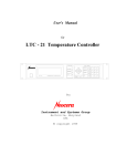
• Check, in the right order, the 4 locations (buttons) indicated on the Figure 1. The
locations are also reported on a figure displayed at the door of the area. The
location to clear is indicated by a lighted green button, which has to be pressed.
At this point you are responsible that nobody is staying in the area.
• When finished, go back to the door. Push the “CALL” button on the door (CCTV
camera and light should come ON).
• When you hear the buzzer, put your black key in the door-lock (and turn it counterclockwise), or press the little black button near the lock, and gently push down
the door-handle.
• Come out, close the door and put back the black keys in their slots.
• The operator should now put by himself the entrance gate in the “red” state. If
not, tell him to close the area (“sperren”).
• Locate the grey box controlling the beam blocker on the left hand side of the
door (“Kanalverschluss KSE301”). Wait until the PSA led is ON (1 minute...)
and press the button AUF to open the beam blocker. After some seconds (30 s.
...) the green led AUF will indicate that the beam blocker is open.
8
2
THE BEAM AREA (πM3.2)
Part I
Figure 1: Location of the 4 RGS buttons of the πM3.2 area
2.2
Entering the area (from Red to Yellow)
To enter in the area for a short time, the user will have to perform some simple operations:
• Close the beam blocker by pushing the button ZU on the grey box located on the
left hand side of the door (“Kanalverscluss KSE301”). Wait until the red led ZU
in ON.
• Call the Control Room via the black “CALL” button (CCTV camera and light
should come ON).
• Be prepared to unlock a black key.
• The operator will switch the entrance gate on the “yellow” state.
• Immediately after that, the black keys will be released (hear the characteristic
click...).
• Each person going in the area should unlock a black key.
• Put one black key in the door-lock and turn it clockwise.
When the buzzer is heard, push the door-handle very gently down, and open the
door.
• Enter and close the door.
• When finished, go back to the door. Push the “CALL” button on the door (CCTV
camera and light should come ON).
• When you hear the buzzer, put your black key in the door-lock (and turn it counterclockwise), or press the little black button near the lock, and gently push down
the door-handle.
• Come out, close the door and put back the black keys in their slots.
• The operator should now put by himself the entrance gate in the “red” state. If
not, tell him to close the area (“sperren”).
• Locate the grey box controlling the beam blocker on the left hand side of the
door. Wait until the PSA led is ON (1 minute...) and press the button AUF to
open the beam blocker. After some seconds (30 s. ...) the green led AUF will
indicate that the beam blocker is open.
2.3
Freeing the area (from Red to Green)
To allow a free access to the area, the user will have to perform some simple operations:
• Close the beam blocker by pushing the button ZU on the grey box located on the
left hand side of the door (“Kanalverscluss KSE301”). Wait until the red led ZU
in ON.
Part I
2
THE BEAM AREA (πM3.2)
9
• Call the Control Room via the black “CALL” button (CCTV camera and light
should come ON).
• Tell the operator to free the access (“Zugang frei”)
• The state of the entrance gate should change to the Green state.
The access is now free.
II.
The instrument
3
General description
The GPS Instrument is permanently installed in area πM3.2, using a so-called “surfacemuon beam” (i.e., positive muons originating from the decay of positive pions stopped
near the surface of the production target M). The typical range of these muons is about
1.5mm in polyethylene or 0.65 mm in aluminum (see also Section 17, page 86). The
πM3 beamline is equipped with an electromagnetic separator/ spin rotator allowing to
rotate the muon-spin direction with respect to the muon momentum.
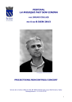
Figure 2: 3D-view of the instrument without sample insert. The muon beam enters the
instrument from the right-hand side.
The instrument is designed for zero- (ZF), longitudinal- (LF), and transverse-field (TF)
µSR experiments in wide ranges of temperature (see Part III, page 17) and external
magnetic field (see Part IV, page 70). A special detector arrangement allows to investigate very small samples. Sample rotation is provided for the study of orientationdependent effects in single crystals.
The GPS Instrument can be used simultaneously with the Low Temperature Facility
(LTF) Instrument either by splitting the beam continuously by widening the spot in
front of the collimators located at the entrance to the septum magnet (see Figure 29,
page 75) or by triggering an electrostatic deflector ("kicker") on request of one of the
Instruments (Muons On REquest, MORE, see also Section 14, page 80).
4
The detectors
The detector arrangement consists of
• A muon detector (M) having a thickness of 0.18 mm.
Part II
4
THE DETECTORS
11
• Six positron detectors (with respect to the beam direction): Forward (F), Backward (B), Up (U), Down (D), Right (R) and Left (L).
Some of these detectors (i.e. U, D, R, and L) are actually composed by two
different subdetectors.
• A so-called “Mobile” detector which is either added to the R or to the L detector
depending on the cryogenic port used.
• Each of the (sub)detector is read on both side by an array (4 or 5) SiPMs photosensors.
• A Backward veto detector (Bveto ). This detector consists of a hollow scintil2
lator pyramid (BLveto , BRveto , BUveto and BD
veto )with a 7x7 mm hole facing the M
counter. The purpose of the Bveto is to collimate the muon beam to a 7x7 mm2
spot and to reject muons (and their decay positrons) missing the aperture ("active
collimation").
• A forward veto detector (Fveto ), rejecting muons which have not stopped in the
sample (and their decay positrons). It is used with small samples. When the
sample/holder assembly stops all muons, Fveto it is usually added to the F detector
to increase the forward solid angle.
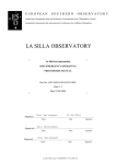
Figure 3: Schematic top view of the detectors. Not shown are the BUveto , BD
veto and the
Up detectors.
12
4
THE DETECTORS
Part II
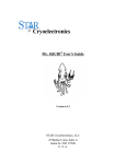
Figure 4: View of the detectors set located up-stream from the sample. The Bveto
pyramid is clearly visible as well as the Backward, Muon detectors. Portions of the
Left and Right detectors are also visible.
Figure 5: View of the detectors set located down-stream from the sample. The U, D,
R (portion), L (portion) and F detectors are visible. The Mobile detector is here in the
“Left” position. The pyramid is the Fveto detector, which can be added or not to the F
definition.
A “stopping” muon is defined as
Mstop = M V
where V represents a veto event, which is defined as V = BLveto + BRveto + BUveto + BD
veto
or V = BLveto + BRveto + BUveto + BD
veto + Fveto in the case of small samples where part of
the Forward detector is used as veto.
Similarly, a positron event is defined as
P = Praw V .
Part II
4
THE DETECTORS
13
In addition the electronics checks for double events, making sure that the detected
positron can unambiguously be connected to a given decaying muon.
14
5
5.1
5
COMPUTERS AND ELECTRONICS
Part II
Computers and Electronics
Data-acquisition and Electronics
Figure 6 shows the overall interconnection of the various hardware items for the GPS
instrument. For the normal users, the main item is the Linux console (pc11318). This
machine is used as an interface for the actual back-end Linux system (psw415) located
in the WHGA building and which runs the data-acquisition.
Figure 6: The overall interconnection of the various hardware items for the GPS instrument
Part II
5.1.1
5
COMPUTERS AND ELECTRONICS
15
New “TDC Electronics”
Introduction:
The new electronics consists of a VME crate with programmable constant fraction discriminators (CFD, PSI CFD950), a multihit TDC ( CAEN V1190) for
digitizing of time information, and a scaler module ( SIS3820) for rate measurements.
The VME frontend process to readout the VME TDC data is running on a frontend Linux PC and connected to the VME crate by a SIS 1100/3100 VME-PCI
interface.
The complete event evaluation is done by software: the TDC is operated in
Continuous Storage Mode, and the frontend process reads all the TDC data. It
searches for events that fulfill logics conditions. The data are sent to the Analyzer
process running on the Backend, which builds the histograms taking into account
post- and pre-pilup conditions, as well as logics conditions (see also Section 4).
The system is also characterized by its flexibility, as the whole logic diagram
is simply stored in special setup files, which can be easily modified and loaded
for a desired configuration into the online database (ODB) of the MIDAS DAQ
system.
Layout:
The Figure 7 represents schematically the different modules used in the VME
crate.
The analog signals are split by an active signal divider (SP950) into a timing
branch sent to the CFD (CFD950 with 8 input channels) and a monitoring
branch for CFD threshold adjustment (see TDC-Elctronics Manual).
Figure 7: Schematics of a typical VME elctronic crate for a bulk muSR experiment.
In additon to the CFDs, TDC, Scaler and VME/PCI interface, the crate is usually also
equipped with a PSI Clock (CD950). Also NIM/ECL PSI converters (LC950) and
Coincidence Units can be installed.
The signals from the CFD’s are sent as ECL signals to the TDC V1190 and
16
5
COMPUTERS AND ELECTRONICS
Part II
also to the scaler. If hardware coincidence is necessary, the ECL or NIM signal
outputs of the CFD can be used with a PSI Coincidence Unit FC950 (available
from Studio E). The signal can be fed back to the TDC and Scaler by the ECL
output of the Coincidence Unit.
The signals from the TDC and Scaler are sent to a MIDAS frontend (Linux PC)
through the optical link VME/PCI interface. In the front-end Linux PC, the
events are checked for coincidence conditions and are sent to the Analyzer process running on the Backend computer, where the histograms are built according
to the trigger and logics conditions defined for a particular setup.
Note that for all the modules developped at PSI, a RS485 connection is available. It allows to setup the module with the MSCB (MIDAS Slow Control Bus)
protocol through a MSCB submaster (connecting the RS485 bus to the ethernet).
Those settings are saved on flash memory on the boards.
Changing the logic:
5.1.2
As said, the logic conditions (as for example switching ON and OFF the Veto
counter) can be changed by software. This is done through the GUI application
deltat (for more information see the Manuals MuSR Graphical User Interface:
deltat and TDC-Elctronics Manual).
Slow Control
The slow control devices are mainly controlled via GPIB (IEEE-488) bus, RS-232
serial line, directly through Ethernet/TCPIP, or through the Midas Slow Control Bus
(MSCB).
• GPIB: Controlled through an Agilent LAN/GPIB Gateways (E5810A).
• RS-232: Controlled either through a Lantronix ETS8PS 8-channel RS232 terminal server.
5.2
Other computers
Some Linux workstations are available. They can be used with the user’s AFS account
or with the local account (account l_musr_tst and password DeltatDeltat).
As described in Section 12.2, the secondary beamline control system, controlling all
beamline elements (magnets, slit systems, separator etc.) between the target station
and the experiment, is now based on the EPICS architecture.
A client-PC is dedicated to control the beamline (hipa-pim3.psi.ch) and is running
under Linux (account acsop and password PSIbeam1).
5.3
Laptop connections
To use your PC or Laptop on the PSI Network you should enable DHCP to get a PSI
TCP/IP address regardless of what host name you choose.
5.4
Printing
CUPS printers are available in the Experimental Hall. The printer WEHA_EG_1 is
located on the gallery between the LTF and GPS cabin. The printer WEHA_E5_2 is
located in the Experimental Hall near the area πE5. It is also equipped with a xerox
machine and a FAX. These printers can be accessed from UNIX and Windows systems (for Windows, just type the print server adress in a Windows Explorer window:
\\winprintw.
III.
6
Sample environment
Quantum cryostats
6.1
6.1.1
Safety
Hazards
The Quantum Continuous Flow Cryostat contains liquid helium. Consequently, like
all equipment using cryogens, certain hazards are present.
The potential hazards are catastrophic rupture of unvented vessels, freezing damage
from splashing cryogens and asphyxiation hazard from high concentrations of helium
gas. Catastrophic rupture can occur if a cryogen is held in a sealed container while
warming. The user should therefore ensure that the necessary valves of the helium
recovery lines are kept open.
6.1.2
Asphyxiation hazard
High concentrations of helium gas in a room constitutes an asphyxiation hazard.
Although non-poisonous, the gas may reduce the concentration of oxygen below safe
levels. When helium concentration is extremely high, then the oxygen in solution in
the blood will diffuse out causing a rapid collapse and possible death.
Every year people die when inhaling helium gas to try the “squeaky voice trick”. A
single deep inhalation of helium gas can be fatal !
18
6.2
6.2.1
6
QUANTUM CRYOSTATS
Part III
Principle of operation
Description
The QUANTUMCOOLER Continuous Flow Cryostat utilizes liquid helium as
a coolant to provide stable, controllable sample temperature. The system is designed for either vertical (cold end down) or horizontal operation. For this reason
the transfer line connection is at 45 degrees, so that it can be operated in either position.
The system consists of 3 components:
• The QUANTUM continuous-flow cryostat
• The QUANTUM return vapor-shielded liquid-helium transfer line
• The QUANTUM removable Sample Stick (“QUANTUMSTICK”)
As shown in Figure 8, liquid helium from the supply dewar travels trough the center of
the transfer line, enters the continuous flow cryostat and the flow is split:
Sample Chamber Flow:
The first flow circuit is for sample cooling. Liquid helium from the transfer line
enters the top of the Phase Separator (PS), and the liquid from the bottom is expanded through the needle valve V4 then is injected in the Sample Chamber. The
cold gas exits at the top of the Sample Chamber and the flow is controlled by the
manual valve V2 and the electromagnetic valve V3b and the pumps PUMP2_A
and PUMP2_B.
Heat Shield Cooling Flow:
The second flow circuit is the heat shield cooling. Liquid helium from the transfer line enters the top of the Phase Separator, and the gas exiting from the top of
the PS is used to cool the sample chamber and the main heat shields (EX). The
cold return gas is then used to cool the transfer line shield. The flow is controlled
by the valve V1 and the pump PUMP1.
Part III
6
QUANTUM CRYOSTATS
Figure 8: Schematic diagram of the Quantum cryostat.
P : pressure; F : flow; V : valve; EX : heat exchanger; PS : phase separator.
19
20
6.2.2
6
QUANTUM CRYOSTATS
Part III
Principle of control action
Phase Separator:
For all desired sample temperatures, the temperature of the Phase Separator (TPS )
should be kept constant.
Utilizing the available DT-470 Lake Shore Diode, and taking into account the
pressure drop through the heat exchangers, and the uncertainties of the sensors,
one should maintain the following temperatures:
Cryostat
Quantum 9505
Quantum 9506
Quantum 9512
TPS
∼ 4.6 K
∼ 4.3 K
∼ 4.1 K
These temperatures are obtained by adjusting, with the valve V1, the mass flow
through the pump PUMP1.
During test runs, stable TPS could be achieved with the following flows:
Cryostat
Quantum 9505
Quantum 9506
Quantum 9512
F1
∼ 13.0 l/min
∼ 11.5 l/min
∼ 12.5 l/min
It is not advisable to operate with a too high flow value, for which temperature
instabilities are again observed.
Sample Chamber:
The He-gas entering the Sample Chamber is heated at the desired temperature by
means of the Diffuser Heater (DH) and its temperature (Tdi f f user ) is monitored
by a Cernox temperature sensor (loop 1 of the temperature controller).
Depending on the desired temperature range, a heater (“Tube Heater”) located
on the He-capillary, after the needle valve V4 (see Figure 9), is used to prevent
the sudden flow of liquid helium in the Sample Chamber.
In order to obtain a faster response of the system, a second heater loop is placed
on the Sample Stick (temperature sensor: Cernox, connected to the loop 2 of the
temperature controller).
The operation may be divided into two overlapping temperature ranges:
• ∼ 2.1K (or ∼ 1.8K using also the PUMP2_B) < Tsample < 10K (“Low
Temperatures”)
• ∼ 4K (cryostat 9512) or 5K (cryostat 9505 & 9506) < Tsample < 300K
(“High Temperatures”)
Part III
6
QUANTUM CRYOSTATS
21
Transfer
line
80-K Shield Temp.
Sensor
PS Temp. Sensor
PS
20-K Shield Temp.
Sensor
PS Heater
Tube Temp. Sensor
Tube Heater
Holder Heater
Diffuser Temp.
Sensors
Holder Temp.
Sensor
Diffuser Heater
Figure 9: Temperature sensors and heaters
Low Temperatures:
In this regime, the manual valve V2 should be kept fully open.
No current should be sent to the Tube Heater.
If a base temperature of ∼ 2.1 K is enough for the foreseen measurements, the
PUMP2_B should not be used. (Control that it is switched OFF).
If a base temperature of ∼ 1.8 K is required, the PUMP2_B should be switched
ON.
The lowest stable temperature is then obtained by gradually closing the
needle valve V4.
As the valve is closed the pressure P2 will gradually decrease and the sample
temperature will decrease correspondingly.
Do not forget to change the setpoint temperature of the temperature controller.
When the minimum flow is reached, further decrease in the needle valve V4 will
result in a rapid warmup of the sample. In this case the needle valve should be
slightly opened and the same operation as above should be repeated.
During test runs, stable base temperatures could be obtained with the following parameters:
22
6
QUANTUM CRYOSTATS
Configuration
PUMP2_A
PUMP2_A + PUMP2_B
Tdi f f user
∼ 2.15 K
∼ 1.8 K
Part III
P2
∼ 32 mbar
∼ 5 mbar
F2
5 l/min
5 l/min
Higher temperatures (up to 10 K) are achieved by keeping the He-flow constant
and solely changing the setpoints of the temperature controller.
Note that a temperature scan in this regime is only possible once the pressure
and flow conditions necessary to reach the lowest temperature are obtained.
Typically, for the lowest temperatures, one will observe a situation with
Tdi f f user slightly above Tholder . Upon warming up Tholder will increase faster
than Tdi f f user in such a way that both sensors will measure a similar temperature
around 3 K. At higher temperatures, Tholder < Tdi f f user and the difference
reaches about 1 K at 15 K (with PUMP2_A + PUMP2_B)].
Extensive tests performed by H. Luetkens have show that the temperature of the
sample closely follows the holder temperature Tholder at all temperatures (see
Figs. 10 and 11). This is true independently of the sample mounting (on a silver
holder or on a fork).
Therefore, in view of the observed temperature gradients in this temperature regime, users are advised to control the temperature by solely setting a
setpoint for Tdi f f user . This can be achieved by putting an arbitrary setpoint of say
1 K for Tholder . Alternatively the temperature controller can be set on a one-loop
mode. For more details see section 6.4.1. The temperature of the sample is the
one given by Tholder .
Part III
6
QUANTUM CRYOSTATS
23
Figure 10: Comparison of the temperatures measured at the diffuser with the ones
measured at the sample holder and at the sample position (“Fork"). Note the gradient and the perfect agreement between the sample holder temperature and the “Fork"
temperature.
Figure 11: Same configuration as in Fig. 10 for higher temperatures. Note that the
gradient is now opposite.
24
6
High Temperatures:
QUANTUM CRYOSTATS
Part III
In this regime, the manual valve V2 is kept closed, and the electromagnetic valve
V3b controls the mass flow through the pump PUMP2_A (make sure that the
PUMP2_B is switched OFF and that the valve V3a is fully open).
A heater current should be sent and kept at all times into the Tube Heater.
Cryostat
Quantum 9505
Quantum 9506
Quantum 9512
Tube Heater Current
230 mA
230 mA
200 mA
The needle valve V4 should be about 0.5 mm open (50 units).
If large temperature oscillations are observed at low temperatures (especially
around 15-20 K), the needle valve V4 should be further slightly closed.
The desired temperature is obtained by choosing the He-flow F2 according to
the Figures 12 (Cryostat 9505), 13 (Cryostat 9506) or 14 (Cryostat 9512) and
by sending the required setpoints to the temperature controller. If the flows necessary to reach the lowest temperatures (in this regime) cannot be reached, the
needle valve V4 should be slightly more opened.
Since the sample holder is solely cooled down by the incoming He-gas
which is stabilized at the temperature of the Diffuser, the time constant necessary to reach a given setpoint by cooling can be extremely long (for an example,
see Figure 15).
It is therefore strongly recommended to perform the required temperature
scans by increasing the temperature.
If long series of runs are required below 10 K, it is strongly recommended to
switch to the Low Temperatures regime (see previous pages) in order to save
He-liquid.
Part III
6
QUANTUM CRYOSTATS
25
Cryostat 9505 :
Figure 12: Temperature dependence of the He-flow through the Sample Chamber (flow F2) in the “High Temperature
regime” (i.e. for 5 K < Tdi f f user < 300 K). This flow should be controlled by the valve V3b. If the recommended low
values of flow are not applied at high temperatures, a temperature gradient is usually observed in the sample chamber.
26
6
QUANTUM CRYOSTATS
Part III
Cryostat 9506 :
20
He-flow through the Sample Chamber High Temperature regime
5
18
4
He-flow (l/min)
16
3
14
2
12
1
10
0
8
0
50
100
150
200
250
300
6
4
2
0
0
5
10
15
20
25
30
35
40
T (K)
Figure 13: Temperature dependence of the He-flow through the Sample Chamber (flow F2) in the “High Temperature
regime” (i.e. for 5 K < Tdi f f user < 300 K). This flow should be controlled by the valve V3b. If the recommended low
values of flow are not applied at high temperatures, a temperature gradient is usually observed in the sample chamber.
Part III
6
QUANTUM CRYOSTATS
27
Cryostat 9512 :
He-flow through the Sample Chamber High Temperature regime
He-flow (l/min)
22
20
5
18
4
16
3
14
2
12
1
10
0
8
0
50
100
150
200
250
300
6
4
2
0
0
5
10
15
20
25
30
35
40
T (K)
Figure 14: Temperature dependence of the He-flow through the Sample Chamber (flow F2) in the “High Temperature
regime” (i.e. for 5 K < Tdi f f user < 300 K). This flow should be controlled by the valve V3b. If the recommended low
values of flow are not applied at high temperatures, a temperature gradient is usually observed in the sample chamber.
28
6
QUANTUM CRYOSTATS
Part III
75
70
T (K)
65
60
55
50
45
0
10
20
30
40
50
Time (min)
Figure 15: Example of heating and cooling curves (solid line: Tdi f f user , dashedline Tholder ). Note the large time
difference between a heating and cooling process. At higher temperatures, the time difference and the undershoot of
Tdi f f user when cooling, due to the rapid change of the He-capillary impedence, are much more pronounced.
Part III
6.2.3
6
QUANTUM CRYOSTATS
29
Configuration in the πM3 area
• Pump PUMP1: Gast membrane pump.
• Pump PUMP2_A: Alcatel ADP 30 oil-free pump.
• Pump PUMP2_B: Alcatel RSV 151B roots pump.
• Electromagnetic Valve V3b: PFEIFFER EVR116 valve controlled by a PFEIFFER RVC300 valve controller (located in the beam area).
• The He-flows are measured by two Hastings transducers connected to two Hastings flowmeter display.
The units are directly liters-gas/minute. The maximum flow which can be measured is 50 l/min.
• The temperature of the Sample Chamber is controlled by a Conductus LTC-20
temperature controller.
– The temperature of the Diffuser Tdi f f user is measured on the channel 1 (loop
1).
– The temperature of the Sample Holder Tholder is measured on the channel 2
(loop 2). The voltage loop 2 of the Conductus controls an external Gossen
power supply.
The Tables 1, 1 and 3 (first loop) and 4, 5 and 6 )second loop) indicate the value
of the PID parameters used by the temperature controller for the two loops.
• A CryoCon 14 (or LakeShore 208) thermometer display indicates the temperature of different heat shields and of the Phase Separator.
– The temperature of the Phase Separator TPS is usually measured on the
channel 1.
– The temperature of the He-capillary (Tube) after the needle valve is usually
measured on the channel 2.
30
6
QUANTUM CRYOSTATS
Part III
Table 1: Cryostat 9505: PID parameters for the Loop 1 (diffuser) of the temperature
controller. The P parameters are rounded when displayed by the controller. The parameters are stored in a PID Table of the Conductus temperature controller. The
maximum power should be fixed at 40 %.
Cryostat 9505 - Loop 1
Break
P
I
D
Heater
point (K)
Range (W)
300
30 20 4
50
150
30 20 4
50
100
100 30 10
5
50
100 10 4
5
20
250 10 1
5
15
150 5
2
5
10
50
5
1
5
4
200 6
2
0.5
3
100 10 2
0.5
1
2
8
2
0.5
Table 2: Cryostat 9506: PID parameters for the Loop 1 (diffuser) of the temperature
controller. The P parameters are rounded when displayed by the controller. The parameters are stored in a PID Table of the Conductus temperature controller. The maximum
power should be fixed at 27 %.
Cryostat 9506 - Loop 1
Break
P
I
D
Heater
point (K)
Range (W)
300
10 40 20
50
200
8
40 20
50
150
6
40 20
50
100
30 120 60
5
50
20 24
6
5
20
15 35 16
5
6
18 10
3
0.5
5.5
18 10
3
0.5
3
20 10
3
0.5
1
20
8
2
0.5
Part III
6
QUANTUM CRYOSTATS
31
Table 3: Cryostat 9512: PID parameters for the Loop 1 (diffuser) of the temperature
controller. The P parameters are rounded when displayed by the controller. The parameters are stored in a PID Table of the Conductus temperature controller. The
maximum power should be fixed at XX %.
Cryostat 9512 - Loop 1
Break
P
I
D
Heater
point (K)
Range (W)
300
30 30 4
50
70
30 30 4
50
60
40 30 5
5
30
40 17 2
5
15
40 13 2
5
10
10
9
1
5
8
10 10 1
5
4
50
5
1
0.5
3
100 10 1
0.5
1
500 10 1
0.5
Table 4: Cryostat 9505: PID parameters for the Loop 2 (Sample Holder) of the temperature controller. The parameters are stored in a PID Table of the Conductus temperature
controller.
Cryostat 9505 - Loop 2
Break
P
I
D
point (K)
300
70 10 2
250
70 10 2
200
70 10 2
150
70 10 2
100
70 10 2
70
10 10 2
40
2 10 2
10
1
8
2
5
1
8
2
1
1
8
2
32
6
QUANTUM CRYOSTATS
Part III
Table 5: Cryostat 9506: PID parameters for the Loop 2 (Sample Holder) of the temperature controller. The parameters are stored in a PID Table of the Conductus temperature
controller.
Cryostat 9506 - Loop 2
Break
P
I
D
point (K)
300
70 10 2
250
70 10 2
200
70 10 2
150
70 10 2
100
70 10 2
70
10 10 2
40
2 10 2
10
1
8
2
5
1
8
2
1
1
8
2
Table 6: Cryostat 9512: PID parameters for the Loop 2 (Sample Holder) of the temperature controller. The parameters are stored in a PID Table of the Conductus temperature
controller.
Cryostat 9512 - Loop 2
Break
P
I
D
point (K)
300
70 10 2
250
70 10 2
200
70 10 2
150
70 10 2
100
70 10 2
70
10 10 2
40
2 10 2
10
1
8
2
5
1
8
2
1
1
8
2
Part III
6.2.4
6
QUANTUM CRYOSTATS
33
Sample change
The following points describe the process of changing a sample in the cryostat.
• For safety reasons, a sample change should only be performed in the “High
Temperature regime” with a sample temperature T > 30 K.
• Switch OFF the heaters by setting the Conductus (or Neocera) temperature controller in the Monitor Mode [by pressing the Local button (if necessary) and
pressing the Monitor button].
• Switch OFF the Tube Heater.
• Disconnect the electrical plug from the sample stick.
• Dismount, if necessary, the rotation motor.
• Stop the He-flow through the pumps PUMP1 and PUMP2_A by closing:
– the two valves V2 and V3a on the pumping line of the Sample Chamber (do
not disconnect the electrical plug of the electrovalve V3b).
– the yellow valve V1 on the transfer-line pump (use the closing-ring without
changing the actual setting of the valve).
• Pressurize slightly the Sample Chamber with He-gas by opening the valve V6
until you reach a pressure P2 slightly above 1000 mbar (check if the He-gas
cylinder is open).
• Check carefully and frequently the pressures P1 and P2 in the Phase Separator
and in the Sample Chamber. (An overpressure in the Sample Chamber could
damage the titanium windows).
• Remove the clamp of the Sample Stick.
• Remove the Sample Stick from the cryostat.
• Immediately mount a blind-flange on the cryostat opening.
• Stop blowing He-gas by closing the valve V6.
• Restart the He-flow through the He-pumps by opening the valves V1, V3a.
When you are ready to insert the Sample Stick with the new sample, you should follow
an analog procedure as above. Namely:
• Stop the He-flow through the pumps by closing:
– the two valves V2 and V3a on the pumping line of the Sample Chamber (do
not disconnect the electrical plug of the electrovalve V3b).
– the yellow valve V1 on the transfer-line pump (use the closing-ring without
changing the actual setting of the valve).
• Pressurize slightly the Sample Chamber with He-gas by opening the valve V6
until you reach a pressure P2 slightly above 1000 mbar (check if the He-gas
cylinder is open).
• Check carefully and frequently the pressures P1 and P2 in the Phase Separator
and in the Sample Chamber.
• Dismount the blind-flange very shortly before inserting the Sample Stick.
• Insert the Sample Stick carefully (to insert a warm Sample Stick requires more
force than to remove a cold Stick).
• Replace the clamp.
• Immediately stop blowing He-gas by closing the valve V6.
• Restart the He-flow through the He-pumps by opening the valves V1, V3a (and
V2 if the low temperature regime is needed).
34
6
QUANTUM CRYOSTATS
Part III
• Readjust the He-flows.
• When a sufficient He-flow is detectable in the Sample Chamber, set the temperature controller in the Control Mode [by pressing the Local button (if necessary)
and pressing the Control button].
Note that if the sample stick was changed, you will have first to configure the
temperature controller via the Console (see Section 6.4.1). You can also switch
the temperature controller on Control Mode from the Console.
• If you want to operate in the High Temperature regime, do not forget to switch
ON the Tube Heater.
Part III
6.2.5
6
QUANTUM CRYOSTATS
35
He-Dewar change
Should the He-Dewar levelmeter read below ∼15 % (in the case of a 100-liters dewar) or below 100 mm ( in the case of a 250-liters dewar), the He-Dewar needs to be
changed.
• For safety reasons, a He-dewar change should only be performed in the
“High Temperature regime” with a sample temperature T > 30 K.
• Stop the He-flow through the pumps PUMP1 and PUMP2_A by closing:
– the two valves V2 and V3a on the pumping line of the Sample Chamber (do
not disconnect the electrical plug of the electrovalve V3b).
– the yellow valve V1 on the transfer-line pump (use the closing-ring).
• Switch OFF the heaters by setting the Conductus (or Neocera) temperature controller in the Monitor Mode [by pressing the Local button (if necessary) and
pressing the Monitor button].
• Switch OFF the Tube Heater.
• Lift up slightly (∼50 cm) the transfer line on the He-dewar side
(the bottom part of the transfer line in the He-dewar should now be above the
liquid-He level).
• Pressurize slightly the Phase Separator with He-gas by opening the valve V5 until
you reach a pressure P1 of about 1000 mbar (check that the He-gas cylinder is
open).
• Check carefully and frequently the pressure P1 and P2 in the Phase Separator
and in the Sample Chamber. (An overpressure in the Sample Chamber could
damage the titanium windows).
• Disengage the adaptor of the transfer line from the top of the dewar by releasing
the O-rings.
• Slide the adaptor upward along the transfer line.
• Remove completely the transfer line on the He-dewar side.
Replace the plug of the He-dewar to prevent freezing of the He-dewar.
• Carefully warm up the transfer line using the available heat-gun.
• Be sure that the sintered end-part is free of any ice.
• Change the He-dewar.
• Check that the He-recovery line is connected to the dewar and that the corresponding valves are open. Be sure that the recovery line is not bent and
that the He-gas can flow freely.
• Insert slowly the transfer line in the new He-dewar.
• As soon as the sintered part is enough inserted in the dewar, lower the adaptor
and connect it to the dewar.
Make sure that the adaptor of the transfer line is well inserted in the dewar,
and that all O-rings are tightened.
Leave the transfer line above the liquid-He level.
• Stop blowing He-gas by closing the valve V5.
• Open the valves on both He-pumps (do not forget, if necessary, to connect the
electrical plug of the electrovalve V3b).
Open the valve V1 completely.
• Wait 30 seconds.
• Pull down slowly the transfer line in the He-dewar.
Check carefully and frequently that the transfer line is well aligned with the
36
6
QUANTUM CRYOSTATS
Part III
dewar and that it does not bent; if necessary move slowly and carefully the
He-dewar to align it with the transfer-line.
Be also sure that the transfer line does not touch the bottom of the He-dewar
(leave it few centimeters above the bottom).
• The He-flow in the transfer line will first show a rapid increase, due to the sudden
overpressure in the He-dewar, which will be followed by a decrease.
After 1-2 minutes, the He-flow through the transfer line will again increase to its
maximum value.
• After a few minutes, the temperature of the Phase Separator should drop to the
nominal value.
• Readjust the He-flows.
(For this last point, experience shows that the transfer line flow F2 should be
maintained for few minutes to a high value and gradually decreased)
• When a sufficient He-flow is detectable in the Sample Chamber, set the temperature controller in the Control Mode [by pressing the Local button (if necessary)
and pressing the Control button].
• If you want to operate in the High Temperature regime, do not forget to switch
ON the Tube Heater.
• Do not forget to tightly close the empty He-dewar and to connect it to the Herecovery line
Part III
6.2.6
6
QUANTUM CRYOSTATS
37
Startup procedure – Cryostat warm
This section is not intended to a normal µSR Facility user.
• Check vacuum space of cryostat and transfer line.
• Connect transfer line to cryostat.
• Open needle valve V4 completely.
• Close valve V1, V2 and V3a.
• Turn ON vacuum pumps PUMP1 and PUMP2_A.
• Open carefully valves V5 and V6 to purge the cryostat.
• Check carefully and frequently the pressure P1 and P2 in the Phase Separator
and in the Sample Chamber. (An overpressure in the Sample Chamber could
damage the titanium windows).
• Insert slowly the transfer line in the new He-dewar.
• As soon as the sintered part is enough inserted in the dewar, lower the adaptor
and connect it to the dewar.
Make sure that the adaptor of the transfer line is well inserted in the dewar,
and that all O-rings are tightened.
Leave the transfer line above the liquid-He level.
• Open the valves on both He-pumps (do not forget, if necessary, to connect the
electrical plug of the electromagnetic valve V3b).
• Wait 3 minutes.
• Pull down slowly the transfer line in the He-dewar.
• Once TPS has reached its nominal temperature (see page 20), the valve V1 should
be partially closed.
If an increase of TPS is observed this indicate that V1 has been closed too much
and insufficient helium is entering the system.
• Once the optimum V1 setting has been achieved, the sample temperature can be
controlled as described in Section 6.2.2.
38
6.2.7
6
QUANTUM CRYOSTATS
Part III
Shutdown procedure
This section is not intended to a normal µSR Facility user.
• Stop the He-flow through the pumps PUMP1 and PUMP2_A by closing:
– the two valves V2 and V3a on the pumping line of the Sample Chamber
(remove the electrical plug of the electrovalve V3b).
– the yellow valve V1 on the transfer-line pump (use the closing-ring).
• Lift up slightly (∼50 cm) the transfer line on the He-dewar side
(the bottom part of the tranfer line in the He-dewar should now be above the
liquid-He level).
• Open the needle valve V4 completely.
• Pressurize slightly the Phase Separator with He-gas by opening the valve V5
until you reach a pressure P1 of about 1000 mbar (check if the He-gas cylinder
is open).
• Check carefully and frequently the pressure P1 and P2 in the Phase Separator
and in the Sample Chamber. (An overpressure in the Sample Chamber could
damage the titanium windows).
• Disengage the adaptor of the transfer line from the top of the dewar by releasing
the O-rings.
• Slide the adaptor upward along the transfer line.
• Remove completely the transfer line on the He-dewar side.
Replace the plug of the He-dewar to prevent freezing of the He-dewar.
• Connect the transfer line to the He-recovery line.
• If time is not pressing, stop blowing He-gas in the system by closing the valves
V5 (blowing He-gas in the system will speed up the warming process, but will
introduce an additional hazard factor...).
• Switch OFF the two vacuum pumps.
Part III
6.2.8
6
QUANTUM CRYOSTATS
39
Trouble shooting
This section is hopefully intended to help the user coping with several known problems.
• In the High Temperature Regime, Tdi f f user is oscillating.
Check that the needle valve V4 is 0.5 mm open (50 units) (very sensitive...).
Check that the Tube Heater is switched ON.
Check that the He-flow F1 through the transfer line is high enough (the TPS
value are given on page 20). Increasing F1 slightly usually helps to keep a
stable Tdi f f user .
• Temperature oscillations around 20 K, in the High Temperature Regime.
Check that the Tube Heater is switched ON
Close slightly the needle valve V4.
• In the High Temperature Regime: large temperature gradient and very low
values of P1.
The needle valve V4 is probably closed too much.
• In the High Temperature Regime one cannot reach the values of He-flow needed
to obtain the lowest temperature in this regime (i.e. 4 or 5 K, depending on the
used cryostat).
Open slightly the needle valve V4.
• In the High Temperature Regime: large temperature oscillations are seen below
10 K.
Make sure that the setpoints for the two loops (diffuser – channel 1 and holder
– channel 2) are set to the same values. The PID parameters are optimized
only for this configuration.
• After a sample change or a long period at high temperature, the lowest temperature in the Low Temperature Regime can hardly be obtained (by closing the
needle valve V4, a large temperature increase is observed).
It is just a matter of waiting long enough...If time is crucial, it is advisable to
perform a first run at about 2.5-3 K even without the optimal values of P2 and
F2 (see Section 2.2.2) but with F2 low enough to avoid temperature gradient
(say about 6-7 l/min). After this first run, one should be able to obtain the optimal values of P2 and F2 which are necessary to reach the lowest temperature
and also to start a temperature scan.
• After a He-dewar change, the flow F1 does not reach the usual values and the
pressure P1 is lower as usual.
Be sure that the bottom of the transfer line does not touched the bottom of the
He-dewar.
If not, the transfer line is probably partially blocked.
Remove it from the He-dewar (following the instructions as for changing the
He-dewar) and warm it up again. Let a flow of He-gas flowing through the
transfer line by opening the valve V5
• Upon reaching the lowest temperature in the Low Temperatures regime, the
temperature controller does not display the sensor #2 (holder sensor) any more
and the controller has jumped to the Monitor Mode.
This happens sometimes at very low temperatures with Diode sensors.Wait few
minutes to see if the display comes back to normal.
If yes, switch the temperature controller to the Control Mode [by pressing the
Local button (if necessary) and pressing the Control button].
If not and you are desperate, put the controller on a one-loop mode with the
help of the deltat program (Tab: Modify Devices, buttons Modify
and Modify setup.)
40
6.3
6
QUANTUM CRYOSTATS
Dimensions
• Dimensions.
• Sample holder dimension.
Part III
Part III
6
QUANTUM CRYOSTATS
Figure 16: Drawing of the internal part of the Quantum cryostat inside the GPS chamber.
41
42
6
QUANTUM CRYOSTATS
Figure 17: Drawing of the coomonly used sample holder.
Part III
Part III
6
QUANTUM CRYOSTATS
43
• Material in beam path :
Up-stream:
Heat Shield Superinsulation
Sample Chamber Window
Material
Aluminized Mylar
Titanium
Thickness
10 µm (2 layers)
10 µm
Same for down-stream
• Window sizes :
Heat Shield
Sample Chamber Window
In
Out
29.0 mm diam.
15 mm diam. 20 mm diam.
44
6.4
6.4.1
6
QUANTUM CRYOSTATS
Part III
Additional Information
Temperature Controller
The Conductus temperature controller connected to the Quantum cryostat is usually
utilized in a REMOTE-mode and can be directly controlled from deltat. The following steps describe how to initialize, configure and use the Conductus temperature
controller from deltat.
• Configuration:
Each time that you change the configuration of the cryostat (new sample stick),
you have to configure the driver controlling the temperature controller.
In the tab Modify Devices choose the temperature controller entry
and hit the buttons Modify and, on the pop-up window, Modify Setup.
Choose the corresponding sample stick from the drop-down list.
Hit the Next button and choose the corresponding Entry for your setup
Remember that the QUANTUM is usually controlled by the Conductus in a
two-loop mode
Hit the Apply & Exit button and at this point the software should automatically detect the PID tables needed and load them into the Conductus
temperature controller.
Remember to put the controller in the CONTROL mode.
• Setting a temperature:
In the tab Modify Devices choose the temperature controller entry and hit
the buttons Modify and, on the pop-up window, Modify Temperature.
On the pop-up window, change for both loops the setpoints and hit the button
Apply Changes.
• Autorun sequences:
Before writing an autorun sequence, be sure that the Conductus in the desired
mode (one or two-loop mode).
In the autorun file, do not forget to give all 6 arguments in the two-loop mode
(only 3 for the one-loop mode).
To change the temperature, you will need an entry like:
SET Temperature 100.0 1.0 30 100.0 1.5 30
WAIT Temperature INRANGE
In this example the setpoints are 100.0 K for both loops, the tolerances
1.0 K for the first loop and 1.5 K for the second loop and the waiting times are
30 seconds.
See also page 22, for a discussion about the Low Temperature setpoints.
• Software setup - done by the µSR Facility team:
The on-line database in the backend computer has to be edited. In the database
directory
/Equipment/templtc/Settings/Devices/LTC21out/DD
the variable Serial Number should be set accordingly.
In the directory /userdisk0/musr/exp/td_musr/dat/ltc/ of the
Backend computer a file ltc_NNNN.tab should exist (where NNNN is the
serial number of the controller).
Part III
6.4.2
6
QUANTUM CRYOSTATS
45
He-flow control
The He-flow trough the “Sample Space” can only be controlled when solely the
Electromagnetic Valve V3b (PFEIFFER EVR116) is used, the big bypass valve V2 is
shut and the PUMP2_B is switched OFF.
The control is performed by the Valve Controller PFEIFFER RVC300. The actual He-flow is measured by a flowmeter (HASTINGS HS-50KS) and is also indicated
on the center display located at the top of the rack.
• Setting a flow from deltat:
In the tab Modify Devices choose the flow controller entry and hit the
Modify button. Enter the new flow value in the pop-up window and close it.
• Setting a flow in an autorun sequence:
A He-flow setpoint can also be included in a auto-run sequence by using the
command SET Flow FLOW XXX command.
Example:
SET Flow FLOW 4.3
With this example, an He-flow setpoint has been set to 4.3 liter-gas/minute.
• Manual setpoint (only in case of emergency):
Locate the RVC300 device in the area rack.
Press the button locate below PARAM.
Press the edit button to edit the SOLL value. Change it with arrow buttons
(note that 100 mV correspond to 1 l/min).
Presse the button locate below SAVE
• Software setup - done by the µSR Facility team The on-line
in the backend computer has to be edited.
In the database
/Equipment/flowr300/Settings/Devices/RVC300/DD,
ables Scale should be set to 100, Flim to 25, Vlim to 6000 and
accordingly.
database
directory
the variOffset
The time needed for the actual He-flow to reach the setpoint value will depend on the
PID parameters of the RVC300 controller.
When increasing the temperature, the He-flow should be changed first, if necessary.
The temperature controller setpoint, should be changed in a second step. The opposite
should be done when decreasing the temperature.
If a large change of flow is required, big temperature overshoots can be observed. To
minimize the overshoots, the He-flow setpoint should be changed in different steps
prior to change the temperature controller setpoint.
Depending on the setting of the needle valve V4 between the “Phase Separator”
and the “Sample Space”, it is possible that a desired He-flow cannot be reached
eventhough the RVC300 controller will fully open the Electromagnetic Valve V3b. To
fix this problem, one should more open the needle valve.
46
6.4.3
6
QUANTUM CRYOSTATS
Part III
Sample rotation
A step motor and its controller (EL734) can be utilized to rotate the sample.
The motor unit can be mounted on the cryostat on the available holders (3). The motor
shaft has to be connected to the sample stick using the available screws (2).
The motor control unit EL734 switches automatically to local mode as soon as a local
operation is performed.
To rotate manually the sample:
• Be sure that the “+” and “-” buttons are lit (otherwise wait few seconds). Press
the green round button corresponding to the motor # 1
The green LED of the button should now be ON.
• Press and hold the “+" (or “-") yellow button to rotate the sample in one or the
other direction
• If during this operation, the green square button suddenly lit, it means that the
computer has taken the control of the device. In this case, wait few seconds and
restart the procedure. The computer connects to the device every 30 seconds...,
so be quick...)
To rotate the sample remotely:
• In deltat, the tab Modify Devices contains the device Position.
Choose this device and hit the Modify button. Enter the new position value
in the pop-up window and close it.
• A rotation of the sample can also be included in a auto-run sequence by using
the command
SET Position ANGLE 100.0
With this example, an angle of 100 is requested.
Part III
6.4.4
6
QUANTUM CRYOSTATS
47
Miscellaneous
• The second loop of the temperature control utilizes the “analog” output of the
temperature controller (CONDUCTUS). The output is utilized to control the
Gossen power supply. Figure 18 indicates the necessary settings to interface
both instruments. The maximum current for the Gossen is therefore limited to
about 0.5 Amp.
A
B
C
D
E
F
H
+
J
K
L
R RI
M N
P
R
S
T
U
V
W X
Y
Z
R PI
U RI
Figure 18: Diagram of the back-connector of the Gossen power supply. URI represents
the voltage provided by the temperature controller (max. 10 Volts). RRI is fixed at
2033 Ohms and RPI at 34Ohms. The current furnished will be given by URI × RPI ×
IFS /(0.6×RRI ) where IFS represents the current full-scale of the Gossen power supply
(see Gossen manual).
48
7
7.1
7
ZÜRICH OVEN
Part III
Zürich Oven
Introduction
Although the “Zürich”-oven can now be used on some Facility spectrometers, it is not
a Facility instrument. Therefore, the users should be aware that only a limited support
will be available from the Facility team.
The oven can be operated between room temperature and 1200 K. The sample holder is
connected to a ”warm” finger and the oven is operated in vacuum. Therefore the users
should take care to obtain a good thermal contact between the sample and the holder.
An appropriate method should be used to attach the sample to the holder (do not use
glue !).
The oven is usually installed on the 2nd cryogeny port of the GPS instrument. As
opposed to the situation in the Quantum cryostat, the vacuum chamber around the oven
is separated from the main vacuum of the spectrometer. Figure 19 shows the pump
connections to the oven.
Therefore, independent pumps are necessary to evacuate this chamber (usually a standard “MOGLI” pumping unit).
Figure 19: Vacuum diagram for the Zürich oven.
7.2
Temperature control
Three thermocouples (type N) are used to monitor and control the temperature of the
different parts of the oven:
• at the heater position,
• at the sample holder,
• on the thermal shield.
The temperature stability loop is based on the thermocouple at the level of the thermocoax heater. The sample temperature is provided by the additional thermocouple
Part III
A
B
C
D
7
ZÜRICH OVEN
E
F
H
+
J
K
L
R RI
49
M N
P
R
S
T
U
V
W X
Y
Z
R PI
U RI
Figure 20: Diagram of the back-connector of the Gossen power supply. URI represents
the voltage provided by the temperature controller (max. 10 Volts). RRI is fixed at
1000 Ohms and RPI at 60 Ohms. The current furnished will be given by URI × RPI ×
IFS /(0.6×RRI ) where IFS represents the current full-scale of the Gossen power supply
(see Gossen manual).
placed on the back of the sample holder. The third thermocouple measures the temperature of the water-cooled shields. Since spare parts are rather difficult to obtain, users
should carefully handle these thermocouples. Please discuss with the Facility team
about an appropriate mounting procedure.
The thermal-shield thermocouple is always connected to the PU5 Thermocouple
Display.
Using the LTC Conductus/Neocera temperature controller:
When using the LTC Conductus/Neocera temperature controller both other thermocouples are also connected to PU5 Thermocouple Display, which provide a linear
output signal to feed the Conductus/Neocera temperature controller.
The PID values of the temperature controller are kept to fix values (10, 250 and 0 for
the parameters P, I and D).
Using the Lakeshore 340 Temperature Controller:
When the Lakeshore 340 Temperature Controller is used, both other thermocouples
are directly connected to the controller and not to the PU5 Thermocouple Display.
The thermocouple for the heater is connected as sensor C and the thermocouple of the
sample is connected as sensor D.
For the Lakeshore, the PID parameters shown on Table 7 are used.
Table 7: Zurich Oven: PID parameters for the Loop 2 of the temperature controller.
The parameters are stored in a PID Table of the Lakeshore temperature controller.
Zurich Oven - Loop 2
Break
P
I
D
point (K)
450
15 1.2 3
500
19 1.8 4
700
24 2.4 4
800
30 3.6 4
1200
50
6
5
To heat up the sample, the analog output of the temperature controllers is sent to
a GOSSEN power supply (use exclusively the type 24K32R4: 32V/4A). Figure 20
indicates the necessary settings to interface both instruments. The maximum current
for the GOSSEN is therefore limited to about 4 Amp.
50
7.3
7
ZÜRICH OVEN
Part III
Sample change
• Stop heating by switching either:
– the temperature controller to MONITOR mode (if necessary depress first
the LOCAL button) in case that a LTC Controller is used.
– or by switching the corresponding button on the HECTOR unit in case that
a LS340 is used.
• Wait until the temperature is below 320 K. Be patient ! This can take a very long
time (hours...).
• Stop pumping by swiching OFF the MOGLI pumping unit . This is performed
by pressing the button LOCK HV on the MOGLI Controller.
• Remove the screws connecting the oven to the vacuum chamber.
• Slowly open the valve V-He to admit He-gas into the chamber. Check carefully
and frequently the pressure in the chamber: do not go beyond 1000mbar.
• Close valve V-He.
• Open the oven.
• Stop the water flow by closing both valves (IN and OUT).
• Change your sample.
• Carefully remount the thermocouple.
• Open the water flow by opening both valves (IN and OUT).
• Insert the oven and connect it to the vacuum chamber with the available screws.
• Start pumping by pressing the button UNLOCK HV on the MOGLI Controller.
Note that the HV valve will only be open when pre-defined conditions will be
fullfilled.
• Check again that the water is flowing and switch ON the temperature controller
by
– pressing the button CONTROL (if necessary depress first the LOCAL button) in case that a LTC Controller is used.
– or by switching the corresponding button on the HECTOR unit in case that
a LS340 is used.
This last point can be performed directly from the Console running the programme deltat.
Part III
7
ZÜRICH OVEN
51
A-A
1 35 °
Q4
0.8
1
8
10
Q
4
14
12
6xM2.5
4
17.5
35
28
12.5
2
2
A
A
groove for Thermocouple
Based on standard Sample Holder MSR 10.02.001
Only modifications shown
Menge
resp. Rubrik Nr.
a
b .
c .
Anlage
Einheit
d .
e .
f .
µSR
Baugruppe
Zurich Oven
Paul Scherrer Institut
Benennung / Merkmale
Sachnummer
Aend.
Aend.
Pos.
Gezeichnet
Geprueft
,Reto Balz
,
27.09.2004
,
.
Ersetzt durch
.
Ersatz fuer
.
Stueckl. Nr.
.
Zusammenst.Nr. .
Sample Holder Oven
,
.
Massst.
2:1
Blatt Nr.
. 1
MSR 12.03.010
Figure 21: Dimensions of the sample holder to be used in the oven. Only the modifications to the standart sample
holder are shown (see Fig. 17).
52
7.4
7
ZÜRICH OVEN
Part III
Setup made by the Instrument Scientist if a LTC Controller is used
Since the Conductus/Neocera can only handle temperatures up to 799 K and voltages
up to 5.8 V, one has to define the output analog voltage limits of the PU5 accordingly:
Table 8: Correspondence between displayed temperature and analog output of the PU5
Display to allow a full scale measurement (800 K) on the Conductus/Neocera temperature controller.
PU5 Display
Celsius
0
526.9
908.4
Kelvins
273.1
800.0
1185.5
Analog Output
Volts
0.0
5.8
10.0
The 10-V value corresponds therefore to 908.4 and has to be set accordingly into the
PU5 Display.
To change the analog output value you must keep [P] pushed and change with [DOWN]
or [UP] to the Parameter P20. Then release [P] and change with [DOWN] or [UP] the
value. You can skip a digit by pushing [P]. Once your desired value is entered, you
have to push [P] for 3 seconds. Horizontal lines on the display indicate that the value
is saved. The PU5 will automatically retum to measuring mode.
The Conductus/Neocera temperature controller should have a table oven_0800K.
With a trick, temperatures higher than 800 K can be achieved. To do so, the reading of
the temperature controller is divided by a factor 10! For example a reading of 100 K
will correspond in reality to 1000 K. For this configuration, the analog output of the
PU5 Display has to be changed accordingly (see table below) and the sensor table
oven_1200K has to be used.
Table 9: Correspondence between displayed temperature and analog output of the PU5
Display to allow measurements up to 1200 K (i.e. 120 K displayed) on the Conductus/Neocera temperature controller.
PU5 Display
Celsius
0
926.9
1598.0
Kelvins
273.1
1200.0
1871.1
Analog Output
Volts
0.0
5.8
10.0
Part III
7.5
7
ZÜRICH OVEN
53
Setup made by the Instrument Scientist if a LakeShore 340 Controller is used
A PID table has to be prepared in the back-end computer (psw408)
with name Zurich_Oven.pid.
It has to be stored in the directory
/usrdisk0/musr/exp/td_musr/dat/ls340/.
! Zurich_Oven.pid
!
! analog loop zone file for zurich oven
!
! CDISP <loop>, ,<resistance>, ,
! -> O=<resistance> Loop 1 only
!
! CLIMIT <loop>,<SPlimit>„<heater max. current>,<heater max. range>
! -> S=<SetPointlimit>
! -> C=<heater max. current> Loop 1 only 1 = 0.25A, 2 = 0.5A,
! 3 = 1.0 A, 4 = 2.0A
! -> R=<heater max. range> Loop 1 only 0 - 5
!
! analog loop is used
! 1200K max. setpoint
S=1200
!
! <zone> <top T> <P>
<I>
<D>
<Mout> <range, loop1 only>
! 1-10
.....
0.0-1000.0 0.0-1000.0 0-1000
0
0-<heater max. range>
!
! 1, 1200, 20, 4, 8, 0, 0 Parameters from Christophe Boo: outdated
!
1,450,15,1.2,3,0,0
2,500,19,1.8,4,0,0
3,700,24,2.4,4,0,0
4,800,30,3.6,4,0,0
5,1200,50,6,5,0,0
$
54
8
8.1
8
“TOP”-LOADING JANIS 4 K-CLOSED CYCLE CRYOSTAT
Part III
“Top”-Loading Janis 4 K-Closed Cycle Cryostat
Introduction
Since 2008, a top-loading Janis 4 K-CCR cryostat is available on the second cryogeny
port (SCP) of the GPS instrument. This Janis 4 K-CCR can be operated between 4 K
and 475 K, though in different modes.
The 4 K-CCR is usually installed on the 2nd cryogeny port of the GPS instrument. As
opposed to the situation in the Quantum cryostat, the vacuum chamber around the 4 KCCR is separated from the main vacuum of the spectrometer. Therefore, independent
pumps are necessary to evacuate this chamber (usually a standard “MOGLI” pumping
unit – see also Section 21).
When operating with the second cryogeny port, the external part of the right positron
detector is removed, reducing further the counting rate of this counter.
The sample is connected to a sample-stick located in a so-called sample chamber. This
sample chamber is located on the side of the cold-head (Sumitomo Heavy-Industries)
with a direct access from the top of the cryostat, allowing therefore rapid top-loading
changes of sample. (see Figure 22). Cooling is provided by a good thermal-link between the second stage of the cold head and the bottom part of the tube of the samplechamber.
An aluminum radiation shield surrounds the sample tube, and is cooled by the refrigerator first stage heat station.
Figure 22: Schematics of the Janis 4 K-CCR.
In the “Low-Temperature Regime” (i.e. up to 300 K), the sample-chamber must contain
helium gas to ensure a good thermal contact with the sample. Within this temperature
mode, the temperature of the sample is controlled through two heating loops; one for
the sample-chamber tube and one for the sample stick. Both loops should have the
same setpoint.
On the other side, during high-temperature measurements (i.e. from 300 to 475 K),
the sample chamber is permanently pumped and thermal contact kept at a minimum
between the stick and the sample-chamber tube. The cold head is also active in this
mode and the sample-chamber tube must be maintained at 280 K with the first heater
loop. The sample stick acts as a “hot”-finger and its temperature is varied with the
second heater loop.
The 4 K-CCR sample holder is similar to the one used for the Quantum cryostat (see
Figure 17).
Part III
8.2
8.2.1
8
“TOP”-LOADING JANIS 4 K-CLOSED CYCLE CRYOSTAT
55
Principle of operation
Low temperature regime (LTR)
As said, this regime extend between 4 K and 300 K.
In this regime the sample-chamber must contain helium gas to ensure a good thermal
contact with the sample.
Preparation:
The 2nd port should be put in position by translating the Quantum cryostat (on
the 1st port) to the position 119.5 mm.
Interconnecting helium supply and return gas lines should be installed between
the cold head and compressor. Tighten each fitting securely with the appropriate
sized wrench. Be sure that supply and return lines do not become crossed during
installation. Plug the cold head’s control power cord into the jack located on the
SHI compressor back panel on one side and on the cold-head on the other side..
Connect the thermometry cables from the electronic rack to the cryostat electrical
feedthroughs [“A” for the cryostat and “B” for sample stick (if already inserted)].
The vacuum chamber around the 4 K-CCR is connected to the 2nd-port chamber of the GPS instrument and therefore separated from the main vacuum of the
spectrometer. Prior to cooldown, connect the “MOGLI” pumping unit and evacuate the second-port vacuum chamber to a pressure of 10−5 mbar or less. Better
vacuum levels provide greater insulation, resulting in shorter cooldown times
and lower final temperatures. After evacuation is complete, the compressor can
be started.
After that the cold-head starts to cooldown, seal the vacuum valve V-2nd firmly
(see Figure 23). Outgassing and O-ring permeation will cause the pressure to
rise slowly over time, therefore periodic re-evacuation will be necessary. Reevacuation is required whenever the minimum temperature obtained begins to
increase.
%&' (
)
!"
#
$
Figure 23: Vacuum diagram for the 4 K-CCR on the GPS 2nd port.
56
8
“TOP”-LOADING JANIS 4 K-CLOSED CYCLE CRYOSTAT
Sample mounting:
Part III
Remove the 4 K-CCR blind-flange at the end of the sample-chamber, insert the
sample-stick in position and fix it using the appropriate clamp. Since within
the LTR mode the sample is cooled by exchange gas, special care in thermally
anchoring the sample to the holder is not really needed. Be sure to correctly
position the sample-stick horizontally and check the longitudinal position (see
Figure 24).
50.7mm
Figure 24: Picture of the outer part of the sample stick with the distance ensuring that
the sample inside the cryostat is located in the beam position.
The MOGLI pumping unit can now be connected to the sample chamber. [valve
“V-2nd” closed; MOGLI on “lock” position; pumping pipes connected to the
Sample Chamber (see Figure 23 and open the “3-ways” valve (‘3/2’ valve) of
the sample-chamber)]. Evacuate the sample chamber by putting the MOGLI on
“unlock”. Once sufficiently evacuate, isolate the MOGLI by putting on “lock”
and allow about 200 mbar of gas in the sample chamber through the valve V-HeA. When done, close the “3-ways” valve to isolate the sample chamber.
Temperature control in LTR:
The temperature control is performed by 2 GaAlAs diodes (LakeShore TG-120SD), controlling two independent heater-loops. The first diode is located on
the sample-chamber tube, the second one is located on the sample stick. The
temperature controller is normally a LakeShore 340
In normal operation in the Low Temperature Regime, identical setpoints should
be provided for both loops.
•
The temperature of the Sample-Chamber tube Ttube (or Theater ) is measured
on the channel 1 (loop 1).
•
The temperature of the Sample Holder Tholder (or Tanalog ) is measured on
the channel 2 (loop 2). The voltage loop 2 of the LakeShore controls an external Gossen power supply (use exclusively the type 24K32R4: 32V/4A).
Figure 25 indicates the necessary settings to interface both instruments.
The maximum current for the Gossen is therefore limited to about XXX
Amp.
•
Do not forget to switch ON the heaters by pressing the corresponding button on the HECTOR unit in case that a LakeShore 340 temperature controller is used.
This last point can be performed directly from the Console running the
application deltat.
•
On the application deltat, the LakeShore 340 is controlled by the frontend Temperature_2nd_port. This front-end should run and configured to
operate with the low temperature PID tables.
Part III
8
“TOP”-LOADING JANIS 4 K-CLOSED CYCLE CRYOSTAT
Sample change in LTR:
57
The sample change can (must) be performed with the compressor/cold-head running
•
Stop the heater by pressing the corresponding button on the HECTOR unit
located near the LakeShore 240 temperature controller.
•
Disconnect the cable “B” from the electrical feedthrough of the sample
chamber.
•
Pressurize the sample chamber with He-gas by opening the “3-ways” valve
(‘3/2’ valve) on the sample chamber and the V-He-A valve. Gas should
blow through the overpressure valve located on the sample chamber.
•
Remove the sample stick and immediately connect the blind flange at the
end of the sample chamber.
•
Isolate the sample chamber by closing the “3-ways” valve (‘3/2’ valve) on
the sample chamber.
•
Change your sample and be sure to dry the sample stick thoroughly.
•
When ready pressurize again the sample chamber with He-gas by opening
the “3-ways” valve (‘3/2’ valve) on the sample chamber and the V-He-A
valve. Gas should blow through the overpressure valve located on the sample chamber.
•
Dismount the blind flange and insert the sample stick.
•
Stop blowing He-gas by closing the valve V-He-A.
•
Decrease the pressure in the sample chamber down to 200 mbar by pumping with the MOGLI pumping unit.
•
Isolate the sample chamber by closing the “3-ways” valve (‘3/2’ valve) on
the sample chamber.
•
Reconnect the cable “B” to the electrical feedthrough of the sample chamber.
•
Enable the heater by pressing the corresponding button on the HECTOR
unit located near the LakeShore 340 temperature controller.
•
Set new setpoints from the computer.
58
8.2.2
8
“TOP”-LOADING JANIS 4 K-CLOSED CYCLE CRYOSTAT
Part III
High temperature regime (HTR)
This regime extend between 300 K and 475 K.
In this regime the sample-chamber must be continuously evacuate and the sample stick
acts as a “hot´´-finger.
Preparation:
The 2nd port should be put in position by translating the Quantum cryostat (on
the 1st port) to the position 119.5 mm.
Interconnecting helium supply and return gas lines should be installed between
the cold head and compressor. Tighten each fitting securely with the appropriate
sized wrench. Be sure that supply and return lines do not become crossed during
installation. Plug the cold head’s control power cord into the jack located on the
SHI compressor back panel on one side and on the cold-head on the other side..
Connect the thermometry cables from the electronic rack to the cryostat electrical
feedthroughs [“A” for the cryostat and “B” for sample stick (if already inserted)].
The vacuum chamber around the 4 K-CCR is connected to the 2nd-port chamber of the GPS instrument and therefore separated from the main vacuum of
the spectrometer. Prior to cooldown, connect the “MOGLI” pumping unit and
evacuate the second-port vacuum chamber to a pressure of 10−5 mbar or less.
Better vacuum levels provide greater insulation, resulting in shorter cooldown
times and lower final temperatures. After evacuation is complete, you can start
the compressor.
After that the cold-head starts to cooldown, seal the vacuum valve V-2nd firmly
(see Figure 23).
Outgassing and O-ring permeation will cause the pressure to rise slowly over
time, therefore periodic re-evacuation will be necessary.
Sample mounting:
Remove the 4 K-CCR blind-flange at the end of the sample-chamber, insert the
sample-stick in position and fix it using the appropriate clamp. Since within
the HTR mode the sample is warmed by the sample-stick heater, special care
in thermally anchoring the sample to the holder is needed. Be sure to correctly
position the sample-stick horizontally and check the longitudinal position (see
Figure 24).
The MOGLI pumping unit can now be connected to the sample chamber. [valve
“V-2nd” closed; MOGLI on “lock” position; pumping pipes connected to the
Sample Chamber (see Figure 23 and open the “3-ways” valve (‘3/2’ valve) of
the sample-chamber)].
Evacuate the sample chamber by putting the MOGLI on “unlock”. Pump continuously the sample chamber during the full operation in High Temperature
Regime.
Temperature control in HTR:
The temperature control is performed by 2 GaAlAs diodes (LakeShore TG-120SD), controlling two independent heater-loops. The first diode is located on
the sample-chamber tube, the second one is located on the sample stick. The
temperature controller is normally a LakeShore 340.
During operation in the High Temperature Regime, the setpoint of the loop of
the sample chamber should be kept at 280K, and the sample-stick setpoint can
be changed as desired.
•
The temperature of the Sample-Chamber tube Ttube (or Theater ) is measured
on the channel 1 (loop 1).
•
The temperature of the Sample Holder Tholder (or Tanalog ) is measured on
the channel 2 (loop 2). The voltage loop 2 of the LakeShore controls an external Gossen power supply (use exclusively the type 24K32R4: 32V/4A).
Figure 25 indicates the necessary settings to interface both instruments.
The maximum current for the Gossen is therefore limited to about XXX
Amp.
•
Do not forget to switch ON the heaters by pressing the corresponding button on the HECTOR unit in case that a LS340 temperature controller is
Part III
8
“TOP”-LOADING JANIS 4 K-CLOSED CYCLE CRYOSTAT
59
used.
This last point can be performed directly from the Console running the
application deltat.
•
Sample change in HTR:
On the application deltat, the LakeShore 340 is controlled by the frontend Temperature_2nd_port. This front-end should run and configured to
operate with the high temperature PID tables.
The sample change must be performed with the compressor/cold-head running
•
Set the sample-stick setpoint to 300 K and wait until the sample-stick temperature is below about 320 K.
•
Stop the heater by pressing the corresponding button on the HECTOR unit
located near the LakeShore 340 temperature controller.
•
Disconnect the cable “B” from the electrical feedthrough of the sample
chamber.
•
Stop pumping in the Sample Chamber by isolating the MOGLI pumping
unit (press the lock button).
•
Pressurize the sample chamber by opening the V-He-A valve [be sure that
the “3-ways” valve (‘3/2’ valve) is open]. Gas should blow through the
overpressure valve located on the sample chamber.
•
Remove the sample stick and immediately connect the blind flange at the
end of the sample chamber.
•
Isolate the sample chamber by closing the “3-ways” valve (‘3/2’ valve) on
the sample chamber.
•
Change your sample.
•
When ready pressurize again the sample chamber with He-gas by opening
the “3-ways” valve (‘3/2’ valve) on the sample chamber and the V-He-A
valve. Gas should blow through the overpressure valve located on the sample chamber.
•
Dismount the blind flange and insert the sample stick.
•
Stop blow He-gas by closing the valve V-He-A.
•
Start pumping in the sample chamber with the pumping unit MOGLI (press
the unlock button)
Be sure that the “3-ways” valve (‘3/2’ valve) is open.
•
Reconnect the cable “B” to the electrical feedthrough of the sample chamber.
•
Enable the heater by pressing the corresponding button on the HECTOR
unit located near the LakeShore 340 temperature controller.
•
Set new setpoints from the computer.
60
8
“TOP”-LOADING JANIS 4 K-CLOSED CYCLE CRYOSTAT
Part III
The Tables 10 and 11 indicate the value of the PID parameters used by the temperature
controller for the two loops.
Table 10: Cryostat Janis 4 K-CCR: PID parameters for the Loop 1 (sample-chamber
tube) of the LakeShore 340 temperature controller. The parameters are stored in a
PID Table in the BackEnd computer and dowloaded on the LakeShore temperature
controller when necessary.
Cryostat Janis 4 K-CCR - Loop 1
Break
P
I
D
Heater
point (K)
Range (W)
130
5 16 8
100
60
12 50 15
100
30
30 30 0
10
8
30 30 0
1
Table 11: Cryostat Janis 4 K-CCR: PID parameters for the Loop 2 (sample stick) of
the LakeShore 340 temperature controller. The parameters are stored in a PID Table in
the BackEnd computer and dowloaded on the LakeShore temperature controller when
necessary.
Cryostat Janis 4 K-CCR - Loop 1
Break
P
I
D
point (K)
450
90 7
3
Part III
8
“TOP”-LOADING JANIS 4 K-CLOSED CYCLE CRYOSTAT
A
B
C
D
E
F
H
+
J
K
L
R RI
M N
P
R
S
T
U
61
V
W X
Y
Z
R PI
U RI
Figure 25: Diagram of the back-connector of the Gossen power supply. URI represents the voltage provided by the temperature controller (max. 10 Volts). RRI is
fixed at XXXX Ohms and RPI at XX Ohms. The current furnished will be given by
URI × RPI × IFS /(0.6 × RRI ) where IFS represents the current full-scale of the Gossen
power supply (see Gossen manual).
Note that when used on the second port of GPS, the settings of the Gossen power supply
can be toggled between the 4 K-CCR configuration and the “Zürich” oven configuration (see Figure 18) with the help of a switch located near the Gossen power supply on
the dedicated SCP rack.
62
8.3
8
“TOP”-LOADING JANIS 4 K-CLOSED CYCLE CRYOSTAT
Part III
Setup made by the Instrument Scientist
For the LTR regime, two PID tables have to be prepared in the back-end computer
(psw408) with name ccr_janis_stick_low.pid and ccr_janis_cryo_low.pid.
They have to be stored in the directory /usrdisk0/musr/exp/td_musr/dat/ls340/.
! ccr_janis_stick_low.pid
!
! analog loop zone file for the janis CCR4K stick at low temperature
!
! AA35
!
! CDISP <loop>„<resistance>„
! -> O=<resistance> Loop 1 only
!
!
! CLIMIT <loop>,<SPlimit>„<heater max. current>,<heater max. range>
! -> S=<SetPointlimit>
! -> C=<heater max. current> Loop 1 only 1 = 0.25A, 2 = 0.5A,
! 3 = 1.0A, 4 = 2.0A
! -> R=<heater max. range> Loop 1 only 0 - 5
!
! analog loop is used
! 310K max. setpoint
S=310
! <zone> <top T> <P>
<I>
<D>
<Mout> <range, loop1 only>
! 1-10
.....
0.0-1000.0 0.0-1000.0 0-1000
0
0-<heater max. range>
!
!Z T P I D M R
!
1, 450, 90, 7, 3, 0, 0
$
Part III
8
“TOP”-LOADING JANIS 4 K-CLOSED CYCLE CRYOSTAT
63
! ccr_janis_cryo_low.pid
!
! heater loop zone file for the janis CCR4K cryo at low temperature
!
! AA35
!
! CDISP <loop>„<resistance>„
! -> O=<resistance> Loop 1 only
!
!
! CLIMIT <loop>,<SPlimit>„<heater max. current>,<heater max. range>
! -> S=<SetPointlimit>
! -> C=<heater max. current> Loop 1 only 1 = 0.25A, 2 = 0.5A,
! 3 = 1.0A, 4 = 2.0A
! -> R=<heater max. range> Loop 1 only 0 - 5
!
! heater loop is used
! 25 Ohm heater, 300K max. setpoint, 2A max. current, 4 max. range
O=25
S=310
C=4
R=5
! <zone> <top T> <P>
<I>
<D>
<Mout> <range, loop1 only>
! 1-10
.....
0.0-1000.0 0.0-1000.0 0-1000
0
0-<heater max. range>
!
!Z T P I D M R
!
1, 8, 30, 30, 0, 0, 3
2, 30, 30, 30, 0, 0, 4
3, 60, 12, 50, 15, 0, 5
4, 130, 5, 16, 8, 0, 5
$
64
8
“TOP”-LOADING JANIS 4 K-CLOSED CYCLE CRYOSTAT
Part III
For the HTR regime, two PID tables have to be prepared in the back-end computer
(psw408) with name ccr_janis_stick_high.pid and ccr_janis_cryo_high.pid.
They have to be stored in the directory /usrdisk0/musr/exp/td_musr/dat/ls340/.
! ccr_janis_stick_high.pid
!
! analog loop zone file for the janis CCR4K stick at high temperature
!
! AA35
!
! CDISP <loop>„<resistance>„
! -> O=<resistance> Loop 1 only
!
!
! CLIMIT <loop>,<SPlimit>„<heater max. current>,<heater max. range>
! -> S=<SetPointlimit>
! -> C=<heater max. current> Loop 1 only 1 = 0.25A, 2 = 0.5A,
! 3 = 1.0A, 4 = 2.0A
! -> R=<heater max. range> Loop 1 only 0 - 5
!
! analog loop is used
! 475K max. setpoint
S=475
! <zone> <top T> <P>
<I>
<D>
<Mout> <range, loop1 only>
! 1-10
.....
0.0-1000.0 0.0-1000.0 0-1000
0
0-<heater max. range>
!
!Z T P I D M R
!
1, 450, 90, 7, 3, 0, 0
$
Part III
8
“TOP”-LOADING JANIS 4 K-CLOSED CYCLE CRYOSTAT
65
! ccr_janis_cryo_high.pid
!
! heater loop zone file for the janis CCR4K cryo at high temperature
!
! AA35
!
! CDISP <loop>„<resistance>„
! -> O=<resistance> Loop 1 only
!
!
! CLIMIT <loop>,<SPlimit>„<heater max. current>,<heater max. range>
! -> S=<SetPointlimit>
! -> C=<heater max. current> Loop 1 only 1 = 0.25A, 2 = 0.5A,
! 3 = 1.0A, 4 = 2.0A
! -> R=<heater max. range> Loop 1 only 0 - 5
!
! heater loop is used
! 25 Ohm heater, 310K max. setpoint, 2A max. current, 4 max. range
O=25
S=310
C=4
R=5
! <zone> <top T> <P>
<I>
<D>
<Mout> <range, loop1 only>
! 1-10
.....
0.0-1000.0 0.0-1000.0 0-1000
0
0-<heater max. range>
!
!Z T P I D M R
!
1, 8, 30, 30, 0, 0, 3
2, 30, 30, 30, 0, 0, 4
3, 60, 12, 50, 15, 0, 5
4, 130, 5, 16, 8, 0, 5
$
66
9
9.1
9
CLOSED CYCLE CRYOSTAT – MARK I
Part III
Closed Cycle Cryostat – Mark I
Introduction
The CCR can be operated between room temperature and about 10 K. The sample
holder is connected to a “cold” finger and the CCR is operated in vacuum. Therefore
the users should take care to obtain a good thermal contact between the sample and the
holder. An appropriate method should be used to attach the sample to the holder.
The CCR sample holder is similar to the one used for the Quantum cryostat (see Figure 17).
The CCR is usually installed on the 2nd cryogeny port of the GPS instrument. As
opposed to the situation in the Quantum cryostat, the vacuum chamber around the
CCR is separated from the main vacuum of the spectrometer. Figure 26 shows the
pump connections to the CCR.
Therefore, independent pumps are necessary to evacuate this chamber (usually a standard “MOGLI” pumping unit).
Figure 26: Vacuum diagram for the CCR.
9.2
Temperature control
Two temperature sensors (Cernox) are used to monitor and control the temperature of
the CCR. They are both mounted at the end of the cold finger.
The PID values of the temperature controller are, of course, dependent on the
temperature controller used.
Part III
9
CLOSED CYCLE CRYOSTAT – MARK I
67
Table 12: CCR: PID parameters of the temperature controller LTC Conductus/Neocera.
The P parameters are rounded when displayed by the controller. The parameters are
stored in a PID Table of the Conductus temperature controller. The maximum power
should be fixed at 20 %.
CCR with LTC
Break
P
I
D
Heater
point (K)
Range (W)
320
15 62 16
50
200
15 62 16
50
199.999
60 62 16
5
77
60 62 16
5
50
42 50 16
5
40
35 37 9
5
25
22 23 6
5
20
22 23 6
5
19.999
100 15 4
0.5
1.4
100 15 4
0.5
Table 13: CCR: PID parameters of the temperature controller Lakeshore 340. The P
parameters are rounded when displayed by the controller. The parameters are stored in
a PID Table of the Lakeshore temperature controller.
CCR with LS 340
Break
P
I
D
Heater
point (K)
Range (W)
320
200 50 3
10
250
200 50 3
10
200
200 50 3
10
150
200 50 3
10
100
200 50 3
10
50
200 12 3
10
40
170 15 5
10
30
300 30 5
1
20
300 50 0
1
10
350 50 15
1
9.3
Sample change
• Heat the sample to room temperature and wait 15 min. after reaching the setpoint.
• Switch OFF the CCR compressor.
• Immediately switch OFF the heater by:
– putting the temperature controller to MONITOR mode (if necessary depress
first the LOCAL button) in case that a LTC Controller is used,
– or by switching the corresponding button on the HECTOR unit in case that
a LS340 is used.
• Stop pumping by swiching OFF the MOGLI pumping unit . This is performed
by pressing the button LOCK HV on the MOGLI Controller.
• Remove the screws connecting the CCR to the vacuum chamber.
• Slowly open the valve V-He to admit He-gas into the chamber. Check carefully
and frequently the pressure in the chamber: do not go beyond 1000mbar.
• Close valve V-He.
• Open the CCR.
68
9
CLOSED CYCLE CRYOSTAT – MARK I
Part III
• Change your sample.
• If necessary remove the moisture of the CCR with a heat gun.
• Insert the CCR and connect it to the vacuum chamber with the available screws.
• Start pumping by pressing the button UNLOCK HV on the MOGLI Controller.
Note that the HV valve will only be open when pre-defined conditions will be
fullfilled.
• Switch ON the temperature controller by
– pressing the button CONTROL (if necessary depress first the LOCAL button) in case that a LTC Controller is used.
– or by switching the corresponding button on the HECTOR unit in case that
a LS340 is used.
This last point can be performed directly from the Console running the programme deltat.
Part III
9.4
9
CLOSED CYCLE CRYOSTAT – MARK I
69
Setup made by the Instrument Scientist if a LakeShore 340 Controller is used
A PID table has to be prepared in the back-end computer (psw408)
with name ccr1.pid.
It has to be stored in the directory
/usrdisk0/musr/exp/td_musr/dat/ls340/.
! ccr1.pid
!
! heater loop zone file for CCR1 cryostat
!
! RA36 21-NOV-2006 zone table taken from Christoph Boo Bericht
!
! CDISP <loop>„<resistance>„
! -> O=<resistance> Loop 1 only
!
!
! CLIMIT <loop>,<SPlimit>„<heater max. current>,<heater max. range>
! -> S=<SetPointlimit>
! -> C=<heater max. current> Loop 1 only 1 = 0.25A, 2 = 0.5A,
! 3 = 1.0A, 4 = 2.0A
! -> R=<heater max. range> Loop 1 only 0 - 5
!
! heater loop is used
! 25 Ohm heater, 300K max. setpoint, 2A max. current, 4 max. range
O=25
S=300
C=4
R=4
! <zone> <top T> <P>
<I>
<D>
<Mout> <range, loop1 only>
! 1-10
.....
0.0-1000.0 0.0-1000.0 0-1000
0
0-<heater max. range>
!
!Z T P I D M R
!
1, 10, 350, 50, 15, 0, 3
2, 20, 300, 50, 0, 0, 3
3, 25, 300, 30, 5, 0, 3
4, 40, 170, 15, 5, 0, 4
5, 50, 200, 12, 3, 0, 4
6, 100, 200, 50, 3, 0, 4
7, 150, 200, 50, 3, 0, 4
8, 200, 200, 50, 3, 0, 4
9, 250, 200, 50, 3, 0, 4
10, 300, 200, 50, 3, 0, 4
$
IV.
10
Instrument magnetic fields
Zero field
Zero-field compensation is regularly performed by the Instrument Scientist. Since this
operation is quite delicate and requires that the cryostat is at room temperature, the
users are not allowed to perform it themselves.
Extensive tests have shown that a weak remanent field is present at the sample region
after that the main field (WED) has been set to high values.
This field has a value of few hundreds of milliGauss and is directed approximately
along the beam direction (angle of about 20 degrees).
High statistic runs have demonstrated that this field can be completely suppressed by
applying, for a very short time, a small field of 100 Gauss with the auxiliary coils
(WEP).
After such a WEP cycling, zero field is dynamically obtained (compensation better than
30 mG) by a newly installed automatic compensation device. Such compensation relies
on a continuous field measurement realized slightly off-center. The correction due to
the off-center position is taken into account and regularly calibrated by the Instrument
Scientist.
When performing measurements in applied (such as Knight-shift measurements), any
stray fields created by the major magnets located in (or near) the experimental hall are
tabulated and automatically compensated by the automatic compensation device.
See here for more information (reachable from PSI intranet):
http://lmu.web.psi.ch/intranet/manuals/Zero_Field_
Compensation_Comprehensive_Manual.pdf
Part IV
11
11.1
11
GPS MAGNETS
71
GPS magnets
Introduction
Two sets of Helmholtz coils are available to produce magnetic fields at the sample
position:
11.2
WED:
These are the main coils, producing a field along the muon-beam direction. This
field is used either for Longitudinal Field studies, when the muon polarization is
along the beam direction, or for Transverse Field measurements, when the muon
spin is rotate with the Spin Rotator.
The maximum field reachable is 5.6 kG (reduced field due to a problem of the
magnet) when the coils are operated with the WED power supply.
If low field value are required (typically below 100 G) or if a high stability
for very low fields is required (typically during muonium studies) the power
supply WEDLow can be utilized. With this latter power a maximum field of
390 G can be reached.
WEP:
This pair of coils produces a horizontal field perpendicular to the muon-beam
direction (along the cryostat axis). This field is typically used for calibration
purposes (total asymmetry, determination of the parameter alpha,...). The highest
field available is 60 G.
Setting a field
Both magnets are controlled by the deltat software.
To set a field, choose the tab Exp. Magnets, choose the desired magnet and provide
the new field value. At this point, the software will send the necessary commands to the
PC server controlling the beamline. Note that when a specific device has been chosen,
the software will automatically switch ON the requested device and switch OFF the
two others. Similarly, when a field 0 is chosen for one power supply, the three power
supplies will be switched OFF.
For Zero Field measurements, the action to set one device to zero, will automatically
switch off all the devices. This is particularly useful in the autorun mode, when a
combination of Zero and Longitudinal Field measurements is requested.
In an autorun-sequence file, the field can be changed as shown in the following example:
Set Magnet WED 1000 30
In this example a field of 1000 G will be applied by the WED power supply, and a
stabilization time of 30 seconds is requested. The device WED can be replaced by
WEDL or WEP.
Note that the power supply settings and readback values are also displayed on the
beamline PC located in the Counting Room. After setting a field from the Workstation,
a star “*” will appear, on the beamline PC, in front of the setting of the concerned
power supply. This is normal and indicates that another client (the deltat software
in this case) has changed the setting.
Do not try to set the power supplies (WED, WEDL and WEP) from the beamline PC.
The Tables 14 give the relation between the field values and the DAC values of the
different power supplies. These tables are already integrated in the DELTAT software
and should NOT be considered by a normal µSR user.
11.3
Phase shifts
Figure 27 shows the WED field profile along the incoming muon beam. In the transverse polarization geometry, this long field extension introduces quite a noticeable rotation of the muon spin before the implantation into the sample (see also “Common
Logbook” #3, page 079).
72
11
GPS MAGNETS
Part IV
Table 14: Relation between the DAC values and the actual field for the different power supplies. The present values can also be found in the directory
/userdisk0/musr/exp/td_musr/expmag/ of the Backend.
WEP
DAC
500
1000
1500
2000
Field (G)
16.385
33.133
49.586
65.798
WEDLow
DAC
0
100
500
1000
2000
Field (G)
0.285
24.291
120.315
240.345
480.405
WED
DAC
51
508
3048
10082
15123
20165
25206
32263
35288
40329
45370
50412
55453
60494
65535
Field (G)
12.63
57.76
307.03
995.49
1489.07
1982.64
2475.66
3165.98
3461.92
3955.08
4448.50
4941.96
5435.00
5928.00
6421.50
Fraction of nominal field (%)
120
110
WED
100
90
80
70
60
50
40
30
20
10
0
0
50
100
Distance (cm)
Figure 27: Calculated field profile (WED magnet) along the beam direction.
Part IV
11
GPS MAGNETS
73
400
350
Initial Phase
Phase (degrees)
300
Right
250
200
Down
150
100
50
0
Up
0
500 1000 1500 2000 2500 3000 3500
Field (Oe)
Figure 28: Measured phase shifts as a function of the applied field (WED) for different
detectors (by courtesy of Joao Gil).
This “negative time” spin rotation introduces a field dependent phase shift for the detectors “Up”, “Down” and “Right” (see Figure 28). The observed phase shift corresponds almost exactly to the calculated one based on the field profile shown in Figure
27. Hence, the phase increase due to the field profile represents about 0.0231 degrees/Gauss.
V.
The muon beamline
12
Beam line, power supplies and settings
12.1
The beamline
The πM3 beam line is currently the only beam line dedicated exclusively to µSR experiments with "surface" muons, although the original channel was optimized for pions of
up to 350 MeV/c. It is attached to the thin target M at 22.5◦ in the forward direction
(see Figure 29) . A 3 m long crossed-field separator, built at CERN, can be used either
as an electron/muon separator or as a muon spin rotator. Due to the optical characteristic of this device, its transmission depends strongly on the high voltage settings. A
compromise between high rates and a high degree of transverse polarization has been
found experimentally, and a muon spin rotation angle as large as 50◦ is used routinely.
More information on the πM3 beam line can be found here:
http://aea.web.psi.ch/beam2lines/beam_pim3.html
Part V
12
BEAM LINE, POWER SUPPLIES AND SETTINGS
Area M3
#
!"
75
021345
*
Target M
+
$%'&)(
$% & ( -
S p i n ro tato r
(
% %',
6879 C D
; EGFIH
: 6 7
;
M
LM
JK
-
$%'. (
$%'. (
LMN
JK
LR
Q
O
OMS
OP
K
K
LMY
JK
LMT
W
M`
JK
Kj
M
LMU
OM
MW
K
KV
LMX
JK
K
K
JK
ef
Z2[]\8^G_
/
<>=?A@AB
k %
(
b cd
e
bcg
efh
ef i
b cd
l /
Ln
W
JK
JKa
M`
m
S
W
LM`
LM`
G P S
JK
Loa
p
m
Lo
L TF
m
Figure 29: Schematic of the beam magnets of the πM3 beamline. Magnet names of the form QXXNN represent
quadrupoles, ASXNN are bending magnets, SSKNN are steering magnets and FSNNN are slits.
The slits FSH31 and FS31 are always fully open. The muon rate at the instrument is controlled with the slits FS302
located just in front of the septum magnet ASS31.
76
12.2
12
BEAM LINE, POWER SUPPLIES AND SETTINGS
Part V
Setting the beamline
Since 2011, all the power supplies for the beam magnets are now controlled by the
system EPICS (Experimental Physics and Industrial Control System). In addition, almost all the power supplies have been replaced and few more will be replaced during
the next shutdown. All but few power supplies (QTH31, QTH32 AND QTH33) are
located on the platform above the GPS cabin (see Figure 30).
All power supplies can be controlled via the Beamline PC (PC8290). The “Experiment
Magnets" (WED, WEDL and WEP) can be controlled through the deltat application
running on the console (PC6012). Both computers run EPICS clients applications.
The heart of the EPICS control for the πM3 beamline is a VME crate located on the
platform above the GPS cabin, in the first left-hand side row of power supplies. This
crate contains a processor module and the interface cards for the power supply. In
addition, the old power supplies have an additional interface (“multi I/O") located in
the same rack.
• The deltat Console is usually utilized to set the WED, WEDL and WEP power
supplies. This is performed directly in deltat as explained in Section 11.2.
• The PC is utilized to set the other power supplies. This is performed by the
application SetPoint.
This application which can be started either:
– with the icon “SetPoint" on the Desktop or
– with the command-line:
/afs/psi/intranet/HIPA/Secondary/bin/setpoint_new.tcl
From this application one can set the magnets, switch them ON/OFF, open/close
the beam-blockers and also control the Spin-Rotator high-voltages.
Some standard settings are normally provided (transverse or longitudinal mode; shared
or not shared, MEG or not MEG...). The names are normally self-explanatory.
How to set the beamline ?
• Start the SetPoint application on the PC8290 (see above).
• When loading a new setpoint-file (.sp files) the values are read and displayed in
the column “File value".
• In order to set the power supplies, one should select them (via the button “Select
All" for example) and press the button “Set File value (–>)". At this point the
power supplies should ramp-up to the desired values.
• For the high-voltage power supplies block, the setting is not automatic and one
should additionally press the drop-down list on the right-hand side and choose
the option “HVSET". Note that the setting of the high-voltage power-supplies
can take several seconds.
• When saving the current setting, the value in the column “Set value" will be
written in the file and the colum “File value" will be updated accordingly.
Due to hysteresis effects, cycle the steering magnets SSK31, SSK32 and SSK33: set
their minimum values (either -10 or -15 Amps); wait few seconds and put back the
proper initial values of the file.
By going from transverse to longitudinal mode, it is sometimes necessary to retune the
spin rotator value. Note that this retuning could be necessary over a long time scale
(hours...).
If better settings are found, it is strongly requested to save them (with the standard
notation and by doing a proper entry in the logbook) to the benefit of the following
users.
NEVER OVERWRITE EXISTING SETTINGS !!
Part V
12
BEAM LINE, POWER SUPPLIES AND SETTINGS
77
Figure 30: Location of the πM3 beamline power supplies located on the platform above the GPS cabin. The list of the
power supplies is given in the Table 20.1 at the page 92.
78
13
13
THE SPIN ROTATOR
Part V
The spin rotator
The spin rotator consists of mutually perpendicular electrical and magnetic fields.
It can be used either as a separator in longitudinal geometry or as a spin rotator in
transverse geometry.
13.1
Longitudinal geometry
It this configuration, the spin rotator is used as a separator. The settings of the two
fields are correlated so that muons of a particular velocity are transmitted.
The rôle of the separator (spin rotator) is to remove contaminant particles (primarily
positrons) from the muon beam.
When the muon beam is deflected by a magnetic field the spin and momentum vectors
remain collinear. However, the same is not true if the beam is passed through an electric
field, when the muon spin is rotated with respect to its momentum vector. The effect
of the electric field in the separator (spin rotator) is to rotate the muon polarization
upwards slightly by about 7◦ so that there is a polarization component transverse to the
momentum direction. This component will for example create an oscillatory signal in
the Up, Down and Right detectors when a longitudinal field is applied.
13.2
Transverse geometry
In this geometry, the spin rotator will rotate the muon spin upward by about 50◦ . By
increasing the angle, the transmission of the spin rotator is dramatically reduced.
When a transverse field (WED) is applied, the detectors Up, Down and Right have a
reduced asymmetry corresponding to the projection of the polarization vector on the
field frame.
13.3
Conditioning and maintenance
If the required voltage for the spin rotator (separator) E-field cannot be reached, a
conditioning of the electrodes is most probably necessary. That is slowly increasing
the voltage with vacuum conditions until the field breaks down and leaving it at this
setting for a period before increasing it further. This process is done each year at the
start of the beam period or when necessary by the instrument scientist.
The spin rotator is operated with a constant and controlled gas flow (Helium-Neon gas
at 1.2×10−4 mbar, PSI Nr. 13.700.0000). The gas bottle has to be changed periodically
(usually done by a dedicated technician). Figure 31 shows the pressure of the gas bottle
as a function of the number of operation days.
Part V
13
THE SPIN ROTATOR
79
120
Separator πM3
Gas Pressure
Pressure (bar)
100
80
60
40
20
0
0
50
100
150
200
Days
Figure 31: Change of bottle gas pressure as a function of time.
80
14
14.1
14
MUONS ON REQUEST (“MORE”)
Part V
Muons on request (“MORE”)
Introduction
In conventional time-differential µSR experiments, an ideal lifetime spectrum would
contain only start-stop events belonging to the same muon. In real experiments using
continuous muon beams, however, there is always a certain number of muons escaping
detection, e.g. those stopping near but not hitting the muon counter. This results in
a random rate of events in the start and stop channels and a random background in
the muon-decay histograms, thus limiting the useful time interval to about 10 µs and
excluding investigations of low muon-spin precession frequencies or slow relaxation
processes.
Pulsed muon beams, on the other hand, deliver many muons per pulse at low repetition
rates (e.g. 50Hz at ISIS). In this technique, the time resolution is limited by the finite
length of the muon pulses (80ns at ISIS compared to 1ns on the GPS instrument at
PSI). However, the background is typically three orders of magnitude lower.
A method to solve the background problem at continuous muon beams has been proposed earlier (see [1, 2]) for surface-muon beams at TRIUMF or KAON but has never
been realized. The basic idea is to extract only one muon at a time out of a continuous
beam by means of a fast-switching electrostatic deflector ("kicker") on request from a
µSR instrument. This makes sure that no other muon reaches the spectrometer until
the extracted one has been processed. Moreover, the concept of "Muons-On-REquest"
(MORE) does not significantly reduce the intensity of the original beam which is therefore available for the simultaneous use by a second spectrometer, i.e. MORE produces
twice as many results of even higher quality (lower background in one spectrometer)
than the conventional technique.
14.2
Experimental Setup in the πM3 Area
The main components (Kicker, Septum magnet) installed for MORE in the surfacemuon beam line piM3 are shown in the Figure 29 (see also Ref. [3]).
The kicker contains two 1m long, 20cm wide electrodes 20cm apart. Two power supplies for dc voltages up to +5kV and -5kV are connected to the electrodes via fast
switches, giving a difference of 20kV between the two field directions and a separation
of the muon trajectories of about 5cm at the intermediate beam focus in front of the
septum magnet located about 5m from the kicker exit. Each switch consists of a series
of 15 high-voltage MOSFET transistors type IXYS 6N100.
The muon detector (M-counter) in the spectrometer (GPS or LTF) is used to trigger
the kicker. The kicker is switched to the spectrometer running in "MORE mode" (say,
GPS) for a maximum of 5µs at a fixed repetition rate (max. 40kHz, usually 37 kHz).
The signal of the first muon hitting the trigger detector (M-counter) after a minimum
delay of 200ns is used to switch the kicker back to the spectrometer running in "parasitic mode" (LTF in this case). The delay is necessary to avoid damage to the power
switches.
Either instrument, GPS or LTF, can be used in MORE mode while the other one is
running in "parasitic" mode.
Part V
14
MUONS ON REQUEST (“MORE”)
81
5 s
P u l se r
8 0 20
22 s
1
D T 10 4
D T 10 4
20 0 n s
2
3
"E n d M a rk "
1
2
N IM /
T T L
D T 10 4
RESET
G P S o r L T F si g n a l
K ic k e r E le c tr o n ic
L a tc h M o d e
3
Figure 32: Schematic of the switching logic for the beamline kicker. The instrument
to which the muon-on-request will be send is defined by i) the setting of the logical
“AND” coincidence, i.e. GPS “AND” and LTF “OFF” for GPS and the opposite for
LTF; ii) by changing the mode of the NIM/TTL converter (either NORMAL or COMPLEMENTARY).
Advantages (but...)
Figure 33 shows an example of µSR in silver in an external magnetic field of 10mT,
taken with the GPS in MORE mode. For comparison a conventional spectrum is shown
taken at the same event rate. The background in MORE mode is at least a factor of 100
lower than in conventional mode, thus allowing the study of muon-spin precession and
relaxation easily up to 20µs.
10000
Silver
Bext = 10 mT
1000
Conventional µSR
100
Fitted function :
-t/
- t
B0 + N0 e τ [1 + A e λ cos(ωt + φ)]
2
A-Afit (%)
Events per bin
14.3
10
1
0
-1
MORE
-2
0
1
0
2
1
4
2
6
8
10
12
14
16
18
Time (µs)
Figure 33: µSR in silver in a magnetic field of 10mT measured at the GPS facility
instrument in conventional and in MORE mode. Insert: Reduced asymmetry plot for
the first 2µs in MORE mode (function fitted for t > 0.4µs).
20
82
14
MUONS ON REQUEST (“MORE”)
Part V
In MORE mode with M-counter trigger we observe a small distortion in the spectra
at times t < 450ns (insert in Figure 33) which is due to the delay between the passage
of the muon and the arrival of the trigger signal at the kicker. During this time, additional muons can enter the spectrometer and "kill" events through pile-up rejection.
Fitting the distorted spectra is possible using different values of the fit parameters N0
(normalizing constant) and B0 (background) in the two regions. However, the MORE
technique is preferentially used for slow signals where cutting off the first channels
does not affect the data analysis.
14.4
Setting up the MORE mode
To measure in MORE mode, the following operations should be performed:
1. Appropriate setting for the beamline magnets (see Section 12.2). The kicker will
be switched ON automatically.
The readback of the kicker should be about 4.6 (corresponding to 4.6 kV)
2. Choose the appropriate MODE for the acquisition software.
(In the
deltat programme, chosse the tab TDC Settings and the button Modify
Settings).
3. Be sure that the MORE electronics is set to send the muon-on request to GPS
(see also Figure 32).
4. Start your measurements
Part V
15
15
VACUUM
83
Vacuum
The beamline vacuum is controlled by different pumps named PS32, PS33 (spinrotator), PS34, and PS321 (GPS Instrument). Other pumps are located on the LTF
branch. Different valves are also located along the beamline: VSD31 (between proton beam and πM3 beamline), VSD32 and VSD33 (up- and down-stream of the spinrotator) and VSD321 (up-stream of the GPS instrument). In addition, two mylar windows (4 µm) are located at the beginning of the beamline and just in front of the GPS
instrument.
The different pumps and valves are controlled from the vacuum-panel located near the
entrance to the πM3.2 (GPS) area. During normal operation, all the valves should be
open and all turbo-molecular pumps should be ON. Interlocks prevent the opening of,
or will close, the valves in case of too large pressure difference.
Since 2011, the whole vacuum equipment of the beamline is operated from the new
vacuum control panel located near the entrance of the GPS and LTF area.
Caution should be taken when operating this touch-panel as pumps and valves will
close without additional warning.
Figure 34: Location of the vacuum touch-panel located near the entrances of the πM3.2
(GPS) and πM3.3 (LTF) area.
Note that the valves VSD31 and VSD321 are coupled with the beam blockers of the
πM3.1 and πM3.2 areas, respectively. Thus, these valves can be operated between
positions CLOSE and OPEN only when the respective beam blocker is OPEN. If the
latter is CLOSED, the valve can only be operated between positions CLOSED and
“SCHARF” (i.e. “READY TO OPEN”). In the “SCHARF” position, the valve will
automatically open when the beam blocker will pass in the OPEN position. The beam
blockers can either be opened locally at the respective doors or through the EPICS
control system (see Section 12.2).
Pressure sensors are located along the beamline at the pumps level. The pressures can
be read from the same touch-panel.
84
15
VACUUM
Part V
Figure 35: Display of one of the screens of the vacuum touch panel located near the entrances of the πM3.2 (GPS)
and πM3.3 (LTF) area. During normal operation all the valves along the beamline should be open (i.e. green on the
display). Also all the turbo-molecular pumps should be running (i.e. green on the display). The rough-pumps will
only be automatically switched ON when needed (pressure in the buffer tank exceeding a given limit).
16
Beam properties
Beam spot size
The beam spot size at the sample position is mainly determined by the shape of the
hole in the Backward-Veto detector. Hence this beam spot size will only marginally
depend on the opening of the slits FS302, which will therefore only act as a regulation
of the event rate.
The beam spot size has been measured without cryostat (but with all detectors in position) with the help of a detector (width 2 mm). Horizontal and vertical scans have been
performed. The results have been deconvolutated to take account of the finite width of
the detector.
10000
Muon beam profile.
GPS sample position.
2 mm detector.
8000
Counts
VI.
FWHM = 5.8 mm
(taking into account
the detector width).
6000
4000
2000
0
-10
-8
-6
-4
-2
0
2
4
6
8
10
12
14
Vertical Position (mm)
Figure 36: Raw data from a vertical scan of the beam spot at the sample position. After
deconvolution, the FWHM is estimated to be 5.8 mm.
86
18
EFFECT OF THE FIELD ON THE α PARAMETER
Part VI
3000
Muon beam profile.
GPS sample position.
2 mm detector.
2500
Counts
2000
FWHM = 5.3 mm
(taking into account
the detector width).
1500
1000
500
0
-10
-8
-6
-4
-2
0
2
4
6
8
10
12
14
Horizontal Position (mm)
Figure 37: Raw data from a horizontal scan of the beam spot at the sample position.
After deconvolution, the FWHM is estimated to be 5.3 mm.
17
Range
The muons in the beam hit the front surface of the sample at about 0.3c (4 MeV) and
are then slowed by interactions within the material before stopping. The implantation
energy of the muons results in them passing through several hundred microns of material before they come to rest. Prior to hit the sample, the muons will go through
different material:
• 2 mylar windows (2×4 µm)
• the M detector (scintillator material: 0.2 mm)
• 2 layers of superinsulation (aluminized mylar: 2×10 µm)
• the cryostat titanium window (10 µm)
When entering the sample, the actual amount of material traversed by the muon and the
width of the muon distribution depend upon the materials density - as a rough guide
the muon range is roughly 130 mg/cm2 (compare to the 180 mg/cm2 just after the
production target) of material i.e. about 1.3 mm of water, 0.6 mm of silicon, etc.
Figure 38 shows the fraction of stopped muons in aluminum foils of different thickness. The experiment was performed by piling up foils on a thick quartz plate and
comparing the diamagnetic and muonium fraction of the µSR signal. The experiment
was performed directly inside of the Quantum cryostat. All muons are stopped for an
aluminum thickness of about 0.6 mm.
18
Effect of the field on the α parameter
In longitudinal configuration, the asymmetry is sometimes extracted from the direct
difference between the Forward and Backward detectors. To take into account the
different design and quality of the detectors, a parameter α is utilized (ideally α = 1).
This parameter is obtained by performing a measurements in a weak transverse field
(usually the WEP magnet – see Section 19)
When a longitudinal field is applied, the interaction of the magnetic field with the
incoming muons and the decay positrons creates a change of the parameter α. Figures
39 and 40 show the deduced asymmetry in longitudinal field by assuming a α parameter
18
EFFECT OF THE FIELD ON THE α PARAMETER
87
1.0
Fraction of stopped muons
Part VI
0.8
0.6
0.4
0.2
0.0
0
100
200
300
400
500
600
700
Aluminium thickness (µm)
Figure 38: Fraction of stopped muons as a function of aluminum thickness.
constant. Both a small silver sample and a silver plate were measure in “Veto” and
“Non-Veto” mode, respectively. This asymmetry change is an artifact that reflects the
change of the parameter α. Hence, measurements performed in transverse polarization
prove that the asymmetry is constant up to 6 kG, pointing therefore to a change of α to
explain the reduction observed for example on Fig 39.
Experimental data can be corrected for this effect; however, the precise form of the
curve depends on the initial value of α, and on the tunning used during the experiment.
The users are therefore advised to perform their own calibration and not rely on the
curves of Figures 41 and 42 which show the relative change of α assuming constant
asymmetry in field.
Note also that the use or not of the Forward Veto counter in the definition of the Forward counter strongly affects the form of the apparent field dependence of the reduced
asymmetry.
88
18
EFFECT OF THE FIELD ON THE α PARAMETER
Part VI
Figure 39: Evolution of the asymmetry deduced from the Forward and Backward detectors by assuming a constant parameter α. Measurements performed in “Veto” mode
on a 4×4mm2 silver sample.
Figure 40: Evolution of the asymmetry deduced from the Forward and Backward detectors by assuming a constant parameter α. Measurements performed in “Non-Veto”
mode on a large silver plate.
Part VI
18
EFFECT OF THE FIELD ON THE α PARAMETER
89
Figure 41: Evolution of the α parameter deduced from the Forward and Backward
detectors by assuming a constant asymmery parameter. Measurements performed in
“Veto” mode on a 4×4mm2 silver sample.
Figure 42: Evolution of the α parameter deduced from the Forward and Backward
detectors by assuming a constant asymmery parameter. Measurements performed in
“Non-Veto” mode on a large silver plate.
90
19
19
WHAT TO MIND WHEN DETERMINING THE α PARAMETER
Part VI
What to mind when determining the α parameter
In addition to the problem explained above, the users should mind some basics points
when determining the α-parameter.
For example, a very slight field dependence of the alpha parameter on the value of the
WEP field can be observed (see Figure 43). This dependence arises from the vertical
shift of the beam-spot on the target. This is demonstrated by the large shift observed in
the α-parameter for the Up/Down detectors measured with the same beam condictions.
On the other side, the effect on the α-parameter for the Forward/Backward is rather low,
but if extremelly precise determination of α are necessary, it is adviced to extrapolate
its value at zero-field by measuring at different WEP values.
Figure 43: Field dependence on the determination of the parameter α by using the WEP
magnet in the longitudinal polarization. Note the much larger shift for the α parameter
of the Up/Down counters compare to the one of the Forward/Backward counters. The
Forward Veto counter was aded in the definition of the Forward counter.
When performing zero-field experiments in the longitudinal polarization, i.e. using
not only the Forward/Backward detectors but also the Up/Down ones, the users should
determine the Up/down α parameter using the WEDLow Magnet and not the WEP one.
This again arises from to the vertical shift of the beam-spot on the target produced by
the WEP magnet (see Figure 44).
Part VI
19
WHAT TO MIND WHEN DETERMINING THE α PARAMETER
91
Figure 44: Field dependence on the determination of the parameter α for the Up/Down
counters by using either the WEDLow or the WEP magnets with a beam having
transversal polarization. Note the much larger shift for the α parameter when using
the WEP magnet, due to the vertical shift of the beam-spot on the target.
VII.
20
20.1
Annex A
Magnet power supplies
List of power supplies
Table 15: List and specification of the magnet power supplies for the πM3 beam line. A layout of the power supplies
location is given on the Figure 30 on page 77.
Magnet
QTH31
QTH32
QTH33
ASL31
QSL31
QSL32
QSL33
QSL34
ASL32
QSL35
QSL36
SSK31
SPIN-ROT
SEP31
SPIN-ROT
HV+
SPIN-ROT
HVQSE31
QSE32
ASK31
QSE33
QSE34
SSK32
QSE35
QSE36
ASS31
SSK33
QSE37
QSE38
ASK32
QSE303
QSL302
QSE304
QSE301
QSL302
QSE302
WED
WEDL
WEP
Current
120
50
50
50
50
50
50
50
50
50
50
10
500
Voltage
50
50
50
12
50
50
50
50
12
50
50
24
80
Limitation
200 kV
200 kV
50
120
120
50
50
10
50
120
500
20
50
50
50
50
50
50
50
50
50
650
50
200
50
50
50
50
50
24
50
50
80
24
50
50
12
24
24
24
24
24
24
300
24
50
100%
100%
100%
VIII.
21
21.1
Annex B
MOGLI Quick references
Starting MOGLI
• Make sure the power ("Netz") is connected to a 380V plug socket and all devices
are switched on.
• Make sure the compressed-air pipe is connected on the local compressed-air system
• Make sure all the vacuum parts are well connected and the manual flood valves
are closed
• If the main switch is on (5F0) the FPS-display should show PST OFF, HV
LOCKED.
• Decide wheter to UNLOCK HV or not (F4, F3). If UNLOCK is choosen, the
HV valve will open when pre-defined pressure conditions are fullfilled.
• The recipient will be evacuated relatively fast. For evacuating slowly (fragile
windows) install an additional fine-adjust-valve between the recipient and the
MOGLI unit.
• Press PST ON (F1) to start MOGLI.
Figure 45: Vacuum diagram of a MOGLI unit.
21.2
MOGLI Running
• While MOGLI is running observe the dual gauge for the actual pressure, the
Turbo Control Unit (TCU) for turbo indicators and the FPS-display for messages
from the controller (see Table 16).
94
21
MOGLI QUICK REFERENCES
Part VIII
• To change the turbo-pump to standby-mode use the TCU front-panel.
• Prior to change recipients or open extern valves while MOGLI is running, you
must first press the button LOCK HV on the FPS Unit.
• Never use the manual flood valves (FV, FVHP) or the manual switches of pneumatic valves (VV, BV, HV) without well-instructed staff and reading carefully
the documentations of MOGLI.
Table 16: Meaning of the FPS indicator LEDs
IN (green LED)
OUT (red LED))
I 01
HP ok.
O 02
HP on
I 02
HP 80%
O 03
VP on
I 03
VP run
O 06
open VV
I 04
VV open
O 07
open BV
I 05 VV closed
O 09
open HV
I 06
BV open
O 11 GP < 0.1mbar
I 07 BV closed
O 12 GH < 1mbar
I 10
HV open
I 11 HV closed
I 14 VP at speed
21.3
Errors
You can find the full version of how to fix an error in the complete documentation. The
FPS shows errors on the display as scrolling text messages.
• FPS shows wrong display text
Solution: load FPS-program “Mogli_v2.fps” from a computer to FPS.
• VP ERROR
VP is not at speed after 30 seconds.
Solution: check wiring, let VP run separately (external power).
• HP ERROR
No feedback HP ok after 30 seconds.
Solution: check wiring and TCU.
• START TIME ERROR
GP > 0.1 mbar after 10 minutes.
Solution: Check Pirani Gauge and vacuum-connections up to HV.
• RECOVERY TIME ERROR
GP > 0.1mbar after 1 hour when HV open.
Recipient Volume could be to big.
Solution: Make sure FV and FVHP are closed. Check GP and GH.
• INGRESS OF AIR
GH > 1 mbar when HV has been open.
Most probably a leak in the vacuum system.
Solution: Fix it.
• COMPRESSED AIR ERROR
Valves do not react.
Solution: check compressed-air connections.
If you fixed an error press ERROR RESET (F5). If the problem is solved the error
message does not appear anymore.
Part VIII
REFERENCES
95
References
[1] J.H. Brewer et al., Hyperfine Interact. 66 (1990) 1137.
[2] J.L. Beveridge et al., Z. Phys. C 56 (1992) S258.
[3] R. Abela, A. Amato, C. Baines, X. Donath, R. Erne, D.C. George, D. Herlach, G.
Irminger, I.D. Reid, D. Renker, G. Solt, D. Suhi, M. Werner and U. Zimmermann,
Hyperfine Interact. 120/121 (1999) 575.